Digital Image Processing

Mathematical tools used in DIP By

Dr. K. M. Bhurchandi

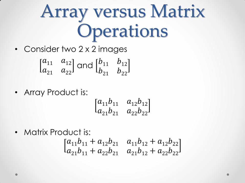
Array versus Matrix Operations

• Consider two 2 x 2 images

𝑎11 𝑎12𝑎21 𝑎22

and 𝑏11 𝑏12𝑏21 𝑏22

• Array Product is: 𝑎11𝑏11 𝑎12𝑏12𝑎21𝑏21 𝑎22𝑏22

• Matrix Product is: 𝑎11𝑏11 + 𝑎12𝑏21 𝑎11𝑏12 + 𝑎12𝑏22𝑎21𝑏11 + 𝑎22𝑏21 𝑎21𝑏12 + 𝑎22𝑏22

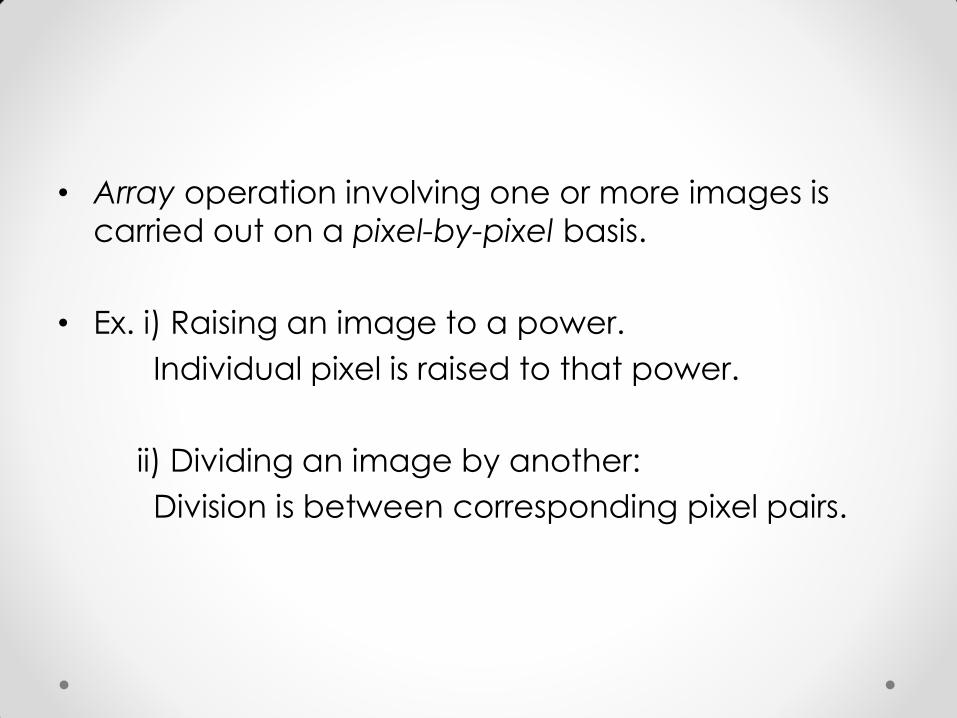
• Array operation involving one or more images is

carried out on a pixel-by-pixel basis.

• Ex. i) Raising an image to a power.

Individual pixel is raised to that power.

ii) Dividing an image by another:

Division is between corresponding pixel pairs.

Linear versus Nonlinear Operations

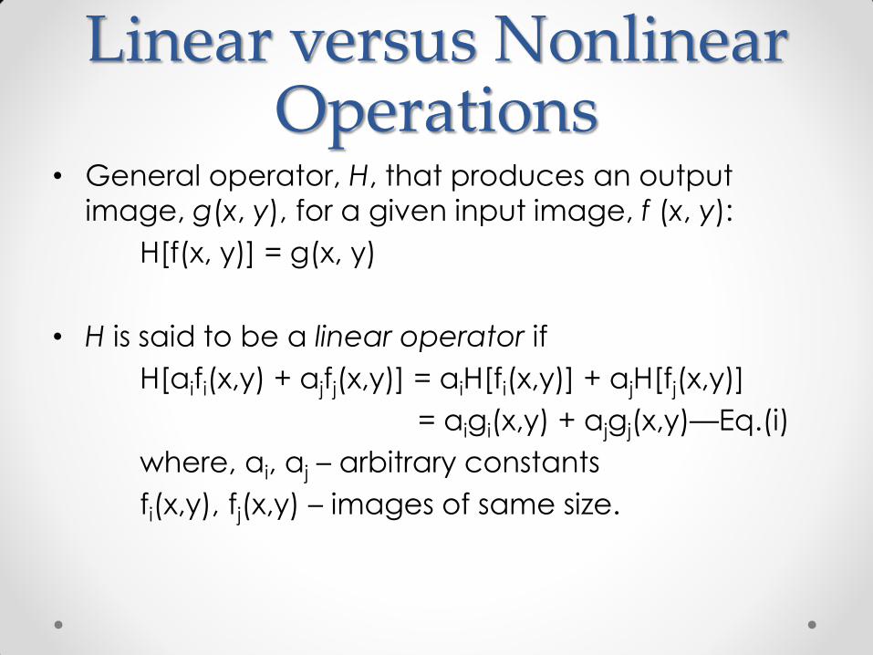
• General operator, H, that produces an output

image, g(x, y), for a given input image, f (x, y):

H[f(x, y)] = g(x, y)

• H is said to be a linear operator if

H[aifi(x,y) + ajfj(x,y)] = aiH[fi(x,y)] + ajH[fj(x,y)]

= aigi(x,y) + ajgj(x,y)—Eq.(i)

where, ai, aj – arbitrary constants

fi(x,y), fj(x,y) – images of same size.

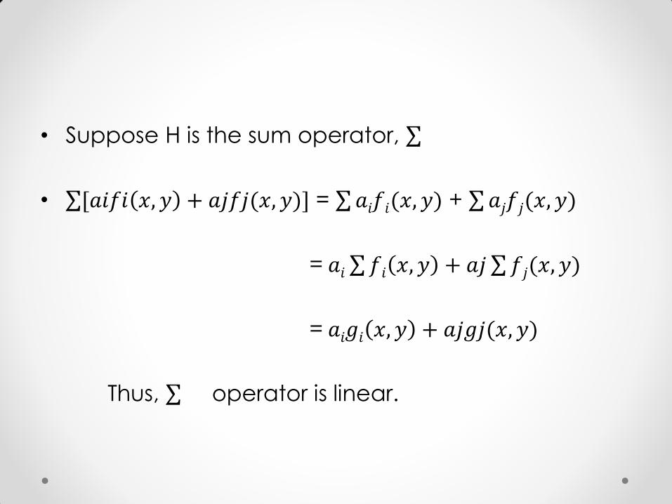
• Suppose H is the sum operator,

• [𝑎𝑖𝑓𝑖 𝑥, 𝑦 + 𝑎𝑗𝑓𝑗(𝑥, 𝑦)] = 𝑎𝑖𝑓𝑖(𝑥, 𝑦) + 𝑎𝑗𝑓𝑗(𝑥, 𝑦)

= 𝑎𝑖 𝑓𝑖 𝑥, 𝑦 + 𝑎𝑗 𝑓𝑗(𝑥, 𝑦)

= 𝑎𝑖𝑔𝑖 𝑥, 𝑦 + 𝑎𝑗𝑔𝑗(𝑥, 𝑦)

Thus, operator is linear.

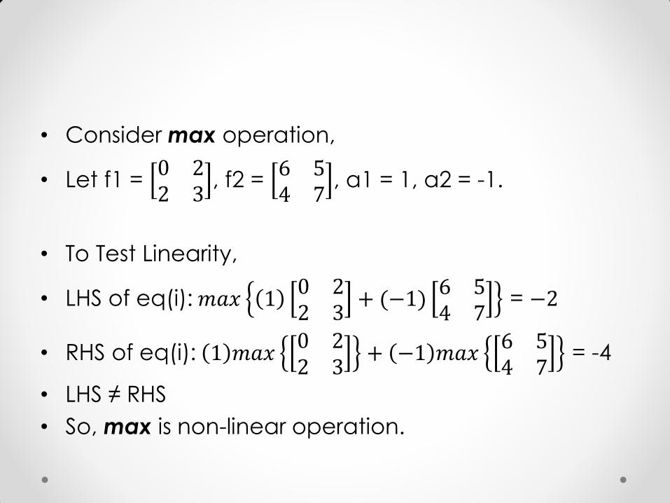
• Consider max operation,

• Let f1 = 0 22 3

, f2 = 6 54 7

, a1 = 1, a2 = -1.

• To Test Linearity,

• LHS of eq(i): 𝑚𝑎𝑥 10 22 3

+ (−1)6 54 7

= −2

• RHS of eq(i): 1 𝑚𝑎𝑥0 22 3

+ −1 𝑚𝑎𝑥6 54 7

= -4

• LHS ≠ RHS

• So, max is non-linear operation.

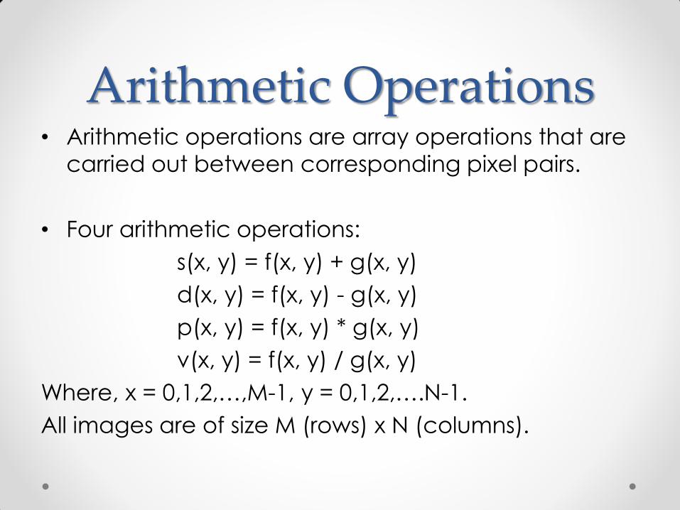
Arithmetic Operations • Arithmetic operations are array operations that are

carried out between corresponding pixel pairs.

• Four arithmetic operations:

s(x, y) = f(x, y) + g(x, y)

d(x, y) = f(x, y) - g(x, y)

p(x, y) = f(x, y) * g(x, y)

v(x, y) = f(x, y) / g(x, y)

Where, x = 0,1,2,…,M-1, y = 0,1,2,….N-1.

All images are of size M (rows) x N (columns).

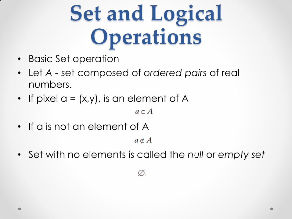
Set and Logical Operations

• Basic Set operation

• Let A - set composed of ordered pairs of real

numbers.

• If pixel a = (x,y), is an element of A

• If a is not an element of A

• Set with no elements is called the null or empty set

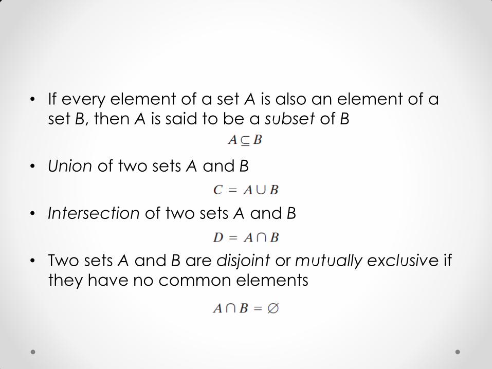
• If every element of a set A is also an element of a

set B, then A is said to be a subset of B

• Union of two sets A and B

• Intersection of two sets A and B

• Two sets A and B are disjoint or mutually exclusive if

they have no common elements

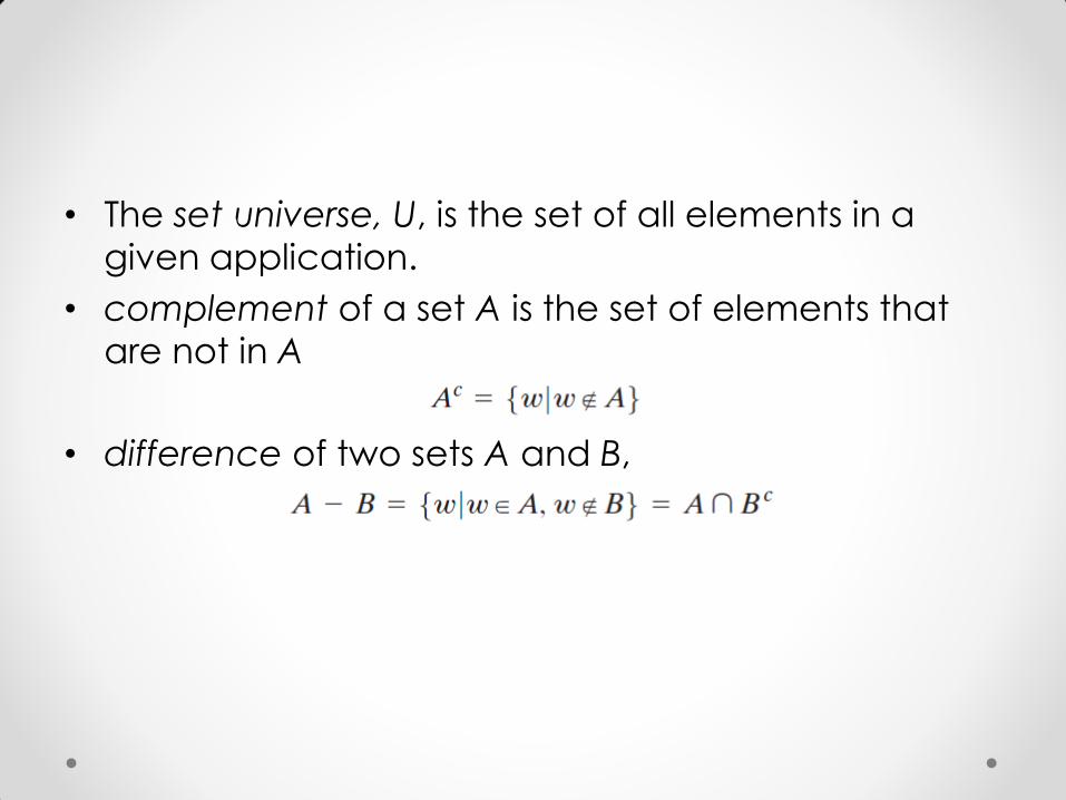
• The set universe, U, is the set of all elements in a

given application.

• complement of a set A is the set of elements that

are not in A

• difference of two sets A and B,

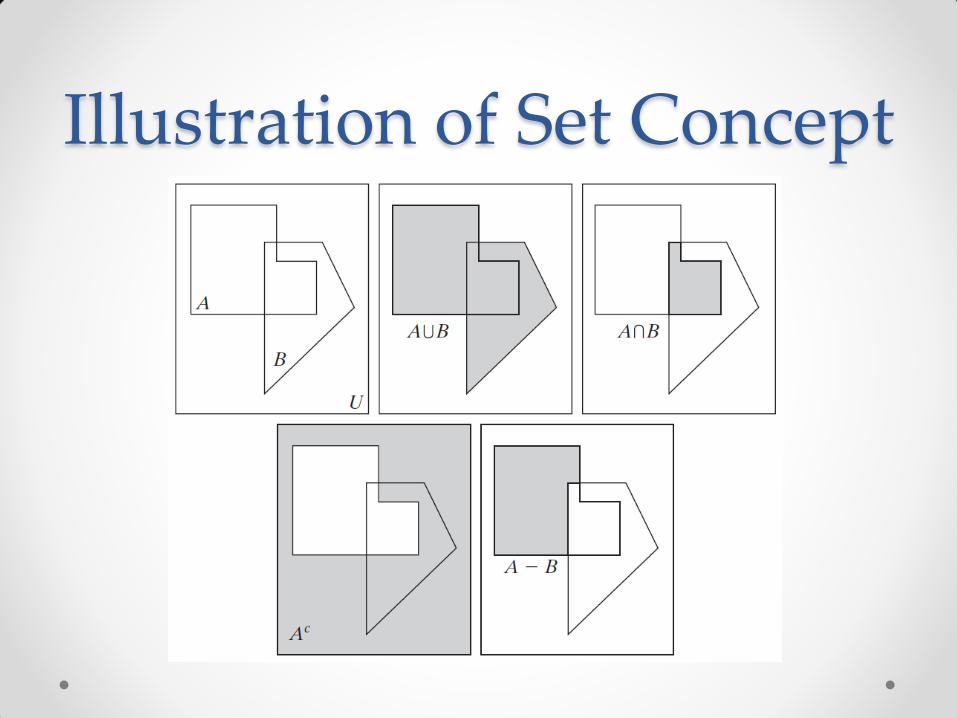
Illustration of Set Concept

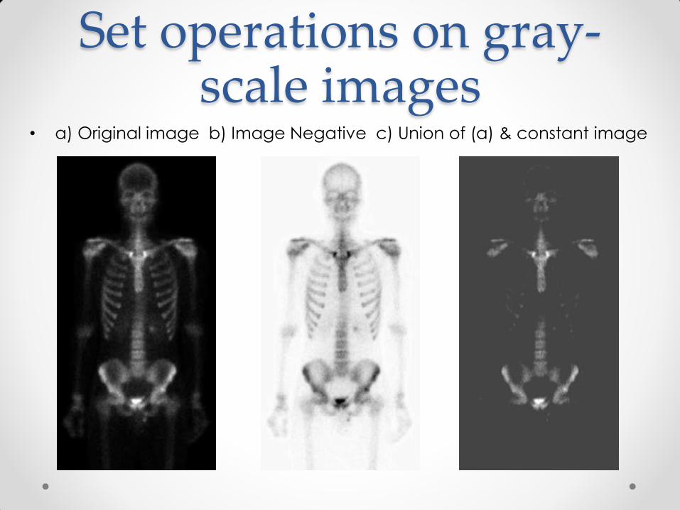
Set operations on gray-scale images

• a) Original image b) Image Negative c) Union of (a) & constant image

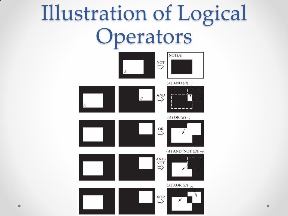
Illustration of Logical Operators

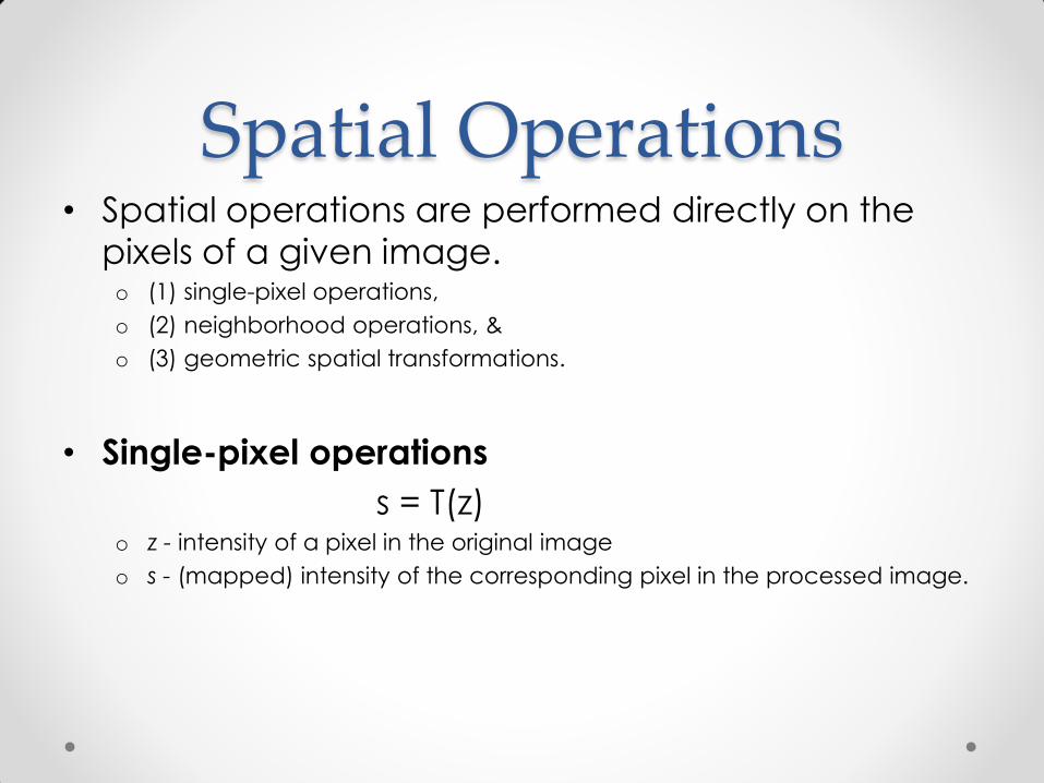
Spatial Operations • Spatial operations are performed directly on the

pixels of a given image. o (1) single-pixel operations,

o (2) neighborhood operations, &

o (3) geometric spatial transformations.

• Single-pixel operations

s = T(z) o z - intensity of a pixel in the original image

o s - (mapped) intensity of the corresponding pixel in the processed image.

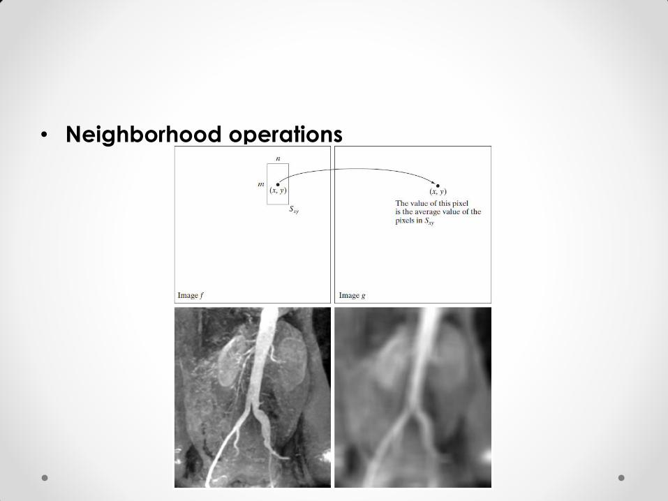
• Neighborhood operations

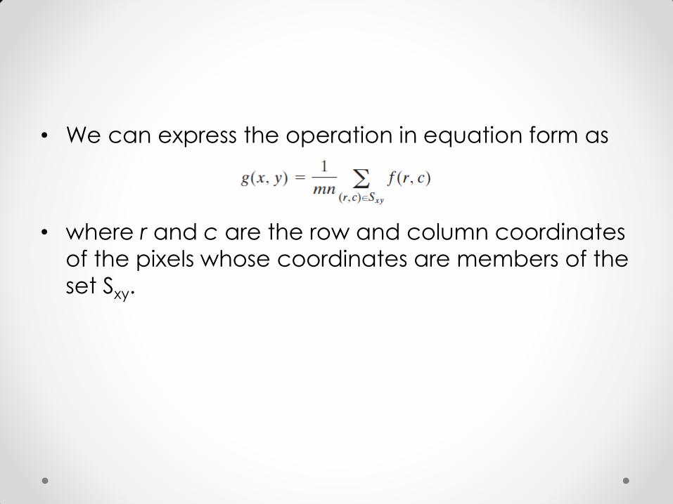
• We can express the operation in equation form as

• where r and c are the row and column coordinates

of the pixels whose coordinates are members of the

set Sxy.

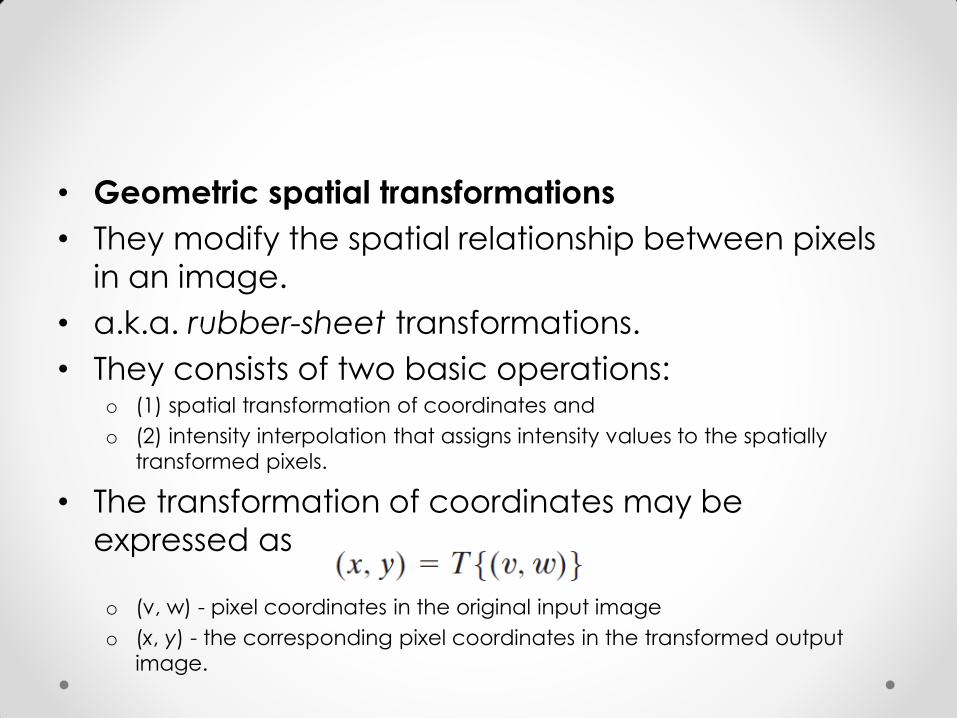
• Geometric spatial transformations

• They modify the spatial relationship between pixels

in an image.

• a.k.a. rubber-sheet transformations.

• They consists of two basic operations: o (1) spatial transformation of coordinates and

o (2) intensity interpolation that assigns intensity values to the spatially

transformed pixels.

• The transformation of coordinates may be

expressed as

o (v, w) - pixel coordinates in the original input image

o (x, y) - the corresponding pixel coordinates in the transformed output

image.

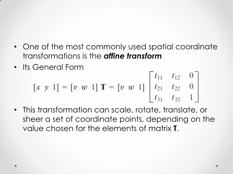
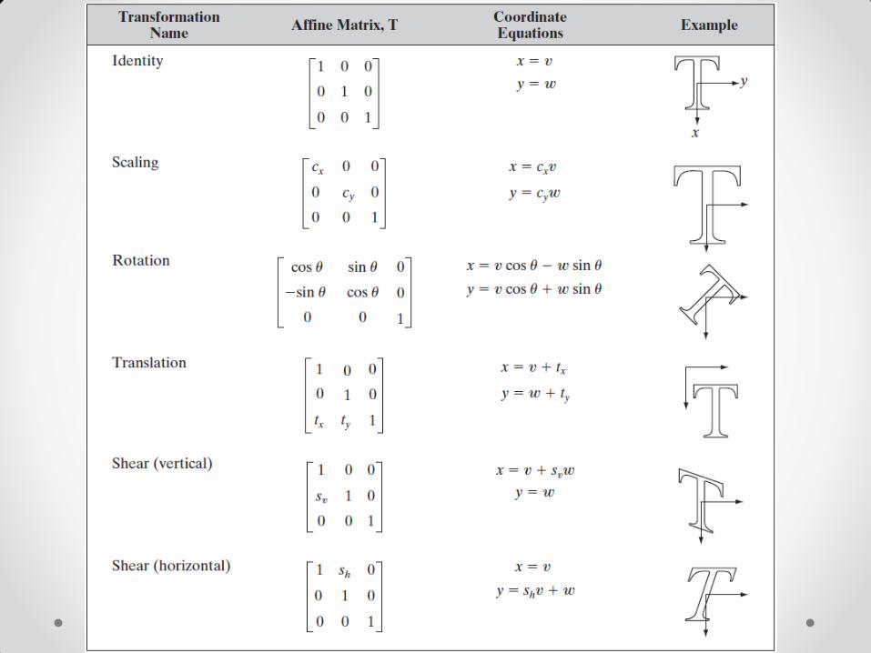
• One of the most commonly used spatial coordinate

transformations is the affine transform

• Its General Form

• This transformation can scale, rotate, translate, or

sheer a set of coordinate points, depending on the

value chosen for the elements of matrix T.

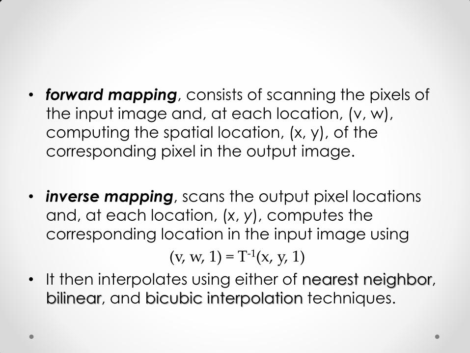
• forward mapping, consists of scanning the pixels of

the input image and, at each location, (v, w),

computing the spatial location, (x, y), of the

corresponding pixel in the output image.

• inverse mapping, scans the output pixel locations

and, at each location, (x, y), computes the

corresponding location in the input image using

(v, w, 1) = T-1(x, y, 1)

• It then interpolates using either of nearest neighbor,

bilinear, and bicubic interpolation techniques.

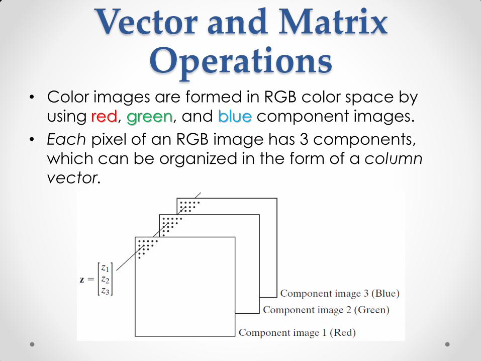
Vector and Matrix Operations

• Color images are formed in RGB color space by

using red, green, and blue component images.

• Each pixel of an RGB image has 3 components,

which can be organized in the form of a column

vector.

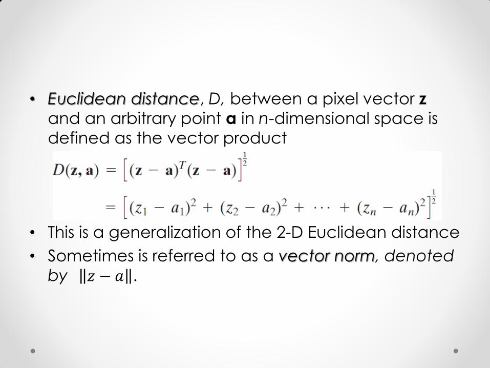
• Euclidean distance, D, between a pixel vector z

and an arbitrary point a in n-dimensional space is

defined as the vector product

• This is a generalization of the 2-D Euclidean distance

• Sometimes is referred to as a vector norm, denoted

by 𝑧 − 𝑎 .

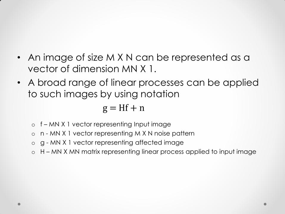
• An image of size M X N can be represented as a

vector of dimension MN X 1.

• A broad range of linear processes can be applied

to such images by using notation

g = Hf + n

o f – MN X 1 vector representing Input image

o n - MN X 1 vector representing M X N noise pattern

o g - MN X 1 vector representing affected image

o H – MN X MN matrix representing linear process applied to input image

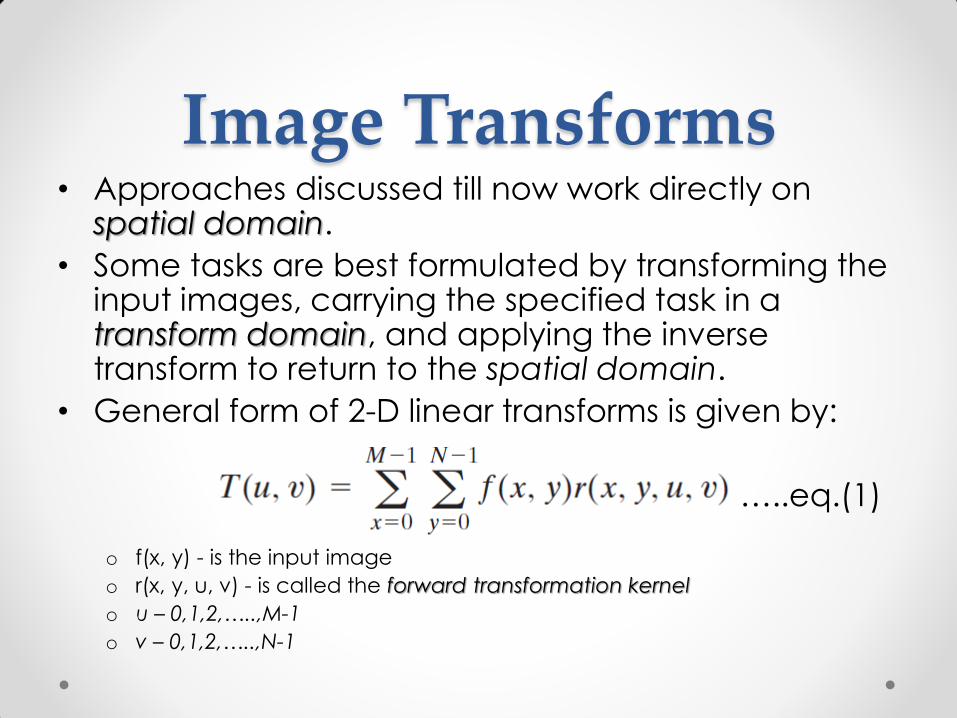
Image Transforms • Approaches discussed till now work directly on

spatial domain.

• Some tasks are best formulated by transforming the input images, carrying the specified task in a transform domain, and applying the inverse transform to return to the spatial domain.

• General form of 2-D linear transforms is given by:

…..eq.(1)

o f(x, y) - is the input image

o r(x, y, u, v) - is called the forward transformation kernel

o u – 0,1,2,…..,M-1

o v – 0,1,2,…..,N-1

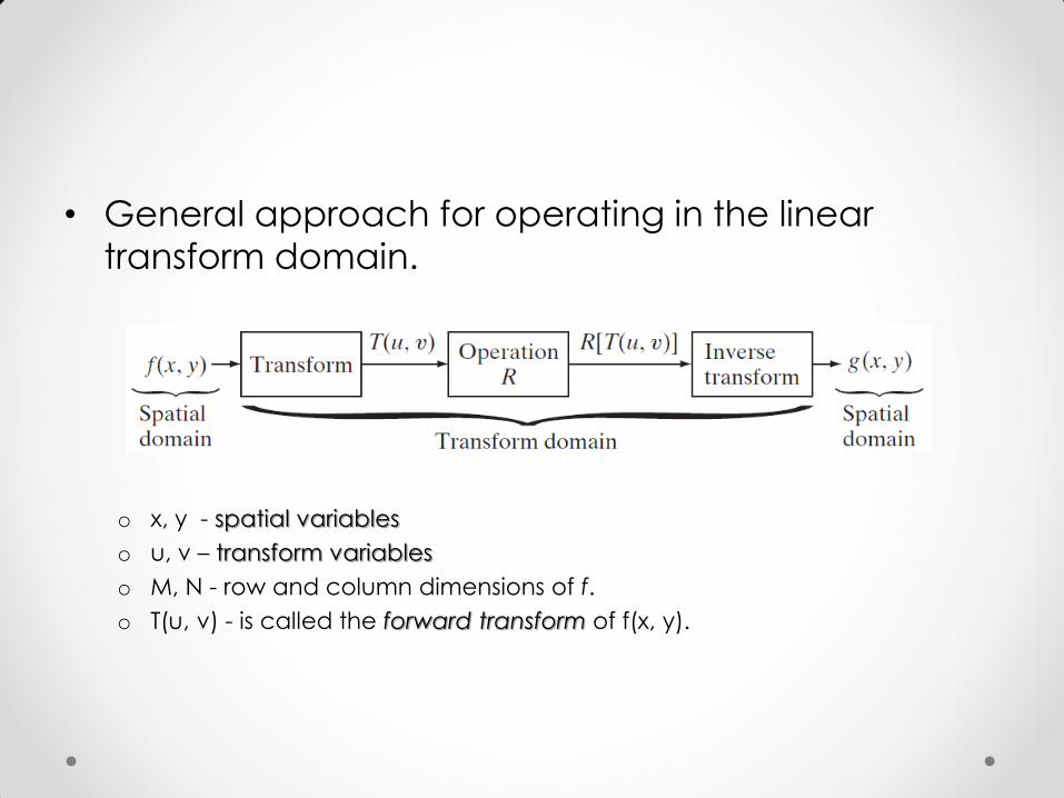
• General approach for operating in the linear

transform domain.

o x, y - spatial variables

o u, v – transform variables

o M, N - row and column dimensions of f.

o T(u, v) - is called the forward transform of f(x, y).

• Given T(u, v) , we can recover f(x, y) using the

inverse transform of T(u, v),

….eq.(2) o x – 0,1,2,…..,M-1

o y – 0,1,2,…..,N-1

o s(x, y, u, v) - is called the inverse transformation kernel.

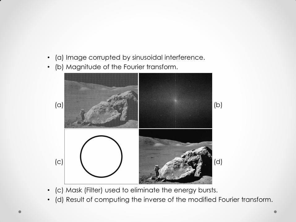
• (a) Image corrupted by sinusoidal interference.

• (b) Magnitude of the Fourier transform.

(a) (b)

(c) (d)

• (c) Mask (Filter) used to eliminate the energy bursts.

• (d) Result of computing the inverse of the modified Fourier transform.

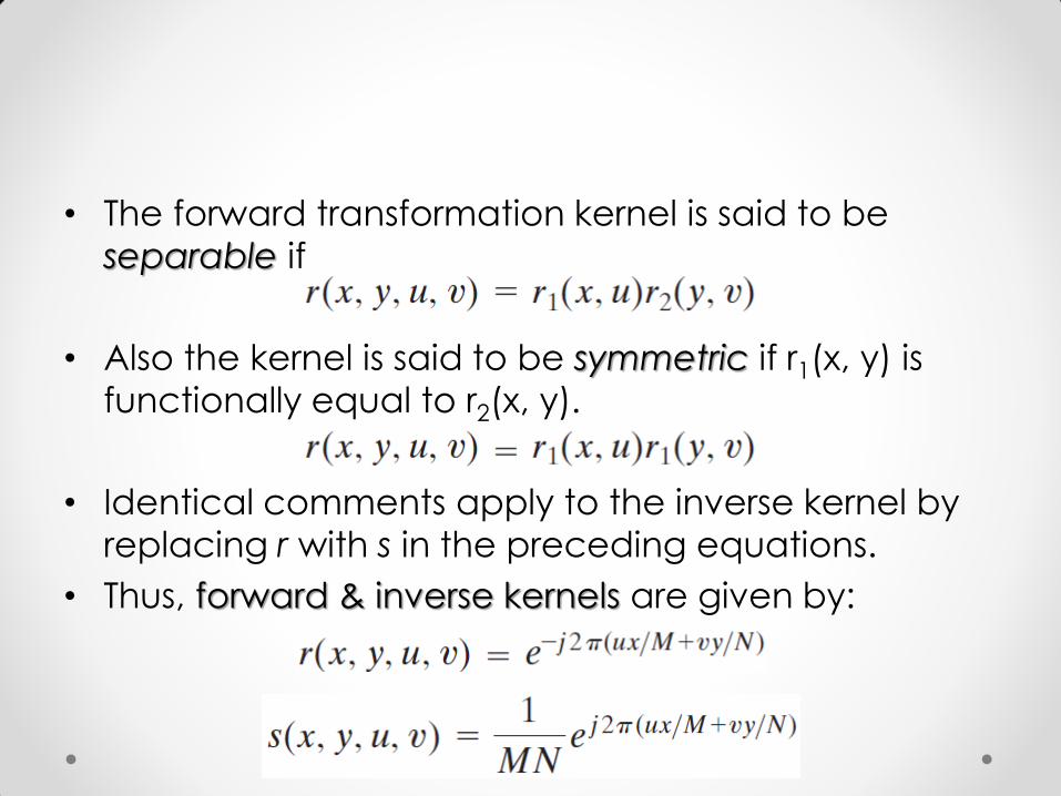
• The forward transformation kernel is said to be

separable if

• Also the kernel is said to be symmetric if r1(x, y) is

functionally equal to r2(x, y).

• Identical comments apply to the inverse kernel by

replacing r with s in the preceding equations.

• Thus, forward & inverse kernels are given by:

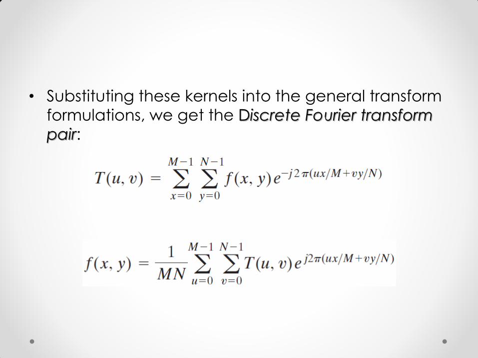
• Substituting these kernels into the general transform

formulations, we get the Discrete Fourier transform

pair:

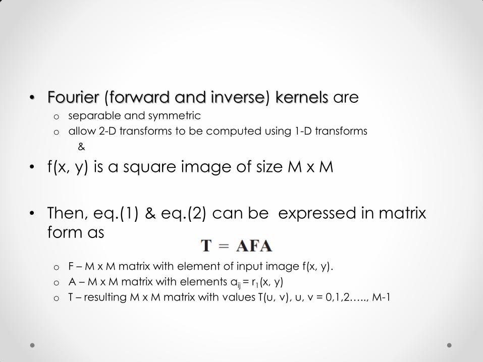
• Fourier (forward and inverse) kernels are o separable and symmetric

o allow 2-D transforms to be computed using 1-D transforms

&

• f(x, y) is a square image of size M x M

• Then, eq.(1) & eq.(2) can be expressed in matrix

form as

o F – M x M matrix with element of input image f(x, y).

o A – M x M matrix with elements aij = r1(x, y)

o T – resulting M x M matrix with values T(u, v), u, v = 0,1,2….., M-1

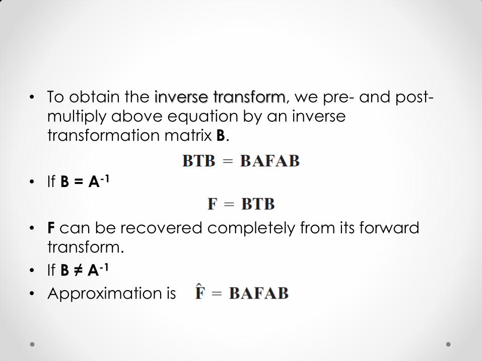
• To obtain the inverse transform, we pre- and post-

multiply above equation by an inverse

transformation matrix B.

• If B = A-1

• F can be recovered completely from its forward

transform.

• If B ≠ A-1

• Approximation is