MATHEMATICAL STUDY OF TRANSPORT …downloads.hindawi.com/journals/mpe/2006/023754.pdf4 Transport...

MATHEMATICAL STUDY OF TRANSPORT PHENOMENAALONG A TUYERE OF THE TENIENTE CONVERTER

J. SAN MARTIN, R. GORMAZ, C. CONCA, F.-Z. SAOURI, A. BENADDI,

R. FUENTES, AND P. RUZ

Received 14 March 2005; Revised 29 July 2005; Accepted 24 August 2005

This paper presents a comprehensive mathematical model of transport phenomena whichoccur along a tuyere of the Teniente converter during injection of oxygen-enriched air.Inlet pressure, gas velocity and temperature, the dimensions of the tuyere, and the prop-erties of gas are the basic data. From these inputs, temperature distribution of the re-fractory walls of the converter around the tuyere as well as the velocity, pressure, and theMach number along the pipe can be calculated. In this model, the heat transfer throughthe metal jacket of the tuyere and the refractory lining are duly taken into account. Moreprecisely, a mathematical model is developed where the equations of momentum and en-ergy of the gas are coupled with the equations of heat transfer inside the solid part. Thisnew model couples a partial differential equation in the solid part with four ordinarydifferential equations in the gas flow.

Copyright © 2006 J. San Martın et al. This is an open access article distributed under theCreative Commons Attribution License, which permits unrestricted use, distribution,and reproduction in any medium, provided the original work is properly cited.

1. Introduction

In Chile, one stage of copper refining is completed in a special cylindrical converter:the Teniente converter (CT) furnace which is intended to eliminate the most oxidizablemetallic elements present in the mineral concentrate. In this stage, oxygen-enriched air isinjected into the smelting bath through an array of tuyeres to feed the chemical reactionswhich separate out the impurities contained in the copper.

Our objective is to carry out a mathematical modeling and numerical experimentsof the air flow that is injected through the tuyeres and its influence on the temperatureof the CT walls. The thermal variables are of primary interest here, but because there isa compressible fluid involved, which is injected at high velocities, the thermal variablesare coupled with the dynamic ones.

In this work, the interaction between the tuyere and the CT walls will be simpli-fied since interest will be focused on a local analysis of the tuyere and the CT walls.

Hindawi Publishing CorporationMathematical Problems in EngineeringVolume 2006, Article ID 23754, Pages 1–12DOI 10.1155/MPE/2006/23754

http://dx.doi.org/10.1155/S1024123X06237542

2 Transport phenomena along a tuyere

Mathematically, the domain can be divided into two regions. The first corresponds to thegas that circulates in the interior of the tuyere, or the “fluid region.” The second corre-sponds to the metallic jacket of the tuyere and the refractory lining as well as the metallicexternal shell, this is the “solid region.”

Krivsky and Schuhmann [3] calculated the distribution of temperatures around atuyere. These authors suppose the temperature of the gas in the tuyere to be known,and using a relaxation method they found the distribution of temperatures in the re-fractory lining. One of our goals in this paper is to carry out an exhaustive study of theflow in the tuyere including heat transfer effects. The model in the fluid region is basedon Hugoniot’s equations, which assume that the gas is compressible, ideal, and has one-dimensional motion along the tuyere. The full model is obtained by coupling Hugoniot’sequations with the heat transfer equation through the metal jacket of the tuyere and thesurrounding converter walls. The interaction of both equations appears in the heat flowtransferred from one zone to another. In mathematical terms, the model presented cor-responds to a system of partial differential equations coupled with a system of ordinarydifferential equations.

The coupled system is solved, numerically, by using an iterative numerical schemedivided into two steps. In the first step, the distribution of temperatures in the solid partof the system is calculated using the finite element method. In this step, it is assumed thatthe distribution of temperatures of the gas and the heat transfer factor in the jacket ofthe tuyere are known. In the second step, the distribution of temperatures of the gas inthe tuyere is calculated. Here we use the distribution of temperatures already calculatedin the previous step.

The paper is presented as follows. In Section 2, we write down the mathematical modelfirst for the solid part, and next, for the gas in the tuyere. In Section 3, we show the numer-ical results, and in Section 4 we give some conclusions and components on the applicationof the results to the real operation of the CT.

2. Modeling of transport phenomena along a tuyere

This section is divided into three parts. Firstly, we derive a mathematical model for theheat transfer inside the solid part. Secondly, we write down general equations for thedynamics of the gas in the tuyere which are simplified for the one-dimensional case inSection 2.2. Finally, in Section 2.3 both models are coupled.

2.1. The model for the solid part. We denote the solid domain by Ωs (see Figure 2.1).This domain, that is found around the tuyere, we assume has cylindrical symmetry. Itsboundary can be divided into the following parts. Γ3 borders Ωs with the interior of theCT, where the liquid copper bath is at a temperature of 1300◦C. Γ4 is that part of theCT which is exposed to external air. Γ1 is the border in the axial direction that definesthe dimensions of the domain under study. It is assumed that this part of the boundaryis sufficiently far from the axis of the tuyere so that heat transfer is zero. The interfacebetween the solid domain and the gaseous domain is Γ2. Furthermore, as the tuyere is

J. San Martın et al. 3

Γ1

Γ3Γ4

Γ5

Γ6

Γ2Symmetry axis

Figure 2.1. Effective domain of calculation.

larger than the walls of the CT, we consider the two additional borders Γ5 and Γ6, asillustrated in Figure 2.1.

We will write the equations of heat propagation in the domain Ωs assuming that theregime is stationary. The equation used in this zone is the classical heat equation

−div(κs gradT

)= 0 in Ωs, (2.1)

where T is the temperature in the solid domain. Here, the coefficient of conductivity inthe solid part, denoted by κs, takes different values in the metal jacket of the tuyere morethan in the refractory brick lining.

The boundary conditions for (2.1) are the following:

κs∂T

∂n= 0 on Γ1, with x ∈ [0,L], (2.2)

κs∂T

∂n= h(T −Text

)on ∂Ωs \Γ1, (2.3)

where h is the heat transfer factor for convection between the solid boundary and theexternal medium. This factor has different values depending on the geometry and the ex-ternal fluid in contact with the calculation domain. Text is the temperature of the externalfluid in contact with our calculation domain. This problem can be solved in various ways,given Text, for example, with the finite elements method which in fact we use here.

2.2. The model for gas in the tuyere. Here we will give the mathematical translation ofthe conservation laws of mass, momentum, and energy in the flow of air injected througha tuyere. We denote the region occupied by the gas in the tuyere by Ω f , which is boundedby Γ2, and the parallel surfaces [x=0.0] and [x=0.9]. Here the one-dimensional variablex runs along the symmetry axis of the tuyere.


The three-dimensional equations of conservation of mass, momentum, and energy inΩ f are, respectively,

divρ�v = 0,

ρ(�v · grad

)�v = divσ + ρ�g,

ρ(�v · grad

)e =�σ : �D

(�v)−div�q+ r,

(2.4)

where ρ is the gas density,�v is the velocity field, σ is the stress tensor, �g is the gravity force,e is the density of the gas internal energy, �q is the heat flow vector in the gas, and r is theexternal heat source by unit of volume.

If we use the averaged values over a cross section of a tuyere, the above equations canbe written in the following unidimensional form:

d

dx

(ρ(x) · v1(x)

)= 0,

d

dx

(mv1(x) +AP(x)

)=−χτ(x),

d

dx

(me(x) +Av1(x)P(x) + m

v21(x)2

+ mgh(x))= q′1(x)A+ qr(x)χ,

P(x)= Rμ(x)

ρT ,

(2.5)

where m(x)= Aρv1 is the constant flow of mass into the tuyere, χ is the perimeter of thetuyere, τ(x) denotes the transversal shear that the walls exert on the gas in the direction−�e1, q1 is the component of the heat flow vector in the direction of the tuyere axis, qrrepresents the component of the heat flow vector in the radial direction, R is the universalconstant of gases, and μ is the molar mass of the gas considered.

The previous system can be interpreted as a linear system of four differential equationswith variable coefficients. In order to simplify this system, we use the relation de/dT = Cv

valid for perfect gases, where Cv is the specific heat of the gas at a constant volume (see [2,page 235]). Other relations of perfect gases used to simplify the previous equations are

Cp = Cv +Rμ

, specific heat of the gas at a constant pressure,

k = Cp

Cv,

c =√

kP

ρ, velocity of sound in the gas,

Ma = v

c, Mach number.

(2.6)


Using the above relations, the above system of equations is transformed into

P′

P= −1(1−M2

a

)((k− 1)M2

aSq−[1 + (k− 1)M2

a

]Sτ +M2

aSμ), (2.7)

T′

T= k− 1

k(1−M2

a

)((

1− kM2a

)Sq + kM2

aSτ − Sμ), (2.8)

ρ(x)= P(x)μ(x)RT(x)

, (2.9)

v(x)= m

ρ(x)A, (2.10)

where

Sτ =−χτ(x)AP

, (2.11)

Sq = q′1(x)A+ qr(x)χAPv

, (2.12)

Sμ =−μ′(x)μ(x)

(2.13)

are the sources of the right-hand side of the equation, which respectively depend on thefriction effort τ, the dissipated heat qr and q′1, and the variation of molar mass μ. We willrefer to (2.7)–(2.10) as Hugoniot’s equations. To couple these equations with the solidpart, it is necessary to model the heat exchange qr with the walls and the friction effortτ. In the following section, we summarize the main known empirical formulas for thesetwo parameters in the case of flow in a tuyere.

2.3. Modeling the heat transfer between the tuyere and the walls. The coupling be-tween the tuyere and rigid walls of the converter appears in (2.3) and (2.12) due to theheat transfer between the gas of the tuyere and its metal jacket. This heat exchange will bemodeled by the following equation:

q = h(Tf −Tp(x)

), (2.14)

where Tf is the temperature of the gas, Tp is the temperature of the wall, and h is thecoefficient of heat transfer factor.

The study of the thermal transfer factor in the case of flows in heat pipes has been donein [4]. There it is shown that

h= CpρvMar, (2.15)

where Cp is the gas’ specific heat at constant pressure, ρ is its density, v is the averagevelocity, and Mar is the so-called Margoulis number. This Margoulis number can be esti-mated from the relation of Dipprey and Sabersky (see Mills [4]):

Mar = f /8

0.9 +(4.8k0.2∗ Pr0.44−7.65

) , (2.16)


Table 3.1. Parameter values for Example 3.1.

Parameter Symbol Value

Inlet pressure of the tuyere P(0) 20 psi

Inlet temperature of the tuyere T(0) 100◦C

Volume flow in the tuyere q = m/A 0.4526 m3/s

Heat transfer factor of the boundary Γ3 h3 1000 W/(m2◦C)


Heat transfer factor of the boundaries Γ5 and Γ6 h5, h6 50 W/(m2◦C)

External temperature at the boundary Γ3 Text,3 1300◦C

External temperature at the boundaries Γ4, Γ5, and Γ6 Text,4, Text,5 50◦C

where f is the friction factor of Darcy in the heat pipe (see the following paragraph),

k∗ = (vrs/ν)√f /8, rs is the average rugosity of the pipe wall, ν is the cinematic viscosity of

the gas, Pr= (νρ/κ)Cp is the Prandtl number, and κ is the thermal conductivity of the gas.The study of the friction factor or the resistance f for the case of heat pipes is done in

[1]. There the dependence on the pipe’s rugosity and on the Reynolds number is shown.The friction factor f can be obtained from the Colebrook-White equation (see [4]):

1√f=−2log

(

0.27rsD

+2.51

Re

√f

)

. (2.17)

3. Numerical results

In this section, we present some numerical results corresponding to the application of theprevious model to the study of temperature distribution along the tuyere and in the sur-rounding walls. As seen in Section 2, this fluid-solid-type interaction leads to a coupledsystem of equations which includes (2.3) for the solid part, (2.7)–(2.10) for the fluid part,and (2.15) along the fluid-solid interface. When solving (2.2)–(2.3), the distribution oftemperatures in the solid part of the system is calculated using standard finite elements.In this step, it is assumed that the distribution of temperatures of the gas and the heattransfer factor in the jacket of the tuyere are known. The resolution of (2.7)–(2.10) yieldsthe distribution of temperatures of the gas in the tuyere. Here the temperatures along thesolid jacket of the tuyere is assumed to be known. The resolution of (2.7)–(2.8) requiresthe prescriptions of two initial or inlet conditions. In our numerical examples, we haveused P(0)= 20 psi (inlet pressure of the tuyere) and T(0)= 100◦C (inlet temperature ofthe tuyere) as shown in Table 3.1.

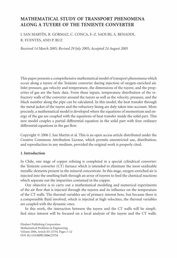
This strategy provides a numerical scheme which we have run using an original C++program. It is worthwhile remarking that Hugoniot’s equations are solved numerically byan order-4 Runge-Kutta scheme, while in the solid part, the resulting finite element linearsystem is solved by the conjugate gradient method. In Figure 3.1, the mesh used for thecalculations is illustrated. It can be seen that in the bottom part (the boundary betweenthe walls and the tuyere), the mesh is finer. This is because the heat transfer here as wellas the temperature gradient are expected to be more important.


0.45 m

0 m 0.4 m 0.9 m

Shell surface

Gas/tuyereinterface

Refractory/bathinterface

Figure 3.1. The mesh to calculate the solid zone.

0.82 m 0.90 m0 m

0.005 m

0.060 m

Figure 3.2. Zoom out of the mesh.

For a better view of the refinement, we include a zoom out of the right bottom meshzone in Figure 3.2.

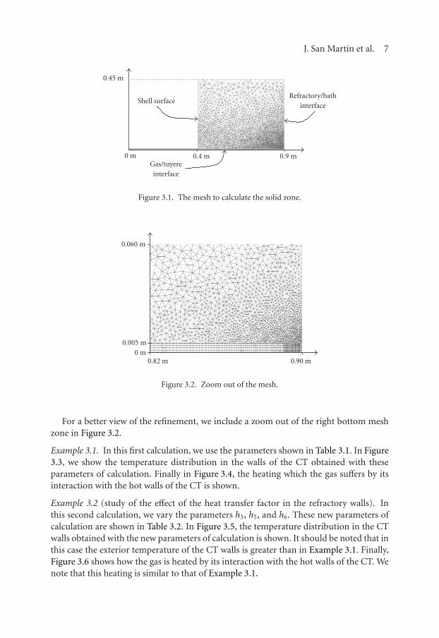
Example 3.1. In this first calculation, we use the parameters shown in Table 3.1. In Figure3.3, we show the temperature distribution in the walls of the CT obtained with theseparameters of calculation. Finally in Figure 3.4, the heating which the gas suffers by itsinteraction with the hot walls of the CT is shown.

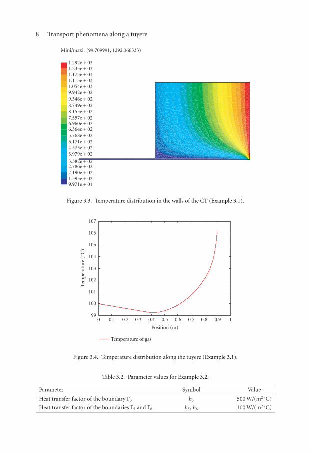
Example 3.2 (study of the effect of the heat transfer factor in the refractory walls). Inthis second calculation, we vary the parameters h3, h5, and h6. These new parameters ofcalculation are shown in Table 3.2. In Figure 3.5, the temperature distribution in the CTwalls obtained with the new parameters of calculation is shown. It should be noted that inthis case the exterior temperature of the CT walls is greater than in Example 3.1. Finally,Figure 3.6 shows how the gas is heated by its interaction with the hot walls of the CT. Wenote that this heating is similar to that of Example 3.1.


1.292e + 031.233e + 031.173e + 031.113e + 031.054e + 039.942e + 029.346e + 028.749e + 028.153e + 027.557e + 026.960e + 026.364e + 025.768e + 025.171e + 024.575e + 023.979e + 02

3.382e + 022.786e + 022.190e + 021.593e + 029.971e + 01

Mini/maxi: (99.709991, 1292.366333)

Figure 3.3. Temperature distribution in the walls of the CT (Example 3.1).

0 0.1 0.2 0.3 0.4 0.5 0.6 0.7 0.8 0.9 1

Position (m)

99

100

101

102

103

104

105

106

107

Tem

per

atu

re(◦

C)

Temperature of gas

Figure 3.4. Temperature distribution along the tuyere (Example 3.1).

Table 3.2. Parameter values for Example 3.2.

Parameter Symbol Value


Heat transfer factor of the boundaries Γ5 and Γ6 h5, h6 100 W/(m2◦C)


1.285e + 031.226e + 031.166e + 031.107e + 031.048e + 039.885e + 029.293e + 028.700e + 028.108e + 027.515e + 026.922e + 026.330e + 025.737e + 025.145e + 024.552e + 023.960e + 023.367e + 022.775e + 022.182e + 021.590e + 029.972e + 01

Mini/maxi: (99.723251, 1284.771606)

Figure 3.5. Temperature distribution in the CT walls (Example 3.2).

0 0.1 0.2 0.3 0.4 0.5 0.6 0.7 0.8 0.9 1

Position (m)

99

100

101

102

103

104

105

106

Tem

per

atu

re(◦

C)

Temperature of gas

Figure 3.6. Temperature distribution along the tuyere (Example 3.2).

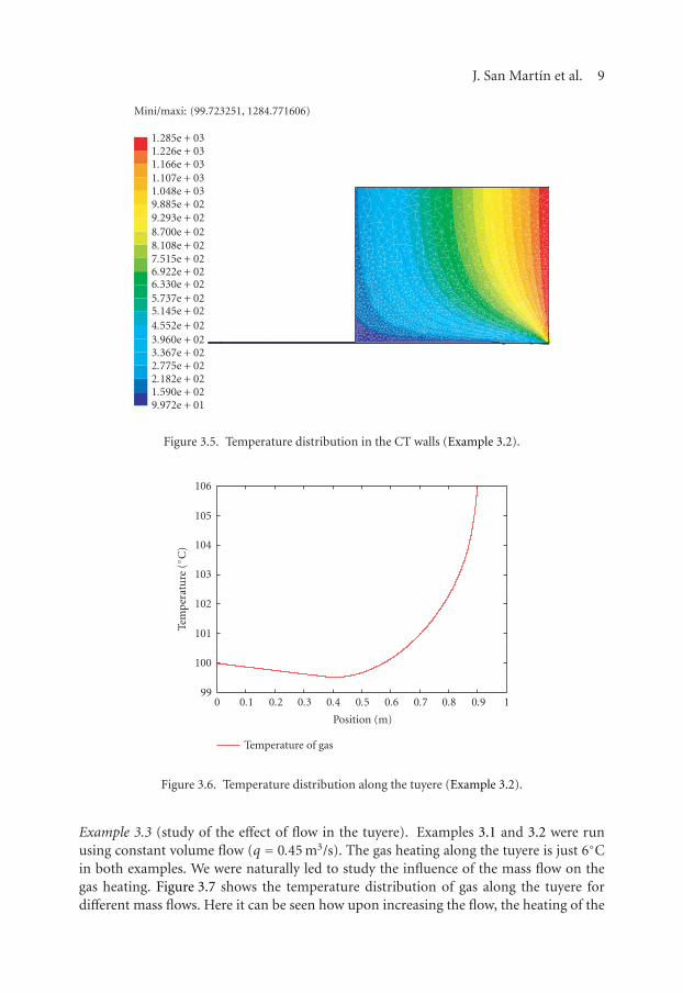
Example 3.3 (study of the effect of flow in the tuyere). Examples 3.1 and 3.2 were runusing constant volume flow (q = 0.45 m3/s). The gas heating along the tuyere is just 6◦Cin both examples. We were naturally led to study the influence of the mass flow on thegas heating. Figure 3.7 shows the temperature distribution of gas along the tuyere fordifferent mass flows. Here it can be seen how upon increasing the flow, the heating of the


0 0.05 0.1 0.15 0.2 0.25 0.3 0.35 0.4 0.45 0.5

Relative position with respect to the shell surface (m)

92

94

96

98

100

102

104

106

108

Tem

per

atu

re(◦

C)

Temperature of gas (q = 1)Temperature of gas (q = 0.7)Temperature of gas (q = 0.45)

Figure 3.7. Temperatures of the tuyere’s gas for different flows.

gas in the tuyere is smaller and even we can see a cooling phenomenon along the tuyere(case 1 in Figure 3.7, q = 1 m3/s).

4. Conclusions

Different results of heat transfer have been presented. The velocity of compressible gaspropagation in the tuyere has been calculated. The numerical calculations show a reheat-ing of the gas at the exit of the pipe along with a cooling of the converter walls near thepipe. In the case of an important flow, a slight cooling of the gas in the pipe is observed.

A mathematical model has been considered for the study of the heat transfer betweenthe walls of the Teniente converter and the oxygen-enriched air injected by the blowingtuyeres. This model allows to calculate the distribution of temperatures in these two do-mains. In continuation, we determine various parameters such as the velocity, the pres-sure, and the density inside the tuyere. The presented model allows as well to determinethe properties of the flow inside tuyeres and the distribution of temperature in the wallsof the CT.

The numerical calculations show an adiabatic cooling of the gas in the part of thetuyere being in the exterior of the converter before the interaction with the walls of theCT and a heating in the zone close to the interior of the CT. This heating, for diverseoperation conditions, does not go beyond ten degrees Celsius. There is a critical outletflow from which a light cooling for the gas in the tuyere is observed. The present calcula-tion allows to see clearly the magnitude and distribution of the cooling of the walls of theconverter near the tuyere.


5. Nomenclature

Here are some definitions of parameters used in this paper.(i) q: unitary flow of heat from the wall (thermal energy by unit of time and area).

(ii) h: coefficient of heat transfer.(iii) q = (1/χ) (dQ/dx):

(a) Q: thermal energy transfer by unit of time,(b) χ: perimeter of the pipe,(c) dx: infinitesimal element of distance through the pipe.

(iv) To calculate h, the Margoulis number Mar is introduced by Mar ≡ h/GCp, G =M/A,(a) M: mass flow,(b) A: transversal area of the pipe,(c) Cp: specific isobaric heat of the flow.

(v) Mar could be estimated from the relation of Dipprey and Sabersky (see Mills [4]):

Mar = h/GCp = (1/(0.9 +√f /8[g∗(k∗,Pr)− 7.65]))( f /8):

(a) g∗(k∗,Pr)= 4.8k∗0.2 Pr0.44,

(b) k∗ = (Vks/ν)√f /8,

(c) f : Darcy’s transversal shear factor,(d) Pr: Prandtl’s number.

(vi) Pr= ν/α.(vii) V : average velocity in the pipe section.

(viii) V =G/ρ:(a) ρ: density of the fluid,(b) ν: cinematic viscosity,(c) α: thermal diffusivity.

(ix) α= κ/ρCp:(a) κ: thermal conductivity of the fluid (Fourier’s law),(b) κs: thermal conductivity of the solid,(c) ks: absolute roughness of the wall of the tuyere.

(x) Re=VDρ/μ (Reynolds number):(a) ρ: density of the fluid,(b) μ: dynamic viscosity of the fluid,(c) D: diameter of the tuyere.

Acknowledgments

This work has been partially supported by FONDEF through Grant D00I-1068. The firsttwo authors gratefully acknowledge financial support from FONDECYT 1050332 and1040918. The first and third authors thank the Chilean and French governments throughthe Scientific Committee ECOS-CONICYT. The authors are endebted to the anonymousreferee for careful reading and criticism of an earlier version of the paper.


References

[1] F. J. Domınguez, Hidraulica, 4th ed., Editorial Universitaria, Santiago de Chile, 1974.[2] G. Duvaut, Mecanique des Milieux Continus, Masson, Paris, 1990.[3] W. A. Krivsky and J. R. Schuhmann, Heat flow and temperature distribution around a copper

converter tuyere, Transactions of the Metallurgical Society of AIME 215 (1959), 82–86.[4] A. F. Mills, Transferencia de Calor, Irwin, Madrid, 1994.

J. San Martın: Departamento de Ingenierıa Matematica and Centro de Modelamiento Matematico,UMR 2071 CNRS-UChile, Facultad de Ciencias Fısicas y Matematicas, Universidad de Chile,Casilla 170/3, Santiago, ChileE-mail address: [email protected]

R. Gormaz: Departamento de Ingenierıa Matematica and Centro de Modelamiento Matematico,UMR 2071 CNRS-UChile, Facultad de Ciencias Fısicas y Matematicas, Universidad de Chile,Casilla 170/3, Santiago, ChileE-mail address: [email protected]

C. Conca: Departamento de Ingenierıa Matematica and Centro de Modelamiento Matematico,,UMR 2071 CNRS-UChile, Facultad de Ciencias Fısicas y Matematicas, Universidad de Chile,Casilla 170/3, Santiago, ChileE-mail address: [email protected]

F.-Z. Saouri: Departamento de Ingenierıa Matematica and Centro de Modelamiento Matematico,UMR 2071 CNRS-UChile, Facultad de Ciencias Fısicas y Matematicas, Universidad de Chile,Casilla 170/3, Santiago, ChileE-mail address: [email protected]

A. Benaddi: Departamento de Ingenierıa Matematica and Centro de Modelamiento Matematico,UMR 2071 CNRS-UChile, Facultad de Ciencias Fısicas y Matematicas, Universidad de Chile,Casilla 170/3, Santiago, ChileE-mail address: [email protected]

R. Fuentes: Instituto de Innovacion en Minerıa y Metalurgia SA, Avenida del Valle 738,Ciudad Empresarial, Huechuraba, ChileE-mail address: [email protected]

P. Ruz: Instituto de Innovacion en Minerıa y Metalurgia SA, Avenida del Valle 738,Ciudad Empresarial, Huechuraba, ChileE-mail address: [email protected]

mailto:[email protected]







Submit your manuscripts athttp://www.hindawi.com

Hindawi Publishing Corporationhttp://www.hindawi.com Volume 2014

MathematicsJournal of


Mathematical Problems in Engineering

Hindawi Publishing Corporationhttp://www.hindawi.com

Differential EquationsInternational Journal of

Volume 2014

Applied MathematicsJournal of


Probability and StatisticsHindawi Publishing Corporationhttp://www.hindawi.com Volume 2014

Journal of


Mathematical PhysicsAdvances in

Complex AnalysisJournal of


OptimizationJournal of


CombinatoricsHindawi Publishing Corporationhttp://www.hindawi.com Volume 2014

International Journal of


Operations ResearchAdvances in

Journal of


Function Spaces

Abstract and Applied AnalysisHindawi Publishing Corporationhttp://www.hindawi.com Volume 2014

International Journal of Mathematics and Mathematical Sciences


The Scientific World JournalHindawi Publishing Corporation http://www.hindawi.com Volume 2014


Algebra

Discrete Dynamics in Nature and Society



Decision SciencesAdvances in

Discrete MathematicsJournal of

Hindawi Publishing Corporationhttp://www.hindawi.com

Volume 2014 Hindawi Publishing Corporationhttp://www.hindawi.com Volume 2014

Stochastic AnalysisInternational Journal of

MATHEMATICAL STUDY OF TRANSPORT …downloads.hindawi.com/journals/mpe/2006/023754.pdf4 Transport...

Documents

Transcript of MATHEMATICAL STUDY OF TRANSPORT …downloads.hindawi.com/journals/mpe/2006/023754.pdf4 Transport...