Mathematical Statistics: Exercises and Solutions

Jun Shao

MathematicalStatistics:Exercises andSolutions

Jun ShaoDepartment of StatisticsUniversity of WisconsinMadison, WI 52706USAshao@stat.wisc.edu

Library of Congress Control Number: 2005923578

ISBN-10: 0-387-24970-2 Printed on acid-free paper.ISBN-13: 978-0387-24970-4

© 2005 Springer Science+Business Media, Inc.All rights reserved. This work may not be translated or copied in whole or in part without thewritten permission of the publisher (Springer Science+Business Media, Inc., 233 Spring Street,New York, NY 10013, USA), except for brief excerpts in connection with reviews or scholarlyanalysis. Use in connection with any form of information storage and retrieval, electronic adap-tation, computer software, or by similar or dissimilar methodology now known or hereafter de-veloped is forbidden.The use in this publication of trade names, trademarks, service marks, and similar terms, evenif they are not identified as such, is not to be taken as an expression of opinion as to whetheror not they are subject to proprietary rights.

Printed in the United States of America. (EB)

9 8 7 6 5 4 3 2 1

springeronline.com

To My Parents

Preface

Since the publication of my book Mathematical Statistics (Shao, 2003), Ihave been asked many times for a solution manual to the exercises in mybook. Without doubt, exercises form an important part of a textbookon mathematical statistics, not only in training students for their researchability in mathematical statistics but also in presenting many additionalresults as complementary material to the main text. Written solutionsto these exercises are important for students who initially do not havethe skills in solving these exercises completely and are very helpful forinstructors of a mathematical statistics course (whether or not my bookMathematical Statistics is used as the textbook) in providing answers tostudents as well as finding additional examples to the main text. Moti-vated by this and encouraged by some of my colleagues and Springer-Verlageditor John Kimmel, I have completed this book, Mathematical Statistics:Exercises and Solutions.

This book consists of solutions to 400 exercises, over 95% of which arein my book Mathematical Statistics. Many of them are standard exercisesthat also appear in other textbooks listed in the references. It is onlya partial solution manual to Mathematical Statistics (which contains over900 exercises). However, the types of exercise in Mathematical Statistics notselected in the current book are (1) exercises that are routine (each exerciseselected in this book has a certain degree of difficulty), (2) exercises similarto one or several exercises selected in the current book, and (3) exercises foradvanced materials that are often not included in a mathematical statisticscourse for first-year Ph.D. students in statistics (e.g., Edgeworth expan-sions and second-order accuracy of confidence sets, empirical likelihoods,statistical functionals, generalized linear models, nonparametric tests, andtheory for the bootstrap and jackknife, etc.). On the other hand, this isa stand-alone book, since exercises and solutions are comprehensibleindependently of their source for likely readers. To help readers notusing this book together with Mathematical Statistics, lists of notation,terminology, and some probability distributions are given in the front ofthe book.

vii

viii Preface

All notational conventions are the same as or very similar to thosein Mathematical Statistics and so is the mathematical level of this book.Readers are assumed to have a good knowledge in advanced calculus. Acourse in real analysis or measure theory is highly recommended. If thisbook is used with a statistics textbook that does not include probabilitytheory, then knowledge in measure-theoretic probability theory is required.

The exercises are grouped into seven chapters with titles matching thosein Mathematical Statistics. A few errors in the exercises from MathematicalStatistics were detected during the preparation of their solutions and thecorrected versions are given in this book. Although exercises are numberedindependently of their source, the corresponding number in MathematicalStatistics is accompanied with each exercise number for convenience ofinstructors and readers who also use Mathematical Statistics as the maintext. For example, Exercise 8 (#2.19) means that Exercise 8 in the currentbook is also Exercise 19 in Chapter 2 of Mathematical Statistics.

A note to students/readers who have a need for exercises accompaniedby solutions is that they should not be completely driven by the solutions.Students/readers are encouraged to try each exercise first without readingits solution. If an exercise is solved with the help of a solution, they areencouraged to provide solutions to similar exercises as well as to think aboutwhether there is an alternative solution to the one given in this book. Afew exercises in this book are accompanied by two solutions and/or notesof brief discussions.

I would like to thank my teaching assistants, Dr. Hansheng Wang, Dr.Bin Cheng, and Mr. Fang Fang, who provided valuable help in preparingsome solutions. Any errors are my own responsibility, and a correction ofthem can be found on my web page http://www.stat.wisc.edu/˜ shao.

Madison, Wisconsin Jun ShaoApril 2005

Contents

Preface . . . . . . . . . . . . . . . . . . . . . . . . . . . . . . . . vii

Notation . . . . . . . . . . . . . . . . . . . . . . . . . . . . . . . xi

Terminology . . . . . . . . . . . . . . . . . . . . . . . . . . . . xv

Some Distributions . . . . . . . . . . . . . . . . . . . . . . . . xxiii

Chapter 1. Probability Theory . . . . . . . . . . . . . . . . 1

Chapter 2. Fundamentals of Statistics . . . . . . . . . . . 51

Chapter 3. Unbiased Estimation . . . . . . . . . . . . . . . 95

Chapter 4. Estimation in Parametric Models . . . . . . . 141

Chapter 5. Estimation in Nonparametric Models . . . . 209

Chapter 6. Hypothesis Tests . . . . . . . . . . . . . . . . . . 251

Chapter 7. Confidence Sets . . . . . . . . . . . . . . . . . . 309

References . . . . . . . . . . . . . . . . . . . . . . . . . . . . . . 351

Index . . . . . . . . . . . . . . . . . . . . . . . . . . . . . . . . . 353

Notation

R: The real line.Rk: The k-dimensional Euclidean space.c = (c1, ..., ck): A vector (element) in Rk with jth component cj ∈ R; c is

considered as a k × 1 matrix (column vector) when matrix algebra isinvolved.

cτ : The transpose of a vector c ∈ Rk considered as a 1 × k matrix (rowvector) when matrix algebra is involved.

‖c‖: The Euclidean norm of a vector c ∈ Rk, ‖c‖2 = cτ c.|c|: The absolute value of c ∈ R.Aτ : The transpose of a matrix A.Det(A) or |A|: The determinant of a matrix A.tr(A): The trace of a matrix A.‖A‖: The norm of a matrix A defined as ‖A‖2 = tr(AτA).A−1: The inverse of a matrix A.A−: The generalized inverse of a matrix A.A1/2: The square root of a nonnegative definite matrix A defined by

A1/2A1/2 = A.A−1/2: The inverse of A1/2.R(A): The linear space generated by rows of a matrix A.Ik: The k × k identity matrix.Jk: The k-dimensional vector of 1’s.∅: The empty set.(a, b): The open interval from a to b.[a, b]: The closed interval from a to b.(a, b]: The interval from a to b including b but not a.[a, b): The interval from a to b including a but not b.a, b, c: The set consisting of the elements a, b, and c.A1 × · · · × Ak: The Cartesian product of sets A1, ..., Ak, A1 × · · · × Ak =

(a1, ..., ak) : a1 ∈ A1, ..., ak ∈ Ak.

xi

xii Notation

σ(C): The smallest σ-field that contains C.σ(X): The smallest σ-field with respect to which X is measurable.ν1 × · · ·× νk: The product measure of ν1,...,νk on σ(F1 × · · ·×Fk), where

νi is a measure on Fi, i = 1, ..., k.B: The Borel σ-field on R.Bk: The Borel σ-field on Rk.Ac: The complement of a set A.A ∪ B: The union of sets A and B.∪Ai: The union of sets A1, A2, ....A ∩ B: The intersection of sets A and B.∩Ai: The intersection of sets A1, A2, ....IA: The indicator function of a set A.P (A): The probability of a set A.∫

fdν: The integral of a Borel function f with respect to a measure ν.∫A

fdν: The integral of f on the set A.∫f(x)dF (x): The integral of f with respect to the probability measure

corresponding to the cumulative distribution function F .λ ν: The measure λ is dominated by the measure ν, i.e., ν(A) = 0

always implies λ(A) = 0.dλdν : The Radon-Nikodym derivative of λ with respect to ν.P: A collection of populations (distributions).a.e.: Almost everywhere.a.s.: Almost surely.a.s. P: A statement holds except on the event A with P (A) = 0 for all

P ∈ P.δx: The point mass at x ∈ Rk or the distribution degenerated at x ∈ Rk.an: A sequence of elements a1, a2, ....an → a or limn an = a: an converges to a as n increases to ∞.lim supn an: The largest limit point of an, lim supn an = infn supk≥n ak.lim infn an: The smallest limit point of an, lim infn an = supn infk≥n ak.→p: Convergence in probability.→d: Convergence in distribution.g′: The derivative of a function g on R.g′′: The second-order derivative of a function g on R.g(k): The kth-order derivative of a function g on R.g(x+): The right limit of a function g at x ∈ R.g(x−): The left limit of a function g at x ∈ R.g+(x): The positive part of a function g, g+(x) = maxg(x), 0.

Notation xiii

g−(x): The negative part of a function g, g−(x) = max−g(x), 0.∂g/∂x: The partial derivative of a function g on Rk.∂2g/∂x∂xτ : The second-order partial derivative of a function g on Rk.expx: The exponential function ex.log x or log(x): The inverse of ex, log(ex) = x.Γ(t): The gamma function defined as Γ(t) =

∫∞0 xt−1e−xdx, t > 0.

F−1(p): The pth quantile of a cumulative distribution function F on R,F−1(t) = infx : F (x) ≥ t.

E(X) or EX: The expectation of a random variable (vector or matrix)X.

Var(X): The variance of a random variable X or the covariance matrix ofa random vector X.

Cov(X, Y ): The covariance between random variables X and Y .E(X|A): The conditional expectation of X given a σ-field A.E(X|Y ): The conditional expectation of X given Y .P (A|A): The conditional probability of A given a σ-field A.P (A|Y ): The conditional probability of A given Y .X(i): The ith order statistic of X1, ..., Xn.X or X·: The sample mean of X1, ..., Xn, X = n−1∑n

i=1 Xi.X·j : The average of Xij ’s over the index i, X·j = n−1∑n

i=1 Xij .S2: The sample variance of X1, ..., Xn, S2 = (n − 1)−1∑n

i=1(Xi − X)2.Fn: The empirical distribution of X1, ..., Xn, Fn(t) = n−1∑n

i=1 δXi(t).(θ): The likelihood function.H0: The null hypothesis in a testing problem.H1: The alternative hypothesis in a testing problem.L(P, a) or L(θ, a): The loss function in a decision problem.RT (P ) or RT (θ): The risk function of a decision rule T .r

T: The Bayes risk of a decision rule T .

N(µ, σ2): The one-dimensional normal distribution with mean µ and vari-ance σ2.

Nk(µ,Σ): The k-dimensional normal distribution with mean vector µ andcovariance matrix Σ.

Φ(x): The cumulative distribution function of N(0, 1).zα: The (1 − α)th quantile of N(0, 1).χ2

r: The chi-square distribution with degrees of freedom r.χ2

r,α: The (1 − α)th quantile of the chi-square distribution χ2r.

χ2r(δ): The noncentral chi-square distribution with degrees of freedom r

and noncentrality parameter δ.

xiv Notation

tr: The t-distribution with degrees of freedom r.tr,α: The (1 − α)th quantile of the t-distribution tr.tr(δ): The noncentral t-distribution with degrees of freedom r and non-

centrality parameter δ.Fa,b: The F-distribution with degrees of freedom a and b.Fa,b,α: The (1 − α)th quantile of the F-distribution Fa,b.Fa,b(δ): The noncentral F-distribution with degrees of freedom a and b

and noncentrality parameter δ.: The end of a solution.

Terminology

σ-field: A collection F of subsets of a set Ω is a σ-field on Ω if (i) theempty set ∅ ∈ F ; (ii) if A ∈ F , then the complement Ac ∈ F ; and(iii) if Ai ∈ F , i = 1, 2, ..., then their union ∪Ai ∈ F .

σ-finite measure: A measure ν on a σ-field F on Ω is σ-finite if there areA1, A2, ... in F such that ∪Ai = Ω and ν(Ai) < ∞ for all i.

Action or decision: Let X be a sample from a population P . An action ordecision is a conclusion we make about P based on the observed X.

Action space: The set of all possible actions.

Admissibility: A decision rule T is admissible under the loss functionL(P, ·), where P is the unknown population, if there is no other de-cision rule T1 that is better than T in the sense that E[L(P, T1)] ≤E[L(P, T )] for all P and E[L(P, T1)] < E[L(P, T )] for some P .

Ancillary statistic: A statistic is ancillary if and only if its distributiondoes not depend on any unknown quantity.

Asymptotic bias: Let Tn be an estimator of θ for every n satisfyingan(Tn−θ) →d Y with E|Y | < ∞, where an is a sequence of positivenumbers satisfying limn an = ∞ or limn an = a > 0. An asymptoticbias of Tn is defined to be EY/an.

Asymptotic level α test: Let X be a sample of size n from P and T (X)be a test for H0 : P ∈ P0 versus H1 : P ∈ P1. If limn E[T (X)] ≤ αfor any P ∈ P0, then T (X) has asymptotic level α.

Asymptotic mean squared error and variance: Let Tn be an estimator ofθ for every n satisfying an(Tn − θ) →d Y with 0 < EY 2 < ∞, wherean is a sequence of positive numbers satisfying limn an = ∞. Theasymptotic mean squared error of Tn is defined to be EY 2/a2

n andthe asymptotic variance of Tn is defined to be Var(Y )/a2

n.

Asymptotic relative efficiency: Let Tn and T ′n be estimators of θ. The

asymptotic relative efficiency of T ′n with respect to Tn is defined to

be the asymptotic mean squared error of Tn divided by the asymptoticmean squared error of Tn.

xv

xvi Terminology

Asymptotically correct confidence set: Let X be a sample of size n fromP and C(X) be a confidence set for θ. If limn P (θ ∈ C(X)) = 1 − α,then C(X) is 1 − α asymptotically correct.

Bayes action: Let X be a sample from a population indexed by θ ∈ Θ ⊂Rk. A Bayes action in a decision problem with action space A and lossfunction L(θ, a) is the action that minimizes the posterior expectedloss E[L(θ, a)] over a ∈ A, where E is the expectation with respectto the posterior distribution of θ given X.

Bayes risk: Let X be a sample from a population indexed by θ ∈ Θ ⊂ Rk.The Bayes risk of a decision rule T is the expected risk of T withrespect to a prior distribution on Θ.

Bayes rule or Bayes estimator: A Bayes rule has the smallest Bayes riskover all decision rules. A Bayes estimator is a Bayes rule in an esti-mation problem.

Borel σ-field Bk: The smallest σ-field containing all open subsets of Rk.

Borel function: A function f from Ω to Rk is Borel with respect to aσ-field F on Ω if and only if f−1(B) ∈ F for any B ∈ Bk.

Characteristic function: The characteristic function of a distribution F onRk is

∫e√−1tτ xdF (x), t ∈ Rk.

Complete (or bounded complete) statistic: Let X be a sample from apopulation P . A statistic T (X) is complete (or bounded complete)for P if and only if, for any Borel (or bounded Borel) f , E[f(T )] = 0for all P implies f = 0 except for a set A with P (X ∈ A) = 0 for allP .

Conditional expectation E(X|A): Let X be an integrable random variableon a probability space (Ω,F , P ) and A be a σ-field contained in F .The conditional expectation of X given A, denoted by E(X|A), isdefined to be the a.s.-unique random variable satisfying (a) E(X|A)is Borel with respect to A and (b)

∫A

E(X|A)dP =∫

AXdP for any

A ∈ A.

Conditional expectation E(X|Y ): The conditional expectation of X givenY , denoted by E(X|Y ), is defined as E(X|Y ) = E(X|σ(Y )).

Confidence coefficient and confidence set: Let X be a sample from a pop-ulation P and θ ∈ Rk be an unknown parameter that is a functionof P . A confidence set C(X) for θ is a Borel set on Rk depend-ing on X. The confidence coefficient of a confidence set C(X) isinfP P (θ ∈ C(X)). A confidence set is said to be a 1 − α confidenceset for θ if its confidence coefficient is 1 − α.

Confidence interval: A confidence interval is a confidence set that is aninterval.

Terminology xvii

Consistent estimator: Let X be a sample of size n from P . An estimatorT (X) of θ is consistent if and only if T (X) →p θ for any P as n →∞. T (X) is strongly consistent if and only if limn T (X) = θ a.s.for any P . T (X) is consistent in mean squared error if and only iflimn E[T (X) − θ]2 = 0 for any P .

Consistent test: Let X be a sample of size n from P . A test T (X) fortesting H0 : P ∈ P0 versus H1 : P ∈ P1 is consistent if and only iflimn E[T (X)] = 1 for any P ∈ P1.

Decision rule (nonrandomized): Let X be a sample from a population P .A (nonrandomized) decision rule is a measurable function from therange of X to the action space.

Discrete probability density: A probability density with respect to thecounting measure on the set of nonnegative integers.

Distribution and cumulative distribution function: The probability mea-sure corresponding to a random vector is called its distribution (orlaw). The cumulative distribution function of a distribution or proba-bility measure P on Bk is F (x1, ..., xk) = P ((−∞, x1]×· · ·×(−∞, xk]),xi ∈ R.

Empirical Bayes rule: An empirical Bayes rule is a Bayes rule with pa-rameters in the prior estimated using data.

Empirical distribution: The empirical distribution based on a randomsample (X1, ..., Xn) is the distribution putting mass n−1 at each Xi,i = 1, ..., n.

Estimability: A parameter θ is estimable if and only if there exists anunbiased estimator of θ.

Estimator: Let X be a sample from a population P and θ ∈ Rk be afunction of P . An estimator of θ is a measurable function of X.

Exponential family: A family of probability densities fθ : θ ∈ Θ (withrespect to a common σ-finite measure ν), Θ ⊂ Rk, is an expo-nential family if and only if fθ(x) = exp

[η(θ)]τT (x) − ξ(θ)

h(x),

where T is a random p-vector with a fixed positive integer p, η isa function from Θ to Rp, h is a nonnegative Borel function, andξ(θ) = log

∫exp[η(θ)]τT (x)h(x)dν

.

Generalized Bayes rule: A generalized Bayes rule is a Bayes rule when theprior distribution is improper.

Improper or proper prior: A prior is improper if it is a measure but not aprobability measure. A prior is proper if it is a probability measure.

Independence: Let (Ω,F , P ) be a probability space. Events in C ⊂ Fare independent if and only if for any positive integer n and distinctevents A1,...,An in C, P (A1 ∩A2 ∩· · ·∩An) = P (A1)P (A2) · · ·P (An).Collections Ci ⊂ F , i ∈ I (an index set that can be uncountable),

xviii Terminology

are independent if and only if events in any collection of the formAi ∈ Ci : i ∈ I are independent. Random elements Xi, i ∈ I, areindependent if and only if σ(Xi), i ∈ I, are independent.

Integration or integral: Let ν be a measure on a σ-field F on a set Ω.The integral of a nonnegative simple function (i.e., a function ofthe form ϕ(ω) =

∑ki=1 aiIAi(ω), where ω ∈ Ω, k is a positive in-

teger, A1, ..., Ak are in F , and a1, ..., ak are nonnegative numbers)is defined as

∫ϕdν =

∑ki=1 aiν(Ai). The integral of a nonnegative

Borel function is defined as∫

fdν = supϕ∈Sf

∫ϕdν, where Sf is the

collection of all nonnegative simple functions that are bounded byf . For a Borel function f , its integral exists if and only if at leastone of

∫maxf, 0dν and

∫max−f, 0dν is finite, in which case∫

fdν =∫

maxf, 0dν −∫

max−f, 0dν. f is integrable if andonly if both

∫maxf, 0dν and

∫max−f, 0dν are finite. When ν

is a probability measure corresponding to the cumulative distributionfunction F on Rk, we write

∫fdν =

∫f(x)dF (x). For any event A,∫

Afdν is defined as

∫IAfdν.

Invariant decision rule: Let X be a sample from P ∈ P and G be a groupof one-to-one transformations of X (gi ∈ G implies g1g2 ∈ G andg−1

i ∈ G). P is invariant under G if and only if g(PX) = Pg(X) is aone-to-one transformation from P onto P for each g ∈ G. A decisionproblem is invariant if and only if P is invariant under G and theloss L(P, a) is invariant in the sense that, for every g ∈ G and everya ∈ A (the collection of all possible actions), there exists a uniqueg(a) ∈ A such that L(PX , a) = L

(Pg(X), g(a)

). A decision rule T (x)

in an invariant decision problem is invariant if and only if, for everyg ∈ G and every x in the range of X, T (g(x)) = g(T (x)).

Invariant estimator: An invariant estimator is an invariant decision rulein an estimation problem.

LR (Likelihood ratio) test: Let (θ) be the likelihood function based ona sample X whose distribution is Pθ, θ ∈ Θ ⊂ Rp for some positiveinteger p. For testing H0 : θ ∈ Θ0 ⊂ Θ versus H1 : θ ∈ Θ0, an LR testis any test that rejects H0 if and only if λ(X) < c, where c ∈ [0, 1]and λ(X) = supθ∈Θ0

(θ)/ supθ∈Θ (θ) is the likelihood ratio.LSE: The least squares estimator.Level α test: A test is of level α if its size is at most α.Level 1 − α confidence set or interval: A confidence set or interval is said

to be of level 1 − α if its confidence coefficient is at least 1 − α.Likelihood function and likelihood equation: Let X be a sample from a

population P indexed by an unknown parameter vector θ ∈ Rk. Thejoint probability density of X treated as a function of θ is called thelikelihood function and denoted by (θ). The likelihood equation is∂ log (θ)/∂θ = 0.

Terminology xix

Location family: A family of Lebesgue densities on R, fµ : µ ∈ R, isa location family with location parameter µ if and only if fµ(x) =f(x − µ), where f is a known Lebesgue density.

Location invariant estimator. Let (X1, ..., Xn) be a random sample from apopulation in a location family. An estimator T (X1, ..., Xn) of the lo-cation parameter is location invariant if and only if T (X1 +c, ..., Xn +c) = T (X1, ..., Xn) + c for any Xi’s and c ∈ R.

Location-scale family: A family of Lebesgue densities on R, fµ,σ : µ ∈R, σ > 0, is a location-scale family with location parameter µ andscale parameter σ if and only if fµ,σ(x) = 1

σ f(

x−µσ

), where f is a

known Lebesgue density.Location-scale invariant estimator. Let (X1, ..., Xn) be a random sam-

ple from a population in a location-scale family with location pa-rameter µ and scale parameter σ. An estimator T (X1, ..., Xn) ofthe location parameter µ is location-scale invariant if and only ifT (rX1 + c, ..., rXn + c) = rT (X1, ..., Xn) + c for any Xi’s, c ∈ R, andr > 0. An estimator S(X1, ..., Xn) of σh with a fixed h = 0 is location-scale invariant if and only if S(rX1 +c, ..., rXn +c) = rhT (X1, ..., Xn)for any Xi’s and r > 0.

Loss function: Let X be a sample from a population P ∈ P and A be theset of all possible actions we may take after we observe X. A lossfunction L(P, a) is a nonnegative Borel function on P × A such thatif a is our action and P is the true population, our loss is L(P, a).

MRIE (minimum risk invariant estimator): The MRIE of an unknownparameter θ is the estimator has the minimum risk within the classof invariant estimators.

MLE (maximum likelihood estimator): Let X be a sample from a popula-tion P indexed by an unknown parameter vector θ ∈ Θ ⊂ Rk and (θ)be the likelihood function. A θ ∈ Θ satisfying (θ) = maxθ∈Θ (θ) iscalled an MLE of θ (Θ may be replaced by its closure in the abovedefinition).

Measure: A set function ν defined on a σ-field F on Ω is a measure if (i)0 ≤ ν(A) ≤ ∞ for any A ∈ F ; (ii) ν(∅) = 0; and (iii) ν (∪∞

i=1Ai) =∑∞i=1 ν(Ai) for disjoint Ai ∈ F , i = 1, 2, ....

Measurable function: a function from a set Ω to a set Λ (with a given σ-field G) is measurable with respect to a σ-field F on Ω if f−1(B) ∈ Ffor any B ∈ G.

Minimax rule: Let X be a sample from a population P and RT (P ) bethe risk of a decision rule T . A minimax rule is the rule minimizessupP RT (P ) over all possible T .

Moment generating function: The moment generating function of a dis-tribution F on Rk is

∫etτ xdF (x), t ∈ Rk, if it is finite.

xx Terminology

Monotone likelihood ratio: The family of densities fθ : θ ∈ Θ withΘ ⊂ R is said to have monotone likelihood ratio in Y (x) if, for anyθ1 < θ2, θi ∈ Θ, fθ2(x)/fθ1(x) is a nondecreasing function of Y (x) forvalues x at which at least one of fθ1(x) and fθ2(x) is positive.

Optimal rule: An optimal rule (within a class of rules) is the rule has thesmallest risk over all possible populations.

Pivotal quantity: A known Borel function R of (X, θ) is called a pivotalquantity if and only if the distribution of R(X, θ) does not depend onany unknown quantity.

Population: The distribution (or probability measure) of an observationfrom a random experiment is called the population.

Power of a test: The power of a test T is the expected value of T withrespect to the true population.

Prior and posterior distribution: Let X be a sample from a populationindexed by θ ∈ Θ ⊂ Rk. A distribution defined on Θ that doesnot depend on X is called a prior. When the population of X isconsidered as the conditional distribution of X given θ and the prioris considered as the distribution of θ, the conditional distribution ofθ given X is called the posterior distribution of θ.

Probability and probability space: A measure P defined on a σ-field Fon a set Ω is called a probability if and only if P (Ω) = 1. The triple(Ω,F , P ) is called a probability space.

Probability density: Let (Ω,F , P ) be a probability space and ν be a σ-finite measure on F . If P ν, then the Radon-Nikodym derivativeof P with respect to ν is the probability density with respect to ν(and is called Lebesgue density if ν is the Lebesgue measure on Rk).

Random sample: A sample X = (X1, ..., Xn), where each Xj is a randomd-vector with a fixed positive integer d, is called a random sample ofsize n from a population or distribution P if X1, ..., Xn are indepen-dent and identically distributed as P .

Randomized decision rule: Let X be a sample with range X , A be theaction space, and FA be a σ-field on A. A randomized decision ruleis a function δ(x, C) on X ×FA such that, for every C ∈ FA, δ(X, C)is a Borel function and, for every X ∈ X , δ(X, C) is a probabilitymeasure on FA. A nonrandomized decision rule T can be viewed asa degenerate randomized decision rule δ, i.e., δ(X, a) = Ia(T (X))for any a ∈ A and X ∈ X .

Risk: The risk of a decision rule is the expectation (with respect to thetrue population) of the loss of the decision rule.

Sample: The observation from a population treated as a random elementis called a sample.

Terminology xxi

Scale family: A family of Lebesgue densities on R, fσ : σ > 0, is a scalefamily with scale parameter σ if and only if fσ(x) = 1

σ f(x/σ), wheref is a known Lebesgue density.

Scale invariant estimator. Let (X1, ..., Xn) be a random sample from apopulation in a scale family with scale parameter σ. An estimatorS(X1, ..., Xn) of σh with a fixed h = 0 is scale invariant if and only ifS(rX1, ..., rXn) = rhT (X1, ..., Xn) for any Xi’s and r > 0.

Simultaneous confidence intervals: Let θt ∈ R, t ∈ T . Confidence intervalsCt(X), t ∈ T , are 1−α simultaneous confidence intervals for θt, t ∈ T ,if P (θt ∈ Ct(X), t ∈ T ) = 1 − α.

Statistic: Let X be a sample from a population P . A known Borel functionof X is called a statistic.

Sufficiency and minimal sufficiency: Let X be a sample from a populationP . A statistic T (X) is sufficient for P if and only if the conditionaldistribution of X given T does not depend on P . A sufficient statisticT is minimal sufficient if and only if, for any other statistic S sufficientfor P , there is a measurable function ψ such that T = ψ(S) exceptfor a set A with P (X ∈ A) = 0 for all P .

Test and its size: Let X be a sample from a population P ∈ P and Pi

i = 0, 1, be subsets of P satisfying P0 ∪ P1 = P and P0 ∩ P1 = ∅. Arandomized test for hypotheses H0 : P ∈ P0 versus H1 : P ∈ P1 is aBorel function T (X) ∈ [0, 1] such that after X is observed, we rejectH0 (conclude P ∈ P1) with probability T (X). If T (X) ∈ 0, 1, thenT is nonrandomized. The size of a test T is supP∈P0

E[T (X)], whereE is the expectation with respect to P .

UMA (uniformly most accurate) confidence set: Let θ ∈ Θ be an unknownparameter and Θ′ be a subset of Θ that does not contain the truevalue of θ. A confidence set C(X) for θ with confidence coefficient1 − α is Θ′-UMA if and only if for any other confidence set C1(X)with significance level 1 − α, P

(θ′ ∈ C(X)

)≤ P(θ′ ∈ C1(X)

)for all

θ′ ∈ Θ′.UMAU (uniformly most accurate unbiased) confidence set: Let θ ∈ Θ be

an unknown parameter and Θ′ be a subset of Θ that does not containthe true value of θ. A confidence set C(X) for θ with confidencecoefficient 1 − α is Θ′-UMAU if and only if C(X) is unbiased and forany other unbiased confidence set C1(X) with significance level 1−α,P(θ′ ∈ C(X)

)≤ P(θ′ ∈ C1(X)

)for all θ′ ∈ Θ′.

UMP (uniformly most powerful) test: A test of size α is UMP for testingH0 : P ∈ P0 versus H1 : P ∈ P1 if and only if, at each P ∈ P1, thepower of T is no smaller than the power of any other level α test.

UMPU (uniformly most powerful unbiased) test: An unbiased test of sizeα is UMPU for testing H0 : P ∈ P0 versus H1 : P ∈ P1 if and only

xxii Terminology

if, at each P ∈ P1, the power of T is no larger than the power of anyother level α unbiased test.

UMVUE (uniformly minimum variance estimator): An estimator is aUMVUE if it has the minimum variance within the class of unbiasedestimators.

Unbiased confidence set: A level 1 − α confidence set C(X) is said to beunbiased if and only if P (θ′ ∈ C(X)) ≤ 1−α for any P and all θ′ = θ.

Unbiased estimator: Let X be a sample from a population P and θ ∈ Rk

be a function of P . If an estimator T (X) of θ satisfies E[T (X)] = θfor any P , where E is the expectation with respect to P , then T (X)is an unbiased estimator of θ.

Unbiased test: A test for hypotheses H0 : P ∈ P0 versus H1 : P ∈ P1 isunbiased if its size is no larger than its power at any P ∈ P1.

Some Distributions

1. Discrete uniform distribution on the set a1, ..., am: The probabilitydensity (with respect to the counting measure) of this distribution is

f(x) =

m−1 x = ai, i = 1, ..., m

0 otherwise,

where ai ∈ R, i = 1, ..., m, and m is a positive integer. The expec-tation of this distribution is a =

∑mj=1 aj/m and the variance of this

distribution is∑m

j=1(aj − a)2/m. The moment generating function ofthis distribution is

∑mj=1 eajt/m, t ∈ R.

2. The binomial distribution with size n and probability p: The probabil-ity density (with respect to the counting measure) of this distributionis

f(x) = (n

x

)px(1 − p)n−x x = 0, 1, ..., n

0 otherwise,

where n is a positive integer and p ∈ [0, 1]. The expectation andvariance of this distributions are np and np(1 − p), respectively. Themoment generating function of this distribution is (pet + 1 − p)n,t ∈ R.

3. The Poisson distribution with mean θ: The probability density (withrespect to the counting measure) of this distribution is

f(x)

θxe−θ

x! x = 0, 1, 2, ...

0 otherwise,

where θ > 0 is the expectation of this distribution. The varianceof this distribution is θ. The moment generating function of thisdistribution is eθ(et−1), t ∈ R.

4. The geometric with mean p−1: The probability density (with respectto the counting measure) of this distribution is

f(x) =

(1 − p)x−1p x = 1, 2, ...

0 otherwise,

xxiii

xxiv Some Distributions

where p ∈ [0, 1]. The expectation and variance of this distribution arep−1 and (1 − p)/p2, respectively. The moment generating function ofthis distribution is pet/[1 − (1 − p)et], t < − log(1 − p).

5. Hypergeometric distribution: The probability density (with respectto the counting measure) of this distribution is

f(x) =

⎧⎨⎩

(nx)( m

r−x)(N

r ) x = 0, 1, ...,minr, n, r − x ≤ m

0 otherwise,

where r, n, and m are positive integers, and N = n + m. The ex-pectation and variance of this distribution are equal to rn/N andrnm(N − r)/[N2(N − 1)], respectively.

6. Negative binomial with size r and probability p: The probabilitydensity (with respect to the counting measure) of this distributionis

f(x) =

(x−1r−1

)pr(1 − p)x−r x = r, r + 1, ...

0 otherwise,

where p ∈ [0, 1] and r is a positive integer. The expectation and vari-ance of this distribution are r/p and r(1−p)/p2, respectively. The mo-ment generating function of this distribution is equal toprert/[1 − (1 − p)et]r, t < − log(1 − p).

7. Log-distribution with probability p: The probability density (withrespect to the counting measure) of this distribution is

f(x) =

−(log p)−1x−1(1 − p)x x = 1, 2, ...

0 otherwise,

where p ∈ (0, 1). The expectation and variance of this distributionare −(1−p)/(p log p) and −(1−p)[1+(1−p)/ log p]/(p2 log p), respec-tively. The moment generating function of this distribution is equal tolog[1 − (1 − p)et]/ log p, t ∈ R.

8. Uniform distribution on the interval (a, b): The Lebesgue density ofthis distribution is

f(x) =1

b − aI(a,b)(x),

where a and b are real numbers with a < b. The expectation andvariance of this distribution are (a + b)/2 and (b − a)2/12, respec-tively. The moment generating function of this distribution is equal to(ebt − eat)/[(b − a)t], t ∈ R.

Some Distributions xxv

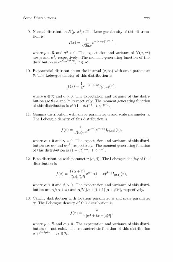
9. Normal distribution N(µ, σ2): The Lebesgue density of this distribu-tion is

f(x) =1√2πσ

e−(x−µ)2/2σ2,

where µ ∈ R and σ2 > 0. The expectation and variance of N(µ, σ2)are µ and σ2, respectively. The moment generating function of thisdistribution is eµt+σ2t2/2, t ∈ R.

10. Exponential distribution on the interval (a,∞) with scale parameterθ: The Lebesgue density of this distribution is

f(x) =1θe−(x−a)/θI(a,∞)(x),

where a ∈ R and θ > 0. The expectation and variance of this distri-bution are θ+a and θ2, respectively. The moment generating functionof this distribution is eat(1 − θt)−1, t < θ−1.

11. Gamma distribution with shape parameter α and scale parameter γ:The Lebesgue density of this distribution is

f(x) =1

Γ(α)γαxα−1e−x/γI(0,∞)(x),

where α > 0 and γ > 0. The expectation and variance of this distri-bution are αγ and αγ2, respectively. The moment generating functionof this distribution is (1 − γt)−α, t < γ−1.

12. Beta distribution with parameter (α, β): The Lebesgue density of thisdistribution is

f(x) =Γ(α + β)Γ(α)Γ(β)

xα−1(1 − x)β−1I(0,1)(x),

where α > 0 and β > 0. The expectation and variance of this distri-bution are α/(α + β) and αβ/[(α + β + 1)(α + β)2], respectively.

13. Cauchy distribution with location parameter µ and scale parameterσ: The Lebesgue density of this distribution is

f(x) =σ

π[σ2 + (x − µ)2],

where µ ∈ R and σ > 0. The expectation and variance of this distri-bution do not exist. The characteristic function of this distributionis e

√−1µt−σ|t|, t ∈ R.

xxvi Some Distributions

14. Log-normal distribution with parameter (µ, σ2): The Lebesgue den-sity of this distribution is

f(x) =1√

2πσxe−(log x−µ)2/2σ2

I(0,∞)(x),

where µ ∈ R and σ2 > 0. The expectation and variance of thisdistribution are eµ+σ2/2 and e2µ+σ2

(eσ2 − 1), respectively.

15. Weibull distribution with shape parameter α and scale parameter θ:The Lebesgue density of this distribution is

f(x) =α

θxα−1e−xα/θI(0,∞)(x),

where α > 0 and θ > 0. The expectation and variance of this distri-bution are θ1/αΓ(α−1 + 1) and θ2/αΓ(2α−1 + 1) − [Γ(α−1 + 1)]2,respectively.

16. Double exponential distribution with location parameter µ and scaleparameter θ: The Lebesgue density of this distribution is

f(x) =12θ

e−|x−µ|/θ,

where µ ∈ R and θ > 0. The expectation and variance of this distri-bution are µ and 2θ2, respectively. The moment generating functionof this distribution is eµt/(1 − θ2t2), |t| < θ−1.

17. Pareto distribution: The Lebesgue density of this distribution is

f(x) = θaθx−(θ+1)I(a,∞)(x),

where a > 0 and θ > 0. The expectation this distribution is θa/(θ−1)when θ > 1 and does not exist when θ ≤ 1. The variance of thisdistribution is θa2/[(θ − 1)2(θ − 2)] when θ > 2 and does not existwhen θ ≤ 2.

18. Logistic distribution with location parameter µ and scale parameterσ: The Lebesgue density of this distribution is

f(x) =e−(x−µ)/σ

σ[1 + e−(x−µ)/σ]2,

where µ ∈ R and σ > 0. The expectation and variance of thisdistribution are µ and σ2π2/3, respectively. The moment generatingfunction of this distribution is eµtΓ(1 + σt)Γ(1 − σt), |t| < σ−1.

Some Distributions xxvii

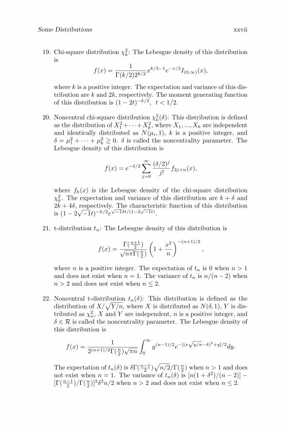
19. Chi-square distribution χ2k: The Lebesgue density of this distribution

is

f(x) =1

Γ(k/2)2k/2 xk/2−1e−x/2I(0,∞)(x),

where k is a positive integer. The expectation and variance of this dis-tribution are k and 2k, respectively. The moment generating functionof this distribution is (1 − 2t)−k/2, t < 1/2.

20. Noncentral chi-square distribution χ2k(δ): This distribution is defined

as the distribution of X21 + · · ·+X2

k , where X1, ..., Xk are independentand identically distributed as N(µi, 1), k is a positive integer, andδ = µ2

1 + · · · + µ2k ≥ 0. δ is called the noncentrality parameter. The

Lebesgue density of this distribution is

f(x) = e−δ/2∞∑

j=0

(δ/2)j

j!f2j+n(x),

where fk(x) is the Lebesgue density of the chi-square distributionχ2

k. The expectation and variance of this distribution are k + δ and2k + 4δ, respectively. The characteristic function of this distributionis (1 − 2

√−1t)−k/2e

√−1δt/(1−2√−1t).

21. t-distribution tn: The Lebesgue density of this distribution is

f(x) =Γ(n+1

2 )√nπΓ(n

2 )

(1 +

x2

n

)−(n+1)/2

,

where n is a positive integer. The expectation of tn is 0 when n > 1and does not exist when n = 1. The variance of tn is n/(n − 2) whenn > 2 and does not exist when n ≤ 2.

22. Noncentral t-distribution tn(δ): This distribution is defined as thedistribution of X/

√Y/n, where X is distributed as N(δ, 1), Y is dis-

tributed as χ2n, X and Y are independent, n is a positive integer, and

δ ∈ R is called the noncentrality parameter. The Lebesgue density ofthis distribution is

f(x) =1

2(n+1)/2Γ(n2 )

√πn

∫ ∞

0y(n−1)/2e−[(x

√y/n−δ)2+y]/2dy.

The expectation of tn(δ) is δΓ(n−12 )√

n/2/Γ(n2 ) when n > 1 and does

not exist when n = 1. The variance of tn(δ) is [n(1 + δ2)/(n − 2)] −[Γ(n−1

2 )/Γ(n2 )]2δ2n/2 when n > 2 and does not exist when n ≤ 2.

xxviii Some Distributions

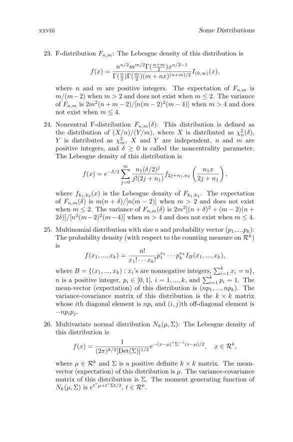
23. F-distribution Fn,m: The Lebesgue density of this distribution is

f(x) =nn/2mm/2Γ(n+m

2 )xn/2−1

Γ(n2 )Γ(m

2 )(m + nx)(n+m)/2 I(0,∞)(x),

where n and m are positive integers. The expectation of Fn,m ism/(m−2) when m > 2 and does not exist when m ≤ 2. The varianceof Fn,m is 2m2(n + m − 2)/[n(m − 2)2(m − 4)] when m > 4 and doesnot exist when m ≤ 4.

24. Noncentral F-distribution Fn,m(δ): This distribution is defined asthe distribution of (X/n)/(Y/m), where X is distributed as χ2

n(δ),Y is distributed as χ2

m, X and Y are independent, n and m arepositive integers, and δ ≥ 0 is called the noncentrality parameter.The Lebesgue density of this distribution is

f(x) = e−δ/2∞∑

j=0

n1(δ/2)j

j!(2j + n1)f2j+n1,n2

(n1x

2j + n1

),

where fk1,k2(x) is the Lebesgue density of Fk1,k2 . The expectationof Fn,m(δ) is m(n + δ)/[n(m − 2)] when m > 2 and does not existwhen m ≤ 2. The variance of Fn,m(δ) is 2m2[(n + δ)2 + (m − 2)(n +2δ)]/[n2(m−2)2(m−4)] when m > 4 and does not exist when m ≤ 4.

25. Multinomial distribution with size n and probability vector (p1,...,pk):The probability density (with respect to the counting measure on Rk)is

f(x1, ..., xk) =n!

x1! · · ·xk!px11 · · · pxk

k IB(x1, ..., xk),

where B = (x1, ..., xk) : xi’s are nonnegative integers,∑k

i=1 xi = n,n is a positive integer, pi ∈ [0, 1], i = 1, ..., k, and

∑ki=1 pi = 1. The

mean-vector (expectation) of this distribution is (np1, ..., npk). Thevariance-covariance matrix of this distribution is the k × k matrixwhose ith diagonal element is npi and (i, j)th off-diagonal element is−npipj .

26. Multivariate normal distribution Nk(µ,Σ): The Lebesgue density ofthis distribution is

f(x) =1

(2π)k/2[Det(Σ)]1/2 e−(x−µ)τΣ−1(x−µ)/2, x ∈ Rk,

where µ ∈ Rk and Σ is a positive definite k × k matrix. The mean-vector (expectation) of this distribution is µ. The variance-covariancematrix of this distribution is Σ. The moment generating function ofNk(µ,Σ) is etτ µ+tτΣt/2, t ∈ Rk.