MATHEMATICAL PROGRAMS WITHEQUILIBRIUM CONSTRAINTS: SOLUTION

TECHNIQUES FROM PARAMETRICOPTIMIZATION

Gemayqzel Bouza Allende

Composition of the Graduation Committee:Prof. Dr. R. Boucherie Universiteit TwenteProf. Dr. J. Guddat Humboldt UnversitatProf. Dr. H.Th. Jongen RWTH Aachen

Dr W. Kern Universiteit TwenteProf. Dr. J.J. Ruckmann Universidad de Las Americas

Dr. O. Stein RWTH AachenDr. G. Still Universiteit Twente

Prof. Dr. G.J. Woeginger TU Eindhoven&Universiteit Twente

MATHEMATICAL PROGRAMS WITH EQUILIBRIUM

CONSTRAINTS: SOLUTION TECHNIQUES FROM

PARAMETRIC OPTIMIZATION

PROEFSCHRIFT

ter verkrijging vande graad van doctor aan de Universiteit Twente,

op gezag van de rector magnificus,prof. dr. W.H.M. Zijm,

volgens besluit van het College voor Promotiesin het openbaar te verdedigen

op donderdag 1 juni 2006 om 13.15 uur

door

Gemayqzel Bouza Allende

geboren op 23 september, 1977La Habana, Cuba

Dit proeschrift is goedgekeurd doorProf. Dr. J. Guddat promotorProf. Dr. G.J. Woeginger promotor

Dr. G. Still assitent-promotor

Acknowledgements

First, I want to thank my supervisors Prof. Dr. Jurgen Guddat and Dr. GeorgStill. Prof. Dr. Guddat introduced me in the world of Parametric Optimizationand kindly accepted to supervise my diploma and master’s thesis in Cuba. Assupervisor he has always supported my work and has always tried to keep mein touch with the new results in the area. Scientific discussions with him werealways an fruitful experience, since they made me know how research can bedone. These years of work supervised by Dr. Still have been really pleasant. Hisideas were really insightful. Despite all the fears you may have in the beginning ofyour Ph.D., he makes you think that Math can be simple. Even when discussingon tough topics, he makes you feel confident, relaxed and motivated. These factshelped me at work, because, from the very beginning, I did not feel embarrassedwhen he corrected my mistakes. Of course there were bad moments, but thenI had also the personal support of both, looking for solutions, improving resultsand redaction and making things lighter.

I also want to thank Prof. Dr. Kees Hoede, who kindly volunteered to readthe manuscript, although he knew it will be a hard task. His suggestions allowedme to improve the initial version of the thesis.

Although I did not spend to much time working directly in the University ofTwente, I enjoyed my stays at the DWMP department. I want to thank DiniHeres, who always helped me with different procedures in a very efficient way.

I also want to thank my (former) professors, in Cuba. I am in debt with themfor the knowledge they gave me during my student years. In this period, I hadalso the support (sometimes electronic) of Dr. Luis Ramiro Pineiro, Dr. VivianSistachs and the members of the groups of Numeric Analysis and Optimizationof U.H. (I will not mention the names because the list will be huge). Sometimesthe words of Loretta, Roxana, Maribel Freyre, Dr. Josefina Martinez, FrancisFuster and friends from ITC-CF and BS-UT, here in Enschede, helped me to goahead despite difficulties.

Finally I want to thank my family, who patiently heard (or read) all mydifficulties and give me an special strength to continue, even when difficultiesappeared. Specially thanks to my grandmother and my parents for putting loveover their own wishes, advising me well and accepting my decisions.

i

ii

Abstract

Equilibrium constrained problems form a special class of mathematical programswhere the decision variables satisfy a finite number of constraints together withan equilibrium condition. Optimization problems with a variational inequalityconstraint, bilevel problems and semi-infinite programs can be seen as particularcases of equilibrium constrained problems. Such models appear in many practicalapplications.

Equilibrium constraint problems can be written in bilevel form with possi-bly a finite number of extra inequality constraints. This opens the way to solvethese programs by applying the so-called Karush-Kuhn-Tucker approach. Herethe lower level problem of the bilevel program is replaced by the Karush-Kuhn-Tucker condition, leading to a mathematical program with complementarity con-straints (MPCC). Unfortunately, MPCC problems cannot be solved by classicalalgorithms since they do not satisfy the standard regularity conditions. To solveMPCCs one has tried to conceive appropriate modifications of standard methods.For example sequential quadratic programming, penalty algorithms, regulariza-tion and smoothing approaches.

The aim of this thesis is twofold. First, as a basis, MPCC problems willbe investigated from a structural and generical viewpoint. We concentrate on aspecial parametric smoothing approach to solve these programs. The convergencebehavior of this method is studied in detail. Although the smoothing approach iswidely used, our results on existence of solutions and on the rate of convergenceare new. We also derive (for the first time) genericity results for the set ofminimizers (generalized critical points) for one-parametric MPCC.

In a second part we will consider the MPCC problem obtained by applying theKKT-approach to equilibrium constrained programs and bilevel problems. Wewill analyze the generic structure of the resulting MPCC programs and adapt therelated smoothing method to these particular cases. All corresponding results arenew.

iii

iv

Contents

Acknowledgements i

Abstract iii

Contents v

1 Introduction 11.1 Introduction . . . . . . . . . . . . . . . . . . . . . . . . . . . . . . 11.2 Relations between the problems . . . . . . . . . . . . . . . . . . . 41.3 Summary of the results . . . . . . . . . . . . . . . . . . . . . . . . 71.4 Applications . . . . . . . . . . . . . . . . . . . . . . . . . . . . . . 11

1.4.1 Applications in economics . . . . . . . . . . . . . . . . . . 111.4.2 Applications from mathematical physics . . . . . . . . . . 13

2 Theoretical background 172.1 Notations and basic results . . . . . . . . . . . . . . . . . . . . . . 172.2 Finite programming problems . . . . . . . . . . . . . . . . . . . . 182.3 Preliminaries from topology . . . . . . . . . . . . . . . . . . . . . 212.4 One-parametric optimization . . . . . . . . . . . . . . . . . . . . . 23

3 Variational Inequality Problems 293.1 Introduction . . . . . . . . . . . . . . . . . . . . . . . . . . . . . . 293.2 The KKT approach for variational inequalities . . . . . . . . . . . 30

3.2.1 Relations between Stampaggia and Minty variational in-equalities . . . . . . . . . . . . . . . . . . . . . . . . . . . 32

3.3 One-parametric variational inequalities . . . . . . . . . . . . . . . 343.4 Embeddings for variational inequalities . . . . . . . . . . . . . . . 36

3.4.1 Standard embedding . . . . . . . . . . . . . . . . . . . . . 383.4.2 Penalty embedding . . . . . . . . . . . . . . . . . . . . . . 43

4 Problems with complementarity constraints 474.1 Introduction . . . . . . . . . . . . . . . . . . . . . . . . . . . . . . 474.2 Structure of the feasible set . . . . . . . . . . . . . . . . . . . . . 494.3 Necessary optimality conditions . . . . . . . . . . . . . . . . . . . 50

v

4.4 Optimality conditions based on the disjunctive structure . . . . . 544.4.1 Genericity results for non-parametric PCC . . . . . . . . . 544.4.2 Optimality conditions for problems PCC . . . . . . . . . . 55

4.5 A parametric solution method . . . . . . . . . . . . . . . . . . . . 574.5.1 Motivating examples . . . . . . . . . . . . . . . . . . . . . 594.5.2 The convergence behavior of the feasible set . . . . . . . . 604.5.3 Convergence results for minimizers . . . . . . . . . . . . . 68

4.6 JJT-regularity results for Pτ . . . . . . . . . . . . . . . . . . . . . 744.7 Parametric problem . . . . . . . . . . . . . . . . . . . . . . . . . . 81

4.7.1 Structure for the special case n = l, q = q0 = 0 . . . . . . . 814.7.2 One parametric PCC . . . . . . . . . . . . . . . . . . . . . 86

5 Bilevel problems 1015.1 Introduction . . . . . . . . . . . . . . . . . . . . . . . . . . . . . . 1015.2 Genericity analysis of the KKT approach . . . . . . . . . . . . . . 1035.3 A numerical approach for solving BL . . . . . . . . . . . . . . . . 1205.4 Numerical examples . . . . . . . . . . . . . . . . . . . . . . . . . . 124

6 Equilibrium constrained problems 1276.1 Introduction . . . . . . . . . . . . . . . . . . . . . . . . . . . . . . 1276.2 Structure of the feasible set . . . . . . . . . . . . . . . . . . . . . 1286.3 Genericity analysis of the KKT approach to EC . . . . . . . . . . 1306.4 Convex case . . . . . . . . . . . . . . . . . . . . . . . . . . . . . . 1326.5 Linear equilibrium constrained problems . . . . . . . . . . . . . . 135

6.5.1 Genericity results. . . . . . . . . . . . . . . . . . . . . . . . 1376.5.2 Algorithm. . . . . . . . . . . . . . . . . . . . . . . . . . . . 143

7 Final remarks 149

Bibliography 151

List of Figures 157

Index 158

vi

Chapter 1

Introduction

1.1 Introduction

An Equilibrium Constrained optimization problem (EC) is a mathematical pro-gram such that a part of the variables should satisfy an equilibrium condition. Inits simplest form, an equilibrium condition is given by the critical point equation∇φ(y) = 0. So the simplest prototype of an EC is:

min f(x, y) (1.1.1)

s.t. ∇yφ(x, y) = 0,

where f : Rn×Rm → R, φ : Rn×Rm → R and∇yφ denotes the partial derivativesof φ with respect to y. For the case that φ(x, y) is convex in y, it can be expressedequivalently as a so-called Bilevel problem (BL):

min f(x, y)s.t. y solves min

y∈Rmφ(x, y).

More generally, we are led to consider BL problems of the following form:

min f(x, y)s.t. (x, y) ∈ C,

y solves Q(x),Q(x) : min

y∈Y (x)φ(x, y),

(1.1.2)

where f, φ : Rn × Rm → R and Y (x) is the feasible set the lower level problemsQ(x) depending on x.

Another classical example of BL arises when considering an equilibrium pointin a 0-sum game with two players. Let us assume that player i may choosestrategies yi from the set Yi ⊂ Rm, i = 1, 2, and that the utility functions areg(y1, y2) for player 1 and −g(y1, y2) for player 2, if player i chooses strategy

1

yi, i = 1, 2. The Nash equilibrium points (y1, y2) are saddle points of g(y1, y2),i.e.,

g(y1, y2) ≥ g(y1, y2) ≥ g(y1, y2), for all y1 ∈ Y1, y2 ∈ Y2,

ory1 solves max

y1∈Y1

g(y1, y2) and y2 solves miny2∈Y2

g(y1, y2).

If we want to minimize a function f(x, y1, y2) under the condition that (y1, y2)are Nash equilibrium points of the previous game, the model becomes a bilevelproblem of the type:

min f(x, y1, y2)s.t. y1 solves max

y1∈Y1

g(y1, y2),

y2 solves miny2∈Y2

g(y1, y2)

with functions f : Rn × Rm × Rm → R, g : Rm × Rm → R.More generally we could consider bilevel problems of the form:

min f(x, y1, . . . , yk)s.t. (x, y1, yk) ∈ C,

yi solves Qi(x), whereQi(x) : min

yi∈Yi(x)φi(x, y1, . . . , yi−1, yi, yi+1, . . . , yk), i = 1, . . . , k.

For simplicity, in this thesis we will only consider the case k = 1, i.e. bilevelproblems of type (1.1.2).

Under smoothness and convexity conditions, a minimizer y of the problemQ(x) in (1.1.2) satisfies the inequality ∇yφ(x, y)T (z − y) ≥ 0, ∀z ∈ Y (x). Moregenerally we examine the so-called variational inequalities

V I : Find y ∈ Y (x) such that Φ(x, y)T (z − y) ≥ 0, ∀z ∈ Y (x),

and we are led to optimization problems of the form

PV I : min f(x, y)s.t. (x, y) ∈ C,

y ∈ Y (x),Φ(x, y)T (z − y) ≥ 0, ∀z ∈ Y (x),

or more generally to

PEC : min f(x, y)s.t. (x, y) ∈ C,

y ∈ Y (x),φ(x, y, z) ≥ 0, ∀z ∈ Y (x),

where f : Rn × Rm → R, φ : Rn × Rm × Rm → R.

2

Remark 1.1.1 PEC can be regarded as a particular case of a Generalized Semi-infinite Optimization Problem

GSIP : min f(x, y) | (x, y) ∈ C, φ(x, y, z) ≥ 0, ∀z ∈ Y (x) . (1.1.3)

Note that PEC contains the additional condition y ∈ Y (x).

The problems considered so far will be called equilibrium constrained problems.We emphasize that in general it is difficult to solve these problems. Due to the

two level structure, even to check feasibility, we have to compute a (global) min-imizer of a general optimization problem or a solution of a variational inequalityproblem.

In this thesis we will deal with the analytic and generic structure of problemsPBL, PV I , and PEC and we are also interested in numerical solution methods.For numerical purposes it is natural to assume that the involved sets Y (x) and Care described analytically. Throughout the thesis we will assume that these setsare defined as:

Y (x) = y ∈ Rm | vi(x, y) ≥ 0, i = 1, . . . , l , (1.1.4)

C = (x, y) ∈ Rn × Rm | gj(x, y) ≥ 0, j = 1, . . . , q , (1.1.5)

with given functions vi and gj, i = 1, . . . , l, j = 1, . . . , q.

So we will consider bilevel problems of the form

PBL : minx,y

f(x, y)

s.t. gj(x, y) ≥ 0, j = 1, . . . , q,y solves Q(x),

Q(x) : miny

φ(x, y)

s.t. y ∈ Y (x)

(1.1.6)

with sets Y (x) defined as in (1.1.4) and functions f, φ, vi, gj : Rn × Rm → R,i = 1, . . . , l, j = 1, . . . , q. The parametric problem Q(x) will be called the lowerlevel problem.

Problems with equilibrium constraints are examined in the form

PEC : minx,y

f(x, y)

s.t. gj(x, y) ≥ 0, j = 1, . . . , q,y ∈ Y (x),

φ(x, y, z) ≥ 0, ∀z ∈ Y (x),

(1.1.7)

where f, vi, gj : Rn×Rm → R, i = 1, . . . , l, j = 1, . . . , q, φ : Rn×Rm×Rm → Rand Y (x) is defined as in (1.1.4).

3

As a particular case, in which the function φ satisfies the conditionφ(x, y, y) = 0, ∀(x, y), we consider the problem with variational inequalitiesconstraints

PV I : minx,y

f(x, y)

s.t. gj(x, y) ≥ 0, j = 1, . . . , q,y ∈ Y (x),

Φ(x, y)T (z − y) ≥ 0, ∀z ∈ Y (x).

(1.1.8)

Another related type of optimization problems are the so-called MathematicalPrograms with Complementarity Constraints (MPCC)

PCC : min f(x)s.t. gj(x) ≥ 0, j = 1, . . . , q,

ri(x) ≥ 0, i = 1, . . . , l,si(x) ≥ 0, i = 1, . . . , l,

ri(x)si(x) = 0, i = 1, . . . , l.

(1.1.9)

As we shall see later on, we will obtain problems of this type if we apply theKarush Kuhn Tucker (KKT) approach to the problems PBL, PV I and PEC . Asa solution method for problems (1.1.9), in the present thesis we will investigatethe so-called one-parametric smoothing approach. In this approach, we considerthe perturbation of PCC (1.1.9)

Pτ : min f(x)s.t. gj(x) ≥ 0, j = 1, . . . , q,

ri(x) ≥ 0, i = 1, . . . , l,si(x) ≥ 0, i = 1, . . . , l,

ri(x)si(x) = τ, i = 1, . . . , l,

(1.1.10)

where τ > 0 is the perturbation parameter. Then Pτ is solved for τ → 0+.

1.2 Relations between the problems

We have already pointed out some connections between the problems PV I , PEC ,PBL and PCC . The aim of this section is to analyze these relations further. Weassume obvious differentiability conditions on the problem functions.

Let us consider the relations between PEC and PBL (see also Stein and Still[59]). By using the fact:

φ(x, y, z) ≥ 0, ∀z ∈ Y (x) ⇔ z ∈ arg minu∈Y (x)

φ(x, y, u) and φ(x, y, z) ≥ 0,

4

the problem PEC turns into the bilevel problem:

minx,y,z

f(x, y)

s.t. gj(x, y) ≥ 0, j = 1, . . . , q,y ∈ Y (x),

φ(x, y, z) ≥ 0,z solves Q(x, y),

Q(x, y) : minφ(x, y, u)s.t. u ∈ Y (x).

(1.2.1)

In the particular case of PEC where φ(x, y, y) = 0, ∀y (e.g. the problems PV I)we can eliminate the variable z as follows. In view of φ(x, y, y) = 0, the conditionφ(x, y, z) ≥ 0, ∀z ∈ Y (x), is equivalent with the fact that y is a global solutionof Q(x, y). So, in this case, PEC is equivalent with:

minx,y

f(x, y)

s.t. gj(x, y) ≥ 0, j = 1, . . . , q,y ∈ Y (x),

y solves Q(x, y),Q(x, y) : min

zφ(x, y, z)

s.t. z ∈ Y (x).

(1.2.2)

Note that this problem has a more complicated structure than PBL, since itcontains a sort of fixed point condition. Indeed, the lower level problem Q(x, y)depends on y, which at the same time should solve Q(x, y). For a comparisonfrom the structural and generical viewpoint between linear PBL and PEC , we referto Birbil, Bouza, Frenk and Still [7] and Still [61].

We now apply the KKT approach to the above bilevel problems. The idea isto replace the minimum condition for the lower level problem Q(x), or Q(x, y),by the KKT optimality condition. This will lead to problems of type PCC .

We begin with the standard bilevel problem PBL in (1.1.6). Let some con-straint qualification such as MFCQ (see Definition 2.2.2) hold for the lower levelproblem Q(x). Then a (local) minimizer of Q(x) will necessarily satisfy theKKT conditions, i.e., the feasible points (x, y) of PBL will fulfill the followingconstraints with some multiplier vector λ ∈ Rl:

∇yφ(x, y)−l∑

i=1

λi∇yvi(x, y) = 0,

vi(x, y) ≥ 0, i = 1, . . . , l, (1.2.3)

λi ≥ 0, i = 1, . . . , l,

vi(x, y)λi = 0, i = 1, . . . , l.

5

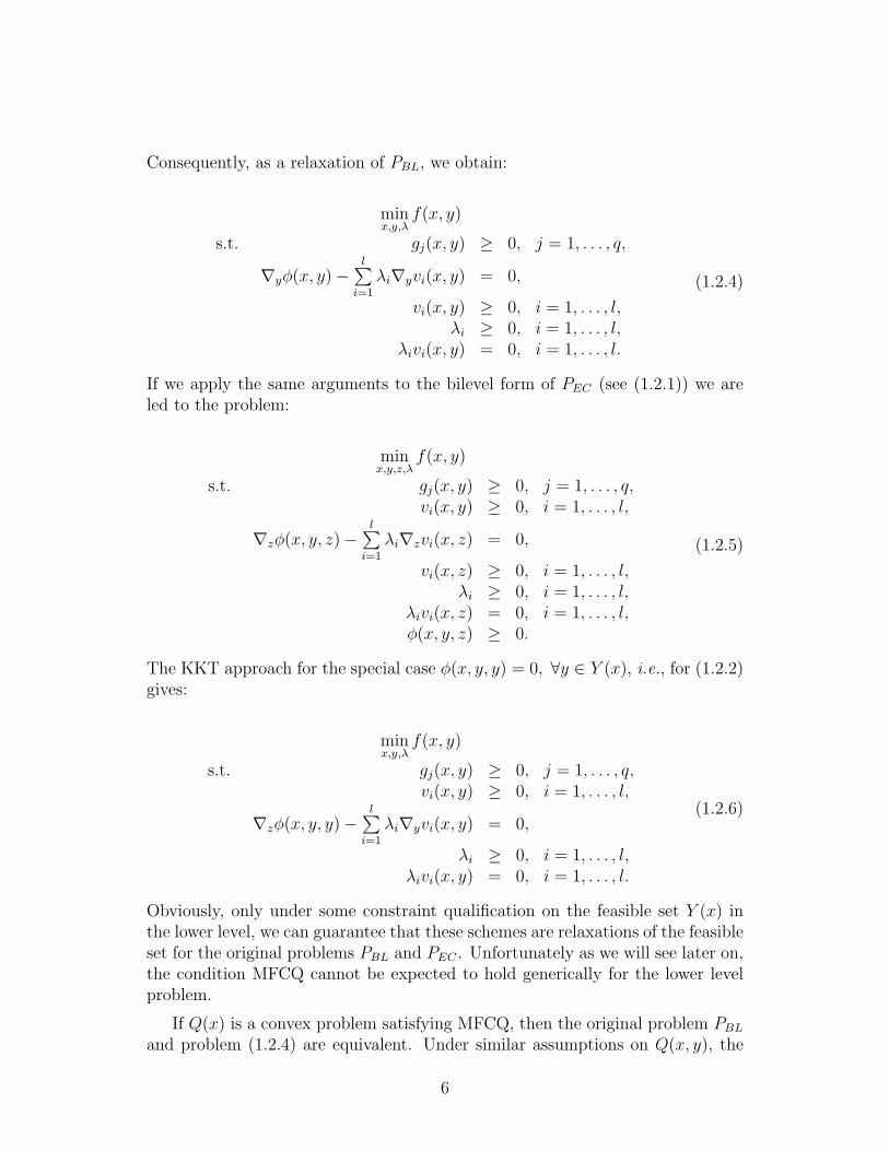
Consequently, as a relaxation of PBL, we obtain:

minx,y,λ

f(x, y)

s.t. gj(x, y) ≥ 0, j = 1, . . . , q,

∇yφ(x, y)−l∑

i=1

λi∇yvi(x, y) = 0,

vi(x, y) ≥ 0, i = 1, . . . , l,λi ≥ 0, i = 1, . . . , l,

λivi(x, y) = 0, i = 1, . . . , l.

(1.2.4)

If we apply the same arguments to the bilevel form of PEC (see (1.2.1)) we areled to the problem:

minx,y,z,λ

f(x, y)

s.t. gj(x, y) ≥ 0, j = 1, . . . , q,vi(x, y) ≥ 0, i = 1, . . . , l,

∇zφ(x, y, z)−l∑

i=1

λi∇zvi(x, z) = 0,

vi(x, z) ≥ 0, i = 1, . . . , l,λi ≥ 0, i = 1, . . . , l,

λivi(x, z) = 0, i = 1, . . . , l,φ(x, y, z) ≥ 0.

(1.2.5)

The KKT approach for the special case φ(x, y, y) = 0, ∀y ∈ Y (x), i.e., for (1.2.2)gives:

minx,y,λ

f(x, y)

s.t. gj(x, y) ≥ 0, j = 1, . . . , q,vi(x, y) ≥ 0, i = 1, . . . , l,

∇zφ(x, y, y)−l∑

i=1

λi∇yvi(x, y) = 0,

λi ≥ 0, i = 1, . . . , l,λivi(x, y) = 0, i = 1, . . . , l.

(1.2.6)

Obviously, only under some constraint qualification on the feasible set Y (x) inthe lower level, we can guarantee that these schemes are relaxations of the feasibleset for the original problems PBL and PEC . Unfortunately as we will see later on,the condition MFCQ cannot be expected to hold generically for the lower levelproblem.

If Q(x) is a convex problem satisfying MFCQ, then the original problem PBL

and problem (1.2.4) are equivalent. Under similar assumptions on Q(x, y), the

6

problem PEC in (1.2.1) is equivalent with the KKT relaxation (1.2.5) and, in caseφ(x, y, y) = 0, ∀y ∈ Y (x), x ∈ Rn, the equivalence holds between PEC in (1.2.2)and problem (1.2.6).

So, this KKT approach opens the way for solving PBL and PEC via programswith complementarity constraints of type PCC (1.1.9).

1.3 Summary of the results

In the present subsection we give a summary of the thesis. We try to sketch theresults also in comparison with earlier investigations. Throughout the expositionall earlier results (lemmas, theorems, propositions) are indicated by giving (atleast) one reference. All results where such a reference does not appear, are (atleast for a substantial part) new.

In essence, the main aim of the thesis is as follows:

• MPCC problems (cf. (1.1.9)) and the parametric smoothing approach forsolving these programs (cf. (1.1.10)) are investigated from a structural andgenerical viewpoint.

• We apply the KKT approach to different types of equilibrium constrainedproblems (VI, BL and EC-problems). Thereby the equilibrium constrainedprograms are transformed into a problem of MPCC type with special struc-ture, cf. Section 1.2. We analyze the generic properties of the resultingMPCC programs and study the behavior of the related parametric smooth-ing method.

The investigations on the analytic and generic structure of mathematical pro-grams, form the basis for the development of any general purpose solution method.In fact the generic structure reveals the typical properties of a problem.

More detailed, the thesis is organized as follows. In Section 1.4, some appli-cations of equilibrium constrained problems are presented.

The investigations of the whole exposition are based on the deep genericityresults for (non-parametric and parametric) finite programming problems devel-oped during the last two decades, starting with the work of Jongen, Jonker andTwilt in [27]-[28]. Further results appear in Guddat, Guerra and Jongen in [22],Gomez, Guddat, Jongen, Ruckmann and Solano in [21], and Jongen, Jonker andTwilt in [29]. The basic concepts and results are outlined in Chapter 2.

Chapter 3 is devoted to Variational Inequality problems (VI). In Section 3.2,the KKT approach to solve VI is described. Section 3.3 summarizes the genericityresults of Gomez [19] for this approach, applied to one-parametric VI problems.

7

In Section 3.4, we extend two different types of parametric embeddings for nonlin-ear programs (the standard embedding and the penalty embedding, see Gomez,Guddat, Jongen, Ruckmann and Solano [21]) to the VI case. We analyze thesesolution methods from a structural and generical perspective. As new results, wecan mention Proposition 3.2.1 (partially new), Example 3.2.2 and the genericityanalysis of the one-parametric embeddings in Propositions 3.4.1-3.4.4.

Chapter 4 deals with general MPCC-problems of the form PCC in (1.1.9).This is a topic of intensive recent research, see e.g. Scheel and Scholtes [49],Scholtes [51], Lin and Fukushima [37], Hu and Ralph [24] and the references inthese contributions.

Firstly we discuss the structure of the feasible set in Section 4.2 (see e.g. Luo,Pang and Ralph [42]) and give some well-known necessary optimality conditionsin Section 4.3 (see Flegel and Kanzow [14]). Section 4.4 derives other necessaryand sufficient conditions for minimizers of order one and two of MPCC, basedon the disjunctive structure, and sketches basic genericity results. Partially theseresults are due to Scholtes and Stohr [53]. The optimality conditions for minimizerof order one in Theorem 4.4.2 and 4.4.3 are new (in the MPCC context) and alsothe only part of Theorem 4.4.4. Section 4.5 is concerned with the convergencebehavior of the parametric smoothing approach Pτ for τ → 0 in (1.1.10). Thisapproach has been studied in Fukushima and Pang [16] from another point ofview. It has been investigated under which conditions the KKT solutions of Pτ

converges to a B-stationary point of PCC . In Stein and Still [60], such resultswere obtained for a similar (interior point) approach for solving semi-infiniteprogramming problems. In this thesis we derive new convergence results for thewhole feasible set and for (local) solutions x(τ) of Pτ for τ → 0, see Lemmas 4.5.2,4.5.3 and Theorem 4.5.1. It is shown that under natural assumptions the rate ofconvergence is O(

√τ). We also give some illustrative Examples 4.5.2-4.5.3.

In Section 4.6 we prove that generically Pτ is regular in the sense of Jon-gen, Jonker, Twilt (JJT), see Definition 2.4.7. These investigations are entirelynew, see as main results Propositions 4.6.1-4.6.2. Section 4.7 deals with one-parametric MPCC problems. In the first part we discuss the one-parametric andnon-parametric (feasibility) problem for the special case n = l. The related newresults are given in Propositions 4.7.1-4.7.4. The second part is devoted to thegeneral one-parametric MPPC problem. In Hu and Ralph [24], this problem hasbeen analyzed only locally around non-degenerate minimizers. In this thesis, wedevelop the global theory and, based on the results of Jongen, Jonker and Twiltin [27]-[28] for nonlinear programs, we are able to describe the characteristics ofgeneric one parametric MPCC programs and their singularities. The correspond-ing new results are contained in Lemma 4.7.3, Theorem 4.7.1. The analysis ofthe behavior of the set of stationary points around each singularity is also new.

Chapter 5 is devoted to bilevel problems, see (1.1.2). These problems have

8

been extensively studied during the last two decades. We refer the reader e.g.to Shimizu and Aiyoshi [55], Bard [3], Luo, Pang and Ralph [42], Dempe [11]and the references therein. It is well-known that in general the structure of BLdoes not allow a local reduction to common finite programs. So special solutionmethods have to be conceived.

In this thesis we consider the KKT approach to solve BL which consists ofa transformation of BL into a special structured MPCC problem (cf. (1.2.4)).This approach has been discussed earlier see e.g. Shimizu and Aiyoshi [55] forthe general case and Stein [58], in connection with semi-infinite problems.

The new contribution of the present thesis is to analyze for the first time theMPCC form of BL programs from a generical viewpoint. This allows to applythe results obtained for MPCC problems in Chapter 4. All results of Section 5.2and 5.3 are new.

In Theorem 5.2.1 of Section 5.2, we show that generically MPCC-LICQ (seeDefinition 4.3.1) holds at all feasible points of the MPCC form of BL. Howevera counterexample reveals that, in contrast to general MPCC problems, for theMPCC form of BL programs the condition MPCC-SC in Definition 4.3.3, is notgenerically fulfilled at minimizers. It follows that the structural difficulties ofthe original BL problem partially reappear in the MPCC formulation. Roughlyspeaking this may happen at solutions of BL where a local reduction to a finitestandard problem is not possible.

Theorem 5.2.2 describes the precise generic structure around a critical point.Corollaries 5.2.3-5.2.5 reveal the relation between (the solutions of) the originalBL and the MPCC form. An example describes a possible bad behavior of theKKT approach. It appears that even in the case of convex lower level problemsit may happen that (x, y, λ) is a minimizer of the KKT form but that the feasiblepoint (x, y) is not a minimizer of the original problem. This bad behavior isstable w.r.t. small smooth perturbations. Based on the results of Section 5.2, inSection 5.3 we discuss the parametric approach for solving the MPCC formulationof BL. This leads to convergence results in Proposition 5.3.1 Also here a stablecounterexample (Example 5.3.1) shows that it is not always possible to approacheach minimizer (x, y, λ) of the KKT formulation by the parametric smoothingprocedure.

A part of our investigation was not yet completely finished at the time whenthe preliminary version of the thesis was send to the members of the DoctorateCommittee. In the meantime this part has been completed and we would like toadd it to the thesis as a supplement (Chapter 6).

In Chapter 6 equilibrium constrained problems EC (see (1.1.7)) are examined.Also this class of mathematical programs is a topic of intensive research in thepast and at present. We refer the reader e.g. to the books Outrata, Kocvara andZowe [43] and Luo, Pang and Ralph [42].

Here we are mainly interested in the structural and generical properties of such

9

problems which are closely related to generalized semi-infinite programs (GSIP).In fact, EC programs can be seen as GSIP in the unknown (x, y) (see (1.1.3))with the extra condition y ∈ Y (x). Many investigations have been conducted onstability and the generic structure of semi-infinite problems. See e.g. Jongen andZwier [34]-[33], Jongen, Twilt and Weber [32], Stein [57], Jongen and Ruckmann[30] and Jongen and Ruckmann [31] for common semi-infinite problems (SIP)(i.e. Y (x) = Y, ∀x) and Stein [58], Still [61], for GSIP.

In this thesis we are mainly devoted to the study of the generic properties ofthe KKT approach for solving EC. We continue the investigations started withthe paper Birbil, Bouza, Frenk and Still [7] where only a special (linear) case wasconsidered.

The Chapter is organized as follows. In Section 6.2 the topological structureof the feasible set of EC is discussed. As in GSIP it appears that the feasibleset need even not to be closed in general. The results here were obtained in[7] (see also Stein [58] for GSIP). In Section 6.3 and 6.4 the MPCC formulationof EC (cf. (1.2.5) is analyzed for the first time from a generical viewpoint. Astable counterexample, Example 6.3.1, reveals that in contradiction to BL herethe condition MPCC-LICQ (see Definition 4.3.1) is not generically fulfilled forall feasible points. This is due to the extra constraint y ∈ Y (x) in EC.

So, in Section 6.4 we restrict ourselves to the class of EC problems with con-vex lower level program Q(x, y) (see (1.2.1)) and satisfying additional regularityassumptions. For this class the MPCC formulation of EC (cf. (1.2.5)) is provento be generically regular in the MPCC sense, see Definition 4.3.3. The corre-sponding new results are contained in Proposition 6.4.1 and Theorem 6.4.1.

In Section 6.5, we consider the special linear case, i.e. EC programs suchthat the MPCC form is given by only linear functions. Such problems havealso been studied in [7] where the generic structure of the feasible set of theoriginal EC program has been described. For this linear class, the structure ofthe KKT approach for EC appears to be similar to the structure for (linear)bilevel problems. So, by modifying the ideas in the proof of Theorems 5.2.1 and5.2.2, we can show in Proposition 6.5.1 that MPCC-LICQ is a generic propertyand in Theorem 6.5.1, we describe the structure around local minimizers in thegeneric situation. The consequences of these results for the original EC programare shown in Corollary 6.5.2 and Proposition 6.5.2.

Finally based on the obtained genericity results, we describe a new algorithmfor solving linear EC problems. The algorithm makes use of the MPCC formand performs descent steps on (faces of) the feasible set of the correspondingprogram. The finite algorithm (eventually) ends up with a local minimizer of theoriginal EC.

10

1.4 Applications

In this section we present a few applications of equilibrium constrained problems.We will consider two main fields, namely applications in economics and applica-tions in mathematical physics. They are mainly taken from [43], see [3] for otherexamples.

1.4.1 Applications in economics

We start with two situations where optimization problems with equilibrium con-straints arise, the Cournot competitive equilibrium and the generalized Nashequilibrium. We begin with some notations and present different ways of model-ing Nash equilibrium points.

Nash equilibrium

Consider a game with n players. For i = 1, 2, . . . , n the set of all possible strategiesfor player i is denoted by Yi ⊂ Rmi . If for all j, the player j chooses strategyyj ∈ Yj, the payoff for player i is equal to ui(y1, . . . , yn). We assume ui to be aconcave C1-function in the variable yi.

A Nash equilibrium point y = (y1, . . . , yn) satisfies:

yi solves maxyi∈Yi

ui(y1, . . . , yi−1, yi, yi+1, . . . yn), ∀i.

In case that, for any i, the set Yi is a non-empty, closed and convex set, the previ-ous optimization problems are convex. Consequently, another way of expressingthat y is a Nash equilibrium is via the following variational inequality. The pointy is a Nash equilibrium if and only if:

y ∈ Y,such that 〈F (y), v − y〉 ≥ 0, ∀v ∈ Y = Y1 × Y2 × . . .× Yn

(1.4.1)

where

F (y) =

−∇y1u1(y)...

−∇ynun(y)

.

Now, as a first application, we will present an optimization problem in which thefeasible set is described by a Nash equilibrium.

Cournot equilibrium

In this model, there are n firms producing a certain good. Each firm has to decidehow many units of the product it will produce. The decision of firm i is denoted

11

by yi. The price of the product is P (T ), where T denotes the total amount ofthe good in the market, i.e., T =

∑ni=1 yi. The cost of producing yi units for the

firm i is described by fi(yi). Its profit is then given by ui(y) = yip(T ) − fi(yi).Of course, here we have Yi ⊂ R+.

Suppose the firm 1 places its production in the market, say y1, first. Knowingthis value, the other firms will plan their productions in order to maximize theirprofits. The first firm must decide the value of y1 that maximizes its profit underthese circumstances. Then it will solve the bilevel problem:

minx,y

f1(x)− xp(x+n∑

j=2

yj)

s.t. x ∈ Y1,and for i = 2, . . . , n

yi solves minzfi(z)− zp(x+

i−1∑j=1

yi + z +n∑

j=i+1

yi)

s.t. z ∈ Yi,

(1.4.2)

Of course if fi(yi)− yip(x +∑n

i=1 yi) ∈ C1 are convex functions of yi and Yi areconvex sets, i = 1, . . . , n, the system (1.4.1) characterizes the equilibrium pointsas solutions of a variational inequality problem. Then we find the equivalentformulation as a PV I :

minx,y

f1(x)− xp(x+n∑

j=2

yj)

s.t. x ∈ Y1,yi ∈ Yi i = 2, . . . , n,

〈F (x, y2, . . . , yn), z − (y2, . . . , yn)T 〉 ≥ 0, ∀z ∈ Y2 × Y3 × . . .× Yn,

where F : Rn → Rn−1 is given by Fi(x, y2, . . . , yn) = f ′i+1(yi+1)−p(T )−yi+1p′(T ),

i = 1, . . . , n− 1 and T = x+n∑

i=2

yi.

Generalized Nash equilibrium problem

In this example we consider a game of n players, where the payoff of player i isdescribed by the function ui, i = 1, 2, . . . , n and the strategies of player i dependon the decisions of the other players. The set of feasible strategies for player i is

Yi(y−i) =

yi ∈ Rmi

∣∣∣∣ gji (yi, y−i) ≥ 0, j = 1, . . . , qi,

gji (yi) ≥ 0, j = 1, . . . , li

if the player j chooses strategy yj for j = 1, . . . i − 1, i + 1, . . . n. Herey−i = (y1, . . . , yi−1, yi+1, . . . , yn). Now the problem is to find y = (y1, . . . , yn)

12

such that, for i = 1, 2, . . . , n,

yi solves maxzui(y1, . . . , yi−1, z, yi+1, . . . , yn)

s.t. z ∈ Yi(y−i).

If we assume that ui is concave in the variable yi and the sets Yi(y−i) are non-empty and convex, the previous model is equivalent to the problem of findingy:

yi ∈ Yi(y−i),such that 〈−∇yi

ui(y), yi − yi〉 ≥ 0, ∀yi ∈ Yi(y−i), i = 1, . . . , n

which is equivalent with finding (y, x) such that:

y ∈ Y (x),〈F (y), y − y〉 ≥ 0, ∀y ∈ Y (x),

x = y,(1.4.3)

where F (y) =

−∇y1u1(y)...

−∇ynun(y)

and Y (x) = Y (x−1)× Y (x−2)× . . .× Y (x−n).

If we write the constraint x = y as min ‖x−y‖2, we have the following formulationof the generalized Nash equilibrium problem as a PV I :

minx,y

‖x− y‖2

s.t. y ∈ Y (x),〈F (y), z − y〉 ≥ 0, ∀z ∈ Y (x).

(1.4.4)

Of course y will be a generalized Nash equilibrium point if and only if (y, y) solvesthe previous problem.

1.4.2 Applications from mathematical physics

One way of finding approximate solutions of control problems is by discretizingthe domain and solving an approximate nonlinear problem. In this part wewill present equilibrium problems appearing when solving control models by adiscretization approach, cf. [43]. Let us first fix some notations. We assumethat α is a function which is differentiable almost everywhere (a.e.). The set offeasible functions is:

U =

α : [0, 1] → [c1, c2]

∣∣∣∣ |∂α∂x (x)| ≤ c3, a.e., x ∈ [0, 1]

.

For α ∈ U , the set Ωα is defined as x ∈ R2 | x1 ∈ [0, 1], 0 < x2 < α(x1). Itsarea will be J(α).

13

Ω0 denotes a fixed domain, that is assumed to be included in (0, 1)× (0, c1). Forfixed α ∈ U , u describes the deformation, by a force f , of a membrane in Ωα. Onthe boundary of Ωα, the membrane is not deformed, i.e,

u(x) = 0, x ∈ ∂Ωα. (1.4.5)

Packaging problem with rigid obstacle

In this problem, given χ, f : [0, 1] × [0, c2] → R, f, χ ∈ L2([0, 1] × [0, c2]), wehave to find α, α ∈ U , that minimizes the area J(α) of Ωα, under the conditionsthat there is a membrane in Ωα, given by u, deformed by f , such that (1.4.5) issatisfied. The membrane lies over the rigid object described by the function χand it has to be in contact with this object in the fixed set Ω0. The model thenis:

minu,α

J(α)

s.t. −∆u(x) ≥ f(x), a.e. in Ωα,u(x) ≥ χ(x), x ∈ Ωα,

(∆u(x) + f(x))(u(x)− χ(x)) = 0, a.e. in Ωα,u(x) = 0, ∀x ∈ ∂Ωα,

Ω0 ⊂ Z(α),α ∈ U,

where u denotes the deformation of the membrane, ∆u the Laplacian of u andZ(α) = x ∈ Ωα | u(x) = χ(x).

In order to solve this problem, the condition Ω0 ⊂ Z(α) is eliminated via apenalty approach and the objective function becomes: J(α)+r

∫Ω0

(u(ξ)−χ(ξ))dξ.

Let Dα(h) be a suitable discretization of the domain Ωα with mesh size h = 1n,

see [43] for details. If the involved functions are approximated by piecewise-linearinterpolating functions, we obtain the following nonlinear approximate problem

minα,v

J(α, h) + rh2∑

i∈D0(h)

vi

s.t. A(α, h)v + A(α, h)χ(α, h)− f(α, h) ≥ 0,v ≥ 0,

〈A(α, h)v + A(α, h)χ(α, h)− f(α, h), v〉 = 0,

α ∈ U .

(1.4.6)

Here αi = α( in), i = 0, 1, . . . , n, D0(h) = Dα(h) ∩ Ω0, and for xj ∈ Dα(h),

j = 1, . . . , |Dα(h)|, we have the following approximations: uj = u(xj),

f(α, h)j = f(xj), χ(α, h)j = χ(xj). The vector v is equal to u − χ(α, h) andA(α, h) denotes the matrix such that [A(α, h)u]j ≈ ∆u(xj), where u(x) is the

14

piecewise-linear function interpolating u in Dα(h). Finally

U =

α ∈ Rn+1

∣∣∣∣ there is a piecewise linear function α ∈ Usuch that αi = α( i

n), i = 0, 1, . . . , n

.

It can be seen that U can be written as the set of vectors α ∈ Rn+1 such thatαi ∈ [c1, c2], i = 0, . . . , n, and

∣∣∣ αi−αi−1

n

∣∣∣ ≤ c3, i = 1, 2, . . . , n.

The problem (1.4.6) is a MPCC problem. Note that it has also the structureof the PV I problem (1.1.8), since the set of feasible solutions can be written as:

α ∈ U , v ≥ 0, 〈A(α)v + A(α)χ(α)− f(α), z − v〉 ≥ 0, ∀z ∈ Rm+ .

Packaging problem with compliant obstacle

In this example the object can be deformed by the membrane. The surface of theobject is described by G(u, x) = k(∆u(x) + f(x)) + χ(x), where χ is the originalshape of the object and 1/k is the compliance of the obstacle material, see [43]for details. The model is

minu,α

J(α)

s.t. −∆u(x) ≥ f(x), a.e. in Ωα,u(x) ≥ G(u, x), a.e. in Ωα,

(∆u(x) + f(x))(u(x)−G(u, x)) = 0, a.e. in Ωα,u(x) = 0, x ∈ ∂Ωα,

Ω0 ⊂ Z(α),α ∈ U.

Again the condition Ω0 ⊂ Z(α) is penalized and the objective function becomesJ(α)+r

∫Ω0

(u(ξ)−G(u, ξ))dξ. In this case, after applying the same discretizationstep of mesh size h, the resulting problem will be:

minα,u

J(α, h) + rh2∑

i∈D0(h)

(u− G(α, h, u))i

s.t. A(α, h)u− f(α, h) ≥ 0,

u− G(α, h, u) ≥ 0,

〈A(α, h)u− f(α, h), u− G(α, h, u)〉 = 0,

where G(α, h, u) = k(f(α, h)−A(α, h)u)+ χ(α, h). Here we have given a MPCCproblem, which cannot be seen as a PV I problem.

15

16

Chapter 2

Theoretical background

The aim of the present chapter is to introduce some notation and concepts inoptimization and to sketch the deep genericity results of finite programming,see e.g. [29]. They form the basis of the structural and genericity analysis forequilibrium constrained programs presented later on.

2.1 Notations and basic results

As usual Rn denotes the n-dimensional Euclidean space. We often use the nota-tion

Rn+ = x ∈ Rn | xi ≥ 0, i = 1, 2, . . . , n

andRn

++ = x ∈ Rn | xi > 0, i = 1, 2, . . . , n.

Given I ⊂ 1, 2, . . . , n, for a vector x ∈ Rn, xI denotes the |I|-dimensional vectorwith components xi, i ∈ I. We define x−I = xIc , with Ic = 1, 2, . . . , n \ I. IfI = i, obviously xI = xi and we often write x−i instead of x−I . For a matrixA ∈ Rm×n, Ai denotes its ith-column and AI is the m× |I|-matrix with columnsAi, i ∈ I. As usual, the matrix In represents the identity n × n-matrix. If n isknown, we simply write I.For denoting a positive (semi)-definite matrix A ∈ Rn×n, we write A 0( 0).We give two classical results from matrix theory used later on.

Lemma 2.1.1 (Farkas Lemma) If M = x ∈ Rn | Ax ≤ 0, A ∈ Rm×n, thencTx ≤ 0, ∀x ∈M , if and only if c = ATy, for some y ≥ 0, y ∈ Rm.

Let B′ be a linear subspace of Rn, and V a matrix whose columns form a basisof B′. We will denote by A|B′ the matrix V TAV .

Proposition 2.1.1 Let A be a symmetric matrix and B a n×p matrix, n ≥ p. IfB′ =

x | BTx = 0

, then the number of positive (negative, zero, respectively)

17

eigenvalues of

(A BBT 0

)is equal to the number of positive (negative, zero,

respectively) eigenvalues of A|B′ plus rank(B) (plus rank(B), plus (p−rank(B)),respectively).

We further introduce ‖x‖p =

(n∑

i=1

| xpi |) 1

p

. ‖x‖ will always be the Euclidean

norm ‖x‖2. The distance of a point x ∈ Rn to a set M ⊂ Rn is defined byd(x,M) = inf‖x− x‖ | x ∈M.We also use the notation Bn

ε (x) = x ∈ Rn | ‖x−x‖ < ε and denote the closureof Bn

ε (x) by Bn

ε (x).For f : Rn → R, ∇f represents the gradient of f taken as a column vector.Finally we consider [Ck]mn as the space of k−times continuously differentiablefunctions with domain Rn and image in Rm. [Ck

S]mn is the space [Ck]mn endowedwith the strong topology, see Section 2.3.

2.2 Finite programming problems

In nonlinear programming a real valued function is minimized on the feasible setM ⊂ Rn described by finitely many equalities and inequalities. In most casesthe involved functions are supposed to be Ck-functions. In this thesis a finiteprogramming problem P is of the form

P : min f(x)s.t. x ∈M (2.2.1)

M =

x ∈ Rn

∣∣∣∣ hi(x) = 0, i = 1, . . . , q0,gj(x) ≥ 0, j = 1, . . . , q

(2.2.2)

with given functions f, hi, gj ∈ [Ck]1n, i = 1, . . . , q0, j = 1, . . . , q, k ≥ 2. We oftenuse the abbreviation h = (h1, . . . , hq0), g = (g1, . . . , gq).

We want to find a (local) minimizer x ∈ M . Assuming that the feasible setM is nonempty and compact, a minimizer always exists.

Definition 2.2.1 Given f : Rn → R, M ⊂ Rn, the point x ∈ M is a localminimizer of f on M , if there is a neighborhood V (x) of x such that:

f(x) ≥ f(x), ∀x ∈ V (x) ∩M.

It is called a global minimizer if this inequality holds ∀x ∈M .We say that x is a local minimizer of order ω, ω > 0, if there is a neighborhood

V (x) of x, and a constant κ > 0, such that:

f(x)− f(x) ≥ κ‖x− x‖ω, ∀x ∈ V (x) ∩M.

18

We introduce some more definitions and notations.

Definition 2.2.2 For x ∈ M the set J0(x) of active indices of x, is denoted asJ0(x) = j | gj(x) = 0. The condition LICQ holds at x if the set of vectors

∇hi(x), i = 1, . . . , q0, ∇gj(x), j ∈ J0(x)

is linearly independent. The constraint qualification MFCQ is satisfied at x if

- ∇hi(x), i = 1, . . . , q0, are linearly independent and

- there is a vector ξ ∈ Rn such that:

ξT∇hi(x) = 0, i = 1, . . . , q0,ξT∇gj(x) > 0, j ∈ J0(x).

As usual the Lagrangean function of the finite problem P near x is defined by

L(x, λ, µ) = f(x)−q0∑

i=1

λihi(x)−∑

j∈J0(x)

µjgj(x),

where the numbers λi, i = 1, . . . , q0, µj, j ∈ J0(x), are called Lagrange multipli-ers.

The following KKT optimality condition is standard, see e.g. Luenberger [41]or Bazara, Sherali and Shetty [4].

Theorem 2.2.1 (First order necessary conditions, cf. [41], [4]) Let x ∈Mbe a local minimizer of f on M such that MFCQ holds at x. Then there exists λi,i = 1, . . . , q0, µj, j ∈ J0(x), such that

∇f(x)−q0∑

i=1

λi∇hi(x)−∑

j∈J0(x)

µj∇gj(x) = 0, (2.2.3)

µj ≥ 0. (2.2.4)

If LICQ holds at x the multipliers λi, i = 1, . . . , q0, µj, j ∈ J0(x), satisfying(2.2.3), are uniquely determined.

Remark 2.2.1 If x is a local minimizer and MFCQ fails, then the so-calledFritz John (FJ) condition is fulfilled, i.e., there exists (λ0, λ, µ) 6= 0, λ0, µj ≥ 0,j ∈ J0(x) such that

λ0∇f(x)−q0∑

i=1

λi∇hi(x)−∑

j∈J0(x)

µj∇gj(x) = 0.

The points x satisfying these conditions are called Fritz John points.

19

Definition 2.2.3 The point x ∈M is called a critical point if LICQ is satisfiedat x and if there are multipliers λi, i = 1, . . . , q0, µj, j ∈ J0(x), such that(x, λ, µ) satisfies the system (2.2.3).If for some (λ, µ), the point x ∈M solves system (2.2.3) and for these multipliersalso (2.2.4) holds, then we call x a stationary point.A point x is a generalized critical point (g.c. point), if the set of vectors

∇f(x), ∇hi(x), i = 1, . . . , q0, ∇gj(x), j ∈ J0(x) (2.2.5)

is linearly dependent. The set of all generalized critical points of P is denoted byΣgc.

Of course at a stationary point where LICQ fails to hold, the multipliers may notbe unique. A necessary and sufficient condition for uniqueness is the so-calledstrong-MFCQ, obtained as a consequence of the Lemma of Farkas, see Lemma2.1.1.

Definition 2.2.4 If x is a stationary point with multipliers (λ, µ), µ ≥ 0, thenthe strong-MFCQ condition is said to hold if:

- The vectors (∇h1, . . . ,∇hq0 ,∇gJ0(x)∩J+(µ))(x) are linearly independent, whereJ+(µ) = j | µj > 0 and

- there is some ξ ∈ Rn such that

[∇hi(x)]T ξ = 0, i = 1, . . . , q0,

[∇gj(x)]T ξ = 0, j ∈ J0(x) ∩ J+(µ),

[∇gj(x)]T ξ > 0, j ∈ J0(x) \ J+(µ).

Let us assume that x ∈M satisfies LICQ. We define the tangent space :

TxM =

ξ ∈ Rn

∣∣∣∣ [∇hi(x)]T ξ = 0, i = 1, . . . , q0,

[∇gj(x)]T ξ = 0, j ∈ J0(x).

and denote by A|TxM the matrix V TAV where the columns of V form a basis ofthe space TxM .

Definition 2.2.5 A point x ∈M is a non-degenerate critical point of P if it isa critical point, with unique multipliers (λ, µ), satisfying:

(i) µj 6= 0, j ∈ J0(x).

(ii) ∇2xL(x, λ, µ)|TxM is non-singular.

A problem P is called regular if at all its feasible points the condition LICQ holdsand if all its critical points are non-degenerate.

20

To formulate genericity results in finite programming, we will identify the set ofproblems P with the function space Pq0+q := (f, h, g) = [Ck]1+q0+q

n . The follow-ing theorem contains the main genericity result in finite nonlinear programming,see [22].

Theorem 2.2.2 (Genericity theorem, cf. [22]) Let F ⊂ Pq0+q denote theset of functions (f, h, g) ∈ [C2]1+q0+q

n such that for the associated optimizationproblem (2.2.1):

(i) LICQ holds at all its feasible points.

(ii) All its critical points are non-degenerate.

Then the set F is a dense and open subset of [C2]1+q0+qn with respect to the strong

topology (see Definition 2.3.1).

2.3 Preliminaries from topology

In this section we will present some definitions on differential manifolds andtopology for the space of smooth functions. For a more detailed discussion onthe topic we refer to Hirsch [23] and [29].

Definition 2.3.1 For finite k, the strong Whitney topology on [Ck]1n is obtainedby considering the following local neighborhood system of the zero function:

V kε(x) =

f(x)

∣∣∣∣ ∣∣∣∣ ∂rf

∂xi1 . . . .∂xir

(x)

∣∣∣∣ < ε(x), ∀x ∈ Rn, r ≤ k

where ε is a continuous functions ε : Rn → R++. We will call this topology Ck

S

topology and we denote the space [Ck]1n endowed with this topology by [CkS]1n.

The C∞S topology in [C∞]1n is the result of taking, as neighborhood system, the

union of all sets V kε(x) for all k ∈ N ∪ 0.

In the case of the set [CkS]mn , [C∞

S ]mn , the strong topology is obtained by the producttopology.

As an important fact, it holds that the topological spaces [CkS]mn , [C∞

S ]mn are Bairespaces, see [29].

Definition 2.3.2 A set B ⊂ [CkS]mn is generic in [Ck

S]mn if B = ∩∞i=1Bi, with Bi

open and dense sets in [CkS]mn .

We also say that a property holds generically in [CkS]mn if it holds for a generic

subset B in [CkS]mn .

Let us now present some definitions on differential manifolds in Rn.

21

Definition 2.3.3 M ⊂ Rn is an r-dimensional Ck-manifold if and only if thereare an open cover Ui, i ∈ Λ, M ⊂

⋃i∈Λ Ui and functions φi such that φi : Ui → Vi,

Vi ⊂ Rr and φi(φ−1j )|Vi

⋂Vj

is a Ck-function, k ≥ 1.

We will mostly use manifolds of Rn+r that can be written as

M = Φ−1(0),

where Φ : Rn+r → Rr, Φ ∈ C1 and ∇Φ(x) has full rank r for all x such thatΦ(x) = 0. In this case, M is an n-dimensional C1 manifold in Rn+r and itsco-dimension is r. Related with this fact there is the concept of regular values ofa function.

Definition 2.3.4 Let the function φ : Rn → Rr be in [C1]rn. The value y ∈ Rr

is said to be a regular value of φ if the matrix ∇φ(x) has rank r for all x ∈ Rn

such that φ(x) = y.

The proof of the genericity results, later on, will mostly be based on thefollowing important result, see [21].

Lemma 2.3.1 (Parameterized Sard Lemma, cf. [21]) Let φ(x, z) be in[Ck]rn+p, with k > max 0, n− r and x ∈ Rn, z ∈ Rp. Let us assume that 0is a regular value of φ. Then for almost every z ∈ Rp, 0 is a regular value of thefunction φz : Rn → Rr, φz(x) = φ(x, z).

We also give a main result in transversality theory.

Definition 2.3.5 Let M1 and M2 be C1-manifolds in Rn. We say that M1, M2

intersect transversally, denoted by M1 t M2, if for every x ∈M1 ∩M2, it followsTxM1 + TxM2 = Rn.

Definition 2.3.6 For F ∈ [Ck]mn , we define the k-jet mapping or k-jet extensionof F by

jkF (x) = (x, F (x),∇xF (x),∇2xF (x), . . . ,∇k

xF (x)),

where the elements of ∇rF (x), r ≥ 2 appear modulus symmetries.The smallest Euclidean space containing the image of jkF (x) is called jet spaceand will be denoted as J(n,m, k). WF =

jkF (x)| x ∈ Rn

is the jet manifold.

For a manifold V in J(n,m, k), the set F ∈ [C∞]mn | WF t V is written astk V .

Theorem 2.3.1 (Jet Transversality theorem, cf. [23]) Let k ∈ N be fixed.Then for all i ∈ N, the set tk V is dense in [C∞]mn with respect to the Ci

S topology.If V is a closed set of J(n,m, k) then the set tk V ⊂ [C∞]mn is open with respectto the Ci

S topology for i ≥ k + 1.

22

2.4 One-parametric optimization

The present section deals with one-parametric finite problems of the form

P (t) : minxf(x, t)

s.t. x ∈M(t)(2.4.1)

M(t) =

x ∈ Rn

∣∣∣∣ hi(x, t) = 0, i = 1, . . . , q0,gj(x, t) ≥ 0, j = 1, . . . , q

(2.4.2)

where t ∈ R is the parameter. For more details the reader is referred to Bank,Guddat, Klatte, Kummer and Tammer [1], [21] and [22]. The concepts in non-parametric optimization can be easily extended to the parametric case.

Definition 2.4.1 (x, t) is called a local minimizer of P (t), also written as(x, t) ∈ Σloc(P (t)), if x is a local minimizer of f(x, t) in M(t).The point (x, t) is a generalized critical point of P (t), if x ∈M(t) and the vectors∇xf(x, t), ∇xhi(x, t), i = 1, . . . , q0, ∇xgj(x, t), j ∈ J0(x, t)

are linearly depen-

dent, where J0(x, t) =j | gj(x, t) = 0

. The set of g.c. points of P (t) is denoted

by Σgc(P (t)).If the problem P (t) is clearly identified, the sets of local minimizers and g.c.points are simply abbreviated as Σloc and Σgc, respectively.

The definitions of LICQ, critical points, Lagrange function L(x, t, λ, µ) near (x, t),Lagrange multipliers, etc., given in Section 2.2, are extended analogously.

For a vector y ∈ Rm we introduce the notation J 6=(y) = i | yi 6= 0.Now we will present 5 types of g.c. points for one-parametric problems. Theywere defined and studied in [27], [28], see also [21] and [22].

In the following, Σigc, i = 1, . . . , 5, denotes the set of g.c. points of type i.

At a critical point (x, t), the vector (λ, µ) represents the uniquely determinedmultipliers such that ∇xL(x, t, λ, µ) = 0. In the g.c. points where LICQ fails,the multipliers (λ, µ) are such that

q0∑i=1

λi∇xhi(x, t)−∑

j∈J0(x,t)

µj∇xgj(x, t) = 0.

W.l.o.g. we assume that J0(x, t) = 1, . . . , p , p ≤ q.

Definition 2.4.2 For (x, t) ∈ Σgc, we write (x, t) ∈ Σ1gc, and say that (x, t) is a

generalized critical point of type 1, if:

(1a) LICQ holds at (x, t).

(1b) J0(x, t) = J 6=(µ), i.e., all multipliers associated to active inequality con-straints are non-zero.

23

(1c) ∇2xL(x, t, λ, µ)|TxM(t) is non-singular.

The previous definition means that (x, t) is a non-degenerate critical point ofP (t). In view of Proposition 2.1.1, this can equivalently be expressed by theconditions

H := ∇2(x,λ,µ)L(x, t, λ, µ) is non-singular and J0(x, t) = J 6=(µ).

By using this result, we can apply the Implicit Function Theorem to the non-linearsystem that describes the critical point condition and show that, locally around(x, t), the set of generalized critical points is a curve (x(t), t) of non-degeneratecritical points.

To define generalized critical points of type 2, we consider the problems

P p(t) : minxf(x, t)

s.t. x ∈Mp(t),

where

Mp(t) =

x ∈ Rn

∣∣∣∣ hi(x, t) = 0, i = 1, . . . , q0,gj(x, t) = 0, j = 1, . . . , p

and

P p−1(t) : minxf(x, t)

s.t. x ∈Mp−1(t),

with

Mp−1(t) =

x ∈ Rn

∣∣∣∣ hi(x, t) = 0, i = 1, . . . , q0,gj(x, t) = 0, j = 1, . . . , p− 1.

Definition 2.4.3 (x, t) ∈ Σgc is a generalized critical point of type 2,(x, t) ∈

∑2gc, if:

(2a) LICQ holds at (x, t).

(2b) J0(x, t)/J6=(µ) consists of one index, w.l.o.g. J0(x, t)/J6=(µ) = p.

(2c) x is a non-degenerate critical point of P p(t) and P p−1(t).

(2d) If (xp−1(t), t), denotes the curve of critical points of P p−1(t) near t thenDtgp(x

p−1(t), t)|t=t 6= 0.

At a g.c. point of type 2, a bifurcation takes place in the set Σgc. There are twobranches of critical points, one associated to problem P p(t) for t ∈ [t−ε, t+ε] andthe other corresponds to the feasible branch of critical points of problem P p−1(t),either for t ∈ [t− ε, t] or t ∈ [t, t+ ε].

24

Definition 2.4.4 We write (x, t) ∈ Σ3gc and say (x, t) is a g.c. point of type 3 if:

(3a) (x, t) is a critical point of P (t), with unique multipliers (λ, µ).

(3b) J0(x, t) = J 6=(µ).

(3c) (x, t, λ, µ) is a non-degenerate critical point of

mint | ∇(x,λ,µ)L(x, t, λ, µ) = 0

.

In such a point the matrix ∇2xL|TxM(t) has exactly one eigenvalue equal to 0.

Geometrically, condition (3c) implies that (x, t) is a quadratic turning point inΣgc.

In the next two types of g.c. points the condition LICQ does not hold. Forsimplicity we introduce the notation

U(x, t) = (∇xh1(x, t), . . . ,∇xhq0(x, t),∇xg1(x, t), . . . ,∇xgp(x, t)) .

Definition 2.4.5 For a g.c. point (x, t) of P (t), we say (x, t) ∈ Σ4gc, i.e., (x, t)

is a point of type 4 if:

(4a) 1 ≤ q0 + p ≤ n and rank(U(x, t)) = q0 + p− 1.

(4b) For all solutions (λ, µ) ∈ Rq0+p of U(x, t)

(λµ

)= 0, it follows µj 6= 0,

j = 1, . . . , p.

(4c) Let us consider the functionH(x, t, λ, µ, λ0) = ∇(x,λ,µ)L(x, t, λ, µ, λ0), where

L(x, t, λ, µ, λ0) = λ0f(x, t)−∑q0

i=1 λihi(x, t)−∑p

j=1 µjgj(x, t) and let (λ, µ)

be the unique solution of U(x, t)

(λµ

)= 0 with µp = 1. The point

(x, t, λ, µ1, . . . µp−1, 0) is a non-degenerate critical point of

G : minx,t,λ,µ1,...,µp−1,λ0

t

s.t. H(x, t, λ, µ1, . . . , µp−1, 1, λ0) = 0.

As in the case of a g.c. point of type 3, the points of type 4 are turning points ofΣgc.

Definition 2.4.6 A g.c. point (x, t) is of type 5, i.e. (x, t) ∈ Σ5gc if:

(5a) q0 + p = n+1 and rank

(U(x, t)

(∇th1, . . . ,∇thq0 ,∇tg1, . . . ,∇tgp) (x, t)

)= n+1.

25

(5b) For any solution (λ, µ) ∈ Rq0 ×Rp of U(x, t)

(λµ

)= 0 it holds µj 6= 0 for

j = 1, . . . , p.

(5c) For any (λ, µ) ∈ Rq0+p such that ∇xL(x, t, λ, µ) = 0, it follows|J0(x, t)/J6=(µ)| ≤ 1.

At a point of type 5 a bifurcation occurs in the following way: for l = 1, 2, . . . , pwe define

P l(t) : min f(x, t)s.t. hi(x, t) = 0, i = 1, . . . , q0,

gj(x, t) = 0, j = 1, 2, . . . , l − 1, l + 1, . . . , p.Then there is some ε, ε > 0 such that exactly one of the sets

Σgc(Pl(t)) ∩ (x, t) ∈ Rn × R | x ∈M(t), t ∈ (t, t+ ε]

or

Σgc(Pl(t)) ∩ (x, t) ∈ Rn × R | x ∈M(t), t ∈ [t− ε, t)

is non-empty (and the other empty) around (x, t). Moreover, locally,Σgc(P (t)) =

⋃pl=1

Σgc(P

l(t)) ∩ (x, t) ∈ Rn × R | x ∈M(t).

Definition 2.4.7 We will say that a one-parametric problem, given by(f, h, g) ∈ [C3

S]1+q0+qn+1 is JJT-regular on T ⊂ R or that (f, h, g) is in the class

F|T if all its generalized critical points (x, t) with t ∈ T , are of type 1, 2, 3, 4 or5.

We end this chapter with the main genericity results for parametric optimizationproblems:

Theorem 2.4.1 (Genericity result, cf [21])(a) Fix any parametric problem P (t) (see (2.4.1)) and T = [0, 1] or T = R.Consider the perturbed problems

P (A, b, c, d) : min f(x, t) + xTAx+ bTxs.t. hi(x, t) + cTi x+ di = 0, i = 1, . . . , q0,

gj(x, t) + cTj+q0x+ dj+q0 ≥ 0, j = 1, . . . , q

where A is a symmetric n × n-matrix, and (b, c1, . . . cq0+q, d) ∈ Rn+n(q0+q)+q0+q.The set of perturbations (A, b, c, d) such that P (A, b, c, d) is not JJT-regular onT has Lebesgue measure zero.(b) The sets F|[0,1] and F|R are open and dense with respect to the strong topology

in [C3S]1+q0+q

n+1 .

26

Remark 2.4.1 The previous theorem means that the JJT-regularity is not astrong condition. It is stable under small perturbations and, for a problem definedby the functions P (t) = (f, h1, . . . hq0 , g1, . . . , gq), there is a sequence of functionscorresponding to JJT-regular problems Pk(t), k ∈ N, converging to P (t) with re-spect to the strong topology. Moreover we can find arbitrarily small quadratic andlinear perturbations of the involved functions leading to regular problems.

27

28

Chapter 3

Variational Inequality Problems

3.1 Introduction

This chapter is devoted to Variational Inequalities (VI), i.e., we consider thefeasibility problem

V I : find y ∈ Y ⊂ Rm

such that Φ(y)T (z − y) ≥ 0, ∀z ∈ Y,

and the one-parametric version

V I(t) : for t ∈ [0, 1], find y ∈ Y (t) ⊂ Rm

such that Φ(y, t)T (z − y) ≥ 0, ∀z ∈ Y (t).

These inequalities are particular cases of equilibrium constraints. A point solvingV I, also called a feasible point of V I, can be obtained by means of a fixed pointalgorithm (Patrickson [45]), with the help of merit functions (Solodov [56]) or byapplying regularization techniques (Ravindran and Gowda [48]).

Let us shortly discuss the problem of the existence of feasible solutions ofV I. In general these problems may have no feasible solution. However convexityconditions lead to the following result.

Theorem 3.1.1 (Existence conditions, cf. [45]) If Y 6= ∅ is convex andΦ(y) is continuous on Y , then each of the following conditions is sufficient forthe existence of a feasible solution of V I:

1. Y is compact.

2. Φ is coercive, i.e., ∃y0 ∈ Y , such that lim‖y‖→∞;y∈Y

Φ(y)T (y−y0)‖y‖ = +∞ holds for

any sequence of points y ∈ Y with ‖y‖ → ∞.

3. Φ is strongly monotone, i.e., ∃κ, κ > 0, such that for all y1, y2 ∈ Y wehave (Φ(y1)− Φ(y2))

T (y1 − y2) ≥ κ‖y1 − y2‖2.

29

Proof. For a proof, which is based on the fixed point theory, we refer to [45]. Seealso [7].

2

The chapter is organized as follows. We firstly apply the KKT approach toV I. Then in Section 3.3 we will outline the genericity results of [19] for the oneparametric problem V I(t). In the last section we analyze embedding proceduresfor solving V I and obtain genericity results for these approaches.

3.2 The KKT approach for variational inequal-

ities

Let us consider the variational inequality problem

V I : find y ∈ Ysuch that Φ(y)T (z − y) ≥ 0, ∀z ∈ Y, (3.2.1)

where the set Y is defined by:

Y =

y ∈ Rm

∣∣∣∣ hi(y) = 0, i = 1, . . . , q0,gj(y) ≥ 0, j = 1, . . . , q.

(3.2.2)

We denote this problem more explicitly by V I(Φ, Y ) or by V I(Φ, h, g), whereh = (h1, . . . , hq0) and g = (g1, . . . , gq).

Throughout the chapter we assume Y 6= ∅ and (Φ, h, g) ∈ [C3]m+q0+qm . The

points y satisfying condition (3.2.1) will be called feasible solutions of V I.As it was already discussed, see Section 1.2, in view of the relation

Φ(y)T (y − y) = 0, a point y ∈ Y is feasible for V I if and only if it solvesthe optimization problem

Q(y) : minz

Φ(y)T (z − y)

s.t. z ∈ Y.(3.2.3)

So a solution y of V I necessarily satisfies a Fritz John condition for the problem(3.2.3). With the active index set J0(y) = j | gj(y) = 0 , and the function

L(y, λ0, λ, µ) = λ0Φ(y)−q0∑

i=1

λi∇hi(y)−∑

j∈J0(y)

µj∇gj(y),

corresponding to the derivative with respect to z of the Lagrangean of prob-lem Q(y), the necessary optimality conditions are summarized in the followingproposition.

30

Theorem 3.2.1 (Necessary feasibility condition, cf. [19]) Let y be a fea-sible solution of V I(Φ, h, g). Then, there are multipliers λ and λ0, µ ≥ 0 not allzero such that L(y, λ0, λ, µ) = 0. Moreover the second order optimality conditionholds:

ξT

− q0∑i=1

λi∇2yhi(y)−

∑j∈J0(y)

µj∇2ygj(y)

ξ ≥ 0 , ∀ξ ∈ TyY.

If LICQ or MFCQ holds at y, then the KKT condition is satisfied, i.e., we canassume λ0 = 1 in L(y, λ0, λ, µ) = 0.

Recall that if the problem (3.2.3) is convex (i.e., the functions hi are lineari = 1, . . . , q0 and −gj are convex, j = 1, . . . , q) then the KKT conditionL(y, 1, λ, µ) = 0, µ ≥ 0, is sufficient for y to be a solution of (3.2.3). In view ofTheorem 3.2.1, if in addition MFCQ holds, the KKT condition and the optimalitycondition for Q(y) are equivalent.

Definition 3.2.1 For y ∈ Y we write y ∈ Σgc, i.e, y is a generalized criticalpoint for V I, if there exist λ0, λi, i = 1, . . . , q0, µj, j ∈ J0(y) not all zero suchthat L(y, λ0, λ, µ) = 0.

We write y ∈ Σcrit if y ∈ Σgc and LICQ holds at y ∈ Y . In this case we considerthe unique multipliers (λ, µ) such that L(y, 1, λ, µ) = 0. The notation y ∈ Σstat

means that y ∈ Σcrit and µj ≥ 0.

Definition 3.2.2 The point y ∈ Σgc is said to be a non-degenerate critical point,denoted as y ∈ Σ1

gc if:

V I-1a: LICQ holds at y.So, there exist unique multipliers (λ, µ) such that L(y, 1, λ, µ) = 0.

V I-1b: µj 6= 0 for all j ∈ J0(y).

V I-1c: ∇yL(y, 1, λ, µ) |TyY is non-singular.

We say that V I(Φ, h, g) is regular if LICQ holds for all y ∈ Y and all solutionsof V I(Φ, h, g) satisfy V I-1a, V I-1b, V I-1c.

As in the case of nonlinear problems, it can be shown that, generically for(Φ, h, g) ∈ [C2

s ]n+q0+qn+1 , the problem V I(Φ, h, g) is regular.

Remark 3.2.1 Under the conditions of Definition 3.2.2, as in standard finiteoptimization, the point y will be an isolated critical point.

31

We emphasize that in contrast to standard optimization, at a solution y of V Idue to the term ∇yΦ(y), the second order matrix ∇yL|TyY does not need to be

symmetric. Moreover, the condition ∇yL|TyY 0 is not a second order necessaryfeasibility condition because at a solution y, negative or even complex eigenvaluesmay appear as is shown in the following example.

Example 3.2.1 Consider V I(Φ,R3), see (3.2.1), with Φ(y) =

−y1

y2 − y3

2y2 + y3

.

The point y = 0 is the solution of the problem. However

∇yL(0)|R3 =

−1 0 00 1 −10 2 1

has negative and non-real eigenvalues.

3.2.1 Relations between Stampaggia and Minty variationalinequalities

In this subsection, we consider the relations between two classical variationalinequalities, the Stampaggia V I, in (3.2.1)

V IS : find y ∈ Ysuch that φS(y, z) := Φ(y)T (z − y) ≥ 0, ∀z ∈ Y, (3.2.4)

and the Minty V I

V IM : find y ∈ Ysuch that φM(y, z) := Φ(z)T (z − y) ≥ 0, ∀z ∈ Y. (3.2.5)

For details the reader is refereed to Kassay [35]. Assume that Y is defined by(3.2.2) and consider the associated problem

Q(y) : minzφ(y, z)

s.t. z ∈ Y.Let us apply the KKT approach. For both functions φS and φM we obtain∇zφS(y, z)|z=y = Φ(y) and ∇zφM(y, z)|z=y = Φ(y) +∇yΦ(y)(z − y)|z=y = Φ(y).So the Stampaggia and the Minty variational inequalities lead to the same KKTsystem:

Φ(y)−q0∑

i=1

λi∇hi(y)−q∑

j=1

µj∇gj(y) = 0,

hi(y) = 0, i = 1, . . . , q0,gj(y) ≥ 0, j = 1, . . . , q,µj ≥ 0, j = 1, . . . , q,

gj(y)µj = 0, j = 1, . . . , q.

(3.2.6)

32

Let us discuss the relations between these two variational inequalities. Assumethat Y is convex and satisfies a constraint qualification. Since the function φS islinear in z, (y, λ, µ) solves the KKT system (3.2.6) if and only if y is feasible forthe Stampaggia variational inequality. In general the function φM is not convex inz. But in case it is, the fact that y solves the KKT system (3.2.6) with some (λ, µ)is equivalent to have y solving both, the Stampaggia and the Minty variationalinequality.

It is easy to see that if Φ is monotone, i.e., if

Φ(z)T (z − y) ≥ Φ(y)T (z − y), ∀y, z ∈ Y,

then each solution of V IS is a solution of V IM and vice versa. More precisely thefollowing relations (partially proved in [35]) hold.

Lemma 3.2.1 Let the set Y be convex. Then:(a) Any solution of V IM is a solution of V IS.(b) Let y be a solution of V IS and assume that the (partial) monotonicity con-dition:

Φ(z)T (z − y) ≥ Φ(y)T (z − y), ∀z ∈ Y, (3.2.7)

holds. Then y is a solution of V IM .(c) Let y be a solution of V IM (and thus of V IS) and let the functionφM(y, z) = Φ(z)T (z − y) be convex in z. Then the condition (3.2.7) is satis-fied.

Proof. (a) Let y be a solution of V IM , i.e.,

Φ(z)T (z − y) ≥ 0, ∀z ∈ Y.

Take any point v ∈ Y and consider z(α) = αy + (1 − α)v. As Y is convex, ifα ∈ (0, 1), it follows that z(α) ∈ Y and

Φ(αy+(1−α)v)T (αy+(1−α)v−y) = (1−α)Φ(αy+(1−α)v)T (v−y) ≥ 0, ∀v ∈ Y.

Dividing by 1− α and letting α→ 1− it follows that Φ(y)T (v − y) ≥ 0, ∀v ∈ Y .

(b) For a solution y of V IS under (3.2.7) we directly obtain:

Φ(z)T (z − y) ≥ Φ(y)T (z − y) ≥ 0, ∀z ∈ Y.

(c) If the function Φ(z)T (z− y) is convex in z, then for all α ∈ (0, 1) and z ∈ Y ,

Φ(αy + (1− α)z)T (αy + (1− α)z − y) ≤ αΦ(y)T (y − y) + (1− α)Φ(z)T (z − y).

So for all α ∈ (0, 1) we find

(1− α)Φ(αy + (1− α)z)T (z − y) ≤ (1− α)Φ(z)T (z − y).

33

Dividing by (1− α) and letting α ↑ 1 yields the monotonicity property,

Φ(y)T (z − y) ≤ Φ(z)T (z − y), for all z ∈ Y.

2

The next example shows that the converse of Lemma 3.2.1(c) is not necessar-ily true, i.e., the monotonicity condition (3.2.7) does not necessarily imply theconvexity of the function φM(y, z) w.r.t. z.

Example 3.2.2 Consider the Minty inequality with the function Φ(y) = sin yand Y = [−π

2, π

2]. The unique solution y ∈ Y of:

sin (z) · (z − y) ≥ 0, ∀z ∈ Y,

is given by y = 0.As Φ′(y) = cos(y) ≥ 0 on Y , the function Φ(y) is monotonically increasing

on the interval [−π2, π

2]. So the monotonicity relation (sin(z)− sin(y))(z− y) ≥ 0

holds. However, the function φ(y, z)M = sin(z)(z − y) is not convex in z ∈ Y .To see this, note that a C2-function φ is convex on Y if and only if φ′′(z) ≥ 0,for z ∈ Y . Differentiating w.r.t. z yields

∇2zφM(y, z) = 2 cos(z)− sin(z)(z − y),

and we see that the second derivative is negative for z = π2.

3.3 One-parametric variational inequalities

In this section we shortly describe the genericity results of [19] for one parametricvariational inequalities. So we consider the parametric V I

V I(t) : find y ∈ Y (t)such that Φ(y, t)T (z − y) ≥ 0, ∀z ∈ Y (t),

(3.3.1)

depending on the variable t ∈ T ⊂ R , where the set Y (t) is defined by

Y (t) =

y ∈ Rm

∣∣∣∣ hi(y, t) = 0, i = 1, . . . , q0,gj(y, t) ≥ 0, j = 1, . . . , q

(3.3.2)

and (Φ, h, g) ∈ [C3]m+q0+qm+1 , with h = (h1, . . . , hq0) and g = (g1, . . . , gq). V I(t) is

also denoted as V I(t; Φ, Y (t)) or as V I(t; Φ, h, g).We will assume that T is a compact connected set, w.l.o.g., T = [0, 1]. We say

that a point (y, t) ∈ Rm × R is feasible for V I(t) if y is feasible for the problemV I(t). In the same way, we can extend the other definitions of Section 3.2 and

34

speak about stationary points, non-degenerate critical points and generalizedcritical points (y, t) ∈ Rm+1 of V I(t) (for details we refer to [19]).

The KKT approach for solving the parametric V I (cf. Sectioon 3.2) leads usto a one-parametric KKT system:

L(y, t, 1, λ, µ) = 0,hi(y, t) = 0, i = 1, . . . , q0,gj(y, t) ≥ 0, j = 1, . . . , q,

µj ≥ 0, j = 1, . . . , q,gj(y, t)µj = 0, j = 1, . . . , q.

(3.3.3)

where L(y, t, 1, λ, µ) = Φ(y, t)−q0∑

i=1

λi∇yhi(y, t)−q∑

j=1

µj∇ygj(y, t).

Near a non-degenerate critical point (y, t) of V I(t), also called g.c. point of type1, there exists a unique curve (y(t), t) of non-degenerate critical points, with(y(t), t) = (y, t).

We are interested in the types of degeneracies which generically may occurin the set of generalized critical points Σgc of V I(t). Extending the singularitiesappearing in one-parametric finite programming (see [27], [28]) 4 types of de-generate generalized critical points (y, t) were defined for V I(t) in [19]. Roughlyspeaking at the singular points the following takes place:

- G.C. points of type 2, V I-2: Condition V I-1b does not hold.

- G.C. points of type 3, V I-3: Condition V I-1c fails.

- G.C. points of type 4, V I-4: LICQ does not hold at (y, t) w.r.t. Y (t) andq0 + |J0(y, t)| ≤ m.

- G.C. points of type 5, V I-5: LICQ does not hold at (y, t) w.r.t. Y (t) andq0 + |J0(y, t)| = m+ 1.

Here we have only listed the condition which is violated in each kind of singularity.In all cases, the defined types have to fulfill additional properties. For a completedefinition of the types and their properties we refer to [19].For V I(t) we denote the set of generalized critical points (y, t) of type i by Σi

gc.Let T be a subset of R. A V I problem where all its g.c. points (y, t), t ∈ T areof type 1, 2, 3, 4 or 5, is called regular on T . In terms of the defining functions(Φ(y, t), h(y, t), g(y, t)) the set of regular one-parametric variational inequalitiesis:

FV I(t)|T =

(Φ, h, g) ∈ [C3S]m+q0+q

m+1

∣∣∣ Σgc(V I(t; Φ, h, g))⋂

[Rm × T ] ⊂ ∪5i=1Σ

igc

.

The following result has been shown in [19].

35

Theorem 3.3.1 (cf. [19]) Given (Φ(y, t), h(y, t), g(y, t)) ∈ [C3S]m+q0+q

m+1 , for al-

most all (A, b, Ch, dh, Cg, dg) ∈ Rm2+m+q0m+q0+qm+q it holds that

(Φ(y, t) + Ay + b, h(y, t) + [Chy + dh]T , g(y, t) + [Cgy + dg]

T ) ∈ FV I(t)|[0,1].

Furthermore, the set FV I(t)|[0,1] is open and dense with respect to the topology in[C3

S]m+q0+qm+1 .

In Figure 3.1 (see [19]) the local structure of Σstat and Σgc is sketched around the5 types of g.c. points appearing in the generic case.

In particular at points of type 5 where MFCQ fails, there exists a neighbor-hood U of y and δ > 0 such that for all ε ∈ (0, δ) either Y (t + ε) ∩ U = ∅ orY (t− ε) ∩ U = ∅Under additional convexity assumptions the points of type 3 are excluded in theset Σstat.

Proposition 3.3.1 Let hi(y, t) = cTi (t)y + di(t), i = 1, . . . , q0, and let, for anyt, −gj(y, t), j = 1, . . . , q, be convex in y. If Φy(y, t) 0 for all (y, t), then forthe corresponding problem V I(t) it follows that Σstat ∩ Σ3

gc = ∅.

Proof . By assumption

∇yL = ∇y

Φ−q0∑

i=1

λi∇yhi −∑

j∈J0(y,t)

µj∇ygj

0

at all (y, t, λ, µ) with µ ≥ 0. So, the matrix ∇yL|TyY (t) is regular and singularpoints of type 3 are excluded.

2

Remark 3.3.1 In particular if for all t ∈ [0, 1] the set Y (t) is convex and Φ(y, t)is strongly monotone for y ∈ Rm (i.e., there is some κ, κ > 0, such thatΦ(y1, t)

T (y1 − y2) − Φ(y2, t)T (y1 − y2) ≥ κ‖y1 − y2‖2, ∀y1, y2 ∈ Rm) it is not

difficult to show that ∇yΦ(y, t) 0, ∀(y, t). So, we have Σstat ∩ Σ3gc = ∅.

3.4 Embeddings for variational inequalities

The idea of an embedding approach to solve a non-parametric optimization prob-lem P , is to construct a one-parametric problem P (t), t ∈ [0, 1], with end problemP (1) = P and an easy starting problem P (0). Then, by using continuation meth-ods, we try to follow the solutions of P (t) from t = 0 to t = 1. We adapt thisapproach to solve non-parametric variational inequalities.

36

Figure 3.1: The behavior of Σstat around the singularities

37

Let be given a non-parametric V I problem V I(Φ(y), h(y), g(y)) in (3.2.1) definedby C3-functions (Φ, h, g) : Rm → Rm+q0+q. We try to construct one-parameterdepending functions (Φ, h1, . . . , hq0 , g1, . . . , gq) : Rm1 ×R → Rm1+q01+q1 such that

the corresponding parametric problem V I(t) = V I(t; Φ(y, t), h(y, t), g(y, t)) sat-isfies:

- V I(0) has a trivial solution.

- For all t ∈ [0, 1], the problem V I(t) has a solution.

- V I(1) is equivalent to V I(Φ, h, g).

Under the assumption that all generalized critical points of V I(t) are of type1, there exists a solution curve (y(t), t), t ∈ [0, 1], which can be followed bycontinuation methods. However this assumption is not generically satisfied. So,we will consider this approach under the weaker regularity assumption that thefunctions (Φ, h, g), defining the parametric embedding V I(t), are contained inthe generic subset FV I(t)|(0,1) introduced in the previous section.

We will discuss two different approaches, the standard embedding and thepenalty embedding. For both methods we will prove genericity results similar tothe general results in Theorem 3.3.1.

3.4.1 Standard embedding

Consider the functions (Φ, h, g) and the associated non-parametric problemV I(Φ, h, g), see (3.2.1). The standard embedding is defined by functions of theform

ΨS(t; Φ, h, g) =

tΦ(y) + (1− t)(y − y0)

thi(y) + (1− t), i = 1, . . . , q0

−tq0∑

i=1

hi(y) + (1− t)

tgj(y) + (1− t), j = 1, . . . , q

and leads to the parametric variational inequality problem

V IS(t; Φ, h, g) : for t ∈ [0, 1], find y ∈ YS(t)such that (tΦ(y) + (1− t)(y − y0))

T (z − y) ≥ 0, ∀z ∈ YS(t),(3.4.1)

where the sets YS(t) are given by, (recall h = (h1, . . . , hq0) and g = (g1, . . . , gq)):

YS(t) =

y ∈ Rm

∣∣∣∣∣∣∣∣thi(y) + (1− t) ≥ 0, i = 1, . . . , q0,

−tq0∑

i=1

hi(y) + (1− t) ≥ 0,

tgj(y) + (1− t) ≥ 0, j = 1, . . . , q.

38

Clearly, for t = 0 the point y0 ∈ Rm is a feasible starting point. Note that YS(1)coincides with the set of feasible solutions of V I(Φ, h, g) because the originalconstraints hi(y) = 0 can be written equivalently as

hi(y) ≥ 0, i = 1, . . . , q0, and −q0∑

i=1

hi(y) ≥ 0.

So V IS(1; Φ, h, g) coincides with V I(Φ, h, g). We refer to Schmidt [50] for astudy of similar embeddings for solving standard mathematical programs. Forour embedding we can prove the following genericity result.

Proposition 3.4.1 The set I =(Φ, h, g) | ΨS(t; Φ, h, g) ∈ FV I(t)|t∈(0,1)

is a

generic set in [C3S]m+q0+q

m .

Proof . Firstly we prove that for any fixed k > 2, the sets

Ik =

(Φ, h, g) | ΨS(t; Φ, h, g) ∈ FV I(t)|t∈[ 1k,1− 1

k]

are open and dense in [C3

S]m+q0+qm .

Ik is open in [C3S]m+q0+q

m : Let (Φ, h, g) ∈ Ik. By Theorem 3.3.1, FV I(t)|[0,1] is open,and it can be proven that FV I(t)|[a,b] is also open for all a, b, 0 < a < b < 1. So,

there is a strong neighborhood U ⊂ [C3S]m+q0+1+q

m+1 of ΨS(t; Φ, h, g) (defined bya continuous function ε(x, t) : Rm+1 → R++) such that U ⊂ FV I(t)|t∈[ 1

k,1− 1

k].

Clearly, (Φ, h1, . . . hq0 , h0, g1, . . . , gq)(y, t) ∈ [C3S]m+q0+1+q

m+1 is in U if and only if forall (y, t) ∈ Rm × [ 1

k, 1− 1

k]

‖Φ(y, t)−[tΦ(y) + (1− t)(y − y0)

]‖ < ε(y, t),

‖hi(y, t)−[thi(y) + (1− t)

]‖ < ε(y, t), i = 1, . . . , q0,

‖h0(y, t)−

[−t

q0∑i=1

hi(y) + (1− t)

]‖ < ε(y, t),

‖gj(y, t)−[tgj(y) + (1− t)

]‖ < ε(y, t), j = 1, . . . , q,

and analogous relations hold for the first and second order partial derivatives.Now we consider an open neighborhood of (Φ, h, g) ∈ [C3]mm × [C3]q0

m × [C3]qmdefined by

ε(y) =

min

t∈[ 1k,1− 1

k]

ε(y,t)q0

if q0 6= 0,

mint∈[ 1

k,1− 1

k]ε(y, t) if q0 = 0.

As the minimum is taken over a compact set and ε(y, t) is a continuous andpositive function, also ε(y) will be a positive and continuous function of y. Let

39

(Φ, h, g) be an element in the neighborhood of (Φ, h, g) defined by ε(y). We claimthat ΨS(t; Φ, h, g) ∈ U .To show this, for q0 ≥ 1 we obtain, for t ∈ [ 1

k, 1− 1

k]:

‖tΦ(y) + (1− t)(y − y0)−[tΦ(y) + (1− t)(y − y0)

]‖ = t‖Φ(y)− Φ(y)‖

< tε(y) ≤ ε(y,t)q0

≤ ε(y, t)

and for q0 = 0,

‖tΦ(y) + (1− t)(y − y0)−[tΦ(y) + (1− t)(y − y0)

]‖ < tε(y) ≤ ε(y, t).

Similarly, it is easy to see that ‖thi(y) + (1 − t) −[thi(y) + (1− t)

]‖ < ε(y, t)

and ‖tgj(y) + (1 − t) −[tgj(y) + (1− t)

]‖ < ε(y, t). The partial derivatives of

first and second order of (Φ, h, g) satisfy an analogous inequality.For q0 = 0, the proof is completed. In the other cases we also have to considerthe bound (t ∈ ( 1

k, 1− 1

k))

‖ − tq0∑

i=1

hi(y) + (1− t)−[−t

q0∑i=1

hi(y) + (1− t)

]‖ = t‖

q0∑i=1

hi(y)−q0∑

i=1

hi(y)‖

≤ tq0∑

i=1

‖hi(y)− hi(y)‖

< q0ε(y) ≤ ε(y, t).

That means, we have found a strong neighborhood U of (Φ, h, g) given by ε(y)such that U ⊂ Ik, hence, Ik is open.

Ik is dense in [C3S]m+q0+q

m : To show this we will first fix the functions (Φ, h, g) andprove that for almost all (A, b, Ch, dh, Cg, dg) it holds that (Φ+Ay+ b, h+[Chy+dh]

T , g + [Cgy + dg]T ) ∈ Ik.

We begin by considering the g.c. points (y, t) where LICQ fails, i.e., there existsµ 6= 0 such that: ∑

j∈J0(y,t)

µj∇ygj(y, t) = 0 (3.4.2)

where gj(y, t) = thj(y)+ (1− t) if j = 1, . . . , q0, gq0+1(y, t) = −tq0∑

i=1

hi(y)+ (1− t)

and gj+q0+1(y, t) = tgj(y) + (1 − t) if j = 1, . . . , q. We will show that for almostall (Ch, dh, Cg, dg) for the corresponding perturbed problem it holds:

(a) LICQ fails only in a discrete set of feasible points (y, t) with t ∈ [ 1k, 1− 1

k]

(we will denote this set by Y0).

(b) For all (y, t) ∈ Y0 and (y, t, µ) solving (3.4.2), it holds that µj 6= 0 for allj ∈ J0(y, t).

40

(c) For all (y, t) ∈ Y0 and (y, t, µ) solving (3.4.2) and j∗ ∈ J0(y, t) the matrix(∑j∈J0(y,t) µj∇(y,t)[∇ygj(y, t)]

T ∇(y,t)gJ0(y,t)(y, t)

[∇ygJ0(y,t)\j∗]T (y, t) 0

)is non-singular.

These conditions will guarantee the fulfillment of conditions (4a)-(4b), (5a)-(5b) inDefinition 2.4.5 and Definition 2.4.6. Note that the feasible set YS(t) has a specialstructure because the same functions hi appear also in the (q0 + 1)th-constraint.For y ∈ YS(t), 0 < t < 1, the first q0 + 1 inequality constraints cannot be activesimultaneously. Indeed if the first q0 constraints are active,

thi(y) + (1− t) = 0, i = 1, . . . , q0,

then

−tq0∑

i=1

hi(y) + (1− t) = (q0 + 1)(1− t) > 0.

For i = 1, . . . , q0 + 1, we consider the sets Yi,S(t) which are obtained from YS(t)by skipping the ith-inequality. Then, in particular, the following holds: for allt ∈

[1k, 1− 1

k

]if y ∈ YS(t) then y ∈ Yi,S(t) for some i ∈ 1, . . . , q0 + 1, and the

ith-inequality is strictly positive at y.Fixing i ∈ 1, . . . , q0 + 1, and following the ideas of the proof of Lemma 6.17pp. 119, in [21], we have that for almost all perturbations (Ch, dh, Cg, dg), theset Y0 ∩ (y, t) | y ∈ YiS(t) is a discrete set, see (a), and for its elements,conditions (b)-(c) hold, i.e., for all (y, t), with y ∈ Y (t), t ∈

[1k, 1− 1

k

]and

J0(y, t) ⊂ 1, 2, . . . , i − 1, i + 1, q0 + 1 + q, if (y, t, µ) solves (3.4.2), thenµj 6= 0, ∀j ∈ J0(y, t). Now if we consider all possible indices i = 1, . . . , q0 +1 andintersect the resulting sets of perturbations, we find that, for almost all param-eters (Ch, dh, Cg, dg), conditions (a)-(b)-(c) are fulfilled for YS(t), and this leadsto the desired result.

Now we fix the parameters (Ch, dh, Cg, dg), and thus the feasible set, suchthat the resulting perturbed problem satisfies conditions (a)-(b)-(c). Followingthe same lines of the proof of Theorem 2.4.1 (see Theorem 6.18 pp. 121 in [21])we can prove that for almost all (A, b) for the associated perturbed problemthe feasible points where LICQ fails are g.c. points of type 4 or 5 and theg.c. points where LICQ holds are of type 1, 2 or 3. The perturbation resultis now a consequence of the Fubini theorem applied to the set of perturbations(Ch, dh, Cg, dg)× (A, b).

Based on this result and with the help of partitions of the unity, the densityof Ik now follows as usual, see [21]. As can easily be seen, the relation I = ∩∞k=3Ikholds. So the set I is generic. 2

Remark 3.4.1 If instead of (tΦ(y) + (1 − t)(y − y0)) we choose the simplerparametric function (tΦ(y) + (1 − t)c) with some c ∈ Rm, c 6= 0, then at t = 0

41

no initial solution exists for YS(0) = Rm. Indeed the initial problem is to find apoint y ∈ Rm such that cT (z − y) ≥ 0, ∀z ∈ Rm, which is impossible.

Remark 3.4.2 Assume that V I(Φ, h, g) is a regular problem, see Definition 3.2.2,and that for all critical points with associated multipliers (λ, µ) it holds thatλi 6= λj, ∀i 6= j. Let us consider a sequence (yk, tk) ∈ Σgc, (yk, tk) → (y, 1),such that y is a feasible point of V I(Φ, h, g). By the regularity assumptions y isa non-degenerate g.c. point of the original problem V I(Φ, h, g). Using this factunder our assumptions, we can prove that (yk, tk) ∈ Σ1

gc for k 1.

We shortly discuss the particularities of the standard embedding when appliedto some special instances of V I problems. The first case is

V I(Φ,Rm+ ) : find y ∈ Rm

+

such that Φ(y)T (z − y) ≥ 0,∀z ∈ Rm+ .

(3.4.3)

It is not difficult to see that it is equivalent with the Non-Linear ComplementarityProblem (NLCP),

NLCP : find y ∈ Rm

such that y ≥ 0,Φ(y) ≥ 0,

Φ(y)Ty = 0.

(3.4.4)

The second case is the box constrained problem V I(Φ, [0, 1]m). It can also bewritten as follows:

find y ∈ Rm

such that yi = 0 ⇒ Φi(y) ≥ 0,yi = 1 ⇒ Φi(y) ≤ 0,yi ∈ (0, 1) ⇒ Φi(y) = 0,∀i = 1, 2, . . . ,m.

(3.4.5)

For numerical reasons we prefer to deal with compact feasible sets. So in thecase of the V I problem defined in (3.4.3), the feasible set Rm

+ is replaced by

Rm+ ∩B

m√p(0) for some p, p > 0 large enough, and we consider the problems,

find y ∈ Ysuch that Φ(y)T (z − y) ≥ 0, ∀z ∈ Y,

where Y =y ∈ Rm

+ | ‖y‖2 ≤ p

in case of NLCPY = [0, 1]m for box-constrained V I.

In both cases LICQ holds for Y and it is easy to find a point y0 ∈ Y . So, inthe embedding approach we can leave the set Y unchanged. This leads to theembedding

V I(t) : for t ∈ [0, 1], find y ∈ Ysuch that (tΦ(y) + (1− t)(y − y0))

T (z − y) ≥ 0, ∀z ∈ Y.

42

As LICQ holds at all feasible points, by using a proof similar to the proof ofTheorem 3, pp. 21 in [19], we can show that generically with respect to thefunction Φ ∈ [C3

S]mm, the problems V I(Φ,Rm+ ∩ Bm√

p(0)) and V I(Φ, [0, 1]m) are

regular for t ∈ (0, 1). Moreover the only possible types of g.c. points, in thegeneric case, are g.c. points of type 1, 2 and 3.

Here in both cases we can choose the embedding tΦ(y) + (1− t)c. A startingsolution y(0) = y0 at t = 0 must necessarily be a boundary point of Y . So wewill start with an active index set J0(y0) 6= ∅. In particular if c is a strictlypositive vector, y0 = 0 will be an starting solution with J0(y0) = 1, . . . ,m anda non-degenerate point of V IS(0,Φ, h, g).

3.4.2 Penalty embedding

Penalty embeddings for common optimization problems have been already de-veloped in Dentcheva, Gollmer, Guddat and Ruckmann [12] and in Gomez [20].The main advantage of these embeddings is that under regularity assumptions, nopoints of type 5 can occur. We extend this approach to variational inequalities,and define, for the non-parametric problem V I(Φ, h, g) the parametric V I

V IP (t) : for t ∈ [0, 1], find (y, v, w)

such that ΦP (y, v, w, t)T

zy − yzv − vzw − w

≥ 0, ∀z = (zy, zv, zw) ∈ YP (t),

where ΦP (y, v, w, t) =

tΦ(y) + (1− t)yv

w − eq

and

YP (t) =

(y, v, w) ∈ Rm+q0+q

∣∣∣∣∣∣thi(y) + (1− t)vi = 0, i = 1, . . . , q0,tgj(y) + (1− t)wj ≥ 0, j = 1, . . . , q,

‖y, v, w‖2 ≤ p.

Here (v, w) ∈ Rq0 × Rq are additional variables, eq is the vector in Rq with allcomponents equal to 1, and p, p 1, is a fixed parameter. A starting solutionfor t = 0 is given by (y, v, w) = (0, 0, eq). This is a point of type 1 for V IP (0).More precisely, it is the unique generalized critical point for V IP (0), see Definition3.2.1, with multipliers µ, µ ≥ 0.

As in the standard case, we will refer to the functions that define the para-metric embedding V IP (t) as

ΨP (t; Φ, h, g) =

ΦP (y, v, w, t)

thi(y) + (1− t)vi, i = 1, . . . , q0tgj(y) + (1− t)wj, j = 1, . . . , q

p− ‖y, v, w‖2

43

Proposition 3.4.2 The set(Φ, h, g) ∈ [C3

S]m+q0+qm

∣∣ΨP (t; Φ, h, g) ∈ FV I(t)|t∈(0,1]

is generic in [C3

S]m+q0+qm .

Proof . We follow the lines of the proof of Proposition 3.4.1. We consider the

sets Ik =

(Φ, h, g) | ΨP (t; Φ, h, g) ∈ FV I(t)|t∈[ 1k,1]

, k = 2, 3, . . . , and prove that

they are open and dense in [C3S]m+q0+q

m . To show that the sets Ik are dense, weagain have to apply a perturbation argument and a partition of unity. For theopen part, we use a local stability theorem and a locally finite cover, see the proofof Theorem 6.25 in [21].The result follows then by noticing that

(Φ, h, g)| ΨP (t; Φ, h, g) ∈ FV I(t)|t∈(0,1]

is equal to ∩∞k=2Ik, and Ik, k ≥ 2, are open and dense sets. 2

Remark 3.4.3 In contrast to the standard embedding, under regularity, therewill not appear points of type 5 for the penalty embedding, because the numberof variables is always greater than or equal to the number of possible active con-straints. However the penalty embedding has the disadvantage of a larger numberof variables.

Consider again the special case of V I given by the NLCP, see (3.4.4), withY = Rm

+ . The penalty embedding leads to the problem,

for t ∈ [0, 1], find y

such that

(tΦ(y) + (1− t)y

w − en

)T (zy − yzw − w

)≥ 0, ∀(zy, zw) ∈ YP (t)

(3.4.6)

with sets

YP (t) =

(y, w) ∈ Rm+m

∣∣∣∣ ty + (1− t)w ≥ 0,‖y, w‖2 ≤ p

which also satisfy the LICQ condition at all their feasible points.

Proposition 3.4.3 Let p > 0 be fixed. Then for all t ∈ [0, 1] the condition LICQis satisfied for problem (3.4.6).

Proof . As the first n constraints are linearly independent, the LICQ conditioncould only fail if the compactification restriction is active and its gradient is alinear combination of the gradients of the other |J0(y, w, t)|−1 active constraints.This linear combination reads:(

tIJ0(y,w,t)\m+1(1− t)IJ0(y,w,t)\m+1

)λ = 2

(yw

)for some λ ∈ Rm. This means that

tλJ0(y,w,t)\m+1 = 2yJ0(y,w,t)\m+1(1− t)λJ0(y,w,t)\m+1 = 2wJ0(y,w,t)\m+1

0 = yJc0(y,w,t)

0 = wJc0(y,w,t).

44

So, J c0(y, w, t) = ∅ because, for i ∈ J c

0(y, w, t), the inequality tyi + (1 − t)wi > 0should hold, in contradiction to wi = yi = 0. Consequently tyi + (1 − t)wi = 0,

i = 1, . . . ,m. Using the first two equations yields t2λi+(1−t)2λi

2= 0, i = 1, . . . ,m.

So, λ = 0 = y = w. But as the compactification constraint is active it wouldfollow p = ‖y‖2 + ‖w‖2 = 0, contradicting p > 0. 2

By Proposition 3.4.3, g.c. points of type 4 and 5 are excluded for problem (3.4.6)and it can be proven that generically w.r.t. Φ, all generalized critical points areof type 1, 2 or 3.

The box constrained V I, i.e., Y = [0, 1]m, can be analogously embedded,leading to the parametric problem

for t ∈ [0, 1] find y

such that

tΦ(y) + (1− t)yw1 − en

w2 + en

T zy − yzw1 − w1

zw2 − w2

≥ 0, ∀(zy, zw1 , zw2) ∈ YP (t),

(3.4.7)where

YP (t) =

(y, w1, w2) ∈ Rm+m+m

∣∣∣∣∣∣ty + (1− t)w1 ≥ 0,ty + (1− t)w2 ≤ t,‖y, w1, w2‖2 ≤ p.

In contrast to the standard embedding the first 2m constraints do not guaranteethat YP (t) is compact. Moreover, LICQ may be violated as is shown by thefollowing result.

Proposition 3.4.4 Let m = 1. For any fixed p, p 0, there is some t, t ∈ [0, 1]and (y, w1, w2) ∈ YP (t), described in (3.4.7), such that LICQ fails.

Proof. We will construct a point (y, w1, w2, t) ∈ R × R × R × (0, 1) such thatall constraints are active and the gradient of the compactification constraint is alinear combination of the others. This means that there exists (λ1, λ2) such thatthe following system has a solution.

tλ1 + tλ2 = 2y,

(1− t)λ1 = 2w1

(1− t)λ2 = 2w2

ty + (1− t)w1 = 0

ty + (1− t)w2 = t,

y2 + w21 + w2

2 = p.

45

Here the first three equations represent the linear combination of the gradientsand the last three, the activity condition J0(y, w1, w2, t) = 1, 2, 3.

Substituting 2( w1

1−t, w2

1−t) for (λ1, λ2) in the first equation, we obtain:

y = tw1 + w2

1− t.

Using this expression in the equations ty + (1− t)w1 = 0, ty + (1− t)w2 = t, itfollows

τw1 + t2w2 = 0

t2w1 + τw2 = (1− t)t

where τ = t2 + (1 − t)2. Therefore, we find (w1, w2) = ( −t3(1−t)(τ−t2)(τ+t2)

, tτ(1−t)(τ−t2)(τ+t2)

)

and y = t2

τ+t2.

Finally, as y2 +w21 +w2

2 = p, we need to prove that there is some t, t ∈ [0, 1] such

that the function p(t) := t4

(τ+t2)2+ t2 (t4+τ2)(1−t)2

(τ−t2)2(τ+t2)2satisfies p(t) = p.

As τ − t2 = (1− t)2 the previous expression simplifies to:

p(t) =t4

(τ + t2)2+ t2

(t4 + τ 2)

(1− t)2(τ + t2)2

When t → 1, it follows that p(t) → +∞ while p(0) = 0 < p. So there is a pointt, t ∈ (0, 1), such that p(t) = p and at the feasible point

(y, w1, w2, t) =

(t2

1− 2t+ 3t2 ,

−t3

(1− t)(1− 2t+ 3t2),

t(1− 2t+ 2t2)

(1− t)(1− 2t+ 3t2), t

)

the LICQ condition fails. 2

With regard to the preceding proposition, for the box constrained V I, thestandard embedding behaves better than the penalty embedding.

46

Chapter 4

Problems with complementarityconstraints

4.1 Introduction

In this chapter, we will study optimization problems of the form:

minx

f(x)

s.t. x ∈MCC

MCC =

x ∈ Rn

∣∣∣∣∣∣∣∣hk(x) = 0, k = 1, . . . , q0,gj(x) ≥ 0, j = 1, . . . , q,

ri(x)si(x) = 0, i = 1, . . . , l,ri(x), si(x) ≥ 0, i = 1, . . . , l

(4.1.1)

where f, hk, gj, ri, si : Rn → R, k = 1, . . . , q0, j = 1, . . . , q, i = 1, . . . , l areassumed to be C2-functions.The constraints ri(x)si(x) = 0, ri(x), si(x) ≥ 0 are called Complementarity Con-straints and such problems will be termed problems with complementarity con-straints, denoted as PCC . To keep the presentation as clear as possible, we omitthe equality constraints hk(x) = 0. So, in the Sections 4.2-4.6, the PCC problemwill be

PCC : minx

f(x)

s.t. x ∈MCC

MCC =

x ∈ Rn

∣∣∣∣∣∣gj(x) ≥ 0, j = 1, . . . , q,

ri(x)si(x) = 0, i = 1, . . . , l,ri(x), si(x) ≥ 0, i = 1, . . . , l.

(4.1.2)

We, however, emphasize that all results of these sections remain true for prob-lem (4.1.1) if additional LICQ conditions are assumed for the equality con-straints hk(x) = 0. We will often use the abbreviations hi(x) := ri(x)si(x)s(x) = (s1(x), . . . , sl(x)), r(x) = (r1(x), . . . , rl(x)) and g(x) = (g1(x), . . . , gq(x)).

47

Complementarity constraints arise in problems with equilibrium conditions,see [43], or as special cases in a so-called Kuhn Tucker approach for solvingproblems with a bilevel structure, see e.g. [60] and Section 1.2. Other practicalexamples appear when solving numerically problems from mathematical physics,as presented in Section 1.4, see also [43].

It is well-known that problems with complementarity constraints cannot besolved by using standard nonlinear programming approaches because the MFCQwill never hold. Indeed, if at a feasible point x the relation ri0(x) = si0(x) = 0holds for some i0 ∈ 1, . . . , l, it follows

∇hi0(x) = si(x)∇ri0(x) + ri0(x)∇si0(x) = 0.

If ri(x) = 0 and si(x) > 0, then ∇hi(x) = si(x)∇ri(x) and there is no vector ξsuch that ∇hi(x)ξ = 0, ∇ri(x)ξ > 0.

To circumvent this problem and to obtain necessary optimality conditions,generalized derivatives have been used in Ye [63], [64]. Pang and Fukushima[44] derived optimality conditions by assuming an Abadie-type constraint quali-fication. Fritz-John type necessary conditions were established by [14] based onthe relation between PCC and certain nonlinear optimization problems withoutcomplementarity constraints via a disjunctive analysis. In this way a KKT-typeoptimality condition can be obtained if a natural constraint qualification holds.

The sensitivity of PCC with respect to parameters has also been studied. Suf-ficient conditions for stability of the value function and the stationary points wereobtained in [24] and [49], respectively.Some specific algorithms for solving complementarity constrained problems havebeen developed. In Schramm and Zowe [54], for example, a bundle methodis constructed. The algorithm PIPA, presented in [42], applies a penalty inte-rior approach and solves the associated optimization problems using SequentialQuadratic Programming (SQP) methods. The convergence of this algorithm isproven under a strong hypothesis. SQP-type methods have been adapted to par-ticular cases such as s(x) = (x1, . . . , xl) and r(x) satisfies a kind of convexitycondition (see Jiang and Ralph [26]) or s(x) = (x1, . . . , xl), r(x) = Qx + q, seeFukushima, Luo and Pang [15], Liu, Perakis and Sun [40] and Zhang and Liu[65].

A promising algorithmic idea is to substitute the complementarity constraintsri(x)si(x) = 0 by the (regularizing) inequality ri(x)si(x) ≤ τ or by the smoothingequality ri(x)si(x) = τ and to let τ → 0+. This kind of techniques have beendiscussed in [51] and Ralph and Wright [47]. In Chen and Fukushima [10], thisapproach is applied when s(x) = x, r(x) = Qx + q, and in Facchinei, Houyuanand Liqun [13], for mathematical problems with V I constraints (1.1.8) usingNCP-functions.

Exact and L1-penalty strategies have also been used, see for example Linand Fukushima [38] and Scholtes and Stohr [52], respectively. Besides, in Hu

48

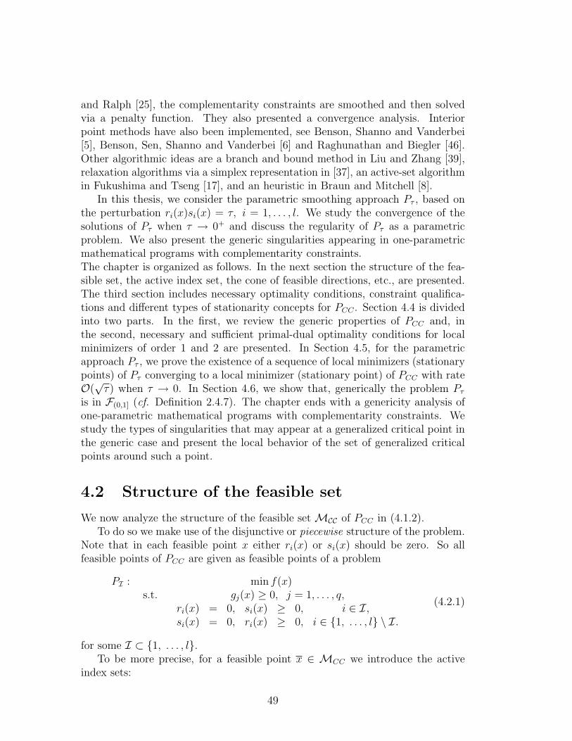
and Ralph [25], the complementarity constraints are smoothed and then solvedvia a penalty function. They also presented a convergence analysis. Interiorpoint methods have also been implemented, see Benson, Shanno and Vanderbei[5], Benson, Sen, Shanno and Vanderbei [6] and Raghunathan and Biegler [46].Other algorithmic ideas are a branch and bound method in Liu and Zhang [39],relaxation algorithms via a simplex representation in [37], an active-set algorithmin Fukushima and Tseng [17], and an heuristic in Braun and Mitchell [8].

In this thesis, we consider the parametric smoothing approach Pτ , based onthe perturbation ri(x)si(x) = τ, i = 1, . . . , l. We study the convergence of thesolutions of Pτ when τ → 0+ and discuss the regularity of Pτ as a parametricproblem. We also present the generic singularities appearing in one-parametricmathematical programs with complementarity constraints.The chapter is organized as follows. In the next section the structure of the fea-sible set, the active index set, the cone of feasible directions, etc., are presented.The third section includes necessary optimality conditions, constraint qualifica-tions and different types of stationarity concepts for PCC . Section 4.4 is dividedinto two parts. In the first, we review the generic properties of PCC and, inthe second, necessary and sufficient primal-dual optimality conditions for localminimizers of order 1 and 2 are presented. In Section 4.5, for the parametricapproach Pτ , we prove the existence of a sequence of local minimizers (stationarypoints) of Pτ converging to a local minimizer (stationary point) of PCC with rateO(√τ) when τ → 0. In Section 4.6, we show that, generically the problem Pτ

is in F(0,1] (cf. Definition 2.4.7). The chapter ends with a genericity analysis ofone-parametric mathematical programs with complementarity constraints. Westudy the types of singularities that may appear at a generalized critical point inthe generic case and present the local behavior of the set of generalized criticalpoints around such a point.

4.2 Structure of the feasible set

We now analyze the structure of the feasible set MCC of PCC in (4.1.2).To do so we make use of the disjunctive or piecewise structure of the problem.

Note that in each feasible point x either ri(x) or si(x) should be zero. So allfeasible points of PCC are given as feasible points of a problem

PI : min f(x)s.t. gj(x) ≥ 0, j = 1, . . . , q,

ri(x) = 0, si(x) ≥ 0, i ∈ I,si(x) = 0, ri(x) ≥ 0, i ∈ 1, . . . , l \ I.

(4.2.1)

for some I ⊂ 1, . . . , l.To be more precise, for a feasible point x ∈ MCC we introduce the active

index sets:

49

J0(x) = j | gj(x) = 0 ,Ir(x) = i | ri(x) = 0, si(x) > 0 ,Is(x) = i | si(x) = 0, ri(x) > 0 ,Irs(x) = i | ri(x) = si(x) = 0 .

For any I ⊂ Irs(x) the problem PI with I = Ir(x) ∪ I will be denoted by PI(x),i.e.,

PI(x) : min f(x)s.t. gj(x) ≥ 0, j = 1, . . . , q,

ri(x) = 0, si(x) ≥ 0, i ∈ Ir(x),si(x) = 0, ri(x) ≥ 0, i ∈ Is(x),ri(x) = 0, si(x) ≥ 0, i ∈ I,si(x) = 0, ri(x) ≥ 0, i ∈ Irs(x) \ I.

(4.2.2)

Let MI(x) denote the feasible set of this program. Then obviously, the followingdisjunctive or piecewise description holds.

Lemma 4.2.1 (cf. [42])(a) There exists a neighborhood Bε(x) (ε > 0) of x such that

MCC ∩Bε(x) =⋃

I⊂Irs(x)

(MI(x) ∩Bε(x)) .

(b) The point x ∈ MCC is a local minimizer of order ω of PCC if and only if xis a local minimizer of order ω of PI(x) for all I ⊂ Irs(x).

Based on this lemma, optimality conditions and genericity results for PI(x) leaddirectly to corresponding results for the complementarity constrained problemPCC . This will be done in the next sections.

4.3 Necessary optimality conditions

This section introduces some notations and deals with different types of necessaryoptimality conditions for PCC . We begin with some definitions. As usual

L(x, λ0, µ, ρ, σ) = λ0f(x)−∑

j∈J0(x)

gj(x)µj−∑

i∈Ir(x)∪Irs(x)

ri(x)ρi−∑

i∈Is(x)∪Irs(x)

si(x)σi

denotes the Lagrangean function. Given x ∈ MCC and I ⊂ Irs(x) we introducethe set of critical directions for PI(x):

CI(x) =

d ∈ Rn

∣∣∣∣∣∣∣∣∣∣∇f(x)d ≤ 0, ∇gj(x)d ≥ 0, j ∈ J0(x),∇ri(x)d = 0, ∇si(x)d ≥ 0, i ∈ I,∇ri(x)d ≥ 0, ∇si(x)d = 0, i ∈ Irs(x) \ I,∇ri(x)d = 0, i ∈ Ir(x),∇si(x)d = 0, i ∈ Is(x).

(4.3.1)

50

We need some constraint qualifications.

Definition 4.3.1 Let x ∈MCC :

- MPCC-LICQ holds at x if ∇ri(x),∇sk(x),∇gj(x), i ∈ Ir(x) ∪ Irs(x),k ∈ Is(x) ∪ Irs(x) j ∈ J0(x), are linearly independent.

- MPCC-MFCQ holds at x if the gradients ∇ri(x),∇sk(x), i ∈ Ir(x) ∪Irs(x), k ∈ Is(x) ∪ Irs(x) are linearly independent and there is a vectorξ such that ∇gj(x)

T ξ > 0, j ∈ J0(x) and ∇ri(x)T ξ = 0,∇sk(x)

T ξ = 0,i ∈ Ir(x) ∪ Irs(x), k ∈ Is(x) ∪ Irs(x).

We now introduce different types of stationarity.

Definition 4.3.2 Let x ∈MCC

- x is a Fritz John point of PCC if it is a Fritz John point for all problemsPI(x), I ⊂ Irs(x) (see (4.2.2)).

- x will be called weakly stationary if there are multipliers (λ0, µ, ρ, σ) notall zero satisfying ∇L(x, λ0, µ, ρ, σ) = 0 and λ0, µ ≥ 0.

- If x is a weakly stationary point with σi · ρi ≥ 0,∀i ∈ Irs(x) for someassociated multiplier vector (λ0, µ, ρ, σ), then x is called a C-stationarypoint.

- x is M-stationary if x is a weakly stationary point with an associatedmultiplier (λ0, µ, ρ, σ) such that λ0 = 1 and for each i ∈ Irs(x) eitherσi > 0, ρi > 0 or σi · ρi = 0 holds.

- If for all I ⊂ Irs(x), x is a stationary point of the nonlinear program PI(x)(see Definition 2.2.3) then x is called a B-stationary point.

- A-stationary points are weakly stationary points with associated multiplier(λ0, µ, ρ, σ) satisfying λ0 = 1 and for all i ∈ Irs(x), σi or ρi is non-negative,i.e, there is some I, I ⊂ Irs(x) such that x is a stationary point of PI(x).

- x is called a strongly stationary point if the weak stationarity conditionsare satisfied with multiplier (λ0, µ, ρ, σ), fulfilling λ0 = 1 and σi, ρi ≥ 0,i ∈ Irs(x).

Let x be feasible for the complementarity constrained problem PCC in (4.1.2).Consider two related problems, the tightened problem

PT (x) : min f(x)s.t. x ∈MT

(4.3.2)

51

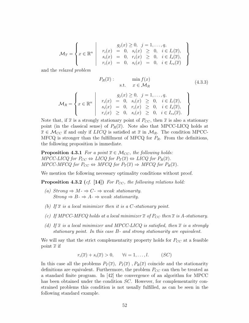
MT =

x ∈ Rn

∣∣∣∣∣∣∣∣gj(x) ≥ 0, j = 1, . . . , q,

ri(x) = 0, si(x) ≥ 0, i ∈ Ir(x),si(x) = 0, ri(x) ≥ 0, i ∈ Is(x),ri(x) = 0, si(x) = 0, i ∈ Irs(x)

and the relaxed problem

PR(x) : min f(x)s.t. x ∈MR

(4.3.3)

MR =

x ∈ Rn

∣∣∣∣∣∣∣∣gj(x) ≥ 0, j = 1, . . . , q,

ri(x) = 0, si(x) ≥ 0, i ∈ Ir(x),si(x) = 0, ri(x) ≥ 0, i ∈ Is(x),ri(x) ≥ 0, si(x) ≥ 0, i ∈ Irs(x).

Note that, if x is a strongly stationary point of PCC , then x is also a stationarypoint (in the classical sense) of PR(x). Note also that MPCC-LICQ holds atx ∈ MCC if and only if LICQ is satisfied at x in MR. The condition MPCC-MFCQ is stronger than the fulfillment of MFCQ for PR. From the definitions,the following proposition is immediate.

Proposition 4.3.1 For a point x ∈MCC, the following holds:MPCC-LICQ for PCC ⇔ LICQ for PT (x) ⇔ LICQ for PR(x).MPCC-MFCQ for PCC ⇔ MFCQ for PT (x) ⇒ MFCQ for PR(x).

We mention the following necessary optimality conditions without proof.

Proposition 4.3.2 (cf. [14]) For PCC, the following relations hold:

(a) Strong ⇒M- ⇒ C- ⇒ weak stationarity.Strong ⇒ B- ⇒ A- ⇒ weak stationarity.

(b) If x is a local minimizer then it is a C-stationary point.

(c) If MPCC-MFCQ holds at a local minimizer x of PCC then x is A-stationary.

(d) If x is a local minimizer and MPCC-LICQ is satisfied, then x is a stronglystationary point. In this case B- and strong stationarity are equivalent.

We will say that the strict complementarity property holds for PCC at a feasiblepoint x if

ri(x) + si(x) > 0, ∀i = 1, . . . , l. (SC)

In this case all the problems PT (x), PI(x) , PR(x) coincide and the stationaritydefinitions are equivalent. Furthermore, the problem PCC can then be treated asa standard finite program. In [42] the convergence of an algorithm for MPCChas been obtained under the condition SC. However, for complementarity con-strained problems this condition is not usually fulfilled, as can be seen in thefollowing standard example.

52

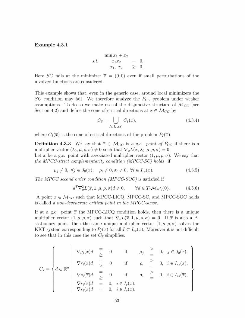
Example 4.3.1

minx1 + x2

s.t. x1x2 = 0,x1, x2 ≥ 0.

Here SC fails at the minimizer x = (0, 0) even if small perturbations of theinvolved functions are considered.

This example shows that, even in the generic case, around local minimizers theSC condition may fail. We therefore analyze the PCC problem under weakerassumptions. To do so we make use of the disjunctive structure of MCC (seeSection 4.2) and define the cone of critical directions at x ∈MCC by

Cx =⋃

I⊂Irs(x)

CI(x), (4.3.4)

where CI(x) is the cone of critical directions of the problem PI(x).

Definition 4.3.3 We say that x ∈ MCC is a g.c. point of PCC if there is amultiplier vector (λ0, µ, ρ, σ) 6= 0 such that ∇xL(x, λ0, µ, ρ, σ) = 0.Let x be a g.c. point with associated multiplier vector (1, µ, ρ, σ). We say thatthe MPCC-strict complementarity condition (MPCC-SC) holds if

µj 6= 0, ∀j ∈ J0(x), ρi 6= 0, σi 6= 0, ∀i ∈ Irs(x). (4.3.5)

The MPCC second order condition (MPCC-SOC) is satisfied if

dT∇2xL(x, 1, µ, ρ, σ)d 6= 0, ∀d ∈ TxMR\0. (4.3.6)

A point x ∈ MCC such that MPCC-LICQ, MPCC-SC, and MPCC-SOC holdsis called a non-degenerate critical point in the MPCC-sense.

If at a g.c. point x the MPCC-LICQ condition holds, then there is a uniquemultiplier vector (1, µ, ρ, σ) such that ∇xL(x, 1, µ, ρ, σ) = 0. If x is also a B-stationary point, then the same unique multiplier vector (1, µ, ρ, σ) solves theKKT system corresponding to PI(x) for all I ⊂ Irs(x). Moreover it is not difficultto see that in this case the set Cx simplifies:

Cx =

d ∈ Rn

∣∣∣∣∣∣∣∣∣∣∣∣∣∣∣∣

∇gj(x)d=≥ 0 if µj

>=

0, j ∈ J0(x),

∇ri(x)d=≥ 0 if ρi

>=

0, i ∈ Irs(x),

∇si(x)d=≥ 0 if σi

>=

0, i ∈ Irs(x),

∇ri(x)d = 0, i ∈ Ir(x),∇si(x)d = 0, i ∈ Is(x).

53

In the case of B-stationary points where MPCC-SC holds, the cone of criticaldirections becomes:

Cx =

d ∈ Rn

∣∣∣∣∣∣∣∣∣∣∣

∇gj(x)d = 0, j ∈ J0(x),

∇ri(x)d = 0, i ∈ Irs(x),∇si(x)d = 0, i ∈ Irs(x),

∇ri(x)d = 0, i ∈ Ir(x),∇si(x)d = 0, i ∈ Is(x)

(4.3.7)

i.e., Cx coincides with TxMR, the tangent subspace of MR in x.

Note that if x is a non-degenerate critical point in the MPCC-sense, thenµj 6= 0, j ∈ J0(x) ρi, σi 6= 0, i ∈ Irs(x) and ∇2

xL|TxMR(x, 1, µ, ρ, σ) is non-

singular. This means x is a non-degenerate critical point of the relaxed problemPR(x) and thus also an (isolated) non-degenerate g.c. point of PCC .

If x is a non-degenerate critical point in the MPCC-sense, such thatµj > 0, j ∈ J0(x) ρi, σi > 0, i ∈ Irs(x) and ∇2

xL|TxMR(x, 1, µ, ρ, σ) 0 are

fulfilled, then x is a local minimizer of PR(x). As locally MCC ⊂ MR holds, xwill also be a local minimizer of PCC in this case.

4.4 Optimality conditions based on the disjunc-

tive structure

In this section we show how optimality conditions can simply be derived fromthe piecewise structure of the problems PCC , see Section 4.2. These conditionsare obtained under assumptions which are shown to be generic.

4.4.1 Genericity results for non-parametric PCC

In this part we will review the genericity results of [53] needed in the next sections.By using the piecewise description (see Lemma 4.2.1) in principle, optimality con-ditions and genericity results for PI(x) lead directly to corresponding results forPCC . Let, in the sequel, all functions f, gj, si, ri be in the space [C2]1n endowedwith the C2

S-topology, see Section 2.3. So, the set of problems PCC can be identi-fied with the set P := (f, g, s, r) = [C2]1+q+2l

n . We say that a property for PCC

is generic if it holds for a subset of P which is dense and open with respect tothe C2

S-topology.From the well-known genericity results for nonlinear programming problems,

see [22], we obtain the following genericity results, see [53].

Theorem 4.4.1 (cf. [53]) Generically for problems PCC the following holds.For any feasible point x ∈ MCC the MPCC-LICQ condition is satisfied. More-over any g.c. point is a non-degenerate critical point in the MPCC-sense, i.e.,the conditions MPCC-LICQ, MPCC-SC and MPCC-SOC are fulfilled.

54

Proof . Let us fix a partition (Ir, Irs, Is) of 1, . . . , l corresponding to the activeindex triplet of a point x ∈MCC . Let PR(x) be the associated relaxed problem.Generically by Theorem 2.2.2, at all feasible points of PR(x), LICQ holds and allits generalized critical points are non-degenerate, see Definition 2.2.5. We takethe (finite) intersection of all these generic sets of functions, corresponding to allfinitely many possible partitions (Ir, Irs, Is). Then the set of functions (f, g, r, s),such that for all corresponding possible problems PR(x) the LICQ condition holdsat all its feasible points and all generalized critical points are non-degenerate, isgeneric.Now, if x ∈MCC , then x is feasible for PR(x) associated with Ir(x), Irs(x), Is(x).As LICQ holds generically for MR, the MPCC-LICQ condition is fulfilled forMCC . Moreover, if x is a g. c. point of PCC , then it is also a generalized criti-cal point of PR(x) (see Definition 2.2.3) and thus, generically, a non-degeneratecritical point of PCC .

2

4.4.2 Optimality conditions for problems PCC

In this part we are interested in necessary and sufficient optimality conditionsfor minimizers of order one and two for problems PCC in (4.1.2), see Definition2.2.1. Using the piecewise description, see Lemma 4.2.1, all standard optimalityconditions for PI(x) can directly be translated into corresponding results for PCC .

We begin with characterizations for minimizers of order one.

Theorem 4.4.2 (Primal conditions of order 1) For x ∈MCC:

Cx = 0 ⇒ x is a (isolated) local minimizer of order 1 of PCC .

If MPCC-LICQ holds at x also the converse is true.

Proof. It is well-known, see e.g. Still and Streng [Th.3.2,3.6] [62], thatCI(x) = 0 implies that x is an (isolated) local minimizer of order 1 of PI(x)and under MPCC-LICQ the converse holds. With regard to the definition of Cx

in (4.3.4) the result follows from Lemma 4.2.1.

2

Theorem 4.4.3 (Dual conditions of order 1) Let MPCC-LICQ hold atx ∈MCC. Then x is an (isolated) local minimizer of order 1 of PCC if and onlyif one of the following equivalent conditions (a) or (b) holds:

55

(a) ∇f(x) ∈ int Q x, where

Q x =

d =

∑j∈J(x)

µj∇gj(x) +∑

i∈Irs(x)

(ρi∇ri(x) + σi∇si(x)

)+

+∑

i∈Ir(x)

ρi∇ri(x) +∑

i∈Is(x)

σi∇si(x)

µj ≥ 0, j ∈ J0(x), ρi ≥ 0, σi ≥ 0, i ∈ Irs(x).

(b) The vector x is a B-stationary point with (unique) multipliers 1, µ, ρ, σ suchthat |J0(x)| + 2|Irs(x)| + |Ir(x)| + |Is(x)| = n and µj > 0, j ∈ J0(x), ρi > 0,σi > 0, i ∈ Irs(x).

Proof. It is well-known that the primal condition CI(x) = 0 is equivalent withthe condition ∇f(x) ∈ int Q I(x), where

Q I(x) =

d =

∑j∈J0(x)

µj∇gj(x) +∑

i∈Irs(x)

(ρi∇ri(x) + σi∇si(x)

)+

+∑

i∈Ir(x)

ρi∇ri(x) +∑

i∈Is(x)

σi∇si(x)

µj ≥ 0, j ∈ J0(x), ρi ≥ 0, i ∈ Irs(x) \ I, σi ≥ 0, i ∈ I

Applying Lemma 4.2.1 under MPCC-LICQ, yields (a).

(b) We now prove that under MPCC-LICQ (a) ⇔ (b). Note that the suf-ficiency is evident. To prove the converse let us assume that ∇f(x) ∈ Q I(x)and |J0(x)| + 2|Irs(x)| + |Ir(x)| + |Is(x)| < n. This means that there existsd, d ∈ Rn, such that d /∈ S0, where S0 is the subspace generated by the vec-tors ∇gj(x), j ∈ J0(x), ∇ri(x), i ∈ Irs(x) ∪ Ir(x), ∇si(x), i ∈ Irs(x) ∪ Is(x).Note that, since (x, 1, µ, ρ, σ) is a B-stationary solution, it follows that S0 =span −∇f(x)∪S0. Consequently, for any ε > 0, εd /∈ span −∇f(x)∪S0and thus ∇f(x) + εd /∈ span S0 in contradiction to (a). Let us now assume thatMPCC-SC does not hold, say µ1 = 0. Then, by MPCC-LICQ, for any ε > 0 thevector ∇f(x)− ε∇g1(x) is not contained in Qx, a contradiction.

2

We now turn to sufficient and necessary optimality conditions of order two. Forthe sufficient part we refer also to [53].

Theorem 4.4.4 (Dual conditions of order 2) Let MPCC-LICQ hold atx ∈ MCC and assume Cx 6= 0, i.e., x is not a local minimizer of order 1.Then x is an (isolated) local minimizer of order 2 of PCC if and only if x is a B-stationary point of PCC with (unique) multipliers (1, µ, ρ, σ) such that MPCC-SCis satisfied and the condition MPCC-SOC holds with dT∇2

xL(x, 1, µ, ρ, σ)d > 0∀d ∈ Cx\0.Under this condition, x is locally a unique B-stationary point of PCC.

56

Proof. Cx 6= 0 implies CI(x) 6= 0 for (at least) one set I ⊂ Irs(x) and by[62, Th.3.6], under LICQ, x is a (isolated) local minimizer of order 2 of PI(x) ifand only if x is a KKT point satisfying the second order sufficient condition atproblem PI(x) for all I ⊂ Irs(x). Again the result follows from Lemma 4.2.1.

2

Note that in view of the genericity result in Theorem 4.4.1 the following is true:

Corollary 4.4.1 Generically each local minimizer of PCC is either of order 1 orof order 2.

It is interesting to note that with respect to the relaxed problem PR(x) (4.3.3)the following holds:

Corollary 4.4.2 Let MPCC-LICQ be satisfied at x ∈ MCC. Then x is a localminimizer of order 1 or 2 of PCC if and only if x is a local minimizer of order 1or 2 of PR(x) (4.3.3).

Proof. Under MPCC-LICQ any local minimizer x of PCC must be a stronglystationary point of PCC with unique multipliers (1, µ, ρ, σ). Note that, as the La-grange functions of PR and PCC are the same, (x, 1, µ, ρ, σ) is also a KKT solutionof PR(x). Moreover the set of critical directions for PR(x) coincides with Cx, see(4.3.7). So the first order optimality condition Cx = 0, cf. Theorem 4.4.2, andthe second order conditions, cf. Theorem 4.4.4, of PCC and PR(x) coincide.

2

4.5 A parametric solution method

As it has been already remarked, to solve PCC (see (4.1.2)) a parametric approachcan be used, see also e.g. [16]. Here we consider the perturbed problem

Pτ : minx

f(x)

s.t. x ∈Mτ

(4.5.1)

Mτ =

x ∈ Rn

∣∣∣∣∣∣gj(x) ≥ 0, j = 1, . . . , q,

ri(x)si(x) = τ, i = 1, . . . , l,ri(x), si(x) ≥ 0, i = 1, . . . , l

where τ, τ > 0, is a perturbation parameter. We expect that, by letting τ → 0,there is a solution xτ of Pτ converging to a solution x of PCC . In the followingwe intend to analyze this approach. Under natural (generic) assumptions it willbe shown that we generally can expect a rate

‖xτ − x‖ = O(√τ).

57

Other regularizations of MPCC problems have been considered in the literaturesuch as

P≤τ : minx

f(x)

s.t. gj(x) ≥ 0, j = 1, . . . , q,ri(x)si(x) ≤ τ, i = 1, . . . , l,

ri(x), si(x) ≥ 0, i = 1, . . . , l.

(4.5.2)

P≤τ : min

xf(x)

s.t. gj(x) ≥ 0, j = 1, . . . , q,rT (x)s(x) ≤ τ,

ri(x), si(x) ≥ 0, i = 1, . . . , l.

(4.5.3)

In [51], assumptions under which stationary points x(τ) of P≤τ , τ ↓ 0, convergeto a B-stationary point of PCC are given. In [47] it is shown that (under naturalconditions) the solutions x(τ) of P≤τ converge to a (nearby) solution x of PCC

with order O(τ). Similar results are stated for the problem P≤τ .

Remark 4.5.1 We emphasize that these regularizations P≤τ , P≤τ structurally

completely differ from the smoothing approach Pτ . For P≤τ , e.g., the following isshown in [51, Th.3.1,Cor.3.2]: If x is a solution of PCC where MPCC-LICQ andMPCC-SC hold then for the (nearby) minimizers xτ of P≤τ (for τ small enough)the complementarity constraints ri(x) si(x) ≤ τ , i ∈ Irs(x), are not active. Moreprecisely,

ri(xτ ) = si(xτ ) = 0 , ∀i ∈ Irs(x),

is true. This fact also directly follows from Corollary 4.4.2. In particular, in thecase Irs(x) = 1, . . . , l (for all small τ > 0) the solution xτ of P≤τ coincides withthe solution x of PCC.

Note that the perturbation ri(x)si(x) = τ in Pτ is also different from the followingparametric MPCC, considered in [24] (see also Section 4.7)

P (τ) : minxf(x, τ)

s.t. gj(x, τ) ≥ 0, j = 1, . . . , q,

ri(x, τ) · si(x, τ) = 0, i = 1, . . . , l,

ri(x, τ) , si(x, τ) ≥ 0, i = 1, . . . , l.

with f, gj, ri, si ∈ C2 (w.r.t. all variables). Near a non-degenerate solution x ofP (τ), the value function will depend smoothly on the parameter τ . However,for the problem Pτ in (4.5.1), the value function does not depend smoothly onτ, τ ≈ 0, even in the non-degenerate case, as can be seen in Example 4.5.1 lateron.

58

Remark 4.5.2 We recall that under appropriate LICQ conditions all resultsfor 4.1.2 remain true for problems PCC in (4.1.1), with additional equality con-straints.

Let in the following ϕ, ϕτ denote the marginal values and MCC , Mτ the feasiblesets of PCC , Pτ respectively.

4.5.1 Motivating examples

We begin with some illustrative examples.

Example 4.5.1minx1 + x2

s.t. x1 x2 = 0,x1, x2 ≥ 0.

Here the set Mτ converges to the set MCC and the solutions xτ = (√τ ,√τ) of

Pτ converge to the solution x = 0 of the original problem with a rate

‖xτ − x‖ =√

2 ·√τ .

In general, we cannot expect that the solutions of Pτ converge to a solution ofPCC . As we can see in the next example, they may even not converge to a feasiblepoint if the feasible set is non-compact:

Example 4.5.2 Consider

min (x2 − 1)2

s.t. x2e−x1 = 0,

x2, e−x1 ≥ 0

with MCC = (x1, 0), x1 ∈ R , and

min (x2 − 1)2

s.t. (x21 + x2

2)e−x1 = 0,

(x21 + x2

2), e−x1 ≥ 0

with MCC = (0, 0) .In both examples the feasible set and the set of minimizers coincide.

Note that in the first example x2 = 0 < e−x1 and ∇x2 6= 0. So MPCC-LICQ holds. However, for all τ, τ > 0, the point (−ln(τ), 1) ∈ Mτ is the globalminimizer of Pτ , and these points do not approach to the set of minimizers ofPCC .In the second example, MCC is bounded but it can be proven that Mτ is not.

The next example shows that to assure Mτ 6= ∅, the MPCC-LICQ conditioncannot be relaxed by the fulfillment of MFCQ in MR, see (4.3.3).

59

Example 4.5.3 Consider the feasible set defined by r1(x) = x, r2(x) = ex − 1,and s1(x) = s2(x) = 1, i.e.,

MCC =

x ∈ R

∣∣∣∣∣∣x · 1 = 0,

(ex − 1) · 1 = 0,x, (ex − 1), 1 ≥ 0.

The unique solution of the complementarity problem is x = 0. However, Mτ = ∅,for any τ, τ > 0. Moreover MFCQ holds at x for MR

The last example shows that a bad convergence rate of the smoothing approachis possible.

Example 4.5.4 (cf. [47])

minxk1 + x2

s.t. x1x2 = 0,x1, x2 ≥ 0,

with k > 0. Here the minimizer is x = (0, 0) and the solution of the corresponding

problem Pτ is xτ = (( τk)

1k+1 , k

1k+1 τ

kk+1 ). So the convergence rate is O(τ

1k ) with

arbitrary large k > 0. Note that for k > 1, the MPCC-SC condition fails at theminimizer x = (0, 0).

In the following we are interested in the convergence of the feasible sets Mτ , thevalue function ϕτ and the solutions xτ of Pτ , i.e., we study the convergence

Mτ →MCC , ϕτ → ϕ and xτ → x for τ → 0.

We will also obtain the rate of this convergence.Firstly, motivated by Example 4.5.2, we restrict the feasible set to a compact

subset X, X ⊂ Rn. Note that, in practice, this does not mean a restriction sinceit is advisable to add (if necessary) e.g. box constraints, xν ≤ ±K, ν = 1, . . . , n,for some large number K. So, we will assume:

A0. Mτ ⊂ X for all τ ≥ 0 where X is a compact subset of Rn. (4.5.4)

4.5.2 The convergence behavior of the feasible set

In this part, we consider the convergence behavior of the feasible set Mτ . Wewill show that, under natural assumptions on the problem PCC for all x ∈MCC ,d(x,Mτ ) = O(

√τ) holds and d(xτ ,MCC) = O(

√τ), for xτ ∈Mτ , τ → 0.

We define the active index sets (J0(x), Ir(x), Is(x), Irs(x)) of x ∈ MCC , as inthe Section 4.2. To avoid the bad behavior in Example 4.5.2 and Example 4.5.3

60

(cf. Section 4.5.1) we will assume that condition A0 (see (4.5.4)), holds and thatMPCC-LICQ is fulfilled for MCC , globally or locally. We emphasize that theseassumptions are generically satisfied, see Theorem 4.4.1. We begin with a generallemma.

Lemma 4.5.1 For any sequence xτ ∈ Mτ and τ → 0 it follows thatd(xτ ,MCC) → 0 uniformly: i.e., to any ε > 0 there exists τ0, τ0 > 0 suchthat for all τ, 0 < τ ≤ τ0, and xτ ∈Mτ , the bound d(xτ ,MCC) < ε holds.

Proof. Assuming that the statement is not true, there must exist γ, γ > 0 anda sequence xτ ∈Mτ , such that, for τ → 0,

d(xτ ,MCC) ≥ γ.

Due to the compactness assumption A0 we can choose a convergent subsequencexτ → x ∈ X. The condition ri(xτ )si(xτ ) = τ , together with the continuity of thefunctions ri, si leads, for τ → 0, to ri(x)si(x) = 0, i.e., x ∈MCC , a contradiction.

2

To prove our main results on the behavior of Mτ , we make use of a local diffeo-morphism. Such a transformation has been applied in [53] to illustrate the localbehavior of MCC . Here we present a complete global analysis. The use of thistransformation makes the proofs of the main results technically much simpler,however this approach relies on the MPCC-LICQ assumption.Consider a point x ∈ MCC with |J0(x)| = q, 2|Irs(x)| + |Ir(x)| + |Is(x)| = l + pwhere p ≤ l, q ≤ q and l + p+ q ≤ n. W.l.o.g. we can assume:

J0(x) = 1, . . . , q, Irs(x) = 1, . . . , p, Ir(x) = p+ 1, . . . , l, Is(x) = ∅.(4.5.5)

By the MPCC-LICQ condition, ∇g1(x), . . . ,∇gq(x), ∇ri(x), i = 1, . . . , l, ∇si(x),i = 1, . . . , p are linearly independent and we can complete these vectors to abasis of Rn by adding vectors vi, i = l + p + q + 1, . . . , n. Now we define thetransformation y = T (x) by:

yi = ri(x), i = 1, . . . , l, yi+l = si(x), i = 1, . . . , p,yl+p+j = gj(x), j = 1, . . . , q, yi = vT

i (x− x), i > l + p+ q.(4.5.6)

By construction the Jacobian ∇T (x) is regular. So T defines locally a diffeomor-phism. This means that there exists ε, ε > 0, and neighborhoods Bn

ε (x) of x andUε(y) := T (Bn

ε (x)) of y = 0 such that T : Bnε (x) → Uε(y) is a bijective mapping

with T, T−1 ∈ C1, T (x) = y and for y = T (x) it follows that

x ∈Mτ ∩Bnε (x) ⇔

yl+p+j ≥ 0, j = 1, . . . , q,yi · yl+i = τ, i = 1, . . . , p,yi · si(y) = τ, i = p+ 1, . . . , l,

yi ≥ 0, i = 1, . . . , l + p,y ∈ Uε(y).

61

where si(y) = si(T−1(y)) = si(x) =: csi , csi > 0, i = p + 1, . . . , l and

gj(y) = gj(T−1(y)) = gj(x) =: cgj , c

gj > 0, j = q + 1, . . . , q.

In particular, since T is a diffeomorphism, the distance between two pointsremains equivalent in the sense that with some constants 0 < κ− < κ+:

κ−‖y1−y2‖ ≤ ‖x1−x2‖ ≤ κ+‖y1−y2‖, ∀x1, x2 ∈ Bnε (x), y1 = T (x1), y2 = T (x2).

So, after applying a diffeomorphism T , we may assume x = 0 and that there issome ε, ε > 0, such that for x ∈ Bn

ε (x):

x ∈Mτ ⇔

gj(x) = xl+p+j ≥ 0, j = 1, . . . , q,

hi(x) = xi · xl+i = τ, i = 1, . . . , p,

hi(x) = xi · si(x) = τ, i = p+ 1, . . . , l,xi ≥ 0, i = 1, . . . , l + p.

(4.5.7)

Moreover, since si(x) =: csi , csi > 0, i = p + 1, . . . , l and gj(x) =: cgj , c

gj > 0,

j = q + 1, . . . , q, by choosing ε small enough we also can assume:

si(x) ≥csi2, i = p+ 1, . . . , l and gj(x) ≥

cgj2, j = q + 1, . . . , q, ∀x ∈ Bn

ε (x).

(4.5.8)

Lemma 4.5.2 Let MPCC-LICQ hold at x ∈MCC.(a) Then there exist ε, τ0, α, β > 0 such that for all τ, 0 < τ ≤ τ0 the followingholds: there exists xτ ∈Mτ with

‖xτ − x‖ ≤ α√τ (4.5.9)

and, for any xτ ∈ Mτ ∩ Bnε (x), there exists a point xτ , xτ ∈ MCC ∩ Bn

ε (x)satisfying

‖xτ − xτ‖ ≤ β√τ . (4.5.10)

Moreover, if SC holds at x (cf. Section 4.3), the statements are true with√τ

replaced by τ .

(b) If the condition SC is not fulfilled at x then the convergence rate O(√τ)

in (4.5.9) is optimal. More precisely, there is some γ, γ > 0, such that for allxτ ∈Mτ the relation ‖xτ − x‖ ≥ γ

√τ holds for all small τ .

Proof. (a) Let MPCC-LICQ hold at x ∈ MCC . As discussed before (afterapplying diffeomorphism) we can assume that x = 0 and that in a neighborhoodBn

ε (x) of x the set Bnε (x) ∩Mτ is described by (4.5.7). To construct an element

xτ ∈ Mτ , we fix the components xτi = xτ

l+i =√τ , i = 1, . . . , p and xτ

i = 0,i = l + p+ 1, . . . , n. From (4.5.7) we then find:

gj(xτ ) = 0, j = 1, . . . , q,

hi(xτ ) = τ, i = 1, . . . , p,

hi(xτ ) = xτ

i · si(xτ ) = τ, i = p+ 1, . . . , l.

62

We only need to consider the remaining relations

hi(x) := xτi · si(x) = τ, i = p+ 1, . . . , l. (4.5.11)

which (for fixed τ) only depend on the remaining variables x = (xτp+1, . . . , x

τl ).

For x = 0 the gradients ∇hi(0) = eisi(0) = eicsi , i = p + 1, . . . , l, are lin-

early independent. So the function H : Rl−p → Rl−p, H = (hp+1, . . . , hl) withH(0) = 0 has locally near x = 0 a C1 inverse such that (for small τ) the vectorxτ := H−1(e τ), with e = (1, . . . , 1) ∈ Rl−p, defines a solution of (4.5.11). Becauseof H−1(0) = 0 it follows that ‖xτ‖ = O(τ).

Altogether with the other fixed components, this vector xτ defines a feasiblepoint xτ ∈Mτ which satisfies

‖xτ − x‖ ≤ O(√τ).

We now prove (4.5.10). As shown above, see (4.5.7), for some ε, ε > 0, thepoint xτ ∈ Bn

ε (x) is in Mτ if and only if x := xτ satisfies the relations

gj(x) = xl+p+j ≥ 0, j = 1, . . . , q,hi(x) = xi · xl+i = τ, i = 1, . . . , p,hi(x) = xi · si(x) = τ, i = p+ 1, . . . , l.

Obviously, minxi, xl+i ≤√τ , i = 1, . . . , p, so w.l.o.g. we assume xi ≤

√τ ,

i = 1, . . . , p. By (4.5.8) for x = xτ ∈ Bnε (x) it follows that

xi =τ

si(x)≤ τ

csi/2≤ τ

cs, i = p+ 1, . . . , l, (4.5.12)

where cs = mincsi/2, i = p+1, . . . , l. Given this element x = xτ ∈Mτ we nowchoose the point xτ of the form xτ = (0, . . . , 0, xl+1, . . . , xn) which is containedin MCC . By using (4.5.12) and xi ≤

√τ , i = 1, . . . , p, we find (x = xτ )

‖xτ − xτ‖ ≤

√p τ + (l − p)

τ 2

c2s≤ O(

√τ).

Let now SC be satisfied at x ∈ MCC , x = 0. Then locally in Bnε (x), see above,

the set Mτ is defined by

gj(x) = xl+p+j ≥ 0, j = 1, . . . , q,xi · si(x) = τ, i = 1, . . . , l,

(4.5.13)

and si(x) ≥ cs1/2, for all x ∈ Bnε (x). As in the first part of proof, we can fix

the coefficients of x = xτ by xl+i = xi(= 0), i = l + 1, . . . , n and find a solutionx ∈Mτ by applying the inverse function theorem to the remaining l equations

hi(x) := xisi(x) = τ , i = 1, . . . , l.

63

only depending on the remaining variables x := (x1, . . . , xl). This provides uswith a solution x = xτ of (4.5.13) with

‖xτ − x‖ = O(τ).

On the other hand for any solution x := xτ of (4.5.13) in Bnε (x) the point

xτ = (0, . . . , 0, xl+1, . . . , xn) is an element in MCC with ‖xτ − xτ‖ = O(τ).

(b) Suppose that SC is not fulfilled at x, i.e., for some i0 ∈ 1, . . . , l, see (a),

hi(x) = xi0 · xl+i0 = 0 with xi0 = xl+i0 = 0.

Then near x any point x := xτ ∈Mτ must satisfy xi0 · xl+i0 = τ which implies

‖xτ − x‖ ≥ maxxi0 , xl+i0 ≥√τ .

Recall that, due to the applied diffeomorphism, this inequality only holds up toa positive constant. 2

Lemma 4.5.2 yields the local convergence of Mτ , near a point x ∈ MCC . Wenow are interested in the global convergence behavior.

Lemma 4.5.3 Let A0 hold, see (4.5.4). Suppose MPCC-LICQ is satisfied ateach point x ∈MCC. Then there are τ0, α, β > 0 such that for all τ, 0 < τ ≤ τ0,the following holds:For each x ∈MCC there exists xτ , xτ ∈Mτ with

‖xτ − x‖ ≤ α√τ , (4.5.14)

and for any xτ ∈Mτ there exists a point xτ , xτ ∈MCC satisfying

‖xτ − xτ‖ ≤ β√τ . (4.5.15)

Moreover, if SC holds at all x ∈ MCC the statements are true with√τ replaced

by τ .

Proof. We firstly prove (4.5.15). Recall the local transformation constructedabove near any point x ∈ MCC , see 4.5.7. The union ∪x∈MCC

Bnε(x)(x) forms an

open cover of the compact feasible set MCC ⊂ X. Consequently we can choosea finite cover, i.e., points xν ∈ MCC , ν = 1, . . . , N , such that with εν = ε(xν)the set ∪ν=1,...,NB

nεν

(xν) provides an open cover of MCC and with βν > 0 thecorresponding condition (4.5.10) holds.By defining Bε(MCC) = x ∈ X | d(x,MCC) < ε we can choose some ε0, ε0 > 0(small) such that

Bε0(MCC) ⊂⋃

ν=1,...,N

Bnεν

(xν).

64

By choosing ε = ε0 and τ0 in Lemma 4.5.1 we find for all τ, 0 ≤ τ ≤ τ0,

Mτ ⊂ Bε0(MCC) ⊂⋃

ν=1,...,N

Bnεν

(xν).

The second convergence result (4.5.15) directly follows by combining the finitecover argument with the local convergence and by noticing that we can chooseas convergence constant the number β = maxβν ; ν = 1, . . . , N.

To prove (4.5.14) we have to show that the following sharpening of the localbound (4.5.9) holds: For x ∈ MCC there exist τ0, τ0 > 0 and ε, ε > 0, suchthat for any x ∈ MCC ∩ Bn

ε (x) and for any τ, 0 ≤ τ ≤ τ0, there is a pointxτ , xτ ∈Mτ with

‖xτ − x‖ ≤ α√τ . (4.5.16)

Then a finite cover argument as above yields the global relation (4.5.14).

We only sketch the proof of (4.5.16). Let x ∈ MCC be fixed. In the proofof Lemma 4.5.2(a) we made use of a local diffeomorphism Tx(x) leading to re-lation (4.5.9). This transformation Tx is constructed depending on the activeindex set Ia(x) := Irs(x) ∪ Ir(x) ∪ Is(x) ∪ J0(x), see (4.5.6). For any x near xwe have Ia(x) ⊂ Ia(x) and there are only finitely many choices for Ia namelyI1a , . . . , I

Ra . So if we fix I i

a, Iia ⊂ Ia(x), any point x near x with Ia(x) = I i

a yieldsa local diffeomorphism Tx which depends smoothly on x, see the construction(4.5.6). So we find a common bound. There exist αi, εi > 0 such that for anyx ∈ MCC ∩ Bn

εi(x), with Ia(x) = I i

a, there is a point xτ , xτ ∈ Mτ such that, forall small τ

‖xτ − x‖ ≤ αi

√τ .

Then, by choosing ε = minεi | i = 1, . . . , R, and α = maxαi | i = 1, . . . , R,we have shown the relation (4.5.16).

2

Remark 4.5.3 Lemma 4.5.3 proves that the convergence in the Hausdorff dis-tance

dH(Mτ ,MCC) := max maxxτ∈Mτ

d(xτ ,MCC) , maxx∈MCC

d(x,Mτ )

between Mτ and MCC satisfies dH(Mτ ,MCC) = O(√τ).

The above convergence results for the feasible sets have been derived underMPCC-LICQ. Example 4.5.3 shows that some constraint qualification is needed.However the MPCC-LICQ condition can be slightly weakened. We show this on

65

a simple special instance of a feasible set, defined by only one complementarityconstraint:

M1 =

x ∈ Rn

∣∣∣∣∣∣r(x)s(x) = 0,

r(x) ≥ 0,s(x) ≥ 0.

The corresponding perturbed feasible set is then

M1τ =

x ∈ Rn

∣∣∣∣∣∣r(x)s(x) = τ,

r(x) ≥ 0,s(x) ≥ 0.

We say that MFCQ’ holds at x ∈ M1 if the common MFCQ condition holds at

x for M1R =

x ∈ Rn

∣∣∣∣ r(x) ≥ 0,s(x) ≥ 0

. Under this hypothesis we can prove the

following result.

Proposition 4.5.1 Let MFCQ’ hold at a point x ∈ M1. Then the following istrue:

(a) For any τ, τ > 0, small enough, there exists a point xτ , xτ ∈M1τ such that

‖x− xτ‖ = O(√τ).

(b) There are some ε, τ0 > 0 such that for any xτ ∈ M1τ ∩ Bn

ε (x),0 < τ ≤ τ0, there exists xτ

0, xτ0 ∈M1, satisfying ‖xτ

0 − xτ‖ = O(√τ).

Proof . (a) Let x ∈ M1 be fixed. First we consider the case in which SC holds,i.e., r(x) > 0, s(x) = 0 or s(x) > 0, r(x) = 0. Then the MFCQ’ condition means∇s(x) 6= 0 or ∇r(x) 6= 0, respectively, i.e., MPCC-LICQ holds. So the proof is aconsequence of Lemma 4.5.2.

If r(x) = s(x) = 0, due to the MFCQ’ there is a vector ξ, ξ ∈ Rn such that:

ξT∇r(x) > 0, ξT∇s(x) > 0.

W.l.o.g. we assume ‖ξ‖ = 1. Note that there is some t0, t0 > 0, small enoughsuch that r(x+ tξ) > 0 and s(x+ tξ) > 0, for all t ≤ t0. Let r(x+ t0ξ)s(x+ t0ξ)be equal to τ0. We will construct, for any τ , 0 < τ ≤ τ0, a point xτ = x + tτξsuch that xτ ∈M1

τ and tτ = O(√τ). Applying the Taylor expansion we find:

r(x+ tξ)s(x+ tξ) = ct2 + o(t2),

where c = (∇r(x)T ξ)(∇s(x)T ξ) > 0.For any τ , 0 < τ < τ0, (τ0 chosen small), by the Mean Value Theorem, there

exists tτ , 0 ≤ tτ ≤ t0, such that r(x+ tτξ)s(x+ tτξ) = τ . As ct2τ + o(t2τ ) = τ , wehave tτ = O(

√τ) and x+ tτξ ∈M1

τ .

66

(b) W.l.o.g. we assume r(x) = 0, s(x) ≥ 0. If r(x) = 0 and s(x) > 0 then MFCQ’implies MPCC-LICQ and the result is a consequence of Lemma 4.5.2.If r(x) = s(x) = 0, the MFCQ’ condition implies ∇r(x) 6= 0 and ∇s(x) 6= 0.We assume that ∇x1r(x) 6= 0 and ∇xj

s(x) 6= 0 (j may be equal to 1). Then,we can choose ε > 0 such that for all x ∈ Bn

ε (x), |∇x1r(x)| > 1Mr

> 0 and∣∣∇xjs(x)

∣∣ > 1Ms

> 0 hold for some Mr, Ms > 0. This means that 1|∇x1r(x)| and

1|∇xj s(x)| are bounded.

Now, we define the following diffeomorphisms, both similar to that used inLemma 4.5.2:

Tr : U → Vr, Tr(x) = (r(x), x2, . . . , xn) .

andTs : U → Vs, Ts(x) = (x1, . . . xj−1, s(x), xj+1, . . . , xn) .

Tr (Ts) defines a local C1-diffeomorphism from U to Vr (Vs respectively), whereU ⊂ Bn

ε (x) and Vr (Vs respectively) are open balls centered at x and (0, x2, . . . , xn)((x1, . . . xj−1, 0, xj+1, . . . , xn) respectively).

Of course, for τ small enough, xτ ∈ U . We now take xrτ = T−1

r (0, (x2, . . . , xn)τ ).By construction, this point is in U and r(xr

τ ) = 0. Moreover,

‖xrτ − xτ‖ = ‖T−1(0, (x2, . . . , xn)τ )− T−1(r(xτ ), (x2, . . . , xn)τ )‖

= O

(‖(∇r(xτ )0|In−1

)−1(r(xτ )

0

)‖

)= O

(| r(xτ )∇x1r(xτ )

|)

= O (|r(xτ )|) .

Analogously if we define the point xsτ = ((x1, . . . xj−1)τ , 0, (xj+1, . . . , xn)τ ), we

find ‖xsτ − xτ‖ = O (|s(xτ )|) and s(xs

τ ) = 0. But as r(xτ )s(xτ ) = τ , one of thefactors should be smaller that or equal to

√τ . If r(xτ ) ≤

√τ we put xτ = xr

τ

and if s(xτ ) ≤√τ , xτ = xs

τ . In both cases it holds that ‖xτ − xτ‖ ≤ O (√τ) and

r(xτ )s(xτ ) = 0. However, possibly r(xτ ) < 0 or s(xτ ) < 0 may occur. So, we

take xτ0 = xτ + t∗d, where d = (xτ−xτ )

‖xτ−xτ‖ and

t∗ = min t | r(xτ + td)s(xτ + td) = 0, t ≥ 0 .

Note that now xτ0 ∈MCC . As

‖xτ0 − xτ‖ = t∗ ≤ ‖xτ − xτ‖ ≤ O(

√τ),

we have ‖xτ0 − xτ‖ = O(

√τ). So xτ

0 has the desired property. 2

Remark 4.5.4 This lemma presents a local convergence result. A global versioncan also be proven by compactness arguments as in Lemma 4.5.3.

67

4.5.3 Convergence results for minimizers

We now discuss the implications of the results so far. In this section x ∈ MCC

denotes a (candidate) minimizer of PCC and xτ a nearby solution of Pτ , τ > 0.We begin with the following assumptions:

A1. There exists a solution x of PCC and a continuous functionα : [0,∞) → [0,∞), α(0) = 0 such that for any τ , small enough, τ > 0, wecan find a point xτ ∈Mτ satisfying

‖xτ − x‖ ≤ α(τ).

A2. There exists a continuous function β : [0,∞) → [0,∞), β(0) = 0 such thatfor any τ , small enough, τ > 0, the following holds: we can find a solution xτ ofPτ and a corresponding point xτ ∈MCC such that

‖xτ − xτ‖ ≤ β(τ).

As we shall see, A1 leads to the upper semi-continuity and A2 to the lower semi-continuity of the value function ϕτ .

As f ∈ C1(X), due to the compactness of X, we can say that the function fis Lipschitz continuous on X with Lipschitz constant L:

|f(x)− f(x)| ≤ L · ‖x− x‖ , ∀x, x ∈ X. (4.5.17)

Lemma 4.5.4 Let the assumptions A0 (see (4.5.4)), A1 and A2 hold and letf ∈ C1(X). Then with the constant L in (4.5.17) it follows for all τ, τ > 0:

Lβ(τ) ≤ ϕτ − ϕ ≤ Lα(τ).

Proof. With the solution x of PCC and the points xτ in A1 we find, using theLipschitz condition (4.5.17),

ϕτ − ϕ ≤ f(xτ )− f(x) ≤ L α(τ)

and in the same way under A2,

ϕ− ϕτ ≤ f(xτ )− f(xτ ) ≤ L β(τ).

2

To obtain results on the rate of convergence for the solutions xτ of Pτ , we haveto assume some growth condition at a solution x of PCC .

A3. We assume x is a local minimizer of PCC of order ω, i.e., that x ∈ MCC

and for some κ, ε > 0 and ω = 1 or ω = 2 the following relation holds:

f(x)− f(x) ≥ κ‖x− x‖ω, ∀x ∈MCC ∩Bnε (x).

Sufficient and necessary conditions for this assumption are to be found in Sub-section 4.4.2.

68

Corollary 4.5.1 Let the assumptions f ∈ C1(X), A0, A1, A2 and A3 hold. Thenwith the minimizers xτ of Pτ in A2 and with some c > 0 it follows that

‖xτ − x‖ ≤ c ·(α(τ) + β(τ)

)1/ω.

Proof. With the points x, xτ ∈MCC and xτ , xτ ∈Mτ in A1, A2 we obtain

f(x) ≤ f(xτ ) ≤ f(xτ ) + L β(τ) ≤ f(xτ ) + L β(τ) ≤ f(x) + L α(τ) + L β(τ)

and thus0 ≤ f(xτ )− f(x) ≤ L α(τ) + L β(τ). (4.5.18)

Again by taking the point xτ ∈MCC in A2 and using the condition A3, togetherwith (4.5.18), it follows that

‖xτ − x‖ ≤ ‖xτ − xτ‖+ ‖xτ − x‖

≤ β(τ) +

(f(xτ )− f(x)

κ

)1/ω

≤ β(τ) +1

κ1/ω(Lα(τ) + Lβ(τ))1/ω ,

which proves the statement.2

Corollary 4.5.2 Let A0 and MPCC-LICQ hold for MCC. Let x ∈ MCC be aglobal (or local) minimizer of order ω = 1 or ω = 2 of PCC. Then for any τ,small enough, τ > 0, there exists a global (or local) minimizer xτ of Pτ and for(each of) these minimizers it follows that:

‖xτ − x‖ ≤ O(√τ

1/ω)

or‖xτ − x‖ ≤ O(τ 1/ω), if SC holds at x.

Proof. By Lemma 4.5.2, Mτ 6= ∅. Then, due to A0, the set Mτ is compact,so Pτ has a global minimizer. Lemma 4.5.3 implies Conditions A1 and A2 withα(τ) = O(

√τ) and β(τ) = O(

√τ). So, for the global minimizers, the inequality

directly follows by combining the results of Lemma 4.5.3 and Corollary 4.5.1.For a local minimizer x we can restrict the feasible sets MCC and Mτ to a

closed neighborhood Bn

ε (x) (closed, to assure the existence of a minimizer xτ ).Then the results hold for the (global) minimizer xτ in Mτ ∩ B

n

ε (x). But sincexτ → x for τ → 0, the points xτ are also in the open set Bn

ε (x), for τ smallenough, i.e., xτ are local minimizers.

2

Let us recall Example 4.5.4 with k = 2.

69

Example 4.5.5 (cf. [47])

minx21 + x2,

s.t. x1 · x2 = 0,x1, x2 ≥ 0

The minimizer x = (0, 0) is of order ω = 2 and it is a critical point satisfying∇f(x) = 0∇r(x)+1∇s(x). So the MPCC-SC condition is not fulfilled. Here the

minimizers of Pτ read xτ =((

τ2

) 13 , (2τ 2)

13

).

The preceding example (see also [47]) shows that at a local minimizer x of or-der two, even under MPCC-LICQ, the convergence rate for ‖xτ − x‖ can beslower than O(

√τ). Note, however, that this example is not a generic one

since the MPCC-SC condition does not hold. We will now show that in thegeneric case this bad behavior is excluded. More precisely under the conditionsMPCC-LICQ, MPCC-SC and MPCC-SOC at a (local) minimizer x, we prove thatthe minimizers xτ of Pτ are (locally) unique and the optimal convergence rate‖xτ − x‖ = O(

√τ) takes place.

Theorem 4.5.1 Let x be a local minimizer of PCC such that MPCC-LICQ,MPCC-SC and MPCC-SOC hold. Then for any τ > 0, small enough, the localminimizers xτ of Pτ (near x) are uniquely determined and satisfy‖xτ − x‖ = O(

√τ).

The same statement holds for the global minimizers x and xτ of P and Pτ , re-spectively.

Proof. To prove this statement we again consider the problem Pτ in standardform, see the problem given in (4.5.7),

Pτ : min f(x)

s.t. hi(x) = xi · xl+i = τ, i = 1, . . . , p,

hi(x) = xi+p · sp+i(x) = τ, i = 1, . . . , l − p,gj(x) = xl+p+j ≥ 0, j = 1, . . . , q,

xi, xl+i ≥ 0, i = 1, . . . , p,xi, si(x) ≥ 0, i = p+ 1, . . . , l.

(4.5.19)

where x = 0 is the local solution of P0 with sp+i(0) = csi > 0, i = 1, . . . , l − p.Under MPCC-LICQ, the KKT condition for x reads:

∇f(x)−p∑

i=1

(ρiei + σiei+l

)−

l∑i=p+1

ρiei −q∑

j=1

µjel+p+j = 0. (4.5.20)

with multiplier vector (µ, ρ, σ). Here ei denotes the canonical ith-canonical vectorof Rn. Due to the fulfillment of the MPCC-SC and MPCC-LICQ conditions at

70

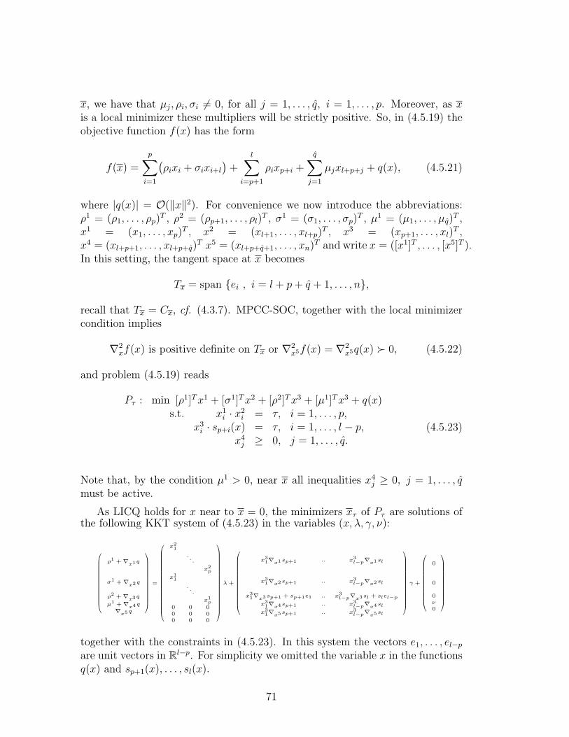
x, we have that µj, ρi, σi 6= 0, for all j = 1, . . . , q, i = 1, . . . , p. Moreover, as xis a local minimizer these multipliers will be strictly positive. So, in (4.5.19) theobjective function f(x) has the form

f(x) =

p∑i=1

(ρixi + σixi+l

)+

l∑i=p+1

ρixp+i +

q∑j=1

µjxl+p+j + q(x), (4.5.21)

where |q(x)| = O(‖x‖2). For convenience we now introduce the abbreviations:ρ1 = (ρ1, . . . , ρp)

T , ρ2 = (ρp+1, . . . , ρl)T , σ1 = (σ1, . . . , σp)

T , µ1 = (µ1, . . . , µq)T ,

x1 = (x1, . . . , xp)T , x2 = (xl+1, . . . , xl+p)

T , x3 = (xp+1, . . . , xl)T ,

x4 = (xl+p+1, . . . , xl+p+q)T x5 = (xl+p+q+1, . . . , xn)T and write x = ([x1]T , . . . , [x5]T ).

In this setting, the tangent space at x becomes

Tx = span ei , i = l + p+ q + 1, . . . , n,

recall that Tx = Cx, cf. (4.3.7). MPCC-SOC, together with the local minimizercondition implies

∇2xf(x) is positive definite on Tx or ∇2

x5f(x) = ∇2x5q(x) 0, (4.5.22)

and problem (4.5.19) reads

Pτ : min [ρ1]Tx1 + [σ1]Tx2 + [ρ2]Tx3 + [µ1]Tx3 + q(x)s.t. x1

i · x2i = τ, i = 1, . . . , p,

x3i · sp+i(x) = τ, i = 1, . . . , l − p,

x4j ≥ 0, j = 1, . . . , q.

(4.5.23)

Note that, by the condition µ1 > 0, near x all inequalities x4j ≥ 0, j = 1, . . . , q

must be active.

As LICQ holds for x near to x = 0, the minimizers xτ of Pτ are solutions ofthe following KKT system of (4.5.23) in the variables (x, λ, γ, ν):

ρ1 + ∇x1q

σ1 + ∇x2q

ρ2 + ∇x3q

µ1 + ∇x4q

∇x5q

=

x21

. . .

x2p

x11

. . .

x1p

0 0 00 0 00 0 0

λ +

x31∇x1sp+1 .. x3

l−p∇x1sl

x31∇x2sp+1 .. x3

l−p∇x2sl

x31∇x3sp+1 + sp+1e1 .. x3

l−p∇x3sl + slel−p

x31∇x4sp+1 .. x3

l−p∇x4sl

x31∇x5sp+1 .. x3

l−p∇x5sl

γ +

0

0

0ν0

together with the constraints in (4.5.23). In this system the vectors e1, . . . , el−p

are unit vectors in Rl−p. For simplicity we omitted the variable x in the functionsq(x) and sp+1(x), . . . , sl(x).

71

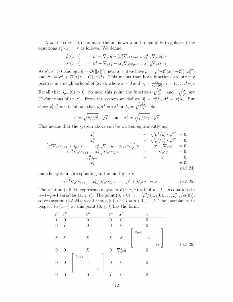
Now the trick is to eliminate the unknown λ and to simplify (regularize) theequations x1

i · x2i = τ as follows. We define:

ρ1(x, γ) := ρ1 +∇x1q − [x31∇x1sp+1 .. x

3l−p∇x1sl]γ

σ1(x, γ) := σ1 +∇x2q − [x31∇x2sp+1 .. x

3l−p∇x2sl]γ.

As ρ1, σ1 > 0 and |q(x)| = O(‖x‖2), near x = 0 we have ρ1 = ρ1+O(x)γ+O(‖x‖2)and σ1 = σ1 + O(x)γ + O(‖x‖2). This means that both functions are strictly

positive in a neighborhood of (x, γ), where x = 0 and γi =ρ2

i

sp+i(0), i = 1, . . . , l−p.

Recall that sp+i(0) > 0. So near this point the functions√

ρ1

σ1 and√

σ1

ρ1 are

C1-functions of (x, γ). From the system we deduce ρ1i = x2

iλi, σ1i = x1

iλi. But

since x1ix

2i = τ it follows that ρ1

i σ1i = τλ2

i or λi =

√ρ1

i σ1i

τ. So

x1i =

√σ1

i /ρ1i ·√τ and x2

i =√ρ1

i /σ1i ·√τ .

This means that the system above can be written equivalently as:

x1i −

√σ1

i /ρ1i ·√τ = 0,

x2i −

√ρ1

i /σ1i ·√τ = 0,[

x31∇x3sp+1 + sp+1e1 . . . x3

l−p∇x3sl + sp+1el−p

]γ − ρ2 −∇x3q = 0,

(x31∇x5sp+1 . . . x

3l−p∇x5sl)γ − ∇x5q = 0,

x3i sp+i − τ = 0,x4

i = 0,(4.5.24)

and the system corresponding to the multiplier ν:

−(x31∇x5sp+1 . . . x

3l−p∇x5sl)γ + µ1 +∇x4q = ν. (4.5.25)

The relation (4.5.24) represents a system F (x, γ, τ) = 0 of n+ l− p equations inn+l−p+1 variables (x, γ, τ). The point (0, γ, 0), γ = (ρ2

1/sp+1(0), . . . , ρ2l−p/sl(0)),

solves system (4.5.24), recall that si(0) > 0, i = p+ 1, . . . , l. The Jacobian withrespect to (x, γ) at this point (0, γ, 0) has the form:

x1 x2 x3 x4 x5 γI 0 0 0 0 00 I 0 0 0 0

X X X X X

sp+1

. . .

sl

0 0 X 0 ∇2

x5q 0

0 0

sp+1

. . .

sl

0 0 0

0 0 0 I 0 0

(4.5.26)

72

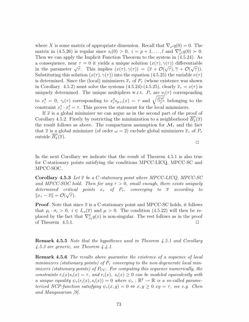
where X is some matrix of appropriate dimension. Recall that ∇xiq(0) = 0. Thematrix in (4.5.26) is regular since si(0) > 0, i = p + 1, . . . , l and ∇2

x5q(0) 0.Then we can apply the Implicit Function Theorem to the system in (4.5.24). Asa consequence, near τ = 0 it yields a unique solution (x(τ), γ(τ)) differentiablein the parameter

√τ . This implies (x(τ), γ(τ)) = (x + O(

√τ), γ + O(

√τ)).

Substituting this solution (x(τ), γ(τ)) into the equation (4.5.25) the variable ν(τ)is determined. Since the (local) minimizers xτ of Pτ (whose existence was shownin Corollary 4.5.2) must solve the systems (4.5.24)-(4.5.25), clearly xτ = x(τ) isuniquely determined. The unique multipliers w.r.t. Pτ are νi(τ) corresponding

to x4i = 0, γi(τ) corresponding to x3

i sp+i(x) = τ and

√ρ1

i σ1i

τbelonging to the

constraint x1i · x2

i = τ . This proves the statement for the local minimizers.If x is a global minimizer we can argue as in the second part of the proof of

Corollary 4.5.2. Firstly by restricting the minimization to a neighborhood Bn

δ (x)the result follows as above. The compactness assumption for Mτ and the factthat x is a global minimizer (of order ω = 2) exclude global minimizers xτ of Pτ

outside Bn

δ (x).2

In the next Corollary we indicate that the result of Theorem 4.5.1 is also truefor C-stationary points satisfying the conditions MPCC-LICQ, MPCC-SC andMPCC-SOC.

Corollary 4.5.3 Let x be a C-stationary point where MPCC-LICQ, MPCC-SCand MPCC-SOC hold. Then for any τ > 0, small enough, there exists uniquelydetermined critical points xτ of Pτ , converging to x according to‖xτ − x‖ = O(

√τ).

Proof . Note that since x is a C-stationary point and MPCC-SC holds, it followsthat ρi · σi > 0, i ∈ Irs(x) and µ > 0. The condition (4.5.22) will then be re-placed by the fact that ∇2

x5q(x) is non-singular. The rest follows as in the proof

of Theorem 4.5.1. 2

Remark 4.5.5 Note that the hypotheses used in Theorem 4.5.1 and Corollary4.5.3 are generic, see Theorem 4.4.1.

Remark 4.5.6 The results above guarantee the existence of a sequence of localminimizers (stationary points) of Pτ converging to the non-degenerate local min-imizers (stationary points) of PCC. For computing this sequence numerically, theconstraints ri(x)si(x) = τ , and ri(x), si(x) ≥ 0 can be modeled equivalently witha unique equality ψτ (ri(x), si(x)) = 0 where ψτ : R2 → R is a so-called parame-terized NCP-function satisfying ψτ (x, y) = 0 ⇔ x, y ≥ 0 xy = τ , see e.g. Chenand Mangasarian [9].

73

Let us note that from the results of this part we also can deduce the convergenceresults for the relaxation P≤

τ , see (4.5.2) and [47], under the stronger MPCC-LICQcondition. Let us reconsider this relaxation P≤

τ . Suppose we have given a localsolution x of PCC such that MPCC-LICQ holds and, with corresponding Lagrangemultipliers, MPCC-SC, MPCC-SOC are satisfied, i.e., by Theorem 4.4.4, x is aminimizer of order ω = 2. In view of Corollary 4.4.2, x is also a solution of therelaxed problem PR(x) in (4.3.3) and by using MPCC-SC it follows that for anyτ > 0, small enough, for the solutions xτ (near x) of P≤τ (see Remark 4.5.1), theconditions ri(x) si(x) ≤ τ , i ∈ Irs(x), are not active but that

ri(xτ ) = si(xτ ) = 0, ∀i ∈ Irs(x), (4.5.27)

holds. So, to analyze the behavior of the solution xτ the whole analysis can bedone under the condition (4.5.27), i.e., we are in the situation as for the case thatthe SC condition holds. Consequently, instead of the convergence O(

√τ) (cf.,

e.g. Lemma 4.5.2), we obtain a rate O(τ) and in the same way the analysis inSection 4.5 simplifies resulting in a convergence behavior ‖xτ − x‖ = O(τ).

Remark 4.5.7 We wish to emphasize that the convergence results of this sectioncan be generalized in a straightforward way to problems Pm, m ≥ 3, containingconstraints of the product form:

r1(x)r2(x) · · · rm(x) = 0, r1(x), r2(x), . . . , rm(x) ≥ 0.

Here at a solution x of Pm where all constraints ri are active, i.e.,

r1(x) = r2(x) = . . . = rm(x) = 0,

a perturbation r1(x)r2(x) · · · rm(x) = τ will lead to a convergence rate

‖xτ − x‖ ≈ O(τ 1/m),

for the solutions xτ of the perturbed problem. Also all other results can be extendedin a straightforward way to this generalization.

4.6 JJT-regularity results for Pτ

In this section we are going to consider Pτ (see (4.5.1)) as a 1-parametric problem.Using the JJT-regularity, we will proof that for a generic PCC (see (4.1.2)) with(f, r1, . . . , rl, s1, . . . , sl, g1, . . . , gq) ∈ [C3]1+l+l+q

n , the one-parametric problem Pτ ,is regular for τ ∈ (0, 1] in the sense of Definition 2.4.7.We firstly deal with the LICQ condition. For this part we can weaken the differ-entiability hypothesis and assume (r1, . . . , rl, s1, . . . , sl, g1, . . . , gq) ∈ [C2]l+l+q

n .

74

Note that, for all x ∈ Mτ , τ > 0, the values of the functions ri(x), si(x)are strictly positive. So the active index set is J0(x, τ) = j | gj(x) = 0. Bydefinition LICQ fails at a point x ∈Mτ , 0 < τ , if

l∑i=1

[si(x)∇ri(x) + ri(x)∇si(x)]λi +∑

j∈J0(x,τ)

µj∇gj(x) = 0, for some (λ, µ) 6= 0.

(4.6.1)

We define the set M0 = (x, τ) | 0 < τ ≤ 1, x ∈Mτ such that (4.6.1) holds,and M1 = (x, τ) ∈M0 | (4.6.1) holds with µj 6= 0, ∀j ∈ J0(x, τ). Then thefollowing is true.

Proposition 4.6.1 Let (r1, . . . , rl, s1, . . . , sl, g1, . . . , gq) ∈ [C2]l+l+qn be given. Then

for almost every linear perturbation of ri, gj, i = 1, . . . , l, j = 1, . . . , q, the setM0 is a discrete set and M0 = M1.

The set of functions (r1, . . . , rl, s1, . . . , sl, g1, . . . , gq) ∈ [C2S]l+l+q

n , see Definition2.3.1, such that M0 is a discrete set and M0 = M1, is generic in [C2

S]l+l+qn .

Proof . As gj, j = 1, . . . , q, are non-parametric functions, not depending on τ ,from the standard genericity results we can conclude that for almost every linearperturbation of gj, the vectors ∇gj(x), j ∈ J0(x, τ) are linearly independentat all points (x, τ), x ∈ Mτ , 0 < τ ≤ 1. So, in the rest of the proof, we willassume that the latter property holds. Now we will prove the statements of theproposition for τ ∈ [ 1

k, 1], where k ∈ N is fixed.

If LICQ is violated for Pτ then, by normalizing and possibly changing indices,the following system is solvable:

∇r1(x)s1(x) +∇s1(x)r1(x) +∑

j∈J0(x,τ)

∇gj(x)µj

+l∑

i=2

λi(∇risi +∇siri)(x) = 0,

ri(x)si(x) = τ, i = 1, . . . , l,gj(x) = 0, j ∈ J0(x, τ),µj = 0, j ∈ JB ⊂ J0(x, τ).

(4.6.2)For the perturbation (ri + bTi x+ ci), i = 1, . . . , l, the Jacobian of the system withrespect to (x, τ, λ, µ), λ = (λ2, . . . , λl)), and the parameters b1, c is of the form:

75

∂x ∂τ ∂λ, µ ∂b1 ∂c

⊗xx 0

⊗ s1 0 . . .

0. . . 0

0 . . . s1

+∇s1 [x1, . . . , xn] ∇s1 |⊗

⊗ −1...−1

0 s1

[x1, . . . , xn

0

] s1

. . .sl

∇T gJ0(x,τ) 0 0 0 0

0 0 0 | I|JB | 0 0(4.6.3)

The matrix :

(diag(s1 . . . s1)n +∇s1 [x1, . . . , xn] ∇s1

s1(x)[x1, . . . , xn] s1(x)

)is non-singular, since

s1(x) > 0 for τ ∈ [ 1k, 1]. Then the first n+1 rows in (4.6.3) are linearly indepen-

dent. So the matrix (4.6.3) has full row rank if and only if the following matrixhas also full row rank:

∂x ∂τ ∂λ, µ ∂b1 ∂c

⊗ −1...−1

0 0

s2

. . .

sl

∇T

x gJ0(x,τ) 0 0 0 00 0 0 | I|JB | 0 0

But the latter is a direct consequence of the facts that si(x) > 0, ∀x ∈Mτ , τ > 0,and the linear independence of ∇xgj(x), j ∈ J0(x, τ).Applying the Parameterized Sard Lemma (cf. Lemma 2.3.1) it follows that foralmost every linear perturbation of ri, i = 1, . . . , l, the sub-matrix of (4.6.3) cor-responding to ∂(x, τ, λ, µ) has full row rank at all solutions (x, τ, λ, µ) of (4.6.2),τ ∈ [ 1

k, 1]. So the number of rows, n+ l + |J0(x, t)|+ |JB|, must be smaller than

or equal to n + 1 + l − 1 + |J0(x, τ)|, the number of unknowns (x, τ, λ, µ). Thisimplies |JB| ≤ 0, i.e., µj 6= 0 for all j ∈ J0(x, τ). Consequently, the full row rankcondition for (4.6.3) implies that for almost all linear perturbations, the followingmatrix is non-singular at all solutions (x, τ, λ, µ) of (4.6.2), τ ∈ [ 1

k, 1]:

∂x ∂τ ∂λ, µ⊗xx 0 ∇x(r2s2) . . .∇x(rlsl)∇T

x gJ0(x,τ)

∇x(r1s1)T −1 0

... −1 0∇x(rlsl)

T −1 0∇xgJ0(x,τ) 0 0

(4.6.4)

76

Here ⊗xx = ∇2x (r1(x)s1(x)) +

l∑i=2

λi∇2x (ri(x)si(x)) +

∑j∈J0(x,τ)

µj∇2xgj(x).

So, as the number of equations and variables of the system (4.6.2) (now with-out the equations µj 6= 0) are the same, it describes a 0-dimensional manifold,i.e., the solution set is discrete.

The perturbation result for τ ∈ (0, 1] follows by taking k = 2, 3, . . . , and byintersecting the corresponding sets of parameters.

Now we will prove the genericity statement for τ ∈ [ 1k, 1], where k ∈ N is

fixed.The dense part follows directly from the above perturbation argument as in theproof of Theorem 2.4.1, cf. Theorem 6.21 of [21].

For the open part, we assume that for the functions (r∗(x), s∗(x), g∗(x)) ∈[C2

S]l+l+qn the property of the proposition holds for all τ ∈ [ 1

k, 1]. We have to

find a neighborhood Vε(x) of r∗(x), s∗(x), g∗(x), given by a continuous positivefunction ε(x), where this property remains stable. (For simplicity we often skipthe variable x).By Theorem 2.4.1, for the parametric problem, there is a neighborhood definedby a function ε0(x, τ) such that for (h0, r0, s0, g0) ∈ Vε0(x,τ)(r

∗s∗−τ, r∗, s∗, g∗), thecorresponding feasible set is regular, e.g., in the feasible set(x, τ) ∈ Rn × R

∣∣∣∣∣∣∣∣g0j(x, τ) ≥ 0, j = 1, . . . , q,r0i(x, τ) ≥ 0, i = 1, . . . , l,s0i(x, τ) ≥ 0, i = 1, . . . , l,

h0i(x, τ) = 0, i = 1, . . . , l

LICQ fails at most in a discrete set. Moreover, at the points (x, τ) where LICQfails we have:

for any non-trivial linear combination of the active constraints, the coefficientscorresponding to the active inequality constraints are no-zero.

(4.6.5)In case of g.c. points of type 4 or 5, this property corresponds to the fulfillmentof condition (4b) and (5b) in Definition 2.4.5 and Definition 2.4.6 respectively.As in the proof of Proposition 3.4.1, we define the continuous and positive functionε(x) = min

τ∈[ 1k,1]ε0(x, τ).

Now let the functions (hi, ri, si, gj) : Rn → R, i = 1, . . . , l, j = 1, . . . , q, be such

that |ri(x) − r∗i (x)| < ε(x), |si(x) − s∗i (x)| < ε(x), |hi(x) − r∗i (x)s∗i (x)| < ε(x),

|gj(x)− g∗j (x)| < ε(x) and the partial derivatives satisfy an analogous inequality.

It is clear that (h− τ, r, s, g) ∈ Vε0(x,τ)(r∗s∗− τ, r∗, s∗, g∗). So, by assumption, for

77

all (h− τ, r, s, g) ∈ Vε(x)(r∗s∗, r∗, s∗, g∗), at the associated parametric set:(x, τ) ∈ Rn × R

∣∣∣∣∣∣∣∣gj(x) ≥ 0, j = 1, . . . , q,ri(x) ≥ 0, i = 1, . . . , l,si(x) ≥ 0, i = 1, . . . , l,

hi(x)− τ = 0, i = 1, . . . , l

LICQ fails in at most a discrete set and condition (4.6.5) holds.

Now we will shrink the function ε(x) to obtain a neighborhood Vε(x) of (r∗, s∗, g)such that (r, s, g) ∈ Vε(x) means (rs, r, s, g) ∈ Vε(x)(r

∗s∗, r∗, s∗, g∗). Let us considerthe C2

S-neighborhood defined by the function:

ε(x) = min

ε(x),

ε(x)

c0(x)

,

where

c0(x) = 4ε(x) +l∑

i=1

[|r∗i (x)|+ |s∗i (x)|+

n∑j=1

[|∂r∗i (x)

∂xj|+ |∂s∗i (x)

∂xj|]]

+l∑

i=1

n∑j=1

n∑k=j

[|∂

2r∗i (x)

∂xj∂xk|+ |∂

2s∗i (x)

∂xj∂xk|].

As ε(x) is the minimum of two continuous and positive functions, Vε(x) defines astrong neighborhood.

If ri ∈ Vε(x)(r∗i ), then |ri(x) − r∗i (x)| < ε(x) ≤ ε(x). A similar relation holds

for the functions si and gi and their first and the second derivatives. Then,ri(x) ∈ Vε(x)(r

∗i ), si(x) ∈ Vε(x)(s

∗i ), gj(x) ∈ Vε(x)(g

∗j ) for i = 1, . . . , l, j = 1, . . . , q.

We now prove that if (ri, si) ∈ Vε(x)(r∗i )× Vε(x)(s

∗i ), then ri(x)si(x) ∈ Vε(x)(r

∗i s∗i ).

So, for all gj ∈ Vε(x)(g∗j ), ri ∈ Vε(x)(r

∗i ), si ∈ Vε(x)(s

∗i ), i = 1, . . . , l, j = 1, . . . , q,

the corresponding set Mτ will satisfy the properties of the proposition. First wehave:

|si(x)ri(x)− r∗i (x)s∗i (x)| ≤ |si(x)||ri(x)− r∗i (x)|+ |r∗i (x)||si(x)− s∗i (x)|

< ε(x) [|si(x)|+ |r∗i (x)|] .

But as |si(x)− s∗i (x)| < ε(x) ≤ ε(x), so |si(x)| ≤ ε(x) + |s∗i (x)| and

|si(x)ri(x)− r∗i (x)s∗i (x)| < ε(x) [ε(x) + |s∗i (x)|+ |r∗i (x)|]

≤ ε(x) [ε(x) + |s∗i (x)|+ |r∗i (x)|]ε(x) + |r∗i (x)|+ |s∗i (x)|

≤ ε(x).

78

For the first order derivatives ∂ = ∂∂xj

, we find:

|∂(risi)− ∂(r∗i s∗i )| = |si∂ri + ri∂si − s∗i∂r

∗i − r∗i ∂s

∗i |

≤ |si∂ri − s∗i∂r∗i |+ |ri∂si − r∗i ∂s

∗i |

≤ |si||∂ri − ∂r∗i |+ |∂r∗i ||si − s∗i |++|ri||∂si − r∗i ∂s

∗i |+ |∂s∗i ||ri − r∗i |

≤ ε(x)[ε(x) + s∗] + |∂r∗i |ε(x) + ε(x)[r∗i + ε(x)] + |∂s|ε(x)= ε(x)[|s∗i |+ |r∗i |+ |∂r∗i |+ |∂s∗i |+ 2ε] ≤ ε(x)c0(x).

Then, using ε(x) ≤ ε(x)c0(x)

, we also obtain:

|∂(risi)− ∂(r∗i s∗i )| ≤ ε(x).

For the second derivatives we can similarly prove the inequality

|∂2(risi)− ∂2(r∗i s∗i )| ≤ ε(x).

Then for all functions (r, s, g) ∈ Vε(x), it holds that (rs, r, s, g) ∈ Vε(x)(r∗s∗, r∗, s∗, g∗)

which proves the open part.

Together with the density we have shown the genericity result for τ ∈ [ 1k, 1].

Now taking the intersection of the corresponding open and dense sets in [C2S]l+l+q

n

for k = 2, 3, . . ., we see that generically M0 is a discrete set and M0 = M1.2

Remark 4.6.1 Note that, as a consequence of the Parameterized Sard Lemma,it also holds that for almost every linear perturbation of (r, g) the matrix (4.6.4)is non-singular for all solutions (x, τ, λ, µ) of system (4.6.1)

Remark 4.6.2 A similar result can be proven if instead of C2S, we consider C3

S.The only difference is that in the open part of the proof the function ε(x) will besmaller in order to assure | ∂3

∂xk1,xk2

,xk3risi(x) − ∂3

∂xk1,xk2

,xk3r∗i s

∗i (x)| < ε(x) for all

i = 1, . . . , l, k1, k2, k3 = 1, . . . , n.

Proposition 4.6.2 Let (f, r1, . . . , rl, s1, . . . , sl, g1, . . . , gq) ∈ [C3S]1+l+l+q

n , be fixed.Then for almost every perturbation, linear in (r1, . . . , rl, s1, . . . , sl, g1, . . . , gq) andquadratic in f , the corresponding parametric problem Pτ , τ ∈ (0, 1] is regular on(0, 1], see Definition 2.4.7.In particular, the set of functions (f, r1, . . . , rl, s1, . . . , sl, g1, . . . , gq) ∈ F|(0,1], isgeneric in [C3

S]1+l+l+qn .

Proof . By Proposition 4.6.1 and Remark 4.6.1, for almost all linear perturbationof (r1, . . . , rl, g1, . . . , gq), LICQ is not fulfilled only in a discrete set (i.e., M0 is

79

a discrete set) M0 = M1 and the matrix (4.6.4) is non-singular at all solutions(x, τ, λ, µ) of system (4.6.1) with (x, τ) ∈M0. Let us fix an arbitrary linear per-turbation (Cr, dr, Cg, dg) ∈ Rln+l+qn+q of the constraints satisfying the previousstatements and denote the associated (perturbed) functions by (r, s, g). Now thecorresponding feasible set Mτ is fixed and we again consider the two cases: thegeneralized critical points (x, τ) where the LICQ condition holds and where itfails.

We now can show that, for almost every quadratic perturbation f of f(x),

given by (A, b) ∈ Rn(n+1)

2+n, the generalized critical points of Pτ , τ ∈ [ 1

k, 1]

(corresponding to (f , r, s, g)) where LICQ holds are of type 1, 2 or 3. This canbe done following the lines of the proof of Theorem 2.4.1 (see Theorem 6.18 of[21]).

Now we consider the case where LICQ fails. Let (x, τ) be an arbitrarily fixedpoint where LICQ fails, i.e., (x, τ) ∈ M0. Note that such a point is a g.c.point. As can be derived using the proof of Theorem 2.4.1 (see Theorem 6.18,[21]) (x, τ) is a g.c. point of type 4 or 5 of the perturbed problem, for almost

all quadratic perturbations f of f(x) given by (A, b) ∈ Rn(n+1)

2+n. As M0 has

only a discrete number of elements, if we intersect for all (x, τ) ∈ M0 the setsof parameters (A, b) such that, for the corresponding perturbed problem, (x, τ)is a g.c. point of type 4 or 5, we obtain that, for almost all quadratic pertur-bations of f(x), all points where LICQ fails are g.c. points of type 4 or 5. Ifwe intersect this set of parameters (A, b) with the set of (A, b) such that the g.c.points satisfying LICQ are of type 1, 2 or 3, we have proven that for almostall arbitrarily fixed (Cr, dr, Cg, dg), for almost every (A, b) the g.c. points of thecorresponding perturbed problem Pτ are of type 1, 2, 3, 4 or 5. Now the first state-ment of the Proposition is a direct consequence of the Fubini theorem in the set

Rln+l+qn+q × Rn(n+1)

2+n.

For the genericity result, we have to show that the set of functions(f, r1, . . . , rl, s1, . . . , sl, g1, . . . , gq) ∈ [C3

S]1+l+l+qn such that the corresponding prob-

lem Pτ , is JJT -regular on [ 1k, 1], is open and dense in [C3

S]1+l+l+qn .

The open part is proved in the same way as in the proof of Proposition 4.6.1 andthe density is obtained as in the classical case by using partitions of unity. 2

Remark 4.6.3 By using ideas similar to those of the proof of Theorem 4.5.1it can be seen that if PCC is regular in the MPCC-sense then, for all (xτ , τ)satisfying (xτ , τ) ∈ Σgc and xτ → x ∈ MCC , when τ → 0+, it follows that forτ 1, (xτ , τ) is a non-degenerate critical point.

The previous results enable us to apply a pathfollowing algorithm for solvingPτ , τ → 0, because, at least locally, a program like PAFO, by Gollmer, Kaus-mann, Nowack, Wendler and Bacallao [18], will be able to perform a continuation

80

proces on the set of g.c. points around points of type 1 and to handle the singu-larities in the generic case for τ ∈ (0, 1].

4.7 Parametric problem

In this section, we consider one-parametric Mathematical Programs with Com-plementarity Constraints

PCC(t) : min f(x, t)s.t. x ∈MCC(t)

(4.7.1)

MCC(t) =

x ∈ Rn

∣∣∣∣∣∣∣∣∣∣hk(x, t) = 0, k = 1, . . . , q0,gj(x, t) ≥ 0, j = 1, . . . , q,ri(x, t) ≥ 0, i = 1, . . . , l,si(x, t) ≥ 0, i = 1, . . . , l,

ri(x, t)si(x, t) = 0, i = 1, . . . , l.

t ∈ R. For simplicity we again use the abbreviations h = (h1, h2, . . . , hq0),g = (g1, g2, . . . , gq), r = (r1, r2, . . . , rl) and s = (s1, s2, . . . , sl) and assume at

least (f, h, g, r, s) ∈ [C2]1+q0+q+l+ln+1 .

The section has two parts. We begin with a brief study of the feasibility problemfind x ∈ MCC(t), t ∈ [0, 1], when n = l, q = q0 = 0. The non-parametric case isalso considered.In the second subsection, the local behavior of the solution set of general problemsPCC(t) is analyzed under generical assumptions. We also describe the singulari-ties that may appear in the generic case.

4.7.1 Structure for the special case n = l, q = q0 = 0

Let us consider the problem:

for each t, find x such that x ∈MCC(t) (4.7.2)

where

MCC(t) =

x ∈ Rn

∣∣∣∣∣∣ri(x, t) ≥ 0, i = 1, . . . , n,si(x, t) ≥ 0, i = 1, . . . , n,

ri(x, t)si(x, t) = 0, i = 1, . . . , n.

A particular case is the so-called 1-parametric nonlinear complementarity prob-lems (NLCP) (for the non-parametric case see (3.4.4)):

for each t find x ∈ Rn such that

x ≥ 0,

Φ(x, t) ≥ 0,Φ(x, t)Tx = 0,

(4.7.3)

81

where Φ ∈ [C3]nn+1. Problem (4.7.3) can also be seen as the 1-parametric V Iproblem V IP (t; Φ(x, t),Rn

+), see (3.2.1).

For the present case, n = l, q = q0 = 0, we will prove that, generically,the set (x, t) | x ∈ MCC(t) may locally be described by a curve (x(t), t), ormay bifurcate into two branches or may have quadratic turning points. In thenon-parametric case we show that generically MCC is a discrete set.

As ri(x, t)si(x, t) = 0 must hold at feasible points, at least one of the functionsri(x, t) or si(x, t) is equal to 0. So, to simplify the presentation we will oftenassume, w.l.o.g., that at a feasible point (x, t), the condition r(x, t) = 0, s(x, t) ≥ 0holds. As usual, we define the active index set as:

Ir(x, t) = i | ri(x, t) = 0, si(x, t) > 0 ,Is(x, t) = i | si(x, t) = 0, ri(x, t) > 0 ,Irs(x, t) = i | ri(x, t) = si(x, t) = 0 .

(4.7.4)

The non-parametric case.

In this part we study the non-parametric version of problem (4.7.2):

Find x ∈ S0, (4.7.5)

S0 =

x ∈ Rn

∣∣∣∣∣∣ri(x)si(x) = 0, i = 1, . . . , n,

ri(x) ≥ 0, i = 1, . . . , n,si(x) ≥ 0, i = 1, . . . , n.

The following genericity result holds for (r, s) ∈ [C∞]n+n

n .

Proposition 4.7.1 Generically, with respect to the [C2S]-topology on [C∞]n+n

n ,the functions (r, s) define a set S0 which is a 0-dimensional manifold, i.e., it isa discrete set. Besides, generically, at each x ∈ S0 it follows Irs(x) = ∅ and[∇rIr(x)(x),∇sIs(x)(x)] is a regular matrix.

Proof . By definition, at all feasible points, at least n constraints are equal to zero.W.l.o.g., and possibly after changing the roles of ri and si, we assume r(x) = 0 ands1(x) = s2(x) = . . . sl0(x) = 0, 0 ≤ l0 ≤ n. The result now is a direct consequenceof the Jet Transversality Theorem, Theorem 2.3.1, applied to the functions (r, s)with respect to the jet-manifold (x, z, u) ∈ Rn+n+n | r(x)− z = 0, s(x)− u = 0and the manifold Rn × 0n+l0 × Rn−l0 .

2

82

The one-parametric case.

Now we turn back to problem (4.7.2) in order to study the structure of the set

M =

(x, t) ∈ Rn × R

∣∣∣∣∣∣ri(x, t)si(x, t) = 0, i = 1, . . . , n,

ri(x, t) ≥ 0, i = 1, . . . , n,si(x, t) ≥ 0, i = 1, . . . , n

We will always assume (r, s) ∈ [C∞]n+n

n+1 . Firstly, we will discuss the differentgeneric types of solution points (x, t) that may appear using first order informa-tion.

Proposition 4.7.2 Generically, with respect to the [C2S]-topology on [C∞]n+n

n+1 ,the corresponding set M is such that if (x, t) ∈ M, then one of the followingthree conditions is fulfilled:

(a) Irs(x, t) = ∅ and ∇x[rIr(x,t)(x, t), sIs(x,t)(x, t)] is non-singular. Then locallyaround (x, t), M is defined by a curve (x(t), t), x(t) = x, t ∈ [t− ε, t+ ε],for some ε, ε > 0.

(b) Irs(x, t) = ∅, ∇x[rIr(x,t)(x, t), sIs(x,t)(x, t)] has rank n − 1 and the matrix∇(x,t)[rIr(x,t)(x, t), sIs(x,t)(x, t)] has rank n.

(c) Irs(x, t) is a singleton, i.e., Irs(x, t) = i∗, and the matrix∇(x,t)

[rIr(x,t)(x, t), sIs(x,t)(x, t), ri∗(x, t), si∗(x, t)

]is non-singular.

Proof . Let the sets Ir(x, t), Irs(x, t), Is(x, t) be fixed. We will assume,w.l.o.g., that Is(x, t) = ∅ and Irs(x, t) = 1, . . . , l0, i.e., r(x, t) = 0 ands1(x, t) = . . . = sl0(x, t) = 0. By the Jet Transversality Theorem, cf. Theorem2.3.1, generically in (r, s), the jet manifold (x, t, r(x, t), s(x, t)) and the manifoldRn × R× 0n+l0 × Rn−l0 intersect transversally.In other words, if we define

M1 =

y = (x, t, z, u) ∈ Rn+1+n+n

∣∣∣∣ r(x, t)− z = 0,s(x, t)− u = 0

and

M2 =

y = (x, t, z, u) ∈ Rn+1+n+n

∣∣∣∣ z = 0,ui = 0, i = 1, . . . , l0

then at all y ∈ M1 ∩M2, the gradients of the functions defining M1 and M2 arelinearly independent. This means that, the following matrix has full row rank atall y ∈M1 ∩M2,

∂x ∂t ∂z ∂u∇xr ∇tr −In 0∇xs ∇ts 0 −In0 0 In 00 0 0 Il0|0

83

Then, the number of columns (n+ 1 + 2n) must be greater than or equal to thenumber of rows 2n + n + l0, i.e., l0 ≤ 1. So, if l0 = 0, due to the rank con-ditions, ∇(x,t)r(x, t) has rank n. In this case either ∇xr(x, t) is non-singular or∇xr(x, t) has rank n − 1, corresponding to conditions (a) and (b). If l0 = 1 thenon-singularity of ∇(x,t)

[rIr(x,t)(x, t), ri∗(x, t), si∗(x, t)

]follows from the rank con-

dition. The result is now a consequence of intersecting the generic sets resultingfor all finitely many possible combinations of Ir(x, t), Irs(x, t), Is(x, t).

2

Remark 4.7.1 If we consider the 1-parametric NLCP, see (4.7.3), as the vari-ational inequality problem V I(t; Φ(x, t),Rn

+), the generic possibilities of Propo-sition 4.7.2 can be identified with the following cases of 1-parametric V I g.c.points, see Definition 3.2.2 and [19]:Points satisfying (a) are non-degenerate critical points of V I(t; Φ(x, t),Rn

+).Case (b) corresponds to points where the condition V I-1c in Definition 3.2.2 is vi-olated. Finally for points satisfying (c) the condition V I-1b, see Definition 3.2.2,fails.

Now we will specify the conditions given in Proposition 4.7.2 (b) and (c) anddefine generic singularities in order to determine the local behavior of M. Inthe case of NLCP, these singularities will coincide with those described for the1-parametric problem V I in Section 3.3.

For a point (x, t) ∈M of type V I-2 we need the fulfilment of condition (c) ofProposition 4.7.2 and the regularity of the matrices :

[∇xrIr(x,t)(x, t), ∇xsIs(x,t)(x, t),∇xri∗(x, t)]

[∇xrIr(x,t)(x, t), ∇xsIs(x,t)(x, t),∇xsi∗(x, t)].(4.7.6)

Proposition 4.7.3 Generically, with respect to the [C3S]-topology on [C∞]n+n

n+1 ,the matrices given in (4.7.6) are regular at the points (x, t) satisfying (c) inProposition 4.7.2.

Under these assumptions, for the case Irs(x, t) = i∗, the set M bifur-cates into two branches: one corresponding to the solutions of rIr(x,t)(x, t) = 0,sIs(x,t)(x, t) = 0, ri∗(x, t) = 0, si∗(x, t) ≥ 0 and the other given by rIr(x,t)(x, t) = 0,sIs(x,t)(x, t) = 0, si∗(x, t) = 0, ri∗(x, t) ≥ 0.

Proof . Let (x, t) ∈M satisfy the condition given in Proposition 4.7.2-c. W.l.o.g.,we assume Is(x, t) = ∅ and Irs(x, t) = 1. First note that ∇xr(x, t) will besingular if and only if, up to some permutations of columns and rows, the followingrelation holds for some n0 > 0:

ra = rcr−1d rb,

84

where ∇xr is decomposed as ∇xr =

(ra rc

rb rd

), rank(∇xr) = rank(rd) and

ra ∈ Rn0×n0 .Now we fix a possible decomposition and consider the manifold

M2 =

y = (x, t, z, u, z1, u1) ∈ Rn+1+n+1+n(n+1)+(n+1)

∣∣∣∣∣∣z = 0,u = 0,

z1a − z1

c [z1d]−1z1

b = 0

and the jet manifold

M1 =

y = (x, t, z, u, z1, u1) ∈ Rn+1+n+1+n(n+1)+(n+1)

∣∣∣∣∣∣∣∣r(x, t)− z = 0,

s1(x, t)− u = 0,∇(x,t)r(x, t)− z1 = 0,

∇(x,t)s1(x, t)− u1 = 0

in the corresponding jet space. Here z1 =

(z1

a z1c z1

e

z1b z1

d z1f

), the sub-matrix

(z1

a z1c

z1b z1

d

)corresponds to∇xr(x, t) and the vector

(z1

e

z1f

)to∇tr(x, t). Using the Jet Transver-

sality Theorem, Theorem 2.3.1, generically in (r, s), it follows M1 t M2. Thismeans that the following matrix has generically full row rank at y ∈M1 ∩M2.

∂x ∂t ∂z ∂u ∂z1 ∂u1

∇xr ∇tr −In 0 0 0∇xs1 ∇ts1 0 −1 0 0∇2

xr∇t∇xr

∇t∇xr∇2

t r0 0 −In(n+1) 0

∇2xs1

∇t∇xs1

∇t∇xs1

∇2t s1

0 0 0 −In+1

0 0 In 0 0 00 0 0 1 0 00 0 0 0 In2

0|⊗

0

This implies that the number of columns is greater than or equal to the numberof rows, i.e., n+ 1 + n+ 1 + (n+ 1)(n+ 1) ≥ n+ 1 + (n+ 1)(n+ 1) + n+ 1 + n2

0.So n0 = 0 or, equivalently, ∇xr has full rank. Taking all possible decompositionsof ∇xr, it follows that, generically, ∇xr(x, t) is regular as desired. Analogously,generically the matrix (∇xr2(x, t), . . . ,∇xrn(x, t)∇xs1(x, t)) is also regular.

We have proven that, generically, the matrices given in (4.7.6) are non-singularfor (x, t) ∈ M satisfying (c) in Proposition 4.7.2. Under this regularity condi-tion, we can guarantee the existence of curves (x1(t), t) and (x2(t), t) satisfyingr(x1(t), t) = 0, t ∈ [t − ε, t + ε], ri(x2(t), t) = 0, i = 2, . . . , n, s1(x2(t), t) = 0,t ∈ [t− ε, t+ ε] and x1(t) = x2(t) = x for some ε > 0.

85

The relation r(x1(t), t) = 0 implies∇xrx1+∇tr = 0. Since the matrix∇(x,t)(r, s1)is non-singular, it must follow that ∇xs1x1 + ∇ts1 6= 0. This means thataround t, s1(x1(t), t) is either an increasing or a decreasing function of t. Inany case, by moving along the curve, in which r(x1(t), t) = 0 holds, one andonly one of the branches, either for t ≥ t or t ≤ t, will be (locally) feasible withs1(x1(t), t) ≥ 0. A similar situation occurs if we consider the curve (x2(t), t) givenby s1(x2(t), t) = 0, ri(x2(t), t) = 0, i = 2, . . . , n.

2

In the case of points (x, t) of type V I-3, see Section 3.3, higher order conditionsshould be added to condition (b) in Proposition 4.7.2. We give the followingresult without proof. For the proof, which can be done along the lines of theproof of Proposition 4.7.3, a 2-jet manifold will also be required.

Proposition 4.7.4 Generically in [C3S]n+n

n+1 , the points (x, t) ∈ M, where condi-tion (b) in Proposition 4.7.2, holds are non-degenerate critical points of:

min ts.t. rIr(x,t)(x, t) = 0,

sIs(x,t)(x, t) = 0.

At points (x, t) where the conditions of the previous proposition hold, the set Mhas a turning point.Concluding, we have obtained the generic types of solution points for problem(4.7.2). In the case of NLCP, these types coincide with the singular points definedin [19] for one-parametric V I.

4.7.2 One parametric PCC

In this section we extend the concepts and regularity results of standard 1-parametric finite problems (2.2.1) to 1-parametric mathematical programs withcomplementarity constraints. We will also present the singularities that may ap-pear generically at g.c. points.Let us consider the parametric problem PCC(t), t ∈ R, where

PCC(t) : min f(x, t)s.t. x ∈MCC(t)

(4.7.7)

MCC(t) =

x ∈ Rn

∣∣∣∣∣∣∣∣∣∣hk(x, t) = 0, k = 1, . . . , q0,gj(x, t) ≥ 0, j = 1, . . . , q,ri(x, t) ≥ 0, i = 1, . . . , l,si(x, t) ≥ 0, i = 1, . . . , l,

ri(x, t)si(x, t) = 0, i = 1, . . . , l.

86

These problems have been studied in [24] from a local viewpoint. The continuityand differentiability of the value function with respect to the parameters was an-alyzed around a non-degenerate stationary point. Here we will study the genericbehavior of the whole set of solution points.

To cover all possible singularities, we analyze the problem with additionalequality constraints. As in the non-parametric case, the active index sets are:

J0(x, t) =j | gj(x, t) = 0

,

Ir(x, t) =i | ri(x, t) = 0, si(x, t) > 0

,

Is(x, t) =i | si(x, t) = 0, ri(x, t) > 0

,

Irs(x, t) =i | ri(x, t) = si(x, t) = 0

.

The definitions of the Lagrange function, multipliers, stationarity, MPCC-SC andMPCC-SOC can also be easily extended from the non-parametric (see Section4.3) to the parametric case.

Definition 4.7.1 Let

L(x, t, λ0, λ, γ, µ, ρ, σ) =λ0f(x, t)−

q0∑k=1

λkhk(x, t)−∑

i∈Irs(x,t)

(ρiri(x, t) + σisi(x, t))

−∑

j∈J0(x,t)

µjgj(x, t)−∑

i∈Ir(x,t)

ρiri(x, t)−∑

i∈Is(x,t)

σisi(x, t)

be the Lagrange function. Then for problem PCC(t):

- MPCC-LICQ (MPCC-MFCQ) holds at (x, t) if it is satisfied at x ∈MCC(t).

- (x, t) is a Fritz John, (weakly, C-, M-, A-, B-, strongly) stationary pointif x is a Fritz John, (weakly, C-, M-, A-, B-, strongly) stationary point ofproblem PCC(t). The set of strongly stationary points will be denoted asΣstat.

- MPCC-SC(SOC) holds at (x, t) if MPCC-SC(SOC) holds at x for problemPCC(t).

As already done in (4.3.3), we will define the relaxed problem corresponding toPCC(t) at a feasible point (x, t)

P(x,t)R (t) : min f(x, t)

s.t x ∈M(x,t)R (t)

(4.7.8)

M(x,t)R (t) =

x ∈ Rn

∣∣∣∣∣∣∣∣∣∣hk(x, t) = 0, k = 1, . . . , q0,gj(x, t) ≥ 0, j = 1, . . . , q,

ri(x, t) = 0, si(x, t) ≥ 0, i ∈ Ir(x, t),si(x, t) = 0 ri(x, t) ≥ 0, i ∈ Is(x, t),ri(x, t) ≥ 0, si(x, t) ≥ 0, i ∈ Irs(x, t).

87

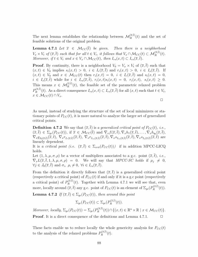
The next lemma establishes the relationship between M(x,t)R (t) and the set of

feasible solutions of the original problem.

Lemma 4.7.1 Let x ∈ MCC(t) be given. Then there is a neighborhood

Vx × Vt of (x, t) such that for all t ∈ Vt, it follows that Vx ∩MCC(t) ⊂M(x,t)R (t).

Moreover, if t ∈ Vt and x ∈ Vx ∩MCC(t), then Irs(x, t) ⊂ Irs(x, t).

Proof . By continuity, there is a neighborhood V0 = Vx × Vt of (x, t) such that(x, t) ∈ V0 implies si(x, t) > 0, i ∈ Ir(x, t) and ri(x, t) > 0, i ∈ Is(x, t). If(x, t) ∈ V0 and x ∈ MCC(t) then ri(x, t) = 0, i ∈ Ir(x, t) and si(x, t) = 0,i ∈ Is(x, t) while for i ∈ Irs(x, t), ri(x, t)si(x, t) = 0, ri(x, t), si(x, t) ≥ 0.

This means x ∈ M(x,t)R (t), the feasible set of the parametric relaxed problem

P(x,t)R (t). As a direct consequence Irs(x, t) ⊂ Irs(x, t) for all (x, t) such that t ∈ Vt,x ∈MCC(t) ∩ Vx.

2

As usual, instead of studying the structure of the set of local minimizers or sta-tionary points of PCC(t), it is more natural to analyze the larger set of generalizedcritical points.

Definition 4.7.2 We say that (x, t) is a generalized critical point of PCC(t), i.e.,(x, t) ∈ Σgc(PCC(t)), if x ∈ MCC(t) and ∇xf(x, t),∇xh1(x, t), . . . ,∇xhq0(x, t),∇xgJ0(x,t)(x, t), ∇xrIr(x,t)(x, t), ∇xrIrs(x,t)(x, t),∇xsIrs(x,t)(x, t),∇xsIs(x,t)(x, t) arelinearly dependent.It is a critical point (i.e. (x, t) ∈ Σcrit(PCC(t))) if in addition MPCC-LICQholds.Let (1, λ, µ, σ, ρ) be a vector of multipliers associated to a g.c. point (x, t), i.e.,∇xL(x, t, 1, λ, µ, σ, ρ) = 0. We will say that MPCC-SC holds if µj 6= 0,∀j ∈ J0(x, t) and σi, ρi 6= 0, ∀i ∈ Irs(x, t).

From the definition it directly follows that (x, t) is a generalized critical point(respectively a critical point) of PCC(t) if and only if it is a g.c point (respectively

a critical point) of P(x,t)R (t). Together with Lemma 4.7.1 we will see that, even

more, locally around (x, t) any g.c. point of PCC(t) is an element of Σgc(P(x,t)R (t)).

Lemma 4.7.2 If (x, t) ∈ Σgc(PCC(t)), then around this point

Σgc(PCC(t)) ⊂ Σgc(P(x,t)R (t)).

Moreover, locally, Σgc(PCC(t)) = Σgc(P(x,t)R (t))∩(x, t) ∈ Rn×R | x ∈MCC(t).

Proof . It is a direct consequence of the definitions and Lemma 4.7.1. 2

These facts enable us to reduce locally the whole genericity analysis for PCC(t)

to the analysis of the relaxed problems P(x,t)R (t).

88

Lemma 4.7.3 The set of functions (f, h, g, r, s) ∈ [C3S]1+q0+q+2l

n+1 such that for all

possible choices of Ir(x, t), Is(x, t), Irs(x, t), the associated problems P(x,t)R (t) are

JJT-regular, contains an open and dense subset of [C3S]1+q0+q+2l

n+1 .

Proof . We apply the same idea as in the proof of Theorem 4.4.1. For a fixed

triplet Ir, Is, Irs, the associated relaxed problem P(x,t)R (t) is a common parametric

nonlinear program. Using the classical JJT-theorem, see Theorem 2.4.1, P(x,t)R (t)

is JJT-regular for an open and dense set S(Ir, Is, Irs) of functions(f, h, g, r, s) ∈ [C3

S]1+q0+q+2ln+1 .

Now we consider all the finitely many possible combinations of Ir, Is, Irs and de-fine the intersection S =

⋂S(Ir, Is, Irs). As S is a finite intersection of open and

dense sets, it is an open and dense set, and the elements in S have the desiredproperties.

2

We have proven that generically the generalized critical points of P(x,t)R (t) are of

type 1, 2, 3, 4 or 5. In view of Definition 4.7.2 and Lemma 4.7.3 we can introducethe different types of g.c. points of PCC(t).

Definition 4.7.3 A g.c. point (x, t) of problem PCC(t) is of type i, i = 1, 2, . . . , 5,

if it is a g.c. point of type i for the corresponding problem P(x,t)R (t).

A problem PCC(t) is called MPCC-regular if all its generalized critical points areof type 1, . . . , 5.

As in the general case, the singular points of type i = 2, . . . , 5 are isolated sin-gularities. The following result is a direct consequence of the previous definition,Lemma 4.7.2 and Lemma 4.7.3.

Theorem 4.7.1 The set of functions (f, h, g, r, s) ∈ [C3S]1+q0+q+2l

n+1 such that PCC(t)

is MPCC-regular contains an open and dense subset of [C3S]1+q0+q+2l

n+1 .

In the following we describe the behavior of the set Σgc(PCC(t)) around any ofthe 5 types of g.c. points in detail. We will see that, locally, Σgc(PCC(t)) can bewritten as the union of the set of g.c. points of certain relaxed problems. We will

always consider (x, t) as an element of Σgc(P(x,t)R (t)), even if eventually it can be

considered as a g.c. point of some other relaxed problem. Note that for MPCC-problems the active index sets do not change in the same way as for nonlinearprograms without complementarity constraints. In fact, the active index setsIr, Irs, Is should always form a partition of 1, . . . , l. Of course, J0(x, t) maychange freely.

For the analysis of the behavior of the set of g.c. points, we again intro-duce the so-called linear and quadratic indexes. For a g.c. point (x, t) of PCC(t)we define the indices LI, (LNI), as the number of positive (negative) multipliers

89

µj, σi, ρi, j ∈ J0(x, t), i ∈ Irs(x, t) of the Lagrangean function associated withgj, j ∈ J0(x, t), ri, si, i ∈ Irs(x, t). The quadratic indices QI, (QNI), repre-sent the number of positive (negative) eigenvalues of the corresponding matrix∇2

xL|TxM(x,t)R (t)

. Evidently, if (x, t) is a strongly stationary point then LNI=0 must

hold and at a local minimizer where MPCC-LICQ holds, LNI=QNI=0. Changesin these indexes imply leaving or entering the set of local minimizers and/or theset of stationary points.

G.C. points of type 1. If (x, t) ∈ Σ1gc(PCC(t)), i.e., (x, t) ∈ Σ1

gc(P(x,t)R (t)),

the set of active indexes will not change locally in Σ1gc(P

(x,t)R (t)). So around

(x, t), Σ1gc(P

(x,t)R (t)) ⊂ (x, t) | x ∈ MCC(t) and, by Lemma 4.7.2,

Σgc(PCC(t)) = Σgc(P(x,t)R (t)), locally. Consequently the following holds in a neigh-

borhood Vx × Vt of (x, t):

- For any (x, t) ∈ Σgc(PCC(t)) ∩ (Vx × Vt), the active index sets do notchange and are J0(x, t) = J0(x, t), Ir(x, t) = Ir(x, t), Is(x, t) = Is(x, t),and Irs(x, t) = Irs(x, t).

- Σgc(PCC(t)) ∩ (Vx × Vt) = Σ1gc(P

(x,t)R ) ∩ (Vx × Vt).

- There is a continuous function x : [t− ε, t+ ε] → Rn, x(t) = x, ε > 0, suchthat Σgc(PCC(t)) ∩ (Vx × Vt) = (x(t), t), [t− ε, t+ ε].

Around a g.c. point (x, t) of type 1, the multipliers ρi, σi, µj i ∈ Irs(x, t),j ∈ J0(x, t) and the eigenvalues of ∇2

xL|TxM(x,t)R (t)

do not change their sign. In

particular the indices (LI, LNI, QI, QNI) = (a, b, c, d) are constant, seeFigure 4.1. So all stationarity types remain locally stable.

The LICQ condition for (x, t) in P(x,t)R (t) is equivalent to MPCC-LICQ in

PCC(t). So B-stationarity and strong stationarity are equivalent. The fulfillmentof the MPCC-SC condition implies the equivalence between M -stationarity andstrong stationarity.

G.C. points of type 2. For the g.c. points of type 2 we have to distinguishbetween two cases.

Definition 4.7.4 A g.c. point (x, t) is a g.c. point of type 2a for PCC(t) if it is

a g.c. point of type 2 for P(x,t)R (t), with µj = 0, for some j ∈ J0(x, t).

It is a g.c. point of type 2b for PCC(t) if it is a g.c. point of type 2 for P(x,t)R (t),

with either ρi∗ = 0 or σi∗ = 0, for some i∗ ∈ Irs(x, t).

In the case of a g.c. point of type 2a, the local structure is the same as in classicalnonlinear programming around a g.c. point of type 2, and locally

Σgc(PCC(t)) = Σgc(P(x,t)R (t)).

90

x

t

(a,b,c,d)

(a,b,c,d)

Figure 4.1: G.C. points of type 1

Let us consider a g.c. point (x, t) of type 2b. W.l.o.g. we assumeσi∗ = si∗(x, t) = 0 for some i∗ ∈ Irs(x, t). As it is a g.c. point of type 2 for

P(x,t)R (t), the possible active constraints for a g.c. point (x, t) of P

(x,t)R (t) near

(x, t), are given by:

B1:

gj(x, t) = 0, j ∈ J0(x, t),ri(x, t) = 0, i ∈ Ir(x, t) ∪ Irs(x, t),sk(x, t) = 0, k ∈ Is(x, t) ∪ Irs(x, t).

B2:

gj(x, t) = 0, j ∈ J0(x, t),ri(x, t) = 0, i ∈ Ir(x, t) ∪ Irs(x, t),sk(x, t) = 0, k ∈ Is(x, t) ∪ Irs(x, t) \ i∗ .

As (x, t) ∈ Σ2gc(P

(x,t)R (t)), around t = t, the set Σgc(P

(x,t)R (t)) bifurcates at (x, t)

into two parts. One part corresponds to the case B1 and is described by adifferentiable curve C1 = (x1(t), t) | t ∈ [t − ε, t + ε], x1(t) = x. The partassociated to B2, denoted as C0, has exactly one feasible branch: if si∗(x, t) > 0,for t > t, the set C0 is (x0(t), t) | t ∈ [t, t+ ε], x0(t) = x and if si∗(x, t) > 0, fort < t, we have C0 = (x0(t), t) | t ∈ [t− ε, t], x0(t) = x. These cases correspondto Dt[si∗(x

0(t), t)](t) > 0 and Dt[si∗(x0(t), t)](t) < 0 respectively. Recall that

since (x, t) is a g.c. point of type 2 of P(x,t)R (t), Dt[si∗(x

0(t), t)](t) 6= 0. Moreoveron the curve (x1(t), t), t ∈ [t− ε, t+ ε], the multiplier σ1

i∗(t) corresponding to theactive constraint si∗(x, t) changes its sign around t.

Note that, around (x, t), for the generalized critical points (x, t) of P(x,t)R (t) it

holds x ∈MCC(t). So, locally, Σgc(PCC(t)) = Σgc(P(x,t)R (t)).

Summarizing, around a g.c. point of type 2b with σi∗ = si∗(x, t) = 0 we have:

91

x

t

PR

PR

Figure 4.2: G.C. point of type 2a

x

t

PR0

PR

Figure 4.3: G.C. point of type 2b

- The possible combination of active indices sets for (x, t) ∈ Σgc(PCC(t)) near(x, t), are

· J0(x, t) = J0(x, t), Ir(x, t) = Ir(x, t), Is(x, t) = Is(x, t),Irs(x, t) = Irs(x, t)

· J0(x, t) = J0(x, t), Ir(x, t) = Ir(x, t) ∪ i∗ , Is(x, t) = Is(x, t),Irs(x, t) = Irs(x, t) \ i∗.

- Σgc(PCC(t)) = C0 ∪ C1 = Σ1gc(PCC(t)) ∪ x, t.

- Around t the multiplier σ1i∗(t) changes its sign.

We want to point out that for (x, t) ∈ C1 the corresponding relaxed problem is

given by P(x,t)R (t), but it changes for (x, t) ∈ C0. We will denote it as P

(x,t)R0 (t).

The picture of the set of generalized critical points around a g.c. point of type2a and 2b is depicted, respectively, in the Figures 4.2 and 4.3.Now we are going to describe the local behavior with regard to stationarity.Around g.c. points of type 2a, a multiplier µj, j ∈ J0(x, t) changes its sign. So,trivially no stationarity type is locally stable.

Let us consider the g.c. points of type 2b, with σi∗ = si∗(x, t) = 0. We willdenote by σ1

i (t), ρ1i (t), i ∈ Irs(x, t), µ

1j(t), j ∈ J0(x, t), the multipliers corre-

sponding to (x1(t), t) ∈ C1 with respect to the functions si, ri, gj, i ∈ Irs(x, t),

92

j ∈ J0(x, t). Analogously σ0i (t), ρ

0i (t), i ∈ Irs(x, t) \ i∗, ρ0

i∗(t) µ0j(t), j ∈ J0(x, t)

are the multipliers associated to (x0(t), t) ∈ C0. Recall si∗(x, t) > 0, for all(x, t) ∈ C0 \ (x, t). W.l.o.g. we assume:

The multiplier σ1i∗(t) is positive for t > t and negative for t < t. (4.7.9)

Due to the conditions for g.c. points of type 2, it follows that the signs ofσ1

i (t), ρ1i (t), µ

1j(t), i ∈ Irs(x, t) \ i∗, j ∈ J0(x, t) and ρ1

i∗(t) coincide with thesigns of σ0

i (t), ρ0i (t), µ

0j(t), i ∈ Irs(x, t) \ i∗, j ∈ J0(x, t) and ρ0

i∗(t) respectively.As MPCC-LICQ holds, B-stationarity and strong stationarity are equivalent

around (x, t). The fulfillment of the MPCC-SC condition (except for (x, t))implies that M -stationarity and B-stationarity are also equivalent (locally) for(x, t) 6= (x, t). So, let us analyze the behavior of strong stationarity.

For simplicity, we assume that the points of C0 \x, t are strongly stationarypoints. This means that σ0

i (t) > 0, ρ0i (t) > 0, ∀i ∈ Irs(x, t) \ i∗, µ0

j(t) > 0,j ∈ J0(x, t) and the sign of ρ0

i∗(t) is free. Then, if ρ0i∗(t) < 0, the points of

C0 \ x, t are strongly stationary points but as i∗ ∈ Irs(x1(t), t), t ∈ [t− ε, t+ ε],

and ρ1i∗(t) < 0, it follows that the elements of C1 are not strongly stationary

points. If ρ0i∗(t) > 0, due to assumption (4.7.9), σ1

i∗(t) > 0 only for t > t. So,(x1(t), t) is a strongly stationary point if and only if t > t.

As for the case 2b the multipliers µj, j ∈ J0(x, t), do not change their sign,weakly stationarity locally remains stable.

Now let us assume that the points of C0 are A-stationary points. If ρ0i∗(t) > 0,

A-stationarity is stable in C1 ∪ C0. However, if ρ0i∗(t) < 0, at (x1(t), t) ∈ C1,

A-stationarity is equivalent with σ1i∗(t) > 0, so it will be fulfilled if and only if

t > t, see condition (4.7.9).In case that C-stationarity holds at C0, again by condition (4.7.9), if ρ0

i∗(t) > 0,the C-stationarity holds for (x1(t), t) ∈ C1 if and only if t > t. If ρ0

i∗(t) < 0, itwill be satisfied for t < t. In both cases only one branch of C1, either for t > t orfor t < t will contain C-stationary points.With respect to the linear and quadratic indices, we can see that around a g.c.point of type 2a, they behave as around a g.c. point of type 2 in the nonlinear

program P(x,t)R (t). In the case of g.c. points of type 2b, we show all possible

combinations of indices (LI, LNI,QI,QNI) in the Figures 4.4, 4.5, 4.6, and 4.7.There, all possible cases for the set of strongly stationary points are also consid-ered. Assuming that the g.c. points in C0, t 6= t, are strongly stationary points,the continuous line represents the set Σstat while the dotted line corresponds tothe set Σgc \ Σstat.

G.C. points of type 3. At a g.c. point (x, t) of type 3, the second ordercondition MPCC-SOC is violated. With the same analysis as for g.c. points of

type 1, it can be seen that, locally, the same relaxed problem P(x,t)R (t) remains

93

x

t

(a,b,c,d)

(a-2,b,c,d+1)

(a-1,b+1,c,d)

Case ddt

[si∗(x0(t), t)] < 0, Dtσ

1i∗(t) < 0.

x

t

(a,b,c,d)

(a-1,b-1,c,d+1)

(a+1,b-1,c,d)

Case ddt

[si∗(x0(t), t)] > 0, Dtσ

1i∗(t) > 0.

Figure 4.4: Type 2b, with ρi∗(t) > 0.

x

t

(a,b,c,d)

(a-1,b-1,c,d+1)

(a-1,b+1,c,d)

Case ddt

[si∗(x0(t), t)] < 0, Dtσ

1i∗(t) < 0.

x

t

(a,b,c,d)

(a,b-2,c,d+1)

(a+1,b-1,c,d)

Case ddt

[si∗(x0(t), t)] > 0, Dtσ

1i∗(t) > 0.

Figure 4.5: Type 2b, with ρi∗(t) < 0.

94

x

t

(a,b,c,d)

(a-2,b,c+1,d)

(a-1,b+1,c,d)

Case Dtσ1i∗(t) < 0, d

dt[si∗(x

0(t), t)] > 0.

x

t

(a,b,c,d)

(a-1,b-1,c+1,d)

(a+1,b-1,c,d)

Case Dtσ1i∗(t) > 0, d

dt[si∗(x

0(t), t)] < 0.

Figure 4.6: Type 2b, with ρi∗(t) > 0.

x

t

(a,b,c,d)

(a-1,b-1,c+1,d)

(a-1,b+1,c,d)

Case ddt

[si∗(x0(t), t)] > 0, Dtσ

1i∗(t) < 0.

x

t

(a,b,c,d)

(a,b-2,c+1,d)

(a+1,b-1,c,d)

Case ddt

[si∗(x0(t), t)] < 0, Dtσ

1i∗(t) > 0.

Figure 4.7: Type 2b, with ρi∗(t) < 0.

95

(a,b,c,d)

(a,b,c-1,d+1)

(a,b,c,d)

(a,b,c+1,d-1)

x

t

Figure 4.8: G.C. points of type 3

valid and that Σgc(PCC(t)) = Σgc(P(x,t)R (t)). So Σgc has a quadratic turning point

as at a g.c. point of type 3 for the standard parametric nonlinear problem P(x,t)R (t).

Moreover, this singularity is isolated and locally Σgc(PCC(t)) = Σ1gc(PCC(t)) ∪

(x, t) (see Figure 4.8).

With respect to stationarity, the situation is as in a g.c. point of type 1.Locally the stationarity type remains unchanged as the sign of the multipliersdoes not change.

Now we will consider the singular points in which MPCC-LICQ is not satisfied. Inthese cases, B-stationarity and strong stationarity are not necessarily equivalent.

G.C. points of type 4. Around a g.c. point (x, t) of type 4, the active indices

do not change in Σgc(P(x,t)R (t)), so locally:

Σgc(PCC(t)) = Σgc(P(x,t)R (t)) = Σ1

gc(PCC(t)) ∪ x, t.

This means that Σgc(PCC(t)) has a quadratic turning point around (x, t). More-over, all multipliers change their sign at (x, t) and ∇xf(x, t) is not a linear com-bination of the active constraints. In particular this means that (x, t) cannot bea stationary point.

Now we will proceed with the analysis of the stationarity types. IfIrs(x, t) = J0(x, t) = ∅ (LI = LNI = 0), all stationarity types are equiva-lent. Moreover, if (x, t) is a critical point then it will also be strongly stationary.As, locally, Irs(x, t) = J0(x, t) = Irs(x, t) = J0(x, t) = ∅, and MPCC-LICQ holdsfor all (x, t) 6= (x, t), the g.c. points with t 6= t are strongly stationary points.

96

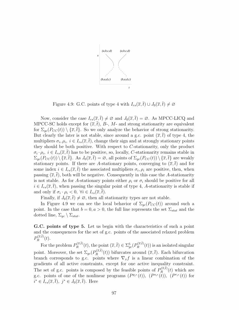
(a,b,c,d)

(b,a,d,c)

(a,b,c,d)

(b,a,d,c)

x

t

Figure 4.9: G.C. points of type 4 with Irs(x, t) ∪ J0(x, t) 6= ∅

Now, consider the case Irs(x, t) 6= ∅ and J0(x, t) = ∅. As MPCC-LICQ andMPCC-SC holds except for (x, t), B-, M - and strong stationarity are equivalentfor Σgc(PCC(t)) \ x, t. So we only analyze the behavior of strong stationarity.But clearly the later is not stable, since around a g.c. point (x, t) of type 4, themultipliers σi, ρi, i ∈ Irs(x, t), change their sign and at strongly stationary pointsthey should be both positive. With respect to C-stationarity, only the productσi ·ρi, i ∈ Irs(x, t) has to be positive, so, locally, C-stationarity remains stable inΣgc(PCC(t))\x, t. As J0(x, t) = ∅, all points of Σgc(PCC(t))\x, t are weaklystationary points. If there are A-stationary points, converging to (x, t) and forsome index i ∈ Irs(x, t) the associated multipliers σi, ρi are positive, then, whenpassing (x, t), both will be negative. Consequently in this case the A-stationarityis not stable. As for A-stationary points either ρi or σi should be positive for alli ∈ Irs(x, t), when passing the singular point of type 4, A-stationarity is stable ifand only if σi · ρi < 0, ∀i ∈ Irs(x, t).

Finally, if J0(x, t) 6= ∅, then all stationarity types are not stable.

In Figure 4.9 we can see the local behavior of Σgc(PCC(t)) around such apoint. In the case that b = 0, a > 0, the full line represents the set Σstat and thedotted line, Σgc \ Σstat.

G.C. points of type 5. Let us begin with the characteristics of such a pointand the consequences for the set of g.c. points of the associated relaxed problem

P(x,t)R (t).

For the problem P(x,t)R (t), the point (x, t) ∈ Σ5

gc(P(x,t)R (t)) is an isolated singular

point. Moreover, the set Σgc(P(x,t)R (t)) bifurcates around (x, t). Each bifurcation

branch corresponds to g.c. points where ∇xf is a linear combination of thegradients of all active constraints, except for one active inequality constraint.

The set of g.c. points is composed by the feasible points of P(x,t)R (t) which are

g.c. points of one of the nonlinear programs (P gj∗ (t)), (P si∗ (t)), (P ri∗ (t)) fori∗ ∈ Irs(x, t), j

∗ ∈ J0(x, t). Here

97

P gj∗ (t) : min f(x, t)s.t. hk(x, t) = 0, k = 1, . . . , q0,

gj(x, t) = 0, j ∈ J0(x, t) \ j∗,ri(x, t) = 0, i ∈ Ir(x, t) ∪ Irs(x, t),si(x, t) = 0, i ∈ Is(x, t) ∪ Irs(x, t),

corresponds to the case where the constraint gj∗(x, t), j∗ ∈ J0(x, t) is not longer

active. In the same way for si∗(x, t), i∗ ∈ Irs(x, t), we define P si∗ (t) and for

ri∗(x, t), i∗ ∈ Irs(x, t), P

ri∗ (t).Now we consider one of these problems, taking P gj∗ (t) w.l.o.g. Due to the

condition

rank(∇(x,t)

[h1, . . . , hq0 , gJ0(x,t), rIr(x,t), rIrs(x,t), sIrs(x,t)sIs(x,t)

](x, t)

)= n+ 1,

the eliminated constraint (gj∗(x, t)) will change its sign around the point (x, t) inthe set of g.c. points of P gj∗ (t). So, exactly one branch, corresponding to t > t

or t < t, will consist of g.c. points of P(x,t)R (t). On this branch the eliminated

constraint will be strictly positive. The branch where this happens, i.e., eitherfor t > t or for t < t, can be determined by using the coefficients of the following(non trivial) linear combination, see e.g., [21]:

q0∑k=1

λk∇xhk(x, t) +∑

j∈J0(x,t)

µj∇xgj(x, t)+

+∑

i∈Ir(x,t)∪Irs(x,t)

ρi∇xri(x, t) +∑

i∈Is(x,t)∪Irs(x,t)

σi∇xsi(x, t) = 0(4.7.10)

Now we will present the meaning of these facts for the set of g.c. points of PCC(t).Note that, for (x, t) near to (x, t), any feasible point x of P gj∗ (t) with

gj∗(x, t) ≥ 0, is also feasible for MCC(t). The same holds in the case that xis a feasible point of P si∗ (t) (respectively P ri∗ (t)) and si∗(x, t) ≥ 0 (respectively

ri∗(x, t) ≥ 0). Consequently Σgc(PCC(t)) = Σgc(P(x,t)R (t)) holds and Σgc(PCC(t))

also bifurcates into |J0(x, t)|+ 2|Irs(x, t)| branches.Now we will consider the relaxed problem that corresponds to each branch.

On the branch where gj∗(x, t) > 0 holds for some j∗ ∈ J0(x, t), locally, the cor-

responding relaxed problem is given by P(x,t)R (t). The branch in which si∗(x, t),

i∗ ∈ Irs(x, t) is no longer active, corresponds to the active index sets, J0(x, t),Ir(x, t)∪i∗ , Is(x, t), Irs(x, t)\i∗. We denote the corresponding relaxed prob-lem by P si∗

R (t). In the case of deactivating ri∗ , i∗ ∈ Irs(x, t) the corresponding

active index sets are J0(x, t), Ir(x, t), Is(x, t) ∪ i∗ , Irs(x, t) \ i∗ and the asso-ciated relaxed problem is denoted by P ri∗

R (t).Considering all possible combinations we can conclude that, locally, the followingholds:

- Σgc(PCC(t)) = Σ1gc(PCC(t)) ∪ (x, t).

- Σgc(PCC(t)) bifurcates into |J0(x, t)|+ 2|Irs(x, t)| branches.

98

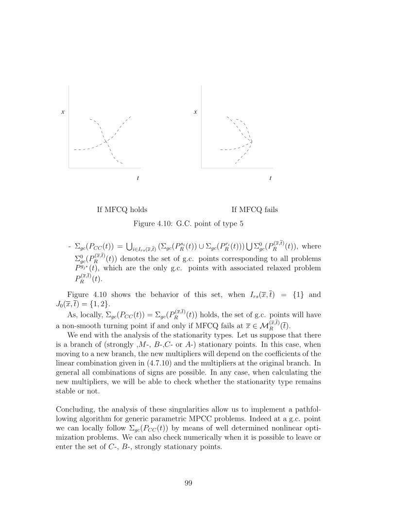
x

t

If MFCQ holds

x

t

If MFCQ fails

Figure 4.10: G.C. point of type 5

- Σgc(PCC(t)) =⋃

i∈Irs(x,t) (Σgc(PsiR (t)) ∪ Σgc(P

riR (t)))

⋃Σ0

gc(P(x,t)R (t)), where

Σ0gc(P

(x,t)R (t)) denotes the set of g.c. points corresponding to all problems

P gj∗ (t), which are the only g.c. points with associated relaxed problem

P(x,t)R (t).

Figure 4.10 shows the behavior of this set, when Irs(x, t) = 1 andJ0(x, t) = 1, 2.

As, locally, Σgc(PCC(t)) = Σgc(P(x,t)R (t)) holds, the set of g.c. points will have

a non-smooth turning point if and only if MFCQ fails at x ∈M(x,t)R (t).

We end with the analysis of the stationarity types. Let us suppose that thereis a branch of (strongly ,M -, B-,C- or A-) stationary points. In this case, whenmoving to a new branch, the new multipliers will depend on the coefficients of thelinear combination given in (4.7.10) and the multipliers at the original branch. Ingeneral all combinations of signs are possible. In any case, when calculating thenew multipliers, we will be able to check whether the stationarity type remainsstable or not.

Concluding, the analysis of these singularities allow us to implement a pathfol-lowing algorithm for generic parametric MPCC problems. Indeed at a g.c. pointwe can locally follow Σgc(PCC(t)) by means of well determined nonlinear opti-mization problems. We can also check numerically when it is possible to leave orenter the set of C-, B-, strongly stationary points.

99

100

Chapter 5

Bilevel problems

5.1 Introduction

Bilevel problems represent another important class of optimization problemswhose structure is

PBL : minx,y

f(x, y)

s.t. (x, y) ∈MBL

(5.1.1)

MBL =

(x, y) ∈ Rn+m

∣∣∣∣ gj(x, y) ≥ 0, j = 1, . . . , q,y solves Q(x).

Here x ∈ Rn, y ∈ Rm and Q(x) stands for the parametric optimization problem

Q(x) : minyφ(x, y)

s.t. y ∈ Y (x)Y (x) = y ∈ Rm | vi(x, y) ≥ 0, i = 1, . . . , l

and is called lower level problem. As usual (f, g1, . . . , gq, ) ∈ [C2]1+q+ln+m . We will

require (φ, v1, . . . , vl) ∈ [C3]1n+m.This kind of problem appears in many applications such as Cournot equi-

librium problems, see (1.4.2), or when solving semi-infinite programs, see [59].However, finding a solution is not an easy problem, because even in order tocheck feasibility one must solve a nonlinear optimization problem Q(x). Bilevelproblems have been investigated in a large number of papers and books, see e.g.,[3], [42], [11] and the references therein.

We may try to solve PBL via a reduction approach as described in [60]. Theidea is, roughly, the following: if we denote the solution of Q(x) by y(x) and if wesuppose that at least near a point x this function behaves well, i.e., y(x) ∈ C1,then locally near x the problem can be written equivalently as the standardprogram:

min f(x, y(x))s.t. gj(x, y(x)) ≥ 0, j = 1, . . . , q.

101

However, this assumption is a very strong hypothesis as can be seen in the fol-lowing example.

Example 5.1.1

min 2x1 + x2 + ys.t. x1 ≥ 0,

y solves Q(x) : min ys.t. x1 + y ≥ 0,

x2 + y ≥ 0.

The solution of the lower level problem is y = −x1 if x1 ≤ x2 and y = −x2 inthe other case. So the function y(x) is not C1 around x = (0, 0) and the point(0, 0, 0) is a global minimizer of the problem.

An alternative solution is via a KKT approach. The constraint y solves Q(x), isreplaced by the KKT condition:

∇yφ(x, y)−l∑

i=1

λi∇yvi(x, y) = 0,

vi(x, y) ≥ 0, i = 1, . . . , l,λi ≥ 0, i = 1, . . . , l,

λivi(x, y) = 0, i = 1, . . . , l.

(5.1.2)

So instead of PBL, we solve the complementarity constrained problem

PKKTBL : minx,y,λ

f(x, y)

s.t. (x, y, λ) ∈MKKTBL,(5.1.3)

where

MKKTBL =

(x, y, λ) ∈ Rn+m+l

∣∣∣∣∣∣∣∣∣∣∣∣

∇yφ(x, y)−l∑

i=1λi∇yvi(x, y) = 0,

vi(x, y) ≥ 0, i = 1, . . . , l,λi ≥ 0, i = 1, . . . , l,

λivi(x, y) = 0, i = 1, . . . , l,gj(x, y) ≥ 0, j = 1, . . . , q.

The FJ necessary condition can also be used. It will lead to a MPCC problemwith a similar structure.

Due to the additional variable λ, the program (5.1.3) can be seen as a liftingprocedure. On the other hand it is a relaxation of the original problem PBL

(5.1.1) in the sense that, if (x, y) ∈ MBL and MFCQ holds at y ∈ Y (x), thenthere is some λ ∈ Rl such that (x, y, λ) ∈MKKTBL. Moreover, if (x, y, λ) is a localsolution of problem (5.1.3) such that y is a minimizer of Q(x) and MFCQ holds

102

at y ∈ Y (x), then (x, y) must also be a local solution of PBL. In the case thatQ(x) is a convex program and MFCQ is satisfied for all y ∈ Y (x), both problems(5.1.1) and (5.1.3) are equivalent.

Obviously, PKKTBL is a special instance of a complementarity constrained prob-lem. So, we can apply the solution method of Chapter 4, i.e., we can try to solvethe perturbed problem Pτ (see problem (4.5.1) in Section 4.6) using standardsoftware of nonlinear programming. For general MPCC problems, this approachhas a favorable convergence behavior under natural assumptions, see Chapter 4.However, since PKKTBL is a MPCC with a special structure, these assumptionsmay not be generically fulfilled. In the sequel, we will study the properties ofPKKTBL from a generical point of view. We will present an algorithm that underthese generical conditions will find a critical point of PBL.

The following question arises. How is the structure of the KKT model com-pared with the structure of the original bilevel program, especially at solutions(x, y) where the reduction approach fails as in Example 5.1.1. We will see thatthe singular behavior of PBL will partially reappear in the KKT formulation.

The chapter is organized as follows. In the next section we study the problem(5.1.3) as a complementarity constrained program and examine its structure froma generical viewpoint. This analysis will be used to obtain in Section 5.3 anumerical procedure for solving bilevel problems. We end with some numericalexamples.

5.2 Genericity analysis of the KKT approach

We consider the KKT formulation (5.1.3) of the bilevel problem PBL . Since it isa complementarity constrained program with a special structure, the genericityresults of Chapter 4, developed for the general case, are no more valid. We have toperform a modified genericity analysis. It appears that also for PKKTBL, genericallyMPCC-LICQ is satisfied at all feasible points. But for the local minimizers(x, y, λ), the situation may be more complicated than for the general MPCCproblems. We will see that the conditions MPCC-SC and MPCC-SOC may failat local minimizers (x, y, λ) of PKKTBL where, for the corresponding minimizer(x, y) of PBL, the lower level problem Q(x) does not allow a local reduction as inExample 5.1.1.

With respect to a feasible point (x, y, λ) of problem PKKTBL, we introduce thefollowing active index sets:

103

J0v(x, y) = i | vi(x, y) = 0,J0(x, y, λ) =

i | vi(x, y) = 0, λi > 0

,

JΛ0(x, y, λ) =i | vi(x, y) = λi = 0

, (5.2.1)

Λ0(x, y, λ) =i | vi(x, y) > 0, λi = 0

,

J0g(x, y) = j | gj(x, y) = 0.

Note that J0v(x, y) = J0(x, y, λ) ∪ JΛ0(x, y, λ). This union does not depend onλ.

Theorem 5.2.1 Let (φ, v1, . . . , vl) ∈ [C3S]1+l

n+m and (g1, . . . , gq) ∈ [C2S]qn+m be fixed.

For almost all (Cxφ , C

yφ, dφ, Cv, dv, Cg, dg) ∈ Rmn+

m(m+1)2

+m+l(n+m)+l+q(n+m)+q, thecondition MPCC-LICQ holds at all feasible points of problem (5.1.3) defined by

φ(x, y) = φ(x, y)+xT [Cxφ ]Ty+

yT [Cyφ]y

2+ dT

φy, v(x, y) = v(x, y)+Cv(x, y)+ dv and

g(x, y) = g(x, y) + Cg(x, y) + dg. Here Rm(m+1)

2 denotes the space of symmetricmatrices of order m.Moreover, generically in the set (φ, v, g) = [C3

S]1+ln+m × [C2

S]qn+m, the conditionMPCC-LICQ holds at all feasible points of the set MKKTBL defined by (φ, v, g).

Proof . Note that a similar result under stronger conditions has been provenin [52] for mathematical programs with variational inequality constraints, seeproblem (1.1.8).The idea of the proof is the following. For any feasible point (x, y, λ) of theproblem given by (φ, v, g), there is a partition J0 = J0(x, y, λ), JΛ0 = JΛ0(x, y, λ),Λ0 = Λ0(x, y, λ) of 1, . . . , l and a set J0g = J0g(x, y) ⊂ 1, . . . , q, such that(x, y, λ) solves the system:

∇yφ(x, y)−l∑

i=1

λi∇yvi(x, y) = 0,

vi(x, y) = 0, i ∈ J0 ∪ JΛ0,λi = 0, i ∈ JΛ0 ∪ Λ0,

gj(x, y) = 0, j ∈ J0g.

(5.2.2)

If MPCC-LICQ fails, then the gradients of the active constraints in (5.2.2)are linearly dependent, i.e., there exists a non-zero vector (α, β, µ, γ) ∈ Rκ,

104

κ = m+ |J0 ∪ JΛ0|+ |J0g|+ |JΛ0 ∪ Λ0|, such that:

∇x[∇yφ(x, y)]T −l∑

i=1

λi∇x[∇yvi(x, y)]T

∇2yφ(x, y)−

l∑i=1

λi∇2yvi(x, y)

α+

+∑

i∈J0∪JΛ0

βi∇(x,y)vi(x, y) +∑

j∈J0g

µj∇(x,y)gj(x, y) = 0,

∇yvi(x, y)Tα = 0, i ∈ J0,

∇yvi(x, y)Tα− γi = 0, i ∈ JΛ0 ∪ Λ0.

(5.2.3)

If α = 0, then γ = 0, and thus at (x, y) the gradients ∇(x,y)gJ0g , ∇(x,y)vJ0∪JΛ0 arelinearly dependent. This means that in this case LICQ fails in M0

KKTBL, where

M0KKTBL =

(x, y) ∈ Rn+m

∣∣∣∣ vi(x, y) ≥ 0, i = 1, . . . , l,gj(x, y) ≥ 0, j = 1, . . . , q.

But asM0KKTBL is the feasible set of a common nonlinear program, it is known that,

for almost every linear perturbation of (v1, . . . , vl, g1, . . . , gq), the LICQ conditionholds for all (x, y) ∈ M0

KKTBL. This means that, for almost every (Cv, dv, Cg, dg)there is no feasible point of MKKTBL solving the system (5.2.3) with α = 0.

So, we only have to consider the remaining case α 6= 0. Let us fix the set ofactive constraints (J0, JΛ0,Λ0). W.l.o.g. we assume α1 6= 0 and take the corre-sponding combination in (5.2.3):

(1, α02, . . . α

0m, β

0, µ0, γ0) = (α

α1

,β

α1

,µ

α1

,γ

α1

).

Note that (α02, . . . , α

0m, β

0, µ0, γ0) ∈ Rκ−1. Then, if MPCC-LICQ fails for

φ = φ(x, y) + xT [Cxφ ]Ty +

yT [Cyφ]y

2+ dT

φy, v = v(x, y) + Cv(x, y) + dv andg = g(x, y) + Cg(x, y) + dg, the condition (5.2.3) for the perturbed problem nowreads:

105

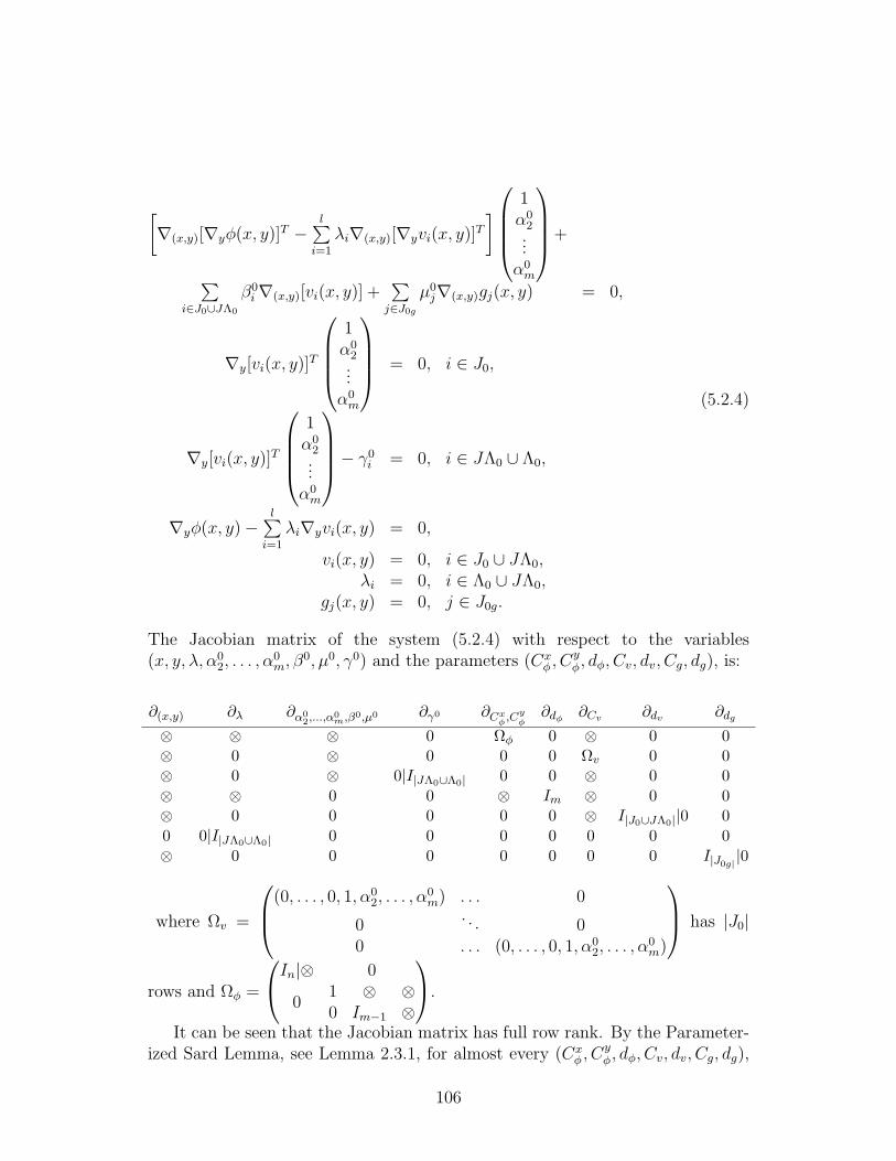
[∇(x,y)[∇yφ(x, y)]T −

l∑i=1

λi∇(x,y)[∇yvi(x, y)]T

]1α0

2...α0

m

+

∑i∈J0∪JΛ0

β0i∇(x,y)[vi(x, y)] +

∑j∈J0g

µ0j∇(x,y)gj(x, y) = 0,

∇y[vi(x, y)]T

1α0

2...α0

m

= 0, i ∈ J0,

∇y[vi(x, y)]T

1α0

2...α0

m

− γ0i = 0, i ∈ JΛ0 ∪ Λ0,

∇yφ(x, y)−l∑

i=1

λi∇yvi(x, y) = 0,

vi(x, y) = 0, i ∈ J0 ∪ JΛ0,λi = 0, i ∈ Λ0 ∪ JΛ0,

gj(x, y) = 0, j ∈ J0g.

(5.2.4)

The Jacobian matrix of the system (5.2.4) with respect to the variables(x, y, λ, α0

2, . . . , α0m, β

0, µ0, γ0) and the parameters (Cxφ , C

yφ, dφ, Cv, dv, Cg, dg), is:

∂(x,y) ∂λ ∂α02,...,α0

m,β0,µ0 ∂γ0 ∂Cxφ ,Cy

φ∂dφ

∂Cv ∂dv ∂dg

⊗ ⊗ ⊗ 0 Ωφ 0 ⊗ 0 0⊗ 0 ⊗ 0 0 0 Ωv 0 0⊗ 0 ⊗ 0|I|JΛ0∪Λ0| 0 0 ⊗ 0 0⊗ ⊗ 0 0 ⊗ Im ⊗ 0 0⊗ 0 0 0 0 0 ⊗ I|J0∪JΛ0||0 00 0|I|JΛ0∪Λ0| 0 0 0 0 0 0 0⊗ 0 0 0 0 0 0 0 I|J0g| |0

where Ωv =

(0, . . . , 0, 1, α02, . . . , α

0m) . . . 0

0. . . 0

0 . . . (0, . . . , 0, 1, α02, . . . , α

0m)

has |J0|

rows and Ωφ =

In|⊗ 0

01 ⊗ ⊗0 Im−1 ⊗

.

It can be seen that the Jacobian matrix has full row rank. By the Parameter-ized Sard Lemma, see Lemma 2.3.1, for almost every (Cx

φ , Cyφ, dφ, Cv, dv, Cg, dg),

106

the matrix formed by the columns of the Jacobian matrix corresponding to thevariables (x, y, λ, α0

2, . . . , α0m, β

0, µ0, γ0) has full row rank. But the number ofrows, n+m+ l +m+ |J0 ∪ JΛ0|+ |JΛ0 ∪ Λ0|+ |J0g|, is larger than the numbern+m+ l+m−1+ |J0∪JΛ0|+ |J0g|+ |JΛ0∪Λ0| of columns. This means that foralmost every parameter, there is no solution of system (5.2.4), i.e., MPCC-LICQholds.If we consider any possible combination of active index sets J0, JΛ0,Λ0 and J0g ananalogous result is obtained. The perturbation result follows by intersecting theset of parameters where MPCC-LICQ holds at the solutions of system (5.2.4),for all possible combinations of active index sets.

We now turn to the proof of the genericity statement. First we will provethat, for fixed N ∈ N, the set of functions (φ, v, g) where MPCC-LICQ holdsat all feasible points (x, y, λ) of MKKTBL with ‖λ‖ ≤ N , is open and dense in[C3

S]1+ln+m × [C2

S]qn+m.

The density part of the statement follows, as usual, directly from the per-turbation result shown above, by using partitions of unity. For more details see[52].

Now we will prove the openness property. We proceed as in the proof ofProposition 4 in [53]. Consider (φ, v1, . . . , vl, g1, . . . , gq) such that, for the result-ing set MKKTBL, MPCC-LICQ holds at all feasible points (x, y, λ), with ‖λ‖ ≤ N .Let us fix (x, y) ∈ Rn × Rm. By continuity, it can be seen that, if

(x, y, λ) 6∈ MKKTBL, then for all λ ∈ Bl

N(0) there is a neighborhood V(x,y) of

(φ, v, g) and U of (x, y) such that for all (φ, v, g) ∈ V(x,y)[U ×B

l

N(0)]∩MKKTBL = ∅

holds for the feasible set MKKTBL corresponding to (φ, v, g).

Let (x, y) be a point such that (x, y, λ) ∈ MKKTBL, for some λ ∈ Bl

N(0). Byassumption, at this point MPCC-LICQ is valid. Using a continuity argument,we can prove that there are neighborhoods U and V(x,y) of (x, y) and (φ, v, g),

respectively, such that, for all (x, y, λ) ∈[U ×B

l

N(0)]∩MKKTBL, the MPCC-LICQ

condition holds at the feasible set MKKTBL corresponding to (φ, v, g) ∈ V(x,y).

Using the neighborhoods V(x,y) and a locally finite cover w.r.t. the (x, y)-

space, we can construct a neighborhood V of (φ, v, g) such that MPCC-LICQholds at all feasible points (x, y, λ) of problem (5.1.3), defined by (φ, v, g) ∈ Vand with ‖λ‖ ≤ N .

Altogether we have proven that the set of functions (φ, v, g) such that theMPCC-LICQ condition is satisfied, at all feasible points (x, y, λ) of MKKTBL with‖λ‖ ≤ N , is open and dense.

107

Finally, if we intersect these open and dense sets for N = 1, 2, . . ., we willobtain the generic set of functions where MPCC-LICQ holds at all feasible points.

2

We now study the structure of the critical points of problem (5.1.3) in the genericcase. The critical points (x, y, λ) are feasible points with associated multipliers(α, β, µ, γ) such that (x, y, λ, α, β, µ, γ) solves the system:

∇(x,y)f(x, y)−∑

i∈J0∪JΛ0

βi∇(x,y)vi(x, y)−∑

j∈J0g

µj∇(x,y)gj(x, y)−

−

∇x[∇yφ(x, y)]T −l∑

i=1

λi∇x[∇yvi(x, y)]T

∇2yφ(x, y)−

l∑i=1

λi∇2yvi(x, y)

α = 0, (5.2.5)

∇yvi(x, y)Tα = 0, i ∈ J0,

∇yvi(x, y)Tα− γi = 0, i ∈ JΛ0 ∪ Λ0

with J0, JΛ0,Λ0, J0g, the active index sets at (x, y, λ), as defined in (5.2.1).Note that, as generically MPCC-LICQ holds, generically any solution of

(5.1.3) must satisfy the KKT conditions (5.2.5). For numerical purposes, it isdesirable that the conditions MPCC-SC and MPCC-SOC hold at critical points.However, as we shall show, MPCC-SC may fail generically. Let us consider theproblem:

min−x− ys.t. y solves Q(x) : min y

s.t. −x+ y ≥ 0,−y ≥ 0.

(5.2.6)

It can easily be seen that in this problem, MFCQ fails at the solution y = 0 ofthe lower level problem Q(0). The point (x, y) = (0, 0) is the minimizer of thebilevel problem and at y the condition MFCQ fails for Q(x). In the Figure 5.1the feasible set and the solution is depicted.

The KKT approach leads to the program:

min−x− ys.t. −x+ y ≥ 0,

−y ≥ 0,1− λ1 + λ2 = 0,

λ1, λ2 ≥ 0,(−x+ y)λ1 = 0,

−yλ2 = 0.

(5.2.7)

108

Set of feasible solutions of

Q(x)

Optimal Solution

Set of feasible solutions of the bilevelproblem

Figure 5.1: Feasible set of bilevel program (5.2.6)

and (x, y, λ1, λ2) = (0, 0, λ1, λ1− 1), λ1 ≥ 1 are global minimizers. If we take thepoint z := (0, 0, 1, 0), the critical point condition for the MPCC problem (5.2.7)is:

−1−100

=

−1100

β1 +

0−100

β2 +

00−11

α+

0001

γ

So the multipliers are α = γ = 0 and β1 = 1, β2 = 2. As JΛ0(z) = 2, MPCC-SC fails.In case we take z = (0, 0, λ1, λ1 − 1), λ1 > 1, although MPCC-SC holds, sinceJΛ0(z) = ∅, the condition MPCC-SOC will fail. Note that TzMKKTBL is gen-erated by the vector (0, 0, 1, 1) while ∇2

(x,y,λ)L(0, 0, λ1, 1 − λ1, 1, 2, 0, 0) = 0, so,

∇2(x,y,λ)L|TzMKKTBL

(0, 0, λ1, 1− λ1, 1, 2, 0, 0) is a singular matrix.As can be seen in Figure 5.1, if we slightly perturb the functions describing theconstraints as −x + y + ε3(x, y) and −y + ε4(x, y), there will be a point (x∗, y∗)satisfying

−x+ y + ε3(x, y) = 0,

−y + ε4(x, y) = 0.

Now, if we perturb the objective function of the lower level problem as y+ε2(x, y),the lower level multipliers λ1, λ2 should fulfill the KKT condition for problemQ(x∗):

1 +∂ε2∂y

(x∗, y∗)− λ1(1 +∂ε3∂y

(x∗, y∗)) + λ2(1−∂ε4∂y

(x∗, y∗)) = 0.

109

So in particular (λ∗1, λ∗2) = (

1+∂ε2∂y

(x,y)

1+∂ε3∂y

(x∗,y∗), 0) solves the previous equation. This

means that the point (x∗, y∗, λ∗1, 0) is a feasible point of MKKTBL for the perturbedfunctions. Now we turn to the objective function of the upper level problem.Assume it is perturbed as −x − y + ε1(x, y) with |ε1(x, y)| 1, |∇ε1(x, y)| 1and |∇2ε1(x, y)| 1, for all (x, y) ∈ Rn × Rm. Then, the critical point systemfor (x, y, λ) = (x∗, y∗, λ∗1, 0), α = γ = 0 reads:

(−1 + ∂ε1

∂x(x∗, y∗)

−1 + ∂ε1∂y

(x∗, y∗)

)=

(−1 + ∂ε3

∂x(x∗, y∗)

1 + ∂ε3∂y

(x∗, y∗)

)β1 +

(∂ε4∂x

(x∗, y∗)−1 + ∂ε4

∂y(x∗, y∗)

)β2.

As |∇εi| 1, i = 3, 4, the matrix

(−1 + ∂ε3

∂x(x∗, y∗) ∂ε4

∂x(x∗, y∗)

1 + ∂ε3∂y

(x∗, y∗) −1 + ∂ε4∂y

(x∗, y∗)

), is non-

singular. From these facts, it follows that the point (x∗, y∗, λ∗1, 0) is a critical pointof this perturbed problem with corresponding multipliers (α, β, γ) and α = γ = 0.

As a consequence we have shown that the failure of MPCC-SC at a solutionof PKKTBL, may remain stable under small perturbations.

The next result describes the generic properties of the critical points:

Theorem 5.2.2 Given (f , φ, v1, . . . , vl, g1, . . . , gq), let us consider the perturbed

functions f = f + bT (x, y), φ = φ(x, y) + cTφy, vi = vi + cTviy + dvi

, gj = gj + dgj.

Then for almost every (b, cφ, cv1 , . . . , cvl, dv, dg), at all solutions (x, y, λ, α, β, γ, µ)

of the corresponding system (5.2.5), i.e. (x, y, λ) is a critical point of problem(5.1.3), the following holds:

BL-1: If α 6= 0, then the MPCC-LICQ, MPCC-SC and MPCC-SOC conditionsare fulfilled w.r.t. the corresponding complementarity constrained problem(5.1.3).

BL-2: If α = 0, then rank(∇yvJ0v(x,y)(x, y)) = m and the multipliers (µ, β) associ-ated with gj(x, y), vi(x, y), j ∈ J0g(x, y), i ∈ J0v(x, y), are not equal to zero.Moreover there is some λ∗ such that (x, y, λ∗) is a critical point of problemPKKTBL and rank(∇yvJ0(x,y,λ∗)(x, y)) =| J0(x, y, λ

∗) |= m. For any λ∗ suchthat the previous condition holds, the MPCC-SOC is satisfied at (x, y, λ∗).

110

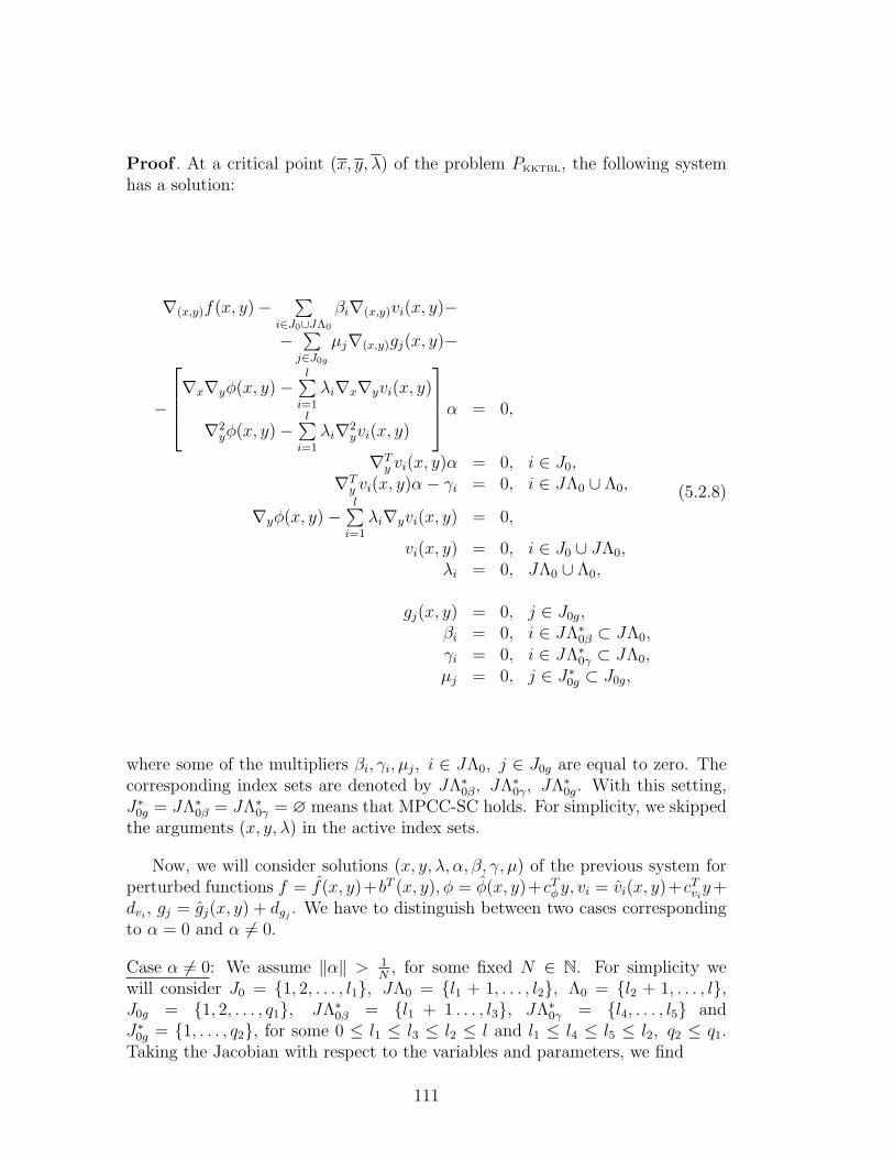
Proof . At a critical point (x, y, λ) of the problem PKKTBL, the following systemhas a solution:

∇(x,y)f(x, y)−∑

i∈J0∪JΛ0

βi∇(x,y)vi(x, y)−

−∑

j∈J0g

µj∇(x,y)gj(x, y)−

−

∇x∇yφ(x, y)−l∑

i=1

λi∇x∇yvi(x, y)

∇2yφ(x, y)−

l∑i=1

λi∇2yvi(x, y)

α = 0,

∇Ty vi(x, y)α = 0, i ∈ J0,

∇Ty vi(x, y)α− γi = 0, i ∈ JΛ0 ∪ Λ0,

∇yφ(x, y)−l∑

i=1

λi∇yvi(x, y) = 0,

vi(x, y) = 0, i ∈ J0 ∪ JΛ0,λi = 0, JΛ0 ∪ Λ0,

gj(x, y) = 0, j ∈ J0g,βi = 0, i ∈ JΛ∗

0β ⊂ JΛ0,γi = 0, i ∈ JΛ∗

0γ ⊂ JΛ0,µj = 0, j ∈ J∗0g ⊂ J0g,

(5.2.8)

where some of the multipliers βi, γi, µj, i ∈ JΛ0, j ∈ J0g are equal to zero. Thecorresponding index sets are denoted by JΛ∗

0β, JΛ∗0γ, JΛ∗

0g. With this setting,J∗0g = JΛ∗

0β = JΛ∗0γ = ∅ means that MPCC-SC holds. For simplicity, we skipped

the arguments (x, y, λ) in the active index sets.

Now, we will consider solutions (x, y, λ, α, β, γ, µ) of the previous system forperturbed functions f = f(x, y)+bT (x, y), φ = φ(x, y)+cTφy, vi = vi(x, y)+cTvi

y+dvi, gj = gj(x, y) + dgj

. We have to distinguish between two cases correspondingto α = 0 and α 6= 0.

Case α 6= 0: We assume ‖α‖ > 1N

, for some fixed N ∈ N. For simplicity wewill consider J0 = 1, 2, . . . , l1, JΛ0 = l1 + 1, . . . , l2, Λ0 = l2 + 1, . . . , l,J0g = 1, 2, . . . , q1, JΛ∗

0β = l1 + 1 . . . , l3, JΛ∗0γ = l4, . . . , l5 and

J∗0g = 1, . . . , q2, for some 0 ≤ l1 ≤ l3 ≤ l2 ≤ l and l1 ≤ l4 ≤ l5 ≤ l2, q2 ≤ q1.Taking the Jacobian with respect to the variables and parameters, we find

111

∂x ∂y ∂λ ∂α ∂β ∂γ ∂µ ∂b ∂cTφ ∂cT

v ∂dvJ0vdgJ0g

⊗ ⊗ ⊗ ⊗ ⊗ 0 ⊗ In+m 0 ⊗ 0

⊗ ⊗ 0[∇yv1]T

...[∇yvl]T

00

Il−l10 0 0 Ω 0

⊗ ⊗ ⊗ 0 0 0 0 0 Im ⊗ 0⊗ ⊗ 0 0 0 0 0 0 0 ⊗ Il2 |0|0|00 0 0|Il−l1 0 0 0 0 0 0 0 0⊗ ⊗ 0 0 0 0 0 0 0 0 0|0|Iq1 |00 0 0 0 0|Iβ∗ |0 0 0 0 0 0 00 0 0 0 0 0|Iγ∗ |0 0 0 0 0 00 0 0 0 0 0 Iµ∗ |0 0 0 0 0

(5.2.9)

where Ω =

αT 0 0

. . .

0 0 αT

has l rows and β∗ = l3 − l1, µ∗ = q2, γ

∗ = l2 − l4.

Evidently, ‖α‖ > 1N

implies α 6= 0 and Ω has rank l. So, it follows directly that therows of the matrix (5.2.9) are linearly independent. Then, by the ParameterizedSard Lemma, for almost every b, cφ, dv, dg, cv, the Jacobian matrix of the system(5.2.8), with respect to variables (x, y, λ) and multipliers (α, β, γ, µ), has rankn+m+ l+m+ |J0v|+ |JΛ0|+ |Λ0|+ |J0g|+ |β∗|+ |µ∗|+ |γ∗|, equal to the number ofrows, at all solutions of the system with ‖α‖ > 1

N. But this rank cannot be greater

than the number n+m+l+m+ |J0|+ |JΛ0|+ |JΛ0|+ |Λ0|+ |J0g|+ |β∗|+ |µ∗|+ |γ∗|of involved variables. So, in view of J0 ∪ JΛ0 = J0v:

|β∗|+ |µ∗|+ |γ∗| = 0.

i.e. MPCC-SC holds.Now, we want to prove the regularity of C = ∇2

(x,y,λ)L|T(x,y,λ)MKKTBL, the Hessian

matrix at the solutions of the perturbed system (5.2.8) with ‖α‖ > 1N

. In viewof Proposition 2.1.1 it is equivalent to prove the regularity of:

B =

(A BBT 0

), (5.2.10)

where A = ∇2(x,y,λ)L(x, y, λ, α, β, γ, µ) and B is the matrix with the gradients of

the active constraints as columns.

Note that B is the upper left part of the matrix (5.2.9), formed by the rows 1to 6, and the columns corresponding to the derivatives ∂(x,y,λ,α,β,γ,µ). So it is non-singular. It is well known that the regularity of B is equivalent to the fulfillmentof MPCC-LICQ and MPCC-SOC.

112

Taking all finitely many possible combinations of active index sets, it followsthat, for almost every linear perturbation of (f, φ, v, g), the solutions of the system(5.2.5) with ‖α‖ > 1

Nare non-degenerate critical points.

By considering the intersection ∩N∈N of all these sets of perturbations, weobtain for almost every linear perturbation the non-degeneracy condition at allcritical points with α 6= 0.Case α = 0: Now we will consider the case of solutions with α = 0. This impliesγi = 0, i ∈ JΛ0 ∪ Λ0, see system (5.2.8). Then for some (β, µ) ∈ R|J0v |+|J0g |, thefollowing system has a solution (x, y, λ):

∇(x,y)f(x, y)−∑

i∈J0v

βi∇(x,y)vi(x, y)−∑

j∈J0g

µj∇(x,y)gj(x, y) = 0,

∇yφ(x, y)−l∑

i=1

λi∇yvi(x, y) = 0,

vi(x, y) = 0, i ∈ J0 ∪ JΛ0,λi = 0, i ∈ JΛ0 ∪ Λ0,

gj(x, y) = 0, j ∈ J0g.(5.2.11)

As the set J0v(x, y) = J0(x, y, λ)∪JΛ0(x, y, λ) does not depend on the particularchoice of λ, this system can be decomposed into two parts. Firstly the system in(x, y, β, µ):

∇(x,y)f(x, y)−∑

i∈J0v

βi∇(x,y)vi(x, y)−∑

j∈J0g

µj∇(x,y)gj(x, y) = 0,

vi(x, y) = 0, i ∈ J0 ∪ JΛ0,gj(x, y) = 0, j ∈ J0g.

(5.2.12)In the second part, for a given solution (x, y) of system (5.2.12), the vector λ hasto solve the following linear system of equalities and inequalities.

φy(x, y)−∑

i∈J0v(x,y)

λi∇yvi(x, y) = 0, (5.2.13)

λ ≥ 0.

Note that, for any solution (x, y, β, µ) of the system (5.2.12), the vector (x, y) isa critical point of the standard problem:

min f(x, y)s.t. vi(x, y) ≥ 0, i = 1, . . . , l,

gj(x, y) ≥ 0, j = 1, . . . , q.(5.2.14)

with corresponding multipliers β and µ.By Caratheodory’s theorem, if the system (5.2.13) is solvable for (x, y), we

can choose a solution λ∗, such that

113

the vectors ∇yvJ0(x,y,λ∗)(x, y) are linearly independent. (5.2.15)

So, in the system (5.2.11) we can assume, w.l.o.g., that the vectors ∇yvi,i ∈ J0(x, y, λ) are linearly independent. Note that J0(x, y, λ) may be the emptyset.

We turn back to the system (5.2.11), where f, φ, g, v are linearly perturbedas in the first part of the proof. We will assume (as in system (5.2.8)) that somemultipliers are zero, e.g., βi = 0, µj = 0, i ∈ JΛ∗

0β, j ∈ J∗0g, with |JΛ∗0β| = β∗

and |J∗0g| = µ∗. So, the critical points will be described by means of the system(5.2.11) and the previous equations for the multipliers (βi, µj). The Jacobian ofthe (augmented) system with respect to variables, multipliers and perturbationparameters has now the form (see also (5.2.9) for the case α 6= 0):

∂x ∂y ∂λ ∂β ∂µ ∂b ∂cTφ ∂dvi∂dgi

⊗ ⊗ 0 ⊗ ⊗ In+m 0 0 0⊗ ⊗ ⊗ 0 0 0 Im 0 0⊗ ⊗ 0 0 0 0 0 I|J0∪JΛ0||0 00 0 0|I|JΛ0∪Λ0| 0 0 0 0 0 0⊗ ⊗ 0 0 0 0 0 0 I|J0g ||0

0 0 0Il4 0 0 00 0 Il3−l1 0

0 0 0 0 0

0 0 0 0 Iµ∗ 0 0 0 0(5.2.16)

Again we assumed J0 = 1, 2, . . . , l1, JΛ0 = l1+1, . . . , l2, Λ0 = l2+1, . . . , l,J0g = 1, 2, . . . , q1, JΛ∗

0β = 1, . . . , l4∪l1+1 . . . , l3, and J∗0g = l1+1, . . . , q2,for some l4 ≤ l1 ≤ l3 ≤ l2 ≤ l, q2 ≤ q1. Using our standard argument, weconclude that, for almost every perturbation (b, cφ, dv, dg), the Jacobian matrixwith respect to the variables and multipliers (x, y, λ, β, µ) has full row rank. Sothe number of variables is greater than or equal to the number of equations, i.e.:

n+m+l+|J0∪JΛ0|+|J0g| ≥ n+m+m+|J0∪JΛ0|+|JΛ0∪Λ0|+|J0g|+|β∗|+|µ∗|

or, equivalently,

|J0| ≥ m+ |β∗|+ |µ∗|.In particular |J0| ≥ m, but our assumption that ∇yvi, i ∈ J0, are linear indepen-dent, see (5.2.15), yields |J0| ≤ m. So,

|J0| = m and |β∗| = |µ∗| = 0. (5.2.17)

To prove the statement concerning MPCC-SOC for the case α = 0, see BL-2 inTheorem 5.2.2, we reconsider the original MPCC-problem (5.1.3) and show that

114

the matrix B =

(A BBT 0

)is regular, where A = ∇2

(x,y,λ)L(x, y, λ, α, β, γ, µ)

and the columns of B are given by the gradients of the active constraints. Fromthe rank condition for matrix (5.2.16) it follows that the square matrix, composedby the row blocks 1, . . . , 5, and the columns corresponding to ∂(x,y,λ,β,µ), is non-singular. We will denote this matrix by:

A′ =

⊗ ⊗ 0 ⊗ ⊗⊗ ⊗ ⊗ 0 0⊗ ⊗ 0 0 00 0 0|I|JΛ0∪Λ0| 0 0⊗ ⊗ 0 0 0

.

Note that B can easily be constructed from A′ as follows: we add the partialderivatives corresponding to the equations ∇yvJ0α = 0, ∇yvJΛ0∪Λ0α = γJΛ0∪Λ0 ,as new rows and the derivatives w.r.t. α and γ as new columns. Exchangingsome rows and columns we have:

B = I1

A′ ⊗ 00 ∇yvJ0 00 ∇yvJΛ0∪Λ0 I|JΛ0∪Λ0|

I2,

where I1 and I2 are appropriate (non-singular) permutations matrices. As ∇yvJ0

is a non-singular matrix, see (5.2.15) and (5.2.17), the regularity of A′ and B areequivalent. This means that, the MPCC-SOC condition holds.

2

From the proof of Theorem 5.2.1 and Theorem 5.2.2 we also obtain the followingfact.

Corollary 5.2.1 For almost all perturbations of (f, φ, v1, . . . , vl, g1, . . . , gq), lin-ear in (f, v1, . . . , vl, g1, . . . , gq) and quadratic in φ, any critical point (x, y, λ) ofthe corresponding problem, PKKTBL with associated multiplier α 6= 0 (see system(5.2.5)) is isolated and non-degenerate in the MPCC sense, see Chapter 4.

We combine the generic properties of the previous results in a definition.

Definition 5.2.1 A bilevel problem PBL is called KKT-regular if its correspond-ing KKT relaxation PKKTBL has the regularity properties of the generic class inTheorem 5.2.1 and Theorem 5.2.2.

As a direct consequence of this definition we obtain the following result.

Corollary 5.2.2 For almost all perturbations of (f, φ, v1, . . . , vl, g1, . . . , gq), lin-ear in (f, v1, . . . , vl, g1, . . . , gq) and quadratic in φ, the problems PBL are KKT-regular.

115

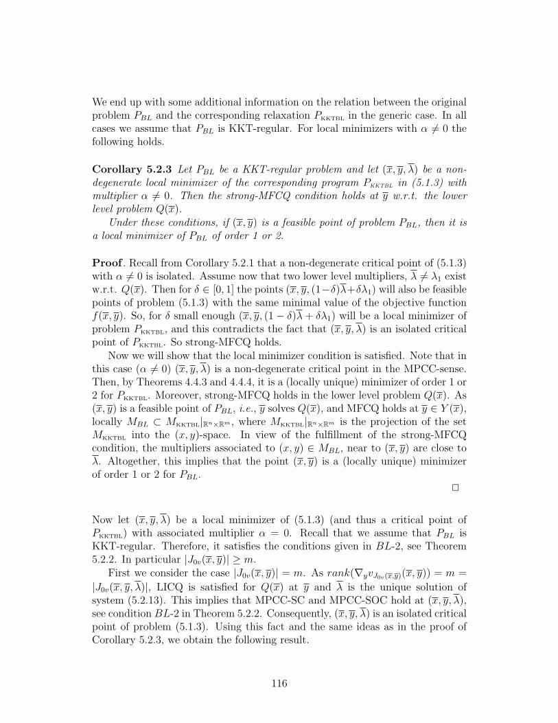
We end up with some additional information on the relation between the originalproblem PBL and the corresponding relaxation PKKTBL in the generic case. In allcases we assume that PBL is KKT-regular. For local minimizers with α 6= 0 thefollowing holds.

Corollary 5.2.3 Let PBL be a KKT-regular problem and let (x, y, λ) be a non-degenerate local minimizer of the corresponding program PKKTBL in (5.1.3) withmultiplier α 6= 0. Then the strong-MFCQ condition holds at y w.r.t. the lowerlevel problem Q(x).

Under these conditions, if (x, y) is a feasible point of problem PBL, then it isa local minimizer of PBL of order 1 or 2.

Proof . Recall from Corollary 5.2.1 that a non-degenerate critical point of (5.1.3)with α 6= 0 is isolated. Assume now that two lower level multipliers, λ 6= λ1 existw.r.t. Q(x). Then for δ ∈ [0, 1] the points (x, y, (1−δ)λ+δλ1) will also be feasiblepoints of problem (5.1.3) with the same minimal value of the objective functionf(x, y). So, for δ small enough (x, y, (1− δ)λ+ δλ1) will be a local minimizer ofproblem PKKTBL, and this contradicts the fact that (x, y, λ) is an isolated criticalpoint of PKKTBL. So strong-MFCQ holds.

Now we will show that the local minimizer condition is satisfied. Note that inthis case (α 6= 0) (x, y, λ) is a non-degenerate critical point in the MPCC-sense.Then, by Theorems 4.4.3 and 4.4.4, it is a (locally unique) minimizer of order 1 or2 for PKKTBL. Moreover, strong-MFCQ holds in the lower level problem Q(x). As(x, y) is a feasible point of PBL, i.e., y solves Q(x), and MFCQ holds at y ∈ Y (x),locally MBL ⊂ MKKTBL|Rn×Rm , where MKKTBL|Rn×Rm is the projection of the setMKKTBL into the (x, y)-space. In view of the fulfillment of the strong-MFCQcondition, the multipliers associated to (x, y) ∈ MBL, near to (x, y) are close toλ. Altogether, this implies that the point (x, y) is a (locally unique) minimizerof order 1 or 2 for PBL.

2

Now let (x, y, λ) be a local minimizer of (5.1.3) (and thus a critical point ofPKKTBL) with associated multiplier α = 0. Recall that we assume that PBL isKKT-regular. Therefore, it satisfies the conditions given in BL-2, see Theorem5.2.2. In particular |J0v(x, y)| ≥ m.

First we consider the case |J0v(x, y)| = m. As rank(∇yvJ0v(x,y)(x, y)) = m =

|J0v(x, y, λ)|, LICQ is satisfied for Q(x) at y and λ is the unique solution ofsystem (5.2.13). This implies that MPCC-SC and MPCC-SOC hold at (x, y, λ),see condition BL-2 in Theorem 5.2.2. Consequently, (x, y, λ) is an isolated criticalpoint of problem (5.1.3). Using this fact and the same ideas as in the proof ofCorollary 5.2.3, we obtain the following result.

116

Corollary 5.2.4 Let PBL be a KKT-regular problem and let (x, y, λ) be a non-degenerate local minimizer of the corresponding program PKKTBL in (5.1.3) withmultiplier α = 0 and rank(∇yvJ0v(x,y)(x, y)) = |J0v(x, y)| = m. Then LICQ holdsat y w.r.t. the lower level problem Q(x).

Under these hypotheses, if (x, y) is a feasible point of problem PBL, then it isa local minimizer of PBL of order 1 or 2.

Now we consider the case that (x, y, λ) is a local minimizer of PKKTBL, withα = 0, where strong-MFCQ fails at Q(x) w.r.t. y, hence |J0v(x, y)| > m.Then the set of solutions of the system (5.2.13) is a polyhedron of dimension d,d ≤ |J0v(x, y)|−m. We will denote this polyhedron by R(x, y). Note that the ver-tices ofR(x, y) are given by those solutions λ∗ such that rank(∇yvJ0(x,y,λ∗)(x, y)) =|J0(x, y, λ

∗)| = m.For each λ∗ ∈ R(x, y), the point (x, y, λ∗) is a critical point of PKKTBL. In

this situation the following bad behavior may occur: the points (x, y, λ) withλ ∈ R(x, y) and JΛ0(x, y, λ) = ∅, i.e., λ is in the relative interior of R(x, y),are local minimizers of PKKTBL, but if λ is a vertex of R(x, y), the point (x, y, λ)is no longer a local minimizer. This means, in particular, that the set of localminimizers may not be closed. We give an example:

Example 5.2.1

min−x+ ys.t. y solves Q(x) : min y

s.t. y ≥ 0,x ≥ 0.

Note that the corresponding KKT relaxation is

min−x+ ys.t. 1− λ1 = 0,

y ≥ 0,x ≥ 0,

λ1, λ2 ≥ 0,yλ1 = 0,xλ2 = 0.

Here, at the minimizer (x, y) = (0, 0), we have J0v(x, y) = 1, 2. So|J0v(x, y)| = 2 > 1 = m. The points (x, y, λ1, λ2) = (0, 0, 1, λ2), with λ2 > 0,are clearly local minimizers of the KKT relaxation, with the same value of theobjective function, f(0, 0) = 0. However, if we take (λ1, λ2) = (1, 0), the ver-tex solution of the corresponding system (5.2.13) (for (x, y) = (0, 0)) the point(0, 0, 1, 0) is no longer a local minimizer. Indeed, when letting x > 0, the value

117

of the objective function will be smaller. Note that (0, 0) is not a local minimizerof the original bilevel problem.

In the case where (x, y, λ) is a local minimizer of PKKTBL, with α = 0, andsuch that strong-MFCQ fails for y at Q(x), in comparison with Corollaries 5.2.3and 5.2.4, we only have the following weaker result.

Corollary 5.2.5 Let PBL be a KKT-regular problem and let (x, y, λ) be a localminimizer of PKKTBL, with α = 0, such that rank[∇vJ0(x,y,λ)(x, y)] = |J0(x, y, λ)| =m (i.e. λ is a vertex solution of system (5.2.13)) and strong-MFCQ fails for yat Q(x). Then (x, y, λ) is an isolated local minimizer of PKKTBL (5.1.3) of order2, in the following sense: There exists κ, κ > 0, such that for all (x, y) near(x, y), with (x, y, λ) ∈ MKKTBL for some λ satisfying λJ0(x,y,λ) > 0, we obtain

f(x, y)− f(x, y) ≥ κ‖(x− x, y − y)‖2.

Proof . At a local minimizer (x, y, λ) the multipliers βJΛ0 , γJΛ0 , µJ0g are non-negative and the Hessian of the Lagrangean of problem (5.1.3), should be positivesemi-definite on T(x,y,λ)MKKTBL, i.e., ∇2

(x,y,λ)L(x, y, λ, α, β, µ, γ)|T(x,y,λ)MKKTBL 0,

see the end of Section 4.3. In this case in view of α = γ = 0 we have:

∇2(x,y,λ)L(x, y, λ, α, β, µ, γ) =

(∇2

(x,y)L(x, y, β, µ) 0

0 0

)where

L(x, y, β, µ) = f(x, y)−∑

i∈J0(x,y,λ)∪JΛ0(x,y,λ)

βivi(x, y)−∑

j∈J0g(x,y)

µjgj(x, y).

Now we will construct the tangent subspace T(x,y,λ)MKKTBL. Recall that, by defi-nition, it is the tangent subspace of the manifold described by the system (5.2.2).As can be easily seen, this sub-space is generated by the k = n − |J0g| − |JΛ0|

columns of the matrix

V

0l−m

where the k columns of V form a basis of the

subspace tangent to ∇(x,y)vJ0v(x,y)(x, y),∇(x,y)gJ0g(x, y) and is the m×k-matrixsolving

∇yvJ0(x,y,λ)(x, y)T = −∇(x,y)[∇yφ−

l∑i=1

λi∇yvi(x, y)]TV.

As a consequence

∇2(x,y,λ)L(x, y, λ, α, β, µ, γ)|T(x,y,λ)MKKTBL

= V T∇2(x,y)L(x, y, β, µ)V 0.

118

But λ is such that rank[∇vJ0(x,y,λ)(x, y)] = |J0(x, y, λ)| = m and for these criticalpoints MPCC-SOC holds, see Condition BL-2 in Theorem 5.2.2. So

∇2(x,y,λ)L(x, y, λ, α, β, µ, γ)|T(x,y,λ)MKKTBL

= V T∇2(x,y)L(x, y, β, µ)V is positive definite.

(5.2.18)Recall that in case α = 0 the regularity means µj, βi 6= 0, for all j ∈ J0g(x, y),i ∈ J0(x, y, λ) ∪ JΛ0(x, y, λ), see Condition BL-2 in Theorem 5.2.2. As (x, y, λ)is a minimizer of PKKTBL, we must have:

βi, µj > 0, ∀i ∈ JΛ0(x, y, λ), j ∈ J0g(x, y). (5.2.19)

Let us consider the problem:

min f(x, y)

s.t. (x, y) ∈ MJ0(x,y,λ)

MJ0(x,y,λ) =

(x, y) ∈ Rn+m

∣∣∣∣∣∣vi(x, y) = 0, i ∈ J0(x, y, λ),

vi(x, y) ≥ 0, i ∈ JΛ0(x, y, λ),gj(x, y) ≥ 0, j = 1, . . . , q.

(5.2.20)

It is easy to see that (x, y) is a critical point of the previous problem with as-sociated multipliers (β, µ). Since the Hessian of the Lagrangean of this problemcoincides with the Hessian of L(x, y, β, µ) and T(x,y)MJ0(x,y,λ) is generated bythe columns of V , conditions (5.2.19) and (5.2.18) mean that (x, y) is a localminimizer of problem (5.2.20) of order 2, i.e., there exists κ, κ > 0, such that,locally,

f(x, y)− f(x, y) ≥ κ‖(x− x, y − y)‖2,∀(x, y) ∈ MJ0(x, y, λ).

Now, we take (x, y) near (x, y) satisfying (x, y, λ) ∈ MKKTBL, for some λ,λJ0(x,y,λ) > 0. By the feasibility of (x, y, λ) we have vJ0(x,y,λ)(x, y) = 0. Then

(x, y) ∈ MJ0(x,y,λ) and the inequality f(x, y)− f(x, y) ≥ κ‖(x−x, y− y)‖2 holds.2

Remark 5.2.1 Note that the condition obtained in Corollary 5.2.5 does not meanthat if (x, y) ∈MBL, then (x, y) is a local minimizer of PBL, as in the other cases.

We now summarize the genericity results of this section. Generically, MPCC-LICQ holds for all feasible points of MKKTBL. At the local minimizers (x, y, λ)of PKKTBL, with corresponding multipliers (α, β, γ, µ), the following cases mayappear generically:

119

- α 6= 0: in this case for the lower level problem Q(x), strong-MFCQ holdsat y and (x, y, λ) is non-degenerate, as a critical point, in the MPCC-sense.

- α = 0: (x, y) is a non-degenerate critical point of problem (5.2.14) andrank(∇yvJ0(x,y,λ)∪JΛ0(x,y,λ)) = m. Moreover there is some vertex solutionλ∗ of the system (5.2.13), such that (x, y, λ∗) is a critical point of PKKTBL,|J0(x, y, λ

∗)| = m and rank(∇yvJ0(x,y,λ∗)(x, y)) = m. More precisely, recallJ0v(x, y) = J0(x, y, λ

∗) ∪ JΛ0(x, y, λ∗), we have :

· in case |J0v(x, y)| = m:λ is the unique solution of system (5.2.13). LICQ holds at y for Q(x)and (x, y, λ) is a non-degenerate critical point of PKKTBL in the MPCC-sense, i.e., MPCC-SOC and MPCC-SC are fulfilled.

· in case |J0v(x, y)| > m:For the vertex solutions λ∗ of the system (5.2.13) it followsJΛ0(x, y, λ

∗) 6= ∅. Moreover MPCC-SC fails for (x, y, λ∗) sinceγi = 0, ∀i ∈ JΛ0(x, y, λ

∗), but MPCC-SOC holds.

5.3 A numerical approach for solving BL

In this part we will present a procedure for computing local minimizers of PKKTBL.As already sketched at the end of Section 5.2, there may appear two differentcases: local minimizers corresponding to critical points where α = 0 or whereα 6= 0. First let us reconsider the reduced problem, see (5.2.14):

min f(x, y)s.t. vi(x, y) ≥ 0, i = 1, . . . , l,

gj(x, y) ≥ 0, j = 1, . . . , q.(5.3.1)

With the aid of this program we have the following possible method.

Conceptual method:

1. Possible solutions with α = 0: Try to compute a critical point (x, y) ofthe reduced nonlinear program (5.3.1). If there is a corresponding solutionλ of system (5.2.13), then (x, y, λ) is a critical point of problem PKKTBL,with α = 0. Now we calculate a vertex solution λ of system (5.2.13).Then, generically, rank(∇yvJ0(x,y,λ)(x, y)) = |J0(x, y, λ)| = m. If conditions

(5.2.19) and (5.2.18) hold, (x, y, λ) is a local minimizer of problem (5.1.3).

2. Possible solutions with α 6= 0: Try to find a solution (x, y, λ) of the fullsystem (5.2.5), by applying the parametric smoothing approach of Chapter4. If the procedure converges to a point (x, y, λ) with α = 0, try to identifythe active index sets J0v(x, y), J0g(x, y) and switch to step 1.

120

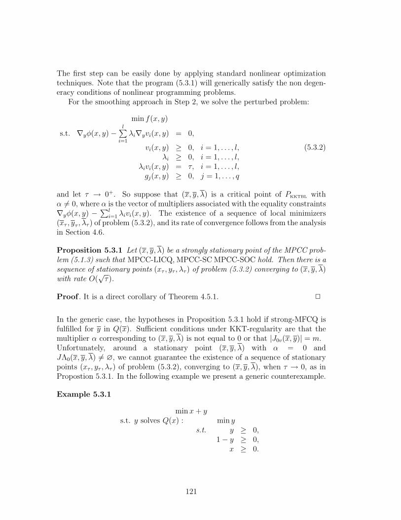
The first step can be easily done by applying standard nonlinear optimizationtechniques. Note that the program (5.3.1) will generically satisfy the non degen-eracy conditions of nonlinear programming problems.

For the smoothing approach in Step 2, we solve the perturbed problem:

min f(x, y)

s.t. ∇yφ(x, y)−l∑

i=1

λi∇yvi(x, y) = 0,

vi(x, y) ≥ 0, i = 1, . . . , l,λi ≥ 0, i = 1, . . . , l,

λivi(x, y) = τ, i = 1, . . . , l,gj(x, y) ≥ 0, j = 1, . . . , q

(5.3.2)

and let τ → 0+. So suppose that (x, y, λ) is a critical point of PKKTBL withα 6= 0, where α is the vector of multipliers associated with the equality constraints∇yφ(x, y) −

∑li=1 λivi(x, y). The existence of a sequence of local minimizers

(xτ , yτ , λτ ) of problem (5.3.2), and its rate of convergence follows from the analysisin Section 4.6.

Proposition 5.3.1 Let (x, y, λ) be a strongly stationary point of the MPCC prob-lem (5.1.3) such that MPCC-LICQ, MPCC-SC MPCC-SOC hold. Then there is asequence of stationary points (xτ , yτ , λτ ) of problem (5.3.2) converging to (x, y, λ)with rate O(

√τ).

Proof . It is a direct corollary of Theorem 4.5.1. 2

In the generic case, the hypotheses in Proposition 5.3.1 hold if strong-MFCQ isfulfilled for y in Q(x). Sufficient conditions under KKT-regularity are that themultiplier α corresponding to (x, y, λ) is not equal to 0 or that |J0v(x, y)| = m.Unfortunately, around a stationary point (x, y, λ) with α = 0 andJΛ0(x, y, λ) 6= ∅, we cannot guarantee the existence of a sequence of stationarypoints (xτ , yτ , λτ ) of problem (5.3.2), converging to (x, y, λ), when τ → 0, as inPropostion 5.3.1. In the following example we present a generic counterexample.

Example 5.3.1

minx+ ys.t. y solves Q(x) : min y

s.t. y ≥ 0,1− y ≥ 0,

x ≥ 0.

121

The KKT approach leads us to the following problem:

minx+ ys.t. 1− λ1 + λ2 = 0,

y ≥ 0,1− y ≥ 0,

x ≥ 0,λi ≥ 0, i = 1, 2, 3,λ1y = 0,

λ2(1− y) = 0,λ3x = 0.

This problem has the solution (x, y, λ) = (0, 0, 1, 0, 0) with multipliersβ1 = β2 = 1, α = γ1 = γ2 = γ3 = 0, and |JΛ0(x, y, λ)| = 1. Now, we con-sider the smoothing parameterization of Section 4.6 and try to solve:

Pτ : minx+ ys.t. 1− λ1 + λ2 = 0,

λ1 ≥ 0,y ≥ 0,λ2 ≥ 0,

1− y ≥ 0,λ3 ≥ 0,x ≥ 0,

yλ1 = τ,(1− y)λ2 = τ,

xλ3 = τ,

for τ → 0+. Note that, for τ > 0 small enough, LICQ holds at any feasible point.In fact, as the active index set is empty, the linear dependence implies that thegradients of equations number 1, 8, 9 and 10 are linearly dependent, i.e., thefollowing system has a non-trivial solution (a, b, c, d):

0 0 0 λ3

0 λ1 −λ2 0−1 y 0 01 0 1− y 00 0 0 x

abcd

= 0.

x > 0 implies d = 0. By multiplying the third and fourth equations by λ21 and

−λ22, respectively, and using the feasibility condition, we obtain:

λ1bτ = λ21a,

−λ2cτ = λ22a.

122

Summing up and using bλ1 − cλ2 = 0, we obtain a(λ21 + λ2

2) = 0. But λ1, λ2 > 0,so a = 0 and this implies b = c = 0, a contradiction to (a, b, c, d) 6= 0.

Now we will prove by contradiction that there cannot exist a sequence ofcritical points of Pτ converging to (0,0,1,0,0) when τ → 0+. The critical pointcondition for problem Pτ reads:

11000

=

0 0 0 λ3

0 λ1 −λ2 0−1 y 0 01 0 1− y 00 0 0 x

abcd

The condition x > 0 yields d = 0, so in the first equation we have 1 = 0contradicting the existence of multipliers (a, b, c, d) solving the system.

We want to recall that there may exist feasible points (x, y) ∈ MBL, or evenminimizers (x, y) of problem PBL in (5.1.1), where the MFCQ condition is violatedin the lower level problem, see problem (5.2.6). So y may not satisfy the KKTcondition for Q(x). Clearly minimizers (x, y), such that the KKT condition failsat y for Q(x), cannot be found by the KKT approach. Therefore from a practicalviewpoint it is advisable to use the FJ approach in which the KKT condition(5.1.2) is replaced by the FJ optimality condition:

λ0∇yφ(x, y)−l∑

i=1

λi∇yvi(x, y) = 0,

λ0 ≥ 0,λi ≥ 0, i = 1, . . . , l,

vi(x, y) ≥ 0, i = 1, . . . , l,λivi(x, y) = 0, i = 1, . . . , l,

λ0 +l∑

i=1

λi = 1.

So we are lead to the problem:

min f(x, y)

s.t. λ0∇yφ(x, y)−l∑

i=1

λi∇yvi(x, y) = 0,

λ0 ≥ 0,λi ≥ 0, i = 1, . . . , l,

vi(x, y) ≥ 0, i = 1, . . . , l,λivi(x, y) = 0, i = 1, . . . , l,

λ0 +l∑

i=1

λi = 1,

gj(x, y) ≥ 0, j = 1, . . . , q.

(5.3.3)

123

The FJ approach leads, up to some technical modification, to a problem with asimilar structure as in the KKT approach. We, therefore, expect similar genericityresults.

5.4 Numerical examples

In this section we will consider four bilevel problems to illustrate the solutionmethod given before. Three of them appear on the web page http://www-unix.mcs.anl.gov/˜leyffer/MacMPEC. The fourth is the problem in Example 5.3.1.We will present the numerical results obtained when solving the problem PKKTBL,corresponding to the KKT approach applied to problem PBL. The solutions arecomputed by means of the smoothing techniques described in Chapter 4. We usethe solver of nonlinear optimization problems of MATLAB, fmincon, to find acritical point of the corresponding problem Pτ , τ → 0+. All programs run underMATLAB 7.0.1.

We want to remark that the numerical results will be displayed with twodecimal places, even if the corresponding number is exact. For instance, thevalues 12 and 12.00009 will be both written as 12.00.

The first problem originally appeared in Bard [2].

min(x1 − 5)2 + (2y + 1)2

s.t. x ≥ 0,y ≥ 0,

y solves Q(x) : min(y − 1)2 − 1.5xys.t. 3x− y − 3 ≥ 0,

−x+ 0.5y + 4 ≥ 0,−x− y + 7 ≥ 0.

The reported local minimizer is (x, y, λ) = (1, 0, 3.5, 0, 0). We obtained:

Method Smoothing methodStarting Solution (0.00, 0.00)

Start lower level multipliers (1.00, 1.00, 1.00)Solution (1.00, 0.00)

Lower level multipliers (3.50, 0.00, 0.00)Value of the obj. function 17.00

CPU time .20

The smoothing method converged to the minimizer. The error between the ap-proximate and the real minimizer for τ = 9.54 e-07 is 0.39 e-06.

We solved the same problem using 50 random starting points on the intervals[−1, 5]2 and [−20, 20]2. It performed as follows:

124

Behavior\Interval [−1, 5]2 [−20, 20]2

Smoothing approach succeeded in 33 cases 16 cases

The second example, also appeared in [2], and reads:

min−x21 − 3x2 − 4y1 + y2

2

s.t.x ≥ 0,y ≥ 0,

−x21 − 2x2 + 4 ≥ 0,

y solves Q(x) : min y21 − 5y2

s.t. x21 − 2x1 + x2

2 − 2y1 + y2 + 3 ≥ 0,x2 + 3y1 − 4y2 − 4 ≥ 0.

The numerical results are given in the next table:

Method Inner pointStarting solution (0.00, 0.00, 0.00, 0.00)

Start lower level multipliers (1.00, 1.00)Solution (0.00, 2.00, 1.88, 0.91)

Lower level multipliers (0.00, 1.25)Value of the objective function -12.67

CPU time 33.31

Again the smoothing approach converges to the reported minimizer,(x, y, λ) = (0, 2, 1.875, 0.9062, 0, 1.25). The error between the obtained pointand the real minimizer is 4.97 e-05 for τ = 9.54 e-07.

Now, by considering 50 starting points randomly generated in the intervals[−1, 5]4 and [−20, 20]4 we obtained:

Behavior\Interval [−1, 5]4 [−20, 20]4

Smoothing approach succeeded in 44 cases 45 cases

Note that in the previous examples, at the solutions we have JΛ0(x, y, λ) = ∅i.e., strong SC holds (see Section 4.3). However, this condition may fail in genericexamples as in Example 5.3.1, where at the solutions (x, y, λ) = (0, 0, 1, 0, λ3),λ3 ≥ 0 the corresponding multiplier satisfies α = 0. Recall the problem is

minx+ ys.t. y solves Q(x) : min y

s.t. y ≥ 0,1− y ≥ 0,

x ≥ 0.

125

With the starting point (0,0,1,1,1), the smoothing approach obtained thesolution (2.17 e-09, 9.54 e-07, 1.00, 9.547 e-07, 438.59). As expected, at thesolution, the lower level multipliers became large. When τ is small, we observedthat the value of λ3 remained almost unchanged. In fact, for τ small, x = τ

438.593

is almost equal to 0. So, the point ( τ438.593

, 0, 1, 0, λ3) solves the critical pointssystem within an acceptable error.

We end with a non-generic example, where MPCC-LICQ fails at the solutionpoint. This example can be found in [13]. The problem is

min−x21 − 2x1 + x2

2 − 2x2 + y21 + y2

2

s.t.x ≥ 0,y ≥ 0,

−x1 + 2 ≥ 0,y solves Q(x) : min y2

1 − 2x1y1 + y22 − 2x2y2

s.t. .25− (y1 − 1)2 ≥ 0,.25− (y2 − 1)2 ≥ 0.

In this case the minimizer is (.5, .5, .5, .5) and the lower level multipliers,λ = (0, 0). At that point, MPCC-LICQ is not satisfied. Our approach behavedsurprisingly good with error of order

√τ for τ ≥ 8.6736 e-19.

126

Chapter 6

Equilibrium constrainedproblems

6.1 Introduction

In this part we will consider the general case of optimization problems withequilibrium constraints (see Section 1.1)

PEC : min f(x, y)s.t. (x, y) ∈MEC

(6.1.1)

MEC =

(x, y) ∈ Rn × Rm

∣∣∣∣∣∣gj(x, y) ≥ 0, j = 1, . . . , q,

y ∈ Y (x),φ(x, y, z) ≥ 0, ∀z ∈ Y (x)

where Y (x) = y ∈ Rm | vi(x, y) ≥ 0, i = 1, . . . , l, f ∈ [C∞]1n+m, φ ∈ [C∞]1n+m+m,(g1, . . . , gq) ∈ [C∞]qn+m and (v1, . . . , vl) ∈ [C∞]ln+m. For simplicity we omit equal-ity constraints.

The following problems can be seen as special instances of PEC :

- Optimization problems with a VI constraint, see (1.1.8), whereφ(x, y, z) = Φ(x, y)T (z − y).

- Stackelberg Games min f(x, y) s.t. y ∈ S(x) where S(x) is the set of Nashstrategies.

- Bilevel problems, see Chapter 5.

- Generalized semi-infinite problem (GSIP), see [58].

As for the case of BL programs, the structure of the feasible set of PEC isnot suitable for classical optimization approaches. Instead, we again propose and

127

analyze the KKT approach based on a transformation of the problems into aprogram with complementarity constraints.

The chapter is organized as follows. Firstly we are interested in the topolog-ical structure of the feasible set of PEC and we give some necessary conditionfor convexity and closedness. In Section 6.3 we consider the MPCC problemobtained by the KKT approach for solving PEC . We will show that one can-not expect MPCC-LICQ to be fulfilled generically at all feasible points. Sec-tion 6.4 deals with the special case where LICQ holds in Y (x), and φ, vi, gj,i = 1, . . . , l, j = 1, . . . , q, satisfy certain convexity conditions. For the MPCCform of PEC we prove that for almost all perturbations MPCC-LICQ is satisfiedat all feasible points and that the critical points are non-degenerate in the MPCC-sense. In the last section we discuss the linear case, where the functions f, vi, gj,i = 1, . . . , l, j = 1, . . . , q are linear and φ(x, y, z) is of the form [C(x, y)+d](z−y).We derive the generic properties for these problems and present a numerical al-gorithm.

6.2 Structure of the feasible set

In this section we are interested in conditions which guarantee that the feasibleset MEC of PEC is closed and/or convex. Note that in general, as in the case ofGSIP (see [58]), MEC need not to be closed. We give the illustrative example:

Example 6.2.1 Choose φ(x, y, z) = z − 32, x ≥ 0, x ≤ π

2, y ∈ Y (x) and

Y (x) = z ∈ R | (z − 2)(z − sin(x))2 ≥ 0, z ≥ 1.

The feasible set then reads:

MEC =

(x, y) ∈ R× R

∣∣∣∣∣∣x ∈ [0, π

2]

y ∈ Y (x),z − 3

2≥ 0, ∀z ∈ Y (x)

.

We find

Y (x) =

[2,∞), for 0 ≤ x < π

2

1 ∪ [2,∞), for x = π2,

leading to the feasible set MEC = [0, π2) × [2,∞), which is neither closed nor

open. Note that this is due to the failure of MFCQ at z = 1 with respect toY (π

2). As a result, the mapping Y (x) is not lower semi-continuous at z = 1, since

there is no sequence (xk, zk) → (π2, 1), with zk ∈ Y (xk). Recall that a set valued

map Y : Rn → 2Rmis called lower semi-continuous at x ∈ Rn if for all open sets

V ⊂ Rm such that V ∩ Y (x) 6= ∅ there is a neighborhood U of x such that forall x ∈ U, Y (x) ∩ V 6= ∅. For more details we refer to Klatte and Kummer [36].

The next result provides sufficient conditions for closedness/convexity of MEC ,see [7] and also [58] for GSIP.

128

Proposition 6.2.1 (cf. [7]) Suppose that Y (x) ⊂ K holds for all x ∈ Rn withsome compact set K, K ⊂ Rm. Assume that for all x ∈ Rn the condition MFCQholds at all z ∈ Y (x). Then the set valued mapping Y (x) is lower semi-continuousand MEC is closed.

Suppose that for any x, the set Y (x) is convex. Let the functions φ(x, y, z)and gj(x, y), j = 1, . . . , q be concave and let Y (αx1 + (1−α)x2) ⊂ αY (x1) + (1−α)Y (x2), α ∈ [0, 1] hold for all x1, x2. Then MEC is convex.

Proof . It is well known that the MFCQ condition implies that Y (x) is lowersemi-continuous, see [36]. To prove that the feasible set MEC is closed, we haveto show:

for all (xk, yk) ∈MEC , (xk, yk) → (x, y), ⇒ (x, y) ∈MEC .

By continuity, the assumptions entail y ∈ Y (x) and gj(x, y) ≥ 0. As Y (x) iscompact, we can consider z∗ ∈ Y (x) such that

z∗ solves minzφ(x, y, z)

s.t. z ∈ Y (x).

But Y (x) is lower semi-continuous, so there is a sequence of points of zk ∈ Y (xk),such that zk → z∗. Due to the feasibility assumption φ(xk, yk, zk) ≥ 0 and takinglimits k →∞, yields 0 ≤ φ(x, y, z∗) ≤ φ(x, y, z), ∀z ∈ Y (x). So, (x, y) ∈MEC .

For the second part, if (x1, y1) and (x2, y2), are two feasible points, by the con-vexity assumptions, it follows (using standard arguments) that for anyα ∈ [0, 1], the point (αx1 + (1− α)x2, αy1 + (1− α)y2), is also feasible.

2

Let us write the program PEC equivalently in the bilevel form:

minx,y,z

f(x, y)

s.t. gj(x, y) ≥ 0, j = 1, . . . , q,y ∈ Y (x),

φ(x, y, z) ≥ 0,z solves Q(x, y) : min

uφ(x, y, u)

s.t. u ∈ Y (x).

(6.2.1)

Unfortunately, even under the strong assumptions of Proposition 6.2.1 we cannotguarantee the convexity of the corresponding feasible set. The reason is that ifzi, i = 1, 2 are minimizers of the problems

minuφ(xi, yi, u)

s.t. u ∈ Y (xi)

129

the point αz1 + (1− α)z2, α ∈ [0, 1] is not necessarily a minimizer of

minuφ(αx1 + (1− α)x2, αy1 + (1− α)y2, u)

s.t. u ∈ Y (αx1 + (1− α)x2).

For instance, by taking φ(x, y, z) = xz and Y (x) = [0, 1], the feasible set MEC is

MEC =

(x, y) ∈ R× R

∣∣∣ y ∈ [0, 1],xz ≥ 0, ∀z ∈ [0, 1]

=

(x, y)

∣∣∣ y ∈ [0, 1],x ≥ 0

.

The feasible set of the corresponding BL problem (6.2.1) reads:

MBL =

(x, y, z) ∈ R× R× R

∣∣∣∣∣∣∣∣y ∈ [0, 1],xz ≥ 0,

z solves Q(x, y) : minuxu

s.t. u ∈ [0, 1].

At x1 = y1 = 0 the set of minimizers of the lower level problem Q(0, 0) is [0,1].Let us take z1 = 1. For x2 = 1, y2 = 0 the only solution of Q(1, 0) is z2 = 0.However the convex combination (1− α)(x1, y1, z1) + α(x2, y2, z2) = (α, 0, 1− α)is not feasible for 0 < α < 1 since z = (1 − α) does not solve the lower levelproblem min

uαu s.t. u ∈ [0, 1].

6.3 Genericity analysis of the KKT approach to

EC

Now we will consider the KKT-relaxation for equilibrium problems PEC in (6.1.1).Firstly the equilibrium problem is written in the bilevel form (6.2.1). Then thelower level minimization problem is replaced by the KKT condition for the min-imizer z of Q(x, y). We obtain the MPCC problem:

PKKTEC : minx,y,z,λ

f(x, y)

s.t. (x, y, z, λ) ∈MKKTEC

(6.3.1)

MKKTEC =

(x, y, z, λ) ∈Rn+m+m+l

∣∣∣∣∣∣∣∣∣∣∣∣∣∣∣∣

gj(x, y) ≥ 0, j = 1, . . . , q,vi(x, y) ≥ 0, i = 1, . . . , l,

∇zφ(x, y, z)−l∑

i=1

λi∇zvi(x, z) = 0,

λi ≥ 0, i = 1, . . . , l,vi(x, z) ≥ 0, i = 1, . . . , l,

λivi(x, z) = 0, i = 1, . . . , l,φ(x, y, z) ≥ 0.

130

Recall that this problem is a relaxation of PEC in the following sense. If MFCQholds for the local minimizer z of Q(x, y), then (x, y, z, λ) ∈ MKKTEC for someλ ∈ Rl

+. Using a notation similar to the previous chapter, for points

(x, y, z, λ) ∈MKKTEC, we introduce the active index sets:

J0v(x, y) = i | vi(x, y) = 0J0(x, z, λ) =

i | vi(x, z) = 0, λi > 0

JΛ0(x, z, λ) =

i | vi(x, z) = λi = 0

(6.3.2)

Λ0(x, z, λ) =i | vi(x, z) > 0, λi = 0

J0g(x, y) = j | gj(x, y) = 0 .

We begin with a negative example which shows that, in contrast with the BL case,MPCC-LICQ is no more generically fulfilled on the whole feasible set MKKTEC.

Example 6.3.1 Consider the problem PEC with feasible set MEC defined byφ(x, y, z) = z + 1, v1(x, y) = y, v2(x, y) = x− y, x, y, z ∈ R and with q = 0, i.e.,no constraints gj(x, y) ≥ 0.

So

MEC =

(x, y) ∈ R× R

∣∣∣∣∣∣y ≥ 0,

x− y ≥ 0,z + 1 ≥ 0, ∀z ∈ [0, x]

The set MKKTEC corresponding to the KKT relaxation PKKTEC is described by:

y ≥ 0,x− y ≥ 0,

1− λ1 + λ2 = 0,λ1, λ2 ≥ 0,

z ≥ 0,x− z ≥ 0,λ1z = 0,

λ2(x− z) = 0,z + 1 ≥ 0.

(6.3.3)

Note that (x, y, z, λ1, λ2) = (0, 0, 0, 1, 0) is feasible. At this point the conditionMPCC-LICQ fails, because the gradients of the active constraints v1(x, y), v2(x, y),v1(x, z), v2(x, z), i.e. the columns of the matrix

0 1 0 11 −1 0 00 0 1 −10 0 0 00 0 0 0

131

are linearly dependent. Moreover this situation is stable under small perturba-tions of the involved functions.

To see this, let us consider the set MKKTEC defined by the functionsv1(x, y) + ε1(x, y), v2(x, y) + ε2(x, y), φ(x, y, z) + ε3(x, y, z) where |εi(x, y)| 1,|∇εi(x, y)| 1, i = 1, 2, |ε3(x, y, z)| 1 and |∇ε3(x, y, z)| 1. As in problem(5.2.6), it can be seen that for fixed functions ε1(x, y), ε2(x, y) small enough thereexists (x∗, y∗) solving:

y + ε1(x, y) = 0,x− y + ε2(x, y) = 0.

The KKT condition of the perturbed problem reads:

1 +∂ε3∂z

(x, y, z)− λ1(1 +∂ε1∂z

(x, z)) + λ2(1−∂ε2∂z

(x, z)) = 0, λ1, λ2 ≥ 0.

Let x = x∗, y = y∗ and z = y∗. As |∇εi| 1, it follows 1 + ∂ε1∂z

(x∗, y∗) > 0 and

1 + ∂ε3∂z

(x∗, y∗) > 0. Then for (λ∗1, λ∗2) =

(1+

∂ε3∂z

(x∗,y∗,y∗)

1+∂ε1∂z

(x∗,y∗), 0

)the point

(x, y, z, λ1, λ2) =

(x∗, y∗, y∗,

1 + ∂ε3∂z

(x∗, y∗, y∗)

1 + ∂ε1∂z

(x∗, y∗), 0

)

is an element of the perturbed set MKKTEC. The gradients of the active con-straints v1(x, y), v2(x, y), v1(x, z), v2(x, z) remain linearly dependent at the point(x, y, z, λ) = (x∗, y∗, y∗, λ∗). So, MPCC-LICQ fails.

Remark 6.3.1 The previous example shows that EC problems are more compli-cated than BL programs. While MPCC-LICQ holds generically for all feasiblepoints of the KKT-relaxation for BL-problems, the extra condition y ∈ Y (x) im-plies that the MPCC-LICQ condition is not generically fulfilled for equilibriumconstrained problems.

In fact the failure of MPCC-LICQ is a consequence of the conditionz, y ∈ Y (x) and the violation of LICQ in problem Q(x, y). Note that if y = zand ∇yvJ0v(x,y)(x, y) are linearly dependent (see (6.3.2)) the MPCC-LICQ condi-tion does not hold at (x, y, z, λ) ∈ MKKTEC. Precisely, as shown in the previousexample, we cannot expect ∇yvJ0v(x,y) to have rank |J0v(x, y)| for all y ∈ Y (x).

6.4 Convex case

In this section we will consider the particular case of problems PEC such that thelower level problem Q(x, y) is a convex problem. More precisely throughout thissection we will always assume:

132

CC-1 : For any (x, y), φ(x, y, z) is a strictly convex function of z.

CC-2 : For any x ∈ Rn, i = 1, . . . , l, vi(x, z) is a concave function of z.

CC-3 : For any x ∈ Rn, LICQ holds for all points y ∈ Y (x).

Under these assumptions, the problems PEC and PKKTEC are equivalent in thesense that (x, y) ∈ MEC if and only if there exists some (z, λ) ∈ Rm × Rl suchthat (x, y, z, λ) ∈MKKTEC, see problems (6.1.1) and (6.3.1).

We want to point out that the previous conditions exclude the bad behaviorof Example 6.3.1. We will show that the LICQ assumption CC-3 for Y (x) willassure that for almost every linear perturbation of (g1, . . . , gq) MPCC-LICQ issatisfied on MKKTEC.

Proposition 6.4.1 Let the functions (g1, . . . , gq, v1, . . . , vl) ∈ [C∞]q+ln+m, and

φ ∈ [C∞]1n+m+m be fixed such that the conditions CC-1, CC-2, CC-3 hold. Thenfor almost every (dg, bφ, cφ) ∈ Rq×Rm×R, the MPCC-LICQ condition holds for

all points of the feasible set MKKTEC corresponding to the functions φ = φ+bφz+cφ,(g1, . . . , gq) = ((g1, . . . , gq) + dg) and (v1, . . . , vl) = (v1, . . . , vl).

Proof . Let (x, y, z, λ) ∈ MKKTEC satisfy φ(x, y, z) = 0. Then, (x, y, z, λ) solvesthe following system of equations:

gj(x, y) = 0, j ∈ J0g,vi(x, y) = 0, i ∈ J0v,

∇zφ(x, y, z)−l∑

i=1

λi∇zvi(x, z) = 0,

vi(x, z) = 0, i ∈ J0 ∪ JΛ0,λi = 0, i ∈ JΛ0 ∪ Λ0,

φ(x, y, z) = 0,

(6.4.1)

for active index sets J0 = J0(x, z, λ), JΛ0 = JΛ0(x, z, λ), Λ0 = Λ0(x, z, λ),J0v = J0v(x, y) and J0g = J0g(x, y), see (6.3.2). W.l.o.g. we assumeJ0 = 1, . . . , l1, JΛ0 = l1+1, . . . , l2, Λ0 = l2+1, . . . , l and J0g = 1, . . . , q1.The Jacobian matrix of the system (6.4.1) takes the form

∂x ∂y ∂z ∂λ ∂dg ∂bφ∂cφ⊗ ⊗

0 0 Iq1|0 0 0⊗∇T

y vJ0v(x, y) 0 0 0 0 0⊗ ⊗ ⊗ ⊗0 Im 0⊗

0 ∇Tz vJ0∪JΛ0 0 0 0 0

0 0 0 0 | Il−l1 0 0 0⊗ ⊗ ⊗0 0

⊗1

(6.4.2)

Since by assumption CC-3, [∇yvJ0v(x, y)] has rank |J0v| and [∇zvJ0∪JΛ0(x, z)] is ofrank |J0∪JΛ0|, the matrix in (6.4.2) has full row rank. So, by the Parameterized

133

Sard Lemma, for almost every dg, bφ, cφ, the matrix composed by the columnscorresponding to ∂x,y,z,λ has full row rank at all solutions (x, y, z, λ) of the system(6.4.1). Consequently, the gradients of the active constraints (i.e. the rowscorresponding to ∂x,y,z,λ are linearly independent.For the case φ(x, y, z) > 0, the same result follows after considering the system(6.4.1) without the condition φ(x, y, z) = 0.Finally by taking all possible combinations of the active index sets we recognizethat, for almost every (dg, bφ, cφ), the condition MPCC-LICQ holds at all feasiblepoints of the corresponding perturbed problem.

2

Remark 6.4.1 The result of Proposition 6.4.1 can be obtained for functionsφ ∈ [C3]1n+m+m, (g1, . . . , gq, ) ∈ [C2]qn+m, (v1, . . . , vl) ∈ [C3]ln+m. To do so, alarger number of parameters has to be taken into account, cf. Lemma 2.3.1.

We are now interested in proving that MPCC-SC and MPCC-SOC are satisfiedat all critical points of PKKTEC for generic perturbations of the objective function.

Theorem 6.4.1 Let the problem functions (f , g, v) ∈ [C∞]1+q+ln+m , φ ∈ [C∞]1n+m+m

be fixed such that MPCC-LICQ holds at all feasible points of MKKTEC. Thenfor almost every b ∈ Rn+m, the conditions MPCC-SC and MPCC-SOC holdat all critical points (x, y, z, λ) of PKKTEC, defined by the perturbed functionsf(x, y) = f(x, y) + bT (x, y), (g, φ, v) = (g, φ, v).

Proof . Let (x, y, z, λ) be a critical point of problem (6.3.1) withφ(x, y, z, ) = 0. Then it satisfies the feasibility conditions given in (6.4.1) and forsome (α, β, γ,∆, δ, µ), it solves the system:

∇xf∇yf

00

=

∇x∇zφ −l∑

i=1λi∇x∇zvi ∇xvJ0∪JΛ0 0 ∇xφ ∇xvJ0v

∇xgJ0g

∇y∇zφ 0 0 ∇yφ ∇yvJ0v∇ygJ0g

∇2zzφ −

l∑i=1

λi∇2zzvi ∇zvJ0∪JΛ0 0 ∇zφ 0 0

−∇Tz v1

.

.

.

−∇Tz vl

00

0|IJΛ0∪Λ00 0 0

αβγ∆δµ

(6.4.3)

with active index sets J0, JΛ0,Λ0, J0v, J0g, see (6.3.2). For the case φ(x, y, z) > 0,we simply assume ∆ = 0.

We will only sketch the main ideas of the proof. Let us fix the active indexsets J0, JΛ0,Λ0, J0v, J0g. Firstly, by contradiction, we show that for almost everyb, there is no critical point such that γi = 0 holds for some i ∈ JΛ0. To doso, let us consider a critical point with JΛ0

0 := i ∈ JΛ0 | γi = 0. From system(6.4.3), we find −∇zvi(x, z)α = 0, i ∈ J0 ∪ JΛ0

0 and −∇zvi(x, z)α + γi = 0,

134

i ∈ [JΛ0 \ JΛ00]∪Λ0. The variables γi can be eliminated and we can equivalently

replace the system:

−∇zvi(x, z)α = 0, i ∈ J0 ∪ JΛ00

−∇zvi(x, z)α+ γ = 0, i ∈ [JΛ0 \ JΛ00] ∪ Λ0

in (6.4.3) by:

−∇zvi(x, z)α = 0, i ∈ J0 ∪ JΛ00.

Considering this reduced system (with the perturbed function f = f + bT (x, y))and the feasibility condition (6.4.1), it can be proven that, under the hypothesesof the theorem, the Jacobian with respect to variables (x, y, z, λ), multipliers(α, β,∆, δ, µ) and the parameter b has full row rank. Then, by the ParameterizedSard Lemma, it follows that for almost every b the Jacobian matrix with respectto ∂x,y,z,λ,α,β,∆,µ,δ has full row rank at all solutions of the (reduced) system. Thismeans that the number of rows has to be smaller than or equal to the number ofcolumns and this fact appears to be equivalent to JΛ0

0 = ∅. So, for almost everyb, the set JΛ0

0 is empty as we wanted to prove.Now we prove the fulfillment of the MPCC-SC. Let us assume that there are

some multipliers βi = 0, δk = 0 and µj = 0, for some i ∈ JΛ0, k ∈ J0v and j ∈ J0g

respectively. W.l.o.g. we take the active index sets as before and assume βi = 0,i ∈ JΛ0

0β ⊂ JΛ0, δk = 0, k ∈ J00v ⊂ J0v and µj = 0, j ∈ J0

0g ⊂ J0g. If we considerthe whole system composed by these conditions, the critical point equations andthe feasibility conditions (see (6.4.3) and (6.4.1) respectively) it can be seen thatits Jacobian with respect to variables, multipliers and the parameter b has alsofull row rank. The application of the Parameterized Sard Lemma means that foralmost every b the Jacobian matrix with respect to ∂x,y,z,λ,α,β,∆,µ,δ has full rowrank at all solutions of the considered system. But the number of rows has to besmaller than or equal to the number of columns and by comparing their dimensionit follows ∆ 6= 0 if φ(x, y, z) = 0 and JΛ0

0β = J00v = J0

0g = ∅. So, the MPCC-SCcondition must be valid. Moreover for almost all perturbations bT (x, y) of f ,the sub-matrix of the Jacobian with columns corresponding to ∂x,y,z,λ,α,β,γ,∆,µ,δ isnon-singular. This fact together with Proposition 2.1.1, implies that the Hessianmatrix of problem (6.3.1) restricted to the tangent subspace is regular. Thismeans that MPCC-SOC is satisfied. Finally, by taking all possible combinationsof active index sets into account, the result is proven.

2

6.5 Linear equilibrium constrained problems

In this section we will study a special case of PEC in which the KKT approachleads to a MPCC-problem with only linear functions. We consider a PEC program

135

(6.1.1) with linear functions f, vi, i = 1, . . . , l, φ(x, y, z) = [C(x, y) + d]T (z − y)and q = 0,

PLEC : min cT (x, y)s.t. (x, y) ∈MLEC

(6.5.1)

MLEC =

(x, y) ∈ Rn × Rm

∣∣∣∣ [C(x, y) + d]T (v − y) ≥ 0, ∀v ∈ Y (x),y ∈ Y (x),

Y (x) = y ∈ Rm | B(x, y) ≥ b

where c ∈ Rn × Rm, B ∈ Rl×(n+m), b ∈ Rl, C ∈ Rm×(n+m) and d ∈ Rm. Thisproblem will be called linear equilibrium constrained problem, LEC for short.Taking into account that φ(x, y, y) = 0 holds, the KKT approach leads to theproblem (see also Section 1.2)

PKKTLEC : min cT zs.t. (z, λ) ∈MKKTLEC

(6.5.2)

MKKTLEC =

(z, λ) ∈ Rn+m+l

∣∣∣∣∣∣∣∣Cz + d−BY Tλ = 0,

Bz ≥ b,λ ≥ 0,

(Bz − b)Tλ = 0,

Here we use the abbreviation z = (x, y) ∈ Rn × Rm and BY ∈ Rl×m is thesubmatrix of B corresponding to the variable y.

Obviously, problem (6.5.2) can be seen as a MPCC program (4.1.2) where thefunctions (f, h, g, r, s) are linear. In this case, the lower level problem

Q(x, y) : minv

(C(x, y) + d)T (v − y)

s.t. v ∈ Y (x)

is a linear problem in v and so

z ∈MLEC ⇔ (z, λ) ∈MKKTLEC for some λ ∈ Rl.

The problem PLEC has also been studied earlier in [7]. In this paper the struc-ture of the feasible set of (6.5.1) was investigated in the generic case. In thepresent section we analyze this problem from the viewpoint of the correspondingcomplementarity constraint program PKKTLEC in (6.5.2).

In the next subsections we firstly present a genericity analysis of problem(6.5.2) and based on this analysis, we then describe a solution method.

136

6.5.1 Genericity results.

We will now prove that generically with respect to the problem data (c, B, b, C, d),the condition MPCC-LICQ holds at all feasible points of PKKTLEC. We also giveconditions, under which, generically the local minimizers of PKKTLEC are of order1 with respect to the z variable.

As before, the active index sets are defined as:

J0(z, λ) =i | [Bz]i = bi, λi > 0

JΛ0(z, λ) =

i | [Bz]i = bi, λi = 0

Λ0(z, λ) =

i | [Bz]i > bi, λi = 0

The matrices BJ0 , BJΛ0 and BΛ0 denote submatrices of B composed by the rowsof B with indices in J0, JΛ0 and Λ0 respectively.

Proposition 6.5.1 In problem (6.5.2) let (c, B, C) be fixed. Then for almost all(b, d) ∈ Rl+m the MPCC-LICQ condition is fulfilled at all feasible points.

Proof . The proof is similar to that of Lemma 5 in [53].Consider a feasible point (z, λ) of (6.5.2). Then with active index sets

J0 = J0(z, λ), JΛ0 = JΛ0(z, λ), Λ0 = Λ0(z, λ) the following system is satis-fied:

Cz + d−BY Tλ = 0BJ0z − bJ0 = 0

BJΛ0z − bJΛ0 = 0

λJΛ0 = 0

λΛ0 = 0

(6.5.3)

The Jacobian of this system w.r.t. (z, λ) and the perturbation parameters (b, d)is of the form:

∂z ∂λ ∂b ∂d

C −BY T 0 ImBJ0

BJΛ0

0−IJ0 0

0 −IJΛ0

0

0 IJΛ0∪Λ0 0 0

This matrix has full row rank. So, from the Parameterized Sard Lemma, Lemma2.3.1, for almost all (b, d) the Jacobian of the (reduced) system with respect tothe variables (z, λ) has full row rank

m+ |J0|+ | JΛ0 | + | JΛ0 | + | Λ0 |= m+ l+ | JΛ0 |

137

at all solution points of system (6.5.3). But this Jacobian has the gradients ofthe active constraints as rows, i.e., MPCC-LICQ holds. Considering all finitelymany possible combinations of active index sets J0, JΛ0,Λ0, the result is proven.

2

Remark 6.5.1 In Proposition 6.5.1 we have shown that MPCC-LICQ holdsgenerically without the assumption of any extra constraint qualification in the setz ∈ Rn+m | Bz ≥ b as needed in the general case (cf. condition CC-3 in Propo-sition 6.4.1). It appears that, MPCC-LICQ will also hold generically without thisconstraint qualification if the function φ satisfies the condition φ(x, y, y) = 0, forall (x, y) ∈ Rn × Rm.

Next we are going to examine the generical properties of the critical points ofproblem (6.5.2). In view of the analysis above, we can generically assume thatthe MPCC-LICQ condition holds for the feasible set.

Let (z, λ) be a critical point of the problem (6.5.2). Then, for some(α, β, γ) ∈ Rm+|J0∪JΛ0|+|JΛ0∪Λ0| it solves with active index sets J0, JΛ0,Λ0 thefollowing system:

(c0

)−(CT

−BY

)α−

([BT

J0∪JΛ0]

0

)β −

(0

IJΛ0∪Λ0

)γ = 0

Cz + d−BY Tλ = 0BJ0z − bJ0 = 0

BJΛ0z − bJΛ0 = 0

λJΛ0∪Λ0 = 0.

(6.5.4)

We are going to investigate whether generically at a critical point of PKKTLEC

the conditions MPCC-SC and MPCC-SOC hold. Since the problem functions inPKKTLEC are linear, MPCC-SOC means that the active gradients span the wholeRn+m+l.

Note that if [Cn+1, . . . , Cn+m] is a symmetric matrix, the problem PKKTLEC isequivalent to the KKT-formulation of the bilevel problem:

min cT (x, y)s.t. y solves Q(x): min

yyT [C1, . . . , Cn]x+ 1

2yT [Cn+1, . . . , Cn+m]y + dTy

s.t. B(x, y) ≥ b.

Applying Theorem 5.2.2 we conclude that, for almost all linear perturbationsof the functions cT (x, y), yT [C1, . . . , Cn]x + 1

2yT [Cn+1, . . . , Cn+m]y + dTy and

138

B(x, y)−b, the critical points of the corresponding problem PKKTLEC, (z, λ), satisfyone of the following two conditions (corresponding to α 6= 0 and α = 0):

- (z, λ) is a non-degenerate critical point in the MPCC-sense, see Definition4.3.3.

- If (z, λ) is a critical point where the multiplier α corresponding toCT z + d − BY Tλ = 0 is the zero vector, then z is a non-degenerate criti-cal point of min cT z s.t. Bz ≥ b and there is some critical point (z, λ∗) ofPKKTLEC such that rank(BYJ0(z,λ∗)(z)) = |J0(z, λ

∗)| = m.

Introducing the polyhedron

R =

(z, λ) ∈ Rn+m × Rl

∣∣∣∣∣∣Bz ≥ b,

Cz + d−BY Tλ = 0,λ ≥ 0.

(6.5.5)

we can prove our next result.

Theorem 6.5.1 For almost every (c, d, B, b), any critical point (z, λ) of problem(6.5.2) (see (6.5.4)) with associated multipliers (α, β, γ) is of one of the followingtwo types:

LEC-1: If α 6= 0 then MPCC-LICQ, MPCC-SC and MPCC-SOC are fulfilled w.r.t.the corresponding problem (6.5.2) and (z, λ) is a non-degenerate vertex ofthe polyhedron R.

LEC-2: If α = 0 then rank[BYJ0(z,λ)∪JΛ0(z,λ)] = m and βi 6= 0 for all i ∈ JΛ0(z, λ)∪J0(z, λ). Moreover, there is some λ∗ such that rank[BYJ0(z,λ∗)] = m =|J0(z, λ

∗)|. If λ∗ is such that rank[BYJ0(z,λ∗)] = |J0(z, λ∗)| = m, then

MPCC-SOC holds and (z, λ∗) is a non-degenerate vertex of the polyhedronR.

Proof . The proof follows the same lines as the proof of the related Theorem 5.2.2.Here we will only present the main ideas and the consequences of conditions BL-1and BL-2 in this case.For critical points (z, λ) with associated multiplier α 6= 0, as in Theorem 5.2.2,we obtain that MPCC-LICQ, MPCC-SC and MPCC-SOC are fulfilled for almostall data (c, d, B, b). These conditions and the linearity of the involved functionsimply that the active constraints generate the whole space Rn+m+l. Togetherwith the fulfillment of the MPCC-LICQ condition it follows that the number ofactive constraints is exactly n+m+ l. So (z, λ) is a non-degenerate vertex of R.If α = 0 holds at the critical point (z, λ), we can analogously, prove that foralmost every (c, d, B, b) the vector z is a non-degenerate critical point of theproblem:

min cT zs.t. Bz ≥ b

139

and that there exists a corresponding solution λ = λ of the system:

Cz + d−BY T[J0∪JΛ0](z)λ = 0,

λ ≥ 0,(6.5.6)

with rank(BYJ0(z,λ) = |J0(z, λ)| = m. Moreover, for these points the MPCC-SOCcondition is satisfied.

Now we prove that, under these generic conditions, the critical point (z, λ) is avertex of R. Again since BYJ0 is a regular matrix, the MPCC-SOC is equivalentto the regularity of matrix (

0 BTJ0∪JΛ0

BJ0∪JΛ0 0

)This implies |J0∪JΛ0| = n+m. As |J0| = m holds, it follows |JΛ0| = n and (z, λ)is a point where n +m + l constraints are active. So, (z, λ) is a non-degeneratevertex of R.

2

Now we consider local minimizers (z, λ) in the generic situation of Theorem 6.5.1and apply the results obtained in Section 5.2 to the present problem PKKTLEC.

Corollary 6.5.1 A local minimizer (z, λ) of problem PKKTLEC where MPCC-LICQ,MPCC-SC and MPCC-SOC holds is a local minimizers of order 1.

Proof . From the proof of Theorem 6.5.1 it follows that (z, λ) is a non degeneratecritical vertex of R, i.e. precisely n + m + l gradients are active. In view ofMPCC-SC, the assumptions of Theorem 4.4.3 are satisfied.

2

Under the assumptions of Corollary 6.5.1, for the original problem PLEC in (6.5.1)we obtain the following result.

Corollary 6.5.2 Let (z, λ) be a local minimizer of problem PKKTLEC where MPCC-LICQ, MPCC-SC and MPCC-SOC hold. Then z is a local minimizers of order1 of problem PLEC.

Proof . Arguing as in the proof of Corollary 5.2.3, there is a neighborhoodV (z) × V (λ) of (z, λ) such that for any z ∈ MLEC ∩ V (z) we have(z, λ) ∈ MKKTLEC ∩ [V (z) × V (λ)] for some λ ∈ Rl. But by Corollary 6.5.1,the point (z, λ) is a local minimizer of order 1 of problem PKKTLEC. So, there issome κ, κ > 0 such that for all (z, λ) ∈MKKTLEC ∩ [V (z)× V (λ)],

cT z − cT z ≥ κ[‖z − z‖+ ‖λ− λ‖

]≥ κ‖z − z‖.

140

This shows that z is a local minimizer of order 1 for problem PLEC .2

In the generic case, the assumptions of the previous corollaries hold for a localminimizer (z, λ) if the associated multiplier satisfies α 6= 0. In the case of alocal minimizer (z, λ) with α = 0, there exists λ∗ ≥ 0 solving system (6.5.6)and rank(BYJ0(z,λ∗)) = |J0(z, λ

∗)| = m. The point (z, λ∗) is a critical pointand a vertex of R, but as in the situation of bilevel problems (see Chapter 5) itmay fail to be a local minimizer of problem PKKTLEC. Moreover the set of localminimizers may be non-closed. The following example illustrates these facts, seealso Example 5.2.1:

min−x+ ys.t. v − y ≥ 0, ∀v ∈ Y (x)

Y (x) =

y

∣∣∣∣ y ≥ 0,x ≥ 0.

By writing (z1, z2) = z = (x, y), the corresponding PKKTLEC problem is of theform:

min−z1 + z2

1− λ2 = 0z1 ≥ 0z2 ≥ 0λ1 ≥ 0λ2 ≥ 0

z1λ1 = 0z2λ2 = 0

(6.5.7)

and coincides with the MPCC problem corresponding to the KKT relaxation ofthe BL problem in Example 5.2.1. As already analyzed in that example, thepoints (0, 0, λ1, 1), λ1 > 0 are local minimizers of the problem (6.5.7) with α = 0.However, (0, 0, 0, 1) is not a local minimizer. Note that the set of local minimizersis non-closed.

If (z, λ) is a vertex of R and a local minimizer of the problem PKKTLEC with α = 0,by applying the same arguments as in the proof of Corollary 5.2.5 we obtainthat generically z is a non-degenerate local minimizer of the corresponding linearproblem (see (5.2.20) for the general case)

PJ0(z,λ) : min cT z

s.t. z ∈MJ0(z,λ),

(6.5.8)

MJ0(z,λ) =

z ∈ Rn+m

∣∣∣∣ BJΛ0(z,λ)z ≥ bJΛ0(z,λ),

BJ0(z,λ)z = bJ0(z,λ).

141

So, generically, z is a local minimizer of order 1 of problem (6.5.8). Again byCorollary 5.2.5, for all z near z with (z, λ) ∈ MKKTLEC for some λ ∈ Rl, we canconclude that z is feasible for (6.5.8) such that locally cT z−cT z ≥ κ‖z−z‖ holds.As a consequence we obtain:

Corollary 6.5.3 Generically all local minimizers (z, λ) of PKKTLEC with multi-plier α = 0 and such that (z, λ) is a vertex of R, are local minimizers of order 1.Moreover z is a local minimizer of problem PJ0(z,λ) in (6.5.8).

Even under the conditions of Corollary 6.5.3 we can not guarantee that z is alocal minimizer of the original problem PLEC as shown in the following example:

Example 6.5.1

minx1 + x2 − x3 − 2ys.t. x1 + y ≥ 0,

x2 − y ≥ 0,x3 + y ≥ 0,

x3 ≥ 0,

(v − y) ≥ 0, ∀v ∈ Y (x) =

v ∈ R

∣∣∣∣∣∣x1 + v ≥ 0,x2 − v ≥ 0,x3 + v ≥ 0.

In this case the problem PKKTLEC is (we again set z = (x, y)):

PKKTLEC min z1 + z2 − z3 − 2z4

s.t. 1− λ1 + λ2 − λ3 = 0,z1 + z4 ≥ 0,z2 − z4 ≥ 0,z3 + z4 ≥ 0,

z3 ≥ 0,λ1, λ2, λ3, λ4 ≥ 0,λ1(z1 + z4) = 0,λ2(z2 − z4) = 0,λ3(z3 + z4) = 0,

z3λ4 = 0.

As can easily be seen, the vertex (z, λ) = (0, 0, 0, 0, 0, 0, 1) ofR is a local minimizerof PKKTLEC. However the vertex (z, λ) = (0, 0, 0, 0, 1, 0, 0) with the same z value,is not. Note that, in fact, the point (0, 0, 0, 0) is not a local minimizer of theoriginal problem, since the points (x, y) = (0, 0, x3, 0), x3 > 0, are also feasiblepoints of PLEC with smaller objective function value.

This example shows the possible bad behavior of the local minimizers due tothe disjunctive structure of the set MKKTLEC. However we can state the followingresult

142

Proposition 6.5.2 Let for all vertex solutions λ of system (6.5.6) (z, λ) be alocal minimizer of PKKTLEC with multipliers (α, β, γ), α = 0, γ = 0. Let us assumethat BYI0 is a regular matrix for all I0 ⊂ 1, . . . , l, |I0| = m (which is genericallyfulfilled). Then z is a local minimizer of PLEC of order 1 i.e. for all z ∈ MLEC

near z, it holds that cT z − cT z ≥ κ‖z − z‖ for some κ > 0.

Proof . Let

J0(z) = J0 ⊂ 1, . . . , l| J0 = J0(z, λ∗) for some vertex solution λ∗ of (6.5.6).

If zk → z, with zk ∈ MLEC , by taking associated lower level multiplier λk suchthat (zk, λk) ∈MKKTLEC and BYJ0(zk,λk) has full rank |J0(zk, λk)|, it can be shownthat zk ∈MJ0 , see (6.5.8) for some J0 ∈ J0(z). So, around z,

MKKTLEC|Rn+m ⊂⋃

J0∈J0(z)

MJ0 (6.5.9)

holds, where MKKTLEC|Rn+m is the projection of the set MKKTLEC onto the z-spaceRn+m.

Let (z, λ∗) ∈ MKKTLEC be such that λ∗ is a vertex solution of the system(6.5.6). By assumption it is a local minimizer of order 1 of problem PJ0(z,λ∗), seeCorollary 6.5.3. Since MEC = MKKTLEC|Rn+m , the result now follows from (6.5.9).

2

If PKKTLEC, has a global minimizer, we can prove the existence of a vertex (z, λ)of R, which is a global minimizer of the problem. Indeed, using the disjunctiveanalysis we can guarantee that if problem PKKTLEC has a global minimizer (z, λ)then, in particular, it should be a minimizer of:

P (JΛ00) min cT z

s.t. Bjz ≥ bj, λ = 0, j ∈ JΛ00 ∪ Λ0,

Bjz = bj, λ ≥ 0, j ∈ J0 ∪ JΛ0 \ JΛ00,

Cz + d−BY λ = 0,

for all JΛ00 ⊂ JΛ0(z, λ). As P (JΛ0

0) is a linear programming problem with afinite solution, there is a vertex of the feasible set which is also a minimizer ofP (JΛ0

0) and feasible for problem PKKTLEC. So, it will be a global minimizer ofPLEC too.

6.5.2 Algorithm.

In this subsection we will sketch a projection algorithm for solving the MPCCproblem PKKTLEC obtained by applying the KKT-approach to the linear equi-librium program PLEC . It is based on the genericity analysis of the previous

143

subsection. Roughly speaking this algorithm proceeds by descent steps in thedirection of the projection of the objective function onto a polyhedral subset ofthe feasible set.The feasible set can be described in a disjunctive form as

MKKTLEC = ∪I0⊂1,...,lMI0

where

MI0 =

(z, λ) ∈ Rn+m+l

∣∣∣∣∣∣[Bz]i = bi, λi ≥ 0, i ∈ I0,[Bz]i ≥ bi, λi = 0, i ∈ 1, . . . , l \ I0,

Cz + d−BY λ = 0.

In particular any feasible point (z, λ) ∈ MKKTLEC will be included in the polyhe-dron:

R(z, λ) =

(z, λ) ∈ Rn+m+l

∣∣∣∣∣∣∣∣[Bz]i = bi, λi ≥ 0, i ∈ J0(z, λ),[Bz]i = bi, λi = 0, i ∈ JΛ0(z, λ),[Bz]i ≥ bi, λi = 0, i ∈ Λ0(z, λ),

Cz + d−BY λ = 0,

which is a face of the polyhedron MI0 if J0 ⊂ I0 and Λ0 ⊂ 1, . . . , l \ I0.The idea of the algorithm is the following. First compute a feasible solution(z0, λ0). Then, we consider the corresponding active index sets J0 = J0(z0, λ0),JΛ0 = JΛ0(z0, λ0), Λ0 = Λ0(z0, λ0) and the associated polyhedron R(z, λ) ofdimension k = n− |JΛ0|.Next we compute the projection s of the objective gradient −(c, 0) (in variables(z, λ)) onto R(z, λ). The new point (z1, λ1) is computed by moving in this descentdirection s, as long as feasibility is maintained.At (z1, λ1) a new constraint will become active and the set JΛ0 will increasebecause either an index of J0(z0, λ0) or of Λ0(z0, λ0) will enter JΛ0(z1, λ1). Weconsider the adjacent face (of MI0) of dimension k, corresponding to the deac-tivation of an active constraint. For instance if i∗ ∈ J0(z0, λ0) ∩ JΛ0(z1, λ1), inthe associated adjacent face of MI0 only the index i∗ changes form J0 to Λ0. Ifthe projected objective function decreases in this face we repeat the procedurewith this k-dimensional face. In the other case, we move to the face of smallerdimension R(z1, λ1). This is repeated until a vertex (z, λ) of R(z, λ) (and henceof R, see (6.5.5)) is reached. Then we try to move to an adjacent vertex withsmaller objective value. As the objective function always decreases and thereonly exists a finite number of faces and vertices, the method must find a localminimizer of PKKTLEC after finitely many steps.

Conceptual algorithm

step 0: Find a feasible solution (z, λ) of PKKTLEC. Compute the active index setsJ0 = i | [Bz]i = bi, λi > 0, JΛ0 = i | [Bz]i = bi, λi = 0 andΛ0 = i | [Bz]i > bi, λi = 0.

144

step 1: Let s = (sz, sλ) be the output of procedure Projection with index setsJ0, JΛ0,Λ0, see (6.5.11).

while | JΛ0 |< n

step 2: Let t be the solution of

max

t∣∣∣∣∣∣BΛ0 [z + tsz] ≥ bΛ0 ,

λi + tsλi ≥ 0, i ∈ J0,t ≥ 0.

(6.5.10)

If t < ∞, update [z, λ] = [z, λ] + t[sz, sλ]. Else exit because the objectivefunction is not bounded.

Consider the following possible cases:

step 3: In case Bi[z + tsz] = bi for some i ∈ Λ0, find output s of Projection withJ0 = J0 ∪ i , JΛ0 = JΛ0, Λ0 = Λ0 \ i.

1. If sλ,i > 0, update index sets: J0 = J0∪i , JΛ0 = JΛ0, Λ0 = Λ0\iand goto 2. Else J0 = J0 JΛ0 = JΛ0 ∪ i Λ0 = Λ0 \ i.

2. Find s resulting from the procedure Projection with the new activeindex sets.

step 4: If λi + tsλi = 0 for some i ∈ J0, find s output of Projection withJ0 = J0 \ i , JΛ0 = JΛ0, Λ0 = Λ0 ∪ i

1. If Bis > 0, update the index sets as J0 = J0 \ i , JΛ0 = JΛ0,Λ0 = Λ0∪i and goto 2. Else J0 = J0\i JΛ0 = JΛ0,∪i Λ0 = Λ0.

2. Find s resulting from the procedure Projection with the new activeindex sets.

end while.Let (z, λ) be the computed vertex of R.

step 5 If there exists a neighboring vertex where the objective function decreases,move to it and goto 5. Else stop, a local minimizer of PKKTLEC was obtained.

We add some comments on the different steps of the algorithm.The procedure Projection computes the projection of [−c, 0|J0|] onto the subspacedefined by:

BJ0sz = 0,BJΛ0sz = 0,

Csz −BY TJ0sλ = 0.

(6.5.11)

145

In step 0, we try to find an initial point by solving:

min cT zCz + d = 0

Bz ≥ b(6.5.12)

The feasible set of this problem is obviously contained in MKKTLEC. Of course, thisproblem may be infeasible although PKKTLEC may have feasible solutions (take forinstance problem (6.5.7)). If a finite solution was found, the algorithm start with(z, 0) as initial feasible point.

Note that generically in (c, d, b) the solutions of problem (6.5.12) are isolatedand non-degenerate vertices of the polyhedron

z ∈ Rn × Rm

∣∣∣∣ Cz + d = 0,Bz ≥ 0

.

So at the starting solution (z0, 0), generically we will have |JΛ0(z0, 0)| = n and(z0, 0) is a vertex of the polyhedronR and only step 5 will be performed. Howeverwe included the other steps for the case that the starting point is computed in adifferent way.

Roughly speaking, in step 5 at a vertex (x, λ) of R, we first calculate a newdirection s = (sz, sλ) obtained by deactivating one active constraint. The possibleactive indexes are i ∈ J0 ∪ JΛ0 for [Bz]i = bi and i ∈ JΛ0 ∪ Λ0 for λi = 0. Ineach case the new direction is calculated as follows:

Case [Bz]i = bi, i ∈ J0 [Bz]i = bi, i ∈ JΛ0

Directionscomputed by

BJ0 0BJΛ0 0C −BYJ0

s =

e|J0|i

00

BJ0 0BJΛ0 0C −BYJ0

s =

0|J0|en

i

0

Case λi = 0, i ∈ JΛ0 λi = 0, i ∈ Λ0

Directionscomputed by

BJ0 0BJΛ0 0C −BJ0

s =

0|J0|0n

BYi

BYJ0 0BJΛ0 0C BYJ0

s =

00

−BΛ0i

here el

j is the jth-unit vector in Rl.If in this direction the objective function decreases, i.e. cT sz < 0, and for t∗

146

solution of the problem (6.5.10) the point (z+t∗sz, λ+t∗sλ) is feasible, we changeto this new vertex. If for all possible n+ l active constraints this procedure fails,we have found a local minimizer of PKKTLEC.

147

148

Chapter 7

Final remarks

In the thesis we have examined the KKT approach for solving variational in-equalities, bilevel problems and equilibrium constrained problems.

The KKT approach leads to a corresponding MPCC problem with a particu-lar structure. As a solution method for the resulting MPCC programs, we havestudied the parametric smoothing approach Pτ , where τ is the smoothing pa-rameter. We proved that for standard MPCC programs this method convergesunder generic assumptions with a rate O(

√τ). We have shown that generically

the parametric problem Pτ is JJT regular which allows to apply pathfollowing so-lution strategies. We mainly concentrated on the theoretical basis of the method.Some further practical research will be:

- A practical implementation of the smoothing approach with the aid of path-following strategies.

- Adapt the known pathfollowing methods to track the set of solutions of aone-parametric MPCC around the generic singularities.

For bilevel problems, we found out that unfortunately the MPCC problem ob-tained by the KKT approach is not MPCC-regular. So we adapted the generalsmoothing scheme in order to cover all possible candidate minimizers. The KKTapproach has the disadvantage that the minimizer of the KKT formulation maynot be a solution of the original bilevel problem (even if it is a feasible point). Sowe can conclude that in practice instead of the KKT relaxation a FJ relaxationshould be used. We expect that our structural and genericity results for the KKTapproach can directly be carried over to the FJ approach. For the FJ approach,research can be done in the following directions:

- Generic properties of the corresponding MPCC problem.

- Detailed analysis on the relation between the FJ relaxation and the originalbilevel problem

149

- A numerical algorithm for this approach with satisfactory convergence prop-erties under generic conditions.

The general equilibrium constrained program has a more difficult structure thana bilevel problem. As a matter of fact, different from BL, for general equilibriumconstrained programs the constraint qualification required for the KKT methodis not generically fulfilled. Only for the convex case with extra constraint qual-ifications in the lower level problem, the MPCC regularity holds generically. Inthe special linear case we obtained results similar to the bilevel case.

Open questions are:

- The generic structure of general equilibrium constrained problems.

- The case of programs with variational inequality constraints.

- Implementation of the projection algorithm and its comparison with thebehavior of the corresponding method for solving linear BL.

150

Bibliography

[1] B. Bank, J. Guddat, D. Klatte, B. Kummer, and D. Tammer. NonlinearParametric Optimization. Birkhauser Verlag, Basel, 1983.

[2] J.F. Bard. Convex two-level optimization. Mathematical Programming,40(1):15–27, 1988.

[3] J.F. Bard. Practical bilevel optimization. Algorithms and applications. Non-convex Optimization and its Applications, 30. Kluwer Academic Publishers,Dordrecht, 1998.

[4] M. S. Bazaraa, H. D. Sherali, and C.M. Shetty. Non linear programmingtheory and Algorithms. John Willey and Sons, 1993.

[5] H. Y. Benson, D. F. Shanno, and R.J. Vanderbei. Interior-point methodsfor non-convex programming: complementarity constraints. Technical re-port, Operations Research and Financial Engineering Department, Prince-ton University, 2002.

[6] H.Y. Benson, A. Sen, D. F. Shanno, and R. J. Vanderbei. Interior-pointalgorithms, penalty methods and equilibrium problems. Technical report,Operations Research and Financial Engineering, Princeton University, 2003.ORFE-03-02.

[7] S. I. Birbil, G. Bouza, J. B. G. Frenk, and G. Still. Equilibrium con-strained optimization problems. European Journal on Operational Research,169(13):1108–1128, 2006.

[8] S. Braun and J.E. Mitchell. A semidefinite programming heuristicfor quadratic programming problems with complementarity constraints.http://www.optimization-online.org/DB HTML/2002/12/579.html, 2002.

[9] C. Chen and O.L. Mangasarian. Smoothing methods for convex inequal-ities and linear complementarity problems. Mathematical Programming,71(1):51–69, 1995.

151

[10] X. Chen and M. Fukushima. A smoothing method for a mathematical pro-gram with P-matrix linear complementarity constraints. Computational Op-timization and Applications, 27(3):223–246, 2004.

[11] S. Dempe. Annotated bibliography on bilevel programming and mathe-matical programs with equilibrium constrains. Optimization, 52(3):333–359,2003.

[12] D. Dentcheva, R. Gollmer, J. Guddat, and J.J. Ruckmann. Pathfollowingmethods in nonlinear optimization. II. Exact penalty methods. In Approxi-mation & Optimization, 8, pages 200–230, Frankfurt am Main, 1995. Lang.

[13] F. Facchinei, J. Houyuan, and Q. Liqun. A smoothing method for mathe-matical programs with equilibrium constraints. Mathematical Programming,85(1):107–134, 1999.

[14] M. Flegel and C. Kanzow. A Fritz John approach to first order optimal-ity conditions for mathematical programming with equilibrium constraints.Optimization, 52(3):277–286, 2003.

[15] M. Fukushima, Z.Q Luo, and J.S. Pang. A globally convergent sequentialquadratic programming algorithm for mathematical programs with linearcomplementarity constraints. Computational Optimization and Applications,10(1):5–34, 1998.

[16] M. Fukushima and J.S. Pang. Convergence of a smoothing continuationmethod for mathematical programs with complementarity constraints. InLecture Notes in Economics and Mathematical Systems, 477, pages 99–110,Berlin, 1999. Springer Verlag.

[17] M. Fukushima and P. Tseng. An implementable active-set algorithm for com-puting a B-stationary point of a mathematical program with linear comple-mentarity constraints. SIAM Journal on Optimization, 12(3):724–739, 2002.

[18] R. Gollmer, U. Kausmann, D. Nowack, K. Wendler, and J. Bacallao Estrada.Computerprogramm PAFO. Humboldt-Universitaet, Institut fuer Mathe-matik, 2004.

[19] W. Gomez. On a generic class of regular one-parametric variational inequal-ities. Mathematical Methods of Operations Research, 51(1):179–201, 2000.

[20] W. Gomez. On generic quadratic penalty embeddings for nonlinear opti-mization problems. Optimization, 50(3-4):279–295, 2001.

[21] W. Gomez, J. Guddat, H. Th. Jongen, J.J. Ruckmann, andC.Solano. Curvas criticas y saltos en la optimizacion no lineal.http://www.emis.de/monographs/curvas/index.html, 2000.

152

[22] J. Guddat, F. Guerra, and H. Th. Jongen. Parametric optimization: sin-gularities, pathfollowing and jumps. Teubner and John Wiley, Chichester,1990.

[23] M. Hirsch. Differential Topology. Springer Verlag, New York, 1976.

[24] X. Hu and D. Ralph. A note on sensitivity of value functions of mathematicalprograms with complementarity constraints. Mathematical Programming,Series A, 93:265–279, 2002.

[25] X. M. Hu and D. Ralph. Convergence of a penalty method for mathematicalprogramming with complementarity constraints. Journal of OptimizationTheory and Applications, 123(2):365–390, 2004.

[26] H. Jiang and D. Ralph. Smooth SQP methods for mathematical programswith nonlinear complementarity constraints. SIAM Journal on Optimization,10(3):779–808, 2000.

[27] H.Th. Jongen, P. Jonker, and F. Twilt. Critical sets in parametric optimiza-tion. Mathematical Programing, 34(3):333–353, 1986.

[28] H.Th. Jongen, P. Jonker, and F. Twilt. On one-parametrer families of op-timization problems: Equality constrains. Journal of Optimization Theoryand Applications, 48(1):141–161, 1986.

[29] H.Th. Jongen, P. Jonker, and F. Twilt. Nonlinear optimization in fi-nite dimensions. Morse theory, Chebyshev approximation, transversality,flows, parametric aspects. Nonconvex Optimization and its Applications,47. Kluwer Academic Publishers, Dordrecht, (2000).

[30] H.Th. Jongen and J.J. Ruckmann. On stability and deformation in semi-infinite optimization. In Rembert et al. Reemtsen, editor, Semi-infinite pro-gramming, number 25 in Nonconvex Optimization Applications, pages 29–67,Boston, 1998. Kluwer Academic Publishers.

[31] H.Th. Jongen and J.J. Ruckmann. One-parameter families of feasible sets insemi-infinite optimization. Journal of Global Optimization, 14(2):181–203,1999.

[32] H.Th. Jongen, F. Twilt, and G.-W. Weber. Semi-infinite optimization: struc-ture and stability of the feasible set. Journal of Optimization Theory andApplications, 72(3):529–552, 1992.

[33] H.Th. Jongen and G. Zwier. On regular semi-infinite optimization. In LectureNotes in Economics and Mathematical Systems, 259, pages 53–64, 1985.

153

[34] H.Th. Jongen and G. Zwier. On the local structure of the feasible setin semi-infinite optimization. In Brosowski Deutsch, editor, InternationaleSchriftenreihe zur Numerischen Mathematik, 72, pages 185–202, Basel, 1985.Birkhauser.

[35] G. Kassay. On equilibrium problems. Technical report, Babes-Bolyai Uni-versity Cluj, Faculty of Mathematics and Computer Science, 2004.

[36] D Klatte and B. Kummer. Nonsmooth equations in optimization. Regular-ity, calculus, methods and applications. Nonconvex Optimization and itsApplications,60. Kluwer Academic Publishers, Dordrecht, 2002.

[37] G.H. Lin and M. Fukushima. New relaxation method for mathematicalprograms with complementarity constraints. Journal of Optimization Theoryand Applications, 118(1):81–116, 2003.

[38] G.H. Lin and M. Fukushima. Some exact penalty results for nonlinear pro-grams and mathematical programs with equilibrium constraints. Journal ofOptimization, Theory and Applications, 118(1):67–80, 2003.

[39] G. S. Liu and J. Z. Zhang. A new branch and bound algorithm for solvingquadratic programs with linear complementarity constraints. Journal ofComputational and Applied Mathematics, 146(1):77–87, 2002.

[40] X. Liu, G. Perakis, and J. Sun. A robust SQP method for mathematical pro-grams with linear complementarity constraints. http://www.optimization-online.org /DB HTML/2003/09/737.html, 2003.

[41] D.G. Luenberger. Linear and nonlinear programming. Addison-Wesley Inc.,Reading, Massachusetts, Second edition, 1984.

[42] Z. Q. Luo, J. S. Pang, and D. Ralph. Mathematical Programs with Equilib-rium Constraints. Cambridge University Press, Cambridge, U.K., 1996.

[43] J. Outrata, M. Kocvara, and J. Zowe. Nonsmooth approach to optimizationproblems with equilibrium constraints. Number 28 in Nonconvex Optimiza-tion and its Applications. Kluwer Academic Publishers, Dordrecht, 1998.

[44] J.S. Pang and M. Fukushima. Complementarity constraint qualications andsimplied B-stationarity conditions for mathematical programs with equi-librium constraints. Computational Optimization and Applications, 13(1-3):111–136, 1999.

[45] M. Patriksson. The traffic assignment problem: models and methods. VSP,Utrecht, Netherlands, 1994.

154

[46] A. U. Raghunathan and L. T. Biegler. Interior point methodsfor mathematical programs with complementarity constraints (MPCCs).http://www.optimization-online.org/ DB HTML/2003/06/667html, 2003.

[47] D. Ralph and S. J. Wright. Some properties of regularization and penaliza-tion schemes for MPEC’s. Optimization Methods and Software, 19(5):527–556, 2004.

[48] G. Ravindran and M. Gowda Seetharama. Regularization of P0-functionsin box variational inequality problems. SIAM Journal on Optimization,11(3):748– 760, 2000/01.

[49] H. Scheel and S. Scholtes. Mathematical programs with complementarityconstraints: Stationarity, optimality and sensitivity. Mathematics of Opera-tions Research, 25(1):1–22, 2000.

[50] R. Schmidt. Eine modifizierte standard Einbettung zur Behandlung vonGleichungs und Ungleichungs Restriktionen. Master’s thesis, Humboldt Uni-versitaet zu Berlin, 2000.

[51] S. Scholtes. Convergence properties of a regularization scheme for mathe-matical programs with complementarity constraints. SIAM Journal on Op-timization, 11(4):918–936, 2001.

[52] S. Scholtes and M. Stoehr. Exact penalization of mathematical programswith equilibrium constraints. SIAM Journal on Control Optimization,37(2):617–652, 1999.

[53] S. Scholtes and M. Stohr. How stringent is the linear independence assump-tion for mathematical programs with stationary constraints? Mathematicsof Operations Research, 26(4):851–863, 2001.

[54] H. Schramm and J. Zowe. A version of the bundle idea for minimizing a non-smooth function: conceptual idea, convergence analysis, numerical results.SIAM Journal on Optimization, 2(1):121–152, 1992.

[55] K. Shimizu and E. Aiyoshi. A new computational method for Stackelberg andmin-max problems by use of a penalty method. Institute of Electrical andElectronics Engineers. Transactions on Automatic Control, AC-26(2):460–466, 1981.

[56] M. V. Solodov. Merit functions and error bounds for generalized variationalinequalities. Journal of Mathematical Analysis and Applications, 287(2):405–414, 2003.

[57] O. Stein. On parametric semi-infinite optimization. Shaker Verlag, Aachen,1996.

155

[58] O. Stein. Bi-level strategies in semi-infinite programming. Nonconvex Op-timization and its Applications, 71. Kluwer Academic Publishers, Boston,MA, 2003.

[59] O. Stein and G. Still. On generalized semi-infinite optimization and bileveloptimization. European Journal of Operational Research, 142(3):444–462,2002.

[60] O. Stein and G. Still. Solving semi-infinite optimization problems withinterior point techniques. SIAM Journal on Control and Optimization,42(3):769–788, 2003.

[61] G. Still. Linear bilevel problems: Genericity results and an efficient methodfor computing local minima. Mathematical Methods of Operations Research,55(3):383–400, 2002.

[62] G. Still and M. Streng. Survey paper: Optimality conditions in smoothnonlinear optimization. Journal of Optimization Theory and Applications,90(3):483–516, 1996.

[63] J.J. Ye. Optimality conditions for optimization problems with complemen-tarity constraints. SIAM Journal on Optimization, 9(2):374–387, 1999.

[64] J.J. Ye. Constraint qualifications and necessary optimality conditions foroptimization problems with variational inequality constraints. SIAM Journalon Optimization, 10(4):943–962, 2000.

[65] J.-Z. Zhang and G.-S. Liu. A new extreme point algorithm and its appli-cation in PSQP algorithms for solving mathematical programs with linearcomplementarity constraints. Journal of Global Optimization, 19(4):345–361,2001.

156

List of Figures

3.1 The behavior of Σstat around the singularities . . . . . . . . . . . 37

4.1 G.C. points of type 1 . . . . . . . . . . . . . . . . . . . . . . . . . 914.2 G.C. point of type 2a . . . . . . . . . . . . . . . . . . . . . . . . . 924.3 G.C. point of type 2b . . . . . . . . . . . . . . . . . . . . . . . . . 924.4 Type 2b, with ρi∗(t) > 0. . . . . . . . . . . . . . . . . . . . . . . . 944.5 Type 2b, with ρi∗(t) < 0. . . . . . . . . . . . . . . . . . . . . . . . 944.6 Type 2b, with ρi∗(t) > 0. . . . . . . . . . . . . . . . . . . . . . . . 954.7 Type 2b, with ρi∗(t) < 0. . . . . . . . . . . . . . . . . . . . . . . . 954.8 G.C. points of type 3 . . . . . . . . . . . . . . . . . . . . . . . . . 964.9 G.C. points of type 4 with Irs(x, t) ∪ J0(x, t) 6= ∅ . . . . . . . . . 974.10 G.C. point of type 5 . . . . . . . . . . . . . . . . . . . . . . . . . 99

5.1 Feasible set of bilevel program (5.2.6) . . . . . . . . . . . . . . . . 109

157

Index

Σgc

one-parametric nonlinear problem,23

nonlinear problem, 20Σi

gc

VI problem, 35

Σigc

one-parametric nonlinear problems,23

A-stationary point, 51

B-stationary point, 51Bilevel problem (BL), 1Box constrained VI problem, 42

C-stationary point, 51complementarity contraints, 47critical poins, 20

differential manifold, 22

Embeddingpenalty, 43Standard , 38

Equilibrium Constrained problem (EC),1

Farkas Lemma, 17FJ condition, 19Fritz John point, 19

of PCC , 51

g.c. point, 20, 23of type 1

MPCC problem, 90nonlinear problem, 23VI problem, 35

of type 2MPCC problem, 90nonlinear problem, 24VI problem, 35

of type 3MPCC problem, 93nonlinear problem, 25VI problem, 35

of type 4MPCC problem, 96nonlinear problem, 25VI problem, 35

of type 5MPCC problem, 97nonlinear problem, 25VI problem, 35

Generalized Semi-infinite OptimizationProblem (GSIP), 3

generic set, 21genericity theorem for

bilevel problem, 110equilibrium problem

convex case, 134linear case, 139

non parametric PCC , 54nonlinear problem, 26one-parametric PCC , 89one-parametric VI problem, 36penalty embedding, 44standard embedding, 39

158

jetmanifold, 22mapping, 22space, 22

Jet Transversality Theorem, 22JJT-regular problem, 26

KKT approach, 5

Lagrange multipliers, 19LICQ, 19local minimizer, 18, 23local minimizer of order ω, 18

M-stationary point, 51Mathematical Programs with Comple-

mentarity Constraints (MPCC),4

MFCQ, 19Minty V I, 32MPCC-LICQ, 51MPCC-MFCQ, 51MPCC-SC, 53MPCC-SOC, 53

Nash equilibrium point, 11NLCP, 42non-degenerate critical point

VI problem, 31nonlinear problem, 20

Parameterized Sard Lemma, 22

regularnon parametric VI, 31bilevel problem, 115nonlinear problem, 20one-parametric PCC , 89VI problem, 35

regular value, 22relaxed problem PR(x), 52

Stampaggia V I, 32stationary point, 20strict complementarity (SC), 52

strong topology[Ck

S]1n, 21[Ck

S]mn , 21strong-MFCQ, 20strongly stationary point, 51

tangent space TxM , 20tightened problem PT (x), 51transversal intersection, 22

Variational Inequalities (VI), 2

weakly stationary point, 51

159

160

About the author

Gemayqzel Bouza Allende was born on September 23rd, 1977, in La Habana,Cuba. From 1982-1992 she attended primary and secondary school in El Co-torro, C. Habana. In 1995 she graduated from I.P.V.C.E. Vladimir Ilich Lenin,C. Habana. Then she started studying Mathematics at University of Havana.During the 1999-2000 academic year she spent a semester at Humboldt Univer-sity. In 2000 she graduated with honors from the University of Havana witha thesis on parametric embeddings for Augmented Lagrangian. Since then sheworks at the Department of Applied Mathematics, teaching numerical analysisand nonlinear programming and doing research in Optimization. In 2001 sheobtained her Master on Optimization (University of Havana).

In February 2004, she started her Ph.D. research under the supervision ofProf. Dr. Jurgen Guddat (Humboldt University) and Dr. Georg Still (Univer-sity of Twente). Her research interest are Equilibrium constrained optimizationproblems and parametric optimization.

161