Mathematical Problems in Engineeringdownloads.hindawi.com/journals/specialissues/935968.pdf ·...

MathematicalProblems inEngineeringTheory, Methods, and Applications

Guest Editors: Ahmad M. Harb, Issa Batarseh, Lamine M. Mili, and Mohamed A. Zohdy

Special IssueBifurcation and Chaos Theory in Electrical Power Systems: Analysis and Control

Hindawi Publishing Corporationhttp://www.hindawi.com

Bifurcation and Chaos Theory inElectrical Power Systems: Analysisand Control

Mathematical Problems in Engineering

Bifurcation and Chaos Theory inElectrical Power Systems: Analysisand Control

Guest Editors: Ahmad M. Harb, Issa Batarseh,Lamine M. Mili, and Mohamed A. Zohdy

Copyright q 2012 Hindawi Publishing Corporation. All rights reserved.

This is a special issue published in “Mathematical Problems in Engineering.” All articles are open access articles distributedunder the Creative Commons Attribution License, which permits unrestricted use, distribution, and reproduction in anymedium, provided the original work is properly cited.

Editorial BoardMohamed Abd El Aziz, EgyptE. M. Abdel-Rahman, CanadaRashid K. Abu Al-Rub, USASalvatore Alfonzetti, ItalyIgor Andrianov, GermanySebastian Anita, RomaniaW. Assawinchaichote, ThailandErwei Bai, USAEzzat G. Bakhoum, USAJose Manoel Balthazar, BrazilRasajit K. Bera, IndiaJonathan N. Blakely, USAStefano Boccaletti, SpainDaniela Boso, ItalyM. Boutayeb, FranceMichael J. Brennan, UKJohn Burns, USASalvatore Caddemi, ItalyPiermarco Cannarsa, ItalyJose E. Capilla, SpainCarlo Cattani, ItalyM. Moreira Cavalcanti, BrazilDiego J. Celentano, ChileMohammed Chadli, FranceArindam Chakraborty, USAYong-Kui Chang, ChinaMichael J. Chappell, UKKui Fu Chen, ChinaXinkai Chen, JapanKue-Hong Chen, TaiwanJyh Horng Chou, TaiwanSlim Choura, TunisiaCesar Cruz-Hernandez, MexicoSwagatam Das, IndiaFilippo de Monte, ItalyM. do R. de Pinho, PortugalAntonio Desimone, ItalyYannis Dimakopoulos, GreeceBaocang Ding, ChinaJoao B. R. Do Val, BrazilDaoyi Dong, AustraliaBalram Dubey, India

Horst Ecker, AustriaM. Onder Efe, TurkeyElmetwally Elabbasy, EgyptAlex Elias-Zuniga, MexicoAnders Eriksson, SwedenVedat S. Erturk, TurkeyQi Fan, USAMoez Feki, TunisiaRicardo Femat, MexicoRolf Findeisen, GermanyR. A. Fontes Valente, PortugalC. R. Fuerte-Esquivel, MexicoZoran Gajic, USAUgo Galvanetto, ItalyFurong Gao, Hong KongXin-Lin Gao, USABehrouz Gatmiri, IranOleg V. Gendelman, IsraelDidier Georges, FranceP. Batista Goncalves, BrazilOded Gottlieb, IsraelFabrizio Greco, ItalyQuang Phuc Ha, AustraliaM. R. Hajj, USAThomas Hanne, SwitzerlandTasawar Hayat, PakistanK. R. (S.) Hedrih, SerbiaM.I. Herreros, SpainWei-Chiang Hong, TaiwanJ. Horacek, Czech RepublicGordon Huang, CanadaChuangxia Huang, ChinaYi Feng Hung, TaiwanHai-Feng Huo, ChinaAsier Ibeas, SpainAnuar Ishak, MalaysiaReza Jazar, AustraliaZhijian Ji, ChinaJ. Jiang, ChinaJ. J. Judice, PortugalTadeusz Kaczorek, PolandTamas Kalmar-Nagy, USA

Tomasz Kapitaniak, PolandHamid Reza Karimi, NorwayMetin O. Kaya, TurkeyNikolaos Kazantzis, USAFarzad Khani, IranK. Krabbenhoft, AustraliaJurgen Kurths, GermanyClaude Lamarque, FranceF. Lamnabhi-Lagarrigue, FranceMarek Lefik, PolandStefano Lenci, ItalyRoman Lewandowski, PolandShanling Li, CanadaTao Li, ChinaMing Li, ChinaJian Li, ChinaShihua Li, ChinaTeh-Lu Liao, TaiwanP. Liatsis, UKShueei M. Lin, TaiwanJui-Sheng Lin, TaiwanBin Liu, AustraliaWanquan Liu, AustraliaYuji Liu, ChinaPaolo Lonetti, ItalyV. C. Loukopoulos, GreeceJunguo Lu, ChinaChien-Yu Lu, TaiwanAlexei Mailybaev, BrazilManoranjan Maiti, IndiaO. Daniel Makinde, South AfricaRafael Martinez-Guerra, MexicoDriss Mehdi, FranceRoderick Melnik, CanadaXinzhu Meng, ChinaY. Vladimirovich Mikhlin, UkraineGradimir Milovanovic, SerbiaEbrahim Momoniat, South AfricaTrung Nguyen Thoi, VietnamHung Nguyen-Xuan, VietnamBen T. Nohara, JapanAnthony Nouy, France

Sotiris K Ntouyas, GreeceGerard Olivar, ColombiaClaudio Padra, ArgentinaFrancesco Pellicano, ItalyMatjaz Perc, SloveniaVu Ngoc Phat, VietnamA. Pogromsky, The NetherlandsSeppo Pohjolainen, FinlandStanislav Potapenko, CanadaSergio Preidikman, USACarsten Proppe, GermanyHector Puebla, MexicoJusto Puerto, SpainDane Quinn, USAK. Ramamani Rajagopal, USAGianluca Ranzi, AustraliaSivaguru Ravindran, USAG. Rega, ItalyPedro Ribeiro, PortugalJ. Rodellar, SpainR. Rodriguez-Lopez, SpainA. J. Rodriguez-Luis, SpainIgnacio Romero, SpainHamid Ronagh, AustraliaCarla Roque, PortugalR Ruiz Garcıa, SpainManouchehr Salehi, IranMiguel A. F. Sanjuan, SpainIlmar Ferreira Santos, DenmarkNickolas S. Sapidis, GreeceBozidar Sarler, Slovenia

Andrey V. Savkin, AustraliaMassimo Scalia, ItalyMohamed A. Seddeek, EgyptAlexander P. Seyranian, RussiaLeonid Shaikhet, UkraineCheng Shao, ChinaDaichao Sheng, AustraliaTony Sheu, TaiwanJian-Jun SHU, SingaporeZhan Shu, UKDan Simon, USALuciano Simoni, ItalyGrigori M. Sisoev, UKChristos H. Skiadas, GreeceDavide Spinello, CanadaSri Sridharan, USARolf Stenberg, FinlandJitao Sun, ChinaXi-Ming Sun, ChinaChangyin Sunb, ChinaAndrzej Swierniak, PolandAllen Tannenbaum, USACristian Toma, RomaniaIrina N. Trendafilova, UKAlberto Trevisani, ItalyJung-Fa Tsai, TaiwanJohn Tsinias, GreeceKuppalapalle Vajravelu, USAVictoria Vampa, ArgentinaJosep Vehi, SpainStefano Vidoli, Italy

Xiaojun Wang, ChinaDan Wang, ChinaYouqing Wang, ChinaMoran Wang, USAYongqi Wang, GermanyYijing Wang, ChinaCheng C. Wang, TaiwanGerhard-Wilhelm Weber, TurkeyJeroen A.S. Witteveen, USAKwok-Wo Wong, Hong KongZheng-Guang Wu, ChinaLigang Wu, ChinaWang Xing-yuan, ChinaX. Frank XU, USAXuping Xu, USAXing-Gang Yan, UKJun-Juh Yan, TaiwanSuh-Yuh Yang, TaiwanMahmoud T. Yassen, EgyptMohammad I. Younis, USAHuang Yuan, GermanyS.P. Yung, Hong KongIon Zaballa, SpainArturo Zavala-Rio, MexicoAshraf M. Zenkour, Saudi ArabiaYingwei Zhang, USAXu Zhang, ChinaLiancun Zheng, ChinaJian Guo Zhou, UKZexuan Zhu, ChinaMustapha Zidi, France

Bifurcation and Chaos Theory in Electrical Power Systems: Analysis and Control,Ahmad M. Harb, Issa Batarseh, Lamine M. Mili, and Mohamed A. ZohdyVolume 2012, Article ID 573910, 2 pages

Bifurcations in a Generalization of the ZAD Technique: Application to a DC-DC Buck PowerConverter, Ludwing Torres, Gerard Olivar, and Simeon CasanovaVolume 2012, Article ID 520296, 13 pages

Lag Synchronization of Coupled Multidelay Systems, Luo Qun, Peng Hai-Peng, Xu Ling-Yu,and Yang Yi XianVolume 2012, Article ID 106830, 9 pages

ANew Four-Scroll Chaotic Attractor Consisted of Two-Scroll Transient Chaotic and Two-ScrollUltimate Chaotic, Yuhua Xu, Bing Li, Yuling Wang, Wuneng Zhou, and Jian-an FangVolume 2012, Article ID 438328, 12 pages

Function Projective Synchronization of a Class of Chaotic Systems with Uncertain Parameters,Junbiao GuanVolume 2012, Article ID 431752, 5 pages

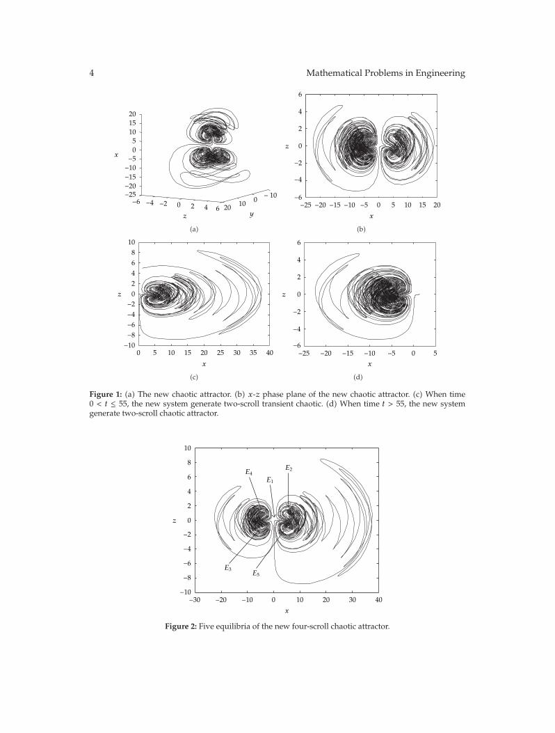
Phase and Antiphase Synchronization between 3-Cell CNN and Volta Fractional-OrderChaotic Systems via Active Control, Zahra Yaghoubi and Hassan ZarabadipourVolume 2012, Article ID 121323, 10 pages

Nonlinear Electrical Circuit Oscillator Control Based on Backstepping Method: A GeneticAlgorithm Approach, Mahsa Khoeiniha, Hasan Zarabadipour, and Ahmad FakharianVolume 2012, Article ID 597328, 14 pages

Hindawi Publishing CorporationMathematical Problems in EngineeringVolume 2012, Article ID 573910, 2 pagesdoi:10.1155/2012/573910

EditorialBifurcation and Chaos Theory in Electrical PowerSystems: Analysis and Control

Ahmad M. Harb,1 Issa Batarseh,2Lamine M. Mili,3 and Mohamed A. Zohdy4

1 School of Natural Resources Engineering and Management, German Jordanian University (GJU),Amman, Jordan

2 Electrical and Computer Engineering Department, University of Central Florida, Orlando, FL, USA3 Department of Electrical and Computer Engineering, Virginia Tech., Falls Church, VA, USA4 Department of Electrical and Computer Engineering, Oakland University, Rochester, MI, USA

Correspondence should be addressed to Ahmad M. Harb, [email protected]

Received 27 August 2012; Accepted 27 August 2012

Copyright q 2012 Ahmad M. Harb et al. This is an open access article distributed under theCreative Commons Attribution License, which permits unrestricted use, distribution, andreproduction in any medium, provided the original work is properly cited.

Everywhere in our daily life we encounter nonlinear phenomena. In fact, it is well knownthat the real life is nonlinear. Because of difficulty of solving nonlinear problems, they used togo for easy way and linearize the problem based on some assumptions. These assumptionsmay lead to loss of important information in the system. Because of that, and to be morerealistic, the objective of this special issue is to use the modern nonlinear theory (bifurcationand chaos) to establish real nonlinear models for practical systems, engineering sciences, andengineering applications.

The scope of this issue is to publish original papers on all topics related to nonlineardynamics and its applications such as, power system, power electronics, electric machines,and renewable energy. The contributions concerned will be discussion of a practical problem,the formulating nonlinear model, and determination of closed form exact or numericalsolutions.

In the past two decades, many researchers have investigated the modern nonlineartheory in electric circuits as well as power systems. In the paper “Nonlinear electrical circuitoscillator control based on backstepping method: a genetic algorithm approach,” M. Khoeiniha etal. investigated the dynamics of nonlinear electrical circuit by means of modern nonlineartechniques and the control of a class of chaotic system by using backstepping method basedon Lyapunov function. The behavior of such nonlinear system when they are under theinfluence of external sinusoidal disturbances with unknown amplitudes has been considered.The objective is to analyze the performance of this system at different amplitudes ofdisturbances. They illustrate the proposed approach for controlling of duffing oscillator

2 Mathematical Problems in Engineering

problem to stabilize this system at the equilibrium point. Also Genetic Algorithm method(GAs) for computing the parameters of controller has been used. GAs can be successfullyapplied to achieve a better controller. Simulation results are shown the effectiveness of theproposed method.

In the paper “Phase and antiphase synchronization between 3-cell CNN and volta fractionalorder chaotic systems via active control,” Z. Yaghoub et al. discussed and analyzed synchroniza-tion of fractional order chaotic dynamical in secure communications of analog and digitalsignals and cryptographic systems. They study the drive-response synchronization methodfor “phase and antiphase synchronization” of a class of fractional-order chaotic systems viaactive control method, using the 3-cell and volta systems as an example. These examples areused to illustrate the effectiveness of the synchronization method.

In the paper “Function projective synchronization of a class of chaotic systems with uncertainparameters,” J. Guan investigates the function projective synchronization of a class of chaoticsystems with uncertain parameters. Based on Lyapunov stability theory, the nonlinearadaptive control law and the parameter update law are derived to make the state of twochaotic systems function projective synchronized. Numerical simulations are presented todemonstrate the e ectiveness of the proposed adaptive scheme.

In the paper “A new four-scroll chaotic attractor consisted of transient chaotic two-scroll andultimate chaotic two-scroll,” Y. Xu et al. used the feedback controlling method to find a newfour-scroll chaotic attractor. The novel chaotic system can generate four scrolls two of whichare transient chaotic and the other two of which are ultimate chaotic. Of particular interestis that this novel system can generate one-scroll, two 2-scroll, and four-scroll with variationof a single parameter. We analyze the new system by means of phase portraits, Lyapunovexponents, fractional dimension, bifurcation diagram, and Poincare map, respectively. Theanalysis results show clearly that this is a new chaotic system which deserves further detailedinvestigation.

In the paper “Lag synchronization of coupled multidelay systems,” L. Qun et al. study thechaos synchronization, which is an active topic, and its possible applications. They presentedan improved method for lag synchronization of chaotic systems with coupled multidelay. TheLyapunov theory is used to consider the sufficient condition for synchronization. The specificexamples will demonstrate and verify the effectiveness of the proposed approach.

In the paper “Bifurcations in a generalization of the ZAD-technique: application to a DC-DC buck power converter,” L. Torres et al. proposed a variation of ZAD technique, whichis to extend the range of zero averaging of the switching surface (in the classic ZAD it istaken in a sampling period), to a number K of sampling periods. This has led to a techniquethat has been named K-ZAD. Assuming a specific value for K = 2, we have studied the 2-ZAD technique. The latter has presented better results in terms of stability, regarding to theoriginal ZAD technique. These results can be demonstrated in different state space graphsand bifurcation diagrams, which have been calculated based on the analysis done about thebehavior of this new strategy.

Ahmad M. HarbIssa Batarseh

Lamine M. MiliMohamed A. Zohdy


Research ArticleBifurcations in a Generalization ofthe ZAD Technique: Application toa DC-DC Buck Power Converter

Ludwing Torres,1 Gerard Olivar,1 and Simeon Casanova2

1 Percepcion y Control Inteligente, Departamento de Ingenierıa Electrica,Facultad de Ingenierıa y Arquitectura, Universidad Nacional de Colombia, Sede Manizales,Electronica y Computacion, Bloque Q, Campus La Nubia, Manizales, Colombia

2 ABC Dynamics, Departamento de Matematicas y Estadıstica,Facultad de Ciencias Exactas y Naturales, Universidad Nacional de Colombia,Sede Manizales, Bloque Y, Campus La Nubia, Manizales, Colombia

Correspondence should be addressed to Gerard Olivar, [email protected]

Received 21 March 2012; Accepted 30 April 2012

Academic Editor: Ahmad M. Harb

Copyright q 2012 Ludwing Torres et al. This is an open access article distributed under theCreative Commons Attribution License, which permits unrestricted use, distribution, andreproduction in any medium, provided the original work is properly cited.

A variation of ZAD technique is proposed, which is to extend the range of zero averaging of theswitching surface (in the classic ZAD it is taken in a sampling period), to a number K of samplingperiods. This has led to a technique that has been named K-ZAD. Assuming a specific value forK = 2, we have studied the 2-ZAD technique. The latter has presented better results in terms ofstability, regarding the original ZAD technique. These results can be demonstrated in differentstate space graphs and bifurcation diagrams, which have been calculated based on the analysisdone about the behavior of this new strategy.

1. Introduction

Currently, power electronics has an important place in industry. This is largely due to thevery extensive number of applications derived from these systems, including control ofpower converters. This was the main motivation for researchers worldwide to develop newadvances in this field and has promoted the investigation on many mathematical models.They correspond usually to variable structure systems, chaos, and control. The practical goalis to obtain better devices or new and improved mechanisms for use in electronic controllers.

Bifurcation, chaos, and control in electronic circuits have been reported in many paperssuch as [1, 2]. Regarding power electronics, early works can be found in the literature fromthe 1980s when first observed in [3, 4]. In 1989 several authors such as Krein and Bass [5], and


Deane and Hamill [6] began to study chaos in various power electronic circuits. In his workWood [7] contributed to the understanding of chaos, showing in phase diagrams that thepattern of the trajectories was messy as small variation on initial conditions and parametersin the system were performed. Meanwhile Deane and Hamill reported some of the best workson bifurcations and chaos applied to electronic circuits. Their studies were based on computersimulations and laboratory experiments [3, 4, 6].

Because of the multiple side effects that generation of chaos caused in these systems,several authors proceeded to develop different control techniques, such as [8] by Ott et al.,who found a way of controlling unstable orbits coexisting with chaos. They used smalldisturbances. This resulted in the so well-known OGY method (after the names of the authorsOtt, Grebogi, and Yorke). Pyragas [9] contributed to this topic with a feedback scheme usinga time-delayed control known as (time-delayed autosynchronization) TDAS.

Also the work by Utkin is very important in the control literature. He studied (pulse-width modulation) PWM systems and variable structure systems [10]. He introduced a nowvery popular control technique so-called sliding-mode control (SMC) and many applicationswere proposed [11]. These studies were taken later as a starting point by Carpita et al. [12].In his work, Carpita presents a sliding mode controller for a (uninterrupted power system)UPS. Carpita uses a sliding surface which is a linear combination of error variable and itsderivative.

Some time after, a new technique, both conceptually different from sliding-modecontrol (although very related to it) and as a practical implementation to SMC, appeared.It was called (zero average dynamics) ZAD by the authors. This control technique forces thesystem to have, at each clock cycle, a zero average of the sliding surface (instead to be zero allthe time, as in sliding-mode control). Application of this technique to a buck converter withcentered pulse and an approximation scheme needed for the practical implementations [12]has obtained very good performance. Robustness, low stationary error, and fixed switchingfrequency have also been achieved [13]. It has been observed that as the main parameterin the surface ks is decreased, chaotic behavior appears which is not desirable in practice.Then, several additional techniques such as TDAS (mentioned before) or (fixed point inducedcontrol) FPIC must be implemented in order to guarantee a wider operation range [13]. FPIChas obtained the best results with regards to stabilization and chaos control. Bifurcationdiagrams have shown flip or period-doubling bifurcations followed by border-collisionbifurcations due to the saturation of the limit cycle. This sequence of bifurcations leads thesystem to chaotic operation for low values of ks. When saturation of the limit cycle appears,the ZAD technique is degraded and thus zero average in each cycle is lost.

In order to solve this problem, we generalize the ZAD technique (from now on calledclassical ZAD) to the so-called K-ZAD technique. This generalization allows the surface to beof zero average not in every cycle (as classical ZAD), but in a sequence of K cycles. Being aweaker condition one can choose the duty cycles in such a way that they are not saturated (atleast not so frequently) and thus zero average and stabilization in a periodic orbit is obtained.

Specifically, our study has focused on the value K = 2, which gives rise to 2-ZAD, thatis, two sampling periods for the zero average in the surface. We compare this generalizationwith the classical ZAD through bifurcation diagrams.

The remaining of this paper is organized as follows. In Section 2 we explain in detailmathematical modelling of this technique and we perform the corresponding algebraiccomputations. In Section 3 the numerical implementation and the results are discussed.Finally, conclusions and future work are stated in Section 4.

Mathematical Problems in Engineering 3

EC1 C2

C3 C4

C

L

R+

−

+

−

(1) (2)

(1)(2)

Figure 1: Scheme of the Buck converter.

2. K-ZAD Strategy

The scheme for the buck converter is shown in Figure 1. We donot take into account thediode full dynamics and thus we assume always continuous conduction mode (alternatively,we can consider bidirectional switches which allow negative currents).

The classical diode-transistor scheme is changed by a transistors bridge linked withthe source. When transistors are in (1) position the pulse magnitude is +E, and when theposition is (2.2), then the magnitude is −E. As a result we have a PWM system which invertsthe polarity at each switching.

With the aim of obtaining a nondimensional system with nondimensional parameters,which leads to easier analysis, we perform the following change of variables [13]:

x1 =v

E, x1ref =

Vref

E, x2 =

1V

√L

Ci, γ =

1R

√L

C. (2.1)

Also we normalize the sampling period

T =Tc√LC

, (2.2)

where Tc = 50μs, R = 20Ω, C = 40μF, L = 2 mH, and E = 40 V. These values come fromlaboratory prototypes which can be found in the literature [13]. Thus we get the value T =0.1767 and the following nondimensional system:

(x1

x2

)=(−γ 1−1 0

)(x1

x2

)+(

01

)u, (2.3)

which can be written in compact form as x = Ax + bu where

A =(−γ 1−1 0

), b =

(01

), x =

(x1

x2

), x =

(x1

x2

). (2.4)


The solution of this piecewise-linear system can be computed algebraically and theexpression for the Poincare map corresponding to sampling every T time units is [14]

x((k + 1)T) = eATx(kT) +(eA(T−dk/2) + I

)A−1(eA(dk/2) − I

)b − eA(dk/2)A−1

(eA(T−dk) − I

)b.

(2.5)

u stands for the control action, which corresponds to a centered pulse, which can be mathe-matically written as

u =

⎧⎪⎪⎪⎪⎪⎪⎪⎪⎨⎪⎪⎪⎪⎪⎪⎪⎪⎩

1, if kT < t < kT +d

2,

−1, if kT +d

2< t < kT +

(T − d

2

),

1, if kT +(T − d

2

)< t < kT + T.

(2.6)

d corresponds to the so-called duty cycle. It will be computed in such a way that the dynam-ical system tends to the sliding surface defined as

s(x(t)) = (x1 − x1ref) + ks(x1 − x1ref). (2.7)

The ZAD technique imposes that the orbit must be such that when the variables arereplaced in the sliding surface in (2.7), the following equation is fulfilled:

∫ (k+1)T

kT

s(x(t))dt = 0. (2.8)

Computing d from (2.8) involves transcendental expressions which should be avoidedin practical applications. Thus in the literature, the sliding surface has been approximatedby a piecewise-linear function. This allows an algebraic solution for d, which is used inapplications.

2.1. Computations for the Classical ZAD Strategy

Figure 2 shows how the classical ZAD strategy works. The area under the curve s(x) must bezero.


S

(k + 1)TkT + d/2t

kT (k + 1)T − d/2

Figure 2: Scheme for the classical ZAD strategy.

Using the piecewise-linear approximation, the integral can be written as

∫ (k+1)T

kT

s(x(t))dt ≈∫kT+d/2

kT

(s(x(kT)) + (t − kT)s1(x(kT))dt

+∫ (k+1)T−d/2

kT+d/2

(s(x(kT)) +

d

2s1(x(kT)) +

(t −(kT +

d

2

))s2(x(kT))

)dt

+∫ (k+1)T

(k+1)T−d/2s(x(kT)) + (T − d)s2(x(kT)) + (t − (k + 1)T + d)s1(x(kT))dt,

(2.9)

where s(x(kT)) is the value of the sliding surface at the sampling instant, s1(x(kT)) is thederivative in the first and third pieces of the piecewise-linear approximation and s2(x(kT)) isthe derivative in the central piece. After some algebra we get

d =2s(x(kT)) + Ts2(x(kT))s2(x(kT)) − s1(x(kT))

. (2.10)

Since a value d > T or d < 0 is practically impossible, when this occurs the duty cycleis saturated in such a way that we take 0 if d ≤ 0 and we take T if d ≥ T . In those cases whered is saturated the ZAD strategy fails and thus the zero average condition is not fulfilled.

2.2. Computations for the K-ZAD Strategy

Now we consider the computations when the zero average condition is weakened to asequence of K cycles instead of every cycle. Previously, with the classical ZAD strategy wehad

∫ (k+1)T

T

s(x(t))dt = 0. (2.11)


S

kT tkT + d1/2 (k + 1)T (k + 1)T + d2/2 (k + 2)T

(k + 1)T − d1/2

(k + 2)T − d2/2

Figure 3: Scheme for the 2-ZAD technique.

Now, with the K-ZAD strategy, we have

∫ (k+1)T

kT

s(x(t))dt +∫ (k+2)T

(k+1)Ts(x(t))dt + · · · +

∫ (k+K)T

(k+(K−1))Ts(x(t))dt = 0. (2.12)

This means that we extend the condition of zero average to an interval of K con-secutive cycles.

2.3. Computations for the 2-ZAD Strategy

In the case K = 2 we get

∫ (k+1)T

kT

s(x(t))dt +∫ (k+2)T

(k+1)Ts(x(t))dt = 0. (2.13)

In Figure 3 we depict a scheme for the 2-ZAD. The area under the curve between t = kT andt = (k + 2)T must be zero.

Since we are now dealing with two cycles, we can have two different duty cycles anddifferent values for the derivatives of the piecewise-linear functions. Thus we introduce thefollowing notation.

(i) In the first cycle we write d1 for the duty cycle and we write d2 for the duty cycle inthe second cycle.

(ii) For the derivatives we use s11 and s21 for the first cycle. They correspond tos1(x(kT)) and s2(x(kT)) for the first cycle. They are computed according to thesign of u and are sampled at the beginning of the first interval (i.e., at t = kT). Inthe second interval we will denote the derivatives by s12 and s22. They correspondto s1(x((k + 1)T)) and s2(x((k + 1)T)) for the second interval. They are computedsampling at the beginning of the second cycle (i.e., at t = (k + 1)T) as it is shown inFigure 3.


With this notation and some further algebra, we get

s = s11(t − kT) + s(x(kT)). (2.14)

For the second piece of the first cycle t ∈ (kT+d1/2, (k+1)T−d1/2), with derivative s21(x(kT))we get

s = s21

(t − kT − d1

2

)+ s11

(d1

2

)+ s(x(kT)). (2.15)

For the third piece t ∈ ((k+1)T−d1/2, (k+1)T) of the first interval, with derivative s11(x(kT)),we get

s = s11(t − (k + 1)T + d1) + s21(T − d1) + s(x(kT)). (2.16)

For the second cycle t ∈ ((k + 1)T, (k + 2)T) we have derivatives s12 and s22 and the dutycycle d2. In the first piece of the second cycle t ∈ ((k + 1)T, (k + 1)T + d2/2), with derivatives12(x((k + 1)T)), we get

s = s12(t − (k + 1)T) + s11(d1) + s21(T − d1) + s(x(kT)). (2.17)

For the second piece in the second cycle t ∈ ((k + 1)T + d2/2, (k + 2)T − d2/2), with derivatives22(x((k + 1)T)), we get

s = s22

(t − (k + 1)T − d2

2

)+ s12

(d2

2

)+ s11(d1) + s21(T − d1) + s(x(kT)). (2.18)

Finally, for the third piece in the second interval t ∈ ((k+2)T −d2/2, (k+2)T), with derivatives12(x((k + 1)T)), we get

s = s12(t − (k + 2)T + d2) + s22(T − d2) + s11(d1) + s21(T − d1) + s(x(kT)). (2.19)

Thus we have

∫T

0s(x(t))dt +

∫2T

T

s(x(t))dt ≈∫kT+d1/2

kT

s11(t − kT) + s(x(kT))dt

+∫ (k+1)T−d1/2

kT+d1/2s21

(t − kT − d1

2

)+ s11

(d1

2

)+ s(x(kT))dt

+∫ (k+1)T

(k+1)T−d1/2s11(t − (k + 1)T + d1) + s21(T − d1) + s(x(kT))dt

+∫ (k+1)T+d2/2

(k+1)Ts12(t − (k + 1)T) + s11(d1) + s21(T − d1) + s(x(kT))dt


∫ (k+2)T−d2/2

(k+1)T+d2/2s22

(t − (k + 1)T − d2

2

)+ s12

(d2

2

)

+ s11(d1) + s21(T − d1) + s(x(kT))dt

+∫ (k+2)T

(k+2)T−d2/2s12(t − (k + 2)T + d2) + s22(T − d2) + s11(d1)

+ s21(T − d1) + s(x(kT))dt.

(2.20)

Solving the integral we have the following expression for d2 as a function of d1:

d2 =−(3d1s11 + 3Ts21 + 4s(x(kT)) + Ts22 − 3d1s21)

(s12 − s22). (2.21)

Since we have d1 as an independent variable and d2 is dependant of d1, we can assumethat d1 is nonsaturated. Then our proposal is to choose d2 to be as the optimal value (ina certain sense) taking d1 between 0 and T . Our optimal condition will be choosing d2 theclosest to the stationary theoretical value as possible. In this way we approximate x1 to thedesired regulation value as much as possible.

3. Numerical Results

Following [13] the stationary theoretical value for the duty cycle was computed as

deq = T1 + x1ref

2. (3.1)

Then according to the previous section, the following results are obtained.

3.1. Results

In the literature it was found that, for the classical ZAD strategy and centered pulse, stabilityof the T -periodic orbit was obtained in the range ks > 3.23, approximately. Below thisvalue, period doubling and border collision bifurcation due to saturations lead the systemto big amplitude chaotic operation, which is inadmissible in practical devices. The rangesconsidered for the 2-ZAD strategy contain values from ks = 0.01 to ks = 5. We can observethe transition from stability to chaos.

Figure 4 shows bifurcations obtained for the classical ZAD strategy, for parametervalues less than ks = 3.23. For parameter values greater than 3.23, the T -periodic orbit isstable. The duty cycle is approximately 0.1590 when x1ref = 0.8 and γ = 0.35. In the figureswe observe that chaos is obtained when ks decreases. For parameter values ks less than 1,big amplitude chaos appears. The regulation error also grows. Close to ks = 3.23 we can alsoobserve a fast transition of the stable 2T -periodic orbit into saturation.

In the computations corresponding to Figure 5 we considered 2-ZAD strategy all thetime, for all values of parameter ks. We allowed saturations when it was impossible to get


0 1 2 3 4 50

0.02

0.04

0.06

0.08

0.12

0.14

0.16

0.18

Dut

y cy

cle d

ks

0.1

(a) Bifurcations in the duty cycle

0 1 2 3 4 50.05

0.15

0.25

0.35

0.45

ks

0.4

0.3

0.2

0.1

x2

(b) Bifurcations associated with the nondimensionalcurrent in the inductor

0 1 2 3 4 50.710.720.730.740.750.760.770.780.79

0.81

ks

0.8

x1

(c) Bifurcations associated with the nondimensionalvoltage in the capacitor

1 2 3 4 5

0.7984

0.7986

0.7988

0.799

0.7992

0.7994

0.7996

ks

0.5 1.5 2.5 3.5 4.5

x1

(d) Zoom of the bifurcation diagram associated withthe nondimensional voltage

Figure 4: Bifurcation diagram with bifurcation parameter ks, in the classical ZAD strategy.

two nonsaturated duty cycles. In these figures it can be observed that the stability rangeof the T -periodic orbit is wider than that for the classical ZAD strategy. From ks = 5 untilapproximately ks = 0.5 the 2-ZAD strategy avoids the orbit to get far from the stable T -periodic orbit. This is mainly due to the existence of nonsaturated duty cycles.

Figures 6, 7, 8, and 9 correspond to a reference value 0.8 and initial conditions x1 = x1ref

and x2 = γx1ref (stable state values according to [13]). Initial conditions close to the stable statevalue are considered in order to check the performance of these techniques. With the aim ofgetting a better insight of the behavior of the orbit in stable state, we take the last values ofthe trajectory. Thus we compare both the classical ZAD strategy with 2-ZAD. Results showthat 2-ZAD performs much better than classical ZAD technique.

Regarding chaotic behavior, Figure 10 shows the Lyapunov exponents for bothtechniques. It can be observed that in the 2-ZAD case the exponents are below zero for awider range than for the classical ZAD strategy. For the 2-ZAD, stability is kept almost untilks close to 0.7. Then some small amplitude period-doubling bifurcations appear. Close toks = 0.25 and below, saturation in the duty cycle cannot be avoided and chaos appears.


0 1 2 3 4 50

0.02

0.04

0.06

0.08

0.12

0.14

0.16

0.18

ks

0.1

Dut

y cy

cle d

(a) Bifurcations of the duty cycle

0 1 2 3 4 5

0.6

0.5

0.4

0.3

0.2

0.1

0

−0.1

ks

x2

(b) Bifurcations of the variable associated with thecurrent in the inductor

0 1 2 3 4 50.74

0.75

0.76

0.77

0.78

0.79

0.81

0.82

0.8

ks

x1

(c) Bifurcations of the variable associated with thevoltage in the capacitor

1 2 3 4 5

0.7993

0.7994

0.7995

0.7996

0.7997

0.7998

0.7999

0.8

0.8001

0.5 1.5 2.5 3.5 4.5

ks

x1

(d) Zoom of the bifurcation diagram correspondingwith the variable associated to the voltage

Figure 5: Bifurcation diagrams with bifurcation parameter ks when 2-ZAD strategy is considered.

0.7998 0.8002 0.8004 0.8006 0.80080.26

0.265

0.27

0.275

0.28

0.285

0.29

0.295

Voltage

Cur

rent

0.3

0.8

State-space plot

(a) Orbit in the state space

0 20 40 60 80 100 120 140 160 180

1

Time

0.9

0.8

0.7

0.6

0.5

0.4

0.3

0.2

Time waveform

Stat

e va

riab

les

(b) Time waveform

Figure 6: 2-ZAD strategy for ks = 2.5 and initial conditions close to the reference value.


0.7985 0.7995 0.8005 0.80150.24

0.25

0.26

0.27

0.28

0.29

0.31

0.32

0.33

Voltage

Cur

rent

0.3

State-space plot


0 20 40 60 80 100 120 140 160 180

1

Time

Time waveform

Stat

e va

riab

les

0.9

0.8

0.7

0.6

0.5

0.4

0.3

0.2

(b) Time waveform

Figure 7: Classical ZAD strategy for ks = 2.5 and initial conditions close to the reference value.

0.7998 0.8002 0.8004 0.8006 0.8008 0.8010.26

0.265

0.27

0.275

0.28

0.285

0.29

0.295

Voltage

Cur

rent

0.3

0.8

State-space plot


0 20 40 60 80 100 120 140 160 180

1

Time

Time waveformSt

ate

vari

able

s

0.9

0.8

0.7

0.6

0.5

0.4

0.3

0.2

(b) Time waveform

Figure 8: 2-ZAD strategy for ks = 1 and initial conditions close to the reference value.

0.24

0.25

0.26

0.27

0.28

0.29

0.31

0.32

0.33

Voltage

Cur

rent

0.3

0.798 0.799 0.8 0.801 0.802

State-space plot


0 20 40 60 80 100 120 140 160 180

1

Time

Time waveform

Stat

e va

riab

les

0.9

0.8

0.7

0.6

0.5

0.4

0.3

0.2

(b) Time waveform

Figure 9: Classical ZAD strategy for ks = 1 and initial conditions close to the reference value.


1 2 3 4 5

−0.15

−0.05

0

0.05

0.15

0.1

−0.1

0.5 1.5 2.5 3.5 4.5

ks

Lyapounov exponents

(a) Lyapunov exponents for the classical ZADtechnique

0 1 2 3 4 5

0−0.2

−0.4

−0.6

−0.8

−1

−1.2

−1.4

0.2

0.4

ks

Lyapounov exponents

(b) Lyapunov exponents for 2-ZAD technique

Figure 10: Comparison of Lyapunov exponents.

4. Conclusions and Future Work

A generalization of the so-called ZAD technique (named K-ZAD) was described. It canbe used as an alternative to classical ZAD when saturation effects lead the system to bigamplitude chaotic behavior. In fact, 2-ZAD shows better performance than classical ZADin all cases (regarding stability and nonsaturation). Even it can be used without additionalstabilization methods such as FPIC or TDAS. Thus the control algorithm becomes simpler.Good performance of K-ZAD is mainly dependent on the way that the (independent) dutycycles are computed. Several criteria can be chosen. The one chosen in this paper showedvery good success. But it is worth to note that different criteria will lead to probably verydifferent dynamics. Thus even better results than those shown in this paper can be obtained.

It is expected that as the value of K is increased, better results can be obtained. Butalso it is evident that the control algorithm gets more complex. Some early results with 3-ZAD (not shown in this paper) confirm this last sentence. Anyway, trying values bigger than2 with some sort of optimal condition is proposed as our next step into further understandingthe ZAD strategy.

Acknowledgments

The authors acknowledge partial financial support to CeiBA Complexity and to the prjectDima-vicerrectorıa de investigacion no. 20201006570 “Calculo Cientıfico para ProcesamientoAvanzado de Biosenales”.

References

[1] L. O. Chua, “Special issue on chaos in electronic systems; tutorial and descriptive articles for thenon-specialist,” Proceedings of the IEEE, vol. 75, no. 8, 1987.

[2] J. Baillieul, R. W. Brockett, and R. B. Washburn, “Chaotic motion in nonlinear feedback systems,” IEEETransactions on Circuits and Systems, vol. 27, no. 11, pp. 990–997, 1980.


[3] J. H. B. Deane and D. C. Hamill, “Instability, subharmonics and chaos in power electronic systems,” inProceedings of the 20th Annual IEEE Power Electronics Specialists Conference (PESC ’89), pp. 34–42, June1989.

[4] J. H. B. Deane and D. C. Hamill, “Analysis, simulation and experimental study of chaos in the buckconverter,” in Proceedings of the 21st Annual IEEE Power Electronics Specialists Conference (PESC ’90), pp.491–498, June 1990.

[5] P. T. Krein and R. M. Bass, “Multiple limit cycle phenomena in switching power converters,” inProceedings of the 4th Annual IEEE Applied Power Electronics Conference and Exposition (APEC ’89), pp.143–148, March 1989.

[6] D. Hamill, “Power electronics: a field rich in nonlinear dynamics,” in Workshop on Nonlinear Dynamicsof Electronic Systems, pp. 164–179, 1995.

[7] J. R. Wood, “Chaos: a real phenomenon in power electronics,” in Proceedings of the 4th Annual IEEEApplied Power Electronics Conference and Exposition (APEC ’89), pp. 115–124, March 1989.

[8] E. Ott, C. Grebogi, and J. A. Yorke, “Controlling chaos,” Physical Review Letters, vol. 64, no. 11, pp.1196–1199, 1990.

[9] K. Pyragas, “Continuous control of chaos by self-controlling feedback,” Physics Letters A, vol. 170, no.6, pp. 421–428, 1992.

[10] V. I. Utkin, “Variable structure systems with sliding modes,” IEEE Transactions on Automatic Control,vol. 22, no. 2, pp. 212–222, 1977.

[11] V. I. Utkin, Sliding Modes and Their Applications in Variable Structure Systems, Mir, Moscow, Russia,1978.

[12] M. Carpita, M. Marchesoni, M. Oberti, and L. Puguisi, “Power conditioning system using slidingmode control,” in Proceedings of the IEEE Power Electronics Specialist Conference, pp. 623–633, 1988.

[13] F. Angulo, Analisis de la Dinamica de Convertidores Electronicos de Potencia Usando PWM basado enPromediado Cero de la Dinaamica del Error (ZAD) [Ph.D. thesis], Universidad Politeecnica de Cataluna,2004.

[14] Y. A. Kuznetsov, Elements of Applied Bifurcation Theory, vol. 112 of Applied Mathematical Sciences,Springer, New York, NY, USA, 3rd edition, 2004.


Research ArticleLag Synchronization ofCoupled Multidelay Systems

Luo Qun, Peng Hai-Peng, Xu Ling-Yu, and Yang Yi Xian

Information Security Center, Beijing University of Posts and Telecommunications,P.O. Box 145, Beijing 100876, China

Correspondence should be addressed to Peng Hai-Peng, [email protected]

Received 23 February 2012; Revised 15 April 2012; Accepted 20 May 2012

Academic Editor: Mohamed A. Zohdy

Copyright q 2012 Luo Qun et al. This is an open access article distributed under the CreativeCommons Attribution License, which permits unrestricted use, distribution, and reproduction inany medium, provided the original work is properly cited.

Chaos synchronization is an active topic, and its possible applications have been studied exten-sively. In this paper we present an improved method for lag synchronization of chaotic systemswith coupled multidelay. The Lyapunov theory is used to consider the sufficient condition for syn-chronization. The specific examples will demonstrate and verify the effectiveness of the proposedapproach.

1. Introduction

Since synchronization of chaotic systems was first realized by Fujisaka and Yamada [1] andPecora and Carroll [2], chaos synchronization has received increasing interest and hasbecome an active research topic. Currently its possible applications in various fields are ingreat interest, for example, applications to control theory [3], telecommunications [4–7], bio-logy [8, 9], lasers [10, 11], secure communications [12], and so on.

Roughly speaking, chaotic communication schemes rely on the synchronization tech-nique: the information signal is mixed at the master, and a driving signal is then generatedand is sent to the slave; as a result, their chaotic trajectories remain in step with each otherduring temporal evolution. Besides identical synchronization [13], several new types of chaossynchronization of coupled oscillators have occurred, that is, generalized synchronization[12], phase synchronization [14], lag synchronization [15], anticipation synchronization [16],and projective synchronization [17].

Lag synchronization can be realized when the strength of the coupling between phase-synchronized oscillators is increased. There, the driving signal is constituted by the sum ofmultiple nonlinear transformations of delayed state variable [18]. Master and slave’s formu-las are in the form of single delay [19, 20] and multidelay [21–23]. From the application point


of view, this new multidelay synchronization, different from conventional synchronizationwithout lag, offers a significant advantage in terms of security of communication. Since theconstructed state variable of the master system with lag becomes more complex than that ofthe conventional system, multilag systems achieve high security. Intruders cannot reconstructthe attractors of driving signal by using conventional reconstruction methods [24, 25] so asnot to decipher the transferred message.

In the present paper, we proposed a systematic and rigorous scheme for lag synchro-nization of coupled multidelay systems based on the Lyapunov stability theory. Furthermore,the zero solution of lag synchronization differential equation is globally asymptotically stable.The effectiveness of the proposed scheme is confirmed by the numerical simulation of specificexample.

2. The Schemes of Lag Synchronization

2.1. The Proposed Lag Synchronization Model

Lag synchronization was first investigated by Rosenblum [15], and it can be considered thatthe state variable of the slave is delayed by the positive time lag τd in comparison with thatof the master while their amplitudes follow each other, that is, limt→∞|y(t) − x(t − τd)| = 0.

We consider the following model of lag synchronization.Master:

dx(t)dt

= −αx(t) +P∑i=1

mifi[x(t − αi)]. (2.1)

Driving signal:

DS(t) =Q∑i=1

kigi[x(t − βi

)]+Wx(t − τd). (2.2)

Slave:

dy(t)dt

= −αy(t) +R∑i=1

nihi

[y(t − γi

)]+ DS(t) −Wy(t), (2.3)

where coefficients α,mi, ki, ni, αi, βi, γi, W ∈ �, and P,Q,R are positive integers. State variablesx, y ∈ �, and fi(·), gi(·), hi(·) ∈ � → � are three continuous nonlinear functions. The drivingsignal DS(t) in (2.2) is constituted by the sum of multiple nonlinear transformations ofdelayed state variable;

∑Qi=1 kigi[x(t−βi)] is added with Wx(t−τd). The polynomial −Wy(t) is

added to the right side of dy(t)/dt = −αy(t) +∑Ri=1 nihi[y(t − γi)] + DS(t), forming the slave

equation which is shown as (2.3).

2.2. Proof for the Lag Synchronization Model

The desired synchronization manifold is expressed by the following relation y(t) → x(t−τd)as t → ∞, where τd is a lag time.


We choose suitable DS(t) to satisfy e(t) = y(t) − x(t − τd) → 0 as t → ∞.

Assumption 2.1. Q = P +R − I, I < min{P,Q,R} where I is integer. When i = 1, . . . , I, fi ≡ gi ≡hi,

γi = αi, βi = αi + τd, ki = mi − ni. (2.4)

Assumption 2.2. When j = 1, . . . , (P − I), gI+j ≡ fI+j ,

kI+j = mI+j , βI+j = αI+j + τd. (2.5)

When j = 1, . . . , (R − I), gP+j ≡ hI+j ,

kP+j = −nI+j , βP+j = γI+j + τd. (2.6)

Assumption 2.3. Nonlinearity fi (i = 1, . . . , I) satisfies Lipshitz condition; that is, there exists apositive constant L for all time variables a and b, such that |fi(a+b)−fi(a)| ≤ L|b| (i = 1, . . . , I).

Here we give the sufficient condition for system synchronization.

Theorem 2.4. If the system (2.1), (2.2), and (2.3) satisfies Assumptions 2.1, 2.2, and 2.3 and if

−α −W +12I +

12

I∑i=1

n2i L

2 < 0, (2.7)

then limt→∞[y(t) − x(t − τd)] = 0.

Proof. The dynamics of synchronization error is

de(t)dt

=dy(t)dt

− dx(t − τd)dt

= − αe(t) +R∑i=1

nihi

[y(t − γi

)]+

Q∑i=1

kigi[x(t − βi

)]+Wx(t − τd) −Wy(t)

−P∑i=1

mifi[x(t − αi − τd)].

(2.8)

By applying Assumption 2.1, (2.8) can be rewritten as

de(t)dt

= − αe(t) −We(t) +I∑i=1

nifi[y(t − γi

)] − I∑i=1

(mi − ki)fi[x(t − αi − τd)]

+R∑

i=I+1

nihi

[y(t − γi

)]+

Q∑i=I+1

kigi[x(t − βi

)] − P∑i=I+1

mifi[x(t − αi − τd)].

(2.9)


By applying Assumption 2.2, if Q−I = (P−I)+(R−I) and y(t−γi) = x(t−γi−τd)+e(t−γi),we have

R∑i=I+1

nihi

[y(t − γi

)]+

Q∑i=I+1

kigi[x(t − βi

)] − P∑i=I+1

mifi[x(t − αi − τd)]

=R−I∑j=1

nI+jhI+j[x(t − γI+j − τd

)+ e

(t − γI+j

)]+

P−I∑j=1

kI+jgI+j[x(t − βI+j

)]

+R−I∑j=1

kP+jgP+j[x(t − βP+j

)] − P−I∑j=1

mI+jfI+j[x(t − αI+j − τd

)]= 0,

(2.10)

where e(t − γI+j) = 0 as well as synchronization established, in fact, e(t − γI+j) reduces duringestablishing the synchronization regime.

From (2.10) and (2.9) we get

de(t)dt

= (−α −W)e(t) +I∑i=1

ni

(fi[x(t − αi − τd) + e(t − αi)] − fi[x(t − αi − τd)]

). (2.11)

Define a Lyapunov function [26] as

V =12e2(t) +

12

I∑i=1

∫ t

t−αi

e2(s)ds. (2.12)

Then, we obtain

dV

dt= e(t)

de(t)dt

+12

I∑i=1

e2(t) − 12

I∑i=1

e2(t − αi). (2.13)

Here, we have

dV

dt= (−α −W)e2(t) +

I∑i=1

nie(t)fi[x(t − αi − τd) + e(t − αi)]

−I∑i=1

(mi − ki)e(t)fi[x(t − αi − τd)] +12

I∑i=1

e2(t) − 12

I∑i=1

e2(t − αi).

(2.14)

According to Assumption 2.1, we have

dV

dt= (−α −W)e2(t) +

I∑i=1

nie(t){fi[x(t − αi − τd) + e(t − αi)] − fi[x(t − αi − τd)]

}

+12

I∑i=1

e2(t) − 12

I∑i=1

e2(t − αi).

(2.15)


In our model, (1/2)∑I

i=1 e2(t) can be rewritten as (1/2)Ie2(t). By Assumption 2.3, we

have

dV

dt≤(−α −W +

12I

)e2(t) +

I∑i=1

nie(t)Le(t − αi) − 12

I∑i=1

e2(t − αi). (2.16)

According to 2xy ≤ x2 + y2, where x, y ∈ �, we get

dV

dt≤(−α −W +

12I

)e2(t) +

12

I∑i=1

n2i L

2e2(t) +12

I∑i=1

e2(t − αi) − 12

I∑i=1

e2(t − αi). (2.17)

Finally, we obtain

dV

dt≤(−α −W +

12I +

12

I∑i=1

n2i L

2

)e2(t). (2.18)

The proof is completed.

Note 1. The advantages of our lag synchronization model are as follows.

(1) The nonlinear function f(·) satisfies |f(a + b) − f(a)| ≤ L|b|, so the zero solution oflag synchronization error system is globally asymptotically stable. The condition forsynchronization is easy to be realized.

(2) We can choose nonlinear function in many ways, and fi, gi, hi vary as i changes.Moreover, the format of function can be different even if i is the same value.

(3) In order to enhance the complexity of the system, P,Q,R can be different positiveintegers, and the number of multiple time delays can be chosen as many values.

3. Numerical Simulations

The following example will demonstrate synchronization between systems with multidelay.Functions of systems are chosen from the set of {sinu, u/(1+u8), u/(1+u10)}. Let us considersynchronization model with the master’s and slave’s equations defined as.

Master:

dx(t)dt

= − αx(t) +m1 sin[x(t − α1)] +m2 sin[x(t − α2)] +m3 sin[x − (t − α3)]

+m4x(t − α4)

1 + x8(t − α4)+m5

x(t − α5)α + x10(t − α5)

.

(3.1)


Slave:

dy(t)dt

= − αy(t) + n1 sin[y(t − γ1

)]+ n2 sin

[y(t − γ2

)]+ n3 sin

[y(t − γ3

)]+ n4 sin

[y(t − γ4

)]+ DS(t) −Wy(t).

(3.2)

Therefore the equation for driving signal is chosen as.Driving signal:

DS(t) = k1 sin[x(t − β1

)]+ k2 sin

[x(t − β2

)]+ k3 sin

[x(t − β3

)]+ k4

x(t − β4

)1 + x8

(t − β4

)

+ k5x(t − β5

)1 + x10

(t − β5

) + k6 sin[x(t − β6

)]+ k7 sin

[x(t − β7

)]+Wx(t − τd),

(3.3)

where P = 5, Q = 7, R = 4, I = 2 satisfy Q = P + R − I.According to (2.4)–(2.6), the relation of the delays and parameters is expressed as

m1 − k1 = n1, m2 − k2 = n2, k3 = m3, k4 = m4, k5 = m5, k6 = −n3, k7 = −n4,

β1 = α1 + τd = γ1 + τd, β2 = α2 + τd = γ2 + τd, β3 = α3 + τd, β4 = α4 + τd, β5 = α5 + τd,β6 = γ3 + τd, β7 = γ4 + τd.

The value of parameters for simulation is adopted as

α = 2.0, W = 100, m1 = −15.4, m2 = −16.0, m3 = −0.35, m4 = −20.0, m5 = −18.5,

n1 = −0.2, n2 = −0.1, n3 = −0.25, n4 = −0.4,

k1 = −15.2, k2 = −15.9, k3 = −0.35, k4 = −20.0, k5 = −18.5, k6 = 0.25, k7 = 0.4,

τd = 3.0, α1 = 3.4, α2 = 4.5, α3 = 6.5, α4 = 5.3, α5 = 2.9,

γ1 = 3.4, γ2 = 4.5, γ3 = 2.0, γ4 = 7.3,

β1 = 6.4, β2 = 7.5, β3 = 9.5, β4 = 8.3, β5 = 5.9, β6 = 5.0, β7 = 10.3.

In Figure 1, the portrait of x(t − τd) versus y(t) illustrates that the lag synchronizationof coupled partly nonidentical systems is established. However their trajectories do notremain in step with each other during a short part of evolution, because they are not in syn-chronization as t < τd.

It is clear to observe from Figure 2 that synchronization error e(t) leaps at a sudden asτd = 3.0 and vanishes eventually in a short time. Then e(t) stays at zero.

As shown in Figure 3, the slave’s state variable is retarded with the time length of τd =3.0 in comparison with master’s. The desired lag synchronization is realized.

4. Conclusions

In this paper, we have presented a lag synchronization model as well as researched on it.Based on Lyapunov theory, the sufficient conditions of the synchronization model are given.Simulation results of the lag synchronization model are provided to illustrate the effective-ness and feasibility of the proposed method.


15

10

5

0

−5

−10

−15151050−5−10−15

y(t)

x(t-τd)

Figure 1: Portrait of x(t − 3.0) versus y(t).

4

3.5

3

2.5

2

1.5

1

0.5

0−0.5−1

e(t)

0 2 4 6 8 10 12 14 16 18 20t

Figure 2: Synchronization error e(t) = y(t) − x(t − 3.0).

10

5

0

−5

−10

x(t)

x(t)

andy(t)

y(t)

0 2 4 6 8 10 12 14 16 18 20t

Figure 3: Time series of state variables x(t) and y(t).


Acknowledgments

This work is supported by the National Natural Science Foundation of China (Grants nos.61170269, 61121061), the Specialized Research Fund for the Doctoral Program of Higher Edu-cation (Grant no. 20100005110002) and the Fundamental Research Funds for the Central Uni-versities (Grant no. BUPT2011RC0211).

References

[1] H. Fujisaka and T. Yamada, “Stability theory of synchronized motion in coupled-oscillator systems,”Progress of Theoretical Physics, vol. 69, no. 1, pp. 32–47, 1983.

[2] L. M. Pecora and T. L. Carroll, “Synchronization in chaotic systems,” Physical Review Letters, vol. 64,no. 8, pp. 821–824, 1990.

[3] K. Pyragas, “Continuous control of chaos by self-controlling feedback,” Physics Letters A, vol. 170, no.6, pp. 421–428, 1992.

[4] K. M. Cuomo and A. V. Oppenheim, “Circuit implementation of synchronized chaos with applica-tions to communications,” Physical Review Letters, vol. 71, no. 1, pp. 65–68, 1993.

[5] C. W. Wu and L. O. Chua, “A unified framework for synchronization and control of dynamical sys-tems,” International Journal of Bifurcation and Chaos in Applied Sciences and Engineering, vol. 4, no. 4, pp.979–998, 1994.

[6] R. Brown, N. F. Rulkov, and E. R. Tracy, “Modeling and synchronizing chaotic systems from time-series data,” Physical Review E, vol. 49, no. 5, pp. 3784–3800, 1994.

[7] L. Kocarev and U. Parlitz, “General approach for chaotic synchronization with applications to com-munication,” Physical Review Letters, vol. 74, no. 25, pp. 5028–5031, 1995.

[8] S. K. Han, C. Kurrer, and Y. Kuramoto, “Dephasing and bursting in coupled neural oscillators,” Phys-ical Review Letters, vol. 75, no. 17, pp. 3190–3193, 1995.

[9] R. C. Elson, A. I. Selverston, R. Huerta, N. F. Rulkov, M. I. Rabinovich, and H. D. I. Abarbanel, “Syn-chronous behavior of two coupled biological neurons,” Physical Review Letters, vol. 81, no. 25, pp.5692–5695, 1998.

[10] L. Fabiny, P. Colet, R. Roy, and D. Lenstra, “Coherence and phase dynamics of spatially coupled solid-state lasers,” Physical Review A, vol. 47, no. 5, pp. 4287–4296, 1993.

[11] W. Yu, J. Cao, K.-W. Wong, and J. Lu, “New communication schemes based on adaptive synchroniza-tion,” Chaos, vol. 17, no. 3, p. 033114, 13, 2007.

[12] N. F. Rulkov, M. M. Sushchik, L. S. Tsimring, and H. D. I. Abarbanel, “Generalized synchronization ofchaos in directionally coupled chaotic systems,” Physical Review E, vol. 51, no. 2, pp. 980–994, 1995.

[13] D. Huang and R. Guo, “Identifying parameter by identical synchronization between different sys-tems,” Chaos, vol. 14, no. 1, pp. 152–159, 2004.

[14] M. G. Rosenblum, A. S. Pikovsky, and J. Kurths, “Phase synchronization of chaotic oscillators,” Phys-ical Review Letters, vol. 76, no. 11, pp. 1804–1807, 1996.

[15] M. G. Rosenblum, A. S. Pikovsky, and J. Kurths, “From phase to lag synchronization in coupled chao-tic oscillators,” Physical Review Letters, vol. 78, no. 22, pp. 4193–4196, 1997.

[16] H. U. Voss, “Anticipating chaotic synchronization,” Physical Review E, vol. 61, no. 5 A, pp. 5115–5119,2000.

[17] R. Mainieri and J. Rehacek, “Projective synchronization in three-dimensional chaotic systems,” Physi-cal Review Letters, vol. 82, no. 15, pp. 3042–3045, 1999.

[18] K. Pyragas, “Syncronization of coupled timedelaysystems: analytical estimations,” Physical Review E,vol. 58, pp. 3067–3071, 1998.

[19] E. M. Shahverdiev, S. Sivaprakasam, and K. A. Shore, “Lag synchronization in time-delayed systems,”Physics Letters, Section A, vol. 292, no. 6, pp. 320–324, 2002.

[20] E. M. Shahverdiev, S. Sivaprakasam, and K. A. Shore, “Lag times and parameter mismatches insynchronization of unidirectionally coupled chaotic external cavity semiconductor lasers,” PhysicalReview E, vol. 66, no. 3, Article ID 037202, pp. 037202/1–037202/4, 2002.

[21] E. M. Shahverdiev, R. A. Nuriev, R. H. Hashimov, and K. A. Shore, “Chaos synchronization betweenthe Mackey-Glass systems with multiple time delays,” Chaos, Solitons and Fractals, vol. 29, no. 4, pp.854–861, 2006.


[22] C. W. Wu and L. O. Chua, “A simple way to synchronize chaotic systems with applications to securecommunication systems,” International Journal of Bifurcation and Chaos, vol. 3, no. 6, pp. 1619–1627,1993.

[23] T. M. Hoang and M. Nakagawa, “Enhancing security for chaos-based communication system withchange in synchronization manifolds’ delay and in encoder’s parameters,” Journal of the Physical Soci-ety of Japan, vol. 75, no. 6, Article ID 064801, 2006.

[24] T. M. Hoang, D. T. Minh, and M. Nakagawa, “Chaos synchronization of multi-delay feedback systemswith multi-delay driving signal,” Journal of the Physical Society of Japan, vol. 74, no. 8, pp. 2374–2378,2005.

[25] T. M. Hoang and M. Nakagawa, “Synchronization of coupled nonidentical multidelay feedback sys-tems,” Physics Letters, Section A, vol. 363, no. 3, pp. 218–224, 2007.

[26] H. K. Khalil, Nonlinear Systems, Prentice Hall, 3rd edition, 2002.


Research ArticleA New Four-Scroll Chaotic AttractorConsisted of Two-Scroll Transient Chaotic andTwo-Scroll Ultimate Chaotic

Yuhua Xu,1, 2, 3 Bing Li,4 Yuling Wang,5Wuneng Zhou,3 and Jian-an Fang3

1 Department of Mathematics and Finance, Yunyang Teachers’ College, Hubei Shiyan 442000, China2 Computer School of Wuhan University, Wuhan 430079, China3 College of Information Science and Technology, Donghua University, Shanghai 201620, China4 NOSTA, The Ministry of Science and Technology of China, GPO Box 2143, Beijing 100045,Tianjin University, Tianjin 300072, China

5 School of Management, Tianjin University, Tianjin 300072, China

Correspondence should be addressed to Yuhua Xu, [email protected]

Received 21 January 2012; Accepted 12 March 2012


Copyright q 2012 Yuhua Xu et al. This is an open access article distributed under the CreativeCommons Attribution License, which permits unrestricted use, distribution, and reproduction inany medium, provided the original work is properly cited.

A new four-scroll chaotic attractor is found by feedback controlling method in this paper. Thenovel chaotic system can generate four scrolls two of which are transient chaotic and the other twoof which are ultimate chaotic. Of particular interest is that this novel chaotic system can generateone-scroll, two 2-scroll and four-scroll chaotic attractor with variation of a single parameter. Weanalyze the new system by means of phase portraits, Lyapunov exponents, fractional dimension,bifurcation diagram, and Poincare map, respectively. The analysis results show clearly that this isa new chaotic system which deserves further detailed investigation.

1. Introduction

Since Lorenz found the first chaotic attractor, considerable research interests have been madein searching for new chaotic attractors. Particularly, research interests are turning in searchingfor new chaotic attractors in the three-dimensional (3D) autonomous ordinary differentialequations. For example, Lorenz system [1], Rossler system [2], Chen and Ueta system [3], Luand Chen system [4], and Liu system [5] were reported and analyzed.

In very recent years, creating complex multiscroll or multiwing chaotic attractors in3D autonomous systems has been rapidly developed [6, 7]. It stimulates the current researchinterest in creating various complex multiscroll chaotic attractors by using simple electroniccircuits and devices. After the rapid development in more than a decade, multiscroll chaotic


attractors generation has become a relatively mature research direction [8]. In fact, most ofthe multiscroll attractors were generated by increasing the breakpoints in the nonlinearity.Recently, a four-wing or three-wing attractor was generated in some 3D systems by relyingon two embedded state-controlled binary switches [9]. But these 3D systems are not usuallysmooth systems. Although a few 3D smooth autonomous chaotic systems have been reportedto display two-, three-, and four-wing attractor, respectively [10–17], how to generatemultiwing chaotic attractors remains an open problem. Therefore, it is important and evennecessary to investigate various possible chaotic behaviors such that we can establish aunified theory for a 3D system generating chaos.

Particularly, over the last two decades chaos in engineering systems, such as nonlinearcircuits, has gradually been moved from simply being a scientific curiosity to a promisingsubject with practical significance and applications. Recently, it has been noticed thatpurposefully creating chaos can be a key issue in many technological applications suchas communication, encryption, and information storage. An appropriate system for suchapplications could be chosen from a category of easier controlled chaotic system to optimizefactors such as robustness to errors in the parameters or immunity to noise [18]. Therefore, itis obviously significant to create more complicated chaotic systems with simple expressionsin three-dimensional for engineering applications such as secure communications.

In this paper, we propose a four-scroll chaotic attractor which consists of the two-scroll transient chaotic and the two-scroll chaotic. It is very desirable for engineeringapplications such as secure communications. For example, in terms of decryption, we cangenerate a certain degree of confusion by using chaos system of transient chaos featureto encrypt. Moreover, this novel system can generate one-scroll, left two-scroll, right two-scroll (according to the system’s geometric locations), and four-scroll chaotic attractors,respectively, with the variation of a single parameter. This paper is devoted to a more detailedanalysis of this new chaotic attractor.

2. New Chaotic System

Based on the chaotification analysis [18, 19], the Liu-Chen system may be added with twoterms, which leads to the finding of the new chaotic attractor.

Start with the controlled Liu-Chen system [10]:

x = bx + cyz + u1,

y = dy + exz + u2,

z = fz + gxy.

(2.1)

By various trial tests, we find a simpler anticontroller, that is,

u1 = ay,

u2 = −z,(2.2)

which yields the following new chaotic system:

x = ay + bx + cyz,

y = dy − z + exz,

z = fz + gxy,

(2.3)

where [x(t), y(t), z(t)]T ∈ R3 is the state vector and a, b, c, d, e, f , and g are real constants.


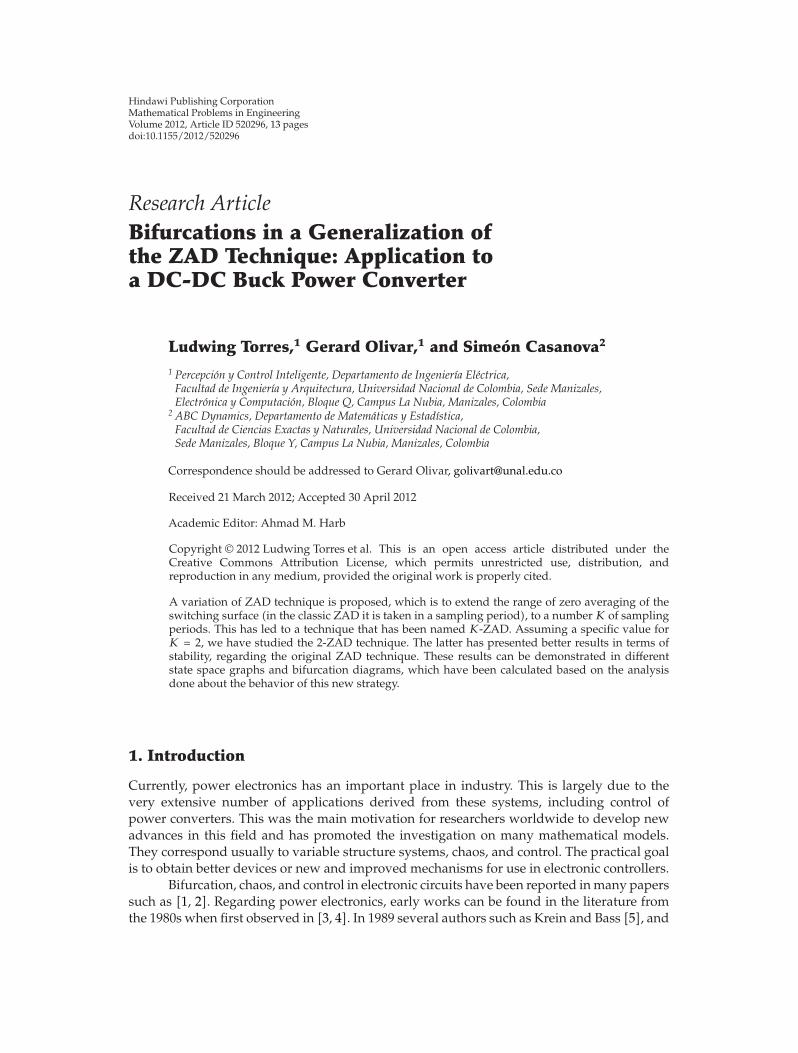
This new system (2.3) is found to be chaotic in a wide parameter range and possessesmany interesting complex dynamical behaviors. For example, the system (2.3) can generatefour-scroll for the parameters a = 2.4, b = −3, c = 14, d = −11, e = 4, f = 5.85, g = −1 and theinitial conditions [1, 3, 5] (see Figure 1(a)).

Sprott [17] has suggested that the long calculation time helps ensure that the solutionsare steady states. Notably, in comparison with those of existing two-scroll or four-scrollchaotic attractors in 3D autonomous systems, the novel chaotic attractor can generate four-scroll consisted of the two-scroll transient chaotic and the two-scroll chaotic (see Figures 1(b)–1(d)). After time t > 55, simulation results show that the attractor is no longer a four-scrollattractor and becomes a two-scroll attractor.

3. Some Basic Properties of the New System

In this section, we will investigate some basic properties of the new system (2.3).

3.1. The Four-Scroll Chaotic Attractor

3.1.1. Equilibria

It is known that the number of equilibrium points of the system and the stabilities at theequilibrium points are very important for the emergence of chaos. In the sequel, we considerthe equilibrium points of system (2.3).

Let

ay + bx + cyz = 0,

dy − z + exz = 0,

fz + gxy = 0.

(3.1)

Let a = 2.4, b = −3, c = 14, d = −11, e = 4, f = 5.85, g = −1. Equation (3.1) has fiveequilibrium points as follows:

E1(0, 0, 0),

E2(4.1379, 1.0050, 0.7109),

E3(−3.8879, 1.2560,−0.8347),

E4(−3.8879 − 0.9981, 0.6633),

E5(4.1379,−1.2473,−0.8823).

(3.2)

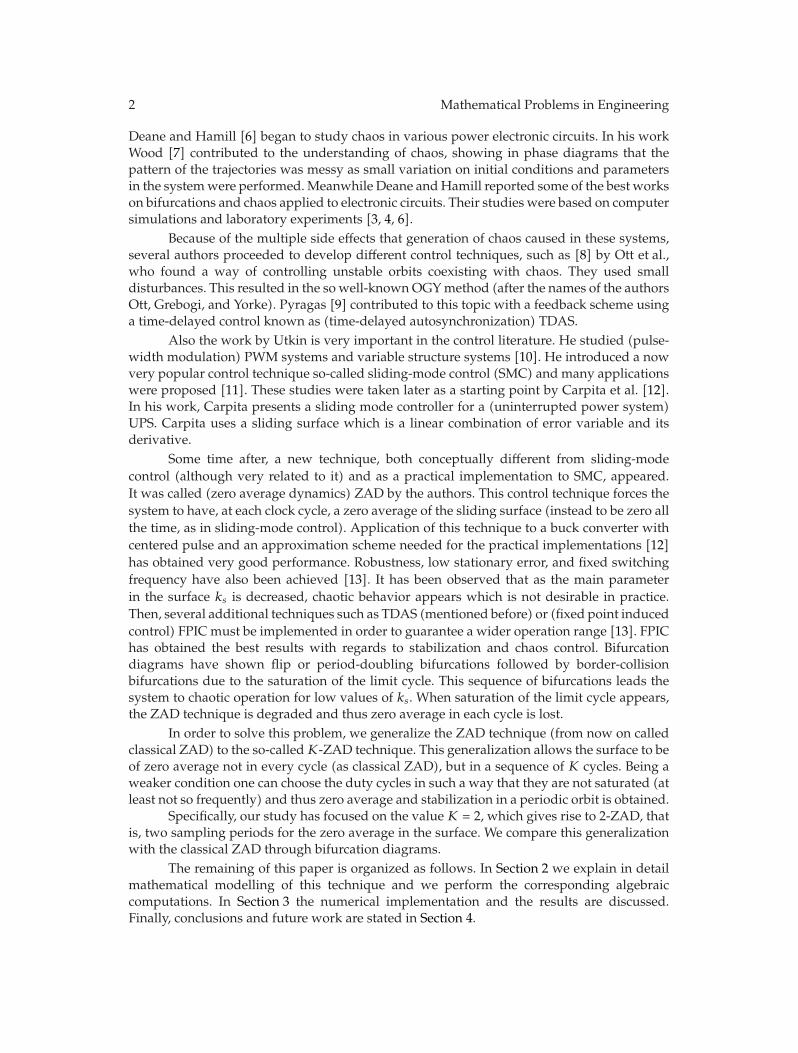
As shown in Figure 2, the equilibria points of system (2.3), E2, E3, E4, and E5 arelocated at the center of the four wings of the attractor, respectively, and the origin (E1) islocated at the center of whole chaotic attractor. Moreover, it can be seen from Figure 2 thatthe equilibria E2, E5 play an important role in generating the two-scroll transients chaotic,while the equilibria E3 and E4 play an important role in ultimate generating two-scroll chaoticattractor.


05

101520

0 10 02 4 6

− 10

yz

x

20

−25−20−15−10−5

−6 −4 −2

(a)

0

2

4

6

z

0 5 10 15 20

x

−6

−4

−2

−25 −20 −15 −10 −5

(b)

02468

10

x

z

0 5 10 15 20 25 30 35 40−10−8−6−4−2

(c)

0

2

4

6

z

−6

−4

−2

x

−25 −20 −15 −10 −5 0 5

(d)

Figure 1: (a) The new chaotic attractor. (b) x-z phase plane of the new chaotic attractor. (c) When time0 < t ≤ 55, the new system generate two-scroll transient chaotic. (d) When time t > 55, the new systemgenerate two-scroll chaotic attractor.

0 10 20 30 40

0

2

4

6

8

10

x

z

E4E2

E1

E3E5

−10

−8

−6

−4

−2

−30 −20 −10

Figure 2: Five equilibria of the new four-scroll chaotic attractor.


For equilibrium E1, the system (2.3) is linearized, and the Jacobian matrix at E1 is asfollows:

J =

⎛⎜⎜⎝

b a + cz cy

ez d ex − 1

gy gx f

⎞⎟⎟⎠ =

⎛⎜⎜⎝

−3 2.4 0

0 −11 −1

0 0 5.85

⎞⎟⎟⎠. (3.3)

To gain its eigenvalues, we let |λI − J | = 0.So the corresponding eigenvalues at E1 are

λ1 = −3, λ2 = −11, λ3 = 5.85. (3.4)

Similarly, the corresponding eigenvalues at E2 are

λ1 = −12.9021, λ2 = 2.3761 + 7.0804i, λ3 = 2.3761 − 7.0804i. (3.5)

The corresponding eigenvalues at E3 are

λ1 = −12.8005, λ2 = 2.3252 + 7.7881i, λ3 = 2.3252 − 7.7881i. (3.6)


λ1 = −12.5469, λ2 = 2.1984 + 6.9804i, λ3 = 2.1984 − 6.9804i. (3.7)


λ1 = −13.1525, λ2 = 2.5013 + 7.8516i, λ3 = 2.5013 − 7.8516i. (3.8)

From (3.4)–(3.8), we know that E1, E2, E3, E4, and E5 are all unstable saddle points.

3.1.2. Dissipativity and the Existence of Attractor

For dynamical system (2.3), we can obtain

∇ · V =∂x

∂x+∂y

∂y+∂z

∂z= b + d + f, (3.9)

where b + d + f = −8.15 is a negative value. Dynamical system (2.3) is a dissipative system,and an exponential contraction of the system (2.3) is

dV

dt= e−8.15. (3.10)

In the dynamical system (2.3), a volume element V0 is apparently contracted by theflow into a volume element V0e

−8.15t in time t. It means that each volume containing thetrajectory of this dynamical system shrinks to zero as t → ∞ at an exponential rate −8.15.So, all this dynamical system orbits are eventually confined to a specific subset that have zerovolume, and the asymptotic motion settles onto an attractor of the system (2.3).


0 50 100 150 200 250 300 350 400 450 500

t

0

2

4

Lyap

unov

expo

nent

−10

−8

−6

−4

−2

Figure 3: Lyapunov exponents.

3.1.3. Lyapunov Exponents and Spectrum Map

Any system containing at least one positive Lyapunov exponents is defined to be chaotic [20].The Lyapunov exponent spectrum of the system (2.3) is found to be L1 = 2.8063, L2 = −0.0050,L3 = −2.8020 (see Figure 3). In addition, the Lyapunov dimension of this system is

DL = j +1∣∣Lj+1∣∣

j∑i=1

Li = 2 +L1 + L2

|L3|

= 2 +2.8013

|−2.8020| = 2.9998,

(3.11)

which means that the system (2.3) is really a dissipative system, and the Lyapunov dimensionof this system is fractional. The fractal nature of an attractor does not merely mean this systemhas nonperiodic orbits; it also causes nearby trajectories to diverge.

We can further find that the spectrum of system (2.3) exhibits a continuous broadbandfeature as shown in Figure 4.

3.1.4. Forming Mechanism of the Four-Scroll Chaotic Attractor Structure

In order to reveal the forming mechanism of the four-scroll chaotic attractor structure, acontrolled system is proposed. The autonomous differential equations of this controlledsystem are expressed as

x = ay + bx + cyz,

y = dy − z + exz,

z = fz + gxy + u.

(3.12)

In this system, u is a parameter of control and the value of u can be changed within acertain range.


0 50 100 150

0

Log

|x|

Frequency (rad/s)

−300

−250

−200

−150

−100

−50

Figure 4: An apparently continuous broadband frequency spectrum Log |x|.

When the parameter u is changed, the chaos behavior of this system can effectively becontrolled. So it is a controller. In the numerical simulation, the initial values of the system(3.12) is (1, 3, 5).

For u = −9, the attractor evolves into the limit cycles; the limit cycles are shown inFigure 5(a).

For u = −5.11, the attractor evolves into the period-doubling bifurcations; period-doubling bifurcations are shown in Figure 5(b).

For u = −1.94, the corresponding strange attractors are shown in Figure 5(c). Moreoverthe attractors are evolved into the one lower-scroll attractor.

For u = −0.45, the strange attractors are shown in Figure 5(d), the attractor evolvesinto the single left two-scroll attractor.

For u = 0.45, the corresponding strange attractors are shown in Figure 5(e); theattractor evolves also into the single right two-scroll attractor.

For u = 1.94, the corresponding strange attractors are shown in Figure 5(f). Moreover,the attractors are evolved into the one upper-scroll attractor.

For u = 5.11, the attractor evolves into the period-doubling bifurcations; period-doubling bifurcations are shown in Figure 5(g).

For u = 9, the attractor evolves into the limit cycles; the limit cycles are shown inFigure 5(h).

In the controller, one can see that when |u| is large enough, chaos attractor disappears;when |u| is small enough, a complete chaos attractor appears. So |u| is an important parameterto control chaos in the nonlinear system.

For −9 ≤ u ≤ 9 the bifurcation diagram of system (3.12) shows the complicatedbifurcation phenomena (see Figure 6). It is clear that the bifurcation phenomenon wellcoincides with the forming mechanism.

3.2. The One-Scroll Chaotic Attractor

The system (2.3) has been found to generate a one-scroll chaotic attractor by only varying asingle parameter. Here, the parameter f is selected to be varied. For example, if we let a = 2.4,b = −3, c = 14, d = −11, e = 4, f = 7, g = −1 then a one-scroll chaotic attractor can be observed,as depicted in Figure 7.


0

0.5

1

1.5

0 1 2y

z

−2.5

−2

−1.5−1

−0.5

−5 −4 −3 −2 −1

(a)

0 1 2 3

00.5

11.5

2

y

z

−3−2.5−2

−1.5−1

−0.5

−6 −5 −4 −3 −2 −1

(b)

0 2 4 6 8

0

1

2

3

y

z

−4

−3

−2

−1

−6 −4 −2

(c)

0

0

1234

x

z

−16 −14 −12 −10 −8 −6 −4 −2−4−3

−2−1

(d)

0 5 10 15 20 25

012345

x

z

−5−4−3−2−1

(e)

01234

0 2 4 6 8y

z

−6 −4 −2−4−3−2−1

(f)

00.5

11.5

22.5

y

z

−1.5

−1−0.5

−2 −1 0 1 2 3 4

(g)

0 12 3 4 5

00.5

11.5

22.5

y

z

−1.5

−1−0.5

−2 −1

(h)

Figure 5: Phase portraits of the system (3.5) at (a) u = −9, (b) u = −5.11, (c) u = −1.94, (d) u = −0.45, (e)u = 0.45, (f) u = 1.94, (g) u = 5.11, (h) u = 9.


40

30

20

10

0

0 108642

x

u

The bifurcation diagram

−10

−20

−30−10 −8 −6 −4 −2

Figure 6: Bifurcation diagram of system states versus parameter −9 ≤ u ≤ 9.

0

2

4

6

zx

y

01

23

05

10

15−6

−4

−2

−3−2

−1

Figure 7: The new one-scroll chaotic attractor.

3.3. The Left and Right Two-Scroll Chaotic Attractor

With parameters a = 2.4, b = −3, c = 14, d = −11, e = 4, f = 6, g = −1, the system (2.3) canexhibit a right two-scroll chaotic attractor (see Figure 8), and with parameters a = 2.4, b = −3,c = 14, d = −11, e = 4, f = 5.5, g = −1, the system (2.3) can exhibit a left two-scroll chaoticattractor (see Figure 9).

4. Poincare Map, Bifurcation Diagram, and the Maximum LyapunovExponent Spectrum of the New Chaotic System

Varying the parameter f , Poincare mapping of the chaotic attractors of the systems (2.3) areshown in Figures 10(a), 10(b), 10(c), and 10(d), respectively. Several sheets of the attractorsare displayed. It is noticeable that the Poincare map of many chaotic systems such as thegeneralized Lorenz system [19] only shows a branch with several twigs. The Poincare map


0 5 10 15 20 25 30

0

2

4

6

8

x

z

−8

−6

−4

−2

Figure 8: The new right two-scroll chaotic attractor.

0

0

1

2

3

4

x

z

−4

−3

−2

−1

−15 −10 −5

Figure 9: The new left two-scroll chaotic attractor.

in Figures 10(a), 10(b), 10(c) and 10(d), however, consists of virtually symmetrical branchesand a number of nearly symmetrical twigs.

The bifurcation diagram would be far better to summarize all of the possible behaviorsas the parameter varies on one diagram. For 1 ≤ f ≤ 9.4 the bifurcation diagram of system(2.3) shows the complicated bifurcation phenomena (see Figure 11).

5. Conclusions

In this paper, a new four-scroll chaotic attractor in 3D autonomous system has been reportedand confirmed analytically and numerically. In comparison with that of existing two-scrollor four-scroll chaotic attractors in 3D autonomous system, the novel chaotic attractor cangenerate four-scroll that consisted of the two-scroll transient chaotic and the two-scrollchaotic. The particular interest is that this novel system can generate different scroll chaotic


0 5 10 15 20 25 30

0

5

10

15

x

y

−15

−10

−5

(a)

0

5

10

15

y

0 10 20 30 40

x

−15

−10

−5

−30 −20 −10

(b)

0 10 20 30 40

x

0

5

10

15

20

y

−20

−15

−10

−5

−30 −20 −10

(c)

0 5 10 15 20 25

02468

10

x

y

−10−8

−6−4−2

−20 −15 −10 −5

(d)

Figure 10: Poincare maps of x-y plane for z = 0, (a) f = 7, (b) f = 6, (c) f = 5.58, (d) f = 5.5.

The bifurcation diagram40

30

20

10

0x

1 2 3 4 5 6 7 8 9 10

f

−10

−20

−30

−40

Figure 11: Bifurcation diagram of system states versus parameter 1 ≤ f ≤ 9.4.


attractors with variation of a single parameter. The topological structure of the new systemshould be completely and thoroughly investigated. It is expected that more detailed theoryanalyses and simulation investigations will be provided in a forthcoming paper.

Acknowledgments

This research is supported by the National Natural Science Foundation of China (61075060),the Innovation Program of Shanghai Municipal Education Commission (12zz064), theKey Basic Research Program of Shanghai City (09JC1400700), the Science and TechnologyResearch Key Program for the Education Department of Hubei Province of China(D20105001, D20126004) and China Postdoctoral Science Foundation (2012M511259).

References

[1] E. N. Lorenz, “Deterministic non-periodic flows,” Journal of the Atmospheric Sciences, vol. 20, pp. 130–148, 1963.

[2] O. E. Rossler, “An equation for continuous chaos,” Physics Letters A, vol. 57, no. 4, pp. 397–398, 1976.[3] G. Chen and T. Ueta, “Yet another chaotic attractor,” International Journal of Bifurcation and Chaos in

Applied Sciences and Engineering, vol. 9, no. 7, pp. 1465–1466, 1999.[4] J. Lu and G. Chen, “A new chaotic attractor coined,” International Journal of Bifurcation and Chaos in

Applied Sciences and Engineering, vol. 12, no. 3, pp. 659–661, 2002.[5] C. Liu, T. Liu, L. Liu, and K. Liu, “A new chaotic attractor,” Chaos, Solitons and Fractals, vol. 22, no. 5,

pp. 1031–1038, 2004.[6] J. Lu, T. Zhou, G. Chen, and X. Yang, “Generating chaos with a switching piecewise-linear controller,”

Chaos, vol. 12, no. 2, pp. 344–349, 2002.[7] W. Liu, W. K. S. Tang, and G. Chen, “2 × 2-scroll attractors generated in a three-dimensional smooth

autonomous system,” International Journal of Bifurcation and Chaos, vol. 17, no. 11, pp. 4153–4157, 2007.[8] J. Lu and G. Chen, “Generating multiscroll chaotic attractors: theories, methods and applications,”

International Journal of Bifurcation and Chaos in Applied Sciences and Engineering, vol. 16, no. 4, pp. 775–858, 2006.

[9] A. S. Elwakil, S. Ozoguz, and M. P. Kennedy, “A four-wing butterfly attractor from a fully autonomoussystem,” International Journal of Bifurcation and Chaos in Applied Sciences and Engineering, vol. 13, no. 10,pp. 3093–3098, 2003.

[10] W. Liu and G. Chen, “A new chaotic system and its generation,” International Journal of Bifurcation andChaos in Applied Sciences and Engineering, vol. 13, no. 1, pp. 261–267, 2003.

[11] G. Qi, G. Chen, S. Li, and Y. Zhang, “Four-wing attractors: from pseudo to real,” International Journalof Bifurcation and Chaos in Applied Sciences and Engineering, vol. 16, no. 4, pp. 859–885, 2006.

[12] J. Lu, G. Chen, and D. Cheng, “A new chaotic system and beyond: the generalized Lorenz-likesystem,” International Journal of Bifurcation and Chaos in Applied Sciences and Engineering, vol. 14, no.5, pp. 1507–1537, 2004.

[13] S. Dadras and H. R. Momeni, “A novel three-dimensional autonomous chaotic system generatingtwo, three and four-scroll attractors,” Physics Letters A, vol. 373, no. 40, pp. 3637–3642, 2009.

[14] A. Chen, J. Lu, J. Lu, and S. Yu, “Generating hyperchaotic Lu attractor via state feedback control,”Physica A, vol. 364, pp. 103–110, 2006.

[15] G. Qi, G. Chen, S. Du, Z. Chen, and Z. Yuan, “Analysis of a new chaotic system,” Physica A, vol. 352,no. 2-4, pp. 295–308, 2005.

[16] G. Qi, G. Chen, M. A. van Wyk, B. J. van Wyk, and Y. Zhang, “A four-wing chaotic attractor generatedfrom a new 3-D quadratic autonomous system,” Chaos, Solitons and Fractals, vol. 38, no. 3, pp. 705–721,2008.

[17] J. C. Sprott, “Some simple chaotic flows,” Physical Review E, vol. 50, no. 2, pp. R647–R650, 1994.[18] T. Ueta and G. Chen, “Bifurcation analysis of Chen’s equation,” International Journal of Bifurcation and

Chaos, vol. 10, pp. 917–931, 2009.[19] S. Celikovsky and G. Chen, “On the generalized Lorenz canonical form,” Chaos, Solitons and Fractals,

vol. 26, no. 5, pp. 1271–1276, 2005.[20] A. Wolf, J. B. Swift, H. L. Swinney, and J. A. Vastano, “Determining Lyapunov exponents from a time

series,” Physica D, vol. 16, no. 3, pp. 285–317, 1985.


Research ArticleFunction Projective Synchronization of a Class ofChaotic Systems with Uncertain Parameters

Junbiao Guan

School of Science, Hangzhou Dianzi University, Hangzhou, Zhejiang 310018, China

Correspondence should be addressed to Junbiao Guan, [email protected]

Received 1 December 2011; Accepted 24 February 2012


Copyright q 2012 Junbiao Guan. This is an open access article distributed under the CreativeCommons Attribution License, which permits unrestricted use, distribution, and reproduction inany medium, provided the original work is properly cited.

This paper investigates the function projective synchronization of a class of chaotic systems withuncertain parameters. Based on Lyapunov stability theory, the nonlinear adaptive control lawand the parameter update law are derived to make the state of two chaotic systems functionprojective synchronized. Numerical simulations are presented to demonstrate the effectivenessof the proposed adaptive scheme.

1. Introduction

Synchronization of chaotic systems has attracted considerable attention from scientists andengineers and has been investigated intensively both theoretically and experimentally overthe last decade. A variety of methods have been introduced for the synchronization ofchaotic systems which include complete synchronization, generalized synchronization, phasesynchronization, lag synchronization, adaptive synchronization, time scale synchronization,intermittent lag synchronization, projective synchronization, and function projective syn-chronization, see [1–6] and references therein. Amongst all these synchronization schemes,it is worthwhile to mention that function projective synchronization has attracted muchattention recently due to its potential application in secure communications. Functionprojective synchronization is the more general definition of projective synchronization. Ascompared with projective synchronization, function projective synchronization means thatthe master and slave systems could be synchronized up to a scaling function, but nota constant. This feature could be used to get more secure communication in applicationto secure communications, because it is obvious that the unpredictability of the scalingfunction in function projective synchronization can additionally enhance the security ofcommunication. Motivated by the aforementioned reasons, this paper investigates functionprojective synchronization of recently developed chaotic systems with uncertain parameters


using nonlinear adaptive controller. The rest of this paper is organized as follows. In Section 2,the nonlinear adaptive controller is designed to synchronize the chaotic system. In Section 3,numerical simulations are presented to demonstrate the effectiveness of the theoreticalanalysis.

2. Adaptive Control Scheme

The chaotic system introduced by Liu [7] recently is described by

x1 = a(x2 − x1 + x2x3),

x2 = bx2 − cx1x3,

x3 = gx2 − hx3,

(2.1)

where a, b, c, g, h are the system parameters, when a = 1, b = 2.5, c = 1, g = 1, h = 4, the systemis chaotic.

We take the system (2.1) as the master system, and the slave system with an adaptivecontrol scheme is given by

y1 = a1(y2 − y1 + y2y3

)+ u1,

y2 = b1y2 − c1y1y3 + u2,

y3 = g1y2 − h1y3 + u3,

(2.2)

where a1, b1, c1, g1, h1 are parameters of the slave system which needs to be estimated,and u1, u2, u3 are the nonlinear controllers such that the two chaotic systems are functionprojective synchronized in the sense that

limt→∞

∥∥yi − α(t)xi

∥∥ = 0, i = 1, 2, 3, (2.3)

where α(t) is the scaling function.From system (2.1) and system (2.2), we get the error dynamical system which can be

written as

e1 = a1(y2 − y1 + y2y3

)+ u1 − aα(t)(x2 − x1 + x2x3) − α(t)x1,

e2 = b1y2 − c1y1y3 + u2 − bα(t)x2 − cα(t)x1x3 − α(t)x2,

e3 = g1y2 − h1y3 + u3 − gα(t)x2 + hα(t)x3 − α(t)x3,

(2.4)

where ei(t) = yi(t) − α(t)xi(t), i = 1, 2, 3.In order to stabilize the error variables of system (2.3) at the origin, we propose the

adaptive control law and the parameter update law for system (2.3) as follows:

u1 = −a1(y2 − y1 + y2y3

)+ α(t)x1 + a1α(t)(x2 − x1 + x2x3) − k1e1,

u2 = −b1(y2 − x2α(t)

)+ c1

(y1y3 + x1x3α(t)

)+ α(t)x2 − k2e2,

u3 = −g1(y2 − x2α(t)

)+ h1

(y3 − x3α(t)

)+ α(t)x3 − k3e3,

(2.5)


and the update rules for the five uncertain parameters a1, b1, c1, g1, and h1 are

a1 = (x1 − x2 − x2x3)α(t)e1 − k4ea,

b1 = −x2α(t)e2 − k5eb,

c1 = −x1x3α(t)e2 − k6ec,

g1 = −x2α(t)e3 − k7eg,

h1 = x3α(t)e3 − k8eh,

(2.6)

where ki > 0 (i = 1, 2, . . . , 8) and ea = a1 − a, eb = b1 − b, ec = c1 − c, eg = g1 − g, eh = h1 − h.

Theorem 2.1. For the given scaling function α(t), the function projective synchronization betweenthe master system (2.1) and the slave system (2.2) can be achieved if the nonlinear controller (2.5)and the update law (2.6) are adopted.

Proof. Construct the following Lyapunov function:

V =12

3∑i=1

eTi ei +12

(e2a + e2

b + e2c + e2

g + e2h

). (2.7)

Calculating the time derivative of V along the trajectory of error system (2.4), we have

V = e1(t)[a1(y2 − y1 + y2y3

)+ u1 − aα(t)(x2 − x1 + x2x3) − α(t)x1

]+ e2(t)

[b1y2 − c1y1y3 + u2 − bα(t)x2 − cα(t)x1x3 − α(t)x2

]+ e3(t)

[g1y2 − h1y3 + u3 − gα(t)x2 + hα(t)x3 − α(t)x3

]+ ea(t)[(x1 − x2 − x2x3)α(t)e1 − k4ea] + eb(t)[−x2α(t)e2 − k5eb]

+ ec(t)[−x1x3α(t)e2 − k6ec] + eg(t)[−x2α(t)e3 − k7eg

]+ eh(t)[x3α(t)e3 − k8eh]

= −eTKe,

(2.8)

where e = [e1, e2, e3, ea, eb, ec, eg, eh]T and K = diag{k1, k2, k3, k4, k5, k6, k7, k8}.

It is clear that V is negative definite and V = 0 if and only if e(t) = 0. Accordingto the Lyapunov stability theorem, the function projective synchronization is achieved. Thiscompletes the proof.

3. Numerical Simulations

In this section, we will perform some numerical simulations to verify the effectiveness ofthe proposed adaptive synchronization controllers. The fourth-order Runge-Kutta method isused to solve the master system (2.1) and the slave system (2.2) with time step size 0.001. Theinitial conditions of the master system are x1(0) = 0.2, x2(0) = −1.2, x3(0) = 0.6, and thoseof the slave system are y1(0) = 0.4, y2(0) = 0.2, y3(0) = −1.8. Moreover, the true values ofthe uncertain parameters are a = 1, b = 2.5, c = 1, g = 1, h = 4, and the initial values of theestimated parameters are chosen as a1(0) = 2, b1(0) = 3, c1(0) = 3, g1(0) = 5, h1(0) = 5, the


−0.06−0.04−0.02

00.020.040.060.08

e 1

0 10 20 30 40 50

t

0 10 20 30 40 50

t

0.15

0.1

0.05

0

−0.05

−0.1

e 2

0 10 20 30 40 50

t

−0.3

−0.2

−0.10

0.1

0.2

e 3

Figure 1: Error dynamics between the master system (2.1) and the slave system (2.2).

0 10 20 30 40 500.920.940.960.98

11.021.041.06

a1

t

0 10 20 30 40 50

2.3

2.4

2.5

2.6

b 1

t

0 10 20 30 40 50

0.90.95

11.051.1

1.151.2

t

c 1

0 10 20 30 40 500.70.80.9

11.11.21.31.4

t

g1

0 10 20 30 40 504

4.2

4.4

4.6

4.8

5

5.2

t

h1

Figure 2: The time evolution of the estimated parameters.


scaling function is chosen as α(t) = 0.3 + 0.2 sin(t). Furthermore, the control gains are chosenas (k1, k2, k3, k4, k5, k6, k7, k8) = (0.2, 0.2, 0.2, 0.2, 0.2, 0.2, 0.2, 0.2). The error variables e1, e2, e3

which tend to zero with t → ∞ are illustrated in Figure 1. Figure 2 shows that the estimatedvalues of the uncertain parameters converge to a = 1, b = 2.5, c = 1, g = 1, h = 4 as t → ∞.

4. Conclusion

In summary, this work has investigated the function projective synchronization of the newchaotic systems with uncertain parameters. Based on the Lyapunov stability theory, we havedesigned the adaptive synchronization controllers with corresponding parameter updatelaws to stabilize the error dynamics between the master and the slave systems. All thetheoretical results are verified by numerical simulations to illustrate the effectiveness of theproposed adaptive function projective synchronization scheme.

References

[1] L. M. Pecora and T. L. Carroll, “Synchronization in chaotic systems,” Physical Review Letters, vol. 64,no. 8, pp. 821–824, 1990.

[2] M. Rosenblum, A. Pikovsky, and J. Kurths, “Phase synchronization of chaotic oscillators,” PhysicalReview Letters, vol. 76, pp. 1804–1807, 1996.

[3] H. Taghvafard and G. H. Erjaee, “Phase and anti-phase synchronization of fractional order chaoticsystems via active control,” Communications in Nonlinear Science and Numerical Simulation, vol. 16, no.10, pp. 4079–4088, 2011.

[4] R. Mainieri and J. Rehacek, “Projective synchronization in three-dimensional chaotic systems,” PhysicalReview Letters, vol. 82, pp. 3042–3045, 1999.

[5] J. Guan, “Synchronization control of two different chaotic systems with known and unknownparameters,” Chinese Physics Letters, vol. 27, Article ID 020502, 2010.

[6] L. Runzi, “Adaptive function project synchronization of Rossler hyperchaotic system with uncertainparameters,” Physics Letters. A, vol. 372, no. 20, pp. 3667–3671, 2008.

[7] C. Liu, “A novel chaotic attractor,” Chaos Solitons & Fractals, vol. 39, pp. 1037–1045, 2009.


Research ArticlePhase and Antiphase Synchronization between3-Cell CNN and Volta Fractional-Order ChaoticSystems via Active Control

Zahra Yaghoubi and Hassan Zarabadipour

Department of Electrical Engineering, Imam Khomeini International University, Qazvin 34149-16818, Iran

Correspondence should be addressed to Zahra Yaghoubi, mn [email protected]

Received 23 November 2011; Revised 10 February 2012; Accepted 12 February 2012


Copyright q 2012 Z. Yaghoubi and H. Zarabadipour. This is an open access article distributedunder the Creative Commons Attribution License, which permits unrestricted use, distribution,and reproduction in any medium, provided the original work is properly cited.

Synchronization of fractional-order chaotic dynamical systems is receiving increasing attentionowing to its interesting applications in secure communications of analog and digital signals andcryptographic systems. In this paper, a drive-response synchronization method is studied for“phase and antiphase synchronization” of a class of fractional-order chaotic systems via activecontrol method, using the 3-cell and Volta systems as an example. These examples are used toillustrate the effectiveness of the synchronization method.

1. Introduction

The theory of fractional calculus is a 300-year-old topic which can trace back to Leibniz,Riemann, Liouville, Grunwald, and Letnikov [1, 2]. However, the fractional calculus didnot attract much attention for a long time. Nowadays, the past three decades havewitnessed significant progress on fractional calculus, because the applications of fractionalcalculus were found in more and more scientific fields, covering mechanics, physics,engineering, informatics, and materials. Nowadays, it has been found that some fractional-order differential systems such as the fractional-order jerk model [3], the fractional-orderRossler system [4], and the fractional-order Arneodo system [5] can demonstrate chaoticbehavior.

Recently, synchronization of fractional-order chaotic systems has started to attractincreasing attention due to its potential applications in secure communication and controlprocessing [6, 7]. The concept of synchronization can be extended to generalized synchro-nization [8], complete synchronization [9], lag synchronization [10], phase synchronization,antiphase synchronization [11], and so on.


Synchronization of fractional-order chaotic systems was first studied by Deng and Li[12] who carried out synchronization in case of the fractional Lu system. Further, they haveinvestigated synchronization of fractional Chen system [13].

In this paper, phase and anti-phase synchronization using is introduced, which is usedto “phase and anti-phase synchronization” for a class of fractional-order chaotic systemsusing active control method [14].

The outline of the rest of the paper is organized as follows. First, Section 2 providesa brief review of the fractional derivative and the numerical algorithm of fractional-orderdifferential equation. Section 3 is devoted to 3-Cell and Volta systems description. Next, inSection 4, the definition of phase and anti-phase synchronization is introduced. In Section5, the proposed method is applied to synchronize two examples of fractional-order chaoticsystems. Finally, Section 6 is the brief conclusion.

2. Fractional Derivative and Numerical Algorithm ofFractional Differential Equation

There are many definitions of fractional derivatives [15, 16]. Many authors formally use theRiemann-Liouville fractional derivatives, defined by

Dαx(t) =dm

dtmJm−αx(t), α > 0, (2.1)

where m = [α], that is, m is the first integer which is not less than α·Jβ is the β-order Riemann-Liouville integral operator, and Γ(·) is the gamma function which is described as follows:

Jαx(t) =1

Γ(α)

∫ t

0(t − τ)α−1f(τ)dτ,

Γ(z) =∫∞

0tz−1e−tdt.

(2.2)

In this paper, the following definition is used:

Dα∗x(t) = Jm−αx(m)(t), α > 0. (2.3)

It is common practice to call operator Dα∗ the Caputo differential operator of order α

[17].The numerical calculation of a fractional differential equation is not so simple as that

of an ordinary differential equation. Here, we choose the Caputo version and use a predictor-corrector algorithm for fractional differential equations [18], which is the generalization ofAdams-Bashforth-Moulton one. When α > 0, the algorithm is universal. The following isa brief introduction of the algorithm. The differential equation

Dα∗x(t) = f(t, x(t)), 0 ≤ t ≤ T,

x(k)(0) = x(k)0 , k = 0, 1, . . . , m − 1.

(2.4)


1

0.5

0

−0.5

−11

10.50.50 0−0.5

−1−1−0.5

z(t)

y(t)x(t)

Figure 1: Chaotic attractor of 3-cell CNN’s system (3.1).

is equivalent to the Volterra integral equation

x(t) =[a]−1∑k−0

tk

k!x(k)0 +

1Γ(α)

∫ t

0(t − τ)α−1f(τ, x(τ))dτ. (2.5)

3. Systems Description

Chua and Yang introduced the cellular neural network (CNN) in 1988 as a nonlineardynamical system composed by an array of elementary and locally interacting nonlinearsubsystems, so called cells [19].

Arena et al. introduced a new class of the CNN with fractional- (noninteger-) ordercells [20].

Hartley et al. introduced a fractional-order Chua’s system [21]. From this considera-tion, the idea of developing a fractional-order CNN arose. This system is described as follows:

Dαx(t) = −x(t) + p1f(x(t)) − sf(y(t)

) − sf(z(t)),

Dαy(t) = −y(t) − sf(x(t)) + p2f(y(t)

) − rf(z(t)),

Dαz(t) = −z(t) − sf(x(t)) + rf(y(t)

)+ p3f(z(t)),

(3.1)

where f(x) = 0.5(|x + 1| − |x − 1|). In Figure 1 is shown the chaotic behavior for fractional-order chaotic system (3.1), where system parameters are p1 = 1.24, s = 3.21, p2 = 1.1, r = 4.4,and p3 = 1, commensurate order of the derivatives is α = 0.99, and the initial conditions arex(0) = 0.1, y(0) = 0.1, and z(0) = 0.1 for the simulation time Tsim = 100 s and time steph = 0.005.

Petras [22, 23] has pointed out that system (3.2) shows chaotic behavior for suitable a,b, and c. Fractional-order Volta system can be written in the form of (3.2) as

Dαx(t) = −x(t) − ay(t) − z(t)y(t),

Dαy(t) = −y(t) − bx(t) − x(t)z(t),

Dαz(t) = cz(t) + x(t)y(t) + 1.

(3.2)


10

10

0

−10

−10

−20

−20

−30

−40

−40 −20

4020 20

0 0z(t)

y(t) x(t)

Figure 2: Chaotic attractor of Volta’s system (3.2).

In Figure 2 is shown the chaotic behavior for fractional-order chaotic system (3.2),where system parameters are a = 19, b = 11, and c = 0.73, commensurate order of thederivatives is α = 0.99, and the initial conditions are x(0) = 8, y(0) = 2, and z(0) = 1 forthe simulation time Tsim = 20 s and time step h = 0.0005.

4. Phase Synchronization

In this section, we study the phase synchronization between the two fractional-order 3-cellCNN and Volta systems by means of active control.

Consider 3-cell CNN system as the drive system

Dαx1(t) = −x1(t) + p1f(x1(t)) − sf(y1(t)

) − sf(z1(t)),

Dαy1(t) = −y1(t) − sf(x1(t)) + p2f(y1(t)

) − rf(z1(t)),

Dαz1(t) = −z1(t) − sf(x1(t)) + rf(y1(t)

)+ p3f(z1(t)).

(4.1)

and Volta system as the response system

Dαx2(t) = −x2(t) − ay2(t) − z2(t)y2(t) + u1(t),

Dαy2(t) = −y2(t) − bx2(t) − x2(t)z2(t) + u2(t),

Dαz2(t) = cz2(t) + x2(t)y2(t) + 1 + u3(t).

(4.2)

Define the error functions as e1 = x2 − x1, e2 = y2 − y1, and e3 = z2 − z1. For phasesynchronization, it is essential that the errors ei tend to a zero as t → ∞. In order to determinethe control functions ui, we subtract (4.1) from (4.2) and obtain

Dαe1(t) = −e1 − ae2 − ay1 − e3e2 − z1e2 − e3y1 − z1y1 − p1f(x1) + sf(y1)+ sf(z1) + u1(t),

Dαe2(t) = −e2 − be1 − bx1 − e1z1 − x1z1 − e1e3 − x1e3 + sf(x1) − p2f(y1)+ rf(z1) + u2(t),

Dαe3(t) = 1 + ce3 + cz1 + e1e2 + x1e2 + e1y1 + x1y1 + z1 + sf(x1) − rf(y1) − p3f(z1)+u3(t).

(4.3)


Choosing the control functions

u1(t) = ay1 + e3e2 + z1e2 + e3y1 + z1y1 + p1f(x1) − sf(y1) − sf(z1) + V1(t),

u2(t) = bx1 + e1z1 + x1z1 + e1e3 + x1e3 − sf(x1) + p2f(y1) − rf(z1) + V2(t),

u3(t) = −cz1 − e1e2 − x1e2 + e1y1 − x1y1 − z1 − sf(x1) + rf(y1)+ p3f(z1)+V 3(t).

(4.4)

Equation (4.3) leads to

Dαe1(t) = −e1 − ae2 + V1(t),

Dαe2(t) = −e2 − be1 + V2(t),

Dαe3(t) = 1 − ce3 + V3(t).

(4.5)

The linear functions V1, V2, and V3 are given by

V1(t) = e1 + ae2 + λ1e1,

V2(t) = e2 + be1 + λ2e2,

V3(t) = −1 + ce3 + λ3e3,

(4.6)

where λ1, λ2, and λ3 are the eigenvalues of the linear system (4.5).

4.1. Simulation Results

Parameters of 3-cell CNN and Volta systems are p1 = 1.24, s = 3.21, p2 = 1.1, r = 4.4, andp3 = 1 and a = 19, b = 11, and c = 0.73, respectively. The initial conditions for drive andresponse systems are x1(0) = 0.1, y1(0) = 0.1, and z1(0) = 0.1 and x2(0) = 8, y2(0) = 2, andz2(0) = 1, respectively. By choosing (λ1, λ2, λ3) = (−1, −1, −1), the control functions can bedetermined, and phase synchronization between signals (x1, x2), (y1, y2), and (z1, z2) willbe achieved, respectively. Numerical results are illustrated in Figures 3(a)–3(c) for fractional-order α = 0.99. The curves of synchronization errors are shown in Figure 4, and the phasediagrams of (4.1) and (4.2) are plotted together in Figure 5.

5. Antiphase Synchronization

In this section, we study the anti-phase synchronization between the two fractional-order3-cell CNN and Volta systems by means of active control.

Consider 3-cell CNN system as the drive system

Dαx1(t) = −x1(t) + p1f(x1(t)) − sf(y1(t)

) − sf(z1(t)),

Dαy1(t) = −y1(t) − sf(x1(t)) + p2f(y1(t)

) − rf(z1(t)),

Dαz1(t) = −z1(t) − sf(x1(t)) + rf(y1(t)

)+ p3f(z1(t)).

(5.1)


4

2

0

−20 2010 30 40

x

tx1

x2

(a)

2

1

0

−2

−1

0 2010 30 40

t

y

y1

y2

(b)

2

1

0

−2

−1

0 2010 30 40

t

z

z1

z2

(c)

Figure 3: Phase synchronization with fractional-order α = 0.99 for signals (x1, x2) in (a), (y1, y2) in (b), and(z1, z2) in (c).

and Volta system as the response system

Dαx2(t) = −x2(t) − ay2(t) − z2(t)y2(t) + u1(t),

Dαy2(t) = −y2(t) − bx2(t) − x2(t)z2(t) + u2(t),

Dαz2(t) = cz2(t) + x2(t)y2(t) + 1 + u3(t).

(5.2)


3

2

1

0

−10 5 10 15 20 25 30 35 40

t

e

e1

e2

e3

Figure 4: Synchronization errors of drive system (4.1) and response system (4.2).

2

1

0

−1

−2−2

0

2

4

1.5 1 0.5 0 −0.5 −1 −1.5

ResponseDrive

z

y

x

Figure 5: The attractors of drive system (4.1) and response system (4.2).

Define the error functions as e1 = x2 + x1, e2 = y2 + y1, and e3 = z2 + z1. For phasesynchronization, it is essential that the errors ei tend to a zero as t → ∞. In order to determinethe control functions ui, we subtract (5.1) from (5.2) and obtain

Dαe1(t) = −e1−ae2−ay1−e3e2 − z1e2 − e3y1 − z1y1 − 2x1 + p1f(x1) − sf(y1) − sf(z1) + u1(t),

Dαe2(t) = −e2−be1−bx1−e1z1 − x1z1 − e1e3 − x1e3 − 2y1 − sf(x1) + p2f(y1) − rf(z1) + u2(t),

Dαe3(t) =1 + ce3 +cz1 + e1e2 + x1e2 + e1y1 + x1y1 − z1 − sf(x1) + rf(y1)+ p3f(z1) + u3(t).

(5.3)

Choosing the control functions

u1(t) = ay1 + e3e2 + z1e2 + e3y1 + z1y1 + 2x1 − p1f(x1) + sf(y1)+ sf(z1) + V1(t),

u2(t) = bx1 + e1z1 + x1z1 + e1e3 + x1e3 + 2y1 + sf(x1) − p2f(y1)+ rf(z1) + V2(t),

u3(t) = −e1e2 − x1e2 − e1y1 − x1y1 − cz1 + z1 + sf(x1) − rf(y1) − p3f(z1)+V 3(t).

(5.4)


2

1

0

−1

−20 5 10 15 20 25 30 35 40

x1x2

x

t

(a)

y1

y2

y

2

1

0

−1

−20 5 10 15 20 25 30 35 40

t

(b)

z1

z2

z

2

1

0

−1

−20 5 10 15 20 25 30 35 40

t

(c)

Figure 6: Antiphase synchronization with fractional-order α = 0.99 for signals (x1, x2) in (a), (y1, y2) in(b), and (z1, z2) in (c).

Equation(5.3) leads to

Dαe1(t) = −e1 − ae2 + V1(t),

Dαe2(t) = −e2 − be1 + V2(t),

Dαe3(t) = 1 + ce3+V 3(t).

(5.5)

The linear functions V1, V2, and V3 are given by

V1(t) = e1 + ae2 + λ1e1,

V2(t) = e2 + be1 + λ2e2,

V3(t) = −1 − ce3 + λ3e3,

(5.6)

where λ1, λ2, and λ3 are the eigenvalues of the linear system (5.5).


3

2

1

0

−10 5 10 15 20 25 30 35 40

e

t

e1

e2

e3

Figure 7: Synchronization errors of drive system (5.1) and response system (5.2).

2

1

0

−1

−2

1.5 1 0.5 0 −0.5 −1 −1.52

1

0

−1

−2z

y

x

DriveResponse

Figure 8: The attractors of drive system (5.1) and response system (5.2).


Parameters of 3-cell CNN and Volta systems are p1 = 1.24, s = 3.21, p2 = 1.1, r = 4.4, andp3 = 1 and a = 19, b = 11, and c = 0.73, respectively. The initial conditions for drive andresponse systems are x1(0) = 0.1, y1(0) = 0.1, and z1(0) = 0.1, and x2(0) = 8, y2(0) = 2, andz2(0) = 1, respectively. By choosing (y1, y2, y3) = (−1, −1, −1), the control functions can bedetermined and phase synchronization between signals (x1, x2), (y1, y2), and (z1, z2) will beachieved, respectively. Numerical results are illustrated in Figures 6(a)–6(c) for fractional-order α = 0.99. The curves of synchronization errors are shown in Figure 7, and the phasediagrams of (5.1) and (5.2) are plotted together in Figure 8.

6. Conclusion

This paper investigated the phase and anti-phase synchronization for the fractional-order chaotic systems. Based on the stability criterion of the fractional-order system andtracking control, a synchronization approach is proposed. Finally, the phase and anti-phasesynchronization between the fractional-order 3-cell CNN system and fractional-order Volta


system are used to demonstrate the effectiveness of phase and anti-phase synchronizationschemes.

References

[1] I. Podlubny, Fractional Differential equations, Academic Press, New York, NY, USA, 1999.[2] R. Hilfer, Applications of Fractional Calculus in Physics, World Scientific, River Edge, NJ, USA, 2001.[3] W. M. Ahmad and J. C. Sprott, “Chaos in fractional-order autonomous nonlinear systems,” Chaos,

Solitons and Fractals, vol. 16, no. 2, pp. 339–351, 2003.[4] C. Li and G. Chen, “Chaos and hyperchaos in the fractional-order Rossler equations,” Physica A, vol.

341, no. 1–4, pp. 55–61, 2004.[5] J. G. Lu, “Chaotic dynamics and synchronization of fractional-order Arneodo’s systems,” Chaos, Soli-

tons and Fractals, vol. 26, no. 4, pp. 1125–1133, 2005.[6] D. Matignon, “Stability results for fractional differential equations with applications to control

processing,” in Proceedings of the Computational Engineering in Systems and Application Multiconference,pp. 963–968, IEEE-SMC, Lille, France, 1996.

[7] S. S. Delshad and M. H. Beheshti, “Generalized projective synchronization of the fractional-orderhyperchaotic Lorenz systems via a vector transmitted signal,” in Proceedings of the 7th InternationalConference on Electrical Engineering, Computing Science and Automatic Control (CCE ’10), pp. 10–15, 2010.

[8] S. S. Yang and C. K. Duan, “Generalized synchronization in chaotic systems,” Chaos, Solitons andFractals, vol. 9, no. 10, pp. 1703–1707, 1998.

[9] H. J. Yu and Y. Liu, “Chaotic synchronization based on stability criterion of linear systems,” PhysicsLetters A, vol. 314, no. 4, pp. 292–298, 2003.

[10] M. G. Rosenblum, A. S. Pikovsky, and J. Kurths, “From phase to lag synchronization in coupledchaotic oscillators,” Physical Review Letters, vol. 78, no. 22, pp. 4193–4196, 1997.

[11] H. Taghvafard and G. H. Erjaee, “Phase and anti-phase synchronization of fractional order chaoticsystems via active control,” Communications in Nonlinear Science and Numerical Simulation, vol. 16, no.10, pp. 4079–4088, 2011.

[12] W. H. Deng and C. P. Li, “Chaos synchronization of the fractional Lu system,” Physica A, vol. 353, no.1–4, pp. 61–72, 2005.

[13] W. Deng and C. Li, “Synchronization of chaotic fractional Chen system,” Journal of the Physical Societyof Japan, vol. 74, no. 6, pp. 1645–1648, 2005.

[14] S. Bhalekar and V. Daftardar-Gejji, “Fractional ordered Liu system with time-delay,” Communicationsin Nonlinear Science and Numerical Simulation, vol. 15, no. 8, pp. 2178–2191, 2010.

[15] P. L. Butzer and U. Westphal, “An introduction to fractional calculus,” in Applications of FractionalCalculus in Physics, R. Hilfer, Ed., pp. 1–85, World Scientific, Singapore, 2000.

[16] K. S. Miller and B. Ross, An Introduction to the Fractional Calculus and Fractional Differential Equations,Wiley–Interscience, New York, NY, USA, 1993.

[17] M. Caputo, “linear models of dissipation whose Q is almost frequency independent-2,” GeophysicalJournal of the Royal Astronomical Society, vol. 13, no. 3, p. 529, 1967.

[18] K. Diethelm, N. J. Ford, and A. D. Freed, “A predictor-corrector approach for the numerical solutionof fractional differential equations,” Nonlinear Dynamics, vol. 29, no. 1–4, pp. 3–22, 2002.

[19] L. O. Chua and L. Yang, “Cellular neural networks: theory,” IEEE Transactions on Circuits and Systems,vol. 35, no. 10, pp. 1257–1272, 1988.

[20] P. Arena, R. Caponetto, L. Fortuna, and D. Porto, “Bifurcation and chaos in noninteger order cellularneural networks,” International Journal of Bifurcation and Chaos in Applied Sciences and Engineering, vol.8, no. 7, pp. 1527–1539, 1998.

[21] T. T. Hartley, C. F. Lorenzo, and H. K. Qammer, “Chaos on a fractional Chua’s system,” IEEETransactions on Circuits and Systems Theory and Applications, vol. 42, no. 8, pp. 485–490, 1995.

[22] I. Petras, “Chaos in the fractional-order Volta’s system: modeling and simulation,” NonlinearDynamics, vol. 57, no. 1-2, pp. 157–170, 2009.

[23] I. Petras, “A note on the fractional-order Volta’s system,” Communications in Nonlinear Science andNumerical Simulation, vol. 15, no. 2, pp. 384–393, 2010.


Research ArticleNonlinear Electrical CircuitOscillator Control Based on Backstepping Method:A Genetic Algorithm Approach

Mahsa Khoeiniha,1 Hasan Zarabadipour,1 and Ahmad Fakharian2

1 Faculty of Engineering and Technology, Department of Electrical Engineering,Imam Khomeini International University, Qazvin 34149-16818, Iran

2 Department of Electrical and Computer Engineering, Islamic Azad University, Qazvin Branch,Qazvin, Iran

Correspondence should be addressed to Ahmad Fakharian, [email protected]

Received 19 November 2011; Accepted 14 January 2012


Copyright q 2012 Mahsa Khoeiniha et al. This is an open access article distributed under theCreative Commons Attribution License, which permits unrestricted use, distribution, andreproduction in any medium, provided the original work is properly cited.

This paper investigated study of dynamics of nonlinear electrical circuit by means of modernnonlinear techniques and the control of a class of chaotic system by using backstepping methodbased on Lyapunov function. The behavior of such nonlinear system when they are under theinfluence of external sinusoidal disturbances with unknown amplitudes has been considered. Theobjective is to analyze the performance of this system at different amplitudes of disturbances. Weillustrate the proposed approach for controlling duffing oscillator problem to stabilize this systemat the equilibrium point. Also Genetic Algorithm method (GA) for computing the parameters ofcontroller has been used. GA can be successfully applied to achieve a better controller. Simulationresults have shown the effectiveness of the proposed method.

1. Introduction

During the past years, many people have assigned a lot of endeavor in both theoreticalresearch and implementation techniques fields to study nonlinear control problems. Thechaotic dynamic systems can be observed in many nonlinear circuits and mechanical systems.Recently, more knowledge is obtained about the nature of chaos and number of possibleapplications of chaotic system increases, and scientific interests are directed to problemof controlling a chaotic system [1, 2]. Control of the chaotic dynamical systems has beena significant research topic in physics, mathematics, and engineering communities [3–8];however, some of them cannot gain desirable control performance, and some of them needconsumedly complex design methods.


R

C NL

Ir I

Ic

E cos wt

Figure 1: The electric circuit obeying to the Duffing equation.

The backstepping method is a technique for stabilizing control of a special class ofnonlinear dynamical systems that has been developed in 1990 by Petar V. Kokotovie andothers. Lyapunov techniques have been proven to be the most efficient for investigatingstability of equilibrium point. Asymptotic stability can be also used to show boundednessof the solutions even when the system has no equilibrium point. In this paper, a combinationof the backstepping method and Lyapunov-based techniques is presented to yield a flexiblecontroller.

In recent years, an optimization method called Genetic Algorithm has been intro-duced, due to the flexibility, versatility, and robustness in solving optimization problems.The main advantages of Genetic Algorithm are (i) fast convergence to near global optimum,(ii) super global searching capability in complicated search space, and (iii) applicability evenwhen gradient information is not readily achievable [9]. In this work the Genetic Algorithmsare applied to determine the optimal values of the parameters of the controller.

The organization of paper is as follows: in Section 2, the mathematical model ofDuffing oscillator is presented. In Section 3, a flexible controller is designed that can betailored to serve slightly target. In Section 4, Genetic Algorithm is used to give the bestcontroller’s parameters that need to be carefully chosen for obtaining the best performance.Finally, conclusions are presented in Section 5.

2. Mathematical Model of Electrical Circuit

A nonlinear electric circuit is shown in Figure 1 derived by a sinusoidal voltage source.The Duffing electrical oscillator consists of the linear resistor, in series with a sinusoidalsource, and both of them are connected in parallel with a capacitor and a nonlinear inductor.According to [10] the nonlinear inductor has ferromagnetic core, which can be modeled, ifan abstraction of the hysteresis phenomenon is made, by using i-ϕ nonlinear characteristic.Nonlinear inductance characteristics described by the following relation:

i = a1ϕ + a3ϕ3, (2.1)

where a1 and a3 are constants that depend on the type of the inductor [11], and ϕ is the fluxover inductor. The nonlinear differential equation of the circuit is given by

VR + VL = E cosωτ,

iR = i + ic,(2.2)


where ir and ic are, respectively, the currents of the resistor and capacitor, and the voltage ofthe resistance and the inductor VR and VL is:

VR = Rir,

VL =dϕ

dτ,

ic = Cdϕ

dτ.

(2.3)

By substituting (2.1) and (2.3) in (2.2), the following differential equation can be obtained:

d2ϕ

dτ2+

1RC

dϕ

dτ+a1

Cϕ +

a3

Cϕ3 =

E0

RCcosωτ. (2.4)

By setting t = ωeτ , ϕ = ϕ0x, ε = 1/RCωe, ω2e = a1/C, b2 = a3ϕ

20/Cωe, u = E0/Ra1ϕ0 cosωt,

electrical circuit is described by the following equation:

d2ϕ

dt2+ ε

dϕ

dt+ ϕ + bϕ3 = u. (2.5)

The following control law, u = f(x1, x2) is proposed, where f is a nonlinear function that shallbe found to stabilize the closed-loop system. The state space formulation is as follows:

[x1

x2

]=[ϕϕ

]=⇒

[x1

x2

]=

[x2

g(x1, x2) + u

],

g(x1, x2) = −εx2 − x1 − b2x31.

(2.6)

And equilibrium points are, x1 = 0, 1/b and x2 = 0.The system dynamics near equilibrium points by using linearization techniques [12]

are given by

[x1

x2

]∼=[

0 1−1 − 3bx2

1 −ε][

x1

x2

]+[

01

]u,

X ∼= AX + BU.

(2.7)

Eigenvalue of resulting A is

λ =12

(−ε ±

√ε2 − 4 − 12bx2

1

). (2.8)

Since ε < 2, the origin equilibrium point will have complex conjugate eigenvalue withnegative real parts indicating stable focus.

The objective of this paper is to design a control law such that the origin is a globallystable equilibrium point and to force the system to approach the origin from any initial


condition while exhibiting a satisfactory transient performance. In the following section, weintroduce a strategy to design a nonlinear recursive control law.

3. Controller Design

3.1. Preliminary Controller Design

In this paper, the backstepping method is used such that the closed-loop system is stabilizedin the origin. The second state of the system (2.6) x2 is used as a virtual control signal forthe system output x1. The following nonlinear dynamics will be considered for the desiredvirtual control signal [13]:

x2d = −C1x1 − C2x32, (3.1)

where C1 and C2 are design parameters that must be carefully selected such that closed-loopsystem is stable. The nonlinear term C2 introduces a nonlinear spring-like action. It shouldbe chosen such that little effect for small output deviation, and a considerable effect when thedeviation from the origin is large. The signal x2d acts as a reference model for the system statex2, the difference between them will be derived to zero in a finite time. The virtual error isgiven by

e = x2 − x2d = x2 + x2

(C1 + C2x

22

). (3.2)

By substituting (3.1) and (3.2) in (2.6), new state-space presentation of system will be

[x1

e

]=[

e − C1x1 − C3x31

x2 + x2(C1 + C2x

21

)] =[

e − C1x1 − C3x31

g(x1, x2) + u + x2(C1 + C2x

21

)]. (3.3)

The stability is investigated by using the Lyapunov second method. By introducing thefollowing positive definite Lyapunov function as

V =12x2

1 +12e2, (3.4)

results

V = x1x1 + ee = −C1x21 − C2x

41 + e

{x1 + g(x1, x2) + u + x2

(C1 + C2x

21

)}. (3.5)

If we have

C3e = −{x1 + g(x1, x2) + u + x2

(C1 + C2x

21

)}, (3.6)

the result is

V = −C1x21 − C2x

41 − C3e

2, (3.7)


where C3 is a design parameter, and the control law u is selected such that V is ensured to benegative definite. By using (3.2) and (3.7), we have

x1 + g(x1, x2) + u + x2

(C1 + C2x

21

)= −C3

(x2 + C1x1 + C2x

31

). (3.8)

This can be rewritten in the following form:

g(x1, x2) + u = −x1(1 + C1C3) − x2(C1 + C3) − x21C2(3x2 + C3x1) = W(x1, x2). (3.9)

The following control law is chosen

u(x1, x2) = W(x1, x2) − g(x1, x2). (3.10)

Because of the special dynamical structure of the system, the designed control u is causal andcan be easily executed by careful choose of the design parameters.

The resulting closed-loop system by using this controller is given by

[ye

]=[[−C1 − C2y

2

−1

]1

−C3

][ye

]. (3.11)

By substituting e = y + C1y + C2y3, e = −y − C3e in (3.11), the output dynamics is

y + y(C1 + C3) + y(1 + C1C3) + C2

(3y2y + C3y

3)= 0. (3.12)

3.2. Choosing the Controller Parameters

With reference to (3.12), there are no constraints on choosing the proposed design parametersCi > 0, i = 1, 2, and 3. This lets us more flexibile in design criteria in transient behavior of thesystem for satisfying a certain performance criterion for the closed-loop system. However,when choosing the best values for the parameters, we should also consider the nonlinearitiesof the system that has been studied and the maximum control effort that can be used to avoidhaving a poor performance. To show this idea, a linear reference model is used by lettingC2 = 0 (the closed-loop system can be made linear, but this will be on the expense of losingthe useful cubic nonlinearity in (3.1)), which can be made a standard linear second-ordersystem whose performance is characterized by two parameters: damping ratio ξ and naturaldamping frequency ωn. So we have

C2 = 0 =⇒ y + y(C1 + C3) + y(1 + C1C3) = yd + 2ζωnyd +ω2ny = 0,

ζ =C1 + C3

2√

1 + C1C3, ωn =

√1 + C1C3.

(3.13)

Hence, there are more constraints on the choice of the remaining control parameters, C1 andC3, depending on the required values of both ξ and ωn.


−1 −0.6 −0.2 0.2 0.6 1−1.5

−1

−0.5

0

0.5

1

X2

X1

(a)

0 10 20 30 40 50 60 70

Time

X1,X

2−1.5

−1

−0.5

0

0.5

1

X1

X2

(b)

Figure 2: (a) Phase portrait, (b) states without input.

Practical and simple solution to this problem is to try to pattern the behavior of thewell-known PID controllers. Since the required equilibrium point is the origin, a PD controlleris sufficient. By using (2.6), (3.7), and (3.10), an explicit form for the control law is given by

u = {x1(−C1C3) + x2(−C1 − C3 + ε)} +{b2x3

1 − C2C3x31 − 3C2x2x

21

}= uPD + uNL, (3.14)

where uPD is the linear PD controller with KP = x1(−C1C3), and KD = (−C1 − C3 + ε). uNL,is the nonlinear term that has a little effect provided that ‖xi‖ ≤ 1, i = 1 and 2. For a givenregion of initial conditions, the control parameters can be chosen such that uPD will alwaysdominate uNL, thus ensuring a self-corrective action that will add robustness to the controllaw design when the system dynamics are partially known. This will indeed be the casewhen the system operates near the origin, and the control law is smooth enough so not toinject sharp incursions in the system states [13].


In this section, we depict some simulation results by using different type of controllers indifferent disturbance conditions.

Figure 2 illustrates Duffing system without any disturbance. The origin has stablefocus and the states after about 50 second converge to the zero with 2% tolerance. Nowdisturbance is applied to the system with amplitude 0.01, which is shown in Figure 3.


−1.5

−1

−0.5

0

0.5

1

X2

X1

−1 −0.6 −0.2 0.2 0.6 1

(a)

X1

X2

0 10 20 30 40 50 60 70

Time

X1,X

2−1.5

−1

−0.5

0

0.5

1

(b)

Figure 3: (a) Phase portrait, (b) states. disturbance with amplitude 0.01.

−1 −0.5 0 0.5 1

X1

−1.2

−1

−0.8

−0.6

−0.4

−0.2

0

0.2

0.4

0.6

0.8

X2

(a)

0 10 20 30 40 50 60 70

Time

X1,X

2

−1.5

−1

−0.5

0

0.5

1

(b)

Figure 4: (a) Phase portrait, (b) states, and disturbance with amplitude 0.1.


−1 −0.5 0 0.5 1

X1

−1 −0.5 0 0.5 1X1

−1.5

−1

−0.50

0.51

X2

−1.5

−1

−0.50

0.5

1

X2

−1

−0.5

0

0.5

X2

−0.5 0 0.5 1

X1

−1.5

−1

−0.5

0

0.5

X2

0 0.8 1.20.60.40.2 1−0.2

X1

(a-1), without disturbance (a-2), dis. = 0.1, uncontrolled

(a-3), dis. = 0.1, nonlinear controller (a-4), dis. = 0.1, nonlinear and linear controller

(a)

−1.5

−1

−0.5

0

0.5

1

X1,X

2

−1.5−1

−0.5

0

0.5

1

X1,X

2

−1.5

−1

−0.5

0

0.51

X1,X

2

−1

−0.5

0

0.5

1

X1,X

2

0 20 40 60 80 100Time

0 20 40 60 80 100

Time

0 20 40 60 80 100

Time

0 20 40 60 80 100

Time

X1

X2

X1

X2

(b-2), dis. = 0.1, uncontrolled

(b-3), dis. = 0.1, nonlinear controller (b-4), dis. = 0.1, nonlinear controller

(b-1), without disturbance

(b)

Figure 5: The effects of linear, nonlinear, and disturbance with amplitude 0.1 (a) phase portrait, (b) states.

Phase portrait shows that the origin is stable focus, but the states have tolerance 4%. Thenamplitude of disturbance increases to 0.1. Phase portrait has a little change to limit cycle, andwe have periodical response, which is shown in Figure 4 (simulations have been done forε = 0.18, b = 1, initial conditions = (1, 0)).

Our controller has two sections, linear and nonlinear parts. The effect of disturbanceand controller (uPD, uNL) is shown in Figure 5 for disturbance 0.1 when the controller


−1.5

−1

−0.5

0

0.5

1

X2

−1 −0.5 0 0.5 1

X1

−1.5 1.5−0.5 0.5

X1

−2

−1

0

1

2

X2

−4

−2

0

2

4

−4 −2 0 2 4

X1

X2

−1

−0.5

0

0.5

−1.5−0.2 0.2 0.6 1

−1 0 1

0.4 0.8 1.20

(a-2), dis. = 1, uncontrolled

(a-3), dis. = 1, nonlinear controller (a-4), dis. = 1, nonlinear and linear controller

(a-1), without disturbance

(a)

−1.5

−1

−0.5

0

0.5

1

X1,X

2

0 20 40 60 80 100

Time

0 20 40 60 80 100

Time

−1.5

−1

−0.5

0

0.5

1

X1,X

2

1.5

−4

−2

0

2

4

0 20 40 60 80 100

Time

X1,X

2

X1

X2

0 20 40 60 80 100

Time

−1.5

−1

−0.5

0

0.5

1

X1,X

2

X1

X2

(b-2), dis. = 1, uncontrolled

(b-3), dis. = 1, nonlinear controller (b-4), dis. = 1, nonlinear and linear controller


(b)

Figure 6: The effects of linear, nonlinear, and disturbance with amplitude 1 (a) phase portrait, (b) states.

parameters are C1 = 4, C2 = 0, C3 = 2. Figures 5(a-1) and 5(b-1) show the states withoutdisturbance and controller. Figures 5(a-2) and 5(b-2) show the states with disturbance thatcauses increasing tolerance, and we have periodic response. Figures 5(a-3) and 5(b-2) showthe states with nonlinear control. Unfortunately, it is seen that the nonlinear controller cannotdecrease tolerance well, but it can decrease amplitude of tolerance. Figures 5(a-4) and 5(b-2)




−0.6 −0.2 0.60.2 1 −0.2 0 0.2 0.4 0.6 0.8 1 1.2−1.2−1

−0.8−0.6−0.4−0.2

00.2

X1

X2

−1

−0.5

0

0.5

1

X2

−0.8 −0.4 0 0.4 0.8

X1

−1.5

−1

−0.5

0

0.5

1

1.5

−1.5 −1 −0.5 0 0.5 1 1.5

X1

X2

−1.5

−1

−0.5

0

0.5

1

X2

−1 −0.5 0 0.5 1

X1

0 10 20 30 40 50 60 70

Time

−1.5

−1

−0.5

0

0.5

1

X1,X

2

−1.5

−1

−0.5

0

0.5

1

X1,X

2

1.5

0 10 20 30 40 50 60 70

Time

−1

−0.5

0

0.5

1

X1,X

2

0 10 20 30 40 50 60 70

Time

−1.5

−1

−0.5

0

0.5

1

X1,X

2

0 10 20 30 40 50 60 70

Time

X1

X2

X1

X2



(a)

(b)



Figure 7: The effects of linear, nonlinear, and disturbance with amplitude 1 (a) phase portrait, (b) states.


8750

8760

8770

8740

8790

8800

8810

8820

8830

8780

2 31 5 64 8 97 10

Figure 8: Cost function after 10 iteration.

show the effects of nonlinear and linear controllers. Tolerance, settling time, rise time, anderror have been decreased.

Now, the amplitude of disturbance increases to 1, and the previous parameters ofcontroller are applied to the system. This result is shown in Figure 6. This controller cannotforce system’s states to converge to origin and decrease tolerance. The result shows that thecontroller does not have a good ability to control disturbance with this parameters. We chooseanother parameters such that C1 = 4, C2 = 1, C3 = 2. The result has been improved but is notsatisfactory yet. This is shown in Figure 7. In the next section, we will see that the GeneticAlgorithm can be employed for choosing appropriate parameters.

4. Genetic Algorithm

In this section, we propose a Genetic Algorithm optimization search to find the bestparameters of controller. The terminology adopted in GAs contains many terms extractedfrom biology, suitably redefined to fit the algorithm context. Thus, GAs act on a set of(artificial) chromosomes, which are string of numbers, generally sequences of binary digits0 and 1. If the objective function of the optimization has many arguments (typically calledcontrol factors or decision variables), each string is partitioned in as many substringsof assigned lengths, one for each argument and correspondingly, we say that eachchromosome is partitioned in (artificial) genes. The genes constitute the so-called genotypeof chromosome, and the substrings, when decoded in real numbers, constitute its phenotype.When the objective function is evaluated in a set of values of the control factors ofchromosome, its value is called the fitness of chromosome. Thus, each chromosome gives riseto an exam solution to the problem in a set of values of its control factors. The GA search isdone by constructing a consecutive of populations of chromosomes. The individuals of eachpopulation are the children of the previous population and the parents of the consecutivepopulation.

The initial population is generated by randomly sampling the bits of all string. At eachstep, the new population gets by manipulating the strings of the old population in orderto arrive at afresh population characterized by an increased mean fitness. This sequence


−3

−2

−1

0

1

−0.5 0 0.5 1X1

X2

−2

−1

0

1

−1 0 1

X2

X1

−2

−1

0

1

2

−2 0 2

X2

X1

−3

−2

−1

0

1

−0.5 0 0.5 1X1

X2




(a)

X1

X2

X1

X2

0 20 40 60 80

Time

−2

−1

0

1

X1,X

2

X1,X

2

−2

−1

0

1

2

0 20 40 60 80

Time

−3

−2

−1

0

1

X1,X

2

0 20 40 60 80

Time

0 20 40 60 80

Time

−3

−2

−1

0

1

X1,X

2




(b)

Figure 9: (a) Phase portrait and (b) states. The effects of linear, nonlinear, and disturbance with amplitude1.


continues until termination criterion is achieved. As for the natural selection, the stringmanipulation consists in selecting and mating pair of chromosomes in order to groom chro-mosomes of next population. This is done by repeatedly performing on the strings of the fourfundamental operations of reproduction, crossover, replacement, and mutation, all based onrandom sampling [14].

In this work, parameters of controller have been found by a Genetic Algorithm con-siders a population of 100 chromosomes. Each chromosome of the three genes, each codingone of the three parameters C1, C2, C3 is made, and the fitness function is

f = 800 sum(

error2). (4.1)

After optimization, the parameters of controller will be found as C1 = 7.5209, C2 = 1.6764,C3 = 8.4173. Figure 8 shows the cost function after 10 iteration. Figure 9 shows that the resultshave been improved, and these parameters are the best one which there are to receive thegoals.

5. Conclusion

Nonlinear control strategy was used for a nonlinear system which describes the dynamicsof resistively Duffing oscillator. The study shows the effectiveness of the proposed techniquefor different amplitude of disturbance. The designed controller has two goals: first stabilizingthe system and second decreasing the error. Usually a contradiction occurs if these two goalsare to be achieved at the same time, but the designed controller resolves such contradictionby introducing a flexible set of controller parameters that adds more freedom in the design.

In absence of disturbance, the phase portrait is focus, then the amplitude of disturb-ance is increased, the phase portrait is converted to limit cycle, and the responses are periodic.

The controller includes two parts: linear and nonlinear. Pay attention that the nonlin-ear effect is weaker than linear effect, and when controller is used, there is tolerance 2%, andit runs to stability soon.

References

[1] H. Zhang, D. Liu, and Z. Wang, Controlling Chaos—Supression, Synchronization and Chaotification,Sprinrer, 2009.

[2] B. R. Andrievskij and A. L. Fradkov, “Control of chaos: methods and applications,” Avtomatika ITelemekhanika, no. 5, pp. 3–45, 2003.

[3] G. Chen and X. Dong, “On feedback control of chaotic continuous-time systems,” IEEE Transactionson Circuits and Systems I, vol. 40, no. 9, pp. 591–601, 1993.

[4] S. S. Ge and C. Wang, “Adaptive control of uncertain Chua’s circuits,” IEEE Transactions on Circuitsand Systems I, vol. 47, no. 9, pp. 1397–1402, 2000.

[5] S. S. Ge, C. Wang, and T. H. Lee, “Adaptive backstepping control ofa class of chaotic systems,”International Journal of Bifurcation and Chaos, vol. 10, no. 5, pp. 1149–1156, 2000.

[6] Z. P. Jiang, “Advanced feedback control of the chaotic Duffing equation,” IEEE Transactions on Circuitsand Systems I, vol. 49, no. 2, pp. 244–249, 2002.

[7] A. Loria, E. Panteley, and H. Nijmeijer, “Control of the chaotic duffing equation with uncertainty inall parameters,” IEEE Transactions on Circuits and Systems I, vol. 45, no. 12, pp. 1252–1255, 1998.

[8] H. Nijmeijer and H. Berghuis, “On Lyapunov control of the duffing equation,” IEEE Transactions onCircuits and Systems I, vol. 42, no. 8, pp. 473–477, 1995.


[9] M. Marseguerra, E. Zio, and F. Cadini, “Genetic algorithm optimization of a model-free fuzzy controlsystem,” Annals of Nuclear Energy, vol. 32, no. 7, pp. 712–728, 2005.

[10] E. T. Wembe and R. Yamapi, “Chaos synchronization of resistively coupled Duffing systems: numer-ical and experimental investigations,” Communications in Nonlinear Science and Numerical Simulation,vol. 14, no. 4, pp. 1439–1453, 2009.

[11] I. M. Kyprianidis, Ch. Volos, I. N. Stouboulos, and J. Hadjidemetriou, “Dynamics of two resistivelycoupled duffing-type electrical oscillators,” International Journal of Bifurcation and Chaos, vol. 16, no. 6,pp. 1765–1775, 2006.

[12] T. S. Parker and L. O. Chua, Practical Numerical Algorithms for Chaotic Systems, Springer, New York,NY, USA, 1989.

[13] A. A. Zaher, “Nonlinear control of systems with multiple equilibria and unknown sinusoidaldisturbance,” Communications in Nonlinear Science and Numerical Simulation, vol. 12, no. 8, pp. 1518–1533, 2007.

[14] D. Goldberg, Genetic Algorithms in Search, Optimization, and Mashine Learning, Addison-Wesley,Reading, Mass, USA, 1989.

Mathematical Problems in Engineeringdownloads.hindawi.com/journals/specialissues/935968.pdf ·...

Documents

Transcript of Mathematical Problems in Engineeringdownloads.hindawi.com/journals/specialissues/935968.pdf ·...