Mathematical modelling of the Germasogeia aquifer … modelling of the Germasogeia aquifer ... which...

Mathematical modelling of the Germasogeia aquiferGraham Benham∗∗ Peter Frolkovič† Tihomir Ivanov‡‡

Raka Mondal∗ Sourav Mondal∗ Vivi Rottschäfer§§

Katerina Kaouri¶¶

July 31, 2017

Team participantsDemetrios Papageorgiou, Department of Mathematics, Imperial College London,

United KingdomChristos Nikolopoulos, Department of Mathematics, University of the Aegean,

GreeceHilary Ockendon, Mathematical Institute, University of Oxford, United Kingdom

Asbjørn Nilsen Riseth, Mathematical Institute, University of Oxford, UnitedKingdom

Andrew Lacey, School of Mathematical & Computer Sciences, Heriot-WattUniversity, Edinburgh, United Kingdom

The problem was presented byNatasa Neokleous, Water Development Department, Cyprus

at the 125th European Study Group with Industry (ESGI125)(1st Study Group with Industry in Cyprus, www.esgi-cy.org)

Abstract

Two challenges related to improving the management of the Germasogeiaaquifer were presented to the Study Group by the Cyprus Water DevelopmentDepartment (WDD), the public organisation responsible for managing the wa-ter resources in Cyprus. The first challenge was how to optimally rechargethe aquifer in order to compensate for the extraction of drinking and irrigationwater whilst preventing sea water intrusion. In order to address this challengewe developed model for the water in the aquifer. Note that by exploiting thelong, thin nature of the aquifer we only develop two-dimensional models in thiswork. We first develop a simple model based on Darcy flows for porous media

∗Mathematical Institute, University of Oxford, United Kingdom, [email protected]†Department of Mathematics and Descriptive Geometry, Slovak University of Technology in

Bratislava, Slovakia, [email protected] (corresponding author)‡Faculty of Mathematics and Informatics, Sofia University, Bulgaria, [email protected]§Mathematical Institute, Leiden University, The Netherlands, [email protected]¶Cyprus University of Technology, Cyprus, [email protected]

1

Mathematical modelling of the Germasogeia aquifer ESGI125

which gives the water table height for given dam seepage rate, recharge andextraction rates; we neglect seawater intrusion. We then use the steady versionof this model to develop an optimized recharge strategy with which we canidentify minimal recharge required for a desired extracted water volume suchthat the minimum prescribed water table is respected. We explore 4 differentscenarios and we find that in certain cases there can be a considerable reductionin the amount of recharged water compared to the current empirical strategythe Water Development Department is employing, where water is recharged andextracted in equal proportions. To incorporate the effects of seawater intrusion,which can be very damaging to the water quality, we next develop transient two-dimensional models of saturated-unsaturated groundwater flow and solve themnumerically using the open source software SUTRASuite and the commercialpackage ANSYS FLUENT; the position of the water table and the seawater-freshwater interface are determined for various extraction/recharge strategies.Data from the WDD are used in some of the simulations. The second importantchallenge we were asked to look at was to predict the transport of pollutants inthe aquifer in the case of an accidental leakage. An advection-diffusion equa-tion for the contaminant concentration is introduced and simulations are under-taken using the commercial package COMSOL. The concentration profiles ofthe contaminant are studied and we find that the effect of contamination variesdepending on where the contamination site is; the closer the contamination siteis to the dam, the larger the extent of contamination will be.

Keywords: groundwater flow, Darcy flow, water table, optimal recharge,water management, contaminant transport

1 IntroductionDuring the Study Group week we worked on two challenges related to the Germaso-geia aquifer, presented by the Cyprus Water Development Department (abbreviatedWDD from now on). The first challenge is how to optimally recharge the aquifer andthe second challenge is modelling the transport of contaminants from an accidentalleakage in the aquifer.

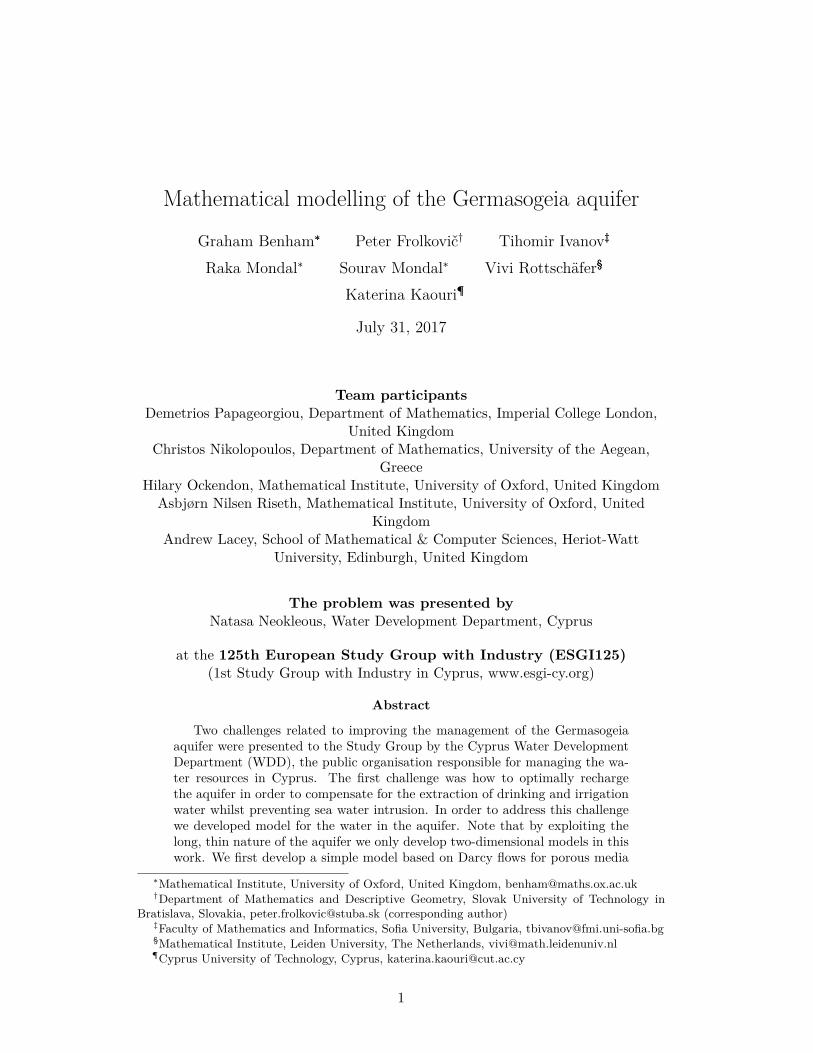
The Germasogeia aquifer is an alluvial aquifer, consisting of loose material, whichenables effective filtering of the water. It lies along the Germasogeia river valley andextends from the Germasogeia dam to the coast. It is 5.5 km long and has anarea of 3 km2. It lies under an urbanised area, the Limassol–Nicosia highway, localimportant roads and several main pipelines. Its width varies from 100 m to 800 m,and its depth from 35 m upstream, near the dam, to 55 m near the sea—see Figure1 for a cross section of the aquifer. The Germasogeia aquifer is the first aquifer inCyprus that has been used as a natural water treatment plant, and it is currentlythe most intensively exploited aquifer in the country. Since 1982, the WDD in thedistrict of Limassol has been using water from the Germasogeia dam to recharge theGermasogeia aquifer, with controlled releases on the surface of the aquifer, at fourrecharge points. See Figure 2 (left) for the locations of recharge points, indicatedby the large green circles.

After natural purification, the ‘treated’ groundwater is pumped out of the aquiferthrough boreholes to supply domestic water to the greater Limassol area. No fur-ther water treatment is carried out except chlorination of the water tanks. At the

2


Figure 1: A cross section of the Germasogeia aquifer. The red dotted line is theminimum acceptable water table level and the other 4 colored curves are watertable levels at the dates specified in the legend. The downward arrows representthe recharge points. The 13 thin grey vertical lines represent boreholes used forobservation.

moment, there are 19 boreholes in operation—see Figure 2 Left for the locations ofthe boreholes (indicated with smaller blue circles). The extraction rates from theseboreholes vary from 40 to 130 m3/hour. The total volume of extracted water variesfrom 5-7 million m3 per year.

The aquifer has impermeable boundaries at the east and west and an imperme-able base, the bedrock where no water can enter or exit. Water enters the aquiferfrom the dam; it seeps through the dam into the aquifer. The sea is located at thesouth boundary. There, fresh water can exit the aquifer and salt water can enterthe aquifer. One important objective for the effective management of the aquifer isto avoid both of these scenarios. It is more important to avoid seawater intrusionbecause if this happens the groundwater can no longer be used as drinking water.If the seawater enters it will leave the aquifer very slowly as the speed of the flowand also the slope of the aquifer are small. Moreover, when fresh water goes to thesea good drinking water, a precious commodity in dry Cyprus is wasted.

The report is organized as follows: in Section 2 we describe the two aquifer chal-lenges in more detail. In Section 3 we develop a two-dimensional aquifer model basedon Darcy flow, and then use it to develop an optimal recharge strategy. In Section4, in order to study seawater intrusion, we develop a two-dimensional aquifer model

3


Figure 2: Top view of the aquifer. Left: the recharge points are indicated with largegreen circles and the extraction points indicated with small circles. Right: Thelocation of the sewage system, indicated with orange.

based on saturated-unsaturated groundwater flow modelling with a variable waterdensity, using the open source software SUTRASuite. In Section 5 we also applythe commercial software FLUENT to do more simulations of the flow in the aquifer.In Section 6, we examine contaminant transport and a related model is developedusing the commercial software COMSOL Multiphysics. Finally, in Section 7 we sum-marise our conclusions and give some recommendations to the Water DevelopmentDepartment for follow-up actions and possibilities for further collaboration.

2 Description of the challengesThe main aims of the WDD for effectively managing the Germasogeia aquifer are: a)supply drinking water of acceptable quality to the greater area of Limassol b) protectthe Germasogeia aquifer from seawater intrusion, and c) minimise groundwater lossesto the sea.

In this connection, we were presented with the following two challenges for theStudy Group week:

1. How can the effectiveness of the recharge process be maximised? At the mo-ment there are four recharge points where water is inserted into the aquiferand 19 boreholes that pump water out. What is the optimal recharge protocol,i.e. for how long and at which locations should we recharge the aquifer whilesimultaneously

(a) protecting the aquifer from seawater intrusion, and

4


(b) minimising water losses to the sea?

2. If there is contamination by sewage or other pollutants, where will the pol-lution spread and how fast? What would this mean for the quality of theextracted water? Which measures should WDD take in order to minimise thecontamination effects?

3 Aquifer modelling with optimal recharge strategyIn this section we derive an approximate, two-dimensional model based on Darcyflow which leads to an equation for the water table level in the aquifer. This modelis related to the Dupuit model [1] for long and thin aquifers. This is a very goodapproximation for the Germasogeia aquifer since its length is L ≈ 5.7 km and itsdepth H ranges from 35m at the dam to 55m at the sea. Also, the width of theaquifer is W ≈ 60 m except close to the sea where the aquifer becomes wider andas a first approximation we assume that the aquifer is a channel of uniform widthand neglect any transverse flow along the width. The slope of the aquifer is small,around 4 degrees so we assume that the base of the aquifer is an inclined plane atconstant slope. Additionally, we assume that the groundwater density, and viscosityand the ground permeability and hydraulic conductivity are all constants.

3.1 Mathematical ModelTherefore we consider a two-dimensional, gravity-driven flow in an inclined, porousaquifer. Beneath the aquifer lies a bed of impermeable bedrock and above it is theground surface (see Figure 3). There is a saturated water table level at some heightbelow the ground. Below the water table the aquifer is fully saturated and above itis approximately dry. Upstream of the aquifer is a dam which holds a large body ofwater behind a concrete barrier. The water seeps through the barrier at flow rate Q.Downstream of the aquifer, the water table meets the sea level at height Hb abovethe bedrock. Water is extracted and injected into the aquifer at specific locationsdecided by the WDD. Let us choose our coordinate system such that the x directionis parallel to the bedrock level, inclined at a constant angle α to the horizontal. InFigure 3, the tangent of α is given by tanα = H/L, where H and L are the lengthand elevation of the aquifer respectively. The angle α ≈ 1/100 radians, i.e. quitesmall since tanα ≈ H/L ≈ 0.01-mathematically -we denote this as α ≪ 1 (see Table1) and we subsequently utilise it in the asymptotic analysis that follows in order tosimplify our model. We also let (u,w) denote the velocities in the (x, z) directionsrespectively, and p denotes the pressure. For flow in porous media, we shall use theDarcy equations

∂u

∂x+

∂w

∂z= s(x, t), (1)

u = −k

µ

(∂p

∂x− ρg sinα

), (2)

w = −k

µ

(∂p

∂z+ ρg cosα

), (3)

5


z

x

L

H Hb SeaBedrock

Extraction (Sink)Recharge (Source)

Ground surfaceQ

Dam

α

Water table: z = h(x, t)

Figure 3: Schematic diagram of the long and thin, sloping aquifer related to themodel equations (1)–(3). The water table level is indicated with the blue curve.The coordinate system x and z is taken respectively along and perpendicular to thebedrock, which is assumed to be a straight line. The inward looking arrow indicatesa recharge point (a source in the model formulation), and the outward looking arrowindicates an extraction point (a sink in the model formulation);α is the angle to thehorizontal level.

where ρ is the groundwater density, g is the gravitational acceleration constant, k isthe ground permeability and µ is the viscosity. In the conservation of mass equation(1), we have a source/sink term s(x, t) which represents the rate at which freshwater is supplied to/extracted from the aquifer–this will be described in moredetail later. At the water table level z = h(x, t), depicted as the blue, dotted curvein Figure 3, we have the following kinematic and dynamic boundary conditions

w =∂h

∂t+ u

∂h

∂x, on z = h(x, t), (4)

p = pa, on z = h(x, t), (5)

where pa is the atmospheric pressure. At the bedrock z = 0, since no water goesthrough there, we have the impermeability condition

w = 0. (6)

Upstream of the aquifer, at x = 0, there is a constant source of water from the dam∫ h(0,t)

0u(0, t) dz =

Q

ℓ, (7)

where ℓ is the typical dam width. Downstream of the aquifer at x = L/ cosα, andthe water table height must be at sea level, that is

h(X, t) = Hb. (8)

6


Now, we non-dimensionalise all variables using the scalings 1

x = Lx, z = Hz, t =L2

KHt, p = ρgHp, u =

KH

Lu,

w =KH2

L2w, s =

KH

L2s, h = Hh,

(9)

where K = kρgµ is the hydraulic conductivity. Since the aquifer is long and thin, we

can make the approximation

ϵ =H

L= tanα ≈ α ≪ 1, (10)

Now equations (1)-(3) become

∂u

∂x+

∂w

∂z= s, (11)

u = 1− ∂p

∂x, (12)

ϵ2w = −1− ∂p

∂z. (13)

Taking the limit of small ϵ, and integrating (13) across the water table 0 ≤ z ≤ h,as well as using boundary conditions (4), (5) and (6), we get the following equationfor the (non-dimensional) water table h:

∂h

∂t+

∂

∂x

(h

(1− ∂h

∂x

))= S, (14)

where S = sh. Boundary conditions from equations (7) and (8) become

h

(1− ∂h

∂x

)= q, at x = 0, (15)

h = H, at x = 1, (16)

where we have introduced the non-dimensional constants q = QLKH2ℓ

and H = HbH .

Equation (14), together with (15), (16) and some initial condition, can be solved forthe water table height, provided we know the source/sink term.Note that in non-dimensional coordinates, the velocity in the x direction is given by

u = 1− ∂h

∂x. (17)

Hence, even though we have not looked at seawater intrusion in the above model,a very useful conclusion can be drawn here: if the gradient of the water table hxis greater than one at x = 1(sea), then we expect seawater intrusion at the water

1 Note that in general the angle α is unrelated to the thin and long geometry of the aquifer. Insuch cases one can still define an aspect ratio for the aquifer, which will be a small parameter, butproceed with arbitrary angles. Here we have small aspect ratio and a small sloping angle.

7


table height. Likewise, if hx is less than one, we expect freshwater to flow outwardsinto the sea. Seawater intrusion is studied with a more detailed model later on.

In Figure 4 h(x, T ) is plotted for T = 5. We see that the solution has reacheda steady state. The green curve is the water table when S = 0 and the red curveis the water table for S < 0, as shown in Fig. 4 with a blue colour. In Fig. 4 wealso plot the line h = x at x = 1 (sea), which shows that both the green and the redcurve have hx < 1 =⇒ u = 1 − hx > 0 at the boundary with the sea and there islittle risk of seawater intrusion.

Figure 4: The water table for T = 5, h(x, 5), drawn when S is zero (green line) andfor non-zero S (red line). The chosen form of the non-zero S is also plotted with ablue line (3 sources, 2 sinks). We also plot the line h = x near x = 1, i.e. hx = 1there to emphasise that hx < 1 =⇒ u = 1 − hx > 0 for both the red and thegreen line, at the boundary with the sea. This indicates that the fresh water flowsoutwards and there is little risk of seawater intrusion.

3.2 Optimal Recharge StrategyIn this section we use the mathematical model given by Equations (14)-(16) toinvestigate how to control the aquifer water table by changing the recharge processin order to waste as little water as possible.Currently, WDD uses four recharge points to recharge the aquifer and extracts waterfrom 19 extraction points. The overall flow rate of extraction and recharge shall bedenoted by m+ and m−, respectively. We assume that the recharge sources are pointsources and we approximate them with rectangular sources (see Fig. 5) at positionsx/L = bi and area Ai, for i = 1, 2, 3, 4, and that the sinks are bundled together intoa distributed sink extending from x/L = a1 and x/L = a2, over a width d (see Fig.5 ).

8


Distance downstream (𝑥)

𝑆 𝑥

Figure 5: The four recharge points approximated as rectangular sources and the 19extraction points bundled together into an extended, uniform, sink.

Therefore S(x, t) mathematically is expressed as

S(x) = M−Θ(x− a1)Θ (a2 − x) +

4∑i=1

M+i δ (x− bi) , (18)

where Θ is the Heaviside function, δ is the Dirac delta function and the strength ofthe distribution M− = m−L

dH2K(a2−a1)and M+

i =m+

i L2

AiH2Kare the non-dimensional flow

rates.The WDD have control over how much water they inject into the aquifer. They wantto recharge with enough water so that the water table does not sink below a criticallevel h(x, t) = f(x) (which has been determined empirically) but they do not wanth(x, t) to be much higher than the minimum acceptable line since this would wastewater unnecessarily. Mathematically this can be cast as an optimisation problem inwhich we aim to minimise the discrepancy between h and f(x) by choosing optimalrecharge rates M+

i . In mathematical terms, this is equivalent to

minM+

i ∈[0,Mmax]|h− f | , (19)

subject to the constraints that h ≥ f , and that h must satisfy equations (14), (15)and (16). We also shall assume that the system is at steady state, so there is noneed for an initial condition.

In Figure 6, for four scenarios of interest, we plot the solution to the optimalcontrol problem (19); the optimal recharge rates and the corresponding water table.We choose as minimum and maximum values of the dam flow rate measured valuessupplied by the WDD as Qmin = 2000m3/day and Qmax = 7000m3/day. For theextraction rate, we also choose a small and a large value to correspond respectivelyto small and large water demand. The chosen values of M− = 1 and M− = 2

9


0.0 0.5 1.0

Distance downstream

0.0

0.2

0.4

0.6

0.8

1.0

Aquifer w

ate

r le

vel

Water table

Minimum level

0.0 0.5 1.00.0

0.1

0.2

0.3

0.4

0.5

Rech

arg

e s

trength

Recharge point

(a) qmax, M−min

0.0 0.5 1.0

Distance downstream

0.0

0.2

0.4

0.6

0.8

1.0

Aquifer w

ate

r le

vel

Water table

Minimum level

0.0 0.5 1.00.0

0.1

0.2

0.3

0.4

0.5

Rech

arg

e s

trength

Recharge point

(b) qmax, M−max

0.0 0.5 1.0

Distance downstream

0.0

0.2

0.4

0.6

0.8

1.0

Aquifer w

ate

r le

vel

Water table

Minimum level

0.0 0.5 1.00.0

0.1

0.2

0.3

0.4

0.5

Rech

arg

e s

trength

Recharge point

(c) qmin, M−min

0.0 0.5 1.0

Distance downstream

0.0

0.2

0.4

0.6

0.8

1.0

Aquifer w

ate

r le

vel

Water table

Minimum level

0.0 0.5 1.00.0

0.1

0.2

0.3

0.4

0.5

Rech

arg

e s

trength

Recharge point

(d) qmin, M−max

Figure 6: Solution of the optimal control problem displayed together with the min-imum water table (red curve) and recharge quantities M+

i . The optimal rechargerates for each scenario are denoted by dots and the corresponding water table withblue. (a) Maximum dam seepage q and minimum extraction rate M−, giving a valueof η = 3.6. (b) Maximum dam seepage and maximum extraction rate, giving a valueof η = 1.6. (c) Minimum dam seepage and minimum extraction rate, giving a valueof η = 2.0. (d) Minimum dam seepage q and maximum extraction rate M−, givinga value of η = 1.9.

correspond to an extraction rate of approximately 20000m3/day and 40000m3/day.We also define the ratio of the rate of extraction to recharge as

η =M− (a2 − a1)∑4

i=1M+

, (20)

which we evaluate for each of the four scenarios above. In each scenario η > 1, and sothe optimal strategy allows more water to be extracted than injected. This is lesswasteful than the current recharge strategy, in which the recharge waterquantity is approximately the same to the extracted water quantity. Also,two immediate conclusions can be drawn from Figure 6: (a) smaller dam seepageflow rates require larger injection rates upstream, (b) and larger extraction ratesrequire larger injection rates downstream. A list of the other parameter values usedin this analysis is given in Table 1.

3.3 ConclusionsIn this section we have presented a simple mathematical model, based on Darcyflow, which can be used to predict aquifer flow for a chosen recharge and extraction

10


Constant Value UnitsQmin 2000 m3/dayQmax 7000 m3/dayH 78 mHb 61 mL 5700 mK 150 m/dayℓ 200 md 200 ma1 0.33a2 0.96b1 0.04b2 0.26b3 0.51b4 0.68

Table 1: List of parameter values.

protocol. The velocity of the flow and the water table level can be easily obtainedusing a simple numerical scheme. We have also designed an optimisation methodwhich we used to determine the minimum flow rate at the recharge points that ensurethat, at steady state, the water table will be above the minimum acceptable waterlevel in the aquifer. The model can be generalised to incorporate variations in thewidth and the base of the aquifer and to include more sources and sinks, as required.Note that the ingress of the seawater has not been considered explicitly here butthe boundary condition (16) at the aquifer-sea boundary allows us to conclude thatthere will be no significant risk of sea intrusion in the scenarios we have examined.More details can be found in [1].

4 Model including seawater intrusion, using the opencode SUTRASuite

In this section we use the open source code SUTRASuite to investigate throughnumerical simulations several extraction/recharge scenarios for the aquifer based onmathematical models of saturated-unsaturated groundwater flows, now includingseawater intrusion. The mathematical model we set up captures all features ofinterest when managing the Germasogeia aquifer:

• the groundwater flow induced by different recharge sources and extraction wells

• the water table level and how it varies for different recharge/extraction sce-narios

• the seawater intrusion effects for different recharge/extraction scenarios. Forthis we allow the groundwater density to be variable due to the presence ofsaltwater.

11


4.1 The mathematical modelIn this section we briefly describe the mathematical model for the flow in the aquiferwhich allows for the possibility of seawater intrusion. This model is implementedusing SUTRASuite below. Note that a more extensive description of a similar (butnot identical) mathematical model can be found in section 5, based on computationalfluid dynamics.

The unknown quantities to be found are the fluid pressure p = p(x, t) and thesalt mass fraction msalt = msalt(x, t). Some physical quantities vary with respectto these functions and they are given by chosen state equations e.g. for the fluiddensity ρ = ρ(msalt) and for the water saturation Sw = Sw(p) = Sw(p(x, t)). Thewater saturation function Sw implicitly describes the position of the water tablethat itself is an abstract interface between the fully saturated zone of aquifer, whereSw ≡ 1, p ≥ 0 with no air presence in the pores, and between the partially saturatedzone, i.e. Sw < 1, p < 0 with a presence of air in the pores.

The groundwater flow is characterized by the so-called Darcy velocity,

q = −kr k

µ(∇p− ρg) (21)

where k = k(x) is the permeability (a tensor in general), µ is the fluid viscosity (ingeneral µ = µ(msalt)) and g is the gravity vector. The function kr = kr(Sw(p))describes the relative permeability such that kr(1) = 1 and kr(Sw) < 1 for Sw < 1.Note that so-called average fluid velocity u with respect to the stationary solidmatrix of porous media [4] is given by u = q/(εSw) where ε denotes the porosity ofaquifer.

The model is a system of two partial differential equations:

∂(εSwρ)

∂t+∇ · (ρq) = Qin +Qout , (22)

∂(εSwρmsalt)

∂t+∇ · (ρmsaltq− εSwρD∇msalt) = msaltQout . (23)

Qin and Qout denote the fluid mass sources and sinks respectively, and D = D(q)describes the diffusion and dispersion tensor [4]. We note that we consider thesources Qinto represent recharge with only fresh water.

A more detailed description can be found in the SUTRASuite documentation [4]where even more general settings are considered like e.g. a solute or heat transportmodelling.

Numerical modelling of groundwater flow has a very long tradition in scientificand engineering studies, see for example the webpage of the U.S. Geological Survey,water.usgs.gov/software/lists/groundwater, where several free software toolsare available. See also [2]. For our purposes the software SutraSuite appears as themost suitable for several reasons. First of all, a user-friendly graphical interface isavailable called ModelMuse which can be used to create 2D/3D computational do-mains and for choosing the control parameters of the simulation. The SUTRA code(the main part of SutraSuite) can numerically solve mathematical models describingall features of interest for the Germasogeia aquifer. In particular, it can cope with

12

water.usgs.gov/ software/lists/groundwater


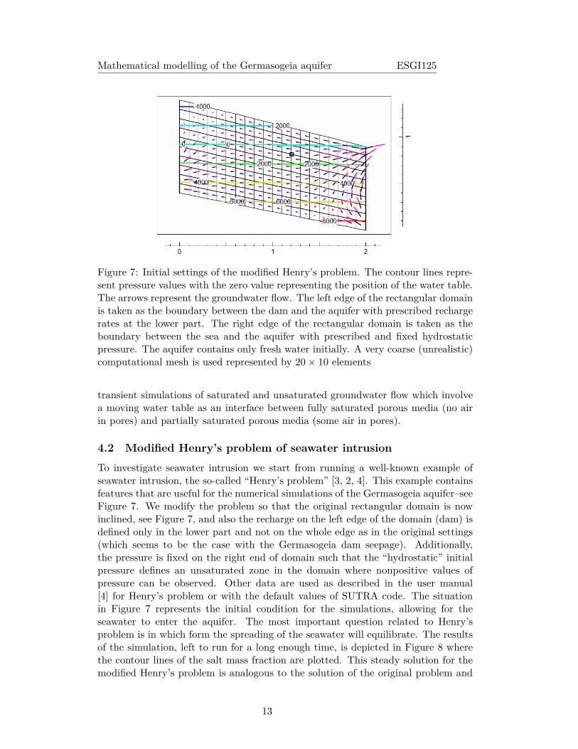
Figure 7: Initial settings of the modified Henry’s problem. The contour lines repre-sent pressure values with the zero value representing the position of the water table.The arrows represent the groundwater flow. The left edge of the rectangular domainis taken as the boundary between the dam and the aquifer with prescribed rechargerates at the lower part. The right edge of the rectangular domain is taken as theboundary between the sea and the aquifer with prescribed and fixed hydrostaticpressure. The aquifer contains only fresh water initially. A very coarse (unrealistic)computational mesh is used represented by 20× 10 elements

transient simulations of saturated and unsaturated groundwater flow which involvea moving water table as an interface between fully saturated porous media (no airin pores) and partially saturated porous media (some air in pores).

4.2 Modified Henry’s problem of seawater intrusionTo investigate seawater intrusion we start from running a well-known example ofseawater intrusion, the so-called “Henry’s problem” [3, 2, 4]. This example containsfeatures that are useful for the numerical simulations of the Germasogeia aquifer–seeFigure 7. We modify the problem so that the original rectangular domain is nowinclined, see Figure 7, and also the recharge on the left edge of the domain (dam) isdefined only in the lower part and not on the whole edge as in the original settings(which seems to be the case with the Germasogeia dam seepage). Additionally,the pressure is fixed on the right end of domain such that the “hydrostatic” initialpressure defines an unsaturated zone in the domain where nonpositive values ofpressure can be observed. Other data are used as described in the user manual[4] for Henry’s problem or with the default values of SUTRA code. The situationin Figure 7 represents the initial condition for the simulations, allowing for theseawater to enter the aquifer. The most important question related to Henry’sproblem is in which form the spreading of the seawater will equilibrate. The resultsof the simulation, left to run for a long enough time, is depicted in Figure 8 wherethe contour lines of the salt mass fraction are plotted. This steady solution for themodified Henry’s problem is analogous to the solution of the original problem and

13


Figure 8: Steady state situation for the transient simulation from initial settings asgiven in Figure 7. The extraction is represented with a single point sink, representedby a square. The contour lines represent now the mass fractions of salt water, so aseawater intrusion occurs in this example.

it will be used to compare it with other simulations later on. Before running severalillustrative examples with different recharge and extraction scenarios to see theirinfluence to the groundwater flow and the salt mass fraction transport of the modifiedHenry’s problem, we comment which data is needed for these simulations. We wantto determine two unknowns - the fluid pressure and the salt mass fraction. Otherphysical quantities such as the fluid density or the flow velocities are derived fromthese two quantities and other given physical parameters. The salt mass fraction inthe domain must be given by users at t = 0, and the initial pressure is computed bySUTRA for data given by the WDD. Both unknown quantities must be prescribedon the boundaries (dam and sea respectively) during the simulation time. In thefollowing simulations we additionally incorporate one extraction sink (which bundlestogether the 19 extraction points) and one recharge source. A description of theemployed mathematical model has been given in Section 4.1.

In the first example we consider we introduce a single extraction point. The usercan easily define the locations of the sources and sinks, and the corresponding ratesof extraction and recharge using the graphical interface ModelMuse. In this examplewe find that a large extraction rate decreases the position of the water table (zeropressure level), see Figure 9, where (nonstationary) results are presented after sometime starting the transient computations with the initial situation given in Figure 7.Clearly, the water table height decreases significantly compared to that in Figure 7.In the next example we choose a more realistic extraction rate. The result of suchcomputation can be found in Figure 10 where the initial pressure is plotted togetherwith the flow velocities. One can see in this Figure that the following three aspectsinfluence the flow comparably: the recharge from the dam, the seawater intrusionand the extraction from the point sink-compare also with Figure 7. When comparingthe results for a nonzero extraction rate in Figure 10 with the results for the zeroextraction rate in Figure 7, one can clearly expect for transient simulations that a

14


Figure 9: Simulation using the initial settings given in Figure 7, with an additionalextraction point source (denoted as a small square in the domain) with a too largeextraction rate. The contour lines represent the pressure. Clearly, a deformationof the water table (the zero pressure line) and large flow velocities from the rightboundary (the sea) are observed.

Figure 10: Initial pressure (the contour lines) and flow velocities for a more realisticextraction rate (singular sink). One can recognize the recharge from the dam on theleft, the seawater inflow from the right and the extraction from the point sink.

15


Figure 11: An illustration of transient simulations starting from the initial situationas given in Figure 10. The salt mass fraction contour lines and the flow velocitiesare plotted. Comparing this plot with Figure 8 in which the zero extraction rate isgiven one can clearly recognize that the seawater intrusion is too large and one canexpect that the salt water enters the extraction well.

larger seawater intrusion must occur. This is confirmed by the results of transientsimulation as presented in Figure 11 where the salt mass fraction contour lines areplotted after some time period and where the salty water reaches the vicinity ofextraction well. Our final illustrative example is based on the addition of rechargeon a part of the top edge of computational domain. The situation for these finalsettings is illustrated in Figure 12 where the rates of both external sources (therecharge) and the rate of sink (the extraction) are plotted.

The results of initial pressure computations and the resulting flow velocities areplotted in Figure 13. One can observe that the addition of recharge at the top ofthe domain can compensate the extraction in the sense that the seawater inflowon the right is not qualitatively different to the situation in Figure 7 with zeroextraction. This is confirmed also by transient simulations for which a stationarysituation could be reached, see Figure 14, where the seawater intrusion is comparablewith the situation in Figure 8.

Finally, we comment on the applicability of SUTRA to solve the challengesposed by the WDD. To perform the numerical simulations of different extractionand recharge scenarios for Germasogeia aquifer the following nontrivial tasks mustbe realised: (a) a more realistic description of the aquifer geometry must be used asdone to some extent in the next section (b) Much finer computational grids must beused to obtain (almost) grid independent numerical solution. (c) The modelling ofthe unsaturated zone in the aquifer needs input data (see Section 4.1), that are noteasy to find and should be obtained by some sort of model calibration.

16


Figure 12: Recharge and extraction distributions. The blue colour represents thenegative rate (the extraction) and the other colours represent the positive values(the recharge).

Figure 13: The initial pressure and flow velocities for the extraction and rechargerates as defined in Figure 12.

17


Figure 14: Stationary numerical results for the salt mass fraction (the contour lines)and the corresponding flow velocities (arrows) for the initial situation given by Figure13.

Figure 15: The two-dimensional aquifer geometry used in the SUTRA simulationsinvestigating seawater intrusion.

4.3 Mathematical model with seawater intrusion, using a more re-alistic aquifer geometry (in SUTRA)

We now implement the more realistic two-dimensional approximation of the aquiferby considering a cross-section of the aquifer, as discussed in the Introduction andin relation to Fig. 1). For the simulations below we take the length L = 5.5km, thewidth at the dam equal to 35 m and width at the sea equal to 55m.

In this setup, we then introduce the 4 recharge points, denoted with squareson the top of the domain in Fig. 15. Several extraction points are incorporated inthe model, having a net out-flux, equivalent to that of the Germasogeia aquifer.The extraction points are depicted with arrows in Fig. 15. We carry out numericalexperiments, in order to study how the recharge rates affect sea intrusion. First, weconsider the recharge rates that correspond to i.e 1000 m3/day, 6000 m3/day, 4000m3/day, 500 m3/day. The sea intrusion area can be seen in Fig. 16.

18


When lowering the recharge rate at the fourth point (i.e., the one that is nearestto the sea), the sea intrusion is larger. We simulate the process for a time rangeof about 3 days and for this period of time, the sea water gets into the aquifer forabout 50m more.

Figure 16: Seawater intrusion for the recharge rates of the Germasogeia aquifer.

Figure 17: Seawater intrusion for a lower influx rate at the last recharge point.

Further work is necessary in order to simulate a complete 3D model of the aquiferincluding a detailed description of all the sources and sinks. Then, the inverseproblem should be formulated and algorithms for its solution should be studied. I.e.,one should consider what recharge rates are necessary, in order to ensure minimalsea water intrusion and enough water level in the aquifer.

5 Modelling with seawater intrusion using ANSYS FLU-ENT

In this section we present another modelling approach for the Germasogeia aquifer,described and implemented in commercial computational fluid dynamics softwareANSYS Fluent [6].

5.1 Model equationsThe incompressible fluid flow field (u) in a porous medium (in case of a smallReynolds number Re ≪ 1) is described by the Darcy-Brinkman formulation (as-

19


suming Newtonian rheology)

ρ∂u

∂t= ∇ ·

[− pI+

µ

ϕ

(∇u+ (∇u)T

)]− µ

ku+ ρg (24)

where µ and ρ are the fluid viscosity and density, k and ϕ are the permeability andporosity of the medium, g is the gravity vector. In the limit of low permeability,typical in groundwater flows, the dimensionless Darcy number Da = k

L2 ≪ 1 (Lis the characteristic length scale). In such an instance, Eq. (24) is reduced to theconventional Darcy’s relation

k

γ

∂u

∂t+ u = −k

µ

(∇p− ρg

)(25)

where γ = µ/ρ is the dynamic viscosity of the fluid. The mass conservation equationreduces to the incompressibility condition

∇ · u = 0 (26)

Using the continuity equation (Eq. 26), the Darcy’s relation Eq. (25) at steady statecan be reduced to Laplace’s equation for pressure as

∇2p = 0 (27)

Now as described in the problem introduction, the level of water in the porousbed is computed as the interface boundary between two fluids. The tracking ofthe interface(s) between the phases is accomplished by the solution of a continuityequation for the volume fraction of the phases. Ignoring interfacial mass transfer,the continuity equation for the ith phase is

1

ρi

[∂

∂t

(βiρi

)+ u · ∇ρiβi

]= 0 (28)

N∑i=1

βi = 1 (29)

where, N is the number of phases, βi is the phase fraction (0 < βi < 1) and ρiis the density of the ith phase. It may be noted here, that the bulk macroscopicproperties (ρ and µ) in Eqs. (24) and (25) follows from the simple mixing rule,ρ (or µ) =

∑ξi=1 βiρi(or µi). Only a single set of the momentum exchange equation,

in the form of the Darcy’s law is solved (Eqs. 25 and 26) to obtain u, which isshared by all the phases i. In the present formulation, one of the phases is waterwhile the other is air. So, based on Eq. (29), βwater = 1− βair denotes the extent ofpartial saturation. Note that βwater = 1 represents a completely saturated porouszone, while βair = 1 is completely unsaturated (dry). The sea water intrusion effectis modelled by allowing a variable water density, vayring as a function of the saltmass fraction (msalt) [10] as follows

ρwater (in g/cc) = 1 + 0.695msalt, (30)

20


where 0 ≥ msalt ≥∼ 0.1. Typically, the mass fraction of salt in sea water ranges inbetween 4-6 wt%. Similarly, the viscosity of water can be correlated with the msalt

[10] asµwater (in cP ) = 1 + 0.09msalt + 0.0093m2

salt. (31)More complex (higher polynomial degree) correlations of the viscosity and densityvariations can be found in [12]. The species convective-diffusive model (consideringthe diluted solution approximation) is solved for the salt concentration,

∂msalt

∂t+ u · ∇msalt = Dsalt∇2msalt, (32)

where Dsalt is the diffusivity of salt in the sea water.

5.2 Problem description and boundary conditionsIn order to proceed with the simulations of the above model we implement theaquifer geometry as in Fig. 18. As described in the beginning, the horizontal lengthof the aquifer is around 5.5 km, while the depth ranges from 35 (upstream, damside) to 55 m (downstream, sea side), and since the width is much smaller thanthe length we continue with the two-dimensional approximation of the geometry.Also, the inclination angle is around 4 degrees. The permeability (k) does varysignificantly along the aquifer, so we assume an average value of k for simplicity asin our previous models. In Fig. 18 the approximate locations of the recharge (R1)and extraction (E1) points are also shown. It may be noted that the recharge andextraction rates considered in the following simulations are the actual field values.

There are 19 working extraction borewells (each having a capacity of 1.08 km3/d)which extract water for urban distribution. In order to simplify the calculation,these 19 points are clubbed together into 6 points (E1−6) withdrawing equivalenttotal amount of water (20.5 km3/d). The extraction rate of E1 equals to that 4borewells, E2,3 equals to that 2 borewells each, E4,5 equals to that 3 borewells eachand E6 equals to that of 5 borewells. In practice, water is withdrawn from the topby the borewells which is mimicked (in the simulation) by considering sinks at thebottom of the aquifer for simplification. Obviously, this will affect the fluid patternsaround the extraction regions (deviation from reality) but our objective to quantifythe water table and sea intrusion effects will be unaffected.

The initial condition is considered to be the minimal water level just sufficientto prevent sea water intrusion. Mathematically this means that the red region inFig. 18 has βwater = 1 while everywhere else it is zero. The boundary condition atthe bottom is no slip as well as no penetration (u = 0) and βwater = 1. While, atthe top, it is the pressure condition (Eq. 33) and βwater = 0. At the upstream wall(dam side), there is a constant influx equivalent to 5k m3/d and βwater = 1 for thebottom half of the wall and the rest u = 0. The boundary condition on the sea sideis the outflow condition for flow while Dirichlet condition for the phase variable (β)

[−pI+ µ(∇u+ (∇u)T )] · n = −p0n (33)βwater = 1 (34)

21


Figure 18: Description of the 2D model geometry with various extraction andrecharge locations. Note 5k m3/d equals to 5000 m3/d and not 5 km3/d

where p0 is the atmospheric pressure. For the species transport, the top and thebottom surface satisfy the no-flux condition

− n · [umsalt −Dsalt∇msalt] = 0 (35)

Since there is no slip at the boundaries, Eq. (35) reduces to the Neumann conditionn · ∇msalt = 0. The concentration boundary condition at the sea side is fixed tothe sea-water salinity msalt = 0.05 and at the upstream (dam side) is zero. Initially(at t = 0), the region containing sea has msalt = 0.05 while everywhere else it iszero. The physical properties of the various fluid properties are considered for thestandard values. The permeability k is taken as 1.54 × 10−10m2 equivalent to thehydraulic conductivity of 130 m/d (in geological units)2.

The system of equations are solved using FLUENTr, which is based on a finitevolume discretisation [6, 7]. The results of the simulations are presented below.

5.3 Technical explanation about the algorithm usedThe momentum equation is discretised using the Quadratic Upstream Interpolationfor Convective Kinematics (popularly known as QUICK) scheme [9], a higher-orderdifferencing scheme based on the weighted average of second-order-upwind and cen-tral interpolations of the variable. One limitation of the shared-fields approximationis that in cases where large velocity differences exist between the phases, the accu-racy of the velocities computed near the interface can be adversely affected. As such,the compressive interface capturing scheme for arbitrary meshes (CICSAM), basedon the Ubbink’s work [13], is a high-resolution differencing scheme. The CICSAMscheme is particularly suitable for flows with high ratios of viscosities between thephases. CICSAM is implemented in FLUENT as an explicit scheme and offers theadvantage of producing an interface that is almost as sharp as the geometric recon-struction scheme [14]. This scheme is the most accurate, robust and is applicablefor general unstructured meshes. Since the flow in the present case is dominatedby body forces (gravity) rather than pressure gradients, a body-forced weighted

2Units note: The permeability (m2) is generally calculated from the hydraulic conductivity(m/d), which is more commonly used in the hydrogeological community. For reference, 0.987 ×10−12 m2 = 1 Darcy unit = 0.831 m/d.

22


scheme with “pressure implicit with splitting of operators” (PISO) algorithm is usedfor pressure correction [8], which is an extension of the SIMPLE algorithm [11] usedfor solution of the momentum equation. The PISO algorithm shifts the repeatedcalculations required by SIMPLE and SIMPLEC inside the solution stage of thepressure-correction equation [8]. After one or more additional PISO loops, the cor-rected velocities satisfy the continuity and momentum equations more closely. Thealgorithm is slightly more CPU intensive, but dramatically reduces the number ofiterations required for convergence, especially in transient problems. Simulationswere initiated with very small time steps and were increased gradually for latertimes with no resultant spurious numerical oscillations in the solution.

The computational domain was meshed using unstructured hexagonal mesh el-ements (total of 27,053 mesh elements) with more refinement along the air-waterinterface (water level). Grid independence was tested at various dimensionless meshsizes starting from 0.00013 to 0.0095. It was observed that the mass continuity isconserved with an accuracy of 10−4 for dimensionless mesh sizes less than 0.0021.Hence, the mesh size of 0.021 was considered adequate for the current numericalsimulations. The region around the interface has a dimensionless minimum andmaximum mesh size of 0.00045 to 0.0021, with an average skewness of 0.78 ± 0.13.Similarly, the remaining geometry has minimum to maximum mesh size of 0.0013-0.0061, with the average skewness of 0.73 ± 0.19.

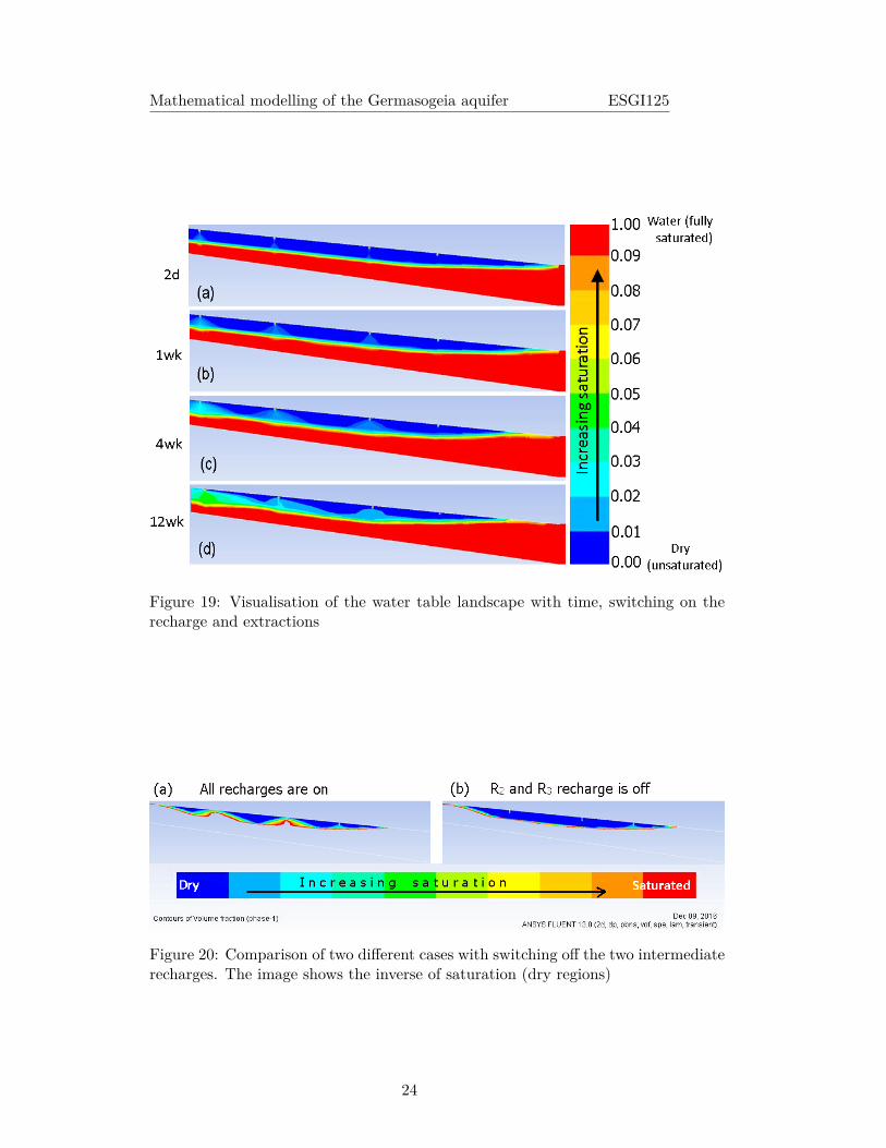
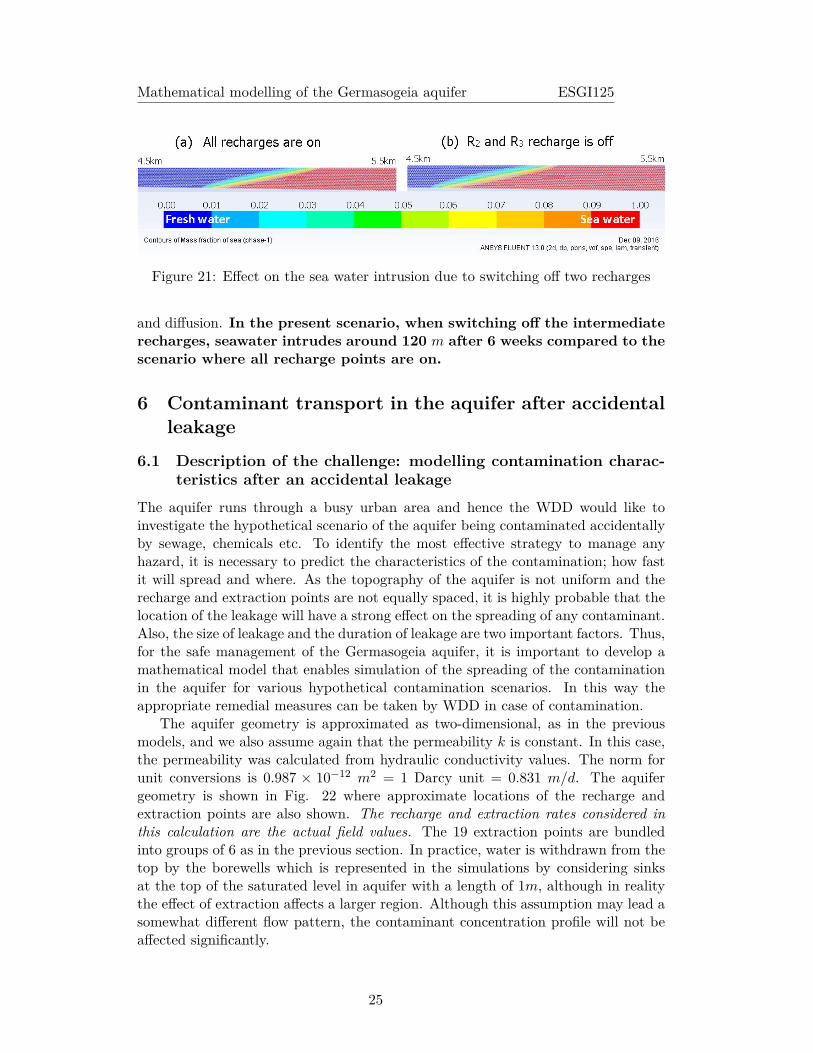
5.4 ResultsThe evolution of the water level is shown in Fig. 19 for a period of 3 months. Theactual aspect ratio of the geometry is scaled to 0.1 times the axial dimension forimproving the visual appearance. The regions in red correspond to the saturatedregion (βwater = 1) while the blue regions are dry. The comparison of the rechargerates on the impact of the water table is illustrated in Fig. 20. The figure shows theinverse of the saturated zones (dry region is shown in the figure) for clear depictionof the difference in the water tables on the two different scenarios. As expectedwith all the recharges switched on, the dry region is less compared to the situationwhen the two intermediate recharge points are switched off. The result gives aquantitative understanding on how much the water level rises locally as well asglobally due to the recharges. Further study on the variation of the recharge ratecan show the measurable change in the water table as a function of the individualpoint recharge rates. This will provide the answer to the inverse problem as what arethe best settings of the recharge rates to minimise sea water intrusion in this specificgeological landscape. Due to switching off the two intermediate recharge points, seawater intrusion is more prominent. It must be emphasised that there is no specialmathematical setting of the seawater-fresh water interface which evolves naturally asa part of the dynamic solution. Fig. 21 shows the seawater-freshwater interface. Asanticipated, as seawater is heavier it is expected to settle towards the bottom if theaquifer with the freshwater on top. However, accounting for the effect of diffusionthe seawater will slowly rise upstream, acting in the opposite direction of gravity.It might be interesting to find the shape of the interface as the seawater intrudesmore upstream and the interface gets diffused due to the combined action of gravity

23


Figure 19: Visualisation of the water table landscape with time, switching on therecharge and extractions

Figure 20: Comparison of two different cases with switching off the two intermediaterecharges. The image shows the inverse of saturation (dry regions)

24


Figure 21: Effect on the sea water intrusion due to switching off two recharges

and diffusion. In the present scenario, when switching off the intermediaterecharges, seawater intrudes around 120 m after 6 weeks compared to thescenario where all recharge points are on.

6 Contaminant transport in the aquifer after accidentalleakage

6.1 Description of the challenge: modelling contamination charac-teristics after an accidental leakage

The aquifer runs through a busy urban area and hence the WDD would like toinvestigate the hypothetical scenario of the aquifer being contaminated accidentallyby sewage, chemicals etc. To identify the most effective strategy to manage anyhazard, it is necessary to predict the characteristics of the contamination; how fastit will spread and where. As the topography of the aquifer is not uniform and therecharge and extraction points are not equally spaced, it is highly probable that thelocation of the leakage will have a strong effect on the spreading of any contaminant.Also, the size of leakage and the duration of leakage are two important factors. Thus,for the safe management of the Germasogeia aquifer, it is important to develop amathematical model that enables simulation of the spreading of the contaminationin the aquifer for various hypothetical contamination scenarios. In this way theappropriate remedial measures can be taken by WDD in case of contamination.

The aquifer geometry is approximated as two-dimensional, as in the previousmodels, and we also assume again that the permeability k is constant. In this case,the permeability was calculated from hydraulic conductivity values. The norm forunit conversions is 0.987 × 10−12 m2 = 1 Darcy unit = 0.831 m/d. The aquifergeometry is shown in Fig. 22 where approximate locations of the recharge andextraction points are also shown. The recharge and extraction rates considered inthis calculation are the actual field values. The 19 extraction points are bundledinto groups of 6 as in the previous section. In practice, water is withdrawn from thetop by the borewells which is represented in the simulations by considering sinksat the top of the saturated level in aquifer with a length of 1m, although in realitythe effect of extraction affects a larger region. Although this assumption may lead asomewhat different flow pattern, the contaminant concentration profile will not beaffected significantly.

25


Figure 22: Schematic of the two-dimensional aquifer geometry implemented in thesimulations; the 4 recharge points are denoted with downward looking arrows and6 extraction sinks are denoted by upward looking arrows. Red is a fully saturatedregion and blue is a dry region.

6.2 Mathematical modelThe modelling of contamination transport involves two parts: prediction of theaquifer water flow, and coupling this to the advection and diffusion of the con-taminant. To model the concentration profile of the contaminant, the followingadvection-diffusion equation is used:

ϕ∂c

∂t+∇ · (−D∇c) + u · ∇c = Rc + Sc (36)

Here, ϕ is the porosity of the aquifer, c is the concentration of contaminant inmol/m3, which is a function of space and time, t is time in d(days), u is the watervelocity (in m/d), obtained by solving Darcy’s law in COMSOL, and Rc and Sc

are the source and sink terms for the pollutant. The red region in Fig. 22 is fullysaturated with water all the time and we expect that the effect of contaminationwill be most prominent in this region. For simplification, we solve for the concen-tration profile of the contaminant in the latter region. The boundary condition atthe bottom of the aquifer is the no-slip condition (u = 0) and the no-penetrationcondition. Also, at the top,there is no penetration of the flow through the edgeof the boundary except at the recharge and extraction points. At the upstreamwall (dam side), we implement a constant influx of water equivalent to 5 km3/d.The boundary condition at the sea is the open atmosphere gauge, p = 0, with anassumption of negligible static water head throughout the depth of the aquifer.

Also, the concentration at the sea and at the dam is set to zero and initially (att = 0), the concentration is everywhere zero, except at the point of leakage. Thephysical properties of the various fluid properties are considered for the standardvalues. The permeability (constant k) is taken as 1.54 × 10−10 m2, equivalent to ahydraulic conductivity of 130 m/d (in geological units).

For the species transport, the dam side and the bottom surface satisfy the no-fluxcondition, defined by

− n · (D∇c) = 0. (37)The only inflow condition for the contaminant is at the leakage points (single ormultiple). As there has never been any leakage in the past, no data are available

26


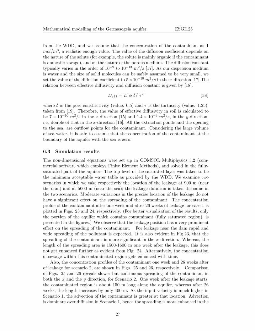
from the WDD, and we assume that the concentration of the contaminant as 1mol/m3, a realistic enough value. The value of the diffusion coefficient depends onthe nature of the solute (for example, the solute is mainly organic if the contaminantis domestic sewage), and on the nature of the porous medium. The diffusion constanttypically varies in the order of 10−9 to 10−13 m2/s [17]. As our dispersion mediumis water and the size of solid molecules can be safely assumed to be very small, weset the value of the diffusion coefficient to 5×10−10 m2/s in the x direction [17].Therelation between effective diffusivity and diffusion constant is given by [18].

Deff = D ϕ δ/ τ2 (38)

where δ is the pore constrictivity (value: 0.5) and τ is the tortuosity (value: 1.25),taken from [19]. Therefore, the value of effective diffusivity in soil is calculated tobe 7 × 10−10 m2/s in the x direction [15] and 1.4 × 10−9 m2/s, in the y-direction,i.e. double of that in the x-direction [16]. All the extraction points and the openingto the sea, are outflow points for the contaminant. Considering the large volumeof sea water, it is safe to assume that the concentration of the contaminant at theboundary of the aquifer with the sea is zero.

6.3 Simulation resultsThe non-dimensional equations were set up in COMSOL Multiphysics 5.2 (com-mercial software which employs Finite Element Methods), and solved in the fully-saturated part of the aquifer. The top level of the saturated layer was taken to bethe minimum acceptable water table as provided by the WDD. We examine twoscenarios in which we take respectively the location of the leakage at 900 m (nearthe dam) and at 5000 m (near the sea); the leakage duration is taken the same inthe two scenarios. Moderate variations in the precise location of the leakage do nothave a significant effect on the spreading of the contaminant. The concentrationprofile of the contaminant after one week and after 26 weeks of leakage for case 1 isplotted in Figs. 23 and 24, respectively. (For better visualisation of the results, onlythe portion of the aquifer which contains contaminant (fully saturated region), ispresented in the figures.) We observe that the leakage position has a very prominenteffect on the spreading of the contaminant. For leakage near the dam rapid andwide spreading of the pollutant is expected. It is also evident in Fig.23, that thespreading of the contaminant is more significant in the x direction. Whereas, thelength of the spreading area is 1500-1600 m one week after the leakage, this doesnot get enhanced further as evident from Fig. 24. Alternatively, the concentrationof sewage within this contaminated region gets enhanced with time.

Also, the concentration profiles of the contaminant one week and 26 weeks afterof leakage for scenario 2, are shown in Figs. 25 and 26, respectively. Comparisonof Figs. 25 and 26 reveals slower but continuous spreading of the contaminant inboth the x and the y direction, for Scenario 2. One week after the leakage starts,the contaminated region is about 150 m long along the aquifer, whereas after 26weeks, the length increases by only 400 m. As the input velocity is much higher inScenario 1, the advection of the contaminant is greater at that location. Advectionis dominant over diffusion in Scenario 1, hence the spreading is more enhanced in the

27


Figure 23: Concentration profile of the contaminant one week after the leakagestarted, at 900 m away from the dam.

Figure 24: Concentration profile of the contaminant 26 weeks after the leakagestarted, at 900 m away from the dam.

Figure 25: Concentration profile after one week of leakage, at 5000 m away from thedam (near the sea).

28


Figure 26: Concentration profile after 26 weeks of leakage, at 5000 m away from thedam.

x direction. Whereas, near the sea, because of the lower input flow rate, the velocitymagnitude is much lower, the diffusion effects are dominant over advection. Hence,the spreading of the contaminant is much slower near the sea side. Also, due to thelarge diffusion coefficient in the vertical direction, the spreading of the contaminantthroughout the depth is very significant, which is more clearly observed for Scenario2, due to the dominance of diffusion.

The nature of the contaminant spreading profile is also investigated in the caseof two leakages, at locations 900 m and 5000 m away from the dam respectively(Scenario 3). The contaminant concentration profile after 26 weeks is provided in27. As in previous scenarios in Scenario 3 the spreading of the contaminant is muchfaster near the dam, whereas the contaminant extends over more depth near thesea. Effect of dominance of diffusion over advection is responsible for this behaviour.Thus, through the above model, given the location and time of leakage, the spread

Figure 27: Concentration profile after 26 week of leakages at both 900 m and 5000m away from the dam.

and speed of a contaminant can be predicted to considerable accuracy. We haveshown that advection has a much more prominent effect on the spreading of thecontaminant. Hence, immediate shut-down of nearest recharge point can lead torestriction of contamination spreading in the x direction.

7 Conclusions and recommendations to the companyFinally, we summarise our conclusions and formulate some recommendations for theWater Development Department (WDD).

29


Firstly, in Section 3 we considered a two-dimensional model of the aquifer flowbased on Darcy flow and then we used this model to compute an optimal rechargestrategy for some scenarios of interest. One of the key results from this modelwas that in certain cases, if the optimal water recharge strategy is employed, thereis a considerable reduction in the amount of wasted water compared to the currentstrategy where water is recharged and extracted in equal proportions. Therefore, therecommendation to the WDD is to consider exploring such optimal, mathematicallydriven strategies in order to recharge the aquifer with less water than with theircurrent empirical approach. Also, even though the above model does not modelthe possibility of seawater intrusion a rough criterion for whether sea water willintrude in the aquifer was presented: if the water speed at the sea-aquifer boundaryis greater than zero the risk of seawater intrusion is small.

In Section 4 we incorporated the effect of seawater intrusion, a topic of utmostinterest by the WDD, by developing a more detailed mathematical model of theaquifer flow based on saturated-unsaturated groundwater flow modelling with vari-able water density. We used the open software tool SUTRASuite and evaluateddifferent extraction/recharge scenarios. We found that this software works well andleads quite quickly to the identification of saltwater-seawater interface in the aquifer.Contrary to the model developed in Section 3 no significant simplifications are nec-essary when deriving the latter mathematical model and computational settings.The software is free available, and there is a large group of users that share theirexperiences on similar problems publicly, through their publications or in internetforums and so on. On the other hand, one cannot expect technical support for suchopen source software tools if some specific difficulties occur.

Computational models can greatly help when evaluating the effectiveness ofrecharge strategies for a given set of extraction wells or even to assess a threatcaused by accidental leakage of contaminants. The most critical issue we see is thatthe transient modelling of the unsaturated zone in the aquifer requires appropriatestate equations to model the water saturation and relative permeability. On theother hand this may be simplified if the water table is described without consideringthe unsaturated zone and it has to be determined with a different open source code,for example MODFLOW (which is compatible with ModelMuse) [5]. Some otherdifficulties to be resolved are mentioned at the end of Section 4. We note that theWDD already has several data and measurements that can be used to validate andfurther develop the models.

Next, in Section 5, we incorporated seawater intrusion in our model using thecommercial code ANSYS FLUENT. Using such a powerful and user friendly softwarecan speed up significantly an appropriate numerical modelling of recharge strategiesfor Germasogeia aquifer; it is however expensive.

Finally, in Section 6 we examined the second challenge posed by the WDD oncontamination and we estimated the speed and spread of the contamination after anaccidental leakage, using the commercial software COMSOL Multiphysics 5.2. Weintroduced an advection-diffusion equation for the contaminant concentration anddetermined the concentration profile of the contaminant at various locations, insidethe fully saturated part of the aquifer. The spreading of the contaminant proceedsthrough advection by the aquifer water flow and by diffusion in both the longitudinal

30


and the vertical direction. It was observed that the advection has a much more dom-inant effect on contaminant spreading than the diffusion. Another important resultwas that the location of the leakage affects the contaminant spreading significantly.If the leakage site is near the dam, the spreading is much more enhanced in thelongitudinal direction and spreads much faster downstream, whereas for a leakagenear the sea, diffusion is dominant over advection. In this case, spreading in thevertical direction is more prominent, and it does not spread much downstream. Themodel can predict the spreading of a contaminant, when the location and the timeof leakage in the aquifer are known. Hence, it can be a useful tool to identify theportion of the aquifer which needs necessary attention for purification. To minimisethe effect of contamination, it is advisable to shut down the immediate upstreamrecharge point. In this way, the effect of advection can be minimised, resulting inmuch lower contamination downstream.

For a more detailed study, some assumptions can be relaxed. Some of the im-provements could be to take realistic values appropriate for the Germasogeia aquiferfor the concentration, diffusivity and lateral dispersion of the contaminant, and im-plement in the models the precise location of recharge and extraction points, etc.Additionally, the duration that the contamination source is active could be varied.These considerations will improve the accuracy of the results. Also, more modellingwork needs to be undertaken to couple this contamination model to sophisticatedflow models, as those developed in Section 4 and 5.

Our work during the Study Group week resolved some aspects of the proposedchallenges but there is strong potential for improvement in the sophistication andaccuracy of our models. We recommend that the Water Development Departmentestablish a long-term collaboration with mathematical modellers in order to explorefurther these interesting and important challenges. Such work could be undertakenby a PhD student over the period of 3-4 years or by more expert researchers in ashorter time frame. Moreover, an even larger project could be pursued and the workcould be extended to the management of other aquifers in Cyprus. We are goingto explore together with the WDD European funding on water management whichcould fund large water management projects.

AcknowledgementsThe Organising Committee of ESGI125 would like to thank the Mathematics forIndustry Network (MI-NET, www.mi-network.org), COST Action TD1409 for gen-erous funding and support with the logistics of this first Study Group with Industryin Cyprus. Many thanks also to the Cyprus University of Technology that providedvenue, organisational and funding support, as well as to all our other sponsors andsupporters, and particularly KPMG Cyprus (major sponsor).

References[1] Bear, J. and Verruijt, A., 1987. Theory and applications of transport in porous

media. Modeling of groundwater flow and pollution, Dordrecht: Reidel.

31


[2] C. J. Voss and W. R. Souza, Variable density flow and solute transport simu-lation of regional aquifers containing a narrow freshwater-saltwater transitionzone, Wat. Res. Res. 23 (1987) 1851-1866.

[3] Henry H.R., Interfaces between salt water and fresh water in coastal aquifers,Water-Supply Paper 1613-C, Sea Water in Coastal Aquifers: C35-70, U.S.Geological Survey (1964).

[4] C. J. Voss and A.M. Provost, SUTRA - A Model for Saturated-Unsaturated,Variable-Density Ground-Water Flow with Solute or Energy Transport, U.S.Geological Survey, Water-Resources Investigations Report 02-4231 (2010) .

[5] Harbaugh, A.W., MODFLOW-2005, U.S. Geological SurveyTechniques andMethods 6-A16 (2005) .2005„ the U.S. Geological Survey modular ground-water model – the Ground-Water Flow Process: U.S. Geological Survey Techniques and Methods 6-A16.

[6] Fluent, A. (2009a). Ansys Fluent 12.0 - porous media flows. Avail-able at http://www.afs.enea.it/project/neptunius/docs/fluent/html/ug/node233.htm.

[7] Fluent, A. (2009b). Ansys Fluent 12.0 User’s guide. Available at http://users.ugent.be/~mvbelleg/flug-12-0.pdf.

[8] Issa, R. I. (1986). Solution of the implicitly discretised fluid flow equations byoperator-splitting. Journal of computational physics, 62(1):40–65.

[9] Leonard, B. P. (1979). A stable and accurate convective modelling procedurebased on quadratic upstream interpolation. Computer methods in applied me-chanics and engineering, 19(1):59–98.

[10] Lide, D. R. (2004). CRC handbook of chemistry and physics, volume 85. CRCpress.

[11] Patankar, S. (1980). Numerical heat transfer and fluid flow. CRC press.

[12] Sharqawy, M. H., Lienhard, J. H., and Zubair, S. M. (2010). Thermophysicalproperties of seawater: a review of existing correlations and data. Desalinationand Water Treatment, 16(1-3):354–380.

[13] Ubbink, O. (1997). Numerical prediction of two fluid systems with sharp inter-faces. PhD thesis, University of London PhD Thesis.

[14] Youngs, D. L. (1982). Time-dependent multi-material flow with large fluiddistortion. Numerical methods for fluid dynamics, 24(2):273–285.

[15] P. G. Smith and P. Coackley, Diffusivity, tortuosity and pore structure of ac-tivated sludge, Water Res. 18 (1984) 117–122.

[16] J.M.P.Q. Delgado, Longitudinal and transverse dispersion in porous media,Chem. Eng. Res. Des. 85 (2007) 1245–1252.

32

http://www.afs.enea.it/project/neptunius/docs/fluent/html/ug/node233.htm

http://www.afs.enea.it/project/neptunius/docs/fluent/html/ug/node233.htm

http://users.ugent.be/~mvbelleg/flug-12-0.pdf

http://users.ugent.be/~mvbelleg/flug-12-0.pdf


[17] W. P. Ball, Long-term sorption of halogenated organic chemicals by aquifermaterial. 2. intraparticle diffusion , Env. Sci. Technol. 25 (1991) 1237–1249.

[18] C. Li, Z. Zheng, X. Y. Liu, T. Chen, W. Y. Tian, L. H. Wang, C. L. Wang, C.L. Liu, The Diffusion of Tc-99 in Beishan Granite-Temperature Effect, WorldJ. Nuclr. Sci. Technol. 3 (2013) 33–39.

[19] G. W. Sun, W. Sun, Y. S. Zhang, Z. Y. Liu, Relationship between chloridediffusivity and pore structure of hardened cement paste, J. Zhejiang Univ-Sci.A (Appl Phys Eng) 12 (2011) 360–367.

33

Mathematical modelling of the Germasogeia aquifer … modelling of the Germasogeia aquifer ... which...

Documents

Transcript of Mathematical modelling of the Germasogeia aquifer … modelling of the Germasogeia aquifer ... which...