HAL Id: hal-00554519https://hal.archives-ouvertes.fr/hal-00554519

Submitted on 11 Jan 2011

HAL is a multi-disciplinary open accessarchive for the deposit and dissemination of sci-entific research documents, whether they are pub-lished or not. The documents may come fromteaching and research institutions in France orabroad, or from public or private research centers.

L’archive ouverte pluridisciplinaire HAL, estdestinée au dépôt et à la diffusion de documentsscientifiques de niveau recherche, publiés ou non,émanant des établissements d’enseignement et derecherche français ou étrangers, des laboratoirespublics ou privés.

Mathematical modelling of fibre-enhanced perfusioninside a tissue-engineering bioreactor

Robert Whittaker, Richard Booth, Rosemary Dyson, Clare Bailey, LouiseParsons Chini, Shailesh Naire, Sevil Payvandi, Zimei Rong, Hannah Woollard,

Linda Cummings, et al.

To cite this version:Robert Whittaker, Richard Booth, Rosemary Dyson, Clare Bailey, Louise Parsons Chini, et al.. Math-ematical modelling of fibre-enhanced perfusion inside a tissue-engineering bioreactor. Journal of The-oretical Biology, Elsevier, 2009, 256 (4), pp.533. �10.1016/j.jtbi.2008.10.013�. �hal-00554519�

www.elsevier.com/locate/yjtbi

Author’s Accepted Manuscript

Mathematical modelling of fibre-enhanced perfusioninside a tissue-engineering bioreactor

RobertWhittaker,RichardBooth,RosemaryDyson,ClareBailey, Louise ParsonsChini, ShaileshNaire,Sevil Payvandi, Zimei Rong, Hannah Woollard,Linda Cummings, Sarah Waters, Lina Mawasse,Julian Chaudhuri, Marianne Ellis, Vipin Michael,Nikki Kuiper

PII: S0022-5193(08)00535-3DOI: doi:10.1016/j.jtbi.2008.10.013Reference: YJTBI5329

To appear in: Journal of Theoretical Biology

Received date: 4 March 2008Revised date: 8 September 2008Accepted date: 7 October 2008

Cite this article as: Robert Whittaker, Richard Booth, Rosemary Dyson, Clare Bai-ley, Louise Parsons Chini, Shailesh Naire, Sevil Payvandi, Zimei Rong, Hannah Wool-lard, Linda Cummings, Sarah Waters, Lina Mawasse, Julian Chaudhuri, Marianne El-lis, Vipin Michael and Nikki Kuiper, Mathematical modelling of fibre-enhanced per-fusion inside a tissue-engineering bioreactor, Journal of Theoretical Biology (2008),doi:10.1016/j.jtbi.2008.10.013

This is a PDF file of an unedited manuscript that has been accepted for publication. Asa service to our customers we are providing this early version of the manuscript. Themanuscript will undergo copyediting, typesetting, and review of the resulting galley proofbefore it is published in its final citable form. Please note that during the production processerrorsmay be discoveredwhich could affect the content, and all legal disclaimers that applyto the journal pertain.

Accep

ted m

anusc

ript

Mathematical modelling of fibre-enhanced

perfusion inside a tissue-engineering

bioreactor

Robert Whittaker a,∗, Richard Booth a, Rosemary Dyson b,c,

Clare Bailey d, Louise Parsons Chini e, Shailesh Naire f,Sevil Payvandi g, Zimei Rong h, Hannah Woollard c,

Linda Cummings i, Sarah Waters a, Lina Mawasse j,Julian Chaudhuri j, Marianne Ellis j, Vipin Michael k,

Nikki Kuiper k, Sarah Cartmell k

aMathematical Institute, University of Oxford, OX1 3LB.bCentre for Plant Integrative Biology, University of Nottingham, LE12 5RD.

cSchool of Mathematical Sciences, University of Nottingham, NG7 2RD.dDept. of Civil & Building Engineering, Loughborough University, LE11 3TU.eComplex Systems Research Center, University of New Hampshire, NH 03824.

fSchool of Computing & Mathematics, University of Keele, ST5 5BG.gDepartment of Bioengineering, Imperial College London, SW7 2AZ.

hInterdisciplinary Research Centre in Biomedical Materials, Queen MaryUniversity of London, E1 4NS.

iDepartment of Mathematical Sciences, New Jersey Institute of Technology,University Heights, Newark, New Jersey, 07102-1982, USA.

jCentre for Regenerative Medicine, Department of Chemical Engineering,University of Bath, BA2 7AY.

kInstitute of Science and Technology, University of Keele, ST4 7QB.

Abstract

We develop a simple mathematical model for forced flow of culture medium througha porous scaffold in a tissue engineering bioreactor. Porous-walled hollow fibres pen-etrate the scaffold and act as additional sources of culture medium. The model,based on Darcy’s law, is used to examine the nutrient and shear stress distributionsthroughout the scaffold. We consider several configurations of fibres and inlet andoutlet pipes. Compared with a numerical solution of the full Navier–Stokes equa-tions within the complex scaffold geometry, the modelling approach is cheap, anddoes not require knowledge of the detailed microstructure of the particular scaffoldbeing used. The potential of this approach is demonstrated through quantificationof the effect the additional flow from the fibres has on the nutrient and shear-stressdistribution.

Key words: Tissue engineering; bioreactor; Darcy flow; mathematical modelling.

Preprint submitted to Elsevier 24 October 2008

Accep

ted m

anusc

ript

1 Introduction

Currently, efforts to induce healing and regeneration of damaged adult carti-lage and bone are being directed towards improving existing cell therapies anddeveloping new tissue-engineering strategies. Small focal cartilage defects canbe successfully treated with autologous cells (Peterson et al., 2000). Multipleand extensive defects require more complex osteochondral tissues, the success-ful engineering of which could potentially provide long-term benefit to a hugenumber of individuals. The general strategy for tissue engineering involvesseeding cells onto a biomaterial scaffold and culturing the seeded scaffold in abioreactor (Martin et al., 2004).

More complex osteochondral tissues require bilayered scaffolds and bespokebioreactors. Furthermore they require close monitoring of the cells. For ex-ample, the cells require complex nutrition that includes oxygen, glucose, andascorbate. Waste products, such as lactate and carbon dioxide, can build uplocally. This lowers the pH of the surrounding culture medium, which canbe harmful to the cells. In addition, bone (Rubin et al., 2006) and cartilage(Knobloch et al., 2008) are mechanosensitive tissues, and so it is critical forthe developing tissue to receive appropriate mechanical stimuli.

A current challenge is the development of bespoke bioreactors that will over-come nutrient transport limitations and subject the cells to optimal dynamiccompression. Current strategies take advantage of the scaffold morphology.Typically, the scaffolds are highly porous (70%–90%), with pore diametersranging from 250 �m to 600 �m. Perfusion bioreactors are used to force cul-ture medium through the scaffold pores, enhancing nutrient transport andproviding mechanical stimuli to the cells (e.g. Abousleiman and Sikavitsas,2006; Cimetta et al., 2007; Kim et al., 2007). For small tissue-engineered con-structs these methods have been shown to be successful in comparison to staticculture (Glowacki et al., 1998; Goldstein et al., 2001; Bancroft et al., 2002;Cartmell et al., 2003). However, problems arise when the tissue size is scaledup. Cells residing away from the inlets and outlets may sit in almost stagnantregions, where both nutrient delivery and shear stress are compromised. If thecentre of the construct is to receive adequate flow, then regions near the inletand outlet may suffer by receiving too much shear stress. The non-uniformityof the flow and shear-stress distributions is problematic.

To address these issues, various new techniques are being developed. For ex-ample, degradable poly(lactic-co-glycolic acid) (PLGA) porous-walled fibresmay be incorporated into the scaffold design. In addition to the standard per-fusion of culture medium through the scaffold, additional culture medium is

∗ Corresponding Author.URL: http://robert.mathmos.net/ (Robert Whittaker).

2

Accep

ted m

anusc

ript

(a) (b)

FibreBonefluid in

Bonefluid out

Fibre fluid in

7.5 mm

fluid inCartilage

fluid outCartilageCartilage

10 mm

6 mm

Bone1 mm

Fig. 1. A photograph (a) and sketch (b) of the two-chamber modular bioreactor, setup for configuration B (see �2). The tubes to the left and right provide flow to andfrom the inlet and outlet pipes, and porous fibre can be inserted through the base.

injected through the fibres. Cartmell et al. (2007) and Michael et al. (2007)describe a dual-chamber bioreactor, as shown in Fig. 1. In the larger bonesection, one or two porous fibres pass though holes drilled in the scaffold fromone side of the chamber to the other. As well as enhancing the distribution ofculture medium, the fibres can act as conduits for sensor probes, which canprovide data on nutrient levels. A typical porous hydroxyapatite scaffold isshown in Fig. 2a (Gittings et al., 2005). A cross-section through the wall of atypical porous fibre is shown in Fig. 2b (Ellis and Chaudhuri, 2007; Morganet al., 2007).

One method of predicting the flow field and nutrient transport in bioreactorsystems of this type is to use Computational Fluid Dynamics (CFD) simula-tions (see, for example Porter et al., 2005; Boschetti et al., 2006). Such sim-ulations can provide detailed solutions on the pore scale for a given system.However, they are computationally expensive, and require detailed knowledgeof the pore-scale microstructure. In this paper, we show how simple mathe-matical modelling can be used used as an alternative to experimental ‘trial anderror’ and full CFD simulations, to allow the optimisation of an experimentalprotocol for desired flow and nutrient transport properties. Our modelling ap-proach does not require full details of the microstructure and can be appliedto a wide variety of bioreactor systems.

Relatively few mathematical modelling studies have focused on bioreactor cul-ture of cell-seeded porous constructs for tissue engineering (see MacArthuret al., 2004; O’Dea et al., 2008). While many studies consider reaction–diffusiontype systems (e.g. Galban and Locke, 1997; Nehring et al., 1999) fewer considerreaction and transport by diffusion and convection within a polymer scaffold(e.g. Lasseux et al., 2004). Some models have been developed that integratemechanical and chemical factors that control the functional development oftissue engineered constructs (Sengers et al., 2004; Lemon et al., 2006). How-ever, these models do not account for coupling between the externally drivenflow and the construct domains.

3

Accep

ted m

anusc

ript

(a) (b)

Fig. 2. (a) A MicroCT image of a capped porous hydroxyapatite scaffold, providedby Jon Gittings and Irene Turner at the University of Bath. (b) An SEM image of atransverse cross-section through the wall of one of the PLGA fibres, manufacturedby Ellis and Chaudhuri. Typical dimensions for both constructs are given in Table 1.

Several theoretical studies have investigated the external flow and nutrientfields surrounding a tissue construct in a bioreactor, in which the construct ismodelled either as an impermeable solid (Galban and Locke, 1999; Humphrey,2003; Cummings and Waters, 2007) or an impermeable fluid bag (Waterset al., 2006). These studies determine the shear stress experienced by, and thenutrient delivery to, the surface of the tissue construct; however, no accountis taken of the processes occurring within the porous scaffold.

In contrast to these studies, we investigate the role of fluid flow within thescaffold, including both externally driven flow and additional perfusion fromthe porous fibres. We consider two flow domains — the fibres and the spaceoccupied by the scaffold around them — and couple the flows via continuityconditions at the interfaces. The scaffold is modelled as a uniform isotropicporous medium, with sources of fluid from inlet and outlet pipes, as well as theporous fibres. Within the fibres, a separate fluid-dynamical problem is solvedto compute the outflow through the fibre walls. We exploit geometric features,such as the slender geometry of the fibres, to simplify the full Navier–Stokesequations, and enable analytical progress. The model results in a Poissonproblem for the flow in the scaffold, which we solve numerically. It is thereforea much cheaper problem to solve than direct numerical simulation of the fullNavier–Stokes equations within the complex scaffold geometry. Once the fluidflow is known, the distributions of shear stress, nutrients and waste productscan be determined, along with the consequences for cell proliferation. Weshow the potential of this approach by providing example solutions to threebioreactor systems similar to those proposed by Cartmell et al. (2007). Wepay particular attention to the effect of the additional flow from the porousfibres, and demonstrate the power of our modelling for making predictions ofthe optimal experimental protocol.

This paper is organised as follows. The bioreactor model is developed in ��2–4.Numerical solutions for the fluid flow throughout the porous scaffold are pre-sented in �5 for three different fibre configurations. In �6, we examine the

4

Accep

ted m

anusc

ript

x

y

z

(0,−a, 0)

Q+

q(x)

(x, 0,−d)2d = 2Da

(x, 0, d)

a

−Q−(0, a, 0)

2h = 2Ha

Fig. 3. An overview of the bioreactor chamber in configuration A, showing thepositions of the inlet and outlet pipes (marked with filled circles), and the twoporous fibres (solid lines). The other configurations are shown in less detail in Fig. 4.

shear stress experienced by the growing cells, and in �7 the problem of nutri-ent delivery and waste-product accumulation within the scaffold is considered.Finally, in �8, we discuss the implications of the modelling results, and identifyareas for future work.

2 Idealised setup and problem description

The general setup is as follows: The bone chamber of the bioreactor comprisesa porous scaffold, with typical pore diameter δ, occupying a circular cylindricalchamber of radius a and height 2h. The chamber is filled with a fluid culturemedium, which is assumed to be Newtonian and incompressible, with uniformdensity ρ and dynamic viscosity μ. Flow is forced through the chamber viainlet and outlet pipes, and also through N identical porous-walled fibres oflength 2� inserted through the scaffold. Fluid is injected at one end of eachfibre and the other end is sealed, so that the fluid is emitted through theporous walls into the scaffold. See Fig. 3 for one possible configuration.

We adopt a Cartesian coordinate system (x, y, z) to describe positions withinthe bioreactor chamber. The fluid velocity u and pressure p in the pore spaceand within the fibres are governed by the incompressible Navier–Stokes equa-tions (see, e.g. Batchelor, 1967):

∇· u = 0 , ρ∂u

∂t+ ρ(u ·∇)u = −∇p+ μ∇2u . (1)

Boundary conditions are no-penetration and no-slip (i.e. u = 0) on the cham-ber walls and on the scaffold pore and fibre surfaces, together with appropriate

5

Accep

ted m

anusc

ript

A B C

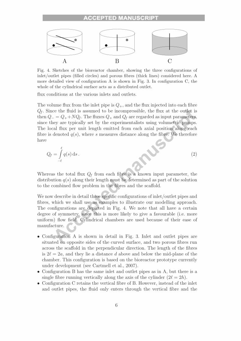
Fig. 4. Sketches of the bioreactor chamber, showing the three configurations ofinlet/outlet pipes (filled circles) and porous fibres (thick lines) considered here. Amore detailed view of configuration A is shown in Fig. 3. In configuration C, thewhole of the cylindrical surface acts as a distributed outlet.

flux conditions at the various inlets and outlets.

The volume flux from the inlet pipe is Q+, and the flux injected into each fibreQf . Since the fluid is assumed to be incompressible, the flux at the outlet isthen Q− = Q++NQf . The fluxes Q+ and Qf are regarded as input parameters,since they are typically set by the experimentalists using volumetric pumps.The local flux per unit length emitted from each axial position along eachfibre is denoted q(s), where s measures distance along the fibre. We thereforehave

Qf =

�∫−�

q(s) ds . (2)

Whereas the total flux Qf from each fibre is a known input parameter, thedistribution q(s) along their length must be determined as part of the solutionto the combined flow problem in the fibres and the scaffold.

We now describe in detail three specific configurations of inlet/outlet pipes andfibres, which we shall use as examples to illustrate our modelling approach.The configurations are depicted in Fig. 4. We note that all have a certaindegree of symmetry, since this is more likely to give a favourable (i.e. moreuniform) flow field. Cylindrical chambers are used because of their ease ofmanufacture.

• Configuration A is shown in detail in Fig. 3. Inlet and outlet pipes aresituated on opposite sides of the curved surface, and two porous fibres runacross the scaffold in the perpendicular direction. The length of the fibresis 2� = 2a, and they lie a distance d above and below the mid-plane of thechamber. This configuration is based on the bioreactor prototype currentlyunder development (see Cartmell et al., 2007).

• Configuration B has the same inlet and outlet pipes as in A, but there is asingle fibre running vertically along the axis of the cylinder (2� = 2h).

• Configuration C retains the vertical fibre of B. However, instead of the inletand outlet pipes, the fluid only enters through the vertical fibre and the

6

Accep

ted m

anusc

ript

whole of the cylindrical surface acts as a distributed outlet.

The distributed outlet in configuration C is different from the outlet pipesused in A and B. It is realised by having a bioreactor chamber of a largerradius than that of the scaffold, so that fluid is able to exit the scaffold inall radial directions. The ease of free flow out of the scaffold relative to flowwithin the scaffold (δ � a) means that the pressure variations outside thescaffold will be minimal compared with those inside. Therefore, in this case,we effectively have a constant pressure boundary condition on x2 + y2 = a2.

In each configuration, we consider the flow in the scaffold and the flow inthe fibres as two separate problems, coupled by the continuity of pressureand volume flux per unit area at the outside of the fibre walls. In both regionsthe full Navier–Stokes equations and complicated geometries can be simplifiedleading to tractable problems. We now consider the scaffold and fibre problemsin turn.

3 Flow within the scaffold

A MicroCT image of a typical scaffold is shown in Fig. 2(a). The pore geometryis of a random nature, with about 30 pores over the height of the scaffold. Allthe pores appear to be interconnected. We model the scaffold as a porousmedium (see e.g. Bear, 1988), with a typical pore diameter δ, porosity φ (thevolume fraction of pore space), and tortuosity τ (defined as the average ratio ofstreamline lengths to the straight-line distance between two points). 1 Typicalvalues for these parameters are given in Table 1.

The ratio of inertial and viscous effects is given by the the pore Reynoldsnumber

Rep =ρ� δ

μ, (3)

where � is a typical interstitial velocity. We estimate � by dividing thetypical volume flux Q− by the typical cross-sectional area of pore space 2φah.This is then modified by a factor of the scaffold tortuosity τ . (The moretortuous the scaffold, the faster the interstitial flow has to be to travel the

1 Note that there are several different definitions of tortuosity in use by variousauthors. In particular, the quantity referred to as tortuosity in Bear (1988) is τ2 inthe notation used here. The equations are unaffected by this different nomenclature.

7

Accep

ted m

anusc

ript

Table 1Dimensions and typical physical properties of the bioreactor setup being developedby Cartmell and Michael.

Quantity Symbol Typical Value

Internal radius of chamber a 7.5 × 10−3 m

Internal height of bone section 2h 1.0 × 10−2 m

Length of each porous fibre 2� 10−2 m †External radius of porous fibres bw 5 × 10−4 m

Internal radius of porous fibres bc 1.7 × 10−4 m

Internal radius of inlet/outlet pipes d 5 × 10−4 m

Pore diameter of scaffold δ 6.8 × 10−4 m

Porosity of scaffold φ 0.8

Tortuosity of scaffold τ 1.15

Permeability of scaffold k 2 × 10−9 m2

Typical pore diameter in fibre wall δw 1 × 10−7 m

Mean radial permeability of fibre wall kw 1 × 10−17 m2

Density of culture medium ρ 1 × 103 kg m−3

Viscosity of culture medium μ 7 × 10−4 kg m−1 s−1

Typical total volume flux Q− 1 × 10−7 m3 s−1

Lengths measured from experimental apparatus. Scaffold properties from analysisof MicroCT data; permeability and tortuosity estimates detailed in Appendix A.1.Fibre permeability estimate explained in Appendix A.2. Culture medium proper-ties measured experimentally at 37◦C. † The length of the fibres in the bioreactordepends on their position and orientation. In the configurations we consider here,we have either � = a or � = h.

longer paths in the same time.) Therefore

� ∼ τ

φ

Q−2ah

, (4)

and using the data in Table 1, we obtain

Rep ∼ ρτQ−δ2φahμ

≈ 2 (5)

as an estimate for the pore Reynolds number.

The large number of pores and the not-too-large pore Reynolds number make

8

Accep

ted m

anusc

ript

it appropriate to use Darcy’s law (see, e.g. Batchelor, 1967; Bear, 1988) tomodel the flow of culture medium through the scaffold. We model the scaf-fold as an isotropic porous medium, with a uniform permeability k. (See Ap-pendix A.1 for a discussion of how to estimate k.)

Although the growth of the bone will alter this permeability, such growthoccurs over a period of several days, which is much longer than the minutesrequired for fluid circulation. The slow variations of k can be captured usinga ‘quasi-static’ approximation, i.e. assuming that at any instant the solutionis as it would be with a constant value of k set by its instantaneous value.For simplicity, and because such variations are likely to be small, we shall justwork with single fixed value of k in this paper.

Darcy’s law is used to relate the Darcy velocity v to the interstitial pressurep. 2 Conservation of fluid is expressed in terms of a source strength per unitvolume ψ(x). We have

v = −kμ

∇p , ∇ ·v = ψ . (6)

The various sources are modelled as points and lines and hence appear as deltafunctions in ψ. Away from these sources ψ = 0.

Since the diameter of the porous fibres and the inlet and outlet pipes arecomparable with the pore size (see Table 1), it is consistent to model them asline and point sources respectively. This simplifies the analysis, and reflects thefact that the actual size of the fibres and pipes, and detailed flow distributionnear them, have little effect on the bulk flow in the scaffold.

Obviously, the point-source approximations will not be valid in the region sur-rounding the real source within a few pore diameters. Thus when interpretingthe results, allowance must be made for the fact that the diverging velocities,pressures and shear stresses in the neighbourhood of the sources are in factbounded and rise only to a magnitude of the order of that predicted a fewpore diameters away. Formally, the model represents an ‘outer’ solution awayfrom the sources, and a separate ‘inner’ solution would be needed to accu-rately describe the flow in the neighbourhood of the sources. Such a solutionwould require knowledge of the detailed pore structure around the source, andis beyond the scope of this study.

2 The Darcy velocity is a local average of the true interstitial velocity, taken overa volume that includes both the pore space and the solid scaffold. Hence, on themacroscale, v gives the volume flux of fluid per unit cross-sectional area. The inter-stitial pressure is the local average of the fluid pressure in the pore space.

9

Accep

ted m

anusc

ript

3.1 Non-dimensionalization

We non-dimensionalize all lengths with the chamber radius a, so in non-dimensional coordinates (X, Y, Z) = (x, y, z)/a, the chamber occupies

X2 + Y 2 ≤ 1 , −H ≤ Z ≤ H , (7)

where H = h/a is the aspect ratio of the chamber. We non-dimensionalize thefluxes with respect to Q−, so that the dimensionless total flux from the fibresis given by

� =NQf

Q−. (8)

The dimensionless flux from each fibre is then �/N , and the dimensionlessflux from the inlet pipe is 1 − �. The distance s along the fibre is non-dimensionalized on the length a, and we introduce ζ = s/a. The local flux perunit length q(s) emitted from each point along the fibre is non-dimensionalizedby writing

q(s) =Qf

aθ(ζ) =

Q−a

�

Nθ(ζ) . (9)

We non-dimensionalize velocities, pressure, and source strength in the naturalway by writing

v =Q−a2

V , p = p0 +μQ−ak

P , ψ =Q−a3

Ψ . (10)

The pressure must be considered relative to a reference pressure p0 ≡ p(x0)taken at a particular point x0 in the scaffold. This is because the scaleQ−/ak isonly for variations in pressure within the scaffold, independent of any additiveconstants. For each configuration, we choose x0 to be a convenient point inthe scaffold away from the singularities caused by the fibres and the inlet andoutlet pipes. For configuration A, we set x0 = 0, so the dimensionless pressureis zero at the centre of the scaffold. For configuration B, we set x0 = (a/2, 0, 0).Finally, for configuration C, we set x0 = (a, 0, 0) so that the dimensionlesspressure is zero on the curved surface of the scaffold.

10

Accep

ted m

anusc

ript

3.2 Dimensionless equations and boundary conditions

In terms of the non-dimensional variables, Darcy’s equation and the continuityequation (6) become

V = −∇P , ∇· V = Ψ . (11)

Combining the two equations in (11), we obtain an equation for the dimen-sionless pressure:

∇2P = −Ψinlet + Ψoutlet − Ψfibres , (12)

where the terms on the right-hand-side each correspond to one of the sourcesor sinks in the obvious way. This equation is then solved within the scaffold,subject to appropriate boundary conditions, to find P . The physical boundaryconditions generally involve the fluid velocity V , and so must be re-writtenin terms of P using (11), so they can be applied to (12). Once P is known,(11) is used to recover V and complete the solution in the scaffold. We nowpresent the source functions and boundary conditions on P for each of thethree configurations.

3.2.1 Configuration A

The fibre source is given by

Ψfibres = 12� θ(X) δ(Y )

(δ(Z −D) + δ(Z +D)

), (13)

representing two fibres running along y = 0, z = −d and y = 0, z = d, fromx = −1 to x = 1. The vertical separation of the fibres is 2D = 2d/a, and δ( · )is the delta-function. The rate of fluid emission by the fibres varies along theirlength and is given by 1

2�θ(X), where θ(X) is as yet unknown. The inlet and

outlet sources are given by

Ψinlet = 2(1 −�) δ(X) δ(Y + 1) δ(Z) , (14)

Ψoutlet = 2 δ(X) δ(Y − 1) δ(Z) , (15)

for an inlet at (0,−1, 0) and an outlet at (0, 1, 0), respectively. Since the pointsources are located on the domain boundary, the strengths are doubled in theabove expression to obtain the correct fluxes inside the domain.

11

Accep

ted m

anusc

ript

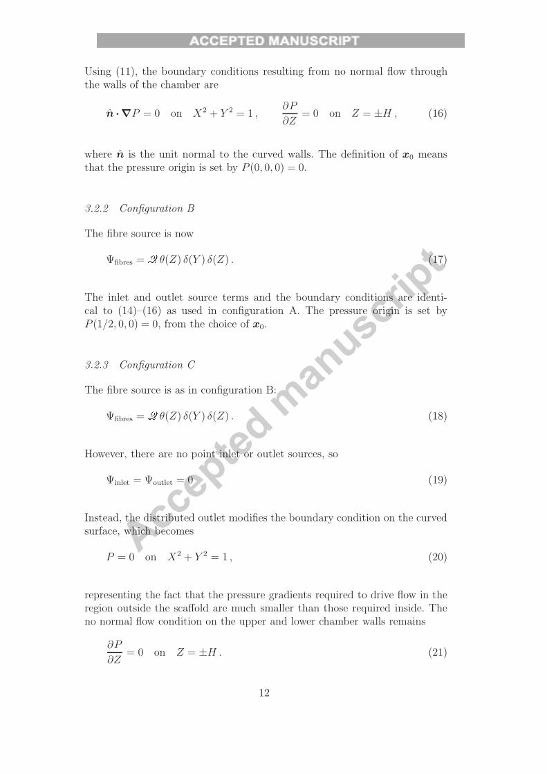
Using (11), the boundary conditions resulting from no normal flow throughthe walls of the chamber are

n ·∇P = 0 on X2 + Y 2 = 1 ,∂P

∂Z= 0 on Z = ±H , (16)

where n is the unit normal to the curved walls. The definition of x0 meansthat the pressure origin is set by P (0, 0, 0) = 0.

3.2.2 Configuration B

The fibre source is now

Ψfibres = � θ(Z) δ(Y ) δ(Z) . (17)

The inlet and outlet source terms and the boundary conditions are identi-cal to (14)–(16) as used in configuration A. The pressure origin is set byP (1/2, 0, 0) = 0, from the choice of x0.

3.2.3 Configuration C

The fibre source is as in configuration B:

Ψfibres = � θ(Z) δ(Y ) δ(Z) . (18)

However, there are no point inlet or outlet sources, so

Ψinlet = Ψoutlet = 0 (19)

Instead, the distributed outlet modifies the boundary condition on the curvedsurface, which becomes

P = 0 on X2 + Y 2 = 1 , (20)

representing the fact that the pressure gradients required to drive flow in theregion outside the scaffold are much smaller than those required inside. Theno normal flow condition on the upper and lower chamber walls remains

∂P

∂Z= 0 on Z = ±H . (21)

12

Accep

ted m

anusc

ript

Table 2Typical values of the various dimensionless parameters appearing in ��2–4, com-puted from the values in Table 1.

H ε λ k/a2 kw/b2c α2

0.7 0.02 3 10−4 10−6 0.07

In all three configurations, the dimensionless flux per unit length θ(ζ) from thefibres depends on the conditions applied at the fibre ends and the properties ofthe fibre. If θ(ζ) is known, then (8), (12), and the appropriate equations from(13)–(21) form a well-posed problem for the pressure P within the scaffold.We now determine θ(ζ) by analysing the flow in the fibres.

4 Flow in the fibres

The porous fibres are modelled as circular cylinders of length 2� and externaldiameter 2bw, with a hollow core of internal diameter 2bc. See Fig. 5. We usecylindrical polar coordinates (r, ϕ, s) aligned with the fibre. In configurationA, we have s = x, r2 = y2 + (z± d)2, and � = a (see Fig. 3). In configurationsB and C, we have s = z, r2 = x2 + y2, and � = h.

The fibre walls are modelled as an axisymmetric and axially uniform porousmedium, governed by Darcy’s law. The radial component of the permeabilitytensor kw is denoted kw(r), and the other principal components are assumedto be no larger than kw. In practice, the fibre pores are aligned predominantlyin the radial direction (see Fig. 2b), so that the resistance to radial flow issignificantly less than the resistance in any other direction, and the radialpermeability is greater than the other components.

Pressures are denoted by p and velocities by u = (u, v, w) with componentsin the cylindrical polar coordinates defined above. We use subscripts c for thecore and w for the walls. In the porous walls, uw represents the Darcy velocity.Boundary conditions are provided by continuity of pressure and radial volumeflux per unit area at r = bw, together with the imposed inlet flux Qf at s = −�,and zero outlet flux at s = �. Assuming the axial flux is dominated by the flowin the core, the flux conditions at the ends of each the fibre can be written as

2π

bc∫0

wc(r,−�) r dr = Qf , 2π

bc∫0

wc(r, �) r dr = 0 . (22)

A number of separations of scales help simplify the analysis of the flow in thefibre, which follows below in ��4.3–4.5. We assume that the fibre is slender

13

Accep

ted m

anusc

ript

r

pc, uc

pw, uw

p, u

s

2�

2bw2bc

Qf

(Darcy flow, kw)

(Darcy flow, k)

Fibre Wall

Fibre Core

Outer Scaffold

(Viscous lubrication flow)

Fig. 5. The geometry of the porous-walled fibres, together with the coordinates andvariables used to describe the flow within them.

(bc/� � 1) and that the walls are relatively impermeable (kw � b2c , kw � k).Both these assumptions are justified by the experimental setup (see table 1).We show that this regime leads to predominantly axial flow in the fibre core,and predominantly radial flow in the fibre walls. We also show that the pressuredifference across the fibre wall is large compared with both the pressure dropalong the length of the fibre, and the typical pressure variations within thesurrounding scaffold. This means that we can solve for the flow in the fibrewithout needing to know the details of the flow and pressure fields in thescaffold. Since the flow in the scaffold has no effect on the flow in the fibre,there is no source of asymmetry, and we may assume axisymmetric flow in thefibre, i.e. v ≡ 0, and no dependence on the azimuthal angle ϕ.

4.1 Non-dimensionalization

We begin by introducing two non-dimensional parameters

ε =bca

� 1 , λ =bwbc

= O(1) , (23)

which describe the aspect ratio and relative wall thickness of the fibre.

The radial and axial coordinates are non-dimensionalized by the inner fibreradius bc and chamber radius a respectively:

ξ =r

bc=

r

εa, ζ =

s

a. (24)

14

Accep

ted m

anusc

ript

The core then occupies 0 < ξ < 1 and the wall 1 < ξ < λ. The non-dimensionallength of the fibre is 2L = 2�/a = O(1), so −L < ζ < L. In configuration A,we have L = 1, while in configurations B and C we have L = H .

We define a mean radial permeability kw for the fibres as the permeability thatwould give a radially uniform fibre the same radial flux for a given transmuralpressure difference. As shown in Appendix A.2, this implies

1

kw

=1

lnλ

bw∫bc

1

rkw(r)dr . (25)

We now non-dimensionalize the permeability as

kw(r) = kw Kw(ξ) . (26)

The non-dimensionalization of the axial velocity in the core and the radialvelocity in both the core and the wall is based on the imposed flux Qf :

wc =Qf

b2cWc , uc =

Qf

bcaUc , uw =

Qf

bcaUw . (27)

The axial velocity ww in the wall is assumed to be much smaller than wc, sincethe flow resistance is much larger in the wall.

The pressure p is scaled with the pressure difference required to drive the fluxQf radially outwards through the fibre walls since, for relatively impermeablewalls, this is expected to be the largest resistance to overcome, and hence willresult in the largest pressure drop. We therefore write

pc = p0 +μQf lnλ

akw

Pc , pw = p0 +μQf lnλ

akw

Pw . (28)

4.2 Boundary conditions

At the ends of the fibres, we apply the flux conditions (22). In dimensionlessform these are

2π

1∫0

Wc(ξ,−L) ξ dξ = 1 , 2π

1∫0

Wc(ξ, L) ξ dξ = 0 . (29)

15

Accep

ted m

anusc

ript

At ξ = 1, the boundary between the fibre wall and the core, we impose conti-nuity of the normal velocity and pressure, giving

Uc(1, ζ) = Uw(1, ζ) , Pc(1, ζ) = Pw(1, ζ). (30)

Since the fibre wall is rigid and relatively impermeable, we have an effectiveno-slip condition on the axial flow in the core:

Wc(1, ζ) = 0 . (31)

At ξ = λ, the outer edge of the fibre wall, we impose continuity of radial fluxand pressure. The flux condition yields an expression for θ:

θ(ζ) =

2π∮0

Uw(λ, ζ)λ dϕ = 2πλUw(λ, ζ) . (32)

Using (10) and (28), the pressure condition is

Pw(λ, ζ) =N

� lnλ

kw

kP . (33)

As both P and Pw are O(1), and the remaining factor on the right-hand sideis very small (kw � k; see table 1), it is appropriate to approximate

Pw(λ, ζ) = 0 . (34)

We now proceed to solve for the flow and pressure field inside the fibres. Thegeneral strategy is to express all the variables in terms of the pressure Pc inthe core, and then apply the boundary conditions to obtain a single equationfor Pc, which we solve. Once Pc is found, the other variables can be recovered.

4.3 Flow in the fibre core

The flow in the core is governed by the (dimensional) steady Navier–Stokesequations

∇· uc = 0 , (35)

ρ (uc · ∇) uc = −∇pc + μ∇2uc . (36)

16

Accep

ted m

anusc

ript

Since the tube is slender, we use a viscous lubrication approximation (seee.g. Ockendon and Ockendon, 1995) to neglect inertia and radial pressuregradients. This relies on the reduced Reynolds number Rec being small, acondition we verify in Appendix B. In the dimensionless variables defined in(24), (27) and (28) the equations reduce to

Pc = Pc(ζ) , (37)

dPc

dζ=α2

16

1

ξ

∂

∂ξ

(ξ∂Wc

∂ξ

), (38)

∂Wc

∂ζ+

1

ξ

∂

∂ξ

(ξUc

)= 0 , (39)

where we have introduced the dimensionless parameter

α2 =16kw

ε4a2 lnλ, (40)

which is a measure of the resistance to axial flow through the core comparedwith that of radial flow out through the walls. The boundary conditions aregiven by (29)–(31).

We now integrate (38) twice with respect to ξ. One constant is set by regularityat ξ = 0, and the other by the boundary condition (31) at ξ = 1. We obtainthe Poiseuille flow

Wc = − 4

α2

dPc

dζ

(1 − ξ2

). (41)

Using mass continuity (39) we recover the radial velocity. The single constantof integration is set by regularity at ξ = 0. We obtain

Uc =1

α2

d2Pc

dζ2ξ(2 − ξ2

). (42)

Substituting for Wc, the flux conditions (29) can be written in terms of Pc as

dPc

dζ

∣∣∣∣∣ζ=−L

= −α2

2π,

dPc

dζ

∣∣∣∣∣ζ=L

= 0 . (43)

17

Accep

ted m

anusc

ript

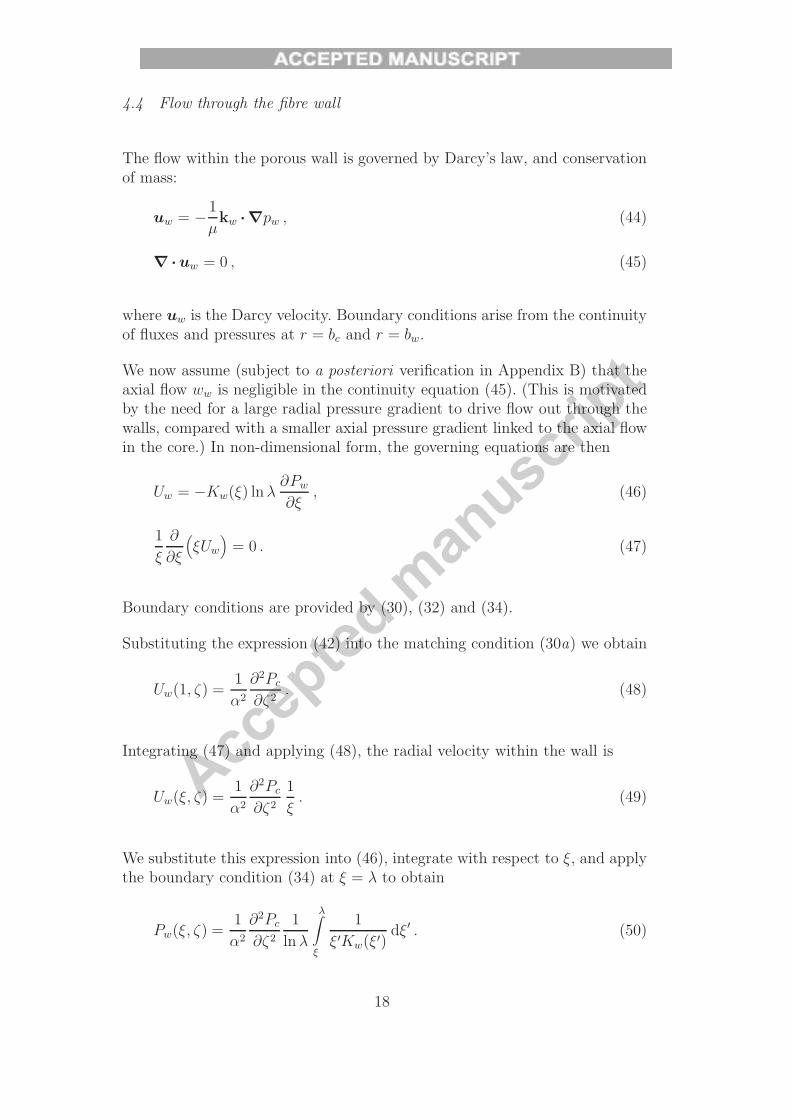
4.4 Flow through the fibre wall

The flow within the porous wall is governed by Darcy’s law, and conservationof mass:

uw = −1

μkw · ∇pw , (44)

∇· uw = 0 , (45)

where uw is the Darcy velocity. Boundary conditions arise from the continuityof fluxes and pressures at r = bc and r = bw.

We now assume (subject to a posteriori verification in Appendix B) that theaxial flow ww is negligible in the continuity equation (45). (This is motivatedby the need for a large radial pressure gradient to drive flow out through thewalls, compared with a smaller axial pressure gradient linked to the axial flowin the core.) In non-dimensional form, the governing equations are then

Uw = −Kw(ξ) lnλ∂Pw

∂ξ, (46)

1

ξ

∂

∂ξ

(ξUw

)= 0 . (47)

Boundary conditions are provided by (30), (32) and (34).

Substituting the expression (42) into the matching condition (30a) we obtain

Uw(1, ζ) =1

α2

∂2Pc

∂ζ2. (48)

Integrating (47) and applying (48), the radial velocity within the wall is

Uw(ξ, ζ) =1

α2

∂2Pc

∂ζ2

1

ξ. (49)

We substitute this expression into (46), integrate with respect to ξ, and applythe boundary condition (34) at ξ = λ to obtain

Pw(ξ, ζ) =1

α2

∂2Pc

∂ζ2

1

lnλ

λ∫ξ

1

ξ′Kw(ξ′)dξ′ . (50)

18

Accep

ted m

anusc

ript

From the definitions (25) and (26), the integral is equal to lnλ at ξ = 1, hence

Pw(1, ζ) =1

α2

∂2Pc

∂ζ2. (51)

4.5 The flux emitted by the fibres

Applying the final boundary condition (30b) to (51), we obtain an equationfor the variation of Pc along the length of the fibre:

d2Pc

dζ2− α2Pc = 0 . (52)

This equation is solved subject to (43), giving

Pc(ζ) =α

2π

cosh[α(L− ζ)]

sinh(2αL). (53)

With this solution, the flux θ(ζ) emitted from the fibre into the outer scaffoldcan be derived from (32) and (49), and is

θ(ζ) =α cosh[α(L− ζ)]

sinh(2αL). (54)

The parameter α, defined in (40), encapsulates how easy it is push fluid outthrough the fibre walls compared with pushing it axially along the core. Forα 1, it is relatively easy for fluid to exit the fibre through the walls. Wethen have

θ(ζ) ∼ α e−α(L+ζ) , (55)

so almost all of the flux Qf leaves through the wall within a distance of O(α−1)from the inlet at ζ = −L. Since this is unlikely to offer any improvementover a bioreactor system without fibres, we reject this possibility, and assumeα ≤ O(1).

For α = O(1), we see a significant variation of θ along the fibre, which is alsolikely to offer less advantage than a uniform flux. At the other extreme, α � 1,we have

θ(ζ) ∼ 1

2L(56)

19

Accep

ted m

anusc

ript

so the emitted flux is uniform along the length of the fibre.

4.6 Summary

We have found the solution for the flow in the fibres. The pressure Pc in thecore is given by (53) and this can be substituted back into the previous expres-sions for the other physical variables. The dimensionless flux per unit lengthθ emitted at each point along the length of the fibre is given by (54). Thisexpression can now be used to complete the model for the flow in the scaffolddeveloped in �3. In Appendix B, we confirm that the various approximationswe have used are valid for the experimental setup being modelled.

5 Numerical solutions for the fluid flow

In all the numerical computations, we take α � 1 so that (56) holds andthe flux emitted by the fibres is uniform along their length. A uniform fluxis desirable from a theoretical standpoint, as it is likely to result in a moreeven distribution of culture medium flow and shear stresses. Furthermore, forthe fibres being considered for use in the prototype bioreactors that motivatedthis study, we have α = O(10−1) � 1 (see (40) and table 2).

With θ(ζ) given by (56), the model developed in �3 then leads to the problem ofsolving Poisson’s equation (12) for the pressure P in the cylindrical bioreactorchamber. We have Dirichlet and/or Neumann boundary conditions on thewalls, and a number of delta-function source terms representing the fibres andinlet/outlet pipes. The equations and boundary conditions for the three fibreconfigurations considered in this paper are given in �3.2.

Similar systems of equations arise in many physical problems, and solutiontechniques are well-developed. We solved the system numerically using theElectrostatics package of the ‘COMSOL Multiphysics’ computer program, 3

which uses a finite element technique. Once the pressure P has been computed,the Darcy velocity V is determined from (11).

For each of the three configurations, the flow may be solved with typicalparameter values to provide insight into how the fibres affect the flow. Inall cases, we used an aspect ratio of H = 0.7, in line with the experimentalprototype shown in figure 1. The graphs show the magnitude |V | of the Darcyvelocity on a planar cross-section through the bioreactor chamber.

3 Developed and distributed by COMSOL Inc. Full details available online athttp://www.comsol.com/.

20

Accep

ted m

anusc

ript

Z

Y

|V |

−0.8 −0.6 −0.4 −0.2 0 0.2 0.4 0.6 0.8

−0.6

−0.4

−0.2

0

0.2

0.4

0.6

0

0.2

0.4

0.6

0.8

1

1.2

1.4

1.6

1.8

2

Fig. 6. The magnitude of the dimensionless Darcy velocity V in the vertical planeX = 0.3 in configuration A with � = 0 (i.e. no flux from the fibres). The inlet isout of the plane to the left, and the outlet lies similarly to the right. The two fibresrun perpendicular to the plane through Y = 0, Z = ±0.35. From the dimension-less Darcy velocity, the dimensional equivalent can be recovered from (10), and anestimate for the shear stress found using (58).

For configuration A, we used a fibre separation 2D = 0.7 (see fig. 3). Re-sults are shown on an off-centre vertical plane perpendicular to the fibres atX = 0.3. We consider a fixed total flux Q− with three different values of theproportion� from the fibres: 0, 0.2, and 0.4. The results are shown in Figs. 6–8. Other parallel planes show essentially the same qualitative structure, witha dipole structure around the fibres and larger velocities in the vicinity of theinlet and outlet pipes. The off-centre planes were chosen to avoid the singu-larities at these points.

For configurations B and C, there is a single vertical fibre, and we use off-centre horizontal cross-sections at Z = 0.3 instead. For configuration B, weagain present results for � = 0, 0.2, 0.4. See Figs. 9–11. For configurationC, there are no separate input flows so � ≡ 1. The solution, which can beobtained analytically, is of purely radial flow, and is shown in Fig. 12.

The computations show that without the fibres (� = 0), flow rates are highestin the vicinity of the inlet and outlet pipes, as would be expected. The slowestregions of the flow are found near the chamber walls on the plane Y = 0. Theaddition of the fibres increases relative flow rates on the downstream side ofthem (Y > 0), but also decreases the flow on the upstream side (Y < 0).These increases and decreases become more pronounced as � increases.

21

Accep

ted m

anusc

ript

Z

Y

|V |

−0.8 −0.6 −0.4 −0.2 0 0.2 0.4 0.6 0.8

−0.6

−0.4

−0.2

0

0.2

0.4

0.6

0

0.2

0.4

0.6

0.8

1

1.2

1.4

1.6

1.8

2

Fig. 7. The magnitude of the dimensionless Darcy velocity in the plane X = 0.3 inconfiguration A with � = 0.2. Other details as in Fig. 6. Flow is generally from leftto right, and fluid is emitted by the fibres.

Z

Y

|V |

−0.8 −0.6 −0.4 −0.2 0 0.2 0.4 0.6 0.8

−0.6

−0.4

−0.2

0

0.2

0.4

0.6

0

0.2

0.4

0.6

0.8

1

1.2

1.4

1.6

1.8

2

Fig. 8. The magnitude of the dimensionless Darcy velocity in the plane X = 0.3 inconfiguration A with � = 0.4. Other details as in Fig. 6. Flow is generally from leftto right, and fluid is emitted by the fibres.

6 Shear stress

As discussed in the introduction, bone cells are sensitive to fluid shear stresses.Some shear stress is necessary for viable growth, but higher levels may damagethe cells. It is therefore important to calculate the shear stress distributionassociated with the flow fields computed in �5. The shear stresses will beproportional to the overall flow rate Q−, which therefore needs to be adjusted

22

Accep

ted m

anusc

ript

X

Y

|V |

−0.8 −0.6 −0.4 −0.2 0 0.2 0.4 0.6 0.8

−0.8

−0.6

−0.4

−0.2

0

0.2

0.4

0.6

0.8

0

0.2

0.4

0.6

0.8

1

1.2

1.4

1.6

1.8

2

Fig. 9. The magnitude of the dimensionless Darcy velocity V in the plane Z = 0.3in configuration B with � = 0 (no flow from the fibre). The single fibre runsperpendicular to the plane, through X = Y = 0. The inlet pipe is to the left andthe outlet pipe to the right, both in the plane Z = 0. From the dimensionless Darcyvelocity, the dimensional equivalent can be recovered from (10), and an estimate forthe shear stress found using (58).

X

Y

|V |

−0.8 −0.6 −0.4 −0.2 0 0.2 0.4 0.6 0.8

−0.8

−0.6

−0.4

−0.2

0

0.2

0.4

0.6

0.8

0

0.2

0.4

0.6

0.8

1

1.2

1.4

1.6

1.8

2

Fig. 10. The magnitude of the Darcy velocity in the plane Z = 0.3 in configurationB with � = 0.2. Other details as in Fig. 9. Flow is generally from left to right, withfluid emitted by the fibre.

23

Accep

ted m

anusc

ript

X

Y

|V |

−0.8 −0.6 −0.4 −0.2 0 0.2 0.4 0.6 0.8

−0.8

−0.6

−0.4

−0.2

0

0.2

0.4

0.6

0.8

0

0.2

0.4

0.6

0.8

1

1.2

1.4

1.6

1.8

2

Fig. 11. The magnitude of the Darcy velocity in the plane Z = 0.3 in configurationB with � = 0.4. Other details as in Fig. 9. Flow is generally from left to right, withfluid emitted by the fibre.

X

Y

|V |

−0.8 −0.6 −0.4 −0.2 0 0.2 0.4 0.6 0.8

−0.8

−0.6

−0.4

−0.2

0

0.2

0.4

0.6

0.8

0

0.2

0.4

0.6

0.8

1

1.2

1.4

1.6

1.8

2

Fig. 12. The magnitude of the Darcy velocity in any horizontal plane Z = Z0 inconfiguration C. Other details as in Fig. 9. Flow is radially outwards from the centralfibre source.

24

Accep

ted m

anusc

ript

so as to provide sufficient shear (and nutrient delivery) over as much of thescaffold as possible, while constraining excessively high shear to as small aregion as possible.

The shear stress experienced by the cells within the individual scaffold porescan be estimated from the Darcy velocity as follows. We first take the estimate� ∼ |v|τ/φ for the mean magnitude of the interstitial velocity. We then usePoiseuille flow of mean velocity � through a circular duct of diameter δ asan approximate model for the local flow within each scaffold pore. With r asa local radial coordinate, the velocity profile is

v ≈ 2�

[1 −

(2r

δ

)2]

(57)

and the wall shear stress is

S = μ

∣∣∣∣∣∂v∂r∣∣∣∣∣(r=δ/2)

≈ 8μ�

δ≈ 8μτ

φδ|v| =

8μQ−τφδa2

|V | . (58)

The first two approximations for S use the velocity profile (57) and the esti-mate for � above; the final equality comes from the non-dimensionalization(10). While obviously not precise, (58) gives a reasonable estimate (at leastin order-of-magnitude terms) for the shear stress experienced by the cells interms of the local Darcy velocity and the fluid and scaffold properties. For thevalues given in Table 1 we obtain

S =(

Q−4.8 × 10−6 m3 s−1

)|V | Pa . (59)

From the numerical results, |V | = O(1) over most of the chamber, and exceeds2 only in small regions near the fibres and inlet / outlet pipes. Thus, to obtainshear stresses of the order of Pascals (as in the experiments referenced in theintroduction), volume fluxes of the order of 10−5 – 10−6 m3 s−1 need to beused. This is somewhat higher than the anticipated value Q− ∼ 10−7 m3 s−1

in Table 1.

However, in any particular experiment, the desirable volume flux will dependon the requirements of the cells and on the exact properties of the bioreactorsystem being used. It may also be constrained by the availability of pumpingequipment and the pressures required to force fluid through the system. Wetherefore leave the results in general terms, rather than trying to make definitepredictions that may not apply in other situations. Another factor to consideris the effect of the flow rate upon nutrient and waste transport. This issue isaddressed in the following section.

25

Accep

ted m

anusc

ript

Table 3Typical values of the experimental parameters related to the nutrient problem.

Parameter Symbol Typical Value

Time scale for fluid circulation tc 3.4 × 100 s

Time scale for cell growth t1/2 2 × 105 s

Time scale for culturing tg 6 × 105 – 3 × 106 s

Initial number of cells per unit volume n0 1 × 1012 cells m−3

All values based on the experimental setup of Cartmell and Michael, apart from tcwhich is calculated using (65). For other properties, see table 1.

7 Nutrient and waste transport

One of the most important requirements for both survival and proliferationof the cells is the supply of nutrients and the removal of waste products. Inthe case of nutrients the supply must be sufficient to meet the demands ofthe proliferating cells, while in the case of waste products we need to ensurethey are removed sufficiently rapidly to prevent any build-up that would beharmful. For example a build-up of lactic acid could cause a harmful changein pH (see Appendix A.3).

We use simple scaling arguments here to determine whether or not nutrient de-pletion or waste product accumulation are significant effects over the relevanttime scales in the culturing process. Key conclusions can be drawn withoutthe need to solve the full system of equations explicitly.

Suppose that the cells are initially seeded on to the scaffold with a density n0

per unit volume 4 and then proliferate over the culturing period. We assumea constant doubling time of t1/2, so that the number of cells per unit volumeat time t after the start of culturing is

n = n0 exp

(t ln 2

t1/2

). (60)

The maximum cell density nmax is achieved when t = tg at the end of theculturing period. Typical values of n0, t1/2 and tg, given in Table 3, indicatethat the cells may double in number around 7 times over the culturing periodtg, leading to nmax ≈ 1.3 × 1014 m−3.

The concentration ci of an individual nutrient or waste product i in the fluid

4 Note that this is number of cells per unit total volume of bioreactor chamber, notthe number per unit volume of pore space.

26

Accep

ted m

anusc

ript

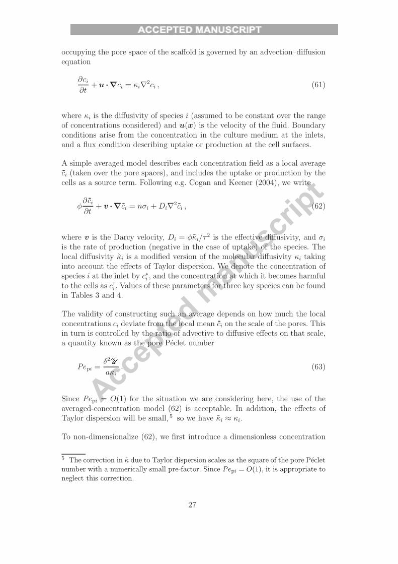
occupying the pore space of the scaffold is governed by an advection–diffusionequation

∂ci∂t

+ u ·∇ci = κi∇2ci , (61)

where κi is the diffusivity of species i (assumed to be constant over the rangeof concentrations considered) and u(x) is the velocity of the fluid. Boundaryconditions arise from the concentration in the culture medium at the inlets,and a flux condition describing uptake or production at the cell surfaces.

A simple averaged model describes each concentration field as a local averageci (taken over the pore spaces), and includes the uptake or production by thecells as a source term. Following e.g. Cogan and Keener (2004), we write

φ∂ci∂t

+ v ·∇ci = nσi +Di∇2ci , (62)

where v is the Darcy velocity, Di = φκi/τ2 is the effective diffusivity, and σi

is the rate of production (negative in the case of uptake) of the species. Thelocal diffusivity κi is a modified version of the molecular diffusivity κi takinginto account the effects of Taylor dispersion. We denote the concentration ofspecies i at the inlet by c∗i , and the concentration at which it becomes harmfulto the cells as c†i. Values of these parameters for three key species can be foundin Tables 3 and 4.

The validity of constructing such an average depends on how much the localconcentrations ci deviate from the local mean ci on the scale of the pores. Thisin turn is controlled by the ratio of advective to diffusive effects on that scale,a quantity known as the pore Peclet number

Pepi =δ2�

aκi. (63)

Since Pepi = O(1) for the situation we are considering here, the use of theaveraged-concentration model (62) is acceptable. In addition, the effects ofTaylor dispersion will be small, 5 so we have κi ≈ κi.

To non-dimensionalize (62), we first introduce a dimensionless concentration

5 The correction in κ due to Taylor dispersion scales as the square of the pore Pecletnumber with a numerically small pre-factor. Since Pepi = O(1), it is appropriate toneglect this correction.

27

Accep

ted m

anusc

ript

Table 4Typical properties relating to two nutrients and a waste product that are relevantto the cells.

Nutrient c∗i c†i κi σi tdi

or product (molm−3) (molm−3) (m2 s−1) (mol cell−1 s−1) (s)

Glucose 5.6 0 7 × 10−10 −8 × 10−17 4.3 × 102

Oxygen (O2) 1.0 0 3 × 10−9 −4.2 × 10−17 1.5 × 102

Lactic acid 0 0.4 1 × 10−9 1.4 × 10−16 1.8 × 101

The initial concentration c∗i in the culture medium as it enters the bioreactor, theconcentration c†

i that would be detrimental to the cells, the diffusivity κi and the rateof production σi (negative in the case of uptake). Glucose concentration from culturemedium product data (Invitrogen, 2008), and initial oxygen concentration based onsolubility in water at 37◦C and 1 atm (Tromans, 1998). Approximate diffusivities fordilute solutions at 25–30◦C from Lide (2007), with the exception of lactic acid fromRibeiro et al. (2005). Typical uptake and production rates inferred from Komarovaet al. (2000). The estimate for c†

i for lactic acid is discussed in Appendix A.3.Depletion/accumulation times tdi calculated using (66), assuming n = nmax = 1.3×1014 and φ = 0.8.

Ci, defined so that

Ci =ci − c∗ic†i − c∗i

. (64)

Then Ci = 0 at the inlet, and Ci = 1 corresponds to the concentration levelthat is detrimental to the cells (either a lack of a nutrient, or a harmful levelof waste product). There are a number of key time scales in the problem,including the fluid circulation time (pore space volume scale divided by totalflux)

tc = φa3/Q− , (65)

the accumulation or depletion time (concentration change divided by produc-tion rate)

tdi =φ(c†i − c∗i )

σin, (66)

and the growth time tg for the cells. (See Tables 3 and 4.)

We non-dimensionalize lengths and velocities as in �3, and times based on the

28

Accep

ted m

anusc

ript

circulation time tc, and write

v =Q−a2

V , t = tcT . (67)

Substituting into (62), we obtain the governing equation for Ci:

∂Ci

∂T+ (V ·∇)Ci =

1

γi+

1

Pe i∇2Ci (68)

where

Pe i =Q−aDi

(69)

is the bulk Peclet number, and

γi =tdi

tc=

(c†i − c∗i )Q−σina3

(70)

is an inverse Damkohler number. This representation shows that the transportproblems for the nutrients and waste products are mathematically equivalent.

The bulk Peclet number Pe i gives the ratio of advective to diffusive effects overthe scale of the whole bioreactor. With values in Tables 3 and 4, we have thatPei ∼ 103 1, so the concentration field is governed primarily by advection,with diffusion having little effect.

The inverse Damkohler number γi gives the ratio of the time td that it wouldtake the cells to use up all the nutrient present at the initial concentration orto produce enough waste to reach harmful levels, to the time tc that it takesthe culture medium to circulate once through the bioreactor. For the case ofnutrients this is also equal to the ratio of the input to cell usage rate. Forwaste products it is the ratio of the maximum removal rate (limited by themass flux and the critical concentration level) to the rate of production by thecells. In terms of the non-dimensional time scale T , γi is the time scale forthe nutrient or waste product to reach harmful levels in the absence of bulktransport in or out of the reactor. We also introduce Γ = tg/tc; the ratio ofthe culturing time of the cells to the circulation time of the culture medium.

For the species listed in Table 4, and n = nmax, we find that γi = 126, 44, 5.3for glucose, oxygen and lactic acid respectively. Therefore, towards the end ofthe culturing period harmful levels (particularly of lactic acid) can be reachedwithin a few circulation times. So if the same parcel of culture medium un-dergoes more than a few cycles through the reactor chamber, harmful levels

29

Accep

ted m

anusc

ript

will be reached. It is therefore important that the culture medium is not con-tinuously cycled in this manner; there must be some combination of a largeexternal reservoir to dilute the changes in concentration that occur within thereactor and periodic replacement of the whole medium.

Since γi � Γ ∼ 106, harmful levels can also be reached over the course of theculturing in any stagnant or low-velocity regions where the culture mediumremains for many circulation times. The physical bioreactor design should beoptimised to reduce such regions and/or the overall flow rate increased to washthem out more quickly.

Of course, we have only considered three particular species in the these cal-culations. Some of the nutrients in the culture medium are present in muchlower concentrations than glucose. The role of some of the proteins present inthe culture medium is not well understood and so it is difficult to model theirdepletion.

Nevertheless, the framework provided in this section allows the key parametersPebi, Pe i, and γi to be calculated given additional data for any new species ofinterest. From these the relative importance of advection and diffusion can beestimated, as can the importance of depletion / accumulation over the courseof the culturing.

8 Discussion and Conclusions

In this paper, we have shown how simple mathematical modelling can be usedas an alternative to experimental ‘trial and error’ or full CFD computationsto investigate the flow and transport properties of a bioreactor system. Whilesome of the specific results may indeed be useful in themselves, this paperis intended more to illustrate the general principle of the modelling, and toinvestigate the efficacy of including porous fibres as a new design feature. Wehave also identified several important dimensionless parameters that shouldbe considered when designing bioreactor systems of this type.

While the modelling of the flow in the scaffold by Darcy’s law lacks the preci-sion and detail of full numerical calculations that take into account the detailedpore geometry (e.g. Porter et al., 2005; Boschetti et al., 2006), it provides goodestimates of the global flow field, shear stresses, and nutrient transport withinthe scaffold. The advantages of this approach are the Darcy model’s simplicity,the ease and rapidity of obtaining results for many different scenarios, and thefact that by averaging the scaffold geometry, we do not require the detailedpore geometry, information that is expensive to obtain and, moreover, changesfrom one scaffold to another.

30

Accep

ted m

anusc

ript

In terms of the shear stresses and nutrient transport within the bioreactor, wehave shown how these may be estimated from the properties of the system un-der consideration. In particular, the theoretical approach can be used to guidethe design of future systems. Using our framework, experimentalists can es-timate in advance the range of flow rates required to achieve a desired shearstress distribution and ensure sufficient nutrient and waste product transport.They can also determine how often the culture medium may need to be re-plenished during the culturing.

Returning to the particular cases studied here, the results shown in Figs. 6–11for configurations A and B suggest that adding fibres perpendicular to themain flow from the inlet and outlet pipes will probably not result in a beneficialchange to the flow distribution. While there is an increase in the flow rateson the downstream side of the fibres, there is a corresponding decrease on theupstream side. However, perhaps oscillating the inlet/outlet or fibre flows maybe able to counteract this. Nevertheless, the presence of the fibres can do littleto increase flow rates in the stagnant corner regions, which are arguably theareas in need of most help.

The final configuration C fares much better. Using the fibre as the only sourceof fluid, and having a distributed outlet, ensures a more uniformly distributedflow. However, since the radial flux (radial velocity times 2πr) is constant,higher velocities, and hence shear rates, are experienced near the axis. De-pending on the precise sensitivity of the cells to the applied shear stress, thismay or may not be problematic.

With regard to the fibres themselves, we have identified a key dimensionlessparameter α, defined in (40), which is a function of the material propertiesand dimensions of the fibre. As discussed in �4.5, the value of α describes therelative ease of flow through the fibre walls compared with flow through thehollow fibre core. An outflow through the walls that is uniform along the lengthof the fibre is obtained if and only if α � 1. Since we are interested in obtaininga uniform distribution of flow, this is the only regime we have considered indetail here. Knowledge of the pressures required to force a particular flow-ratethrough a particular fibre should prove useful in guiding the choice of fibreproperties and pump setup.

Acknowledgements

This paper came about as an extension to a problem (Bailey et al., 2006)considered at the 6th Mathematics in Medicine Study Group, held at the Uni-versity of Nottingham in September 2006, with funding from the Engineeringand Physical Sciences Research Council (EPSRC).

31

Accep

ted m

anusc

ript

The authors would also like to specifically acknowledge Jon Gittings and IreneTurner who manufacture the scaffolds (see Gittings et al., 2005) for the projectthat motivated this study.

Dr Cartmell and Dr Kuiper wish to acknowledge the financial support of aprivate local charity. Dr Waters is grateful to the EPSRC for funding in theform of an Advanced Research Fellowship. Dr Cummings wishes to thank theCity College of New York’s Department of Chemical Engineering and LevichInstitute for hospitality during a stay as a visiting professor.

A Miscellaneous calculations and estimates

A.1 Permeability and tortuosity of the scaffold

The permeabilities and tortuosities of the scaffolds to be used in the systemthat motivated this study have not been determined experimentally, so wemust rely on other data and results to estimate these parameters.

First we observe that the permeability k can be written as

k = � δ2 , (A.1)

where δ is the typical pore diameter, and � is a dimensionless parameterthat is a scale-independent function of the scaffold geometry. A theoreticalcalculation assuming the porous medium comprises randomly orientated equalcircular pipes of diameter δ (see Bear, 1988, �5.10) gives

� =φ

96, (A.2)

where φ is the porosity of the medium.

For similarly structured highly porous media, it is reasonable to believe � ∝ φ.Haddock et al. (1999) have determined various properties of similar (thoughslightly less porous) hydroxyapatite scaffolds. Using their results (taking δ tobe their quoted trabecular separation) we obtain

� ≈ φ

160. (A.3)

Pleasingly, this is the same order of magnitude as the theoretical estimate. Weshall therefore use this value of � to estimate our permeability k. Using the

32

Accep

ted m

anusc

ript

values of φ and δ from Table 1, we obtain

k =φ δ2

160= 2.3 × 10−9 m2 . (A.4)

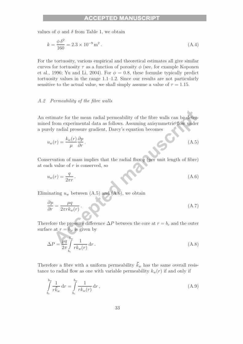
For the tortuosity, various empirical and theoretical estimates all give similarcurves for tortuosity τ as a function of porosity φ (see, for example Koponenet al., 1996; Yu and Li, 2004). For φ = 0.8, these formulæ typically predicttortuosity values in the range 1.1–1.2. Since our results are not particularlysensitive to the actual value, we shall simply assume a value of τ = 1.15.

A.2 Permeability of the fibre walls

An estimate for the mean radial permeability of the fibre walls can be deter-mined from experimental data as follows. Assuming axisymmetric flow undera purely radial pressure gradient, Darcy’s equation becomes

uw(r) =kw(r)

μ

∂p

∂r. (A.5)

Conservation of mass implies that the radial flux q (per unit length of fibre)at each value of r is conserved, so

uw(r) =q

2πr. (A.6)

Eliminating uw between (A.5) and (A.6), we obtain

∂p

∂r=

μq

2πrkw(r). (A.7)

Therefore the pressure difference ΔP between the core at r = bc and the outersurface at r = bw is given by

ΔP =μq

2π

bw∫bc

1

rkw(r)dr . (A.8)

Therefore a fibre with a uniform permeability kw has the same overall resis-tance to radial flow as one with variable permeability kw(r) if and only if

bw∫bc

1

rkw

dr =

bw∫bc

1

rkw(r)dr , (A.9)

33

Accep

ted m

anusc

ript

which is the definition for kw used in (25). Using this definition to eliminatekw(r) from (A.8), we find that

kw =μq

2πΔPln

(bwbc

). (A.10)

Preliminary experimental data from Ellis & Chaudhuri (unpublished) suggestsan order of magnitude estimate of kw ∼ 10−17 m2, but this figure is likely tobe quite sensitive to changes in the manufacturing conditions.

A.3 Harmful concentration of lactic acid

In this appendix, we describe how we estimate the concentration of lacticacid that would be harmful to the growing cells (see Table 4). When the pHdrops the proliferation of cells is strongly inhibited. Each molecule of glucoseproduces two molecules of lactic acid and so the rate of production of lacticacid is twice the rate of glucose consumption.

The culture medium is initially at a pH of 8, and we assume that the growingcells can tolerate a pH change of up to ±0.5, though growth rates are likelyto be affected near to the extremities of this range.

In this pH range, lactic acid is almost fully dissociated and so behaves as astrong acid. Therefore in the absence of buffering the concentration of lacticacid required to cause a drop from 8 to 7.5 is given by

(10−7.5 − 10−8) mol dm−3 ≈ 2 × 10−5 mol m−3 . (A.11)

This is a tiny amount relative to the rates at which lactic acid is known tobe produced by the cells, so it is therefore necessary to take the buffering intoaccount.

Culture media typically contain a large number of different proteins, salts, andother nutrients, which will interact with each other in complex ways underapplied pH changes. We therefore make no attempt to model the bufferingeffect, and instead appeal to experimental results. Fig. A.1 shows data fromtwo titrations of lactic acid into a typical culture medium. From this data, wesee that the concentration of lactic acid that results in a pH drop of 0.5 isroughly 0.4 mol m−3. We use this for the value of c†i in �7.

34

Accep

ted m

anusc

ript

6.5

7

7.5

8

0 0.2 0.4 0.6 0.8 1 1.2 1.4

pH

Concentration of Lactic Acid (mol m−3)

Fig. A.1. The results of two titrations lactic acid into a typical culture mediumto assess the level of buffering present. The culture medium comprised D-MEM(Invitrogen, 2008) with 10% Fetal Calf Serum. Lactic acid was added drop-wiseusing a pipette, and data points comprising the volume added together with the pHof the solution were recorded. The agreement between the two titrations indicatesgood reproducibility.

B Consistency of the approximations used in �4

In this appendix, we check the consistency of the various approximations usedin �4 to model the flow in the fibre. These approximations simplified theequations in the core and wall. We check their validity by comparing the sizesof the neglected terms to those retained.

To obtain the viscous lubrication approximation (37)–(39) in the fibre core, weassumed that the appropriate Reynolds number is small, and that the radialpressure variation Δpr required to drive the radial flow is small comparedwith the axial pressure variation Δps. The Reynolds number is estimated bycomparing the steady inertia term with the viscous term. We find that

Rec =ρw2

c/a

μwc/b2c∼ ρQf

μa=ρQ−μa

�

N≈ 20�

N� O(1) . (B.1)

While this may not be formally small, low-Reynolds-number approximationsare generally found to be acceptable even at O(1) Reynolds numbers. More-over, in the α2 � 1 regime of primary interest here, O(1) errors in the viscouspressure drop along the fibre will not affect the pressure difference across thewall, and so the emitted flux will be unchanged.

The pressure variations Δpr and Δps are estimated from the viscous drag due

35

Accep

ted m

anusc

ript

to the velocity components. We therefore have

Δps

L∼ μ

wc

b2c∼ μQf

b4c,

Δpr

bc∼ μ

uc

b2c∼ μQf

ab3c, (B.2)

and hence

Δpr

Δps

∼ b2c�a2

∼ ε2 . (B.3)

We have already assumed that ε� 1, so the approximation is justified.

Secondly, when forming equations (46)–(47) for the flow in the wall, we as-sumed that the axial flow made no contribution to the continuity equation,and so could be neglected. Knowing that the axial pressure variations in thewall are tied to pc(s) from (30b), we can now estimate

∂ww

∂s� kw

μ

∂2pc

∂s2∼ Qf

a3

∂2Pc

∂ζ2∼ α2Qf

a3∼ Qfkw

ε4a5. (B.4)

This must be small compared with uw/bc ∼ Qf/(ε2a3). Hence we require

kw � ε2a2 = b2c , (B.5)

a condition that we had already noted.

References

Abousleiman, R. I., Sikavitsas, V. I., 2006. Bioreactors for tissues of the mus-culoskeletal system. Adv. Exp. Med. Biol. 585, 243–259.

Bailey, C., et al., 2006. Optimisation of fluid distribution inside a porous con-struct. In: Proceedings of the 6th Mathematics in Medicine Study Group.University of Nottingham.

Bancroft, G., Sikavitsas, V., van den Dolder, J., Sheffield, T., Ambrose, C.,Jansen, J., Mikos, A., 2002. Fluid flow increases mineralized matrix de-position in 3D perfusion culture of marrow stromal osteoblasts in a dose-dependent manner. Proc. Nat. Acad. Sci. USA 99 (20), 12600–12605.

Batchelor, G. K., 1967. An Introduction to Fluid Dynamics. Camb. Univ.Press.

Bear, J., 1988. Dynamics of Fluids in Porous Media. Dover.Boschetti, F., Raimondo, M. T., Migliavacca, F., Dubini, G., 2006. Predic-

tion of the micro-fluid dynamic environment imposed to three-dimensionalengineered cell systems in bioreactors. J. Biomech. 39, 418–425.

36

Accep

ted m

anusc

ript

Cartmell, S. H., Gittings, J. P., Turner, I. G., Chaudhuri, J. B., Ellis, M. J.,Waters, S. L., Cummings, L. J., Kuiper, N. J., Michael, V., 2007. Bioreactordesign for osteochondral tissue. In: Am. Soc. Bone Miner. Res. 29th AnnualMeeting Abstracts Supplement. Vol. 22S1 of J. Bone Miner. Res. p. S162.

Cartmell, S. H., Porter, B. D., Garcia, A. J., Guldberg, R. E., 2003. Effects ofmedium perfusion rate on cell-seeded three-dimensional bone constructs invitro. Tissue Engr. 9 (6), 1197–1203.

Cimetta, E., Flaibani, M., Mella, M., Serena, E., Boldrin, L., De Coppi, P.,Elvassore, N., 2007. Enhancement of viability of muscle precursor cells on3D scaffold in a perfusion bioreactor. Int. J. Artif. Organs 30 (5), 415–428.

Cogan, N. G., Keener, J. P., 2004. The role of the biofilm matrix in structuraldevelopment. Math. Med. Biol. 21, 147–166.

Cummings, L. J., Waters, S. L., 2007. Tissue growth in a rotating bioreactor.Part II: Flow and nutrient transport problems. Math. Med. Biol. 24, 169–208.

Ellis, M. J., Chaudhuri, J. B., 2007. Poly(lactic-co-glycolic acid) hollow fibremembranes for use as a tissue engineering scaffold. Biotech. Bioengr. 96 (1),177–187.

Galban, C. J., Locke, B. R., 1997. Analysis of cell growth in a polymer scaffoldusing a moving boundary approach. Biotech. Bioengr. 56 (4), 422–432.

Galban, C. J., Locke, B. R., 1999. Effects of spatial variations of cells andnutrient and product concentrations coupled with product inhibition oncell growth in a polymer scaffold. Biotech. Bioengr. 64 (6), 633–643.

Gittings, J. P., Turner, I. G., Miles, A. W., 2005. Calcium phosphate openporous scaffold bioceramics. Key Engr. Mat. 284–286, 349–354.

Glowacki, J., Mizuno, S., Greenberger, J. S., 1998. Perfusion enhances func-tions of bone marrow stromal cells in three-dimensional culture. Cell Transp.7 (3), 319–26.

Goldstein, A., Juarez, T., Helmke, C., Gustin, M., Mikos, A., 2001. Effect ofconvection on osteoblastic cell growth and function in biodegradable poly-mer foam scaffolds. Biomat. 22 (11), 1279–1288.

Haddock, S. M., Debes, J. C., Nauman, E. A., Fong, K. E., Arramon, Y. P.,Keaveny, T. M., 1999. Structure-function relationships for coralline hydrox-yapatite bone substitute. Journal of Biomedical Materials Research 47 (1),71–78.

Humphrey, J. D., 2003. Continuum biomechanics of soft biological tissues.Proc. R. Soc. Lond. A 459 (1), 3–46.

Invitrogen, 2008. Dulbecco’s Modified Eagle Medium (D-MEM) (1X)#22320022. Media formulations, Invitrogen.

Kim, S. S., Penkala, R., Abrahimi, P., 2007. A perfusion bioreactor for intesti-nal tissue engineering. J Surg Res 142 (2), 327–331.

Knobloch, T. J., Madhavan, S., Nam, J., Agarwal, S., J., Agarwal, S.,2008. Regulation of chondrocytic gene expression by biomechanical signals.CREGE 18 (2), 139–150.

Komarova, S. V., Ataullakhanov, F. I., Globus, R. K., 2000. Bioenergetics and

37

Accep

ted m

anusc

ript

mitochondrial transmembrane potential during differentiation of culturedosteoblasts. Am. J. Physiol. Cell Physiol. 279, C1220–C1229.

Koponen, A., Kataja, M., Timonen, J., 1996. Tortuous flow in porous media.Phys. Rev. E 54 (1), 406–410.

Lasseux, D., Ahmadi, A., Cleis, X., Garnier, J., 2004. A macroscopic modelfor species transport during in vitro tissue growth obtained by the volumeaveraging method. Chem. Engr. Sci. 59 (10), 1949–1964.

Lemon, G., King, J. R., Byrne, H. M., Jensen, O. E., Shakesheff, K. M., 2006.Mathematical modelling of engineered tissue growth using a multiphaseporous flow mixture theory. J. Math. Biol. 52 (5), 571–594.

Lide, D. R. (Ed.), 2007. CRC Handbook of Chemistry and Physics, 87th Edi-tion. CRC.

MacArthur, B. D., Please, C. P., Taylor, M., Oreffo, R. O. C., 2004. Math-ematical modelling of skeletal repair. Biochem. Biophys. Res. Comm. 313,825–833.

Martin, I., Wendt, D., Heberer, M., 2004. The role of bioreactors in tissueengineering. Trends Biotech. 22 (2).

Michael, V., Gittings, J. P., Turner, I. G., Chaudhuri, J. B., Ellis, M. J.,Waters, S. L., Cummings, L. J., Goodstone, N. J., Cartmell, S. H., 2007.Co-culture bioreactor design for skeletal tissue engineering, In ERMIS-EUMeeting Abstracts. Tissue Engr. 13 (7), 1657–1658.

Morgan, S. M., Tilley, S., Perera, S., Ellis, M. J., Kanczler, J., Chaudhuri,J. B., Oreffo, R. O. C., 2007. Expansion of human bone marrow stromalcells on poly-(dl-lactide-co-glycolide) (P(DL)LGA) hollow fibres designedfor use in skeletal tissue engineering. Biomat. 28 (35), 5332–5343.

Nehring, D., Adamietz, P., Meenen, N. M., Portner, R., 1999. Perfusion cul-tures and modelling of oxygen uptake with three-dimensional chondrocytepellets. Biotech. Techniques 13 (10), 701–706.

Ockendon, H., Ockendon, John, R., 1995. Viscous Flow. Camb. Univ. Press.O’Dea, R. D., Waters, S. L., Byrne, H. M., 2008. A two-fluid model for tissue

growth within a dynamic flow environment. Eur. J. Appl. Math.Peterson, L., Minas, T., Brittberg, M., Nilsson, A., Sjogren-Jansson, E., Lin-

dahl, A., 2000. Two to nine year outcome after autologous chondrocytetransplantation of the knee. CORR 374, 212–234.

Porter, B., Zauel, R., Stockman, H., Guldberg, R., Fyhrie, D., 2005. 3D compu-tational modeling of media flow through scaffolds in a perfusion bioreactor.J. Biomech. 38 (3), 543–549.

Ribeiro, A. C. F., Lobo, V. M. M., Leaist, D. G., Natividade, J. J. S., Verssimo,L. P., Barros, M. C. F., Cabral, A. M. T. D. P. V., 2005. Binary diffusioncoefficients for aqueous solutions of lactic acid. J. Soltn Chem. 34, 1009–1016.

Rubin, J., Rubin, C., Jacobs, C. R., 2006. Molecular pathways mediatingmechanical signaling in bone. Gene 367, 1–16.

Sengers, B. G., Oomens, C. W. J., Baaijens, F. P. T., 2004. An integratedfinite-element approach to mechanics, transport and biosynthesis in tissue

38

Accep

ted m

anusc

ript

engineering. J. Biomech. Engr. 126 (1), 82–91.Tromans, D., 1998. Temperature and pressure dependent solubility of oxygen

in water: a thermodynamic analysis. Hydrometallurgy 48 (3), 327–342.Waters, S. L., Cummings, L. J., Shakesheff, K. M., Rose, F. R. A. J., 2006.

Tissue growth in a rotating bioreactor. Part I: Mechanical stability. Math.Med. Biol. 23, 311–337.

Yu, B.-M., Li, J.-H., 2004. A geometry model for tortuosity of flow path inporous media. Chinese Phys. Lett. 21 (8), 1569–1571.

39