Mathematical Modelling in the Natural Sciences SS21 ...

Mathematical Modelling in the Natural Sciences SS21Solutions to Exercises on Sheet 7

Exercises und Lecture Notes

Contents

• Exercise 1: Cerclage Model 1 Task . . . . . . . . . . . . . . . . . . . . . . . . . . . . . . . . . . . . . . . . . . . . . . 1 Solution . . . . . . . . . . . . . . . . . . . . . . . . . . . . . . . . . . . . . . . . . . . . 2

• Exercise 2: Bungee Cord 10 Task . . . . . . . . . . . . . . . . . . . . . . . . . . . . . . . . . . . . . . . . . . . . . . 10 Solution . . . . . . . . . . . . . . . . . . . . . . . . . . . . . . . . . . . . . . . . . . . . 10

• Exercise 3: Pastry Sheet 14 Task . . . . . . . . . . . . . . . . . . . . . . . . . . . . . . . . . . . . . . . . . . . . . . 14 Solution . . . . . . . . . . . . . . . . . . . . . . . . . . . . . . . . . . . . . . . . . . . . 14

• Exercise 4: Meditation Model 23 Task . . . . . . . . . . . . . . . . . . . . . . . . . . . . . . . . . . . . . . . . . . . . . . 23 Solution . . . . . . . . . . . . . . . . . . . . . . . . . . . . . . . . . . . . . . . . . . . . 23

• Exercise 5: Comparison of Membrane Models 38 Task . . . . . . . . . . . . . . . . . . . . . . . . . . . . . . . . . . . . . . . . . . . . . . 38 Solution . . . . . . . . . . . . . . . . . . . . . . . . . . . . . . . . . . . . . . . . . . . . 38

• Exercise 1: Cerclage Model

Task

Derive the necessary stationarity condition on page 190 of the lecture notes,

−

T (u)uuφ√u2 + u2

φ

sinφ

φ

+ T (u)2u2 + u2

φ√u2 + u2

φ

sinφ

=

f(u sinφ, u cosφ)(u cosφ)φ√u2 + u2

φ

+ (p1 + λ)

u2 sinφ, 0 < φ < π,

uφ = 0, φ = 0, π,

∫ π

0u3 sinφdφ = 2r3

1

Write a Matlab code to solve this system as indicated on pages 191 - 192, i.e., by iterating a cellcentered finite difference approximation of[

A(u) K(u)K∗(u) 0

] [vλ

]=

[F (u, p)G(u)

]u = u+ αvp = p+ αλ

1

https://imsc.uni-graz.at/keeling/modII_ss21/sheet07.pdf

https://imsc.uni-graz.at/keeling/skripten/modnsc.pdf

where

A(u)v = −

T (u)u sinφ√u2 + u2

φ

vφ

φ

+T (u)u sinφ√u2 + u2

φ

v ≈ −δFδu

(u; v)

K(u)λ = −λu2 sinφ ≈ −δFδp

(p;λ), K∗(u)v = −∫ π

0vu2 sinφdφ ≈ −δG

δu(u; v)

F (u, p) = −A(u)u− T (u) sinφ√u2 + u2

φ+f(u sinφ, u cosφ)(u cosφ)φ√u2 + u2

φ

+ p

u2 sinφ

G(u) =

∫ π

0u3 sinφdφ− 2r3

1

Solution

In the lecture notes the model of the band force f(u sin(φ), u cos(φ)) is given on page 187 and themodel of tension T (u) is given on pages 188-189. The Lagrangian functional on page 186,

L(u, λ) = 12π [Ji(u) + Je(u)− λJc(u)]

has the variational derivatives seen on page 184,

δJi

δu(u; v) = 2π

∫ π

0T (u)

u2φv + 2u2v + uuφvφ√

u2 + u2φ

sin(φ)dφ

and on page 186

δJe

δu(u; v) = −2π

∫ π

0

f(u cos(φ), u sin(φ))(u cos(φ))φ√u2 + u2

φ

+ p

vu2 sin(φ)dφ

and the variational derivative of the contraint functional Jc on page 186 is given by

δJc

δu(u; v) = 2π

∫ π

0u2v sin(φ)dφ.

Setting δL(u; v)/δu = 0 gives the condition∫ π

0T (u)

u2φv + 2u2v + uuφvφ√

u2 + u2φ

sin(φ)dφ

−∫ π

0

f(u cos(φ), u sin(φ))(u cos(φ))φ√u2 + u2

φ

+ p

vu2 sin(φ)dφ

−λ2π

∫ π

0u2v sin(φ)dφ = 0, ∀v ∈ C([0, π])

The only term among these which contains a derivative of a test function v is∫ π

0T (u)

uuφvφ√u2 + u2

φ

sin(φ)dφ = −∫ π

0

T (u)sin(φ)uuφ√u2 + u2

φ

φ

vdφ+

T (u)sin(φ)uuφ√u2 + u2

φ

φ

v

∣∣∣∣∣π

0

2

Setting the test function v to be concentrated in the iterior of the interval (0, π) gives the necessarystationarity condition on u,

−

T (u)uuφ√u2 + u2

φ

sinφ

φ

+ T (u)2u2 + u2

φ√u2 + u2

φ

sinφ

=

f(u sinφ, u cosφ)(u cosφ)φ√u2 + u2

φ

+ (p1 + λ)

u2 sinφ, 0 < φ < π,

,

∫ π

0u3 sinφdφ = 2r3

1

Letting the test function v be concentrated on the boundary of the interval gives the Neumannboundary condition,

uφ = 0, φ = 0, π

Finally setting δL(λ;µ)/δλ = 0 gives the condition∫ π

0u?3 sin(φ)dφ = 2r3

1.

The saddle point problem is solved using the following Matlab code, in which various parametersappear as indicated in the lecture notes.

h1 = figure(1);

close(h1);

h1 = figure(1);

set(h1,’Position’,[0 0 384 384])

h2 = figure(2);

close(h2);

h2 = figure(2);

set(h2,’Position’,[400 0 384 384])

h3 = figure(3);

close(h3);

h3 = figure(3);

set(h3,’Position’,[800 0 384 384])

n = 101; % number of phi subintervals

h = pi/n; % width of subinterval

phib = h*(0:n)’; % subinterval boundaries

phic = phib(1:n) + 0.5*h; % subinterval centroids

r1 = 12.25; % normal radius is 12 mm

% p1 = 23.0; % normal pressure is 20 mmHg

p1 = 20.0; % normal pressure is 20 mmHg

T1 = 0.5*p1*r1; % Laplace Law

V1 = 4.0*pi*r1^3/3.0; % initial volume

Ed_m = 16232.0; % elasticity modulus * membrane thickness

3

% Ed_m = 21753.0; % elasticity modulus * membrane thickness

rg = 1.0/80.0; % occular rigidity

p0 = p1;

V0 = V1 + log(p0/p1)/rg;

r0 = (0.75*V0/pi)^(1/3);

p1 = p0;

V1 = V0;

r1 = r0;

T1 = 0.5*p1*r1;

% Ed_b = 14852.0*0.75; % elasticity modulus * band thickness

% Ed_b = 19578.0*0.75; % elasticity modulus * band thickness

Ed_b = 24453.0*0.75; % elasticity modulus * band thickness

Rhat = 10.35; % rest radius of band

bt = 1.0; % half the band width

phi1 = acos(bt/r1); % first angle of band edge

phi2 = pi - phi1; % second angle of band edge

z1 = r1*cos(phi1); % plane of lower band edge

z2 = r1*cos(phi2); % plane of upper band edge

R1 = r1*sin(phi1); % height of lower band edge

R2 = r1*sin(phi2); % height of upper band edge

ax = 15; % x-axis radius

ay = 15; % y-axis radius

mxp = 100000; % max iterations to reach original pressure

mxv = 100000; % max iterations to solve for geometry

tolp = 1.0e-6; % pressure iteration tolerance

tolv = 1.0e-6; % geometry interation tolerance

ep = 1.0e-15; % code zero

rx = 0.9; % geometry relaxation parameter 0 < rx =< 1

r0 = r1; % set the first equilibrium state

V0 = V1;

p0 = p1;

T0 = T1;

Vs = V1; % initialize state histories

ps = p1;

Ts = T1;

% set min pressure greater than p1

pm = 2.0*p1;

for itp=1:mxp

% initialize residual histories

er = 1.0;

es = 1.0;

4

% set equilibrium state without band

v = r0*ones(n,1);

V = V0;

p = p0;

T = T0*ones(n,1);

rz = rx;

for itv=1:mxv

if (mod(itv,100) == 0)

rz = 0.5*rz;

end

% build band force:

vc = v.*cos(phic);

vs = v.*sin(phic);

% build v’ at cell centers

vp = (v(3:end)-v(1:end-2))/(2.0*h);

vp = [2.0*vp(1)-vp(2),vp’,2.0*vp(end)-vp(end-1)]’;

sq = sqrt(v.^2 + vp.^2);

% band force

f = (vp.*cos(phic)-v.*sin(phic))./sq;

f = Ed_b*f.*(1.0/Rhat - 1.0./vs).* (vs > Rhat)...

.* (z2 <= vc) .* (vc <= z1);

% coefficient for 0th order term in PDE

a0 = T.*vs./sq;

% coefficient for 1st order term in PDE

a1 = (a0(2:n)+a0(1:(n-1)))/(2.0*h^2);

% build discretized differential operator

A = diag(a0) + diag([a1;0]) + diag([0;a1])...

- diag(a1,-1) - diag(a1,1);

% multiplier coefficient

k = -3.0*v.*vs;

% build discretized SQP operator

B = [[A,k];[k’,0]];

% build rhs for SQP equation

b = (f + p).*v.*vs - A*v - T.*sin(phic).*sq;

e = sum((v.^3).*sin(phic)) - 0.75*V/(pi*sin(h/2));

F = [b;e];

% solve SQP system

u = B\F;

lambda = u(n+1);

u = u(1:n);

% update v and p

vo = v;

v = vo + rz*u;

po = p;

p = po + rz*lambda;

5

p = max([p,ep]);

v = 0.5*(v + v(end:-1:1));

v = min(v,1.5*r0*ones(n,1));

v = max(v,Rhat*ones(n,1));

u = v-vo;

lambda = p-po;

% update tension

vp = (v(3:end)-v(1:end-2))/(2.0*h);

vp = [2.0*vp(1)-vp(2),vp’,2.0*vp(end)-vp(end-1)]’;

vs = v.*sin(phic);

T = T0 + Ed_m*(sum(sqrt(v.^2+vp.^2).*vs)/sum(r0^2*sin(phic))-1);

% record histories

ps = [ps,p];

% plot pressure history

if (mod(itv,mxv) == 0)

figure(2);

plot(1:length(ps),ps,’b-’);

axis([(-0.1*length(ps)) length(ps) 0 100]);

hold on

plot([-0.1*length(ps),length(ps)],[20,20],’k:’);

hold off

xlabel(’Iterations’);

ylabel(’Pressure, mmHg’);

title(’Pressure History’);

end

% plot new geometry:

% points on spherical eye

x0 = r0*cos(phic);

x0 = [x0;x0(n:-1:1);x0(1)];

y0 = r0*sin(phic);

y0 = [y0;-y0(n:-1:1);y0(1)];

% points on eye before operation

x1 = r1*cos(phic);

x1 = [x1;x1(n:-1:1);x1(1)];

y1 = r1*sin(phic);

y1 = [y1;-y1(n:-1:1);y1(1)];

% points on eye after the operation

x2 = v.*cos(phic);

x2 = [x2;x2(n:-1:1);x2(1)];

y2 = v.*sin(phic);

y2 = [y2;-y2(n:-1:1);y2(1)];

% points on eye under the band

vc = v.*cos(phic);

fi = find((phi1 <= phic) & (phic <= phi2));

x3 = v(fi).*cos(phic(fi));

y3 = v(fi).*sin(phic(fi));

x4 = x3(end:-1:1);

y4 = -y3(end:-1:1);

6

if (mod(itv,1000000) == 0)

% plot 360 degrees

figure(3);

plot(y1,x1,’g’,y2,x2,’b’);

axis([-ax ax -ay ay]);

pbaspect([1 1 1]);

legend(’preop’,’intraop’,0, ...

’Location’,[0.47 0.45 0.1 0.1]);

hold on;

plot([-ax ax ax -ax -ax], ...

[z2 z2 z1 z1 z2],’r’)

plot([-Rhat Rhat Rhat -Rhat -Rhat], ...

[-ay -ay ay ay -ay],’k:’)

title(’Postoperative State’);

hold off;

drawnow;

end

% break with small residual errors

if ((max(abs(u)) < tolv*max(abs(v)))...

&& (abs(lambda) < tolv*p))

figure(3);

plot(y1,x1,’g’, ...

y2,x2,’b’, ...

y0,x0,’c’);


pbaspect([1 1 1]);

legend(’preop’,’postop’,’bandfree’,0, ...

’Location’,[0.47 0.45 0.1 0.1]);

hold on;


[z2 z2 z1 z1 z2],’r’);



title(’Postoperative State’);

hold off;

drawnow;

figure(2);

plot(1:length(ps),ps,’b-’);

axis([(-0.1*length(ps)) length(ps) 0 100])

hold on

plot([-0.1*length(ps),length(ps)],[20,20],’k:’);

hold off

xlabel(’Iterations’);

ylabel(’Pressure, mmHg’);

title(’Pressure History’);

7

break;

end

end

if (itv == mxv)

error(’max inner iterations reached’);

end

if (itp == 1)

disp(’Intraoperative State:’);

disp(strcat(’Equation residual=’,num2str(er(end))));

disp(strcat(’Pressure residual=’,num2str(abs(lambda))));

disp(strcat(’Volume residual=’,num2str(es(end))));

disp(strcat(’Pressure comparison: p1=’,num2str(p1),’ p=’,num2str(p)));

disp(strcat(’Tension comparison: T1=’,num2str(T1),’ T=’,num2str(T)));

disp(strcat(’Geometry comparison: r1=’,num2str(r1),’ r=’,num2str(r1)));

disp(strcat(’min/max v=’,num2str(min(v)),’,’,num2str(max(v))));

disp(strcat(’Volume comparison: V1=’,num2str(V1),’ V=’,num2str(V1)));

% plot 360 degrees

figure(1);

plot(y1,x1,’g’,y2,x2,’b’);


pbaspect([1 1 1]);

legend(’preop’,’intraop’,0, ...

’Location’,[0.47 0.45 0.1 0.1]);

hold on;


[z2 z2 z1 z1 z2],’r’)



title(’Intraoperative State’);

hold off;

drawnow;

end

pm = min([pm,p]); % update min pressure

if (pm >= p1)

pb = p1;

rb = r1;

fb = p;

ra = Rhat;

Va = 4.0*pi*ra^3/3.0;

pa = p1*exp(rg*(Va-V1));

if (pa < ep)

pa = ep;

Va = V1 + log(pa/p1)/rg;

8

ra = (0.75*Va/pi)^(1/3);

end

fa = 0;

% update equilibrium state without band

p0 = pa;

V0 = Va;

r0 = ra;

T0 = 0.5*p0*r0;

else % p0=pa :=> p<p1, p0=pb :=> p>p1

if (p > p1)

rb = r0; % if p>p1 move rb inward to r0

fb = p;

else

ra = r0; % if p<=p1 move ra inward to r0

fa = p;

end % secant/bisect, r0 = weighted ave(ra,rb)

r0 = ((fb-p1)*ra + (p1-fa)*rb)/(fb-fa);

if ((r0 < ra) || (r0 > rb))

r0 = 0.5*(ra + rb);

end

% update equilibrium state without band

V0 = 4.0*pi*r0^3/3.0;

p0 = p1*exp(rg*(V0-V1));

if (p0 < ep)

p0 = ep;

V0 = V1 + log(p0/p1)/rg;

r0 = (0.75*V0/pi)^(1/3);

end

T0 = 0.5*p0*r0;

end

% break with small pressure error

if (abs(p-p1) < tolp*p1)

break;

end

end

disp(’Postoperative State:’);

disp(strcat(’Equation residual=’,num2str(er(end))));

disp(strcat(’Pressure residual=’,num2str(abs(lambda))));

disp(strcat(’Volume residual=’,num2str(es(end))));

disp(strcat(’Pressure comparison: p1=’,num2str(p1),’ p0=’,num2str(p0)));

disp(strcat(’Tension comparison: T0=’,num2str(T0),’ T=’,num2str(T)));

disp(strcat(’Geometry comparison: r1=’,num2str(r1),’ r0=’,num2str(r0)));

disp(strcat(’min/max v=’,num2str(min(v)),’,’,num2str(max(v))));

disp(strcat(’Volume comparison: V1=’,num2str(V1),’ V0=’,num2str(V0)));

9

The results from this code are shown graphically as follows.

• Exercise 2: Bungee Cord

Task

Recall the constructions in the lecture notes on pages 204-207 for modelling the dynamic state of abungee cord. Develop a Matlab code to simulate the cord displacement. Hint: Consider this code,which contains yet some riddles.

Solution

% setup figure

h1 = figure(1);

close(h1);

h1 = figure(1);

set(h1,’Position’,[10 10 500 500]);

% model parameters

r0 = 1.0e0; % elasticity

c0 = 1.0e0; % damping

f0 = 1.0e0; % downward force

clampall = true; % true => xmin/xmax, otherwise xmin

% grid parameters

Nx = 20; % Nx cells

xmin = 0; xmax = 1;

x = linspace(xmin,xmax,Nx+1); % x(i) is a "node"

hx = x(2)-x(1);

xc = x(1:Nx) + hx/2; % xc(i) is a "cut" (cell center)

dt = 1.0e-2;

Nt = 10000;

T = Nt*dt; % final time

10

https://imsc.uni-graz.at/keeling/numpde_ss16/bungee.m

tol = 1.0e-4; % termination criterion

th = 1.0; % theta time stepping

% gradient, from nodes to cuts directly between them

dx = spdiags(ones(Nx,1),1,Nx,Nx+1) ...

- spdiags(ones(Nx,1),0,Nx,Nx+1);

dx = dx/hx;

% zeros and identities

Z = sparse(Nx+1,Nx+1);

Z3 = kron(speye(3),Z);

I = speye(Nx+1);

I3 = kron(speye(3),I);


% boundary projection

if (clampall)

b = ones(Nx+1,1); b(1)=0; b(Nx+1)=0;

Bd = spdiags(b,0,Nx+1,Nx+1);

else

b = ones(Nx+1,1); b(1)=0;

Bd = spdiags(b,0,Nx+1,Nx+1);

end

% damping acting only away from Dirchlet BCs

C = c0*Bd;

C3 = kron(speye(3),C);

% downward force acting only away from Dirichlet BCs

f1 = zeros(Nx+1,1); f1 = Bd*f1;

f2 = zeros(Nx+1,1); f2 = Bd*f2;

f3 = -f0*ones(Nx+1,1); f3 = Bd*f3;

f = [f1;f2;f3];

F = [zeros(3*(Nx+1),1);f];

% initial state, displacements

u1 = x’;

u2 = zeros(Nx+1,1);

u3 = zeros(Nx+1,1);

% and velocities

u1t = zeros(Nx+1,1);



% the state vector

U = [u1;u2;u3;u1t;u2t;u3t];

% start time stepping

11

for k=1:Nt

t = k*dt; % current time

Ua = U; % save for stopping criterion

% ensure BCs

u1 = U( 1: (Nx+1));

u2 = U( (Nx+1)+1:2*(Nx+1));

u3 = U(2*(Nx+1)+1:3*(Nx+1));

if (clampall)

u1(1)=xmin; u1(Nx+1)=xmax;

u2(1)=0; u2(Nx+1)=0;

u3(1)=0; u3(Nx+1)=0;

else

u1(1)=xmin;

u2(1)=0;

u3(1)=0;

end

U(1:3*(Nx+1)) = [u1;u2;u3];

% gradients at cuts

u1x = dx*u1;

u2x = dx*u2;

u3x = dx*u3;

% length increments on cuts

dL = sqrt(u1x.^2 + u2x.^2 + u3x.^2);

% coefficients on cuts

cf = r0*(1 - 1./dL);

% second order differential operator

L = dx’*spdiags(cf(:),0,Nx,Nx)*dx;

L = Bd*L;

L3 = kron(speye(3),L);

% U’ = A*U + F

A6 = [Z3,I3;-L3,-C3];

% update with the theta method

U = (I6 - th*dt*A6) \ ((I6 + (1-th)*dt*A6)*U + dt*F);

% graph the current state

plot3(u1,u2,u3,’LineWidth’,3);

title(sprintf(’t=%0.1e, |dU|=%0.1e’,t,norm(U-Ua)/norm(U)))

xlabel(’u1’); ylabel(’u2’); zlabel(’u3’);

grid on;

if (clampall)

d = 0.6; axis([0.5-d,0.5+d,0.0-d,0.0+d,0.1-2*d,0.1]);

12

else

d = 1.0; axis([0.5-d,0.5+d,0.0-d,0.0+d,0.1-2*d,0.1]);

end

pbaspect([1 1 1]);

drawnow;

if (norm(U-Ua) <= tol*norm(U)) % stop when iterates

break; % do not differ

end

end

The result at time t = 1 for a cord falling while fastened at both ends is shown graphically as follows.

The result at time t = 2 for a cord falling while fastened at only one end is shown graphically as

13

follows.

• Exercise 3: Pastry Sheet

Task

Recall the definitions on page 210 of the lecture notes. Based upon the principle of least action, derivethe stationary state for the Lagrangian functional

L(u) =

∫ T

0

∫ 1

0

∫ 1

0

[12ρ‖ut‖

2 − 12κ(‖uξ × uη‖ − 1)2 + f · u

]dξdηdt

u(ξ, 0, t) = (ξ, 0, 0), u(ξ, η, 0) = (ξ, η, 0), ut(ξ, η, 0) = (0, 0, 0)

with gravity f = (0, 0,−φ/ρ) and ρ, κ, φ > 0. Develop a Matlab code to simulate the membranedisplacement. Hint: Consider this code, which contains yet some riddles.

Solution

Let Ω = (0, 1)2 and Q = Ω×(0, T ) and suppose a test function v is sufficiently smooth and vanishes atthe spatial boundary η = 0 and at initial and final times t = 0, T . For the computation of variational

14

https://imsc.uni-graz.at/keeling/numpde_ss16/sheet.m

derivatives note that

d

dε[(u+ εv)ξ × (u+ εv)η] · [(u+ εv)ξ × (u+ εv)η] =

d

dε[(u+ εv)ξ × (u+ εv)η]

· [(u+ εv)ξ × (u+ εv)η] + [(u+ εv)ξ × (u+ εv)η] ·

d

dε[(u+ εv)ξ × (u+ εv)η]

=

[d

dε(u+ εv)ξ

]× (u+ εv)η + (u+ εv)ξ ×

[d

dε(u+ εv)η

]· [(u+ εv)ξ × (u+ εv)η]

+ [(u+ εv)ξ × (u+ εv)η] ·[

d

dε(u+ εv)ξ

]× (u+ εv)η + (u+ εv)ξ ×

[d

dε(u+ εv)η

]= vξ × (u+ εv)η + (u+ εv)ξ × vη · [(u+ εv)ξ × (u+ εv)η]+ [(u+ εv)ξ × (u+ εv)η] · vξ × (u+ εv)η + (u+ εv)ξ × vη

ε→0−→ (vξ × uη + uξ × vη) · (uξ × uη) + (uξ × uη) · (vξ × uη + uξ × vη)= 2(uξ × uη) · (vξ × uη + uξ × vη)

= 2(uη × uξ) · (uη × vξ) + 2(uξ × uη) · (uξ × vη)

and using the following notation

a =

a1

a2

a3

, [[a]] =

0 −a3 +a2

+a3 0 −a1

−a2 +a1 0

, u× v = [[u]]v = −[[u]]>v

the derivative becomes

= 2([[uξ]]uη) · ([[uξ]]vη) + 2([[uη]]uξ) · ([[uη]]vξ)= 2u>η [[uξ]]

>[[uξ]]vη + 2u>ξ [[uη]]>[[uη]]vξ = −2u>η [[uξ]]

2vη − 2u>ξ [[uη]]2vξ.

Then the variational derivative of L is given by

δL

δu(u; v) =

∫Q

[ρut · vt + κ(‖uξ × uη‖ − 1)

u>η [[uξ]]2vη + u>ξ [[uη]]

2vξ

‖uξ × uη‖+ f · v

]

=

∫Qv ·

[−ρutt +

(κ

1− ‖uξ × uη‖‖uξ × uη‖

[[uη]]2uξ

)ξ

+

(κ

1− ‖uξ × uη‖‖uξ × uη‖

[[uξ]]2uη

)η

+ f

]

+

∫Ωρut · v

∣∣∣∣t=Tt=0

+

∫ T

0κ‖uξ × uη‖ − 1

‖uξ × uη‖u>ξ [[uη]]

2v

∣∣∣∣ξ=1

ξ=0

+

∫ T

0κ‖uξ × uη‖ − 1

‖uξ × uη‖u>η [[uξ]]

2v

∣∣∣∣η=1

η=0

or with g = f/ρ = (0, 0,−φ)

δL

∂u(u; v) = ρ

∫Qv · [−utt + (A(u)uξ)ξ + (B(u)uη)η + g]

+ρ

∫Ωut · v

∣∣∣∣t=Tt=0

− ρ∫ T

0u>ξ A(u)v

∣∣∣∣ξ=1

ξ=0

− ρ∫ T

0u>η B(u)v

∣∣∣∣η=1

η=0

where the following are defined

δ(u) =κ

ρ

1− ‖uξ × uη‖‖uξ × uη‖

, A(u) = δ(u)[[uξ]]2 = A(u)>, B(u) = δ(u)[[uη]]

2 = B(u)>.

15

Since v = 0 at t = 0, T , for the first integral vanishes and implicitly requires initial and final timeconditions on u, but instead the initial position and velocity are imposed,

u(ξ, η, 0) = (ξ, η, 0), ut(ξ, η, 0) = (0, 0, 0)

and under the condition of well-posedness of the resulting intial- and boundary-value problem, thefinal time values u(ξ, η, T ) may be regarded as having been imposed as a condition on the Lagrangianfunctional L. The condition that v = 0 hold at η = 0 corresponds to the given Dirichlet boundarycondition

u(ξ, 0, t) = (ξ, 0, 0), ξ ∈ [0, 1], t ∈ [0, T ].

Letting v be concentrated on ∂Q at η = 1 gives the natural boundary condition

B(u)uη(ξ, 1, t) = (0, 0, 0), ξ ∈ [0, 1], t ∈ [0, T ].

Letting v be concentrated on ∂Q at ξ = 0, 1 gives the natural boundary conditions

A(u)[uξ(0, η, t)− (1, 0, 0)] = (0, 0, 0)A(u)[uξ(1, η, t)− (1, 0, 0)] = (0, 0, 0)

η ∈ [0, 1], t ∈ [0, T ]

where the term−(1, 0, 0) is required for compatibility with the Dirichlet boundary condition u(ξ, 0, t) =(ξ, 0, 0) at η = 0. The necessary optimality condition for a stationary u is

ρutt = (A(u)uξ)ξ + (B(u)uξ)η + f, (ξ, η, t) ∈ Qu(ξ, 0, t) = (ξ, 0, 0), B(u)uη(ξ, 1, t) = (0, 0, 0), ξ ∈ [0, 1], t ∈ [0, T ]A(u)[uξ(ξ, η, t)− (1, 0, 0)] = (0, 0, 0), ξ = 0, 1, η ∈ [0, 1], t ∈ [0, T ]u(ξ, η, 0) = (ξ, η, 0), ut(ξ, η, 0) = (0, 0, 0), (ξ, η) ∈ Ω

The following Matlab code is used to solve the initial and boundary-value problem.

% setup figure

h1 = figure(1);

close(h1);

h1 = figure(1);

set(h1,’Position’,[10 10 500 500]);

% model parameters

r0 = 5.0e-1; % elasticity

c0 = 2.0e-1; % damping

f0 = 1.0e-1; % downward force

clampall = false; % true => x,y,min/max

% otherwise y=ymin

% grid parameters

Nx = 10; % Nx X Ny cells

Ny = 10; % (Nx+1) X (Ny+1) "nodes"

xmin = 0; xmax = 1;

ymin = 0; ymax = 1;

x = linspace(xmin,xmax,Nx+1); % (x(i),y(j)) is a "node"

y = linspace(ymin,ymax,Ny+1);

hx = x(2)-x(1);

hy = y(2)-y(1);

16

xc = x(1:Nx) + hx/2; % (xc(i),y(j)) is an "x-cut"

yc = y(1:Ny) + hy/2; % (x(i),yc(j)) is a "y-cut"

dt = 1.0e-2;

Nt = 100000;

T = Nt*dt; % final time

dt = T/Nt;

tol = 1.0e-6; % termination criterion

th = 1; % theta time stepping

% gradient, from nodes to cuts directly between them

dx = spdiags(ones(Nx,1),1,Nx,Nx+1) ...

- spdiags(ones(Nx,1),0,Nx,Nx+1);

dx = dx/hx;

iy = speye(Ny+1);

Dx = kron(iy,dx); % x-derivative, nodes to x-cuts

dy = spdiags(ones(Ny,1),1,Ny,Ny+1) ...

- spdiags(ones(Ny,1),0,Ny,Ny+1);

dy = dy/hy;

ix = speye(Nx+1);

Dy = kron(dy,ix); % y-derivative, nodes to y-cuts

% gradient, from nodes to cuts opposite direction

dx = spdiags(ones(Nx+1,1),+1,Nx+1,Nx+1) ...

- spdiags(ones(Nx+1,1),-1,Nx+1,Nx+1); % x-derivative, nodes to nodes

dx = dx/(2*hx);

dx( 1, 1) = -1/hx; dx( 1, 2) = 1/hx; % one-sided at boundary

dx(Nx+1,Nx) = -1/hx; dx(Nx+1,Nx+1) = 1/hx;

ay = spdiags(ones(Ny,1), 1,Ny,Ny+1) ... % y-average, nodes to y-cuts

+ spdiags(ones(Ny,1), 0,Ny,Ny+1);

ay = ay/2;

Cx = kron(ay,dx); % nodes to y-cuts

dy = spdiags(ones(Ny+1,1),+1,Ny+1,Ny+1) ...

- spdiags(ones(Ny+1,1),-1,Ny+1,Ny+1); % y-derivative, nodes to nodes

dy = dy/(2*hy);

dy( 1, 1) = -1/hy; dy( 1, 2) = 1/hy; % one-sided at boundary

dy(Ny+1,Ny) = -1/hy; dy(Ny+1,Ny+1) = 1/hy;

ax = spdiags(ones(Nx,1), 1,Nx,Nx+1) ... % x-average, nodes to x-cuts

+ spdiags(ones(Nx,1), 0,Nx,Nx+1);

ax = ax/2;

Cy = kron(dy,ax); % nodes to x-cuts

% zeros and identities

Z = sparse((Nx+1)*(Ny+1),(Nx+1)*(Ny+1));

Z3 = kron(speye(3),Z);

I = speye((Nx+1)*(Ny+1));


17


% boundary projection

if (clampall)

b = ones(Nx+1,Ny+1);

b(1,:)=0; b(Nx+1,:)=0; b(:,1)=0; b(:,Ny+1)=0; b=b(:);

Bd = spdiags(b,0,(Nx+1)*(Ny+1),(Nx+1)*(Ny+1));

Bd3 = kron(speye(3),Bd); % Dirichlet

Bx = I;

Bx3 = I3; % Neumann, x-direction

By = I;

By3 = I3; % Neumann, y-direction

else


b(:,1)=0; b=b(:);

Bd = spdiags(b,0,(Nx+1)*(Ny+1),(Nx+1)*(Ny+1));

Bd3 = kron(speye(3),Bd); % Dirichlet


b(1,:)=0; b(Nx+1,:)=0; b=b(:);

Bx = spdiags(b,0,(Nx+1)*(Ny+1),(Nx+1)*(Ny+1));

Bx3 = kron(speye(3),Bx); % Neumann, x-direction


b(:,Ny+1)=0; b=b(:);

By = spdiags(b,0,(Nx+1)*(Ny+1),(Nx+1)*(Ny+1));

By3 = kron(speye(3),By); % Neumann, y-direction

end

% damping acting only away from Dirchlet BCs

C = c0*Bd;

C3 = kron(speye(3),C);

% downward force acting only away from Dirichlet BCs

f1 = zeros(Nx+1,Ny+1); f1 = Bd*f1(:);

f2 = zeros(Nx+1,Ny+1); f2 = Bd*f2(:);

f3 = -f0*ones(Nx+1,Ny+1); f3 = Bd*f3(:);

f = [f1;f2;f3];

% initial state, displacements (saved in v1,v2,v3)

u1 = kron(x’,ones(1,Ny+1)); u1 = u1(:); v1=u1;

u2 = kron(ones(Nx+1,1),y); u2 = u2(:); v2=u2;

u3 = zeros(Nx+1,Ny+1); u3 = u3(:); v3=u3;

% and velocities

u1t = zeros(Nx+1,Ny+1); u1t = u1t(:);



% the state vector

U = [u1;u2;u3;u1t;u2t;u3t];

18


for k=1:Nt

t = k*dt; % current time

Ua = U; % save for stopping criterion

% ensure BCs

u1 = reshape(U( 1: (Nx+1)*(Ny+1)),Nx+1,Ny+1);

u2 = reshape(U( (Nx+1)*(Ny+1)+1:2*(Nx+1)*(Ny+1)),Nx+1,Ny+1);

u3 = reshape(U(2*(Nx+1)*(Ny+1)+1:3*(Nx+1)*(Ny+1)),Nx+1,Ny+1);

if (clampall)

u1(1,:)=xmin; u1(Nx+1,:)=xmax;

u1(:,1)=x’; u1(:,Ny+1)=x’;

u2(1,:)=y; u2(Nx+1,:)=y;

u2(:,1)=ymin; u2(:,Ny+1)=ymax;

u3(1,:)=0; u3(Nx+1,:)=0;

u3(:,1)=0; u3(:,Ny+1)=0;

else

u1(:,1)=x’;

u2(:,1)=ymin;

u3(:,1)=0;

end

u1 = u1(:); u2 = u2(:); u3 = u3(:);

U(1:3*(Nx+1)*(Ny+1)) = [u1;u2;u3];

% gradients at x-cuts

u1x = Dx*u1; u2x = Dx*u2; u3x = Dx*u3;

u1y_ = Cy*u1; u2y_ = Cy*u2; u3y_ = Cy*u3;

% gradients at y-cuts

u1x_ = Cx*u1; u2x_ = Cx*u2; u3x_ = Cx*u3;

u1y = Dy*u1; u2y = Dy*u2; u3y = Dy*u3;

% area increments on x-cuts

dEx = sqrt((u2x.*u3y_ - u3x.*u2y_).^2 + ...

(u1x.*u3y_ - u3x.*u1y_).^2 + ...

(u1x.*u2y_ - u2x.*u1y_).^2);

% area increments on y-cuts

dEy = sqrt((u2x_.*u3y - u3x_.*u2y).^2 + ...

(u1x_.*u3y - u3x_.*u1y).^2 + ...

(u1x_.*u2y - u2x_.*u1y).^2);

% coefficients on x- and y-cuts

cfx = r0*(1 - 1./dEx);

cfy = r0*(1 - 1./dEy);

% coefficients in the second order differential operator

19

% utt + c ut = -Lu + f

% Lu = Dx’ r0 (1 - 1/|ux X uy|)[uy]’[uy] Dx u

% + Dy’ r0 (1 - 1/|ux X uy|)[ux]’[ux] Dy u

%

% [u] = [ 0,-u3, u2; u3, 0,-u1;-u2, u1, 0]

%

% [u]’[u] = [u2^2+u3^2,-u1u2,-u1u3;-u1u2,u1^2+u3^2,-u2u3;-u1u3,-u2u3,u1^2+u2^2]

% compute coefficients [uy]’*[uy] on x-cuts

Uy = [spdiags(u2y_.^2 + u3y_.^2,0,Nx*(Ny+1),Nx*(Ny+1)), ...

spdiags( -u1y_.*u2y_,0,Nx*(Ny+1),Nx*(Ny+1)), ...

spdiags( -u1y_.*u3y_,0,Nx*(Ny+1),Nx*(Ny+1)); ...


spdiags(u1y_.^2 + u3y_.^2,0,Nx*(Ny+1),Nx*(Ny+1)), ...

spdiags( -u2y_.*u3y_,0,Nx*(Ny+1),Nx*(Ny+1)); ...



spdiags(u1y_.^2 + u2y_.^2,0,Nx*(Ny+1),Nx*(Ny+1))];

% compute coefficients [ux]’*[ux] on y-cuts

Ux = [spdiags(u2x_.^2 + u3x_.^2,0,(Nx+1)*Ny,(Nx+1)*Ny), ...

spdiags( -u1x_.*u2x_,0,(Nx+1)*Ny,(Nx+1)*Ny), ...

spdiags( -u1x_.*u3x_,0,(Nx+1)*Ny,(Nx+1)*Ny); ...


spdiags(u1x_.^2 + u3x_.^2,0,(Nx+1)*Ny,(Nx+1)*Ny), ...

spdiags( -u2x_.*u3x_,0,(Nx+1)*Ny,(Nx+1)*Ny); ...



spdiags(u1x_.^2 + u2x_.^2,0,(Nx+1)*Ny,(Nx+1)*Ny)];

% second order differential operator

Lx = kron(speye(3),Dx’)* ...

kron(speye(3),spdiags(cfx,0,Nx*(Ny+1),Nx*(Ny+1)))*Uy ...

*kron(speye(3),Dx);

Ly = kron(speye(3),Dy’)* ...

kron(speye(3),spdiags(cfy,0,(Nx+1)*Ny,(Nx+1)*Ny))*Ux ...

*kron(speye(3),Dy);

L3 = Lx + Ly;

L3 = Bd3*L3; % only away from Dirichlet BCs

% U’ = A*U + F

A6 = [Z3,I3;-L3,-C3];

dv = (I3-Bx3)*L3*[v1;0*v2;0*v3]; % Neumann BC for compatibility

F = [zeros(3*(Nx+1)*(Ny+1),1);f + dv]; % total force

% update with the theta method

U = (I6 - th*dt*A6) \ ((I6 + (1-th)*dt*A6)*U + dt*F);

U = U.*(abs(U) > tol); % purely for round-off

20

% increase damping otherwise

% graph the current state

surf(reshape(u1,Nx+1,Ny+1), ...

reshape(u2,Nx+1,Ny+1), ...

reshape(u3,Nx+1,Ny+1));

xlabel(’u1’); ylabel(’u2’); zlabel(’u3’);

view([135,30])

% view([30*t,30])

grid on;

if (clampall)

d=0.6; axis([0.5-d,0.5+d,0.5-d,0.5+d,0.1-2*d,0.1]);

else

d=1.0; axis([0.5-d,0.5+d,0.5-d,0.5+d,0.1-2*d,0.1]);

end

pbaspect([1 1 1]);

title(sprintf(’t=%0.1e, |dU|=%0.1e’,t,norm(U-Ua)/norm(U)))

drawnow;

if (norm(U-Ua) <= tol*norm(U)) % stop when iterates

break; % do not differ

end

end

The result at time t = 5 for a membrane falling while fastened on all sides is shown graphically as

21

follows.

The result at time t = 4 for a membrane falling while fastened only along one edge is shown graphically

22

as follows.

• Exercise 4: Meditation Model

Task

Develop a wave equation model for the phenomena illustrated in this video of a simulation, andimplement your model in Matlab.

Solution

The following model is proposed for the simulation of known neurophysiological phenomena associatedwith waking and dream or meditative states. First, the spatial domain Ω = (0, 1)2 is divided intohalves,

Ωl = (x, y) ∈ Ω : y ∈ [0, 12 ], Ωr = (x, y) ∈ Ω : y ∈ [1

2 , 1]

where Ωl models the left hemisphere of the brain and Ωr the right. Let n denote a unit vector which isoutwardly directed with respect to ∂Ωl and ∂Ωr. Let A(u) = diag(α, ω) be the diagonal matrix withwave speeds

√α and

√ω in the x- and y-directions respectively. Let f be a forcing function yet to be

specified. Then the wave displacement u is modelled according to:utt = ∇ · (A∇u) + f(u), (x, y) ∈ (0, 1)2, t ∈ (0, T )

u(0, y, t) = u(1, y, t), y ∈ [0, 1], t ∈ [0, T ]ut(x, y, t) = n>A∇u(x, y, t), x ∈ [0, 1], y ∈ 0, 1/2±, 1, t ∈ [0, T ]

u = 0, (x, y) ∈ (0, 1)2, t = 0ut = 0, (x, y) ∈ (0, 1)2, t = 0.

23

https://imsc.uni-graz.at/keeling/modII_ss20/medi.mpg

Since the left hemisphere has been found to carry out serial processing, this characteristic is modelledby allowing waves to propagate in only one direction according to

α = 0, ω > 0, Ωl.

On the other hand, the right hemisphere has been found to carry out parallel processing, and thischaracteristic is modelled by letting waves travel unhindered in any direction according to

α, ω > 0, Ωr.

At the boundary between the hemispheres transmission is accomplished through f(u) discussed below,but otherwise

ω = 0, ∂Ωr ∩ ∂Ωl.

The squared wave speeds α and ω are otherwise spatially varying,

α = α(x, y), ω = ω(x, y)

where more spatially uniform wave speeds are thought to correspond to the result of meditativepractice as discussed below.

The spatial geometry is torus-like with periodic boundary conditions at x = 0, 1. Also the left andright hemispheres are connected at y = 0, 1 and at y = ±1

2 . For instance, a given wave function udefined on cells Nx×Ny in Ω may be mapped onto a torus-like surface according to

a = kron(ones(Ny,1),linspace(0,2*pi,Nx));

b = kron(linspace(0,2*pi,Ny)’,ones(1,Nx));

y = (2-(1+cos(b)).*cos(b)).*cos(a);

z = (2-(1+cos(b)).*cos(b)).*sin(a);

x = 2*(1+cos(b)).*sin(b);

surf(x,y,z,u);

to illustrate the modelling of waves on and connections between the left and right hemispheres as

24

illustrated in the following graphic.

The boundary conditions at y ∈ 0, 1/2±, 1 are non-reflecting

ut −√ωuy = 0, y = 0

ut +√ωuy = 0, y = 1/2−

ut −√ωuy = 0, y = 1/2+

ut +√ωuy = 0, y = 1.

To illustrate these, note that

a left-travelling (y = −t√ω) wave u = u(y + t

√ω) satisfies (∂t −

√ω∂y)u(y + t

√ω) = 0

and

a right-travelling (y = +t√ω) wave u = u(y − t

√ω) satisfies (∂t +

√ω∂y)u(y −

√ωt) = 0.

Thus, at the boundaries of Ωl or Ωr at y ∈ 0, 1/2±, 1 only out-going waves and no in-coming wavesare supported.

One aspect of the forcing function f(u) is to facillitate transmission of waves between hemispheres.For instance, when a wave from the right hemisphere impinges on (a cell near) its boundary at x = xand y = 1/2− with a certain threshold intensity, then a wave is initiated in the left hemisphere from itsboundary at y = 1/2+. Since in waking states such impulses are networked, this wave is propagatedfrom several locations at (cells near) xj = xj(x) ∈ [0, 1] and y = 1/2+. Since in dream and meditativestates this networking is not active, the wave is propagated only from (a cell at) x = x and y = 1/2+.Because of the non-reflecting boundary conditions at y = 1/2±, the impinging wave from the righthemisphere does not reflect back from where it came, and the wave initiated in the left hemispheremarches only forward into the left hemisphere. This process may be regarded as conscious thoughtsemerging from the subconscious. In a waking states, a wave in the left brain impinges on (a cellnear) its boundary at x = x and y = 0 with a certain intensity, and it then initiates a wave in theright hemisphere from its boundary at (a cell near) x = x and y = 1. Because of the non-reflectingboundary conditions at y = 0, 1, the impinging wave from the left hemisphere does not reflect back

25

from where it came, and the wave initiated in the right hemisphere marches only forward into the righthemisphere. This process may be regarded as a feedback mechanism whereby conscious thoughts affectsubconscious memory. In a dream or meditative state, this feedback mechanism is absent. Finally, theforcing function f(u) initiates impulses in the right brain with a probability which gives advantage toa natural rhythm on the one hand but also allows competing random impulses.

The following Matlab code is used to solve the initial and boundary-value problem.

% set up figure

h1 = figure(1);

close(h1);

h1 = figure(1);

set(h1,’Position’,[10 30 1000 400]);

% true if meditating

med = true;

% max wave speeds and max excitation

al0 = 1;

om0 = 1;

u0 = 2;

% there are Nx x Ny cells, Nt time steps and left-right interface at My

Nx = 51;

Ny = 51;

My = round(Ny/2);

Nt = 1200;

% dimensions of domain

xmin = 0;

xmax = 1;

ymin = 0;

ymax = 1;

T = Nt/500;

% cell sizes

hx = (xmax-xmin)/Nx;

hy = (ymax-ymin)/Ny;

ht = T/Nt;

% cell centers

x = linspace(xmin,xmax,Nx)’;

y = linspace(ymin,ymax,Ny);

xx = kron(x,ones(1,Ny));

yy = kron(ones(Nx,1),y);

% first order differential operators

dx = spdiags(ones(Nx,1), 0,Nx,Nx) ...

- spdiags(ones(Nx,1),-1,Nx,Nx); dx(1,Nx) = -1;

26

dx = dx/hx;

iy = speye(Ny);

Dx = kron(iy,dx);

dy = spdiags(ones(Ny-1,1),1,Ny-1,Ny) ...

- spdiags(ones(Ny-1,1),0,Ny-1,Ny);

dy = dy/hy;

ix = speye(Nx);

Dy = kron(dy,ix);

% (squared) wave speeds

if (med)

al = zeros(Nx,Ny); al(:,My+1:Ny) = al0;

om = om0*ones(Nx,Ny-1); om(:,My) = 0;

else

al = zeros(Nx,Ny); al(:,My+1:Ny) = al0*(1 + rand(Nx,Ny-My))/2;

om = om0*(1 + rand(Nx,Ny-1))/2; om(:,My) = 0;

end

% second order differential operators

Lx = Dx’*spdiags(al(:),0,Nx*Ny,Nx*Ny)*Dx;

Ly = Dy’*spdiags(om(:),0,Nx*(Ny-1),Nx*(Ny-1))*Dy;

L = Lx + Ly;

% identities and zeros

I = speye(Nx*Ny);


Z = sparse(Nx*Ny,Nx*Ny);

% non-reflecting boundary conditions through proper damping coefficient

c = zeros(Nx,Ny);

c(:,1) = sqrt(om(:,1))/hy;

c(:,My) = sqrt(om(:,My-1))/hy;

c(:,My+1) = sqrt(om(:,My+1))/hy;

c(:,Ny) = sqrt(om(:,Ny-1))/hy;

C = spdiags(c(:),0,Nx*Ny,Nx*Ny);

B = [Z,I;-L,-C];

% time stepping method

th = 1.0;

% starting state

u = zeros(Nx,Ny);

ut = zeros(Nx,Ny);

U = [u(:);ut(:)];

% association of serial excitations in left brain

r = randperm(Nx);

27

R = zeros(Nx,Nx);

nc = 5;

l = mod(Nx,nc);

for i=1:nc:(Nx-l)

for j=0:(nc-1)

for k=0:(nc-1)

R(r(i+j),r(i+k)) = 1;

end

end

end

if (l ~= 0)

i = i+nc;

for j=0:(l-1)

for k=0:(l-1)

R(r(i+j),r(i+k)) = 1;

end

end

end

% initialize activation measure

uact = sqrt((sum((sqrt(al(:))*(Dx*u(:))).^2) ...

+ sum((sqrt(om(:))*(Dy*u(:))).^2) ...

+ sum(ut(:).^2))*hx*hy);


for k=1:Nt

% random excitation in right brain

urmax = max(abs(u(:,My+1:Ny)));

if (urmax < 0.01*u0)

u(round(Nx/2),round((My+Ny)/2)) = u0;

else

if (rand(1) < 0.005)

i = randi(Nx); j = randi(Ny-My-2)+My+1;

u(i,j) = u0;

end

end

% excitation from right brain into left brain

urmax = max(abs(u(:,My+1)));

ulmax = max(max(abs(u(:,1:My))));

if ((urmax > 0.005*u0) && (ulmax < 0.01*u0))

i = find(abs(u(:,My+1)) == urmax,1);

% if med, then only one impulse, otherwise assciated impulses

if (med)

u(i,My) = u0; ut(i,My) = -u0/hy;

else

r = find(R(:,i));

28

u(r,My) = u0; ut(r,My) = -u0/hy;

end

end

% if not med, excitation from left brain into right brain

if (~med)

ulmax = max(max(abs(u(:,1))));

if (ulmax > 0.1*u0)

i = find(abs(u(:,1)) == ulmax);

for j=i

if (max(abs(u(j,Ny))) < 0.01*u0)

u(j,Ny) = u0; ut(j,Ny) = -u0/hy;

end

end

end

end

U = [u(:);ut(:)];

U = (I2 - th*ht*B) \ ((I2 + (1-th)*ht*B)*U);

% update activation measure

uact = [uact,sqrt((sum((sqrt(al(:))*(Dx*u(:))).^2) ...

+ sum((sqrt(om(:))*(Dy*u(:))).^2) ...

+ sum(ut(:).^2))*hx*hy)];

% decompose state vector for plot of excitation waves

u = reshape(U(1:Nx*Ny),Nx,Ny);

ut = reshape(U(1+Nx*Ny:2*Nx*Ny),Nx,Ny);

% plot excitation waves

subplot(1,2,1)

surf(xx,yy,u)

xlabel(sprintf(’width,\nperiodic bcs’));

ylabel(sprintf(’depth, non-reflecting bcs,\ntransmission w/o medi’));

zlabel(sprintf(’excitation, serial\ncoupling w/o medi’));

axis([xmin xmax ymin ymax -1 1])

title(sprintf(’serial: 0<depth<1/2,\nparallel: 1/2<depth<1’))

view([45,45]);

set(gca,’XTick’,[0.0 0.5 1.0], ...

’YTick’,[0.0 0.5 1.0], ...

’ZTick’,[-1.0 0.0 +1.0])

drawnow;

% plot activation measure

if (mod(k,50) == 0)

subplot(1,2,2)

plot(0:k,uact,’b’,[0,k],[mean(uact),mean(uact)],’r:’)

axis([0 k 0 10])

29

legend(’activity’,’mean’)

xlabel(’steps’)

ylabel(’||energy||’)

if (med)

title(sprintf(’excitation\nw/ medi’));

else

title(sprintf(’excitation\nw/o medi’));

end

drawnow;

end

end

30

Following are graphical representations of the results with med = false,

and with med = true,

31

Note that the mean energy level

1

|Ω|T

∫ T

0

∫Ω

[u2t +∇u>A2∇u]dxdt

is significantly lower in the model with meditation than in the model without.

To investigate the effect of random or uniform wave speeds, which presumably can be affected bymeditative practice, the eigenfunctions of the second order differential operator are shown as imagesfor the respective cases as follows. The following Matlab code used to produce these images.

% true if meditating

med = true;

% max wave speeds and max excitation

al0 = 1;

om0 = 1;

% there are Nx x Ny cells, Nt time steps and left-right interface at My

Nx = 51;

Ny = 51;

% dimensions of domain

xmin = 0; xmax = 1;

ymin = 0; ymax = 1;

% cell sizes

hx = (xmax - xmin)/Nx;

hy = (ymax - ymin)/Ny;

% first order differential operators

dx = spdiags(ones(Nx,1), 0,Nx,Nx) ...

- spdiags(ones(Nx,1),-1,Nx,Nx); dx(1,Nx) = -1;

dx = dx/hx;

iy = speye(Ny);

Dx = kron(iy,dx);

dy = spdiags(ones(Ny-1,1),1,Ny-1,Ny) ...

- spdiags(ones(Ny-1,1),0,Ny-1,Ny);

dy = dy/hy;

ix = speye(Nx);

Dy = kron(dy,ix);

% (squared) wave speeds

if (med)

al = al0*ones(Nx,Ny);

om = om0*ones(Nx,Ny-1);

else

al = al0*rand(Nx,Ny);

om = om0*rand(Nx,Ny-1);

end

32

% second order differential operators

Lx = Dx’*spdiags(al(:),0,Nx*Ny,Nx*Ny)*Dx;

Ly = Dy’*spdiags(om(:),0,Nx*(Ny-1),Nx*(Ny-1))*Dy;

L = Lx + Ly;

% eigenspace decomposition

[V,D] = eig(full(L));

% set up figure

h1 = figure(1);

close(h1);

h1 = figure(1);

set(h1,’Position’,[10 30 800 800]);

% display high energy states

for i=1:4

subplot(2,2,i)

imagesc(reshape(V(:,Nx*Ny-i+1),Nx,Ny))

axis image; axis off;

if (med)

title(sprintf([’High Energy Eigenfunction #%0.0f\n’, ...

’Uniform Wave Speeds’],Nx*Ny-i+1))

else

title(sprintf([’High Energy Eigenfunction #%0.0f\n’, ...

’Random Wave Speeds’],Nx*Ny-i+1))

end

end

% set up figure

h2 = figure(2);

close(h2);

h2 = figure(2);

set(h2,’Position’,[10 30 800 800]);

% display low energy states

for i=1:4

subplot(2,2,i)

imagesc(reshape(V(:,i),Nx,Ny))

axis image; axis off;

if (med)

title(sprintf([’Low Energy Eigenfunction #%0.0f\n’, ...

’Uniform Wave Speeds’],i))

else

title(sprintf([’Low Energy Eigenfunction #%0.0f\n’, ...

’Random Wave Speeds’],i))

end

end

33

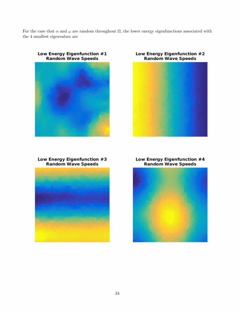
For the case that α and ω are random throughout Ω, the lower energy eigenfunctions associated withthe 4 smallest eigenvalues are

34

and the higher energy eigenfunctions associated with the 4 largest eigenvalues are

35

For the case that α and ω are uniform throughout Ω, the lower energy eigenfunctions associated withthe 4 smallest eigenvalues are

36

and the higher energy eigenfunctions associated with the 4 largest eigenvalues are

Note that the forms of the low energy states are comparable when the wave speeds are either randomor uniform, although those associated with random wave speeds are noisier. Yet the forms of the

37

high energy states are conspicuously more localized for the random wave speeds in relation to broadlysupported one for the uniform wave speeds.

• Exercise 5: Comparison of Membrane Models

Task

Summarize the functionals used in the lecture to model membranes or strings and explain underwhat circumstances the minimizing or stationary state for one functional agrees with that of anotherfunctional.

Solution

For simplicity only clamped string models are considered. The observations have natural counterpartsfor membranes.

Let u ∈ R3 represent a point on a continuously smooth string in R3. Let the position u(t) along thestring be parameterized by t ∈ [0, T ]. Then the length of the string is

L = L(u) =

∫ T

0‖u′(t)‖dt. (1)

When the string is reparameterized according to an arclength variable

s(t) =

∫ t

0‖u′(τ)‖dτ, s′(t) = ‖u′(t)‖, t ∈ [0, T ], s(T ) = L

then it follows

u′(s) = u′(t)t′(s) = u′(t)/s′(t) =u′(t)

‖u′(t)‖and thus

‖u′(s)‖ = 1. (2)

The string of shortest length connecting two points

u(0) = u, u(T ) = u

must satisfy

0 =δL

δu(u;v) =

∫ T

0

u′(t) · v′(t)‖u′(t)‖

dt, ∀v ∈ C∞0 ([0, T ],R3)

or after integration by parts,

0 =

∫ T

0v(t) ·

(u′(t)

‖u′(t)‖

)′dt+

u′(t) · v(t)

‖u′(t)‖

∣∣∣∣t=Tt=0

=

∫ T

0v(t) ·

(u′(t)

‖u′(t)‖

)′dt, ∀v ∈ C∞0 ([0, T ],R3).

Thus u must satisfy the boundary value problem(u′(t)

‖u′(t)‖

)′= 0, u(0) = u, u(T ) = u

and is uniquely determined by

u′(s)∣∣s=s(t)

=u′(t)

‖u′(t)‖= c ∈ R3

38

or with the boundary conditions, c = (u− u)/L,

u(s) = (1− s/L)u + (s/L)u, s ∈ [0, L]. (3)

As expected, the string lies along the straight line connecting the endpoints.

Now let w ∈ R3 represent a point on the string in the presence of an external force per unit lengthf ∈ R3. Let the position w(s) along the string be parameterized by arclength s in the absence of theforce. Suppose w satisfies the boundary conditions as before,

w(0) = u, w(L) = u

but now, in contrast to (2), there holds in the presence of the force,

‖w′(s)‖ 6= 1, s ∈ [0, L].

The work per unit length performed by the external force is of the product, force × displacement,f(s) · [w(s)− u(s)], s ∈ [0, L], and the total work performed by the external force is

Je(w) =

∫ L

0f(s) · [w(s)− u(s)]ds.

The elastic force acting tangentially along the string in the direction w′(s)/‖w′(s)‖ is the tension T .The relative change in length of the string in response to a stress is the strain,

τ(s) =‖w′(s)‖ − ‖u′(s)‖

‖u′(s)‖= ‖w′(s)‖ − 1. (4)

Here, (2) has been applied. Let the tension be modelled to depend linearly on the strain,

T (s) = κτ(s)w′(s)

‖w′(s)‖, s ∈ [0, L]. (5)

Then the strain energy

Ji(w) =1

2

∫ L

0κ(‖w′(s)‖ − 1)2ds (6)

results from integrating the variational derivative,

δJi

δw(w;v) =

∫ L

0T (s) · v′(s)ds =

∫ L

0

[κ(‖w′(s)‖ − 1)

w′(s)

‖w′(s)‖

]· v′(s)ds (7)

with the tension in (5) × the displacement dv = v′(s)ds. Thus, the total energy combining theopposing work efforts is given by

J(w) = Ji(w)− Je(w) =1

2

∫ L

0κ(‖w′(s)‖ − 1)2ds−

∫ L

0f(s) · [w(s)− u(s)]ds

which should be minimized by the position w(s). The variational derivative of J is given by

δJ

δw(w;v) = −

∫ L

0v(s) ·

[κ(‖w′(s)‖ − 1)

w′(s)

‖w′(s)‖

]′+ f(s)

ds

39

and so the position of the string is determined by the solution to the boundary value problem,

−[κ(‖w′(s)‖ − 1)

w′(s)

‖w′(s)‖

]′= f(s), w(0) = u, w(0) = u.

If the tension is modelled to be (at least approximately) independent of strain,

T (s) = κw′(s)

‖w′(s)‖with ‖T (s)‖ = κ for s ∈ [0, L] (8)

then integrating the variational derivative

δJi

δw(w;v) =

∫ L

0T (s) · v′(s)ds =

∫ L

0

[κ

w′(s)

‖w′(s)‖

]· v′(s)ds

gives an elastic energy

Ji(w) =

∫ L

0κ(‖w′(s)‖ − 1)ds =

∫ L

0κτ(s)ds (9)

involving only the strain (4) itself. Comparing (9) with (1) shows that minimizing Ji minimizes thelength of the string. In this context, the total energy combining the opposing work efforts is given by

J(w) = Ji(w)− Je(w) =

∫ L

0κ(‖w′(s)‖ − 1)ds−

∫ L

0f(s) · [w(s)− u(s)]ds.

The variational derivative of J is given by

δJ

δw(w;v) = −

∫ L

0v(s) ·

[κ

w′(s)

‖w′(s)‖

]′+ f(s)

ds

and so the position of the string is determined by the solution to the boundary value problem,

−[κ

w′(s)

‖w′(s)‖

]′= f(s), w(0) = u, w(L) = u.

Consider the circumstances under which the strain model in (5) may be justifiably approximated bythe strain model in (8). Suppose first that the motion of the string is purely in the longitudinaldirection. Then

w(s) = (w(s), 0, 0), w′(s) = (w′(s), 0, 0), ‖w′(s)‖ = |w′(s)|

and for (5) and (8) to be comparable, it must be that

|w′(s)| ≈ 1 + κ/κ ∈ (1,∞).

More generally, if the string is not necessarily strictly restricted to longitudinal motion but it is verytaut and with relatively constant tautness,

‖w′(s)‖ ≈ θ 1, s ∈ [0, L]

then for (5) and (8) to be comparable, it must be that

θ ≈ 1 + κ/κ ∈ (1,∞).

40

Now suppose that the motion of the string is purely in the transverse direction. Then

w(s) = (s, 0, w(s)), w′(s) = (1, 0, w′(s)), ‖w′(s)‖ =√

1 + w′(s)2

and for (5) and (8) to be comparable, it must be that

κ(√

1 + w′(s)2 − 1) ≈ κ or |w′(s)| ≈√

(κ/κ+ 1)2 − 1.

In the situation of small transverse displacements with |w′(s)| 1, κ must be sufficiently small inrelation to κ. When the string is very taut and |w′(s)| 1, then the form w(s) = (s, 0, w(s)) is notrealistic but rather

w(s) = (u(s), 0, w(s)), w′(s) = (u′(s), 0, w′(s)), ‖w′(s)‖ =√u′(s)2 + w′(s)2 ≈ |u′(s)|

which reverts back to the first case considered, in which motion is in the longitudinal direction.

In the case of small transverse displacements with w(s) = (s, 0, w(s)), the strain may be approximatedas quadratic

τ(s) =√

1 + w′(s)2 − 1 ≈ 12w′(s)2.

Then elastic energy becomes

Ji(w) =1

2

∫ L

0κw′(s)2ds

and the position of the string is determined by the solution to the linear Poisson boundary valueproblem,

−κ∆w = f, w(0) = u, w(L) = u

where u = (0, 0, u) and u = (0, 0, u).

These formulations may be considered in the context of thermodynamics, in which the infinitesimalformulation of energy is given by a sum of terms of type with force × displacement,

dF = KdL − ΦdA. (10)

Here, dL and dA have qualities of changes in length and area respectively. Length is measured alongthe string and area corresponds to that between an infinitesimal piece of unloaded string and its loadedcounterpart. The terms K and Φ are force terms with appropriate units so that F corresponds toan energy. In light of foregoing considerations, it is evident that the delicate term is dL. With thetension model (8), dL in (10) may be associated with the variational derivative of the length in (1),

δL

δw(w;v) =

∫ L

0dL(w;v), dL(w;v) =

w′(s) · v′(s)‖w′(s)‖

ds. (11)

Then with K = κ, the elastic energy is given by (9). On the other hand, the following variant of dLfor (10) results from the tension model (5),

dL(w;v) =

[(‖w′(s)‖ − 1)

w′(s)

‖w′(s)‖

]· v′(s)ds. (12)

With K = κτ , the elastic energy is given by (6).

41

Mathematical Modelling in the Natural Sciences SS21 ...

Documents

Transcript of Mathematical Modelling in the Natural Sciences SS21 ...