MATHEMATICAL MODELLING AND COMPUTER SIMULATIONS …

MATHEMATICAL MODELLING AND

COMPUTER SIMULATIONS OF

INDUCED VOLTAGE CALCULATIONS IN

AC ELECTRIC TRACTION

IMTITHAL M ABDULAZIZ

DOCTOR OF PHILOSOPHY

NAPIER UNIVERSITY, EDINBURGH

APRIL 2003

MATHEMATICAL MODELLING AND

COMPUTER SIMULATIONS OF INDUCED

VOLTAGE CALCULATIONS IN AC

ELECTRIC TRACTION

Imtithal Mohammed Abdulaziz

A thesis submitted in partial fulfilment of the requirements

of Napier University for the Degree of Doctor of

Philosophy

April 2003

DEDICATED TO

Basma, Mohammed, and Hiba

NOMENCLATURE

Abbreviations used:

A =

ABC

AC

AT

B

BR

BT

CCITT=

CCM

COS

CNS

CW

DC

EMC

emf

EMI

EW

F

FDTD =

FDM

FEM

FF

IV

Aerial earth wire

Absorbing Boundary Condition

Alternating Current

Auto1rransformers

Buried earth wire

British Rail

Booster 1rransformer

International1relegraph and 1relephone Consultative Committee

Carson's Correction Method

Cable on the Other Side

Cable on the Normal Side

Contact Wire

Direct Current

ElectroMagnetic Compatibility

ElectroMotive Force

ElectroMagnetic Interference

Earth Wire

Feeder wire

Finite Difference 1rime Domain

Frequency Division Multiplex

Finite Element Method

Self and mutual impedance of Feed system matrix

Induced Voltage

11

LM LocoMotives

M Messenger wire

mmf Magneto motive force

MTL Multi-conductor Transmission Line

OCS Overhead Catenary System

OHE OverHead Electrification

Olll. OverHead Line

PEC Perfect Electric Conductor

PUL Per-Unit Length

RF Mutual impedance of Return system against Feed system matrix

RR Self and mutual impedances of Return system matrix

R T Return conductor

TL Transmission Line

TP Touch Potential

3D Three Dimension

111

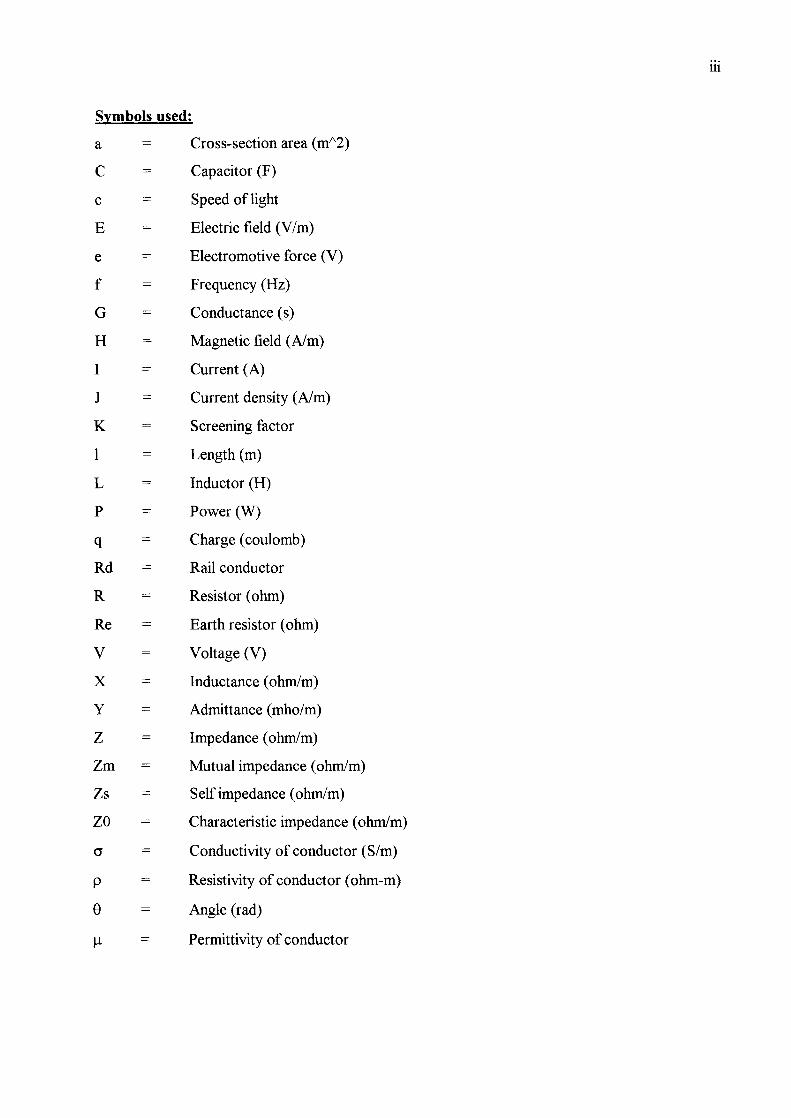
Symbols used:

a = Cross-section area (m"2)

C Capacitor (F)

c Speed oflight

E Electric field (Vim)

e Electromotive force (V)

f Frequency (Hz)

G Conductance (s)

H Magnetic field (Aim)

I Current (A)

J Current density (Aim)

K Screening factor

Length (m)

L Inductor (H)

P Power (W)

q Charge (coulomb)

Rd Rail conductor

R = Resistor (ohm)

Re Earth resistor (ohm)

V Voltage (V)

X Inductance (ohm/m)

y Admittance (mho/m)

Z Impedance (ohm/m)

Zm Mutual impedance (ohm/m)

Zs Self impedance (ohm/m)

ZO Characteristic impedance (ohm/m)

cr Conductivity of conductor (S/m)

p Resistivity of conductor (ohm-m)

e Angle (rad)

Il Permittivity of conductor

IV

E Permeability of conductor

0 Skin depth

a Attenuation constant

y Propagation constant

ro Angular frequency (rad/s)

\If Magnetic flux (weber)

7t pi (22/7)

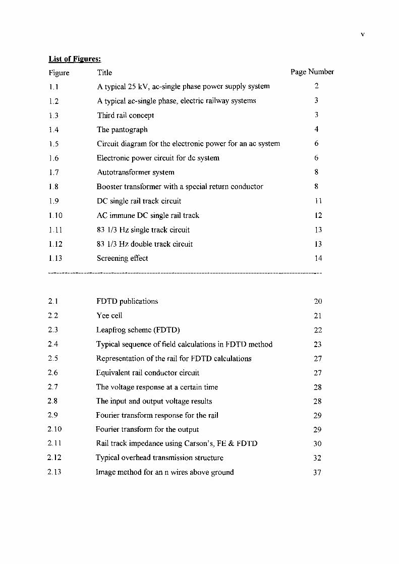
List of Figures:

Figure

1.1

1.2

1.3

1.4

1.5

1.6

1.7

1.8

1.9

1.10

1.11

l.12

l.13

2.1

2.2

2.3

2.4

2.5

2.6

2.7

2.8

2.9

2.10

2.11

2.12

2.13

Title Page Number

A typical 25 kV, ac-single phase power supply system 2

A typical ac-single phase, electric railway systems 3

Third rail concept 3

The pantograph 4

Circuit diagram for the electronic power for an ac system 6

Electronic power circuit for dc system 6

Autotransformer system 8

Booster transformer with a special return conductor 8

DC single rail track circuit 11

AC immune DC single rail track 12

83 1/3 Hz single track circuit 13

83 1/3 Hz double track circuit 13

Screening effect 14

FDTD publications 20

Yee cell 21

Leapfrog scheme (FDTD) 22

Typical sequence of field calculations in FDTD method 23

Representation of the rail for FDTD calculations 27

Equivalent rail conductor circuit 27

The voltage response at a certain time 28

The input and output voltage results 28

Fourier transform response for the rail 29

Fourier transform for the output 29

Rail track impedance using Carson's, FE & FDTD 30

Typical overhead transmission structure 32

Image method for an n wires above ground 37

v

VI

2.14 Diffusion of current and fields into semi-infinite conductor 40

2.15 Inductance calculated from flux through S and current on TL 42

2.16 One track case with 1250 A OCS, cable on normal side 44

2.17 One track case, 1250 A cable on the other side 45

2.18 One track case, 760 A cable on normal side 45

2.19 One track case, 760 A cable on the other side 46

2.20 One track for compensated system 47

2.21 Two track compensated system 48

2.22 n wires above ground 53

2.23 Per-unit length equivalent circuit 53

2.24 Per-unit length MTL model 54

2.25 Two conductor TL 56

2.26 FDTD method for two conductor TL 57

2.27 Typical non-homogeneous medium voltage result 59

2.28 Typical homogeneous medium voltage result 59

3.1 Uncompensated system (no BT) 61

3.2 Current, potential and impedance for a railway section 62

3.3 Mutual interaction among conductors 64

3.4 Distance between load and substation 69

3.5 Induced voltage at 30 km exposure, 1250 A (normal side) 78



3.8 Induced voltage at 30 km exposure, 1250 A (other side) 80






VB




3.17 Induced voltage at 30 km exposure, 1250 (CNS) Rl eliminated 86



3.20 Induced voltage at 30 km exposure, 1250 (CNS) R2 eliminated 87



3.23 Induced voltage at 30 km exposure, 1250 (COS) R1 eliminated 88

3.24 Induced voltage at 12 km exposure, 1250 (COS) R2 eliminated 88

4.1 Touch potential effect 91

4.2 Voltage position in different quadrate 92

4.3 Position of the cable AB (inside exposure) 93

4.4 Position of cable AB (outside exposure) 94

4.5 Touch potential, 1250 A CNS, load I=1250A 96

4.6 Touch potential inside exposure, CNS, 1250 A 96

4.7 Touch potential inside exposure, 1250 A, CNS, R1 eliminated 99

4.8 Touch potential inside exposure, 1250 A, CNS, R2 eliminated 99

5.1 Rail connected BT 102

5.2 BT with return conductor 103

5.3 One track case for load on the feed side of the BT 104

5.4 One track case load on the far side of the BT 104

5.5 Ideal transformer 105

5.6 BT for impedance calculations 105

5.7 Components involved for the transformer 106

Vlll

5.8 Current in return conductor 108

5.9 Earth current 108

5.10 Rail current 109

5.11 Rail voltage 109

5.12 One track case load at feed end ofBT 116

5.13 One track case load at far end BT 118

5.14 Two track case load at feed end 119

5.15 Two track case load at far end BT 124

6.1 Compensated system under short circuit current 133

6.2 Compensated component of short circuit condition 134

6.3 Uncompensated components of short circuit condition 134

6.4 Induced voltage for fault at feed end 136

6.5 Induced voltage for fault at far end 137

6.6 Induced voltage for fault at either side 137

6.7 Induced voltage for fault at feed end, 1m =3000 A 138

6.8 Induced voltage for fault at far end, im = 3000A 138

6.9 Induced voltage for fault at feed end, 1m = 668 A 139

6.10 Induced voltage for fault at far end, 1m = 668 A 139

6.11 Induced voltage for fault at either end R1, 1m = 6000A 140

6.12 Induced voltage fault at either end, R2, 1m = 6000A 140

6.13 Induced voltage fault at feed end, Rl, 1m = 6000A 141

6.14 Induced voltage fault at far end, R1, 1m = 6000A 142

6.15 Induced voltage fault at either end, R2, 1m = 6000A 142

6.16 Induced voltage fault at either end, R2 & R4, 1m =6000A 143

6.17 Induced voltage fault at either end, Rl & R3, Im=6000A 144

6.18 Induced voltage, fault at either-end, two-track, Rl&R3 eliminated 144

6.19 Induced voltage, fault at either-end, two-track, R2&R4 eliminated 145

6.20 Induced voltage using Carson & FDTD methods, two-rail 146

6.21 Induced voltage using Carson & FDTD, one-rail 146

List of tables:

Table

2.1

2.2

2.3

2.4

2.5

2.6

2.7

2.8

2.9

3.1

3.2

3.3

3.4

3.5

4.1

4.2

4.3

4.4

4.5

4.6

4.7

Title

Rail impedance using analytical and numerical methods

Conductor materials and properties

Open track, 1250A cable on normal side

Open track cable on the other side, 1250A

Open track 760 A, cable on normal side

Open track, 760A, cable on the other side

One track in an open area, compensated systems

Two track in an open area

Data for other conductors used

Load and fault currents for 1250A




Induced voltage and screening factor

Maximum touch potential

Comparison of max potential against max induced voltage

T ouch potential outside exposure

Maximum touch potential, R1 eliminated

Maximum touch potential, R2 eliminated

Max touch potential against max induced voltage (R1)

Max touch potential against max induced voltage (R2)

Page number

30

33

44

44

45

46

46

47

48

75

76

76

77

78

95

95

97

98

98

98

99

IX

5.1

5.2

5.3

5.4

5.5

5.6

6.1

6.2

6.3

Induced voltage outside for load at either end

Induced voltage inside, load at either end

Induced voltage inside, load at feed end

Induced voltage inside, load at far end

Induced voltage outside at feed end

Induced voltage outside at far end

Induced voltage using Carson & FDTD, load at either end

Induced voltage using Carson & FDTD, load at feed-end

Currents in the rail, earth & return, using CAD & FDTD

125

125

126

126

127

127

147

147

147

x

NOMENCLATURE

ABSTRACT

ACKNOWLEDGEMENTS

DECLARATION

CHAPTER (1)

CONTENTS

Introduction

1.1 Overview of electric railway systems and its problems

1.1.1 Electrification

1.1.2 Electric traction systems

1.1.3 Components of electric railway systems

1.1.4 Electrified railway configurations

1.1.5 Interference mitigation methods

1.1.6 Signalling and Telecommunications

1.1. 7 Track circuit

1.1.8 Screening factor

1.1.9 QuantifYing interference

1.2. Reasons for Calculations

1.3. Literature review

1.4. Summary

Xl

XVII

XVlll

XIX

1

2

2

4

4

5

7

10

11

14

15

15

16

17

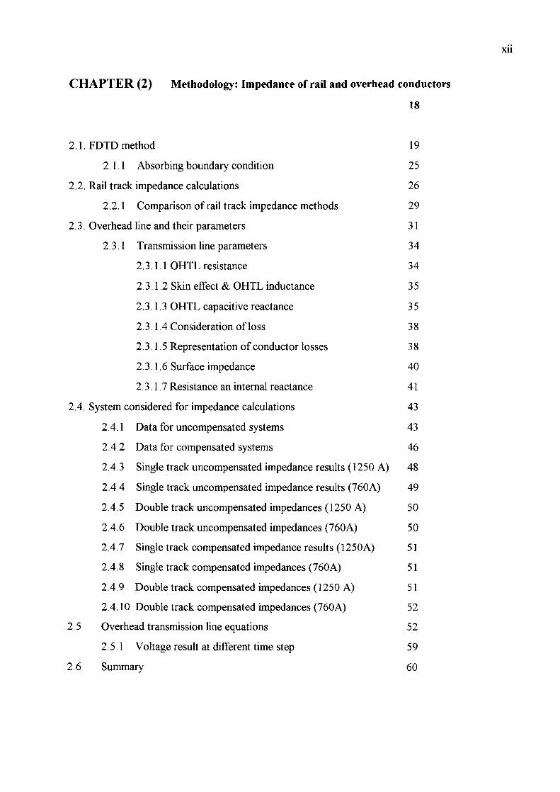
CHAPTER (2) Methodology: Impedance of rail and overhead conductors

18

2.1. FDTD method 19

2.1.1 Absorbing boundary condition 25

2.2. Rail track impedance calculations 26

2.2.1 Comparison of rail track impedance methods 29

2.3. Overhead line and their parameters 31

2.3.1 Transmission line parameters 34

2.3.1.1 OHTL resistance 34

2.3.1.2 Skin effect & OHTL inductance 35

2.3.1.3 OHTL capacitive reactance 35

2.3.1.4 Consideration ofloss 38

2.3.1.5 Representation of conductor losses 38

2.3.1.6 Surface impedance 40

2.3. 1. 7 Resistance an internal reactance 41

2.4. System considered for impedance calculations 43

2.5

2.6

2.4.1 Data for uncompensated systems 43

2.4.2 Data for compensated systems 46

2.4.3 Single track uncompensated impedance results (1250 A) 48

2.4.4 Single track uncompensated impedance results (760A) 49

2.4.5 Double track uncompensated impedances (1250 A) 50

2.4.6 Double track uncompensated impedances (760A) 50

2.4.7 Single track compensated impedance results (1250A) 51

2.4.8 Single track compensated impedances (760A) 51

2.4.9 Double track compensated impedances (1250 A) 51

2.4.10 Double track compensated impedances (760A) 52

Overhead transmission line equations

2.5. 1 Voltage result at different time step

Summary

52

59

60

Xll

Xlll

CHAPTER (3) Induced Voltage in Uncompensated Systems: Normal Operation

Conditions 61

3.1 Uncompensated system configurations 61

3.1.1 Conduction and induction current calculations 68

3.1.2 Voltage induced due to return system 71

3.1.3 Voltage induced due to feed system 71

3.1.4 System considered 73

3.2 Two-tracks rail return systems 74

3.2.1 Results for two tracks 74

3.2 One-rail return configuration 83

3.2.1 Calculations for one rail system 83

3.3.2 Results for one rail system 85

3.3 Summary 88

CHAPTER (4) Induced Voltage in Uncompensated System under Fault Condition:

The Touch Potential Effect 90

4.1 Touch potential 90

4.1.1 Formulation of touch potential 91

4.1.2 Determination of touch potential 93

4.1.3 Results 95

4.2 Touch potential for one-rail 97

4.2.1 Results 97

4.3 Summary 100

XIV

CHAPTER (5) Induced Voltage in Compensated Systems under Normal Operations

Conditions: A BT Compensation 101

5.1 BT with a Special return conductor 102

5.1.1 Induction effect from BT System 103

5.1.2 BT and its mathematical formulation 105

5.2 Compensated systems under normal operation 110

5.3 BT with return conductors 111

5.4 Rail connected BT 113

5.5 Two-rail return compensated 113

5.6 One-track case 116

5.6.1 Calculations for zone 1 116

5.6.2 Calculations for zone 2 118

5.6.2 Calculations for load at far end ofBT 118

5.6.2.1 Zone 1 118

5.6.2.2 Zone 2 119

5.7 Two-track case 119

5.7.1 Load at the feed end ofBT 119

5.7.1.1 Zone 1 121

5.7.1.2 Zone 2 122

5.7.1.3 Zone 3 123

5.7.2 Load at the far end of the B T 123

5.7.2.1 Zone 1 124

5.7.2.2 Zone 2 124

5.7.2.3 Zone 3 124

5.7.3 Results 125

5.8 one-rail return systems 126

5.8.1 Results 126

5.9 Summary 129

xv

CHAPTER (6) Induced Voltage in Compensated Systems under Short Circuit

Conditions 130

6.1 Method of Calculations l33

6.1.1 Compensated components l34

6.1.2 Uncompensated components l34

6.1.3 Calculation examples l34

6.1.4 Results l35

6.2 One-rail return systems 141

6.2.1 Results 141

6.3 Validation of the FDTD method 145

6.4 Summary 148

CHAPTER (7) Conclusion 149

7.1 Uncompensated systems 151

7.2 Compensated systems 152

7.3 Limitation of the Method 153

7.4 Future work 153

7.5 Summary 154

CHAPTER (8) References 155

XVI

APPENDICES

A Al Data Used 161

A1.1 Uncompensated systems 161

A1.2 compensated systems 163

A2 Program sample 164

B Derivations and formulae not included in the thesis 169

B.1 Carson's method 169

B.2 Skin effect and Inductance of OHTL 172

B.3 Transmission line equations from Maxwell's 178

C List of Publications 180

XVll

ABSTRACT

This thesis studies the foundation of a new method to calculate the induced voltage into line-side

signalling circuits using numerical modelling technique.

The need for accurate calculations of induction due to the high power overhead line has prompted

the development of such a new approach. Due to the complexity of the railway systems,

measurements are not always possible. An alternative approach, either analytical or numerical

analysis, is required. The analytical method has been developed and applied since the beginning of

electrification. Although this method provided reasonable results, it has certain limitations with

respect to frequency range, and hence accuracy. The development of computers provided us with

a new and exciting analysis, that is, mathematical modelling techniques. This project devised a new

method based on the finite difference time domain to calculate the impedances of the rail track and

overhead line and the longitudinal induced voltage into nearby signalling systems. The method is

simple and has been developed using known software (MATHCAD & APLAC) in order to reduce

any additional cost that may arise.

Calculations have been carried out for uncompensated systems (no booster transformer) and

compensated systems for various overhead catenary configurations relating to one-track and two

track layouts in open areas. Two different overhead ratings namely 1250 Amps and 760 Amps

have been considered. The signalling cable can be placed at either side of the track(s). Both

positions haven been considered as well as normal and fault conditions.

The position of the signalling cable has greater effect for one-track case than two-track or more.

The level of induction is also greatly related to the number of the track used (i.e. worse induction

for one track than for two, four or more). The design of the booster transformer is very important

in order to reduce any induction, this becomes more evident at short circuit conditions when the

magnetising current effect is more evident.

XV111

ACKNOWLEDGMENTS

My thanks first go to Dr Naren Gupta, my supervisor, whose continuous support and feedback on

the work have been invaluable. I am grateful to him for his kind help throughout, including in the

preparation of this thesis and ensuring timely completion of this project.

For one reason or the other, the author would also like to thank Prof. A Almaini, Mr J Sharp,

Prof. S Gair, Dr W Buchanan and Dr T Grassie.

My research-student colleagues participated with discussions and useful criticism. I am grateful to

all the staff in the school of Engineering, in particular Mr B Young and Mr B Campbell for

providing technical support. Many thanks to Ms Linda Dunn who has willingly helped with my

studentship arrangements.

I thank Professor Jorge Kubie, Head of department, and the whole of Napier University for giving

me the opportunity to do this work.

I have always been grateful to my parents who have enriched my life with great values.

Finally, my special thanks go to Osman for his on-going support and encouragement throughout

the project, without him I couldn't have done it.

DECLARATION

I declare that this thesis was composed and originated entirely by myself: other than those items

acknowledged in the text. The work was completed under a full time supervised program at

Napier University between March 2000 and March 2003.

XIX

Imtithal M Abdulaziz

CHAPTER (1)

Introduction

AC single-phase 25 kV, 50 Hz systems are commonly used for electrified railways world-wide.

A major problem with this system is the interference it causes into nearby signalling systems.

This interference can be very severe and endangers personnel and equipment. To constrain any

interference caused, booster transformers have been employed. However, these transformers

can add significantly to the cost of the railway systems. Hence to justify their use, it is essential

to know the level of longitudinal induced voltage into the signalling systems. This thesis relates

to work carried out by my supervisor Dr N K Gupta on models for induced voltage

calculations into line-side signalling cables. Gupta's model uses Carson's method for

impedance calculations, whereas in this thesis impedances have been calculated by FDTD

(finite-different-time-domain method). It also provides a mathematical model, which can be

modified and applied to different systems.

The main problems addressed in this thesis are:

1. Calculations of self and mutual impedance of return and feed conductors.

2. Calculations of the induced voltage for uncompensated systems both under normal and

short circuit conditions.

3. Calculations of the induced voltage for compensated systems both under normal and short

circuit conditions.

In this chapter, the general concept of interference will be discussed along with an overview of

relevant previous work in this field.

2

1.1 Overview of electric railway systems and its problems

1.1.1 Electrification

Electrification means the removal of the prime mover from the train. This provides a technical

strength because it removes items, which can fail and are costly to maintain and hence improve

performance. Although economically, this can be considered as a weakness in the sense that it

provides energy greatly in excess of that previously utilised and hence increases the initial cost,

but the long-term benefits outweigh the initial disadvantages.

The complete electrification of all major lines was carried out in the then British railway (BR)

by 1960, except between England and Scotland, which due to cost implications was completed

in 1967. Since then electric trains have proved to be more reliable and environment friendly

compared to the old fashioned steam or diesel trains.

A typical 25 kV a.c single-phase power supply system and an electric traction system are

shown in Figures 1.1 48 and 1.278.

I Supply authcui:ty 132 k:VT point

><

,

L.LI 132;25 kV, 1 phie iii -Transformer

c===J ____ .L ---c-----~

33 k"V. ET.EC-:T. Board Busbar

I R."_y_='y

- -1-

::=:>t<:::

~~

- ~'"

~ I ; <h~erheacl lines

~~ Signalling cables

- - - -

~ 1 .. -.><.. ><

_,-_L~ ..L'_, __ R..ail~-a.y feeder I -s~tion '

~.:: I >t< _ ::::.~ ......L. __ -'--__

Figure 1.1: A typical 25 kV, a.c single-phase power supply system

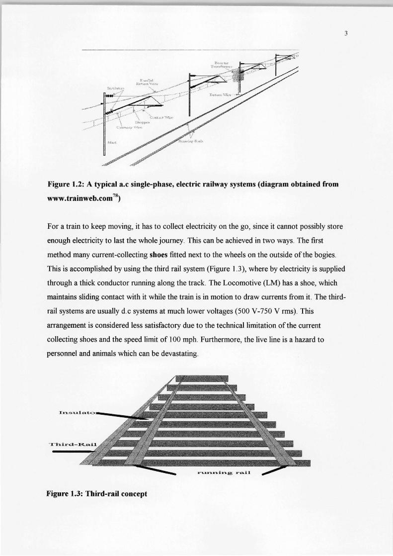
Figure 1.2: A typical a.c single-phase, electric railway systems (diagram obtained from

www.trainweb.com78)

3

For a train to keep moving, it has to collect electricity on the go, since it cannot possibly store

enough electricity to last the whole journey. This can be achieved in two ways. The first

method many current-collecting shoes fitted next to the wheels on the outside of the bogies.

This is accomplished by using the third rail system (Figure 1.3), where by electricity is supplied

through a thick conductor running along the track. The Locomotive (LM) has a shoe, which

maintains sliding contact with it while the train is in motion to draw currents from it. The third

rail systems are usually d.c systems at much lower voltages (500 V-750 V rms). This

arrangement is considered less satisfactory due to the technical limitation of the current

collecting shoes and the speed limit of 100 mph. Furthermore, the live line is a hazard to

personnel and animals which can be devastating.

r"l.1r1r1i:r::a.g ra.i.1

Figure 1.3: Third-rail concept

The second method uses a retractable pantograph (Figure 1.4) fitted to the top of one or

more of the carriages, the following discussion concentrates mainly on this system.

Figure 1.4: The pantograph (diagram obtained from trainweb.com78)

1.1.2 Electric traction systems

An electric traction system is basically composed of three groups of equipment; (a) Fixed

equipment required for bringing power from the supply point to the collecting devices on the

train. (b) The motive power units, and ( c) Other components which, although not directly part

of the first and second groups, contribute to or are influenced by the conditions within these

groups such as neighbouring telecommunication systems, the signalling systems and the rails

on which the motive power units run13.

4

A traction supply system is very complex compared to the normal power supply. Whereas in

power supply transmission systems the places at which the load is imposed are known and

definite, the load imposed on a traction supply system by individual motive power units' moves

between one point of supply and another as the train moves between one point and another.

Next follows a brief discussion of the components of electric railways.

1.1.3 Components of electric railway systems

An electric railway system is mainly composed of3:

1. Feeder stations, which supply power to the overhead wires.

2. Pantographs fitted to the electric trains, which collect the required traction current from

the overhead lines.

3. Return conductors, which return the current back to the feeder stations.

The return current passes via the wheels of the vehicle to the running rails and hence to the

supply point through the earthy bar connection. Aerial earth wires act as additional return

conductors.

1.1.4 Electrified railway configurations

In overhead electrification (OHE) systems, the supply of electricity is through an overhead

system of suspended cables known as the catenary. A contact wire or cable actually carries the

electricity; it is suspended from or attached to other cables above it, which ensure that the

contact cable is at a uniform height and in the right position.

The locomotive (LM) itself uses a pantograph, a metal structure that can be raised or lowered,

to make contact with the overhead contact cable to draw electricity to power its motors. The

electric current usually passes first through a transformer and not directly to the motors. The

return path for the electricity is through the body of the LM and the wheels to the tracks,

which are electrically grounded. Modern electric LM have some fairly sophisticated electronic

circuitry to control the motors depending on the speed, load, etc., often after first converting

the incoming 25kV AC supply to an internal AC supply with more precisely controlled

frequency and phase characteristics to drive AC motors.

The two types of power supply for the electric traction systems discussed above are:

(a) AC Single system: The overhead catenary is fed electricity at 25kV a.c (single-phase) from

electric sub-stations positioned at frequent intervals (35-50km) along the route. The sub

stations are spaced closer (10-20km) in areas where there is high load or traffic.

These sub-stations in turn are fed electricity at 750kV a.c or so from the regional grids

operated by state electricity authorities. A Remote Control Centre, usually close to the

divisional traffic control office, has facilities for controlling the power supply to different

sections of the catenaries fed by several sub-stations in the area. Figure 1.578 below shows the

electronic power of an a.c system.

5

+ve AC Overhead Line

Axle Brush -'Ie return through wheel and Iunrring rail

AC-DC Rectifier

Battary

* ~ DCoutput

Figure 1.5: Circuit diagram for the electronic power for an a.c system

6

(b) DC System: In d.c systems with overhead catenary, the basic principle is the same, with

the catenary being supplied electricity at I.SkV d.c. Usually the current from the catenary goes

directly to the motors. A d.c LM may however convert the d.c supply to a.c internally using

inverters or a motor-generator combination, which then drives a.c motors.

The a.c system is more expensive as the traction motors aboard a train usually requires a d.c

supply, hence a heavy and expensive transformer-rectifier has to be included in the multiple

unit. If a.c traction motors were used instead, an expensive frequency-alternator would have to

be included so that the traction speed of the motor can be controlled. The electronic power of

the dc system is shown in Figure 1.678.

Axle BlUsh

+ve DC Overhe~d Line

DC-AC Motor C:onvertor

DC-AC Auxiliary Convertor

-ve return through '\.Vheel and IUIUling rail

\ 2X3-Phae Motors

_____ Transfro:rner ____________ --

~~.~'

Battary

= =

Figure 1.6: Electronic power circuit for d.c system

The reason AC is now the preferred option for electrification is because AC substations are

much easier to build, as 25kV AC supply is available directly from the national grid. However,

the AC scheme causes some other troubles. For instance, with the basic system, the 2SkV AC

supply to the energised catenary can cause severe interference in telecommunication and other

circuits, which are in close vicinity. The induced voltage can be quite high; in the hundreds of

volts.

7

To mitigate this problem, a return conductor is provided parallel to the catenary, usually a little

above and to the side of the catenary. There are also booster transformers provided at

intervals. This method usually reduces the induced voltages in telephone and other circuits to

below 60V (although under fault conditions 400V-500V or more of induced voltage is not

unusual). Sometimes the return conductor is also connected to the rails at some points, to

ensure that more of the return current flowing through the rail stays in them rather than going

through the surrounding ground. This can also cause interference and other problems, although

not to the magnitude as that seen in a.c systems without booster transformers (Uncompensated

systems).

1.1.5 Interference mitigation methods

There two main methods that can be used to control and reduce any interference caused into

line-side signalling and telecommunication cables, these are:

(A) Dual system (a.c): In the dual a.c system (or 2 * 25kV a.c system), the supplied

electricity from the substations is actually at 50kV a.c. An autotransformer connected across

the 50kV supply has a centre tap connected to the rails, whereas connections from either end

of the transformer winding go to the catenary and the return conductor, this is shown in Figure

1.7. Thus, there is a 25kV differential between the catenary and the rails as before, but now

there is a 50kV difference between the catenary and the return conductor. (Note, however,

that the centre tap of the autotransformer, and hence the rails, are grounded to avoid hazards

to people or animals walking across the tracks). Also, at points further away from the

substation, the centre tap of the autotransformer can be adjusted so that the voltage between

catenary and rails is always 25kV, even as the total voltage across the catenary and the return

conductor drops due to resistive or impedance losses. So this allows substations to be spaced

further apart (30-50km). Thus far the dual system is only used in about 10% of British

'1 16 ral ways .

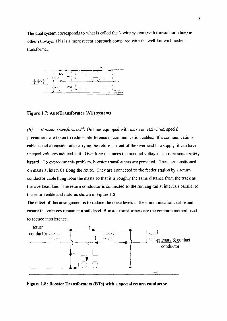
The dual system corresponds to what is called the 3-wire system (with transmission line) in

other railways. This is a more recent approach compared with the well-known booster

transformer.

-111tv

--1Ui:AU

"UU\-:i.--WI -<

2 kV "")

track [

\ Cantenary

Feeder ~-----~================~---

Figure 1.7: AutoTransformer (AT) systems

(B) Booster Transjormers15: On lines equipped with a.c overhead wires, special

8

precautions are taken to reduce interference in communication cables. If a communications

cable is laid alongside rails carrying the return current of the overhead line supply, it can have

unequal voltages induced in it. Over long distances the unequal voltages can represent a safety

hazard. To overcome this problem, booster transformers are provided. These are positioned

on masts at intervals along the route. They are connected to the feeder station by a return

conductor cable hung from the masts so that it is roughly the same distance from the track as

the overhead line. The return conductor is connected to the running rail at intervals parallel to

the return cable and rails, as shown in Figure 1.8.

The effect of this arrangement is to reduce the noise levels in the communications cable and

ensure the voltages remain at a safe level. Booster transformers are the common method used

to reduce interference.

return conductor L~AJ. ___ ----Jly~Vy '--_-4-__ .....--___ -'

l_~J

L..----4I---<'--_---l n'1latenary & contact conductor

rail

Figure 1.8: Booster Transformers (BTs) with a special return conductor

The normal arrangement of the conductors (overhead wires and running rails) for the a. c

single-phase system of railway electrification forms an unbalanced circuit. The effect is that by

magnetic induction the traction current causes induced voltages to appear in neighbouring

parallel conductors such as telecommunication cables, the effect varying directly with the

traction currents. The booster transformers are in effect power current transformers with unity

ratio and are used with their primary windings connected in series with overhead line and with

their secondary connected either directly to the running rails or to special return conductor.

9

The most important effect is the increase in impedance of the power circuit, which because of

its influence on voltage drop on the distribution system requires special attention to ensure that

the performance of the traction equipment is not adversely affected. There is also the effect on

the action on the definite distance impedance protective system fitted to the track feeder

equipment. Although the sensitivity of this equipment is increased to some extent by the

increase in impedance per unit length the step in impedance at the booster transformer itself

causes the location of the fault by the system to be less exact.

With the system with booster transformers connected directly to the running rails the potential

of the rail when several trains are taking current becomes progressively higher in steps until the

feeder station is reached.

It is important when designing the booster transformer insulation that the magnitude of

induced voltages from normal service has to be differentiated from the load due to:

• Cables & accessories

• Auxiliary supplies

• Battery equipment

• Feeder station

• Main transformers.

Booster transformer connected to a special return conductor is the most commonly used

method, and is discussed in detail later in the thesis.

10

1.1.6 Signalling and Telecommunications

For the railway to function, it is vital to have telecommunication and signalling equipment in

the near vicinity. This has a particular effect of the inevitable transfer of energy by induction

from one circuit to a neighbouring one. The extent of this transfer is dependent upon a number

offactors; in the case of three phase power lines, for instance, the currents are normally

balanced in all three phases and the resulting imbalance, which causes interference, is small.

Interference derived from harmonic currents may occur with both ac and dc electrification, and

this is an issue that needs special consideration to avoid undue noise in the light current

circuits.

Magnetic induction is the main cause of interference and its extent clearly depends upon the

magnitude of the currents in the power circuit. Some of the protective measures l that can be

applied to control interference are:

(a) At the source

(b) In the low current circuits affected and,

( c) By screening.

• Screening by cable sheath

• Induction from power cables

• Screening by rails.

Conductive coupling is another source of interference that remains to be mentioned in

connection with effects on railway signalling circuits. This occurs when two circuits have

common branch and there are three choices of protective measures against this type of

interference,

• Screening cables

• Compensation of supply

• Booster transformers.

Good grounding and shielding of cables also playa vital role in reducing electromagnetic

interference.

Railway signalling system uses track circuits to detect the different positions of the train. A

brief description about the different track circuits available are given in the section below

(1.1. 7)

1.1. 7 Track circuit

11

Track circuits provide means for detecting trains in various section of a track and, hence form

the basis for railway signalling. Although there are several types of track, the basic principle

underlying their application is the same. The entire length of the track is divided into a number

of track sections. For each section, current is fed in at one end and a relay is energised at the

other end when the section is clear (i.e. not occupied by a train). The presence of a train in the

track section causes the track relay to de-energise, because the supply current is diverted

through the axles of the train44,45. As mentioned there many different type of track circuits,

these are d.c, Reed, TI 21, and HVI covering different range of frequencies. In this thesis only

d.c track circuit as applied in a.c railway are discussed.

Track circuits for one-rail traction return systems are called single-track. Both d.c and a.c

single track circuits can be used for one-rail ac traction return systems.

The simplest track circuit, utilising a battery feed as shown in Figure 1.947 below, is not owing

to the false operation, which can be caused by ac potentials across the track.

1 I

DC feed

1,2 = Insulated block joints

Figure 1.9: DC single rail track circuit

Track relay

In other words, the relay, which is energised in the absence of a train, might not de-energise

when a train enters into the section. One remedy of this wrong-side failure would be to fit a

choke in series with the relay. Nevertheless, it would still be unsafe, because if the choke

12

became short circuited, the relay would no longer be immune to ac voltages and would readily

pick up due to the effects of ac current, when a train is standing on the track circuit. Almost all

dc track circuits therefore employ track relays, which are especially designed to be immune to

ac voltages. Additionally a choke may however be fitted at the feed-end of this track circuit in

order to reduce the ac current flowing through the track feed battery46,62,63. From above it

follows that a suitable dc track circuit would be as shown in Figure 1.10 below.

I

i I '<1 //~

J' /

/

• Iii I --I r --+

L ~I 1

DC feed 1 I

AC irrnnune track relay

Figure 1.10: AC immune DC single rail track circuit

In a two-rail return traction system, the traction current returning to the sub-station is shared

between the two rails; also the track circuit uses both rails. Ac track circuits are used in such

systems, which by virtue of their use in two-rail traction return systems are called double-rail

ac track circuits.

The frequency for single or double rail ac track circuits must be clear of 50 Hz and its

harmonics. 83113 Hz track circuits have been employed; this frequency may be obtained by

using a motor alternator set in which a synchronous motor having 3 pole pairs is coupled to an

alternator having 5 pole pairs. The motor speed would be 1000 rpm and the output from the

alternator is thus 505/3=83113 HZ46,47,48.

In 831/3 Hz track circuits, a central power supply is employed which provides two phases of

83113 Hz over a signalling area. Figure 1.1147 below shows one arrangement of the 831/3 Hz

single rail track circuits.

For optimum operation the local and control voltages on the relay should be in quadrature;

thus if the two 83113 Hz supply phases are in quadrature, the track circuit equipment should be

designed to produce a minimum phase shift. The feed-end equipment consists of a step-down

transformer and track-feed resistor.

13

At the relay end there is a filter tined to 831/3 Hz and a saturable transformer. The filter will

reject all normal levels of 50Hz. Whilst under fault conditions the saturable transformer will

prevent the relay from operating. This happens even if at the same time there were to be some

infiltrated 50Hz voltage of the correct phase relationship on the local winding of the track

relay, provided this does not exceed the level at which the detection equipment is set to

operate49.

---1--------•• ~-----------------------' ~.~~----

_________ ."l).~_------+--------//-________ /

~~~

~XIIO

NXt~~\ 1/3 Hz

N~CIIO EX'IIO

BXII0 NXI10

Figure 1.11: 83113 Hz single-track circuits

c? :- 83 113 Hz fil er I: ~.-

-~~O hI cc c=--r'l satura e trans,"ormer

I I track relay

The 83113 double rail track circuits are similar to single track one and are shown in Figure

1.1247

I I oa;,~, /~ I L: I c '1 ... -t! ~

1 ]1). [ fl' I~ r r BX~ll 0 83 113 Hz filt';;~ I ~

} ~I/3IIz ~ ~ NXII

NX'l10 BX'lIO -J,Jo

, rfv.-';:::;;aturahle transformer

JY~L.., BX' 11 0-- -=< i I

~ A NX'110 >~~ I L BXII0 NXII0 track relay

Figure 1.12: 83113 Hz double track circuit

The track-feed resistor may be of a lower voltage type due to reduced out-of-balance 50 Hz

voltages across the track. As the track circuit rail voltages are less for the double rail track

circuit an ac type auto impedance bond is used, designed to saturate at a low rail voltage in

order to prevent high voltages being fed to the track circuit equipment under fault conditions.

Signalling cables unlike telecommunication cables are unscreened, this is due to the fact that

only trained personnel are allowed in those area. However some sort of screening can be still

be achieved from the nearby earthed conductor. This is explained briefly in section 1. 1.8

below.

1.1.8 Screening factor of return system

The earthed conductors in the near vicinity such as cable sheaths, metal pipes, earth wire and

rails provide screening effect, which helps in reducing the induction caused. This effect is

known as the screening factor and is defined as:

The voltage induced in the presence of the conductor to which the screening factor refers to,

divided by the voltage that would be induced if the conductor to which the screening factor

refers were absent52,53,54

This effect is better understood from the Figure (1.13) below.

CD . 11

13

-:{-')--_.- __ 13

l V13 = ZI3*I1 12

23 I3=Y13/Z3 .. ~) L C') . ~

iign-"lli.==-c.=..ca=b=l -Y-2-3-=Z--1

23

*D "-12-=Z 12 *11 .~--~

Figure 1.13: Screening factor effect

14

The current I in the overhead line induces a longitudinal voltage ~2 in the neighbouring

signalling line. The railway and signalling lines can be considered as loop circuits each having

earth return. These two loops have mutual impedance and the induced voltage is directly

proportional to this mutual impedance and to the current following in the railway circuit.

1.1.9 Quantifying interference

15

One of the most controversial issues is the magnitude of electric disturbance caused to

signalling and telecommunication circuits along or near the electrified lines. When

electrification was carried out, cables replaced existing open wire routes on poles whose

sheaths could form an adequate screen against induction. However, it was important to remove

them for locating the overhead contact system supports.

The use of unbalanced circuits for dialling and ringing was a common practice. Due to the

huge cost of altering such work, it was decided to restrict the interference at the source. One

way of doing so is to introduce a return conductor with booster transformers at intervals of

about 2 miles. It is now common practice to use BTs and return conductors to reduce the level

of induced voltage. With the introduction of the EMC directive in 1996, further analysis and

quantification of the problem was required.

1.2 Reasons for Calculations

As BTs can add significantly to the cost of railway systems, their use should be justified. This

can only be accomplished if the level of the induced voltage is known. The methods used to

calculate this induction are not new and have been investigated for many years. However, the

work in this thesis is about a new approach which uses finite different time domain method for

mathematical and computer simulation.

The following section provides a brief account of some of the main contributions in this field.

1.3 Literature review

This section contains a brief review of literature helpful for understanding the material

presented in this thesis. The references in this section are relevant to the thesis as a whole and

to the material presented in Chapters (2),(3), and (4) in particular.

16

Several textbooks outside the field of railway and power engineering were particularly useful

for this project. The derivations and computational methods presented in Chapters (2) require

an understanding of differential form of Maxwell's equations. The first two chapters of

[Tatlove, 2000] 1 and the first chapter of [Sullivan, 2000]2 are recommended. [Roters, 1992f is

an excellent reference for electromagnetic and transmission line computations and [Grivet,

1990t for transmission of the high power line. [Perry, 1992f is an accessible and clear

reference for C programming. [Karmel, 1998t is a popular reference for electromagnetic.

[Magid, 1968f is a valuable reference concerning electromagnetic computations and is most

frequently cited in transmission systems papers concerning voltage and current computations.

[Yee, 1966t presents an explanation of the basic and the application of FDTD method, which

forms the backbone of the methods in this report.

The fundamentals of transmission line and its parameters are covered in [Wodelifi, 1978t, and

[Galloway, 1964]10. Electric traction is discussed in [Dover, 1963]1l, and [Partab, 1973]12.

[Electrification, 60]13 by lEE is a most comprehensive reference that contains different papers

on the basic of ac single-phase electrification. [Klewe, 1958] 14 describes interference problem

with respect to telecommunication cables. [Rosen, 1956]15 has the clearest explanation of the

interference problem. Supplemental to these, [Gupta, 1985t7 and [Millet, 1987, 1990] 16,17,18

provide good explanation of induced voltage calculations.

Gupta and Millet have forwarded an approach of the induced voltage analysis using

computational method, influential to this thesis. Gupta has applied his method to signalling

cables, while Millet's work is related to telecommunication cables. Millet also provided the

useful comparison between booster transformers and autotransformers. [CCITT, 1980]19

directive, suggesting the use of computers in these calculations, was also useful source.

[Tierney, 1983]20 contains a broad range of ideas and experiences concerning booster

transformers. Further references are given throughout the thesis.

1.4 Summary

This thesis demonstrates that the longitudinal voltage induced into signalling systems can be

computed with respect to any system parameter using mathematical modelling.

17

In this chapter, the use of booster transformers in reducing the interference and the voltage

level induced was discussed. Also considered was the usefulness of accurate computing of the

parameters involved. The layout of the remainder of the thesis is as follow:

Chapter (2) provides the methodology for calculating the impedances of rail-track and

overhead conductors and the general framework and assumption used for voltages and current

calculations.

Chapter (3) provides calculations and results of induced voltage for uncompensated systems

under normal operation conditions for one and two track layouts, for 1250 A and 760 A

overhead ratings.

Chapter (4) describes calculations and results for uncompensated systems under fault

conditions for the one and two track layouts

Chapter (5) gives the calculations and results of induced voltage for compensated systems

under normal operation for one and two track layouts and the two overhead ratings, as well as

analysis of the booster transformer itself.

Chapter (6) provides calculations and results of induced voltage under short circuit conditions

for compensated systems of one and two track layouts.

Chapter (7) discusses the results obtained, comparison with existing methods, limitation of the

project, suggestions for future work and draws conclusions.

Chapter (8) provides references

Appendix A gives data used in the thesis and sample of program developed.

Appendix B contains some formula derivation that is not included in the text.

Appendix C gives list of publications based on this thesis.

18

CHAPTER (2)

Methodology: The self and Mutual Impedance

of Rail and Overhead Conductors

Introduction

In order to calculate the voltage induced into signalling cables, the self and mutual impedances

of all conductors used, are required. It is important that the calculations are as accurate as

possible.

The most commonly used method for the calculation of rail impedance and overhead

parameters with respect to railways is Carson's correction method.

This standard analytical method was first introduced by 1. R. Carson21 in the US and almost

simultaneously by F. Pollaczek22 in Germany. Known as Carson's correction method today, it

provided the first analytical approach that included the earth return effect. Carson's method is

effectively used today and can produce reliable results for the lower range of frequency (load

flow studies). At higher frequencies however, the results converge very quickly and errors are

produced resulting in inaccurate calculations. This is due to the assumption made that the earth

is a semi-infinite series and the correction terms can be tedious and time consuming. With the

improvement in computer systems, it is now possible to use as many correction terms as

needed and hence improve the results. Moreover, developments in computer speed have made

the use of mathematical modelling possible. However the need for higher frequency analysis

has prompted engineers to find alternative approaches.

Hill and carpenter23 provided a complete investigation for the calculation of the rail tack

impedance using Finite Element Method (FEM), which requires the solution of Maxwell's

19

equations. The FEM requires that an appropriate boundary be defined first, and all bodies

(including the air and the ground) included in the boundary are modelled as areas. Each area

has its own geometric shape and physical properties, such as conductivity, permeability, non

linearly of magnetisation etc. All areas are subdivided into first order triangular finite elements.

The boundary conditions must then be given to allow Maxwell's equations to be solved

correctly according to the nature of the problem. The electromagnetic energy of the system is

then solved and, using energy relation, the impedance of the track is obtained. The FEM is a

powerful tool that is able to consider the skin and proximity effects simultaneously and give

accurate results. The disadvantages of the FEM include the high cost of software and

hardware, long computation times and the need for experience in using the software (training

cost).

This prompted the search for a more simple approach that can give the same as or close

reliability to the FEM. This has been accomplished by the use of Finite Difference Time

Domain method (FDTD). The FDTD method has been growing rapidly in the electromagnetic

calculations, its main advantage is that it is a direct solution of Maxwell's equation. The

method is simple to develop and implement.

In this section the impedance of rail track and overhead line conductors are calculated using

the FDTD approach. Existing software (MA TRCAD & APLAC) are used for these

calculations and hence any added cost is reduced. First a brief explanation of the FDTD

method is given in the following section.

2.1 FDTD Method

The Finite-Difference Time-Domain (FDTD) method is becoming one of the most popular

numerical methods for electromagnetic solutions. The method was first introduced by Yee8in

1966 and is also known as the Vee algorithm. The popularity ofFDTD has continued to grow

as computing costs declined. Furthermore, much research has gone into improving the method

and more work is still continuing in this field. The method is very useful for engineering

research since it is a direct solution of Maxwell's equations which is simply and elegantly

discretized. The method employs leapfrog scheme to solve the electric and magnetic field over

a wide range of frequencies. Although the method is very simple and easy to implement, it

20

received little attention when first introduced due to the high computational cost and speed

required at that time. With the progress in computers achieved, the interest in the FDTD began

to soar. An estimate of the progress in publications is shown in Figure 2.19. The FDTD method

can be applied in many areas where numerical and accurate calculations are required, such as

power and telecommunications engineering. This is particularly useful for complex systems

where practical measurements are not always possible.

2000 ~--------------------------------~

1990U-------------------------~~--b~

1980U---------------~~~

1960

1 5 10 20 40 350 440

Figure 2.1: FDTD publications (showing years between 1950-1995)

Maxwell's differential equations;

8E 6-+J=V x H

& 8H

Ii 8t = - V x E -----------(2 .1)

V·E=P 6

V·H=O

These four equations express the basic laws of electricity and magnetism. From the above it

can be seen that any change in the electric field (E) with respect to time causes a change in the

magnetic field (H) relative to distance.

In formulation, Maxwell's continuous equations convert to a discrete form, which is then

solved by a computer. The FDTD has the advantage over other methods in that it can take into

account all fields (electric & magnetic) in a three-dimensional (3D) model ifrequired24. A 3D

Yee cell is shown in Figure 2.2.

t delta z

Ez t Ex

-4- ----~-.-__

Z delta x

i /1 L_X

Figure 2.2: Typical Yee cell

/ /

/~ /'

./delta y

21

Another benefit of the FDTD method is that, since it is a time-domain technique, it can cover a

wide frequency range with a single simulation run. Electromagnetic simulation involves

representing the system required by a mathematical model. The type of model usually depends

on the required accuracy, simulation time and type of results required

The FDTD method belongs to the general class of differential time domain numerical

modelling methods. Maxwell's (differential form) equations are simply modified to central

difference equations, discretized and implemented in software. The equations are solved in a

leap-frog manner (see Figure 2.3); that is, the electric field is solved at a given instant in time

then the magnetic fields are solved at the next instant in time, and the process is repeated over

and over again25,26.

22

Wn+l /2 H"n+312

E"n-l E"n E"n+l

Figure 2.3: Leapfrog scheme

When Maxwell' s differential equations are examined, it can be seen that the time derivative of

the E field is dependent on the Curl of the H field. This can be simplified to state that the

change in the E field (time derivative) is dependent on the change in the H field across space

(the Curl) . This results in the basic FDTD equation in that the new value ofthe E field is

dependent on the old value of the H field on either side of the E field point in space. Naturally

this is a simplified description, which has omitted some details, such as constants, etc. showing

only the overall effect.

The H field is found in the same manner. The new value of the H field is dependent on the old

value of the H field (hence the difference in time), and also depends on the difference in the E

field on either side of the H field point. In order to use FDTD a computational domain must be

established. The computational domain is simply the ' space' where the simulation will be

performed. The E and H fields will be determined at every point within the computational

domain. The material of each cell within the computational domain must be specified.

Typically, the material will be free-space (air), metal (perfect electrical conductors (PEC)), or

dielectric. Any material can be used as long as the permeability, permitivity and conductivity

can be specified27.

Once the computational domain and the grid material are established, a source is specified. The

source can be an impinging plane wave, a current on a wire, or an electric field between metal

plates (basically a voltage between the two plates) depending on the type of the situation to be

modelled.

23

Since the E and H fields are determined directly, the output ofthe simulation is usually either

the E or H field at a point or a series of points within the computational domain. The sequence

of the FDTD method is better understood from Figure 2.4 below;

.. -.--~.---=:1 1=:IC1.>la~e 13 over enbre grid I

L- I

i-=:-forcc physical and absorbing ~ b01.>ndary coudibons

---T .--~------

C d'Vaced t:iYT1e by delta ~/2

-------,------

,------- ---,

ca.lcula.~e ~ over entire grid I

Figure 2.4: Typical sequence of field calculations in FDTD method

For a uniform perfect electric conductor, Maxwell's equations become:

oH J1-=-VxE

& ------------(2.2)

&oE/& = VxH

Consider the equation in the i (x) direction:

M! till till J1-_x = -Y __ z -----------(2.3)

M M ~y

Using the central difference approximation on both time and space to provide discrete

approximations:

1 1 .. n+- . n-- ~t

(HX1,},k) 2 = (HX1,j,k) 2 + J1& [(Eyi,j,kr- - (Eyi,j,k -lrJ----------(2.4)

~t ~y [(Ezi,j,kr - (Ezi -l,j,krJ

The half time-steps indicate that E & H are calculated alternately to obtain central differences

for the time derivatives.

24

There are six equations similar to (2.4) in total. These define the E & H fields in the x, y, and z

directions and are shown below.

The permittivity (E) and permeability (J.l) values in these cases are set to approximate values

depending on the location of each of the field component.

n+~ n-~ /).1 (Hxi,j,k) 2 = (Hxi,j,k) 2 +-[(Eyi,j,kf -

,,!J..z

(Eyi,j,k -If]-~[(Ezi,j,k)n - (Ezi -I,j,kf] ,,/).y

1 1 .. n+2 _ .. n-2 /).1 .. n

(HYl,},k) - (HYl,},k) +-[(EZl,},k)-,,!J..x

(Ezi,j,k -If] -~[(E-Xi,j,kf - (Exi -I,j,kf] ,,!J..z

n+~ n-~ ~t (Hzi,j,k) 2 = (Hzi,j,k) - +-[(Exi,j,kf

,,/).y

(Exi,j,k _I)n] - ~[(EYi,j,k)n - (Eyi -l,j,k)n] fIIJ..x

---------(2.5)

1 111 n+--

(Exi,j,k)n=l = (Exi,j,k) 11 +-[(Hzi,j+l,k) 2_

Jll1y 1 1

11+- 111 n+-(Hzi,j,k) 2 ]--[(Hyi,j,k) 2 -(Hyi-I,j,k)

Jl/1z

1 n+-

1 ~t n+-

(£yi,j,k)"+1 = (Eyi,j,k)" +-[(Hxi,j,k+l) 2

Jl/1z 1

n-+- - ~t

(Hxi,j,k-I) 2 ]--[(Hzi,j,k+l) Jl/1z

1 n + -

2 - (Hzi - I, j, k)

1 I1t n+-

(Ezi, j', k) 11 + 1 = (Ezi, j, k) 11 + -[(Hyi + I, j, k) 2_

. Jl/1x

1 nt-

1 1 1 11 + - 111

(Hyi,j,k-I) 2 ]--[(Hxi,j+l,k) Jll1y

n+- n+-

2 -(Hxi,j,k) 2] ------(2.6)

It is important that the time step is set to a certain limit for the stability criteria requirement,

this given as;

where c is the speed of light.

25

Now that the model and the equations are set, the boundary conditions on the sources and the

conductor model are required to obtain reliable results. It is important that the right boundary

condition should be applied for meaningful results.

2.1.1 Absorbing boundary condition (ABC)

The main solution using FDTD method is within the computation region set at the beginning of

the simulation. For open structure such as overhead and rail conductors and antennas, it is

important that analysis should extent beyond the computation region to infinity in order to

obtain meaningful results for these calculations. Now an obvious problem is how to extend the

simulating structure to infinity rather than the computation region.

The solution is, instead, to terminate the computing region with absorbing boundary

conditions that "eat" the incoming wave or pulse in a way that does not give rise to any

reflections. In the realm of FDTD simulations no perfect absorbing boundaries exist - they all

reflect some part of the incoming wave or pulse. However, these boundaries absorb most of

the wave and therefore open structures can be modelled with sufficient accuracy. Quite often

an absorbing boundary condition is abbreviated to ABC in the FDTD literature1,28,29,30,31.

26

From the definition of the FDTD method we proceed to the system considered and calculation

steps.

The steps taken to calculate the induced voltage into signalling systems are as follows;

Step 1: Calculation of rail track impedance

Step 2: Calculation of overhead transmission line parameters (inductance, resistance &

capacitance) .

Step 3: development of the voltage and current equations.

2.2 Stepl: Rail-track impedance calculations

In this thesis the rail-track conductor above ground is solved simply by dividing it up into

appropriately sized unit cells, each with a certain value, setting initial values for all of the field

components, then calculating the field equations iteratively for as long as the response is of

interest.

The behaviour of the field components over the problem space gives an essentially complete

characterisation of the behaviour of the structure. It can then be post-processed and

information over a broad frequency range can be obtained in a single run. This algorithm, as

well as giving an understanding of the operations implied by Maxwell's equations, is a powerful

and practical solution method.

Note: certain assumptions have been made in order to simplify the model, these are:

1) All track materials are assumed to be anisotropic,

2) The rails, ballast and sleepers are assumed to be homogeneous,

3) The ground is stratified into homogenous horizontal layers that can be assigned different

material properties,

4) The rail fastenings to the sleepers are not modelled.

The impedance of the rail track is solved first and, using the same approach, the overhead

parameters are obtained. The rail track impedance model is shown in Figure 2.5 below;

Rail '\

"

Ground Plane

Figure 2.5: Representation of the rail track

The equivalent electric circuit for two rail conductor is as shown in Figure 2.6.

o~ ____________________ ~ .. []

Figure 2.6: Two rail conductor circuit

27

The above rail structure is analysed using APLAC (see Appendix B, for program description);

an electromagnetic software which has built-in components and FDTD analysis facilities. The

required components are set and the program is written in a code similar to C, an example is

shown in Appendix A.

The voltage response and the currents are obtained for the rail-track and hence the impedance

is calculated. The results in Figures 2.7-2.10 are for 50Hz system frequency. The frequency

can be changed according to requirements.

Response of a rail conductor Aplac 7.70 User: Napier University Nov 13 2002 1.00~--------------------------------'

Volta 0.50

V

0.00

-0.50

-1.00+-~--~~----~~--~----r-------;

0.000 10.000 20.000 30.000 position/cells

(h*vect)

Figure 2.7: The voltage response at a certain time

Response of a rail conductor

40.000

Aplac 7.70 User: Napier University Nov 13 2002 1.00 1.00

input 0.50

V

0.00

-0.50

outpu 0.50

V

0.00

-0.50

-1.oo+---------~--------~--------~---------+-1.00 0.000 250.000p 500.000p 750.000p 1.000n

tirne/s Vern ("Rail" I 13 ····""·······Vern ("Rail" I 13

Figure 2.8: The input and output voltage results

28

Once the computational domain and the grid material are established, a source is specified. The

source can be an impinging plane wave, a current on a wire, or an electric field between metal

plates (basically a voltage between the two plates) depending on the type of the situation to be

modelled.

(h*vect) Aplac 7.70 User: Napier University Nov 12 2002 0.30~----------------------------------,

V

0.22

0.15

0.07

0.116

spectrum

0.232 Hz

0.348

Figure 2.9: Fourier transform for the rail

Vem("Rail", 13, 8, 0, 13, 8, 1)

0.463

Aplac 7.70 User: Napier University Nov 13 2002 0.20~----------------------------------,

V

0.15 .

0.10

0.05

O.OO~~'"~'----~--~-'~-r--~----~~~~~ 0.000 155.925G 311.850G 467.775G 623.700G

Hz DFT

Figure 2.10: Fourier transform for the output.

2.2.1 Comparison of rail track impedance methods

In order to establish the credibility of the method mentioned above, comparison with an

existing method is required.

29

The rail impedance results over the frequency range of 50Hz-IMHz are given for three

different methods; Carson's correction term, FEM and FDTD. The results are shown in Table

2.1.

Frequency (Hz) Carson (ohm/km) FE (ohm/km) FDTD (ohm/km)

50 0.402 0.400 0.401

100 0.475 0.456 0.457

1k 1.59 1.230 1.301

5k l.672 l.251 l.312

8k l.691 1.273 1.324

10k 2.258 2.451 2.431

30k 2.432 2.458 2.441

60k 2.545 2.537 2.489

80k 2.621 2.562 2.576

lOOk 4.102 3.572 3.631

200k 9.746 3.924 4.113

400k 12.589 4.127 4.213

600k 14.972 4.365 4.387

800k 15.134 4.392 4.401

1M 15.785 4.689 4.712

Table 2.1: Rail impedance using analytical and numerical methods

18

16

14

E 12 .c o -; 10 CJ

; 8 "C GI C. 6 .E

4

-+-Carson (ohm/km) FE (ohm/km) FDTD (ohm/km)

50 100 1k 5k 8k 10k 30k 60k 80k 100k 200k 400k 600k 800k 1M

Frequency (Hz)

Figure 2.11: Rail-track impedance using Carson's, FE & FDTD methods

30

31

Figure 2.11 shows the results of the rail-track impedance using three different methods. From

the figure we can see that the FE and FDTD methods provide better results for the calculations

of conductor above ground impedance. Although all three methods provide almost exactly the

same results for frequency up to 80K Hz, it is clearly obvious that Carson's method

overestimates the value of the impedance, this is due to the assumption used (earth is semi

infinite series). The FDTD provides reliable results and is in agreement with the FE method,

this is due to the fact these methods take into account the material properties of the conductors

and the ground in the from of the conductivity, permeability and permittivity.

2.3 Step 2: Overhead lines (OHL) and their parameters

Overhead transmission lines are used to carry electrical power for large-scale electricity supply.

The lines form a network joining generating stations and load centres. Transformers are used

to connect lines operating at different voltage levels. For the control of the voltage and power

factor and to protect against lightening and other disturbances, electrical calculations for the

transmission lines are required.

For a short power line only the series impedance has an effect on its behaviour, the capacitance

effect can be considered as negligible. The line impedance consists of two parameters;

resistance of the conductor and the reactance which is caused by magnetic flux surrounding the

conductors and passing between them. Those two parameters can be measured or calculated

using the line dimensions and certain other factors as will be described33.

F or the line shunt admittance, only the line capacitive susceptance can be considered since

conductance currents to ground and between conductors are negligible for overhead lines. The

capacitive shunt reactance can also be calculated from line dimensions.

The types of conductors used in overhead power transmission lines are stranded hollow

conductors of different constructions. Solid conductors are also used to a certain extent. Some

typical overhead line support structures with the conductors are shown in Figure 2.12.

/ \ ff=~--.~ _.-1i (~ / '---'

>--------C>---~

6 6 (:S 6 6 6

/ \

,----..

Figure 2.12: Some typical overhead transmission structure

The conductor materials which are in general use for OHL are; hard-drawn-high conductivity

copper, hard-drawn aluminium, aluminium alloy and steel-cored aluminium. Data relating to

these materials and to stranded conductors made from these materials are given in Table

(2.2)34.

32

+ Application

Contact Wire

Messenger

Earth Wire

Feeder

Buried Earth

Wlre

Continuity

Rail

Table 2.2:

Material Composition Overall DIA. Resistance

No. ofStrandslDIA. (MM) (MM) (ohms/km)

HD.Copper Solid ]2.3 0.1695

AWAC Alumoweld 6/2.42 16.9 0.1903

Aluminium 3112.42

ACSR Steel 712.89 16.3 0.2143

Aluminium 1612.57

ACSR Steel 7/2.89 23.5 0.1027

Aluminium 26/3.72

Bare 7/3.5 13.0 0.280

Copper (67.4 mmA2)

Steel 19/3.81 20.0 0.670

Steel (146.0)* 0.024

+ Data given for new contact wire-for impedance and current rating

calculations, 25% reduction in area due to wear is allowed

* Diameter of equivalent conductor, having circular cross-section.

The most important property of an OHL conductor material is high tensile strength (high

breaking load), so that longer spans can be achieved with the smallest possible sag. This

provides a reduction in the number and height of the towers (or poles) and the number of

insulators required. It is also important that the conductors have low resistance to reduce

power loss and voltage drop35,36.

33

For the development of overhead line parameter calculations, many simplifying assumptions

have been made and calculations were carried out for single track and double track at system

frequency (50 Hz). Generally the parameter calculations are based on conductor configuration

for every system. The bonding of the rails are neglected throughout the study.

34

2.3.1 Transmission line parameters (TL)

The parameters of multi-conductor transmission line (MTL) can generally be divided into two

groups; those at power frequency and those at higher frequencies. The first are required for

load flow studies, system stability, and fault levels. The second are needed for re-striking

voltages, radio interference, propagation characteristics of power line and switching over

voltages.

In steady state (SS) the resistance of an overhead TL determines the energy loss and therefore

the current carrying capacity of the line. The series reactance controls directly the maximum

power flow capability of the line and to some extent the system fault level. The shunt

susceptance determines the V AR generation and affects the system voltage profile.

2.3.1.1 Overhead transmission line (OHTL) resistance

The effective resistance ( = power loss (w/rms)/ I 2 (amp)), is equal to dc resistance of the

conductor only if the current distribution over the cross area of the conductor is uniform. The

dc resistance is given by;

Rdc = pL/ A (ohm)-----(2.8)

where;

p= resistivity of conductor material

L = length

A = cross-section area.

Or

Rdc = 2.Sp/JTa 2 ohmlmile----(2.9)

a = conductor radius

The dc resistance of stranded conductors is greater than that computed above due to spiralling

of the strands which makes them longer than conductor length. The increased resistance due to

spiralling was estimated as 2%37 for concentrically stranded conductors.

35

2.3.1.2 The skin effect and OHTL inductance

When an alternating current flows in a conductor, the alternating magnetic flux within the

conductor induces an e.m.f., which causes the current density to decrease in the interior of the

conductor and increase on the surface. This phenomenon is known as the skin effect which

results in changes of the resistance and internal inductance of the conductor. Skin effect

becomes more pronounced as the frequency increases and for large diameters of the conductor.

Analytical and approximated methods have been developed to estimate the resistance ratio

(Rae / Rdc ) and the internal inductance ratio (L; ac / L; de)' These approximated methods are

based on Bessees and Butterworth39. Bessel function provides better results for higher

frequency (> 12kHz) while Butterworth can be used effectively for frequencies up to 12 kHz,

both formulas can be found in Appendix B.

The inductance of an overhead line on the other hand is a combination of internal (due to

internal flux linkages) and external (due to external flux linkages) inductance (derivations are

given in Appendix B) and is given as;

L = L. + L --------(2 10) mt ext .

where, f.1 Lint = - and

8JT f.1 D Lext = - ·In( -) --------(2.11)

2JT r

giving the total inductance reactance of

f.1 1 D L = -(- + In( -)------(2.12)

2JT 4 r

where D = distance between conductors.

2.3.1.3 OHTL capacitive reactance

In order to calculate the capacitance, the following assumptions are made:

1. OHTL conductors are on straight lines at average heights above the ground and parallel to

it.

2. Each conductor is at the same potential throughout its length and the charge on it is

uniformly distributed.

36

3. The existence of the line impedance is neglected.

4. Effect of surrounding structure is neglected.

5. Earth surface is an equi-potential plane of zero potential.

For a multi-conductor line, the inductance and capacitance matrices are shown below;

For L matrix, the inductance is obtained from the relationship of the total magnetic flux in the

i-th circuit, to all the line currents producing it as;

[ ¥F ] = [ L ][ 1]

expanding; --------( 2. 13)

¥FI II! 112 lIn II

¥F2 112 122 I ... 12n 12 =

¥Fn lIn 12n Inn In

If we interpret the above relations in a manner similar to the n-port parameters, we obtain the

following relations for the entries in L:

Thus the inductance can be computed by placing a current on one conductor and setting the

current on all other conductors to zero. The definition of the i-th circuit is critically important

in obtaining the correct value and sign of these elements.

Now the capacitance matrix entries are considered. C relates the total charge on the i-th

conductor PUL to all of the line voltages producing it as;

[Q]=[C] [V]-----(2. 15)

Expanding the above;

37

n

LCIk - C12 - c1n

~ q1 k=l n

q2 - C12 LCU - C2n V2 ------(2.16) =

k=l

qn n V

LCnk n

1n - c2n k=l

Applying the same approach above, the c matrices can be obtained as;

The C matrix can also be obtained from the relation:

[V]=[P][Q]-----(2.18)

And [C]=[PY'-1.-----(2.19)

Using the method of images as described below, the inductance and capacitance of an "n" wire

above ground can be obtained form the Figure 2.13.

Ii

hi

~. ( . ) ~

Ii

Ij~O

/~~

( (~ ) /

~~,/

Figure 2.13: Images method for an "n" wires above ground

hj

hj

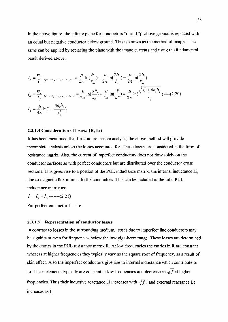
38

In the above figure, the infinite plane for conductors "i" and ')" above ground is replaced with

an equal but negative conductor below ground. This is known as the method of images. The

same can be applied by replacing the plane with the image currents and using the fundamental

result derived above;

II'. I /I h /I 2h /I 2h I = -""-' = -r""-ln(-' ) + -r""-ln(-' ) = -r""-ln(-' )

II I h ~ ... =1;_1 ~1;+1 = ... =ln~O 2 2 h 2 i 7[ r.wi 7[ , 7[ rwi

Vi I J1 S * J1 S J1 ~S~ + 4hihj 1=- ______ =-In(-)+-ln(-)=-ln( )----(2.20)

lj I. 11 - .•• -1 fi-l-1 j+l-···-1 n -0 27[ S 27[ S * 27[ S J lj Ij

/I 4hh I =_r"" In(I+-' _J)

Ij 47[ S2 lj

2.3.1.4 Consideration oflosses: (R, Li)

It has been mentioned that for comprehensive analysis, the above method will provide

incomplete analysis unless the losses accounted for. These losses are considered in the form of

resistance matrix. Also, the current of imperfect conductors does not flow solely on the

conductor surfaces as with perfect conductors but are distributed over the conductor cross

sections. This gives rise to a portion of the PUL inductance matrix, the internal inductance Li,

due to magnetic flux internal to the conductors. This can be included in the total PUL

inductance matrix as:

L = L + L -------(221) 'e .

For perfect conductor L = Le

2.3.1.5 Representation of conductor losses

In contrast to losses in the surrounding medium, losses due to imperfect line conductors may

be significant even for frequencies below the low giga-hertz range. These losses are determined

by the entries in the PUL resistance matrix R. At low frequencies the entries in R are constant

whereas at higher frequencies they typically vary as the square root of frequency, as a result of

skin effect. Also the imperfect conductors give rise to internal inductance which contribute to

Li. These elements typically are constant at low frequencies and decrease as Jl at higher

frequencies. Thus their inductive reactance Li increases with .J7, and external reactance Le

increases as f

The current density and the electric and magnetic fields in good conductors are governed by

the diffusion equation. Ampere's law relates the magnetic field to the sum of conduction

current and displacement current as:

- - -V x H = aE + jOJ&E --------(2.22)

39

In a good conductor, the conduction current greatly exceeds the displacement current which is

satisfied for most metallic conductors and frequencies of reasonable interest.

Thus the above equation can be approximated as:

- -V x H = jaE -----(2.23)

Similarly Faraday's law:

- -V x E = - jOJ/lH -----(2.24)

Taking the curl of Faraday's law gives

- - 2 - . V xCV xE) = V ·(V·E - V ·E) = - jOJ/lV xH ------(2.25)

Substituting Gusses's law:

V· &oE = 0 -------(2.26)

Gives;

2 - . -V . E = jOJ/laE ----(2.27) (since j = crE)

V 2 • j = jOJ/l(Jj -----(2.28)

Now the resistance of a wire and internal inductance may be considered:

F or circular cylindrical conductors (wires), two identical wires in homogeneous medium with

radius r wand separated by s;

40

r = 2Rs ( s ) ------(2.29) ohm/m 2:rrw 2rw

~( s)' 1 2rw

where

1 ~7if,ll Rs = uo = ~ -----(2.30)

2.3.1.6 Surface impedance of plane conductors

Consider a semi-infinite conductor half-space with parameters 0', E, /l, whose surface lie in x-y

plane as shown in Figure 2.14.

E'O E'O E'O

\ <" ---

< « ------/1

"

<:/ ---------- --- .. (J ,f.!,£

Figure 2.14: Diffusion of current and fields into semi-infinite conductor half-space

Assuming that electric field (E) and associated conductor current density are directed in the z

direction, diffusion equation term of z directed E field becomes:

2 ~

d F; z = jclJ,lIU E z --------(2.3 1 ) dx

Similarly for magnetic field, Hy, and jz;

where

0= ~(Skin-dePth) JTjf.1u

--------( 2.32)

H 0' Eo, .10' are surface quantities.

41

The surface impedance can be defined as the ratio of the z-directed E field to surface and total

current density;

Eo Zs = -. ------(2.33)

it

.I = J:' .I ,dx = .10 -----(2.34) t 0 - 1+.1

Z s= Rs + jOJL; ------(2.35)

1 J JTjf.1 Rs = uo = ----;;- -----(2.36)

If roL; = Rs ' then

Zs = J;; -----(2.37)

2.3.1. 7 Resistance (R) and internal inductance (L j ) of wires

F or a circular cylindrical conductor (wire) and perfect conducting, the current flows on the

surface of the conductor. Rand L j result from the current and magnetic flux internal to the

imperfect conductors in a fashion similar to that of the surface impedance ofa plane conductor.

Lj results from magnetic flux internal to the conductor that links the current.

F or a wire, assuming current is symmetric about the axis of the wire, the radius is r w ;

42

Using the above information the inductance and resistance can be obtained from the FDTD

analysis. From the FDTD figure for transmission line the flux integral would be performed on

the surface S with the direction ofthe surface vector DS as shown in Figure 2.15. The current

integral would be performed along the contour C.

reter~e condu.ctor C

~ ~-

Figure 2.15: Inductance calculated from flux through S and current on the transmission

line

¢ f B.ds f J1l! .ds L = - = = ------(2.39)

I fH.d! fH.d!

In the FDTD grid these integral translate into sums as given by;

f.1LH.~.~ L = -------(2.40)

LH.~

Thus, an inductance per unit length can be calculated by taking the ratio of the sum of the H

field values over the surface S, and the sum of the H fields in the direction of dL divided by the

length along the transmission line that the surface extends over.

The capacitance is defined as the ratio of the charge in an enclosed surface to the

electromagnetic potential of the surface region.

Q f D.ds f&E.d~ C = - = = -----(2.41)

V f E.dl f E.dl

In the FDTD grid, these integrals translate into sums as given by:

&LE.11.11 c = -----(2.42) LE.11

F or the calculations of the self and mutual impedances of the conductor i and j at system

frequency (50Hz), the equations are as follow;

2.4 System considered for self and mutual impedances calculations

43

The data for the system considered are shown below, the self and mutual impedance for single

track and double track railway systems with two different overhead rating (1250 and 760

Amps) were calculated and the results are given below:

Note: self and mutual impedances were calculated at system frequency, hence the impedance

consists of resistance and inductance only as the capacitance effect is considered to be

negligible

2.4.1 Data for uncompensated systems

Tables 2.3-2.6 show the position (x & y) of the conductors for uncompensated systems with

two different overhead ratings and cable (signalling) position. Their positions are shown in

Figures 2.16-2.18 and 2.19 respectivel/7.

44

Conductor X(m) Y(m)

Rl -.08 0.1524

R2 0.8 0.1524

Bl -4.5 -1.66

EWI -2.988 6.875

EW2 -3.463 6.093

M 0 6.6

CW 0 5.7

F -4.18 6.543

Table 2.3: Open track 1250 amps cable on normal side (Figure 2.16)

EWI

F

~l~YI -"~R2 ! x o "~

~/ ",,-

Figure 2.16: One-track case with 1250 Amps OCS configuration, cable on normal side

Conductor X(m) Y(m)

Rl -.08 0.1524

R2 0.8 0.1524

B2 4.5 -1.66

EWI -2.988 6.875

EW2 -3.463 6.093

M 0 6.6

CW 0 5.7

F -4.18 6.543

Table 2.4: open track 1250 amps cable on the other side (Figure 2.17)

45

E"W2c>--_

Figure 2.17: One-track case with 1250 Amps oes configuration, cable on the other side

Conductor X(m) Y(m)

Rl -.08 0.1524

R2 0.8 0.1524

Bl -4.5 -1.66

EWI -2.988 6.875

M 0 6.6

CW 0 5.7

Table 2.5: Open track 760 amps cable on normal side (Figure 2.18)

i-I -JL_-//

I~~I'

~ Bl Cable

EWI

Figure 2.18: One-track case with 760 Amps oes configuration, cable on normal side

Conductor X(m) Y(m)

R1 -.08 0.1524

R2 0.8 0.1524

B2 4.5 -1.66

EW1 -2.988 6.875

M 0 6.6

CW 0 5.7

Table 2.6: Open track 760 amps cable on the other side (Figure 2.19)

Figure 2.19: One-track case with 760 Amps oes configuration, cable on the other side

2.4.2 Data for compensated systems

Here we have the data (Tables 2.7 and 2.8) and diagrams (2.20 and 2.21) for compensated

system conductors47.

Conductor X(m) Y(m)

R1 0.73152 0.1524

R2 -0.73152 0.1524

RT 3.048 5.7912

CW 0 4.7244

F 0 -4.732

Table 2.7: One track configurations in an open area (Figure 2.20)

46

47

'W

R2

x cable co-ordinates - (2.7rn-O.6m)

Figure 2.20: One-track configuration for a compensated system

Conductor X(rn) Y(rn)

Rl -2.40792 0.1524

R2 -0.97536 0.1524

R3 2.40792 0.1524

R4 0.97536 0.1524

RTI -4.45008 5.7912

RT2 4.45008 5.7912

CWI -1.69164 4.7244

CW2 1.69164 4.7244

Fl -1.69164 5.6388

F2 1.69164 5.6388

Table 2.8: Two track configurations in an open area(Figure 2.21)

y

~RTI .~

- / )--_++.-,,).11 ~--+-.

cl)C'Nl I

=+~ R3$--cable co-ordinates

X (4.39164rn O.6rn)

Figure 2.21: Two-track configuration for a compensated system

The other data used for the above calculations are shown in Table 2.947.

Conductor Height (m) Radius (mm) Dc resistance Internal reactance

(ohm/mile) (mho/mile)

Buried earth wire 0.1 6.5 0.4508 0.06484

Aerial earth wire 6.875 8.15 0.34502 0.04778

Messenger wire 6.6 8.45 0.30638 0.03260

Contact wire 5.7 6.15 0.27290 0.03033

Feeder wire 6.543 1l.75 0.16535 0.07807

Table 2.9: Data for other Conductors

The self and mutual impedance were calculated using the above information for

uncompensated systems (no booster transformer), using Mathcad and Aplac the results

obtained, at 50Hz frequency, were as follow:

2.4.3 Single-track uncompensated results, 1250 Amps ratings

Here we have the self and mutual impedances of return conductors (rail & earth) (RR) and

feed conductors (overhead) (FF) and return against feed conductors (RF).

48

49

Z12 Z13 Z14 Z15

Z21 Z22 Z23 Z24 Z25

RR:= Z31 Z32 Z33 Z34 Z35

Z41 Z42 Z43 Z44 Z45

Z51 Z52 Z53 Z54 Z55

ZI7 ZI8

0.134t- 2.208i 0.0951- 0.877i 0.0951- 0.718i 0.0951- 0.554i 0.0951- 0.621'

0.0951- 0.877i 134+ 2.208i 0.0951- 0.718i 0.0951- 0.599i 0.0951- 0.621'

RR= 0.0951-0.718iO.0951-0.718i 0.546t-1.34li -0.098- 0.047iO.0951-0.439·

0.0951- 0.554i 0.0951- 0.599i -0.098- 0.047i 0.44t- 1.783i 0.0951- 0.865"

0.0951- 0.627i 0.0951- 0.627i 0.0951- 0.439i 0.0951- 0.865i 0.44+ 1.783i

0.095+ 0.453i 0.095+ 0.488i 0.095+ 0.60li

Z26 Z27 Z28

Rr':= Z36 Z37 Z38

Z46 Z47 Z48

Z56 Z57 Z58

[

Z67 Z68] FF:= Z76 Z77 Z78

Z86 Z87 Z88

0.095+ 0.453i 0.095+ 0.488i 0.095+ 0.62li

RF = 0.095+ 0.572i 0.095+ 0.593i 0.095+ 0.285i

0.095+ 0.8i 0.095+ 0.784i 0.095+ 0.903i

0.095+ 0.78i 0.095+ 0.782i 0.095+ 0.934i

[

0.402+ l.77i 0.095+0.368i 0.095+0.76ij

FF = 0.095+ 0.368i 0.368+ 1.784i 0.095+ 0.755i

0.095+ 0.76i 0.095+ 0.755i 0.261+ 1.798i

Results at higher frequencies can be obtained by changing the frequency accordingly in the

program.

2.4.4 Single-track uncompensated results, 760 Amps ratings

0.133+ 2.212i 0.095+ 0.88li 0.095+ 0.723i 0.095+ 0.603i 0.095+ 0.645i

0.095+ 0.88li 0.0133+ 2.212i 0.095+ 0.723i 0.095+ 0.603i 0.095+ 0.645i

RR= 0.095+0.88Ii 0.095+0.723i 0.623+ 1.43li 0.095+0.052i 0.095+0.523i

0.095+ 0.603i 0.095+ 0.678i 0.095+ 0.052i 0.439+ 1.792i 0.095+ 0.90Ii

0.095+ 0.645i 0.095+ 0.645i 0.095+ 0.456i 0.095+ 0.90 Ii 0.439+ 1.792i

0.095+ 0.473i 0.095+ 0.489i 0.095+ 0.611i

0.095+ 0.473i 0.095+ 0.489i 0.095+ 0.631 i

RF= 0.095+ 0.61li 0.095+ 0.6li 0.095+ 0.3li

0.095+ 0.80li 0.095+ 0.789i 0.095+ 0.9li

0.095+ 0.79i 0.095+ 0.79li 0.095+ 0.923i

[

0.42 ht- l.77i 0.095+ 0.376i 0.095+ 0.762i]

FF= 0.095+ 0.376i 0.366+ l.77li 0.095+ 0.762i

0.095+ 0.763i 0.095+ 0.763i 0.263+ 1.78i

2.4.5 Double-track uncompensated, 1250 Amps ratings

0.133+ 2.202i 0.095+ 0.873i 0.095+ 0.669i 0.095+ 0.543i 0.095+ 0.623i

0.095+ 0.872i 0.133+ 2.202i 0.095+ 0.669i 0.095+ 0.598i 0.095+ 0.623i

RR.= 0.095+ 0.872li 0.095+ 0.669i 0.523+ l.311i 0.095+ 0.042i 0.095+ 0.423i

0.095+ 0.598i 0.095+ 0.678i 0.095+ 0.042i 0.439+ 1.782i 0.095+ 0.84li

0.095+ 0.623i 0.095+ 0.623i 0.095+ 0.439i O.l)95+ 0.84li 0.439+ 1.782i

0.095+ 0.443i 0.095+ 0.488i 0.095+ 0.6i

0.095+ 0.443i 0.095+ 0.488i 0.095+ 0.62li

RF= 0.095+ 0.62li 0.095+ 0.59li 0.095+ 0.278i

0.095+ 0.787i 0.095+ 0.783i 0.095+ 0.891i

0.095+0.69i 0.095+0.71li 0.095+0.892i

[

0.40 lit- l.77i 0.095+ 0.366i 0.095+ 0.76i]

FF= 0.095+ 0.366i 0.366+ 1.77i 0.095+ 0.76i

0.095+ 0.76i 0.095+ 0.76i 0.263+ 1.77i

2.4.6 Double-track uncompensated, 760 Amps ratings

0.133+ 2.205i 0.095+ 0.877i 0.095+ 0.71li 0.095+ 0.543i 0.095+ 0.623i

0.095+ 0.872i 0.133+ 2.202i 0.095+ 0.71li 0.095+ 0.598i 0.095+ 0.623i

RR= 0.095+ 0.877li 0.095+ O.77li 0.523+ l.31li 0.095+ 0.042i 0.095+ 0.423i

0.095+ 0.598i 0.095+ 0.678i 0.095+ 0.042i 0.439+ 1.782i 0.095+ 0.84li

0.095+ 0.623i 0.095+ 0.623i 0.095+ 0.439i 0.095+ 0.84li 0.439+ 1.782i

0.095+ 0.447i 0.095+ 0.489i 0'()95+ 0.60li

0.095+ 0.447i 0.095+ 0.489i 0.095+ 0.61li

RF= 0.095+ 0.61li 0.095+ 0.59li 0.095+ 0.278i

0.095+ 0.787i 0.095+ 0.783i 0.095+ O.89li

0.095+ 0.69i 0.095+ 0.71li 0.095+ 0.89li

[

0.401i;- l.77i 0.095+ 0.369i 0.095+ 0.763i]

FF= 0.095+ 0.369i 0.366+ 1.77i 0.095+ 0.763i

0.095+ 0.763i 0.095+ 0.762i 0.263+ l.77i

Now the compensated (system with booster transformers) are considered, using the same

approach as above. The same overhead ratings and track as above are analysed.

50

2.4.7 Single-track compensated results, 1250 Amps ratings

R1 R2 Rt

R1 [Zrl Zrlr2 Zrtr1 RR= Z21 Z22 Z23

[

Zll Z12 Z131

R2 RR:= Zrlr2 Zrl Zrtr Z31 Z32 Z33

Rt Zrtr Zrtr Zrt

Rt CW F

Rt CW F [

Zrt Zrtew

RF:= Zrtew Zew

Zrtf Zewf

Zrtf 1 Ze"f

Zfw [

Z44 Z45 Z461 RF= Z54 Z55 Z56

Z64 Z65 Z66

CW F

CW FF :=[zew ZeWf] F Zewf Zfw

[Z55 Z56] FF-Z65 Z66

2.4.8 Single-track compensated, 760 Amps ratings

[

0.132+ 0.908i 0.079+ 0.366i 0.079+ 0.306il

RR = 0.079+ 0.366i 0.132+ 0.908i 0.079+ 0.306i

0.079+ 0.306i 0.079+ 0.306i 0.262+ 0.615i

[

0.264+ 0.62i 0.079+ 0.467i 0.079+ 0.478i1

RF-= 0.079+ 0.467i 0.37+ 0.62li 0.079+ 0.63i

0.079+ 0.478i 0.079+ 0.63i 0.762+ 0.65li

[0.37+ 0.62li 0.079+ 0.63i]

FF= 0.079+ 0.63i 0.76~+ 0.65i

2.4.9 Double-track compensated, 1250 Amps ratings

[

0.133+ 0.907i 0.079+ 0.368i 0.079+ 0.289i1

RR= 0.079+ 0.368i 0.133+ 0.908i 0.079+ 0.289i

0.079+ 0.289i 0.079+ 0.289i 0.264+ 0.6li

[

0.264+ 0.62i 0.079+ 0.447i 0.079+ 0.468il

RF= 0.079+ 0.447i 0.37+ 0.62li 0.079+ 0.63i

0.079+ O.468i 0.079+ 0.63i 0.762+ 0.63li

51

fO.37+ 0.62li 0.079+ 0.63i 1

FF= 0.079+ 0.63i 0.762+ 0.63li

2.4.10 Double-track compensated, 760 Amps ratings

52

r

0.131+ 0.9i 0.079+ 0.358i 0.079+ 0.287i]

RR= 0.079+ 0.358i 0.133+ 0.90h 0.079+ 0.287i

0.079+ 0.287i 0.079+ 0.288i 0.264+ 0.617i r

0.254+ 0.62i 0.079+ 0.437i 0.079+ 0.448ij

RF= 0.079+ 0.437i 0.37+ 0.62li 0.079+ 0.63i

0.079+ 0.448i 0.079+ 0.63i 0.762+ 0.62li

fO.37+ 0.62li 0.079+ O.63il

FF= 0.079+0.63i O.762+0.62li

2.5: Step 3: Overhead transmission line equations

Knowing the impedances of the conductors, the OHTL equations can be derived.

Note: In all the calculations carried out, the line is considered as immersed in a homogeneous

medium (free space). The derivation of the transmission line equations can be determined in

three different ways:

1. From the integral form of Maxwell's equations,

2. From the differential form of Maxwell's equations,

3. From the per-unit-Iength equivalent circuit.

The last approach is used in this thesis for its simplicity. A derivation form Maxwell's

equations are also shown in Appendix B.

For an n line above ground shown in Figure 2.22:

x

,r '\ \) n (I

--- --- -------~

z

Figure 2.22: n wires above ground

TL Per-unit-Iength equivalent circuit derivation:

Consider the circuit shown in Figure 2.23.

rdz 1& ----ID---~JjL/~~--.--

gdz

lJl cdz

-. V(z,t) gdz

cdz

.4-------~&~----~ dz

Figure 2.23: Per-un it-length equivalent circuit

The current is broken into small dz length sub-sections. "I" represents the magnetic flux

passing between the conductors due to current in them. "c" is the displacement current

between the two conductors, and "g" represents the transverse conduction current flowing

between two conductors.

To account for loss, the resistance "r" is included.

From the circuit following Kirchoff's voltage and current law;

53

af(z,t) V(z + dZ,t) - V(z,t) = -rdzf(z,t) -Idz------'-a-t ---'---

--------(2.44 ) aV(z,t)

f(z + dZ,t) - f(z,t) = -gdzV(z + dZ,t) - cdz at

Dividing the above equations by dz and taking the limit dz = 0, we obtain the voltage and

current TL equations;

aV(z,t) = -rf(z,t) -I af(z,t)

az at ------(2.45)

af~t) = -gV(z,t)-c af~,t)

For homogeneous surroundings the following identity is valid;

Ie = IlE

gl = all

For the second order of the TL equations above, we differentiate with respect to z and t

respectively;

For MTL equations, consider the circuit shown in Figure 2.24 below;

hl(z+dz,t~ •

Ij (z t) Ij (z+dz t) • =-- '\ 1 " . •

T \ 1" gijdzl "d Vj (z,t) J. 1J dz Vj (z+dz,t)

CIJ z

ridz I~ '~~ ". Ii (z+dz,t) . . --c=--- hi dz Ii (z,t) ,-/ ) r gii dz cii dz Vi (z,t) gjj dz cjj dz Vi (z+dz,t)

rO dz . . "'- lk (z, I) .. lk (z + dz, I)

Figure 2.24: Per-unit length MTL model

54

From the circuit using Kirchhoff's voltage law around the i-th circuit consisting of the i-th

conductor and the reference conductor yields;

55

Dividing both sides by delta.z and taking the limit as deltaz=O, once again yields the first TL

equation given above, with the collection for all "I" given in matrix form. Similarly the second

transmission line equation can be obtained by applying K- current law from the above circuit;

- l.(z + Ilz, t) + l.(z, t) = -glllz(V - VI) - ... -g .. Ilz(V - V) - ... - g .. Ilz(V - V) - ... I I I I ~ I } /I I n -----(2.48)

_ Ilz 0(11; -V;) _ _ Ilz.w; _ _ Ilz OUi -V;,) Cil it ... Cii it ... Cin or

Dividing both sides by delta z and taking the limit =0 and collecting terms once again yields the

second MTL equation.

O[V](z,t) __ [ ][ ] _ IJJ(z,t) &- - R J (z,t) L it

------(2.49) O[J](z,t) [][] [ ] O[V](z,t)

&- = - G V (z,t) - C iJt

The above equation are a set of 2n, coupled, first order differential equations. They can be put

in a more compact form as;

~[(V)(Z't)l = _[ 0 (R)][(V)(z,t): _ [0 (L)] o[(V)(Z,t)] _____ 250 & (I)(z,t) (G) 0 (I)(z,t) (C) 0 t (I)(z,t) (.)

For perfect conductors; R=O and if the surrounding medium is loss-less (segma=O), G=O, the

above equation reduces to;

~[(V)(Z,t)] = _[ ° (L)] O[(V)(Z,t)] _____ 2,51 & (I)(z,t) (C) ° t (I)(z,t) ( )

The analysis is carried out at system frequency where the capacitance and conductance effect

can be neglected, Hence the parameters of the overhead line are based on the resistance

(power loss) and inductance, which can be written as Z,

F or self impedance;

Z = R + J'wi-----(2 52) 11 11 11 •

And for mutual impedance;

Z = 1) + J' wi ------(2 53) V 1~ V '

From the parameters of the conductors above, the voltage and current of the TL can be

obtained using FDTD method as described below,

In order to illustrate the method, consider a two-conductor, loss-less transmission line of

length L and distance of separation between the conductors equal to d ,as depicted in Figure

2,25,

L

"I +

V(z,t) Rc RL u

z=O z=L

Figure 2.25: Two conductor transmission lines

For the above, the source generates a voltage pulse Vs at z = 0, that changes from zero volts

to some value for a specified length of time and then switches back to zero,

When the source voltage transitions to the "on" state at time t =0, a voltage propagates down

the TL.

56

The propagation speed of this voltage disturbance and the reflection from the load and some

ends of the TL are determined at any time.

57

In this work, the voltage on the TL is solved in a different fashion. Here a numerical method is

used to compute the voltage at a discrete set of points along the TL and at a discrete set of

times. This is accomplished by using the FDTD method.

As mentioned earlier, in the FDTD method, the TL is divided into nz segments as shown below

(Figure 2.26)1,2,3,4.

I~ + 1 + 2 !lZ+

Vnz+l u

z=o z= L

Figure 2.26: FDTD Method for the above Circuits

The voltage will be computed at the nz+l "nodes" and at a discrete number of "nt" time

instances. Each of these times is separated by an equal amount dt that is computed later. The

FDTD solution is accomplished by applying the central difference approximation for the

derivatives in space and time that appear in the equations for the voltages and current below.

aV(z,t) I aI(z,t) 1( ) V ( ) --'--'-~+ +r z,t = F z,t

az at ____________ ( 2. 54)

aI(z,t) aV(z,t) V( ) I ( ) --'--'--'--+ c + g z,t = F z,t az at

Where "I" and c are the per-unit-Iength inductance and capacitance of the TL respectively, and

V (z,t ), I (z,t) are the line voltage and current along the TL respectively.

The FDTD technique seeks to approximate the derivatives in (2.49) with regard to the discrete

solution points defined by spatial and temporal cells.

According to this notation, the finite difference representation of the spatial and temporal

derivative of a function f (z,t ) is written as:

af(x,t) =

jn+l _ jn+l k+l k

ax Llx --------(2.55) af(x,t) fkn+l - fkn

= at /1t

Substituting (2.50) into (2.49), the finite difference approximation yields:

vk+l _ Vn+l ]n+3/2 _ ]n+1/2 n+l k + I k k = °

& /1t ---------(2.56) I n+1I2 _ In-liZ vn+1 _ Vn

k k-l +1 k k = ° &- I1t

Where Vk/\n, Ik/\n are defined as;

vkn =V((k-1)·&,n·/1t)

---------(2.57) I; =]((k-1I2)·&,n·/1t)

Equation (2.61) is solved by extracting vt+l ,1;+3/2;

vn+1 = vn _~(In+1I2 _In+112) k k C . Llx k k-I

---------(2.58) I n+312 = I n+1I2 _ ~(vn+l _ V n+l )

k k I. Llx k+l k

The above equations can be solved in a "bootstrapping "fashion 1.

58

At each time step "n" the voltages along the line are computed in terms of the previous voltage

and current values (starting with an initially relaxed line at t =0). Afterwards, the currents

along the line are evaluated for the next temporal cell. The final step for the determination of

the FDTD code is the incorporation of terminal constraints of the TL.

Under the assumption of TEM propagation along the TL mentioned above, the lumped

resistive loads at the two ends of the TL could be characterised as:

V(O,t) = Vs - Rs * I(O,t) -----------(2. 59)

V(L,t) = VL + RL * I(L,t)

Where VS, VL are the lumped voltage sources at the near-and far-end of the TL.

Incorporating the latter equations in (2.53), the final FDTD code is obtained. For each time

step "n" the voltage at the near-and far-end of the TL are evaluated byTaflove1:

117 n+l _ 1 -

V 11+1 1..70t+1

Also, the voltage and current at each intermediate spatial segment is evaluated by equations

(2.58). This procedure goes on for each time cell until final solution time is reached.

2.5.1 Voltage result at different time step

59

Figure 2.27 and 2.28 shows the voltage at a different time step as calculated by the FDTD for

non-homogeneous medium and homogeneous medium.

20.0 L. ... _1._ 1.1 COO ,----~-,--~---,~~--,-~----,-~------,

0.0

·70 a

4('1.0

-60.0

-80.0

-100.0

___ . _L __ ~...L....~ .L..___ .L __ 58.0 116.0 1740 232.0 290 a

TIME (PICOSECONDS) 346.0

~'2 __ -:: O.SElDa

t>J ~ 0.4400

co >

0.0000 00 69.0 138.0 207.0

TIME (PICOSECONDS)

Figure 2.27: Typical non-homogeneous medium voltage result

1,1000 20,0 190

: 08800 in

" I- 150 --f0- e: " 0.6£00 > ~ ~ 110 -w I "'-'" I <! n 44[10 w f- '" -',0

" « > I-

02200 ...j a

I > 3.0

O.ODOO I -1,0 00 27.0 54.0 a1.0 108.0 133,0 0.0

TIME (PICOSECONDS)

Figure 2.28: Typical homogeneous medium voltage result

2760 346 0

133.U

60

2.6 Summary

The method used for the calculations of the self and mutual impedances of rail track and

overhead line conductors have been developed as well as the calculations of the voltage and

currents in the overhead lines (feed systems) and the return systems. The results obtained have

also been presented. The self and mutual impedance have been calculated using finite

difference time domain (FDTD) method which is a mathematical modelling technique based on

solving Maxwell's equations. The results obtained have been compared with existing standard

approach. The method provides better and more accurate results for these calculations. Using

the impedance results obtained here, further analysis and calculations of the induced voltage

for the uncompensated and compensated systems under normal and short circuits conditions

are given in chapters (3), (4), (5), & (6).

61

CHAPTER (3)

Induced Voltage In Uncompensated Systems

under Normal Operation Conditions

Introduction

In the previous chapter the self and mutual impedances of feed and return conductors have

been calculated and generalised formulae for the line voltage and current have been developed.

Using this information we now proceed to calculate the induced voltage into line-side

signalling cables. In this section uncompensated (no booster transformers) systems of one and

two track layouts in an open area have been considered. Calculations and results given in this

section are for normal operation condition.

3.1 Uncompensated system configuration

In order to establish the induction effects caused into line-side signalling cables, consider the

uncompensated system shown in Figure 3. 1.

contact system & cate~!y

rails

Figure 3.1: Uncompensated system (no BT)

The equivalent electric circuit for Figure (3.1) is shown in Figure 3.2.

II U1

U2 12

Figure 3.2: Current, potential and impedance for a railway section with feeding station

& load

Where, PI = node 1 is the feeding station

P2 = node 2 is the load

62

It is important to consider not just the induction effects from the railway system on signalling

circuits in the neighbourhood of the track, but also the voltages between the rails and the earth

especially from the point of view of danger.

From Figure 3.2, the current at P2 that is fed into the rail system is divided in two current

components, one has the direction to the feeding station and thus flows in the opposite

direction to the current in the contact conductor (-II)' while the other one is directed from the

feeding station. The currents in the rail system outside the feeding section (to the left of P 1 and

right of P2) are attenuated in a manner that is determined by the longitudinal impedance of the

rail system and the leakance. Usually it can be assumed that the sections outside PI & P2 are

so long that their properties can be represented by the characteristic impedance of the circuit

established by the rails and the earth48,49.

F or the assumption that the properties of the system conductors do not vary along the line, the

following differential equations are valid.

dUI ---=Z2 .12 +Z12 .11

dx ------(3. 1)

where, x is measured from PI

The solution of the equation system is:

where;

r 2 = ~Z2 . Y2 = a 2 + /32 (Propagation coefficient)

The potential of the rail system is;

where;

Z, = ;, = ~ ;: (Characteristic impedance)

For the system considered in this thesis, the overhead conductor system (or feed system)

consists of contact wire (CW), feed wire (F), and messenger wire (M) and the return

conductor system consists of two rails (Rl and R2), earth wire (EW) and buried earth wire

(Bl), Figure 3.347. The self and mutual impedances of these return and feed conductors have

been determined as shown chapter (2).

63

H Z6 --I-- 16 /(;6

~-~t'··r-\~

Z7 ~ -

'" 00 N r-N

H TR (es" Z8 '.~./

~I1 J Zl

~31 c-(:': 12 N ~ J Z2

~l N

~e3 13 Z3 -I .~ " " J~l N N

N

r~~ c_ ----1 Z4

~\r or; or; or; or,

N ,..,

'" ;-N N N

~!I5 J Z5

~ 1 krn --

I

I I I I I

00 00 00 00

N r-N '"

..,. N r- N N

N " r-

'" N '" '" N N '" <'1

'" N N

I

00 or; N

r- r-..,. or,

N '" N '" " or; N N

'\

" eed uctors conJd

~

'\ return nductors cf:>:

)

64

Figure 3.3: Mutual interaction among conductors (return & feed systems) for 1 km long

mesh

Assume that the overhead catenary system (OeS) has a current ofl Amps. First the current is

considered as equally divided among feed conductors. Hence from the Figure 3.3, 16 , 17 and

18 (messenger, contact wire and feeder wire currents respectively) will be 113 I Amps.

Induced voltage calculation were carried out using the method described below47:

The current in the feed conductors will induce voltages e1 , e2 , e3 , e4 , and e5 in the return

conductors, such that;

e1 = e61 + e71 + e81

e2 = e62 + en + e82

e3 = e63 + e73 + e83 -------(3.4)

e4 = e64 +e74 +e84

e 5 = e 65 + e 75 + e 85

where,

hence,

eJ = ZI6 * 16 + Z17* 17 + ZIS * Is -----(3.6)

For the current 1= 1 Amps, then 16 = 17 = Is = 1/3 Amps

Hence,

or -------(3.7)

where;

n = Number of feed conductors in the system

ZIT = Sum of element in the 1 st row ofRF-matrix

Similarly the formulae are developed for all the voltages

Now that the voltages induced in the return system are known, the return currents can be

calculated as:

e l ZI1 Z12 Z)3 Z14 Z15 II

e2 Z21 Z22 Z23 Z24 Z25 12

e3 Z31 Z32 Z33 Z34 Z35 13

e4 Z41 Z42 Z43 Z44 Z45 14

e5 Z51 Z52 Z53 Z54 Z55 15

and --------(3.8)

II ZII Z\2 Z)3 ZI4 Z15 -I

e l

12 Z21 Z22 Z23 Z24 Z25 e2

13 Z31 Z32 Z33 Z34 Z35 e3

14 Z41 Z42 Z43 Z44 Z45 e4

15 Z51 Z52 Z53 Z54 Z55 e5

Following the same approach used for return current calculations, the current in the feed

conductors can be calculated;

65

The currents in the return conductors induce voltages e6 , e7 , and e8 in the feed conductors,

such the;

e6 =Z16 .11 +Z26 .12 +Z36 .13 +Z46 .14 +Z% ·15-----(3.9)

Similar approach is applied for e7 and e8 , and the total equation can be written in a matrix

from as;

II

lellZ" Z26 Z36 Z46

Z"J 12

e7 ZI7 Z27 Z37 Z47 Z57 . 13 ---------(3.10)

e8 ZI8 Z28 Z38 Z48 Z58 14

15

Where, the above impedance matrix is the transposed of RF matrix.

Knowing the feed voltages e 6' e 7, e 8' the currents 16, 17, 18 can be determined from the

following relationship;

le, j lZ~ Z67 Zoo jf' j e7 = Z76 Z77 Z78 17

e8 Z86 Z87 Z88 18

or ----------(3.11 )

n lZ~ Z67

Z'lfj 17 = Z76 Z77 Z78 e7

18 Z86 Z87 Z88 e8

66

The above method was developed based on the assumption that the OCS is divided equally

between the feed systems. However this may not be true in real life, therefore consideration for

inequality is required. This is achieved by applying simple correction method as shown below.

Consider the incorrect currents I6i' I7i ,I 8i (not add up to 1 Amps), and I Ti = I6i + I7i + I8i IS

the total incorrect current, then the corresponding corrected currents I6c,!7c,!8care;

I = I6i 6c I

Ti

I7c = 17i ---------(3.12) IT,

I = I8i 8c I

TI

Using the above method the return and feed currents were recalculated as;

ZI7

Z27

Z37

Z47

Z57

and hence the return current can be determined as;

r

elc l r

Zl1 ZI2 ZI3 ZI4 ZI5 TIle l e2c Z21 Z22

7 Z24 Z25 II 12c I £., 23

I e3c 1= Z31 Z32 Z33 Z34 Z" III,] Z41 Z42

'7 Z44 Z:: II I:~ l e4c I L43

e5c J l Z51 Z52 Z53 Z54 Z55 JlI5<

and ---------(3.14 )

IIlc IZ"

Z12 ZI3 ZI4 ZI5 -I

etc

Z21 '7 Z23

'7 Z25 I 2c L22 L24 e2c

13c

~ l~:: Z32 Z33 Z34 Z35 e3c

I 4c Z42 Z43 Z44 Z45 e4c

15c J Z51 Z52 Z53 Z54 Z55J e5c

Next the characteristic impedance and propagation coefficient of the return system can be

determined as;

From the corrected return current and voltages the impedance of each conductor can be

obtained using ohm's law;

fl ~Ic

Z = - -----(1 15) Ie 1 ,-. Ie

67

The admittance is the reverse of the impedance

I: = 1';c + Yzc + Y;c + ~c + ~c or

1 ZCT=y-

cT

-------(3. 16)

The propagation coefficient is obtained from transmission line relation as;

~ r = vR: -----(3.17)

where, Re = resistance to earth

and

Z 0 = Characteristic impedance

3.1.1 Determination of conduction and induction currents

68

The rail as a conductor has a very small resistance. The inductance on the other hand is very

large and varies with the level of traction current in the rails49,50,51. The attenuation is so large

that the alternating current is diverted completely to earth after a few kilometres, or even

sooner with higher frequencies. If the distance between the load and the sub-station is large

and if the track is homogeneous, the rail currents divide equally in both directions at load or

sub-station without any preference for inside direction. With a shorter distance, the impedance

inside is much lower and as a result more current flows inside than outside.

With very small distance, the total current will flow back directly from the loading to the

feeding end.

Consider a length of exposure as d (distance between load and sub-station) as shown in Figure

3.447.

I---"-"~-"-"---"--

1-"-"- -"--x- "-~-I

L ..

dl2

d

.. .. .. -d/2

Figure 3.4: Distance between load (L) and substation (s) for a length of exposure d

Where, 0 is the centre of exposure, such that x is the distance measured from the centre

towards the load and -x towards the sub-station;

OL = +d/2

OS=-d/2

If inductive coupling between the primary (inducing) and the secondary (induced) circuits is

not considered, then the conduction current is given by;

d - x 5 - "2 (outside sub-station)

d Ie = I· e-r(x) . sinh(y("2»--------(3.19)

d -x~--

2 or (between load and sub-station)

d xs-

2

-r(~) led = I· e 2. cosh(y(x» ------(3.20)

d . X ~"2 (outsIde the load)

led =I'e-r(x) .sinh(y(d»------(3.21) 2

where, I = primary current (OCS current)

69

The above equations express the complete dc effect. For an ac effect a further current induced

in the rails is superposed on the return current flowing in the rails and the earth. If the rails are

perfectly earthed, then induced current lid is;

I· jwM ps ld = - -------(3.22)

I Rs + jwLs

M ps = Mutual inductance between primary and secondary circuit PUL

This induced current can be re-written as;

lid = - Eid -------(3.23) Zs

The current outside exposure in this case is negligible. However, if the rails are not perfectly

earthed, the value of - Eid / Zs will be attained only in the middle ofa long section. Near the

ends, the induced current lid decreases, but now flows outside the exposure.

The induction current can be given by;

- x ::; -d / 2 (outside sub-station)

lid = - id . (e-r(X) ,sinh(r(~))-------(3.24)

s

-X2 -d/2

or x::; d / 2 (between load and sub-station)

I Eid ( -r(~) h( ( )) ( ) id = --. e . cos r x ------- 3.25

Zs

x 2 d /2 (outside the load)

lid = - id . (e-r(X) . Sinh(r(~)) ---------(3 .26)

s

From the above it can be noted that, induction current has two expression for outside the

exposure; one for outside load and the other for outside the sub-satiation, as in conduction

current.

70

71

3.1.2 Determination of voltage induced due to return system

The total current (induction & conduction) at any arbitrary point c (to coincide with the centre

of the cable) from the centre of the exposure 0, such that OC = ± x may now be calculated,

using equation (3.25), if the point is inside the exposure, or (3.26) if outside.

The total current now divided among the conductors in the return system is proportion to their

admittances;

Such that,

It = I In + l2n + l3n + l4n + l5n

where -------(3.27)

1';c lIn =yolr

c

To determine the voltage induced into the cable the voltage induced in B1 may be determined,

to which should then be added the voltage induced from the BEW (B 1 ).This can be done since

the cable is very close to B 1 (about 0.05 m apart), hence the total voltage induced into the

cable from the return conductors will be given by;

where, Z cb = mutual impedance between the cable and BEW B 1.

3.1.3 Determination of voltage induced due to feed system

Since BEW Bland the cable are very close, the distance of the cable from the feed conductors

may be considered to be same as the distance of the BEW from the feed conductors.

Hence the total voltage induced in the cable is;

(e3 in section)

The total voltage induced will be the vector resultant of the return induced voltage er plus the

feed induced voltage e f ;

~ ~ ~ ( e = e + e ------ 3 30) r f .

72

e f is fixed in magnitude and direction for a given oes configuration and does not vary with

exposure, while e r is a function of exposure.

If there is a third parallel conductor in the vicinity connected to earth at both ends, it will carry

a current 13 due to the induced voltage from the railway line. It should be noted that the

current 13 due to the induced voltage 11;3 tends to flow in the direction opposite to the traction

current I]. 13 therefore induces a voltage V23 in the signalling line, which is in the opposite

direction of 11;2 . This opposing action gives rise to screening and this additional third

conductor, which provides screening is called screen.

Hence, from the above;

and the screening factor is;

smce;

e r is the induced return voltage, e f is the induced feed voltage and e is the total induction

obtained from above;

e = e r + e f -----( 3 . 33)

Hence screening factor for the return system is;

K = ef = ef -------(3.34) e er + ef

In the case that there are more than one train, considerations for these effects have to be taken

into account for worst-case scenarios. Hence a concentrated load of two trains should be

taken.

For example if a train A is assumed to be situated at a distance 30 km from the sub-station,

then for a given headway of 8 km, another train B may be regarded as present at 22 km from

the sub-station.

73

Using the above steps, the total voltage induced el and e2 (30 km & 22 km exposure), into a

cable, situated inside or outside the two exposures or inside one exposure (outside the other),

may be determined for 1 A of OCS current and 1 km length of cable.

el and e2 may be written as;

If the load currents at 30 km and 22km are Ixl and Ix2 , and if the length of the cable is L, then

the total induced voltage will be;

3.1.4 Systems considered

There are two different line-side cable conductors utilised for signalling control and indication

fu . 47

nctlOn ;

1. Direct wire, dc circuits or

2. Frequency division multiplex FDM system of transmission lines.

In the case of dc relay circuit, line sectionlisation will necessitate the use of a repeater relay for

each circuit at each isolation point, together with an isolated power supply. The use of

screened cable would increase the permitted distance between isolation points. But the

relatively higher cost of screened cable to eliminate any consequential risk to maintenance

technicians is a matter to be weighted against the respective economic/ technical

consideration54,55,56.

74

For FDM system, the case to be considered is much simpler. In such a system, a single pair of

wires may be used to carry analogue commands by a number of channels of different

frequencies. Line sectionlisation for each FDM system may be achieved by means of either an

active line amplifier or a line isolation transformer. The standard configuration adopted for

cables in ac electrified areas is one of interposing transformer and amplifier from section to

section, at suitable separation distance in accordance with the signalling and traction

conditions57,58,59.

Using the same system configurations in chapter 2 and the method described in the above

sections (3.1.1-3.1.4) the induced voltage can now be calculated.

The data used in the calculations for induced voltage (e.g. resistance to earth, length of cable

etc) are given in Appendix A.

Note: Load and fault current values depend on the distance of the load or fault from the sub

station, this is because the impedance of the system changes with distance.

3.2 Two-track rail return systems

The self and mutual impedances for this system configuration are obtained from chapter 2, the

induced voltages into signalling system have been calculated using the above formula in

MATHCAD and the results obtained were as follow.

3.2.1 Two-track results

Results have been obtained using the load current values from Tables 3.1 and 3.2 for 1250

Amps, Tables 3.33 and 3.34 for 760 Amps OCS ratings47. For fault current results, substituted

fault currents (also given in the above tables) for the corresponding load current values, have

been used.

75

Distance from SS (km) (x) Load current (A) OC S fault current

30 1230 2545

29 1250 2686

28 1300 2743

27 1350 2857

26 1400 2900

25 1400 2910

24 1450 3143

23 1500 3257

22 1540 3371

21 1600 3450

20 1640 3455

19 1700 3700

18 1735 3714

17 1800 4057

16 1900 4150

15 1920 4182

14 2000 4364

Table 3.1: Load and fault currents for 1250 A oes configuration

76

Distance from SS (km) (x) Load current (A) DeS fault current

13 2100 4546

12* 2200 4818

11* 2300 5000

10* 2400 5273

9* 2500 5646

8* 2650 5910

7* 2800 6270

6* 2950 6546

5* 3150 7091

4* 3350 7728

3* 3360 8182

2* 3950 8910

1* 4350 9819


Distance from SS (km) (x) Load current (A) oe S fault current

30 780 1635

29 800 1637

28 830 1706

27 860 1775

26 890 1845

25 910 1914

24 940 2000

23 970 2091

22 1000 2182

21 1050 2273

20 1080 2364

19 1130 2455

18 1180 2546


Distance from SS (km) (x) Load current (A) OC S fault current

17 1200 2637

16 1280 2728

15 1320 2910

14 1400 3014

13 1450 3188

12* 1550 3364

11* 1650 3546

10* 1750 3819

9* 1850 4029

8* 2000 4429

7* 2150 4728

6* 2350 5182

5* 2550 5643

4* 2800 6171

3* 3150 6928

2* 3500 8000

1* 4050 9159

* Note: at each of these distances a maXimum load current of 1500A for two concentrated loads has been

assumed. Therefore, load currents for up to 12 km from the sub-station have been taken as 1500A in the

calculations.

Table 3.4: Load and fault currents for 760 A DeS configurations

The induced voltage and screening factor results for one-track case are shown in Table 3.5

below;

77

78

OCS rating (A) Track-layout Cable position Induced voltage (V) Screening factor

1250 One-track Normal 63 0.057

open area

1250 One-track Other side 60 0.053

open area

760 One-track Normal 54 0.076

open area

760 One-track Other side 57 0.079

open area

Table 3.5: Induced voltage and screening factor for two different oes ratings and cable

position

The induced voltage was also determined at the centre of30km exposure and at 12 km and 2

km exposures for two-track return systems, 1250 and 760 A OCS and for two different

positions of the cable, the results are shown in Figures 3.5-3.16 below;

90

80

70

60

Induced voltage 50 (V) 40

30

20

10

Induced voltage at 30 km exposure, eNS (1250 A)

o ~~~~~~~~~~~~~~~~~~~~~~~~ 36 34 32 30 28 26 24 22 20 18 16 14 12 10 8 6 4 2 0 2 4 6 8 10

x (km) exposure (distance from SUb-station)

Figure 3.5: Induced voltage at 30 km exposure (1250 A) open track, normal cable

position

Induced voltage at 12 km exposure (CNS, 1250 A)

180

160

140

120

Induced voltage 1 00 (V) 80

60 40

20

O~~~~~,--~~~~~~~,-~~~~~~~,~~-,

181614 1210 8 6 4 2 0 2 4 6 8

x (km) exposure

Figure 3.6: induced voltage at 12 km exposure (1250 A) normal cable position

Induced voltage at 2 km exposure, 1250 A, CNS

180

160

140

120

Induced voltage 1 00

(V) 80

60

40

20

o-~~,-,------;

x(km) 4 2 302

Figure 3.7: induced voltage for 2k exposure (1250 A) normal cable position

The Figures (3.8-3.10) below gives the highest voltage induced for the same exposures as

above, but different position of the cable.

79

90 80

~ 70 ~ 60 ~ 50 g 40 -g 30 (J

-5 20 .E 10

Induced voltage at 30 km exposure, 1250 A, COS

o~~~~~~~~~~~~~~~~~~~~~~--~

36 34 32 30 28 26 24 22 20 18 16 14 12 10 8 6 4 2 0 2 4 6 8 10

x(km)

Figure 3.8: Induced voltage at 30 km exposure (1250 A) other side cable position

180 160

~ 140 ~ 120 ~ 100 g 80

B 60

-5 40 j .E 20

Induced voltage at 12 km, 1250 A, COS

0~1~~~~~~~~~~~~~~~~~~~~~~ 18 16 14 12 10 8 6 4 2 0 2 4 6 8

x(km)



180

160

~ 140

\\I 120 til C'iI 100 :t= 0 > 80 "C \\I U 60 :::J

"C .E 40

20

01

x (km) 4 2 3 0 2

Figure 3.10: Induced voltage for 2k exposure (1250 A) other side cable position

80

90 80

~ 70

& 60 4l! 50 o > 40

"8 30 .ij 20 .E 10

Induced voltage at 30 km, 760 A, CNS

o -I----.------.------,---,--,---,-----,-----,---,--,----,--~__, ~,---,,---,-----,- -,--,---,------.-----.-

3634 32 30 2826242220181614 1210 8 6 4 2 0 2 4 6 8 10

x (km)

Figure 3.11: Induced voltage at 30 km exposure (760 A) normal cable position

180 160

~140 GI 120 CI III

100 := 0 > 80 "0

60 GI CJ :::I 40 "0 .E 20

0

Induced voltage at 12 km, 760 A, CNS

/

18 16 1412 10 8 6 4 2 0 2 4 6 8

x (km)



180

160

140 ~

120 GI CI III 100 15 > 80 "0 GI CJ 60 :::I

"0 .E 40

20

0

4 2 302 x(km)


81

90 80

~ 70 ~ 60 ~ 50 g 40 "C ~ 30 ~ 20 .E 10


3634 32 30 2826242220181614 12 10 8 6 4 2 0 2 4 6 8 10

x (km)

82

Figure 3.14: Induced voltage at 30 km exposure (760 A) cable on the other side position

~ CII CI III

~ > "C CII U ::I "C .E

180 160 140

120 100 80 60

40 20 0


1816141210 8 6 4 2 0 2 4 6 8 x (km)



180

160

~ 140

CII 120 CI III 100 ~ 0 > 80 "C CII u 60 ::I "C .E

~. 4 230 2

x(km)

Figure 3.16: Induced voltage for 2k exposure (760 A) other side cable position

The following section deals with calculations and results for one-rail return systems.

3.3 One-rail return configuration

In one-rail traction return system, the traction currents returns to the sub-station in one rail

only, while both running rails are used for track circuits.

3.3.1 Method of calculations for one-rail system

The method of calculation of induced voltage for one rail track follows the same approach as

two rail return system described in chapter 2, once the rails, which do not carry the traction

current, are eliminated.

Elimination of rails:

Using matrix elimination approach, RI is eliminated from the complete impedance matrix,

shown below.

RI R2 BI EW, I EW 2 M CW F

RI Z" ZI2 Z13 ZI4 ZI5 ZI6 ZI7 ZI8

Rz Z21 Z22

BI Z31

E~ Z41

EW2 Z51

M Z61

CW Z71

F Z81

Eliminating rail! (RI) from the above matrix gives;

83

84

R2 Bj E~ EW2 M CW F

R2 Z~2 Z;3 Z~4 Z~5 Z~6 Z;7 Z;8 BJ Z~2 Z;3 E~ Z;2 EW2 Z~2 M Z~2 CW Z;2 F Z:2

RR, FF, RF matrices can now be extracted as below:

R2 BJ E~ EW2

Z;2 Z;3 Z;4 Z;5 R2

RR= Z~2 Z;3 Z~4 Z~5 BJ

Z;2 Z;3 Z' 44 Z;5 E~

Z~2 Z;3 Z;4 Z;5 EW2

RR matrix for one-rail traction return system (return conductor impedance)

CW M F

Z;6 Z;7 Z;8 R2 Z;6 Z;7 Z~8 BJ

Z' 46 Z;7 Z;8 E~

RF= Z;6 Z;7 Z;8 EW2

Z~6 Z~7 Z~8 CW Z;6 Z;7 Z;8 M

Z:6 Z~7 Z:8 F

RF matrix for one-rail traction return system (feed conductors against return)

CW M F

[Z~ Z~7 z:'rw FF = Z;6 Z;7 Z;8 M

Z~6 Z:7 Z' F 88

FF matrix for one-rail traction return system (feed conductors impedance)

3.3.2 Results obtained for one-rail return system

For one rail return systems, the induce voltage results for one-track layouts in open areas are

given below; the exposure considered are:

1. That which gives highest induced voltage inside the exposure

2. That which gives highest induced voltage outside exposure

3. The maximum exposure, i.e. 30 km.

The above results also represent a broken rail situation for two-rail return system, where one

of the two rails is broken and the other carries the traction return current.

One track in an open area

85

As in two rail systems, the maximum voltage induced inside the exposure is at 2 km, and

maximum outside exposure is at 12 km. However the results for one rail are greater than those

for two rails.

From an induction point of view two rail return systems are better than one-rail. In one rail, it

is better if the rail on the farther side of the cable carries the traction return current.

In order to consider the effect of a broken rail, elimination of each rail has been carried out one

by one. The case of two broken rails has also been considered, even though this situation has

an unlikely occurrence.

In all cases 2 km exposure gives the highest voltage induced inside the exposure, and 12 km

exposure gives the highest voltage induced outside the exposure.

Results obtained are shown in Figures 3. 17-3.24 below.

1-- ;n~uc:: ~olta.e fo. one·',;! IC~S, 12 •• A, ., ellmlnatedl

70 1 60

50 Induced voltage

IV) 40

30

Figure 3.17: Induced voltage, open track, 1250 A, CNS, Rl eliminated

Induced voltage, one-rail, eNS, 1250 A, R2 eliminated

100

80

Induced voltage 60 IV)

40

20

o

x (km)

Figure 3.18: Induced voltage, open track, 1250 A, CNS, R2 eliminated

!'nduced voltage, one-rail, 1250 A, COS, R1 eliminated

I 90 l 80

70

60

Induced voHage 50 (V) 40

30 -

20

10

0> C"J 1.0 t-- 0> .-x (km)

Figure 3.19: Induced voltage, open track, 1250 A, COS, Rl eliminated

86

I

Induced voltage, one-rail, 1250 A, COS, R2 eliminated

90

80

70

60


30

20

10

O+-~~~-r~~~~~~-r~'-~~~-'~~'-~~ C') LO r- (J) ~ C') LO

-- x(km,--

Figure 3.20: Induced voltage, open track, 1250 A, eNS, R2 eliminated

-

Induced voltage, one-rail, 760 A, CNS, R1 eliminated

90

80

70

60


30

20

10

O+-~-,~~~-.,-~~~.-~-,~,-~-,~~~ C') ~ r- m ~ C') ~ r- m ~ C') ~ ~ __ __ __ __ N N N

x(km)

Figure 3.21: Induced voltage, open track, 760A, CNS, Rl eliminated

Induced voltage, one-rail, 760 A, CNS, R2 eliminated

80

70

60

I 50

Iinduced voltage

I (V) 40

30

20

10

O+-.-~~~~~-,-.~,-,-.-~~~~~-,-.~,-,-~ LO (J) ~ M LO r- (J)

..-- ..--x (km)

Figure 3.22: Induced voltage, open track, 760A, CNS, R2 eliminated

87

Induced vol1age, one;ctil, COS, 760 A, R1 eliminated I 80

70

60

50 Induced voltage 40

(V) 30

20

10

O+~~~~~~~;~~~~~~~~,-,~~~~

~~ ------------------------------------

x(km)

Figure 3.23: Induced voltage, open track, 760 A, COS, Rl eliminated

I I

Induced vol1age one~ail, 760 A, COS, R2 eliminated

80

70

60

50 Induced voltage

(V) 40

30

20

10

o

Figure 3.24: Induced voltage, open track, 760 A, COS, R2 eliminated

3.4 Summary

88

The induced voltages for uncompensated systems under normal operation conditions have been

calculated for one and two track layouts and two different overhead ratings (1250, & 760

Amps). The induced voltages have been analysed for inside exposure where the return

induction is more dominant and outside exposure where the feed conductor effect is more

obvious. The position of the signalling cable, whether it is on the normal or other side of the

track has also been considered.

89

Induced voltage curves of this chapter follow the established trend47; however, the calculated

values for the curves are different. This is because the impedance values used are different and

have been calculated by FDTD method, described earlier in this thesis.

CHAPTER (4)

Induced Voltage in Uncompensated Systems

Under Fault Condition: A Touch Potential

Effect

Introduction

90

The previous chapter dealt with the calculation of induced voltage for uncompensated systems

under normal operation conditions. In order to establish a complete analysis of the system, it is

important to understand the behaviour of the system under fault conditions, namely touch

potential fault. In this section the induced voltage under fault conditions is analysed and

calculations are given for one and two track layouts.

4.1 Touch Potential

The maximum voltage at different points either inside or outside exposures, induced into a

section of the unscreened signalling cable in an open area is known from chapter (3) above.

If a cable fault develops due to contact between a conductor and the return system, the

signalling equipment will be subjected to the sum of potentials set up in the conductive loop

formed. This is known as the touch potential voltage in respect to danger to personnel and is

also known as stress voltage in respect to equipment, it is therefore very important to know its

level (Figure 4. 1) 47.

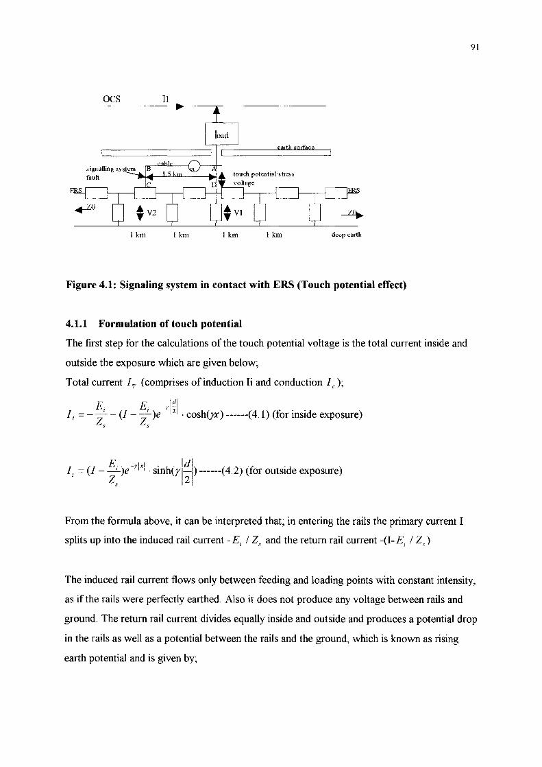
OCS 11

earth surface

1 km 1 km 1 km 1 km deep earth

Figure 4.1: Signaling system in contact with ERS (Touch potential effect)

4.1.1 Formulation of touch potential

The first step for the calculations of the touch potential voltage is the total current inside and

outside the exposure which are given below;

Total current IT (comprises of induction Ii and conduction Ie);

E E -yl~1 It = --t -(1- -t)e 1

21, cosh(yx-) ------(4.1) (for inside exposure)

s s

/ '/ E, -ylxl 'h'ldl) (42' 'fi 'd ) t = ( - _I)e I I 'SIll (r - ------ .) ( or outSl e exposure Zs 2

From the formula above, it can be interpreted that; in entering the rails the primary current 1

splits up into the induced rail current - Ei / Zs and the return rail current -(1- E; / ZJ

91

The induced rail current flows only between feeding and loading points with constant intensity,

as if the rails were perfectly earthed. Also it does not produce any voltage between rails and

ground. The return rail current divides equally inside and outside and produces a potential drop

in the rails as well as a potential between the rails and the ground, which is known as rising

earth potential and is given by;

92

---------(4.3) (between the load and the sub-station)

v = Zo (I - ~i)e y I d!21 sinh()X) s

--------(4.4) (outside the load or sub-station)

Referring to Figure 4.1 above, if the Bend of the cable comes into contact with the return

system at C, the resultant potential set up due to the conductive fault loop, identified by points

ABC and D, will be given by the vectorial sum of potentials V;, V2 and e (VI' V2 are the

rising earth potentials at the two ends and e is the total induced voltage in the cable). V; & V1 ,

when drawn with respect to deep earth as origin, may be regarded to be in the 1 st quadrant as

shown in Figure 4.2.

On the other hand vector e may lie in any of the quadrants 1, 2,Of 3, but its origin has to be

shifted to coincide with the end of vector V2 because the cable comes into contact with return

system at the V2 end

• in 1st quad e in 3rd quad

/

Figure 4.2: Voltage position in different quadrants

The touch potential in all cases, is the same and is given by;

e T = VI - (Vz + e) --------(4.5)

'I I eT=CA'~V\'-(V2'+<')

I

93

4.1.2 Determination of touch potential

Consider the Figure 4.3 below, to determine the touch potential for the cable AB, positioned as

shown in Figure 4.3;

P2 il-(L-O-a-d)---'---------- l-------------~ (sub-station)

.B

X2 --____.. ..

.. Xl

~ -----~--- ---,- '-' ---------------------.,

d

Figure 4.3: Position of the cable of length AD (inside exposure)

The sum of conduction and induction current It at any distance x inside the exposure is given

by equation;

E E Id/l It = --' - (1- -' )e-r 2 cosh}'X

Zs Zs ---------(4.6)

for cable AB;

X

f, E E -rl dl21

I = - -' - (1 - -' )e cosh}'X . dx tAB Z Z

X 2 S S

or -------( 4.7)

E ( ) 1 ( E) -rldl2j ( . h . h ) ItAB =--' Xl -X2 -- 1-_' e sm }'Xl-sm }'X2

Zs r Zs

Calculations for current in section 3.1.1, may now be repeated by substituting It by It4B .

Note: ercalculated in this case, will be for the full length of the cable and not for its unit

length, as in section 3. I since the integration is carried out over the entire length.

Voltage induced from the feed system e f in this case will be e f of step lOin section 3. 1

multiplied by the length of the cable (Xl - X2 ) . Hence, resultant voltage e induced in a length

(Xl - X2 ) , will be known.

From equation, ~~ and V2 are

Knowing e, ~ and V2 , the touch potential eTP for an OCS current of 1 A, may now be

determine by;

eTP =~~ -(V2 +e)--------(4.9)

MUltiplying equation 4.9 above by the total OCS current gives the total touch potential.

94

TP for a cable situated outside the exposure, as shown in the above figure is exactly the same.

The only difference lies in that It, the total current (conduction + induction) and rising earth

potentials vI and v2 are all to be used as for the outside exposure (see Figure 4.4).

~.----. ~··---·-··---1-~ P2 (Load)

o --··-~--1

PI (sub-station)

A B

X2

.. Xl

d

Figure 4.4: Position of the cable AD (outside exposure)

It = ](1- ~i ). e-r1xl . sinh(rld /21· dx -------(4.10) X 2 s

hence

therefore;

~ (A) = Zo (J - E; ). e -rixd . sinh(y . d 12) Zs

V2 (B) = Zo(J - :; ). e -ri Xli . sinh(y· d 12)

s

4.1.3 Results

--------(4. 12)

On the basis of results obtained for one track and two track, it has been established that the

touch potential maintains the same profile irrespective of the exposure and the OCS

configuration or track layout.

95

Touch potential inside the exposure (Figure 4.5 & Table 4.1» is minimum at the centre of

exposure. It rises gradually on moving away from the centre on either side to a maximum value

at the load or sub-station. Outside exposure (Table 4.2), touch potential decays rapidly from a

maximum value at load or sub-station to almost nothing at about 10 km away from load or

sub-station.

Inside exposure Outside exposure

Configuration Figures x (km) (exposure) Max. TP (V) x (km) Max. TP (V)

2.15 2 142 13 19

2.16 2 139 13 21

2.17 2 131 12 16

2.18 2 135 12 16

Table 4.1: maximum touch potential (TP)

Inside exposure I Outside exposure Inside exposure I Outside exposure

Configuration x (km) Max. IV x (km) Max. IV x (km) Ma. x (km) Max. TP

Figures (V) (V) TP (V) (V)

2.15 2 1158 12 152 2 145 13 19

2.16 2 158 12 149 2 140 13 21

2.17 2 148 12 145 2 131 12 16

2.18 2 140 12 141 2 135 12 16

Table 4.2: comparison of Maximum TP against Max induced voltage (IV)

Touch potential (TP) at 30 km exposure (Load current = 1230 A)

so

60

Touch potential 40 (V)

20

O+-~~-.-.~.-.-.-~~-.~.-~~~~-.-.~.-.

~ ~ ~ ~ ~ ~ ~ ~ ~ ~ ~ ~ ~ x(km)

Figure 4.5: TP open track, 1250 A cable on normal side, 30 Km exposure

96

From Figure 4.5 above; with the contraction of exposure, the touch potential curve inside the

exposure rises higher. For the range of exposure considered 2 -30 km, the shortest exposure

i.e. 2 km gives the highest touch potential. While Figure 4.6 shows touch potential at different

exposures for inside exposure and Table 4.3 for outside exposure.

Touch potential (inside exposure at 30, 24, 18, 12 & 4 km)

160 140

120 100

Touch potential (V) SO 60

40 20

O+-··'---r-r--·~-·'····T··,'···-,···"'-··r'·--'-T··"···+ .. , ..... ~-r~~~

~ ~ ~ ~ ~ ~ ~ ~ ~ ~ ~ ~ ~

x(km)

Figure 4.6: TP inside exposure, cable on normal side, 1250 A

.-.---- V1 (30km)

V2 (24km)

V3 (1Skm)

........ V4 (12km)

-------V5 (4km)

97

VI (V) x (km) V2

(V) x (km) V3 (V) x (km)

4 36 4 28 6 20

6 34 6 26 7 18

8 32 10 24 14 16

10 30 14 22 19 14

V4 (V) x (km) V5 (V) x (km)

7 12 6 4

9 10 7 2

15 8 10 0

17 6

_______ ~ __ ~ _________ ~_~ __________ ~ ____ J

Table 4.3: TP outside exposure, cable on normal side for V1, V2, V3, V 4, & V5

Outside the exposure, the touch potential is maximum in the mid exposure range (e.g. 13 km),

its value decreases with the increase or decrease of exposure, beyond this range so that with

the increasing exposure, it is minimum for 30 km exposure and with decreasing exposure, it is

minimum for 2 km exposure.

4.2 One-rail touch potential

It can be calculated in the same manner as for two-rail return system. The three basic matrices,

RR, RF, FF of the two-rail for the relevant OCS configuration and track layout are modified in

order to include for the elimination of rails, which no longer would carry the traction current.

The new sets of matrices are substituted for the old one and the same method is applied as

before. Elimination is carried using standard matrix elimination method.

4.2.1 Results

As it would be expected the profiles of the touch potential curves, whether for inside or

outside the exposure, remain the same as those in a two-rail return system. The maximum

touch potential values inside and outside, however are greater than the corresponding values in

a two-rail system. Results are shown in tables 4.4-4.7 and Figures 4.7 & 4.8 below.

98


Configuration Figures used x (km) Max. TP (V) x (km) Max. TP (V)

2.15 2 192 12 43

2.16 2 183 12 43

2.17 2 178 12 39

2.18 2 178 13 36

Table 4.4: maximum TP (Rl eliminated)


Configuration figures x (km) Max. TP (V) x (km) Max. TP (V)

2.15 2 186 12 43

2.16 2 191 12 48

2,17 2 174 13 36

2.18 2 185 12 41

Table 4.5: Maximum TP (R2) eliminated


Configuration x (km) Max. IV x (km) Max. IV x (km) Ma. x (km) Max. TP

Figures (V) (V) TP (V) (V)

2.15 2 153 12 130 2 192 13 44

2.16 2 175 12 134 2 183 13 44

2.17 2 153 12 132 2 178 12 40

2.18 2 159 12 141 2 178 12 36

Table 4.6: comparison of maximum TP against Max IV (Rl eliminated)

99


Configuration x (km) Max. IV x (km) Max. IV x (km) Ma. x (km)

Figures (V) (V) TP (V)

2.15 2 174 12 142 2 185 13

2.16 2 160 12 127 2 189 13

2.17 2 178 12 145 2 176 12

2.18 2 150 12 131 2 185 12

Table 4.7: maximum TP against Max IV (R2) eliminated)

Touch potential, one-rail, R1 eliminated for different exposure

250

200

150 Touch potential (V)

100

50

V1 (30km)

V2 (24km)

V3 (18km)

V4 (12km)

I· V5 (4km)

~ ~ ~ ~ ~ ~ ~ ~ ~ ~ ~ ~ ~ x(km)

Figure 4.7: TP inside exposure, 1250 A, cable on normal side Rl eliminated

Touch potential, one-rail, R2 eliminated, different exposures

200

150

Touch potential 00 (V) 1

50

O+T·Ty··ii·'····.,..·····,i··· .. Y··· .... · .. ,_·· ... ·,-···r·.,..·Y····+·r··~~~·T .. T···'--,

~ ~ ~ ~ ~ ~ ~ ~ ~ ~ ~ ~ ~

x (km)

V1 (30km)

V2 (24km)

V3 (18km)

'--V4{12km)

V5 (4km)

Figure 4.8: TP inside exposure, 1250 A, cable on normal side R2 eliminated

Max. TP

(V)

44

48

36

41

CHAPTER (5)

Induced Voltage in Compensated systems

Under Normal Operation Conditions: A

Booster Transformer Compensations

Introduction

101

The level of induced voltage due to the ac-single-phase, 25 kv, 50 Hz, should not exceed

certain limits. The European Directive (CCITT)19 for the protection of signalling and

telecommunication lines sets these limits against harmful effects from the overhead power lines

and are as given below:

1. 60 V rms under normal conditions (100 V rms for signalling cables)

2. 430 V rms under power systems fault conditions

To fulfil these requirements further suppression of any induction is needed. This is achieved by

using booster transformers (BTs) connected to the contact wire and either directly to the rail

or via a special return conductor. BTs were first introduced to suppress any interference

caused to the post office lines (unbalanced lines), due to their effectiveness it was decided that

they should be used in all major railway lines. Booster transformer suppression is now one of

the most commonly used methods to constrain the level of induced voltage to the required

limits.

The BTs are in effect current transformers with a 1: 1 ratio. Their function is to force the return

current to flow along a special return or rail to which the secondary of the transformer is

connected.

102

As mentioned before their connection can be achieved in two different ways, either directly to

the rail (Rail connected BT), where almost all of the return current is confined to the rails

(Figure 5.1) small part flows through earth. In Britain the distance between two such

transformers is 1 mile. It is apparent that this system is not effective, due to the difference

between the distances of two current carrying conductors (catenary and rail) from the cable is

very large and hence the residual resultant induced voltage in the cable is high. Also the

impedance of the rails rises with frequency and causes a greater loss. For these reason

suppression using the rail connected booster transformers has proved unreliable.

The second connection can be achieved by connecting the BT to a special return conductor.

This type of connection provided better suppression when tested at the beginning of

electrification and it is now widely used in the UK and Overseas. In this thesis only the latter is

investigated.

catenary & contact

.. I ! ...

1"\" l.J\.p~~) L~~ L;J~AJ

conductor (Y'--V Y"V~ ~'~C'Y]

,Ir

J~ [ J ( \ ( ) .. ) ...

rall

Figure 5.1: Rail connected BT

5.1 Booster Transformer (BT) with a special return conductor

A typical booster transformer with a special return conductor is shown in Figure 5.2. It is

important that the return conductor should be placed as close as possible with the contact wire

in order to reduce magnetic coupling between the power line and signalling/telecommunication

cables. In practice however, the configuration of the conductors provide an inducing loop,

which causes induced current in adjacent conductors and in traction rails. The value of this

current depends on the rail impedance and rail-to-earth leakage resistance69.

return conductor I b~r-------~~----'~~~A

___ I'Il...---_+--_,.,...--4----'

I

I

--'---+---oIIIIt----"~{yyl catenary & contact conductor

rail

Figure 5.2: BT with a special return conductor

103

The connection of the rails to the return conductor is midway between consecutive BTs. The

return path of the magnetising current is via the rails. This magnetising current is very small

under normal condition. For the short circuit faults, saturation occurs in the transformer core

and higher magnetising currents results.

The effect of the magnetising current under fault condition can be very severe hence further

precautions are required. This is established by providing insulated overlaps across BT primary

sides in the overhead line.

The magnitude of the BT magnetising current affects its size. Employing high magnetising

current can reduce the size of the BT, but this could affect the current balance between primary

and secondary, which in effect will contribute towards magnetic induction.

The series connection of the BTs with the supply system, can cause some voltage drop in the

overhead line, this is due to leakage impednaces. The impedance of the simple feeding circuit is

less by about 30% than that of this system70.

5.1.1 Induction effect from BT system

For booster transformer systems with a return conductor, two main effects need to be

considered. The first is induction from through currents, i.e. those currents taken by the trains

well beyond the parallelism and confided wholly to the contact wire and return conductor

(Figure 5.3). The second is induction due to a train in section, i.e. where the train is within or

near to parallelism, and current flows along the rails (Figure 5.4).

return BI conductor L~)r-------4----'----'

BI

rails

Figure 5.3: Train in section effect: case 1

return conductor L~A_A_' uJ catenary & ry"y,

contact conductor '---__ -._~_-,---l ~YY1,---_____ _

r il L'

uncompensate section

Figure 5.4: Train in section effect: case 2

Load

The BT has also an effect on the increase of the impedance of the power circuit. The

impedance of a single track system employing BT and return conductor is about 505% more

than that of the non-boostered system (simple feeding systemfl This increase of the system

impedance results in the need for closer ac substations.

104

Another effect is the size of the return conductor, since the secondary voltage ofBT varies

with the impedance of the return conductor and consequently the capacity of the transformer

varies with the size of the conductor.

5.1.2 BT and its Mathematical model formation

Consider the equivalent ideal transformer shown in Figure 5.5.

j~ I' 1

Nl: N2

Figure 5.5: Ideal transformer equivalent circuit

And the simplified circuit below (Figure 5.6) for impedance calculations.

1:1 Z2 ! f-l[

Vil " Vs ~

tV2 1

Figure 5.6: BT system for impedance calculations

From the above circuit, the impedance of the BT can be calculated as;

where,

II = Ie ( contact/catenary current)

12 = I rt (return conductor current)

105

Writing the above equation in matrix form gives;

For the railway system with booster transformers and a special return conductor, the

components involved are the catenary (C), return conductor (re) and rail conductor (R), the

equivalent circuit for the calculation of the admittance and current of the BT in shown in

Figure 5.7 below.

Ie Ire

~-F----'i""-C_~. _____ .~

ll __ •• -----~ir~"~.~

Figure 5.7: Component involved for BT system

Where, Z 0 = input source impedance

Z l' Z 2 = primary and secondary impedance of feeding transformer.

From the circuit;

106

V~ =~Vo ---(5.3) n)

112 2 ZI = (-) (ZO +ZI)---(5.4)

n)

II =-~Ic ---(5.5) nl

Ie + Ire =0---(5.7)

Ve - v,'e = Z2 * Ire + Vs - - - (5.8)

V,e - Vc = Z 2 * Ire - Vs - - - (5.9)

Substituting (5.3), (5.4), (5.5), in (5.6) gives:

v = V' + I * Z' - - - (5. 11) s 0 e I

or

v = V' - I * Z - - - (5 12) sOre 1 .

and;

Ve - v'e = V~ + Ie * Z; + Ie * Z2 - - - (5.13)

V - V = -V' + I * Z' + I * Z - - - (5.14) re e 0 re I re 2

Vc -V,e = V~ +Ie(Z; +Z2)---(5.15)

V - V = -V' + I (Z' + Z ) - - - (5 16) re cOrel 2 .

In matrix form;

107

U sing matrix manipulation the above can be rearranged to the required formula, and hence the

admittance of the circuit can be obtained as:

108

[YJ ~ l~: l ~ l::' l-l;~ J + [J ,1-------( 5 18)

For the ac single-phase 25 kV, 50 Hz system with booster transformers connected to a return

conductor, the above calculations are carried out using Mathcad and some of the results

obtained are given below (Figure 5.8-5.11).

I

Current in the return conductor (with BT) at 18 km exposure

I

250

200 -J:::=========::::::==+------------

~ 100 +-------------~----------I

C( 150

:; 50+--------------\-------------o

-50 5 10 15 20 25 30 35

x (km) exposure

Figure 5.8: Current in the return conductor for BT spacing 3.2 km, train position at 18

km

1------ Current in the rail (BT) at 18 km exposure-----·i

250

200

g 150 1: 100 ~ :; 50 u

0

/ \

+-----~-------/ \ / \

-50 5 10 15 20 25 30 35

x (km) exposure

Figure 5.9: Rail current for BT 3.2 km spacing, train position at 18 km

109

10

8 g 6 ~-~-

4

5 10 15 20 25 30 35

x (km) exposure

----~~--~-~~

Figure 5.10: Earth current for BT 3.2 km spacing, train position at 18 km

Rail voltage (BT) at 18 kmexposure ~~I

20

~ 15 CII CI 10 .s g 5

0

0 5 10 15 20 25 30 35

x (km) exposure

Figure 5.11: Rail voltage with BT system with rail return (train position at 18 km)

The above section shows the calculation for the booster transformer it self The calculations of

the induced voltage in the nearby signalling cables for one and two track layouts under normal

operation conditions are given in the following section (5.5,5.6 & 5.8).

110

5.2 Compensated systems under normal operation

As mentioned before interference with signalling and communication circuits is a problem that

has been greatly accentuated with advent of 50 Hz traction supply.

There are many different possible remedial measures that can be adopted for the prevention of

any interference these are72:

1. To connect booster transformers with their primary windings connected in series with

overhead line and their secondary windings connected either directly to the running rails or

connect to a special return conductor as shown above.

2. To provide heavy magnetic and electric shielding on signalling and telecommunication

cables which parallel the track.

3. To design signal and telecommunication circuits, which would be immune from the effects

of, induced voltage and thus save cost of providing series booster transformers and special

shielding of the cables.

4. To sectionalise the cable with the use of a device such as an isolating transformer, which

may be provided in the cable circuits to act as barrier to the induced voltage. The device at

most allows a small fraction of this voltage to reach the terminal apparatus or personnel

working on the termination of the circuit.

All of the methods mentioned above have been tried in different lines at the beginning of

electrification project in Britain. The most effective method was found to be booster

transformers connected to a special return conductor. Shielding and good grounding have also

been used to provide further suppression. With the introduction of electromagnetic

compatibility EMC Directive (January 1996) it is now required by law that all new electric and

electronic equipment should be immune from the effect of interference as well as having little

interference produced by them. Unfortunately, many of the old equipment are still in use now a

da/3.

The European directive concerning the protection of telecommunication lines against harmful

effects from power lines, specify that cables which are not terminated by suitably constructed

transformers should not be subject to longitudinally induced voltage in excess of the limits

mentioned earlier. Where transformers of suitable construction are employed to terminate the

cable circuit, the CCITT19 directive recommend that under fault conditions, the maximum

possible longitudinally induced voltage may be increased to 60% of the cable conductor

sheath-test voltage.

III

If the calculated values of induced voltage exceed the limit set by the CCITT, one of the

options of remedial measure mentioned above has to be considered. It is desirable first to see if

the induction can be reduced to the safe limits by sectionlisation of the cable. In such an event

the cost is likely to be significantly less than incurred using BT, if they are to be employed.

However, this may be true for cases where only a reasonable number of sections are necessary.

In other cases, it may very well be possible that the findings show a balance in favour of the

use ofBT on the grounds of economy.

Since the booster transformer suppression is commonly used in the UK, this project

concentrated on the analysis of such system.

5.3 BT with return conductors

Reducing the magnetic field caused by the current flowing in the traction line can reduce

induced voltage to an acceptable level.

Theoretically this field can be reduced to zero in the space around the traction line if the

current of the same magnitude and phase as the traction current, but in the opposite direction

flows through a conductor in the immediate vicinity of the OHL.

The aim therefore, is to pass the return current through a special return conductor, running

parallel and as close as possible to the OHL, thereby reducing the leakage current to a

minimum, which returns to the sub-station via earth or the running rails. This is achieved by

having BT in the circuit as shown in Figure 5.2. In Britain the distance between two BT with

return conductor is 2 miles. The return current flows in the rail up to the nearest point at which

the return conductor is bonded to the rails. From there it flows through the return conductor

back to the feeder point (Figures 5.3 & 5.4).

Two limitations of suppression at source using BT with return conductor may be mentioned

here;

Considering a single-track line with BT return, the field produced by the current in the return

conductor is 1800 out of phase with the field produced by the current in the catenary system.

112

If the whole of the return current flowed in the return conductor and if there were no other

parallel conductors to carry induced currents, the field produced respectively by the catenary

current and the return current would sum to zero at all points that were equi-distant from the

two conductors. These points would lie on a neutral plane that passed mid-way between the

catenary and the return conductor and was as right angles to the line joining them. For any

point in this plane there is a perfect suppression at source.

• The first limitation of suppression at source occurs when there is more than one track. The

induced field at any given point is the vector sum of the fields produced by all the catenary

systems to several tracks, as well as by all the return conductors and other current-carrying

conductors. For such a system a neutral plane is no longer relevant.

• The second limitation is set by the fact that the return current after leaving the wheels of

the electric vehicle does not reach the return conductor until the nearest point at which this

conductor is bonded to the rails (the return conductor is connected to the rails at every

mid-point between two transformers).

Hence between the load and the nearest mid-point connection or in a train section as it is

commonly referred to, the return current is confided mainly to the rails (a small part flows

through earth). Although the currents in the two current-carrying conductors (catenary & rail,

return conductor & rail) are equal in magnitude and phase but opposite in direction (assuming

no current flowing into earth), the level of induced voltage is very high in a train section. This

is because of a large difference in the distance between the two current carrying conductors

and the cable, which subsequently causes a large difference in two opposing mutual induction.

The longest train section therefore, gives the worst-case scenarios and the shortest is the best

case. With a distance of 2 miles between two BTs, the maximum length of a train section is 1

mile.

This condition is achieved when the train is at the BT and is commonly known as I-mile effect.

On the other hand the shortest train section length is fulfilled when the train is at the mid-point

connection. Hence the nearer the train is to the BT, the less perfect is the compensation.

113

5.4 Rail connected BT

Even though this type of connection has proved unreliable as motioned earlier, a brief

description is given here. With this scheme nearly all the return current is confided to the rails.

In Britain distance between two such transformers is 1 mile74

From the diagram (see Figure 5.1) it is apparent that this system is not as effective as the BT

return system, this is due to;

1. The difference between the distances of the two current-carrying conductors (OR catenary

and rail) from the cable is very large. Thus residual resultant induced voltage in the cable is

very high.

2. The impedance of the rails rises with frequency and causes a greater loss of current from the

track

3. Between BT locations, the return traction current tends to find its own low impedance path

down all the running rails. This means that the return traction current tends to leave a

single-rail track circuit and join a double rail track because of its lower impedance. The

result of these transverse current is to raise the potential difference between the rails on

double-rail track circuit.

4. There is also the effect on rail potential to earth. The potential of the rail when several trains

are taking current steps progressively higher until the feeder station is reached.

In the following sections, the calculation of induced voltage under normal for compensated

return conductor only, has been considered, since this system is the most widely used due to

efficiency compared to BT running rail. Fault conditions in the form of short circuit faults for

compensated systems are given in the next chapter (6).

As in an uncompensated system the starting point in the calculation is the determination of self

and mutual impedance values for track layouts and oes configurations considered.

5.5 Two-rail return compensated system

In uncompensated systems, the distribution of current in a multi-track case follows the same

rule as in a one-rail track case as far as the direction of currents in different conductors is

114

connected. In other words, in such systems, as a general rule, it can be said that the currents in

feed conductors are always in one direction and those in return conductors in the other.

This general rule however, does not apply for compensated systems, because as it will be seen

later, the current distribution pattern in these systems is different for different number of tracks

considered.

As a result in contrast to uncompensated systems, where the method of calculation has been

explained by taking one case (i.e. one-track as an example), here in compensated systems each

track case will have to be considered separately.

In this section the method of calculation for one-track and two-track cases for the track layout

and oes configuration in given in chapter 2 (Figures 2.11,2.12) are considered receptively.

Furthermore, in compensated systems induced voltage to be calculated is twice the number of

times as in uncompensated systems. This is due to the fact that two different situation arise in

this type of systems, depending on whether the load is positioned at the feed end or the far end

of the transformer. Both position of the load have been considered.

It is noteworthy that, irrespective of the position of the load it is always the length of the cable

between the load and the nearest connection of the return conductor to the rail (cable within

train section), which is the subject to the most severe induction. The maximum possible length

of such cable is 1 mile, since the BTs are spaced at 2 miles apart and the return conductor is

connected to the rail at every mid point between two transformers (Figure 5.2). The induction

outside the train section at the feed end is independent of the load position and so is the

induction outside at the far end75.

In the calculations of this and next chapter, it has been assumed that the currents in the rails

remain confided to the rails (no flow to earth). This assumption is valid since in normal

operation the magnetising current of the BT is very small and can be neglected. In short circuit

conditions, however, as well be seen later, magnetising current is very important factor of

consideration and cannot be ignored. In both norma110ad and sic calculations the impedance of

the transformer has to be taken into account. If this impedance is to be included, then it's value

per km is to be added to the impedance values per km of the conductors, to which the

windings of these transformers are connected.

It is some times convenient if two or more conductors, which are in effect sic by zero

impedance, are bundled together. This also has the advantage of reducing the number of

conductors to be dealt with.

Using standard method of bundling, the conductors from RR, RF and FF matrices may be

bundled as shown below.

Bundling of conductors from RR, RF, FF matrices:

RR, RF, and FF matrices are considered as;

RI R2 RT RCAB

ZII Z12 Z13 Zl4 RI

RR= Z21 Z22 Z23 Z24 R2

-------( 5. 19) Z31 Z32 Z33 Z34 RT Z41 Z42 Z43 Z44 RCAB

= rails

= return conductor

= cable

CW F

ZI5 ZI6 RI

RF= Z25 Z26 R2 ------( 5.20)

Z35 Z36 RT Z45 Z46 RCAB

CW = contact wire

F = feeder wire

CW F

Z56J CW Z66 F

--------( 5.21 )

llS

116

Combing the above matrices (5. 19-5.21) to form one large symmetrical matrix (M r ) as:

Z1I Z12 Z\3 Z14 Z15 Z16

Z21 Z22 Z23 Z24 Z25 Z26

[ (RR) (RF)] Z31 Z32 Z33 Z34 Z35 Z36 --------(5.22) Mr = (RFr) (FF) - Z41 Z42 Z43 Z44 Z45 Z46

Z51 Z52 Z53 Z54 Z55 Z56

Z61 Z62 Z63 Z64 Z65 Z66

where, M r = total of matrices (RR, RF, & FF)

Hence any two conductors can easily be bundled at a time, using standard method.

5.6 One-track case

5.6.1 Load at the feed-end of the BT

Consider Figure 5.1247, the calculations are carried out for the two current-carrying zones as

shown below;

I OCS

Load

I

rail

Zone 1 ------------------~~ Zone 2 (up to feeder station)

Figure 5.12: One-track case for load at the feed end of the BT

It may be noted that only the current-carrying conductors are shown in each zone.

From the computed self and mutual impedance of all conductors using their co-ordinates, the

matrices of the RR, RF, FF are formed in the same manner as uncompensated system. For

easiness of the calculation the cable eAB is considered to be one of the return conductors,

hence as are all other conductors, it is to be included in the RR and RF matrices.

117

R} & R2 in the RR matrix can be bundled together and represented by a single conductor R.

similarly contact wire and feeder wires in FF matrix can be bundled together and represented

by a single conductor oes. The resulting matrix is;

Z77 Z73 Z78 Z74

M - Z37 Z~3 Z38 Z~4 --------(5.23 ) T -

Z87 Z83 Z88 Z84

Z47 Z~3 Z48 Z' 44

5.6.1.1 Zone 1 calculation

Here the return conductor carries no current; hence it is eliminated from the total matrix

(5.23), giving the resulting matrix as;

Z;4] Z;4 -------(5.24)

Z" 44

For a current 1 in the oes, the rail current =-1 (opposite direction of the oes current, the

function of the BT)

From the matrix above, the mutual impedance between the cable and oes = Z;8 and the

mutual impedance between cable and rails = Z;4

Hence the total voltage induced in the cable

e C4B = - J . Z ~8 + J . Z;4 , , ---------(5.25) (V/km)

eCAB = J(Z74 - Z48)

For the current in oes 1 =1

The total voltage in the cable is:

eCAB = Z;4 - Z~8 ------(5.26) (Vlkm)

5.6.1.2 Zone 2 calculations

The rails in this case carries no current, hence R is eliminated from the total matrix (5.23)

above, giving:

Z;4J Z:8 --------(5.2 7)

Z'" 44

If the current in return conductor =-1

and mutual impedance between cable and oe S = Z:8

and mutual impedance between cable and return conductor = Z;4

The total voltage in the cable;

eCAB =1(Z;4 -Z:8)

1 = 1 --------( 5.28) (V Ikm)

Z " Z" eCAB = 34 - 48

5.6.2 Calculations for load at the far-end of the BT

Referring to Figure 5.1347, the calculation are carried out for two current carrying zones;

I --Y"~Y--,

r----------r--~~ i

Load I

fa ... Zone 1

ocs

return conductor

Zone 2 (up to feeder station)

Figure 5.13: One-track case, load at the far end of the BT

5.6.2.1 Zone 1

oes current =0, hence when it is eliminated form the total matrix (5.23) the following is

obtained;

118

[

Z;7 Z;7 M"'= Z' Z'" T 73 33

Z;4 Z;;

Z;4J Z~ -------(5.29)

Z'" 44

F or the current in rails =1

The current in return conductor =-1

The mutual impedance between cable and rail = Z;4

The mutual impedance between cable and return conductor = Z;;

Hence total voltage is:

e =1(Z'" -Z") CAB ", 34 ,,74 -------(5.30) (V/km)

eCAB = Z34 - Z74

5.6.2.2 Zone 2

The calculations and results are the same as in the case of load at the feed end of the

transformer.

5.7 Two track case

5.7.1 Load at the feed end of the BT

There are three zones in this case and are as shown in Figure 5.1447 below;

12 ,..11 OCSI

RT2

~·~--------------~·~--~Z~o~n~e'l----~~~ ~ Zone 3 (up to end of feeder section Zone 2 (up to feeder station)

Figure 5.14: Two-track case, load at the feed end of the BT.

119

120

Note: only current carrying conductors are shown in the above figure.

The RR, FF, RF can be composed from the computed self and mutual impedance from chapter

(2),

RI R2 R3 R4 RTJ RT2 RCAB

Zl1 ZI2 Z13 ZI4 ZI5 ZI6 ZI7 RI

Z21 Z22 Z23 Z24 Z25 Z26 Z27 R2

Z31 Z32 Z33 Z34 Z35 Z36 Z37 R3

RR= Z41 Z42 Z43 Z44 Z45 Z46 Z47 R4 ---------( 5.3 1 )

Z51 Z52 Z53 Z54 Z55 Z56 Z57 RTJ

Z61 Z62 Z63 Z64 Z65 Z66 Z67 RT2

Z71 ZZn Z73 Z74 Z75 Z76 Z77 RCAB

RR matrix consists of the return conductors impedance.

ZI8 ZI9 ZI.IO ZI.l1

Z28 Z29 Z2,10 Z2,11

Z38 Z39 Z 3,10 Z3,11

RF= Z48 Z49 Z4,1O Z4,11 --------(5.32)

Z58 Z59 Z5,10 Z5,11

Z68 Z69 Z6,1O Z6,11

Z78 Z79 Z7,10 Z7,11

RF matrix consists offeed against return conductors impedance.

Z88 Z89 Z8,1O Z811

FF= Z98 Z99 Z9,10 Z911

--------( 5 . 3 3 ) ZIO,8 ZIO,9 ZIO,IO ZIO,II

Zl1,8 Zl1,9 ZlI,1O Zll,l1

FF matrix consists of feed conductor impedance.

Form the above the following conductors are bundled;

1. R I , R2

, R3 & R4 to make R (conductor no.12)

2. CWI &}; to make (DeSI ) (conductor no.I3)

3. eW2 & F2 CW2 (DeS 2 )( conductor no .14)

The new matrices are;

R Rn RT2 RCAB

Z12,12 ZI2,5 ZI2,6 Z12,7 R

RR' = Z5,12 Z;5 Z;6 Z;7 Rn -------(5.34)

Z6,12 Z~5 Z~6 Z~7 RT2

Z7,12 Z;5 Z;6 Z;7 RCAB

The new matrix RR' consists of the bundled return conductor impedance.

Where,

Z12,13

RF" = Z5.13

Z6,13

Z713

Z 12 = The results of the bundled rail conductors RI ,R2 ,R3 & R4

Z I = The new value as a result of bundling

ZI2,14

Z5,14 -------( 5.35)

Z614

Z7,14

The new RF' matrix consist of the bundled feed against return conductors impedance.

Where, Z 13 = The result of the bundled feed conductors e~ & F;

EF' = (ZI3,13 Z14,13

Z13,14J

Z14,14

-------(5.36)

The new FF' matrix consists of the bundled feed conductors impedance.

Where, Z13 = The result of the bundled feed conductors e~ & F;

ZI4 = The result of the bundled feed conductors eW2 & F2

The total new matrix (combining 5.34-5.36) is:

ZI2,12 Z125 ZI26 Z12,13 ZI2,14 Z12,7

Z512 Z;5 Z;6 Z5,13 Z 5,14 Z;7

M"I- Z6,12 Z~5 Z~6 Z6,13 Z6,14 Z~7 ------( 5.37) T -

Z13,12 Z13,5 Z13,6 ZI3.13 Z13,14 ZI3,7

Z14,12 Z14,5 Z14,6 ZI4,13 Z14,14 Z14,7

Z7.12 Z;5 Z;6 Z7,13 Z7,14 Z;7

5.7.1.1 Calculations for zone 1

mutual impedance between cable and oes] = Z713

121

" " " DeSI = Z7,14

" " Rn = Z;5

" " " RTJ = Z;6

" " " rails = Z 7.12

Current II and 12 inOCSmaybeassumedtobeequal, 11=12 =I12 (I = total current).

Hence the current in RTJ = I12,

The current in 142 = -I/2,

And the current in the rails = -I.

The total induced voltage in the cable;

eCAB = - ~ . Z7,13 - ~. Z7,14 + ~ . Z;5 + ~ . Z;6 + I· Z7,12

or

eCAB = ~ (2Z7,12 + Z;6 + Z;5 - Z7,13 - Z7.14)

5.7.1.2 Calculation for zone 2

------(5.38) (V/km)

122

In this case the rails carry no current, hence eliminating the 1 st row and column from the above

matrix (5.37) gives;

Z;5 Z;6 Z~,13 Z;,14 Z;7 Z" 65 Z:6 Z~ 13 Z~,14 Z:7

M""-T - Z' 13,5 Z;36 Z;3.13 Z' 13,14 Z;3,7 --------(5.39)

Z;4,5 Z;4,6 Z;4,13 Z;4,14 Z;47 Z; Z;6 Z;,13 Z;14 Z;7

Z' & Z" are the new values resulting from eliminating the rail (first raw & column) from the

matrix in (5.37).

Mutual impedance between cable and DeSI = Z;,13

" " " DCS2 = Z;,14

" " "

" " "

Current II and 12 in OCS may be assumed to be equal, II = 12 = 1/ 2 (I = total current)

Hence the current in 141 = 112,

The current in 142 = -112,

And the current in the rails = -I.

The total induced voltage in the cable;

eC4B

=_~.Z' _~.Z' _~.Z" +~.Z" . 2 7.13 2 7,14 2 75 2 76

or -------( 5.40) (V Ikm)

eC"AB = ~ (2Z;6 + Z;5 + Z;5 - Z;,13 - Z;,14)

5.7.1.3 Calculations for zone 3

123

In this case the rails do not carry any current therefore the same matrix for zone 2 calculations

has been used.

Hence the total induced voltage in the cable;

eC"B =~.Z' _~.Z' _~.Z" +~.Z" "' 2 7,13 2 7,14 2 75 2 76

or ---------( 5.41) (V Ikm)

eC'AB = ~ (Z;,13 - Z;,14 - Z;~ + Z;6)

5.7.2 Calculations for load at the far end of the BT

Again there are three zones in this case as shown in Figure 5.1547 below.

124

I ... 11 OCSI

~,

... 12 RTI

·11 OCS2

~2 RT2

fa

... 1...·1 • Zone 3 (up to end of feeder section Zone 1 Zone 2 (up to feeder station)

Figure 5.15: Two-track case, load at the far end of the BT

5.7.2.1 Zone 1

The mutual impedance are obtained from the original matrix (5.37) for;

Cable & DeS1 = Z713

CAB & DCS2 = Z7,14

CAB & RTJ = Z;5

CAB & 142 - Z' 76

CAB & rail = Z7.12

The total induced voltage is;

or --------( 5.42) (V Ikm)

eCAB = £(Z713 - Z7 14 + Z;5 + Z;6 - 2Z712 ) 2" .

5.7.2.2 Zone 2

Calculations are the same as for load at the feed-end.

5.7.2.3 Zone 3

The same also follows as for load at the feed-end.

125

5.7.3 Results

It is only within a train section (between load and the nearest mid-point rail to return conductor

connection) that the rails carry current. Rails being much closer to the cable induce a much

higher voltage, which pre-dominates the induction from the other conductors.

The current in the rails, reverses in direction as the load moves from one position to another,

i.e. from the feed-end to the far-end side of the transformer and vice versa. Therefore, the

resultant voltages have opposite signs in the two load positions.

Outside the section, the induction is much lower than inside, this is because the rails do not

carry current and the induction due to OCS is to a great extent cancelled by the induction from

the return conductors, the two induction's being opposite in direction.

The induction outside a train section on the feed-end side of the transformer, are same for both

load positions. Similarly the induction outside on the far end side of the transformer are

independent of the side of the transformer on which the load is. Results obtained are shown in

tables 5.1 and 5.2 below.

Induced voltage (V)

Outside Two track One track

induction

CNS COS

At feed end ofBT -0.00057+0.00373i -0. 00097+0. 00867i -0.00122-0.00935i

At far end ofBT 0.00011 +0.0073i

Table 5.1: Induced voltage outside for load at either end: feed-end of the transformer

Induced voltage (V)

Outside induction Two track One track

CNS COS

At feed end ofBT 0.00038+0.05073i -0.00191 +0.071 09i -0.00167 -0. 07004i

At far end ofBT -0.00255-0.04291 i 0.00251-0.06763i 0.00226-0.08565i

Table 5.2: Induced voltage inside, when load is at: feed-end and far-end of the

transformer

126

5.8 One-rail Return systems

Calculations in this case can be carried out using the same approach as for two-track system

described above, provided that the rails, which do not carry traction current, are eliminated

from the relevant matrices. The remaining rails, which do carry the traction current, may then

be bundled together to from a single conductor, which carries the total rail current.

In order to consider the effects of broken rails, such rails are to be eliminated and all the

current carrying rails can be bundled together. Results obtained are shown in tables 5.3-5.6.

5.8.1 Results

Eliminated rails Induced voltage (V)

Two track One track

CNS COS

R1 0.00289+0.04883i 0.00539+0.0203i 0.0045+0.05461i

R2 0.00477+0.0331 Ii 0.0071+0.05489i 0.0059+0.01656i

R3 0.00415+0.01264i

R4 0.00391+0.02195i

R1 & R3 0.00455+0.01012i

R2 & R4 0.00357+0.02343i

Table 5.3: Induced voltages inside when load at the feed end of the BT


Two track One track

CNS COS

R j -0.0042-0.04244i -0.00402-0.01511 i -0.00202-0.07064i

R2 -0.00608-0.02614i -0.00225-0.05008i -0.00438-0.03127i

R3 -0.00535-0.0079i

R4 -0.005l6-0.01551i

R1& R3 -0.00554-0.0018i

R2 & R4 -0.00451-0.01382i

Table 5.4: Induced voltages inside when load at the far end of the BT


Two track One track

CNS COS

R1 -0.00056+0.00374i -0.00097+0.00868i -0.00122-0.00935 i

Rz -0.00057+0.00375i -0.00097+0.00867i -0.00121-0.00936i

R3 -0.00056+0.00375i

R4 -0.00056+00375i

R1 & R3 -0.00056+0.00374i

Rz & R4 -0.00056+0.00375i

Table 5.5: Induced voltages outside at the feed end with load at either end


Two track One track

CNS COS

R1 0.00014+0.00728i

Rz 0.00012+0.00728i

R3 0.00013+0.00729i

R4 0.00013+0.00728i

R1 & R3 0.00013+0.00728i

Rz & R4 -0.00012+0.00729i

Table 5.6: Induced voltages outside at the far end with load at either end

The above results are for one rail return systems and broken rail situations.

For one track case

Within a train section (between load and mid point rail connection to the return conductor)

induced voltages are still higher than those outside.

127

The level of induction is considerably reduced if the rail nearer to the cable is eliminated. This

holds true irrespective of whether the load is at the feed-end or far-end of the BT

128

There is no induction outside a train section at the far end because there are no current

carrying conductors in this zone. Outside a train section at the feed end, the results are

unaffected and remain the same as in a two rail return system, since the rails do not carry any

current irrespective of which rail is eliminated.

For two-track case

Within a train section, the results follow the same trend as in a one-track case. If one of the

rails were to be broken, the induced voltage is highest when the rail farthest from the cable is

eliminated. Since R3 is nearest to the cable, followed in succession by R4, Rz and R1, the

induced voltage increases in progression from a minimum value when R3 is eliminated, to a

maximum when R1 is eliminated. This is true irrespective of whether the load is at the feed-end

or far end. However the corresponding values are higher when the load is at the feed end

position.

In a one rail return system, either rails Rz and R4 or rails R1 and R3, will carry the traction

return current. In the first case, rails R1 and R3 will have to be eliminated and in the second

case rails R2 and R4 .

Induced voltage with Rz and R3 eliminated is considerably less than that with Rz and R4

eliminated, this is true for both load positions. However as seen in the case of a broken rail

situation, the corresponding values are higher when the load is at the feed end than those when

it is at the far end.

As in one track case, the induced voltage outside a train section is the same irrespective of

whether it is a two rail or a one rail return system, or a broken rail situation, because the rails

outside a train section do not carry any current. However, on contrast to a one-track case, in a

two-track case there is induction on the feed end as well as the far end. This is because the

oes and return conductors overhead have currents flowing in them. The level of induction is

greater outside at the far end than at the feed end.

129

5.9 Summary

The induced voltage in compensated systems (with BTs) under normal operation conditions for

one and two track layouts have been calculated in this chapter. For two-rail return system, the

highest induction occur within a train section (train in-section), since the rails carry current in

this section. The direction of the rail current changes as the load moves from one position to

another (feed-end to the far-end side of the BT and vice versa), hence the voltage have

different sign for the two load positions. For outside section (out-section of the train) induction

is much lower than that of in-section (no current in the rail). Induction for out-section is the

same for the both load positions.

One-rail return systems, the highest induction is the same as two-rail. There is no induction in

the out-section of the train for load at the far-end of the booster transformers, while for the

load at the feed-end the results are the same as for two-rail systems. The level of induced

voltage is at its highest when the rail farthest from the cable is eliminated. It can be concluded

that induction in compensated systems under normal operation conditions is dependent on the

position of the load with respect to the booster transformer. Calculations under short circuit

fault conditions are discussed in the following chapter (6).

CHAPTER (6)

Induced Voltage in Compensated Systems:

Short Circuit Condition

Introduction

The effect of the inducing current in a booster transformer with return conductor is divided

into three parts47:

130

1. A compensated component, in which equal and opposite currents flow in the catenary and

return conductor between the supply transformer and the load.

2. An uncompensated component due to the magnetising current in the BT, which flows in the

catenary between the same points and returns via rails and earth.

3. An uncompensated component due to current which flows in the catenary or return

conductor between the load point and the nearest mid-point strap and returns via rails and

earth.

In normal conditions, the magnetising current effect is small and can be neglected, whereas for

short circuit conditions, the magnetising current is of such importance that, from a first

approximation, the compensated component can be neglected. In short circuit conditions

therefore, a booster transformer does not give perfect results because the magnetising current

of the BT returns via the running rails and earth. This gives rise to problems because of the

rather severe interference in the nearby conductor under BT saturation conditions, when the

magnetising current becomes very high. Thus knowledge of the magnetising current taken by

BT with heavy load is essential for a pre-determination of the effect of short circuit76.

131

To a certain extent, the magnetising components will depend on the type, make and rating of

the transformer. The transformer used by BR is an oil-immersed current transformer, with 1: 1

ratio. The current ratings of the BR are shown below (BR, B. spec AC 7/4, 1972)63

Continuous current (A)

100

150

200

300

peak current

500

600

600

600

The continuos' rating is the rms current, which the transformer can withstand continuously.

The peak current rating is the maximum rms current that the transformer can withstand for a

time of 15 minutes.

The primary side of the transformer is insulated for 44 kV, 50 Hz and the secondary side for

3.3 kV (encountered under fault condition), thus meeting the requirements ofBS 23363.

The overhead system is designed for spark-less current collection at all speeds, but under

abnormal conditions a degree of sparking may occur and the equipment should be capable of

withstanding the resultant transient effect. Finally the transformer should be capable of

operating throughout the temperature range -25°C to 55°C in a polluted atmosphere.

From the current transformer theory, the main components are the magnetising and leakage

impedance. The magnetising impedance appears due to the core properties of the transformer.

Consider the ideal transformer with no load connected across the secondary as shown in Figure

5.5. If a voltage is applied at the primary side, a current known as the exciting current flows in

the circuit. Part of this current form the magnetising current, which produces magnetic flux in

the core. For a load to be connected across the secondary windings, the exciting current will

combine with the secondary current to give the total primary current.

132

The magnetising impedance consists of two components connected in parallel, a resistance Rm

and an inductance Lm' The resistance represent the core losses (hystresis and eddy current).

The inductance produces magnetic field inside the core that links the primary with the

secondary winding. Both components are affected by the frequency. Rm is proportional to

frequency while Lm is inversely. If the applied voltage exceeds a certain value the saturation of

the transformer starts. This causes a sudden drop in the value of Lm and as a result the exciting

current increases considerably depending on the degree of the core saturation.

The windings of the transformer are also not perfect due to the winding resistance and

leakance flux. A component of the magnetic flux in the core will always link one winding

without linking the other.

Under load conditions therefore the windings develop an electromotive force (emf), which acts

in opposition to the applied voltage, producing voltage regulation.

The leakance flux can be represented by impedance Zl connected in series with the equivalent

circuit of the transformer. This impedance is made up of RJ and LJ . RJ represents the winding

resistance (dc resistance) and the eddy current losses developed in the windings when the

transformer is in operation. LJ is the opposing emf as mentioned.

In the event of short circuit (sic) fault on the OHL, a high current several times the value ofthe

normal operating current, will flow in the primary of the B T. this will cause saturation of the

BT, its exciting impedance will be reduced suddenly and the BT efficiency will decrease

dramatically. The magnetising current is very high and since this returns via the rails and earth

only part of the total sic current flows through the return conductor or in other words, is

compensated. The current flowing in the return conductor or through the secondary of the

transformer will be the total short circuit current less the magnet ising current.

The system under these conditions behaves like a composite system, since it is partly

compensated and partly uncompensated.

133

For the following calculations an sic current of 6000 A has been assumed for the calculations.

A typical value of the magnetising current for this value of sic current will be 668 A, as given

by one of the transformer manufacturer.

6.1 Method of calculations

Consider the circuit shown in Figure 6.1 below47;

Isle oes 4

Lv~.AJ ! 4 LAJI-_"J _____ ---111'---_----"( I \~ ____ --.-__ JOoL-rt"-JrYYYl~: __ ---;~~r--=-e-'-turn-c-o-n~duetor

Isle sub-station

Irt

1m ~

Rail

Figure 6.1: Compensated systems (with BT and return conductor) under sic current

F or a short circuit current I / = 6000 A and a magnetising current of the transformer I = scm

668 A, the current through the return conductor is obtained from the following relation;

or --------( 6. 1 )

Hence, I rt = 5332 A

Note: 1m reaches the sub-station via the rails and earth.

For simplicity, the above circuit is divided into two components;

(a) Compensated

(b) Uncompensated

6.1.1 Compensated components

Compensated components are as shown in Figure 6.2 below47

.

Irt ocs ______ ~F~==+----·-------:;::::~~--~·-. r-e~-'~-on-ductor I

Irt

Irt

Figure 6.2: Compensated components

6.1.2 Uncompensated component

1m ..

Irt

l_A_A..AJ ______ ---J~ L-__ t--______ ---J''Y .• ,._j

1m

Figure 6.3: Uncompensated components

sub-station

Rail

ocs

return conductor

~

1m

sub-station

Rail

134

From the figure (6.3) the magnetising current 1m on entering the rails splits into I ml on the left

and I mr on the right. I ml reaches the sub-station via the rails and earth, and so eventually does

I ml . On reaching the sub-station, they combine to produce 1m again.

Calculations for compensated component can be carried out using the method described in

chapter 5, and those for the uncompensated component by method in chapter 3.

The compensated and compensated may then be summed up to solve for short circuit situation.

6.1.3 Calculation examples

Consider a one-track configuration in an open area with cable on the normal side as shown in

figure 2.17 in chapter 2. If the magnetising current is zero, the induced voltage results will be

as in section 5.7.5 for two-rail return systems and 5.8.1 for one rail return configuration, which

135

are already known from the earlier study of compensated systems (chapter (5)). On the other

hand if the entire sic current was to be the magnetising current, then the induced curves of

Figures 6.11, 6.12 are nothing but familiar results for an uncompensated systems47

.

If the compensated and magnetising currents are each assumed to constitute 50% of the total

fault current, i.e. if compensated current = uncompensated current = 3000A for a fault current

of6000A, then the summation of the compensated and uncompensated will be as in Figures

6.7 and 6.8 and for the fault at the feed end and far end respectively.

For an assumed value of the magnetising current of668 A, the induced voltage values are as

shown in Figures 6.9 and 6. 10.

It would appear from Figures 6.4,6.5,6.11 and 6.12, that the highest level of induced voltage

is obtained either in a fully compensated system or in a fully uncompensated system and not in

a composite system.

Using the same approach as in previous chapters and the computer programs that have been

developed, the maximum induced voltage when a fault occurs can be calculated for inside and

outside exposure for fault at the feed end and far end of the transformer, results obtained are

shown in Figures 6.4-6.12.

6.1.4 Results

The results for one track and two tracks are given below. It can be seen that the induced

voltage level decreases as the number of tracks increases.

For one-track case: cable on the normal side

The results are the same for faults at both the feed end and far end. The maximum voltage

inside exposure is obtained when exposure = 32 km and the system is fully uncompensated.

The maximum voltage outside exposure is obtained at 16 km and the system is fully

uncompensated.

For cable on the other side: fault at feed end

The maximum voltage inside exposure is obtained when exposure = 32 km and the system is

fully uncompensated.

136

The maximum voltage outside exposure is obtained when exposure = 16 km and the system is

fully uncompensated.

For fault at thefar end

For inside exposure the results are the same as above.

For outside exposure the maximum induced voltage is obtained at 32 km and the system is

fully compensated.

For two-track case: fault at feed end

The maximum voltage inside exposure is obtained at 32 km fully compensated.

For outside exposure it was found at 19 km for a fully uncompensated components.

For fault at the far end

Inside exposure maximum voltage induced was at 32 km fully uncompensated and for the

outside exposure was at 32 km for fully compensated components.

Induced voltage (IV) for fully compensated current (1m =0), fault at feed-end of BT

800 700 600


300 200

10~t-~ __ ~~~~~~==~~==~~==~~~ __ ~~ __ ~~ 34 32 30 28 26 24 22 20 18 16 14 12 10 8 6 4 3 2

x (km) exposure (distance from sub-station)

Figure 6.4: Induced voltage fault at feed-end, compensated I =6000A, 1m =0, one-track

cable on normal side

Induced voltage for fully compensated current (1m =0), fault at far~ndofBT

700 I<mm«««m««;

600 &Xl

Induced voltage 400

(V) 300

200 100

0+--.-.--.--.-.--.--.-.--.--.-.,-.--.-.,-.--.-. 34 32 30 28 26 24 22 20 18 16 14 12 10 8 6 4 3 2

x(km) exposure

Figure 6.5: Induced voltage fault at far-end, compensated I =6000A, J m =0, one-track


Induced voltage for fully uncompenstaed current (1m =0), fault at either side of BT

800

700

600

500 Induced voltage

(V) 400

300

200 1 100

O+-'--r~-.--~'--.~-.--~'--.~~--r-'-~~~~

40 33 32 29 28 26 25 23 22 20 18 16 13 12 10 9 7 4 3 2 0

x (km) exposure

137

Figure 6.6: Induced voltage fault at either side, compensated I =0, J m =6000A, one track


Induced voltage for equally COIJ1)ensated & ul1COl11Jensated curre~ talut at feed-end d BT

400

3s)

300

2s) Induced voltage

(V) 200

1s)

100

S)

O+-.-.-.-,,-r-.-.-.-.--.-.-.-.-.-,,-.-r-.-.-. 40 33 32 29 28 26 25 23 22 20 18 16 13 12 10 9 7 4 3 2 0

x (km) exposure

Figure 6.7: Induced voltage for fault at feed-end compensated I =3000A, 1m =3000A,

one-track cable on normal side

Induced voltage for equally compensated & uncompensated currents, fault at far-end of the BT

800

700

600

500 Induced voltage

(V) 400

300

200

100

40 33 32 29 28 26 25 23 22 20 18 16 13 12 10 9 7 4 3 2 0

x (km) exposure

138

Figure 6.8: Induced voltage for fault at far-end compensated I =3000A, 1m =3000A, one

track cable on normal side

Induced voltage for for a higher compensated current (1)lm), fault at the feed-end of the BT

700

600

500


200

100

40 33 32 29 28 26 25 23 22 20 18 16 13 12 10 9 7 4 3 2 0

x (km) exposure

139

Figure 6.9: Induced voltage for fault at feed-end compensated I =5332A, 1m =668A, one

track cable on normal side

Induced voltage for higher compensated current (>Im), fault at the feed-end of the 8T

700

600

500

Induced voltage 400

(V) 300

200

100 o I ..

40 33 32 29 28 26 25 23 22 20 18 16 13 12 10 9 7 4 3 2 0

x (km) exposure

Figure 6.10: Induced voltage for fault at feed-end compensated I =5332A, 1m =668A,

one-track cable on normal side

IrdI2d vdta9! fa'fUly l.I1CQ11eI1Silt a.nert ~m =&XX) ~ taut at feed.erxl dthe BT

&0.-----------------------------------------------. &X)

400

InducEd wItage D

(V) 3X)

100

O+-~~~_T~--~~~~_r~~--~~~~_r~~--~

40 33 32 29 28 Z6 25 23 22 20 18 16 13 12 10 -100 .1.:..-....:.::...-==--=-=o-==-==--==-=--=-=---..:.:::........:.=--.:=--==-....:..::...-=---=--------'------'~=_______:r X (km) eJCpOSLI'e

Figure 6.11: Induced voltage for fault at feed-end two-track for both inside exposure

(compensated I =6000, 1m =0), and outside exposure (compensated I =0, 1m = 6000A)

Induced voltage for fully uncompensated current (1m = 6000 A), fault at the far-end of the BT

600

500

400 Induced voltage

(V) 300

200

100

O+-~~~~~_r_r~~~~~~~~~~~~~~~

X 40 33 32 29 28 26 25 23 22 20 18 16 13 12 10 9 7 4 3 2 0

x (km) exposure

Figure 6.12: Induced voltage for fault at far-end, two-track, for inside exposure (1=

6000A, 1m =0), and outside exposure (1=0, 1m =6000A)

140

141

6.2 One rail return systems under short circuit condition

This follows the same method as for two rail return system. The rails that carry traction return

current are bundled together to form a single conductor, which carries the total rail current. In

one-rail systems some rails would not carry any current and these must be eliminated.

To consider a broken rail effect, they have to be eliminated, and all current carrying conductors

are the bumbled.

6.2.1 Results

For one-track case: cable on normal side

The highest value of the induced voltage is the same irrespective of which rail is eliminated.

This value is lower than the maximum value in a two rail return system.

The worst case always corresponds to a totally uncompensated system, i.e. when the entire

fault is magnetising current Figures 6.13-6.15.

Induced \Oltage for fully uncompens ated current (lm=6000A), fault at either end ofthe BT, Rl eliminated (32 & 16 km exposure)

800

700

600

500 btduced voltage

(V) 400 300

200

100

O+-'-~,,-'~~~~~'-~~-'-r~~~'-~ ~ ~ ~ ~ m ~ ~ ~ ~ m ~

T""" ~ T""" N

x (km) exposure

Figure 6.13: induced voltage fault at either end, compensated I =0, 1m = 6000A, one

track, cable on normal side R\ eliminated

Induced voltage fOl' fully uncompensated cunent, fault at either end of the

BT, R2 eliminated (32 & 16 km exposm'e)

800

700

600


(V) 300

200

100

o lD t- (j)

x (kIn) exposure

·IV(32 km)

IV (16 kID) I ~~~

Figure 6.14: Induced voltage fault at either end, compensated I =0, 1m = 6000A, one

track cable on normal side, R2 eliminated

InckJced voltage for JUly lJ1COI11)ensated curert, one-track, R1 elininated

~1(xx) 8,8X> ~600 ~400 ~200 :::I

~ O+-"-r-..-,,~-r'-,,,,-.~.-,,-r-..-ro

~~ ,..,0;) ,..,(0 ,..,~ ,..,~ ,,(0 ,,"" 0;)

x(lun)

IV(3a<m)

-IV(16km)

142

Figure 6.15: Induced voltage fault at feed-end, compensated I =0, 1m =6000A, one track,

cable on the other side, RJ eliminated

For cable on the other side

Highest of induced voltage is the same as above. This value is lower than the maximum value

in the case of two rail return systems.

The highest induced voltage is always obtained in a totally uncompensated system with the

exception of one case.

This occurs in the event of a fault at the far end and on elimination of rail R 1, when the

maximum induced voltage outside exposure will be obtained if the system was totally

compensated, Figure (6.16).

For two-track case

With any rails (except R1 ) eliminated the highest induced voltage is the same irrespective of

the fault (feed or far) with R1 eliminated the curve for maximum induced voltage within the

exposure for fault at the feed end is different from that at the far end.

The highest induced voltage is obtained when R1 is eliminated (which is lower than the

maximum induced voltage in two rail return), Figures 6.13,6.16.

143

The highest induced voltage when R1 and R3 (Figure 6.18) are eliminated is greater than that

when R2 andR4 (Figure 6.19) are eliminated (lower than that obtained when R1 is eliminated).

Induced voltage for fault at the far-end of the 8T, R1 eliminated

900

800 700


(V) 400

300

200 100 o+-~~-.~.-~~~-.~.-~~~~~~

~ ~ ~ ~ ~ ~ ~ ~ ~ ~ ~

x (km) exposure

... ··_·_·IV (32 km)

·· ... ·······IV (16 km)

Figure 6.16: Induced voltage fault at far-end, one track, cable on the other side, R1

eliminated

Induced voltage fault at either end, fully uncompensated cunent, R2 eliminated

900

800

700

600

Induced voltage !i)()

(V) 400

300 200

100

0+-.-.-.-,,-.-.-.-.-.-.-.-.-.-.-..-.-.-.-.

x (km) exposure

IV(32km)

IV(16km)

144

Figure 6.17: Induced voltage for fault at either end, 1=0, 1m =6000A, one track, cable on

the other side, R2 eliminated

Induced voltage for fault at either end and fully uncompensated current, R1 & R3 eliminated

450

400

350

300


150

100

50

O+-.-.-"ro-.-.-.-r-r~~.-.-.-.-~ro-.-.

x (km) exposure

IV (32km)

IV (16 km)

Figure 6.18: Induced voltage for fault at either end, I compensated = 0, 1m =6000A, two

track, R) & R3 eliminated

Induced voltage for fault at either end and fully uncompensa1ed current, R2 & R4 elimina1ed

450 400 350 300

Induced voltage250 (V) 200

150 100

50 O+-~ro-.-.~.-.-~,,~-r-..-~.-,,~-'

,.,'=' ,.,'" ",'b ",'=' ",,,, ,,'b ,,'" ,,()

x (km) exposure

-IV (32 km)

IV (16 km)

145

Figure 6.19: Induced voltage for fault at either end, I compensated = 0, 1m =6000A, two

track, R2 & R4 eliminated

6.3 Validation of the FDTD Method

The method used in this thesis is a mathematical modelling technique based on the finite

different time domain method. The main objectives of the project is to provide a reliable, easy

to implement and cost effective approach for the calculations of the rail-track and overhead

line impedance and hence better results and analysis of the induced voltage. This have been

achieved and the FDTD provides comparable results to the finite element method and the well

known Carson's correction method for the calculations of the impedances.

It is noteworthy that calculation of frequency-dependent impedance is important not only in

power engineering, but also in other areas involving high frequency applications like

communications and semiconductor microchip design. In fact, as the frequency increases to

several GHz (109Hz), a small segment of the conductor in a microchip behaves just like a

100-km-Iong power transmission line working at 60 Hz. Consequently, the methods for

calculating power line frequency-dependent impedance are also applicable to the analysis of

electromagnetic interference in printed circuit boards and integrated circuits.

146

To validate the FDTD method, calculations are carried out for the induced voltage in

uncompensated and compensated systems under normal operation conditions for one-rail and

two-rail return systems using the standard analytical approach (Carson's correction term). The

results obtained are shown in Figures 6.20,6.21 and Tables 6.1,6.2 below.

Induced voltage using FDTD & Carson's methods

100

90

80

70 60

Induced voltage (V) 50

40

30 /l:,l'

20''/ .;

10 f

Or,~~~~~~~~~~~~~

x (km) exposure

I '. ww Induced voltage (V).

l FOlD Induced voltage (V). Carson

Figure 6.20: Induced voltage for two-rail return system in an open area

(uncompensated, 1250 Amps ratings, 30 km exposure) using Carson's & FDTD methods

Induced voltage using FDTD & Carson's methods

100,

90 ~ 80 1

70 60

Induced voltage (V) 50·

40

30 20

10 o~~~~~~~~~~~~~~~

o ~

x (km) exposure

N N

Induced voltage (V). FOlD

'" Induced voltage (V). Carson L ---

Figure 6.21: Induced voltage for one-rail return system in an open area

(uncompensated,1250 A, 30 km exposure) using Carson's and FDTD methods

Induced voltage (V)

Outside Two-track Two-track

induction (FDTD) (Carson)

At feed end ofBT 0.00038+0.05073i 0.00062+0.0067i

At far end ofBT -0.00255-0.04291 i -0.00534-0.0063i

Table 6.1: Induced voltage inside for load at either end for two-rail return system

(compensated, 1250 A) using Carson & FDTD methods


Two-track (FDTD) Two-track (Carson)

R) 0.00289+0.04883i 0.00539+0.0393i

R2 0.00477+0.03311i 0.0071 +0.05489i

Table 6.2: Induced voltages inside when load at the feed-end of the BT, for one-rail

return system using Carson & FDTD methods

147

Comparison have also been made between the rail, earth and return current of the compensated

systems obtained in (section 5.1.4) with published data23 , the results obtained are as follows:

Current FDTD method CAD method23

Earth current 10 (A) 16 (A)

Rail current 220 (A) 195 (A)

Return current 210 (A) 200 (A)

Table 6.3: Currents in the rails, earth and return conductor using FDTD & CAD

method

It is always desirable to obtain measurements, however due to the complexity of the railway

system this was not possible. Hence comparison can be achieved from published work, which

in this case is slightly difficult since many of the publications deals with telecommunication

(screened) cables rather than the unscreened signalling cables.

148

Models for induced voltage calculations for un screened signalling cables were obtained and

published for the first time by Gupta47 His work, however, uses Carson's method for

impedance calculations. For the work in this thesis impedances were calculated by FDTD

method. The shape of the induced voltage curves in this thesis are identical to those obtained

by Gupta. Since the results obtained by two different approaches are identical it can be

established that FDTD is a valid method. Moreover, it has been already shown that the method

is more accurate than Carson's method. FDTD method has a wide scope for novel applications

in EMC analysis in railway systems.

6.4 Summary

The induced voltages have been calculated for compensated systems under short circuit

conditions. Two different track layouts have been investigated as well as the position of the

cable. The results obtained showed that the induced voltage depends very much on the position

of the fault where it is at the feed end or far end of the booster transformer. Results obtained

here are based on the assumption that the short circuit current is 6000A. A different fault

current can be tried easily by replacing the fault current in the program.

149

CHAPTER (7)

Conclusion

The aim of this project was to develop a mathematical tool for studying the interference

problem caused due to the ac-single-phase, 25 kV, 50 Hz systems into line-side signalling

systems. Knowing the magnitude of this induction is essential in understanding the behaviour

of the systems to provide protection measures accordingly. Due to the complexity and the

many components involved for such a system it has been difficult to provide a complete and

reliable analysis of the longitudinal induced voltage. In particular, the primary objective has

been to develop a mathematical model based on the finite difference time domain to provide

reliable calculations of the self and mutual impedance of the conductors used, namely the rail

track conductor ( return) and feed conductor (overhead line).

Until recently, these parameters have been analysed using Carson's21 correction term

developed over seventy years ago. The method provides the only analytical calculation that

includes the earth return effect and has been proved to be very reliable for calculations at the

low frequency range (e.g. load flow studies, voltage drop, etc.). However, at a higher

frequency range, >10kHz (section 2.2.1), the method converges very quickly with a high

calculation error due to the assumption that the earth is semi-infinite.

For this reason it was very important to find an alternative approach especially for

electromagnetic compatibility. The development in computer system speed has prompted

engineers to find an alternative approach~ mathematical modelling techniques. Another reason

for the popularity of mathematical modelling is that it is not always possible to obtain results

from direct measurement techniques. This is due the interaction problems that arise from the

150

complexity of the system as well as the measurement environment, which is impossible to

control in a busy system like the railways. Therefore it is reasonable to obtain results via an

alternative approach that enables us to represent the system and its parameters as accurate as

possible. This cannot be achieved using the analytical approach.

Many researchers provided improvements in Carson's method and obtained better results for

these calculations. One such a modification is Gray's34 method, known as the complex return

system, in which the skin depth effect is added to Carson's impedance method. This method

received little attention because it was merely experimental and no mathematical proof was

given. Waie4 tested the method and obtained good results for frequencies higher than 10 kHz.

Hill and Carpenter23 on the other hand, took advantage of the development in mathematical

modelling techniques and provided analysis for the rail track impedances using finite element

method. The FEM is an electromagnetic method that is based on solving Maxwell's equations

and from the stored energy results given; the impedance of the rail track can be extracted. The

results obtained using this method have provided great accuracy and showed that Carson's

method overestimates the values of the impedances. FEM has proved to be very reliable and

takes into account the material properties of the conductor and its physical shape. However, it

is a too complex procedure, requires long time simulation and introduces added cost in the

form of the software and the training required to use the system.

An alternative approach, which has the same or close enough reliability as the FEM but

requires less training and software cost, is now needed. This has been achieved in this project

by using finite difference time domain method. The method is a direct solution of Maxwell's

equations, hence it is easy to implement and understand. Furthermore, since it is a time domain

method it covers a wide rang of frequencies with one simulation. The rail tack and overhead

line impedance has been calculated using existing software therefore cost is greatly reduced.

The software has built-in FDTD facilities and enables program writing according to required

specifications. From Maxwell' equations the electric and magnetic field are solved for the

required boundary conditions and the impedance of the conductor was extracted using

Ampere's law.

The self and mutual impedance results were almost exactly the same as those obtained by FEM

and Carson's up to 10 kHz, and the same as the FEM at frequencies >10 kHz (section 2.2.3).

151

Although the results obtained were very comparable to that published by other researchers,

great care should be taken when applying the boundary conditions as incorrect application can

result in great errors and increased simulation time. It is hoped that this can be overcome by

trial and error through experience.

As mentioned before, the main objective was to find the level of induced voltage into signalling

systems. The induced voltage was calculated for both compensated and uncompensated

systems under normal and short circuit conditions for the two different track layouts and

overhead rating. The position of the cable was also investigated.

7.1 Uncompensated systems

Analysis for this system was carried out for inside and outside exposure (also known as in

section and out-section). For long exposure where the outer section effect can be considered as

negligible, the induced voltage was found to be maximal at the centre of the exposure (Figure

3.3). The voltage level starts to decrease towards the load or the sub-station until the induction

from the feed conductors is greater than that of the return conductors. The voltage level rises

again when the induction from the return conductors exceeds that from the feed one. In the

case of short exposure, where the outer section effect can not be neglected, the return

conductor induction is more dominant and the shape of the induced voltage is the reversed of

that obtained for the long exposure (see Figure 3.7). For both cases the curve is symmetrical

about the centre of exposure.

For outside exposure, the induced voltage is always maximal at the load or the sub-station but

decreases later. The induction from the return conductor is more dominant in this case.

For fault condition when there is contact between the cable and the conductor, the induction is

minimum at the centre with maximum values at the load or sub-station (Figure 4.2).

The induced voltage depends on many different effects, the maximum voltage induced for

uncompensated systems was found to be 67 V rms. The induced voltage level depends on the

position of the exposure (inside or outside), making its level maximal at the centre for outside

exposure and minimal for inside exposure. Under fault conditions, namely touch potential; the

induced voltage attained a maximum value at the load and sub-station. The value of the

induced voltage varied between 470-500 V rms.

152

7.2 Compensated systems

For systems compensated with booster transformer connected to a special return conductor,

two different situations arise depending on the position of the load. If the load is at the feed

end of the transformer, the induced voltage is maximal within the exposure from the load up to

the mid point of the rail return conductor connection (Figure 5.4). If the load is at the far end

of the transformer, the maximum voltage is outside the exposure from the load to the outside

connection (Figure 5.5). For both cases the zone between the load and the mid point

connection is the most important, elsewhere induction is very small, hence we can say that the

worse induction case occurs at this section.

Induced voltage outside at the sub-station end is zero. For one track at the load end, the

voltage induced outside the sub-station is zero, while a small value is found for two track

layouts.

Under short circuit conditions, a combination of uncompensated and compensated effect

occurs. The compensated situation occurs as a result of the compensated current and the

uncompensated situation is due to the magnetising current of the booster transformer.

For better understanding different theoretical considerations have been investigated. If the

entire short circuit current is assumed to be the magnetising current, the induced voltage is at

its worst level. For other cases, the worst induction is obtained between the load and mid point

connection, the entire short circuit is assumed to be compensated.

F or compensated systems using booster transformer method connected to a special return

conductor, the induced voltage depends on the position of the load (far end or feed end of the

transformer). For the load at far end induced voltage is maximum within exposure for the

section between the load and the return conductor connection, the level was found to be 57 V

rms. For far end load, the maximum voltage is outside the exposure, again from the load but to

outside mid-point connection, the level was found to be 56 V rms. The induced voltage outside

at the sub-station end is zero as well as at load end in a one-track case this is zero, but has

small values in two-track.

For short circuit conditions the effect of the magnetising current of the booster is evident. Two

different situations occur, the level of the induced voltage varies depending on the magnetising

153

current level and the compensated current. If the magnetising current is higher the worst

induction occurs. On the other hand if the compensated current is greater the results are the

same as above. It is therefore very important when designing the booster transformer that the

no load current is made small to avoid any interference.

7.3 Limitations of the method

Higher frequency effect and harmonic studies have not been covered in this thesis, although

higher frequency analysis can be done using the same approach by changing the frequency

values. Also the analysis carried out mainly deals with unscreened signalling cables, but can be

modified for analysing screened telecommunication cables. Due to the size of the model only

one and two-track layouts have been considered.

It is always desirable to verify the numerical calculations by experiments. Unfortunately,

however, due to the complexity of the systems and because it is not always easy to gain access

to the railway lines for measurements, it was not possible to obtain experimental analysis.

Nevertheless, the data used in this thesis is a real time data obtained from a Brazilian railway

line.

Although not much research has gone into signalling systems, a valid comparison can,

arguably, be made between the studies for induction into telecommunication systems that can

be found in Kewlel5, Rosenl6, Mellitt l7, and Pickford33

. It is not an easy task to carry out

interference tests in a complex and busy railway network of today, due to the limits imposed

on the amount of time available for extermination due to traffic and demands. Some of the

results obtained, however, have been compared to similar test carried out in a German railway

line and Hong Kong.

7.4 Future work

Although the emphasis of the methods presented in this thesis has been mainly on signalling

cables, the work enables methods on similar lines to be devised for telecommunication cables,

pipe-line cable etc. Analysis of tunnel and higher track lines can also make an area of future

work.

Another area of future work will be the investigation of increasing the voltage level of the

booster transformers for high-speed trains using power electronic techniques.

154

The effect of harmonics on the system behaviour and for compensated and uncompensated

system is an area ofa whole research in itself. Finally, the application of the method developed

in this thesis to an autotransformer compensated systems would also be useful.

7.5 Summary

A mathematical modelling technique method that is different from the conventional standard

method of calculating the induced voltage into line-side signalling cables has been developed

and examined. The rail track impedance and overhead transmission line parameters have been

calculated using finite difference time domain method over a frequency of 50Hz - 1 MHz. The

self and mutual impedance of the rail-track at system frequency (50 Hz), were, 0.67 and 0.87,

respectively. The method used had an accuracy of±O.5% in the determination of rail track

impedance, and ±0.6% for over-head parameters compared to finite element approach and

O. 1 %-0 .2%, compared to Carson standard approach. This in effect provided more accurate

results for the calculations of induced voltage. The induced voltage has been calculated for one

and two tracks in an open area, and for two different overhead ratings 1250 and 760 Amps. All

calculations have been carried out for uncompensated (no Booster) and compensated systems

under both normal and short circuit. The results obtained in this thesis provide a more detailed

analysis of induced voltage calculations and provide improved calculations compared to the

published work in this field.

CHAPTER (8)

References

1. Taflove A, Hagness S C, "Computational Electrodynamics: The Finite Difference Time

Domain Method", Artech, London 2000.

155

2. Sullivan D M, "Electromagnetic Simulation using the FDTD Method", IEEE Press Series

on RF and Microwave Technology, IEEE 2000.

3. Roters H C, "Electromagnetic Devices", John Wiley & Son, Inc, New York, 1992.

4. Grivet P, "The Physics of Transmission Lines at High and Very High Frequencies",

Academic Press, London, 1991.

5. Perry G, C by Example, Que, 1992.

6. Karmel P R, Cole G D, and Camisa R L, "Introduction to Electromagnetic and Microwave

Engineering", John Wiley & Sons, INC, 1998.

7. Magid L M, "Electromagnetic fields, energy and waves" (Wiley, 1968).

8. Yee K S, "Numerical Solution of Initial Boundary Value Problems Involving Maxwell

Equations in Isotropic Media", IEEE Transaction on Antennas and Propagation, Vol. AP-

14, No.3, May 1966.

9. Kurt L S and John B S, "A Survey of the Finite-Difference Time-Domain Literature",

1999.

10. Wedepohl L M and Efthymiadi A E s, "Wave Propagation in Transmission Lines Over

Lossy Ground: A New Complete Field Solution", lEE Proc, Vol. 125, No.6 JuneI978.

11. Galloway R H, Sharrocks W B, and LM Wedepohl, "Calculation of Electrical Parameters

for Short and Long Poly-phase Transmission Lines", lEE PROC., Vol. Ill, No.I2,

December 1964.

12. Dover A T, "Electric Traction", 4th Edition, Pitman, 1963.

13. Partab H, "Modem Electric Traction", Pritam Surat, New Delhi, 1973.

14. "British Railway Electrification Conference", Publications by lEE, London 1960

15. Klewe H R J, "Interference Between Power Systems & Telecommunication Lines",

Edward Arnold, 1958

16. Rosen A, "Interference in Railway Line-Side Telephone Circuits From 25 kV, 50 Hz

Traction Systems", Proc.IRSE, 1956.

156

17. Mellitt B, Allan J, Johnston W B, "Software Modelling for Induced Voltage Calculations

In Railways", Conference on Railway Engineering Perth, Sept 1987, pp. 87-11.

18. Mellitt B, Allan J, Shao Z Y, "CAD Techniques for Power Studies and electromagnetic

Screening Calculations in AC Railways", Conference Paper 1987, pages: 145-172.

19. Mellitt B, Allan J, Shao Z Y, "Computer-based Methods for Induced-voltage Calculations

in AC Railways", lEE Proc., Vol. 137, Pt. B, No.1, January 1990.

20. "CCITT Directives Concerning the Protection of Telecommunication Lines against

Harmful Effects from Electric Power and Electrified Railway Lines", (CCITT, Geneva,

1989), 9 Vols.

21. Treirney J R and Turner R, "Improvement to booster Transformer Return Conductor

Method of Suppressing 50 Hz Interference From AC Electrified Railway Systems", lEE

Discussion, AC Traction Interference, London, 1980, Paper No.1, Railway Engineering

Forum Meeting.

22. Carson J R, "Wave Propagation in Overhead wires with Ground Return", Bell System

Technical Journal, 1926,5, pp. 539-556.

23. Pollaczek F, "The Field in an Infinitely Long Conductor Carrying Alternating Current",

Elec. 1926,3, (9), pp. 339-359.

24. Hill R J, Carpenter DC, "Determination of Rail Internal Impedance for Electric Railway

Traction System Simulation", lEE Proc-B, Vo1.138, No.6, Nov. 1991.

25. Buchanan W, "Analysis of Electromagnetic Wave Propagation Using The 3D Finite

Difference Time Domain Method With Parallel Processing", PhD Thesis, Napier

University, 1996.

26. Paul C R, "Introduction To Electromagnetic Compatibility", Wiley Series In Microwave

and Optical Engineering, John Wiley, 1992.

27. Roden J A, Paul C R, Smith W T and Gedney S D, "Finite-Difference Time-Domain

Analysis Of Lossy Transmission Lines", IEEE Trans. Electromag. Compat., Vol. 38, No.

1, pp.15-24, 1996.

157

28. Mur G, "Absorbing Boundary Condition for the Finite-Difference Approximation of the

Time-Domain Electromagnetic Field Equations," IEEE Transactions on Electromagnetic

Compatibility, pp. 377-382, November 1981.

29. Silvester P P, Ferrari R L, "Finite Elements for Electrical Engineers" (CUP, Cambridge

UK,1983).

30. Ruehli A E, "Circuit Oriented Electromagnetic Solutions in the Time and Frequency

Domain", IEICE Trans. Commun., Vol. E80-B, No. 11, Nov. 1997.

31. Nonweiler T R F, "Computational Mathematics: An Introduction to Numerical

Approximation", Ellis Horwood Ltd, 1984.

32. Abdulaziz I M and Gupta N K, ''FDTD Method in Calculating Induced Voltage in

Railways", lJEEE Journal, Submitted.

33. Bickford J P, "Transient in Power Systems: The Calculation of Transmission Line

Constants", UMIST, 1983.

34. Alias Q M, "Calculation of Overhead Line Parameters with Particular Reference to

Railway Systems", Msc Dissertation, UMIST, 1977.

35. Deri A, Teva G, Semlyen A and Castanheira A, "The Complex Ground Return Plane; A

simplified Model for Homogenous and Multi-Layer Earth Return", IEEE Trans. Power

Appa. Syst, 1981, 100 (8), pp. 3686-3693.

36. Agrawal A K, Price H J and Gurbaxani S H, "Transient Response of Multi-conductor

Transmission Lines Excited by a Non-uniform Electromagnetic Field", IEEE Trans. EMC,

Vol. 22, No.2, pp. 119-129, 1980.

37. Trueblood H M and Waschek G, "Investigation of Rail Impedances", AlEE Trans, 1934,

53, pp. 1771-1780.

38. Butterworth S, Electrical Characteristics of Overhead Lines, Report, 1954.

39. Abdulaziz I M and Gupta N K, Rail Track Impedance Calculations using Carson's FE and

FDTD Methods, lEE Proc. Elect. Power Applic., Under Review.

40. Macentee J A, Railway Track as a short Transmission Line, Msc Dissertation, University

of Birmingham, 1972.

41. Siemens W A, "Will 50kv Become A World Standard?", Railway Gazette International,

April 1978, pages: 201-204.

42. R J Hill and I H Cevik, "On-line Simulation of Voltage Regulation in Autotransformer-Fed

AC Electric Railroad Traction Networks", IEEE Trans. Vehicular Technology, Vol.42,

No.3, August 1993.

158

43. Allan J, Mellitt B, Brown J C, Taufiq J A, "A Computer-based Portable Analyser

Assessment of Harmonic Effects in AC and DC Railways", Proc. OfInternational Comprail

Conference, Frankfurt, 1987, pp.l03-119.

44. Bozkaya H, Shao Z Y, Allan J, Mellitt B, "A Comparison Between Autotransformers and

Booster Transformers for AC Traction Supply", Con.Paper, International Electric Railway

Systems for A New Century, lEE, London, 1987, pp.114-118.

45. Abdulaziz I M, Gupta N K, Induced Voltage Calculations in Electrified Railways,

University Power Engineering Conference (UPEC) Proceedings, University of Wales,

Swansea, September 2001.

46. Brunton L J, "Earth-Leakage Problems and Solutions on the Tyne and Wear Metro", lEE

PROC., Vol. 136, Pt. B, No.3, May1989.

47. Gupta N K, "Inductive Interference into a Line-Side Signalling Cable in AC Electric

Railway Systems", PhD Thesis, UMIST, October 1985.

48. Barnes R, Wong K T, "Unbalanced Tunnel Rail", lEE Proc-B, Vol. 138, No.2,

March1991.

49. Abdulaziz I M, and Gupta N K, Power Supply in Electric Railways, Energize Power

Journal, SAIEE, March 2003.

50. Conlon M, Wilcox D and McGrath D, "Transient and Harmonic Induction from

Underground Power Circuits into Parallel Communication Services", Proc. International

Power Conference, 1984.

51. Shipp D G, "Track Circuit in DC Electrified Areas", Proc.IRSE, 1952, pp.108-134.

52. Mellitt B, "Electromagnetic Compatibility in DC railways Using Power Electronic Control.

'Railway Safety, Control and Automation Towards the 21 st Century", IRSE International

Conference, London, September 1984.

53. Abdulaziz I M and Gupta N K, Electromagnetic Interference in Electric Railway Systems,

International Power Engineering Conference (IPEC) Proceedings, Singapore, May 2001.

54. Tierney J R and Grose B H, "Telecommunication Systems in Relation To 50 Hz AC

Electric Traction", lEE Proc., Vo1.119, (4), pp.441-455, 1972.

55. Wright A, "Current Transformers", 1st Edition, 1968, Chapman and Hall Ltd, London.

56. Hardman A R, "Interference and its Effects on Track Circuits", Proc. IRSE, 1976-77.

57. Nedelchev N, "Influence of Earth Connection on the Operation of Railway Track

Circuits", lEE Proceeding (EPA), Volume 144, No.3, May 1997

58. Hill RJ, Carpenter DJ, "Rail Track Transmission Line Distributed Impedance and

Admittance Theoretical Modelling and Experimental Results", IEEE Trans, Veh.

Technology, 1993, 42, (2), pp.225-241.

159

59. Abdulaziz I M and Gupta N K, "Booster Transformers in Railways", UPEC, University of

Staffordshire, UK, September 2002.

60. Littler G E, "Harmonic Performance of an Autotransformer Type High Voltage AC

Railway Electrification System", lEE Proc. Elect Energy Conference, pp.85-90, Australia,

1986.

61. Holtz J and Klein H J, "The Propagation of Harmonic Currents Generated by Inverter-Fed

Locomotive in the Distributed Overhead Supply System, IEEE Trans. Power Electronics",

Vol.4 APR, pp.168-174, 1989.

62. Pettersson G A and Svensson S, "Compensation from Rails, Return Conductor and

Booster Transformers oflnduction Caused By Electrified Railways, TELE, Pt.2, pp96-

128, 1961.

63. Turner DR, "Interference from Power Lines and Traction Circuits", Proc. IRSE, 1953.

64. Efthymiadis A E, "Wave Propagation in Transmission Lines Over Lossy Ground", PhD

Thesis, UMIST, 1977.

65. Helmer 0, Petterson G A, and Swederborg, "The Induction Effects of Swedish Electrified

Railways on Parallel Telecommunication Lines", Tele. English Edition, 1955.

66. Wilcox D J, "Implementation of non-homogenous Theory in Transient Analysis of Cross

Bonded Cable Systems", Proc. lEE, Vol. 125, 1978.

67. Klewe H R, "The Interference Problem", Paper 9, BR Electrification Conference, London,

1960.

68. Webb W J, "The Power Supply", Paper 5, BR Electrification Conference, London 1960.

69. Cobbe D W, "Effect on Post Office Circuits", paper 37, BR Electrification Conference,

London 1960.

70. Woodbridge A W, "Signalling and Telecommunication", Paper 10, BRElectrification

Conference, London 1960.

71. Allen C E, and Goldring A G, "Overhead Equipment: The Catenary System", paper 33,

BR Electrification Conference, London 1960.

72. Casson E, "Power Supply: The Railway Load", paper 28, BR Electrification Conference,

London 1960.

160

73. KOSTIS A G, "Booster Transformers in British Rail Traction Systems", Msc Dissertation,

UMIST, 1976.

74. Abdulaziz I M and Gupta N K, "Compensated Systems in Electrified Railways and the use

of Booster Transformers", SAIEE Proceedings, Under Review.

75. Gergory N and Scott R, "Telecommunication in an AC Environment: Audio Frequency

Interference into Line side telecommunication Cable Circuits", Railway Engineering

Forum, London, 1980.

76. Woodbridge A W, Klewe H R, and Kapp R 0, "Inductive Interference and its

Measurement on Electrified Railways", Proc. IRSE, 1962.

77. Abdulaziz I M and Gupta N K, "EMC in Railways", Electronic Journal, SAIEE, In Print.

78. www.trainweb.com

APPENDIX

A.I Data Used (Chapter (2»47

A.LI Uncompensated systems

Frequency = 60 Hz

Deep soil resistivity = 100000 ohm-m

Near soil resistivity = 3500 ohm-m

Length of cable = 1.5 km

A

Mutual impedance between cable and buried earth wire = 0.0922+0.99328i

Maximum exposure = 30 km

A.LLI Data for rails

Weight = 130 lb/yard

Height = 0.1524 m

Internal reactance = 0.26 ohm/mile

Perimeter = 25.75 in

Permeability= 275 gauss

Resistivity= 20xlOI\-6 ohm-cm

DC resistance= 0.0386 ohm/mile

A.LL2Buried earth wire

No of strand = 7; 1 in layer 1 and 6 in layer 2

Radius of strand ( a) = 1. 75 mm

161

Overall radius of conductor (R) = 6.5 mm

A.I.I.4 Return conductor

No of strands = 23 ; 1 of steel in layer 1

6 of steel in layer 2

16 of aluminium in layer 3

Radius of steel strand (as) = 1.445 mm

Radius of aluminium strand (aa) =1.285 mm

Total radius = 8.15 mm

A.I.I.S Messenger wire

No of strand 37;

Radius of strand = 1.21 mm

Total radius = 8.45 mm

A.I.I.6 Contact wire

1 in layer 1

6 in layer 2

12 in layer 3

18 in layer 4

N of strands = 1 (solid conductor)

Radius of strand (a) = 6.15 mm

A.I.I.7 Feeder wire

No of strands = 33;

Steel radius = 1.445 mm

Aluminium radius = 1. 86 mm

Total radius = 23.5





162

A.1.1.8 Resistance to earth

Earthing resistance Re = pnlpi*L(Logh(2L1sqrt.(2rd)-2)

Pn = near soil resistivity

L = length

r= radius of buried earth wire

d= depth of buried earth wire

For L = 5000m, pn = 3500, r = 0.0065, d = 1.66

Re = 10.17 ohm/m

A.1.2 Data for compensated systems

Frequency= 50 Hz

Resistance to earth = 10.17

Length of cable in normal load calculations = 1 km

Length of cable in fault load calculations = 1.61 km

Mutual impedance between cable and buried earth wire = 0.0922+0.99328i

Maximum exposure = 32.18 km

A.1.2.1 Data for rails

Weight = 100 lb/yard

Height = 0.1524 m

Internal reactance = 0.30 ohm/mile

Perimeter = 24.63 in

Permeability = 300 gauss

Resistivity = 20x 1 0/\-6 ohm-cm

DC resistance = 0.0526 ohm/mile

163

A.1.2.2 Other conductor data

Conductor Height (m) Dc resistance (ohm/mile) Internal reactance Radius

(ohm/mile) (mm)

Return 5.7912 0.182735 0.0337 10.55

conductor

Contact 4.7244 0.27128 0.02528 6.17

Wlre

Feeder 5.638 0.676 0.033 5.93

Wlre

A.2 For Rail track impedance calculations using APLAC software (section 2.2),

sample of written program:

#define freq 1 kHz "frequency setting"

#define DX "cell size defined"

#define DY

#define DZ

#define EPSR 1 "permittivity"

Declare APLACV AR TT NL ZO h W ereff

Declare VECTOR zaxis REAL 41

Declare VECTOR vect REAL 41

Call h = 3 *DZ "hieght of the cell"

Call W = 4*DX "cell wedth"

Call ereff= Mlin_epse«w/h),O,lOO,EPSR)

Call ZO = Mlin_Z01«w/h), 0, 100, EPSR)/sqrt(erefl) "characteristic impedance"

ElectroMagnetics Rail "perform electromagnetic calculations"

+ HARMONIC freq

+ TIMESTEP MARGIN 99.9% (time-step dt)

+ DIV 264012

+ CELL SIZE DX DY DZ

+ SIMTIME LOOPS 1200

+ ABCTYPE ZHA03 "Absorbing boundary condition"

164

+ ABCTRIM X ereff ereff

+ ABCTRIM Y ereff ereff

DetEMPort sequencer

+ NAME excitation 1 NAME excitation2

+ SYMMETRIC

+ STORE sw2.s2p

EMPort excitation 1

+DIR+Z

+ SPAN 13 8 0 13 8 1

+RZO

+STOREsw21.t

Patch pin_at j)ort_1

+ SPAN 13 8 1 13 8 3

EMPort excitation2

+DIR+Z

+ SPAN 13 320 13 32 1

+RZO

+ STORE sw22.t

Patch pin_atj)ort_2

+ SPAN 13 32 1 13 323

Sleeper substrate

+ SPANO 0 0 26 40 3

+EREPSR

Patch ground ~lane

+ SPANO 0 0 26 40 0

Rail

+ SPAN 11 83 15323

+ SPAN 4 19 3 22 23 3

EndElectroMagnetics

Call TT = EMSimTime("Rail")

Call NL = EMSimLoops("Rail")

Sweep "Response of a rail conductor"

165

+ LOOP NL TIME LIN ° TT

+ WINDOW ° + X "position" "cells" 042

+ Y "Voltage" "V" -1 1

+ WINDOW 1

+ X "time" "s" ° l.Ons

+ Y "input voltage" "V" -1 1

+ Y2 "output voltage" "V" -1 1

Call Ev("Rail", 12,0,2, 12,42,2, Z, zaxis, vect)

Show WINDOW ° VECTOR 41 XY zaxis (h*vect) ERASE

Show WINDOW 1 Y Vem("Rail", 12,8,0, 12,8, 1) PEN 1

Show WINDOW 1 Y2 Vem("Rail", 12,30,0, 12,30, 1) PEN 3

End Sweep

166

B.2.2 Similar approach is applied for overhead conductor (Conductor above ground)

$ define cell sizes

#define DX

#define DY

#define DZ

$ define the conductor permittivity

#define EPSR 1

$ define output axis vector

Declare VECTOR yaxis REAL 41

$ define output value vector

Declare VECTOR ezfields REAL 41

Declare APLACV AR TT NL ZO h w ereff

$ height of the conductor

Call h = 3*DZ

$ length of the conductor

Call L = 4*DX

$ epsilon J _ eff.

Call ereff= Mlin_epse((w/h), 0, 80, EPSR)

$ charac.imp.ofT.line

Call ZO = Mlin_Z01«w/h), 0, 80, EPSR)

Here is the Electromagnetics block initialisation for the upcoming structure.

Electromagnetics conductor

+ PULSED

+ TIMESTEP MARGIN 99.9%

+ DIV 26 4012

+ CELL SIZE DX DY DZ

+ SIMTIME LOOPS 2400

+ ABCTYPE ZHA03

+ ABCTRIM X ereff ereff

+ ABCTRIM Y ereff ereff

This means that:

167

- we launch a pulse (as opposed to a sinusoidal wave). This creates a wide band simulation (as

opposed to harmonic simulation)

- the timestep size is 99.9% of the maximal

- there are 26 x 40 x 12 cells in the computation region (XYZ)

- cell size is DX x DY x DZ (values defined above)

- the simulation is run for 2400 loops.

- ABC is "good", ZHAO 3rd order ABC

- the ABC X and Y walls are optimised to absorb a wave propagating at medium having ereff

= ereff.

For S-parameter derivation, we can use these lines:

DefEMPort sequencer

+ NAME excitation 1 NAME excitation2

+ SYMMETRIC

+ STORE OHAs2p

+ FREQS 5010 1MHz

Note the following:

- EMPorts of the structure are referred to with names (EMPorts will be defined below).

- Typically a 2-port is symmetric: S21 = S12, and Sll = S22. This cuts down the simulation

time by half, since only one excitation is required.

- The S-parameters are always stored to a file, they can not be used directly in APLAC.

However, they can be read with an Nport to an ordinary circuit related APLAC simulation.

- the EMPorts are directed so that the plus node of the port is in the +Z direction

- Span of e.g. the first port is from 0 to 3 at X = 13, Y = 8.

- The internal resistance is ZO (defined elsewhere, often 41.6 Ohms).

- The time domain voltages and currents are stored to two datafiles.

Finally (very important):

EndElectroMagnetics

168

NOTE: Avoid placing small instances very close to and ABC plane (ABCs might get unstable).

A small instance is anything that is to the direction of the ABC plane normal, thinner than the

degree of the ABC in terms of cells, and smaller than the plane itself in the tangential

directions.

The Sweep that runs the simulation is

Sweep "OH voltage"

+ LOOP NL TIME LIN 0 TT

+ WINDOW 0

+ X "position" "cells" 040

+ Y "voltage" "V" -1 1

+ WINDOW 1

+ X "time" "s" 0 1.92ns

+ Y "input voltage" "V" -1 1

+ Y2 "output voltage" "V" -1 1

Call Ev("OH", 13,0,2, 13,40,2, Z, yaxis, ezfields)

Show WINDOW 0

+ VECTOR 41 XY yaxis (h*ezfields) ERASE

Show WINDOW 1

+ Y Vem("OH", 13, 8, 0, 13, 8,3) PEN 1

Show WINDOW 1

+ Y2 Vem("OH", 13,32,0,13,32,3) PEN 3

NOTE: These two functions should be added in front of the Sweep statement:

Call TT = EMSimTime("OH")

Call NL = EMSirnLoops("OH")

169

APPENDIX

B

B.l Carson's Method (Chapter (2)21:

(A). Self Impedance

Self impedance includes three components: the reactance of the loop inductance Lii assuming

that the line and the earth are perfect conductors, the internal impedance of line Zc, and the

impedance of the ground Zg. The impedance of conductor i can then be written as

Z = JL + Z + Z ------(B 1) 11 11 C g .

The loop inductance is given by

110 2hj Lil = -In(-) ---------(B.2) 21C r i

The internal impedance of conductor Zc is given by

Zjj =Rd j mr(1-S2)x (b~r.mr+ jbe~.mr)+¢(ker:mr+ jkei'r:zr) -------(B.3) 2 (ber 'mr+ jber ·mr)+¢(ker ·mr+ jker ·mr)

where Rd = 1/[ ps (r 2/\-q 2 )] is the DC resistance of the conductor, q and r are the inner and

outer radii of the conductor, S = q/r is the ratio of the inner to the outer radius, which is zero

170

for a solid line, m =. !lOS is a variable related to the frequency is the radian frequency, s is the

conductivity and !l0 is the permeability ofthe conductor. The variable fin Equation (B.3) is

given by

¢ = - be~' . mq + jb~{ . mq ---------(B.4) ker 'mq+ jkei ·mq

where ber, bei, ker and kei are Kelvin's functions which belong to the Bessel function family,

and ber', bei', ker' and kei' are their derivatives, respectively (Andrews, 1992). Kelvin's

functions are often defined as

ber· x + jbei· x = Io(x,Jj) - - - (B.S)

WJte~9Md j(,Q ~~~ :t~fflodifk4 »~el functions of the 1 &1 and the 2nd kinds of order zero,

respectively. Many scientific Fortran libraries provide subroutines for calculation of Kelvin's

functions with satisfactory accuracy, which makes application of the tubular conductor model

easier. It is noteworthy that the inner radius q equals zero for a solid line, leading to the result f

=0.

The ground impedance Zg is expressed by

Z = R +}:x ---------(B 7) g g g .

Calculation of Zg will be discussed in the next section.

(B). Mutual Impedance

The mutual impedance Zij of two conductors i andj, both parallel to the ground with their

respective heights above the ground being hi and hj, has two components. The first component

is the mutual inductance Lij between the two conductors when the conductors and the ground

are perfectly conductive.

The second component is the impedance of the earth return path Zgm that is common to the

currents in conductors i and j. The mutual impedance Zij can be written as

Z = J'L + Z --------(B.8 1 1J 1J gm '/

The mutual inductance Lij is given by:

L = &'-In( D ~) ------(B. 9) l} 2 D IT lJ

where Dij is the distance between conductors i and j, and D ij I is the distance between

conductor i and the image of conductor j. The impedance of the earth return path Zgm is;

Z = R +JX -------jB 10 1 gm gm gm \,. '/

171

Carson's correction terms for the self and mutual impedances due to the earth path impedances

Zg and Zgm are given by (Carson, 1926; Meliopoulos, 1988).

Rg = 4m * 10-7 (IT -hlk+h2[(C 2 -lnk)k2]+h3k3 -d4k 4 - ...... )---(B.12)

8

Xg =4m*1O-7{~(O.6159315-1nk)+hJk-d2k2 +h3k3 -h4[(C4 -lnk)k4]+ ... }---(B.13) 2

Rgm = 4m .10-7 {; - hJkm cos8 + hZ [(C2 -In k m )km 2 cos28 + (km 2 sin 28]

+ h3 k m 3 cos38 -d4k m

4 cos48 - ... } - - - (B.14)

-7 1 2 3 X gm =4m*10 {2(O.6159315-1nkm)+hJkmcos8-d2km cos28+h3km cos38

- h 4 [( C 4 - In k m )k m 4 cos 48 + Ok m 4 sin 48] + ... } - - - (B. 15)

where;

J2 bl =----(B.16) 6 1

b = - - - - (E. 17) 2 16

b = b sign - - - (B.I8) 1 1-2 i(i + 2)

C = C +!+-1----(B.19) 1 1-2 i i + 2

C2 = 1.3659315 - - - (B.20)

7[ d =-b ---(B.21)

1 4 1

In Equation (B.17), the sign of coefficient bi changes every four terms.

172

That is, sign = +1 when i = 1,2,3,4; sign = -1 when i = 5, 6, 7, 8 and so on. Variables k and

km in Equations. (B .11) & (B. 14) are frequency-related and are given by:

k =4n-.J5 * 101'-4 (2h i ) -.Jf/p---- (B22)

k m =4n-.J5 * 10 /\-4 D ij '-.Jf/p--- (B.23)

where f refers to the frequency and p to the resistivity of the ground. The angle 9 is the angle

between I-I' and I-j " and is expressed by

9= sin/\ -1 (x ij ID ' ij )------(B. 24)

D.2 Skin effect and inductance of OHTL explanation (Section 2.3.1.2)33

Analytical and approximated methods for resistance ratio (RaclRdc) and internal inductance

ratio (LiaclLidc);

Rae Jo(jfFmor) =---=---Rde J I (j.fJ 0 m 0 r)

where --------(B.25)

m~t~tu

JO = Bessel function of first kind and zero order

J I = Bessel function of first kind and first order

173

For stranded conductors, because of the spiralling the increase of resistance, and the decrease

in internal inductance caused by skin effect is appreciated and approximate calculation methods

have been developed54 for high frequencies. For low frequency «2 kHz) and low number of

strands in the conductor, the ratios can be acceptably calculated the same way as for solid

round conductor of the same dc resistance.

F or stranded conductor with steel core, the ratio formulas for a tubular conductor can be used

at higher frequencies as an approximate method with small error. For large size solid

conductors or at high frequencies an approximate method is adopted. This method uses an

effective depth of penetration of current 56 . By which it is assumed that the effective ac

resistance is the same as the dc offered by a hollow conductor of the same external dimension

and thickness equal to;

50330JP --=.[!j==="if - ------(B. 26)

Another approximate method given by Butterworth57 using a semi-empirical formulae for (,1.R)

which is;

M A? 6720+47A? Rdc = 180[ 448 + 33//? ]

A = 0.0010111

Rdc

------(B .27)

,1.R = increase in resistance due to skin effect (ohm/mile).

For iron and steel conductors the resistance and internal inductance ratios can be obtained by

assuming an effective average value for the permeability to be constant through the conductor

since both permeability and resistivity vary within wide limits according to the frequency, size

of conductor and current flowing. When these conductors are carrying alternating currents, the

174

increase in their effective resistance is due principally to skin effect, but also to some extent to

hysteresis.

Butterworth's formula are used for the calculations of ac resistance for all conductors in a

traction system except for the rails. The method provide reliable results for frequencies up to

12kHz. For higher frequencies, Bessel's function as described in equation (2.10).

For internal inductance;

TL inductive reactance

When a magnetic flux links any electrical circuit, and e.m.f. proportional to the rate of change

of the flux linkages is induced in the circuit. It is convenient to divide the current flow into

elements, each of which are linked with some flux and then summing to find the total flux

linkages.

Inductance due to flux linkages within the conductor (internal inductance):

Consider a long conductor worse cross section is shown Figure 2.12, the skin effect at the

operating frequency is neglected, non-uniformity due to stranding or magnetisation of steel

core if present is neglected, as well as the proximity effect due to the current in the return path.

Figure B.I: internal inductance due to flux inside the conductor

The magneto-motive force mmf around any closed path is;

mmf = fH.ds = J -----(B.29)

H = magnetic field intensity

S = distance along the path

I = current enclosed.

175

Integrating around the circular path concentric with the conductor x distance from the centre

gIves;

assume uniform current density give;

me 2

J = -J -----(B 31) x 2 t . nr

flux density at x distance from the centre of the conductor is;

B = f.1ll = pI t ------(B 32) x x 2nr2 .

the flux d<l> is;

d¢ = JlJt dx------(B.33) 2nr2

now the flux linkage per unit length (PUL) of the fraction of current linked is;

integrating from the centre of the conductor to radius r to find total flux linkages inside the

conductor gives;

J1l If/ int = 8JZ"

hence ---------(B. 3 5)

f.1 Lint = 8JZ"

Note: the above analysis assumes non-magnetic homogeneous conductor.

Inductance due to flux linkages outside the conductor (external inductance)

Consider Figure 2.13, in which a conductor of a radius r is carrying a current 1.

Figure B.2: Inductance due to external flux

The inductance of the conductor due to flux linkages surrounding the conductor up to a

distance D from the centre is proved following the same principle as above.

Hence from the above equations;

176

H =~ x 27lX

and

d¢=~dx 27lX

so

jJl D 1f/12 = -2 In( - )

7r r

and

fl D L =-In(-) 12 27r r

177

------(B.36)

Inductive reactance of a single-phase two conductor line

J Figure B.3 : Two conductor line

For a solid, round conductors shown above, the inductive reactance formula for one conductor

I DI2 XII = Xii + 0.0020223· f .In(-;=-) + 0.0020223· f 'In(-l-) -----(2.22) (ohm/mile)

Xi I = internal reactance of the conductor

0.0020223fln(lIr) = inductive reactance due to flux outside the conductor to a radius of one

foot.

O.0020223flin(DI2/1) is inductive reactance due to flux external from one foot radius to Dl2

feet.

Dl2 = distance between conductor I and 2.

178

Method of images (as mentioned in chapter (2)

Consider a point Q situated at height h above an infinite perfectly conducting plane as shown in

figure. We can replace the infinite plane with an equal but negative charge -Q at a distance h

below the previous location of the surface plane.

i I

h

"// /7 /.~// 7 ///// / / / r / / h j

Q

Figure B.4: -Q is the image of +Q. the same can be done for currents.

B.3 Derivation of transmission line equation form differential form of Maxwell's

equations (Section 2.St,7

rdelt z I delta z r delta z I delta z I(z+delt z, t)

I • n m~c----.f\J\' I ~ • .

III 1 1(',1) )1 I g delta z "Ul I ~I ·c delta z V(z,t) g delta z III ~ delta z

L, I V(z+delta z,t)

V~+&,t)-V(z,t)~-r&Az,t)L~I(. I I • a" -------(B. 3 7)

f(z4- t..z,t) I(z~~az gt..zV(z + t..z,t~cAz ~V(z; Azdf~az

z z+delta z

Figure B.5: The per-unit-Iength model for use in deriving the IL equations

Divide by delta z and taking the limit=O gives;

179

J(z+&,t)-J(z,t) =_ Vi( )_ aV(z,t) A_[ '( ) (I )aJ(z,t) l a2(z,t)]_(B 38) g z,t c +~ grII z,t + g +rc + c 2 .

& at at at

Taking the limit as delta z=o gives the second TL equation:

aJ(z,t) = igV(z,t) _ c aV(z,t) -----(B.39) az at

Ampere's law

gives; ------(BAO)

J H=-

t 21Y'

Gusses's law

States that there are no (known) isolated sources of the magnetic field. Thus the total magnetic

flux through a closed surface must be zero;

s

R2 Jil 'If m = & f-· dr ------(BA2)

R2nr 1

Jil R2 'lfm = &-In(-)

2:rr RJ

Faraday's law

- -V x E = - j OJf.iH ------(B A 3)

APPENDIX

c

C.l List of publications

1. Abdulaziz I M and Gupta N K, "Electromagnetic Interference in Electric Railway

Systems", International Power Engineering Conference (IPEC) Refereed Proceedings,

Singapore, May 2001.

2. Abdulaziz I M, Gupta N K, "Induced Voltage Calculations in Electrified Railways using

Mathematical Modelling", University Power Engineering Conference (UPEC) Refereed

Proceedings, University of Wales, Swansea, September 2001.

3. Abdulaziz I M and Gupta N K, "Booster Transformers in Railways", UPEC Refereed

Proceedings, University of Staffordshire, UK, September 2002.

4. Abdulaziz I M, and Gupta N K, "Power Supply in Electric Railways", Energize Power

Journal, March 2003.

5. Abdulaziz I M and Gupta N K "EMC in Railways", Electronic Journal, Accepted "in

print".

180

6. Abdulaziz I M and Gupta N K, "Rail Track Impedance Calculations using Carson's FE and

FDTD Methods", lEE Proc. Elect. Power Applic., to be submitted.

7. Abdulaziz I M and Gupta N K, "FDTD Method in Calculating Induced Voltage in

Railways", SAIEE Proceedings, Submitted "Under Review".

8. Abdulaziz I M and Gupta N K, "Compensated Systems in Electrified Railways: The Use of

Booster Transformers", SAIEE Proceedings, Submitted ''under review"

Missing pages are unavailable

MATHEMATICAL MODELLING AND COMPUTER SIMULATIONS …

Documents

Transcript of MATHEMATICAL MODELLING AND COMPUTER SIMULATIONS …