Mathematical Methods - Imperial College Londonjb/teaching/mathematical-methods/all.pdf ·...
131
Mathematical Methods for Computer Science Peter Harrison and Jeremy Bradley Room 372. Email: pgh,jb @doc.ic.ac.uk Web page: http://www.doc.ic.ac.uk/ jb/teaching/145/ Department of Computing, Imperial College London Produced with prosper and L A T E X METHODS [10/06] – p. 1/129
Transcript of Mathematical Methods - Imperial College Londonjb/teaching/mathematical-methods/all.pdf ·...
Mathematical Methodsfor Computer Science
Peter Harrison and Jeremy BradleyRoom 372.
Email: fpgh,[email protected] page: http://www.doc.ic.ac.uk/�jb/teaching/145/
Department of Computing, Imperial College London
Produced with prosper and LATEX
METHODS [10/06] – p. 1/129
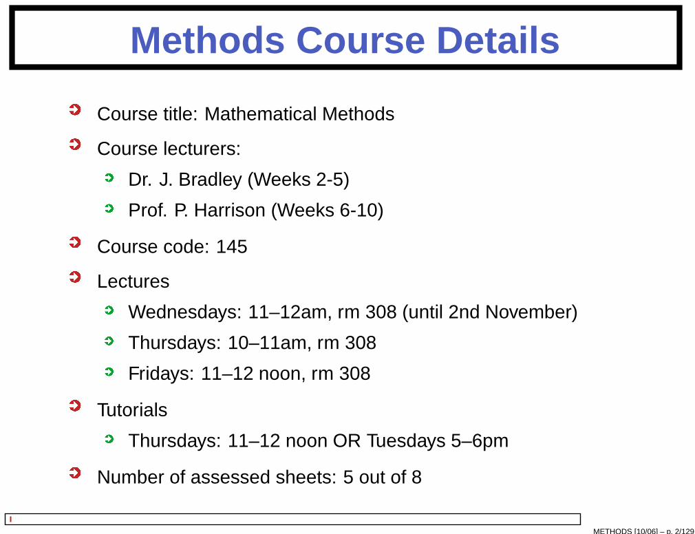
Methods Course Details
Course title: Mathematical Methods
Course lecturers:
Dr. J. Bradley (Weeks 2-5)
Prof. P. Harrison (Weeks 6-10)
Course code: 145
Lectures
Wednesdays: 11–12am, rm 308 (until 2nd November)
Thursdays: 10–11am, rm 308
Fridays: 11–12 noon, rm 308
Tutorials
Thursdays: 11–12 noon OR Tuesdays 5–6pm
Number of assessed sheets: 5 out of 8
METHODS [10/06] – p. 2/129

Assessed Exercises
Submission: through CATEhttps://sparrow.doc.ic.ac.uk/�cate/
Assessed exercises (for 1st half of course):1. set 13 Oct; due 27 Oct2. set 19 Oct; due 3 Nov3. set 26 Oct; due 10 Nov
METHODS [10/06] – p. 3/129

Recommended Books
You will find one of the following useful – no needto buy all of them:
Mathematical Methods for Science Students.(2nd Ed). G Stephenson. Longman 1973.[38]
Engineering Mathematics. (5th Ed). K AStroud. Macmillan 2001. [21]
Interactive Computer Graphics. P Burger andD Gillies. Addison Wesley 1989. [22]
Analysis: with an introduction to proof. StevenR Lay. 4th edition, Prentice Hall, 2005.
METHODS [10/06] – p. 4/129
Maths and Computer Science
Why is Maths important to ComputerScience?
Maths underpins most computingconcepts/applications, e.g.:
computer graphics and animationstock market modelsinformation search and retrievalperformance of integrated circuitscomputer visionneural computinggenetic algorithms
METHODS [10/06] – p. 5/129
Highlighted Examples
Search enginesGoogle and the PageRank algorithm
Computer graphicsnear photo realism from wireframe andvector representation
METHODS [10/06] – p. 6/129

Searching with...
METHODS [10/06] – p. 7/129

Searching for...
How does Google know to put Imperial’s website top?
METHODS [10/06] – p. 8/129

The PageRank Algorithm
List of Universities
Imperial CollegeImperial College
Imperial College
BBC News:
Imperial CollegeImperial College
Education
IEEE Research
Imperial CollegeImperial College
Awards
PageRank is based on the underlying web graph
METHODS [10/06] – p. 9/129

Propagation of PageRank
List of Universities
Imperial CollegeImperial College
Imperial College
BBC News:
Imperial CollegeImperial College
Education
IEEE Research
Imperial CollegeImperial College
Awards
Computing
Physics
Imperial CollegeComputing
Imperial CollegePhysics
METHODS [10/06] – p. 10/129
PageRank
So where’s the Maths?Web graph is represented as a matrixMatrix is 9 billion � 9 billion in sizePageRank calculation is turned into aneigenvector calculationDoes it converge? How fast does itconverge?
METHODS [10/06] – p. 11/129
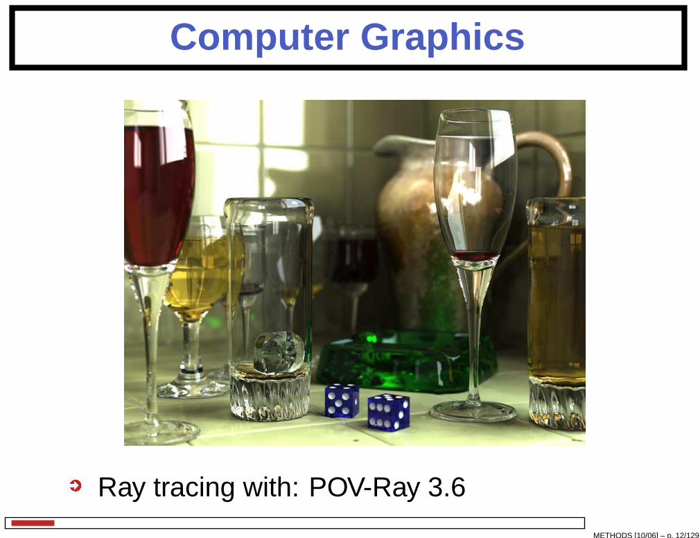
Computer Graphics
Ray tracing with: POV-Ray 3.6
METHODS [10/06] – p. 12/129

Computer Graphics
Underlying wiremesh model
METHODS [10/06] – p. 13/129
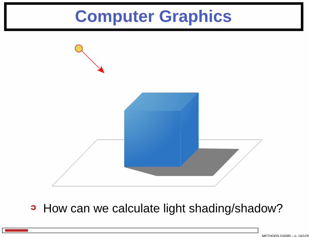
Computer Graphics
How can we calculate light shading/shadow?
METHODS [10/06] – p. 14/129
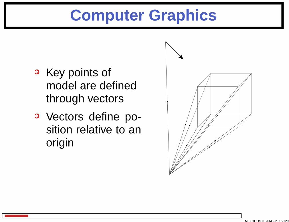
Computer Graphics
Key points ofmodel are definedthrough vectors
Vectors define po-sition relative to anorigin
METHODS [10/06] – p. 15/129
Vectors
Used in (amongst others):Computational Techniques (2nd Year)Graphics (3rd Year)Computational Finance (3rd Year)Modelling and Simulation (3rd Year)Performance Analysis (3rd Year)Digital Libraries and Search Engines (3rdYear)Computer Vision (4th Year)
METHODS [10/06] – p. 16/129
Vector Contents
What is a vector?
Useful vector tools:Vector magnitudeVector additionScalar multiplicationDot productCross product
Useful results – finding the intersection of:a line with a linea line with a planea plane with a plane
METHODS [10/06] – p. 17/129

What is a vector?
A vector is used :to convey both direction and magnitude
to store data (usually numbers) in anordered form~p = (10; 5; 7) is a row vector
~p =0B� 10571CA is a column vector
A vector is used in computer graphics torepresent the position coordinates for a point
METHODS [10/06] – p. 18/129
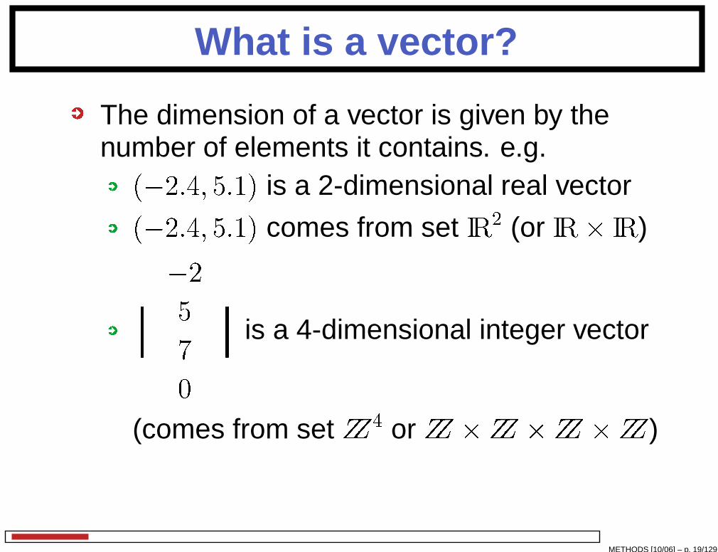
What is a vector?
The dimension of a vector is given by thenumber of elements it contains. e.g.(�2:4; 5:1) is a 2-dimensional real vector(�2:4; 5:1) comes from set IR2 (or IR� IR)0BBB�
�25701CCCA is a 4-dimensional integer vector
(comes from set ZZ4 or ZZ � ZZ � ZZ � ZZ)
METHODS [10/06] – p. 19/129
Vector Magnitude
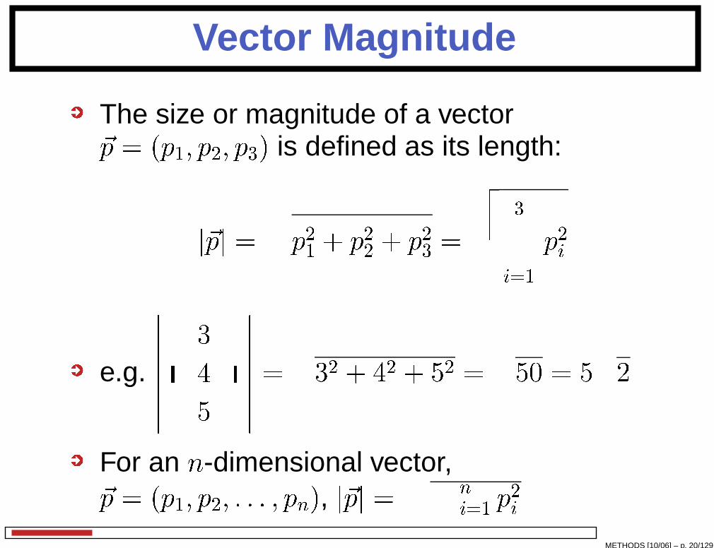
The size or magnitude of a vector~p = (p1; p2; p3) is defined as its length:
j~pj =qp21 + p22 + p23 =vuut 3X
i=1 p2i
e.g.
�������0B� 3451CA������� =
p32 + 42 + 52 = p50 = 5p2
For an n-dimensional vector,~p = (p1; p2; : : : ; pn), j~pj =pPni=1 p2i
METHODS [10/06] – p. 20/129

Vector Direction
xy
z�x
�y�zMETHODS [10/06] – p. 21/129
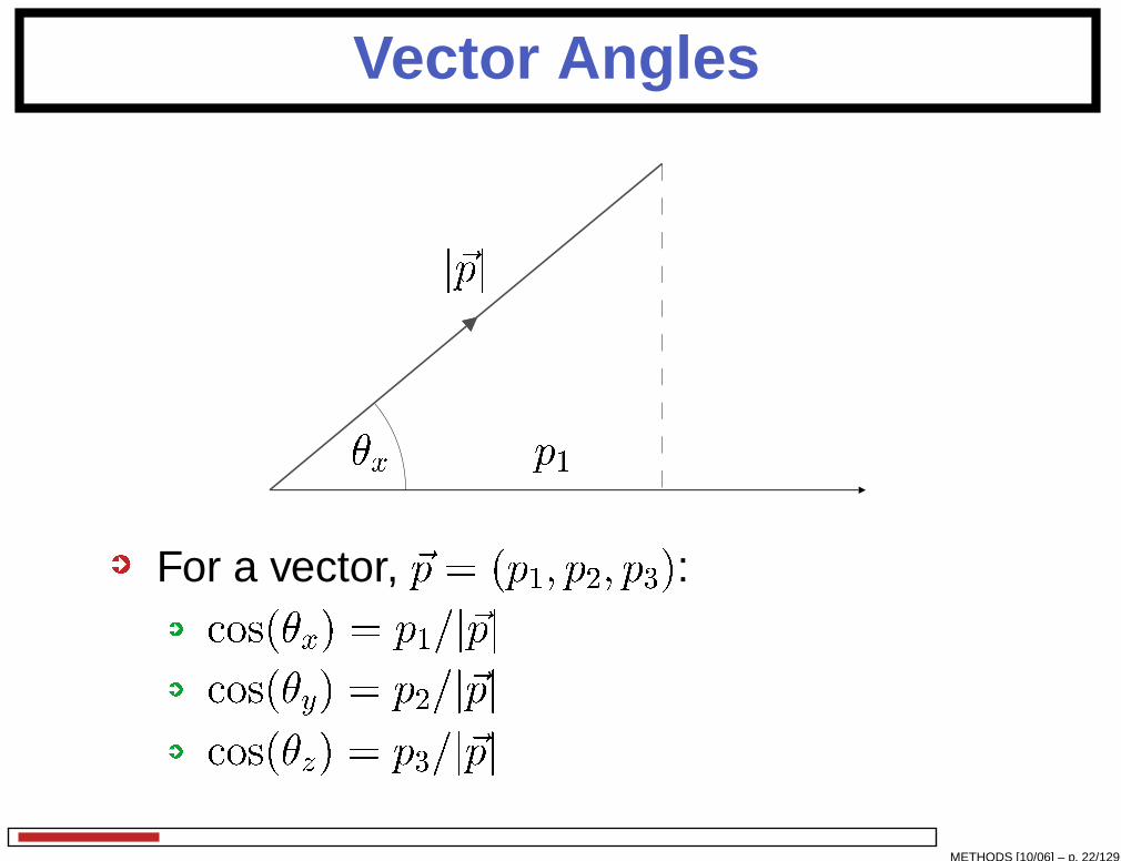
Vector Angles
�xj~pj
p1For a vector, ~p = (p1; p2; p3): os(�x) = p1=j~pj os(�y) = p2=j~pj os(�z) = p3=j~pj
METHODS [10/06] – p. 22/129
Vector addition
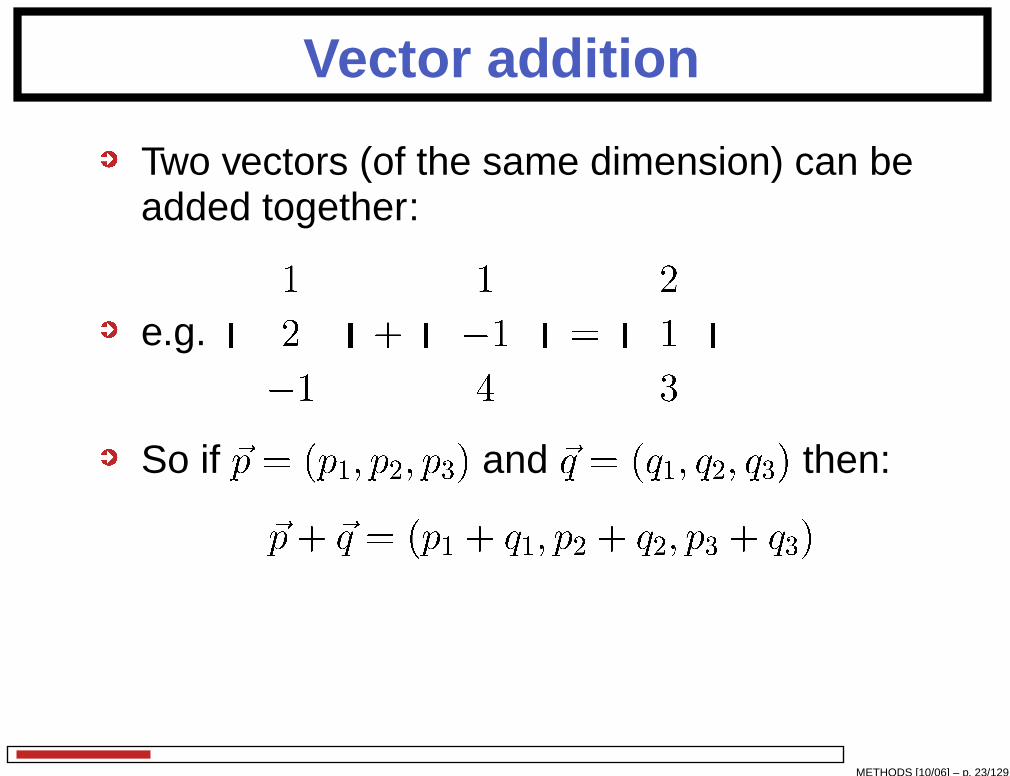
Two vectors (of the same dimension) can beadded together:
e.g.
0B� 12�11CA+0B� 1�141CA =0B� 2131CA
So if ~p = (p1; p2; p3) and ~q = (q1; q2; q3) then:~p+ ~q = (p1 + q1; p2 + q2; p3 + q3)
METHODS [10/06] – p. 23/129
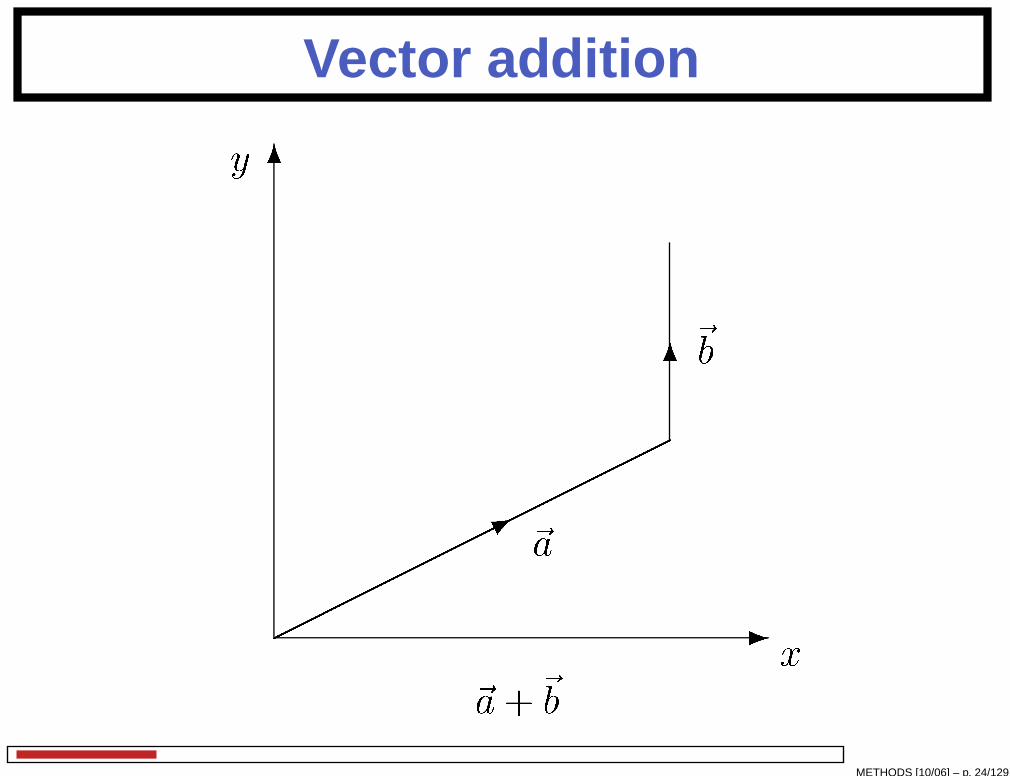
Vector addition
-
6������
��*6
y
x
~a~b
~a+~b
METHODS [10/06] – p. 24/129
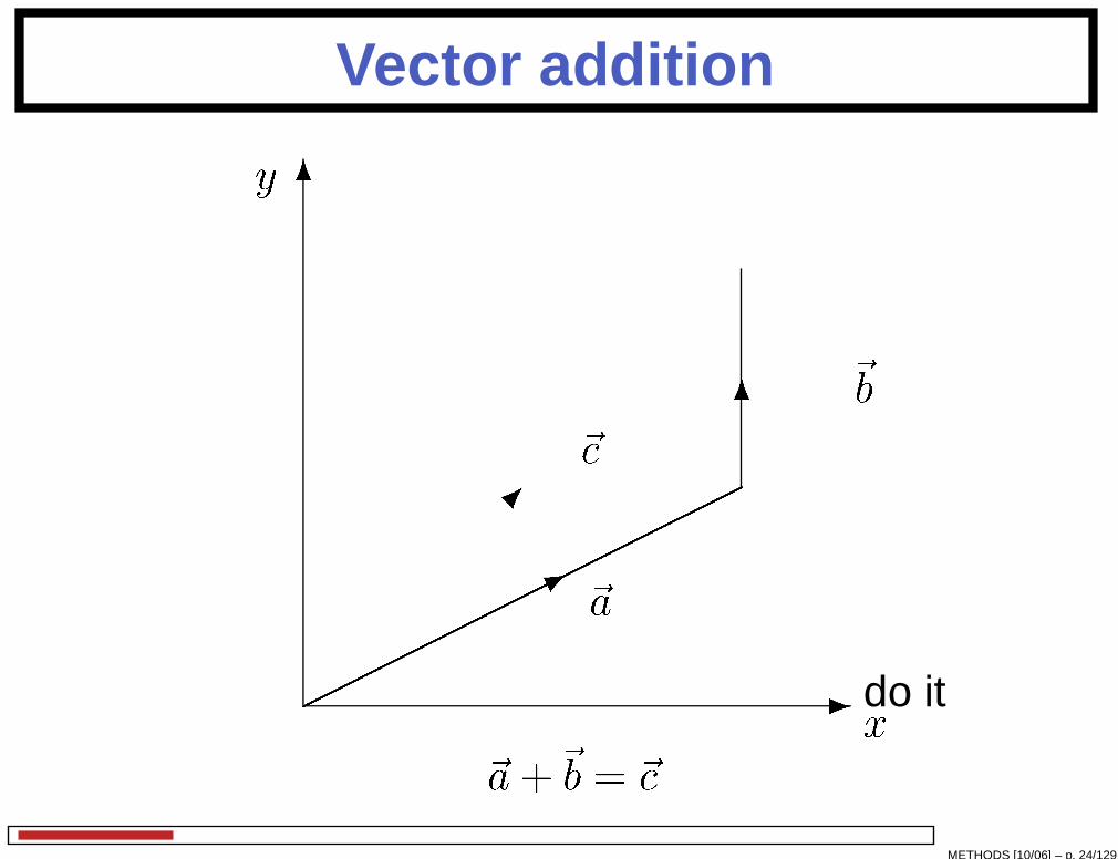
Vector addition
-
6������
��*������
��� 6
y
x
~ado it
~b~ ~a+~b = ~
METHODS [10/06] – p. 24/129

Scalar Multiplication
A scalar is just a number, e.g. 3. Unlike avector, it has no direction.
Multiplication of a vector ~p by a scalar �means that each element of the vector ismultiplied by the scalar
So if ~p = (p1; p2; p3) then:�~p = (�p1; �p2; �p3)
METHODS [10/06] – p. 25/129
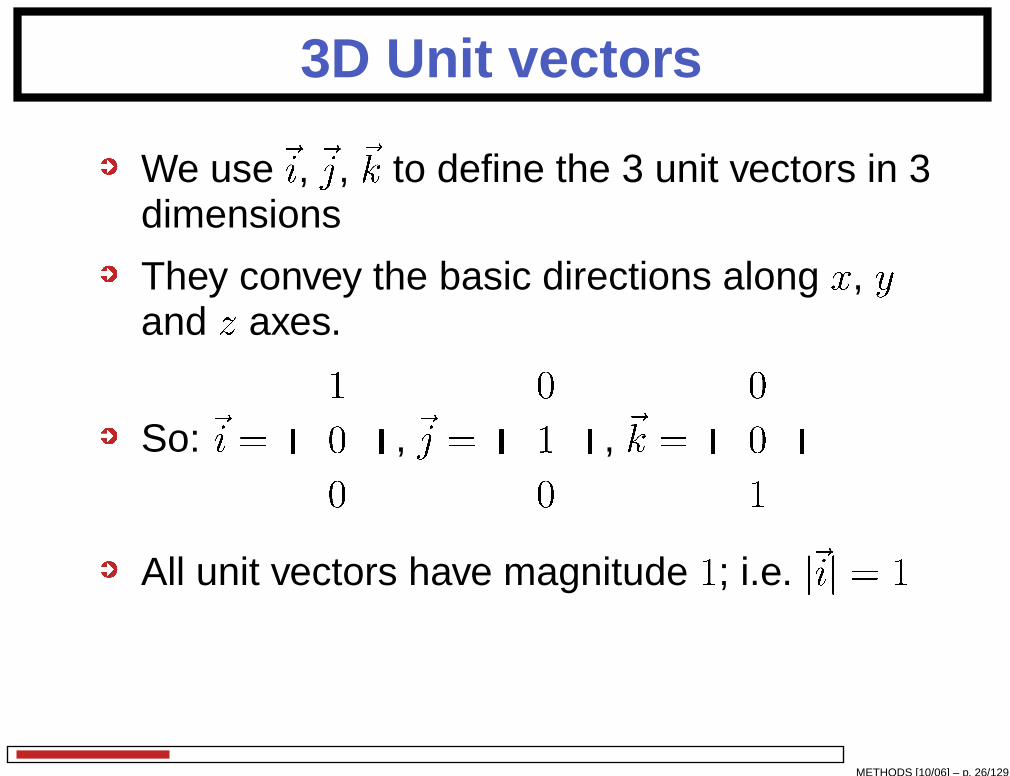
3D Unit vectors
We use~i, ~j, ~k to define the 3 unit vectors in 3dimensions
They convey the basic directions along x, yand z axes.
So: ~i =0B� 1001CA, ~j =0B� 0101CA, ~k =0B� 0011CA
All unit vectors have magnitude 1; i.e. j~ij = 1
METHODS [10/06] – p. 26/129
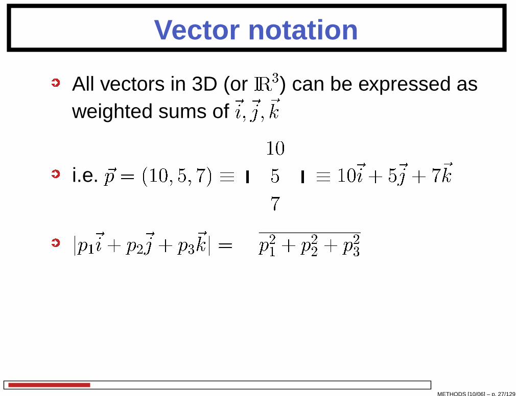
Vector notation
All vectors in 3D (or IR3) can be expressed asweighted sums of~i;~j;~ki.e. ~p = (10; 5; 7) �
0B� 10571CA � 10~i+ 5~j + 7~k
jp1~i+ p2~j + p3~kj =pp21 + p22 + p23
METHODS [10/06] – p. 27/129

Dot Product
Also known as: scalar product
Used to determine how close 2 vectors are tobeing parallel/perpendicular
The dot product of two vectors ~p and ~q is:~p � ~q = j~pj j~qj os �where � is angle between the vectors ~p and ~q
For ~p = (p1; p2; p3) and ~q = (q1; q2; q3) then:~p � ~q = p1q1 + p2q2 + p3q3
METHODS [10/06] – p. 28/129
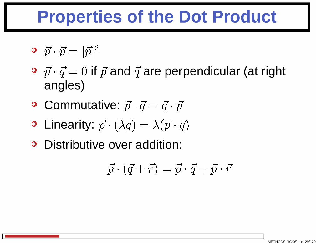
Properties of the Dot Product
~p � ~p = j~pj2~p � ~q = 0 if ~p and ~q are perpendicular (at rightangles)
Commutative: ~p � ~q = ~q � ~pLinearity: ~p � (�~q) = �(~p � ~q)Distributive over addition:~p � (~q + ~r) = ~p � ~q + ~p � ~r
METHODS [10/06] – p. 29/129
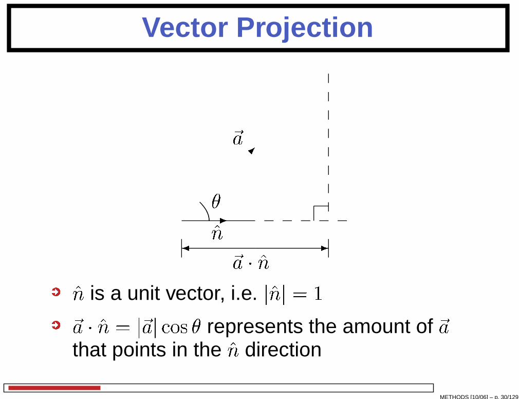
Vector Projection
������
���
- -� ^n~a
�~a � ^n^n is a unit vector, i.e. j^nj = 1~a � ^n = j~aj os � represents the amount of ~a
that points in the ^n direction
METHODS [10/06] – p. 30/129
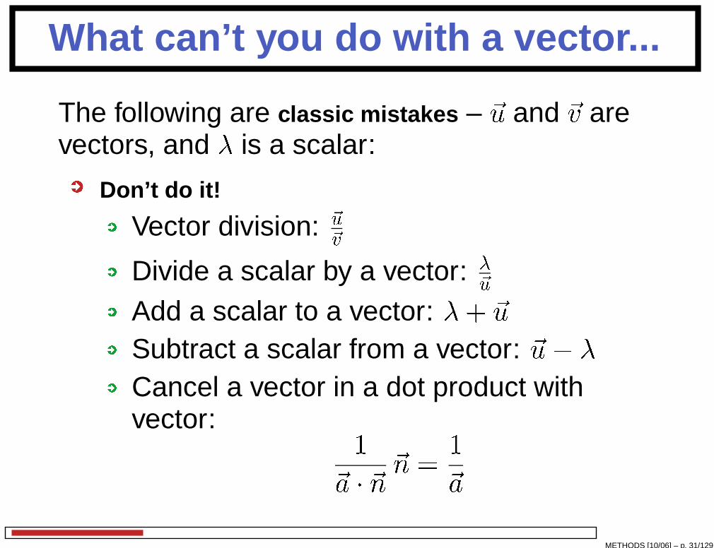
What can’t you do with a vector...
The following are classic mistakes – ~u and ~v arevectors, and � is a scalar:
Don’t do it!
Vector division: ~u~vDivide a scalar by a vector: �~uAdd a scalar to a vector: �+ ~uSubtract a scalar from a vector: ~u� �
Cancel a vector in a dot product withvector: 1~a � ~n ~n = 1~a��
METHODS [10/06] – p. 31/129
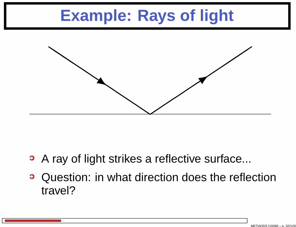
Example: Rays of light
���������������3QQQQQ sA ray of light strikes a reflective surface...
Question: in what direction does the reflectiontravel?
METHODS [10/06] – p. 32/129
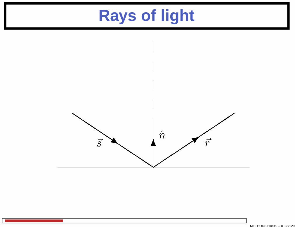
Rays of light
���������������3QQQQQ s 6~s ~r^n
���������������3QQQQQ s QQQ k6~s ~r
�~s^n��
~r ~s ^n
METHODS [10/06] – p. 33/129
Rays of light
���������������3QQQQQ s QQQ k6~s ~r
�~s^n��
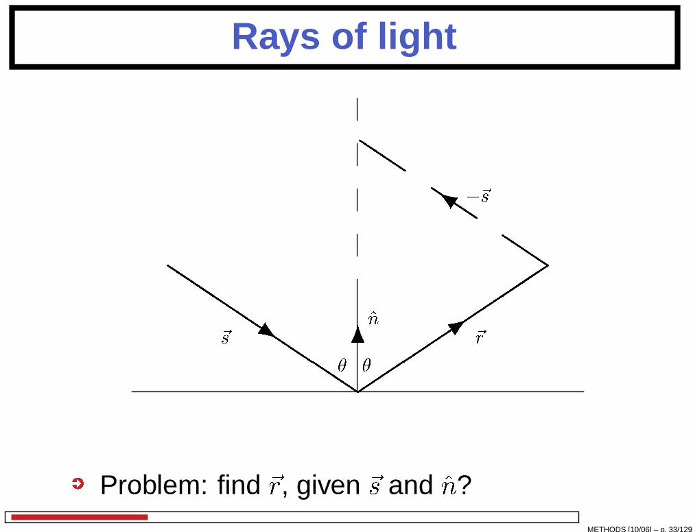
Problem: find ~r, given ~s and ^n?METHODS [10/06] – p. 33/129
Rays of light
���������������3QQQQQ s QQQ k6~s ~r
�~s^n��
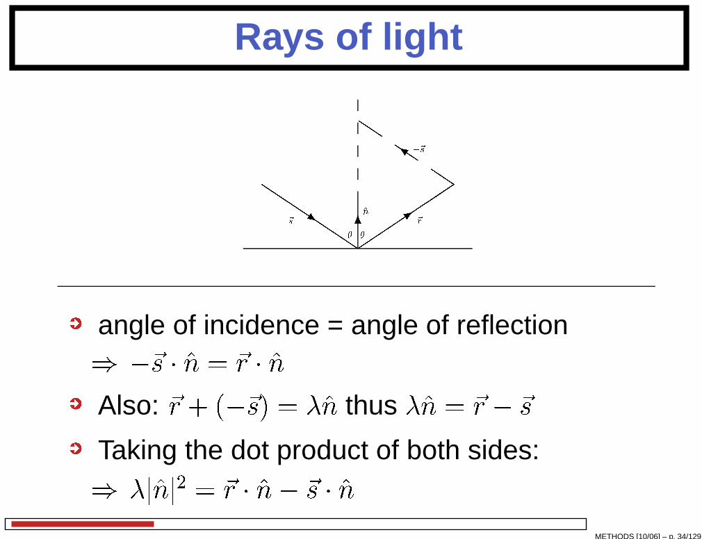
angle of incidence = angle of reflection) �~s � ^n = ~r � ^nAlso: ~r + (�~s) = �^n thus �^n = ~r � ~s
Taking the dot product of both sides:) �j^nj2 = ~r � ^n� ~s � ^n
METHODS [10/06] – p. 34/129
Rays of light
���������������3QQQQQ s QQQ k6~s ~r
�~s^n��
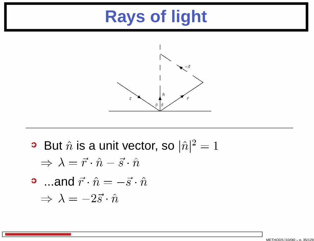
But ^n is a unit vector, so j^nj2 = 1) � = ~r � ^n� ~s � ^n...and ~r � ^n = �~s � ^n) � = �2~s � ^n
METHODS [10/06] – p. 35/129
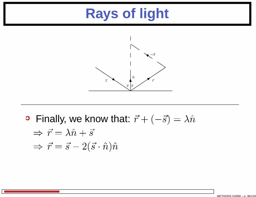
Rays of light
���������������3QQQQQ s QQQ k6~s ~r
�~s^n��
Finally, we know that: ~r + (�~s) = �^n) ~r = �^n+ ~s) ~r = ~s� 2(~s � ^n)^n
METHODS [10/06] – p. 36/129

Equation of a line
������������
��������
����*���
��� I ������
������
�~d ~r
~aO
For a general point, ~r, on the line:~r = ~a+ �~d
where: ~a is a point on the line and ~d is avector parallel to the line
METHODS [10/06] – p. 37/129
Equation of a plane
Equation of a plane. For a general point, ~r, inthe plane, ~r has the property that:~r:^n = mwhere:^n is the unit vector perpendicular to the
planejmj is the distance from the plane to theorigin (at its closest point)
METHODS [10/06] – p. 38/129
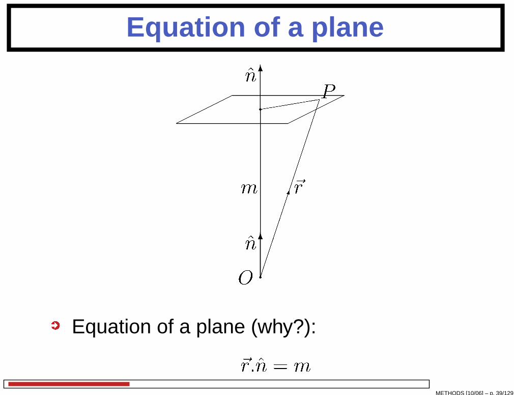
Equation of a plane
����� �����q
q���
������
�������
������
��Æ((((((
66
~r^n
^nm
ON P
Equation of a plane (why?):~r:^n = m
METHODS [10/06] – p. 39/129

How to solve Vector Problems
1. IMPORTANT: Draw a diagram!
2. Write down the equations that you aregiven/apply to the situation
3. Write down what you are trying to find?
4. Try variable substitution
5. Try taking the dot product of one or moreequations
What vector to dot with?Answer: if eqn (1) has term ~r in and eqn (2) has
term ~r � ~s in: dot eqn (1) with ~s.METHODS [10/06] – p. 40/129
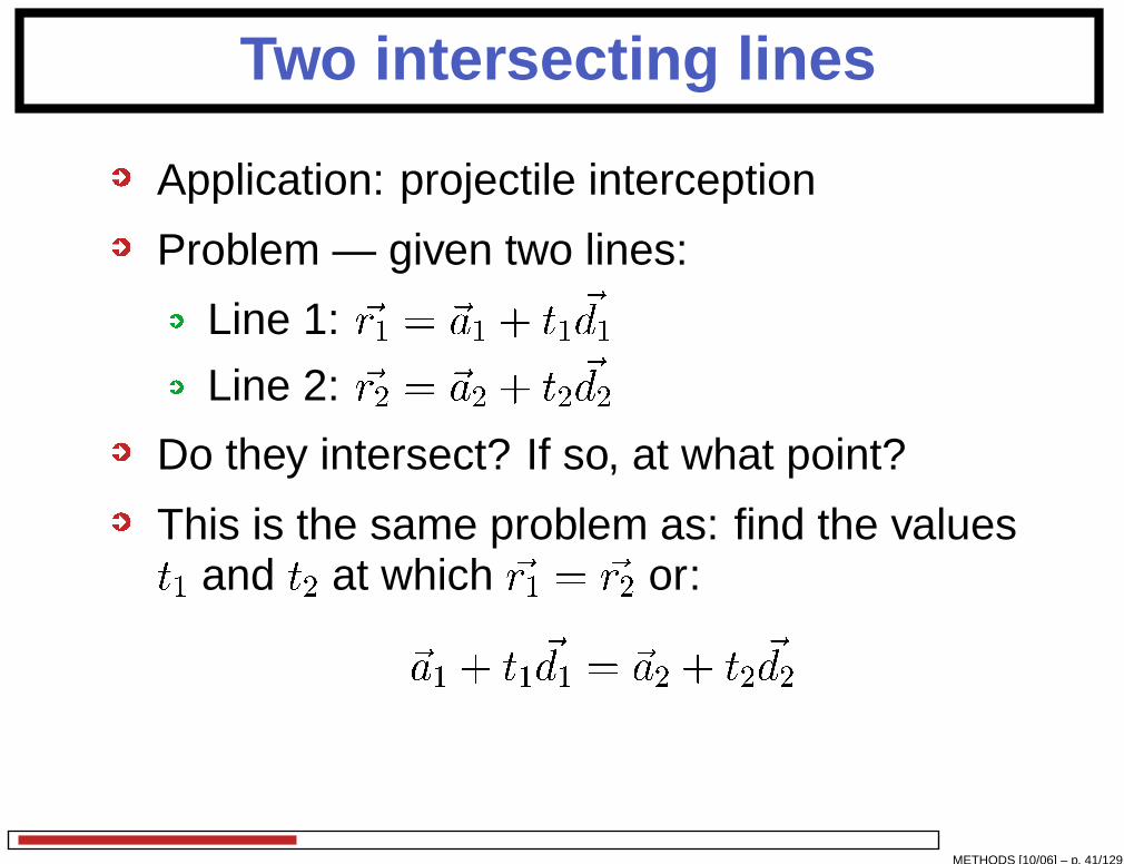
Two intersecting lines
Application: projectile interception
Problem — given two lines:
Line 1: ~r1 = ~a1 + t1 ~d1Line 2: ~r2 = ~a2 + t2 ~d2
Do they intersect? If so, at what point?
This is the same problem as: find the valuest1 and t2 at which ~r1 = ~r2 or:
~a1 + t1 ~d1 = ~a2 + t2 ~d2
METHODS [10/06] – p. 41/129
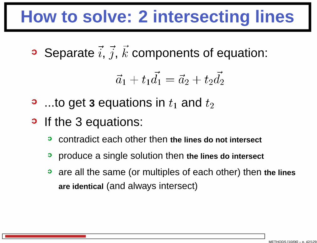
How to solve: 2 intersecting lines
Separate~i, ~j, ~k components of equation:
~a1 + t1 ~d1 = ~a2 + t2 ~d2...to get 3 equations in t1 and t2If the 3 equations:
contradict each other then the lines do not intersect
produce a single solution then the lines do intersect
are all the same (or multiples of each other) then the lines
are identical (and always intersect)
METHODS [10/06] – p. 42/129
Intersection of a line and plane
����� �����
QQQQQQQQQs 6^n~d
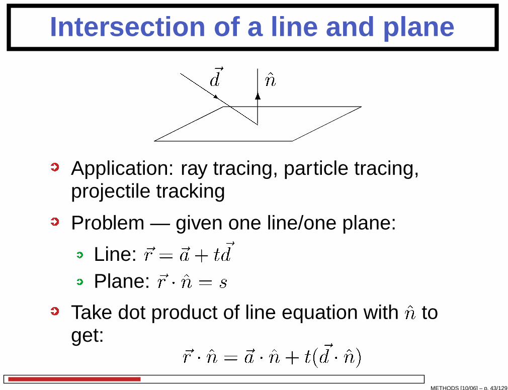
Application: ray tracing, particle tracing,projectile tracking
Problem — given one line/one plane:
Line: ~r = ~a+ t~dPlane: ~r � ^n = s
Take dot product of line equation with ^n toget: ~r � ^n = ~a � ^n+ t(~d � ^n)
METHODS [10/06] – p. 43/129

Intersection of a line and plane
With ~r � ^n = ~a � ^n+ t(~d � ^n) — what are wetrying to find?
We are trying to find a specific value of tthat corresponds to the point of intersection
Since ~r � ^n = s at intersection, we get:t = s�~a�^n~d�^n
So using line equation we get our point ofintersection, ~r0:
~r0 = ~a+ s� ~a � ^n~d � ^n ~d
METHODS [10/06] – p. 44/129
Example: intersecting planes
������
�����
���q6
HHHHHH####
### aaaaaaq����^n1 ^n2
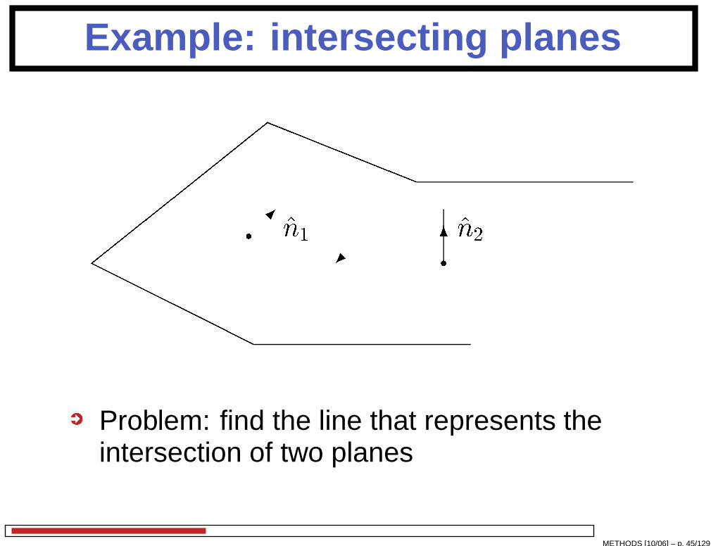
Problem: find the line that represents theintersection of two planes
METHODS [10/06] – p. 45/129

Intersecting planes
Application: edge detection
Equations of planes:Plane 1: ~r � ^n1 = s1Plane 2: ~r � ^n2 = s2
We want to find the line of intesection, i.e. find~a and ~d in: ~s = ~a+ �~dIf ~s = x~i+ y~j + z~k is on the intersection line:) it also lies in both planes 1 and 2) ~s � ^n1 = s1 and ~s � ^n2 = s2
Can use these two equations to generateequation of line
METHODS [10/06] – p. 46/129
Example: Intersecting planes
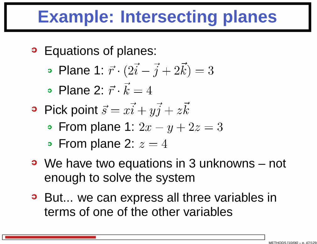
Equations of planes:
Plane 1: ~r � (2~i�~j + 2~k) = 3Plane 2: ~r � ~k = 4
Pick point ~s = x~i+ y~j + z~kFrom plane 1: 2x� y + 2z = 3From plane 2: z = 4
We have two equations in 3 unknowns – notenough to solve the system
But... we can express all three variables interms of one of the other variables
METHODS [10/06] – p. 47/129
Example: Intersecting planes
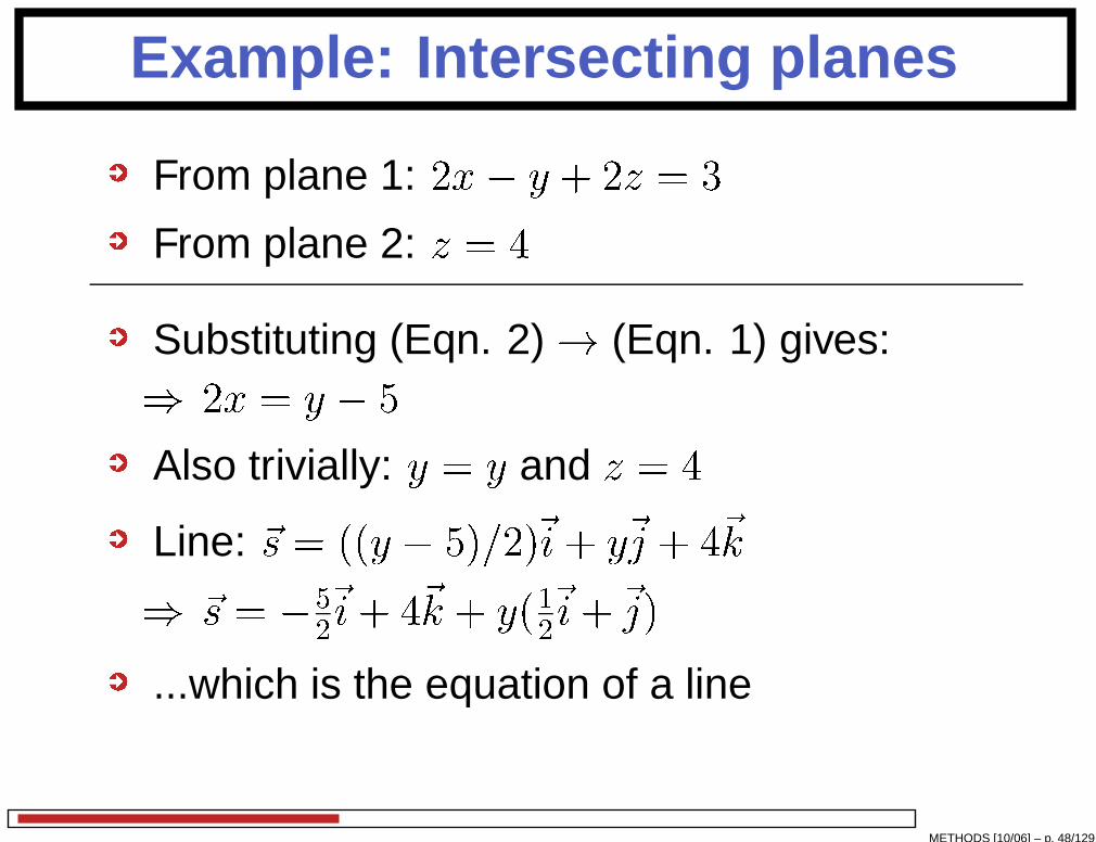
From plane 1: 2x� y + 2z = 3From plane 2: z = 4
Substituting (Eqn. 2) ! (Eqn. 1) gives:) 2x = y � 5
Also trivially: y = y and z = 4Line: ~s = ((y � 5)=2)~i + y~j + 4~k) ~s = �52~i+ 4~k + y(12~i+~j)
...which is the equation of a line
METHODS [10/06] – p. 48/129
Cross Product
HHHHHHHHj��������16 ~p~q�~p� ~q
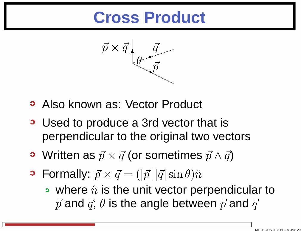
Also known as: Vector Product
Used to produce a 3rd vector that isperpendicular to the original two vectors
Written as ~p� ~q (or sometimes ~p ^ ~q)Formally: ~p� ~q = (j~pj j~qj sin �)^n
where ^n is the unit vector perpendicular to~p and ~q; � is the angle between ~p and ~q
METHODS [10/06] – p. 49/129

Cross Product
From definition: j~p� ~qj = j~pj j~qj sin �In coordinate form: ~a�~b =
�������0B� ~i ~j ~ka1 a2 a3b1 b2 b31CA�������) ~a�~b =(a2b3�a3b2)~i� (a1b3�a3b1)~j+(a1b2�a2b1)~k
Useful for: e.g. given 2 lines in a plane, writedown the equation of the plane
METHODS [10/06] – p. 50/129

Properties of Cross Product
~p� ~q is itself a vector that is perpendicular to both ~pand ~q, so:~p � (~p� ~q) = 0 and ~q � (~p� ~q) = 0If ~p is parallel to ~q then ~p� ~q = ~0
where ~0 = 0~i+ 0~j + 0~kNOT commutative: ~a�~b 6= ~b� ~a
In fact: ~a�~b = �~b� ~aNOT associative: (~a�~b)� ~ 6= ~a� (~b� ~ )
Left distributive: ~a� (~b+ ~ ) = ~a�~b+ ~a� ~
Right distributive: (~b+ ~ )� ~a = ~b� ~a+ ~ � ~a
METHODS [10/06] – p. 51/129
Properties of Cross Product
Final important vector product identity:~a� (~b� ~ ) = (~a � ~ )~b� (~a �~b)~ which says that: ~a� (~b� ~ ) = �~b+ �~ i.e. the vector ~a� (~b� ~ ) lies in the planecreated by ~b and ~
METHODS [10/06] – p. 52/129
Matrices
Used in (amongst others):Computational Techniques (2nd Year)Graphics (3rd Year)Performance Analysis (3rd Year)Digital Libraries and Search Engines (3rdYear)Computing for Optimal Decisions (4th Year)Quantum Computing (4th Year)Computer Vision (4th Year)
METHODS [10/06] – p. 53/129

Matrix Contents
What is a Matrix?Useful Matrix tools:
Matrix addition
Matrix multiplication
Matrix transpose
Matrix determinant
Matrix inverse
Gaussian Elimination
Eigenvectors and eigenvalues
Useful results:solution of linear systems
Google’s PageRank algorithm
METHODS [10/06] – p. 54/129

What is a Matrix?
A matrix is a 2 dimensional array of numbers
Used to represent, for instance, a network:
i i
i� -
6
������
���I1 2
3
�!0B� 0 1 11 0 10 0 01CA
METHODS [10/06] – p. 55/129

Application: Markov Chains
Example: What is the probability that it will besunny today given that it rained yesterday?(Answer: 0.25)
0:6 0:40:25 0:75!Sun Rain
Today
Sun
Rain
Yest
erda
y
Example question: what is the probability thatit’s raining on Thursday given that it’s sunnyon Monday?
METHODS [10/06] – p. 56/129
Matrix Addition
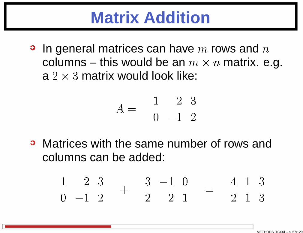
In general matrices can have m rows and ncolumns – this would be an m� n matrix. e.g.a 2� 3 matrix would look like:
A = 1 2 30 �1 2!
Matrices with the same number of rows andcolumns can be added: 1 2 30 �1 2
!+ 3 �1 02 2 1! = 4 1 32 1 3!
METHODS [10/06] – p. 57/129
Scalar multiplication
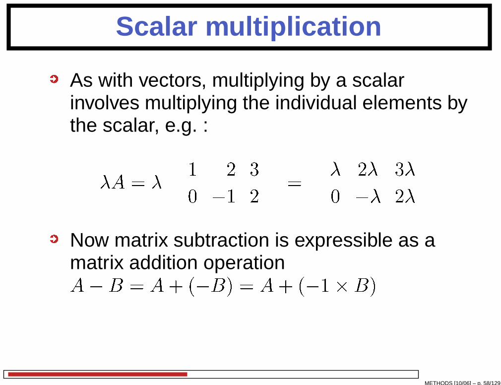
As with vectors, multiplying by a scalarinvolves multiplying the individual elements bythe scalar, e.g. :
�A = � 1 2 30 �1 2! = � 2� 3�0 �� 2�!
Now matrix subtraction is expressible as amatrix addition operationA�B = A+ (�B) = A+ (�1�B)
METHODS [10/06] – p. 58/129
Matrix Identities
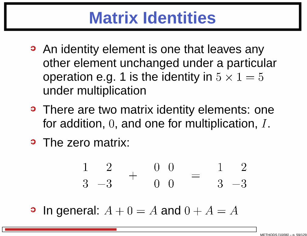
An identity element is one that leaves anyother element unchanged under a particularoperation e.g. 1 is the identity in 5� 1 = 5under multiplication
There are two matrix identity elements: onefor addition, 0, and one for multiplication, I.
The zero matrix: 1 23 �3!+ 0 00 0! = 1 23 �3!
In general: A+ 0 = A and 0 + A = A
METHODS [10/06] – p. 59/129
Matrix Identities
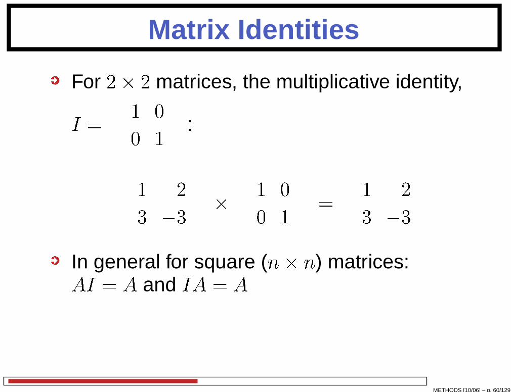
For 2� 2 matrices, the multiplicative identity,
I = 1 00 1!
:
1 23 �3!� 1 00 1! = 1 23 �3!
In general for square (n� n) matrices:AI = A and IA = A
METHODS [10/06] – p. 60/129
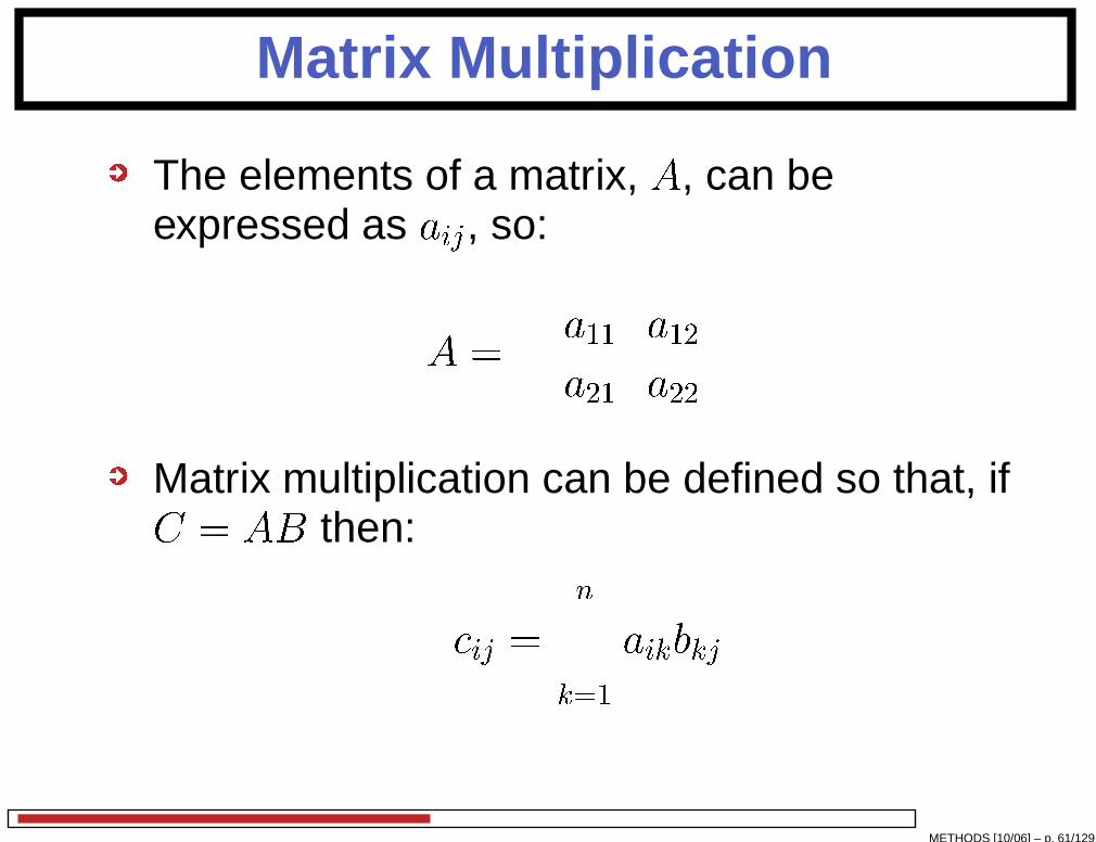
Matrix Multiplication
The elements of a matrix, A, can beexpressed as aij, so:
A = a11 a12a21 a22!
Matrix multiplication can be defined so that, ifC = AB then:
ij = nXk=1 aikbkj
METHODS [10/06] – p. 61/129

Matrix Multiplication
Multiplication, AB, is only well defined if thenumber of columns of A = the number of rowsof B. i.e.A can be m� nB has to be n� p
the result, AB, is m� pExample:0� 0 1 23 4 5 1A0BB� 6 78 910 11
1CCA = 0� 0� 6 + 1� 8 + 2� 10 0� 7 + 1� 9 + 2� 113� 6 + 4� 8 + 5� 10 3� 7 + 4� 9 + 5� 11 1A
METHODS [10/06] – p. 62/129

Matrix Properties
A+B = B + A(A+B) + C = A+ (B + C)�A = A��(A+B) = �A+ �B(AB)C = A(BC)(A+B)C = AC +BC; C(A+B) = CA+ CB
But... AB 6= BA i.e. matrix multiplication isNOT commutative0� 0 11 �1
1A0� 1 11 11A = 0� 1 10 01A 6= 0� 1 11 11A0� 0 11 �11A
METHODS [10/06] – p. 63/129
Matrices in Graphics
Matrix multiplication is a simple way toencode different transformations of objects incomputer graphics, e.g. :
reflection
scaling
rotation
translation (requires 4� 4 transformationmatrix)
METHODS [10/06] – p. 64/129
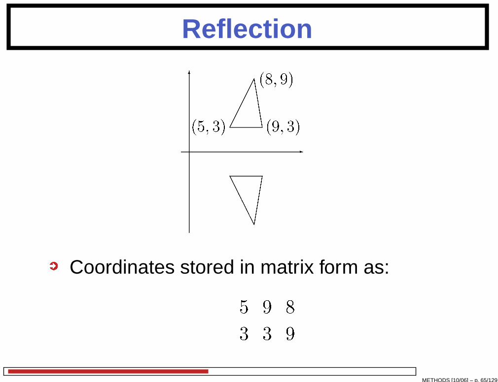
Reflection
-
6AAAAAA�������
������
EEEEEEE(5; 3) (9; 3)
(8; 9)Coordinates stored in matrix form as: 5 9 83 3 9
!
METHODS [10/06] – p. 65/129
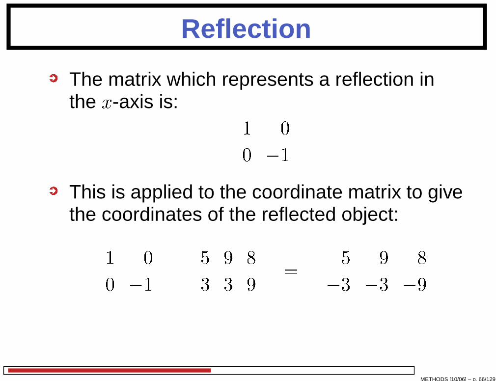
Reflection
The matrix which represents a reflection inthe x-axis is: 1 00 �1
!This is applied to the coordinate matrix to givethe coordinates of the reflected object: 1 00 �1
! 5 9 83 3 9! = 5 9 8�3 �3 �9!
METHODS [10/06] – p. 66/129
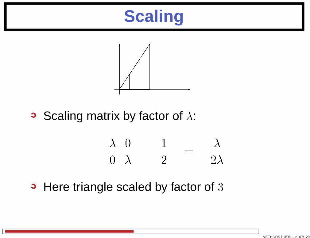
Scaling
-
6
Scaling matrix by factor of �: � 00 �! 12! = �2�!
Here triangle scaled by factor of 3
METHODS [10/06] – p. 67/129
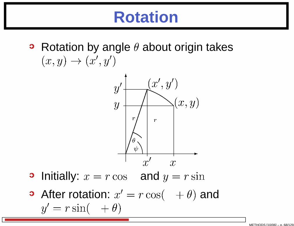
Rotation
Rotation by angle � about origin takes(x; y)! (x0; y0)
-
6���������
������ (x; y)
xx0(x0; y0)yy0 rr
�Initially: x = r os and y = r sin
After rotation: x0 = r os( + �) andy0 = r sin( + �)METHODS [10/06] – p. 68/129

Rotation
Require matrix R s.t.:
x0y0! = R xy!Initially: x = r os and y = r sin Start with x0 = r os( + �)) x0 = r os | {z }x os � � r sin | {z }y sin �
) x0 = x os � � y sin �Similarly: y0 = x sin � + y os �
Thus R = 0� os � � sin �sin � os �1A
METHODS [10/06] – p. 69/129
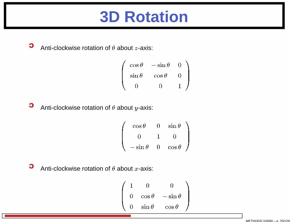
3D Rotation
Anti-clockwise rotation of � about z-axis:0BB� os � � sin � 0sin � os � 00 0 11CCA
Anti-clockwise rotation of � about y-axis:0BB� os � 0 sin �0 1 0� sin � 0 os �1CCA
Anti-clockwise rotation of � about x-axis:0BB� 1 0 00 os � � sin �0 sin � os �1CCA
METHODS [10/06] – p. 70/129
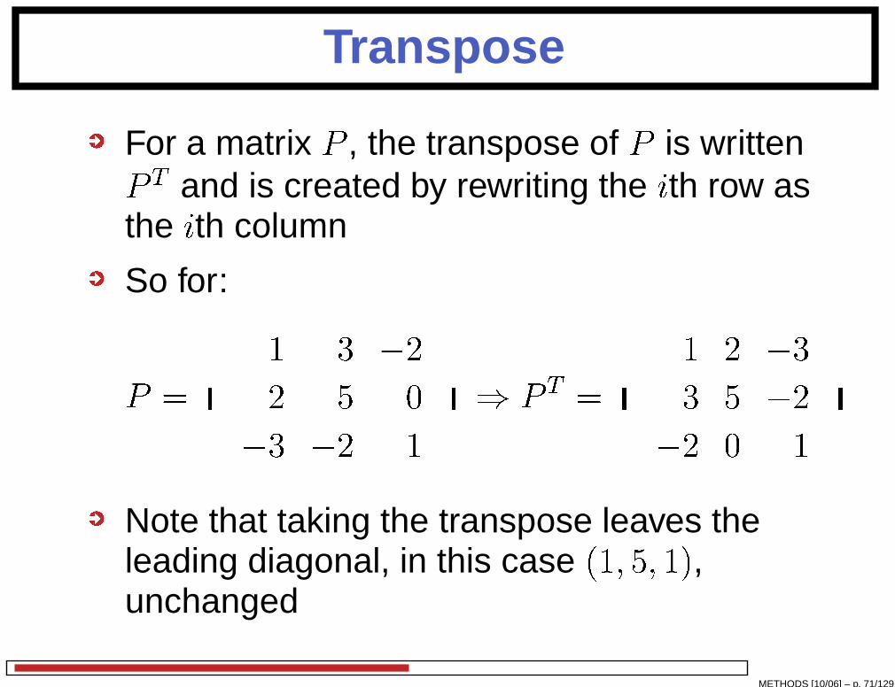
Transpose
For a matrix P , the transpose of P is writtenP T and is created by rewriting the ith row asthe ith column
So for:
P =0B� 1 3 �22 5 0�3 �2 11CA) P T =0B� 1 2 �33 5 �2�2 0 11CA
Note that taking the transpose leaves theleading diagonal, in this case (1; 5; 1),unchanged
METHODS [10/06] – p. 71/129
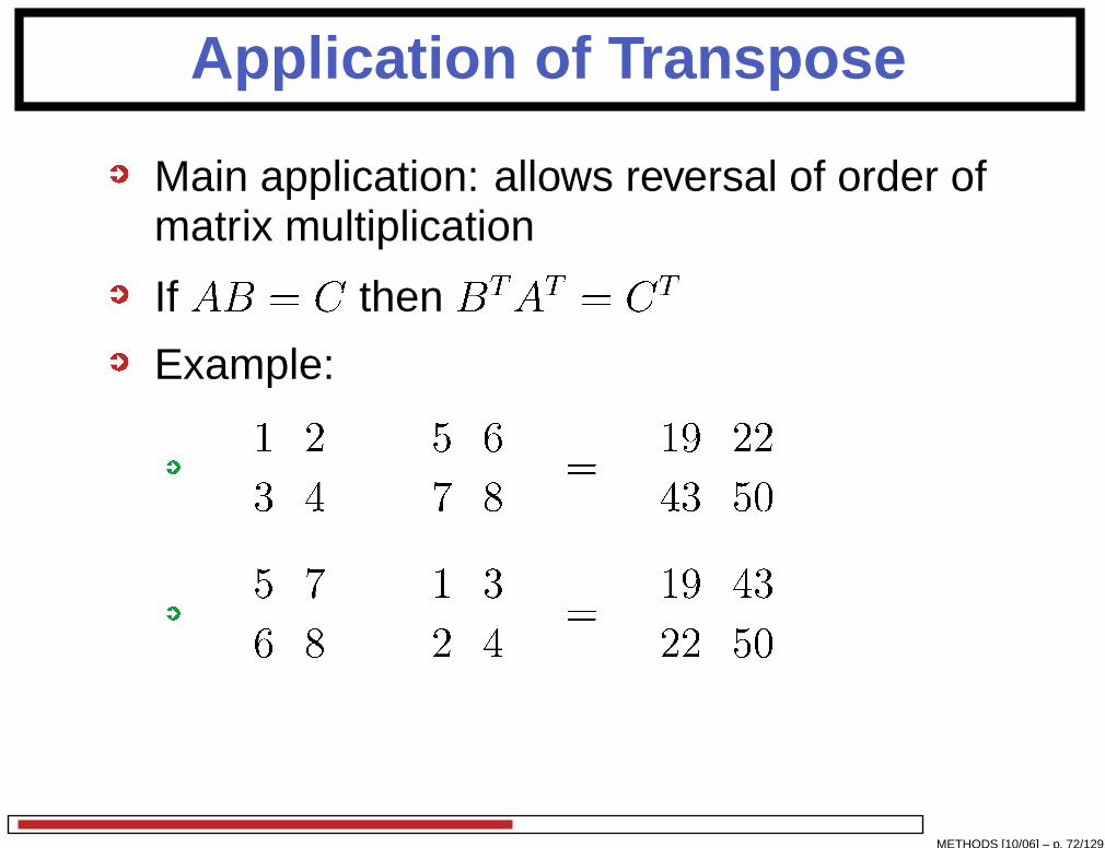
Application of Transpose
Main application: allows reversal of order ofmatrix multiplication
If AB = C then BTAT = CTExample: 1 23 4
! 5 67 8! = 19 2243 50!
5 76 8! 1 32 4! = 19 4322 50!
METHODS [10/06] – p. 72/129
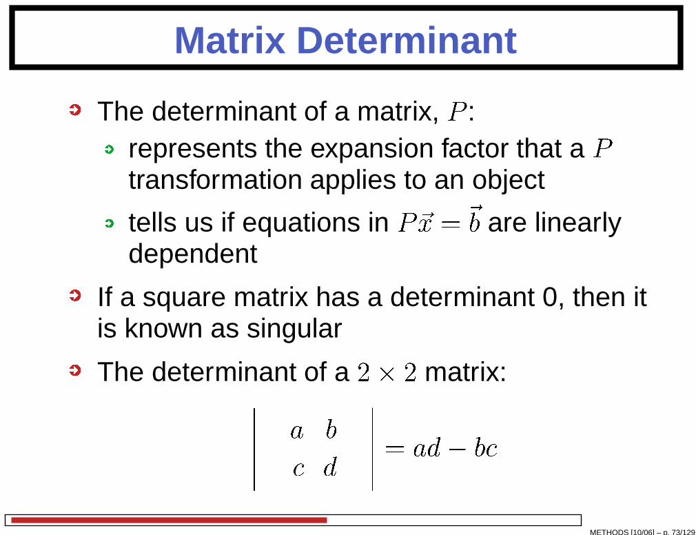
Matrix Determinant
The determinant of a matrix, P :represents the expansion factor that a Ptransformation applies to an object
tells us if equations in P~x = ~b are linearlydependent
If a square matrix has a determinant 0, then itis known as singular
The determinant of a 2� 2 matrix:����� a b d!����� = ad� b
METHODS [10/06] – p. 73/129

3� 3 Matrix Determinant
For a 3� 3 matrix:
A =0B� a1 a2 a3b1 b2 b3 1 2 31CA
...the determinant can be calculated by:
a1 ����� b2 b3 2 3!������a2����� b1 b3 1 3!�����+a3����� b1 b2 1 2!�����
= a1(b2 3� b3 2)� a2(b1 3� b3 1) + a3(b1 2� b2 1)
METHODS [10/06] – p. 74/129
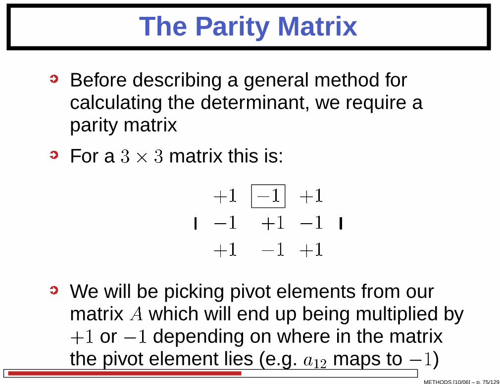
The Parity Matrix
Before describing a general method forcalculating the determinant, we require aparity matrix
For a 3� 3 matrix this is:0B� +1 �1 +1�1 +1 �1+1 �1 +11CA
We will be picking pivot elements from ourmatrix A which will end up being multiplied by+1 or �1 depending on where in the matrixthe pivot element lies (e.g. a12 maps to �1)
METHODS [10/06] – p. 75/129
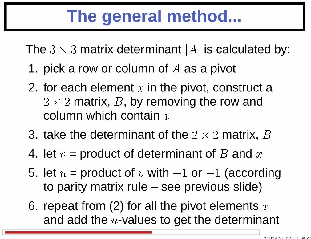
The general method...
The 3� 3 matrix determinant jAj is calculated by:
1. pick a row or column of A as a pivot
2. for each element x in the pivot, construct a2� 2 matrix, B, by removing the row andcolumn which contain x
3. take the determinant of the 2� 2 matrix, B
4. let v = product of determinant of B and x
5. let u = product of v with +1 or �1 (accordingto parity matrix rule – see previous slide)
6. repeat from (2) for all the pivot elements x
and add the u-values to get the determinantMETHODS [10/06] – p. 76/129
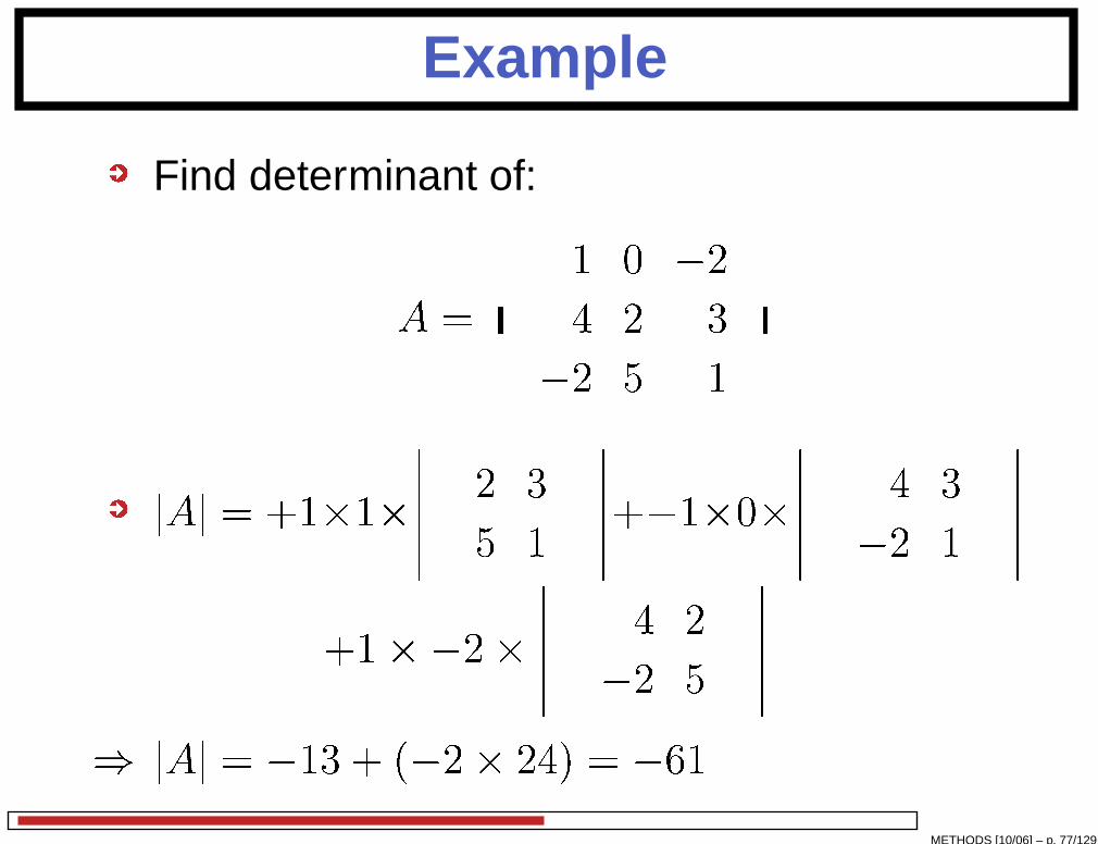
Example
Find determinant of:
A =0B� 1 0 �24 2 3�2 5 11CA
jAj = +1�1������ 2 35 1!�����+�1�0������ 4 3�2 1!�����
+1��2� ����� 4 2�2 5!�����) jAj = �13 + (�2� 24) = �61
METHODS [10/06] – p. 77/129

Matrix Inverse
The inverse of a matrix describes the reversetransformation that the original matrixdescribed
A matrix, A, multiplied by its inverse, A�1,gives the identity matrix, IThat is: AA�1 = I and A�1A = I
METHODS [10/06] – p. 78/129
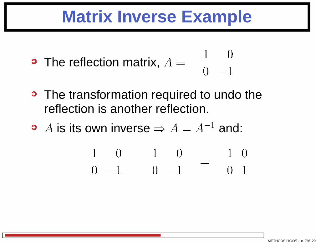
Matrix Inverse Example
The reflection matrix, A = 1 00 �1!The transformation required to undo thereflection is another reflection.A is its own inverse ) A = A�1 and: 1 00 �1
! 1 00 �1! = 1 00 1!
METHODS [10/06] – p. 79/129
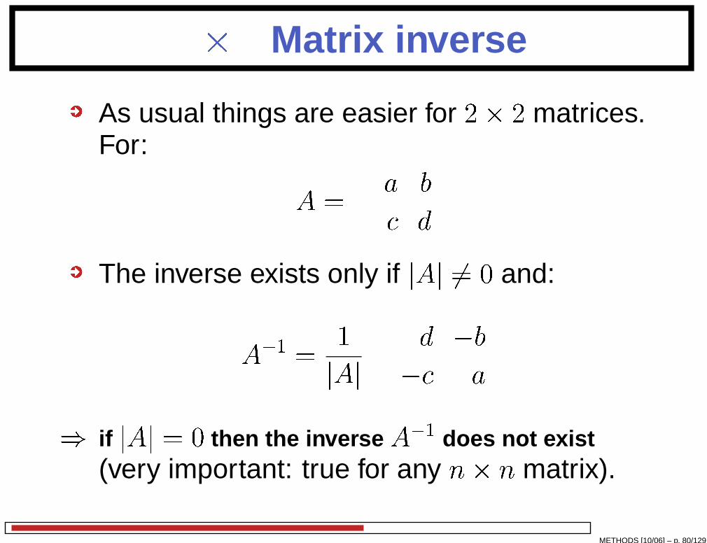
2� 2 Matrix inverse
As usual things are easier for 2� 2 matrices.For: A = a b d
!The inverse exists only if jAj 6= 0 and:
A�1 = 1jAj d �b� a!
) if jAj = 0 then the inverse A�1 does not exist(very important: true for any n� n matrix).
METHODS [10/06] – p. 80/129

n� n Matrix Inverse
First we need to define C, the cofactorsmatrix of a matrix, A, to have elements ij = � minor of aij, using the parity matrix asbefore to determine whether is gets multipliedby +1 or �1
(The minor of an element is thedeterminant of the matrix formed bydeleting the row/column containing thatelement, as before)
Then the n� n inverse of A is:A�1 = 1jAjCT
METHODS [10/06] – p. 81/129
Linear Systems
Linear systems are used in all branches ofscience and scientific computing
Example of a simple linear system:If 3 PCs and 5 Macs emit 151W of heat in1 room, and 6 PCs together with 2 Macsemit 142W in another. How much energydoes a single PC or Mac emit?When a linear system has 2 variables alsocalled simultaneous equationHere we have: 3p+ 5m = 151 and6p+ 2m = 142
METHODS [10/06] – p. 82/129
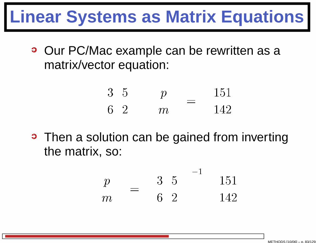
Linear Systems as Matrix Equations
Our PC/Mac example can be rewritten as amatrix/vector equation: 3 56 2
! pm! = 151142!
Then a solution can be gained from invertingthe matrix, so: pm
! = 3 56 2!�1 151142!
METHODS [10/06] – p. 83/129
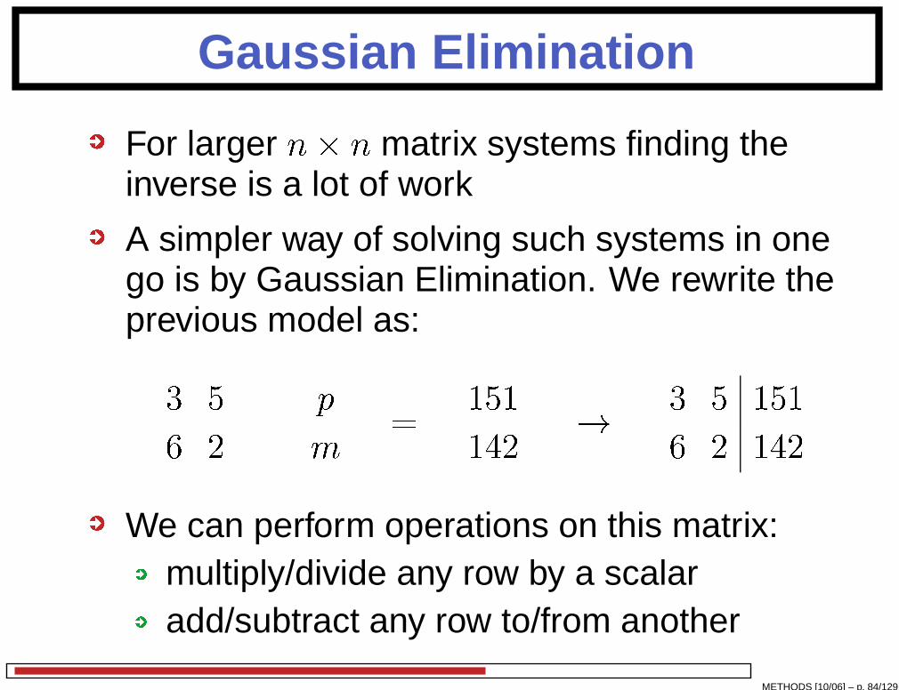
Gaussian Elimination
For larger n� n matrix systems finding theinverse is a lot of work
A simpler way of solving such systems in onego is by Gaussian Elimination. We rewrite theprevious model as: 3 56 2
! pm! = 151142! ! 3 5 1516 2 142!
We can perform operations on this matrix:multiply/divide any row by a scalaradd/subtract any row to/from another
METHODS [10/06] – p. 84/129
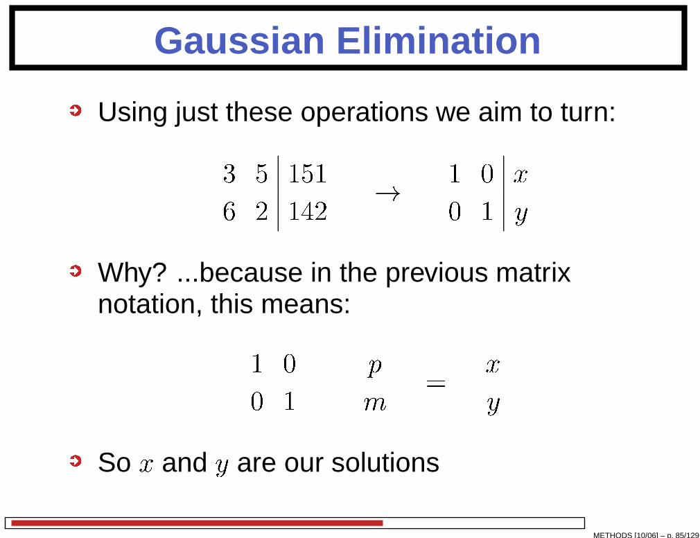
Gaussian Elimination
Using just these operations we aim to turn: 3 5 1516 2 142! ! 1 0 x0 1 y!
Why? ...because in the previous matrixnotation, this means: 1 00 1
! pm! = xy!
So x and y are our solutions
METHODS [10/06] – p. 85/129
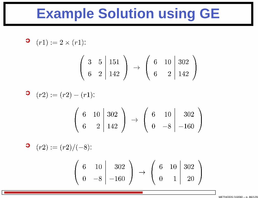
Example Solution using GE
(r1) := 2� (r1):0� 3 5 1516 2 1421A ! 0� 6 10 3026 2 1421A
(r2) := (r2)� (r1):0� 6 10 3026 2 1421A ! 0� 6 10 3020 �8 �1601A
(r2) := (r2)=(�8):0� 6 10 3020 �8 �1601A ! 0� 6 10 3020 1 201A
METHODS [10/06] – p. 86/129
Example Solution using GE
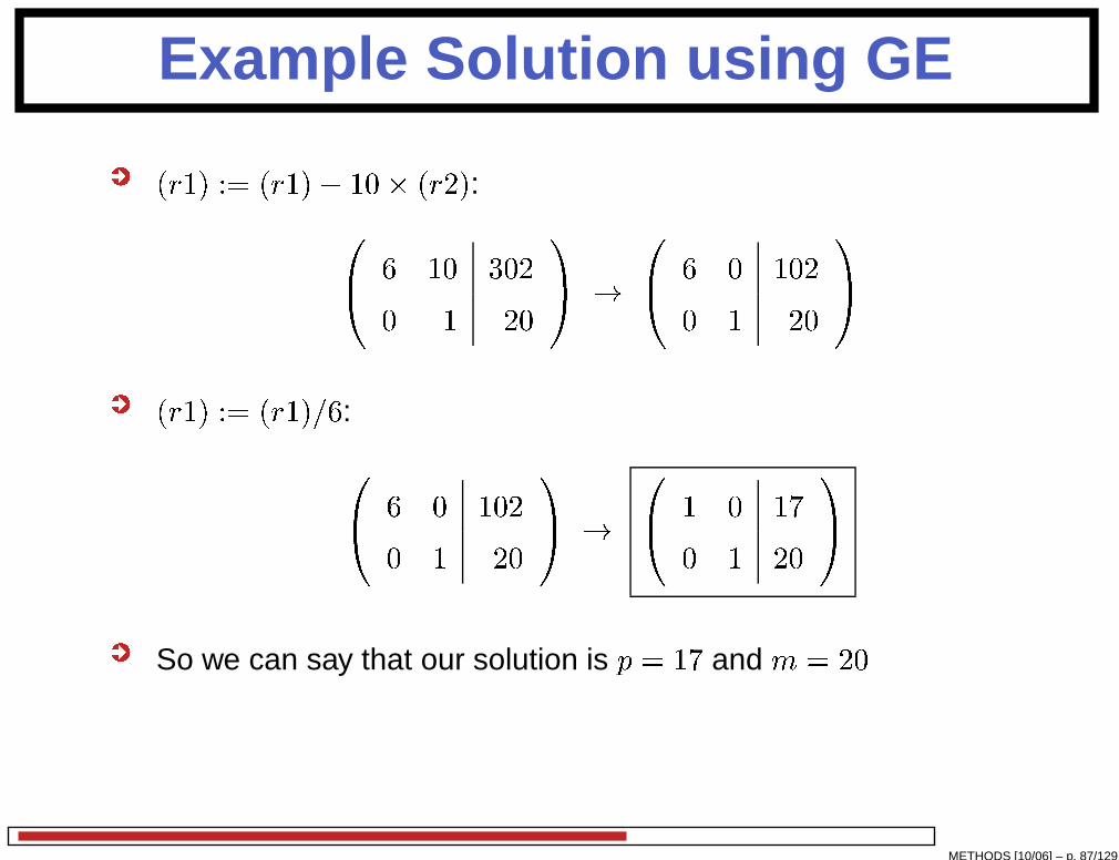
(r1) := (r1)� 10� (r2):0� 6 10 3020 1 201A ! 0� 6 0 1020 1 201A
(r1) := (r1)=6:0� 6 0 1020 1 201A ! 0� 1 0 170 1 201A
So we can say that our solution is p = 17 and m = 20
METHODS [10/06] – p. 87/129

Gaussian Elimination: 3� 31.
0B� a � � �� � � �� � � �1CA !0B� 1 � � �0 � � �0 � � �1CA
2.
0B� 1 � � �0 b � �0 � � �1CA !0B� 1 � � �0 1 � �0 0 � �1CA
3.
0B� 1 � � �0 1 � �0 0 �1CA !0B� 1 � � �0 1 � �0 0 1 �1CA
METHODS [10/06] – p. 88/129

Gaussian Elimination: 3� 34.
0B� 1 � � �0 1 � �0 0 1 �1CA !0B� 1 � 0 �0 1 0 �0 0 1 �1CA
5.
0B� 1 � 0 �0 1 0 �0 0 1 �1CA !0B� 1 0 0 �0 1 0 �0 0 1 �1CA
* represents an unknown entry
METHODS [10/06] – p. 89/129

Linear Dependence
System of n equations is linearly dependent:if one or more of the equations can beformed from a linear sum of the remainingequations
For example – if our Mac/PC system were:3p+ 5m = 151 (1)6p+ 10m = 302 (2)
This is linearly dependent as:eqn (2) = 2� eqn (1)i.e. we get no extra information from eqn (2)
...and there is no single solution for p and m
METHODS [10/06] – p. 90/129
Linear Dependence
If P represents a matrix in P~x = ~b then theequations generated by P~x are linearlydependent
iff jP j = 0 (i.e. P is singular)
The rank of the matrix P represents thenumber of linearly independent equations inP~x
We can use Gaussian elimination to calculatethe rank of a matrix
METHODS [10/06] – p. 91/129
Calculating the Rank
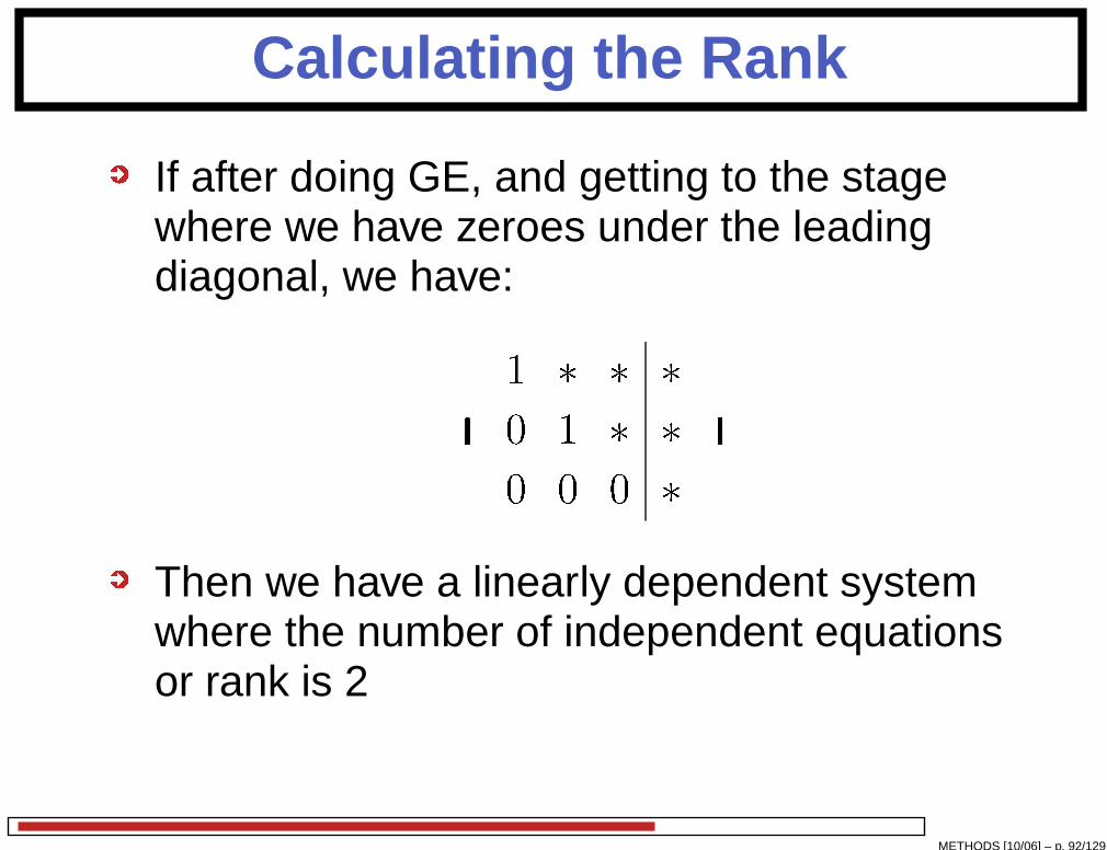
If after doing GE, and getting to the stagewhere we have zeroes under the leadingdiagonal, we have:0B� 1 � � �0 1 � �0 0 0 �
1CAThen we have a linearly dependent systemwhere the number of independent equationsor rank is 2
METHODS [10/06] – p. 92/129
Rank and Nullity
If we consider multiplication by a matrix M as afunction:M :: IR3 ! IR3
Input set is called the domain
Set of possible outputs is called the range
The Rank is the dimension of the range (i.e. thedimension of right-hand sides, ~b, that give systems,M~x = ~b, that don’t contradict)
The Nullity is the dimension of space (subset of thedomain) that maps onto a single point in the range.(Alternatively, the dimension of the space which solvesM~x = ~0).
METHODS [10/06] – p. 93/129
Rank/Nullity theorem
If we consider multiplication by a matrix M asa function:M :: IR3 ! IR3
If rank is calculated from number of linearlyindependent rows of M : nullity is number ofdependent rows
We have the following theorem:
Rank of M+Nullity of M = dim(Domain of M )
METHODS [10/06] – p. 94/129

PageRank Algorithm
Used by Google (and others?) to calculate aranking vector for the whole web!
Ranking vector is used to order search resultsreturned from a user query
PageRank of a webpage, u, is proportional to:Xv:pages with links to u PageRank of v
Number of links out of v
For a PageRank vector, ~r, and a web graphmatrix, P : P~r = �~r
METHODS [10/06] – p. 95/129
PageRank and Eigenvectors
PageRank vector is an eigenvector of thematrix which defines the web graph
An eigenvector, ~v of a matrix A is a vectorwhich satisfies the following equation:
A~v = �~v (�)where � is an eigenvalue of the matrix A
If A is an n� n matrix then there may be asmany as n possible interesting ~v; �
eigenvector/eigenvalue pairs which solveequation (*)
METHODS [10/06] – p. 96/129
Calculating the eigenvector
From the definition (*) of the eigenvector,A~v = �~v) A~v � �~v = ~0) (A� �I)~v = ~0
Let M be the matrix A� �I then if jM j 6= 0
then: ~v =M�1~0 = ~0This means that any interesting solutions of(*) must occur when jM j = 0 thus:jA� �Ij = 0
METHODS [10/06] – p. 97/129

Eigenvector Example
Find eigenvectors and eigenvalues of
A = 4 12 3!
Using jA� �Ij = 0, we get:����� 4 12 3!� � 1 00 1!����� = 0
) ����� 4� � 12 3� �!����� = 0
METHODS [10/06] – p. 98/129
Eigenvector Example
Thus by definition of a 2� 2 determinant, weget:(4� �)(3� �)� 2 = 0This is just a quadratic equation in � whichwill give us two possible eigenvalues�2 � 7�+ 10 = 0) (�� 5)(�� 2) = 0� = 5 or 2We have two eigenvalues and there will beone eigenvector solution for � = 5 andanother for � = 2
METHODS [10/06] – p. 99/129
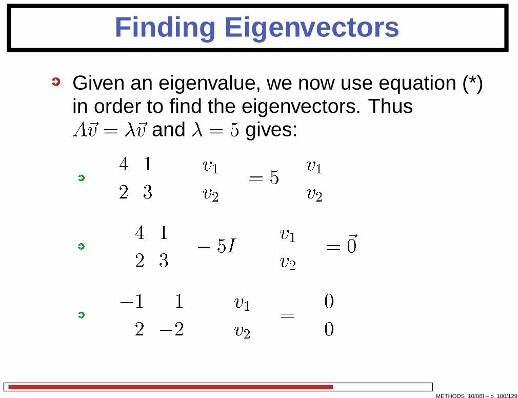
Finding Eigenvectors
Given an eigenvalue, we now use equation (*)in order to find the eigenvectors. ThusA~v = �~v and � = 5 gives: 4 12 3
! v1v2! = 5 v1v2!
4 12 3!� 5I! v1v2! = ~0 �1 12 �2
! v1v2! = 00!
METHODS [10/06] – p. 100/129

Finding Eigenvectors
This gives us two equations in v1 and v2:�v1 + v2 = 0 (1:a)2v1 � 2v2 = 0 (1:b)These are linearly dependent: which meansthat equation (1.b) is a multiple of equation(1.a) and vice versa(1:b) = �2� (1:a)
This is expected in situations wherejM j = 0 in M~v = ~0Eqn. (1.a) or (1.b) ) v1 = v2
METHODS [10/06] – p. 101/129
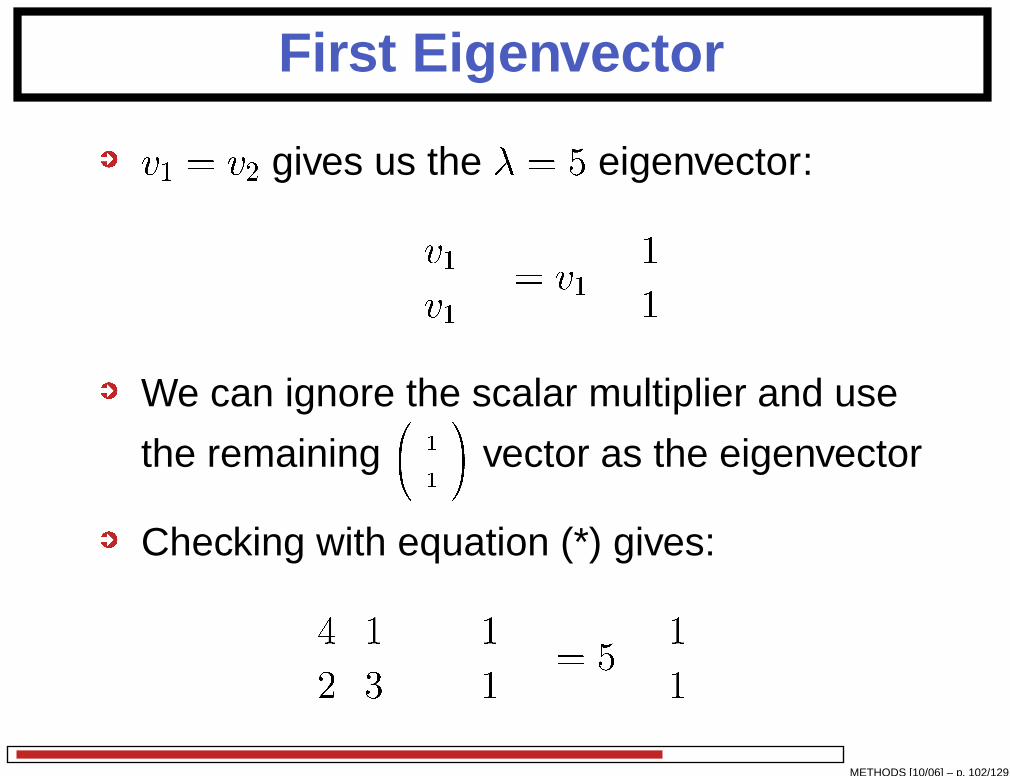
First Eigenvector
v1 = v2 gives us the � = 5 eigenvector: v1v1! = v1 11!
We can ignore the scalar multiplier and use
the remaining
0� 11 1A vector as the eigenvector
Checking with equation (*) gives: 4 12 3! 11! = 5 11! p
METHODS [10/06] – p. 102/129

Second Eigenvector
For A~v = �~v and � = 2:
) 2 12 1! v1v2! = 00!
) 2v1 + v2 = 0 (and 2v1 + v2 = 0)) v2 = �2v1Thus second eigenvector is ~v = v1 1�2
!
...or just ~v = 1�2!
METHODS [10/06] – p. 103/129

Differential Equations: Contents
What are differential equations used for?
Useful differential equation solutions:1st order, constant coefficient1st order, variable coefficient2nd order, constant coefficientCoupled ODEs, 1st order, constantcoefficient
Useful for:Performance modelling (3rd year)Simulation and modelling (3rd year)
METHODS [10/06] – p. 104/129
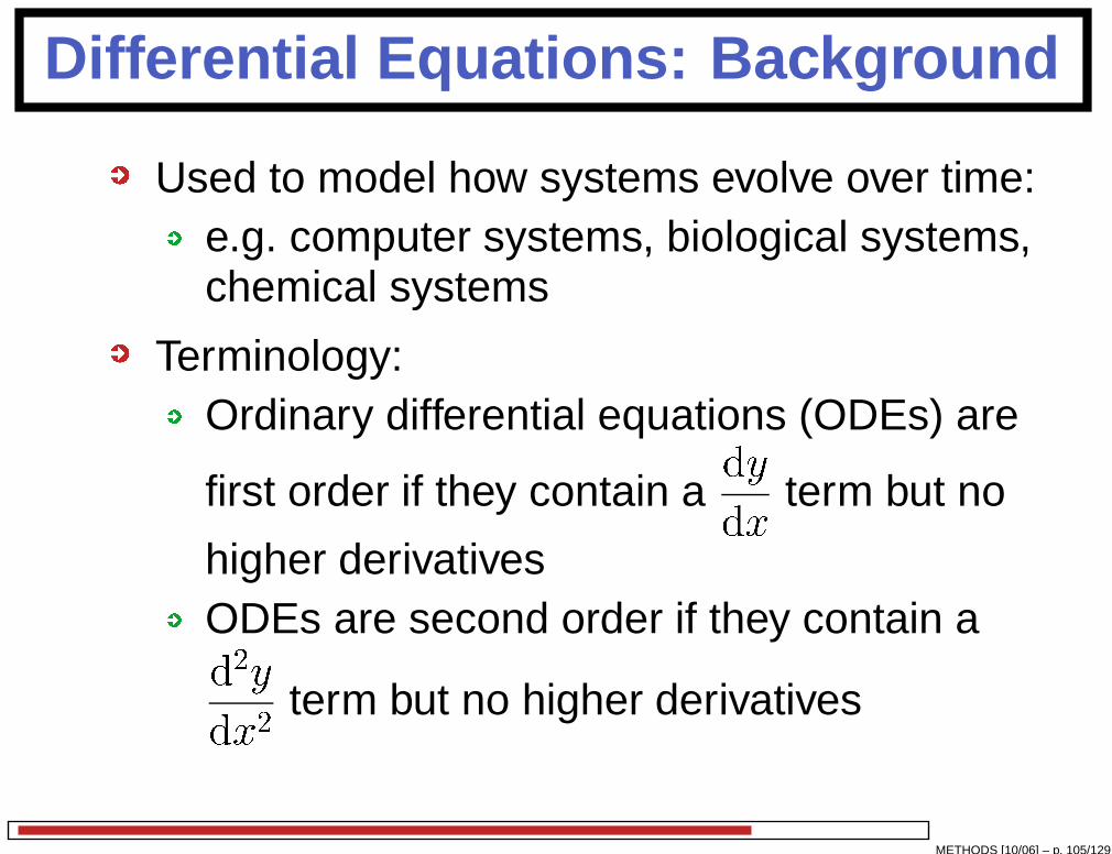
Differential Equations: Background
Used to model how systems evolve over time:e.g. computer systems, biological systems,chemical systems
Terminology:Ordinary differential equations (ODEs) are
first order if they contain a
dydx term but no
higher derivativesODEs are second order if they contain ad2ydx2 term but no higher derivatives
METHODS [10/06] – p. 105/129

Ordinary Differential Equations
First order, constant coefficients:
For example, 2dydx + y = 0 (�)Try: y = emx) 2memx + emx = 0) emx(2m + 1) = 0) emx = 0 or m = �12emx 6= 0 for any x;m. Therefore m = �12
General solution to (�):y = Ae� 12x
METHODS [10/06] – p. 106/129
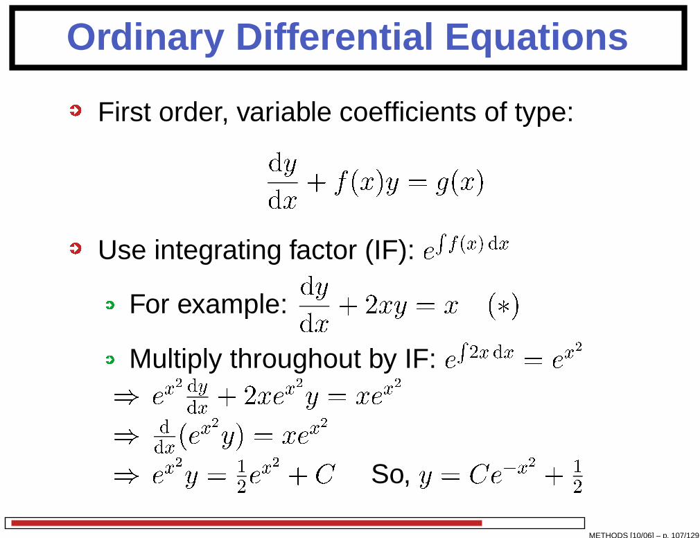
Ordinary Differential Equations
First order, variable coefficients of type:dydx + f(x)y = g(x)Use integrating factor (IF): eR f(x) dx
For example:
dydx + 2xy = x (�)
Multiply throughout by IF: eR 2x dx = ex2) ex2 dydx + 2xex2y = xex2) ddx(ex2y) = xex2) ex2y = 12ex2 + C So, y = Ce�x2 + 12
METHODS [10/06] – p. 107/129
Ordinary Differential Equations
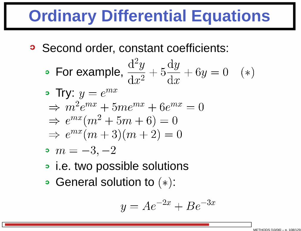
Second order, constant coefficients:
For example,
d2ydx2 + 5dydx + 6y = 0 (�)Try: y = emx) m2emx + 5memx + 6emx = 0) emx(m2 + 5m+ 6) = 0) emx(m+ 3)(m + 2) = 0m = �3;�2i.e. two possible solutionsGeneral solution to (�):
y = Ae�2x +Be�3x
METHODS [10/06] – p. 108/129

Ordinary Differential Equations
Second order, constant coefficients:If y = f(x) and y = g(x) are distinctsolutions to (�)
Then y = Af(x) +Bg(x) is also a solutionof (�) by following argument:d2dx2 (Af(x) +Bg(x)) + 5 ddx(Af(x) +Bg(x))+ 6(Af(x) +Bg(x)) = 0A� d2dx2f(x) + 5 ddxf(x) + 6f(x)�| {z }=0+ B� d2dx2 g(x) + 5 ddxg(x) + 6g(x)�| {z }=0 = 0
METHODS [10/06] – p. 109/129
Ordinary Differential Equations
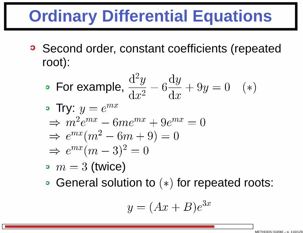
Second order, constant coefficients (repeatedroot):
For example,
d2ydx2 � 6dydx + 9y = 0 (�)
Try: y = emx) m2emx � 6memx + 9emx = 0) emx(m2 � 6m+ 9) = 0) emx(m� 3)2 = 0m = 3 (twice)General solution to (�) for repeated roots:
y = (Ax+B)e3x
METHODS [10/06] – p. 110/129

Applications: Coupled ODEs
Coupled ODEs are used to model massivestate-space physical and computer systems
Coupled Ordinary Differential Equations areused to model:
chemical reactions and concentrationsbiological systemsepidemics and viral infection spreadlarge state-space computer systems (e.g.distributed publish-subscribe systems
METHODS [10/06] – p. 111/129
Coupled ODEs
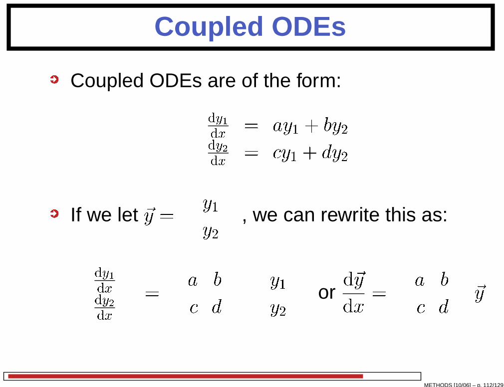
Coupled ODEs are of the form:( dy1dx = ay1 + by2dy2dx = y1 + dy2If we let ~y = y1y2
!, we can rewrite this as:
dy1dxdy2dx! = a b d! y1y2!
or
d~ydx = a b d! ~y
METHODS [10/06] – p. 112/129

Coupled ODE solutions
For coupled ODE of type:
d~ydx = A~y (�)Try ~y = ~ve�x so,
d~ydx = �~ve�xBut also
d~ydx = A~y, so A~ve�x = �~ve�x
Now solution of (�) can be derived from aneigenvector solution of A~v = �~v
For n eigenvectors ~v1; : : : ; ~vn and corresp.eigenvalues �1; : : : ; �n : general solution of(�) is ~y = B1~v1e�1x + � � �+Bn~vne�nx
METHODS [10/06] – p. 113/129

Coupled ODEs: Example
Example coupled ODEs:( dy1dx = 2y1 + 8y2dy2dx = 5y1 + 5y2So d~ydx = 2 85 5
! ~yRequire to find eigenvectors/values of
A = 2 85 5!
METHODS [10/06] – p. 114/129
Coupled ODEs: Example
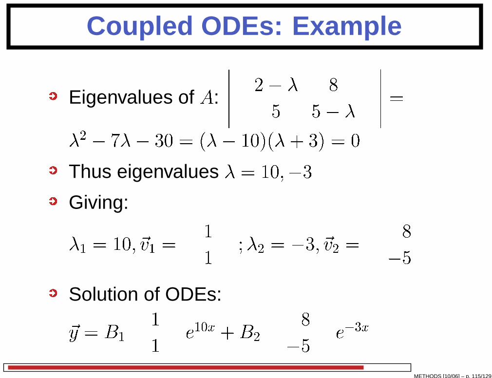
Eigenvalues of A:
����� 2� � 85 5� �!����� =�2 � 7�� 30 = (�� 10)(�+ 3) = 0Thus eigenvalues � = 10;�3Giving:
�1 = 10; ~v1 = 11! ;�2 = �3; ~v2 = 8�5!
Solution of ODEs:~y = B1 11! e10x +B2 8�5! e�3x
METHODS [10/06] – p. 115/129
Partial Derivatives
Used in (amongst others):
Computational Techniques (2nd Year)Optimisation (3rd Year)Computational Finance (3rd Year)
METHODS [10/06] – p. 116/129
Differentiation Contents
What is a (partial) differentiation used for?
Useful (partial) differentiation tools:Differentiation from first principlesPartial derivative chain ruleDerivatives of a parametric functionMultiple partial derivatives
METHODS [10/06] – p. 117/129

Optimisation
Example: look to find best predicted gain inportfolio given different possible shareholdings in portfolio
Optimum value
0
5
10
15
20 0
5
10
15
20
0
50
100
150
200
METHODS [10/06] – p. 118/129
Differentiation
0
5
10
15
20
25
0 1 2 3 4 5
y=x^2
Æx Æy
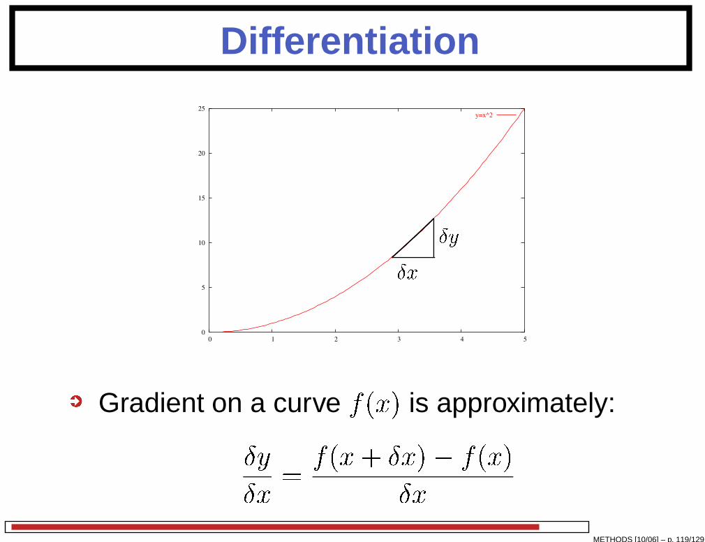
Gradient on a curve f(x) is approximately:ÆyÆx = f(x+ Æx)� f(x)Æx
METHODS [10/06] – p. 119/129
Definition of derivative
The derivative at a point x is defined by:dfdx = limÆx!0 f(x+ Æx)� f(x)ÆxTake f(x) = xn
We want to show that:dfdx = nxn�1
METHODS [10/06] – p. 120/129
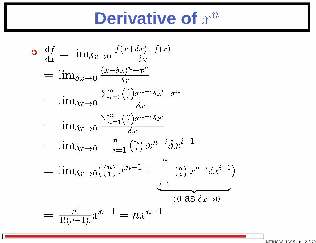
Derivative of xn
dfdx = limÆx!0 f(x+Æx)�f(x)Æx= limÆx!0 (x+Æx)n�xnÆx= limÆx!0 Pni=0(ni)xn�iÆxi�xnÆx= limÆx!0 Pni=1(ni)xn�iÆxiÆx= limÆx!0Pni=1 (ni) xn�iÆxi�1
= limÆx!0((n1) xn�1 + nXi=2 �ni�xn�iÆxi�1| {z }!0 as Æx!0)
= n!1!(n�1)!xn�1 = nxn�1
METHODS [10/06] – p. 121/129

Partial Differentiation
Ordinary differentiation dfdx applies to functionsof one variable i.e. f � f(x)What if function f depends on one or morevariables e.g. f � f(x1; x2)Finding the derivative involves finding thegradient of the function by varying onevariable and keeping the others constant
For example for f(x; y) = x2y + xy3; partialderivatives are written:�f�x = 2xy + y3 and �f�y = x2 + 3xy2
METHODS [10/06] – p. 122/129
Partial Derivative: example
Parabaloid
-10
-5
0
5
10 -10
-5
0
5
10
0
50
100
150
200
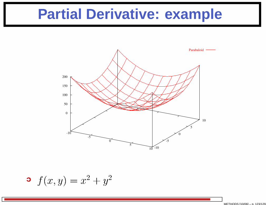
f(x; y) = x2 + y2METHODS [10/06] – p. 123/129
Partial Derivative: example
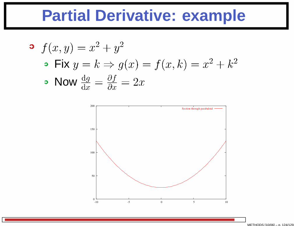
f(x; y) = x2 + y2
Fix y = k ) g(x) = f(x; k) = x2 + k2Now dgdx = �f�x = 2x
0
50
100
150
200
-10 -5 0 5 10
Section through parabaloid
METHODS [10/06] – p. 124/129

Further Examples
f(x; y) = (x+ 2y3)2) �f�x = 2(x+ 2y3) ��x(x+ 2y3) = 2(x+ 2y3)If x and y are themselves functions of t thendfdt = �f�x dxdt + �f�y dydtSo if f(x; y) = x2 + 2y where x = sin t andy = os t then:dfdt = 2x os t� 2 sin t = 2 sin t( os t� 1)
METHODS [10/06] – p. 125/129
Extended Chain Rule
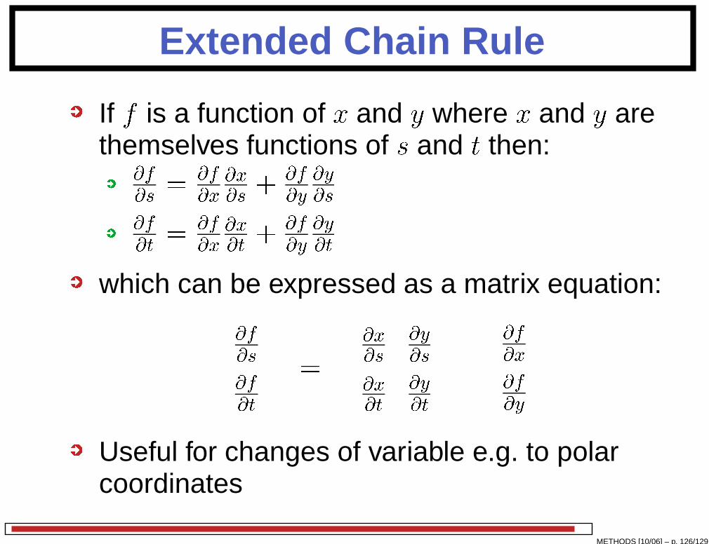
If f is a function of x and y where x and y arethemselves functions of s and t then:�f�s = �f�x �x�s + �f�y �y�s�f�t = �f�x �x�t + �f�y �y�twhich can be expressed as a matrix equation: �f�s�f�t
! = �x�s �y�s�x�t �y�t! �f�x�f�y!
Useful for changes of variable e.g. to polarcoordinates
METHODS [10/06] – p. 126/129
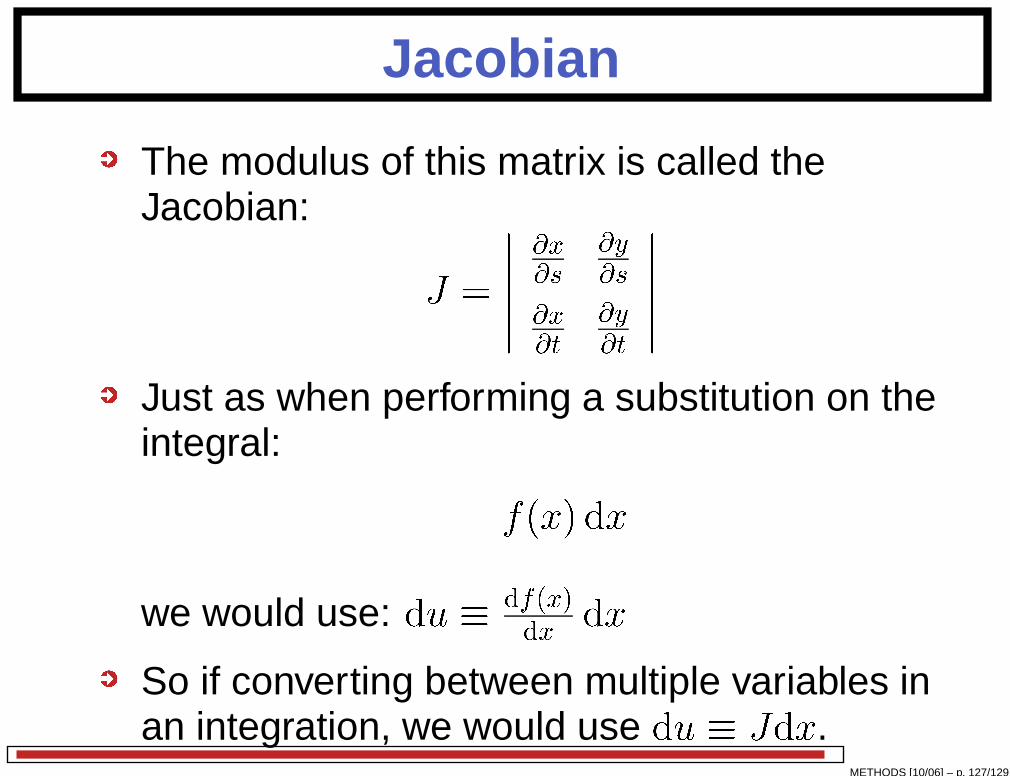
Jacobian
The modulus of this matrix is called theJacobian:
J = ����� �x�s �y�s�x�t �y�t�����
Just as when performing a substitution on theintegral: Z f(x) dx
we would use: du � df(x)dx dx
So if converting between multiple variables inan integration, we would use du � Jdx.
METHODS [10/06] – p. 127/129
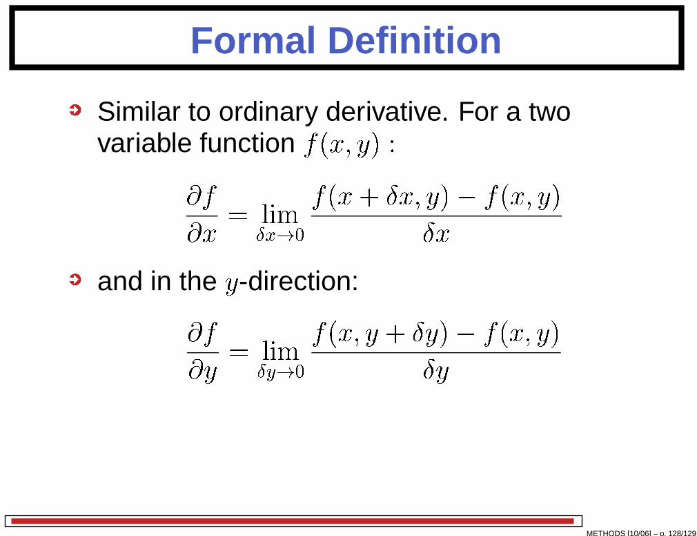
Formal Definition
Similar to ordinary derivative. For a twovariable function f(x; y) :�f�x = limÆx!0 f(x+ Æx; y)� f(x; y)Æxand in the y-direction:�f�y = limÆy!0 f(x; y + Æy)� f(x; y)Æy
METHODS [10/06] – p. 128/129
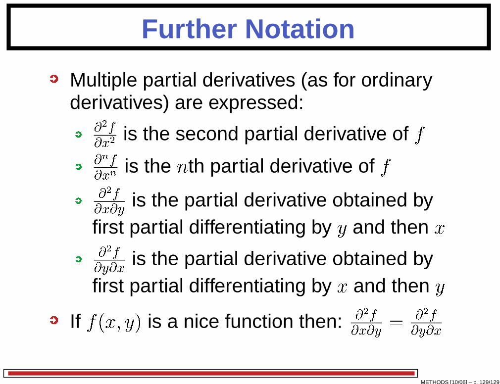
Further Notation
Multiple partial derivatives (as for ordinaryderivatives) are expressed:�2f�x2 is the second partial derivative of f�nf�xn is the nth partial derivative of f�2f�x�y is the partial derivative obtained by
first partial differentiating by y and then x�2f�y�x is the partial derivative obtained byfirst partial differentiating by x and then y
If f(x; y) is a nice function then: �2f�x�y = �2f�y�x
METHODS [10/06] – p. 129/129