Mathematical Methods for...

II/IV B.Tech CSE & ECM Mathematical Methods for Computing (11BS203) Chapter-1

Drgsk@KLUniversity

NUMERICAL METHODS

The limitations of analytical methods have led the engineers and scientists to evolve numerical methods. Numerical methods are techniques by which mathematical problems are

formulated so that they can be solved with arithmetic and logical operations. Because digital computers excel at performing such operations, numerical methods are sometimes referred to as

computer mathematics. With the advantage of high speed digital computers and increasing demand for numerical answers to various problems, numerical techniques have become indispensible tool in the hands of engineers.

Why should we study numerical methods?

There are several reasons to study numerical methods:

Numerical methods greatly expand the types of problems you can address. They are capable of handling large systems of equations, nonlinearities, and complicated

geometries that are not uncommon in engineering and science and that are often impossible to solve analytically with standard calculus. As such, they greatly enhance

your problem-solving skills.

Numerical methods allow you to use canned software with insight. During your career,

you will invariably have occasion to use commercially available prepackaged computer programs that involve numerical methods. The intelligent use of these programs is greatly

enhanced by an understanding of the basic theory underlying the methods. In the absence of such understanding, you will be left to treat such packages as black boxes with little

critical insight into their inner workings or the validity of the results they produce.

Many problems cannot be approached using canned programs. If you are conversant with

numerical methods, and are adept at computer programming, you can design your own programs to solve problems without having to buy or commission expensive software.

Numerical methods are an efficient vehicle for learning to use computers. Because

numerical methods are expressly designed for computer implementation, they are ideal for illustrating the computers powers and limitations. When you successfully implement numerical methods on a computer, and then apply them to solve otherwise intractable

problems, you will be provided with a dramatic demonstration of how computers can serve your professional development. At the same time, you will also learn to

acknowledge and control the errors of approximation that are part and parcel of large-scale numerical calculations.

Numerical methods provide a vehicle for you to reinforce your understanding of mathematics. Because one function of numerical methods is to reduce higher

mathematics to basic arithmetic operations, they get at the .nuts and bolts. of some otherwise obscure topics. Enhanced understanding and insight can result from this

alternative perspective.

Chapter-1


Drgsk@KLUniversity

What is the nature of the numerical methods?

Numerical methods are often, of a repetitive nature. These consist in repeated execution of the same process where at each step the result of the preceding is used. This is known as iteration process and is repeated till the result is obtained to a desired degree of accuracy.

Mathematical Model: A mathematical model can be defined as a formulation or equation that

expresses the essential features of a physical system or process in mathematical terms. In a very

general sense, it can be represented as a functional relationship of the form

Dependent variable = f (independent variables, parameters, forcing functions)

where the dependent variable is a characteristic that typically reflects the behavior or state of the

system; the independent variables are usually dimensions, such as time and space, along which

the systems behavior is being determined; the parameters are reflective of the systems properties

or composition; and the forcing functions are external influences acting upon it.

A simple mathematical model: (Bungee-Jumper problem)(free falling body)

Air resistance can be formulated in a variety of ways. From fluid mechanics a good first

approximation would be to assume that it is proportional to the square of the velocity,

FU = – Cd v2,

Where Cd is proportionality constant called the drag coefficient (kg/m). Thus, the

greater the fall velocity, the greater the upward force due to air resistance. The parameter Cd accounts for properties of the falling object, such as shape or surface roughness, that affect

air resistance. For the present case, Cd might be a function of the type of clothing or the orientation used by the jumper during free fall. Therefore,

F = mg – Cd v2

ma = mg – Cd v2

Let m be the mass of the bungee jumper and v(t) be the velocity

at time t after jumping. From the Newton second law of motion

(time rate of change of momentum of a body is equal to the

resulting force acting on it).

F = ma,

where F is the net force acting on the jumper, a is its acceleration (m/s2). The net force is composed of two opposite forces: the

downward pull of gravity FD and the upward force of air resistance FU i.e.

F = FD + FU. Again from the Newton second law of motion the downward force FD = mg due to gravity, where g is the acceleration due to

gravity (9.81 m/s2).


Drgsk@KLUniversity

2

d vCmgdt

dvm

2d vm

Cg

dt

dv

Is a model that relates the acceleration of a falling object to the forces acting on it. It is a differential equation. If the jumper is initially at rest i.e. v = 0 at t = 0, then the solution of the

initial value problem is

.tm

gCtanh

C

gmv(t) d

d

Errors : Engineers and scientists constantly find themselves having to accomplish objectives based on uncertain information. Although perfection is a laudable goal, it is rarely if ever attained. For example, despite the fact that the model developed from Newton’s second law is an

excellent approximation, it would never in practice exactly predict the jumpers fall. A variety of factors such as winds and slight variations in air resistance would result in deviations from the

prediction. If these deviations are systematically high or low, then we might need to develop a new model. However, if they are randomly distributed and tightly grouped around the prediction, then the deviations might be considered negligible and the model deemed adequate. Numerical

approximations also introduce similar discrepancies into the analysis. The errors associated with both calculations and measurements can be characterized with

regard to their accuracy and precision. Accuracy refers to how closely a computed or measured value agrees with the true value. Precision refers to how closely individual computed or measured values agree with each other.

Numerical errors arise from the use of approximations to represent exact mathematical operations and quantities. For such errors, the relationship between the exact, or true, result

and the approximation can be formulated as True value = approximation + error.

Therefore

True error = true value – approximation. (1)

For numerical methods, the true value will only be known when we deal with functions that

can be solved analytically. Such will typically be the case when we investigate the theoretical behavior of a particular technique for simple systems. However, in real-world applications,

we will obviously not know the true answer a priori. For these situations, an alternative is to normalize the error using the best available estimate of the true value that is, to the approximation itself, as in

100%ionapproximat

error eapproximatεa (2)

where the subscript ‘a’ signifies that the error is normalized to an approximate value. Note also that for real-world applications, Eq(1) cannot be used to calculate the error term in the numerator

of Eq. (2). One of the challenges of numerical methods is to determine error estimates in the absence of knowledge regarding the true value. For example, certain numerical methods use iteration to compute answers. In such cases, a present approximation is made on the basis of a


Drgsk@KLUniversity

previous approximation. This process is performed repeatedly, or iteratively, to successively compute (hopefully) better and better approximations. For such cases, the error is often estimated

as the difference between the previous and present approximations. Thus, percent relative error is determined according to

100%ionapproximatpresent

ionsapproximat previous -ionapproximatpresent εa .

Solution of algebraic and transcendental equations:

A problem of great importance in applied mathematics and engineering is that of

determining the solution (root) of an equation

,0)(xf

Where the function f may be given explicitly, for example

0 ,)( 011

10 aaxaxaxaxf nnnn

a polynomial of degree ‘n’ in ‘x’, or f(x) may be known only implicitly as a transcendental

function. A number ‘c’ is a solution of f(x) = 0 if f(c) = 0. Such a solution is a root of f(x) = 0.

Roots in Engineering and Science:

Although they arise in other problem contexts, roots of equations frequently occur in the area of design. Table-1 lists a number of fundamental principles that are routinely used in

design work. Mathematical equations or models derived from these principles are employed to predict dependent variables as a function of independent variables, forcing functions, and parameters. Note that in each case, the dependent variables reflect the state or performance of the

system, whereas the parameters represent its properties or composition.

Table – 1 (Fundamental principles used in design problems)

Fundamental Principle

Dependent variable

Independent variable

Parameters

Heat balance Temperature Time and position

Thermal properties of material, system geometry.

Mass balance Concentration or quantity of mass

Time and position

Chemical behavior of material, mass transfer, system geometry.

Force balance Magnitude and direction of force

Time and position

Strength of material, structural properties, system geometry.

Energy balance Changes in

kinetic and potential energy

Time and

position

Thermal properties, mass of material,

system geometry.

Newton’s laws of

motion

Acceleration,

velocity or location

Time and

position

Mass of material, system geometry,

dissipative parameters

Kirchhoff’s laws Currents and

voltages

Time Electrical properties (resistance,

capacitance, inductance)


Drgsk@KLUniversity

Now we can see that the answer to the problem is the value of m that makes the function equal to zero. Hence, we call this a roots problem.

Bisection method:

It is a simplest method of bracketing the roots of a function and requires an initial interval which is guaranteed to contain a root -- if a and b are the endpoints of the interval then f(a) must differ in sign from f(b). This ensures that the function crosses zero at least once in the interval. If a

valid initial interval is used then these algorithm cannot fail, provided the function is well behaved.

On each iteration, the interval is bisected

and the value of the function at the midpoint is calculated. The sign of this value is used to determine which half of

the interval does not contain a root. That half is discarded to give a new, smaller

interval containing the root. This method can be continued indefinitely until the interval is sufficiently small. At any time,

the current estimate of the root is taken as the midpoint of the interval.

Bisection method has linear convergence. Linear convergence means that successive significant

figures are won linearly with computational effort.

When an interval contains more than one root, the bisection method can find one of them. When an interval contains a singularity, the bisection method converges to that singularity.

Medical studies have established that a bungee

jumpers chances of sustaining a significant vertebrae injury increase significantly if the free- fall velocity

exceeds 36 m/s after 4 s of free fall. Suppose, we want to determine the mass at which this criterion is exceeded given a drag coefficient of 0.25 kg/m.

We know that the analytical solution can be used to predict fall velocity as a function of time:

.tm

gCtanh

C

gmv(t) d

d

An alternative way of looking at the problem involves subtracting v(t) from both sides to give a new function:

v(t).tm

gCtanh

C

gmf(m) d

d


Drgsk@KLUniversity

Working Procedure

1. Given algebraic or transcendental equation put in the form of f(x) = 0. 2. Choose ‘a’ and ‘b’ such that f(a) and f(b) are opposite sign or f(a)f(b) < 0.

3. The first approximate root of the equation in (a, b) is .2

1

bax

4. If f(x1) = 0, then x1 is the root of the given equation. Otherwise, bisect the interval (a, b)

at mid point x1. Now, the root lies in (a, x1) or (x1, b) according to f(x1) positive or negative.

5. Again bisect the interval as before and continue the process until the root is found in

desired accuracy.

Example#1 Find a root of the equation x3 – 4x – 9 = 0, using bisection method in four stages. Sol. Let f(x) = x3 – 4x – 9, then the equation become f(x) = 0.

f(2) = (2)3 – 4(2) – 9 = -9 < 0 f(3) = (3)3 – 4(3) – 9 = 6 > 0.

Since f(2) and f(3) are opposite sign, the root lies between 2 and 3.

Therefore, the first approximate root .5.22

5

2

321x

f(x1) = f(2.5) = (2.5)3 – 4(2.5) – 9 = -3.375 < 0.

Since f(2.5) and f(3) are opposite sign, the root lies between 2.5 and 3.

The second approximate root .75.22

35.22x

f(x2) = f(2.75) = (2.75)3 – 4(2.75) – 9 = 0.7969 > 0.

Since f(x1) and f(x2) are opposite sign, the root lies between 2.5 and 2.75.

The third approximate root .625.22

75.25.23x

f(x3) = f(2.625) = (2.625)3 – 4(2.625) – 9 = -1.4121 < 0. Since f(x3) and f(x2) are opposite sign, the root lies between 2.625 and 2.75.

The fourth approximate root .6875.22

75.2625.24x

Hence the approximate root of the given equation in fourth stage by bisection method is 2.6875.

Example#2 By using the bisection method, find an approximate root of the equation sin x = 1/x, that lies between x = 1 and x = 1.5 (measured in radians). Carry out computations upto the 7th

stage. Sol. Let f(x) = x sin x – 1, then the equation become f(x) = 0.

f(1) = 1 sin(1) – 1 = -0.15849 < 0 f(1.5) = 1.5 sin(1.5) – 1 = 0.49625 > 0.

Since f(1) and f(1.5) are opposite sign, the root lies between 1 and 1.5.


Drgsk@KLUniversity

Therefore, the first approximate root .25.12

5.2

2

5.111x Then

f(x1) = f(1.25) = 1.25 sin(1.25) – 1 = 0.18627 > 0.

Therefore, root lies between 1 and x1 = 1.25.

Thus, the second approximate to the root is .125.12

25.2

2

25.112x Then

f(x2) = f(1.125) = 1.125 sin(1.125) – 1 = 0.01509 > 0.

Therefore, root lies between 1 and x2 = 1.125.

Thus, the third approximate to the root is .0625.12

125.2

2

125.113x Then

f(x3) = f(1.0625) = 1.0625 sin(1.0625) – 1 = – 0.0718 < 0. Therefore, root lies between x3 = 1.0625 and x2 = 1.125.

Thus, the fourth approximate to the root is .09375.12

125.10625.14x Then


Thus, the fifth approximate to the root is .10937.12

125.109375.14x Then


Thus, the sixth approximate to the root is .11719.12

125.110937.16x Then

f(x6) = f(1.11719) = 1.11719 sin(1.11719) – 1 = 0.00421 > 0. Therefore, root lies between x5 = 1.10937 and x6 = 1.11719.

Thus, the seventh approximate to the root is .11328.12

1.1171910937.17x

Hence the desired approximate to the root is 1.11328.

Example#3. Use bisection to determine the drag coefficient needed so that an 80-kg bungee jumper has a velocity of 36 m/s after 4 s of free fall. The acceleration of gravity is 9.81 m/s2.

Start with initial guesses of xl = 0.1 and xu = 0.2 and iterate until the approximate relative error falls below 2%.

Sol. We know that the velocity of the bungee jumper at any time t is

.tm

gCtanh

C

gmv(t) d

d

Here mass of the jumper m = 80 kg, velocity of the jumper at t = 4 sec, v(4) = 36m/s and g =

9.81 m/s2. Substituting the values, we have

.(4)80

9.81Ctanh

C

(9.81)8036 d

d

Rewriting the equation


Drgsk@KLUniversity

.036C11375.04tanhC

781.8d

d

Let 36C11375.04tanhC

781.8)f(C d

dd . Now, we have to find the root of the equation

f(Cd) = 0 using bisection method.

Iteration Method: Consider an equation f(x) = 0 which can take in the form x = φ(x), where

φ(x) satisfies the following conditions; (i) For two real numbers a and b, a ≤ x ≤ b implies a ≤ φ (x) ≤ b and

(ii) For all x1, x2 lying in the interval (a, b), we have | φ (x1) – φ (x2)| ≤ m|x1 – x2|, where m is

a constant such that 0 ≤ m ≤ 1. Then the equation x = φ (x) has a unique root in the interval (a, b). To find the approximate root

of this equation, we use the following iterative formula; The nth approximate root is xn = φ (xn-1), n = 1, 2, 3, … . We start with an initial approximation x0 and continue iterations until the two successive approximations are identical.

The following theorem states the sufficient condition for the convergence of the iterative formula xn = φ (xn-1).

Theorem#1. Let I = (a, b) an interval containing a root of the equation x = φ (x). If | φ'(x)|<1, for all x in I, then for any value of x0 in I, the iteration xn = φ (xn-1) is convergent for all n ≥ 1.

Example#1. Determine the approximate root of the equation x3 – 2x – 5 = 0 near to x = 2, using

fixed point iterative method. Sol. Given equation x3 – 2x – 5 = 0 can be written as x3 = 2x + 5 and x = (2x + 5)1/3. This is of

the form x = φ (x), where φ (x) = (2x + 5)1/3. Also 3

2

5)3(2x

2(x) and | φ '(x)|<1, for 2<x<3.

Hence the iteration xn = φ (xn-1), n = 1, 2, 3, … near x = 2 is convergent. Let us take the initial approximation x0 = 2.

The first approximation to the root is x1 = φ (x0) = φ (2) = [2(2)+5]1/3 = 91/3 = 2.08008. The second approximation to the root is x2 = φ (x1) = φ (2.08008) = [2(2.08008)+5]1/3 = 2.09235. The third approximation to the root is x3 = φ (x2) = φ (2.09235) = [2(2.09235)+5]1/3 = 2.09422.

The fourth approximation to the root is x4 = φ (x3) = φ (2.09422) = [2(2.09422)+5]1/3 = 2.09450. The fifth approximation to the root is x5 = φ (x4) = φ (2.09450) = [2(2.09450)+5]1/3 = 2.09454.

The sixth approximation to the root is x6 = φ (x5) = φ (2.09454) = [2(2.09454)+5]1/3 = 2.09455. Since x5 and x6 are identical up to 4 decimal places, we take x6 = 2.09455 as the required root of the given equation.

Example#2. Determine the approximate root of the equation tan-1x – x + 1 = 0, using fixed point

iterative method.


Drgsk@KLUniversity

Sol. The given equation can be written as x = φ (x), where φ (x) = 1 + tan-1x. Clearly,

2x1

1(x) and | φ '(x)| < 1 for 0 < x < 1. Hence the iteration xn = φ (xn-1), n = 1, 2, 3, … is

convergent. Let us take the initial approximation x0 = 1.

The first approximation to the root is x1 = φ (x0) = φ (1) = 1 + tan-1(1) = 1.7854. The first approximation to the root is x2 = φ (x1) = φ (1.7854) = 1 + tan-1(1.7854) = 2.0602.

Similarly the successive iterations are x3 = 2.1189, x4 = 2.1318, x5 = 2.1322, x6 = 2.13231, x7 = 2.13132. Since x6 and x7 are identical up to 4 decimal places, we take x7 = 2.13132 as the required root of

the given equation.

Newton-Raphson Method:

Newton-Raphson method, is a root-finding algorithm that uses the first few terms of the Taylor series of a function f(x) in the vicinity of a suspected root.

(x)f2!

h(x)fhf(x)h)f(x

2

Let x0 be initial approximate root of the equation f(x)=0, then the first approximate root is

The nth approximate root is

Example#1. Determine the approximate root of the equation x3 – 3x – 5 = 0, using Newton-Raphson method.

Sol. Let f(x) = x3 – 3x – 5, then the given equation become f(x) = 0. f(1) = 13 – 3(1) – 5 = 1 – 3 – 5 = – 7 < 0, f(2) = 23 – 3(2) – 5 = 8 – 6 – 5 = 3 > 0.

Since f(1) and f(2) are opposite signs, therefore the root lies between 1 and 2. Let us take initial

approximation x0 = 2. Since f(x) = x3 – 3x – 5, we have f '(x) = 3x2 – 3 = 3(x2 – 1).

Newton-Raphson iterative formula is

.)(xf

)f(xxx

0

0

01

1,2,3,n ,)(xf

)f(xxx

1n

1n1nn

Newton algorithm begins with an

initial guess for the location of the

root. On each iteration, a line tangent

to the function f is drawn at that

position. The point where this line

crosses the x-axis becomes the new

guess. Newton method converges

quadratically for single roots, and

linearly for multiple roots.


Drgsk@KLUniversity

The first approximate to the root

.3333.29

21

)12(3

5)2(2

)1(3

52

2

3

20

30

1x

xx

The second approximate to the root

.2806.2]1)3333.2[(3

5)3333.2(2

)1(3

52

2

3

21

31

2x

xx

The third approximate to the root

.2790.2]1)2806.2[(3

5)2806.2(2

)1(3

52

2

3

22

32

3x

xx

The fourth approximate to the root

.2790.2]1)2790.2[(3

5)2790.2(2

)1(3

52

2

3

23

33

4x

xx

Since x3 and x4 are identical up to 4 decimal places, we take x4 = 2.2790 as the required root of the given equation.

Example#2. Apply Newton-Raphson method to find an approximate root correct to five decimal places, of the equation ex – 3x = 0 that lies between 0 and 1.

Sol. Let f(x) = ex – 3x, then f (x) = ex – 3. f(0) = e0 – 3(0) = 1 – 0 = 1 > 0 f(1) = e1 – 3(1) = e – 3 = -0.2817 < 0.

Therefore, the root lies between 0 and 1. Let us take initial approximation x0 = 0.5. Newton-Raphson iterative formula is

The first approximate to the root

.61006.03

)15.0(

3

)1(

5.0

5.00

10

0

e

e

e

exx

x

x

The second approximate to the root

0,1,2,n ,1)3(x

52x

1)3(x

53xxx

)(xf

)f(xxx

2n

3n

2n

n3n

nn

nn1n

0,1,2,n ,3e

1)e(x

3e

3xex

)(xf

)f(xxx

n

n

n

n

x

xn

x

nx

nn

nn1n


Drgsk@KLUniversity

.618996.03

)161006.0(

3

)1(

61006.0

61006.01

21

1

e

e

e

exx

x

x

The third approximate to the root

.619061.03

)1618996.0(

3

)1(

618996.0

618996.02

32

2

e

e

e

exx

x

x

The fourth approximate to the root

.619061.03

)1619061.0(

3

)1(

619061.0

619061.03

43

3

e

e

e

exx

x

x

Since x3 and x4 are identical up to 5 decimal places, we take x4 = 0.619061 as the required root of the given equation.

Example#3. Determine the mass of the bungee jumper with a drag coefficient of 0.25 kg/m to have a velocity of 36 m/s after 4 seconds of free fall, use Newton-Raphson method near to

142kg. Sol. We know that the velocity of the bungee jumper at any time t is

.tm

gCtanh

C

gmv(t) d

d

Here velocity of the jumper at t = 4 sec is v(4) = 36m/s, drag coefficient Cd = 0.25 kg/m and g = 9.81 m/s2. Substituting the values, we have

.(4)m

9.81(0.25)tanh

0.25

m 9.8136

Rewriting the equation

036m

39.24 tanh39.24m .

Let 36m

39.24 tanh39.24mf(m) . Now, we have to find the root of the equation f(m) =

0 using Newton-Raphson method.

Some Useful Deduction: Derive the following

(1) Iterative formula to find 1/N is xn+1= xn(2 - Nxn)

(2) Iterative formula to find √N is n

n1nx

Nx

2

1x .

(3) Iterative formula to find 1/√N is n

n1nNx

1x

2

1x .

(4) Iterative formula to find k√N is .x

N1)x(k

k

1x

kn

n1n


Drgsk@KLUniversity

Proof. (1) Let x = 1/N, then 1/x – N = 0. Taking f(x) = 1/x – N, f '(x) = –x-2. By Newton’s formula

(2) Let Nx , then x2 – N = 0. Taking f(x) = x2 – N, f '(x) = 2x. By Newton’s formula

(3) Let N

1x , then 0.

N

1x 2 Taking

N

1xf(x) 2 , f ' (x) = 2x. By Newton’s formula

(4) Let k Nx , then xk – N = 0. Taking f(x) = xk – N, f ' (x) = k xk-1. By Newton’s formula

(1) Develop a recurrence formula for finding 1/N, using Newton-Raphson method and hence compute 1/31 correct to four decimal places.

Ans : 0.0323 (2) Develop a recurrence formula for finding √N, using Newton-Raphson method and hence compute √28 correct to four decimal places.

Ans : 5.2915 (3) Develop a recurrence formula for finding 1/√N, (N>0) using Newton-Raphson method and

hence compute 1/√14 correct to four decimal places. Ans : 0.2673 (4) Develop an algorithm using Newton-Raphson method , to find the cube root of N>0, and

hence find 3√24 correct to four decimal places. Ans : 2.8845

).Nx(2x

Nx-xxxNx

1 x

x

N)(1/xx

)(xf

)f(xxx

nn

2

nnn

2

n

n

n

2

n

nn

n

nn1n

.x

Nx

2

1

2x

Nx

2

1 - x

2x

Nxx

)(xf

)f(xxx

n

n

n

nn

n

2

nn

n

nn1n

.Nx

1x

2

1

2Nx

1x

2

1 - x

2x

N/1xx

)(xf

)f(xxx

n

n

n

nn

n

2

nn

n

nn1n

.x

N1)x-(k

k

1

kx

Nx

k

1 - x

kx

Nxx

)(xf

)f(xxx

1-kn

n1-kn

nn

1-kn

kn

nn

nn1n


Drgsk@KLUniversity

System of Linear Algebraic Equations:

Systems of equations arise in all branches of engineering and science. These equations

may be algebraic, transcendental (i.e., involving trigonometric, logarithmic, exponential, etc., functions), ordinary differential equations, or partial differential equations. The equations may be

linear or nonlinear. This section is devoted to the solution of systems of linear algebraic equations of the following form:

a11 x1 + a12 x2 + … + a1n xn = b1

a21 x1 + a22 x2 + … + a2n xn = b2

…………………………………

an1 x1 + an2 x2 + … + ann xn = bn. Linear Algebraic Equations in Engineering and Science:

Many of the fundamental equations of engineering and science are based on conservation

laws. Some familiar quantities that conform to such laws are mass, energy, and momentum. In mathematical terms, these principles lead to balance or continuity equations that relates system

behavior as represented by the levels or response of the quantity being modeled to the properties or characteristics of the system and the external stimuli or forcing functions acting on the system.

Suppose that three jumpers are connected by bungee cords. They are held in place

vertically so that each cord is fully extended but unstretched. We can define three distances, x1, x2, and x3, as measured downward from each of their unstretched positions. After they are

released, gravity takes hold and the jumpers will eventually come to the equilibrium positions. Suppose that you are asked to compute the displacement of each of the jumpers. If we

assume that each cord behaves as a linear spring and follows Hooke’s law(states that the

restoring force of a spring is directly proportional to a small displacement. In equation form, we write F = -kx, where x is the size of the displacement) can be developed for each jumper.

Using Newton’s second law, a steady state force balance can be written for each jumper; m1 g + k2 (x2 – x1) – k1 x1 = 0 m2 g + k3 (x3 – x2) – k2 (x2 – x1) = 0

m3 g – k3 (x3 – x2) = 0 where mi is the mass of the jumper i (kg), kj is the spring constant for cord j (N/m), xi is the

displacement of jumper i measured downward from the equilibrium position(m) and g gravitational acceleration(9.81 m/s2).

(k1 + k2)x1 – k2 x2 = m1 g

–k2x1 + (k2 + k3)x2 – k3x3 = m2 g – k3x2 + k3x3 = m3 g.

Thus, the problem reduces to solving a system of three simultaneous equations for the three unknown displacements. Because we have used a linear law for the cords, these equations are linear algebraic equations.

Applications in Electrical Circuits:

One of the most important applications of linear algebra to electronics is to analyze electronic circuits that cannot be described using the rules for resistors in series or parallel such as the one shown in below. The goal is to calculate the current flowing in each branch of the

circuit or to calculate the voltage at each node of the circuit.


Drgsk@KLUniversity

Knowing the branch currents, the nodal voltages can easily be calculated, and knowing the nodal voltages, the branch currents can easily be calculated. Loop analysis finds the currents directly

and nodal analysis finds the voltages directly. Which method is simpler depends on the given circuit. Nodal analysis is important because its answers can be directly compared with voltage

measurements taken in a circuit, whereas currents are not so easily measured in a circuit. The steps involved in finding current in the circuit:

1. Count the number of loop currents required. Call this number n.

2. Choose ‘n’ independent loop currents, call them I1, I2, . . . , In and draw them on the circuit

diagram.

3. Write down Kirchoff’s Voltage Law for each loop. The result, after simplification, is a system of n linear equations in the n unknown loop currents in this form:

R11 I1 + R12 I2 + … + R1n In = V1

R21 I1 + R22 I2 + … + R2n In = V2

………………………………… Rn1 I1 + Rn2 I2 + … + Rnn In = Vn.

where R11, R12, . . . , Rnn and V1, V2, . . . , Vn are constants. 4. Solve the system of equations for the ‘n’ loop currents I1, I2, . . . , In.

Solutions of linear simultaneous equations: Simultaneous linear equations occur in various engineering problems. These equations can be solved by Cramer’s rule and matrix method. But

these methods become tedious for large systems. However, there exist other numerical methods of solutions which are well suited for computing machines. We now discuss some iterative

methods of solutions. Iterative methods are started an approximate to the true solution and obtain better and better approximations from a computation cycle repeated as often as may be necessary for

achieving a desired accuracy. Simple iterative methods can be devised for systems in which the coefficient of the leading diagonal are large compared to others. We now discuss two such

methods. (1) Jacobi’s iterative method: Consider the linear system with three equations and three

unknowns;


Drgsk@KLUniversity

a11 x + a12 y + a13 z = b1 a21 x + a22 y + a23 z = b2

a31 x + a32 y + a33 z = b3. If a11, a22, a33 are absolutely large as compared to other coefficients, then the equations can be

written in the following form x = (b1 – a12 y – a13 z)/ a11 y = (b2 – a21 x – a23 z)/ a22

z = (b3. – a31 x – a32 y)/ a33. The Jacobi’ iterative formula is

xn+1 = (b1 – a12 yn – a13 zn)/ a11 yn+1 = (b2 – a21 xn – a23 zn)/ a22 zn+1 = (b3 – a31 xn – a32 yn)/ a33, n = 0, 1, 2, …

Let us start with the initial approximations x0 = y0 = z0 = 0 for the values of x, y, z. Substituting in iterative formula, we get first approximations. This process is repeated till the

difference between two consecutive approximations is negligible. Example#1. Determine the solution of the following system of linear equations

20x + y – 2z = 17

3x + 20y – z = –18 2x – 3y + 20z = 25

using Jacobi method. Sol. The diagonal coefficients are larger than the other coefficients, the equations expressed in the following form;

3y).2x(2520

1z

z)3x18(20

1y

2z)y(1720

1x

The Jacobi iterative formula is

2, 1, 0,n ),3y2x(2520

1z

)z3x18(20

1y

)2zy(1720

1x

nn1n

nn1n

nn1n

Taking the initial approximation x0 = y0 = z0 = 0. Therefore, the first approximate to the solution

is


Drgsk@KLUniversity

.25.120

25)0025(

20

1)3y2x(25

20

1z

9.020

18)0018(

20

1)z3x18(

20

1y

85.020

17)0017(

20

1)2zy(17

20

1x

001

001

001

The second approximate to the solution is

.1515.1)]9.0(3)85.0(225[20

1)3y2x(25

20

1z

965.0)25.1)85.0(318[20

1)z3x18(

20

1y

02.1)]25.1(2)9.0(17[20

1)2zy(17

20

1x

112

112

112

The third approximate to the solution is

.003.1)]965.0(3)02.1(225[20

1)3y2x(25

20

1z

9954.0)1515.1)02.1(318[20

1)z3x18(

20

1y

0134.1)]1515.1(2)965.0(17[20

1)2zy(17

20

1x

223

223

223

The fourth approximate to the solution is

.9993.0)]9954.0(3)0134.1(225[20

1)3y2x(25

20

1z

0018.1)003.1)0134.1(318[20

1)z3x18(

20

1y

0009.1)]003.1(2)9954.0(17[20

1)2zy(17

20

1x

334

334

334

The fifth approximate to the solution is

.9996.0)]0018.1(3)0009.1(225[20

1)3y2x(25

20

1z

0002.1)9993.0)0009.1(318[20

1)z3x18(

20

1y

0000.1)]9993.0(2)0018.1(17[20

1)2zy(17

20

1x

445

445

445

The fifth approximate to the solution is


Drgsk@KLUniversity

.0000.1)]0002.1(3)0000.1(225[20

1)3y2x(25

20

1z

0000.1)9996.0)0000.1(318[20

1)z3x18(

20

1y

0000.1)]9996.0(2)0002.1(17[20

1)2zy(17

20

1x

556

556

556

The difference between fifth and sixth approximations is negligible. Therefore the solution of the given system of equations are x = 1, y = –1, z = 1.

Example#2. Determine the current flowing in each branch of the following circuit using Jacobi

method.

Sol. The number of loops in the given circuit is 3, therefore we have to determine 3 loop

currents. Let I1, I2, I3 be the current in the three loops and taking the direction of the current towards right.

Applying Kirchoff‟ s Voltage Law for each loop, we get the following system of equations;

1.I1 + 25(I1 – I2) + 50(I1 – I3) = 10 25(I2 – I1) + 30 I2 + 1 (I2 – I3) = 0

50(I3 –I1) + 1 (I3 – I2) + 55 I3 = 0. Simplifying equations, we have

76 I1 – 25 I2 – 50 I3 = 10

– 25 I1 + 56 I2 – I3 = 0

– 50 I1 – I2 + 106 I3 = 0.

Solving equations, we get I1 = 0.245, I2 =0.111, I3 =0.117.


Drgsk@KLUniversity

(2) Gauss-Seidel iterative method: This is a modification of the Jacobi’s iterative method. In this method the most recent approximation of the unknowns are used while proceeding to

the next step. Solution procedure is same as in Jacobi method. Here we use the following Gauss-Seidel iterative formula

xn+1 = (b1 – a12 yn – a13 zn)/ a11 yn+1 = (b2 – a21 xn+1 – a23 zn)/ a22 zn+1 = (b3 – a31 xn+1 – a32 yn+1)/ a33, n = 0, 1, 2, …

for the given system of three equation a11 x + a12 y + a13 z = b1

a21 x + a22 y + a23 z = b2 a31 x + a32 y + a33 z = b3.

Example#1. Determine the solution of the following system of linear equations

20x + y – 2z = 17 3x + 20y – z = –18

2x – 3y + 20z = 25 using Gauss-Seidel iterative method. Sol. The diagonal coefficients are larger than the other coefficients, the equations expressed in

the following form;

3y).2x(2520

1z

z)3x18(20

1y

2z)y(1720

1x

The Gauss-Seidel iterative formula is

2, 1, 0,n ),3y2x(2520

1z

)z3x18(20

1y

)2zy(1720

1x

1n1n1n

n1n1n

nn1n

Taking the initial approximation x0 = y0 = z0 = 0. Therefore, the first approximate to the solution is

.0109.1)]0275.1(3)85.0(225[20

1)3y2x(25

20

1z

0275.1]0)85.0(318[20

1)z3x18(

20

1y

85.020

17)0017(

20

1)2zy(17

20

1x

111

011

001

The second approximate to the solution is


Drgsk@KLUniversity

.9998.0)]9998.0(3)0025.1(225[20

1)3y2x(25

20

1z

9998.0]0109.1)0025.1(318[20

1)z3x18(

20

1y

0025.1)]0109.1(2)0275.1(17[20

1)2zy(17

20

1x

222

122

112

The third approximate to the solution is

.0000.1)]0000.1(3)0000.1(225[20

1)3y2x(25

20

1z

0000.1]9998.0)0000.1(318[20

1)z3x18(

20

1y

0000.1)]9998.0(2)9998.0(17[20

1)2zy(17

20

1x

333

233

223

The difference between second and third approximations is negligible. Therefore, the solution of

the given system of equations are x = 1, y = –1, z = 1. Example#3. Suppose that three jumpers are connected by bungee cords. The parameters mass,

spring constant and cord lengths are given in the following table;

Jumper Mass (kg) Spring constant (N/m) Un-stretched cord length (m)

Top (1) 60 50 20

Middle (2) 70 100 20

Bottom (3) 80 50 20

Determine the displacement of each bungee jumper after they released to jump and find their positions relative to the platform.

Sol.

After simplification, we have 150x – 100y = 588.6 –100x + 150y – 50z = 686.7

–50y + 50z = 784.8 Solving these equations using Jacobi or Gauss-Seidel method, we get x = 41.2020, y = 55.9170

and z = 71.6130. Because jumpers were connected by 20 meters cords, their initial positions are x0 = 20, y0 = 40, z0 = 60. Thus, their final positions xf = x + x0 = 41.2020 + 20 = 61.2020

yf = y + y0 = 55.9170 + 40 = 95.9170 zf = z + z0 = 71.6130 + 60 = 131.6130.

Let x, y, z be the displacement of jumpers (1), (2), (3) respectively and is measured

downward from the equilibrium position. Since the system is in equilibrium, using the steady state force balance for each jumper,

we have the following system of equations; (50+100)x – 100y = 60×9.81

–100x + (100+50)y – 50z = 70×9.81 –50y + 50z = 80×9.81.

x=0

y=0

z=0

Un-stretched

Stretched


Drgsk@KLUniversity

Example#4. A firm can produce three types of cloths A, B and C. Three kinds of wool are required for it, say red, green and blue wool. One unit of type ‘A’ cloth needs 2 yards of red

wool, 8 yards of green and one yard of blue wool; one unit length of type ‘B’ cloth needs one yard of red, 3 yards of green and 5 yards of blue wool; one unit length of type ‘C’ cloth needs 6

yards red, 2 yards of green and one yard of blue wool. The firm has only a stock of 9 yards red, 13 yards green and 7 yards of blue wool. If total stock is used, then determine the number of units of cloth A, B and C.

Sol. Let x, y and z be the number of units of cloth types ‘A’, ‘B’ and ‘C’ produced by the firm. Write the given data in the following form

Types of the cloth stock A B C available Red 2 1 6 9

Green 8 3 2 13 Blue 1 5 1 7

The total quantity of red wool required to prepare x, y and z yards of cloths A, B and C is 2x + y + 6z

Since the stock of red wool available is 9 and we used whole. Therefore

2x + y + 6z = 9. Similarly total quantity of green and blue wool required

8x + 3y + 2z = 13, x + 5y + z = 7.

Hence the problem of firm formulated as to find x, y and z which satisfies the following

equations 2x + y + 6z = 9

8x + 3y + 2z = 13, x + 5y + z = 7.

Solving these equations using Jacobi or Gauss-Seidel method, we get x = y = z = 1.

Problems

1. Apply bisection to find the root of the following equations correct to three decimal places. (i) x3-2x-5=0

(ii) x4-x-10=0 (iii) xlog10x=1.2 which lies between 2 and 3

(iv) ex-x=2 lying between 2 and 3 (v) x-cos x = 0.

2. Apply Newton-Raphson and iterative method, to find real root of the following equations

(i) x4-12x+7=0 (ii) x sin x + cos x=0, near x=π.

(iv) tan x = 1.5x which is near x=1.5 (v) cos x = x ex (vi) log x – cos x=0

3. The upward velocity of a rocket can be computed by the following formula:


Drgsk@KLUniversity

,m

mln

0

0 gtqt

uv

where v = upward velocity, u = the velocity at which fuel is expelled relative to the rocket, m0 = the initial mass of the rocket at time t=0, q=the fuel consumption rate, and

g=the downward acceleration of gravity (assumed constant = 9.81 m/s2). If u = 2000 m/s, m0 = 150,000 kg, and q= 2700 kg/s, compute the time at which v = 750 m/s, using bisection method carryout computation up to 5th stage. (Hint: time t is somewhere

between 10 and 50 seconds). 4. Determine an approximate root of the equation x log10 x = 1.2, that lies between x=2.5

and x=3 using bisection method. Carry out computations up to 5th stage. 5. Apply Newton’s iterative method, find the real root of 10x + x – 4 = 0 correct to five

decimal places.

6. Develop a recurrence formula to find the 4th root of a positive number N, using Newton-

Raphson method and hence compute correct to four decimal places.

7. Your designing a spherical tank to hold water for small village in a developing country.

The volume of liquid it can hold can be computed as ,3

h3RπhV 2 where

V=volume(m3), h=depth of water in tank(m) and R=the tank radius(m). If R=3m, what depth must the tank be filled to so that it hold 30 m3? Use three iterations of the most

efficient numerical method possible to determine your answer. Determine the approximate relative error after each iteration.

8. Determine an approximate solution of the following system of simultaneous linear

equations, using Jacobi iterative method starting with (0.5, 1.5, 2.5); x + 2y + 5z = 20

5x + 2y + z = 12 x + 4y + 2z = 15.

9. Determine an approximate solution of the following system of simultaneous linear

equations, using Gauss-Seidel iterative method; 2x + 17y + 4z = 35

x + 3y + 10z = 24 28x + 4y - z = 32.

10. Find a root of the equation x3-4x-9 using the bisection method in four stages.

11. By using bisection method, find an approximate root of the equation Sin x = 1/x, that lies

between x=1 and x=1.5 (measured in radians), carry out computation up to 7 th stage.

12. Using the bisection method, find a real root of the equation xlog10x=1.2 lying between 2

and 3.

13. Using the bisection method, find a real root of the equation ex-x=2 lying between 1 and

1.4.

14. Using Newton’s iterative method, find the real root of xlog10x=1.2, correct to five

decimal places.

15. Find by Newton’s method, a root of the equation x3-3x+1=0, correct to 3 decimal places.

16. Find by Newton’s method, a root of the equation xlog10x=3.375.


Drgsk@KLUniversity

17. Develop an iterative formula to find 1/N, using Newton-Raphson method and hence

compute 1/31 to the 3rd decimal place.

18. Develop an iterative formula to find , using Newton-Raphson method and hence

compute to the 3rd decimal place.

19. Develop an algorithm using Newton-Raphson method to find the 4th root of a +ve number

N and hence find .

20. Solve by Jacob’s iteration method, the equations 20x+y-2z=17; 3x+20y-z=-18; 2x-

3y+20z=25

21. Solve the equations 54x+y+z=110; 2x+15y+6z=72; -x+6y+27z=85 by Gauss-Seidel

method.

22. Apply Gauss-Seidal iteration method to solve the equations 10x1-2x2-x3-x4=3;

-2x1+10x2-x3-x4=15; -x1-x2+10x3-2x4=27 and –x1-x2-2x3+10x4= -9.

23. A civil engineer involved in construction requires 4800, 5800 and 5700 m3 of sand, fine

gravel, and coarse gravel respectively for a building project. There are three pits from

which these materials can be obtained. The composition of these pits is;

Sand Fine gravel Coarse gravel

Pit 1 55 30 15

Pit 2 25 45 30

Pit 3 25 20 55

How many cubic meters must be hauled from each pit in order to meet the engineer’s

need?

24. The following system of equations is designed to determine concentrations (the c’s in

g/m3) in a series of coupled reactors as a function of the amount of mass input to each

reactor(the right-hand sides in g/day);

15c1 – 3c2 – c3 = 3800

-3c1 + 18c2 – 6c3 = 1200

-4c1 – c2 + 12c3 =2350.

Determine the concentrations using Gauss-Seidel method, the approximate relative error

fall below 5%.

25. Three masses are suspended vertically by a series of identical springs where mass 1 is at

top and mass 3 is at bottom. If g = 9.81 m/s2, m1 = 2kg, m2 = 3kg, m3 = 2.5kg and spring

constants (k’s) = 10kg/s2, solve for the displacements.

26. Given that 30y , 121y , 812y , 2003y , 1004y 85y then without forming the

difference table find 0

5 y and verify your answer with the forward difference table.

27. Express 12643 234 xxxx as a factorial polynomial and find differences of all

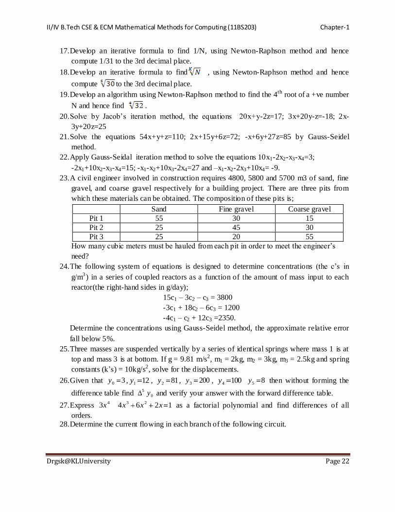
orders. 28. Determine the current flowing in each branch of the following circuit.


Drgsk@KLUniversity

29. Water is flowing in trapezoidal channel at a rate of Q = 20 m3/s. The critical depth y for

such a channel must satisfy the equation B.Ag

Q10

3c

2

where g = 9.81 m/s2, Ac =

cross-sectional of the area (m2) and B = the width of the channel at the surface (m). For this case, the width and the cross sectional area can be related to depth y by

B = 3 + y and 2

y3yA

2

c . Solve for the critical depth using bisection method

with initial guesses of 5.0lx and 5.2ux and iterate until the approximate error

falls below 1%.

30. The trajectory of a ball thrown by a right fielder is defined by the (x,y) coordinates as displayed in the

figure. The trajectory can be modeled as

0

0

22

0

2

0cos2

)(tan yv

xgxy . Find the

approximate initial angle 0 using Newton-Raphson

method, if smv /200 , the distance to the catcher is

35 m. Note that the throw leaves the right fielders

hand at an elevation of m2 and the catcher receives it at m1 .

31. A civil engineer involved in construction requires 4800, 5800, 5700 m3 of sand, fine gravel, coarse gravel respectively for a building project. There are 3 pits from which

these materials can be obtained. The composition of these pits is

Sand % Fine gravel % Coarse gravel %

Pit 1 55 30 15

Pit2 25 45 30

Pit3 25 20 55

x

y

θ0

v0

+ -

+ - + -

8v

4v 6v


Drgsk@KLUniversity

How many cubic meters must be hauled from each pit in order to meet the engineer’s

needs using Jacobi’s iterative method starting with (24, 91, 46).

32. Apply Gauss-Seidel method to solve the following system of equations to a tolerance of ’s = 5% starting with (5, 5, 1).

.20278

3473

3862

321

321

321

xxx

xxx

xxx

Mathematical Methods for...

Documents

Transcript of Mathematical Methods for...