Mathematical Foundations of Elasticity Theory - People · Mathematical Foundations of Elasticity...
269
Mathematical Foundations of Elasticity Theory John Ball Oxford Centre for Nonlinear PDE ©J.M.Ball
Transcript of Mathematical Foundations of Elasticity Theory - People · Mathematical Foundations of Elasticity...

Mathematical Foundations of
Elasticity Theory
John Ball
Oxford Centre for Nonlinear PDE
©J.M.Ball
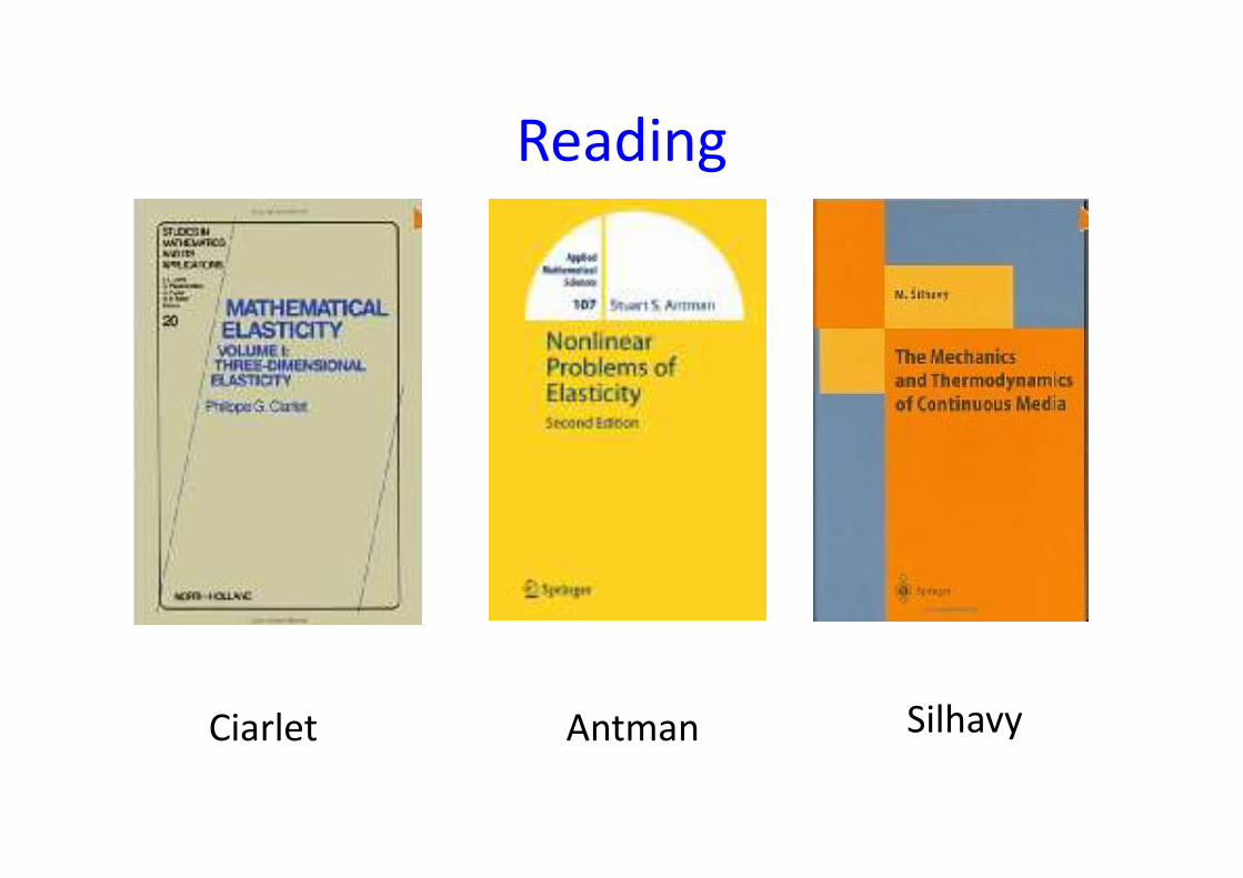
Reading
Ciarlet Antman Silhavy
Prentice Hall 1983
Lecture note 2/1998
Variational models for microstructure
and phase transitions
Stefan Müller
http://www.mis.mpg.de/


J.M. Ball, Some open problems in
elasticity. In Geometry, Mechanics,
and Dynamics, pages 3--59,
Springer, New York, 2002.
You can download this from my webpage
http://www.maths.ox.ac.uk/~ball

Elasticity Theory
The central model of solid mechanics. Rubber, metals (and
alloys), rock, wood, bone … can all be modelled as elastic
materials, even though their chemical compositions are very
different.
For example, metals and alloys are crystalline, with grains
consisting of regular arrays of atoms. Polymers (such as rubber)
consist of long chain molecules that are wriggling in thermal
motion, often joined to each other by chemical bonds called
crosslinks. Wood and bone have a cellular structure …
6

A brief history
1678 Hooke's Law
1705 Jacob Bernoulli
1742 Daniel Bernoulli
1744 L. Euler elastica (elastic rod)
1821 Navier, special case of linear elasticity via molecular model
(Dalton’s atomic theory was 1807)
1822 Cauchy, stress, nonlinear and linear elasticity
For a long time the nonlinear theory was ignored/forgotten.
1927 A.E.H. Love, Treatise on linear elasticity
1950's R. Rivlin, Exact solutions in incompressible nonlinear elasticity
(rubber)
1960 -- 80 Nonlinear theory clarified by J.L. Ericksen, C. Truesdell …
1980 -- Mathematical developments, applications to materials,
biology … 7

Kinematics
Label the material points of the body by the
positions x ∈ Ω they occupy in the reference
configuration. 8

Deformation gradient
F = Dy(x, t), Fiα = ∂yi∂xα
.
9

Invertibility
To avoid interpenetration of matter, we re-
quire that for each t, y(·, t) is invertible on Ω,
with sufficiently smooth inverse x(·, t). We also
suppose that y(·, t) is orientation preserving;
hence
J = detF (x, t) > 0 for x ∈ Ω. (1)
By the inverse function theorem, if y(·, t) is C1,
(1) implies that y(·, t) is locally invertible.10

11

Global inverse function theorem for
C1 deformations
Let Ω ⊂ Rn be a bounded domain with Lips-
chitz boundary ∂Ω (in particular Ω lies on one
side of ∂Ω locally). Let y ∈ C1(Ω;Rn) with
detDy(x) > 0 for all x ∈ Ω
and y|∂Ω one-to-one. Then y is invertible on
Ω.
12
Proof uses degree theory. cf Meisters and Olech,
Duke Math. J. 30 (1963) 63-80.

Notation
Mn×n = real n× n matricesMn×n
+ = F ∈Mn×n : detF > 0SO(n) = R ∈Mn×n : RTR = 1,detR = 1
= rotations.If a ∈ Rn, b ∈ Rn, the tensor product a ⊗ b is
the matrix with the components
(a⊗ b)ij = aibj.
[Thus (a⊗ b)c = (b · c)a if c ∈ Rn.]

Variational formulation of nonlinear
elastostatics
We suppose for simplicity that the body is ho-
mogeneous, i.e. the material response is the
same at each point. In this case the total elas-
tic energy corresponding to the deformation
y = y(x) is given by
I(y) =
ΩW (Dy(x)) dx,
where W = W (F ) is the stored-energy function
of the material. We suppose that W : M3×3+ →
R is C1 and bounded below, so that without
loss of generality W ≥ 0.

We will study the existence/nonexistence of
minimizers of I subject to suitable boundary
conditions.
Issues.1. What function space should we seek a
minimizer in? This controls the allowable sin-
gularities in deformations and is part of the
mathematical model.
2. What boundary conditions should be
specified?
3. What properties should we assume
about W?

The Sobolev space W1,p
W1,p = y : Ω → R3 : y1,p <∞, where
y1,p =
(Ω[|y(x)|p + |Dy(x)|p] dx)1/p if 1 ≤ p <∞
ess supx∈Ω (|y(x)|+ |Dy(x)|) if p = ∞
Dy is interpreted in the weak (or distributional)
sense, so that
Ω
∂yi∂xα
ϕdx = −
Ωyi
∂ϕ
∂xαdx
for all ϕ ∈ C∞0 (Ω).

We assume that y belongs to the largest Sobolev
space W1,1 = W1,1(Ω;R3), so that in particu-
lar Dy(x) is well defined for a.e. x ∈ Ω, and
I(y) ∈ [0,∞].

y ∈W1,∞
y ∈W1,1
(because every y ∈ W1,1 is absolutely contin-
uous on almost every line parallel to a given
direction)
Lipschitz

y(x) =1+|x||x| x
y ∈W1,p for 1 ≤ p < 3.
Exercise: prove this.
Cavitation

Boundary conditions
We suppose that ∂Ω = ∂Ω1 ∪ ∂Ω2 ∪N , where
∂Ω1, ∂Ω2 are disjoint relatively open subsets
of ∂Ω and N has two-dimensional Hausdorff
measure H2(N) = 0 (i.e. N has zero area).
We suppose that y satisfies mixed boundary
conditions of the form
y|∂Ω1= y(·),
where y : ∂Ω1 → R3 is a given boundary dis-
placement.

By formally computing
d
dτI(y+τϕ)|τ=0 =
d
dτ
ΩW (Dy+τDϕ) dx|t=0 = 0,
we obtain the weak form of the Euler-Lagrange
equation for I, that is
ΩDFW(Dy) ·Dϕdx = 0 (∗)
for all smooth ϕ with ϕ|∂Ω1= 0.
TR(F ) = DFW (F ) is the
Piola-Kirchhoff stress tensor.
(A ·B = tr ATB)

If y, ∂Ω1 and ∂Ω2 are sufficiently regular then
(*) is equivalent to the pointwise form of the
equilibrium equations
DivDFW (Dy) = 0 in Ω,
together with the natural boundary condition
of zero applied traction
DFW (Dy)N = 0 on ∂Ω2,
where N = N(x) denotes the unit outward nor-
mal to ∂Ω at x.

∂Ω2
∂Ω2
∂Ω1
∂Ω1
y(x) = x y(x1, x2, x3) = (λx1, x2, x3)
1
y(∂Ω2) traction free
λ < 1
Example: boundary conditions for buckling of a bar

Hence our variational problem becomes:
Does there exist y∗ minimizing
I(y) =
ΩW (Dy) dx
in
A = y ∈W1,1 : y invertible, y|∂Ω1= y?
We will make the invertibility condition more
precise later.

Properties of W
To try to ensure that deformations are invert-
ible, we suppose that
(H1) W (F ) →∞ as detF → 0 + .
So as to also prevent orientation reversal we
define W (F ) = ∞ if detF ≤ 0. Then
W : M3×3 → [0,∞] is continuous.

Thus if I(y) < ∞ then detDy(x) > 0 a.e..
However this does not imply local invertibil-
ity (think of the map (r, θ) → (r,2θ) in plane
polar coordinates, which has constant positive
Jacobian but is not invertible near the origin),
nor is it clear that detDy(x) ≥ µ > 0 a.e..

We suppose that W is frame-indifferent, i.e.
(H2) W (RF ) = W (F )
for all R ∈ SO(3), F ∈M3×3.
In order to analyze (H2) we need some linear
algebra.

Square root theorem
Let C be a positive symmetric n × n matrix.
Then there is a unique positive definite sym-
metric n× n matrix U such that
C = U2
(we write U = C1/2).
28
Formula for the square root
Since C is symmetric it has a spectral decom-
position
C =n
i=1
λiei ⊗ ei.
Since C > 0, it follows that λi > 0. Then
U =n
i=1
λ1/2i ei ⊗ ei
satisfies U2 = C. 29

Polar decomposition theorem
Let F ∈Mn×n+ . Then there exist positive defi-
nite symmetric U , V and R ∈ SO(n) such that
F = RU = V R.
These representations (right and left respec-
tively) are unique.
30

Proof. Suppose F = RU . Then U2 = FTF :=
C. Thus if the right representation exists U
must be the square root of C. But if a ∈R
n is nonzero, Ca · a = |Fa|2 > 0, since F is
nonsingular. Hence C > 0. So by the square
root theorem, U = C1/2 exists and is unique.
Let R = FU−1. Then
RTR = U−1FTFU−1 = 1
and detR = detF (detU)−1 = +1.
The representation F = V R1 is obtained simi-
larly using B := FFT , and it remains to prove
R = R1. But this follows from F = R1
RT
1V R1
,
and the uniqueness of the right representation.31
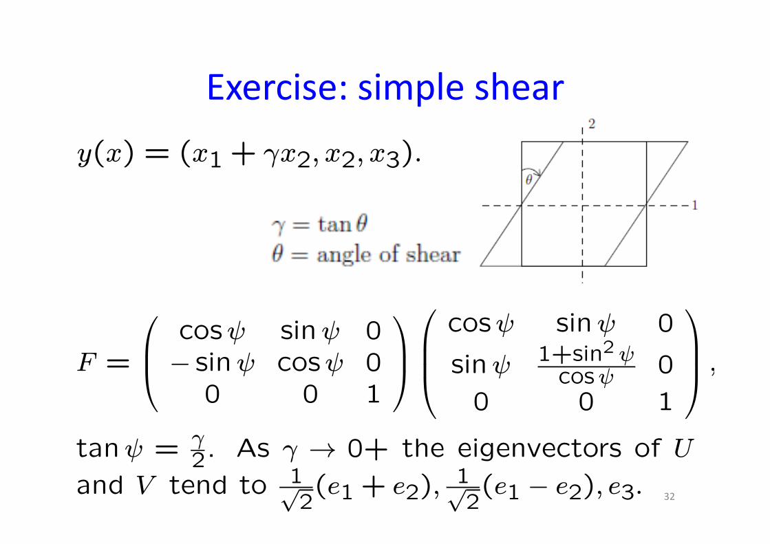
Exercise: simple shear
y(x) = (x1 + γx2, x2, x3).
F =
cosψ sinψ 0− sinψ cosψ 0
0 0 1
cosψ sinψ 0
sinψ 1+sin2 ψcosψ 0
0 0 1
,
tanψ = γ2. As γ → 0+ the eigenvectors of U
and V tend to 1√2(e1 + e2),
1√2(e1 − e2), e3. 32

Hence (H2) implies that
W (F ) = W (RU) = W (U) = W (C).
Conversely if W (F ) = W (U) or W (F ) = W (C)
then (H2) holds.
Thus frame-indifference reduces the dependence
of W on the 9 elements of F to the 6 elements
of U or C.

Material Symmetry
In addition, if the material has a nontrivial
isotropy group S, W satisfies the material sym-
metry condition
W (FQ) = W (F ) for all Q ∈ S, F ∈M3×3+ .
The case S = SO(3) corresponds to an isotropic
material.

The strictly positive eigenvalues v1, v2, v3 of U
(or V ) are called the principal stretches.
Proposition 1
W is isotropic iff W (F ) = Φ(v1, v2, v3), where
Φ is symmetric with respect to permutations
of the vi.
Proof. Suppose W is isotropic. Then F =
RDQ for R,Q ∈ SO(3) and D = diag (v1, v2, v3).
Hence W = W (D). But for any permutation
P of 1,2,3 there exists Q such that
Qdiag (v1, v2, v3)QT = diag (vP1, vP2, vP3).
The converse holds since QTFTFQ has the
same eigenvalues (namely v2i ) as FTF .

(H1) and (H2) are not sufficient to prove the
existence of energy minimizers. We also need
growth and convexity conditions on W . The
growth condition will say something about how
fast W grow for large values of F . The convex-
ity condition corresponds to a statement of the
type ‘stress increases with strain’. We return
to the question of what the correct form of this
convexity condition is later; for a summary of
older thinking on this question see Truesdell &
Noll.

Why minimize energy?
This is the deep problem of the approach to
equilibrium, having its origins in the Second
Law of Thermodynamics.
We will see how rather generally the balance
of energy plus a statement of the Second Law
lead to the existence of a Lyapunov function
for the governing equations.

d
dt
E
1
2ρR|yt|2 + U
dx =
Eb · yt dx
+
∂EtR · yt dS +
Er dx−
∂EqR ·N dS, (1)
for all E ⊂ Ω, where ρR = ρR(x) is the density
in the reference configuration, U is the internal
energy density, b is the body force, tR is the
Piola-Kirchhoff stress vector, qR the reference
heat flux vector and r the heat supply.
Balance of Energy
We assume this holds in the form of the Clausius
Duhem inequality
d
dt
Eη dx ≥ −
∂E
qR ·Nθ
dS +
E
r
θdx (2)
for all E, where η is the entropy and θ the
temperature.
Second Law of Thermodynamics

The Ballistic Free Energy
Suppose that the the mechanical boundary con-
ditions are that y = y(x, t) satisfies
y(·, t)|∂Ω1= y(·) and the condition that the
applied traction on ∂Ω2 is zero, and that the
thermal boundary condition is
θ(·, t)|∂Ω3= θ0, qR ·N |∂Ω\∂Ω3
= 0,
where θ0 > 0 is a constant. Assume that the
heat supply r is zero, and that the body force
is given by b = −gradyh(x, y),

Thus from (1), (2) with E = Ω and the bound-
ary conditions
d
dt
Ω
1
2ρR|yt|2 + U − θ0η + h
dx ≤
∂ΩtR · yt dS −
∂Ω
1− θ0
θ
qR ·N dS = 0.
So E =Ω
12ρR|yt|2 + U − θ0η + h
dx is a Lya-
punov function, and it is reasonable to suppose
that typically (yt, y, θ) tends as t→∞ to a (lo-
cal) minimizer of E.

For thermoelasticity, W (F, θ) can be identi-
fied with the Helmholtz free energy U(F, θ) −θη(F, θ). Hence, if the dynamics and bound-
ary conditions are such that as t→∞ we have
yt → 0 and θ → θ0, then this is close to saying
that y tends to a local minimizer of
Iθ0(y) =
Ω[W (Dy, θ0) + h(x, y)] dx.
The calculation given follows work of Duhem,
Ericksen and Coleman & Dill.

Of course a lot of work would be needed to
justify this (we would need well-posedness of
suitable dynamic equations plus information on
asymptotic compactness of solutions and more;
this is currently out of reach). Note that it is
not the Helmoltz free energy that appears in
the expression for E but U − θ0η, where θ0 is
the boundary temperature.
For some remarks on the case when θ0 depends
on x see J.M. Ball and G. Knowles,
Lyapunov functions for thermoelasticity with
spatially varying boundary temperatures. Arch.
Rat. Mech. Anal., 92:193—204, 1986.

Existence in one dimension
To make the problem nontrivial we consider
an inhomogeneous one-dimensional elastic ma-
terial with reference configuration Ω = (0,1)
and stored-energy function W (x, p), with cor-
responding total elastic energy
I(y) = 1
0[W (x, yx(x)) + h(x, y(x))] dx,
where h is the potential energy of the body
force.

We seek to minimize I in the set of admissible
deformations
A = y ∈W1,1(0,1) : yx(x) > 0 a.e.,
y(0) = α, y(1) = β,where α < β. (We could also consider mixed
boundary conditions y(0) = α, y(1) free.)
(Note the simple form taken by the invertibility
condition.)

Hypotheses on W :
We suppose for simplicity that
W : [0,1]× (0,∞) → [0,∞) is continuous.
(H1) W (x, p) →∞ as p→ 0+.
As before we define W (x, p) = ∞ if p ≤ 0.
(H2) is automatically satisfied in 1D.
(H3) W (x, p) ≥ Ψ(p) for all p > 0,
x ∈ (0,1), where Ψ : (0,∞) → [0,∞)
is continuous with limp→∞ Ψ(p)p = ∞.

(H4) W (x, p) is convex in p, i.e.
W (x, λp+(1−λ)q) ≤ λW (x, p)+(1−λ)W (x, q)
for all p > 0, q > 0, λ ∈ (0,1), x ∈ (0,1).
If W is C1 in p then (H4) is equivalent to
the stress Wp(x, p) being nondecreasing in the
strain p.
(H5) h : [0,1]×R→ [0,∞) is continuous.

Theorem 1
Under the hypotheses (H1)-(H5) there exists
y∗ that minimizes I in A.
Proof.
A is nonempty since z(x) = α + (β − α)x
belongs to A. Since W ≥ 0, h ≥ 0,
0 ≤ l = infy∈A I(y) <∞.
Let y(j) be a minimizing sequence,
i.e. y(j) ∈ A, I(y(j)) → l as j →∞.

We may assume that
limj→∞ 10 W (x, y
(j)x ) dx = l1,
limj→∞ 10 h(x, y(j)) dx = l2,
where l = l1 + l2.
SinceΩ Ψ(y
(j)x ) dx ≤ M < ∞, by the de la
Vallee Poussin criterion (see e.g. One-dimensional
variational problems, G. Buttazzo, M. Giaquinta,
S. Hildebrandt, OUP, 1998 p 77) there exists
a subsequence, which we continue to call y(j)x
converging weakly in L1(0,1) to some z.

Let y∗(x) = α+ x0 z(s) ds, so that y∗x = z. Then
y(j)(x) = α + x0 y
(j)x (s) ds→ y∗(x)
for all x ∈ [0,1]. In particular y∗(0) = α,
y∗(1) = β.
By Mazur’s theorem, there exists a sequence
z(k) =∞
j=k λ(k)j y
(j)x of finite convex combi-
nations of the y(j)x converging strongly to z,
and so without loss of generality almost every-
where.

By convexity
1
0W (x, z(k)) dx ≤
1
0
∞
j=k
λ(k)j W (x, y
(j)x ) dx
≤ supj≥k
1
0W (x, y
(j)x ) dx.
Letting k →∞, by Fatou’s lemma 1
0W (x, y∗x) dx =
1
0W (x, z) dx ≤ l1.
But this implies that y∗x(x) > 0 a.e. and so
y∗ ∈ A.

Also by Fatou’s lemma 1
0h(x, y∗) dx ≤ lim inf
j→∞
1
0h(x, y(j)) dx = l2.
Hence l ≤ I(y∗) ≤ l1 + l2 = l.
So I(y∗) = l and y∗ is a minimizer.

Discussion of (H3)We interpret the superlinear growth condition
(H3) for a homogeneous material.
1/p 1
y(x) = px
Total stored-energy = W(p)p .
So limp→∞ W (p)p = ∞ says that you can’t get
a finite line segment from an infinitesimal one
with finite energy.

x = 0
x = 1
y(0) = 0
y(1) = α
Assume constant density
ρR and pressure pR in the
reference configuration.
Assume gas deforms
adiabatically so that the
pressure p and density ρ
satisfy pρ−γ = pRρ−γR ,
where γ > 1 is a constant.
Simplified model of atmosphere

The potential energy of the column is
I(y) = 1
0
pR
(γ − 1)yx(x)γ−1+ ρRgy(x)
dx
= ρRg 1
0
k
yx(x)γ−1+ (1− x)yx(x)
dx,
where k =pR
ρRg(γ−1).
We seek to minimize I in
A = y ∈W1,1(0,1) : yx > 0 a.e.,
y(0) = 0, y(1) = α.

Then the minimum of I(y) on A is attained iff
α ≤ αcrit, where αcrit = γγ−1
pRρRg
1/γ.
αcrit can be interpreted
as the finite height of
the atmosphere predicted
by this simplified model
(cf Sommerfeld).
If α > αcrit then minimizing sequences y(j) for
I converge to the minimizer for α = αcrit plus
a vertical portion.
x
yα
αcrit
1

For details of the calculation see J.M. Ball,
Loss of the constraint in convex variational
problems, in Analyse Mathematiques et Appli-
cations, Gauthier-Villars, Paris, 1988, where a
general framework is presented for minimizing
a convex functional subject to a convex con-
straint, and is applied to other problems such
as Thomas-Fermi and coagulation-fragmentation
equations.

Discussion of (H4)
For simplicity consider the case of a homo-
geneous material with stored-energy function
W = W(p). The proof of existence of a min-
imizer used the direct method of the calculus
of variations, the key point being that if W is
convex then
E(p) =
1
0W (p) dx
is weakly lower semicontinuous in L1(0,1), i.e.
p(j) p in L1(0,1) (that is 10 p(j)v dx→ 1
0 pv dx
for all v ∈ L∞(0,1)) implies
1
0W (p) dx ≤ lim inf
j→∞
1
0W(p(j)) dx.

Proof. Define p(j) as shown.
1
p
q
Proposition 2 (Tonelli)
If E is weakly lower semicontinuous in L1(0,1)
then W is convex.
λj
1−λj
2j
p(j) λp + (1− λ)q in L1(0,1) 10 W (p(j)) dx = λW (p) + (1− λ)W(q)
≥W (λp + (1− λ)q)
p(j)
x

If W (x, ·) is not convex then the minimum is
in general not attained. For example consider
the problem
infy(0)=0,y(1)=3
2
1
0
(yx − 1)2(yx − 2)2
yx+ (y − 3
2x)2
dx.
Then the infimum is zero
but is not attained.
1
3/2
slopes 1 and 2

More generally we have the following result.
Theorem 2
If W : R→ [0,∞] is continuous and
I(y) = 10 [W (yx) + h(x, y)] dx
attains a minimum on
A = y ∈W1,1 : y(0) = 0, y(1) = βfor all continuous h : [0,1]×R→ [0,∞) and all
β then W is convex.

Let l = infy∈A 10 W (yx) dx,
m = infy∈A 10 [W (yx) + |y − βx|2] dx.
Then l ≤ m. Let ε > 0 and pick z ∈ A with 10 W (zx) dx ≤ l + ε.
Define z(j) ∈ A by
z(j)(x) = βk
j+ j−1z(j(x− k
j))
fork
j≤ x ≤ k + 1
j, k = 0, . . . , j − 1.

Then
|z(j)(x)− βx| = |β(k
j− x) + j−1z(j(x− k
j))|
≤ Cj−1 fork
j≤ x ≤ k + 1
j.
So
I(z(j)) =j−1
k=0
j+1k
jk
W (zx(j(x−k
j)) dx +
1
0|z(j) − βx|2 dx
≤j−1
k=0
j−1 1
0W (zx) dx + Cj−2
≤ l + 2ε
for j sufficiently large. Hence m ≤ l and so
l = m.

But by assumption there exists y∗ with
I(y∗) = 10 W (y∗x) dx +
10 |y∗ − βx|2dx = l.
Hence y∗(x) = βx and thus 10 W (yx) dx ≥W (β)
for all y ∈ A.
Taking in particular
y(x) =
px if 0 ≤ x ≤ λqx + λ(p− q) if λ ≤ x ≤ 1,
with β = λp + (1− λ)q we obtain
W (λp + (1− λ)q) ≤ λW (p) + (1− λ)W (q)
as required.

There are two curious special cases when the
minimum is nevertheless attained when W is
not convex. Suppose that (H1), (H3) hold
and that either
(i) I(y) = 10 W (x, yx) dx, or
(ii) I(y) = 10 [W (yx) + h(y)] dx.
Then I attains a minimum on A.

(i) can be found in Aubert & Tahraoui (J. Dif-
ferential Eqns 1979) and uses the fact that
infy∈A 10 W (x, yx) dx = infy∈A
10 W ∗∗(x, yx) dx,
where W ∗∗ is the lower convex envelope of W .
W (x, p)
p
W ∗∗(x, p)
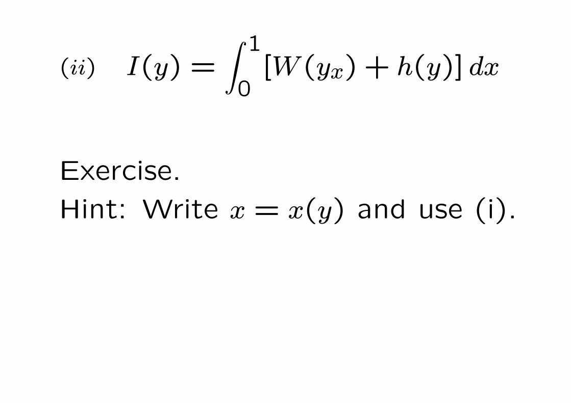
I(y) =
1
0[W (yx) + h(y)] dx(ii)
Exercise.
Hint: Write x = x(y) and use (i).

The Euler-Lagrange equation in 1D
Let y minimize I in A and let ϕ ∈ C∞0 (0,1).
Formally calculating
d
dτI(y + τϕ)|τ=0 = 0
we obtain the weak form of the Euler-Lagrange
equation 1
0[Wp(x, yx)ϕx + hy(x, y)ϕ] dx = 0.
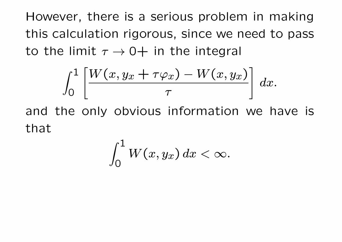
However, there is a serious problem in making
this calculation rigorous, since we need to pass
to the limit τ → 0+ in the integral
1
0
W (x, yx + τϕx)−W(x, yx)
τ
dx.
and the only obvious information we have is
that 1
0W (x, yx) dx <∞.

But Wp can be much bigger than W . For
example, when p is small and W (p) = 1p then
|Wp(p)| = 1p2
is much bigger than W (p). Or if
p is large and W (p) = exp p2 then
|Wp(p)| = 2p exp p2 is much bigger than W (p).
It turns out that this is a real problem and
not just a technicality. Even for smooth ellip-
tic integrands satisfying a superlinear growth
condition there is no general theorem of the
one-dimensional calculus of variations saying
that a minimizer satisfies the Euler-Lagrange
equation.

Consider a general one-dimensional integral of
the calculus of variations
I(u) =
1
0f(x, u, ux) dx,
where f is smooth and elliptic (regular), i.e.
fpp ≥ µ > 0 for all x, u, p.
Suppose also that
lim|p|→∞
f(x, u, p)
|p| = ∞ for all x, u.

It follows that u is a smooth solution of the
Euler-Lagrange equation ddxfp = fu on (0,1).
Suppose u ∈W1,1(0,1) satisfies the weak form
of the Euler-Lagrange equation 1
0[fpϕx + fuϕ] dx = 0 for all ϕ ∈ C∞0 (0,1),
so that in particular fp, fu ∈ L1loc(0,1).
Then
fp =
x
afu + const
where a ∈ (0,1), and hence (Exercise) ux is
bounded on compact subsets of (0,1).


Also if u(j) ∈W1,∞ converges a.e. to u∗ then
I(u(j)) →∞(the repulsion property), explaining the numer-
ical results.
For this problem one has that
I(u∗ + tϕ) = ∞ for t = 0, if ϕ(0) = 0.
u∗
u∗ + tϕ

Derivation of the EL equation for 1D
elasticity
Theorem 3
Let (H1) and (H5) hold and suppose further
that Wp exists and is continuous in (x, p) ∈[0,1]×(0,∞), and that hy exists and is contin-
uous in (x, y) ∈ [0,1] × R. If y minimizes I in
A then Wp(·, yx(·)) ∈ C1([0,1]) and
d
dxWp(x, yx(x)) = hy(x, y(x)) for all x ∈ [0,1]. (EL)
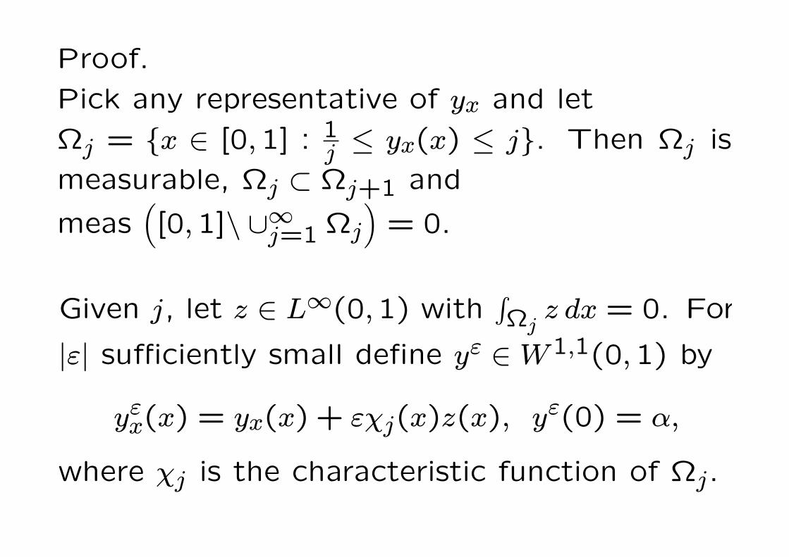
Proof.
Pick any representative of yx and let
Ωj = x ∈ [0,1] : 1j ≤ yx(x) ≤ j. Then Ωj is
measurable, Ωj ⊂ Ωj+1 and
meas[0,1]\ ∪∞j=1 Ωj
= 0.
Given j, let z ∈ L∞(0,1) withΩj
z dx = 0. For
|ε| sufficiently small define yε ∈W1,1(0,1) by
yεx(x) = yx(x) + εχj(x)z(x), yε(0) = α,
where χj is the characteristic function of Ωj.

Then
d
dεI(yε)|ε=0
=
Ω
Wp(x, yx)z + hy
x
0χjz ds
dx
=
Ωj
Wp(x, yx)−
x
0hy(s, y(s)) ds
z(x) dx
= 0.
Hence
Wp(x, yx)− x
0hy(s, y(s)) ds = Cj in Ωj,
and clearly Cj is independent of j.

Corollary 1
Let the hypotheses of Theorem 3 hold and
assume further that
limp→0+
maxx∈[0,1]
Wp(x, p) = −∞ (∗).
Then there exists µ > 0 such that
yx(x) ≥ µ > 0 a.e. x ∈ [0,1].
Proof.
Wp(x, yx(x)) ≥ C > −∞ by (EL).

Remark.
(*) is satisfied if W (x, p) is convex in p for all
x ∈ [0,1],0 < p ≤ ε for some ε > 0 and if
(H1+) limp→0+
minx∈[0,1]
W (x, p) = ∞.
Proof.
Wp(x, p) ≤W (x, ε)−W (x, p)
ε− p.

Corollary 2.
If (*), (H3) and the hypotheses of Theorem
3 hold, and if W (x, ·) is strictly convex then y
has a representative in C1([0,1]).
Proof.
Wp(x, yx(x)) has a continuous representative.
So there is a subset S ⊂ [0,1] of full measure
such that Wp(x, yx(x)) is continuous on S. We
need to show that that if xj, xj ⊂ S with
xj → x, xj → x then the limits limj→∞ yx(xj),
limj→∞ yx(xj) exist and are finite and equal.

By (H3) and convexity,
limp→∞minx∈[0,1] Wp(x, p) = ∞. Hence we may
assume that yx(xj) → z, yx(xj) → z ∈ [µ,∞)
with z = z. Hence Wp(x, z) = Wp(x, z), which
by strict convexity implies z = z.

Existence of minimizers in 3D
elastostatics

Minimize
I(y) =
ΩW (Dy) dx
in
A = y ∈ W1,1 : detDy(x) > 0 a.e., y|∂Ω1= y.
(Note that we have for the time being replaced
the invertibility condition by the local conditi-
ion detDy(x) > 0 a.e., which is easier to han-
dle.)

So far we have assumed that W : M3×3+ → [0,∞)
is continuous, and that
(H1) W (F ) →∞ as detF → 0+,
so that setting W (F ) = ∞ if detF ≤ 0, we
have that W : M3×3 → [0,∞] is continuous,
and that W is frame-indifferent, i.e.
(H2) W (RF ) = W (F ) for all R ∈ SO(3), F ∈ M3×3.
(In fact (H2) plays no direct role in the
existence theory.)

Growth condition
1|F |
y = Fx
lim|F |→∞
W (F )
|F |3 = ∞
says that you can’t get a finite line segment
from an infinitesimal cube with finite energy.
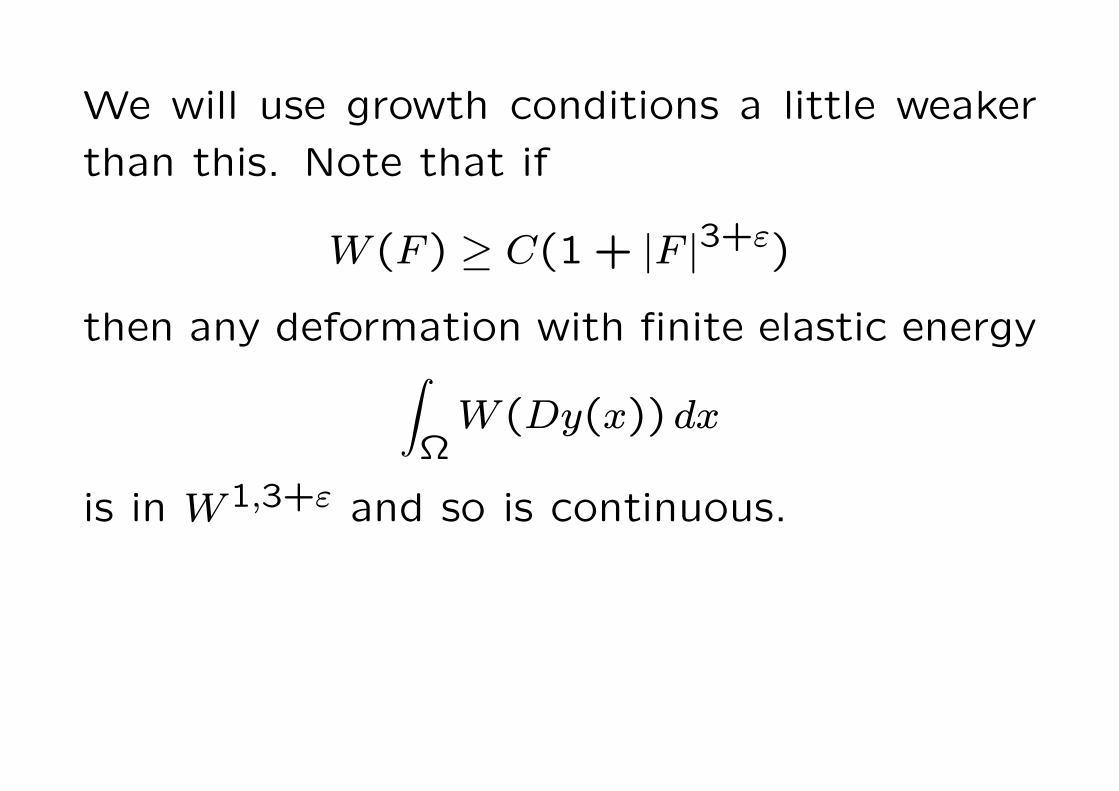
We will use growth conditions a little weaker
than this. Note that if
W (F ) ≥ C(1 + |F |3+ε)
then any deformation with finite elastic energy
ΩW (Dy(x)) dx
is in W1,3+ε and so is continuous.

Convexity conditions
The key difficulty is that W is never convex, so
that we can’t use the same method to prove
existence of minimizers as in 1D.
Reasons
1. Convexity of W is inconsistent with (H1)
because M3×3+ is not convex.

detF < 0 detF > 0
A = diag (1,1,1)
B = diag (−1,−1,1)
12(A + B) = diag (0,0,1)
W (12(A + B)) = ∞
> 12W (A) + 1
2W (B)
Remark: M3×3+ is
not simply-connected.

2. If W is convex, then any equilibrium solution
(solution of the EL equations) is an absolute
minimizer of the elastic energy
I(y) =
ΩW(Dy) dx.
Proof.
I(z) =
ΩW (Dz) dx ≥
Ω[W (Dy) + DW (Dy) · (Dz −Dy)] dx = I(y).
This contradicts common experience of nonunique
equlibria, e.g. buckling.

Pure zero traction problem.
Examples of nonunique equilibrium solutions

For an isotropic material could we assume in-
stead that Φ(v1, v2, v3) is convex in the princi-
pal stretches v1, v2, v3?
This is a consequence of
the Coleman-Noll inequality.
While it is consistent with
(H1) it is not in general
satisfied for rubber-like
materials, which are almost
incompressible (v1v2v3 = 1),
and so have nonconvex
sublevel sets.
v3 = 1
v1
v2
v1v2 = 1
nonconvex
sublevel set
Φ ≤ c

Rank-one matrices and the Hadamard
jump conditionN
Dy = A, x ·N > k
Dy = B, x ·N < k x ·N = k
y piecewise affine
Let C = A − B. Then Cx = 0 if x · N = 0.
Thus C(z − (z · N)N) = 0 for all z, and so
Cz = (CN ⊗N)z. Hence
A−B = a⊗NHadamard
jump condition

x0
N
More generally this holds for y piecewise C1,
with Dy jumping across a C1 surface.
Dy+(x0) = A
Dy−(x0) = B A−B = a⊗N
Exercise: prove this by blowing up around x
using yε(x) = εy(x−x0ε ).

Rank-one convexity
W is rank-one convex if the map
t →W (F + ta⊗N) is convex for each
F ∈M3×3 and a ∈ R3, N ∈ R3.
Equivalently,
W (λF + (1− λ)G) ≤ λW (F ) + (1− λ)W (G)
if F,G ∈ M3×3 with F − G = a ⊗ N and λ ∈(0,1).
(Same definition for Mm×n.)

Rank-one convexity is consistent with (H1) be-
cause det(F+ta⊗N) is linear in t, so that M3×3+
is rank-one convex
(i.e. if F,G ∈ M3×3+ with F − G = a ⊗ N then
λF + (1− λ)G ∈M3×3+ .)
Rank-one cone
Λ = a⊗N : a,N ∈ R3F

Such a W is rank-one convex because if
F,G ∈M3×3+ with F −G = a⊗N , and
λ ∈ (0,1) then
W (λF + (1− λ)G) = h(λdetF + (1− λ) detG)
≤ λh(detF ) + (1− λ)h(detG)
= λW (F ) + (1− λ)W (G).
A specific example of a rank-one convex W is
an elastic fluid for which
W (F ) = h(detF ),
with h convex and limδ→0+ h(δ) = ∞.

If W ∈ C1(M3×3+ ) then W is rank-one convex
iff t → DW (F + ta⊗N) ·a⊗N is nondecreasing.
The linear map
y(x) = (F + ta⊗N)x = Fx + ta(x ·N)
represents a shear relative to Fx parallel to a
plane Π with normal N in the reference config-
uration, in the direction a. The corresponding
stress vector across the plane Π is
tR = DW (F + ta⊗N)N,
and so rank-one convexity says that the com-
ponent tR · a in the direction of the shear is
monotone in the magnitude of the shear.

If W ∈ C2(M3×3+ ) then W is rank-one convex
iff
d2
dt2W (F + ta⊗N)|t=0 ≥ 0,
for all F ∈M3×3+ , a,N ∈ R3, or equivalently
D2W (F )(a⊗N, a⊗N) =∂2W (F )
∂Fiα∂FjβaiNαajNβ ≥ 0,
(Legendre-Hadamard condition).

The strengthened version
D2W (F )(a⊗N, a⊗N) =∂2W (F )
∂Fiα∂FjβaiNαajNβ ≥ µ|a|2|N |2,
for all F, a,N and some constant µ > 0 is called
strong ellipticity.
One consequence of strong ellipticity is that
it implies the reality of wave speeds for the
equations of elastodynamics linearized around
a uniform state y = Fx.

Equation of motion of pure elastodynamics
ρRy = DivDW (Dy),
where ρR is the (constant) density in the
reference configuration.
Linearized around the uniform state y = Fx
the equations become
ρRui =∂2W (F )
∂Fiα∂Fjβuj,αβ.

The plane wave
u = af(x ·N − ct)
is a solution if
C(F)a = c2ρRa,
where
Cij =∂2W (F )
∂Fiα∂FjβNαNβ.
Since C(F ) > 0 by strong ellipticity, it follows
that c2 > 0 as claimed.

Quasiconvexity (C.B. Morrey, 1952)
Let W : Mm×n → [0,∞] be Borel measurable.
W is said to be quasiconvex at F ∈ Mm×n if
the inequality
ΩW (F + Dϕ(x)) dx ≥
ΩW (F ) dx
holds for any ϕ ∈ W1,∞0 (Ω;Rm), and is quasi-
convex if it is quasiconvex at every F ∈Mm×n.
Here Ω ⊂ Rn is any bounded open set whose
boundary ∂Ω has zero n-dimensional Lebesgue
measure.

Remark
W1,∞0 (Ω;Rm) is defined as the closure of
C∞0 (Ω;Rm) in the weak* topology of
W1,∞(Ω;Rm) (and not in the norm topology
- why?). That is ϕ ∈ W1,∞0 (Ω;Rm) if there
exists a sequence ϕ(j) ∈ C∞0 (Ω;Rm) such that
ϕ(j) ∗ ϕ, Dϕ(j) ∗
Dϕ in L∞.
Sometimes the definition is given with C∞0 re-
placing W1,∞0 . This is the same if W is finite
and continuous, but it is not clear (to me) if
it is the same if W is continuous and takes the
value +∞.

Setting m = n = 3 we see that W is
quasiconvex if for any F ∈ M3×3 the pure dis-
placement problem to minimize
I(y) =
ΩW (Dy(x)) dx
subject to the linear boundary condition
y(x) = Fx, x ∈ ∂Ω,
has y(x) = Fx as a minimizer.

Proposition 3
Quasiconvexity is independent of Ω.
Proof. Suppose the definition holds for Ω, and
let Ω1 be another bounded open subset of Rn
such that ∂Ω1 has n-dimensional measure zero.
By the Vitali covering theorem we can write Ω
as a disjoint union
Ω =∞
i=1
(ai + εiΩ1) ∪N,
where N is of zero measure.
ΩΩ1
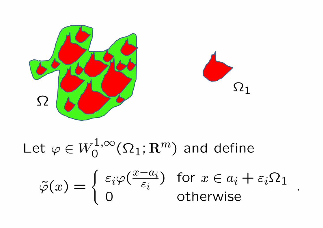
Let ϕ ∈W1,∞0 (Ω1;R
m) and define
ϕ(x) =
εiϕ(x−ai
εi) for x ∈ ai + εiΩ1
0 otherwise.

Then ϕ ∈W1,∞0 (Ω;Rm) and
ΩW (F + Dϕ(x)) dx
=∞
i=1
ai+εiΩ1
W (F + Dϕ
x− ai
εi
) dx
=
∞
i=1
εni
Ω1
W (F + Dϕ(x)) dx
=
measΩ
measΩ1
Ω1
W (F + Dϕ(x)) dx
≥ (measΩ)W (F).

Another form of the definition that is equiva-
lent for finite continuous W is that
QW (Dy) dx ≥ (measQ)W (F )
for any y ∈W1,∞ such that Dy is the restriction
to a cube Q (e.g. Q = (0,1)n) of a Q-periodic
map on Rn with 1measQ
QDy dx = F .
One can even replace periodicity with almost
periodicity (see J.M. Ball, J.C. Currie, and P.J.
Olver. Null Lagrangians, weak continuity, and
variational problems of arbitrary order. J. Func-
tional Anal., 41:135—174, 1981).

Theorem 4
If W is continuous and quasiconvex then W is
rank-one convex.
Remark
This is not true in general if W is not contin-
uous. As an example, define for given nonzero
a,N
W (0) = W (a⊗N) = 0,W (F ) = ∞ otherwise.
Then W is clearly not rank-one convex, but it
is quasiconvex because given F = 0, a⊗N there
is no ϕ ∈ W1,∞0 with F + Dϕ(x) ∈ 0, a ⊗ N

Proof
We prove that
W (F ) ≤ λW (F−(1−λ)a⊗N)+(1−λ)W (F+λa⊗N)
for any F ∈Mm×n, a ∈ Rm, N ∈ Rn, λ ∈ (0,1).
Without loss of generality we suppose that
N = e1. We follow an argument of Morrey.
Let D = (−(1− λ), λ)× (−ρ, ρ)n−1 and let D±j
be the pyramid that is the convex hull of the
origin and the face of D with normal ±ej.

λ−(1− λ)
ρ
−ρ
x1
xj
Dϕ = λa⊗ e1 −(1− λ)a⊗ e1
Let ϕ ∈W1,∞0 (D;Rm) be affine in each
D±j with ϕ(0) = λ(1− λ)a.
−ρ−1λ(1− λ)a⊗ ej
ρ−1λ(1− λ)a⊗ ejD1
+D1-
Dj+
Dj-
The values of Dϕ are shown.

By quasiconvexity
(2ρ)n−1W (F ) ≤ (2ρ)n−1λ
nW (F − (1− λ)a⊗ e1)
+(2ρ)n−1(1− λ)
nW (F + λa⊗ e1)
+n
j=2
(2ρ)n−1
2n[W (F + ρ−1λ(1− λ)a⊗ ej)
+W (F − ρ−1λ(1− λ)a⊗ ej)]
Suppose W (F ) <∞. Then dividing by (2ρ)n−1,
letting ρ→ 0+ and using the continuity of W ,
we obtain
W (F) ≤ λW (F − (1− λ)a⊗ e1) + (1− λ)W (F + λa⊗ e1)
as required.

Now suppose that W (F − (1 − λ)a ⊗ e1) and
W (F +λa⊗e1) are finite. Then g(τ) = W (F +
τa⊗ e1) lies below the chord joining the points
(−(1− λ), g(−(1− λ))), (λ, g(λ)) whenever
g(τ) < ∞, and since g is continuous it follows
that g(0) = W (F ) <∞.
λ−(1− λ)
g

Corollary 3
If m = 1 or n = 1 then a continuous W :
Mm×n → [0,∞] is quasiconvex iff it is convex.
Proof.
If m = 1 or n = 1 then rank-one convexity is
the same as convexity. If W is convex (for any
dimensions) then W is quasiconvex by Jensen’s
inequality:
1
measΩ
ΩW (F + Dϕ) dx
≥W
1
measΩ
Ω(F + Dϕ) dx
= W (F ).

Theorem 5
Let W : Mm×n → [0,∞] be Borel measurable,
and Ω ⊂ Rn a bounded open set. A necessary
condition for
I(y) =
ΩW (Dy) dx
to be sequentially weak* lower semicontinuous
on W1,∞(Ω;Rm) is that W is quasiconvex.
Proof.
Let F ∈Mm×n, ϕ ∈W1,∞0 (Q;Rm), where
Q = (0,1)n.

Given k write Ω as the disjoint union
Ω =∞
j=1
(a(k)j + ε
(k)j Q) ∪Nk,
where a(k)j ∈ Rm, |ε(k)j | < 1/k,measNk = 0, and
define
y(k)(x) =
Fx + ε(k)j ϕ
x−a(k)j
ε(k)j
for x ∈ a(k)j + ε
(k)j Q
Fx otherwise
.

Then y(k) ∗ Fx in W1,∞ as k →∞ and so
(measΩ)W (F ) ≤ lim infk→∞
I(y(k))
=∞
j=1
a(k)j +ε
(k)j Q
W (F + Dϕ
x− a
(k)j
ε(k)j
) dx
=∞
j=1
ε(k)nj
QW (F + Dϕ) dx
=
measΩ
measQ
QW (F + Dϕ) dx

Theorem 6 (Morrey, Acerbi-Fusco, Marcellini)
Let Ω ⊂ Rn be bounded and open. Let
W : Mm×n → [0,∞) be quasiconvex and let
1 ≤ p ≤ ∞. If p <∞ assume that
0 ≤W (F) ≤ c(1 + |F |p) for all F ∈Mm×n.
Then
I(y) =
ΩW (Dy) dx
is sequentially weakly lower semicontinuous (weak*
if p = ∞) on W1,p.
Proof omitted. Unfortunately the growth con-
dition conflicts with (H1), so we can’t use this
to prove existence in 3D elasticity.

Theorem 7 (Ball & Murat)
Let W : Mm×n → [0,∞] be Borel measurable,
and let Ω ⊂ Rn be bounded open and have
boundary of zero n-dimensional measure. If
I(y) =
Ω[W (Dy) + h(x, y)] dx
attains an absolute minimum on A = y : y −Fx ∈ W
1,10 (Ω;Rm) for all F and all smooth
nonnegative h, then W is quasiconvex.
Proof (Exercise: use the same method as
Theorem 2 and Vitali.)

Theorem 8 (van Hove)
Let W(F ) = cijklFijFkl be quadratic. Then
W is rank-one convex ⇔ W is quasiconvex.
Proof.
Let W be rank-one convex. Since for any
ϕ ∈W1,∞0
Ω[W (F + Dϕ)−W (F )] dx =
Ωcijklϕi,jϕk,l dx
we just need to show that the RHS is ≥ 0.
Extend ϕ by zero to the whole of Rn and take
Fourier transforms.

By the Plancherel formula
Ωcijklϕi,jϕk,l dx =
Rncijklϕi,jϕk,l dx
= 4π2
RnRe [cijklϕiξj ¯ϕkξl] dξ
≥ 0
as required.

Null Lagrangians
When does equality hold in the quasiconvexity
condition? That is, for what L is
ΩL(F + Dϕ(x)) dx =
ΩL(F ) dx
for all ϕ ∈ W1,∞0 (Ω;Rm)? We call such L
quasiaffine.

Theorem 9 (Landers, Morrey, Reshetnyak ...)
If L : Mm×n → R is continuous then the fol-
lowing are equivalent:
(i) L is quasiaffine.(ii) L is a (smooth) null Lagrangian, i.e. the
Euler-Lagrange equations DivDFL(Du) = 0
hold for all smooth u.
(iii) L(F ) = constant +d(m,n)
k=1 ckJk(F),
where J(F ) = (J1(F ), . . . , Jd(m,n)(F)) consists
of all the minors of F . (e.g. m = n = 3:
L(F ) = const. + C · F + D · cofF + edetF ).
(iv) u → L(Du) is sequentially weakly contin-
uous from W1,p → L1 for sufficiently large p
(p > min(m,n) will do).

Ideas of proofs.
(i) ⇒ (iii) use L rank-one affine (Theorem 4).
(iii)⇒(iv) Take e.g.
J(Du) = u1,1u2,2 − u1,2u2,1
= (u1u2,2),1 − (u1u2,1),2
if u is smooth.
So if ϕ ∈ C∞0 (Ω)
ΩJ(Du) · ϕdx =
Ω[u1u2,1ϕ,2 − u1u2,2ϕ,1) dx.
True for u ∈W1,2 by approximation.

If u(j) u in W1,p, p > 2, then
ΩJ(Du(j))ϕdx =
Ω[u
(j)1 u
(j)2,1ϕ,2 − u
(j)1 u
(j)2,2ϕ,1] dx
→
ΩJ(Du)ϕdx
since u(j)1 → u1 in Lp′, u
(j)2,1 u2,1 in Lp, and
since J(Du(j)) is bounded in Lp/2 it follows
that J(Du(j)) J(Du) in Lp/2.
For the higher-order Jacobians we use
induction based on the identity
∂(u1, . . . , um)
∂(x1, . . . , xm)=
m
s=1
(−1)s+1 ∂
∂xs
u1∂(u2, . . . , um)
∂(x1, . . . , xs, . . . , xm)

For example, suppose m = n = 3, p ≥ 2,
u(j) u in W1,p, cofDu(j) bounded in Lp′,
detDu(j) χ in L1. Then χ = detDu.
(iv)⇒(i) by Theorem 5.
(i)⇔(ii)
d
dt
ΩL(F + Dϕ + tDψ) dx
t=0
= 0
for all ϕ, ψ ∈ C∞0⇒
ΩDL(F + Dϕ !
Du
) ·Dψ dx = 0.

Polyconvexity
Definition
W is polyconvex if there exists a convex func-
tion g : Rd(m,n) → (−∞,∞] such that
W (F ) = g(J(F )) for all F ∈Mm×n.
e.g. W (F ) = g(F,detF ) if m = n = 2,
W (F ) = g(F, cofF,detF ) if m = n = 3,
with g convex.

Theorem 10
Let W : Mm×n → [0,∞] be Borel measurable
and polyconvex, with g lower semicontinuous.
Then W is quasiconvex.
Proof. Writing
−
Ωf dx =
1
measΩ
Ωf dx,
−
ΩW (F + Dϕ(x)) dx = −
Ωg(J(F + Dϕ(x))) dx
Jensen≥ g
−
ΩJ(F + Dϕ) dx
= g(J(F ))
= W (F ).

Remark
If m ≥ 3, n ≥ 3 then there are quadratic rank-
one convex W that are not polyconvex. Such
W cannot be written in the form
W (F ) = Q(F ) +N
l=1
αlJ(l)2 (F ),
where Q ≥ 0 is quadratic and the J(l)2 are 2×2
minors (Terpstra, D. Serre).

Examples and counterexamples
We have shown that
W convex ⇒ W polyconvex ⇒ W quasiconvex
⇒ W rank-one convex.
The reverse implications are all false if
m > 1, n > 1, except that it is not known
whether W rank-one convex ⇒ W quasicon-
vex when n ≥ m = 2.
W polyconvex ⇒ W convex since any minor is
polyconvex.

Example (Dacorogna & Marcellini)
m = n = 2
Wγ(F ) = |F |4 − 2γ|F |2 detF, γ ∈ R,
where |F |2 = tr (FTF ).
It is not known for what γ the function Wγ is
quasiconvex.

Wγ is convex ⇔ |γ| ≤ 2
3
√2
polyconvex ⇔ |γ| ≤ 1
quasiconvex ⇔ |γ| ≤ 1 + ε
for some (unknown) ε > 0
rank-one convex ⇔ |γ| ≤ 2√3≃ 1.1547....
Numerically (Dacorogna-Haeberly)
1 + ε = 1.1547....
In particular W quasiconvex ⇒ W polyconvex
(see also later).

Theorem 11 (Sverak 1992)
If n ≥ 2,m ≥ 3 then W rank-one convex ⇒ W
quasiconvex.
Sketch of proof.
It is enough to consider the case n = 2,m = 3.
Consider the periodic function u : R2 → R3
u(x) =1
2π
sin 2πx1sin 2πx2
sin 2π(x1 + x2)
.

Then
Du(x) =
cos 2πx1 00 cos 2πx2
cos2π(x1 + x2) cos2π(x1 + x2)
∈ L :=
r 00 st t
: r, s, t ∈ R
a.e.
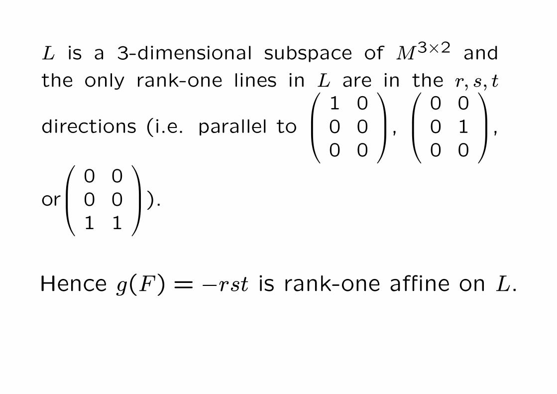
L is a 3-dimensional subspace of M3×2 and
the only rank-one lines in L are in the r, s, t
directions (i.e. parallel to
1 00 00 0
,
0 00 10 0
,
or
0 00 01 1
).
Hence g(F ) = −rst is rank-one affine on L.

However
−
(0,1)2g(Du) dx = −1
4< 0 = g
−
(0,1)2Dudx
,
violating quasiconvexity.
For F ∈M3×2 define
fε,k(F ) = g(PF ) + ε(|F |2 + |F |4) + k|F − PF |2,where P : M3×2 → L is orthogonal projection.
Can check that for each ε > 0 there exists
k(ε) > 0 such that fε = fε,k(ε) is rank-one con-
vex, and we still get a contradiction.

So is there a tractable characterization of
quasiconvexity? This is the main road-block
of the subject.
Theorem 12 (Kristensen 1999)
For m ≥ 3, n ≥ 2 there is no local condition
equivalent to quasiconvexity (for example, no
condition involving W and any number of its
derivatives at an arbitrary matrix F ).
Idea of proof. Sverak’s W is ‘locally quasi-
convex’, i.e. it coincides with a quasiconvex
function in a neighbourhood of any F .

This might lead one to think that no charac-
terization of quasiconvexity is possible. On the
other hand Kristensen also proved
Theorem 13 (Kristensen)
For m ≥ 2, n ≥ 2 polyconvexity is not a local
condition.
For example, one might contemplate a
characterization of the type
W quasiconvex ⇔ W is the supremum of a
family of special quasiconvex functions (includ-
ing null Lagrangians).

Existence based on polyconvexity
We will show that it is possible to prove the ex-
istence of minimizers for mixed boundary value
problems if we assume W is polyconvex and
satisfies (H1) and appropriate growth condi-
tions. Furthermore the hypotheses are satis-
fied by various commonly used models of nat-
ural rubber and other materials.

Theorem 14
Suppose that W satisfies (H1) and the hy-
potheses
(H3) W (F ) ≥ c0(|F |2 + |cof F |3/2)− c1 for all
F ∈M3×3, where c0 > 0,
(H4) W is polyconvex, i.e. W (F ) = g(F, cof F,detF )
for all F ∈ M3×3 for some continuous convex
g.
Assume that there exists some y in
A = y ∈W1,1(Ω;R3) : y|∂Ω1= y
with I(y) <∞, where H2(∂Ω1) > 0 and
y : ∂Ω1 → R3 is measurable. Then there exists
a global minimizer y∗ of I in A.

Theorem 14 is a refinement (weakening the
growth conditions) of
J.M. Ball, Convexity conditions and existence
theorems in nonlinear elasticity. Arch. Rat.
Mech. Anal., 63:337—403, 1977
(see also J.M. Ball. Constitutive inequalities
and existence theorems in nonlinear elastostat-
ics. In R.J. Knops, editor, Nonlinear Analysis
and Mechanics, Heriot-Watt Symposium, Vol.
1. Pitman, 1977.)
due to
S. Muller, T. Qi, and B.S. Yan. On a new
class of elastic deformations not allowing for
cavitation. Ann. Inst. Henri Poincare, Anal-
yse Nonlineaire, 11:217243, 1994.

Proof of Theorem 14
To give a reasonably simple proof we will com-
bine (H1), (H3), (H4) into the single hypoth-
esis
W (F ) = g(F, cof F,detF )
for some continuous convex function g : M3×3×M3×3 × R → R ∪ +∞ with g(F,H, δ) < ∞ iff
δ > 0 and
g(F,H, δ) ≥ c0(|F |p + |H|p′) + h(δ),
for all F ∈ M3×3, where p ≥ 2, 1p + 1
p′ = 1,
c0 > 0 and h : R → [0,∞] is continuous with
h(δ) <∞ iff δ > 0 and limδ→∞h(δ)δ = ∞.

Let l = infy∈A I(y) and let y(j) be a minimizing
sequence for I in A, so that
limj→∞
I(y(j)) = l.
Then since by assumption l < ∞ we may as-
sume that
l + 1 ≥ I(y(j))
≥
Ω
c0[|Dy(j)|p + |cof Dy(j)|p′]
+h(detDy(j))dx
for all j.

Lemma 1
There exists a constant d > 0 such that
Ω|z|pdx ≤ d
Ω|Dz|pdx +
∂Ω1
z dA
p
for all z ∈W1,p(Ω;R3).
Proof.
Suppose not. Then there exists z(j) such that
1 =
Ω|z(j)|pdx ≥ j
Ω|Dz(j)|pdx +
∂Ω1
z(j) dA
p
for all j.

Thus z(j) is bounded in W1,p and so there is
a subsequence z(jk) z in W1,p. Since Ω is
Lipschitz we have by the embedding and trace
theorems that
z(jk) → z strongly in Lp, z(jk) z in L1(∂Ω).
In particularΩ |z|pdx = 1.

Hence Dz = 0 in Ω, and since Ω is connected
it follows that z = constant a.e. in Ω. But
also we have that∂Ω1
z dA = 0, and since
H2(∂Ω1) > 0 it follows that z = 0, contradict-
ingΩ |z|pdx = 1.
But since | · |p is convex we have that
Ω|Dz|pdx ≤ lim inf
k→∞
Ω|Dz(jk)|pdx = 0.

By Lemma 1 the minimizing sequence y(j) is
bounded in W1,p and so we may assume that
y(j) y∗ in W1,p for some y∗.
But also we have that cof Dy(j) is bounded in
Lp′ and thatΩ h(detDy(j)) dx is bounded. So
we may assume that cof Dy(j) H in Lp′ and
that detDy(j) δ in L1.
By the results on the weak continuity of minors
we deduce that H = cof Dy∗ and δ = detDy∗.
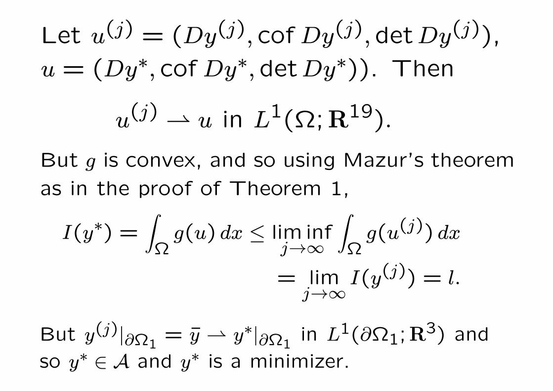
Let u(j) = (Dy(j), cof Dy(j),detDy(j)),
u = (Dy∗, cof Dy∗,detDy∗)). Then
u(j) u in L1(Ω;R19).
But g is convex, and so using Mazur’s theorem
as in the proof of Theorem 1,
I(y∗) =
Ωg(u) dx ≤ lim inf
j→∞
Ωg(u(j)) dx
= limj→∞
I(y(j)) = l.
But y(j)|∂Ω1= y y∗|∂Ω1
in L1(∂Ω1;R3) and
so y∗ ∈ A and y∗ is a minimizer.

Incompressible elasticity
Rubber is almost incompressible. Thus very
large forces, and a lot of energy, are required
to change its volume significantly. Such mate-
rials are well modelled by the constrained the-
ory of incompressible elasticity, in which the
deformation gradient is required to satisfy the
pointwise constraint
detF = 1.

Existence of minimizers in
incompressible elasticityTheorem 15
Let U = F ∈ M3×3 : detF = 1. Suppose
W : U → [0,∞) is continuous and such that
(H3)’ W(F ) ≥ c0(|F |2 + |cof F |32)− c1
for all F ∈ U ,
(H4)’ W is polyconvex, i.e. W (F ) = g(F, cof F )
for all F ∈ U for some continuous convex g.
Assume that there exists some y in
A = y ∈ W1,1(Ω;R3) : detDy(x) = 1 a.e., y|∂Ω1= y
with I(y) <∞, where H2(∂Ω1) > 0 and
y : ∂Ω1 → R3 is measurable. Then there exists
a global minimizer y∗ of I in A.

Proof.
For simplicity suppose that
W (F ) = g(F, cof F ) for some continuous con-
vex g : M3×3 ×M3×3 → R, where
g(F,H) ≥ c0(|F |p+ |H|q)−c1 for all F,H, where
p ≥ 2, q ≥ p′ and c0 > 0.
Letting y(j) be a minimizing sequence the only
new point is to show that the constraint is sat-
isfied. But since detDy(j) = 1 we have by the
weak continuity properties that for a subse-
quence detDy(j) ∗ detDy in L∞, so that the
weak limit satisfies detDy = 1.

Models of natural rubber
1. Modelled as an incompressible isotropic
material.
Constraint is detF = v1v2v3 = 1.
Neo-Hookean material
Φ = α(v21 + v2
2 + v23 − 3),
where α > 0 is a constant. This can be derived
from a simple statistical mechanics model of
long-chain molecules.

Mooney-Rivlin material.
Φ = α(v21 + v22 + v2
3 − 3)
+β((v2v3)2 + (v3v1)
2 + (v1v2)2 − 3),
where α > 0, β > 0 are constants. Gives a
better fit to bi-axial experiments of Rivlin &
Saunders.
Ogden materials.
Φ =N
i=1
αi(vpi1 + v
pi2 + v
pi3 − 3)
+M
i=1
βi((v2v3)qi + (v3v1)
qi + (v1v2)qi − 3),
where αi, βi, pi, qi are constants.

e.g. for a certain vulcanised rubber a good fit
is given by N = 2,M = 1, p1 = 5.0,
p2 = 1.3, q1 = 2, α1 = 2.4× 10⁻³, α2 = 4.8,
β1 = 0.05kg/cm2. The high power 5 allows a
better modelling of the tautening of rubber as
the long-chain molecules are highly stretched
and the cross-links tend to prevent further stretch-
ing.

2. Modelled as compressible isotropic material
Add h(v1v2v3) to above Φ, where h is convex,
h(δ) → ∞ as δ → 0+, and h has a steep mini-
mum near δ = 1.

Convexity properties of isotropic
functions
Let Rn+ = x = (x1, . . . , xn) ∈ Rn : xi ≥ 0.
Theorem 16 (Thompson & Freede)
Let n ≥ 1 and for F ∈Mn×n let
W (F ) = Φ(v1, . . . , vn),
where Φ is a symmetric real-valued function of
the singular values vi of F . Then W is convex
on Mn×n iff Φ is convex on Rn+ and nonde-
creasing in each vi.
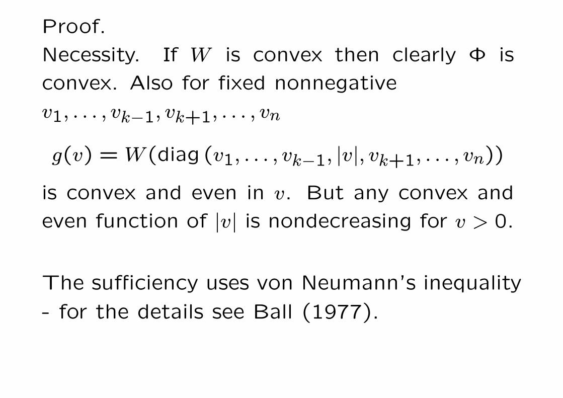
Proof.
Necessity. If W is convex then clearly Φ is
convex. Also for fixed nonnegative
v1, . . . , vk−1, vk+1, . . . , vn
g(v) = W (diag (v1, . . . , vk−1, |v|, vk+1, . . . , vn))
is convex and even in v. But any convex and
even function of |v| is nondecreasing for v > 0.
The sufficiency uses von Neumann’s inequality
- for the details see Ball (1977).

Lemma 2 (von Neumann)
Let A,B ∈Mn×n have singular values
v1(A) ≥ . . . ≥ vn(A), v1(B) ≥ . . . ≥ vn(B)
respectively. Then
maxQ,R∈O(n)
tr (QARB) =n
i=1
vi(A)vi(B).

Applying Theorem 16 we see that if p ≥ 1 then
Φp(F ) = vp1 + v
p2 + v
p3
is a convex function of F .
Since the singular values of cof F are
v2v3, v3v1, v1v2 it also follows that if q ≥ 1
Ψq(F ) = (v2v3)q + (v3v1)
q + (v1v2)q
is a convex function of cof F .

Hence the incompressible Ogden material
Φ =N
i=1
αi(vpi1 + v
pi2 + v
pi3 − 3)
+M
i=1
βi((v2v3)qi + (v3v1)
qi + (v1v2)qi − 3),
is polyconvex if the αi ≥ 0, βi ≥ 0,
p1 ≥ . . . ≥ pN ≥ 1, q1 ≥ . . . ≥ qM ≥ 1.
And in the compressible case if we add a con-
vex function h = h(detF ) of detF then under
the same conditions the stored-energy function
is polyconvex.

It remains to check the growth condition of
Theorems 14, 15, namely
W (F) ≥ c0(|F |2 + |cof F |3/2)− c1for all F ∈M3×3, where c0 > 0.
This holds for the Ogden materials provided
p1 ≥ 2, q1 ≥ 32 and α1 > 0, β1 > 0.
This includes the case of the Mooney-Rivlin
material, but not the neo-Hookean material.
In the incompressible case, Theorem 15 covers
the case of the stored-energy function
Φ = α(vp1 + v
p2 + v
p3 − 3)
if p ≥ 3.

For the neo-Hookean material (incompressible
or with h(detF ) added) it is not known if there
exists an energy minimizer in A, but it seems
unlikely because of the phenomenon of cavita-
tion.

In particular the stored-energy function
W(F ) = α(|F |2 − 3) + h(detF )
is not W1,2 quasiconvex (same definition but
with the test functions ϕ ∈ W1,20 instead of
W1,∞0 ).
To see this consider the radial deformation y :
B(0,1) → R3 given by
y(x) =r(R)
Rx,
where R = |x|.

Since yi = r(R)R xi it follows that
yi,α =r(R)
Rδiα +
r′ − r
R
R
xixα
R,
that is
Dy(x) =r
R1+
r′ − r
R
x
R⊗ x
R.
In particular
|Dy(x)|2 = r′2 + 2
r(R)
R
2
.

Set F = λ1 where λ > 0. Then
W (λ1) = 3α(λ2 − 1) + h(λ3).
On the other hand, if we choose
r3(R) = R3 + λ3 − 1,
then y(x) = λx for |x| = 1 and
detDy(x) = r′ r
R
2= 1.

Then
B(0,1)[α(|Dy(x)|2 − 3) + h(detDy(x))] dx
= 4π 1
0R2
α
R3 + λ3 − 1
R3
−43
+2
R3 + λ3 − 1
R3
23
− 3
+ h(1)
dR,
which is of order λ2 for large λ.
Hence
B(0,1)W (Dy(x)) dx <
B(0,1)W (λ1) dx
for large λ.

Since W1,2 quasiconvexity is necessary for weak
lower semicontinuity of I(y) in W1,2 this sug-
gests that the minimum is not attained. (For
a further argument suggesting this see
J.M. Ball, Progress and Puzzles in Nonlinear
Elasticity, Proceedings of course on Poly-, Quasi-
and Rank-One Convexity in Applied Mechan-
ics, CISM, Udine, 2010.

However there is an existence theory that cov-
ers the neo-Hookean and other cases of poly-
convex energies with slow growth, due to
M. Giaquinta, G. Modica and J. Soucek, Arch.
Rational Mech. Anal. 106 (1989), no. 2, 97-
159
using Cartesian currents. In the previous exam-
ple this would give as the minimizer y(x) = λx,
i.e. the function space setting does not allow
cavitation. A simpler proof of this result is in
S. Muller,Weak continuity of determinants and
nonlinear elasticity, C. R. Acad. Sci. Paris Ser.
I Math. 307 (1988), no. 9, 501-506.

The Euler-Lagrange equations
As we have seen the standard form of these
are formally obtained by computing
d
dτI(y+τϕ)|τ=0 =
d
dτ
ΩW (Dy+τDϕ) dx|t=0 = 0,
for smooth ϕ with ϕ|∂Ω1= 0.
Suppose that W ∈ C1(M3×3+ ). Can we show
that the minimizer y∗ in Theorem 14 satisfies
the weak form of the Euler-Lagrange equa-
tions?

This leads to the weak form
ΩDFW (Dy) ·Dϕdx = 0
for all smooth ϕ with ϕ|∂Ω1= 0.
As we have seen, the problem in deriving this
weak form is that |DW (Dy)| can be bigger than
W (Dy), and that we do not know if
detDy(x) ≥ µ > 0 a.e.
It is an open problem to give hypotheses un-
der which this or the above weak form can be
proved.

However, it turns out to be possible to de-
rive other weak forms of the Euler-Lagrange
equations by using variations involving compo-
sitions of maps.
We consider the following conditions that may
be satisfied by W :
(C1) |DFW (F )FT | ≤ K(W (F )+1) for all F ∈M3×3+ ,
where K > 0 is a constant, and
(C2) |FTDFW(F )| ≤ K(W (F )+1) for all F ∈M3×3+ ,
where K > 0 is a constant.

As usual, | · | denotes the Euclidean norm on
M3×3, for which the inequalities |F ·G| ≤ |F |·|G|and |FG| ≤ |F | · |G| hold. But of course the
conditions are independent of the norm used
up to a possible change in the constant K.
Proposition 4
Let W satisfy (C2). Then W satisfies (C1).

Proof
Since W is frame-indifferent the matrix DFW (F )FT
is symmetric (this is equivalent to the symme-
try of the Cauchy stress tensor
T = (detF )−1TR(F )FT). To prove this, note
that
d
dtW (exp(Kt)F )|t=0 = DFW (F ) · (KF ) = 0
for all skew K. Hence
|DFW (F)FT |2 = [DFW (F )FT ] · [F (DFW (F ))T ]
= [FTDFW (F)] · [FTDFW (F )]T
≤ |FTDFW (F )|2,from which the result follows.

Example
Let
W (F ) = (FTF )11 +1
detF.
Then W is frame-indifferent and satisfies (C1)
but not (C2).
Exercise: check this.
As before let
A = y ∈W1,1(Ω;R3) : y|∂Ω1= y.

We say that y is a W1,p local minimizer of
I(y) =
ΩW (Dy) dx
in A if I(y) <∞ and
I(z) ≥ I(y) for all z ∈ A
with z − y1,p sufficiently small.

Theorem 17
For some 1 ≤ p < ∞ let y ∈ A ∩W1,p(Ω;R3)
be a W1,p local minimizer of I in A.
(i) Let W satisfy (C1). Then
Ω[DFW (Dy)DyT ] ·Dϕ(y) dx = 0
for all ϕ ∈ C1(R3;R3) such that ϕ and Dϕ are
uniformly bounded and satisfy ϕ(y)|∂Ω1= 0 in
the sense of trace.
(ii) Let W satisfy (C2). Then
Ω[W (Dy)1−DyTDFW (Dy)] ·Dϕdx = 0
for all ϕ ∈ C10(Ω;R3).

We use the following simple lemma.
Lemma 3
(a) If W satisfies (C1) then there exists γ > 0
such that if C ∈M3×3+ and |C − 1| < γ then
|DFW (CF )FT | ≤ 3K(W (F ) + 1) for all F ∈M3×3+ .
(b) If W satisfies (C2) then there exists γ > 0
such that if C ∈M3×3+ and |C − 1| < γ then
|FTDFW (FC)| ≤ 3K(W (F ) + 1) for all F ∈M3×3+ .

Proof of Lemma 3
We prove (a); the proof of (b) is similar. We
first show that there exists γ > 0 such that if
|C − 1| < γ then
W (CF ) + 1 ≤ 3
2(W (F ) + 1) for all F ∈M3×3
+ .
For t ∈ [0,1] let C(t) = tC + (1− t)1. Choose
γ ∈ (0, 16K) sufficiently small so that |C−1| < γ
implies that |C(t)−1| ≤ 2 for all t ∈ [0,1].
This is possible since |1| =√
3 < 2.

For |C − 1| < γ we have that
W (CF )−W (F )
= 1
0
d
dtW (C(t)F ) dt
= 1
0DFW (C(t)F ) · [(C − 1)F ] dt
= 1
0DFW (C(t)F )(C(t)F )T · ((C − 1)C(t)−1) dt
≤ K 1
0[W (C(t)F ) + 1] · |C − 1| · |C(t)−1| dt
≤ 2Kγ 1
0(W (C(t)F) + 1) dt.

Let θ(F ) = sup|C−1|<γ W (CF ). Then
W (CF )−W (F ) ≤ θ(F )−W (F )
≤ 2Kγ(θ(F ) + 1).
Hence
(θ(F ) + 1)(1− 2Kγ) ≤W (F ) + 1,
from which
W (CF ) + 1 ≤ 3
2(W (F ) + 1)
follows.
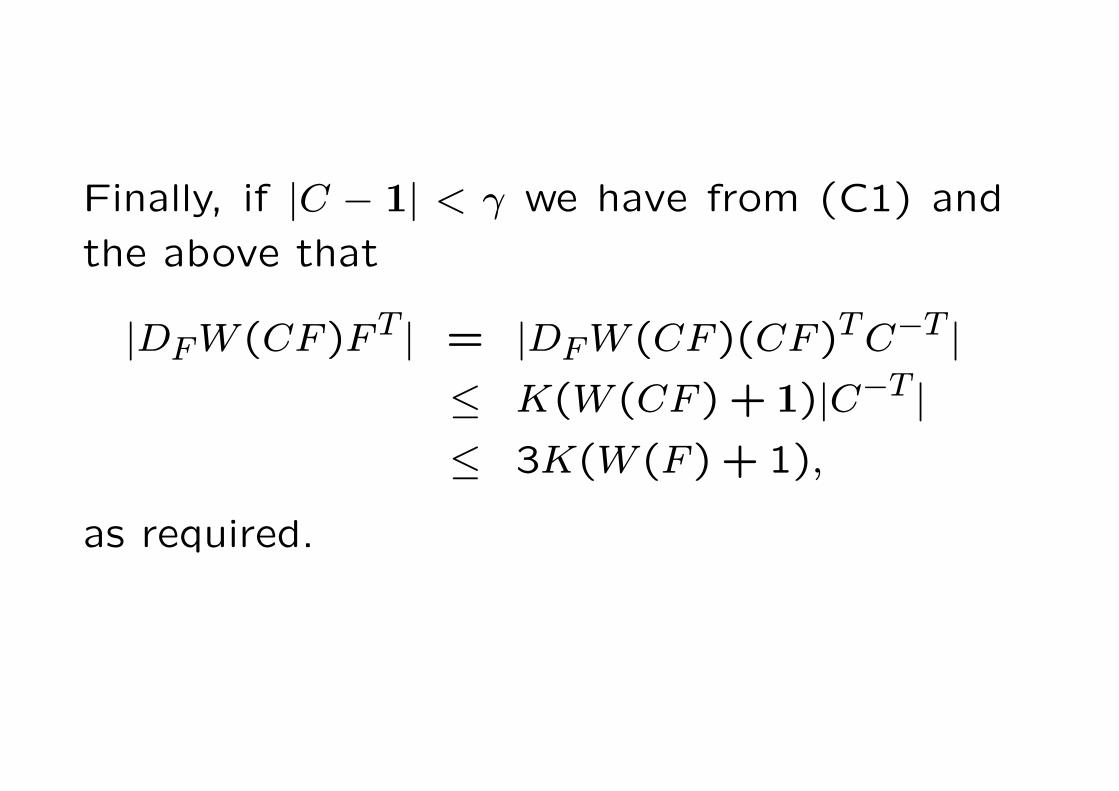
Finally, if |C − 1| < γ we have from (C1) and
the above that
|DFW (CF)FT | = |DFW (CF)(CF)TC−T |≤ K(W (CF ) + 1)|C−T |≤ 3K(W (F ) + 1),
as required.

Proof of Theorem 17
Given ϕ as in the theorem, define for |τ | suffi-
ciently small
yτ(x) := y(x) + τϕ(y(x)).
Then
Dyτ(x) = (1+ τDϕ(y(x)))Dy(x) a.e. x ∈ Ω.
and so yτ ∈ A. Also detDyτ(x) > 0 for a.e.
x ∈ Ω and limτ→0 yτ − yW1,p = 0.

Hence I(yτ) ≥ I(y) for |τ | sufficiently small.
But
1
τ(I(yτ)− I(y))
=1
τ
Ω
1
0
d
dsW ((1+ sτDϕ(y(x)))Dy(x)) ds dx
=
Ω
1
0DW ((1+ sτDϕ(y(x)))Dy(x))
· [Dϕ(y(x))Dy(x)] ds dx.
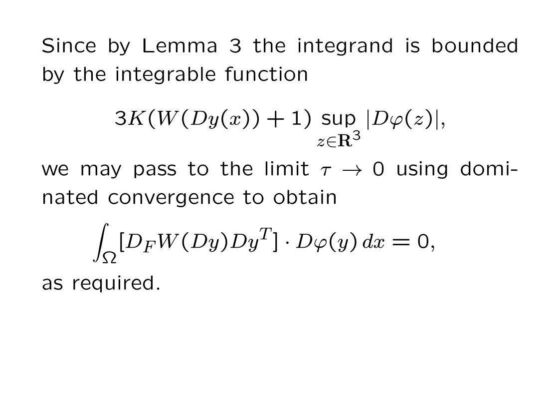
Since by Lemma 3 the integrand is bounded
by the integrable function
3K(W (Dy(x)) + 1) supz∈R3
|Dϕ(z)|,
we may pass to the limit τ → 0 using domi-
nated convergence to obtain
Ω[DFW (Dy)DyT ] ·Dϕ(y) dx = 0,
as required.

(ii) This follows in a similar way to (i) from
Lemma 3(b). We just sketch the idea. Let
ϕ ∈ C10(Ω;R3). For sufficiently small τ > 0 the
mapping θτ defined by
θτ(z) := z + τϕ(z)
belongs to C1(Ω;R3), satisfies detDθτ(z) > 0,
and coincides with the identity on ∂Ω. By the
global inverse function theorem θτ is a diffeo-
morphism of Ω to itself.

Thus the ‘inner variation’
yτ(x) := y(zτ), x = zτ + τϕ(zτ)
defines a mapping yτ ∈ A, and
Dyτ(x) = Dy(zτ)[1 + τDϕ(zτ)]−1 a.e. x ∈ Ω.
Since y ∈W1,p it follows easily that
yτ − yW1,p → 0 as τ → 0.
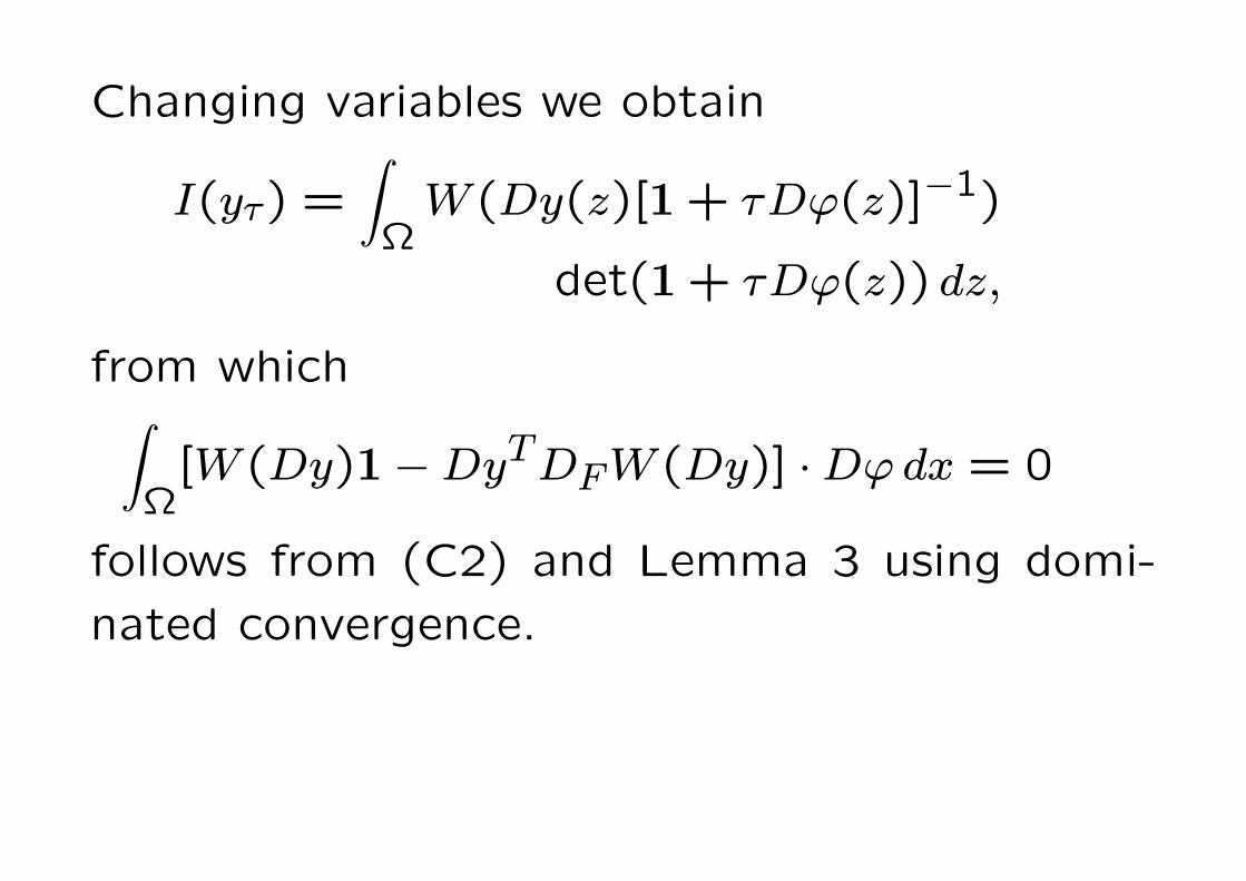
Changing variables we obtain
I(yτ) =
ΩW(Dy(z)[1+ τDϕ(z)]−1)
det(1+ τDϕ(z)) dz,
from which
Ω[W (Dy)1−DyTDFW (Dy)] ·Dϕdx = 0
follows from (C2) and Lemma 3 using domi-
nated convergence.

Interpretations of the weak forms
To interpret Theorem 17 (i), we make the fol-
lowing
Invertibility Hypothesis.
y is a homeomorphism of Ω onto Ω′ := y(Ω),
Ω′ is a bounded domain, and the change of
variables formula
Ωf(y(x)) detDy(x) dx =
Ω′ f(z) dz
holds whenever f : R3 → R is measurable, pro-
vided that one of the integrals exists.

Theorem 18
Assume that the hypotheses of Theorem 17
and the Invertibility Hypothesis hold. Then
Ω′ σ(z) ·Dϕ(z) dz = 0
for all ϕ ∈ C1(R3;R3) such that ϕ|y(∂Ω1)= 0,
where the Cauchy stress tensor σ is defined by
σ(z) := T (y−1(z)), z ∈ Ω′
and T (x) = (detDy(x))−1DFW (Dy(x))Dy(x)T .
Proof. Since by assumption y(Ω) is bounded,
we can assume that ϕ and Dϕ are uniformly
bounded. The result then follows straighfor-
wardly.

Thus Theorem 17 (i) asserts that y satisfies
the spatial (Eulerian) form of the equilibrium
equations. Theorem 17 (ii), on the other hand,
involves the so-called energy-momentum ten-
sor
E(F ) = W (F )1− FTDFW (F ),
and is a multi-dimensional version of the Du
Bois Reymond or Erdmann equation of the
one-dimensional calculus of variations, and is
the weak form of the equation
DivE(Dy) = 0.

The hypotheses (C1) and (C2) imply that W
has polynomial growth.
Proposition 4
Suppose W satisfies (C1) or (C2). Then for
some s > 0
W (F ) ≤M(|F |s + |F−1|s) for all F ∈M3×3+ .

Proof
Let V ∈M3×3 be symmetric. For t ≥ 0d
dtW (etV )
= |(DFW (etV )etV ) · V |
= |(etV DFW (etV )) · V |≤ K(W (etV ) + 1)|V |.
From this it follows that
W (eV ) + 1 ≤ (W (1) + 1)eK|V |.
Now set V = lnU, where U = UT > 0, and
denote by vi the eigenvalues of U .

Since
| lnU | = (3
i=1
(ln vi)2)1/2 ≤
3
i=1
| ln vi|,
it follows that
eK| lnU | ≤ (vK1 + v−K1 )(vK2 + v−K
2 )(vK3 + v−K3 )
≤ 3−3(3
i=1
vKi +3
i=1
v−Ki )3
≤ C(3
i=1
v3Ki +
3
i=1
v−3Ki )
≤ C1[|U |3K + |U−1|3K],
where C > 0, C1 > 0 are constants.

We thus obtain
W (U) ≤M(|U |3K + |U−1|3K),
where M = C1(W (1) + 1). The result now
follows from the polar decomposition F = RU
of an arbitrary F ∈ M3×3+ , where R ∈ SO(3),
U = UT > 0.

If W = Φ(v1, v2, v3) is isotropic then both (C1)
and (C2) are equivalent (Exercise) to the con-
dition that
|(v1Φ,1, v2Φ,2, v3Φ,3)| ≤ K(Φ(v1, v2, v3) + 1)
for all vi > 0 and some K > 0, where Φ,i =
∂Φ/∂vi.
Now for p ≥ 0, q ≥ 0
3
i=1
vi∂
∂vi(v
p1 + v
p2 + v
p3)
= p(vp1 + v
p2 + v
p3),
3
i=1
vi∂
∂vi((v2v3)
q + (v3v1)q + (v1v2)
q)
= 2q((v2v3)q + (v3v1)
q + (v1v2)q)

And
3
i=1
vi∂
∂vih(v1v2v3)
= 3v1v2v3|h′(v1v2v3)|.
Hence both (C1) and (C2) hold for compress-
ible Ogden materials if pi ≥ 0, qi ≥ 0, αi ≥0, βi ≥ 0, and h ≥ 0,
|δh′(δ)| ≤ K1(h(δ) + 1)
for all δ > 0.

Exercise.
Work out a corresponding treatment of weak
forms of the Euler-Lagrange equation in the
incompressible case.

Existence of minimizers with body and
surface forces
Mixed displacement-traction problems.
Suppose that ∂Ω = ∂Ω1 ∪ ∂Ω2, where
∂Ω1∩∂Ω2 = ∅. Consider the ‘dead load’ bound-
ary conditions:
y|∂Ω1= y
tR|∂Ω2= tR,
where tR(x) = DFW (Dy(x))N(x) is the Piola-
Kirchhoff stress vector, N(x) is the unit out-
ward normal to ∂Ω and tR ∈ L1(∂Ω2;R3).

Suppose the body force b is conservative, so
that
b(y) = −gradyΨ(y),
where Ψ = Ψ(y) is a real-valued potential.
The most important example is gravity, for
which b = −ρRe3, where e3 = (0,0,1), where
the density in the reference configuration ρR >
0 is constant. In this case we can take
Ψ(y) = −gy3.

Consider the functional
I(y) =
Ω[W (Dy) + Ψ(y)] dx−
∂Ω2
tR · y dA.
Then formally a local minimizer y satisfies
Ω[DFW (Dy)·Dϕ−b(y)·ϕ] dx−
∂Ω2
tR·ϕdA = 0
for all smooth ϕ with ϕ|∂Ω1= 0, and thus
DivDFW (Dy) + b = 0 in Ω,
tR|∂Ω2= tR.

Theorem 19
Suppose that W satisfies (H1) and
(H3) W (F ) ≥ c0(|F |2 + |cof F |3/2)− c1 for all
F ∈M3×3, where c0 > 0,
(H4) W is polyconvex, i.e. W (F ) = g(F, cof F,detF)
for all F ∈ M3×3 for some continuous convex
g. Assume further that Ψ is continuous and
such that
Ψ(y) ≥ −d0|y|s − d1
for constants d0 > 0, d1 > 0,1 ≤ s < 2, and
that tR ∈ L2(∂Ω2;R3).

Assume that there exists some y in
A = y ∈W1,1(Ω;R3) : y|∂Ω1= y
with I(y) <∞, where H2(∂Ω1) > 0 and
y : ∂Ω1 → R3 is measurable. Then there exists
a global minimizer y∗ of I in A.
Sketch of proof.
We need to get a bound on a minimizing se-
quence y(j). By the trace theorem there is a
constant c2 > 0 such that
Ω[|Dy|2 + |y|2] dx ≥ d0
∂Ω2
|y|2dA
for all y ∈W1,2.
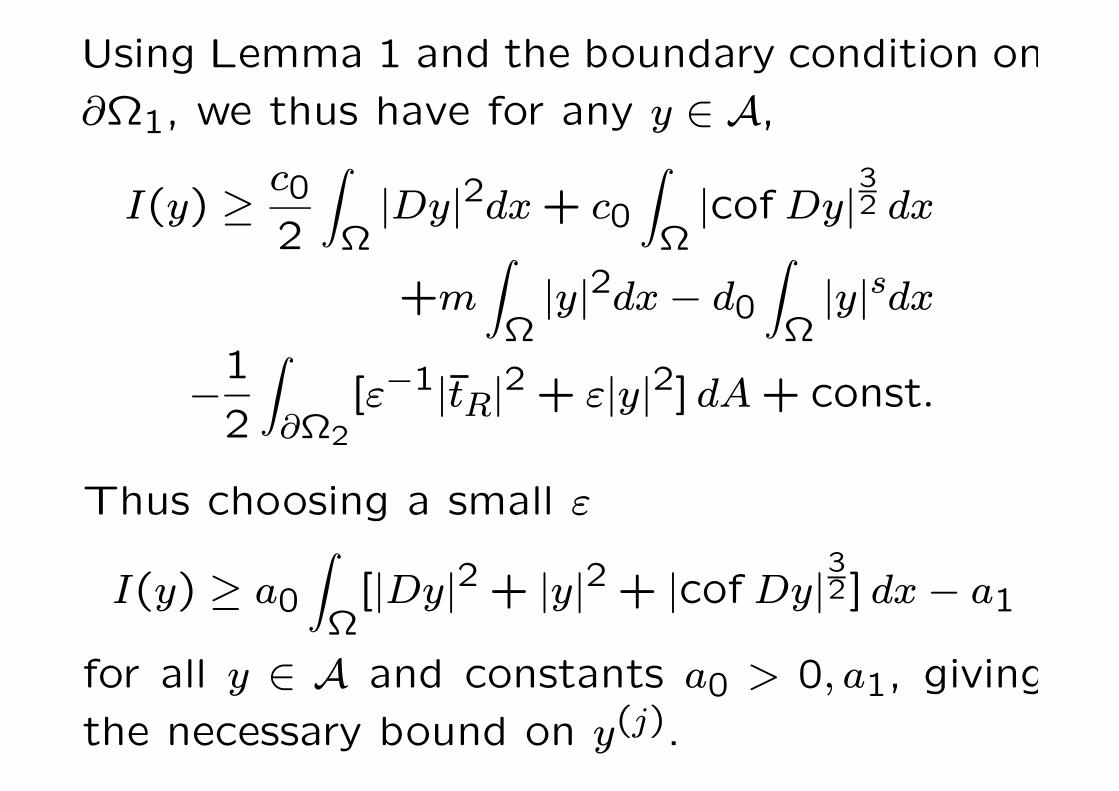
Using Lemma 1 and the boundary condition on
∂Ω1, we thus have for any y ∈ A,
I(y) ≥ c02
Ω|Dy|2dx + c0
Ω|cof Dy|
32 dx
+m
Ω|y|2dx− d0
Ω|y|sdx
−1
2
∂Ω2
[ε−1|tR|2 + ε|y|2] dA + const.
Thus choosing a small ε
I(y) ≥ a0
Ω[|Dy|2 + |y|2 + |cof Dy|
32] dx− a1
for all y ∈ A and constants a0 > 0, a1, giving
the necessary bound on y(j).

Pure traction problems.
Suppose ∂Ω1 = ∅ and that b = b0 is constant.
Then choosing ϕ = const. we find that a nec-
essary condition for a local minimum is that
Ωb0 dx +
∂Ω2
tRdA = 0,
saying that the total applied force on the body
is zero.
If this condition holds then I is invariant to
the addition of constants, and it is convenient
to remove this indeterminacy by minimizing I
subject to the constraint
Ωy dx = 0.

We then get the existence of a minimizer under
the same hypotheses as Theorem 19, but using
the Poincare inequality
Ω|y|2dx ≤ C
Ω|Dy|2dx +
Ωy dx
2
.
It is also possible to treat mixed displacement
pressure boundary conditions (see Ball 1977),
which are conservative.

Invertibility
Recall the Global Inverse Function Theorem,
that if Ω ⊂ Rn is a bounded domain with Lip-
schitz boundary ∂Ω and if y ∈ C1(Ω;Rn) with
detDy(x) > 0 for all x ∈ Ω
and y|∂Ω one-to-one, then y is invertible on Ω.
Can we prove a similar theorem for mappings
in a Sobolev space?

Before discussing this question let us note an
amusing example showing that failure of y to
be C1 at just two points of the boundary can
invalidate the theorem.
Rubber sheet
stuck to rigid
wires
Inner wire twisted
through π about
vertical axis
Yellow region
double covered
y

A. Weinstein, A global invertibility theorem for
manifolds with boundary, Proc. Royal Soc.
Edinburgh, 99 (1985) 283—284.
shows that a local homeomorphism from a com-
pact, connected manifold with boundary to a
simply connected manifold without boundary
is invertible if it is one-to-one on each compo-
nent of the boundary.

Results for y ∈W1,p, p > n,
(so that y is continuous).
J.M. Ball, Global invertibility of Sobolev func-
tions and the interpenetration of matter, Proc.
Royal Soc. Edinburgh 90a(1981)315-328.

Theorem 20
Let Ω ⊂ Rn be a bounded domain with Lip-
schitz boundary. Let y : Ω → Rn be contin-
uous in Ω and one-to-one in Ω. Let p > n
and let y ∈ W1,p(Ω;Rn) satisfy y|∂Ω = y|∂Ω,
detDy(x) > 0 a.e. in Ω. Then
(i) y(Ω) = y(Ω),
(ii) y maps measurable sets in Ω to measur-
able sets in y(Ω), and the change of variables
formula
Af(y(x)) detDy(x) dx =
y(A)f(v) dv

holds for any measurable A ⊂ Ω and any mea-
surable f : Rn → R, provided one of the inte-
grals exist,
(iii) y is one-to-one a.e., i.e. the set
S = v ∈ y(Ω) : y−1(v) contains more
than one elementhas measure zero,
(iv) if v ∈ y(Ω) then y−1(v) is a continuum
contained in Ω, while if v ∈ ∂y(Ω) then each
connected component of y−1(v) intersects ∂Ω.

y
vy−1(v)
v
y−1(v)
Note that y(Ω) is open by invariance of do-
main. Proof of theorem uses degree theory
and change of variables formula of Marcus and
Mizel. Examples with complicated inverse im-
ages y−1(v) can be constructed.

Theorem 21
Let the hypotheses of Theorem 20 hold, let
y(Ω) satisfy the cone condition, and suppose
that for some q > n
Ω|(Dy(x))−1|q detDy(x) dx <∞.
Then y is a homeomorphism of Ω onto y(Ω),
and the inverse function x(y) belongs to
W1,q(y(Ω);Rn). The matrix of weak deriva-
tives x(·) is given by
Dx(v) = Dy(x(v))−1 a.e. in y(Ω).
If further y(Ω) is Lipschitz then y is a homeo-
morphism of Ω onto y(Ω).

Note that formally we have
Ω|(Dy(x))−1|q detDy(x) dx
=
y(Ω)|Dx(v)|qdv.
Idea of proof.
Get the inverse as the limit of a sequence of
mollified mappings. Suppose x(·) is the in-
verse of y. Let ρε be a mollifier, i.e. ρε ≥ 0,
supp ρε ⊂⊂ B(0, ε),R
n ρε(v) dv = 1, and define
xε(v) =
y(Ω)ρε(v − u)x(u) du.

Changing variables we have
xε(v) =
Ωρε(v − y(z))z detDy(z) dz.
In this way the mollified inverse is expressible
directly in terms of y, and one can show that
for any smooth domain D ⊂⊂ y(Ω) we have
D|Dxε(v)|q dv ≤M <∞,
where M is independent of sufficiently small
ε. Then we can extract a weakly convergent
subsequence in W1,p(D;Rn) for every D, giving
a candidate inverse.

For the pure displacement boundary-value prob-
lem with boundary condition
y|∂Ω = y|∂Ωfor which the existence of minimizers was proved
in Theorem 14, we get that any minimizer is a
homeomorphism provided we strengthen (H3)
by assuming that
W (F ) ≥ c0(|F |p + |cofF |q + (detF )−s)− c1,
where p > 3, q > 3, s > 2qq−3, and that y satisfies
the hypotheses of Theorem 21.

With this assumption we have that for any
y ∈ A with I(y) <∞,
Ω|Dy(x)−1|σ detDy(x) dx
=
Ω|cofDy(x)|σ(detDy(x))1−σdx
≤ c
Ω(|cofDy|q + (detDy)(1−σ)( q
σ)′) dx
<∞,
where σ = q(1+s)q+s > 3, since (1− σ)
qσ
′= −s.

An interesting approach to the problem of in-
vertibility (i.e. non-interpenetration of matter)
in mixed boundary-value problems is given in
P.G. Ciarlet and J. Necas, Unilateral problems
in nonlinear three-dimensional elasticity, Arch.
Rational Mech. Anal., 87:(1985) 319—338.
They proposed minimizing
I(y) =
ΩW (Dy) dx
subject to the boundary condition y|∂Ω1= y
and the global constraint
ΩdetDy(x) dx ≤ volume (y(Ω)),

If y ∈ W1,p(Ω;R3) with p > 3 then a result of
Marcus & Mizel says that
ΩdetDy(x) dx =
y(Ω)card y−1(v) dv.
so that the constraint implies that y is one-to-
one almost everywhere.
They showed that IF the minimizer y∗ is suffi-
ciently smooth then this constraint corresponds
to smooth self-contact.
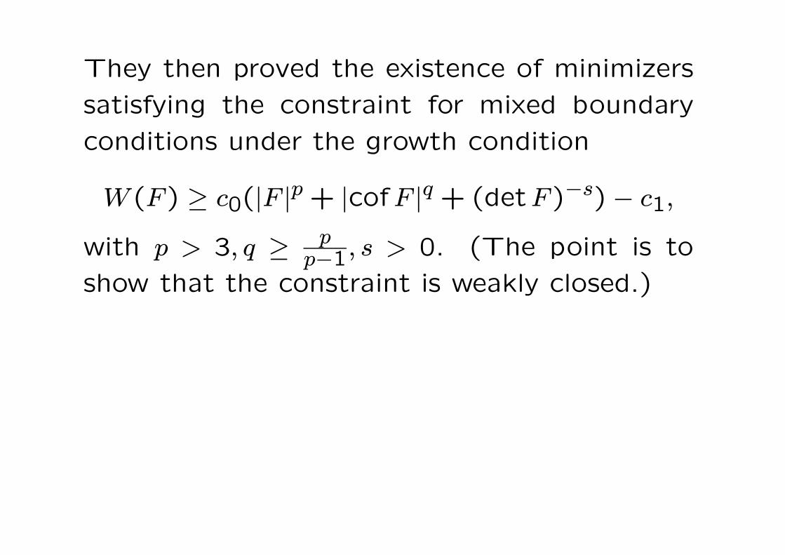
They then proved the existence of minimizers
satisfying the constraint for mixed boundary
conditions under the growth condition
W (F) ≥ c0(|F |p + |cofF |q + (detF )−s)− c1,
with p > 3, q ≥ pp−1, s > 0. (The point is to
show that the constraint is weakly closed.)

Results in the space
A+p,q(Ω) = y : Ω → R
n;Dy ∈ Lp(Ω;Mn×n),
cofDy ∈ Lq(Ω;Mn×n),detDy(x) > 0 a.e. in Ω,following V. Sverak, Regularity properties of
deformations with finite energy, Arch. Rat.
Mech. Anal. 100(1988)105-127.
For the results we are interested in Sverak as-
sumes p > n − 1, q ≥ pp−1, but Qi, Muller, Yan
show his results go through with p > n− 1, q ≥n
n−1, which we assume. Notice that then,since
(detF )1 = F (cofF )T , we have, taking deter-
minants, that |detF |n−1 ≤ |det cofF | ≤ |cofF |n,so that detDy ∈ L1(Ω).

In fact, if Dy ∈ Ln−1, cofDy ∈ Ln
n−1 then detDy
belongs to the Hardy space H1(Ω) (Iwaniec &
Onninen 2002).
If y ∈ A+p,q(Ω) with p > n− 1, q ≥ n
n−1 then it is
possible to define for every a ∈ Ω a set-valued
image F (a, y), and thus the image F (A) of a
subset A of Ω by
F (A) = ∪a∈AF (a, y).

Furthermore
Theorem 22
Assume p ≤ n.
(i) y has a representative y which is continuous
outside a singular set S of Hausdorff dimension
n− p.
(ii) Hn−1(F (a)) = 0 for all a ∈ Ω.
(iii) For each measurable A ⊂ Ω, F (A) is mea-
surable and
Ln(F (A)) ≤
AdetDy(x) dx.
In particular Ln(F (S)) = 0.

We suppose that Ω is C∞ and for simplicity
that y is a diffeomorphism of some open neigh-
bourhood Ω0 of Ω onto y(Ω0). Now suppose
that y ∈ A+p,q(Ω) with y|∂Ω = y|∂Ω.
Given v ∈ y(Ω), let
G(v) = x ∈ Ω : v ∈ F (x).
Thus G(v) consists of all inverse images of v.

Theorem 23
(i) For each v ∈ y(Ω) the set G(v) is a nonempty
continuum in Ω.
(ii) For each measurable A ⊂ y(Ω) the set
G(A) = ∪v∈AG(v) is measurable and
Ln(A) =
G(A)detDy(x) dx.
(iii) Let T = v ∈ y(Ω); diamG(v) > 0. Then
Hn−1(T ) = 0.
Thus we can define the inverse function x(v)
for all v ∈ T , and Sverak proves that
x(·) ∈ W1,1(y(Ω)).

Regularity of minimizers
Open Problem: Decide whether or not the
global minimizer y∗ in Theorem 14 is smooth.
Here smooth means C∞ in Ω, and C∞ up to
the boundary (except in the neighbourhood of
points x0 ∈ ∂Ω1 ∩ ∂Ω2 where singularities can
be expected).

Clearly additional hypotheses on W are needed
for this to be true. One might assume, for
example, that W : M3×3+ → R is C∞, and that
W is strictly polyconvex (i.e. that g is strictly
convex). Also for regularity up to the boundary
we would need to assume both smoothness of
the boundary (except perhaps at ∂Ω1 ∩ ∂Ω2)
and that y is smooth. The precise nature of
these extra hypotheses is to be determined.

The regularity is unsolved even in the sim-
plest special cases. In fact the only situa-
tion in which smoothness of y∗ seems to have
been proved is for the pure displacement prob-
lem with small boundary displacements from a
stress-free state. For this case Zhang (1991),
following work of Sivaloganathan, gave hypothe-
ses under which the smooth solution to the
equilibrium equations delivered by the implicit
function theorem was in fact the unique global
minimizer y∗ of I given by Theorem 14.

An even more ambitious target would be to
somehow classify possible singularities in mini-
mizers of I for generic stored-energy functions
W . If at the same time one could associate
with each such singularity a condition on W
that prevented it, one would also, by impos-
ing all such conditions simultaneously, possess
a set of hypotheses implying regularity.
It is possible to go a little way in this direction.

Jumps in the deformation gradient
N
Dy = A, x ·N > k
Dy = B, x ·N < k x ·N = k
y piecewise affine
A−B = a⊗N .
When can such a y with A = B be a weak
solution of the equilibrium equations?

Theorem 24
Suppose that W : M3×3+ → R has a local min-
imizer F0. Then every piecewise affine map y
as above is C1 (i.e. A = B) iff W is strictly
rank-one convex, i.e. the map
t →W (F + ta⊗N) is strictly convex for each
F ∈M3×3 and a ∈ R3, N ∈ R3.
J.M. Ball, Strict convexity, strong ellipticity,
and regularity in the calculus of variations. Proc.
Camb. Phil. Soc., 87(1980)501—513.
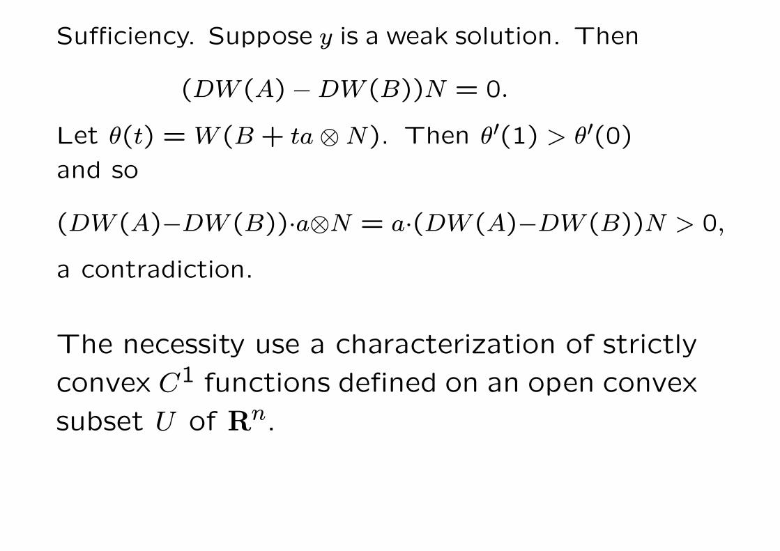
Sufficiency. Suppose y is a weak solution. Then
(DW (A)−DW (B))N = 0.
Let θ(t) = W (B + ta⊗N). Then θ′(1) > θ′(0)
and so
(DW(A)−DW (B))·a⊗N = a·(DW(A)−DW (B))N > 0,
a contradiction.
The necessity use a characterization of strictly
convex C1 functions defined on an open convex
subset U of Rn.

Theorem 25
A function ϕ ∈ C1(U) is strictly convex iff
(i) there exists some z ∈ U with
ϕ(w) ≥ ϕ(z) +∇ϕ(z) · (w − z)
for |w − z| sufficiently small, and
(ii) ∇ϕ is one-to-one.
The sufficiency follows by applying this to
ϕ(a) = W (B + a⊗N).
the assumption implying that ∇ϕ is one-to-
one.

Proof of Theorem 25 for the case when U =
Rn and ϕ(z)
|z| →∞ as |z| → ∞.
Let z ∈ Rn. Let w ∈ Rn minimize
h(v) = ϕ(v)−∇ϕ(z) · v.By the growth condition w exists and so
∇h(w) = ∇ϕ(w)−∇ϕ(z) = 0.
Hence w = z, the minimum is unique, and so
ϕ(v) > ϕ(z) +∇ϕ(z) · (v − z)
for all v = z, giving the strict convexity.

Discontinuities in y
An example is cavitation, which we know is
prevented (together with other discontinuities)
e.g. by
W (F) ≥ c0|F |n − c1.

Counterexamples to regularity


Quasiconvexity and partial regularity


In view of the above and other counterexam-
ples for elliptic systems, if minimizers are smooth
it must be for special reasons applying to elas-
ticity. Plausible such reasons are:
(a) the integrand depends only on Dy (and
perhaps x), and not y
(b) the dimensions m = n = 3 are low,
(c) the frame-indifference of W .
(d) invertibility of y.
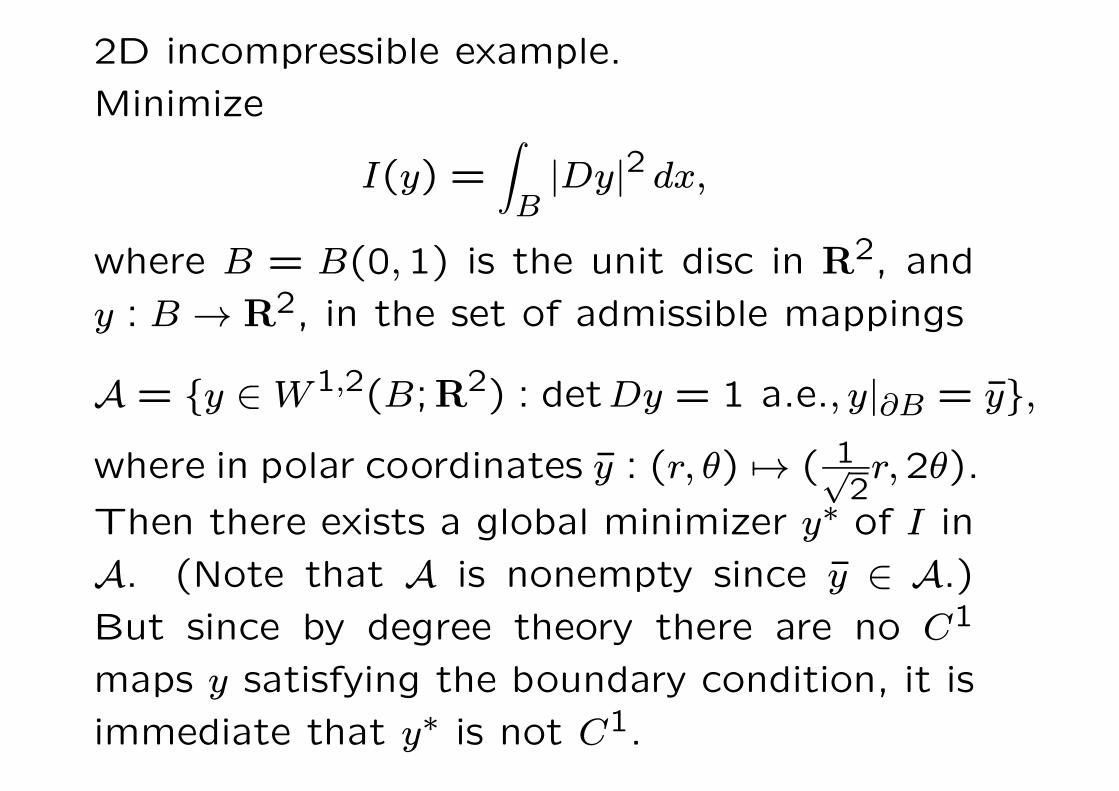
2D incompressible example.
Minimize
I(y) =
B|Dy|2 dx,
where B = B(0,1) is the unit disc in R2, and
y : B → R2, in the set of admissible mappings
A = y ∈W1,2(B;R2) : detDy = 1 a.e., y|∂B = y,where in polar coordinates y : (r, θ) → ( 1√
2r,2θ).
Then there exists a global minimizer y∗ of I in
A. (Note that A is nonempty since y ∈ A.)
But since by degree theory there are no C1
maps y satisfying the boundary condition, it is
immediate that y∗ is not C1.

Solid phase transformations
Displacive phase transformations are charac-
terized by a change of shape in the crystal lat-
tice at a critical temperature.
e.g. cubic → tetragonal

Energy minimization problem
for single crystal

Frame-indifference requires
ψ(RF, θ) = ψ(F, θ) for all R ∈ SO(3).
If the material has cubic symmetry then also
ψ(FQ, θ) = ψ(F, θ) for all Q ∈ P24,
where P24 is the group of rotations of a cube.

Energy-well structure
Assume
Assuming the austenite has cubic symmetry,
and given the transformation strain U1 say, the
N variants Ui are the distinct matrices QU1QT ,
where Q ∈ P24.
austenite
martensite
K(θ) = F ∈M3×3+ : F minimizes ψ(·, θ)

Cubic to tetragonal (e.g. Ni65Al35)
N = 3
U1 = diag (η2, η1, η1)
U2 = diag (η1, η2, η1)
U3 = diag (η1, η1, η2)

Exchange of
stability

Atomistically sharp interfaces for cubic
to tetragonal transformation in NiMn
Baele, van Tenderloo, Amelinckx

252
Macrotwins in Ni65Al35 involving two tetragonal
variants (Boullay/Schryvers)

253
Martensitic microstructures in CuAlNi (Chu/James)

There are no rank-one connections between
matrices A,B in the same energy well. In gen-
eral there is no rank-one connection between
A ∈ SO(3) and B ∈ SO(3)Ui.

Theorem 26
Let D = U2 − V 2 have eigenvalues λ1 ≤ λ2 ≤λ3. Then SO(3)U and SO(3)V are rank-one
connected iff λ2 = 0. There are exactly two
solutions up to rotation provided λ1 < λ2 =
0 < λ3, and the corresponding N ’s are orthog-
onal iff trU2 = trV 2, i.e. λ1 = −λ3.


257
Gradient Young measures
y(j) : Ω → Rm

The Young measure encodes the information
on weak limits of all continuous functions of
Dy(jk). Thus
f(Dy(jk))∗ #νx, f$.
In particular Dy(jk) ∗ νx = Dy(x).
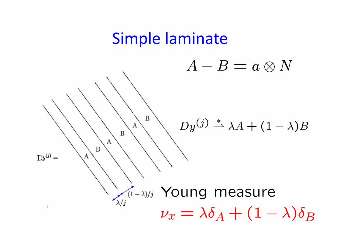
Simple laminate
A− B = a⊗N
Dy(j) ∗ λA + (1− λ)B
Young measure
νx = λδA + (1− λ)δB

260

(Classical) austenite-martensite interface in CuAlNi(C-H Chu and R.D. James)
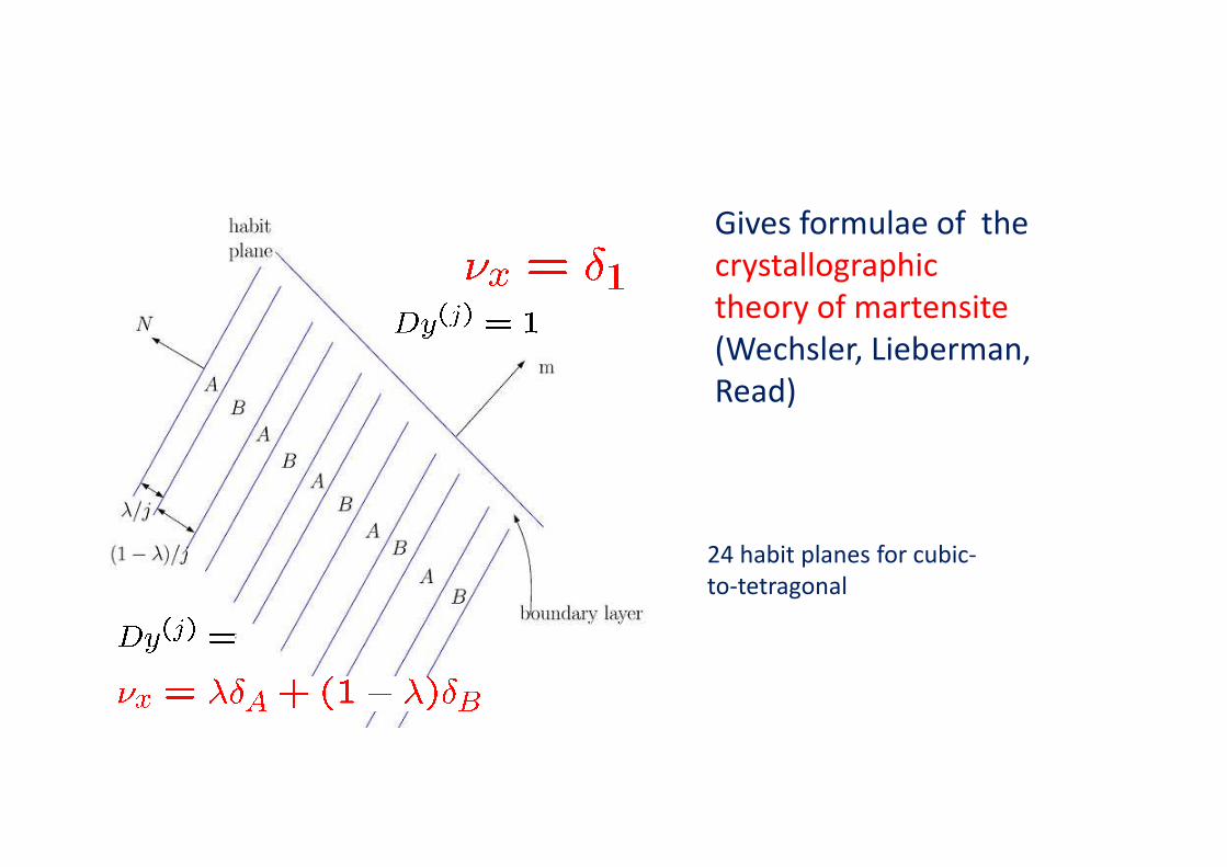
Gives formulae of the
crystallographic
theory of martensite
(Wechsler, Lieberman,
Read)
24 habit planes for cubic-
to-tetragonal

Rank-one connections for A/M interface

Possible lattice parameters
for classical austenite-martensite
interface.

265
Quasiconvexification

266

Nonattainment of minimum energy
Because of the rank-one connections between
energy wells, ψ is not rank-one convex, hence
not quasiconvex. Thus we expect that the
minimum energy is not in general attained. We
can prove this for the case of two martensitic
energy wells.

268
Two-well problem
Theorem 28 (Ball\James)
K(θ)qc consists of those F ∈M3×3+ such that
FTF =
a c 0c b 0
0 0 η21
,
where ab− c2 = η21η
22, a + b− |2c| ≤ η2
1 + η22.
If Dy(x) ∈ K(θ)qc a.e. then y is a plane strain.

269
Corollary 4 (Ball\ Carstensen)
Let F ∈ K(θ)qc with F ∈ K(θ). Then the min-
imum of Iθ(y) subject to y|∂Ω = Fx is not at-
tained.