
Mathematical Economics and Finance Applications of...
595
Stochastic Mechanics Random Media Signal Processing and Image Synthesis Mathematical Economics and Finance Stochastic Optimization Stochastic Control Stochastic Models in Life Sciences Stochastic Modelling and Applied Probability (Formerly: Applications of Mathematics) 67 Edited by B. Rozovski˘ ı P.W. Glynn Advisory Board M. Hairer I. Karatzas F.P. Kelly A. Kyprianou Y. Le Jan B. Øksendal G. Papanicolaou E. Pardoux E. Perkins H.M. Soner
Transcript of Mathematical Economics and Finance Applications of...

Stochastic Mechanics
Random Media
Signal Processing
and Image Synthesis
Mathematical Economics and Finance
Stochastic Optimization
Stochastic Control
Stochastic Models in Life Sciences
Stochastic Modellingand Applied Probability
(Formerly:Applications of Mathematics)
67Edited by B. Rozovskiı
P.W. Glynn
Advisory Board M. HairerI. KaratzasF.P. KellyA. KyprianouY. Le JanB. ØksendalG. PapanicolaouE. PardouxE. PerkinsH.M. Soner

Jean Jacod � Philip Protter
Discretizationof Processes

Jean JacodInstitut de MathématiquesUniversité Paris VI – Pierre et Marie CuriePlace Jussieu 4Paris Cedex, Paris [email protected]
Philip ProtterDepartment of StatisticsColumbia UniversityAmsterdam Av. 1255New York, NY [email protected]
Managing EditorsBoris RozovskiiDivision of Applied MathematicsBrown University182 George StProvidence, RI [email protected]
Peter W. GlynnInstitute of Computationaland Mathematical EngineeringStanford UniversityVia Ortega 475Stanford, CA [email protected]
ISSN 0172-4568 Stochastic Modelling and Applied ProbabilityISBN 978-3-642-24126-0 e-ISBN 978-3-642-24127-7DOI 10.1007/978-3-642-24127-7Springer Heidelberg Dordrecht London New York
Library of Congress Control Number: 2011941186
Mathematics Subject Classification (2010): 60F05, 60G44, 60H10, 60H35, 60J75, 60G51, 60G57,60H05, 60J65, 60J25
© Springer-Verlag Berlin Heidelberg 2012This work is subject to copyright. All rights are reserved, whether the whole or part of the material isconcerned, specifically the rights of translation, reprinting, reuse of illustrations, recitation, broadcasting,reproduction on microfilm or in any other way, and storage in data banks. Duplication of this publicationor parts thereof is permitted only under the provisions of the German Copyright Law of September 9,1965, in its current version, and permission for use must always be obtained from Springer. Violationsare liable to prosecution under the German Copyright Law.The use of general descriptive names, registered names, trademarks, etc. in this publication does notimply, even in the absence of a specific statement, that such names are exempt from the relevant protectivelaws and regulations and therefore free for general use.
Cover design: deblik
Printed on acid-free paper
Springer is part of Springer Science+Business Media (www.springer.com)

Preface
Two decades ago the authors of this book undertook the study of the errors onemakes when numerically approximating the solutions of stochastic differential equa-tions driven by Lévy processes. In particular we were interested in the normalizedasymptotic errors of approximations via an Euler scheme, and it turned out weneeded sophisticated laws of large numbers and central limit theorems that did notyet exist. While developing such tools, it became apparent that they would be usefulin a wide range of applications.
One usually explains the difference between probability and statistics as beingthat probability theory lays the basis for a family of models, and statistics uses datato infer which member or members of that family best fit the data. Often this re-duces to parameter estimation, and estimators are shown to be consistent via a Lawof Large Numbers (LLN), and the accuracy of an estimator is determined using aCentral Limit Theorem (CLT), when possible. The case of stochastic processes, andeven stochastic dynamical systems, is of course more difficult, since often one is nolonger estimating just a parameter, but rather one is estimating a stochastic process,or—worse—trying to tell which family of models actually does fit the data. Exam-ples include using data to determine whether or not a model governing a dynamicalsystem has continuous paths or has jumps, or trying to determine the dimension ofthe driving Brownian forces in a system of stochastic differential equations. Thissubject, broadly speaking, is a very old subject, especially as concerns asymptoticstudies when the time parameter tends to infinity. The novelty presented here in thisbook is a systematic study of the case where the time interval is fixed and compact(also known as the finite horizon case). Even in the finite horizon case however,efforts predate the authors’ study of numerical methods for stochastic differentialequations, and go back 5 years earlier to attempts to find the volatility coefficient ofan Itô process, via a fine analysis of its quadratic variation, by the first author jointwith Valentine Genon-Catalot. This in turn builds on the earlier work of G. Dohnal,which itself builds on earlier work; it is indeed an old yet still interesting subject.
There are different variations of LLNs and CLTs one might use to study suchquestions, and over the last two decades substantial progress has been made infinding such results, and also in applying them via data to delve further into the
v

vi Preface
unknown, and to reveal structures governing complicated stochastic systems. Themost common examples used in recent times are those of financial models, but theseideas can be used in models of biological, chemical, and electrical applications aswell. In this book we establish, in a systematic way, many of the recent results. Theensuing theorems are often complicated both to state, and especially to prove, andthe technical level of the book is (inevitably, it seems) quite demanding. This is atheory book, and we do not treat applications, although we do reference papers thatuse these kinds of results for applications, and we do indicate at the end of mostchapters how this theory can be used for applications.
An introduction explaining our approach, and an outline of how we have orga-nized the book, can be found in the Introductory Chapter 1. In addition, in Chap. 1we present several sketches of frameworks for potential applications of our theory,and indeed, these frameworks have inspired much of the development of the theorywe present in this book.
If one were to trace back how we came to be interested in this theory, the historywould have to center on the work and personality of Denis Talay and his “équipe”at INRIA in Sophia-Antipolis, as well as that of Jean Mémin at the University ofRennes. Both of these researchers influenced our taste in problems in enduring ways.We would also like to thank our many collaborators in this area over the years, witha special mention to Tom Kurtz, whose work with the second author started thiswhole enterprise in earnest, and also to Yacine Aït-Sahalia, who has provided awealth of motivations through applications to economics. We also wish to thankO.E. Barndorff-Nielsen, S. Delattre, J. Douglas, Jr., V. Genon-Catalot, S.E. Gra-versen, T. Hayashi, Yingying Li, Jin Ma, S. Méléard, P. Mykland, M. Podolskij,J. San Martin, N. Shephard, V. Todorov, S. Torres, M. Vetter, and N. Yoshida, aswell as A. Diop, for his careful reading of an earlier version of the manuscript.
The authors wish to thank Hadda and Diane for their forbearance and supportduring the several years involved in the writing of this book.
The second author wishes to thank the Fulbright Foundation for its support for aone semester visit to Paris, and the National Science Foundation, whose continualgrant support has made this trans-Atlantic collaboration possible.
Jean JacodPhilip Protter
Paris, FranceNew York, USA

Contents
Part I Introduction and Preliminary Material
1 Introduction . . . . . . . . . . . . . . . . . . . . . . . . . . . . . . . . 31.1 Content and Organization of the Book . . . . . . . . . . . . . . . 61.2 When X is a Brownian Motion . . . . . . . . . . . . . . . . . . . 9
1.2.1 The Normalized Functionals V ′n(f,X) . . . . . . . . . . . 91.2.2 The Non-normalized Functionals V n(f,X) . . . . . . . . . 12
1.3 When X is a Brownian Motion Plus Drift . . . . . . . . . . . . . . 141.3.1 The Normalized Functionals V ′n(f,X) . . . . . . . . . . . 141.3.2 The Non-normalized Functionals V n(f,X) . . . . . . . . . 15
1.4 When X is a Brownian Motion Plus Drift Plus a CompoundPoisson Process . . . . . . . . . . . . . . . . . . . . . . . . . . . 161.4.1 The Law of Large Numbers . . . . . . . . . . . . . . . . . 161.4.2 The Central Limit Theorem . . . . . . . . . . . . . . . . . 18
2 Some Prerequisites . . . . . . . . . . . . . . . . . . . . . . . . . . . . 232.1 Semimartingales . . . . . . . . . . . . . . . . . . . . . . . . . . . 23
2.1.1 First Decompositions and the Basic Propertiesof a Semimartingale . . . . . . . . . . . . . . . . . . . . . 24
2.1.2 Second Decomposition and Characteristicsof a Semimartingale . . . . . . . . . . . . . . . . . . . . . 29
2.1.3 A Fundamental Example: Lévy Processes . . . . . . . . . 332.1.4 Itô Semimartingales . . . . . . . . . . . . . . . . . . . . . 352.1.5 Some Estimates for Itô Semimartingales . . . . . . . . . . 392.1.6 Estimates for Bigger Filtrations . . . . . . . . . . . . . . . 442.1.7 The Lenglart Domination Property . . . . . . . . . . . . . 45
2.2 Limit Theorems . . . . . . . . . . . . . . . . . . . . . . . . . . . 452.2.1 Stable Convergence in Law . . . . . . . . . . . . . . . . . 462.2.2 Convergence for Processes . . . . . . . . . . . . . . . . . 482.2.3 Criteria for Convergence of Processes . . . . . . . . . . . . 502.2.4 Triangular Arrays: Asymptotic Negligibility . . . . . . . . 53
vii

viii Contents
2.2.5 Convergence in Law of Triangular Arrays . . . . . . . . . 56Bibliographical Notes . . . . . . . . . . . . . . . . . . . . . . . . 59
Part II The Basic Results
3 Laws of Large Numbers: The Basic Results . . . . . . . . . . . . . . 633.1 Discretization Schemes . . . . . . . . . . . . . . . . . . . . . . . 633.2 Semimartingales with p-Summable Jumps . . . . . . . . . . . . . 663.3 Law of Large Numbers Without Normalization . . . . . . . . . . . 69
3.3.1 The Results . . . . . . . . . . . . . . . . . . . . . . . . . 693.3.2 The Proofs . . . . . . . . . . . . . . . . . . . . . . . . . . 73
3.4 Law of Large Numbers with Normalization . . . . . . . . . . . . . 793.4.1 Preliminary Comments . . . . . . . . . . . . . . . . . . . 793.4.2 The Results . . . . . . . . . . . . . . . . . . . . . . . . . 803.4.3 The Proofs . . . . . . . . . . . . . . . . . . . . . . . . . . 83
3.5 Applications . . . . . . . . . . . . . . . . . . . . . . . . . . . . . 913.5.1 Estimation of the Volatility . . . . . . . . . . . . . . . . . 923.5.2 Detection of Jumps . . . . . . . . . . . . . . . . . . . . . 93Bibliographical Notes . . . . . . . . . . . . . . . . . . . . . . . . 96
4 Central Limit Theorems: Technical Tools . . . . . . . . . . . . . . . 974.1 Processes with F -Conditionally Independent Increments . . . . . . 97
4.1.1 The Continuous Case . . . . . . . . . . . . . . . . . . . . 984.1.2 The Discontinuous Case . . . . . . . . . . . . . . . . . . . 1004.1.3 The Mixed Case . . . . . . . . . . . . . . . . . . . . . . . 104
4.2 Stable Convergence Result in the Continuous Case . . . . . . . . . 1054.3 A Stable Convergence Result in the Discontinuous Case . . . . . . 1084.4 An Application to Itô Semimartingales . . . . . . . . . . . . . . . 114
4.4.1 The Localization Procedure . . . . . . . . . . . . . . . . . 1144.4.2 A Stable Convergence for Itô Semimartingales . . . . . . . 121
5 Central Limit Theorems: The Basic Results . . . . . . . . . . . . . . 1255.1 The Central Limit Theorem for Functionals Without Normalization 125
5.1.1 The Central Limit Theorem, Without Normalization . . . . 1265.1.2 Proof of the Central Limit Theorem, Without Normalization 129
5.2 The Central Limit Theorem for Normalized Functionals:Centering with Conditional Expectations . . . . . . . . . . . . . . 1335.2.1 Statement of the Results . . . . . . . . . . . . . . . . . . . 1345.2.2 The Proof . . . . . . . . . . . . . . . . . . . . . . . . . . 137
5.3 The Central Limit Theorem for the Processes V′n(f,X) . . . . . . 144
5.3.1 Assumptions and Results . . . . . . . . . . . . . . . . . . 1455.3.2 Localization and Elimination of Jumps . . . . . . . . . . . 1495.3.3 Proof of the Central Limit Theorem for V ′n(f,X) . . . . . 151
5.4 The Central Limit Theorem for Quadratic Variation . . . . . . . . 1605.5 A Joint Central Limit Theorem . . . . . . . . . . . . . . . . . . . 1735.6 Applications . . . . . . . . . . . . . . . . . . . . . . . . . . . . . 176
5.6.1 Estimation of the Volatility . . . . . . . . . . . . . . . . . 176

Contents ix
5.6.2 Detection of Jumps . . . . . . . . . . . . . . . . . . . . . 1795.6.3 Euler Schemes for Stochastic Differential Equations . . . . 179Bibliographical Notes . . . . . . . . . . . . . . . . . . . . . . . . 185
6 Integrated Discretization Error . . . . . . . . . . . . . . . . . . . . . 1876.1 Statements of the Results . . . . . . . . . . . . . . . . . . . . . . 1886.2 Preliminaries . . . . . . . . . . . . . . . . . . . . . . . . . . . . . 192
6.2.1 An Application of Itô’s Formula . . . . . . . . . . . . . . . 1936.2.2 Reduction of the Problem . . . . . . . . . . . . . . . . . . 196
6.3 Proof of the Theorems . . . . . . . . . . . . . . . . . . . . . . . . 2016.3.1 Proof of Theorem 6.1.2 . . . . . . . . . . . . . . . . . . . 2026.3.2 Proof of Theorem 6.1.3 . . . . . . . . . . . . . . . . . . . 2086.3.3 Proof of Theorem 6.1.4 . . . . . . . . . . . . . . . . . . . 2086.3.4 Proof of Theorem 6.1.8 . . . . . . . . . . . . . . . . . . . 210
Part III More Laws of Large Numbers
7 First Extension: Random Weights . . . . . . . . . . . . . . . . . . . . 2157.1 Introduction . . . . . . . . . . . . . . . . . . . . . . . . . . . . . 2157.2 The Laws of Large Numbers for V ′n(F,X) . . . . . . . . . . . . . 2177.3 The Laws of Large Numbers for V n(F,X) . . . . . . . . . . . . . 2197.4 Application to Some Parametric Statistical Problems . . . . . . . . 222
8 Second Extension: Functions of Several Increments . . . . . . . . . . 2278.1 Introduction . . . . . . . . . . . . . . . . . . . . . . . . . . . . . 2278.2 The Law of Large Numbers for V n(F,X) and Vn(F,X) . . . . . . 2308.3 The Law of Large Numbers for V n(Φ,kn,X) . . . . . . . . . . . 2348.4 The LLN for V ′n(F,X), V ′n(F,X) and V ′n(Φ, kn,X) . . . . . . . 238
8.4.1 The Results . . . . . . . . . . . . . . . . . . . . . . . . . 2388.4.2 The Proofs . . . . . . . . . . . . . . . . . . . . . . . . . . 239
8.5 Applications to Volatility . . . . . . . . . . . . . . . . . . . . . . 244
9 Third Extension: Truncated Functionals . . . . . . . . . . . . . . . . 2479.1 Approximation for Jumps . . . . . . . . . . . . . . . . . . . . . . 2489.2 Approximation for the Continuous Part of X . . . . . . . . . . . . 2509.3 Local Approximation for the Continuous Part of X: Part I . . . . . 2549.4 From Local Approximation to Global Approximation . . . . . . . 2619.5 Local Approximation for the Continuous Part of X: Part II . . . . . 2649.6 Applications to Volatility . . . . . . . . . . . . . . . . . . . . . . 269
Part IV Extensions of the Central Limit Theorems
10 The Central Limit Theorem for Random Weights . . . . . . . . . . . 27310.1 Functionals of Non-normalized Increments—Part I . . . . . . . . . 27310.2 Functionals of Non-normalized Increments—Part II . . . . . . . . 27810.3 Functionals of Normalized Increments . . . . . . . . . . . . . . . 28310.4 Application to Parametric Estimation . . . . . . . . . . . . . . . . 290
Bibliographical Notes . . . . . . . . . . . . . . . . . . . . . . . . 296
x Contents
11 The Central Limit Theorem for Functions of a Finite Numberof Increments . . . . . . . . . . . . . . . . . . . . . . . . . . . . . . . 29711.1 Functionals of Non-normalized Increments . . . . . . . . . . . . . 297
11.1.1 The Results . . . . . . . . . . . . . . . . . . . . . . . . . 29811.1.2 An Auxiliary Stable Convergence . . . . . . . . . . . . . . 30111.1.3 Proof of Theorem 11.1.2 . . . . . . . . . . . . . . . . . . . 304
11.2 Functionals of Normalized Increments . . . . . . . . . . . . . . . 31011.2.1 The Results . . . . . . . . . . . . . . . . . . . . . . . . . 31011.2.2 Elimination of Jumps . . . . . . . . . . . . . . . . . . . . 31411.2.3 Preliminaries for the Continuous Case . . . . . . . . . . . 31511.2.4 The Processes Yn and Yn . . . . . . . . . . . . . . . . . . 31711.2.5 Proof of Lemma 11.2.7 . . . . . . . . . . . . . . . . . . . 322
11.3 Joint Central Limit Theorems . . . . . . . . . . . . . . . . . . . . 32511.4 Applications . . . . . . . . . . . . . . . . . . . . . . . . . . . . . 329
11.4.1 Multipower Variations and Volatility . . . . . . . . . . . . 32911.4.2 Sums of Powers of Jumps . . . . . . . . . . . . . . . . . . 33011.4.3 Detection of Jumps . . . . . . . . . . . . . . . . . . . . . 332Bibliographical Notes . . . . . . . . . . . . . . . . . . . . . . . . 337
12 The Central Limit Theorem for Functions of an Increasing Numberof Increments . . . . . . . . . . . . . . . . . . . . . . . . . . . . . . . 33912.1 Functionals of Non-normalized Increments . . . . . . . . . . . . . 340
12.1.1 The Results . . . . . . . . . . . . . . . . . . . . . . . . . 34012.1.2 An Auxiliary Stable Convergence Result . . . . . . . . . . 34412.1.3 Proof of Theorem 12.1.2 . . . . . . . . . . . . . . . . . . . 352
12.2 Functionals of Normalized Increments . . . . . . . . . . . . . . . 35512.2.1 The Results . . . . . . . . . . . . . . . . . . . . . . . . . 35612.2.2 Preliminaries for the Proof . . . . . . . . . . . . . . . . . . 35812.2.3 Proof of Lemma 12.2.4 . . . . . . . . . . . . . . . . . . . 36012.2.4 Block Splitting . . . . . . . . . . . . . . . . . . . . . . . . 36412.2.5 Proof of Lemma 12.2.3 . . . . . . . . . . . . . . . . . . . 367
13 The Central Limit Theorem for Truncated Functionals . . . . . . . . 37113.1 A Central Limit Theorem for Approximating the Jumps . . . . . . 37113.2 Central Limit Theorem for Approximating the Continuous Part . . 377
13.2.1 The Results . . . . . . . . . . . . . . . . . . . . . . . . . 37813.2.2 Proofs . . . . . . . . . . . . . . . . . . . . . . . . . . . . 384
13.3 Central Limit Theorem for the Local Approximationof the Continuous Part of X . . . . . . . . . . . . . . . . . . . . . 38813.3.1 Statements of Results . . . . . . . . . . . . . . . . . . . . 38913.3.2 Elimination of the Jumps and of the Truncation . . . . . . . 39613.3.3 The Scheme of the Proof in the Continuous Case . . . . . . 40013.3.4 Proof of Lemma 13.3.12 . . . . . . . . . . . . . . . . . . . 40113.3.5 Proof of Lemma 13.3.13 . . . . . . . . . . . . . . . . . . . 40413.3.6 Proof of Theorem 13.3.8 . . . . . . . . . . . . . . . . . . . 409
13.4 Another Central Limit Theorem Using Approximationsof the Spot Volatility . . . . . . . . . . . . . . . . . . . . . . . . . 410

Contents xi
13.4.1 Statements of Results . . . . . . . . . . . . . . . . . . . . 41113.4.2 Proofs . . . . . . . . . . . . . . . . . . . . . . . . . . . . 414
13.5 Application to Volatility . . . . . . . . . . . . . . . . . . . . . . . 422Bibliographical Notes . . . . . . . . . . . . . . . . . . . . . . . . 426
Part V Various Extensions
14 Irregular Discretization Schemes . . . . . . . . . . . . . . . . . . . . 42914.1 Restricted Discretization Schemes . . . . . . . . . . . . . . . . . . 43014.2 Law of Large Numbers for Normalized Functionals . . . . . . . . 43714.3 Central Limit Theorem for Normalized Functionals . . . . . . . . 444
14.3.1 The Results . . . . . . . . . . . . . . . . . . . . . . . . . 44414.3.2 Preliminaries . . . . . . . . . . . . . . . . . . . . . . . . . 44714.3.3 The Scheme of the Proof when X is Continuous . . . . . . 45014.3.4 Proof of Lemma 14.3.4 . . . . . . . . . . . . . . . . . . . 45114.3.5 Proof of Lemma 14.3.5 . . . . . . . . . . . . . . . . . . . 453
14.4 Application to Volatility . . . . . . . . . . . . . . . . . . . . . . . 458Bibliographical Notes . . . . . . . . . . . . . . . . . . . . . . . . 460
15 Higher Order Limit Theorems . . . . . . . . . . . . . . . . . . . . . 46115.1 Examples of Degenerate Situations . . . . . . . . . . . . . . . . . 46215.2 Functionals of Non-normalized Increments . . . . . . . . . . . . . 46415.3 Applications . . . . . . . . . . . . . . . . . . . . . . . . . . . . . 474
Bibliographical Notes . . . . . . . . . . . . . . . . . . . . . . . . 477
16 Semimartingales Contaminated by Noise . . . . . . . . . . . . . . . . 47916.1 Structure of the Noise and the Pre-averaging Scheme . . . . . . . . 480
16.1.1 Structure of the Noise . . . . . . . . . . . . . . . . . . . . 48016.1.2 The Pre-averaging Scheme . . . . . . . . . . . . . . . . . 482
16.2 Law of Large Numbers for General (Noisy) Semimartingales . . . 48516.3 Central Limit Theorem for Functionals of Non-normalized
Increments . . . . . . . . . . . . . . . . . . . . . . . . . . . . . . 48816.3.1 The Results . . . . . . . . . . . . . . . . . . . . . . . . . 48916.3.2 A Local Stable Convergence Result . . . . . . . . . . . . . 49216.3.3 A Global Stable Convergence Result . . . . . . . . . . . . 50316.3.4 Proof of Theorem 16.3.1 . . . . . . . . . . . . . . . . . . . 510
16.4 Laws of Large Numbers for Normalized Functionalsand Truncated Functionals . . . . . . . . . . . . . . . . . . . . . . 51216.4.1 Statement of Results . . . . . . . . . . . . . . . . . . . . . 51216.4.2 The Proofs . . . . . . . . . . . . . . . . . . . . . . . . . . 514
16.5 Laws of Large Numbers and Central Limit Theorems for IntegralPower Functionals . . . . . . . . . . . . . . . . . . . . . . . . . . 52116.5.1 The Laws of Large Numbers . . . . . . . . . . . . . . . . 52116.5.2 Central Limit Theorems: The Results . . . . . . . . . . . . 53016.5.3 Some Estimates . . . . . . . . . . . . . . . . . . . . . . . 53516.5.4 Proof of Theorem 16.5.7 . . . . . . . . . . . . . . . . . . . 546
16.6 The Quadratic Variation . . . . . . . . . . . . . . . . . . . . . . . 554Bibliographical Notes . . . . . . . . . . . . . . . . . . . . . . . . 563

xii Contents
Appendix . . . . . . . . . . . . . . . . . . . . . . . . . . . . . . . . . . . . 565A.1 Estimates for Itô Semimartingales . . . . . . . . . . . . . . . . . . 565A.2 Convergence of Processes . . . . . . . . . . . . . . . . . . . . . . 572A.3 Triangular Arrays . . . . . . . . . . . . . . . . . . . . . . . . . . 577A.4 Processes of Finite Variation . . . . . . . . . . . . . . . . . . . . . 579A.5 Some Results on Lévy Processes . . . . . . . . . . . . . . . . . . 581
Assumptions on the Process X . . . . . . . . . . . . . . . . . . . . . . . . 583
References . . . . . . . . . . . . . . . . . . . . . . . . . . . . . . . . . . . 585
Index of Functionals . . . . . . . . . . . . . . . . . . . . . . . . . . . . . . 589
Index . . . . . . . . . . . . . . . . . . . . . . . . . . . . . . . . . . . . . . 593

Basic Notation
R = the set of real numbers, R+ = [0,∞)Q = the set of rational numbers, Q+ =Q∩R+N = the set {0,1, . . . } of natural integers, N∗ = {1,2, . . . }Z = the set of relative integersRd = the Euclidean d-dimensional space;
the components of x ∈Rd are (x1, . . . , xd)
Rd = the Borel σ -field of Rd , R=R1
M+d×d = the set of nonnegative symmetric d × d matrices
M++d×d = the set of nonnegative symmetric invertible d × d matrices
|x| = the absolute value of x ∈R, ‖x‖ = Euclidean norm of x ∈Rd
d(x,B) = the distance between a point x and a subset B , in a metric spacey∗ = the transpose of the vector or matrix y[x] = the integer part of x ∈R (biggest n ∈ Z such that n≤ x)a ∨ b = sup(a, b), a ∧ b= inf(a, b), if a, b ∈R
x+ = x ∨ 0, x− = (−x)∨ 0, if x ∈R
1A = the indicator function of the set AAc = the complement of the set Aεa = the Dirac measure sitting at point aδij = the Kronecker symbol, equal to 1 if i = j and to 0 otherwise
Notation for convergences:a.s.−→ a.s. (almost sure) convergence for random variablesP−→ convergence in probability for random variablesL−→ convergence in law for random variablesL-s−→ stable convergence in law for random variablesa.s.=⇒ a.s. convergence for processes, for Skorokhod’s topologyP=⇒ convergence in probability for processes, for Skorokhod’s topology
u.c.p.=⇒ convergence in probability for processes, for the local uniform topology
xiii

xiv Basic Notation
L=⇒ convergence in law for processes, for Skorokhod’s topologyL-s=⇒ stable convergence in law for processes, for Skorokhod’s topology
Miscellaneous:f (x)= o(g(x)) as x→ x0 if f (x)/g(x)→ 0 as x→ x0f (x)=O(g(x)) as x→ x0 if lim supx→x0
|f (x)/g(x)|<∞càdlàg = “right-continuous with left limits”càglàd = “left-continuous with right limits”un vn means that both sequences un/vn and vn/un are bounded

Part IIntroduction and Preliminary Material
This introductory part contains two chapters. The first one is a detailed introduction:the whole book is devoted to many variations around two basic theorems, undervarious conditions and with various degrees of generality, and we explain how itcan be used by a reader interested in a specific result or a special topic. The firstchapter also contains (without proofs) a simplified version of the two basic theoremsin three very special cases, when the underlying process is a Brownian motion,or a Brownian motion plus a drift, or when it is a Brownian motion plus a driftand a Poisson process: this part could be skipped, but its aim is to give a flavor ofthe subsequent material, without complicated assumptions or notation or technicaldetails.
The second chapter mainly is a record of known facts about semimartingales andlimit theorems. By “known” we mean that they can be found in a number of books.Some of these facts are elementary, others are more sophisticated, but it would taketoo much space and be outside the scope of this book to present the proofs. A fewproperties in this chapter are new, at least in a book form, and their proofs are givenin the Appendix.

Chapter 1Introduction
Discretization of stochastic processes indexed by the interval [0, T ] or by the half-line [0,∞) occurs very often. Historically it has been first used to deduce results oncontinuous-time processes from similar and often simpler results for discrete-timeprocesses: for example Markov processes may be considered as limits of Markovchains, which are much simpler to analyze; or, stable processes as limits of randomwalks. This also applies to the theory of stochastic integration: the first constructionsof stochastic integrals, by N. Wiener and K. Itô, were based on a Riemann-typeapproximation, which is a kind of discretization in time. More recently but stillquite old, and a kind of archetype of what is done in this book, is the approximationof the quadratic variation process of a semimartingale by the approximate quadraticvariation process: this result, due to P.A. Meyer [76] in its utmost generality, turnsout to be one of the most useful results for applications.
Discretization of processes has become an increasingly popular tool in practicalapplications, for mainly (but not only) two reasons: one is the overwhelming exten-sion of Monte-Carlo methods, which serve to compute numerically the expectationsof a wide range of random variables which are often very complicated functionsof a stochastic process: this is made available by the increasing power of comput-ers. The second reason is related to statistics: although any stochastic process canonly be observed at finitely many times, with modern techniques the frequency ofobservations increases steadily: in finance for example one observes and recordsprices every second, or even more frequently; in biology one measures electrical orchemical activity at an even higher frequency.
Let us be more specific, by describing a simple but fundamental example of someof the problems at hand. Suppose that we have a one-dimensional diffusion processX of the form
dXt = a(Xt ) dt + σ(Xt ) dWt , X0 = x0. (1.0.1)
Here the initial value x0 ∈ R is given, and W denotes a Brownian motion definedon some probability space, about which we do not care in this introduction. Thedrift and diffusion coefficients a and σ are nice enough, so the above equation hasa unique solution.
J. Jacod, P. Protter, Discretization of Processes,Stochastic Modelling and Applied Probability 67,DOI 10.1007/978-3-642-24127-7_1, © Springer-Verlag Berlin Heidelberg 2012
3

4 1 Introduction
Problem 1) We know a and σ , and we are interested in the law of the variable X1.This law is usually not explicitly known, so to compute it, that is to compute theexpected value E(f (X1)) for various test functions f , one may use a Monte-Carlotechnique (other techniques based on PDEs are also available, especially in the one-dimensional case, but do not work so well in high dimensions). To implement thiswe simulate on a computer a number N of independent variables X(j)1 having thelaw of X1, and an approximation of E(f (X1)) is
ZN = 1
N
N∑
j=1
f(X(j)1
). (1.0.2)
Indeed, by the law of large numbers the sequence ZN converges almost surely toE(f (X1)) as N→∞, and moreover the central limit theorem tells us that, when fis for example bounded, the error made in replacing E(f (X1)) by ZN is of order1/√N .
This presumes that one knows how to simulate X1, which is about as scarceas the cases when E(f (X1)) can be explicitly computed. (More accurately somerecent techniques due to A. Beskos, O. Papaspiliopoulos and G.O. Roberts, see [16]and [17] for example, allow to simulate X1 exactly, but they require that σ doesnot vanish and, more important, that the dimension is 1; moreover, in contrast towhat follows, they cannot be extended to equations driven by processes other thana Brownian motion.) Hence we have to rely on approximations, and the simplestway for this is to use an Euler scheme. That is, for any integer n≥ 1 we recursivelydefine the approximation Xni/n for i = 1, . . . , n, by setting
Xn0 = x0, Xni/n =Xn(i−1)/n +1
na(Xn(i−1)/n
)+ σ (Xn(i−1)/n
)(Wi/n −W(i−1)/n),
the increments of the Brownian motion being easily simulated. Other, more sophis-ticated, schemes can be used, but they all rely upon the same basic ideas.
Then in (1.0.2) we substitute theX(j)1’s withN independent copies of the simu-lated variables Xn1 , giving rise to an average ZnN which now converges to E(f (Xn1 ))
for each given n. Therefore we need to assert how close E(f (Xn1 )) and E(f (X1))
are, and this more or less amounts to estimating the difference (X1 −Xn1 )2. Somecalculations show that this boils down to evaluating the difference
n∑
i=1
gn(ω, (i − 1)/n
)((Wi/n −W(i−1)/n)
2 − 1
n
)
for suitable functions gn(ω, t), where ω �→ gn(ω, t) is measurable with respect tothe σ -field FWt of the past ofW before time t . That is, we have to determine the be-havior of “functionals” of the increments ofW of the form above: do they convergewhen n→∞? And if so, what is the rate of convergence?
Problem 2) The setting is the same, that is we know a and σ , but we want to find thelaw of Y = ∫ 1
0 h(Xs) ds for some known function h. Again, one can use a Monte-
1 Introduction 5
Carlo technique, coupled with a preliminary Euler method: we set
Yn = 1
n
n∑
i=1
h(Xni/n),
where Xn is the Euler approximation introduced above. We can then simulate Nindependent versions Yn(1), . . . , Y n(N) of the variable Yn above, and
1
N
N∑
j=1
h(Yn(j))
is our approximation of E(h(Y )). IfXn is a good approximation ofX, then certainlyYn is a good approximation of 1
n
∑ni=1 h(Xi/n), provided h satisfies some suitable
smoothness assumptions. However we have an additional problem here, namely toevaluate the difference
1
n
n∑
i=1
h(Xi/n)−∫ 1
0h(Xs) ds.
The convergence to 0 of this difference is ensured by Riemann approximation, butthe rate at which it takes place is not clear, in view of the fact that the paths of X arenot smooth, albeit continuous. This is another discretization problem.
Problem 3) Suppose now that the functions a and σ are known, but depend on an ad-ditional parameter, say θ , so we have a = a(x, θ) and σ = σ(x, θ). We observe theprocessX =Xθ , which now depends on θ , over [0,1], and we want to infer θ . How-ever, in any realistic situation we cannot really observe the whole path t �→ Xt(ω)
for t ∈ [0,1], and we simply have “discrete” observations, say at times 0, 1n, . . . , n
n,
so we have n+ 1 observations.We are here in the classical setting of a parametric statistical problem. For any
given n there is no way exactly to infer θ , unless a and σ have a very special form.But we may hope for good asymptotic estimators as n→∞. All estimation meth-ods, and there are many, are based on the behavior of functionals of the form
n∑
i=1
fn(θ,ω, (i − 1)/n,Xi/n −X(i−1)/n
)(1.0.3)
for suitable functions fn(θ,ω, t, x), where again ω �→ fn(θ,ω, t, x) is FWt measur-able. The consistency of the estimators is deduced from the convergence of func-tionals as above, and rates of convergence are deduced from associated central limittheorems for those functionals.
Problem 4) Here the functions a and σ are unknown, and they may additionallydepend on (ω, t), as for example σ = σ(ω, t, x). We observe X at the same discrete

6 1 Introduction
times 0, 1n, . . . , n
nas above. We want to infer some knowledge about the coefficients
a and σ . As is well known, we usually can say nothing about a in this setting, butthe convergence of the approximate quadratic variation mentioned before says that:
[nt]∑
i=1
(Xi/n −X(i−1)/n)2 →
∫ t
0σ(Xs)
2 ds
(convergence in probability, for each t ; here, [nt] denotes the integer part of thereal nt). This allows us in principle to determine asymptotically the functiont �→ σ(ω, t,Xt (ω)) on [0,1], and under suitable assumptions we even have ratesof convergence. Here again, everything hinges upon functionals as in the left sideabove. Note that here we have a statistical problem similar to Problem 3, except thatwe do not want to infer a parameter θ but a quantity which is fundamentally ran-dom: this occurs for example in finance, for the estimation of the so-called stochasticvolatility.
Problem 5) A more basic problem is perhaps the following one, which deals directlywith discretized processes. Namely, let us call an n-discretized process of X theprocess defined byX(n)t =X[nt]/n. Then of courseX(n)→X pointwise in ω, locallyuniformly in time when X is continuous and for the Skorokhod topology when X isright-continuous and with left limits. But, what is the rate of convergence?
The common feature of all the problems described above, as different as they mayappear, is the need to consider the asymptotic behavior of functionals like (1.0.3).And, when the process X is discontinuous, many other problems about the jumpscan also be solved by using functionals of the same type.
1.1 Content and Organization of the Book
In the whole book we consider a basic underlying d-dimensional process X, al-ways a semimartingale. This process is sampled at discrete times, most of the timeregularly spaced: that is, we have a mesh Δn > 0 and we consider the increments
Δni X = XiΔn −X(i−1)Δn
and two types of functionals, where f is a function on Rd :
V n(f,X)t =[t/Δn]∑
i=1
f(Δni X)
“non-normalized functional”
V ′n(f,X)t =Δn[t/Δn]∑
i=1
f(Δni X/
√Δn)
“normalized functional”.
(1.1.1)

1.1 Content and Organization of the Book 7
The aim of this book is to provide a comprehensive treatment of the mathematicalresults about functionals of this form, when the mesh Δn goes to 0. We will notrestrict ourselves to the simple case of (1.1.1), and will also consider more general(but similar) types of functionals:
• f may depend on k successive increments of X for k ≥ 2.• f = fn may depend on n, and also on kn successive increments, with kn→∞.• f = f (ω, t, x) may be a function on Ω ×R+ ×R
d , so that f (Δni X) is replacedby f (ω, (i − 1)Δn,Δni X) in the first formula (1.1.1), for example.
• The sampling times are not necessarily equally spaced.
Basically, there are two different levels of results:
Level 1: We have (under appropriate assumptions, of course, and sometimes afternormalization) convergence of the functionals to a limiting process, say for exampleV n(f,X)→ V (f,X). This convergence typically takes place in probability, eitherfor a fixed time t , or “functionally” for the local uniform (in time) topology, or forthe Skorokhod topology. We call this type of convergence a Law of Large Numbers,or LLN.
Level 2: There is a “second order” type of results, which we qualify as Central LimitTheorems, or CLT. Namely, for a proper normalizing factor un→∞ the sequenceun(V
n(f,X)− V (f,X)) for example converges to a limiting process. In this case,the convergence (for a given time t , or functionally as above) is typically in law,or more accurately “stably in law” (the definition of stable convergence in law isrecalled in detail in Chap. 2).
In connection with the previous examples, it should be emphasized that, eventhough the mathematical results given below have some interest from a purely the-oretical viewpoint, the main motivation is practical. This motivation is stressed bythe fact that the last section of most chapters contains a brief account of possible ap-plications. These applications have indeed been the reason for which all this theoryhas been developed.
As it is written, one can hardly consider this book as “applied”. Nevertheless,we hope that the reader will get some feeling about the applications, through thelast sections mentioned above. In particular, the problem of estimating the volatilityis recurrent through the whole book, and appears in Chaps. 3, 5, 8, 9, 11, 13, 14and 16.
Two last general comments are in order:
1. A special feature of this book is that it concentrates on the case where the un-derlying process X has a non-trivial continuous martingale part Xc, which isXct =
∫ t0 σ(Xs) dWs in the case of (1.0.1). All results are of course still true in
the degenerate situation where the continuous martingale part vanishes identi-cally, but most of them become “trivial”, in the sense that the limiting processesare also vanishing. That is, in this degenerate situation one should employ othernormalization, and use different techniques for the proofs.

8 1 Introduction
2. We are concerned with the behavior of functionals like (1.1.1) as Δn→ 0, butnot as the time t goes to infinity. That is, we only consider the “finite horizon”case. When t →∞ the results for these functionals requires some ergodicityassumptions on the process X: the results, as well as the techniques needed forthe proofs, are then fundamentally different.
Synopsis of the Book: Chapter 2 is devoted to recalling the basic necessary re-sults about semimartingales and the various notions of convergence used later (Sko-rokhod topology, stable convergence in law, and a few useful convergence criteria).The rest of the book is divided into four main parts:
Part II: This part is about the “simple” functionals, as introduced in (1.1.1):
• Chapter 3 is devoted to the Laws of Large Numbers (first level).• Chapter 4 contains the technical results needed for Central Limit Theorems. To
avoid fastidious repetitions, these technical results are general enough to providefor the proofs of the CLTs for more general functionals than those of (1.1.1).
• Chapter 5 is about Central Limit Theorems (second level). For V ′n(f,X) it re-quires few assumptions on the function f but quite a lot about the jumps of X, ifany; for V n(f,X) it requires little of X, but (in, say, the one-dimensional case) itbasically needs either f (x)∼ x2 or f (x)/|x|3 → 0 as x→ 0.
• Chapter 6 gives another kind of Central Limit Theorems (in the extended senseused in this book) for V n(f,X), when f (x) = x: this is a case left out in theprevious Chap. 5, but it is also important because V n(f,X)t is then X(Δn)t −X0,where X(Δn) is the “discretized process” X(Δn)t =XΔn[t/Δn].
Part III: This part concerns various extensions of the Law of Large Numbers:
• In Chap. 7 the test function f is random, that is, it depends on (ω, t, x).• In Chap. 8 the test function f = fn may depend on n and on k (fixed) or kn (going
to infinity) successive increments.• In Chap. 9 the test function f is truncated at a level un, with un going to
0 as Δn does; that is, instead of f (Δni X) we consider f (Δni X)1{|Δni X|≤un} orf (Δni X)1{|Δni X|>un}, for example. The function f can also depend on severalsuccessive increments.
Part IV: In this part we study the Central Limit Theorems associated with the ex-tended LLNs of the previous part:
• Chapter 10 gives the CLTs associated with Chap. 7 (random test functions).• Chapter 11 gives the CLTs associated with Chap. 8 when the test function depends
on k successive increments.• Chapter 12 gives the CLTs associated with Chap. 8 when the test function depends
on kn successive increments, with kn→∞.• Chapter 13 gives the CLTs associated with Chap. 9 (truncated test functions).

1.2 When X is a Brownian Motion 9
Part V: The last part is devoted to three problems which do not fall within the scopeof the previous chapters, but are of interest for applications:
• In Chap. 14 we consider the situation where the discretization scheme is not reg-ular. This is of fundamental importance for applications, but only very partialresults are provided here, and only when the process X is continuous.
• In Chap. 15 we study some degenerate situations where the rate of convergenceis not the standard 1/
√Δn one.
• In Chap. 16 we consider a situation motivated again by practical applications:we replace the process X by a “noisy” version, that is by Zt = Xt + εt whereεt is a noise, not necessarily white but subject to some specifications. Then weexamine how the functionals (based on the observations ZiΔn instead of XiΔn )should be modified, in order to obtain limits which are basically the same as inthe non-noisy case, and in particular do not depend on the noise.
1.2 When X is a Brownian Motion
Before proceeding to the main stream of the book, we give in some detail and withheuristic explanations, but without formal proofs, the simplest form of the results:we suppose that the one-dimensional process X is either a Brownian motion, or aBrownian motion with a drift, or a Brownian motion plus a drift plus a compoundPoisson process.
Although elementary, these examples essentially show most qualitative featuresfound later on, although of course the simple structure accounts for much simplerstatements. So the remainder of this chapter may be skipped without harm, andits aim is to exhibit the class of results given in this book, and their variety, in anespecially simple situation.
We start with the Brownian case, that is
X = σW, where W is a Brownian motion and σ > 0; we set c= σ 2. (1.2.1)
We will also use, for any process Y , its “discretized” version at stage n:
Y(Δn)t = YΔn[t/Δn].
1.2.1 The Normalized Functionals V ′n(f,X)
Recalling (1.1.1), the functionals V ′n(f,X) are easier than V n(f,X) to analyze.Indeed, the summands f (Δni X/
√Δn ) are not only i.i.d. as i varies, but they also
have the same law as n varies. We let ρc be the centered Gaussian law N (0, c) andwrite ρc(f )=
∫f (x)ρc(dx) when the integral exists. Then, as soon as f is Borel
and integrable, resp. square integrable, with respect to ρc, then f (Δni X/√Δn ) has
expectation ρc(f ) and variance ρc(f 2)− ρc(f )2.

10 1 Introduction
The ordinary Law of Large Numbers (LLN) and Central Limit Theorem (CLT)readily give us the following two convergence results:
V ′n(f,X)tP−→ tρc(f )
(1.2.2)1√Δn
(V ′n(f,X)t − tρc(f )
) L−→ N(0, t(ρc(f 2)− ρc(f )2
)),
whereP−→ and
L−→ stand for the convergence in probability and the convergencein law, respectively. This example shows why we have put the normalizing factor1/√Δn inside the function f .
The first subtle point we encounter, even in this basic case, is that, contrary tothe usual LLN, we get convergence in probability but not almost surely in the firstpart of (1.2.2). The reason is as follows: let ζi be a sequence of i.i.d. variables withthe same law as f (X1). The LLN implies that Zn = t
[t/Δn]∑[t/Δn]i=1 ζi converges a.s.
to tρc(f ). Since V ′n(f,X)t has the same law as Zn we deduce the convergence inprobability in (1.2.2) because, for a deterministic limit, convergence in probabilityand convergence in law are equivalent. However the variables V ′n(f,X)t are con-nected one with the others in a way we do not really control when n varies, so wecannot conclude that V ′n(f,X)t→ tρc(f ) a.s.
(1.2.2) gives us the convergence for any time t , but we also have a “functional”convergence:
1) First, recall that a sequence gn of nonnegative increasing functions on R+ con-verging pointwise to a continuous function g also converges locally uniformly; then,from the first part of (1.2.2) applied separately for the positive and negative parts f+and f− of f and using a “subsequence principle” for the convergence in probability,we obtain
V ′n(f,X)tu.c.p.=⇒ tρc(f ) (1.2.3)
where Zntu.c.p.=⇒ Zt means “convergence in probability, locally uniformly in time”:
that is, sups≤t |Zns −Zs | P−→ 0 for all t finite.
2) Next, if instead of the one-dimensional CLT we use the “functional CLT”, orDonsker’s Theorem, we obtain
(1√Δn
(V ′n(f,X)t − tρc(f )
))
t≥0
L=⇒√ρc(f 2)− ρc(f )2 B (1.2.4)
where B is another standard Brownian motion, andL=⇒ stands for the convergence
in law of processes (for the Skorokhod topology, see later for details on this topol-ogy, even though in this special case we could also use the “local uniform topology”,since the limit is continuous).
In (1.2.4) we see a new Brownian motion B appear. What is its connection withthe basic underlying Brownian motion W ? To study that, one can try to prove the

1.2 When X is a Brownian Motion 11
“joint convergence” of the processes on the left side of (1.2.4) together with W (orequivalently X) itself.
This is an easy task: consider the 2-dimensional process Zn whose first com-ponent is W and the second component is the left side of (1.2.4). The discretizedversion of Zn is (Zn)(Δn)t =√Δn ∑[t/Δn]i=1 ζ ni , where the ζ ni are 2-dimensional i.i.d.variables as i varies, with the same distribution as (W1, f (σW1) − ρc(f )). Thenthe 2-dimensional version of Donsker’s Theorem gives us that the pair of processeswith components W(Δn) and 1√
Δn(ΔnV
′n(f,X)t − tρc(f )) converges in law to a2-dimensional Brownian motion with variance-covariance matrix at time 1 given by
(1 ρc(g)
ρc(g) ρc(f2)− ρc(f )2
), where g(x)= xf (x)/σ.
We write this as
(W(Δn)t ,
1√Δn
(V ′n(f,X)t − tρc(f )
))
t≥0
L=⇒ (W,aW + a′W ′),
where a = ρc(g), a′ =(ρc(f 2)− ρc(f )2 − ρc(g)2
)1/2, (1.2.5)
where W ′ is a standard Brownian motion independent of W .In (1.2.5) we could have used another symbol in place of W since what really
matters is the joint law of the pair (W,W ′). However for the first component, notonly do we have convergence in law but pathwise convergence W(Δn)→W . Thisexplains why we use the notation W here, and in fact this results in a stronger formof convergence for the second component as well. This mode of convergence, calledstable convergence in law, will be explained in detail in the next chapter.
Remark 1.2.1 We can even make f = fn depend on n, in such a way that fn con-verges to some limit f fast enough. This is straightforward, and useful in someapplications.
Remark 1.2.2 (1.2.5) is stated in a unified way, but there are really two—quitedifferent—types of results here, according to the parity properties of f :
a) If f is an even function then ρc(f ) �= 0 in general, and a = 0. The limit in theCLT is (W,a′W ′), with two independent components.
b) If f is an odd function then ρc(f )= 0 and a �= 0 in general. The limit in theCLT has two dependent components. A special case is f (x) = x: then a = σ anda′ = 0, so the limit is (W,X)= (W,σW). This was to be anticipated, since in thiscase V ′n(f,X) =√ΔnX(Δn), and the convergence in (1.2.5) takes place not onlyin law, but even in probability.
In general, the structure of the limit is thus much simpler in case (a), and mostapplications use this convergence for test functions f which are even.

12 1 Introduction
1.2.2 The Non-normalized Functionals V n(f,X)
We now turn to the processes V n(f,X). Their behavior results from the behaviorof the processes V ′n(f,X), but already in this simple case they show some dis-tinctive features that will be encountered in more general situations. Basically, allincrements Δni X become small as n increases, so the behavior of f near 0 is of theutmost importance, and in fact it conditions the normalization we have to use for theconvergence.
To begin with, we consider power functions:
fr(x) = |x|r , f r (x) = |x|rsign(x),
where r > 0 and where sign(x) takes the value +1, 0 or −1, according to whetherx > 0, x = 0 or x < 0. Note that
V n(fr ,X) = Δr/2−1n V ′n(fr ,X)
and the same for f r . Moreover, if mp denotes the p absolute moment of N (0,1),that ismp = ρ1(fp), and if hr(x)= xfr(x)/σ and hr(x)= xf ′r (x)/σ (recall σ > 0),we have
ρc(fr) = mrσr, ρc
(f 2r
) = m2rσ2r , ρc(hr) = 0,
ρc(f r) = 0, ρc(f 2r
) = m2rσ2r , ρc(hr) = mr+1σ
r .
Hence we can rewrite (1.2.3) and (1.2.5) as follows, where W ′ denotes a standardBrownian motion independent of W (we single out the two cases fr and f r , whichcorrespond to cases (a) and (b) in Remark 1.2.2):
Δ1−r/2n V n(fr ,X)t
u.c.p.=⇒ tmrσr ,
(1.2.6)(W(Δn)t ,
1√Δn
(Δ
1−r/2n V n(fr ,X)t − tmrσ r
))
t≥0
L=⇒ (W,σ r√m2r −m2
r W′),
Δ1−r/2n V n(f r ,X)
u.c.p.=⇒ 0,(1.2.7)
(W(Δn),Δ
1/2−r/2n V n(f r ,X)
) L=⇒ (W,σ r(mr+1W +√m2r −m2
r+1W′)).
Note that the second statement implies the first one in these two properties.Next, we consider functions f which vanish on a neighborhood of 0, say over
some interval [−ε, ε]. SinceX is continuous, we have supi≤[t/Δn] |Δni X|→ 0 point-wise for all t , and thus for each t there is a (random) integer At such that
n≥At ⇒ V n(f,X)s = 0 ∀s ≤ t. (1.2.8)
Finally, we consider “general” functions f , say Borel and with polynomialgrowth. If we combine (1.2.6) or (1.2.7) with (1.2.8), we see that the behavior of f

1.2 When X is a Brownian Motion 13
far from 0 does not matter at all, whereas the behavior near 0 is crucial for V n(f,X)to converge (with or without normalization). So it is no wonder that we get the fol-lowing result:
f (x)∼ fr(x) as x→ 0 ⇒ Δ1−r/2n V n(f,X)t
u.c.p.=⇒ tmrσr ,
f (x)∼ f r(x) as x→ 0 ⇒ Δ1−r/2n V n(f,X)t
u.c.p.=⇒ 0.(1.2.9)
These results are trivial consequences of the previous ones when f coincides withfr or f r on a neighborhood of 0, whereas if they are only equivalent one needsan (easy) additional argument. As for the CLT, we need f to coincide with fr orf r on a neighborhood of 0 (“close enough” would be sufficient, but how “close”is difficult to express, and “equivalent” is not enough). So we have, for any ε > 0(recall that f is of polynomial growth):
f (x)= fr(x) if |x| ≤ ε ⇒(W(Δn)t ,
1√Δn
(Δ
1−r/2n V n(f,X)t − tmrσ r
))
t≥0
L=⇒ (W,σ r√m2r −m2
r W′),
(1.2.10)
f (x)= f r(x) if |x| ≤ ε ⇒(W(Δn),Δ
1/2−r/2n V n(f,X)
) L=⇒ (W,σ r(mr+1W +√m2r −m2
r+1 W′))
(1.2.11)
where again W ′ is a standard Brownian motion independent of W .These results do not exhaust all possibilities for the convergence of V n(f,X).
For example one can prove the following:
f (x)= |x|r log |x| ⇒ Δ1−r/2n
log(1/Δn)V n(f,X)
u.c.p.=⇒ −1
2tmrσ
r ,
and a CLT is also available in this situation. Or, we could consider functions f whichbehave like xr as x ↓↓ 0 and like (−x)r ′ as x ↑↑ 0. However, we essentially restrictour attention to functions behaving like fr or f r near the origin: for simplicity, andbecause more general functions do not really occur in applications, and also becausethe extension to processes X more general than the Brownian motion is not easy, ornot available at all, for other functions.
Example 1.2.3 Convergence of the approximate quadratic variation. The functional
V n(f2,X)t =[t/Δn]∑
i=1
(Δni X)2
is called the “approximate quadratic variation”, and “realized quadratic variation”or “realized volatility” in the econometrics literature. It is of course well known, and

14 1 Introduction
a consequence of (1.2.6), that it converges in probability, locally uniformly in time,to the “true” quadratic variation which here is σ 2t . Then (1.2.6) also gives the rateof convergence, namely that 1√
Δn(V n(f2,X)t − tσ 2) converges in law to 2σ 4W ′;
and we even have the joint convergence with X itself, and in the limitW ′ and X (orW ) are independent.
1.3 When X is a Brownian Motion Plus Drift
Here we replace (1.2.1) by
Xt = bt + σWt, where σ ≥ 0 and b �= 0.
1.3.1 The Normalized Functionals V ′n(f,X)
We first assume that σ > 0. The normalized increments Δni X/√Δn are still i.i.d.
when i varies, but now their laws depend on n. However,Δni X/√Δn = Yni +b
√Δn
with Yni being N (0, σ 2) distributed. Then, clearly enough, f (Δni X/√Δn ) and
f (Y ni ) are almost the same, at least when f is continuous, and it is no wonderthat (1.2.3) remains valid (with the same limit) here, that is
V ′n(f,X)tu.c.p.=⇒ tρc(f ).
Moreover, it turns out that the continuity of f is not even necessary for this, beingBorel with some growth condition is again enough.
For the CLT, things are more complicated. When X = σW the CLT (1.2.4) boilsdown to the ordinary (functional) CLT, or Donsker’s theorem, for the i.i.d. centeredvariables ζ ni = f (Δni X/
√Δn )− ρc(f ), but now while these variables are still i.i.d.
when i varies, they are no longer centered, and their laws depend on n.In fact ζ ni is distributed as f (σU+b√Δn )−ρc(f ), whereU denotes an N (0,1)
variable. Now, assume that f is C1, with a derivative f ′ having at most polynomialgrowth. Then f (σU + b√Δn )− f (σU) is approximately equal to f ′(σU)b
√Δn.
It follows that the variables ζ ni satisfy
E(ζ ni)=√Δn
(bρc(f ′)+ o(1)
)
E((ζ ni)2)= ρc
(f 2)− ρc(f )2 + o(1)
E((ζ ni)4)=O(1).
A CLT for triangular arrays of i.i.d. variables (see the next chapter) gives us(
1√Δn
(V ′n(f,X)t − tρc(f )
))
t≥0
L=⇒ (b ρc(f ′)t +√ρc(f 2)− ρc(f )2Bt
)t≥0.
(1.3.1)

1.3 When X is a Brownian Motion Plus Drift 15
Comparing with (1.2.4), we see an additional bias coming in here. Exactly as in(1.2.5), we also have a joint convergence (and stable convergence in law as well).With the notation a, a′ and W ′ of (1.2.5), the expression is(W(Δn)t ,
1√Δn
(bV ′n(f,X)t− tρc(f )
))
t≥0
L=⇒ (Wt,b ρc(f ′)t+aWt+a′W ′
t
)t≥0.
(1.3.2)
Remark 1.3.1 We have the same dichotomy as in Remark 1.2.2. When f is an evenfunction, the limit in (1.3.2) is simply (W,a′W ′), with a′ =√ρc(f 2)− ρc(f )2, andin particular there is no bias (observe that f ′ is then odd, so ρc(f ′)= 0). When fis an odd function, we do have ρc(f ′) �= 0 in general, and the bias does appear. Aspecial case again is when f (x) = x, so a = σ and a′ = 0 and ρc(f ′) = 1, so thelimit is (W,X) again, as it should be from the property V ′n(f,X)=√ΔnX(Δn).
Suppose now σ = 0, that isXt = bt . Then of course there is no more randomness,and all results ought to be elementary, but they are different from the previous ones.For example if f is differentiable at 0, we have
1√Δn
(V ′n(f,X)t − tf (0)
) → b f ′(0) t,
locally uniformly in t . This can be considered as a special case of (1.3.1), withρ0 being the Dirac mass at 0. Note that the normalization 1/
√Δn inside the test
function f is not really adapted to this situation, a more natural normalization wouldbe 1/Δn.
1.3.2 The Non-normalized Functionals V n(f,X)
For the functionals V n(f,X) we deduce the results from the previous subsection,exactly as for Brownian motion, at least when σ > 0. We have (1.2.8) when fvanishes on a neighborhood of 0, because this property holds for any continuousprocess X. Then we have (1.2.9), and also (1.2.10) when r ≥ 1 (use Remark 1.3.1,the condition r ≥ 1 ensures that fr is C1, except at 0 when r = 1). Only (1.2.11)needs to be modified, as follows, and again with r ≥ 1:
f (x)= f r(x) if |x| ≤ ε ⇒ (W(Δn),Δ
1/2−r/2n V n(f,X)
)
L=⇒ (Wt, r mr−1bt + σ r(mr+1Wt +
√m2r −m2
r+1 W′t
))t≥0. (1.3.3)
The case of the approximate quadratic variation is exactly as in Example 1.2.3.Finally when σ = 0 we have V n(f,X)t = f (bΔn)Δn[t/Δn], and thus trivially
f differentiable at 0 ⇒ 1
Δn
(V n(f,X)t − f (0) t
) → b f ′(0) t.

16 1 Introduction
1.4 When X is a Brownian Motion Plus Drift Plus a CompoundPoisson Process
In this section the structure of the process X is
X = Y +Z, Yt = bt + σWt, Zt =∑
n≥1
Ψn1{Tn≤t}, (1.4.1)
where b ∈ R, σ ≥ 0 and W is a Brownian motion, and Z is a compound Poissonprocess: that is, the times T1 < T2 < · · · are the arrival times of a Poisson processon R+, say with parameter λ > 0, and independent of W , and the Ψn’s are i.i.d.variables with law F , say, and independent of everything else. For convenience, weput T0 = 0 and Nt =∑n≥1 1{Tn≤t} (which is the Poisson process mentioned above).To avoid trivial complications, we assume λ > 0 and F({0})= 0.
Before proceeding, we state an important remark:
Remark 1.4.1 The Poisson process N , hence X as well, has a.s. infinitely manyjumps on the whole of R+. However, in practice we are usually interested in thebehavior of our functionals on a given fixed finite interval [0, T ]. Then the subsetΩT ofΩ on whichN andX have no jump on this interval has a positive probability.On ΩT we have Xt = Yt for all t ≤ T , hence for example V n(f,X)t = V n(f,Y )tfor t ≤ T as well. Then, in restriction to the set ΩT , (V n(f,X)t )t∈[0,T ] behavesas (V n(f,Y )t )t∈[0,T ], as described in the previous section: there is no problem for(1.2.9) since the convergence in probability is well defined in restriction to the subsetΩT . For the convergence in law in (1.2.10) and (1.2.11) saying that it holds “inrestriction to ΩT ” makes a priori no sense; however, as mentioned before, we dohave also the stronger stable convergence in law, for which it makes sense to speakof the convergence in restriction to ΩT : this is our first example of the importanceof stable convergence, from a purely theoretical viewpoint.
The functionals V ′n(f,X) are particularly ill-suited when X has jumps, becausethe normalized increment Δni X/
√Δn “explodes” as n→∞ if we take i = in such
that the interval ((i − 1)Δn, iΔn] contains a jump. More precisely, Δni X/√Δn is
equivalent to Ψ/√Δn if Ψ is the size of the jump occurring in this interval. So gen-
eral results for these functionals ask for very specific properties of f near infinity.Therefore, below we restrict our attention to V n(f,X).
1.4.1 The Law of Large Numbers
The key point now is that (1.2.8) fails. In the situation at hand, for any t thereare at most finitely many q’s with Tq ≤ t , or equivalently Nt <∞. The differ-ence V n(f,X)t − V n(f,Y )t is constant in t on each interval [iΔn, jΔn) such that(iΔn, (j − 1)Δn] contains no jump. Moreover, let us denote by Ωnt the subset of

1.4 Brownian Motion Plus Drift Plus Compound Poisson 17
Ω on which Tq − Tq−1 ≥Δn for all q such that Tq ≤ t , and by i(n, q) the unique(random) integer i such that (i − 1)Δn < Tq ≤ iΔn. Note that Ωnt tends to Ω asn→∞, for all t . Then if we set
ζ nq = f(Ψq +Δni(n,q)Y
)− f (Δni(n,q)Y), V
n(f )t =
N(Δn)t∑
q=1
ζ nq ,
where Ψq is as in (1.4.1), we have
V n(f,X)s = V n(f,Y )s + V n(f )s, ∀s ≤ t, on the set Ωnt . (1.4.2)
Observe that Δni(n,q)
Y → 0 for all q , because Y is continuous. Then as soon asf is continuous and vanishes at 0, we have ζ nq → f (Ψq), hence ζ ′nq → f (Ψq) as
well. Since N(Δn)t ≤ Nt <∞ and since P(ΔXt �= 0) = 0 for any given t (becausethe Poisson process N has no fixed time of discontinuity), we deduce
Vn(f )t
a.s.−→Nt∑
q=1
f (Ψq) =∑
s≤tf (ΔXs),
where ΔXs = Xs −Xs− denotes the size of the jump of X at time s. This conver-gence is not local uniform in time. However, it holds for the Skorokhod topology(see Chap. 2 for details), and we write
Vn(f )t
a.s.=⇒∑
s≤tf (ΔXs). (1.4.3)
When f vanishes on a neighborhood of 0 and is continuous, and if we combinethe above with (1.2.8) for Y , with (1.4.2) and with Ωnt → Ω , we see that (1.2.8)ought to be replaced by
V n(f,X)tP=⇒∑
s≤tf (ΔXs) (1.4.4)
(convergence in probability for the Skorokhod topology).The general case is also a combination of (1.4.2) and (1.4.4) with (1.2.9) applied
to the process Y : it all depends on the behavior of the normalizing factor Δ1−r/2n in
front of V n(f,Y ), which ensures the convergence. If r > 2 the normalizing factorblows up, so V n(f,Y ) goes to 0; when r < 2 then V n(f,Y ) blows up (at least in thefirst case of (1.2.9)) and when r = 2 the functionals V n(f,Y ) go to a limit, withoutnormalization. Therefore we end up with the following LLNs (we always supposef continuous, and is of polynomial growth in the last statement below; this meansthat |f (x)| ≤K(1+ |x|p) for some constants K and p):
f (x)= o(|x|2) as x→ 0 ⇒ V n(f,X)t
P=⇒∑
s≤tf (ΔXs)
18 1 Introduction
f (x)∼ x2 as x→ 0 ⇒ V n(f,X)tP=⇒ ct +
∑
s≤tf (ΔXs)
(1.4.5)
f (x)∼ |x|r as x→ 0 ⇒⎧⎨
⎩V n(f,X)t
P−→+∞ if r ∈ (0,2) and t > 0
Δ1−r/2n V n(f,X)t
u.c.p.=⇒ tmrσr .
Once more, this does not cover all possible test functions f .
1.4.2 The Central Limit Theorem
We have different CLTs associated with the different LLNs in (1.4.5). The resultsrely again upon the decomposition (1.4.2). In view of (1.4.2), and since we alreadyhave the CLT for V n(f,Y ), we basically need to establish a CLT for V
n(f ), for
which the LLN takes the form (1.4.3). Due to some peculiarity of the Skorokhodtopology, (1.4.3) does not imply that the difference V
n(f )t −∑s≤t f (ΔXs) goes
to 0 for this topology. However we do have Skorokhod convergence to 0 of thediscretized processes, that is
V n(f )t := Vn(f )t −
∑
s≤Δn[t/Δn]f (ΔXs)
a.s.=⇒ 0,
and we are looking for a CLT for these processes V n(f ).The key steps of the argument are as follows:
Step 1) We rewrite V n(f )t as V n(f )t =∑N(Δn)t
q=1 ηnq , where
ηnq = f(Ψq +Δni(n,q)Y
)− f (Ψq)− f(Δni(n,q)Y
).
Assuming that f is C1 with f (0)= 0, and recalling Δni(n,q)
Y → 0, a Taylor expan-sion gives
ηnq =(f ′(Ψq)− f ′(0)
)Δni(n,q)Y
(1+ o(Δni(n,q)Y
)).
Since Δni(n,q)Y = bΔn + σ√Δn Δ
ni(n,q)W , we deduce (this has to be justified, of
course):
ηnq =(f ′(Ψq)− f ′(0)
)σΔni(n,q)W + o(
√Δn ). (1.4.6)
Step 2) The jump times Tq and sizes Ψq , hence the random integers i(n, q), areindependent of W . Moreover one can check that the sequence (Δn
i(n,q)W)q≥1
is asymptotically independent of the process X as n→∞, whereas in restric-tion to the set Ωnt the variables Δni(n,q)W for q = 1, . . . ,Nt are independent andN (0,Δn).

1.4 Brownian Motion Plus Drift Plus Compound Poisson 19
Therefore, if (Φq)q≥1 denotes a sequence of independent N (0,1) variables, in-dependent of the process X, we deduce the following joint convergence in law, asn→∞:
(X,
(1√Δn
ηnq
)
q≥1
)L−→ (X, ((f ′(Ψq)− f ′(0)
)σ Φq)q≥1
).
Step 3) The previous step and (1.4.6) give
(X,
1√Δn
V n(f )
)L=⇒ (X, V (f )), where V (f )t =
Nt∑
q=1
(f ′(Ψq)− f ′(0)
)σ Φq
(1.4.7)(we also have the stable convergence in law). This is the desired CLT for V n.
Step 4) It remains to combine (1.4.7) with the result of the previous section, in thelight of the decomposition (1.4.2). In order to stay simple, although keeping thevariety of possible results, we only consider the absolute power functions fr(x)=|x|r . The results strongly depend on r , as did the LLNs (1.4.5) already, but here wehave more cases.
For getting a clear picture of what happens, it is useful to rewrite (1.4.7) in asomewhat loose form (in particular the “equality” below is in law only), as follows,at least when r > 1 so fr is C1 and f ′r (0)= 0:
Vn(fr)t = Ant +Bnt + o(
√Δn ) “in law”, where
Ant =N(Δn)t∑
q=1
fr(Ψq), Bnt =√Δn
Nt∑
q=1
f ′r (Ψq)σ Φq. (1.4.8)
Analogously, we can rewrite (1.2.10) for Y as follows:
V n(fr , Y )t = A′nt +B ′nt + o(Δr/2−1/2n
)“in law”, where
A′nt = Δr/2−1n mrσ
r t, B ′nt = Δr/2−1/2n σ r
√m2r −m2
r W′t .
Note that Ant � Bnt (meaning Bnt /Ant
P−→ 0 as n→∞), and A′nt � B ′nt . Then wecan single out seven (!) different cases. For simplicity we do not write the joint con-vergence with the process X itself, but this joint convergence nevertheless alwaysholds.
1) If r > 3: We have Bnt �A′nt , hence
1√Δn
(V n(fr ,X)
nt −
N(Δn)t∑
q=1
fr(Ψq)
)L=⇒
Nt∑
q=1
f ′r (Ψq)σ Φq.

20 1 Introduction
2) If r = 3: Both terms Bnt and A′nt are of the same order of magnitude, hence
1√Δn
(V n(f3,X)
nt −
N(Δn)t∑
q=1
f3(Ψq)
)L=⇒ m3σ
3 t +Nt∑
q=1
f ′3(Ψq)σ Φq.
3) If 2< r < 3: We have Ant �A′nt � Bnt . Then we do not have a proper CLT here,but the following two properties:
1
Δr/2−1n
(V n(fr ,X)
nt −
N(Δn)t∑
q=1
fr(Ψq)
)u.c.p.=⇒ mrσ
r t,
1√Δn
(V n(fr ,X)
nt −
N(Δn)t∑
q=1
fr(Ψq)−Δr/2−1n mrσ
r t
)L=⇒
Nt∑
q=1
f ′r (Ψq)σ Φq.
4) If r = 2: Both terms Ant and A′nt , resp. Bnt and B ′nt , are of the same order ofmagnitude, and one can show that
1√Δn
(V n(f2,X)
nt − σ 2t +
N(Δn)t∑
q=1
(Ψq)2
)L=⇒ √
2σ 2W ′t + 2
Nt∑
q=1
Ψq σ Φq
(recallm2 = 1 andm4 = 3 and f ′2(x)= 2x). HereW ′ is a Brownian motion indepen-dent of X, and also of the sequence (Φq). Note that, if we replace t by Δn[t/Δn] inthe left side above, which does not affect the convergence, this left side is the differ-ence between the approximate quadratic variation and the discretized true quadraticvariation.
5) If 1< r < 2: We have A′nt � Ant � B ′nt � Bnt . Then as in Case 3 we have tworesults:
1
Δ1−r/2n
(Δ
1−r/2n V n(fr ,X)
nt −mrσ r t
) P=⇒Nt∑
q=1
fr(Ψq),
1
Δr/2−1/2n
(V n(fr ,X)
nt −Δr/2−1
n mrσr t −
N(Δn)t∑
q=1
fr(Ψq)
)L=⇒ σ r√m2r −m2
r W′t .
6) If r = 1: The function f1 is not differentiable at 0, but one can show that Vn(f1)
has a decomposition (1.4.8) with the same Ant and with a Bnt satisfying Ant � Bnt .Now, Ant and B ′nt have the same order of magnitude, so we get
1√Δn
(√Δn V
n(f1,X)nt −m1σ t
) L=⇒Nt∑
q=1
|Ψq | + |σ |√
1−m21 W
′t .

1.4 Brownian Motion Plus Drift Plus Compound Poisson 21
7) If 0 < r < 1: Again the function fr is not differentiable at 0, but obviouslyVn(fr)t stays bounded in probability. Then we have:
1√Δn
(Δ
1−r/2n V n(fr ,X)
nt −mrσ r t
) L=⇒ σ r√m2r −m2
r W′t .
The jumps have disappeared from the picture in this case, which is as in (1.2.10).
From this brief description, we are able to conclude a moral that pervades thetheory: including processes with jumps complicate matters more than one mightnaively suspect.

Chapter 2Some Prerequisites
This second preliminary chapter is very different from the first one. Its aim is toestablish notation to be used throughout the book, and to recall some properties ofsemimartingales and a few limit theorems which are basic to our study. Most of theseresults are available in book form already, and the proofs are omitted: we refer to thebooks of Jacod and Shiryaev [57] for most results, and of Protter [83] or Ikeda andWatanabe [50] for some specific results on semimartingales and stochastic calculus.A few results are new in book form, and those are mostly proved in the Appendix.
2.1 Semimartingales
The basic process whose “discretization” is studied in this book is a d-dimensionalsemimartingale, say X. This means a process indexed by nonnegative times t , withd components X1, . . . ,Xd , and such that each component Xi = (Xit )t≥0 is a semi-martingale.
We need to be a bit more specific: we start with a probability space (Ω,F ,P)endowed with a filtration (Ft )t≥0, that is an increasing (meaning Fs ⊂Ft if s ≤ t)and right-continuous (meaning Ft = ∩s>tFs ) family of sub-σ -fields Ft of F . Wesay that (Ω,F , (Ft )t≥0,P) is a filtered probability space. We do not make the usualassumption that the filtration is “complete”, since this property does not play anyrole in the sequel.
A real-valued process Y on this filtered probability space is called a semimartin-gale if
(i) it is adapted (to the underlying filtration, i.e., each Yt is Ft measurable);(ii) it has càdlàg (the acronym for “right-continuous with left limits”, in French)
paths;(iii) there is a sequence (Tn) of stopping times increasing to ∞ such that for any
n the stopped process Y(n)= Yt∧Tn is the sum of a martingale plus a processwhose paths have bounded variation over each finite interval (such a process iscalled “process of finite variation”).
J. Jacod, P. Protter, Discretization of Processes,Stochastic Modelling and Applied Probability 67,DOI 10.1007/978-3-642-24127-7_2, © Springer-Verlag Berlin Heidelberg 2012
23

24 2 Some Prerequisites
Property (iii) is the crucial one, and it may be expressed equivalently by saying thatY is the sum of a local martingale plus a process of finite variation. A d-dimensionalprocess is a semimartingale if its components are real-valued semimartingales.
Among all processes, semimartingales play a very special role. For example theyare the most general processes with respect to which a (stochastic) integration the-ory, having the usual “nice” properties like a Lebesgue convergence theorem, can beconstructed. This fact may even be used as the definition of the semimartingales, seee.g. Protter [83]. In mathematical finance they also play a special role, since one ofthe most basic results (the so-called “fundamental asset pricing theorem”) says thatif no arbitrage is allowed, then the price process should at least be a semimartingale.
We are not going to describe the properties of semimartingales at large, as thisconstitutes a whole theory by itself, and one may for example consult Dellacherie& Meyer [25] for a comprehensive study. Rather, we will focus our attention on theproperties which are most useful for our purposes.
Before proceeding, we recall two useful notions:
• a localizing sequence of stopping times is a sequence of stopping times whichincreases to +∞,
• an Rd -valued process H is locally bounded if supω∈Ω,0<t≤Tn(ω) ‖Ht(ω)‖ <∞
for some localizing sequence (Tn) of stopping times (‖.‖ denotes the Euclideannorm on R
d ).
Note that in the second definition above we take sup0<t≤Tn ‖Ht‖ instead of themost customary sup0≤t≤Tn ‖Ht‖: when H is right-continuous this makes no differ-ence on the set {Tn > 0}, and when H is the integrand of a (stochastic or ordinary)integral the value H0 plays no role at all. The reason for this slightly weaker defini-tion is the following: saying that sup0≤t≤Tn ‖Ht‖ is bounded automatically impliesthat the initial variable H0 is bounded, and in most cases we do not want such arestriction.
2.1.1 First Decompositions and the Basic Propertiesof a Semimartingale
Let X be a real semimartingale on a filtered space (Ω,F , (Ft )t≥0,P).
1) We have a first decomposition of X, which is
Xt = X0 +At +Xct +Mt (2.1.1)
where A0 = Xc0 =M0 = 0 and A is an adapted process whose paths are of finitevariation, and Xc is a continuous local martingale, and M is a local martingalewhich is orthogonal to all continuous local martingales, meaning that the productMN is a local martingale for any continuous local martingale N . One says that Mis “purely discontinuous”, although this does not refer to sample path behavior: for

2.1 Semimartingales 25
example Yt − t where Y is a standard Poisson process is a purely discontinuousmartingale in this sense.
The decomposition (2.1.1) is by no way unique. However, any other decomposi-tion Xt =X0+A′t +X′ct +M ′
t of the same type is such that X′c =Xc outside a nullset. We usually identify two processes whose paths are a.s. the same, so we say thatXc is the continuous local martingale part of X.
2) Next, we define “stochastic integrals” with respect to X. This is first done forintegrands H which are “simple”, that is of the form Ht =∑m≥1Um1(Tm,Tm+1](t)(where 1A denotes the indicator function of any set A), for a sequence (Tm) of timesincreasing to +∞ and random variables Um. The integral process is then defined as
∫ t
0Hs dXs =
∑
m≥1
Um (Xt∧Tm+1 −Xt∧Tm). (2.1.2)
This is the “naive” integral, taken ω-wise, of a piecewise constant function t �→Ht(ω) with respect to the “measure” having the distribution function t �→Xt(ω).
Of course, there is no such measure in general. Nevertheless, the above elemen-tary integral can be extended to the set of all predictable and bounded (or, locallybounded,) processes. For this, we first recall that the predictable σ -field P is theσ -field on Ω × R+ which is generated by all processes Y which are adapted andcontinuous (or only left-continuous, the σ -field is the same). A predictable processis a process which, considered as a map from Ω × R+ into R, is P measurable.Note that a simple process H as above is predictable as soon as the Tm’s are stop-ping times and the Um’s are FTm measurable.
The extendability of (2.1.2) means that, for any predictable and locally boundedprocess H , one can define (in a unique way, up to null sets) a process called the“stochastic integral process” and denoted as
Zt =∫ t
0Hs dXs,
in such a way that it coincides with (2.1.2) when H is simple and predictable, andthat we further have a “dominated convergence theorem” which is stated as Proposi-tion 2.2.7 in Sect. 2.2 (in which all limit theorems are gathered). The above notationimplicitly means the integral is taken over the interval (0, t], with t included in, and0 excluded from, the domain of integration.
When t varies, this defines a process Z = (Zt ) which itself is a semimartingale,as we see below: indeed, if we consider any decomposition like (2.1.1), and since allthree processes A, Xc and M are semimartingales, we can integrate H with respectto each of these, and we have
∫ t
0Hs dXs =
∫ t
0Hs dAs +
∫ t
0Hs dX
cs +∫ t
0Hs dMs. (2.1.3)
This provides a decomposition of the type (2.1.1) for Z, and in particular Zc =∫ t0 Hs dX
cs .

26 2 Some Prerequisites
One may in fact define stochastic integrals for a class of integrandsH larger thanthe set of predictable locally bounded processes, and a precise description of thoseH which are “integrable” with respect to a given semimartingale X is available,although not immediately obvious. We do not need this here, except when X is aBrownian motion: in this case the set of integrable processes is the set of all progres-sively measurable processes H (meaning that for any t the map (ω, s) �→Hs(ω) onΩ × (0, t] is Ft ⊗B([0, t]) measurable), such that
∫ t
0H 2s ds < ∞ a.s. for all t ∈R+.
For example any adapted càdlàg process H is integrable with respect to the Brow-nian motion, and its integral coincides with the integral of the left-continuous pro-cess H−.
3) Now we look at the “jumps” of a càdlàg process Y , say Rd -valued. We set
Yt− = lims↑↑t Ys (with the convention Y0− = Y0),
ΔYt = Yt − Yt−, D(Y ) = {(ω, t) : ΔYt(ω) �= 0}.
The jump process (ΔYt ) is Rd -valued, and for each ω the set D(Y)(ω) =
{t : (ω, t) ∈ D(Y)} of all times at which Y jumps is at most countable, althoughtypically it may be a dense subset of R+. However, even in this case, the set{t : ‖ΔYt‖> ε} is locally finite for any ε > 0, because of the càdlàg property.
If X is a semimartingale and Zt =∫ t
0 Hs dXs is the stochastic integral of a pre-dictable process H , then we can find a version of the integral process Z satisfyingidentically:
ΔZt = Ht ΔXt . (2.1.4)
4) At this point we can introduce the quadratic variation of X. First if Y is acontinuous local martingale with Y0 = 0, there is a unique increasing adapted andcontinuous process, null at 0, and denoted by 〈Y,Y 〉, such that Y 2−〈Y,Y 〉 is a localmartingale (this is the Doob-Meyer decomposition of the local submartingale Y 2).Next, for X a one-dimensional semimartingale, we set
[X,X]t =⟨Xc,Xc
⟩t+∑
s≤t(ΔXs)
2. (2.1.5)
The sum above makes sense, since it is a sum of positive numbers on the countablesetD(X)(ω)∩[0, t]. What is not immediately obvious is that it is a.s. finite, but thisfact is one of the main properties of semimartingales. Hence the process [X,X] isincreasing and càdlàg, and also adapted (another not immediately obvious property),and it is called the quadratic variation process of X, or sometimes the “squarebracket”. Note that [X,X] = 〈X,X〉 when X is a continuous local martingale. Alsonote that, for any semimartingale, [Xc,Xc] = 〈Xc,Xc〉 is the “continuous part” ofthe increasing process [X,X] (not to be confused with its “continuous martingalepart”, which is identically 0).

2.1 Semimartingales 27
When Y and Y ′ are two continuous local martingales, null at 0, we analogouslyhave a unique process 〈Y,Y ′〉 which is continuous, adapted, null at 0 and of locallyfinite variation, and such that YY ′ − 〈Y,Y ′〉 is a local martingale. We have 〈Y,Y ′〉 =〈Y ′, Y 〉. When X and X′ are two real-valued semimartingales we then set
[X,X′]t= ⟨Xc,X′c⟩
t+∑
s≤tΔXs ΔX
′s .
Here again the sum above is a.s. absolutely convergent, by the finiteness in (2.1.5)for X and X′ and the Cauchy-Schwarz inequality. The process [X,X′] = [X′,X] isadapted and locally of finite variation, but not necessarily increasing any more, andis called the quadratic covariation process of X and X′. We also have for any reala and any other semimartingale X′′:
[X+ aX′,X′′] = [X,X′′]+ a[X′,X′′]. (2.1.6)
Another useful property, which immediately follows from this, is the polarizationidentity:
[X,X′] = 1
4
([X+X′,X+X′]− [X−X′,X−X′]). (2.1.7)
To put an end to this topic, let us mention a fundamental property of the quadraticvariation. Take any sequence of subdivisions of R+ with meshes going to 0: we caneven consider random subdivisions, that is for each n we have a sequence (T (n, i) :i ≥ 0) of stopping times, which strictly increases to +∞, and with T (n,0)= 0, andsuch that sup(T (n, i + 1) ∧ t − T (n, i) ∧ t : i ≥ 0) goes to 0 in probability for allt > 0 as n→∞. Then we have the following convergence in probability, for allt ≥ 0, and as n→∞:
∑
i≥1
(Xt∧T (n,i) −Xt∧T (n,i−1))(X′t∧T (n,i) −X′t∧T (n,i−1)
) P−→ [X,X′]t. (2.1.8)
This is a very simple consequence of the forthcoming Itô’s formula and the dom-inated convergence theorem for stochastic integrals, and in view of its importancefor this book we will prove it later.
5) Let now A be an increasing adapted càdlàg process, null at 0, and whichis locally integrable: the latter means that E(ATn) <∞ for all n, for a localizingsequence (Tn) of stopping times. Then A is a local submartingale and by the Doob-Meyer decomposition again there is an almost surely unique, increasing càdlàg pre-dictable process A′ with A′0 = 0, such that A−A′ is a local martingale. The sameholds when A is adapted, càdlàg and of locally integrable variation (meaning: it isthe difference of two increasing locally integrable processes), except that A′ is nolonger increasing but of finite (and even locally integrable) variation.
In these two cases, A′ is called the compensator, or “predictable compensator”,of A. When A is of locally finite variation adapted and continuous withA0 = 0, thenit is necessarily of locally integrable variation, and its compensator is A′ =A.

28 2 Some Prerequisites
6) The above notion applies in particular to the quadratic variation process of asemimartingale X. Suppose that [X,X] is locally integrable. In this case, we denoteby 〈X,X〉, and call “angle bracket” or “predictable quadratic variation process”, thecompensator of [X,X]. This notation does not conflict with the notation 〈X,X〉 pre-viously defined as the quadratic variation when X is a continuous local martingale:indeed, in this case the quadratic variation is continuous increasing adapted, hencepredictable and locally integrable, hence its own compensator.
More generally if X and X′ are two semimartingales with both [X,X] and[X′,X′] locally integrable, then [X,X′] is of locally integrable variation, and〈X,X′〉 denotes its compensator.
Note that the local integrability of [X,X] may fail, in which case the predictablequadratic variation is not defined.
7) Now we consider a d-dimensional semimartingaleX = (Xi)i≤d . First, we stillhave (many) decompositions like (2.1.1), which should be read component by com-ponent: that is, we have A= (Ai)i≤d and Xc = (Xi,c)i≤d and M = (Mi)i≤d . Next,we can integrate locally bounded predictable processesH which are d-dimensional,sayH = (H i)i≤d , and the stochastic integral process is (withH� denoting the trans-pose):
Zt =∫ t
0H�s dXs :=
d∑
i=1
∫ t
0His dX
is,
where on the right side we have a collection of “one-dimensional” integrals definedas before. We still have a formula as in (2.1.3), which gives a decomposition of thetype (2.1.1) for Z, and (2.1.4) holds as well. And, if H is “simple”, we again have(2.1.2) with the summands U�m (Xt∧Tm+1 −Xt∧Tm).
Turning to the quadratic variation, we now have a collection [X,X] = ([Xi,Xj ] :1 ≤ i, j ≤ d) of adapted càdlàg processes of locally finite variation. By (2.1.6) ap-plied twice it is easy to check that [X,X] takes its values in the set M+
d×d of allnonnegative symmetric d × d matrices, and it is non-decreasing for the strong orderof this set (the last qualifier means that [X,X]t+s − [X,X]t belongs to M+
d×d forall s, t ≥ 0).
If further all increasing processes [Xj ,Xj ] are locally integrable, we have the“angle bracket” 〈X,X〉 = (〈Xj ,Xk〉 : 1≤ j, k ≤ d), which again takes its values inthe set M+
d×d , and is non-decreasing for the strong order of this set.
8) We end this subsection with a statement of Itô’s formula. If X is a d-dimensional semimartingale and if f is a C2 function on R
d (C2 = twice contin-uously differentiable), then the process f (X) is also a semimartingale. Moreover,with ∂if and ∂2
ij f denoting the first and second partial derivatives of f , we have
f (Xt ) = f (X0)+d∑
i=1
∫ t
0∂if (Xs−) dXis +
1
2
d∑
i,j=1
∫ t
0∂2ij f (Xs−) d
⟨Xic,Xjc
⟩s

2.1 Semimartingales 29
+∑
s≤t
(f (Xs− +ΔXs)− f (Xs−)−
d∑
i=1
∂if (Xs−)ΔXis
). (2.1.9)
The integrals above are meaningful because ∂if (X−) and ∂2ij f (X−) are predictable
and locally bounded, and it turns out that the last sum is absolutely convergentfor all t , even though, separately, the sums
∑s≤t (f (Xs− +ΔXs)− f (Xs−)) and∑
s≤t ∂if (Xs−)ΔXis may diverge.
Important Warning: We have often seen the qualifier “up to a null set” appear inthe text above. And indeed, the brackets [X,X], and 〈X,X〉 when it exists, and thestochastic integrals, and the predictable compensators, are all defined uniquely, upto a P null set. Therefore it is convenient—and without harm—to identify two pro-cesses X and X′ which have the same paths outside a P null set: this identificationwill be made, usually without further mention, in the whole book.
2.1.2 Second Decomposition and Characteristicsof a Semimartingale
Here again the filtered probability space (Ω,F , (Ft )t≥0,P) and the semimartingaleX are fixed.
1) First, we associate with X the following d-dimensional process
X′t = Xt −X0 − Jt , where Jt =∑
s≤tΔXs 1{‖ΔXs‖>1}.
The sum defining Jt is for all ω and t a finite sum, and the process J is adaptedand càdlàg and obviously of finite variation. Hence it is a semimartingale, and so isX′. Moreover ‖ΔX′‖ ≤ 1 by construction. Then X′ is, or rather each of its d com-ponents are, “special” semimartingales. This implies that among all decompositions(2.1.1) for X′, there is one and only one (recall the above warning: the uniquenessis up to null sets) such that the process A is predictable, in addition to being of finitevariation. We write this decomposition as
X′t = X0 +Bt +Xct +Mt,where B0 =M0 = 0 and B is predictable and (component by component) of locallyfinite variation, and M is (component by component again) a purely discontinuouslocal martingale, and Xc is the same as in (2.1.1) (recall that Xc does not depend onthe decomposition). This yields
Xt = X0 +Bt +Xct +Mt +∑
s≤tΔXs 1{‖ΔXs‖>1}. (2.1.10)

30 2 Some Prerequisites
It is important to mention that this decomposition is unique (up to null sets). Notethat B is not necessarily continuous, but its jump process satisfies ‖ΔB‖ ≤ 1, andthus ‖ΔM‖ ≤ 2.
2) Next, we associate with X a random measure μ (or, μX if we want to empha-size the dependency on X), called the jump measure of X, by the formula
μ(ω;dt, dx) =∑
(ω,s)∈D(X)ε(s,ΔXs(ω))(dt, dx).
Here εa denotes the Dirac measure charging a ∈R+ ×Rd , so for each ω, μ(ω; .) is
an integer-valued measure on R+ ×Rd , which charges neither the set {0}×R
d , northe set R+ × {0}, and such that μ({t} ×R
d) equals 1 if t ∈D(X) and 0 otherwise.For any Borel subset A of Rd we have
1A � μt := μ((0, t] ×A) =
∑
s≤t1A(ΔXs). (2.1.11)
The process 1A � μ is non-decreasing and adapted, although it may take the value+∞ at some time t > 0, or even at all times t > 0. However whenA lies at a positivedistance from 0 the process 1A � μ is càdlàg, N-valued and with jumps of size 1,hence locally integrable; then it admits a predictable compensator which we denoteby 1A � ν, and which is a predictable increasing process, null at 0, and also locallyintegrable.
Moreover A �→ 1A � μt is σ -additive, and it follows that A �→ 1A � νt is almostsurely σ -additive. So it is no wonder that there exists a genuine positive randommeasure ν(ω;dt, dx) on R+ ×R
d such that
1A � ν(ω)t = ν(ω; (0, t] ×A) (2.1.12)
for all A as above (the compensator being defined up to a null set, one should rathersay: there is a measure ν such that the formula (2.1.12) defines a version 1A�ν of thecompensator of 1A � μ). Not surprisingly, the measure ν is called the (predictable)compensator of μ.
We extend the notation (2.1.11) or (2.1.12) to more general integrands. If δ =δ(ω, t, x) is a real function on Ω ×R+ ×R
d , we write
δ � μt =∫
[0,t]×Rdδ(ω, s, x)μ(ω;ds, dx),
δ � νt =∫
[0,t]×Rdδ(ω, s, x)ν(ω;ds, dx),
(2.1.13)
as soon as these integrals make sense. In particular if the first one makes sense, wehave
δ � μt =∑
s≤tδ(s,ΔXs). (2.1.14)

2.1 Semimartingales 31
3) At this point, we can define the characteristics, also known as “predictablecharacteristics” or “local characteristics”, of the semimartingale X. These charac-teristics consist of the triplet (B,C, ν), where
⎧⎪⎪⎪⎨
⎪⎪⎪⎩
• B = (Bi)1≤i≤d is the predictable process of locally finite variationwith B0 = 0, occurring in (2.1.10),
• C = (Cij )1≤i,j≤d , where Cij = 〈Xi,c,Xj,c〉,• ν is the compensator of the jump measure μ, as defined above.
It is useful to express the quadratic variation process [X,X], and also the anglebracket 〈X,X〉 when it exists, in terms of the previous quantities. First we havealways
[Xi,Xj
] = Cij + (xixj ) � μ.Here the last process is δ � μ (notation (2.1.14)) for the function δ(ω, t, x)= xixj ,where (xi)1≤i≤d denote the components of x ∈R
d ).Second, it can be shown that the angle bracket exists if and only if (xi)2 �νt <∞
a.s. for all t and i, or equivalently if (xi)2 � μ is locally integrable for all i. In thiscase we have
⟨Xi,Xj
⟩t= C
ijt +(xixj)� νt −
∑
s≤tΔBisΔB
js . (2.1.15)
4) The integrals in (2.1.13) are Lebesgue integrals with respect to two positivemeasures, for any fixed ω. Now, the signed measureμ−ν is a “martingale measure,”in the sense that for any Borel subset A of Rd at a positive distance of 0 the process1A � (μ− ν) = 1A � μ− 1A � ν is a local martingale. So we also have a notion ofstochastic integral with respect to μ− ν, which proves quite useful.
We will say that a function δ onΩ×R+×Rd is predictable if it is P measurable,
where P =P⊗Rd , where P is the predictable σ -field onΩ×R+ and Rd the Borelσ -field of Rd . Clearly δ(ω, t, x)= 1A(x) is predictable in this sense when A ∈Rd .
Let us take a predictable function δ as above. If
(δ2 ∧ |δ|) � νt < ∞ ∀t > 0, (2.1.16)
we can define a process denoted by
∫ t
0
∫
Rd
δ(s, x)(μ− ν)(ds, dx), or δ � (μ− ν)t ,
and called the stochastic integral of δ with respect to μ− ν: this is the unique (upto null sets) purely discontinuous local martingale whose jumps are given by
Δ(δ � (μ− ν))
t=∫δ(t, x)(μ− ν)({t}, dx)= δ(t,ΔXt)−
∫δ(t, x)ν
({t}, dx),(2.1.17)

32 2 Some Prerequisites
and moreover it coincides with the difference δ � μ − δ � ν when both processesδ � μ and δ � ν are well-defined and finite-valued. (Here again one could define thestochastic integral δ ∗ (μ − ν) for predictable integrands δ satisfying a conditionslightly weaker than (2.1.16), but more complicated to state; the condition (2.1.16)will however be enough for our purposes.)
5) With this notion of stochastic integral, we arrive at the final decomposition ofa semimartingale. Namely, we have
X =X0 +B +Xc + (x1{‖x‖≤1}) � (μ− ν)+ (x1{‖x‖>1}) � μ. (2.1.18)
This is called the Lévy-Itô decomposition of the semimartingale, by analogy withthe formula bearing the same name for Lévy processes, see the next subsection. Itis in fact another way of writing the decomposition (2.1.10), with the same B andXc, and the last two terms in each of the two decompositions are the same. SoM in(2.1.10) is equal to the stochastic integral (x1{‖x‖≤1})�(μ−ν), which should be readcomponent by component and is δ∗(μ−ν)with the function δ(ω, t, x)= x1{‖x‖≤1}.Note that this function δ is predictable, and it satisfies (2.1.16) because the thirdcharacteristic ν of X always satisfies
(‖x‖2 ∧ 1)� νt < ∞ ∀ t > 0. (2.1.19)
The latter property comes from the fact that (‖x‖2 ∧ 1) � μt =∑s≤t ‖ΔXs‖2 ∧ 1 isfinite-valued and with bounded jumps, hence locally integrable.
6) Finally we give a version of Itô’s formula based on the characteristics. Thisversion is a straightforward consequence of the classical formula (2.1.9) and of theprevious properties of random measures and the decomposition (2.1.18). If f is aC2 function,
f (Xt ) = f (X0)+d∑
i=1
∫ t
0∂if (Xs−) dBis +
1
2
d∑
i,j=1
∫ t
0∂2ij f (Xs−) dC
ijs
+((f (X− + x)− f (X−)−
d∑
i=1
∂if (X−)xi)
1{‖x‖≤1}
)� νt
+d∑
i=1
∫ t
0∂if (Xs−) dXics +
((f (X− + x)− f (X−)
)1{‖x‖≤1}
)� (μ− ν)t
+ ((f (X− + x)− f (X−))1{‖x‖>1}
)� μt . (2.1.20)
This formula looks complicated, but it turns out to be quite useful. We use a shorthand notation here, for example (f (X− + x)− f (X−))1{‖x‖>1} stands for the pre-dictable function δ(ω, t, x) = (f (Xt−(ω) + x) − f (Xt−(ω)))1{‖x‖>1}. The rightside gives a decomposition of the semimartingale f (X) which is somewhat similarto (2.1.18): apart from the initial value f (X0), the sum of the first three terms is

2.1 Semimartingales 33
a predictable process of locally finite variation, the fourth term is the continuousmartingale part f (X)c, the fifth one is a purely discontinuous local martingale withlocally bounded jumps, and the last one is a finite sum of “big” jumps of f (X).
2.1.3 A Fundamental Example: Lévy Processes
An adapted d-dimensional process X on (Ω,F , (Ft )t≥0,P) is said to have (Ft )-independent increments, if for all s, t ≥ 0, the increment Xt+s −Xs is independentof the σ -field Ft . We have the following general result: if X is a d-dimensionalsemimartingale, it is a process with (Ft )-independent increments if and only if itscharacteristics (B,C, ν) have a deterministic version, that is B is a d-dimensionalcàdlàg function with locally finite variation, C is a continuous function with valuesin the set M+
d×d and increasing in this set, and ν is a (non-random) positive measureon R+ ×R
d .It turns out that there exist processes with independent increments, even càdlàg
ones, which are not semimartingales. For example a deterministic process Xt =f (t) is always a process with independent increments, whereas it is a semimartin-gale if and only if the function f is càdlàg and of locally finite variation.
This, however, cannot happen if we assume in addition that the process has sta-tionary increments. We say that X is an (Ft )-Lévy process if it is càdlàg adaptedwith X0 = 0 and if the increments Xt+s −Xt are independent of Ft and with a lawdepending on s of course, but not on t . When (Ft ) is the filtration generated by X,we simply say Lévy process. We then have the following fundamental result:⎧⎪⎪⎪⎨
⎪⎪⎪⎩
• Any (Ft )-Lévy process X is a semimartingale on (Ω,F , (Ft )t≥0,P),
• A d-dimensional semimartingale X is an (Ft )-Lévy process if andonly if X0 = 0 and its characteristics have the form
Bt(ω)= bt, Ct (ω)= ct, ν(ω;dt, dx)= dt ⊗ F(dx).(2.1.21)
Here we have:
b= (bi)i≤d ∈Rd, c= (cij )i,j≤d ∈M+
d×d, F is a positive
measure on Rd with F({0})= 0 and
∫(‖x‖2 ∧ 1)F (dx) <∞. (2.1.22)
The term (b, c,F ) is called the characteristic triplet ofX; b is the “drift”, c is thecovariance of the “Gaussian part”, and F is the “Lévy measure”. Conversely, withany triplet (b, c,F ) satisfying (2.1.22) one associates a Lévy process X, and thetriplet (b, c,F ) completely characterizes the law of the process X (hence the name“characteristics”) via the independence and stationarity of the increments, and theLévy-Khintchine formula which gives the characteristic function of the variable Xt .With vector notation, the Lévy-Khintchine formula reads as follows, for all u ∈R
d :
E(eiu
�Xt)= exp t
(u�b− 1
2u� c u+
∫ (eiu
�x − 1− iu�x1{‖x‖≤1})F(dx)
).

34 2 Some Prerequisites
Now, assuming that X is an (Ft )-Lévy process with the above triplet, we canlook at the specific form taken by the decomposition (2.1.18). We have X0 = 0 andBt = bt , as said before. The continuous local martingale Xc has quadratic variation〈Xc,Xc〉t = ct , and by one of Lévy’s theorems this implies that Xc is in fact aGaussian martingale; more specifically, if σ denotes a square-root of c, that is ad × d matrix such that σσ� = c, we can write Xc = σW where W is a standardd-dimensional Brownian motion (to be more accurate one should say that, if k isthe rank of c, we can choose σ such that its d − k last columns vanish, so that onlythe first k components ofW really matter; in particular when c= 0 then Xc = 0 andno Brownian motion at all comes into the picture).
As for the jump measure μ = μX , it turns out to be a Poisson random mea-sure on R+ ×R
d , with (deterministic) intensity measure ν. This means that for anyfinite family (Ai) of Borel subsets of R+×R
d which are pairwise disjoint, the vari-ables μ(Ai) are independent, with E(μ(Ai)) = ν(Ai). Moreover μ(Ai) =∞ a.s.if ν(Ai) =∞, and otherwise μ(Ai) is a Poisson random variable with parameterν(Ai).
The Lévy-Itô decomposition (2.1.18) of X takes the form
Xt = bt + σWt + (x1{‖x‖≤1}) � (μ− ν)+ (x1{‖x‖>1}) � μ. (2.1.23)
The four terms in the right side are independent, and each one is again an (Ft )-Lévyprocess. The last term is also a compound Poisson process.
Lévy processes have a lot of other nice properties. Some will be mentioned laterin this book, and the reader can consult the books of Bertoin [15] or Sato [87] formuch more complete accounts.
Semimartingales do not necessarily behave like Lévy processes, however a spe-cial class of semimartingales does: this class is introduced and studied in the nextsubsection. It is the most often encountered class of semimartingales in applica-tions: for example the solutions of stochastic differential equations often belong tothis class.
We end this subsection with some facts about Poisson random measures whichare not necessarily the jump measure of a Lévy process. Let (E,E) be a Polish space(= a metric, complete and separable space) endowed with its Borel σ -field. In thisbook we will call an (Ft )-Poisson random measure on R+ ×E a random measurep= p(ω;dt, dx) on R+ ×E, which is a sum of Dirac masses, no two such masseslying on the same “vertical” line {t}×E, and such that for some σ -finite measure λon (E,E) and all A ∈ E with λ(A) <∞ we have
• 1A � pt = p([0, t] ×A) is an (Ft )-Lévy process
• E(1A � pt ) = tλ(A).(2.1.24)
Note that when λ(A)=∞ then 1A � pt =∞ a.s. for all t > 0, and otherwise 1A � pis an ordinary Poisson process with parameter λ(A).
The measure λ is called the Lévy measure of p, by analogy with the case of Lévyprocesses: indeed, the jump measure μ of an (Ft )-Lévy process is of this type, withE =R
d and the same measure λ= F in (2.1.21) and (2.1.24).

2.1 Semimartingales 35
With p as above, we set q(A)= E(p(A)) for any A ∈R+⊗E (this is the intensitymeasure). Then q is also the “compensator” of p in the sense that the process 1A�qt =q([0, t]×A) is the (predictable) compensator of the process 1A � p for all A ∈ E suchthat λ(A) <∞.
At this point, one may introduce stochastic integrals δ�(p−q) as in (2.1.17) for all
predictable functions δ onΩ×R+×E (with P =P⊗E here) which satisfy (2.1.16)for q instead of ν. Everything in this respect works as in the previous subsection, with
μ= μX substituted with p.
2.1.4 Itô Semimartingales
1) In this subsection we will be slightly more formal and go into more details thanbefore, since what follows is not as standard as what precedes. We start with adefinition:
Definition 2.1.1 A d-dimensional semimartingale X is an Itô semimartingale if itscharacteristics (B,C, ν) are absolutely continuous with respect to Lebesgue mea-sure, that is
Bt =∫ t
0bs ds, Ct =
∫ t
0cs ds, ν(dt, dx) = dt Ft (dx), (2.1.25)
where b = (bt ) is an Rd -valued process, c = (ct ) is an M+
d×d -valued process, andFt = Ft (ω,dx) is for each (ω, t) a measure on R
d .
These bt , ct and Ft necessarily have some additional measurability properties, sothat (2.1.25) makes sense. It is always possible to choose versions of them such thatbt and ct are predictable processes, as well as Ft(A) for all A ∈Rd . Further, since(2.1.19) holds, we can also choose a version of F which satisfies identically
∫ (‖x‖2 ∧ 1)Ft(ω,dx) < ∞.
However, the predictability of b, c and F is not necessary, the minimal assumptionbeing that they are progressively measurable (for F that means that the processFt(A) is progressively measurable for all A ∈Rd ): this property, which will alwaysbe assumed in the sequel when we speak of Itô semimartingales, is enough to ensurethe predictability of (B,C, ν), as given by (2.1.25).
Obviously, an (Ft )-Lévy process with characteristic triplet (b, c,F ) is an Itôsemimartingale, with bt (ω)= b and ct (ω)= c and Ft(ω, .)= F .
2) Our next aim is to give a representation of all d-dimensional Itô semimartin-gales in terms of a d-dimensional (Ft )-Brownian motion W (that is an (Ft )-Lévyprocess which is a Brownian motion) and of an (Ft )-Poisson random measure p.

36 2 Some Prerequisites
For this we have to be careful, because the space (Ω,F , (Ft )t≥0,P) may be toosmall to support a Brownian motion or a Poisson random measure. In the extremecase,Xt = t is a semimartingale on the space (Ω,F , (Ft )t≥0,P)whenΩ contains asingle point ω, with the probability P({ω})= 1, and evidently there is no Brownianmotion on this space. This example is perhaps too trivial, but we may also have thefollowing situation: suppose thatXt =W(t−1)+ whereW is a Brownian motion; thenX is a semimartingale, relative to the filtration (Ft ) which it generates. ObviouslyFt is the trivial σ -algebra when t < 1, so again there is no (Ft )-Brownian motionon this space.
Hence to solve our problem we need to enlarge the space (Ω,F , (Ft )t≥0,P).This question will arise quite often in this book, so here we give some details aboutthe procedure.
The space (Ω,F , (Ft )t≥0,P) is fixed and given. We consider another measurablespace (Ω ′,F ′) and a transition probability Q(ω, dω′) from (Ω,F) into (Ω ′,F ′).Then we define the products
Ω = Ω ×Ω ′, F = F ⊗F ′, P(dω,dω′
) = P(dω) Q(ω,dω′
).
(2.1.26)The probability space (Ω, F , P) is called an extension of (Ω,F ,P). Any variableor process which is defined on eitherΩ orΩ ′ can, as usual, be considered as definedon Ω : for example Xt(ω,ω′)=Xt(ω) if Xt is defined on Ω . In the same way, a setA ⊂ Ω is identified with the set A ×Ω ′ ⊂ Ω , and we can thus identify Ft withFt ⊗ {∅,Ω ′}, so (Ω, F , (Ft )t≥0, P) is a filtered space.
The filtration (Ft ) on the extended space is not enough, because it does not incor-porate any information about the second factor Ω ′. To bridge this gap we consideranother filtration (Ft )t≥0 on (Ω, F), with the inclusion property
Ft ⊂ Ft ∀t ≥ 0.
The filtered space (Ω, F , (Ft )t≥0, P) is called a filtered extension of the filteredspace (Ω,F , (Ft )t≥0,P).
In many, but not all, cases the filtration (Ft ) has the product form
Ft = ∩s>t Fs ⊗F ′s (2.1.27)
where (F ′t ) is a filtration on (Ω ′,F ′). In many, but not all, cases again the transitionprobability Q has the simple form Q(ω, dω′) = P
′(dω′) for some probability on(Ω ′,F ′). In the latter case we say that the extension is a product extension, and iffurther (2.1.27) holds we say that we have a product filtered extension: this is simplythe product of two filtered spaces.
A filtered extension is called very good if it satisfies
ω �→∫
1A(ω,ω′)Q(ω,dω′
)is Ft measurable for all A ∈ Ft , all t ≥ 0.
(2.1.28)Under (2.1.27), this is equivalent to saying that ω �→Q(ω,A′) is Ft measurable forall A′ ∈F ′t , all t ≥ 0. A very good filtered extension is very good because it has the

2.1 Semimartingales 37
following nice properties:
• any martingale, local martingale, submartingale, supermartingaleon (Ω,F , (Ft )t≥0,P) is also a martingale, local martingale,submartingale, supermartingale on (Ω, F , (Ft )t≥0, P),
• a semimartingale on (Ω,F , (Ft )t≥0,P) is a semimartingale on(Ω, F , (Ft )t≥0, P), with the same characteristics
⎫⎪⎪⎪⎪⎪⎬
⎪⎪⎪⎪⎪⎭
(2.1.29)
(in fact, (2.1.28) is equivalent to the fact that any bounded martingale on (Ω,F ,(Ft )t≥0,P) is a martingale on (Ω, F , (Ft )t≥0, P)). For example a Brownian mo-tion on (Ω,F , (Ft )t≥0,P) is also a Brownian motion on (Ω, F , (Ft )t≥0, P) if theextension is very good, and the same holds for Poisson measures.
Note that many extensions are not very good: let for example Q(ω, .) be theDirac mass εU(ω), on the space (Ω ′,F ′)= (R,R) endowed with the filtration F ′t =F ′ for all t , and whereU is an R-valued variable on (Ω,F)which is not measurablewith respect to the P completion of F1, say. Then Q(ω,A′) = 1A′(U(ω)) is notF1 measurable in general, whereas A′ ∈ F ′1, and the extension (with the productfiltration (2.1.27)) is not very good.
3) Now we are ready to give our representation theorem. The difficult part comesfrom the jumps of our semimartingale, and it is fundamentally a representation the-orem for integer-valued random measures in terms of a Poisson random measure, aresult essentially due to Grigelionis [39]. The form given below is Theorem (14.68)of [52]. In this theorem, d ′ is an arbitrary integer with d ′ ≥ d , and E is an ar-bitrary Polish space with a σ -finite and infinite measure λ having no atom, andq(dt, dx)= dt ⊗ λ(dx).
Theorem 2.1.2 Let X be a d-dimensional Itô semimartingale on the space(Ω,F , (Ft )t≥0,P), with characteristics (B,C, ν) given by (2.1.25). There is avery good filtered extension, say (Ω, F , (Ft )t≥0, P), on which are defined a d ′-dimensional Brownian motionW and a Poisson random measure p on R+ ×E withLévy measure λ, such that
Xt =X0+∫ t
0bs ds+
∫ t
0σs dWs+(δ1{‖δ‖≤1})�(p−q)t+(δ1{‖δ‖>1})�pt , (2.1.30)
and where σt is an Rd ⊗ R
d ′ -valued predictable (or simply progressively measur-able) process on (Ω,F , (Ft )t≥0,P), and δ is a predictable R
d -valued function onΩ ×R+ ×E.
Moreover, outside a null set, we have σtσ �t = ct , and Ft (ω, .) is the image of themeasure λ restricted to the set {x : δ(ω, t, x) �= 0} by the map x �→ δ(ω, t, x).
Conversely, any process of the form (2.1.30) (with possibly b, σ and δ definedon the extension instead of on (Ω,F , (Ft )t≥0,P)) is an Itô semimartingale on(Ω, F , (Ft )t≥0, P), and also on (Ω,F , (Ft )t≥0,P) if it is further adapted to (Ft ).

38 2 Some Prerequisites
Once more, (2.1.30) should be read component by component, and the ith com-ponent of
∫ t0 σs dWs is the integral of σ i.t = (σ ijt : 1 ≤ j ≤ d ′) with respect to the
d ′-dimensional process W .There is a lot of freedom for choosing the extension, of course, but also the space
E, and the function δ, and even the dimension d ′ and the process σ (the requirementbeing that σtσ �t = ct ): we can always take an arbitrary d ′ ≥ d , or more generallynot smaller than the maximal rank of the matrices ct (ω). A natural choice for Econsists in taking E = R
d , but this is not compulsory and we may take in all casesE = R with λ being the Lebesgue measure. For example if we have several Itôsemimartingales, and even countably many of them, we can use the same measure pfor representing all of them at once. Any decomposition as in (2.1.30) will be calleda Grigelionis decomposition of X.
Remark 2.1.3 Even when the measure λ has atoms, or is finite, (2.1.30) gives an Itôsemimartingale. Moreover, in the same spirit as for the choice of the dimension d ′above, when A = sup(ω,t) Fω,t (R
d) is finite, we can find a Grigelionis representa-tion for any choice of the measure λ without atom and total mass λ(E)≥A.
Note that the fact that an extension of the space is needed is a rather commonfact in stochastic calculus. For example the celebrated Dubins theorem accordingto which any continuous local martingale M null at 0 is a time-changed Brownianmotion also necessitates an extension of the space to be true, unless 〈M,M〉∞ =∞a.s. Here we have a similar phenomenon: when for example X is continuous and therank of ct is everywhere d , the extension is not needed, but it is otherwise.
Example 2.1.4 Lévy processes: Let X be an (Ft )-Lévy process with triplet(b, c,F ), and take E = R
d and λ= F (even though this measure may have atomsand/or may be finite, or even null). Then (2.1.30) holds with δ(ω, t, x) = x andp = μ, and it is then nothing else than the Lévy-Itô decomposition (2.1.23). Moregenerally, for an Itô semimartingale the decompositions (2.1.18) and (2.1.30) agree,term by term.
As a matter of fact, the representation (2.1.30) may serve as a definition for anItô semimartingale, if we do not mind about extending the space. This is in linewith the processes that are solutions of stochastic differential equations driven by aBrownian motion and a Poisson measure: the “strong” solutions have the represen-tation (2.1.30), whereas the “weak” solutions are Itô semimartingales in the senseof Definition 2.1.1.
In any case, and since in the questions studied below it is innocuous to enlargethe underlying probability space, throughout the remainder of this book all Itô semi-martingales will be of the form (2.1.30), and we assume that both W and the Pois-son measure p are defined on (Ω,F , (Ft )t≥0,P). By analogy with the stochasticdifferential equation case, the terms b, σ and δ will be called the coefficients of X,respectively the drift, the diffusion, and the jump coefficients.

2.1 Semimartingales 39
Finally, as soon the process
∫ t
0ds
∫‖x‖2Fs(dx) =
∫ t
0ds
∫ ∥∥δ(s, z)∥∥2λ(dz)
is finite-valued for all t , the angle bracket of X exists, and it is given by
⟨Xi,Xj
⟩t= Cijt +
∫ t
0ds
∫xixj Fs(dx)= Cijt +
∫ t
0ds
∫ (δi(s, z)δj (s, z)
)λ(dz)
(2.1.31)(compare with (2.1.15)).
2.1.5 Some Estimates for Itô Semimartingales
This subsection is devoted to various estimates for Itô semimartingales. Most ofthem are rather standard, but scarcely appear in book form, and a few of them arenew. So although only the results are presented in this chapter, the proofs are fullygiven in the Appendix.
Before starting, we recall the Burkholder-Davis-Gundy inequalities. They play akey role here, and can be found for example in Protter [83]: for each real p ≥ 1 thereare two constants 0< cp < Cp <∞ such that, for any local martingale M startingat M0 = 0 and any two stopping times S ≤ T , we have
cp E(([M,M]T − [M,M]S
)p/2 |FS)
≤ E
(sup
t∈R+:S<t≤T|Mt −MS |p |FS
)
≤ Cp E(([M,M]T − [M,M]S
)p/2 |FS)
(2.1.32)
(most often, these inequalities are stated in expectation only, and with S = 0; themeaning of [M,M]T on the set {T =∞} is [M,M]T = limt→∞ [M,M]t , an in-creasing limit which may be infinite; when p > 1 these inequalities are simplyBurkholder-Gundy inequalities.)
The results below are stated, and will be used, in the d-dimensional setting. But,as seen from the proofs, they are fundamentally one-dimensional estimates. Theyare moment estimates, typically of the form E(|Zt |p) ≤ zt , where Zt is the vari-able of interest (a stochastic integral, or some specific semimartingale) and zt is anappropriate bound. However, a semimartingale, even of the form (2.1.30), has nomoments in general; so it may very well happen in the forthcoming inequalities thatboth members are infinite; however, if the right member zt is finite, then so is theleft member E(|Zt |p).
Below, constants appear everywhere. They are usually written as K , and changefrom line to line, or even within a line. If they depend on a parameter of interest,say p, they are written as Kp (for example in estimates for the p moment, they

40 2 Some Prerequisites
usually depend on p and it may be useful to keep track of this). On the other hand,constants occurring in estimates for a given X may also depend on its character-istics, or at least on some bounds for the characteristics, and we are usually notinterested in keeping track of this and so they are just written as K , unless explicitlystated.
The Itô semimartingale X has the Grigelionis decomposition (2.1.30), and belowwe give estimates about, successively, the four terms (besides the initial value X0)occurring in this decomposition. We start with estimates which require no specificassumptions, and we consider a finite-valued stopping time T and some s > 0. Theconstants often depend on p, but neither on T nor on s.
1) The drift term. The first estimate is simple (it is Hölder’s inequality) and givenfor completeness. Note that it is “ω-wise”, and valid for p ≥ 1:
sup0≤u≤s
∥∥∥∥∥
∫ T+u
T
br dr
∥∥∥∥∥
p
≤(∫ T+s
T
‖bu‖du)p
≤ sp
(1
s
∫ T+s
T
‖bu‖p du).
(2.1.33)
The way the last term above is written may look strange: it has the advantage ofsingling out the term sp which is typically the order of magnitude of the wholeexpression, times a term which is typically of “order 1” (here, the average of ‖bu‖pover [T ,T + s]).
Note that this term of “typical order 1” may in some cases be infinite: the inequal-ity becomes trivial but totally useless. The same comment applies to all forthcominginequalities.
2) Continuous martingales. Here we consider the continuous martingale part∫ t0 σs dWs , where W is a d ′-dimensional Brownian motion and σt is R
d ⊗ Rd ′ -
valued. Applying the Burkholder-Davis-Gundy inequality for each component, wededuce that for all p ≥ 1 we have
E
(sup
0≤u≤s
∥∥∥∥∥
∫ T+u
T
σrdWr
∥∥∥∥∥
p
|FT)≤Kp sp/2 E
((1
s
∫ T+s
T
‖σu‖2du
)p/2|FT).
(2.1.34)
Note that the constant Kp here depends on Cp in (2.1.32), and also (implicitly) onthe dimensions d and d ′.
3) Purely discontinuous martingales. The next estimates are less classical. We statethem as lemmas, to be proved in the Appendix. We consider the integral of a d-dimensional predictable function δ on Ω × R+ × E, without any reference to thesemimartingale X.
To keep in line with the above way of singling out a “main term” which is apower of s and a factor which is “typically of order 1”, we introduce a series ofnotation associated with a given function δ. Below, p ∈ [0,∞) and a ∈ (0,∞]:

2.1 Semimartingales 41
δ(p, a)t,s = 1
s
∫ t+s
t
du
∫
{‖δ(u,z)‖≤a}∥∥δ(u, z)
∥∥p λ(dz), δ(p)= δ(p,∞)
δ′(p)t,s = δ(p,1)+ 1
s
∫ t+s
t
du
∫
{‖δ(u,z)‖>1}∥∥δ(u, z)
∥∥λ(dz) (2.1.35)
δ′′(p)t,s = δ(p,1)+ 1
s
∫ t+s
t
λ({z : ∥∥δ(u, z)∥∥> 1
})du.
Lemma 2.1.5 Suppose that∫ t
0 ds∫ ‖δ(s, z)‖2λ(dz) <∞ for all t . Then the process
Y = δ � (p− q) is a locally square integrable martingale, and for all finite stoppingtimes T and s > 0 and p ∈ [1,2] we have
E
(sup
0≤u≤s‖YT+u − YT ‖p |FT
)≤Kp s E
(δ(p)T ,s |FT
)(2.1.36)
and also for p ≥ 2:
E
(sup
0≤u≤s‖YT+u − YT ‖p |FT
)≤Kp(sE(δ(p)T ,s |FT
)+ sp/2E( δ(2)p/2T ,s |FT)).
(2.1.37)
These two inequalities agree when p = 2. The variables δ(p)T ,s may be infinite,and are neither increasing nor decreasing as p increases, in general. However, assoon as δ is bounded, our assumption implies that δ(p)T ,s is finite for all p ≥ 2,whereas it may be infinite for p < 2, and typically is so, for all p small. Hence itis often the case that the right side of (2.1.37) (where p ≥ 2) is finite, whereas theright side of (2.1.36) (where p ≤ 2) is infinite, contrary to what one would perhapsthink at first glance.
There is a fundamental difference between the estimates given so far, as s→ 0. In(2.1.33) the right side is basically of order sp , in (2.1.34) it is sp/2, and in (2.1.36)and (2.1.37) it is s, irrespective of the value of p ≥ 1. This phenomenon alreadyoccurs when Yt = Nt − t , where N is a standard Poisson process: in this case, foreach integer p ≥ 1 we have E(|Ys |p)∼ αps as s→ 0, for some constant αp > 0.
The inequality (2.1.36), when the right side is finite for some p < 2, implies that
(YT+s − YT )/√s P−→ 0 (2.1.38)
as s→ 0. As said before the right side of (2.1.36) is often infinite, but nevertheless(2.1.38) holds when Y = δ ∗ (p− q) under quite general circumstances. We provide auseful lemma to this effect: (2.1.38) follows from (2.1.39) below by taking q = 1/2and r = 2.
Lemma 2.1.6 Let r ∈ [1,2]. There exists a constant K > 0 depending on r, d ,such that for all q ∈ [0,1/r] and s ∈ [0,1], all finite stopping times T , and all

42 2 Some Prerequisites
d-dimensional processes Y = δ � (p− q), we have
E
(supu≤s
(‖YT+u − YT ‖sq
∧1
)r|FT)
≤ Ks1−qrE(δ(r, s
q2)T ,s+ s q(r−1)
2 δ′(r)T ,s |FT), (2.1.39)
where δ(r, a) and δ′(r) are associated with δ by (2.1.35).
4) Purely discontinuous processes of finite variation. Here we consider the case ofδ � p, where again δ is predictable. The results (and the proofs as well) parallel thosefor δ � (p− q), with different powers.
Lemma 2.1.7 a) If∫ t
0 λ({z : δ(r, z) �= 0}) dr <∞ for all t , the process Y = δ � phas almost surely finitely many jumps on any finite interval.
b) Suppose that∫ t
0 ds∫ ‖δ(s, z)‖λ(dz) <∞ for all t . Then the process Y = δ � p
is of locally integrable variation, and for all finite stopping times T and s > 0 andp ∈ (0,1] we have
E
(sup
0≤u≤s‖YT+u − YT ‖p |FT
)≤ Kp s E
(δ(p)T ,s |FT
), (2.1.40)
and also for p ≥ 1
E
(sup
0≤u≤s‖YT+u − YT ‖p |FT
)≤Kp(sE(δ(p)T ,s |FT
)+ spE( δ(1)pT ,s |FT)).
(2.1.41)
Next, we have a result similar to Lemmas 2.1.6:
Lemma 2.1.8 Let r ∈ (0,1]. There exists a constant K > 0 depending on r, d ,such that for all q ∈ [0,1/r] and s ∈ [0,1], all finite stopping times T , and alld-dimensional processes Y = δ � p, we have
E
(supu≤s
(‖YT+u − YT ‖sq
∧1
)r|FT)
≤Ks1−qrE(δ(r, s
q2)T ,s+ s rq2 δ′′(r)T ,s |FT
), (2.1.42)
where δ(r, a) and δ′′(r) are associated with δ by (2.1.35).
5) Itô semimartingales. The previous estimates will be used under various hypothe-ses and with various choices of the powers under consideration. However, the mostuseful results are about Itô semimartingales X of the form (2.1.30). Then if T is afinite stopping time, and s > 0, and p ≥ 2, we have

2.1 Semimartingales 43
E
(supu≤s‖XT+u −XT ‖p |FT
)
≤KE
((∫ T+s
T
‖bu‖du)p
+(∫ T+s
T
‖σu‖2 du
)p/2+∫ T+s
T
du
∫ ∥∥δ(r, z)∥∥pλ(dz)
+(∫ T+s
T
du
∫
{z:‖δ(u,z)‖≤1}∥∥δ(u, z)
∥∥2λ(dz))p/2
+(∫ T+s
T
du
∫
{z:‖δ(u,z)‖>1}∥∥δ(u, z)
∥∥λ(dz))p|FT). (2.1.43)
In the “bounded” case, we get for p ≥ 2 again
∥∥bt (ω)∥∥≤ β, ∥∥σt (ω)
∥∥≤ α, ∥∥δ(ω, t, z)∥∥≤ Γ (z) =⇒
E
(supu≤s‖XT+u −XT ‖p |FT
)≤ K
(spβp + sp/2αp + s
∫Γ (z)pλ(dz)
+ sp/2(∫
Γ (z)21{Γ (z)≤1} λ(dz))p/2
+ sp(∫
Γ (z)1{Γ (z)>1} λ(dz))p)
.
(2.1.44)
These are applications of the “non-normalized” estimates (2.1.33), (2.1.34),(2.1.37) and (2.1.41). In the “bounded” case we also have a simple statement forthe normalized estimates (2.1.39) and (2.1.42). These normalized estimates are use-ful typically for a power p ≤ 2. In view of their usefulness, we state these estimatesin a corollary, proved in the Appendix.
Corollary 2.1.9 Let the d-dimensional predictable function δ be such that ‖δ(ω, t,z)‖ ≤ Γ (z) for some measurable function Γ on E, and let p > 0, r ∈ (0,2] andq ∈ [0,1/r).
a) If r ∈ (1,2] and∫(Γ (z)r ∧ Γ (z))λ(dz) <∞, the process Y = δ ∗ (p − q)
satisfies
E
(supu≤s
(‖YT+u − YT ‖sq
∧1
)p|FT)≤{Ksp(1−qr)/r φ(s) if p ≤ rKs1−qr φ(s) if p ≥ r (2.1.45)
for all s ∈ (0,1] and all finite stopping times T , where K and φ depend on r,p, q ,Γ and λ, and φ(s)→ 0 as s→ 0 when q > 0, and supφ <∞ when q = 0.

44 2 Some Prerequisites
b) If r ∈ (0,1] and∫(Γ (z)r ∨ Γ (z))λ(dz) <∞, the process Y = δ ∗ (p − q)
satisfies
E
(supu≤s
(‖YT+u − YT ‖sq
∧1
)p|FT)≤ Ks1−qr φ(s) if p > 1, q <
p− 1
p− r(2.1.46)
for all s ∈ (0,1] and all finite stopping times T , with K and φ as in (a).c) If r ∈ (0,1] and
∫(Γ (z)r ∧ 1) λ(dz) <∞, the process Y = δ ∗ p satisfies
E
(supu≤s
(‖YT+u − YT ‖sq
∧1
)p|FT)≤{Ksp(1−qr)/r φ(s) if p ≤ rKs1−qr φ(s) if p ≥ r (2.1.47)
for all s ∈ (0,1] and all finite stopping times T , with K and φ as in (a).
2.1.6 Estimates for Bigger Filtrations
The estimates of the previous subsection hold when T is a stopping time for a fil-tration (Ft ) with respect to which W and p are a Brownian motion and a Poissonrandom measure. In practice the filtration (Ft ) is usually given a priori, but it turnsout that those estimates are also valid for (suitable) bigger filtrations. This will besometimes a useful tool.
More specifically, we start with (Ft ),W and p as above. Consider a (non-random)measurable subset A of E. We denote by HA the σ -field generated by the restrictionof the measure p to R+×A, that is the σ -field generated by all the random variablesp(B), where B ranges through all measurable subsets of R+ × A. We also denoteby HW the σ -field generated by the process W , that is HW = σ(Wt : t ≥ 0). Thenwe set(GAt)= the smallest filtration containing (Ft ) and with HA ⊂ GA0(
GA,Wt
)= the smallest filtration containing (Ft ) and with HA ∪HW⊂GA,W0 .
(2.1.48)
Proposition 2.1.10 In the above setting, we have:a) The process W is a Brownian motion relative to the filtration (GAt ), and
(2.1.34) holds if σ is (Ft )-optional and T is a stopping time relative to the filtration(GAt ) and the conditional expectations are taken relative to GAT .
b) The restriction p′ of p to the set R+ ×Ac is a Poisson random measure with
respect to the filtration (GA,Wt ), and its Lévy measure λ′ is the restriction of λ to Ac .Moreover if δ is (Ft )-predictable and satisfies δ(ω, t, z) = 0 for all (ω, t, z) withz ∈ A, Lemmas 2.1.5, 2.1.6, 2.1.7 and 2.1.8 hold if T is a stopping time relative tothe filtration (GA,Wt ) and the conditional expectations are taken relative to GA,WT .

2.2 Limit Theorems 45
2.1.7 The Lenglart Domination Property
We end this section with a property that is quite useful for limit theorems. It isabout the comparison between two càdlàg adapted processes Y and A, where A isincreasing with A0 = 0. We say that Y is Lenglart-dominated by A if E(|YT |) ≤E(AT ) for all finite stopping times T , both expectations being possibly infinite.
The following result has been proved by Lenglart in [70], and a proof can befound in Lemma I.3.30 of [57]. Suppose that Y is Lenglart-dominated by A. Thenfor any (possibly infinite) stopping time T and all ε, η > 0 we have
P
(sups≤T
|Ys | ≥ ε)≤{ ηε+ P(AT ≥ η) if A is predictable
1ε(η+E(sups≤T ΔAs))+ P(AT ≥ η) otherwise.
(2.1.49)
This result is typically applied when Y is also an increasing process, and either A isthe predictable compensator of Y (the first inequality is used), or Y is the predictablecompensator of A (the second inequality is used).
2.2 Limit Theorems
The aims of this section are twofold: first we define stable convergence in law. Sec-ond, we recall a few limit theorems for partial sums of triangular arrays of randomvariables.
Before getting started, and in view of a comparison with stable convergence inlaw, we recall the notion of convergence in law. Let (Zn) be a sequence of E-valuedrandom variables, whereE is some topological space endowed with its Borel σ -fieldE , and each Zn is defined on some probability space (Ωn,Fn,Pn); these spaces maydiffer as n varies. We say that Zn converges in law if there is a probability measureμ on (E,E) such that
E(f (Zn)
) →∫f (x)μ(dx) (2.2.1)
for all functions f onE that are bounded and continuous. It is customary to “realize”the limit as a random variable Z with law μ, on some space (Ω,F ,P) (for exampleon (Ω,F ,P) = (E,E,μ) with the canonical variable Z(x) = x), and then (2.2.1)reads as
E(f (Zn)
) → E(f (Z))
(2.2.2)
for all f as before, and we usually write ZnL−→ Z.
The above definition only requires E to be a topological space, but as soon asone wants to prove results one needs additional properties, at least that E is a metricspace, and very often that E is a Polish space. In the latter case, it is a known factthat the convergence (2.2.2) for all functions f which are bounded and Lipschitz isenough to imply the convergence in law, see e.g. Parthasarathy [78].

46 2 Some Prerequisites
2.2.1 Stable Convergence in Law
The notion of stable convergence in law has been introduced by Rényi [84], for thevery same “statistical” reason as we need it here and which we shortly explain justbelow. We refer to [4] for a very simple exposition and to [57] for more details, andalso to the book [43] of Hall and Heyde for some different insights on the subject.However the same notion or very similar ones appear in different guises in controltheory, in the theory of fuzzy random variables and randomized times, and also forsolving stochastic differential equations in the weak sense.
In an asymptotic statistical context, stable convergence in law appears in the fol-lowing situation: we wish to estimate some parameter with a sequence of statistics,say Zn, or use such a sequence to derive some testing procedure. Quite often thevariables Zn converge in law to a limit Z which has, say, a mixed centered normaldistribution: that is, Z = ΣU where U is an N (0,1) variable and Σ is a positivevariable independent of U . This poses no problem other than computational whenthe law of Σ is known. However, in many instances the law of Σ is unknown, butwe can find a sequence of statistics Σn such that the pair (Zn,Σn) converges in lawto (Z,Σ). So, although the law of the pair (Z,Σ) is unknown, the variable Zn/Σnconverges in law to N (0,1) and we can base estimation or testing procedures onthese new statistics Zn/Σn. This is where stable convergence in law comes intoplay.
The formal definition is a bit involved. It applies to a sequence of random vari-ables Zn, all defined on the same probability space (Ω,F ,P), and taking theirvalues in the same state space (E,E), assumed to be a Polish space. We say thatZn stably converges in law if there is a probability measure η on the product(Ω ×E,F ⊗ E), such that
E(Yf (Zn)
) →∫Y(ω)f (x)η(dω,dx) (2.2.3)
for all bounded continuous functions f onE and all bounded random variables Y on(Ω,F). Taking f = 1 and Y = 1A above yields in particular that η(A×E)= P(A)
for all A ∈F .This is an “abstract” definition, similar to (2.2.1). Now, exactly as we prefer to
write the convergence in law as in (2.2.2), it is convenient to “realize” the limit Z forthe stable convergence in law as well. Since, in contrast with mere convergence inlaw, all Zn here are necessarily on the same space (Ω,F ,P), it is natural to realizeZ on an arbitrary extension (Ω, F , P) of (Ω,F ,P), as defined by (2.1.26). LettingZ be an E-valued random variable defined on this extension, (2.2.3) is equivalent tosaying (with E denoting the expectation w.r.t. P)
E(Yf (Zn)
) → E(Yf (Z)
)(2.2.4)
for all f and Y as above, as soon as P(A∩ {Z ∈ B})= η(A×B) for all A ∈F andB ∈ E . We then say that Zn converges stably to Z, and this convergence is denoted
by ZnL-s−→ Z. Note that, exactly as for (2.2.3), the stable convergence in law holds

2.2 Limit Theorems 47
as soon as we have (2.2.4) for all Y as above and all functions f which are boundedand Lipschitz.
We can always do this in the following simple way: take Ω =Ω ×E and F =F ⊗ E and endow (Ω, F) with the probability η, and put Z(ω,x) = x. However,exactly as in the case of the convergence in law where usually (2.2.2) is stated withan “arbitrary” Z with law μ, here we prefer to write (2.2.4) with an arbitrary Z,defined on an arbitrary extension of the original space.
Clearly, when η is given, the property P(A∩ {Z ∈ B})= η(A×B) for all A ∈Fand B ∈ E simply amounts to specifying the law of Z, conditionally on the σ -
field F , that is under the measures Q(ω, .) of (2.1.26). Therefore, saying ZnL-s−→ Z
amounts to saying that we have stable convergence in law towards a variable Z,defined on any extension (Ω, F , P) of (Ω,F ,P), and with a specified conditionallaw, knowing F .
Stable convergence in law obviously implies convergence in law. But it impliesmuch more, and in particular the following crucial result: if Yn and Y are variablesdefined on (Ω,F ,P) and with values in the same Polish space F , then
ZnL-s−→ Z, Yn
P−→ Y ⇒ (Yn,Zn)L-s−→ (Y,Z). (2.2.5)
Let us mention the following useful extensions of (2.2.2) and (2.2.4):
• Zn L−→ Z ⇒ E(f (Zn)) → E(f (Z)) for all f bounded, Borel,and μ-a.s. continuous,
• Zn L-s−→ Z ⇒ E(F (.,Zn)) → E(F (.,Z)) for all F bounded,F ⊗ E-measurable on Ω ×E and x �→ F(ω,x) iscontinuous at each point (ω, x) ∈A for some setA ∈F ⊗ E with P({(ω,ω′) : (ω,Z(ω,ω′) ∈A})= 1.
⎫⎪⎪⎪⎪⎪⎪⎪⎪⎬
⎪⎪⎪⎪⎪⎪⎪⎪⎭
(2.2.6)Among all criteria for stable convergence in law, the following one is quite use-
ful. The σ -field generated by all Zn is separable, that is generated by a countablealgebra, say G. Then if, for any finite family (Ap : 1 ≤ p ≤ q) in G, the sequence(Zn, (1Ap)1≤p≤q) of E × R
q -valued variables converges in law as n→∞, thennecessarily Zn converges stably in law. Also, if Z is defined on the same space asall Zn’s, we have
ZnP−→ Z ⇐⇒ Zn
L-s−→ Z (2.2.7)
(the implication from left to right is obvious, the converse is much more involvedbut will not be used in this book).
Finally, let us mention a slightly different setting in which stable convergencecan occur. Let Zn be a sequence of E-valued variables, each one being defined onsome extension (Ωn,Fn,Pn) of the same space (Ω,F ,P). These extensions maybe different when n varies. Then we say that Zn converges stably in law to Z, alsodefined on still another extension (Ω, F, P) of (Ω,F ,P), if for all Y and f as in

48 2 Some Prerequisites
(2.2.4) we have
En
(Yf (Zn)
) → E(Yf (Z)
). (2.2.8)
We still write ZnL-s−→ Z for this notion, which is the same as the previous one when
(Ωn,Fn,Pn)= (Ω,F ,P) for all n. However, one has to be careful when applyingthe properties of stable convergence in law in this extended setting. For example
(2.2.5) still holds, but only with the following interpretation of YnP−→ Y : each vari-
able Yn is defined on (Ωn,Fn,Pn) and takes its values in some Polish space Fwith a distance d ; the variable Y is also F -valued, and defined on (Ω,F ,P); and
YnP−→ Y means that for all ε > 0 we have Pn(d(Yn,Y ) > ε)→ 0 as n→∞. In a
similar way, (2.2.7) holds with the same interpretation of the convergence in proba-bility.
A special case of this setting is as follows: we have a probability space (Ω,G,P)and a sub-σ -field F of G, and (Ωn,Fn,Pn) = (Ω,G,P) for all n. Then, in this
situation, ZnL-s−→ Z amounts to the “ordinary” stable convergence in law when F =
G, and to ZnL−→ Z (“ordinary” convergence in law) when F = {Ω,∅} is the trivial
σ -field, and to something “in between” when F is a non-trivial proper sub-σ -fieldof G.
2.2.2 Convergence for Processes
In this book we study sequences of random variables, but also of processes, aimingto prove the convergence in probability, or in law, or stably in law.
If we consider a sequence Zn = (Znt )t≥0 of Rd -valued stochastic processes, wefirst have the so-called “finite-dimensional convergence”: this means the conver-gence of (Znt1 , . . . ,Z
ntk) for any choice of the integer k and of the times t1, . . . , tk .
When the convergence is in probability, the convergence for any single fixed t ob-viously implies finite-dimensional convergence, but this is no longer true when theconvergence is in law, or stably in law.
There is another, more restricted, kind of convergence for processes, called“functional” convergence. That means that we consider each process Zn as tak-ing its values in some functional space (= a space of functions from R+ into R
d ),and we endow this functional space with a topology which makes it a Polish space.
The simplest functional space having this structure is the space Cd =C(R+,Rd)of all continuous functions from R+ into R
d , endowed with the local uniformtopology corresponding for example to the distance d(x, y) = ∑n≥1 2−n(1 ∧sups≤n ‖x(s)− y(s)‖). The Borel σ -field for this topology is σ(x(s) : s ≥ 0).
However, although many of our limiting processes will be continuous, it is (al-most) never the case of the pre-limiting processes which typically are partial sumsof the form
∑[nt]i=1 ζ
ni for suitable random variables ζ ni and [nt] denotes the integer
part of nt . Such a process has discontinuous, although càdlàg, paths.

2.2 Limit Theorems 49
This is why we need to consider, in an essential way, the space Dd =D(R+,Rd)
of all càdlàg functions from R+ into Rd . This space is called the Skorokhod space,
and it may be endowed with the Skorokhod topology, introduced by Skorokhod in[89] under the name “J1-topology”. Under this topology D
d is a Polish space, andagain the Borel σ -field is σ(x(s) : s ≥ 0). We are not going to define this topologyhere, and the reader is referred to the books of Billingsley [18] or Ethier and Kurtz[31] or Jacod and Shiryaev [57]. The convergence of a sequence (xn) towards x, for
this topology, will be denoted by xnSk−→ x.
Let us just point out a small number of important properties which will be usedin the sequel. The main drawback of the Skorokhod topology is that it is not com-
patible with the natural linear structure of the space: we may have xnSk−→ x and
ynSk−→ y without xn + yn converging to x + y. We do have, however (with x(t−)
denoting the left limit of x at time t):
xnSk−→ x, yn
Sk−→ y, t �→ y(t) is continuous ⇒ xn + yn Sk−→ x + y, (2.2.9)
xnSk−→ x, x(t)= x(t−), ⇒ xn(t)→ x(t), (2.2.10)
xnSk−→ x, t �→ x(t) is continuous ⇒ sup
s∈[0,T ]
∥∥xn(s)−x(s)∥∥→ 0 ∀T . (2.2.11)
For the last property that we want to recall, we need to introduce a sequence ofsubdivisions: for each n, we have a sequence (t (n, i) : i ≥ 0)which increases strictlyto+∞ and has t (n,0)= 0. With x ∈D
d we associate the “discretized” function x(n)
as follows:
x(n)(t) = x(t (n, i)
)if t (n, i)≤ t < t (n, i + 1). (2.2.12)
This defines a new function x(n) ∈ Dd . Then for any sequence yn of functions,
we have (this is Proposition VI.6.37 of Jacod and Shiryaev [57] applied with non-random functions):
limn→∞ sup
i≥1
(t ∧ t (n, i)− t ∧ t (n, i − 1)
)= 0 ∀t > 0, ynSk−→ y ⇒ y(n)n
Sk−→ y.
(2.2.13)Now we consider a sequence of càdlàg R
d -valued processes (Xn) and anothercàdlàg R
d -valued process X. They can be considered as random variables takingtheir values in the space D
d , and then we have the notion of convergence of Xn
towards X in law, or stably in law, or in probability (in the first case X is defined onan arbitrary probability space, in the second case it is defined on an extension, andin the third case it is defined on the same space as are all the Xn’s). When the un-derlying topology on D
d under which the convergence takes place is the Skorokhodtopology, we write these three convergences, respectively, as follows
XnL=⇒ X, Xn
L-s=⇒ X, XnP=⇒ X. (2.2.14)
50 2 Some Prerequisites
For convenience of notation, we sometimes write the above as XntL=⇒ Xt or
XntL-s=⇒ Xt or Xnt
P=⇒ Xt : these should not be confused with XntL−→ Xt or
XntL-s−→Xt or Xnt
P−→Xt , which mean the convergence, in law or stably in law orin probability, of the variables Xnt towards Xt for some fixed t .
Since we are establishing notation, and with Xn and X being càdlàg processes,we continue with the following conventions:
• Un a.s.−→ U for random variables means almost sure convergence• Xn a.s.=⇒ X (or Xnt
a.s.=⇒Xt ) means almost sureconvergence for the Skorokhod topology
• Xn Lf−→ X means finite-dimensional convergence in law
• Xn Lf -s−→ X means finite-dimensional stable convergence in law
• Xn u.c.p.=⇒ X (or Xntu.c.p.=⇒ Xt ) means sups≤t ‖Xns −Xs‖ P−→ 0 for all t .
⎫⎪⎪⎪⎪⎪⎪⎪⎪⎪⎬
⎪⎪⎪⎪⎪⎪⎪⎪⎪⎭
(2.2.15)
2.2.3 Criteria for Convergence of Processes
In this subsection we gather a few criteria which help to prove that a sequence ofprocesses converges in probability, or in law, or stably in law. These criteria willoften be used below.
To begin with, there is a simple result for real-valued processes with increasingpaths:
if Xn and X have increasing paths and X is continuous, then
XntP−→ Xt ∀t ∈D, with D a dense subset of R+ ⇒ Xn
u.c.p.=⇒ X.
(2.2.16)
Second, there is a well known trick, called the subsequences principle. It con-cerns a sequence (Zn) of E-valued random variables with E a Polish space, andthus also applies to processes viewed as variables taking values in the functionalspaces Cd or Dd . This “principle” goes as follows:
we have ZnP−→ Z, resp. Zn
L−→ Z, resp. ZnL-s−→Z if and only if,
from any subsequence nk→∞ we can extract a sub-subsequence nklsuch that Znkl
P−→Z, resp. ZnklL−→ Z, resp. Znkl
L-s−→Z. (2.2.17)
For the convergence in probability or in law, this simply comes from the fact thatthose are convergence for a metric. For the stable convergence in law, it comes fromthe fact that for any given Y and f as in (2.2.4) the “subsequences principle” holdsfor the convergence of the real numbers E(Y f (Zn)).

2.2 Limit Theorems 51
In connection with this, we state two well known and useful results. The secondone is called the Skorokhod representation theorem. The setting is as before.
ZnP−→ Z ⇒ there is a sequence nk→∞ with Znk
a.s.−→ Z (2.2.18)
ZnL−→ Z ⇒ there exist variables Z′n and Z′ defined on the
same probability space, having the same laws
as Zn and Z respectively, and with Z′na.s.−→ Z′.
⎫⎪⎬
⎪⎭(2.2.19)
In many instances we have a sequence (Xn) of d-dimensional processes, whoseconvergence towards X we seek, and for which a natural decomposition arises forany integer m≥ 1
Xn = X(m)n +X′(m)n (2.2.20)
and for which the convergence of X(m)n (as n→∞) to a limit X(m) can be easilyproved. Then, showing that X′(m)n goes to 0 asm→∞, “uniformly in n”, and thatX(m) converges to X, allows one to prove the desired result. Depending on whichkind of convergence we are looking for, the precise statements are as follows.
Proposition 2.2.1 Let Xn and X be defined on the same probability space. For
XnP=⇒X it is enough that there are decompositions (2.2.20) and alsoX =X(m)+
X′(m), with the following properties:
∀m≥ 1, X(m)nP=⇒ X(m), as n→∞ (2.2.21)
X(m)u.c.p.=⇒ X, as m→∞, (2.2.22)
∀η, t > 0, limm→∞ lim sup
n→∞P
(sups≤t∥∥X′(m)ns
∥∥> η)= 0. (2.2.23)
Proposition 2.2.2 ForXnL=⇒X it is enough that there are decompositions (2.2.20)
satisfying (2.2.23) and
∀m≥ 1, X(m)nL=⇒ X(m), as n→∞ (2.2.24)
for some limiting processes X(m), which in turn satisfy
X(m)L=⇒ X, as m→∞.
Remark 2.2.3 In the previous proposition, the processes Xn may be defined ondifferent spaces (Ωn,Fn,Pn), the decompositions (2.2.20) taking place on thosespaces, of course. If this is the case, in (2.2.23) one should have Pn instead of P.To avoid even more cumbersome notation, we still write P instead of Pn. The samecomment applies also to the next results.

52 2 Some Prerequisites
The similar statement about stable convergence needs more care. The most com-mon situation is when all processes Xn are defined on the same probability space(Ω,F ,P) and have the decompositions (2.2.20), and the limit X is defined on anextension (Ω, F , P). However, (2.2.21) or (2.2.24) are replaced by the stable con-vergence in law. This means that for eachm we have a (possibly different) extension(Ωm, Fm, Pm), on which the limit process X(m) is defined.
With our “extended” notion of stable convergence, as given in (2.2.8), each Xn
is defined on some extension (Ωn,Fn,Pn) of the same space (Ω,F ,P), and Xn
has the decomposition (2.2.20) on (Ωn,Fn,Pn). And again, for each m we have anextension (Ωm, Fm, Pm) of (Ω,F ,P), on which the limit process X(m) is defined.
Proposition 2.2.4 In the above two settings, for XnL-s=⇒ X it is enough that there
are decompositions (2.2.20) satisfying (2.2.23), and
∀m≥ 1, X(m)nL-s=⇒ X(m), as n→∞
for some limiting processes X(m), which in turn satisfy
X(m)L-s=⇒ X, as m→∞.
These three results are proved in the Appendix, as well as the forthcoming propo-sitions which are all well known, but used constantly.
Proposition 2.2.5 Let (Mn) be a sequence of local martingales on the space
(Ω,F , (Ft )t≥0,P), with Mn0 = 0. Then Mn u.c.p.=⇒ 0 as soon as one of the following
two conditions holds:(i) each Mn admits an angle bracket and 〈Mn,Mn〉t P−→ 0 for all t > 0,
(ii) we have |ΔMns | ≤K for a constant K , and [Mn,Mn]t P−→ 0 for all t > 0.
In the next result, μ is the jump measure of a càdlàg d-dimensional process (inwhich case E =R
d below), or a Poisson random measure on R+×E for E a Polishspace, and in both cases ν is the compensator of μ.
Proposition 2.2.6 Let (δn) be a sequence of predictable functions onΩ ×R+ ×E,each δn satisfying (2.1.16). Then
((δn)
2 ∧ |δn|)� νt
P−→ 0 ∀t > 0 ⇒ δn � (μ− ν) u.c.p.=⇒ 0. (2.2.25)
The “dominated convergence theorem for stochastic integrals” mentioned earlieris:
Proposition 2.2.7 Let X be a semimartingale and (Hn) a sequence of predictableprocesses satisfying |Hn| ≤ H ′ for some predictable and locally bounded process

2.2 Limit Theorems 53
H ′. Then if outside a null set we have Hnt → Ht for all t , where H is anotherpredictable process, we have
∫ t
0Hns dXs
u.c.p.=⇒∫ t
0Hs dXs.
Finally, we also have the convergence of “Riemann sums” for stochastic inte-grals, under some regularity of the integrand process. Below, X and H may be rand d × r-dimensional, respectively, so that the integral process is d-dimensional.
Proposition 2.2.8 Let X be a semimartingale and H be a càglàd adapted process.For each n let (T (n, i) : i ≥ 0) be a sequence of stopping times, which strictly in-creases to +∞, with T (n,0)= 0, and such that sup(T (n, i + 1)∧ t − T (n, i)∧ t :i ≥ 0) goes to 0 in probability for all t as n→∞. Then
∑
i≥1, T (n,i)≤tHT (n,i−1)(XT (n,i) −XT (n,i−1))
P=⇒∫ t
0Hs dXs (2.2.26)
(convergence for the Skorokhod topology). If furtherX is continuous the same holdsalso when H is adapted càdlàg, and we even have the local uniform convergence inprobability.
2.2.4 Triangular Arrays: Asymptotic Negligibility
In this subsection we give a few limit theorems for sums of triangular arrays: theresults are stated in a somewhat abstract setting, but the connection with discretizedprocesses is explained in Remark 2.2.3 below, and they will be of constant use inthis book.
A d-dimensional triangular array is a double sequence (ζ ni : n, i ≥ 1) of d-
dimensional variables ζ ni = (ζ n,ji )1≤j≤d . Associated with the nth row (ζ ni )i≥1, wehave a stopping rule, that is a process Nn satisfying:
t �→Nn(t) is N-valued, càdlàg increasing, with jumps equal to 1
and Nn(0)= 0 and limt→∞ Nn(t)=∞. (2.2.27)
We are interested in the behavior of the partial sums
Snt =Nn(t)∑
i=1
ζ ni , (2.2.28)
which are càdlàg processes, with finite variation.To accommodate the applications we have in mind, we have to be careful about
the structure of those triangular arrays and associated stopping rules. Each row

54 2 Some Prerequisites
(ζ ni )i≥1 and its associated stopping ruleNn(t) are defined on some probability space(Ωn,Gn,Pn), which is endowed with a discrete-time filtration (Gni )i∈N, and the ba-sic assumptions are as follows:
• n≥ 1, i ≥ 1 ⇒ ζ ni is Gni measurable
• n≥ 1, t ≥ 0 ⇒ Nn(t) is a(Gni)-stopping time.
(2.2.29)
We also consider the continuous-time filtration Fnt = GnNn(t), and we set
T (n, i) = inf(t : Nn(t)≥ i
). (2.2.30)
The following (easy) properties are proved in §II.3b of [57]: we have T (n,0)= 0,and for i ≥ 1 the variable T (n, i) is a predictable (Fnt )-stopping time such thatFnT (n,i) = Gni and FnT (n,i)− = Gni−1. Then we can rewrite Sn as
Snt =∑
i≥1
ζ ni 1{T (n,i)≤t}
and obviously Sn is (Fnt )-adapted. If further each ζ ni is integrable this process Sn
admits a predictable compensator (relative to (Fnt )) which, since each T (n, i) ispredictable and FnT (n,i)− = Gni−1, takes the form
S′nt =∑
i≥1
E(ζ ni | Gni−1
)1{T (n,i)≤t} (2.2.31)
(we use the notation E for the expectation with respect to Pn when no confusion mayarise, otherwise we write En). The form (2.2.31) is indeed the key ingredient forproving the limit theorems for triangular arrays, and for this the condition (2.2.29)is crucial.
Remark 2.2.9 Most of the time in this book, triangular arrays occur as follows. Onan underlying (continuous-time) filtered space (Ω,F , (Ft )t≥0,P), and for each n,there is a strictly increasing sequence (T (n, i) : i ≥ 0) of finite (Ft )-stopping timeswith limit +∞ and T (n,0)= 0. The stopping rule is
Nn(t) = sup(i : T (n, i)≤ t) =
∑
i≥1
1{T (n,i)≤t}, (2.2.32)
which satisfies (2.2.27): note that (2.2.32) and (2.2.30) are indeed equivalent. Fi-nally, we have a double sequence (ζ ni ) such that each ζ ni is FT (n,i) measurable:for example, ζ ni may be a function of the increment YT (n,i) − YT (n,i−1), for someunderlying adapted càdlàg process Y .
To fit this into the previous setting, we take (Ωn,Gn,Pn)= (Ω,F ,P). There isa problem, though, for defining the discrete-time filtration (Gni ) in such a way that(2.2.29) holds. Two situations may arise:

2.2 Limit Theorems 55
1 All T (n, i) are deterministic, or more generally they are “strongly predictable”stopping times, that is stopping times such that T (n, i+ 1) is FT (n,i) measurable.Then (2.2.28) holds with Gni =FT (n,i), and the σ -field Fnt = GnNn(t) is the σ -fieldsatisfying
Fnt ∩{T (n, i)≤ t < T (n, i + 1)
} = FT (n,i) ∩{T (n, i)≤ t < T (n, i + 1)
}
for all i ≥ 0. In particular Fnt ⊂Ft and FnT (n,i) =FT (n,i) for all i.2 The T (n, i)’s are arbitrary stopping times. Then (2.2.28) does not usually hold
with Gni =FT (n,i). It holds with Gni =FT (n,i) ∨ σ(T (n, i + 1)), and
Fnt ∩{T (n, i)≤ t < T (n, i + 1)
}
= FT (n,i) ∨ σ(T (n, i + 1)
)∩ {T (n, i)≤ t < T (n, i + 1)},
but the inclusion Fnt ⊂Ft is no longer valid.
This is one of the reasons why discretization along stopping times is significantlymore difficult to study than discretization along deterministic times.
In the rest of this subsection we give criteria for a triangular array to be asymp-totically negligible, or AN in short, in the sense that
Nn(t)∑
i=1
ζ niu.c.p.=⇒ 0, ∀t > 0. (2.2.33)
In other words, sups≤t |∑Nn(s)i=1 ζ ni |
P−→ 0, or equivalently sups≤t |∑Nn(s)i=1 ζ ni |
L−→0. This makes sense even when each row (ζ ni : i ≥ 1) and the associated stoppingrule Nn are defined on some probability spaces (Ωn,Gn,Pn) depending on n. TheAN property is about the array (ζ ni ) together with the stopping rulesNn(t), althoughwe just write that the array is AN: usually Nn(t) is clear from the context.
The AN property is a property for each component, so the following criteria areall stated for one-dimensional arrays. The first property below is a trivial conse-quence of (2.2.16), whereas the last implication is obvious:
Nn(t)∑
i=1
∣∣ζ ni∣∣ P−→ 0 ∀t > 0 ⇔ (∣∣ζ ni
∣∣) is AN ⇒ (ζ ni)
is AN.
The following lemmas are proved in the Appendix, and we always assume (2.2.29).
Lemma 2.2.10 The array (ζ ni ) is AN as soon as the array (E(|ζ ni | | Gni−1)) is AN.
Lemma 2.2.11 Let (ζ ni ) be a triangular array such that each ζ ni is square-integrable. Then the array (ζ ni − E(ζ ni | Gni−1)) is AN under each of the followingthree conditions:

56 2 Some Prerequisites
(a) The array (E(|ζ ni |2 | Gni−1)) is AN.
(b) The sequence of variables (∑Nn(t)i=1 E(|ζ ni |2 1{|ζ ni |>1} | Gni−1))n≥1 is bounded in
probability for each t > 0, and the array (|ζ ni |2) is AN.(c) We have |ζ ni | ≤K for a constant K , and the array (|ζ ni |2) is AN.
In particular if (ζ ni ) is a “martingale difference” array, that is E(ζ ni | Gni−1)= 0 forall i, n≥ 1, then either one of the above conditions implies that it is AN.
As a simple consequence of this lemma, we get:
Lemma 2.2.12 Let A be an Rd -valued (deterministic) function and (ζ ni ) a d-
dimensional array. If
Nn(t)∑
i=1
E(ζ ni | Gni−1
) u.c.p.=⇒ At (2.2.34)
and if the array (ζ ni ) satisfies any one of (a), (b), (c) of the previous lemma, we
have∑Nn(t)i=1 ζ ni
u.c.p.=⇒ At . The same holds when A is a process, provided all spaces(Ωn,Gn,Pn) are the same.
Another (trivial, but extremely convenient) consequence is that the array (ζ ni ) isAN as soon as at least one of the following two properties is satisfied:
E
(Nn(t)∑
i=1
∣∣ζ ni∣∣)→ 0 ∀ t
E
(Nn(t)∑
i=1
∣∣ζ ni∣∣2)→ 0 ∀ t and E
(ζ ni | Gni−1
) = 0 ∀ i, n.(2.2.35)
2.2.5 Convergence in Law of Triangular Arrays
Here we study the convergence in law. We do not give the most general resultsavailable, and only state a special case of the results of §VIII.3c of [57]. Here againwe assume (2.2.29).
Theorem 2.2.13 Assume (2.2.34) for some (deterministic) continuous Rd -valued
function of locally finite variation A, and also the following two conditions, for allj, k = 1, . . . d for the first one and for some p > 2 for the second one:
Nn(t)∑
i=1
(E(ζn,ji ζ
n,ki | Gni−1
)−E(ζn,ji | Gni−1
)E(ζn,ki | Gni−1
)) P−→ Cjkt ∀t > 0,
(2.2.36)

2.2 Limit Theorems 57
Nn(t)∑
i=1
E(∥∥ζ ni∥∥p | Gni−1
) P−→ 0 ∀t > 0, (2.2.37)
where C = (Cjk) is a (deterministic) continuous M+d×d -valued function (it is then
necessarily increasing for the strong order in M+d×d ), then we have
Nn(t)∑
i=1
ζ niL=⇒ A+ Y, (2.2.38)
where Y is a continuous centered Gaussian Rd -valued process with independent
increments having E(Yjt Y
kt )= Cjkt .
The above conditions, of course, completely characterize the law of the processY . Equivalently we could say that Y is a Gaussian martingale (relative to the filtra-tion it generates), starting from 0, and with quadratic variation process C.
Note that if (2.2.37) holds for some t , it also holds for all t ′ ≤ t , but this is nottrue of (2.2.36), which should hold for each t (in fact, it would be enough that itholds for all t in a dense subset of R+): if (2.2.36) and (2.2.37) and
∑Nn(t)i=1 E(ζ ni |
Gni−1)P−→ At hold for a single time t , we cannot conclude (2.2.38), and even the
convergence∑Nn(t)i=1 ζ ni
L−→ At + Yt for this particular t fails in general. There isan exception, however, when the variables ζ ni are independent by rows and Nnt isnon-random. Indeed, as seen for example in Theorem VII-2-36 of [57], we have:
Theorem 2.2.14 Assume that for each n the variables (ζ ni : i ≥ 1) are independent,and let ln be integers, possibly infinite. Assume also that, for all j, k = 1, . . . d andfor some p > 2,
ln∑
i=1
E(ζn,ji
) P−→ Aj ,
ln∑
i=1
(E(ζn,ji ζ
n,ki
)−E(ζn,ji
)E(ζn,ki
)) P−→ Cjk,
ln∑
i=1
E(∥∥ζ ni∥∥p) P−→ 0,
where Cjk and Aj are (deterministic) numbers. Then the variables∑lni=1 ζ
ni con-
verge in law to a Gaussian vector with mean A = (Aj ) and covariance matrixC = (Cjk).
Finally we turn to stable convergence in law. The reader will have observed thatthe conditions (2.2.34) and (2.2.36) are very restrictive, because the limits are non-

58 2 Some Prerequisites
random. Such a situation rarely occurs, whereas quite often these conditions aresatisfied with A and C random. Then we need an extra condition, under which itturns out that the convergence holds not only in law, but even stably in law.
As before, for each n we have the sequence (ζ ni )i≥1, the stopping rules Nn(t)and the associated stopping times T (n, i), all defined on some space (Ωn,Gn,Pn)with the discrete-time and the continuous-time filtrations (Gni ) and (Fnt ). But herewe need some more structure on these objects. Namely, we assume that we have afiltered space (Ω,F , (Ft )t≥0,P) such that, for each n,
(Ωn,Gn,
(Fnt),Pn)
is a very good filtered extension of(Ω,F , (Ft ),P
). (2.2.39)
Quite often, but not always, we will have (Ωn,Gn, (Fn
t ),Pn)= (Ω,F , (Ft ),P).We also single out, among all martingales on (Ω,F , (Ft )t≥0,P), a q-dimensional
Brownian motionW , and a subset N of bounded martingales, all orthogonal (in themartingale sense) to W and such that the set {N∞ : N ∈N } is total for L1 conver-gence in the set of the terminal variables of all bounded martingales orthogonal toW (when q = 0, we have W = 0).
Theorem 2.2.15 We suppose that (2.2.29) and (2.2.39) hold. Assume that (2.2.34)holds for some R
d -valued process A, and (2.2.36) for some continuous adaptedprocess C = (Cjk) with values in M+
d×d , both A and C being defined on(Ω,F , (Ft )t≥0,P). Assume also (2.2.37) for some p > 2, and
Nn(t)∑
i=1
E(ζ ni (MT (n,i) −MT (n,i−1)) | Gni−1
) P−→ 0 ∀t > 0 (2.2.40)
whenever M is one of the components of W or is in a set N as described before.Then we have
Nn(t)∑
i=1
ζ niL-s=⇒ A+ Y,
where Y is a continuous process defined on a very good filtered extension(Ω, F , (Ft )t≥0, P) of (Ω,F , (Ft )t≥0,P) and which, conditionally on the σ -fieldF , is a centered Gaussian R
d -valued process with independent increments satisfy-ing E(Y
jt Y
kt |F)= Cjkt .
Proof When (Ωn,Gn, (Fn
t ),Pn)= (Ω,F , (Ft ),P), this is a particular case of The-orem IX.7.28 of [57], except that this theorem is stated when T (n, i)= i/n, but theextension to the present situation is totally straightforward.
When (Ωn,Gn, (Fn
t ),Pn) �= (Ω,F , (Ft ),P), the result does not formally followfrom the above-quoted theorem. However, this theorem is based on Theorem IX.7.3of [57]: the proof of this latter theorem can be reproduced word for word: indeed, theonly two differences are in the last display of p. 587, where the first equality holdshere because of (2.2.39), and in Step 5 of the proof where Xnt should be excludedfrom the definition of H. �

Bibliographical Notes 59
In view of the comments made before (2.2.5), the conditions stated above com-pletely specify the conditional law of Y , knowing F , so the stable convergencein law is well defined. Processes like Y above will be studied more thoroughly inChap. 4, but we mention right away some of their nice properties: Y is a continu-ous local martingale on (Ω, F, (Ft )t≥0, P), whose quadratic variation process is C.Moreover it is orthogonal to any martingale on the space (Ω,F , (Ft )t≥0,P), but ofcourse it is no longer a (unconditionally) Gaussian process in general.
Bibliographical Notes
An historical sketch of the development of the theory of semimartingales andstochastic integration with respect to semimartingales and random measures is out-side the scope of these short bibliographical notes, although one cannot avoid tomention at least the two pioneering names of K. Itô and P. Lévy, and also P.A. Meyerwho, with many collaborators, established the final state of the theory. An interestedreader should consult Dellacherie and Meyer [25], or Jarrow and Protter [65] for anhistorical account.
The characteristics of a semimartingale are implicit in the work of K. Itô, andhave formally been introduced by Grigelionis [40] in the case of what is called anItô semimartingale in this book, and by Jacod and Mémin [51] in general. What wecall the “Grigelionis form” of an Itô semimartingale is basically due to Grigelio-nis [39] of course, see also El Karoui and Lepeltier [30], and the form given here isin Jacod [52]. Section 2.1.5 about estimates for semimartingales contains some newmaterial, but related estimates or special cases are quite common in the literature,in which they have been proved when need arose, and repeatedly, by many authors.The Burkholder-Davis-Gundy inequalities were proved by Burkholder and Gundyin [20] for the case p > 1, and in [21] when p = 1. The Lenglart inequalities wereproved in [70].
Likewise, all results of Sect. 2.2 are taken from [57], which contains a relativelydetailed account on the (long) history of the subject. Let us just emphasize the factsthat stable convergence in law has been introduced by Rényi [84] and largely de-veloped by Aldous and Eagleson [4] and Hall and Heyde [43]. The Skorokhod con-vergence was introduced by Skorokhod in [89] and subsequently developed andexpounded in book form by Skorokhod himself [90], Billingsley [18] or Ethier andKurtz [31].

Part IIThe Basic Results
We now reach the main core of this book, that is the behavior of processes, or “func-tionals”, which have the form (1.1.1) for a test function f and a process X, underassumptions on f and X, and also on the discretization scheme, which will be cho-sen to be as weak as possible.
The first chapter of this part is devoted to the convergence in probability of ourfunctionals, that is, the “Laws of Large Numbers”.
In the second chapter we introduce some tools for the “Central Limit Theorems”,or distributional results, associated with the convergences obtained in the first chap-ter, and the central limit theorems themselves are presented in the third chapter.
The fourth chapter of this part concerns the case where the test function isf (x)= x, a case not covered (at least for the CLT) by the previous results. This isimportant because the associated functional is then simply the “discretized” process,and the type of CLT obtained in this situation is quite different from the previousones.

Chapter 3Laws of Large Numbers: The Basic Results
In this chapter we prove the “Law of Large Numbers”, LLN in short, for the twotypes of functionals introduced in (1.1.1). By this, we mean their convergence inprobability. One should perhaps call these results “weak” laws of large numbers, butin our setting there is never a result like the “strong” law of large numbers, featuringalmost sure convergence. Two important points should be mentioned: unlike in theusual LLN setting, the limit is usually not deterministic, but random; and, wheneverpossible, we consider functional convergence (as processes).
The first type of LLNs concerns raw sums, without normalization, and the resultsessentially do not depend on the discretization schemes, as soon as the discretizationmesh goes to 0. The second type is about normalized sums of functions of normal-ized increments, and it requires the underlying process to be an Itô semimartingaleand also the discretization scheme to be regular (irregular schemes in this contextwill be studied in Chap. 14, and are much more difficult to analyze).
We start with two preliminary sections: the first one is about “general” discretiza-tion schemes, to set up notation and a few simple properties. The second one studiessemimartingales which have p-summable jumps, meaning that
∑s≤t ‖ΔXs‖p is
almost surely finite for all t : this is always true for p ≥ 2, but it may fail when0≤ p < 2.
3.1 Discretization Schemes
1) A discretization grid is a strictly increasing sequence of times, starting at 0 andwith limit +∞, and which in practice represents the times at which an underlyingprocess is sampled. In most cases these times are non-random, and quite often regu-larly spaced. In some instances it is natural to assume that they are random, perhapsindependent of the underlying process, or perhaps not.
For a given discretization grid, very little can be said. Things become interestingwhen we consider a discretization scheme, that is a sequence of discretization gridsindexed by n, and such that the meshes of the grids go to 0 as n→∞. This notionhas already appeared at some places in the previous chapter, for example in (2.1.8)
J. Jacod, P. Protter, Discretization of Processes,Stochastic Modelling and Applied Probability 67,DOI 10.1007/978-3-642-24127-7_3, © Springer-Verlag Berlin Heidelberg 2012
63
64 3 Laws of Large Numbers: The Basic Results
and (2.2.26), and we formalize it as follows. Below, when we speak of a “random”discretization scheme, we assume that the filtered space (Ω,F , (Ft )t≥0,P) is given.
Definition 3.1.1 a) A random discretization scheme is a sequence T = (Tn)n≥1defined as follows: each Tn consists of a strictly increasing sequence (T (n, i) : i ≥0) of finite stopping times, with T (n,0)= 0 and T (n, i)→∞ as i→∞, and also
∀t > 0, supi≥1
(T (n, i)∧ t − T (n, i − 1)∧ t) P−→ 0. (3.1.1)
b) A discretization scheme is as above, with all T (n, i) deterministic, and toemphasize this fact we usually write T (n, i)= t (n, i) with lower case letters.
c) The scheme is called regular if t (n, i) = iΔn for a sequence Δn of positivenumbers going to 0 as n→∞.
The condition (3.1.1) expresses the fact that the mesh goes to 0. With any (ran-dom) discretization scheme we associate the quantities (where t ≥ 0 and i ≥ 1):
Δ(n, i)= T (n, i)− T (n, i − 1), Nn(t)=∑
i≥1
1{T (n,i)≤t},
Tn(t)= T(n,Nn(t)
), I (n, i)= (T (n, i − 1), T (n, i)
].
(3.1.2)
In the regular case Δ(n, i) = Δn and Nn(t) = [t/Δn]. Random schemes T (n, i)and the associated notation Nn(t) have been already encountered in Sect. 2.2.4 ofChap. 2.
Regular schemes are the most common in practice, but it is also important toconsider non-regular ones to deal with “missing data” and, more important, withcases where a process is observed at irregularly spaced times, as is often the case infinance.
Note that in many applications the time horizon T is fixed and observations occurbefore or at time T . In this context, for each n we have finitely many T (n, i) only,all smaller than T . However one can always add fictitious extra observation timesafter T so that we are in the framework described here.
2) We consider a d-dimensional process X = (Xt )t≥0 defined on the space(Ω,F , (Ft )t≥0,P), with components Xi for i = 1, . . . , d . Suppose that a randomdiscretization scheme T = (Tn) is given, with Tn = (T (n, i) : i ≥ 0). We will usethe following notation:
Δni X = XT (n,i) −XT (n,i−1).
Note that this notation is relative to the discretization scheme T , although this doesnot show explicitly. We will study various sums of functions of the above incre-ments, with or without normalization. The most basic one, called non-normalizedfunctional, is as follows. We have an arbitrary function f on R
d (it may be real-valued, or R
q -valued, in which case the following should be read component by

3.1 Discretization Schemes 65
component):
V n(f,X)t = V (Tn;f,X)t =Nn(t)∑
i=1
f (Δni X). (3.1.3)
The second notation emphasizes the dependency on the discretization grid Tn.By construction the process V n(f,X) is piecewise constant, and in some appli-
cations it may be useful to consider an “interpolated” version, which we define asfollows:
V nint(f,X)t = V n(f,X)t + f (Xt −XTn(t))=∑
i≥1
f (Xt∧T (n,i) −Xt∧T (n,i−1)).
(3.1.4)We have V nint(f,X)T (n,i) = V n(f,X)T (n,i), but unlike V n(f,X) the processV nint(f,X) varies on each interval I (n, i) along the path of X transformed by f .
3) We have already encountered the functionals V n(f,X) in two special cases.The first case is when f (x)= x, the identity map on R
d for which we have
V n(f,X)t = XTn(t) −X0, V nint(f,X)t = Xt −X0.
Then, up to the initial value X0, the process V n(f,X) is the discretized version ofthe process X. The discretization y(n)(t) = y(t (n, i)) of a given càdlàg function yalong a (non-random) discretization scheme (t (n, i) : i ≥ 0) always converges to yin the Skorokhod sense as the mesh of the scheme goes to 0 in the sense of (3.1.1):this is a special case of (2.2.13). We thus deduce by the subsequence principle that
V n(f,X)P=⇒ X−X0, for f (x)= x (3.1.5)
(recall that this is convergence in probability, for the Skorokhod topology). Whenthe convergence (3.1.1) holds for all ω instead of in probability, for example when
the T (n, i)= t (n, i) are non-random, we get of course V n(f,X)(ω)Sk−→ X(ω)−
X0(ω) for each ω.Another particular case is when f (x)= xjxk (the product of two components of
x ∈Rd ). Then, provided X is a semimartingale, we can rewrite (2.1.8) as follows:
V nint(f,X)tP−→ [Xj ,Xk]
t.
This is wrong in general for V n(f,X)t , unless t is not a fixed time of discontinuityof X, that is P(ΔXt = 0)= 1. This fact is a reason to consider the interpolated func-tionals, although in practical applications we only know, or can use, the variablesXT (n,i), the other Xt ’s being unavailable. More generally, if f (x)= xjxk , later we
will see that V nint(f,X)u.c.p.=⇒ [Xj ,Xk] (convergence in probability, locally uniformly
in time) and V n(f,X)P=⇒ [Xj ,Xk], the latter implying V n(f,X)t
P−→ [Xj ,Xk]tonly when P(ΔXt = 0)= 1.

66 3 Laws of Large Numbers: The Basic Results
4) Another case is of special interest. Suppose that d = 1. Then with f (x)= |x|we have
V n(f,X)t =Nn(t)∑
i=1
∣∣Δni X∣∣
V nint(f,X)t =∑
i≥1
|Xt∧T (n,i) −Xt∧T (n,i−1)|,
which are two versions of the “approximate total variation” at time t and stage n(or, for the grid Tn) of X. In general these variables explode as n→∞. However, ifX is of finite variation (meaning, with paths of finite variation over finite intervals),and if Var(X)t denotes the total variation of the path s �→Xs over (0, t], then bothV n(f,X)t and V nint(f,X)t are smaller than Var(X)t (note that Var(X) = Var(X −X0) here). We have more, namely the following result, whose proof is given in theAppendix (although it is, except for the Skorokhod convergence, an old result, seee.g. Grosswald [42]):
Proposition 3.1.2 Suppose that the one-dimensional processX is of finite variation,and let f (x)= |x|. Then for any random discretization scheme we have:
V n(f,X)P=⇒ Var(X)
V n(f,X)t −Var(X)Tn(t)u.c.p.=⇒ 0
V nint(f,X)u.c.p.=⇒ Var(X).
(3.1.6)
This result is stated for convergence in probability, because (3.1.1) holds in prob-ability. But this is really a “pathwise” result, that is the convergence holds for any ωfor which the left side of (3.1.1) goes to 0. The property (3.1.6) emphasizes the dif-
ferences between V n(f,X) and V nint(f,X). We do not have V n(f,X)u.c.p.=⇒ Var(X)
in general, unless X is continuous: indeed if X jumps at time S then Var(X) has thejump |ΔXS | at time S, and V n(f,X) has a jump of approximate size |ΔXS | at timeTn(S)= inf(T (n, i) : i ≥ 1, T (n, i)≥ S), and Tn(S) converges to S but in general isnot equal to S.
3.2 Semimartingales with p-Summable Jumps
In this section X is a d-dimensional semimartingale on (Ω,F , (Ft )t≥0,P), and wedenote by μ its jump measure and by (B,C, ν) its characteristics. The processes
Σ(p,X)t =∑
s≤t‖ΔXs‖p = ‖x‖p � μt (3.2.1)
will play a central role. Here, p ≥ 0, and we use the convention 00 = 0: henceΣ(0,X)t =∑s≤t 1{ΔXs �=0} is simply the number of jumps of X before time t .

3.2 Semimartingales with p-Summable Jumps 67
Each processΣ(X,p) is well-defined, with values in [0,∞]. It is adapted, null at0, has left limits everywhere and is right-continuous on [0, T )∪ (T ,∞), where T =inf(t :Σ(p,X)t =∞). Then we associate with X the following subset of [0,∞):
I(X) = {p ≥ 0 : the process Σ(p,X) is a.s. finite-valued}. (3.2.2)
We will also say that X has p-summable jumps if p ∈ I(X).
Lemma 3.2.1 a) We have 2 ∈ I(X) always, and I(X) is an interval of the form(p0,∞) or [p0,∞), for some p0 ∈ [0,2].
b) A real p < 2 belongs to I(X) if and only if the process (‖x‖p ∧ 1) � ν is a.s.finite-valued.
In particular when X is a Lévy process, with Lévy measure F , then V (p,X)t <∞ a.s. for all t if and only if
∫(‖x‖p∧1)F (dx) <∞ (once more, this is always true
when p ≥ 2), and otherwise it can be shown (see the Appendix) that V (p,X)t =∞a.s. for all t > 0: this is an old result of Blumenthal and Getoor in [19], and theinfimum p0 of the set I(X) in the Lévy case is called the Blumenthal-Getoor indexof the process. When X is a stable process, the Blumenthal-Getoor index is thestability index.
Coming back to semimartingales, when 1 ∈ I(X) the jumps are summable (onfinite time intervals, of course) and the process (‖x‖ ∧ 1) � ν is a.s. finite-valued.Then we may rewrite the Lévy-Itô decomposition (2.1.18) as
X =X0 +B ′ +Xc + x � μ, where B ′ = B − (x1{‖x‖≤1}) � ν. (3.2.3)
Proof a) The property 2 ∈ I(X) follows from (2.1.5). If p ≥ q we have ‖x‖p ≤‖x‖q + ‖x‖p1{‖x‖>1}, hence
Σ(p,X)t ≤ Σ(q,X)t +∑
s≤t‖ΔXs‖p1{‖ΔXs‖>1}.
The last sum above is a finite sum, so q ∈ I(X) implies p ∈ I(X). This proves (a).b) Let p < 2. Exactly as above, we see that Σ(p,X)t <∞ if and only if At :=
(‖x‖p1{‖x‖≤1}) � μt <∞. Set also A′ = (‖x‖p1{‖x‖≤1}) � ν. The processes A andA′ are increasing with bounded jumps, so they are finite-valued if and only if theyare locally integrable. Since for any stopping time T we have E(AT )= E(A′T ), theclaim follows. �
We end this section with an extension of Itô’s formula to a wider class of testfunctions f , when we have p ∈ I(X) for some p < 2 and Xc = 0.
The usual Itô’s formula (2.1.9) requires f to be C2, and indeed the second deriva-tives ∂2
ij f appear in the right side. The C2 property can be somewhat relaxed, andreplaced by the fact that f is convex (or the difference of two convex functions),and there is still an Itô’s formula, but it involves the local times of X and is thencalled Itô-Tanaka Formula or Itô-Meyer Formula.

68 3 Laws of Large Numbers: The Basic Results
However, whenXc = 0, or equivalently when the second characteristic C is iden-tically 0, then the second derivatives do not show up any more, and one may expect asimilar formula with less smoothness on f , provided of course the last term involv-ing the jumps converges. This is what we will do now: when Xc = 0 we extend Itô’sformula for functions f that are Cp for p < 2, as soon as p ∈ I(X): when p > 0 isnot an integer, saying that a function is Cp means that it is [p] times differentiable,and its [p]th partial derivatives are Hölder with index p−[p] on every compact set.In particular when 0<p < 1, Cp is the same as “locally Hölder with index p”.
Theorem 3.2.2 Assume that Xc = 0 and that p ∈ I(X). Thena) If 1≤ p < 2 and if f is a Cp function (in the sense above), the process f (X)
is a semimartingale satisfying
f (Xt ) = f (X0)+d∑
i=1
∫ t
0∂if (Xs−) dXis
+∑
s≤t
(f (Xs− +ΔXs)− f (Xs−)−
d∑
i=1
∂if (Xs−)ΔXis
). (3.2.4)
b) If 0 ≤ p ≤ 1 and if further the process B ′ of (3.2.3) vanishes, then for anyfunction f which is locally Hölder with index p when p > 0, and which is measur-able when p = 0, the process f (X) is a semimartingale satisfying
f (Xt ) = f (X0)+∑
s≤t
(f (Xs− +ΔXs)− f (Xs−)
). (3.2.5)
Before proceeding to the proof, we give some comments. If f is Cp , the sthsummand in either one of these two formulas is of order of magnitude ‖ΔXs‖p , ormore precisely there is a locally bounded process (Ht ) such that the sth summandis smaller than Hs‖ΔXs‖p as soon as ‖ΔXs‖ ≤ 1 (see the proof below). So if p ∈I(X), the hypothesis that f is Cp is exactly what we need for the series in (3.2.4)and in (3.2.5) to be absolutely convergent.
This extended Itô’s formula is not the same as the Itô-Tanaka formula for convexfunctions. Note that (3.2.5) when p = 0 is trivial, and added here for completeness(under the assumptions of (b) we simply have Xt = X0 +∑s≤t ΔXs , and when0 ∈ I(S) this sum is a finite sum).
In (b) with p = 1, the function f needs to be locally Lipschitz, a weaker as-sumption than in (a) with p = 1, but the process X is more restricted. Both formulas(3.2.4) and (3.2.5) are the same when p = 1 and the assumptions of (a) and (b) areall satisfied.
Proof (a) We assume that 1 ≤ p < 2 and that f is Cp . We associate with f thefunction gf (x, y)= f (x+y)−f (x)−∑d
i=1 ∂if (x)yi . For each integer q ≥ 1 there
is a constant Γq such that |∂if (x)| ≤ Γq and (by the Hölder property of index p− 1for the derivatives) |∂if (x + y) − ∂if i(x)| ≤ Γq‖y‖p−1 whenever ‖x‖,‖y‖ ≤ q .
3.3 Law of Large Numbers Without Normalization 69
There is a continuous increasing function h on R+ satisfying h(q − 1) ≥ Γqd forall q ≥ 1, and we deduce that for all x, y ∈R
d :∣∣∂if (x)
∣∣ ≤ h(‖x‖), ‖y‖ ≤ 1 ⇒ ∣∣gf (x, y)
∣∣ ≤ h(‖x‖)‖y‖p. (3.2.6)
Now, the summand in the last sum of (3.2.4), at any time s such that ‖ΔXs‖ ≤ 1, issmaller than h(‖Xs−‖)‖ΔXs‖p . Since p ∈ I(X), this implies that the last term in(3.2.4) is an absolutely convergent sum.
Denote by fn the convolution of f with a C∞ nonnegative function φn on Rd ,
with support in {x : ‖x‖ ≤ 1/n} and∫φn(x) dx = 1. We deduce from (3.2.6) that
fn → f, ∂ifn → ∂if, gfn → gf∣∣∂ifn(x)∣∣ ≤ h
(‖x‖ + 1), ‖y‖ ≤ 1 ⇒ ∣∣gfn(x, y)
∣∣ ≤ h(‖x‖ + 1
)‖y‖p.(3.2.7)
Each fn is C∞, so the usual Itô’s formula and Xc = 0 yield
fn(Xt )− fn(X0)=d∑
i=1
∫ t
0∂ifn(Xs−) dXis +
∫ t
0
∫
Rd
gfn(Xs−, y)μ(ds, dy).
(3.2.8)By (3.2.7) the left side of (3.2.8) converges to f (Xt ) − f (X0), and the domi-
nated convergence theorem for stochastic integrals yields∫ t
0 ∂ifn(Xs−) dXis
P−→∫ t0 ∂if (Xs−) dX
is . Furthermore, since Σ(p,X)t < ∞ for all t , the convergence
gfn → gf and the last estimate in (3.2.7) yield, together with the (ordinary)dominated convergence theorem, that
∫ t0
∫Rdgfn(Xs−, y)μ(ds, dy)→
∫ t0
∫Rdgf ×
(Xs−, y)μ(ds, dy). Then we deduce (3.2.4) from (3.2.8), and the semimartingaleproperty of f (X) follows from (3.2.4).
(b) Since the case p = 0 is trivial, we assume that 0<p ≤ 1 and that f is locallyHölder with index p, and also that p ∈ I(X) and Xt =X0 +∑s≤t ΔXs . As in (a),there is a continuous increasing function h on R+ such that |f (x + y)− f (x)| ≤h(‖x‖)|y|p−1 if ‖y‖ ≤ 1, so the right side of (3.2.5) is an absolutely convergent sum.Both sides of (3.2.5) are processes which are sums of their jumps, they have the samejumps, and the same initial value, so they are equal. Finally, the semimartingaleproperty is again obvious. �
3.3 Law of Large Numbers Without Normalization
3.3.1 The Results
Here again X is a d-dimensional semimartingale on (Ω,F , (Ft )t≥0,P), with jumpmeasure μ and characteristics (B,C, ν). We are also given a random discretizationscheme T = (Tn) with Tn = (T (n, i) : i ≥ 0). Apart from being subject to (3.1.1),this scheme is totally arbitrary.

70 3 Laws of Large Numbers: The Basic Results
Our aim is to prove that V n(f,X) converges in probability, for the Skorokhodtopology. When f = (f i)i≥q is q-dimensional the Skorokhod-convergence of eachV n(f i,X) does not imply the Skorokhod-convergence of V n(f,X), so below westate the multidimensional result.
We obviously need some conditions on f . Typically, most increments Δni X are(very) small, so the behavior of f near the origin plays a crucial role. On the otherhand, at least whenX has jumps, someΔni X are big, hence the behavior of f outsidethe origin cannot be totally ignored: this explains the continuity assumption madebelow.
The results are rather diverse, and far from covering all possible behaviors of fnear 0, especially in the multidimensional case d ≥ 2, but they at least completelydescribe what happens for the functions f (x)= |x|p for all p > 0 when d = 1. Fora better understanding of (C) below, remember that when 1 ∈ I(X) and Xc = 0, wehave
Xt = X0 +B ′t +∑
s≤tΔXs (3.3.1)
where B ′ is the “genuine” drift, which is a continuous process of locally finite vari-ation.
Theorem 3.3.1 Let X be a d-dimensional semimartingale and T = (Tn) be anyrandom discretization scheme. Let also f be a continuous function from R
d into Rq .
A) Under either one of the following four conditions on f and X:
(A-a) f (x)= o(‖x‖2) as x→ 0,(A-b) Xc = 0 and there is a p ∈ I(X)∩ (1,2] such that f (x)= O(‖x‖p) as x→ 0,(A-c) Xc = 0 and 1 ∈ I(X) and f (x)= o(‖x‖) as x→ 0,(A-d) Xc = 0 and there is a p ∈ I(X)∩[0,1] such that f (x)= O(‖x‖p) as x→ 0,
and further B ′ = 0 in (3.3.1),
we have the following Skorokhod convergence in probability:
V n(f,X)P=⇒ V (f,X) := f � μ. (3.3.2)
B) If f (x)=∑di,j=1 αij x
ixj+o(‖x‖2) as x→ 0, for some αij ∈Rq , then
V n(f,X)P=⇒ V (f,X) :=
d∑
i,j=1
αijCij + f � μ. (3.3.3)
C) Assume 1 ∈ I(X) and Xc = 0. If f (x) =∑di=1 αi |xi |+o(‖x‖) as x→ 0, for
some αi ∈Rq , then
V n(f,X)P=⇒ V (f,X) :=
d∑
i=1
αiVar(B ′i)+ f � μ. (3.3.4)

3.3 Law of Large Numbers Without Normalization 71
D) In all these cases, we also have
V nint(f,X)u.c.p.=⇒ V (f,X). (3.3.5)
E) Suppose that f (x)= ‖x‖p on a neighborhood of the origin. Then there exists atime t > 0 such that the sequence of variables V n(f,X)t is not bounded in proba-bility, as soon as one of the following (non-exclusive) conditions is satisfied:
(E-a) p < 2 and Xc is not identically 0,(E-b) p /∈ I(X),(E-c) p < 1 ∈ I(X) and B ′ is not identically 0.
When further X is a Lévy process, we even have V n(f,X)tP−→+∞ for all t > 0
under either one of (E-a), (E-b) or (E-c) above.
The limit V (f,X) in this theorem is defined unambiguously: when f satisfiestwo different assumptions at once, the process V (f,X) is the same in the two con-vergence statements.
In (B) the condition on f is equivalent to saying that it is twice differentiable at0, with f (0)= 0 and ∂if (0)= 0. In (C-a) the condition on f is equivalent to sayingthat it is once differentiable at 0, with f (0) = 0. Note that (E) shows—for a veryspecial type of test functions f—that the hypotheses on the process X in (A,B,C)are necessary as well as sufficient to have convergence. For a general f , however,no necessary conditions are available.
Remark 3.3.2 The key result is (3.3.5), which by virtue of (2.2.13) and the subse-quences principle immediately implies (3.3.2)–(3.3.4). It also implies the following:
for a given finite (random) time T , we have V n(f,X)TP−→ V (f,X)T in two non-
exclusive cases:
(i) we have P(ΔXT �= 0)= 0;(ii) for each n large enough the time T belongs to the discretization scheme, in the
sense that ∪i≥1{T (n, i)= T } =Ω almost surely.
Otherwise, V n(f,X)TP−→ V (f,X)T may fail, even when T = t is not random: for
example if Xt = 1[s,∞)(t) is non-random and T (n, i)= i/n and f (x)= |x|p , thenV n(f,X)s = 0 does not converge to V (f,X)s = 1 if s is irrational.
Remark 3.3.3 When d = 1 and f (x) = |x|p for p > 1, the convergence
V n(f,X)tP−→ V (f,X)t when t belongs to the (non-random) discretization scheme
goes back to Lépingle [71], and the case p = 2 is simply the convergence (2.1.8).Indeed, Lépingle proved the almost sure convergence in this setting, when p > 2and also when p > 1 and Xc = 0, provided of course (3.1.1) holds almost surely. Ifthe latter hypothesis holds, we have in fact the almost sure convergence in all casesof (A) and (C) (but not in (B)).

72 3 Laws of Large Numbers: The Basic Results
In the setting of the previous remark, Lépingle also shows that (3.3.2) holds notonly when Xc = 0 and p ∈ I(X) but also, without these “global” assumptions, inrestriction to the set on whichXcs = 0 for all s ≤ t andΣ(p,X)t <∞. This propertyis of importance for applications, so we state a result in this direction. We improveon (A-b,d) only, but (A-c) and (C) could be improved accordingly:
Corollary 3.3.4 In the setting of Theorem 3.3.1, let T be a finite stopping time withP(ΔXT �= 0) = 0 and f be a continuous function on R
d with f (x) = O(‖x‖p)as x→ 0, for some p ∈ [0,2). Then the stopped processes V n(f,X)t∧T convergein probability, for the Skorokhod topology, to the stopped process V (f,X)t∧T , inrestriction to the set
ΩT ={{CT = 0} ∩ {Σ(p,X)T <∞} if p > 1
{CT = 0} ∩ {Σ(p,X)T <∞}∩ {B ′s = 0 ∀s ≤ T } if p ≤ 1.
There is also an improvement of the theorem in another direction, namely whenone (partially) drops out the continuity of the test function. This is quite useful,because in some applications one needs to use a test function f of the form f =g1A, where A is a Borel subset of Rd and g satisfies the conditions of the theorem.
Theorem 3.3.5 Statements (A, B, C, D) of Theorem 3.3.1 hold if we replace thecontinuity of the test function f by the fact that it is Borel and that either one of thefollowing two equivalent conditions holds, withDf denoting the set of all x ∈R
d atwhich f is not continuous:
(i) P(∃t > 0 : ΔXt ∈Df )= 0;(ii) 1Df ∗ ν∞ = 0 almost surely.
Accordingly, the statement of Corollary 3.3.4 holds when f is not continuous, inrestriction to the set ΩT ∩ {1Df ∗ νT = 0}.
Remark 3.3.6 When q = d and f (x) = x we have (3.1.5). As a matter of fact,if we set g(x) = x and take f as in the above theorem, we could prove that thepairs (V n(f,X),V n(g,X)) converge in probability to (V (f,X),X − X0) for theSkorokhod topology on D
q+d , and the proof would be essentially the same. As
a consequence, if A is any q × d matrix, we deduce that V n(f + Ag,X) P=⇒V (f )+A(X−X0), and this allows one to get limits for functions satisfying weakerhypotheses. For example we may deduce from (C) that if 1 ∈ I(X) and Xc = 0 andf (x)=∑d
i=1 αixi+o(‖x‖) as x→ 0 for some αi ∈R
q , then
V n(f,X)P=⇒ V (f,X) :=
d∑
i=1
αiB′i + f � μ.
The same comments apply for the interpolated functionals V nint(f,X). These exten-sions, which do not seem to be particularly useful in practice, are left to the reader.
3.3 Law of Large Numbers Without Normalization 73
3.3.2 The Proofs
Proving Theorems 3.3.1 and 3.3.5 requires first to show the convergence in a varietyof special cases, which will be studied in several lemmas. Before proceeding, weobserve that it is no restriction to suppose that our discretization scheme satisfies
∀t > 0, supi≥1
(T (n, i)∧ t − T (n, i − 1)∧ t) → 0 (3.3.6)
for all ω ∈Ω , instead of a mere convergence in probability as in (3.1.1). Indeed, theleft side of (3.1.1) is non-decreasing in t , and using (2.2.18), we see that from anysubsequence of integers one may extract a further subsequence along which (3.1.1)holds, simultaneously for all t , pointwise in ω outside a null set. Then, upon usingthe subsequences principle (2.2.17) and upon discarding a null set, it is enough toprove the results when (3.3.6) holds identically.
Omitting the mention of X, we write
Wn(f ) = V nint(f,X)− V (f,X). (3.3.7)
The key step of the proof consists in showing that, under the appropriate conditionson f , we have
Wn(f )u.c.p.=⇒ 0. (3.3.8)
This is (D), which implies (A), (B), (C), as said before. The proof of (E) will begiven at the end. As for the proof of (3.3.8), it is carried out under two different setsof assumptions on the test function f , and then the two cases are pasted together:
Case 1: The function f vanishes on a neighborhood of 0 and satisfies
outside a P null set, f is continuous at each point ΔXt(ω). (3.3.9)
Case 2: The function f is of the class Cp , as described before Theorem 3.2.2, forsome p > 0; furthermore f (x) = 0 if ‖x‖> 1, and f has an appropriate behaviorat 0, depending on the properties of X.
Lemma 3.3.7 In Case 1 above,Wn(f )t→ 0 locally uniformly in t , and for each ω.
Proof Let S1, S2, . . . be the successive jump times of X corresponding to jumpswith norm bigger than ε/2, where ε > 0 is such that f (x) = 0 when ‖x‖ ≤ ε. Wehave Sq→∞ as q→∞. SetX′ =X−(x1{‖x‖>ε/2})�μ. By construction ‖ΔX′‖ ≤ε/2, hence for any T > 0 we have
lim supθ→0
sup0≤t<s≤T , s−t≤θ
∥∥X′t (ω)−X′s(ω)∥∥ ≤ ε
2.

74 3 Laws of Large Numbers: The Basic Results
for all ω. In view of (3.3.6) it follows that for all T > 0 and ω ∈Ω there is an integerMT (ω) with the following properties: if n≥MT , for all i ≤Nn(T )+ 1, we have
• either the interval I (n, i) contains no Sq (recall (3.1.2)), and
s ∈ I (n, i) ⇒ ‖Xs −XT (n,i−1)‖ ≤ ε• or I (n, i) contains exactly one Sq , and we write i = i(n, q), and
s ∈ I (n, i) ⇒ ‖Xs −XT (n,i−1) −ΔXSq 1{Sq≤s}‖ ≤ ε.
(3.3.10)
Therefore, with Qt denoting the number of q such that Sq ≤ t , and since f (x)= 0when ‖x‖ ≤ ε, when n≥MT and t ≤ T we have
Wn(f )t =QT∑
q=1
(f (Xt∧T (n,i(n,q)) −XT (n,i(n,q)−1))− f (ΔXSq )
).
Now, on the set {Sq ≤ t} we have Xt∧T (n,i(n,q)) − XT (n,i(n,q)−1) → ΔXSq ,because X is càdlàg. Since f satisfies (3.3.9) and QT is finite, we deducesupt≤T ‖Wn(f )‖→ 0. �
For Case (2) above, we single out the three possible situations: we may haveno restriction on X (so p = 2 and Xc is arbitrary), or we may have p ∈ (1,2] andp ∈ I(X) and Xc = 0, or we may have p ∈ [0,1] and p ∈ I(X) and Xc = 0 andB ′ = 0.
Lemma 3.3.8 Let f be a C2 function from Rd into R
q with f (0)= 0 and ∂if (0)=0 for all i, and also f (x)= 0 if ‖x‖ ≥ 1. Then (3.3.8) holds.
Proof Our assumptions imply that f satisfies (B) of Theorem 3.3.1 with αij =12 ∂
2ij f (0). Therefore in the definition (3.3.7) of Wn(f ) we have V (f,X) =
12
∑di,j=1 ∂
2ij f (0)C
ij + f ∗ μ, where f ∗ μ is well defined because ‖f (x)‖ ≤K(‖x‖2 ∧ 1).
For each n we introduce the following adapted left-continuous process Yn:
Yn0 = 0, Y nt = Xt− −XT (n,i−1) if T (n, i − 1) < t ≤ T (n, i).We associate with f three functions: Rd ×R
d→Rq by setting
k(y, x) = f (y + x)− f (y)− f (x)
g(y, x) = f (y + x)− f (y)− f (x)−(
d∑
i=1
∂if (y)xi
)1{‖x‖≤1}
h(y, x) = f (y + x)− f (y)− f (x)−d∑
i=1
∂if (y)xi .

3.3 Law of Large Numbers Without Normalization 75
The following estimates are easy:∥∥k(y, x)
∥∥ ≤ K(‖x‖ ∧ 1
),
∥∥g(y, x)∥∥ ≤ K
(‖x‖2 ∧ 1). (3.3.11)
Recall that V nint(f,X)t is the sum of all f (Xt∧T (n,i)−XT (n,i−1)) for i ≤Nn(t)+1. Since f is C2 we can evaluate each of these summands by applying Itô’s for-mula for the process XT (n,i−1)+s − XT (n,i−1). By subtracting V (f,X)t∧T (n,i) −V (f,X)t∧T (n,i−1) to the ith summand, we obtain
Wn(f )t =d∑
j=1
∫ t
0∂jf(Yns)dX
js
+ 1
2
d∑
j,k=1
∫ t
0
(∂2jkf(Yns)− ∂2
jkf (0))dC
jks + h
(Yn, x)� μt . (3.3.12)
By (3.3.11) the process g(Y n, x) � μ has locally integrable variation, with compen-sator g(Y n, x) � ν. Then if we use the Lévy-Itô decomposition (2.1.18) for X, wededuce that Wn(f )=An +Mn, where
Ant =d∑
j=1
∫ t
0∂jf(Yns)dB
js
+ 1
2
d∑
j,k=1
∫ t
0
(∂2jkf(Yns)− ∂2
jkf (0))dC
jks + g
(Yn, x)� νt ,
Mnt =
d∑
j=1
∫ t
0∂jf(Yns)dX
jcs + k
(Yn, x)� (μ− ν)t .
Now we observe that, outside a null set, we have Yns → 0 for all s (we use (3.3.6)once more here). In view of the assumptions on f , we deduce that outside a null setagain we have ∂jf (Y ns )→ 0 and ∂2
jkf (Yns )− ∂2
jkf (0)→ 0 and g(Y ns , x)→ 0 and
k(Y ns , x)→ 0 for all s and x, whereas (3.3.11) holds and ∂jf and ∂2jkf are bounded.
Then the Lebesgue dominated convergence theorem (for ordinary and stochastic
integrals) and (2.2.25) yield Wn(f )u.c.p.=⇒ 0. �
Lemma 3.3.9 Assume that p ∈ [1,2] ∩ I(X) and Xc = 0. Let f be a Cp functionfrom R
d into Rq with f (0)= 0 and ∂if (0)= 0 for all i, and also f (x)= 0 when
‖x‖ ≥ 1. Then (3.3.8) holds.
Proof We use the notation of the previous proof. Instead of (3.3.11) we have∥∥k(y, x)
∥∥ ≤ K(‖x‖ ∧ 1
),
∥∥g(y, x)∥∥ ≤ K
(‖x‖p ∧ 1). (3.3.13)
The process f � μ is well defined because ‖f (x)‖ ≤K(‖x‖p ∧ 1) in this case.

76 3 Laws of Large Numbers: The Basic Results
The extension (3.2.4) of Itô’s formula yields, instead of (3.3.12),
Wn(f )t =d∑
j=1
∫ t
0∂jf(Yns)dX
js + h(Yn, x)� μt .
By (3.3.13) the process g(Y n, x) �μ is of locally integrable variation, with compen-sator g(Y n, x)�ν. Then as in the previous proof we deduce thatWn(f )=An+Mn,where
Ant =d∑
j=1
∫ t
0∂jf(Yns)dB
js +g(Yn, x)� νt , Mn
t = k(Yn, x)� (μ− ν)t . (3.3.14)
We end the proof exactly as in the previous lemma. Namely, Yns → 0 for all s,hence ∂jf (Y ns )→ 0. Moreover g(Y ns , x)→ 0 and k(Y ns , x)→ 0, hence in view of(3.3.13) and of (‖x‖p∧1)�νt <∞ (see Lemma 3.2.1) we have ‖g(Y n, x)‖�νt→ 0
and k(Y n, x)2 � νt→ a.s. Then (3.3.14) and (2.2.25) again yield Wn(f )u.c.p.=⇒ 0. �
Lemma 3.3.10 Assume that 1 ∈ I(X) and Xc = 0. Let f (x) =∑dj=1 αj |xj | for
some αj ∈Rq . Then (3.3.8) holds.
Proof The assumptions imply that each component Xj is of finite variation,see (3.3.1), so if h(y) = |y|, Proposition 3.1.2 yields Wn(h,Xj ) := V n(h,Xj ) −Var(Xj )
u.c.p.=⇒ 0. Since f (x) = ∑dj=1 αjh(xj ), we have Wn(f ) = ∑d
j=1 αj ×Wn(h,Xj ), and the result follows. �
Lemma 3.3.11 Assume that p ∈ [0,1] ∩ I(X) and Xc = 0 and B ′ = 0. Let f bea function from R
d into Rq with f (0) = 0 and f (x) = 0 if ‖x‖ ≥ 1, and which is
Hölder with index p. Then (3.3.8) holds.
Proof Again we use the notation of the previous proofs. The function g is no longerdefined, but k is, and f and k satisfy
∥∥f (x)∥∥ ≤ K
(‖x‖p ∧ 1),
∥∥k(x, y)∥∥ ≤ K
(‖x‖p ∧ 1). (3.3.15)
Then U = f � μ is well defined. The extension (3.2.5) of Itô’s formula shows thatWn(f )= k(Y n, x) � μ. Here again, outside a null set we have k(Y ns , x)→ 0 for all
s and x, so (3.3.15) yields k(Y n, x) � μu.c.p.=⇒ 0, and we have the result. �
Proof of Theorem 3.3.5 1) The equivalence of two properties (i) and (ii) in the state-ment of the theorem is easy to prove: indeed (i), which is the same as (3.3.9),amounts to saying that E(1Df ∗ μ∞) = 0. Now, Df is a Borel subset of R
d ,hence 1Dj ∗ ν is the predictable compensator of 1Df ∗μ, and thus E(1Df ∗μ∞)=E(1Df ∗ ν∞).
2) As said before, we can assume (3.3.6) and we will prove (3.3.8), which is (D)and implies (A), (B) and (C).

3.3 Law of Large Numbers Without Normalization 77
Let us introduce another notation, to be used throughout this proof and alsothroughout the whole book:
ψ is a C∞ function: R+ → [0,1], with 1[1,∞)(x)≤ψ(x)≤ 1[1/2,∞),ψε(x) = ψ
(‖x‖/ε), ψ ′ε = 1−ψε. (3.3.16)
We set gp(x)= ‖x‖p , and for each ε ∈ (0,1] we introduce the two functions
fε = f − f ′ε, f ′ε(x) =
⎧⎪⎨
⎪⎩
f (x)ψ ′ε(x) for (A)∑di,j=1 αij x
ixjψ ′ε(x) for (B)∑di=1 αi |xi | for (C).
Since Wn(f ) =Wn(fε)+Wn(f ′ε), in order to obtain (3.3.8) it is enough (as aparticular case of Proposition 2.2.1) to prove the following two properties:
ε > 0 ⇒ Wn(fε)u.c.p.=⇒ 0 (as n→∞)
t, η > 0 ⇒ limε→0
lim supn
P
(sups≤t∥∥Wn(f ′ε)s
∥∥> η)= 0.
(3.3.17)
3) Here we prove (3.3.17) in case (A). The function fε satisfies (3.3.9) and van-ishes on a neighborhood of 0, so the first part of (3.3.17) follows from Lemma 3.3.7.In case (A-a), resp. (A-c), we have ‖f ′ε‖ ≤ θ(ε)h, where θ(ε)→ 0 as ε→ 0, andh= g2ψ
′1, resp. h= g1ψ
′1. Coming back to the definition ofWn(f ′ε) we see that this
implies∥∥Wn(f ′ε)∥∥ ≤ θ(ε)V nint(h,X)+ θ(ε)h � μ.
The function h and the process X satisfy the assumptions of Lemma 3.3.8 inCase (A-a), whereas in Case (A-c) we have the estimate V nint(h,X)≤Var(X), hencein both cases the sequence of variables sups≤t V nint(h,X)s is bounded in probability,whereas h � μt <∞ because 2 ∈ I(X), resp. 1 ∈ I(X). Then the second part of(3.3.17) becomes obvious.
In Case (A-b) we have 1< p ≤ 2 and Xc = 0 and the function h′ε = gpψ ′ε is ofclass Cp with support in {x : ‖x‖ ≤ ε}, and h′ε(0)= ∂ih′ε(0)= 0. Then Wn(h′ε)t =V n(hε)t − h′ε � μTn(t). We also have ‖f ′ε‖ ≤Kh′ε , and thus
∥∥Wn(f ′ε)∥∥ ≤ KV nint
(h′ε,X)+Kh′ε � μ ≤ K
∣∣Wn(h′ε)∣∣+ 2Kh′ε � μ.
Lemma 3.3.9 yieldsWn(h′ε)u.c.p.=⇒ 0, whereas h′ε �μt→ 0 as ε→ 0 by the dominated
convergence theorem, because p ∈ I(X). Then the previous estimate gives us thesecond part of (3.3.17) in this case.
Case (A-d) is treated in the same way, except that 0 ≤ p ≤ 1, so nowV (h′ε) = h′ε � μ, and Xc = 0 and B ′ = 0. We then apply Lemma 3.3.11 insteadof Lemma 3.3.9, to deduce the second part of (3.3.17).
4) Next we prove (3.3.8) in case (B). In view of the definition of fε , we seethat fε(x) = o(‖x‖2). Then we deduce the first part of (3.3.17) from case (A-a).

78 3 Laws of Large Numbers: The Basic Results
Moreover, Lemma 3.3.8 yields, in view of the definition of Gε , that Wn(f ′ε)u.c.p.=⇒ 0
for each ε > 0, so the second part of (3.3.17) a fortiori holds.
5) Finally we prove (3.3.8) in case (C). We have fε(x)= o(‖x‖), hence the firstpart of (3.3.17) follows from case (A-c). Moreover, f ′ε does not depend on ε andLemma 3.3.10 gives the second part of (3.3.17). �
Proof of Theorem 3.3.1 Since Theorem 3.3.5 has already been proved, it remains toshow (E). Therefore we suppose that f = gp on a neighborhood of the origin, sayon {x : ‖x‖ ≤ 2η} for some η ∈ (0,1]. By (A-a), and since f −gpψ ′η satisfies (3.3.9)and vanishes on a neighborhood of 0, the sequence of variables (V n(f −gpψ ′η,X)t )is bounded in probability for any t ≥ 0. Hence it suffices to prove the result whenf = gpψ ′η. We single out three cases which, although phrased differently, cover thethree cases in the theorem.
Case (1): we assume here that p < 2 and that Xc does not vanish identically, sothere is a t > 0 such that P(ΔXt �= 0) = 0 and P(Dt > 0), where Dt =∑d
i=1Ciit .
Set hε = g2ψ′ε . Observe that f ≥ εp−2hε if ε ∈ (0, η], hence by (B) we have
V n(f,X)t ≥ εp−2V n(hε,X)tP−→ εp−2(Dt + hε � μt ) ≥ εp−2Dt .
This implies that, for all A > 0, lim infn P(V n(f,X)t > A) ≥ P(Dt > Aε2−p),
which goes to P(Dt > 0) > 0 when ε→ 0. Hence the sequence (V n(f,X)t ) isnot bounded in probability.
When X is a Lévy process, then Xc �= 0 implies that P(Dt > 0)= 1 for all t > 0,
hence lim infn P(V n(f,X)t > A) = 1 for all A, which means that V n(f,X)tP−→
+∞.
Case (2): we assume here Xc = 0 and p /∈ I(X) and either 1 ≤ p < 2, or 0 ≤p < 1 and 1 ∈ I and B ′ = 0. There is t > 0 such that P(ΔXt �= 0) = 0 andP(Σ(p,X)t−s =∞) for some s ∈ (0, t). We have fψε ≤ f , hence by (A-a) weget
V n(f,X)t ≥ V n(fψε,X)tP−→ (fψε) � μt ,
and (fψε) � μt increases to +∞ as ε decreases to 0 by the monotone convergencetheorem if Σ(p,X)t−s =∞. For all A > 0 we thus have lim infn P(V n(f,X)t >A)≥ P(Σ(p,X)t−s =∞) > 0. Therefore the sequence (V n(f,X)t ) is not boundedin probability.
When further X is a Lévy process, in addition to the other assumptions, we have
P(Σ(p,X)t−s =∞)= 1 for all t > s and we conclude as above that V n(f,X)tP−→
+∞.
Case (3): we assume here Xc = 0 and 1 ∈ I(X) and B ′ �= 0, and 0≤ p < 1. There isa t > 0 such that P(ΔXt �= 0)= 0 and P(B ′t �= 0). Set h′ε(x)= 1
d
∑dj=1 |xj |ψ ′ε(x).
Observe that f ≥ εp−1h′ε if ε ∈ (0, η], hence by (C-b) we have with D =

3.4 Law of Large Numbers with Normalization 79
1d
∑dj=1 Var(B ′j ):
V n(f,X)t ≥ εp−1V n(h′ε,X)t
P−→ εp−1(Dt + hε � μt ) ≥ εp−2Dt .
SinceDt > 0 if B ′t �= 0, we conclude that the sequence (V n(fp,X)t ) is not boundedin probability, and also that it converges in probability to +∞ when P(B ′t �= 0)= 1(for example in the Lévy case), exactly as for case (1). �
Proof of Corollary 3.3.4 Let
Tq = inf(t : Ct �= 0)∧ inf(t :Σ(p,X)t ≥ q
),
and denote by X(q)t = Xt∧Tq the process X stopped at time Tq . First, X(q) is asemimartingale with p ∈ I(X(q)) and X(q)ct = 0 for all t . Therefore under our
standing assumptions on f , Theorem 3.3.1 yields V n(f,X(q))P=⇒ V (f,X(q)) as
n→∞ for each fixed q . Moreover P(ΔX(q)T �= 0)= 0 by hypothesis, so the con-tinuity of the stopping mapping for the Skorokhod topology when the stopping time
is a time of continuity for the limit yields that V n(f,X(q))t∧TP=⇒ V (f,X(q))t∧T
as n→∞.It remains to observe that V n(f,X)s = V n(f,X(q))s and V (f,X)s =
V (f,X(q))s for all s ≤ Tq , whereas ΩT ∩ {Tq ≤ T } ↓ ∅ as q →∞, and the re-sult readily follows. �
3.4 Law of Large Numbers with Normalization
3.4.1 Preliminary Comments
We turn now to a second—very different—type of LLN. In Theorem 3.3.1, the be-havior of f near 0 is the determining factor, and even the only one whenX is contin-uous, for obtaining a limit. In what follows, we consider another type of functionals,whose behavior depends on the entire test function f . More specifically, instead ofthe functionals V n(f,X) of (3.1.3), we consider functionals of the “normalized”increments:
Nn(t)∑
i=1
f(Δni X/u(n, i)
)(3.4.1)
perhaps with an “outside” normalization as well. Here, f is an arbitrary functionon R
d , and u(n, i) > 0 is a “suitable” normalizing factor chosen in such a waythat “most” of the variables Δni X/u(n, i) are neither going to 0 nor exploding. Thiscannot be achieved in general, unless u(n, i) strongly depends on the structure ofthe process X itself over the interval I (n, i).
For example, let X be a one-dimensional continuous Gaussian martingale withangle bracket C = 〈X,X〉 (a deterministic continuous increasing function). Witha (non-random) scheme T = (t (n, i) : i ≥ 0)n≥1, the variables Δni X/u(n, i) areN (0,1) if we take u(n, i) = √Δni C, whereas |Δni X|/u(n, i) goes to 0, resp. ∞

80 3 Laws of Large Numbers: The Basic Results
if u(n, i)/√Δni C goes to ∞, resp. 0. When the scheme is random, we do not know
how to choose a priori a normalization ensuring that |Δni X|/u(n, i) and its inverseare tight. Even worse: with the function f ≡ 1 (so u(n, i) no longer enters the pic-ture), (3.4.1) is equal to Nn(t), and in general there is no normalizing factor vnsuch that vnNn(t) converges for all t to a finite and non-vanishing limit, even for anon-random scheme.
These considerations lead us to consider regular discretization schemes below,that is t (n, i)= iΔn for a sequence Δn→ 0 (see however Chap. 14 for some spe-cial cases of irregular schemes). In this case Nn(t)= [t/Δn]. With the view of ob-taining results holding at least for Brownian motion (see Chap. 1), we introduce thefollowing functionals, with both an “inside” and an “outside” normalization:
V ′n(f,X)t = V ′(Δn;f,X)t = Δn
[t/Δn]∑
i=1
f(Δni X/
√Δn)
(3.4.2)
(we use the first notation most of the time, and V ′(Δn;f,X) when we want toemphasize the dependency on Δn.) The normalizing factor
√Δn is designed for
the Brownian term, but it works for all Itô semimartingales having a non-vanishingcontinuous martingale part.
In the particular case f (x)= ‖x‖p , or more generally when f is positively homo-geneous of degree p > 0, meaning that f (λx)= λpf (x) for all x ∈ R
d and λ ≥ 0,the functionals V ′(Δn;f,X) and V (Tn;f,X), which will be written as V (Δn;f,X)when Tn is a regular grid with stepsize Δn, are essentially the same object: namely,we have
f positively homogeneous of degree p
⇒ V ′(Δn;f,X)=Δ1−p/2n V (Δn;f,X). (3.4.3)
Exactly as for V n(f,X), there is an interpolated version of V ′n(f,X):
V ′nint(f,X)t = Δn∑
i≥1
f
(Xt∧(iΔn) −Xt∧((i−1)Δn)√
Δn
).
However this has little interest, and although the forthcoming results holds forV ′nint(f,X) under exactly the same assumptions as for V ′n(f,X), we will not pur-sue this case here.
3.4.2 The Results
Before stating the results, we need some additional notation, recall that M+d×d is
the set of all d × d symmetric nonnegative matrices:
if ∈M+d×d , then ρa denotes the centered Gaussian law
with covariance matrix a, and ρa(f )=∫f (x)ρa(dx).
}(3.4.4)

3.4 Law of Large Numbers with Normalization 81
In contrast with Theorem 3.3.1, we state the next result for a one-dimensional testfunction. This automatically implies the same result when f is q-dimensional, be-cause when all components of a sequence of multidimensional processes convergein the u.c.p. sense, the same is true of the multidimensional processes themselves.
Below, X is an Itô semimartingale. Its characteristics have the form (2.1.25), thatis
Bt =∫ t
0bs ds, Ct =
∫ t
0cs ds, ν(dt, dx) = dt Ft (dx). (3.4.5)
In particular the process ct plays a crucial role below. The notation ‖ct‖ denotes theEuclidean norm of the d × d matrix ct , considered as a vector in R
d2.
Theorem 3.4.1 Assume that X is a d-dimensional Itô semimartingale and that thediscretization scheme is regular with stepsize Δn. Let f be a continuous function,which satisfies one of the following three conditions:
(a) f (x)= o(‖x‖2) as ‖x‖→∞,(b) f (x)= O(‖x‖2) as ‖x‖→∞, and X is continuous,(c) f (x) = O(‖x‖p) as ‖x‖ →∞ for some p > 2, and X is continuous and
satisfies∫ t
0‖bs‖2p/(2+p) ds < ∞,
∫ t
0‖cs‖p/2 ds < ∞. (3.4.6)
Then
V ′n(f,X) u.c.p.=⇒ V ′(f,X)t =∫ t
0ρcs (f ) ds. (3.4.7)
Conversely, if for some p ≥ 2 the processes V ′n(gp,X) converge in probabilitylocally uniformly in time to a continuous process, where gp(x) = ‖x‖p , then X iscontinuous.
Condition (3.4.6) for p = 2 holds for any Itô semimartingale (cf. (2.1.25)), so(b) is exactly (c) with p = 2. Observe also that 2p/(2+ p) < 2 always.
The last claim is not a complete converse for the cases (b) and (c). However, ifV ′(gp,X) is finite-valued for some p ≥ 2, then obviously the second part of (3.4.6)holds. Moreover, the next example shows that for any p > 2 and ε > 0 there is an
Itô semimartingale such that V ′n(gp,X)u.c.p.=⇒ V ′(gp,X), and the first part of (3.4.6)
holds for p but not for p + ε. So the exponent 2p2+p is in some sense “optimal”,
although we do not know whether the first part of (3.4.6) is actually necessary for
having V ′n(gp,X)u.c.p.=⇒ V ′(gp,X).
Example 3.4.2 This example is a very simple “Itô semimartingale”, namely an ab-solutely continuous increasing function (no randomness here). So d = 1, andX = Bis the function
Bt = tα, hence bt = αtα−1,

82 3 Laws of Large Numbers: The Basic Results
for some α ∈ (0, 12 ). Here V ′(f,X)= 0 for any function f . We take p > 2. We have
V ′n(gp,B)t = Δ1−p/2n
[t/Δn]∑
i=1
(Δni B)p = Δ
1−p/2+pαn
(1+
[t/Δn]∑
i=1
ui
), (3.4.8)
where ui = ipα((1+ 1/i)α − 1)p . One easily checks that the partial sums of the se-ries∑ui behave as follows, as n→∞, and for a suitable constantA=A(p,α)>0:
n∑
i=1
ui
⎧⎨
⎩
→ A if p(1− α) > 1∼ A logn if p(1− α)= 1∼ An1−(1−α)p if p(1− α) < 1.
Substituting this in (3.4.8) gives V ′n(gp,B)t→ 0 if and only if p < 21−2α .
On the other hand, we have∫ t
0 |bs |qds <∞ for all t if and only if q < 11−α .
Then, if p < 21−2α , (3.4.6) holds for p, but not for p+ ε, where ε = 2−p(1−2α)
1−2α is as
small as one wishes when α is close to p−24 .
The result for V ′n(f,X) can be transformed into a result for V n(f,X), evenwhen f is not homogeneous, in some cases. These cases cover some of the situationsin Theorem 3.3.1 where the convergence does not take place.
Corollary 3.4.3 Assume that the discretization scheme is regular with stepsize Δn.Let f be a Borel function which satisfies f (x) ∼ h(x) as x → 0, where h is apositively homogeneous continuous function of degree p ∈ (0,2) on R
d . Then
Δ1−p/2n V n(f,X)t
u.c.p.=⇒∫ t
0ρcs (h) ds, (3.4.9)
and the same holds for the interpolated functionals V nint(f,X).
We see once more that for V n(f,X), only the behavior of f near 0 matters, sincethe limit depends on h only.
Finally, the continuity assumption in Theorem 3.4.1 can be relaxed, in the samespirit as Theorem 3.3.5 extends Theorem 3.3.1:
Corollary 3.4.4 All statements of Theorem 3.4.1 remain valid if we replace thecontinuity of the test function f by the fact that it is Borel and locally bounded and,with Df denoting the set of all x ∈R
d where f is not continuous,
E
(∫ ∞
0ρcs (Df )ds
)= 0. (3.4.10)
When the matrix cs(ω) is P(dω) ⊗ ds almost everywhere invertible, (3.4.10)amounts to saying that the Lebesgue measure (on R
d ) of the set Df is null, because

3.4 Law of Large Numbers with Normalization 83
in this case the measures ρcs have positive densities. Otherwise, this property ismore complicated to interpret, except when d = 1: in this case, (3.4.10) means thatf is Lebesgue-almost everywhere continuous, and further it is continuous at 0 whenP(∫∞
0 1{cs=0} ds > 0) > 0.
3.4.3 The Proofs
When X = σW with σ a constant matrix, the variable V ′n(f,X)t is Δn times thesum of [t/Δn] i.i.d. random variables with a law not depending on n and expectationρσσ ∗(f ): so the result amounts to the LLN for i.i.d. variables. In the general case,the proof takes the following steps:
1) It is enough to show the result when X satisfies some strengthened assump-tions, mainly boundedness of its characteristics, in a suitable sense; this is called the“localization step”.
2) The jumps do not matter (the “elimination of jumps step”), under appropriateassumptions on f : in the present case, the assumption (a).
3) If X is continuous with the additional boundedness assumptions of Step 1,then it is “locally” sufficiently close to being a Brownian motion, so that the afore-mentioned trivial LLN in the “pure Brownian” case holds in a “local” sense.
This is the scheme of the present proof, and of many forthcoming proofs as well,when the processes of interest are of the type V ′n(f,X) or extensions of these, andincluding the proofs of the central limit theorems: usually Step 1 is easy and it is thesame or almost the same for most theorems; Step 2 is often more complicated, andthe difficulty of Step 3 greatly varies with the problem at hand.
Before proceeding, and with ε ∈ (0,1] and p ≥ 2, we associate with any Itôsemimartingale X with characteristics given by (3.4.5) the following processes:
γ (ε)Xt = γ (ε)t =∫
{‖x‖≤ε}‖x‖2Ft(dx), γ ′Xt = γ ′t =
∫ (‖x‖2 ∧ 1)Ft (dx),
(3.4.11)
A(p)Xt =A(p)t =∫ t
0
(‖bs‖2p/(2+p) + ‖cs‖p/2 + γ ′s)ds. (3.4.12)
Then A(2) is always finite-valued, and in the continuous case A(p) is finite-valuedif and only (3.4.6) holds. Below, we set p = 2 in Cases (a) and (b) of the theorem.Recall also that we can write a Grigelionis decomposition for X:
Xt = X0+∫ t
0bs ds+
∫ t
0σs dWs+(δ1{‖δ‖≤1})�(p−q)t+(δ1{‖δ‖>1})�pt (3.4.13)
(see Sect. 2.1.4 for details about the Brownian motion W and the Poisson measurep with compensator q(dt, dz)= dt ⊗ λ(dz), which may require an extension of theunderlying space, still denoted by (Ω,F , (Ft )t≥0,P)). Note that we can take d ′ = dand choose a square-root σt of ct which is symmetric nonnegative to obtain a processsatisfying ‖σt‖2 ≤K‖ct‖ for a constant K .

84 3 Laws of Large Numbers: The Basic Results
Lemma 3.4.5 (Localization) Let f be a function on Rd and p ≥ 2 be such that
the convergence V ′n(f,X) u.c.p.=⇒ V ′(f,X) holds for all Itô semimartingales X whichsatisfies
supωA(p)X∞(ω) < ∞, sup
(ω,t)
∥∥ΔXt(ω)∥∥{<∞ in case (1)= 0 in case (2).
(3.4.14)
Then V ′n(f,X) u.c.p.=⇒ V ′(f,X) for all Itô semimartingales X satisfying A(p)Xt <∞for all finite t , and which further are continuous in case (2).
Proof Let X be given by (3.4.13) and satisfy A(p)Xt <∞ for all finite t , and befurther continuous in case (2). Then Tm = inf(t :A(p)Xt +‖ΔXt‖>m) for m ∈N
∗defines a sequence of stopping times increasing to +∞. Consider the semimartin-gale
X(m)t = X0 +∫ t∧Tm
0bs ds +
∫ t∧Tm
0σs dWs
+ (δ1{‖δ‖≤1}) � (p− q)t∧Tm + (δ1{1<‖δ‖≤m}) � pt∧Tm.Then Xt =X(m)t for all t < Tm, hence
P
(sups≤t∣∣V ′n(f,X)s − V ′(f,X)s
∣∣>η)
≤ P(Tm ≤ t)+ P
(sups≤t∣∣V ′n(f,X(m)
)s− V ′(f,X(m))
s
∣∣>η).
Moreover X(m) satisfies (3.4.14), since A(p)X(m)∞ ≤A(p)XTm ≤m and ‖ΔX(m)‖ ≤m, andX(m) is continuous whenX is continuous. Hence P(sups≤t |V ′n(f,X(m))s−V ′(f,X(m))s |> η)→ 0 as n→∞ for all m by hypothesis. Since P(Tm ≤ t)→ 0as m→∞, we deduce
P
(sups≤t∣∣V ′n(f,X)s − V ′(f,X)s
∣∣> η)→ 0,
and the result is proved. �
From now on, we suppose thatX satisfies (3.4.14) for the relevant p (recall p = 2in cases (a,b)). We can then take a version of δ satisfying ‖δ‖ ≤K for some constantK , and we can rewrite (3.4.13) as
X =X′ +X′′, where X′t =X0 +∫ t
0b′′s ds +
∫ t
0σs dWs, X′′ = δ � (p− q),
(3.4.15)where b′′t = bt +
∫{‖δ(t,z)‖>1} δ(t, z)λ(dz). Note that the processes of (3.4.11) are
γ (ε)t =∫
{‖δ(t,z)‖≤ε}∥∥δ(t, z)
∥∥2 λ(dz), γ ′t =∫ (∥∥δ(t, z)
∥∥2 ∧ 1)λ(dz).

3.4 Law of Large Numbers with Normalization 85
Lemma 3.4.6 (Elimination of Jumps) Assume (3.4.14) for p = 2 and let f be con-
tinuous with f (x)= o(‖x‖2) as ‖x‖→∞. The property V ′n(f,X′) u.c.p.=⇒ V ′(f,X′)implies V ′n(f,X) u.c.p.=⇒ V ′(f,X).
Proof By hypothesis we have for 0< ε < 1<A:
‖x‖ ≤ 2A ⇒ ∣∣f (x)∣∣≤Φ(A)
‖x‖ ≤ 2A, ‖y‖ ≤ ε ⇒ ∣∣f (x + y)− f (x)∣∣≤Φ ′A(ε)‖x‖>A ⇒ ∣∣f (x)
∣∣≤Φ ′′(A)‖x‖2
where Φ(A) <∞, and Φ ′A(ε)→ 0 as ε→ 0, and Φ ′′(A)→ 0 as A→∞. Theseproperties easily yield that for all x, y ∈R
d ,
∣∣f (x + y)− f (x)∣∣ ≤ Φ ′A(ε)+2Φ(A)(‖y‖2 ∧ 1)
ε2+ 2Φ ′′(A)
(‖x‖2 + ‖y‖2).(3.4.16)
Now we provide some estimates. First, from (2.1.33) and (2.1.34), plus the factsthat ‖b′′t ‖ ≤ ‖bt‖ +Kγ ′t and that A(2)∞ ≤K , we get
E(∥∥Δni X
′∥∥2) ≤ E(Δni A(2)+
(Δni A(2)
)2) ≤ KE(Δni A(2)
). (3.4.17)
Next, with the notation (2.1.35) and since ‖δ‖ ≤K , we have
δ′(2)t,s ≤ δ(2)t,s ≤ Ks
∫ t+s
t
γ ′u du, δ(2, ε)t,s = 1
s
∫ t+s
t
γ (ε)u du.
Then (2.1.36) with p = 2 and (2.1.39) with r = 2 and q = 1/2 yield
E(∥∥Δni X
′′∥∥2) ≤ KE(Δni A(2)
)
(3.4.18)
E
((‖Δni X′′‖√Δn
∧1
)2)≤ K
ΔnE
(Δ
1/4n Δni A(2)+
∫ iΔn
(i−1)δnγ(Δ
1/4n
)sds
).
Therefore if we take x =Δni X′/√Δn and y =Δni X′′/
√Δn in (3.4.16), we deduce
from the estimates (3.4.17) and (3.4.18) that
E(∣∣f (Δni X/
√Δn )− f
(Δni X
′/√Δn)∣∣)
≤Φ ′A(ε)+K(Φ ′′(A)Δn
+ Φ(A)
ε2Δ3/4n
)E(Δni A(2)
)
+ KΦ(A)ε2Δn
E
(∫ iΔn
(i−1)Δnγ(Δ
1/4n
)sds
).

86 3 Laws of Large Numbers: The Basic Results
ApplyingA(2)∞ ≤K once more, plus the property V (f,X)= V (f,X′), we deduce
an(t) := E
(sups≤t∣∣V ′n(f,X)s − V ′n(f,X)s
∣∣)
≤ K(Φ ′A(ε)t +Φ ′′(A)+
Φ(A)Δ1/4n
ε2+ Φ(A)
ε2E
(∫ t
0γ(Δ
1/4n
)sds
)).
The variables γ (Δ1/4n )s are smaller than γ ′s and go to 0 as n→∞, hence by
the dominated convergence theorem lim supn an(t) ≤ a′(t, ε,A) = K(Φ ′A(ε)t +Φ ′′(A)). This is true for all ε ∈ (0,1) andA> 1, and since limA→∞ lim supε→0 a
′(t,ε,A)= 0, the result follows. �
So far, we have achieved Steps 1 and 2. For Step 3 we begin with two lemmas.
Lemma 3.4.7 IfX is continuous andA(2)∞ is bounded, if σ is bounded and contin-
uous, and if f is bounded and uniformly continuous, then V ′n(f,X) u.c.p.=⇒ V ′(f,X).
Proof 1) Consider the processes
Unt = Δn
[t/Δn]∑
i=1
f(βni), where βni = σ(i−1)ΔnΔ
ni W/√Δn
U ′nt = Δn
[t/Δn]∑
i=1
ρc(i−1)Δn(f ).
On the one hand ρct (f ) = E(f (σtU)), where the expectation is taken for thed ′-dimensional variable U , which is N (0, Id ′). Hence the function t �→ ρct (f ) isbounded continuous, and by Riemann integration we have
U ′ntu.c.p.=⇒∫ t
0ρcs (f ) ds.
On the other hand Unt − U ′nt = ∑[t/Δn]i=1 (ζ ni − E(ζ ni | F(i−1)Δn)), where ζ ni =Δnf (β
ni ) is FiΔn measurable (because βni is independent of F(i−1)Δn , with law
ρc(i−1)Δn), and |ζ ni | ≤ KΔn, so the array (|ζ ni |2) is asymptotically negligible.
Then (2.2.29) holds with Gni = FiΔn and Nn(t) = [t/Δn], and by case (c) of
Lemma 2.2.11 we have Un −U ′n u.c.p.=⇒ 0. Hence we deduce
Untu.c.p.=⇒∫ t
0ρcs (f ) ds. (3.4.19)
2) In view of (3.4.19), it remains to prove that
E
(Δn
[t/Δn]∑
i=1
∣∣χni∣∣)→ 0, where χni = f
(Δni X/
√Δn)− f (βni
). (3.4.20)

3.4 Law of Large Numbers with Normalization 87
To this end, we note that our assumption on f yields a constant K and a positivefunction θ satisfying θ(ε)→ 0 as ε→ 0, such that
∣∣f (x + y)− f (x)∣∣≤ θ(ε)+K‖y‖2/ε2 (3.4.21)
for all ε > 0 and x, y ∈ Rd . This, applied with x = βni and y = Δni X/
√Δn − βni ,
yields
E(∣∣χni∣∣) ≤ θ(ε)+ K
ε2E(∥∥Δni X
c/√Δn − βni
∥∥2).
Now, if ηnt = supi≤[t/Δn]Δni A(2), we deduce from (2.1.34) that, for i ≤ [t/Δn],
E(∥∥Δni X/
√Δn − βni
∥∥2)≤ K
ΔnE
(ηnt Δ
ni A(2)+
∫ iΔn
(i−1)Δn‖σs − σΔn[s/Δn]‖2 ds
).
(3.4.22)Therefore, since A(2)∞ ≤K ,
E
(Δn
[t/Δn]∑
i=1
∣∣χni∣∣)≤ tθ(ε)+ K
ε2E
(ηnt +∫ t
0‖σs − σΔn[s/Δn]‖2 ds
). (3.4.23)
In the right side above, the second term goes to 0 by the dominated convergencetheorem, because σ is continuous and bounded, and ηnt goes to 0 and is smaller than
K . Then if ε ∈ (0,1] we have lim supn E(Δn∑[t/Δn]i=1 |χni |) ≤ tθ(ε) and (3.4.20)
follows from θ(ε)→ 0 as ε→ 0. �
Lemma 3.4.8 If X is continuous and A(2)∞ is bounded, and if f is bounded and
uniformly continuous, then V ′n(f,X) u.c.p.=⇒ V ′(f,X).
Proof By a classical density argument, and in view of A(2)∞ ≤K , one can find asequence σ(m) of adapted bounded and continuous processes satisfying
E
(∫ ∞
0
∥∥σ(m)s − σs∥∥2 ds)→ 0 (3.4.24)
as m→∞. With each m we associate the semimartingale
X(m)t = X0 +∫ t
0bs ds +
∫ t
0σ(m)s dWs.
The previous lemma yields that V ′n(f,X(m)) u.c.p.=⇒ V ′(f,X(m)) as n→∞, for
each m. Therefore to obtain V ′n(f,X) u.c.p.=⇒ V ′(f,X), and by Proposition 2.2.1, itsuffices to prove the following two properties, where c(m)= σ(m)σ(m)�:
sups≤t
∣∣∣∣∫ s
0ρc(m)r (f ) dr −
∫ s
0ρcr (f ) dr
∣∣∣∣P−→ 0, (3.4.25)

88 3 Laws of Large Numbers: The Basic Results
limm→∞ lim sup
n→∞E
(sups≤t∣∣V ′n(f,X)s − V ′n
(f,X(m)
)s
∣∣)→ 0, ∀t > 0. (3.4.26)
By the subsequence principle, in order to prove (3.4.25) for a given t , it is norestriction to assume as a consequence of (3.4.24) that σ(m)s → σs almost every-where for the measure P(dω)⊗ ds, on Ω × [0, t]. Since a �→ ρa(f ) is continuouswe obtain (3.4.25).
Next, with χ(m)ni = f (Δni X/√Δn )− f (Δni X(m)/
√Δn ), (3.4.26) will follow
from
limm→∞ lim sup
n→∞E
(Δn
[t/Δn]∑
i=1
∣∣χ(m)ni∣∣)= 0, ∀t > 0.
To see this, we use Xt − X(m)t =∫ t
0 (σs − σ(m)s) dWs and apply (2.1.34) and(3.4.21) with y = 0 and x =Δni X/
√Δn to get
E
(Δn
[t/Δn]∑
i=1
∣∣χ(m)ni∣∣)≤ tθ(ε)+ K
ε2E
(∫ t
0
∥∥σs − σ(m)s∥∥2 ds).
Then the result readily follows from (3.4.24) and the property θ(ε)→ 0 as ε→ 0. �
Proof of Theorem 3.4.1 1) By the localization lemma we may assume that X satis-fies (3.4.14) for the relevant p. Then (3.4.7) under (b) is a particular case of (3.4.7)under (c), whereas under (a) it follows from Lemma 3.4.6 if we know it under (b).So it is enough to consider the case (c).
For A> 1 we use the notation ψA and ψ ′A of (3.3.16), that is
ψ is a C∞ function: R+ → [0,1], with 1[1,∞)(x)≤ψ(x)≤ 1[1/2,∞),
ψA(x) = ψ(‖x‖/A), ψ ′A = 1−ψA.
Recalling gp(x)= ‖x‖p , we have for a constant independent of A> 1:
|fψA| ≤ Kgp. (3.4.27)
The function fψ ′A is bounded and uniformly continuous, so V ′n(fψ ′A,X)tu.c.p.=⇒∫ t
0 ρcs (fψ′A)ds by Lemma 3.4.8. Thus by Proposition 2.2.1 it is enough to prove
the following two properties:
∫ t
0ρcs (fψA)ds
u.c.p.=⇒ 0 as A→∞, (3.4.28)
∀η > 0, t > 0, limA→∞ lim sup
n→∞P
(sups≤t∣∣V ′n(fψA,X)s
∣∣> η)= 0. (3.4.29)
The first property (3.4.28) is an obvious consequence of (3.4.27) and fψA→ 0as A→∞ and |ρc(gp)| ≤K‖c‖p/2. As for (3.4.29), since X =X0 + B +Xc and

3.4 Law of Large Numbers with Normalization 89
|fψA| ≤ KgpψA and (gpψA)(x + y) ≤ Kp(gpψ2A)(x) +Kpgp(y), it suffices toprove the two properties
∀η > 0, t > 0, limn→∞ P
(V ′n(gp,B)t > η
) = 0 (3.4.30)
∀η > 0, t > 0, limA→∞ lim sup
n→∞P(V ′n(gpψA,X
c)t> η) = 0. (3.4.31)
2) We start with (3.4.30). We set ηnt = supi≤[t/Δn](Δni A(p)), which goes to 0 as
n→∞. Using Hölder’s inequality for the second inequality below, we have
V ′n(gp,B)t ≤ Δ1−p/2n
∑
i≥1
∥∥∥∥∥
∫ t∧(iΔn)
t∧((i−1)Δn)bs ds
∥∥∥∥∥
p
≤∑
i≥1
(∫ t∧(iΔn)
t∧((i−1)Δn)‖bs‖2p/(2+p) ds
)1+p/2≤ A(p)t
(ηnt)p/2
.
This goes to 0, and (3.4.30) is proved.
3) Now we prove (3.4.31). We set σ(m)= σ1{‖σ‖≤m} and Y(m)t =∫ t
0 σ(m)s dWs
and Y ′(m)=Xc − Y(m). Using again (gpψA)(x + y)≤ 12α ((gpψ2A)(x)+ gp(y))
for some constant α > 0 (depending on p), we obtain
P(V ′n(gpψA,X
c)t> η) ≤ P(V ′n(gpψ2A,Y (m)
)t> αη)
+ P(V ′n(gp,Y
′(m))t> αη). (3.4.32)
On the one hand (2.1.34) and the property (gpψ2A)(x)≤ 4‖x‖p+1/A yield
E(V ′n(gpψA/2, Y (m)
)t
)
≤ 4Δ1/2−p/2n
A
∑
i≥1
E
(∥∥∥∥∥
∫ t∧(iΔn)
t∧((i−1)Δn)σ (m)s dWs
∥∥∥∥∥
p+1)
≤ KΔ1/2−p/2n
A
∑
i≥1
E
((∫ t∧(iΔn)
t∧((i−1)Δn)‖σ(m)s‖2 ds
)p/2+1/2)≤ Ktm
p+1
A,
and thus
limA→∞ lim sup
n→∞P(V ′n(gpψA/2, Y (m)
)t> αη) = 0. (3.4.33)
On the other hand, (2.1.34) and Hölder’s inequality give us the following stringof inequalities:
E(V ′n(gp,Y
′(m))t
)
≤KΔ1−p/2n
∑
i≥1
E
(∥∥∥∥∥
∫ t∧(iΔn)
t∧((i−1)Δn)
(σs − σ(m)s
)dWs
∥∥∥∥∥
p)

90 3 Laws of Large Numbers: The Basic Results
≤KΔ1−p/2n
∑
i≥1
E
((∫ t∧(iΔn)
t∧((i−1)Δn)
∥∥σs − σ(m)s∥∥2 ds)p/2)
≤K∑
i≥1
E
(∫ t∧(iΔn)
t∧((i−1)Δn)
∥∥σs − σ(m)s∥∥p ds)
≤KE
(∫ t
0
∥∥σs − σ(m)s∥∥p ds).
Since σs − σ(m)s = σs1{‖σs‖>m}, the last expression above goes to 0 as m→∞because A(2)∞ ≤K . Hence
limm→∞ sup
nP(V ′n(gp,Y
′(m))t> αη) = 0.
Combining this with (3.4.32) and (3.4.33) readily gives (3.4.31).
4) Finally, we prove the last claim of the theorem. Let p ≥ 2 and suppose that
V ′n(gp,X)u.c.p.=⇒ Y , where Y is a continuous process. When p = 2, we know that
(3.4.6) holds, and V ′n(g2,X)= V n(g2,X) (recall (3.4.2)) converges in probabilityto the process V (g2,X) of (3.3.3). Therefore V (g2,X) = Y is continuous, whichimplies that the process X itself is continuous.
Now assume p > 2. Suppose that X has a jump at some (random) time T .If i(n,T ) is the unique (random) integer such that T belongs to the intervalI (n, i(n,T )), when T < ∞, we have Δni(n,T )X → ΔXT . Therefore on the set{T <∞} the process V ′n(gp,X) has a jump at time Ti(n,T ) which is equivalent, as
n→∞, to Δ1−p/2n ‖ΔXT ‖p , whereas Ti(n,T )
P−→ T . Since p > 2 this implies that
V ′n(gp,X)tP−→+∞ on the set {T <∞} and we obtain a contradiction. Therefore
X should be continuous. �
Proof of Corollary 3.4.3 Since h is continuous and positively homogeneous of de-gree p ∈ (0,2), the same is true of |h|, and we have |h| ≤Kgp . Thus (3.4.3) and (a)of the previous theorem give us
Δ1−p/2n V n(h,X)t = V ′n(h,X)t
u.c.p.=⇒∫ t
0ρcs (h) ds
Δ1−p/2n V n
(|h|,X)t= V ′n
(|h|,X)t
u.c.p.=⇒∫ t
0ρcs(|h|)ds.
(3.4.34)
For each ε > 0, the function (|f | + |h|)ψε vanishes on a neighborhood of 0 (recallthe notation (3.3.16) for ψε), so (3.3.2) yields that V n((|f | + |h|)ψε,X) convergesin probability in the Skorokhod sense. Since p < 2 it follows that
Δ1−p/2n V n
((|f | + |h|)ψε,X) u.c.p.=⇒ 0. (3.4.35)

3.5 Applications 91
Now, the assumption f ∼ h near 0 implies the existence of a nonnegative func-tion k on R+ such that k(ε)→ 0 as ε→ 0 and |f − h| ≤ k(ε)|h| + (|f | + |h|)ψε .Therefore
∣∣Δ1−p/2n V n(f,X)−Δ1−p/2
n V n(h,X)∣∣
≤ k(ε)Δ1−p/2n V n
(|h|,X)+Δ1−p/2n V n
((|f | + |h|)ψε,X).
Then (3.4.9) follows from (3.4.34) and (3.4.35). The same argument holds for theprocesses V nint(f,X) as well. �
Proof of Corollary 3.4.4 Let f be a Borel locally bounded function on Rd , satisfy-
ing (3.4.10), and also the conditions (a), (b) or (c) of the theorem, according to thecase. There is a positive function f ′ which is continuous, and |f | ≤ f ′ identically,and which satisfies (a), (b) or (c) as well.
Up to using the decomposition f = f+ − f− and (2.2.16), plus the fact thatV ′(f,X) is continuous in time, it is in fact enough to prove that for any fixed t ,
V ′n(f,X)tP−→∫ t
0ρcs (f ) ds. (3.4.36)
Below we fix t ≥ 0. The formula mn(A)= V ′n(f ′1A,X)t for all A ∈Rd definesa (random) positive finite measuremn =mn(ω,dx) on R
d , and accordinglym(A)=∫ t0 ρcs (f
′1A)ds defines a random measurem. For any continuous bounded function
g the product f ′g satisfies (a), (b) or (c). Then Theorem 3.4.1 yields mn(g)P−→
m(g) for any such g. Moreover, (3.4.10) yields that for all ω outside a P null set Nthe bounded function f/f ′ is m(ω,dx) almost surely continuous.
Now, we know that there exists a countable family G of continuous boundedfunctions on R
d which is convergence determining, that is if ηn(g)→ η(g) for allg ∈ G, where ηn and η are (positive) finite measures on R
d , then ηn→ η weakly.Because G is countable, from any sequence nk→∞ one can extract a subsequencenkm→∞ such that, for all ω outside a P null set N ′ containing the set N describedabove, we have mnkm (ω,g)→ m(ω,g) for all g ∈ G. It follows that, still whenω /∈ N , we have mnkm (ω, .)→ m(ω, .) weakly. Therefore, since the function f/f ′is bounded and m(ω, .) almost everywhere continuous when ω /∈ N ′, we deducemnkm(f/f
′)→m(f/f ′) outside N ′, that is almost surely.Observe that the left and right sides of (3.4.36) are respectively equal tomn(f/f ′)
and m(f/f ′). Hence, so far, we have proved that from any subsequence nk we canextract a further subsequence nkm along which the convergence (3.4.36) is almostsure. By the subsequences principle (2.2.17), we deduce (3.4.36). �
3.5 Applications
In this last section we introduce two of the fundamental problems which motivatethis entire book. We explain how the results of this chapter contribute to their solu-tion, and also why they are insufficient for a complete solution: the same examples,

92 3 Laws of Large Numbers: The Basic Results
together with a few others, will be pursued in a systematic way at the end of mostforthcoming chapters.
3.5.1 Estimation of the Volatility
Our first example is of particular interest in mathematical finance. In this field, theprice or the log-price of an asset is typically a semimartingale, and indeed an Itôsemimartingale, under virtually all models that have been used to date. That is, wehave
Xt =X0+∫ t
0bs ds+
∫ s
0σs dWs+ (δ1{‖δ‖≤1})�(p− q)t + (δ1{‖δ‖>1})�pt , (3.5.1)
when we write its Grigelionis form. In this equation X represents the logarithm ofa price, the quantity σt is called the volatility (or spot volatility) of the price, and itturns out to be of primary importance for many purposes in finance.
Actually, it should be clear from (3.5.1) that if we replace σt by −σt for all t insome (random, progressively measurable) set, the model is not changed, so really itis |σt | that is important. In most models one imposes the condition σt ≥ 0 which,as we have just seen, is not a restriction. More generally, in the multivariate casewhere X is a vector of (log)-prices, the important quantity is the diffusion matrixct = σtσ ∗t .
Quite often the volatility is a random process, as above, but even when it is non-random it varies quite significantly with time, typically with seasonal variationswithin each day (for instance it is usually quite smaller at lunch time than at thebeginning or at the end of the day). So perhaps an even more useful quantity toevaluate is the “average volatility” for some given period, typically a day. In themultidimensional case, one wants to evaluate the average of ct .
Evidently the average of σ 2s over, say, the interval [0, t], is not the same as the
squared average of |σs |, and after all the qth-root of the average of |σs |q is also, forany q > 0, a kind of average of |σs | over [0, t]. However the power q = 2 has, hereas in many other places, very special and nice properties, and it is the only power forwhich there is a straightforward multivariate extension because in this case c= σσ ∗is uniquely determined. This explains why most of the interest has been focusedon the evaluation of the averaged squared-volatility, or equivalently the so-called(somewhat misleadingly) integrated volatility:
∫ t
0σ 2s ds, or
∫ t
0cs ds in the multivariate case.
So, as said before, we will study this problem throughout the book. At this stage,we can say only one thing, namely
X is continuous ⇒[t/Δn]∑
i=1
Δni Xj Δni X
k u.c.p.=⇒∫ t
0cjks ds, (3.5.2)

3.5 Applications 93
which comes from Theorem 3.3.1, and even from the long known result (2.1.8). Thisis far from fully solving the problem, for two reasons: one is that it requires X tobe continuous, otherwise the result is wrong, and to overcome this difficulty we willneed to “truncate” the increments, see Chap. 9. The second reason is that, even when(3.5.2) holds, it is useful in practice only if we know whether the approximation isaccurate. Mathematically speaking this means that we need a “rate of convergence”in (3.5.2): this is the object of the Central Limit Theorem which we start developingin the next chapter.
Finally, other integrated powers∫ t
0 |σs |p ds for p > 0 may also sometimes be ofinterest, for instance this quantity with p = 4 arises naturally in the CLT for (3.5.2).Then the normalized LLN proved above gives us the following result, say in theone-dimensional case. We introduce the notation
D(X,p,Δn)t =[t/Δn]∑
i=1
∣∣Δni X∣∣p (3.5.3)
which is V n(f,X)t , or equivalently Δp/2n V ′n(f,X) for the function f (x) = |x|p .We will see later the reason for this new notation, which emphasizes the time stepΔn. Then when X is continuous and p ≥ 2 and (3.4.6) holds, and also for all Itôsemimartingales when p < 2, we have
Δ1−p/2n D(X,p,Δn)t
u.c.p.=⇒ mp
∫ t
0|σs |p ds, (3.5.4)
where mp = E(|U |p) is the p absolute moment of an N (0,1) random variable U .
3.5.2 Detection of Jumps
The second example is about the problem of deciding whether a discretely observedprocess is continuous or not. More specifically, the one-dimensional process X isobserved at all times iΔn (with i ∈ N) within a fixed time interval [0, t], and wewant to decide whether the partially observed path is continuous or not.
This seems an impossible question to answer, since any discrete set of observa-tions is compatible (in many different ways, obviously) with a continuous path, andalso with a discontinuous path. However, when X is an Itô semimartingale, thereis a procedure which allows one to solve this question in a consistent way, as Δnbecomes small.
By “procedure” we mean the following: at stage n, the set of all possible (rele-vant) observations is RNn(t)+1. Recall thatNn(t)+1 is the number of integers i suchthat iΔn lies in the interval [0, t]. Then a procedure is the assessment, for each n,of a subset An of the set RNn(t)+1, such that if the observations fall in An we decidethat the observed path is continuous, and if they fall outside An we decide that theobserved path is discontinuous. The procedure is called consistent, and one should

94 3 Laws of Large Numbers: The Basic Results
indeed say “weakly consistent”, if the probability of taking the right decision goesto 1 as n→∞.
Mathematically speaking we divide the sample space Ω into a 2-sets partition:
Ω(c)t = {ω : s �→Xs(ω) is continuous on [0, t]}
Ω(d)t = {ω : s �→Xs(ω) is not continuous on [0, t]}.
It may be that Ω(c)t = Ω , when the specific model for X does not allow jumps,that is δ ≡ 0 in (3.5.1). It may be also that Ω(c)t = ∅, for example when the “purelydiscontinuous” part ofX (the last two terms in (3.5.1)) is a Lévy process with infiniteLévy measure: in these two cases we have a classical statistical testing problem tosolve. But it may also be that neither Ω(c)t nor Ω(d)t are empty, when for examplethe purely discontinuous part of X is a Poisson or a compound Poisson process. Inthis case the statistical problem is not quite classical: we do not have to test whethersome parameter of the model takes a specific value or lies in a specific domain.Instead we have to test whether the (random) outcome ω lies in some specific subsetof the sample space Ω .
In the face of such a problem, the statistician has to come up with a procedureAn as described above: if Cn is the subset ofΩ on which (XiΔn)0≤i≤Nn(t) ∈An, thestatistician decides for “continuous” if ω ∈ Cn and for “discontinuous” otherwise.One may see Cn as the critical (rejection) region for testing the null hypothesis thatX is discontinuous. The procedure An, or Cn, is consistent if
P(Ω(c)t
)> 0 ⇒ P
(Cn |Ω(c)t
) → 1
P(Ω(d)t
)> 0 ⇒ P
((Cn)
c |Ω(d)t) → 1
(3.5.5)
(here (Cn)c is the complement of Cn in Ω , and P(. | A) is the ordinary conditionalprobability).
The two LLNs proved in this chapter provide a simple solution to this problem.To see that, we take some real p > 2 and some integer k ≥ 2 and, recalling (3.5.3),we set
Sn = D(X,p, kΔn)t
D(X,p,Δn)t. (3.5.6)
Theorem 3.5.1 Let p > 2 and let k ≥ 2 be an integer, and t > 0 and Sn givenby (3.5.6).
a) If X is a semimartingale and if P(ΔXt �= 0)= 0, then
SnP−→ 1 in restriction to the set Ω(d)t . (3.5.7)
b) If X is an Itô semimartingale and the process∫{|δ(s,z)|≤1} δ(s, z)
2 λ(dz) is lo-
cally bounded, and bs and cs satisfy (3.4.6), and if further∫ t
0 cs ds > 0 a.s., then
SnP−→ kp/2−1 in restriction to the set Ω(c)t . (3.5.8)

3.5 Applications 95
Before providing the proof, we show how this result solves our problem, at leastpartially. Define the critical region Cn by
Cn = {Sn < x}, where x ∈ (1, kp/2−1). (3.5.9)
(3.5.8) gives us P(Cn ∩Ω(c)t )→ 0 and P((Cn)c ∩Ω(d)t )→ 0, from which (3.5.5)
follows. That is, we have thus constructed a consistent procedure for our problem.This is a purely asymptotic result, in which the choice of the cut-off x is arbi-
trary in (1, kp/2−1). But it should be clear that if, for example, we choose x veryclose to 1, the second convergence in (3.5.5) may be very slow, and in practice forfinite samples P((Cn)
c |Ω(d)t ) may be close to 0 instead of 1. Therefore we needto improve on the procedure by choosing an x appropriate to the size Δn, or to thenumber Nn(t)+ 1 of observations. Typically the choice x = xn will depend on n,and is based (as usual in asymptotic statistics) on a rate of convergence in (3.5.8).This is why we need some kind of CLT, in both cases (3.5.7) and (3.5.8).
Another comment: if we relax the assumption∫ t
0 cs ds > 0, the convergence in
(3.5.8) holds on the set Ω(c)t ∩ΩWt , where
ΩWt ={ω :∫ t
0cs ds > 0
}. (3.5.10)
And, of course, in virtually all models the set Ω(c)t ∩ (ΩWt )c is empty (on this set,the path of X is a “pure drift” over the whole interval [0, t]).
Proof of Theorem 3.5.1 a) (3.3.2) applied with f (x) = |x|p , plus the propertyP(ΔXt �= 0)= 0, gives us that both D(p,Δn)t and D(p,kΔn)t converge in proba-bility to the same limit
∑s≤t |ΔXs |p , which is positive on the set Ω(d)t . This yields
the convergence (3.5.7).b) Suppose that X is continuous. By (3.5.6), the variables Δ1−p/2
n D(p,Δn)t andΔ
1−p/2n D(p, kΔn)t converge in probability to Dt =mp
∫ t0 |σs |ds and to kp/2−1Dt
respectively. Since Dt > 0 a.s. by hypothesis, we deduce SnP−→ kp/2−1.
For proving the same convergence in restriction to Ω(c)t when X is not contin-uous, we need some preparation, somewhat similar to the proof of Corollary 3.3.4.We set
us = λ({z : δ(s, z) �= 0
}), vs =
∫
{|δ(s,z)|≤1}δ(s, z)2 λ(dz),
Tq = inf
(s :∫ s
0ur dr ≥ q
), ws =
{∫{|δ(s,z)|≤1} δ(s, z)λ(dz) if us <∞+∞ otherwise.
We have
E(1{|δ|>0} ∗ pTq ) = E(1{|δ|>0} ∗ qTq ) = E
(∫ Tq
0us ds
)≤ q, (3.5.11)

96 3 Laws of Large Numbers: The Basic Results
hence 1{|δ|>0} ∗pTq <∞ a.s. andX has almost surely finitely many jumps on [0, Tq ].The Cauchy-Schwarz inequality yields |ws | ≤ √usvs , hence
∫ t∧Tq0 w2
s ds <∞ be-cause by hypothesis the process vs is locally bounded. Therefore if we stop bothmembers of (3.5.1) at time Tq , we get
Xt∧Tq =X(q)t∧Tq +∑
s≤t∧TqΔXs,
where X(q)t =X0 +∫ t∧Tq
0(bs −ws)ds +
∫ t
0σs dWs.
The processX(q) is a continuous Itô semimartingale which satisfies (3.4.2) (for this
we apply (3.4.2) for b and c, and also∫ t∧Tq
0 w2s ds <∞ and 2p
2+p < 2), and with thesame process c as X. Therefore what precedes yields, as n→∞:
Sn(q) = D(X(q),p, kΔn)t
D(X(q),p,Δn)t
P−→ kp/2−1. (3.5.12)
On the set Ω(c)t ∩ {Tq ≥ t} we see that Xs = X(q)s for all s ≤ t , hence also
Sn = Sn(q). Thus, in view of (3.5.12), it remains to prove thatΩ(c)t ⊂∪q≥1{Tq ≥ t}almost surely. To see this, we set S = inf(s : ΔXs �= 0) and we observe that Ω(c)t ⊂{S ≥ t} (note that we may have S = t on Ω(c)t , if there is a sequence of jump timesdecreasing strictly to t). The same argument as for (3.5.11) gives E(
∫ S0 us ds) =
E(1 ∗ μS) ≤ 1 (here μ is the jump measure of X). Therefore∫ S
0 us ds <∞ a.s.,implying that {S ≥ t} ⊂ ∪q≥1{Tq ≥ t} almost surely. This completes the proof. �
Bibliographical Notes
The generalized Itô’s formula of Theorem 3.2.2 is taken from Jacod, Jakubowskiand Mémin [56]. The basic Law of Large Numbers (Theorem 3.3.1) has a relativelylong history: it has been proved by Greenwood and Fristedt [38] for Lévy processes,for some classes of test functions f , and with an almost sure convergence in somecases. The same result for semimartingales, when the test function is a power andabsolute power function, is due to Lépingle [71], including again the almost sureconvergence in some cases. This result builds on the convergence of the approximatequadratic variation, which is a result as old as martingales and stochastic calculus inspecial cases, and due to Meyer [76] for arbitrary semimartingales. The second basicLaw of Large Numbers (Theorem 3.4.1) can be found in many places, under variousspecial hypotheses, especially in the statistical literature for diffusion processes; thegeneral version given here is taken from Jacod [60].

Chapter 4Central Limit Theorems: Technical Tools
Usually, Laws of Large Numbers are adorned with an associated Central Limit The-orem, which describes the “rate of convergence” at which they take place, and alsothe limiting variable or process that are obtained after normalization. The two LLNsof Chap. 3 are no exceptions: we have a rate, that is a sequence vn of positive num-bers going to infinity, such that the processes vn(V n(f,X)−V (f,X)) in the settingof Theorem 3.3.1, or vn(V ′n(f,X) − V ′(f,X)) in the setting of Theorem 3.4.1,converge to a limiting process which is not degenerate, which means that it is finite-valued but not identically 0.
For the first case, the LLN was obtained without any restriction on the randomdiscretization scheme, and the semimartingale X was arbitrary, whereas in the sec-ond case we needed regular schemes and X to be an Itô semimartingale. For theCLT, a regular scheme and that X is an Itô semimartingale is needed in both cases.Then, not surprisingly, the rate of convergence will be vn = 1/
√Δn always.
Central Limit Theorems have lengthy proofs. This is why we start with a pre-liminary chapter which sets up the basic notions and tools that we will need. TheCLTs themselves will be stated and proved in the next chapter. This means that areader can skip the present chapter, except perhaps the first section which describesthe limiting processes, and can come back to it when a specific technical result isneeded.
4.1 Processes with F -Conditionally Independent Increments
We have seen in Theorem 2.2.15 a situation where a triangular array of randomvariables is defined on some space (Ω,F , (Ft )t≥0,P), and the associated rows ofpartial sums converge stably in law to a limit A + Y , where A is defined on Ωand Y is defined on a very good filtered extension of (Ω,F , (Ft )t≥0,P) and is,conditionally on F , a continuous Gaussian martingale with a quadratic variation Cbeing F measurable.
In this section, we give a “concrete” construction of Y , at least when the processC is absolutely continuous with respect to Lebesgue measure. We also extend thisconstruction to some cases where Y is discontinuous.
J. Jacod, P. Protter, Discretization of Processes,Stochastic Modelling and Applied Probability 67,DOI 10.1007/978-3-642-24127-7_4, © Springer-Verlag Berlin Heidelberg 2012
97

98 4 Central Limit Theorems: Technical Tools
4.1.1 The Continuous Case
We consider the following problem: let C be a process on (Ω,F , (Ft )t≥0,P), of theform Ct =
∫ t0 cs ds, where c takes its values in the set M+
q×q of all q × q symmet-ric nonnegative matrices and is progressively measurable (or predictable). We wantto construct a q-dimensional process Y , defined on a very good filtered extension(Ω, F , (Ft )t≥0, P) of the original space, which conditionally on F is a centeredGaussian process with independent increments and (conditional) covariance
E(Y it Y
jt |F) = C
ijt =
∫ t
0cijs ds. (4.1.1)
Recall that this is equivalent to saying that, conditionally on F , the process Y is acontinuous martingale with “deterministic” quadratic variation-covariation processC, and since C is continuous and Y is conditionally Gaussian, it is also necessarilya.s. continuous. This problem is studied in Sect. II.7 of [57] but, in view of itsimportance in the present book, we repeat the construction in detail here.
For solving this problem, we consider an auxiliary filtered probability space(Ω ′,F ′, (F ′t )t≥0,P
′), and we consider the product filtered extension (Ω, F ,(Ft )t≥0, P), as defined by (2.1.26) with Q(ω, dω′)= P
′(dω′) and (2.1.27). This isa “very good extension”, and we start with a general result, of independent interest.
Proposition 4.1.1 In the above setting, assume further that F ′t− = ∨s<tF ′s is a sep-arable σ -field for each t > 0. Let Z = Zt(ω,ω′) be a martingale on the extendedspace, which is orthogonal to all bounded martingales on (Ω,F , (Ft )t≥0,P).Then for P almost all ω the process (ω′, t) �→ Zt(ω,ω
′) is a martingale on(Ω ′,F ′, (F ′t )t≥0,P
′).
Proof Any M in the set Mb of all bounded martingales on (Ω,F , (Ft )t≥0,P) isalso a martingale on (Ω, F , (Ft )t≥0, P) because the extension is very good. Ourassumption on Z means that the product MZ is again a martingale on the extendedspace for all M ∈Mb .
We want to prove that for all ω outside a P null set, we have∫Zt(ω,ω′)1A′(ω′)P′(dω′) =∫Zs(ω,ω′)1A′(ω′)P′(dω′)
(4.1.2)
for all 0≤ s ≤ t and A′ ∈F ′s . Since Z is right-continuous, it is enough to prove thiswhen s, t are rational and A ∈ F ′s−. Since further F ′s− is separable, it is enough toprove it when A′ ranges through a countable algebra generating F ′s−. At this stage,we can permute “for P almost all ω” and “for all s, t,A′ ”; that is we need to provethat, for any given s, t,A′ as above we have (4.1.2) for P almost all ω. Since bothsides of (4.1.2) are Ft measurable, when considered as functions of ω, we are thenleft to show that for all s ≤ t and A′ ∈F ′s and A ∈Ft , we have
E(Zt 1A×A′) = E(Zs 1A×A′). (4.1.3)

4.1 Processes with F -Conditionally Independent Increments 99
Consider the bounded martingale Mr = P(A | Fr ) on (Ω,F , (Ft )t≥0,P). Wehave
E(Zt 1A×A′)= E(Zt Mt 1A′)= E(Zs Ms 1A′)= E(Zs Mt 1A′)= E(Zs 1A×A′)
where the second and third equalities come from A′ ∈ Fs and, respectively, the factsthat ZM and M are martingales on (Ω, F, (Ft )t≥0, P). Hence (4.1.3) holds. �
Next, we assume that (Ω ′,F ′, (F ′t )t≥0,P′) supports a q-dimensional (F ′t )-
Brownian motionW ′: we use a “prime” here because it is defined onΩ ′, and shouldnot be confused with the Brownian motion W on (Ω,F , (Ft )t≥0,P) which entersthe Grigelionis decomposition of the basic semimartingale X in which we are inter-ested. Finally, the process c admits a progressively measurable square-root σ , thatis a q × q matrix-valued process having c = σ σ �, and with the additional propertythat ‖σ‖2 ≤ K ‖c‖ for some constant K (one may take for example a symmetricsquare-root).
Proposition 4.1.2 In the above setting, the process
Yt =∫ t
0σs dW
′s with components Y it =
q∑
j=1
∫ t
0σijs dW
′js , (4.1.4)
is well defined on the extension, and defines a process which, conditionally on F ,is a centered continuous Gaussian process with independent increments satisfy-ing (4.1.1).
Proof The progressive measurability of σ and ‖σ‖2 ≤ K ‖c‖ ensures that thestochastic integral (4.1.4) is well defined, and defines a continuous q-dimensionallocal martingale Y on the extended space, with angle bracket C. This holds regard-less of the filtration (F ′t ) on the second factorΩ ′, as soon as it makes the processW ′an (F ′t )-Brownian motion, so it is no restriction here to assume that (F ′t ) is indeedthe filtration generated by W ′, hence in particular each F ′t− is a separable σ -field.
We set Tn = inf(t : ∫ t0 ‖cs‖ds ≥ n), which is a sequence of (Ft )-stopping timesincreasing to infinity. Each stopped processZ(n, i)t = Y it∧Tn is a martingale (and notonly a local martingale), as well as each process Z′(n, i, j)t = Z(n, i)tZ(n, j)t −Cijt∧Tn . Moreover since W ′ is obviously orthogonal to each element of Mb because
we have taken a product extension, and since Z(n, i) and Z′(n, i, j) are stochasticintegrals with respect to W ′ (use Itô’s formula to check this for Z′(n, i, j)), thoseprocesses Z(n, i) and Z′(n, i, j) are orthogonal to all elements of Mb.
At this stage, the previous proposition yields that for P almost all ω, the processesZ(n, i)(ω, .) and Z′(n, i, j)(ω, .) are continuous martingales on (Ω ′,F ′, (F ′t )t≥0,
P′). Using the fact that the stopping times Tn are functions of ω only, we de-
duce that Y i(ω, .) and Y i(ω, .)Y j (ω, .) − Cij (ω) are continuous martingales on(Ω ′,F ′, (F ′t )t≥0,P
′). Since C(ω) does not depend on ω′, it follows that (for P

100 4 Central Limit Theorems: Technical Tools
almost all ω again) the process Y(ω, .) is a centered Gaussian process with inde-pendent increments on (Ω ′,F ′, (F ′t )t≥0,P
′), satisfying∫(Y it Y
jt )(ω,ω
′)P′(dω′) =Cijt (ω), and the result is proved. �
4.1.2 The Discontinuous Case
So far, we have constructed continuous processes which, F -conditionally, have in-dependent increments. Here we will again construct processes with F -conditionallyindependent increments, but they will be “purely discontinuous”, with the unusualfeature that they will jump only at “fixed times of discontinuity”. Even though thisdoes not cover the most general case of discontinuous processes which conditionallyon F have independent increments, it will be enough for our purposes.
The situation is as follows: we have a probability measure η on Rr for some
integer r ≥ 1, and an optional process V on the space (Ω,F , (Ft )t≥0,P), taking itsvalues in the set of all q × r matrices, and such that the sets D(V,ω)= {t : Vt(ω) �=0} are at most countable for all ω ∈Ω and do not contain 0. Our aim is to constructa q-dimensional process Y on an extension of the initial probability space, such thatconditionally on F (that is, loosely speaking, for each ω ∈Ω) the process Y(ω, .)can be written as
Y(ω, .)t =∑
s≤tVs(ω)Us (4.1.5)
(with matrix notation), where the Us ’s are i.i.d. with law η. In a more mathematicalway, this amounts to constructing a process Y which conditionally on F has inde-pendent increments and a characteristic functions for the increments (where u ∈R
q
and u∗ denotes the transpose, so u∗v is the scalar product when u,v ∈Rq ) given by
E(eiu
� (Yt+s−Yt ) |F) =∏
v∈(t,t+s]∩D(V,ω)
∫eiu
�Vv(ω)xη(dx). (4.1.6)
Typically, this will be used with Vt = f (ΔXt), for a matrix-valued function on Rd
vanishing at 0 and for X a d-dimensional semimartingale.(4.1.5) is not really meaningful, but (4.1.6) makes sense, under appropriate con-
ditions ensuring that the possibly infinite product on the right side converges. Belowwe give two different sets of conditions for this, and we reformulate (4.1.5) so thatit becomes meaningful.
The construction is based on the existence of weakly exhausting sequencesfor the set D(V, .): by this we mean a sequence (Tn)n≥1 of stopping times on(Ω,F , (Ft )t≥0,P), such that for all ω outside a null set, we have D(V,ω) ⊂{Tn(ω) : n≥ 1, Tn(ω) <∞} and also Tn(ω) �= Tm(ω) whenever n �=m and Tn(ω) <∞. When furtherD(V,ω)= {Tn(ω) : n≥ 1, Tn(ω) <∞}we have an exhausting se-quence. The existence of exhausting, and a fortiori of weakly exhausting, sequencesis a well known fact of the “general theory of processes”, see e.g. Dellacherie [24],and as a rule there are many different exhausting sequences for a given set D(V ).

4.1 Processes with F -Conditionally Independent Increments 101
In view of this, we consider an auxiliary probability space (Ω ′,F ′,P′), endowedwith a sequence (Un)n≥1 of i.i.d. r-dimensional variables with law η. We take theproduct (Ω, F , P) of (Ω,F ,P) and (Ω ′,F ′,P′), and we interpret (4.1.5) as
Yt =∑
n: Tn≤tVTnUn (4.1.7)
(we still need conditions for this “series” to converge in a suitable sense). The naturalfiltration to consider on the extended space is the following one:
(Ft ) is the smallest filtration containing (Ft )and such that Un is FTn measurable for all n.
We thus get a filtered extension (Ω, F , (Ft )t≥0, P), and it is immediate to verifythat it is very good.
Proposition 4.1.3 Assume that the variables Un have a finite first moment μ1 ∈Rr .
As soon as∑
s≤t‖Vs‖ ≤ ∞ a.s. ∀t > 0, (4.1.8)
for any weakly exhausting sequence (Tn) for D(V, .) the series∑n: Tn≤t VTnUn in
(4.1.7) is a.s. absolutely convergent for all t > 0, and this formula defines a càdlàgadapted process with finite variation on the extended space, which conditionally onF has independent increments, and satisfies
E(Yt |F) = μ1
∑
s≤tVs (4.1.9)
and also (4.1.6). In particular the F -conditional law of Y does not depend on theweakly exhausting sequence (Tn).
Proof The formula Y ′t =∑n: Tn≤t ‖VTn‖‖Un‖ defines a [0,∞]-valued increasing
process on the extension, and obviously
E(Y ′t |F
) = μ′1∑
n: Tn≤t‖VTn‖,
where μ′1 is the expected value of ‖Un‖. Then (4.1.8) implies that the above is a.s.finite, hence Y ′t <∞ a.s. This implies the first claim, and (4.1.9) is obvious, as isthe independent increments property of Y conditionally on F . By construction theleft side of (4.1.6) equals
∏
n: t<Tn(ω)≤t+s
∫eiu
�VTn (ω)xη(dx),
hence (4.1.6) holds. Finally the last claim follows. �

102 4 Central Limit Theorems: Technical Tools
Proposition 4.1.4 Assume that the variables Un are centered and have a finitevariance-covariance matrix μ2 = (μij2 )1≤i,j≤r . As soon as
∑
s≤t‖Vs‖2 < ∞ a.s. ∀t > 0, (4.1.10)
for any weakly exhausting sequence (Tn) for D(V, .) the series∑n: Tn≤t VTnUn in
(4.1.7) converges in probability for all t > 0, and this formula defines an adaptedprocess on the extended space, which is a.s. càdlàg and is F -conditionally centeredwith independent increments and finite second moments (hence a square-integrablemartingale) and satisfies
E(Y it Y
jt |F) =∑
s≤t
r∑
k,l=1
V iks μkl2 V
jls , (4.1.11)
and also (4.1.6). In particular the F -conditional law of Y does not depend on theweakly exhausting sequence (Tn). Moreover:
a) If the random vectors Un are Gaussian, the process Y is F -conditionally Gaus-sian.
b) If the process∑s≤t ‖Vs‖2 is locally integrable, then Y is a locally square-
integrable martingale on the extended space.
Proof 1) We denote by N the P null set outside of which∑s≤t ‖Vs‖2 <∞ for all t .
For all m≥ 1 and t ≥ 0 we set Im(t)= {n : 1≤ n≤m,Tn ≤ t} and
Z(m)t =∑
n∈Im(t)VTnUn,
which obviously is well defined and Ft measurable. We write Zω(m)t (ω′) forZ(m)t (ω,ω
′), and we put cijs =∑rk,l=1 V
iks μ
kl2 V
jls . The following properties are
elementary:
under P′ the process Zω(m) is centered with independentincrements and is a square-integrable martingale,
E′(Zω(m)it Zω(m)
jt
)=∑n∈Im(t)(ω) cijTn(ω),
E′(eiu�(Zω(m)t+s−Z(m)t )
)=∏n∈Im(t+s)(ω)\Im(t)(ω)∫eiu
�VTn (ω)xη(dx).
⎫⎪⎪⎪⎬
⎪⎪⎪⎭(4.1.12)
2) By classical results on sums of independent centered random variables, for anyfixed ω such that
∑s≤t ‖Vs(ω)‖2 <∞, the sequence Zω(m)t converges in L
2(P′),as m→∞. This being true for all ω /∈N , for any ε > 0 we have
P(∥∥Z(m)t −Z
(m′)t
∥∥> ε)=∫
P(dω) P′(∥∥Zω(m)t −Zω
(m′)t
∥∥> ε) → 0

4.1 Processes with F -Conditionally Independent Increments 103
as m,m′ →∞. Hence the sequence Z(m)t is a Cauchy sequence for convergencein probability on (Ω, F , P) and thus it converges in probability to a limit Zt whichis Ft measurable. Moreover, for each t ≥ 0 and ω /∈N ,
Zω(m)t → Zt(ω, .) in L2(Ω ′,F ′,P′
),∫
Zit(ω,ω′)Zjt
(ω,ω′)P′(dω′) =∑
s≤tcijs (ω)
(4.1.13)
(use (4.1.12) for the last equality). Then we define the (Ft )-adapted process Y by
Yt = lim sup(s↓↓t,s∈Q)
Zs. (4.1.14)
3) (4.1.14) looks like the construction of a càdlàg version of a martingale,which should not come as a surprise. Indeed, by the first part of (4.1.13), theprocess (Zt (ω, .))t≥0 is a (not necessarily càdlàg) square-integrable martingale on(Ω ′,F ′,P′), relative to the filtration it generates (because under P′ the variables Unare centered and independent), and also a process with independent increments. Bythe regularization scheme for martingales we get that the process (Yt (ω, .))t≥0 is amodification of (Zt (ω, .))t≥0 under the measure P
′, with P′ a.s. càdlàg paths. Then
we readily deduce the following properties:
• The process Y is P a.s. càdlàg.• We have (4.1.13) with Y in place of Z.
It follows that conditionally on F the process Y is centered with independent in-crements, and a square-integrable martingale, and satisfies (4.1.6) and (4.1.11): allthese are consequences of (4.1.12) and (4.1.13) applied with Y .
4) It remains to prove (a) and (b). When η is a Gaussian measure, the processesZω(m) are Gaussian under P′, so (a) again follows from (4.1.13) applied with Y .
Finally, for (b) we assume the existence of a localizing sequence (Sp) of (Ft )-stopping times, such that ap := E(
∑s≤Sp ‖Vs‖2) <∞ for all p. Now, (4.1.13) im-
plies thatZ(m)t∧Sp converges in P-probability to Yt∧Sp , and E(‖Z(m)t∧Sp‖2)≤ ap ,so in fact the convergence holds in L
1(P) as well. Then it is enough to prove thateach stopped process Z(m)t∧Sp is a martingale. Since Z(m)=∑m
n=1N(n), whereN(n) = VTnUn1{Tn≤t}, it is even enough to prove that each N(n)t∧Sp is a martin-gale.
For this we take 0 ≤ t < s and we observe that Ft is contained in the σ -fieldgenerated by the sets of the form A∩B ∩C, where A ∈Ft and B ∈ σ(Up : p �= n)and C ∈ σ(Un) is such that C ∩ {Tn > t} is either empty or equal to {Tn > t}. Henceis it enough to prove that z := E(1A∩B∩C(N(n)s∧Sp − N(n)t∧Sp )) vanishes. Thisis obvious when C ∩ {Tn > t} = ∅, and otherwise C ∩ {Tn > t} = {Tn > t} and wehave
z = E(1A∩{t∧Sp<Tn≤s∧Sp} VTn)∫Un(ω′)1B(ω′)P′(dω′) = 0
because Un is centered and independent of B under P′. This ends the proof. �

104 4 Central Limit Theorems: Technical Tools
4.1.3 The Mixed Case
In Propositions 4.1.2, 4.1.3 and 4.1.4, the F -conditional law of Y is completelycharacterized by the independent increments property, plus the conditional charac-teristic function of the increments, given by (4.1.6) in the latter cases, and in the firstcase by
E(eiu
�(Yt+s−Yt ) |F) = e−12 u
�(Ct+s−Ct )u.
In several applications one needs to “mix” the two kinds of processes: first, wewant a q-dimensional process Y on a very good filtered extension (Ω, F , (Ft )t≥0, P)
of the space, with
• Y has independent increments, conditionally on F• Y0 = 0 and the paths of Y are a.s. càdlàg• the F-conditional characteristic function of the increment Yt+s − Yt is
E(eiu
�(Yt+s−Yt ) |F)= e− 12 u
�(Ct+s−Ct )u∏v∈(t,t+s]∩D(V,ω)
∫eiu
�Vv(ω)xη(dx).
⎫⎪⎪⎪⎬
⎪⎪⎪⎭
(4.1.15)Here, C, V and η are as in the previous two subsections.
Solving this problem simply amounts to pasting together the previous construc-tions. We consider an auxiliary probability space (Ω ′,F ′,P′) endowed with a q-dimensional Brownian motionW ′, and with a sequence (Un) of i.i.d. variables withlaw η, and independent of the process W ′. Then we define (Ω, F , (Ft )t≥0, P) asfollows:
Ω = Ω ×Ω ′, F = F ⊗F ′, P = P⊗ P′
(Ft ) is the smallest filtration containing (Ft ), to whichW ′ is adapted, and such that Un is FTn measurable for all n.
⎫⎬
⎭ (4.1.16)
Again, (Ω, F , (Ft )t≥0, P) is a very good filtered extension of (Ω,F , (Ft )t≥0,P),and W ′ is an (Ft )-Brownian motion. A mix of the proofs of Propositions 4.1.2 and4.1.4 gives the following (the—easy—details are left to the reader):
Proposition 4.1.5 In the previous setting, let (Tn) be any weakly exhausting se-quence (Tn) for D(V, .), and assume that C has the form (4.1.1) with ct = σt σ ∗t ,that V satisfies (4.1.10), and that η is centered with variance-covariance matrix μ2.In the formula
Yt =∫ t
0σs dW
′s +
∞∑
n=1
VTnUn 1{Tn≤t},
the series converges in probability for all t , and this formula defines an adaptedprocess on the extended space, which is a.s. càdlàg and is F -conditionally centeredwith independent increments and finite second moments (hence a square-integrable

4.2 Stable Convergence Result in the Continuous Case 105
martingale) and satisfies
E(Y it Y
jt |F) = C
ijt +∑
s≤t
r∑
k,l=1
V iks μkl2 V
jls ,
and also (4.1.15). In particular the F -conditional law of Y does not depend on theweakly exhausting sequence (Tn). Moreover:
a) If the random vectors Un are Gaussian, the process Y is F -conditionally Gaus-sian.
b) If the process∑s≤t ‖Vs‖2 is locally integrable, then Y is a locally square-
integrable martingale on the extended space.
4.2 Stable Convergence Result in the Continuous Case
In this section, we have a d ′-dimensional Brownian motion W on the filtered prob-ability space (Ω,F , (Ft )t≥0,P). The main problem which we want to solve is thefollowing: let σ be a càdlàg adapted d × d ′-dimensional process, and c= σσ ∗. Forall i, n≥ 1, and in the setting of a regular discretization scheme with time step Δn,we define the following d-dimensional variables:
βni =1√Δn
σ(i−1)ΔnΔni W. (4.2.1)
For any Borel function g from Rd into R
q with at most polynomial growth, andrecalling that, if a ∈M+
d×d , then ρa denotes the law N (0, a) on Rd , we introduce
the processes
Un(g)t =
√Δn
[t/Δn]∑
i=1
(g(βni)− ρc(i−1)Δn
(g)). (4.2.2)
Our aim to describe the limiting behavior of the processes Un(g).
It turns out that the techniques for solving this problem work in a much moregeneral context, and sometimes we need to consider more complex processes thanUn(g) above. This is why we extend the setting to a situation which may seem a
priori disturbingly general, but will prove useful later. The ingredients are as fol-lows:
1. a sequence un > 0 of numbers which goes to 0;2. an adapted càdlàg q × q ′ matrix-valued process θ and an adapted càdlàg R
w-valued process Y on (Ω,F , (Ft )t≥0,P);
3. a function Φ from ΩW into Rq ′ (where (ΩW ,FW, (FWt ),PW) denotes the
canonical d ′-dimensional Wiener space and EW is the associated expectation).
We suppose that Φ satisfies
Φ is FW1 measurable, and EW(‖Φ‖p)<∞ for all p > 0. (4.2.3)

106 4 Central Limit Theorems: Technical Tools
In (4.2.1) and (4.2.2) we then replace the increments Δni W by the processes
w(n, i)s = 1√un(W(i−1+s)un −W(i−1)un). (4.2.4)
These are Brownian motions, and will be considered as ΩW -valued random vari-ables.
We need some notation. Let α be a q × q ′ matrix and F = F(x, y) and G =G(x,y) be two real Borel functions on R
w ×Rq with at most polynomial growth.
The function Φ is as in (4.2.3), the canonical process on ΩW is denoted by W , andits transpose (a row vector) is W ∗. Then we set
γΦα (x,F )= EW(F(x,αΦ)
), γ Φα (x,F )= E
W(F(x,αΦ)W ∗
1
),
γ Φα (x,F,G)= EW((F(x,αΦ)− γ Φα (x,F )W1
)(G(x,αΦ)− γ Φα (x,G)W1
))
− γΦα (x,F )γ Φα (x,G).
⎫⎪⎬
⎪⎭(4.2.5)
Note that F(x,αΦ) − γ Φα (x,F )W1 is the orthogonal projection of the variableF(x,αΦ), in the space L
2(ΩW ,PW), on the subspace orthogonal to all variablesWj
1 , and its mean value is γΦα (x,F ), so γΦα (F,G) is a covariance. In particular, if(Gj )1≤j≤q is a family of Borel functions, we have:
the matrix(γΦα(x,Gj ,Gk
))1≤j,k≤r is symmetric nonnegative.
Observe that α �→ γΦα (x,F ), α �→ γ Φα (x,F ) and α �→ γΦα (x,F,G) are measurable,and even continuous when F and G are continuous in y, whereas x �→ γΦα (x,F ),x �→ γ Φα (x,F ) and x �→ γΦα (x,F,G) are continuous in x when F and G are con-tinuous in x.
Our functionals of interest are
Un(G)t =√un
[t/un]∑
i=1
(G(Y(i−1)un, θ(i−1)unΦ
(w(n, i)
))− γΦθ(i−1)un(Y(i−1)un ,G)
).
(4.2.6)The similitude of notation with (4.2.2) is not by chance: if q = d and q ′ = d ′ andΦ(y)= y(1) and θt = σt and G(x,y)= g(y) and un =Δn, then U
n(g)=Un(G).
We recall that a (possibly multi-dimensional) function f on Rq for some integer
q is of polynomial growth if ‖f (x)‖ ≤K(1+‖x‖p) for some positive constants Kand p.
Theorem 4.2.1 Let Φ satisfy (4.2.3) and G= (Gj )1≤j≤r be continuous with poly-nomial growth, and suppose that θ and Y are adapted and càdlàg. Then the pro-cesses U
n(G) of (4.2.6) converge stably in law to an r-dimensional continuous pro-
cess U(G)= (U(G)j )1≤j≤r which can be written as
U(G)jt =
d ′∑
k=1
∫ t
0γ Φθs
(Ys,G
j)kdWk
s +U ′(G)jt , (4.2.7)

4.2 Stable Convergence Result in the Continuous Case 107
where U′(G) is a continuous process on a very good extension (Ω, F , (Ft ), P) of
(Ω,F , (Ft ),P), and which conditionally on F is a centered Gaussian process withindependent increments satisfying
E(U′(G)
jt U
′(G)k |F) =
∫ t
0γΦθs
(Ys,G
j ,Gk)ds. (4.2.8)
The process U′(G) above can be “realized” as explained in Proposition 4.1.2.
Proof By a localization argument similar (and indeed quite simpler) to what is donein Lemma 3.4.5, we may assume that θ is bounded. In view of (4.2.5), and with thenotation
ηn,ji = Gj
(Y(i−1)un , θ(i−1)unΦ
(w(n, i)
))−d ′∑
k=1
γ Φθ(i−1)un
(Y(i−1)un ,G
j)kw(n, i)k1,
(recall w(n, i)1 = 1√un(Wiun − W(i−1)un)), we can write U(G)nt =
∑[t/un]i=1 (ζ ni +
ζ ′ni ), where
ζn,ji =
d∑
k=1
γ Φθ(i−1)un
(Y(i−1)un,G
j)k (Wkiun−Wk
(i−1)un
),
ζ′n,ji = √
un(ηn,ji − γΦθ(i−1)un
(Y(i−1)un,G
j)),
Observe that∑[t/Δn]i=1 ζ
n,ji is a Riemann sum, for the sum over k of the stochastic
integrals occurring in the right side of (4.2.7), whereas the “integrand” processesγ Φθt (Yt ,G
j )k are càdlàg. Then as a consequence of the Riemann approximation forstochastic integrals (Proposition 2.2.8), we deduce that
[t/un]∑
i=1
ζn,ji
u.c.p.=⇒d ′∑
k=1
∫ t
0γ Φθs
(Ys,G
j)kdWk
s .
So, in view of the fact that (Zn,Yn)L-s−→ (Z,Y ) when Zn
L-s−→Z and YnP−→ Y , see
(2.2.5), it remains to prove that
[t/un]∑
i=1
ζ ′niL-s=⇒ U
′(G)t . (4.2.9)
We will deduce (4.2.9) from Theorem 2.2.15 applied to ζ ′ni , with Nn(t)= [t/un]and T (n, i)= iun and (Ωn,Gn, (F
n
t ),Pn)= (Ω,F , (Ft ),P) and Gni =Fiun , so wetrivially have (2.2.29) and (2.2.39). The heart of the proof is that, conditionallyon F(i−1)un , the process w(n, i) is a d ′-dimensional Brownian motion. In view of

108 4 Central Limit Theorems: Technical Tools
the definition of ηn,ji and of (4.2.3) and (4.2.5), plus the boundedness of θ andthe polynomial growth of all gj ’s, we obtain E(ζ ′ni | F(i−1)un) = 0 and E(‖ζ ′ni ‖4 |F(i−1)un)≤ Γtu2
n if iun ≤ t for some locally bounded process Γ , and also
E(ζ′n,ji ζ
′n,ki |F(i−1)un
) = un γΦθ(i−1)un
(Y(i−1)un ,G
j ,Gk).
Then (2.2.34) holds with A = 0, and (2.2.37) holds. Since t �→ γΦθt (Yt ,Gj ,Gk) is
càdlàg, we also deduce (2.2.36) with Cjkt being the right side of (4.2.8). It thusremains to prove (2.2.40), which will of course follow from
E(ζ′n,ji (Miun −M(i−1)un) |F(i−1)un
) = 0 (4.2.10)
whenM =Wm for m= 1, . . . , d ′, and whenM is a bounded martingale orthogonalto W .
The left side of (4.2.10) is√unE(η
n,ji (Miun −M(i−1)un) |F(i−1)un), becauseM
is a martingale. When M = Wm, this equals EW(Gj (x,αΦ)Wm
1 ) − γ Φα (x,Gj )mevaluated at α = θ(i−1)un and x = Y(i−1)un , and thus (4.2.10) holds.
Assume now that M is a bounded martingale, orthogonal to W . The variableζ ′ni is integrable and depends only on θ(i−1)un , Y(i−1)un and w(n, i), hence by themartingale representation theorem for the Brownian motion (see e.g. [57]) it can bewritten as ζ ′ni = Y + Y ′, where Y is F(i−1)un measurable and Y ′ is the value at iunof a martingale which vanishes at time (i− 1)un and is a stochastic integral with re-spect toW . SinceM andW are orthogonal, we deduce that E(Y ′(Miun−M(i−1)un) |F(i−1)un) = 0, whereas E(Y (Miun −M(i−1)un) | F(i−1)un) = 0 is obvious becauseof the martingale property of M . This completes the proof of (4.2.10). �
4.3 A Stable Convergence Result in the Discontinuous Case
In this section we suppose that the space (Ω,F , (Ft )t≥0,P) is endowed with thed ′-dimensional Brownian motion W as before, and also with a Poisson randommeasure p on R+ × E, where (E,E) is a Polish space. Its intensity measure, orpredictable compensator, is q(dt, dz)= dt ⊗ λ(dz) for some σ -finite measure λ onE, see (2.1.24).
The set D(ω)= {t : p(ω; {t}×E)= 1} is countable, and we choose an “exhaust-ing sequence” (Sp) of stopping times for this set, in the sense of Sect. 4.1.2, in aspecial way. Namely, let A0 = ∅ and (Am)m≥1 be a sequence of Borel subsets ofE, increasing to E, and such that λ(Am) <∞ for all m. The sequence (Sp) is thenconstructed as follows:
(Sp)p≥1 is a reordering of the double sequence(S(m, j) :m,j ≥ 1), where S(m,1), S(m,2), . . . are thesuccessive jump times of the Poisson process 1{Am\Am−1} ∗ p.
⎫⎬
⎭ (4.3.1)
Next, we pick two sequences un > 0 and vn > 0 of numbers going to 0. We associatewith un the processes w(n, i) by (4.2.4), and we set for n,p ≥ 1:

4.3 A Stable Convergence Result in the Discontinuous Case 109
w(n,p)s = 1√vn
(W(i−1+s)vn −W(i−1)vn
)
κ(n,p)= Spvn− i
}on the set
{ivn < Sp ≤ (i + 1)vn
}.
(4.3.2)With this notation, each w(n,p) is a Brownian motion, as is each w(n, i), andκ(n,p) is a (0,1]-valued variable.
Our aim is toward a joint limit theorem for the variables or processes of (4.3.2),together with the processes U
n(G) associated by (4.2.6) with an r-dimensional con-
tinuous function G= (Gj ) having polynomial growth on Rw ×R
q , and with a q ′-dimensional function Φ satisfying (4.2.3), and a càdlàg adapted R
q ⊗ Rq ′ -valued
process θ and a càdlàg adapted Rw-valued process Y .
For describing the limit, we consider an auxiliary space (Ω ′,F ′,P′) on which aredefined an r-dimensional Brownian motion W ′, a sequence (κp)p≥1 of variablesuniformly distributed over (0,1], and a sequence (W ′′(p) = (W ′′(p)t )t≥0)p≥1 ofd ′-dimensional Brownian motions, all these being mutually independent. The verygood filtered extended space (Ω, F, (Ft )t≥0, P) is defined by (4.1.16), where Tnand Un are substituted with Sn and (κn,W ′′(n)). The process U(G), which by The-orem 4.2.1 is the limit of U
n(G), can be realized on the extension by setting (with
matrix notation)
U(G)t =∫ t
0γ Φθs (Ys,G)dWs +U
′(G)t , U
′(G)t =
∫ t
0Hs dW
′s, (4.3.3)
where H is an adapted càdlàg r × r matrix-valued process whose square HtH�tequals the matrix with entries γΦθt (Yt ,G
j ,Gk). Note that U(G) is independent ofthe sequence (κp,W ′′(p)).
Theorem 4.3.1 With the previous notation and assumptions, we have
(Un(G),(w(n,p), κ(n,p)
)p≥1
) L-s−→ (U(G), (W ′′(p), κp)p≥1
),
for the product topology on the space Dr × (Dd ′ ×R)N
�.
Proof Step 1) As mentioned after (2.2.4), it suffices for the stable convergencein law to prove this convergence for test functions f which are bounded and Lip-schitz. We can even further restrict the set of test functions to be any convergence-determining set of functions (for the weak convergence). By virtue of the propertiesof the product topology and of the Skorokhod topology, it is then enough to provethe following convergence:
E
(Z F(Un(G)) l∏
p=1
Fp(w(n,p)
)fp(κ(n,p)
))
→ E
(Z F(U(G)) l∏
p=1
Fp(W ′′(n)
)fp(κp)
),

110 4 Central Limit Theorems: Technical Tools
where Z is any bounded F measurable variable, and l ∈ N∗, and the fp’s are
bounded C∞ functions on R, and F and the Fp’s are bounded Lipschitz func-tions on D
q and Dd ′ respectively, and further Fp(x)= Fp(y) for any two x, y ∈D
d ′
such that x(t)= y(t) for all t ≤ T , for some T ≥ 1, and the same for F on Dq .
We will reduce this problem to simpler ones, along several steps, and the firstreduction is elementary. We use the simplifying notation Vn =∏lp=1Fp(w(n,p))×fp(κ(n,p)). Then, since under P the variables or processes W ′, W ′′(p), κp are allindependent, and independent of F , what precedes amounts to
E(Z F(Un(G))Vn)→ E
(Z F(U(G))) l∏
p=1
E′(Fp(W ′′(p)
))E′(fp(κp)
).
(4.3.4)Step 2) The next reduction consists in showing that it is enough to prove (4.3.4)
when Z is measurable with respect to a suitable sub-σ -field H of F which is sepa-rable, that is, generated by a countable algebra. We take for H the σ -field generatedby the processes W , θ , Y and the measure p. Observing that U
′n(G)t and Vn are H
measurable, and U′(G)t is H⊗F ′ measurable, we can substitute Z with E(Z |H)
in both members of (4.3.4), so it is indeed enough to prove (4.3.4) when Z is Hmeasurable.
In fact, we can even replace the filtration (Ft ) by the smaller filtration (H∩Ft ),without changing any of the properties of (W, p), nor those of the extended space.So, below, we can and will assume that (Ft ) is a filtration of the separable σ -field F .
Step 3) Let us introduce some notation. The integer l and the constant T are fixed.We denote by S the l-dimensional vector S = (S1, . . . , Sl). For any j ≥ 1 we intro-duce the random set Bj = ∪lp=1[(Sp − 1/j)+, Sp + 1/j ], and the (random) familyI(n, j) of all integers i ≥ 1 such that ((i − 1)un, iun] ∩Bj �= ∅. We also denote by(Gt ) the smallest filtration containing (Ft ) and such that S is G0 measurable.
The processes 1{Am\Am−1} ∗ p in (4.3.1) are independent Poisson processes, alsoindependent of W . Therefore on the one hand the l-dimensional vector S admits adensity h on R
l , which is C∞ in the interior of its support. On the other hand theprocess W is a (Gt )-Brownian motion (because it is independent of the variable S)and {s ∈ Bj } ∈ G0 for all s, hence we can define the following two processes:
W(j)t =∫ t
01Bj (s) dWs, W(j)t =
∫ t
01Bcj (s) dWs = Wt −W(j)t .
With the notation (4.3.3), we also define on the extended space:
U(j)
t =∫ t
0γ Φθs (Ys,G)1Bcj dWs +
∫ t
0Hs 1Bcj (s) dW
′s
(compare with (4.3.3)). We end the set of notation by putting
ζ ni =√un(G(Y(i−1)un, θ(i−1))unΦ
(w(n, i)
))− γΦθ(i−1))un(Y(i−1)un ,G)
)

4.3 A Stable Convergence Result in the Discontinuous Case 111
ζ′n,(j)i = ζ ni 1{i∈I(n,j)}
Un,(j)
t =[t/un]∑
i=1
ζ ni 1{i /∈I(n,j)}, U′n,(j)t =
[t/un]∑
i=1
ζ′n,(j)i =Un(G)t −Un,(j)t .
Step 4) Since Bj decreases to the finite set {S1, . . . , Sl}, we have
U(j) u.c.p.=⇒ U(G) as j→∞. (4.3.5)
On the other hand, we have {i ∈ I(n, j)} ∈ G0, hence E(ζ′n,(j)i | G(i−1)un) = 0 and
the process U′n,(j)
is a partial sum of martingale increments. Furthermore, since Gis of polynomial growth, E(‖ζ ′n,(j)i ‖2 | G(i−1)un) ≤ Htun 1{i∈I(n,j)} when iun ≤ tfor a locally bounded processH : there is a localizing sequence of stopping timesRmsuch that Ht ≤m if t ≤m. Then by Doob’s inequality and the fact that the cardinalof I(n, j) is at most l(1+ [2/jun]), and that the set I(n, j) is G0-measurable, weget
E
(sups≤Rm
∥∥U ′n,(j)s
∥∥2)≤ KE
([Rm/un]∑
i=1
∥∥ζ ′n,(j)i
∥∥2)≤ Klm
j.
Hence, since y �→ F(y) is Lipschitz and bounded and depends on the restriction of
y to [0, T ] only, whereas Un(G)=Un,(j) +U ′n,(j), we deduce that
E(∣∣F(Un,(j))− F (Un(G))∣∣) ≤ KP(Rm < T )+K
√lm/j
for all m≥ 1. Now P(Rm < T )→ 0 as m→∞, so
limj→∞ sup
nE(∣∣F(Un,(j))− F (Un(G))∣∣) = 0.
Thus, by using also (4.3.5) we see that, instead of (4.3.4), it is enough to prove thatfor each j , we have
E(Z F(Un,(j))
Vn)→ E
(Z F(U(j))) l∏
p=1
E′(Fp(W ′′(p)
))E′(fp(κp)
). (4.3.6)
Step 5) In the sequel we fix j . Introduce the σ -fields HW(j) generated by thevariables W(j)s for s ≥ 0, and the filtration (G(j)t ) which is the smallest filtrationcontaining (Gt ) and such that HW(j) ⊂ G(j)0. Since F is separable, there is a regu-lar version Qω(.) of the probability P on (Ω,F), conditional on G(j)0, and we setQω =Qω ⊗ P
′.Under Qω, the processes w(n, i) restricted to the time interval [0,1], and for
i /∈ I(n, j)(ω) (recall that I(n, j) is G0 measurable), are constructed via (4.2.4) on
the basis of a (G(j)t )-Brownian motion. Hence Un,(j)
is exactly like Un(G), except
that we discard the summands for which i ∈ I (n, j), because the set I (n, j) is a.s.

112 4 Central Limit Theorems: Technical Tools
deterministic under Qω . Then we can reproduce the proof of Theorem 4.2.1, withP and P and (Ft ) substituted with Qω and Qω and (G(j)t ), and with the process
in (4.2.7) being substituted with U(j)
(since Bcj is a finite union of intervals). We
deduce that Un,(j)
converges stably in law under the measure Qω towards U(j)
,hence
EQω
(Z F(Un,(j))) → E
Qω
(Z F(U(j)))
. (4.3.7)
Now, as soon as vnT < 1/2j , that is for all n large enough, we have (i − 1)vn >Sp − 1/j and (i − 1+ T )vn < Sp + 1/j if ivn < Sp ≤ (i + 1)vn. Thus the variableVn is G(j)0 measurable and
E(Z F(Un,(j))
Vn)−E(Vn EQ.
(Z F(U(j))))
= E(Vn(EQ.
(Z F(Un,(j)))−E
Q.
(Z F(U(j))))) → 0,
where the last convergence comes from (4.3.7) (all variables and functions are uni-
formly bounded, here). Moreover, Z′ = EQ.(Z F (U
(j))) is G(j)0 measurable and
E(Z F(U(j))) = E(Z′). Thus (4.3.6) amounts to having, for any bounded G(j)0
measurable variable Z′,
E(Z′ Vn) → E
(Z′) l∏
p=1
E′(Fp(W ′′(p)
))E′(fp(κp)
). (4.3.8)
Step 6) In this step we show that it is enough to prove (4.3.8) when Z′ is G0
measurable. Since G(j)0 = G0∨HW(j), the set A of all products Z′ = Z′′L(W(j)),where Z′′ is bounded G0 measurable and L is a bounded Lipschitz function onDd ′ , is total in the set L1(Ω,G(j)0,P). Hence it suffices to prove (4.3.8) whenZ′ = Z′′L(W(j)) ∈A.
Let Fn be the union of all intervals (ivn, (i+T )vn] which contain at least one Spfor p ≤ l, and set Wn(j)t =
∫ t0 1Fcn (s) dW(j)s . Since vn→ 0 we have Wn(j)
u.c.p.=⇒W(j) as n→∞, hence L(Wn(j))
P−→ L(W(j)), and thus since Z′′, L and Vn arebounded,
E(Z′′L(Wn(j)
)Vn)−E(Z′′L(W(j))Vn) → 0
E(L(Wn(j)
)) → E(L(W(j))).
(4.3.9)
Therefore we can substitute the left side of (4.3.8) with E(Z′′L(Wn(j))Vn), whichequals E(Z′′ Vn)E(L(Wn(j))) because (Vn,Z′′) and Wn(j) are independent. Thesecond part of (4.3.9) shows that indeed we can even substitute the left side of (4.3.8)with the product E(Z′′ Vn)E(L(W(j))).
Since E(Z′)= E(Z′′)E(L(W(j))) because Z′′ andW(j) are independent, it nowsuffices to prove (4.3.8) with Z′′ instead of Z′, or equivalently to prove (4.3.8) whenZ′ is G0 measurable.
4.3 A Stable Convergence Result in the Discontinuous Case 113
Step 7) Let Ωnl be the G0 measurable set on which vnT is smaller than all dif-ferences |Sp − Sq | for 0 ≤ p < q ≤ l (with S0 = 0). Conditionally on G0, and inrestriction to Ωnl , the stopped processes w(n,p)t∧T are independent Brownian mo-tion stopped at time T , hence
E(Z′1Ωnl Vn
)= E
(Z′1Ωnl
l∏
p=1
fp(κ(n,p)
))
l∏
p=1
E′(Fp(W ′′(p)
)).
Since P(Ωnl )→ 1, we are thus left to prove
E
(Z′
l∏
p=1
fp(κ(n,p)
))→ E(Z′) l∏
p=1
E′(fp(κp)
)
when Z′ is G0 measurable. We can even go further: recalling that G0 is generated byF0 and the random vector S, which is independent of F0, and since all κ(n,p) arefunctions of S, it is even enough to prove that for any bounded measurable functionf on R
l ,
E
(f (S)
l∏
p=1
fp(κ(n,p)
))→ E(f (S)) l∏
p=1
E′(fp(κp)
). (4.3.10)
Yet another density argument (as in the beginning of Step 6) yields that it evenenough to check (4.3.10) with f Lipschitz with compact support and satisfyingf (s1, . . . , sl)= 0 on the set ∪1≤p<q≤l ({|sp − sq | ≤ ε} ∪ {sp ≤ ε}).
Step 8) Finally we prove (4.3.10), which when l = 1 is very close to an old resultof Kosulajeff [67] and Tuckey [92]. We use the notation I ′(n, i)= (ivn, (i + 1)vn]and recall that h is the density of S. For any family I = (i1, . . . , il), as soon asvn < ε we have
γn(I) = E
(f (S)
l∏
p=1
fp(κ(n,p)
)1I ′(n,ip)(Sp)
)
= E
(f (S)
l∏
p=1
fp
(Sp
un− ip)
1I ′(n,ip)(Sp)
)
=∫∏lp=1 I
′(n,ip)(f h)(s1, . . . , sr )
l∏
p=1
fp((sp − ipvn)/vn
)ds1 . . . dsr
= vln (f h)(i1vn, . . . , ilvn)l∏
p=1
∫ 1
0fp(s) ds + γ ′n(I)
by a change of variable, and where γ ′n(I) vanishes if at least one of the ip is biggerthan A/vn for some A, and |γ ′n(I)| ≤Kvl+1
n always (due to the Lipschitz property

114 4 Central Limit Theorems: Technical Tools
of the product f h). It remains to observe that the left side of (4.3.10) is∑
I γn(I),where the sum is extended over all possible families I of indices. By what precedes,this sum converges to the Lebesgue integral of f h on R
l , times∏lp=1 E
′(fp(κp)),and this product is the right side of (4.3.10). �
4.4 An Application to Itô Semimartingales
In the rest of this chapter, we have an underlying processX which is a d-dimensionalItô semimartingale on (Ω,F , (Ft )t≥0,P). Its characteristics have the form (2.1.25)and the jump measure of X is called μ, but we mainly use a Grigelionis representa-tion (2.1.30) for it, possibly defined on an extended space which is still denoted as(Ω,F , (Ft )t≥0,P):
Xt =X0+∫ t
0bs ds+
∫ t
0σs dWs+ (δ1{‖δ‖≤1})� (p− q)t + (δ1{‖δ‖>1})�pt , (4.4.1)
where W is a Brownian motion and p is a Poisson measure with compensatorq(dt, dz) = dt ⊗ λ(dz). As we know, it is always possible to take the dimensionof W to be d . However in many applications the semimartingale of interest is di-rectly given in the form (4.4.1), withW and p given, and there is no reason to assumethat the dimensions of X andW are the same. We thus denote by d ′ the (a priori ar-bitrary) dimension ofW . Then of course σ is d× d ′-dimensional, whereas c= σσ�is necessarily d × d-dimensional. Note that W and p are exactly as in the previoussection.
In this section, we develop two technical tools, in constant use in the sequel. Oneconcerns a localization procedure which has already been used in a simple situation(Lemma 3.4.5), but below we extend it to a wider setting. The other one concerns aconsequence of Theorem 4.3.1 which will be one of our main tools later.
4.4.1 The Localization Procedure
The localization procedure is a commonly used technique in stochastic calculus.For example, let M be a continuous local martingale starting at M0 = 0 and sup-pose that one wants to prove that the difference N =M2 − [M,M] is a local mar-tingale (a well known result, of course). Typically, the proof goes as follows. Westart by proving the property for all bounded M , that is when supt |Mt | ≤ K forsome constant K . Then, assuming this, the result for an arbitrary continuous localmartingale is proved via the localization procedure: letting Tq = inf(t : |Mt |> p),the stopped process M(q)t =Mt∧Tq is a bounded martingale, so N(q)=M(q)2 −[M(q),M(q)] is a local martingale (and even a martingale, indeed). Next, observ-ing that [M(q),M(q)]t = [M,M]t∧Tq , we see thatN(q)t =Nt∧Tq . Thus, since each
4.4 An Application to Itô Semimartingales 115
N(q) is a martingale and since the sequence Tq of stopping times increases to∞, wededuce from the definition of local martingales that N is indeed a local martingale.
The same procedure can be put to use in much more complex situations.In this book, we use it extensively in the following setting. We have a space(Ω,F , (Ft )t≥0,P) on which we consider the class S of all semimartingales Xsatisfying some specific assumption, say (ABC). With any X in S we asso-ciate a sequence of q-dimensional càdlàg processes Un(X) on (Ω,F , (Ft )t≥0,P),and another q-dimensional càdlàg process U(X) which may be defined on(Ω,F , (Ft )t≥0,P), or on an extension (Ω, F, (Ft )t≥0, P) of it; this extension maydepend on X itself.
The processes Un(X) and U(X) are subject to the following conditions, whereX and X′ are any two semimartingales in the class S , and S is any (Ft )-stoppingtime:
Xt =X′t a.s. ∀t < S ⇒• t < S ⇒ Un(X)t =Un(X′)t a.s.• the F-conditional laws of (U(X)t )t<S and (U(X′)t )t<S are a.s. equal.
(4.4.2)When U(X) is defined on (Ω,F , (Ft )t≥0,P) itself, the second condition aboveamounts to U(X)t = U(X′)t a.s. for all t , on {t < S}: this is the case below, whenwe speak about convergence in probability.
The properties of interest for us are either one of the following properties:
• The processes Un(X) converge in probability to U(X)• The variables Un(X)t converge in probability to U(X)t• The processes Un(X) converge stably in law to U(X)• The variables Un(X)t converge stably in law to U(X)t .
(4.4.3)
Definition 4.4.1 In the previous setting, and if (SABC) is an assumption strongerthan (ABC), we say that the localization procedure “from (SABC) to (ABC)” ap-plies when we have the following: if one of the properties (4.4.3) holds for all semi-martingales satisfying (SABC), it also holds for semimartingales satisfying (ABC).
The terminology “localization procedure” may not be clear from the previousdefinition; however it is substantiated by the facts that, on the one hand the prop-erties (4.4.2) mean that the functionals Un(X) are “local” in some sense, and onthe other hand the assumption (ABC) to which we apply the procedure is typicallya “localized version” of the assumption (SABC), in the same sense as the class oflocal martingales, for example, is the localized version of the class of martingales.
Now we turn to some concrete forms of the assumption (ABC). In this subsectionwe only consider three assumptions, among many others in this book. These threeassumptions exhibit all the difficulties involved by the localization procedure, andthe extension to the other assumptions which we will encountered is obvious.
The first assumption is the most basic one:
Assumption 4.4.2 (or (H)) X is an Itô semimartingale of the form (4.4.1), and wehave:

116 4 Central Limit Theorems: Technical Tools
(i) The process b is locally bounded.(ii) The process σ is càdlàg.
(iii) There is a localizing sequence (τn) of stopping times and, for each n, a de-terministic nonnegative function Γn on E satisfying
∫Γn(z)
2 λ(dz) <∞ andsuch that ‖δ(ω, t, z)‖ ∧ 1≤ Γn(z) for all (ω, t, z) with t ≤ τn(ω).
The second assumption is basically (H) plus the fact that the process σ occurringin (5.0.1) is itself an Itô semimartingale, hence the pair (X,σ ) as well. We could thenwrite various Grigelionis representations of this pair, globally driven by a Brownianmotion and a Poisson random measure.
However, it is more convenient to express our needed regularity assumptionsin terms of the following decomposition of σ , which is a kind of “projection” ofthe process σ on the Brownian motion W which drives (together with the Poissonmeasure p) the process X in (5.0.1). Namely, as soon as it is an Itô semimartingale,σ can be written as
σt = σ0 +∫ t
0 bs ds +∫ t
0 σs dWs +Mt +∑s≤t Δσs 1{‖Δσs‖>1},
•M is a local martingale with ‖ΔMt‖ ≤ 1, orthogonal toW ,and its predictable quadratic covariation processhas the form 〈M,M〉t =
∫ t0 as ds
• the compensator of∑s≤t 1{‖Δσs‖>1} is
∫ t0 as ds.
⎫⎪⎪⎪⎪⎪⎬
⎪⎪⎪⎪⎪⎭
(4.4.4)
This is in matrix form: b and M are d × d ′-dimensional, and σ is d × d ′ × d ′-dimensional (for example the (ij)th component of the stochastic integral with re-spect toW is
∑d ′k=1
∫ t0 σ
ijks dWk
s ), and a is d ′4-dimensional and a is one-dimensionalnonnegative.
Assumption 4.4.3 (or (K)) We have (H) and the process σ is also an Itô semi-martingale. Furthermore, with the notation of (4.4.4), we have:
(i) the processes b, a and a are locally bounded and progressively measurable;(ii) the processes σ and b are càdlàg or càglàd (and adapted, of course).
Note that the distinction as to whether b and σ are càdlàg or are càglàd is irrele-vant here, because these processes are determined up to a Lebesgue-null set in timeanyway.
(K) implies that the process c= σσ� is also an Itô semimartingale. On the otherhand, assuming that c is an Itô semimartingale is not quite enough to obtain a“square-root” σ which is also an Itô semimartingale, unless both processes ct andct− are everywhere invertible. This invertibility property is sometimes important, sowe state:
Assumption 4.4.4 (or (K’)) We have (K) and both processes ct and ct− take theirvalues in the set M++
d×d of all symmetric positive definite d × d matrices.

4.4 An Application to Itô Semimartingales 117
Remark 4.4.5 (H) will be in force for most of the CLTs proved in this book, and itis rather mild, in the setting of Itô semimartingales.
For example
Xt = X0 +∫ t
0Hs dZs,
where Z is a multidimensional Lévy process and H is a predictable and locallybounded process (we use here matrix notation), defines an Itô semimartingale Xwhich automatically satisfies (H). Note that if Z has no Gaussian part then σ ≡ 0.Otherwise, the Gaussian part of Z has the form αW for some multidimensionalBrownian motion and a (non-random) matrix α, and a version of σ is σt = Htα,which is càglàd and not càdlàg. However, σ ′t =Ht+α is a càdlàg version of σ , in thesense that σ ′t = σt for all t outside a countable set and thus
∫ t0 σ
′sσ′∗s ds =
∫ t0 σsσ
∗s ds.
Assumption (K) is stronger than (H), but nevertheless very often satisfied. It isthe case, for example, when X is the solution (weak or strong, when it exists) of astochastic differential equation of the form
Xt = X0 +∫ t
0f (s,Xs−) dZs,
with Z again a Lévy process, and f a C1,2 function on R+ ×Rd .
As the reader will have noticed already, estimates of various kinds play an im-portant role in our topic, and will do so even more in the sequel. Now, as seen inSect. 2.1.5 for example, “good” estimates are only available under suitable bound-edness assumptions on (b, σ, δ), when X has the form (4.4.1). These boundednesshypotheses are not satisfied under (H), (K) or (K’), so we strengthen those assump-tions as follows.
Assumption 4.4.6 (or (SH)) We have (H), and there are a constant A and a non-negative function Γ on E, such that
∥∥bt (ω)∥∥≤A, ∥∥σt (ω)
∥∥≤A, ∥∥Xt(ω)∥∥≤A∥∥δ(ω, t, z)
∥∥≤ Γ (z), Γ (z)≤A, ∫ Γ (z)2λ(dz)≤A. (4.4.5)
Assumption 4.4.7 (or (SK)) We have (K), and there are a constant A and a non-negative function Γ on E, such that (4.4.5) holds, and also
∥∥bt (ω)∥∥≤A, ∥∥σt (ω)
∥∥≤A, ∥∥at (ω)∥∥≤A, ‖at (ω)‖ ≤A. (4.4.6)
Assumption 4.4.8 (or (SK’)) We have (SK), and the process ct has an inverse whichis (uniformly) bounded.
The localization lemma is then the following one:

118 4 Central Limit Theorems: Technical Tools
Lemma 4.4.9 (Localization) The localization procedure applies, from (SH) to (H),and from (SK) to (K), and from (SK’) to (K’).
Proof 1) We take (ABC) to be equal to (H) or (K) or (K’), and the correspondingstrengthened assumption (SABC) is (SH) or (SK) or (SK’), accordingly. We supposethat one of the properties in (4.4.3) holds under (SABC) and we want to show thatit also holds under (ABC). So we take Un(X) and U(X) which satisfy (4.4.2).
Since by (2.2.7) stable convergence in law and convergence in probability arethe same when the limit is defined on the original space, the last two propertiesin (4.4.3) are the same as the first two ones when U(X) is defined on (Ω,F ,P).Also, observing that for any fixed t the processes U ′n(X)s = Un(X)t 1{s≥t} and
U ′(X)s = U(X)t 1{s≥t} satisfy (4.4.2), and U ′n(X) L-s=⇒ U ′(X) (functional stable
convergence in law) if and only if U ′n(X)tL-s−→U ′(X)t (convergence of variables),
it is enough below to consider the first property in (4.4.3).
2) We let X be any semimartingale satisfying (ABC). Suppose for a moment theexistence of a localizing sequence Sp of stopping times, such that
• t < Sp ⇒ X(p)t = Xt a.s.• each X(p) satisfies (SABC).
(4.4.7)
We want to prove that Un(X)L-s=⇒ U(X), which means that for any bounded
measurable variable Z on (Ω,F ,P) and any bounded continuous function F onDq =D(R+,Rq) for the Skorokhod topology, we have
E(ZF(Un(X)
)) → E(ZF(U(X))). (4.4.8)
We reformulate (4.4.8) as follows: let QX be a regular version of the F -conditionaldistribution of the process U(X). This is a transition probability QX(ω,dx) from(Ω,F) into (Dq,Dq), where Dq is the Borel σ -field of D
q . Then if QX(F) de-notes the expectation of F with respect to QX(ω, .), we have E(Z F(U(X))) =E(ZQX(F)). In other words, (4.4.8) is exactly
E(ZF(Un(X)
)) → E(ZQX(F)
). (4.4.9)
Since the Skorokhod topology is “local” in time, it is enough to prove (4.4.9)when F satisfies F(x)= F(y) whenever x(s)= y(s) for all s ≤ t , with t arbitrarilylarge but finite, and we suppose further on that this is the case. Since Sp→∞ andsince Z and F are bounded, it is then enough to prove that for any p ≥ 1 we have
E(ZF(Un(X)
)1{t<Sp}
) → E(ZQX(F)1{t<Sp}
). (4.4.10)
Now, taking into account the special structure of F , the first part of (4.4.2) yields thaton the set {t < Sp}we have F(Un(X))= F(Un(X(p)) a.s., whereas the second partyields that on the same set we have QX(F) =QX(p)(F ). Hence (4.4.10) amountsto
E(ZF(Un(X(p)))
1{t<Sp}) → E
(ZQX(p)(F )1{t<Sp}
). (4.4.11)

4.4 An Application to Itô Semimartingales 119
It remains to apply the hypothesis, which says that for each p ≥ 1 we have
Un(X(p))L-s=⇒ U(X(p)) as n→∞. This gives (4.4.11), hence at this stage it re-
mains to prove the existence of the processes X(p) satisfying (4.4.7).
3) We start with the case (ABC) = (H), so here X satisfies (H). The processb is locally bounded and without loss of generality we may take b0 = 0, so thereis a localizing sequence Tp such that ‖bt‖ ≤ p if 0 ≤ t ≤ Tp . Next, the stoppingtimes Rp = inf(t : ‖Xt‖ + ‖σt‖ ≥ p) increase to +∞ as well. Then, letting τn bethe stopping times occurring in (H)-(iii), we set Sp = Tp ∧Rp ∧ τp and we choosea d × d ′ non-random matrix with ‖α‖< 1. Then we set
b(p)t = bt∧Sp , σ
(p)t = σt∧Sp 1{‖σt∧Sp ‖≤p}
δ(p)(t, z) = δ(t ∧ Sp, z) 1{‖δ(t∧Sp,z)‖≤2p}.(4.4.12)
This defines three terms (b(p), σ (p), δ(p)) analogous to (b, σ, δ). By construction‖b(p)‖ ≤ p and ‖σ (p)‖ ≤ p and σ (p) is càdlàg, and also ‖δ(p)(ω, t, z)‖ ≤ Γ (p)(z),where Γ (p) = p(Γp ∧ 1). Hence the process X(p) given by
X(p)t =
⎧⎪⎪⎪⎨
⎪⎪⎪⎩
0 if Sp = 0
X0 +∫ t
0 b(p)s ds + ∫ s0 σ (p)s dWs
+ (δ(p)1{‖δ(p)‖≤1}) � (p− q)t+ (δ(p)1{‖δ(p)‖>1}) � pt if Sp > 0
(4.4.13)
satisfies (SH) (note that ‖X(p)t‖ ≤ 3p), and it remains to prove the first part of(4.4.7).
We denote by Y(p, i)t for i = 1,2,3,4 the four last terms in the right side of(4.4.13), and in the same way the Y(i)t ’s denote the four last terms in the right sideof (4.4.1). Then (4.4.7) will follow from the properties
t < Sp ⇒ Y(p, i)t = Y(i)t a.s. (4.4.14)
for i = 1,2,3,4. That (4.4.14) holds for i = 1 is obvious, and for i = 2 it followsfrom the fact that σ (p)t = σt when t < Sp . For i = 3,4 we first recall the followingrepresentation for the Poisson random measure p: this is a random measure on R+×E, and with Δ being an additional point outside E, we can find an E ∪ {Δ}-valuedoptional process θt such that
p(dt, dz) =∑
s:θs (ω)∈Eε(s,θs (ω))(dt, dz)
where εa denotes the Dirac mass sitting at a. We also extend δ and δ(p) bysetting δ(ω, t,Δ) = δ(p)(ω, t,Δ) = 0. Then, outside a P null set N , we haveΔXs = δ(s, θs) and ΔX(p)s = δ(p)(s, θs) for all s. If s < Sp we also have s < Rpand thus ΔXs ≤ 2p, therefore outside N , and in view of (4.4.12), we must haveδ(s, θs)= δ(p)(s, θs) for all s < Sp . Then (4.4.14) for i = 4 readily follows. Further-more outside N , we also have δ(s, θs)= δ(p)(s, θs) for all s ≤ Sp as soon as either

120 4 Central Limit Theorems: Technical Tools
‖δ(s, θs)‖ or ‖δ(p)(s, θs)‖ belongs to (0,1]. Therefore the two purely discontinu-ous local martingales Y(3) and Y(p,3) have the same jumps on the interval (0, Sp],hence they must be a.s. equal on this interval (because the difference Y(3)−Y(p,3),stopped at time Sp , is a purely discontinuous local martingale which is also a.s. con-tinuous, hence it vanishes). This proves (4.4.14) for i = 3.
4) Now we consider the case (ABC) = (K), so here X satisfies (K). We canalways use the left continuous version of the process σ , which is locally bounded,as well as b, a and a, which can also be all taken equal to 0 at time t = 0. Hence wefirst have a localizing sequence Tp such that
0< t ≤ Tp ⇒ ‖bt‖ ≤ p, t ≤ Tp ⇒ ‖bt‖ + ‖σt‖ + ‖at‖ + at ≤ p(we cannot assume here b0 = 0, in the case it is càdlàg). The stopping times Rp areas in the previous step, as is Sp = Tp ∧Rp ∧ τp and we choose a d×d ′ non-random
matrix with ‖α‖ ≤ 1. Then we define δ(p) as in (4.4.12) and set b(p)t = bt∧Sp 1{Sp>0}and
σ(p)t =
⎧⎪⎨
⎪⎩
α if Sp = 0
σ(p)
0 + ∫ t∧Sp0 bs ds +∫ t∧Sp
0 σs dWs +Mt∧Sp+∑s≤t, s<Sp Δσs 1{‖Δσs‖>1} if Sp > 0.
(4.4.15)
By construction ‖σ (p)‖ ≤ p + 1 (recall that ‖ΔM‖ ≤ 1). Moreover σ (p) is againof the form (4.4.4), with the associated processes ‖b(p)‖, ‖σ (p)‖, ‖a(p)‖ and a(p)
bounded by p (this is simple, except for a(p): for this case we consider the twoprocesses Yt =∑s≤t∧Sp 1{‖Δσ‖>1} and Y ′t =
∑s≤t, s<Sp 1{‖Δσ(p)‖>1}, with respec-
tive compensators Y and Y ′; observing that Yt − Y ′t = 1{‖ΔσSp ‖>1} 1{t≥Sp} is non-
decreasing, the same is true of Y − Y ′; therefore Y ′t =∫a(p)s ds for some a(p) satis-
fying 0≤ a(p)t ≤ at∧Sp ≤ p).
Then, the process X(p) defined by (4.4.4) satisfies (SK) and, since σ (p)t = σtwhen t < Sp , we obtain the first part of (4.4.7) exactly as in Step 3.
5) Finally we let (ABC) = (K’), so X satisfies (K’). The processes ct and ct− areeverywhere invertible, so γt = sups≤t ‖c−1
s ‖ is finite-valued (if γt =∞ for some t ,there is a sequence sn converging to a limit s ≤ t , either increasingly or decreasingly,and with ‖c−1
sn‖→∞; this implies ‖c−1
s ‖ =∞ in the first case, and ‖c−1s−‖ =∞ in
the second case, thus bringing a contradiction).We repeat the construction of Step 4, with the following changes. We keep the
same Tp and Rp and set T ′p = inf(t : γt ≥ p), which increases to ∞, and we nowtake Sp = Tp ∧ Rp ∧ T ′p ∧ τp . We choose α such that a = αα∗ is invertible, and
set ρ = ‖a−1‖. We also choose another non-random d × d ′ matrix α′p such that forany matrix α′′ with ‖α′′‖ ≤ p+ 1, then A= (α + α′p)(α + α′p)∗ is invertible with a
(Euclidean) norm of the inverse satisfying ‖A−1‖ ≤ 1: an easy computation showsthat it is possible for some α′ satisfying ‖α′‖ ≤ ρ′ = (p + 1)(d ′ + 1). Then at this

4.4 An Application to Itô Semimartingales 121
stage, we replace the second part of (4.4.15) by
σ(p)t = σ (p)0 +
∫ t∧Sp
0bs ds +
∫ t∧Sp
0σs dWs
+Mt∧Sp +∑
s≤t, s<SpΔσs 1{‖Δσs‖>1} + α′ 1{t≥Sp}.
Hence σ (p)t = σt for all t < Sp , and ‖σ (p)t ‖ ≤ p+1+ρ′ and also, due to our choices
of α and α′, such that c(p)t = σ (p)t σ(p)∗t is invertible, with ‖c(p)−1
t ‖ ≤ p+ 1+ ρ. Sothe process X(p) defined by (4.4.13) satisfies (SK’), and the proof of the first partof (4.4.7) is as in the two previous steps. �
4.4.2 A Stable Convergence for Itô Semimartingales
We will now show how Theorem 4.3.1 can be applied to the semimartingale Xsatisfying the strengthened Assumption (SH), that is Assumption 4.4.6. In partic-ular the function Γ on E satisfies (4.4.5). Then we may define the sequence (Sp)of stopping times by (4.3.1), upon taking Am = {z : Γ (z) > 1/m}. This sequenceweakly exhausts the jump of X, in the sense of Sect. 4.1.2. We consider a regulardiscretization scheme with time step Δn, and the d-dimensional variables
S−(n,p)= (i − 1)Δn, S+(n,p) = iΔn
R−(n,p)= 1√Δn
(XSp− −X(i−1)Δn
)
R+(n,p)= 1√Δn
(XiΔn −XSp
)
⎫⎪⎬
⎪⎭if (i − 1)Δn < Sp ≤ iΔn. (4.4.16)
We want to describe the limiting behavior of these variables, together with pro-cesses U
n(G) as in (4.2.6). Those processes are associated with a sequence un > 0
going to 0, and a function Φ satisfying (4.2.3) and an adapted càdlàg Rq ⊗ R
q ′ -valued process θ , and an adapted càdlàg R
w-valued process Y , and an r-dimensionalcontinuous function G= (Gj ) on R
w ×Rq with polynomial growth.
For describing the limit, and as in Sect. 4.3, we consider an auxiliary space(Ω ′,F ′,P′) endowed with an r-dimensional Brownian motion W ′, a sequence(κp)p≥1 of variables uniformly distributed over (0,1], and two sequences (Ψp−)p≥1
and (Ψp+)p≥1 of d ′-dimensional centered Gaussian variables with covariance theidentity matrix, all mutually independent. The very good filtered extension is de-fined by (4.1.16), where Tn and Un are substituted with Sn and (κn,Ψn−,Ψn+). Thelimiting processU(G) of the sequenceU
n(G) is defined on the extension by (4.3.3).
Finally the limits of the variables R±(n,p) will also be defined on the extension, asthe following d-dimensional variables:
Rp− = √κp σTp−Ψp−, Rp+ =
√1− κp σTp Ψp+. (4.4.17)

122 4 Central Limit Theorems: Technical Tools
Proposition 4.4.10 If X satisfies (SH), and with the previous notation and assump-tions, we have
(Un(G),(R−(n,p),R+(n,p)
)p≥1
) L-s−→ (U(G), (Rp−,Rp+)p≥1)
(4.4.18)
for the product topology on the space Dr × (R2)N
∗.
Proof 1) We have the extended space (Ω, F , (Ft )t≥0, P) as defined above, and an-other extended space (Ω ′, F ′, (F ′t )t≥0, P
′) which supports the limit described inTheorem 4.3.1: this limit is denoted as (U(G)′, (W ′′(p)′, κ ′p)p≥1). On the secondextension, we set
Ψ ′p− =1√κ ′p
(W ′′(p)′1+κ ′p −W
′′(p)′1), Ψ ′p+ =
1√1−κ ′p
(W ′′(p)′2−W ′′(p)′1+κ ′p
)
R′p− =√κ ′p σTp−Ψ ′p−, R′p+ =
√1−κ ′p σTp Ψ ′p+.
SinceW ′′(p)′ is a Brownian motion independent of κ ′p , one easily checks that thethree variables Ψ ′p−,Ψ ′p+, κ ′p are independent, the first two being N (0, Id ′). Hence
the F -conditional law of the family (U(G)′, (κ ′p,Ψ ′p−,Ψ ′p+)) on the second exten-
sion is the same as the F -conditional law of the family (U(G), (κp,Ψp−,Ψp+))on the first extension. Thus, the F -conditional laws of the two families (U(g)′,(R′p−,R′p+)) and (U(G), (Rp−,Rp+)) are also the same, and it is enough to prove
(4.4.18) with (U(G)′, (R′p−,R′p+)) in the right side.
2) Now, we put
α−(n,p)= 1√Δn(WSp −WS−(n,p)), α+(n,p)= 1√
Δn(WS+(n,p) −WSp).
With the notation (4.3.2), and with vn =Δn, we have
α−(n,p)=w(n,p)κ(n,p)+1 −w(n,p)1, α−(n,p)=w(n,p)2 −w(n,p)κ(n,p)+1.
Since the map (t,w) �→ w(t) from R+ × Dd ′ is continuous at any (t,w) such that
w(t)=w(t−), and recalling the definition of Ψ ′p±, we deduce from Theorem 4.3.1that
(Un(G),(α−(n,p),α−(n,p)
)p≥1
) L-s−→ (U(G)′, (√κ ′p Ψ ′p−,
√1− κ ′p Ψ ′p+
)p≥1
).
By virtue of the definition of R±(n,p) and R′p±, and from the fact that σ is càdlàg,it remains to prove that for any p ≥ 1 we have
R−(n,p)−σS−(n,p)α−(n,p) P−→ 0, R+(n,p)−σSpα+(n,p) P−→ 0. (4.4.19)

4.4 An Application to Itô Semimartingales 123
3) For proving (4.4.19) we need some notation. First, recallingAm = {z : Γ (z) >1/m}, we set
b(m)t = bt −∫Am∩{z:‖δ(t,z)‖≤1} δ(t, z)λ(dz),
X(m)t = X0 +∫ t
0 b(m)s ds +∫ t
0 σs dWs + (δ 1Acm) � (p− q)t ,
X′(m) = X−X(m) = (δ 1Am) � p.
⎫⎪⎬
⎪⎭(4.4.20)
Next, with I (n, i)= ((i − 1)Δn, iΔn], we write
Ωn(T ,m)= the set of all ω such that each interval [0, T ] ∩ I (n, i)contains at most one jump of X′(m)(ω), and that‖X(m)(ω)t+s −X(m)(ω)t‖ ≤ 2/m for all t ∈ [0, T ], s ∈ [0,Δn].
(4.4.21)
By construction, X(m) is a càdlàg process with jumps smaller than 1/m, whereasX′(m) has finitely many jumps on [0, T ]. Therefore, for all T > 0 and m ≥ 1 wehave
P(Ωn(T ,m)
) → 1 as n→∞. (4.4.22)
By (4.3.1) we have Sp = S(m, j) for somem,j ≥ 1. Then on the setΩn(T ,m)∩{Sp < T } we have R−(n,p) = (X(m)Sp − X(m)S−(n,p))/
√Δn and R+(n,p) =
(X(m)S+(n,p) − X(m)Sp )/√Δn. Hence in view of (4.4.22), the property (4.4.19)
follows from
wnp :=∣∣∣∣
1√Δn
(X(m)Sp −X(m)S−(n,p)
)− σS−(n,p)α−(n,p)∣∣∣∣
+∣∣∣∣
1√Δn
(X(m)S+(n,p) −X(m)Sp
)− σSpα+(n,p)∣∣∣∣
P−→ 0. (4.4.23)
Let (Gt ) be the filtration (GAmt ) associated with the set Am by (2.1.48). Notethat S+(n,p) and S−(n,p) and Sp are stopping times with respect to (Gt ), so byProposition 2.1.10 we can apply (2.1.33) and (2.1.34) and (2.1.39) (with r = 2 andq = 1/2), twice to the three integral processes in the definition of X(m) with thestopping times S−(n,p) and Sp , to deduce from the definition of wnp that
E((wnp)2 ∧ 1) ≤ K√Δn +K
∫
{Γ (z)≤Δ1/4n }Γ (z)2λ(dz)
+KE
(sup
0<u≤Δn
(‖σSp−u − σSp−‖2 + ‖σSp+u − σSp‖2)).
All three terms on the right above go to 0 as n→∞ (use the dominated con-vergence theorem for the last one, in which σ is càdlàg and bounded). Then wehave (4.4.23). �

Chapter 5Central Limit Theorems: The Basic Results
After having established some key tools in the previous chapter, we are now readyfor the Central Limit Theorems associated with the Laws of Large Numbers ofChap. 3. We begin with the CLT for the non-normalized functionals and continuewith the CLT for the normalized ones. The first CLT is significantly more compli-cated to state than the second one, but the proof is somewhat simpler. We end thechapter with a CLT for the “approximate” quadratic variation, that is for the basicconvergence exhibited in (2.1.8).
For all these results we needX to be a d-dimensional Itô semimartingale, definedon a filtered probability space (Ω,F , (Ft )t≥0,P). Its characteristics have the form(2.1.25) and the jump measure of X is called μ. We will also use a Grigelionisrepresentation (2.1.30) for it, possibly defined on an extended space, still denotedas (Ω,F , (Ft )t≥0,P). That is,
Xt =X0+∫ t
0bs ds+
∫ t
0σs dWs+ (δ1{‖δ‖≤1})� (p− q)t + (δ1{‖δ‖>1})�pt , (5.0.1)
whereW is a d ′-dimensional Brownian motion and p is a Poisson measure on R+×E. Here, (E,E) is some Polish space, and the intensity measure, or compensator, ofp is of the form q(dt, dz)= dt ⊗ λ(dz), where λ is a σ -finite measure on E. Then σis d × d ′-dimensional, whereas c= σσ� is d × d-dimensional.
We also need, in a fundamental way, that the discretization scheme is a regularscheme, whose time step we denote by Δn.
5.1 The Central Limit Theorem for Functionals WithoutNormalization
We consider here the non-normalized functionals
V n(f,X)t =[t/Δn]∑
i=1
f(Δni X).
J. Jacod, P. Protter, Discretization of Processes,Stochastic Modelling and Applied Probability 67,DOI 10.1007/978-3-642-24127-7_5, © Springer-Verlag Berlin Heidelberg 2012
125

126 5 Central Limit Theorems: The Basic Results
The CLT will be available when f (x)= o(‖x‖3) as x→ 0, plus some mild smooth-ness conditions: this corresponds to a special case of (A-a) of Theorem 3.3.1, when
V n(f,X)P=⇒ f ∗μ. In Sect. 5.4 below we will also obtain a CLT corresponding to
case (B). For the other cases of this theorem no CLT is available in general: this wasalready shown in the introductory chapter 1 for the example of a Brownian motionplus a compound Poisson process and f (x) = |x|p: there is no CLT in this casewhen p < 2 or 2<p < 3, and a CLT with a bias term when p = 3.
5.1.1 The Central Limit Theorem, Without Normalization
We need Assumption (H), introduced as Assumption 4.4.2 in the previous chapter,and which we briefly recall below for the reader’s convenience:
Assumption (H) X is an Itô semimartingale of the form (5.0.1), where the processb is locally bounded, the process σ is càdlàg, and ‖δ(ω, t, z)‖ ∧ 1 ≤ Γn(z) for all(ω, t, z) with t ≤ τn(ω), where (τn) is a localizing sequence (τn) of stopping timesand each Γn is a nonnegative function on E satisfying
∫Γn(z)
2λ(dz) <∞.
We also describe the ingredients coming into the limiting process, which is infact as described in (4.1.7). We have an auxiliary space (Ω ′,F ′,P′) endowed witha triple sequence (Ψn−,Ψn+, κn)n≥1 of variables, all independent, and with the fol-lowing laws:
Ψn± are d ′-dimensional, N (0, Id ′), κn is uniform on [0,1]. (5.1.1)
We also consider an arbitrary weakly exhausting sequence (Tn)n≥1 of stopping timesfor the jumps of X, which means that Tn �= Tm is n �=m and Tn <∞, and that forany (ω, s) with ΔXs(ω) �= 0 there is some n with Tn = s. The very good filteredextension (Ω, F , (Ft )t≥0, P) of (Ω,F , (Ft )t≥0,P) is defined by (4.1.16), that is:
Ω = Ω ×Ω ′, F = F ⊗F ′, P = P⊗ P′
(Ft ) is the smallest filtration containing (Ft ) and such that(Ψn−,Ψn+, κn) is FTn measurable for all n
⎫⎪⎬
⎪⎭(5.1.2)
(an additional Brownian motion W ′ is not necessary here). We also introduce thefollowing d-dimensional random variables, see (4.4.17), with σ being the processoccurring in (5.0.1):
Rn =Rn− +Rn+, where Rn− =√κn σTn−Ψn−, Rn+ =√
1− κn σTnΨn+.(5.1.3)
The following proposition describes some properties of the limiting process, andsome intuition about why it takes this form will be given after the statement of theCLT.

5.1 The Central Limit Theorem for Functionals Without Normalization 127
Proposition 5.1.1 Assume (H). Let f be a C1 function from Rd into R
q , with∂if (x)= O(‖x‖) as x→ 0, where ∂if for i = 1, . . . , d denotes the q-dimensionalpartial derivatives of f . The formula
V (f,X)t =∞∑
n=1
(d∑
i=1
∂if (ΔXTn)Rin
)1{Tn≤t} (5.1.4)
defines a q-dimensional process V (f,X) on (Ω, F , (Ft )t≥0, P) which is a.s.càdlàg, adapted, and conditionally on F has centered and independent incrementsand satisfies
E(V (f,X)it V (f,X)
jt |F)= 1
2
∑
s≤t
d∑
k,l=1
(∂kf
i ∂lfj)(ΔXs)
(ckls− + ckls
), (5.1.5)
and its F -conditional law does not depend on the choice of the weakly exhaustingsequence Tn. If further the processes X and σ have no common jumps, the processV (f,X) is F -conditionally Gaussian.
Proof As in Proposition 4.1.4, writing that (5.1.4) “defines” a process means thatfor all t the series converge in probability.
For the first claim, the only thing we have to do is to show that (5.1.5) is nothingelse than (4.1.7) for a suitable process Vt and suitable random variables Un. Wetake r = 2d ′ and Uin =√κn Φin− if 1≤ i ≤ d ′ and Uin =
√1− κn Φd ′+in+ if d ′ + 1≤
i ≤ r . The Un’s are i.i.d. centered with covariance μij2 = 12 when i = j and μij2 = 0
otherwise. Next, we take
Vijs =
{∑dk=1 ∂kf
i(ΔXs)σkjs− if 1≤ j ≤ d ′
∑dk=1 ∂kf
i(ΔXs)σk,j−d ′s if d ′ + 1≤ j ≤ r.
The hypothesis on f implies ‖Vs‖ ≤K‖ΔXs‖(‖σs−‖+‖σs‖) as soon as ‖ΔXs‖ ≤1. Since sups≤t ‖σs‖<∞ for all t by (H), and
∑s≤t ‖ΔXs‖2 <∞, we clearly have
that∑s≤t ‖Vs‖2 <∞ for all t , which is the condition (4.1.10) of Proposition 4.1.4.
Since (5.1.4) is of the form∑n:Tn≤t VTnUTn , the result is proved, upon observing
that because c= σσ�, (5.1.5) amounts to (4.1.11).We now prove the final claim, assuming that X and σ have no common jump.
This means that σTn = σTn− on the set {ΔXTn �= 0}, for all n. In this case Rn =σTnU
′n on the same set, where U ′n =√κn Ψn−+
√1− κn Ψn+ has obviously the law
N (0, Id ′). Moreover if V ′s = (V ijs )1≤i≤q,1≤j≤d ′ we also have VTnUn = V ′TnU ′n, and
of course∑s≤t ‖V ′s‖2 <∞. Then the claim follows from (a) of Proposition 4.1.4. �
We are now ready to state the main result:
Theorem 5.1.2 (CLT without Normalization) Assume (H), and let f be a C2 func-tion from R
d into Rq , with f (0)= 0 and ∂if (0)= 0 and ∂2
ij f (x)= o(‖x‖) for all

128 5 Central Limit Theorems: The Basic Results
i, j = 1, . . . , d as x→ 0. Then the processes
Vn(f,X)t = 1√
Δn
(V n(f,X)t − f � μΔn[t/Δn]
)(5.1.6)
converge stably in law to V (f,X), as defined by (5.1.4), and for each fixed t we alsohave
1√Δn
(V n(f,X)t − f � μt
) L-s−→ V (f,X)t . (5.1.7)
(stable convergence in law of q-dimensional variables). Moreover, if X(n)t =XΔn[t/Δn] is the discretized version of the process X we also have the stable conver-
gence in law (X(n),Vn(f,X))
L-s=⇒ (X,V (f,X)) for the Skorokhod topology.
When f (x) = ‖x‖p , our assumption on f is satisfied if and only if p > 3. The
really new result here is Vn(f,X)
L-s=⇒ V (f,X), whereas we already know that
X(n)Sk−→ X pathwise. The joint convergence of (X(n),V
n(f,X)) is usually not a
trivial consequence of the convergence ofX(n) and Vn(f,X) separately, but here we
get it almost for free, and it turns out to be necessary for an important application,the convergence of Euler schemes for stochastic differential equations.
Remark 5.1.3 (Important comment) It would be nice to have the stable convergencein law of the processes Yn = 1√
Δn(V n(f,X)− f �μ) to V (f,X), but this is unfor-
tunately not true. Suppose for example that X =W + N , where W is a Brownianmotion and N a standard Poisson process (so d = 1), and let S the first jump time ofN and S−n =Δn[S/Δn] and S+n = S−n +Δn. We have S−n < S < S+n almost surely,so if f (x)= x4, say, Yn has a jump of size −1/
√Δn at time S. This rules out the
convergence in law of Yn, and we even have supt≤S |Y ′nt | →∞. By the same to-ken, the process Y ′n = 1√
Δn(V nint (f,X)− f � μ) using the interpolated functional
satisfies Y ′nS+n− Y ′nS = ((1+WS+n −WS−n )4 − (1+WS −WS−n )4)/
√Δn (for n large
enough, so the second jump time of N is bigger than S+n ), which does not go to 0,whereas S+n − S→ 0: again, this rules out the convergence in law of Y ′n.
On the other hand, if t is fixed, the difference f �μt−f �μΔn[t/Δn] involves onlythe jumps between Δn[t/Δn] and t , and those are “very small” with a large prob-ability, in such a way that this difference divided by
√Δn becomes asymptotically
negligible; so we have the convergence in law of Ynt , as random variables.
Remark 5.1.4 (The intuition behind the limiting process) The process V (f,X)comes as a sum over all jump times of X, but the idea underlying the form of eachsummand is quite simple. To see it, we suppose that q = d = d ′ = 1 and that there isa single jump forX, say at time T1 = T , and we setX′t =Xt−ΔXT 1{T≤t}. For eachn we have a (random) integer in such that the interval I (n, in)= ((in− 1)Δn, inΔn]contains T . We see that V
n(f,X)t is the sum of the variables f (Δni X
′)/√Δn for

5.1 The Central Limit Theorem for Functionals Without Normalization 129
all i ≤ [t/Δn], plus the variable
Zn = 1√Δn
(f(ΔXT +ΔninX′
)− f (ΔninX′)− f (ΔXT )
)
if t ≥ inΔn. Since X′ is a continuous Itô semimartingale, each Δni X′ is “of or-
der”√Δn and thus f (Δni X
′)/√Δn is of order o(Δn) because f (x) = o(|x|3)
as x → 0. The sum of the [t/Δn] summands of this type is thus negligible (thisneeds a proof, of course, and this is why we make a rather strong assumptionon the behavior of f near 0). Thus V
n(f,X)t is close to Zn, which by a Tay-
lor’s expansion is approximately ∂f (ΔXT )ΔninX′/√Δn. It remains to observe that
ΔninX′/√Δn is approximately (σT−(WT −X(in−1)Δn)+ σT (WinΔn −WT ))/
√Δn.
Moreover κ(n)= (T − (in−1)Δn)/Δn and Ψ (n)− = (WT −X(in−1)Δn)/√Δn κ(n)
and Ψ (n)+ = (WinΔn −WT )/√Δn(1− κ(n)) are asymptotically independent, con-
verging in law to κ1 and Ψ1− and Ψ1+ (even stably in law, as proved in Theo-rem 4.3.1). In other words, when t > T the variable V
n(f,X)t is approximately
∂f (ΔXT )R1, which in our simple case is V (f,X)t .
5.1.2 Proof of the Central Limit Theorem, Without Normalization
The proof of this theorem requires several steps, which basically straighten out theintuitive argument explained in Remark 5.1.4. We start with a useful observation: theprocesses V n(f,X) and V (f,X) satisfy the condition (4.4.2), so we deduce fromthe localization Lemma 4.4.9 that it is enough to prove the result when X satisfies(SH), that is Assumption 4.4.6, recalled below:
Assumption (SH) We have (H), and there are a constant A and a nonnegative func-tion Γ on E, such that
∥∥bt (ω)∥∥≤A, ∥∥σt (ω)
∥∥≤A, ∥∥Xt(ω)∥∥≤A
∥∥δ(ω, t, z)∥∥≤ Γ (z)≤A,
∫Γ (z)2λ(dz)≤A. (5.1.8)
Step 1) We set Yn(f,X)= (X(n),V n(f,X)), and we use the notation of the previ-
ous Chapter: first, (4.3.1) with Am = {z : Γ (z) > 1/m}, that is, (S(m, j) : j ≥ 1)are the successive jump times of the Poisson process 1Am\Am−1 ∗μ and (Sp)p≥1 is areordering of the double sequence (S(m, j)), and we let Pm denote the set of all in-dices p such that Sp = S(m′, j) for some j ≥ 1 and some m′ ≤m; second, (4.4.16),(4.4.20) and (4.4.21), which are
S−(n,p)= (i − 1)Δn, S+(n,p) = iΔn
R−(n,p)= 1√Δn(XSp− −X(i−1)Δn)
R+(n,p)= 1√Δn(XiΔn −XSp)
⎫⎪⎬
⎪⎭if (i − 1)Δn < Sp ≤ iΔn. (5.1.9)

130 5 Central Limit Theorems: The Basic Results
b(m)t = bt −∫Am∩{z:‖δ(t,z)‖≤1} δ(t, z)λ(dz)
X(m)t = X0 +∫ t
0 b(m)s ds +∫ t
0 σs dWs + (δ 1Acm) � (p− q)t
X′(m) = X−X(m) = (δ 1Am) � p
⎫⎪⎪⎬
⎪⎪⎭(5.1.10)
Ωn(T ,m)= the set of all ω such that each interval [0, T ] ∩ I (n, i)contains at most one jump of X′(m)(ω), and that∥∥X(m)(ω)t+s −X(m)(ω)t
∥∥≤ 2/m for all t ∈ [0, T ], s ∈ [0,Δn].(5.1.11)
We also set
R(n,p)=R−(n,p)+R+(n,p) = 1√Δn
(XS+(n,p) −XS−(n,p) −ΔXSp)
ζ np =1√Δn
(f(ΔXSp +
√ΔnR(n,p)
)− f (ΔXSp)− f(√ΔnR(n,p)
))
ζn
p =(ΔXSp, ζ
np
)
Yn(m)t =∑
p∈Pm:Sp≤Δn[t/Δn]ζ np , Y
n(m)t =
∑
p∈Pm:Sp≤Δn[t/Δn]ζn
p.
(5.1.12)The d first components of Y
n(m)t are exactly X′(m)(n)t , whereas
Vn(f,X)t = V n
(f,X(m)
)t+ Yn(m)t ∀t ≤ T , on the set Ωn(T ,m). (5.1.13)
Step 2) With p fixed, the sequence R(n,p) is bounded in probability (use Proposi-tion 4.4.10). Since f is C2 and f (x)= o(‖x‖3) as x→ 0, the definition of ζ np and a
Taylor expansion of f aroundΔXSp yield that ζ np−∑di=1 ∂if (ΔXSp)R(n,p)
i P−→0 as n→∞. Therefore, another application of Proposition 4.4.10 yields
(ζn
p
)p≥1
L-s−→ (ζ p)p≥1, where ζp =(ΔXSp,
d∑
i=1
∂if (ΔXSp)Rip
), (5.1.14)
and where the variables Rp = (Rip)1≤i≤d are as in (5.1.3). Since the set {Sp : p ∈Pm} ∩ [0, t] is finite for all t , it follows that Y
n(m)
L-s=⇒ Y (m), where Y (m)t =∑p∈Pm:Sp≤t ζ p . Note that the first d components of Y(m) equal X′(m), whereas
the last q ones are the process V (f,X′(m)) which is defined in (5.1.4), with X′(m)instead of X. In other words, we have proved
(X′(m)(n), Y n(m)
) L-s=⇒ (X′(m),V (f,X′(m))).
On the other hand, we know that X(m)(n)Sk−→X(m) (pathwise), whereas X(m)
has no jump at the same time as (X′(m),V (f,X′(m))). Therefore a well knownproperty of the Skorokhod topology allows us to deduce from the above that
(X(n), Y n(m)
) L-s=⇒ (X,V (f,X′(m))). (5.1.15)

5.1 The Central Limit Theorem for Functionals Without Normalization 131
Step 3) Now we vary m. With our definition of V (f,X′(m)), these processes areall defined on the same extension. Since V (f,X) − V (f,X′(m)) = V (f,X(m))is a square-integrable martingale, conditionally on F , we deduce from (5.1.5) andDoob’s inequality that
E
(sups≤t∥∥V (f,X)s − V
(f,X′(m)
)s
∥∥2)
= E
(E
(sups≤t∥∥V(f,X(m)
)s
∥∥2 |F))
≤ KE
(∑
s≤t
d∑
i=1
‖∂if ‖2(ΔX(m)s)(‖cs−‖+ ‖cs‖
)).
Since ct is bounded and the ∂if ’s are bounded on {x : ‖x‖ ≤ 1}, the variable in thelast expectation above is smaller than K
∑s≤t ‖ΔXs‖21{‖ΔXs‖≤1/m}. Moreover
E
(∑
s≤t
∥∥ΔX(m)s∥∥2)= E((‖x‖21{‖x‖≤1/m}
)� νt)
≤ t∫
{z:Γ (z)≤1/m}Γ (z)2λ(dz),
which goes to 0 as m→∞. Therefore
V(f,X′(m)
) u.c.p.=⇒ V (f,X). (5.1.16)
Now, by Proposition 2.2.4, and in view of (5.1.13), (5.1.15) and (5.1.16),
and since limn P(Ωn(t,m)) = 1 by (4.4.22), for proving (X(n),Vn(f,X))
L-s=⇒(X,V (f,X)) it remains to show that, for all η > 0, we have
limm→∞ lim sup
n→∞P
(Ωn(t,m)∩
{sups≤t∥∥V n(f,X(m)
)s
∥∥> η})= 0. (5.1.17)
Step 4) Here we prove (5.1.17), and it is enough to do this when f is one-dimensional. We set
k(x, y)= f (x + y)− f (x)− f (y), g(x, y)= k(x, y)−d∑
i=1
∂if (x)yi .
(5.1.18)Recall (4.4.20) and that f is C2. Applying Itô’s formula to the process X(m)t −X(m)(i−1)Δn and the function f , we get for t > (i − 1)Δn:
f(X(m)t −X(m)(i−1)Δn
)−∑
(i−1)Δn<s≤tf(ΔX(m)s
)
=A(n,m, i)t +M(n,m, i)t , (5.1.19)

132 5 Central Limit Theorems: The Basic Results
where M(n,m, i) is a square-integrable martingale with predictable bracketA′(n,m, i), and
A(n,m, i)t =∫ t
(i−1)Δna(n,m, i)u du, A′(n,m, i)t =
∫ t
(i−1)Δna′(n,m, i)u du,
(5.1.20)and
⎧⎪⎪⎪⎪⎪⎪⎪⎨
⎪⎪⎪⎪⎪⎪⎪⎩
a(n,m, i)t =∑dj=1 ∂jf
(X(m)t −X(m)(i−1)Δn
)b(m)
jt
+ 12
∑dj,l=1 ∂
2j lf(X(m)t −X(m)(i−1)Δn
)cjlt
+ ∫Amg(X(m)t −X(m)(i−1)Δn, δ(t, z)
)λ(dz)
a′(n,m, i)t =∑dj,l=1(∂jf ∂lf )
(X(m)t −X(m)(i−1)Δn
)cjlt
+ ∫Amk(X(m)t −X(m)(i−1)Δn, δ(t, z)
)2λ(dz).
Now we set T (n,m, i)= inf(s > (i − 1)Δn : ‖X(m)s −X(m)(i−1)Δn‖> 2/m).On the set Ωn(t,m) we have by construction T (n,m, i) > iΔn for all i ≤ [t/Δn].Therefore in view of (5.1.19), and on this set, the variable |V n(f,X(m))t | is smallerthan:
1√Δn
[t/Δn]∑
i=1
∣∣A(n,m, i)(iΔn)∧T (n,m,i)∣∣+ 1√
Δn
∣∣∣∣∣
[t/Δn]∑
i=1
M(n,m, i)(iΔn)∧T (n,m,i)
∣∣∣∣∣.
Henceforth in order to get (5.1.17), it is enough to prove the following:
limm→∞ lim sup
n
1√Δn
E
([t/Δn]∑
i=1
∣∣A(n,m, i)(iΔn)∧T (n,m,i)∣∣)= 0,
limm→∞ lim sup
n
1
ΔnE
([t/Δn]∑
i=1
A′(n,m, i)(iΔn)∧T (n,m,i)
)= 0.
(5.1.21)
Recall that f (0)= 0 and ∂if (0)= 0 and ∂2ij f (x)= o(‖x‖) as x→ 0, so
‖x‖ ≤ 3
m⇒ ∣∣f (x)∣∣≤ αm ‖x‖3,
∣∣∂if (x)∣∣≤ αm ‖x‖2,
∣∣∂2ij f (x)
∣∣≤ αm ‖x‖
for some αm going to 0 as m→∞. By singling out the two cases ‖y‖ ≤ ‖x‖ and‖x‖< ‖y‖ and by Taylor’s formula, one deduces
‖x‖ ≤ 3
m, ‖y‖ ≤ 1
m⇒ ∣∣k(x, y)∣∣≤Kαm‖x‖‖y‖,
∣∣g(x, y)∣∣≤Kαm‖x‖‖y‖2.
(5.1.22)
We have ‖X(m)s∧T (n,m,i) −X(m)(i−1)Δn‖ ≤ 3/m for s ≥ iΔn, because the jumpsof X(m) are smaller than 1/m. Moreover the definition of b(m) in (4.4.20) allows

5.2 Normalized Functionals: Centering with Conditional Expectations 133
us to deduce, by the Markov inequality and ‖δ(t, z)‖ ≤ Γ (z), that ‖b(m)t‖ ≤Km.Then in view of (SH) and (5.1.22) we obtain for (i − 1)Δn ≤ t ≤ T (n,m, i) (then‖X(m)t −X(m)(i−1)Δn‖ ≤ 3/m):
∣∣a(n,m, i)t∣∣≤Kαm
(∥∥X(m)t−X(m)(i−1)Δn
∥∥+m∥∥X(m)t−X(m)(i−1)Δn
∥∥2)
a′(n,m, i)t ≤Kα2m
∥∥X(m)t −X(m)(i−1)Δn
∥∥2.(5.1.23)
Now, applying (2.1.44) to X(m) when p = 2, plus the Cauchy-Schwarz inequalitywhen p = 1, and using again ‖b(m)‖ ≤ Km, we deduce that for p = 1,2 and s ∈[0,1],
E(∥∥X(m)t+s −X(m)t
∥∥p) ≤ K(s(p/2)∧1 +mpsp). (5.1.24)
This gives that the two “lim sup” in (5.1.21) are smaller than Ktαm and Ktα2m re-
spectively. Hence (5.1.21) holds, and the last claim of the theorem (which obviouslyimplies the first one) is proved.
Step 5) It remains to prove the second claim, that is (5.1.7). Since t is not a fixedtime of discontinuity of the process V (f,X), we deduce from the first claim that
Vn(f,X)t
L-s−→ V (f,X)t for any given t . Therefore, (5.1.7) will follow if we canprove that
Un := 1√Δn
|f � μΔn[t/Δn] − f � μt | P−→ 0. (5.1.25)
Let Ωn be the set on which there is no jump of X bigger than 1 between the timest−Δn and t . We haveΩn ↑Ω as n→∞, so it is enough to prove that E(Un1Ωn)→0. The properties of f yield that |f (x)| ≤K‖x‖2, as soon as ‖x‖ ≤ 1, hence Un ≤K√Δn
∑t−Δn<s≤t ‖ΔXs‖2 on the set Ωn. Therefore
E(Un1Ωn) ≤K√Δn
E
(∑
t−Δn<s≤t‖ΔXs‖2
)
= K√Δn
E
(∫ t
t−Δnds
∫ ∥∥δ(s, z)∥∥2λ(dz)
),
which is smaller than KA√Δn by (SH), and the result follows.
5.2 The Central Limit Theorem for Normalized Functionals:Centering with Conditional Expectations
Now we turn to the processes V ′n(f,X)t =Δn∑[t/Δn]i=1 f (Δni X/√Δn ), for which
the LLN has been given in Theorem 3.4.1 under appropriate assumptions. The as-

134 5 Central Limit Theorems: The Basic Results
sociated CLT should be a limit theorem for the processes
V′n(f,X)t = 1√
Δn
(V ′n(f,X)t −
∫ t
0ρcs (f ) ds
). (5.2.1)
Theorem 4.2.1 gives a CLT for the processes Un(f ), defined by (4.2.2) and
which look similar to the V′n(f,X)’s. However, these processes differ in two main
ways: the first – obvious – one is that Un(f ) involves the summands f (βni ) =
f (σ(i−1)ΔnΔni W/
√Δn ) instead of f (Δni X/
√Δn ). The second difference is more
subtle: the centering in Un(f ) is not the integral
∫ t0 ρcs (f ) ds, but the sum of the
terms Δn ρc(i−1)Δn(f ), a Riemann sum for the previous integral, and at the same
time it makes each summand a martingale difference, a property which was key forobtaining the CLT.
Henceforth there are two kinds of CLTs for V ′n(f,X). A first kind concernsthe case where the centering is the conditional expectation of f (Δni X/
√Δn ), and
this type of CLT requires minimal assumptions on b and σ . The other kind isthe CLT for V
′n(f,X) itself, and it requires stronger assumptions to ensure that
E(f (Δni X/√n) | F(i−1)Δn) is close enough to ρc(i−1)Δn
(f ), and also that the Rie-mann sums hinted at above converge to the integral at a rate faster than 1/
√Δn.
Although the second kind of CLT is more natural in some sense, and much moreuseful for applications, it needs more assumptions and is more difficult to prove: sowe begin with the first kind of CLT, to which this section is devoted.
5.2.1 Statement of the Results
Below, X is again a d-dimensional Itô semimartingale, which we write in its Grige-lionis form (5.0.1). We also use its Lévy measure Ft and the process c= σσ�.
In order to “center” each increment f (Δni X/√Δn ) by its conditional expec-
tation, we need it to be integrable. This is the case in some situations, when fis bounded of course, or when it has polynomial growth and the coefficients in(5.0.1) are bounded, but in general this is not the case. Hence we need to truncatethose increments before taking their conditional expectations. For this, and sincethe test function f = (f j )1≤j≤q may be multi-dimensional, we define a componentby component truncation based on the functions ψ ′A(x) = ψ ′(x/A) of (3.3.16), inwhich ψ ′ is a C∞ function on R+ with 1[0,1/2](x)≤ψ ′(x)≤ 1[0,1](x):
fn(x)j = f (x)j ψ ′1/√Δn
(f (x)j
). (5.2.2)
Then fn is bounded continuous, whatever the continuous function f , and fn(x)j =f (x)j when |f (x)j | ≤ 1/
√Δn. We consider the following two processes:

5.2 Normalized Functionals: Centering with Conditional Expectations 135
Yn(f,X)t =√Δn
[t/Δn]∑
i=1
(f(Δni X/
√Δn)−E(f(Δni X/
√Δn) |F(i−1)Δn
))
Y ′n(f,X)t=√Δn
[t/Δn]∑
i=1
(f(Δni X/
√Δn)−E(fn(Δni X/
√Δn)|F(i−1)Δn
)).
(5.2.3)The first process is well defined when the f (Δni X/
√Δn )’s are integrable, the sec-
ond one is always well defined.Next, in order to describe the limit we need some notation. If α is a d×d ′ matrix
and a = αα∗ and f,g are Borel function on Rd with polynomial growth and U is
an N (0, Id ′) distributed variable, we set
γα(f ) = E(f (αU)U�
)(a d ′-dimensional row vector)
γ α(f, g) = E((f (αU)− γα(f )U
)(g(αU)− γα(g)U
))− ρa(f )ρa(g).(5.2.4)
When f and g are globally even, i.e. f (x) = f (−x) and g(x) = g(−x) for all x,the following is obvious:
γα(f ) = γα(g) = 0, γ α(f, g) = ρa(fg)− ρa(f )ρa(g). (5.2.5)
For a q-dimensional function (f j )1≤j≤q , the matrix (γ α(fj , f k))1≤j,k≤q is sym-
metric nonnegative, and α �→ γα(f ) and α �→ γ α(f, g) are measurable, and evencontinuous when f and g are continuous.
Remark 5.2.1 These are notation used in (4.2.5) when G(x,y)= g(y) and the pro-cess Y does not enter the picture and Φ in (4.2.3) is Φ(y) = y(1), so the integersq and q ′ in (4.2.5) are here q = d and q ′ = d ′. Then we have γΦα (f )= ρa(f ) andγ Φα (f )= γα(f ) and γΦα (f,g)= γ α(f, g).
We can now state the result. It is remarkable that the assumptions in the followingare exactly the same as in the LLN (Theorem 3.4.1), except for the rate at which fcan grow at infinity, whose exponent is exactly divided by 2.
Theorem 5.2.2 Let X be a d-dimensional Itô semimartingale. Let f be a continu-ous q-dimensional function which satisfies one of the following three conditions:
(a) ‖f (x)‖ = o(‖x‖) as ‖x‖→∞,(b) ‖f (x)‖ = O(‖x‖) as ‖x‖→∞, and X is continuous,(c) ‖f (x)‖ = O(‖x‖p) as ‖x‖→∞ for some p > 1, and X is continuous and
satisfies∫ t
0‖bs‖2p/(p+1) ds < ∞,
∫ t
0‖cs‖p ds < ∞. (5.2.6)

136 5 Central Limit Theorems: The Basic Results
Then:(i) The sequence of q-dimensional processes Y ′n(f,X) converges stably in law
to a q-dimensional process of the form Y(f,X)=U(f,X)+U ′(f,X), where
U(f,X)jt =
r∑
k=1
∫ t
0γσs(f j)kdWk
s (5.2.7)
and U′(f,X), defined on a very good filtered extension (Ω, F , (Ft )t≥0, P) of the
space (Ω,F , (Ft )t≥0,P), is continuous and conditionally on F is a centered Gaus-sian process with independent increments satisfying
E(U′(f,X)
jt U
′(f,X)kt |F
) =∫ t
0γ σs
(f j , f k
)ds. (5.2.8)
When further the function f is globally even, we have U(f,X) = 0, andγ σs (f
j , f k)= ρcs (f jf k)− ρcs (f j )ρcs (f k).(ii) The sequence Yn(f,X) also converges stably in law to Y (f,X) when the
function f is bounded, or in case (a) when
t <∞ ⇒ E
(∫ t
0
(‖bs‖ + ‖cs‖ +
∫ (‖x‖2 ∧ ‖x‖)Ft(dx))ds
)< ∞,
(5.2.9)or in cases (b) and (c) when b and c are bounded.
(iii) Conversely, and with the notation gp(x) = ‖x‖p , if either for some p > 1the sequence of processes Y ′n(gp,X) is tight, or the sequence Y ′n(g1,X) convergesin law to a continuous process and the three processes b and σ and
∫(‖x‖2 ∧
‖x‖)Ft (dx) are bounded, then necessarily the process X is continuous.
The conditions on f and X in (ii) ensure the integrability of all the variablesf (Δni X/
√Δn ), hence the conditional expectations in the definition of Yn(f,X) do
exist. Again, (iii) is not a genuine converse to (i), but it indicates that when X isdiscontinuous one cannot substantially weaken the growth assumption on the testfunction f if one wants the convergence of Y ′n(f,X) towards Y(f,X).
Remark 5.2.3 The second property in (5.2.6) is exactly the condition needed forthe process Y (f,X) to be well defined. Indeed, by (5.2.4) we have ‖γα(f j )‖ ≤K(1+‖α‖p) and |γ α(f j , f k)| ≤K(1+‖α‖2p) if f is as in the theorem. Thereforethis second property implies that the stochastic integral (5.2.7) makes sense and theintegral (5.2.8) is finite.
Conversely, considering the one-dimensional case d = d ′ = q = 1 for exampleand the (even) function f (x)= |x|p , we see that the right side of (5.2.8) is exactly(m2p −m2
p)∫ t
0 cps ds, so the second property (5.2.6) is necessary for the theorem to
hold for this f .As to the first property (5.2.6), which is the same as the first part of (3.4.6), with
2p instead of p, and exactly as for Theorem 3.4.1, we do not know whether it isnecessary.

5.2 Normalized Functionals: Centering with Conditional Expectations 137
Remark 5.2.4 The truncation in (5.2.2) could be made differently, for exampleone could truncate globally as fn(x)= f (x)ψ ′1/√Δn (‖f (x)‖). The results and theproofs would be similar.
5.2.2 The Proof
Below, p is taken to be p = 1 in cases (a) and (b), and it is the number occurring inthe statement of case (c) otherwise. Recall that X is continuous, except in case (a).As in (3.4.12), for any r ≥ 2 we use the notation:
A(r)Xt = A(r)t =∫ t
0
(‖bs‖2r/(r+2)) + ‖cs‖r/2 +
∫ (‖x‖2 ∧ 1)Fs(dx)
)ds.
Here, A(2) is always finite-valued, and A(2p) is finite if and only if (5.2.6) holds.The proof of (i) and (ii) basically follows the same route as for Theorem 3.4.1.
However the three steps of that proof are not so well identified here: for example, thelocalization procedure is not as straightforward as in Lemma 3.4.5, mainly becausethe localization does not “commute” with the conditional expectations. Neverthelesswe heavily use the following additional conditions, similar to (3.4.14):
supω
(A(2p)
)∞ < ∞, sup
(ω,t)
‖ΔXt(ω)‖ < ∞. (5.2.10)
So we postpone the localization procedure, and start proving the results under(5.2.10), and when f is bounded: in this case fn = f for n large enough, soY ′n(f,X)= Yn(f,X).
Before getting started, we recall some notation and properties of the previous twochapters. First, under (5.2.10) we have the decomposition X =X′ +X′′, where
X′t =X0 +∫ t
0b′′s ds +
∫ t
0σs dWs, X′′ = δ � (p− q),
and b′′t = bt +∫{‖δ(t,z)‖>1} δ(t, z)λ(dz). With ηnt = supi≤[t/Δn Δ
ni A(2), the esti-
mates (3.4.17), (3.4.18) and (3.4.22) read as
E(∥∥Δni X′
∥∥2) ≤ E(Δni A(2)+
(Δni A(2)
)2)
E(∥∥Δni X′/
√Δn − βni
∥∥2)
≤ KΔn
E(ηnt Δ
ni A(2)+
∫ iΔn(i−1)Δn
‖σs − σΔn[s/Δn]‖2 ds)
E
(( ‖Δni X′′‖√Δn
∧1)2)
≤ KΔn
E(Δ
1/4n Δni A(2)+
∫ iΔn(i−1)δn
ds∫{‖x‖≤Δ1/4
n } ‖x‖2Fs(dx)).
⎫⎪⎪⎪⎪⎪⎪⎪⎪⎪⎪⎬
⎪⎪⎪⎪⎪⎪⎪⎪⎪⎪⎭
(5.2.11)

138 5 Central Limit Theorems: The Basic Results
Next, we set
βni =1√Δn
σ(i−1)ΔnΔni W, U
n(f )t =
√Δn
[t/Δn]∑
i=1
(f(βni)− ρc(i−1)Δn
(f )).
(5.2.12)
Lemma 5.2.5 If (5.2.10) holds for p = 1 and σ is bounded continuous and f is
bounded and uniformly continuous, we have Yn(f,X)L-s=⇒ Y(f,X).
Proof With G as in Remark 5.2.1, the processes Un(f ) et Y (f,X) are exactly
Un(G) and U(G), as defined by (4.2.6) and (4.2.5), provided we take θ = σ and
un = Δn. Thus in view of Theorem 4.2.1, it suffices to prove that Yn(f,X) −Un(f )
u.c.p.=⇒ 0. We have Yn(f,X)t − Un(f )t =∑[t/Δn]i=1 (ζ ni − E(ζ ni | F(i−1)Δn)),where
ζ ni =√Δn(f(Δni X/
√Δn)− f (βni
)).
Hence by virtue of Lemma 2.2.11, case (a), it is enough to show that
ant = E
([t/Δn]∑
i=1
∥∥ζ ni∥∥2)→ 0. (5.2.13)
Our assumptions on f yield a constant K and a positive function θ satisfyingθ(ε)→ 0 as ε→ 0, such that for all ε > 0 and x, y, z ∈R
d we have:
∥∥f (x + y + z)− f (x)∥∥2 ≤ θ(ε)+K1{|y+z‖>ε} ≤ θ(ε)+ K(‖y‖2 ∧ 1)
ε2+ K‖z‖
2
ε2.
(5.2.14)
We apply this with x = βni and z=Δni X′/√Δn− βni and y =Δni X′′/
√Δn and use
the estimates (5.2.11). We deduce that, similar with (3.4.23), and since A(2)∞ ≤K :
ant ≤ tθ(ε)+K
ε2E
(ηnt +Δ1/4
n +∫ t
0
(‖σs − σΔn[s/Δn]‖2
+∫
{‖x‖≤Δ1/4n }‖x‖2Fs(dx)
)ds
).
The expectation above goes to 0 by, because all three sequences of variables ηnt ,∫ t0 ‖σs−σΔn[s/Δn]‖2 ds and
∫ t0 ds∫{‖x‖≤Δ1/4
n } ‖x‖2Fs(dx) go to 0 as n→∞ and areuniformly bounded (use again A(2)∞ ≤K and also ‖σt‖ ≤K , and the dominatedconvergence theorem). Since θ(ε)→ as ε→ 0, (5.2.13) follows. �
Lemma 5.2.6 If (5.2.10) holds for p = 1 and f is bounded uniformly continuous,
we have Yn(f,X)L-s=⇒ Y(f,X).

5.2 Normalized Functionals: Centering with Conditional Expectations 139
Proof 1) As in Lemma 3.4.8, there is a sequence σ(m) of adapted bounded con-tinuous processes such that am = E(
∫∞0 ‖σ(m)s − σs‖2 ds)→ 0. We associate the
semimartingales
X(m)t = X0 +∫ t
0b′′s ds +
∫ t
0σ(m)s dWs + δ � (p− q)t .
The previous lemma yields Yn(f,X(m))L-s=⇒ Y (f,X(m)) as n→∞, for each m.
Hence, by Proposition 2.2.4, it suffices to prove the following two properties, for allt > 0, η > 0 for the first one:
limm→∞ lim sup
n→∞P
(sups≤t∥∥Yn(f,X)s − Yn
(f,X(m)
)s
∥∥> η)= 0, (5.2.15)
Y(f,X(m)
) L-s=⇒ Y (f,X) as m→∞. (5.2.16)
(Recall (2.2.8) for the definition of the stable convergence for processes which aredefined on extensions of the original space.)
2) We set ζ(m)ni =√Δn(f (Δ
ni X/
√Δn )− f (Δni X(m)/
√Δn )), so
Yn(f,X)t − Yn(f,X(m)
)t=
[t/Δn]∑
i=1
(ζ(m)ni −E
(ζ(m)ni |F(i−1)Δn
)). (5.2.17)
Therefore by Doob’s inequality,
a(m)nt = E
(sups≤t∥∥Yn(f,X)s − Yn
(f,X(m)
)s
∥∥2)≤ K
[t/Δn]∑
i=1
E(∥∥ζ(m)ni
∥∥2).
Exactly as in the previous lemma, upon using (5.2.14) with x = Δni X/√Δn and
z=Δni (X(m)−X)/√Δn and y = 0, we obtain
a(m)nt ≤ Ktθ(ε)+ Kε2
E
(∫ t
0
∥∥σs − σ(m)s∥∥2 ds)≤ Ktθ(ε)+ Kam
ε2.
Then supn a(m)nt → 0 as m→∞ because am→ 0 and θ(ε)→ 0 as ε→ 0, and
(5.2.15) follows.
3) It remains to prove (5.2.16). First, α �→ γα(f ) is continuous and bounded bythe same bound as f , so E(
∫ t0 ‖γσ (m)s (f )− γσs (f )‖2 ds)→ 0 by am→ 0 and the
dominated convergence theorem. Hence U(f,X(m))u.c.p.=⇒ U(f,X), and by (2.2.5)
it is enough to show that
U′(f,X(m)
) L-s=⇒ U′(f,X). (5.2.18)

140 5 Central Limit Theorems: The Basic Results
Recall that the processes U′(f,X(m)) and U
′(f,X) are possibly defined on differ-
ent extensions of our original space, but conditionally on F they are centered Gaus-sian with independent increments and covariances given by (5.2.8), with σ(m)s inplace of σs for the former. For (5.2.18) it is clearly enough to show that the F -conditional laws of the processes U
′(f,X(m)) weakly converge, in P-probability,
to the F -conditional law of the process U′(f,X), and for this it is even enough to
prove the convergence in probability of the covariances, conditional on F , by a wellknown property of continuous Gaussian processes with independent increments.
Now, α �→ γ α(fj , f k) is continuous and bounded. Therefore, the same argument
as above shows that the right side of (5.2.8) for σ(m)s converges in probability, andeven in L
1(P), to the same with σs , and (5.2.18) follows. �
The next lemma is what replaces the localization Lemma 3.4.5.
Lemma 5.2.7 We have Yn(f,X)L-s=⇒ Y (f,X) if f is bounded and uniformly con-
tinuous.
Proof We no longer assume (5.2.10). However, the stopping times Tm = inf(t :A(2)t ≥ m or ‖ΔXs‖ > m) increase to infinity, and the processes X(m) definedby
X(m)t = X0 +∫ t∧Tm
0bs ds +
∫ t∧Tm
0σs dWs
+ (δ1{‖δ‖≤1}) � (p− q)t∧Tm + (δ1{1<‖δ‖≤m}) � pt∧Tm(warning: these are not the same as in the proof of the previous lemma) satisfy
(5.2.10). Thus Yn(f,X(m))L-s=⇒ Y (f,X(m)) for each fixed m, and exactly as in the
previous proof it then suffices to prove (5.2.15) and (5.2.16).For (5.2.16) the argument is easy: in view of the special structure of X(m), one
may realize the limit Y (f,X(m)) on the same extension as Y (f,X), simply bystopping, that is Y (f,X(m))t = Y(f,X)t∧Tm , and then (5.2.16) is obvious becauseTm→∞.
For (5.2.15) things are a bit more complicated. We use the same notation ζ(m)nias in the previous proof, and observe that ‖ζ(m)ni ‖ ≤K
√Δn because f is bounded,
and also ζ(m)ni = 0 if Tm > iΔn. Therefore on the set {Tm > t}we have for all s ≤ t :
∥∥Yn(f,X(m)
)s− Yn(f,X)s
∥∥ =∥∥∥∥∥
[s/Δn]∑
i=1
E(ζ(m)ni 1{Tm≤iΔn} |F(i−1)Δn
)∥∥∥∥∥
≤ K√Δn[t/Δn]∑
i=1
P(Tm ≤ iΔn) |F(i−1)Δn)

5.2 Normalized Functionals: Centering with Conditional Expectations 141
Therefore, we deduce that for all η > 0,
P
(sups≤t∥∥Yn(f,X)s − Yn
(f,X(m)
)s
∥∥> η)
≤ P(Tm ≤ t)+ K√Δn
η
[t/Δn]∑
i=1
E(P(Tm ≤ iΔn) |F(i−1)Δn
)1{Tm>t})
≤ P(Tm ≤ t)+ K√Δn
η
[t/Δn]∑
i=1
E(P((i − 1)Δn < Tm ≤ iΔn
) |F(i−1)Δn
)
≤ P(Tm ≤ t)+ K√Δn
η.
Since Tm→∞ as m→∞, (5.2.15) follows. �
Lemma 5.2.8 Under the assumptions of Theorem 5.2.2, and recalling the functions
fn of (5.2.2), we have Yn(fn,X)L-s=⇒ Y (f,X).
Proof For each m the function fm is bounded and uniformly continuous, so
the previous lemma yields Yn(fm,X)L-s=⇒ Y(fm,X) as n→∞. With Y(m)nt =
sups≤t ‖Yn(fm,X)s − Yn(fn,X)s‖, it is thus enough to show, as in Lemma 5.2.6,the following two properties:
η, t > 0 ⇒ limm→∞ lim sup
n→∞P(Y(m)nt > η
) = 0, (5.2.19)
Y (fm,X)L-s=⇒ Y (f,X) as m→∞. (5.2.20)
1) Let us first prove (5.2.19). Observe that Yn(fm,X)t − Yn(fn,X)t is equalto the right side of (5.2.17), if we take ζ(m)ni =
√Δn (fm − fn)(Δni X/
√Δn).
Hence Doob’s inequality yields that, for any stopping time T , and with the nota-tion D(m)nt =
∑[t/Δn]i=1 ‖ζ(m)ni ‖2,
E((Y(m)nT
)2) ≤ K E(D(m)nT
).
In other words, the process (Z(m)n)2 is Lenglart-dominated (see Sect. 2.1.7) bythe increasing adapted process D(m)n, and the second part of (2.1.49) yields for allη, ε, t > 0:
P(Y(m)nt > η
) ≤ 1
η2
(ε+E
(sups≤tΔD(m)ns
))+ P(D(m)nt ≥ ε
). (5.2.21)
Now we deduce from (5.2.2) that ‖fm − fn‖2 ≤ hm for all n > m, where hmis some continuous function on R
d , satisfying hm(x)≤K‖x‖2p1{‖x‖>am} for some

142 5 Central Limit Theorems: The Basic Results
sequence am going to ∞. Then clearly, with the notation (3.4.2), we have
D(m)n ≤ V ′n(hm,X).
The assumptions of Theorem 3.4.1 are satisfied by X and hm, with 2p in place of
p, so V ′n(hm,X)u.c.p.=⇒ H(m)t =
∫ t0 ρcs (hm)ds. Moreover hm→ 0 pointwise to 0
as m→∞ and hm(x) ≤ K‖x‖2p , so by the dominated convergence theorem (use
also (5.2.6) here) we have H(m)u.c.p.=⇒ 0 as m→∞. Then for any θ, ε > 0 there are
integers m0 and n0(m)≥m such that
m≥m0, n≥ n0(m) ⇒ P(D(m)nt ≥ ε
) ≤ θ.
Taking (5.2.2) into consideration, we see that ‖fn(x)‖ ≤K/√Δn for all x ∈Rd ,
hence ‖ζ(m)ni ‖ ≤K , and the jumps of D(m)n are bounded by a constant K . HenceE(sups≤t ΔD(m)ns )≤ ε+KP(D(m)nt ≥ ε). Plugging these in (5.2.21) yields
m≥m0, n≥ n0(m) ⇒ P(Y(m)nt > η
) ≤ 2ε+Kθη2
+ θ,
and since ε and θ are arbitrary, (5.2.19) follows.
2) Next we prove (5.2.20). We have fm→ f pointwise, and ‖fm(x)‖ ≤K(1+‖x‖p). Then γσs (fm)→ γσs (f ) and γ σs (f
jm,f
km)→ γ σs (f
j , f k) pointwise, to-
gether with the estimates ‖γσs (fm)‖ ≤K(1+‖cs‖p/2) and ‖γ σs (f jm,f k)‖ ≤K(1+‖cs‖p). Hence the dominated convergence theorem and the second part of (5.2.6)yield∫ t
0
∥∥γσs (fm)− γσs (f )∥∥2 ds → 0,
∫ t
0γ σs
(fjm,f
km
)ds →
∫ t
0γ σs
(f j , f k
)ds.
The first property above implies that U′′(fm,X)
u.c.p.=⇒ U′′(f,X), and at this point we
conclude (5.2.20) exactly as in Step 3 of the proof of Lemma 5.2.6. �
Proof of Theorem 5.2.2 (i) The last claims concerning even functions follow from
(5.2.5). In order to prove Y ′n(f,X) L-s=⇒ Y (f,X), by Lemma 5.2.8 it is enough to
show that Y ′n(f,X)− Yn(fn,X) u.c.p.=⇒ 0. To check this, we set
ζ ni =√Δn(f(Δni X/
√Δn)− fn
(Δni X/
√Δn)),
and we observe that Y ′n(f,X)t −Yn(fn,X)t =∑[t/Δn]i=1 ζ ni . Recalling the definition(5.2.2) of fn, we see that by virtue of the growth assumption on f the differencef (x) − fn(x) vanishes when ‖x‖ < 1/KΔ1/2p
n for some constant K and, if it isnot 0, its modulus is smaller than ‖f (x)‖, which itself is bigger than 1/2
√Δn.
Therefore for A> 0 we have, for n large enough:
∥∥f (x)− fn(x)∥∥ ≤ K
√Δn∥∥f (x)
∥∥2ψA(x).

5.2 Normalized Functionals: Centering with Conditional Expectations 143
Then
sups≤t∥∥Y ′n(f,X)s − Yn(fn,X)s
∥∥ ≤ K V ′n(‖f ‖2ψA,X
). (5.2.22)
Once more, the assumptions of Theorem 3.4.1 are met by X and the func-
tion ‖f ‖2ψ ′A, with again 2p instead of p. Then V ′n(‖f ‖2ψA,X)tu.c.p.=⇒ H(A)t =∫ t
0 ρcs (‖f ‖ψA)ds, whereas H(A)u.c.p.=⇒ 0 as A→∞ because ‖f ‖2ψA converges
pointwise to ‖f ‖ and is smaller than K‖x‖2p . Combining this with (5.2.22) and
letting first n→∞ and then A→∞, we conclude Y ′n(f,X)− Yn(fn,X) u.c.p.=⇒ 0.
(ii) As said before, only the unbounded case for f needs to be proved, and prov-
ing Yn(f,X)− Y ′n(f,X) u.c.p.=⇒ 0 is enough. We have
Y ′n(f,X)t − Yn(f,X)t =[t/Δn]∑
i=1
E(ζ ni |F(i−1)Δn
). (5.2.23)
As in (i) above, the assumption on f yields, for some sequence εn→ 0 and con-stant K :
∥∥f (x)− fn(x)∥∥ ≤{εn‖x‖1{‖x‖>1/K
√Δn} in case (a)
K‖x‖p1{‖x‖>1/KΔ1/2pn } in cases (b), (c)
Then we use the inequality ‖x + y‖p1{‖x+y||>a} ≤ K(‖x‖p1{‖x||>a/2} +‖y‖p1{‖y||>a/2}), and we decompose X − X0 into the sum of the four terms B ,Xc, Z = (δ1{‖δ‖≤1}) � (p− q) and Z′ = (δ1{‖δ‖>1}) � p, to get
∥∥ζ ni∥∥ ≤{εnK(‖Δni B‖ + ‖Δni Xc‖2 + ‖Δni Z‖2 + ‖Δni Z′‖) in case (a)
KΔ1+1/2pn ‖Δni X/
√Δn‖p+1 in cases (b), (c).
In case (a) we deduce from (2.1.33) and (2.1.40) with p = 1 on the one hand, from(2.1.34) and (2.1.36) with p = 2 on the other hand, that
[t/Δn]∑
i=1
E(∥∥ζ ni∥∥)≤ εnKE
(∫ t
0
(‖bs‖+‖cs‖+
∫ (∥∥δ(s, z)∥∥2∧∥∥δ(s, z)∥∥)λ(dz)
)ds
)
and the expectation on the right is exactly the one in (5.2.9). In view of (5.2.23), the
condition (5.2.9) obviously implies that Yn(f,X)− Y ′n(f,X) u.c.p.=⇒ 0.In cases (b) and (c), (2.1.44) gives E(‖ζ ni ‖)≤KΔ1+1/2p
n , and the result followsas above.
(iii) By construction (gp)n ≤K/√Δn, and when further p = 1 and the processesb and c and
∫(‖x‖2 ∧ ‖x‖)Ft (dx) are bounded we can apply (2.1.33), (2.1.34),
(2.1.36) and (2.1.40) to get E((g1)n(Δni X/
√Δn ) |F(i−1)Δn)≤K .

144 5 Central Limit Theorems: The Basic Results
Suppose now that X has a jump at T , of absolute size Z = ‖ΔXT ‖ > 0 on theset {T <∞}. The jump of Y ′n(f,X) at time Δn[T/Δn] is equal to
Zn =√Δn(gp(Δni X/
√Δn)−E(gp(Δni X/
√Δn) |F(i−1)Δn
)), (5.2.24)
taken at i = [T/Δn]. We then deduce from the previous estimates that Zn is approx-imately equal to Zp/Δp/2n (in all cases the conditional expectation in (5.2.24) is al-ways asymptotically negligible in front of the first term). It follows that when p > 1the sequence of processes Y ′n(gp,X) cannot be tight, and that when p = 1 andwhen it is tight, any of its limiting processes has a jump. This finishes the proof. �
5.3 The Central Limit Theorem for the Processes V′n
(f,X)
Now we turn to the processes V′n(f,X) of (5.2.1). We have
V′n(f,X) = Yn(f,X)+An(f,X), where
An(f,X)t = 1√Δn
(Δn
[t/Δn]∑
i=1
E(f(Δni X/
√Δn) |F(i−1)Δn
)−∫ t
0ρcs (f ) ds
)
(5.3.1)
as soon as the process Yn(f,X) is well defined, and the previous section provides aCLT for Yn(f,X). Hence at this point, finding the asymptotic behavior of V
′n(f,X)
essentially amounts to determining the asymptotic behavior of An(f,X).To this end, and because those processes have an exploding factor 1/
√Δn in
front, we need some assumptions on the coefficients b and especially σ , signifi-cantly stronger than the weak ones under which Theorem 5.2.2 holds. We also needstronger assumptions on the test function f , leading to a trade-off between the as-sumptions on (b, σ ) and those on f . In order to get some insight as to why ratherstrong assumptions on σ are necessary, we give an elementary example.
Example 5.3.1 We suppose that X is continuous, one-dimensional, with bt = 0and σt deterministic, and bounded as well as 1/σt . We take f (x) = |x|p . In thiscase Δni X/
√Δn is independent of F(i−1)Δn and centered normal with variance
1Δn
∫ iΔn(i−1)Δn
cs ds. The process An(f,X) is non-random and takes the simple form
An(f,X)t = mp√Δn∑[t/Δn]i=1 ani + a′n(t), where mp is the p absolute moment ofthe law N (0,1), and
ani =(
1
Δn
∫ iΔn
(i−1)Δncs ds
)p/2− 1
Δn
∫ iΔn
(i−1)Δncp/2s ds,
and a′n(t) is a “boundary term” corresponding to the integral of ρcs (f ) betweenΔn[t/Δn] and t , and which is O(
√Δn ). If ct (or equivalently σt = √ct ) is, say,

5.3 The Central Limit Theorem for the Processes V′n(f,X) 145
Hölder with index α ∈ [0,1], the typical magnitude of each ani isΔαn , so we concludeAn(f,X)t → 0 if α > 1/2, whereas An(f,X) does not go to 0 if α = 1/2 and evenexplodes if α < 1/2.
A special case, though, is p = 2, because we then have ani = 0. This explainswhy, when considering f (x)= x2, which amounts to looking at the convergence ofthe “approximate quadratic variation” towards the quadratic variation, the assump-tions on σ which we need are much less stringent, as we will see in Sect. 5.4.
This example is somewhat artificial, since when σt is deterministic it is oftennatural to assume that it is also differentiable, or at least Lipschitz. When X is acontinuous Markov process σ is typically of the form σt = g(Xt ): in this case, evenif g is a C∞ function, the process σ inherits the path properties of X itself, and thusit is typically Hölder in time with any index α < 1/2, but not Hölder with index1/2, not to speak of the case where X, hence σ , have jumps. It is also customary toconsider situations where σ is a itself the solution of another stochastic differentialequation, as in the case of “stochastic volatility”.
5.3.1 Assumptions and Results
The process X has the form (5.0.1), and another—fundamental—structural assump-tion is that the process σ occurring in (5.0.1) is itself an Itô semimartingale, hencethe pair (X,σ ) as well. We will use the assumption (K), already introduced as As-sumption 4.4.3, and which we recall:
Assumption (K) We have (H) and
σt = σ0 +∫ t
0bs ds +
∫ t
0σs dWs +Mt +
∑
s≤tΔσs 1{‖Δσs‖>1}, (5.3.2)
where
• M is a local martingale with ‖ΔMt‖ ≤ 1, orthogonal to W , and an angle bracketof the form 〈M,M〉t =
∫ t0 as ds
• the compensator of∑s≤t 1{‖Δσs‖>1} has the form
∫ t0 as ds.
Moreover, the processes b, a and a are locally bounded, and the processes σ and bare càdlàg or càglàd.
The next assumption involves a number r ∈ [0,1].
Assumption 5.3.2 (or (K-r)) We have (K), except that b is not required to be càdlàgor càglàd, and
(i) There is a localizing sequence (τn) of stopping times and, for each n, a deter-ministic nonnegative function Γn on E satisfying
∫Γn(z)
rλ(dz) <∞ (with the

146 5 Central Limit Theorems: The Basic Results
convention 00 = 0) and such that ‖δ(ω, t, z)‖ ∧ 1 ≤ Γn(z) for all (ω, t, z) witht ≤ τn(ω);
(ii) The process
b′t = bt −∫
{‖δ(t,z)‖≤1}δ(t, z)λ(dz) (5.3.3)
(which is well defined under (i) with r ≤ 1) is càdlàg or càglàd.
WhenX is continuous then (K-r) is the same as (K) for all r . Here again, whetherb′ is càdlàg or càglàd does not matter. However, b′ is typically càglàd rather thancàdlàg, because of the predictability requirement on δ. The condition r ≤ 1, neces-sary for the process b′ to be well defined, implies that the processX has r-summablejumps, that is
∑s≤t ‖ΔXs‖r <∞ a.s. for all t , see Lemma 3.2.1. Observe also that
(K-r) for some r ∈ [0,1] implies (K-r ′) for all r ′ ∈ [r,1].
Remark 5.3.3 When the processX is the solution of the stochastic differential equa-tion
Xt = X0 +∫ t
0f (s,Xs−) dZs,
where Z is a multidimensional Lévy process and f is a C1,2 function on R+ ×Rd ,
we have seen that (K) holds in Remark 4.4.5. If further Z has r-summable jumpswith r ≤ 1, then Assumption (K-r) is also satisfied. In particular, if X itself is aLévy process with r-summable jumps, it satisfies (K-r).
In some circumstances, we also need the following assumptions, the first onehaving been already introduced as Assumption 4.4.4:
Assumption (K’) We have (K) and both processes ct and ct− take their values inthe set M++
d×d of all symmetric positive definite d × d matrices.
Assumption 5.3.4 (or (K’-r)) We have (K-r) and both processes ct and ct− taketheir values in M++
d×d .
We are now ready to state the main results of this section. They are given in twotheorems, which only differ by their assumptions: the first one has quite simple as-sumptions, and it describes the most useful case. The second one is also sometimesuseful, but unfortunately is rather cumbersome to state.
Each theorem contains two parts: the most useful and simple one concerns testfunctions f that are globally even, the other one is about “general” functions f .Exactly as in Theorem 5.2.2 these statements differ by the description of the limitingprocess, which is simple in the globally even case and complicated otherwise. Inorder to describe the limit in the non-even case, we need the notation γα(f ) andγ α(f, g) of (5.2.4) and to introduce a further one. For any Borel function g with

5.3 The Central Limit Theorem for the Processes V′n(f,X) 147
polynomial growth and any d × d ′ matrix α we define a d ′ × d ′ matrix with entries
γ ′α(g)jk = E
(g(αW1)
∫ 1
0Wjs dW
ks
). (5.3.4)
Below f is q-dimensional and ∇f denotes the gradient, that is the q× d matrix-valued function (∂if j ). The reader will observe that the process b′t of (5.3.3) explic-itly occurs in the limit below, so the summability
∑s≤t ‖ΔXs‖<∞ seems to be a
necessary condition for the validity of the following claim.
Theorem 5.3.5 (CLT with Normalization – I) Let X be a d-dimensional Itô semi-martingale and f be a C1 function from R
d into Rq , with polynomial growth as
well as ∇f . Assume either one of the following three properties:
(α) (K) holds and X is continuous,(β) (K-1) holds and f and ∇f are bounded,(γ ) For some r, r ′ ∈ [0,1), we have (K-r) and ‖f (x)‖ ≤K(1+ ‖x‖r ′).
(i) When the function f is globally even, the sequence of q-dimensional processesV′n(f,X) in (5.2.1) converges stably in law to a continuous process V
′(f,X) =
U′(f,X) which is defined on a very good filtered extension (Ω, F, (Ft )t≥0, P) of
(Ω,F , (Ft )t≥0,P), and conditionally on F is a centered Gaussian process withindependent increments satisfying
E(U′(f,X)
jt U
′(f,X)kt |F
)=∫ t
0
(ρcs(f jf k)− ρcs
(f j)ρcs(f k))ds. (5.3.5)
(ii) Otherwise, the sequence V′n(f,X) converges stably in law to a process of
the form
V′(f,X) = U
′(f,X)+A(f,X)+A′(f,X)+U(f,X), (5.3.6)
where U′(f,X) is as above, except that (5.3.5) is replaced by
E(U′(f,X)
jt U
′(f,X)kt |F
) =∫ t
0γ σs
(f j , f k
)ds (5.3.7)
and where, with σt and b′t as given in (5.3.2) and (5.3.3),
A(f,X)it =∑dj=1
∫ t0 b′js ρcs (∂jf
i) ds
A′(f,X)it =
∑dj=1∑d ′m,k=1
∫ t0 σ
jkms γ ′σs (∂j f
i)mk ds
U(f,X)it =∑d ′k=1
∫ t0 γσs (f
i)k dWks .
⎫⎪⎬
⎪⎭(5.3.8)
When f is even, the three processes in (5.3.8) vanish since ρct (∂kfi) =
γ ′σt (∂kfi)= γσt (f i)= 0, and also γ σs (f
j , f k)= ρcs (f jf k)− ρcs (f j )ρcs (f k), so
(i) is a special case of (ii). The two processes U(f,X) and U′(f,X) are those ap-
pearing in Theorem 5.2.2. The process A(f,X)+ A′(f,X) is a drift term adapted

148 5 Central Limit Theorems: The Basic Results
to the filtration (Ft ), and U(f,X) is an (Ft )-martingale which, conditionally onF , may also be interpreted as a “drift term”: namely, the limit V
′(f,X) is, con-
ditionally on F , a Gaussian process with independent increments and mean valueA(f,X)t +A′(f,X)t +U(f,X)t and variance given by (5.3.7).
The main drawback of this result is this: it holds for the power function f (x)=|xj |w only when w > 1 and X is continuous. Relaxing these restrictions is the pri-mary aim of the next theorem, whose statement is unfortunately somewhat cumber-some. For this statement, we recall that an affine hyperplane of Rd is a set of theform {x ∈R
d : x∗y = a} for some a ∈R and some unitary vector y in Rd .
Theorem 5.3.6 (CLT with Normalization – II) Let X be a d-dimensional Itô semi-martingale. Let f be a function from R
d into Rq , with polynomial growth, and C1
outside a subset B of Rd which is a finite union of affine hyperplanes. With d(x,B)denoting the distance between x ∈R
d and B , assume also that for some w ∈ (0,1]and p ≥ 0 we have
x ∈ Bc ⇒ ∥∥∇f (x)∥∥≤K(1+ ‖x‖p)(
1+ 1
d(x,B)1−w
), (5.3.9)
x ∈ Bc, ‖y‖ ≤ 1∧ d(x,B)
2
⇒ ∥∥∇f (x + y)−∇f (x)∥∥≤K‖y‖(1+ ‖x‖p + ‖y‖p)(
1+ 1
d(x,B)2−w
).
(5.3.10)
Finally, assume either (K’) and X to be continuous, or that for some 0< r ≤ r ′ < 1and some p ≥ 0 we have (K’-r) and
∥∥f (x + y)− f (x)∥∥ ≤ K(1+ ‖x‖p) (‖y‖r + ‖y‖r ′). (5.3.11)
Then the sequence of q-dimensional processes V′n(f,X) converges stably in law
to the q-dimensional process V′(f,X), as described in Theorem 5.3.5, in both cases
(i) and (ii).
Although f is not everywhere differentiable, the variables ρcs (∂kfi) and
γ ′σs (∂kfi) are well defined, hence the limiting processes as well: this is because ∇f
exists outside the set B , which has vanishing Lebesgue measure, hence ρcs (B)= 0.
Remark 5.3.7 The condition (5.3.11) should be compared with the condition‖f (x)‖ ≤ K(1 + ‖x‖r ′), called (A) in this remark, and which is used instead of(5.3.11) in Theorem 5.3.5 when X is discontinuous. Recall that in both conditionsr ′ should be smaller than 1.
In one direction, (5.3.11) implies (A) with the same r ′ (but of course a differentconstant K). In the other direction, if f is C1 on R
d and ‖∇f (x)‖ ≤K(1+ ‖x‖q)for some q ≥ 0, then (A) implies (5.3.11) with r = r ′ and p = q ∨ r ′. The latterimplication, however, is no longer true when f is C1 outside a non-empty set B , butnot on R
d itself.

5.3 The Central Limit Theorem for the Processes V′n(f,X) 149
Example 5.3.8 The conditions on f , in connection with the assumptions on X, areespecially designed to accommodate the functions
f (x) =d∏
j=1
∣∣xj∣∣wj , wj ≥ 0, v =w1 + · · · +wd > 0,
with the convention 00 = 1, and we set u to be the minimum of all wi which do notvanish. This function is C1 if u > 1, in which case Theorem 5.3.5 does not applywhen X jumps.
Suppose that u ≤ 1, so f is C1 outside the set B which is the union of the hy-perplanes {x ∈R
d : xi = 0} for all i such that 0<wi ≤ 1. Then (5.3.9) and (5.3.10)are satisfied with w = u and p = v − u: so the result holds for these functions, if Xis continuous and satisfies (K’).
When X jumps, we further need (5.3.11) for some 0< r ≤ r ′ < 1: this is the caseif and only if v < 1 and then (5.3.11) holds with p = r ′ = v and r = u. Then thetheorem applies under (K’-r).
Remark 5.3.9 As seen in the previous example, when X has jumps the assumptionson f are quite restrictive, and subsequently we will consider other normalized func-tionals (“truncated”, or depending on several successive increments), with the aimof weakening these assumptions, and with some success.
However, there is also a very strong assumption on the jumps of X, somewhathidden in (K-1): the jumps are summable. This assumption can never be relaxedin CLTs for normalized functionals, even for the extensions hinted at above: seefor example the recent work of Vetter [93] for functionals depending on severalincrements, or Mancini [75] for truncated functionals.
We now proceed to the proof of these two theorems, through several steps.
5.3.2 Localization and Elimination of Jumps
As for the proof of Theorem 5.0.1, we begin by stating some strengthened assump-tions, partially introduced in the previous chapter already:
Assumption (SK) We have (K), and there is a constant A such that∥∥bt (ω)
∥∥+ ∥∥bt (ω)∥∥+ ∥∥σt (ω)
∥∥+ ∥∥σt (ω)∥∥+ ∥∥Xt(ω)
∥∥+ at (ω)+∥∥at (ω)
∥∥≤A.(5.3.12)
Assumption 5.3.10 (or (SK-r)) We have (K-r), and there are a constant A and afunction Γ on E, such that (5.3.12) holds, and also
∥∥δ(ω, t, z)∥∥≤ Γ (z), Γ (z) ≤ A,
∫Γ (z)rλ(dz) ≤ A.

150 5 Central Limit Theorems: The Basic Results
Assumption (SK’) We have (SK) and c−1t is bounded.
Assumption 5.3.11 (or (SK’-r)) We have (SK-r) and c−1t is bounded.
Then by the localization Lemma 4.4.9 and a trivial extension of it when (ABC)=(K-r) or (ABC) = (K’-r), we have the following:
Lemma 5.3.12 (Localization) It is enough to prove Theorems 5.3.5 and 5.3.6 when(K), (K-1), (K’) and (K’-r) are replaced by (SK), (SK-1), (SK’) and (SK’-r), re-spectively.
From now on, we assume at least (SK-1). Recalling (5.3.3), we have
X =X0 +X′ +X′′, where X′t =∫ t
0b′s ds +
∫ t
0σs dWs, X
′′ = δ ∗ p (5.3.13)
and b′t is bounded. The following lemma shows that it is enough to prove theresults for the process X′, because in the case (β) of Theorem 5.3.5 we have‖f (x + y)− f (x)‖ ≤K(‖y‖ ∧ 1), whereas in case (γ ) we have (5.3.11), as men-tioned in Remark 5.3.7.
Lemma 5.3.13 Assume either (SK-1) and ‖f (x + y) − f (x)‖ ≤ K(‖y‖ ∧ 1), or
(SK-r) and (5.3.11) with 0< r ≤ r ′ < 1. Then 1√Δn(V ′n(f,X)−V ′n(f,X′)) u.c.p.=⇒ 0.
Proof Observe that 1√Δn(V ′n(f,X)t − V ′n(f,X′)t )=∑[t/Δn]i=1 ζ ni , where
ζ ni =√Δn E(f(Δni X/
√Δn)− f (Δni X′/
√Δn) |F(i−1)Δn
).
Therefore it is enough to prove that for all t > 0 we have∑[t/Δn]i=1 E(‖ζ ni ‖)→ 0.
In the first case, (SK-1) allows us to apply (2.1.47) with p = r = 1 and q = 1/2to obtain
E(∥∥ζ ni∥∥) ≤ K
√Δn E((∥∥Δni X
′′∥∥/√Δn)∧ 1) ≤ KΔn θn
for some sequence θn of numbers going to 0, and this in turn implies∑[t/Δn]i=1 E(‖ζ ni ‖)→ 0.In the second case, with the notation ηni = ‖Δni X′‖/
√Δn, (5.3.11) yields
E(∥∥ζ ni∥∥)≤KΔ
1−r2n E((
1+ (ηni)p)∥∥Δni X
′′∥∥r)+KΔ1−r′
2n E((
1+ (ηni)p)∥∥Δni X
′′∥∥r ′)
(SK-r) together with (2.1.33), (2.1.34) and Lemma 2.1.7 imply E((ηni )q)≤Kq for
all q > 0 and E(‖Δni X′′‖q) ≤ KqΔn for all q ∈ [r,1]. Then, since r ≤ r ′ < 1,Hölder’s inequality with the exponent 4
3+r for ‖Δni X′′‖r and 43+r ′ for ‖Δni X′′‖r
′re-
spectively yields E(‖ζ ni ‖)≤K(Δ1+ 1−r
4n +Δ1+ 1−r′
4n ), and again
∑[t/Δn]i=1 E(‖ζ ni ‖)→
0 follows. �

5.3 The Central Limit Theorem for the Processes V′n(f,X) 151
We end this subsection by stating some consequences of (SK-1). Since σt isbounded, the process Nt =∑s≤t Δσs 1{‖Δσs‖>1} admits a compensator of the form
N ′t =∫ t
0 a′s ds with a′t bounded, and M ′ =M +N −N ′ is again a local martingale
orthogonal to W and with predictable bracket∫ t
0 a′s ds with a′s bounded. So (5.3.2)
takes the form
σt = σ0 +∫ t
0b′s ds +
∫ t
0σs dWs +M ′
t , (5.3.14)
where b′t = bt + a′t is bounded. We also have a Grigelionis representation of thefollowing form for the Itô martingale M ′:
M ′t =∫ t
0σ ′s dW ′
s + δ′ �(p′ − q′)t, (5.3.15)
relative to some Poisson random measure p′ on R+ × E′ (which could indeed betaken equal to p, although this is not necessary) and its deterministic compensatorq′(dt, dz)= dt⊗λ′(dz), and with respect to a d×d ′-dimensional Brownian motionW ′, which can be taken orthogonal to W because M ′ is so. Moreover since a′t isbounded, it is clearly possible to choose σ ′t and δ′ above in such a way that
∥∥σ ′t (ω)∥∥ ≤ K,
∥∥δ′(ω, t, z)∥∥ ≤ K,
∫
E′
∥∥δ′(ω, t, z)∥∥2 λ′(dz) ≤ K.
(5.3.16)Observe that putting (5.3.14) and (5.3.15) together, we get the following Grige-
lionis representation for σt :
σt = σ0 +∫ t
0b′s ds +
∫ t
0σs dWs +
∫ t
0σ ′s dW ′
s + δ′ �(p′ − q′)t. (5.3.17)
5.3.3 Proof of the Central Limit Theorem for V ′n(f,X)
A – Outline of the proof As already mentioned, (i) is a special case of (ii) inTheorem 5.3.5. As seen in Remark 5.3.7, the assumptions on f in Lemma 5.3.13are satisfied under the hypothesis (β) or (γ ) of Theorem 5.3.5. Hence this lemmaand the localization Lemma 5.3.12 yield that we only need to prove the CLT for theprocesses V ′n(f,X′), and under the strengthened assumptions.
In other words, we may and will assume in the sequel that X =X′ is continuous.We prove both theorems together, in this continuous case and under the strengthenedassumptions. For this we will set B = ∅ and d(x,∅)=∞ for all x when f is C1 onRd , so the next notation always makes sense:
φB(x) = 1+ 1
d(x,B). (5.3.18)

152 5 Central Limit Theorems: The Basic Results
Next, if A> 1 we set
MA = the set of all d × d ′ matrices α with ‖α‖ ≤AM′
A ={α ∈MA : αα∗ is invertible, with
∥∥(αα∗)−1∥∥≤A}. (5.3.19)
Then we have to study the following two cases, where A> 1 is some constant, andwhich correspond to Theorems 5.3.5 and 5.3.6, respectively:
(a) B = ∅, (SK), f is C1, ∇f has polynomial growth, σt ∈MA
(b) B �= ∅, (SK’), f has polynomial growth with (5.3.9)and 5.3.10), σt ∈M′
A.
(5.3.20)
We can now rewrite our assumptions on f . With w = 1 in case (a) and w ∈ (0,1]as in (5.3.9) and (5.3.10) in case (b), the function f is C1 outside of B and satisfies
x /∈ B ⇒ ∥∥∇f (x)∥∥ ≤ K(1+ ‖x‖p)φB(x)1−w, (5.3.21)
which reduces to K(1+ ‖x‖p) in case (a). Moreover, recalling that f is C1 in case(a), we have
∥∥∇f j (x + y)−∇f j (x)∥∥≤
⎧⎪⎪⎪⎨
⎪⎪⎪⎩
φ′C(ε)+ KC(‖x‖p+1 + ‖y‖p+1)+ KCp‖y‖
ε
in case (a)
K(1+ ‖x‖p + ‖y‖p)φB(x)2−w‖y‖in case (b) and if x /∈ B,‖y‖ ≤ d(x,B)
2(5.3.22)
for some p and for all C ≥ 1 and ε ∈ (0,1], and where φ′C(ε)→ 0 as ε→ 0 forall C.
Recalling the notation (5.3.1), we can now outline the scheme of the proof:
1. In the decomposition (5.3.1) we use Theorem 5.2.1-(ii), whose assumption (c)
is satisfied here, because (5.2.6) holds for all p, to get Yn(f,X)L-s=⇒ Y (f,X)=
U(f,X)+U ′(f,X).2. Taking advantage of the property ρc(i−1)Δn
(f ) = E(f (βni ) | F(i−1)Δn) (recallβni = σ(i−1)ΔnΔ
ni W/
√Δn), we write An(f,X)=An(1)+An(2), where
An(1)t =√Δn
[t/Δn]∑
i=1
E(f(Δni X/
√Δn)− f (βni ) |F(i−1)Δn
)
An(2)t = 1√Δn
( [t/Δn]∑
i=1
Δn ρci−1)Δn(f )−
∫ t
0ρcs (f ) ds
).
(5.3.23)
3. At this stage, it remains to prove the following two properties:
An(2)u.c.p.=⇒ 0 (5.3.24)
An(1)u.c.p.=⇒ A(f,X)+A′(f,X). (5.3.25)

5.3 The Central Limit Theorem for the Processes V′n(f,X) 153
B – Proof of (5.3.24) Among the two properties (5.3.24) and (5.3.25) which re-main to be proved, the hard one is the latter, so we begin with (5.3.24), which issimple enough and goes through two steps:
Step 1) Upon arguing component by component, we can assume that f is one-dimensional. Set
ψ(α) = ραα�(f ) = E(f (αU)
), (5.3.26)
where U is an N (0, Id ′) random vector.In case (a) we deduce from Lebesgue’s theorem that the function ψ is C1
b onthe set MA of (5.3.19). In case (b) this is no longer necessarily true, however ifα ∈M′
A, we have
ψ(α) = 1
(2π)d/2det(αα�)1/2
∫f (x) exp
(−1
2x�(αα�)−1x
)dx.
We deduce that ψ is C∞b on the set M′A (actually, we only need f to be Borel
with polynomial growth here). Thus in both cases (a) and (b) we have (here ∇ψ isRd×d ′ -valued):
∣∣ψ(σt )∣∣+ ∥∥∇ψ(σt )
∥∥ ≤ K∣∣ψ(σt )−ψ(σs)∣∣ ≤ K‖σt − σs‖∣∣ψ(σt )−ψ(σs)−∇ψ(σs)(σt − σs)
∣∣ ≤ Ψ(‖σt − σs‖
) ‖σt − σs‖(5.3.27)
for some constant K and some increasing function Ψ on R+, continuous and nullat 0.
A Taylor expansion gives An(2)t =−ηnt −∑[t/Δn]i=1 (ηni + η′ni ), where
ηnt =1√Δn
∫ t
[t/Δn]Δnψ(σs) ds
ηni =1√Δn
∇ψ(σ(i−1)Δn)
∫
I (n,i)
(σu − σ(i−1)Δn) du
η′ni =1√Δn
∫
I (n,i)
(ψ(σu)−ψ(σ(i−1)Δn)−∇ψ(σ(i−1)Δn)(σu − σ(i−1)Δn)
)du.
Step 2) (5.3.16) implies∫ ‖δ′(t, z)‖lλ′(dz) ≤ Kl for any l ≥ 2. Then in view of
(5.3.17) we deduce from (2.1.33), (2.1.34) and (2.1.37) that for u ∈ I (n, i) andl ≥ 2:
E(‖σu − σ(i−1)Δn‖l |F(i−1)Δn
) ≤ Kl Δn. (5.3.28)Moreover
E(σu − σ(i−1)Δn |F(i−1)Δn) = E
(∫ u
(i−1)Δnb′v dv |F(i−1)Δn
),

154 5 Central Limit Theorems: The Basic Results
whose norm is smaller than KΔn. Then, taking (5.3.27) into consideration, we get
∣∣E(ηni |F(i−1)Δn
)∣∣≤KΔ3/2n , E
(∣∣ηni∣∣2 |F(i−1)Δn
)≤KΔ2n
(use (5.3.28) and the Cauchy-Schwarz inequality for the second estimate). Fromthis and Doob’s inequality for the discrete time martingale
∑i≤j (ηni − E(ηni |
F(i−1)Δn)), we deduce
E
(sups≤t
∣∣∣∣∣
[s/Δn]∑
i=1
ηni
∣∣∣∣∣
)≤ K(t +√t )√Δn.
Next, (5.3.27) yields for any ε ∈ (0,1):∣∣η′ni∣∣≤ Ψ (ε)√
Δn
∫
I (n,i)
‖σu − σ(i−1)Δn‖ du+1
ε√Δn
∫
I (n,i)
‖σu − σ(i−1)Δn‖2 du.
Then (5.3.28) and the Cauchy-Schwarz inequality yield E(|η′ni |) ≤ KΨ (ε)Δn +KΔ
3/2n
ε. Since moreover |ηnt | ≤K
√Δn, we deduce from all that precedes that
E
(sups≤t∣∣An(2)s
∣∣)≤ K(t +√t )
(Ψ (ε)+
√Δn
ε
). (5.3.29)
So lim supnE(sups≤t |An(2)s |) ≤ K(t +√t )Ψ (ε), and limε→0Ψ (ε) = 0 gives
(5.3.24).
C – Proof of (5.3.25) For this last claim, we have many more steps to go. It sufficesto prove the claim for each component, hence we suppose that q = 1, and in case(a) f is C1, and in case (b) f is C1 outside the non-empty set B .
Step 1) (Preliminaries and notation.) Set
θni =Δni X√Δn
− βni =1√Δn
∫
I (n,i)
bs ds + 1√Δn
∫
I (n,i)
(σs − σ(i−1)Δn) dWs.
(5.3.30)We will constantly use the following estimates on βni and θni , which follow from(SK) (the one about βni is obvious from the definition of βni and the scaling propertyof the Brownian motion; for θni we use (5.3.28) and we apply (2.1.33) and (2.1.34)plus Hölder’s inequality when l < 2, recall X is continuous):
l > 0 ⇒ E(∥∥βni∥∥l) ≤ Kl, E
(∥∥θni∥∥l) ≤ KlΔ
(l/2)∧1n . (5.3.31)
Next, we can and will always assume that Δn ≤ 1 for all n. In view of (5.3.14),we have the decomposition θni = 1√
Δn
∑4j=1 ζ(j)
ni , where (with matrix notation)
ζ(1)ni = Δn b(i−1)Δn
ζ(2)ni =∫
I (n,i)
(σ(i−1)Δn(Ws −W(i−1)Δn)
)dWs

5.3 The Central Limit Theorem for the Processes V′n(f,X) 155
ζ(3)ni =∫
I (n,i)
(M ′s −M ′
(i−1)Δn
)dWs
ζ(4)ni =∫
I (n,i)
(bs − b(i−1)Δn) ds +∫
I (n,i)
(∫ s
(i−1)Δnb′udu)dWs
+∫
I (n,i)
(∫ s
(i−1)Δn(σu − σ(i−1)Δn) dWu
)dWs.
We also set
Ani ={∥∥θni∥∥> d(βni ,B)/2}.
We can express the difference f (βni + θni )− f (βni ), using a Taylor expansion if weare on the set (Ani )
c , to get
f(βni + θni
)−f (βni) = ∇f (βni
)θni +(f(βni + θni
)− f (βni))
1Ani
−∇f (βni)θni 1Ani +
(∇f (βni +uni θni)−∇f (βni
))θni 1(Ani )c
(5.3.32)
where uni is some (random) number between 0 and 1: note that ∇f (βni + uni θni ) iswell defined on (Ani )
c because then βni + uni θni belongs to Bc . As to ∇f (βni ), it iswell defined in case (a), and a.s. well defined in case (b) because in this case B hasLebesgue measure 0 and βni has a density by (SK’). Observe also that Ani = ∅ incase (a).
Then, taking (5.3.23) and (5.3.32) into consideration, we have
An(1) =∑7
j=1Dn(j), (5.3.33)
where
Dn(j)t =[t/Δn]∑
i=1
δ(j)ni , δ(j)ni = E(δ′(j)ni |F(i−1)Δn
), and
δ′(j)ni =d∑
k=1
∂kf(βni)ζ(j)
n,ki for j = 1,2,3,4
δ′(5)ni =√Δn
d∑
k=1
∂kf(βni)θn,ki 1Ani (5.3.34)
δ′(6)ni =√Δn
d∑
k=1
(∂kf(βni + uni θni
)− ∂kf(βni))θn,ki 1(Ani )c
δ′(7)ni =√Δn(f(βni + θni
)− f (βni))
1Ani .

156 5 Central Limit Theorems: The Basic Results
Finally, we need an additional notation:
αni =Δ3/2n +E
(∫
I (n,i)
(‖bs − b(i−1)Δn‖2 + ‖σs − σ(i−1)Δn‖2)ds). (5.3.35)
Step 2) (Estimates on ζ(j)ni .) A repeated use of (2.1.34) gives for all l ≥ 2:
E(∥∥ζ(1)ni
∥∥l)+E(∥∥ζ(2)ni
∥∥l)≤KlΔln, E(∥∥ζ(4)ni
∥∥l)≤Kl Δl−1n αni . (5.3.36)
As seen before, E(‖M ′t+s −M ′
t‖l) ≤ Kl s for any l ≥ 1, and it follows from theBurkholder-Davis-Gundy inequality (2.1.32) that
E(∥∥ζ(3)ni
∥∥l) ≤ KΔl/2+(1∧(l/2))n . (5.3.37)
Next, recalling the function φB(x)= 1+ 1/d(x,B) of (5.3.18), we introduce thefollowing variables:
γ ni ={
1 if w = 1φB(β
ni ) if w < 1.
(5.3.38)
Lemma 5.3.14 For any t ∈ [0,1) we have
E((γ ni)t |F(i−1)Δn
) ≤ Kt . (5.3.39)
Proof In case (a) we have γ ni = 1, hence the result. In case (b), B = ∪Ll=1Bl whereBl = {x ∈ R
d : x∗yl = zl} for some zl ∈ R and yl ∈ Rd1 := {x ∈ R
d : ‖x‖ = 1}.Since d(x,B)=min1≤l≤L d(x,Bl)we have γ ni ≤ 1+∑L
l=1 1/d(βni ,Bl). Moreoverd(x,Bl) = |x∗yl − zl |, and conditionally on F(i−1)Δn the variable βni has the lawρc(i−1)Δn
. Thus it is enough to show the following property (too strong for what we
need here, but it is for free), where M(A)d×d = {a ∈M++
d×d : ‖a−1‖ ≤A}:
t ∈ (0,1), A > 0 ⇒ supz∈R, y∈Rd1 , a∈M(A)
d×d
∫1
|x∗y − z|t ρa(dx) <∞.
With U standard normal, the integral above is E(|√y∗ay U − z|−t ), always smallerthan (y∗ay)−t/2 E(|U |−t ), and the result readily follows. �
Lemma 5.3.15 Let Φni be arbitrary variables, satisfying for all n, i:
s > 0 ⇒ E(∣∣Φni∣∣s) ≤ Ks. (5.3.40)
Then for all s > 0 and m ∈ [0,1), we have:
j = 1,2,3, l < 2 ⇒ E(∣∣Φni∣∣s ∥∥ζ(j)ni
∥∥l (γ ni)m) ≤ Ks,l,m Δ
ln. (5.3.41)

5.3 The Central Limit Theorem for the Processes V′n(f,X) 157
u ∈(
0, (1−m)∧ l2
)⇒
E(∣∣Φni∣∣s ∥∥ζ(4)ni
∥∥l (γ ni)m)≤Ks,l,m,u Δl−un
(αni)u ≤Ks,l,m,uΔln. (5.3.42)
Proof 1) The last inequality in (5.3.42) follows from αni ≤KΔn. Suppose that weknow that
p < 2, r ∈ [0,1), j = 1,2,3 ⇒ E(∥∥ζ(j)ni
∥∥p (γ ni)r)≤Kp,r Δpn
p ≥ 1, r ∈ [0,1), v ∈(
0, (1− r)∧ p2
)⇒ (5.3.43)
E(∥∥ζ(4)ni
∥∥p (γ ni)r)≤Kp,r,v Δp−vn
(αni)v.
By Hölder’s inequality and (5.3.40), we have for all j and all γ > 1:
E(∣∣Φni∣∣s ∥∥ζ(j)ni
∥∥l (γ ni)m) ≤ Ks,γ
(E(∥∥ζ(j)ni
∥∥lγ (γ ni)mγ ))1/γ
.
This, together with the first part of (5.3.43) applied with p = lγ and r = mγ ,yields (5.3.41) if we choose γ ∈ (1, (1/m) ∧ (2/l). Together with the second partof (5.3.43) with again p = lγ and r =mγ and v = uγ , this also gives (5.3.43) uponchoosing γ ∈ (1,1/(u+m)). Therefore, we are left to prove (5.3.43).
2) Hölder’s inequality and a combination of (5.3.36) and (5.3.39) give (5.3.43)for j = 1,2,4. However, this does not work for j = 3, because (5.3.37) only holdsfor the exponent 2, and we need a more sophisticated argument.
We denote by (F ′t ) the filtration (depending on (n, i), although this is not shownin the notation) such that F ′t = Ft if t < (i − 1)Δn and F ′t = Ft
∨σ(Ws : s ≥ 0)
otherwise. Recall the Grigelionis representation (5.3.15) forM ′. The three termsW ,W ′ and p′ are independent, and by the integration by parts formula we see that
ζ(3)ni = Δni M ′Δni W −∫
I (n,i)
σ ′s(Ws −W(i−1)Δn) dW′s
−∫
I (n,i)
∫
E′δ′(s, z)(Ws −W(i−1)Δn)
(p′ − q′)(ds, dz). (5.3.44)
The last two terms above, as well as the two terms on the right of (5.3.15), arestochastic integrals with respect to the original filtration (Ft ), and also with respectto the augmented filtration (F ′t ) because, due to the independence ofW ′ and p′ fromW , those are an (F ′t )-Brownian motion and an (F ′t )-Poisson measure, respectively.It follows that all three terms on the right of (5.3.44) are (F ′t )-martingale incre-ments. Therefore, if Wn
i = sups∈I (n,i) ‖Ws −W(i−1)Δn‖, we deduce from (2.1.34)and (2.1.37) plus Hölder’s inequality, and from (5.3.16), that
l ≤ 2 ⇒ E(∥∥ζ(3)ni
∥∥l |F ′(i−1)Δn
) ≤ Kl Δl/2n
(Wni
)l. (5.3.45)

158 5 Central Limit Theorems: The Basic Results
Since γ ni is F ′(i−1)Δnmeasurable, we deduce
E(∥∥ζ(3)ni
∥∥l (γ ni)m)≤Kl Δl/2n E
((γ ni)m (
Wni
)l).
Finally we have E((W ni )p) ≤ KpΔp/2n for all p > 0, so another application of
Hölder’s inequality and (5.3.39) gives (5.3.43) for j = 3. �
Step 3) The aim of this step is to prove the following lemma.
Lemma 5.3.16 We have Dn(j)u.c.p.=⇒ 0 for j = 4,5,6,7.
Proof 1) We begin with a consequence of Hölder’s inequality and (5.3.35): if v ∈(0,1],
Δ1−vn
[t/Δn]∑
i=1
(αni)v ≤ t1−v
([t/Δn]∑
i=1
αni
)v
≤ KtΔvn +Kt1−v(E
(∫ t
0
(‖bs − bΔn[s/Δn]‖2 + ‖σs − σΔn[s/Δn]‖2)ds))v
.
Then, since b′ and σ are bounded and càdlàg or càglàd, we deduce from Lebesgue’sTheorem that
0< v ≤ 1 ⇒ Δ1−vn
[t/Δn]∑
i=1
(αni)v → 0. (5.3.46)
In view of (5.3.34), and since E(|δ(j)ni |)≤ E(|δ′(j)ni |), it is enough to prove thatfor any t > 0 and j = 4,5,6,7 we have
[t/Δn]∑
i=1
E(∣∣δ′(j)ni
∣∣) → 0. (5.3.47)
2) Consider j = 4. We deduce from (5.3.21) that
∣∣δ′(4)ni∣∣ ≤ KΦni
∥∥ζ(4)∥∥ (γ ni)1−w
, where Φni = 1+ ∥∥βni∥∥p, (5.3.48)
and where γ ni is given by (5.3.38). By (5.3.31), Φni satisfies (5.3.40). Then (5.3.42)with l = 1 and m= 1−w yields
[t/Δn]∑
i=1
E(∣∣δ′(4)ni
∣∣) ≤ KΔ1−un
[t/Δn]∑
i=1
(αni)u,
where u ∈ (0,1). Then (5.3.47) for j = 4 follows from (5.3.46).3) Next we prove the result for j = 5,6,7 in case (a). When j = 5,7 there is
nothing to prove, since then Ani = ∅ and thus δ′(j)ni = 0. For j = 6 we use the first

5.3 The Central Limit Theorem for the Processes V′n(f,X) 159
part of (5.3.22) and recall that the random variable uni in the definition of δ′(6)ni is[0,1]-valued, to deduce
∣∣δ′(6)ni∣∣≤√Δn
(φ′C(ε)∥∥θni∥∥+ K
C
(∥∥βni∥∥p+1 + ∥∥θni
∥∥p+1)∥∥θni∥∥+ KC
p
ε
∥∥θni∥∥2).
Then we deduce from (5.3.31) and an application of Hölder’s inequality that
E(∣∣δ′(6)ni
∣∣) ≤ KΔnφ′C(ε)+
K
CΔn + KC
p
εΔ
3/2n . (5.3.49)
Thus the lim sup of the left side of (5.3.47) for j = 6 is smaller than Ktφ′C(ε)+Kt/C, which can be made arbitrarily small by choosing first C large and then εsmall. Then we have the result.
4) Now we turn to j = 5,6,7 in case (b). By (5.3.21) and (5.3.22), and recallingthat uni ∈ [0,1], we have
∣∣δ′(j)ni∣∣≤
⎧⎪⎪⎨
⎪⎪⎩
K√Δn(1+ ∥∥βni
∥∥p + ∥∥θni∥∥p) ∥∥θni
∥∥ φB(βni
)1−w 1Ani if j = 5
K√Δn(1+ ∥∥βni
∥∥p + ∥∥θni∥∥p) ∥∥θni
∥∥2 φB(βni
)2−w1(Ani )c if j = 6
K√Δn(1+ ∥∥βni
∥∥p + ∥∥θni∥∥p) ∥∥θni
∥∥1Ani if j = 7.
On the set Ani we have ‖θni ‖φB(βni ) ≥ 1/2, whereas on the complement (Ani )c we
have ‖θni ‖φB(βni ) ≤ ‖θni ‖ + 1/2. Since w2 < 1− w
2 and φB ≥ 1, we see that in allthree cases,
∣∣δ′(j)ni∣∣≤K√Δn
(1+ ∥∥βni
∥∥p+1 + ∥∥θni∥∥p+1) ∥∥θni
∥∥1+w/2 φB(βni)1−w/2
. (5.3.50)
Note that 1 + ‖βni ‖p+1 + ‖θni ‖p+1 satisfies (5.3.40) by (5.3.31), and√Δn θ
ni =∑4
j=1 ζ(j)ni and φB(βni ) = γ ni here. Then (5.3.41) and (5.3.42) applied with m =
1−w/2 and l = 1+w/2 yield E(|δ′(j)ni |) ≤KΔ1+w/4n . Thus (5.3.47) holds, and
the proof is complete. �
Step 4) In view of Lemma 5.3.16 and of (5.3.33), the property (5.3.25) will followfrom the next three lemmas. Note that, because of Lemma 5.3.13, this will end theproof of both Theorems 5.3.5 and 5.3.6.
Lemma 5.3.17 We have Dn(3)u.c.p.=⇒ 0.
Proof As seen in the proof of Lemma 5.3.15, see (5.3.44), ζ(3)ni is a martingaleincrement over the interval ((i − 1)Δn, iΔn], relative to the augmented filtration(F ′t ) (which depends on (n, i)), whereas βni is F ′(i−1)Δn
measurable. Henceforth bysuccessive conditioning we have E(∇f (βni ) ζ(j)ni |F(i−1)Δn)= 0, and thus Dn(3)is identically 0. �
Lemma 5.3.18 We have Dn(1)u.c.p.=⇒ A(f,X).

160 5 Central Limit Theorems: The Basic Results
Proof Since
E(∂jf(βni)lζ(1)n,ji |F(i−1)Δn
)=Δn bj(i−1)Δnρc(i−1)Δn
(∂jf
l), (5.3.51)
and all s �→ ρcs (∂j fl) are càdlàg the result follows from Riemann integration. �
Lemma 5.3.19 We have Dn(2)u.c.p.=⇒ A
′(f,X).
Proof By the scaling property of the Brownian motion and (5.3.4), we have
E(∂jf(βni)lζ(2)n,ji |F(i−1)Δn
)=Δnr∑
k,m=1
σjkm
(i−1)Δnγ ′σ(i−1)Δn
(∂jf
l)mk. (5.3.52)
Moreover all s �→ γ ′σs (∂j fl) are càdlàg, so again Riemann integration yields the
result. �
5.4 The Central Limit Theorem for Quadratic Variation
So far, and for a power function f (x)= |x|p in the one-dimensional case, say, wehave two Central Limit Theorems for the processes V n(f,X):
• Theorem 5.1.2, which holds for p > 3 and requires the normalizing factor Δ−1/2n
and for which the limit Z(f,X) essentially depends on the jumps of X, and inparticular vanishes if there is no jump.
• Theorem 5.3.5, which applies for such an f when X is continuous only, andwhich is also a CLT for the process V n(f,X)=Δp/2−1
n V ′n(f,X), with the nor-malizing factor Δ1/2−p/2
n in front of V n(f,X).
These two normalizing factors coincide when p = 2, although in this case neitherone of the two theorems applies when X jumps. Nevertheless, we have a CLT forthis case, even in the discontinuous case. Although there is a result available for alltest functions which are “close enough to quadratic” near the origin, we give theresult for the quadratic variation only, that is for the test function f on R
d withcomponents f ij (x)= xixj .
We start again with a d-dimensional semimartingale. Recall that [X,X] is theM+
d×d -valued process whose components are the quadratic covariation processes[Xj ,Xk]. The “approximate” quadratic variation associated with the stepsize Δn is
[X,X]n = ([Xj ,Xk]n)1≤j,k≤d , where[Xj ,Xk
]nt=[t/Δn]∑
i=1
Δni XjΔni X
k.
We know that [X,X]n P=⇒ [X,X], see e.g. (B) of Theorem 3.3.1, and with no as-sumption whatsoever on the semimartingale X. The associated CLT needs the fol-lowing assumption, which is significantly weaker than (H) when X is continuous.

5.4 The Central Limit Theorem for Quadratic Variation 161
Assumption 5.4.1 (or (Q)) X is an Itô semimartingale of the form (4.4.1), with:
(i) If X is continuous, then∫ t
0 (‖bs‖2 + ‖cs‖2) ds <∞ for all t > 0.(ii) If X has jumps, then it satisfies (H), that is Assumption 4.4.2.
The CLT is about the convergence of the normalized and discretized processes
Zn
t =1√Δn
([X,X]nt − [X,X]Δn[t/Δn]). (5.4.1)
As said before, one has [X,X]n = V n(f,X) = V ′n(f,X), for the d2-dimensionalglobally even test function f with components f ij (x) = xixj . It is thus not a sur-prise that the limiting process of Z
nis
Z = V (f,X)+ V ′(f,X) (5.4.2)
for this particular test function, where V (f,X) given by (5.1.4) accounts for thejump part, and V
′(f,X) (as defined in Theorem 5.2.2) accounts for the continuous
part.However, we need these two limiting processes to be defined together on the
same extension. For this we do as in Proposition 4.1.5. We choose a progressivelymeasurable “square-root” σs of the M+
d2×d2 -valued process cs with entries c ij,kls =ciks c
jls , so the matrix with entries 1√
2(σij,kls + σ j i,kls ) is a square-root of the matrix
with entries c ij,kls + c il,jks (due to the symmetry of the matrix cs ). We also choosea weakly exhausting sequence (Tn) for the jumps of X, see before (5.1.2), withTn =∞ for all n when X is continuous.
Next, let (Ω ′,F ′,P′) be an auxiliary space supporting a triple sequence(Ψn−,Ψn+, κn) of variables, all independent and satisfying (5.1.1), and a d2-dimensional Brownian motion W ′ independent of the above sequence. The verygood filtered extension (Ω, F , (Ft )t≥0, P) is defined by (5.1.2), except that we ad-ditionally require W ′ to be (Ft )-adapted. Then when X has jumps, so σt is càdlàg,we define Rn by (5.1.3), and in all cases the limiting process will have the compo-nents:
Zij
t =1√2
d∑
k,l=1
∫ t
0
(σij,kls + σ j i,kls
)dW ′kl
s +∞∑
p=1
(ΔX
jTpRip +ΔXiTpRjp
)1{Tp≤t}.
(5.4.3)When X is continuous the last sum above is absent, and otherwise it makes sense
by Proposition 5.1.1, and it is indeed V (f ij ,X), with f ij as above. The stochasticintegral in (5.4.3) is the (ij)th component of V
′(f,X), as characterized in Theo-
rem 5.2.2, because γ σs (fij , f kl) = c ij,kls + c j i,kls by an elementary computation
on Gaussian vectors. Therefore we have (5.4.2), where conditionally on F the twoprocesses V (f,X) and V
′(f,X) are independent, centered, with independent incre-

162 5 Central Limit Theorems: The Basic Results
ments, and moreover
E(Zij
t Zkl
t |F) = 1
2
∑
s≤t
(ΔXisΔX
ks
(cjls− + cjls
)+ΔXisΔXls(cjks− + cjks
)
+ΔXjs ΔXks(cils− + cils
)+ΔXjs ΔXls(ciks− + ciks
))
+∫ t
0
(ciks c
jls + cils cjks
)ds (5.4.4)
(use (5.1.5) and (5.2.8); again, when X is continuous, σs− does not necessarily existunder (Q), but only the last integral above appears in the formula). The CLT is asfollows.
Theorem 5.4.2 LetX be an Itô semimartingale satisfying Assumption (Q). Then thed × d-dimensional processes Z
ndefined in (5.4.1) converge stably in law to a pro-
cess Z = (Zij )1≤i,j≤d , defined on a very good filtered extension (Ω, F , (Ft )t≥0, P)
of (Ω,F , (Ft )t≥0,P) and which, conditionally on F , is centered with independentincrements and finite second moments given by (5.4.4). This process Z can be real-ized as (5.4.3), and it is F -conditionally Gaussian if further the processes X and σhave no common jumps.
Moreover, the same is true of the processes 1√Δn([X,X]n − [X,X]) when X is
continuous, and otherwise for each t we have the following stable convergence ofvariables
1√Δn
([X,X]nt − [X,X]t) L-s−→ Zt . (5.4.5)
Remark 5.4.3 Exactly as in Remark 5.1.3, and for the same reason, when X jumpsthe processes 1√
Δn([X,X]n − [X,X]) do not converge in law for the Skorokhod
topology.
Remark 5.4.4 This result is surprising by its assumptions, when compared withTheorem 5.3.5 in the (simple) case X is continuous: the results are formally thesame, but the assumptions are deeply different, since (K) is much stronger than (Q).This is of course due to the very special properties of the quadratic test functionf (x)ij = xixj .
Remark 5.4.5 Assumption (Q) is obviously not the weakest possible assumption, atleast when X is discontinuous. What is really needed is that (i) of (Q) holds and thatσ is càdlàg at each jump time of X. However, unless X has locally finitely manyjumps, this latter property is “almost” the same as σ being càdlàg everywhere.
The ij th and jith components of the process (5.4.1) are the same, as are Zij
and
Zji
in (5.4.3). By Itô’s formula,
Zn,ij = Z
n,ijt +Zn,jit , (5.4.6)

5.4 The Central Limit Theorem for Quadratic Variation 163
where
Zn,jkt = 1√
Δn
[t/Δn]∑
i=1
∫
I (n,i)
(Xjs− −Xj(i−1)Δn
)dXks . (5.4.7)
Therefore it is natural to give also a CLT for the process Zn = (Zn,ij )1≤i,j≤d , and infact the previous theorem will be a simple consequence of the following one (as forTheorem 5.1.2 we give a joint convergence with the discretized process X(n)). Thelimiting process can be defined on the same very good filtered extension describedbefore (5.4.3), and with the notation Rn± of (5.1.3), as
Zijt =
1√2
d∑
k,l=1
∫ t
0σij,kls dW ′kl
s +∞∑
p=1
(ΔX
jTpRip− +ΔXiTpRjp+
)1{Tn≤t}. (5.4.8)
The process Z has the same properties as Z, except that (5.4.4) is replaced by
E(Zijt Z
klt |F)= 1
2
∑
s≤t
(ΔXis ΔX
ks cjls +ΔXjs ΔXls ciks−
)+ 1
2
∫ t
0ciks c
jls ds. (5.4.9)
Theorem 5.4.6 Let X be an Itô semimartingale satisfying Assumption (Q). Thenthe (d + d2)-dimensional processes (X(n),Zn) with Zn given by (5.4.7) convergestably in law to (X,Z), where the process Z = (Zij )1≤i,j≤d is defined on a verygood filtered extension (Ω, F , (Ft )t≥0, P) of (Ω,F , (Ft )t≥0,P) and, conditionallyon F , is centered with independent increments and finite second moments given by(5.4.9). This processZ can be realized as (5.4.8), and it is F -conditionally Gaussianif further the processes X and σ have no common jumps.
We will first prove Theorem 5.4.6 and then deduce Theorem 5.4.2. The proof pro-ceeds by several lemmas, which basically establish the result for bigger and biggerclasses of processes X.
First we establish some notation: The processes Zn and Z depend on X, and wemake this explicit by writing Zn(X) and Z(X). For any two real semimartingalesY,Y ′ we set
ζ(Y,Y ′)ni= 1√
Δn
∫
I (n,i)
(Ys− − Y(i−1)Δn) dY′s .
By a localization argument similar to Lemma 4.4.9, and which we omit, we canand will replace (Q) by the following strengthened assumption.
Assumption 5.4.7 (or (SQ)) We have (Q) and
(i) if X is continuous, then∫∞
0 (‖bs‖2 + ‖cs‖2) ds ≤A for some constant A;(ii) if X is discontinuous, then (SH) (that is, Assumption 4.4.6) holds.
As usual the F -conditional distribution of the limiting process Z(X) does notdepend on the choice of the exhausting sequence (Tp). So below we choose the

164 5 Central Limit Theorems: The Basic Results
sequence (Sp) described before (5.1.9), and Rp± is associated by (5.1.3) with Tp =Sp . In connection with this, and on the extended space described above, we definethe d2-dimensional variables ηp with components:
ηjkp = R
jp−ΔXkSp +Rkp+ΔXjSp . (5.4.10)
We start with an auxiliary result in the continuous case. For l, r = 1, . . . , d ′ andj, k = 1, . . . , d we set
ξn,lri = 1√
Δn
∫
I (n,i)
(Wls− −Wl
(i−1)Δn
)dWr
s
ζ′n,jki =
d ′∑
l,r=1
σjl
(i−1)Δnσ kr(i−1)Δnξ
n,lri (5.4.11)
ρn,jki = ζ
(Xj ,Xk
)ni− ζ ′n,jki .
Lemma 5.4.8 Assume that X is continuous, with σ càdlàg bounded and b boundedand piecewise constant, in the sense that
bs =∑
q≥0
btq1[tq ,tq+1)(t) (5.4.12)
for a sequence tq of (deterministic) times increasing strictly to +∞. Then for all
j, k = 1, . . . , d the array (ρn,jki ) is asymptotically negligible (or, AN: see (2.2.33)).
Proof We have ρn,jki =∑4m=1 ζ(m)
n,jki , where
ζ(1)n,jki = ζ(Bj ,Bk
)ni, ζ(2)n,jki = ζ
(Xc,j ,Bk
)ni
ζ(3)n,jki = ζ(Bj ,Xc,k
)ni, ζ(4)n,jki = ζ
(Xc,j ,Xc,k
)ni− ζ ′n,jki
(recall Bt =∫ t
0 bs ds and Xct =∫ t
0 σs dWs .) Thus it is enough to prove the AN prop-
erty of the array ζ(m)n,jki for each m= 1,2,3,4.
We have |ζ(1)n,jki | ≤ KΔ3/2n , so the AN property for m = 1 readily follows.
Next, E((ζ(m)n,jki )2)≤KΔ2n for m= 2,3, and also
E(ζ(m)
n,jki |F(i−1)Δn
) = 0 (5.4.13)
for all i when m= 3: then (2.2.35) yields the AN property for m= 3. When m= 2the equality (5.4.13) holds for all i such that the interval I (n, i) contains no times tp ,because on these intervals bt = b(i−1)Δn . That is, (5.4.13) holds for all i ≤ [t/Δn]except at most Nt of them, where Nt = sup(p : tp ≤ t), and we then deduce from

5.4 The Central Limit Theorem for Quadratic Variation 165
E((ζ(2)n,jki )2)≤KΔ2n that
E
(( [t/Δn]∑
i=1
ζ(2)n,jki
)2)≤ KΔnt(1+Nt),
thus obtaining the AN property for m= 2. Finally, we have
ζ(4)n,jki = 1√Δn
∫
I (n,i)
(∫ t
(i−1)Δn
d ′∑
l=1
(σjls − σ jl(i−1)Δn
)dWl
s
)dX
c,kt
+ 1√Δn
∫
I (n,i)
d ′∑
l,r=1
σjl
(i−1)Δn
(Wlt −Wl
(i−1)Δn
) (σkrs − σkr(i−1)Δn
)dWr
s .
By (2.1.34) applied repeatedly, plus the Cauchy-Schwarz inequality, we deduce
E((ζ(4)n,jki
)2) ≤ K√Δn
(E
(∫
I (n,i)
‖σt − σ(i−1)Δn‖4 dt
))1/2
,
which in turn implies
[t/Δn]∑
i=1
E((ζ(4)n,jki
)2) ≤ K√t
(E
(∫ t
0‖σs − σΔn[s/Δn]‖4 ds
))1.2
.
Since σ is right-continuous and bounded, the above goes to 0 by the dominatedconvergence theorem. Since (5.4.13) holds for m = 4, the AN property for m = 4follows from (2.2.35) again. �
Lemma 5.4.9 Assume that X is continuous, with σ càdlàg bounded and∫∞0 ‖bs‖2 ds ≤A for a constant A. Then for all j, k = 1, . . . , d the array (ρn,jki ) is
asymptotically negligible.
Proof Exactly as in Lemma 3.4.8, there is a sequence b(p) of adapted processes,all bounded and of the form (5.4.12), and such that
E
(∫ ∞
0
∥∥b(p)s∥∥2)≤2A, α(p)=:E
(∫ ∞
0
∥∥b(p)s −bs∥∥2 ds)→0 as p→∞.
(5.4.14)Recall X =X0 +B +Xc with Bt =
∫ t0 bs ds and Xct =
∫ t0 σs dWs , and set
B(p)t =∫ t
0b(p)s ds, X(p)=X0 +B(p)+Xc, B(p)= B −B(p).

166 5 Central Limit Theorems: The Basic Results
The previous lemma applies to each process X(p), and the variables ζ ′n,jki arethe same for X and X(p). Therefore it is enough to show that, for any T ,
limp→∞ sup
nE
([t/Δn]∑
i=1
∣∣ζ(Xj ,Xk
)ni− ζ (X(p)j ,X(p)k)n
i
∣∣)→ 0. (5.4.15)
We have
ζ(Xj ,Xk
)ni− ζ (X(p)j ,X(p)k)n
i= 1√
Δn
3∑
r=1
χ(p, r)ni , where
χ(p,1)ni =∫
I (n,i)
(B(p)
js −B(p)j(i−1)Δn
)bks ds
χ(p,2)ni =∫
I (n,i)
(X(p)
js −X(p)j(i−1)Δn
) (bks − b(p)ks
)ds
χ(p,3)ni =d ′∑
l=1
∫
I (n,i)
(B(p)
js −B(p)j(i−1)Δn
)σkls dW
ls ,
and (5.4.15) will follow if we prove that for all t > 0 and r = 1,2,3, and as p→∞:
supn
1√Δn
E
([t/Δn]∑
i=1
∣∣χ(p, r)ni∣∣)→ 0. (5.4.16)
Recalling (5.4.14) and the boundedness of σ , we deduce from (2.1.33) and(2.1.34) that
E
(sup
t∈I (n,i)
∣∣X(p)jt −X(p)j(i−1)Δn
∣∣2)≤ KΔn.
Therefore, with the notation α(p)ni = E(∫I (n,i)
‖bs − b(p)s‖2 ds), further applica-tions of (2.1.33) and (2.1.34) and the Cauchy-Schwarz inequality yield
E(∣∣χ(p, r)ni
∣∣) ≤{KΔn
√α(p)ni if r = 1,2
KΔn α(p)ni if r = 3.
Since∑i≥1 α(p)
ni ≤ α(p) and
∑[t/Δn]i=1
√α(p)ni ≤
√tα(p)/Δn, we deduce (5.4.16).
�
Lemma 5.4.10 Assume that X has the form
Xt = X0 +∫ t
0bs ds +
∫ t
0σs dWs + δ � pt , (5.4.17)

5.4 The Central Limit Theorem for Quadratic Variation 167
where b and σ are as in the previous lemma, and where δ is as in (5.1.8), withfurther
δ(ω, t, z) �= 0 ⇒ Γ (z) >1
p(5.4.18)
for some integer p ≥ 1. Then (X(n),Zn(X))L-s=⇒ (X,Z(X)).
Proof 1) Below, we write X′ = δ ∗ p and X′′ = X − X′. We also use the notation(5.1.9), including Pm and the stopping times Sp . Recalling (5.4.10), we also set
η(n,p)jk =R−(n,p)j ΔXkSp +R+(n,p)k ΔXjSp
η(n,p)= (ΔXSp,η(n,p)), ηp = (ΔX,ηp)
Θnt =∑p:Sp≤Δn[t/Δn] η(n,p), Θ
n
t =∑p:Sp≤Δn[t/Δn] η(n,p)
Θt =∑p:Sp≤t ηp
(5.4.19)
(η(n,p) = ηp = 0 if p /∈ Pm because of (5.4.18), so the sums above are finite
sums). So Θn
t and Θt are (d + d2)-dimensional, and the first d components ofΘn
are the discretized process X′(n), and Θ = (X′,Z(X′)). Finally, Zn,jk(X′′) =∑[t/Δn]i=1 (ζ(Bj ,Bk)ni + ζ(Xc,j ,Bk)ni + ζ(Bj ,Xc,k)ni + ζ(Xc,j ,Xc,k)ni ), so we
deduce from the previous lemma that, with the notation (5.4.11) and ζ ′ni =(ζ′n,jki )1≤j,k≤d ,
Zn(X′′)−Z′n u.c.p.=⇒ 0, where Z′nt =
[t/Δn]∑
i=1
ζ ′ni . (5.4.20)
2) Let us now consider the setting of Theorem 4.2.1, with un = Δn and q =d2 and q ′ = d ′2. We choose a d ′2-dimensional FW1 -measurable function Φ on thecanonical Wiener space ΩW such that
Φlm =∫ 1
0Wls dW
ms P
W -almost surely
(with PW the Wiener measure), so (4.2.3) is satisfied. Finally we take θ with com-
ponents θjk,lm = σ jlσ km, and G(x,y)= y for y ∈ Rd2
(so the process Y does notshow). Then, with the notation U
n(G) and U(G) of (4.2.6) and (4.2.7), Proposi-
tion 4.4.10 implies
(Un(G),(η(n,p)
)p≥1
) L-s−→ (U(G), (ηp)p≥1). (5.4.21)
The quantities in (4.2.5) are easily computed and write as follows:
γΦα (x,G)= 0, γ Φα (x,G)= 0, γ Φα(x,Gjk,Gj
′k′)= 1
2
d ′∑
l,r=1
αjk,lrαj′k′,lr

168 5 Central Limit Theorems: The Basic Results
for any d2 × d ′2 matrix α. This has two consequences: first, that Un(G)= Z′n, as
defined by (5.4.20); second, that γΦθs (x,Gjk,Gj
′k′)= 12 c
jks c
j ′k′s , which implies that
U(G) is a version of the process Z(Xc) associated with the continuous process Xc
by (5.4.9). Thus (5.4.21) is the same as
(Z′n,(η(n,p)
)p≥1
) L-s−→ (Z(Xc), (ηp)p≥1), (5.4.22)
where the convergence takes place in the space Dd2 × (Rd)N∗ . Using (5.4.20) and
X′′(n) P=⇒X′′ and the continuity of X′′, we deduce (recall (2.2.5) and (2.2.9)):
((X′′(n),Zn
(X′′)),(η(n,p)
)p≥1
) L-s−→ ((X′′,Z(Xc)), (ηp)p≥1)
in Dd+d2 × (Rd)N∗ . Since the set {Sp : p ∈ Pm} is locally finite, this yields
((X′′(n),Zn
(X′′)),Θ
n) L-s=⇒ ((X′′,Z(Xc)),Θ)
for the product topology on Dd+d2 × D
d+d2. Now, (X′′(n),Zn(X′′)) + Θn =
(X(n),Zn(X′′)+Θn) and Θ = (X′,Z(X′)) and (X′,Z(Xc)) is continuous, so an-other application of (2.2.9) allows us to deduce
(X(n),Zn
(X′′)+Θn) L-s=⇒ (X′′ +X′,Z(Xc)+Z(X′)) = (X,Z(X)). (5.4.23)
To finish the proof, we plug X =X′ +X′′ into ζ(Xj ,Xk)ni and develop linearly,to obtain the following property: on the set ΩnT on which |Sp − Sq | > Δn for allp,q ∈ Pm with Sp ≤ T , we have for all i ≤ [T/Δn]:
ζ(Xj ,Xk
)ni= ζ(X′′j ,X′′k
)ni+∑
p≥1
η(n,p)jk 1{Sp∈I (n,i)}.
Hence
t ≤ T ⇒ Z(X)nt = Z(X′′)nt+Θnt on the set ΩnT .
Since P(ΩnT )→ 1, we deduce (X(n),Zn(X))L-s=⇒ (X,Z(X)) from (5.4.23). �
Lemma 5.4.11 Assume that X is continuous and (SQ)-(i) holds. Then (X(n),
Zn(X))L-s=⇒ (X,Z(X)).
Proof The proof is somewhat similar to the proof of Lemma 5.4.9. One can find asequence σ(p) of adapted bounded and càdlàg processes, such that
E
(∫ ∞
0
∥∥σ(p)s∥∥4 ds)≤ 2A, α′(p) := E
(∫ ∞
0
∥∥σ(p)s − σs∥∥4 ds)→ 0
(5.4.24)

5.4 The Central Limit Theorem for Quadratic Variation 169
as p→∞. Set
X(p)ct =∫ t
0σ(p)s dWs, X(p)=X0 +B +X(p)c, X(p)=X−X(p).
For each p, the processes (X(p)(n),Zn(X(p))) converge stably in law to(X(p),Z(X(p))) by the previous lemma. Thus, by Proposition 2.2.4, it sufficesto prove the following three properties, as p→∞:
X(p)u.c.p.=⇒ 0, η > 0, t > 0 ⇒ supn P
(sups≤t
∥∥X(n)s∥∥> η)→ 0 (5.4.25)
η > 0, t > 0 ⇒ supn P
(sups≤t
∥∥Zn(X)s −Zn(X(p))s
∥∥> η)→ 0 (5.4.26)
Z(X(p)) L-s=⇒ Z(X). (5.4.27)
The proof of (5.4.27) is exactly the same as for (5.2.20) in Lemma 5.2.8. ByDoob’s inequality we have E(sups≤t ‖X(p)s‖2)≤ 4E(
∫ t0 ‖σ(p)s − σs‖2 ds), which
goes to 0 by (5.4.24). This implies the first claim in (5.4.25), which in turn impliesthe second one.
It remains to prove (5.4.26). For this, observe that
Zn(X)jkt −Zn
(X(p))jkt= 1√
Δn
4∑
r=1
[t/Δn]∑
i=1
χ(p, r)ni , where
χ(p,1)ni =∫
I (n,i)
(X(p)
js −X(p)j(i−1)Δn
)bks ds
χ(p,2)ni =d ′∑
l=1
∫
I (n,i)
(Bjs −Bj(i−1)Δn
) (σkls − σ(p)kls
)dWl
s
χ(p,3)ni =d ′∑
l=1
∫
I (n,i)
(X(p)
c,js −X(p)c,j(i−1)Δn
) (σkls − σ(p)kls
)dWl
s
χ(p,4)ni =d ′∑
l=1
∫
I (n,i)
(X(p)
js −X(p)j(i−1)Δn
)σkls dW
ls .
Moreover χ(p, r)ni is a martingale increment for r = 2,3,4. Therefore (5.4.26) willfollow if we prove that for all t > 0 we have, as p→∞:
supn
1
Δv/2n
E
([t/Δn]∑
i=1
∣∣χ(p, r)ni∣∣v)→ 0 when
{either r = 1,2 and v = 1or r = 3,4 and v = 2.
(5.4.28)

170 5 Central Limit Theorems: The Basic Results
We set
ani = E
(∫
I (n,i)
‖bs‖2 ds
), a′(p)ni = E
(∫
I (n,i)
∥∥σ(p)s∥∥4 ds)
α′(p)ni = E
(∫
I (n,i)
∥∥σs − σ(p)s∥∥4 ds).
We deduce from (2.1.34) and the Cauchy-Schwarz inequality that
E
(sup
t∈I (n,i)
∣∣X(p)jt −X(p)j(i−1)Δn
∣∣4)≤ KΔn α
′(p)ni
E
(sup
t∈I (n,i)
∣∣X(p)c,jt −X(p)c,j(i−1)Δn
∣∣4)≤ KΔn a
′(p)ni
E
(sup
t∈I (n,i)
∣∣Bjt −Bj(i−1)Δn
∣∣2)≤ KΔn a
ni .
Then we obtain, by a repeated use of the Cauchy-Schwarz inequality and (2.1.34)again:
E(∣∣χ(p, r)ni
∣∣v) ≤
⎧⎪⎨
⎪⎩
KΔ3/4n (α′(p)ni )1/4 (a
ni )
1/2 if r = 1,2 and v = 1
KΔn (α′(p)ni )1/2 (a′(p)
ni )
1/2 if r = 3, v = 2
KΔ3/2n
√α′(p)ni if r = 4, v = 2.
Hölder’s inequality and∑i≥1 a
ni ≤A and
∑i≥1 a
′(p)ni ≤ 2A yield
[t/Δn]∑
i=1
(α′(p)ni
)1/4 (ani)1/2 ≤√A t1/4
Δ1/4n
α′(p)1/4
[t/Δn]∑
i=1
(α′(p)ni
)1/2 (a′(p)ni
)1/2 ≤√2Aα′(p)1/2
[t/Δn]∑
i=1
(α′(p)ni
)1/2 ≤ t1/2
Δ1/2n
α′(p)1/2.
At this stage, we deduce (5.4.28) from the property α′(p)→ 0. �
Lemma 5.4.12 Assume (SH). Then (X(n),Zn(X))L-s=⇒ (X,Z(X)).
Proof 1) For each p ∈N∗ we set
X#(p) = (δ1{Γ≤1/p}) � (p− q), X(p) = X−X#(p). (5.4.29)

5.4 The Central Limit Theorem for Quadratic Variation 171
We can also write X(p) as (5.4.17), provided we replace δ by δ(p) = δ 1{Γ>1/p}and bt by b(p)t = bt −
∫{z:Γ (z)>1/p,‖δ(t,z)‖≤1} δ(t, z)λ(dz). Observe that δ(p) sat-
isfies (5.4.18), and b(p) is bounded for any fixed p. Thus (X(p)(n),Zn(X(p))L-s=⇒
(X(p),Z(X(p)) for each p by Lemma 5.4.10. Therefore, by Proposition 2.2.4, itsuffices to prove the three properties (5.4.25), (5.4.26) and (5.4.27), as p→∞ (withof course the present definition of X(p)).
2) We can realize all processes Z(X(p)) and also Z(X) on the same extensionof the space, with the same W ′, Rn− and Rn+, via the formula (5.4.3). Then
Z(X)ijt −Z
(X(p))ijt= Z(X#(p)
)ijt
=∞∑
q=1
(ΔX#(p)
jTqRjq− +ΔX#(p)iTqR
jp+)
1{Tq≤t}.
Hence, since ct is bounded, and with a(p)= ∫{z:Γ (z)≤1/p} Γ (z)2 λ(dz), we have
E
(sups≤t∥∥Z(X)s −Z
(X(p))s
∥∥2)≤KE
(∑
s≤t
∥∥ΔX#(p)s∥∥2)≤Kt a(p)
because ‖δ(ω, t, z)‖ ≤ Γ (z). Since a(p)→ 0 as p→∞, we have (5.4.27). More-over, we also have E(sups≤t ‖X#(p)s‖2)≤Kta(p), hence (5.4.25).
3) It remains to prove (5.4.26), and this is done as in the previous lemma. Wehave
Zn(X)jkt −Zn
(X(p))jkt= 1√
Δn
4∑
r=1
[t/Δn]∑
i=1
χ(p, r)ni , where
χ(p,1)ni =∫
I (n,i)
(X(p)
#,js− −X(p)#,j(i−1)Δn
)bks ds
χ(p,2)ni =d ′∑
l=1
∫
I (n,i)
(X(p)
#,js− −X(p)#,j(i−1)Δn
)σkls dW
ls
χ(p,3)ni =∫
I (n,i)
∫ (X(p)
#,js− −X(p)#,j(i−1)Δn
)δ(s, z)k (p− q)(ds, dz)
χ(p,4)ni =∫
I (n,i)
∫
{z:Γ (z)≤1/p}(Xjs− −Xj(i−1)Δn
)δ(s, z)k (p− q)(ds, dz).
Since χ(p, r)ni for r = 2,3,4 are martingale increments, (5.4.26) will follow if weprove that for all t > 0, and as p→∞, we have (5.4.28) for r = v = 1, and forr = 2,3,4 and v = 2.

172 5 Central Limit Theorems: The Basic Results
(2.1.33), (2.1.34) and (2.1.37), plus (SH), yield
s ∈ I (n, i) ⇒{E((Xjs− −Xj(i−1)Δn
)2) ≤ KΔn
E((X(p)
#,js− −X(p)#,j(i−1)Δn
)2) ≤ Ka(p)Δn.
Another application of the same properties and the Cauchy-Schwarz inequality thenyield
E(∣∣χ(p,1)ni
∣∣) ≤ KΔ2n
√a(p)
r = 2,3,4 ⇒ E(∣∣χ(p, r)ni
∣∣2) ≤ KΔ2n a(p).
Thus the left side of (5.4.28) is smaller thanKt√Δn a(p) when r = v = 1, and than
Kta(p) when r = 2,3,4 and v = 2. The result follows because a(p)→ 0. �
Proof of Theorem 5.4.6 As said before, we can assume (SQ). Under this assumption,
the convergence (X(n),Zn(X))L-s=⇒ (X,Z(X)) has been proved in Lemma 5.4.12
when X has jumps and satisfies (SH), and in Lemma 5.4.11 when X is continuousbecause in this case X has the form (5.4.17) with a vanishing δ.
When X and σ have no common jumps, the discontinuous part of Z(X) is F -conditionally Gaussian by Proposition 5.1.1, and its continuous part is always F -conditionally Gaussian, and those two parts are F -conditionally independent: thenZ(X) itself is F -conditionally Gaussian. �
Proof of Theorem 5.4.2 In view of (5.4.6) and since Zij = Zij +Zji , the first claim
follows from Theorem 5.4.6.It remains to prove the last claims, for which we can again assume (SQ). With
the notation tn =Δn[t/Δn] and f ij (x)= xixj , we have
[X,X]t−[X,X]Δn[t/Δn] = ηnt +η′nt , ηnt =∫ t
tn
cs ds, η′nt =∑
tn<s≤tf (ΔXs).
On the one hand, we have for all m≥ 1:
∥∥ηnt∥∥ ≤∫ t
tn
(‖cr‖ ∧m)dr +∫ t
tn
(‖cr‖ −m)+dr
≤ mΔn +(Δn
∫ t
tn
((‖cr‖ −m)+)2
dr
)1/2
,
because t− tn ≤Δn, and where the second inequality comes from Cauchy-Schwarz.Then
limn
sups≤t
1√Δn
∥∥ηns∥∥ ≤(∫ t
0
((‖cr‖ −m)+)2
dr
)1/2

5.5 A Joint Central Limit Theorem 173
for all m, and since∫ t
0 ‖cs‖2 ds <∞ we deduce ηnt /√Δn
u.c.p.=⇒ 0. From this and the
property 1√Δn([X,X]nt − [X,X]Δn[t/Δn]) L-s=⇒Z it follows that, when X is continu-
ous, we indeed have 1√Δn([X,X]n − [X,X]) L-s=⇒Z.
Finally whenX has jumps, and under (SH), we still have ηnt /√Δn
u.c.p.=⇒ 0 becausec is bounded, and we also have
E(∥∥η′nt∥∥)≤KE
(∑
tn<s≤t‖ΔXs‖2
)=KE
(‖δ‖2 � qt− ‖δ‖2 � q
tn
)≤KΔn,
hence η′nt /√Δn
P−→ 0. Then the stable convergence in law of the variables (5.4.5)towards Zt follows. �
5.5 A Joint Central Limit Theorem
In the previous section, we have obtained a CLT for Vn(f,X), another one for
V′n(f,X), and a last one for Z
nor Zn, as defined in (5.4.1) and (5.4.7). How-
ever, there also exists a joint CLT for the triples (Vn(f,X),V
′n(f ′,X),Zn) or
(Vn(f,X),V
′n(f ′,X),Zn). Such a joint CLT, besides its own interest, has applica-
tions in various problems for high-frequency data: for example it is used (or, rather,an extension of it, given in Chap. 11, is used) for testing whether a process jumpsor not; it is also used for estimating the relative importance of the “jump part” (asmeasured by a suitable functional of type V n(f,X)) and the continuous martingalepart (as measured by some V ′n(f ′,X)).
The assumptions for the joint CLT are those under which the CLT for each ofthe non-vanishing components holds, as they should be. The two test functions fand f ′ are of dimensions q and q ′, and of course we suppose that at least one ofthem is not identically 0, and also that they satisfy the conditions in Theorems 5.1.2respectively in Theorems 5.3.5 or 5.3.6, in connection with the properties of X.
The limit of the processes (Vn(f,X),V
′n(f ′,X),Zn), for example, is expected
to be the process (V (f,X),V′(f ′,X),Z), but this triple is a priori meaningless as
long as we have not specified the “joint” law of this triple. For this, we do as follows:
• With the same Rp± (recall (5.1.2) and (5.1.3)), define V (f,X) by (5.1.4) and theprocess Z′′ by
Z′′ijt =
∞∑
p=1
(ΔX
jTpRip− +ΔXiTpRjp+
)1{Tp≤t}. (5.5.1)
• Let (U′(f ′,X),Z′) be a (q ′ + d2)-dimensional continuous process on the ex-
tended space, which conditionally on F is a centered Gaussian martingale inde-pendent of all Rp± and with variance-covariance given by (5.3.7) with f ′ instead

174 5 Central Limit Theorems: The Basic Results
of f and by
E(Z′ijt Z
′klt |F) = 1
2
∫ t
0ciks c
jls ds
E(U′(f ′i ,X
)tZ′klt |F)=
∫ t
0γσs(f ′i)klds,
(5.5.2)
where, for a d × d ′ matrix α and a function g on Rd we have set
γα(g)kl = E
((g(αU)− γα(g)
)U (αU)k (αU)l
)(5.5.3)
(this complements the notation (5.2.4), and U is an N (0, Id ′)-distributed vari-able).
• Set Z = Z′ +Z′′, and Zij = Zij +Zji .
• Set V′(f ′,X)= U ′(f ′,X)+A(f ′,X)+A′(f ′,X)+U ′′(f ′,X), where we use
the notation (5.3.8).
The above completely specifies the process (V (f,X),V′(f ′,X),Z,Z) “glob-
ally”, and separately the processes V (f,X), V′(f ′,X), Z, Z are the same as in the
individual CLTs.
Theorem 5.5.1 Let f be as in Theorem 5.1.2, and assume either that f ′ = 0 and(H) holds, or that f ′ and X satisfy any one of the sets of assumptions of Theo-rems 5.3.5 or 5.3.6. Then we have the following stable convergence in law:
(Vn(f,X),V
′n(f ′,X),Zn
) L-s=⇒ (V (f,X),V (f ′,X),Z)(Vn(f,X),V
′n(f ′,X),Zn
) L-s=⇒ (V (f,X),V (f ′,X),Z)(5.5.4)
with (V (f,X),V (f ′,X),Z) and (V (f,X),V (f ′,X),Z) as above.
Proof Exactly as for Theorem 5.4.2, it suffices to prove the second convergence.By localization we may assume (SH) in all cases, and also (SK), (SK-r) and (SK’)when relevant, depending on the properties of f ′.
1) The key ingredient is an extension of (5.4.21). As in the proof of Lemma 5.4.10we consider the setting of Theorem 4.2.1 with un = Δn, but now q and q ′ in thistheorem are d + d2 and d ′ + d ′2 here. The function Φ on ΩW , satisfying (4.2.3),is (d ′ + d ′2)-dimensional with the following components (with obvious notation forthe labels of the components):
Φi = Wi1, Φlm =
∫ 1
0Wls dW
ms P
W -almost surely.
The process θ is in principle (d + d2)(d ′ + d ′2)-dimensional, but the only non-vanishing components are
θi,r = σ ir , θjk,lm = σ jlσ km. (5.5.5)

5.5 A Joint Central Limit Theorem 175
The (q ′ + d2)-dimensional function G on Rw × (Rd ×R
d2) is given by
x ∈Rw, y ∈R
d, z ∈Rd2 � Gi
(x, (y, z)
)= f ′i (y), Gjk(x, (y, z)
)= zjk.
With this set of notation, the process Un(G) of (4.2.6) has the components
Un(Gj) = U
n(f ′), U
n(Gjk) = Z′n,jk, (5.5.6)
where Un(f ′) is given by (5.2.12) (with f ′ instead of f ) and Z′n is given by
(5.4.20).Moreover, the process U(G) of (4.2.7), with θ again given by (5.5.5), is char-
acterized by the numbers given in (4.2.5) (the argument x does not appear here),in which α is a (d + d2)× (d ′ + d ′2) matrix which will eventually take the valuesθt . Using these numbers, an elementary computation allows us to check that, withU(f ′,X)=U ′(f ′,X)+U ′′(f ′,X) and Z′ as described before the statement of thetheorem, the pair (U(f ′,X),Z′) is a version of U(G).
To complete the picture, we also recall that, with the notation (5.1.12) and with
ζp =∑di=1 ∂if (ΔXSp)R(n,p)
i , we have ζ np − ζp P−→ 0 for all p. Then, at thisstage, we deduce from Proposition 4.4.10 that as soon as X satisfies (SH), and withη(n,p) and ηp as in the proof of Lemma 5.4.10,
(Un(f ′),Z′n,(ζ np , η(n,p)
)p≥1
) L-s−→ (U(f ′,X),Z′, (ζp, ηp)p≥1)
(5.5.7)
(we also use (5.5.6) here), for the product topology on Dq ′+d2 × (Rq+d2
)N∗.
2) In this step, we fix the integer m ≥ 1. We use the notation of the previoussections, in addition to the already mentioned Z′n and ζ np : in particular X(m),X′(m), Yn(m) are given by (5.1.10) and (5.1.12). As for the processes introducedin (5.4.29), we employ another notation to distinguish them from the previouslydefined X(m): namely, we set
X(m)=X− (δ 1Acm) ∗ (p− q).
We also set
Θn(m)t =∑
p∈Pm:Sp≤Δn[t/Δn]η(n,p), Θ(m)t =
∑
p∈Pm:Sp≤tηp (5.5.8)
which are the process Θn and the last d2 components of the process Θ associatedwith X(m) by (5.4.19). In view of the definitions of Θ(m)n and Yn(m) and of thefact that
V(f,X′(m)
)t=
∑
p∈Pm:Sp≤Δn[t/Δn]
d∑
i=1
∂fi(ΔXSp)Rip,

176 5 Central Limit Theorems: The Basic Results
we deduce from (5.5.7) that
(Yn(m),U
n(f ′),Z′n +Θ(m)n) L-s=⇒ (V (f,X′(m)),U(f ′,X),Z′ +Θ(m)).
(5.5.9)The process X(m) satisfies the assumptions of Lemma 5.4.10 (with b replaced
by the bounded process b(m) of (5.1.10)), and X(m)c = Xc for all m. Therefore,by (5.4.20) and the final step of the proof of Lemma 5.4.10, we deduce from (5.5.9)that(Yn(m),U
n(f ′),Zn(X(m))) L-s=⇒ (V (f,X′(m),U ′(f ′,X)),Z′ +Θ(m)).
(5.5.10)3) Now we are ready to prove the second convergence in (5.5.4). The convergence
(5.5.10) holds for any m, and as m→∞ we have seen V (f,X(m))u.c.p.=⇒ V (f,X)
in (5.1.16), and Θ(m)u.c.p.=⇒ Z′′ in step 2 of the proof of Lemma 5.4.12. Therefore, it
remains to prove the following three properties (for all T ,η > 0):
limm→∞ lim sup
n→∞P
(supt≤T∥∥V n(f,X)t − Yn(m)t
∥∥> η)= 0 (5.5.11)
limm→∞ lim sup
n→∞P
(supt≤T∥∥Zn(X)t −Zn
(X(m))t
∥∥> η)= 0 (5.5.12)
V′n(f ′,X)−Un(f ′) u.c.p.=⇒ A
(f ′,X)+A′(f ′,X). (5.5.13)
(5.5.11) results from the property limn P(Ωn(T ,m)) = 1 for all m and a com-bination of (5.1.13) and (5.1.17). (5.5.12) is shown in step 3 of the proof ofLemma 5.4.12. As for (5.5.13), it follows from the next three arguments: first, in
Lemma 5.2.5 we have Un(f ′) − Yn(f ′,X) u.c.p.=⇒ 0, under the conditions of The-
orem 5.2.2 (on f ′, instead of f ; these conditions are satisfied under the assump-tions of the present theorem). Second, by Lemma 5.3.13 it is enough to provethe result when X is continuous. Third, recalling the decomposition (5.3.1), it re-
mains to prove that An(f,X)u.c.p.=⇒ A(f ′,X)+A′(f ′,X), and this is exactly (5.3.24)
plus (5.3.25).Thus all three properties above are satisfied, and the proof is complete. �
5.6 Applications
In this section we pursue the applications which have been outlined in the previouschapter, and give another very important application which is the Euler approxima-tion schemes for a stochastic differential equation.
5.6.1 Estimation of the Volatility
To begin with, we consider the problem of estimating the volatility or the integratedvolatility. This has been introduced in Sect. 3.5.1, from which we borrow all nota-

5.6 Applications 177
tion, and we suppose that the underlying process is continuous. That is, we have aone-dimensional Itô semimartingale X of the form
Xt = X0 +∫ t
0bs ds +
∫ s
0σs dWs. (5.6.1)
Our concern is to “estimate” the variable∫ t
0 cs ds at some terminal time t , wherect = σ 2
t .Let us recall the following first. We set for p > 0:
D(X,p,Δn)t =[t/Δn]∑
i=1
∣∣Δni X∣∣p.
Then when p ≤ 2, or p > 2 and (3.4.6) holds, and if σ is càdlàg, we have
Δ1−p/2n D(X,p,Δn)t
u.c.p.=⇒ mpA(p)t , where A(p)t =∫ t
0|σs |p ds (5.6.2)
(since X is continuous) and mp = E(|U |p) is the p absolute moment of an N (0,1)random variable U .
When p = 2, thenD(X,2,Δn)= [X,X]n is the approximate quadratic variationand, if X is continuous, we can rewrite Theorem 5.4.2 as
1√Δn
(D(X,2,Δn)−A(2)
) L-s=⇒ Zt =√
2∫ t
0cs dW
′s, (5.6.3)
andW ′ is another Brownian motion, defined on a very good extension of the originalfiltered probability space, and is independent of F . This holds without the càdlàgproperty of σ , but we need
∫ t0 b
2s ds <∞ for all t .
This results tells us that the approximation of the integrated volatilityA(2)t givenby D(X,2,Δn)t is accurate with the “rate”
√Δn. However this is of little help for
constructing, for example, a confidence interval for the (unknown) value A(2)t onthe basis of the observations XiΔn at stage n. To this end we need more, namely astandardized version of the CLT, which goes as follows (we are not looking here forthe minimal hypotheses):
Theorem 5.6.1 Let X be a continuous Itô semimartingale satisfying Assumption(H). Then for each t > 0 the random variables
√3 (D(X,2,Δn)t −A(2)t )√
2D(X,4,Δn)t(5.6.4)
converge stably in law to a limit which is N (0,1) and independent of F , in restric-tion to the set ΩWt = {A(2)t > 0} of (3.5.10).
Proof On the one hand the left side of (5.6.3) at time t , say Znt , converges stablyin law to Zt . On the other hand, Gnt = 1
ΔnD(X,4,Δn)t converges in probability
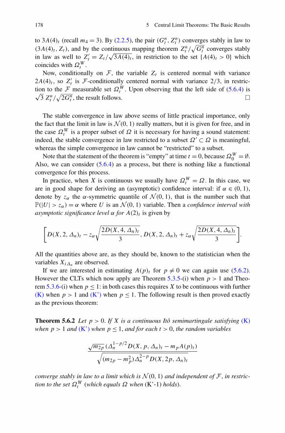
178 5 Central Limit Theorems: The Basic Results
to 3A(4)t (recall m4 = 3). By (2.2.5), the pair (Gnt ,Znt ) converges stably in law to
(3A(4)t ,Zt ), and by the continuous mapping theorem Znt /√Gnt converges stably
in law as well to Z′t = Zt/√
3A(4)t , in restriction to the set {A(4)t > 0} whichcoincides with ΩWt .
Now, conditionally on F , the variable Zt is centered normal with variance2A(4)t , so Z′t is F -conditionally centered normal with variance 2/3, in restric-tion to the F measurable set ΩWt . Upon observing that the left side of (5.6.4) is√
3 Znt /√
2Gnt , the result follows. �
The stable convergence in law above seems of little practical importance, onlythe fact that the limit in law is N (0,1) really matters, but it is given for free, and inthe case ΩWt is a proper subset of Ω it is necessary for having a sound statement:indeed, the stable convergence in law restricted to a subset Ω ′ ⊂Ω is meaningful,whereas the simple convergence in law cannot be “restricted” to a subset.
Note that the statement of the theorem is “empty” at time t = 0, becauseΩW0 = ∅.Also, we can consider (5.6.4) as a process, but there is nothing like a functionalconvergence for this process.
In practice, when X is continuous we usually have ΩWt = Ω . In this case, weare in good shape for deriving an (asymptotic) confidence interval: if α ∈ (0,1),denote by zα the α-symmetric quantile of N (0,1), that is the number such thatP(|U | > zα) = α where U is an N (0,1) variable. Then a confidence interval withasymptotic significance level α for A(2)t is given by
[D(X,2,Δn)t − zα
√2D(X,4,Δn)t
3,D(X,2,Δn)t + zα
√2D(X,4,Δn)t
3
].
All the quantities above are, as they should be, known to the statistician when thevariables XiΔn are observed.
If we are interested in estimating A(p)t for p �= 0 we can again use (5.6.2).However the CLTs which now apply are Theorem 5.3.5-(i) when p > 1 and Theo-rem 5.3.6-(i) when p ≤ 1: in both cases this requiresX to be continuous with further(K) when p > 1 and (K’) when p ≤ 1. The following result is then proved exactlyas the previous theorem:
Theorem 5.6.2 Let p > 0. If X is a continuous Itô semimartingale satisfying (K)when p > 1 and (K’) when p ≤ 1, and for each t > 0, the random variables
√m2p (Δ
1−p/2n D(X,p,Δn)t −mpA(p)t )√
(m2p −m2p)Δ
2−pn D(X,2p,Δn)t
converge stably in law to a limit which is N (0,1) and independent of F , in restric-tion to the set ΩWt (which equals Ω when (K’-1) holds).

5.6 Applications 179
A confidence interval with asymptotic significance level α forA(p)t is then givenby
[Δ
1−p/2n
mp
(D(X,p,Δn)t − zα
√(m2p −m2
p)D(X,2p,Δn)tm2p
),
Δ1−p/2n
mp
(D(X,p,Δn)t + zα
√(m2p −m2
p)D(X,2p,Δn)tm2p
)].
Finally, observe that when p ∈ (0,1) the same holds even if X has jumps, pro-vided it satisfies (K’-p), but this is wrong if p ≥ 1.
5.6.2 Detection of Jumps
For the problem of jump detection, as expounded in Sect. 3.5.2, we do not havethe tools for going further. Indeed, the choice of the cut-off level x = xn in (3.5.9)requires a CLT for the statistic Sn of (3.5.6). In this chapter we do have a CLTfor D(X,p,Δn)t or D(X,p, kΔn)t when X is continuous (or equivalently, inrestriction to Ω(c)t ), as seen just above. Theorem 5.1.2 also provide a CLT forD(X,p,Δn)t or D(X,p, kΔn)t in restriction to Ω(d)t . But in both cases we needa joint CLT for the pair (D(X,p,Δn)t ,D(X,p, kΔn)t ), and such results will begiven in Chap. 11 only.
5.6.3 Euler Schemes for Stochastic Differential Equations
This subsection is concerned with probably the most useful and widespread ex-ample of discretization of processes, outside the realm of statistics of processes.Historically speaking, it is also the oldest example, its roots going back to Eulerwho introduced the well known method bearing his name for solving differentialequations.
This example necessitates some non-trivial background about the general theoryof stochastic differential equations (SDE, in short). A comprehensive exposition ofthe theory would go way beyond the scope of this book, and we will make useof the results of the theory (including the convergence results) without reprovingeverything. For the most basic results and a general understanding of the setting ofSDEs, we refer for example to Protter [83].
1 – The setting. The setting is as follows: we have a filtered probability space(Ω,F , (Ft )t≥0,P) endowed with a q-dimensional driving process X for the SDE.The most usual case, which gives rise to Itô differential equations, is the continuouscase where X is a (d − 1)-dimensional Brownian motion, plus a last component

180 5 Central Limit Theorems: The Basic Results
which is the drift t . However, here we consider a more general situation where thedriving process X is a d-dimensional Itô semimartingale satisfying Assumption (H)(the initial value X0 of X is irrelevant here).
Our SDE will be q-dimensional, and apart from the driving process X it involvestwo other ingredients: one is the initial condition, which for simplicity we take non-random, as a given point y0 in R
q . The other is the coefficient, which is a functionf from R
q into Rq ⊗R
d (the set of q × d matrices). The equation reads as follows:
dYt = f (Yt−) dXt , Y0 = y0 (5.6.5)
or, component-wise and in integral form, as
i = 1, . . . , q ⇒ Y it = yi0 +d∑
j=1
∫ t
0f (Ys−)ij dXjs . (5.6.6)
Below we consider only the most common case where the function f is C1
and with linear growth, that is ‖f (y)‖ ≤ K(1 + ‖y‖) for some constant K . Thisimplies that the equation has a unique (strong) solution: that is, there is a processY which is a semimartingale on (Ω,F , (Ft )t≥0,P) satisfying (5.6.6), and any othersemimartingale satisfying the same is almost surely equal to Y . Furthermore, thesolution is a strong Markov process as soon as the driving process X is a Lévyprocess.
2 – The Euler scheme. Although existence and uniqueness are ensured, the “explicit”solution and its law are in general not available. However for practical purposes it isoften the case that we need to evaluate the law of Y , at least in the following sense:we want E(g(Yt )) for some functions g on R
q , or maybe E(G(Y )) for a functionG on the Skorokhod space D
q . In the absence of explicit or closed formulas, thisevaluation is necessarily done via a numerical approximation.
Now, suppose that X is a Lévy process. If we want E(g(Yt )), which is a func-tion h(y0) of the starting point, we can use the integro-differential equation (orpseudo-differential equation) which is satisfied by the function h and try to solveit numerically: there are several ways for doing this when X, hence Y as well, arecontinuous, since in this case h satisfies a partial differential equation whose coef-ficients are specified by the coefficient f . However these methods work effectivelyonly when the dimension q is small, and are not really available when X is not con-tinuous. Moreover evaluating E(G(Y )) for a functional G on the Skorokhod spaceis virtually impossible by analytical methods. And of course, when X is a generalsemimartingale, no analytical method is available, even for E(g(Yt )).
Therefore we must rely in general on Monte-Carlo simulations. This means thatwe “simulate” a large number N of independent copies of Y , say Y (1), . . . , Y (N).By the ordinary Law of Large Numbers, as N→∞ we have
1
N
N∑
r=1
G(Y (r)) → E
(G(Y)). (5.6.7)

5.6 Applications 181
This leads to another problem: how do we simulate the process Y ? An exact sim-ulation is in general impossible again, and this is where the Euler schemes comeinto play. First, simulating the whole driving process X, say on a fixed time interval[0, T ], is numerically meaningless. At the best, we can simulate the discrete ap-proximation X(n)t =XΔn[t/Δn] for some time step Δn > 0 which is as small as onewishes (non regular discretization schemes are of course possible here). SimulatingX(n) amounts to simulating the increments Δni X. This is still in general an arduoustask, although for quite a few Lévy processes it is indeed possible: if the compo-nents of X are Brownian motions, of course, or stable processes, or tempered stableprocesses, there are easy methods to perform the simulation in a very efficient way.
Now we turn to the simulation of the solution Y itself, assuming that simulatingthe increments Δni X is actually feasible. At stage n, the Euler approximation of Yis the process Yn defined recursively on i as follows:
Yn0 = y0, Y niΔn = Yn(i−1)Δn + f(Yn(i−1)Δn
)Δni X (5.6.8)
(we use here a matrix notation). This defines Yn on the grid (iΔn : i ∈ N), in afeasible way in the sense of simulation. For the mathematical analysis, we need toextend Yn to all times t . The simplest way consists in setting
t ∈ [(i − 1)Δn, iΔn) ⇒ Ynt = Yn(i−1)Δn, (5.6.9)
which is of course consistent with (5.6.8).At this point, we have to emphasize the fact that Yn is not the discretized version
Y (n) of the solution X, in the sense of (5.6.7).
3 – The error process. Our main concern will be an evaluation of the error incurredby replacing Y with its Euler approximation Yn. There are two sorts of errors: oneis the “weak” error, that is E(g(Y nt )) − E(g(Yt )), or E(G(Yn)) − E(G(Y )) for afunctional G, but this is in general impossible to evaluate accurately, especially fora functionalG, and especially also whenX is an arbitrary semimartingale. The othersort of error is the “strong” error, that is Yn − Y . Of course, the only sensible thingto do is to compare Yn and Y on the grid points, so our strong error process will bethe piecewise constant process
Un = Yn − Y (n). (5.6.10)
Our analysis of the behavior of Un is based upon a result from Kurtz and Protter[68], which will be stated without proof. We first need some notation. For any tworeal-valued semimartingales V and V ′, we write
Z(V,V ′)nt=
[t/Δn]∑
i=1
∫
I (n,i)
(Vs− − V(i−1)Δn) dV′s .

182 5 Central Limit Theorems: The Basic Results
Next, a sequence V n of processes of the form V nt =∑[t/Δn]i=1 ζ ni with ζ ni being FiΔn
measurable is said to have the P-UT property if for each t the sequence of variables
[t/Δn]∑
i=1
(∣∣E(ζ ni 1{|ζ ni |≤1} |F(i−1)Δn
)∣∣+E(∣∣ζ ni∣∣2 1{|ζ ni |≤1} |F(i−1)Δn
)
−E(ζ ni 1{|ζ ni |≤1} |F(i−1)Δn
)2 + ∣∣ζ ni∣∣1{|ζ ni |>1}
)(5.6.11)
is bounded in probability. This is the P-UT property stated in Jacod and Shiryaev[57], see Theorem VI.6.15, the acronym meaning “predictably uniformly tight”, andrestricted here to processes that are constant on each interval [(i − 1)Δn, iΔn].
The next theorem gathers the results that are needed later. It says that the EulerapproximationXn always converges to the solutionX, and it provides a criterion forobtaining a rate of convergence. The statement below is a mixture of Theorem 3.2of Jacod and Protter [55] and Theorem 2.2 of Jacod [58].
Theorem 5.6.3 Let X be a q-dimensional semimartingale and f be a C1 functionfrom R
q into Rq ⊗R
d , with linear growth.
a) We have Unu.c.p.=⇒ 0.
b) Suppose that, for some sequence αn of positive numbers tending to infin-ity, each sequence (αnZ(Xi,Xj )n) has the P-UT property, and suppose alsothat (X(n), (αnZ(Xi,Xj )n)1≤i,j≤q) converges stably in law to (X,Z), whereZ = (Z ij )1≤i,j≤q is defined on a very good filtered extension of the space(Ω,F , (Ft )t≥0,P). Then Z is a semimartingale on the extended space and αnUn
converges stably in law to U , where U = (Ui)1≤i≤d is the unique solution on theextended space of the following linear equation:
Uit =d∑
j=1
q∑
k=1
∫ t
0∂kf
ij (Ys−)Uks− dXjs −
d∑
j,l=1
q∑
k=1
∫ t
0∂kf
ij (Ys−)f kl(Ys−) dZ ljs .
(5.6.12)
Taking this theorem for granted, we are now in a position to state (and prove)the CLT-type result which we want for Un. In this result, the ingredients Tp , Rp−,Rp+, W ′ and c and σ are exactly those occurring in (5.4.3), and in particular W ′and Rp− and Rp+ are defined on a very good extension (Ω, F , (Ft )t≥0, P) of(Ω,F , (Ft )t≥0,P).
Theorem 5.6.4 Let X be a d-dimensional Itô semimartingale which satisfies As-sumption (Q). Let f be a C1 function from R
q into Rq ⊗ R
d , with linear growth.Let Un be the error process (5.6.10) of the Euler scheme Zn associated by (5.6.9)with (5.6.5).
Then 1√ΔnUn converges stably in law to a limiting process U which is the unique
solution on the extended space (Ω, F, (Ft )t≥0, P) of the following linear equation:

5.6 Applications 183
Uit =d∑
j=1
q∑
k=1
∫ t
0∂kf
ij (Ys−)Uks− dXjs
− 1√2
d∑
j,l,m,r=1
q∑
k=1
∫ t
0∂kf
ij (Ys−)f kl(Ys−)c lj,mrs dW ′mrs
−d∑
j,l=1
q∑
k=1
∞∑
p=1
∂kfij (YTp−)f kl(YTp−)
× (ΔXjTp Rlp− +ΔXlTn Rjp+)1{Tp≤t}. (5.6.13)
This equation is (5.6.12), written with Z = Z, the process given by (5.4.3), in linewith Theorem 5.4.6 and the fact that Zn in that theorem is (Z(Xi,Xj )n/
√Δn )i,j≤d
here.Coming back to the computation of E(G(Y )) for a continuous functional G on
the Skorokhod space, we use (5.6.7) with N simulated copies of the Euler approx-imation Yn, for some given time step Δn. The limit in (5.6.7) (as N→∞) is thenE(G(Yn)) and, on top of the statistical (Monte-Carlo) error of order 1/
√N , we have
the approximation error E(G(Yn))− E(G(Y )). This is where the theorem helps: itbasically says that, provided G is well behaved, this approximation error is of order√Δn. It also gives (in principle) a way to evaluate this error by using the equation
(5.6.13) in the same way as in the “standardization” made in Theorem 5.6.1.Note however that, although the rate
√Δn is sharp “in general”, it is not so for
the error E(g(Y nt )) − E(g(Yt )), and when X is a Lévy process: in this case, andprovided Δn is such that t/Δn is an integer, this error is of order Δn: see Talay andTubaro [91] or Jacod, Kurtz, Méléard and Protter [59].
Proof By localization, it is enough to prove the result whenX satisfies (SQ). In viewof Theorems 5.4.6 and 5.6.3, it remains to prove that for all j, k ≤ d the sequenceof processes Zn,jk has the P-UT property.
1) Letting V nt =∑[t/Δn]i=1 ζ ni be adapted processes, we give two criteria for the
P-UT property. First, the expectation of (5.6.11) is smaller than 2E(∑[t/Δn]i=1 |ζ ni |),
so
supn
E
([t/Δn]∑
i=1
∣∣ζ ni∣∣)< ∞ ∀t ⇒ (
V n)
has P-UT. (5.6.14)
Second, suppose that E(ζ ni | F(i−1)Δn) = 0 (we have martingale increments). Thefirst summand in (5.6.11) equals |E(ζ ni 1{|ζ ni |>1} | F(i−1)Δn)|, and |ζ ni 1{|ζ ni |>1}| ≤(ζ ni )
2. Then the expectation of (5.6.11) is smaller than 2E(∑[t/Δn]i=1 |ζ ni |2), and we
have
E(ζ ni |F(i−1)Δn
)= 0
supn E(∑[t/Δn]
i=1
∣∣ζ ni∣∣2)<∞ ∀t
}⇒ (V n) has P-UT. (5.6.15)

184 5 Central Limit Theorems: The Basic Results
Another evident property is that if, two sequences (V n) and (V ′n) have the P-UTproperty, then so does the sum (V n + V ′n).
2) For any process Y we write for s ≥ (i − 1)Δn:
Yni,s = Ys − Y(i−1)Δn . (5.6.16)
Under (SH) we set b′t = bt +∫{‖δ(t,z)>1} δ(t, z)λ(dz), so we have
Zn,jkt =
d+2∑
l=1
[t/Δn]∑
i=1
ζ(l)ni , where
ζ(l)ni =
⎧⎪⎪⎪⎨
⎪⎪⎪⎩
1√Δn
∫I (n,i)
Xj,ni,s− σkls dWl
s if l = 1, . . . , d
1√Δn
∫I (n,i)
∫Xj,ni,s− δ(s, z)k (p− q)(ds, dz) if l = d + 1
1√Δn
∫I (n,i)
Xj,ni,s− b′ks ds if l = d + 2
and it is enough to prove that each sequence V (l)n =∑[t/Δn]i=1 ζ(l)ni has the P-UTproperty. (2.1.33), (2.1.34) and (2.1.36) yield E(‖Xni,s‖2)≤KΔn if s ∈ I (n, i), andb′ and σ are bounded. Therefore by the Cauchy-Schwarz and Doob’s inequalitiesE(|ζ(l)ni |p)≤KΔn if p = 2 and l = 1, . . . , d + 1, and also if p = 1 and l = d + 2.Then the P-UT property for Y(l)n follows from (5.6.15) for l = 1, . . . , d + 1 andfrom (5.6.14) for l = d + 2.
3) Finally we suppose that X is continuous and∫ t
0 (‖bs‖2 + ‖cs‖2) ds ≤ Kt for
all t . Then X =X0 +B +Xc and Zn,jkt =∑2d+2l=1∑[t/Δn]i=1 ζ(l)ni , where
ζ(l)ni =
⎧⎪⎪⎪⎪⎪⎪⎨
⎪⎪⎪⎪⎪⎪⎩
1√Δn
∫I (n,i)
Xc,j,ni,s− σkls dWl
s if l = 1, . . . , d
1√Δn
∫I (n,i)
Bj,ni,s− σkls dWl
s if l = d + 1, . . . ,2d
1√Δn
∫I (n,i)
Xc,j,ni,s− bks ds if l = 2d + 1
1√Δn
∫I (n,i)
Bj,ni,s− bks ds if l = 2d + 2.
Again it is enough to prove that each sequence Y(l)n =∑[t/Δn]i=1 ζ(l)ni has the P-UTproperty. (2.1.33) and (2.1.34) yield for all p ≥ 2 and s ∈ I (n, i):
∥∥Bni,s∥∥2 ≤Δn
∫
I (n,i)
‖br‖2 dr, E(∥∥Xc,ni,s
∥∥p)≤KpΔp/2−1n E
(∫
I (n,i)
‖cr‖p/2 dr).
Therefore by the Cauchy-Schwarz and Burkholder-Davis-Gundy inequalities, weget

Bibliographical Notes 185
E(∣∣ζ(l)ni
∣∣p)≤
⎧⎪⎪⎪⎪⎨
⎪⎪⎪⎪⎩
E(∫I (n,i)
‖cs‖2 ds)
if p = 2, l = 1, . . . , d
E(∫I (n,i)
‖bs‖2 ds∫I (n,i)
‖cs‖ds)
if p = 2, l = d + 1, . . . ,2d
E(∫I (n,i)
(‖bs‖2 + ‖cs‖) ds)
if p = 1, l = 2d + 1√Δn E(∫I (n,i)
‖bs‖2 ds)
if p = 1, l = 2d + 2.
Since∫ t
0 ‖bs‖2 ds and∫ t
0 ‖cs‖2 ds and∫ t
0 ‖cs‖ds are bounded by hypothesis, it fol-lows that the array ζ(l)ni satisfies the conditions in (5.6.15) when l = 1, . . . ,2d andin (5.6.14) when l = 2d + 1,2d + 2. This completes the proof. �
Bibliographical Notes
Processes with conditionally independent increments have been introduced byGrigelionis [41]. The associated convergence result (Theorem 4.2.1) comes fromJacod [54], and the unpublished paper [53] contains a more general version of theCentral Limit Theorem 5.3.6 when the underlying Itô semimartingale is continuous.A CLT of the type of Theorem 5.3.5 was already proved, in a statistical context andfor diffusions, by Dohnal [29]. The first CLT for discontinuous Itô semimartingalesseems to appear in Jacod and Protter [55], which also contains the analysis of theEuler scheme made in Sect. 5.6.3. One can also mention that, often independently,results about the quadratic variation in the continuous case are scattered throughthe econometrical literature, as in Andersen, Bollerslev, Diebold and Labys [6] forexample. The theorems of Sects. 5.1 and 5.3, are taken from Jacod [60], except The-orem 5.3.6 which was proved in more generality by Barndorff-Nielsen, Graversen,Jacod, Podolskij and Shephard [11].

Chapter 6Integrated Discretization Error
In contrast with the previous chapters and most of the forthcoming ones, here westudy a different kind of functionals, namely
∑Nn(t)i=1 f (X(i−1)Δn), for a regular dis-
cretization scheme with time step Δn→ 0.The law of large numbers for this sort of functionals is evident: as soon as the
d-dimensional process X is, say, càdlàg and f is a continuous function on Rd , we
have
Δn
[t/Δn]∑
i=1
f (X(i−1)Δn) →∫ t
0f (Xs) ds,
the convergence taking place for each ω and being locally uniform in time: thiscomes from the convergence of Riemann sums. The choice of X(i−1)Δn in theith summand is arbitrary, we could have taken Xtn,i for any tn,i ∈ I (n, i) = ((i −1)Δn, iΔn] instead, but it fits better for later results.
The associated Central Limit Theorem is more interesting. It concerns the behav-ior of the following processes (recall the discretized versionX(n)t =XΔn[t/Δn] of theprocess X):
V n(f,X)t = Δn[t/Δn]∑
i=1
f (X(i−1)Δn)−∫ Δn[t/Δn]
0f (Xs) ds
=∫ Δn[t/Δn]
0
(f(X(n)s)− f (Xs)
)ds
(taking Δn[t/Δn] instead of t as the upper bound is for convenience: it avoidsboundary terms). The variable V n(f,X) may be viewed as a kind of “integrated”measure of the error incurred by the discretization, whenX is replaced byX(n). Per-haps more to the point, we could take the absolute value of the error, or some powerof it, which leads us to introduce the following processes for a priori any p > 0:
V n(f,p,X)t =∫ Δn[t/Δn]
0
∣∣f(X(n)s)− f (Xs)
∣∣p ds.
J. Jacod, P. Protter, Discretization of Processes,Stochastic Modelling and Applied Probability 67,DOI 10.1007/978-3-642-24127-7_6, © Springer-Verlag Berlin Heidelberg 2012
187

188 6 Integrated Discretization Error
It may appear that this chapter digresses from the main stream of this book.However, consider for a moment the case of the identity function f (x) = x. Thefunctional V n(f,X)t =∑[t/Δn]i=1 f (Δni X) is equal to X(n)t − X0, which convergespathwise to Xt − X0 for the Skorokhod topology. In this case the CLT given inTheorem 5.1.2 does not apply, whereas Theorem 5.3.6 amounts simply to X(n) −X0 →X−X0, because with the notation of this theorem we have in the present caseV′n(f,X) = X(n) − X0 and U
′(f,X) = A′(f,X) = 0 and A(f,X)+ U ′′(f,X) =
X−X0.In other words, one can view a CLT for V n(f,X) or for V n(f,p,X) as a sub-
stitute of proper CLTs for V n(f,X) or V ′n(f,X), which do not exist as such whenf (x)= x.
The content of this chapter is taken from the paper [56] of Jacod, Jakubowski andMémin, with a few improvements.
6.1 Statements of the Results
The process of interest X is a d-dimensional Itô semimartingale, on the filteredprobability space (Ω,F , (Ft )t≥0,P), written in its Grigelionis form as
Xt =X0+∫ t
0bs ds+
∫ t
0σs dWs+ (δ1{‖δ‖≤1}) � (p− q)t + (δ1{‖δ‖>1}) � pt . (6.1.1)
Here,W is a d ′-dimensional Brownian motion and p is a Poisson measure on R+ ×E with compensator q(dt, dz)= dt⊗λ(dz) (λ is a σ -finite measure on the auxiliaryspace (E,E)). Then b and δ are d-dimensional and σ is d × d ′-dimensional, and asusual c= σσ�.
Most of the time, we will need an assumption of the same type but stronger thanAssumption 4.4.2, or (H). Below, r is a real in [0,2].
Assumption 6.1.1 (or (H-r)) X is an Itô semimartingale given by (6.1.1), and wehave:
(i) The process b is locally bounded.(ii) The process σ is càdlàg.
(iii) There is a localizing sequence (τn) of stopping times and, for each n, a deter-ministic nonnegative function Γn on E such that
∫Γn(z)
rλ(dz) <∞ (with theconvention 00 = 0) and ‖δ(ω, t, z)‖∧1≤ Γn(z) for all (ω, t, z)with t ≤ τn(ω).
(H-2) is exactly (H), whereas (H-r) for r ∈ [0,2) implies r ∈ I(X) where, ac-cording to (3.2.2), I(X) is the set of all p ≥ 0 such that
∑s≤t ‖ΔXs‖p <∞ a.s.
for all t . In fact, (H-r) when r < 2 is slightly stronger than (H) plus the propertyr ∈ I(X). Furthermore all (H-r) are the same as (H) whenX is continuous. Observealso that, as far as the coefficient δ is concerned, (H-r) is the same as Assumption5.3.2, that is (K-r), except that we do not require r ≤ 1. Finally (H-r) implies (H-r ′)for all r ′ ∈ [r,2].

6.1 Statements of the Results 189
The results are somewhat similar to Theorem 5.4.2, and we start with a descrip-tion of the limiting processes. As in the previous chapter, we consider an auxiliaryspace (Ω ′,F ′,P′) supporting a d ′-dimensional Brownian motion W ′ (the same di-mension as for W ) and a sequence (κn)n≥1 of i.i.d. variables, uniformly distributedon (0,1) and independent of W ′. We also consider an arbitrary weakly exhaustingsequence (Tn)n≥1 for the jumps ofX, see, e.g., before (5.1.2). Then we construct thevery good filtered extension (Ω, F , (Ft )t≥0, P) of (Ω,F , (Ft )t≥0,P) by (4.1.16),that is:
Ω = Ω ×Ω ′, F = F ⊗F ′, P = P⊗ P′
(Ft ) is the smallest filtration containing (Ft ) and such thatκn is FTn measurable for all n andW ′ is (Ft )-adapted.
Then W ′ is a Brownian motion independent of (W, p), and p is a Poisson measurewith compensator q and independent of (W,W ′), on the extended space.
We start with the processes V n(f,X), or rather with−V n(f,X)which are some-what more natural to consider.
Theorem 6.1.2 Let f be a C2 function from Rd into R
q . Assume that X is an Itôsemimartingale, which either is continuous or satisfies (H) (that is, (H-2)). Then theprocesses − 1
ΔnV n(f,X) converge stably in law to the process
V (f,X)t = 1
2
(f (Xt )− f (X0)
)+ V ′(f,X)t + V ′′(f,X)t , (6.1.2)
where
V ′(f,X)t = 1√12
d∑
j=1
d ′∑
k=1
∫ t
0∂jf (Xs)σ
jks dW ′k
s (6.1.3)
V ′′(f,X)t =∑
n:Tn≤t
(f (XTn− +ΔXTn)− f (XTn−)
)(κn − 1
2
). (6.1.4)
The first term in (6.1.2) is a sort of “bias”, analogous to the last three terms in(5.3.6), and it is defined on the original space, whereas V ′(f,X) and V ′′(f,X) in-volve extra randomness and necessitates the extension of the space. The processV ′(f,X) is obviously well defined. The process V ′′(f,X) is well defined by Propo-sition 4.1.4, because the variables κn − 1/2 are centered and
∑
s≤t
∥∥f (Xs− +ΔXs)− f (Xs−)∥∥2 < ∞ (6.1.5)
for all t . Note also that V ′(f,X) and V ′′(f,X) are, conditionally on F , two inde-pendent processes with independent increments, centered and with covariances
E(V ′(f j ,X)tV ′(f k,X)t|F) = 1
12
d∑
l,m=1
∫ t
0∂lf
j (Xs) clms ∂mf
k(Xs) ds

190 6 Integrated Discretization Error
E(V ′′(f j ,X)tV ′′(f k,X)t|F) = 1
12
∑
s≤t
(f j (Xs− +ΔXs)− f j (Xs−)
)
× (f k(Xs− +ΔXs)− f k(Xs−))
(we use here the fact that the variance of κn is 1/12).Now, (6.1.5) holds as soon as f is C1, but the C2 property of f is heavily used
in the proof, through Itô’s formula. However, we can take advantage of the gener-alized Itô’s formula given in Theorem 3.2.2, to obtain a similar result under weakerconditions on f (but stronger assumptions on X).
For this we recall that a Cp function, when p is not an integer, is a [p]-continuously differentiable function whose [p]th partial derivatives are Hölder withindex p− [p] on every compact subset of Rd . We also need the following process,well defined as soon as 1 ∈ I(X):
B ′t =∫ t
0bs ds − (δ 1{‖δ‖≤1}) ∗ qt . (6.1.6)
Theorem 6.1.3 Let f be a Cr function from Rd into R
q , for some r ∈ (0,2), andassume that X satisfies (H-r), with moreover Xc = 0 when r ∈ [1,2) and Xc =B ′ = 0 when r < 1. Then the processes − 1
ΔnV n(f,X) converge stably in law to the
process
V (f,X)t = 1
2
(f (Xt )− f (X0)
)+ V ′′(f,X)t , (6.1.7)
where V ′′(f,X) is again defined by (6.1.4).
Above, we have r ∈ I(X) and (6.1.5) holds when f is Cr/2, hence a fortioriwhen it is Cr : so again V ′′(f,X) is well defined. Since Xc = 0 we have V ′(f,X)=0, and the two formulas (6.1.2) and (6.1.7) agree. Note also that V ′(f,X) is of finitevariation when r ≤ 1, but in general not when r > 1. Moreover, again when r < 1,the limit (6.1.7) can also be written as
V (f,X)t =∑
n:Tn≤t
(f (XTn− +ΔXTn)− f (XTn−)
)κn,
because then Xt =X0 +∑n:Tn≤t ΔXTn by our assumption B ′ = 0.Now we turn to the processes V n(f,p,X). Of course, here, f is one-dimen-
sional, and for simplicity we assume that is C2, although C1 would be enough whenr ≤ 1 below.
Theorem 6.1.4 Let p > 0 and f be a C2 real-valued function on Rd . Assume that
X satisfies (H-r), where r = p ∧ 2, with moreover Xc = 0 when p ∈ (1,2) andXc = B ′ = 0 when p ≤ 1. Then the processes 1
ΔnV n(f,p,X) converge stably in
law to the following limit:

6.1 Statements of the Results 191
V (f,p,X)t ={
12
∑dj,k=1
∫ t0 ∂jf (Xs)∂kf (Xs)c
jks ds + V ′(f,p,X)t if p = 2
V ′(f,p,X)t otherwise,(6.1.8)
where
V ′(f,p,X)t =∑
n:Tn≤t
∣∣f (XTn− +ΔXTn)− f (XTn−)∣∣p κn. (6.1.9)
Note that our assumptions imply∑
s≤t
∣∣f (Xs− +ΔXs)− f (Xs−)∣∣p < ∞,
hence V ′(f,p,X) is finite-valued (by Proposition 4.1.3 in this case). The limitingprocess V (f,p,X) is increasing in time, as it should be because each V n(f,p,X)is also increasing by construction. The forms of the limits in Theorems 6.1.2 and6.1.4 are thus deeply different.
Remark 6.1.5 The reader will observe that, in contrast with Theorem 6.1.3, we as-sume B ′ = 0 when p = r ≤ 1, and not just when p < 1. The asymptotic behaviorof V n(f,1,X) when Xc = 0 and B ′ �= 0 is unknown, although it is known that foreach t the sequence of variables V n(f,1,X)t/Δn is bounded in probability.
Remark 6.1.6 This result is remarkable in the sense that, since V n(f,p,X) is a kindof pth power of the error involved when replacing f (Xs) by f (X(n)s ), one wouldexpect the rate to be the pth power of a basic rate. But this is not the case: the rateis always 1/Δn.
This is of course due to the jumps. Indeed, if there is a single jump in the intervalI (n, i)= ((i−1)Δn, iΔn], say at time T , the integral
∫I (n,i)
|f (X(n)s )−f (Xs)|p dsis approximately |f (X(i−1)Δn +ΔXT )−f (X(i−1)Δn)|p (iΔn−T ), whose order ofmagnitude is always Δn.
Remark 6.1.7 Assumption (H-r) for any r ∈ [0,2] entails that σt is càdlàg, but thisproperty is not required for the previous result, as will be apparent from the proof.We only need σt to be locally bounded. This will not be the case in the forthcomingresult, for which the càdlàg property is needed when p �= 2.
When X is continuous we have another result, with a “true rate”. This resultcoincides with the previous one when p = 2 and improves on it when p > 2. It alsoshows that, when p < 2, one cannot have a result like Theorem 6.1.4, unless weassume Xc = 0.
To describe the limit, we need a notation. For x = (xj )1≤j≤d ′ ∈ Rd ′ and p > 0
we set (the dimension d ′ is implicit in the next formula):
ρ(p,x) = E
(∫ 1
0
∣∣∣∣∣
d ′∑
j=1
xj Wjs
∣∣∣∣∣
p
ds
). (6.1.10)

192 6 Integrated Discretization Error
These are explicitly calculable, using the multinomial formula, when p is an eveninteger, and in particular ρ(2, x)= ‖x‖2/2, implying that for p = 2 the limit belowis the same as in (6.1.8) in the absence of jumps. When d ′ = 1 and for all p > 0, it isalso explicit: we have ρ(p,x)= 2mp|x|p/(p + 2), where as usual mp is the p ab-solute moment of the law N (0,1). Moreover ρ(p,x) is obviously continuous in x.
Theorem 6.1.8 Let f be a C2 function on Rd , and let p > 0. Assume also that X
is a continuous Itô semimartingale satisfying (H). Then if ξt is the d ′-dimensionalcàdlàg process with components ξkt =
∑dj=1 ∂jf (Xt ) σ
jkt , we have
1
Δp/2n
V n(f,p,X)tu.c.p.=⇒∫ t
0ρ(p, ξs) ds.
This result is in fact a law of large numbers, in contrast with Theorem 6.1.4, andone could look for an associated CLT. We will not do that here.
6.2 Preliminaries
The theorems of this chapter encompass two cases:
(a) The process X is a continuous Itô semimartingale, we then set r = 2.(b) The process X satisfies (H-r) for some r ∈ (0,2].As is now customary for us, we introduce a strengthened version of (H-r):
Assumption 6.2.1 (or (SH-r)) We have (H-r), and the processes b and σ arebounded, and ‖δ(ω, t, z)‖ ∧ 1≤ Γ (z) with Γ bounded and
∫Γ (z)r λ(dz) <∞.
An obvious extension of the localization Lemma 4.4.9 yields that, if one of ourtheorems holds for all X satisfying (SH-r), it also holds for any X satisfying (H-r).So in case (b) above we may replace (H-r) by (SH-r), and in both cases the processX itself is bounded. Then a further (trivial) localization allows us to reduce theproblem to the following two cases, still labeled (a) and (b), and where A is someconstant:
• case (a): X is continuous, r = 2, and∫ t0 ‖bs‖ds +
∫ t0 ‖σs‖2 dt + ‖Xt‖ ≤A
• case (b):∥∥δ(t, z)
∥∥≤ Γ (z) andΓ (z)+ ∫ Γ (z)rλ(dz)+ ‖bt‖ + ‖σt‖ + ‖Xt‖ ≤A.
⎫⎪⎪⎪⎬
⎪⎪⎪⎭(6.2.1)
In case (b) we also use the following notation:
b′′t = bt +∫
{‖δ(t,z)‖>1}δ(t, z)λ(dz)
r ≤ 1 ⇒ b′t = bt −∫
{‖δ(t,z)‖≤1}δ(t, z)λ(dz).
(6.2.2)

6.2 Preliminaries 193
Then ‖b′′t ‖ ≤A+A2, and ‖b′t‖ ≤ 2A when r ≤ 1. We can rewrite (6.1.1) as
Xt =X0 +∫ t
0b′′s ds +
∫ t
0σs dWs + δ ∗ (p− q)t if r ∈ (0,2]
Xt =X0 +∫ t
0b′s ds +
∫ t
0σs dWs + δ ∗ pt if r ∈ (0,1].
(6.2.3)
Then B ′t =∫ t
0 b′s ds is the same as in (6.1.6).
6.2.1 An Application of Itô’s Formula
The functionals V n(f,X) and V n(f,p,X) involve in an essential way the variablesf (Xs)− f (X(i−1)Δn) and |f (Xs)− f (X(i−1)Δn)|p , and to evaluate these variableswe use Itô’s formula, in its classical version when f is C2 or p ≥ 2 and in itsextended form of Theorem 3.2.2 when f is Cr or p < 2. Note that under (6.2.1) thevalues that f (x) takes when ‖x‖>A are irrelevant, so it is no restriction to assumethat f has compact support.
The two types of variables above are quite different, the second one showing aninterplay between f and the exponent p. In order to treat both at once, we considerbelow a (possibly multidimensional) function g = g(y;x) on R
d ×Rd (we use this
special notation because y plays the role of a parameter). We will assume either oneof the following two properties for g:
g is continuous with compact support, and (y, x) �→ g(y;x) is Cr. (6.2.4)
g is Lipschitz, with compact support. (6.2.5)
So (6.2.5) is slightly weaker than (6.2.4) with r = 1, and typically below r ∈ (0,2]will be the same number here and in (6.2.1).
We denote by ∂jg and ∂2jkg the partial derivatives of the function x �→ g(y;x),
when they exist (derivatives with respect to y will not be used).We associate the function h, and also the function k when r ≥ 1, on R
d ×Rd ×
Rd , by
h(y;x,w)=g(y;x+w)−g(y;x), k(y;x,w)=h(y;x,w)−d∑
j=1
∂jg(y;x)wj .
Then h, and k when r ≥ 1, are continuous, and∥∥h(y;x,w)∥∥ ≤ K‖w‖r∧1, r ≥ 1 ⇒ ∥∥k(y;x,w)∥∥ ≤ K‖w‖r . (6.2.6)
Our processes of interest in this subsection are, for s ≥ (i − 1)Δn:
s �→ g(Xni ;Xs
), where Xni = X(i−1)Δn .
We give the results in three lemmas, starting with the simplest case r ≤ 1.

194 6 Integrated Discretization Error
Lemma 6.2.2 Assume (6.2.1), case (b) with r ≤ 1 and B ′ = Xc = 0. Then under(6.2.5) when r = 1 and (6.2.4) when r < 1, we have for s ≥ (i − 1)Δn:
g(Xni ;Xs
) =∫ s
(i−1)Δn
∫
E
h(Xni ;Xv−, δ(v, z)
)p(dv, dz). (6.2.7)
Proof We have Xs = Xni +∑(i−1)Δn<v≤s ΔXv and the result is a simple conse-
quence of (3.2.5) (which is a “pathwise” result) applied with f (x)= g(Xni ;x). �
Lemma 6.2.3 Assume (6.2.1), case (b), with 1 ≤ r < 2 and Xc = 0. Then under(6.2.4) we have for s ≥ (i − 1)Δn:
g(Xni ,Xs
) =∫ s
(i−1)Δnγ(Xni ;X
)vdv
+∫ s
(i−1)Δn
∫
E
h(Xni ;Xv−, δ(v, z)
)(p− q)(dv, dz), (6.2.8)
where
γ (y;X)v =d∑
j=1
∂jg(y;Xv)b′′jv +∫
E
k(y;Xv−, δ(v, z)
)λ(dz). (6.2.9)
If further X satisfies (SH-1) and b′t is given by (6.2.2), we also have
g(Xni ;Xs
) =d∑
j=1
∫ s
(i−1)Δn∂jg(Xni ;X
)vb′jv dv
+∫ s
(i−1)Δn
∫
E
h(Xni ;Xv−, δ(v, z)
)p(dv, dz). (6.2.10)
Note that the integrand in the last part of (6.2.9) has a norm smaller thanKΓ (z)r
by (6.2.1) and (6.2.6), so ‖γ (y,X)v‖ ≤K .
Proof Here we use (3.2.4) with f (x) = g(Xni ;x) as in the previous proof, on thetime interval [(i− 1)Δn,∞) instead of [0,∞). Taking the first formula (6.2.3) withσ ≡ 0 into consideration, and if γ ′(y;X)v and γ ′′(y;X)v denote the first and thesecond terms in the right side of (6.2.9), this gives
g(Xni ;Xs
) =∫ s
(i−1)Δnγ ′(Xni ;X
)vdv
+∫ s
(i−1)Δn
∫
E
k(Xni ;Xv−, δ(v, z)
)p(dv, dz)
+∫ s
(i−1)Δn
∫
E
d∑
j=1
∂jg(Xni ;Xv−
)δ(v, z)j (p− q)(dv, dz).

6.2 Preliminaries 195
Since ‖k(Xni ;Xv−, δ(v, z))‖ ≤ KΓ (z)r by (6.2.6), the second term on the rightabove has locally integrable variation. Its compensator is the same integral withrespect to q, that is the process
∫ s(i−1)Δn
γ ′′(Xni ;X)v dv. So this term is in fact
∫ s
(i−1)Δnγ ′′(Xni ;X
)vdv+∫ s
(i−1)Δn
∫
E
k(Xni ;Xv−, δ(v, z)
)(p− q)(dv, dz).
Since k(y;x,w)+∑dj=1 ∂jg(y;x)wj = g(y;x), we deduce (6.2.8).
Finally under (SH-1), and by (6.2.6), the last integral in (6.2.8) is an ordinaryintegral, which splits into two integrals with respect to p and q, respectively. We alsohave b′′t − b′t =
∫Eδ(t, z)λ(dz), so (6.2.10) is just another of writing (6.2.8). �
Lemma 6.2.4 Assume (6.2.1), case (b) with r = 2. Then under (6.2.4) with r = 2also, we have for s ≥ (i − 1)Δn:
g(Xni ;Xs
) =∫ s
(i−1)Δn
(γ(Xni ;X
)v+ γ (Xni ;X
)v
)dv
+d ′∑
j=1
∫ s
(i−1)Δnγ ′(Xni ;X
)jvdWj
v
+∫ s
(i−1)Δn
∫
E
h(Xni ;Xv−, δ(v, z)
)(p− q)(dv, dz), (6.2.11)
where γ is as in (6.2.9) and
γ (y;X)v = 1
2
d∑
j,k=1
∂2jkg(y;Xv)cjkv , γ ′(y;X)kv =
d∑
j=1
∂jg(y;Xv)σ jkv .
If further X satisfies (SH-1) and b′t is given by (6.2.2), we also have
g(Xni ;Xs
) =d∑
j=1
∫ s
(i−1)Δn∂j g(Xni ;X
)vb′jv dv
+∫ s
(i−1)Δnγ(Xni ;X
)vdv++
d ′∑
j=1
∫ s
(i−1)Δnγ ′(Xni ;X
)jvdWj
v
+∫ s
(i−1)Δn
∫
E
h(Xni ;Xv−, δ(v, z)
)p(dv, dz). (6.2.12)
Proof Taking into account the first formula (6.2.3) again, plus the fact that the jumpsof X are bounded by A, this is exactly the version (2.1.20) of Itô’s formula appliedwith the same f as in the previous proof and on the time interval [(i − 1)Δn,∞).The only difference is that instead of the truncation level 1 for the jumps, here wetake A, so in last term of (2.1.20) vanishes and in the one before the last we can

196 6 Integrated Discretization Error
delete the indicator function. We then get exactly (6.2.11), and under the additionalassumption (SH-1), we deduce (6.2.12) from (6.2.11) as in the previous lemma. �
6.2.2 Reduction of the Problem
In this subsection we show that, in case (b), we can reduce the problem to the situa-tion where X has only finitely many jumps on finite intervals, exactly as in Chap. 5.For proving this, we need some notation. We set Am = {z : Γ (z) > 1/m} for m≥ 1an integer, and
X(m)t =X0 +∫ t
0b′′s ds +
∫ t
0σs dWs + δm ∗ (p− q)t , where δm = δ 1Am.
Lemma 6.2.5 Assume (6.2.1), case (b). On the extended space, we have:
(i) If f is Cr with compact support, V (f,X(m))u.c.p.=⇒ V (f,X) as m→∞.
(ii) If f is C2 with compact support and p ≥ r , V (f,p,X(m)) u.c.p.=⇒ V (f,p,X) asm→∞.
Proof 1) We may assume f to be one-dimensional here. First, by Doob’s inequality,
E
(sups≤t∥∥X(m)s −Xs
∥∥2)≤ 4E((‖δ‖2 1Acm
) ∗ qt
) ≤ amt,
where am = 4∫AcmΓ (z)2λ(dz) goes to 0 as m→∞ by Lebesgue’s theorem. Hence
X(m)u.c.p.=⇒ X as m→∞. (6.2.13)
Therefore the dominated convergence theorem for stochastic and ordinary integralsyields
∫ t
0∂jf(X(m)s
)σjks dW ′k
s
u.c.p.=⇒∫ t
0∂jf (Xs)σ
jks dW ′k
s
∫ t
0∂jf(X(m)s
)∂kf(X(m)s
)cjks ds
u.c.p.=⇒∫ t
0∂jf (Xs) ∂kf (Xs) c
jks ds
as soon as f is C1, because ∂jf is then continuous and bounded. We also have
f (X(m))u.c.p.=⇒ f (X). Hence in view of (6.1.2) and (6.1.3) if r = 2, or (6.1.7) if
r < 2, and of (6.1.8), it remains to prove that V ′′(f,X(m)) u.c.p.=⇒ V ′′(f,X) and
V ′(f,p,X(m)) u.c.p.=⇒ V ′(f,p,X).2) The difference V ′′(f,X(m))− V ′′(f,X) is a square-integrable martingale on
the extended space, and its quadratic variation process is
F(m)t =∑
n:Tn≤t
(f(X(m)Tn− +ΔX(m)Tn
)− f (X(m)Tn−)
− f (XTn− +ΔX(m)Tn)+ f (XTn−)
)2(κn − 1
2
)2
.

6.2 Preliminaries 197
Each summand in F(m)t above goes to 0 by (6.2.13) and is smaller thanK‖ΔXTn‖2r∧2, because ‖ΔX(m)‖ ≤ ‖ΔX‖ and f is Cr with compact support.Since E(
∑n:Tn≤t ‖ΔXTn‖2r∧2) <∞ by hypothesis, an application of the Lebesgue
theorem yields E(F (m)t )→ 0. Then we conclude V ′′(f,X(m))− V ′′(f,X) u.c.p.=⇒ 0from Doob’s inequality.
3) Observe that |V ′(f,p,X(m))s − V ′(f,p,X)s | is smaller for s ≤ t than∑
q:Tq≤t
∣∣∣∣f(X(m)Tq− +ΔX(m)Tq
)− f (X(m)Tq−)∣∣p
− ∣∣f (XTq− +ΔXTq )− f (XTq−)∣∣p∣∣.
The qth summand above is smaller than K‖ΔXTq‖p when f is C2 with compactsupport, and it goes to 0 in probability, so the dominated convergence theorem andthe property
∑s≤t ‖ΔXs‖p <∞ gives the convergence to 0 of the above sum. �
Lemma 6.2.6 Assume (6.2.1), case (b), with Xc = 0 if r < 2 and also B ′ = 0 iffurther r < 1. Let f be Cr with compact support. Then
limm→∞ sup
nE
(1
Δnsups≤t∣∣V n(f,X(m)
)s− V n(f,X)s
∣∣)= 0.
Proof 1) Again we may assume f to be one-dimensional. The proof is somewhatreminiscent of the proof of Theorem 5.1.2. We apply Lemmas 6.2.2, 6.2.3 or 6.2.4,according to the value of r , with the function g(y;x)= f (y)−f (x) which satisfies(6.2.4). With the notation of those lemmas, and recalling I (n, i)= ((i−1)Δn, iΔn],we see that
V n(f,X)t − V n(f,X(m)
)t=[t/Δn]∑
i=1
∫
I (n,i)
(g(X(m)ni ;X(m)s
)− g(Xni ;Xs))ds.
(6.2.14)2) We consider first the case r ≥ 1, and observe that in view of the form of
the function g, the functions h(y;x,w) and k(y;x,w) and the variables γ (y;X)v ,γ (y;X)v and γ ′(y;X)v do not depend on y. Then we set
θ(m,1)v ={γ(X(m))v− γ (X)v if r < 2
γ(X(m))v− γ (X)v + γ
(X(m))v− γ (X)v if r = 2
θ(m,2)v =
⎧⎪⎪⎨
⎪⎪⎩
∫E
(h(X(m)v−, δm(v, z)
)− h(Xv−, δ(v, z)))2λ(dz) if r < 2
∫E
(h(X(m)v−, δm(v, z)
)− h(Xv−, δ(v, z)))2λ(dz)
+∑d ′j=1
(γ ′(X(m)v
)j − γ ′(Xv)j)2 if r = 2
ρ(m)ni,s =∫ s
(i−1)Δn
∫
E
(h(X(m)v−, δm(v, z)
)− h(Xv−, δ(v, z)))(p− q)(dv, dz).

198 6 Integrated Discretization Error
Then (6.2.14) and Lemmas 6.2.3 or 6.2.4, according to the case, yield
V n(f,X)t − V n(f,X(m)
)t=[t/Δn]∑
i=1
∫
I (n,i)
(ζ(m,1)ni,s + ζ(m,2)ni,s
)ds, with
ζ(m,1)ni,s =∫ s
(i−1)Δnθ(m,1)v dv,
ζ(m,2)ni,s={ρ(m)ni,s if r < 2
ρ(m)ni,s +∑d ′j=1
∫ s(i−1)Δn
(γ ′(X(m))jv −γ ′(X)jv) dWjv if r = 2
We are thus left to prove that, for l = 1,2,
1
ΔnE
(sups≤t
∣∣∣∣∣
[s/Δn]∑
i=1
∫
I (n,i)
ζ(m, l)ni,s ds
∣∣∣∣∣
)→ 0. (6.2.15)
Now we use (6.2.13) and the facts that δm converges pointwise to δ (becauseδ(t, z)= 0 if z /∈ ∪m≥1Am) with ‖δm(ω, t, z)‖ ≤ Γ (z) and
∫Γ (z)rλ(dz) <∞, and
that g(y;x)= f (y)− f (x) is Cr with compact support and r ≥ 1, and (6.2.6): allthese, plus Lebesgue’s theorem for the second statement below, give the followingproperties for l = 1,2.
∣∣θ(m, l)t∣∣ ≤ K, θ(m, l)t
P−→ 0 ∀ t as m→∞. (6.2.16)
We are now ready to prove (6.2.15). First, we have | ∫I (n,i)
ζ(m,1)ni,s ds| ≤Δn∫I (n,i)
|θ(m,1)s |ds, therefore the left-hand side of (6.2.15) is smaller than
E(∫ t
0 |θ(m,1)s |ds) and (6.2.15) for l = 1 follows from (6.2.16). Second,∫I (n,i)
ζ(m,
2)ni,s ds is a martingale increment for the discrete-time filtration (FiΔn)i≥1, and asimple calculation shows that
E
((∫
I (n,i)
ζ(m,2)ni,s ds
)2)≤ Δ2
nE
(∫
I (n,i)
θ(m,2)s ds
). (6.2.17)
Hence by the Doob and Cauchy-Schwarz inequalities,
E
(sups≤t
∣∣∣∣∣
[s/Δn]∑
i=1
∫
I (n,i)
ζ(m,2)ni,s ds
∣∣∣∣∣
)≤ 2Δn
√√√√E
(∫ t
0θ(m,2)s ds
),
and we conclude (6.2.15) for l = 2 using (6.2.16) again.
3) Finally we assume r < 1, so Xc = 0 and B ′ = 0. In this case we set
θ(m)t =∫
E
∣∣h(X(m)t−, δm(t, z)
)− h(Xt−, δ(t, z))∣∣λ(dz)

6.2 Preliminaries 199
ζ(m)ni,s =∫ s
(i−1)Δn
∫
E
(h(X(m)v−, δm(v, z)
)− h(Xv−, δ(v, z)))p(dv, dz).
Exactly as for (6.2.16) we have
θ(m)t ≤ K, θ(m)tP−→ 0 ∀ t as m→∞. (6.2.18)
By Lemma 6.2.2 and (6.2.14) we now obtain
V n(f,X)t − V n(f,X(m)
)t=
[t/Δn]∑
i=1
∫
I (n,i)
ζ(m)ni,s ds. (6.2.19)
On the other hand we have E(|ζ(m)ni,s |)≤ E(∫ s(i−1)Δn
θ(m)v dv). Therefore
E
(sups≤t∣∣V n(f,X(m)
)s− V n(f,X)s
∣∣)≤[t/Δn]∑
i=1
E
(∫
I (n,i)
∣∣ζ(m)ni,s∣∣ds)
≤ ΔnE(∫ t
0θ(m)s ds
)
and E(∫ t
0 θ(m)s ds)→ 0 by (6.2.18) as m→∞. This completes the proof. �
Lemma 6.2.7 Assume (6.2.1), case (b), with Xc = 0 if r < 2 and also B ′ = 0 iffurther r ≤ 1. Let f be C2 with compact support and p ≥ r . Then
limm→∞ sup
nE
(1
Δnsups≤t∣∣V n(f,p,X(m)
)s− V n(f,p,X)s
∣∣)= 0.
Proof 1) We apply again Lemmas 6.2.2, 6.2.3 or 6.2.4, with the function g(y;x)=|f (x)− f (y)|p which satisfies (6.2.4) when p > r or p = r �= 1, and (6.2.5) whenp = r = 1, because f is C2 with compact support. We then have
V n(f,p,X(m)
)t− V n(f,p,X)t
=[t/Δn]∑
i=1
∫
I (n,i)
(g(X(m)ni ;X(m)s
)− g(Xni ;Xs))ds. (6.2.20)
At this point we reproduce the proof of the previous lemma, with the followingchanges. We recall the notation Xni =X(i−1)Δn .
2) We consider first the case r > 1, and we introduce some notation, in whichs ≥ (i − 1)Δn; when 1< r < 2 we set
θ(m,1)ni,s = γ(X(m)ni ;X(m)
)v− γ (Xni ;X
)s
θ(m,2)ni,s =∫
E
(h(X(m)ni ;X(m)s−, δm(s, z)
)− h(Xni ;Xs−, δ(s, z)))2λ(dz),

200 6 Integrated Discretization Error
whereas when r = 2 we set
θ(m,1)ni,s = γ(X(m)ni ;X(m)
)s− γ (Xni ;X
)s+ γ (X(m)ni ;X(m)
)s− γ (X)s
θ(m,2)ni,s =∫
E
(h(X(m)ni ;X(m)s−, δm(s, z)
)− h(Xni ;Xs−, δ(s, z)))2λ(dz)
+d ′∑
j=1
(γ ′(X(m)s
)j − γ ′(Xni ;Xs)j )2
and for all r > 1,
ρ(m)ni,s =∫ s
(i−1)Δn
∫
E
(h(X(m)ni ;X(m)v−, δm(v, z)
)
− h(Xni ;Xv−, δ(v, z)))(p− q)(dv, dz).
Then (6.2.20) and Lemmas 6.2.3 or 6.2.4 yield
V n(f,p,X(m)
)t− V n(f,p,X)t =
[t/Δn]∑
i=1
∫
I (n,i)
(ζ(m,1)ni,s + ζ(m,2)ni,s
)ds,
where ζ(m,1)ni,s =∫ s
(i−1)Δnθ(m,1)ni,v dv and
r < 2 ⇒ ζ(m,2)ni,s = ρ(m)ni,sr = 2 ⇒ ζ(m,2)ni,s = ρ(m)ni,s
+d ′∑
j=1
∫ s
(i−1)Δn
(γ ′(X(m)ni ;X(m)
)jv− γ ′(Xni ;X
)jv
)dWj
v
and as in the previous lemma we are left to prove that (6.2.15) holds for l = 1,2.With
θ(m, l)nt = θ(m, l)ni,t if (i − 1)Δn ≤ t < iΔn, θ′(m, l)t = sup
nθ(m, l)nt ,
the same arguments as for (6.2.16) yield here that, for l = 1,2:
∣∣θ ′(m, l)t∣∣ ≤ K, θ
′(m, l)t
P−→ 0 ∀ t as m→∞. (6.2.21)
We have | ∫I (n,i)
ζ(m,1)ni,s ds| ≤Δn∫I (n,i)
|θ(m,1)ni,s |ds, so for l = 1 the left-hand
side of (6.2.15) is smaller than E(∫ t
0 |θ′(m,1)s |ds) and (6.2.15) for l = 1 follows
from (6.2.21). Next, the same argument as in the previous lemma yields that, insteadof (6.2.17), we have
E
((∫
I (n,i)
ζ(m,2)ni,s ds
)2)≤ Δ2
nE
(∫
I (n,i)
θ′(m,2)s ds
).

6.3 Proof of the Theorems 201
We conclude (6.2.15) for l = 2 as in the previous lemma again.
3) Finally we assume r ≤ 1, and we set, again for s ≥ (i − 1)Δn:
θ(m)ni,s =∫
E
∣∣h(X(m)ni ;X(m)s−, δm(v, z)
)− h(Xni ;Xs−, δ(s, z))∣∣λ(dz)
ζ(m)ni,s =∫ s
(i−1)Δn
∫
E
(h(X(m)ni ;X(m)s−, δm(s, z)
)
− h(Xni ;Xs−, δ(s, z)))p(ds, dz)
θ(m)nt = θ(m)ni,t if (i − 1)Δn ≤ t < iΔn, θ′(m)t = sup
nθ(m)nt .
Exactly as for (6.2.21) we have
θ′(m)t ≤ K, θ
′(m)t
P−→ 0 ∀ t as m→∞.Now we have (6.2.19) and E(|ζ(m)ni,s |)≤ E(
∫ s(i−1)Δn
θ(m)ni,v dv). Hence
E
(sups≤t∣∣V n(f,X(m)
)s− V n(f,X)s
∣∣)≤ ΔnE
(∫ t
0θ′(m)s ds
)
again, and E(∫ t
0 θ′(m)s ds)→ 0 by (6.2.18). This completes the proof. �
Combining the three previous lemmas and Proposition 2.2.4, we deduce the fol-lowing:
Corollary 6.2.8 Assume (6.2.1), case (b).(i) Let f be Cr with compact support, and Xc = 0 when r < 2 and also B ′ = 0
when further r < 1. If for each m≥ 1 we have − 1ΔnV n(f,X(m))
L-s=⇒ V (f,X(m))
as n→∞, then we also have − 1ΔnV n(f,X)
L-s=⇒ V (f,X).
(ii) Let f is C2 with compact support and p be such that r = p ∧ 2, andXc = 0 when p < 2 and also B ′ = 0 when further p ≤ 1. If for each m ≥ 1
we have 1ΔnV n(f,p,X(m))
L-s=⇒ V (f,p,X(m)) as n→∞, then we also have
1ΔnV n(f,p,X)
L-s=⇒ V (f,p,X).
6.3 Proof of the Theorems
On top of (6.2.1), and in the light of Corollary 6.2.8, when X is discontinuous wesee that it suffices to prove the results for each process X(m). This process satisfies(6.2.1) and its jump coefficient δm is smaller in modulus than Γ (z)1Am(z). Put in

202 6 Integrated Discretization Error
another way, we have to prove the result when X satisfies (6.2.1) with, in case (b), afunction Γ having the following property:
Γ (z) ≤ A, λ({z : Γ (z) > 0
})< ∞. (6.3.1)
We can take for the weakly exhausting sequence (Tn) of stopping times the succes-sive jump times of the Poisson process 1{Γ>0} ∗ p, whose parameter is λ({z : Γ (z) >0}). Moreover, (6.3.1) implies that actually (SH-0) holds, so we can use the secondform (6.2.3), that is
Xt = X0 +∫ t
0b′s ds +
∫ t
0σs dWs + δ ∗ pt .
Finally, as already said, we can assume f to be with compact support.
6.3.1 Proof of Theorem 6.1.2
Step 1) This step is devoted to the following lemma.
Lemma 6.3.1 Let at be a progressively measurable process which satisfiesE(∫ t
0 |as |ds) <∞ for all t , and set At =∫ t
0 as ds. Then
1
Δn
[t/Δn]∑
i=1
∫
I (n,i)
ds
∫ s
(i−1)Δnav dv
u.c.p.=⇒ At/2
1
Δn
[t/Δn]∑
i=1
E
(∫
I (n,i)
ds
∫ s
(i−1)Δnav dv |F(i−1)Δn
)u.c.p.=⇒ At/2
(6.3.2)
1
Δ2n
[t/Δn]∑
i=1
∫
I (n,i)
ds
∫
I (n,i)
ds′∫ s∧s′
(i−1)Δnav dv
u.c.p.=⇒ At/3
1
Δ2n
[t/Δn]∑
i=1
E
(∫
I (n,i)
ds
∫
I (n,i)
ds′∫ s∧s′
(i−1)Δnav dv |F(i−1)Δn
)u.c.p.=⇒ At/3.
Proof We prove only the second claim, the first claim being similar, and evenslightly simpler. Write A(a)nt and A′(a)nt for the two left sides of (6.3.2), andA(a)t =
∫ t0 as ds, to emphasize the dependency on at .
1) Here we proveA(a)nu.c.p.=⇒ A(a)/3. Suppose first that a is continuous. For each
t the variables θ(n, t)= sup(|a(s + r)− a(s)| : s ≤ t, r ≤Δn) go to 0 as n→∞.

6.3 Proof of the Theorems 203
Since∫I (n,i)
ds∫I (n,i)
ds′∫ s∧s′(i−1)Δn
dv =Δ3n/3, we have
sups≤t
∣∣∣∣∣A(a)ns −
Δn
3
[s/Δn]∑
i=1
a(i−1)Δn
∣∣∣∣∣ ≤t
3θ(n, t).
Then A(a)nu.c.p.=⇒ A(a)/3 follows from Riemann integration.
When a is not continuous but satisfies E(∫ t
0 |as |ds) < ∞ for all t , we canfind a sequence a(q) of continuous adapted processes satisfying the same inte-grability condition and such that E(
∫ t0 |a(q)s − as |ds)→ 0 as q→∞. We have
A(a(q))nu.c.p.=⇒ A(a(q))/3 as n→∞ by what precedes, whereas A(a(q))
u.c.p.=⇒ A(a)
as q→∞, and
∣∣A(a(q))nt−A(a)nt
∣∣ ≤∫ t
0
∣∣a(q)s − as∣∣ds,
hence A(a)nu.c.p.=⇒ A(a)/3 follows.
2) Next, we prove A′(a)n u.c.p.=⇒ A(a)/3, which in view of what precedes amounts
to showing that Mn =A(a)n −A′(a)n u.c.p.=⇒ 0. Set
a(m)t = at 1{|at |≤m}, M(m)n = A(a(m))n −A′(a(m))n
a′(m)t = at 1{|at |>m}, M ′(m)n = A(a′(m))n −A′(a′(m))n.
We then have
M(m)nt =[t/Δn]∑
i=1
ζ(m)ni , where ζ(m)ni = η(m)ni − ξ(m)ni and
η(m)ni =1
Δ2n
∫
I (n,i)
ds
∫
I (n,i)
ds′∫ s∧s′
(i−1)Δna(m)v dv
ξ(m)ni = E(η(m)ni |F(i−1)Δn
),
and the same for M ′(m) with the variables ζ ′(m)ni , η′(m)ni and ξ ′(m)ni .On the one hand, |η(m)ni | ≤mΔn by the definition of a(m)t , so |ζ(m)ni | ≤ 2mΔn,
and thus E(∑[t/Δn]i=1 |ζ(m)ni |2)≤ 4m2tΔn. SinceM(m)n is a martingale for the filtra-
tion (FΔn[t/Δn]), for any given m we deduceM(m)nu.c.p.=⇒ 0 as n→∞ from Doob’s
inequality.On the other hand, it is obvious that |η′(m)ni | ≤
∫I (n,i)
|a′(m)s |ds, henceE(|ζ ′(m)ni |)≤ 2E(
∫I (n,i)
|a′(m)s |ds) by the contraction property of the conditionalexpectation. Therefore
E
(sups≤t∣∣M ′(m)ns
∣∣)≤ 2E
(∫ t
0|as |1{|as |>m} ds
),

204 6 Integrated Discretization Error
which tends to 0 as m→∞ by the dominated convergence theorem and our as-
sumption on at . Combining this withM(m)nu.c.p.=⇒ 0 as n→∞ and Proposition 2.2.1
and gives Mn =M(m)n +M ′(m)n u.c.p.=⇒ 0, and the result is proved. �
Step 2) For any t we denote by Ωn(t) the set on which any interval I (n, i) includedinto [0, t + 1] contains at most one stopping time Tq , so
P(Ωn(t)) → 1 as n→∞. (6.3.3)
We also use the following notation, with the convention T0 = 0:
i(n, q) = i, κ(n, q) = i − Tq/Δn on the set{Tq ∈ I (n, i)
}
Nnt = q on the set{Tq ≤Δn[t/Δn]< Tq+1
}.
(6.3.4)
We can apply the Itô’s formulas (6.2.12) in case (a) and (6.2.7) in case (b) (recallthen that (SH-0) holds), and with the function g(y;x)= f (x)− f (y) which here isC2 by the assumptions of the theorem. With the notation
wt =d∑
j=1
∂jf (Xt )b′jt +
1
2
d∑
j,k=1
∂2jkf (Xt )c
jkt , ξ kt =
d∑
j=1
∂jf (Xt )σjkt
(6.3.5)(so ξ is the process showing in Theorem 6.1.8) we deduce that, on the setΩn(t), wehave
− 1
ΔnV n(f,X)t =
[t/Δn]∑
i=1
(ζ ni + ζ ′ni + ζ ′′ni
)+Nnt∑
q=1
(η(q)n − η′(q)n), (6.3.6)
where
ζ ′′ni = 1
Δn
∫
I (n,i)
ds
∫ s
(i−1)Δnwv dv, ζ ′ni =
1
2
d ′∑
k=1
∫
I (n,i)
ξ ks dWks
ζ ni =1
Δn
d ′∑
k=1
∫
I (n,i)
ds
∫ s
(i−1)Δnξkv dW
kv − ζ ′ni
η(q)n = (f (XTq− +ΔXTq )− f (XTq−))κ(n, q)
η′(q)n = ζ ni(n,q) + ζ ′ni(n,q) + ζ ′′ni(n,q).On the other hand, we can write the limit (6.1.2) as follows, by Itô’s formula
again and because the sum over the Tq ’s below is a finite sum:
V (f,X) = 1
2
∫ t
0ws ds + 1
2
d ′∑
k=1
∫ t
0ξks dW
ks +
1
12
d ′∑
k=1
∫ t
0ξks dW
′ks
+∑
q:Tq≤t
(f (XTq− +ΔXTq )− f (XTq−)
)κq. (6.3.7)

6.3 Proof of the Theorems 205
Step 3) Our assumptions imply the following:
• in case (a):∫∞
0
(‖ws‖ + ‖ξks ‖2)ds ≤ K, η(q)n = η′(q)n = 0
• in case (b): ‖ws‖ + ‖ξks ‖ ≤ K.(6.3.8)
Then Lemma 6.3.1 yields in both cases:
[t/Δn]∑
i=1
ζ ′′niu.c.p.=⇒ 1
2
∫ t
0ws ds.
Next, the variable ζ ′ni is the increment over the interval I (n, i) of the continuous
process 12
∑d ′k=1
∫ t0 ξ
ks dW
ks , so we know that
[t/Δn]∑
i=1
ζ ′niu.c.p.=⇒ 1
2
d ′∑
k=1
∫ t
0ξks dW
ks .
Therefore we deduce from (6.3.3), (6.3.6) and (6.3.7) and the property supn Nnt <∞
that it is enough to prove the following two convergences:
q ≥ 1 ⇒ η′(q)n P−→ 0 (6.3.9)
[t/Δn]∑
i=1
ζ ni +Nnt∑
q=1
η(q)nL-s=⇒ 1√
12
d ′∑
k=1
∫ t
0ξks dW
′ks
+∑
q:Tq≤t
(f (XTq− +ΔXTq )− f (XTq−)
)κq. (6.3.10)
Step 4) In this step we prove (6.3.9). In case (a) there is nothing to prove. In case(b), wt and ξk are bounded, hence ‖ζ ′′ni ‖ ≤ KΔn and E(‖ζ ′ni(n,q)‖2) ≤ KΔn and
E(‖ζ ni(n,q)‖2) ≤ KΔn by an application of Proposition 2.1.10-(a) with A = E, be-
cause the integers i(n, q) are then GA0 measurable. Therefore (6.3.9) holds.
Step 5) In this step we prove a part of (6.3.10), namely
[t/Δn]∑
i=1
ζ niL-s=⇒ Yt = 1√
12
d ′∑
k=1
∫ t
0ξks dW
′ks . (6.3.11)
For this we will apply Theorem 2.2.15 to the array (ζ ni ), which is an array of mar-tingale differences for the discrete-time filtrations (Gni =FiΔn)i≥0. In particular we
have (2.2.39) with (Ωn,Gn, (Fn
t ),Pn) = (Ω,F , (Ft ),P). Recall that ζ ni = (ζ n,li )and ξkt = (ξk,ls ) are q-dimensional. Moreover the limiting process Y above is, con-

206 6 Integrated Discretization Error
ditionally on F , a continuous centered Gaussian martingale with
E(Y lt Y
mt |F) = 1
12
∫ t
0
d ′∑
k=1
ξk,ls ξ k,ms ds.
Therefore, to obtain (6.3.11) it is enough to prove the following three properties,where M is either one of the components of W or is a bounded martingale on(Ω,F , (Ft )t≥0,P) which is orthogonal to W , and t ≥ 0:
[t/Δn]∑
i=1
E(∥∥ζ ni∥∥4 |F(i−1)Δn
) P−→ 0 (6.3.12)
[t/Δn]∑
i=1
E(ζn,li ζ
n,mi |F(i−1)Δn
) P−→ 1
12
∫ t
0
d ′∑
k=1
ξk,ls ξ k,ms ds (6.3.13)
[t/Δn]∑
i=1
E(ζ ni Δ
ni M |F(i−1)Δn
) P−→ 0. (6.3.14)
An easy calculation using (2.1.34) shows that
E(∥∥ζ ni∥∥4 |F(i−1)Δn
) ≤ K
d ′∑
k=1
E
((∫
I (n,i)
∥∥ξks∥∥2 ds)2
|F(i−1)Δn
).
In case (b), ξk is bounded, so the right side above is smaller than KΔ2n and (6.3.12)
follows. In case (a), it is smaller than K∑d ′k=1 E(θ(t)n
∫I (n,i)
‖ξks ‖2 ds | F(i−1)Δn)
if i ≤ [t/Δn], where θ(t)n = supi≤[t/Δn]∑d ′k=1
∫I (n,i)
‖ξks ‖2 ds. Hence the left sideof (6.3.12) has an expectation smaller than
KE
(θ(t)n
d ′∑
k=1
∫ t
0
∥∥ξks∥∥2),
which goes to 0 by the dominated convergence theorem (recall (6.3.8), which in par-ticular yields that θ(t)n is bounded and goes to 0 as n→∞). Hence again (6.3.12)holds.
Next, we have
ζn,li ζ
n,mi = 1
Δ2n
d ′∑
k,k′=1
∫
I (n,i)
ds
∫
I (n,i)
ds′∫ s
(i−1)Δnξk,lv dWk
v
∫ s′
(i−1)Δnξk′,mv′ dWk′
v′
− 1
2Δn
d ′∑
k,k′=1
∫
I (n,i)
ds
∫ s
(i−1)Δnξk,lv dWk
v
∫
I (n,i)
ξk′,mv′ dWk′
v′

6.3 Proof of the Theorems 207
− 1
2Δn
d ′∑
k,k′=1
∫
I (n,i)
ds
∫ s
(i−1)Δnξk,mv dWk
v
∫
I (n,i)
ξk′,lv′ dW
k′v′
+ 1
4
d ′∑
k,k′=1
∫
I (n,i)
ξ k,mv dWkv
∫
I (n,i)
ξk′,lv′ dW
k′v′ .
Then by standard stochastic calculus and Fubini’s theorem, we get that E(ζ n,li ζn,mi |
F(i−1)Δn)= E(θn,l,mi |F(i−1)Δn), where
θn,l,mi = 1
Δ2n
d ′∑
k=1
∫
I (n,i)
ds
∫
I (n,i)
ds′∫ s∧s′
(i−1)Δnξk,lv ξ k,mv dv
− 1
Δn
d ′∑
k=1
∫
I (n,i)
ds
∫ s
(i−1)Δnξk,lv ξ k,mv dv+ 1
4
d ′∑
k=1
∫
I (n,i)
ξ k,mv ξk,lv dv.
At this stage, (6.3.13) follows from (6.3.8) and Lemma 6.3.1, because 13 − 1
2 +14 = 1
12 .When M is a bounded martingale and is orthogonal to W , we have E(ζ ni Δ
ni M |
F(i−1)Δn) = 0 because ζ ni is a stochastic integral with respect to W , and (6.3.14)holds. If M =Wk , we see that E(ζ ni Δ
ni M |F(i−1)Δn)= E(θni |F(i−1)Δn), where
θni =1
Δn
∫
I (n,i)
ds
∫ s
(i−1)Δnξkv dv−
1
2
∫
I (n,i)
ξ ks ds.
Then Lemma 6.3.1 yields∑[t/Δn]i=1 E(θni |F(i−1)Δn)
P−→ 0, giving (6.3.14). We havethus finished the proof of (6.3.11).
Step 6) In this final step, we prove (6.3.10), which is equivalent to proving([t/Δn]∑
i=1
ζ ni ,(κ(n, q)
)q≥1
)L-s−→(
1√12
d ′∑
k=1
∫ t
0ξks dW
′ks , (κq)q≥1
)(6.3.15)
by the same argument which allows us to deduce (5.1.15) from (5.1.14), for exam-ple.
In order to obtain (6.3.15), we can use Theorem 4.3.1, with vn = Δn: there isa slight difference here, since κ(n, q) in (6.3.4) is the variable 1− κ(n, q) in thatlemma, but since κq and 1− κq have the same law it makes no difference. Let usrecall that a consequence of that theorem (and with its notation) is that
(Un(g),(κ(n, q)
)q≥1
) L-s−→ (U(g), (κq)q≥1). (6.3.16)
Hence here we need to replace the processes Un(g) and U(g) by
∑[t/Δn]i=1 ζ ni and
1√12
∑d ′k=1
∫ t0 ξ
ks dW
′ks , respectively. We can then copy the proof of that theorem with

208 6 Integrated Discretization Error
these changes, so that the key property (4.3.7), itself implied by (4.3.5), is providedby (6.3.11), which holds under the measure P, and also under the measures Qωwhich are a regular version of the conditional distribution P(. | G0) where (Gt ) is asin Step 3. We leave the details to the reader (the proof is slightly simpler, becausewe do not need the processes w(n,p) and W ′′(p) here). We end up with (6.3.16),which completes the proof of Theorem 6.1.2.
6.3.2 Proof of Theorem 6.1.3
The proof is the same as in the previous subsection, with a few changes and simpli-fications. We are in case (b) here, with r < 2 (and still (SH-0), according to (6.3.1)).
We still have (6.3.6) (the function g is now Cr only), with ξkt = 0 and:
wt ={∑d
j=1 ∂jf (Xt )b′jt if r ≥ 1
0 if r < 1,
hence ζ ni = ζ ′ni = 0, and also ζ ′′ni = 0 if r < 1. Furthermore (6.3.7) still holds, Step 4is irrelevant, and the rest of the proof is the same.
6.3.3 Proof of Theorem 6.1.4
Step 1) For this theorem, f is one-dimensional. We are in case (b) of (6.2.1), andwe also have (SH-0) because of (6.3.1).
We use the notation Ωn(t) of (6.3.3), as well as (6.3.4) and (6.3.5), and for anytwo reals y and z > 0 we write {y}z = |y|z sign(y).
First, suppose p ≥ 2. We then apply the version (6.2.12) of Itô’s formula (because(SH-0) holds) with the function g(y;x)= |f (x)− f (y)|p , which is C2 with com-pact support and satisfies ∂jg(y;x)= p{f (x)−f (y)}p−1 ∂jf (x) and ∂2
jkg(y;x)=p{f (x)− f (y)}p−1 ∂2
jkf (x)+p(p− 1)|f (x)− f (y)|p−2 ∂jf (x) ∂kf (x). We thenobtain on the set Ωn(t):
1
ΔnV n(f,p,X)t =
[t/Δn]∑
i=1
(ζ ni + ζ ′ni + ζ ′′ni
)+Nnt∑
q=1
(η(q)n − η′(q)n + η′′(q)n),
(6.3.17)where, with Yni,s = f (Xs)− f (X(i−1)Δn):
ζ ni =p
Δn
∫
I (n,i)
ds
∫ s
(i−1)Δn
{Yni,v}p−1
wv dv
ζ ′ni =p
Δn
d ′∑
k=1
∫
I (n,i)
ds
∫ s
(i−1)Δn
{Yni,v}p−1
ξkv dWkv

6.3 Proof of the Theorems 209
ζ ′′ni = p(p− 1)
2Δn
d ′∑
k=1
∫
I (n,i)
ds
∫ s
(i−1)Δn
∣∣Yni,v∣∣p−2(
ξkv)2dv
η(q)n = ∣∣f (XTq− +ΔXTq )− f (XTq−)∣∣p κ(n, q)
η′(q)n = ζ ni(n,q) + ζ ′ni(n,q) + ζ ′′ni(n,q)η′′(q)n = (∣∣f (XTq− +ΔXTq )− f (X(i(n,q)−1)Δn)
∣∣p
− ∣∣f (XTq−)− f (X(i(n,q)−1)Δn)∣∣p
− ∣∣f (XTq− +ΔXTq )− f (XTq−)∣∣p)κ(n, q).
Next if 1 ≤ p < 2 we apply (6.2.10) to obtain (6.3.17) on the set Ωn(t), withζ ′ni = ζ ′′ni = 0 and η′(q)n = ζ ni(n,q), and wt =∑d
j=1 ∂jf (Xt )b′jt . Finally, when p ≤
1 we apply (6.2.7) to obtain (6.3.17) again on the setΩn(t), with ζ ni = ζ ′ni = ζ ′′ni = 0and η′(q)n = 0.
Step 2) In view of (6.2.1), case (b), we deduce from (2.1.44) that if l > 0 ands ∈ I (n, i),
E(∣∣Yni,v∣∣l) ≤ KΔ
1∧(l/2)n .
Then since w and ξk are bounded, we deduce when p ≥ 1:
E(∣∣ζ ni∣∣) ≤ KΔ
1+(2∧(p−1))/2n , E
(∣∣ζ ′′ni∣∣) ≤ KΔ
1+(2∧(p−2))/2n ,
E(ζ ′ni |F(i−1)Δn
) = 0, E(∣∣ζ ′ni∣∣2) ≤ KΔ
p∧2n ,
(6.3.18)
from which the following properties readily follow:
p > 1 ⇒ E(∑[t/Δn]
i=1
∣∣ζ ni∣∣) → 0
p > 1 ⇒ E(sups≤t
∣∣∑[s/Δn]i=1 ζ ′ni
∣∣2) → 0
p > 2 ⇒ E(∑[t/Δn]
i=1 |ζ ′′ni |) → 0.
⎫⎪⎪⎬
⎪⎪⎭(6.3.19)
When p = 2 we have ζ ′′ni = 1Δn
∑d ′k=1
∫I (n,i)
ds∫ s(i−1)Δn
(ξkv )2 dv, so Lemma 6.3.1
yields
p = 2 ⇒[t/Δn]∑
i=1
ζ ′′niu.c.p.=⇒ 1
2
d∑
j,k=1
∫ t
0∂jf (Xs) ∂kf (Xs) c
jks ds. (6.3.20)
Moreover X(i(n,r)−1)Δn → XTr−, hence by (6.3.18) and the same argument as inStep 3 of the proof of Theorem 6.1.2, we get for all q ≥ 1:
η′(q)n P−→ 0, η′′(q)n → 0. (6.3.21)

210 6 Integrated Discretization Error
At this stage we put (6.3.17) and (6.3.3) together with (6.3.19), (6.3.20) and(6.3.21), plus the fact that ζ ′ni = ζ ′′ni = 0 when p < 2 and ζ ni = 0 when p ≤ 1: inview of (6.1.8) and (6.1.9), we deduce that for proving the claim it suffices to showthat
Nnt∑
q=1
η(q)nL-s−→
∑
q:Tq≤t
∣∣f (XTq− +ΔXTq )− f (XTq−)∣∣p κn.
Now, as in Step 5 of the proof of Theorem 6.1.2, this amounts to proving
(κ(n, q))q≥1L-s−→ (κq)q≥1, and this follows from Theorem 4.3.1.
6.3.4 Proof of Theorem 6.1.8
Here we suppose that X is a continuous Itô semimartingale satisfying (H), and f isa C2 function, and p > 0. For proving Theorem 6.1.8, and by localization, we canagain suppose that for some constant A,
∥∥bt (ω)∥∥ ≤ A,
∥∥σt (ω)∥∥ ≤ A,
∥∥X(ω)∥∥ ≤ A.
Then, as before, it is no restriction to suppose that f has compact support. We canalso exclude the case p = 2, which has been shown in Theorem 6.1.4.
1) Since f is C2, with the notation wt and ξkt of (6.3.5), we deduce from (6.2.12)applied to g(y;x)= f (x)− g(y) and from the continuity of X that
f (Xs)− f (X(i−1)Δn) =∫ s
(i−1)Δnwv dv+
d ′∑
k=1
∫ s
(i−1)Δnξkv dW
kv .
Hence with the additional notation
βni,s =∫ s
(i−1)Δnwv dv
β ′ni,s =d ′∑
j=1
∫ s
(i−1)Δn
(ξkv − ξk(i−1)Δn
)dWk
v
β ′′ni,s =d ′∑
k=1
ξk(i−1)Δn
(Wks −Wk
(i−1)Δn
)
αni,s =∣∣βni,s + β ′ni,s + β ′′ni,s
∣∣p − ∣∣β ′′ni,s∣∣p
ζ ni =1
Δp/2n
∫
I (n,i)
∣∣β ′′ni,s∣∣p ds, ζ ′ni =
1
Δp/2n
∫
I (n,i)
αni,s ds

6.3 Proof of the Theorems 211
we have
1
Δp/2n
V n(f,p,X)t =[t/Δn]∑
i=1
(ζ ni + ζ ′ni
). (6.3.22)
2) In this step we show that the array (ζ ′ni ) is asymptotically negligible, that is∑[t/Δn]i=1 ζ ′ni
u.c.p.=⇒ 0. For this we recall the elementary estimates, for x, y ∈ R andε ∈ (0,1]:∣∣|x + y|p − |x|p∣∣ ≤
{ |y|p if p ≤ 1
Kp(|x|p−1|y| + |y|p) ≤ ε|x|p +Kp,ε|y|p if p ≥ 1,
and also |x + y|p ≤Kp(|x|p + |y|p). Applying this twice, we see that in all casesfor p,
∣∣αni,s∣∣ ≤ ε
∣∣β ′′ni,s∣∣p +Kε
∣∣βni,s∣∣p +Kε
∣∣β ′ni,s∣∣p,
where Kε also depends on p (which here is fixed).Since wt and ξkt | are bounded, we have |βni,s |p ≤KΔpn and E(|β ′′ni,s |p)≤KΔp/2n
by the properties of the Brownian motion. If we set a(n, i, q)=∑d ′k=1 E(
∫I (n,i)
|ξkv −ξk(i−1)Δn
|q dv), we deduce from the Hölder and Burkholder-Davis-Gundy inequali-ties that
E(∣∣β ′ni,s∣∣p) ≤ KΔ
(p/2−1)+n a(n, i,p ∨ 2)(p/2)∧1.
Putting together all these estimates results in
E(∣∣αni,s∣∣) ≤ KεΔ
p/2n +KεΔ(p/2−1)+
n a(n, i,p ∨ 2)(p/2)∧1 +KεΔpn ,which in turn gives by Hölder’s inequality again when p < 2
[t/Δn]∑
i=1
E(∣∣ζ ′ni∣∣) ≤ Ktε+KεtΔp/2n +
([t/Δn]∑
i=1
a(n, i,p ∨ 2)
)(p/2)∧1
. (6.3.23)
We have∑[t/Δn]i=1 a(n, i, q) ≤∑d ′
k=1 E(∫ t
0 |ξks − ξkΔn[s/Δn]|qds), which goes to 0 as
n→∞ for all q > 0 because the process ξk is càdlàg and bounded. Then lettingfirst n→∞, then ε→ 0 in (6.3.23), we deduce that
∑[t/Δn]i=1 E(|ζ ′ni |)→ 0, which
prove the asymptotic negligibility of the array (ζ ′ni ).3) At this stage, and by (6.3.22), it remains to prove that, with the notation
(6.1.10),
[t/Δn]∑
i=1
ζ niu.c.p.=⇒∫ t
0ρ(p, ξs) ds.
To see this, we introduce the variables ηni = E(ζ ni |F(i−1)Δn). In view of the form ofζ ni , and since ξ(i−1)Δn = (ξk(i−1)Δn
)1≤k≤d ′ is measurable with respect to F(i−1)Δn ,

212 6 Integrated Discretization Error
whereasWs−W(i−1)Δn is independent of that σ -field when s ≥ (i−1)Δn, a simpleapplication of the scaling property of the Brownian motion yields that indeed ηni =Δn ρ(p,d
′, ξ(i−1)Δn). Thus
[t/Δn]∑
i=1
ηniu.c.p.=⇒∫ t
0ρ(p,d ′, ξs
)ds
by Riemann integration, because x �→ ρ(p,d ′, x) is continuous and ξt is càdlàg.Hence it remains to prove that the array (ζ ni − ηni ) is asymptotically negli-
gible. To this end, we observe that E((ζ ni )2 | F(i−1)Δn) ≤ KΔ2
n, implying thatthe array (E((ζ ni )
2 | F(i−1)Δn)) is asymptotically negligible, and we conclude byLemma 2.2.11.

Part IIIMore Laws of Large Numbers
The basic setting considered in the previous chapters is far from covering all casesof interest:
• From a theoretical viewpoint, it would be interesting to see what happens whenthe test function f is not “smooth enough”, or in the degenerate case where thelimiting processes vanish and thus other normalizing factors are needed.
• From a purely statistical viewpoint, in parametric statistics one needs test func-tions f which depend not only on the increments Δni X of the process X, butalso on the value X(i−1)Δn , or maybe on the whole “past” path of X before time(i−1)Δn. Also, as seen in Sect. 5.6, we need to consider test functions which de-pend on several successive increments, or on the “truncated” increments to allowus to estimate for example the volatility when the process X has jumps.
• From a practical viewpoint, regular discretization schemes are obviously insuf-ficient. Very often the process X is observed at irregular, and perhaps random,times. Even worse, in the multivariate case, the discretization schemes may bedifferent for each component of the process of interest.
Below, we study some of these situations. This part is concerned with the law oflarge numbers only, and the associated central limit theorems will be considered inthe next part.
The relevant bibliographical notes are not given in this part; they are provided atthe end of the chapters of Part IV, together with the historical comments about thecorresponding Central Limit Theorems.
Chapter 7First Extension: Random Weights
In this chapter, we give a first—and rather straightforward—extension of the Lawsof Large Numbers of Chap. 3, in the case where the test function f is random.
7.1 Introduction
Let X be our basic d-dimensional semimartingale, on the filtered space (Ω,F ,(Ft )t≥0,P). So far, we have considered the behavior of following two functionals:
V n(f,X)t =Nn(t)∑
i=1
f(Δni X)
V ′n(f,X)t =Δn[t/Δn]∑
i=1
f(Δni X/
√Δn),
(7.1.1)
where f is a function on Rd , and whereΔni X is the increment ofX over the interval
I (n, i)= (T (n, i− 1), T (n, i)]. The LLN for V n(f,X) allows for arbitrary randomdiscretization schemes, whereas for V ′n(f,X) we consider only regular schemesT (n, i)= iΔn.
Our aim is to replace the summands f (Δni X) or f (Δni X/√Δn ) by more general
ones, still depending on Δni X of course, but also on other random inputs and, whynot, on i and n as well. This can be done in many ways, the most general one beingsimply to replace f (Δni X) by an arbitrary variable χni , in which case obviouslyanything can happen!
In fact, we want somehow to retain the structure (7.1.1), and the simplest wayfor extending the first functional V n(f,X), for example, is to consider weights χni(random or not), that is the processes
Nn(t)∑
i=1
χni f(Δni X).
J. Jacod, P. Protter, Discretization of Processes,Stochastic Modelling and Applied Probability 67,DOI 10.1007/978-3-642-24127-7_7, © Springer-Verlag Berlin Heidelberg 2012
215

216 7 First Extension: Random Weights
Again, this formulation is so general that it allows for about any possible limitingbehavior. However, one can immediately single out two natural special cases:
(1) Take non-random numbers χni , with some nice limiting behavior, in connectionwith the sequence Δn, for example χni = g(τ(n, i)) for some given function gon R+ and some points τ(n, i) in I (n, i)= [T (n, i− 1), T (n, i)]. This amountsto affecting the summand f (Δni X) with a weight which is the value of the func-tion g, at the time τ(n, i) at which this summands physically occurs. Such asetting may be aimed to put more emphasis on certain parts of the half line thanon others.
(2) Take the weights χni to be of the form g(Xτ(n,i)), where τ(n, i) ∈ I (n, i), andfor some given function g on R
d . This amounts to put more emphasis on certainparts of the “space”, that is when X is in the regions of Rd where g is biggest.
The setting (2) above is heavily used, for example, in statistics of processes incase of high frequency data, and especially in parametric statistics, as we shall seein Sect. 7.4 below.
Summarizing the previous discussion, it appears that the proper extensions of thetwo functionals V n(f,X) and V ′n(f,X) are
V n(F,X)t =Nn(t)∑
i=1
F(., τ (n, i),Δni X
),
V ′n(F,X)t = Δn
[t/Δn]∑
i=1
F(., τ (n, i),Δni X/
√Δn).
(7.1.2)
Here, F = F(ω, t, x) is a function on Ω ×R+ ×Rd , but as usual we omit to men-
tion the sample point ω, and τ(n, i) is a—possibly random—time in the interval[T (n, i − 1), T (n, i)]. As for (7.1.1), the T (n, i) are arbitrary stopping times whenwe consider V n(F,X), but are T (n, i) = iΔn when we consider V ′n(F,X), andNn(t)= sup(i : T (n, i)≤ t). The function F may have values in R
q .As a function of the last argument x, F(ω, t, x) should of course satisfy the
same conditions as in Theorems 3.3.5 and 3.4.1 respectively, more or less uniformlyin (ω, t). We also need some regularity in t , and global measurability in (ω, t, x).However, for the LLN’s there is no need of any sort of adaptation property to thefiltration (Ft )t≥0. This is because the limiting results in Chap. 3 are “pathwise”results, up to taking subsequences which allow us to replace the convergence inprobability by the almost sure convergence. This is most apparent for V ′n(F,X):the argument is straightforward and has indeed nothing to do with the structure ofthe process X: as soon as we have an LLN for V ′n(f,X) for all test functions f , wehave the LLN for V ′n(F,X). Therefore we begin with this case.

7.2 The Laws of Large Numbers for V ′n(F,X) 217
7.2 The Laws of Large Numbers for V ′n(F,X)
Here we extend Theorem 3.4.1, whose notation and assumptions are in force. Inparticular we have a regular discretization scheme with stepsize Δn→ 0, and X isa d-dimensional Itô semimartingale, with characteristics (B,C, ν) having the form(2.1.25), that is
Bt =∫ t
0bs ds, Ct =
∫ t
0cs ds, ν(dt, dx) = dt Ft (dx).
We consider the processes V ′n(F,X) of (7.1.2), and we suppose the following onF and the times τ(n, i):
Assumption 7.2.1 (i) Each τ(n, i) is a measurable variable with values in [(i −1)Δn, iΔn].
(ii) F is a measurable function on (Ω ×R+ ×Rd,F ⊗R+ ⊗Rd), and the set
DF of all (ω, t, x) such that (s, y) �→ F(ω, s, y) is not continuous at the point (t, x)satisfies:
E
(∫ ∞
0ρcs (DF,.,s) ds
)= 0 (7.2.1)
where DF,ω,t = {x : (ω, t, x) ∈ DF } (compare with (3.4.10); here, according to(3.4.4), and for any matrix a ∈M+
d×d , the notation ρa stands for the normal lawN0, a)).
(iii) There is localizing sequence of random times τn (not necessarily stoppingtimes), and continuous positive functions fn on R
d , such that
t < τn(ω) ⇒∣∣F(ω, t, x)
∣∣ ≤ fn(x). (7.2.2)
The same comments as after Corollary 3.4.4 apply here, about the condition(7.2.1). In particular, when ct is everywhere invertible, this condition amounts tosaying that for almost all ω the function (t, x) �→ F(ω, t, x) is Lebesgue-almosteverywhere continuous on R+ ×R
d .
Theorem 7.2.2 Assume that X is a d-dimensional Itô semimartingale, and that thediscretization scheme is regular with stepsizeΔn. Let F satisfy Assumption 7.2.1, inwhich each function fn satisfies one of the following three conditions (the same forall n):
(a) fn(x)= o(‖x‖2) as ‖x‖→∞,(b) fn(x)=O(‖x‖2) as ‖x‖→∞, and X is continuous,(c) fn(x) = O(‖x‖p) as ‖x‖ →∞ for some p > 2, and X is continuous and
satisfies∫ t
0‖bs‖2p/(2+p) ds < ∞,
∫ t
0‖cs‖p/2 ds < ∞.

218 7 First Extension: Random Weights
Then
V ′n(F,X)tu.c.p.=⇒ V ′(F,X)t :=
∫ t
0ds
∫
Rd
F (s, x)ρcs (dx).
Once more, the conditions on X are exactly the same as for Theorem 3.4.1,whereas the limiting process is a straightforward extension of (3.4.7).
Example 7.2.3 The simplest (non-trivial) functions F satisfying Assumption 7.2.1for all processes X are F(ω, t, x) = g(Xt (ω), x) and F(ω, t, x) = g(Xt−(ω), x),where g is a continuous function on R
d ×Rd such that |g(y, x)| ≤ f (x) for some
positive continuous function f . Then under the assumptions of the theorem on fn =f we have
Δn
[t/Δn]∑
i=1
g(Xτ(n,i),Δ
ni X/√Δn) u.c.p.=⇒
∫ t
0ds
∫
Rd
g(Xs, x)ρcs (dx)
and the same if we take Xτ(n,i)− instead of Xτ(n,i) above, and whatever τ(n, i) isinside I (n, i): for example one can take for τ(n, i) the time at which X reaches itsmaximum (in the one-dimensional case), or its minimum, inside I (n, i), if such athing exists, or the time at which the biggest jump of X occurs within I (n, i).
Proof The proof is an extension of the proof of Corollary 3.4.4, and exactly as inthat proof it is enough to show that for each fixed t we have
V ′n(F,X)tP−→∫ t
0ds
∫
Rd
F (s, x)ρcs (dx). (7.2.3)
Below, we fix t > 0. Since τn→∞ in (7.2.2), it is enough to show (7.2.3) onthe set {τm > t}, for any given m ≥ 1. In other words, it is enough to prove theresult when |F(ω, s, x)| ≤ f (x) for all s ≤ t and some function f > 0 satisfying theappropriate condition (a), (b) or (c), according to the case. For each n we introducethe positive finite (random) measure mn =mn(ω,ds, dx) on R+ ×R
d :
mn(ω,ds, dx) = Δn
[t/Δn]∑
i=1
f(Δni X(ω)/
√Δn)ε(τ(n,i)(ω),Δni X(ω)/
√Δn )(ds, dx)
(εa is the Dirac mass at a). We also consider the measure m:
m(ω,ds, dx) = 1[0,t](s) f (x) ds ρcs(ω)(dx).
Note that (7.2.1) yields that, for all ω outside a P null set N , the bounded functionF/f = F(ω, s, x)/f (x) is m(ω,ds, dx) almost everywhere continuous.
We set θn(s) = 0 if s < τ(n,1) and θn(s) = t ∧ (iΔn) if τ(n, i) ≤ s < τ(n, i +1) for some i ≥ 1. For any bounded function g on R
d , we have mn(1[0,s] ⊗ g) =V ′n(gf,X)θn(s) and m(1[0,s] ⊗ g)= V ′(gf,X)s∧t (notation (3.4.7)). Since θn(s)→

7.3 The Laws of Large Numbers for V n(F,X) 219
s∧ t uniformly in s, we deduce from Theorem 3.4.1 that for any bounded continuousg we have
mn(1[0,s] ⊗ g) P−→ m(1[0,s] ⊗ g).We take a countable family G of continuous bounded functions on R
d which isconvergence determining, so the family (1[0,s] ⊗ g; s ∈Q+, g ∈ G) is convergence-determining for the measures on R+×R
d . Hence, as in the proof of Corollary 3.4.4,from any sequence nk→∞ one can extract a subsequence nkl →∞ such that, forall ω outside a P null set N ′ containing the set N , we have mnkl (ω, .)→ m(ω, .)
weakly. Since the function F/f is bounded and m(ω, .) almost everywhere contin-uous when ω /∈ N ′, we deduce mnkl (F/f )→ m(F/f ) outside N ′, that is almostsurely. The left and right sides of (7.2.3) are respectively equal to mn(F/f ) andm(F/f ), so by the subsequence principle (2.2.17) we deduce that (7.2.3) holds. �
7.3 The Laws of Large Numbers for V n(F,X)
In this section, X is an arbitrary semimartingale with characteristics (B,C, ν) andjump measure μ, on (Ω,F , (Ft )t≥0,P), and we consider a random discretizationscheme T = (T (n, i)i≥0 : n≥ 1) satisfying (3.1.1), recall Definition 3.1.1.
The processes of interest are V n(F,X), as given by (7.1.2), but we can no longerchoose τ(n, i) arbitrary in I (n, i). Basically we have to choose either end point ofthat interval, thus giving rise to two different functionals (“l” and “r” are for “left”and “right”, respectively):
V n,l(F,X)t =Nn(t)∑
i=1
F(T (n, i − 1),Δni X
)
V n,r (F,X)t =Nn(t)∑
i=1
F(T (n, i),Δni X
).
(7.3.1)
Our aim is to extend Theorem 3.3.1 to this situation. We use all notation ofSect. 3.3 below, and in particular when 1 ∈ I(X) we recall that
Xt =X0 +B ′t +Xct +∑
s≤tΔXs,
where B ′ is a predictable process of finite variation.Actually, we will extend part (A) of Theorem 3.4.1 in full detail, and simply
indicate the extensions of parts (B) and (C) without proof, since they will not beused in the sequel and they are a bit messy to prove.
We have two different assumptions on the test function F , regarding the behaviorin time, according to which—left or right—functionals we consider. As in Chap. 3,we allow F to be q-dimensional. We denote by DlF and DrF respectively the set of

220 7 First Extension: Random Weights
all (ω, t, x) for which there exist sequences tn→ t and xn→ x, with further tn < t ,resp. tn ≥ t , and such that F(ω, tn, xn) does not converge to F(ω, t, x). ThenDlF,ω,tand DrF,ω,t are the (ω, t)-sections of DlF and DrF , as in Assumption 7.2.1.
Assumption 7.3.1 The function F is F ⊗R+ ⊗Rd measurable, and
P({ω : ∃t > 0 : (ω, t,ΔXt(ω)
) ∈DlF}) = 0. (7.3.2)
Moreover, for some θ > 0 we have a sequence fn of nonnegative functions on Rd
and a localizing sequence (τn) of random times (not necessarily stopping times),such that ‖F(ω, t, x)‖ ≤ fn(x) for t < τn(ω) and ‖x‖ ≤ θ .
Assumption 7.3.2 The same as above, upon substituting DlF with DrF .
Note that Assumption 7.3.1 implies that F is essentially left-continuous in time,whereas Assumption 7.3.2 implies that it is essentially right-continuous. We cannotreplace (7.3.2) by E(1DlF
∗ νt ) = 0 for all t , contrary to what happens in Theo-rem 3.3.5, unless the set DF is predictable.
Theorem 7.3.3 Let X be a d-dimensional semimartingale and T be any randomdiscretization scheme and F be a q-dimensional function on Ω × R+ × R
d . Leteither V n(F,X) = V n,l(F,X) and F satisfy Assumption 7.3.1, or V n(F,X) =V n,r (F,X) and F satisfy Assumption 7.3.2. Assume that each n the function fnand X satisfy any one of the following four conditions (the same for all n):
(A-a) fn(x)= o(‖x‖2) as x→ 0,(A-b) Xc = 0 and there is a p ∈ I(X)∩(1,2] such that fn(x)=O(‖x‖p) as x→ 0,(A-c) Xc = 0 and 1 ∈ I(X) and fn(x)= o(‖x‖) as x→ 0,(A-d) Xc = 0 and there is a p ∈ I(X)∩[0,1] such that fn(x)=O(‖x‖p) as x→ 0,
and B ′ = 0.
Then we have the following Skorokhod convergence in probability:
V n(F,X)P=⇒ V (F,X) := F � μ.
The remarks made after Theorem 3.3.1 also hold in this more general setting. Inparticular, we have the following slightly stronger property:
Wn(F)t = V n(F,X)t − V (F,X)Tn(t) u.c.p.=⇒ 0. (7.3.3)
We emphasize once more than there is no adaptation to (Ft ) required from F .The integral F ∗μt in the limit above is an ordinary (Lebesgue) integral, which ex-ists and is finite in all cases because of the specific assumptions on F , in connectionwith those on X.
Proof We consider only the case V n(F,X)= V n,l(F,X), the other case being sim-ilar. As for Theorem 3.4.1, we prove the stronger statement (7.3.3).

7.3 The Laws of Large Numbers for V n(F,X) 221
In a first step we extend Lemma 3.3.7 to obtain (7.3.3) when F satisfies (7.3.2)and F(ω, t, x)= 0 when ‖x‖ ≤ ε, for some ε > 0. Using the notation of that lemma,we can in fact reproduce its proof, the only change being that
Wn(F)t =
QT∑
q=1
(F(T(n, i(n, q)− 1
),Δni(n,q)X
′ +ΔXSq)
− F(Sq,ΔXSq ))1{Sq≤Nn(t)}.
Outside a null set, Δni(n,q)X′ → 0 by (3.3.6), whereas T (n, i(n, q) − 1) is
strictly smaller than Sq and tends to Sq . Then (7.3.2) yields F(T (n, i(n, q) −1),Δni(n,q)X
′ + ΔXSq )→ F(Sq,ΔXSq )) a.s. and, since QT is finite, we deduce(7.3.3).
Now we turn to the general case. By our usual localization argument, we cansuppose that ‖F(ω, t, x)‖ ≤ f1(x) for all ω ∈Ω , t ≥ 0, and all x with ‖x‖ ≤ θ (thatis, τ1 =∞). With the notation of (3.3.16), we set
Gε(ω, t, x) = F(ω, t, x)ψ ′ε(x), Fε = F −Gε.Then, for (7.3.3) it is enough to prove (3.3.17), which we recall below:
ε > 0 ⇒ Wn(Fε)
u.c.p.=⇒ 0
t, η > 0 ⇒ limε→0
lim supn
P
(sups≤t∥∥Wn
(Gε)s∥∥> η)= 0.
(7.3.4)
Since Fε(ω, t, x)= 0 when ‖x‖ ≤ ε, and since obviously Fε satisfies (7.3.2), Step 1yields the first part of (7.3.4). On the other hand ‖Gε(ω, t, x)‖ ≤ f1(x) as soonas ε < θ . In this case it follows that we have exactly the same upper bound for‖Wn
(Gε)t‖ here as in Part 2 of the proof of Theorem 3.3.1, with the same controlfunctions h or hε on R
d . Hence the same proof yields the second part of (7.3.4), andthe proof is complete. �
For extending (B) of Theorem 3.4.1 we need F(t, x) to be close enough to aquadratic function of x near 0, with coefficients which are random processes them-selves:
Assumption 7.3.4 The function F is F ⊗ R+ ⊗ Rd measurable, and satisfies(7.3.2). Moreover, for some θ > 0 we have a sequence fn of nonnegative functionson R
d and a localizing sequence (τn) of random times (not necessarily stoppingtimes), such that ‖F(ω, t, x) −∑f
j,k=1 α(ω)jkt x
j xk‖ ≤ fn(x) for t < τn(ω) and
‖x‖ ≤ θ , where the αjk are q-dimensional measurable processes (not necessarilyadapted), whose paths are left continuous with right limits.
Assumption 7.3.5 The same as above, upon substituting DlF with DrF in (7.3.2),and with αjk being càdlàg.

222 7 First Extension: Random Weights
As said before, we state the result without proof:
Theorem 7.3.6 Let X be a d-dimensional semimartingale and T be any randomdiscretization scheme and F be a q-dimensional function on Ω × R+ × R
d . Leteither V n(F,X) = V n,l(F,X) and F satisfy Assumption 7.3.4, or V n(F,X) =V n,r (F,X) and F satisfy Assumption 7.3.5, with fn(x) = o(‖x‖2) as x→ 0 forall n. Then
V n(F,X)P=⇒ V (F,X)t :=
d∑
j,k=1
∫ t
0αjks dC
jks + F � μt .
Finally for extending (C) of Theorem 3.4.1 we need the following:
Assumption 7.3.7 The function F is F ⊗ R+ ⊗ Rd measurable, and satisfies(7.3.2). Moreover, for some θ > 0 we have a sequence fn of nonnegative func-tions on R
d and a localizing sequence (τn) of random times (not necessarily stop-ping times), such that ‖F(ω, t, x) −∑f
j=1 α(ω)jt x
j‖ ≤ fn(x) for t < τn(ω) and
‖x‖ ≤ θ , where the αj are q-dimensional measurable processes (not necessarilyadapted), whose paths are left continuous with right limits.
Assumption 7.3.8 The same as above, upon substituting DlF with DrF in (7.3.2),and with αj being càdlàg.
Theorem 7.3.9 Let X be a d-dimensional semimartingale with 1 ∈ I(X) and Xc =0, and T be any random discretization scheme and F be a q-dimensional functionon Ω × R+ × R
d . Let either V n(F,X) = V n,l(F,X) and F satisfy Assumption7.3.7, or V n(F,X) = V n,r (F,X) and F satisfy Assumption 7.3.8, with fn(x) =o(‖x‖) as x→ 0 for all n. Then
V n(F,X)P=⇒ V (F,X)t :=
d∑
j=1
∫ t
0αjs dVar
(B ′j)s+ F � μt .
7.4 Application to Some Parametric Statistical Problems
Among many other applications, the previous results can be used for estimating aparameter θ in some parametric statistical models for processes observed at discretetimes, on a finite time interval.
Although more general situations are amenable to a similar analysis, we considerbelow the case of a (continuous) diffusion process, with a diffusion coefficient de-pending on an unknown parameter θ lying in some domain Θ of Rq . That is, wehave
Xθt = x +∫ t
0b(s,Xθs)ds +∫ t
0σ(θ, s,Xθs
)dWs.

7.4 Application to Some Parametric Statistical Problems 223
Here, x ∈ Rd is the (known) starting point, b is a (possibly unknown) function on
R+ ×Rd , and σ is a known function on Θ ×R+ ×R
d . Of courseW is a Brownianmotion, say d ′-dimensional, and the functions b and σ(θ, .) are nice enough forthe above equation to have a unique solution. The “true” (unknown) value of theparameter is θ0, and we observe the process Xθ0 at all times iΔn within some fixedinterval [0, T ].
As is customary in statistics, we use the “weak” formulation. That is, we considerthe filtered space (Ω,F , (Ft )) which is the canonical space Cd of all continuous d-dimensional functions on R+, and X denotes the canonical process Xt(ω)= ω(t).Then for each θ the law of Xθ is a probability measure Pθ on it. Upon enlarging thiscanonical space if necessary, so that it accommodates a d ′-dimensional Brownianmotion, and without changing the notation, the canonical process X satisfies
Xt = x +∫ t
0b(s,Xs) ds +
∫ t
0σ(θ, s,Xs) dWs, Pθ -almost surely.
(Note that the Brownian motion W depends on θ , in this formulation.)The aim here is to estimate θ in a consistent way, asΔn→ 0. This means finding,
for each n, a function hn on (Rd)[T/Δn] (not depending on θ , of course), whichsatisfies the weak consistency condition
θn := hn(XΔn,X2Δn, . . . ,XΔn[T/Δn])Pθ−→ θ ∀ θ ∈Θ.
Of course, this is only the first step for the solution of the statistical problem. Ifit can be achieved, a second step consists in finding, among all such θn, the “best”ones, for which θn − θ goes to 0 as fast as possible. The first step requires Lawsof Large Numbers in our sense, whereas the second step needs a Central LimitTheorem, and will be considered in Chap. 10 only.
Typically, estimation problems are solved by using the maximum likelihood es-timator, when available. Here, the likelihood at stage n is not available if the driftcoefficient b is unknown, and even when it is known it is (almost) never explicit.So a lot of work has been done on this topic, using substitutes like “approximatedlikelihoods” or “quasi-likelihoods”. We will not go deep into this, and will onlyconsider simple contrast functions, in the spirit of Genon-Catalot and Jacod [37].
As usual, we set c(θ, t, x) = σ(θ, t, x)σ (θ, t, x)∗, which takes its values inM+
d×d . We consider a function g on M+d×d ×R
d , and the associated contrast func-tions (they are functions of θ , depending on the observed values of the X at stage nonly):
Φn(θ) = Δn
[T/Δn]∑
i=1
g
(c(θ, (i − 1)Δn,X(i−1)Δn
),Δni X√Δn
).
The assumptions made below on c and g imply that each Φn(θ) is continuous in θ ,and as customary for this kind of problem we assume that Θ is compact. Then wetake for θn the minimum contrast estimator:
θn = any value realizing the minimum of θ �→Φn(θ).

224 7 First Extension: Random Weights
Since c is a known function and g is chosen by the statistician, θn is indeed a func-tion hn of the observations XiΔn at stage n.
In order to achieve consistency, we need two types of conditions:
1 – The function (θ, t, x) �→ c(θ, t, x) is continuous, and (t, x) �→ b(t, x) is locallybounded.
2 – The function g is continuous with at most polynomial growth, and for all a, a′ ∈M+
d×d we have:
G(a, a′)=∫g(a, x)ρa′(dx) satisfies G
(a, a′)> G(a′, a′)
if a �= a′. (7.4.1)
Furthermore, consistent estimators cannot exist, of course, if for different valuesof θ the processes Xθ are the same. This leads us to introduce the sets
ΩθT ={∫ T
0
∥∥c(θ ′, s,Xs
)− c(θ, s,Xs)∥∥ds > 0 ∀ θ ′ �= θ
}.
On the σ -field FT , the measures Pθ ′ for θ ′ �= θ are all singular with respect toPθ in restriction to the set ΩθT , whereas there exists θ ′ �= θ such that Pθ and Pθ ′are equivalent in restriction to the complement (ΩθT )
c: therefore, on (ΩθT )c one
cannot distinguish between θ and θ ′ even when the whole path of Xt for t ∈ [0, T ]is observed, hence there are no estimators which are consistent for estimating θ onthis set.
Theorem 7.4.1 In the previous setting and under the previous assumptions, theestimators θn satisfy for all θ0:
θn −→ θ0 in Pθ0 -probability, in restriction to the set Ωθ0T .
As mentioned before, the convergence above cannot hold outside Ωθ0T . Quite
fortunately, this set is equal or almost surely equal to Ω itself in many cases, forexample when c is continuous and c(θ,0, x) �= c(θ ′,0, x) for all θ �= θ ′, where x isthe initial condition.
Notice the compactness assumption on Θ . When Θ is closed but unbounded, itmay happen that θn is not well defined, or that it drifts away to infinity instead ofgoing to θ0. To avoid these two problems, one needs additional assumptions on thebehavior of c(θ, t, x) as ‖θ‖→∞, a very strong one being that for all A large wehave ‖c(θ ′, t, x)− c(θ, t, x)‖ ≥ CA for a positive constant CA, for all t ∈ [0, T ] andall ‖x‖ ≤A and all ‖θ ′‖>A and ‖θ‖ ≤A/2. Weaker assumptions are possible butcomplicated.
It can also happen that Θ is an open set, so θn may drift toward the boundary.The problem is similar to the previous one, but the conditions ensuring consistencyare more difficult to state, although in the same spirit. We will not pursue this topichere.

7.4 Application to Some Parametric Statistical Problems 225
Proof The “true” value θ0 is fixed, and for simplicity we write P = Pθ0 . Under P,the process X is a continuous Itô semimartingale satisfying (H).
1) We observe that Φn(θ)= V n(Fθ ,X)T , provided τ(n, i)= (i − 1)Δn and Fθis
Fθ(ω, t, x) = g(c(θ, s,Xs(ω)
), x).
Our hypotheses imply Assumption (7.2.1) and (c) of Theorem 7.2.2 (here, bt =b(t,Xt ) and ct = c(θ0, t,Xt )). Then this theorem implies, with the notation G of(7.4.1), that
Φn(θ)P−→ Φ(θ) =
∫ t
0G(c(θ, s,Xs), c(θ0, s,Xs)
)ds. (7.4.2)
This is a convergence for each fixed θ ∈ Θ . However, by localization we mayassume that ‖Xt‖ ≤ C for some constant C and all t , whereas Θ is compact byhypothesis and thus the assumptions on c and g yield for all A> 1:
‖x‖ ≤ C, ∥∥θ−θ ′∥∥≤ ε ⇒ ∣∣g(c(θ, s, x), y)−g(c(θ ′, s, x), y)∣∣≤ φA(ε)+K ‖y‖p
A
for some p ≥ 1 and functions φA satisfying φA(ε)→ 0 as ε→ 0. It follows that
E
(sup
θ,θ ′: ‖θ−θ ′‖≤ε
∣∣Φn(θ)−Φn(θ ′)∣∣)+ supθ,θ ′: ‖θ−θ ′‖≤ε
∣∣Φ(θ)−Φ(θ ′)∣∣ ≤ φA(ε)+ KTA
because E(‖Δni X‖p) ≤ KΔp/2n for all i, n and also ‖c(θ0, s,Xs)‖ ≤ K , which inturn implies
∫ ‖y‖p ρc(θ0,s,Xs)(dy) ≤ K . The compact set Θ may be covered byNε balls of radius ε, with centers θi for i = 1, . . . ,Nε , and we deduce from whatprecedes that for all η > 0:
P
(supθ
∣∣Φn(θ)−Φ(θ)∣∣> η)≤ P
(sup
1≤i≤Nε
∣∣Φn(θi)−Φ(θi)∣∣>
η
3
)
+ P
(sup
θ,θ ′: ‖θ−θ ′‖≤ε
∣∣Φn(θ)−Φn(θ ′)∣∣>
η
3
)
+ P
(sup
θ,θ ′: ‖θ−θ ′‖≤ε
∣∣Φ(θ)−Φ(θ ′)∣∣> η3
)
≤Nε∑
i=1
P
(∣∣Φn(θi)−Φ(θi)∣∣> η
3
)+ 6
ηφA(ε)+ KT
A.
The first term in the right member above goes to 0 as n→∞ by (7.4.2) for eachε > 0 fixed. Since A is arbitrarily large and φA(ε)→ 0 as ε→ 0, we then deduce
supθ
∣∣Φn(θ)−Φ(θ)∣∣ P−→ 0. (7.4.3)

226 7 First Extension: Random Weights
2) By the subsequence principle, we can replace the convergence in probability in(7.4.3) by the convergence for all ω in a full setΩ0, and below we fix ω ∈Ω0∩Ωθ0
T .On the one hand, Φn converges to Φ uniformly on Θ and, being continuous, admitsat least a minimum on the compact set Θ at some (not necessarily unique) pointθn. On the other hand, (7.4.1) implies that Φ has a unique minimum at θ0 (becausewe are on Ωθ0
T ). Hence, necessarily, θn(ω)→ θ0 if ω ∈Ω0 ∩Ωθ0T . This finishes the
proof. �
Example 7.4.2 The simplest choice for the function g is probably the following one:
g(a, x) =d∑
i,j=1
(aij − xixj )2.
The associated function G is
G(a, a′) =
d∑
i,j=1
(aij − a′ij )2 +
d∑
i,j=1
(a′ii a′jj + (a′ij )2),
which clearly satisfies (7.4.1).
Example 7.4.3 The previous choice may be the simplest one, but it is not the op-timal one, as we will see in Chap. 10 (although it gives rise to the “optimal” rateof convergence). An optimal choice is not available in general, but it is under theadditional assumption that the diffusion coefficient c(θ, t, x) is invertible, that is,takes its values in the set M++
d×d . In this case it is enough to define the function g onM++
d×d (the argument is exactly the same as in the previous theorem), and one maytake
g(a, x) = log deta + x∗ a−1 x,
which is also − logha(x) if ha denotes the product of (2π)d/2 and the density ofthe measure ρa . Then the associated function G is
G(a, a′)=−
∫logha(x)ρa′(dx)=G
(a′, a′)−∫
logha(x)
ha′(x)ρa′(dx).
Since∫ha(x)ha′ (x)
ρa′(dx) = 1 we deduce from Jensen’s inequality that G(a,a′) ≥G(a′, a′), with equality if and only if ha/ha′ = 1 almost everywhere, that is ifa = a′. Hence, here again, we have (7.4.1).
When b≡ 0 and c(θ, t, x)= c(θ) does not depend on (t, x) (so X is a Brownianmotion with variance c(θ) under Pθ ), the contrast Φn is, up to a constant, minus thelikelihood: our estimator is thus the MLE (maximum likelihood estimator), and theoptimality properties are not a surprise (but of course we need here the invertibilityof c).

Chapter 8Second Extension: Functions of SeveralIncrements
8.1 Introduction
Now we want to extend the Laws of Large Numbers to functionals in which the testfunction depends on several successive increments, which may indeed mean severaldifferent things.
1) The most natural meaning is the following one. We take an integer k ≥ 2 and afunction F on (Rd)k , and we substitute V n(f,X) and V ′n(f,X) with
V n(F,X)t =Nn(t)−k+1∑
i=1
F(Δni X,Δ
ni+1X, . . . ,Δ
ni+k−1X
), (8.1.1)
V ′n(F,X)t =Δn[t/Δn]−k+1∑
i=1
F(Δni X/
√Δn,Δ
ni+1X/
√Δn, . . . ,Δ
ni+k−1X/
√Δn).
(8.1.2)
For V n(F,X) the discretization scheme is arbitrary, whereas for V ′n(F, x) it isregular. Note that the upper limit Nn(t)− k + 1 is exactly what is needed to use allincrements Δni X occurring up to time t .
In these two definitions the same increment Δni X occurs into several differentsummands. This breaks down the “almost independence” of the summands whichin the previous chapters was important for proving the LLN, and even more for theCLT.
To overcome these difficulties we can add up summands which involve non-overlapping intervals and discard the others. This leads us to introduce the processes
Vn(F,X)t =[Nn(t)/k]∑
i=1
F(Δnik−k+1X, . . . ,Δ
nikX)
V ′n(F,X)t =Δn[t/kΔn]∑
i=1
F(Δnik−k+1X/
√Δn, . . . ,Δ
nikX/√Δn).
(8.1.3)
J. Jacod, P. Protter, Discretization of Processes,Stochastic Modelling and Applied Probability 67,DOI 10.1007/978-3-642-24127-7_8, © Springer-Verlag Berlin Heidelberg 2012
227

228 8 Second Extension: Functions of Several Increments
These functionals are much easier to handle than the previous ones, but also withless practical interest unless F is invariant by a permutation of its k arguments (thisproperty is referred to as F being a symmetrical function). When F is not symmetri-cal, they put more emphasis on some increments than on others: for example if k = 2and F(x, y) = f (x) does not depend on the second argument, then Vn(F,X) andV ′n(F,X) skip all increments with an even index. This fact implies that Vn(F,X)simply does not converge in general when F is not symmetrical.
2) In most applications, the test function F is of one of the following non-exclusiveforms:
• Product form, that is
F(x1, . . . , xk) =k∏
j=1
fj (xj ). (8.1.4)
• Positively homogeneous of degree w ≥ 0, that is, it satisfies
λ≥ 0, xi ∈Rd ⇒ F(λx1, . . . , λxk) = λwF(x1, . . . , xk),
with the non-standard convention 00 = 1.• Extended multipower, that is of product form with each fj being positively ho-
mogeneous of some degree wj ≥ 0. Then F is positively homogeneous of degreew =w1 + · · · +wk .
• Multipower, that is
F(x1, . . . , xk) =k∏
j=1
d∏
i=1
∣∣xij∣∣wij , wij ≥ 0, (8.1.5)
where again 00 = 1, so that when wij = 0 the factor |xij |wij does not show. A
multipower is an extended multipower with degree w = w1 + · · · + wk , wherewj =w1
j + · · ·+wdj . Conversely, when d = 1 any extended multipower is a mul-tipower.
A multipower variation, or realized multipower variation, is the functional V ′n(F,X)with F of the form (8.1.5). These functionals have been introduced by Barndorff-Nielsen and Shephard [8]. Observe that, as soon as F is positively homogeneous ofdegree w, and if the scheme is regular, we have
V n(F,X) = Δw/2−1n V ′n(F,X), Vn(F,X) = Δ
w/2−1n V ′n(F,X).
3) In some applications we need to consider functionals whose summands dependon a number kn of increments which increases to infinity as n→∞. This occurs forexample when the process X is corrupted by a noise, as we shall see in Chap. 16,and to eliminate the noise one takes a moving average of kn successive observations,and typically kn is then of the order 1/
√Δn or bigger.

8.1 Introduction 229
We could plug in kn in (8.1.1) or (8.1.2), but then at stage n the function F = Fndepends on n since it is a function on (Rd)kn . Therefore any limit theorem needssome sort of “compatibility” between the Fn’s, which is not easy to formulate forfunctions on different spaces!
This is a rather tricky issue, which so far has no satisfactory answer for generaldiscretization schemes. However, for a regular scheme, and among several possibil-ities, an appealing way to solve this issue is as follows. The objective is to replaceV n(F,X), say, by
[t/Δn]−kn+1∑
i=1
Fn(Δni X,Δ
ni+1X, . . . ,Δ
ni+kn−1X
). (8.1.6)
The ith summand involves the increments of X over the interval [(i − 1)Δn, (i −1+ kn)Δn], whose length is
un = knΔn.
Then we re-scale time in such a way that this interval becomes [0,1], by putting
t ∈ [0,1] �→ X(n, i)t = X(i−1)Δn+tun −X(i−1)Δn . (8.1.7)
The increments of X in the ith summand convey exactly the same information asthe restriction to the time interval [0,1] of the discretized version of the processX(n, i), along the regular discretization scheme with time step 1/kn, that is (a no-tation similar to (2.2.12), except that the time interval is restricted to [0,1]):
t ∈ [0,1] �→ X(n, i)(n)t = X(n, i)[knt]/kn . (8.1.8)
The paths of the processes X(n, i) and X(n, i)(n) belong to the space Dd1 of all
càdlàg functions from [0,1] into Rd (a function in D
d1 , as just defined, may have a
jump at time 1, so Dd1 is different from the “usual” Skorokhod space D([0,1],Rd),
whose elements are continuous at time 1). Then it is natural, instead of the sequenceof functions Fn on (Rd)kn , to take a single function Φ on the space D
d1 , and to
interpret the sum (8.1.6) as being
V n(Φ,kn,X)t =[t/Δn]−kn+1∑
i=1
Φ(X(n, i)(n)
). (8.1.9)
Put another way, (8.1.6) is the same as (8.1.9), when the functions Fn are given by
Fn(x1, . . . , xkn) = Φ(y(n)), where y(n)(t)=
kn∑
j=1
xj1{j/kn≤t}. (8.1.10)
This provides us the needed “compatibility relation” between the different Fn’s.

230 8 Second Extension: Functions of Several Increments
The “normalized” version is as follows:
V ′n(Φ, kn,X)t = Δn
[t/Δn]−kn+1∑
i=1
Φ
(1√unX(n, i)(n)
). (8.1.11)
The argument of Φ is somewhat similar to the Brownian motion w(n, i) defined in(4.2.4), and is actually the same when X = W is a Brownian motion. This is thereason motivating the choice of the normalizing factor 1/
√un. Because of the time
change performed in (8.1.8), this is the same as the factor 1/√Δn for the increments
Δni X.We will use a few specific notations below. The space D
d1 can be identified with
the (closed) subspace of Dd consisting of all functions which are constant after time1, and we endow it with the relative topology, still called the Skorokhod topology,and with the associated Borel σ -field, which is Dd1 = σ(x(t) : t ∈ [0,1]). We alsoneed the sup norm
x# = sup(∥∥x(t)
∥∥ : t ∈ [0,1]). (8.1.12)
We always assume that the test function Φ on Dd1 satisfies the following (note that
the continuity for the Skorokhod topology implies the continuity for the sup-norm,but does not imply the uniform continuity for the sup-norm on bounded sets):
For each v ≥ 0 the function Φ is continuous for the Skorokhod topology,and also bounded and uniformly continuous for the sup-normon the set {x : x# ≤ v}; we then set Φ#(v)= supx∈Dd1 :x#≤v |Φ(x)|.
⎫⎬
⎭
(8.1.13)4) In the whole chapter, X is a d-dimensional semimartingale defined on (Ω,F ,(Ft )t≥0,P), with characteristics (B,C, ν) and jump measure μ. The LLNs forV n(F,X) and Vn(F,X) on the one hand, and for V n(Φ,kn,X) on the other hand,are studied in two different sections, and they do not reduce one to the other. Incontrast, the LLNs for V ′n(F,X), V ′n(F,X) and V ′n(Φ, kn,X) are essentially thesame and are treated in a single theorem.
8.2 The Law of Large Numbers for V n(F,X) and Vn(F,X)
Here, we extend Case (A-a) of Theorem 3.3.1. Cases (A-b,c,d) can be dealt with inthe same way, but are not treated here because of their limited interest for applica-tions. Cases (B) and (C) are significantly more complicated, and are not treated atall below.
Theorem 8.2.1 Let X be a d-dimensional semimartingale and T = (Tn) be anyrandom discretization scheme. Let also F be a continuous function from (Rd)k intoRq , which satisfies
F(z) = o(‖z‖2) as z→ 0 in
(Rd)k. (8.2.1)

8.2 The Law of Large Numbers for V n(F,X) and Vn(F,X) 231
Then for each t we have the following convergence in probability, where fj denotesthe function fj (x) = F(0, . . . ,0, x,0, . . . ,0) on R
d with x occurring as the j thargument:
V n(F,X)tP−→ V (F,X)t :=
k∑
j=1
fj � μt , in restriction to the set {ΔXt = 0}.(8.2.2)
If further F is a symmetrical function, hence all fj are equal to the same function f ,we have the following Skorokhod convergence in probability:
Vn(F,X) P=⇒ V (f,X) := f � μ. (8.2.3)
Remark 8.2.2 When F is a symmetrical function we have a bit more than (8.2.3),namely
Wn
t = Vn(F,X)t − V (f,X)kΔn[t/kΔn] u.c.p.=⇒ 0. (8.2.4)
The process Wn
is the discretized version of a process similar to (3.3.7), which in-volves a suitably defined interpolation of V n(F,X) and could be shown to convergeto 0 in the u.c.p. sense as well.
When F is not symmetrical, the convergence (8.2.3) fails. For example let d = 1andX be a Poisson process with jump times T1, T2, . . . , and k = 2 and F(x, y)= x4.Suppose also that we have a regular scheme with Δn = 1/n. On the set A= {T1 <
1/4, T2 > 1} the variables Vn(F,X)s equals 1 when [nT1] is even, and to 0 when[nT1] is odd, if n≥ 4 and for all s ∈ (1/2,1]. Hence the processes Vn(F,X) do notconverge.
Remark 8.2.3 The convergence in (8.2.2) does not take place on the set {ΔXt �= 0},usually. The reason is basically the same as for the lack of convergence of V(F,X)twhen F is not symmetrical (or, for that matter, of V n(f,X)t in Theorem 3.3.1):indeed, if t is one of the discretization points T (n, i) for infinitely many n’s, and isnot a discretization point for infinitely many n’s also, the two—usually different—quantities
∑k−1j=1 fj ∗μt + fk ∗μt− and
∑k−1j=1 fj ∗μt + fk ∗μt are limit points of
the sequence V n(F,X)t .
Remark 8.2.4 It is important to observe that we cannot replace (8.2.2) by Skorokhodconvergence in probability, even when F is symmetrical, and this is a fundamentaldifference with Theorem 3.3.1. Indeed, ifX has a jump at time S, say, and if T (n, i−1) < S ≤ T (n, i), the process V n(F,X) has a jump of approximate size fj (ΔXS) attime T (n, i + k − j); then as soon as at least two of the variables fj (ΔXS) are notvanishing, the process V n(F,X) has two “big jumps” at two distinct times lesserapart than kΔn, and this prevents the convergence for the Skorokhod topology.
Example 8.2.5 Suppose that d = 1 and write gp(x)= |x|p . A useful example is
F(x1, . . . , xk) = |x1 + · · · + xk|p, (8.2.5)

232 8 Second Extension: Functions of Several Increments
which is symmetrical, and satisfies (8.2.1) when p > 2. Then (8.2.3) yields
Vn(F,X) P=⇒ gp ∗ μ, which can also be interpreted as a consequence of Theo-rem 3.3.1 for the function f = gp and the discretization scheme T ′(n, i)= T (n, ik)for i ≥ 0 and n ≥ 1. As to (8.2.2), it reads as V n(F,X)t
P−→ k gp ∗ μt on the set{ΔXt = 0}.
Another useful example is the multipower function
F(x1, . . . , xk) =k∏
j=1
|xj |pj (8.2.6)
which satisfies (8.2.1) if p = p1 + · · · + pk > 2. Unless all pj but one vanish,
V n(F,X)tP−→ 0 on the set {ΔXt = 0} because the functions fj are then all iden-
tically 0. In other words, the previous theorem gives a trivial result and is not sharpenough to capture the genuine behavior of V n(F,X). We will see in Chap. 15 howto circumvent this problem.
Proof of Theorem 8.2.1 Although the results here are significantly different fromthose in Theorem 3.3.1, the proof is basically the same.
Step 1) This step is the counterpart of Lemma 3.3.7, and this is where the differencebetween (3.3.2) and (8.2.2) really occurs. We wish to prove the results when F iscontinuous and, for some ε > 0, satisfies F(x1, . . . , xk)= 0 if ‖xj‖ ≤ ε for all j .
We use the notation of Lemma 3.3.7: the successive jump times S1, . . . of Xwith size bigger than ε/2 and the number QT of such jumps occurring within thetime interval [0, T ]. We also set X′ =X− (x 1{‖x‖>ε/2})∗μ. Recalling the intervalsI (n, i) = (T (n, i − 1), T (n, i)], we also have an integer-valued variable MT suchthat for all n≥MT and i ≤Nn(T );
• either the interval I (n, i) contains no Sq (recall (3.1.2)), ands ∈ I (n, i) ⇒ ‖Xs −XT (n,i−1)‖ ≤ ε
• or I (n, i) contains exactly one Sq , and we write i = i(n, q), ands ∈ I (n, i) ⇒ ‖Xs −XT (n,i−1) −ΔXSq 1{Sq≤s}‖ ≤ ε
• q ≥ 0, Sq < T ⇒ Sq+1 ∧ T > T (n, i(n, q)+ k)
⎫⎪⎪⎪⎪⎪⎬
⎪⎪⎪⎪⎪⎭
(8.2.7)
(this is (3.3.10) plus an additional property). We write the (random) integer i(n, q)as i(n, q) = m(n,q) + l(n, q), where l(n, q) ∈ {0,1, . . . , k − 1} and m(n,q) is amultiple of k.
(a) We start by proving (8.2.4), which implies (8.2.3), when F is symmetrical. Inthis case the process W
nof (8.2.4) satisfies, for n≥MT and t ≤ T ,
Wn
t =QT∑
q=1
(ζ nq − f (ΔXSq )
)1{Sq≤k[t/kΔn]}, where
ζ nq = F(Δnm(n,q)+1X, . . . ,Δ
nm(n,q)+kX
),

8.2 The Law of Large Numbers for V n(F,X) and Vn(F,X) 233
and Δnm(n,q)+jX equals Δnm(n,q)+jX′ if j = 1, . . . , k, except when j = l(n, q), inwhich case it equals Δni(n,q)X
′ +ΔXSq . Since X′ is continuous at time Sq and F iscontinuous and symmetrical, we have ζ nq → f (ΔXSq ) by the definition of f , and(8.2.4) follows.
(b) Next, we prove (8.2.2). By (3.3.10) and (8.2.7) we have for n≥MT , and onthe set {ΔXT = 0}:
V n(F,X)T =QT∑
q=1
k∑
j=1
ζ(n, j, q), where
ζ(n, j, q) = F(Δni(n,q)+1−jX, . . . ,Δ
ni(n,q)+k−jX
′),
and Δni(n,q)+lX equals Δni(n,q)+lX′ if l = 1 − j, . . . , k − j , except when l = 0, inwhich case it equals Δni(n,q)X
′ +ΔXSq . Here again, ζ(n, j, q)→ fj (ΔXSq ), and(8.2.2) follows.
Step 2) We are now ready to prove the claims when F is continuous and satisfies(8.2.1). We consider the functions of (3.3.16), which are ψ ′ε = 1−ψε and ψε(x)=ψ(‖x‖/ε), where ψ is C∞ on R with 1[1,∞) ≤ψ ≤ 1[1/2,∞). The two functions
F ′ε(x1, . . . , xk) = F(x1, . . . , xk)
k∏
j=1
ψ ′ε(xj ), Fε = F − F ′ε
are continuous and Fε vanishes on a neighborhood of 0, hence Step 1 yields
V n(Fε,X)tP−→∑k
j=1(fjψε)∗μt on the set {ΔXt = 0}. Moreover (fjψε)∗μ u.c.p.=⇒fj ∗ μ as ε→ 0 by the dominated convergence theorem (since ‖(fjψε)(x)‖ ≤K‖x‖2 by (8.2.1) and ψε→ 1 and
∑s≤t ‖ΔXs‖2 <∞). Therefore, for (8.2.2) it
suffices to prove that
t, η > 0 ⇒ limε→0
lim supn
P
(sups≤t∥∥V n(F ′ε)s
∥∥> η)= 0. (8.2.8)
For this, we first deduce from (8.2.1) and the definition of F ′ε that we have‖F ′ε(x1, . . . , xk)‖ ≤ θ(ε)((‖x1‖2 ∧ 1) + · · · + (‖xk‖2 ∧ 1)), where θ(ε)→ 0 asε→ 0. Then if h(x)= ‖x‖2 ∧ 1, we have
sups≤t∥∥V n(F ′ε)s
∥∥ ≤ k θ(ε)V n(h,X)t .
Since V n(h,X) converges in probability for the Skorokhod topology by Theo-rem 3.3.1-(B), we deduce (8.2.8) θ(ε)→ 0 as ε→ 0.
When F is symmetrical, the proof of (8.2.3) is the same, upon observing that Fεis also symmetrical and thus Vn(Fε,X)
P=⇒ (fψε) ∗μ by Step 1. �

234 8 Second Extension: Functions of Several Increments
8.3 The Law of Large Numbers for V n(Φ,kn,X)
We now turn to the process V n(Φ,kn,X), as defined in (8.1.9), and when the dis-cretization scheme is regular. If z ∈ R
d and t ∈ (0,1] we define the step functionyz,t by
s ∈ [0,1] �→ yz,t (s) = z1{s≥t}.
The map (t, z) �→ yt,z from (0,1] × Rd into D
d1 is continuous for the Skorokhod
topology, including at the points (1, z) because of our specific definition of thistopology. Hence if the test function Φ satisfies (8.1.13), the map (t, z) �→Φ(yt,z) iscontinuous, and bounded on (0,1] × {z : ‖z‖ ≤ v} for any v > 0. Thus the formula
Φ(z) =∫ 1
0Φ(yz,t ) dt, (8.3.1)
defines a continuous and locally bounded function Φ on Rd .
Theorem 8.3.1 Let X be a d-dimensional semimartingale and T be a regular dis-cretization scheme, and assume that kn→∞ and un = knΔn→ 0. Let also Φ be aq-dimensional function on D
d , which satisfies (8.1.13) and
Φ#(v) = o(v2) as v→ 0. (8.3.2)
Then for each t we have the following convergence in probability:
1
knV n(Φ,kn,X)t
P−→ V (Φ,X)t := Φ ∗μt−. (8.3.3)
Remark 8.3.2 The limit in (8.3.3) is equal to Φ ∗ μt on the set {ΔXt = 0}, so thisresult partially extends (8.2.2). More specifically, but only in the regular scheme set-ting, if k is an integer and F is a continuous function on (Rd)k satisfying (8.2.1) it issimple to construct a function Φ on D
d satisfying (8.1.13) and (8.3.2), and such that(8.1.10) holds with kn = k, and also such that Φ(yz,t ) = fj (z) when j−1
k≤ t < j
k:
then (8.2.2) is just another way of writing (8.3.3).However, this does not provide another proof of Theorem 8.2.1 for regular
schemes, since we need kn →∞ for the above theorem to apply: it simply re-flects the “compatibility” of the two results. There are also obvious differences:for instance, the fact that kn→∞ “kills” any particular summand in the defini-tion of V n(Φ,kn,X)t , and this is why the limit in (8.3.3) is not restricted to the set{ΔXt �= 0}.
Remark 8.3.3 Exactly as for Theorem 8.2.1, we cannot replace (8.3.3) by Sko-rokhod convergence in probability. The reason is in a sense the opposite: the limitin (8.3.3) is purely discontinuous, whereas the processes which converge have alljumps smaller than U/kn for some (random) U .

8.3 The Law of Large Numbers for V n(Φ,kn,X) 235
As for Theorem 3.3.1, we begin the proof with a special case.
Lemma 8.3.4 When Φ is such that Φ#(ε) = 0 for some ε > 0, the convergence(8.3.3) holds, and it even holds for every ω.
Proof Step 1) We again use the notation of Lemma 3.3.7: the successivejump times S1, . . . of X with size bigger than ε/2, the process X′t = Xt −∑q≥1:Sq≤t ΔXSq , and now Qt denotes the number of jumps in the open interval
(0, t) (a slight change of notation). Similar to (8.2.7), and since un→ 0, we obtainthat for some finite (random) integerMt(ω) we have for all i ≤ [t/Δn], and as soonas n≥Mt ,
• X′(n, i)# ≤ ε•Qt ≥ 1 ⇒ S1 > un, SQt < t − un• 2≤ q ≤Qt ⇒ Sq − Sq−1 > un.
⎫⎪⎬
⎪⎭(8.3.4)
Let i(n, q) be the unique integer such that (i(n, q)− 1)Δn < Sq ≤ i(n, q)Δn, andset
Y(n, q, j)s = ΔXSq 1{s≥j/kn} = yΔXSq , j/kn(s)
α(n, q, j) = Φ(X′(n, i(n, q)+ 1− j)(n) + Y(n, q, j))
ζ nq =1
kn
kn∧i(n,q)∑
j=1
α(n, q, j),
Ant ={ 1knΦ(X(n,1− kn + t/Δn)) if t/Δn is an integer and SQt+1 = t
0 otherwise.
We have Φ(X(n, i)(n)) = Φ(X′(n, i)(n)) = 0 when n ≥Mt and i is such that theinterval ((i−1)Δn, (i−1)Δn+un] is in [0, t] and contains no Sq , becauseΦ#(ε)=0. Hence
n≥Mt ⇒ 1
knV n(Φ,kn,X)t =
Qt∑
q=1
ζ nq +Ant . (8.3.5)
On the one hand, if n≥Mt and t/Δn is an integer, (8.3.4) yields X(n,1− kn +t/Δn)
# ≤ ε+ ‖ΔXt‖. Hence (8.1.13) yields Ant → 0. On the other hand if ‖z‖ ≤ εwe have y#
z,s ≤ ε, hence Φ(yz,s)= 0 by our assumption on Φ , and thus Φ(z) = 0.
This implies Φ ∗μt− =∑Qtq=1Φ(ΔXsq ). Therefore in view of (8.3.4) we only have
to prove that
1≤ q ≤Qt ⇒ ζ nq → Φ(ΔXSq ). (8.3.6)
Step 2) Below we fix ω and also q between 1 and Qt and we always take n ≥Mt .Then i(n, q) > kn and thus ζ nq = 1
kn
∑knj=1 α(n, q, j). This step is devoted to proving

236 8 Second Extension: Functions of Several Increments
that
ζ nq − ζ ′nq → 0, where ζ ′nq = 1
kn
kn∑
j=1
Φ(Y(n, q, j)
). (8.3.7)
For this, we first observe that, since X′ is continuous at time Sq , we have
χn = sup1≤j≤kn
X′(n, i(n, q)+ 1− j)# → 0. (8.3.8)
Then there is some v > 0 such that χn+‖ΔXSq‖ ≤ v for all n, and by (8.1.13) thereis a function φ(ε) such that φ(ε)→ 0 as ε→ 0 and |Φ(x+ y)−Φ(x)| ≤ φ(y#) forall x, y ∈D
d1 such that x# ≤ v and (x + y)# ≤ v. It follows that
1≤ j ≤ kn ⇒ ∣∣α(n, q, j)−Φ(Y(n, q, j))∣∣ ≤ φ(χn).
Therefore |ζ nq − ζ ′nq | ≤ φ(χn), and (8.3.7) follows from (8.3.8).
Step 3) Now we are ready to prove (8.3.6), which by (8.3.7) amounts to
ζ ′nq → Φ(ΔXsq ). (8.3.9)
Recalling the definition of ζ ′nq and the fact that Y(n, q, j)= yz,j/kn with z=ΔXSq ,
we see that ζ ′nq is a Riemann approximation of the integral Φ(z) = ∫ 10 Φ(yz,s) ds.
Since s �→ Φ(yz,s) is bounded and continuous on (0,1] for any fixed z, (8.3.9)readily follows. �
Proof of Theorem 8.3.1 Step 1) For any ε ∈ (0,1) we decompose Φ as Φε +Φ ′ε ,where
Φε(x) = Φ(x)ψε(x#), Φ ′ε(x) = Φ(x)ψ ′ε
(x#)
(here, ψε and ψ ′ε are as before (8.2.8) or in (3.3.16)). The function Φε satisfies theassumptions of the previous lemma, hence 1
knV n(Φε, kn,X)t → Φε ∗ μt− point-
wise. Thus it remains to prove the following two properties:
Φε ∗μt− P−→ Φ ∗μt− as ε→ 0, (8.3.10)
η > 0 ⇒ limε→0
lim supn
P
(1
kn
∣∣V n(Φ ′ε, kn,X
)t
∣∣> η)= 0. (8.3.11)
The first property is easy. Indeed, on the one hand, (yz,s)# = ‖z‖ and thus if‖z‖ ≥ ε we have Φ(yz,s)=Φε(yz,s) for all s ∈ (0,1], hence Φ(z)=Φε(z): there-fore Φε → Φ pointwise. On the other hand (8.3.2) yields Φε(z) = o(‖z‖2) asz→ 0. Since
∑s≤t ‖ΔXs‖2 <∞, (8.3.10) follows from the dominated convergence
theorem.
Step 2) The proof of (8.3.11) is more involved. We set T0 = 0 and let T1, . . . be thesuccessive jump times of X with size bigger than 1, and X′t =Xt − (x1{‖x‖≤1}) ∗μ.

8.3 The Law of Large Numbers for V n(Φ,kn,X) 237
Let Ωnt be the set on which, for each q ≥ 1 with Tq ≤ t , we have Tq − Tq−1 > unand sups∈(0,un](‖XTq+s −XTq‖ + ‖XTq− −XTq−s‖) ≤ 1/2. We have Ωnt →Ω asn→∞, so it is enough to prove that
η > 0 ⇒ limε→0
lim supn
P
(Ωnt ∩{
1
kn
∣∣V n(Φ ′ε, kn,X
)t
∣∣> η})
= 0.
Recall that ψ ′ε(v) = 0 if v ≥ ε. Then if ε < 1/2 and on the set Ωnt we have(X(n, i)(n))# ≥ ε for any i such that Tq ∈ (iΔn, iΔn+un] for some q , in which caseΦ ′ε(X(n, i)(n))= 0. For the other values of i we have X(n, i)=X′(n, i). Therefore|V n(Φ ′ε, kn,X)t | ≤ V n(|Φ ′ε, kn,X′)t , and it is enough to show that
η > 0 ⇒ limε→0
lim supn
1
knE(V n(∣∣Φ ′ε∣∣, kn,X′
)t
) = 0. (8.3.12)
Step 3) Recall the decomposition X′ =X0 + B +Xc + (x1{‖x‖≤1}) ∗ (μ− ν) and,with Var(Bi) denoting the variation process of the ith component Bi , set
A =d∑
i=1
(Var(Bi)+Cii)+ (‖x‖21{‖x‖≤1}
) ∗ ν.
This increasing process has jumps smaller than 2 because ‖ΔB‖ ≤ 1 identically, soit is locally bounded, and our usual localization procedure shows that it is enoughto prove (8.3.12) when the process A is in fact bounded by a constant.
The processM =Xc+(x1{‖x‖≤1})∗(μ−ν) is a square integrable martingale, thepredictable quadratic variation of its ith component being such that A−〈Mi,Mi〉 isnon-decreasing. Therefore we deduce from the definition of A and its boundednessand from Doob’s inequality that
E
(sups∈[0,1]
∥∥X′(n, i)s∥∥2)≤ KE(A(i−1)Δn+un −A(i−1)Δn). (8.3.13)
Now, (8.3.2) yields an increasing function θ on R+ such that limv→0 θ(v) = 0and Φ(y) ≤ (y#)2 θ(y#) for all y ∈ D
d . In view of the definition of Φ ′ε , we deduce|Φ ′ε(y)| ≤ (y#)2 θ(ε). Then by (8.3.13) we obtain
1
knE(V n(Φ ′ε, kn,X′
)t
) ≤ Kθ(2ε) 1
kn
[t/Δn]−kn+1∑
i=1
E(A(i−1)Δn+un −A(i−1)Δn)
≤ Kθ(ε)E(At+un).
At this point, and since θ(ε)→ 0 as ε→ 0, (8.3.12) follows. �

238 8 Second Extension: Functions of Several Increments
8.4 The LLN for V ′n(F,X), V ′n(F,X) and V ′n(Φ,kn,X)
Now we turn to the processes V ′n(F,X) and V ′n(F,X) of (8.1.2) and (8.1.3), andalso V ′n(Φ, kn,X) of (8.1.11), and we extend Theorem 3.4.1. In particular, we sup-pose that the discretization scheme is regular, with stepsize Δn at stage n.
8.4.1 The Results
Theorem 3.4.1 has been proved when X is an Itô semimartingale, and here we makethe same hypothesis. For convenience, we recall that X has a Grigelionis represen-tation, possibly defined on an extended space still denoted as (Ω,F , (Ft )t≥0,P),that is
Xt =X0+∫ t
0bs ds+
∫ t
0σs dWs+ (δ1{‖δ‖≤1})� (p− q)t + (δ1{‖δ‖>1})�pt , (8.4.1)
where W is a d ′-dimensional Wiener process and p is a Poisson measure with com-pensator q(dt, dz) = dt ⊗ λ(dz). Recall that a version of the process Ct is givenby
Ct =∫ t
0cs ds, where ct = σtσ ∗t .
In fact, for simplicity we do not do extend Theorem 3.4.1 in the utmost generality,and rather we make the Assumption (H), or Assumption 4.4.2, which we recall here:
Assumption (H) X has the form (4.2.1), with bt locally bounded and σt càdlàg.Moreover ‖δ(ω, t, z)‖ ∧ 1 ≤ Γn(z) for all (ω, t, z) with t ≤ τn(ω), where (τn)is a localizing sequence of stopping times and each function Γn on E satisfies∫Γn(z)
2λ(dz) <∞.
When a ∈M+d×d (a d × d symmetric nonnegative matrix), we use the notation
ρa =N (0, a) of (3.4.4). Then ρk⊗a denotes the kth power of ρa and is a Gaussianlaw on (Rd)k . We also denote by ρa the law (on the space D
d and also, by restric-tion, on the space D
d1 ) of the (non-standard) d-dimensional Brownian motion with
covariance matrix a at time 1.We state the results in two different theorems.
Theorem 8.4.1 Assume that X satisfies (H). Let F be a continuous function on(Rd)k , which is of polynomial growth when X is continuous and which satisfies thefollowing property when X jumps:
∣∣F(x1, . . . , xk)∣∣ ≤
k∏
j=1
Ψ(‖xj‖)(
1+ ‖xj‖2) (8.4.2)

8.4 The LLN for V ′n(F,X), V ′n(F,X) and V ′n(Φ, kn,X) 239
where Ψ is a continuous function on [0,∞) which goes to 0 at infinity. Then, withcs = σsσ ∗s , we have
V ′n(F,X)tu.c.p.=⇒ V ′(F,X)t :=
∫ t
0ρk⊗cs (F )ds, (8.4.3)
V ′n(F,X) u.c.p.=⇒ 1
kV ′(F,X). (8.4.4)
Theorem 8.4.2 Assume that X satisfies (H). Let Φ be a function on Dd1 satisfy-
ing (8.1.13) and with Φ# being of polynomial growth when X is continuous, andsatisfying Φ#(v) = o(v2) as v →∞ when X jumps. If moreover kn →∞ andun = knΔn→ 0, and with cs = σsσ ∗s , we have
V ′n(Φ, kn,X)tu.c.p.=⇒ V ′(Φ,X)t :=
∫ t
0ρcs (Φ)ds. (8.4.5)
Before giving the proof, we state a corollary similar to Corollary 3.4.3.
Corollary 8.4.3 Assume that X satisfies (H). Let F be a Borel function on (Rd)k
which satisfies F(z)∼H(z) as z→ 0, where H is a positively homogeneous con-tinuous function of degree p ∈ (0,2) on (Rd)k . Then, with cs = σsσ ∗s , we have
Δ1−p/2n V n(F,X)t
u.c.p.=⇒∫ t
0ρk⊗cs (H)ds.
Example 8.4.4 The first theorem takes the following form, when F has the productform (8.1.4) with each fi continuous and of polynomial growth: If X is continuous,then
V ′n(F,X)tu.c.p.=⇒∫ t
0
k∏
i=1
ρcs (fi) ds.
The same holds when X jumps, provided each fi satisfies fi(x) = o(‖x‖2) as‖x‖→∞.
When further the fi are positively homogeneous of order pi , and again under (H)and either supi=1,...,k pi < 2 or X continuous, we deduce that
Δ1− 1
2 (p1+···+pk)n V n(F,X)t
u.c.p.=⇒∫ t
0
k∏
i=1
ρcs (fi) ds.
8.4.2 The Proofs
Proof of Theorem 8.4.2 Step 1) The proof is basically the same as for Theo-rem 3.4.1, with some simplifications due to the fact that we assume (H). To begin

240 8 Second Extension: Functions of Several Increments
with, by virtue of the localization lemma 4.4.9 we can replace Assumption (H) bythe strengthened Assumption (SH) (Assumption 4.4.6, according to which we fur-ther have bt and σt and Xt are bounded and also ‖δ(ω, t, x)‖ ≤ Γ (z) for a boundedfunction Γ satisfying
∫Γ (z)2λ(dz) <∞). Then, up to modifying the drift term in
the Grigelionis decomposition (8.4.1), we can write
X =X′ +X′′, where X′t =X0 +∫ t
0b′s ds +
∫ t
0σs dWs, X
′′t = δ � (p− q)t ,
(8.4.6)and b′t and σt are bounded, σt is càdlàg, and ‖δ(t, z)‖ ≤ Γ (z) with Γ bounded andwith∫Γ (z)2λ(dz) <∞.
Step 2) In this step, we deduce from (SH) a number of estimates, after some notation:
β(n, i)= 1√unσ(i−1)Δn W(n, i), X(n, i)= 1√
unX(n, i),
X′(n, i)= 1√
unX′(n, i), X
′′(n, i)= 1√
unX′′(n, i)
⎫⎬
⎭ (8.4.7)
(recall the notation Y(n, i) of (8.1.7), associated with any process Y , and also x# asgiven by (8.1.12)). We also set
γ ni = E
(1
un
∫ (i−1)Δn+un
(i−1)Δn‖σs − σ(i−1)Δn‖2 ds
)
γ ′n =∫
{z:Γ (z)≤u1/4n }Γ (z)2λ(dz).
(8.4.8)
Then (SH) and (2.1.44) yield for q > 0:
E(β(n, i)#q
)+E(X′(n, i)#q
) ≤ Kq, E(X′′(n, i)#2) ≤ K. (8.4.9)
Since X′(n, i)− β(n, i)= 1√
un
∫ (i−1)Δn+un(i−1)Δn
(b′s ds + (σs − σ(i−1)Δn) dWs), we de-duce from (2.1.43) that for q ≥ 2,
E((X′(n, i)− β(n, i))#q) ≤ Kq
(uq/2n + γ ni
). (8.4.10)
Finally, (2.1.39) applied with r = 2 and q = 1/2 gives
E(X′′(n, i)#2 ∧ 1
) ≤ K(u
1/4n + γ ′n
). (8.4.11)
Step 3) We associate with the test function Φ on Dd1 the following variables:
ζ ni =ΔnΦ(β(n, i)(n)), Unt =∑[t/Δn]−kn+1i=1 ζ ni
ζ ′ni = E(ζ ni |F(i−1)Δn), U ′nt = ∑[t/Δn]−kn+1i=1 ζ ′ni
ζ ′′ni =Δnρc(i−1)Δn(Φ), U ′′nt = ∑[t/Δn]−kn+1
i=1 ζ ′′ni .
⎫⎪⎪⎬
⎪⎪⎭(8.4.12)

8.4 The LLN for V ′n(F,X), V ′n(F,X) and V ′n(Φ, kn,X) 241
In this step we prove that
Untu.c.p.=⇒∫ t
0ρcs (Φ)ds. (8.4.13)
We start by showing that
U ′n −U ′′n u.c.p.=⇒ 0. (8.4.14)
To see this, observe that ζ ′ni =Δnρc(i−1)Δn(Φ(n)), where Φ(n)(x)=Φ(x(n)) for all
x ∈ Dd1 and x(n) denotes the discretized version of x, as defined by (8.1.8). Then
(8.4.14) will follow from the property
supa:‖a‖≤K
∣∣ρa(Φ(n))− ρa(Φ)
∣∣ → 0 (8.4.15)
for any K > 0, because our assumptions yield ‖ct‖ ≤ K . If (8.4.15) fails, wehave a sequence (αn) of d × d ′ matrices converging to a limit α, such thatlim supn |ρanα∗n (Φ(n)) − ραnα∗n (Φ)| > 0. Then if W ′ denotes a d ′-dimensional
standard Brownian motion with time interval [0,1], we have ραnα∗n (Φ(n)) =
E(Φ(αnW′(n))) and ραnα∗n (Φ) = E(Φ(αnW
′)). On the one hand, αnW ′(n)→ αW ′
uniformly over [0,1], hence Φ(αnW ′(n))) → Φ(αnW′) because Φ is continu-
ous for the sup-norm. On the other hand the growth assumption on Φ implies|Φ(αnW ′(n)))| ≤ K(1 + W ′#q) for some q ≥ 0, and this variable is integrable.Hence ραnα∗n (Φ
(n))→ ραnα∗n (Φ) by the dominated convergence theorem, and weget a contradiction: so (8.4.15) holds, hence (8.4.14) as well.
Next, since Φ is the difference of two nonnegative functions having the samecontinuity and growth properties, it suffices to consider the case when Φ ≥ 0. In
this case, by the criterion (2.2.16), proving (8.4.13) amounts to proving UnyP−→∫ t
0 ρcs (Φ)ds for any given t . Therefore, in view of (8.4.12) and of the (pathwise)convergence U ′′nt → ∫ t0 ρcs (Φ)ds, which follows from Riemann integration be-cause t �→ ρct (Φ) is càdlàg, it is enough to prove that for all t ,
E
(([t/Δn]∑
i=1
(ζ ni − ζ ′ni
))2)
→ 0. (8.4.16)
The variables ζ ni − ζ ′ni are centered, and because of the growth condition on Φwe have E((ζ ni − ζ ′ni )2) ≤ KΔ2
n. Furthermore, E((ζ ni − ζ ′ni )(ζ nj − ζ ′nj )) = 0 when|i − j |> kn. Hence the left side of (8.4.16) is smaller than Ktun, and this finishesthe proof of (8.4.13).
Step 4) At this stage, it remains to prove that
Hnt := E
([t/Δn]−kn+1∑
i=1
∣∣χni∣∣)→ 0, where χni =ΔnΦ
(X(n, i)/
√un)− ζ ni .
(8.4.17)

242 8 Second Extension: Functions of Several Increments
Suppose first that X is continuous and that the function Φ# has polynomialgrowth. Using (8.1.13), we obtain the following property: there are two positiveconstants K and p, and for any A> 1 a positive function θA satisfying θA(ε)→ 0as ε→ 0, such that for all x, y ∈D
d all ε ∈ (0,1] and all A> 1, we have:
∣∣Φ(x + y)−Φ(x)∣∣ ≤ θA(ε)+ Ap y#2
ε2+K x
#2p + y#2p
Ap. (8.4.18)
This applied to x = β(n, i) and y = X(n, i) − β(n, i) allows us to deduce from(8.4.9) and (8.4.10) that
Hnt ≤ t(θA(ε)+ K
Ap
)+ KA
p
ε2
(t√un +E
(∫ t
0sup
v∈[(s−un)+,s]‖σv − σs‖2 ds
)),
where K depends on p. The càdlàg and boundedness properties of σ yield thatthe last term above goes to 0 as n→∞. Therefore lim supn H
nt ≤ t
k(θA(ε)+ K
Ap),
for all A > 1 and ε ∈ (0,1]. By taking A large first, and then ε small, we deduce(8.4.17).
Second, suppose that X has jumps, so Φ#(v)= o(v2) as v→∞, and there is apositive function Ψ on R+ with Ψ (v)→ 0 as v→∞, such that Φ#(v)≤ Ψ (v)v2.Then there are functions θA as above, such that for all x, y, z ∈ D
d1 and ε ∈ (0,1]
and A> 3 we have:∣∣Φ(x + y + z)−Φ(x)∣∣
≤ θA(ε)+K(Ψ (A)(x#2 + y#2 + z#2)+ A
2y#2
ε2+ A
2(z#2 ∧ 1)
ε2
). (8.4.19)
This applied with x = β(n, i) and y = X′(n, i) − β(n, i) and z = X′′(n, i), plus(8.4.9)–(8.4.11), yields
Hnt ≤ t(θA(ε)+KΨ (A)
)
+ KA2
ε2
(tu
1/4n + tγ ′n +E
(∫ t
0sup
v∈[(s−un)+,s]‖σs − σv‖2 ds
)),
and we conclude (8.4.17) as above. �
Proof of Theorem 8.4.1 The convergence (8.4.3) looks like a particular case of(8.4.5): take kn = k for all n, and define the function Φ on D
d as
Φ(x) = F
(x
(1
k
)− x(0), x
(2
k
)− x(
1
k
), . . . , x(1)− x
(k − 1
k
)).
Then V ′n(F,X)= V ′n(Φ, kn,X) and also ρa(Φ)= ρk⊗a (F ).In fact, we cannot deduce (8.4.3) from (8.4.5) straight away for two reasons: here
kn does not go to infinity (a fact explicitly used for showing (8.4.15)), and when

8.4 The LLN for V ′n(F,X), V ′n(F,X) and V ′n(Φ, kn,X) 243
X jumps the assumption (8.4.2) does not imply the required growth condition onΦ . However here, and with the notation (8.4.12) and Φ as above, we simply haveζ ′′ni = ζ ′ni identically and thus U ′n = U ′′n. Therefore the previous proof applieswithout changes in the case X is continuous, and we have (8.4.3).
When X jumps, we have to take care of the weakened growth condition (8.4.2),and this leads us to reproduce the previous proof with some changes which we nowexplain. We use the notation (8.4.12) and (8.4.17), except that
βni,j = σ(i−1)ΔnΔni+j−1W/
√Δn
ζni =ΔnF(βni,1, . . . , β
ni,k
), ζ ′′ni =Δnρk⊗c(i−1)Δn
(F )
χni = Δn(F(Δni X/
√Δn, . . . ,Δ
ni+k−1X/
√Δn)− ζ ni
(so here ζ ′ni = ζ ′′ni ). Then we replace (8.4.9)–(8.4.11) by estimates on conditionalexpectations, for the second moments only, and we get in exactly the same way that
E
(∥∥βni,j∥∥2 + ‖Δ
ni+j−1X‖2
Δn|F(i+j−2)Δn
)≤ K,
E
(∥∥∥∥Δni+j−1X√
Δn− βni,j
∥∥∥∥2
∧ 1 |F(i+j−2)Δn
)≤KΔ1/4
n +Kγ ′n (8.4.20)
+ K
ΔnE
(∫ (i+j−1)Δn
(i+j−2)Δn‖σs − σ(i−1)Δn‖2 ds |F(i+j−2)Δn
).
The estimate (8.4.19) is no longer valid, but (8.4.2) gives the following: for allε ∈ (0,1] and A> 3 and xi, yi ∈R
d we have
∣∣F(x1 + y1, . . . , xk + yk)− F(x1, . . . , xk)∣∣
≤ θA(ε)+KΨ (A)k∏
j=1
(1+‖xj‖2+‖yj‖2)+KA2k
k∑
j=1
(‖yj‖2∧1
ε2
). (8.4.21)
Applying this with xj = βni,j and yj =Δni+j−1X/√Δn − βni,j and (8.4.20) repeat-
edly, and by successive conditioning, we see that
E
([t/Δn]−kn+1∑
i=1
∣∣χni∣∣)≤ Kt(θA(ε)+Ψ (A)+ A
2k
ε2
(Δ
1/4n + γ ′n
))
+ KA2k
ε2E
(∫ t
0sup
v∈[(s−un)+,s]‖σs − σv‖2 ds
), (8.4.22)
which goes to 0 by the same argument as in the previous theorem.

244 8 Second Extension: Functions of Several Increments
Finally, the convergence (8.4.4) is proved in exactly the same way. The onlydifference is that we now have
U ′nt =[t/Δn]−kn+1∑
i=1
ρk⊗c(i−1)kΔn(F ),
which is a Riemann sum for 1k
∫ t0 ρ
k⊗cs(F )ds. �
Proof of Corollary 8.4.3 Since H is continuous and positively homogeneous ofdegree p ∈ (0,2), (8.4.3) yields, for j = 1,2, and where H1 =H and H2 = |H |;
Δ1−p/2n V n(Hj ,X)t = V ′n(Hj ,X)t
u.c.p.=⇒∫ t
0ρk⊗cs (Hj ) ds. (8.4.23)
Using the same functions ψε as in the proof of Theorem 8.2.1 (or (3.3.16)) forε ∈ (0,1], we see that the function Gε(z)= (|F(z)| +H2(z))ψε(‖z‖) vanishes on aneighborhood of 0, so Theorem 8.2.1 yields that V n(Gε,X) converges in probabilityin the Skorokhod sense. Since p < 2 it follows that
Δ1−p/2n V n(Gε,X)
u.c.p.=⇒ 0. (8.4.24)
Moreover the assumption F ∼H near 0 implies the existence of a function θ on R+such that θ(ε)→ 0 as ε→ 0, and that |F −H | ≤ θ(ε)H2 +Gε . Therefore
∣∣Δ1−p/2n V n(F,X)−Δ1−p/2
n V n(H1,X)∣∣
≤ θ(ε)Δ1−p/2n V n(H2,X)+Δ1−p/2
n V n(Gε,X),
and the result follows from (8.4.23) and (8.4.24). �
8.5 Applications to Volatility
We continue the first example started in Chap. 3 about the estimation of the inte-grated (squared) volatility, or other powers of it.
The setting is as in the previous section: an Itô semimartingaleX given by (8.4.1),and a regular discretization scheme, and we start with the d = 1 dimensional case.We look for estimates for
A(p)t =∫ t
0|σs |p ds.
WhenX is continuous, or when p < 2, we have already seen thatΔ1−p/2n D(X,p,
Δn)t converges to mpA(p)t in probability, see (3.5.4), and we even have an associ-ated CLT when X is continuous, see Theorem 5.6.1. When X has jumps and p ≥ 2these estimators badly fail, since they actually converge to another limit, but an al-ternative method is provided by Theorem 8.4.1 via the multipower variations whichhave been introduced by Barndorff-Nielsen and Shephard [8] especially for thisreason. We briefly explain this here.

8.5 Applications to Volatility 245
We take the special product form (8.2.6) for F . Then Theorem 8.4.1 yields that
D(X,p1, . . . , pk,Δn)t =[t/Δn]−k+1∑
i=1
∣∣Δni X∣∣p1∣∣Δni+1X
∣∣p2 · · · ∣∣Δni+k−1X∣∣pk
(the realized multipower variation with indices p1, . . . , pk) satisfies under (H):
Δ1−(p1+···+pk)/2n D(X,p1, . . . , pk,Δn)t
u.c.p.=⇒k∏
j=1
mpj A(p1 + · · · + pk), (8.5.1)
as soon as pj < 2 for all j . This provides (many) estimators forA(p)t , for any valueof p. For example the equal-multipowers variation, with all pj the same, gives us
k >p
2⇒ Δ
1−p/2n
[t/Δn]−k+1∑
i=1
k∏
j=1
∣∣Δni+j−1X∣∣p/k u.c.p.=⇒ mkp/k A(p)t .
Next, we turn to the d-dimensional case. The counterpart of A(p) is thefollowing family of processes, indexed by all multi-indices of the form I =(l; (rj ,mj ,pj )1≤j≤l ), where l ∈ N
∗ and rj and mj range through {1, . . . , d}, andthe powers pj range through (0,∞) if rj =mj , and through N∗ otherwise:
A(I)t =∫ t
0
l∏
j=1
(crjmjs
)pj ds.
When l ≥ 2 and rj =mj for all j , we easily extend (8.5.1) to obtain the following(below, all kj are integers, and we set K0 = 0 and Kj = k1 + · · · + kj and p =p1 + · · · + pl):
kj > pj ∀j ⇒⎧⎨
⎩Δ
1−pn
∑[t/Δn]−Kl+1i=1
∏lj=1∏kju=1 |Δni+Kj−1+u−1X
rj |2pj /kju.c.p.=⇒ ∏lj=1m
kj2pj /kj
∫ t0
∏lj=1(c
rj rjs )pj ds.
(8.5.2)It is more difficult to approximate A(I)t when the indices rj andmj are different
and the pj ’s are not integers. However when all pj ’s are integers (so in fact we mayassume that pj = 1 for all j , up to repeating the same indices) we may use theequalities uv = 1
2 ((u+ v)2 − u2 − v2) and uv = 14 ((u+ v)2 − (u− v)2) to obtain
that, for example,
Δ1−ln
[t/Δn]−2l+1∑
i=1
l∏
j=1
(∣∣Δni+2j−2Xrj +Δni+2j−2X
mj∣∣ ∣∣Δni+2j−1X
rj +Δni+2j−1Xmj∣∣
− ∣∣Δni+2j−2Xrj∣∣ ∣∣Δni+2j−1X
rj∣∣− ∣∣Δni+2l−2X
mj∣∣ ∣∣Δni+2j−1X
mj∣∣)
u.c.p.=⇒ 2l m2l1
∫ t
0
l∏
j=1
crjmjs ds (8.5.3)

246 8 Second Extension: Functions of Several Increments
and
Δ1−ln
[t/Δn]−2l+1∑
i=1
l∏
j=1
(∣∣Δni+2j−2Xrj +Δni+2j−2X
mj∣∣ ∣∣Δni+2j−1X
rj +Δni+2j−1Xmj∣∣
− ∣∣Δni+2j−2Xrj −Δni+2l−2X
mj∣∣ ∣∣Δni+2j−1X
rj −Δni+2j−1Xmj∣∣)
u.c.p.=⇒ 4l m2l1
∫ t
0
l∏
j=1
crjmjs ds. (8.5.4)

Chapter 9Third Extension: Truncated Functionals
As seen before, the results of Chap. 3 do not allow one to approximate, or estimate,such quantities as the second characteristic C = 〈Xc,Xc〉 of a discontinuous semi-martingale X. The realized multipower variations allow one to do so when X is anItô semimartingale. Here we propose another method, in many respect more naturaland easier to understand, and which consists in “truncating” the increments at somelevel. This method allows us to separate the jumps and the continuous martingalepart of X, and it requires less assumptions on the test functions than multipowervariations.
The choice of the truncation level should be done in connection with the meshof the discretization scheme, and should also be related with the process X itself.These two requirements can be fulfilled in a reasonably simple way only when wehave a regular discretization scheme and X is an Itô semimartingale. So in thewhole chapter, X is an Itô semimartingale with the Grigelionis decomposition
Xt =X0+∫ t
0bs ds+
∫ t
0σs dWs+ (δ1{‖δ‖≤1})� (p− q)t + (δ1{‖δ‖>1})�pt , (9.0.1)
where W is a d ′-dimensional Wiener process and p is a Poisson measure with com-pensator q(dt, dz)= dt ⊗ λ(dz). Recall that ct = σtσ ∗t is a version of the process ctsuch that Ct =
∫ t0 cs ds. We also set
X′t = X0 +∫ t
0bs ds +
∫ t
0σs dWs, X′′t = Xt −X′t . (9.0.2)
The basic observation is that, for a regular scheme with time step Δn, a typi-cal increment Δni X
′ is of order of magnitude√Δn, whereas an increment Δni X
′′is either “big” because there is a big jump in the interval ((i − 1)Δn, iΔn], or it isnegligible with respect to
√Δn, as illustrated by Lemmas 2.1.6 and 2.1.8 for exam-
ple. Therefore a solution to our problem is to “truncate” the increments Δni X frombelow or from above, depending on whether we want to approximate the jumps orthe continuous part. The truncation level vn goes to 0, but not as fast as
√Δn. Do-
J. Jacod, P. Protter, Discretization of Processes,Stochastic Modelling and Applied Probability 67,DOI 10.1007/978-3-642-24127-7_9, © Springer-Verlag Berlin Heidelberg 2012
247

248 9 Third Extension: Truncated Functionals
ing so, we may hope that Δni X 1{‖Δni X‖≤vn} is approximately equal to Δni X′, and
Δni X 1{‖Δni X‖>vn} is approximately equal to Δni X′′.
This idea originates in Mancini [73], who takes vn =√Δn log(1/Δn). This par-
ticular choice of vn is good in some cases, and “too close” to√Δn for other results.
So it is more convenient to take
vn = αΔ�n for some α > 0, � ∈(
0,1
2
)(9.0.3)
(when � = .48 or .49 the difference between the convergence rates toward 0 ofthis vn and of
√Δn log(1/Δn) is tiny; moreover, in practice, what is important are
the relative sizes of vn and of a “typical” increment Δni X, so that the choice of theconstant α, in connection with the “average” value of σt , is probably more importantthan the choice of the exponent � ).
Then, instead of the functionals V n(f,X) for example, we have the upwards anddownwards truncated functionals, defined as
V n(f, vn+,X)t =[t/Δn]∑
i=1
f(Δni X)
1{‖Δni X‖>vn}
V n(f, vn−,X)t =[t/Δn]∑
i=1
f(Δni X)
1{‖Δni X‖≤vn}.
(9.0.4)
The last subsections of this chapter are devoted to another important, and closelyrelated, question: we want to approximate the matrix-valued variable ct for a giventime t or maybe cT for some finite stopping time T . We call these approximations“local approximations”.
9.1 Approximation for Jumps
In this first section we consider the simplest question, which is the approximation off ∗μ. Although a version for arbitrary discretization schemes is available, we con-sider only a regular scheme here, and in this case the upwards truncated functionalsV n(f, vn+,X) answer the question.
The next result looks like (A) of Theorem 3.3.1, but the assumptions on f , inconnection with those on X itself, are much weaker when the number p below issmaller than 2. On the other hand, we need X to be an Itô semimartingale and,although it is not necessary when r = 2 below, we make the simplifying assumption(H-r), or Assumption 6.1.1, for some r ∈ [0,2]. This assumption, which is the sameas (H) when r = 2, is recalled below:
Assumption (H-r) X has the form (9.0.1), with bt locally bounded and σt càdlàg.Moreover ‖δ(ω, t, z)‖ ∧ 1 ≤ Γn(z) for all (ω, t, z) with t ≤ τn(ω), where (τn)is a localizing sequence of stopping times and each function Γn on E satisfies∫Γn(z)
rλ(dz) <∞.

9.1 Approximation for Jumps 249
Under (H-1) we have the decomposition (3.2.3), that is
X = X0 +B ′ +Xc + x � μ, B ′ = B − (x1{‖x‖≤1}) ∗ ν. (9.1.1)
Since (9.0.1) holds, we also have in this case:
B ′t =∫ t
0b′s ds, b′t = bt −
∫δ(t, z)1{‖δ(t,z)‖≤1} λ(dz).
Theorem 9.1.1 LetX be an Itô semimartingale satisfying (H-r) for some r ∈ [0,2].If f is a q-dimensional continuous function on R
d , such that f (x) = O(‖x‖r ) asx → 0, and if vn satisfy (9.0.3), we have the following convergence for the Sko-rokhod topology:
V n(f, vn+,X) P=⇒ V (f,X) := f � μ. (9.1.2)
Proof As for Theorem 3.3.1 we prove slightly more, namely
Wn(f )t := V n(f, vn+,X)t − f ∗μΔn[t/Δn] u.c.p.=⇒ 0. (9.1.3)
As usual, by localization we may assume the strengthened assumption (SH-r),that is we suppose, additionally to (H-r), that bt and σt and Xt are bounded and‖δ(ω, t, z)‖ ≤ Γ (z), with Γ bounded and
∫Γ (z)rλ(dz) < ∞. Then b′t is also
bounded when r ≤ 1.When the function f vanishes on a neighborhood of 0, say f (x)= 0 for ‖x‖ ≤
ε, we have V n(f, vn+,X) = V n(f,X) as soon as vn ≤ ε, and (9.1.3) amounts toLemma 3.3.7.
Coming back to a general function f , we consider the functions of (3.3.16),which are ψ ′ε = 1 − ψε and ψε(x) = ψ(‖x‖/ε), where ψ is C∞ on R with1[1,∞) ≤ ψ ≤ 1[1/2,∞). Letting fε = fψε and f ′ε = fψ ′ε , what precedes shows that
V n(fε, vn+,X) P=⇒ fε ∗μ, whereas fε ∗μ u.c.p.=⇒ f ∗μ as ε→ 0 by the dominatedconvergence theorem (recalling
∑s≤t ‖ΔXs‖r <∞ and ‖fε(x)‖ ≤ K‖x‖r when
‖x‖ ≤ 1). Hence it remains to prove that
t, η > 0 ⇒ limε→0
lim supn
P
(sups≤t∥∥Wn(
f ′ε)s
∥∥> η)= 0.
Let h′ε(x)= ‖x‖rψ ′ε(x), so ‖f ′ε‖ ≤Kh′ε and
∥∥Wn(f ′ε)t
∥∥ ≤ KV n(h′ε, vn+,X
)t+Kh′ε ∗μt .
Since h′ε ∗μt→ 0 as ε→ 0 by the same argument as above, we are left to prove
t, η > 0 ⇒ limε→0
lim supn
P(V n(hε, vn+,X)t > η
)= 0. (9.1.4)

250 9 Third Extension: Truncated Functionals
We first consider the case 1< r ≤ 2, and we use the decomposition (9.0.2). Then(2.1.33) and (2.1.34) yield E(‖Δni X′‖p)≤KpΔp/2n for all p, and Markov’s inequal-ity yields
[t/Δn]∑
i=1
P(∥∥Δni X
′∥∥> vn/2)≤ 23/(1−2�)
v3/(1−2�)n
[t/Δn]∑
i=1
E(∥∥Δni X
′∥∥3/(1−2�))≤Kt√Δn.(9.1.5)
Then the set Ωnt on which ‖Δni X′‖ ≤ vn/2 for all i ≤ [t/Δn] satisfies P(Ωnt )→ 1.On Ωnt , and if ‖Δni X‖ > vn, we must have ‖Δni X′′‖ > vn/2 and thus ‖Δni X‖ ≤2‖Δni X′′‖. It follows that
V n(h′ε, vn+,X
)t≤ 2r V n
(h′ε,X′′
)t
on Ωnt . (9.1.6)
Theorem 3.3.1-(A-b) yields V n(h′ε,X′′)tP−→ h′ε ∗μt , hence we conclude (9.1.4) as
above.Next, suppose that 0 ≤ r ≤ 1. We use (9.1.1) and put X
′t = X0 + B ′t + Xct and
X′′ =X−X′. The assumptions implies thatX
′satisfies (9.1.5), so as above we have
(9.1.6) with X′′
instead of X′′, on a set Ω ′nt whose probability goes to 1 as n→∞.
Since Theorem 3.3.1-(A-d) yields V n(h′ε,X′′)t
P−→ h′ε ∗ μt , we conclude (9.1.4)again. �
We can weaken the continuity assumption on f exactly as in Theorem 3.3.5.More interesting is the following version of Corollary 3.3.4, whose proof is omittedbecause it is exactly the same:
Corollary 9.1.2 Let X be an Itô semimartingale satisfying (H), and let f be aq-dimensional continuous function on R
d such that f (x) = O(‖x‖r ) as x → 0,for some r ∈ [0,2]. Then if T is a finite stopping time with P(ΔXT �= 0) = 0,the stopped processes V n(f, vn+,X)t∧T converge in probability, for the Skorokhodtopology, to the stopped process f ∗μt∧T , in restriction to the set
ΩT ={∑
s≤T‖ΔXs‖r <∞
}.
9.2 Approximation for the Continuous Part of X
The second main result of this chapter is a version of the Law of Large Numbers forfunctionals of normalized increments, similar to Theorem 3.4.1. Now we truncatefrom above, using cut-off levels vn satisfying (9.0.3): that is, instead of V ′n(f,X),we consider
V ′n(f, vn−,X)t = Δn
[t/Δn]∑
i=1
f(Δni X/
√Δn)
1{‖Δni X‖≤vn}.

9.2 Approximation for the Continuous Part of X 251
More generally, and it is useful for applications, we can consider functionals ofsuccessive increments, as in Chap. 8, but subject to truncation. If k is an integer andF is a function on (Rd)k
V ′n(F, vn−,X)t =Δn[t/Δn]−k+1∑
i=1
F
(Δni X√Δn, . . . ,
Δni+k−1X√Δn
) k−1∏
l=0
1{‖Δni+lX‖≤vn}.
(9.2.1)
We do not consider the analogue of V ′n(F,X) here, neither the analogue ofV ′n(Φ, kn,X) when at stage n we have a functional of kn successive incre-ments, with kn → ∞. However, when in (9.2.1) the function F has the formF(x1, . . . , xk) = f (x1 + · · · + xk), another truncated functional is probably morenatural than V ′n(F, vn−,X), and given by
V ′n(f, k, vn−,X)t
=Δn[t/Δn]−k+1∑
i=1
f
(Δni X+ · · · +Δni+k−1X√
Δn
)1{‖Δni X+···+Δni+k−1X‖≤vn}. (9.2.2)
When k = 1 this is again the same as V ′n(f, vn−,X)t ; it can also be viewed as thesum∑k−1i=0 V
′n(f, vn−,X(n, i))t−iΔn , whenΔn is replaced by kΔn, andX(n, i)t =Xt−iΔn −XiΔn .
As in Theorem 8.4.1, ρk⊗a denotes the k-fold product of the law ρa = N (0, a)on R
d .
Theorem 9.2.1 Assume that X satisfies (H-r) for some r ∈ [0,2], and let vn satisfy(9.0.3). Let F be a continuous function on (Rd)k which satisfies for some p ≥ 0:
∣∣F(x1, . . . , xk)∣∣ ≤ K
k∏
j=1
(1+ ‖xj‖p
). (9.2.3)
Then when X is continuous, or when X jumps and either p ≤ 2 or
p > 2, 0< r < 2, � ≥ p− 2
2(p− r) , (9.2.4)
we have, with cs = σsσ ∗s :
V ′n(F, vn−,X)t u.c.p.=⇒ V ′(F,X)t :=∫ t
0ρk⊗cs (F )ds. (9.2.5)
If f is a function on Rd satisfying |f (x)| ≤ K(1+ ‖x‖p), and under the same
conditions on X and p, we also have for all integers k ≥ 1:
V ′n(f, k, vn−,X)t u.c.p.=⇒ V ′(f,X)t :=∫ t
0ρkcs (F )ds. (9.2.6)

252 9 Third Extension: Truncated Functionals
An analogue of Corollary 8.4.3 also holds, and we leave the details to the reader.When X is continuous, this is simply the version of Theorem 8.4.1 for the trun-
cated functionals, a result indeed of very little interest. When X is discontinuousand under (H-2) = (H) and when k = 1, this gives—for truncated functionals—a seemingly very slight improvement upon Theorem 3.4.1, or of Theorem 8.4.1when k ≥ 2: namely we replace the assumption f (x)= o(‖x‖2) by the assumptionf (x)= O(‖x‖2), as ‖x‖→∞, or the assumption (8.4.2) by (9.2.3) with p = 2. Itis however quite significant for applications, because f (x) = xjxl satisfies (9.2.3)with p = 2 and we deduce that
[t/Δn]∑
i=1
Δni XjΔni X
l 1{‖Δni X‖≤vn}u.c.p.=⇒ C
jlt =
∫ t
0cjls ds.
This is simpler than the estimators given in (8.5.3) and (8.5.4) for l = 1. This alsogives, together with (9.1.2) for the same function f , and with j, l ranging from 1 tod , a way of estimating separately the continuous part and the purely discontinuouspart of the quadratic variation-covariation of X.
If (H-r) holds for some r < 2 the improvement is more significant: indeed, what-ever p in (9.2.3), we can choose� (hence vn) in such a way that the theorem holds.
Proof We mainly focus on (9.2.5). By our usual localization argument it is enoughto prove the result under the strengthened Assumption (SH-r) recalled in the proofof Theorem 9.1.1, instead of (H-r). Without loss of generality we can assume thatp ≥ 2 because the condition (9.2.3) weakens as p increases. Then as in (3.4.15),and instead of the decomposition (9.0.2), we can write
X′t =X0 +∫ t
0b′′s ds +
∫ t
0σs dWs, X′′ =X−X′ = δ ∗ (p− q), (9.2.7)
where b′′t = bt+∫δ(t, z)1{‖δ(t,z)‖>1} λ(dz) is bounded. Below, we also use the func-
tions ψ,ψε,ψ ′ε of the proof of Theorem 9.1.1.
Step 1) Set
Fm(x1, . . . , xk)= F(x1, . . . , xk)
k∏
j=1
ψ ′m(xj ). (9.2.8)
Each function Fm being continuous and bounded, Theorem 8.4.1 yields, as n→∞:
V ′n(Fm,X)tu.c.p.=⇒∫ t
0ρk⊗cs (Fm)ds. (9.2.9)
Since F is of polynomial growth and ct is bounded, we have∫ t
0 ρk⊗cs(Fm)ds
u.c.p.=⇒∫ t0 ρ
k⊗cs(F )ds as m→∞, by Lebesgue’s theorem (we have Fm→ F pointwise and
|Fm| ≤ |F |). Hence by Proposition 2.2.1, and in view of (9.2.9), we are left to prove

9.2 Approximation for the Continuous Part of X 253
that for all t ,
limm→∞ lim sup
n→∞E
(sups≤t∣∣V ′n(F, vn−,X)s − V ′n(Fm,X)s
∣∣)= 0. (9.2.10)
Step 2) For all n bigger than some nm we have m ≤ un := vn/√Δn because of(9.0.3), and thus ψ ′m(x)≤ 1{‖x‖≤un}. Thus (9.2.3) implies
∣∣∣∣∣F(x1, . . . , xk)
k∏
j=1
1{‖xj ‖≤un} − Fm(x1, . . . , xk)
∣∣∣∣∣
≤ K
k∏
j=1
(1+ ‖xj‖p 1{‖xj ‖≤un}
) k∑
j=1
1{‖xj ‖>m2 }.
By singling out the two cases ‖y‖ ≤ ‖x‖/2 and ‖y‖> ‖x‖/2, we also get
1+ ‖x + y‖p 1{‖x+y‖≤un} ≤ K(1+ ‖x‖p + ‖y‖p ∧ upn
)
(1+ ‖x + y‖p 1{‖x+y‖≤un}
)1{‖x+y‖>m2 } ≤
K
m‖x‖p+1 +K ‖y‖p ∧ upn .
Therefore
n≥ nm ⇒ sups≤t∣∣V ′n(F, vn−,X)s − V ′n(Fm,X)s
∣∣ ≤ K
k∑
j=1
Un,m,jt ,
where, with the notation (9.2.7),
Un,m,jt =
[t/Δn]∑
i=1
ζ(j,m)ni
ζ(j,m)ni =Δnj−1∏
l=1
Zni+l−1
k∏
l=j+1
Zni+l−1 Z(m)ni+j−1
Zni = 1+(‖Δni X′‖√
Δn
)p+(‖Δni X′′‖√
Δn
∧un
)p
Z(m)ni =1
m
(‖Δni X′‖√Δn
)p+1
+(‖Δni X′′‖√
Δn
∧un
)p.
Hence it is enough to prove that for all j and t ,
limm→∞ lim sup
n→∞E(Un,m,jt
) = 0. (9.2.11)
Step 3) By (SH-r) and (2.1.33) and (2.1.34) we have, with the notation (9.0.2),
E(∥∥Δni X
′/√Δn∥∥q |F(i−1)Δn
) ≤ Kq (9.2.12)

254 9 Third Extension: Truncated Functionals
for all q > 0. On the other hand, we apply (2.1.45) when r > 1 and (2.1.46) when0< r ≤ 1 with q =� and p = 2 to get when r > 0:
E(∥∥Δni X
′′/Δ�n∥∥2∧1 |F(i−1)Δn
) ≤ KΔ1−r�n φn, (9.2.13)
where φn→ 0 as n→∞. Since p ≥ 2 we also have∣∣(∥∥Δni X
∥∥/√Δn)∧ un
∣∣p = upn∣∣(∥∥Δni X
∥∥/un√Δn)∧ 1∣∣p
≤ Kupn∣∣(∥∥Δni X
∥∥/Δ�n)∧ 1∣∣2.
Since p ≥ 2, and with the convention that κ = 0 when X = X′ is continuous andκ = 1 otherwise, we deduce from (9.2.12) and (9.2.13) that
E(Zni |F(i−1)Δn
)≤K + κ K Δwn φnE(Z(m)ni |F(i−1)Δn
)≤ Km+ κ K Δwn φn
where w =�(p− r)+ 1− p2.
(9.2.14)Observe that, since � ∈ (0,1/2) and r ∈ (0,2], we have w ≥ 0 when p = 2 or
when (9.2.4) holds. Hence, coming back to the definition of ζ(j,m)ni , by successiveconditioning we deduce from the previous estimates that, under this condition,
E(ζ(j,m)ni
) ≤ KΔn
(1
m+ φn). (9.2.15)
Then E(Un,m,jt )≤Kt(φn + 1/m) and since φn→ 0 we obtain (9.2.11).
Step 4) It remains to prove (9.2.6), which is of course a particular case of (9.2.5)when k = 1. When k ≥ 2, the proof is exactly similar, and left to the reader, af-ter pointing out that when F(x1, . . . , xk) = f (x1 + · · · + xk) we have ρk⊗cs (F ) =ρkcs (f ). (One could also argue that this is an application of (9.2.5) with k = 1, foreach of the k processes V ′n(f, vn−,X(n, i)) corresponding to kΔn instead of Δn,as introduced after (9.2.2); although X(n, i) depends on n, it is basically the sameas X itself.) �
9.3 Local Approximation for the Continuous Part of X: Part I
Instead of approximating the process Ct , it is may be useful to approximate ct atsome given time t . This is possible, using the methods of the previous section or ofChap. 8.
We could more generally approximate the variable g(ct ), at least for functionsg on M+
d×d which have the form g(a) = ρk⊗a (F ) for some function F on (Rd)k
to which Theorem 9.2.1 applies, for example. However, below we will only do theapproximation for ct itself. The reason is that, if the sequence c nt approximates ct ,then g(c nt ) approximates g(ct ) as soon as g is continuous; moreover, the perfor-mances of the approximation g(c nt ) are just as good as those obtained by a directapproximation of g(ct ).

9.3 Local Approximation for the Continuous Part of X: Part I 255
The idea is straightforward. Suppose for a moment that X is continuous. Anapproximation of Cijt is given by
∑[t/Δn]i=1 Δni X
iΔni Xj , hence an approximation of
Cijt+s − Cijt is
∑[(t+s)/Δn]i=[t/Δn]+1Δ
ni X
iΔni Xj , and in turn 1
s(Cijt+s − Cijt ) converges to
cijt as s → 0, because c is assumed to be right-continuous. If we mix these two
approximations, we may hope that
1
knΔn
[t/Δn]+kn∑
i=[t/Δn]+1
Δni Xi Δni X
j
converges to cijt , provided we take a sequence of integers kn increasing to ∞ andsuch that knΔn→ 0. It is indeed the case, and this section is devoted to proving thisproperty.
When X jumps, the same heuristic argument leads first to eliminate the jumps,and this can be done in two ways: we truncate the increments, or we take multipow-ers. The first method requires choosing cut-off levels vn as in (9.0.3), the secondone needs an appropriate (but relatively arbitrary) choice of the powers, and we willuse the same as in (8.5.4) with l = 1. This leads us to introduce the following threesequences of variables:
c ni (kn)jl = 1
knΔn
kn−1∑
m=0
Δni+mXj Δni+mX
l
c ′n(kn)jli =π
8knΔn
kn−1∑
m=0
(∣∣Δni+mXj +Δni+mXl
∣∣ ∣∣Δni+m+1Xj +Δni+m+1X
l∣∣
− ∣∣Δni+mXj −Δni+mXl∣∣ ∣∣Δni+m+1X
j −Δni+m+1Xl∣∣)
c ni (kn, vn)jl = 1
knΔn
kn−1∑
m=0
Δni+mXj Δni+mX
l 1{‖Δni+mX‖≤vn}.
(9.3.1)
Of course we do this for all j, l = 1, . . . , d , thus obtaining M+d×d -valued variables
c ni (kn), c′ni (kn) and c ni (kn, vn). These variables are a priori well defined when
i ≥ 1. However, for convenience we make the following convention:
i ∈ Z, i ≤ 0 ⇒ Δni Y = 0 for any process Y . (9.3.2)
Then the variables c ni (kn), c′ni (kn) and c ni (kn, vn) become also defined by (9.3.1)
when i ≤ 0, and of course they vanish identically when i ≤−kn.These variables approximate ciΔn , but we usually want an approximation of ct or
ct− for some time t , possibly random. For this, recalling I (n, i)= ((i−1)Δn, iΔn],we can take

256 9 Third Extension: Truncated Functionals
t ∈ I (n, i) ⇒
⎧⎪⎨
⎪⎩
c n(kn, t−)= c ni−kn(kn), c n(kn, t)= c ni+1(kn)
c ′n(kn, t−)= c ′ni−kn−k+1(kn), c ′n(kn, t)= c ′ni+1(kn)
c n(kn, vn, t−)= c ni−kn(kn, vn), c n(kn, vn, t)= c ni+1(kn, vn).
(9.3.3)So with the convention (9.3.2), when for example t > 0, the variables c n(kn, t−) arewell defined for all n, and not only when n is big enough to have t ≥ (kn + 2)Δn.Note also that c n(kn,0)= c n1 (kn).
Remark 9.3.1 In (9.3.3) the choice of the indices i − kn and i + 1 is somewhatarbitrary, but designed in such a way that, for example, c n(kn, t−) and c n(kn, t)involve the increments of X over the kn successive intervals which are closest to ton the left and right sides of t respectively, but do not contain t itself.
We could alternatively take the indices i − ln and i + ln − kn, for any sequenceln ∈N such that ln/kn→ 1: the results would be the same for the LLN below, at theprice of a slightly more complicated proof when t is inside the intervals on whichthe increments are taken, but the associated CLT described in Chap. 13 would thenfail unless (ln − kn)/√kn→ 0.
When cs is almost surely continuous at time t , we can take c n(kn, t) to be c nin(kn)with any sequence in of integer such that inΔn→ t , and using a window of sizeknΔn which is approximately symmetrical about t is clearly best.
The same comments apply to the other estimators as well.
For the second claim of the next theorem, we recall that if both X and c are Itôsemimartingales, the pair (X, c) is also a d + d2-dimensional Itô semimartingale.Moreover, it has a “joint” Grigelionis representation, and the Poisson random mea-sure appearing in this representation is called a driving Poisson measure for (X, c)(recall also that there are many Grigelionis representations, hence many possibledriving Poisson measures).
Theorem 9.3.2 Assume that X satisfies (H), and let kn satisfy kn → ∞ andknΔn→ 0, and vn satisfy (9.0.4). Let T be a stopping time.
a) In restriction to the set {T <∞} we have
c n(kn, T )P−→ cT , c ′n(kn, T )
P−→ cT , c n(kn, vn, T )P−→ cT . (9.3.4)
b) In restriction to the set {0< T <∞} we have
c n(kn, T−) P−→ cT−, c ′n(kn, T−) P−→ cT−, c n(kn, vn, T−) P−→ cT−,(9.3.5)
provided either one of the following two hypotheses holds:
(b-1) for some stopping time S we have T > S identically and T is FS measurable,(b-2) the process ct is an Itô semimartingale, and on the set {0< T <∞} we have
p({T } × E) = 1, that is T is a “jump time” of p, for some driving Poissonmeasure p for the pair (X, c).

9.3 Local Approximation for the Continuous Part of X: Part I 257
The condition (b-1) is satisfied when T is non-random, but otherwise it is veryrestrictive. When ct is an Itô semimartingale the condition (b-2) is satisfied in par-ticular by any stopping time T satisfying ‖ΔXT ‖ + ‖ΔcT ‖> 0 on {0 < T <∞}:quite happily, this is a rather mild condition, because on the set {ΔcT = 0} we haveof course cT− = cT , and on this set we can use c n(kn, T+) instead of c n(kn, T−),for example. Moreover, there are many stopping times T satisfying (b-2), although‖ΔXT ‖ + ‖ΔcT ‖> 0 fails.
The convergence of the truncated and bipower approximate quadratic variationstowards cT in (9.3.4), for example, is intuitive, since these quantities are designed
to eliminate the jumps ofX. In contrast, the convergence c n(kn, T )P−→ cT is rather
counter-intuitive when X has jumps. This convergence is due to the fact that, sinceT is fixed (albeit random), the discontinuous part of X on the shrinking interval(T ,T + (kn + 2)Δn] is asymptotically negligible in front of its Brownian part, asseen from Corollary 2.1.9, which will play a crucial role in the proof.
So it may seem that considering c n(kn, vn, T ) and c ′n(kn, T ) is superfluous.However, from a practical point of view, and when knΔn is not very small, it maybe wise to use the truncated or bipower versions in case of jumps. Furthermore,as we will see in the next section, the truncated versions are also useful from amathematical viewpoint.
Proof Step 1) We will prove in a unified way (a), and (b) under the hypothesis(b-1), whereas (b) under (b-2) will be deduced at the very end.
We begin with some preliminaries. It is enough to prove the results separatelyfor each component (j, l). Then by the polarization identity (2.1.7) this amounts toproving the result for the one-dimensional processes Xj +Xl and Xj −Xl . In otherwords, it is no restriction to assume that X is one-dimensional. Up to modifying theBrownian motion W and the process σ (but not c), we can also assume that W isone-dimensional.
Next, as usual our localization procedure allows us to assume the strengthenedassumption (SH) instead of (H).
Another simplification arises naturally in the context of (b-1): it is enough toprove (9.3.5) in restriction to the set {T −S ≥ a} for all a > 0. Thus, up to replacingT by T ∨ (S + a), we can suppose that T − S ≥ a identically for some a > 0, andof course we can suppose also that n is large enough to have (kn+ 3)Δn < a. A lastsimplification is possible: upon replacing T by T ∧ N (which satisfies (b-1) withS ∧ (N − a) when T satisfies (b-1)), for N arbitrarily large, it is no restriction toassume that T is bounded.
Finally we will vary the process X in the course of the proof, so we mention it inour notation, writing for example c ni (kn, vn,X) instead of c ni (kn, vn).
We will unify the proof as follows. When we prove (a), if T ∈ I (n, i) we setin = i + 1 and Tn = (in − 1)Δn, so cTn → cT . When we prove (b) under (b-1) andif T ∈ I (n, i) again, we set in = i − kn for the first and last parts of (9.3.5), andin = i − kn − 1 for the second part; in these cases we again set Tn = (in − 1)Δn, socTn→ cT−. Therefore in both cases Tn is a stopping time, and our claims amount to

258 9 Third Extension: Truncated Functionals
the following:
c nin(kn,X)−cTnP−→ 0, c ′nin (kn,X)−cTn
P−→ 0, c nin(kn, vn,X)−cTnP−→ 0.
Step 2) We introduce the processes
Ynt = σTn(Wt −WTn)1{Tn≤t}, Y ′nt =∫ t
Tn∧t(σs − σTn) dWs
and in this step we prove that
c nin
(kn,Y
n)− cTn P−→ 0, c ′nin
(kn,Y
n)− cTn P−→ 0. (9.3.6)
Observe that (9.3.1) and (9.3.3) for Yn give us (recalling that σt and W are one-dimensional, and our definition of Tn) that c nin(kn,Y
n) = cTn cn and c ′nin (kn,Yn) =
cTn c′n, where
cn = 1
knΔn
kn−1∑
i=0
(Δnin+iW
)2, c′n =
π
2knΔn
kn−1∑
i=0
∣∣Δnin+iW∣∣ ∣∣Δnin+i+1W
∣∣.
Therefore, (9.3.6) will be a consequence of
cnP−→ 1, c′n
P−→ 1. (9.3.7)
Since Tn is a stopping time, the variables Δnin+iW for i ≥ 0 are i.i.d. with the law
N (0,√Δn ). Thus (9.3.7) follows from standard calculations (both cn and c′n have
mean 1 and a variance going to 0), and (9.3.6) is proved.At this stage, it thus remains to prove the following three properties:
Zn = c nin(kn,X)− c nin(kn,Y n)P−→ 0
Z′n = c ′nin (kn,X)− c ′nin (kn,Y n)P−→ 0
Z′′n = c nin(kn, vn,X)− c nin(kn,Y n)P−→ 0.
⎫⎪⎪⎬
⎪⎪⎭(9.3.8)
Step 3) In this step we prove the last part of (9.3.8). Since |(x + y)2 − x2| ≤ εx2 +1+εεy2 for all x, y ∈ R and ε > 0, we observe that for all v ≥ 1 and ε ∈ (0,1] we
have
∣∣(x+y+ z+w)2 1{|x+y+z+w|≤v} −x2∣∣≤K |x|
4
v2+ εx2+ K
ε
((v2∧y2)+ z2+w2).
(9.3.9)Recalling (9.2.7) and putting B ′′t =
∫ t0 b′′s ds, we use the above with x =Δnin+iY n/√
Δn and y =Δnin+iX′′/√Δn and z=Δnin+iY ′n/
√Δn and w =Δnin+iB ′′/
√Δn (so

9.3 Local Approximation for the Continuous Part of X: Part I 259
x + y + z+w =Δnin+iX/√Δn), and v = vn/√Δn = αΔ�−1/2
n , to get
∣∣Z′′n∣∣ ≤ 1
kn
kn−1∑
i=0
(KΔ1−2�
n
∣∣∣∣Δnin+iY
n
√Δn
∣∣∣∣4
+ ε∣∣∣∣Δnin+iY
n
√Δn
∣∣∣∣2
+ KεΔ2�−1n
∣∣∣∣Δnin+iX
′′
Δ�n
∧1
∣∣∣∣2
+ Kε
∣∣∣∣Δnin+iY
′n√Δn
∣∣∣∣2
+ Kε
∣∣∣∣Δnin+iB
′′√Δn
∣∣∣∣2).
We set γn = sups∈[Tn,Tn+(kn+2)Δn) |σs − σTn |2, which is bounded and goes to 0for each ω because of our definition of in. In view of (SH), (2.1.33), (2.1.34), and(2.1.45) applied with p = 2 and q =� and r = 2, plus the fact that (in + i − 1)Δnis a stopping time for all i ≥ 0, we deduce that for some sequence φn of numbersdecreasing to 0 and all q ≥ 2 we have for 0≤ i ≤ kn − 1:
∣∣Δnin+iB′′∣∣ ≤ KΔn, E
(∣∣Δnin+iYn∣∣q |F(in+i−1)Δn
)≤KqΔq/2n
E(∣∣Δnin+iY
′n∣∣q |F(in+i−1)Δn
)≤KqΔq/2n E(γn |F(in+i−1)Δn)≤KqΔq/2n
E
( |Δnin+iX′′|Δ�n
∧1 |F(in+i−1)Δn
)≤KΔ1−2�
n φn.
(9.3.10)
Therefore
E(|Zn|) ≤ Kε+ K
ε
(Δ1−2�n + φn +E(γn)
).
Letting first n→∞ and then ε→ 0, we deduce the first part of (9.3.8).
Step 4) Next, we prove the second part of (9.3.8). Instead of (9.3.9) we use thefollowing, which holds for all A≥ 1:
∣∣|x + y + z+w| |x′ + y′ + z′ +w′| − |x| |x′|∣∣
≤ |x + y + z+w|(A(|y′| ∧ 1
)+ |y′|2A2
+ |z′| + |w′|)
+ |x′ + y′ + z′ +w′|(A(|y| ∧ 1
)+ |y|2
A2+ |z| + |w|
).
Using this formula with x, y, z,w as in Step 4 and x′ =Δnin+i+1Yn/√Δn and y′ =
Δnin+i+1X′′/√Δn, z′ =Δnin+i+1Y
′/√Δn and w′ =Δnin+i+1B
′′/√Δn, we get
∣∣Z′n∣∣ ≤ 1
kn
kn−1∑
i=0
[ |Δnin+iX|√Δn
(A
( |Δnin+i+1X′′|√
Δn
∧1
)
+ |Δnin+i+1X
′′|2A2Δn
+ |Δnin+i+1Y
′n|√Δn
+ |Δnin+i+1B
′′|√Δn
)

260 9 Third Extension: Truncated Functionals
+(A
( |Δnin+iX′′|√Δn
∧1
)+ |Δ
nin+iX
′′|2A2√Δn
+ |Δnin+iY
′n|√Δn
+ |Δnin+iB
′′|√Δn
)
× |Δnin+i+1X|√Δn
].
Then, by the same argument (and with the same notation) as in Step 3, and uponusing (2.1.45) with p = 1 and q = 1/2 and r = 2 now and also the propertiesE(|Δnin+iX′′|2 | F(in+i−1)Δn)≤KΔn and E(|Δnin+iX| | F(in+i−1)Δn)≤K
√Δn, we
get by successive conditioning:
E(∣∣Z′n∣∣) ≤ K
(Aφn + 1
A2+√Δn +E(
√γn )
).
Letting first n→∞ and then A→∞, we deduce the second part of (9.3.8).
Step 5) Next, we prove the first part of (9.3.8). We complement the notation (9.2.7)by putting X′′(κ) = (δ1{Γ≤κ}) ∗ (p − q) and B ′′(κ) = B ′′ − (δ1{Γ>κ}) ∗ q, for anyκ ∈ (0,1). The set Ωn(κ) on which the Poisson process p([0, t] × {z : Γ (z) > κ})has no jump on the interval (T − (kn + 2)Δn,T )∪ (T ,T + (kn + 2)Δn] convergesto Ω as n→∞, and on this set we have Δni X = Δni B ′′(κ) + Δni Y n + Δni Y ′n +Δni X
′′(κ) for i = in, in+ 1, . . . , in+ kn− 1. Then we can apply (9.3.9) with v =∞(so the first term on the right does not show), with x = Δnin+iY n/
√Δn and y =
Δnin+iX′′(κ)/
√Δn and z=Δnin+iY ′n/
√Δn and w =Δnin+iB ′′(κ)/
√Δn, to get that
on the set Ωn(κ) we have |Zn| ≤ Zn(κ), where
Zn(κ) = 1
kn
kn−1∑
i=0
(ε2∣∣∣∣Δnin+iY
n
√Δn
∣∣∣∣2
+ Kε
∣∣∣∣Δnin+iX
′′(κ)√Δn
∣∣∣∣2
+ Kε
∣∣∣∣Δnin+iY
′n√Δn
∣∣∣∣2
+ Kε
∣∣∣∣Δnin+iB
′′(κ)√Δn
∣∣∣∣2).
Then we use (9.3.10) and also |Δni B ′′(κ)| ≤ KκΔn and E(|Δnin+iX′′(κ)|2) ≤KΔnθ(κ), where θ(κ) = ∫{z:Γ (z)≤κ} Γ (z)2 λ(dz) (the latter coming from (2.1.36)with p = 2): we then deduce
E(Zn(κ)
) ≤ Kε2 + Kθ(κ)ε
+ KεE(γn)+ KκΔn
ε. (9.3.11)
On the other hand, for all η > 0 we have P(|Zn|> η)≤ P(Ωn(κ))+ 1ηE(Zn(κ)).
Letting n→∞, we deduce from (9.3.11) and Ωn(κ)→Ω that
lim supn
P(|Zn|> η
) ≤ Kε2
η+ Kθ(κ)
ε η.
This is true for all ε, κ ∈ (0,1). Letting ε = θ(κ)1/3 and taking advantage of theproperty θ(κ)→ 0 as κ→ 0, we deduce that P(|Zn|> η)→ 0, and this completesthe proof of the first part of (9.3.8).

9.4 From Local Approximation to Global Approximation 261
Step 6) So far, we have proved (a) and (b) under (b-1). We now turn to (b) under(b-2), and we will consider the first convergence in (9.3.5) only, the other two beingproved in the same way. We come back to the general case d ≥ 1. The assumptionis that p({T } ×E)= 1 if 0< T <∞, where p is a driving Poisson measure for thepair (X,σ ).
Choose any function Γ ′ : E→ (0,∞) such that∫Γ ′(z)λ(dz) <∞. Let A =
{z : Γ ′(z) > 1/m} for somem ∈N∗ (so λ(A) <∞), and denote by (Gt ) the smallest
filtration containing (Ft ) and such that the restriction of p to R+ × A is G0 mea-surable. Let R1,R2, . . . be the successive jump times of the Poisson process 1A ∗ p,and XAt =Xt −
∑p≥1ΔXRp 1{Rp≤t}. By Proposition 2.1.10, page 44, W is a (Gt )-
Brownian motion, and the restriction p′ of p to R+×Ac is a Poisson measure whosecompensator is the restriction q′ of q to the same set.
Then XA is an Itô semimartingale, relative to the filtration (Gt ), with the sameGrigelionis representation (9.0.1) as X, except that p and q are replaced by p′ and q′,and bt is replaced by bAt = bt −
∫{‖δ(t,z)‖≤1}∩A δ(t, z)λ(dz), whereasW , σ and δ are
unchanged. In particular, XA satisfies (H).Observe that eachRp is positive and G0 measurable, so it satisfies (b-1) (with S =
0), relative to the filtration (Gt ). Therefore we deduce that c n(kn,Rp−,XA) P−→cRp−. For p ≥ 1, the set Ωnp = {Rp−1 < Rp − (kn + 2)Δn}) (with R0 = 0) goesto Ω as n→∞, because knΔn → 0. Since Δni X = Δni XA if there is no Rq inI (n, i), we see that on Ωnp we have c n(kn,Rp−,XA)= c n(kn,Rp−,X), and thus
c n(kn,Rp−,X) P−→ cRp−. Then if Gm = {R1,R2, . . . } (this depends on m, as arethe Rp’s implicitly), the previous property obviously yields
c n(kn, T−,X) P−→ cT− (9.3.12)
in restriction to the set {T ∈Gm}, hence also in restriction to the set {T ∈ ∪m≥1Gm}.It remains to observe that {0< T <∞}= {T ∈ ∪m≥1Gm}. �
9.4 From Local Approximation to Global Approximation
As seen before, and still in the same general setting, one of the main problems isthe approximation of the integral
∫ t0 g(cs) ds for some test function g on the space
M+d×d . When g has the form g(a) = ρk⊗a (F ) for a suitable function F on (Rd)k ,
Theorems 8.4.1 or 9.2.1 provide approximations, under suitable assumptions on F .Now, we can also use our local estimators: since the variables of (9.3.1) are ap-
proximations of ciΔn , one may hope that the variables
Cn(g, kn,X)t = Δn
[t/Δn]−kn+1∑
i=1
g(c ni (kn)
)

262 9 Third Extension: Truncated Functionals
Cn(g, kn, vn,X)t = Δn
[t/Δn]−kn+1∑
i=1
g(c ni (kn, vn)
)
converge to∫ t
0 g(cs) ds, under appropriate assumptions on g (we leave out the esti-mators based on the bipower approximations c ′ni (kn)). This is the object of the nextresult:
Theorem 9.4.1 Assume that X satisfies (H), and let g be a continuous function onM+
d×d , satisfying for some p ≥ 0:∣∣g(x)∣∣ ≤ K
(1+ ‖x‖p). (9.4.1)
a) If either X is continuous or p < 1, we have
Cn(g, kn,X)tu.c.p.=⇒∫ t
0g(cs) ds. (9.4.2)
b) If either p ≤ 1, or (H-r) holds for some r ∈ [0,2) and
p > 1, � ≥ p− 1
2p− r , (9.4.3)
we have
Cn(g, kn, vn,X)tu.c.p.=⇒∫ t
0g(cs) ds. (9.4.4)
The bigger r is, the more stringent is (9.4.3): when r increases we need to trun-cate more, and the same when p increases.
Remark 9.4.2 We can compare this result with Theorem 9.2.1. We want to approx-imate
∫ t0 g(cs) ds. On the one hand, if g(a) = ρk⊗a (F ) with some k and some F ,
the condition (9.2.3) on F with p = q is basically the condition (9.4.1) on g, withp = q/2, and the assumptions in Theorem 9.2.1 and in (b) above are thus basicallythe same: so, as far as the growth of the test function is concerned, the two theoremsare very similar.
On the other hand, the existence of k and F such that g(a)= ρk⊗a (F ) is a seriousrestriction on g. For example it implies that g is C∞ on the restriction of g to the setof invertible matrices, whereas in Theorem 9.4.1 only the continuity of g is needed.This is perhaps of little practical relevance, but mathematically speaking it meansthat the present theorem quite significantly improves on Theorem 9.2.1.
Finally, in most practical situations g is given and, when it corresponds to somek and F , finding an explicit function F solving this question is often difficult.
Example 9.4.3 When X has jumps, (9.4.2) fails in general when we do not have(9.4.1) with p < 1. For example take g(x) = x. Then, up to some (negligible)boundary terms, Cn(g, kn,X) is the approximate quadratic variation, which doesnot converge to Ct =
∫ t0 cs ds.

9.4 From Local Approximation to Global Approximation 263
Proof of Theorem 9.4.1 By localization we can and will assume (SH-r) throughoutthe proof, with r = 2 when p ≤ 1. Up to proving the desired convergence sepa-rately for g+ and g−, we can also assume g ≥ 0, and then it is enough to prove theconvergence in probability for each t fixed.
1) We first prove the results when g is bounded. For any t > 0 we havec n(kn, t)= c ni (kn) when (i − 2)Δn ≤ t < (i − 1)Δn, hence
Cn(g, kn,X)t = Δng(c n1 (kn)
)+∫ ([t/Δn]−kn)Δn
0g(c n(kn, s)
)ds.
Thus
E
(∣∣∣∣∣Cn(g, kn, g)t −
∫ t
0g(cs) ds
∣∣∣∣∣
)≤ KknΔn +
∫ ([t/Δn]−kn)Δn
0an(s) ds,
where an(s) = E(|g(c n(kn, s))− g(cs)|). Now, (9.3.4) implies that an(s)→ 0 foreach s and stays bounded uniformly in (n, s) because g is bounded. Hence (9.4.2)follows from the dominated convergence theorem, and (9.4.4) is obtained in exactlythe same way.
2) With ψε,ψ ′ε as given by (3.3.16) or in the proof of Theorem 9.1.1, we writegm = gψm and g′m = gψ ′m. The function g′m is continuous and bounded, so the
previous step yields Cn(g′m,kn,X)tP−→ ∫ t0 g′m(cs) ds and Cn(g′m,kn, vn,X)t
P−→∫ t0 g
′m(cs) ds for any m fixed, and
∫ t0 g
′m(cs) ds =
∫ t0 g(cs) ds for all m large enough
because cs is bounded. On the other hand g′m(x) ≤K‖x‖p 1{‖x‖>m} for all m ≥ 1.Then it remains to prove that
limm→∞ lim sup
n→∞E
(Δn
[t/Δn]∑
i=1
∥∥c ni (kn)∥∥p 1{‖c ni (vn)‖>m}
)= 0 (9.4.5)
limm→∞ lim sup
n→∞E
(Δn
[t/Δn]∑
i=1
∥∥cni (kn, vn)∥∥p 1{‖c ni (kn,vn)‖>m}
)= 0, (9.4.6)
under the relevant assumptions in (a) or (b).We start with (9.4.5). Letting κ = 0 when X is continuous and κ = 1 otherwise,
for all q ≥ 2 we have by (2.1.44) and (SH-2):
E(∥∥Δni X
∥∥q) ≤ Kq(Δq/2n + κ Δ(q/2)∧1
n
).
In view of the definition of c ni (kn), we deduce from Hölder’s inequality, and forq ≥ 1:
E(∥∥c ni (kn)
∥∥q) ≤ Kq(1+ κ Δq∧1−q
n
).

264 9 Third Extension: Truncated Functionals
Therefore if q > p, Markov’s inequality yields
E(∥∥c ni (kn)
∥∥p 1{‖c ni (vn)‖>m}) ≤ Kq
mq−p(1+ κ Δq∧1−q
n
).
Taking q = 2p in the continuous case and q = 1>p otherwise, we deduce (9.4.5).Now we turn to (9.4.6), with a proof somewhat similar to the proof of (9.2.10).
Without loss of generality, we may assume p ≥ 1. For all n bigger than some nmwe have 2m ≤ un = vn/√Δn. With the notation (9.2.7) we have ‖c ni (kn, vn)‖ ≤ζ ′ni + ζ ′ni , where
ζ ′ni = 1
kn
kn−1∑
j=0
(‖Δni+jX′‖√Δn
)2
, ζ ′′ni = u2n
kn
kn−1∑
j=0
(‖Δni+jX′′‖Δ�n
∧1
)2
.
Therefore∥∥c ni (kn, vn)
∥∥1{‖c ni (kn,vn)‖>m} ≤2
m
(ζ ′ni)2 + 2ζ ′′ni .
By (9.2.12), (9.2.13) and Hölder’s inequality, for all q ≥ 1 we have
E(∣∣ζ ′ni∣∣q |F(i−1)Δn
) ≤ Kq, E(∥∥ζ ′′ni∥∥q |F(i−1)Δn
) ≤ Ku2qn Δ
1−r�n φn
for some sequence φn→ 0. Setting w = 1− p+�(2p− r), we deduce
E(∥∥c ni (kn, vn)
∥∥p 1{‖c ni (kn,vn)‖>m} |F(i−1)Δn
) ≤ K
mp+KΔwn φn. (9.4.7)
Since w ≥ 0 when either p = 1 or (9.4.3) holds, (9.4.6) follows. �
9.5 Local Approximation for the Continuous Part of X: Part II
Still another family of processes occurs in applications, when the process X jumps.For example we may have to approximate such quantities as
∑
s≤tf (ΔXs)g(cs−) or
∑
s≤tf (ΔXs)g(cs)
for suitable functions f and g: we have already seen such expressions in (5.1.5) forexample. This sort of process mixes the jumps with the “local” value of ct , and theapproximation for them mixes the approach of Theorem 3.3.1 when f (x)= o(‖x‖2)
as x→ 0 and Theorem 9.1.1 otherwise, with the results of the two previous sections.More generally, we may have to approximate a process of the form
∑
s≤tG(ΔXs, cs−, cs),

9.5 Local Approximation for the Continuous Part of X: Part II 265
of which the two previous ones are special cases. This leads us to introduce thefollowing: we consider a function G on R
d ×M+d×d ×M+
d×d . We also take asequence kn of integers with kn→∞ and knΔn→ 0, and a cut-off sequence vnas in (9.0.3), with which we associate the M+
d×d -valued variables c ni (kn, vn) by(9.3.1). Then we set
V n(G; kn, vn,X)t =[t/Δn]−kn∑
i=kn+1
G(Δni X, c
ni−kn(kn, vn), c
ni+1(kn, vn)
)1{‖Δni X‖>vn}.
(9.5.1)
The summation bounds are chosen in such a way that the right side only dependson the increments Δni X within the interval [0, t], and that one does not use theconvention (9.3.2). If we are willing to use it we can start the summation at i = 0.When G(x,y, y′) only depends on (x, y), one can extend the summation up to i =[t/Δn]: the results below are not modified if we perform those changes.
Theorem 9.5.1 Assume that X satisfies (H-r) for some r ∈ [0,2], and choose vn asin (9.0.3) and kn such that kn→∞ and knΔn→ 0. Let G be a continuous functionon R
d ×M+d×d ×M+
d×d and, when r > 0, assume
‖x‖ ≤ η ⇒ ∣∣G(x, y, y′)∣∣≤ f (x)(1+ ‖y‖p)(1+ ∥∥y′∥∥p) (9.5.2)
for some η > 0, with f a function on Rd satisfying f (x)= o(‖x‖r ) as x→ 0, and
either p ∈ [0,1], or p > 1 and (9.4.3) holds. Then, we have the following Skorokhodconvergence in probability:
V n(G; kn, vn,X)t P=⇒∑
s≤tG(ΔXs, cs−, cs). (9.5.3)
Under (H-r) we have∑s≤t ‖ΔXs‖r <∞ for all t , hence the assumptions on G
made above imply that the limiting process in (9.5.3) is well defined and càdlàg offinite variation. The condition f (x)= o(‖x‖r ) as x→ 0 is not really restrictive forapplications, although in view of Theorem 9.1.1 one would rather expect f (x) =O(‖x‖r ); however, we do not know how to prove the result under this (slightly)weaker condition on f .
Remark 9.5.2 The functionals V n(G; kn, vn,X) involve two truncations.a) It is possible to use two different truncation levels vn = αΔ�n and v′n = α′Δ� ′
n
with α,α′ > 0 and �,� ′ ∈ (0,1/2), and replace ‖Δni X‖> vn by ‖Δni X‖> v′n in(9.5.1). However, since both truncations serve the same purpose of separating thejumps from the “continuous” part of X, there seems to be no need for taking twodifferent levels vn and v′n.
b) On the other hand, one could delete one, or even both, truncations: whenf (x) = o(‖x‖2) as x → 0 one can dispense with the first one (v′n above), and

266 9 Third Extension: Truncated Functionals
when p < 1 in (9.5.2) we can use the non-truncated c ni (kn). If for example f (x)=o(‖x‖2) as x→ 0 in (9.5.2) the processes
[t/Δn]−kn∑
i=kn+1
G(Δni X, c
ni−kn(kn, vn), c
ni+1(kn, vn)
)
also satisfy (9.5.3). In practice, however, it is probably better always to use thetruncated versions.
c) One could also replace cni (kn, vn) by the bipower version c′ni (kn), and theresults would be the same.
Remark 9.5.3 The reader will notice that no growth condition on (y, y′) �→G(x,y, y′) is required when ‖x‖> η, whereas η > 0 is also arbitrarily small. Thisis due to the fact that for any given η > 0 and on any fixed time interval [0, t], thereare finitely many jumps of X bigger than η, hence also a (bounded in n) number ofincrements Δni X bigger than η, and thus the continuity of (x, y, y′) �→G(x,y, y′)when ‖x‖> ε is enough to imply the convergence of the corresponding summandsin (9.5.1) to those in (9.5.3).
One could even weaken the continuity assumption, exactly as in Theorem 3.3.5.Namely, if D is a subset of Rd such that P(∃t > 0 : ΔXt ∈D)= 0, or equivalently1D ∗ν∞ = 0 a.s., the previous result holds when the functionG is continuous outsideD×M+
d×d ×M+d×d .
Proof Step 1) By localization we may assume (SH-r). We use the simplifyingnotation V n(G)= V n(G; kn, vn,X), because only G will vary in the proof, and theright side of (9.5.3) is denoted by V (G)t . We have
V n(G)t =[t/Δn]−kn∑
i=kn+1
ζ(G)ni , where
ζ(G)ni = G(Δni X, c
ni−kn(kn, vn), c
ni+1(kn, vn)
)1{‖Δni X‖>vn}. (9.5.4)
Step 2) In this step, and according to the scheme of the proof of Theorem 9.1.1, towhich the present theorem reduces when G(x,y, y′) = f (x), we prove the resultwhen G(x,y, y′)= 0 if ‖x‖ ≤ ε, for some ε > 0.
(SH-r) implies ‖δ(ω, t, z)‖ ≤ Γ (z) for some bounded function Γ with∫Γ (z)r ×
λ(dz) < ∞. We let Sq be the successive jumps times of the Poisson process1{Γ>ε/2} ∗ p, with the convention S0 = 0, and i(n, q) denotes the unique randominteger i such that Sq ∈ I (n, i). The jumps of X outside the set ∪q≥1{Sq} have asize smaller than ε/2, hence the properties of G yields for some (random) inte-gers nt :
• s /∈ ∪q≥1{Sq(ω)} ⇒ G(ΔXs(ω), cs−(ω), cs(ω))= 0• Δni(n,q)X(ω)→ΔXSq (ω) as n→∞• n≥ nt,ω, i ∈{j : 1≤ j ≤ [Δn/t]}\{i(n, q)(ω) : q ≥ 1} ⇒ ζ(G)ni (ω)= 0.

9.5 Local Approximation for the Continuous Part of X: Part II 267
Then, in view of (9.5.4) and of the continuity ofG, the convergence (9.5.3) holds assoon as for each q ≥ 1 we have
c ni(n,q)−kn(kn, vn)P−→ cSq−, c ni(n,q)+1(kn, vn)
P−→ cSq . (9.5.5)
Since Sq is a jump time of the driving Poisson measure p, these two convergencesfollow from Theorem 9.3.2.
When r = 0 we take for Sq the successive jump times of 1{Γ>0} ∗ p. We knowthat ‖Δni X‖ ≤ vn, hence ζ(G)ni = 0, for all i smaller than [t/Δn] and different fromall i(n, q), on a set whose probability goes to 1 as n→∞. Then the same argumentas above shows the convergence (9.5.2), without any growth restriction on G, andthe theorem is proved in this case.
Step 3) In this step we provide some estimates. It is understood below that the integeri satisfies i ≥ kn+1, and for simplicity we write ξni = 1+‖c ni (kn, vn)‖p . First, (SH-r) and the fact that either p ≤ 1 or (9.4.3) holds imply (9.4.7) withw ≥ 0 andm= 1,and we deduce
E(∣∣ξni∣∣ |F(i−1)Δn
) ≤ K. (9.5.6)
Next, we take ε ∈ (0,1) and we set
Aε ={z : Γ (z)≤ ε}, a(ε) =
∫
Aε
Γ (z)r λ(dz).
We use the decomposition X = X′ + X′′ of (9.0.2) and we also set X(ε) = X −(δ 1Acε ) ∗ p. Thus X(ε)= Y(ε)+ Y ′(ε), where
r ∈ (1,2] ⇒ Y(ε)= (δ 1Aε) ∗ (p− q), Y ′(ε)=X′ − (δ 1{‖δ‖≤1}∩Acε ) ∗ qr ∈ (0,1] ⇒ Y(ε)= (δ 1Aε) ∗ p, Y ′(ε)=X′ − (δ 1{‖δ‖≤1}) ∗ q.
Since ‖δ(s, z)‖ ≤ Γ (z), we deduce from (2.1.36) when r > 1 and (2.1.40) whenr ≤ 1 that
E(∥∥Δni Y (ε)
∥∥r |F(i−1)Δn
) ≤ KΔn a(ε), (9.5.7)
where a(ε)→ 0 as ε→ 0. Moreover when r ≤ 1 the process Y ′(ε) is as X′ in(9.0.2), except that bt is substituted with b(ε)t = bt −
∫{‖δ(t,z)‖≤1} δ(t, z)λ(dz),
which satisfies ‖b(ε)t‖ ≤ K for a constant K which does not depend on ε. Whenr > 1 we have the same, except that now b(ε)t = bt −
∫{‖δ(t,z)‖≤1}∩Acε δ(t, z)λ(dz)
satisfies ‖b(ε)t‖ ≤ Kε1−r . Hence in both cases we deduce from (2.1.33) and(2.1.34) that, for all q > 0:
E(∥∥Δni Y
′(ε)∥∥q |F(i−1)Δn
) ≤ Kq(Δq/2n +Δqn ε−q(r−1)+). (9.5.8)
Now, ‖x + y‖r 1{‖x+y‖>vn} ≤Kq(‖x‖q+r/vqn + ‖y‖r ) for all x, y ∈Rd and q >
0. Taking q = 4−r1−2� and putting together (9.5.7) and (9.5.8), plus X(ε) = Y(ε)+

268 9 Third Extension: Truncated Functionals
Y ′(ε), we obtain
E(∥∥Δni X(ε)
∥∥r 1{‖Δni X(ε)‖>vn} |F(i−1)Δn
) ≤ Kε Δ2n +KΔn a(ε). (9.5.9)
Step 4) We use once more the functions ψε and ψ ′ε of (3.3.16) and we set
Gε(x, y, y′
)=G(x, y, y′)ψε(x), G′ε(x, y, y′
)=G(x, y, y′)ψ ′ε(x).
Step 2 gives us V n(Gε)P=⇒ V (Gε) for each ε > 0. On the other hand, the processes
c and ΔX are bounded by (SH-r), so (9.5.2) yields |G(ΔXt, ct−, ct )| ≤K‖ΔXt‖r .Hence the behavior of f near 0 and the fact that r ∈ I(X) yield that V (Gε)
u.c.p.=⇒V (G) as ε→ 0. It thus remains to prove that
t > 0 ⇒ limε→0
lim supn
E
(sups≤t∣∣V n(G′ε)s
∣∣)= 0.
Our assumptions on G yield that, as soon as ε < η, we have |G′ε(x, y, y′)| ≤θ(ε)‖x‖r (1+ ‖y‖p)(1+ ‖y′‖p)1{‖x‖≤ε} for some continuous function θ on [0,1]with θ(0)= 0. Then, if T (ε)1, T (ε)2, . . . are the successive jump times of the Pois-son process 1Acε ∗ p, and recalling the notation ξni of Step 3 and also (9.5.4), we seethat∣∣ζ(G′ε)ni
∣∣
≤{K θ(ε) εrξni−knξ
ni+1 if T (ε)q ∈ I (n, i) for some q ≥ 1
K‖Δni X(ε)‖r ξni−knξni+1 1{‖Δni X(ε)‖>vn} otherwise.
Therefore we see that |V n(G′ε)t | ≤ KZn(ε)t +Kθ(ε)Z′n(ε)t , where
Zn(ε)t =[t/Δn]−kn∑
i=kn+1
∥∥Δni X(ε)∥∥r ξni−knξ
ni+1 1{‖Δni X(ε)‖>vn}
Z′n(ε)t = εr[t/Δn]−kn∑
i=kn+1
ξni−knξni+1 z(ε)
ni
z(ε)ni = 1∪q≥1{T (ε)q∈I (n,i)}
and, since θ(ε)→ 0 as ε→ 0, it remains to prove that
limε→0
lim supn→∞
E(Zn(ε)t
) = 0, supn≥1, ε∈(0,1)
E(Z′n(ε)t
)< ∞. (9.5.10)
Combining (9.5.6), (9.5.9) and the FiΔn measurability of ξni+1, we get by succes-sive conditioning that E(Zn(ε)t )≤ t (KεΔn +Ka(ε)), and the first part of (9.5.10)follows because a(ε)→ 0 as ε→ 0.
Another application of (9.5.6) and of the FiΔn -measurability of ξni−kn z(ε)ni yields
E(ξni−knξni+1 z(ε)
ni |FiΔn)≤Kξni−kn z(ε)ni . By definition of the T (ε)q ’s, the variable

9.6 Applications to Volatility 269
z(ε)ni is independent of F(i−1)Δn and satisfies, with the notation a′(ε)= λ({Γ > ε}):E(z(ε)ni |F(i−1)Δn
) = P(z(ε)ni = 1
) = 1− e−Δna′(ε) ≤ Δn a′(ε).
Therefore by conditioning on F(i−1)Δn and then taking the expectation and us-ing once more (9.5.6), we obtain E(ξni−knξ
ni+1 z(ε)
ni ) ≤ KΔn a′(ε), from which
we deduce E(Z′n(ε)t ) ≤ K t εr a′(ε). The assumption∫Γ (z)rλ(dz) <∞ yields
εr a′(ε)≤K , and the second part of (9.5.10) follows. �
9.6 Applications to Volatility
We continue again the application about the estimation of the volatility. The settingis as in the previous section: an Itô semimartingaleX given by (8.4.1) and satisfying(H), and a regular discretization scheme. Below, we will put in use the truncatedfunctional, with vn as in (9.0.3).
We have seen in (8.5.2), (8.5.3) and (8.5.4) how to estimate the variable∫ t0
∏lj=1(c
rjmjs )pj ds for all integers rj and mj in {1, . . . , d} and all integers pj , or
all reals pj > 0 when further mj = rj for all j , using the multipower variations.The same quantities can also be approximated with the help of Theorem 9.2.1.Namely, if kj are integers, and K0 = 0 and Kj = k1 + · · · + kj and pj > 0 andp = p1 + · · · + pl , we have
kj > pj/2 ∀j ⇒
Δ1−pn
[t/Δn]−Kl+1∑
i=1
l∏
j=1
kj∏
u=1
∣∣Δni+Kj−1+u−1Xrj∣∣2pj /kj 1{‖Δni+Kj−1+u−1X‖≤vn}
u.c.p.=⇒l∏
j=1
mkj2pj /kj
∫ t
0
l∏
j=1
(crj rjs
)pj ds, (9.6.1)
and also, when mj does not necessarily agree with rj ,
Δ1−ln
[t/Δn]−l+1∑
i=1
l∏
j=1
Δni+j−1Xrj Δni+j−1X
mj 1{‖Δni+j−1X‖≤αΔ�n }
u.c.p.=⇒∫ t
0
l∏
j=1
crjmjs ds. (9.6.2)
There is no theoretical reason to prefer either (8.5.2) or (9.6.1), when X jumps.We recall that when X is continuous, we also have
Δ1−pn
[t/Δn]−l+1∑
i=1
l∏
j=1
∣∣Δni+Kj−1+u−1Xrj∣∣2pj u.c.p.=⇒
l∏
j=1
m2pj
∫ t
0
l∏
j=1
(crj rjs
)pj ds
(9.6.3)

270 9 Third Extension: Truncated Functionals
(by Theorem 8.4.1). This last estimator is better behaved from a practical viewpointthan those in both (8.5.2) and (9.6.1), in the continuous case: we will see that, al-though the rate of convergence of all these estimators is the same, the asymptoticvariance of (9.6.3) is less than for the others.
Note that Theorem 9.4.1 provides still another method for approximating theright side of (9.6.2), namely
Δn
[t/Δn]−kn+1∑
i=1
l∏
j=1
c ni (kn, vn)rjmj
u.c.p.=⇒∫ t
0
l∏
j=1
crjmjs ds
where kn→∞ and knΔn→ 0. However, unless l = 1 above, we need to have (H-r)for some r < 2 and � ≥ l−1
2l−r .Another application of truncated functionals consists in determining the “pro-
portion of jumps” for an observed path of a one-dimensional process X. This is arather vague notion, often understood as follows: what is the ratio of the part ofthe quadratic variation due to the jumps (or, to the continuous part), over the totalquadratic variation? These ratios are
Rt = [X,X]t −Ct[X,X]t , 1−Rt = Ct
[X,X]t .
The motivation for looking at those ratios is that, at least when t is large enough,[X,X]t and Ct are roughly proportional to the “variance of the increments” and the“variance of the increments of the continuous part”, respectively, the drift part beingtreated roughly as a non-random factor. This statement is of course mathematicallyrather unfounded, but the variable Rt is well defined and does provide some insighton the relative importance of the jumps versus the continuous part.
If we put together Theorems 9.1.1 and 9.2.1, we get an estimator for Rt , on thebasis of a discretely (and regularly) observed path. Namely, if we complement thenotation D(X,p,Δn)t of (5.3.23) by putting
D(X,p,vn+,Δn)t =[t/Δn]∑
i=1
∣∣Δni X∣∣p 1{|Δni X|>vn},
D(X,p, vn−,Δn)t =[t/Δn]∑
i=1
∣∣Δni X∣∣p 1{|Δni X|≤vn},
we have for t > 0:
D(X,2, vn+,Δn)tD(X,2,Δn)t
P−→ Rt .

Part IVExtensions of the Central Limit
Theorems
The applications sketched at the end of most previous chapters show us that, asuseful as the Laws of Large Numbers may be, they are not enough. In all cases weneed a way to assert the rate at which our functionals converge. This is the aim ofthis part: stating and proving Central Limit Theorems associated with the LLNs ofthe four previous chapters.
Chapter 10The Central Limit Theoremfor Random Weights
In this chapter, the setting and notation are the same as in Chap. 7.Only regular discretization schemes are considered. The basic d-dimensional
process X is an Itô semimartingale on the space (Ω,F , (Ft )t≥0,P), with the Grige-lionis decomposition
Xt =X0+∫ t
0bs ds+
∫ t
0σs dWs+(δ1{‖δ‖≤1})�(p−q)t+(δ1{‖δ‖>1})�pt , (10.0.1)
where W is a d ′-dimensional Wiener process and p is a Poisson measure with com-pensator q(dt, dz)= dt ⊗ λ(dz). We set c= σσ�, and μ= μX is the jump measureof X.
The process X will satisfy various additional conditions, according to the case.But it will at least satisfy Assumption (H), or 4.4.2, which we recall here:
Assumption (H) We have (10.0.1), with bt locally bounded and σt càdlàg, and‖δ(ω, t, z)‖ ∧ 1 ≤ Γn(z) for all (ω, t, z) with t ≤ τn(ω), where (τn) is a localizingsequence of stopping times and each function Γn satisfies
∫Γn(z)
2λ(dz) <∞.
10.1 Functionals of Non-normalized Increments—Part I
The test function, here and in the whole chapter, is “random”, that is, it is a functionF onΩ ×R+ ×R
d . For the non-normalized functional associated with F , we haveintroduced in (7.3.1) two different versions, according to whether we plug the left orthe right endpoint of the discretization interval I (n, i), as the time argument in F .For the Central Limit Theorem it will be important to take the left endpoint. Hencewe consider the following, called V n,l(F,X) in Chap. 7:
V n(F,X)t =[t/Δn]∑
i=1
F(., (i − 1)Δn,Δ
ni X). (10.1.1)
J. Jacod, P. Protter, Discretization of Processes,Stochastic Modelling and Applied Probability 67,DOI 10.1007/978-3-642-24127-7_10, © Springer-Verlag Berlin Heidelberg 2012
273

274 10 The Central Limit Theorem for Random Weights
The function F onΩ ×R+ ×Rd is q-dimensional. Under appropriate assumptions
on F we have proved (Theorem 7.3.3) that V n(F,X)P=⇒ F ∗ μ (convergence in
probability for the Skorokhod topology).Our aim is toward an associated CLT and, as in Chap. 5, we will need F to be C2
in x and o(‖x‖3) as x→ 0. But this is not enough. Indeed, the key point in the proofof Theorem 5.1.2 is the behavior of the variables ζ np defined in (5.1.12), page 130,and which are of the form
ζ np =1√Δn
(f(ΔXSp +
√ΔnR(n,p)
)− f (ΔXSp)− f(√ΔnR(n,p)
)),
where R(n,p) is a suitable sequence of d-dimensional variables which converges(stably in law) as n→∞, and Sp is a stopping time. Then we use a Taylor’s expan-sion for f , which says that ζ np is approximately equal to ∇f (ΔXSp)R(n,p). In thepresent setting, and for the left functional V n,l(F,X) for example, the variable ζ nptakes the form
ζ np =1√Δn
(F(S−(n,p),ΔXSp +
√ΔnR(n,p)
)
− F(Sp,ΔXSp)− F(S−(n,p),
√ΔnR(n,p)
)), (10.1.2)
where S−(p,n)= (i − 1)Δn when (i − 1)Δn < Sp ≤ iΔn. Therefore we need alsosome smoothness of F(ω, t, x), as a function of t , in order to find an equivalentto ζ np : the situation here is akin to the situation in Theorem 5.3.5, regarding theregularity of σt as a function of t , see after Example 5.3.1. A way to solve theproblem is to assume the following:
Assumption 10.1.1 The q-dimensional function F is such that the maps ω �→F(ω, t, x) are Ft measurable for all (t, x). Each function x �→ F(ω, t, x) is ofclass C2 (the partial derivatives are denoted ∂iF and ∂2
ijF ), and the functionst �→ ∂iF (ω, t, x) are càdlàg, and F(ω, t,0)= ∂iF (ω, t,0)= 0.
Moreover there is a real γ ∈ (1/2,1], a localizing sequence (τn) of stoppingtimes and, for each n, two continuous functions fn and f n on R
d , with fn(x) =o(‖x‖) and f n(x)= O(‖x‖2) as x→ 0, and such that we have identically
s, t ≤ τn(ω) ⇒{‖∂2ijF (ω, t, x)‖ ≤ fn(x)
‖F(ω, t, x)− F(ω, s, x)‖ ≤ f n(x)|t − s|γ .(10.1.3)
This implies Assumption 7.3.1, because (t, x) �→ F(ω, t, x) is continuous.We have to describe the limiting process, and for this we basically need the same
ingredients as in Sect. 5.1.1: we consider an arbitrary weakly exhausting sequence(Tn)n≥1 for the jumps of X; we also consider an auxiliary space (Ω ′,F ′,P′) en-dowed with a triple sequence (Ψn−,Ψn+, κn)n≥1 of variables, all independent, andwith the following laws:
Ψn± are d ′-dimensional, N (0, Id ′), κn is uniform on [0,1].

10.1 Functionals of Non-normalized Increments—Part I 275
Then we consider the very good filtered extension (Ω, F , (Ft )t≥0, P) of (Ω,F ,(Ft )t≥0,P) defined as in (4.1.16), that is
Ω = Ω ×Ω ′, F = F ⊗F ′, P = P⊗ P′
(Ft ) is the smallest filtration containing (Ft ),such that (Ψn−,Ψn+, κn) is FTn measurable for all n.
We define the d-dimensional random variables
Rn = √κn σTn−Ψn− +
√1− κn σTnΨn+
where σ is the process occurring in (10.0.1).The next proposition describes the limiting process, and it is proved exactly as
Proposition 5.1.1, using Proposition 4.1.4, page 102.
Proposition 10.1.2 Suppose that X satisfies Assumption (H) and that F satisfiesAssumption 10.1.1. The formula
V (F,X)t =∞∑
n=1
(d∑
i=1
∂iF (Tn−,ΔXTn)Rin)
1{Tn≤t} (10.1.4)
defines a q-dimensional process Z(F,X) on (Ω, F, (Ft )t≥0, P) which is a.s.càdlàg, adapted, and conditionally on F has centered and independent incrementsand satisfies
E(V (F,X)it V (F,X)
jt |F) = 1
2
∑
s≤t
d∑
k,l=1
(∂kF
i ∂lFj)(s−,ΔXs)
(ckls− + ckls
),
and its F -conditional law does not depend on the choice of the exhausting se-quence Tn. Moreover, if X and σ have no common jumps, the process V (F,X)is F -conditionally Gaussian.
The main result is the exact analogue of Theorem 5.1.2, recall that X(n) is thediscretized process X(n)t =X[Δn[t/Δn].Theorem 10.1.3 Suppose that X satisfies Assumption (H) and that F satisfies As-sumption 10.1.1. Then if
Vn(F,X)t = 1√
Δn
(V n(F,X)t − F � μΔn[t/Δn]
),
where V n(F,X) is given by (10.1.1), the (d + q)-dimensional processes (X(n),Vn(F,X)) converge stably in law to (X,V (F,X)), where V (F,X) is defined in
(10.1.4). Moreover, for each fixed t the variables
1√Δn
(V n(F,X)t − F � μt
)(10.1.5)
converge stably in law to the variable V (F,X)t .

276 10 The Central Limit Theorem for Random Weights
Proof The proof is essentially the same as for Theorem 5.1.2, page 127. To avoidlengthy developments, we constantly refer to the proof of that theorem and use thesame notation, and we only point out the necessary changes to be made to thatproof.
Step 1) The localization lemma 4.4.9, page 118, applies, so we can suppose that Xsatisfies the strengthened Assumption (SH), or 4.4.6: in addition to (H) the processesbt and σt and Xt are all bounded by a constant A, and ‖δ(ω, t, z)‖ ≤ Γ (z) with Γbounded and
∫Γ (z)2λ(dz) <∞. In particular, ‖Δni X‖ ≤ 2A always, so it is no
restriction to suppose that F(ω, t, x) = 0 whenever ‖x‖ ≥ 3A, and we can thenchoose the functions fn and f n in Assumption 10.1.1 to vanish as well when ‖x‖ ≥4A, so that they are bounded.
A further localization procedure can be performed, along the sequence τn of As-sumption 10.1.1. For each q set Fq(ω, t, x) = F(ω, t ∧ τq(ω), x). Assuming thatthe result holds for each Fq , and since V
n(Fq,X)t = V n(F,X)t and V (Fq,X)t =
V (F,X)t for all t ≤ τq , we deduce that (X(n),Vn(F,X))
L-s=⇒ (X,V (F,X)) inrestriction to the time interval [0, T ] (as processes indexed by time), and to
the set {τq ≥ T }. Since P(τq ≥ T )→ 1, we indeed have (X(n),Vn(F,X))
L-s=⇒(X,V (F,X)) in restriction to any time interval [0, T ], hence also on the wholehalf-line R+. The same argument works for (10.1.5) as well.
Therefore it is enough to prove the results for each Fq , or equivalently for afunction F which satisfies Assumption 10.1.1 and vanishes when ‖x‖>A for someA> 0 and satisfies also
∥∥∂2ijF (ω, t, x)
∥∥≤ ‖x‖ θ(‖x‖), ∥∥F(ω, t, x)− F(ω, s, x)∥∥≤K(‖x‖2 ∧ 1) |s − t |γ
(10.1.6)where γ > 1
2 and the function θ on R+ is bounded, increasing and continuous withθ(0)= 0. Then, since F(ω, t,0)= ∂iF (ω, t,0)= 0, we also have∥∥F(ω, t, x)
∥∥ ≤ K‖x‖3 θ(‖x‖), ∥∥∂iF (ω, t, x)
∥∥ ≤ K‖x‖2 θ(‖x‖)∥∥∂iF (ω, t, x)− ∂iF (ω, t, y)
∥∥ ≤ K‖x − y‖. (10.1.7)
Step 2) We use the same specific choice Sp as in Sect. 5.1.2 for the sequence ofstopping times that weakly exhausts the jumps of X, and we also use the notation(5.1.9)–(5.1.12), page 129, except that ζ np is now given by (10.1.2). Then the ana-logue of (5.1.13) becomes
Vn(F,X)t = V n
(F,X(m)
)t+ Yn(m)t ∀t ≤ T , on the set Ωn(T ,m).
We can rewrite ζ np as ζ np = ζ n,1p + ζ n,2p + ζ n,3p , where
ζ n,1p = 1√Δn
(F(S−(n,p),ΔXSp +
√ΔnR(n,p)
)
− F (Sp,ΔXSp +√ΔnR(n,p)
))

10.1 Functionals of Non-normalized Increments—Part I 277
ζ n,2p = 1√Δn
(F(Sp,ΔXSp +
√ΔnR(n,p)
)− F(Sp,ΔXSp))
ζ n,3p =− 1√ΔnF(S−(n,p),
√ΔnR(n,p)
).
The last part of (10.1.6) implies ‖ζ n,1p ‖ ≤KΔγ−1/2n , and since the sequence R(n,p)
is bounded in probability the first part of (10.1.7) yields ζ n,3pP−→ 0. Therefore a
Taylor expansion for the term ζn,2p gives us that
p ≥ 1 ⇒ ζ np −d∑
i=1
∂iF (Sp,ΔXSp)R(n,p)i P−→ 0. (10.1.8)
Then, another application of Proposition 4.4.10 allows us to deduce from (10.1.8)that
(ζn
p
)p≥1
L-s−→ (ζp)p≥1, where ζp =(ΔXSp,
d∑
i=1
∂iF (Sp,ΔXSp)Rip
).
(10.1.9)This is the present form for (5.1.14), from which we deduce (5.1.15), page 130,(with V (F,X′(m))). Then we can go along the proof of Theorem 5.1.2 down to(5.1.17), that is, in order to prove our first claim it is enough to show that:
limm→∞ lim sup
n→∞P
(Ωn(t,m)∩
{sups≤t∥∥V n(F,X(m)
)s
∥∥> η})= 0. (10.1.10)
Step 3) For proving (10.1.10) we proceed again as in Theorem 5.1.2, with F beingone-dimensional, with a few changes. Instead of (5.1.18), we set
kni (ω;x, y)= F(ω, (i−1)Δn, x + y
)− F (ω, (i−1)Δn, x)− F (ω, (i−1)Δn, y
)
(10.1.11)
gni (ω;x, y)= kni (ω;x, y)−d∑
i=1
∂iF(ω, (i − 1)Δn, x
)yi .
These, as well as F(ω, (i − 1)Δn, x), are F(i−1)Δn measurable. Therefore we canapply Itô’s formula to the process X(m)t −X(m)(i−1)Δn for t > (i − 1)Δn, to get
ξ(m)ni := F((i − 1)Δn,Δ
ni X(m)
)−∑
s∈I (n,i)F((i − 1)Δn,ΔX(m)s
)
= A(n,m, i)iΔn +M(n,m, i)iΔn,
where M(n,m, i) and A(n,m, i) are the same as in Theorem 5.1.2, except that inthe definitions of a(n,m, i)t and a′(n,m, i)t one substitutes k and g with kni and gni .

278 10 The Central Limit Theorem for Random Weights
Now, (10.1.7) implies that the functions kni and gni satisfy (5.1.22), uni-formly in ω,n, i, so the estimates (5.1.23), and of course (5.1.24), are valid here.Then, with the same notation for T (n,m, i), we have (5.1.21), and if Zn(m)t =
1√Δn
∑[t/Δn]i=1 ξ(m)ni we deduce as in Theorem 5.1.2 that
limm→∞ lim sup
n→∞P
(Ωn(t,m)∩
{sups≤t∣∣Zn(m)s
∣∣>η
2
})= 0. (10.1.12)
Therefore, proving (10.1.10) amounts to showing that
limm→∞ lim sup
n→∞P
(sups≤t∣∣V n(F,X(m)
)s−Zn(m)s
∣∣>η
2
)= 0. (10.1.13)
For this, we observe that Vn(F,X(m))t −Zn(m)t = 1√
Δn
∑[t/Δn]i=1 ξ ′(m)ni , where
ξ ′(m)ni =∑
s∈I (n,i)
(F((i − 1)Δn,ΔX(m)s
)− F (s,ΔX(m)s)).
(10.1.6) yields |ξ ′(m)ni | ≤ KΔγn∑s∈I (n,i) ‖ΔX(m)s‖2, and since the variable∑
s≤t ‖ΔX(m)s‖2 is finite and γ > 12 , we readily deduce (10.1.13), and thus
(10.1.10) follows.
Step 4) It remains to prove the second claim, that is 1√Δn(V n(F,X)t −F �μt) L-s−→
V (F,X)t for any fixed t . This is deduced from the first claim exactly as in Theo-rem 5.1.2, page 133. �
10.2 Functionals of Non-normalized Increments—Part II
Assumption 10.1.1 is reasonably weak, except for the second part of (10.1.3). Atypical test function F which we want to consider in applications is of the formF(ω, t, x)= F(Yt (ω), x) for an auxiliary Itô semimartingale Y and a smooth func-tion F , but then this assumption fails because t �→ Yt is not Hölder with indexγ > 1
2 . Note that in such a case we can always consider the Itô semimartingale Z =(X,Y ) and of course V n(F,X) = V n(G,Z), where G(ω, t, (x, y)) = F(ω, t, x).This is why, without any loss of generality, we state the result when Y =X.
Therefore we consider the functionals
V n(F(X),X
)t=
[t/Δn]∑
i=1
F(X(i−1)Δn,Δ
ni X).
The precise assumptions on F are as follows:

10.2 Functionals of Non-normalized Increments—Part II 279
Assumption 10.2.1 The q-dimensional function F on Rd ×R
d is C2 and satisfiesfor all A> 0:
⎧⎪⎪⎪⎨
⎪⎪⎪⎩
F(y,0) = ∂∂xjF (y,0) = 0,
limx→0 supy:‖y‖≤A 1‖x‖∥∥ ∂2
∂xj ∂xkF (y, x)
∥∥ = 0,
sup(y,x):‖y‖≤A,0<‖x‖≤A 1‖x‖2
∥∥ ∂∂yjF (y, x)
∥∥ < ∞.
The limiting process takes a different form here. We still use the previous nota-tion Tn, Ψn−, Ψn+, κn. Below, when writing the partial derivatives of F , the twoarguments are ordered according to the notation F(y, x). Note that for all A> 0, allfirst partial derivatives of F (with respect to the components of y or those of x) aresmaller than KA‖x‖ when ‖y‖ ≤ A and ‖x‖ ≤ 1. Then again the next propositionis proved exactly as Proposition 5.1.1, page 127.
Proposition 10.2.2 Suppose that X satisfies (H) and that F satisfies Assump-tion 10.2.1. The formula
V(F(X),X
)t=
∞∑
n=1
(d∑
i=1
(∂F
∂xi− ∂F∂yi
)(XTn−,ΔXTn)
√κn (σTn−Ψn−)i
+d∑
i=1
∂F
∂xi(XTn−,ΔXTn)
√1− κn (σTnΨn+)i
)1{Tn≤t} (10.2.1)
defines a q-dimensional process V (F(X),X) on (Ω, F, (Ft )t≥0, P) which is a.s.càdlàg, adapted, and conditionally on F has centered and independent incrementsand satisfies
E(V(F(X),X
)itV(F(X),X
)jt|F)
= 1
2
∑
s≤t
d∑
k,l=1
((∂F
i
∂xk− ∂F
i
∂yk
)(∂F
j
∂xl− ∂F
j
∂yl
)(Xs−,ΔXs)ckls−
+(∂F
i
∂xk
∂Fj
∂xl
)(Xs−,ΔXs)ckls
),
and its F -conditional law does not depend on the choice of the exhausting se-quence Tn. If further the processes X and σ have no common jumps, the processZ(F(X),X) is F -conditionally Gaussian.
Our second main theorem is as follows (the notation F(X−) ∗μ means the inte-gral process of (ω, t, x) �→ F(Xt−(ω), x) with respect to μ):

280 10 The Central Limit Theorem for Random Weights
Theorem 10.2.3 Suppose that X satisfies (H) and that F satisfies Assumption10.2.1. Then if
Vn(F(X),X
)t= 1√
Δn
(V n(F(X),X
)t− F(X−) ∗μΔn[t/Δn]
),
the processes (X(n),Vn(F (X),X)) converge stably in law to the process (X,
V (F (X),X)), where V (F(X),X) is defined in (10.2.1). Moreover for each fixedt the variables
1√Δn
(V n(F(X),X
)t− F(X−) ∗μt
)
converge stably in law to the variable V (F(X),X)t .
Remark 10.2.4 In the definition of Rn, hence in the process V (F,X) of (10.1.4),there is a complete symmetry between “before” and “after” a jump, because
√κn
and√
1− κn have the same distribution. On the other hand, the process Z(F ,X)of (10.2.1) exhibits an essential dissymmetry, due to the fact the ith summand inV n(F (X),X) involves Δni X, which is “symmetrical” around the jump time if thereis one, and also X(i−1)Δn which only involves what happens before the jump.
Remark 10.2.5 One could also take F satisfying a “mixture” of the two Assump-tions 10.1.1 and 10.2.1, namely
F(ω, t, x) = G(ω, t,Xt (ω), x
)
with a function G(ω, t, y, x) that satisfies Assumption 10.1.1 when considered asa function of (ω, t, x) (with some uniformity in y), and that satisfies Assump-tion 10.2.1 when considered as a function of (y, x). Details are left to the reader.
Proof Step 1) The proof is basically the same as for Theorem 10.1.3, and webriefly indicate the necessary changes.
First, we can again assume (SH) and thus, since X is bounded, the values of Foutside some compact set do not matter. So we can suppose that F and its derivativesare bounded, hence
∥∥∥∥∂2
∂xi∂xjF (y, x)
∥∥∥∥≤(‖x‖ ∧ 1
)θ(‖x‖),
∥∥∥∥∂
∂xiF (y, x)
∥∥∥∥≤(‖x‖2 ∧ 1
)θ(‖x‖),
∥∥F(y, x)∥∥≤ (‖x‖3 ∧ 1
)θ(‖x‖),
∥∥∥∥∂
∂yiF (y, x)
∥∥∥∥≤K(‖x‖2 ∧ 1
),
(10.2.2)
where θ is as in the proof of Theorem 10.1.3.Here again, the second claim follows from the first one as in Step 5 of
the proof of Theorem 5.1.2, page 133, so we concentrate on the convergence
(X(n),Vn(F (X),X))
L-s=⇒ (X,V (F (X),X)).

10.2 Functionals of Non-normalized Increments—Part II 281
Step 2) As in the previous proof, we use the notation (5.1.9)–(5.1.12), except thatζ np is now given by
ζ np =1√Δn
(F(XS−(n,p),ΔXSp +
√ΔnR(n,p)
)
− F(XSp−,ΔXSp)− F(XS−(n,p),
√ΔnR(n,p)
)).
This can be rewritten as ζ np = ζ n,1p + ζ n,2p , where
ζ n,1p = 1√Δn
(F(XSp− −
√ΔnR−(n,p),ΔXSp +
√ΔnR−(n,p)
+√ΔnR+(n,p))− F(XSp−,ΔXSp)
)
ζ n,2p = − 1√ΔnF(XS−(n,p),
√ΔnR(n,p)
).
The sequences R−(n,p) and R+(n,p) are bounded in probability, so as in the pre-
vious theorem we have ζ n,2pP−→ 0 by (10.2.2), and a Taylor’s expansion in ζ n,1p
gives, with the notation F1 = ∂F/∂xi and F
2 = F 1 − ∂F/∂yi :
ζ np −d∑
i=1
(F
2(XSp−,ΔXSp)R−(n,p)i + F 1
(XSp−,ΔXSp)R+(n,p)i) P−→ 0.
(10.2.3)
Then Proposition 4.4.10 and (10.2.3) yield (10.1.9), where now
ζn
p =(ΔXSp,
d∑
i=1
(F
2i (XSp−,ΔXSp)Rip− + F 1
i (XSp−,ΔXSp)Rip+)).
At this point, the same argument as in the previous theorem shows that we are leftto prove the analogue of (10.1.10), that is
limm→∞ lim sup
n→∞P
(Ωn(t,m)∩
{sups≤t∥∥V n(F(X),X(m)
)s
∥∥> η})= 0. (10.2.4)
Step 3) For proving (10.2.4) we can again assume that F is one-dimensional, andwe replace (10.1.11) by
kni (ω;x, y)= F(X(i−1)Δn(ω), x + y
)− F (X(i−1)Δn(ω), x)− F (X(i−1)Δn(ω), y
)
gni (ω;x, y)= kni (ω;x, y)−d∑
i=1
F1i
(X(i−1)Δn(ω), x
)yi.

282 10 The Central Limit Theorem for Random Weights
By (10.2.2) and F(y,0) = F 1i (y,0) = 0, we see that kni and gni satisfy (5.1.22),
page 132, uniformly in ω,n, i. Hence as in the previous theorem we deduce(10.1.12), where now Zn(m)s = 1√
Δn
∑[t/Δn]i=1 ξ(m)ni and
ξ(m)ni = F(X(i−1)Δn,Δ
ni X(m)
)−∑
s∈I (n,i)F(X(i−1)Δn,ΔX(m)s
).
Therefore (10.2.4) will follow if we can prove
limm→∞ lim sup
n→∞P
(sups≤t∣∣V n(F(X),X(m)
)s−Zn(m)s
∣∣>η
2
)= 0. (10.2.5)
We still have Vn(F (X),X(m))t −Zn(m)t = 1√
Δn
∑[t/Δn]i=1 ξ ′(m)ni , except that now
ξ ′(m)ni =∑
s∈I (n,i)
(F(X(i−1)Δn,ΔX(m)s
)− F (Xs−,ΔX(m)s)).
The last property in (10.2.2) yields |F(y′, x)− F(y, x)| ≤K‖x‖2 ‖y′ − y‖. Re-calling ΔX(m)s =
∫{z:Γ (z)≤1/m} δ(s, z)p({s}, dz) and ‖δ(t, z)‖ ≤ Γ (z), we obtain
with um =∫{z:Γ (z)≤1/m} Γ (z)
2λ(dz), and using the fact that q is the compensatorof p:
E(∣∣ξ ′(m)ni
∣∣) ≤ KE
(∑
s∈I (n,i)‖X(i−1)Δn −Xs−‖
∥∥ΔX(m)s∥∥2)
= KE
(∫
I (n,i)
∫
{z:Γ (z)≤1/m}‖X(i−1)Δn −Xs−‖
∥∥δ(s, z)∥∥2 p(ds, dz)
)
= KE
(∫
I (n,i)
∫
{z:Γ (z)≤1/m}‖X(i−1)Δn −Xs−‖
∥∥δ(s, z)∥∥2 q(ds, dz)
)
≤ KumE(∫
I (n,i)
‖X(i−1)Δn −Xs−‖ds).
(SH) implies E(‖X(i−1)Δn − Xs−‖) ≤ K√Δn if s ∈ I (n, i), thus E(|ξ ′(m)ni |) ≤
KumΔ3/2n , which yields
E
([t/Δn]∑
i=1
∣∣ξ ′(m)ni∣∣)≤ Kt um
√Δn,
and (10.2.5) follows because limm→∞ um = 0. This ends the proof. �

10.3 Functionals of Normalized Increments 283
10.3 Functionals of Normalized Increments
For the Central Limit Theorem for functionals of normalized increments, it is asimportant as before to take the time τ(n, i)= (i − 1)Δn at the left endpoint of thediscretization interval I (n, i). That is, we consider the functionals
V ′n(F,X)t = Δn
[t/Δn]∑
i=1
F(., (i − 1)Δn,Δ
ni X/√Δn).
Exactly as in Chap. 5, there is a CLT like Theorem 5.2.2 when we “center” eachsummand in V ′n(F,X) around its F(i−1)Δn -conditional expectation: this basicallyrequires Assumption 7.2.1 on F , plus the Ft measurability of ω �→ F(ω, t, x). Wedo not do this here, since it is mainly a tool for proving the CLT when we centerV ′n(F,X) around
∫ t0 ds∫RdF (s, x)ρcs (dx), which is then an extension of Theo-
rems 5.3.5 and 5.3.6.For this, and in addition to the properties of F(ω, t, x) as a function of x, we also
need some regularity in t . This can be the Hölder property (10.1.3), with γ > 1/2,or we can instead consider F(ω, t, x)= F(Xt(ω), x) as in the previous section. Forthe application to statistics which we develop in the next section we really need amixture of the two approaches. That is, we consider functionals of the form
V ′n(F(X),X
)t= Δn
[t/Δn]∑
i=1
F((i − 1)Δn,X(i−1)Δn,Δ
ni X/√Δn),
where F is a (non-random) function on R+ ×Rd ×R
d . In view of Theorem 7.2.2,the CLT will describe the behavior of the following processes (recall that for a ∈M+
d×d , ρa denotes the N (0, a) law):
V′n(F(X),X
)t= 1√
Δn
(V ′n(F(X),X
)t−∫ t
0ds
∫
Rd
F (s,Xs, x)ρcs (dx)
).
(10.3.1)
The assumptions on x �→ F(t, y, x) are the same as in Theorems 5.3.5 or 5.3.6,with some kind of uniformity in (t, y), plus some smoothness in t and y. We gatherin a single statement the extensions of both Theorems 5.3.5 and 5.3.6, so we alsostate the assumptions on F as a whole package, although only a part of them isused in any specific situation. Recall that F is an R
q -valued function on R+×Rd ×
Rd . We suppose the existence of an integer q ′ ∈ {0, . . . , q} and, when q ′ < q , of a
nonempty subset B of Rd which is a finite union of affine hyperplanes, such that
j ≤ q ′ ⇒ x �→ Fj(t, y, x) is C1 on R
d
j > q ′ ⇒ x �→ Fj(t, y, x) is C1 outside the set B.
(10.3.2)
We denote by d(x,B) the distance between x ∈ Rd and B . For each A > 0 we
have a function gA on Rd of polynomial growth, which varies with A of course, but

284 10 The Central Limit Theorem for Random Weights
may also be different in each of the conditions under consideration below, whereasw ∈ (0,1] and 0< s ≤ s′ always:
t ≤A, ‖y‖ ≤A ⇒ ∥∥F(t, y, x)∥∥ ≤ gA(x) (10.3.3)
t ≤A,‖y‖ ≤A ⇒∣∣∣∣∂
∂xiFj(t, y, x)
∣∣∣∣≤{gA(x) if j ≤ q ′gA(x)(1+ 1
d(x,B)1−w)
if j > q ′, x ∈ Bc(10.3.4)
t ≤A, ‖y‖ ≤A, x ∈ Bc, ‖z‖ ≤ 1∧ d(x,B)
2, j > q ′
⇒∣∣∣∣∂
∂xiFj(t, y, x + z)− ∂
∂xiFj(t, y, x)
∣∣∣∣
≤ (gA(x)+ gA(z))(
1+ 1
d(x,B)2−w
)‖z‖ (10.3.5)
t ≤A, ‖y‖ ≤A ⇒ ∥∥F(t, y, x + z)− F(t, y, x)∥∥≤ gA(x)(‖z‖s + ‖z‖s′)
(10.3.6)
u, t ≤A, ‖y‖ ≤A ⇒ ∥∥F(t, y, x)− F(u,y, x)∥∥ ≤ gA(x)|t − u|γ . (10.3.7)
Observe that (10.3.3) with the function gA and (10.3.6) with the (possibly differ-ent) function g′A imply ‖F(t, y, x)‖ ≤ LA(1 + ‖x‖r ′) when t ≤ A and ‖y‖ ≤ A,with the constant LA = gA(0)+ 2g′A(0). In the opposite direction, and exactly as inRemark 5.3.7, if ‖F(t, y, x)‖ ≤ LA(1+ ‖x‖r ′) and (10.3.4) hold, then the compo-
nents Fj
for j ≤ q ′ satisfy (10.3.6). Note also the two powers s and s′ in (10.3.6):the biggest one controls the behavior of the left side as ‖z‖→∞, the smallest onecontrols its behavior as z→ 0.
Remark 10.3.1 Splitting the components of F into two distinct families may seemstrange at first glance. This is done because we extend both Theorems 5.3.5 or 5.3.6in a single statement: the components that are everywhere C1 need no condition like(10.3.5), which is a kind of (local) Lipschitz condition for the derivative, outside B .
As for X, we need the assumptions (K), (K-r), (K’) or (K’-r), which we brieflyrecall (below, r is a number in [0,1)):Assumption (K) We have (H) and
σt = σ0 +∫ t
0bs ds +
∫ t
0σs dWs +Mt +
∑
s≤tΔσs 1{‖Δσs‖>1}
where M is a local martingale with ‖ΔMt‖ ≤ 1, orthogonal to W , and 〈M,M〉t =∫ t0 as ds and the compensator of
∑s≤t 1{‖Δσs‖>1} is
∫ t0 as ds, with the following
properties: the processes b, σ , a and a are progressively measurable, the processesb, a and a are locally bounded, and the processes σ and b are càdlàg or càglàd.

10.3 Functionals of Normalized Increments 285
Assumption (K-r) (for r ∈ [0,1)) We have (K) except for the càdlàg or càglàdproperty of b, and ‖δ(ω, t, z)‖ ∧ 1 ≤ Γn(z) for all (ω, t, z) with t ≤ τn(ω), where(τn) is a localizing sequence of stopping times and the Borel functions Γn on E sat-isfy∫Γn(z)
rλ(dz) <∞. Moreover the process b′t = bt −∫{‖δ(t,z)‖≤1} δ(t, z)λ(dz)
is càdlàg or càglàd.
Assumption (K’) We have (K) and both processes ct and ct− take their valuesin M++
d×d .
Assumption (K’-r) We have (K-r) and both processes ct and ct− take their valuesin M++
d×d .
Finally, in the limiting process we need the notation ρa of course, but also thenotation of (5.2.4) and (5.3.4) which we state again (below, α is a d × d ′ matrix, Uis an N (0, Id ′) variable, and W is the d ′-dimensional standard Brownian motion,and a = αα∗, and g,g′ are continuous with polynomial growth on R
d ):
γα(g) = E(g(αU)U∗), γ ′α(g)jk = E(g(αW1)∫ 1
0 Wjs dW
ks )
γ α(g, g′)= E((g(αU)− γα(g)U) (g′(αU)− γα(g′)U))− ρa(g)ρa(g′).
}
(10.3.8)These functions are one-dimensional, except for γα(g) which is a d ′-dimensionalrow vector. They all are continuous, as functions of α. They will be applied to the“sections” of F or its derivatives, which we denote below as F t,y(x)= F(t, y, x),and ∂jF t,y(x)= ∂
∂xjF (t, y, x).
Theorem 10.3.2 Let X be a d-dimensional Itô semimartingale, and F be a q-dimensional function on R+ ×R
d ×Rd which is continuous and satisfies (10.3.2).
We also assume (10.3.3) and (10.3.4) and (10.3.7) for some γ > 12 (recall that each
gA is of polynomial growth, and w ∈ (0,1]), plus one of the following five sets ofhypotheses:
(a) We have q ′ = q and (K) and X is continuous.(b) We have (K’) and (10.3.5) for some w ∈ (0,1] and X is continuous.(c) We have q ′ = q and (K-1) and the functions gA in (10.3.3) and (10.3.4) are
bounded.(d) We have q ′ = q and (K-r) and (10.3.6) with r ≤ s ≤ s′ < 1.(e) We have (K’-r) and (10.3.5) and (10.3.6) with r ≤ s ≤ s′ < 1.
Then
V′n(F(X),X
) L-s=⇒ V′(F(X),X
)
(stable convergence in law), with the following limiting process:(i) When, for all t ,y, the function x �→ F(t, y, x) is globally even, the pro-
cess V′(F (X),X) = U ′(F ′X),X) is defined on a very good filtered extension

286 10 The Central Limit Theorem for Random Weights
(Ω, F , (Ft )t≥0, P) of the initial space (Ω,F , (Ft )t≥0,P), and conditionally on Fis a continuous centered Gaussian process with independent increments satisfying
E(U′(F(X),X
)jtU′(F ,X)kt |F
)
=∫ t
0
(ρcs(Fj
s,XsFk
s,Xs
)− ρcs(Fj
s,Xs
)ρcs(Fj
s,Xs
))ds. (10.3.9)
(ii) Otherwise, we have
V′(F(X),X
)=U ′(F(X),X)+A(F(X),X)+A′(F(X),X)+U(F(X),X),
where U′(F (X),X) is as in (i), except that (10.3.9) is replaced with
E(U′(F(X),X
)jtU′(F ,X)kt |F
)=∫ t
0γ σs
(Fj
s,Xs,F
k
s,Xs
)ds,
and where, with σt and b′t as in (5.3.2) and (5.3.3),
A(F(X),X
)it=
d∑
j=1
∫ t
0b′js ρcs(∂jF
i
s,Xs
)ds
A′(F(X),X
)it=
d∑
j=1
d ′∑
m,k=1
∫ t
0σjkms γ ′σs
(∂jF
i
s,Xs
)mkds
U(F(X),X
)it=
d ′∑
k=1
∫ t
0γσs(Fi
s,Xs
)kdWk
s .
As for Theorems 5.3.5 and 5.3.6, when x �→ F(t, y, x) is even, (ii) reduces to (i).
Remark 10.3.3 Suppose that F(t, y, x)= g(y)f (x). Then
V n(F(X),X
)t=[t/Δn]∑
i=1
g(X(i−1)Δn)Δni V
n(f,X)
V ′n(F(X),X
)t=[t/Δn]∑
i=1
g(X(i−1)Δn)Δni V
′n(f,X).
Put otherwise, V n(F (X),X) is the integral process, with respect to the processV n(f,X), of the piecewise constant process taking the value g(X(i−1)Δn) on eachinterval I (n, i), and the same for V ′n(F (X),X).
This leads one to guess that the limit of these functionals is of the same type,that is
∫ t0 g(Xs−) dV (g,X)s and
∫ t0 g(Xs−) dV
′(g,X)s , under appropriate assump-tions, of course: this is exactly what Theorems 7.3.3 and 7.2.2 say, in this prod-uct situation. Then one would also guess the same for the limit in the associated

10.3 Functionals of Normalized Increments 287
CLT. And indeed, this is what happens in Theorem 10.3.2, that is V′(F (X),X)t =∫ t
0 g(Xs−) dV′(f,X)s , as an elementary calculation based on (10.3.8) and on the
form of V′(F (X),X) shows.
On the other hand, for the limits of the CLT for the non-normalized functionals,we do not have Z(F(X),X)t =
∫ t0 g(Xs−) dZ(f,X)s , because the derivative of g
also enters the picture. In other words, the two Theorems 10.2.3 and 10.3.2 areindeed deeply different.
Remark 10.3.4 One could of course suppose that F = F(ω, t, y, x) depends on ωas well, in an adapted way. If the conditions (10.3.4)–(10.3.7) are uniform in ω,Theorem 10.3.2 still holds, with the same proof. However, we cannot think of anyapplication for which this generalized setting would be useful.
Proof It is enough to prove (ii), and (i) is a particular case.As we have seen, Theorems 5.3.5 and 5.3.6 are rather long to prove, and here
we need only slight modifications of their proofs. Thus below we use all notationof those proofs and simply point out the changes which are needed for dealing withthe present situation.
Step 1) The localization lemma 5.3.12 holds in this context, so we can replace(K), (K’), (K-r) or (K’-r) by the strengthened assumptions (SK), (SK’), (SK-r)or (SK’-r), respectively, and which are
Assumption (SK) We have (K) and the processes b, b, σ , X, σ , a and a arebounded, and ‖δ(ω, t, z)‖ ≤ Γ (z) with Γ bounded and
∫Γ (z)2 λ(dz) <∞.
Assumption (SK-r) We have (SK) and also∫Γ (z)r λ(dz) <∞.
Assumption (SK’) We have (SK) and the process c−1 is bounded.
Assumption (SK’-r) We have (SK-r) and the process c−1 is bounded.
It is of course enough to prove the convergence results in restriction to any finiteinterval, andX is bounded: so the argument (t, y) in F(t, y, x) remains in a compactand the values of F outside this compact are irrelevant. In other words, we mayassume that in all properties (10.3.3)–(10.3.7) the functions gA is replaced by asingle function g, not depending on A.
Note that if (10.3.6) holds for some s ≤ s′, it also holds with the exponents r, r ′if r ≤ s and r ′ ≥ s′. Then, a glance at the proof of Lemma 5.3.13 shows that thisproof does not change if we substitute V ′n(f,X) with V ′n(F (X),X), implying thatwe need only to prove the CLT for V ′n(F (X),X′) instead of V ′n(F (X),X). Awarning should however be issued here: the second argument of F should remainX, that is, those processes are
V ′n(F(X),X′
)t= Δn
[t/Δn]∑
i=1
F((i − 1)Δn,X(i−1)Δn,Δ
ni X
′/√Δn).

288 10 The Central Limit Theorem for Random Weights
Step 2) As in (5.3.1), we have V′n(F (X),X′)= Yn +An, where
Ynt =√Δn
[t/Δn]∑
i=1
(ζ ni −E
(ζ ni |F(i−1)Δn
))
ζ ni = F (i−1)Δn,X(i−1)Δn
(Δni X
′/√Δn)
Ant =1√Δn
(Δn
[t/Δn]∑
i=1
E(ζ ni |F(i−1)Δn
)−∫ t
0ρcs (F s,Xs ) ds
).
When F is bounded, and since as a function of the third argument x itsatisfies (5.2.14), uniformly in (t, y) by Step 1, we can reproduce the proof
of Lemma 5.2.5 to obtain that Yn−Un(F ) u.c.p.=⇒ 0, where, with the notationβni =σ(i−1)ΔnΔ
ni W/
√Δn,
Un(F )t =
√Δn
[t/Δn]∑
i=1
(F (i−1)Δn,X(i−1)Δn
(βni)− ρσ(i−1)Δn
(F (i−1)Δn,X(i−1)Δn))
(note that (5.2.10) holds here because of (SK-1)). When F is not bounded, the sameproperty Yn − Un(F ) u.c.p.=⇒ 0 (under our standing assumptions on F ) is deducedfrom the bounded case exactly as in Lemma 5.2.8, upon using again the fact that theestimates in (5.3.21) and (5.3.22) are uniform in (t, y).
At this stage, we apply Theorem 4.2.1 with θ = σ and Y =X and Φ(y)= y(1)and un =Δn to obtain that U
n(F )
L-s=⇒ U(F(X),X)+U ′(F (X),X), as defined in(ii). From what precedes, we deduce
YnL-s=⇒ U
(F(X),X
)+U ′(F(X),X).
Step 3) In view of the decomposition V′n(F (X),X′)= Yn+An, it remains to prove
that
Anu.c.p.=⇒ A
(F(X),X
)+A′(F(X),X).It is enough to prove this property for each component, so we can and will assumebelow F to be one-dimensional. In this case, either q ′ = 1 (under the hypotheses(a,c,d) here), or q ′ = 0 (under the hypotheses (b,e) here). We can thus suppose thatwe are in case (a) of (5.3.20), page 152, for X′ (when q ′ = 1) or in case (b) of(5.3.20) for X′ (when q ′ = 0), and each function F(t, y, .) satisfies (5.3.21) and(5.3.22) uniformly in (t, y).
Step 4) Let us introduce the notation, similar to (5.3.23), page 152:
An(1)t =√Δn
[t/Δn]∑
i=1
E
(F (i−1)Δn,X(i−1)Δn
(Δni X
′√Δn
)

10.3 Functionals of Normalized Increments 289
− F (i−1)Δn,X(i−1)Δn
(βni) |F(i−1)Δn
)
An(2)t = 1√Δn
(Δn
[t/Δn]∑
i=1
ρci−1)Δn(F (i−1)Δn,X(i−1)Δn
)−∫ t
0ρcs (F s,Xs ) ds
),
we are left to prove
An(1)u.c.p.=⇒ A
(F(X),X
)+A′(F(X),X), (10.3.10)
An(2)u.c.p.=⇒ 0. (10.3.11)
For (10.3.10) one can reproduce the proof given in Part C of Sect. 5.3.3, pages154–160, with f substituted with F (i−1)Δn,X(i−1)Δn
. We also substitute bs with b′s(because we use the process X′, instead of X, supposed to be continuous in Sect.5.3.3 but not necessarily here), and we use again the uniformity in (t, y) of all esti-mates for F t,y . The only (small) changes occur in the proofs of Lemmas 5.3.18 and5.3.19, where the right sides of (5.3.51) and (5.3.52) are respectively
Δn
d∑
j=1
b′j(i−1)Δn
ρc(i−1)Δn
(∂jF
l
(i−1)Δn,X(i−1)Δn
), and
Δn
d∑
j=1
r∑
k,m=1
σjkm
(i−1)Δnγ ′σ(i−1)Δn
(∂jF
l
(i−1)Δn,X(i−1)Δn
)mk.
In both cases those variables are Riemann approximations for the integrals of thetwo càdlàg processes
d∑
j=1
b′js ρcs(∂jF
l
(i−1)Δn,X(i−1)Δn
)
d∑
j=1
r∑
k,m=1
σjkms γ ′σs
(∂jF
l
(i−1)Δn,X(i−1)Δn
)mk,
and (10.3.10) follows.
Step 5) It remains to prove (10.3.11). With the notation ψt(α, y)= ραα∗(F t,y) whenα is a d × d ′ matrix, we have
An(2)t = 1√Δn
(Δn
[t/Δn]∑
i=1
ψ(i−1)Δn(σ(i−1)Δn,Xi−1)Δn)−∫ t
0ψs(σs,Xs) ds
)
= −ηnt −[t/Δn]∑
i=1
ζ ni −[t/Δn]∑
i=1
ζ ′ni ,

290 10 The Central Limit Theorem for Random Weights
where
ηnt =1√Δn
∫ t
[t/Δn]Δnψs(σs,Xs) ds
ζ ni =1√Δn
∫
I (n,i)
(ψ(i−1)Δn(σu,Xu)−ψ(i−1)Δn(σ(i−1)Δn,X(i−1)Δn)
)du
ζ ′ni = 1√Δn
∫
I (n,i)
(ψu(σu,Xu)−ψ(i−1)Δn(σu,Xu)
)du.
Exactly as for (5.3.27), the function ψt is C1 on the set MA×Rd or M′
A×Rd ,
according to whether we are in case (a) or (b) of (5.3.20), and with ∇ψt denotingthe family of all first partial derivatives and Zt = (σt ,Xt ) (a d×d ′ +d-dimensionalbounded process), we have∣∣ψs(Zt )
∣∣+ ∥∥∇ψs(Zt )∥∥ ≤ K∣∣ψs(Zt )−ψs(Zs)
∣∣ ≤ K‖Zt −Zs‖∣∣ψs(Zt )−ψs(Zs)−∇ψs(Zs)(Zt −Zs)∣∣ ≤ Ψ
(‖Zt −Zs |) (‖Zt −Zs‖
)∣∣ψt(Zt )−ψs(Zt )
∣∣ ≤ K|t − s|γ
⎫⎪⎪⎪⎬
⎪⎪⎪⎭
(10.3.12)for some constant K and some increasing function Ψ on R+, continuous and nullat 0.
The first and last properties in (10.3.12) yield |ηnt | ≤ K√Δn and |ζ ′ni | ≤
KΔ1/2+γn , hence ηnt
u.c.p.=⇒ 0 and∑[t/Δn]i=1 ζ ′ni
u.c.p.=⇒ 0, because γ > 12 for the latter.
It thus remains to prove that∑[t/Δn]i=1 ζ ni
u.c.p.=⇒ 0. But for this we observe that, since(SK-1) holds, the process Z is an Itô semimartingale satisfying (SH). Therefore theargument of Part B of Sect. 5.3.3, see page 153, which is performed for the Itôsemimartingale σ satisfying (SH) and for the function ψ satisfying (5.3.27), worksidentically here forZ and the functionψt which satisfies (10.3.12) (note that ζ ni here
is the analogue of ηni + η′ni there). Thus we get∑[t/Δn]i=1 ζ ni
u.c.p.=⇒ 0, hence (10.3.11),and the proof is complete. �
10.4 Application to Parametric Estimation
We continue here our (rather sketchy) description of the application of the function-als “with random weights” to the estimation of a parameter, which was begun inChap. 7. We recall the setting: the d-dimensional canonical continuous process Xis, under the probability measure Pθ (where θ belongs to a compact subset Θ ofRq ), a diffusion of the form
Xt = x +∫ t
0b(s,Xs) ds +
∫ t
0σ(θ, s,Xs) dWs.

10.4 Application to Parametric Estimation 291
Here, the initial value x ∈ Rd is known, as well as the function c(θ, s, x) =
σ(θ, s, x)σ (θ, s, x)∗, whereas the function b is not necessarily known. The processX is observed at times iΔn, within a fixed time interval [0, T ].
We have introduced a minimum contrast estimator for estimating θ as follows.We choose a smooth enough function g on M+
d×d ×Rd and we set
Φn(θ) = Δn
[T/Δn]∑
i=1
g
(c(θ, (i − 1)Δn,X(i−1)Δn
),Δni X√Δn
).
Then we set
θn = any value realizing the minimum of θ �→Φn(θ).
Here we want to study the asymptotic behavior of the estimation error θn − θunder Pθ , and for this we need assumptions on the coefficient c and on the chosenfunctions g which are stronger than in Chap. 7. Namely, we assume the following(the smoothness of g could be slightly relaxed but, since g is at the choice of thestatistician, it is innocuous to use assumptions which may be too strong):
1 – The function (t, x) �→ b(t, x) is locally bounded, continuous in x and eithercàdlàg or càglàd in t .
2 – The function θ �→ σ(θ, t, x) is C2, and the functions σ(θ, t, x) and ∂∂θjσ (θ, t, x)
for j = 1, . . . , q are locally Hölder in t with some Hölder exponent γ > 12 , and C2
in x.
3 – The function g is C3 in both argument with third derivatives of at most polyno-mial growth, and x �→ g(y, x) is globally even on R
d , and it satisfies slightly morethan (7.4.1), namely the C3 function a �→ G(a,a′) = ∫ g(a, x)ρa′(dx) on M+
d×dsatisfies
(i) a = a′ is the unique minimum of G(., a′)(ii) the d2 × d2 symmetrical matrix ∂2G(a,a′)/∂aij ∂ai′j ′ is
definite positive and denoted by H(a)ij,i′j ′ , when a = a′.
(10.4.1)
As seen in Theorem 7.4.1 we have the consistency, that is
θnPθ0−→ θ0 on the set Ωθ0
T ={∫ T
0
∥∥c(θ, s,Xs)− c(θ0, s,Xs)∥∥ds > 0 ∀ θ �= θ0
}.
Saying that ω ∈Ωθ0T is saying that the observed path satisfies a “global” identifia-
bility condition. This is not enough for having a distributional result about the errorθn − θ0, and for this we also need a “local” identifiability condition, expressed bythe following:
Ω′θ0T ={∫ T
0
∥∥∇θ c(θ0, s,Xs)∥∥ds > 0
}, (10.4.2)

292 10 The Central Limit Theorem for Random Weights
where ∇θ c denotes the family of all first partial derivatives with respect to θ (for allcomponents of c as well). Note that if ω ∈Ω ′θ0
T then the integrals in the definition of
Ωθ0T are positive for θ �= θ0 which are close enough to θ0. In a sense, the distinction
between global and local identifiability looks like the distinction between (i) and (ii)in (10.4.1), corresponding to a = a′ being a global or a local minimum of G(., a′).
We need some more notation. The time T is fixed, and we introduce the followingq × q (random) symmetric matrices with components
A(θ)lm =d∑
j,k,j ′,k′=1
∫ T
0ds
∫∂
∂ajkg(c(θ, s,Xs), x
) ∂
∂aj′k′ g(c(θ, s,Xs), x
)
× ∂
∂θ lc(θ, s,Xs)
jk ∂
∂θmc(θ, s,Xs)
j ′k′ ρc(θ,s,Xs)(dx) (10.4.3)
B(θ)lm =d∑
j,k,j ′,k′=1
∫ T
0ds
∫∂2
∂ajk ∂aj′k′ g(c(θ, s,Xs), x
)
× ∂
∂θ lc(θ, s,Xs)
jk ∂
∂θmc(θ, s,Xs)
j ′k′ ρc(θ,s,Xs)(dx). (10.4.4)
Observe that, by (10.4.1) and (10.4.2), the symmetric matrix B(θ0) is nonnegative,and also invertible on the set Ω ′θ0
T . We also consider the variables
An(θ)lm = Δn
[T/Δn]∑
i=1
d∑
j,k,j ′,k′=1
∂
∂ajkg
(c(θ, (i − 1)Δn,X(i−1)Δn
),Δni X√Δn
)
× ∂
∂aj′k′ g
(c(θ, (i − 1)Δn,X(i−1)Δn
),Δni X√Δn
)
× ∂
∂θ lc(θ, (i − 1)Δn,X(i−1)Δn
)jk ∂
∂θmc(θ, (i − 1)Δn,X(i−1)Δn
)j ′k′
Bn(θ)lm = Δn
[T/Δn]∑
i=1
d∑
j,k,j ′,k′=1
× ∂2
∂ajk ∂aj′k′ g
(c(θ, (i − 1)Δn,X(i−1)Δn
),Δni X√Δn
)
× ∂
∂θ lc(θ, (i − 1)Δn,X(i−1)Δn
)jk ∂
∂θmc(θ, (i − 1)Δn,X(i−1)Δn
)j ′k′.
The variable An(θ) takes its values in the set M+q×q ; when it is invertible, that is it
belongs to M++q×q , we need to take below a version of the square-root of its inverse,
written An(θ)−1/2. We need to do that in a “continuous” way, that is when we writeAn(θ)
−1/2 we implicitly use a map a �→ a−1/2 which is continuous on M++q×q (for
example if q = 1 then a−1/2 is always√a, or always −√a ).

10.4 Application to Parametric Estimation 293
Theorem 10.4.1 In the previous setting and under the previous assumptions, as-sume further that θ0 belongs to the interior of Θ . Then, under the measure Pθ0 , wehave:
(i) The sequence 1√Δn(θn − θ0) converges stably in law, in restriction to the set
Ωθ0T ∩Ω ′θ0
T , to a variable defined on an extension of the space and which, condi-tionally on F , is centered Gaussian with covariance matrix
B(θ0)−1A(θ0)B(θ0)
−1 (10.4.5)
where A(θ) and B(θ) are defined by (10.4.3) and (10.4.4).(ii) In restriction to the set Ωθ0
T ∩ Ω ′θ0T ∩ {A(θ0) is invertible}, the symmetric
nonnegative matrix An(θn) is invertible for all n large enough, and the standardizedsequence
1√ΔnAn(θn)
−1/2Bn(θn) (θn − θ0)
(where An(θn)−1/2 is chosen arbitrarily when An(θn) is not invertible) convergesstably in law to a variable defined on an extension of the space and which, condi-tionally on F , is centered Gaussian with the identity matrix as its covariance.
Proof For simplicity we write P = Pθ0 . Our assumptions on b and σ yield that Xsatisfies Assumption (K).
1) We begin with some preliminaries. We introduce the two following multidi-mensional functions on R+ ×R
d ×Rd , depending on θ :
Fθ(t, y, x)l =
d∑
j,k=1
∂
∂ajkg(c(θ, t, y), x
) ∂∂θ l
cjk(θ, t, y)
Gθ (t, y, x)lm =
d∑
j,k,j ′,k′=1
∂2
∂ajk ∂aj′k′ g(c(θ, t, y), x
)
× ∂
∂θ lcjk(θ, t, y)
∂
∂θmcj′,k′(θ, t, y)
+d∑
j,k=1
∂
∂ajkg(c(θ, t, y), x
) ∂2
∂θ l ∂θmcjk(θ, t, y),
where l, l′ range between 1 and q . With this notation we see that the first two partialderivatives of the contrast function Φn(θ), which is clearly C2, are
∂
∂θ lΦn(θ)= V ′n
(Fl
θ (X),X)T,
∂2
∂θ l ∂θmΦn(θ)= V ′n
(Glm
θ (X),X)T.

294 10 The Central Limit Theorem for Random Weights
In the proof of Theorem 7.4.1, see (7.4.3), we have proved that Φn(θ) convergesin probability, uniformly in θ , to
Φ(θ)=∫ T
0ds
∫g(c(θ, s,Xs), x
)ρc(θ0,s,Xs)(dx).
Note that Φ is C2, with
∂
∂θ lΦ(θ)=
∫ T
0ds
∫Fθ(s,Xs, x)
l ρc(θ0,s,Xs)(dx)
∂2
∂θ l ∂θmΦ(θ)=
∫ T
0ds
∫Gθ(s,Xs, x)
lm ρc(θ0,s,Xs)(dx).
By (10.4.1), for all (s, y), the function θ �→ ∫ g(c(θ, t, y), x)ρc(θ0,t,y)(dx) reachesits minimum at θ = θ0, hence with the notation H of (10.4.1) we have for all t, y:∫Fθ0(t, y, x)
l ρc(θ0,t,y)(dx)= 0
∫Gθ0(t, y, x)
lm ρc(θ0,t,y)(dx)
=d∑
j,k,j ′,k′=1
H(c(θ0, t, y)
)jk,j ′k′ ∂∂θ l
cjk(θ, t, y)∂
∂θmcj′,k′(θ, t, y).
(10.4.6)
It follows in particular that, by comparing with (10.4.4),
∂2
∂θ l ∂θmΦ(θ0) = B(θ0)
lm. (10.4.7)
2) Now we give some limit theorems. First, the function Glm
θ satisfies Assump-tion 7.2.1, and is continuous in θ , so we can reproduce the proof of the uniformconvergence (7.4.3) to obtain that
supθ
∣∣∣∣∂2
∂θ l ∂θmΦn(θ)− ∂2
∂θ l ∂θmΦ(θ)
∣∣∣∣P−→ 0.
Since θnP−→ θ0 on Ωθ0
T , we deduce that
∂2
∂θ l ∂θmΦn(θn)
P−→ B(θ0)lm on Ωθ0
T . (10.4.8)
In exactly the same way, we also obtain
An(θn)lm P−→ A(θ0)
lm, Bn(θn)lm P−→ B(θ0)
lm on Ωθ0T . (10.4.9)

10.4 Application to Parametric Estimation 295
Second, the function Fθ0 satisfies (10.3.4), (10.3.5) withB = ∅, and (10.3.7) withthe Hölder exponent γ > 1
2 of σ and its derivatives in θ , considered as functions oftime. We can then apply Theorem 10.3.2, case (a), and with a vanishing centeringterm in (10.3.1) because of (10.4.6). We thus obtain
(1√Δn
∂
∂θlΦn(θ0)
)
1≤j≤qL-s−→ Z, (10.4.10)
where Z is defined on an extension on the space (Ω,F ,P) and, conditionally on F ,is centered Gaussian with covariance
E(Zl Zm |F) =
∫ T
0ds
∫Fθ0(s,Xs, x)
l F θ0(s,Xs, x)m ρc(θ0,s,Xs)(dx)
= A(θ0)lm.
3) We can now start solving the statistical problem. The—well established—ideaconsists in putting together two facts, both relying upon the smoothness of Φn:
(i) on the set Ωn where θn is a minimum of Φn and belongs to the interior of Θ ,we have ∂
∂θjΦn(θn)= 0.
(ii) we can use a Taylor expansion to evaluate the difference ∂∂θjΦn(θn) −
∂∂θjΦn(θ0), on the setΩ ′n on which the ball centered at θ0 and with radius ‖θn− θ0‖
is contained in Θ .In other words, on the set Ωn ∩Ω ′n, and with vector notation, we have
0= ∂
∂θjΦn(θn)= ∂
∂θjΦn(θ0)+
q∑
l=1
∂2
∂θj ∂θ lΦn(θn)
(θ ln − θ l0
), (10.4.11)
where θn is random, with ‖θn−θ0‖ ≤ ‖θn−θ0‖. Since θ0 is in the interior ofΘ , onereadily checks that P(Ωθ0
T \(Ωn ∩Ω ′n))→ 0. Therefore we deduce from (10.4.10)
and (10.4.11) that the random vector with components 1√Δn
∑q
l=1∂2
∂θj ∂θ lΦn(θn)×
(θ ln − θ l0) converges stably in law to Z, in restriction to Ωθ0T .
On the other hand, (10.4.7), (10.4.8) and θnP−→ θ0 on the set Ωθ0
T imply that∂2
∂θj ∂θ lΦn(θn)
P−→ B(θ0)jl on the setΩθ0
T . Since further B(θ0) is invertible onΩ ′θ0T ,
we deduce that
1√Δn(θn − θ0)
L-s−→ B(θ0)−1Z in restriction to the set Ωθ0
T ∩Ω ′θ0T . (10.4.12)
The variable on the right side above is F -conditionally centered Gaussian with co-variance given by (10.4.5), and (i) is proved.
4) It remains to prove (ii), whose first claim readily follows from (10.4.9). Inview of (10.4.12), and exactly as in the proof of Theorem 5.6.1 for example, the
second claim follows from the fact that An(θn)−1/2Bn(θn)P−→A(θ0)
−1/2B(θ0) on

296 10 The Central Limit Theorem for Random Weights
the setΩθ0T ∩ {A(θ0) is invertible}, which in turn follows from (10.4.9) and from the
“continuous” choice made for a−1/2 when a ∈M++q×q . �
Example 10.4.2 Let us come back to Example 7.4.2, with the function g(a, x) =∑di,j=1(a
ij − xixj )2. Then (10.4.1) is satisfied (the second derivative of G is theidentity matrix). Moreover we have
A(θ)lm = 4d∑
j,k,j ′,k′=1
∫ T
0
(cjj
′ckk
′ + cjk′cj ′k)(θ, s,Xs)
× ∂
∂θ lc(θ, s,Xs)
jk ∂
∂θmc(θ, s,Xs)
j ′k′ ds
B(θ)lm = 2d∑
j,k=1
∫ T
0
∂
∂θ lc(θ, s,Xs)
jk ∂
∂θmc(θ, s,Xs)
jk ds.
Example 10.4.3 Now we turn to Example 7.4.3, assuming that c(θ, t, x) ∈M++d×d
identically, and the function g is g(a, x)= log deta + x∗ a−1 x. In this case it turnsout that
A(θ)= 2B(θ), B(θ)lm =∫ T
0trace
(∂c
∂θ lc−1 ∂c
∂θmc−1)(θ, s,Xs) ds,
see Genon-Catalot and Jacod [37] for a proof. Note that this form of B(θ) impliesthat g satisfies (10.4.1).
Under the assumption that c is invertible, it can be checked that the valueB(θ0)
−1A(θ0)B(θ0)−1 with A,B as above realizes the “minimum” of all possi-
ble asymptotic covariances of minimum contrast estimators, in the sense that if an-other sequence of estimators θ ′n is associated with another function g′ giving riseto the matrices A′(θ0) and B ′(θ0), then the difference B ′(θ0)
−1A′(θ0)B′(θ0)
−1 −B(θ0)
−1A(θ0)B(θ0)−1 is always nonnegative. Thus the contrast associated with the
present function g is best in the asymptotic sense, provided of course we deal witha model in which c is everywhere invertible.
Bibliographical Notes
The results of this chapter and the corresponding Laws of Large Numbers of Chap. 7seem to have appeared for the first time in the statistical literature for parametricinference for Markov diffusions, as described in Sects. 7.4 and 10.4. For exam-ple, a special case of the Law of Large Numbers (Theorem 7.3.6) and the CentralLimit Theorem 10.3.2 can be found in the paper [29] of Dohnal, and a more gen-eral version, in the continuous Markov case again, may be found in the paper [37]by Genon-Catalot and Jacod. A version of the results when X is a continuous Itôsemimartingale is in [53].
The present form of these two chapters is essentially taken from the thesis [27]of Diop, see also [28].

Chapter 11The Central Limit Theorem for Functionsof a Finite Number of Increments
In this chapter we give the Central Limit Theorems associated with the Laws ofLarge Numbers of Chap. 8, when the number of increments in the test function isfixed, the case when the number of increments increases to infinity being postponedto the next chapter. This is again a rather straightforward extension of Chap. 5.
Only regular discretization schemes are considered. The d-dimensional Itô semi-martingale X has the Grigelionis decomposition
Xt =X0+∫ t
0bs ds+
∫ t
0σs dWs+(δ1{‖δ‖≤1})�(p−q)t+(δ1{‖δ‖>1})�pt , (11.0.1)
where W is a d ′-dimensional Wiener process and p is a Poisson measure with com-pensator q(dt, dz) = dt ⊗ λ(dz), and c = σσ�. We also assume at least Assump-tion (H), that is
Assumption (H) In (11.0.1), bt is locally bounded and σt is càdlàg, and ‖δ(ω, t, z)‖∧ 1≤ Γn(z) for all (ω, t, z) with t ≤ τn(ω), where (τn) is a localizing sequence ofstopping times and each function Γn satisfies
∫Γn(z)
2λ(dz) <∞.
11.1 Functionals of Non-normalized Increments
In this section we consider the functionals
V n(F,X)t =[t/Δn]−k+1∑
i=1
F(Δni X,Δ
ni+1X, . . . ,Δ
ni+k−1X
),
Vn(F,X)t =[t/kΔn]∑
i=1
F(Δnik−k+1X,Δ
nik−k+2X, . . . ,Δ
nikX),
J. Jacod, P. Protter, Discretization of Processes,Stochastic Modelling and Applied Probability 67,DOI 10.1007/978-3-642-24127-7_11, © Springer-Verlag Berlin Heidelberg 2012
297

298 11 CLT for Functions of a Finite Number of Increments
where k is an integer and F is a function on (Rd)k . We have seen in Theorem 8.2.1that, if F is continuous and F(z)= o(‖z‖2) as z→ 0 in (Rd)k , then
• t > 0 ⇒ V n(F,X)tP−→ ∑k
j=1 fj ∗μt• F symmetrical ⇒ Vn(F,X)t
P=⇒ f ∗μ(11.1.1)
where fj (x) = F(0, . . . ,0, x,0, . . . ,0) (with x at the j th place), and where f =f1 = . . . , fk in the symmetrical case (meaning that F is invariant by all the permu-tations of the k variables in R
d ), and μ = μX is the jump measure of X. The firstconvergence holds onΩ here, because P(ΔXt �= 0)= 0 for any t under our standingassumption (H).
We wish to provide the CLTs associated with these two convergences. The readerwill have noticed the difference in the two statements (11.1.1): functional conver-gence for Vn(F,X) (so we may hope for a “functional” CLT), convergence for anyfixed time t for V n(F,X) (so we may only hope for a finite-dimensional CLT).
11.1.1 The Results
The description of the limiting process involves more auxiliary random variablesthan for Theorem 5.1.2. We set K− = {−k + 1,−k + 2, . . . ,−1} and K+ ={1,2, . . . , k − 1} and K = K− ∪ K+. We have a family of variables ((Ψn,j )j∈K,Ψn−,Ψn+, κn,Ln)n≥1, defined on an auxiliary space (Ω ′,F ′,P′), all independent,and with the following laws:
Ψn,j ,Ψn−,Ψn− are d ′-dimensional, N (0, Id ′),κn is uniform on [0,1],Ln is integer-valued, uniform on {0,1, . . . , k − 1}.
(11.1.2)
We also consider an arbitrary weakly exhausting sequence (Tn)n≥1 for the jumps of
X (see after (5.1.1), page 126). The very good filtered extension (Ω, F , (Ft )t≥0, P)
of (Ω,F , (Ft )t≥0,P) is defined by (4.1.16), that is:
Ω = Ω ×Ω ′, F = F ⊗F ′, P = P⊗ P′
(Ft ) is the smallest filtration containing (Ft ) and such that((Ψn,j )j∈K,Ψn−,Ψn+, κn,Ln
)is FTn measurable for all n.
(11.1.3)
We also define the d-dimensional random variables
Rn,j =
⎧⎪⎨
⎪⎩
σTn−Ψn,j if j ∈K−√κn σTn−Ψn− +
√1− κn σTnΨn+ if j = 0
σTnΨn,j if j ∈K+.(11.1.4)

11.1 Functionals of Non-normalized Increments 299
Next, the test function F is a Rq -valued function on (Rd)k , where k ≥ 2, and we
assume that is it C2. Exactly as in the case k = 1, the limiting process involves thederivatives of F , but here they are taken at points like (0, . . . ,0,ΔXs,0, . . . ,0),and we must establish carefully our notation, which is unfortunately but neces-sarily cumbersome. The first and second partial derivatives ∂F/∂xil (where xl =(xil )1≤i≤d ∈R
d ) and ∂2F/∂xil ∂xj
l′ are denoted globally as ∇F and ∇2F . We asso-ciate the following R
q -valued functions on Rd :
fj (x)= F(0, . . . ,0, x,0, . . . ,0)∂if(l);j (x)= ∂F
∂xil(0, . . . ,0, x,0, . . . ,0)
}where x is at the j th place. (11.1.5)
Note that ∂if(l);l = ∂ifl , with the usual notation ∂if = ∂f/∂xi . When F is sym-metrical there are a function f and a family of functions (∂∗i f )1≤i≤d on R
d suchthat
1≤ i ≤ d, 1≤ j, l ≤ k ⇒ fj = f, ∂if(l);j ={∂if if l = j∂∗i f if l �= j (11.1.6)
(as the notation suggests, ∂∗i f is a partial derivative, but the “ ∗ ” indicates that it isnot the derivative of f ; it is in fact the ith partial derivative of the function y �→F(x, y,0, . . . ,0), evaluated at y = 0).
The next proposition introduces the limiting processes.
Proposition 11.1.1 Assume (H), and suppose that F satisfies ‖∂if(l);j (x)‖ ≤K‖x‖when ‖x‖ ≤ 1 for all l, j ≤ k and i ≤ d . The formulas
V (F,X)t =∞∑
n=1
(k∑
j,l=1
d∑
i=1
∂if(l);j (ΔXTn)Rin,l−j
)1{Tn≤t} (11.1.7)
and, when further F is symmetrical,
V(F,X)t =∞∑
n=1
(k∑
j,l=1
d∑
i=1
∂if(l);j (ΔXTn)Rin,l−j 1{Ln=j−1}
)1{Tn≤t} (11.1.8)
define two q-dimensional processes V (F,X) and V(F,X) on (Ω, F , (Ft )t≥0, P)
which are a.s. càdlàg, adapted, and conditionally on F have centered and indepen-dent increments and satisfy (recall c= σσ ∗):
E(V (F,X)it V (F,X)
i′t |F)
=∑
s≤t
d∑
r,r ′=1
(1
2
k∑
j,j ′=1
(∂rf
i(j);j ∂r ′f
i′(j ′);j ′)(ΔXs)
(crr
′s− + crr
′s
)

300 11 CLT for Functions of a Finite Number of Increments
+k∑
j=2
j−1∑
l=1
k+l−j∑
l′=1
(∂rf
i(l);j ∂r ′f
i′(l′);j+l′−l
)(ΔXs) c
rr ′s−
+k−1∑
j=1
k∑
l=j+1
k∑
l′=1+l−j
(∂rf
i(l);j ∂r ′f
i′(l′);j+l′−l
)(ΔXs) c
rr ′s
)(11.1.9)
E(V(F,X)it V(F,X)i
′t |F)
=∑
s≤t
d∑
r,r ′=1
1
2
(∂rf
i ∂r ′fi′ + (k − 1)∂∗r f i ∂∗r ′f
i′)(ΔXs)(crr
′s− + crr
′s
)(11.1.10)
and their F -conditional laws do not depend on the choice of the exhausting se-quence Tn. If further the processes X and σ have no common jumps, both processesare F -conditionally Gaussian processes.
Proof The process V (F,X) is formally of the form (4.1.7), that is the nth summandin (11.1.7) is VTnUn1{Tn≤t}, where
Un =((Ψn,j )j∈K,
√κn Ψn−,
√1− κn Ψn+
)
and Vt is a suitable process whose components are linear combinations of thecomponents of σt and σt− times the components of the functions ∂if(l);j for allpossible values of j, l, i. Moreover the Un’s are i.i.d. centered variables inde-pendent of F , with moments of all orders, whereas our assumption on F yields‖Vt‖ ≤ K(‖σt‖ + ‖σt−‖)‖ΔXt‖ as soon as ‖ΔXt‖ ≤ 1. Then (4.1.10) holds, andProposition 4.1.4 gives that the process Z(F,X) satisfies all the claims, providedwe prove that the right sides of (4.1.11) and (11.1.9) agree.
This last property comes from the fact, again, that the Un are i.i.d. centered andindependent of F , from the obvious property
E(Rin,j R
i′n,j ′ |F
) =
⎧⎪⎪⎪⎪⎨
⎪⎪⎪⎪⎩
cii′Tn− if j = j ′ ∈K−
12 (c
ii′Tn− + cii
′Tn) if j = j ′ = 0
cii′Tn
if j = j ′ ∈K+0 otherwise
and from rather tedious but elementary calculations.The proof for the process Z(F,X) is similar, provided we take
Un =((Ψn,j1{Ln=l})j∈K,0≤l≤k−1,
(√κn Ψn−1{Ln=l}
)0≤l≤k−1,
(√1− κn Ψn+1{Ln=l}
)0≤l≤k−1
)
which are still i.i.d. centered with all moments and independent of F . The calcula-tion of (11.1.10) is simpler than (11.1.9), due to the simpler structure (11.1.6). �

11.1 Functionals of Non-normalized Increments 301
We are now ready to state the main results of this section.
Theorem 11.1.2 Assume (H), and let F be a C2 function from (Rd)k into Rq , sat-
isfying
F(0)= 0, ∇F(0)= 0,∥∥∇2F(z)
∥∥= o(‖z‖) as z→ 0 in
(Rd)k.
(11.1.11)a) For each t , the q-dimensional variables
1√Δn
(V n(F,X)t −
k∑
j=1
fj � μt
)(11.1.12)
converge stably in law to the variable V (F,X)t defined by (11.1.7).b) If further F is symmetrical, the q-dimensional processes
1√Δn
(Vn(F,X)t − f � μkΔn[t/kΔn]
)(11.1.13)
converge stably in law to the process V(F,X) defined by (11.1.8). Moreover, foreach fixed t , the variables
1√Δn
(Vn(F,X)t − f � μt
)(11.1.14)
converge stably in law to the variable V(F,X)t .
The condition (11.1.11) obviously implies the assumptions of Proposition 11.1.1.When k = 1, so F = f is a function on R
d , we have Vn(F,X) = V n(F,X) =V n(f,X), and (11.1.11) is exactly what is imposed on the function f in Theo-rem 5.1.2, which is thus a particular case of the above (except for the joint Sko-rokhod convergence with the discretized process X(n), which does not hold whenk ≥ 2). Indeed, we then have Rn,0 = Rn (notation (5.1.3)) and ∂if(1);1 = ∂if andfurther Ln = 0, so the processes (5.1.4), (11.1.7) and (11.1.8) are all the same.
11.1.2 An Auxiliary Stable Convergence
Before starting the proof, and by the localization lemma 4.4.9, we see that wecan replace (H) by the stronger assumption (SH), that is Assumption 4.4.6, underwhich bt and σt and Xt are bounded and ‖δ(ω, t, z)‖ ≤ Γ (z) with Γ bounded and∫Γ (z)2λ(dz) <∞.In this subsection we basically extend Proposition 4.4.10 to the present situation,
and in the case where the process Un(G) is absent.

302 11 CLT for Functions of a Finite Number of Increments
We first introduce some notation. The integer k is fixed, and m ≥ 1 is anotherinteger and T > 0. We take Am = {z : Γ (z) > 1/m}. We choose the weakly ex-hausting sequence for the jumps of X to be the sequence (Sp) defined in (4.3.1),that is
(Sp)p≥1 is a reordering of the double sequence (S(m, j) :m,j ≥ 1)where S(m,1), S(m,2), . . . are the successive jump times ofthe process 1{Am\Am−1} ∗ p.
⎫⎬
⎭
Next, similar to (4.4.20) and (4.4.21), we set
b(m)t = bt −∫Am∩{z:‖δ(t,z)‖≤1} δ(t, z)λ(dz),
X(m)t =X0 +∫ t
0 b(m)s ds +∫ t
0 σs dWs + (δ 1Acm) � (p− q)t ,
X′(m)=X−X(m) = (δ 1Am) � p.
⎫⎪⎬
⎪⎭(11.1.15)
Ωn(T ,m)= the set of all ω such that the jumps of X′(m) in[0, T ] are spaced by more than kΔn, and no suchjump occurs in [0, kΔn] or [T − kΔn,T ], andfor all t ∈ [0, T ], s ∈ [0, kΔn]we have ‖X(m)t+s −X(m)t‖ ≤ 2/m.
(11.1.16)
Note the slight modification in the definition of the sets Ωn(T ,m), which neverthe-less satisfy
P(Ωn(T ,m)
) → 1 as n→∞. (11.1.17)
Last, for j ∈K, and with the convention Δni Y = 0 when i ≤ 0, we define the vari-ables
R(n,p, j)= 1√ΔnΔni+jX
R(n,p,0)= 1√Δn(Δni X−ΔXSp)
L(n,p)= i − 1− k[ i−1k
]
⎫⎪⎪⎬
⎪⎪⎭if (i − 1)Δn < Sp ≤ iΔn (11.1.18)
(compare with (4.4.16), we have R(n,p,0)=R−(n,p)+R+(n,p)).
Lemma 11.1.3 Under (SH), and recalling the notation Rp,j of (11.1.4), we have
((R(n,p, j)
)−k+1≤j≤k−1,L(n,p)
)p≥1
L-s−→ ((Rp,j )−k+1≤j≤k−1,Lp)p≥1.
(11.1.19)
Proof The proof is basically the same as for Proposition 4.4.10. On the set {(i −1)Δn < Sp ≤ iΔn} we put
α(n,p, j)= 1√ΔnΔni+jW
α−(n,p)= 1√Δn(WSp −W(i−1)Δn), α+(n,p)= 1√
Δn(WiΔn −WSp)

11.1 Functionals of Non-normalized Increments 303
w′(n,p)s = 1√kΔn
(W([(i−1)/k]−1+s)kΔn −W([(i−1)/k]−1)kΔn)
κ(n,p)= Sp
Δn− (i − 1), κ ′(n,p)= Sp
kΔn−[i − 1
k
]
(so w′(n,p)s and κ ′(n,p) are exactly like w(n,p) and κ(n,p) in (4.3.2) withvn = kΔn, and further κ ′(n,p) = (L(n,p) + κ(n,p))/k). Then a simple calcula-tion shows:
α(n,p, j)=√k (w′(n,p)1+(L(n,p)+j+1)/k−w′(n,p)1+(L(n,p)+j)/k),α−(n,p)=
√k (w′(n,p)1+κ ′(n,p) −w′(n,p)1+L(n,p)/k),
α+(n,p)=√k (w′(n,p)1+(1+L(n,p))k −w′(n,p)1+κ ′(n,p)),
L(n,p)= j − 1 on the set{ j−1k< κ ′(n,p)≤ j
k
}, j = 1 . . . , k.
⎫⎪⎪⎪⎪⎪⎬
⎪⎪⎪⎪⎪⎭
(11.1.20)
Theorem 4.3.1 implies that (w′(n,p), κ ′(n,p))p≥1L-s−→ (W ′′(p), κ ′p)p≥1 where
the W ′′(p) and κ ′p are all independent one from another and from F as well, andeachW ′′(p) is a d ′-dimensional Brownian motion and κ ′p is uniform over [0,1]. We
then put Lp = j − 1 on the set { j−1k< κ ′p ≤ j
k} for j = 1 . . . , k. Taking advantage
of (11.1.20), and since the law of κ ′p has no atom, we deduce (as for (5.3.25)) that
((α(n,p, j)
)j∈K, α−(n,p),α+(n,p),L(n,p)
)p≥1
L-s−→ ((√k (W ′′(p)1+(L′p+j+1)/k −W ′′(p)1+(L′p+j)/k))j∈K,
√k(W ′′(p)1+κ ′p −W ′′(p)1+L′p/k
),
√k(W ′′(p)1+(1+L′p)/k −W ′′(p)1+κ ′p
),L′p)p≥1. (11.1.21)
At this stage we set κp = κ ′p − Lp/k. Since κ ′p is uniform over (0,1], itis easy to check that Lp is uniform over {0, . . . , k − 1} and independent ofκp , which itself is uniform over (0,1]. Because of the independence betweenW ′′(p) and κ ′p , plus the scaling property and the independence of the incrementsof W ′′(p), we see that the right side of (11.1.21) has exactly the same law as((Ψp,j )j∈K,
√κp Ψp−,
√1− κp Ψp−,Lp)p≥1, as given by (11.1.2), and is indepen-
dent of F . In other words, we have proved that
(α(n,p, j)j∈K, α−(n,p),α+(n,p),L(n,p)
)p≥1
L-s−→ ((Ψp,j )j∈K,√κp Ψp− ,√
1− κp Ψp+,Lp)p≥1.
Therefore, since σt is càdlàg, it is now enough to prove that for any p ≥ 1 wehave, with S−(n,p, j)= sup(iΔn : iΔn < Sp) for j ≤ 0 and S+(n,p, j)= inf((i −

304 11 CLT for Functions of a Finite Number of Increments
1)Δn : iΔn ≥ Sp) when j ≥ 1:
R(n,p,0)− σS−(n,p,0)α−(n,p)− σSpα+(n,p) P−→ 0
j ∈K− ⇒ R(n,p, j)− σS′−(n,p,j)α(n,p, j)P−→ 0
j ∈K+ ⇒ R(n,p, j)− σS′+(n,p,j)α(n,p, j)P−→ 0.
⎫⎪⎪⎪⎬
⎪⎪⎪⎭
The first part above is in fact (4.4.19). The two other parts are shown in exactly thesame way. �
11.1.3 Proof of Theorem 11.1.2
Now we proceed to the proof of Theorem 11.1.2. As said before, we can and willassume (SH). We heavily use the notation (11.1.5), as well as those of the previoussubsection, and we closely follow the proof of Theorem 5.1.2. We consider the twoprocesses
Vn(F,X)t = 1√
Δn
(V n(F,X)t −
k∑
j=1
fj ∗μXt),
Vn(F,X)t = 1√Δn
(Vn(F,X)t − f � μXkΔn[t/kΔn]
),
which replace (5.1.6), the second one being defined when F is symmetrical only.
Step 1) As before, Pm denotes the set of all indices p such that Sp = S(m′, j) forsome j ≥ 1 and somem′ ≤m, and i(n,p) is the integer such that (i(n,p)−1)Δn <Sp ≤ i(n,p)Δn. As in (5.1.12), we set
Yn(m)t =∑
p∈Pm: Sp≤Δn[t/Δn]ζ np , where ζ np =
1√Δn
k∑
j=1
ζ(j)np and
ζ(j)np = F(√ΔnR(n,p,1− j), . . . ,ΔXSp
+√ΔnR(n,p,0), . . . ,√ΔnR(n,p, k− j)
)− fj (ΔXSp)− F (√ΔnR(n,p,1− j), . . . ,
√ΔnR(n,p,0), . . . ,
√ΔnR(n,p, k− j)
).
In view of (11.1.16) and (11.1.18), we have
Vn(F,X)T = V n
(F,X(m)
)T+ Yn(m)T on the set Ωn(T ,m). (11.1.22)
(In contrast with (5.1.13), this equality holds for T , but not for all t ≤ T ; it holds infact for any t ≤ T such that |t − Sp|> (k + 1)Δn for all p ∈ Pm, but not for the t’swhich are too close to some Sp .)

11.1 Functionals of Non-normalized Increments 305
For any (p, j) the sequence R(n,p, j) is bounded in probability by (11.1.19).Since F is C2 and satisfies (11.1.11), the definition of ζ(j)np and a Taylor expansionof F around (0, . . . ,0,ΔXSp ,0, . . . ,0) give
1√Δnζ(j)np −
k∑
l=1
d∑
i=1
∂if(l);j (ΔXSp)R(n,p, l − j)i P−→ 0. (11.1.23)
Then another application of Lemma 11.1.3 yields that
(ζ np)p≥1
L-s−→ (ζp)p≥1, where ζp =k∑
j,l=1
d∑
i=1
∂if(l);j (ΔXSp)Rip,l−j .
Since the set {Sp : p ∈Pm} ∩ [0, t] is finite, we deduce that, as n→∞:
Yn(m)L-s=⇒ V
(F,X′(m)
), (11.1.24)
where V (F,X′(m)) is associated with the process X′(m) of (11.1.15) by (11.1.7).
Step 2) When F is symmetrical we have a similar result. We set, with ζ(j)np asabove:
Yn(m)t =∑
p∈Pm: Sp≤tζ ′np , where ζ ′np =
1√Δn
k∑
j=1
ζ ′(j)np 1{L(n,p)=j−1}
and now we have
Vn(F,X)t = Vn(F,X(m)
)t+Yn(m)t ∀t ≤ T , on the set Ωn(T ,m) (11.1.25)
(note the difference with (11.1.22): this holds for all t ≤ T ). Using again (11.1.23),we deduce from Lemma 11.1.3 that
(ζ ′np)p≥1
L-s−→ (ζ ′p)p≥1, where ζ ′p =
k∑
j,l=1
d∑
i=1
∂if(l);j (ΔXSp)Rip,l−j 1{Lp=j−1}.
Therefore we have, as n→∞,
Yn(m) L-s=⇒ V(f,X′(m)
). (11.1.26)
Step 3) All processes V (F,X′(m)) are defined on the same extension, andV (F,X) = V (F,X′(m)) + V (F,X(m)). Then, using the properties (11.1.2), wecan reproduce the proof of (5.1.16) to obtain that (with F symmetrical for the sec-ond statement below):
V(F,X′(m)
) u.c.p.=⇒ V (F,X), V(F,X′(m)
) u.c.p.=⇒ V(F,X). (11.1.27)

306 11 CLT for Functions of a Finite Number of Increments
At this stage, and in view of (11.1.17) and (11.1.22), in order to prove (a) itremains to show that for all t > 0, η > 0 we have
limm→∞ lim sup
n→∞P(∣∣V n(F,X(m)
)t
∣∣> η) = 0. (11.1.28)
Analogously, for (b) it suffices, by (11.1.25), to show that for all t > 0, η > 0 wehave
limm→∞ lim sup
n→∞P
(sups≤t∣∣Vn(F,X(m)
)s
∣∣> η)= 0 (11.1.29)
(this gives the convergence of (11.1.13), which in turn implies the convergence of(11.1.14) by Step 5 of the proof of Theorem 5.1.2).
Step 4) In this step we begin the proof of (11.1.28), and it is enough to do thiswhen F is one-dimensional. We fix t > 0. For j = 1, . . . , k we setGj(x1, . . . , xj )=F(x1, . . . , xj ,0, . . . ,0), a function on (Rd)j . Note thatG1 = f1 andGk = F . SinceF(0)= 0, an easy computation shows that, as soon as kΔn < t ,
Vn(F,X)t =
k∑
j=1
Yn,j (X)t −Wn(X)t −W ′n(X)t ,
where
Yn,j (X)t = 1√Δn
[t/Δn]−k+1∑
i=1
ζn,ji (X)
ζn,ji (X)=Gj (Δni X, . . . ,Δni+j−1X
)−Gj (Δni X, . . . ,Δni+j−2X,0)
−Δni+j−1
(fj ∗μX
)
Wn(X)t = 1√Δn
k∑
j=2
fj ∗μX(j−1)Δn
W ′n(X)t = 1√Δn
k∑
j=1
(fj ∗μXt − fj ∗μXΔn([t/Δn]+j−k)
).
Therefore, in view of (11.1.17), it is enough to prove the following properties, forall η > 0:
limm→∞ lim sup
n→∞P(Ωn(t,m)∩
{∣∣Yn,j(X(m))t
∣∣> η}) = 0. (11.1.30)
lim supn→∞
P(∣∣Wn(X(m))t
∣∣> η) = 0, lim sup
n→∞P(∣∣W ′n(X(m)
)t
∣∣> η) = 0.
(11.1.31)

11.1 Functionals of Non-normalized Increments 307
The proof of (11.1.31) is elementary. Indeed, |fj (x)| ≤ K‖x‖2 if ‖x‖ ≤ 1 by(11.1.11), hence
E(∣∣fj ∗μX(m)s+r − fj ∗μX(m)s
∣∣) ≤ E(‖δ‖2 ∗ q
s+r − ‖δ‖2 ∗ qs|) ≤ Kr,
where the last inequality comes from (SH). Thus both E(|Wn(X(m))|) andE(|W ′n(X(m))|) are smaller than Kk
√Δn, implying (11.1.31).
Step 5) The next two steps are devoted to proving (11.1.30), so j is fixed. In thepresent step we generalize the notation (5.1.18) and the estimates (5.1.22).
We denote by u= (x1, . . . , xj−1) the current point in (Rd)j−1, soGj(x1, . . . , xj )
is also written as Gj(u, xj ). We set (compare with (5.1.18), page 131):
ku(x, y) = Gj(u, x + y)−Gj(u, x)−Gj(0, y),
gu(x, y) = ku(x, y)−d∑
i=1
∂Gj
∂xi(u, x)yi .
Below, ∇Gj and ∇2Gj denote the families of all first and second order derivativesof Gj , with respect to all variables x1, . . . , xj . The hypothesis (11.1.11) yields that,for some αm going to 0 as m→∞, and recalling that Gj is one-dimensional here,
‖u‖ ≤ 2k
m, ‖x‖ ≤ 3
m⇒
⎧⎪⎨
⎪⎩
|Gj(u, x)| ≤ αm(‖u‖3 + ‖x‖3)
|∇Gj(u, x)| ≤ αm(‖u‖2 + ‖x‖2)
|∇2Gj(u, x)| ≤ αm(‖u‖ + ‖x‖).(11.1.32)
This implies
‖u‖ ≤ 2k
m, ‖x‖ ≤ 3
m, ‖y‖ ≤ 1
m⇒{ |ku(x, y)| ≤Kαm(‖u‖ + ‖x‖)‖y‖|gu(x, y)| ≤Kαm(‖u‖ + ‖x‖)‖y‖2,
(11.1.33)although the proof is not as straightforward as for (5.1.22). More precisely, underthe above condition on x, y,u, a Taylor expansion (with y being the “increment”of the variable) and (11.1.32) yield |ku(x, y)| ≤ Kαm(‖u‖2 + ‖x‖2 + ‖y‖2)‖y‖and |gu(x, y)| ≤ Kαm(‖u‖ + ‖x‖ + ‖y‖)‖y‖2, which give (11.1.33) when ‖y‖ ≤‖u‖ ∨ ‖x‖.
When ‖y‖ is bigger than both ‖u‖ and ‖x‖, we use Taylor’s formula for u and(11.1.32) again to get that |ku(x, y)−k0(x, y)| and |gu(x, y)−g0(x, y)| are smallerthan Kαm ‖y‖2 ‖u‖, and then we can apply (5.1.22), page 132, to the functions k0
and g0, to finally obtain (11.1.33) again.
Step 6) Here we prove (11.1.30). We will in fact prove more, namely
limm→∞ lim sup
n→∞P
(Ωn(t,m)∩
{sups≤t∣∣Yn,j(X(m))s
∣∣> η})= 0. (11.1.34)

308 11 CLT for Functions of a Finite Number of Increments
We will construct a decomposition
1√Δnζn,ji
(X(m))= η(m)ni + η′(m)ni on the set Ωn(t,m), (11.1.35)
in such a way that we have
η′(m)ni is F(i+j−1)Δn measurable and E(η′(m)ni |F(i+j−2)Δn
)= 0, (11.1.36)
limm→∞ lim supn→∞ E(∑[t/Δn]−k+1
i=1 |η(m)ni |)= 0
limm→∞ lim supn→∞ E(∑[t/Δn]−k+1
i=1 (η′(m)ni )2)= 0.
}(11.1.37)
By (11.1.36) the expectation in the second part of (11.1.37) is also the expectation ofthe variable (
∑[t/Δn]−k+1i=1 η′(m)ni )2. Hence it is clear that (11.1.35)–(11.1.37) imply
(11.1.34).For each i ≥ 1 write U(n,m, i) = (Δni X(m), . . . ,Δni+j−2X(m)). As in Theo-
rem 5.1.2, we set T (n,m, i)= inf(s > (i + j − 2)Δn : ‖X(m)s −X(m)(i−1)Δn‖>2/m), so T (n,m, i) > (i + j − 1)Δn for all i ≤ [t/Δn] − k + 1 on Ωn(t,m).Moreover, on the set Ωn(t,m) we have ‖Δni X(m)‖ ≤ 2/m for all i ≤ t/Δn, soΩn(t,m)⊂ B(n,m, i) := {‖U(n,m, i)‖ ≤ 2k/m} for all i ≤ t/Δn−k+1. Then wecan apply Itô’s formula to the processX(m)t−X(m)(i+j−2)Δn for t ≥ (i+j−2)Δnand to the C2 function x �→ Gj(u, x): this yields the decomposition (11.1.35),with
η(m)ni =1√Δn
1B(n,m,i)
∫ (i+j−1)Δn∧T (n,m,i)
(i+j−2)Δna(U(n,m, i), n,m, i
)sds
η′(m)ni =1√Δn
1B(n,m,i) M(U(n,m, i), n,m, i
)(i+j−1)Δn∧T (n,m,i),
where, on the one hand,
a(u,n,m, i)s =d∑
r=1
∂Gj
∂xr
(u,X(m)s −X(m)(i+j−2)Δn
)b(m)rs
+ 1
2
d∑
r,l=1
∂2Gj
∂xr ∂xl
(u,X(m)s −X(m)(i+j−2)Δn
)crls
+∫
Am
gu(X(m)t −X(m)(i+j−2)Δn, δ(s, z)
)λ(dz)
and on the other hand M(u,n,m, i)t for t ≥ (i + j − 2)Δn is a square-integrablemartingale vanishing at time (i+j−2)Δn and with predictable bracket
∫ t(i−1)Δn
a′(u,

11.1 Functionals of Non-normalized Increments 309
n,m, i)s ds, where a′(u,n,m, i)s is given by
a′(u,n,m, i)s =d∑
r,l=1
(∂Gj
∂xr
∂Gj
∂xl
)(u,X(m)s −X(m)(i+j−2)Δn
)crls
+∫
Am
ku(X(m)s −X(m)(i+j−2)Δn, δ(s, z)
)2λ(dz).
In particular, we have (11.1.36), and also
E((η′(m)ni
)2 = 1
ΔnE
(1B(n,m,i)
∫ (i+j−2)Δn∧T (n,m,i)
(i+j−2)Δna′(U(n,m, i), n,m, i
)sds
).
We can now reproduce the end of Step 4 of the proof of Theorem 5.1.2: by (SH)we have ‖δ(t, z)‖ ≤ Γ (z) and ‖b(m)t‖ ≤Km. Then (11.1.32) and (11.1.33) yield,as soon as (i − 1)Δn ≤ t ≤ T (n,m, i) (so ‖X(m)t −X(m)(i−1)Δn‖ ≤ 3/m), and onthe set B(n,m, i):
∣∣a(n,m, i)t∣∣ ≤ Kαm
(∥∥U(n,m, i)∥∥+ (∥∥X(m)t −X(m)(i−1)Δn
∥∥
+m(∥∥U(n,m, i)∥∥2 + ∥∥X(m)t −X(m)(i−1)Δn
∥∥2))
a′(n,m, i)t ≤ Kα2m
(∥∥U(n,m, i)∥∥2 + ∥∥X(m)t −X(m)(i−1)Δn
∥∥2).
We also have (5.1.24), page 133, which implies for p = 1,2:
E(∥∥U(m,n, i)
∥∥p) ≤ K(s(p/2)∧1 +mpsp).
At this stage, we get that the two “lim sup” in (11.1.37) are smaller than Ktαm andKtα2
m respectively. This ends the proof of (11.1.37), hence of (11.1.30), hence alsoof (a) of Theorem 11.1.2.
Step 7) It remains to prove (11.1.29), when F is symmetrical. For this, we observethat with the same notation ζ n,ji (X) as in Step 4 above, except that now fj = f forall j , we have
Vn(F,X)t =k∑
j=1
Yn,j (X)t , Yn,j (X)t = 1√Δn
[t/kΔn]∑
i=1
ζn,j
ki−k+1(X).
We have the decomposition (11.1.35) with (11.1.36), and we have proved the lim-iting results (11.1.37). Those results also hold if, instead of summing over all ibetween 1 and [t/Δn] − k + 1, we sum over i = kl − k + 1 for all l ranging from 1to [t/kΔn]. Hence, similar to (11.1.34), we get for all η > 0:
limm→∞ lim sup
n→∞P
(Ωn(t,m)∩
{sups≤t∣∣Yn,j(X(m))s
∣∣> η})= 0,
and we deduce (11.1.29).

310 11 CLT for Functions of a Finite Number of Increments
11.2 Functionals of Normalized Increments
In this section we study the functionals
V ′n(F,X)t =Δn[t/Δn]−k+1∑
i=1
F(Δni X/
√Δn, . . . ,Δ
ni+k−1X/
√Δn)
(11.2.1)
V ′n(F,X)t =Δn[t/kΔn]∑
i=1
F(Δnik−k+1X/
√Δn, . . . ,Δ
nikX/√Δn).
Under appropriate conditions on F they converge in the u.c.p. sense to∫ t
0 ρk⊗cs(F )ds
and 1k
∫ t0 ρ
k⊗cs(F )ds respectively, see Theorem 8.4.1. The associated CLTs are thus
about the processes:
V′n(F,X)t = 1√
Δn
(V ′n(F,X)t −
∫ t
0ρk⊗cs (F )ds
)(11.2.2)
and
V ′n(F,X)t = 1√Δn
(V ′n(F,X)t − 1
k
∫ t
0ρk⊗cs (F )ds
). (11.2.3)
11.2.1 The Results
Not surprisingly, we need the same assumptions on X as for Theorems 5.3.5and 5.3.6, in connection with the assumptions on the test function F . Those as-sumptions, namely 4.4.3, 5.3.2, 4.4.4 and 5.3.4, are briefly recalled for the reader’sconvenience below:
Assumption (K) We have (H) and
σt = σ0 +∫ t
0bs ds +
∫ t
0σs dWs +Mt +
∑
s≤tΔσs 1{‖Δσs‖>1}
where M is a local martingale with ‖ΔMt‖ ≤ 1, orthogonal to W , and 〈M,M〉t =∫ t0 as ds and the compensator of
∑s≤t 1{‖Δσs‖>1} is
∫ t0 as ds, with the following
properties: the processes b, σ , a and a are progressively measurable, the processesb, a and a are locally bounded, and the processes σ and b are càdlàg or càglàd.
Assumption (K-r) (for r ∈ [0,1]) We have (K) except for the càdlàg or càglàdproperty of b, and ‖δ(ω, t, z)‖ ∧ 1 ≤ Γn(z) for all (ω, t, z) with t ≤ τn(ω), where(τn) is a localizing sequence of stopping times and the Borel functions Γn on E sat-isfy∫Γn(z)
rλ(dz) <∞. Moreover the process b′t = bt −∫{‖δ(t,z)‖≤1} δ(t, z)λ(dz)
is càdlàg or càglàd.

11.2 Functionals of Normalized Increments 311
Assumption (K’) We have (K) and both processes ct and ct− take their valuesin M++
d×d .
Assumption (K’-r) We have (K-r) and both processes ct and ct− take their valuesin M++
d×d .
Under appropriate conditions on F , the limit will be like the process U′(f,X)
in Theorem 5.3.5, that is an F -conditionally continuous centered Gaussian pro-cess with independent increments. The description of the conditional variance isslightly more involved: if a ∈M+
d×d , we take independent N (0, a) distributedvariables U1,U2, . . . , we consider the σ -fields G = σ(U1, . . . ,Uk−1) and G′ =σ(U1, . . . ,Uk) and we set for any two functions F andG on (Rd)k with polynomialgrowth:
Ra(F,G) =k−1∑
j,j ′=0
E(E(F(Uk−j , . . . ,U2k−j−1) | G′
)
×E(G(Uk−j ′ , . . . ,U2k−j ′−1) | G′
)
−E(F(Uk−j , . . . ,U2k−j−1) | G
)
×E(G(Uk−j ′ , . . . ,U2k−j ′−1) | G′
)). (11.2.4)
This has a covariance structure, in the sense that the matrix with entries Ra(Fi,Fj )is symmetric nonnegative for any functions F1, . . . ,Fq . When k = 1 we have thesimple expression Ra(F,G)= ρa(FG)− ρa(F )ρa(G).
Below, we combine the extensions of both Theorems 5.3.5 and 5.3.6 into a singlestatement, as in the previous chapter, and we present all assumptions on F together.However, depending on the hypotheses made on the process X, only a part of themis used for each statement. For simplicity we consider only the “globally even” case,which here means that the function F on (Rd)k satisfies for all x1, . . . , xk ∈R
d :
F(−x1, . . . ,−xk) = F(x1, . . . , xk). (11.2.5)
We need a multivariate result, that is, F = (F 1, . . . ,F q) is q-dimensional. Wehave some integer q ′ ∈ {0, . . . , q} and, when q ′ < q we also have a non-empty subsetB of (Rd)k which is a finite union of affine hyperplanes, and we suppose that
j ≤ q ′ ⇒ x �→ Fj (x) is C1 on(Rd)k
j > q ′ ⇒ x �→ Fj (x) is continuous on(Rd)k and C1 outside B.
(11.2.6)
We denote by d(z,B) the distance between z ∈ (Rd)k and B . Below, xj and v runthrough R
d , and z and y run through (Rd)k . As usual, ∇F is the family of all firstpartial derivatives of F . In the forthcoming conditions, the numbers w, s, s′,p aresubject to 0<w ≤ 1 and 0< s ≤ s′ and p ≥ 0, but otherwise unspecified, althoughin the various statements of the theorem some of them may be further restricted:

312 11 CLT for Functions of a Finite Number of Increments
∥∥F(z)∥∥ ≤ K
(1+ ‖z‖p) (11.2.7)
∣∣∇Fj (z)∣∣≤{K(1+ ‖z‖p) if j ≤ q ′K(1+ ‖z‖p)(1+ 1
d(z,B)1−w)
if j > q ′ and z ∈ Bc (11.2.8)
z ∈ Bc, ‖y‖ ≤ 1∧ d(z,B)
2, j > q ′ ⇒
∣∣∇Fj (z+ y)−∇Fj (z)∣∣≤ K ‖y‖(
1+ 1
d(z,B)2−w
)(1+ ‖z‖p) (11.2.9)
∥∥F(x1, . . . , xj−1, xj + v, xj+1, . . . , xk)− F(x1, . . . , xk)∥∥
≤ K(‖v‖s + ‖v‖s′)
k∏
l=1
(1+ ‖xl‖2). (11.2.10)
As already mentioned, in the last condition above s controls the behavior as v→ 0,and s′ controls the behavior as ‖v‖→∞. The last condition implies the first one,with p = (k − 1)p′ + s′. Conversely, and as in Remark 5.3.7, when q ′ = q the twoconditions (11.2.7) and (11.2.8) imply (11.2.10) with s = 1 ∧ p and p′ = s′ = p.The same comments as in Remark 10.3.1) apply to the present set of assumptions,and the reader will notice that in (11.2.10) we have all ‖xl‖ to the power 2, insteadof ‖x‖ to an arbitrary power p in (5.3.11): this is due to the fact that we considerseveral increments instead of a single one in our functional V ′n(F,X).
Theorem 11.2.1 Let X be a d-dimensional Itô semimartingale and F be a functionfrom (Rd)k into R
q which is continuous, globally even, and satisfies (11.2.6). Wealso assume (11.2.7) and (11.2.8) (recall w ∈ (0,1]), plus one of the following fivesets of hypotheses:
(a) We have q ′ = q and (K) and X is continuous.(b) We have (K’) and (11.2.9) and X is continuous.(c) We have q ′ = q and (K-1), and F and ∇F are bounded.(d) We have q ′ = q and (K-r) with some r ∈ (0,1), and (11.2.10) with r≤ s≤ s′<1.(e) We have (K’-r) with some r ∈ (0,1), and (11.2.9) and (11.2.10) with r ≤ s ≤
s′ < 1.
Then the sequence of processes V′n(F,X) in (11.2.2) converges stably in law
to a continuous process V′(F,X) which is defined on a very good filtered exten-
sion (Ω, F , (Ft )t≥0, P) of (Ω,F , (Ft )t≥0,P), and conditionally on F is a centeredGaussian process with independent increments satisfying
E(V′(F i,X)tV′(Fj ,X
) |F)=∫ t
0Rcs(F i,F j
)ds. (11.2.11)
The same holds for the sequence V ′n(F,X) of (11.2.3), with a limit V ′(F,X) whichconditionally on F is a centered Gaussian process with independent increments

11.2 Functionals of Normalized Increments 313
satisfying
E(V ′(F i,X)tV ′(Fj ,X
) |F)= 1
k
∫ t
0
(ρk⊗cs(F iF j)− ρk⊗cs
(F i)ρk⊗cs(Fj))ds.
(11.2.12)
The reader will notice the difference in the covariances in (11.2.11) and (11.2.12),which is due to the fact that in the first case the functional involves overlappingintervals and thus has a more complicated covariance structure. In the discontinuouscase the conditions are rather restrictive, as shown in the following example:
Example 11.2.2 We consider the multipower variations, corresponding to the testfunctions (8.1.5), that is
F(x1, . . . , xk) =k∏
j=1
d∏
i=1
∣∣xij∣∣wij , wij ≥ 0 (11.2.13)
(recall the non-standard convention 00 = 1, so that the factor |xij |wij does not show
when wij = 0). Let u be the minimum of all non-vanishing wij , and wj =w1j +· · ·+
wdj . The function F is C1 on (Rd)k if and only if u > 1, in which case it satisfies
(11.2.7) and (11.2.8) (case j ≤ q ′). When u ≤ 1, F is C1 outside B = ∪kdj=1{z ∈(Rd)k : zj = 0}, and it satisfies (11.2.7), (11.2.8) and (11.2.9) (case j > q ′) withp =∑j wj and w = u. As for (11.2.10), and with w as above, it is satisfied withr =w and r ′ = p′ = supj wj .
Therefore in the continuous case the theorem applies under (K), and also (K’)if there is at least a wij in the interval (0,1]. In the discontinuous case, we needwj < 1 for all j (hence w < 1), and also (K’-r) with r =w. This is quite restrictive,but Vetter [93] has shown that the result as stated in the above theorem fails indimension d = 1, when for example k = 2 and w1 =w2 = 1 and (K’-1) holds.
Example 11.2.3 Another interesting example is
F(x1, . . . , xk) =d∏
i=1
∣∣xi1 + · · · + xik∣∣wi , wi ≥ 0 (11.2.14)
(in Sect. 11.4.3 below we will use a 2-dimensional test function, when d = 1, whosefirst component is given by (11.2.13) and second component given by (11.2.14)).Here u is the smallest non-vanishing power wi . Then F is C1 on (Rd)k if and onlyif u > 1, in which case it satisfies (11.2.7) and (11.2.8) (case j ≤ q ′). When u≤ 1,F is C1 outside B = ∪dj=1{z = (x1, . . . , xk) : xj1 + · · · + xjk = 0}, which is againa finite union of hyperplanes. It then satisfies (11.2.7), (11.2.8) and (11.2.9) (casej > q ′) with p =∑i w
i and w = u, and also (11.2.10) with r =w and r ′ = p′ = p.

314 11 CLT for Functions of a Finite Number of Increments
11.2.2 Elimination of Jumps
The proof of Theorem 11.2.1 goes along the same route as Theorems 5.3.5 and 5.3.6.First of all, the localization Lemma 5.3.12 holds here without change, so instead
of (K), (K-r), (K’) or (K’-r) we can and will assume the strengthened versions(SK), (SK-r), (SK’) or (SK’-r), that is Assumptions 4.4.7, 5.3.10, 4.4.8 or 5.3.11.In other words, ‖δ(ω, t, z)‖ ≤ Γ (z) with Γ bounded and
∫Γ (z)rλ(dz) <∞, and
all processes b, σ , b, σ , a, a are bounded, and furthermore in case of (SK’) or (SK’-r) the inverse process c−1
t exists and is also bounded. In particular we can write Xas in (5.3.13), that is
X =X′ +X′′ where X′t =X0+∫ t
0b′s ds+
∫ t
0σs dWs, X′′ = δ ∗ p, (11.2.15)
where b′t = bt −∫{z:‖δ(t,z)‖≤1} δ(t, z)λ(dz) is also bounded.
Second, the next lemma, similar to Lemma 5.3.13, shows that we only need toprove the results when X =X′ is continuous.
Lemma 11.2.4 Under (SK-1) and the assumptions (c), or under (SK-r) and theassumptions (d) or (e), we have
1√Δn
(V ′n(F,X)− V ′n(F,X′)) u.c.p.=⇒ 0
1√Δn
(V ′n(F,X)− V ′n
(F,X′)) u.c.p.=⇒ 0.
Proof The two claims are proved in the same way, and we prove the first one only.We need to show that the array (ηni ) defined by
ηni =√Δn
(F
(Δni X√Δn, . . . ,
Δni+k−1X√Δn
)− F(Δni X
′√Δn, . . . ,
Δni+k−1X′
√Δn
))
is asymptotically negligible, that is∑[t/Δn]i=1 ηni
u.c.p.=⇒ 0. For j = 0, . . . , k we set
Xn
i,j =(Δni X√Δn, . . . ,
Δni+j−1X√Δn
,Δni+jX′√Δn
, . . . ,Δni+k−1X
′√Δn
), (11.2.16)
with obvious conventions when j = 0 (there is only X′) and when j = k (there isonly X). Then
ηni =k−1∑
j=0
ηni,j where ηni,j =√Δn(F(Xn
i,j+1
)− F (Xni,j)),
and it suffices to prove that for each j the array (ηni,j ) is asymptotically negligible.

11.2 Functionals of Normalized Increments 315
In case (c) the function F is C1b on (Rd)k , hence ‖ηni,j‖ ≤ K
√Δn (1 ∧
‖Δni+jX′′/√Δn‖) and we conclude as in Lemma 5.3.13, page 150.
In cases (d) and (e) the function F satisfies (11.2.10), with p′ ≤ 2 and r ≤ s ≤s′ < 1, and we can always take s = r . Hence
∥∥ηni,j∥∥≤K√Δn
((αni+j)r + (αni+j
)s′)j−1∏
l=0
αni+lk−1∏
l=jα′ni+l , where
αni = 1+ ∥∥Δni X/√Δn∥∥2,
α′ni = 1+ ∥∥Δni X′/√Δn∥∥2, αni =
∥∥Δni X′′/√Δn∥∥.
As in the proof of Lemma 5.3.13, we have E(αni | F(i−1)Δn) ≤ K and E((α′ni )q |F(i−1)Δn) ≤ Kq for all q > 0 and E((αni )
q | F(i−1)Δn) ≤ KqΔ1−q/2n for all q ∈
[r,1]. By Hölder’s inequality and successive conditioning we get E(‖ηni,j‖) ≤K(Δ
1+ 1−r4
n + Δ1+ 1−s′4
n ), again as in Lemma 5.3.13, page 150, and the result fol-lows. �
11.2.3 Preliminaries for the Continuous Case
In view of Lemma 11.2.4, we need only to consider the case where X =X′ is con-tinuous, under the strengthened assumptions. In other words we only have to prove(a) and (b) and, as in (5.3.20), page 152 and with the notation (5.3.19), in those twocases we have for some A≥ 1:
(a) q ′ = q, (SK), F is C1 and ∇F has polynomial growth, σt ∈MA
(b) q ′ < q, (SK’), F satisfies (11.2.7), (11.2.8), (11.2.9), σt ∈M′A.
(11.2.17)
As in pages 151–152, we use the notation (5.3.18), that is φB(z)= 1+1/d(z,B)with the convention B = ∅ and d(z,B) =∞ in case (a) (now, φB is a function on(Rd)k). Then F is C1 outside B and our assumptions on F yield for z, y ∈ (Rd)k ,and some w ∈ (0,1] and p ≥ 0:∥∥F(z)
∥∥≤K(1+ ‖z‖p), z /∈ B ⇒ ∥∥∇F(z)∥∥≤K(1+ ‖z‖p)φB(z)1−w(11.2.18)
∥∥F(z+ y − F(z))∥∥≤ φ′C(ε)+
K
C
(‖z‖p+1 + ‖y‖p+1)+ KCp‖y‖ε
(11.2.19)
∥∥∇Fj (z+ y)−∇Fj (z)∥∥≤
⎧⎪⎨
⎪⎩
φ′C(ε)+ KC(‖z‖p+1+‖y‖p+1)+ KCp‖y‖
εif j ≤ q ′
K(1+ ‖z‖p + ‖y‖p)φB(z)2−w‖y‖if j > q ′ and if z /∈ B,‖y‖ ≤ d(z,B)
2(11.2.20)

316 11 CLT for Functions of a Finite Number of Increments
for some p (which may be bigger than the values p appearing in the conditions(11.2.7)–(11.2.9), because we use here the Euclidean norm of z and y), and for allC ≥ 1 and ε ∈ (0,1], and where φ′C(ε)→ 0 as ε→ 0 for all C.
Next we introduce some notation, somewhat similar to (8.4.7), and wherei, j ≥1:
βni,j = σ(i−1)Δn Δni+j−1W/
√Δn, β
n
i =(βni,1, . . . , β
ni,k
), X
n
i =Xni,k (11.2.21)
with the notation (11.2.16). Note that βn
i andXn
i are (Rd)k-valued random variables.We have the following extension of (5.3.30):
Δni+j−1X√Δn
− βni,j =1√Δn
∫
I (n,i+j−1)bs ds
+ 1√Δn
∫
I (n,i+j−1)(σs − σ(i−1)Δn) dWs.
Using this for all j = 1, . . . , k, and similar to (5.3.31), we deduce from (SK) thefollowing estimates, where l ≥ 2 (below, the constants K also depend on k; recallthat X =X′):
E(∥∥βni∥∥l)+E
(∥∥Xni∥∥l) ≤ Kl, E
(∥∥Xni − βni∥∥l)≤Kl Δn. (11.2.22)
Therefore, since F is of polynomial growth, the variables F(Xn
i ) and F(βn
i ) areintegrable, and the following q-dimensional variables are well-defined:
χni =√Δn(F(Xn
i
))− F (βni)), χ ′ni = E
(χni |F(i−1)Δn
), χ ′′ni = χni − χ ′ni
ζ ni =√Δn(F(βn
i
)−E(F(βn
i
) |F(i−1)Δn
))=√Δn(F(βn
i
)− ρk⊗c(i−1)Δn(F )).
(11.2.23)We now write the decomposition V
′n(F,X) = Yn + An(0) + An(1) + An(2),
where Yn+An(0) is analogous to Yn(F,X) in (5.2.3), and An(1) and An(2) are asin (5.3.23):
Ynt =∑[t/Δn]−k+1i=1 ζ ni , An(0)t =∑[t/Δn]−k+1
i=1 χ ′′niAn(1)t =∑[t/Δn]−k+1
i=1 χ ′niAn(2)t = 1√
Δn
(∑[t/Δn]−k+1i=1 Δn ρ
k⊗c(i−1)Δn
(F )− ∫ t0 ρk⊗cs (F )ds).
⎫⎪⎪⎪⎬
⎪⎪⎪⎭(11.2.24)
We also have V ′n(F,X)= Yn +An(0)+An(1)+An(2), where
Ynt =∑[t/kΔn]i=1 ζ nik−k+1, An(0)t =∑[t/kΔn]i=1 χ ′′nik−k+1
An(1)t =∑[t/kΔn]i=1 χ ′nik−k+1
An(2)t = 1√Δn
(∑[t/kΔn]i=1 Δn ρ
k⊗c(ik−k)Δn (F )− 1
k
∫ t0 ρ
k⊗cs(F )ds
).
⎫⎪⎪⎪⎬
⎪⎪⎪⎭(11.2.25)
Therefore the theorem will follow from the next three lemmas:

11.2 Functionals of Normalized Increments 317
Lemma 11.2.5 Under (11.2.17) we have YnL-s=⇒ V
′(F,X).
Lemma 11.2.6 Under (11.2.17) we have Yn L-s=⇒ V ′(F,X).
Lemma 11.2.7 Under (11.2.17), for j = 0,1,2 we have
An(j)u.c.p.=⇒ 0, An(j) u.c.p.=⇒ 0. (11.2.26)
11.2.4 The Processes Yn and Yn
Proof of Lemma 11.2.6 We apply Theorem 4.2.1, page 106, in the following setting:take un = kΔn and q ′ = kd ′ and q = kd , and the functionΦ onΩW and the processθ with components Φ(y)jl = yl(j/k)− yl((j − 1)/k) and θj,i,j
′,l = σ il1{j=j ′} forj, j ′ = 1, . . . , k and l = 1, . . . , d ′ and i = 1, . . . , d , and finally G(y,x)= F(√k x)for x ∈ (Rd)k , so the process Y does not enter the picture. With these conventions,we have Yn = 1√
kUn(G), where U
n(G) is defined by (4.2.6), page 106.
Now, since F satisfies (11.2.5), it is straightforward to check that the functionsof (4.2.5) satisfy γ Φθt (x,G
j )=0 and γΦθt (x,Gj ,Gl)=ρk⊗ct (F jF l)−ρk⊗ct (F j )×
ρk⊗cy (Fl). Therefore the lemma is a special case of Theorem 4.2.1. �
The previous proof is simple because the summands in Yn involve non-overlapping intervals. For Yn this is no longer the case: we do have E(ζ ni |F(i−1)Δn)) = 0, but ζ ni is not FiΔn measurable but only F(i+k−1)Δn measurable.So we need to rewrite Yn as a sum of martingale increments for the discrete-timefiltration (FiΔn)i≥0. Doing so, we significantly complicate the form of the (discrete-time) predictable quadratic variation, and we need a non trivial extension of the con-vergence Δn
∑[t/Δn]i=1 g(Z(i−1)Δn)→
∫ t0 g(Zs) ds when Z is a càdlàg process and g
a continuous function.We begin by solving the second problem. We will use the simplifying notation
wni =Δni W/√Δn, σni = σiΔn, cni = ciΔn, (11.2.27)
so in particular βni,j = σni−1wni+j−1. Next, we let u,v ≥ 1 be integers and D be a
compact subset of Rv , and g be a function on D2 × (Rd ′)u such that, for some
γ ≥ 0,
g is continuous and∣∣g(z1, z2;y1, . . . , yu)
∣∣≤Ku∏
j=1
(1+ ‖yj‖γ
). (11.2.28)
Lemma 11.2.8 Let g be as above with 1≤ u≤ k − 1 and Z be a D-valued càdlàgadapted process satisfying
s, t ≥ 0 ⇒ E(‖Zt+s −Zt‖2) ≤ K s. (11.2.29)

318 11 CLT for Functions of a Finite Number of Increments
Then if 1≤ j, j ′ ≤ k we have, with the notation (11.2.27) and Zni = ZiΔn ,
Δn
[t/Δn]∑
i=kg(Zni−j ,Z
ni−j ′ ;wni−u, . . . ,wni−1
)
P−→∫ t
0ds
∫g(Zs,Zs;y1, . . . , yu)ρ(dy1) . . . ρ(dyu). (11.2.30)
Proof Set
μni =Δn g(Zni−k,Z
ni−k;wni−u, . . . ,wni−1
)
Γs =∫g(Zs,Zs;y1, . . . , yu)ρ(dy1) . . . ρ(dyu).
(11.2.28) yields the existence of a family of continuous increasing function θC withθC(0)= 0 such that, for any ε ∈ (0,1] and C > 1, we have
∣∣g(z1, z2;y1, . . . , yu)− g(z, z;y1, . . . , yu)∣∣
≤Ku∏
j=1
(1+ ‖yj‖γ+1)
(θC(ε)+ 1
C+ ‖z1 − z‖ + ‖z2 − z‖
ε
).
The variables wni have moments of all order (they are N (0,1)), so in view of(11.2.29) we can combine the previous estimate and the Cauchy-Schwarz inequalityto get
E
([t/Δn]∑
i=1
∣∣Δn g(Zni−j ,Z
ni−j ′ ;wni−u
)−μni∣∣)≤ Kt
(θC(ε)+ 1
C+√Δn
ε
).
By choosing first C large, then ε small, then n large, we deduce that the left sideabove actually goes to 0 as n→∞. Therefore, (11.2.30) will hold, provided wehave
[t/Δn]∑
i=kμni
P−→∫ t
0Γs ds.
For this, we observe that μni is F(i−1)Δn measurable, and we set μ′ni = E(μni |F(i−k)Δn) and μ′′ni = μni −μ′ni . We deduce from (11.2.28) that
E(∣∣μni∣∣2)≤KΔ2
n, E(∣∣μ′′ni∣∣2)≤KΔ2
n, j ≥ k ⇒ E(μ′′ni μ
′′ni+j)= 0.
Hence
E
(([t/Δn]∑
i=kμ′′ni
)2)≤ KktΔn → 0

11.2 Functionals of Normalized Increments 319
and it remains to show∑[t/Δn]i=k μ′ni
P−→ ∫ t0 Γs ds. Observe that μ′ni = Γ(i−k)Δn ,whereas Γs is càdlàg because Zs is so and g is continuous. Then the result followsbecause
∑[t/Δn]i=k μ′ni is a Riemann approximation of
∫ t0 Γs ds. �
Proof of Lemma 11.2.5 1) For j ∈ {0, . . . , k − 1}, we define by a downward induc-tion on j the following functions Fj on MA× (Rd ′)j , and with ρ as in the previouslemma:
Fk(α;y1, . . . , yk) = F(αy1, . . . , αyk),
Fj (α;y1, . . . , yj ) =∫Fj+1(α;y1, . . . , yj , z)ρ(dz).
(11.2.31)
In particular F0(α)= ρk⊗αα∗(F ). With this notation, we have the decomposition
ζ ni =k−1∑
j=0
ζ ni,j , where
ζ ni,j =√Δn(Fj+1(σni−1;wni , . . . ,wni+j
)− Fj(σni−1;wni , . . . ,wni+j−1
))
(recall (11.2.23) and (11.2.27)). Therefore, if we set
U′nt =
[t/Δn]∑
i=kηni , where ηni =
k−1∑
j=0
ζ ni−j,j
(11.2.32)
Lnt =k−1∑
j=0
(k−j−1∑
i=1
ζ ni,j −[t/Δn]−j∑
i=[t/Δn]−k+1
ζ ni,j
),
we have Ynt = U ′nt + Lnt . Observe that ζ ni−j,j is FiΔn measurable, and wni is inde-pendent of F(i−1)Δn and with law ρ, so E(ζ ni−j,j | F(i−1)Δn)= 0. Thus ηni is FiΔnmeasurable and E(ηni |F(i−1)Δn)= 0, and the process U
′nis a discrete sum of mar-
tingale increments.
2) In this step, we prove
sups≤t∥∥Lns∥∥ P−→ 0. (11.2.33)
By (11.2.17), as soon as i + j ≤ [t/Δn] we have ‖ζ ni,j‖ ≤ K√ΔnZ
nt , where
Znt = 1+ sup(‖wni ‖p : 1≤ i ≤ [t/Δn]) with p as in (11.2.7). Since E(‖Δni W‖8p)≤KΔ
4pn , Markov’s inequality yields P(‖Δni W‖ > Δ1/2−1/4p
n ) ≤ KpΔ2n, and thus
Znt ≤Δ−1/4n when n is bigger than some a.s. finite variable Mt . Since Lnt contains
less than k2 summands we deduce sups≤t ‖Lns ‖ ≤ Kk2√ΔnZnt ≤ Kk2Δ1/4n when
n≥Mt , hence the result.

320 11 CLT for Functions of a Finite Number of Increments
3) Due to the decomposition Ynt =U ′nt +Lnt and to (11.2.33), it remains to provethat the sequence U
′nconverges stably in law to V
′(F,X). Since ηni are martingale
increments, by Theorem 2.2.15 it is enough to show the following three properties:
[t/Δn]∑
i=kE(∥∥ηni∥∥4 |F(i−1)Δn
) P−→ 0 (11.2.34)
[t/Δn]∑
i=kE(ηn,li η
n,ri |F(i−1)Δn
) P−→∫ t
0Rcs(F l,F r
)ds (11.2.35)
[t/Δn]∑
i=kE(ηni Δ
ni N |F(i−1)Δn
) P−→ 0 (11.2.36)
for all t > 0 and for any bounded martingale N orthogonal to W and also for N =Wl for any l.
As in the previous step, ‖ηni ‖ ≤ K√Δn (1 +∑k−1
j=0 ‖wni−j‖p). Hence the ex-pected value of the left side of (11.2.34) is smaller than KtΔn, thus goes to 0, and(11.2.34) holds.
4) In this step we prove (11.2.36). When N is a bounded martingale orthogonalto W , exactly the same argument as for (4.2.10), page 108, shows that the left sideof (11.2.36) vanishes. So it remains to consider the case N =Wl . For simplicity, wewrite
ζn
i,j = E(ζ ni,j Δ
ni+jW
l |F(i+j−1)Δn
), (11.2.37)
and we will prove the following:
(i) ζn
i,j is F(i+k−1)Δn-measurable
(ii) E(ζn
i,j |F(i−1)Δn
)= 0
(iii)∑[t/Δn]i=1 E
(∥∥ζ ni,j∥∥2) → 0.
(11.2.38)
Indeed, assuming this, a simple computation shows that
E
(∥∥∥∥∥
[t/Δn]∑
i=1
ζn
i,j
∥∥∥∥∥
2)≤ (2k − 1)
[t/Δn]∑
i=1
E(∥∥ζ ni,j∥∥2) → 0
and we conclude (11.2.36) by the definition (11.2.32) of ηni .Now we proceed to prove (11.2.38). The variables wni , . . . ,w
ni+j−1 are
F(i+j−1)Δn -measurable, and Δni Wi+j =√Δnw
ni+j . Therefore
ζn
i,j = Δn
∫Fj+1(σni−1;wni , . . . ,wni+j−1, z
)zl ρ(dz)
and, since the function F is of polynomial growth, the same is true of each Fj .Thus E(‖ζ ni,j‖2) ≤ KΔ2
n, and the part (iii) of (11.2.38) follows, whereas part (i)is obvious since j ≤ k − 1. For (ii), we deduce from what precedes and from the

11.2 Functionals of Normalized Increments 321
definition of the functions Fj that
E(ζn
i,j |Fi−1)Δn
) =∫Fj+1(σni−1, z1, . . . , zj+1
)zlj+1 ρ(dz1) . . . ρ(dzj+1)
=∫Fk(σni−1, z1, . . . , zk
)zlj+1 ρ(dz1) . . . ρ(dzk).
Since F is globally even, the function G(z1, . . . , zk) = Fk(α; z1, . . . , zk) zrj+1 is
globally odd in the sense that G(−y) = −G(y) for all y ∈ (Rd)k . Thus the aboveintegral vanishes, and (i) of (11.2.38) is proved, hence (11.2.36) as well.
5) For (11.2.35) we need to evaluate E(ηn,li η
n,ri | F(i−1)Δn). For j, j ′ between 0
and k− 1 we introduce some new functions on MA ×MA × (Rd ′)j∨j ′ :
F lrj,j ′(α,α′;y1, . . . , yj∨j ′
) =∫F lj+1(α;y1+(j ′−j)+ , . . . , yj∨j ′ , y)
× F rj ′+1
(α′;y1+(j−j ′)+ , . . . , yj∨j ′ , y
)ρ(dy)
− F lj (α;y1+(j ′−j)+ , . . . , yj∨j ′)
× F rj ′(α′;y1+(j−j ′)+ , . . . , yj∨j ′
)(11.2.39)
A simple calculation shows that
E(ζn,li−j,j ζ
n,ri−j ′,j ′ |F(i−1)Δn
)=>Δn F lrj,j ′(σni−j−1, σ
ni−j ′−1;wni−j∨j ′ , . . . ,wni−1
).
(11.2.40)
Summing these over j, j ′ between 0 and k− 1 gives us the left side of (11.2.35),but it also gives the right side, as seen below. Indeed, a version of the variablesU1,U2, . . . inside (11.2.4) is given by Ui = αwi if a = αα∗: in this formula, andif one takes F = F l and G = F r and the σ -fields G = F(k−1)Δn and G′ = FkΔn ,the (j, j ′)th summand is exactly E(ζ
n,lk−j,j ζ
n,rk−j ′,j ′ | F(k−1)Δn) in the case σt = α
identically. In other words,
Rαα∗(F l,F r
)=k−1∑
j,j ′=0
∫F lrj,j ′(α,α;y1, . . . , yj∨j ′) ρ(dy1) . . . ρ(dyj∨j ′).
(11.2.41)Since E(ηn,li η
n,ri |F(i−1)Δn)=
∑k−1j,j ′=0 E(ζ
n,li−j,j ζ
n,ri−j ′,j ′ |F(i−1)Δn), by (11.2.40)
and (11.2.41) we see that (11.2.35) amounts to the convergence (11.2.30) for thefunctions g = F lr
j,j ′ and the processZt = σt . That is, we have to check the conditionsof Lemma 11.2.8.
For this, we first observe that under (SK) the process Zt = σt satisfies (11.2.29)and takes its values in the compact sets D =MA or D =M′
A, according to thecase. Next, in view of the definitions of Fj and F lr
j,j ′ , plus the continuity of thetest function F and (11.2.7), by repeated applications of the dominated convergencetheorem we can check that the function g = F lr
j,j ′ satisfies (11.2.28). This completesthe proof. �

322 11 CLT for Functions of a Finite Number of Increments
11.2.5 Proof of Lemma 11.2.7
For proving (11.2.26) we can argue component by component, so we assume herethat F is one-dimensional. That is, q = 1 and in case (a) q ′ = 1, whereas in case (b)q ′ = 0. We only prove the results for An(j), since for An(j) it is the same.
Step 1) The process An(2) is the same as in (5.3.23) except that [t/Δn] and ρcs aresubstituted with [t/Δn] − k+ 1 and ρk⊗cs . So the proof of Part B of Sect. 5.3.3 holds
here as well, giving An(2)u.c.p.=⇒ 0.
Step 2) We use the notation (11.2.23). The variable χ ′′ni is F(i+k−1)Δn -measurableand E(χ ′′ni |F(i−1)Δn)= 0 by construction. Hence, exactly as in (11.2.38) and right
after this, for proving An(0)u.c.p.=⇒ 0 it suffices to show that
[t/Δn]∑
i=1
E(∣∣χni∣∣2) → 0. (11.2.42)
Combining (11.2.19) and the estimates (11.2.22), we deduce from the definition ofχni that
E
([t/Δn]∑
i=1
∣∣χni∣∣2)≤ Kt
(φ′C(ε)2 +
1
C2+ ΔnC
2p
ε2
). (11.2.43)
Letting n→∞, then ε→ 0, then C→∞, we deduce (11.2.42), and An(0)u.c.p.=⇒ 0
is proved.
Step 3) We now start the proof of An(1)u.c.p.=⇒ 0. The argument is the same as for the
proof of (5.3.25), pages 152–160, except that we argue with the function F on (Rd)k
and thus replace βni and Δni X/√Δn by β
n
i and Xn
i , hence θni by θn
i =Xni − βni .The variable θ
n
i is indeed kd-dimensional, with the components
θn,j l
i = Δni+j−1Xl
√Δn
− (σ(i−1)ΔnΔni+j−1W)
l
√Δn
,
for j = 1 . . . , k and l = 1, . . . , d . Then, exactly as after (5.3.31), we have a de-composition θ
n
i = 1√Δn
∑4r=1 ζ (r)
ni , where the d-dimensional variables ζ (r)n,j.i =
(ζ (r)n,j li )1≤l≤d are given by
ζ (1)n,j.i = Δn b(i−1)Δn
ζ (2)n,j.i =∫
I (n,i+j−1)
(σ(i−1)Δn(Ws −W(i−1)Δn)
)dWs
ζ (3)n,j.i =∫
I (n,i+j−1)
(M ′s −M ′
(i−1)Δn
)dWs

11.2 Functionals of Normalized Increments 323
ζ (4)n,j.i =∫
I (n,i+j−1)(bs − b(i−1)Δn) ds +
∫
I (n,i+j−1)
(∫ s
(i−1)Δnb′udu)dWs
+∫
I (n,i+j−1)
(∫ s
(i−1)Δn(σu − σ(i−1)Δn) dWu
)dWs. (11.2.44)
We also set
Ani ={∥∥θni∥∥> d(βn
i,j ,B)/2}.
Then, with obvious vector notation (the gradient ∇F is kd-dimensional, and below∇F(.)θni stands for the usual scalar product), (5.3.32) becomes
F(Yn
i
)− F (βni) = ∇F (βni
)θn
i +(F(βn
i + θni)− F (βni
))1Ani
−∇jF(βn
i
)θn
i 1Ani +(∇jF(βn
i + uni θni)−∇jF
(βn
i
))θn
i 1(Ani )c
where uni is a random number between 0 and 1. Exactly as for (5.3.32), all variablesin the right side above are almost surely well defined.
We still have the decomposition (5.3.33), that is An(1)=∑7r=1D
n(r), where
Dn(r)t =[t/Δn]−k+1∑
i=1
δ(r)ni , δ(r)ni = E(δ′(r)ni |F(i−1)Δn
)and
δ′(r)ni = ∇F (βni)ζ (r)ni for r = 1,2,3,4
δ′(5)ni = −√Δn ∇F(βn
i
)θn
i 1Ani
δ′(6)ni =√Δn(∇F (βni + uni θni
)−∇F (βni))θn
i 1(Ani )c
δ′(7)ni =√Δn (F
(βn
i + θni)− F (βni
)1Ani .
Step 4) We replace the definition (5.3.35) of αni by
αni = Δ3/2n +E
(∫ (i+k−1)Δn
(i−1)Δn
(‖bs − b(i−1)Δn‖2 + ‖σs − σ(i−1)Δn‖2)ds).
(11.2.45)Then (5.3.36) and (5.3.37) become for any l > 0 (here and below the constantsdepend on k, without special mention):
E(∥∥ζ(1)ni
∥∥l)+E(∥∥ζ(2)ni
∥∥l)≤KlΔlnE(∥∥ζ(4)ni
∥∥l)≤Kl Δl−1n αni , E
(∥∥ζ(3)ni∥∥l)≤KlΔl/2+(1∧(l/2))n .
(11.2.46)
Next, we set
γ ni ={
1 if w = 1φB(β
n
i ) if w < 1

324 11 CLT for Functions of a Finite Number of Increments
(in particular in case (a) we have γ ni = 1). When w < 1, we have σt ∈M′A, hence
conditionally on F(i−1)Δn the kd-dimensional vector βn
i is centered Gaussian witha covariance which is bounded, as well as its inverse (by a non-random bound).Then Lemma 5.3.14 applies in this situation, giving us E((γ ni )
t ) ≤ Kt for all t ∈(0,1). In view of this, the proof of Lemma 5.3.15 applies without changes otherthan notational, apart from Step 2 of that proof. For this step, for any fixed j oneshould replace (5.3.44) by
ζ (3)n,j.i = (M ′(i+j−1)Δn −M ′
(i−1)Δn
)Δni+j−1W
−∫
I (n,i+j−1)σ ′s(Ws −W(i+j−2)Δn) dW
′s
−∫
I (n,i+j−1)
∫
E′δ′(s, z)(Ws −W(i+j−2)Δn)
(p′ − q′)(ds, dz),
and take the augmented filtration defined by F ′t = Ft if t < (i + j − 1)Δn andF ′t =Ft ∧ σ(Ws : s ≥ 0) otherwise. Then with
Wni = sup
s∈((i−1)Δn,(i+k−1)Δn]‖Ws −W(i−1)Δn‖
we still have the estimate (5.3.45) for ζ (3)n,j.i , conditionally on F(i+j−2)Δn . If wedo this for all j , we end up with
l ≤ 2 ⇒ E(∥∥ζ (3)ni
∥∥l |F ′(i−1)Δn
)≤Kl Δl/2n(Wni
)l, (11.2.47)
and the rest of the proof of Lemma 5.3.15 is unchanged.The proof of Lemma 5.3.16, page 158, also goes true without major changes, due
to the properties (11.2.18)–(11.2.20) of F : since we have here
E(∥∥βni∥∥l) ≤ Kl, E
(∥∥θni∥∥l) ≤ KnΔ
(l/2)∧1n
for all l ≥ 0, the arguments which all rely upon a repeated use of Hölder’s inequality
and Lemma 5.3.15 are still true. Therefore we obtain that Dn(r)u.c.p.=⇒ 0 for r =
4,5,6,7.
Step 5) At this stage, it remains to prove only Dn(r)u.c.p.=⇒ 0 for r = 1,2,3, and this
property is clearly true if we have
r = 1,2,3 ⇒ E(∇F (βni
)ζ (r)ni |F(i−1)Δn
) = 0.
For this, it is enough to prove that, for all j = 1, . . . , k and j = 1, . . . , d and r =1,2,3, we have with G= ∂F/∂xlj :
E(G(βn
i
)ζ (r)
n,j li |F(i−1)Δn
) = 0. (11.2.48)

11.3 Joint Central Limit Theorems 325
When r = 3, this property is proved exactly as in Lemma 5.3.17, page 159,
upon taking the augmented filtration (F ′t ) described in Step 4 above: then βn,j.
i
is F ′(i+j−1)Δnmeasurable, whereas as in Step 3 of the proof of Lemma 5.3.15,
page 156, one sees that E(ζ (3)n,j li |F ′(i+j−1)Δn)= 0, hence (11.2.48) follows.
Finally, suppose that r = 1 or r = 2. Let Ys =W(i−1)Δn+s −W(i−1)Δn which, asa process, takes its values in the space C
d ′ of all continuous functions from R+ intoRd ′ . We endow this space with the σ -field Cd ′ generated by all coordinates y �→y(s) and the Wiener measure PW , which is the law of W , and also the F(i−1)Δn -
conditional law of Y . From the definition of ζn,j l
i , we see that this variable is almostsurely equal (and even everywhere equal when r = 1) to L(ω,Y ) for an appropriatefunction L on Ω × C
d ′ , which is F(i−1)Δn ⊗ Cd ′ -measurable and is “even” in thesense that L(ω,−y)= L(ω,y). As forG(β
n
i ), it is also (everywhere) equal to somefunction L′(ω,Y ), with the same property as L except that now it is “odd”, thatis L′(ω,−y) = −L(ω,y): this is because F is globally even, so its first partialderivative is globally odd. Hence the product L′′ = LL′ is odd in this sense.
Now, a version of the conditional expectation in (11.2.48) is given by∫L′′(ω, y)×
PW(dy), and since PW is invariant by the map y �→ −y and y �→ L′′(ω, y) is odd,we obtain (11.2.48). This completes the proof.
11.3 Joint Central Limit Theorems
So far, we have “separate” CLTs for the non-normalized functionals V n(F,X) andthe normalized functionals V ′n(F,X). In some applications, we need a “joint” CLTfor these two functionals, with different test functions and perhaps different numbersof increments k. And even, in some cases, it is necessary to have a joint CLT forthese, together with the approximate quadratic variation [X,X]n studied in Chap. 5.In other words, we need an analogue of Theorem 5.5.1, see page 174, in the settingof the present chapter.
The two test functions are F and F ′, respectively with dimensions q and q ′, andit is no restriction to suppose that both are defined on (Rd)k with the same k. We set
Vn#(F,X)t = 1√
Δn
(V n(F,X)t −
k∑
j=1
fj ∗μt)
V′n(F ′,X)t= 1√
Δn
(V ′n(F,X)t −
∫ t
0ρk⊗cs (F )ds
)
(11.3.1)
Zn#,j lt = 1√
Δn
([t/Δn]−k+1∑
i=1
Δni XjΔni X
l − [Xj ,Xl]t
)
Zn,jl
t = 1√Δn
([t/Δn]∑
i=1
Δni XjΔni X
l − [Xj ,Xl]Δn[t/Δn]
).

326 11 CLT for Functions of a Finite Number of Increments
In particular Vn#(F,X) is as in (11.1.12), and V
′(F ′,X) as in (11.2.2), and Z
nas
in (5.4.1).The joint CLT will be considered in two cases:
case (A): for the variables (Vn#(F,X)t ,V
′n(F ′,X)t ,Z
n#t ), with t fixed
case (B): for the processes (V′n(F ′,X),Zn).
Basically, the joint CLT combines the CLTs for the components, and needs a de-scription of the dependency between the components of the limit. For describingthe “joint” limit we do as in Sect. 5.5, see page 173:
• We define V (F,X) by (11.1.7) and, with the same Rn,j , we set
Z′′ijt =
∞∑
p=1
∞∑
n=1
(ΔXiTp R
j
p,0 +ΔXjTp Rip,0)
1{Tp≤t}. (11.3.2)
• We consider the Rd2
-valued function on (Rd)k whose components are Fij(x1,
. . . , xk) = xi1 xj1 . Then we use the notation Ra(F,G) of (11.2.4) with F and Gbeing the components of F ′ or those of F ; note that, due to the special form ofF , we have
Ra(Fij,F
ml) = aimajl + ailajm. (11.3.3)
• Let (V′(F ′,X),Z′) be a (q ′ + d2)-dimensional continuous process on the ex-
tended space, which conditionally on F is a centered Gaussian martingale inde-pendent of all Rp,j and with variance-covariance given by
E(V′(F i,X)tV′(Fj ,X
) |F)=∫ t
0Rcs(F i,F j
)ds
E(V′(F i,X)tZ′lmt |F)=
∫ t
0Rcs(F i,F
lm)ds (11.3.4)
E(Z′ijt Z
′lmt |F)=
∫ t
0Rcs(Fij,F
lm)ds.
• Set Z = Z′ +Z′′.The results are as follows:
Theorem 11.3.1 Let F be a C2 function from (Rd)k into Rq , satisfying (11.1.11),
and let F ′ be a function from (Rd)k into Rq ′ . Assume
• either X satisfies (H) and F ′ is identically 0,• or F ′ andX satisfy the conditions of Theorem 11.2.1 (in particular, F ′ is globally
even, and (H) still holds).

11.3 Joint Central Limit Theorems 327
Then for each t we have
(Vn#(F,X)t ,V
′n(F ′,X)t,Z
n#t
) L-s−→ (V (F,X)t ,V ′(F ′,X)t,Zt). (11.3.5)
Theorem 11.3.2 If F ′ and X satisfy the conditions of Theorem 11.2.1, we have the(functional) stable convergence in law
(V′n(F ′,X),Z
n) L-s=⇒ (V ′(F ′,X),Z). (11.3.6)
Proof of Theorems 11.3.1 and 11.3.2 The proof of the two theorems is conductedtogether, and it is an extension of the proof of Theorem 5.5.1. We freely use the nota-tion of the previous sections. It as usual, by localization we assume the strengthenedassumptions (SH), (SK), (SK’), (SK-r), according to the case.
1) Set
Z′n,j lt = 1√
Δn
[t/Δn]−k+1∑
i=1
(d ′∑
u,v=1
σju
(i−1)Δnσ lv(i−1)ΔnΔ
ni W
uΔni Wv − cjl(i−1)Δn
).
We let G be the (q ′ + d2)-dimensional function on (Rd)k whose components are(with obvious notation for the labels of components):
Gi(x1, . . . , xk)= F ′i (x1, . . . , xk), Glm(x1, . . . , xk)= F lm(x1).
Lemma 11.2.5 is valid with the function G instead of F ′, and it then takes the form
(Yn,Z
′n) L-s=⇒ (U ′(G,X),Z′). (11.3.7)
This result is indeed based on Theorem 4.2.1, but we also have a joint conver-gence with the “jumps”. Namely, as in Theorem 4.3.1 (and with the same proof),Lemma 11.1.3 can be improved to give
(Yn,Z
′n,((R(n,p, j)
)−k+1≤j≤k−1,L(n,p)
)p≥1
)
L-s−→ (U ′(F ′,X),Z′, ((Rp,j )−k+1≤j≤k−1,Lp)p≥1
). (11.3.8)
2) We fix the integer m ≥ 1 for this step of the proof. Recall Yn(m), as givenbefore (11.1.22), and set accordingly
Θn(m)jlt =
∑
p∈Pm:Sp≤Δn([t/Δn]−k+1)
(R(n,p,0)j ΔXlSp +R(n,p,0)l ΔXjSp
)
Θ(m)jlt =
∑
p∈Pm:Sp≤t
(Rj
p,0ΔXlSp+Rlp,0ΔXjSp
).

328 11 CLT for Functions of a Finite Number of Increments
Then (11.3.8) and the same argument as for deriving (11.1.24) from (11.1.19) givethe following functional convergence, as n→∞:
(Yn(m),Y n,Z
′n+ Θn(m)) L-s=⇒ (V (F,X′(m)),U ′(F ′,X),Z′ + Θ(m)). (11.3.9)
3) We are now in a position to prove (11.3.6). We have (11.3.9) for each m, and
Θ(m)u.c.p.=⇒ Z
′′as m→∞ is proved as in Step 2 of the proof of Lemma 5.4.12.
Then, assuming that
V′n(F ′,X)− Yn u.c.p.=⇒ 0 ∀T ,η > 0 (11.3.10)
and
limm→∞ lim sup
nP
(supt≤T∥∥Zn(t−(k−1)Δn)+ −Z
′nt − Θn(m)t
∥∥> η)= 0, (11.3.11)
we deduce that(V′n(F ′,X)t,Z
n
(t−(k−1)Δn)+) L-s=⇒ (U ′(F ′,X),Z).
Since U′(F ′,X) is continuous we also have the convergence, toward the same
limit, of the sequence (V′n(F ′,X)(t−(k−1)Δn)+ ,Z
n
(t−(k−1)Δn)+). This in turn yields(11.3.6).
So it remains to prove (11.3.10) and (11.3.11). By Lemma 11.2.4 it suf-fices to prove (11.3.10) when X is continuous, and then this property fol-lows from Lemma 11.2.7. As for (11.3.11), we observe that with the notationZ′n,Z′,Θn(m),Θ(m) used in (5.5.9), page 176, we have
Z′n,ijt = Z′n,ij
(t−(k−1)Δn)+ +Z′n,ji(t−(k−1)Δn)+ , Z
′ijt = Z′ijt +Z′jit
Θn(m)ijt =Θn(m)ij(t−(k−1)Δn)+ +Θn(m)
ij
(t−(k−1)Δn)+ ,
Θ(m)ijt =Θ(m)ijt +Θ(m)ijt .
Therefore (5.5.12) and the same argument as for deducing (5.5.10) from (5.5.9) giveus (11.3.11).
4) Finally we turn to the proof of (11.3.5). We have seen in (11.1.27) that
V (F,X(m))u.c.p.=⇒ V (F,X) as m→∞. Moreover, if t is fixed, we have
Zn#t −Zn(t−(k−1)Δn)+ =−
1√Δn
([X,X]t − [X,X]Δn([t/Δn]−k+1)+) P−→ 0,
where the last convergence is shown in the proof of Theorem 5.4.2, page 172 (this isproved when k = 1, but the proof is valid for any k). Therefore, in view of (11.3.9),(11.3.10) and (11.3.11), it remains to show that
limm→∞ lim sup
n→∞P(Vn(F,X)T − Yn(m)T |> η
)= 0
for all t . This is a consequence of (11.1.22) and limn P(Ωn(T ,m))= 1 for allm and(11.1.28), and therefore the proof is complete. �

11.4 Applications 329
11.4 Applications
We pursue here the two applications started in Chap. 3. For simplicity we considerthe one-dimensional case (d = d ′ = 1) only. We observe the semimartingale X atall times iΔn within a fixed time interval [0, t]. We also assume that X satisfies, atleast, the following:
We have (K) and∫ t
0cs ds > 0 a.s. (11.4.1)
11.4.1 Multipower Variations and Volatility
Again, our aim is to estimate the quantity
A(p)t =∫ t
0|σs |p ds, (11.4.2)
mainly when p = 2, on the basis of the discrete observations of XiΔn for alli = 0, . . . , [t/Δn]. When the process X is continuous, the problem was solved inSect. 5.6.
When X jumps, though, these methods do not work, especially in the most in-teresting case p = 2. However we have seen in Sect. 8.5 that, for example, if p > 0and k is an integer and
D(X;p,k;Δn)t =[t/Δn]−k+1∑
i=1
k∏
j=1
∣∣Δni+j−1X∣∣p/k, (11.4.3)
(the “equal-multipower” variation), then
k >p
2⇒ Δ
1−p/2n D(X;p,k;Δn) u.c.p.=⇒ (mp/k)
k A(p). (11.4.4)
Now, Theorem 11.2.1 allows us to obtain a rate of convergence in (11.4.4), underappropriate conditions. More precisely, the left side of (11.4.4) is ΔnV ′n(F,X)t forthe function F(x1, . . . , xk) =∏kj=1 |xj |p/k . As mentioned in Example 11.2.2, this
function is C1 (and even C∞) on (R\{0})k and satisfies (11.2.7), and also (11.2.8)and (11.2.9) with w = 1 ∧ (p/k), and also (11.2.10) with r = r ′ = p/k. So werequire k > p.
In this case, the asymptotic variance for the CLT is easily computed. Indeed,one has an explicit form for Ra(F,F ) in (11.2.4), which is (after some tediouscalculations):
Ra(F,F )=M(p,k)ap where
M(p,k)= (m2p/k)k+1+ (m2p/k)
k (mp/k)2− (2k+1)m2p/k (mp/k)
2k+ (2k−1)(mp/k)2k+2
m2p/k − (mp/k)2 .
(11.4.5)
330 11 CLT for Functions of a Finite Number of Increments
If we want Δ1−p/2n D(X;p,k;Δn)t to be a feasible estimator for the variable
(mp/k)k A(p)t , we also need a consistent estimator for the asymptotic variance,
which is M(p,k)A(2p)t . For this, we can use again (11.4.4), and the same proofas for Theorem 5.6.1, page 177, gives us the following, by taking advantage ofTheorem 11.2.1 (note that under our standing assumption (11.4.1) the set ΩWt of(3.5.10) has probability 1, and thus A(p)t > 0 a.s. for all p > 0):
Theorem 11.4.1 Let p > 0. If X is a (possibly discontinuous) Itô semimartingalesatisfying (11.4.1) and (K’-r) for some r < 1 and if k is an integer satisfying
p < k ≤ p
r,
then for each t > 0 the random variables
(m2p/k)k/2 (Δ
1−p/2n D(X;p,k;Δn)t − (mp/k)k A(p)t )√M(p,k)Δ
2−pn D(X;2p,k,Δn)t
converge stably in law to a limit which is N (0,1) and independent of F .
11.4.2 Sums of Powers of Jumps
Here we consider the problem of estimating the quantity
A(p)t =∑
s≤t|ΔXs |p
when p > 3. This as such is of doubtful interest for applications, but it plays acrucial role for the detection of jumps, as we will see in the next subsection. Thecondition p > 3 is not needed for consistency, but is crucial for obtaining rates ofconvergence.
The previous results provide us with a whole family of possible estimators. In-deed, fix an integer k and consider the function F on R
k given by
F(x1, . . . , xk) = |x1 + · · · + xk|p,
that is (8.2.5). It is symmetric and satisfies (11.1.11) because p > 3. The associatedfunction f is f (x)= |x|p , whose first derivative is ∂f (x)= p{x}p , with the nota-tion {y}p = yp when y ≥ 0 and {y}p =−|y|p when y < 0. More generally with thenotation (11.1.5) we have ∂f(l);j (x)= p{x}p−1 for all j, l.
By Theorem 8.2.1, both variables 1kV n(F,X)t and Vn(F,X)t are estimators
for A(p)t , as is also the variable V n(f,X)t (which is V n(f,X)t = V n(F,X)t =

11.4 Applications 331
Vn(F,X)t if we take k = 1). The normalized “estimation errors” are then
E(p, k)n = 1√Δn
(1
kV n(F,X)t −A(p)t
)
E(p, k)n = 1√Δn
(Vn(F,X)t −A(p)t
).
(11.4.6)
Theorem 11.1.2 says that
E(p, k)nL-s−→
E(p, k)= pk
∞∑
n=1
{ΔXTn}p−1(kRn,0 +k−1∑
j=1
(k − j)(Rn,j +Rn,−j )1{Tn≤t}
E(p, k)nL-s−→
E(p, k)= p∞∑
n=1
{ΔXTn}p−1
(k∑
j=1
k∑
l=1
Rin,l−j 1{Ln=j−1}
)1{Tn≤t}
respectively, where {x}q = |x|qsign(x). The associated F -conditional variances are
E(E(p, k)2 |F) = (2k2 + 1)p2
6k
∑
s≤t|ΔXs |2p−2(cs− + cs),
(11.4.7)
E(E(p, k)2 |F) = kp2
2
∑
s≤t|ΔXs |2p−2(cs− + cs).
It is interesting to see that (11.4.8) follows from (5.1.5), without resorting toTheorem 11.1.2 at all: indeed Vn(F,X) is nothing else than V n(f,X), but for theregular discretization scheme with stepsize kΔn, so, taking into account the fact thatone normalizes by 1√
Δnto get the limit, we see that (11.4.8) is exactly the same as
(5.1.5) in this case.We can compare the variances. The following inequalities are simple:
E(E(p,1)2 |F) ≤ E
(E(p, k)2 |F) ≤ E
(E(p, k)2 |F).
Therefore it is always best (asymptotically) to use the simple estimator V n(f,X)t .As to the ratio of the variance of E(p, k) over the variance of E(p, k), it decreasesfrom 1 to 2/3 as k increases from 1 to ∞: this means that if we need to use anestimator with k ≥ 2, it is always best to use 1
kV n(F,X)t , and the advantage over
Vn(F,X)t is bigger when k is large.

332 11 CLT for Functions of a Finite Number of Increments
11.4.3 Detection of Jumps
Now we turn to detection of jumps, as started in Sect. 3.5.2, page 93. With k ≥ 2 aninteger, p > 3, and F and f as above, we introduce two different test statistics:
S(p, k)n = V n(F,X)t
kV n(f,X)t, S(p, k)n = Vn(F,X)t
V n(f,X)t, (11.4.8)
Note that S(p, k)n is the same as Sn in (3.5.6). Recalling the two subsets Ω(c)t andΩ(d)t on which the path s �→Xs on [0, t] is continuous or not, and recalling (11.4.1),
we have
S(p, k)nP−→{
1 on the set Ω(d)tkp/2−1 on the set Ω(c)t ,
according to Theorem 3.5.1. The very same proof as for this theorem, based uponTheorems 8.2.1 and 8.4.1, shows that, under the same assumptions, we have thesame result for S(p, k)n:
S(p, k)nP−→{
1 on the set Ω(d)tkp/2−1 on the set Ω(c)t .
To establish the distributional asymptotic behavior of these test statistics,we need a joint Central Limit Theorem for the pairs (V n(f,X)t ,V n(F,X)t )or (V n(f,X)t ,Vn(F,X)t ). This amounts to a CLT for the pairs of variables(E(p,1)n,E(p, k)n) and (E(p,1)n,E(p, k)n), with the notation (11.4.6).
Proposition 11.4.2 In the above setting, the following holds:a) The pair (E(p,1)n,E(p, k)n) converges stably in law to a 2-dimensional vari-
able (Z,Z) which, conditionally on F , is centered with covariance
E(Z2 |F) = E(ZZ |F) = p2
2
∑
s≤t|ΔXs |2p−2 (cs− + cs)
(11.4.9)
E(Z
2 |F) = (2k2 + 1)p2
6k
∑
s≤t|ΔXs |2p−2(cs− + cs).
b) The pair (E(p,1)n,E(p, k)n) converges stably in law to a 2-dimensional vari-able (Z, Z) which, conditionally on F , is centered, with
E(Z2 |F) = E(Z Z |F) = p2
2
∑
s≤t|ΔXs |2p−2 (cs− + cs)
(11.4.10)
E(Z2 |F) = kp2
2
∑
s≤t|ΔXs |2p−2(cs− + cs).

11.4 Applications 333
Moreover when the processesX and σ have no common jumps, the variables (Z,Z)and (Z, Z) are F -conditionally Gaussian.
Proof a) Consider the two-dimensional function G on (Rd)k whose first com-ponent is G1 = F and second component is G2(x1, . . . , xk) = |x1|p . We haveV n(G1,X)t = V n(F,X)t and V n(G2,X)t = V n(f,X)([t/Δn]−k+1)Δn .
Set tn = ([t/Δn] − k + 1)Δn. We have tn→ t and the limiting process Z(f,X)of (5.1.4) is a.s. continuous at time t . Then we deduce from Theorem 5.1.2 that
1√Δn
(V n(f,X)tn −A(p)Δn[tn/Δn]
)− 1√Δn
(V n(f,X)t −A(p)Δn[t/Δn]
)
converges in law to 0, hence also in probability. Moreover, we have (5.1.25) with t ,
and also with tn (same proof), so (V n(G2,X)t − V n(f,X)t )/√Δn P−→ 0. In otherwords, proving (a) amounts to proving(
1√Δn
(V n(G2,X
)t−A(p)t
),
1√Δn
(V n(G1,X
)t− kA(p)t
)) L-s−→ (Z,Z).
(11.4.11)Now, the function G satisfies (11.1.11), and g1
j = f for all j , and g21 = f and
g2j = 0 when j = 2, . . . , k. Moreover g′1j (l)(x)= g′21(1)(x)= p{x}p−1 for all j, l and
also g′2j (l)= 0 when j and l are not both equal to 1. Therefore (a) of Theorem 11.1.2
yields that the pair of variables (11.4.11) converge stably in law to V (G,X)t , whichis F -conditionally centered, and whose components and Z = V (G2,X)t and Z =1kV (G1,X)t satisfy (11.4.9) by a simple computation based on (11.1.9).
b) Here we consider the two-dimensional function G on (Rd)k with compo-nents G1 = F and G2(x1, . . . , xk) = |x1|p + · · · + |xk|p , so G is symmetrical. Wehave Vn(G1,X)t = Vn(F,X)t and Vn(G2,X)t = V n(f,X)(kΔn[t/kΔn]. Exactly as
above, we have (Vn(G2,X)t − V n(f,X)t )/√Δn P−→ 0, so we need to prove(
1√Δn
(Vn(G2,X
)t−A(p)t
),
1√Δn
(Vn(G1,X
)t−A(p)t
)) L-s−→ (Z, Z).
(11.4.12)The function G satisfies (11.1.11), and g1
j = g2j = f for all j , and g′1
j (l)(x) =
g′2j (j)(x) = p{x}p−1 for all j, l and also g′2j (l) = 0 when j �= l. Therefore (b)of Theorem 11.1.2 yields that the variables (11.4.12) converge stably in law to(Z, Z) = V(G,X)t , which is F -conditionally centered and satisfies (11.4.10) be-cause of (11.1.10). �
This result becomes degenerate (all limits vanish) when X is continuous. In thiscase, we should replace E(p, k)n and E(p, k)n by
E′(p, k)n = 1√Δn
(Δ
1−p/2n
kV n(F,X)t − kp/2−1mpA(p)t
)

334 11 CLT for Functions of a Finite Number of Increments
E ′(p, k)n = 1√Δn
(Δ
1−p/2n Vn(F,X)t − kp/2−1mpA(p)t
)
(we use here the notation (11.4.2)). To express the result, we again need some nota-tion. Recall that d = 1 here. We then set
Mp(k, l)=R1(F,G), where
F(x1, . . . , xk)= |x1 + · · · + xk|p, G(x1, . . . , xk)= |x1 + · · · + xl |p
M′p(k)= E
(|U |p |U +√k− 1V |p), whereU and V are independent N (0,1).
(11.4.13)
There is no explicit form for these quantities, unless p is an even integer or whenk = l = 1, in which case Mp(1,1)=m2p −m2
p and M′p(1)=m2p .
Proposition 11.4.3 In the above setting, and if further X is continuous, we have:a) The pair (E′(p,1)n,E′(p, k)n) converges stably in law to a 2-dimensional
variable (Z′,Z′) which, conditionally on F , is centered Gaussian with covariance
E(Z′2 |F) = Mp(1,1)A(2p)t =
(m2p −m2
p
)A(2p)t
E(Z′Z′ |F) = 1
kMp(k,1)A(2p)t
E(Z′2 |F) = 1
k2Mp(k, k)A(2p)t .
b) The pair (E′(p,1)n,E ′(p, k)n) converges stably in law to a 2-dimensionalvariable (Z′, Z′) which, conditionally on F , is centered Gaussian with covariance
E(Z′2 |F) = (m2p −m2
p
)A(2p)t
E(Z′ Z′ |F)= (M ′
p(k)− kp/2m2p
)A(2p)t
E(Z′2 |F)= kp−1(m2p −m2
p
)A(2p)t .
(This proposition does not require p > 3, it holds for all p > 1, and even forp ∈ (0,1] when σs and σs− never vanish).
Proof a) We use the same functionG and times tn as in (a) of the previous proof. Wehave E′(p, k)n = 1
kV′n(G1,X)t , where we use the notation (11.2.2). We also have
E′(p,1)n = V ′n(G2,X)tn +αn, where αn = 1√Δnmp∫ ttncp/2s ds. As in the previous
proof again, V′n(G2,X)tn − V ′n(G2,X)t
P−→ 0, and obviously αn→ 0 becauset − tn ≤ kΔn. Therefore (k E′(p, k)n,E′(p,1)n) has the same stable limit in lawas V
′n(G,X)t . The assumptions of (a) of Theorem 11.2.1 being fulfilled, the result
follows from this theorem and the definition (11.4.13).b) Now we use G as in (b) of the previous proof, and again the result is a conse-
quence of the same Theorem 11.2.1, part (b). �

11.4 Applications 335
Coming back to the variables S(p, k)n and S(p, k)n of (11.4.8), we have thefollowing behavior.
Theorem 11.4.4 Assume (11.4.1). With the notation ut = λ({z : δ(t, z) �= 0}) andT = inf(t : ∫ t0 us ds =∞), assume also that the process
wt ={∫
{|δ(t,z)|≤1} δ(t, z)λ(dz) if ut <∞+∞ otherwise.
(11.4.14)
is Lebesgue-almost everywhere equal on the interval [0, T ] to an R+-valued càdlàg(resp. càglàd) process if b is càdlàg (resp. càglàd). Then we have:
a) The variables 1√Δn(S(p, k)n − 1) and 1√
Δn(S(p, k)n − 1) converge stably in
law, in restriction to the set Ω(d)t on which X has at least one jump on the interval[0, t], to two variables S(p, k) and S(p, k) which are F -conditionally centered withconditional variances
E(S(p, k)2 |F)= (k−1)(2k−1)
6k
∑s≤t |ΔXs |2p−2 (cs−+cs )(∑s≤t |ΔXs |p)2
E(S(p, k)2 |F)= k−1
2
∑s≤t |ΔXs |2p−2 (cs−+cs)(∑s≤t |ΔXs |p)2 .
⎫⎪⎬
⎪⎭(11.4.15)
Moreover when the processes X and σ have no common jumps, the variablesS(p, k) and S(p, k) are F -conditionally Gaussian.
b) The variables 1√Δn(S(p, k)n − kp/2−1) and 1√
Δn(S(p, k)n − kp/2−1) con-
verge stably in law, in restriction to the set Ω(c)t on which X is continuous on theinterval [0, t], to two variables S′(p, k) and S ′(p, k), which are F -conditionallycentered Gaussian with conditional variances
E(S′(p, k)2 |F)= Mp(k,k)−2kp/2Mp(k,1)+kpMp(1,1)
k2m2p
A(2p)t(A(p)t )2
E(S ′(p, k)2 |F)= kp−2((k+1)m2p+(k−1)m2
p)−2kp/2−1M′p(k)
m2p
A(2p)t(A(p)t )2
.
⎫⎪⎬
⎪⎭(11.4.16)
Proof The first claim (a) is an application of Proposition 11.4.2, upon using theso-called “delta method” in statistics. The second claim (b) follows analogouslyfrom Proposition 11.4.3, at least when X is continuous, that is when Ω(c)t =Ω . Toaccommodate the case Ω(c)t �=Ω (which is the real case of interest), we do exactlyas in the proof of Theorem 3.5.1, whose notation is used, see page 94. The onlychange is that we need the semimartingales X(q) of that proof to satisfy (11.4.1),and for this the only thing to prove is that the process b − w is either càdlàg orcàglàd on [0, T ].
For this we observe that we can modify the function z �→ δ(ω, t, z) on a set oftimes t having a vanishing Lebesgue measure, without altering (11.0.1). Thereforeour assumption implies that, upon choosing a “good” version of δ, one may supposethat w itself is càdlàg (resp. càglàd) when b is càdlàg (resp. càglàd). This completesthe proof. �

336 11 CLT for Functions of a Finite Number of Increments
We also have a standardized version for these results, exactly as in Theo-rem 11.4.1. That is, we can find positive variables Γn, depending only on the valuesXiΔn for 0≤ i ≤ [t/Δn] at stage n, and such that
S(p, k)n − 1
Γn
L-s−→ S on Ω(c)t , where
S is F-conditionally centered with variance 1
S(p, k)n − kp/2−1
Γn
L-s−→ S onΩ(d)t , where
S is F-conditionally N (0,1)
(11.4.17)
and the same for S(p, k)n. Of course Γn is not the same in the two statements above,and it depends on (p, k). More precisely, for the first case above, (Γn)2 shouldconverge in probability to the first conditional variance in (11.4.15), in restriction tothe set Ω(d)t , and for the second case it should converge in probability to the firstconditional variance in (11.4.16), in restriction to the set Ω(c)t .
There are in fact many choices for Γn, all relying upon “estimators” for therandom quantities appearing in the numerator and the denominator of the rightsides of (11.4.15) and (11.4.16). For A(p)t and A(2p)t we can use the variablesD(X;q, k′;Δn)t of (11.4.3) (with q = p and q = 2p and a suitable choice of k′),or those given in Chap. 9. For A(p)t , appearing in the denominator of (11.4.15) wemay use the square of
∑[t/Δn]i=1 |Δni X|p . For the numerator of (11.4.15) we may use
the estimators provided in Theorem 9.5.1.We are now ready to construct the test. At each stage n, and based upon the
statistics Sn = S(p, k)n or Sn = S(p, k)n, the critical (rejection) region for the nullhypotheses Ω(d)t and Ω(c)t respectively will be
Cdn = {Sn > 1+ γn}, Ccn ={Sn < k
p/2−1 − γ ′n}.
Here γn and γ ′n are positive “observable” variables (that is, depending on XiΔn fori = 0,1, . . . only), and chosen so that the asymptotic level of either family of testsis some prescribed value α ∈ (0,1).
Consider for example the second test, for which the normalized variables (Sn −kp/2−1)/Γn are asymptotically N (0,1) (conditionally under the null hypothesisΩ(c)t ), where Γn is as in (11.4.17). We can then take γn = Γnzα , where zα is the
α-quantile of N (0,1), that is the number such that P(U > zα) = α, where U isN (0,1). For the first test, the suitably normalized (Sn − 1)/Γn is asymptoticallycentered with variance 1, but no longer necessarily Gaussian, so we can replace zαby a quantity constructed using the Markov inequality, which is of course too large,or we may do “conditional simulations” to get a hand on the correct value of theα-quantile.
In any case, the precise definition of the asymptotic level, and even more of theasymptotic power, would take us too far here, and leads to rather intricate problems.For more information, the reader can consult Aït-Sahalia and Jacod [2] for testsbased on S(p, k)n, whereas Fan and Fan [32] have introduced the (more accurate)tests based on S(p, k)n.

Bibliographical Notes 337
Comments: We have in fact a whole family of tests, according to whether we chooseS(p, k) or S(p, k), and according to the values of k and p. Comparing two tests withdifferent k’s and/or p’s is a delicate matter, and comparing the asymptotic variancesof the test statistics is of course not enough: if k′p′/2−1 > kp/2−1 the two possiblelimit values of S(p′, k′)n are easier to distinguish for S(p′, k′)n than for S(p, k)n,but the asymptotic variance may also be bigger, for one of the two tests, or for both.
Let us just say that, and in restriction to Ω(d)t , the ratio of the asymptotic vari-ances of S(p, k)n and S(p, k)n is 2k−1
3k , which increases from 1/2 when k = 2 to 2/3when k increases to infinity. This suggests that one should preferably use S(p, k) ifone wants to construct a test on the basis of this theorem.
Bibliographical Notes
This chapter and its companion Chap. 8 are motivated by the multipower variationsand also by the problem of jump detection. Multipower variations were introducedby Barndorff-Nielsen and Shephard [8] for the estimation of the integrated volatilitywhen there are jumps, and the Law of Large Numbers of Theorem 8.4.1 was provedby these authors in the case of multipower variations. The literature, essentially ineconometrics, is vast, and we can quote for example Barndorff-Nielsen and Shep-hard [10], and Woerner [94, 95]; this topic includes estimation based on the rangeswept by the observed process between two successive observation times (this is afunctional of the form (8.1.9) or (8.1.11)), see Garman and Klass [36] and Parkinson[77] for early works, Christensen and Podolskij [22] for a more recent one.
The first Central Limit Theorem 11.1.2 is taken from Jacod [60], the second one(Theorem 11.2.1) is a simple extension of similar results when X is continuous, dueto Barndorff-Nielsen, Graversen, Jacod, Podolskij and Shephard [11], in the spiritof Kinnebrock and Podolskij [66]; however, an earlier version of this result, whenfurther the stochastic volatility is independent of the process X, may be found inBarndorff-Nielsen and Shephard [10]. When there are jumps, it is new, althoughBarndorff-Nielsen, Shephard and Winkel [12] have a version for Lévy jumps. Theapplications to volatility estimation, to the relative importance of jumps, or to thedetection of jumps, may be found in the above mentioned papers and in other papersby Huang and Tauchen [48], Aït-Sahalia and Jacod [2], and Fan and Fan [32] forthe comparison given in Theorem 11.4.4.

Chapter 12The Central Limit Theorem for Functionsof an Increasing Number of Increments
As the name suggests, the topic of this chapter is the same as the previous one,except that the number of successive increments involved in each summand of thefunctionals is no longer fixed but goes to infinity as the time step goes to 0.
Only regular discretization schemes are considered. The d-dimensional Itô semi-martingale X has the Grigelionis decomposition
Xt =X0+∫ t
0bs ds+
∫ t
0σs dWs+(δ1{‖δ‖≤1})�(p−q)t+(δ1{‖δ‖>1})�pt , (12.0.1)
where W is a d ′-dimensional Wiener process and p is a Poisson measure with com-pensator q(dt, dz) = dt ⊗ λ(dz), and c = σσ�. We also assume at least Assump-tion (H), that is
Assumption (H) In (12.0.1), bt is locally bounded and σt is càdlàg, and ‖δ(ω, t, z)‖∧ 1≤ Γn(z) for all (ω, t, z) with t ≤ τn(ω), where (τn) is a localizing sequence ofstopping times and each function Γn satisfies
∫Γn(z)
2λ(dz) <∞.
Before starting, we recall the general setting of Chap. 8. We have a sequence knof integers satisfying
kn → ∞, un = knΔn → 0. (12.0.2)
We define the re-scaled processes X(n, i), with time ranging through [0,1], and the“discretized” versions X(n, i)(n) of those, along the time step 1/kn, according to
X(n, i)t =X(i−1)Δn+tun −X(i−1)Δn, X(n, i)(n)t =X(n, i)[knt]/kn .
Then X(n, i)(n) only involves the increments ΔnjX for j = 0, . . . , kn− 1. The func-tionals of interest here are
J. Jacod, P. Protter, Discretization of Processes,Stochastic Modelling and Applied Probability 67,DOI 10.1007/978-3-642-24127-7_12, © Springer-Verlag Berlin Heidelberg 2012
339

340 12 CLT: Functions of an Increasing Number of Increments
V n(Φ,kn,X)t =[t/Δn]−kn+1∑
i=1
Φ(X(n, i)(n)
)
V ′n(Φ, kn,X)t = Δn
[t/Δn]−kn+1∑
i=1
Φ(X(n, i)(n)/
√un),
whereΦ is a function on the Skorokhod space Dd1 (recall the comments after (8.1.8),about the Skorokhod topology on this space).
As for functionals depending on a single increment, the central limit theoremsrequire some kind of differentiability of the function Φ . Differentiability for a func-tion on D
d1 is not a trivial notion, and to avoid many complications we will restrict
ourselves to a very special situation. Namely, we say that Φ is a moving averagefunction if it has the form
Φ(x) = f(∫x(s)G(ds)
), where
• f is a continuous function on Rd
• G is a signed finite measure on [0,1] with G({0})= 0.
⎫⎬
⎭ (12.0.3)
Such a function Φ on Dd1 satisfies the basic assumption (8.1.13), page 230. For a
better understanding of this class of functions, let us consider the left-continuousfunction
g(s) = G([s,1]). (12.0.4)
A simple computation shows that the ith summand in V n(Φ,k,X)t is
Φ(X(n, i)(n)
) = f
(kn∑
j=1
g(j/kn)Δni+j−1X
).
For example, if G is the Dirac mass at 1, then Φ(X(n, i)(n)) is equal tof (X(i−1+kn)Δn −X(i−1)Δn), which reduces to Φ(X(n, i)(n))= f (Δni X) when fur-ther kn = 1 (a case excluded in this chapter, however).
Although very restrictive in a sense, this setting covers many statistical applica-tions, especially in the case when there is an observation noise: see Chap. 16.
The content of this chapter is formally new, although partly contained in thepaper [63] of Jacod, Podolskij and Vetter, and its main motivation is to serve as anintroduction to Chap. 16 on noise.
12.1 Functionals of Non-normalized Increments
12.1.1 The Results
Below, the test function Φ is always a moving average function. As soon as thefunction f in (12.0.3) satisfies f (z)= o(‖z‖2) as z→ 0 in R
d (the same as in (A-a)

12.1 Functionals of Non-normalized Increments 341
of Theorem 3.3.1), for each t > 0 we have by Theorem 8.3.1:
1
knV n(Φ,kn,X)t = 1
kn
[t/Δn]−kn+1∑
i=1
f
(kn∑
j=1
g(j/kn)Δni+j−1X
)
P−→∑
s<t
∫ 1
0f(g(u)ΔXs
)du (12.1.1)
(we do not have Skorokhod convergence here). In this formulation the measure Ghas disappeared and only the function g shows up, but it is important that g beleft-continuous with bounded variation.
In particular, in the one-dimensional case d = 1, we get when p > 2:
1
kn
[t/Δn]−kn+1∑
i=1
∣∣∣∣∣
kn∑
j=1
g(j/kn)Δni+j−1X
∣∣∣∣∣
pP−→(∫ 1
0
∣∣g(u)∣∣p du)∑
s<t
|ΔXs |p.
Here we aim to a CLT associated with (12.1.1), and as usual we give a multi-dimensional result. That is, we consider an R
q -valued function Φ on Dd , whose
coordinates Φl are of the form (12.0.3) with the associated measures Gl and func-tions f l and gl . Moreover, the functions f l should have a very special form, namelythey should be linear combinations of positively homogeneous functions, as intro-duced before (3.4.3): recall that h is a positively homogeneous function with degreep > 0 if it satisfies
x ∈Rd , λ≥ 0 ⇒ h(λx)= λp h(x), or equivalently h(x)= ‖x‖p h(x/‖x‖).
This is of course very restrictive; for example if d = 1 this is equivalent to sayingthat h(x) = α+xp for x ≥ 0 and h(x) = α−(−x)p if x < 0, for α± arbitrary reals.In any dimension, it implies h(0)= 0.
The “rate of convergence” will be√un, so we are interested in the convergence
of the q-dimensional process Yn(X) with components
Yn(X)lt =1√un
(1
kn
[t/Δn]−kn+1∑
i=1
f l
(kn∑
j=1
gl(j/kn)Δni+j−1X
)
−∑
s≤t
∫ 1
0f l(gl(u)ΔXs
)du
)(12.1.2)
when each f l is a linear combination of positively homogeneous functions, hencein particular f l(0)= 0.
We have to describe the limiting process, which again is rather tedious. We beginwith some notation. We assume that each function f l is C1 on R
d , and we set for

342 12 CLT: Functions of an Increasing Number of Increments
x ∈Rd and t ∈ [0,1] and j, j ′ = 1, . . . , q and i, i′ = 1, . . . , d :
h−(x, t)ji =∫ t
0 ∂ifj (gj (s + 1− t)x) gj (s) ds
h+(x, t)ji =∫ 1t∂if
j (gj (s − t)x) gj (s) dsH−(x)jj
′ii′ =
∫ 10 h−(x, t)
ji h−(x, t)
j ′i′ dt
H+(x)jj′
ii′ =∫ 1
0 h+(x, t)ji h+(x, t)
j ′i′ dt.
⎫⎪⎪⎪⎪⎪⎬
⎪⎪⎪⎪⎪⎭
(12.1.3)
For i, i′ fixed, the Rq⊗Rq -valued functionH±ii′ on R
d is locally bounded and takesits values in the set M+
q×q of all q × q symmetric nonnegative matrices. Moreover,
the assumptions made on f below will imply that |Ht(x)jj′
ii′ | = o(‖x‖4) as x→ 0. Inthis case, and recalling c = σσ ∗, the following formulas define two M+
q×q -valued
processes ξs = (ξ jj′
s ) and Ξt = (Ξjj′
t ), the second one being non-decreasing for thestrong order in M+
q×q :
ξjj ′s =
d∑
i,i′=1
(cii
′s−H−(ΔXs)
jj ′ii′ + cii
′s H+(ΔXs)
jj ′ii′), Ξt =
∑
s≤tξs . (12.1.4)
This is enough to characterize the limiting process, which will be as follows:
Y(X) is defined on a very good filtered extension (Ω, F, (Ft )t≥0, P) of(Ω,F , (Ft )t≥0,P) and, conditionally on F , is a purely discontinuous
centered Gaussian martingale with E(Y (X)jt Y (X)
i′t |F)=Ξjj
′t .
⎫⎬
⎭
(12.1.5)As usual, it is convenient to give a “concrete” realization of this limit. To this
end, we consider an auxiliary space (Ω ′,F ′,P′) endowed with a sequence (Ψn)n≥1of independent q-dimensional variables, standard centered normal. We also con-sider an arbitrary weakly exhausting sequence (Tn)n≥1 for the jumps of X (seeafter (5.1.1), page 126). The very good filtered extension (Ω, F , (Ft )t≥0, P) of(Ω,F , (Ft )t≥0,P) is defined by (4.1.16), page 104, as
Ω = Ω ×Ω ′, F = F ⊗F ′, P = P⊗ P′
(Ft ) is the smallest filtration containing (Ft ) and such thatΨn is FTn measurable for all n.
We also need a “square-root” of the matrix-valued process ξ , that is a Rq ⊗ R
q -
valued process αt = (αjlt )1≤j,l≤q which is optional and satisfies∑q
l=1 αjlt α
j ′lt =
ξjj ′t . Since Ξt above is finite-valued, Proposition 4.1.3, page 101, implies that the
following process
Y(X)t =∑
n≥1: Tn≤tαTnΨn (12.1.6)
is well defined on the extended space and satisfies (12.1.5).

12.1 Functionals of Non-normalized Increments 343
Remark 12.1.1 We can make another, more concrete but “high-dimensional”,choice for αt . The matrices H±(x) admit a measurable (in x) (qd) × (qd)-dimensional square-root H±(x) in the sense that
H±(x)jj′
ii′ =q∑
l=1
d∑
r=1
H±(x)jlir H±(x)j ′li′r .
This procedure is purely non-random. Then in (12.1.6) we take independent stan-dard centered Gaussian variables Ψn which are qdd ′-dimensional, instead of beingq-dimensional, and then we use (12.1.6) with the following choice of αt (which nowis Rq ⊗R
qdd ′ -valued):
αj,lrvt =
q∑
i=1
(H−(ΔXt)jlir σ
ivt− + H+(ΔXt)jlir σ ivt
).
Theorem 12.1.2 Assume (H), and let f be a q-dimensional function on Rd , whose
components are linear combinations of positively homogeneous C2 functions withdegree strictly bigger than 3. For j = 1, . . . , q , let Gj be finite signed measuressupported by (0,1], the associated functions gj by (12.0.4) being all Hölder withsome index θ ∈ (0,1]. Finally, assume that
un = knΔn → 0, k2θ+1n Δn → ∞. (12.1.7)
Then for each t > 0 the q-dimensional variables Yn(X)t defined by (12.1.2) con-verge stably in law to the variable Y(X)t which is the value at time t of the processcharacterized by (12.1.5), or equivalently defined by (12.1.6).
Remark 12.1.3 When f is a linear combination of r positively homogeneous C2
functions with degrees p1, . . . , pr , saying that pi > 3 for all i (that is, the assump-tion in the theorem) is equivalent to saying that
f (0) = ∂if (0) = 0, ∂2ij f (x) = o
(‖x‖) as ‖x‖→ 0. (12.1.8)
This is exactly the same condition as for the CLT for V n(f,X).The fact that f is a linear combination of r positively homogeneous functions
will be needed, in a crucial way, in the proof of Lemma 12.1.8 below.
Remark 12.1.4 The second condition in (12.1.7) may look strange. It comesfrom the last—centering—term in (12.1.2): we have to approximate the integral∫ 1
0 fl(gl(u)ΔXs)du by Riemann sums with stepsize 1/kn, at a rate faster than
√un.
Now, under our assumptions the function u �→ f l(gl(u)ΔXs) is Hölder with indexθ , so the necessary rate is achieved only under (12.1.7).
Upon replacing the last term in (12.1.2) by
∑
s≤t
1
kn
kn∑
r=1
f l(gl(r/kn)ΔXs
), (12.1.9)
we would obtain the above CLT with no conditions on kn except (12.0.2).

344 12 CLT: Functions of an Increasing Number of Increments
Remark 12.1.5 When all measures Gj equal the Dirac mass at 1, and with kn = 1,the process Yn(X) is exactly the process 1√
Δn(V n(f,X)− f ∗ μ) of (5.1.7), and
this is the case even if we replace the last centering term in (12.1.2) by (12.1.9).However, the limit obtained in Theorem 5.1.2, page 127, is not the same than thelimit we would obtain if Theorem 12.1.2 were true for kn = 1, and for example thelatter is always F -conditionally Gaussian, whereas the former is so only when theprocesses X and σ do not jump at the same times. The conclusion is that, even withthe version using (12.1.9), the assumption kn→∞ is crucial.
12.1.2 An Auxiliary Stable Convergence Result
The localization lemma 4.4.9 applies here, so instead of (H) we assume (SH), that is,the processes b and σ and X are bounded, and ‖δ(ω, t, z)‖ ≤ Γ (z) with Γ boundedand∫Γ (z)2λ(dz) <∞.
For any Rd -valued process U we write
U(gj)ni=
kn∑
r=1
gj(r
kn
)Δni+r−1U. (12.1.10)
The components of U(gj )ni are denoted by U(gj )n,vi for v = 1, . . . , d . There isanother way to write these variables, when U is a semimartingale. Namely, if we set
gjn(t) =
kn∑
r=1
gj (r/kn)1((r−1)Δn,rΔn](t) (12.1.11)
(those are step functions on R), we have
U(gj)ni=∫ (i−1)Δn+un
(i−1)Δngjn
(s − (i − 1)Δn
un
)dUs. (12.1.12)
Below we make use of the notation of Sect. 4.4.2: we set Am = {z : Γ (z) >1/m}. We choose the weakly exhausting sequence for the jumps of X to be thesequence (Sp) defined in (4.3.1), that is
(Sp)p≥1 is a reordering of the double sequence (S(m, j) :m,j ≥ 1),where S(m,1), S(m,2), . . . are the successive jump timesof the process 1{Am\Am−1} ∗ p.
⎫⎬
⎭
Next, similar to (4.4.20), we set
b(m)t = bt −∫
Am∩{z:‖δ(t,z)‖≤1}δ(t, z)λ(dz)
X(m)t =X0 +∫ t
0b(m)s ds +
∫ t
0σs dWs + (δ 1Acm) � (p− q)t (12.1.13)

12.1 Functionals of Non-normalized Increments 345
X′(m)=X−X(m) = (δ 1Am) � p,
whereas we slightly modify (4.4.21) by setting
Ωn(T ,m)= the set on which the jumps of X′(m) in [0, T ] are morethan un apart, and no such jump occurs in [0, un] nor,in [T − un,T ], and ‖X(m)t+s −X(m)t‖ ≤ 2/mfor all t ∈ [0, T ], s ∈ [0, un],
(12.1.14)
so we still have for all m≥ 1:
P(Ωn(T ,m)
) → 1 as n→∞. (12.1.15)
Finally, we define the q-dimensional variables R(n,p) as follows: with i(n,p)being the unique integer with i(n,p)Δn < Sp ≤ (i(n,p)+ 1)Δn, we set (recall thatX(g) is defined by (12.1.10) with U =X)
R(n,p)j = 1
kn√un
i(n,p)∑
l=(i(n,p)−kn+1)∨1
(f j(X(gj)nl
)
− f j(gj(i(n,p)− l + 1
kn
)ΔXSp
)). (12.1.16)
The aim of this subsection is to prove the following key proposition:
Proposition 12.1.6 Assume (SH) and the hypotheses of Theorem 12.1.2 about fand the gj ’s. Then, with αt and Ψp as in (12.1.6), we have
(R(n,p)
)p≥1
L-s−→ (Rp)p≥1, where Rp = αSp Ψp. (12.1.17)
The proof follows the same scheme as for Proposition 4.4.10, but it is technicallymore demanding, and we divide it into a series of lemmas. Before starting, we recallthat (as in Theorem 4.3.1 for example) it is enough to prove
(R(n,p)
)1≤p≤P
L-s−→ (Rp)1≤p≤P (12.1.18)
for any finite P . Below we fix P , as well as the smallest integer m such that for anyp = 1, . . . ,P we have Sp = S(m′, j) for somem′ ≤m and some j ≥ 1. The processX(m) associated with m by (12.1.13) will play a crucial role.
To begin with, we put for x ∈Rd , 1≤ j ≤ q and 1≤ l ≤ d and 1≤ r ≤ kn:
h−(x, j, l)nr =1
kn
r∑
u=1
∂lfj
(gj(u+ kn − r
kn
)x
)gj(u
kn
)
(12.1.19)
h+(x, j, l)nr =1
kn
kn∑
u=1+r∂lf
j
(gj(u− rkn
)x
)gj(u
kn
).

346 12 CLT: Functions of an Increasing Number of Increments
Next, for 1≤ v ≤ d ′, and with the convention Δni Y = 0 when i ≤ 0, we set
zn,j lvp− (x)= 1√
un
kn−1∑
r=1
h−(x, j, l)nr Δni(n,p)−kn+rWv,
(12.1.20)
zn,j lvp+ (x)= 1√
un
kn−1∑
r=1
h+(x, j, l)nr Δni(n,p)+rWv,
zn,jp−(x)=
1√un
kn−1∑
r=1
d∑
l=1
h−(x, j, l)nr Δni(n,p)−kn+rX(m)l,
(12.1.21)
zn,jp+(x)=
1√un
kn−1∑
r=1
d∑
l=1
h+(x, j, l)nr Δni(n,p)+rX(m)l,
We end this series of notation by introducing the smallest filtration (Gt ) onΩ whichcontains (Ft ) and such that Sp is G0 measurable for all p ≤ P : this is the same asin Theorem 4.3.1 (with P instead of l), and we know that W is a (Gt )-Brownianmotion, and the representation (12.1.13) for X(m) is the same relative to (Ft ) andto (Gt ).
Lemma 12.1.7 Assume (SH) and the hypotheses of Theorem 12.1.2 about f andthe gj ’s. Then for each p ≤ P we have
R(n,p)j − (zn,jp−(ΔXSp)+ zn,jp+(ΔXSp)) P−→ 0. (12.1.22)
Proof It is enough to prove (12.1.22) on the set {un < Sp < T } for T arbitrary large.So below T is fixed, as well as j , and we may suppose that i(n,p)≥ kn.
On the setΩn(T ,m)∩ {Sp < T } we have Δni X =Δni X(m) if i(n,p)− kn+ 1≤i < i(n,p) and Δni X =Δni X(m)+ΔXSp when i = i(n,p), where X(m) is givenby (12.1.13). Hence on Ωn(T ,m) ∩ {Sp < T }, and by virtue of (12.1.10), the lthsummand in (12.1.16) is
f j(gj(i(n,p)− l+1
kn
)ΔXSp +X(m)
(gj)nl
)− f j(gj(i(n,p)− l+1
kn
)ΔXSp
).
A Taylor expansion shows that this difference is Bnl + B ′nl , where the leading termis
Bnl =d∑
v=1
∂vfj
(gj(i(n,p)− l + 1
kn
)ΔXSp
)X(m)(gj)n,vl
(12.1.23)
and the remainder term satisfies∣∣B ′nl∣∣≤K(∥∥X(m)(gj )n
l
∥∥2 + ∥∥X(m)(gj )nl
∥∥2+w) (12.1.24)

12.1 Functionals of Non-normalized Increments 347
for some w ≥ 0, because ∇2f has polynomial growth and gj is bounded, as well asΔXSp . Moreover, by a change of order of summation and a relabeling, it is tediousbut straightforward to deduce from (12.1.10), (12.1.19) and (12.1.21) that
1
kn√un
i(n,p)∑
l=i(n,p)−kn+1
Bnl = zn,jp−(ΔXSp)+ zn,jp+(ΔXSp)+B ′′n,(12.1.25)
with B ′′n = 1√un
d∑
v=1
h+(ΔXSp , j, v)n0Δni(n,p)X(m)
v.
Since ΔXSp is bounded and supn |h+(x, j, v)n0 | is locally bounded in x, we have|h+(ΔXSp , j, v)n0 | ≤K . Hence, putting these facts together, we see that, on the set{Sp < T } ∩Ωn(T ,m), the left side of (12.1.22) is smaller in absolute value than
K
kn√un
i(n,p)∑
l=i(n,p)−kn+1
(∥∥X(m)(gj)nl
∥∥2 + ∥∥X(m)(gj )nl
∥∥2+w)
+ K√un
∥∥Δni(n,r)X(m)∥∥.
Taking advantage of (12.1.15), we see that the result will hold if we can prove
E(∥∥Δni(n,r)X(m)
∥∥)≤K√Δn(12.1.26)
E
(i(n,p)∑
l=(i(n,p)−kn+1)∨1
∥∥X(m)(gj)nl
∥∥w′)≤Kknun
for any w′ ≥ 2; Since X(m) has the representation (12.1.13) relative to the filtration(Gt ) and since i(n,p) is G0 measurable, the first part of (12.1.26) comes from (SH)and (2.1.44). The second part holds for the same reason, because of (12.1.12) and|gjn(t)| ≤K . �
Lemma 12.1.8 Assume (SH) and the hypotheses of Theorem 12.1.2 about f andthe gj ’s. Then for each p ≤ P we have
zn,jp−(ΔXSp)−
d∑
l=1
d ′∑
v=1
σ lvSp−zn,j lvp− (ΔXSp)
P−→ 0
zn,jp+(ΔXSp)−
d∑
l=1
d ′∑
v=1
σ lvSpzn,j lvp+ (ΔXSp)
P−→ 0.
Proof The proofs of the two claims are similar, and we only prove the first one. Wehave |h−(ΔXSp , j, l)nr | ≤K because ‖ΔXSp‖ ≤K . Therefore E(|zn,j lvp− (ΔXSp)|)≤

348 12 CLT: Functions of an Increasing Number of Increments
K and, since σ is càdlàg, the first claim is equivalent to proving that
Bn :=(zn,jp−(ΔXSp)−
d∑
l=1
d ′∑
v=1
σ lvSp−un zn,j lvp− (ΔXSp)
)1{Sp>un}
P−→ 0. (12.1.27)
Now we apply the property f j =∑Rr=1 αrf
jr , where f jr is positively homoge-
neous of degree w(r, j) > 3. By construction, the maps f �→ zn,jp− and f �→ z
n,j lvp−
are linear, so it is obviously enough to prove the result with each f jr instead off j , or equivalently to suppose that f j itself is positively homogeneous of degreew > 3. Therefore each ∂lf j is also positively homogeneous of degree w− 1, hence∂lf
j (zx) = |z|w−1(∂lfj (x)1{z>0} + ∂lf j (−x)1{z<0}) for all z ∈ R and x ∈ R
d .Plugging this into (12.1.19) gives us
h−(x, j, l)nr = ∂lfj (x)h−+(j, l)nr + ∂lf j (−x)h−−(j, l)nr , where
h−+(j, l)nr =1
kn
r∑
u=1
∣∣∣∣gj
(u+ kn − r
kn
)∣∣∣∣w−1
gj(u
kn
)1{gj ( u+kn−r
kn)>0}
h−−(j, l)nr =1
kn
r∑
u=1
∣∣∣∣gj
(u+ kn − r
kn
)∣∣∣∣w−1
gj(u
kn
)1{gj ( u+kn−r
kn)<0}.
Comparing (12.1.20) and (12.1.21), and using the above, we see that, if Sp > un,
Bn =d∑
l=1
(∂lf
j (ΔXSp)Bln+ + ∂lf j (−ΔXSp)Bln−
)(12.1.28)
where, with the notation φln±(t)=∑kn−1r=1 h−±(j, l)nr 1((r−1)Δn,rΔn](t),
Bln± =1√un
∫ (i(n,p)−1)Δn
(i(n,p)−kn)+Δnφln±(s − (i(n,p)− kn
)Δn)
×(dX(m)ls −
d ′∑
u=1
σ lu(Sp−un)+ dW
us
).
In view of (12.1.28), in order to get (12.1.27) it suffices to prove that
Bln+P−→ 0, Bln−
P−→ 0. (12.1.29)
For this, we proceed as in the proof of Proposition 4.4.10: recalling (12.1.13), weapply (2.1.33), (2.1.34) and (2.1.39) (with r = 2 and q = 1/2 and s = un), all rela-tive to the filtration (Gt ) (so i(n,p) is G0 measurable), plus the fact that |φln±| ≤K ,to obtain

12.1 Functionals of Non-normalized Increments 349
E((Bln±)2 ∧ 1) ≤ K√un +K
∫
{Γ (z)≤u1/4n }Γ (z)2 λ(dz)
+KE
(sup
0≤s≤un‖σ(Sp−un)++s − σ(Sp−un)+‖2
)
which goes to 0. Hence (12.1.29) holds. �
We can consider x �→ zn,j lvp± (x) as two processes znp± indexed by R
d and with
values in Rqdd ′ , and as such they have continuous paths because x �→ h±(x, t) are
Lipschitz, uniformly in t , on every compact subset of Rd (recall that f is C2 andall gj are bounded). In other words znp− and znp+ are random variables taking their
values in the set C= C(Rd,Rqdd′) of continuous functions, a set which we endow
with the local uniform topology.We are now going to prove that these processes converge stably in law, hence
we need to describe the limits. Those are defined as follows, on an auxiliary space(Ω ′,F ′,P′) which supports two independent i.i.d. sequences (W(p−) : p ≥ 1) and(W(p+) : p ≥ 1) of standard d ′-dimensional Brownian motions. Then, with x rang-ing through R
d and j, l, v ranging through the appropriate sets of indices, we set
zjlvp−(x)=
∫ 1
0h−(x, t)jl dW(p−)vt , z
jlvp+(x)=
∫ 1
0h+(x, t)jl dW(p+)vt .
(12.1.30)Those are independent centered Gaussian processes, the laws of all zp−, resp. allzp+, being the same, and it turns out that they have versions with paths in C (thiswill be a consequence of the forthcoming proof). As is usual for stable convergence,we take the product extension (4.1.16), page 104. The following lemma is stated forp between 1 to P , but there is a version for all p ≥ 1. It could be deduced fromTheorem 4.3.1, but a direct proof is in fact simpler.
Lemma 12.1.9 Assume (SH) and the hypotheses of Theorem 12.1.2 about f andthe gj ’s. Then
(znp−, znp+
)1≤p≤P
L-s−→ (zp−, zp+)1≤p≤P
for the product topology on (C(Rd ,Rqdd′)× C(Rd ,Rqdd
′))P , each C(Rd,Rqdd
′)
being endowed with the local uniform topology.
Proof 1) We need to prove that if F1±, . . . ,FP± are bounded Lipschitz functions onC and Z is a bounded variable on (Ω,F), and if Vn =∏Pp=1Fp−(znp−)Fp+(znp+)and z− and z+ are two independent processes on (Ω ′,F ′,P′) with the same laws aszp− and zp+, then
E(Z Vn) → E(Z)
P∏
p=1
E′(Fp−(z−)
)E′(Fp+(z+)
). (12.1.31)

350 12 CLT: Functions of an Increasing Number of Increments
This is the analogue of (4.3.4), where the processes Un(g) and the variables
κ(n,p) do not show up, and w(n,p) and W ′′(p) are replaced by (znp−, znp+)and (zp−, zp+); moreover (znp−, znp+) has exactly the same measurability proper-ties as w(n,p), namely it depends only on Sp and on the increments of W over((Sp − un)+, Sp + un]. Hence the proof of Theorem 4.3.1, page 109, goes throughwithout change down to the end of Step 6, showing that it is enough to prove(12.1.31) when Z is G0 measurable, where G0 is as before Lemma 12.1.7.
Step 7 of that proof is not valid here. However, put
zn,j lv− (x)= 1√
un
kn−1∑
r=1
h−(x, j, l)nr ΔnrWv
zn,j lv+ (x)= 1√
un
kn−1∑
r=1
h+(x, j, l)nr ΔnrWv.
Then in restriction to the set Ωn on which Sp > un and |Sp − Sp′ | > 2un for allp,p′ ∈ {1, . . . ,P }, the processes (znp−, znp+ : 1 ≤ p ≤ P) are all independent, andindependent of G0, with the same laws as zn− and zn+ above. Therefore
E(Z 1Ωn Vn) = E(Z 1Ωn)P∏
p=1
E(Fp−(zn−))E(Fp+(zn+)).
Since P(Ωn)→ 1, (12.1.31) follows from the convergence in law (we no longerneed stable convergence here) of zn− and zn+ to z− and z+, respectively.
2) We prove for example zn−L−→ z− (the proof of zn+
L−→ z+ is similar). Thiscan be done in two independent steps: one consists in proving the finite-dimensionalconvergence in law, the other consists in proving that the processes zn− are “C-tight”,which together with the first step also implies that there is a continuous version forthe limit x �→ z−(x).
The first step amounts to (zn−(x1), . . . , zn−(xI ))
L−→ (z−(x1), . . . , z−(xI )) for ar-bitrary x1, . . . , xI in R
d . The (qdd ′I )-dimensional random vector with componentszn,j lv− (xi) is centered Gaussian with covariance
E(zn,j lv− (xi) z
n,j ′l′v′− (xi′)
)={
1kn
∑kn−1r=1 h−(xi, j, l)nr h−(xi′ , j ′, l′)nr if v = v′
0 if v �= v′.
Recalling (12.1.19), when v = v′ the right side above is a Riemann approximationfor the triple integral
∫ 1
0
(∫ t
0∂lf
j(gj (s)xi
)ds
∫ t
0∂l′f
j ′(gj ′(s′)xi′)ds′)dt.

12.1 Functionals of Non-normalized Increments 351
Hence, recalling (12.1.3), we get
E(zn,j lv− (xi) z
n,j ′l′v′− (xi′)
)→ c(i, i′, j, j ′, l, l′
)
:= δvv′∫ 1
0h−(xi, t)jl h−(xi′ , t)
j ′l′ dt .
In view of (12.1.30), we have c(i, i′, j, j ′, l, l′)= E(zjlv− (xi) z
j ′l′v′− (xi′)), which im-
plies the desired convergence in law because the processes are Gaussian.The second step, according to a C-tightness criterion which extends Kol-
mogorov’s continuity criterion and may be found for example in Ibragimov andHas’minski [49], is accomplished if one can prove that for any A> 0, we have
‖x‖, ‖x′‖ ≤A ⇒ E(∣∣zn,j lv− (x)− zn,j lv−
(x′)∣∣w) ≤ KA‖x − x′‖w′ (12.1.32)
for some w > 0 and w′ > d (since d is the dimension of the “parameter” x here).Proving (12.1.32) is simple: our assumptions on f and gj yield |h−(x, j, l)nr −h−(x′, j ; l)nr | ≤ KA‖x − x′‖ if ‖x‖, ‖x′‖ ≤ A, and clearly the law of the process(zn−(x) : x ∈ R
d) does not depend on i(n,p), so we may assume that i(n,p)= kn.Then an application of the Burkholder-Davis-Gundy inequality yields for w ≥ 1:
E(∣∣zn,j lv− (x)− zn,j lv−
(x′)∣∣w)
≤ K
uw/2n
E
((kn−1∑
r=1
∣∣h−(x, j, l)nr − h−(x′, j, l
)nr
∣∣2 ∣∣ΔnrWv∣∣2)w/2)
≤ KA,w‖x − x′‖wuw/2n
E
((kn−1∑
r=1
∣∣ΔnrWv∣∣2)w/2)
≤KA,w‖x − x′‖w,
the last equality above coming from Hölder’s inequality and E(|Δni W |w) ≤KwΔ
w/2n . Then we get (12.1.32), upon choosing w =w′ > d . �
Proof of Proposition 12.1.6 First, by (2.2.5) and the previous lemma,
(d∑
l=1
d ′∑
v=1
(σ lvSp−z
n,j lvp− + σ lvSpzn,j lvp+
))
p,j
L-s=⇒(
d∑
l=1
d ′∑
v=1
(σ lvSp−z
jlvp− + σ lvSpzjlvp+
))
p,j
(12.1.33)
where p and j range through {1, . . . ,P } and {1, . . . , q} respectively. The above areprocesses with paths in C′ = C(Rd ,R), and the convergence takes place for thelocal uniform topology.
At this stage, we give a useful property of the stable convergence. Let Zn =(Znx )x∈Ra be a sequence of processes on (Ω,F ,P), with paths in the set C′′ =C(Ra,Rb) of continuous functions, for some a, b ∈N
∗, and which converges stably

352 12 CLT: Functions of an Increasing Number of Increments
in law to a limiting process Z = (Zx)x∈Ra , given on an extension (Ω, F , P) of theoriginal space. Then, for any R
a-valued variable V on (Ω,F), we have
ZnVL-s−→ ZV . (12.1.34)
This is a simple consequence of the second half of (2.2.6), page 47: indeed, let-ting Y be bounded measurable on (Ω,F) and φ be bounded continuous on R
b, wesee that the function G(ω, z) = Y(ω)φ(z(V (ω))) on Ω × C′′ is bounded measur-able, and continuous in z ∈ C′′. Then we deduce from (2.2.6) that E(Y φ(ZnV ))→E(Y φ(ZV )), which is (12.1.34).
We deduce from (12.1.33) and (12.1.34) that
(d∑
l=1
d ′∑
v=1
(σ lvSp−z
n,j lvp− (ΔXSp)+ σ lvSpzn,j lvp+ (ΔXSp)
))
p,j
L-s−→(
d∑
l=1
d ′∑
v=1
(σ lvSp−z
jlvp−(ΔXSp)+ σ lvSpzjlvp+(ΔXSp)
))
p,j
which, combined with Lemmas 12.1.7 and 12.1.8, yields
(R(n,p)j
)p,j
L-s−→(
d∑
l=1
d ′∑
v=1
(σ lvSp−z
jlvp−(ΔXSp)+ σ lvSpzjlvp+(ΔXSp)
))
p,j
.
Then in view of (12.1.22), and in order to obtain (12.1.18), it remains to observethat the right side above is the same as (Rjp)1≤p≤P,1≤j≤q , as given by (12.1.17), inthe sense that both Pq-dimensional random vectors have the same F -conditionaldistribution. This property is an easy consequence of (12.1.3), (12.1.4), (12.1.6) and(12.1.30). �
12.1.3 Proof of Theorem 12.1.2
As said before, we may assume (SH). The time t is fixed throughout. The proof isbasically the same as for Theorems 5.1.2 and 11.1.2.
Step 1) We use the notation Am, X(m), X′(m), Ωn(t,m), i(n,p) of Sect. 12.1.2,see page 344, and Pm is the set of all indices p such that Sp = S(m′, j) for somej ≥ 1 and some m′ ≤m.
With the notation (12.1.2) and (12.1.10), we get
Yn(X)t = Yn(X(m))t+Zn(m)t on the set Ωn(t,m), (12.1.35)

12.1 Functionals of Non-normalized Increments 353
where Zn(m)t =∑p∈Pm: Sp≤t ζnp , and ζ np = (ζ n,jp )1≤j≤q is given by
ζn,jp = 1√
un
(1
kn
i(n,p)∑
l=(i(n,p)−kn+1)∨1
(f j(X(gj)nl
)− f j (X(m)(gj )nl
))
−∫ 1
0f j(gj (u)ΔXSp
)du
).
Moreover, again on the set Ωn(t,m), we have with the notation (12.1.16):
ζn,jp = R(n,p)j + γ (p, j)n + γ ′(j,p)n, where
γ (j,p)n =− 1
kn√un
i(n,p)∑
l=i(n,p)−kn+1
f j(X(m)(gj)nl
)
γ ′(j,p)n =− 1√un
∫ 1
0
(f j(gj (u)ΔXSp
)− f j (gj ((1+ [ukn])/kn)ΔXSp))du.
Step 2) By hypothesis, u �→ f j (gj (u)ΔXSp) is Hölder with index θ (pathwise
in ω), hence (12.1.7) implies γ ′(j,p)nP−→ 0. On the other hand, (12.1.8) yields
|f j (X(m)(gj )nl )| ≤K‖X(m)(gj )nl )‖2 on the setΩn(t,m)∩{Sp ≤ t} (recall the endof the definition (12.1.14) ofΩn(T ,m)). This, in view of (12.1.15) and (12.1.26) and
un→ 0, implies γ (j,p)nP−→ 0. Therefore ζ n,jp − R(n,p)j P−→ 0 and, by Propo-
sition 12.1.6, we obtain exactly as for (5.1.15):
Zn(m)tL-s−→ Y
(X′(m)
)t, as n→∞,
where Y(X′(m)) is associated with the process X′(m) by (12.1.6), that is with thesum extended over the stopping times Sp (instead of Tp) for p ∈Pm only.
The convergence Y(X′(m))tP−→ Y(X)t follows from (12.1.6) and the property∑
s≤t ‖ξs‖<∞. Hence we are left to prove that, for all t > 0 and η > 0,
limm→∞ lim sup
n→∞P(∣∣Yn(X(m))t
∣∣> η) = 0. (12.1.36)
Step 3) For (12.1.36) it suffices to consider the one-dimensional case q = 1. So wedrop the index j everywhere. With gn associated to g = gj by (12.1.11), we write
X(n,m, i)t =∫ (i−1)Δn+t
(i−1)Δngn
(s − (i − 1)Δn
un
)dX(m)s.

354 12 CLT: Functions of an Increasing Number of Increments
We thus have X(m)(g)ni =X(n,m, i)un by (12.1.12). We also set
Y ′n(X(m))t= 1
kn√un
[t/Δn]−kn+1∑
i=1
(f(X(n,m, i)un
)−∑
s≤unf(ΔX(n,m, i)s
)).
(12.1.37)Observe that when (r − 1)Δn < t ≤ rΔn for some r = 1, . . . , kn, we haveΔX(n,m, i)t = g( rkn )ΔX(m)(i−1)Δn+t . Then, comparing (12.1.37) with (12.1.2),we see that
Yn(X(m))t− Y ′n(X(m))
t= W(n,m)t +W ′(n,m)t +W ′′(n,m)t ,
where, with J (n, r, t) being the union of the two intervals (0, (r − 1)Δn] and(([ t
Δn] − kn + r)Δn, [ tΔn ]Δn],
W(n,m)t =− 1√un
∑
[t/Δn]Δn<s≤t
∫ 1
0f(g(u)ΔX(m)s
)du
W ′(n,m)t = 1√un
∑
s≤[t/Δn]Δn
(1
kn
kn∑
r=1
f
(g
(r
kn
)ΔX(m)s
)
−∫ 1
0f(g(u)ΔX(m)s
)du
)
W ′′(n,m)t =− 1
kn√un
kn∑
r=1
∑
s∈J (n,r,t)f
(g
(r
kn
)ΔX(m)s
).
We have ‖ΔX(m)‖ ≤ 1, and E(∑v∈(t,t+s] ‖ΔX(m)v‖2)≤Ks by (SH), and our
assumptions on f and g yield
‖x‖ ≤ 1 ⇒ ∣∣f (g(u)x)∣∣≤K‖x‖2,∣∣f(g(u)x)− f (g(u′)x)∣∣≤K‖x‖2
∣∣u− u′∣∣θ .Hence we have E(|W(n,m)t |) ≤ KΔn√
unand E(|W ′(n,m)t |) ≤ Kt
kθn√un
, and also
E(|W ′′(n,m)t |) ≤ K√un, which all go to 0 as n → ∞. Therefore instead of(12.1.36) it is enough to prove
limm→∞ lim sup
n→∞P(Ωn(t,m)∩
{∣∣Y ′n(X(m))t
∣∣> η}) = 0.
At this stage, we reproduce Step 4 of the proof of Theorem 5.1.2, with the processX(n,m, i) instead of X(m)t −X(m)(i−1)Δn . The only difference is that instead of(5.1.21) we now have to prove
limm→∞ lim sup
n
1
kn√un
E
([t/Δn]−kn+1∑
i=1
∣∣A(n,m, i)((i−1)Δn+un)∧T (n,m,i)∣∣)= 0
(12.1.38)

12.2 Functionals of Normalized Increments 355
limm→∞ lim sup
n
1
k2nun
E
([t/Δn]−kn+1∑
i=1
A′(n,m, i)((i−1)Δn+un)∧T (n,m,i)
)= 0,
(12.1.39)where A(n,m, i) and A′(n,m, i) are still given by (5.1.20), and with the formula(5.1.23), page 133, replaced by
∣∣a(n,m, i)t∣∣≤Kαm
(∥∥X(n,m, i)t∥∥+m∥∥X(n,m, i)t
∥∥2)
a′(n,m, i)t ≤Kα2m
∥∥X(n,m, i)t∥∥2
(recall that αm is some sequence going to 0 asm→∞). Now, since |gn| ≤K we ob-tain E(‖X(n,m, i)un‖2)≤K(un +m2u2
n), and both (12.1.38) and (12.1.39) follow.
12.2 Functionals of Normalized Increments
We keep the setting of the previous section, but now we are interested in the func-tionals V ′n(Φ, kn,X). Recall the notation ρa for the law (on D
d or on Dd1 ) of a
d-dimensional Brownian motion with covariance matrix a at time 1. Theorem 8.4.2yields that, when X satisfies (H),
V ′n(Φ, kn,X)tu.c.p.=⇒∫ t
0ρcs (Φ)ds
as soon as the function f in (12.0.3) is of polynomial growth when X is contin-uous, and f (x) = o(‖x‖2) as ‖x‖ →∞ otherwise. Moreover one has an explicitform for ραα∗(Φ) when α is a d × d ′ matrix and if Φ satisfies (12.0.3): indeed,the d-dimensional variable
∫ 10 αWs G(ds) is centered Gaussian with covariance
Λ(g)αα∗, where
Λ(g)=∫
(0,1]2(s ∧ t)G(ds)G(dt)=
∫
(0,1]2G(ds)G(dt)
∫ s∧t
0du=∫ 1
0g(s)2 ds
(12.2.1)(the third equality comes from Fubini’s theorem). Therefore ρa(Φ)= ρΛ(g)a(f ) forany d × d covariance matrix a.
We give an associated CLT, in the q-dimensional case. For j = 1, . . . , q , wehave a test function Φj of the form (12.0.3), with the associated measure Gj andthe functions f j and gj (see (12.0.4)) and the (strictly) positive numbers Λ(gj ) de-fined above. We will derive the asymptotic behavior of the q-dimensional processesY ′n(X) with components:
Y ′n(X)jt =1√un
([t/Δn]−kn+1∑
i=1
f j
(1√un
kn∑
r=1
gj (r/kn)Δni+r−1X
)
−∫ t
0ρΛ(gj )cs
(f j)ds
). (12.2.2)

356 12 CLT: Functions of an Increasing Number of Increments
In Theorem 11.2.1 we were faced with two additional difficulties, in compar-ison with the CLT for functionals depending on a single increment: one was thedescription of the limit, the other was the lack of (conditional) independence of thesummands of the functional, because of the overlapping intervals.
Here the two same problems arise. The solution of the first one—the descriptionof the limit—is a simple extension of the description in Sect. 11.2.1. The solutionof the second one is significantly more difficult here, because the (conditional) in-dependence of summands is ensured only if they are more than kn indices apart,whereas kn→∞. The solution will be achieved by splitting the sum into big blockswhich will be independent when we “separate” them by “small” blocks of kn suc-cessive summands. Then the independence ensures a CLT for the sum of the bigblocks, and the sum of the small blocks is seen to be asymptotically negligible whenthe relative sizes of big versus small blocks goes to infinity.
12.2.1 The Results
Once more, we extend both Theorems 5.3.5 and 5.3.6 at once, but only in thecase of an “even” function. According to the case, we need one of the assump-tions 4.4.3, 5.3.2, 4.4.4 and 5.3.4, which we recall below:
Assumption (K) We have (H) and
σt = σ0 +∫ t
0bs ds +
∫ t
0σs dWs +Mt +
∑
s≤tΔσs 1{‖Δσs‖>1}
where M is a local martingale with ‖ΔMt‖ ≤ 1, orthogonal to W , and 〈M,M〉t =∫ t0 as ds and the compensator of
∑s≤t 1{‖Δσs‖>1} is
∫ t0 as ds, with the following
properties: the processes b, σ , a and a are progressively measurable, the processesb, a and a are locally bounded, and the processes σ and b are càdlàg or càglàd.
Assumption (K-r) (for r ∈ [0,1]) We have (K) except for the càdlàg or càglàdproperty of b, and ‖δ(ω, t, z)‖ ∧ 1 ≤ Γn(z) for all (ω, t, z) with t ≤ τn(ω), where(τn) is a localizing sequence of stopping times and the Borel functions Γn on E sat-isfy∫Γn(z)
rλ(dz) <∞. Moreover the process b′t = bt −∫{‖δ(t,z)‖≤1} δ(t, z)λ(dz)
is càdlàg or càglàd.
Assumption (K’) We have (K) and both processes ct and ct− take their valuesin M++
d×d .
Assumption (K’-r) We have (K-r) and both processes ct and ct− take their valuesin M++
d×d .
As for the test function, the assumptions on f = (f j )1≤j≤q will vary, exactlyas in the afore-mentioned theorems. For the same reasons (see e.g. Remark 10.3.1)

12.2 Functionals of Normalized Increments 357
we split the components into two parts, and suppose that for some integer q ′ ∈{0, . . . , q} we have
j ≤ q ′ ⇒ x �→ f j (x) is C1 on Rd
j > q ′ ⇒ x �→ Fj (x) is continuous on Rd and C1 outside B,
(12.2.3)
where, when q ′ < q , B is non empty and a finite union of affine hyperplanes ofRd . We denote by d(x,B) the distance between x ∈R
d and B . Below, the numbersw, s, s′,p are subject to 0<w ≤ 1 and 0< s ≤ s′ and p ≥ 0. Then we set
∥∥f (x)∥∥ ≤ K
(1+ ‖x‖p) (12.2.4)
∣∣∇f j (x)∣∣≤{K(1+ ‖x‖p) if j ≤ q ′K(1+ ‖x‖p)(1+ 1
d(x,B)1−w)
if j > q ′ and x ∈ Bc (12.2.5)
x ∈ Bc, ‖y‖ ≤ 1∧ d(x,B)
2, j > q ′ ⇒
∣∣∇f j (x + y)−∇f j (x)∣∣≤ K ‖y‖(
1+ 1
d(x,B)2−w
)(1+ ‖x‖p) (12.2.6)
∥∥f (x + y)− f (x)∥∥ ≤ K(1+ ‖x‖p)(‖y‖r + ‖y‖r ′). (12.2.7)
Next, we describe the limit. To this end, we observe that the formula
L(gj)t=∫ t+1
t
gj (s − t) dWls (12.2.8)
defines a family (L(gj ) : 1≤ j ≤ q) of d ′-dimensional centered processes which isglobally Gaussian and stationary, with covariance structure
E(L(gj)itL(gl)ms
) = δim∫ (t+1)∧(s+1)
t∨sgj (u− t) gl(u− s) du.
If α is a d×d ′ matrix, we write αL(gj )t for the d-dimensional variable with compo-nents∑d ′m=1 α
imL(gj )mt . The law of the family (αL(gj ) : 1≤ j ≤ q) only dependson the gj ’s and on a = αα∗. This is reflected in the following notation, in which weuse the notation (12.2.1), and which makes sense because all f j have polynomialgrowth:
Rjla =∫ 2
0E(f j(αL(gj)
1
)f l(αL(gl)t
))dt − 2ρΛ(gj ) a
(f j)ρΛ(gl) a
(f l).
(12.2.9)Observing that ρΛ(gj ) a(f
j )= E(f j (αL(gj )t ) for all t , we easily check that Ra isa covariance matrix (which depends on the families f j and gj , although it does notshow in the notation).
We are now ready to state the result.

358 12 CLT: Functions of an Increasing Number of Increments
Theorem 12.2.1 Let X be a d-dimensional Itô semimartingale, and f = (f j ) bea globally even q-dimensional function on R
d which satisfies (12.2.3). We also as-sume (12.2.4) and (12.2.5) (recall w ∈ (0,1]), plus one of the following five sets ofhypotheses:
(a) We have q ′ = q and (K) and X is continuous.(b) We have (K’) and (12.2.6) and X is continuous.(c) We have q ′ = q and (K-1), and f and ∇f are bounded.(d) We have q ′ = q and (K-r) for some r ∈ [0,1), and (12.2.8) with r ≤ s ≤ s′ < 1.(e) We have (K’-r) with some r ∈ (0,1), and (12.2.7) and (12.2.8) with r ≤ s ≤
s′ < 1.
Finally, we let Gj be finite signed measures supported by (0,1], such that the func-tions gj associated by (12.0.4) are Hölder with some index θ ∈ (0,1], and we as-sume (12.1.7).
Then the processes Y ′n(X) of (12.2.2) converge stably in law to a process Y ′(X)which is defined on a very good filtered extension (Ω, F , (Ft )t≥0, P) of the space(Ω,F , (Ft )t≥0,P), and conditionally on F is a continuous centered Gaussian pro-cess with independent increments satisfying
E(Y ′(X)jt Y ′(X)lt |F
) =∫ t
0Rjlcs ds. (12.2.10)
12.2.2 Preliminaries for the Proof
We follow the scheme of the proof of Theorem 11.2.1.
1) First, by the localization lemma 5.3.12, instead of (K), (K-r), (K’) or (K’-r) wecan and will assume the strengthened versions (SK), (SK-r), (SK’) or (SK’-r), thatis Assumptions 4.4.7, 5.3.10, 4.4.8 or 5.3.11. In other words, ‖δ(ω, t, z)‖ ≤ Γ (z)with Γ bounded and
∫Γ (z)rλ(dz) <∞, and all processes b, σ , X, b, σ , a, a are
bounded, and furthermore in case of (SK’) or (SK’-r) the inverse process c−1t is also
bounded. In particular we can write X as in (5.3.13), that is
X =X′ +X′′ where X′t =X0 +∫ t
0b′s ds +
∫ t
0σs dWs, X′′ = δ ∗ p,
where b′t = bt −∫{z:‖δ(t,z)‖≤1} δ(t, z)λ(dz) is also bounded. As in (5.3.14), we can
also write σ as
σt = σ0 +∫ t
0b′s ds +
∫ t
0σs dWs +M ′
t , (12.2.11)
where b′t = bt + a′t is bounded and M ′ is a martingale orthogonal to W , withbounded jumps, and predictable bracket
∫ t0 a
′s ds where ‖a′t‖ is bounded.
2) The aim of the next lemma is to eliminate the jumps.

12.2 Functionals of Normalized Increments 359
Lemma 12.2.2 Under (SK-1) and the assumption (c), or under (SK-r) and theassumptions (d) or (e), we have
Y ′n(X)− Y ′n(X′) u.c.p.=⇒ 0.
Proof By (12.2.2), and with the notation X(gj ) of (12.1.10), the result is equivalentto asymptotic negligibility, for each j = 1, . . . , q , of the array
ζ ni =Δn√un
(f j(X(gj)ni/√un)− f j (X′(gj )n
i/√un)).
In case (c), |ζ ni | ≤ KΔn√un(1 ∧ (‖X′′(gj )ni ‖/
√un )). Then (12.1.12), (SK-1) and
(2.1.47) yield E(|ζ ni |) ≤ KΔn φn, with φn→ 0. The asymptotic negligibility fol-lows.
In cases (d) and (e) the function f satisfies (12.2.8), with p′ ≤ 2 and r ≤ s ≤s′ < 1, and we can always take s = r . Hence
∥∥ζ ni∥∥≤K Δn√
un
((α′′ni)r + (α′′ni
)s′)α′ni , where
α′ni = 1+ (∥∥X′(gj )ni
∥∥/√un)2, α′′ni = ∥∥X′′(gj )n
i
∥∥/√un.
(SK-r) together with (12.1.12), (2.1.33), (2.1.34) and Lemma 2.1.7 implyE((α′ni )q) ≤ Kq for all q ≥ 0 and E((α′′ni )q) ≤ Kqu1−q/2
n for all q ≥ r . Apply-ing twice Hölder’s inequality with the first exponent equal to 4
3+r and 43+r ′ , we
obtain E(|ζ ni |)≤KΔn(u1−r
4n +u
1−r′4
n ), and the asymptotic negligibility follows fromun→ 0. �
3) In view of this lemma, it remains to consider the case whenX =X′ is continuous,and we have the same two cases as in (5.3.20):
(a) q ′ = q, (SK), f is C1 and ∇f has polynomial growth, σt ∈MA
(b) q ′ < qt, (SK’), f satisfies (12.2.4), (12.2.5) and (12.2.6), σt ∈M′A
for some A> 0. These assumptions will be in force throughout the rest of the sec-tion.
Now we introduce some notation. Recalling (12.1.11), we set
βn,j
i = 1√unσ(i−1)Δn
∫ (i−1)Δn+un(i−1)Δn
gj(s−(i−1)Δn
un
)dWs
β′n,ji = 1√
unσ(i−1)Δn
∫ (i−1)Δn+un(i−1)Δn
gjn
(s−(i−1)Δn
un
)dWs.
⎫⎬
⎭ (12.2.12)
The d-dimensional random vectors βn,j
i and β′n,ji are, conditionally on F(i−1)Δn ,
centered Gaussian with respective covariances Λ(gj ) c(i−1)Δn and Λ(gjn)c(i−1)Δn ,
where for any function h on [0,1] we set Λ(h) = ∫ 10 h(s)
2 ds (an extension of

360 12 CLT: Functions of an Increasing Number of Increments
(12.2.1)). Then, exactly as for (8.4.9)–(8.4.11) and upon using (12.1.12), we havethe following estimates for all v ≥ 2 (recall that X is continuous and |gjn(t)| ≤K):
E(∥∥βn,ji
∥∥v)+E(∥∥β ′n,ji
∥∥v)+E(∥∥X(gj)ni/√un∥∥v) ≤ Kv, (12.2.13)
E(∥∥ 1√
unX(gj )ni − β ′n,ji
∥∥v)≤Kv(uv/2n + 1
unγ ni
),
where γ ni = E(∫ (i−1)Δn+un(i−1)Δn
‖σs − σ(i−1)Δn‖2ds) ≤ Ku2
n.
⎫⎬
⎭ (12.2.14)
Since f is of polynomial growth, the variables f j (X(gj )ni /√un ), f j (β
n,j
i ) and
f j (β′n,ji ) are integrable, so we can set
χn,ji = Δn√
un
(f j(X(gj )ni /
√un)− f j (β ′n,ji
))
χn,ji = Δn√
un
(f j(β′n,ji
)− f j (βn,ji))
χ′n,ji = E
(χn,ji |F(i−1)Δn
), χ
′n,ji = E
(χn,ji |F(i−1)Δn
)
χ′′n,ji = χn,ji − χ ′n,ji , χ
′′n,ji = χn,ji − χ ′n,ji .
Next, we define a family of processes:
Hn(1)jt = Δn√un
∑[t/Δn]−kn+1i=1
(f j(βn,j
i
)− ρΛ(gj ) c(i−1)Δn(f j ))
Hn(2)jt =∑[t/Δn]−kn+1i=1 χ
′′n,ji , Hn(3)jt =
∑[t/Δn]−kn+1i=1 χ
′n,ji ,
Hn(4)jt =∑[t/Δn]−kn+1i=1 χ
′′n,ji , Hn(5)jt =
∑[t/Δn]−kn+1i=1 χ
′n,ji ,
Hn(6)jt = 1√un
(Δn∑[t/Δn]−kn+1i=1 ρΛ(gj ) c(i−1)Δn
(f j )− ∫ t0 ρΛ(gj ) cs (f j ) ds).
⎫⎪⎪⎪⎪⎪⎬
⎪⎪⎪⎪⎪⎭
(12.2.15)Then we have
Y ′n(X)j =6∑
l=1
Hn(l)j ,
and the theorem will follow from the next two lemmas:
Lemma 12.2.3 The processes (Hn(1)j )1≤j≤q converge stably in law to the process
U′(F,X).
Lemma 12.2.4 For l = 2,3,4,5,6 and j = 1, . . . , q we have
Hn(l)ju.c.p.=⇒ 0. (12.2.16)
12.2.3 Proof of Lemma 12.2.4
We want to prove (12.2.16), and for this we can argue component by component:that is, we can assume q = 1 and the index j does not show up: we simply write fand g, and χni , χ ′ni , and so on.

12.2 Functionals of Normalized Increments 361
Step 1) We first study Hn(6). With the notation (5.3.23), page 152, in which wesubstitute cs with Λ(g)cs , we have
Hn(6)t = 1√knAn(2)(t−un)+ −
1√un
∫ t
(t−un)+ρΛ(g)cs (f ) ds.
The absolute value of the last term in the right side above is smaller thanK√un, and
the first term goes to 0 locally uniformly in t by (5.3.24): these two facts obviouslyimply (12.2.16) for l = 6.
Step 2) Next, we study Hn(5), and this is where the second condition in (12.1.7)comes into play. With the same function ψ(α) = ραα∗(f ) as in (5.3.26), we haveHn(5)t =∑[t/Δn]−kn+1
i=1 ζ ni , where
ζ ni =Δn√un
(ψ(√Λ(gn)σ(i−1)Δn
)−ψ(√Λ(g)σ(i−1)Δn
)).
The function ψ is C1b on the set MA in case (a), and on the set M′
A in case (b).Moreover, since Λ(g) > 0, we have 1
C≤Λ(gn)≤ C for some C > 0 and all n large
enough, and thus
∣∣ζ ni∣∣ ≤ KΔn√
un
∣∣√Λ(gn)−√Λ(g)∣∣ ≤ KΔn√
un
∣∣Λ(gn)−Λ(g)∣∣
by the C1b property of ψ and the boundedness of σt .
The Hölder property of g and (12.1.11) yield |gn − g| ≤ Kk−θn , hence (12.2.1)gives |Λ(gn) − Λ(g)| ≤ Kk−θn as well. Then |ζ ni | ≤ KΔn/(k2θ+1
n Δn)1/2 and
(12.1.18) for l = 5 follows from (12.1.7).
Step 3) Next, we study Hn(2). The conditions on f yield, for some p ≥ 0 and allε ∈ (0,1):∣∣f (x + y)− f (x)∣∣≤K(1+ ‖x‖p + ‖y‖p)
(‖y‖ε+ 1{d(x,B)≤ε}
)(12.2.17)
in both cases (a) and (b) (in case (a), d(x,B)=∞ for all x). Observe that when B �=∅, the proof of Lemma 5.3.14, page 156, written for γ ni = φB(βni ), works equally
well if we replace βni by β′ni = β ′n,ji , because
√Λ(gn) stays in an interval [a, a′]
away from 0. We deduce that in case (b), we have E(d(β′ni ,B)
−1/2)≤K , and thus
P(d(βn
i ,B)≤ ε) ≤ K
√ε
by Markov’s inequality. This fact, plus (12.2.13) and (12.2.14), plus the Cauchy-Schwarz inequality, allows us to deduce from (12.2.17) that
E(∣∣χni∣∣2) ≤ K
Δ2n
un
(√un
ε2+ ε1/4
). (12.2.18)

362 12 CLT: Functions of an Increasing Number of Increments
We have Hn(2) =∑kn−1r=0 H
n(2, r), with Hn(2, r)t =∑ln(r,t)i=1 χ ′′n(i−1)kn+r+1 and
ln(r, t)= [([t/Δn] − r)/kn]. The variables χ ′′n(i−1)kn+r+1 are martingale increments,relative to the discrete time filtration (F(ikn+r)Δn)i≥0. Therefore by Doob’s inequal-ity and (12.2.18):
E
(sups≤t∣∣Hn(2, r)s
∣∣2)≤ 4E
(ln(r,t)∑
i=1
∣∣χn(i−1)kn+r+1
∣∣2)≤Kt 1
k2n
(√un
ε2+ ε1/4
).
Then, taking the square-root and summing up over r yields for all ε ∈ (0,1):
E
(sups≤t∣∣Hn(2)s
∣∣)≤ K
√t
(u
1/4n
ε+ ε1/8
).
and we conclude (12.2.16) for l = 2 because un→ 0 and ε > 0 is arbitrarily small.
Step 4) Here we study Hn(4). The random vector β′ni − βni is, conditionally on
F(i−1)Δn , centered Gaussian with covariance an c(i−1)Δn , where an =∫ 1
0 (gn(s) −g(s))2ds. The Hölder property of g implies an ≤Kk−2θ
n , and thus E(‖β ′ni −βni ‖r )≤Krk
−rθn for any r > 0. Using (12.2.17), and exactly as for (12.2.18), we deduce
E(∣∣χni∣∣2) ≤ K
Δ2n
un
(1
ε2 k2θn
+ ε1/4).
We can then repeat the end of the previous step to conclude (12.2.16) for l = 4.
Step 5) Now we start the proof of (12.2.16) for l = 3, and this essentially reproducesPart C of Sect. 5.3.3, pages 154–160, except that Δn is substituted with un. Insteadof (5.3.30), and by virtue of (12.1.12), we have
θni :=X(g)ni√un
− β ′ni = 1√un
∫ (i−1)Δn+un
(i−1)Δngn(s − (i − 1)Δn
)bs ds
+ 1√un
∫ (i−1)Δn+un
(i−1)Δngn(s − (i − 1)Δn
)(σs − σ(i−1)Δn) dWs.
Then as for (5.3.31),
l > 0 ⇒ E(∥∥θni∥∥l) ≤ Klu
(l/2)∧1n .
Next, since X is continuous, and recalling (12.2.11), we have the decompositionθni = 1√
un
∑4j=1 ζ(j)
ni , where
ζ(1)ni = b(i−1)Δn
∫ (i−1)Δn+un
(i−1)Δngn
(s − (i − 1)Δn
un
)ds
ζ(2)ni =∫ (i−1)Δn+un
(i−1)Δngn
(s − (i − 1)Δn
un
)(σ(i−1)Δn(Ws −W(i−1)Δn)
)dWs

12.2 Functionals of Normalized Increments 363
ζ(3)ni =∫ (i−1)Δn+un
(i−1)Δngn
(s − (i − 1)Δn
un
)(M ′s −M ′
(i−1)Δn
)dWs
ζ(4)ni =∫ (i−1)Δn+un
(i−1)Δngn
(s − (i − 1)Δn
un
)(bs − b(i−1)Δn) ds
+∫ (i−1)Δn+un
(i−1)Δngn
(s − (i − 1)Δn
un
)(∫ s
(i−1)Δnb′udu)dWs
+∫ (i−1)Δn+un
(i−1)Δngn
(s− (i−1)Δn
un
)(∫ s
(i−1)Δn(σu− σ(i−1)Δn) dWu
)dWs.
The other notation of Part C of Sect. 5.3.3 are unchanged, except for βni which isreplaced by β
n
i everywhere. Then
Hn(3) =7∑
j=1
Dn(j) (12.2.19)
where, with uni a random number with values in [0,1] and Ani = {‖θni ‖ >d(β
n
i ,B)/2} and, with vector notation,
Dn(j)t =[t/Δn]−kn+1∑
i=1
δ(j)ni , where δ(j)ni = E(δ′(j)ni |F(i−1)Δn
), and
δ′(j)ni =1
kn∇f (βni
)ζ(j)ni for j = 1,2,3,4
δ′(5)ni = −√un
kn∇f (βni
)θni 1Ani
δ′(6)ni =√un
kn
(∇f (βni + uni θni)−∇f (βni
))θni 1(Ani )c
δ′(7)ni =√un
kn
(f(βn
i + θni)− f (βni
))1Ani .
Next, we replace (5.3.35) by
αni = u3/2n +E
(∫ (i−1)Δn+un
(i−1)Δn
(‖bs − b(i−1)Δn‖2 + ‖σs − σ(i−1)Δn‖2)ds).
Step 6) As seen in Step 3, (5.3.39) holds true here, with γ ni associated by (5.3.38)
with β′ni instead of βni . Then (5.3.36), (5.3.37) and Lemma 5.3.15 holds with un
instead of Δn.

364 12 CLT: Functions of an Increasing Number of Increments
Now we proceed to Lemma 5.3.16, page 158, which we prove in the presentsetting. First, because 1
kn
∑[t/Δn]i=1 αni → 0, we have instead of (5.3.46):
0< v ≤ 1 ⇒ Δn
uvn
[t/Δn]∑
i=1
(αni)v → 0. (12.2.20)
Then it remains to prove (5.3.47) for j = 4,5,6,7. (5.3.48) holds with the additionalfactor 1/kn, hence
[t/Δn]∑
i=1
E(∣∣δ′(4)ni
∣∣) ≤ KΔn
uvn
[t/Δn]∑
i=1
(αni)v,
for some v ∈ (0,1), and (5.3.47) for j = 4 follows from (12.2.20).In case (a) the result for j = 5,7 is again obvious, and for j = 6 we see that,
instead of (5.3.49), we have
E(∣∣δ′(6)ni
∣∣) ≤ Kun
kn
(φ′C(ε)+
1
C+ Kε
√un
).
By un/kn =Δn and un→ 0, we conclude (5.3.47) for j = 6 as in Lemma 5.3.16.In case (b), we get (5.3.50) with
√un /kn instead of
√Δn. We deduce
E(|δ′(j)ni |) ≤ Ku1+w/4n /kn = KΔnuw/4n for some w > 0, and again we conclude
(5.3.47) for j = 5,6,7.
Step 7) The proof of Lemma 5.3.17 remains valid here, to give Dn(3)= 0. Finallywe can reproduce the proof of Step 5 of Sect. 11.2.5 to obtain that, since f is glob-ally even on R
d , we also have Dn(1)=Dn(2)= 0 identically. In view of (12.2.19),this ends the proof of Lemma 12.2.4.
12.2.4 Block Splitting
Now we start the proof of Lemma 12.2.3. We are concerned with the processHn(1)t =∑[t/Δn]−kn+1
i=1 ζ ni , where the components of ζ ni are
ζn,ji = Δn√
un
(f j(βn,j
i
)− ρΛ(gj ) c(i−1)Δn
(f j)).
Although the variable ζ ni has a vanishing F(i−1)Δn -conditional expectation, it isnot FiΔn measurable. To tackle this problem, we split the sum over i into blocksof size mkn, separated by blocks of size kn, in order to ensure some “conditionalindependence” of the successive summands, and it remains a residual sum for thesummands occurring just before time t .

12.2 Functionals of Normalized Increments 365
More specifically, we fix an integer m ≥ 2 (which will eventually go to infin-ity). The lth block of size mkn contains ζ ni for all i between I (m,n, l)= (l − 1)×(m + 1)kn + 1 and I (m,n, l) + mkn − 1. The number of such blocks which canbe accommodated without using data after time t is then ln(m, t) = [[t/Δn]−1
(m+1)kn].
The “real” times corresponding to the beginning of the lth big block is thent (m,n, l)= (I (m,n, l)− 1)Δn.
At this stage, we set
ζ(m)ni =mkn−1∑
r=0
ζ nI (m,n,i)+r , Zn(m)t =ln(m,t)∑
i=1
ζ(m)ni .
The process Zn(m) is still difficult to analyze because any one summand ζ(m)ni in itinvolves the process σs evaluated at many different times. It is convenient to modifythe definition by freezing the volatility at the beginning of each large block, and thisleads to set (below, i + r ≥ 1 always):
βn,ji,r = 1√
unσ(i−1−r)Δn
∫ (i−1)Δn+un(i−1)Δn
gj(s−(i−1)Δn
un
)dWs
ηn,ji,r = Δn√
un(f j (β
n,ji,r )− ρΛ(gj ) c(i−1−r)Δn (f
j ))
η(m)ni =∑mkn−1r=0 ηnI (m,n,i)+r,r
Mn(m)t = ∑ln(m,t)i=1 η(m)ni .
⎫⎪⎪⎪⎪⎬
⎪⎪⎪⎪⎭
(12.2.21)
The variables ηn,ji,r are one-dimensional, but the variables βn,ji,r are d-dimensional,
and we write its components as βn,lji,r for l = 1, . . . , d .The rest of this subsection is devoted to proving that Hn(1) has the “same be-
havior” as Mn(m), asymptotically as n→∞ and also m→∞.
Lemma 12.2.5 We have for all t > 0:
limm→∞ lim sup
n→∞E
(sups≤t∥∥Hn(1)s −Zn(m)s
∥∥)= 0. (12.2.22)
Proof Denote by J (n,m, t) the set of all integers j between 1 and [t/Δn]− kn+ 1,which are not in the big blocks, that is not of the form I (m,n, i) + l for somei ≥ 1 and 0 ≤ l ≤ mkn − 1. We further divide J (n,m, t) into kn disjoint subsetsJ (n,m, t, r) for r = 1, . . . , kn, where J (n,m, t, r) is the set of all j ∈ J (n,m, t)equal to r modulo kn. Then
Hn(1)t −Zn(m)t =kn∑
r=1
Zn(m, r)t , Z
n(m, r)t =
∑
j∈J (n,m,t,r)ζ nj . (12.2.23)
Observe that E(ζ nj | F(j−1)Δn) = 0 and ζ nj is F(j+kn)Δn measurable. Then
Zn(m, r)t is a sum of martingale increments, because any two distinct indices in

366 12 CLT: Functions of an Increasing Number of Increments
J (n,m, t, r) are more than kn apart. Furthermore (12.2.13) and the polynomialgrowth of f imply that E(‖ζ nj ‖2)≤KΔ2
n/un. Therefore by Doob’s inequality,
E
(sups≤t∥∥Zn(m, r)s
∥∥2)≤ 4E
(∑
j∈J (n,m,t,r)
∥∥ζ nj∥∥2)≤ Kt
Δ2n
mu2n
,
where the last inequality comes from the fact that the number of points inJ (n,m, t, r) is not more than ln(m, t), which is less than t/mun. Therefore
E
(sups≤t∥∥Zn(m, r)s
∥∥)≤ K
√tΔn√mun
= K√t
1√mkn
.
By virtue of (12.2.23), we deduce that the expectation in (12.2.22) is less thanK√t /√m, and the result follows. �
Lemma 12.2.6 We have for all t > 0 and all m≥ 1:
E
(sups≤t∥∥Zn(m)s −Mn(m)s
∥∥)→ 0.
Proof 1) We start as in the previous lemma: J ′(n,m, t) the set of all integers jbetween 1 and [t/Δn] − kn + 1, which are inside the big blocks, that is of the formj = I (m,n, i)+ l for some i ≥ 1 and l ∈ {0, . . . ,mkn − 1}. Then J ′(n,m, t, r) isthe set of all j ∈ J (n,m, t) equal to r modulo kn. Hence
Zn(m)t −Mn(m)t =kn∑
r=1
Mn(m, r)t , Mn(m, r)t =∑
j∈J (n,m,t,r)θnj , (12.2.24)
where θnj = ζ nj − ηnj,l when j = I (m,n, i)+ l. Then, as in the previous lemma,
E
(sups≤t∥∥M ′n(m, r)s
∥∥2)≤ 4E
(∑
i∈J ′(n,m,t,r)
∥∥θni∥∥2). (12.2.25)
2) Now we give an estimate for E(‖θnj ‖2) for j ∈ J (n,m, t, r). When j =I (m,n, i)+ l again, we can write
θnj =√un
kn
(f(√Λ(g)σ(j−1)ΔnU
)− f (√Λ(g)σ(j−1−l)ΔnU)
− (ψ(√Λ(g)σ(j−1)Δn
)−ψ(√Λ(g)σ(j−1−l)Δn))), (12.2.26)
where ψ(α)= E(f (αU)) is as in (5.3.26) once more and U is N (0, Id ′).Now (SK) implies, as in (5.3.28) and because lΔn ≤mun,
E(‖σ(j−1)Δn − σ(j−1−l)Δn‖2) ≤ Kmun. (12.2.27)

12.2 Functionals of Normalized Increments 367
On the other hand we have (12.2.17), which, exactly as for (12.2.18), yields for allε ∈ (0,1), all A′ > 1 and α,α′ ∈MA′ in case (a) or α,α′ ∈M′
A′ in case (b):
E(∥∥f (αU)− f (α′U)∥∥2) ≤ KA′
(‖α− α′‖2
ε2+ ε1/4
). (12.2.28)
Combining (12.2.26), (12.2.27) and (12.2.28), and using that√Λ(g)σt takes its
values in MA′ in case (a) and in M′A′ in case (b), where A′ =A(Λ(g)∨ 1
Λ(g)), and
by successive conditioning, we obtain for all ε ∈ (0,1):
E(∥∥θnj∥∥2) ≤ Kun
k2n
(mun
ε2+ ε1/4
). (12.2.29)
Then by (12.2.25), and since J ′(n,m, k, r) contains at most [t/un] points, we get
E
(sups≤t∥∥Mn(m, r)s
∥∥2)≤ Kt
k2n
(mun
ε2+ ε1/4
).
It remains to use (12.2.24), which yields
E
(sups≤t∥∥Zn(m)s −Mn(m)s
∥∥)≤ K
√t
(√mun
ε+ ε1/8
)
and the result follows because ε is arbitrarily small. �
12.2.5 Proof of Lemma 12.2.3
We are now almost ready to prove Lemma 12.2.3. The key step is a CLT for theprocesses Mn(m) of (12.2.21). Recalling the processes L(gj ) of (12.2.8), we canset
A(α; s, t)j l = E(f j(αL(gj)s
)f l(αL(gl)t
))− ρΛ(gj )αα∗(f j)ρΛ(gl)αα∗
(f l),
and we have:
Lemma 12.2.7 For each m ≥ 1 the processes Mn(m) converge stably in lawto a limit M(m) defined on a very good extension (Ω, F , (Ft )t≥0, P) of (Ω,F ,(Ft )t≥0,P), and which conditionally on F is a continuous centered Gaussian pro-cess with independent increments with
E(M(m)
jt M(m)
lt |F)= 1
m
∫ t
0
(∫
[0,m]2A(σs;u,v)jl dudv
)ds. (12.2.30)

368 12 CLT: Functions of an Increasing Number of Increments
Proof 1) We will apply Theorem 2.2.15, page 58, to the array (η(m)ni ), with
Nn(t) = [t/un(m + 1)] and T (n, i) = t (m,n, i + 1) and (Ωn,Gn, (Fn
t ),Pn) =(Ω,F , (Ft ),P) and Gni =Ft (m,n,i+1), so we have (2.2.29) and (2.2.39).
First, E(η(m)ni | Gni−1) = 0 is clear. Since f has polynomial growth and ctis bounded, we have E(‖ηni,r‖4 | F(i−1−r)Δn) ≤ KΔ4
n/u2n, hence E(‖η(m)ni ‖4 |
Gni−1)≤Km4u2n and it follows that
ln(m,t)∑
i=1
E(∥∥η(m)ni
∥∥4 | Gni−1
) P−→ 0 (12.2.31)
for any t > 0 because ln(m, t)≤ t/mun.Next, we show that
E(η(m)ni (Nt(m,n,i+1) −Nt(m,n,i)) | Gni−1
) = 0 (12.2.32)
for any martingale N which either is bounded and orthogonal to the Brownianmotion W , or is one of the components of W . In the former case, (12.2.32) isproved exactly as at the very end of the proof of Theorem 4.2.1, because ζ(m)′niis a function of the process W(m,n, i)s = Wt(m,n,i)+s − Wt(m,n,i). In the lattercase, η(m)ni (Nt(m,n,i+1) −Nt(m,n,i)) is again a function of the process W(m,n, i),sayG(W(m,n, i)), which satisfiesG(−W(m,n, i))=−G(W(m,n, i)) because thefunction f is globally even; since the Gni−1-conditional laws of W(m,n, i) and−W(m,n, i) are the same, we have (12.2.32).
2) At this stage, by Theorem 2.2.15 it remains to prove the following conver-gence, for all t > 0, and where C(m)jlt denotes the right side of (12.2.30):
ln(m,t)∑
i=1
E(η(m)
n,ji η(m)
n,li | Gni−1
) P−→ C(m)jlt . (12.2.33)
We fix for a moment i and n, and we set I = I (m,n, i). Then from the firstformula in (12.2.21) one easily sees that the Gni−1-conditional distribution of the
family of variables (βn,jwI+r,r : r ≥ 0,1 ≤ w ≤ d,1 ≤ j ≤ q) is the same as the law
of the variables (αL(gj )wr/kn : r ≥ 0,1 ≤ w ≤ d,1≤ j ≤ q) taken at α = σ(I−1)Δn .Thus
E(ηn,jI+r,r η
n,lI+r ′,r ′ | Gni−1
) = Δ2n
unA(σ(I−1)Δn; r/kn, r ′/kn
)j l,
and a simple calculation yields
E(η(m)
n,ji η(m)
n,li | Gni−1
)= unk2n
mkn−1∑
r,r ′=0
A(σ(I (m,n,i)−1)Δn; r/kn, r ′/kn
)j l.
(12.2.34)

12.2 Functionals of Normalized Increments 369
The functions gj being Hölder on [0,∞), it is clear from (12.2.8) that the processL(gj )t is continuous in probability in t , and is a Gaussian process, and the f j
have polynomial growth and are continuous. So it readily follows that the functions(α, s, t) �→ A(α; s, t)j l are continuous. Now, the right side of (12.2.34) is un timesa Riemann sum for the integral
∫[0,m]2 A(σ(I (m,n,i)−1)Δn;u,v)jl dudv, and the left
side of (12.2.33) is thus a Riemann sum for the triple integral (times 1/m) definingC(m)
jlt . Therefore (12.2.33) follows from the continuity of the function A(.)jl . �
Proof of Lemma 12.2.3 In view of Lemmas 12.2.5, 12.2.6 and 12.2.7, and becauseof Proposition 2.2.4, the only property which remains to be proved is
M(m)L-s=⇒ Y ′(X) as m→∞, (12.2.35)
where Y ′(X) is as in Theorem 12.2.1. Recall that M(m) and Y ′(X) are, condition-ally on F , centered, Gaussian, continuous and with independent increments andwith covariances at time t respectively C(m)jlt and Cjlt , where Cjlt is the right sideof (12.2.10). Therefore, (12.2.35) follows from the fact that the F -conditional dis-tributions of M(m) converge to the F -conditional distribution of Y ′(x), and this isimplied by
C(m)jlt
P−→ Cjlt as m→∞
for all t . In turn, and since the function A(.)jl is locally bounded, this is implied by
1
m
∫
[0,m]2A(α;u,v)jl dudv → R
jlαα∗ (12.2.36)
for each d × d ′ matrix α.To see this, we first observe that (we drop the indices j, l below)
Rαα∗ =∫ 2
0A(α;1, t) dt. (12.2.37)
Next, since the process L(α) is stationary, we have A(α;u+ t, v + t)=A(α;u,v)for all u,v, t ≥ 0. Moreover the variables L(α)t and L(α)s are independent if |s −t |> 1, and thus A(α; t, s)= 0 in this case. Hence
1
m
∫
[0,m]2A(α;u,v) dudv = 1
m
∫ m
0du
∫ (u+1)∧m
(u−1)∨0A(α;1, v− u+ 1) dv
= 1
m
∫ m
0du
∫ 2∧(m+1−u)
(u−1)+A(α;1, t) dt
and, in view of (12.2.37), the property (12.2.36) is straightforward by the dominatedconvergence theorem. �

Chapter 13The Central Limit Theorem for TruncatedFunctionals
In this chapter we prove the Central Limit Theorems associated with the Laws ofLarge Numbers of Chap. 9. The proofs use techniques which we have establishedand employed earlier in this book, with one exception: new techniques are neededfor studying the local estimators of the volatility ct .
Only regular discretization schemes are considered. The d-dimensional Itô semi-martingale X has the Grigelionis decomposition
Xt =X0+∫ t
0bs ds+
∫ t
0σs dWs+(δ1{‖δ‖≤1})�(p−q)t+(δ1{‖δ‖>1})�pt , (13.0.1)
where W is a d ′-dimensional Wiener process and p is a Poisson measure with com-pensator q(dt, dz) = dt ⊗ λ(dz), and c = σσ�. We also assume at least Assump-tion (H-r) for some r ∈ [0,2] (recall that (H-2) = (H)), that is Assumption 6.1.1,recalled below:
Assumption (H-r) We have (13.0.1) with bt locally bounded and σt càdlàg and‖δ(ω, t, z)‖ ∧ 1 ≤ Γn(z) for all (ω, t, z) with t ≤ τn(ω), where (τn) is a localizingsequence of stopping times and each function Γn satisfies
∫Γn(z)
rλ(dz) <∞.
We also consider a sequence of truncation levels vn satisfying
vn = αΔ�n for some α > 0, � ∈(
0,1
2
). (13.0.2)
13.1 A Central Limit Theorem for Approximating the Jumps
Here we consider the functionals
V n(f, vn+,X)t =[t/Δn]∑
i=1
f (Δni X)1{‖Δni X‖>vn}.
J. Jacod, P. Protter, Discretization of Processes,Stochastic Modelling and Applied Probability 67,DOI 10.1007/978-3-642-24127-7_13, © Springer-Verlag Berlin Heidelberg 2012
371

372 13 The Central Limit Theorem for Truncated Functionals
Assuming (H-r), we know by Theorem 9.1.1, page 249, that V n(f, vn+,X) P=⇒f ∗ μ if f (x) = O(‖x‖r ) as x → 0, and we are now looking for the associatedcentral limit theorem, which describes the behavior of the processes
Vn(f, vn+,X)t = 1√
Δn
(V n(f, vn+,X)t − f � μΔn[t/Δn]
).
Although the assumptions on f are different, the results look very much likeTheorem 5.1.2, and in particular the limiting process is the same. We briefly recallhow this limiting process is constructed. We have an auxiliary space (Ω ′,F ′,P′)endowed with a triple sequence (Ψn−,Ψn+, κn)n≥1 of variables, all independent,and with the following laws:
Ψn± are d ′-dimensional, N (0, Id ′), κn is uniform on [0,1].We take an arbitrary weakly exhausting sequence (Tn)n≥1 of stopping timesfor the jumps of X. The very good filtered extension (Ω, F , (Ft )t≥0, P) of(Ω,F , (Ft )t≥0,P) is
Ω = Ω ×Ω ′, F = F ⊗F ′, P = P⊗ P′
(Ft ) is the smallest filtration containing (Ft ) and such that(Ψn−,Ψn+, κn) is FTn measurable for all n,
⎫⎬
⎭
and finally we set
Rn =Rn− +Rn+, where Rn− =√κn σTn−Ψn−, Rn+ =√
1− κn σTnΨn+.(13.1.1)
Under (H-r), the proof of Proposition 5.1.1 goes through for a q-dimensionalC1 test function f satisfying ∂if (x)= O(‖x‖r/2), in which case we can define theprocess Z(f,X) by (5.1.4), that is
V (f,X)t =∞∑
n=1
(d∑
i=1
∂if (ΔXTn)Rin
)1{Tn≤t}.
This process has a version which is càdlàg, adapted, and conditionally on F hascentered and independent increments and satisfies
E(V (f,X)it V (f,X)
jt |F)= 1
2
∑
s≤t
d∑
k,l=1
(∂kf
i ∂lfj)(ΔXs)
(ckls− + ckls
). (13.1.2)
As in Theorem 5.1.2, we give a joint convergence with the discretized processesX(n)t =XΔn[t/Δn]:
Theorem 13.1.1 Assume (H-r) for some r ∈ [0,2], and let f be a C1 function fromRd into R
q , with f (0)= 0 and ∂if (x)= O(‖x‖p−1) for all i = 1, . . . , d as x→ 0,

13.1 A Central Limit Theorem for Approximating the Jumps 373
for some p > 1. If further
p > r + 1∨ r, 1
2(p− r) < � <1
2
∧ 1
2r, (13.1.3)
then(X(n),V
n(f, vn+,X)
) L-s=⇒ (X,V (f,X)) (13.1.4)
and also, for each fixed t ,
1√Δn
(V n(f, vn+,X)t − f � μt
) L-s−→ V (f,X)t .
The comments made after Theorem 5.1.2, page 128, hold here as well.
Remark 13.1.2 It is enlightening to compare the conditions on f and X in the twotheorems, and for this we consider the case f (x)= gp(x)= ‖x‖p for some p > 1,so f is C1 and ∂if (x)= O(‖x‖p−1) as x→ 0. Under (H-r), Theorem 5.1.2 appliesif p > 3, and Theorem 13.1.1 applies (with a proper choice of � ) if p > r + 1∨ r ,and the latter is smaller than 3 if and only if r < 3
2 .So the conditions on the power p for the function gp may be more or less strin-
gent in these two theorems, according to the properties of X.
Remark 13.1.3 The previous remark leads one to inquire why those two theoremshave such different assumptions. For Theorem 5.1.2 the reason for which p shouldbe bigger than 3 when f = gp comes from the interference with the “Brownianpart”. In Theorem 13.1.1 the Brownian part is eliminated, but the “correct” centeringfor the processes V n(f, vn,X) should be (f (x)1{‖x‖>vn}) ∗ μ rather than f ∗ μ.Then, although η(f )nt = (f (x)1{‖x‖>vn}) ∗ μ− f ∗ μ goes to 0 under (H-r) whenf = gp and p ≥ r , the rate of convergence may be smaller than
√Δn. Indeed, in the
proof below, we prove the CLT with the “correctly centered” processes, and thendeduce the CLT as stated in the theorem.
In fact, the second condition in (13.1.3) is designed for a rate faster than√Δn
in the above convergence. Of course this condition is not sharp in the literal sense:for example when r = 0, that is when X has locally finitely many jumps, the resultholds (in a straightforward way) with no condition on f except differentiability, andno condition on � except 0 < � < 1
2 . On the other hand, if the jumps of X are
those of a stable process with index β ∈ (0,2), then 1√Δnη(gp)
nt
P−→ 0 if and onlyif p > β + 1/2� , whereas (H-r) is satisfied if and only if r > β: so the secondcondition (13.1.3) is indeed sharp.
Proof By localization we can assume (SH-r), that is Assumption 6.2.1 accord-ing to which we have (H-r) and the processes b, σ and X are bounded, and‖δ(ω, t, z)‖ ≤ Γ (z) with Γ bounded and
∫Γ (z)rλ(dz) <∞. Note also that the
last claim is deduced from the first one, as in Theorem 5.1.2, so we only have toprove (13.1.4).

374 13 The Central Limit Theorem for Truncated Functionals
Step 1) We introduce the auxiliary processes
Yn(f, vn+,X)t = 1√
Δn
(V n(f, vn+,X)t −
(f (x)1{‖x‖>vn}
) ∗μΔn[t/Δn]).
In this step we show that it is enough to prove
(X(n), Y
n(f, vn+,X)
) L-s=⇒ (X,V (f,X)). (13.1.5)
To show this, it clearly suffices to prove that
t > 0 ⇒ Unt =1√Δn
(∥∥f (x)∥∥1{‖x‖≤vn}
) ∗μt P−→ 0. (13.1.6)
The assumption of f implies ‖f (x)‖ ≤K‖x‖p if ‖x‖ ≤ 1. Hence (SH-r) yields
E(Unt)≤ K√
ΔnE((Γ ∧ vn)p ∗ pt
)≤ K t vp−rn√Δn
∫Γ (z)r λ(dz)≤ K t v
p−rn√Δn
,
and 12(p−r) < � in (13.1.3) yields (13.1.6).
Step 2) In this step we suppose that f (x)= 0 when ‖x‖ ≤ ε for some ε > 0. In thiscase Y
n(f, vn+,X) = V n(f,X), as given by (5.1.6), as soon as vn ≤ ε. Then our
result is nothing else than Theorem 5.1.2, except that f is C1 instead of C2.However, coming back to the proof of Theorem 5.1.2 and using its notation,
we see that when m> 2/ε we have Vn(f,X(m))t = 0 and V (f,X(m))t = 0 for all
t ≤ T , on the setΩn(T ,m). Hence, only Step 1 of that proof is needed for a functionf as above, and only the C1 property is used there. In other words, when f is C1
and vanishes on a neighborhood of 0 we have Theorem 5.1.2 and our present resultas well.
Step 3) Here we use the function ψ of (3.3.16) (a C∞ function on R+ with 1[1,∞) ≤ψ ≤ 1[1/2,∞)), and ψε = ψ(‖x‖/ε) and ψ ′ε = 1 − ψε . The function fε = fψε isC1 and vanishes on a neighborhood of 0. Then by the previous step and Proposi-tion 2.2.4, it remains to prove the following two properties, where f ′ε = fψ ′ε:
V(f ′ε,X) u.c.p.=⇒ 0 as ε→ 0 (13.1.7)
t > 0, η > 0 ⇒ limε→0
lim supn→∞
P
(sups≤t∥∥Yn(f ′ε, vn+,X
)s
∥∥> η)= 0. (13.1.8)
It is enough to prove these for each component, so below we assume that q = 1.For (13.1.7), V (f ′ε,X) is F -conditionally a martingale satisfying (13.1.2),
whereas our assumption on f and the facts that ψ ′ε(x) ≤ 1{‖x‖≤ε} and |∂iψ ′ε(x)| ≤Kε
1{‖x‖≤ε} imply
ε ∈ (0,1] ⇒ ∣∣f ′ε(x)∣∣≤K‖x‖p 1{‖x‖≤ε},
∣∣∂if ′ε(x)∣∣≤K‖x‖p−1 1{‖x‖≤ε}.
(13.1.9)

13.1 A Central Limit Theorem for Approximating the Jumps 375
Then, since (13.1.3) implies p − 1 ≥ r , Doob’s inequality and the boundedness ofct yield
E
(sups≤t∣∣V(f ′ε,X)s
∣∣2)≤ KE
(∑
s≤t‖ΔXs‖2r 1{‖ΔXs‖≤ε}
)
= K∫ t
0E
(∫
{‖δ(s,z)‖≤ε}∥∥δ(s, z)
∥∥2r λ(dz))ds.
Using ‖δ(s, z)‖ ≤ Γ (z) and∫Γ (z)2r λ(dz) <∞, we then deduce (13.1.7) from
Lebesgue’s theorem.
Step 4) We start proving (13.1.8). Set H(ε)nt =∑s≤t f ′ε(ΔXs)1{‖ΔXs‖>vn}. Then
Yn(fε, vn+,X)t =
[t/Δn]∑
i=1
ζ(ε)ni , where
ζ(ε)ni =1√Δn
(f ′ε(Δni X)
1{‖Δni X‖>vn} −Δni H(ε)n)
and in this step we show that it is enough to exhibit subsets Ani of Ω and variablesζ ′(ε)ni ≥ 0 such that
|ζ(ε)ni | ≤ ζ ′(ε)ni on the set Anit > 0 ⇒ ∑[t/Δn]
i=1 P((Ani )c) → 0 as n→∞
t > 0 ⇒ limε→0 lim supn→∞ E(∑[t/Δn]
i=1 ζ ′(ε)ni) = 0.
⎫⎪⎬
⎪⎭(13.1.10)
Indeed, assuming the above properties, we see that the second one yields P(Ωnt )→1, where Ωnt = ∩i≤[t/Δn]Ani , and the first one implies that on the set Ωnt we
have |Yn(fε, vn+,X)s | ≤∑[s/Δn]i=1 ζ ′(ε)ni for all s ≤ t : so the third property andP(Ωnt )→ 1 yield (13.1.8).
Step 5) The conditions in (13.1.3) imply that one can choose a real l with
1 < l <1
2r�, r > 1 ⇒ l <
2(p− 1)� − 1
2(r − 1)�. (13.1.11)
We set un = (vn)l and Fn = {z : Γ (z) > un} and
X′′n = (δ 1Fn) ∗ p, X′′(ε)n = (δ 1Fn∩{‖δ‖≤2ε}) ∗ p, Nnt = 1Fn ∗ pX′nt =Xt −X′′nt
=X0 +∫ t
0bs ds +
∫ t
0σs dWs + (δ1(Fn)c ) ∗ (p− q)t − (δ1{|δ|≤1}∩Fn) ∗ qt
Ani ={∥∥Δni X
′n∥∥≤ vn/2}∩ {Δni Nn ≤ 1
}.

376 13 The Central Limit Theorem for Truncated Functionals
Below we use an argument already encountered several times, see for examplethe proof of Theorem 4.3.1, Step 3: Let (Gnt ) denote the smallest filtration con-taining (Ft ) and such that the restriction of the measure p to R+ × Fn is Gn0 mea-surable. Then W and the restriction p
nof p to R+ × (Fn)c are still a Brownian
motion and a Poisson measure relative to (Gnt ), and the stochastic integrals definingX′n, which are with respect to W and p
n, can be taken relative to (Ft ) or to (Gnt )
without difference. Hence, taking advantage of the strengthened assumption (SH-r),we can use the estimate (2.1.44) and the properties
∫FcnΓ (z)m λ(dz)≤Kum−rn and
∫FnΓ (z)λ(dz)≤Ku−(r−1)+
n to get for m≥ 2:
E(∥∥Δni X
′n∥∥m | Gn0) ≤ KmΔn
(Δm/2−1n + um−rn +Δm−1
n u−m(r−1)+n
). (13.1.12)
We have r ≤ 2 and (13.1.11) implies 2(r − 1)+l� ≤ 1, so taking m= 2 yields
E(∥∥Δni X
′n∥∥2 | Gn0) ≤ KΔn. (13.1.13)
On the other hand Nn is a Poisson process with parameter λ(Fn), which issmaller than K/urn, and we deduce
P(Δni N
n ≥ 2) ≤ KΔ2
nu−2rn . (13.1.14)
Then (13.1.12), Markov’s inequality, un = αlΔl�n and (13.1.14) yield for m≥ 2:
[t/Δn]∑
i=1
P((Ani)c) ≤ Km t
(Δm(1/2−�)−1n +Δm�(l−1)−rl�
n
+Δm(1−�−l�(r−1)+)−1n +Δ1−2rl�
n
).
We have 1− 2rl� > 0 and 1/2−� > 0 and l > 1 and 1−� − l�(r − 1)+ > 0,so by taking m large enough we conclude the second part of (13.1.10).
On the set Ani , and if vn ≤ ε, we have four mutually exclusive possibilities:
1. Δni Nn=0, which impliesΔni X=Δni X′n, hence f ′ε(Δni X)=0, andΔni H(ε)
n=0.2. Δni N
n = 1 and Δni X′′n = Δni X
′′(ε)ni = 0, hence again f ′ε(Δni X) = 0 =Δni H(ε)
n = 0.3. Δni N
n = 1 and Δni X′′n �= 0 and Δni X
′′(ε)ni = 0; so the only jump of X inside theinterval ((i − 1)Δn, iΔn] with size bigger than vn has in fact a size bigger than2ε and then Δni H(ε)
n = 0, and also ‖Δni X′′n‖ > 2ε, implying ‖Δni X‖> ε andthus f ′ε(Δni X)= 0.
4. Δni Nn = 1 and Δni X
′′n =Δni X′′(ε)ni �= 0; then Δni X =Δni X′n +Δni X′′(ε)n andΔni H(ε)
ni = f ′ε(Δni X′′(ε)ni )1{‖Δni X′′(ε)ni ‖>vn}.
Therefore the first part of (13.1.10) is satisfied as soon as vn ≤ ε, if we take
ζ ′(ε)ni =1√Δn
∣∣f ′ε(Δni X
′n +Δni X′′(ε)n)
1{‖Δni X′n+Δni X′′(ε)n‖>vn}
− f ′ε(Δni X
′′(ε)n)1{‖Δni X′′(ε)n‖>vn}
∣∣1{‖Δni X′n‖≤vn/2}.

13.2 Central Limit Theorem for Approximating the Continuous Part 377
Step 6) In this step we prove the last part of (13.1.10), with the above choice forζ ′(ε)ni . One deduces from (13.1.9) that
∣∣f ′ε(x + z)1{‖x+z‖>v} − f ′ε(x)1{‖x‖>v}∣∣1{‖z‖≤v/2}
≤ K(‖x‖p−1 ‖z‖ + ‖x‖p 1{‖x‖≤2v}
).
It is then enough to prove the following two properties:
1√Δn
[t/Δn]∑
i=1
E(∥∥Δni X
′′(ε)n∥∥p 1{‖Δni X′′(ε)n‖≤2vn}
) → 0 as n→∞ (13.1.15)
limε→0
lim supn→∞
1√Δn
[t/Δn]∑
i=1
E(∥∥Δni X
′′(ε)n∥∥p−1 ∥∥Δni X
′n∥∥) = 0. (13.1.16)
For (13.1.15) we use ‖x‖p 1{‖x‖≤2vn} ≤Kvp−r∧1n ‖x‖r∧1. The variables δn(q)s,t
associated with δ(t, z)1Fn(z) by (2.1.35) satisfy δn(r)s,t ≤ K and also δn(1)s,t ≤K/ur−1
n when r > 1, so (2.1.40) yields
E(∥∥Δni X
′′(ε)n∥∥p 1{‖Δni X′′(ε)n‖≤2vn}
) ≤ KΔ1+(p−r∧1−l(r−1)+)�n .
By (13.1.3) and (13.1.11) we have (p− r ∧ 1− l(r − 1)+)� > 12 , hence (13.1.15)
holds.For (13.1.16), observe that ‖Δni X′′(ε)ni ‖ ≤ Δni G(ε)n, where G(ε)nt = ((Γ ∧
(2ε))1Fn) ∗ p. When p ≤ 2 we use p ≥ r + 1 and (2.1.40), and when p > 2we use (2.1.41) and also (Δn/ur−1
n )p−1 ≤ KΔn if further r > 1 (because in thiscase (p − 1)(1 − (r − 1)l�) ≥ 1 by 2rl� < 1), to get that E((Δni G(ε)
n)p−1) ≤KΔn(φ(ε)+Δ1/(p−1)
n ), where φ(ε)→ 0 as ε→ 0. Thus (13.1.13) and the Cauchy-Schwarz inequality, plus the Gn0 measurability of Δni G(ε)
n, yield
E(∥∥Δni X
′′(ε)n∥∥p−1 ∥∥Δni X
′n∥∥) = E((Δni G(ε)
n)p−1
E(∥∥Δni X
′n∥∥ | Gn0))
≤ K√ΔnE((Δni G(ε)
n)p−1)≤KΔ3/2
n
(φ(ε)+Δ1/(p−1)
n
).
At this stage, (13.1.16) follows from φ(ε)→ 0 as ε→ 0. �
13.2 Central Limit Theorem for Approximatingthe Continuous Part
Now we turn to the functionals
V ′n(F, vn−,X)t =Δn[t/Δn]−k+1∑
i=1
F
(Δni X√Δn, . . . ,
Δni+k−1X√Δn
) k−1∏
l=0
1{‖Δni+lX‖≤vn}.

378 13 The Central Limit Theorem for Truncated Functionals
which converge to∫ t
0 ρk⊗cs(F )ds. Recall that k is an integer and F a continuous
function on (Rd)k growing at a rate less than ‖x‖p in each of the k arguments. Thisconvergence holds under (H) when X is continuous, and also when it jumps andp ≤ 2, whereas we need (H-r) with r < 2 and � ≥ (p − 2)/2(p − r) when p > 2and X jumps. Here we are looking for the associated Central Limit Theorem, that iswe want to find the behavior of the processes
V′n(F, vn−,X)t = 1√
Δn
(V ′n(F, vn−,X)t −
∫ t
0ρk⊗cs (F )ds
). (13.2.1)
When f is a function on Rd , the following functionals are also of interest, see
(9.2.2):
V ′n(f, k, vn−,X)t
=Δn[t/Δn]−k+1∑
i=1
f
(Δni X+ · · · +Δni+k−1X√
Δn
)1{‖Δni X+···+Δni+k−1X‖≤vn}.
(13.2.2)
13.2.1 The Results
The problem is almost the same as in Sect. 11.2, and the result similar to Theo-rem 11.2.1. More precisely, when X is continuous, we have the following property:for any t , outside a set whose probability goes to 0 as n→∞, and for all s ≤ twe have V
′n(F, vn−,X)s = V ′n(F,X)s , as given by (11.2.2) (see the proof below);
then the asymptotic results are exactly the same, and no further proof is needed.When X has jumps, the truncation basically eliminates the jumps and consequentlythe assumptions on the test function F are much weaker for V
′n(F, vn−,X) than
for V′n(F,X).
The assumptions onX will be 4.4.3, 5.3.2, 4.4.4 or 5.3.4, which we briefly recall:
Assumption (K) We have (H) and
σt = σ0 +∫ t
0bs ds +
∫ t
0σs dWs +Mt +
∑
s≤tΔσs 1{‖Δσs‖>1}
where M is a local martingale with ‖ΔMt‖ ≤ 1, orthogonal to W , and 〈M,M〉t =∫ t0 as ds and the compensator of
∑s≤t 1{‖Δσs‖>1} is
∫ t0 as ds, with the following
properties: the processes b, σ , a and a are progressively measurable, the processesb, a and a are locally bounded, and the processes σ and b are càdlàg or càglàd.
Assumption (K-r) (for r ∈ [0,1]) We have (K) except for the càdlàg or càglàdproperty of b, and ‖δ(ω, t, z)‖ ∧ 1 ≤ Γn(z) for all (ω, t, z) with t ≤ τn(ω), where

13.2 Central Limit Theorem for Approximating the Continuous Part 379
(τn) is a localizing sequence of stopping times and the Borel functions Γn on E sat-isfy∫Γn(z)
rλ(dz) <∞. Moreover the process b′t = bt −∫{‖δ(t,z)‖≤1} δ(t, z)λ(dz)
is càdlàg or càglàd.
Assumption (K’) We have (K) and both processes ct and ct− take their valuesin M++
d×d .
Assumption (K’-r) We have (K-r) and both processes ct and ct− take their valuesin M++
d×d .
We restate the conditions on F given in (11.2.7)–(11.2.10), with slight but im-portant modifications in the exponents. The function F is globally even on (Rd)k
and q-dimensional. For some integer q ′ ∈ {0, . . . , q} and, when q ′ < q , for somesubset B of (Rd)k which is a finite union of affine hyperplanes, we have
j ≤ q ′ ⇒ x �→ Fj (x) is C1 on(Rd)k
j > q ′ ⇒ x �→ Fj (x) is continuous on(Rd)k and C1 outside B.
(13.2.3)
We denote by d(z,B) the distance between z ∈ (Rd)k and B . In the conditionsbelow we always have w ∈ (0,1], and z and y run through (Rd)k , and xj and v runthrough R
d . The numbers p,p′, s, s′,w are subject to 0<w ≤ 1 and 0< s ≤ s′ andp,p′ ≥ 0, but otherwise arbitrary, and ∇F stands for the family of all first partialderivatives of F :∥∥F(z)
∥∥ ≤ K(1+ ‖z‖p) (13.2.4)
∣∣∇Fj (z)∣∣≤{K(1+ ‖z‖p) if j ≤ q ′
K(1+ ‖z‖p)(1+ 1
d(z,B)1−w)
if j > q ′ and z ∈ Bc (13.2.5)
z ∈ Bc, ‖y‖ ≤ 1∧ d(z,B)
2, j > q ′
⇒ ∣∣∇Fj (z+ y)−∇Fj (z)∣∣≤ K ‖y‖(
1+ 1
d(z,B)2−w
)(1+ ‖z‖p)
(13.2.6)
∥∥F(x1, . . . , xj−1, xj + v, xj+1, . . . , xk)− F(x1, . . . , xk)∥∥
≤ K(‖v‖s + ‖v‖s′)
k∏
l=1
(1+ ‖xl‖p′
). (13.2.7)
These are exactly the same as (11.2.7)–(11.2.10) (see after (11.2.10), page 312, forcomments about the connections between those conditions), except for the last onein which the exponent 2 for ‖xl‖ is replaced by p′.
The limiting process is the same as in Theorem 11.2.1, page 312. It is basedon the following quantities, where F and G are two functions on (Rd)k with

380 13 The Central Limit Theorem for Truncated Functionals
polynomial growth and a ∈ M+d×d and the variables U1,U2, . . . are indepen-
dent N (0, a) distributed, and we use the two σ -fields G = σ(U1, . . . ,Uk−1 andG′ = σ(U1, . . . ,Uk):
Ra(F,G) =k−1∑
j,j ′=0
E(E(F(Uk−j , . . . ,U2k−j−1) | G′
)
×E(G(Uk−j ′ , . . . ,U2k−j ′−1) | G′
)
−E(F(Uk−j , . . . ,U2k−j−1) | G
)
×E(G(Uk−j ′ , . . . ,U2k−j ′−1) | G′
)). (13.2.8)
Theorem 13.2.1 Let X be a d-dimensional Itô semimartingale and F be a func-tion from (Rd)k into R
q which is continuous, globally even, and satisfies (13.2.3),(13.2.4) and (13.2.5). We also assume (13.0.2) for the truncation levels vn, and oneof the following four sets of hypotheses:
(a) We have q ′ = q and (K) and X is continuous.(b) We have (K’) and (13.2.6) and X is continuous.(c) We have q ′ = q and (K-r) for some r ∈ (0,1], and (13.2.7) with r ≤ s ≤ 1≤ s′,
and
� ≥ p′ − 2
2(p′ − r) if k ≥ 2 and p′ > 2, and
{r = 1 ⇒ s = s′ = 1r < 1 ⇒ s ≥ r
2−r , � ≥ s′−12(s′−r) .(13.2.9)
(d) We have (K’-r) with some r ∈ (0,1], and (13.2.6) and (13.2.7) with r ≤ s ≤ 1≤s′, as well as (13.2.9).
Then the processes V′n(F, vn−,X) of (13.2.1) converge stably in law to a
continuous process V′(F,X) which is defined on a very good filtered extension
(Ω, F , (Ft )t≥0, P) of (Ω,F , (Ft )t≥0,P), and conditionally on F is a centeredGaussian process with independent increments satisfying, with the notation (13.2.8):
E(V′(F i,X)tV′(Fj ,X
) |F)=∫ t
0Rcs(F i,F j
)ds.
Moreover, under the same conditions, and for any real γ > 0, we have
1√Δn
(V ′n(F, γ vn−,X)− V ′n(F, vn−,X)
) u.c.p.=⇒ 0, (13.2.10)
and also, recalling (13.2.2),
1√Δn
(V ′n(f, k, γ vn−,X)− V ′n(F, vn−,X)
) u.c.p.=⇒ 0 (13.2.11)
when F takes the form F(x1, . . . , xk)= f (x1 + · · · + xk) for a function f on Rd .

13.2 Central Limit Theorem for Approximating the Continuous Part 381
Observe that, when k = 1, (13.2.7) implies (13.2.4), or equivalently (9.2.3) (seepage 251) with p = s′, whereas when k ≥ 2 it implies (9.2.3) with p = p′. Thus(9.2.4) is weaker than (13.2.9), as it should be because the CLT implies the LLN.
The condition (13.2.4) agrees with (9.2.3), page 251, so (9.2.4) is weaker than(13.2.9), as it should be because the CLT implies the LLN.
This theorem is the same as Theorem 11.2.1 when X is continuous, and in thatcase there is no reason to look at truncated functionals anyway: so (a) and (b) aboveare here just for completeness. The main improvement upon Theorem 11.2.1, whenX has jumps, is due to the way Condition (13.2.7) is used: here we allow s′ ≥ 1and p′ > 2, and those two numbers can actually be arbitrarily large, upon choosing� appropriately. This improvement is illustrated, in a more concrete way, by thefollowing example, which deals with the same test function F as Example 11.2.2,page 313.
Example 13.2.2 Consider the truncated multipower variations, corresponding to theone-dimensional test function (11.2.13):
F(x) =k∏
j=1
d∏
i=1
∣∣xij∣∣wij , wij ≥ 0,
and suppose that X has jumps. Let wj = w1j + · · · + wdj and u = min(wij : wij >
0,1 ≤ i ≤ d,1 ≤ j ≤ k). (13.2.4)–(13.2.7) hold with p =∑j wj and p′ = s′ =1∨max(w1, . . . ,wd), and s = 1∧ u, and with B =∪kdj=1{z ∈ (Rd)k : zj = 0} whenu ≤ 1 (otherwise B = ∅, or equivalently we are in the case q ′ = q = 1). Then if(K’-r) holds for some r ∈ [0,1), the above theorem applies as soon as s ≥ r and� ∈ [ p′−1
2(p′−r) ,12 ).
Another interesting case is
F(x) =k∏
j=1
d∏
i=1
(xij)wij , wij ∈N. (13.2.12)
(There are no absolute values, which is why the wij ’s are integers.) This functionis differentiable, so we have q ′ = q = 1 in (13.2.3). Then (13.2.4), (13.2.5) and(13.2.7) hold with p,p′, s′ as above and s = 1. It is globally even if and only if thesum of all wij is even. In this case the theorem applies under (K-1) if s′ = 1, which
amounts to having F(x)=∏kj=1 xmjj for indices mj in {1, . . . , d}: this is of course
an uninteresting case where ρk⊗cs (F )= 0. It also applies under (K-r) when r < 1 for
any function like (13.2.12), provided � ∈ [ p′−12(p′−r) ,
12 ).
Remark 13.2.3 If (K-1) holds but not (K-r) for any r < 1, the present theorem needsF to have linear growth in each variable xj , because (13.2.7) with s′ = s = 1 im-plies for example ‖F(x1, . . . , xk)‖ ≤G(x1, . . . , xk−1)(1+ ‖xk‖) for some function

382 13 The Central Limit Theorem for Truncated Functionals
G, and then there is no restriction on the truncation levels vn other than (13.0.2).This contrasts with Theorem 11.2.1, which needs F and ∇F to be bounded in thissituation.
When (K-r) holds for some r < 1, Theorem 13.2.1 applies without restrictionon the growth of F and ∇F (say, when F is C1 everywhere) apart from beingpolynomial, again in contrast with Theorem 11.2.1 which needs a sub-linear growthfor F . On the other hand, there is a restriction on the truncation levels, which shouldbe “small enough” (that is, � big enough). Note at this juncture that, when X andF satisfy the conditions of the theorem, it is always possible to find an � < 1/2which satisfies (13.2.1).
When k = 1 the theorem above is similar to Theorems 5.3.5 and 5.3.6, pages147–148, and in (K-r) the property that the process σt is an Itô semimartingaleis crucial. However we have also proved a CLT for the quadratic variation, whenX jumps, under the hypothesis (H) only. We may wonder whether the “truncatedrealized quadratic variation”, defined by
Cn(vn−,X)jlt =[t/Δn]∑
i=1
Δni Xj Δni X
l 1{‖Δni X‖≤vn}
enjoys the same property (note that Cn(vn−,X)jl =ΔnV ′n(F, vn−,X) with k = 1and F(x) = xjxl). This is indeed true, provided we have (H-r) with r < 1. Whenonly (H-1) holds one does not know whether or not this result holds, and Mancini[75] has shown that it fails when the discontinuous part of X is a Cauchy process,which satisfies (H-r) for all r > 1 but not for r = 1.
For some applications, we need a joint CLT for the above process and the ap-proximate quadratic variation [X,X]n itself. That is, we consider the two processes
Zn
t =1√Δn
([X,X]nt − [X,X]Δn[t/Δn])
Cn(vn−,X)t = 1√
Δn
(Cn(vn−,X)t −Ct
) (13.2.13)
(Zn
is as in (5.4.1)). The limit is, as usual, defined on a very good exten-sion (Ω, F , (Ft )t≥0, P) of (Ω,F , (Ft )t≥0,P): recalling the process Z defined by(5.4.3), page 161, we define two d × d-dimensional processes by
Z′ijt =
1√2
d∑
k,l=1
∫ t
0
(σij,kls + σ j i,kls
)dW ′kl
s
Z′′ijt =
∞∑
p=1
(ΔX
jTpRip +ΔXiTpRjp
)1{Tp≤t},
(13.2.14)
so that Z = Z′ + Z′′; here, Rp is as in (13.1.1) and W ′ is a d ′ × d ′-dimensional
Brownian motion independent of the Rp’s and of F . Note that Z′
is, conditionally

13.2 Central Limit Theorem for Approximating the Continuous Part 383
on F , a continuous centered Gaussian martingale with variance-covariance given by
E(Z′ijt Z
′klt |F) =∫ t
0
(ciks c
jls + cils cjks
)ds. (13.2.15)
Theorem 13.2.4 Assume (H-r) for some r ∈ (0,1), and suppose that in (13.0.2) wehave � ∈ [ 1
4−2r ,12 ). Then with the notation (13.2.13) we have the following stable
(functional) convergence in law:
(Zn,C
n(vn−,X)
) L-s=⇒ (Z′ +Z′′,Z′),
where Z′
and Z′′
are defined by (13.2.14).
Therefore in this case, not only does V n(2;vn−,X)jl converge to the “continu-ous limit” Cjlt , but the CLT for C
n(vn−,X) is the same as if X were continuous.
Finally, we state a theorem which extends Theorem 11.3.2 (page 327), and “al-most” includes the previous one as a particular case (take F = 0 below, but theassumptions on X are stronger than in the previous theorem). The process Z
′′is as
in (13.2.14); the function F on (Rd)k is q-dimensional, and the pair (V′(F,X),Z
′)
denotes (as on page 326) a (q + d × d)-dimensional process which, conditionallyon F , is continuous, centered, Gaussian, independent of Z
′′, and with variance-
covariance given by
E(V′(F i,X)tV′(Fj ,X
) |F)=∫ t
0Rcs(F i,F j
)ds
E(V′(F i,X)tZ′lmt |F)=
∫ t
0Rcs(F i,F
lm)ds (13.2.16)
E(Z′ijt Z
′lmt |F)=
∫ t
0Rcs(Fij,F
lm)ds,
where Fij(x1, . . . , xk)= xi1xj1 . Finally we consider the normalized (non-truncated)
functionals V ′n(F,X), and the associated processes (the same as in (11.2.2)):
V′n(F,X)t = 1√
Δn
(V ′n(F,X)t −
∫ t
0ρk⊗cs (F )ds
).
Theorem 13.2.5 Let X be a d-dimensional Itô semimartingale and F be a functionfrom (Rd)k into R
q which is continuous, globally even, and satisfies (13.2.3). Wealso assume (13.2.4) and (13.2.5) (recall w ∈ (0,1]), plus one of the following foursets of hypotheses:
(a) We have q ′ = q and (K) and X is continuous; then we set r = 0.(b) We have (K’) and (13.2.6) and X is continuous; then we set r = 0.(d) We have q ′ = q and (K-r) for some r < 1, and (13.2.7) with r ≤ s ≤ s′ < 1 and
p′ ≤ 2.

384 13 The Central Limit Theorem for Truncated Functionals
(e) We have (K’-r) with some r ∈ (0,1), and (13.2.6), and (13.2.7) with r ≤ s ≤s′ < 1 and p′ ≤ 2.
Let also vn satisfy (13.0.2) with� ∈ [ 14−2r ,
12 ). Then we have the following stable
(functional) convergence in law:
(V′n(F,X),Z
n,C
n(vn−,X)
) L-s=⇒ (V ′(F,X),Z′ +Z′′,Z′).
The cases considered here are the same as in Theorem 11.2.1, page 312, andthe reader will notice that there is no (c) here! This is because we need r < 1 forthe CLT for Cn(vn−,X) to hold, hence no joint CLT is available in case (c) ofTheorem 11.2.1.
This theorem is useful in some statistical applications, but one could as well have
a joint CLT for a sequence of functionals whose components are of the form Zn,ij
orV n(F,X) or V n(F, vn+,X) or V ′n(F,X) or V ′n(F, vn−,X), that is, all processesconsidered so far.
13.2.2 Proofs
We begin with a lemma which requires only (SH-r) for some r ∈ [0,2], and will beused several times in the sequel. According to the value of r , we set
X′ =X−X′′, X′′ ={δ ∗ p if r ≤ 1δ ∗ (p− q) if r > 1. (13.2.17)
Although this differs from (11.2.15) when r > 1, we use the notation Xn
i,j of(11.2.16), that is
Xn
i,j =(Δni X√Δn, . . . ,
Δni+j−1X√Δn
,Δni+jX′√Δn
, . . . ,Δni+k−1X
′√Δn
), (13.2.18)
with the process X′ as defined here. Then, recalling un = αΔ�n , we set
Fu(x1, . . . , xk) = F(x1, . . . , xk)
k∏
j=1
1{‖xj ‖≤u} for u > 0, (13.2.19)
ηnij = Fvn/√Δn
(Xn
i,j+1
)− Fvn/√Δn(Xn
i,j
)for j = 0,1, . . . , k − 1. (13.2.20)
Lemma 13.2.6 Assume (SH-r) for some r ∈ (0,2], and suppose that F satisfies(13.2.7) for some p′ ≥ 0 and s′ ≥ 1 ≥ s > 0. Let m ≥ 1 and suppose that k = 1 or� ≥ m(p′∨2)−2
2(m(p′∨2)−r) . Then, with θ > 0 arbitrarily fixed when r > 1 and θ = 0 when
r ≤ 1, there is a sequence φn (depending on m,s, s′, θ ) of positive numbers going

13.2 Central Limit Theorem for Approximating the Continuous Part 385
to 0 as n→∞, such that
E(∥∥ηni,j∥∥m |F(i−1)Δn
)≤ (Δ2−r
2 (1∧msr)−θ
n +Δ(1−r�)(1∧ms′r)−ms′ 1−2�
2 −θn
)φn.
(13.2.21)
Proof The assumption on F weakens when p′ increases, so we can assume p′ ≥ 2.For simplicity we write un = vn/√Δn = αΔ�−1/2
n , which goes to ∞.Recall ‖δ(t, z)‖ ≤ Γ (z) with Γ bounded and
∫Γ (z)r λ(dz) <∞. We set Y =
Γ ∗ p when r ≤ 1 and Y = X′′ otherwise, so in all cases ‖Δni X′′‖ ≤ ‖Δni Y‖. Thenwe set
Uni =‖Δni X′‖√Δn
, V ni =‖Δni Y‖Δ�n
∧1, Wn
i =‖Δni Y‖√Δn
∧1,
Zni,j = u−2/(1−2�)n
(Uni+j)p′+2/(1−2�) + (1+ (Uni+j
)p′)(Wni+j)s
+ (1+ (Uni+j)p′)
us′n
(V ni+j)s′.
Below we suppose that n is large enough to have un > 1. Singling out the case‖xj + y‖ ≤ un and ‖xj‖ ≤ un (implying ‖y‖ ≤ 2un) for which (13.2.7) is used,and the three cases ‖xj + y‖ ≤ un < ‖xj‖, and un
2 < ‖xj‖ ≤ un < ‖xj + y‖, and2‖xj‖ ≤ un < ‖xj + y‖ (implying ‖y‖> un/2), for which (13.2.4) is used, we seethat for j = 0, . . . , k − 1 we have∥∥Fun(x1, . . . , xj , xj+1 + y, xj+2, . . . , xk)− Fun(x1, . . . , xk)
∥∥
≤ K
j∏
l=1
(1+ ‖xl‖p′ ∧ up
′n
) k∏
l=j+2
(1+ ‖xl‖p′
)
× (u−2/(1−2�)n ‖xj+1‖p′+2/(1−2�)+ (1+‖xj+1‖p′
)(‖y‖s ∧ 1+‖y‖s′ ∧ us′n))
(an empty product is set to 1). This is applied with xl = Δni+l−1X/√Δn when
l ≤ j and xl =Δni+l−1X′/√Δn when l > j and y =Δni+jX′′/
√Δn. Then, observ-
ing that ‖Δni Y/√Δn ‖ ∧ un ≤ un
1∧α Vni , we see that ‖xl‖p′ ∧ up
′n ≤K((Uni+l−1)
p′ +up′n (V
ni+l−1)
2) (recall p′ ≥ 2) if l ≤ j , and ‖y‖s ∧ 1 = (Wni+j )s , and ‖y‖s′ ∧ us′n ≤
us′n (V
ni+l−1)
s′ , and thus
∥∥ηni,j∥∥≤K
j∏
l=1
(1+ up′n
(V ni+l−1
)2 + (Uni+l−1
)p′)k∏
l=j+2
(1+ (Uni+l−1
)p′)Zni,j .
Now we give some estimates based on (SH-r). We apply Proposition 2.1.10(page 44) with Gt = GEt given by (2.1.48) with the set A=E, and we deduce from(2.1.33), and (2.1.34) (pages 40–40) that
m> 0 ⇒ E((Uni)m | G(i−1)Δn
) ≤ Km. (13.2.22)

386 13 The Central Limit Theorem for Truncated Functionals
Next, Corollary 2.1.9 (use (a) or (c), according to whether r > 1 or not) yields that,for a suitable sequence φn going to 0 (this sequence varies from line to line below,for example it depends on m in the next formula):
E((V ni)m |F(i−1)Δn
)≤Δ(1−r�)(1∧mr)
n φn
E((Wni
)m |F(i−1)Δn
)≤Δ2−r
2 (1∧mr)
n φn.
(13.2.23)
Assuming r ≤ 1 first, we observe that the variables Wni+j and V ni+j are
G(i+j−1)Δn measurable. Then, recalling ms′ ≥ 1, we deduce from (13.2.22) and(13.2.23) and successive conditioning that we have, with θ = 0:
E(∣∣Zni,j∣∣m |F(i+j−1)Δn
)
≤KΔmn +(Δ
2−r2 (1∧ms
r)−θ
n +Δ(1−r�)(1∧ms′r)−ms′ 1−2�
2 −θn
)φn, (13.2.24)
and we can indeed dispense with the first term on the right when m≥ 1, because thelast exponent of Δn is strictly smaller than 1.
When r > 1 the successive conditioning argument no longer works, but we mayinstead apply Hölder’s inequality, to get (13.2.24) with an arbitrarily small θ > 0(and then of course K =Kθ depends on θ ).
(13.2.22) and (13.2.23) also yield
E(∣∣1+up′n
(V ni+l−1
)2+ (Uni+l−1
)p′ ∣∣m |F(i+l−2)Δn
)≤Km(1+Δ1−p′m/2+�(p′m−r)
n
)
E(∣∣1+ (Uni+l−1
)p′ ∣∣m |F(i+l−2)Δn
) ≤ Km.
The first expression above is smaller than K if � ≥ p′m−22(p′m−r) , and is needed
when j ≥ 1, that is when k ≥ 2. Then by successive conditioning again, we get(13.2.21). �
Proof of Theorem 13.2.1 By our usual localization procedure we can assume thestrengthened assumption (SH-r), in addition to (K), (K’), (K-r) or (K’-r), accordingto the case.
Suppose first that X is continuous. As seen in the proof of Theorem 13.1.1, thesets Ani = {‖Δni X‖ ≤ vn} satisfy
∑[t/Δn]i=1 P((Ani )
c) <∞. Then on the set Ωnt =∩i≤[t/Δn]Ani , whose probability goes to 1 as n→∞, we have V
′n(F, vn−,X)s =
V′n(F,X)s for all s ≤ t , and thus the result amounts to Theorem 11.2.1, page 312.
Note that the left side of (13.2.10) vanishes in this case (for all times t ≤ T ) when nis large enough (depending on T ). When F(x1, . . . , xk)= f (x1+ · · · + xk), the leftside of (13.2.11) also vanishes for all times t ≤ T when n is large enough, by thesame argument.
It remains to consider the cases (c) and (d). The process X′ satisfies (K) in case(c) and (K’) in case (d), so V
′n(F, vn−,X′) converges stably in law to V
′(F,X)=

13.2 Central Limit Theorem for Approximating the Continuous Part 387
V′(F,X′) by what precedes. Hence it remains to prove that
1√Δn
(V ′n(F, vn−,X)− V ′n
(F,vn−,X′
)) u.c.p.=⇒ 0. (13.2.25)
With the notation (13.2.20), at time t the left side above is equal to√Δn∑k−1j=0×∑[t/Δn]−k+1
i=1 ηni,j , hence it is enough to prove that E(‖ηni,j‖) ≤ K√Δn φn for a
sequence of numbers φn going to 0. By virtue of the previous lemma, applied withm = 1 and with θ = 0 because r ≤ 1, it is a simple matter to check that this holdsunder the condition (13.2.9), which in fact is exactly designed for this purpose. Thiscompletes the proof of the stable convergence result in cases (c) and (d).
Finally, (13.2.25) holds as well with γ vn instead of vn, and the same argument(based in fact on Lemma 13.2.6 for k = 1) shows that when F(x1, . . . , xk)= f (x1+· · · + xk) we also have
1√Δn
(V ′n(f, k, γ vn−,X)− V ′n
(f, k, γ vn−,X′
)) u.c.p.=⇒ 0.
Then we deduce (13.2.10) and (13.2.11) in cases (c) and (d) from the same for thecontinuous process X′. �
Proof of Theorems 13.2.4 and 13.2.5 In all cases of the two theorems we have atleast (H-r) for some r < 1, and by localization we may and will assume the strength-ened assumption (SH-r). We write Z
n(X) and Z(X), Z
′(X), Z
′′(X) instead of Z
n
and Z, Z′, Z
′′, to emphasize the dependency upon the processX. We also set (with-
out discretization of the process C):
Cn(X′) = 1√
Δn
([X′,X′
]n −C).
We consider the 2d-dimensional process Y = (X′,X): it satisfies (SH-r) andthe volatility process of Y , say σ , is σ i,j = σ i+d,j = σ ij for i = 1, . . . , d and j =1, . . . , d ′, and X′ is continuous. Therefore a version of the (2d)× (2d)-dimensionalprocess Z(Y )= Z′(Y )+Z′′(Y ), see (13.2.14), is given, component by componentfor i, j = 1, . . . , d , by
Z(Y )ij = Z(X)i,j+d = Z′(X)i+d,j = Z′(X)ijZ(Y )i+d,j+d = Z′(X)ij +Z′′(X)ij .
Moreover, if we extend F so that it becomes a function on (Rd × Rd)k by
F((x1, y1), . . . ) = F(x1, . . . ), the pair (Y,F ) satisfies the assumptions of Theo-rem 11.3.2, page 327, as soon as (X,F ) satisfies those of Theorem 13.2.5, andof course V
′n(F,X′)= V ′n(F,Y ). Therefore
(V′n(F,X′),Z
n(X′),Z
n(X)) L-s=⇒ (V ′(F,X′),Z′(X),Z′(X)+Z′′(X)),
(13.2.26)

388 13 The Central Limit Theorem for Truncated Functionals
where Z′(X) is given by (13.2.14) and (V
′(F,X′),Z′(X)) is as in (13.2.16). The
convergence (13.2.26) is used for proving Theorem 13.2.5, but, when we prove The-orem 13.2.4, we can take F = 0 and this convergence is implied by Theorem 5.4.2,page 162, and thus the assumption (H) is enough.
In view of (13.2.26), and for proving both theorems, it thus remains to show that
V′n(F,X′)− V ′n(F,X) u.c.p.=⇒ 0, Z
n(X′)−Cn(vn−,X) u.c.p.=⇒ 0.
The first property above is given by Lemma 11.2.4, page 314. For the second one,we observe that Cn(vn−,X′)s = [X′,X′]ns for all s ≤ t on a setΩnt whose probabil-
ity goes to 1, whereas 1√Δn(Ct − CΔn[t/Δn]) u.c.p.=⇒ 0 because ct is locally bounded.
Therefore this second property amounts to
1√Δn
(Cn(vn−,X)− Cn
(vn−,X′
)) u.c.p.=⇒ 0. (13.2.27)
The left side above, evaluated at time t , is√Δn∑[t/Δn]i=1 ηni,0, where ηni,0 is given
by (13.2.20) with k = 1 and the function F(x)jk = xjxk . This function satisfies(13.2.4) and (13.2.7) with p = s′ = 2 and s = 1, so when r < 1 and � ≥ 1
4−2rwe deduce from (13.2.21) with θ = 0 and m = 1 that E(‖ηni,0‖) ≤
√Δn φn, and
(13.2.27) follows. �
13.3 Central Limit Theorem for the Local Approximationof the Continuous Part of X
This section is devoted to establishing a Central Limit Theorem for the approxima-tions of the “spot volatility” ct given in Sect. 9.3. To do this we need an assumptionwhich is almost the same as (K) plus (H-r), and goes as follows, for some r ∈ [0,2]:
Assumption 13.3.1 (or (K-r)) The process X satisfies (H-r), and the process σsatisfies (H) = (H-2).
Although not obvious at first glance, this assumption implies (K), except that itdoes not require the process bt to be càdlàg or càglàd. Conversely, (K) “almost”implies (K-2). To see this, under (K) we can write a “global” Grigelionis repre-sentation for the pair (X,σ ): we have a Wiener process W and a Poisson randommeasure p, and X is given by (13.0.1) and σ by
σt = σ0+∫ t
0bs ds+
∫ t
0σs dWs+ (δ1{‖δ‖≤1})� (p− q)t + (δ1{‖δ‖>1})�pt , (13.3.1)
for some predictable function δ(ω, t, z) on Ω × R+ × E. (5.3.2) holds with thesame b and σ , and with M = (δ1{‖δ‖≤1}) � (p− q) and, as soon as further δ satisfies
a condition similar to the condition on δ in (H-2), we have (K-2).

13.3 CLT for the Local Approximation of the Continuous Part of X 389
Warning: One has to be aware of the following fact. Under (K) we have (5.3.2)for some local martingale M which may have a non-vanishing continuous martin-gale part Mc
t =∫ t
0 σ′s dW
′s (again in vector notation), where W ′ is a q-dimensional
Wiener process orthogonal to W . This means that we have not considered a globalGrigelionis representation for the pair (X,σ ), and the Brownian motionW drives Xbut is not enough to drive the continuous part of σ . In this case we can write (13.3.1)with (W,W ′) instead of W , and with a process σ which indeed is a mix of the twoprocesses σ and σ ′ (associated with M as above) showing in (5.3.2).
Apart from some necessary conditions on the jumps of σ , the reason for intro-ducing (K-2) instead of simply (K) is precisely that we want the process σ showingin the Grigelionis representation of σ to be càdl‘àg: as we will see, its left limitappears in the limits obtained below.
Note also that (K-r) is very close to (K-r) as well, except that (K-r) is meaningfulfor r ≤ 1 only.
13.3.1 Statements of Results
We first recall the estimators for the processes ct and ct−, as introduced in Sect. 9.3.Only the non-truncated and truncated estimators are studied below, because the anal-ysis of the estimators based on multipowers is more difficult to do. The truncationlevels vn are of the form (13.0.2), and we choose a sequence kn of integers withkn→∞ and knΔn→ 0. We again use the convention (9.3.2), page 255, accordingto which Δni Y = 0 for any process Y when i is a nonpositive integer. Then if i ∈ Z
we define the M+d×d -valued variables c ni (kn) and c ni (kn, vn) by
c ni (kn)jl = 1
knΔn
kn−1∑
m=0
Δni+mXj Δni+mX
l
c ni (kn, vn)jl = 1
knΔn
kn−1∑
m=0
Δni+mXj Δni+mX
l 1{‖Δni+mX‖≤vn}.
Recalling I (n, i)= ((i − 1)Δn, iΔn], the estimators of ct− and ct are respectively
c n(kn, t−)= c ni−kn(kn), c n(kn, t)= c ni+1(kn)
c n(kn, vn, t−)= c ni−kn(kn, vn), c n(kn, vn, t)= c ni+1(kn, vn)
}if t ∈ I (n, i).
(13.3.2)(Note that, with the convention (9.3.2), c ni (kn) for example is defined for all i ∈ Z,and vanishes when i ≤−kn; hence c n(kn, t−) is defined even when t ≤ knΔn, andvanishes when t ≤ 0; also, t = 0 is considered as belonging to I (n,0) above.)
According to Theorem 9.3.2, and since we assume at least (K-2) below, for anystopping time T we have

390 13 The Central Limit Theorem for Truncated Functionals
c n(kn, T )P−→ cT , c n(kn, vn, T−) P−→ cT on {T <∞}
c n(kn, T−) P−→ cT−, c n(kn, vn, T−) P−→ cT− on {0< T <∞}(13.3.3)
without restriction for the first line, and under either one of the next two conditionsfor the second one (where p is a driving Poisson measure for (X,σ )):
(b-1) T > S and T is FS measurable for some stopping time S(b-2) p({T } ×E)= 1 almost surely on {0< T <∞}. (13.3.4)
Under (K-2), if T satisfies (b-1) it is predictable, hence cT− = cT a.s. So if we wantto have access to the left limits of the process ct we need stopping times satisfying(b-2). Of course if T = T1∧T2 where T1 and T2 satisfy (b-1) and (b-2), respectively,we also have the second line of (13.3.3).
Our aim is to prove an associated central limit theorem. We give a multivariateversion, so we have a set L which indexes the times Tl and T ′l at which the “pre”and “post” estimators are taken. There is no special reason for taking the same indexset for both, but it is also not a restriction. There is no restriction on the size ofL, which may be infinite and even uncountable, although, since we consider theproduct topology below, this is essentially irrelevant and using only finite sets Lwould be the same. We wish to determine the asymptotic behavior of the “estimationerrors” in the truncated case
Zn−l = c n(kn, vn, Tl−)− cTl−, Zn+l = c n(kn, vn, T ′l)− cT ′l , (13.3.5)
or in the non-truncated case
Zn−l = c n(kn, Tl−)− cTl−, Zn+l = c n(kn, T ′l)− cT ′l . (13.3.6)
Below we need quite strong restrictions on the stopping times Tl , because thoseshould satisfy at least (13.3.4), and also unfortunately on T ′l . Heuristically, becausewe want a joint convergence of the Zn±l above for all l, we need that the randomtimes Tl and T ′l be in some sense independent of the Wiener process W . The pre-cise structure of the family (Tl, T ′l )l∈L is as follows, in connection with the drivingPoisson measure p showing in (13.0.1) and (13.3.1):
• Tl = tl ∧ Sl and T ′l = t ′l ∧ S′l , where− tl and t ′l are non-random, in (0,∞) and [0,∞) respectively,− Sl and S′l are stopping times,− if S = Sl or S = S′l , then p({S} ×E)= 1 on {S <∞}.
• for all l �=m we have Tl �= Tm and T ′l �= T ′m almost surely.
(13.3.7)
The condition on S is satisfied if ‖ΔXS‖+‖ΔσS‖> 0 on {S <∞}. The last condi-tion above is essential: as we will see, the (suitably normalized) errors Zn−l and Zn−mfor example are, asymptotically, F -conditionally independent when l �=m, and thisis clearly wrong on the set {Tl = Tm} because they are equal on this set. However,we do not impose or exclude any relation between the two families (Tl) and (T ′l ) :we may for example have P(T ′l = Tm) > 0 for some l,m.

13.3 CLT for the Local Approximation of the Continuous Part of X 391
Remark 13.3.2 One could very slightly weaken this assumption: if there is a T ′l ,say T ′1, which is bigger than all others (that is T ′1 > T ′l for all l �= 1), we can relaxthe condition on this T ′1 to be an arbitrary finite stopping time. This “improvement”looks ridiculous, but it means that the forthcoming theorem also gives the asymp-totic behavior of the “post” estimators c n(kn, vn, T ) and c n(kn, T ) for any finitestopping time T .
For example if L = {1,2} and T ′1 > T ′2 there is no restriction on T ′1 (other thanbeing a finite stopping time), but the result does not extend to the case where T ′2 isan arbitrary stopping time.
3) Next, we describe the limit. We assume (K-r), and the càdlàg process σt of(13.3.1) has components (σ ij,kt )1≤i≤d,1≤j,k≤d ′ . Let (Ω, F , (Ft )t≥0, P) be a verygood filtered extension of (Ω,F , (Ft )t≥0,P) which supports two independent fam-ilies of i.i.d. variables (Y (−, l), Y ′(−, l)) and (Y (+, l), Y ′(+, l)) indexed by L, in-dependent of F , all with the same law as (Y,Y ′), as described below (δij is theKronecker symbol):
• Y = (Y jk : 1≤ j, k ≤ d ′) and Y ′ = (Y ′j : 1≤ j ≤ d ′)are independent centered Gaussian vectors,
• E(Y jk Y uv) = δjuδkv + δjvδku, E(Y ′j Y ′k) = δjk/3.(13.3.8)
With the notation
Aij,kwt = σ ikt σ jwt , A
ij,wt =
d ′∑
k=1
(σ ikt σ
jk,wt + σ jkt σ ik,wt
), (13.3.9)
we associate the d2-dimensional variables with components
Z(−, l)ij =d ′∑
k,w=1
Aij,kwTl− Y(−, l)kw, Z(+, l)ij =
d ′∑
k,w=1
Aij,kw
T ′lY (+, l)kw
Z′(−, l)ij =d ′∑
w=1
Aij,wTl− Y
′(−, l)w, Z′(+, l)ij =d ′∑
w=1
Aij,w
T ′lY ′(+, l)w.
(13.3.10)
The variables Z(−, l), Z(+, l), Z′(−, l) and Z′(+, l) are also characterized by theirF -conditional (global) law: they are F -conditionally independent centered Gaus-sian, with conditional covariances (compare with (13.2.15)):
E(Z(−, l)ij Z(−, l)kw |F) = cikTl− c
jwTl− + ciwTl− c
jkTl−
E(Z(+, l)ij Z(+, l)kw |F) = cik
T ′lcjw
T ′l+ ciw
T ′lcjk
T ′l
E(Z′(−, l)ij Z′(−, l)kw |F) =
d ′∑
v=1
Aij,vTl− A
kw,vTl−
E(Z′(+, l)ij Z′(+, l)kw |F) =
d ′∑
v=1
Aij,v
T ′lAkw,v
T ′l.
(13.3.11)

392 13 The Central Limit Theorem for Truncated Functionals
Theorem 13.3.3 Let X satisfy (K-r) for some r ∈ [0,2), and let (Tl, T ′l )l∈L satisfy(13.3.7). Let vn be as in (13.0.2) and let kn satisfy, for some β ∈ [0,∞]:
kn → ∞, knΔn → 0, kn√Δn → β. (13.3.12)
a) If X is continuous, both the truncated versions (13.3.5) and the non-truncatedversions (13.3.6) satisfy
β = 0⇒ (√kn Z
n−l ,
√kn Z
n+l )l∈L
L-s−→ (Z(−, l),Z(+, l))l∈L0< β <∞⇒ (
√kn Z
n−l ,
√kn Z
n+l )l∈L
L-s−→ (Z(−, l)+ β Z′(−, l),Z(+, l)+ β Z′(+, l))l∈pβ =∞⇒ ( 1√
knΔnZn−l ,
1√knΔn
Zn+l)l∈L
L-s−→ (Z′(−, l),Z′(+, l))l∈L.
⎫⎪⎪⎪⎪⎪⎪⎬
⎪⎪⎪⎪⎪⎪⎭
(13.3.13)
b) If
knΔτn → β ′ ∈ (0,∞), where τ ∈ (0,1) (13.3.14)
(so (13.3.12) holds, with β = 0 when τ < 12 , and β = β ′ if τ = 1
2 , and β =∞ whenτ > 1
2 ), we have (13.3.13) for the non-truncated versions (13.3.6), as soon as
either r <4
3, or
4
3≤ r < 2
1+ τ(
and then τ <1
2
). (13.3.15)
c) Under (13.3.14) we have (13.3.13) for the truncated versions (13.3.5), as soonas
r <2
1+ τ ∧ (1− τ) , � >τ ∧ (1− τ)
2(2− r) , (13.3.16)
The convergence in (13.3.13) is for the product topology, so when L is infiniteit really amounts to the convergence for any finite subset of L. We also see whythe last condition in (13.3.7) is necessary: the limits of, say, Zn−l and Zn−m are F -conditionally independent if l �= m, and this cannot be true in restriction to the set{Tl = Tm}, because Zn−l = Zn−m on this set.
This result is in deep contrast with Theorem 13.2.4 when X is not continuous,and a few comments are in order:
• Instead of (H-r), this theorem requires the stronger assumption (K-r): from itsvery formulation, which involves the process σ (at least in some cases), we seethat it cannot hold if we only assume (H-r).
• On the other hand, there is virtually no restriction on the jumps of X, that is onthe value of r in (K-r), except that r < 2 is required: for a given r , there is alwaysa choice of τ in (13.3.14) and � satisfying (13.3.16) (since the first condition in(13.3.16) implies τ∧(1−τ)2(2−r) <
12 ).
• Even more, in all cases we can use the non-truncated version of the estimators(with a suitable “rate” for kn, as expressed by the number τ and depending onthe number r such that Assumption (K-r) holds). However, when X jumps, it isprobably wiser from a practical standpoint to use the truncated versions.

13.3 CLT for the Local Approximation of the Continuous Part of X 393
• In practice, the discretization step Δn is fixed by the structure of the data, butwe can choose the window length kn at will. In the case of (13.3.14), the “rateof convergence” of the estimator is Δ(τ∧(1−τ))/2n and thus the “optimal” choice,leading to the asymptotically smallest estimation variance, is τ = 1/2 (the rateis then Δ1/4
n ), with β small. However in the discontinuous case this works onlywhen r < 4
3 , both for the truncated and the non-truncated versions.• For practical purposes again, we also need an estimator for the asymptotic vari-
ance, as given by (13.3.11). There is no reasonable way to estimate σT , hencein practice choosing β > 0 should be avoided, and this is why we have chosento single out the case β = 0 in (13.3.13), although it can be viewed as the sec-ond convergence taken with β = 0. In the light of the previous comment, under(13.3.14) we should choose τ smaller than, but as close as possible to 1
2 if r ≤ 43 ,
and τ = 2−rr
if r > 43 (if, by chance, the smallest value of r for which (K-r) holds
is known).
Remark 13.3.4 From the comments above, only the case β = 0 in (13.3.13) haspractical relevance. However the three cases are interesting from a mathematicalstandpoint, and are easily understood. If ct were constant the error would be oforder 1/
√kn because we basically use kn approximately i.i.d. variables (the squared
increments of X) to estimate a variance. Now, ct varies over an interval of lengthknΔn, and by a quantity of order of magnitude
√knΔn because of (K-r). So the two
rates√kn and 1/
√knΔn compete: the first one is smaller when β = 0 and bigger
when β =∞, and both are of the same order when 0< β <∞.
Remark 13.3.5 We have chosen to assume (K-r), that is basically (H-r) (which is“necessary” here) plus the fact that σt is an Itô semimartingale. This is a naturalchoice in the general setting of this book, but other types of requirements could beimposed on σt , such as assuming for example that E(‖ct+s − ct‖ ∧ 1) ≤ K sθ forsome constants K and θ . Then we would have the first convergence in (13.3.13) assoon as knΔ
2θ/(1+2θ)n → 0.
Remark 13.3.6 In Chap. 9 other estimators c ′n(kn, T±) have been introduced. Theyare based on bipower variations, and we recall their definition. We set
c ′n(kn)jl = π
8knΔn
kn−1∑
m=0
(∣∣Δni+mXj +Δni+mXl
∣∣ ∣∣Δni+m+1Xj +Δni+m+1X
l∣∣
− ∣∣Δni+mXj −Δni+mXl∣∣ ∣∣Δni+m+1X
j −Δni+m+1Xl∣∣)
and the estimators are
c ′n(kn, t−) = c n[t/Δn]−kn−1(kn), c ′n(kn, t) = c n[t/Δn]+2(kn).
These also satisfy (13.3.13) (under appropriate conditions), but with differentasymptotic variances.

394 13 The Central Limit Theorem for Truncated Functionals
For example suppose that we are in the one-dimensional case d = 1, and wehave a single stopping time T1 = T , and we are in the case (13.3.14) with τ < 1
2 .Then
√kn (c
n(kn, T )− cT ) converges stably in law to Z = √2 cT Y (+,1) by ourtheorem, and one can show that
√kn (c
′n(kn, T )− cT ) converges stably in law toZ = π
2
√M(2,2) cT Y (+,1), where M(p,k) is given by (11.4.5): this is of course
not a surprise, in view of Theorem 11.2.1 applied with k = 2 and the functionF(x, y)= |xy|. However, after some elementary computation, we see that
E(Z
2 |F) =(π2
2+ π
2− 3
)c2T ≈ 3.5 c2
T ,
to be compared with E(Z2 | F) = 2c2T . In other words, from an asymptotic view-
point, it is always better to use c n(kn, T ) rather than c ′n(kn, T ) for estimating cT .
Next, we state a trivial but interesting consequence of that theorem. We can con-sider (c n(kn, t))t≥0 as a process, which by construction is piecewise constant in
time. For any fixed t we have c n(kn, t)P−→ ct . Do we also have stable convergence
in law of c n(kn, t)− ct as processes, after a suitable normalization ?The candidate for the limit is as follows: we have a process (Yt , Y ′t )t≥0 on a
very good filtered extension (Ω, F , (Ft )t≥0, P) of (Ω,F , (Ft )t≥0,P), such that thevariables (Yt , Y ′t ) are i.i.d. with the same law as (Y,Y ′) in (13.3.8) when t varies.Then, as in (13.3.10), set
Zijt =
d ′∑
k,w=1
Aij,kwt Y kwt , Z
′ijt =
d ′∑
w=1
Aij,wt Y ′wt .
Then Theorem 13.3.3 readily gives the following:
Theorem 13.3.7 Let X satisfy (K-r) for some r ∈ [0,2). If either X is continu-ous and (13.3.12) holds, or (13.3.14) and (13.3.15) hold, we have the following
finite-dimensional stable convergence in law (denoted asLf -s−→ below, see (2.2.15),
page 50):
β = 0⇒ (√kn(c n(kn, t)− ct
))t≥0
Lf -s−→ (Zt )t≥0
0< β <∞⇒ (√kn(c n(kn, t)− ct
))t≥0
Lf -s−→ (Zt + β Z′t)t≥0
β =∞⇒(
1√knΔn
(c n(kn, t)− ct
))
t≥0
Lf -s−→ (Z′t)t≥0.
There is no way to obtain a functional convergence here. Indeed, the processes(Yt ) and (Y ′t ) are white noise processes, and thus (Zt ) and (Z′t ) as well have thepath structure of white noises, and for example their paths are almost surely notBorel, as functions of t . Note that a similar result would hold for the “pre-t” esti-mators c n(kn, t−), and even for the joint pre- and post-t estimators, and also for thetruncated estimators under (13.3.16).

13.3 CLT for the Local Approximation of the Continuous Part of X 395
We end this set of results with an extension of Theorem 13.3.3 in the case whereone consider simultaneously the estimators c ni (kn, vn) for several values of kn. Thisis in view of some applications, and to stay relatively simple we consider two ofthem only, with kn and with mkn respectively, where m≥ 2 is an integer. So, in thesetting of this theorem, we consider Zn±l as defined by (13.3.5) or 13.3.6), and also
Zn−l = c n(mkn, vn, Tl−)− cTl−, Z
n+l = c n(mkn, vn, T ′l
)− cT ′l ,or in the non-truncated case
Zn−l = c n(mkn,Tl−)− cTl−, Z
n+l = c n(mkn,T ′l
)− cT ′l .
We also suppose that the extension (Ω, F , (Ft )t≥0, P) supports, in addition to thevariables (Y (±, l), Y ′(±, l)), another family (Y (±, l), Y ′(±, l)) independent of thefirst one and of F , and with the same law, characterized by (13.3.8). Finally, wecomplement (13.3.10) with the variables
Z(−, l)ij = 1
m
d ′∑
k,w=1
Aij,kwTl−(Y(−, l)kw +√m− 1 Y (−, l)kw)
Z(+, l)ij = 1
m
d ′∑
k,w=1
Aij,kw
T ′l
(Y(+, l)kw +√m− 1 Y (+, l)kw)
Z′(−, l)ij = 1
2m
d ′∑
w=1
Aij,wTl−((3m− 1)Y ′(−, l)kw + (m− 1)
√4m− 1 Y ′(−, l)kw)
Z′(+, l)ij = 1
2m
d ′∑
w=1
Aij,w
T ′l
((3m− 1)Y ′(+, l)kw + (m− 1)
√4m− 1 Y ′(+, l)kw).
(13.3.17)
Theorem 13.3.8 Under the assumptions of Theorem 13.3.3, and in the three cases(a), (b), (c) of this theorem, we have the following stable convergence in law:
β = 0⇒√kn(Zn−l ,Z
n+l ,Z
n−l ,Z
n+l
)l∈L
L-s−→ (Z(−, l),Z(+, l),Z(−, l),Z(+, l))l∈L
0< β <∞⇒√kn(Zn−l ,Z
n+l ,Z
n−l ,Z
n+l
)l∈L
L-s−→ (Z(−, l)+ βZ′(−, l),Z(+, l)+ βZ′(+, l),Z(−, l)+ βZ′(−, l),Z(+, l)+ βZ′(+, l))
l∈p
β =∞⇒ 1√knΔn
(Zn−l ,Z
n+l ,Z
n−l ,Z
n+l
)l∈L
L-s−→ (Z′(−, l),Z′(+, l),Z′(−, l),Z′(+, l))l∈L.

396 13 The Central Limit Theorem for Truncated Functionals
The next three subsections are devoted to the proof of Theorem 13.3.3. In thelast subsection below we briefly show how the proof has to be modified in order toobtain Theorem 13.3.8.
13.3.2 Elimination of the Jumps and of the Truncation
We begin with some notation. The rate of convergence in (13.3.13) can be writtenas
zn ={√
kn if β <∞1√knΔn
if β =∞ , hence zn ≤K(√kn∧ 1√
knΔn
). (13.3.18)
Recalling the Poisson random measure p of (13.0.1) and (13.3.1), we choose a pos-itive Borel function Γ ′ on E which is λ-integrable and with λ({z : Γ ′(z) > 1}) > 0,and we define the double sequence of (finite) stopping times R(m,p) for m,p ≥ 1as follows:
(R(m,p) : p ≥ 1) are the successive jump timesof the Poisson process 1{Γ ′>1/m} ∗ p.
The next lemma shows that it is enough to prove the result when the doublesequence (Tl, T ′l ) has a special form: the index set L is finite, with a partition L=L1 ∪L2, and
• if l ∈ L1 then Tl = tl ∈ (0,∞) and T ′l = t ′l ∈ [0,∞) (tl , t ′l non-random)• if l ∈ L2 then Tl = T ′l =R(ml,pl) for some pl,ml ≥ 1• l �=m ⇒ Tl �= Tm, T ′l �= T ′m almost surely.
(13.3.19)
Lemma 13.3.9 If any one of the claims of Theorem 13.3.3 holds for all families(Tl, T
′l )l∈L satisfying (13.3.19), it also holds when L is arbitrary and (Tl, T ′l )l∈L
satisfies (13.3.7) only.
Proof In this proof the times Tl, T ′l vary, so to emphasize the dependency we writeZn±(R) instead of Zn±l when Tl = R or T ′l = R, and for either the truncated or thenon-truncated version, according to the case. We also consider the case β = 0 in(13.3.13), the other cases being proved in the same way.
We are given a family (Tl, T′l )l∈L satisfying (13.3.7), with the associated
(Sl, S′l , tl , t
′l ), and we want to prove (13.3.13). As said before, it is enough to con-
sider a finite L, say L= {1, . . . ,Q}, and we can assume also that tl �= tl′ and t ′l �= t ′l′when l′ �= l.
For any m≥ 1 we set T (m)l = tl and T ′(m)l = t ′l when 1≤ l ≤Q, and T (m)l =T ′(m)l = R(m, l −Q) when l > Q. Any finite sub-family (T (m)l, T ′(m)l)1≤l≤Msatisfies (13.3.19) because the tl’s, resp. the t ′l ’s, are pairwise distinct, and because

13.3 CLT for the Local Approximation of the Continuous Part of X 397
P(R(m,p)= t)= 0 for any t ≥ 0. Therefore we can apply the hypothesis: for any fi-nite sub-family, hence also for the whole family, we have the convergence (13.3.13)for (T (m)l, T ′(m)l)l≥1, that is
(√kn Z
n−(T (m)l),√kn Z
n+(T ′(m)l))l≥1
L-s−→ (Z(m−, l),Z(m+, l))l≥1,
(13.3.20)
where the limits Z(m±, l) are associated with T (m)l and T ′(m)l by (13.3.10).With any two sets L = {p1 < · · · < pQ} and L′ = {p′1 < · · · < p′Q} of pos-
itive integers we put Ωm,L,L′ = ∩Ql=1({Tl = T (m)pl } ∩ {T ′l = T ′(m)p′l }). On
Ωm,L,L′ we have Zn−(Tl)= Zn(T (m)pl ) and Zn+(T ′l )= Zn+(T ′(m)p′l ), whereas,by virtue of the definition (13.3.10), the F -conditional law of the variable(Z(m−,pl),Z(m+,p′l ))l∈L is the same, in restriction to ΩL, as the F -conditionallaw of (Z(−, l)Z(+, l))l∈L. Then, due to a basic property of stable convergence inlaw, we deduce from (13.3.20) that
(√kn Z
n−(Tl),√kn Z
n+(T ′l))l∈L
L-s−→ (Z(−, l),Z(+, l))l∈L
in restriction to Ωm,L,L′ .
Therefore, another basic property of the stable convergence in law yields the aboveconvergence holds on Ω ′ = ∪m≥1Ωm, where Ωm is the union of all Ωm,L,L′ overall families L and L′ of Q distinct positive integers.
At this stage, it thus remains to check that P(Ω ′)= 1. We put Bm = {R(m,p) :p ≥ 1}. Observe that Ωm is the set on which, for all l ∈ L, we have either Tl = tlor Tl ∈ Bm, together with either T ′l = t ′l or T ′l ∈ Bm. The sets Bm increase to the setB = {t > 0 : p({t} × E) = 1}, hence Ω ′ is the set on which, for all l ∈ L, we haveeither Tl = tl or Tl ∈ B , together with either T ′l = t ′l or T ′l ∈ B . Since by hypothesisSl ∈ B and S′l ∈ B almost surely and Tl = tl ∧ Sl and T ′l = t ′l ∧ S′l , we see thatP(Ω ′)= 1, and the proof is complete. �
In view of this lemma, below we restrict our attention to families (Tl, T ′l )l∈L ofthe form (13.3.19). We associate with (Tl, T ′l ) the following notation:
Tl ∈ I (n, i) ⇒ in(−, l)= (i − kn − 1)+
T ′l ∈ I (n, i) ⇒ in(+, l)= iSn(±, l)= in(±, l)Δn.
(13.3.21)
Note that in(±, l) ≥ 0 always, and as soon as in(−, l) ≥ 1 (that is, for all n largeenough) we have
c n(kn, vn, Tl−) = c nin(−,l)+1(kn, vn), c n(kn, Tl−) = c nin(−,l)+1(kn),
c n(kn, vn, T′l ) = c nin(+,l)+1(kn, vn), c n(kn, T
′l ) = c nin(+,l)+1(kn).
(13.3.22)

398 13 The Central Limit Theorem for Truncated Functionals
In the next lemma we compare the above estimators when we vary the pro-cess X, so we explicitly mention this process in our notation, writing for examplec n(kn, vn, Tl−, Y ) when we use a given process Y .
Lemma 13.3.10 Assume (SH-r) for some r ∈ (0,2), and let X = X′ + X′′ be thedecomposition introduced in (13.2.17).
a) When X =X′, or when (13.3.14) and � ≤ 1−τr
hold, we have
P(c n(kn, vn, Tl−,X) �= c n(kn, Tl−,X)
) → 0
P(c n(kn, vn, T
′l ,X) �= c n(kn, T ′l ,X)
) → 0.(13.3.23)
b) Under (13.3.14) and (13.3.16) we have (recall (13.3.18) for zn)
zn(c n(kn, vn, Tl−,X)− c n(kn, vn, Tl−,X′)
) P−→ 0
zn(c n(kn, vn, T
′l ,X)− c n(kn, vn, T ′l ,X′)
) P−→ 0.(13.3.24)
Proof 1) We start with the statements relative to T ′l in both (13.3.23) and (13.3.24),and we set in = in(+, l). We have P(c n(kn, vn, T
′l ,X) �= c n(kn, T
′l ,X)) ≤∑kn
i=1 a(n, j), where
a(n, j) = P(∥∥Δnin+jX
∥∥> vn)
≤ P(∥∥Δnin+jX
′∥∥> vn/2)+ P(∥∥Δnin+jX
′′∥∥> vn/2).
If j ≥ 0 we have {in+j = i} ∈F(i−1)Δn because Sn(+, l) is a stopping time. There-fore we can apply (13.2.22) and (13.2.23) on each of these sets and then sum up overi to obtain
P(∥∥Δnin+jX
′∥∥> vn/2) ≤ KmΔm(1/2−�)n
∑
i≥1
E((Unin+j)m 1{in+j=i}
)
≤ KmΔm(1/2−�)n
P(∥∥Δnin+jX
′′∥∥> vn/2) ≤ K
∑
i≥1
E((V nin+j)r 1{in+j=i}
) ≤ Δ1−r�n φn,
where φn → 0 as n→∞, and m > 0 is arbitrary. Upon taking m big enough,and since � < 1
2 , we deduce that a(n, j) ≤ Δn when X = X′, and this read-ily gives (13.3.23) for T ′l when X = X′ because knΔn→ 0. Otherwise, we havea(n, j)≤ 2Δ1−r�
n φn, which again implies (13.3.23) when (13.3.14) and � ≤ 1−τr
hold, because we then have knΔ1−r�n φn ≤Kφn→ 0.
Next, assume (13.3.14) and (13.3.16). With the notation (13.2.20), we have
c n(kn, vn, T
′l ,X)j l − c n(kn, vn, T ′l ,X′
)j l = 1
kn
kn∑
w=1
ηnin+w,0,

13.3 CLT for the Local Approximation of the Continuous Part of X 399
provided we take k = 1 and F(x) = xjxl . This function satisfies (13.2.4) and(13.2.7) with p = s′ = 2 and s = 1. Applying (13.2.21) with m= 1, in restriction tothe sets {in = i − 1}, and summing over i ≥ 1, we deduce
E(∥∥c n(kn, vn, T
′l ,X)− c n(kn, vn, T ′l ,X′
)∥∥) ≤ (Δ2−r
2 (1∧ 1r)−θ
n +Δ(2−r)�−θn
)φn,
where θ > 0 is arbitrarily small and φn→ 0 again. Under (13.3.14) we have zn ≤K/Δ
(τ∧(1−τ))/2n . Then, as soon as (13.3.16) holds, we deduce (13.3.24) for T ′l .
2) Observe that the previous argument proves the results for T ′l because we have(13.3.22) and Sn(+, l) is a stopping time. It works as well for Tl−, as long asSn(−, l) is a stopping time, which is the case when l ∈ L1. When l ∈ L2, however,Sn(−, l) is no longer a stopping time, so the previous proof fails.
We thus resort to the same trick as in Step 7 of the proof of Theorem 9.3.2. Wehave Tl = R(m,p) for some p,m ≥ 1, and we denote by (Gt ) the smallest filtra-tion containing (Ft ) and such that (R(m,q) : q ≥ 1) is G0 measurable. By Propo-sition 2.1.10, page 44, W is a (Gt )-Brownian motion, and the restriction p′ of p toR+ × {z : Γ ′(s) ≤ 1
m} is a (Gt )-Poisson measure whose compensator is the restric-
tion q′ of q to the same set. Then Xt = Xt −∑q≥1ΔXR(m,q)1{R(m,q)≤t} is an Itôsemimartingale, relative to the filtration (Gt ), with the same Grigelionis represen-tation (13.0.1) as X, except that p and q are replaced by p′ and q′, and the process
bt is replaced by another bounded process b′t , and W , σ and δ are unchanged. In
particular, X satisfies (SH-r) relative to (Gt ). Moreover, by a simple calculation, thedecomposition X =X′ +X′′ similar to X =X′ +X′′ is
X′t −X′t =
∫ t
0αs ds, where αs =
{0 if r ≤ 1− ∫{z:Γ ′(z)>1/m} δ(t, z)λ(dz) if r > 1.
Now we can prove the results, using the fact that Sn(−, l) is a (Gt )-stopping time:
(i) (13.3.23) with Tl− holds forX′, and forX under (13.3.14) and� ≤ 1−τr
. SinceR(m,p − 1) < Tl − (kn + 2)Δn for all large n, hence c n(kn, vn, Tl−,X) =c n(kn, vn, Tl−,X) and the same for the non-truncated versions: thus (13.3.23)with Tl− holds for X itself, under the same conditions.
(ii) (13.3.24) with Tl− holds for the pair (X,X′). As seen above, we have
c n(kn, vn, Tl−,X) = c n(kn, vn, Tl−,X) for all n large enough, whereas wehave (13.3.23) for both X′ and X
′, so to get (13.3.24) with Tl− for the pair
(X,X′) it remains to prove that
zn(c n(kn, Tl−,X′
)− c n(kn, Tl−,X′)) P−→ 0. (13.3.25)
To see this, we set At =∫ t
0 αs ds, soΔni X′ =Δni X
′ +Δni A and ‖Δni A‖ ≤KΔn (be-
cause α is bounded), hence |Δni X′jΔni X′l −Δni X′jΔni X
′l | ≤KΔ2n+KΔn‖Δni X
′‖.
Since E(‖Δni X′‖ | G(i−1)Δn)≤K
√Δn (by (13.2.22) for example), we deduce
E(∥∥c ni(kn,X
′)− c ni(kn,X
′)∥∥ | G(i−1)Δn
) ≤ K√Δn.

400 13 The Central Limit Theorem for Truncated Functionals
Applying this on each set {in(−, l)= i − 1} (which belongs to G(i−1)Δn ), summingover i ≥ 1, and since zn
√Δn→ 0, we deduce (13.3.25). �
We are now ready to state the last result of this subsection:
Lemma 13.3.11 Assume that (a) of Theorem 13.3.3 holds for the non-truncatedversions (13.3.6). Then (b) of this theorem also holds, as well as (a) and (c) for thetruncated versions.
Proof We consider a family (Tl, T ′l )l∈L which, by virtue of Lemma 13.3.9, maybe assumed to satisfy (13.3.19). Since (K-r) implies (H-r), by localization we mayassume (SH-r), so the previous lemma applies.
Our hypothesis is that (13.3.13) holds when X is continuous and for the non-truncated versions (13.3.6) of the estimators. A first application of (13.3.23) (withX = X′) gives that (13.3.13) holds as well for the truncated versions, when X iscontinuous.
Next, assume X discontinuous, and (13.3.14) and (13.3.16). Then the fact that(13.3.13) holds for X′ and the truncated version, together with (13.3.24), immedi-ately yield that (13.3.13) holds for X and the truncated versions.
Finally, assume X discontinuous, and (13.3.14) and (13.3.15). We have the firstpart of (13.3.16), and we can also find a � ∈ (0, 1
2 ) which satisfies the second partof (13.3.16), together with � ≤ 1−τ
r. Then, with vn =Δ�n for this particular value
of � , we have (13.3.13) for X and the truncated versions, and that it also holds forthe non-truncated versions then readily follows from (13.3.23) again. �
13.3.3 The Scheme of the Proof in the Continuous Case
In view of Lemma 13.3.9 and 13.3.11, and upon localizing, it remains to prove theconvergence (13.3.13) under the following strengthened assumption:
Assumption (SK) We have (K-r) with X continuous (so the value of r here isirrelevant), and the processes b, b, σ and σ are bounded, and we have ‖δ(ω, t, z)‖∧1≤ Γ (z) with a function Γ on E which is bounded and with
∫EΓ (z)2λ(dz).
It is also enough to consider the non-truncated estimators, so we use the version(13.3.6) for Zn±l , and a family (Tl, T ′l )l∈L which satisfies (13.3.19) with a finiteset L. Below, and until the end of the section, all these hypotheses are in force.
We again introduce some notation, complementing (13.3.9) and (13.3.21). Belowwe write the various components of all these variables: the indices j,m are between1 and d , whereas u,w are between 1 and d ′:
Yn(±, l)uw = 1
knΔn
kn∑
i=1
Δnin(±,l)+iWuΔnin(±,l)+iW
w − δuw (13.3.26)

13.3 CLT for the Local Approximation of the Continuous Part of X 401
Y ′n(+, l)u = 1
kn
kn∑
i=1
(Wu(in(+,l)+i−1)Δn −Wu
in(+,l)Δn)
Y ′n(−, l)u = 1
kn
kn∑
i=1
(Wu(in(−,l)+i−1)Δn −Wu
(in(−,l)+kn−1)Δn
)
Zn(±, l)jm =d ′∑
u,w=1
Ajm,uw
Sn(±,l) Yn(±, l)uw
Z′n(±, l)jm =d ′∑
w=1
Ajm,w
Sn(±,l) Y′n(±, l)w.
(13.3.27)
The reader will observe the differences in the definitions of Y ′n(+, l) and Y ′n(−, l).The main terms are Zn(±, l) and Z′n(±, l), and the remainder terms are naturallythe differences
Z′′n(+, l) = Zn+l −Zn(+, l)−Z′n(+, l)Z′′n(−, l) = Zn−l −Zn(−, l)−Z′n(−, l). (13.3.28)
Upon multiplying both members of these two equalities by zn, as given by(13.3.18), and observing that zn/
√kn = 1 and zn
√knΔn → β when β < ∞,
whereas zn/√kn→ 0 and zn
√knΔn = 1 when β =∞, we see that all three cases
of (13.3.13) follow from the next two lemmas:
Lemma 13.3.12 Assuming (SK), we have the following stable convergence:(√kn Z
n(−, l),√kn Zn(+, l), 1√knΔn
Z′n(−, l), 1√knΔn
Z′n(+, l))
l∈LL-s−→ (Z(−, l),Z(+, l),Z′(−, l),Z′(+, l))
l∈L. (13.3.29)
Lemma 13.3.13 Under (SK) we have for all l ∈ L:
zn Z′′n(−, l) P−→ 0, zn Z
′′n(+, l) P−→ 0.
The remainder of this section is thus devoted to proving these two lemmas.
13.3.4 Proof of Lemma 13.3.12
We start with two preliminary results. First, let (Un)n≥1 be an i.i.d. sequence ofN (0, Id ′)-distributed variables on some space (Ω ′,F ′,P′), and set for 1≤u,v≤d ′:
Yuvn = k−1/2n
kn∑
i=1
(Uui U
vi − δuv
), Y ′un = k
−3/2n
kn∑
i=1
(kn − i)Uui .

402 13 The Central Limit Theorem for Truncated Functionals
Lemma 13.3.14 The variables (Yn,Y ′n) converge in law to (Y,Y ′), as defined in(13.3.8).
Proof The pair (Yn,Y ′n) is equal to∑kni=1(ζ
ni , ζ
′ni ), where ζ ni and ζ ′ni are d ′2 and d ′
dimensional variable with components:
ζn,uvi = k
−1/2n
(Uui U
vi − δuv
), ζ
′n,ui = k
−3/2n (kn − i)Uui . (13.3.30)
The variables (ζ ni , ζ′ni ) are centered, and independent when i varies, for each n.
Moreover
kn∑
i=1
E′(ζ n,uvi ζ
n,wsi
)= δuwδvs + δusδvw
kn∑
i=1
E′(ζ n,uvi ζ
′n,wi
)= 0
(13.3.31)kn∑
i=1
E′(ζ ′n,ui ζ
′n,vi
)=kn∑
i=1
(kn − i)2k3n
δuv → 1
3δuv
kn∑
i=1
E′(∥∥ζ ni∥∥4)+
kn∑
i=1
E′(∥∥ζ ′ni∥∥4) ≤ K
kn→ 0.
The result then follows from Theorem 2.2.14. �
The next stable convergence result does not formally follows from the conver-gence (4.3.4) in Theorem 4.3.1, but it is very similar, although simpler to prove.
Lemma 13.3.15 With Y(±, l) and Y ′(±, l) as defined before (13.3.8), we have thefollowing stable convergence:
(√kn Y
n(±, l), 1√knΔn
Y ′n(±, l))
l∈LL-s−→ (Y(±, l), Y ′(±, l))
l∈L.
Proof Put Yn(±, l) = √
kn Yn(±, l) and Y
′n(±, l) = 1√
knΔnY ′n(±, l), and let
(Y,Y ′) be as in (13.3.8) again. We need to prove that
E(Z)∏
l∈Lfl(Yn(−, l))gl
(Yn(+, l))f ′l
(Y′n(−, l))g′q
(Y′n(+, l))
→ E(Z)∏
l∈LE′(fl(Y )
)E′(gl(Y )
)E′(f ′l(Y ′))E′(g′l(Y ′)), (13.3.32)
for any continuous bounded functions fl and gl on Md ′×d ′ (the set of all d ′ × d ′matrices) and f ′l and g′l on R
d ′ , and any F measurable bounded variable Z on(Ω,F ,P).

13.3 CLT for the Local Approximation of the Continuous Part of X 403
Recalling (13.3.19), we set G = σ(Tl, T ′l : l ∈ L) and H = σ(Wt : t ≥ 0)∨
G.Since the variables Yn±l are H measurable, we can replace Z by Z = E(Z |H). Inother words it is enough to prove (13.3.32) when Z is H measurable. Moreover theprocessW is independent of G by (13.3.19), hence is an (Ht )-Wiener process where(Ht ) is the smallest filtration such that G ⊂H0 and to whichW is adapted. For eachj ≥ 1 the set
Bj = ∪l∈L(((Tl − 1/j)+, Tl
]∪ (T ′l , T ′l + 1/j])
is (Ht )-predictable. We can thus define W(j) and W(j) as in Theorem 4.3.1, andset Hj = σ(W(j)t : t ≥ 0)
∨G. The σ -fields Hj increase with j , and
∨j Hj =H.
Hence if Z is bounded H measurable, we have Zj = E(Z | Hj )→ Z in L1(P).
Thus if (13.3.32) holds for each Zj , it also holds for Z. In other words it is enoughto prove (13.3.32) when Z is Hj -measurable for any given j ≥ 1.
Second, we use the simplifying notation un = (kn + 1)Δn. We let Ωn be the seton which Tl > un and |Tl − Tl′ | > 2un and |T ′l − T ′l′ | > 2un for all l, l′ ∈ L withl �= l′, and also either Tl = T ′l′ or |Tl − T ′l′ |> 2un for all l, l′ ∈ L. Since un→ 0, wehave Ωn→Ω . Therefore, instead of (13.3.32) it is enough to prove that
E(Z)1Ωn∏
l∈Lfl(Yn(−, l))gl
(Yn(+, l))f ′l
(Y′n(−, l))g′q
(Y′n(+, l))
→ E(Z)∏
l∈LE′(fl(Y )
)E′(gl(Y )
)E′(f ′l(Y ′))E′(g′l(Y ′)), (13.3.33)
when Z is bounded and Hj measurable. Below we take n sufficiently large to haveun <
1j
. Then we observe that, because of the independence ofW and G, and in viewof (13.3.26) and of the scaling and symmetry properties of the (Ht )-Wiener processW , we have the following: in restriction to the G measurable set Ωn, for any l ∈ Lthe G-conditional law of (Y
n(±, l), Y ′n(±+, l)) is the same as the law of (Yn,Y ′n),
as given by (13.3.29); moreover, again conditionally on G and in restriction to Ωn,the variables (Y
n(−, l), Y ′n(−, l)) and (Y
n(+, l′), Y ′n(+, l′)) are independent when
l, l′ range through L, and they are globally independent of the σ -field Hj . Thereforewhen Z is Hj measurable, the left side of (13.3.33) takes the form
E(Z 1Ωn)∏
l∈LE′(fl(Yn)f ′l
(Y ′n))
E′(gl(Yn)g′l
(Y ′n)).
Since E(Z1Ωn)→ E(Z), (13.3.32) amounts to (Yn,Y ′n)L−→ (Y,Y ′), which is the
previous lemma. �
We are now ready to prove Lemma 13.3.12. We have (13.3.27), which is anal-ogous to (13.3.10) except that we replace Tl− and T ′l by Sn(−, l) and Sn(+, l),and of course Y(±, l) and Y ′(±, l) by Yn(±, l) and Y ′n(±, l). Now, from thedefinition (13.3.21) of Sn(±, l) and the càdlàg property of σ and σ , we see thatASn(−,l)→ATl− and ASn(+,l)→AT ′l , and analogously for ASn(±,l). Then (13.3.29)follows from the previous lemma and the property (2.2.5) of stable convergence.

404 13 The Central Limit Theorem for Truncated Functionals
13.3.5 Proof of Lemma 13.3.13
For the proof of Theorem 13.3.3 it thus remains to prove Lemma 13.3.13, which wedo in a number of steps.
Step 1) We assume (SK), so we can rewrite (13.3.1) as
σt = σ0 +∫ t
0b′s ds +
∫ t
0σs dWs +Mt, (13.3.34)
where b′ is again bounded, andM = δ ∗ (p− q). The index l is fixed in the statementof the lemma, and we omit it in our notation: for example we write in(±), T andT ′ instead of in(±, l), Tl and T ′l . Our first task is to express the remainder termZ′′n(±)= Z′′n(±, l) into tractable pieces.
For this, for i between 1 and kn, we first define the following variables (we usevector notation there, βni (±) is d-dimensional, the others are d × d ′-dimensional):
ξni (±)= σSn(±)(WSn(±)+(i−1)Δn −WSn(±)),ξ ′ni (±)= σSn(±)+(i−1)Δn − σSn(±)ξ ni (±)= ξ ′ni (±)− ξni (±), βni (±)= σSn(±)+(i−1)ΔnΔ
nin(±)+iW.
A rather tedious, but otherwise elementary, computation based on (13.3.27) and(13.3.28), and of course on the basic formulas (13.3.1), (13.3.2) and (13.3.6), allowsus to check that
Z′′n(±) =6∑
j=1
ζ n(j,±), (13.3.35)
where
ζ n(1,+)= cSn(+) − cT ′ , ζ n(1,−)= cSn(−)+knΔn − cT−ζ n(2,+)= 0
ζ n(2,−)jm = cjmSn(−) − cjm
Sn(−)+(kn−1)Δn+
d ′∑
w=1
Ajm,w
Sn(−)(WwSn(−)+(kn−1)Δn −Wv
Sn(−))
and further for j = 3,4,5,6 we have
ζ n(j,±) = 1
knΔn
kn∑
i=1
ηni (j,±) (13.3.36)
where
ηni (3,±)jm =Δnin(±)+iXj Δnin(±)+iXm − βni (±)j βni (±)m

13.3 CLT for the Local Approximation of the Continuous Part of X 405
ηni (4,±)jm =d ′∑
u,v,w=1
(σju
Sn(±) σmv,wSn(±) + σmuSn(±) σ
jv,w
Sn(±))
× (Δnin(±)+iWuΔnin(±)+iWv −Δnδuv
)(WwSn(±,l)+(i−1)Δn −Ww
Sn(±))
ηni (5,±)jm =d ′∑
u,w=1
ξ ′ni (±)ju ξ ′ni (±)mw Δnin(±)+iWuΔnin(±)+iWw
ηni (6,±)jm =d ′∑
u,w=1
(σju
Sn(±)ξni (±)mw + σmuSn(±)ξ ni (±)jw
)Δnin(±)+iW
uΔnin(±)+iWw.
In view of the decomposition (13.3.35), it is thus enough to prove that, for j =1,2,3,4,5,6, we have
zn ζn(j,±) P−→ 0. (13.3.37)
Step 2) In this step we prove (13.3.37) when Sn(±) is a stopping time, that is forSn(+), and for Sn(−) when T = Tl with l ∈ L1 (as in (13.3.19)). To simplify thenotation, we write in = in(±) and Sn = Sn(±).
Proof of (13.3.37) for j = 1 Recall that (SK) implies E(‖σR − σR′‖2)≤KΔn forany two stopping times R,R′ with R ≤ R′ ≤ R +Δn, and since σ is bounded wededuce E(‖cR − cR′ ‖2)≤KΔn as well.
Applying this with R = T ′ and R′ = Sn(+) gives the result for ζ n(+,1), becauseznΔn→ 0. Applying this with R = Sn(−)+ (kn − 1)Δn and R′ = T , plus the factthat cT− = cT a.s. because T is non-random here, we get the result for ζ n(1,−). �
Proof of (13.3.37) for j = 3 Let ρni (±)=Δnin+iX− βni (±). We deduce from (SK)and (2.1.44), page 43, and the fact that (in+ i− 1)Δn is a stopping time that, for alli ≥ 1 and q ≥ 2,
E(∥∥ρni (±)
∥∥q) ≤ KqΔ1+q/2n , E
(∥∥βni (±)∥∥q) ≤ KΔ
q/2n . (13.3.38)
We have ‖ηni (3,±)‖ ≤ 2‖ρni (±)‖2+‖ρni (±)‖‖βni (±)‖, hence (13.3.38) and theCauchy-Schwarz inequality yield E(‖ζ ni (3,±)‖) ≤ K
√Δn and the result follows
from zn√Δn→ 0. �
Proof of (13.3.37) for j = 4 Observe that
ζ n(4,±)jm =d ′∑
u,v,w=1
A(j,m,u, v,w)n Φ(j,m,u, v,w)n,

406 13 The Central Limit Theorem for Truncated Functionals
where each A(j,m,u, v,w)n is bounded FSn(±) measurable and
Φ(j,m,u, v,w)n
= 1
knΔn
kn∑
i=1
(Ww(in+i−1)Δn −Ww
Sn
)(Δnin+iW
uΔnin+iWv −Δnδuv
).
A straightforward computation shows that the first two FSn -conditional momentsof the variables Φ(j,m,u, v,w)n are respectively 0 and smaller than KΔn. Then
1√ΔnΦ(j,m,u, v,w)n is bounded in probability as n varies, and the result follows,
again because zn√Δn→ 0. �
Proof of (13.3.37) for j = 5 As in the proof for j = 1, we have E(‖ξ ′ni (±)‖2) ≤KknΔn. Since ξ ′ni (±) is FSn+(i−1)Δn measurable, successive conditioning yieldsE(‖ηni (5,±)‖) ≤ KknΔ2
n, hence E(‖ζ(5,±)‖) ≤ KknΔn. The result follows be-cause znknΔn→ 0. �
Proof of (13.3.37) for j = 6 Recalling (13.3.34) and (SK), we have
ξ ni (±) =∫ Sn+(i−1)Δn
Sn
b′s ds
+∫ Sn+(i−1)Δn
Sn
(σs − σSn) dWs +MSn+(i−1)Δn −MSn, (13.3.39)
where M = δ ∗ (p− q) and b′t = bt +∫{‖δ(t,z)‖>1} δ(t, z)λ(dz) is bounded. Then if
ε ∈ (0,1], on the set Ω(n, i, ε)= {‖ΔMs‖ ≤ ε ∀ s ∈ (Sn, Sn+ (i − 1)Δn]} we have
ξ ni (±) =∫ Sn+(i−1)Δn
Sn
b(ε)s ds
+∫ Sn+(i−1)Δn
Sn
(σs − σSn) dWs +M(ε)Sn+(i−1)Δn −M(ε)Sn,
where M(ε)= (δ 1{Γ≤ε}) ∗ (p− q) and b(ε)t = b′t −∫{Γ (z)>ε} δ(t, z)λ(dz) (here Γ
is the function appearing in (SK)). We have∫{Γ (z)>ε} ‖δ(t, z)‖2 λ(dz) ≤ φ(ε) :=∫
{Γ (z)>ε} Γ (z)2 λ(dz), which goes to 0 as ε→ 0, hence also ‖b(ε)t‖ ≤K/ε. Then,
with the notation
γn = 1
knΔnE
(∫ Sn+knΔn
Sn
‖σSn+s − σSn‖2 ds
),
we deduce that
E(∥∥ξni (±)
∥∥2 1Ω(n,i,ε))≤KknΔnρ(n, ε), where ρ(n, ε)= knΔn
ε+ γn + φ(ε).

13.3 CLT for the Local Approximation of the Continuous Part of X 407
Observing that ξ ni (±) and Ω(n, i, ε) are F(in+i−1)Δn measurable, we deduce bysuccessive conditioning and the above, plus the boundedness of σ and the Cauchy-Schwarz inequality, that
E(∥∥ηni (6,±)
∥∥1Ω(n,i,ε)) ≤ KΔn
√knΔnρ(n, ε).
Since Ω(n, kn, ε) ⊂ Ω(n, i, ε) if 1 ≤ i ≤ kn, the previous estimate and (13.3.36)yield
E(∥∥ζ ni (6,±)
∥∥1Ω(n,kn,ε)) ≤ K
√knΔnρ(n, ε). (13.3.40)
Now, since σ is càdlàg and either Sn + knΔn < T and sn → T , or Sn > T ′and Sn + knΔn → T ′, we see that γn → 0. This and limε→0 φ(ε) = 0 yieldlimε→0 lim supn ρ(n, ε) = 0. Moreover the sequence zn
√knΔn is bounded, so we
deduce
limε→0
lim supn
znE(∥∥ζ n(6,±)∥∥1Ω(n,kn,ε)
) = 0.
Finally, P(Ω(n, kn, ε)) → 1 as n → ∞ for each ε > 0 because the interval(Sn, Sn + (kn − 1)Δn] tends to the empty set. Then what precedes immediatelyyields (13.3.37) for j = 6. �
Proof of (13.3.37) for j = 2 Only ζ n(2,−) needs to be considered. Using (K), wecan apply Itô’s formula to ct = σtσ ∗t to get, with S′n = Sn + (kn − 1)Δn:
ζ n(2,−) =∫ S′n
Sn(−)bs ds −
∫ S′n
Sn(−)(As − ASn) dWs +MS′n −MSn(−),
where ‖bs‖ ≤K and A is given by (13.3.9) and M =G ∗ (p− q) with
Gjm(t, z) = −d ′∑
u=1
(δju(t, z)δmu(t, z)+ σ jut− δmu(t, z)+ σmut− δju(t, z)
).
Observe that (13.3.37) is similar to (13.3.39), and A is càdlàg and ‖G(t, z)‖ ≤KΓ (z). Then the same proof as in the previous step yields that ζ n(2,−) sat-isfies (13.3.40) for all ε ∈ (0,1], where now Ω(n, kn, ε) = {‖ΔMs‖ ≤ ε ∀ s ∈(Sn, Sn + (kn − 1)Δn}. Then we conclude (13.3.37) for j = 2 in the same wayas for j = 6. �
Step 3) In this short step we extend the previous result to a slightly more generalsituation. Above we have Sn(±)= in(±)Δn; however, we could replace Sn(±) by amore general stopping time, which is not necessarily a multiple of Δn. Namely wecould take any S′n(±) satisfying
S′n(±) is a stopping time and, according to the case,S′n(−)+ knΔn < T ≤ Sn(−)+ (kn + 2)Δn, T ′ ≤ S′n(+)≤ T ′ + 2Δn.
(13.3.41)

408 13 The Central Limit Theorem for Truncated Functionals
We thus replace in(±) by i′n(±) = S′n(±)/Δn, which is no longer an integer ingeneral. However, if for any process Y we naturally define the increment Δn
i′n(±)+iYas being
Δni′n(±)+iY = YS′n(±)+iΔn − YS′n(±) (13.3.42)
then we can define the processes ζ ′n(j,±) as ζ n(j,±), with S′n(±) and i′n(±) in-stead of Sn(±) and in(±) everywhere. Moreover, the property (13.3.41) is the onlyproperty (in addition to (SK) of course) which is used in the above proof. Thereforewe have
(13.3.41) ⇒ znζ′n(j,±) P−→ 0 for j = 1,2,3,4,5,6. (13.3.43)
Step 4) It remains to prove (13.3.37) for ζ n(j,−) when Sn(−) is not a stoppingtime, that is when T = Tl =R(m,p) for some p,m≥ 1.
We use the same trick as in Lemma 13.3.10, slightly modified as follows:with the convention R(m,0) = 0 when p = 1, we transfer the initial time at R =R(m,p− 1), that is we consider the filtration F ′t =FR+t and the enlarged filtration(G′t ) which is the smallest one containing (F ′t ) and such that all (R(m,q) : q ≥ 1)are G′0 measurable. Then we consider the process W ′
t =WR+t −WR and, recallingthat R(m,q) are the successive jump times of 1G ∗ p where G = {z : Γ ′(z) > 1
m},
the measure p′ defined by p′((0, t] × A) = p((R,R + t] × (A ∩Gc)). By Proposi-tion 2.1.10, page 44, W ′ is a (G′t )-Wiener process and p′ is a (G′t )-Poisson randommeasure with compensator q′(dt, dz)= dt⊗ (1Gc(z)λ(dz)). Then, with the notation
δ(t, z)= δ(R + t, z), σ ′t = σR+t , b′t = bR+t −∫
{‖δ′(t,z)‖≤1}∩Gδ′(t, z)λ(dz)
(note that δ′ is a (G′t )-predictable function), we can define the processes (X′, σ ′) by
σ ′t = σR +∫ t
0bR+sds +
∫ t
0σ ′s dW ′
s +(δ′1{‖δ′‖≤1}
)�(p′ − q′)t+ ( δ′1{‖δ′‖>1}
)� p′t
X′t =XR +∫ t
0bR+sds +
∫ t
0σ ′s dW ′
s .
The process X′ satisfies (SK), because X does. Moreover if i′n(−) = (in(−) −R/Δn)
+, then S′n(−) = i′n(−)Δn is a (G′t )-stopping time because R and T =R(m,p) are G′0 measurable,. In other words, we are in the situation of (13.3.41)with T replaced by R(m,p) − R, at least as soon as n is large enough for hav-ing i′n(−) > 0 Then if we use the notation (13.3.42) and associate ζ ′n(j,−) with(i′n(−), S′n(−),X′,W ′, σ ′, σ ′) instead of (in(−), Sn(−),X,W,σ, σ ) we thus obtain(13.3.43) by virtue of Step 3.
Now, the definition of σ ′ implies σ ′t = σt −∑q≥p ΔσR(m,q)1{R(m,q)−R≤t}.
Therefore σ ′t = σR+t , hence also X′t =XR+t , for all t < R(m,p)−R = Tl−R. Us-ing (13.3.42), we deduce that Δn
i′n(−)+iX′ =Δn
in(−)+iX for all i = 1, . . . , kn, when

13.3 CLT for the Local Approximation of the Continuous Part of X 409
i′n(−) > 0, and the same for W ′ and W . It follows that for all n large enough wehave ζ ′n(j,−)= ζ n(j,−), and we thus deduce (13.3.37) from (13.3.43).
This ends the proof of Lemma 13.3.13, hence of Theorem 13.3.3 as well.
13.3.6 Proof of Theorem 13.3.8
Now we consider Theorem 13.3.8. First, Lemma 13.3.9 holds for this theorem aswell as for Theorem 13.3.3, with exactly the same proof, whereas the claims ofLemma 13.3.10 are clearly true if we replace kn by mkn. Hence Lemma 13.3.11also holds in the setting of Theorem 13.3.8.
Next, we define Yn(±, l) and Y
′n(±, l) as in the previous subsection, except
that kn is substituted with mkn. This allows us to define Zn(±, l) and Z
′n(±, l)
by (13.3.27) with Yn(±, l) and Y
′n(±, l) instead of Yn(±, l) and Y ′n(±, l), and
Z′′n(±, l) = Zn±l − Zn(±, l) − Z′n(±, l), as in (13.3.28). Upon replacing kn by
mkn all the way through, the proof of Lemma 13.3.13 gives
zn Z′′n(−, l) P−→ 0, zn Z
′′n(+, l) P−→ 0.
At this stage, it thus remains to prove that
(√kn Z
n(−, l),√kn Zn(+, l),√kn Z
n(−, l),√kn Zn(+, l),
1√knΔn
Z′n(−, l), 1√knΔn
Z′n(+, l), 1√knΔn
Z′n(−, l), 1√
knΔnZ′n(+, l))
l∈LL-s−→ (Z(−, l),Z(+, l),Z(−, l),Z(+, l),
Z′(−, l),Z′(+, l),Z′(−, l),Z′(+, l))l∈L. (13.3.44)
To this aim, we complement the notation Yn and Y ′n of Lemma 13.3.14 by setting
Yuv
n =1
m√kn
mkn∑
i=1
(Uui U
vi − δuv
), Y
′un =
1
mk3/2n
mkn∑
i=1
(mkn − i)Uui .
Then, if (Y , Y ′) is another pair of variables independent from and with the same lawas (Y,Y ′), we obtain the following extension of Lemma 13.3.14:
Lemma 13.3.16 The variables (Yn,Y n,Y ′n,Y′n) converge in law to
(Y,
1
m
(Y +√m− 1 Y
), Y ′, 1
2m
((3m− 1)Y ′ + (m− 1)
√4m− 1 Y ′
)).

410 13 The Central Limit Theorem for Truncated Functionals
Proof We can write (Yn,Y n,Y ′n,Y′n) as is
∑mkni=1 (ζ
ni , ζ
n
i , ζ′ni , ζ
′ni ), where ζ ni and ζ ′ni
are given by (13.3.30) when i ≤ kn and vanish otherwise, and
ζn,uv
i = 1
m√kn
(Uui U
vi − δuv
), ζ
′n,ui = 1
mk3/2n
(mkn − i)Uui .
All those variables are centered and independent when i varies, for each n. We stillhave (13.3.31), and also
mkn∑
i=1
E′( ζ n,uvi ζ
n,ws
i
)= 1
m
(δuwδvs + δusδvw)
mkn∑
i=1
E′(ζ n,uvi ζ
n,ws
i
)= 1
m
(δuwδvs + δusδvw)
mkn∑
i=1
E′( ζ n,uvi ζ
′n,wi
)=mkn∑
i=1
E′( ζ n,uvi ζ
′n,wi
)=mkn∑
i=1
E′(ζ n,uvi ζ
′n,wi
)= 0
mkn∑
i=1
E′( ζ ′n,ui ζ
′n,vi
)=mkn∑
i=1
(mkn − i)2m2k3
n
δuv → m
3δuv
mkn∑
i=1
E′(ζ ′n,ui ζ
′n,vi
)=kn∑
i=1
(mkn − i)(kn − i)mk3
n
δuv → 3m− 1
6mδuv
mkn∑
i=1
E′(∥∥ζ ni∥∥4)+
mkn∑
i=1
E′(∥∥ζ ′ni∥∥4) ≤ K
kn→ 0.
Then again the result follows from Theorem 2.2.14, plus a simple calculation of thevariance-covariance. �
Finally, we can reproduce the proof of Lemma 13.3.15, to deduce (13.3.44) fromthe previous lemma, and the proof of Theorem 13.3.8 is complete.
13.4 Another Central Limit Theorem Using Approximationsof the Spot Volatility
In this section we consider another Central Limit Theorem related to the local ap-proximations of the volatility, and which about the processes
V n(G; kn, vn,X)t =[t/Δn]−kn∑
i=kn+1
G(Δni X, c
ni−kn(kn, vn), c
ni+1(kn, vn)
)1{‖Δni X‖>vn},
(13.4.1)

13.4 Another CLT Using Approximations of the Spot Volatility 411
whereG is a function on Rd ×M+
d×d ×M+d×d . This was introduced in (9.5.1), and
under appropriate conditions it converges to the following limit;
V (G,X)t =∑
s≤tG(ΔXs, cs−, cs). (13.4.2)
Here we have two approximations; one is for the jumps of X, and the typicalrate of convergence is
√Δn; the other is for the spot volatility, with a typical rate
1/√kn. Since we must have knΔn→ 0, the rate for approximating the spot volatility
is always slower than the rate for approximating the jumps. Therefore the rate atwhich V n(G; kn, vn,X) converges to V (G) will be the slowest of the two, that is1/√kn.
For practical purposes we need to consider two functionals V n(G; kn, vn,X) andV n(G;mkn, vn,X) simultaneously, where m ≥ 2 is a fixed integer. On the otherhand, for simplicity we consider only the one-dimensional case d = 1, so we mayalso take d ′ = 1 here, and the test function F is also one-dimensional.
13.4.1 Statements of Results
We will have two different CLTs here, depending on the properties of the test func-tion G. In both cases, for the applications we need to somehow relax the continuityassumption on G, in the spirit of Remark 9.5.3. Toward this aim, we consider asubset A of R (recall that X is one-dimensional here) which satisfies
A is open, with a finite complement, andD := {x : P(∃s > 0 : ΔXs = x) > 0} ⊂A. (13.4.3)
Then ifG satisfies the hypotheses of Theorem 9.5.1 except that the continuity holds
only on A×R+×R+, then we still have V n(G; kn, vn,X) P=⇒ V (G) (since d = 1,we can identify M+
d×d with R+ here). Note that 0 ∈A necessarily here.For the first result, we make the following assumptions onG, which is a function
of three variables (x, y, y′); when it is differentiable we write ∂Gi for ∂xG(x, y, y′)and ∂yG(x, y, y′) and ∂y′G(x,y, y′), when i = 1,2,3 respectively, and similarlyfor higher order derivatives when they exist.
• A satisfies (13.4.3) and ε > 0 satisfies [−ε, ε] ⊂A• G is C1 on A×R
2+, G(0, y, y′)= 0• ∂1G(x,y, y
′)/x2 is locally bounded on A×R2+
• |∂jG(x, y, y′)| ≤Kx2 on [−ε, ε] ×R2+ for j = 2,3.
(13.4.4)
The third condition above implies ∂jG(0, y, y′)= 0 for j = 2,3.In order to describe the limiting process we take a weakly exhausting sequence
(Tn) of stopping times for the jumps of X, and a very good filtered extension(Ω, F , (Ft )t≥0, P) of (Ω,F , (Ft )t≥0,P) of the same type as the one in Sect. 13.1,

412 13 The Central Limit Theorem for Truncated Functionals
except that it supports four sequence (Ψn−,Ψn+,Ψ ′n−,Ψ ′n+) of independent stan-dard normal variables, independent of F . The limiting processes will be combina-tions of the following two processes
Ut =√
2∑
q≥1
(∂2G(ΔXTq , cTq−, cTq )cTq−Ψq−
+ ∂3G(ΔXTq , cTq−, cTq )cTqΨq−)
1{Tq≤t}(13.4.5)
U ′t =√
2∑
q≥1
(∂2G(ΔXTq , cTq−, cTq )cTq−Ψ ′q−
+ ∂3G(ΔXTq , cTq−, cTq )cTpΨq−)
1{Tq≤t}.
These processes are well defined, and F -conditionally they are purely discontinu-ous Gaussian martingales, as soon as X satisfies (H-r) and (13.4.4) holds with thesame r , by an application of Proposition 4.1.4, and further they are F -conditionallyindependent, with the following (conditional) variances:
E((Ut )2 |F
)= E((U ′t)2 |F)
= 2∑
s≤t
(c2s− ∂2G(ΔXs, cs−, cs)2 + c2
s ∂3G(ΔXs, cs−, cs)2).
(13.4.6)
Our first result goes as follows.
Theorem 13.4.1 Assume (K-r) for some r ∈ [0,2), and let G satisfy (13.4.4) forsome ε ≥ 0. We take vn Δ�n for some � ∈ (0, 1
2 ) and kn such that knΔτn→ β ′for some β ′ ∈ (0,∞) and some τ ∈ (0, 1
2 ). We also assume one of the following twoconditions:
(a) either G(x,y, y′)= 0 when |x| ≤ η, for some η > 0,(c) or (in addition to �,τ ∈ (0, 1
2 ))
r <4
3,
1
4− r ≤� <1
2r, τ < 2�(2− r). (13.4.7)
Then, for any t and any integer m≥ 2 we have the following stable convergence inlaw of 2-dimensional variables:
(√kn(V n(G; kn, vn,X
)t− V (G,X)t
),√kn(V n(G;mkn, vn,X)t − V (G,X)t
))
L-s−→(Ut ,
1
m
(Ut +
√m− 1U ′t
)). (13.4.8)
Remark 13.4.2 In this situation we typically do not have functional convergencefor the Skorokhod topology, even when the process V (G,X) is replaced by its dis-cretized version. This is because, if X has a jump at time T , then V n(G; kn,un,X)

13.4 Another CLT Using Approximations of the Spot Volatility 413
and V n(G;mkn,un,X) have a jump of approximately the same size, at times([T/Δn] − kn)Δn and ([T/Δn] − mkn)Δn. However, we would obtain the func-tional convergence, were we taking V n(G; kn, vn,X)t − V (G,X)([t/Δn]−kn)Δn forthe first component, V n(G; kn, vn,X)t+(m−1)knΔn − V (G,X)([t/Δn]−kn)Δn for thesecond one.
An analogous joint convergence holds, with any number of integersm. There arealso (much more complicated) versions in the multidimensional case d ≥ 2, or whenτ ≥ 1
2 , or when G is multidimensional.
The second result is relative to the case where, in the previous theorem, the limitvanishes identically (this is a “degenerate case”, in the spirit of the forthcomingChap. 15, but it is more convenient to study this case here). We then need a differentnormalization, and also stronger assumptions on the test functionG. Namely, on topof (13.4.4), we also assume:
• G(x,y, y′) is C2 in (y, y′) on A×R2+
• ∣∣∂2j,iG(x, y, y
′)∣∣≤K|x|2 on [−ε, ε] ×R
2+ for j, i = 2,3• x ∈A, y > 0 ⇒ G(x,y, y)= ∂2F(x, y, y)= ∂3G(x,y, y)= 0.
(13.4.9)
The limiting processes will now be combinations of the following processes:
U t =∑
q≥1
c2Tq
(∂2
22G(ΔXTq , cTq , cTq )Ψ2q− + 2∂2
23G(ΔXTq , cTq , cTq )Ψq−Ψq+
+ ∂233G(ΔXTq , cTq , cTq )Ψ
2q+)
1{Tq≤t}
U ′t =1
m2
∑
q≥1
c2Tq
(∂2
22G(ΔXTq , cTq , cTq )(Ψq− +√m− 1Ψ ′q−)2
+ 2∂223G(ΔXTq , cTq , cTq )
(Ψq− +
√m− 1Ψ ′q−
)(Ψq+ +
√m− 1Ψ ′q+
)
+ ∂233G(ΔXTq , cTq , cTq )
(Ψq+ +
√m− 1Ψ ′q+
)2)1{Tq≤t}.
(13.4.10)
These are again well defined, by Proposition 4.1.3 this time. Moreover, althoughno longer F -conditional martingale, they have F -conditionally independent incre-ments, with finite variation, and their (conditional) means are
E(U t |F)= Bt , E(U ′t |F)= 1mBt , where
Bt =∑s≤t c2s
(∂2
22G(ΔXs, cs, cs)+ ∂233(ΔXs, cs, cs)
).
(13.4.11)
Theorem 13.4.3 Assume (K-r) for some r ∈ [0,2), and let G satisfy (13.4.4) and(13.4.9) for some ε ≥ 0. We take vn Δ�n for some � ∈ (0, 1
2 ) and kn such thatknΔ
τn→ β ′ for some β ′ ∈ (0,∞) and some τ ∈ (0, 1
2 ). We also assume the followingcondition on X, with A as in (13.4.4):
∀t > 0, ΔXt ∈A\{0} ⇒ Δct = 0, (13.4.12)

414 13 The Central Limit Theorem for Truncated Functionals
and also one of the following two conditions:
(a) either G(x,y, y′)= 0 when |x| ≤ η, for some η > 0,(c) or (in addition to �,τ ∈ (0, 1
2 ))
r <4
3,
1
4− r ≤� <1
2r, τ <
(2�(2− r))∧ ((3− r)� ). (13.4.13)
Then, for any t and any integer m≥ 2 we have the following stable convergence inlaw of 2-dimensional variables:
(knV
n(G; kn, vn,X)t , knV n(G;mkn, vn,X)t) L-s−→ (U t ,U ′t
). (13.4.14)
For the sake of comparison with the previous theorem, it is worth mentioning thatunder (13.4.12) we have V (G,X)= 0 identically, so (13.4.14) does not contradicts(13.4.8).
13.4.2 Proofs
The proofs of both theorems are conducted together and necessitate quite a fewsteps.
Step 1. This step is devoted to some preliminaries. First, by localization, we can andwill assume the strengthened assumptions according to which X satisfies (SH-r),and σ satisfies (SH).
Next, we use the notation (4.3.1): the function Γ is as in (SH-r), and Al = {z :Γ (z) > 1/l}, and (S(l, q) : q ≥ 1) is the sequence of successive jump times of theprocess 1Al\Al−1 ∗ p, and (Sq)q≥1 is a reordering of the double sequence (S(l, j) :l, j ≥ 1), and i(n, q) is the (random) integer such that Sq ∈ I (n, i(n, q)). We let Plbe the set of all q such that Sq = S(l′, j) for some j ≥ 1 and some l′ ≤ l.
Similar with (5.1.10), we also write
b(l)t = bt −∫
Al∩{z:‖δ(t,z)‖≤1}δ(t, z)λ(dz)
X(l)t = X0 +∫ t
0b(l)s ds +
∫ t
0σs dWs + (δ 1Acl ) � (p− q)t
X′(l) = X−X(l) = (δ 1Al ) � p
X(l)t = X0 +∫ t
0b(l)s ds +
∫ t
0σs dWs.
Ωn(t, l)= the set on which each interval [0, t] ∩ I (n, i)contains at most one jump of X′(l), and that|X(l)t+s −X(l)t | ≤ 2/l for all t ∈ [0, t], s ∈ [0,Δn]

13.4 Another CLT Using Approximations of the Spot Volatility 415
and we complement this by setting (the fixed integer m is as in our theorems):
Ω ′n(t, l)=Ωn(t, l)∩(∩q∈Pl {Sq < t −mknΔn or Sq > t}
). (13.4.15)
We also denote by (G(l)t ) the smallest filtration containing (Ft ) and such that therestriction of p to Al × R+ is G(l)0 -measurable. We recall that, by our standard es-
timates, E(|Δni X(l)|2 | G(l)(i−1)Δn)≤KlΔn for any i, including random indices, pro-
vided they are G(l)0 -measurable. In particular, this yields
q ∈Pl ⇒ Δni(n,q)X(l) = OP(√Δn ). (13.4.16)
We can apply Theorem 13.3.8 with the sequence of stopping times Tq = T ′q = Sq .
Since τ < 12 we are in the case β = 0, and d = d ′ = 1 yields that the process At of
(13.3.9) is At = ct . We then obtain the following stable convergence in law (inprinciple for any finite sub-family, but since this convergence is for the producttopology it also holds for the whole sequence):
√kn(c ni(n,q)−kn(kn, vn)− cSq−, c ni(n,q)+1(kn, vn)− cSq ,c ni(n,q)−mkn(mkn, vn)− cSq−, c ni(n,q)+1(mkn, vn)− cSq
)q≥1
L-s−→√2(cTp−Ψp−, cTpΨp+, 1
mcTp−(Ψp− +
√m− 1Ψ ′q−
),
1mcTp(Ψp+ +
√m− 1Ψ ′q+)
)q≥1
(13.4.17)
Step 2. This step is devoted to proving an auxiliary result which is somehow similarto Lemma 13.3.10, with a precise estimate.
Lemma 13.4.4 Under (SH-r) for X and (SH) for σ , and as soon as
� ≥ 1
4− r , τ ≤ 2(2− r)�, (13.4.18)
we have for j = 1, . . . , kn + 1:
E(∣∣c ni (kn, vn)− c(i−j)Δn
∣∣2 |F(i−1)Δn
)≤ Kkn. (13.4.19)
Proof We will write below c ni (kn, vn;X) to emphasize the dependency on theprocess X, and recall that c ni (kn;X)) is the estimator with no truncation (or,vn = ∞). We use the decomposition (13.2.17) for X, and we recall the follow-ing estimates, following from Corollary 2.1.9 (as (13.2.23)), and for q ≥ 2 and anyj = 1, . . . , kn + 1 and v ∈ (0, 1
2 ):
E(∣∣Δni X
∣∣q |F(i−1)Δn
)≤KqΔn, E(∣∣Δni X
′∣∣q |F(i−1)Δn
)≤KqΔq/2n
E(∣∣Δni X
′ − σ(i−jΔni W∣∣q |F(i−1)Δn
)≤KqΔq/2+1n kn (13.4.20)

416 13 The Central Limit Theorem for Truncated Functionals
E
(∣∣∣∣Δni X
′′
Δvn
∧1
∣∣∣∣q
|F(i−1)Δn
)≤KqΔ(1−rv)n .
First, c ni (kn;W)= 1knΔn
∑kn−1i=0 (Δ
ni W)
2, so a simple calculation shows E((c ni (kn;W) − 1)2 | F(i−1)Δn) = 2/kn. Next, the second part of (13.4.20) and Hólder’s in-equality yield, for any θ > 0:
E((c ni(kn;X′
)− c(i−j)Δn c ni (kn;W))2 |F(i−1)Δn
)≤KθΔ1−θn .
Third, for all x, y ∈R, v > 0, q,w > 0 we have
∣∣|x + y|21{|x+y|≤v} − x2∣∣q ≤ K
((|y| ∧ v)2q + |x|q(|y| ∧ v)q + |x|q(2+w)
vqw
).
We apply this with x = Δni X′ and y = Δni X′′ and v = vn and w such that w(1−2�)≥ 2: using Hölder’s inequality and (13.4.20) again, we deduce
E(∣∣(Δni X
)21{|Δni X|≤un} −
(Δni X
′)2∣∣q |F(i−1)Δn
)≤KqΔ1+(2q−r)�n ,
if q = 1,2. By successive conditioning, we deduce
E((c ni (kn, vn;X)− c ni
(kn;X′
))2 |F(i−1)Δn
)≤K(Δ2(2−r)�n + Δ
(4−r)�−1n
kn
).
Putting all these estimates together, and taking advantage of (13.4.18) for the choiceof θ and of the boundedness of c, we obtain (13.4.19). �
Step 3. In this step we fix l. We prove the result for the process X′(l), whereas westill keep the spot volatility estimators to be those constructed on the basis of X.That is, in this step V n(G; kn, vn,X′(l)) denotes the process defined by (13.4.1)with c ni (kn, vn) as above, but with Δni X substituted with Δni X
′(l). The limiting
processes, when associated with X′(l), are denoted as U(l), U ′(l), U(l) and U ′(l):they are given by (13.4.5) and (13.4.10), except that the sum on q is taken for q ∈Plinstead of q ≥ 1.
Observing that Δni X′(l) �= 0 only when i = i(n, q) for some q ∈ Pl , we see that
on the set Ω ′n(t, l), and for w = 1 or w =m, we have
V n(G;wkn, vn,X′(l)
)t− V (G,X′(l))
t=∑
q∈Plζ (l,w)nq 1{Sq≤t},
ζ(l,w)nq =(G(ΔXSq , c
ni(n,q)−kn(wkn, vn), c
ni(n,q)+1(wkn, vn)
)
−G(ΔXSq , cSq−, cSq ))1{|ΔXSq |>vn} −G(ΔXSq , cSq−, cSq )1{|ΔXSq |≤vn}.
(13.4.21)

13.4 Another CLT Using Approximations of the Spot Volatility 417
With the same notation as in (13.4.5) or (13.4.10), we also write
ζq =√
2(∂2G(ΔXSq , cSq−, cSq )cSq−Ψq− + ∂3G(ΔXTq , cSq−, cSq )cSqΨq−
)
ζ ′q =√
2(∂2G(ΔXSq , cSq−, cSq )cSq−Ψ ′q− + ∂3G(ΔXSq , cSq−, cSq )cSqΨq−
)
ζ q = c2Sq
(∂2
22G(ΔXSq , cSq , cSq )Ψ2q− + 2∂2
23G(ΔXSq , cSq , cSq )Ψq−Ψq+)
+ ∂233G(ΔXSq , cSq , cSq )Ψ
2q+
ζ′q =
1
m2
(∂2
22G(ΔXSq , cSq , cSq )(Ψq− +
√m− 1Ψ ′q−
)2
+ 2∂223G(ΔXSq , cSq , cSq )
(Ψq− +
√m− 1Ψ ′q−
)(Ψq+ +
√m− 1Ψ ′q+
)
+ ∂233G(ΔXSq , cSq , cSq )
(Ψq+ +
√m− 1Ψ ′q+
)2).
(13.4.22)
We have (13.4.16) and P(Ω ′n(t, l))→ 1 as n→∞, hence for proving Theo-rem 13.4.1 it is enough to show the following stable convergence
(√kn ζ(l,1)
nq,√kn ζ(l,m)
nq
)q∈Pl
L-s−→(ζq,
1
m
(ζq +
√m− 1 ζ ′q
))
q∈Pl, (13.4.23)
whereas for Theorem 13.4.3 it is enough to show
(knζ(l,1)
nq, knζ(l,m)
nq
)q∈Pl
L-s−→ ( ζ q, ζ ′q)q∈Pl , (13.4.24)
For the first of these two claims, recalling (13.4.3) and (13.4.4) and using a Taylorexpansion for the function G, we obtain for any q , and as n→∞:
ζ(l,w)ni = O(v2n
)+ (∂2G(ΔXSq , cSq−, cSq )(c ni(n,q)−kn(wkn, vn)− cSq−
)
+ ∂3G(ΔXSq , cSq , cSq )(c ni(n,q)+1(wkn, vn)− cSq
))1{|ΔXSp |>vn}
+ o(∣∣c ni(n,q)(wkn,vn)−kn − cSq−
∣∣+ ∣∣c ni(n,q)+1(wkn, vn)− cSq∣∣).
Since τ < 4� , with the help of (13.4.16) and (13.4.17) one deduces (13.4.23).For the second claim, by (13.4.9) and (13.4.12), we have V (G,X) ≡ 0 and
cTq− = cTq , hence ∂iG(ΔXTq , cSq−, cSq ) = 0 for i = 2,3 and all q . Then we haveto resort upon a second order Taylor’s expansion, which gives
ζ(w)ni = O(v2n
)+ 1
2
(∂2
22G(ΔXSq , cSq−, cSq )(c ni(n,q)−kn(wkn, vn)− cSq−
)2
+ 2∂223G(ΔXSq , cSq−, cSq )
(c ni(n,q)−kn(wkn, vn)− cSq−
)
× (c ni(n,q)+1(wkn, vn)− cSq)

418 13 The Central Limit Theorem for Truncated Functionals
+ ∂233G(ΔXSq , cSq , cSq )
(c ni(n,q)+1(wkn, vn)− cSq
)2)1{|ΔXSp |>vn}
+ o(|c ni(n,q)(wkn,vn)−kn − cSq−|2 + |c ni(n,q)+1(wkn, vn)− cSq |2
)
By τ < 2� and (13.4.16) and (13.4.17) we now deduce (13.4.24). This completesthe proof of both theorems, for the process X′(l).
Step 4. The previous step yields the convergences (13.4.8) or (13.4.14) when wesubstitute X with X′(l), without modifying c ni (kn, vn). Moreover, by the assump-
tions (13.4.4) or (13.4.9) on G it is straightforward to check that U(l) u.c.p.=⇒ Uand U ′(l) u.c.p.=⇒ U ′ in case of Theorem 13.4.1 and U(l) u.c.p.=⇒ U and U ′(l) u.c.p.=⇒ U ′
in case of Theorem 13.4.3, on the extended space, and as l → ∞. Thus, ob-serving that V (G,X) − V (G,X′(l)) = V (G,X(l)) (which is identically 0 incase of Theorem 13.4.3), and with the notation V n(w, l) = V (G;wkn, vn,X) −V (G;wkn, vn,X′(l))−V (G,X(l)) and κ = 1
2 in case of Theorem 13.4.1 and κ = 1in case of Theorem 13.4.3, by Proposition 2.2.2 it remains to show the followingproperty
liml→∞ lim sup
n→∞P(kκn
∣∣V n(w, l)t∣∣> ρ)= 0
for all t, ρ > 0 and for w = 1 and w = m. The proof is of course the same whenw = 1 and when w =m, so we will prove this for w = 1 only.
Below we fix t . We will specify, in restriction to the setΩ ′n(t, l), a decompositionof V n(1, l)t as a sum
∑6j=1A(j, l)n for suitable variables A(j, l)n. Then, since
P(Ω ′n(t, l))→ 1 as n→∞, it will be enough to prove that, for all ρ > 0 and j =1,2,3,4,5,6,
liml→∞ lim sup
n→∞P(kκn
∣∣A(j, l)n∣∣> ρ)= 0. (13.4.25)
Step 5. For simplicity, we write c ni instead of c ni (kn, vn). A simple calculation shows
that indeed we have V n(1, l)t =∑6j=1A(j, l)n on Ω ′n(t, l), provided we define
A(j, l)n as follows: First, for j = 1,2 we set
An(1, l)=−∑
s∈J (n,t)G(ΔX(l)s, cs−, cs
), where
J (n, y)= (0, knΔn] ∪(([t/Δn] − kn
)Δn, t]
An(2, l)=∑
q∈Pl :Sq≤tη(l)nq, where
η(l)nq =G(ΔXSq +Δni(n,q)X(l), c ni(n,q)−kn , c ni(n,q)+1
)1{|ΔXSq+Δni(n,q)X(l)|>vn}
−G(Δni(n,q)X(l), c ni(n,q)−kn , c ni(n,q)+1
)1{|Δn
i(n,q)X(l)|>vn}
−G(ΔXSq , c ni(n,q)−kn , c ni(n,q)+1
)1{|ΔXSq |>vn}.

13.4 Another CLT Using Approximations of the Spot Volatility 419
Secondly, for j = 3,4,5,6,7 we set An(j, l)=∑[t/Δn]−kni=kn+1 ζ(j, l)ni , where
ζ(3, l)ni = −∑
s∈I (n,i)G(ΔX(l)s, c(i−1)Δn, ciΔn
)1{ΔX(l)s |≤vn}
ζ(4, l)ni =∑
s∈I (n,i)
(G(ΔX(l)s, c(i−1)Δn, ciΔn
)−G(ΔX(l)s, cs−, cs))
ζ(5, l)ni =G(Δni X(l), c(i−1)Δn, ciΔn
)1{|Δn
i(n,q)X(l)|>vn}
−∑
s∈I (n,i)G(ΔX(l)s, c(i−1)Δn, ciΔn
)1{ΔX(l)s |>vn})
ζ(6, l)ni =(G(Δni X(l), c
ni−kn, c
ni+1
)−G(Δni X(l), c(i−1)Δn, ciΔn))
× 1{vn<|Δni(n,q)X(l)|≤2/l}.
Step 6. In this step we treat the easy cases j = 1,2,3. Since eventually l goes to∞ in (13.4.25), it is no restriction below to assume that 2
l< ε, where ε > 0 is the
number occurring in (13.4.4).We have |G(x,y, y′)| ≤ KA|x|3 when |y|, |y′| ≤ A, whereas (SH) for X
yields E(|Δni X(l)|q) ≤ Kl,qΔn for all q ≥ 2, thus E(|A(1, l)t |) ≤ KknΔn. Since
kn√Δn → 0 (because τ < 1
2 ), we deduce knA(1, l)nP−→ 0 as n→∞, for any
fixed l: hence (13.4.25) holds for j = 1 and κ = 1.(13.4.4) and the boundedness in probability of both sequences c ni(n,q)−kn and
c ni(n,q)+1 and Δn
i(n,q)X(l)
P−→ 0 yield that, for each q , we have η(l, q)n =OP(|Δni(n,q)X(l)|) (argue separately in the two cases ΔXSq = 0 and ΔXSq �= 0)
Hence (13.4.16) gives us knA(2, l)nP−→ 0 as n→ ∞, for any fixed l: hence
(13.4.25) holds for j = 2 and κ = 1.Finally, using again |G(x,y, y′)| ≤KA|x|3 when |y|, |y′| ≤A, we can write
E(∣∣A(3, l)n
∣∣)≤Kv3−rn E
(∑
s≤t|ΔXs |r
)≤Ktv3−r
n .
Hence (13.4.25) for j = 3 holds when κ = 12 as soon as τ < 2(3−r)� (hence under
(13.4.7)), and when κ = 1 as soon as τ < (3− r)� (hence under (13.4.13)).
Step 7. This step is devoted to proving (13.4.25) for j = 4 and κ = 1. We have|ζ(4, l)ni | ≤K(ζ(−, l)ni + ζ(+, l)ni , where
ζ(−, l)ni =∑
s∈I (n,i)
∣∣ΔX(l)s∣∣2 |cs− − c(i−1)Δn |
ζ(+, l)ni =∑
s∈I (n,i)
∣∣ΔX(l)s∣∣2|ciΔn − cc|.

420 13 The Central Limit Theorem for Truncated Functionals
Recall that E(|cT+u − cT | | FT )≤K√u for all u > 0 and all finite stopping timesT . On the one hand, we may write
E(∣∣ζ(−, l)ni
∣∣) = E
(∫
I (n,i)
∫
Acl
δ(s, z)2|cs− − c(i−1)Δn | p(ds, dz)
≤ E
(∫
I (n,i)
|cs− − c(i−1)Δn |ds∫
Acl
Γ (z)2 λ(dz) ≤ KΔ3/2n .
On the other hand, by successive conditioning we obtain
E(∣∣ζ(+, l)ni
∣∣) = E
(∑
q≥1
|ΔXSq |2 (ciΔn − cSq |1{Sq∈I (n,i)})
≤ K√ΔnE(∑
s∈I (n,i)|ΔXs |2
)≤ KΔ
3/2n .
Putting these two estimates together, we get E(|A(4, l)n|) ≤ Kt√Δn and, sincekn√Δn→ 0, we conclude (13.4.25) when j = 4 and κ = 1.
Step 8. Here we consider the case j = 5. We choose a number u ∈ (1, 12r� ∧ 1
2� ),which is possible because� < 1/2r . We write ln = [1/vun] (the integer part), so forall n large enough we have 1/ln < vn < 1/l. We then set
A′n =Aln ∩ (Al)c, Y n = (δ(s, z)1A′n) ∗ p
b(l, n)t = b(l)t −∫
A′nδ(t, z)λ(dz)
Yn
t =X(l)t − Ynt =X0 +∫ t
0b(l, n)s ds +
∫ t
0σs dWs + (δ1(A′n)c ) ∗ (p− q)t
Nnt = p([0, t] ×A′n
), H(n, i)=
{∣∣Δni Yn∣∣≤ un
2
}∩ {Δni Nn ≤ 1
}.
First, Nn is a Poisson process with parameter λ(A′n)≤Klrn. Hence
P(Δni N
n ≥ 2) ≤ KΔ2−2ru�
n ≤ KΔn ρn, where ρn→ 0. (13.4.26)
Second, Δnlrn ≤K and |b(l, n)t | ≤Kl(r−1)+n and Lemma 2.1.5 and 2.1.7 yield
w ≥ r ⇒ E(∣∣Δni Y
n∣∣w | G(ln)(i−1)Δn
)≤Kw(Δw/2n +Δ1+u�(w−r)
n
). (13.4.27)
We apply this with w large enough and use Markov’s inequality to get P(|Δni Yn|>
vn/2)≤KΔ2n. Therefore ifΩ ′′n (t)=∩1≤i≤[t/Δn]H(n, i), this property and (13.4.27)
imply P(Ω ′′n (t))→ 1.

13.4 Another CLT Using Approximations of the Spot Volatility 421
Next, on the set H(n, i), we have |Δni Yn| ≤ vn/2 and |Δni Y n| ≤ 1/l, and also
|ΔX(l)s | ≤ vn for all s ∈ I (n, i) except, whenΔni Nn = 1, for a single value of s for
which ΔX(l)s =Δni Y n (whose absolute value may be smaller or greater than vn).In other words, on H(n, i) we have
ζ(5, l)ni =(G(Δni Y
n +Δni Y n, c(i−1)Δn, ciΔn)
1{|Δni Y n+Δni Yn|>vn}
−G(Δni Y n, c(i−1)Δn, ciΔn)
1{|Δni Y n|>vn})
1{|Δni Y n|≤1/m, |Δni Yn|≤vn/2}.
The following estimate, for v ∈ (0,1) and y, z ∈ (0,A] for some A, and also |x| ≤ 1and |x′| ≤ v/2, follows from (13.4.4):
∣∣G(x + x′, y, z)1{|x+x′|>v} −G(x,y, z)1{|x|>v}
∣∣≤K(x2|x′| + (|x| ∧ v)3).Therefore, on the set H(n, i) again, we have
|ζ(5, l)ni | ≤K(∣∣Δni Y
n∣∣2∣∣Δni Y
n∣∣+ (∣∣Δni Y n∣∣∧ vn)3)
and by (2.1.42) applied to δ 1A′n and r = 0 we get E((|Δni Y n|∧un)3)≤KΔ1+(3−r)�n .
Applying (13.4.27) with w = 2 and the Cauchy-Schwarz inequality to obtainE(|Δni Y
n| | G(ln)(i−1)Δn) ≤ K√Δn. We also have |Δni Y n| ≤ Δni ((Γ 1A′n) ∗ p), which
is G(ln)0 -measurable. Then by successive conditioning and (2.1.41), we obtain
E(∣∣Δni Y
n|2Δni Y n∣∣)≤K√ΔnE
(∣∣((Γ 1A′n) ∗ p)∣∣2)≤KΔn
(√Δn +Δ1−2u�
n
).
We then deduce from the previous estimates that
E(∣∣A(5, l)n
∣∣1Ω ′′n (t)) ≤ Kt
(√Δn +Δ1−2u�
n +Δ(3−r)�n
).
Since P(Ω ′′n (t))→ 1, we deduce that (13.4.25) holds for j = 6 and κ = 1.
Step 9. In this step we consider j = 6. For q = 1,2 we introduce the notation
η(l, q)ni =∣∣Δni X(l)
∣∣2 1{|Δni X(l)|>vn}(∣∣c ni+1 − ciΔn
∣∣q + ∣∣c ni−kn − c(i−1)Δn
∣∣q).
(SH) and the inequality |x + y|2 1{|x+y|>vn} ≤ K(x2 + |y|2+w/vwn ) for all w > 0imply, by our usual estimates, that
E(Δni X(l)
2 1{|Δni X(l)|>vn} |F(i−1)Δn
)≤Δn(KlΔn +Kφl),
where φl =∫AclΓ (z)2 λ(dz) → 0 as l → ∞. Then, since Δni X(l) is FiΔn -
measurable and c ni−kn − c(i−1)Δn is F(i−1)Δn -measurable, by successive condition-ing and Lemma 13.4.4 and summing up on i, we obtain
E(η(l, q)ni
)≤ Δn
kq/2n
(KlΔn +Kφl). (13.4.28)

422 13 The Central Limit Theorem for Truncated Functionals
We now single out the two situations of Theorems 13.4.1 and 13.4.3. For the firsttheorem, and since 2/l < ε, we have |ζ(6, l)ni | ≤Kη(l,1)ni . Hence (13.4.28) yields
E(|A(6, l)n|
)≤ t√kn(KlΔn +Kφl),
which gives (13.4.25) for j = 6 and κ = 1/2.In the situation of Theorem 13.4.3 this estimate is not sufficient. However, we
can now use (13.4.9) and (13.4.9) and do a Taylor expansion for G around the point(Δni X(l), ciΔn, ciΔn), to get
∣∣ζ(6, l)ni∣∣≤K(η(l,2)ni + η(l)ni
), with η(l)ni =
∣∣Δni X(l)∣∣2 |ciΔn − c(i−1)Δn |2.
In order to evaluate the expectation of η(l)ni we prove an elementary auxiliary result.Let U and V be two Itô semimartingales satisfying (SH), and with no commonjumps and U0 = V0 = 0. Then Itô’s formula yields
U2t V
2t =Mt +
∫ t
0
(asU
2s + a′sUsVs + a′′s V 2
s
)ds,
where M is a martingale and a, a′, a′′ are suitable processes, and also E(U2t ) +
E(V 2t ) ≤ α t , where the number α and the processes a, a′, a′′ are bounded by a
constant depending only on the bounds on the characteristics of U and V . Takingthe expectation above, we get E(U2
t V2t )≤ α′t2, where again α′ only depends on the
bounds on the characteristics ofU and V . Applying this toUt =X(l)t−X(l)(i−1)Δnand V = ct −c(i−1)Δn for t ≥ (i−1)Δn, we deduce that E(η(l)ni )≤KlΔ2
n. This and(13.4.28) with q = 2 yield
E(∣∣A(6, l)n
∣∣)≤ t
kn(KlΔn +KlΔnkn +Kφl),
which gives (13.4.25) for j = 6 and κ = 1.
Step 10. So far, we have proved Theorems 13.4.1 and 13.4.3 in case (b). If weconsider case (a) of these theorems, as soon as l is large enough for havingG(x,y, y′) = 0 whenever |x| ≤ 2/l, we see that A(j, l)n = 0 for j = 1,3,4,5,6on the set Ω ′n(t, l), so we only need to show (13.4.25) when j = 2, and this wasdone in Step 6, without requiring (13.4.7) or (13.4.13). So the proof of both theo-rems is complete.
13.5 Application to Volatility
1) First, we come back to the problem of estimating, in the d = 1 dimensional case,the quantity
A(p)t =∫ t
0|σs |p ds.

13.5 Application to Volatility 423
In Chap. 11 we used the multipower variations given by (11.4.3), but instead we canuse the truncated multipower variations, with vn is as in (13.0.2):
D(X;p,k;vn−,Δn)t =[t/Δn]−k+1∑
i=1
k∏
j=1
∣∣Δni+j−1X∣∣p/k 1{|Δni+j−1X|≤vn},
which of course includes the truncated power variation
D(X;p;vn−,Δn)t :=D(X;p,1;vn−,Δn)t =[t/Δn]∑
i=1
∣∣Δni X∣∣p 1{|Δni X|≤vn}.
(13.5.1)Then, referring to Example 13.2.2, we obtain exactly the same result as in Theo-rem 11.4.1, with different requirements: in both cases we assume (K-r) for somer ∈ [0,1), and the CLT holds for the multipower variations if k > p/r , whereasfor the truncated multipower variations the value of k is arbitrary (and in particularmay be k = 1), but we need � ≥ (p − 2)/2(p − r). More precisely, the analogueof Theorem 11.4.1 becomes (with the same proof, note that in Theorem 11.4.1 theproperty (11.4.1), implying ΩWt =Ω a.s., was assumed):
Theorem 13.5.1 Let p ≥ 1 and letX is a (possibly discontinuous) one-dimensionalItô semimartingale satisfying (K’-p) when p = 1 and (K-r) for some r ∈ [0,1] whenp > 1. Then for each t > 0 the random variables
√m2p (Δ
1−p/2n D(X;p;vn−,Δn)t −mp A(p)t )√
(m2p −m2p)Δ
2−pn D(X;2p;vn−,Δn)t
(13.5.2)
converge stably in law to a limit which is N (0,1) and independent of F , in restric-tion to the set ΩWt = {A(p)t > 0} (which is Ω when (K’-1) holds), provided eitherX is continuous, or
r = 1 ⇒ p = 1, r < 1 ⇒ p ≥ r
2− r , � ≥ p− 1
2(p− r) .
We state the result only for the truncated uni-power variations, but a result forthe truncated multi-powers is available, and in fact formally takes exactly the sameform as in Theorem 11.4.1, with exactly the same assumptions (with everywhere psubstituted with p/k).
A common feature with (non-truncated) multipower variations is that we need thejumps of X to be summable, and even a bit more, as expressed by (K-r) for somer ≤ 1. This seems unavoidable, although quite restrictive, and if this assumptionfails the results are simply not true in general, see the already mentioned papers byVetter [93] for multipowers and Mancini [75] for truncated powers.

424 13 The Central Limit Theorem for Truncated Functionals
So far and, say, for p ≥ 2 (the relevant case in practice), we have a whole familyof estimators for A(p)t enjoying an associated Central Limit Theorem:
A(p, k)n = 1
(mp/k)kΔ
1−p/2n D(X;p,k;vn−,Δn)t , k ≥ 1,
p− 1
2(p− r) ≤� < 12
A′(p, k)n = 1
(mp/k)kΔ
1−p/2n D(X;p,k,Δn)t , k >
p
2
(and of course vn = αΔ�n ). Then we can compare these estimators on severalgrounds:
From the viewpoint of the assumptions needed for the CLT: When p > 2, all esti-mators need (K-r) (for A(p, k)n) or (K’-r) (for A(p, k)n), for some r < 1. So thetruncated uni-powers is what requires less assumptions, but only marginally.
On the other hand, when p = 2, we still need (K-r) or (K’-r), for A(2, k)n orA′(2, k)n, except for A(2,1)n; by virtue of Theorem 13.2.4, in this case we onlyneed (H-r), again for some r < 1. This is of course significantly less demanding.
From the “feasibility” viewpoint: A(p, k)n needs to specify the truncation level vn,with � in ( p−k
2(p−kr ,12 ): so a more precise prior knowledge of the value of r is re-
quired. Furthermore, these are asymptotic results, but for finite samples the chosenvalue of vn, hence of the constant α in (13.0.2) as well, play a fundamental role.Therefore in practice the usage of truncated powers needs some preliminary “esti-mation” of the proper cut-off level vn, in connection with the “average” value ofthe volatility σt on the interval of interest. These drawbacks do not exist for non-truncated multi-powers.
From the viewpoint of the asymptotic variance of the estimator: here the asymptoticvariance is the same for A(p, k)n and for A′(p, k)n, for any fixed k ≥ 1. Now, thisasymptotic behavior is hidden in a result like the convergence of (13.5.2). Howeverwe also know that, after normalization by the same factor 1/
√Δn, the asymptotic
variances of A(p, k)n and A′(p, k)n are v(p, k)A(2p)t , where
v(p, k) = M(p,k)
(mp/k)2k,
where M(p,k) is given by (11.4.5), with of course M(p,1) = m2p − m2p , hence
v(p,1)= (m2p −m2p)/m
2p . So the “best” from this viewpoint consists in taking the
integer k which minimizes v(p, k), with of course p fixed. In this direction, onemay show for example that v(2, k) increases from 2 to π2, as k increases from 1to ∞. Note that v(2,1)= 2 is the Cramer-Rao bound for the variance of unbiasedestimators of a for an i.i.d. sample of N (0, a)-distributed variables.
A consequence of these facts is that one should choose k as small as possible, andthus the truncated power (13.5.1) is better (asymptotically) than the multipower.However the gain is relatively slight: for example when p = 2 we have v(2,1) =2 and v(2,2) = (π−2)(π+6)
4 , which is approximately 2.61, so the ratio of the two

13.5 Application to Volatility 425
asymptotic standard deviations is approximately 1.27, bigger than but close to 1. Inpractice, this has to be weighted against the feasibility issues mentioned above.
2) Next, we turn to the multidimensional case d ≥ 2, and suppose that we want toestimate the following integral
Cjkt =
∫ t
0cjks ds.
According to Theorem 13.2.4, we may use the estimator Cn(vn−,X)jkt . The asso-ciated standardized CLT again easily follows, upon taking the following estimatorfor the F -conditional variance
Hn,jkt =
[t/Δn]−1∑
i=1
((Δni X
j)2 (Δni+1X
k)2 +Δni Xj Δni Xk Δni+1X
j Δni+1Xk)
1{‖Δni X‖≤vn,‖Δni+1X‖≤vn},
Theorem 13.5.2 If X is a (possibly discontinuous) Itô semimartingale satisfy-ing (H-r) for some r ∈ [0,1), for each t > 0 the random variables
Cn(vn−,X)jkt −Cjkt√Hn,jkt
converge stably in law to a limit which is N (0,1) and independent of F , in re-striction to the set {C11
t > 0,C22t > 0}, provided either X is continuous or � ∈
[ 14−2r ,
12 ).
The estimators Cn(vn−,X)jkt have to be compared with the two distinct bipowerestimators constructed in (8.5.3) and (8.5.4) (with l = 1), which take the followingforms with the present notation:
4
π
[t/Δn]−1∑
i=1
(∣∣Δni Xj +Δni Xk
∣∣ ∣∣Δni+1Xj +Δni+1X
k∣∣
− ∣∣Δni Xj∣∣ ∣∣Δni+1X
j∣∣− ∣∣Δni Xk
∣∣ ∣∣Δni+1Xk∣∣)
8
π
[t/Δn]−1∑
i=1
(∣∣Δni Xj +Δni Xk
∣∣ ∣∣Δni+1Xj +Δni+1X
k∣∣
− ∣∣Δni Xj −Δni Xk∣∣ ∣∣Δni+1X
j −Δni+1Xk∣∣).
Here again, one may show that these two estimators satisfy a CLT similar tothe above. Their asymptotic variances are bigger than the asymptotic variance ofCn(vn−,X)jkt , but again they do not suffer the drawback of having to choose the

426 13 The Central Limit Theorem for Truncated Functionals
truncation level vn. However one needs (K-r) for some r < 1, instead of (H-r), fora CLT to hold for those bipower estimators.
Bibliographical Notes
Truncated functionals have been introduced by Mancini [73, 74] for estimat-ing the volatility in the presence of jumps (with a threshold vn equivalent toα√Δn log(1/Δn), and also by Shimizu and Yoshida [88] (with a threshold of the
form (13.0.2)) in a parametric context for diffusion processes with jumps. Thresh-olds are also underlying in the paper [1] of Aït-Sahalia, and truncated functionalshave been heavily used by Aït-Sahalia and Jacod for constructing various tests con-nected with the jumps of the process, see e.g. [2].
The results referred to as “approximations for jumps” are new. The other resultsalso have a new formulation in both this chapter and Chap. 9. However the Lawof Large Numbers of Theorem 9.2.1 when k = 1 and for power variations is dueto Mancini [73]. In the same setting, various versions of the Central Limit Theo-rem 13.2.1 can be found in the papers of Mancini [74, 75], Cont and Mancini [23]or Jacod [60].
The spot estimation of the volatility and the associated Central Limit Theorem ismostly new, but related estimators can be found in Lee and Mykland [72] for detect-ing jumps, see also Alvarez, Panloup, Pontier and Savy [5]. The content of Sect. 9.5is basically taken from Aït-Sahalia and Jacod [2]. The content of Sect. 9.4 is alsooriginal, but the reader will notice that no associated CLT is given: this is an openquestion which, once solved, could perhaps provide a solution to the problem ofestimating the integrated volatility when there are jumps with index activity biggerthan 1 (that is, when (H-1) is not satisfied).
Finally, Sect. 13.4 is taken from Jacod and Todorov [64], with a few simplifica-tions, and the aim of this CLT is to provide tests for common arrival of jumps in theunderlying process X and its volatility process.

Part VVarious Extensions
This last part is concerned with partial answers to some of the problems which havebeen omitted so far. First we consider the situation where the discretization schemeis not regular. Second, and back to regular discretization, we study some degeneratesituations where the rate of convergence is not the standard one of 1/
√Δn.
Finally we study a case which is clearly motivated by applications, and in par-ticular financial applications, even more than the previous results: this is when theprocess is subject to some kind of measurement error. The error can be “additive”,which typically occurs in many physical applications, or it can have a more complexstructure, as occurring in finance under the name “microstructure noise”, and it ismore difficult to analyze.

Chapter 14Irregular Discretization Schemes
In practice, the observation times at stage n are quite often not regularly spaced.A reason can be that some data are missing. More important, the observations maybe more frequent during some periods of time, or when the observed process is insome regions of space, or when it is “more active”. Or, the observations may occurrandomly, for example according to the arrival times of a Poisson or Poisson-likeprocess, with an intensity which in turn may depend on time or on the process itself.
The aim of this chapter is to study what happens to our laws of large numbersand central limit theorems when we relax the assumption of regularly spaced obser-vations.
We know by Theorem 3.3.1 that the law of large numbers for non-normalizedfunctionals holds for completely general discretization schemes. On the other hand,the associated central limit theorem is so far unproved, except when the discretiza-tion scheme is irregular but not random, and in addition under very strong assump-tions on the asymptotic behavior of the sampling times. So we omit this topic here.
Henceforth we consider only the normalized functionals for one or several incre-ments, truncated or not. Consequently, we suppose in the whole chapter that X isan Itô semimartingale on the filtered probability space (Ω,F , (Ft )t≥0,P), with theGrigelionis decomposition
Xt =X0 +∫ t
0bs ds +
∫ t
0σs dWs + (δ1{‖δ‖≤1}) � (p− q)t + (δ1{‖δ‖>1}) � pt .
(14.0.1)The first question which arises is how to normalize the increments in order to ob-
tain some limit theorems. As we will see, in addition to finding the proper normal-ization, solving this problem requires some structure on the discretization scheme,and explaining these additional assumptions is the object of the first section below.
An important comment should be made here: the underlying process X can be,and will be, multidimensional. But, at each stage n all its components are observedat the same times T (n, i). This is natural in some applications, when for exampleone observes the position of a randomly moving object, so all 3 components aremeasured simultaneously. For other applications it is an over-simplifying hypothe-sis: for example if X is the vector of the prices of 3 (or 300) different assets, then
J. Jacod, P. Protter, Discretization of Processes,Stochastic Modelling and Applied Probability 67,DOI 10.1007/978-3-642-24127-7_14, © Springer-Verlag Berlin Heidelberg 2012
429

430 14 Irregular Discretization Schemes
typically the observation times are not equidistant, but they are also different for dif-ferent assets. The treatment of a vector-valued semimartingale whose componentsare observed at different times is much more difficult than when the observations aresimultaneous, see for example Hayashi and Yoshida [44, 46], and this topic will notbe considered at all in the sequel.
14.1 Restricted Discretization Schemes
Let us recall that a random discretization scheme is a double sequence (T (n, i) : i ≥0, n≥ 1) of finite stopping times, increasing in i, with T (n,0)= 0 and
∀n≥ 1 : T (n, i) <∞ ⇒ T (n, i) < T (n, i + 1), limi→∞T (n, i)=∞
∀t > 0 : πnt := supi≥1
(T (n, i)∧ t − T (n, i − 1)∧ t) P−→ 0.
(14.1.1)
We use the notation (3.1.1), that is
Δ(n, i) = T (n, i)− T (n, i − 1), Nn(t) =∑
i≥1
1{T (n,i)≤t}
Tn(t) = T(n,Nn(t)
), I (n, i)= (T (n, i − 1), T (n, i)
].
In the regular case we have seen before that V ′n(f,X) converges. The expressionfor V ′n(f,X) exhibits two normalizing factors: One inside the test function becausewe use f (Δni X/
√Δn ), and one outside, which is Δn. The inside normalization
is here to ensure that Δni X/√Δn is approximately σ(i−1)ΔnU
ni for some N (0, Id ′)
random variable Uni independent of F(i−1)Δn . In particular a summand is typicallyneither vanishing nor exploding, and thus the external normalization is the inverseof the number of summands, up to the factor t . In the irregular case, neither one ofthese two kinds of normalization stays valid, and here we discuss the first—inside—one.
A natural substitute of f (Δni /√Δn ) is f (Δni X/
√Δ(n, i) ). However, the vari-
ableΔni X/√Δ(n, i) is close to Uni as before only ifΔ(n, i), or equivalently T (n, i),
is FT (n,i−1) measurable. This property is called the strong predictability conditionof the sampling scheme.
The strong predictability condition accommodates all deterministic schemes, ofcourse, but otherwise is very restrictive. In particular it rules out two interestingsituations:
(i) When T (n, i)= inf(t > T (n, i − 1) :Xt −XT (n,i−1) ∈ An) for some Borel setAn: for example when d = 1 with An = {−1/n,1/n}.
(ii) When for each n the T (n, i)’s are random and independent of X; for examplethey form a Poisson process with parameter n, or a renewal process.

14.1 Restricted Discretization Schemes 431
Although case (i) describes what happens in some specific applied situations, wewill not treat it at all: An interested reader can consult the papers [33] or [34] ofFukasawa for example. Rather, we will consider an extension of case (ii), in whichthe observation time T (n, i) may depend on FT (n,i−1) and also on some extraneousrandom input.
The setting is as follows: we have the space (Ω,F , (Ft )t≥0,P) on which the pro-cess X is defined and satisfies (14.0.1), and to accommodate the extra randomnesswithout changing too much the notation we suppose that P is defined on a σ -field Gwhich is bigger than F .
Definition 14.1.1 a) A restricted pre-discretization scheme is a double sequence(T (n, i) : i ≥ 0, n≥ 1) with T (n,0)= 0 and
T (n, i) = T (n, i − 1)+ θnT (n,i−1) ε(n, i) (14.1.2)
where1) The variables ε(n, i) are (0,∞)-valued, and they generate a σ -field H which
is contained in G and independent of F .2) For each n≥ 1 the sequence (ε(n, i) : i ≥ 1) is i.i.d. with
q > 0 ⇒ m′q(n) = E(ε(n, i)q
)< ∞, m′1(n) = 1, (14.1.3)
3) Each θn = (θnt )t≥0 is an (Fnt )-adapted càdlàg process, where (Fnt ) is thesmallest filtration containing (Ft ) and for which all T (n, i) for i ≥ 1 are stoppingtimes, and further neither θnt nor θnt− vanish.
b) A restricted (random) discretization scheme is a restricted pre-discretizationscheme which satisfies (14.1.1).
The last condition in (14.1.3) is innocuous: if it were not satisfied we could re-place θn by θn/m′1(n). The condition that all moments of ε(n, i) are finite is herefor convenience and could be relaxed, but it seems a mild condition from a practicalviewpoint. Likewise, the càdlàg property of θn could be replaced by progressivemeasurability, although the assumption infs≤t θns > 0 for all t and n (which is im-plied by (2) above) is important, as we shall see.
Note that no assumption is made as to relations between the sequences (ε(n, i) :i ≥ 1) for different values of n: this is irrelevant to our analysis.
Every deterministic scheme is a restricted scheme: take ε(n, i) ≡ 1 and θnt =Δ(n, i) for T (n, i − 1) ≤ t < T (n, i) for example. Any scheme such that each se-quence (T (n, i))i≥1 forms a renewal process independent of (X,W, p) and withinter-arrival times having all moments, is also a restricted scheme. But restrictedschemes are indeed much more general than that, since by (14.1.3) Δ(n, i) maydepend on the whole past FnT (n,i−1) before time T (n, i − 1). Moreover the strongpredictability condition, as stated before Definition 14.1.1, is not necessarily satis-fied by a restricted scheme. However the general schemes described in (i) above arestill not restricted schemes in general.

432 14 Irregular Discretization Schemes
Remark 14.1.2 We have seen in the previous chapters that, for some applications, itis useful to consider several time steps at once: for example, in the regular setting,one compares variables like V n(f,X)t computed for the time step Δn, with thesame computed with the time step 2Δn.
Here we have to be careful: doing this in an irregular scheme setting amounts tocomparing the scheme (T (n, i) : i ≥ 0)with the scheme (T (n,2i) : i ≥ 1). However,if (T (n, i)) is a restricted scheme, the new scheme (T (n,2i)) is usually no longer arestricted scheme in the mathematical sense stated above. That is, the notion definedabove is not preserved by a thinning of data.
Restricted pre-discretization schemes are easy to construct, via (14.1.2), andstarting with the processes θn and the variables ε(n, i). The first part of (14.1.1)is automatically satisfied because T (n, k)≥ (infs≤t θns ) Snk on the set {T (n, k)≤ t},where Snk =
∑ki=1 ε(n, i), and because Snk →∞ as k→∞ for any fixed n. In con-
trast, the property πntP−→ 0 is not a completely trivial matter, and no necessary and
sufficient condition for this is known.In the sequel, we need to assume πnt
P−→ 0, of course, and also to prescribe arate of convergence to 0 for the mesh πnt : for this, we suppose that this rate is deter-ministic, and the same for all times t . This is of course a further serious restriction,which is mathematically expressed in the following assumption:
Assumption 14.1.3 (or (D)) There is a sequence of positive numbers rn→∞ anda càdlàg (Ft )-adapted process θ such that neither θt nor θt− vanish and
rn θn u.c.p.=⇒ θ . (14.1.4)
Moreover for all p > 0 we have m′p(n)→ m′p <∞ as n→∞ (this is of coursealways true for p = 1 with m′1 = 1, and also for p = 0 with m′0 = 1).
A regular discretization scheme obviously satisfies (D) with rn = 1/Δn andθt = 1 (take ε(n, i)= 1).
Remark 14.1.4 The fact that all moments of ε(n, i) converge as n→∞ could beweakened: for each result below the convergence of moments of suitable orderswould be enough. Assuming the convergence for all moments seems, however, in-nocuous for applications.
A key property of restricted schemes satisfying (D) concerns the following in-creasing processes, where p ≥ 0:
H(p)nt =Nn(t)∑
i=1
Δ(n, i)p. (14.1.5)
These are, as are many other processes to be seen later, partial sums of a triangulararray for the stopping rules (Nn(t) : t ≥ 0), exactly as in (2.2.28), and with ζ ni =

14.1 Restricted Discretization Schemes 433
Δ(n, i)p in the present case. Of course, we have the basic relation (2.2.30), thatis T (n, i) = inf(t : Nn(t) ≥ i). However in order to obtain limit theorems for suchtriangular arrays, quite often we also need the property (2.2.29): namely there is adiscrete-time filtration (Gni )i≥0, such that ζ ni is Gni measurable and
n≥ 1, t ≥ 0 ⇒ Nn(t) is a(Gni)-stopping time. (14.1.6)
If this holds, we also recall that each T (n, i) is a predictable stopping time withrespect to the continuous-time filtration (Fnt )t≥0 defined by Fnt = GnNn(t), and that
FnT (n,i) = Gni and FnT (n,i)− = Gni−1 when i ≥ 1. As we see just below, (14.1.6) holdsif we take
Gni = FnT (n,i)∨σ(ε(n, i + 1)
) (hence FnT (n,i) ⊂ Gni ⊂FnT (n,i+1)
). (14.1.7)
The next lemma provides some insight about the “average” behavior of restricteddiscretization schemes, as defined above, over any time interval [0, t]. It turns outalso to be a key technical result for the proofs of the LLN and CLT given later.
Lemma 14.1.5 a) For any restricted pre-discretization scheme the choice (14.1.7)for Gni yields (14.1.6), and in this case we have Fnt ⊂Fnt , and for each n the space
(Ω,G, (Fnt )t≥0,P) is a very good filtered extension of (Ω,F , (Ft )t≥0,P).b) Any restricted pre-discretization scheme satisfying (D) is a discretization
scheme, that is, it satisfies (14.1.1). Moreover for all t ≥ 0 and p ≥ 0 we have
rp−1n H(p)nt
P−→ m′p∫ t
0(θs)
p−1 ds (14.1.8)
and also
η > 0 ⇒ r1−ηn πnt
P−→ 0, (14.1.9)
1
rnNn(t)
P−→∫ t
0
1
θsds. (14.1.10)
Remark 14.1.6 Although (14.1.10) is simply (14.1.8) for p = 0, we state it sepa-rately because it gives some insight to the meaning of the “rate” rn: this is approxi-mately the number of observations up to time t , divided by a positive (random) quan-tity (increasing with t , of course), namely
∫ t0
1θsds. According to (14.1.10), 1/rn is
also “almost” the rate at which πnt goes to 0. The property of (Ω,G, (Fnt )t≥0,P)
being a very good filtered extension of (Ω,F , (Ft )t≥0,P) is not used for the LLN,but is a crucial property for the CLT.
Proof 1) We begin with (a). Since θn is adapted to the filtration (Fnt ), it followsfrom (14.1.2) that T (n, i + 1) is Gni measurable, as well as T (n, i). Since {Nn(t)=i} = {T (n, i) ≤ t < T (n, i + 1)}, we deduce that Nn(t) is a (Gni )-stopping time,
hence (14.1.6) holds. The inclusion Fnt ⊂Fnt follows.

434 14 Irregular Discretization Schemes
It remains to prove the “very good” property of the extension. Using the σ -fieldH of Definition 14.1.1, we define a new filtration by setting F ′t = ∩s>t (H
∨Fs).
Each T (n, i) is an (F ′t )-stopping time (immediate, by induction on i), so Fnt ⊂F ′t .Moreover Gni ⊂F ′
T (n,i)by (14.1.7) and what precedes, so since T (n,Nn(t))≤ t we
further deduce that Fnt ⊂F ′t .It is then enough to show that any bounded (Ft )-martingale M is also a mar-
tingale relative to (F ′t ). Since M is right-continuous and bounded, this amounts toshowing that
E((Mr+t+s −Mr+t )1A
) = 0 (14.1.11)
for all r, s, t > 0 and A ∈Fr ⊗H. By a monotone class argument it is even enoughto show (14.1.11) when A = A′ ∩ A′′, with A′ ∈ Fr and A′′ ∈ H. But then, dueto the independence of F and H, the left side of (14.1.11) is P(A′′)E((Mr+t+s −Mr+t )1A′), which vanishes becauseM is an (Ft )-martingale. So the result is proved.
2) Next, we start proving (b) by showing that (14.1.8) for all p > 0 implies(14.1.9). Under (14.1.8),M(p)nt+1 = sups≤t+1 r
p−1n ΔH(p)ns tends to 0 in probabil-
ity as n→∞, and rp−1n (H(p)nt+1 −H(p)nt )
P−→m′p∫ t+1t(θs)
p−1ds > 0. This lastproperty yields P(T (n,Nn(t)+1)≤ t+1)→ 1, whereas if T (n,Nn(t)+1)≤ t+1we have rp−1
n (πnt )p ≤M(p)nt+1. Then (14.1.9) with η= 1/p follows.
3) In this step we show that by localization, and for proving (14.1.8), we mayassume
1
C≤ θt ≤ C,
1
C≤ rnθnt ≤ C (14.1.12)
identically, for some constant C > 1. This is different from our usual localizationprocedure, but may be easily seen as follows. For C > 1 set SC = inf(t : θt ≤ 1
Cor
θt ≥ C) and SnC = inf(t : rnθnt ≤ 1C
or rnθnt ≥ C), and also
θ(C)t ={θt if t < SCθSC− if t ≥ SC θ(C)nt =
{θnt if t < SnCθnSnC− if t ≥ SnC.
Consider the restricted discretization scheme associated by (14.1.2) with θ(C)n andthe same ε(n, i) as before. This new scheme satisfies (14.1.12) and (D) with thesame sequence rn. Moreover the associated processesH(C,p)n (by (14.1.5)) satisfyH(C,p)nt = H(p)nt if t < SnC , whereas the limiting variables in (14.1.8) are thesame for θ and θ(C) if t ≤ SS .
Therefore if (14.1.8) holds for the schemes associated with all C, it will thenhold for the original scheme, provided P(SC < t)→ 0 and lim supn P(S
nC ≤ t)→ 0
as C→∞. These properties are satisfied because θt and θt− do not vanish (henceSC→∞ as C→∞), and because of (14.1.4).
4) In all the sequel we suppose that (14.1.12) holds, and in this step we undertakea further reduction of the problem. Namely we show that, for any a priori given

14.1 Restricted Discretization Schemes 435
number γ > 0, we can assume
ε(n, i) ≤ rγn . (14.1.13)
To see this we consider a new scheme with the same processes θn and the newauxiliary variables ε′(n, i)= ε(n, i)∧ rγn , which satisfy (14.1.13). This new schemealso satisfies (D) because
m′p(n)−E(ε′(n, i)p
) = E((ε(n, i)p − rpγn
)1{ε(n,i)>rpγn }
) ≤ m′2p(n)
r2pγn
→ 0
for all p (note that E(ε′(n, i)) < 1 in general, but this will have no consequences).We also set Snk =
∑kj=1 ε(n, j) and Rnt = inf(k : Snk ≥ trn). In view of the second set
of inequalities in (14.1.12), and for any sequence kn of integers, it is clear that thevariables H(p)nt for the original scheme and for the new scheme are equal outsidethe setΩn,t on which either RnCt > kn or sup1≤i≤kn ε(n, i) > r
γn . Since the variables
(ε(n, i) : i ≥ 1) are independent with E(ε(n, i))= 1 and E(ε(n, i)2)≤K , we havefor all k ∈N
∗ and x > 0:
E((Snk − k
)2) ≤ Kk, P
(sup
1≤i≤kε(n, i) > x
)≤ k
m′2/γ (n)x2/γ
≤ Kk
x2/γ.
We take kn = [Ctrn] + [rn] + 2, so RnCt > kn implies Snkn − kn ≤ −rn. Thus, upon
taking x = rγn above, we get
P(Ωn,t ) ≤ Kkn
r2n
→ 0.
Therefore if (14.1.8) holds for the new scheme it also holds for the original scheme.In other words, we can and will assume both (14.1.12) and (14.1.13) in what follows.
5) Now we apply the results of Sect. 2.2.4 to the arrays and sums
ζ(p,L)ni = rp−1n LT (n,i−1)Δ(n, i)
p, Z(p,L)nt =Nn(t)+1∑
i=1
ζ(p,L)ni
ζ ′(p,L)ni = E(ζ(p,L)ni |FnT (n,i−1)
), Z′(p,L)nt =
Nn(t)+1∑
i=1
ζ ′(p,L)ni ,
where L is an arbitrary bounded and nonnegative càdlàg process, adapted to thefiltration (Ft ). The sums above are of the form (2.2.28), with the summand ζ(p,L)nibeing FnT (n,i)-measurable and stopping rules Nn(t)+1 which are stopping times forthe discrete filtrations (FT (n,i))i≥0. Moreover if p ≤ 1/γ , and in view of (14.1.12)and (14.1.13), we have |ζ(p,L)ni | ≤K . Therefore, for all p ≤ 1/γ Lemma 2.2.11

436 14 Irregular Discretization Schemes
yields
Z′′(p,L)nt :=Nn(t)+1∑
i=1
(ζ(p,L)ni
)2 u.c.p.=⇒ 0 ⇒ Z(p,L)n −Z′(p,L)n u.c.p.=⇒ 0.
(14.1.14)
Note also that, since πnsP−→ 0 for all s, we have π ′nt = sup(Δ(n, i) : 1 ≤ i ≤
Nn(t)+ 1)P−→ 0 as well.
First take p = 1. Since π ′ntP−→ 0 we see that Z(1,L)nt is a Riemann sum approx-
imation of the integral∫ t
0 Ls ds. Since L is càdlàg, we deduce that Z(1,L)ntu.c.p.=⇒
∫ t0 Ls ds. FurthermoreZ′′(1,L)nt ≤Z(1,L2)nt π
′nt , soZ′′(1,L)n u.c.p.=⇒ 0 and (14.1.14)
yields
1
rn
Nn(t)+1∑
i=1
LT (n,i−1) rnθnT (n,i−1)
u.c.p.=⇒∫ t
0Ls ds
because ζ ′(1,L)ni = LT (n,i−1)θnT (n,i−1). Since rnθn ≥ 1/C we deduce that the
sequence of variables 1rn
∑N ′n(t)i=1 LT (n,i−1) is bounded in probability, and using
(14.1.4) we end up with
1
rn
Nn(t)+1∑
i=1
LT (n,i−1) θT (n,i−1)u.c.p.=⇒∫ t
0Ls ds . (14.1.15)
Next we take p < 1/γ and observe that ζ ′(p,1)ni = rp−1n (θnT (n,i−1))
pm′p(n).Then, by (14.1.4) and m′p(n)→ m′p , and applying (14.1.15) with L = θp−1, weobtain
Z′(p,1)ntu.c.p.=⇒ m′p
∫ t
0(θs)
p−1 ds.
Now (14.1.12) and (14.1.13) yieldΔ(n, i)≤K/r1−γn , henceZ′′(p,1)nt ≤ K
r1+γ−2pγn
×Z(1,1)nt , which goes to 0 as soon as p < 1+γ
2γ . In this case, another application of(14.1.14) gives
Z(p,1)ntu.c.p.=⇒ m′p
∫ t
0(θs)
p−1 ds.
Observing that Z(p,1)nt is in fact rp−1n H(p)ns taken at time s = T (n,Nn(t)+ 1),
which converges in probability to t , we deduce (14.1.8).In other words, when p < 1+γ
2γ we have proved (14.1.8) when (14.1.13) holds,hence also for the original scheme. Since γ is arbitrarily small, we deduce (14.1.8)for all p ≥ 0. �

14.2 Law of Large Numbers for Normalized Functionals 437
14.2 Law of Large Numbers for Normalized Functionals
As said before, the inside normalization of the increment Δni X should be√Δ(n, i).
We still have a problem with the outside normalization. A natural approach consistsin normalizing each summand with the length Δ(n, i) of the relevant interval, thatis to consider functionals of the form
V ′n(f,X)t =Nn(t)∑
i=1
Δ(n, i) f(Δni X/
√Δ(n, i)
).
In a sense, this is the most straightforward generalization of the formula (3.4.2),and this is the normalization introduced by Barndorff-Nielsen and Shephard in [9].Likewise, one can consider a function F on (Rd)k and set, as in (8.1.2):
V ′n(F,X)t =Nn(t)−k+1∑
i=1
Δ(n, i)F
(Δni X√Δ(n, i)
, . . . ,Δni+k−1X√
Δ(n, i + k− 1)
). (14.2.1)
Another possibility of outside normalization, when (D) holds, would be
V ′n(F,p,X)t = rp−1n
Nn(t)−k+1∑
i=1
Δ(n, i)p F
(Δni X√Δ(n, i)
, . . . ,Δni+k−1X√
Δ(n, i + k − 1)
)
(14.2.2)and clearly V ′n(F,X)= V ′n(F,1,X).
Finally, it is also possible to consider truncated functionals. The truncation is asin (9.0.3), page 248, so it naturally depends on the length of the interval. That is, thetruncation level for the ith interval is
v(n, i) = αΔ(n, i)� for some α > 0,� ∈(
0,1
2
). (14.2.3)
With this notation, the extension of (9.2.1), page 251, takes the following form
V ′n(F, vn−,X)t =Nn(t)−k+1∑
i=1
Δ(n, i)F
(Δni X√Δ(n, i)
, . . . ,Δni+k−1X√
Δ(n, i + k − 1)
)
×k−1∏
l=0
1{‖Δni+lX‖≤vn(n,i+l)} (14.2.4)
and also the analogue of (14.2.2):
V ′n(F,p, vn−,X)t = rp−1n
Nn(t)−k+1∑
i=1
Δ(n, i)pF
(Δni X√Δ(n, i)
, . . . ,Δni+k−1X√Δ(n, i+k−1)
)
×k−1∏
l=0
1{‖Δni+lX‖≤vn(n,i+l)}. (14.2.5)

438 14 Irregular Discretization Schemes
The results are analogous to Theorems 8.4.1 and 9.2.1, and need (H-r), or Assump-tion 6.1.1, which we recall:
Assumption (H-r) X has the form (14.0.1), with bt locally bounded and σt càdlàg.Moreover ‖δ(ω, t, z)‖ ∧ 1 ≤ Γn(z) for all (ω, t, z) with t ≤ τn(ω), where (τn)is a localizing sequence of stopping times and each function Γn on E satisfies∫Γn(z)
rλ(dz) <∞.
Theorem 14.2.1 Assume that X satisfies (H-r) for some r ∈ (0,2]. Let p ≥ 0, andassume that we have a restricted discretization scheme satisfying (D).
a) Let F be a continuous function on (Rd)k , which is of polynomial growth whenX is continuous and which satisfies the following property when X jumps:
∣∣F(x1, . . . , xk)∣∣ ≤
k∏
j=1
Ψ(‖xj‖)(
1+ ‖xj‖2) (14.2.6)
where Ψ is a continuous function on [0,∞) that goes to 0 at infinity. Then
V ′n(F,p,X)tu.c.p.=⇒ V ′(F,p,X)t := m′p
∫ t
0ρk⊗cs (F ) (θs)
p−1 ds. (14.2.7)
b) Let F be a continuous function on (Rd)k which satisfies for some q ≥ 0:
∣∣F(x1, . . . , xk)∣∣ ≤ K
k∏
j=1
(1+ ‖xj‖q
). (14.2.8)
Then
V ′n(F,p, vn−,X) u.c.p.=⇒ V ′(F,p,X) (14.2.9)
when X is continuous, and when X jumps and either q ≤ 2 or
q > 2, r < 2, � ≥ q − 2
2(q − r) .
Proof 1) The proof is as for Theorems 8.4.1 and 9.2.1. By localization, wecan assume (SH-r) (that is, (H-r) with further bt and σt and Xt bounded, and‖δ(ω, t, z)‖ ≤ Γ (z) with Γ bounded and
∫Γ (z)rλ(dz) <∞). Also, exactly as
in the proof of Lemma 14.1.5, we can assume that the properties (14.1.12) and(14.1.13) hold, the latter for a γ ∈ (0, 1
2 ) as small as needed (the choice depends onk and on the test function F ). Note that (14.1.12) and (14.1.13) imply that for all nlarge enough we have identically
πnt ≤ rγ−1n ≤ 1√
rn. (14.2.10)

14.2 Law of Large Numbers for Normalized Functionals 439
A further localization based on the boundedness of θ and on (14.1.8) allows us toassume that for some constants Cp depending on p we have identically
rp−1n H(p)nt ≤ Cp t. (14.2.11)
In the course of the proof, we heavily use the following property, deduced from(14.1.8) and which holds for every càdlàg process L:
rp−1n
Nn(t)∑
i=1
LT (n,i−1) Δ(n, i)p u.c.p.=⇒ m′p
∫ t
0Ls θ
1−ps ds. (14.2.12)
2) A second simplification of the problem arises as follows. We slightly modifythe processes of interest, by setting
V ′n(F,p,X)t = rp−1n
Nn(t)∑
i=1
Δ(n, i)p F
(Δni X√Δ(n, i)
, . . . ,Δni+k−1X√
Δ(n, i + k − 1)
),
(14.2.13)that is V ′n(F,p,X)t = V ′n(F,p,X)T (n,Nn(t)+k−1), and analogously we set V ′n(F,p, vn−,X)t = V ′n(F,p, vn−,X)T (n,Nn(t)+k−1). The reason for this is that the stop-ping rule Nn(t) in this new formula becomes a (Gni )i≥0-stopping time, whereasNn(t)− k + 1 is not, unless k = 1. Then, we claim that it is enough to prove that,for each t ,
V ′n(F,p,X)tP−→ V ′(F,p,X)t , or V ′n(F,p, vn−,X)t P−→ V ′(F,p,X)t ,
(14.2.14)under the appropriate assumptions.
Indeed, when F ≥ 0, these properties imply the convergence in the u.c.p. sense,by the criterion (2.2.16). Since F is the difference of two nonnegative functions hav-ing the same continuity and growth properties as F itself, we deduce that (14.2.14)implies the u.c.p. convergence without restriction on the sign of F .
Moreover, the properties of our sampling scheme imply that the differenceT (n,Nn(t)+ k − 1)− t goes to 0 in probability, locally uniformly in t . Therefore
V ′n(F,p,X) u.c.p.=⇒ V ′(F,p,X), for example, implies V ′n(F,p,X) u.c.p.=⇒ V ′(F,p,X)as well. This shows that it is enough to prove the first or the second part of (14.2.14),respectively, for any given t , instead of (14.2.7) or (14.2.9).
3) We introduce some notation, somewhat analogous to those of the proof ofTheorem 8.4.1, see pages 243–244:
βni,j = σT (n,i−1)Δni+j−1W√Δ(n, i + j − 1)
,
ζ ni = F(βni,1, . . . , β
ni,k
), ζ ′′ni = ρk⊗cT (n,i−1)
(F ),
χni = F(
Δni X√Δ(n, i)
, . . . ,Δni+k−1X√
Δ(n, i + k− 1)
)− ζ ni .

440 14 Irregular Discretization Schemes
(Warning: unlike in Theorem 8.4.1, there is no outside normalization in ζ ni , ζ ′′ni andχni ), and also
an(t) = rp−1n E
(Nn(t)∑
i=1
Δ(n, i)p∣∣χni∣∣).
Under our assumptions, the process ρk⊗ct (F ) is càdlàg. Thus (14.2.12) yields
rp−1n
Nn(t)∑
i=1
Δ(n, i)p ζ ′′niu.c.p.=⇒ V ′(F,p,X).
Moreover the properties of restricted discretization schemes imply that E(ζ ni |Gni−1)=ζ ′′ni , with Gni given by (14.1.7). Then the first part of (14.2.14) will follow if weprove the next two properties:
an(t) → 0 (14.2.15)
Gnt := rp−1n
Nn(t)∑
i=1
Δ(n, i)p ζ ′niP−→ 0, where ζ ′ni = ζ ni − ζ ′′ni . (14.2.16)
4) In this step we prove (14.2.15) when X is discontinuous. To this end, we firstuse the fact that Nn(t) is a (Gni )i≥0-stopping time, to get
an(t) ≤ rp−1n E
(Nn(t)∑
i=1
Δ(n, i)p E(∣∣χni∣∣ | Gni−1
)). (14.2.17)
We replace the variables γ ni and the numbers γ ′n of (8.4.8) by
γ ni = sups∈[T (n,i−1),T (n,i+k)]
‖σs − σT (n,i−1)‖2
γ ′n =∫
{z:Γ (z)≤r−1/8n }
Γ (z)2 λ(dz).
Once more, the properties of restricted schemes and our usual estimates yield that(8.4.20), page 243, can be replaced by the following:
E
(∥∥βni,j∥∥2 + ‖Δni+j−1X‖2
Δ(n, i + j − 1)| Gni+j−2
)≤K
E
(∥∥∥∥Δni+j−1X√
Δ(n, i + j − 1)− βni,j
∥∥∥∥2∧
1 | Gni+j−2
)
≤KE(r−1/8n + γ ′n + γ ni | Gni+j−2
)on the set
{T (n, i + j − 1)≤ t}
(14.2.18)

14.2 Law of Large Numbers for Normalized Functionals 441
(we use here (14.2.10) and the fact that Δ(n, i)≤ 1/√rn if T (n, i − 1)≤ t). Then,
in view of (14.2.17) and since F satisfies (14.2.6), we can use (8.4.21), page 243, todeduce, as for (8.4.22), page 243), that for all ε ∈ (0,1) and A> 3 we have
an(t) ≤ K E(L(A,ε)nt+1
), (14.2.19)
as soon as k/√rn < 1 (so T (n, i+ k− 1)≤ t + 1 if i ≤Nn(t), recall (14.2.10)), and
where
L(A,ε)nt+1 = rp−1n
(H(p)nt+1
(θA(ε)+Ψ (A)+ A
2k
ε2
(r−1/8n + γ ′n
))
+ A2k
ε2
Nn(t+1)∑
i=1
Δ(n, i)p γ ni
).
If η > 0 and if (Sq)q≥1 denote the successive jump times of σt with size biggerthan η, for all n large enough we have γ ni ≤ 2η for all i ≤ Nn(t + 1) such that|T (n, i) − Sq | > (k + 1)πnt for all q ≥ 1, and otherwise γ ni ≤ K . Hence for all n
large enough∑Nn(t+1)i=1 Δ(n, i)pγ ni ≤ 2ηH(p)nt+1 +KQt(πnt )p , where Qt denotes
the number of Sq smaller than t + 1. Therefore, using (14.2.10), we get
L(A,ε)nt+1 ≤(θA(ε)+Ψ (A)+ A
2k
ε2
(2η+ r−1/8
n + γ ′n))rp−1n H(p)nt
+ KA2k
ε2Qtr
pγ/2−1n .
In view of (14.2.11) and if γ is such that pγ/2< 1, the lim sup (as n→∞) of the
right side above is smaller than a(A, ε, η)=K(θA(ε)+Ψ (A)+ 2ηA2k
ε2 ). Moreover,again by (14.2.11) and the boundedness of σ and the very definition of L(A,ε)nt+1,we have L(A,ε)nt ≤ KA,ε(t + 1). Hence, by virtue of (14.2.19) we deducethat lim supn an(t) ≤ Ka(A,ε, η). Since limε→0 limA→∞ limη→0 a(A, ε, η) = 0,(14.2.15) follows.
5) Next, we prove (14.2.15) when X is continuous. In this case (14.2.18) can bestrengthened as follows, for any q ≥ 2:
E
(∥∥βni,j∥∥q + ‖Δni+j−1X‖q
Δ(n, i + j − 1)q:2| Gni+j−2
)≤ Kq
E
(∥∥∥∥Δni+j−1X√
Δ(n, i + j − 1)− βni,j
∥∥∥∥2
| Gni+j−2
)
≤Kq(
1√rn+E(γ ni | Gni+j−2
))on the set
{T (n, i + j − 1)≤ t}.
(14.2.20)

442 14 Irregular Discretization Schemes
Since now F has polynomial growth, we have, similar to (8.4.18),
∣∣F(x1 + y1, . . . , xk + yk)− F(x1, . . . , xk)∣∣
≤ θA(ε)+ KAq
ε2
k∑
j=1
‖yj‖2 + K
Aq
k∏
j=1
(‖xj‖2q + ‖yj‖2q)
for some q ≥ 2. Then (14.2.19) holds with
L(A,ε)nt+1 = rp−1n
(H(p)nt+1
(θA(ε)+ Aq
ε2√rn +1
Aq
)+ A
q
ε2
Nn(t+1)∑
i=1
Δ(n, i)p γ ni
)
when k/√rn < 1. The proof of (14.2.15) is then analogous to the discontinuous
case.
6) For the claim (a) it remains to prove (14.2.16). Here again we have to becareful: ζ ′ni satisfies E(ζ ′ni | Gni−1) = 0, but is only Gni+k−1-measurable. With t
fixed, we write uni = rp−1n Δ(n, i)p ζ ′ni 1{T (n,i)≤t}. Then uni is Gni+k−1-measurable
and E(unj | Gni+k−1)= 0 if j ≥ i + k. Therefore, since Gnt =∑Nn(t)i=1 uni , we have
E((Gnt)2) ≤ E
(∑
1≤i,j≤Nn(t),|i−j |<kuni u
nj
)
+ 2E
(∑
1≤i<i+k≤j≤Nn(t)uni E(unj | Gni+k−1
))
≤ kE(Nn(t)∑
i=1
(uni)2)= kE
(Nn(t)∑
i=1
E((uni)2 | Gni−1
)).
In view of the definition of uni , we deduce
E((Gnt)2) ≤ kE
(r
2p−2n
∑
i≥1
Δ(n, i)2p E(∣∣ζ ni∣∣2 | Gni−1
)1{T (n,i)≤t}
)
≤ KE(r
2p−2n H(2p)nt
)
where we have used the property E(|ζ ni |2 | Gni−1) ≤ K for the last inequality. By(14.2.11) applied with 2p, the above goes to 0 as n→∞. This shows (14.2.16).
7) Finally we prove (b), which amounts to the second part of (14.2.14). For this,we basically reproduce the proof of Theorem 9.2.1, pages 252–254. Using (a) for

14.2 Law of Large Numbers for Normalized Functionals 443
the bounded continuous function Fm given by
Fm(x1, . . . , xk)= F(x1, . . . , xk)
k∏
j=1
ψ ′m(xj ),
(that is, (9.2.8)) we see that it is enough to show
limm→∞ lim sup
n→∞E(∣∣V ′n(F, vn−,X)t − V ′n(Fm,X)t
∣∣) = 0. (14.2.21)
In the proof of Theorem 9.2.1, we replace everywhere vn by v(n, i), hence un byu(n, i)= 1/αΔ(n, i)1/2−� . Thus for any m≥ 1 and t > 0 we have m≤ u(n, i) forall i such that T (n, i) ≤ t , as soon as n is bigger than some (random) integer nm,t .It follows that (14.2.21) amounts to
limm→∞ lim sup
n→∞E(Un,m,jt
) = 0, (14.2.22)
where now (with q as in (14.2.8), we can assume q ≥ 2):
Un,m,jt = r
p−1n
Nn(t)∑
i=1
Δ(n, i)p ζ(j,m)ni
ζ(j,m)ni =j−1∏
l=1
Zni+l−1
k∏
l=j+1
Zni+l−1 Z(m)ni+j−1,
Zni = 1+( ‖Δni X′‖√
Δ(n, i)
)q+( ‖Δni X′′‖√
Δ(n, i)
∧u(n, i)
)q
Z(m)ni =1
m
( ‖Δni X′‖√Δ(n, i)
)q+1
+( ‖Δni X′′‖√
Δ(n, i)
∧u(n, i)
)q.
Applying (14.2.20) and (2.1.45) we get, as in (9.2.12) and (9.2.13), page 253,and for all s > 0:
E
( ‖Δni X′‖sΔ(n, i)s/2
| Gni−1
)≤ Ks
E
( ‖Δni X′′‖2
Δ(n, i)2�
∧1 | Gni−1
)≤ KΔ(n, i)1−r� φn
where φn→ 0 as n→∞. Then, as for (9.2.14), we get
E(Zni | Gni−1
) ≤ K(1+ κΔ(n, i)wφn
),
E(Z(m)ni | Gni−1
) ≤ Km+ κKΔ(n, i)wφn.
where w =�(q − r)+ 1− q2.

444 14 Irregular Discretization Schemes
Then under the conditions of (b), we end up with the following, instead of (9.2.15):
E(ζ(j,m)ni | Gni−1
) ≤ KΔ(n, i)
(1
m+ φn).
Then E(Un,m,jt ) ≤ K(φn + 1/m)E(rp−1
n H(p)nt ), which by (14.2.11) is smallerthan Kt(φn + 1/m). Then we obtain (14.2.22), and this finishes the proof. �
14.3 Central Limit Theorem for Normalized Functionals
14.3.1 The Results
Here we give a central limit theorem associated with Theorem 14.2.1. Although it ispossible to give a CLT when the test function F depends on k successive increments,we restrict our attention to the case where a single increment is involved, the resultfor k ≥ 2 being much more difficult to prove. That is, we have a function f on R
d
and a real p ≥ 0, and we are looking for the limiting behavior of the processes
V′n(f,p,X) = √
rn(V ′n(f,p,X)− V ′(f,p,X))
V′n(f,p, vn−,X) = √
rn(V ′n(f,p, vn−,X)− V ′(f,p,X)
),
where V ′(f,p,X) is given by (14.2.7). The assumptions on X will be the same asin Theorems 11.2.1 or 13.2.1; that is, one of these:
Assumption (K) We have (H) and
σt = σ0 +∫ t
0bs ds +
∫ t
0σs dWs +Mt +
∑
s≤tΔσs 1{‖Δσs‖>1}
where M is a local martingale with ‖ΔMt‖ ≤ 1, orthogonal to W , and 〈M,M〉t =∫ t0 as ds and the compensator of
∑s≤t 1{‖Δσs‖>1} is
∫ t0 as ds, with the following
properties: the processes b, σ , a and a are progressively measurable, the processesb, a and a are locally bounded, and the processes σ and b are càdlàg or càglàd.
Assumption (K-r) (for r ∈ [0,1)) We have (K) except for the càdlàg or càglàdproperty of b, and ‖δ(ω, t, z)‖ ∧ 1 ≤ Γn(z) for all (ω, t, z) with t ≤ τn(ω), where(τn) is a localizing sequence of stopping times and the Borel functions Γn on E sat-isfy∫Γn(z)
rλ(dz) <∞. Moreover the process b′t = bt −∫{‖δ(t,z)‖≤1} δ(t, z)λ(dz)
is càdlàg or càglàd.
Assumption (K’) We have (K) and both processes ct and ct− take their valuesin M++
d×d .

14.3 Central Limit Theorem for Normalized Functionals 445
Assumption (K’-r) We have (K-r) and both processes ct and ct− take their valuesin M++
d×d .
Concerning the discretization scheme, Assumption (D) is not enough. The limit-ing process θt of the intensities rnθnt is a kind of “volatility” of the inter-observationtimes, so we need it to satisfy the same properties as σt in (K), for example. More-over, the rate in the CLT will be 1/
√rn, because the number of observations up to
time t is Nn(t), whose order of magnitude is rn. However, in the genuine irregularcase we also have an intrinsic variability in the sampling times which might over-come the “statistical” variability, and we want to avoid this. Taking care of all ofthese problems leads us to impose the following assumption:
Assumption 14.3.1 (or (E)) The discretization scheme is a restricted scheme satis-fying (D) and also
√rn(rn θ
n − θ) u.c.p.=⇒ 0,√rn(m′p(n) −m′p
) → 0 (14.3.1)
for all p ≥ 0. Furthermore the process θt is an Itô semimartingale relative to thefiltration (Ft ), and it satisfies the same properties as σt does in Assumption (K).
Now we turn to the test function f , which is q-dimensional. As in Chap. 11, see(11.2.6), we have an integer q ′ ∈ {0, . . . , q} and, when q ′ < q , a subset B of (Rd)k
which is a finite union of affine hyperplanes, and we suppose that
j ≤ q ′ ⇒ x �→ f j (x) is C1 on(Rd)k
j > q ′ ⇒ x �→ f j (x) is continuous on(Rd)k and C1 outside B.
(14.3.2)
We denote by d(z,B) the distance between z ∈ Rd and B , and we reproduce the
conditions (11.2.7)–(11.2.10) (with p′′ instead of p, because here p is already usedin the definition of V ′n(f,p,X), and k = 1):
∥∥f (x)∥∥ ≤ K
(1+ ‖x‖p′′) (14.3.3)
∣∣∇f j (x)∣∣≤{K(1+ ‖x‖p′′) if j ≤ q ′
K(1+ ‖x‖p′′)(1+ 1
d(x,B)1−w)
if j > q ′ and x ∈ Bc (14.3.4)
x ∈ Bc, ‖y‖ ≤ 1∧ d(x,B)
2, j > q ′
⇒ ∣∣∇f j (x+y)−∇f j (x)∣∣≤K ‖y‖(
1+ 1
d(x,B)2−w
)(1+‖x‖p′′) (14.3.5)
∥∥f (x + y)− f (x)∥∥ ≤ K(‖y‖s + ‖y‖s′)(1+ ‖x‖p′). (14.3.6)
Recall that 0<w ≤ 1 and 0< s ≤ s′ and p′′,p′ ≥ 0.

446 14 Irregular Discretization Schemes
Before stating the result, it is perhaps worthwhile to recall that we have a basicfiltered space (Ω,F , (Ft )t≥0,P) on which X is defined, and also a σ -field G whichis bigger than F and on which the probability measure P is also well defined. How-ever, the stable convergence in law proved below is relative to the σ -field F . This isin accordance with the standing notation of this book, see for example (2.2.8).
Theorem 14.3.2 Suppose that we have a restricted discretization scheme satisfy-ing (E) (Assumption 14.3.1). Suppose also that the test function f is continuous,globally even, with the property (14.3.2), and satisfies at least (14.3.3) and (14.3.4).
(i) Assume further any one of the following five sets of hypotheses:
(a) We have q ′ = q and (K) and X is continuous.(b) We have (K’) and (14.3.5) and X is continuous.(c) We have q ′ = q and (K-1), and f and ∇f are bounded.(d) We have q ′ = q and (K-r) for some r < 1 and (14.3.6) with r ≤ s ≤ s′ < 1 and
p′ ≤ 2.(e) We have (K’-r) for some r ∈ (0,1), and (14.3.5) and (14.3.6) with r ≤ s ≤ s′ < 1
and p′ ≤ 2.
Then, for any p ≥ 0, the q-dimensional processes V′n(f,p,X) converges stably in
law (relative to F ) to a limiting process V′(f,p,X) which is a continuous process
defined on a very good filtered extension (Ω, F, (Ft )t≥0, P) of (Ω,F , (Ft )t≥0,P),and conditionally on F is a continuous centered Gaussian martingale with inde-pendent increments satisfying
E(V′(f i,p,X
)tV′(f j ,p,X
) |F)=∫ t
0Rcs(p;f i, f j ) (θs)2p−1 ds,
where Ra(p;g,h) is defined for any two real-valued functions g and h by
Ra(p;g,h)=m′2p ρa(gh)−(2m′p+1m
′p −(m′p)2m′2)ρa(g)ρa(h). (14.3.7)
(ii) The same is true of the (truncated) processes V′n(f,p, vn−,X), provided we
have either (a) or (b) above, or any one of the following two sets of hypotheses:
(f) We have q ′ = q and (K-r) for some r ∈ (0,1], and (14.3.6) with r ≤ s ≤ 1≤ s′,and
r = 1 ⇒ s = s′ = 1
r < 1 ⇒ s ≥ r
2− r , � ≥ s′ − 1
2(s′ − r) .(14.3.8)
(g) We have (K’-r) with some r ∈ (0,1], and (14.3.5) and (14.3.6) with r ≤ s ≤ 1≤s′, as well as (14.3.8).

14.3 Central Limit Theorem for Normalized Functionals 447
14.3.2 Preliminaries
In this subsection we perform our usual localization procedure and we eliminate thejumps: this means that we reduce the problem to proving (i) of the theorem in cases(a) and (b).
1) First, by the localization lemma, we can replace (K), (K’), (K-r) or (K’-r), ac-cording to the case, by (SK), (SK’), (SK-r) or (SK-r) (for which the processes Xt ,bt , bt , σt , σt , at , a′t , and also c−1
t in cases of (SK’) and (SK’-r), are bounded, and all‖δ(ω, t, z)‖ ≤ Γ (z) with Γ bounded and
∫Γ (z)rλ(dz <∞). By the same token,
recalling that (E) implies that θt has a decomposition similar to the decompositionof σt in Assumption (K), we can assume that the coefficients of this decompositionsatisfy the same boundedness hypotheses: we then say that we have (SE).
Next, exactly as in Lemma 14.1.5 we can assume that
1
c≤ θt ≤ c,
1
c≤ rnθ
nt ≤ c (14.3.9)
for some constant c > 1 and, in view of (14.3.1), that
√rn∣∣rnθnt − θt
∣∣ ≤ c. (14.3.10)
Again as in the proof of Lemma 14.1.5, one may also assume that for some γ ∈(0, 1
8 ∧ 18p ] (which, apart from those bounds, is not specified now, but will only
depend on the test function f ), we have
ε(n, i) ≤ rγn , hence rn Δ(n, i) ≤ C r
γn ≤ C r
18∧ 1
8pn . (14.3.11)
Finally, exactly as in the proof of Theorem 14.2.1 we may assume
Nn(t) ≤ C t rn, u ∈U ⇒ H(u)nt ≤ Ku t r1−un , (14.3.12)
for any given finite set U : this is the same as (14.2.11) for p = 0 and all p ∈U , andbelow we need U to contain 3/2, 2, 3 and p+ 1 (in fact, using Hölder’s inequality,one might prove that if the above holds for U = {u0}, then it holds for U = [0, u0],but we do not need this refinement here).
2) The next step consists in eliminating the jumps, for claim (i). Since we have atleast (SK-1) we may write, as in (5.3.13):
X =X′ +X′′ where X′t =X0 +∫ t
0b′s ds +
∫ t
0σs dWs , X′′ = δ ∗ p,
where b′t = bt −∫{z:‖δ(t,z)‖≤1} δ(t, z)λ(dz) is bounded. The elimination of jumps
amounts to the following, analogous to Lemma 11.2.4:

448 14 Irregular Discretization Schemes
Lemma 14.3.3 Under the assumptions of Theorem 14.3.2-(i), plus the reinforcedassumptions of Step 1 above, we have
√rn(V ′n(f,p,X)− V ′n(f,p,X′)) u.c.p.=⇒ 0.
Proof We follow the proof of Lemma 5.3.13, page 150. It suffices to show that
ηni = rp−1/2n Δ(n, i)p
(f(Δni X/
√Δ(n, i)
)− f (Δni X′/√Δ(n, i)
))
satisfies
E
(Nn(t)∑
i=1
‖ηi‖)→ 0. (14.3.13)
Below we use the notation
αni = 1+ ‖Δni X‖2
Δ(n, i), α′ni = 1+ ‖Δ
ni X
′‖2
Δ(n, i), α′ni = ‖Δni X′′‖√
Δ(n, i).
In case (c), f is C1 with bounded derivatives. In cases (d) and (e) we have (14.3.6)with p′ ≤ 2 and s = r ≤ s′ < 1, hence
∥∥ηni∥∥≤{Kr
p−1/2n Δ(n, i)p (1∧ αni ) in case (c)
Krp−1/2n Δ(n, i)p ((αni )
r + (αni )s′)αni in cases (d), (e).
Next, we recall the σ -fields Gni of (14.1.6). Observing that conditionally on Gni−1the incrementΔni X
′′ is independent ofΔ(n, i) (since the latter is Gni−1-measurable),we can apply (2.1.47) with p = r = 1 and q = 1/2 to the increment Δni X
′′, withFT (n,i−1) replaced by Gni−1. This gives us that under (SK-1), and for some sequenceφn→ 0,
E(1∧ αni | Gni−1
) ≤ K√Δ(n, i)φn. (14.3.14)
In the same way using (2.1.40) and (2.1.44), we get that under (SK-r) and r≤ s′<1:
E(αni + α′ni | Gni−1
) ≤ K, E((αni)s′ | Gni−1
) ≤ KΔ(n, i)1−s′/2.
Since E(Δ(n, i)v | FnT (n,i−1)) ≤ Kv/rvn for all v ≥ 0 by (14.3.9) and m′v(n) ≤ Kv ,we can use (14.1.7) to get that E(‖ηni ‖ | Gni−1)≤Kφn/rn, where φn is as in (14.3.14)
in case (c) and φn = 1/r(1−s′)/2
n in cases (d,e). Then the left side of (14.3.13)is smaller than KφnE(Nn(t)), which by (14.3.12) is smaller than Ktφn. Thus(14.3.13) follows because in all cases φn→ 0. �
3) In this step we show that, under our strengthened assumptions, (ii) followsfrom (i). To this end, we essentially reproduce the proof of Theorem 13.2.1,pages 384–386.

14.3 Central Limit Theorem for Normalized Functionals 449
Suppose first that X is continuous, so E(‖Δni X‖m | Gni−1) ≤ KmΔ(n, i)m/2 forall m> 0. Since � < 1/2, Markov’s inequality yields
P(∥∥Δni X
∥∥> αΔ(n, i)� | Gni−1
) ≤ KΔ(n, i)2.
Hence the set Ωnt = {‖Δni X‖ ≤ αΔ(n, i)� : i = 1,2, . . . ,Nn(t)} satisfies
P((Ωnt)c) ≤ E
(Nn(t)∑
i=1
1{‖Δni X‖>αΔ(n,i)� }
)≤ KE
(Nn(t)∑
i=1
Δ(n, i)2
)
= KE(H(2)nt
) ≤ Krn
by (14.3.12). Since on the set Ωnt we have V ′n(f,p, vn−,X)s = V ′n(f,p,X)s forall s ≤ t , we deduce (ii) from (i).
Next we consider the discontinuous case, so (SK-1) holds. Assuming (i), whatprecedes shows that (ii) holds true for the continuous process X′ =X− δ ∗ p (whichhas the same volatility σt as X), hence it remains to prove that
1√rn
(V ′n(f,p, vn−,X)− V ′n
(f,p, vn−,X′
)) u.c.p.=⇒ 0.
We modify (13.2.20) (with k = 1, so the index j is absent)) as follows:
ηni = f
(Δni X√Δ(n, i)
)1{‖Δni X‖≤v(n,i)} − f
(Δni X√Δ(n, i)
).
The proof of Lemma 13.2.6, page 384, works with obvious changes of notation.This gives us, by taking m= 1 in this lemma, and under (SH-r) for some r ≤ 1 and(14.3.6) for some p′ ≥ 0 and r ≤ s ≤ 1≤ s′:
E(∥∥ηni∥∥m | Gni−1
)≤ (Δ(n, i) 2−r2 +Δ(n, i)(1−r�)−s′ 1−2�
2)φn
where φn is a sequence of non random numbers going to 0; note that θ does notappear here because we assume r ≤ 1, and there is no condition on � (other thanbeing inside (0,1/2), of course) because here k = 1. Then if (14.3.8) holds, we have
E(∥∥ηni∥∥ | Gni−1
) ≤ K√Δ(n, i + j)φn. (14.3.15)
Now, if Ant = rp−1/2n
∑Nn(t)i=1 Δ(n, i)p‖ηni ‖, we have
sups≤t
∣∣∣∣1√rn
(V ′n(f,p, vn−,X)s − V ′n
(f,p, vn−,X′
)s
)∣∣∣∣ ≤ Ant .
Thus it remains to prove that AntP−→ 0 for all t > 0. For this, we can use the fact
that T (n, i) is Gni−1-measurable and (14.3.15) to get

450 14 Irregular Discretization Schemes
E(Ant) ≤ rp−1/2
n
∑
i≥1
E(Δ(n, i)p
∥∥ηni∥∥1{T (n,i)≤t}
)
≤ Kφn rp−1/2n E
(H(p+ 1/2)nt
) ≤ Kt φn,
where the last inequality comes from (14.3.12). Since φn→ 0, the result is proved.
14.3.3 The Scheme of the Proof when X is Continuous
In view of the preliminaries above, it remains to prove (i) in cases (a) and (b), andunder the strengthened assumptions. Thus below X is continuous, and we are inthe setting of Sect. 5.3.3, page 151, that is (MA is the set of all d × d ′ matricessuch that ‖α‖ ≤ A, and M′
A the set of all α ∈MA such that αα∗ is invertible and‖(αα∗)−1‖ ≤A):
(a) q ′ = q, (SK), f is C1 and ∇F has polynomial growth, σt ∈MA
(b) q ′ < q, (SK’), f satisfies (14.3.3), (14.3.4), (14.3.5), σt ∈M′A.
(14.3.16)
We then set
σni = σT (n,i), cni = cT (n,i), θn
i = rnθnT (n,i)wni =
Δni W√Δ(n, i)
, βni = σni−1wni .
Let us also introduce the variables
χni = rp−1/2n Δ(n, i)p
(f(Xni)− f (βni
))
χ ′ni = E(χni | Gni−1
), χ ′′ni = χni − χ ′ni
ζ ni = rp−1/2n Δ(n, i)p f
(βni)−√rn m′p(n)Δ(n, i)
(θn
i−1
)p−1ρcni−1
(f ),
and the processes
Ynt =Nn(t)∑
i=1
ζ ni , An(0)t =Nn(t)∑
i=1
χ ′′ni , An(1)t =Nn(t)∑
i=1
χ ′ni ,
An(2)t =√rn(m′p(n)
Nn(t)∑
i=1
Δ(n, i)(θn
i−1
)p−1ρci−1(f )−m′p
∫ t
0ρcs (f ) (θs)
p−1 ds
).
We see that V′n(f,p,X)= Yn +An(0)+An(1)+An(2), and the claim (i) will
follow from the next two lemmas:

14.3 Central Limit Theorem for Normalized Functionals 451
Lemma 14.3.4 Under the assumptions (14.3.16) and (14.3.9)–(14.3.12) the pro-cesses Yn converge stably in law to V
′(f,p,X).
Lemma 14.3.5 Under the assumptions (14.3.16) and (14.3.9)–(14.3.12) we havefor j = 0,1,2:
An(j)u.c.p.=⇒ 0. (14.3.17)
14.3.4 Proof of Lemma 14.3.4
Step 1) The proof is based on the general criterion for stable convergence of trian-gular arrays, given by Theorem 2.2.15. The discrete-time filtrations which we haveto consider are not the (Gni ), as defined by (14.1.7), but (FnT (n,i))i∈N, with respect towhich the stopping rules Nn(t) are not stopping times. To overcome this difficulty,instead of Yn we consider the following processes
Y ′nt =Nn(t)+1∑
i=1
ζ ni ,
and use the fact that Nn(t) + 1 is an (FnT (n,i))-stopping time. This is in the samespirit as the replacement of V ′n(F,p,X) by V ′n(F,p,X) in the proof of Theo-
rem 14.2.1 and, exactly as in that proof, the property Y ′n L-s=⇒ V′(f,p,X) implies
YnL-s=⇒ V
′(f,p,X).
Observe that ζ ni is FnT (n,i) measurable, and
E(ζ ni | Gni−1
) = rp−1/2n
(Δ(n, i)p −m′p(n)Δ(n, i)
(θnT (n,i−1)
)p−1)ρcni−1
(f ),
and since E(Δ(n, i)q | FT (n,i−1)) = m′q(n)(θnT (n,i−1))q and m′1(n) = 1, we de-
duce E(ζ ni | FnT (n,i−1)) = 0. Moreover, by Lemma 14.1.5 we have (2.2.39) with
(Ωn,Gn, (Fn
t ),Pn)= (Ω,G, (Fnt ),P). Therefore, by virtue of Theorem 2.2.15, it isenough to prove the following three properties:
Nn(t)+1∑
i=1
E(∥∥ζ ni∥∥4 |FnT (n,i−1)
) P−→ 0 (14.3.18)
Nn(t)+1∑
i=1
E(ζn,li ζ
n,ri |FnT (n,i−1)
) P−→∫ t
0R(p;f l, f r) (θs)2p−1 ds (14.3.19)
Nn(t)+1∑
i=1
E(ζ ni Δ
ni N |FnT (n,i−1)
) P−→ 0 (14.3.20)
for all t > 0 and N =Wj for some j = 1, . . . , d ′ or when N belongs to the set Nof all bounded (Ft )-martingales which are orthogonal to W .

452 14 Irregular Discretization Schemes
Step 2) Because f is of polynomial growth and ct is bounded, and upon using(14.3.9) and (14.3.11), we see that
∥∥ζ ni∥∥ ≤ K
(rp−1/2n Δ(n, i)
(1+ ∥∥wni
∥∥v)+√rnΔ(n, i)) ≤ K
r1/2−pγn
(1+ ∥∥wni
∥∥v)
for some v ≥ 0, hence the left side of (14.3.18) is smaller than K(Nn(t) +1)/r2−4pγ
n , which by (14.3.12) is smaller than Kt/r1−4pγn . Since 1> 4pγ we de-
duce the property (14.3.18).Next, (14.3.20) holds if each summand vanishes, and this is true if we have
E(ζ ni Δni N | Gni−1)= 0. Observe that, since N is an (Ft )-martingale,
E(ζ ni Δ
ni N | Gni
) = rp−1/2n Δ(n, i)p E
(f(βni)Δni N | Gni−1
).
Now, the conditional expectation E(f (βni )Δni N | Gni−1) vanishes when N ∈N by
exactly the same argument as for 4.2.10, page 108. When N =Wj , this conditionalexpectation is simply
√Δ(n, i)E(f (U)Uj ), where U is a standard d ′-dimensional
Gaussian random vector. Since f is globally even, this expectation vanishes, andthus (14.3.20) holds in all cases.
Step 3) Now we turn to (14.3.19). First, we have
E(ζn,li ζ
n,ri | Gni−1
) = r2p−1n Δ(n, i)2p ρcni−1
(f lf r)
− 2rpn m′p(n)Δ(n, i)
p+1 ( θni−1
)p−1ρcni−1
(f r)
+ rn m′p(n)2Δ(n, i)2(θn
i−1
)2p−2ρcni−1
(f l)ρcni−1
(f r).
This yields
E(ζn,li ζ
n,ri |FnT (n,i−1)
)= 1
rn
(θn
i−1
)2p(m′2p(n)ρcni−1
(f lf r)
− (2m′p(n)m′p+1(n)−m′p(n)2m′2(n))ρcni−1
(f r)).
(14.3.21)
Now, (14.1.10) yields, for any càdlàg process Z:
1
rn
Nn(t)+1∑
i=1
ZT (n,i−1)P−→∫ t
0
Zs
θsds,
from which we deduce that if Znu.c.p.=⇒ Z, then
1
rn
Nn(t)+1∑
i=1
ZnT (n,i−1)P−→∫ t
0
Zs
θsds.

14.3 Central Limit Theorem for Normalized Functionals 453
In view of (14.3.21), the above applied with Znt = (rnθnt )2p(m′2p(n)ρct (f lf r ) −(2m′p(n)m′p+1(n) − m′p(n)2m′2(n)ρct (f l)ρct (f r )), which converges in the u.c.p.
sense to Zt = (θt )2p Rct (p;f l, f r), due to (14.3.1) and (14.3.7).
14.3.5 Proof of Lemma 14.3.5
For Lemma 14.3.5 we can and will assume that f is one-dimensional.
The case j = 2. The proof of (14.3.17) for j = 2 exhibits some significant differ-ences with Lemma 11.2.7. We set
Zs = ρcs (f ), Z′s = (θs)p−1Zs
An(3)t =m′p√rn
(Nn(t)∑
i=1
Z′T (n,i−1) Δ(n, i)−∫ t
0Z′s ds)
An(4)t =(m′p(n)−m′p
)√rn
Nn(t)∑
i=1
Z′T (n,i−1) Δ(n, i)
An(5)t =m′p(n)√rn
Nn(t)∑
i=1
ZT (n,i−1)((θn
i−1
)p−1 − (θT (n,i−1))p−1)Δ(n, i).
Then An(2)=An(3)+An(4)+An(5), and it is enough to prove (14.3.17) for j =3,4,5.
Since∑Nn(t)i=1 Δ(n, i) ≤ t and Zt and θt are (uniformly) bounded, (14.3.17) for
j = 4 and j = 5 follow from (14.3.1).Exactly as in Part B of Sect. 5.3.3 (pages 153–154), the functionψ(α)= ραα∗(f )
is C∞b on the set M=MA in case (a) and M=M′A in case (b). The function ψ
defined on [1/C,C]×M by ψ(x,α)= xp−1ψ(α) is also C∞b , so with the notationVt = (θt , σt ) we have, instead of (5.3.27),
∣∣ψ(Vt )∣∣+ ∥∥∇ψ(Vt )
∥∥ ≤ K∣∣ψ(Vt )−ψ(Vs)
∣∣ ≤ K ‖Vt − Vs‖∣∣ψ(Vt )−ψ(Vs)−∇ψ(Vs)(Vt − Vs)
∣∣ ≤ Ψ(‖Vt − Vs‖
) ‖Vt − Vs‖for some constant K and some increasing function Ψ on R+, continuous and nullat 0. ThenZ′t =ψ(Vt ) andAn(3)nt =m′p(−ηnt −
∑Nn(t)i=1 (η
ni +η′ni )), where (recalling
I (n, i)= (T (n, i − 1), T (n, i)]):
ηnt =√rn
∫ t
T (n,Nn(t))
Zs ds

454 14 Irregular Discretization Schemes
ηni =√rn ∇ψ(VT (n,(i−1))
∫
I (n,i)
(Vu − VT (n,i−1)) du
η′ni =√rn
∫
I (n,i)
(ψ(Vu)−ψ(VT (n,i−1))−∇ψ(VT (n,i−1))(Vu − VT (n,i−1))
)du.
Our assumptions (SK) and (SE) imply that the process Vt is an (Ft )-Itô semi-martingale whose “integrands” satisfy the same boundedness as those of σt in (SK).So exactly as on page 154 we obtain
∣∣E(ηni | Gni−1
)∣∣ ≤ K√rn Δ(n, i)
2, E(∣∣ηni∣∣2 | Gni−1
) ≤ KrnΔ(n, i)3.
Following the same proof of Sect. 5.3.3, and with the notation H(q)n of (14.1.5),we then get
E
(sups≤t
∣∣∣∣∣
Nn(s)∑
i=1
ηni
∣∣∣∣∣
2)≤ KrnE
(H(3)nt +
(H(2)nt
)2) ≤ Kt
rn, (14.3.22)
where the last inequality comes from (14.3.12). We also obtain, for some nonnega-tive function Ψ which is continuous and vanishes at 0, that for all ε > 0
E(∣∣η′ni∣∣ | Gni−1
) ≤ K√rn
(Ψ (ε)Δ(n, i)3/2 + Δ(n, i)
2
ε
).
This yields by (14.3.12) again:
E
(Nn(t)∑
i=1
∣∣η′ni∣∣)≤ K√rn
(Ψ (ε)E
(H(3/2)nt
)+ 1
εE((H(2)nt
)))
≤ Kt(Ψ (ε)+ 1
ε√rn
).
Here, ε > 0 is arbitrary and Ψ (ε)→ 0 as ε→ 0. So, letting first n→∞ and thenε→ 0, we deduce from this and (14.3.22) and |ηnt | ≤K/r1/4
n (which follows from(14.3.11)), that (14.3.17) holds for j = 3, hence also for j = 2.
The case j = 0. We start with a notation similar to (5.3.30), except that we use Θniinstead of θni which in this chapter is used in the description of the sampling scheme:
Θni =Δni X√Δ(n, i)
− βni .
By the properties of restricted schemes and (SK) we get as for (5.3.31):
l > 0 ⇒ E(∥∥βni∥∥l | Gni−1
) ≤ Kl, E(∥∥Θni∥∥l | Gni−1
) ≤ Kl Δ(n, i)(l/2)∧1.
(14.3.23)

14.3 Central Limit Theorem for Normalized Functionals 455
We have (11.2.19) (page 315) with some p′′ ≥ 1 (instead of p), hence in view of theprevious estimates we have
E
(Nn(t)∑
i=1
∣∣χni∣∣2)≤ K r2p−1
n E
((φ′C(ε)2 +
1
C2
)H(2p)nt +
C2p′′
ε2H(p+ 1)nt
)
≤ Kt(φ′C(ε)2 +
1
C2+ C
2p′′
rn ε2
),
where the last inequality follows from (14.3.12). Then, taking first C large and thenε small, then n large, we deduce that E(
∑Nn(t)i=1 |χni |2)→ 0. Since the χ ′′ni are mar-
tingale increments relative to the filtration (Gni )i∈N, the convergence An(0)u.c.p.=⇒ 0
follows.
The case j = 1. Here we reproduce the proof of (5.3.25), pages 154–160, with avanishing limit.
1) We have Θni = 1√Δ(n,i)
∑4j=1 ζ(j)
ni , where
ζ(1)ni = Δ(n, i + j − 1) bT (n,i−1)
ζ(2)ni =∫
I (n,i)
(σT (n,i−1)(Ws −WT (n,i−1))
)dWs
ζ(3)ni =∫
I (n,i)
(M ′s −M ′
T (n,i−1)
)dWs
ζ(4)ni =∫
I (n,i)
(bs − bT (n,i−1)) ds +∫
I (n,i)
(∫ s
T (n,i−1)b′u du)dWs
+∫
I (n,i)
(∫ s
T (n,i−1)(σu − σT (n,i−1)) dWu
)dWs.
We set Ani = {‖Θni ‖> d(βni ,B)/2} (with the convention B = ∅ when f is C1 ev-erywhere, as in case (a)). Then, upon substituting θni with Θni , we have the decom-position (5.3.32), hence also (5.3.33): that is, An(1)=∑7
r=1Dn(r), where now
Dn(r)t =Nn(t)∑
i=1
δ(r)ni , where δ(r)ni = E(δ′(r)ni | Gi−1
)and
δ′(r)ni = rp−1/2n Δ(n, i)p−1/2∇f (βni
)ζ(r)ni for r = 1,2,3,4
δ′(5)ni =−rp−1/2n Δ(n, i)p ∇f (βni
)Θni 1Ani
δ′(6)ni = rp−1/2n Δ(n, i)p
(∇f (βni + uni Θni)−∇f (βni
))Θni 1(Ani )c
δ′(7)ni = rp−1/2n Δ(n, i)p
(f(βni +Θni
)− f (βni))
1Ani
and uni is some [0,1]-valued random variable (we use vector notation above).

456 14 Irregular Discretization Schemes
2) Next, we replace (5.3.35) by
αni =Δ(n, i)3/2 +E
(∫
I (n,i)
(‖bs − bT (n,i−1)‖2 + ‖σs − σT (n,i−1)‖2)ds |Gni−1
),
(14.3.24)and (5.3.36) and (5.3.37) become, for all l ≥ 2:
E(∥∥ζ(1)ni
∥∥l + ∥∥ζ(2)ni∥∥l | Gni−1
) ≤ Kl Δ(n, i)l
E(∥∥ζ(4)ni
∥∥l | Gni−1
) ≤ Kl Δ(n, i)l−1 αni
E(∥∥ζ(3)ni
∥∥l | Gni−1
) ≤ Kl Δ(n, i)l/2+(1∧(l/2)).
We also use the same notation
γ ni ={
1 if w = 1φB(βni,j
)if w < 1, φB(x)= 1+ 1
d(x,B),
as in (5.3.38), where w is as in (14.3.4) and (14.3.5) in case (b), and w = 1 incase (a).
At this stage, we reproduce the proof of Lemma 5.3.15, with the conditionalexpectations relative to Gni− instead of ordinary expectations. This gives us, for anysequence of variables Φni satisfying
s > 0 ⇒ supn,i
E(∣∣Φni∣∣r | Gni−1
)< ∞,
the following estimates:
r = 1,2,3, l < 2 ⇒ E(∣∣Φni∣∣s ∥∥ζ(r)ni
∥∥l (γ ni)m | Gni−1
) ≤ Ks,l,m Δ(n, i)l
u ∈(
0, (1−m)∧ l2
)⇒ E(∣∣Φni∣∣s ∥∥ζ(4)ni
∥∥l (γ ni)m | Gni−1
)
≤ Ks,l,m,u Δ(n, i + j)l−u (αni )u ≤ Ks,l,m,uΔ(n, i)l .
(14.3.25)
3) Note that, when r = 1,2,3, by exactly the same argument as in Step 5 of theproof of Lemma 11.2.7, we see that indeed δ(r)ni = 0 for all i, due to the fact that
f is globally even. So it remains to prove Dn(r)u.c.p.=⇒ 0 for r = 4,5,6,7. This is
Lemma 5.3.16, page 158, whose proof is followed below with the relevant modifi-cations.
We first have to state the analogue of (5.3.46). Letting v ∈ (0,1/2), we set
L(v)nt = rp−1/2n
Nn(t)∑
i=1
Δ(n, i)p+1/2−v (αni)v.
By Hölder’s inequality, and if L′nt = E(∑Nn(t)i=1 αni ), we get
E(L(u)nt) ≤ r
p−1/2n
(L′nt)v(E
(H
(2p+ 1− 2v
2(1− v))n
t
))1−v≤ Kt1−v
(L′nt)v,

14.3 Central Limit Theorem for Normalized Functionals 457
where the last inequality follows from (14.3.12). Since Nn(t) is a (Gni )-stoppingtime, we have
L′nt = E
(H(3/2)nt +
∫ T (n,Nn(t))
0
(‖bs − bT (n,Nn(s))‖2 +‖σs − σT (n,Nn(s))‖2)ds).
The variable whose expectation is taken in the right side above goes pointwise to0 (use (14.3.12) and the càdlàg or càglàd properties of b′ and σ ) and is bounded,hence L′nt → 0, and we deduce
E(L(v)nt) → 0 . (14.3.26)
Next, the property (5.3.21) is valid here, hence (5.3.48) as well. Then (14.3.25)applied with l = 1 and m= 1−w and some v ∈ (0,1/2) yields
E
(Nn(t)∑
i=1
∣∣δ(4)ni∣∣)≤ E
(Nn(t)∑
i=1
∣∣δ′(4)ni∣∣)≤ K E
(L(v)nt)
with the notation of the previous step. Hence (14.3.26) yields Dn(4)u.c.p.=⇒ 0.
In case (a) we have Dn(5) = Dn(7) = 0 (as in Lemma 5.3.16, page 158), and
now we prove Dn(6)u.c.p.=⇒ 0 in case (a). We can reproduce the corresponding proof
in Lemma 5.3.16, with Θni instead of θni , and using (14.3.23). Instead of (5.3.49)we end up, for all C > 1 and ε ∈ (0,1) and for some p′′ ≥ 1, with
E(∣∣δ′(6)ni
∣∣ | Gni−1
)≤Krp−1/2n E
(Δ(n, i)p+1/2
(φ′C(ε)+
1
C+ C
p′′
ε
√Δ(n, i)
))
Then, since
E
(sups≤t∣∣Dn(6)s
∣∣)≤ E
(Nn(t)∑
i=1
∣∣δ(6)ni∣∣)≤ E
(Nn(t)∑
i=1
∣∣δ′(6)ni∣∣)
(using again the property of Nn(t) to be a (Gni )-stopping time), we deduce
E
(sups≤t∣∣Dn(6)s
∣∣)≤ Krp−1/2
n
(φ′C(ε)+
1
C
)E(H(p+ 1/2)nt
)
+Krp−1/2n
Cp′′
εE(H(p+ 1)nt
)
≤ Kt(φ′C(ε)+
1
C+ Cp
′′
ε√rn
),
where the last inequality follows from (14.3.12). Taking C large, and then ε small,
then n large, gives Dn(6)u.c.p.=⇒ 0.

458 14 Irregular Discretization Schemes
Next we turn to case (b). Again we reproduce the corresponding proof inLemma 5.3.16, and instead of the estimate E(|δ′(j)ni |) ≤ KΔ1+w/4
n which is ob-tained in that proof, the same argument (based on (14.3.25) here) gives
E(∣∣δ′(j)ni
∣∣ | Gni−1
) ≤ K rp−1/2n Δ(n, i)p+1+w/4.
Hence, just as above, we deduce
E
(sups≤t∣∣Dn(j)s
∣∣)≤ Kr
p−1/2n E
(H(p+ 1/2+w/4)nt
) ≤ Kt
rw/4n
.
Therefore Dn(j)
u.c.p.=⇒ 0 for j = 5,6,7 in case (b), completing the proof ofLemma 14.3.5, hence of Part (i) of our theorem.
14.4 Application to Volatility
We are still interested here in the estimation of the volatility, but now in the con-text of an irregular discretization scheme, and more specifically when we have arestricted discretization scheme which satisfies at least Assumption (D), that is As-sumption 14.1.3. As said before, this setting is not very realistic for a multivariateprocess, hence we consider only the case where d = d ′ = 1 below: for a more re-alistic situation in the multivariate case, when the sampling times are different fordifferent components, see Hayashi and Yoshida ([44] and [46]).
We again want to estimate
A(q)t =∫ t
0|σs |q ds
for some q > 0, typically q = 2. The laws of large numbers of Sect. 14.2 provide awhole family of estimators, based on power or multipower variations, truncated ornot. For simplicity, and also because of the asymptotic comparison between powerand multipower variations made in the previous chapter, we consider below estima-tors based only on a single increment in each summand.
However, we have another parameter coming in naturally, that is the power p ≥ 0which affects the length of the successive intervals Δ(n, i). That is, in accordancewith (14.2.2) and (14.2.4), applied with k = 1 and F(x)= |x|q , we can set
D(X;p,q)nt =Nn(t)∑
i=1
Δ(n, i)p−q/2∣∣Δni X∣∣q
and, with the notation v(n, i)= αΔ(n, i)� of (14.2.3) with α > 0 and � ∈ (0, 12 ),
we have the truncated versions:
D(X;p,q, vn−)nt =Nn(t)∑
i=1
Δ(n, i)p−q/2∣∣Δni X∣∣q 1{‖Δni X‖≤v(n,i)}. (14.4.1)

14.4 Application to Volatility 459
First, an application of Theorem 14.2.1 gives us
rp−1n D(X;p,q)n u.c.p.=⇒ mq m
′p A(p,q), where A(p,q)t =
∫ t
0|σs |q (θs)p−1 ds.
(14.4.2)Here, we assume (D) about the discretization scheme, and (H-2) for X, and whenX has jumps this is true only when q < 2. Similarly if we assume (H-r) for somer ∈ [0,2] and either q ≤ 2 or q > 2 and 1 < r < 2 and � ≥ q(−2
2(q−r) , or q > 2 andr ≤ 1 (without condition on � , other than being in (0,1/2)), we also have
rp−1n D(X;p,q, vn−)n u.c.p.=⇒ mq m
′p A(p,q). (14.4.3)
Second, the associated central limit theorem 14.3.2 gives us
√rn(rp−1n D(X;p,q)n −mqm′pA(p,q)
)
L-s=⇒√m2qm
′2p −m2
q
(2m′p+1m
′p −(m′p)2m′2)∫ t
0|σs |q (θs)p−1/2 dBs (14.4.4)
where the stable convergence in law is relative to the σ -field F , and B is a Wienerprocess on a very good filtered extension, independent of F (use (14.3.7) to identifythe limit). For this, we need Assumption (E) on the discretization scheme, and (K)if q > 1 and (K’) if q ≤ 1 when X is continuous; in the discontinuous case we needq < 1 and (K’-q). The truncated version D(X;p,q, vn−)n also satisfies (14.4.4)under relaxed conditions in the discontinuous case:
q > 1 ⇒ (K-r) for some r < 1 and with� ≥ q−12(q−r)
q = 1 ⇒ (K’-1)
q < 1 ⇒ (K’-r) for some r ≤ 2q1+q .
These results, as such, are still far from being applicable. First, we are usually notinterested in estimating A(p,q)t , but rather A(q)t . Recalling m′1 = 1, this is easilydone by taking p = 1, that is (14.4.1) and (14.4.2) yield
D(X;1, q)n u.c.p.=⇒ mq A(q), D(X;1, q, vn−)n u.c.p.=⇒ mq A(q)
under the conditions stated above.Next, to be practically feasible, the associated CLT requires an estimation of the
asymptotic variance. This asymptotic variance is (m2q − m2q)m
′2A(2,2q)t , which
can be estimated by rnm2q−m2
q
m2qD(X;2,2q)nt or by rn
m2q−m2q
m2qD(X;2,2q, vn−)nt .
This leads to the following result:
Theorem 14.4.1 Let q > 0 and letX be a (possibly discontinuous) one-dimensionalItô semimartingale satisfying (K’-r) when q ≤ 1 and (K-r) otherwise, for some

460 14 Irregular Discretization Schemes
r ∈ [0,1]. Assume also (E) for the discretization scheme. Then for each t > 0 therandom variables
√m2q (D(X;1, q;vn−)nt −mq A(q)t )√(m2q −m2
q)D(X;2,2q, vn−)ntconverge stably in law to a limit which is N (0,1) and independent of F , in restric-tion to the set ΩWt = {A(q)t > 0} (which is Ω when (K’-1) holds), provided eitherX is continuous, or we have
r = 1 ⇒ q = 1, r < 1 ⇒ q ≥ r
2− r , � ≥ q − 1
2(q − r)(in addition to 0 <� < 1
2 ). If X is continuous, we have the same results with thenon-truncated versions D(X;1, q)nt and D(X;2,2q)nt .
In practice the time stepsΔ(n, i) are observed, and thus the quantitiesD(X;p,q,vn−)nt are computable from the data set. On the other hand, neither the “rate” rn,nor the moments m′p , are known to the statistician (in general). So for example notonly (14.4.2) and (14.4.3) do not provide estimators for interesting quantities whenp �= 1, but they are not even “statistics” in the usual sense because rn is unknown. Incontrast, when p = 1, the previous theorem allows us to find confidence intervals forA(q)t , for example, on the basis of completely observable quantities. In this sense,the previous theorem is quite remarkable (and even “too good” in a sense, becauseit gives an answer, regardless of whether the required assumption (E) is satisfied ornot).
Bibliographical Notes
The problem of irregular discretization schemes has recently attracted much atten-tion, because of its practical relevance. An early Central Limit Theorem can befound in Jacod [53], but in the somewhat unrealistic setting of “strongly predictable”observation times. The content of this chapter is mainly taken from Hayashi, Jacodand Yoshida [47], and is based on ideas of Barndorff-Nielsen and Shephard [9] andHayashi and Yoshida [44–46], and the latter authors also consider the more inter-esting case of several components observed at non-synchronous times. One shouldalso mention some recent work by Phillips and Yu [79], by Fukasawa [33, 34], byRobert and Rosenbaum [85] and Fukasawa and Rosenbaum [35].

Chapter 15Higher Order Limit Theorems
The Central Limit Theorems expounded in the previous chapters are sometimes“degenerate”, in the sense that the limit vanishes identically. This of course happenswhen the test function is for example a constant. But, apart from such trivial cases,this may occur in a variety of interesting situations, in connection with the propertiesof the underlying process X itself.
This chapter is concerned with examples of such situations, and indeed only veryfew of them. The typology of degenerate cases is vast, and very few have beenconsidered so far in the literature.
In the whole chapter we assume that we have a regular discretization schemeand that the d-dimensional semimartingale X, defined on the filtered space(Ω,F , (Ft )t≥0,P), has the Grigelionis decomposition
Xt =X0+∫ t
0bs ds+
∫ t
0σs dWs+(δ1{‖δ‖≤1})�(p−q)t+(δ1{‖δ‖>1})�pt , (15.0.1)
where W is a d ′-dimensional Wiener process and p is a Poisson measure with com-pensator q(dt, dz)= dt ⊗ λ(dz), and c= σσ�. Moreover μ is the jump measure ofX, and ν its compensator.
We will analyze the behavior of the following functionals
V n(F,X)t =[t/Δn]−k+1∑
i=1
F(Δni X, . . . ,Δ
ni+k−1X
)
V ′n(F,X)t = Δn
[t/Δn]−k+1∑
i=1
F(Δni X/
√Δn, . . . ,Δ
ni+k−1X/
√Δn),
where the test function F on (Rd)k presents some degeneracy, in connection withthe properties of X itself.
J. Jacod, P. Protter, Discretization of Processes,Stochastic Modelling and Applied Probability 67,DOI 10.1007/978-3-642-24127-7_15, © Springer-Verlag Berlin Heidelberg 2012
461

462 15 Higher Order Limit Theorems
15.1 Examples of Degenerate Situations
1) In all the previous chapters, the limit of the normalized functionals V ′n(F,X) isalways a process which, apart from F itself, depends only on the process ct . More-over all the limits in the CLTs, for both normalized and non-normalized functionals,involve this process ct and actually vanish identically when ct does.
In other words, when in (15.0.1) the continuous martingale part∫ t
0 σs dWs isabsent, then none of the previous results has any significant content, apart form thefirst LLN given in Theorem 3.3.1.
In some cases, this is irremediable. Suppose for example that we have a “purejump” process
Xt = X0 +∑
p≥1
ΔXSp1{Sp≤t}
for a sequence Sp of stopping times increasing strictly to infinity, and considerV n(f,X) (take k = 1 and f a function on R
d ). Then for all t > 0, and all n largeenough (depending on t) we have
s ≤ t ⇒ V n(f,X)z =∑
p≥f (ΔXSp)1{Sp≤Δn[s/Δn]} = f ∗μΔn[s/Δn].
So, assuming for example Δn = 1/n, we see that V n(f,X)t is actually equal toV (f,X)1 = f ∗ μ1 for all n large: the LLN is obvious, and there is no non-trivialassociated CLT.
In other cases we do have some kind of CLT, and we give below an example.
Example 15.1.1 We suppose that X is a standard symmetrical (one-dimensio-nal) stable process with index α ∈ (0,2). This is the Lévy process with charac-teristic function E(eiuXt ) = exp−t |u|α . We consider the normalized functionalsV ′n(f,X)1, and with f of the form f (x)= |x|p for some p > 0. We also considerbelow a generic variable U having the same law as X1.
For each n, the variables f (Δni X/√Δn ) are i.i.d., with the same law as
f (UΔ1/α−1/2n )=Δp(1/α−1/2)
n |U |p , because for all s, t ≥ 0 the variable Xt+s −Xthas the same law as s1/αU . If moreover p < α the variable |U |p has a finite mean,say m′p . In this case, and since V ′n(f,X)t is the sum of [t/Δn] variables as above,the usual law of large numbers readily gives
Δp( 1
2− 1α)
n V ′n(f,X)1u.c.p.=⇒ m′p t. (15.1.1)
By the way, this suggests that the normalized functionals, with the inside normaliz-ing factor 1/
√Δn, is not the proper one; one should rather use here
V ′′n(f,X)t = Δn
[t/Δn]∑
i=1
f(Δni X/Δ
1/αn
)
and then (15.1.1) would read as V ′′n(f,X)1u.c.p.=⇒ m′pt .

15.1 Examples of Degenerate Situations 463
In other words, in this situation the LLN of Theorem 3.4.1 is degenerate, and
should be replaced by (15.1.1), with the normalizing factor Δp( 1
2− 1α)
n going to infin-ity. The usual Donsker’s theorem also yields an associated CLT, under the additionalassumption that 2p < α. It reads as follows:
1√Δn
(Δp( 1
2− 1α)
n V ′n(f,X)1 − m′p t) L=⇒ (m′2p −m′2p
)B,
where B is a standard Wiener process. And it turns out that this is even a stable con-vergence in law, with B being defined on an extension of the space and independentof F .
When p ≥ α the situation is quite different, because then m′p =∞. However, inthis case the law of |U |p belongs to the domain of attraction of a stable distributionwith index α/p. Hence a result like (15.1.1) simply cannot hold, even with anothernormalization. What happens is that, when p > α,
Δp/2−1n V ′n(f,X)1
L=⇒ Z (15.1.2)
where Z is a stable subordinator (that is, an increasing Lévy process which is also astable process) with index α/p. When p = α the situation is more complicated, andthe normalizing factor involves a logarithmic term log(1/Δn). Moreover, the con-vergence in (15.1.2) also holds stably in law, with Z being defined on an extensionof the space and again being independent of F .
This shows in particular that the “first order” limit theorem with a non-triviallimit is a CLT-type result, since we have a (stable) convergence in law, but not inprobability.
This simple example shows the need of a theory for semimartingales with nocontinuous martingale part. But nothing more will be said about this here.
2) We come back to the situation where ct in (15.0.1) is not identically vanishing.Suppose that d = 2 with X continuous, but that the rank of the matrix ct is always0 or 1, and consider the normalized functionals V ′n(F,X) with k = 2 and
F(x, y) = ((x1)2 + (y1)2)((x2)2 + (y2)2)− (x1x2 + y1y2)2
= (x1y2)2 + (x2y1)2 − 2x1x2y1y2,
which is the determinant of the 2× 2 matrix xx∗ + yy∗. Then if a ∈M+2×2 we have
ρ2⊗a (F )= 3 det(a), with our standing notation ρa =N (0, a). Hence our assumption
on ct yields, by Theorem 8.4.1, that V ′n(F,X) u.c.p.=⇒ 0.If further σt is itself an Itô semimartingale, and more precisely if (K), that is
Assumption 4.4.3, holds, we can apply Theorem 11.2.1. However, a (tedious) com-putation shows that the number Ra(F,F ) defined by (11.2.4) vanishes as soon asdet(a)= 0. Therefore, not only the limit of V ′n(F,X) vanishes, but also the limit inthe associated CLT.

464 15 Higher Order Limit Theorems
In this setting, one could show 1ΔnV ′n(F,X) converges stably in law (but not in
probability) to a non-trivial limit, under some additional assumptions, and in par-ticular the assumption that the volatility σ of the process σt in its decomposition(5.3.2) is itself an Itô semimartingale, and σt is continuous.
We will not pursue here how to find a substitute of the CLT of Theorem 11.2.1for the normalized functionals in the degenerate case, mainly because it is largelyan open problem for the time being. We will however study in the next section adegenerate case for the functionals V n(F,X) when X jumps.
15.2 Functionals of Non-normalized Increments
1) We consider below a situation where Theorem 11.1.2 gives a degenerate result.For further use, we recall in some detail the notation of this theorem. First the as-sumption on the process X is (H), that is:
Assumption (H) In (15.0.1), bt is locally bounded and σt is càdlàg, and ‖δ(ω, t, z)‖∧ 1≤ Γn(z) for all (ω, t, z) with t ≤ τn(ω), where (τn) is a localizing sequence ofstopping times and each function Γn satisfies
∫Γn(z)
2λ(dz) <∞.
Next, the first and second partial derivatives of the q-dimensional test functionF are globally denoted as ∇F and ∇2F , and we define the following R
q -valuedfunctions on R
d :
fj (x)= F(0, . . . ,0, x,0, . . . ,0)∂if(l);j (x)= ∂F
∂xil(0, . . . ,0, x,0, . . . ,0)
∂2i,i′f(l,l′);j (x)= ∂2F
∂xil ∂xi′l′(0, . . . ,0, x,0, . . . ,0)
⎫⎪⎪⎬
⎪⎪⎭with x at the j th place. (15.2.1)
Next, let K− = {−k + 1,−k + 2, . . . ,−1} and K+ = {1,2, . . . , k − 1} andK=K− ∪K+. We choose an arbitrary weakly exhausting sequence (Tn)n≥1 for the
jumps of X, and a very good filtered extension (Ω, F, (Ft )t≥0, P)
of (Ω,F , (Ft )t≥0,P) on which are defined some FTn -measurable variables((Ψn,j )j∈K,Ψn−,Ψn+, κn) for n ≥ 1. Those variables are, conditionally on F , allindependent and with the following laws:
• Ψn,j ,Ψn−,Ψn− are d ′-dimensional, N (0, Id ′),
• κn is uniform on [0,1].Finally, we define the d-dimensional random variables
Rn,j =⎧⎨
⎩
σTn−Ψn,j if j ∈K−√κn σTn−Ψn− +
√1− κn σTnΨn+ if j = 0
σTnΨn,j if j ∈K+.

15.2 Functionals of Non-normalized Increments 465
Theorem 11.1.2 says that, if F is C2 with F(0) = 0 and ∇F(0) = 0 and‖∇2F(x)‖ = o(‖x‖) as x→ 0, and with the notation
V (F,X)t =∞∑
n=1
(k∑
j=1
k∑
l=1
d∑
i=1
∂if(l);j (ΔXTn)Rin,l−j
)1{Tn≤t}, (15.2.2)
for each t we have
1√Δn
(V n(F,X)t −
k∑
j=1
fj � μt
)L-s−→ V (F,X)t .
When k = 1 (so F = f ) we also have 1√Δn(V n(f,X)t − f � μΔn[t/Δn]) L-s=⇒
V (f,X).
2) It may happen that the limit V (F,X) is identically 0. This occurs in some “triv-ial” situations, when σt = 0 identically or ΔXt = 0 identically, and more gen-erally if σt = σt− = 0 whenever ΔXt �= 0. It also happen when the multipliers∂if(l);j (ΔXTn) in (15.2.2) vanish identically, and this can occur in some non-trivialsituations, as Theorem 15.2.4 below shows.
With the notation (15.2.1), an assumption implying degeneracy is
1≤ j, l ≤ k, 1≤ i ≤ d, ⇒∑
s≥0
∥∥∂if(l);j (ΔXs)∥∥ = 0. (15.2.3)
Under (15.2.3) the limit V (F,X) in (15.2.2) vanishes, and one may look for anothernormalization, for which a non-trivial limit exists. It turns out that it is possible,under some more smoothness of the function F .
The limiting process can be constructed as follows, using the same ingredientsRn as above:
V (F,X)t = 1
2
∞∑
n=1
(k∑
j,l,l′=1
d∑
i,i′=1
∂2i,i′f(l,l′),j (ΔXTn)R
in,l−j R
i′n,l′−j
)1{Tn≤t}.
(15.2.4)The same proof as for Proposition 11.1.1, page 299, except that we use Proposi-tion 4.1.3, page 101, instead of Proposition 4.1.4 (because the productsRin,l−j R
i′n,l′−j
are no longer F -conditionally centered), shows that this process is well defined assoon as ‖∂2
i,i′f(l,l′),j‖ ≤K‖x‖2 when ‖x‖ ≤ 1 for all l, l′, j ≤ k and i, i′ ≤ d . Note
that, conditionally on F , the process V (F,X) has again independent incrementsand is of finite variation, but neither centered nor Gaussian. Its F -conditional law,again, does not depend upon the chosen exhausting sequence (Tn). Computing theF -conditional variance is possible but not extremely useful. The F -conditionalmean, however, is useful, and it takes the form

466 15 Higher Order Limit Theorems
E(V (F,X)t |F
)=1
2
∑
s≤t
d∑
i,i′=1
k∑
j,l=1
∂2i,i′f(l,l),l(ΔXs)
×(cii
′s−(
1{j>l} + 1
21{j=l})+ cii′s(
1{j<l} + 1
21{j=l})).
(15.2.5)
Note that the r th component of this process is increasing (in t) as soon as the r thcomponent F r is a convex function of each of its k arguments.
It turns out that the degeneracy condition (15.2.3) is not enough to have a “higherorder” CLT, and we need an additional condition on the behavior of F near 0. Sowe begin with a simple result, in which we simply assume that F vanishes on aneighborhood of 0:
Theorem 15.2.1 Assume (H), and let F be a C2 function from (Rd)k into Rq which
vanishes on a neighborhood of 0 and satisfies the “degeneracy condition” (15.2.3).Then for each t , we have the following stable convergence in law:
1
Δn
(V n(F,X)t −
k∑
j=1
fj � μt
)L-s−→ V (F,X)t (15.2.6)
where V (F,X)t is defined by (15.2.4).
When k = 1, one could also prove the “functional” stable convergence in(15.2.6), whereas this functional convergence does not hold when k ≥ 2 in gen-eral. Note that in the above situation all summands in (15.2.4) vanish except finitelymany of them.
Of course, this result is interesting only when, in addition to (15.2.3), we do nothave
1≤ j, l ≤ k, 1≤ i, i′ ≤ d, ⇒∑
s≥0
∥∥∂2i,i′f(l,l),j (ΔXs)
∥∥ = 0,
otherwise V (F,X)t = 0 identically. In this case, assuming that F is C3 and stillvanishing in a neighborhood of 0, we can derive a “third order” CLT of the sametype, with rate 1/Δ3/2
n and involving the third derivatives of F . And if this is alsowith a vanishing limit we can go further to get a CLT with rate 1/Δ2
n. Once theabove theorem established, this is a boring but easy task.
Remark 15.2.2 The condition (15.2.3) is rather extreme, an more typical is the situ-ation where the set
Ωt = ∩1≤j,l≤k, 1≤i,i′≤d
{∑
s≤t
∥∥∂if(l),j (ΔXs)∥∥= 0
}

15.2 Functionals of Non-normalized Increments 467
satisfies 0< P(Ωt ) < 1. Then, by combining Theorems 11.1.2, page 301, and 15.2.1and using the properties of the stable convergence in law, we easily obtain
• 1√Δn
(V n(F,X)t −∑k
j=1 fj � μt) L-s−→ V (F,X)t in restriction to (Ωt )c
• 1Δn
(V n(F,X)t −∑k
j=1 fj � μt) L-s−→ V (F,X)t in restriction to Ωt .
(15.2.7)
This is justified in the same way as in Corollary 3.3.4 for example: the first part of(15.2.7) always holds, and we easily construct another semimartingaleX′ satisfying(H), such thatX′s =Xs for all s ≤ t on the setΩt , and which satisfies (15.2.3) identi-cally for the function F , thus obtaining the second part by applying Theorem 15.2.1to X′.
Remark 15.2.3 Another problem arises with the conditions of the previous theo-rem. In applications, one may start with a C2 function F satisfying (15.2.3) butnot vanishing on a neighborhood of 0 in (Rd)k . The latter property is obtained bymultiplying F by a function G which vanishes around 0 and equals 1 outside an-other neighborhood of 0: for example G(z) = ψε(z), where as usual ψε is definedby (3.3.16).
If we take G to be C2, like G = ψε , the problem is that in general the productFG does not satisfies (15.2.3). Another possibility consists in simply “truncating”F , by taking for example Fε to be
either Fε(x1, . . . , xk)= F(x1, . . . , xk)1{‖(x1,...,xk)‖>ε}or Fε(x1, . . . , xk)= F(x1, . . . , xk)
(1−∏kj=1 1{‖xj ‖≤ε}
) (15.2.8)
for some ε > 0 (and where z = (x1, . . . , xk) in the last formula). Doing so, weloose the C2 property. However, as the proof of the theorem will show, the onlyrequirement is really that F be twice continuously differentiable at each point ofa set D ⊂ (Rd)k , with the following property: for almost all ω, it contains thepoint (0, . . . ,0,ΔXs(ω),0, . . . ,0) for all s > 0 and any position for ΔXs between1 and k.
Thus if ε > 0 is such that almost surely we have ‖ΔXs‖ �= ε for all s > 0, wededuce that if F is C2 and satisfies (15.2.3), then (15.2.6) holds for Fε for any one ofthe two versions in (15.2.8). Moreover this property of ε is satisfied for Lebesgue-almost all values in (0,∞).
3) When F does not vanish in a neighborhood of 0, things are much more com-plicated. To understand why, and since the rate will still be 1/Δn, we can considerfor a moment the case where X is continuous: in this case we want 1
ΔnV n(F,X)
to converge, because μ= 0; when F is globally homogeneous of degree p, that isto say that F(az) = apF(z) for all a ∈ R and z ∈ (Rd)k , we have 1
ΔnV n(F,X)=
Δp/2−2n V ′n(F,X); these processes converge to 0 when p > 4, to
∫ t0 ρ
k⊗Fcs
(F )ds
when p = 4, and do not converge in general if p < 4.

468 15 Higher Order Limit Theorems
Coming back to the case with jumps, we see that, instead of F(z) = o(‖z‖3),we need either F(z) = o(‖z‖4) (as z→ 0), or F(z) = O(‖z‖4) and in this secondcase we need further F to behave as an homogeneous function of degree 4 near theorigin. Even under these stronger assumptions, it is not known in general whether aCLT holds with the rate 1/Δn. Thus, instead of a “general” result, we simply give aresult in a very special case.
Namely, on the one hand we suppose that X is 2-dimensional (d = 2), with thefollowing special structure:
ΔX1t ΔX
2t = 0 identically. (15.2.9)
In other words, the two components X1 and X2 never jump at the same times. Onthe other hand, we take for F a 2-dimensional function on (R2)k with the followingcomponents (below, a vector x in R
2 has components x1 and x2, and x1, . . . , xk allbelong to R
2):
Fj (x1, . . . , xk)={f (x1) if j = 1f (x1 + · · · + xk) if j = 2
where f (x)= (x1 x2)2.(15.2.10)
This function is C2 with F(z)= O(‖z‖4) as z→ 0, and it is also globally homoge-neous with degree 4. We obviously have
∂1f (x)= 2x1(x2)2, ∂2f (x)= 2
(x1)2x2
∂211f (x)= 2
(x2)2, ∂2
22f (x)= 2(x1)2, ∂2
12f (x)= 4x1x2,
(15.2.11)
and the functions associated with F in (15.2.1) become
f 11 = f 2
j = f, ∂if1(1);1 = ∂if 2
(l);j = ∂if, ∂2i,i′f
1(1,1);1 = ∂2
i,i′f2(l,l′);j = ∂2
ii′f,(15.2.12)
with all other functions f 1j , ∂if 1
(l);j and ∂2i,i′f
1(l,l′);j being 0.
Under (15.2.9), the function F satisfies the degeneracy condition (15.2.3), andalso fj ∗μ= 0 identically.
Theorem 15.2.4 Assume (H) with d = 2 and the condition (15.2.9). Let F be thefunction defined by (15.2.10). Then for each t , we have the following stable conver-gence in law
1
ΔnV n(F,X)t
L-s−→ V (F,X)t +C(F)t , (15.2.13)
where V (F,X)t is defined by (15.2.4) and C(F) is the following 2-dimensionalprocess:
C(F)jt ={Ht if j = 1k2Ht if j = 2,
where Ht =∫ t
0
(c11s c
22s + 2
(c12s
)2)ds.
(15.2.14)

15.2 Functionals of Non-normalized Increments 469
A simple calculation, based on (15.2.5), (15.2.11) and (15.2.12), plus the prop-erty (15.2.9), shows that the F -conditional expectation of V (F j ,X)t is
E(V(Fj ,X
)t|F) =
{H ′t if j = 1k2H ′t if j = 2,
where
(15.2.15)
H ′t =1
2
∑
s≤t
((ΔX1
s
)2(c11s− + c11
s
)+ (ΔX2s
)2(c22s− + c22
s
)).
Remark 15.2.5 The same result holds if we assume that F has the form (15.2.10)on a neighborhood of the origin only, provided it also satisfies (15.2.3). But then wedo not necessarily have fj ∗μ= 0, and in (15.2.13) the left side should then be thesame as in (15.2.6).
Remark 15.2.6 If in (15.2.10) we take f (x)= |x1x2|p with p > 2 instead of p = 2,
we are in a case of degeneracy for the above result, that is 1ΔnV n(F,X)t
P−→ 0.
When p is an integer we do have a CLT with the rate 1/Δp/2n , and otherwise theprecise behavior of V n(F,X) is unknown.
Proof of Theorem 15.2.1 The whole proof is copied from the proof of Theo-rem 11.1.2, which we will use freely below: see pages 302–304.
To begin with, by localization we can replace (H) by the strengthened assumption(SH). Next, we use the notation Am, b(m), X(m), X′(m) given by (11.1.15), andΩn(T ,m) of (11.1.16), so (11.1.17) holds. The exhausting sequence for the jumps ofX is (Sp), defined before (11.1.15) (or equivalently by (4.3.1)), and Pm denotes theset of all indices p such that Sp = S(m′, j) for some j ≥ 1 and some m′ ≤m, andi(n,p) is the unique integer with (i(n,p)− 1)Δn < Sp ≤ i(n,p)Δn, and L(n,p)and R(n,p, j) are given by (11.1.18). We also set
V n(F,X)t = 1
Δn
(V n(F,X)t −
k∑
j=1
fj ∗μXt).
With ζ(j)np being as before (11.1.22), we set
Zn(m)t =∑
p∈Pm: Sp≤tζ np , where ζ np =
1
Δn
k∑
j=1
ζ(j)np.
Then, similar to (11.1.22), we obtain
V n(F,X)t = V n(F,X(m)
)t+Zn(m)t on the set Ωn(t,m). (15.2.16)
To evaluate ζ(j)np we use a Taylor expansion. Here, in view of (15.2.3), we needa Taylor’s expansion up to the second order, around the point (0, . . . ,0,ΔXSp ,0,

470 15 Higher Order Limit Theorems
. . . ,0), with ΔXSp at the j th place (this is the only occurrence of the C2 prop-erty of F , and it explains why the extension of the theorem, as mentioned in Re-mark 15.2.3, is true). Using the tightness of the sequences R(n,p, j), which followsfrom (11.1.19), we obtain
1
Δnζ(j)np−
1
2
k∑
l,l′=1
d∑
i,i′=1
∂2i,i′f(l,l′),j (ΔXSp)R(n,p, l− j)i R
(n,p, l′ − j)i′ P−→ 0.
Then the convergence (11.1.19) again yields that (ζ np )p≥1 converges stably in lawto (ζp)p≥1, where the q-dimensional variables ζp are defined on the extended spaceby
ζp = 1
2
k∑
j,l,l′=1
d∑
i,i′=1
∂2i,i′f(l,l′),j (ΔXSp)R
ip,l−j R
i′p,l′−j .
Since the set {Sp : p ∈Pm} ∩ [0, t] is finite, we deduce that, as n→∞:
Zn(m)L-s=⇒ V
(F,X′(m)
), (15.2.17)
where V (F,X′(m)) is associated with the process X′(m) by (15.2.4).Now we use the hypothesis that F(z) = 0 if ‖z‖ ≤ ε for some ε > 0. We
then choose m > 1/ε. First, since ‖ΔX(m)s‖ ≤ 1m
by construction, we haveV (F,X(m))= V (F,X) and fj ∗μX(m) = 0. Second, recalling ‖Δni X(m)‖ ≤ 2
mfor
all i ≤ [t/Δn] on the set Ωn(t,m) by its very definition, we deduce that on this setwe have V n(F,X(m))t = 0, hence also V n(F,X(m))t = 0. Combining these factswith (15.2.16) and the property P(Ωn(t,m))→ 1 as n→∞ allows us to deduce(15.2.6) from (15.2.17). �
Proof of Theorem 15.2.4 Step 1) As for the previous theorem we may assume(SH), and the previous proof works in exactly the same way down to (15.2.17), withfurther V n(F,X) = 1
ΔnV n(F,X) and V n(F,X(m)) = 1
ΔnV n(F,X(m)), because
F ∗μ≡ 0 here.(15.2.12) implies that the nth summand in the right side of (15.2.4) for
V (F,X(m))t is smaller than K‖ΔX(m)s‖2∑kl=−k ‖Rn,l‖2. Now, we have
V (F,X)− V (F,X′(m)) = V (F,X(m)) and E(‖Rn,l‖2 | F) ≤ K by (SH), so wededuce
E
(sups≤t∥∥V (F,X)s − V
(F,X′(m)
)s
∥∥)≤ KE
(∑
s≤t
∥∥ΔX(m)s∥∥2)
≤ t∫
Acm
Γ (z)2λ(dz),
which goes to 0 as m→∞. Hence
V(F,X′(m)
) u.c.p.=⇒ V (F,X). (15.2.18)

15.2 Functionals of Non-normalized Increments 471
At this stage, combining (15.2.16), (15.2.17), (15.2.18), plus the propertyP(Ωn(t,m))→ 1 as n→∞, we deduce from Proposition 2.2.4, page 52, that itremains to show that, for all η > 0, we have for j = 1,2:
limm→∞ lim sup
n→∞P
(∣∣∣∣1
ΔnV n(Fj ,X(m)
)t−C(F)jt
∣∣∣∣> η)= 0. (15.2.19)
Note that when k = 1 we have F 2 = F 1 and C(F)2 = C(F)1, so it is indeed enoughto show this for j = 2. So below we forget about F 1 and simply write F = F 2 andalso C(F)= C(F)2.
Step 2) We can write X(m)=X′(m)+X′′(m), where
X′(m)t =X0 +
∫ t
0b(m)s ds +
∫ t
0σs dWs, X
′′(m)= (δ 1Acm) ∗ (p− q).
Since F = F 2 is homogeneous of degree 4, we have V n(F,X′(m)) = Δn V ′n(F,
X′(m)). Moreover, with the usual notation ρa = N (0, a), we easily check that
ρk⊗cs (F )= k2(c11s c
22s +2(c12
s )2). Hence, sinceX
′(m) is continuous and satisfies (H),
we deduce from Theorem 8.4.1 that, as n→∞,
1
ΔnV n(F,X
′(m)) u.c.p.=⇒ C(F).
Thus, instead of (15.2.19) (for j = 2), it suffices to prove
limm→∞ lim sup
n→∞E
(1
Δn
∣∣V n(F,X(m)
)t− V n(F,X′(m))
t
∣∣)= 0.
For any process we write
Δ′ni Y = Y(i+k−1)Δn − Y(i−1)Δn
(this is our usual increment Δni Y , but with the discretization step kΔn and a start-ing time (i − 1)Δn which is not necessarily a multiple of kΔn). Then, recall-ing (15.2.10) for j = 2 and the function f (x) = (x1x2)2, we have V n(F,Y )t =∑[t/Δn]−k+1i=1 f (Δ′ni Y ) and thus
1
Δn
∣∣V n(F,X(m)
)t− V n(F,X′(m))
t
∣∣ ≤[t/Δn]∑
i=1
ζ(m)ni ,
where
ζ(m)ni =1
Δn
∣∣ f(Δ′ni X(m)
)− f (Δ′ni X′(m))∣∣.

472 15 Higher Order Limit Theorems
Therefore we are left to prove
limm→∞ lim sup
n→∞E
([t/Δn]∑
i=1
ζ(m)ni
)= 0. (15.2.20)
Step 3) The form of f implies that for each ε > 0 there is a constant Kε with
∣∣f (x + y)− f (x)∣∣ ≤ ε‖x‖4 +Kε‖x‖2 ‖y‖2 +Kεf (y).
Hence
ζ(m)ni ≤ εU(m)ni +Kε U ′(m)ni +Kε U ′′(m)ni , where
U(m)ni =1
Δn
∥∥Δ′ni X′(m)∥∥4
U ′(m)ni =1
Δn
∥∥Δ′ni X′(m)∥∥2 ∥∥Δ′ni X
′′(m)∥∥2
U ′′(m)ni =1
Δnf(Δ′ni X
′′(m)). (15.2.21)
Below, φm denotes a sequence which may change from line to line, but alwaysgoes to 0 as m→∞. Recalling that σt is bounded and ‖b(m)t‖ ≤Km, we obtainfrom (2.1.44), and for all q > 0:
E
(sups≤kΔn
∥∥X′(m)(i−1)Δn+s −X′(m)(i−1)Δn
∥∥q)≤KqΔq/2n +Kqmq Δqn
E
(sups≤kΔn
∥∥X′′(m)(i−1)Δn+s −X′′(m)(i−1)Δn
∥∥q)≤KqΔ(q/2)∧1
n φm.(15.2.22)
This yields
E(U(m)ni
) ≤ KΔn +Km4Δ3n. (15.2.23)
Step 4) In this step we study U ′(m)ni . We apply Itô’s formula to the pair of processes
(X′(m),X
′′(m)), between the times S = (i − 1)Δn and S′ = S + kΔn, to obtain
ΔnU′(m)ni =M ′(n,m, i)S′ +
∫ S′
S
H ′m(X′(m)s −X′(m)S,X′′(m)s −X′′(m)S
)sds,
where
H ′m(x, y)s = 2‖y‖22∑
j=1
b(m)js xj + ‖y‖2
2∑
j=1
cjjs + ‖x‖2
∫
Acm
∥∥δ(s, z)∥∥2 λ(dz),
(15.2.24)

15.2 Functionals of Non-normalized Increments 473
and M ′(n,m, i) is a locally square-integrable martingale vanishing on [0, S], andwhose predictable bracket is
∫ S′
S
H′m
(X′(m)s −X′(m)S,X′′(m)s −X′′(m)S
)sds
for a (random) function H′m(x, y)s which is a polynomial in (x, y) with bounded
(random) coefficients, exactly as Hm(x, y)s . By virtue of (15.2.22) we deduce thatE(H
′m(x, y)s)≤K , hence M ′(m,n, i) is indeed a martingale, and thus
E(U ′(m)ni
)= 1
δn
∫ S′
S
E(H ′m(X′(m)s −X′(m)S,X′′(m)s −X′′(m)S
)s
)ds.
The definition (15.2.24) gives |H ′m(x, y)s | ≤ K(m‖y‖2 ‖x‖ + ‖y‖2 + φm‖x‖2)
because again ‖b(m)t‖ ≤ Km and ‖ct‖ ≤ K , and also ‖δ(t, z)‖ ≤ Γ (z). Then(15.2.22) and Hölder’s inequality yield
E(U ′(m)ni
) ≤ KΔn(mΔ
1/4n + φm
)(15.2.25)
(recall that φm changes from line to line).
Step 5) In the last step we study U ′′(m)ni . We use again Itô’s formula to get
ΔnU′′(m)ni = M ′′(n,m, i)S′ +
∫ S′
S
H ′′m(X′′(m)s −X′′(m)S
)sds,
where, for the same reason as in Step 4, M ′′(n,m, i) is a martingale, and
H ′′m(x)s =∫
Acm
(f(x + δ(s, z))− f (x)−∇f (x)δ(s, z)) λ(dz).
Now, (15.2.9) implies that δ1δ2 vanishes p almost everywhere, hence q almost every-where as well (because it is a predictable function). This implies that, for P(dω)⊗dsalmost all (ω, s), we have
∫ |δ(ω, s, z)1|u|δ(ω, s, z)2|v λ(dz)= 0 for any u,v > 0.Coming back to the specific form of f and its derivatives given by (15.2.11), we seethat in fact H ′′m is also
H ′′m(x)s =∫
Acm
((x1)2(δ(t, z)2
)2 + (x2)2(δ(t, z)1)2)λ(dz),
and thus 0≤H ′′m(x)≤ φm ‖x‖2. At this stage, (15.2.22) allows us to deduce
E(U ′(m)ni
)= 1
δn
∫ S′
S
E(H ′′m(X′′(m)s −X′′(m)S
)s
)ds ≤ KΔn φm. (15.2.26)

474 15 Higher Order Limit Theorems
Now, we plug (15.2.23), (15.2.25) and (15.2.26) into (15.2.21) to get
E
([t/Δn]∑
i=1
ζ(m)ni
)≤ t(Kε(1+m4Δ2
n
)+Kε mΔ1/4n +Kε φm
).
This is true for all ε > 0. Hence, letting first n→∞, then m→∞, then ε→ 0, weobtain (15.2.20). This completes the proof. �
15.3 Applications
A natural application of the previous results, and especially of Theorem 15.2.4,concerns testing procedures for deciding whether two components of a given pro-cess have jumps at the same time, or not. This is clearly a 2-dimensional problem,since in the multidimensional situation one can perform the tests for any pair ofcomponents. So below we assume that X = (X1,X2) is 2-dimensional. We alsoassume (H).
In contrast with the construction of test statistics for deciding whether one com-ponent has jumps or not, where the same test statistics may be used for testing bothnull hypotheses of “jumps” and “no jumps”, here we need two different test statis-tics for the two possible null hypotheses. More specifically, these two hypothesesare
Ωcjt ={ω : s �→X1
s (ω) and s �→X2s (ω) have common jumps on [0, t]}
Ωdjt = {ω : both s �→X1
s (ω) and s �→X2s (ω) have jumps, but they have
no common jump, on [0, t]}.Note that the time t > 0 is fixed here. The union of these two disjoint sets is not Ω ,but their global complement is
Ωcct = {ω : both s �→X1s (ω) and s �→X2
s (ω) are continuous on [0, t]}.All three sets above may have a positive probability. However, before testing forcommon jumps we should of course be (reasonably) sure in advance that both com-ponents have jumps on the interval of interest.
We consider the function f (x)= (x1x2)2 on R2 and the functionG on (Rd)k for
some integer k ≥ 2, defined by G(x1, . . . , xk)= f (x1 + · · · + xk) (so G= F 2, withthe notation (15.2.10)). Then we introduce the following two statistics (below, t > 0is fixed):
T (k)n = V n(G,X)t
V n(f,X)t, T ′n = V n(f,X)t .
The motivation for these test statistics is the following result.

15.3 Applications 475
Theorem 15.3.1 Assume (H).(a) We have
T (k)nP−→ k in restriction to the set Ωcjt , (15.3.1)
and
T (k)nL-s−→ T (k) := Dt + k2Ht
D′t +Htin restriction to the set Ωdjt , (15.3.2)
where Ht is given by (15.2.14) and where Dt and D′t are two variables defined on
an extension of the space, and conditionally on F and on being in Ωdjt the pair
(Dt ,D′t ) admit a density, hence T (k) �= 1 almost surely on Ωdjt .
(b) We have
T ′nP−→{f � μt > 0 in restriction to the set Ωcjt0 in restriction to the set Ωdjt .
In fact (b) and the first claim of (a) need no assumption except that X is a semi-martingale, plus the propertyΔXt = 0 a.s. for (15.3.1). In contrast, (15.3.2) requiresthe full force of (H).
Proof (b) is easily deduced from our previous results: indeed Theorem 3.4.1,
page 81, yields that V n(f,X)tP−→ f ∗ μt as soon as ΔXt = 0 a.s., and f ∗ μt
is positive onΩcjt and vanishes onΩdjt . By Theorem 8.2.1, page 230, we also know
that V n(G,X)tP−→ kf ∗μt , so (15.3.1) follows.
Now we turn to (15.3.2). Suppose first that X1 and X2 have no common jumps atall, that is (15.2.9) holds. The function F of (15.2.11) has the components F 2 =Gand F 1(x1, . . . , xk) = f (x1), hence V n(F 2,X)t = V n(G,X)t , and V n(F 1,X)t =V n(f,X)t−(k−1)Δn . A look at the proof of Theorem 15.2.4 shows that the con-vergence (15.2.13) also holds if we replace V n(F 1,X)t by V n(F 1,X)t+(k−1)Δn =V n(f,X)t . Therefore we have
(1
ΔnV n(f,X)t ,
1
ΔnV n(F,X)t
)L-s−→ (V (F 1,X
)t+Ct , V
(F 2,X
)t+ k2Ct
).
(15.3.3)At this point, (15.3.2) follows easily, upon setting Dt = V (F 2,X)t and D′t =V (F 1,X)t . The fact that the pair (Dt ,D′t ) admits a density, F -conditionally, is aconsequence of the definition (15.2.4) and of the property that ∂2
i,i′fr(l,l′);j vanishes
identically when r = 1 if l + l′ + j ≥ 4, whereas it does not when r = 2. The lastclaim that T (k) �= 1 a.s. then follows.
Finally, it may happen that 0< P(Ωdjt ) < 1. In this case, we proceed exactly as in
Theorem 3.5.1, page 94: we replace the definitions of us and vs given before (3.5.11)

476 15 Higher Order Limit Theorems
by
us = λ({z : δ(s, z)1δ(s, z)2 �= 0
}), vs =
∫
{‖δ(s,z)‖≤1}∥∥δ(s, z)
∥∥2 λ(dz),
and the rest of the proof is the same. �
This theorem suggests that T (k)n is a test statistic which allows us to test thenull hypothesis Ωcjt that there are common jumps on the interval [0, t], whereas T ′nis useful for the other null hypothesis Ωdjt that all jumps are “disjoint”. Of course,exactly as in Chap. 11, in order to be able to construct a test with a prescribed(asymptotic) level, we need Central Limit Theorems for both T (k)n and T ′n, underthe relevant null hypotheses.
The CLT for T (k)n is in the “non-degenerate” case and uses Theorem 11.1.2.More precisely, exactly as for Proposition 11.4.2, page 332, we have:
Proposition 15.3.2 Assume (H). With the above notation, we have
(1√Δn
(V n(f,X)t − f ∗μt
),
1√Δn
(V n(G,X)t − kf ∗μt
))
L-s−→ (Zt ,Z′t)
where the pair (Zt ,Z′t ) (defined by (11.1.7) as (V (F 1,X)t ,V (F2,X)t ) with F
given by (15.2.11)) is defined on an extension of the space and is F -conditionallycentered, and Gaussian ifX and σ do not jump together, and with the F -conditionalvariance-covariance given by
E((Zt )
2 |F) = H ′′tE(Zt Z
′t |F) = kH ′′t
E((Z′t)2 |F) = 2k3 + k
3H ′′t ,
where
H ′′t = 2∑
s≤t
(ΔX1
s
)2(ΔX2
s
)2((ΔX2
s
)2(c11s− + c11
s
)+ 2ΔX1s ΔX
2s
(c12s− + c12
s
)
+ (ΔX1s
)2(c22s− + c11
s
)).
At this point, it remains to use again the “delta method”, to obtain the followingtheorem, which in turn can be used to derive a concrete test when the null hypothesisis “common jumps”:
Theorem 15.3.3 Assume (H). In restriction to the set Ωcjt the sequence1√Δn(T (k)n − k) converges stably in law to a variable T (k) which, conditionally

Bibliographical Notes 477
on F , is centered with variance
E((T (k))2 |F) = k(k − 1)(2k − 1)H ′′t
3(f ∗μt)2and is Gaussian conditionally on F if further the processes X and σ have no com-mon jumps.
For the other null hypothesis of “disjoint jumps”, we need a result saying at whichrate T ′n goes to 0 on the set Ωdjt . This is essentially the same as for (15.3.2), andeven simpler because we only have to worry about the single degenerate functionalV n(f,X). In fact, it follows from (15.3.3) and also (15.2.5) that:
Theorem 15.3.4 Assume (H). In restriction to the set Ωdjt the sequence 1ΔnT ′n con-
verges stably in law to a variable T ′ which, conditionally on F , is positive withmean E(T ′ |F)=Ht , as given by (15.2.15).
Bibliographical Notes
The content of this chapter is new, but based on Jacod and Todorov [62], to whichthe application in Sect. 15.3 is borrowed, with some simplifications. We view theresults presented in this chapter as only a start on this topic, and we hope that morethorough studies will be undertaken by interested researchers.

Chapter 16Semimartingales Contaminated by Noise
Our last chapter is, even more than the others, motivated by applications. The settingcan be sketchily described as follows: our process of interest is the semimartingaleX, and as in most of what precedes it is sampled at regularly spaced observationtimes, with a “small” time step Δn. However, the observations are not totally accu-rate, but are contaminated with some kind of noise. That is, if an observation takesplace at time t , instead of Xt we actually observe a variable of the form
Zt = Xt + χt (16.0.1)
where χt is a “measurement error,” or “noise.” Then the question arises of whathappens to functionals like V n(f,X) or V ′n(f,X) if we substitute X with Z. Or,from a more applied viewpoint, and assuming that X is an Itô semimartingale, canwe still estimate, say, the integrated volatility, and how could we do so?
The answer, of course, depends fundamentally on the properties of χt . At oneend of the spectrum, the process χt may itself be a semimartingale. Then Z is asemimartingale and the previous theory applies to it: We can for example estimatethe integrated volatility of the sum Z =X + χ , but there is no way to estimate theintegrated volatility ofX itself. At the other end of the spectrum, we have a standard“additive white noise”, meaning that the variables χt are i.i.d. centered and globallyindependent of X. Then the behavior of the functionals V n(f,Z) or V ′n(f,Z) istypically dominated by the noise and, nevertheless, it is possible consistently toestimate the integrated volatility of X (and there is a vast literature on this centraltopic).
These two cases are by far not the only cases encountered in practice. We oftenhave a significant rounding noise due to the fact that the observed values of Xtare recorded with a limited number of decimal points. For example, in financialapplications, prices are given in cents, so for a stock at the average price of $20the rounding error is about 0.05% of the value: when the price is observed everysecond, one thus observes that it typically does not change for a few seconds in arow; if we use an Itô semimartingale model, this effect is due, in particular, to therounding. In the case of a “pure rounding noise” when the observed value Zt is thebiggest multiple of a given rounding level a > 0 smaller than or equal to Xt (that is
J. Jacod, P. Protter, Discretization of Processes,Stochastic Modelling and Applied Probability 67,DOI 10.1007/978-3-642-24127-7_16, © Springer-Verlag Berlin Heidelberg 2012
479

480 16 Semimartingales Contaminated by Noise
Zt = a[Xt/a]), there is again no way to estimate the integrated volatility of X. Onthe other hand when the level a is “small”, that is a = an goes to 0 as Δn→ 0, thisestimation becomes (theoretically) possible.
We devote the first section below to a precise description of the type of noisewhich will be considered, and this does not include “pure rounding,” unfortunately:this case is so far very poorly understood, and is excluded here, although we al-low for some kind of rounding below, because rounding is an everywhere presentfeature.
16.1 Structure of the Noise and the Pre-averaging Scheme
16.1.1 Structure of the Noise
The formulation (16.0.1) does not really fit reality, since the noise exists only whenwe observe something: that is, instead of observing XiΔn we observe XiΔn + χniwhere χni is the noise at time iΔn. However, it does no harm to suppose that χt isactually defined for all times, although it is immaterial outside the set of observationtimes.
Another preliminary remark should also be made: in (16.0.1) the “level” of noisedoes not depend on the sampling frequency 1/Δn. But in some applications it nat-urally does. For example a physicist may increase the sampling frequency togetherwith the accuracy of measurement. Perhaps more to the point, the statistician doessome asymptotic estimation by pretending that Δn goes to 0, but in practice Δn ismaybe small but given; then if the (fixed) level of noise is also small, a rather natu-ral asymptotic setting to consider is that Δn→ 0 and simultaneously the noise levelshrinks to 0. A shrinking noise is somewhat difficult to model in a realistic way, ex-cept in one situation: namely, the noise depends on n through a multiplicative factorgoing to 0. This is what we will do below.
Now we come to the description of the noise. Basically, χt should be, condition-ally on the whole process X, a family of independent, centered random variables.This implies that the variables χt are (unconditionally) centered. However we em-phasize the fact that, again unconditionally, they are not necessarily mutually inde-pendent, nor independent of X. This can be formalized in different ways, and herewe use the following convenient method.
We have first a filtered probability space (Ω(0),F (0), (F (0)t )t≥0,P(0)), on which
our basic d-dimensional semimartingale X is defined. Second, for each time t wehave a transition probability Qt(ω(0), dz) from (Ω(0),F (0)t ) into R
d . We endowthe space Ω(1) = (Rd)[0,∞) with the product Borel σ -field F (1) and the “canoni-cal process” (χt : t ≥ 0) and the canonical filtration F (1)t = ∩s>tσ (χr : r ≤ s), andthe probability Q(ω(0), dω(1)) which is the product ⊗t≥0 Qt(ω
(0), .). We then de-fine a filtered probability space (Ω,F , (Ft )t≥0,P) and a (bigger) filtration (Ht ) as

16.1 Structure of the Noise and the Pre-averaging Scheme 481
follows:
Ω = Ω(0) ×Ω(1), F = F (0) ⊗F (1)
Ft = ∩s>t (F (0)s ⊗F (1)s ) Ht = F (0) ⊗F (1)tP(dω(0), dω(1))= P
(0)(dω(0)) Q(ω(0), dω(1)).
⎫⎪⎬
⎪⎭(16.1.1)
Any variable or process defined on either Ω(0) or Ω(1) is considered in the usualway as a variable or a process on Ω . Since ω(0) �→ Q(ω(0),A) is F (0)t mea-surable if A ∈ σ(χs : s ∈ [0, t)), by (2.1.28) and (2.1.29) the filtered extension(Ω,F , (Ft )t≥0,P) of (Ω(0),F (0), (F (0)t )t≥0,P
(0)) is very good, and X is a semi-martingale on the extension with the same characteristics as on the original space,and also the same Grigelionis form when it is an Itô semimartingale.
The (non-normalized) error process is the canonical process χ defined above,with components denoted (χjt )1≤j≤d . By construction, the variables χt are mutuallyindependent, conditionally on F (0), but we need more:
Assumption 16.1.1 (or (N)): For each q > 0 the process∫Qt(ω
(0), dz)‖z‖q is
locally bounded on the space (Ω(0),F (0), (F (0)t ),P(0)), and we have∫Qt(ω(0), dz
)z = 0. (16.1.2)
The second and third conditional moments will be explicitly used below, and aredenoted as:
Υijt
(ω(0))=∫Qt(ω(0), dz
)zizj
Υ′ijkt
(ω(0))=∫Qt(ω(0), dz
)zizj zk.
(16.1.3)
Finally, the (potentially) observed process at stage n is the following process:
Znt = Xt + (Δn)η χt , where η ≥ 0. (16.1.4)
Once more, the most useful case is when η = 0, so Zn = Z =X + χ . When η > 0we have a shrinking noise with shrinking factor un = (Δn)η . For the shrinking fac-tor one could use any sequence un > 0, but the relative behavior of Δn and un isfundamental here, so assuming un =Δηn is a significant simplification.
Remark 16.1.2 The local boundedness of the all moments of the noise is not a se-rious practical restriction. It would be possible to require local boundedness for themoments up to order q only, with q depending on the specific results one wants toprove.
On the other hand, the conditional centering property (16.1.2) is quite restrictive,see Example 16.1.4, but cannot be dispensed with. It could be replaced by the factthat Yt =
∫Qt(ω
(0), dz) z is a semimartingale but, in this case, and when η = 0 in(16.1.4), it would be impossible to disentangle X from X+ Y .

482 16 Semimartingales Contaminated by Noise
Example 16.1.3 Additive noise: This is when the χt are (unconditionally) mutuallyindependent and independent of X. It means that Qt(ω(0), dz) =Qt(dz) does notdepend on ω(0). In most cases with additive noise we have that Qt =Q does notdepend on t either, so Υ ijt = Υ ij and Υ ′ijkt = Υ ′ijk are just numbers. This caseis by far the most frequent case considered in the literature, probably because it isthe easiest to handle, and also because it corresponds to the common idea about“measurement errors”. However, this type of noise does not properly account forthe so-called “microstructure noise” in mathematical finance: in this application,the rounding noise explained below is probably dominant.
Example 16.1.4 Pure rounding noise: Letting α > 0 be the rounding level, weobserve Zt = α[Xt/α], say (rounding from below). Then conditionally on F (0)the variables χt = α[Xt/α] − Xt are independent (because they are indeed F (0)-measurable) and with bounded moments. However (16.1.2) fails, since χt is F (0)measurable andQt is the Dirac mass sitting at χt . Hence pure rounding is excludedin what follows.
This is of course not surprising. If for example X = σW with σ > 0 and W aBrownian motion, we will see later that the discrete observation of Z when Δn→ 0allows us to recover σ , under Assumption 16.1.1. However if Z is the roundedversion of X, the σ -field generated by the variables Zt is the σ -field generated bythe upcrossings and downcrossings by X of all levels kα for k ∈ Z. So even if thewhole path of the noisy process Z were known over some finite interval [0, t], onecould not infer the value of σ .
Example 16.1.5 Additive noise plus rounding: Here we again fix a rounding levelα > 0. For each t we consider two variables Lt and Ut , where Ut is uniform over[0,1] and Lt is Z-valued centered with moments of all order bounded in t , andLt ,Ut are mutually independent and independent of X. We observe the process
Zt = α(Lt + [Ut +Xt/α]
).
This fits our general model. Assumption (N) holds here, and more preciselyQt(ω
(0), dz) is the law of α(Lt + [Xt(ω(0))/α + Ut ]) (checking (16.1.2), whichamounts to E([u+Ut ])= u, is straightforward). This model amounts to having anadditive noise of the form Lt + αUt , followed by rounding.
This also accommodate shrinking noise: indeed the normalized noise Δηn χt fol-lows a model of the same type, with Δηn α instead of α.
16.1.2 The Pre-averaging Scheme
Recall that our aim is to obtain estimators for quantities connected with X, and weare not a priori interested by the noise. For example, consider the caseX = σW anda non-shrinking additive noise with law independent of time. We want to estimatec= σ 2.

16.1 Structure of the Noise and the Pre-averaging Scheme 483
The first (and wrong) idea is to use the approximate quadratic variation ofthe noisy process, that is
∑[t/Δn]i=1 (Δni Z)
2. The ith summand here has the samelaw as (σ
√ΔnU + χ − χ ′)2, where U,χ,χ ′ are independent, U is N (0,1) and
χ and χ ′ have the same law as all χt ’s. Hence (Δni Z)2 is approximately the
same as (χ − χ ′)2 in law when n is large, and the summands are independent assoon as they are separated by more than one time step. So it is easy to see that
Δn∑[t/Δn]i=1 (Δni Z)
2 P−→ 2tΥ (here, according to (16.1.3), Υ is the second momentof the noise, so E((χ − χ ′)2) = 2Υ ). In other words, the approximate quadraticvariation explodes, and once properly normalized its limit depends on the noise butnot on the quantity of interest σ .
Another simple idea consists in taking the average of kn successive values, sayYiΔn = 1
kn
∑kn−1j=0 Z(i+j)Δn , and then take
∑[t/Δn]−kni=0 (Y(i+kn)Δn −YiΔn)2. Since the
χt are i.i.d. centered, the variable YiΔn is close to the average 1kn
∑kn−1j=0 X(i+j)Δn
when kn is large, and thus the above sum is close to the variable 1k2nV (Φ,2kn,X)t ,
where V n(Φ,2kn,X) is given by (8.1.9) and with Φ(y) = 4(∫ 1
1/2 y(t) dt −∫ 1/20 y(t) dt)2: so we may hope to obtain, after proper normalization, an approx-
imation of c.The second idea works in our more general setting, due to the fact that condi-
tionally on X the variables χt are independent and centered, although with a lawdepending on t and on the process X. Taking the plain average as above may notbe the best idea, so we introduce a “weighted average” below, which includes theprevious one and is called “pre-averaging”. It is also another name for the so-called“kernel methods”, although there are some slight differences (mainly about the treat-ment of the first few and last few data in the time interval of interest). As one willsee, the pre-averaging scheme is also a special case of the “average functions” in-troduced in Chap. 12, see (12.0.3).
We need two ingredients:
• a sequence of integers kn satisfying
kn = 1
θ Δη′n
(1+ o(Δ(1−η′)/2n
))where θ > 0, η′ ∈ (0,1), (16.1.5)
and we write un = knΔn;• a real-valued (weight) function g on [0,1], satisfying
g is continuous, piecewise C1 with a piecewise Lipschitz derivative g′,
g(0)= g(1)= 0,∫ 1
0g(s)2 ds > 0.
(16.1.6)
The sequence kn is fixed throughout, the weight function g will sometimes vary,but always satisfies (16.1.6). Note that g can be written as in (12.0.4) for a signedmeasure G on [0,1], which has no atom and mass G([0,1]) = 0, but here we re-quire some additional smoothness. This leads us to use and generalize the notation

484 16 Semimartingales Contaminated by Noise
(12.2.1) for p > 0 and any function h on [0,1]:
Λ(h,p)=∫ 1
0
∣∣h(s)∣∣p ds, Λ(h)=Λ(h,2)=
∫ 1
0h(s)2 ds. (16.1.7)
It is convenient to extend g to the whole of R by setting g(s) = 0 if s /∈ [0,1].We associate with g the following numbers, where p ∈ (0,∞) and i ∈ Z:
gni = g(i/kn), g′ni = gni − gni−1,
Λn(g,p) =kn∑
i=1
∣∣gni∣∣p, Λ′n(g,p)n =
kn∑
i=1
∣∣g′ni∣∣p (16.1.8)
(g′ni is not g′(i/kn) for the derivative g′ of g, which in general is not a weight func-tion anyway. In fact, g′ni is “close” to g′(i/kn)/kn, at least when g′ is everywherecontinuous). (16.1.6) yields, as n→∞,
Λn(g,p)= knΛ(g,p)+O(1), Λ′n(g,p)= k1−pn Λ(g′,p)+O(k−pn
).
(16.1.9)If U = (Ut )t≥0 is a q-dimensional process, we rewrite the notation (12.1.10) and
extend it as follows, for i ≥ 1 (recall that gn0 = gnkn = 0, hence∑knj=1 g
′nj = 0):
U(g)ni =kn−1∑
j=1
gnj Δni+j−1U =−
kn∑
j=1
g′nj U(i+j−2)Δn
=−kn∑
j=1
g′nj (U(i+j−2)Δn −U(i−1)Δn)
U(g)n,lmi =
kn∑
j=1
(g′nj)2Δni+j−1U
l Δni+j−1Um.
(16.1.10)
The variables U(g)ni are q-dimensional, and U (g)ni = (U(g)n,lmi )1≤l,m≤q is M+q×q -
valued. We also recall the notation (8.1.7) and (8.1.8), which are
t ∈ [0,1] �→ Y(n, i)t = Y(i−1)Δn+tun − Y(i−1)Δn
Y (n, i)(n)t = Y(n, i)[knt]/kn .
(16.1.11)
Now we can define some of the processes of interest for us. We consider a con-tinuous function f on R
d and the function Φ =Φf,g on Dd1 defined by
Φ(x) = f(Ψ (x)), where Ψ (x) = −
∫ 1
0x(s) g′(s) ds, (16.1.12)
which is the same as in (12.0.3). Taking into account the last equality in the firstline of (16.1.10), plus (16.1.11), one readily checks that Ψ (U(n, i)(n)) = U(g)ni .

16.2 Law of Large Numbers for General (Noisy) Semimartingales 485
Therefore the processes V n(Φ,kn,U) and V ′n(Φ, kn,U) of (8.1.9) and (8.1.11)take the form:
V n(Φ,kn,U)t =[t/Δn]−kn+1∑
i=1
f(U(g)ni
)
V ′n(Φ, kn,U)t = Δn
[t/Δn]−kn+1∑
i=1
f(U(g)ni /
√un),
(16.1.13)
and when we plug in the noisy process, then U = Zn =X+Δηnχ .
Remark 16.1.6 It is possible to introduce different weight functions for each com-ponent of the process. Up to more cumbersome notation, the mathematical treatmentand results would be the same.
Example 16.1.7 The simplest weight function is g(s)= 2(s∧ (1− s)) for s ∈ [0,1].Then Λ(g,p)= 1
2(p+1) and Λ(g′,p)= 2p and also, when kn = 2k′n is even,
U(g)ni =1
k′n(U(i+k′n−1)Δn + · · · +U(i+2k′n−2)Δn)
− 1
k′n(U(i−1)Δn + · · · +U(i+k′n−2)Δn)
U(g)n,lmi = 4
k′2n
2k′n∑
j=1
Δni+j−1UlΔni+j−1U
m.
In this case, U(g)ni is simply the difference between two successive (non-overlapping) averages of k′n values of U .
16.2 Law of Large Numbers for General (Noisy)Semimartingales
Throughout the rest of the chapter, we have a regular discretization and the integerskn satisfy (16.1.5) and the weight function g satisfies (16.1.6), and Φ is associatedby (16.1.12), and further the setting (16.1.1) is in force.
Here we consider an arbitrary d-dimensional semimartingale. Recalling the noisyprocess Zn of (16.1.4), we give a law of large numbers for V n(Φ,kn,Zn) of(16.1.13).
Theorem 16.2.1 Let X be a d-dimensional semimartingale with jump measure μ,and assume (N) for the noise. Let f be a continuous function on R
d satisfying

486 16 Semimartingales Contaminated by Noise
f (x)= o(‖x‖p) as x→ 0 for some p ≥ 2. Let Zn = X + (Δn)ηχ with η ≥ 0 andtake kn satisfying (16.1.5) with η′ > 0 and also
η′ ≥ 21− pη2+ p . (16.2.1)
Then, for each t > 0, we have the following:
1
knV n(Φ,kn,Z
n)t
P−→ Φ ∗μt−, where Φ(z)=∫ 1
0f(zg(s))ds. (16.2.2)
When there is no noise (that is, Zn =X), this result is Theorem 8.3.1, except thathere we additionally assume that kn behaves like a power of 1/Δn, plus the structure(16.1.12) for Φ: indeed in this case the definitions (8.3.1) and (16.2.2) for Φ agree,and we can take η arbitrarily large and so (16.2.1) is satisfied. And of course, as inTheorem 8.3.1, the convergence (16.2.2) does not hold for the Skorokhod topology.
When (16.2.1) fails, one does not know the precise behavior of the processesV n(Φ,kn,Z
n), but presumably the noise “dominates”.
Remark 16.2.2 The condition (16.2.1) means that kn goes fast enough to ∞, therate depending on the behavior of f at 0 and also on the rate with which the noiseshrinks: the faster it shrinks, the slower kn needs to increase. Two extreme cases areworth emphasizing:
• When η ≥ 12 , that is the noise shrinks fast enough, (16.2.1) is fulfilled for all
p ≥ 2, as soon as η′ > 0. In other words, and as anticipated, a very small noisehas no influence.
• When η = 0, that is the noise is not shrinking, the condition becomes η′ ≥ 22+p ,
which is satisfied for all p ≥ 2 when η′ ≥ 12 .
Observe also that the right side of (16.2.1) decreases when p increases, and is neverbigger than 1
2 when p ≥ 2.
Before giving the proof, we introduce a strengthened version of Assumption (N):
Assumption 16.2.3 (or (SN)): We have (N), and for all q > 0 we also havesupω(0),t
∫Qt(ω
(0), dz)‖z‖q <∞.
We also give estimates on the noise, which hold under (SN) and will be of con-stant use. Recalling the filtration (Ht ) defined in (16.1.1), and since |g′nj | ≤K/kn,
and conditionally on F (0) the χt ’s are independent and centered, we deduce fromthe Burkholder-Davis-Gundy and Hölder’s inequalities that, for all p > 0,
E(∥∥χ(g)ni
∥∥p |H(i−1)Δn
)≤Kp k−p/2n , E(∥∥χ (g)ni
∥∥p |H(i−1)Δn
)≤Kp k−pn(16.2.3)
(here, χ(g)ni and χ (g)ni are associated with the noise process χ by (16.1.10)).

16.2 Law of Large Numbers for General (Noisy) Semimartingales 487
Proof of Theorem 16.2.1 1) We essentially copy the proof of Theorem 8.3.1 (seepages 235–237), to which we make constant reference. By localization it is no re-striction to assume (SN). Below, we heavily use the notation (16.1.11), (16.1.12),and also Φ(U(n, i)(n))= f (U(g)ni ) and Z
n(g)ni =X(g)ni + (Δn)η χ(g)ni .
Before starting, we observe that (16.2.3) yields for any q ≥ 0:
E
(sup
1≤i≤[t/Δn]
∥∥χ(g)ni∥∥q)≤ E
([t/Δn]∑
i=1
∥∥χ(g)ni∥∥q)≤KtΔqη′/2−1
n . (16.2.4)
2) For any ε > 0 we have the functions ψε and ψ ′ε = 1 − ψε of (3.3.16), inwhich ψε(x) = ψ(‖x‖/ε) and ψ is C∞ on R with 1[1,∞) ≤ ψ ≤ 1[1/2,∞). We setΦε(x) = (fψε)(Ψ (x)) and Φ ′ε(x) = (fψ ′ε)(Ψ (x)) for x ∈ D
d1 (warning: they are
not the same as in the proof of Theorem 8.3.1; here, Ψ is given by (16.1.12)). Wealso associate Φε and Φ
′ε with Φε and Φ ′ε by (16.2.2), and we still have (8.3.10),
that is Φε ∗μt− P−→Φ ∗μt− as ε→ 0. Therefore we are left to prove the followingtwo properties:
ε ∈ (0,1] ⇒ 1
knV n(Φε, kn,Z
n)t
P−→ Φε ∗μt−, (16.2.5)
ζ > 0 ⇒ limε→0
lim supn
P
(1
kn
∣∣V n(Φ ′ε, kn,Zn
)t
∣∣> ζ)= 0. (16.2.6)
3) Here, following the proof of Lemma 8.3.4, we show (16.2.5). In this step,ε ∈ (0,1] is fixed and A= sup(|g′(s)|). The successive jump times of X with sizebigger than ε/8A are S1, S2, . . . , and we set Qt =∑q≥1 1{Sq<t} and X′t = Xt −∑q≥1:Sq≤t ΔXSq .Since X′ has no jump bigger than ε/8A, the set Ω ′nt , on which ‖X′v − X′w‖ ≤
ε/4A for all v,w ∈ [0, t] with |v−w| ≤ 2un, satisfiesΩ ′nt →Ω as n→∞. In viewof (16.1.11) and X′(g)ni = Ψ (X′(n, i)(n)) and |g′| ≤A, we deduce
∥∥X′(g)ni∥∥ ≤ ε
4on Ω ′nt , if i ≤ [t/Δn]. (16.2.7)
Now, we modify the definition of α(n, q, j) and Ant in the proof of Lemma 8.3.4as follows:
α(n, q, j) = (fψε)(X′(g)ni(n,q)+1−j + gnjΔXSq + (Δn)η χ(g)ni(n,q)+1−j
),
Ant =⎧⎨
⎩
1kn(fψε)(X(g)
nt/Δn
+ (Δn)η χ(g)nt/Δn) if t/Δn is an integerand SQt+1 = t
0 otherwise,
and we still set ζ nq = 1kn
∑kn∧i(n,q)j=1 α(n, q, j). By (16.2.4) and (16.2.7) and Ω ′nt →
Ω we see that the set Ωnt = Ω ′nt ∩ {sup1≤i≤[t/Δn] ‖(Δn)ηχ(g)ni ‖ ≤ ε4 } satisfies

488 16 Semimartingales Contaminated by Noise
P(Ωnt )→ 1 and also that, since (fψε)(x)= 0 when ‖x‖ ≤ ε/2,
1
knV n(Φε, kn,Z
n)t=
Qt∑
q=1
ζ nq +Ant on the set Ωnt .
As in Lemma 8.3.4 we have ζ ′nq := 1kn
∑knj=1 f (g
nj ΔXSq )→ Φε(ΔXSq ) by Rie-
mann approximation. Hence, using P(Ωnt )→ 1, it remains to prove that
Ant 1Ωnt → 0, q ≤Qt ⇒(ζ nq − ζ ′nq
)1Ωnt
P−→ 0. (16.2.8)
As seen before, we have ‖X′(g)ni +(Δn)η χ(g)ni ‖ ≤ ε/2 onΩnt if i ≤ [t/Δn], and
also X′(g)ni(n,q)+1−j + (Δn)η χ(g)ni(n,q)+1−jP−→ 0 for all q ≤Qt and j ≥ 0 (use
(16.2.4) again and the continuity ofX′ at each time Sq ). Then, since f is continuousand thus locally bounded, we immediately deduce the first part of (16.2.8), and
also α(n, q, j)− f (gnj ΔXSq )P−→ 0 and |α(n, q, j)| ≤K for all q, j , which in turn
implies the second part of (16.2.8).
4) Finally we prove (16.2.6). Our assumption on f yields |f (x)| ≤ φ(‖x‖)2 ‖x‖pfor some increasing continuous function φ satisfying φ(0) = 0. By singling outthe two cases ‖y‖ ≤ 2‖x‖ and ‖y‖ > 2‖x‖ and since ψ ′ε(x) = 0 when ‖x‖ ≥ ε,we see that |(fψ ′ε)(x + y)| ≤Kφ(ε)(φ(3‖x‖)‖x‖p +‖y‖p). Therefore, if f (x)=φ(3‖x‖)‖x‖p and Φ(x)= f (Ψ (x)), we deduce
∣∣V n(Φ ′ε, kn,Zn
)t
∣∣≤Kφ(ε)(V n(Φ, kn,X)t +Δpηn
[t/Δn]∑
i=1
∥∥χ(g)ni∥∥p).
On the one hand, the function f is continuous and is o(‖x‖2) as x→ 0, so Theo-rem 8.3.1 yields that 1
knV n(Φ, kn,X)t converges in probability to a finite limit. On
the other hand (16.2.4) yields Δpηn
knE(∑[t/Δn]i=1 ‖χ(g)ni ‖p) ≤ Kt as soon as (16.2.1)
holds. Since φ(ε)→ 0 as ε→ 0, we deduce (16.2.6). �
16.3 Central Limit Theorem for Functionals of Non-normalizedIncrements
We now consider the central limit theorem associated with Theorem 16.2.1, whenX is an Itô semimartingale with Grigelionis decomposition
Xt =X0+∫ t
0bs ds+
∫ t
0σs dWs+(δ1{‖δ‖≤1})�(p−q)t+(δ1{‖δ‖>1})�pt . (16.3.1)
(W is a d ′-dimensional Wiener process and p is a Poisson measure with compensatorq(dt, dz)= dt ⊗ λ(dz), and c= σσ�.) The noise is as before, and the noisy processis still Zn =X+Δηnχ , as in (16.1.4). Recall the following assumption (H-r):

16.3 Central Limit Theorem for Functionals of Non-normalized Increments 489
Assumption (H-r) In (16.3.1), bt is locally bounded and σt is càdlàg, and‖δ(ω, t, z)‖ ∧ 1 ≤ Γn(z) if t ≤ τn(ω), where (τn) is a localizing sequence of stop-ping times and each function Γn satisfies
∫Γn(z)
rλ(dz) <∞.
Below, we always assume at least (H) = (H-2).
16.3.1 The Results
Just as Theorem 16.2.1 is an extension of Theorem 8.3.1 (page 234), with the samelimit, we find here a result very similar to Theorem 12.1.2. As usual we give amultidimensional version, with q weight functions gj satisfying (16.1.6), and qfunctions f j on R
d , and the functions Ψ j and Φj associated by (16.1.12). Wecannot do any better than in Theorem 12.1.2, and thus we suppose that all functionsf j are C2 and are linear combinations of positively homogeneous functions on R
d
with an homogeneity degree bigger than 3: recall that h is positively homogeneouswith degree p if
x ∈Rd, λ > 0 ⇒ f j (λx)= λp f j (x).
Recall the notation un = knΔn. We are interested in the following q-dimensionalvariables with components:
Yn(Zn)jt= 1√
un
(1
knV n(Φj , kn,Z
n)t−∑
s<t
∫ 1
0f j(gj (u)ΔXs
)du
). (16.3.2)
The results depends on how fast kn goes to ∞; if it is fast enough we have thesame limit as without noise, otherwise there is an additional term. To describe thelimit we need to recall and extend the notation (12.1.3)–(12.1.6). We set for x ∈R
d
and t ∈ [0,1] and j, j ′ = 1, . . . , q and i, i′ = 1, . . . , d , and with (gj )′ denoting thederivative of gj , which is defined almost everywhere:
h−(x, t)ji =∫ t
0∂if
j(gj (s + 1− t)x)gj (s) ds
h′−(x, t)ji =∫ t
0∂if
j(gj (s + 1− t)x) (gj )′(s) ds
h+(x, t)ji =∫ 1
t
∂ifj(gj (s − t)x)gj (s) ds
h′−(x, t)ji =∫ 1
t
∂ifj(gj (s − t)x) (gj )(s) ds
(16.3.3)
H−(x)jj′
ii′ =∫ 1
0h−(x, t)ji h−(x, t)
j ′i′ dt

490 16 Semimartingales Contaminated by Noise
H ′−(x)jj ′ii′ =∫ 1
0h′−(x, t)
ji h′−(x, t)
j ′i′ dt
H+(x)jj′
ii′ =∫ 1
0h+(x, t)ji h+(x, t)
j ′i′ dt
H ′+(x)jj ′ii′ =∫ 1
0h′+(x, t)
ji h′+(x, t)
j ′i′ dt.
For i, i′ fixed, the functions H±ii′ and H ′±ii′ on Rd are M+
d×q -valued, and are
o(‖x‖4) as x→ 0 because ∂if j (x) = o(‖x‖2) by the fact that each f j is a linearcombination of positively homogeneous functions with degree bigger than 3. Re-calling c= σσ ∗ and assuming that the conditional variance process Υ in (16.1.3) iscàdlàg, we associate the M+
q×q -valued processes ξs , ξ ′s , Ξt and Ξ ′t defined, compo-nent by component, as follows (this extends (12.1.4)):
ξjj ′s =
d∑
i,i′=1
(cii
′s−H−(ΔXs)
jj ′ii′ + cii
′s H+(ΔXs)
jj ′ii′), Ξt =
∑
s≤tξs
ξ′jj ′s =
d∑
i,i′=1
(Υ ii
′s−H ′−(ΔXs)
jj ′ii′ +Υ ii
′s H
′+(ΔXs)jj ′ii′), Ξ ′t =
∑
s≤tξ ′s .
(16.3.4)
The following characterizes the two q-dimensional processes Y(X) and Y′(χ):
Y(X) and Y′(χ) are defined on a very good filtered extension
(Ω, F , (Ft )t≥0, P) of (Ω,F , (Ft )t≥0,P) and, conditionally on F ,they are two independent purely discontinuous centered Gaussianmartingales with
E(Y (X)
jt Y (X)
i′t |F)=Ξjj ′t , E
(Y′(χ)
jt Y
′(χ)i
′t |F)=Ξ ′jj ′t .
⎫⎪⎪⎪⎪⎬
⎪⎪⎪⎪⎭
Note that Y (X) is exactly as in (12.1.5).Furthermore, we can “realize” the pair (Y (X),Y
′(χ)) as
Y (X)t =∑
n≥1: Tn≤tαTnΨn, Y
′(χ)t =
∑
n≥1: Tn≤tα′TnΨ
′n (16.3.5)
where αt and α′t are optional q × q-dimensional square-roots of the processes ξtand ξ ′t , and (Tn) is a weakly exhausting sequence for the jumps of X, and (Ψn,Ψ ′n :n ≥ 1) are independent N (0, Iq) variables on an auxiliary space (Ω ′,F ′,P′), and(Ω, F , (Ft )t≥0, P) is the product extension:
Ω = Ω ×Ω ′, F = F ⊗F ′, P = P⊗ P′
(Ft ) is the smallest filtration containing (Ft ) and such thatΨn and Ψ ′n are FTn measurable for all n.
⎫⎬
⎭

16.3 Central Limit Theorem for Functionals of Non-normalized Increments 491
Finally, we need an assumption which connects the exponents η and η′ occurringin (16.1.4) and (16.1.5):
η+ η′ ≥ 1
2, and we set θ ′ =
{θ if η+ η′ = 1/20 if η+ η′ > 1/2.
(16.3.6)
The notation θ ′ is introduced for unifying the results below. Recall that η′ > 0, sonecessarily θ ′ = 0 when η ≥ 1
2 , that is when the noise shrinks fast enough.
Theorem 16.3.1 Assume (H) = (H-2) for X and (N) for the noise. We let kn sat-isfy (16.1.5) and Zn = X + (Δn)ηχ , with (16.3.6). When θ ′ = θ > 0, assume fur-ther that the process Υ admits a càdlàg d × d-dimensional square-root υt (that is,Υt = υt υ∗), and let f be a q-dimensional C2 function on R
d whose componentsare linear combinations of positively homogeneous functions with degree (strictly)bigger than 3. Then for each t ≥ 0 the variables Yn(Zn)t of (16.3.2) converge stablyin law to the following limit:
Yn(Zn)t
L-s−→ Y (X)t + θ ′ Y ′(χ)t .
When θ ′ = 0 the limit is Y (X)t , the same as in Theorem 12.1.2, without noise.So at this point the reader may wonder why we insist on having a result also whenθ ′ = θ > 0, since the case θ ′ = 0 is simpler to state (and much simpler to prove).The reason is that the rate of convergence of V n(Φ,kn,Zn)t , which reflects the rateof convergence of the estimators for jumps which we might construct, is
√knΔn:
this sequence goes to 0, but it should do so as fast as possible (as a function of Δn)for better estimators. This leads us to take η′ as small as possible, that is η′ = 1
2 − η(= 1
2 when the noise is not shrinking), and to investigate what happens in this lim-iting case.
Remark 16.3.2 When θ ′ = θ > 0, the limit Y′′ = Y (X)+ θ ′ Y ′(χ) is, conditionally
on F , a purely discontinuous Gaussian martingale with
E(Yj
t Yj ′t |F) = Ξ
jj ′t + θ ′2Ξ ′jj ′t . (16.3.7)
It can be realized as Y t =∑n≥1, Tn≤t α′′TnΦ ′′n , where (Φ ′′n) is a sequence like (Φ ′n)
above, and where α′′t is a q×q-dimensional optional square root of the process ξt +θ ′2 ξ ′t . We prefer the formulation Y(X)+ θ ′ Y ′(χ), which emphasizes the respectiveimportance of the limit Y (X) due to X itself and the limit Y
′(χ) due to the noise,
and the role of the constant θ introduced in (16.1.5).
Remark 16.3.3 The behavior of f near 0 is the same as in Theorem 12.1.2,page 343, and in accordance with all usual CLTs for functionals of non-normalizedincrements.

492 16 Semimartingales Contaminated by Noise
Remark 16.3.4 In the most interesting case of a non-shrinking noise η = 0, thecutoff level for η′ is 1/2, and if η′ < 1/2 nothing is known, but probably (as inTheorem 16.2.1 when (16.2.1) fails) the noise is the leading term.
16.3.2 A Local Stable Convergence Result
This subsection is, even more than usual, very technical. It aims towards a stableconvergence result, joint for the Brownian motion and the noise, and it extendsProposition 5.1.1 (page 127) in two directions, in addition to incorporating the noise:it is “local” in time, right before or after a given stopping time, and it is for theconditional laws knowing the past.
This needs some preparation. For some integer J ≥ 1 and each j between 1 andJ we have numbers (h(j)nr , h
′(j)nr : 1 ≤ r ≤ kn) and piecewise Lipschitz (hencebounded) functions hj and h′j on [0,1] such that for some finite integer N :
∣∣∣∣h(j)nr − hj
(r
kn
)∣∣∣∣+∣∣∣∣h′(j)nr − h′j
(r
kn
)∣∣∣∣≤⎧⎨
⎩
K alwaysK/kn for all r , except
at most N of them.(16.3.8)
For example if the gj ’s are weight functions satisfying (16.1.6) the terms h(j)nr =(gj )nr and h′(j)nr = kn(gj )′nr , together with hj = gj and h′j = (gj )′, satisfy this;but we will also encounter other situations, where h′j is not the derivative of hj .Associated with this, we consider the following variables:
W (j)ni =kn∑
r=1
h(j)nrΔni+r−1W, χ(j)ni =
kn∑
r=1
h′(j)nr χ(i+r−2)Δn .
Note that in the example above, and by virtue of (16.1.10), we have W (j)ni =W(gj )ni and χ (j)ni =−knχ(gj )ni .
We will be interested in the limits of some functionals of the above variables,but before stating the problem we introduce some processes which are analogous toL(gj ) in (12.2.8). We consider an auxiliary filtered space (Ω ′,F ′, (F ′t )t≥0,P
′) sup-porting two independent Brownian motions W and W ′, with respective dimensionsd ′ and d , and we define two J × d ′ and J × d-dimensional processes indexed byR+, and with components
Ljlt =
∫ t+1
t
hj (s − t) dW ls , L
′j lt =
∫ t+1
t
h′j (s − t) dW ′ls . (16.3.9)
We also use the following notation:
S(dx, dy) = the law on DJd ′+Jd of the pair
(L,L′). (16.3.10)

16.3 Central Limit Theorem for Functionals of Non-normalized Increments 493
Lemma 16.3.5 The (Jd ′ + Jd)-dimensional process (L,L′) is Gaussian cen-tered and stationary, L and L′ are independent, and the variables (Lt ,L′t ) and(Lt+s ,L′t+s) are independent if s ≥ 1. Moreover (L,L′) has a continuous version,and for all p > 0 we have
E′(‖Lt‖p
) ≤ Kp, E′(∥∥L′t∥∥p) ≤ Kp. (16.3.11)
Proof All claims are simple, except (16.3.11) and the stationarity and the existenceof a continuous version. For those properties it is enough to consider separatelyL and L′ (by independence) and, both having the same structure, it is enough toconsider, say, the process L. If t, s ≥ 0 we have
E′(Ljlt L
j ′l′t+s)={∫ t+1
t+s hj (r − t)hj ′(r − t − s) dr if s < 1, l = l′
0 otherwise.
The integral on the right is also∫ 1shj (r)hj
′(r − s) dr , which does not depend on t ,
and this proves the stationarity. Moreover we also deduce when s ∈ [0,1]:
as := E′((Ljlt+s −Ljlt
)2)= 2∫ s
0
(hj (r))2dr + 2
∫ 1
s
hj (r)(hj (r)− hj (r − s))dr.
The piecewise Lipschitz property of hj implies that |hj (r)− hj (r − s)| ≤ Ks forall r except on a finite union of intervals with length 2s, hence, since we alsohave |hj | ≤ K , we get as ≤ Ks. Since Ljlt+s − Ljlt is Gaussian centered, we de-
duce E′((Ljlt+s − Ljlt )4) = 3a2
s ≤ Ks2, and by Kolmogorov’s criterion the processLjl admits a continuous version. Finally (16.3.11) follows from the stationarity andfrom the fact that the process is Gaussian. �
Next, we fix a sequence of—possibly random—integers in ≥ 1, and we considerthe càdlàg processes Ln and L′n indexed by R+, with components:
1≤ j ≤ J, 1≤ l ≤ d ′ �→ Ln,jlt = 1√
unW (j)
n,lin+[knt]
1≤ j ≤ J, 1≤ l ≤ d �→ L′n,j lt = 1√
knχ(j)
n,lin+[knt].
⎫⎬
⎭ (16.3.12)
The sequence in does not show in the notation, but those processes clearly dependon it. For the next statement, let us recall that if T is an (Ft )-stopping time, then foreach ω(0) ∈Ω(0) the variable T (ω(0), .) on Ω(1) is an (F (1)t )-stopping time.
Lemma 16.3.6 Assume (SN) and, in the above setting, that Tn = (in − 1)Δn is astopping time relative to the filtration (Ft ). Then for all p ≥ 1 and s, t ≥ 0 and ω(0)
we have, with the notation Q=Q(ω(0), .):
E(∥∥Lnt∥∥p |FTn
) ≤ Kp
E(∥∥Lnt+s −Lnt
∥∥p |FTn)≤Kp
(s ∨ 1
kn
)p/2 (16.3.13)

494 16 Semimartingales Contaminated by Noise
EQ
(∥∥L′nt∥∥p |F (1)
Tn(ω(0),.)
)≤KpEQ
(∥∥L′nt+s −L′nt∥∥p |F (1)
Tn(ω(0),.)
)≤Kp(s ∨ 1
kn
)p/2.
(16.3.14)
Note that we cannot replace (s ∨ 1kn)p/2 by sp/2: otherwise this would imply the
continuity of the paths of Ln and L′n, which are in fact piecewise constant and thusdiscontinuous.
Proof We begin with (16.3.14). By hypothesis, ω(1) �→ Tn(ω(0),ω(1)) is an (F (1)t )-
stopping time taking its values in {iΔn : i ∈ N}. Therefore, although t �→ χt is notmeasurable, the quantities χTn+iΔn for i ≥ 1 are (measurable) random variables.With the convention that h′(j)nl = 0 when l < 1 or l > kn, we see that
L′n,j lt = 1√
kn
∑
i≥0
δn,ji (t)χlTn+iΔn, where δn,ji (t)= h′(j)ni+1−[knt].
The variables χTn+iΔn for i = 0,1, . . . are mutually independent, and independentof F (1)Tn , centered, with bounded moments of any order. Then we deduce from theBurkholder-Gundy inequality for p > 1 that
EQ
(∥∥L′nt∥∥p |F (1)Tn
)≤Kp EQ
((1
kn
∑
i≥0
∥∥δni (t)∥∥2 ‖χTn+iΔn‖2
)p/2|F (1)Tn)
EQ
(∥∥L′nt+s −L′nt∥∥p |F (1)Tn
)
≤Kp EQ
((1
kn
∑
i≥0
∥∥δni (t + s)− δni (t)∥∥2 ‖χTn+iΔn‖2
)p/2|F (1)Tn).
(16.3.15)The condition (16.3.8) implies ‖δni (t)‖ ≤K , and δni (t)= 0 for all i except those
in a (random and F (1)Tn measurable) set An of cardinality not bigger than kn. Hencethe first part of (16.3.14), Hölder’s inequality and (SN) give
EQ
(∥∥L′nt∥∥p |F (1)Tn
)≤Kp EQ
(1
kn
∑
i∈An
∥∥δni (t)∥∥p ‖χTn+iΔn‖p |F (1)Tn
)≤Kp,
thus giving the first parts of (16.3.14).From (16.3.8) again, αni (t, s) = ‖δni (t + s) − δni (t)‖ vanishes for all i out-
side an F (1)Tn measurable) set An of cardinality not bigger than 2kn, and is al-ways smaller than some constant K . Moreover there is a subset A′n ⊂ An withcard(An\A′n) ≤ 2N , such that αni (t, s) ≤K/kn + ‖h′((i + 1− [kn(t + s)])/kn)−h′((i + 1 − [knt])/kn)‖ (where h′ is the function with components h′j ), for alli ∈ A′n. Finally, the piecewise Lipschitz property of all h′j yields that ‖h′((i + 1−[kn(t+ s)])/kn)−h′((i+1−[knt])/kn)‖ ≤K(s∨ 1
kn) for all i in a subset A′′n ⊂A′n
such that card(A′n\A′′n)≤ (C + 1)(1+ [kns]), where C ≥ 1 is the number of subin-

16.3 Central Limit Theorem for Functionals of Non-normalized Increments 495
tervals of [0,1] on which h′ is Lipschitz. Therefore αni (t, s)≤K(s + 1kn) if i ∈ A′′n
and αni (t, s)≤K if i ∈ Bn =An\A′′n, hence (16.3.15) yields
EQ
(∥∥L′nt+s −L′nt∥∥p |F (1)
Tn(ω(0),.)
)
≤Kp(s + 1
kn
)p/2EQ
((1
kn
∑
i∈A′′n‖χTn+iΔn‖2
)p/2|F (1)Tn)
+Kp EQ
((1
kn
∑
i∈Bn‖χTn+iΔn‖2
)p/2|F (1)Tn).
The first term on the right is smaller than Kp(s + 1kn)p/2 because card(A′′n) ≤ 2kn
and by (SN) and Hölder’s inequality. The second term satisfies the same inequality,because card(Bn) ≤ K(1+ kns). Since s + 1
kn≤ 2(s ∨ 1
kn), we deduce the second
part of (16.3.14).The proof of (16.3.13) is similar: we argue under P, we use the independence of
the increments Δni W for i ≥ in from FTn , and the normalization by 1/√un is easily
seen to be the proper one because the moments of Δni W behave like Δp/2n . �
As with (L,L′), each process (Ln,L′n) may be viewed as a DJd ′+Jd -valued
random variable. We need a family of semi-norms on this space, depending on nand on some “time horizon” m ∈N, and defined as follows:
‖x‖(n,m) =∥∥x(0)∥∥+ 1
kn
mkn−1∑
j=1
∥∥x(j/kn)∥∥+ ∥∥x(m)∥∥.
Then, we are given a sequence (fn) of functions on DJd ′+Jd which satisfies for
some m ∈N and w ≥ 0, and for all n≥ 1 and all A> 0:∣∣fn(x)
∣∣ ≤ K(1+ ‖x‖w(n,m)
)
limε→0
sup(∣∣fn(x)− fn(y)
∣∣ : ‖x‖(n,m) ≤A, ‖x − y‖(n,m) ≤ ε,n≥ 1)= 0.
(16.3.16)(Note that these conditions imply that each fn(x) depends on x only through itsrestriction to the interval [0,m].)
In the next result, we write fn(x, y) where x, y are respectively in DJd ′ and D
Jd .We also use the following convention: if x ∈ D
Jd ′ and y ∈ DJd and if α and β are
d× d ′ and d× d matrices, then αx ∈DJd and βy ∈D
Jd are defined, component bycomponent, by
(αx)(t)j l =d ′∑
r=1
αlrx(t)jr , (βy)(t)j l =d ′∑
r=1
βlry(t)jr . (16.3.17)
For example υsnL′n below is the Jd-dimensional process with the (j, l)th compo-
nent given by t �→∑dr=1 υsn(ω)
lrL′n,jrt (ω).

496 16 Semimartingales Contaminated by Noise
Lemma 16.3.7 Assume (SN) and that the process Υ of (16.1.3) admits a càdlàgadapted square-root υt , and also that Tn = (in − 1)Δn is a stopping time. Finally,assume that the sequence (fn) satisfies (16.3.16) with some m ∈ N and convergespointwise to a limit f , and that Tn→ T with T finite-valued, and that we are ineither one of the following two cases (recall un = knΔn):
(1) T > 0 and Tn ≤ (T − (m+ 1)un)+ for all n,in which case we set υ(T ) = υT− and F(T ) =FT−
(2) Tn ≥ T ∀n, in which case we set υ(T ) = υT and F(T ) =FT .(16.3.18)
Then for every bounded random variable Z, and if S(dx, dy) is given by (16.3.10),we have
E(Zfn(Ln,L′n
) |FTn) P−→ E
(Z
∫f (x,υ(T )y) S(dx, dy) |F(T )
). (16.3.19)
This can be interpreted as a kind of “stable convergence in law” for the pair(Ln,L′n), under the conditional expectations.
Proof Step 1) We start with an auxiliary result. As in the previous lemma, wefix ω(0) ∈ Ω(0) and consider the probability space (Ω(1),F (1),Q), where Q =Q(ω(0), .). Our aim in this step is to show that under Q,
L′n L=⇒ υ(T )(ω(0))L′, (16.3.20)
(functional convergence in law), where we use the notation (16.3.17).We begin with the finite-dimensional convergence. Let 0 ≤ t1 < · · · < tr . By
(16.3.12) and (16.1.10) the rJd-dimensional variable Yn = (L′nti : 1≤ i ≤ r) is
Yn =∑
w≥1
ynw, where yn,ij lw = an,ijw χl(in+w−2)Δn
and an,ijw ={
1√knh′(j)nw−[knti ] if 1+ [knti] ≤w ≤ kn + [knti]
0 otherwise.
By (SN), and under Q, the variables ynw are independent when w varies and satisfy(use the consequence |h′(j)ni | ≤K of (16.3.8)):
EQ
(ynw) = 0, EQ
(∥∥ynw∥∥4)≤Kk−2
n ,∑
w≥1
EQ
(∥∥ynw∥∥4) → 0,
∑
w≥1
EQ
(yn,ij lw yn,i
′j ′l′w
) = 1
kn
∑
m≥1
Υ ll′
(in+m−2)Δn
(ω(0))an,ijm a
n,i′j ′m .
On the one hand υ(in+w−1)Δn(ω(0)) converges uniformly in w ≤ kn + [trkn] to
υ(T )(ω(0)) by (16.3.18). On the other hand, (16.3.8) and a Riemann approximation

16.3 Central Limit Theorem for Functionals of Non-normalized Increments 497
yield for i ≤ i′:∑
w≥1
an,ijw an,i′j ′
w → ci,j,i′,j ′ :=
∫ ti+1
ti′∧(ti+1)h′j (s − ti ) h′j ′(s − ti′) ds.
Hence∑
w≥1
EQ
(yn,ij lw yn,i
′j ′l′w
)→ cij l,i′j ′l′ := ci,j,i′,j ′ (υ(T )υ∗(T )
)ll′(ω(0)). (16.3.21)
Then Theorem 2.2.14 yields that Yn converges in law under Q to a centered Gaus-sian variable with covariance matrix ( cij l,i
′j ′l′). In view of (16.3.9), this matrix isthe covariance of the centered Gaussian vector (υ(T )(ω(0))L′ti : 1 ≤ i ≤ r), and thefinite-dimensional convergence in (16.3.20) is proved.
To obtain the functional convergence in (16.3.20) it remains to prove that the pro-cesses L′n are C-tight, and for this we use a special case of Kolmogorov’s criterion,see Ibragimov and Has’minski [49], as already explained in (12.1.32) for example:namely, a sequence of processes V n indexed by R+ is C-tight as soon as
t ≥ 0, v ∈ (0,1] ⇒ E(∣∣V nt+v − V nt
∣∣p) ≤ Kvp/2 (16.3.22)
for some p > 2. Of course, as seen in Step 1, this fails for L′n because other-wise those processes would be continuous. However the C-tightness of the se-quence (L′n)’s is implied by the C-tightness of the sequence (L
′n) of the “linearized
versions”, defined as follows: L′n
is continuous, coincides with L′n on the gridGn = {j/kn : j ∈N} and each of its components is affine between successive pointsof the grid. Now, (16.3.14) yields (16.3.22) for L
′n. So the sequence L
′nis C-tight,
and so also is the sequence L′n, hence completing the proof of (16.3.20).
Step 2) Here we essentially do the same job for the processes Ln, proving that
LnL=⇒ L. (16.3.23)
For this, we see that if 0 ≤ t1 < · · · < tr the variables Yn = (Lnti : 1 ≤ i ≤ r) stillsatisfy Yn =∑w≥1 y
nw , but now
yn,ij lw = an,ijw Δnin+w−1Wl, where
an,ijw ={
1√unh(j)nw−[knti ] if 1+ [knti] ≤w ≤ kn + [knti]
0 otherwise.
Then the proof of (16.3.23), both for the finite-dimensional convergence and the C-tightness, is exactly the same as for (16.3.20) (when i ≤ i′, the right side of (16.3.21)is replaced by δll′
∫ ti+1ti′∧(ti+1) h
j (s− ti )hj ′(s− ti′) dv, which is the covariance matrixof (Lti : 1≤ i ≤ r)).

498 16 Semimartingales Contaminated by Noise
Step 3) We prove again an auxiliary result, which is more or less classical and holdsin a much more general context and under weaker conditions, but we stick to our set-ting of the convergence of processes. For each n let Yn be a q-dimensional processes
satisfying YnL=⇒ Y , where Y is a continuous process. Let also gn be a sequence of
functions on Dq which satisfies
∣∣gn(x)∣∣ ≤ K
limε→0
sup(∣∣gn(x)− gn(y)
∣∣ : ‖x‖(n,m) ≤A, ‖x − y‖(n,m) ≤ ε,n≥ 1)= 0
(16.3.24)(the same as (16.3.16) with w = 0, except that the space is Dq ). Then we have
E(gn(Yn))−E(gn(Y ))→ 0
gn→ g pointwise
}⇒ E(gn(Yn))→ E
(g(Y )). (16.3.25)
For proving this we use the Skorokhod representation theorem, see for example(2.2.19); namely, there are processes Y ′n and Y ′, all defined on the same probabilityspace, with the same laws as Yn and Y (so E(gn(Y
′n))= E(gn(Yn)), and the same
for Y,Y ′), and such that Y ′n→ Y ′ a.s. Now, if yn→ y in the Skorokhod space, wehave ‖yn − y‖(n,m)→ 0 if y is continuous, and gn(yn)− gn(y)→ 0 follows from(16.3.24). Therefore gn(Y ′n)− gn(Y ′)→ 0 a.s., and
E(gn(Yn))−E
(gn(Y )) = E
(gn(Y ′n))−E
(gn(Y ′)) → 0
by the dominated convergence theorem, because |gn| ≤K .When gn→ 0 pointwise, we have E(gn(Y ))→ E(g(Y )) by the dominated con-
vergence theorem, hence (16.3.25) follows from the above.
Step 4) In this step we start the proof of (16.3.19) by showing that it is enough toprove it under the additional assumption that |fn| ≤ K identically. We denote byΨn(fn,Z) and Ψ (f,Z) the left and right sides of (16.3.19). For each A > 1 weconsider the functions ξA(z) = A ∧ ((−A) ∨ z) and ξ ′A(z) = z − ξA(z) on R, andwe observe that the functions ξA ◦ fn satisfy (16.3.16) and converge pointwise toξA ◦ f . So in this step we suppose that
Ψn(ξA ◦ fn,Z) P−→ Ψ (ξA ◦ f,Z) ∀A> 0,
and to prove the result, that is Ψn(fn,Z)P−→ Ψ (f,Z), it is then enough to show
that
limA→∞ sup
nE(∣∣Ψn(ξ ′A ◦ fn,Z
)∣∣)= 0, limA→∞ E
(∣∣Ψ(ξ ′A ◦ f,Z
)∣∣)= 0. (16.3.26)
The second property of (16.3.16) and Hölder’s inequality yield
∣∣fn(x)∣∣≤K(
1+ ∥∥x(0)∥∥w + 1
kn
mkn−1∑
j=1
∥∥x(j/kn)∥∥w + ∥∥x(m)∥∥w
). (16.3.27)

16.3 Central Limit Theorem for Functionals of Non-normalized Increments 499
Since fn(x)→ f (x), by passing to the limit we deduce
∣∣f (x)∣∣≤K(
1+ ∥∥x(0)∥∥w +∫ m
0
∥∥x(s)∥∥w ds + ∥∥x(m)∥∥w
). (16.3.28)
Recalling that Z is bounded and the definition of Ψn(fn,Z), we have
E(∣∣Ψn(ξ ′A ◦ fn,Z
)∣∣)≤KE(∣∣ξ ′A ◦ fn
(Ln,L′n
)∣∣)≤ KA
E(∣∣fn(Ln,L′n
)∣∣).
Combining this with (16.3.27) and Lemma 16.3.6, we readily obtain the first part of(16.3.26). In the same way, we have with L= (L,L′):
E(∣∣Ψ(ξ ′A ◦ f,Z
)∣∣) ≤ KA
E
(∫ ∣∣f (x,υ(T )y)∣∣2 S(dx, dy)
)
≤ KA
(1+E
′(‖L0‖w)+∫ m
0E′(‖Ls‖w
)ds +E
′(‖Lm‖w)),
where the second inequality comes from (16.3.28) and the boundedness of thevariable υ(T ) and the definition of the measure S(dx, dy). Then (16.3.11) givesE(|Ψ (ξ ′A ◦ f,Z)|)≤K/A, hence the second part of (16.3.26) holds as well.
Step 5) In view of what precedes we may and will assume further on that |fn| ≤K .In this step we show that it is enough to prove
Ψn(fn,1)P−→ Ψ (f,1). (16.3.29)
Indeed, assume this, and take an arbitrary bounded variable Z. We consider thecàdlàg version of the bounded martingale Zt = E(Z |Ft ).
Suppose first that we are in Case (1). Then T is a predictable time andthe variable Ψ (f,1) is FT− measurable, and so is fn(Ln,L′n) in restriction tothe set Ωn = {T > (m + 1)un}. We deduce Ψ (f,Z) = ZT−Ψ (f,1), and alsoΨn(fn,Z) = Ψ (fn,ZT−) on Ωn because ZT− = E(Z | FT−). We also obviously
have Ψn(fn,ZTn)= Ψn(fn,1)ZTn P−→ Ψ (f,1)ZT− by (16.3.29) and ZTn→ZT−.
So it remains to observe thatΩn→Ω , and that Ψn(fn,ZTn)−Ψn(fn,ZT−) P−→ 0,which follows from the fact that E(|Ψn(fn,ZTn) − Ψn(fn,ZT−)|) ≤ KE(|ZTn −ZT−|) (because |fn| ≤ K), whereas E(|ZTn − ZT−|)→ 0 by ZTn → ZT− again,and also by the boundedness of the sequence ZTn .
Suppose now that we are in Case (2). Then Ψ (f,Z) = ZT Ψ (f,1) andΨn(fn,ZT ) = ZT Ψn(fn,1). Moreover if T ′′n = Tn + (m + 1)un (those are againstopping times), fn(Ln,L′n) is FT ′′n measurable, so Ψn(fn,Z) = Ψf (fn,ZT ′′n ).Since T ′′n → T and T ′′n > T , we have ZT ′′n → ZT , and the same argument as above
shows that Ψn(fn,ZT ′′n )−Ψn(fn,ZT )P−→ 0. The result follows.

500 16 Semimartingales Contaminated by Noise
Step 6) We are now ready to prove the convergence (16.3.29). We set for y ∈DJd :
hnω(0)(y)= f (Ln(ω(0)), y)
Anj(ω(0))=
⎧⎪⎨
⎪⎩
∫hnω(0)(L′n(ω(1)))Q(ω(0), dω(1)), if j = 1
∫hnω(0)(υTn(ω
(0))y) S(dx, dy), if j = 2∫hnω(0)(υ(T )(ω
(0))y) S(dx, dy), if j = 3.
We also define the following function of the d × d matrix β:
F(β)=∫f (x,βy)S(dx, dy), Fn(β)=
∫E(fn(Ln,βy
))S(dx, dy).
These are related to our quantities of interest as follows: using the F (0)-conditionalindependence of the χt ’s for the first relation below, we have
Ψn(fn,1) = E(An1 |FTn
), Ψ (f,1) = F(υ(T )).
We will apply (16.3.25) several times:1) First, with Yn = Ln and the functions gn(x)= fn(x,βny), which converge point-wise to g(x, y) = f (x,βy) if βn→ β and satisfy (16.3.24); taking (16.3.23) intoconsideration, this gives E(fn(Ln,βny))→ E
′(f (x,βy)). Then, due to the defini-tion of S (which is indeed a product S(dx, dy)= S1(dx)S2(dy)), we deduce
βn → β ⇒ Fn(βn) → F(β).
2) Second, with Yn = L′n and gn = hn(ω(0)); taking (16.3.20) into consideration, this
gives An1(ω(0))−An3(ω(0))→ 0.
3) Third, with Yn = υTn(ω(0))L′, which converges to Y = υ(T )(ω(0))L′, and gn =hn(ω(0))
; we then get E′(gn(υTn(ω(0))L′)) − E
′(gn(υ(T )(ω(0))L′)), which is also
An2(ω(0))−An3(ω(0))→ 0.
Putting all these together, and recalling that all variables under considerationhere are uniformly bounded, we deduce on the one hand that Fn(υTn)→ Ψ (f,1),
and on the other hand that Ψn(fn,1)−E(An2 |FTn)P−→ 0. It remains to observe that
indeed E(An2 |FTn)= Fn(υTn), which follows from the fact that (WTn+t −WTn)t≥0is independent of FTn : the proof is thus complete. �
The previous result gives the behavior of W(g) and χ(g) for a weight functiong, but not the behavior of χ (g). For this, we have the following result:
Lemma 16.3.8 Let g be a weight function, and assume (SN) and that Υt is càdlàg.If in is a random integer satisfying the condition of Lemma 16.3.7 for some m ∈N,and with Υ(T ) equal to ΥT− or ΥT , according to the case of (16.3.18), and with thenotation Λ(g′) of (16.1.7), for any ω(0) we have, with Q=Q(ω(0), .):
supt∈[0,m]
∣∣kn χ(g)n,lmin+[knt] − 2Λ(g′)Υ lm(T )
∣∣ Q−→ 0. (16.3.30)

16.3 Central Limit Theorem for Functionals of Non-normalized Increments 501
Proof 1) We argue under the probability Q = Q(ω(0), .). We also fix the indicesl,m. We make the convention g′nr = 0 if r < 1 or r > kn, and set Tn = (in − 1)Δn.We also set
ζ ni = χlTn+iΔnχmTn+iΔn −Υ lmTn+iΔnζ ′ni = χlTn+iΔnχmTn+(i−1)Δn + χlTn+(i−1)Δnχ
mTn+iΔn
δni (t)= kn(g′ni−[knt]
)2.
Observe that
kn χ(g)n,lmin+[knt] − 2Λ
(g′)Υ lm(T ) =
5∑
j=1
An(j)t ,
where
An(1)t =∑
i≥0
δni (t) ζni , An(2)t =
∑
i≥0
δni+1(t) ζni
An(3)t =−∑
i≥0
δn2i (t) ζ′n2i , An(4)t =−
∑
i≥0
δn2i+1(t) ζ′n2i+1
An(5)t = knkn∑
r=1
(g′nr)2(Υ lmTn+([knt]+r)Δn + Υ lmTn+([knt]+r−1)Δn
)− 2Λ(g′)Υ lm(T ) .
2) Recalling that Tn ≤ (T − (m + 1)un)+ in case (1) and Tn ≥ T in case (2),and Tn→ T always, we see that Υ lmTn+([knt]+r−j)Δn) converges to Υ lm(T ) for j = 0,1,uniformly in t ∈ [0,m]. Therefore it readily follows from knΛn(g
′,2)→ Λ(g′),recall (16.1.9), that
supt∈[0,m]
∣∣An(j)t∣∣ Q−→ 0 (16.3.31)
when j = 5 (in this case, it is even a “sure” convergence, since An(j)t only de-pends on ω through ω(0), which here is fixed). It thus remains to prove this forj = 1,2,3,4. Under Q the variables ζ ni are independent centered with boundedmoments of all order, and the same holds for the two sequences ζ ′n2i and ζ ′n2i+1 (butnot for the “full” sequence ζ ′ni , of course). The argument for proving (16.3.31) isbased on the above properties and on the form of δni (t), so it works in the same wayfor j = 1,2,3,4 and we only consider the case j = 1 below.
Using these properties, we can apply Burkholder-Gundy and Hölder’s inequal-ities, plus the fact that δni (t) = 0 is always smaller than K/kn and vanishes wheni ≤ [knt] or i > [knt] + kn, to get for p ≥ 2:
EQ
((An(1)t
)p) ≤ EQ
((∑
i≥1
∣∣δni (t)∣∣2∣∣ζ ni∣∣2)p/2)
≤ Kp
kp/2n
. (16.3.32)

502 16 Semimartingales Contaminated by Noise
Hence An(1)tQ−→ 0, and it remains to prove that the sequence An(1) is C-tight.
For this, we observe that (16.3.32) a fortiori implies EQ(|An(1)t+s −An(1)t |p)≤Kp/k
p/2n , hence by the same argument as in Step 3 of the previous proof we deduce
the C-tightness. This completes the proof. �
We can now combine the previous two results, at least when we consider weightfunctions g1, . . . , gq . That is, we look for the joint behavior of the three processes
1≤ j ≤ q, 1≤ l ≤ d ′ �→ Ln,jlt = 1√
unW(gj )
n,lin+[knt]
1≤ j ≤ q, 1≤ l ≤ d �→ L′n,j lt = √
kn χ(gj )n,lin+[knt]
1≤ j ≤ q, 1≤ l,m≤ d �→ Ln,j lmt = kn χ(g
j )n,lmin+[knt].
⎫⎪⎪⎬
⎪⎪⎭(16.3.33)
The first two processes above are the same as in (16.3.12), upon choosing J = q andhj = gj , h(j)ni = (gj )ni , h′j = (gj )′, h′(j)ni = kn(gj )′ni (which all satisfy (16.3.8)).
We will also multiply the Brownian motion by the volatility, and use the notation(16.3.17). We assume that Υt has a càdlàg square-root υt , and also (16.3.18) for thesequences in and Tn = (in − 1)Δn. Then in case 1 we set Υ(T ) = ΥT− as above andalso σ(T ) = σT−, and in case 2 we set Υ(T ) = ΥT and σ(T ) = σT . Finally, in view of
(16.3.30), we consider the following “constant” element z0 ∈Dqd2
defined by
1≤ j ≤ q, 1≤ l,m≤ d, t ≥ 0 �→ (Λ(g′)Υ(T ))(t)j lm =Λ((gj )′)Υ lm(T ).
(16.3.34)
Lemma 16.3.9 In the previous setting, and under the assumptions of Lemma 16.3.7plus (SH), and if the sequence of functions fn on D
qd+qd+qd2satisfies (16.3.16) and
converges pointwise to some limit f , and with S(dx, dy) as defined in (16.3.10), wehave for any bounded random variable Z:
E(Zfn(σTnL
n,L′n, Ln) |FTn
)
P−→ E
(Z
∫f(σ(T )x,υ(T )y,2Λ
(g′)Υ(T ))S(dx, dy) |F(T )
). (16.3.35)
Proof First, exactly as in Step 4 of the proof of Lemma 16.3.7, one can show that itis enough to consider the case where |fn| ≤K identically, for some constant K (weadditionally use the facts that Υ is bounded under (SN) and that E(‖Lnt ‖p) ≤ Kpfor all t , which in turn readily follows from (16.2.3)).
If α is a d × d ′ matrix we define the following functions on Dqd2 ×D
qd ′ ×Dqd :
Gn(α; z, x, y) = fn(αx, y, z), G(α; z, x, y) = f (αx, y, z).
Observe that by (16.3.16) we have for all A> 0:
limε→0
sup(∣∣Gn(α′; z′, x, y)−Gn(α; z, x, y)
∣∣ :

16.3 Central Limit Theorem for Functionals of Non-normalized Increments 503
n≥ 1, ‖α − α′‖ + ‖z− z′‖(n,m) ≤ ε,‖x‖(n,m) + ‖y‖(n,m) + ‖z‖(n,m) + ‖α‖ ≤A
) = 0.
First, Lemma 16.3.7 yields that the two sequences Ln and L′n are tight, so the
above property ofGn yieldsGn(αn; zn,Ln,L′n)−Gn(α; z,Ln,L′n) P−→ 0 if αn→α and ‖z− z′‖(n,m)→ 0. Second, the same lemma yields
Fn(α, z) := E(ZGn(α; z,Ln,L′n) |FTn
)
P−→ F(α, z) := E
(Z
∫G(α; z, x,υ(T )y)S(dx, dy) |F(T )
)
and thus
αn→ α, ‖z− z′‖(n,m)→ 0 ⇒ Fn(αn, zn)P−→ F(α, z). (16.3.36)
Third, let Φ ′n = E(Zfn(σTnLn,L′n,2Λ(g′)ΥTn) | FTn) and Φn be the left side of
(16.3.35). In view of the assumptions (16.3.16) and (16.3.18), of |fn| ≤ K and ofthe convergences (16.3.30) and ΥTn→ Γ(T ), we see that E(|Φn −Φ ′n|)→ 0, so
Φn −Φ ′n P−→ 0. (16.3.37)
Now since σTn and ΥTn are FTn measurable, Φ ′n = Fn(σTn,2Λ(g′)ΥTn). Byvirtue of σTn → σ(T ) and ΥTn → Υ(T ), (16.3.36) yields that Φ ′n converges toF(σ(T ),2Λ(g′)Υ(T )), which is the right side of (16.3.35). Then we conclude by(16.3.37). �
16.3.3 A Global Stable Convergence Result
This subsection, with almost the same title as Sect. 12.1.2, is devoted to proving aresult analogous to Proposition 12.1.6, but in a noisy setting. We constantly refer tothat proposition and its proof, and thus will use freely the notation of Sect. 12.1.2,for example (12.1.11)–(12.1.17), pages 344–345, to begin with.
We will assume below the strengthened assumption (SH) = (SH-2), where (SH-r) is (H-r) plus the facts that bt and σt and Xt are bounded and ‖δ(ω, t, z)‖ ≤ Γ (z)with Γ bounded and
∫Γ (z)rλ(dz) <∞. As for notation, we recall only that i(n,p)
is the unique integer with i(n,p)Δn < Sp ≤ (i(n,p)+ 1)Δn, where the Sp’s are areordering of the successive jump times S(m,q) of 1Am ∗ p whenm,q ≥ 1 vary, andwhere Am = {z : Γ (z) ≥ 1/m}. Then instead of the variables R(n,p) of (12.1.16)we use the following ones:
R′′(n,p)j = 1
kn√un
i(n,p)∑
l=(i(n,p)−kn+1)∨1
(f j(X(gj)nl+ (Δn)η χ
(gj)ni
)
− f j(gj(i(n,p)− l + 1
kn
)ΔXSp
)).

504 16 Semimartingales Contaminated by Noise
Then, with Ψp , Ψ ′p , αTp and α′Tp as in (16.3.5) (so Rp is as in (12.1.17)), we set
Rp = αTp Ψp, R′p = α′Tp Ψ′p, R′′p = Rp + θ ′R′p. (16.3.38)
Our aim in this subsection is the following result:
Proposition 16.3.10 Assume (SH), (SN) and the hypotheses of Theorem 16.3.1about f and η′, and that Υ has a càdlàg square-root if θ ′ = θ > 0. Then the se-quence (R′′(n,p))p≥1 converges stably in law to (R′′p)p≥1.
As usual, it is enough to prove that for any finite integer P we have
(R′′(n,p)
)1≤p≤P
L-s−→ (R′′p)
1≤p≤P .
Below we fix P and consider the smallest integer m such that for any p = 1, . . . ,Pwe have Sp = S(m′, j) for some m′ ≤ m and some j ≥ 1. Recall that gj (l/kn) isdenoted by (gj )nl , and (gj )′nl = gj (l/kn)− gj ((l − 1)/kn), and that χni = χiΔn .
We use the notation (12.1.19)–(12.1.21), complemented with
h′−(x, j, l)nr =r∑
u=1
∂lfj
(gj(u+ kn − r
kn
)x
) (gj)′nu
h′+(x, j, l)nr =kn∑
u=1+r∂lf
j
(gj(u− rkn
)x
) (gj)′nu
z′n,j lvp− (x)= 1√
kn
kn∑
r=1
h′−(x, j, l)nr χv(i(n,p)−kn+r−1)Δn
z′n,j lvp+ (x)= 1√
kn
kn−1∑
r=1
h′+(x, j, l)nr χv(i(n,p)+r−1)Δn .
(16.3.39)
Finally (Gt ) is the smallest filtration which contains (Ft ) and such that Sp is G0
measurable for all p ≥ 1, so the variables i(n,p) are G0 measurable, and W isa (Gt )-Brownian motion, and the representation (12.1.13) for X(m) is the samerelative to three filtrations (F (0)t ) and (Ft ) and (Gt ).
Observe that |h′±(x, j, i)nr | ≤Kx for any x, with x �→Kx being locally bounded.Thus we have estimates similar to (16.2.3), for all q,A > 0 (we argue under eachprobability Q(ω(0), .)):
‖x‖ ≤A, q ≥ 1 ⇒ E(∥∥z′np±(x)
∥∥q)≤Kq,A. (16.3.40)
Lemma 16.3.11 Under the assumptions of Proposition 16.3.10, for each p ≤ P wehave

16.3 Central Limit Theorem for Functionals of Non-normalized Increments 505
R′′(n,p)j − (zn,jp−(ΔXSp)+ zn,jp+(ΔXSp))
+ Δη−1/2n
kn
(z′n,jp− (ΔXSp)+ z′n,jp+ (ΔXSp)
) P−→ 0. (16.3.41)
Proof The proof is as in Lemma 12.1.7, with the following changes. We substituteR(n,p) with R′′(n,p), and (12.1.23) becomes
Bnl =d∑
v=1
∂vfj
(gj(i(n,p)− l + 1
kn
)ΔXSp
)(X(m)(gj)n,vl+ (Δn)η χ
(gj)n,vl
),
and (12.1.24) is replaced by the following:
∣∣B ′nl∣∣ ≤ K(∥∥X(m)(gj )n
l
∥∥2 + ∥∥X(m)(gj )nl
∥∥2+w
+ ((Δn)η∥∥χ(gj)nl
∥∥)2 + ((Δn)η∥∥χ(gj)nl
∥∥)2+w).
Then instead of (12.1.25), the variable 1kn√un
∑i(n,p)
l=i(n,p)−kn+1Bnl equals
zn,jp−(ΔXSp)+ zn,jp+(ΔXSp)−
Δη−1/2n
kn
(z′n,jp− (ΔXSp)+ z′n,jp+ (ΔXSp)
)+B ′′n
with the same B ′′n as in (12.1.25). Therefore, since we have (12.1.26), it remains toprove that
1
kn√un
i(n,p)∑
l=i(n,p)−kn+1
(((Δn)
η∥∥χ(gj)nl
∥∥)2 + ((Δn)η∥∥χ(gj)nl
∥∥)2+w) P−→ 0.
(16.3.42)We can use (16.2.3) to obtain that the expectation of the left side of (16.3.42) issmaller than KΔ2η
n /kn√un, so (16.3.42) follows from η+ η′ ≥ 1/2. �
Now we extend Lemma 12.1.9 to the quadruple (znp−, znp+, z′np−, z′np+). Recallthat znp± are processes indexed by R
d , and the same is true of z′np±. We de-scribe the joint limit on an auxiliary space (Ω ′,F ′,P′) which supports the d ′-dimensional Brownian motions W(p−) and W(p+), and also another independentfamily (W ′(p−),W ′(p+)) of standard d-dimensional Brownian motions, all inde-pendent. Then the limits z± of znp± are described by (12.1.30), and we set
z′j lvp− (x)=
∫ 1
0h′−(x, t)
jl dW
′(p−)vt , zjlvp+(x)=
∫ 1
0h′+(x, t)
jl dW
′(p+)vt .
All those are still independent centered Gaussian, with paths in C′ =C(Rd ,Rqdd),defined on (Ω ′,F ′,P′), and we take the product extension (see e.g. (4.1.16)). Webegin with a “finite-dimensional” version of the result, namely:

506 16 Semimartingales Contaminated by Noise
Lemma 16.3.12 Assume (SH), (SN), and that Υt admits a càdlàg adapted square-root υt . Then for any family x1, . . . , xN in R
d we have(znp−(xi), znp+(xi), z′np−(xi), z′np+(xi)
)1≤p≤P,1≤i≤N
L-s−→ (zp−(xi), zp+(xi), υSp−z′p−(xi), υSpzp+(xi))
1≤p≤P,1≤i≤N .
Proof 1) We write Ln
p− for the Nqdd ′-dimensional variable with components
Ln,ij lv
p− = zn,j lvp− (xi), and likewise for Ln
p+, L′np− and L
′np+, the last two variables be-
ing Nqdd-dimensional. Accordingly, we set Lijlv
p± = zjlvp±(xi) and L′ij lvp± = z′j lvp± (xi);
then the limits of Ln
± will be L±, and with the notation (16.3.17) the limits of L′np−
and L′np+ will be υSp−L
′p− and υSpL
′p+.
We need to show that, for all bounded F measurable variables Z and boundedLipschitz functions Fp− and Fp+ on R
Nqdd ′+Nqdd , and with
Ynp± = Fp±(Ln
p±,Ln
p±),
then
E
(Z
P∏
p=1
Ynp− Ynp+
)→ E
(Z
P∏
p=1
Fp−(Lp−, υSp−Lp−)Fp+(Lp+, υSpLp+)).
(16.3.43)2) In this step we explain how the variables L
n
p± and L′np± are connected with
the processes studied in Lemma 16.3.7. The index j in that lemma, denoted hereby J , will be the triple J = (ij l), so J =Nqd . When considering L
n
p− and L′np−,
the functions and sequences showing in (16.3.8) are, with the notation (12.1.3),(12.1.19), (16.3.3) and (16.3.39):
hJ (t)= h−(xi, t)jlh′J (t)= h′−(xi, t)jlh(J )nr = h−(xi, j, l)nr 1{1,...,kn−1}(r)
h′(J )nr = kn h′−(xi, j, l)nr 1{1,...,kn}(r).
In view of the properties (16.1.6) of the weight functions gj and the fact that f isC2, checking that (16.3.8) holds is a simple matter. Now, recall that the processesLn and L′n of (16.3.12) depend also on a sequence in of integers. Then we have:
in = i(n,p)− kn + 1 ⇒ Ln0 = Lnp−, L′n0 = L′np−.
In the same way, when we consider Ln
p+ and L′np+, we take
hJ (t)= h+(xi, t)jl

16.3 Central Limit Theorem for Functionals of Non-normalized Increments 507
h′J (t)= h′+(xi, t)jlh(J )nr = h+(xi, j, l)nr 1{1,...,kn−1}(r)
h′(J )nr = kn h′+(xi, j, l)nr 1{0,...,kn−1}(r),
and we get
in = i(n,p)+ 1 ⇒ Ln0 = Lnp+, L′n0 = L′np+.Now, with S±(dx, dy) denoting the law on R
Nqd ′×RNqd of the pair (Lp±,L
′p±),
we set
Yp− =∫Fp−(x,υSp−y)S−(dx, dy), Yp+ =
∫Fp+(x,υSpy)S+(dx, dy).
Then with the notation of Lemma 16.3.7, and if we take in = i(n,p)−kn+1, we seethat Yp− =
∫f (x,υSp−y)S(dx, dy) with the function f (x, y)= Fp−(x(0), y(0)),
and likewise for Yp+ when in = i(n,p)+ 1.At this stage, we use Lemma 16.3.7 with the filtration (Gt ), with respect to which
Tn = (i(n,p)− kn)+Δn (resp. Tn = i(n,p)Δn) are stopping times and case 1 (resp.2) of (16.3.18) holds. Since Fp− and Fp+ are bounded Lipschitz, this lemma appliedwith fn(x, y)= Fp±(x(0), y(0)) yields that for all bounded variables Z,
E(ZYnp− | G(i(n,p)−kn)Δn
) P−→ E(Z Yp− | GSp−)E(ZYnp+ | Gi(n,p)Δn
) P−→ E(Z Yp+ | GSp ).(16.3.44)
Using the Gi(n,p)Δn measurability of (Ln
p−,L′np−) and the GSp measurability of Yp−,
we have
E(ZYnp− Ynp+ | G(i(n,p)−kn)Δn
)= E(Ynp−E
(ZYnp+| Gi(n,p)Δn
)| G(i(n,p)−kn)Δn)
E(Z Yp− Yp+ | GSp−)= E(Yp−E(ZYp+ | GSp ) | GSp−
).
Since all variables are bounded, the convergence in (16.3.44) also takes place in L1.
Then if we use the second convergence with Z, and then the first convergence withE(ZYp+ | GSp ) instead of Z, we readily deduce from the above that
E(ZYnp− Ynp+ | G(i(n,p)−kn)Δn
) L1−→ E(Z Yp− Yp+ | GSp−). (16.3.45)
3) We are now ready to prove (16.3.43). On the set {SP − SP−1 > 3un}, whichconverges to Ω , the variables Ynp± for p ≤ P − 1 are G(i(n,P )−kn)Δn measurable.Hence the left side of (16.3.43) is equal to
E
(P−1∏
p=1
(Ynp−Ynp+
)E(ZYnP− Y
nP+ | G(i(n,P )−kn)Δn
))+Rn,

508 16 Semimartingales Contaminated by Noise
where the remainder term Rn satisfies |Rn| ≤KP(SP − SP−1 ≤ 3un). Then if Z′ =E(Z Yp− Yp+ | GSp−), we deduce from (16.3.45) and Rn→ 0 that
E
(Z
P∏
p=1
(Ynp− Ynp+
))−E
(Z′P−1∏
p=1
(Ynp− Ynp+
))→ 0.
Now we observe that the right side of (16.3.43) is equal to
E
(Z
P∏
p=1
(Yp− Yp+))= E
(Z′P−1∏
p=1
(Yp− Yp+)).
Therefore if we have (16.3.43) for P − 1 and all bounded Z, we deduce that it holdsfor P as well. Since it trivially holds for P = 0, it is proved by induction for all P . �
The functional version is as follows:
Lemma 16.3.13 Assume (SH), (SN), and that Υt admits a càdlàg (F (0)t )-adaptedsquare-root υt . Then
(znp−, znp+, z′np−, z′np+
)1≤p≤P
L-s−→ (zp−, zp+, υSp−z′p−, υSpz′p+)
1≤p≤P (16.3.46)
for the product topology on (C(Rd ,Rqdd′) × C(Rd,Rqdd
′) × C(Rd ,Rqdd) ×
C(Rd,Rqdd))P .
Proof Let Zn and Z be the left and right sides of (16.3.46). They can be consideredas taking values in C=C(Rd ,R2Pqdd ′+2Pqdd), and we need to prove that
E(ZF(Zn)) → E
(ZF(Z)
), (16.3.47)
where Z is bounded F measurable and F is bounded continuous on C for the localuniform topology. It is of course enough to show this when Z ≥ 0 and E(Z)= 1, inwhich case (16.3.47) amounts to
EP′(F(Zn)) → E
P′(F(Z)), (16.3.48)
for all continuous bounded F , where P′ and P
′ are the probability measures admit-ting the Radon-Nikodym density Z with respect to P and P.
Now, (16.3.48) is the convergence in law Zn L=⇒ Z under P′, and the previ-
ous lemma shows that we have the finite-dimensional convergence in law under P′.Therefore, in order to get (16.3.48) it only remains to prove the C-tightness of thesequence Zn, which is a property of each of their components. In other words itremains to show that any given component of Zn forms a C-tight sequence underP′, for any measure P
′ absolutely continuous with respect to P, and this property isclearly implied by the C-tightness under P.

16.3 Central Limit Theorem for Functionals of Non-normalized Increments 509
The C-tightness of each component zn,j lrp± has been proved in Lemma 12.1.9. For
the components z′n,j lrp− and z′n,j lrp+ it is proved in exactly the same way: it is enoughto show that they satisfy (12.1.32) for some v > 0 and v′ > d .
This is simple: we have ‖h′−(x, j, l)n − h′−(x′, j, l)n‖ ≤ KA‖x − x′‖ if ‖x‖,‖x′‖ ≤ A by our assumptions on f and gj , and the Burkholder-Davis-Gundy in-equality yields for v ≥ 1:
E(∣∣z′n,j lmp− (x)− z′n,j lmp−
(x′)∣∣v)
≤ K
kv/2n
E
((kn∑
r=1
∣∣h′−(x, j, l)nr − h′−(x′, j, l
)nr
∣∣2 ∣∣χm(i(n,p)−kn+r−1)Δn
∣∣2)v/2)
≤ KA,v‖x − x′‖v
knE
(kn∑
r=1
∣∣χm(i(n,p)−kn+r−1)Δn
∣∣v)
≤KA,v‖x − x′‖v, (16.3.49)
where the second inequality uses Hölder’s inequality, and the last one comes from(SN) and the fact that (i(n,p)− kn− 1)Δn is a stopping time for the filtration (Ht )of (16.1.1), hence the variables χm
(i(n,p)−kn+r−1)Δnfor r ≥ 1 are H(i(n,p)−kn−1)Δn -
conditionally independent with bounded moments of all orders. The same estimate(16.3.49) holds for z′np+, hence we get (12.1.32), upon choosing v = v′ > d . �
Proof of Proposition 16.3.10 First, observe that the estimates (16.3.40) and(16.3.49) require no assumption on Υt other than being bounded, and they implythat the processes x �→ z′np−(x) are C-tight, and the same for z′np+. Therefore thevariables z′np±(ΔXSp) are bounded in probability. Under (16.3.6) with θ ′ = 0 we
have Δη−1/2n /kn → 0, and thus the last term on the left of (16.3.41) goes to 0
in probability. In other words we have (12.1.22), and our proposition reduces toProposition 12.1.6.
It remains to consider the case where θ ′ = θ > 0. In this case Δη+1/2n → θ , so
(16.3.41) implies
R′′(n,p)j − ( zn,jp−(ΔXSp)+ zn,jp+(ΔXSp))+ θ (z′n,jp− (ΔXSp)+ z′n,jp+ (ΔXSp)
) P−→0.
Now we can use Lemma 12.1.8 (this is where, again, one uses the fact that the f j ’sare linear combination of positively homogeneous functions) to deduce
R′′(n,p)j −(
d∑
l=1
d ′∑
v=1
(σ lvSp− z
n,j lvp− (ΔXSp)+ σSp zn,j lvp+ (ΔXSp)
))
+ θ (z′n,jp− (ΔXSp)+ z′n,jp+ (ΔXSp)) P−→ 0.

510 16 Semimartingales Contaminated by Noise
The same argument as in the proof of Proposition 12.1.6 allows us to deducefrom (16.3.46), instead of (12.1.33), that
(R′′(n,p)j
)j,p
L-s−→(
d∑
l=1
d ′∑
v=1
(σ lvSp− z
jlvp−(ΔXSp)+ σSp zjlvp+(ΔXSp)
)
− θd∑
l=1
d∑
v=1
(υlvSp−z
′j lvp− (ΔXSp)+ υlvSpz′j lvp+ (ΔXSp)
))
j,p
,
where p ranges from 1 to P . It is straightforward to check that the right side abovehas the same F -conditional law as the family (R′′jp )p,j , as defined by (16.3.38), andthis completes the proof. �
16.3.4 Proof of Theorem 16.3.1
The proof is the same as for Theorem 12.1.2, whose notation is used, and we mainlyemphasize the few changes to be made. The time t is fixed throughout.
By localization we can assume (SH) and (SN). Recalling (16.3.2), we replace(12.1.35) by
Yn(Zn)t= Yn(X(m)+ (Δn)η χ
)t+Zn(m)t on the set Ωn(t,m), (16.3.50)
where Zn(m)t =∑p∈Pm: Sp≤t ζnp , and ζ np = (ζ n,jp )1≤j≤q is given by
ζn,jp = 1√
un
(1
kn
i(n,p)∑
l=(i(n,p)−kn+1)∨1
(f j(X(gj)nl+ (Δn)ηχ
(gj)nl
)
− f j (X(m)(gj )nl+ (Δn)ηχ
(gj)nl
))−∫ 1
0f j(gj (u)ΔXSp
)du
).
Hence, again on the setΩn(t,m), we have ζ n,jp −R′′(n,p)j = γ (j,p)n+γ ′(j,p)n,where
γ (j,p)n = − 1
kn√un
i(n,p)∑
l=(i(n,p)−kn+1)∨1
f j(X(m)(gj)nl+ (Δn)ηχ
(gj)nl
)
γ ′(j,p)n = − 1√un
∫ 1
0
(f j(gj (u)ΔXSp
)− f j (gj (kn(1+ [u/kn]
)ΔXSp)))du.
That γ ′(j,p)nP−→ 0 is explicitly proved in Theorem 12.1.2. On the other hand,
∣∣f j(X(m)(gj)nl+ (Δn)ηχ
(gj)nl
)∣∣ ≤ K(∥∥X(m)
(gj)nl
∥∥2 + (Δn)η∥∥χ(gj)nl
∥∥2)

16.3 Central Limit Theorem for Functionals of Non-normalized Increments 511
on the set Ωn(t,m) ∩ {Sp ≤ t}. In view of (12.1.15) and (12.1.26) and (16.2.3) we
deduce that γ (j,p)nP−→ 0, hence ζ n,jp − R′′(n,p)j P−→ 0. Then for each m, t
fixed, it follows from Proposition 16.3.10 that
Zn(m)tL-s−→ Y
(X′(m)
)t+ θ ′ Y ′(m,χ)t , (16.3.51)
where Y(X′(m)) is associated with the process X′(m) by (12.1.6), and Y′(m,χ)
is as Y′(χ) in (16.3.5), except that the sum is extended over the stopping times
Sp (instead of Tn) for p ∈ Pm only. Since obviously Y (X′(m))t → Y (X)t and
Y′(m,χ)t → Y
′(χ)t in probability as m→∞, we are left to prove that for all
η > 0 we have
limm→∞ lim sup
n→∞P(∣∣Yn(X(m)+ (Δn)η χ
)t
∣∣> η) = 0.
Since we have (12.1.36), it is thus enough to prove the following, for each j :
limm→∞ lim sup
n→∞E
(1
kn√un
[t/Δn]∑
i=1
∣∣f j(X(m)(gj)ni
+ (Δn)η χ(gj)ni
)− f j (X(m)(gj )ni
)∣∣)= 0. (16.3.52)
For proving (16.3.52) we can assume d = 1, so we omit the index j . Recall thatf is C2 with ∇f (x)= o(‖x‖2) and f (x)= o(‖x‖3) as x→ 0, and f and ∇f areof polynomial growth with powers p′ +1 and p′, for some p′ > 2. Then, by singlingout the cases ‖y‖ ≤ ‖x‖ and ‖y‖> ‖x‖, we deduce that for some function φ suchthat φ(s)→ 0 as s→ 0, we have for all ε ∈ (0,1):∣∣f (x + y)− f (x)∣∣
≤ K
(‖y‖(φ(ε)‖x‖2 + ‖x‖
3
ε+ ‖x‖p′
)+ φ(ε)‖y‖3 + ‖y‖
4
ε+ ‖y‖p′+1
).
By the representation (12.1.12) for X(m)(g)ni and (2.1.44) and (SH), we have
E(∥∥X(m)(g)ni
∥∥2) ≤ Kun
q > 2 ⇒ E(∥∥X(m)(g)ni
∥∥q) ≤ Kqun ρm, with ρm→ 0.
Since p′ > 0, by combining these estimates and (16.2.3) and doing successive con-ditioning, we deduce that
E(∣∣f(X(m)(g)ni + (Δn)η χ(g)ni
)− f (X(m)(g)ni)∣∣)
≤ Kφ(ε)
(unΔ
ηn√kn+ Δ
3ηn
k3/2n
)+ Kε
(unΔ
ηnρm√kn
+ Δ4ηn
k2n
).

512 16 Semimartingales Contaminated by Noise
The expectation in (16.3.52) is then smaller than
K t
((φ(ε)+ ρm
ε
)Δη+η′−1/2n + φ(ε)Δ3η+5η′/2−3/2
n + 1
εΔ
4η+4η′−3/2n
).
The powers of Δn appearing above are all nonnegative under (16.3.6). Then, lettingfirst n→∞, then m→∞, then ε→ 0, we deduce (16.3.52), and the proof iscomplete.
16.4 Laws of Large Numbers for Normalized Functionalsand Truncated Functionals
16.4.1 Statement of Results
Here we turn to the normalized functionals V ′n(Φ, kn,Zn), as given by (16.1.13) forthe processes Zn =X+ (Δn)η χ . Here,Φ is associated with some function f on R
d
and some weight function g by (16.1.12). As a matter of fact, functionals dependingonly on the averagesZn(g)ni are not enough, and we need functionals that depend onZn(g)ni as well, see (16.1.10). Therefore we will consider the following functionals,
where g is a weight function and f a function on Rd ×R
d2:
V ′n(f, g, kn,Y )t = Δn
[t/Δn]−kn+1∑
i=1
f
(Y (g)ni√un,Y (g)ni
un
).
Our aim is to extend Theorem 8.4.2 to the noisy case, and we suppose that X is anItô semimartingale, with the Grigelionis decomposition (16.3.1).
It is convenient to extend the notation ρa where a ∈M+d×d , which comes in
under the form ρcs in our LLNs. Namely, if a′ is another matrix in M+d×d , and
recalling (16.1.7), we use the notation:
ρg;a,a′(dx, dy) = the law of two independent variables with respective laws
N(0,Λ(g)a
)and N
(0,Λ(g′)a′).
Theorem 16.4.1 Assume that X satisfies (H) and that the noise satisfies (N) with asquare-root υt of Υt which is càdlàg, and Zn =X+ (Δn)η χ , and let g be a weightfunction. Let f be a continuous function on R
d ×Rd2
satisfying:∣∣f (x, y)
∣∣ ≤ K(1+ ‖x‖p + ‖y‖p/2) (16.4.1)
for some p ≥ 0 with further p < 2 when X has jumps. Then, if kn satisfies (16.1.5)and (16.3.6) holds, we have
V ′n(f,g, kn,Z
n)t
u.c.p.=⇒∫ t
0ds
∫f(x + θ ′ y,2θ ′2Λ(g′)Υs
)ρg,cs ,Υs (dx, dy).
(16.4.2)

16.4 LLN for Normalized Functionals and Truncated Functionals 513
As in Theorem 16.3.1, we have two different limits according to whether θ ′ = 0or θ ′ = θ > 0 in (16.3.6). When θ ′ = 0 the limit is exactly the same as in Theo-rem 8.4.2, as a simple calculation shows. However, as for Theorem 16.3.1 the ratein the associated CLT is
√un, so for practical purposes we need to have kn, hence
η′, as small as possible: this is why again the case η′ = 1−2η2 is of importance.
Unless θ ′ = 0, the limit above is a complicated function of cs and Υs , whereasin practice one wants some information on cs , and more rarely on Υs to get someidea about the size of the noise. This seems a very arduous task in general, but it istractable in the one-dimensional case, as we will see in the next section.
When X jumps, the growth condition on f in Theorem 16.4.1 is quite stringent,although it is (almost) the same as in Theorem 8.4.2. To remove these restrictions,we may use a truncation procedure, as in Chap. 9. We need in fact two truncationlevels, one for the variablesZ(g)ni and another one for the variables Z(g)ni , which donot have the same order of magnitude. These truncation levels have a form similarto (9.0.3):
vn = α u�n , v′n = α′Δ1−η′−� ′n for some α,α′ > 0, � ∈
(0,
1
2
), � ′ > 0.
(16.4.3)The choice of vn is as in (9.0.3) with Δn substituted with un, and this is motivatedby the fact that the typical order of magnitude of Zn(g)ni under (16.3.6) is
√un
when X is continuous. As for v′n, the number� ′ is of course not arbitrary: its rangewill be specified in the next theorem. Then we introduce the downwards truncatedfunctionals by
V ′n(f, g, vn−, kn,Y )t
=Δn[t/Δn]−kn+1∑
i=1
f
(Y(g)ni√un,Y (g)ni
un
)1{‖Y(g)ni ‖≤vn} 1{‖Y (g)ni ‖≤v′n}. (16.4.4)
Theorem 16.4.2 Assume that X satisfies (H-r) (that is, Assumption 6.1.1) for somer ∈ [0,2] and that the noise satisfies (N) with a square-root υt of Υt which is càdlàg,and Zn = X + (Δn)η χ , and let g be a weight function. Let f be a continuousfunction on R
d ×Rd2 satisfying (16.4.1). Then, if kn satisfies (16.1.5) and (16.3.6)
holds, we have
V ′n(f,g, vn−, kn,Zn
)t
u.c.p.=⇒∫ t
0ds
∫f(x + θ ′ y,2θ ′2Λ(g′)Υs
)ρg,cs ,Υs (dx, dy)
(16.4.5)in the following two cases:
(a) X is continuous;(b) X may be discontinuous and either p ≤ 2 or
p > 2, r < 2, � ≥ p− 2
2(p− r) , �′ < 2
p− 2. (16.4.6)

514 16 Semimartingales Contaminated by Noise
When the function f (x, y) does not depend on y, there is of course no reasonto truncate the second argument, and the second indicator function in (16.4.4) canbe dropped. Note also that the conditions on (p, r,�) above are exactly those ofTheorem 9.2.1.
16.4.2 The Proofs
As usual, by localization we may assume (SN) and (SH), or (SH-r) for Theo-rem 16.4.2. We then have the decomposition X = X′ + X′′ as in (8.4.6), withX′′ = δ ∗ (p− q). We unify the different cases by putting:
w ={
0 if X is continuous1 otherwise
(16.4.7)
and introduce some new notation:
βn
i =1√unσ(i−1)Δn W(g)
ni , βni =
Δ2ηn
unχ(g)ni
β′ni =
1√unX(g)ni − βni , β ′ni =
1
unZn(g)ni − βni
ξnt = sups:|t−s|≤un
‖σt − σs‖2, ξ ′nt (ρ)=∫
{‖δ(t,z)‖≤uρn }∥∥δ(t, z)
∥∥2λ(dz).
Some of the estimates below were already proved before and are recalled for con-venience, and some will be used in the next sections only. Below, Γ is the functionoccurring in (SH).
Lemma 16.4.3 Under (SH) and (SN) and (16.3.6), and with the notation (16.4.7),we have for some ρ ∈ (0,1) and all q > 0:
E(∥∥βni∥∥q |F(i−1)Δn
) ≤ Kq (16.4.8)
E
((‖Zn(g)ni ‖√un
)q|F(i−1)Δn
)
≤Kq(
1+ w
u(q/2−1)+n
(∫Γ (z)q∨2λ(dz)
)(q/2)∧1)≤Kq(
1+ w
u(q/2−1)+n
)
(16.4.9)
E(∥∥β ′ni∥∥2 ∧ 1 |F(i−1)Δn
)
≤ Kun +Kwuρn +K
unE
(∫ (i−1)Δn+un
(i−1)Δn
(ξns +wξ ′ns (ρ)
)ds |F(i−1)Δn
)
(16.4.10)

16.4 LLN for Normalized Functionals and Truncated Functionals 515
E
((‖Zn(g)ni ‖un
)q|F(i−1)Δn
)≤Kq(Δ
2qη′n +Δ(2η+2η′−1)q
n +wΔq∧1+2qη′−qn
)
(16.4.11)
E(∥∥β ′ni∥∥q |F(i−1)Δn
)≤Kq(Δ
2qη′n +wΔq∧1+2qη′−q
n
). (16.4.12)
Proof Recalling (12.1.12) (page 344), which we apply with U = X′ and U = X′′and gn given by (12.1.11) and thus satisfying |gn(s)| ≤K , and by (SH), we deduceexactly as for (8.4.9), (8.4.10) and (8.4.11) (page 240) that for all q > 0 and forsome ρ ∈ (0,1) we have (16.4.8), and also
E(∥∥X′(g)ni
∥∥q |F(i−1)Δn
)≤Kquq/2n
E(∥∥X′′(g)ni
∥∥q |F(i−1)Δn
)≤Kq(uq/2n +(un
∫Γ (z)q∨2λ(dz)
)(q/2)∧1)
E
(∥∥∥∥X′(g)ni√un
− βni∥∥∥∥q
|F(i−1)Δn
)
≤Kquq/2n + Kqun
E
(∫ (i−1)Δn+un
(i−1)Δn‖σs − σ(i−1)Δn‖2 ds |F(i−1)Δn
)
E
(‖X′′(g)ni ‖2
un∧ 1 |F(i−1)Δn
)
≤Kuρn +K
unE
(∫ (i−1)Δn+un
(i−1)Δnξ ′ns (ρ) ds |F(i−1)Δn
).
These estimates, plus ξns + ξ ′ns (ρ)≤K and (16.2.3) and the property (Δn)η/√un ≤
K/√kn which is implied by (16.3.6), yield (16.4.9) and (16.4.10).
Next,
E(∥∥Δni X
∥∥q |F(i−1)Δn
) ≤ Kq(Δq/2n +wΔ(q/2)∧1
n
)(16.4.13)
for all q > 0. Then by Hölder’s inequality and |g′ni | ≤K/kn we deduce
E
((‖X(g)ni ‖un
)q|F(i−1)Δn
)
≤ Kq
(knun)q
(Δqn +wΔq∧1
n
)≤Kq(Δ
2qη′n +wΔq∧1+2qη′−q
n
). (16.4.14)
This, together with 16.2.3) and Zn(g)ni ≤ K(X(g)ni + Δ2ηn χ(g)
ni ), and Δ2η
n ≤Kknun, yield (16.4.11).

516 16 Semimartingales Contaminated by Noise
Finally, we have β ′ni = 1unX(g)ni + ani + a′ni , where
an,lmi = Δ
ηn
un
[kn/2]∑
j=1
(g′n2j)2(Δni+2j−1X
lΔni+2j−1χm +Δni+2j−1χ
lΔni+2j−1Xm)
a′n,lmi = Δ
ηn
un
[(kn−1)/2]∑
j=0
(g′n2j+1
)2(Δni+2jX
lΔni+2jχm +Δni+2jχ
lΔni+2jXm).
The j th summand in ani is a martingale increment, relative to the filtration(H(i+2j−1)Δn)j≥0. Then by the Burkholder-Davis-Gundy and Hölder inequalities,plus (SN) and (16.4.13), we get
E(∥∥ani∥∥q |F(i−1)Δn
) ≤ Kq(Δ(η+5η′/2−1/2)qn +wΔ(η+5η′/2−1)q+(q/2)∧1
n
)
for q ≥ 1, hence also for q ∈ (0,1) by Hölder’s inequality again. The same holds fora′ni . Then, upon using (16.4.14) and η+ 5η′/2− 1/2≥ 2η′, we obtain (16.4.12). �
For further reference, we need slightly more general results than what is strictlyneeded for Theorems 16.4.1 and 16.4.2. We have integers mn ≥ 0 and ln ≥ kn, withpossibly mn random, such that the variables Rn =mnΔn are stopping times, henceR′n =Rn + lnΔn as well, and we consider three cases, where t > 0 is a real numberand R a stopping time:
case (1): mn = 0, ln = [t/Δn] ∨ kncase (2): Rn→R and R′n ≤R for all ncase (3): R′n→R and Rn ≥R for all n.
(16.4.15)
We need the following process, which is càdlàg under the assumptions of the twotheorems:
γt =∫f(x + θ ′y,2θ ′2Λ(g′)Υt
)ρg,ct ,Υt (dx, dy), (16.4.16)
and we associate the variable
γ =⎧⎨
⎩
1t
∫ t0 γs ds in case (1)
γR− in case (2)γR in case (3)
(16.4.17)
Lemma 16.4.4 Under the assumptions of Theorem 16.4.1, and if ln/kn→∞, wehave
1
ln Δn
(V ′n(f,g, kn,Z
n)R′n− V ′n(f,g, kn,Zn
)Rn
) P−→ γ .

16.4 LLN for Normalized Functionals and Truncated Functionals 517
Proof 1) We can assume (SH) and (SN). In a first step we prove that, under (16.3.6),and with the additional notation βni = (Δn)
η√unχ(g)ni , we have
Hnt := E
(1
ln
mn+ln∑
i=mn+1
∣∣∣∣f(Zn(g)ni√un
,Zn(g)ni
un
)− f (βni + βni , βni
)∣∣∣∣
)→ 0. (16.4.18)
We let p′ = 2 if w = 1 and p′ = 2p if w = 0, where p is the exponent appearing inthe assumption (16.4.1). This assumption and the continuity of f yield
∣∣f(x + x′, y + y′)− f (x, y)∣∣
≤ψA(ε)+K(Ap ‖x′‖2 ∧ 1
ε2+ A
p ‖y′‖ε
+ ‖x + x′‖p′ + ‖y + y′‖p′/2Ap
′−p
).
for all ε ∈ (0,1], A≥ 1, x, x′ ∈Rd and y, y′ ∈R
d2, and where each ψA is a contin-
uous increasing function ψA null at 0. We apply this with x = βni + βni , x′ = β ′ni ,y = βni and y′ = β ′ni and use (16.2.3), (16.4.9), (16.4.10), (16.4.11) and (16.4.12)plus the fact that p′ = 2 when w = 1 and the property (Δn)η/
√un→ 0, to get
Hnt ≤ ψA(ε)+K(Apu
ρn
ε2+ A
p
ε2E
(1
R′n −Rn∫ R′n
Rn
(ξns + ξ ′ns (ρ)
)ds
)
+ Ap Δ
2η′n
ε+ 1
Ap′−p
).
We have η′ > 0 and ρ > 0, and also ξns + ξ ′ns (ρ) ≤ K , whereas ξnt → 0 andξ ′nt (ρ)→ 0 for almost all t . Therefore lim supn H
nt ≤ψA(ε)+K/Ap′−p . By choos-
ing first A large, and then ε small, we obtain (16.4.18).
2) If ζ ni = f (βni + βni , βni ), we deduce from (16.4.18) that it remains to prove
1
ln
ln∑
i=1
ζ nmn+iP−→ γ . (16.4.19)
Set ζ ′ni = E(ζ ni |F(i−1)Δn) and ζ ′′ni = ζ ni − ζ ′ni . Since (mn+ i − 1)Δn is a stoppingtime for each i ≥ 1 and ζ nmn+i is F(mn+i+kn−1)Δn measurable, we have
E
((1
ln
ln∑
i=1
ζ ′′nmn+i
)2)≤ 2
l2n
ln∑
i=1
kn−1∑
j=0
∣∣E(ζ nmn+i ζ
nmn+i+j
)∣∣≤ 2knl2n
ln+kn∑
i=1
E(∣∣ζ nmn+i
∣∣2).
(16.2.3), (16.4.1) and (16.4.8), plus (Δn)η ≤ K√knun, yield E(|ζ ni |2) ≤ K and|ζ ′ni | ≤ K . In particular the right side above goes to 0 because kn/ ln→ 0, and in-

518 16 Semimartingales Contaminated by Noise
stead of (16.4.19) it is then enough to prove
1
ln
ln∑
i=1
ζ ′nmn+iP−→ γ . (16.4.20)
With γ nt = ζ ′ni for (i − 1)Δn ≤ t < iΔn, the left side of (16.4.20) is
1
R′n −Rn∫ R′n
Rn
γ ns ds =∫ 1
0γ nRn+s(R′n−Rn) ds.
In case (1) we have γ = ∫ 10 γst ds and Rn = 0 and R′n→ t . Since γs is càdlàg and
|γ ns | ≤K and |γs | ≤K , and by using the dominated convergence theorem, we seethat, for obtaining (16.4.20), it is enough to prove the following:
s ∈ (0,1) ⇒ γ nRn+s(R′n−Rn)P−→⎧⎨
⎩
γ(st)− in case (1)γR− in case (2)γR in case (3)
(16.4.21)
3) Below we fix s ∈ [0,1), and we consider the (random) sequence in of integers,defined by in = i if (i − 1)Δn ≤ Rn + s(R′n − Rn) < iΔn, so Tn = (in − 1)Δnsatisfies (16.3.18)-(1) with T = st in case (1) and T =R in case (2), and (16.3.18)-(2) with T =R in case (3), and m= 0 in all three cases. So we apply Lemma 16.3.9with this sequence in and with Z = 1, J = 1, h(1)ni = gni and h′(1)ni = kng′ni , so(16.3.8) holds with h(1) = g and h′(1) = g′. With the notation (16.3.33) we haveσTnL
n0 = βnin and L′n0 =
√kn χ(g)
nin
and Ln0 = knχ(g)nin . We also take the functions
fn on Dd ′+d+d2
defined by
fn(x, y, z) = f
(x(0)− Δ
ηn√knun
y(0),Δ
2ηn
knunz(0)
),
They satisfy (16.3.16) with some w ≥ 0 and m = 0 by (16.4.1), and convergepointwise to a limit denoted by F here, and which is F(x, y, z) = f (x(0) −θ ′y(0), θ ′2z(0)). Moreover, with the notation (16.3.34) forΛ(g′)Υ(T ) and (16.3.10)for S(dx, dy), we have
γ nRn+s(R′n−Rn) = ζ ′nin = E(fn(σTnL
n,L′n, Ln) |FTn
)
γ(T ) =∫F(σ(T )x, y,2Λ
(g′)Υ(T )t)S(dx, dy),
(for the second part above, we use the fact that the image of the measure S by themapping (x, y) �→ (σ(T )x(0), υ(T )y(0)) is ρg;c(T ),Υ(T ) . Then (16.4.21) follows fromLemma 16.3.9. �
Proof of Theorem 16.4.1 In the setting of the previous lemma, case (1), we haveRn = 0 and R′n = [t/Δn]Δn. Therefore we have V ′n(f, g, kn,Zn)Rn = 0 and

16.4 LLN for Normalized Functionals and Truncated Functionals 519
V ′n(f, g, kn,Zn)R′n = V ′n(f, g, kn,Zn)t . Hence Lemma 16.4.4 yields that the con-vergences (16.4.2), under the appropriate conditions, in probability for any fixed t .The limit being continuous, they also hold uniformly in t ∈ [0,N] for any N , whenf ≥ 0. Then by difference the local uniform convergence holds for f taking positiveand negative values. �
Lemma 16.4.5 In the setting of Lemma 16.4.4, and under the assumptions of The-orem 16.4.2 and ln/kn→∞, we have
1
ln Δn
(V ′n(f,g, vn−, kn,Zn
)R′n− V ′n(f,g, vn−, kn,Zn
)Rn
) P−→ γ . (16.4.22)
Proof 1) We may assume (SH-r) and (SN), and also p ≥ 2. We set
Un(h) = 1
ln Δn
(V ′n(h,g, kn,Z
n)R′n− V ′n(h,g, kn,Zn
)Rn
)
U ′n(h) =1
ln Δn
(V ′n(h,g, vn−, kn,Zn
)R′n− V ′n(h,g, vn−, kn,Zn
)Rn
)
for any function h. We basically reproduce the proof of Theorem 9.2.1. We use thefunction ψ ′ε of (3.3.16) (the same notation is used when the argument is in R
d or in
Rd2
), with ε =M an integer. Instead of (9.2.8) we set
fM(x, y) = f (x, y)ψ ′M(x)ψ ′M2(y),
which is a continuous bounded function, so for each M Theorem 16.4.1 yields
Un(fM)P−→ γ (M) as n→∞, where γ (M) is associated by (16.4.16) and (16.4.17)
with the function fM . Moreover fM → f pointwise and |fM(x, y)| ≤ K(1 +‖x‖p + ‖y‖p/2) uniformly in M , so γ (M)→ γ as M →∞. Therefore we areleft to prove that
limM→∞ lim sup
n→∞E(∣∣U ′n(f )−Un(fM)
∣∣) = 0.
2) We set vn = vn/√un and v′n = v′n/un, which both go to ∞, so vn ≥M andv′n ≥M2 for all n bigger than some nM . Hence if n < nM , (16.4.1) implies
∣∣f (x, y)1{‖x‖≤vn,‖y‖≤v′n} − fM(x, y)∣∣
≤ K(‖x‖p 1{M2 <‖x‖≤vn} + ‖y‖
p/2 1{M22 <‖y‖≤v′n}
),
and thus
∣∣U ′n(f )−Un(fM)∣∣ ≤ K
ln
ln∑
i=1
ζ(M)nmn+i , (16.4.23)

520 16 Semimartingales Contaminated by Noise
where, with the notation An
i = ‖Zn(g)ni ‖/√un and Ani = ‖Zn(g)ni ‖/un,
ζ(M)ni =(An
i
)p1{M2 <A
ni ≤vn} +
(Ani)p/2
1{M22 <A
ni ≤v′n}
. (16.4.24)
3) Exactly as for (9.2.13) (page 254), since X′′(g)ni =∫ (i−1)Δn+un(i−1)Δn
gn(s − (i −1)Δn)dX′′s with |gn(s)| ≤ K , we deduce from (SH-r) and (2.1.45) that for somesequence φn→ 0:
E(∥∥X′′(g)ni /u
�n
∥∥2 ∧ 1 |F(i−1)Δn
) ≤ Ku1−r�n φn.
Moreover E(‖X′(g)ni ‖q) ≤ Kquq/2n and E(‖χ(g)ni ‖q) ≤ K/kq/2n for all q > 0.Then, recalling Zn(g)ni = X′(g)ni + X′′(g)ni + (Δn)ηχ(g)ni , and as in the proof ofTheorem 9.2.1,
E((An
i
)p 1{M2 <Ani ≤vn} |F(i−1)Δn
)
≤ KM
E
((‖X′(g)ni ‖√un
)p+1
+(Δηn ‖χ(g)ni ‖√
un
)p+1)
+wKvpnE((‖X′′(g)ni ‖
u�n
)2
∧ 1 |F(i−1)Δn
)
≤ KM+ K
M
(Δηn
kn√Δn
)p+1
+wK vpn u1−r�n φn
≤K(
1
M+wup(�−1/2)+1−r�
n φn
),
where we have used (16.3.6) for the last inequality.On the other hand,
0≤ z≤ z1 + z2 + z3 ⇒ zp/21{M22 <z≤v′n}
≤K(zp/2+11
M2+ z
p/2+12
M2+ v′p/2−1
n z3
).
Since ‖Zn(g)ni ‖ ≤ K(‖X′(g)ni ‖ + w‖X′′(g)ni ‖ + Δ2ηn ‖χ(g)ni ‖), by using (16.2.3)
and Δ2ηn ≤ Kknun, plus (16.4.14) (once with q = p/2 + 1 and w = 0, once with
q = 1), we get
E((Ani)p 1{M2
2 <Ani ≤v′n}
|F(i−1)Δn
)
≤ K
M2E
((‖X′(g)ni ‖un
)p/2+1
+(Δ
2ηn ‖χ(g)ni ‖un
)p/2+1)
+wKv′p/2−1n E
(‖X′′(g)ni ‖un
|F(i−1)Δn
)

16.5 LLN and CLT for Integral Power Functionals 521
≤ K
M2
(Δ(p+2)η′n + 1
)+wK v′p/2−1n Δ2η′
n ≤ K
(1
M2+wΔ1−(p/2−1)� ′
n
).
If we combine these estimates with (16.4.24), we obtain
E(ζ(M)ni |F(i−1)Δn
) ≤ K
(1
M+wup(�−1/2)+1−r�
n φn +wΔ1−(p/2−1)� ′n
).
Then in view of (16.4.23) plus the fact that (mn + i − 1)Δn is a stopping time foreach i ≥ 1, we see that
lim supn
E(∣∣U ′n(f )−Un(fM)
∣∣) ≤ K/M
for all p when w = 0, whereas when w = 1 this holds provided p(� − 1/2)+ 1−r� ≥ 0 and 1− (p/2− 1)� ′ > 0: these conditions are satisfied when p = 2, andunder (16.4.6) otherwise. This ends the proof. �
Proof of Theorem 16.4.2 In the setting of the previous lemma, case (1), we now haveV ′n(f, g, vn−, kn,Zn)Rn = 0 and V ′n(f, g, vn−, kn,Zn)R′n = V ′n(f, g, vn−, kn,Zn)t , so this lemma yields the convergences (16.4.5) for any fixed t . We concludethe local uniform convergence as for Theorem 16.4.1. �
16.5 Laws of Large Numbers and Central Limit Theoremsfor Integral Power Functionals
16.5.1 The Laws of Large Numbers
In this section we suppose that X is an Itô semimartingale with dimension d = 1,and in (16.3.1) it is no restriction to suppose that the dimension of W is d ′ = 1 aswell. Recall that ct = σ 2
t in this case, and the noise is of course one-dimensional aswell.
Our aim is to infer the value∫ t
0 cps ds for some p, or perhaps of
∫ t0 cps Υ
qs ds. In
contrast with the no-noise case, the theorems of the previous section do not a prioriprovide estimators for these quantities. However, if we take for f a polynomial, thelimit in the right side of (16.4.2) is a linear combination of the variables
∫ t0 cps Υ
qs ds
for various (integer) values of p and q . Therefore an appropriate choice of the poly-nomial f may result in a limit which is exactly
∫ t0 cps ds or
∫ t0 cps Υ
qs ds, but of course
only when p and q are integers.This is what we do in this section, through a rather complicated procedure which
can probably be extended to the multi-dimensional case, although the extension doesnot seem totally straightforward! As of this writing, such an extension has not beendone.

522 16 Semimartingales Contaminated by Noise
To this end, for each integer p ≥ 1 we introduce the numbers ζp,l for l = 0, . . . , pwhich are the solutions of the following triangular system of linear equations (Cqp =
p!q!(p−q)! are the binomial coefficients):
ζp,0 = 1,j∑
l=0
2l m2j−2l C2p−2j2p−2l ζp,l = 0, j = 1,2, . . . , p.
(16.5.1)
These could be explicitly computed, and for example
ζp,1 =−1
2C2
2p, ζp,2 = 3
4C4
2p, ζp,3 =−15
8C6
2p.
When q is also an integer, we define the functions fp,q and fp on R2 by
fp,q(x, z)=p∑
l=0
ζp,l |x|2p−2l |z|q+l , fp = fp,0. (16.5.2)
Theorem 16.5.1 Assume d = 1 and (N) with Υt càdlàg, and Zn = X + (Δn)η χ ,and let kn satisfy (16.1.5) and (16.3.6). Let p,q ∈N.
(a) If X is continuous and satisfies (H), we have
V ′n(fp,q, g, kn,Z
n)t
u.c.p.=⇒ m2p 2q θ ′2q Λ(g)p Λ(g′)q∫ t
0cps Υ
qs ds.
(b) Assume (H-r) for some r ∈ [0,2], and (16.4.3). Then if X is continuous, or ifX jumps and either p+ q ≤ 1 or
p+ q > 1, r < 2, � ≥ p+ q − 1
2p+ 2q − r , �′ < 1
p+ q − 1, (16.5.3)
we have
V ′n(fp,q, g, vn−, kn,Zn
)t
u.c.p.=⇒ m2p 2q θ ′2q Λ(g)p Λ(g′)q∫ t
0cps Υ
qs ds.
In particular, when q = 0, and under the above conditions, we have
V ′n(fp,g, kn,Z
n)t
u.c.p.=⇒ m2p Λ(g)p
∫ t
0cps ds, (16.5.4)
V ′n(fp,g, vn−, kn,Zn
)t
u.c.p.=⇒ m2p Λ(g)p
∫ t
0cps ds. (16.5.5)
When q > 0 this is useful when θ ′ > 0, otherwise the limits vanish, whereaswhen q = 0 and θ ′ = 0 one would rather use the fact that
V ′n(f,g, kn,Z
n)t
u.c.p.=⇒ m2p Λ(g)p
∫ t
0cps ds

16.5 LLN and CLT for Integral Power Functionals 523
if we simply take f (x) = |x|2p (this is then true even if p is not an integer). Notethat θ ′ > 0 implies η < 1
2 , because η′ > 0. In fact, when η ≥ 12 the noise is too small
to be disentangled from the process X itself, and is in fact “negligible”.
Proof The function fp,q satisfies (16.4.1) with 2p + 2q instead of p. Hence byvirtue of Theorem 16.4.1 and 16.4.2 it is enough to prove that
∫fp,q(x + θ ′ y,2θ ′2Λ(g′)Υs
)ρg,cs ,Υs (dx, dy)
=m2p 2q θ ′2q Λ(g)p Λ(g′)qcps Υ
qs . (16.5.6)
In view of (16.5.2), the left side above is equal to
p∑
l=0
ζp,l
p−l∑
j=0
C2j2p−2l m2j m2p−2l−2j Λ(g)
j Λ(g′)q+p−j2q+l θ ′2q+2p−2j c
js Υ
q+p−js
=p∑
j=0
m2j 2q Λ(g)j Λ(g′)q+p−j
θ ′2q+2p−2j cjs Υ
q+p−js
×p−j∑
l=0
2l ζp,l C2j2p−2l m2p−2l−2j .
The last sum above vanishes for j = 0, . . . , p − 1 and equals 1 for j = p, by(16.5.1), and (16.5.6) follows. �
The particular case p+q = 1 of the previous theorem is worth a special mention,given in the following corollary, for which we use the fact that ζ1,1 =−1/2:
Corollary 16.5.2 Assume d = 1 and (H) and (N) with Υt càdlàg. Let Zn = X +(Δn)
η χ , and let kn satisfy (16.1.5) and (16.3.6). Recalling the notation (16.1.10)for Zn(g)ni and Zn(g)ni , we have
1
kn
[t/Δn]−kn+1∑
i=1
((Zn(g)ni
)2 − 1
2Zn(g)ni
)1{|Zn(g)ni |≤vn, Zn(g)ni ≤v′n}
u.c.p.=⇒ Λ(g)
∫ t
0cs ds
1
kn
[t/Δn]−kn+1∑
i=1
Zn(g)ni 1{|Zn(g)ni )|≤vn, Zn(g)ni ≤v′n}u.c.p.=⇒ 2θ ′2Λ
(g′)∫ t
0Υs ds

524 16 Semimartingales Contaminated by Noise
and also, when further X is continuous,
1
kn
[t/Δn]−kn+1∑
i=1
((Zn(g)ni
)2 − 1
2Zn(g)ni
)u.c.p.=⇒ Λ(g)
∫ t
0cs ds (16.5.7)
1
kn
[t/Δn]−kn+1∑
i=1
Zn(g)niu.c.p.=⇒ 2θ ′2Λ
(g′)∫ t
0Υs ds.
Next, when X is discontinuous and p ≥ 2, it is possible to specify the behav-ior of the non-truncated functionals V ′n(fp, g, kn,Zn), even when X is not an Itôsemimartingale:
Theorem 16.5.3 Let X be an arbitrary one-dimensional semimartingale, and as-sume (N) and Zn = X + (Δn)η χ . Let kn satisfy (16.1.5) and p ≥ 2 be an integer,such that
η′ > 21− 2pη
1+ 2p. (16.5.8)
Then for all t ≥ 0 we have, with the notationΛ(g,2p)= ∫ 10 g(s)
2p ds, and recalling(16.5.2) for fp:
up−1n V ′n
(fp,g, kn,Z
n)t
P−→ Λ(g,2p)∑
s<t
|ΔXs |2p. (16.5.9)
Proof 1) By localization we can assume (SN). We write hq(x) = |x|q for all realq > 0, and hp,l(x, z)= |x|2p−2l |z|l . We have fp =∑p
l=0 ζp,lhp,l and hp,0 =H 2p ,hence
V ′n(fp,g, kn,Z
n) = V ′n
(h2p, g, kn,Z
n)+
p∑
l=1
ζp,lV′n(hp,l, g, kn,Zn
).
(16.5.10)First, V ′n(h2p, g, kn,Z
n)= ΔnupnV n(Φ, kn,Z
n), where Φ is associated with x �→|x|2p by (16.1.12), so in (16.2.2) we have Φ(z) = |z|2pΛ(g,2p). Thus, since(16.5.8) for p implies (16.2.1) for some q ∈ [2,2p), so h2p(x)= o(‖x‖q) as x→ 0,we deduce from Theorem 16.2.1 that
up−1n V ′n
(h2p, g, kn,Z
n)t
P−→ Λ(g,2p)∑
s<t
|ΔXs |2p. (16.5.11)
We are thus left to prove that up−1n V ′n(hp,l, g, kn,Zn)t
P−→ 0 for l = 1, . . . , p.
2) For further reference, we prove a more general result. Namely, we look forconditions implying, for some given α ≥ 0:
l = 1, . . . , p ⇒ up−1−αn V ′n
(hp,l, g, kn,Z
n)t
P−→ 0. (16.5.12)

16.5 LLN and CLT for Integral Power Functionals 525
For any q ≥ 1, we set U(q)nt = Δnuqn
∑[t/Δn]−kn+1i=1 |Zn(g)ni |q . If r ∈ (0,1) and 1 ≤
l < p, Hölder’s inequality yields
up−1−αn V ′n
(hp,l, g, kn,Z
n)t
≤ (up−l1−r−1n V ′n
(h2 p−l1−r
, kn,Zn)t
)1−r (ul−αr−1
n U(l/r)nt)r.
Exactly as for (16.5.11), we deduce from Theorem 16.2.1 that the variablesuq−1n V ′n(h2q, kn,Z
n)t converge in probability to a finite limit, as soon as q ≥ 1and η′ > (1− 2qη)/(1+ q). When q = p−l
1−r , the latter condition amounts to η′(p−l + r − 1) > 1− r − 2(p− l)η. On the other hand, we have V ′n(hp,p, g, kn,Zn)=U(p)n. Therefore the property (16.5.12) will hold if we have
ul−αr−1
n U(l/r)ntP−→ 0 (16.5.13)
for some r satisfying
if l = p : r = 1if 1≤ l ≤ p− 1 : 0< r < 1, η′ > 1−r−2(p−l)η
1−r+p−l .(16.5.14)
On the one hand we have Zn(g)ni ≤ 2X(g)ni + 2Δ2ηn χ(g)
ni . On the other
hand, X(g)ni ≤ K
k2n
∑knj=1(Δ
ni+j−1X)
2 because |g′ni | ≤ K/kn, hence |X(g)ni |q ≤K
kq+1n
∑knj=1(Δ
ni+j−1X)
2q when q ≥ 1. It follows thatU(q)n ≤K(U ′(q)n+U ′′(q)n),where
U ′(q)nt =Δn
kqn u
qn
[t/Δn]∑
i=1
∣∣Δni X∣∣2q, U ′′(q)nt =
Δ1+2qηn
uqn
[t/Δn]−kn+1∑
i=1
∣∣χ (g)ni∣∣q .
As soon as q ≥ 1 the sequence∑[t/Δn]i=1 |Δni X|2q converges in probability to a
finite limit by Theorem 3.3.1, whereas (SN) and (16.2.3) imply E(U ′′(q)nt ) ≤KtΔ
2qηn /k
qnuqn . Therefore (16.5.13) holds provided k1+l/r
n uα/rn and k1+l/r
n uα/rn ×
Δ1−2ηl/rn go to ∞, which amounts to
η′(l + α + r) > α ∨ (α − 2ηl + r). (16.5.15)
Hence we will have (16.5.12) as soon as for each l = 1, . . . , p we can find r , suchthat both (16.5.14) and (16.5.15) are true. A tedious but straightforward calculationshows that this is the case if
η′ > 1+ α − 2pη
1+ α+ p∨ α
1+ α . (16.5.16)
In particular, when α = 0 this reduces to (16.5.8), hence the theorem is proved. �

526 16 Semimartingales Contaminated by Noise
For statistical reasons, we also need approximations for the processes Ξt and Ξ ′tshowing in (16.3.4), at least when the test functions f j which are used to constructthose processes, through (12.1.3) and (16.3.3), are even polynomials. The associatedfunctions H± and H ′± are then even polynomials as well. In other words, we wantto approximate the following processes, for any integer p ≥ 1:
Ξ−(p)t =∑
s≤tcs−|ΔXs |2p, Ξ+(p)t =
∑
s≤tcs |ΔXs |2p
Ξ ′−(p)t =∑
s≤tΥs−|ΔXs |2p, Ξ ′+(p)t =
∑
s≤tΥs |ΔXs |2p,
(16.5.17)
when Υt is càdlàg for the last two ones, of course. This is accomplished by a methodanalogous to what is done in Theorems 9.5.1 and 16.5.1: we start with a choice oftruncation levels vn and v′n, as in (16.4.3), plus another sequence k′n of integerssatisfying
k′n/kn → ∞, k′nΔn → 0. (16.5.18)
Then we set, for a given weight function g:
Ξn+(p,g)t = 1
knk′nun
[t/Δn]−k′n−kn+1∑
i=1
∣∣Zn(g)ni∣∣2p 1{|Zn(g)ni |>vn}
×k′n∑
j=1
((Zn(g)ni+j
)2 − 1
2Zn(g)ni+j
)1{|Zn(g)ni+j |≤vn, Zn(g)ni+j≤v′n}
Ξn−(p,g)t = 1
knk′nun
[t/Δn]−kn+1∑
i=kn+k′n
∣∣Zn(g)ni∣∣2p 1{|Zn(g)ni |>vn}
×kn+k′n−1∑
j=kn
((Zn(g)ni−j
)2 − 1
2Zn(g)ni−j
)1{|Zn(g)ni−j |≤vn, Zn(g)ni−j≤v′n}
(16.5.19)
Ξ ′n+(p,g)t = 1
knk′nun
[t/Δn]−k′n−kn+1∑
i=1
∣∣Zn(g)ni∣∣2p 1{|Zn(g)ni |>vn}
×k′n∑
j=1
Zn(g)ni+j 1{|Zn(g)ni+j |≤vn, Zn(g)ni+j≤v′n}
Ξ ′n−(p,g)t = 1
knk′nun
[t/Δn]−kn+1∑
i=kn+k′n
∣∣Zn(g)ni∣∣2p 1{|Zn(g)ni |>vn}
×kn+k′n−1∑
j=knZn(g)ni−j 1{|Zn(g)ni−j |≤vn, Zn(g)ni−j≤v′n}.

16.5 LLN and CLT for Integral Power Functionals 527
Theorem 16.5.4 Assume d = 1 and (H) and (N) with Υt càdlàg, and Zn = X +(Δn)
η χ , and (16.3.6) and (16.5.18). Then for any p > 1 we have
Ξn+(p,g)tP−→ Λ(g)Λ(g,2p)Ξ+(p)t
Ξ ′n+(p,g)tP−→ 2θ ′2Λ
(g′)Λ(g,2p)Ξ ′+(p)t
Ξn−(p,g)tP−→ Λ(g)Λ(g,2p)Ξ−(p)t
Ξ ′n−(p,g)tP−→ 2θ ′2Λ
(g′)Λ(g,2p)Ξ ′−(p)t .
Remark 16.5.5 We could dispense with the truncation from below in this re-sult. That is, the theorem remains true if in (16.5.19) we replace everywhere(Zn(g)ni )
2p 1{|Zn(g)ni |>vn} by (Zn(g)ni )2p . The proof is exactly the same.
We do not need here p to be an integer, the result holds for any real p > 1.
Proof Step 1) By localization, we may assume (SH) and (SN). We only provethe statements about Ξn−(p,g) and Ξ ′n−(p,g), the others being similar. Tounify the proof we write Ξn−(p,g) = Ξ(1)n and Ξ ′n−(p,g) = Ξ(2)n, and alsoΛ(g)Λ(g,2p)Ξ−(p)= Ξ(1) and 2θ ′2Λ(g′)Λ(g,2p)Ξ ′−(p)= Ξ(2). We intro-duce some notation, where m= 1 or m= 2:
ρ(1)ni =((Zn(g)ni
)2 − 1
2Zn(g)ni
)1{|Zn(g)ni |≤vn, Zn(g)ni ≤v′n}
ρ(2)ni = Zn(g)ni 1{|Zn(g)ni |≤vn, Zn(g)ni ≤v′n}
ηni =∣∣Zn(g)ni
∣∣2p 1{|Zn(g)ni |>vn}
ζ(m)ni =1
k′nun
(kn+k′n−1)∧(i−1)∑
j=knρ(m)ni−j .
Then we have
Ξ(m)nt =1
kn
[t/Δn]−kn+1∑
i=kn+k′nζ(m)ni η
ni .
Step 2) In this step we use the notation of Step 2 of the proof of Theorem 9.5.1,with r = 2: We pick ε > 0 and denote by (Sq)q≥1 the successive jump times ofthe Poisson process 1{Γ>ε/2} ∗ p, where Γ is the dominating function occurring in(SH), and S0 = 0. Then i(n, q) is the random integer such that (i(n, q)− 1)Δn <Sq ≤ i(n, q)Δn, and (Gt ) is the smallest filtration containing (Ft ) and such that allSq are G0 measurable. We also denote by Ωnt the set on which all Sq ≤ t satisfy

528 16 Semimartingales Contaminated by Noise
Sq−1 + 3(kn + k′n) < Sq < t − 3(kn + k′n), so that P(Ωnt )→ 1. We set
X(ε)t = Xt −∑
q:Sq≤tΔXSq ,
which is a (Gt )-semimartingale satisfying (SH).The aim of this step is to prove the analogue of (9.5.5), namely that, for all q ≥ 1,
ζ(m)ni(n,q)P−→ ζ ∗(m)q, where
ζ ∗(1)q =Λ(g)cSq−, ζ ∗(2)q = 2θ ′2Λ(g′)ΥSq−.(16.5.20)
Fix a > 0, and take n large enough for having (kn + k′n)Δn < a. The integers mn =i(n, q)∨[a/Δn]−k′n and ln = k′n satisfy the conditions before and in (16.4.15), case(2) with R = Sq ∨ a, and relative to the filtration (Gt ). The variable γ of (16.4.17) isΛ(g)cT− if f = f2 (notation (16.5.2)) and 2θ ′2Λ(g′)ΥT− if f = f0,1. In restrictionto {a < Sq ≤ t} ∩Ωnt , and since on this set we have mn = i(n, q)− k′n, we see thatthe variable ζ(m)ni(n,q) equals the left side of (16.4.22) for f = f2 if m= 1 and forf = f0,1 if m= 2, computed with X(ε) instead of X. Hence Lemma 16.4.5 appliedwith (Gt ) and X(ε), plus P(Ωnt )→ 1, yield (16.5.20) in restriction to {a < Sq ≤ t}.Since a, t > 0 are arbitrary, (16.5.20) holds.
Step 3) Now we give some estimates. If we combine (16.4.9) and (16.4.11) for Xand the filtration (Ft ), and for X(ε) and the filtration (Gt ) plus the fact that i(n, q)is G0 measurable, we obtain for m= 1,2 and all i ≥ 1 and j = 1, . . . , kn + k′n:
E(∣∣ρ(m)ni
∣∣)≤Kun, E(∣∣ρ(m)n
(i(n,q)−j)+∣∣1{Sq≤t}∩Ωnt
)≤Kun, (16.5.21)
where for the latter we also use the fact that on {Sq ≤ t} ∩ Ωnt the variablesρ(m)n
(i(n,q)−j)+ are the same for the processes X and X(ε) if 1 ≤ j ≤ kn + k′n.Therefore
E(∣∣ζ(m)ni
∣∣)≤K, E(∣∣ζ(m)n
(i(n,q)−j)+∣∣1{Sq≤t}∩Ωnt
)≤K. (16.5.22)
Next, on the set {Sq ≤ t} ∩Ωnt we have for i(n, q)− kn + 1≤ i ≤ i(n, q):
ζ(m)ni − ζ(m)ni(n,q)
= 1
k′nun
(i(n,q)−i+kn+k′n−1∑
j=kn+k′nρ(m)ni(n,q)−j −
i(n,q)−i+kn−1∑
j=knρ(m)ni(n,q)−j
),
and each sum above has at most kn summands. Therefore (16.5.21) yields
E(∣∣ζ(m)ni − ζ(m)ni(n,q)
∣∣1{Sq≤t}∩Ωnt) ≤ Kkn/k
′n.

16.5 LLN and CLT for Integral Power Functionals 529
Since kn/k′n→ 0 and P(Ωnt )→ 1, we then deduce from (16.1.9) and (16.5.20) that
1
kn
i(n,q)∑
i=i(n,q)−kn+1
ζ(m)ni
∣∣gni(n,q)−i+1
∣∣2p P−→ Λ(g,2p)ζ ∗(m)q . (16.5.23)
Our last estimates are about ηni and η(ε)ni = (Zn(ε)(g)ni )2p 1{|Zn(ε)(g)ni |>vn}, where
Zn(ε) = X(ε) + (Δn)ηχ , and they readily follow from (16.4.9), upon using (Gt )and X(ε) instead of (Ft ) and X (so Γ is replaced by Γ 1{Γ≤ε/2}) for the secondestimate:
E(ηni |F(i−1)Δn
)≤Kun, E(η(ε)ni | G(i−1)Δn
)≤K(upn + unε2p−2).(16.5.24)
Step 4) For m= 1,2 and with the notation (16.5.20), we set
Ξ(m,ε)t =∑
q≥1
ζ ∗(m)q |ΔXSp |2p 1{Sq≤t}
B(m,ε)nt =1
kn
[t/Δn]−kn+1∑
i=kn+k′nζ(m)ni η(ε)
ni
Ξ(m,ε)nt =Ξ(m)nt −B(m,ε)nt .Observing that ζ(m)ni is F(i−1)Δn measurable, by successive conditioning we de-duce from (16.5.22) and (16.5.24):
E(∣∣B(m,ε)nt
∣∣) ≤ K t(up−1n + ε2p−2).
Hence, since p > 1,
limε→0
lim supn→∞
E(∣∣B(m,ε)nt
∣∣) = 0.
Since cs and Υs are bounded, by the Lebesgue theorem and the definition of Ξ(m)twe get Ξ(m,ε)t → Ξ(m)t , as ε→ 0. Therefore it remains to prove that, for m =1,2 and ε fixed and n→∞,
Ξ(m,ε)ntP−→ Ξ(m,ε)t . (16.5.25)
Step 5) In restriction to the set Ωnt , we have
Ξ(m,ε)nt =∑
q≥1
ξ(m)nq 1{Sq≤t}, where
ξ(m)nq =1
kn
i(n,q)∑
i=i(n,q)−kn+1
ζ(m)ni(ηni − η(ε)ni
)

530 16 Semimartingales Contaminated by Noise
because ηni = η(ε)ni when i is not between i(n, q) − kn + 1 and i(n, q) for some
q . Hence (16.5.25) will follow if we prove ξ(m)nqP−→Λ(g,2p)ζ (m)q |ΔXSq |2p . In
view of (16.5.23), it thus remains to show
ξ ′(m)nq :=1
kn
i(n,q)∑
i=i(n,q)−kn+1
ζ(m)ni(ηni − η(ε)ni −
∣∣gni(n,q)−i+1ΔXSq∣∣2p) P−→ 0.
(16.5.26)When i(n, q) − kn + 1 ≤ i ≤ i(n, q), and on the set {Sq ≤ t} ∩ Ωnt , we have
Zn(g)ni = Z(ε)n(g)ni + wni , where wni = gni(n,q)+1−iΔXSq . For any x, y ∈ R wehave the estimate
∣∣|x + y|2p 1{|x+y|>vn} − |x|2p 1{|x|>vn} − |y|2p∣∣
≤K(vn|y|2p−1 + |x|2p + |y|2p−1 |x|).
We apply this with x = Z(ε)n(g)ni and y = wni , which is uniformly bounded, andwe use (16.4.9) for X(ε) and the filtration (Gt ), to get for i as above:
E(∣∣ηni − η(ε)ni −
∣∣wni∣∣2p∣∣ | G(i−1)Δn
)1{Sq≤t}∩Ωnt ≤ K(vn +√un ).
Since ζ(m)ni is G(i−1)Δn measurable for i as above, by successive conditioning wededuce from the above and from (16.5.22) that
E(∣∣ξ ′(m)ni
∣∣1{Sq≤t}∩Ωnt) ≤ K(vn +√un ),
and (16.5.26) follows because P(Ωnt )→ 1 and un→ 0 and vn→ 0. �
16.5.2 Central Limit Theorems: The Results
Our next task is to exhibit the Central Limit Theorems associated with the Lawsof Large Numbers proved in the previous subsection. One could of course look fora CLT associated with Theorem 16.4.1, but this is probably quite complicated andso far not proved, and also of dubious practical relevance. So we concentrate onthe one-dimensional case for X and test functions like fp in (16.5.2) for p an inte-ger. Even in this case, we only consider the CLTs associated with the convergence(16.5.4) when X is continuous, and with the convergence (16.5.9).
In the whole section we suppose that X is an Itô semimartingale, written as in(16.3.1), and with d = d ′ = 1. We are given a family g = (gj )1≤j≤q of weightfunctions, and a family f = (f j )1≤j≤q of functions on R × R, each componentbeing f j = fpj , as given by (16.5.2) for some integer pj ≥ 1.
The first, simplest, result is the CLT associated with Theorem 16.5.3: in thiscase, our processes of interest are the q-dimensional processes defined component

16.5 LLN and CLT for Integral Power Functionals 531
by component by
Yn,j
t = 1√un
(upj−1n V ′n
(fpj , g
j , kn,Zn)t−Λ(gj ,2pj
) ∑
s≤t|ΔXs |2pj
).
(16.5.27)The result is exactly the same as the result of Theorem 16.3.1 for the following testfunctions:
h= (hj )1≤j≤q, hj (x)= h2pj (x)= x2pj . (16.5.28)
This means that the functionals V ′n(f, g, kn,Zn) behave exactly alike when thetest function is f = fp and when it is f = h2p , as far as the LLN and CLT areconcerned: among all summands like (Zn(g)ni )
2p−2l (Zn(g)ni )l , only those with l =
0 really matter when the process X has jumps.
Theorem 16.5.6 Let X be a one-dimensional Itô semimartingale satisfying (H),and assume that the noise satisfies (N) with Υt càdlàg, and that Zn =X+ (Δn)ηχ .Assume that (16.1.5) and (16.3.6) hold and, for all j = 1, . . . , q ,
pj ≥ 2, η′ >3− 4pjη
3+ 2pj
∨ 1
3. (16.5.29)
Then for each t > 0 the q-dimensional variables Yn
t defined by (16.5.27) converge
stably in law to the variable Y (X)t + θ ′ Y ′(χ)t , associated as in Theorem 16.3.1with the test function h= (hj ) of (16.5.28).
When the noise is not shrinking (η = 0) the second condition in (16.5.29)amounts to η′ > 3
7 when pj = 2 for at least one j , and to η′ > 13 when pj ≥ 3
for all j .Conditionally on F , the two q-dimensional processes Y(X) and Y
′(χ) are inde-
pendent and centered Gaussian, with conditional covariances Ξt and Ξ ′t given by
(12.1.4) and (16.3.4). Here the functions Hjj′
± and H ′jj′
± involved in the definitionof Ξt and Ξ ′t are
H±(x)jj′ = c(pj ,pj ′ , x)α(pj ,pj ′)jj ′ , H ′±(x)jj
′ = c(pj ,pj ′ , x)α′(pj ,pj ′)jj ′ ,
where c(p,p′, x)= 4pp′ x2p+2p′−2 and where and α(pj ,pj ′)jj′
and α′(pj ,pj ′)jj′
are constants, easily computable in terms of the functions gj and gj′
and their firstderivatives. So with the notation (16.5.17) and Y
′′ = Y (X)+ θ ′Y ′(χ) we have
E(Y′′jt Y
′′j ′t |F) = 4pjpj ′
(α(pj ,pj ′)
jj ′(Ξ−(pj + pj ′ − 2)+Ξ+(pj + pj ′ − 2))
+ α′(pj ,pj ′)jj ′(Ξ ′−(pj + pj ′ − 2)+Ξ ′+(pj + pj ′ − 2)
)).
Therefore Theorem 16.5.4 provides an estimator for this conditional covariance.

532 16 Semimartingales Contaminated by Noise
The proof of this theorem is rather simple, and we give it right away:
Proof We recall the decomposition (16.5.10), and observe that hpj ,0 in that decom-
position is the function hj = h2pj of (16.5.28). Therefore we have upj−1n V ′n(hj , gj ,
kn,Zn) = 1
knV n(Φj , gj , kn,Z
n), where Φj is associated with hj by (16.1.12).
Since each hj is positively homogeneous with degree 2pj > 3, we see that Theo-rem 16.5.6 reduces to Theorem 16.3.1, provided we have (16.5.12) with α = 1/2,for each pj and weight function gj . This property has been proved under the con-dition (16.5.16), which amounts to (16.5.29). �
Now we turn to the CLT associated with (16.5.4), when X is continuous. Thesetting is as before, but we are now interested in the process Y
′nwith components
Y′n,jt = 1√
un
(V ′n(fpj , g
j , kn,Zn)t−m2pj Λ
(gj)pj∫ t
0cpjs ds
). (16.5.30)
Of course, this is a CLT for the same processes V ′n(fpj , gj , kn,Zn) which occurin (16.5.27), but with different normalization and centering: so this is possible onlywhen the limit in Theorem 16.5.6 is trivial, that is when X is continuous.
For a description of the limit, we use the processes
L(gj)t=∫ t+1
t
gj (s − t) dWs, L′(gj)t=∫ t+1
t
(gj)′(s − t) dW ′
s
associated with two independent one-dimensional Brownian motions W and W′
defined on an auxiliary space (Ω ′,F ′, (F ′t )t≥0,P′) (those are the same as in (16.3.9)
with hj = gj and h′j = (gj )′ and d = d ′ = 1). The processes L = (L(gj ))1≤j≤qand L′ = (L′(gj ))1≤j≤q are independent, stationary, centered, Gaussian, with thecovariance structure
E′(L(gj)tL(gl)s
) =∫ (t+1)∧(s+1)
t∨sgj (u− t) gl(u− s) du
E′(L′(gj)tL′(gl)s
) =∫ (t+1)∧(s+1)
t∨s(gj)′(u− t) (gl)′(u− s) du.
(16.5.31)
Next, we set (the stationarity of (L,L′) implies that the first expression belowdoes not depend on s):
μ(v, v′)j = E
′(f j(vL(gj)s+ v′L′(gj )
s,2v′2Λ
((gj)′)))
μ′(v, v′; s, s′)j l = E
′(f j(vL(gj)s+ v′L′(gj )
s,2v′2Λ
((gj)′))
× f l(vL(gl)s′ + v′L′
(gl)s′ ,2v
′2Λ((gl)′)))
R(v, v′)j l =∫ 2
0
(μ′(v, v′;1, s)j l −μ(v, v′)jμ(v, v′)l)ds.
(16.5.32)

16.5 LLN and CLT for Integral Power Functionals 533
The matrix (R(v, v′)jl : 1 ≤ j, l ≤ q) is symmetric nonnegative. We will see moreexplicit forms for those quantities at the end of this subsection. When v′ = 0, werecover the covariance Rjla as given by (12.2.9) (with d = d ′ = 1), namely
R(v,0)jl = Rjl
v2 .
Finally, before stating the result, we recall Assumption (K), or 4.4.3:
Assumption (K) We have (H) and
σt = σ0 +∫ t
0bs ds +
∫ t
0σs dWs +Mt +
∑
s≤tΔσs 1{‖Δσs‖>1}, (16.5.33)
where
• M is a local martingale with ‖ΔMt‖ ≤ 1, orthogonal to W , and an angle bracketof the form 〈M,M〉t =
∫ t0 as ds
• the compensator of∑s≤t 1{‖Δσs‖>1} has the form
∫ t0 as ds.
Moreover, the processes b, a and a are locally bounded, and the processes σ and bare càdlàg or càglàd.
Theorem 16.5.7 Let X be a one-dimensional continuous Itô semimartingale sat-isfying (K), and assume that the noise satisfies (N) with Υt càdlàg, and we setυt = √Υt . We also assume that Zn = X + (Δn)ηχ , and we let kn satisfy (16.1.5)and with (16.3.6) and
η′ > 1
3. (16.5.34)
Then the q-dimensional processes Y′n
of (16.5.30) converge stably in law to aprocess Y
′defined on a very good extension (Ω, F, (Ft )t≥0, P) of the space
(Ω,F , (Ft )t≥0,P), and which conditionally on F is a continuous centered Gaus-sian process with independent increments satisfying
E(Y′jt Y
′lt |F) =∫ t
0R(σs, θ
′υs)j lds. (16.5.35)
Remark 16.5.8 As previously, when θ ′ = 0, that is η + η′ > 12 , the limit above is
exactly the same as in Theorem 12.2.1. However, even when there is no noise, weneed the extra condition (16.5.34); this is not really restrictive for applications (itis implied by (16.3.6) when the noise is not shrinking, for example). This extracondition is needed because we have the correcting terms Zn(gj )ni , which are ofcourse superfluous when there is no noise, and indeed potentially harmful in thiscase: one could show that this correcting term introduces a bias when η′ = 1
3 , andchanges the rate of convergence when η′ < 1
3 .

534 16 Semimartingales Contaminated by Noise
For concrete applications, one also needs an estimator for the (conditional)variance-covariance in (16.5.35). For this we may use the explicit form of f j andexpand the polynomials in (16.5.32). We thus obtain that R(v, v′)jl is a polynomialin (v, v′). First, using (16.5.2) with qj = 0 allows us to deduce from (16.5.1) (as inthe proof of Theorem 16.5.1) and from (16.5.31) that μ(v, v′)j does not depend onv′ and is
μ(v, v′)j = m2pj Λ
(gj)pj v2pj .
Next, we have
μ′(v, v′; s, s′)jj ′ =
pj+pj ′∑
w=0
a(w; s, s′)jj ′ v2w v
′2pj+2pj ′−2w, where
μ′(v, v′; s, s′)jj ′ =
pj+pj ′∑
w=0
a(w; s, s′)jj ′ v2w v
′2pj+2pj ′−2w, with
a(w; s, s′)jj ′ =
pj∑
l=0
pj ′∑
l′=0
(2pj ′−2l′)∧(2w)∑
w′=(2w−2pj−2l)+
ζpj ,lζpj ′ ,l′ C2w−w′2pj−2l C
w′2pj ′−2l′ 2
l+l′Λ((gj)′)lΛ((gj
′)′)l′
E′(L(gj)2w−w′s
L(gj
′)w′s′)E′(L′(gj)2pj−2w+w′s
L′(gj
′)2pj ′−w′s′
).
Finally,
R(v, v′)jj ′ =
pj+pj ′∑
w=0
Ajj′
w v2w v′2pj+2pj ′−2w
, where
Ajj′
w =∫ 2
0a(w;1, s)jj ′ ds + 2m2pjm2pj ′ Λ
(gj)pj Λ(gj
′)pj ′ 1{w=pj+pj ′ }.
Therefore we deduce from Theorem 16.5.1 that:
Proposition 16.5.9 Assume (H) with d = 1 and X continuous, and (N), and Zn =X+ (Δn)ηχ , and kn satisfying (16.1.5) and (16.3.6). Let g be a weight function and
f (x, z) =pj+pj ′∑
w=0
A′jj ′w
pj+pj ′∑
l=0
ζpj+pj ′ ,l |x|2w−2l |z|pj+pj ′−w+l
where A′jj ′w = Ajj′
w /(m2w 2pj+pj ′−w Λ(g)w Λ
(g′)pj+pj ′−w).

16.5 LLN and CLT for Integral Power Functionals 535
Then we have, with the notation (16.4.3) and (16.4.4) for the second claim:
V′n(f,g, kn,Z
n)t
u.c.p.=⇒∫ t
0R(σs, θ
′υs)jj ′
ds,
V′n(f,g, vn−, kn,Zn
)t
u.c.p.=⇒∫ t
0R(σs, θ
′υs)jj ′
ds.
Moreover the latter also holds when X is discontinuous, provided we have (16.5.3)with pj + pj ′ instead of p+ q .
Remark 16.5.10 The previous proposition gives the behavior of the estimators ofthe conditional covariance (16.5.35), even when X has jumps, under appropriateconditions. This is useful in some testing questions, for example for testing whetherthere are jumps or not. Under the statistical hypothesis that there is no jump, oneuses the CLT of Theorem 16.5.7, and it is also necessary to determine the behaviorof the test statistics under the alternative hypothesis that there are jumps.
However, we do not give a CLT for the LLN (16.5.5) which would allow one toestimate
∫ t0 cps ds when there are jumps by the means of the truncated functionals.
Such a CLT is so far unknown.
The subsequent subsections are devoted to the proof of Theorem 16.5.7.
16.5.3 Some Estimates
By localization we can assume (SN), and also the strengthened assumption (SK),according to which one can rewrite the equation for σ as
σt = σ0 +∫ t
0bs ds +
∫ t
0σs dWs +Mt,
where now M (which is not necessarily the same as in (K) is a square-integrablemartingale with bounded jumps and 〈M,M〉t =
∫ t0 as ds, and bt , σt , at are bounded.
We then have for all s, t ≥ 0 and p ≥ 2:
E
(supr∈[0,s]
|σt+r − σt |p |Ft)≤ Kp s. (16.5.36)
Next, we introduce some notation. Recalling the number ζp,l of (16.5.1), withany process Y and weight function g and integer p ≥ 1 we associate the variables
φ(g,p,Y )ni =p∑
l=0
ζp,l(Y(g)ni /
√un)2p−2l (
Y (g)ni /un)l. (16.5.37)

536 16 Semimartingales Contaminated by Noise
These are such that
V ′n(f j , gj , kn,Y
)t= Δn
[t/Δn]−kn+1∑
i=1
φ(gj ,pj ,Y
)ni.
We also set for all integers i ≥ 1 and 0≤ j ≤ i − 1:
κ(g)ni,j = σ(i−j−1)ΔnW(g)ni +Δηn χ(g)ni
φ(g,p)ni,j =p∑
l=0
ζp,l(κ(g)ni,j /
√un)2p−2l (
Δ2ηn χ(g)
ni /un)l.
(16.5.38)
With any process Y , we associate the variables
Γ (Y )ni = supt∈[(i−1)Δn,iΔn+un]
‖Yt − Y(i−1)Δn‖
Γ ′(Y )ni =(E((Γ (Y )ni
)4 |F(i−1)Δn
))1/4.
(16.5.39)
The rest of the subsection is devoted to various technical results. The first one isabout the (conditional) moments of the noise, and more specifically of the associ-ated variables χ(g)ni and χ (g)ni . These moments will be expressed in terms of thefollowing variables, whose notation is similar to Y (g)ni in (16.1.10) (recall d = 1):
Υ (g)ni =kn∑
j=1
(g′nj)2Υi+j−2. (16.5.40)
For random variables Uγ and Vγ indexed by a parameter γ (for example γ = (n, i)just below), with Vγ > 0, we write Uγ = Ou(Vγ ) if the family Uγ /Vγ is boundedin probability.
Lemma 16.5.11 Assume (SN) and let v and r be integers with v + r ≥ 1. Recallthat mp is the p absolute moment of N (0,1), and (Ht ) is the filtration defined in(16.1.1). Then we have the following estimates, uniform in i ≥ 1, as n→∞:
a) If v is even,
E((χ(g)ni
)v (χ (g)ni
)r |H(i−1)Δn
)
= mv2r(Υ (g)ni
)r+v/2 +Ou
(1
kr+1+v/2n
)(16.5.41)
= mv 2r
kr+v/2n
Λ(g′)r+v/2
(Υ(i−1)Δn)r+v/2
+Ou
(1
kr+v/2n
(1
kn+ Γ (Υ )ni
)), (16.5.42)

16.5 LLN and CLT for Integral Power Functionals 537
b) If v is odd, and recalling Υ ′t in (16.1.3),
E((χ(g)ni
)v (χ(g)ni
)r |H(i−1)Δn
)
= 6r + v− 1
6kr+v/2+1/2n
Λ(g′)r+v/2−3/2
∫ 1
0g′(s)3ds (Υ(i−1)Δn)
r+v/2−3/2Υ ′(i−1)Δn
+Ou
(1
kr+v/2+1/2n
(1
kn+ Γ (Υ )ni + Γ
(Υ ′)ni
))(16.5.43)
=Ou
(1
kr+v/2+1/2n
). (16.5.44)
Proof Step 1) Recalling the notation (16.1.8), we have∣∣Υ (g)ni −Λ′n(g,2)Υ(i−1)Δn
∣∣≤Λ′n(g,2)Γ (Υ )ni ,so (16.5.42) follows from (16.5.41) and (16.3.7) and the fact that Υt is bounded.Since Υ ′t is also bounded, (16.5.44) follows from (16.5.43). Hence it is enough toprove (16.5.41) and (16.5.43).
Step 2) We write χnj = χiΔn . Using the definition (16.1.10), we see that the product(χ(g)ni )
v(χ(g)ni )r is the sum of all the terms of the form
Φ(J, s)n = (−1)v+sv∏
l=1
g′njl χni+jl−2
s∏
l=1
(g′nj ′lχni+j ′l+j ′′l −2
)2
×r∏
l=s+1
2(g′nj ′l
)2χni+j ′l−1χ
ni+j ′′l −2, (16.5.45)
extended over all s ∈ {0, . . . , r} and J = (j1, . . . , jv, j′1, . . . , j
′r , j
′′1 , . . . , j
′′s ) in the
set J ns = {1, . . . , kn}v+r × {0,1}s . We denote by I (J ) the set of all distinct indices
j of the form jl for 1 ≤ l ≤ v, or j ′l + j ′′l for 1≤ l ≤ s, or j ′l + 1 or j ′l for s + 1 ≤l ≤ r . For any given s, we also denote by D(u, s)n the class of all J ∈ J n
s suchthat #I (J )= u and that each index appears at least twice. Note that D(u, s)n = ∅ ifu > r + v/2, because in (16.5.45) χnj appears for v + 2r times, for various valuesof j .
By the F (0)-conditional independence of the χt ’s and (16.1.2), plus |g′nj | ≤K/knand (SN), we obtain that |E(Φ(J, s)n | H(i−1)Δn)| is smaller than K/kv+2r
n , and
vanishes if J ∈ J ns \ ∪r+[v/2]u=1 D(u, s)n. Hence
E((χ(g)ni
)v(χ(g)ni
)r |H(i−1)Δn
) =r+[v/2]∑
u=1
Φn
u, where
Φn
u =r∑
s=0
Φ(u, s)n, Φ(u, s)n =∑
J∈D(u,s)nE(Φ(J, s)n | Gni
).

538 16 Semimartingales Contaminated by Noise
Moreover #D(u, s)n ≤Kkun , so |Φnu| ≤Kku−v−2rn ≤KKk−r−1−v/2
n if u≤ r − 1+v/2. We deduce that it is enough to prove that Φ
n
u equals the right side of (16.5.41)for u= r+v/2 when v is even, and the right side of (16.5.43) for u= r+v/2−1/2when v is odd.
Step 3) In this step we prove that Φn
u equals the right side of (16.5.41) when v iseven and u= r + v/2. By definition of D(u, s)n, if J ∈D(u, s)n there is an integerw such that the variable Φ(J, s)n is the product of v+s+r−w2 terms, of three types,all for different indices j for χnj :
(1) s −w+ v/2 terms as (g′nj χni+j−2)
2 or (g′nj χni+j−1)
2,
(2) w terms as −2(g′nj )3g′nj+1(χ
ni+j−2χ
ni+j−1)
2,
(3) r−s−w2 terms as 4(g′nj )4(χ
ni+j−2χ
ni+j−1)
2.
When s < r the number of those terms is not bigger than r + v2 − 1
2 , hence thanr + v
2 − 1 because it is an integer and v is even. Since the indices range from 1 to
kn we thus have #D(u, s)n ≤ Kkr+v/2−1n (this improves upon the bound given in
Step 2), and we deduce
s < r ⇒ ∣∣Φ(u, s)n∣∣ ≤ K/k
r+v/2+1n . (16.5.46)
It thus remains to prove that Φ(u, r)n is equal to the right side of (16.5.41).If J ∈ D(u, r)n then Φ(J, r)n contains only terms of type (1). In fact D(u, r)n
contains exactly the families J ∈ J nr for which I (J ) is the pairwise disjoint union
J1∪J2∪J3, where J1 is the set of all distinct j1, . . . , jv (there are v/2 of them, eachone appearing twice), and J2 = {j ′l + j ′′l : 1≤ l ≤ r, j ′′l = 0} and J3 = {j ′l + j ′′l : 1≤l ≤ r, j ′′l = 1} have distinct indices. With this notation, we have (with u terms alltogether in the products):
E(Φ(J, r)n |H(i−1)Δn
)=∏
j∈J1∪J2
(g′nj)2Υ n(i+j−2)Δn
∏
j∈J3
(g′nj−1
)2Υ n(i+j−2)Δn .
(16.5.47)Observe that when J ranges through D(u, r)r , so kn ≥ u, then I (J ) ranges
trough the set Lnu of all subsets of {1, . . . , kn} having u points. If L ∈ Lnu we usethe notation
w(L) = the number of all J ∈D(u, r)n such that I (J )= L.
This number does not depend on n, and can be evaluated as follows: we fix L. Thereare Cru many ways of choosing the two complementary subsets J1 and J2 ∪ J3 ofL. Next, with J1 given, there are (v/2)! (v− 1)(v− 3) · · ·3 · 1 ways of choosing theindices jl so that j1, . . . , jv contains v/2 paired distinct indices which are the indicesin J1, and we recall that (v− 1)(v− 3) · · ·3 · 1=mv (if v = 0 then J1 is empty andthere is m0 = 1 ways again of choosing J1). Finally with J2 ∪ J3 fixed, there are2r r! ways of choosing the indices j ′l + j ′′l , all different, when the smallest index in

16.5 LLN and CLT for Integral Power Functionals 539
J2 ∪ J3 is bigger than 1, and 2r−1 r! ways if this smallest index is 1. Summarizing,and with L′nu denoting the subset of all L ∈ Lnu such that 1 /∈ L, we get
L ∈ Lnu ⇒ w(L)≤mv 2r u!, L ∈ L′nu ⇒ w(L)=mv 2r u!. (16.5.48)
Now we come back to Φ(J, r)n. The property (16.1.6) yields |g′nj − g′nj−1| ≤K/k2
n, except for j belonging to the set Qn of indices for which g′ fails to exist orto be Lipschitz on the interval [(j − 1)/kn, jkn], so #Qn ≤K . Since Υ is bounded,we thus have
E(Φ(J, r)n |H(i−1)Δn
)
={∏
j∈I (J )(g′nj )2Υ(i+j−2)Δn) +Ou(k−2u−1n ) ifQn ∩ I (J )= ∅
Ou(k−2un ) always.
Since #D(u, r)n ≤ Kkun and supn #Qn <∞, the number of J ∈ D(u, r)n suchthat Qn ∩ I (J ) �= ∅ is smaller than Kku−1
n , and we also have #(Lnu\L′nu ) ≤ ku−1n .
Hence we deduce from the above that
Φ(u, r)n =∑
L∈L′nuw(L)∏
j∈L
(g′nj)2Υ(i+j−2)Δn +Ou
(1
ku+1n
). (16.5.49)
On the other hand (16.1.6) and (16.5.40) yield
(Υ (g)ni
)u = u!∑
L∈Lnu
∏
j∈L
(g′nj)2Υ(i+j−2)Δn +Ou
(1
ku+1n
)
= u!∑
L∈L′nu
∏
j∈L
(g′nj)2Υ(i+j−2)Δn +Ou
(1
ku+1n
). (16.5.50)
Therefore by (16.5.48), and comparing (16.5.49) and (16.5.50), we deduce thatΦ(u, r)n is equal tomr2r (Υ (g)ni )
u+Ou(1/ku+1n ). So the proof of (16.5.41) is com-
plete.
Step 4) Finally we prove thatΦn
u equals the right side of (16.5.43) when v is odd andu= r+v/2−1/2. If J ∈D(u, s)n, there is a number w′ in {0,1} and a nonnegativeinteger w as in Step 4, such that Φ(J, s)n is the product of v+s+r−w−1
2 terms, all fordifferent indices j for χnj , with s −w+w′ + v−3
2 terms of type 1, w terms of type
2, r−s−w−2w′2 terms of type 3, and 1−w′ and w′ terms respectively of the types (4)
and (5) described below:
(4) terms as (g′nj χni+j−2)
3 or (g′nj )2g′nj+1(χ
ni+j−1)
3,
(5) terms as −2(g′nj )4g′nj+1(χni+j−2)
3(χni+j−1)2,
or as −2(g′nj )3(g′nj+1)
2(χni+j−2)2(χni+j−1)
3,

540 16 Semimartingales Contaminated by Noise
the whole product being multiplied by −1. It follows that #D(u, s)n ≤ K/k(v+r+s−1)/2n and E(|Φ(J, s)n| |H(i−1)Δn)≤K/kv+2r
n still holds. Hence, instead of
(16.5.46) we get |Φ(u, s)n| ≤ K/kr+v/2+1+(r−s−1)/2n , and it thus enough to prove
that Φ(u, r)n is equal to the right side of (16.5.43).If J ∈D(u, r)n then Φ(J,n) has u− 1 terms of type (1) and one of type (4) (one
has w =w′ = 0). Therefore,D(u, r)n contains exactly the families J ∈ J nu with the
following properties: there is some p ∈ {1, . . . , v} such that either jp = jp′ = jp′′for p,p′,p′′ distinct (case (a), with v ≥ 3, and we set (l, l′) = (jp,0) ), or jp =j ′q + j ′′q for some q ∈ {1, . . . , r} (case (b), with r ≥ 1, and we set (l, l′)= (j ′q, j ′′q ) );moreover I (J ) is the pairwise disjoint union J ′0 ∪ J ′1 ∪ J ′2 ∪ J ′3, where J ′0 = {l + l′}and J ′1 is like in J1 in Step 3, except that v/2 is substituted with v/2− 1/2 and jpis omitted in case (b), and with v/2− 3/2 and jp, jp′ , jp′′ omitted in case (a), andwith J ′2 and J ′3 are like J1 and J2 except that r is substituted with r − 1 and j ′q + j ′′qis omitted in case (b). Therefore, instead of (16.5.47) we have
E(Φ(J, r)n |H(i−1)Δn
)=− (g′nl)2g′nl+l′ Υ
′(i+l+l′−2)Δn
×∏
j∈J ′1∪J ′2
(g′nj)2Υ(i+j−2)Δn
∏
j∈J ′3
(g′nj−1
)2Υ(i+j−2)Δn .
(16.5.51)
Now if j ∈ {1, . . . , kn} we denote by Lnm,u−1 the set of all L ∈ Lnu−1 which donot contain m, and for such an L we set
w′(L, j)= the number of J ∈D(u, r)n for which l = j and J ′1 ∪ J ′2 ∪ J ′3 = L.
Then by the same argument as for (16.5.48) we obtain
L ∈ Lnj,u−1 ⇒ w′(L, j)≤mv+1 2r (u− 1)! 6r + v− 1
6
L ∈ L′nj,u−1, j �= 1, 1 /∈ L ⇒ w′(L, j)=mv+1 2r (u− 1)! 6r + v − 1
6.
Below, we denote by Rn a quantity changing from line to line, but which issimilar to the last term in (16.5.43) with A = 1, that is Ou( 1
ku+1n
( 1kn+ Γ (Υ,1)ni +
Γ (Υ ′,1)ni )). We also set Υn
i = Υ ′(i−1)Δn(Υ(i−1)Δn)
u−1. Coming back to Φ(u, r)n,we deduce from (16.5.51) and from the properties of g that
E(Φ(J, r)n |H(i−1)Δn
)
={−Υ ni∏j∈J ′1∪J ′2∪J ′3(g
′nj )
2 +Rn/kun ifQn ∩ I (J )= ∅Rn/k
u−1n otherwise.

16.5 LLN and CLT for Integral Power Functionals 541
Then, exactly as for (16.5.49), we deduce
Φ(u, r)n = −Υ nikn∑
j=1
(g′nj)3 ∑
L∈Lnm,u−1
w′(L,m)∏
l∈L
(g′nl)2 +Rn
= −mv+1 2r (u− 1)! 6r + v− 1
6Υn
i
kn∑
j=1
(g′nj)3 ∑
L∈Lnu−1
∏
l∈L
(g′nl)2 +Rn
= −mv+1 2r6r + v − 1
6Υn
i
kn∑
j=1
(g′nj)3(kn∑
l=1
(g′nl)2)u−1
+Rn.
Finally we have (16.1.9) and also∑knj=1(g
′nj )
3 = k−2n
∫ 10 g
′(s)3 ds+ O(k−3n ). Then
Φ(u, r)n is equal to the right side of (16.5.43). �
Now we apply the previous lemma to the variables φ(g,p)ni,r of (16.5.38). Weuse below the notation (16.5.39), and also
β(g)ni,r =1√unσ(i−r−1)ΔnW(g)
ni
Ψ (g,p)ni,r = E(φ(g,p)ni,r |H(i−1)Δn
)− (β(g)ni,r)2p.
(16.5.52)
Lemma 16.5.12 Assume (SN) and σt bounded. Then
∣∣E(Ψ (g,p)ni,r |F(i−1)Δn
)∣∣≤ Kkn+ KΔ
η+η′−1/2n√kn
(Γ ′(Υ )ni + Γ ′
(Υ ′)ni
), (16.5.53)
E(∣∣Ψ (g,p)ni,r
∣∣2 |F(i−1)Δn
) ≤ K/kn. (16.5.54)
Proof The index i is fixed, and for simplicity we write ρn =Δ2ηn /un, and also
An(u, v)= E((χ(g)ni
)u (χ (g)ni
)v |H(i−1)Δn
).
In view of (16.5.38) and since β(g)ni,r is H(i−1)Δn measurable, we have
Ψ (g,p)ni,r =p∑
l=0
ζp,l
2p−2l∑
w=0
Cw2p−2l
(β(g)ni,r
)wρp−w/2n An(2p−2l−w, l)−(β(g)ni
)2p.
By (16.5.1) and a change of the order of summation, we easily get
p∑
l=0
p−l∑
u=0
C2u2p−2l ζp,l 2l m2p−2l−2u
(β(g)ni,r
)2u (ρnΥ (g)
ni,r
)p−v = (β(g)ni,r)2p,

542 16 Semimartingales Contaminated by Noise
hence Ψ (g,p)ni = Bn +B ′n, where
Bn =p∑
l=0
p−l∑
u=0
C2u2p−2l ζp,l
(β(g)ni,r
)2uρp−un
× (An(2p− 2l − 2u, l)− 2l m2pj−2l−2u(Υ (g)ni,r
)p−u)
B ′n =p∑
l=0
p−l−1∑
u=0
C2u+12p−2l ζp,l
(β(g)ni,r
)2u+1ρp−u−1/2n An(2p− 2l − 2u− 1, l).
It is then enough to show that both Bn and B ′n satisfy (16.5.53) and (16.5.54).For this we apply Lemma 16.5.13. First, (16.5.41) yields
Bn =p∑
u=0
(β(g)ni,r
)2uOu(ρp−un /k
p+1−un
) =p∑
u=0
(β(g)ni,r
)2uOu(1/kn),
where the last estimate comes from the fact that ρn/kn ≤ K . Since we haveE((β(g)ni,r )
q |F(i−1)Δn)≤Kq by (16.4.8), we obtain E(|Bn|q |F(i−1)Δn)≤Kq/kqnfor all q > 0 and the two results are proved for Bn.
Now we turn to B ′n. The same argument, now based on (16.5.44), shows that(16.5.54) is satisfied. For (16.5.53) we use (16.5.43), which yields B ′n = Bn + B ′n,where Bn =∑p
u=0 γ2u+1n αni for some F(i−1)Δn measurable variables αni , and
B′n =
p−1∑
u=0
(β(g)ni,r
)2u+1 Ou
(ρp−u−1/2n
kp−un
(1
kn+ Γ (Υ )ni + Γ
(Υ ′)ni
)).
Again, the same argument, plus the Cauchy-Schwarz inequality and the property
that ρn/kn ≤ KΔ2η+2η′−1n ≤ K , imply that E(|B ′n| | F(i−1)Δn) is smaller than the
right side of (16.5.53). Finally, E((β(g)ni,r )q | F(i−1)Δn) = 0 for all odd integers q
because, conditionally on F(i−1)Δn the variable W(g)ni,r has a law which is sym-
metrical about 0. Hence E(Bn |F(i−1)Δn)= 0, and this finishes the proof. �
In the next lemma, we compare φ(g,p,Zn)n,ji and φ(g,p)ni .
Lemma 16.5.13 Assume (SH) with X continuous, and (SN) and η+ η′ ≥ 12 . Then
for all q > 0 we have
E(∣∣φ(g,p,Zn
)ni
∣∣q + ∣∣φ(g,p)ni,0∣∣q |F(i−1)Δn
) ≤ Kq (16.5.55)
E(∣∣φ(g,p,Zn
)n,ji− φ(g,p)ni,0
∣∣2 |F(i−1)Δn
)≤K(un +(Γ ′(σ )ni
)2 +Δ4η′n
).
(16.5.56)

16.5 LLN and CLT for Integral Power Functionals 543
Proof First, (16.4.9), (16.4.11), (16.2.3) and Δ2ηn ≤Kknun yield for all q > 0:
E(∣∣Zn(g)ni /
√un∣∣q |F(i−1)Δn
)+E(∣∣Zn(g)ni /un
∣∣q |F(i−1)Δn
) ≤ Kq
E(∣∣κ(g)ni /
√un∣∣q |F(i−1)Δn
)+E(∣∣Δ2η
n χ(g)ni /un∣∣q |F(i−1)Δn
) ≤ Kq
(16.5.57)
because w = 0 here. Next, (16.4.12) gives
E(∣∣Zn(g)ni /un −Δ2η
n χ(g)ni /un∣∣q |F(i−1)Δn
) ≤ KΔ2qη′n .
Moreover we know that, with gn(s) = ∑knj=1 g
nj 1((j−1)Δn,jΔn](s) (hence
|gn(s)|≤K),
Zn(g)ni − κ(g)ni,0 =∫ (i−1)Δn+un
(i−1)Δngn(s − (i − 1)Δn
)(bs ds + (σs − σ(i−1)Δn) dWs
).
Then we deduce from (2.1.33), (2.1.34) and the boundedness of bt and σt that
E(∣∣(Zn(g)ni,0 − κ(g)ni
)/√un∣∣4 |F(i−1)Δn
)≤Kq u2n
(u2n +(Γ ′(σ )ni
)4).
These estimates and Hölder’s inequality give for l = 0, . . . , p:
E
(∣∣∣∣
(Zn(g)ni√un
)2p−2l ( Zn(g)niun
)l∣∣∣∣q
|F(i−1)Δn
)≤ Kp
E
(∣∣∣∣
(Zn(gj )ni√
un
)2p−2l ( Zn(g)niun
)l−(κ(g)ni√un
)2p−2l (Δ2ηn χ(g)
ni
un
)l∣∣∣∣2
|F(i−1)Δn
)
≤ K(un +(Γ ′(σ )ni
)2 +Δ4η′n
)
in view of (16.5.37) and (16.5.38), we deduce (16.5.55) and (16.5.56). �
Unfortunately, (16.5.56) is still not enough for us, and we need a more sophisti-cated estimate, which uses the full force of (SK).
Lemma 16.5.14 Assume (SK), (SN) and η+ η′ ≥ 12 . Then
∣∣E(φ(g,p,Zn
)ni− φ(g,p)ni,0 |F(i−1)Δn
)∣∣≤K√un δni , where
δni =√un +Δη
′/2n +Δ2η′−1/2
n + Γ ′(b)ni + Γ ′(σ )ni + Γ ′(Υ )ni . (16.5.58)
Proof 1) In view of (16.5.37) and (16.5.38), it is enough to prove that for l =0, . . . , p,
∣∣E((Zn(g)ni
)2p−2l(Zn(g)ni
)l − (κ(g)ni,0)2p−2l(
Δ2ηn χ(g)
ni
)l |F(i−1)Δn
)∣∣
≤ Kup+1/2n δni .

544 16 Semimartingales Contaminated by Noise
We fix i and l and use the simplifying notation S = (i − 1)Δn. It is enough to showthat, for r = 1,2,3,
∣∣E(Fnr |FS
)∣∣ ≤ Kup+1/2n δni , (16.5.59)
where
Fnr =
⎧⎪⎪⎨
⎪⎪⎩
(κni,0)2p−2l ((Zn(g)ni )
l − (Δ2ηn χ(g)
ni )l) if r = 1
(Δ2ηn χ(g)
ni )l((Zn(g)ni )
2p−2l − (κ(g)ni )2p−2l ) if r = 2
((Zn(g)ni )2p−2l − (κ(g)ni,0)2p−2l )((Zn(g)ni )
l − (Δ2ηn χ(g)
ni )l) if r = 3.
When r = 1,3 we have Fnr = 0 if l = 0, and |E(F nr | FS)| ≤ KupnΔ2η′n if l ≥ 1
(apply (16.4.12) with w = 0 and (16.5.57) and the Cauchy-Schwarz inequality),hence (16.5.59) holds.
2) It remains to consider the case r = 2, with l < p because Fn2 = 0 whenl = p. Recalling (16.5.33), we have Zn(g)ni = κ(g)ni,0 + λn, where λn = X(g)ni −σ(i−1)ΔnW(g)
ni , hence
Fn2 =2p−2l∑
u=1
Cu2p−2l Gnu, Gnu =
(Δ2ηn χ(g)
ni
)l (κ(g)ni,0
)2p−2l−u(λn)
u,
and we prove (16.5.59) separately for each Gnu. First, we have λn = ξn + ξ ′n, where
ξn =∫ S+un
S
gn(s − S)((bs − bS) ds +
(∫ s
S
(br dr + (σr − σS) dWr
))dWs
),
ξ ′n =∫ S+un
S
gn(s − S)(bS ds + σS(Ws −WS)dWs + (Ms −MS)dWs
),
with gn as in the previous proof. Then for q ≥ 1 and since |gn(s)| ≤ K andbt , bt , σt , at are bounded, where 〈M,M〉t =
∫ t0 as ds, we have for q ≥ 2:
E(|ξn|q |FS
) ≤ Kquqn
(uq/2n + (Γ ′(b)ni
)2 + (Γ ′(σ )ni)2)
E(|ξ ′n|q |FS
) ≤ Kquq/2+1n , E
(|λn|q |FS) ≤ Kqu
q/2+1n .
(16.5.60)
3) Next we prove that, for u an odd integer,
E((W(g)ni
)uξ ′n |FS
) = 0. (16.5.61)
We prove this separately for each of the three terms constituting ξ ′n. Since x �→ xu
is an odd function, this is obvious for the term involving bS , and also for the terminvolving σ ni (in both cases the corresponding variable whose conditional expecta-tion is taken is an odd function of the path of s �→WS+s −WS and is integrable).

16.5 LLN and CLT for Integral Power Functionals 545
For the term involving M , we have (W(g)ni )u = Y + ∫ S+un
Sγs dWs for some FS
measurable variable Y and a process γ adapted to the filtration (FWt ) generated bythe Brownian motion. Since this term is a martingale increment we are left to proveE(US+un |FS)= 0, where
Ut =(∫ t
S
γs dWs
)(∫ S+un
S
gn(s − S)(Ms −MS)dWs).
Itô’s formula yields Ut =M ′t +∫ tSgn(s − S)γs(Ms −MS)ds for t ≥ S, where M ′
is a martingale with M ′S = 0, so it is enough to prove that
E(γt (Mt −MS) |FS
)= 0.
For any fixed t ≥ T we again have γt = Y ′t +∫ tSγ ′s dWs where Y ′t is FS measurable.
Hence the above follows from the orthogonality ofW andM , and we have (16.5.61).
4) At this stage, we use the form of Gnu as a product of three terms at the re-spective powers l, r = 2p − 2l − u and u. Hölder’s inequality with the respec-tive exponents l′, r ′, u′ with 1
l′ + 1r ′ + 1
u′ = 1 and (16.5.57) and (16.5.60) yield
E(|Gnu| | FS) ≤ Kup+u′′
n , where u′′ = (u/2) ∧ (1/u′). When u ≥ 2 we can chooseu′′ = 1/u′ = 1− ε, hence (16.5.59) holds for Gnu when u≥ 2.
It remains to study Gn1 , which is the sum G′n +G′′n, where
G′n =(Δ2ηn χ(g)
ni
)l (κ(g)ni,0
)2p−2l−1ξn
G′′n =(Δ2ηn χ(g)
ni
)l (κ(g)ni,0
)2p−2l−1ξ ′n.
By (16.5.57) and (16.5.60) and Hölder’s inequality as above, we get E(|G′n| |FS)≤Ku
p+1/2n δni . Finally G′′n =
∑2p−2l−1w=0 Cw2p−2l−1a
nw , where
anw =(Δ2ηn χ(g)
ni
)l (σSW
n
i
)2p−2l−1−w (Δηnχ(g)
ni
)wξ ′n.
By successive conditioning, (16.5.44), (16.5.57) and (16.5.60) yield that E(|anw| |FS)) ≤ Kup+1/2
n Δη′/2n when w is odd. When w is even, the same argument with
(16.5.42), plus (16.5.61) and the fact that p− 2l − 1−w is then odd yields∣∣E(anw |FS
)∣∣ ≤ Kup+1/2n
(Δηn + Γ ′(Υ )ni
).
If we put together all these estimates, we deduce that Gn1 also satisfies (16.5.59),and this finishes the proof. �
Our last result is about asymptotically negligible arrays, and more specificallythose which satisfy
0≤ δni ≤K, ΔnE
([t/Δn]∑
i=1
δni
)→ 0 ∀t > 0. (16.5.62)

546 16 Semimartingales Contaminated by Noise
Lemma 16.5.15 a) If an array (δni ) satisfies (16.5.62) then for any q > 0 the array(|δni |q) also satisfies (16.5.62).
b) If Y is a càdlàg bounded process, then the two arrays (Γ (Y )ni ) and (Γ ′(Y )ni )satisfy (16.5.62).
Proof a) If q > 1, we have∑[t/Δn]i=1 |δni |q ≤ K
∑[t/Δn]i=1 δni , so (|δni |q) satisfies
(16.5.62). When q < 1 we have by a repeated use of Hölder’s inequality:
(ΔnE
([t/Δn]∑
i=1
δni
))1/q
≤ Δ1/qn E
(([t/Δn]∑
i=1
δni
)1/q)
≤ Δ1/qn E
(Δ
1−1/qn
[t/Δn]∑
i=1
δni
).
Then again (|δni |q) satisfies (16.5.62).b) Let δni = Γ (Y )ni . If ε > 0, let N(ε)t be the number of jumps of Y with size
bigger than ε on the interval [0, t], and let v(ε, t, η) be the supremum of |Ys − Yr |over all pairs (r, s) with s ≤ r ≤ s + η and s ≤ t and such that N(ε)s −N(ε)r = 0.Since Y is bounded,
ΔnE
([t/Δn]∑
i=1
δni
)≤ E(t v(ε, t + 1,2un)+ (Kt)∧
(K unN(ε)t+1
))
as soon as 2un ≤ 1. Since lim supn→∞ v(ε, t + 1,2un)≤ ε, Fatou’s lemma impliesthat the lim sup of the left side above is smaller than Ktε, so (16.5.62) holdsbecause ε is arbitrarily small.
By (a), the array (Γ (Y )ni )4 satisfies (16.5.62). Since E((Γ ′(Y )ni )4) =
E((Γ (Y )ni )4), we deduce that the array (Γ ′(Y )ni )4 also satisfies (16.5.62), and an-
other application of (a) implies that Γ ′(Y )ni satisfies (16.5.62) as well. �
16.5.4 Proof of Theorem 16.5.7
At this stage, the proof is analogous to the proof of Theorem 12.2.1, under thesimplest assumption (a) of this theorem because we have (K) and the test functionf is a polynomial. As before, we may assume (SK) and (SN).
Step 1) To begin with, and in view of the specific form of f and of (16.5.37),(16.5.38) and (16.5.52), we have the decomposition
Y′n(Zn) =
4∑
l=1
H(l)n, where

16.5 LLN and CLT for Integral Power Functionals 547
H(1)n,jt = Δn√un
[t/Δn]−kn+1∑
i=1
(φ(gj ,pj
)ni,0 −E
(φ(gj ,pj
)ni,0 |F(i−1)Δn
))
H(2)n,jt = Δn√un
[t/Δn]−kn+1∑
i=1
(φ(gj ,pj ,Z
n)ni− φ(gj ,pj
)ni,0
)
H(3)n,jt = Δn√un
[t/Δn]−kn+1∑
i=1
E(Ψ(gj ,pj
)ni,0 |F(i−1)Δn
)
H(4)nt =1√un
(Δn
[t/Δn]−kn+1∑
i=1
E(∣∣βn,ji
∣∣2pj |F(i−1)Δn
)
−m2pj Λ(gj)pj∫ t
0cpjs ds
).
Then the theorem will follow from the next two lemmas:
Lemma 16.5.16 Under (SK) and (SN) and η′ > 13 the processes H(1)n converge
stably in law to the process Y′
described in Theorem 16.5.7, page 533.
Lemma 16.5.17 Under (SK) and (SN) and if η′ > 13 and η + η′ ≥ 1
2 we have
H(l)nu.c.p.=⇒ 0 for l = 2,3,4.
Step 2)
Proof of Lemma 16.5.17 We begin with H(2)nu.c.p.=⇒ 0, and we set
ζ ni =Δn√un
(φ(gj ,pj ,Z
n)n,ji− φ(gj ,pj
)ni,0
)
ζ ′ni = E(ζ ni |F(i−1)Δn
), ζ ′′ni = ζ ni − ζ ′ni .
Thus the result follows if the two arrays (ζ ′ni ) and (ζ ′′ni ) are asymptotically neg-ligible. For (ζ ′ni ) this is easy: indeed (16.5.58) yields E(‖ζ ′ni ‖) ≤ KΔnE(δni ), so
Lemma 16.5.15 and our assumptions on b, σ ,Υ yield that∑[t/Δn]i=1 E(‖ζ ′ni ‖)→ 0
as soon as η′ > 15 .
For (ζ ′′ni )we operate as in Step 3 of Sect. 12.2.3. We observe that∑[t/Δn]−kn+1i=1 ×
ζ ′′ni =∑kn−1r=0 H(2, r)
nt where, with the notation ln(r, t)= [([t/Δn]−r)/kn]−1, we
takeH(2, r)nt =∑ln(r,t)i=0 ζ ′′nikn+r+1. The variables ζ ′′nikn+r+1 are martingale increments
for the discrete time filtration (F((i+1)kn+r)Δn)i≥0. Therefore by Doob’s inequality
E
(sups≤t
∥∥∥∥∥
[s/Δn]−kn+1∑
i=0
ζ ′′ni
∥∥∥∥∥
2)≤ 4E
(ln(r,t)∑
i=0
∥∥ζ nikn+r+1
∥∥2)

548 16 Semimartingales Contaminated by Noise
≤ KΔ2n
un
ln(r,t)∑
i=0
(un +E
((Γ ′(σ )nikn+r+1
)2)+Δ4η′n
)
≤ K t Δ2n
un
(1+ Δ
4η′n
un
)(16.5.63)
where the second inequality comes from (16.5.56) and the last one from (16.5.36)and ln(r, t)≤Kt/un. Taking the square-root and summing up over r yields
E
(sups≤t
∥∥∥∥∥
[s/Δn]−kn+1∑
i=0
ζ ′′ni
∥∥∥∥∥
)≤ K
√t(√un +Δ2η′
n
). (16.5.64)
This finishes the proof of Lemma 16.5.17 for l = 2. �
Second, we observe that H(3)nu.c.p.=⇒ 0 is an immediate consequence of (16.5.53)
and Lemma 16.5.15, and the assumptions η′ > 13 and 2η+ 2η′ ≥ 1.
Finally, we observe that the variable β(gj )ni is nothing else than the variable
βn,j
i defined in (12.2.12). Therefore with the notation (12.2.15) and the func-tion f j (x) = |x|2pj (instead of the function f j associated with pj by (16.5.2)),
we see that H(4)n,jt = H(3)n,jt + H(6)n,jt . Therefore H(4)nu.c.p.=⇒ 0 follows from
Lemma 12.2.4.
Step 3) (block splitting) We rewrite H(1)n as
H(1)nt =[t/Δn]−kn+1∑
i=1
ζ ni , where
ζ′n,ji = Δn√
unψ(gj)ni,0, ζ
′′n,ji = E
(ζ′n,ji |F(i−1)Δn
), ζ
n,ji = ζ ′n,ji − ζ ′′n,ji .
The variables ζ ni are not martingale differences. So to prove Lemma 16.5.16, andfor the very same reason of forcing the martingale property, we do as in the proofof Theorem 12.2.1: we fix an integer m ≥ 1, and we divide the summands in thedefinition of H(1)n into blocks of sizes mkn and kn.
The lth big block, of size mkn, contains the indices between I (m,n, l) = (l −1)(m+ 1)kn + 1 and I (m,n, l)+mkn − 1. The number of such blocks before timet is ln(m, t)= [[t/Δn]−1
(m+1)kn]. These big blocks are separated by small blocks of size kn,
and the “real” time corresponding to the beginning of the lth big block is t (m,n, l)=(I (m,n, l)− 1)Δn. Then we introduce the following q-dimensional variables andprocesses:
ζ(m)ni =mkn−1∑
r=0
ζ nI (m,n,i)+r , Z(m)nt =ln(m,t)∑
i=1
δ(m)ni .

16.5 LLN and CLT for Integral Power Functionals 549
We end this step by proving that Hn(1)−Z(m)n is asymptotically negligible:
Lemma 16.5.18 Under (SK) and (SN) and η+ η′ ≥ 12 we have for all t > 0:
limm→∞ lim sup
n→∞E
(sups≤t∥∥Hn(1)s −Zn(m)s
∥∥)= 0.
Proof The proof is exactly the same as for Lemma 12.2.5, the only difference beingthat the inequality E(‖ζ ni ‖2)≤KΔ2
n/un is now implied by (16.5.57). �
Step 4) As for Theorem 12.2.1, we modify the process Z(m) in such a way that eachsummand involves the volatility at the beginning of the corresponding large block.Set
ηn,ji,r =
Δn√un
(φ(gj ,pj
)ni,r−E(φ(gj ,pj
)ni,r|F(i−r−1)Δn
))
η′n,ji,r =
Δn√un
(E(φ(gj ,pj
)ni,r|F(i−r−1)Δn
)−E(φ(gj ,pj
)ni,r|F(i−1)Δn
))
η(m)ni =mkn−1∑
r=0
ηni+r,r , η(m)′ni =mkn−1∑
r=0
η′ni+r,r
Mn(m)t =ln(m,t)∑
i=1
η(m)nI (m,n,i), M ′n(m)t =ln(m,t)∑
i=1
η(m)′nI (m,n,i).
(16.5.65)
Lemma 16.5.19 Under (SK) and (SN) and η+ η′ ≥ 12 we have
limn→∞ E
(sups≤t∥∥Zn(m)s −Mn(m)s −M ′n(m)s
∥∥)= 0.
Proof Here again, the proof is the same as for Lemma 12.2.6, with the followingchanges: we substitute Mn(m) with Mn(m) +M ′n(m) and, instead of (12.2.29),we use (16.5.36) and (16.5.57). Then we obtain the better estimate E(‖θni ‖2) ≤KmΔ2
n =Kmu2n/k
2n (this is because the test function is polynomial here). �
Lemma 16.5.20 Under (SK) and (SN) and η+ η′ ≥ 12 we have
limn→∞ E
(sups≤t∥∥M ′n(m)s
∥∥)= 0.
Proof The variables η(m)′ni are martingale increments relative to the discrete
time filtration Gni = Ft (m,n,i+1). Then it is enough to prove that∑ln(m,t)i=1 E×
(‖η(m)′nI (m,n,i)‖2)→ 0 as n→∞ by Doob’s inequality, and for this it suffices toshow that
E(∥∥η(m)′ni
∥∥2) ≤ Km2Δn (16.5.66)

550 16 Semimartingales Contaminated by Noise
because ln(m, t)≤ t/un and Δn/un→ 0. Now we observe that
η′n,ji,r =
Δn√un
(E(Ψ(gj ,pj
)ni,r|F(i−r−1)Δn
)−E(Ψ(gj ,pj
)ni,r|F(i−1)Δn
)),
because W(gj )ni is independent of F(i−1)Δn . Then (16.5.54) yields that E(|Ψ (gj ,pj )ni,r |2)≤K/kn. Since there are mkn summands in η(m)′ni , (16.5.66) follows. �
Step 5) At this stage we prove a CLT for the processes Mn(m), for each fixed m.We use the notation (16.5.32) and we set
γ (m)jt =mμ
(σt , θ
′υt)j, γ ′(m)jj
′t =∫ m
0ds
∫ m
0ds′μ′(σt , θ
′υt ; s, s′)jj ′.
Lemma 16.5.21 Under (SK) and (SN) and η + η′ ≥ 12 , and for each m ≥ 1, the
processes Mn(m) converge stably in law to a limit Y′(m) defined on a very good
extension (Ω, F, (Ft )t≥0, P) of (Ω,F , (Ft )t≥0,P), and which conditionally on Fis a continuous centered Gaussian process with independent increments with
E(M(m)
jt M(m)
lt |F) = 1
m+ 1
∫ t
0
(γ ′(m)jj
′s − γ (m)js γ (m)j
′s
)ds.
Proof Once more, the proof is analogous to the proof of Lemma 12.2.7, whosenotation is used. We will apply Theorem 2.2.15 to the array (η(m)ni ), with Nn(t)=[t/un(m + 1)] and T (n, i) = t (m,n, i + 1) and the discrete-time filtration Gni =Ft (m,n,i+1). We have E(η(m)ni | Gni−1)= 0, and also (12.2.31) by applying (16.5.57),hence it remains to prove
ln(m,t)∑
i=1
E(η(m)
n,j
I (m,n,i) η(m)n,j ′I (m,n,i) | Gni−1
)
P−→ 1
m+ 1
∫ t
0
(γ ′(m)jj
′s − γ (m)js γ (m)j
′s
)ds (16.5.67)
and also, for any bounded martingale N ,
ln(m,t)∑
i=1
E(η(m)nI (m,n,i) (Nt(m,n,i+1) −Nt(m,n,i)) | Gni−1
) P−→ 0. (16.5.68)
1) We start by proving (16.5.67), in a similar fashion as in the proof of Theo-rem 16.4.1. The integer m≥ 1 is fixed, and we set
ζ′′n,ji = 1
kn
mkn−1∑
r=0
φ(gj ,pj
)ni+r,r ,

16.5 LLN and CLT for Integral Power Functionals 551
ζn,ji = E
(ζ′′n,ji |F(i−1)Δn
), ζ
′n,jj ′i = E
(ζ′′n,ji ζ
′′n,j ′i |F(i−1)Δn
),
t (m,n, i)≤ t < t (n,m, i + 1) ⇒ γ′n,jj ′t = ζ ′n,jj ′i , γ
n,jt = ζ n,ji ζ
n,j ′i .
The convergence (16.5.67) amounts to
un
ln(m,t)∑
i=1
(ζ′n,jj ′i − ζ n,ji ζ
n,j ′i
) P−→ 1
m+ 1
∫ t
0
(γ ′(m)jj
′s − γ (m)js γ (m)j
′s
)ds.
Exactly as for (16.4.20), and because un ln(m, t)→ tm+1 , this will be satisfied as
soon as, for all t , we have
γn,jt
P−→ γ (m)jt , γ
′n,jj ′t
P−→ γ ′(m)jj′
t . (16.5.69)
We fix t and we apply Lemma 16.3.9 with the sequence in = i+1 if (i−1)Δn ≤t < iΔn (so Tn = (in − 1)Δn satisfies (2) of (16.3.18) with T = t), and with Z = 1.With the notation (16.3.33) we have ζ ′′n,jin
= Fjn (σTnLn,j ,L′n,j , Ln,j ), where Fjn isthe function on D
q ×Dq ×D
q defined by
Fjn (x, y, z) = 1
kn
mkn−1∑
r=0
f j(x
(r
kn
)j− Δ
ηn√knun
y
(r
kn
),Δ
2ηn
knunz
(r
kn
)).
The functions Fjn and Fjn Fj ′n satisfy (16.3.16) with m+ 1 instead of m, and they
converge pointwise to Fj and FjF j′, where
Fj (x, y, z) =∫ m
0f j(x(s)− θ ′y(s), θ ′2z(s))ds.
At this stage, we deduce (16.5.69) from (16.3.35) with Z = 1 (so the conditionalexpectation in the right side disappears), plus the fact that under Sg the laws of(y(s) : s ≥ 0) and (−y(s) : s ≥ 0) are the same, and the result is proved.
2) The proof of (16.5.68) is more complicated than in Lemma 12.2.7, because ofthe noise. For any process Y we write Dni (Y ) = Yt(m,n,i+1) − Yt(m,n,i). In view ofthe definition (16.5.65) of η(m)ni , and since we only consider bounded martingalesN which thus satisfy E(D(N)ni | Gni−1)= 0, it is enough to prove that for any weightfunction g and any integer p ≥ 1 we have
ln(m,t)∑
i=1
E(ζ nI (m,n,i) D(N)
ni | Gni−1
) P−→ 0, where ζ ni =Δn√un
mkn−1∑
r=0
φ(g,p)ni+r,r .
(16.5.70)

552 16 Semimartingales Contaminated by Noise
By (16.5.57) we have E(|φ(g,p)ni |2) ≤ K , hence E(|ζ ni |2) ≤ Kun and, if N is asquare-integrable martingale, the Cauchy-Schwarz and Doob inequalities yield:
ln(m,t)∑
i=1
E(∣∣ζ nI (m,n,i)D
ni (N)∣∣) ≤(ln(m,t)∑
i=1
E(∣∣ζ nI (m,n,i)
∣∣2)ln(m,t)∑
i=1
E(∣∣Dni (N)
∣∣2))1/2
≤ K√E(N2t
). (16.5.71)
With the notation (16.5.52) and ζ ′ni = Δn√un
∑mkn−1r=0 Ψ (g,p)ni+r,r , the same argument
and (16.5.54) also yield
ln(m,t)∑
i=1
E(∣∣ζ ′nI (m,n,i)D
ni (N)∣∣) ≤ K
kn
√E(N2t
). (16.5.72)
By virtue of (16.5.71), the set of all square-integrable martingales N satisfying(16.5.70) is closed under L2-convergence. Suppose now that (16.5.68) holds whenN belongs to the set of N (0) of all bounded (F (0)t )-martingales, and whenN belongsto the set N (1) of all martingales having N∞ = h(χt1 , . . . , χtw ), where h is a Borelbounded function on R
w and t1 < · · ·< tw and w ≥ 1. Since N (0) ∪N (1) is total inthe set N of all bounded (Ft )-martingales for the L
2-convergence, we deduce that(16.5.70), hence (16.5.68) as well, holds for all N ∈N .
It thus remains to prove (16.5.70) forN ∈N (i), i = 0,1. We start withN ∈N (0),in which case D(N)ni is H∞ measurable. Therefore E(ζ nI (m,n,i) D(N)
ni | Gni−1) is
equal to
E(ζ ′nI (m,n,i) D(N)
ni | Gni−1
)+E
(mkn−1∑
r=0
(β(g)nI (m,n,i)+r
)2pD(N)ni | Gni−1
),
with again the notation (16.5.52). We have seen in the proof of Lemma 12.2.5 thatthe last conditional expectation above vanishes: so in view of (16.5.72) we have thefollowing inequality, which implies the result:
E
(ln(m,t)∑
i=1
∣∣E(ζ nI (m,n,i) D(N)
ni | Gni−1
)∣∣)≤ K
kn
√E(N2t
). (16.5.73)
Finally, let N ∈N (1) be associated with h and w and the ti ’s. In view of (16.1.1)it is easy to check that N takes the following form (by convention t0 = 0 and tw+1 =∞):
tl ≤ t < tl+1 ⇒ Nt = M(l;Zt1, . . . ,Ztl )tfor l = 0, . . . ,w, and where M(l; z1, . . . , zl) is a version of the martingale
M(l; z1, . . . , zl)t = E(0)
(∫ w∏
r=l+1
Qtr (dzr)h(z1, . . . , zl, zl+1, . . . , zw) |F (0)t)

16.5 LLN and CLT for Integral Power Functionals 553
(with obvious conventions when l = 0 and l =w). Each M(l; z1, . . . , zl) is in N (0)
and those martingales are bounded uniformly in (l; z1, . . . , zl,ω(0), t), so if we apply
(16.5.73) for these martingales we obtain for each l:
E
(∑
i≥1: tl≤t (m,n,i)<t(m,n,i+1)<tl+1
∣∣E(ζ nI (mn,i) D(N)
ni | Gni−1
)∣∣)≤ K
kn.
Furthermore, each summand on the left side of (16.5.71) is smaller than K√un
because E(|ζ ni |2)≤Kun. Therefore
E
(ln(m,t)∑
i=1
∣∣E(ζ nI (m,n,i) D(N)
ni | Gni−1
)∣∣)≤ Kw
(1
kn+√un
),
and we deduce (16.5.70). This finishes the proof of our lemma. �
Step 6) We are now ready to prove Lemma 16.5.16, and this will end the proof ofTheorem 16.5.7.
Proof of Lemma 16.5.16 If we combine Lemmas 16.5.18, 16.5.19 and 16.5.20 withthe general criterion of Proposition 2.2.4, we see that the only thing left to prove
is the stable convergence in law Y′(m)
L-s=⇒ Y′, as m→∞. For this, and as in the
proof of Lemma 12.2.3, we only need to show that
1
m+ 1
∫ t
0
(γ ′(m)jj
′s − γ (m)js γ (m)j
′s
)ds→
∫ t
0R(σt , θ
′υt)jj ′
ds (16.5.74)
for all t . Recall once more that the process (L,L′) is stationary, and the vari-ables (Lt ,L′t ) and (Ls,L′s) are independent if |s − t | ≥ 1, so μ′(v, v′; s, s′)jj ′ =μ(v, v′)j μ(v, v′)j ′ when |s − s′| ≥ 1, and μ′(v, v′; s, s′)jj ′t = μ′(v, v′;1, s′ + 1−s)jj
′for all s, s′ ≥ 0 with s′ + 1− s ≥ 0. Then if m≥ 2 and μj = μ(σt , θ ′υt )j and
μ′(s, s′)jj ′ = μ′(σt , θ ′υt ; s, s′) we have
γ ′(m)jj′
t − γ (m)jt γ (m)j′t =
∫ m
0ds
∫ m
0μ′(s, s′)jj ′
ds′ −m2μj μj′
=∫ m
0ds
∫ m∧(s+1)
(s−1)+
(μ′(1, s′ + 1− s)jj ′ −μjμj ′)ds′
= (m− 1)∫ 2
0
(μ′(1, s′)jj ′ −μjμj ′)ds′
+∫ 1
0ds
∫ 2
1−s(μ′(1, s′ + 1− s)jj ′ −μjμj ′)ds′.
Since μ(σt , θ ′υt )j and μ′(σt , θ ′υt ; s, s′) are bounded, (16.5.74) follows. �

554 16 Semimartingales Contaminated by Noise
16.6 The Quadratic Variation
Finally we give a central limit theorem for the quadratic variation, again in the one-dimensional case only. When X is continuous the approximation of the quadraticvariation is given by (16.5.7), in which we see the necessity of a “de-biasing” term.We will do the same when, possibly, there are jumps.
We assume that X is an Itô semimartingale X written as (16.3.1), and we taked ′ = 1 as well, and we want to estimate the brackets [X,X]. We fix a weight functiong. The observed process at stage n is again Zn =X+ (Δn)η χ , and the approximatequadratic variation is V
′n(f1, g, kn,Z
n), which below is written as
Unt =1
kn
[t/Δn]−kn+1∑
i=1
((Zn(g)ni
)2 − 1
2Zn(g)ni
). (16.6.1)
Theorem 16.6.1 Under (H) and (N), and if η + η′ ≥ 12 , we have Unt
P−→Λ(g) [X,X]t for any fixed t .
In the continuous case this is (16.5.7), and in the general case it is easy to prove.In fact for us it will be a consequence of the following associated Central LimitTheorem (albeit under slightly stronger conditions on η′ than necessary). This CLTis about the normalized difference
Un
t =1√un
(Unt −Λ(g) [X,X]t
). (16.6.2)
The limit will of course be a mixture of the limit for the “jump part” as givenin Theorem 16.5.6 (although the condition p ≥ 2 is not satisfied, since here p = 1)and the limit for the “continuous part”, as given in Theorem 16.5.7. So on the onehand we define the processesΞ andΞ ′ by (16.3.4) (they are one-dimensional here),where
H−(x)= 4x2∫ 1
0dt
(∫ t
0g(s + 1− t) g(s) ds
)2
H+(x)= 4x2∫ 1
0dt
(∫ t
0g(s − t) g(s) ds
)2
H ′−(x)= 4x2∫ 1
0dt
(∫ t
0g(s + 1− t) g′(s) ds
)2
H ′+(x)= 4x2∫ 1
0dt
(∫ t
0g(s − t) g′(s) ds
)2
.
(16.6.3)
On the other hand we have R(v, v′) as given by (16.5.32), with j = l = 1 here.Then we can define three processes Y (X), Y
′(χ) and Y
′′on a very good exten-
sion (Ω, F , (Ft )t≥0, P) of (Ω,F , (Ft )t≥0,P), which conditionally on F are inde-pendent, centered Gaussian with independent increments, the first two ones being

16.6 The Quadratic Variation 555
purely discontinuous and the last one being continuous, and with (conditional) vari-ances (where as usual υt =√Υt )
E((Y (X)t
)2 |F)=Ξt, E((Y′(χ)t)2 |F)=Ξ ′t
E((Y′′t
)2 |F)=∫ t
0R(σs, θ
′υs) ds.(16.6.4)
Theorem 16.6.2 Assume (H) and (N) with Υt càdlàg and let kn satisfy (16.1.5),with further (16.3.6) and (16.5.34). Then for each t the variables U
n
t of (16.6.2)converges stably in law to the variable Y (X)t + θ ′Y ′(χ)t +Y ′′t , as described above.
When further X is continuous, the processes Un
converge stably (in the func-tional sense) to the process Y
′′.
The second claim is a particular case of Theorem 16.5.7, except that (K) is notneeded here, exactly as in Chap. 5 (and Y
′′here is the same as Y
′in Theorem 16.5.7).
As said before, we will prove only the second theorem, which implies the first oneunder the extra assumption (16.5.35).
Remark 16.6.3 Although we will not do it here, we could prove a similar resultfor the cross quadratic variation [Xj ,Xl] between any two components Xj and Xl ,when X is multi-dimensional. Then (16.6.1) would be substituted with
Un,jlt = 1
kn
[t/Δn]−kn+1∑
i=1
(Zn(g)
n,ji Zn(g)
n,li − 1
2Zn(g)
n,j li
),
and (16.6.2) with
Un,jl
t = 1√un
(Un,jlt −Λ(g)[Xj ,Xl]
t
).
One even has the multi-dimensional stable convergence in law for the variables
(Un,jl
t ,1≤ j, l ≤ d). The proof is basically the same.
Proof of Theorem 16.6.2 The proof is done through several steps, and as usual wemay assume (SH) and (SN). As a rule, we omit to mention the weight function g.In contrast, we will vary the process X in the course of the proof: so we mentionit explicitly by writing Un(X) and U
n(X) (warning: those processes also depend
on the noise, of course). Analogously, for the limit we write Y (X) and Y′(X,χ)
(despite the notation, the process Y′(χ), related to the noise, is in fact dependent on
Υt but not on the noise per se, and it depends on X as well through its jumps), andY′′(X) (which depends on X through σt ). Finally the three conditional variances in
(16.6.4) will be denoted by Ξ(X) and Ξ ′(X), and also Ξ ′′(X) for the third one.
Step 1) In this step we prove the result when the process X has locally finitely manyjumps, and when σ is piecewise constant. More specifically, we fix some integer

556 16 Semimartingales Contaminated by Noise
m ≥ 1 and use our customary notation Am = {z : Γ (z) > 1/m}, where Γ is thefunction appearing in (SH), and S(m, j) for the successive jump times of the process1Am ∗ p. According to (2.1.48), (GAmt ) is the smallest filtration containing (Ft ) and
such that the restriction of the measure p to the set R+ ×Am is GAm0 -measurable.Then, in addition to (SH), we suppose the following:
Γ (z)≤ 1/m ⇒ δ(ω, t, z)= 0
σs =∑q≥1 σTq1[Tq ,Tq+1)(t)
}(16.6.5)
for some m ≥ 1 and where 0 = T0 < T1 < · · · is a sequence of random times, in-creasing to infinity, and such that each Tq is GAm0 -measurable.
1) We set X′′t =∑s≤t ΔXs and X′t = Xt − X′′t = X0 +
∫ t0 b′s ds +
∫ t0 σs dWs ,
where b′s = bs −∫δ(t, x)1{|δ(y,z)|≤1} λ(dz). With the notation of the proof of Theo-
rem 16.3.1 (or Theorem 12.1.2), the process X(m) of (12.1.13) is equal to X′, andit is a continuous (Gt )-Itô semimartingale. Similar to (16.3.50), we have
Un(X)t = U
n(X′)t+ Ynt −
1
2Y ′nt
on the set Ωn(t,m), where Ynt =∑p∈Pm:Sp≤t ζ
np and Y ′nt =
∑p∈Pm:Sp≤t ζ
′np , and
where ζ np is as ζ np after (16.3.50) with f j (x)= x2 (so the last term in the definition
of ζ np is −Λ(g)|ΔXSp |2) and
ζ ′np = Λ′n(g,2)kn√un
((ΔXSp)
2 + 2ΔXSp Δni(n,p)
(X′ +Δηnχ
)).
We have |Λ′n(g,2)| ≤K/kn, and as soon as η′ > 15 we obtain E(|ζ ′np |) P−→ 0 by the
estimates already used (recall that the jumps of X are bounded). Therefore Y ′ntP−→
0, whereas exactly as in (16.3.51) we have
YntL-s−→ Y (X)t + θ ′ Y ′(X,χ)t . (16.6.6)
2) Next we prove that Un(X′) L-s=⇒ Y
′′(X). Since X′ is driven by W only and
since W is a (GAmt -Brownian motion, we can argue relatively to the filtration (gAmt )
instead of (Ft ), and also conditionally on GAm9 : in other words, the times Tr can beconsidered as being non-random.
The property Un(X′) L-s=⇒ Y
′′(X) is Theorem 16.5.7 for p = 1, except that here
we do not assume (SK), but only (SH). However a look at the proof of this theoremshows that (SK) instead of (SH) is used in the proof of Lemma 16.5.17 only, inthree places: to prove the asymptotic negligibility of the array (ζ ′ni ) of this lemma(for which (16.5.58) is used), for the asymptotic negligibility of the arrays (ζ ′′ni )of the same lemma (because one deduces (16.5.64) from (16.5.63)), and for theproof in the case l = 4. For the latter occurrence, this is as in Lemma 12.2.4 (case

16.6 The Quadratic Variation 557
l = 6) and the Itô semimartingale property of σ can be replaced by the fact that σtis piecewise constant (the result is then much simpler to prove).
In the present situation, (16.5.58) may fail. However because of (16.6.5), andwith again the notation of the proof of Lemma 16.5.17, we indeed have ζ ni = 0 forall i except those for which iΔn ∈ [Tr − un,Tr ] for some r , whereas E(|ζ ni |t)≤Kby (16.5.55). It follows that
E
([t/Δn]−kn+1∑
i=1
∣∣ζ ni∣∣ | GAm0
)≤ K
Δn√unrt kn ≤ Krt
√un,
where rt = sup(r : Tr ≤ t). Then we deduce the asymptotic negligibility of the ar-ray (ζ ni ) without using the decomposition ζ ni = ζ ′ni + ζ ′′ni . This ends the proof of
Un(X′) L-s=⇒ Y
′′(X).
3) So far we haveUn(X′) L-s=⇒ Y
′′(X) and (16.6.6). However, by exactly the same
kind of argument as in Theorem 4.2.1 one may show the joint stable convergencein law (the formal argument is rather tedious to develop, but the idea is exactly thesame as in the afore-mentioned proposition). This implies that for all t we have
Un(X)t
L-s−→ Y(X)t + θ ′ Y ′(X,χ)t + Y ′′(X)t .Step 2) From now on, we suppose that X satisfies (SH), but not (16.6.5) any longer.In this step we construct an approximation of X satisfying (16.6.5).
Since Γ is bounded, we recall the decomposition
Xt =X0 +∫ t
0b′s ds +
∫ t
0σs dWs + (δ 1(Am)c ) ∗ (p− q)+ (δ 1Am) ∗ (p− q)t ,
where b′t = bt +∫{|δ(t,z)|>1} δ(t, z)λ(dz). We let 0 = T (m)0 < T (m)1 < · · · be the
successive times in the set F(m)= {i/2m : i ∈N} ∪ {S(m, i) : i ≥ 1}, and we set
σ(m)t = σT (m)i if T (m)i ≤ t < T (m)i+1.
Since σ is càdlàg bounded and F(m) increases as m increases, we have
ε(m)t := E
(∫ t
0
∣∣σ(m)s − σs∣∣2 ds)→ 0 as m→∞ (16.6.7)
for all t . Then, for any m≥ 1 we set
X(m)t =X0 +∫ t
0b′s ds +
∫ t
0σ(m)s dWs + (δ1Am) ∗ (p− q)t . (16.6.8)
By construction X(m) satisfies (16.6.5), so Step 1 gives us
Un(X(m))t
L-s−→ Y(X(m))t+ θ ′ Y ′(X(m),χ)
t+ Y ′′(X(m))
t(16.6.9)

558 16 Semimartingales Contaminated by Noise
for any t and m ≥ 1, and the convergence even holds in the functional sense whenX (hence X(m)) is continuous.
Step 3) Now we consider the F -conditional variances (16.6.4). In view of theirdefinitions in (16.3.4) and of the fact that the functions in (16.6.3) are of the forma±x2 and a′±x2, and with the notation Dm = {(ω, t) : p(ω, {t} × {z : 0 < Γ (z) ≤1/m})= 0}, we have
Ξ(X(m))t=∑
s≤t
(a−σ(m)2s− + a+σ(m)2s
)(ΔXs)
21Dm(s)
Ξ ′(X(m))t=∑
s≤t
(a′−Υs− + a′+Υs
)(ΔXs)
21Dm(s)
(because ΔX(m)s equals ΔXs when s ∈Dm and vanishes otherwise), and similarformulas for Ξ(X) and Ξ ′(X), with σ(m) andDm substituted with σ andΩ ×R+.Now,Dm increases toΩ×R+ and
∑s≤t |ΔXs |2 <∞ and |σ(m)| ≤K and Υ ≤K ;
moreover, for all s ∈Dm such that ΔXs �= 0 we have σ(m)s = σs and σ(m)s− →σs− by construction. Then by the dominated convergence theorem we obtain, asm→∞:
Ξ(X(m)) u.c.p.=⇒ Ξ(X), Ξ ′
(X(m)) u.c.p.=⇒ Ξ ′(X).
Next, we recall that Ξ ′′(X)t =∫ t
0 R(σs, θ′υs) ds, whereas the function R of
(16.5.32) is continuous. Hence (16.6.7) yields Ξ ′′(X(m)) u.c.p.=⇒ Ξ ′′(X) as m→∞.Putting this together with the previous convergence, we deduce
(Ξ(X(m)),Ξ ′(X(m)),Ξ ′′(X(m))) u.c.p.=⇒ (Ξ(X),Ξ ′(X),Ξ ′′(X)). (16.6.10)
Conditionally on F , the three processes Y(X(m)), Y′(X(m),χ) and Y
′′(X(m))
are centered Gaussian with independent increments and respective covariancesΞ(X(m))t , Ξ ′(X(m))t and Ξ ′′(X(m))t at time t , and they are F -conditionallyindependent. Then it follows from (16.6.10) that
Y(X(m))+ θ ′Y ′(X(m),χ)+ Y ′′(X(m))
L-s=⇒ Y (X)+ θ ′Y ′(X,χ)+ Y ′′(X)as m→∞. Hence, in view of (16.6.9), the theorem will be proved if we show thefollowing: for all t, η > 0 we have
limm→∞ lim sup
n→∞P
(sups≤t∣∣Un(X(m))s−Un(X)s
∣∣> η)= 0 (16.6.11)
when X is continuous, a case referred to as case C, whereas in the general casewhere X may be discontinuous, referred as case D, it is enough to show
limm→∞ lim sup
n→∞P(∣∣Un(X(m))t−Un(X)t
∣∣> η)= 0. (16.6.12)

16.6 The Quadratic Variation 559
Step 4) Recall that we usually omit g, writing for example Xn
i =X(g)ni . We have
un(φ(g,2,Zn
)ni− φ(g,2,X(m)+ (Δn)η χ
)ni
)
= (Xni)2 − (X(m)ni
)2 + 2(Δn)η χni(Xn
i −X(m)ni)− 1
2vni
where
vni =kn∑
j=1
(g′nj)2((
Δni+j−1X)2 − (Δni+j−1X(m)
)2
+ 2(Δn)η Δni+j−1χ
(Δni+j−1X−Δni+j−1X(m)
)).
Therefore
Un(X)t −Un
(X(m))t= G1(m)nt +G2(m)nt −
1
2V nt ,
where
V nt =1
kn√un
[t/Δn]−kn+1∑
i=1
vni
G1(m)nt =1√un
(1
kn
[t/Δn]−kn+1∑
i=1
((Xn
i
)2 − (X(m)ni)2)
−Λ(g)([X,X]t −[X(m),X(m)
]t
))
G2(m)nt =2Δηnkn√un
[t/Δn]−kn+1∑
i=1
χni(Xn
i −X(m)ni).
Since E(|Δni X|2) + E′(|Δni X(m)|2) ≤ KΔn and |g′nj | ≤ K/kn and E(|Δni χ |2) ≤
K , we have E(|vni |) ≤ K(Δn + Δη+1/2n )/kn. We deduce that E(sups≤t |V ns |) ≤
Kt(Δ(5η′−1)/2n +Δ(5η′+2η−2)/2
n ), which goes to 0 because η+η′ ≥ 1/2 and η′ > 1/3.Therefore, instead of (16.6.11), we are left to prove for l = 1,2, and according thecase C (continuous) or D (possibly discontinuous):
C: limm→∞ lim sup
n→∞P
(sups≤t∣∣Gl(m)ns
∣∣> η)= 0
D: limm→∞ lim sup
n→∞P(∣∣Gl(m)nt
∣∣> η)= 0.
(16.6.13)
Step 5) We begin proving (16.6.13) for l = 2. We split the sum in the definition ofG2(m)nt into two parts: G3(m)nt is the sum over those i’s for which the fractionalpart of i/2kn is in [0,1/2), and G4(m)nt which is the sum when the fractional part

560 16 Semimartingales Contaminated by Noise
is in [1/2,1). It enough to show (16.6.13) for l = 3 and l = 4, and we do it for l = 3only. We have
G3(m)nt =Jn(t)+1∑
j=0
ζ(m, r)ni ,
ζ(m)nj =2Δηnkn√un
(2jkn+kn−1)∧([t/Δn]−kn+1)∑
i=(2jkn)∨1
χni(Xn
i −X(m)ni),
where Jn(t) is the integer part of ([t/Δn]−kn)/2kn (all ζ(m)nj have at most kn sum-mands). Note that ζ(m)nj is Fn2(j+1)kn
measurable, and by successive conditioningE(ζ(m)nj |Fn2jkn)= 0. Therefore by a martingale argument (16.6.13) will follow, ifwe prove
limm→∞ lim sup
n→∞E
(Jn(t)∑
j=0
∣∣ζ(m)nj∣∣2)= 0. (16.6.14)
Recalling (16.6.7), we set
ε(m)ni = ε(m)iΔn+un − ε(m)iΔn, εm =∫
{z:Γ (z)≤1/m}Γ (z)2 λ(dz).
Then (16.6.7) and (16.6.11), together with (16.2.3) and our usual estimates for Itôsemimartingales applied to X−X(m) (as for (16.4.9)) and successive conditioning,yield
E((χni)2 (
Xn
i −X(m)ni)2) ≤ K
kn
(ε(m)ni + un εm
),
and so the expectation in (16.6.14) is smaller thanKΔ2η+2η′−1n (ε(m)t+ tεm). Hence
(16.6.14) holds by (16.6.7) and 2η+ 2η′ ≥ 1 and the property εm→ 0 as m→∞.
Step 6) Now we turn to the case l = 1 in (16.6.13). We write G1(m)nt =G5(m)nt +G6(m)nt where, with gn as in the proof of Lemma 16.5.13 and A(m) = [X,X] −[X(m),X(m)],
G5(m)nt =[t/Δn]−kn+1∑
i=1
ϑ(m)ni
ϑ(m)ni =1
kn√un
((Xn
i
)2 − (X(m)ni)2 −∫ iΔn+un
iΔn
gn(s − iΔn)2 dA(m)s)
G6(m)nt =1√un
(1
kn
[t/Δn]−kn+1∑
i=1
∫ iΔn+un
iΔn
gn(s − iΔn)2 dA(m)s −Λ(g)A(m)t).

16.6 The Quadratic Variation 561
In this step we prove that G6(m)n satisfies (16.6.13). A simple calculation shows
G6(m)nt =1√un
∫ t
0
(Λn(g,2)
kn−Λ(g)
)dA(m)s + v(m, r)nt ,
where the remainder term v(m, r)nt satisfies, with A′(m) being the variation processof A(m):
∣∣v(m)nt∣∣ ≤ K√
un
(A′(m)un +
(A′(m)t −A′(m)t−2un
)).
In the continuous case C we have A′(m)s+un − A′(m)s ≤ Kun, hencesups≤t |v(m)ns | ≤ K√un. In the discontinuous case D this fails, but we have
E(A′(m)s+un − A′(m)s) ≤ Kun, so v(m)ntP−→ 0 as n→∞. Then if we apply
(16.1.9) we obtain (16.6.13) for l = 6.
Step 7) It remains to prove (16.6.13) for l = 5. For this we use Itô’s formula, to get,with the notation Yn,it = ∫ t
iΔngn(s − iΔn)dYs for any semimartingale Y , and for
t ≥ iΔn:
(Xn
i
)2 −∫ iΔn+un
iΔn
gn(s − iΔn)2 d[X,X]s = 2∫ iΔn+un
iΔn
Xn,is gn(s − iΔn)dXs,
and a similar expression for (X(m)n
i )2. Therefore, recalling that X#(m)t := Xt −
X(m)t =∫ t
0 (σs − σ(m)s) dWs + (δ 1(Am)c ) ∗ (p− q)t , we see that
ϑ(m)ni =2
kn√un
5∑
j=1
η(m, j)ni ,
where, with the notation I (n, i)= (iΔn, iΔn + un],
η(m,1)ni =∫
I (n,i)
X#(m)n,is gn(s − iΔn)b′s ds
η(m,2)ni =∫
I (n,i)
X#(m)n,is gn(s − iΔn)σs dWs
η(m,3)ni =∫
I (n,i)
X(m)n,is gn(s − iΔn)(σs − σ(m)s
)dWs
η(m,4)ni =∫
I (n,i)
∫
(Am)cXn,is− gn(s − iΔn) δ(s, z) (p− q)(ds, dz)
η(m,5)ni =∫
I (n,i)
∫
Am
X#(m)n,is− gn(s − iΔn) δ(s, z) (p− q)(ds, dz).

562 16 Semimartingales Contaminated by Noise
We also set
a(m, j, q)nt = E
([t/Δn]−kn+1∑
i=1
∣∣η(m, j)ni∣∣q).
Since for j = 2,3,4,5 the variables η(m, j)ni are F(i+kn)Δn measurable and satisfyE(η(m, j)ni | F(i−1)Δn)= 0, we see that (16.6.13) for l = 5 will follow if we provethat for all t > 0:
j = 1 ⇒ limm→∞ lim sup
n→∞1
kn√una(m, j,1)nt = 0
j = 2,3,4,5 ⇒ limm→∞ lim sup
n→∞1
k2nun
a(m, j,2)nt = 0.
(16.6.15)
Below, we use the notation ε(m)ni and εm of Step 4. Our usual estimates yield fors ∈ I (n, i) and p ≥ 2:
E
(supt≤s∣∣X#(m)
n,it
∣∣2)≤ K(ε(m)ni + unεm
)
E
(supt≤s∣∣X(m)n,it
∣∣p)+E
(supt≤s∣∣Xn,it∣∣p)≤ Kpun
and since∫Am|δ(s, z)|2λ(dz) ≤ ∫ Γ (z)2λ(dz) <∞ and |gn| ≤ K and ε(m)ni ≤ K
and εm ≤K , it follows that
j = 1 ⇒ E(∣∣η(m, j)ni
∣∣)≤Kun(√ε(m)ni +
√un εm)
j = 2,3,4,5 ⇒ E(∣∣η(m, j)ni
∣∣2)≤Kun(√ε(m)ni + un
).
By Hölder’s inequality
([t/Δn]−kn+1∑
i=1
√ε(m)ni
)2
≤ t
Δn
[t/Δn]−kn+1∑
i=1
ε(m)ni ≤knt
Δnε(m)t .
Therefore
a(m,1,1)nt ≤Kkn√un(√t ε(m)t + t√εm
)
and, for j = 2,3,4,5,
a(m, j,2)nt ≤Kkn√un(√t ε(m)t + t√un
).
Since ε(m)t → 0 and εm→ 0 as m→∞ and η′ ≥ 13 , we deduce (16.6.15), and the
proof is complete. �

Bibliographical Notes 563
Bibliographical Notes
The question of noisy observations has long been considered in statistics. Histor-ically, for financial data (with which this chapter is really concerned), researchershave considered first the case where the noise is additive i.i.d. centered, and quiteoften Gaussian, see for example Bandi and Russell [7], Aït-Sahalia, Mykland andZhang [3]. Various methods have been proposed in this case, like the “two-scales”method of Zhang, Mykland and Aït-Sahalia [96], the “multi-scale” approach ofZhang [97], the “kernel” approach of Barndorff-Nielsen, Hansen, Lunde and Shep-hard [13], or Podolskij and Vetter [80].
Now, as explained in the chapter itself, additive noise is often not adequate tomodel the reality of financial data. Round-off errors are prevalent, and in the case ofa shrinking noise this has been studied by Delattre and Jacod [26] in the diffusionsetting and by Rosenbaum [86] in a more realistic framework. A fundamental paperabout the possible structure of the noise is [69] by Li and Mykland.
The pre-averaging method has been introduced in the continuous case by Jacod,Li, Mykland, Podolskij and Vetter [61] and by Podolskij and Vetter [81] when thereare jumps, and the account given here closely follows Jacod, Podolskij and Vetter[63], except that in this book we also allow for a shrinking noise. This approach isin a sense another name for the so-called realized kernels approach of [13]. Finally,the paper [14] of Barndorff-Nielsen, Hansen, Lunde and Shephard mixes the multi-variate non-synchronous observation times with a noise which may be more generalthan an additive noise.

Appendix
In the Appendix we prove the results left unproved in Chap. 2, plus a few others.For clarity, we re-state the results before their proofs.
A.1 Estimates for Itô Semimartingales
Here we prove the lemmas of Sect. 2.1.5. The first one is essentially contained inProtter and Talay [82], although the setting here is more general, and the proofsomewhat simpler. Recall that δ is a d-dimensional predictable function, and weassociate with it and with q ≥ 0 the variables
δ(q, a)t,s = 1
s
∫ t+s
t
du
∫
{‖δ(u,z)‖≤a}∥∥δ(u, z)
∥∥q λ(dz), δ(q)= δ(q,∞)
δ′(q)t,s = δ(q,1)+ 1
s
∫ t+s
t
du
∫
{‖δ(u,z)‖>1}∥∥δ(u, z)
∥∥λ(dz) (A.1)
δ′′(q)t,s = δ(q,1)+ 1
s
∫ t+s
t
λ({z : ∥∥δ(u, z)∥∥> 1
})du.
Lemma 2.1.5 Suppose that∫ t
0 ds∫ ‖δ(s, z)‖2λ(dz) <∞ for all t . Then the process
Y = δ � (p− q) is a locally square integrable martingale, and for all finite stoppingtimes T and s > 0 and p ∈ [1,2] we have
E
(sup
0≤u≤s‖YT+u − YT ‖p |FT
)≤Kp s E
(δ(p)T ,s |FT
)(A.2)
and also for p ≥ 2:
E
(sup
0≤u≤s‖YT+u − YT ‖p |FT
)≤Kp(sE(δ(p)T ,s |FT
)+ sp/2E( δ(2)p/2T ,s |FT)).
(A.3)
J. Jacod, P. Protter, Discretization of Processes,Stochastic Modelling and Applied Probability 67,DOI 10.1007/978-3-642-24127-7, © Springer-Verlag Berlin Heidelberg 2012
565

566 Appendix
Proof 1) Upon arguing component by component, we can assume that the dimen-sion is d = 1. The fact that Y is a locally square-integrable martingale has alreadybeen mentioned in (2.1.31) for example. The finite stopping time T is fixed, and forall w ≥ 0 we introduce the increasing processes
Z(w)= (|δ|w 1(T ,∞)) ∗ p, Z(w)= (|δ|w 1(T ,∞)
) ∗ q,
which are [0,∞]-valued, and Z(w)T+s = sδ(w)T ,s .By the Burkholder-Davis-Gundy inequality (2.1.32) we have when p ≥ 1:
E
(sup
0≤u≤s|YT+u − YT |p |FT
)≤ Kq E
(Z(2)p/2T+s |FT
). (A.4)
2) Suppose p ∈ [1,2]. Then (x2 + y2)p/2 ≤ xp + yp for all x, y ≥ 0, and thusZ(2)p/2 ≤ Z(p). Moreover, q being the predictable compensator of p, we have
E(Z(w)T+s | FT )= E(Z(w)T+s | FT ), those variables being finite or infinite, and(A.2) follows.
3) From now on we assume p > 2. In view of (A.4), we need to prove that
E(Z(2)p/2T+s |FT
) ≤ Kp E(Z(p)T+s + Z(2)p/2T+s |FT
). (A.5)
Set Sn = inf(t : Z(2)t + Z(p)t ≥ n), which satisfies Sn ≥ T . Suppose that we haveshown
E(Z(2)p/2(T+s)∧Sn |FT
)≤Kp E(Z(p)(T+s)∧Sn + Z(2)p/q(T+s)∧Sn |FT
)(A.6)
for all n. Let S = limn Sn and B = {P(S ≤ T + s | FT )= 0}. As n→∞, the rightside of (A.6) increases to the right side of (A.5), which is infinite on Bc. On the setB , we have S > T + s almost surely, so the left side of (A.6) increases a.s. to theleft side of (A.5) on this set: thus (A.3) holds on B , and also (trivially) on Bc .
We are thus left to proving (A.6) for any given n. Upon stopping all processes attime Sn, this amounts to proving (A.5) under the additional assumption that
Z(p)∞ ≤ K, Z(2)∞ ≤ K,
and by Hölder’s inequality we also have Z(w)∞ ≤ Kw for all w ∈ [2,p]. Forthose w’s, the process Z(w) is the predictable compensator of Z(w), and M(w)=Z(w)− Z(w) is a martingale with quadratic variation Z(2w), and the Burkholder-Davis-Gundy inequality yields for r ≥ 1:
E(∣∣M(w)T+s
∣∣r |FT) ≤ Kr E
(Z(2w)r/2T+s |FT
).
Then, writing Z(w)=M(w)+ Z(w), we get for q ≤w ≤ p and r ≥ 1:
E(Z(w)rT+s |FT
) ≤ Kr E(Z(w)rT+s +Z(2w)r/2T+s |FT
). (A.7)

A.1 Estimates for Itô Semimartingales 567
4) We have 2n < p ≤ 2n+1 for some integer n ≥ 1. Applying (A.7) repeatedly,we deduce that
E(Z(2)T+s
)p/2 |FT ) ≤ Kp E(Z(2)p/2T+s +Z(4)p/4T+s |FT
)
≤ Kp E(Z(2)p/2T+s + Z(4)p/4T+s +Z(8)p/8T+s |FT
)
≤ · · · (repeat the argument)
≤ Kp E(
n∑
j=1
Z(2j)p/2jT+s +Z
(2n+1)p/2n+1
T+s |FT). (A.8)
Now, by the definition of Z(w) and Hölder’s inequality, we have
Z(2j)T+s ≤ Z(2)(p−2j )/(p−2)
T+s Z(p)(2j−2)/(p−2)T+s ,
for j = 1, . . . , n, and another application of Hölder’s inequality yields
E(Z(2j)p/2jT+s |FT
)
≤ E(Z(2)p/2T+s |FT
)2(p−2j )/2j (p−2)E(Z(p)T+s |FT
)p(2j−2)/2j (p−2)
≤ E(Z(2)p/2T+s |FT
)+E(Z(p)T+s |FT
),
where the last inequality comes from xuyv ≤ x + y when x, y,u, v ≥ 0 and u +v = 1. On the other hand since p/2n+1 ≤ 1 we have Z(2n+1)p/2
n+1 ≤ Z(p), henceE(Z(2n)p/2
n |FT )≤ E(Z(p) |FT ). Plugging all these in (A.8) gives us (A.5), andthe proof is finished. �
Lemma 2.1.7 a) If∫ t
0 λ({z : δ(r, z) �= 0}) dr <∞ for all t , the process Y = δ � p hasfinitely many jumps on any finite interval.
b) Suppose that∫ t
0 ds∫ ‖δ(s, z)‖λ(dz) <∞ for all t . Then the process Y = δ � p
is of locally integrable variation, and for all finite stopping times T and s > 0 andp ∈ (0,1] we have
E
(sup
0≤u≤s‖YT+u − YT ‖p |FT
)≤ Kp s E
(δ(p)T ,s |FT
), (A.9)
and also for p ≥ 1
E
(sup
0≤u≤s‖YT+u − YT ‖p |FT
)≤Kp(s E(δ(p)T ,s |FT
)+ sp E( δ(1)p |FT)).
(A.10)
Proof We still can assume that δ is one-dimensional.a) The assumption amounts to saying that the continuous increasing process
1{δ �=0} � q is finite-valued, hence locally integrable, thus 1{δ �=0} �p is also finite-valuedand the result follows.

568 Appendix
b) By hypothesis |δ| � q is finite-valued, and being continuous it is also locallyintegrable. Then |δ| � p is also locally integrable, and thus Y is of locally integrablevariation.
We use the notation of the previous proof, and the left sides of (A.9) and (A.10)are smaller than E(Z(1)pT+s | FT ). When p ∈ (0,1] we have Z(1)p ≤ Z(p), hence(A.9) follows. When p > 1, the proof of (A.10) is exactly the same as in the previouslemma for (A.3), except thatZ(2) and p/2 are substituted with Z(1) and p. We have2n < p ≤ 2n+1 for some integer n≥ 0, and (A.8) is replaced by
E((Z(1)T+s
)p |FT) ≤ Kp E
(n∑
j=0
Z(2j)p/2jT+s +Z
(2n+1)p/2n+1
T+s |FT).
The rest of the proof goes in the same way. �
Next, we prove Lemmas 2.1.6 and 2.1.8 and Corollary 2.1.9.
Lemma 2.1.6 Let r ∈ [1,2]. There exists a constant K > 0 depending on r, d ,such that for all q ∈ [0,1/r] and s ∈ [0,1], all finite stopping times T , and alld-dimensional processes Y = δ � (p− q), we have
E
(supu≤s
(‖YT+u − YT ‖sq
∧1
)r|FT)
≤Ks1−qrE(δ(r, s
q2)T ,s+ s q(r−1)
2 δ′(r)T ,s |FT), (A.11)
where δ(r, a) and δ′(r) are associated with δ by (A.1).
Proof 1) Again we argue in the one-dimensional case. The stopping time T , thenumbers r, q and the time s ∈ (0,1] are fixed throughout, and we use the simplifyingnotation
γ (a)= E(δ(r, a)T ,s |FT
), γ ′ = E
(δ′(r) |FT
).
The set Ωs = {γ ′ <∞} is FT measurable, and outside this set there is nothing toprove.
We put δ′(ω,u, z) = δ(ω,u, z)1Ωs (ω)1(T (ω),T (ω)+s)(u). The function δ′ is pre-dictable and by definition ofΩs and r ≤ 2 it satisfies (|δ′|2 ∧ |δ′|) ∗ q
t<∞ for all t .
We deduce that for any ε ∈ (0,1] the following processes are well defined:
N(ε)= 1{|δ′|>ε}�p, M(ε)= (δ′1{|δ′|≤ε})�(p−q), B(ε)=−(δ′1{|δ′|>ε}
)�q,
and they vanish at all times t ≤ T , and on the set Ωs we have
N(ε)T+s = 0, u ∈ [0, s] ⇒ YT+u − YT = M(ε)T+u +B(ε)T+u.

A.1 Estimates for Itô Semimartingales 569
Therefore, since (|x + y| ∧ 1)r ≤K(|x|r + |y|) because r > 1, we have on Ωs :
supu≤s
( |YT+u − YT |sq
∧1
)r
≤K(
1{N(ε)T+s>0} + s−qr supu≤s∣∣M(ε)T+u
∣∣r + s−q supu≤s∣∣B(ε)T+u
∣∣). (A.12)
2) In the second step we give a few simple estimates. First, N(ε) is non-decreasing and integer-valued, with compensator 1{|δ′|>ε} � q, hence
P(N(ε)T+s > 0 |FT
)
≤ E(N(ε)T+s |FT
)= E((1{|δ′|>ε}) � qT+s |FT
)≤ s ε−rγ ′, (A.13)
the last inequality coming from 1{|δ′|>ε} ≤ ε−r (|δ′|r 1{|δ′|≤1} + |δ′|1{|δ′|>1}). Second,(A.2) yields
E
(supu≤s∣∣M(ε)T+u
∣∣r |FT)≤ Ks γ (ε). (A.14)
Third, |δ′| ≤ ε1−r (|δ′|r 1{|δ′|≤1} + |δ′|1{|δ′|>1}), because r ≥ 1, hence
E
(supu≤s∣∣B(ε)T+u
∣∣ |FT)≤ s ε1−r γ ′. (A.15)
3) We can now turn to the proof itself. By (A.12) and the estimates (A.13), (A.14)and (A.15), and with ε = sq/2, we see that on the set Ωs the left side of (A.11) issmaller than
Ks1−qr (γ(sq/2)+ (sq(r−1)/2 + sqr/2γ ′)),
which completes the proof. �
Lemma 2.1.8 Let r ∈ (0,1]. There exists a constant K > 0 depending on r, d ,such that for all q ∈ [0,1/r] and s ∈ [0,1], all finite stopping times T , and alld-dimensional processes Y = δ � p, we have
E
(supu≤s
(‖YT+u − YT ‖sq
∧1
)r|FT)
≤Ks1−qrE(δ(r, s
q2)T ,s+ s rq2 δ′′(r)T ,s |FT
), (A.16)
where δ(r, a) and δ′′(r) are associated with δ by (A.1).
Proof The proof is similar—and slightly simpler—than for the previous lemma, towhich we borrow the notation, and in particular γ (a), whereas we set
γ ′′ = E(δ′′(r) |FT
), Ωs =
{γ ′′ <∞},
and again it suffices to prove the result on the set Ωs .

570 Appendix
We define δ′ andN(ε) as in the previous proof, and we setA(ε)= (δ′1{|δ′|≤ε})�p,which is well defined on the set Ωs , and instead of (A.12) we have
N(ε)T+s = 0, u ∈ [0, s] ⇒ YT+u − YT = A(ε)T+u,
which yields on Ωs :
supu≤s
( |YT+u − YT |sq
∧1
)r≤ 1{N(ε)T+s>0} + s−qr sup
u≤s|A(ε)T+u|r . (A.17)
Observing that 1{|δ′|>ε} ≤ ε−r |δ′|r 1{|δ′|≤1} + 1{|δ′|>1}, we replace (A.13) by
P(N(ε)T+s > 0 |FT
) ≤ s ε−r γ ′′.
Moreover, (A.9) implies
E
(supu≤s∣∣A(ε)T+u
∣∣r |FT)≤ Ksγ (ε)s .
These estimates and (A.17) yield, upon taking ε = sq/2, that the left side of (A.16)is smaller on Ωs than Ks1−qr (sqr/2δ′ + δ(sq/2)), hence (A.16) holds. �
Corollary 2.1.9 Assume that the d-dimensional predictable function δ satisfy‖δ(ω, t, z)‖ ≤ Γ (z) for some measurable function Γ on E, and let p > 0, r ∈ (0,2]and q ∈ [0,1/r).
a) If r ∈ (1,2] and∫(Γ (z)r ∧ Γ (z))λ(dz) <∞, the process Y = δ ∗ (p − q)
satisfies
E
(supu≤s
(‖YT+u − YT ‖sq
∧1
)p|FT)≤{Ksp(1−qr)/r φ(s) if p ≤ rKs1−qr φ(s) if p ≥ r (A.18)
for all s ∈ (0,1] and all finite stopping times T , where K and φ depend on r,p, q ,Γ and λ, and φ(s)→ 0 as s→ 0 when q > 0, and supφ <∞ when q = 0.
b) If r ∈ (0,1] and∫(Γ (z)r ∨ Γ (z))λ(dz) <∞, the process Y = δ ∗ (p − q)
satisfies
E
(supu≤s
(‖YT+u − YT ‖sq
∧1
)p|FT)≤Ks1−qr φ(s) if p > 1, q <
p− 1
p− r .(A.19)
for all s ∈ (0,1] and all finite stopping times T , with K and φ as in (a).c) If r ∈ (0,1] and
∫(Γ (z)r ∧ 1) λ(dz) <∞, the process Y = δ ∗ p satisfies
E
(supu≤s
(‖YT+u − YT ‖sq
∧1
)p|FT)≤{Ksp(1−qr)/r φ(s) if p ≤ rKs1−qr φ(s) if p ≥ r. (A.20)
for all s ∈ (0,1] and all finite stopping times T , with K and φ as in (a).

A.1 Estimates for Itô Semimartingales 571
Proof Despite the name “corollary”, this result does not follow stricto sensu fromthe two previous lemmas, for the following reason: assuming ‖δ(ω, t, z)‖ ≤ Γ (z),we have δ(q)t,s ≤
∫Γ (z)q λ(dz), but with the notation
δ(q, a)=∫
{z:Γ (z)≤a}Γ (z)q λ(dz), δ′(q)= δ(q,1)+
∫Γ (z)1{Γ (z)>1} λ(dz)
δ′′(q)= δ(q,1)+ λ({z : Γ (z) > 1}),
the inequalities δ(q, a)t,s ≤ δ(q, a) or δ′(q)t,s ≤ δ′(q) or δ′′(q)t,s ≤ δ′′(q) may fail.However, we can replace N(ε), M(ε) and B(ε) in the proof of Lemma 2.1.6 by
N(ε)= 1{Γ>ε} ∗ p, M(ε)= (δ1{Γ≤ε}) ∗ (p− q), B(ε)= (δ1{Γ>ε}) ∗ q.
These processes are well defined if δ′(r) < ∞ for some r ∈ [1,2], and in thiscase we have (A.12), because ‖δ(ω, t, z)‖ ≤ Γ (z). Moreover, the estimates (A.13),(A.14) and (A.15) hold if we substitute γ ′ and γ (ε)with δ′(r) and δ(r, ε). Therefore,we have (A.11) with δ(r, sq/2) and δ′(r) instead of δ(r, sq/2) and δ′(r). In exactlythe same way, (A.16) holds when r ∈ [0,1] with δ′′(r) instead of δ′′(r).
These new versions of (A.11) and (A.16) give (A.18) and (A.20) when p = r ,upon taking φ(s) = δ(r, sq/2)+ sq(r−1)/2 in the first case, and φ(s) = δ(r, sq/2)+sqr/2 in the second case. Now, (A.18) and (A.20) for p < r follow by Hölder’sinequality, and for p > r from the fact that the left sides when p > r is smaller thanthe left side for p = r .
It remains to prove (b), and this can be done separately for Y = δ ∗ p and forY = δ ∗ q. The case Y = δ ∗ p reduces to (A.20) applied when p > r , because herer ≤ 1 < p. For Y = δ ∗ q one observes that ‖Yt+s − Yt‖ ≤ Ks: the result follows,
upon taking φ(s)= sp−pq−1+qr , which goes to 0 as s→ 0 (when p ≥ r) if and onlyif p > 1 and q < p−1
p−r . �
Finally we prove Proposition 2.1.10. Recall that A is a measurable subset ofE. We denote by HA the σ -field generated by the restriction of the measure p toR+ ×A, and by HW the σ -field generated by the process W , and we set
(GAt)= the smallest filtration containing (Ft ) and with HA ⊂ GA0
(A.21)(GA,Wt
)= the smallest filtration containing (Ft ) and with HA∪HW⊂GA,W0
Proposition 2.1.10 In the above setting, we have:a) The process W is a Brownian motion relative to the filtration (GAt ), and
(2.1.34) holds if σ is (Ft )-optional and T is a stopping time relative to the filtration(GAt ) and the conditional expectations are taken relative to GAT .
b) The restriction p′ of p to the set R+ ×Ac is a Poisson random measure with
respect to the filtration (GA,Wt ), and its Lévy measure λ′ is the restriction of λ to Ac .Moreover if δ is (Ft )-predictable and satisfies δ(ω, t, z) = 0 for all (ω, t, z) with

572 Appendix
z ∈ A, Lemmas 2.1.5, 2.1.6, 2.1.7 and 2.1.8 hold if T is a stopping time relative tothe filtration (GA,Wt ) and the conditional expectations are taken relative to GA,WT .
Proof a) Since W and p are independent, the process W is still a Brownian motionwith respect to the filtration (GAt ). Since σt is (Ft )-optional, it is a fortiori (GAt )-optional, and the stochastic integral
∫ t0 σs dWs is the same, relative to both filtrations.
The result follows.b) The first claim follows from the independence of p′ and the σ -field HA ∪HW ,
and both the (Ft ) and (GA,Wt ) compensators of p′ are equal to the restriction q′of q to R+ × Ac. Now, if δ is (Ft )-predictable and satisfies δ(ω, t, z) = 0 whenz ∈A, we have δ ∗ (p− q)= δ ∗ (p′ − q′) as soon as any one of these two stochasticintegrals exists, because they have the same jumps and are purely discontinuouslocal martingales vanishing at 0. This is all relative to (Ft ), however by virtue ofExercice 9.4, p. 294, of [52], the stochastic integral δ ∗ (p′ − q′) is the same, relative
to (Ft ) and to (GA,Wt ). And, obviously, δ∗μ= δ∗μ′ as soon as any one of these two(ordinary) integrals exists, and in this case δ ∗ μ′ does not depend on the filtration.Applying Lemmas 2.1.5, 2.1.6, 2.1.7 or 2.1.8 for the filtration (GA,Wt ) gives the lastclaim. �
A.2 Convergence of Processes
Here we prove the convergence results of Sect. 2.2.2. First we study the processeshaving the decomposition (2.2.20), that is, we prove Propositions 2.2.1, 2.2.2 and2.2.4. Recall that we have d-dimensional processes Xn and X with, for each m≥ 1,the decompositions
Xn = X(m)n +X′(m)n. (A.22)
Proposition 2.2.1 Let Xn and X be defined on the same probability space. For
XnP=⇒X it is enough that there are decompositions (A.22) and also X =X(m)+
X′(m), with the following properties:
∀m≥ 1, X(m)nP=⇒ X(m), as n→∞
X(m)u.c.p.=⇒ X, as m→∞,
∀η, t > 0, limm→∞ lim sup
n→∞P
(sups≤t∥∥X′(m)ns
∥∥> η)= 0. (A.23)
Proof We will denote δU and δS two distances on the space Dd which are com-
patible with the local uniform topology and the Skorokhod topology, respectively.Among all possible choices, we can choose them in such a way that δS(x, y) ≤δS(x, z)+ δU (z, y) for all x, y, z ∈D
d (this is in line with the property (2.2.9)), andalso such that δU (x, y)≤ 1/n when x(t)= y(t) for all t ≤ n. For example δU = δlu

A.2 Convergence of Processes 573
and δS = δ′, as defined in (VI.1.2) and Remark VI.1.27 of [57], provides such achoice.
With this notation, and using (A.22), we can rewrite the three hypotheses aboveas
∀m≥ 1, δS(X(m)n,X(m)
) P−→ 0, as n→∞δu(X(m),X
) P−→ 0, as m→∞, (A.24)
∀η > 0, limm→∞ lim sup
n→∞P(δU(Xn,X(m)n
)> η) = 0. (A.25)
The properties of δU and δS give
δS(Xn,X
) ≤ δS(X(m)n,X(m)
)+ δU(X(m),X
)+ δU(Xn,X(m)n
).
Therefore for all η > 0, the number P(δS(Xn,X) > 3η) is not bigger than
P(δS(X(m)n,X(m)
)> η)+ P(δU(X(m),X
)> η)+ P(δU(Xn,X(m)n
)> η).
By choosing first m large, and then N large, this quantity can be made arbitrarilysmall, uniformly in n≥N . Hence P(δS(X
n,X) > 3η)→ 0 as n→∞. �
Proposition 2.2.2 For XnL=⇒X it is enough that there are decompositions (A.22)
satisfying (A.23) and
∀m≥ 1, X(m)nL=⇒ X(m), as n→∞
for some limiting processes X(m), which in turn satisfy
X(m)L=⇒ X, as m→∞.
Proof The notation is as in the previous proof. As mentioned after (2.2.2), it sufficesto check the convergence of the integrals of any bounded Lipschitz function. Hencehere we only need to prove that E(f (Xn))→ E(f (X) for any bounded function fon D
d which is Lipschitz for the distance δS . The assumptions imply (A.24), (A.25),and
∀m≥ 1, E(f(X(m)n
)) → E(f(X(m)))
as n→∞,E(f(X(m))) → E
(f (X))
as m→∞.
}(A.26)
The Lipschitz property of f , plus δS ≤ δU , yield∣∣f(Xn)− f (X(m)n)∣∣ ≤ δU
(Xn,X(m)n
)∧Kwhere K is twice the bound of f . Therefore |E(f (Xn))− E(f (X))| is not biggerthan
∣∣E(f(X(m)n
))−E(f(X(m)))∣∣+E
(δU(Xn,X(m)n
)∧K)

574 Appendix
+ ∣∣E(f (X(m)))−E(f (X))∣∣.
Exactly as in the previous proof, this quantity may be made as small as one wishesfor all n large enough, by (A.25) and (A.26), and the result follows. �
Proposition 2.2.4 For XnL-s=⇒X it is enough that there are decompositions (A.22)
satisfying (A.23), and
∀m≥ 1, X(m)nL-s=⇒ X(m), as n→∞
for some limiting processes X(m), which in turn satisfy
X(m)L-s=⇒ X, as m→∞.
Proof Recall that here X and X(m) are defined on their own extensions (Ω, F , P)and (Ωm,Fm, Pm) of the space (Ω,F ,P). As to the processes Xn and X(m)n, theyare defined on an extension (Ωn,Fn,Pn) of the same space (Ω,F ,P). We need toprove that En(Yf (Xn))→ E(Yf (X)) for any function f as in the previous proof,and any F measurable variable Y which is bounded by 1. The assumptions imply(A.24), (A.25), and
∀m≥ 1, En
(Yf(X(m)n
)) → Em
(Yf(X(m)))
as n→∞Em
(Yf(X(m))) → E
(Yf (X)
)as m→∞.
Then the proof goes exactly as in the previous proposition. �
Now we turn to the “martingale” results.
Proposition 2.2.5 Let (Mn) be a sequence of local martingales on the filtered
space (Ω,F , (Ft )t≥0,P), with Mn0 = 0. We have Mn u.c.p.=⇒ 0 as soon as one of the
following two conditions holds:
(i) each Mn admits an angle bracket and 〈Mn,Mn〉t P−→ 0 for all t > 0,
(ii) we have |ΔMns | ≤K for a constant K , and [Mn,Mn]t P−→ 0 for all t > 0.
Proof We first prove the result under (i). SinceMn0 = 0, our assumption implies the
existence of a localizing sequence (Tn) of stopping times such that E((MnT∧Tn)
2)=E(〈Mn,Mn〉T∧Tn) for any finite stopping time T , and by Fatou’s lemma and themonotone convergence theorem we have E((Mn
T )2) ≤ E(〈Mn,Mn〉T ). That is,
(Mn)2 is Lenglart-dominated by 〈Mn,Mn〉, and the first part of (2.1.49) yields
P
(sups≤t(Mns
)2 ≥ ε)≤ η
ε+ P(⟨Mn,Mn
⟩t≥ η)
for all t, ε, η > 0. Choosing first η small and then n large, we see that for all ε > 0the left side above goes to 0 as n→∞, and the result follows.

A.2 Convergence of Processes 575
Next, we suppose that we have (ii), which implies that 〈Mn,Mn〉 exists, so by
what precedes it is enough to prove that 〈Mn,Mn〉t P−→ 0. The process 〈Mn,Mn〉is Lenglart-dominated by the process [Mn,Mn], which is adapted increasing withjumps smaller than K2. Hence the second part of (2.1.49) yields
P(⟨Mn,Mn
⟩t≥ ε) ≤ η
ε+ 1
εE(K2 ∧ [Mn,Mn
]t
)+ P([Mn,Mn
]t≥ η)
for all t, ε, η > 0. The second term on the right side above goes to 0 as n→∞ by thedominated convergence theorem and (ii), as well as the third term. Then obviouslyP(〈Mn,Mn〉t ≥ ε)→ 0, and we have the result. �
Remark A.1 This proposition is stated when all local martingales are on the samefiltered space (Ω,F , (Ft )t≥0,P), but this is not necessary. Each process Mn canbe a local martingale on a filtered space (Ωn,Fn, (Fnt )t≥0,Pn) depending on n: theresults are not modified (we apply Lenglart’s inequality on each filtered space). Thisslight extension will be used later.
In the next result, μ is the jump measure of a càdlàg d-dimensional process,hence E =R
d , or it is a Poisson random measure on R+ ×E for E a Polish space,and ν is its compensator.
Proposition 2.2.6 Let (δn) be a sequence of predictable functions onΩ ×R+ ×E,each δn satisfying (2.1.16). Then
((δn)
2 ∧ |δn|)� νt
P−→ 0 ∀t > 0 ⇒ δn � (μ− ν) u.c.p.=⇒ 0. (A.27)
Proof Mn = δn ∗ (μ− ν) can be written as Mn =M ′n +M ′′n, where
M ′n = (δn 1{|δn|≤1}) � (μ− ν), M ′′n = (δn 1{|δ|>1}) � (μ− ν).First, M ′n is a local martingale with bounded jumps, so its angle bracket exists andit turns out to be (see e.g. [57]):
⟨M ′n,M ′n⟩
t= (δ2
n 1{|δn|≤1})� νt −
∑
s≤t
(∫δn(s, x)1{|δn(s,x)|≤1}ν
({s}, dx))2
,
which is smaller than (δ2n 1{|δn|≤1})�νt , so our assumption yields 〈M ′n,M ′n〉t P−→ 0,
hence M ′n u.c.p.=⇒ 0 follows from the previous proposition.Second, the process M ′′n is of finite variation, and by the properties of the
predictable compensators it is Lenglart-dominated by the increasing predictableprocess Bn = 2(|x|1{|x|>1}) � νM
n. Then the first part of (2.1.49) yields for all
t, η, ε > 0:
P
(sups≤t∣∣M ′′n
s
∣∣≥ ε)≤ η
ε+ P(Bnt ≥ η
).

576 Appendix
The last term above goes to 0 as n→∞ by the assumption in (A.27), hence
M ′′n u.c.p.=⇒ 0. This finishes the proof. �
Proposition 2.2.7 Let X be a semimartingale and (Hn) a sequence of predictableprocesses satisfying |Hn| ≤ H ′ for some predictable and locally bounded processH ′. If outside a null set we have Hnt →Ht for all t , where H is another predictableprocess, then we have
∫ t
0Hns dXs
u.c.p.=⇒∫ t
0Hs dXs.
Proof Using the decomposition (2.1.10), we can writeX =X0+A+M , whereA isa process of locally finite variation andM is a local martingale with bounded jumps.
Obviously,∫ t
0 Hns dAs
u.c.p.=⇒ ∫ t0 Hs dAs by the “ordinary” Lebesgue dominated con-vergence theorem, so it remains to prove that
Nnu.c.p.=⇒ 0, where Nnt =
∫ t
0Hns dMs −
∫ t
0Hs dMs =
∫ t
0
(Hns −Hs
)dMs.
Since M has bounded jumps, 〈M,M〉 exists, as well as the angle bracket of Nn,which indeed is
⟨Nn,Nn
⟩t=∫ t
0
(Hns −Hs
)2d〈M,M〉s .
This goes to 0 a.s. by the ordinary Lebesgue theorem again, and we conclude byProposition 2.2.5. �
Proposition 2.2.8 Let X be a semimartingale and H be a càglàd adapted process.For each n let (T (n, i) : i ≥ 0) be a sequence of stopping times, which strictly in-creases to +∞, and with T (n,0)= 0, and such that sup(T (n, i+ 1)∧ t −T (n, i)∧t : i ≥ 0) goes to 0 in probability for all t as n→∞. Then we have
∑
i≥1, T (n,i)≤tHT (n,i−1)(XT (n,i) −XT (n,i−1))
P=⇒∫ t
0Hs dXs (A.28)
(convergence for the Skorokhod topology). If furtherX is continuous the same holdsalso when H is adapted càdlàg.
Proof (a) We first suppose H càglàg adapted, so H ′t = sups≤t ‖Hs‖ is a lo-cally bounded predictable process. Moreover the processes Hn defined by Hnt =HT (n,i−1) if T (n, i − 1) < t ≤ T (n, i) and Hn0 =H0 are predictable, with ‖Hn‖ ≤H ′, and converge pointwise to H as n→∞. Then Proposition 2.2.7 yields that
Ynt :=∫ t
0 Hns dXs
u.c.p.=⇒ Yt :=∫ t
0 Hs dXs .Below we use the notation (2.2.12) with t (n, i) = T (n, i) and the process Yn,
thus giving rise to the “discretized process” Yn,(n)t = YnT (n,i) if T (n, i) ≤ t <

A.3 Triangular Arrays 577
T (n, i + 1). The left side of (A.28) is Yn,(n)t . Then (2.2.13) and the subsequencesprinciple (2.2.17) give us the convergence (A.28).
(b) Now suppose that X is continuous and H is adapted càdlàg. The processH ′ is no longer predictable and locally bounded, but its left limit process H ′− is.Moreover we have ‖Hn‖ ≤H ′−, and Hn→H− pointwise, so what precedes yieldsthat the left side of (A.28) converges in the u.c.p. sense to
∫ t0 Hs−dXs . We conclude
by observing that, since X is continuous, the integral∫ t
0 Hs dXs is actually welldefined and coincides with
∫ t0 Hs−dXs . �
A.3 Triangular Arrays
Here we prove Lemmas 2.2.10 and 2.2.11. We have a one-dimensional triangulararray (ζ ni ) and the stopping rules Nn(t), and a discrete-time filtration (Gni )i∈N, withthe following basic assumption:
• n≥ 1, i ≥ 1 ⇒ ζ ni is Gni measurable
• n≥ 1, t ≥ 0 ⇒ Nn(t) is a (Gni )-stopping time.
We also recall the following property, stated in (2.2.31), and which plays an impor-tant role: assuming that the ζ ni ’s are either all integrable or all nonnegative, then,
with Fnt = GnNn(t)
,
the(Fnt)-compensator of Snt =
Nn(t)∑
i=1
ζ ni is S′nt =Nn(t)∑
i=1
E(ζ ni | Gni−1
). (A.29)
Lemma 2.2.10 The array (ζ ni ) is AN as soon as the array (E(|ζ ni | | Gni−1)) is AN.
Proof Without restriction we can assume ζ ni ≥ 0. We use the notation (A.29), whichimplies that Sn is Lenglart-dominated by the predictable increasing process S′n. Thefirst part of (2.1.49) yields
P(Snt ≥ ε
) ≤ η
ε+ P(S′nt ≥ η
)
for all t, ε, η > 0. By (a) we have S′ntP−→ 0, so we deduce from the above that
SntP−→ 0, which is the result. �
Lemma 2.2.11 Let (ζ ni ) be a triangular array such that each ζ ni is square-integrable. Then the array (ζ ni − E(ζ ni | Gni−1)) is AN under each of the followingthree conditions:
(a) The array (E(|ζ ni |2 | Gni−1)) is AN .
(b) The sequence of variables (∑Nn(t)i=1 E(|ζ ni |2 1{|ζ ni |>1} | Gni−1))n≥1 is bounded
in probability for each t > 0, and the array (|ζ ni |2) is AN.

578 Appendix
(c) We have |ζ ni | ≤K for a constant K , and the array (|ζ ni |2) is AN.In particular if (ζ ni ) is a “martingale difference” array, that is E(ζ ni | Gni−1)= 0 forall i, n≥ 1, then either one of the above conditions imply that it is AN.
Proof We set ζ ′ni = ζ ni − E(ζ ni | Gni−1). The process Mnt =∑Nn(t)i=1 ζ ′ni is a (Fnt )-
locally square-integrable martingale, with brackets given by
[Mn,Mn
]t=
Nn(t)∑
i=1
∣∣ζ ′ni∣∣2,
⟨Mn,Mn
⟩t=
Nn(t)∑
i=1
E(∣∣ζ ′ni∣∣2 | Gni−1
) ≤ Ant =Nn(t)∑
i=1
E(∣∣ζ ni∣∣2 | Gni−1
)
(the form of the angle bracket comes from (A.29)). Then we have 〈Mn,Mn〉t P−→ 0under (a), and also under (c) by the same proof as for Proposition 2.2.5 under (ii),so this proposition and Remark A.1 yield the result.
It remains to prove the result under (b), which we assume below. For any a ≥ 1,set
ζ ni (a−)= ζ ni 1{|ζ ni |≤a}, ζ ′ni (a−)= ζ ni (a−)−E(ζ ni (a−) | Gni−1
)
ζ ni (a+)= ζ ni 1{|ζ ni |>a}, ζ ni (a+)= ζ ni (a+)−E(ζ ni (a+) | Gni−1
)
Ant (a)=Nn(t)∑
i=1
E(∣∣ζ ni (a+)
∣∣ | Gni−1
), Bnt =
Nn(t)∑
i=1
E(∣∣ζ ni∣∣2 1{|ζ ni |>1} | Gni−1
).
For each fixed a the array (ζ ni (a−)) satisfies (c) (with K = a), hence what precedesyields that the array (ζ ′ni (a−)) is AN. Since ζ ′ni = ζ ′ni (a−) + ζ ′ni (a+), it is thusenough to prove
lima→∞ sup
nP
(sups≤t
∣∣∣∣∣
Nn(s)∑
i=1
ζ ′ni (a+)∣∣∣∣∣> ε)= 0 (A.30)
for all t, ε > 0. Observe that if s ≤ t ,∣∣∣∣∣
Nn(s)∑
i=1
ζ ′ni (a+)∣∣∣∣∣ ≤
Nn(t)∑
i=1
(∣∣ζ ni (a+)∣∣+E(∣∣ζ ni (a+)
∣∣ | Gni−1
)),
which is Lenglart-dominated by the predictable increasing process 2Ant (a). Henceby the first part of (2.1.49),
P
(sups≤t
∣∣∣∣∣
Nn(s)∑
i=1
ζ ′ni (a+)∣∣∣∣∣> ε)≤ ε
η+ P(2Ant (a)≥ η
). (A.31)

A.4 Processes of Finite Variation 579
Now, we have Ant (a) ≤ Bnt /a and by hypothesis the sequence (Bnt )n≥1 is boundedin probability, from which we deduce that P(2Ant (a)≥ η)≤ P(Bnt ≥ aη/2), whichfor each η > 0 goes to 0 as a→∞, uniformly in n. Then (A.30) readily followsfrom (A.31). �
A.4 Processes of Finite Variation
This subsection is devoted to proving Proposition 3.1.2 of Chap. 3, to which werefer for the notation.
Proposition 3.1.2 Suppose that the one-dimensional processX is of finite variation,and let f (x)= x. Then for any random discretization scheme we have
V n(f,X)P=⇒ Var(X), V n(f,X)t −Var(X)Tn(t)
u.c.p.=⇒ 0
V nint (f,X)P=⇒ Var(X), V nint (f,X)
u.c.p.=⇒ Var(X).
}(A.32)
Proof 1) This result is a pathwise result, which holds when X and the T (n, i)’s arenon-random, and then the extension as convergence in probability to the case whenX is random and the subdivision scheme satisfies (3.2.1) becomes straightforward.So henceforth we suppose that X and T (n, i) are non-random. There are two in-creasing right-continuous functions A and A′, null at 0, such that X−X0 =A−A′and Y =Var(X)=A+A′.
Since V n(f,X)t = V nint (f,X)Tn(t) is the discretized version of V nint (f,X), thelast claim in (A.32) implies the first three ones (use (2.2.14)). So below we fix t > 0,and we are left to prove that, if for short we write V n = V nint (f,X) in this proof,
sups≤t∣∣V ns − Ys
∣∣ → 0. (A.33)
When Yt = 0 the left side above vanishes and there is nothing to prove. Hence belowwe assume Yt > 0.
2) Since t is fixed we clearly can assume t = T (n,Nn(t)) for each n. We considerthe probability measurem on (0, t]whose repartition function is s �→ Ys/Yt , and Em
is the expectation with respect to m. The set (0, t] is endowed with the Borel σ -fieldG, and also for each n with the σ -field Gn generated by the intervals I (n, i) fori = 1, . . . ,Nn(t).
Let Z be a Borel bounded function on (0, t]. We set Us =∫ s
0 Z(r) dYr and, foreach n≥ 1, we define the function Zn on (0, t] by
s ∈ I (n, i), i ≤Nn(t) ⇒ Zn(s) = Δni U
Δni Y(A.34)
(with the convention 0/0= 0). If Δni Y > 0 we have
Em(Zn1I (n,i))= Δni U
Δni Ym(I (n, i)
) = 1
YtΔni U =
1
Yt
∫
I (n,i)
ZrdYr = Em(Z1I (n,i)),

580 Appendix
whereas Em(Zn1I (n,i)) = Em(Z1I (n,i)) = 0 if Δni Y = 0. Hence by the definitionof Gn,
Zn = Em(Z | Gn). (A.35)
3) In this step we prove that, for any Z as above, we have
ZnL
1(m)−→ Z. (A.36)
We have Δni U = Z(T (n, i − 1))Δni Y+ O(w(Z, εn)), where
w(Z, θ)= sup(∣∣Z(s + r)−Z(s)∣∣ : 0≤ s ≤ s + r ≤ t, r ≤ θ)
and εn = sup(Δ(n, i) : 1 ≤ i ≤ Nn(t)). If Z is continuous we have w(Z,εn)→ 0,hence (A.34) implies that Zn(s)→Z(s) for all s, and (A.36) follows.
Suppose now that Z is Borel, bounded. One can find a sequence (Zp : p ≥ 1)of continuous functions converging to Z in L
1(m). For each p, the sequence Zpnassociated with Zp by (A.34) converges to Zp in L
1(m), from what precedes. Onthe other hand, (A.35) yields
En
(|Zn −Z|) ≤ Em
(∣∣Zpn −Zp∣∣)+ 2Em
(∣∣Zp −Z∣∣)
because the conditional expectation is a contraction on L1(m). Therefore (A.36)
follows.
4) We turn back to the situation at hand. There is a Borel function Z takingonly the values ±1, such that As =
∫ s0 Z(r)
+dYr and A′s =∫ s
0 Z(r)−dYr , and we
associate the function Zn by (A.34), so that αn = Em(||Zn| − 1|)→ 0 by (A.36).Observing that V nTn(s) = Em(|Zn|1(0,Tn(s)]) and YTn(s) =m((0, Tn(s)]), we see that
sups≤t∣∣V nTn(s) − YTn(s)
∣∣ ≤ αn → 0. (A.37)
Let now η > 0 and S1, . . . , Sq the q successive times in (0, t] at whichX has a jump of size bigger than η (we may have q = 0), and X′s = Xs −∑r=1 qΔXSr 1{Sr≤s} and Y ′ = Var(X′), and finally w′(θ) = sup(|X′s+r − X′s | +
Y ′s+r − Y ′s : 0 ≤ s ≤ s + r ≤ t, r ≤ θ). Recalling the mesh εn of the subdivision atstage n over [0, t], as defined in Step 3 above, and since |ΔX′s | + ΔY ′s ≤ 2η, wehave lim supn w
′(εn)≤ 3η. In view of the definitions of V n = V nint (f,X) and of Y ,we have for s ∈ (0, t], and with S0 = 0:
inf1≤r≤q(Sr − Sr−1) > εn ⇒ ∣∣∣∣V ns − V nTn(s)
∣∣− (Ys − YTn(s))∣∣ ≤ w′(εn)
(the condition on the left above implies that each interval I (n, i) included into (0, t]contains at most one time Sr ). Therefore we deduce from (A.37) that
lim supn
sups≤t∣∣V ns − Ys
∣∣ ≤ 3η.
Since η > 0 is arbitrarily small, we have (A.33). �

A.5 Some Results on Lévy Processes 581
A.5 Some Results on Lévy Processes
In this last part, we prove some (classical) results about Lévy processes. We recallthat Σ(p,X)t =∑s≤t ‖ΔXs‖p .
Lemma A.2 Let X be a d-dimensional Lévy process, with Lévy measure F , andp ∈ [0,2). Then
a) If∫(‖x‖p ∧ 1)F (dx) <∞ we have Σ(p,X)t <∞ a.s. for all t ≥ 0.
b) If∫(‖x‖p ∧ 1)F (dx)=∞ we have Σ(p,X)t =∞ a.s. for all t > 0.
Proof (a) follows from general results about semimartingales, proved in Chap. 2.So we suppose now that
∫(‖x‖p ∧ 1)F (dx) =∞. Recalling that the jump mea-
sure μ of X is a Poisson random measure with (deterministic) intensity measureν(ds, dx)= ds ⊗ F(dx), for any nonnegative function f on R+ ×R
d we have
E(e−∫f dμ) = exp−
∫ (1− e−λf )dν
(by the form of the “Laplace functional” of a Poisson random measure). Applyingthis to the function f (s, x) = λ(‖x‖p ∧ 1)1(0,t](s) and observing that
∫f dμ =∑
s≤t (‖ΔXs‖p ∧ 1), we obtain
E(e−∑s≤t (‖ΔXs‖p∧1)) = exp
(−t∫ (
1− e−‖x‖p∧1)F(dx)). (A.38)
Our assumption implies that∫(1− e−(‖x‖p∧1))F (dx)=∞. Therefore the left side
of (A.38) vanishes, hence the result. �

Assumptions on the Process X
We list below the various assumptions which are made on the process X, at onetime or another. They are listed in alphabetical order, except that a “strengthened”assumption is stated right after its non-strengthened version. They all suppose thatX is an Itô semimartingale with Grigelionis form
Xt =X0 +∫ t
0bs ds +
∫ t
0σs dWs + (δ1{‖δ‖≤1}) � (p− q)t + (δ1{‖δ‖>1}) � pt .
Some involve a number r , always in [0,2]. We also set ct = σtσ ∗t .
Assumption (H) The same as (H-2) below.
Assumption (SH) The same as (SH-2) below.
Assumption (H-r) (for r ∈ [0,2]) The process b is locally bounded, the process σis càdlàg. and there is a localizing sequence (τn) of stopping times and, for each n,a deterministic nonnegative function Γn on E satisfying
∫Γn(z)
rλ(dz) <∞ (withthe convention 00 = 0) and such that ‖δ(ω, t, z)‖ ∧ 1 ≤ Γn(z) for all (ω, t, z) witht ≤ τn(ω).
Assumption (SH-r) (for r ∈ [0,2]) We have (H-r), and there are a constant A anda nonnegative function Γ on E, such that
∥∥bt (ω)∥∥≤A, ∥∥σt (ω)
∥∥≤A, ∥∥Xt(ω)∥∥≤A
∥∥δ(ω, t, z)∥∥≤ Γ (z), Γ (z)≤A, ∫ Γ (z)rλ(dz)≤A.
Assumption (K) We have (H) and
σt = σ0 +∫ t
0bs ds +
∫ t
0σs dWs +Mt +
∑
s≤tΔσs 1{‖Δσs‖>1}
J. Jacod, P. Protter, Discretization of Processes,Stochastic Modelling and Applied Probability 67,DOI 10.1007/978-3-642-24127-7, © Springer-Verlag Berlin Heidelberg 2012
583

584 Assumptions on the Process X
where M is a local martingale with ‖ΔMt‖ ≤ 1, orthogonal to W , and 〈M,M〉t =∫ t0 as ds and the compensator of
∑s≤t 1{‖Δσs‖>1} is
∫ t0 as ds, with the following
properties: the processes b, σ , a and a are progressively measurable, the processesb, a and a are locally bounded, and the processes σ and b are càdlàg or càglàd.
Assumption (SK) We have (K), (SH-2), and there is a constant A such that∥∥bt (ω)
∥∥+ ∥∥σt (ω)∥∥+ at (ω)+
∥∥at (ω)∥∥ ≤ A.
Assumption (K-r) (for r ∈ [0,1]) We have (K) except for the càdlàg or càglàdproperty of b, and ‖δ(ω, t, z)‖ ∧ 1 ≤ Γn(z) for all (ω, t, z) with t ≤ τn(ω), where(τn) is a localizing sequence of stopping times and the Borel functions Γn on E sat-isfy∫Γn(z)
rλ(dz) <∞. Moreover the process b′t = bt −∫{‖δ(t,z)‖≤1} δ(t, z)λ(dz)
is càdlàg or càglàd.
Assumption (SK-r) (for r ∈ [0,1]) We have (K-r), (SH-r) and there is a constantA such that
∥∥bt (ω)∥∥+ ∥∥σt (ω)
∥∥+ at (ω)+∥∥at (ω)
∥∥ ≤ A.
Assumption (K’) We have (K) and both processes ct and ct− take their values inthe set M++
d×d of all symmetric positive definite d × d matrices.
Assumption (SK’) We have (SK) and (K’) and the process c−1t is bounded.
Assumption (K’-r) (for r ∈ [0,1]) We have (K-r) and both processes ct and ct−take their values in the set M++
d×d of all symmetric positive definite d × d matrices.
Assumption (SK’-r) (for r ∈ [0,1]) We have (SK-r) and (K’) and the process c−1t
is bounded.
Assumption (K-r) (for r ∈ [0,1]) The process X satisfies (K-r), and the process σsatisfies (H).
Assumption (Q) Either X is continuous and∫ t
0 (‖bs‖2 + ‖cs‖2) ds <∞ for allt > 0, or X has jumps and then it satisfies (H).
Assumption (SQ) Either X is continuous and∫ t
0 (‖bs‖2 + ‖cs‖2) ds ≤A for someconstant A, or X has jumps and then it satisfies (SH).

References
1. Aït-Sahalia, Y. (2004). Disentangling diffusions from jumps. J. of Financial Economics 74,487–528.
2. Aït-Sahalia Y. and J. Jacod (2009). Testing for jumps in a discretely observed process. Annalsof Statistics 37, 184–222.
3. Aït-Sahalia Y., P. Mykland and L. Zhang (2011). Ultra high frequency volatility estimationwith dependent microstructure noise. Journal of Econometrics 160, 190–203.
4. Aldous D. and G.K. Eagleson (1978). On mixing and stability of limit theorems. AnnalsProbab. 6, 325–331.
5. Alvarez A., F. Panloup, M. Pontier and N. Savy (2010). Estimation of the instantaneous volatil-ity. Preprint.
6. Andersen, T.G., T. Bollerslev, F.X. Diebold and P. Labys (2001). The distribution of realizedstock returns. J. of Financial Economics 1 43–67.
7. Bandi, F.M. and J.R. Russell (2006). Separating microstructure noise from volatility. J. ofFinancial Economics 79, 655–692.
8. Barndorff-Nielsen O.E. and N. Shephard (2004). Power and bipower variation with stochasticvolatility and jumps. J. of Financial Econometrics 2, 1–48.
9. Barndorff-Nielsen O.E. and N. Shephard (2005). Power variation and time change. TheoryProbab. and its Appl. 50, 1–15.
10. Barndorff-Nielsen O.E. and N. Shephard (2006). Econometrics of testing for jumps in finan-cial economics using bipower variation. J. of Financial Econometrics 4, 1–30.
11. Barndorff-Nielsen O.E., S.E. Graversen, J. Jacod, M. Podolskij and N. Shephard (2006). Acentral limit theorem for realised power and bipower variations of continuous semimartin-gales. In From Stochastic Calculus to Mathematical Finance. Festschrift in Honour of A.N.Shiryaev, Yu. Kabanov, R. Liptser and J. Stoyanov, eds., 33–68. Springer Verlag: Heidelberg.
12. Barndorff-Nielsen, O.E., N. Shephard and M. Winkel (2006). Limit theorems for multipowervariation in the presence of jumps. Stoch. Proc. Appl. 116, 796–806.
13. Barndorff-Nielsen O.E., P.R. Hansen, A. Lunde and N. Shephard (2008). Designing realisedkernels to measure the ex-post variation of equity prices in the presence of noise. Economet-rica 76, 1481–1536.
14. Barndorff-Nielsen O.E., P.R. Hansen, A. Lunde and N. Shephard. Multivariate realised ker-nels: Consistent positive semi-definite estimators of the covariation of equity prices with noiseand non-synchronous trading. Preprint.
15. Bertoin J. (1998). Lévy Processes. Cambridge University Press: Cambridge.16. Beskos A. and G.O. Roberts (2005). Exact simulation of diffusions. Annals Applied Probab.
15, 2422–2444.17. Beskos A., O. Papaspiliopoulos and G.O. Roberts (2006). Retrospective exact simulation of
diffusion sample paths with applications. Bernoulli 12, 1077–1098.
J. Jacod, P. Protter, Discretization of Processes,Stochastic Modelling and Applied Probability 67,DOI 10.1007/978-3-642-24127-7, © Springer-Verlag Berlin Heidelberg 2012
585

586 References
18. Billingsley P. (1999). Convergence of Probability Measures, second edition. John Wiley andSons: New York.
19. Blumenthal R.M. and R.K. Getoor (1961). Sample functions of stochastic processes with sta-tionary independent increments. Journal of Mathematics and Mechanics 10, 493–516.
20. Burkholder D. and R. Gundy (1970). Extrapolation and interpolation of quasi-linear operatorson martingales. Acta Mathematica 124, 249–304.
21. Burkholder D., B. Davis and R. Gundy (1972). Integral inequalities for convex functions ofoperators on martingales. In Proceedings 6th Berkeley Symp. Math. Stat. Probab. Vol. 2, 223–240.
22. Christensen K. and M. Podolskij (2007). Realized range-based estimation of integrated vari-ance. J. of Econometrics 141, 323–349.
23. Cont R. and C. Mancini (2009). Nonparametric tests for pathwise properties of semimartin-gales. Preprint.
24. Dellacherie C. (1972). Capacités et Processus Stochastiques. Springer Verlag: Heidelberg.25. Dellacherie C. and P.-A. Meyer (1975–1992). Probabilités et Potentiel, Vol. I–V. Hermann:
Paris.26. Delattre S. and J. Jacod (1997). A central limit theorem for normalized functions of the incre-
ments of a diffusion process, in the presence of round-off errors. Bernoulli 3 1–28.27. Diop A. (2009). Convergence fonctionnelle de semimartingales discrétisées, Phd Thesis, Uni-
versité Pierre et Marie Curie, Paris.28. Diop A. (2010). Convergence of some random functionals of discretized semimartingales.
Bernoulli, in press.29. Dohnal G. (1987). On estimating the diffusion coefficient. J. Applied Probab. 24, 105–114.30. El Karoui N. and J.P. Lepeltier (1977). Représentation des processus ponctuels multivariés à
l’aide d’un processus de Poisson. Z. für Wahrscheinlichkeitstheorie Verw. Geb. 59, 111–134.31. Ethier S.N. and T.G. Kurtz (1986). Markov Processes: Characterization and Convergence.
John Wiley and Sons: New York.32. Fan Y. and J. Fan (2008). Testing and detecting jumps based on a discretely observed process.
Preprint.33. Fukasawa M. (2010). Central limit theorem for the realized volatility based on tick time sam-
pling. Finance and Stochastics 34, 209–233.34. Fukasawa M. (2010). Realized volatility with stochastic sampling. Preprint.35. Fukasawa M. and M. Rosenbaum (2010). Central limit theorems for realized volatility under
hitting times of an irregular grid. Preprint.36. Garman M.B. and M.J. Klass (1980). On the estimation of security prices volatilities from
historical data. J. of Business 53, 67–78.37. Genon-Catalot V. and J. Jacod (1993). On the estimation of the diffusion coefficient for multi-
dimensional diffusion processes. Annales Inst. H. Poincaré (B) 29, 119–151.38. Greenwood P. and B. Fristedt (1972). Variation of processes with stationary independent in-
crements. Z. Wahrscheinlichkeitstheorie verw. Gebiete 23, 171–186.39. Grigelionis B. (1971). On the representation of integer-valued random measures by means of
stochastic integrals with respect to the Poisson measure. Litovsk. Math. Sbornik 11, 93–108.40. Grigelionis B. (1971). On the absolute continuity of measures corresponding to stochastic
processes. Litovsk. Math. Sbornik 11, 783–794.41. Grigelionis B. (1975). The characterization of stochastic processes with conditionally inde-
pendent increments. Litovsk. Math. Sbornik 15, 53–60.42. Grosswald E. (1950). Functions of bounded variation. Duke Math. J. 17, 313–315.43. Hall P. and C.C. Heyde (1980). Martingale Limit Theory and its Applications. Academic Press:
New York.44. Hayashi T. and N. Yoshida (2005). On covariance estimation of nonsynchronously observed
diffusion processes. Bernoulli 11, 359–379.45. Hayashi T. and N. Yoshida (2006). Nonsynchronous covariance estimator and limit theorems.
Preprint.

References 587
46. Hayashi T. and N. Yoshida (2008). Asymptotic normality of a covariance estimator for non-synchronously observed diffusion processes. Annals of the Institute of Statistical Mathematics60, 357–396.
47. Hayashi T., J. Jacod and N. Yoshida (2011). Irregular sampling and central limit theorems forpower variations: The continuous case. Annales Inst. H. Poincaré, Prob. Stat. 47, 1197–1218.
48. Huang X. and G. Tauchen (2005). The relative contribution of jumps to total price variance. J.Financial Econometrics 3, 456–499.
49. Ibragimov I.A. and R.Z. Has’minski (1981). Statistical Estimation: Asymptotic Theory.Springer Verlag: Heidelberg.
50. Ikeda N. and S. Watanabe (1981). Stochastic Differential Equations and Diffusion Processes.North-Holland: Amsterdam.
51. Jacod J. and J. Mémin (1976). Caractéristiques locales et conditions de continuité absoluepour les semimartingales. Z. für Wahrscheinlichkeitstheorie Verw. Geb. 35, 1–37.
52. Jacod J. (1979). Calcul Stochastique et Problèmes de Martingales. Lectures Notes in Mathe-matics 714. Springer Verlag: Heidelberg.
53. Jacod J. (1994). Limit of random measures associated with the increments of a Browniansemimartingale. Preprint.
54. Jacod J. (1997). On continuous Gaussian martingales and stable convergence in law. In Sémi-naire de Probabilités XXXI, Lectures Notes in Mathematics 851, 169–212. Springer Verlag:Heidelberg.
55. Jacod J. and P. Protter (1998). Asymptotic error distributions for the Euler method for stochas-tic differential equations. Annals of Probab. 26, 297–307.
56. Jacod J., A. Jakubowski and J. Mémin (2003). On asymptotic errors in discretization of pro-cesses. Annals of Probab. 31, 592–608.
57. Jacod J. and A.N. Shiryaev (2003). Limit Theorems for Stochastic Processes, second edition.Springer Verlag: Heidelberg.
58. Jacod J. (2004). The Euler scheme for Lévy driven stochastic differential equations: Limittheorems. Ann. I.H. Poincaré (PS) 32, 1830–1872.
59. Jacod J., T.G. Kurtz, S. Méléard and P. Protter (2005). The approximate Euler method forLévy driven stochastic differential equations. Ann. I.H. Poincaré (PS) 41, 523–558.
60. Jacod J. (2008). Asymptotic properties of realized power variations and associated functionalsof semimartingales. Stoch. Proc. Appl. 118, 517–559.
61. Jacod J., Y. Li, P. Mykland, M. Podolskij and M. Vetter (2009). Microstructure noise in thecontinuous case: The pre-averaging approach. Stoch. Proc. Appl. 119, 2249–2276.
62. Jacod J. and V. Todorov (2009). Testing for common arrivals of jumps for discretely observedmultidimensional processes. Annals of Statistics 37, 1792–1838.
63. Jacod J., M. Podolskij and M. Vetter (2010). Limit theorems for moving averages of dis-cretized processes plus noise. Annals of Statistics 38, 1478–1545.
64. Jacod J. and V. Todorov (2010). Do price and volatility jump together? Annals of AppliedProbab. 20, 1425–1469.
65. Jarrow R. and P. Protter (2004). A short history of stochastic integration and mathematicalfinance: The early years, 1880–1970. In The Herman Rubin Festschrift, Anirban Das Gupta,ed., IMS Lecture Notes 45, 75–91.
66. Kinnebrock S. and M. Podolskij (2008). A note on the central limit theorem for bipowervariation of general functions. Stoch. Proc. Appl. 118, 1056–1070.
67. Kosulajeff P. (1937). Sur le répartition de la partie fractionnaire d’une variable aléatoire. Math.Sbornik 2, 1017–1019.
68. Kurtz T.G. and P. Protter (1991). Wong-Zakai corrections, random evolutions and numericalschemes for SDEs. In Stochastic Analysis, 331–346. Academic Press: New York.
69. Lee Z. and P.A. Mykland (1991). Jumps in financial markets: a new nonparametric test andjump dynamics. Review of Financial Studies 21, 2535–2563.
70. Lenglart E. (1977). Relation de domination entre deux processus. Annales Inst. H. Poincaré(B) 13, 171–179.
71. Lépingle D. (1976). La variation d’ordre p des semi-martingales. Z. Wahrscheinlichkeitstheo-rie verw. Gebiete 36, 295–316.

588 References
72. Li, Y. and P. Mykland (2007). Are volatility estimators robust with respect to modeling as-sumptions? Bernoulli 13 (3), 601–622.
73. Mancini C. (2001). Disentangling the jumps of the diffusion in a geometric jumping Brownianmotion. Giornale dell’Istituto Italiano degli Attuari LXIV, 19–47.
74. Mancini, C. (2009). Non-parametric threshold estimation for models with diffusion coefficientand jumps. Scandinavian J. Statistics 36, 270–296.
75. Mancini C. (2010). Speed of convergence of the threshold estimator of integrated variance.Preprint.
76. Meyer P.A. (1967). Intégrales stochastiques – 1. In Séminaire de Probabilités I, Lectures Notesin Mathematics 39, 72–94. Springer Verlag: Heidelberg.
77. Parkinson M. (1980). The extreme value method for estimating the variance of the rate ofreturn. J. of Business 53, 61–65.
78. Parthasarathy K.S. (1967). Probability Measures on Metric Spaces. Academic Press: NewYork.
79. Phillips, P.C.B. and J. Yu (2008). Information loss in volatility measurement with flat pricetrading. Preprint.
80. Podolskij M. and M. Vetter (2009). Bipower-type estimation in a noisy diffusion setting. Stoch.Proc. Appl. 119, 2803–2831.
81. Podolskij M. and M. Vetter (2009). Estimation of volatility functionals in the simultaneouspresence of microstructure noise and jumps. Bernoulli 15, 634–658.
82. Protter P. and D. Talay (1997). The Euler scheme for Lévy driven stochastic differential equa-tions. Annals Probab. 25, 393–423.
83. Protter P. (2005). Stochastic Integration and Differential Equations, second edition, version2.1. Springer Verlag: Heidelberg.
84. Rényi A. (1963). On stable sequences of events. Sankya, Series A 25, 293–302.85. Robert C.Y. and M. Rosenbaum (2009). Volatility and covariation estimation when mi-
crostructure noise and trading times are endogeneous. Math. Finance, in press.86. Rosembaum M. (2009). Integrated volatility and round-off errors. Bernoulli 15 687–720.87. Sato K.I. (1999). Lévy Processes and Infinitely Divisible Distributions. Cambridge University
Press: Cambridge.88. Shimizu Y. and N. Yoshida (2006). Estimation of parameters for diffusion processes with
jumps from discrete observations. Stat. Inf. for Stochastic Processes 9, 227–277.89. Skorokhod A.V. (1956). Limit theorems for stochastic processes. Theory Probab. Appl. 1,
261–290.90. Skorokhod A.V. (1965). Studies in the Theory of Random Processes. Addison-Wesley: Read-
ing.91. Talay D. and L. Tubaro (1990). Expansion of the global error for numerical schemes solving
stochastic differential equations. Stochastic Analysis Appl. 8, 94–120.92. Tuckey J.W. (1937). On the distribution of the fractional part of a statistical variable. Mat.
Sbornik 4, 561–563.93. Vetter M. (2010). Limit theorems for bipower variation of semimartingales. Stoch. Proc. Appl.
120, 22–38.94. Woerner, J. (2005). Estimation of integrated volatility in stochastic volatility models. Appl.
Stochastic Models Bus. Ind. 21, 27–44.95. Woerner J. (2006). Power and multipower variations: Inference for high frequency data. In
Stochastic Finance, A.N. Shiryaev, M.R. Grossinho, P.E. Oliveira and M.L. Esquivel, eds.,343–354. Springer-Verlag: New-York.
96. Zhang, L., P.A. Mykland, and Y. Aït-Sahalia (2005). A tale of two time scales: Determin-ing integrated volatility with noisy high-frequency data. Journal of the American StatisticalAssociation 100, 1394–1411.
97. Zhang, L. (2006). Efficient estimation of volatility using noisy observations. Bernoulli 12 (6),1019–1043.

Index of Functionals
Increments and discretized processes
Δni X =XT (n,i) −XT (n,i−1), I (n, i)= (T (n, i − 1), T (n, i)]
Nn(t)=∑
i≥1
1{T (n,i)≤t}
X(n)t =∑
i≥0
XT (n,i) 1{T (n,i)≤t<T (n,i+1)}
Non-normalized functionalsf a function on R
d :
V n(f,X)t =[t/Δn]∑
i=1
f(Δni X)
p. 65
V nint (f,X)t =∑
i≥1
f(Xt∧(iΔn) −Xt∧(i−1)Δn
)p. 65
V n(f, vn+,X)t =[t/Δn]∑
i=1
f(Δni X)
1{‖Δni X‖>vn} p. 248
V n(f, vn−,X)t =[t/Δn]∑
i=1
f(Δni X)
1{‖Δni X‖≤vn} p. 248
F a function on (Rd)k :
V n(F,X)t =[t/Δn]−k+1∑
i=1
F(Δni X,Δ
ni+1X, . . . ,Δ
ni+k−1X
)p. 227
Vn(F,X)t =[Nn(t)/k]∑
i=1
F(Δnik−k+1X, . . . ,Δ
nikX)
p. 227
J. Jacod, P. Protter, Discretization of Processes,Stochastic Modelling and Applied Probability 67,DOI 10.1007/978-3-642-24127-7, © Springer-Verlag Berlin Heidelberg 2012
589

590 Index of Functionals
Φ a function on the Skorokhod space Dd1 :
V n(Φ,kn,X)t =[t/Δn]−kn+1∑
i=1
Φ(X(n, i)(n)
)p. 229
F a function on Ω ×R+ ×Rd :
V n,l(F,X)t =Nn(t)∑
i=1
F(ω,T (n, i − 1),Δni X
)p. 219
V n,r (F,X)t =Nn(t)∑
i=1
F(ω,T (n, i),Δni X
)p. 219
V n(F,X)t =[t/Δn]∑
i=1
F(ω, (i − 1)Δn,Δ
ni X)
p. 273
F a function on Rd ×R
d :
V n(F(X),X
)t=[t/Δn]∑
i=1
F(X(i−1)Δn,Δ
ni X)
p. 279
Normalized functionals (for regular schemes)f a function on R
d :
V ′n(f,X)t =Δn[t/Δn]∑
i=1
f
(Δni X√Δn
)p. 80
V ′n(f, vn−,X)t =Δn[t/Δn]∑
i=1
f
(Δni X√Δn
)1{‖Δni X‖≤vn} p. 251
F a function on (Rd)k :
V ′n(F,X)t =Δn[t/Δn]−k+1∑
i=1
F
(Δni X√Δn,Δni+1X√Δn
, . . . ,Δni+k−1X√
Δn
)p. 227
V ′n(F,X)t =Δn[t/kΔn]∑
i=1
F(Δnik−k+1X/
√Δn, . . . ,Δ
nikX/√Δn)
p. 227
V ′n(F, vn−,X)t =Δn[t/Δn]−k+1∑
i=1
F
(Δni X√Δn, . . . ,
Δni+k−1X√Δn
)
×1∩k−1l=0 {‖Δni+lX‖≤vn} p. 251

Index of Functionals 591
Φ a function on the Skorokhod space Dd1 :
V ′n(Φ, kn,X)t =Δn[t/Δn]−kn+1∑
i=1
Φ
(1√unX(n, i)(n)
)p. 230
F a function on Ω ×R+ ×Rd :
V ′n(F,X)t =Δn[t/Δn]∑
i=1
F
(ω,τ(n, i),
Δni X√Δn
)p. 216
V ′n(F,X)t =Δn[t/Δn]∑
i=1
F
(ω, (i − 1)Δn,
Δni X√Δn
)p. 216
F a function on Rd ×R
d :
V ′n(F (X),X)t =Δn[t/Δn]∑
i=1
F
(X(i−1)Δn,
Δni X√Δn
)p. 283
Integrated error processes (for regular schemes, f on Rd )
V n(f,X)t =∫ Δn[t/Δn]
0
(f(X(n)s)− f (Xs)
)ds p. 187
V n(f,p,X)t =∫ Δn[t/Δn]
0
∣∣f(X(n)s)− f (Xs)
∣∣p ds p. 187
Local estimators for the volatility
c ni (kn)jl = 1
knΔn
kn−1∑
m=0
Δni+mXj Δni+mX
l p. 255
c ni (kn, vn)jl = 1
knΔn
kn−1∑
m=0
Δni+mXj Δni+mX
l 1{‖Δni+mX‖≤vn} p. 255
c n(kn, t−)= c ni−kn(kn)c n(kn, t)= c ni+1(kn)
c n(kn, vn, t−)= c ni−kn(kn, vn)c n(kn, vn, t)= c ni+1(kn, vn)
⎫⎪⎪⎪⎪⎬
⎪⎪⎪⎪⎭
if t ∈ I (n, i) p. 256
V n(G; kn, vn,X)t =[t/Δn]−kn∑
i=kn+1
1{‖Δni X‖>vn}
×G(Δni X, c ni−kn(kn, vn), c ni+1(kn, vn))1{‖Δni X‖>vn} p. 265

Index
SymbolsAni , 155, 323A(p)t the integrated pth power of the
volatility, 177, 244, 329B (or BX) the first characteristic of the
semimartingale X, 31bt (or b) the drift of the Itô semimartingale X,
35, 37b′t (or b′) the “true” drift of X under (K-1), 146bt (or b) the drift of the volatility, 116C (or CX) the second characteristic of the
semimartingale X, 31ct = σt σ ∗t (or c= σσ ∗) the diffusion
coefficient of the Itôsemimartingale X, 35
D(X) the set of jump times of the càdlàgprocess X, 26
Ft the Lévy measure of the Itôsemimartingale X, 35
h±(x, t), 342, 489H±(x), 342, 489, 554h′±(x, t), 489H ′±(x), 489, 554I(X), 67L(g)t , 357L(n,p), 302MA, 152M′
A, 152Qt(ω
(0), dz) (or Qt ) the conditional law of thenoise, 480
R(n,p, j), 302R±(n,p), 121Rjla , 357Rn, 126, 275, 372Rn,j , 298Rp±, 121S(dx, dy), 492
S(m, j), 108S±(n,p), 121Sp a weakly exhausting sequence for the
jumps of X, 108I (n, i)= (T (n, i), T (n, i − 1)], or
((i − 1)Δn, iΔn] for a regularscheme, 64
U(g)ni , 344
Un(g), 105
vn = αΔ�n , 248, 371W the standard (usually d ′-dimensional)
Brownian motion, 37w(n,p), 108X(n, i), 229, 339X(n, i)(n), 229, 339Xc the continuous (local) martingale part of
the semimartingale X, 25〈X,Y 〉 the predictable covariation of the
semimartingales X and Y , 26[X,X] the quadratic variation of the
semimartingale X, 26[X,Y ] the quadratic covariation of the
semimartingales X and Y , 27yz,t , 234Znt (or Zn) in Chapter 16, the observed noisy
process, 481
1A ∗μ, δ ∗μ the integral process of 1A or δwith respect to the randommeasure μ, 30
Δ(n, i)= T (n, i)− T (n, i − 1), 64ΔX the jump process of the càdlàg process X,
26Δni X =XT (n,i) −XT (n,i−1), or
XiΔn −X(i−1)Δn for a regularscheme, 64
J. Jacod, P. Protter, Discretization of Processes,Stochastic Modelling and Applied Probability 67,DOI 10.1007/978-3-642-24127-7, © Springer-Verlag Berlin Heidelberg 2012
593

594 Index
Ω(0), 480Ω(1), 480Ωn(T ,m), 123, 302Ω(c)t , 94
Ω(d)t , 94
Υijt , Υ ′ijkt , conditional moments of the noise,
481%t , 342, 490%′t , 490βni , 105χt (or χ ) the noise, 479δ(ω, t, z) (or δ) the jump coefficient of the Itô
semimartingale X, 37δ ∗ (μ− ν) the (stochastic) integral process of
δ with respect to the (compensated)random measure μ− ν, 31
δ ∗μ the (ordinary) integral process of δ withrespect to the random measure μ, 30
κ(n,p), 108GAt , 44GA,Wt , 44K, K±, 298, 464N (0, c) the centered Gaussian measure on R
d
with variance-covariance matrix c, 9P the predictable σ -field, 25μ (or μX) the third characteristic of the
semimartingale X, 31μX the jump measure of the càdlàg process X,
30∇f the gradient of the function f on R
d , 147Φ(z), 234ρg;a,a′ (dx, dy), 512∂if the first ith partial derivative of the
function f on Rd , 28
∂2ij f the second (i, j)th partial derivative of
the function f on Rd , 28
φB , 151ψε and ψ ′ε , 77ρ(p,x), 191ρc the centered Gaussian measure on R
d withvariance-covariance matrix c, 9
ρc(f ) the integral of f with respect to ρc , 9ρk⊗c the kth-fold tensor product of ρc , 238σt (or σ ) the volatility of the Itô
semimartingale X, 37p the Poisson random measure, 34q the intensity measure of the Poisson random
measure p, 35ζ(Y,Y ′)nt , 163x# the sup norm of a function x on R+, 230σt (or σ ) the volatility of the volatility, 116γα(f ), 135γ α(f, g), 135
P=⇒ convergence in probability for theSkorokhod topology, 49
L-s=⇒ stable convergence in law for theSkorokhod topology, 49
L=⇒ convergence in law for the Skorokhodtopology, 49
a.s.=⇒ almost sure convergence for theSkorokhod topology, 50
u.c.p.=⇒ convergence in probability for the localuniform topology, 50
Sk−→ convergence for the Skorokhod topology,49
P−→ convergence in probability, 47L-s−→ stable convergence in law, 47Lf -s−→ finite-dimensional stable convergence in
law, 50Lf−→ finite-dimensional convergence in law, 50L−→ convergence in law, 47
a.s.−→ almost sure convergence, 50
AAdapted (to a filtration), 23Additive noise, 479, 482Additive noise plus rounding, 482Affine hyperplane, 148Angle bracket, 28Approximate quadratic variation, 6, 13, 160,
483, 554Approximate total variation, 66Assumption (D), 432Assumption (E), 445Assumption (H), 115, 126, 238, 273, 297, 339,
464, 583Assumption (H-r), 188, 248, 371, 438, 489,
583Assumption (K), 116, 145, 284, 310, 356, 378,
444, 533, 583Assumption (K’), 116, 146, 285, 311, 356,
379, 444, 584Assumption (K-r), 145, 285, 310, 356, 378,
444, 584Assumption (K-r), 388, 584Assumption (K’-r), 146, 285, 311, 356, 379,
445, 584Assumption (N), 481Assumption (Q), 161, 584Assumption (SH), 117, 129, 583Assumption (SH-r), 192, 583Assumption (SK), 149, 287, 584Assumption (SK’), 150, 287, 584Assumption (SK-r), 149, 287, 584

Index 595
Assumption (SK’-r), 150, 287, 584Assumption (SN), 486Assumption (SQ), 163, 584Asymptotic variance, 424Asymptotically negligible, 55
BBlock splitting, 364Blumenthal-Getoor index, 67Brownian motion (or, Wiener process), 9, 16Burkholder-Davis-Gundy inequalities, 39
CC-tightness criterion, 351, 497Càdlàg, or “right-continuous with left limits”,
23Centered Gaussian process with independent
increments, 98Characteristic triplet (of a Lévy process), 33Characteristics (of a semimartingale), 31Compensator, or predictable compensator, of a
process with locally integrablevariation, 27
Compensator, or predictable compensator, of arandom measure, 30
Compound Poisson process, 9, 16, 34Consistent, weakly consistent, 94, 224Continuous local martingale part of a
semimartingale, 7, 25Contrast functions, 223Convergence determining, 91Convergence in law, 45
DDegeneracy assumption, 465Detection of jumps, 93, 179, 332Diffusion coefficient, 3Discretization grid, 63Discretization scheme, 63, 64Dominated convergence theorem for stochastic
integrals, 27, 52Donsker’s theorem, 10, 14Doob-Meyer decomposition, 26, 27Drift coefficient, 3, 33Driving Poisson measure, 256Dubins’ theorem, 38
EEuler (approximation, or scheme), 4, 179, 181Exhausting sequence of stopping times, 100Extended multipower (for a test function), 228Extension of a probability space, 36
FFiltered extension of a probability space, 36Filtered probability space, 23Filtration, 23
GGaussian part of a Lévy process, 33Generalized Itô’s formula, 68Globally even function on (Rd )k , 135Grigelionis decomposition of an Itô
semimartingale, 38
I(Ft )-independent increments, 33Integrated volatility, 92, 244Interpolated functional, 65, 80Itô semimartingale, 35Itô’s formula, 28, 32Itô’s formula (generalized), 68
JJoint Central Limit Theorem, 173, 325, 332Jump measure (of the process X, denoted μ
or μX), 30
KKolmogorov’s continuity criterion, 351, 497
LLenglart-dominated, 45, 141, 574, 577Lévy measure (of a Lévy process), 33Lévy measure (of a Poisson random measure),
34Lévy process,(Ft )-Lévy process, 33, 71, 117,
581Lévy-Itô decomposition of a semimartingale,
32Lévy-Khintchine formula, 33Local approximation (for the volatility), 248,
254, 255Local characteristics (of a semimartingale), 31Local martingale, 24Local uniform topology, 10Localization (procedure), 84, 118Localizing sequence of stopping times, 24Locally bounded (process), 24Locally integrable (increasing process), 27
MMartingale difference array, 56Martingale measure, 31Maximum likelihood estimator, 226Minimum contrast estimator, 223, 291

596 Index
Monte Carlo technique, Monte Carlosimulation, 4, 180
Moving average function, 340Multipower (for a test function), 228Multipower variation, 228, 313, 329
NNon-normalized functional, 64Normalized functional, 80Normalized increments, 79
OOrthogonal (local martingales), 24
Pp-summable jumps, 67, 146P-UT property, or “predictably uniformly
tight”, 182Parametric statistical problem, 5, 222, 290Poisson random measure, 34(Ft )-Poisson random measure, 34Polarization identity, 27, 257Polish space (= metric, complete and
separable), 34Polynomial growth (of a function), 17, 106Positively homogeneous function, 80, 341Positively homogeneous function on (Rd )k ,
228Power function, 12Pre-averaging scheme, 483Predictable characteristics (of a
semimartingale), 31Predictable (function on Ω ×R+ ×E), 31Predictable (process), 25Process of finite variation, 23, 579Product extension of a probability space, 36Product filtered extension of a probability
space, 36Product form (for a test function), 228Progressively measurable, 26Proportion of jumps, 270Pure rounding noise, 479, 482Purely discontinuous (local martingale), 24
QQuadratic covariation variation, 27Quadratic variation, 26
RRandom discretization scheme, 64Random measure, 30Realized quadratic variation, 13Realized volatility, 13Regular discretization scheme, 64, 80, 217Restricted discretization scheme, 431Restricted pre-discretization scheme, 431Riemann approximation, 5Rounding noise, 479
SSemimartingale, 23Separable (for a σ -field), 47Simple (integrand), 25Skorokhod representation theorem, 51Skorokhod space, 49, 229Skorokhod topology, 6, 49Special semimartingale, 29Spot volatility, 92Stable convergence in law, 7, 11, 46, 48Stationary increments, 33Stochastic integral with respect to a martingale
measure, 31Stochastic integral with respect to a
semimartingale, 25Stopping rule, 53Strong predictability (for a discretization
scheme), 430Subsequence principle, 10, 50Symmetrical function on (Rd )k , 228, 298
TTriangular array, 53Truncated functional, 248Truncated multipower variation, 381, 423Truncated realized quadratic variation, 382
VVery good (filtered extension), 36Volatility, stochastic volatility, 6, 7, 92, 176,
269, 422, 458
WWeak consistency, 223Weakly exhausting sequence of stopping
times, 100, 302Weighted average, 483