Mathematical Economics and Finance Applications of...

Stochastic Mechanics

Random Media

Signal Processing and Image Synthesis

Mathematical Economics and Finance

Stochastic Optimization

Stochastic Control

Stochastic Models in Life Sciences

Edited by B. Rozovskii G. Grimmett

Advisory Board D. Dawson D. Geman I. Karatzas F. Kelly Y. Le Jan B. Øksendal G. Papanicolaou E. Pardoux

Stochastic Modelling and Applied Probability

57

(Formerly:Applications of Mathematics)

Stochastic Modelling and Applied Probabilityformerly: Applications of Mathematics

1 Fleming/Rishel, Deterministic and Stochastic Optimal Control (1975)2 Marchuk, Methods of Numerical Mathematics (1975, 2nd. ed. 1982)3 Balakrishnan, Applied Functional Analysis (1976, 2nd. ed. 1981)4 Borovkov, Stochastic Processes in Queueing Theory (1976)5 Liptser/Shiryaev, Statistics of Random Processes I: General Theory (1977, 2nd. ed. 2001)6 Liptser/Shiryaev, Statistics of Random Processes II: Applications (1978, 2nd. ed. 2001)7 Vorob’ev, Game Theory: Lectures for Economists and Systems Scientists (1977)8 Shiryaev, Optimal Stopping Rules (1978)9 Ibragimov/Rozanov, Gaussian Random Processes (1978)

10 Wonham, Linear Multivariable Control: A Geometric Approach (1979, 2nd. ed. 1985)11 Hida, Brownian Motion (1980)12 Hestenes, Conjugate Direction Methods in Optimization (1980)13 Kallianpur, Stochastic Filtering Theory (1980)14 Krylov, Controlled Diffusion Processes (1980)15 Prabhu, Stochastic Storage Processes: Queues, Insurance Risk, and Dams (1980)16 Ibragimov/Has’minskii, Statistical Estimation: Asymptotic Theory (1981)17 Cesari, Optimization: Theory and Applications (1982)18 Elliott, Stochastic Calculus and Applications (1982)19 Marchuk/Shaidourov, Difference Methods and Their Extrapolations (1983)20 Hijab, Stabilization of Control Systems (1986)21 Protter, Stochastic Integration and Differential Equations (1990)22 Benveniste/Métivier/Priouret, Adaptive Algorithms and Stochastic Approximations (1990)23

1999)24

(1992)25 Fleming/Soner, Controlled Markov Processes and Viscosity Solutions (1993)26 Baccelli/Brémaud, Elements of Queueing Theory (1994, 2nd. ed. 2003)27

2003)28 Kalpazidou, Cycle Representations of Markov Processes (1995)29 Elliott/Aggoun/Moore, Hidden Markov Models: Estimation and Control (1995)30 Hernández-Lerma/Lasserre, Discrete-Time Markov Control Processes (1995)31 Devroye/Györfi/Lugosi, A Probabilistic Theory of Pattern Recognition (1996)32 Maitra/Sudderth, Discrete Gambling and Stochastic Games (1996)33

corr. 4th printing 2003)34 Duflo, Random Iterative Models (1997)35 Kushner/Yin, Stochastic Approximation Algorithms and Applications (1997)36 Musiela/Rutkowski, Martingale Methods in Financial Modelling (1997, 2nd. ed. 2005)37 Yin, Continuous-Time Markov Chains and Applications (1998)38 Dembo/Zeitouni, Large Deviations Techniques and Applications (1998)39 Karatzas, Methods of Mathematical Finance (1998)40 Fayolle/Iasnogorodski/Malyshev, Random Walks in the Quarter-Plane (1999)41 Aven/Jensen, Stochastic Models in Reliability (1999)4243 Yong/Zhou, Stochastic Controls. Hamiltonian Systems and HJB Equations (1999)44 Serfozo, Introduction to Stochastic Networks (1999)45 Steele, Stochastic Calculus and Financial Applications (2001)46

(2001)4748 Fernholz, Stochastic Portfolio Theory (2002)49 Kabanov/Pergamenshchikov, Two-Scale Stochastic Systems (2003)50 Han, Information-Spectrum Methods in Information Theory (2003)

(continued after index)

Kloeden/Platen, Numerical Solution of Stochastic Differential Equations (1992, corr. 3rd printing

Kushner/Dupuis, Numerical Methods for Stochastic Control Problems in Continuous Time

Winkler, Image Analysis, Random Fields and Dynamic Monte Carlo Methods (1995, 2nd. ed.

Embrechts/Klüppelberg/Mikosch, Modelling Extremal Events for Insurance and Finance (1997,

Hernandez-Lerma/Lasserre, Further Topics on Discrete-Time Markov Control Processes (1999)

Chen/Yao, Fundamentals of Queuing Networks: Performance, Asymptotics, and Optimization

Kushner, Heavy Traffic Analysis of Controlled Queueing and Communications Networks (2001)

Søren Asmussen Peter W. Glynn

Stochastic Simulation: Algorithms and Analysis

Mathematics Subject Classifi cation (2000): 65C05, 60-08, 62-01, 68-01

Library of Congress Control Number: 2007926471

ISSN: 0172-4568ISBN-13: 978-0-387-30679-7 e-ISBN-13: 978-0-387-69033-9

© 2007 Springer Science+Business Media, LLCAll rights reserved. This work may not be translated or copied in whole or in part without the written permission of the publisher (Springer Science+Business Media, LLC, 233 Spring Street, New York, NY 10013, USA), except for brief excerpts in connection with reviews or scholarly analysis. Use in connection with any form of information storage and retrieval, electronic adaptation, computer software, or by similar or dissimilar methodology now known or hereafter developed is forbidden.The use in this publication of trade names, trademarks, service marks, and similar terms, even if they are not identifi ed as such, is not to be taken as an expression of opinion as to whether or not they are subject to proprietary rights.

Printed on acid-free paper.

9 8 7 6 5 4 3 2 1

springer.com

Authors

Søren Asmussen Peter W. GlynnDepartment of Theoretical Statistics Department of Management Science Department of Mathematical Sciences and EngineeringAarhus University Institute for Computational and Ny Munkegade Mathematical EngineeringDK–8000 Aarhus C, Denmark Stanford [email protected] Stanford, CA 94305–4026 [email protected]

Managing Editors

B. Rozovskii G. GrimmettDivision of Applied Mathematics Centre for Mathematical Sciences182 George St. Wilberforce Road, Cambridge CB3 0WB, Providence, RI 02912 UKUSA [email protected]@dam.brown.edu

Preface

Sampling-based computational methods have become a fundamental partof the numerical toolset of practitioners and researchers across an enormousnumber of different applied domains and academic disciplines. This bookis intended to provide a broad treatment of the basic ideas and algorithmsassociated with sampling-based methods, often also referred to as MonteCarlo algorithms or as stochastic simulation. The reach of these ideas isillustrated here by discussing a wide range of different applications. Ourgoal is to provide coverage that reflects the richness of both the applicationsand the models that have found wide usage.

Of course, the models that are used differ widely from one disciplineto another. Some methods apply across the entire simulation spectrum,whereas certain models raise particular computational challenges specificto those model formulations. As a consequence, the first part of the bookfocuses on general methods, whereas the second half discusses model-specific algorithms. The mathematical level is intended to accommodate thereader, so that for models for which even the model formulation demandssome sophistication on the part of the reader (e.g., stochastic differentialequations), the mathematical discussion will be at a different level fromthat presented elsewhere. While we deliver an honest discussion of thebasic mathematical issues that arise in both describing and analyzing al-gorithms, we have chosen not to be too fussy with regard to providingprecise conditions and assumptions guaranteeing validity of the stated re-sults. For example, some theorem statements may omit conditions (such asmoment hypotheses) that, while necessary mathematically, are not key to

vi Preface

understanding the practical domain of applicability of the result. Likewise,in some arguments, we have provided an outline of the key mathematicalsteps necessary to understand (for example) a rate of convergence issue,without giving all the mathematical details that would serve to provide acomplete and rigorous proof.

As a result, we believe that this book can be a useful simulation resourceto readers with backgrounds ranging from an exposure to introductoryprobability to a much more advanced knowledge of the area. Given the widerange of examples and application areas addressed, our expectation is thatstudents, practitioners, and researchers in statistics, probability, operationsresearch, economics, finance, engineering, biology, chemistry, and physicswill find the book to be of value. In addition to providing a development ofthe area pertinent to each reader’s specific interests, our hope is that thebook also serves to broaden our audience’s view of both Monte Carlo andstochastic modeling, in general.

There exists an extensive number of texts on simulation and MonteCarlo methods. Classical general references in the areas covered by thisbook are (in chronological order) Hammersley & Handscombe [173], Ru-binstein [313], Ripley [300], and Fishman [118]. A number of further onescan be found in the list of references; many of them contain much practi-cally oriented discussion not at all covered by this book. There are furthera number of books dealing with special subareas, for example Gilks etal. [129] on Markov chain Monte Carlo methods, Newman & Barkema [276]on applications to statistical physics, Glasserman [133] on applications tomathematical finance, and Rubinstein & Kroese [318] on the cross-entropymethod.

In addition to standard journals in statistics and applied probability,the reader interested in pursuing the literature should be aware of journalslike ACM TOMACS (ACM Transactions of Modeling and Computer Sim-ulation), Management Science, and the IEEE journals. Of course, todaysystematic scans of journals are to a large extent replaced by searches onthe web. At the end of the book after the References section, we give someselected web links, being fully aware that such a list is likely to be out-dated soon. These links also point to some important recurrent conferenceson simulation, see in particular [w3.14], [w3.16], [w3.17], [w3.20].

The book is designed as a potential teaching and learning vehicle foruse in a wide variety of courses. Our expectation is that the appropriateselection of material will be highly discipline-dependent, typically coveringa large portion of the material in Part A on general methods and using thosespecial topics chapters in Part B that reflect the models most widely usedwithin that discipline. In teaching this material, we view some assignmentof computer exercises as being essential to gaining an understanding andintuition for the material. In teaching graduate students from this book, oneof us (SA) assigns a computer lab of three hours per week to complementlectures of two hours per week. Exercises labeled (A) are designed for such

Preface vii

a computer lab (although whether three hours is sufficient will depend onthe students, and certainly some home preparation is needed). We have alsodeliberately chosen to not focus the book on a specific simulation languageor software environment. Given the broad range of models covered, no singleprogramming environment would provide a good universal fit. We prefer tolet the user or teacher make the software choice herself. Finally, as a matterof teaching philosophy, we do not believe that programming should take acentral role in a course taught from this book. Rather, the focus should beon understanding the intuition underlying the algorithms described here,as well as their strengths and weaknesses. In fact, to avoid a focus on theprogramming per se, we often hand out pieces of code for parts that aretedious to program but do not involve advanced ideas. Exercises marked(TP) are theoretical problems, highly varying in difficulty.

Since the first slow start of the writing of this book in 1999, we havereceived a large number of useful comments, suggestions, and correctionson earlier version of the manuscript. Thanks go first of all to the largenumber of students who have endured coping with these early versions. Itwould go too far to mention all the colleagues who have helped in one wayor another. However, for a detailed reading of larger parts it is a pleasure tothank Hansjörg Albrecher, Morten Fenger-Grøn, Pierre L’Ecuyer, ThomasMikosch, Leonardo Rojas-Nandayapa, and Jan Rosiński. At the technicallevel, Lars Madsen helped with many problems that were beyond our LATEXability.

A list of typos will be kept at [w3.1], and we are greatful to be informedof misprints as well as of more serious mistakes and omissions.

Aarhus and Stanford Søren AsmussenFebruary 2007 Peter W. Glynn

Contents

Preface v

Notation xii

I What This Book Is About 11 An Illustrative Example: The Single-Server Queue . . . 12 The Monte Carlo Method . . . . . . . . . . . . . . . . 53 Second Example: Option Pricing . . . . . . . . . . . . . 64 Issues Arising in the Monte Carlo Context . . . . . . . 95 Further Examples . . . . . . . . . . . . . . . . . . . . . 136 Introductory Exercises . . . . . . . . . . . . . . . . . . 25

Part A: General Methods and Algorithms 29

II Generating Random Objects 301 Uniform Random Variables . . . . . . . . . . . . . . . . 302 Nonuniform Random Variables . . . . . . . . . . . . . . 363 Multivariate Random Variables . . . . . . . . . . . . . 494 Simple Stochastic Processes . . . . . . . . . . . . . . . 595 Further Selected Random Objects . . . . . . . . . . . . 626 Discrete-Event Systems and GSMPs . . . . . . . . . . 65

III Output Analysis 681 Normal Confidence Intervals . . . . . . . . . . . . . . . 68

Contents ix

2 Two-Stage and Sequential Procedures . . . . . . . . . . 713 Computing Smooth Functions of Expectations . . . . . 734 Computing Roots of Equations Defined by Expectations 775 Sectioning, Jackknifing, and Bootstrapping . . . . . . . 806 Variance/Bias Trade-Off Issues . . . . . . . . . . . . . 867 Multivariate Output Analysis . . . . . . . . . . . . . . 888 Small-Sample Theory . . . . . . . . . . . . . . . . . . . 909 Simulations Driven by Empirical Distributions . . . . . 9110 The Simulation Budget . . . . . . . . . . . . . . . . . . 93

IV Steady-State Simulation 961 Introduction . . . . . . . . . . . . . . . . . . . . . . . . 962 Formulas for the Bias and Variance . . . . . . . . . . . 1023 Variance Estimation for Stationary Processes . . . . . 1044 The Regenerative Method . . . . . . . . . . . . . . . . 1055 The Method of Batch Means . . . . . . . . . . . . . . . 1096 Further Refinements . . . . . . . . . . . . . . . . . . . 1107 Duality Representations . . . . . . . . . . . . . . . . . 1188 Perfect Sampling . . . . . . . . . . . . . . . . . . . . . 120

V Variance-Reduction Methods 1261 Importance Sampling . . . . . . . . . . . . . . . . . . . 1272 Control Variates . . . . . . . . . . . . . . . . . . . . . . 1383 Antithetic Sampling . . . . . . . . . . . . . . . . . . . . 1444 Conditional Monte Carlo . . . . . . . . . . . . . . . . . 1455 Splitting . . . . . . . . . . . . . . . . . . . . . . . . . . 1476 Common Random Numbers . . . . . . . . . . . . . . . 1497 Stratification . . . . . . . . . . . . . . . . . . . . . . . . 1508 Indirect Estimation . . . . . . . . . . . . . . . . . . . . 155

VI Rare-Event Simulation 1581 Efficiency Issues . . . . . . . . . . . . . . . . . . . . . . 1582 Examples of Efficient Algorithms: Light Tails . . . . . 1633 Examples of Efficient Algorithms: Heavy Tails . . . . . 1734 Tail Estimation . . . . . . . . . . . . . . . . . . . . . . 1785 Conditioned Limit Theorems . . . . . . . . . . . . . . . 1836 Large-Deviations or Optimal-Path Approach . . . . . . 1877 Markov Chains and the h-Transform . . . . . . . . . . 1908 Adaptive Importance Sampling via the Cross-Entropy

Method . . . . . . . . . . . . . . . . . . . . . . . . . . . 1959 Multilevel Splitting . . . . . . . . . . . . . . . . . . . . 201

VII Derivative Estimation 2061 Finite Differences . . . . . . . . . . . . . . . . . . . . . 2092 Infinitesimal Perturbation Analysis . . . . . . . . . . . 214

x Contents

3 The Likelihood Ratio Method: Basic Theory . . . . . . 2204 The Likelihood Ratio Method: Stochastic Processes . . 2245 Examples and Special Methods . . . . . . . . . . . . . 231

VIII Stochastic Optimization 2421 Introduction . . . . . . . . . . . . . . . . . . . . . . . . 2422 Stochastic Approximation Algorithms . . . . . . . . . . 2433 Convergence Analysis . . . . . . . . . . . . . . . . . . . 2454 Polyak–Ruppert Averaging . . . . . . . . . . . . . . . . 2505 Examples . . . . . . . . . . . . . . . . . . . . . . . . . . 253

Part B: Algorithms for Special Models 259

IX Numerical Integration 2601 Numerical Integration in One Dimension . . . . . . . . 2602 Numerical Integration in Higher Dimensions . . . . . . 2633 Quasi-Monte Carlo Integration . . . . . . . . . . . . . . 265

X Stochastic Differential Equations 2741 Generalities about Stochastic Process Simulation . . . 2742 Brownian Motion . . . . . . . . . . . . . . . . . . . . . 2763 The Euler Scheme for SDEs . . . . . . . . . . . . . . . 2804 The Milstein and Other Higher-Order Schemes . . . . . 2875 Convergence Orders for SDEs: Proofs . . . . . . . . . . 2926 Approximate Error Distributions for SDEs . . . . . . . 2987 Multidimensional SDEs . . . . . . . . . . . . . . . . . . 3008 Reflected Diffusions . . . . . . . . . . . . . . . . . . . . 301

XI Gaussian Processes 3061 Introduction . . . . . . . . . . . . . . . . . . . . . . . . 3062 Cholesky Factorization. Prediction . . . . . . . . . . . 3113 Circulant-Embeddings . . . . . . . . . . . . . . . . . . 3144 Spectral Simulation. FFT . . . . . . . . . . . . . . . . 3165 Further Algorithms . . . . . . . . . . . . . . . . . . . . 3206 Fractional Brownian Motion . . . . . . . . . . . . . . . 321

XII Lévy Processes 3251 Introduction . . . . . . . . . . . . . . . . . . . . . . . . 3252 First Remarks on Simulation . . . . . . . . . . . . . . . 3313 Dealing with the Small Jumps . . . . . . . . . . . . . . 3344 Series Representations . . . . . . . . . . . . . . . . . . 3385 Subordination . . . . . . . . . . . . . . . . . . . . . . . 3436 Variance Reduction . . . . . . . . . . . . . . . . . . . . 3447 The Multidimensional Case . . . . . . . . . . . . . . . 3468 Lévy-Driven SDEs . . . . . . . . . . . . . . . . . . . . . 348

Contents xi

XIII Markov Chain Monte Carlo Methods 3501 Introduction . . . . . . . . . . . . . . . . . . . . . . . . 3502 Application Areas . . . . . . . . . . . . . . . . . . . . . 3523 The Metropolis–Hastings Algorithm . . . . . . . . . . . 3614 Special Samplers . . . . . . . . . . . . . . . . . . . . . 3675 The Gibbs Sampler . . . . . . . . . . . . . . . . . . . . 375

XIV Selected Topics and Extended Examples 3811 Randomized Algorithms for Deterministic Optimization 3812 Resampling and Particle Filtering . . . . . . . . . . . . 3853 Counting and Measuring . . . . . . . . . . . . . . . . . 3914 MCMC for the Ising Model and Square Ice . . . . . . . 3955 Exponential Change of Measure in Markov-Modulated

Models . . . . . . . . . . . . . . . . . . . . . . . . . . . 4036 Further Examples of Change of Measure . . . . . . . . 4077 Black-Box Algorithms . . . . . . . . . . . . . . . . . . . 4168 Perfect Sampling of Regenerative Processes . . . . . . . 4209 Parallel Simulation . . . . . . . . . . . . . . . . . . . . 42410 Branching Processes . . . . . . . . . . . . . . . . . . . 42611 Importance Sampling for Portfolio VaR . . . . . . . . . 43212 Importance Sampling for Dependability Models . . . . 43513 Special Algorithms for the GI/G/1 Queue . . . . . . . 437

Appendix 442A1 Standard Distributions . . . . . . . . . . . . . . . . . . 442A2 Some Central Limit Theory . . . . . . . . . . . . . . . 444A3 FFT . . . . . . . . . . . . . . . . . . . . . . . . . . . . 444A4 The EM Algorithm . . . . . . . . . . . . . . . . . . . . 445A5 Filtering . . . . . . . . . . . . . . . . . . . . . . . . . . 447A6 Itô’s Formula . . . . . . . . . . . . . . . . . . . . . . . 448A7 Inequalities . . . . . . . . . . . . . . . . . . . . . . . . . 450A8 Integral Formulas . . . . . . . . . . . . . . . . . . . . . 450

Bibliography 452

Web Links 469

Index 471

Notation

Internal Reference SystemThe chapter number is specified only if it is not the current one. As exam-ples, Proposition 1.3, formula (5.7) or Section 5 of Chapter IV are referredto as IV.1.3, IV.(5.7) and IV.5, respectively, in all chapters other than IVwhere we write Proposition 1.3, formula (5.7) (or just (5.7)) and Section 5.

Special Typefaced differential like in dx, dt, F (dx); to be distinguished from a

variable or constant d, a function d(x) etc.

e the base 2.71 . . . of the natural logarithm; to be distinguishedfrom e which can be a variable or a different constant.

i the imaginary unit√−1; to be distinguished from a variable i

(typically an index).

1 the indicator function, for example 1A, 1x∈A, 1{x ∈ A},1{X(t) > 0 for some t ∈ [0, 1]}.

O, o the Landau symbols. That is, f(x) . = O(g(x)

)means that

f(x)/g(x) stays bounded in some limit, say x→∞ or x→ 0,whereas f(x) = o

(g(x)

)means f(x)/g(x) → 0.

π 3.1416 . . .; to be distinguished from π which is often used for astationary distribution or other.

Notation xiii

N(μ, σ2

)the normal distribution with mean μ and variance σ2.

Probability, expectation, variance, covariance are denoted P, E, Var, Cov.The standard sets are R (the real line (−∞,∞)), the complex numbers C,the natural numbers N = {0, 1, 2, . . .}, the integers Z = {0,±1,±2, . . .}.Matrices and vectors are most often denoted by bold typeface, C, Σ, x, αetc., though exceptions occur. The transpose of A is denoted AT.

Miscellaneous Mathematical Notationdef= a defining equality.a.s.→ a.s. convergenceP→ convergence in probabilityD→ convergence in distributionD= equality in distribution

←− an assignment in an algorithm (not used throughout)

| · | in addition to absolute value, also used for the number ofelements (cardinality) |S| of a set S, or its Lebesgue measure|S|.

E[X ; A] E[X1A].

∼ usually, a(x) ∼ b(x) means a(x)/b(x) → 1 in some limitlike x → 0 or x → ∞, but occassionally, other posssibilitiesoccur. E.g. X ∼ N

(μ, σ2

)specifies X to have a N

(μ, σ2

)

distribution.≈ a different type of asymptotics, often just at the heuristical

level.D≈ approximate equality in distribution.

∝ proportional to.

F [·] the m.g.f. of a distribution F . Thus F [is] is the characteristicfunction at s. Sometimes F [·] is also used for the probabilitygenerating function of a discrete r.v.

The letter U is usually reserved for a uniform(0, 1) r.v., and the letter zfor a quantity to be estimated by simulation, Z for a r.v. with EZ = z. Asis standard, Φ is used for the c.d.f. of N (0, 1) and ϕ(x) def= e−x

2/2/√

2π

for the density.. zα often denotes the α-quantile of N (0, 1). A standardBrownian motion is denoted B and one with possibly drift μ = 0 and/orvariance σ2 by W. Exceptions to all of this occur occasionally.

xiv Notation

Conventions for a few selected standard distributions are given in A1.

AbbreviationsA-R acceptance-rejectionBM Brownian motionc.g.f. cumulant generating function (the log of the m.g.f.)c.d.f. cumulative distribution function, like F (x) = P(X ≤ x)CIR Cox-Ingersoll-RossCLT central limit theoremCMC crude Monte CarloECM exponential change of measurefBM fractional Brownian motionFD finite differencesFIFO First-in-first-outGBM geometric Brownian motionGSMP generalized semi-Markov processGW Galton-Watsoni.i.d. independent identically distributedi.o. infinitely oftenIPA infinitesimal perturbation analysisl.h.s. left hand sideLLN law of large numbersLR likelihood ratioMAP Markov additive processMCMC Markov chain Monte CarloMH Metropolis-Hastingsm.g.f. moment generating functionMSE mean square errorNIG normal inverse GaussianODE ordinary differential equationO-U Ornstein-UhlenbeckPDE partial differential equationQMC quasi Monte CarloRBM reflected Brownian motionr.h.s. right hand sider.v. random variables.c.v. squared coefficient of variationSDE stochastic differential equationTAVC time average variance constantVaR Value-at-Riskw.l.o.g. without loss of generalityw.p. with probability

Chapter IWhat This Book Is About

1 An Illustrative Example: The Single-Server Queue

We start by introducing one of the classical models of applied probability,namely the single-server queue. Queuing models are widely used across anenormous variety of application areas, and arise naturally when resourcecontention among multiple users creates congestion effects. We shall use thesingle-server queue as a vehicle for introducing some of the key issues thata simulator may need to confront when using simulation as a numericaltool; a parallel area illustrative for this purpose, option pricing, will beintroduced in Section 3.

Consider a single-server queue possessing an infinite capacity waitingroom and processing customers according to a “first-in–first out” (FIFO)queue discipline. Let An, Dn, and Wn be the arrival time, departure time,and waiting time (exclusive of service) for the nth customer to enter thequeue. The FIFO discipline then clearly implies that

Wn+1 =[Dn −An+1

]+,

where [x]+ def= max(0, x) ( def= means a defining equality). Also, it is evidentthat Dn = An +Wn + Vn, where Vn is the service time of customer n, andhence

Wn+1 =[Wn + Vn − Tn

]+ (1.1)

(the Lindley recursion), where Tndef= An+1 − An is the time between the

arrivals of customers n and n + 1, n = 0, 1, 2, . . . Suppose that {Vn}n≥0

2 Chapter I. What This Book Is About

and {Tn}n≥0 are independent sequences of independent and identicallydistributed (i.i.d.) random variables (r.v.’s). Then the single-server queuemodel that we have described is known as the GI/G/1 queue.

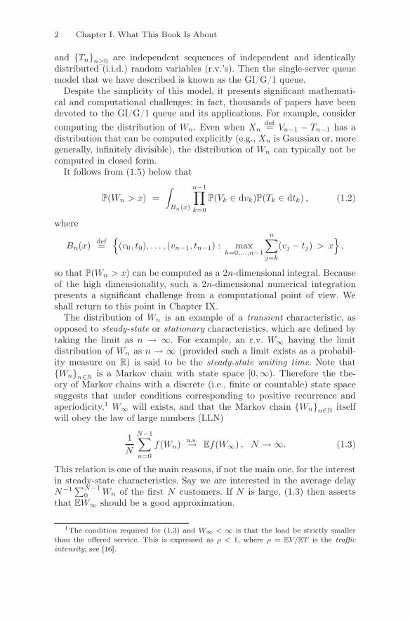
Despite the simplicity of this model, it presents significant mathemati-cal and computational challenges; in fact, thousands of papers have beendevoted to the GI/G/1 queue and its applications. For example, considercomputing the distribution of Wn. Even when Xn

def= Vn−1 − Tn−1 has adistribution that can be computed explicitly (e.g., Xn is Gaussian or, moregenerally, infinitely divisible), the distribution of Wn can typically not becomputed in closed form.

It follows from (1.5) below that

P(Wn > x) =∫

Bn(x)

n−1∏

k=0

P(Vk ∈ dvk)P(Tk ∈ dtk) , (1.2)

where

Bn(x)def=

{(v0, t0), . . . , (vn−1, tn−1) : max

k=0,...,n−1

n∑

j=k

(vj − tj) > x},

so that P(Wn > x) can be computed as a 2n-dimensional integral. Becauseof the high dimensionality, such a 2n-dimensional numerical integrationpresents a significant challenge from a computational point of view. Weshall return to this point in Chapter IX.

The distribution of Wn is an example of a transient characteristic, asopposed to steady-state or stationary characteristics, which are defined bytaking the limit as n → ∞. For example, an r.v. W∞ having the limitdistribution of Wn as n → ∞ (provided such a limit exists as a probabil-ity measure on R) is said to be the steady-state waiting time. Note that{Wn}n∈N

is a Markov chain with state space [0,∞). Therefore the the-ory of Markov chains with a discrete (i.e., finite or countable) state spacesuggests that under conditions corresponding to positive recurrence andaperiodicity,1 W∞ will exists, and that the Markov chain {Wn}n∈N

itselfwill obey the law of large numbers (LLN)

1N

N−1∑

n=0

f(Wn)a.s.→ Ef(W∞) , N →∞. (1.3)

This relation is one of the main reasons, if not the main one, for the interestin steady-state characteristics. Say we are interested in the average delayN−1

∑N−10 Wn of the first N customers. If N is large, (1.3) then asserts

that EW∞ should be a good approximation.

1The condition required for (1.3) and W∞ < ∞ is that the load be strictly smallerthan the offered service. This is expressed as ρ < 1, where ρ = EV/ET is the trafficintensity; see [16].

1. An Illustrative Example: The Single-Server Queue 3

Further transient characteristics of interest are first passage time quanti-ties such as the time inf {n : Wn > x} until a customer experiences a longdelay x, the number σ def= inf {n > 0 : Wn = 0} of customers served in abusy period (recall W0 = 0), and the total length V0 + · · · + Vσ−1 of thebusy period. For both transient and steady-state characteristics, it is alsoof obvious interest to consider other stochastic processes associated withthe system, such as the number Q(t) of customers in system at time t (in-cluding the one being presently served), and the workload V (t) (time toempty the system provided no new arrivals occur).

One of the key properties of the single-server queue is its close connectionto random walk theory, which as a nice specific feature allows representa-tions of steady-state distributions (equation (1.6) below) as well as transientcharacteristics (equation (1.5) below) in terms of an associated randomwalk. To make this connection precise, write as above Xk = Vk−1 − Tk−1

and Sndef= X1 + · · ·+Xn (with S0 = 0), and note that if customer 0 enters

an empty queue at time 0, then by (1.1),

W1 = max(X1, 0) = max(S1 − S0, S1 − S1

),

W2 = max(W1 +X2, 0)= max

(max(S1 − S0, S1 − S1) + S2 − S1, S2 − S2

)

= max(S2 − S0, S2 − S1, S2 − S2) = S2 −min

(S0, S1, S2

),

and in general,

Wn = Sn − mink=0,...,n

Sk = maxk=0,...,n

[Sn − Sk] . (1.4)

Under our basic assumption that {Vn}n≥0 and {Tn}n≥1 are independentsequences of i.i.d. r.v.’s, {Sn}n≥0 is a classical random walk, and (1.4)makes clear the connection between the GI/G/1 queue and the randomwalk.

Whereas (1.4) is a sample-path relation, a time-reversion argument trans-lates (1.4) into a distributional relation of a simpler form. Indeed, usingthat(Sn − Sn, Sn − Sn−1, Sn − Sn−2, . . . , Sn − S1, Sn − S0

)

=(0, Xn, Xn +Xn−1 , . . . , Xn + · · ·+X2, Xn + · · ·+X1

)

D=(0, X1, X1 +X2, . . . , X1 + · · ·+Xn−1, X1 + · · ·+Xn

)

=(S0, S1, S2, . . . , Sn−1, Sn

),

where D= denotes equality in distribution, we get

Wn = maxk=0,...,n

[Sn − Sk]D= max

k=0,...,nSk

def= Mn . (1.5)


As a consequence, WnD→W∞ as n→∞, where

W∞D= M

def= maxk≥0

Sk . (1.6)

It follows that if ρ = EV0/ET0 < 1 (i.e., the mean arrival rate 1/ET0 issmaller than the service rate 1/EV0), then W∞ is a proper r.v. (so that thesteady state is well defined), and

P(W∞ > x) = P(M > x) = P(τ(x) <∞) , (1.7)

where τ(x) def= min {n > 0 : Sn > x}.It is easily seen that P(W∞ > x) satisfies the integral equation

P(W∞ > x) =∫ ∞

0

P(W∞ ∈ dy)P(X1 > x− y) (1.8)

(the analogue of the stationarity equation for a Markov chain). One possiblemeans of computing the distribution ofW∞ is therefore to numerically solve(1.8). However, rewriting (1.8) in the equivalent form

P(W∞ ≤ x) =∫ ∞

0

P(W∞ ≤ x− y)P(X1 ∈ dy)

shows that (1.8) is of Wiener–Hopf type, and such equations are known tobe numerically challenging.

The analytically most tractable special case of the GI/G/1 queue is theM/M/1 queue, where both the interarrival time and the service time distri-bution are exponential,2 say with rates (inverse means) λ, μ. Then ρ = λ/μ,and the distribution of W∞ is explicitly available,

P(W∞ ≤ x) = 1− ρ + ρ(1− e−γx) ,

where γ def= μ − λ; the probabilistic meaning of this formula is that theprobability P(W∞ = 0) that a customer gets served immediately equals 1−ρ, whereas a customer experiences delay w.p. ρ, and conditionally upon thisthe delay has an exponential distribution with rate parameter γ. Further,this is also the distribution of the steady-state workload V (∞), and thesteady-state queue length Q(∞) is geometric with success parameter 1− ρ(cf. A1), i.e., P

(Q(∞) = n

)= (1 − ρ)ρn, n ∈ N. There are also explicit

formulas for a number of transient characteristics such as the busy perioddensity and the transition probabilities ptij = P

(Q(s + t) = j

∣∣Q(s) = i

)

of the Markov process {Q(t)}t≥0, but the expressions are complicated andinvolve Bessel functions, even infinite sums of such, cf. [16, Section III.9].

Beyond the M/M/1 queue, the easiest special case of the GI/G/1 queueis GI/M/1 (exponential services), where steady-state quantitites have an

2M stands for Markovian or Memoryless. Note that the arrival process is just aPoisson process with rate λ.

2. The Monte Carlo Method 5

explicit distribution given that one has solved the transcendental equationEeγ(V−T ) = 1. Also, M/G/1 (Poisson arrivals) simplifies considerably, asdiscussed in Example 5.15 below.

2 The Monte Carlo Method

Given the stochastic origin of the integration problem (1.3), it is natural toconsider computing P(Wn > x) by appealing to a sampling-based method.In particular, suppose that we could implement algorithms (on one’s com-puter) capable of generating two independent sequences of i.i.d. r.v.’s{Vn}n≥0 and {Tn}n≥0 with the appropriate service-time and interarrival-time distributions. Then, by recursively computing the Wk according to theLindley recursion (1.1), we would thereby obtain the r.v. Wn. By repeat-edly drawing additional Vk and Tk, one could then obtain R i.i.d. copiesW1n, . . . ,WRn of Wn. The probability z def= P(Wn > x) could then be com-puted via the sample proportion of the Wrn that are greater than x, namelyvia the estimator

zdef= zR

def=1R

R∑

r=1

1{Wrn > x}

(1 = indicator function). The LLN (1.3) guarantees, of course, that thealgorithm converges to z = P(Wn > x) as the number R of independentreplications tends to ∞.

This example exposes a basic idea in the area of stochastic simulation,namely to simulate independent realizations of the stochastic phenomenonunder consideration and then to compute an estimate for the probabil-ity or expectation of interest via an appropriate estimator obtained fromindependent samples.

To be more precise, suppose that we want to compute z = EZ. The ideais to develop an algorithm that will generate i.i.d. copies Z1, . . . , ZR of ther.v. Z and then to estimate z via the sample-mean estimator

zdef= zR

def=1R

R∑

r=1

Zr . (2.1)

In other words, one runs R independent computer experiments replicatingthe r.v. Z, and then computes z from the sample. Use of random samplingor a method for computing a probability or expectation is often called theMonte Carlo method. When the estimator z of z = EZ is an average ofi.i.d. copies of Z as in (2.1), then we refer to z as a crude Monte Carlo(CMC) estimator.

Note that an LLN also holds for many dependent and asymptoticallystationary sequences, see, for example, the discussion surrounding (1.3) for


Markov chains and Chapter IV. As a consequence, one can compute char-acteristics like

∫fdπ of the limiting stationary distribution π by averaging

over a long simulation-time horizon. For example, the integral equation(1.8) can be solved numerically in this way.

3 Second Example: Option Pricing

Financial mathematics has in recent years become one of the major ap-plication areas of stochastics. It draws on the one hand from a bodyof well-established theory, and on the other, it raises new problems andchallenges, both from the theoretical and computational points of view.

The most classical problem in financial mathematics is option pricing,which we use here to parallel the single-server queue as a vehicle for il-lustrating some of the key issues arising in simulation. The prototype ofan option is a European call option, which gives the holder the right (butnot the obligation) to buy a certain amount of a given asset at the priceK at time T (the maturity time). For example, the asset can be crude oil,and the option then works as an insurance against high oil prices. Moreprecisely, if S(T ) is the market price3 of the specified amount of oil at timeT and S(T ) < K, the holder will not exercise his right to buy at price K,but will buy at the market at price S(T ). Conversely, if S(T ) > K, theholder will buy and thereby make a gain of S(T )−K compared to buyingat the market price. Thus,

[S(T )−K

]+ is the value of exercising the op-tion relative to buying at market price. What price Π should one pay foracquiring this option at time t = 0?

Let r be the continuously compounded interest rate (the short rate), sothat the value at time 0 of receiving one monetary unit at time t is e−rt.Traditional thinking would just lead to the price e−rTE

[S(T )−K]+ of the

option because the LLN predicts that this on average will favor neither thebuyer nor the seller, assuming that both trade a large number of optionsover time. This is indeed how, for example, actuaries price their insurancecontracts. Economists take a different starting point, the principle of noarbitrage, which states that the market will balance itself in such a waythat there is no way of making money without risk (no free lunches). The“market” needs specification in each case, but is often a world with onlytwo objects to invest in at time 0 ≤ t < T : the bank account (which mayhave a negative value) yielding a risk-free return at short rate r and theunderlying asset priced at S(t). Indeed, this leads to a different price of theoption, as we will now demonstrate via an extremely simple example.

3Since S(T ) is not known at time t = 0, this is a random quantity, and we use P, E torefer to this; for example, the expected gain of holding the option is e−rT

E[S(T )−K

]+.

3. Second Example: Option Pricing 7

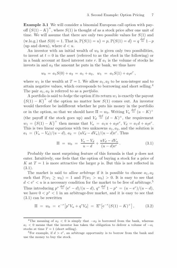
Example 3.1 We will consider a binomial European call option with pay-off(S(1)−K)+, where S(1) is thought of as a stock price after one unit of

time. We will assume that there are only two possible values for S(1) and(w.lo.g.) that S(0) = 1. That is, P

(S(1) = u

)= p, P

(S(1) = d

)= q

def= 1−p(up and down), where d < u.

An investor with an initial wealth of w0 is given only two possibilities,to invest at t = 0 in the asset (referred to as the stock in the following) orin a bank account at fixed interest rate r. If a1 is the volume of stocks heinvests in and a2 the amount he puts in the bank, we thus have

w0 = a1S(0) + a2 = a1 + a2, w1 = a1S(1) + a2er ,

where w1 is the wealth at T = 1. We allow a1, a2 to be non-integer and toattain negative values, which corresponds to borrowing and short selling.4The pair a1, a2 is referred to as a portfolio.

A portfolio is said to hedge the option if its return w1 is exactly the payout(S(1) − K

)+ of the option no matter how S(1) comes out. An investorwould therefore be indifferent whether he puts his money in the portfolioor in the option, so that we should have Π = w0. Writing Vu

def= (u−K)+

(the payoff if the stock goes up) and Vddef= (d − K)+, the requirement

w1 =(S(1) − K

)+ then means that Vu = a1u + a2er, Vd = a1d + a2er.This is two linear equations with two unknowns a1, a2, and the solution isa1 = (Vu − Vd)/(u− d), a2 = (uVd − dVu)/(u− d)er . Thus

Π = w0 =Vu − Vdu− d

+uVd − dVu(u − d)er

. (3.1)

Probably the most surprising feature of this formula is that p does notenter. Intuitively, one feels that the option of buying a stock for a price ofK at T = 1 is more attractive the larger p is. But this is not reflected in(3.1).

The market is said to allow arbitrage if it is possible to choose a1, a2

such that P(w1 ≥ w0) = 1 and P(w1 > w0) > 0. It is easy to see thatd < er < u is a necessary condition for the market to be free of arbitrage.5

Thus introducing p∗ def= (er − d)/(u − d), q∗ def= 1− p∗ = (u− er)/(u− d),we have 0 < p∗ < 1 in an arbitrage-free market, and it is easy to see that(3.1) can be rewritten

Π = w0 = e−r[p∗Vu + q∗Vd] = E

∗[e−r(S(1)−K)+], (3.2)

4The meaning of a2 < 0 is simply that −a2 is borrowed from the bank, whereasa1 < 0 means that the investor has taken the obligation to deliver a volume of −a1

stocks at time T = 1 (short selling).5For example, if d > er , an arbitrage opportunity is to borrow from the bank and

use the money to buy the stock.


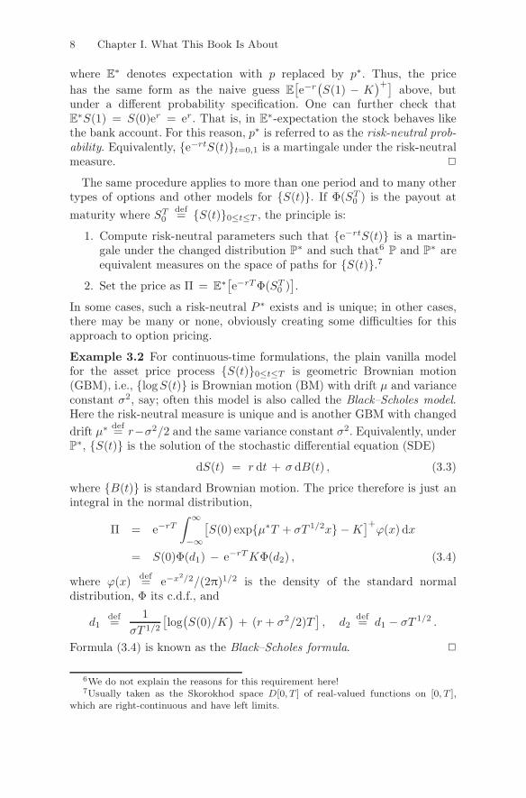
where E∗ denotes expectation with p replaced by p∗. Thus, the price

has the same form as the naive guess E[e−r

(S(1) − K

)+] above, butunder a different probability specification. One can further check thatE∗S(1) = S(0)er = er. That is, in E

∗-expectation the stock behaves likethe bank account. For this reason, p∗ is referred to as the risk-neutral prob-ability. Equivalently, {e−rtS(t)}t=0,1 is a martingale under the risk-neutralmeasure. �

The same procedure applies to more than one period and to many othertypes of options and other models for {S(t)}. If Φ(ST0 ) is the payout atmaturity where ST0

def= {S(t)}0≤t≤T , the principle is:

1. Compute risk-neutral parameters such that {e−rtS(t)} is a martin-gale under the changed distribution P

∗ and such that6 P and P∗ are

equivalent measures on the space of paths for {S(t)}.72. Set the price as Π = E

∗[e−rTΦ(ST0 )].

In some cases, such a risk-neutral P ∗ exists and is unique; in other cases,there may be many or none, obviously creating some difficulties for thisapproach to option pricing.

Example 3.2 For continuous-time formulations, the plain vanilla modelfor the asset price process {S(t)}0≤t≤T is geometric Brownian motion(GBM), i.e., {logS(t)} is Brownian motion (BM) with drift μ and varianceconstant σ2, say; often this model is also called the Black–Scholes model.Here the risk-neutral measure is unique and is another GBM with changeddrift μ∗ def= r−σ2/2 and the same variance constant σ2. Equivalently, underP∗, {S(t)} is the solution of the stochastic differential equation (SDE)

dS(t) = r dt + σ dB(t) , (3.3)

where {B(t)} is standard Brownian motion. The price therefore is just anintegral in the normal distribution,

Π = e−rT∫ ∞

−∞

[S(0) exp{μ∗T + σT 1/2x} −K

]+ϕ(x) dx

= S(0)Φ(d1) − e−rTKΦ(d2) , (3.4)

where ϕ(x) def= e−x2/2/(2π)1/2 is the density of the standard normal

distribution, Φ its c.d.f., and

d1def=

1σT 1/2

[log(S(0)/K

)+ (r + σ2/2)T

], d2

def= d1 − σT 1/2 .

Formula (3.4) is known as the Black–Scholes formula. �

6We do not explain the reasons for this requirement here!7Usually taken as the Skorokhod space D[0, T ] of real-valued functions on [0, T ],

which are right-continuous and have left limits.

4. Issues Arising in the Monte Carlo Context 9

In view of the Black–Scholes formula, Monte Carlo simulation is notrequired to price a European call option in the GBM model. The needarises when one goes beyond this model, e.g., in the case of basket options(see below) or Lévy models, which have recently become popular, see Cont& Tankov [75] and Chapter XII.

Further examples of options include:

Asian (call) options, where the payoff Φ(ST0 ) is (A − K)+, where A isan arithmetic average, either T−1

∫ T0S(t) dt (continuous sampling)

or N−1∑N

1 S(nT/N) (discrete sampling). In the example where theunderlying asset is the oil price and the buyer an oil consumer, theAsian option serves to ensure a maximal spending of NK in [0, T ].

Put options, where the options gives the right to sell rather than to buy.For example, an European put option has payoff Φ(ST0 ) =

[K −

S(T )]+ and ensures a minimum price of K for the asset when sold

at time T . Similar remarks apply to Asian put options with Φ(ST0 ) =(A−K)+.

Barrier options, where in addition to the strike price K one specifies alower barrier L < K and the payout depends on whether the lowerbarrier is crossed before T . There are now a variety of payoff functions,e.g., Φ(ST0 ) =

(S(T )−K)+1 {τ > T} (“down and out”), where τ def=

inf{t : S(t) < L}.Basket options, where, as one example, S(t) can be the weighted sum of

several stock prices, that is, the value of a portfolio of stocks.

For the GBM Black–Scholes model, there are explicit formulas for theprice of many types of options. Even so, Monte Carlo simulation is requiredto price some options in this model, e.g., a discretely sampled Asian option.For most other models, explicit price formulas are typically not availableeven for European options. In addition to alternative assumptions on thedynamics of {S(t)}, examples of model extensions beyond Black–Scholesinclude stochastic volatility and stochastic interest rate models, where theσ in (3.3) (the volatility) and/or the short rate r are replaced by stochasticprocesses {σ(t)}, {r(t)}.

4 Issues Arising in the Monte Carlo Context

We turn next to a discussion of some of the computational issues that arisein the Monte Carlo context.

Issue 1: How do we generate the needed input random variables?

Our above discussion for the GI/G/1 queue assumes the ability to generate


independent sequences {Vn} and {Tn} of i.i.d. r.v.’s with appropriately de-fined distributions. Similarly, in the example of European options, we needto be able to generate S(T ) under the distributional assumption under con-sideration. The simplest examples are the M/M/1 queue, where the Vk, Tkare exponential, and the the Black-Scholes model where S(T ) is lognor-mal or, equivalently, log S(T ) is normal, but more complicated models canoccur, see, for example, Chapter XII.

As will be seen in Chapter II, all such algorithms work by transforming asequence of uniform i.i.d. r.v.’s into the appropriate randomness needed fora given application. Thus, we shall need to discuss the generation of i.i.d.uniform r.v.’s (II.1 = Section 1 of Chapter II) and to show how such uniformrandomness can be transformed into the required nonuniform randomnessneeded by the simulation experiment (II.2–II.6).

In the option-pricing example, we have the additional difficulty that wecannot simulate the entire path {S(t)}0≤t≤T . At best, we can simulate{S(t)}0≤t≤T only at a finite number of discrete time points. Furthermore,because {S(t)} typically evolves continuously through dynamics specifiedvia an SDE, the same difficulties can arise here as in the solution of ordinary(deterministic) differential equations (ODEs). In particular, the forwardsimulation via the process with a finite-difference approximation induces asystematic bias into the simulated process. This is comparable to the errorassociated with finite-difference schemes for ODEs; see further Chapter X.

Issue 2: How many computer experiments should we do?

Given that we intend to use the Monte Carlo method as a computationaltool, some means of assessing the accuracy of the estimator is needed. Sim-ulation output analysis comprises the body of methods intended to addressthis issue (Chapter III). One standard way of assessing estimator accuracyis to compute a (normal) confidence interval for the parameter of interest,so a great deal of our discussion relates to computing such confidence in-tervals. Special difficulties arise in:(a) the computation of steady-state expectations, as occurs in analyzingthe steady-state waiting time r.v. W∞ of the GI/G/1 queue (the limit indistribution of Wn as n→∞), see Chapter IV;(b) quantile estimation, as occurs in value-at-risk (VaR) calculations forportfolios; see Example 5.17 and III.4a.

A necessary condition for approaching item (a) at all is of course thatwe be able to deal with the following issue.

Issue 3: How do we compute expectations associated with limiting station-ary distributions?

For the GI/G/1 queue, the problem is of course that the relationWnD→W∞

and the possibility of generating an r.v. distributed as Wn does not allowus to generate an r.v. distributed as W∞. In other words, we are facing

4. Issues Arising in the Monte Carlo Context 11

an infinite-horizon problem, in which an ordinary Monte Carlo experimentcannot provide an answer in finite time. This is also clearly seen from theformula (1.7), stating that P(W∞ > x) = P(M > x) = P(τ(x) < ∞),where τ(x) = min {n > 0 : Sn > x} and M = maxn=0,1,2,... Sn. Indeed,simulating a finite number n of steps of the random walk Sn cannot de-termine the value of M but only of Mn, and furthermore, one can getan answer only to whether the event {τ(x) ≤ n} occurs but not whether{τ(x) <∞} does.

Of course, one possible approach is to use a single long run of the Wn

and appeal to the LLN; cf. the concluding remarks of Section 2. Here,the complication is that error assessment will be challenging because theobservations are serially correlated.

Option-pricing examples typically involve only a finite horizon. However,a currently extremely active area of steady-state simulation with a ratherdifferent flavor from that of queuing models is Markov chain Monte Carlomethods (MCMC), which we treat separately in Chapter XIII; some keyapplication areas are statistics, image analysis, and statistical physics.

Issue 4: Can we exploit problem structure to speed up the computation?

Unlike the sampling environment within which statisticians work, themodel that is generating the sample is completely known to the simulator.This presents the simulator with an opportunity to improve the computa-tional efficiency (i.e., the convergence speed as a function of the computertime expended) by exploiting the structure of the model.

For example, in a discretely sampled Asian option, the geometric averageAgeom

def=[S(T/N) · S(2T/N) · · ·S(T )

]1/N has a lognormal distribu-tion with easily computable parameters in the Black–Scholes model. ThusEAgeom is known, and for any choice of λ ∈ R,

(A−K)+ − λ(Ageom − EAgeom

)

is again an estimator having mean E(A−K)+. Hence, in computing E(A−K)+, the simulator can choose λ to minimize the variance of the resultingestimator, thereby improving the efficiency of the naive estimator.

Similarly, in the context of the GI/G/1 queue, EX1 is known, so that forany choice of λ ∈ R,

Wn − λ(Sn − nEX1

)

is again an estimator having mean EWn.The common idea of these two examples is just one example of variance

reduction (and is the one specifically known as the method of control vari-ates). Use of good variance-reduction methods can significantly enhancethe efficiency of a simulation (and is discussed in detail in Chapter V).

Issue 5: How does one efficiently compute probabilities of rare events?

Suppose that we wish to compute the probability that a typical customer in


steady state waits more than x prior to receiving service, i.e., P(W∞ > x).If x is large, z def= P(W∞ > x) (or, equivalently, z = P(τ(x) < ∞)) isthe probability of a rare event. For example, if z = 10−6, the fraction ofcustomers experiencing waiting times exceeding x is one in a million, sothat the simulation of 10 million customers provides the simulator with(on average) only 10 samples of the rare event. This suggests that accuratecomputation of rare-event probabilities presents significant challenges tothe simulator.

Chapter VI is devoted to a discussion of several different methods for in-creasing the frequency of rare events, and thereby improving the efficiencyof rare-event simulation. The topic is probably more relevant for queuingtheory and its communications applications than for option pricing. How-ever, at least some option-pricing problems exhibit similar features, say aEuropean call option that is out-of-the-money (P

(S(T ) > K

)is small),

and rare events also occur in VaR calculations, in which a not uncommonquantile to look for is the 99.97% quantile, cf. McNeil et al. [252].

Issue 6: How do we estimate the sensitivity of a stochastic model tochanges in a parameter?

The need to estimate such sensitivities arises in mathematical finance inhedging. More precisely, in a hedging portfolio formed by a bank accountand the asset underlying the option one tries to hedge, it holds rathergenerally (Björk [45]) that the amount to invest in the asset at time t shouldequal what is called the the delta, the partial derivative of the expectedpayout at maturity w.r.t. the current asset price. For another example,assume that in the Black–Scholes model the volatility σ is not completelyknown but provided as an estimate σ. This introduces some uncertaintyin the option price Π, for the quantification of which we need ∂Π/∂σ, thevega.

In the GI/G/1 queue, suppose we are uncertain about the load the sys-tem will face. In such circumstances, it may be of interest to compute thesensitivity of system performance to changes in the arrival rate. More pre-cisely, suppose that we consider a parameterized system in which the arrivalepochs are given by the sequence

{λ−1An

}, so that λ/EA1 is the arrival

rate. The sensitivity of the system performance relating to long delays isthen (d/dλ)P(W∞ > x).

Chapter VII discusses the efficient computation of such derivatives (or,more generally, gradients).

Issue 7: How do we use simulation to optimize our choice of decision pa-rameters?

Suppose that in the GI/G/1 queue with a high arrival rate (say exceedingλ0), we intend to route a proportion p of the arriving customers to an alter-native facility that has higher cost but is less congested, in order to ensure

5. Further Examples 13

that customers are served promptly. There is a trade-off between increas-ing customer satisfaction (increasing p) and decreasing costs (decreasing p).The optimal trade-off can be determined as the solution to an optimizationproblem in which the objective function is computed via simulation.

Also, the pricing of some options involves an optimization problem. Forexample, an American option can be exercised at any stopping time τ ≤ T

and then pays(S(τ)−K)+. Optimizing τ for American options is a high-

dimensional optimization problem, which due to its complexity and specialnature is beyond the scope of this book (we refer to Glasserman [133,Chapter 8]), but is mentioned here for the sake of completeness.

A discussion of algorithms appropriate to simulation-based optimizationis offered in Chapter VIII.

5 Further Examples

The GI/G/1 queue and option pricing are of course only two among manyexamples in which simulation is useful. Also, in some cases, other appli-cations involve other specific problems than those discussed in Section 4,and the evaluation of an expected value is far from the only application ofsimulation. The following examples are intended to illustrate these pointsas well as to introduce some of the models and problems that serve asrecurrent examples throughout the book.

Example 5.1 Let f : (0, 1)d → R be a function defined on the d-dimensionalhypercube and assume we want to compute

zdef=

∫

(0,1)d

f(u1, . . . , ud

)du1 · · · dud =

∫

(0,1)d

f(u) du ,

where u def=(u1, . . . , ud

). We can then write z = Ef

(U1, . . . , Ud

)=

Ef(U), where U1, . . . , Ud are i.i.d. r.v.’s with a uniform(0, 1) distributionand U def=

(U1, . . . , Ud

), and apply the Monte Carlo method as for the

GI/G/1 queue to estimate z via

zdef=

1R

(f(U1) + · · ·+ f(UR)

),

where U1, . . . ,UR are i.i.d. replicates of U ; these can most often be easilygenerated by taking advantage of the fact that uniform(0, 1) variables arebuilt in as standard in most numerical software packages (a totality of dRsuch variables is required).

Of course, the nonrandomized computation of the integral z has beenthe topic of extensive studies in numerical analysis, and for small d andsmooth integrands f , standard quadrature rules perform excellently andare in general superior to Monte Carlo methods (see further Chapter IX).


More generally, let f : Ω → R be defined on a domain Ω ∈ Rd. We can

then choose some reference density g(x) on Ω and write

z =∫

Ω

f(x) dx =∫

Ω

f(x)g(x)

g(x) dx = E

[f(X)g(X)

],

whereX is an r.v. with density g(x). Thus replicatingX provides a MonteCarlo estimate of z as the average of the f(Xr)/g(Xr). For example, g(x)could be the N (0, Id) density or, if Ω ⊆ (0,∞)d, the density e−x1−···−xd ofd i.i.d. standard exponentials. Another procedure in the case of a generalΩ is to use a transformation ϕ : Ω → (0, 1)d, where ϕ is 1-to-1 onto ϕ(Ω).Then

z =∫

Ω

f(x) dx =∫

ϕ(Ω)

f(ψ(u))J(u) du = E[f(ψ(U))J(U )

],

where ψ def= ϕ−1 and J(u) is the Jacobian, that is, the absolute value ofthe determinant of the matrix

(∂x∂u

)=

⎛

⎜⎜⎝

∂ψ1(u)∂u1

. . . ∂ψd(u)∂u1

......

∂ψ1(u)∂ud

. . . ∂ψd(u)∂ud

⎞

⎟⎟⎠ .

We return to integration in Chapter IX. �

Example 5.2 An example of a similar flavor as the last part of Exam-ple 5.1 occurs in certain statistical situations in which the normalizingconstant z(θ) determining a likelihood fθ(x)/z(θ) is not easily calculated.That is, we have an observation x that is the outcome of a r.v. X takingvalues in Ω (where Ω is some arbitrary space) with distribution Fθ governedby a parameter θ, such that the density w.r.t. some reference measure μ(independent of θ) on Ω is fθ(y)/z(θ), where thus z(θ) def=

∫Ωfθ(y)μ(dy).

However, there are situations in which z(θ) is not easily calculated, even ifthe form of fθ(y) is simple.

If r.v.’s X1, . . . , XR with density fθ(x)/z(θ) are easily simulated, we mayjust for each θ calculate z(θ) as the average of the Z def= fθ(Xr). However,often this is not the case, whereas generation from a reference distributionG with density g(x) is easy. One may then write

z(θ) =∫

Ω

fθ(y)g(y)

g(y)μ(dy) = EGZ(θ) ,

where Z(θ) def= fθ(X)/g(X), and determine z(θ) by Monte Carlo simulation,whereX is generated from G. A suitable choice of G could often be G = Fθ0for some θ0 such that Fθ0 has particularly simple properties.

The procedure is a first instance of importance sampling, to which wereturn in V.1.

5. Further Examples 15

Consider, for example, point processes in a bounded region Ω in the plane(or in R

d), which are often specified in terms of an unnormalized densityfθ w.r.t. the standard Poisson process. One example is the Strauss process.A point x in the sample space can be identified with a finite (unordered)collection a1, . . . ,am, where m = m(x) is the number of points and ai theposition of the ith. Then fθ(x) = λm(x)ηt(x) for the Strauss process, where

θ = (λ, η) ∈ (0,∞)× [0, 1] , t(x) def=∑

i�=j1{d(ai,aj) < r}

(Euclidean distance) and 0 < r < ∞ is given. For η = 1, this is just thePoisson(λ) process, whereas η = 0 corresponds to a so-called hard-coremodel, in this case a Poisson process conditioned to have no pair of pointsat distance less than r; the interpretation of the intermediate case 0 < r < 1is some repulsion against points being closer than r. For simulation of z(θ),one would obviously take θ0 = (λ, 1) since a Poisson process is easy tosimulate. See further Møller & Waagepetersen [265]. �

Example 5.3 A further related example is counting the number of ele-ments z def= |S| of a finite but huge and not easily enumerated set S. Assumethat S ⊆ T with T finite and that some r.v. X on T is easily simulated,say the point probabilies are p(x) def= P(X = x). We can then write

z =∑

x∈T1x∈S =

∑

x∈T

1p(x)

1x∈S p(x) = EZ ,

where Z def= 1X∈S/p(X), and apply the Monte Carlo method.For example, consider the graph-coloring problem in which S is the set

of possible colorings of the edges E of a graph G = (V,E) (V is the set ofvertices) with colors 1, . . . , q such that no two edges emanating from thesame vertex have the same color. Say V is a set of countries on a map andtwo vertices are connected by an edge if the corresponding countries havea piece of common border. An obvious choice is then to take T as the setof all possible colorings (the cardinality is n def= |E|q) and X as uniform onT such that p(x) = 1/n.

This is an instance of a randomized algorithm, that is, an algorithm thatinvolves coin-tossing (generated randomness) to solve a problem that is inprinciple deterministic. There are many examples of this, with Motwani &Raghavan [263] being a standard reference. We return to some in XIV.1.Other main ones like QUICKSORT, which sorts a list of n items, are notdiscussed because the involved simulation methodology is elementary.

Note that the suggested algorithm for the graph-coloring problem issomewhat deceiving because in practice |T | is much bigger than |S|, makingthe algorithm inefficient (for efficiency, p(·) should be have substantial masson S, cf. Exercise V.1.3). We return to alternative strategies in XIV.3. �


Example 5.4 An important area of application of randomized algorithmsis optimization, that is, finding and locating the minimum of a deterministicfunction H(x) on some feasible region S.

One approach involves the Boltzmann distribution with density f(x) def=e−H(x)/T /C w.r.t. some measure μ(dx), where C = C(T ) is a normalizingconstant ensuring

∫f dμ = 1. Here one refers to H as the Hamiltonian or

energy function, and to T as the temperature (sometimes the definition alsoinvolves Planck’s constant, which, however, conveniently can be absorbedinto T ). At high temperatures, the distribution is close to μ; at low, itconcentrates its mass on x-values with a small H(x). By choosing T smalland generating an r.v.X according to f , the outcome ofH(X) will thereforewith high probability be close to the minimum.

We return to this and further examples in XIV.1. �

Example 5.5 Filtering or smoothing means giving information about anunobserved quantity X from an observation Y . Often, the joint densityf(x, y) of X,Y is readily available, but the desired conditional density

f(x|y) =f(x, y)∫f(x′, y) dx′

(5.1)

of X given Y involves a normalization constant obtained by integrating x′out in f(x′, y), a problem that is often far from trivial. Examples of filteringare reconstructing the current location of a target from noisy observationsand reconstructing a signal or an image from blurred observations; seefurther XIII.2d and A5. Here often the observations arrive sequentially intime and X is a segment of a Markov chain with possibly nondiscrete statespace. The problem is essentially the same as that of Bayesian statistics(see XIII.2a), where X plays the role of an unknown parameter (usuallydenoted by θ) with a prior π0(x), so that the joint density of (X,Y ) isf(x, y) = π0(x)f(y |x), where f(y |x) is the likelihood, and (5.1) is theposterior on x.

In the setting of filtering, Bayesian statistics, likelihood computations asin Example 5.2, the Bolztmann distribution, a uniform distribution on afinite set S with an unknown number S of elements (cf. Example 5.3), andmany other situations with a density f(x) only known up to a constant,most standard methods for generating r.v.’s from f(x) fail. For example,how do we generate a realization of the Strauss process, or a point patternthat at least approximately has the same distributional properties?

One approach is provided by Markov chain Monte Carlo methods, a topicof intense current activity, as further discussed in Chapter XIII. Anotheris resampling methods and particle filtering, as surveyed briefly in XIV.2.

�

Example 5.6 A PERT net is a certain type of directed graph with oneintial node � and one terminal node �. It models a production process,whose stages are represented by the edges of the graph (PERT = Project

Mathematical Economics and Finance Applications of...

Documents

Transcript of Mathematical Economics and Finance Applications of...