MATHEMATICAL CONCEPTS IN HYDRAULIC WELL ANALYSIS

by

Tom Arnold Abstract

Analytical concepts have long been available to aid in the drilling, completion and production of oil and gas wells. However, a vast majority of the wells were shallow and located in well understood areas making the need for such technology minimal at best. The story is quite different today. Wells are being drilled to great depths in an effort to locate untapped reservoirs. This also means drilling unknown areas. For this reason, focus has now shifted to ways of detecting approaching pressures, ways of keeping the drilling operation moving on schedule with the lowest cost, ways of preventing and killing kicks, etc. It is to these concepts that this paper is dedicated. A. HYDRAULIC SYSTEM PRESSURE LOSSES Since the advent of rotary drilling, it has been an objective of the highest importance to calculate the hydraulic pressure losses present in a circulating system. To this end, many companies have produced a number of graphs, slide-rules and other devices in order to make the use of these simple mathematical concepts. However, the major drawback with the equations and the calculating devices is that each took about the same amount of time to use. With the introduction of today's modern programmable calculators, these equations can be written, saved and used with lightning speed and accuracy. Two methods of calculation are in use today; Bingham Plastic and Power Law. The Bingham Plastic model was developed first and has now been replaced by the more accurate Power Law model. Basically, the difference in the two approaches is the number of variables taken into account. All of which have a very marked effect on the fluid properties present in the circulating system. The rotating viscometer makes the analysis of two of the most important fluid properties possible, plastic viscosity and yield point. These values are derived from the Ө600 (600 rpm reading) and Ө300 (300 rpm reading). In order to begin calculating using the Power Law model we must first define n as the Shear Stress vs

Shear Rate. From this ratio we obtain a curve which allows derivation of the slope and intercept in the Power Law model. n can now be defined as: n = 3.32 * log (Ө600/Ө300) and k(intercept) is defined as:

𝑘 =Ө300

511𝑛

1. Internal Pressure Losses With knowledge of the slope and intercept of the Shear Stress vs Shear Rate we can begin analysis of the pressure losses inside the drilling string. In order to take into consideration as many variables as possible, we need an understanding of the factors effecting internal system pressure losses. Pressure losses are affected by: 1. depth 2. fluid properties i.e. mud wt., vis., yield, etc. 3. inside diameter of pipe 4. flow rate Taking these variables and fitting them into equations will yield direct calculation of the system pressure losses. Bingham Plastic Flow Model for Internal Pressure Loss The following equation should be applied to each segment of the drill string. The final summation of all the segments will then be the total system pressure loss. The equation is given by:

(PV) 𝑉𝑓 L + Y L

P = 90000 𝐷𝑖2 225 𝐷𝑖2 Where: P = segment pressure loss (psi) PV = plastic viscosity

𝑉𝑓 = fluid velocity (ft/min)

L = length of segment

Di = ID of pipe in segment Y = yield point Power Law Flow Model for Internal Pressure Loss Following is the equation used to calculate internal flow characteristics using the Power Law Model. It also is a segment equation with the final of segments being the total pressure loss.

P = ( 1.6 ∗Vf

Di ∗ ((3 ∗ n + 1)/4 ∗ n) )𝑛 ∗ ((𝑘 ∗ 𝐿)/(Ө300 ∗ 𝐷𝑖))

where: V = fluid velocity (ft/min) Di = ID of the pipe n = slope k = intercept L = length of segment P = pressure loss (psi)

Pump output will be required in subsequent equations. It is given by:

Q = (𝑃𝑂) ∗ 𝐶𝑃𝑀 ∗ 2 where: PO = BBL/STK CPM = strokes/min. Q = flow rate gal/min. Next, we must calculate the nozzle area in square inches. This equation is given by:

An = ((𝑁1/32)2 + (𝑁2/32)2 + (𝑁3/32)2 + (𝑁4/32)2) ∗ 𝝅 where: An = nozzle area (sq/in) Nl = nozzle #1 (32.nds of an inch) N2 = nozzle #2 " N3 = nozzle #3 " N4 = nozzle #4 "

The nozzle velocity is the next parameter which we must calculate before moving on to the pressure loss through the bit. The velocity equation is given by:

Vn = . 32 ∗ 𝑄 𝐴𝑛 where: Vn = nozzle velocity (ft/min) Q = circulation rate (gal/min) An = nozzle area in sq/in At this point, we are now ready to give the final equation for calculation of the bit nozzle pressure drop. This is given by the following equation:

P = 𝑀𝑊 ∗ 𝑉𝑛2 1120

where: P = pressure drop @ the bit (psi) MW = mud weight (ppg) Vn = velocity of the fluid in ft/min through the bit

2. Annular Pressure Losses In relating equations to the calculation of pressure losses in the annulus we must again consider the two models previously discussed; Bingham Plastic and Power Law. Both approaches produce designs capable of calculating annular pressure losses in addition to internal pressure losses. Again it is important to understand the factors acting upon this portion of the circulating system. The variables at play are: 1. depth 2. hole ID 3. pipe OD 4. circulation rate Taking into consideration these variables in addition to the variables present in each member of the above list we can give the following equations for annular pressure loss.

Bingham Plastic Flow Model for Annular Pressure Loss Keeping in mind the values calculated earlier i.e. Nozzle Area, Circulating Rate and Nozzle Velocity we give the following equation for Bingham Plastic:

𝑃 =𝑃𝑉 𝑥 𝐿 𝑥 𝑉

6000 (𝐷𝑕−𝐷𝑝)2 + 𝑌 𝑥 𝐿

200 ( 𝐷𝑕−𝐷𝑝)

where: P = pressure loss in that segment PV = plastic viscosity Y = yield point L= length of segment V= annular velocity where:

V = 24.5 𝑥 𝑄

(𝐷𝑕2− 𝐷𝑝2)

where: Q = circulation rate (gal/min) L = length of segment Dh = diameter of hole Dp = OD of drill pipe This time as before, this is a segmented equation. Thus the summation of all segments is the total system pressure loss. Power Law Model for Annular Pressure Loss Recalling the usage of the n(slope) and k(intercept) discussed earlier, we can now give the equation for annular pressure loss in the Power Law model:

P = (2.4 𝑥 𝑉)

(𝐷𝑕−𝐷𝑝)𝑥

(2 𝑥 𝑛+1)

3 𝑥 𝑛

𝑛

x 𝐾 𝑥 𝐿

300 (𝐷𝑕−𝐷𝑝)

P = annular pressure loss (psi) V= annular velocity (ft/min)

Dh = diameter of hole or casing Dp = OD of pipe or collars L= length of segment At this point, we have a clear picture of both internal and annular pressure losses occuring in our circulating system. As noted before, the Power Law model is the more accurate of the two models and should therefore be given the greater attention.

2.A. Reynolds #

Internal Re = (15,47 p Vf D) / vis Annular Re= (15.47 p Vf (Dh-Dp) )/ vis where: p = mud wt. ppg Vf = fluid velocity FPM pipe D = pipe diameter Vis= viscosity Dh= Diameter of hole Dp=Diameter of pipe Note: turbulent flow = Re = 3000 (transitional flow)

2.B. Friction Loss Calculations (From Reed Slide Rule)

A. Laminar Flow: 1. Annulus: P = YP (Dh - Dt) + PV x Va

.225 1.5 (𝐷𝑢 − 𝐷𝑡)2 2. Internal: P = YP (Dt) + PV x Va

.225 1.5 (𝐷𝑡)2 B. Turbulent Flow:

1. Annulus: P = .000228 𝑥 𝑉𝑎 1.8𝑥 𝑃𝑉 .2 𝑥 𝑝 .8

(𝐷𝑢−𝐷𝑡)1.2

2. Inside: P = .0765 𝑥 𝑄1.82 𝑥 𝑝 .82 𝑥 𝑃𝑉

𝐷𝑡4.82

.18

Where: P = Pressure loss in psi/1000 ft. YP = Yield Point

Du = Diameter of hole in inches Dt = Diameter of tube in inches (OD or ID) Va = Annular vel. fpm PV = Plastic Viscosity in cp P =Mud density in ppg Q =Pump Rate in gpm

2C Power Law Model for Turbulent and Laminar Flow

1. Internal Velocity ( Ft./min.):

Vf = 𝑄

2.45 𝑥 𝐼𝐷2 X 60

Where: Q = pump output (gal./min.) ID = pipe internal diameter in inches

2. Reynolds Number: Internal:

R =15.47 𝑥 𝑝 𝑥 𝑉𝑓 𝑥 𝐷

𝑣𝑖𝑠

Annular:

R = 15.47 𝑥 𝑃 𝑥 𝑉𝑓 𝑥 (𝐷𝑕−𝐷𝑝)

𝑣𝑖𝑠

Where : p = mud weight ppg Vf = fluid Velocity (ft./min.) D = hole size Dh = diameter of hole

Dp = pipe diameter

3. Turbulent Flow: Internal:

P = 7.7 𝑥 10 −5 𝑥 𝑝 .8𝑥 𝑄1.8 𝑥 𝑃𝑉 .2 𝐿

𝐼𝐷4.82

External:

𝑃 = 7.7 𝑥 10−5 𝑥 𝑝 .8𝑥 𝑄1.8 𝑥 𝑃𝑉 .2 𝑥 𝐿

𝐷𝑕−𝐷𝑝 3𝑥 𝐷𝐻+𝐷𝑝 1.8

Where: P = pressure loss for that segment in psi P = mud weight Q = pump output (gal./min.) L = length of segment

3. Laminar Flow Internal:

𝑃 = 1.6 𝑥 𝑉

𝐼𝐷𝑋

3 𝑥 𝑛+1

4 𝑥 𝑛 𝑛

X 𝐾 𝑥 𝐿

300 𝑥 𝐼𝐷

External:

P = 2.4 𝑥 𝑉

(𝐷𝑕−𝐷𝑝)𝑋

2 𝑥 𝑁+1

3 𝑥 𝑁

𝑛

X 𝐾 𝑥 𝐿

300 𝑥 (𝐷𝑕−𝐷𝑃)

Where: V = internal fluid velocity or external fluid velocity n = see page 1 K = see page 1 P = Laminar pressure loss psi

3. Equivalent Circulating Density (ECD) Now that we have methods where by we can calculate the total annular pressure drop, it is now possible to calculate what extra effect the fluid flow rate has upon the Mud weight. This extra effect is called the EQUIVALENT CIRCULATING DENSITY.

We must first calculate the pressure exerted by the mud column. This is given by: H = .052 * MW * L where: H = mud column pressure (psi) MW = mud weight (ppg) L = well depth feet Next we must calculate the total bottom hole pressure. This is given by: Ht = H + Tapl where: Ht = bottom hole pressure (psi) H = mud column pressure Tapl = total annular pressure loss (psi) We can now calculate the ECD by: ECD = Ht .052 L where: ECD = ECD in ppg Ht = total bottom hole pressure L = well depth The importance of the ECD becomes quite clear when near balance drilling is used to make the most hole in ght least amount of time without encountering a kick. Sometimes the extra effect of the pumps makes the difference in keeping the formation fluids in the formation.

4. Hydraulic Horsepower and Impact Force Two other important calculations are also available which allow calculation of the bottom hole horsepower and the effect of the fluid impacting on the formation. Both equations use data already calculated making the process quite simple. The first equation to be given will be that of Hydraulic Horsepower: HP = Pb * P.O. 1714

where: HP = hydraulic horsepower Pb = pressure drop @ bit (psi) . P0 = Pump Out put gal/min Next we can give the equation for Impact Force by:

IF = .0173 x PO x 𝑃𝑏 𝑥 𝑀𝑊 Where: IF = impact force PO = pump out in gal/min Pb = pressure drop @ bit (psi) MW = Mud weight (ppg)

SLIP VELOCITY (Terminal Settling Velocity) The ability of a drilling fluid to move a particle out of the hole is of the utmost importance when you consider the consequences of stuck pipe. For this reason it is valuable to know what annular velocity will best clean a well bore. The factors affecting this are: 1. Mud weight, Plastic Vis. 2. diameter of the particle 3. density of the particle With these variables in mind, we can give the first equation of three used in determining the best annular velocity.

Vs =.45 x 𝑃𝑉

(𝑀𝑊 𝑥 𝐷𝑝) x

36800

𝑃𝑉

𝑀𝑊 𝑥 𝐷𝑝

2 𝑥 𝐷𝑝 𝑥 𝑑𝑒𝑛𝑝 𝑥 8.33

𝑀𝑊 − 1 + 1 -1

Where: Vs = Slip velocity (ft/min) PV = Plastic Viscosity MW = Mud weight Dp = diameter of particle denp = density of particle (gm/cc) now we have: Vac = 2 * Vs

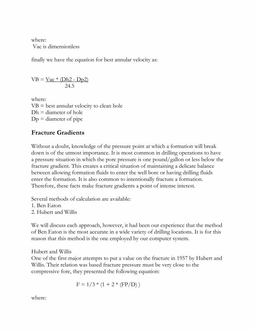
where: Vac is dimensionless finally we have the equation for best annular velocity as: VB = Vac * (Dh2 - Dp2) 24.5 where: VB = best annular velocity to clean hole Dh = diameter of hole Dp = diameter of pipe

Fracture Gradients Without a doubt, knowledge of the pressure point at which a formation will break down is of the utmost importance. It is most common in drilling operations to have a pressure situation in which the pore pressure is one pound/gallon or less below the fracture gradient. This creates a critical situation of maintaining a delicate balance between allowing formation fluids to enter the well bore or having drilling fluids enter the formation. It is also common to intentionally fracture a formation. Therefore, these facts make fracture gradients a point of intense interest. Several methods of calculation are available: 1. Ben Eaton 2. Hubert and Willis We will discuss each approach, however, it had been our experience that the method of Ben Eaton is the most accurate in a wide variety of drilling locations. It is for this reason that this method is the one employed by our computer system. Hubert and Willis One of the first major attempts to put a value on the fracture in 1957 by Hubert and Willis. Their relation was based fracture pressure must be very close to the compressive fore, they presented the following equation: F = 1/3 * (1 + 2 * (FP/D) ) where:

F = formation fracture gradient (psi/ft) FP = formation pressure (psi) D = depth The term "Fracture Gradient" refers to the maximum pressure required to break a formation at a given depth in either a fresh or salt water environment. Dr. Ben Eaton proposed a method whereby several variables are introduced: over - burdened stress, Os, Poisson's Ratio, V, Depth, D, Pore Pressure, Pp. In addition to these standard variables, other factors effecting the depth are taken into consideration. These include depth to land or water, depth of the water, length from rotary to flow line. Since the native fluid is also of paramount importance, this must also be injected into the calculation framework. By way or review, these two variables are .465 for salt water and .433 for fresh water. Ben Eaton's basic equation form Fracture Pressure is given by:

F = 𝑂𝑠−𝑃𝑝

𝐷 x

𝑉

1−𝑉 +

𝑃𝑝

𝐷 x 19.23

Where F is the fracture pressure in pounds per gallon now overburden stress Os for land operation is calculated by: Os = [proprietary to T Arnold] Poisson's ratio is the next step in calculation. This equation is given by: V = [proprietary to T Arnold] Special Note: For water based operations, overburden stress is given by: Os = [proprietary to T Arnold] Os = (Gradient + Os) * 1000 Compensating for equivalent depth may be accomplished in the three steps that follow: 1. We must compensate for the water depth by: P = D * N Where: P = pressure exerted by water )psi)

D = depth of the water N – normal gradient… (.465 psi/ft for salt water) (.433 psi/ft for fresh water) Now equating the water pressure to equivalent formation depth by: De = P/ (S/D) where: De = equivalent depth P = pressure exerted by the water S/D = overburden stress (depth of water + depth of interest from chart) 2. For the depth of interest we have: Di = De + D where: Di = equivalent of depth of interest (ft) De = equivalent depth of water D = depth from sea floor to depth of interest 3. Substituting in Ben Eaton's Equation we have: F = (S/Di - P/Di) * (V/(1-V)) + (P/Di) and thus computing the effective fracture gradient we have: Fe = F * 19.23 Di where: Fe = fracture pressure @ the depth of interest (ppg)

Ben Eaton In 1969, Ben Eaton introduced the most accurate and reliable calculation for fracture gradients in use today. He expanded on the work of Hubert and Willis by the addition of a new term relating horizontal stress and vertical stress by Poisson's ratio. This, together with the matrix stress coeff. ,produced the following relationship: , F = (S/D - P/D) * (V/(1-V)) + (P/D) where: F = fracture gradient (psi/ft) S/D = overburden stress gradient (from chart) P = formation pressure (psi) V= Poisson's ratio (from chart) D= depth of interest Depending on the drilling location, you must use the proper chart for your local drilling area. To obtain the overburden stress (S/D), for the Gulf Coast you would use figure one. For overburden stress in hard rock you would use figure 2. In order to obtain Poisson's ratio for Gulf Coast, normal shale, or west Texas, you would use chart #3. West Texas is used as region of tectonic activity where the shale base line is used as meaning isostatically quiet areas. In drilling operations located in offshore environments, some compensation for depth is necessary when you could have 1000 ft of water and the rig may stand 100 ft above the surface. This additional depth can become critical and is therefore taken into consideration by equating it to a particular depth of sediment. Compensating for equivalent depth may be accomplished in the three steps that follow: 1. We must compensate for the water depth by: P = D * N where: P = pressure exerted by the water (psi) D= depth of the water N= normal gradient (.465 psi/ft for salt water) (.433 psi/ft for fresh water)

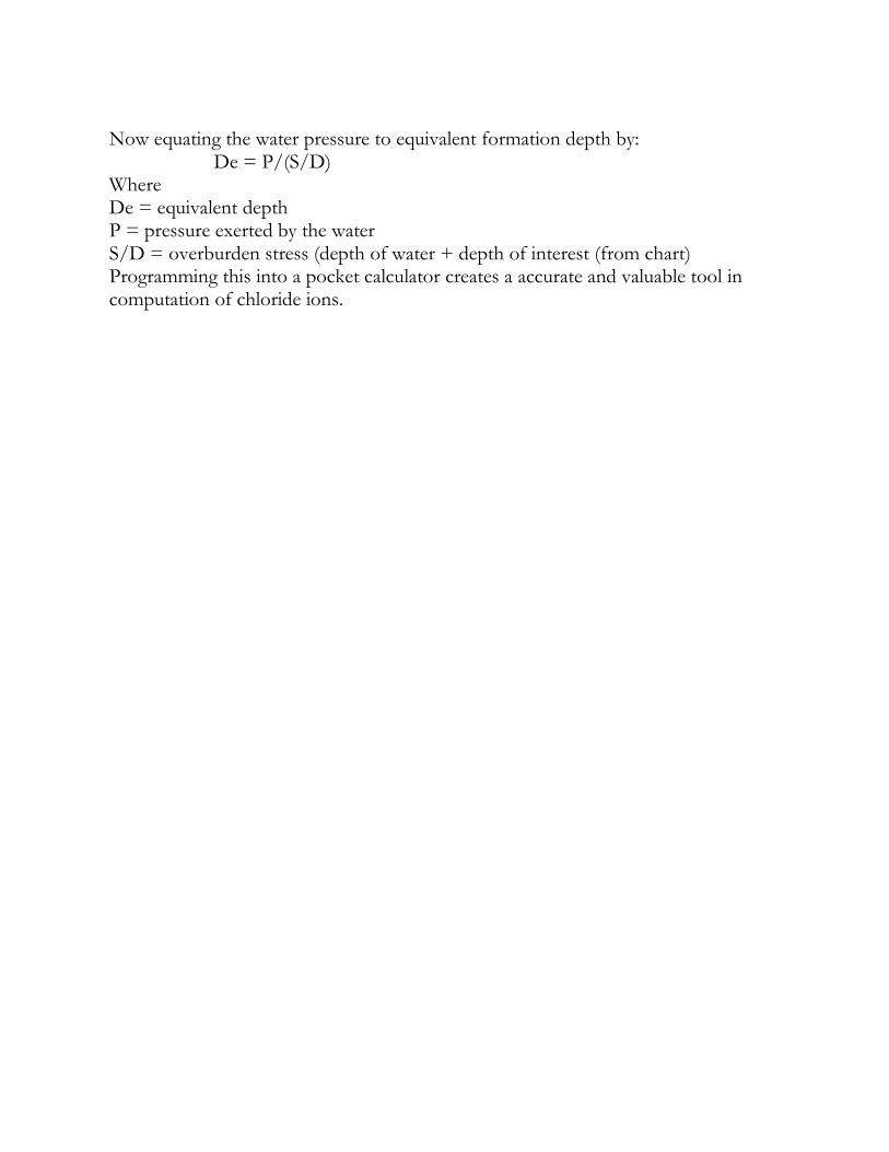
Now equating the water pressure to equivalent formation depth by: De = P/(S/D) Where De = equivalent depth P = pressure exerted by the water S/D = overburden stress (depth of water + depth of interest (from chart) Programming this into a pocket calculator creates a accurate and valuable tool in computation of chloride ions.

2. For the depth of interest we have: Di= De + D where: Di = equivalent for depth of interest (ft) De = equivalent depth of water D = depth from sea floor to depth of interest 3. Substituting in Ben Eaton's Equation we have: F = (S/Di - P/Di) * (V/(1-V)) + (P/Di) and thus computing the effective fracture gradient we have: Fe = F * 19.23 Di where: Fe = fracture pressure @ the depth of interest (ppg)

Process of Abnormal Pressure Detection ( DxC) Jordon and Shirley published their paper on abnormal pressure detection using the DxC in 1966. Their work was based on the following drilling relationship:

P = K * (𝑊/𝐷𝑑 ) x N where: P = penetration rate (ft/hr) K= formation drillability D= bit diameter W= weigth on bit N= rotary speed d = weight on bit exponent e = rotary speed exponent It was their contention that the formation drillability (K) equaled one and e (rotary exponent)also equaled one since penetration rate varied directly as rotary speed. These are rather shakey assumptions, but as long as K and N don't change to much the results are acceptable. Therefore, after a little rearranging of terms in our first equation we have:

P = 12 𝑥 𝑊

106 𝑥 𝐷X (60 x N)

thus the final logarithmic calculation can be shown as:

𝐷𝑒𝑥 = 𝑙𝑜𝑔

60 𝑥 𝑁

𝑃

𝑙𝑜𝑔106 𝑥 𝐷

12 𝑥 𝑊

where: P = penetration rate N= rotary speed D= bit diameter W= weight on bit

𝐷𝑒𝑥 = normalization of terms

In order to correct the 𝐷𝑒𝑥 for the normal drilling gradient, we must produce another relation as follows:

𝐷𝑐𝑒𝑥 = 𝐷𝑒𝑥 𝑥 𝑛

𝑀𝑊

where:

𝐷𝑐𝑒𝑥 = corrected normalization of terms n = normal gradient (9 lb or 8.33 lb) MW = mud weight (ppg) With this valus, we can now determine a pore pressure using the following equation:

F = 𝑁 ( 𝐷𝐶𝑛 /𝐷𝐶𝑒𝑥 ) where: F= formation pressure in ppg N = normal gradient for area (ppg)

DC = normal 𝐷𝐶𝑒𝑥 for experienced @ known formation pressure

𝐷𝐶𝑒𝑥 = observed Dc value In order to decrease the effect of widely varying penetration rates, wob and rotary speed, the final values for formation pressures are evaluated using a least squares trend line fit. Since much empirical data is available on wells in south Louisiana the starting point for the slope of the trend line is taken as .0000400623 which can be

changed mathematically to accommodate a particular situation. It is emphasized that this is only a starting place and is reevaluated statistically as changes occur.

Normalized Rate of Penetration PRn = Pr x (𝑊𝑜− −5

𝑊𝑛−(−5) x

𝑁𝑜𝜆

𝑁𝑛 x

𝑄𝑜 𝑥 𝑃𝐵𝑜

𝑄𝑛 𝑥 𝑃𝐵𝑛

% change = PR/PRn PSI = 14.54 * % change Formation Pressure (ppg) =(( PSI * 19.23)/Depth) + MW where: PRn = normalized ROP PR = observed ROB Wo = obser. WOB (in 1,000's lbs) Wn = norm. WOB No= obser. RPM Nn= norm. RPM λ= .6 (soft rock) or .8 (hard rock) Qn = normal flow rate (gal/min) Qo = observ. flow rate (gal/min) PBn = norm. Press. drop @ Bit PBo = observ. Press. drop @ Bit MW = Mud weight (ppg) This is the best method for pore pressure determination due to the fact it takes into consideration both hydraulic parameters as well as drilling parameters. Each set of parameters is effected by changes in formation pressure and taken collectively will respond to smaller formation pressure changes than any other detection tool.

Calculation of Chloride Ions Using Temperature and Resistivity Accurate and speedy detecting of chloride ion changes in the drilling fluid system is most effective in detecting approaches to abnormal pressure zones. In addition, they allow information on possible show zones and salt water flows.

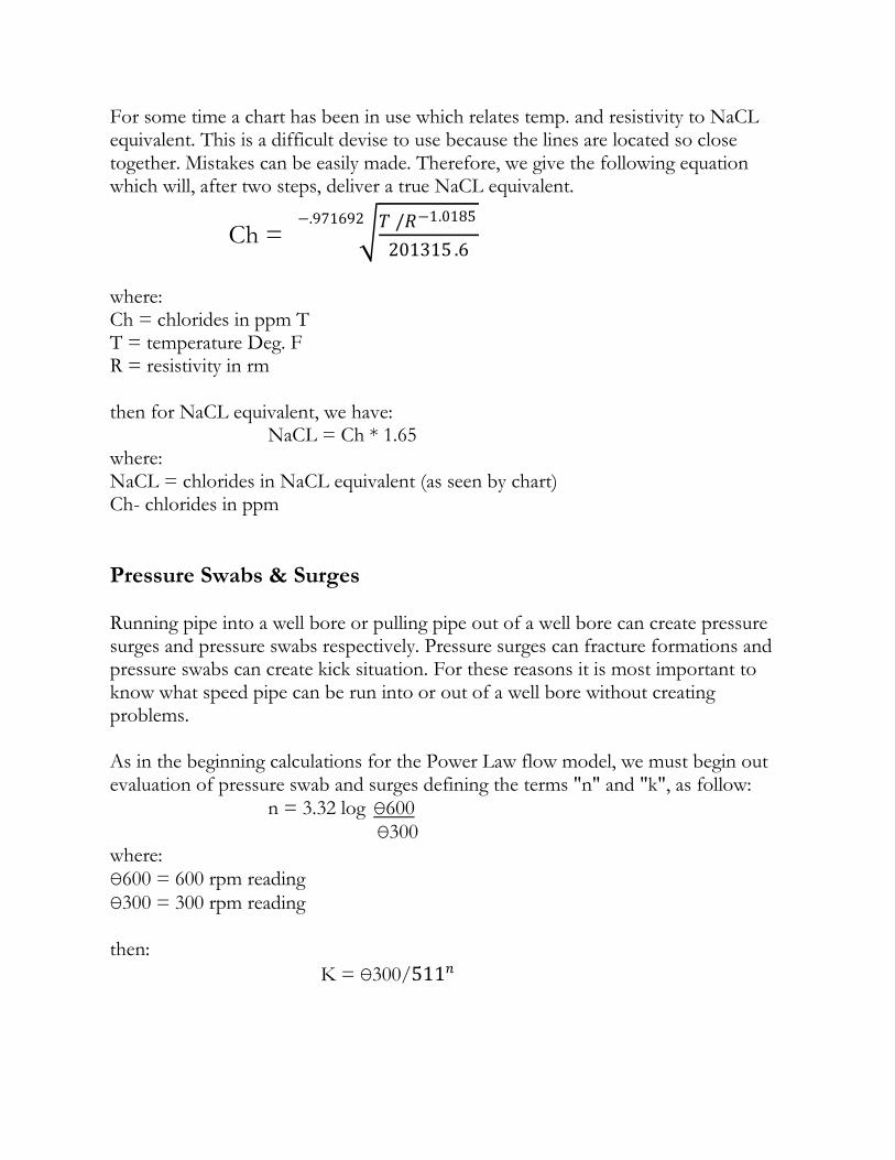
For some time a chart has been in use which relates temp. and resistivity to NaCL equivalent. This is a difficult devise to use because the lines are located so close together. Mistakes can be easily made. Therefore, we give the following equation which will, after two steps, deliver a true NaCL equivalent.

Ch = 𝑇 /𝑅−1.0185

201315 .6

−.971692

where: Ch = chlorides in ppm T T = temperature Deg. F R = resistivity in rm then for NaCL equivalent, we have: NaCL = Ch * 1.65 where: NaCL = chlorides in NaCL equivalent (as seen by chart) Ch- chlorides in ppm

Pressure Swabs & Surges Running pipe into a well bore or pulling pipe out of a well bore can create pressure surges and pressure swabs respectively. Pressure surges can fracture formations and pressure swabs can create kick situation. For these reasons it is most important to know what speed pipe can be run into or out of a well bore without creating problems. As in the beginning calculations for the Power Law flow model, we must begin out evaluation of pressure swab and surges defining the terms "n" and "k", as follow: n = 3.32 log Ө600

Ө300 where:

Ө600 = 600 rpm reading

Ө300 = 300 rpm reading then:

K = Ө300/511𝑛

Now we must calculate based upon wheather or not the pipe is plugged with mud or open. The first values to be found are interim variables "v" and "vm". We will calculate with Closed pipe first. CLOSED DRILL PIPE

V = K + 𝐷𝑝2

𝐷𝑕2−𝐷𝑝2 Vp

Then vm = 1.5 v where: Dp = pipe OD Dh = hole ID Vp = pipe velocity (ft/min) OPEN DRILL PIPE

V = K + 𝐷𝑝2−𝐷𝑖2

𝐷𝑕2−𝐷𝑝2+𝐷𝑖2 x Vp

then we have: Vm = 1.5 V SURGES: At this point we are now ready to introduce the equation for surge pressure surrounding the drill pipe. This is given as:

Ps = 2.4 𝑥 𝑉𝑚

𝐷𝑕−𝐷𝑝𝑥

2 𝑥 𝑛+1

3 𝑥 𝑛 𝑛

x 𝐾 𝑥 𝐿

300 ( 𝐷𝑕−𝐷𝑝)

where: Ps = pressure surge psi Dh = hole diameter Dp = pipe OD K = constant previously calculated L = length of the segment Note: as in other equations of this type, this is a segmented drill string approach.

We must now calculate the pressure surge around the drill collars. First we can assume that under these conditions fluid flow around the collars will be turbulent. Therefore, we give the following equation for turbulent drill collar surge:

Ps = 7.7 𝑥 10−5 𝑥 𝑝 .8𝑥 𝑄1.8 𝑥 𝑃𝑉 .2 𝑥 𝐿

𝐷𝑕−𝐷𝑝 3𝑥 (𝐷𝑕+𝐷𝑝)1.8

where:

Q= vm/an. vol. bbl./ft 42 Q = turbulent collar flow (gal/min) PV = plactic viscosity Dh = hole size Dp = pipe OD L = length of the segment p = mud weight At this point we have now calculated the pressure in psi caused by the surging action of the drill string while running into the hole. Compare this value to the psi value of the fracture gradient. If the surge is higher you will likely fracture the formation. We are now ready to consider pressure swabs. Again we must decide whether'our pipe is plugged or open. We will assume PLUGGED pipe first. Plugged Swab

PS = .000162 𝑥 𝑝 2𝑥 𝐿 𝑥 𝐷𝑝 2𝑥 𝑉𝑝

𝐷𝑕2−𝐷𝑝2

where: Ps = pressure swab in psi L = length of segment Dp = pipe OD Vp = pipe velocity (ft/min) p = mud weight Open Swab

PS = .000162 𝑥 𝑝 𝑥 𝐷𝑝2−𝐷𝑖2 𝑥 𝑉𝑝 𝑥 𝐿

(𝐷𝑕2−𝐷𝑝2+𝐷𝑖2

where: Ps = pressure swab in psi Dp = pipe OD

Di = pipe ID Vp = pipe velocity (ft/min) L = length of segment p = mud weight the total swab now becomes the summation of all segments:

Pst = 𝑃𝑆𝑛𝑖=1

where: Pst = total pipe movement swab in psi Ps = summation of all segments Note: this summation routine works for pressure surges as well. Now we can compare the total pressure swab in psi to the formation pressure in psi to see if the velocity at which our pipe is running will create possible kick situation. If it does, then slow the pipe velocity down.