MATHEMATICA - studia.ubbcluj.ro · EDITORIAL BOARD OF STUDIA UNIVERSITATIS BABEŞ-BOLYAI...
154
MATHEMATICA 1/2018
Transcript of MATHEMATICA - studia.ubbcluj.ro · EDITORIAL BOARD OF STUDIA UNIVERSITATIS BABEŞ-BOLYAI...
MATHEMATICA
1/2018

STUDIA UNIVERSITATIS BABEŞ-BOLYAI
MATHEMATICA
1/2018
EDITORIAL BOARD OF STUDIA UNIVERSITATIS BABEŞ -BOLYAI MATHEMATICA
EDITORS: Radu Precup, Babeş-Bolyai University, Cluj-Napoca, Romania (Editor-in-Chief) Octavian Agratini, Babeş-Bolyai University, Cluj-Napoca, Romania Simion Breaz, Babeş-Bolyai University, Cluj-Napoca, Romania Csaba Varga, Babeş-Bolyai University, Cluj-Napoca, Romania
MEMBERS OF THE BOARD: Ulrich Albrecht, Auburn University, USA Francesco Altomare, University of Bari, Italy Dorin Andrica, Babeş-Bolyai University, Cluj-Napoca, Romania Silvana Bazzoni, University of Padova, Italy Petru Blaga, Babeş-Bolyai University, Cluj-Napoca, Romania Wolfgang Breckner, Babeş-Bolyai University, Cluj-Napoca, Romania Teodor Bulboacă, Babeş-Bolyai University, Cluj-Napoca, Romania Gheorghe Coman, Babeş-Bolyai University, Cluj-Napoca, Romania Louis Funar, University of Grenoble, France Ioan Gavrea, Technical University, Cluj-Napoca, Romania Vijay Gupta, Netaji Subhas Institute of Technology, New Delhi, India Gábor Kassay, Babeş-Bolyai University, Cluj-Napoca, Romania Mirela Kohr, Babeş-Bolyai University, Cluj-Napoca, Romania Iosif Kolumbán, Babeş-Bolyai University, Cluj-Napoca, Romania Alexandru Kristály, Babeş-Bolyai University, Cluj-Napoca, Romania Andrei Mărcuş, Babeş-Bolyai University, Cluj-Napoca, Romania Waclaw Marzantowicz, Adam Mickiewicz, Poznan, Poland Giuseppe Mastroianni, University of Basilicata, Potenza, ItalyMihail Megan, West University of Timişoara, RomaniaGradimir V. Milovanović, Megatrend University, Belgrade, SerbiaBoris Mordukhovich, Wayne State University, Detroit, USA András Némethi, Rényi Alfréd Institute of Mathematics, Hungary Rafael Ortega, University of Granada, Spain Adrian Petruşel, Babeş-Bolyai University, Cluj-Napoca, Romania Cornel Pintea, Babeş-Bolyai University, Cluj-Napoca, Romania Patrizia Pucci, University of Perugia, Italy Ioan Purdea, Babeş-Bolyai University, Cluj-Napoca, Romania John M. Rassias, National and Capodistrian University of Athens, Greece Themistocles M. Rassias, National Technical University of Athens, Greece Ioan A. Rus, Babeş-Bolyai University, Cluj-Napoca, Romania Grigore Sălăgean, Babeş-Bolyai University, Cluj-Napoca, Romania Mircea Sofonea, University of Perpignan, France Anna Soós, Babeş-Bolyai University, Cluj-Napoca, Romania András Stipsicz, Rényi Alfréd Institute of Mathematics, Hungary Ferenc Szenkovits, Babeş-Bolyai University, Cluj-Napoca, Romania Michel Théra, University of Limoges, France
BOOK REVIEWS: Ştefan Cobzaş, Babeş-Bolyai University, Cluj-Napoca, Romania
SECRETARIES OF THE BOARD: Teodora Cătinaş, Babeş-Bolyai University, Cluj-Napoca, Romania Hannelore Lisei, Babeş-Bolyai University, Cluj-Napoca, Romania
TECHNICAL EDITOR: Georgeta Bonda, Babeş-Bolyai University, Cluj-Napoca, Romania
YEAR (LXIII) 2018MONTH MARCHISSUE 1
S T U D I AUNIVERSITATIS BABES-BOLYAI
MATHEMATICA1
Redactia: 400084 Cluj-Napoca, str. M. Kogalniceanu nr. 1Telefon: 0264 405300
CONTENTS
George A. Anastassiou, Conformable fractional approximation bymax-product operators . . . . . . . . . . . . . . . . . . . . . . . . . . . . . . . . . . . . . . . . . . . . . . . . . . . . . . 3
Ghulam Farid and Ghulam Abbas, Generalizations of some fractionalintegral inequalities for m-convex functions via generalized Mittag-Lefflerfunction . . . . . . . . . . . . . . . . . . . . . . . . . . . . . . . . . . . . . . . . . . . . . . . . . . . . . . . . . . . . . . . . . . . 23
Sever S. Dragomir, Inequalities for the area balance of absolutelycontinuous functions . . . . . . . . . . . . . . . . . . . . . . . . . . . . . . . . . . . . . . . . . . . . . . . . . . . . . . . 37
Santosh B. Joshi, Sayali S. Joshi and Haridas Pawar, Applicationsof generalized fractional integral operator to unified subclass ofprestarlike functions with negative coefficients . . . . . . . . . . . . . . . . . . . . . . . . . . . . . .59
Nanjundan Magesh, Saurabh Porwal and Chinnaswamy Abirami,Starlike and convex properties for Poisson distribution series . . . . . . . . . . . . . . . 71
Yuji Liu, Solvability of BVPs for impulsive fractional differential equationsinvolving the Riemann-Liouvile fractional derivatives . . . . . . . . . . . . . . . . . . . . . . . 79
Arpad Szaz, Generalizations of an asymptotic stability theorem of Bahyrycz,Pales and Piszczek on Cauchy differences to generalized cocycles . . . . . . . . . . 109
Sevda Orhan and Burcak Kolay, Korovkin type approximation fordouble sequences via statistical A-summation process on modularspaces . . . . . . . . . . . . . . . . . . . . . . . . . . . . . . . . . . . . . . . . . . . . . . . . . . . . . . . . . . . . . . . . . . . . 125
Ram Kishun Lodhi and Hradyesh Kumar Mishra, Quintic B-splinemethod for numerical solution of fourth order singular perturbationboundary value problems . . . . . . . . . . . . . . . . . . . . . . . . . . . . . . . . . . . . . . . . . . . . . . . . . 141

Stud. Univ. Babes-Bolyai Math. 63(2018), No. 1, 3–22DOI: 10.24193/subbmath.2018.1.01
Conformable fractional approximationby max-product operators
George A. Anastassiou
Abstract. Here we study the approximation of functions by a big variety of Max-product operators under conformable fractional differentiability. These are posi-tive sublinear operators. Our study is based on our general results about positivesublinear operators. We produce Jackson type inequalities under conformablefractional initial conditions. So our approach is quantitative by producing in-equalities with their right hand sides involving the modulus of continuity of ahigh order conformable fractional derivative of the function under approxima-tion.
Mathematics Subject Classification (2010): 26A33, 41A17, 41A25, 41A36.
Keywords: positive sublinear operators, Max-product operators, modulus of con-tinuity, conformable fractional derivative.
1. Introduction
The main motivation here is the monograph by B. Bede, L. Coroianu and S. Gal[4], 2016.
Let N ∈ N, the well-known Bernstein polynomials ([7]) are positive linear oper-ators, defined by the formula
BN (f) (x) =
N∑k=0
(Nk
)xk (1− x)
N−kf
(k
N
), x ∈ [0, 1] , f ∈ C ([0, 1]) . (1.1)
T. Popoviciu in [8], 1935, proved for f ∈ C ([0, 1]) that
|BN (f) (x)− f (x)| ≤ 5
4ω1
(f,
1√N
), ∀ x ∈ [0, 1] , (1.2)
where
ω1 (f, δ) = supx,y∈[0,1]:|x−y|≤δ
|f (x)− f (y)| , δ > 0, (1.3)
4 George A. Anastassiou
is the first modulus of continuity.G.G. Lorentz in [7], 1986, p. 21, proved for f ∈ C1 ([0, 1]) that
|BN (f) (x)− f (x)| ≤ 3
4√Nω1
(f ′,
1√N
), ∀ x ∈ [0, 1] , (1.4)
In [4], p. 10, the authors introduced the basic Max-product Bernstein operators,
B(M)N (f) (x) =
∨Nk=0 pN,k (x) f
(kN
)∨Nk=0 pN,k (x)
, N ∈ N, (1.5)
where∨
stands for maximum, and
pN,k (x) =
(Nk
)xk (1− x)
N−k
and f : [0, 1]→ R+ = [0,∞).These are nonlinear and piecewise rational operators.The authors in [4] studied similar such nonlinear operators such as: the Max-
product Favard-Szasz-Mirakjan operators and their truncated version, the Max-product Baskakov operators and their truncated version, also many other similarspecific operators. The study in [4] is based on presented there general theory of sub-linear operators. These Max-product operators tend to converge faster to the on handfunction.
So we mention from [4], p. 30, that for f : [0, 1] → R+ continuous, we have theestimate∣∣∣B(M)
N (f) (x)− f (x)∣∣∣ ≤ 12ω1
(f,
1√N + 1
), for all N ∈ N, x ∈ [0, 1] , (1.6)
Also from [4], p. 36, we mention that for f : [0, 1] → R+ being concave function weget that ∣∣∣B(M)
N (f) (x)− f (x)∣∣∣ ≤ 2ω1
(f,
1
N
), for all x ∈ [0, 1] , (1.7)
a much faster convergence.In this article we expand the study in [4] by considering conformable fractional
smoothness of functions. So our inequalities are with respect to ω1 (Dnαf, δ), δ > 0,
n ∈ N, where Dnαf is the nth order conformable α-fractional derivative, α ∈ (0, 1], see
[1], [6].We present at first some background and general related theory of sublinear
operators and then we apply it to specific as above Max-product operators.
2. Background
We make
Definition 2.1. Let f : [0,∞) → R and α ∈ (0, 1]. We say that f is an α-fractionalcontinuous function, iff ∀ ε > 0 ∃ δ > 0 : for any x, y ∈ [0,∞) such that |xα − yα| ≤ δwe get that |f (x)− f (y)| ≤ ε.
We give
Conformable fractional approximation by max-product operators 5
Theorem 2.2. Over [a, b] ⊆ [0,∞), α ∈ [0, 1], a α-fractional continuous function is auniformly continuous function and vice versa, a uniformly continuous function is anα-fractional continuous function.
(Theorem 2.2 is not valid over [0,∞).)Note. Let x, y ∈ [a, b] ⊆ [0,∞), and g (x) = xα, 0 < α ≤ 1, then
g′ (x) = αxα−1 =α
x1−α, for x ∈ (0,∞) .
Since a ≤ x ≤ b, then 1x ≥
1b > 0 and α
x1−α ≥ αb1−α > 0.
Assume y > x. By the mean value theorem we get
yα − xα =α
ξ1−α(y − x) , where ξ ∈ (x, y) . (2.1)
A similar to (2.1) equality when x > y is true.Then we obtain
α
b1−α|y − x| ≤ |yα − xα| = α
ξ1−α|y − x| . (2.2)
Thus, it holdsα
b1−α|y − x| ≤ |yα − xα| . (2.3)
Proof of Theorem 2.2.(⇒) Assume that f is α-fractional continuous function on [a, b] ⊆ [0,∞). It
means ∀ ε > 0 ∃ δ > 0 : whenever x, y ∈ [a, b] : |xα − yα| ≤ δ, then |f (x)− f (y)| ≤ ε.Let for xnn∈N ∈ [a, b] : xn → λ ∈ [a, b]⇔ xαn → λα, it implies f (xn) → f (λ),therefore f is continuous in λ. Therefore f is uniformly continuous over [a, b] .
For the converse we use the following criterion:
Lemma 2.3. A necessary and sufficient condition that the function f is not α-fractionalcontinuous (α ∈ (0, 1]) over [a, b] ⊆ [0,∞) is that there exist ε0 > 0, and two se-quences X = (xn), Y = (yn) in [a, b] such that if n ∈ N, then |xαn − yαn | ≤ 1
n and|f (xn)− f (yn)| > ε0.
Proof. Obvious. (Proof of Theorem 2.2 continuous) (⇐) Uniform continuity implies α-fractional con-tinuity on [a, b] ⊆ [0,+∞). Indeed: let f uniformly continuous on [a, b], hence fcontinuous on [a, b]. Assume that f is not α-fractional continuous on [a, b]. Then byLemma 2.3 there exist ε0 > 0, and two sequences X = (xn), Y = (yn) in [a, b] suchthat if n ∈ N, then |xαn − yαn | ≤ 1
n and
|f (xn)− f (yn)| > ε0. (2.4)
Since [a, b] is compact, the sequences xn , yn are bounded. By the Bolzano-Weierstrass theorem, there is a subsequence
xn(k)
of xn which converges to an
element z. Since [a, b] is closed, the limit z ∈ [a, b], and f is continuous at z.We have also that
α
b1−α|xn − yn| ≤ |xαn − yαn | ≤
1
n, (2.5)
6 George A. Anastassiou
hence
|xn − yn| ≤b1−α
αn. (2.6)
It is clear that the corrsponding subsequence(yn(k)
)of Y also converges to z. Hence
f(xn(k)
)→ f (z), and f
(yn(k)
)→ f (z). Therefore, when k is sufficiently large we
have∣∣f (xn(k))− f (yn(k))∣∣ < ε0, contradicting (2.4).
We need
Definition 2.4. Let [a, b] ⊆ [0,∞), α ∈ [0, 1]. We define the α-fractional modulus ofcontinuity:
ωα1 (f, δ) := supx,y∈[a,b]:|xα−yα|≤δ
|f (x)− f (y)| , δ > 0. (2.7)
The same definition holds over [0,∞).Properties.
1) ωα1 (f, 0) = 0.2) ωα1 (f, δ)→ 0 as δ ↓ 0, iff f is in the set of all α-fractional continuous functions,
denoted as f ∈ Cα ([a, b] ,R) (= C ([a, b] ,R)).
Proof. (⇒) Let ωα1 (f, δ) → 0 as δ ↓ 0. Then ∀ ε > 0, ∃ δ > 0 with ωα1 (f, δ) ≤ ε, i.e.∀ x, y ∈ [a, b] : |xα − yα| ≤ δ we get |f (x)− f (y)| ≤ ε. That is f ∈ Cα ([a, b] ,R) .
(⇐) Let f ∈ Cα ([a, b] ,R). Then ∀ ε > 0, ∃ δ > 0 : whenever |xα − yα| ≤ δ,x, y ∈ [a, b] , it implies |f (x)− f (y)| ≤ ε, i.e. ∀ ε > 0, ∃ δ > 0 : ωα1 (f, δ) ≤ ε. That isωα1 (f, δ)→ 0, as δ ↓ 0.
3) ωα1 is ≥ 0 and non-decreasing on R+.4) ωα1 is subadditive:
ωα1 (f, t1 + t2) ≤ ωα1 (f, t1) + ωα1 (f, t2) . (2.8)
Proof. If |xα − yα| ≤ t1 + t2 (x, y ∈ [a, b]), there is a point z ∈ [a, b] for which|xα − zα| ≤ t1, |yα − zα| ≤ t2, and |f (x)− f (y)| ≤ |f (x)− f (z)|+ |f (z)− f (y)| ≤ωα1 (f, t1) + ωα1 (f, t2), implying ωα1 (f, t1 + t2) ≤ ωα1 (f, t1) + ωα1 (f, t2) .
5) ωα1 is continuous on R+.
Proof. We get|ωα1 (f, t1 + t2)− ωα1 (f, t1)| ≤ ωα1 (f, t2) . (2.9)
By properties 2), 3), 4), we get that ωα1 (f, t) is continuous at each t ≥ 0.
6) Clearly it holds
ωα1 (f, t1 + ...+ tn) ≤ ωα1 (f, t1) + ...+ ωα1 (f, tn) , (2.10)
for t = t1 = ... = tn, we obtain
ωα1 (f, nt) = nωα1 (f, t) . (2.11)
7) Let λ ≥ 0, λ /∈ N, we get
ωα1 (f, λt) ≤ (λ+ 1)ωα1 (f, t) . (2.12)
Conformable fractional approximation by max-product operators 7
Proof. Let n ∈ Z+ : n ≤ λ < n+ 1, we see that
ωα1 (f, λt) ≤ ωα1 (f, (n+ 1) t) ≤ (n+ 1)ωα1 (f, t) ≤ (λ+ 1)ωα1 (f, t) .
Properties 1), 3), 4), 6), 7) are valid also for ωα1 defined over [0,∞).We notice that ωα1 (f, δ) is finite when f is uniformly continuous on [a, b].
If f : [0,∞)→ R is bounded then ωα1 (f, δ) is again finite.We need
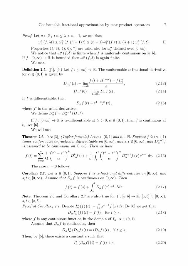
Definition 2.5. ([1], [6]) Let f : [0,∞) → R. The conformable α-fractional derivativefor α ∈ (0, 1] is given by
Dαf (t) := limε→0
f(t+ εt1−α
)− f (t)
ε, (2.13)
Dαf (0) = limt→0+
Dαf (t) . (2.14)
If f is differentiable, thenDαf (t) = t1−αf ′ (t) , (2.15)
where f ′ is the usual derivative.We define Dn
αf = Dn−1α (Dαf) .
If f : [0,∞)→ R is α-differentiable at t0 > 0, α ∈ (0, 1], then f is continuous att0, see [6].
We will use
Theorem 2.6. (see [3]) (Taylor formula) Let α ∈ (0, 1] and n ∈ N. Suppose f is (n+ 1)times conformable α-fractional differentiable on [0,∞), and s, t ∈ [0,∞), and Dn+1
α fis assumed to be continuous on [0,∞). Then we have
f (t) =
n∑k=0
1
k!
(tα − sα
α
)kDkαf (s) +
1
n!
∫ t
s
(tα − τα
α
)nDn+1α f (τ) τa−1dτ. (2.16)
The case n = 0 follows.
Corollary 2.7. Let α ∈ (0, 1]. Suppose f is α-fractional differentiable on [0,∞), ands, t ∈ [0,∞). Assume that Dαf is continuous on [0,∞). Then
f (t) = f (s) +
∫ t
s
Dαf (τ) τa−1dτ. (2.17)
Note. Theorem 2.6 and Corollary 2.7 are also true for f : [a, b] → R, [a, b] ⊆ [0,∞),s, t ∈ [a, b] .
Proof of Corollary 2.7. Denote Isα (f) (t) :=∫ tsxα−1f (x) dx. By [6] we get that
DαIsα (f) (t) = f (t) , for t ≥ s, (2.18)
where f is any continuous function in the domain of Iα, α ∈ (0, 1) .Assume that Dαf is continuous, then
DαIsα (Dαf) (t) = (Dαf) (t) , ∀ t ≥ s. (2.19)
Then, by [5], there exists a constant c such that
Isα (Dαf) (t) = f (t) + c. (2.20)
8 George A. Anastassiou
Hence
0 = Isα (Dαf) (s) = f (s) + c, (2.21)
then c = −f (s) .Therefore
Isα (Dαf) (t) = f (t)− f (s) =
∫ t
s
(Dαf) (τ) τα−1dτ. (2.22)
The same proof applies for any s ≥ t.
3. Main results
We give
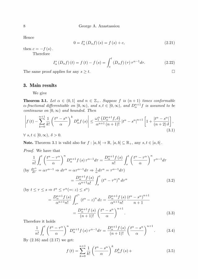
Theorem 3.1. Let α ∈ (0, 1] and n ∈ Z+. Suppose f is (n+ 1) times conformableα-fractional differentiable on [0,∞), and s, t ∈ [0,∞), and Dn+1
α f is assumed to becontinuous on [0,∞) and bounded. Then∣∣∣∣∣f (t)−
n+1∑k=0
1
k!
(tα − sα
α
)kDkαf (s)
∣∣∣∣∣ ≤ ωα1(Dn+1α f, δ
)αn+1 (n+ 1)!
|tα − sα|n+1
[1 +|tα − sα|(n+ 2) δ
],
(3.1)∀ s, t ∈ [0,∞), δ > 0.
Note. Theorem 3.1 is valid also for f : [a, b]→ R, [a, b] ⊆ R+, any s, t ∈ [a, b] .
Proof. We have that
1
n!
∫ t
s
(tα − τα
α
)nDn+1α f (s) τα−1dτ =
Dn+1α f (s)
n!
∫ t
s
(tα − τα
α
)nτα−1dτ
(by dτα
dτ = ατα−1 ⇒ dτα = ατα−1dτ ⇒ 1αdτ
α = τα−1dτ)
=Dn+1α f (s)
αn+1n!
∫ t
s
(tα − τα)ndτα (3.2)
(by t ≤ τ ≤ s⇒ tα ≤ τα(=: z) ≤ sα)
=Dn+1α f (s)
αn+1n!
∫ tα
sα(tα − z)n dz =
Dn+1α f (s)
αn+1n!
(tα − sα)n+1
n+ 1
=Dn+1α f (s)
(n+ 1)!
(tα − sα
α
)n+1
. (3.3)
Therefore it holds
1
n!
∫ t
s
(tα − τα
α
)nDn+1α f (s) τα−1dτ =
Dn+1α f (s)
(n+ 1)!
(tα − sα
α
)n+1
. (3.4)
By (2.16) and (2.17) we get:
f (t) =
n+1∑k=0
1
k!
(tα − sα
α
)kDkαf (s) + (3.5)
Conformable fractional approximation by max-product operators 9
1
n!
∫ t
s
(tα − τα
α
)n (Dn+1α f (τ)−Dn+1
α f (s))τα−1dτ.
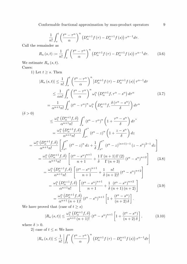
Call the remainder as
Rn (s, t) :=1
n!
∫ t
s
(tα − τα
α
)n (Dn+1α f (τ)−Dn+1
α f (s))τα−1dτ. (3.6)
We estimate Rn (s, t).Cases:
1) Let t ≥ s. Then
|Rn (s, t)| ≤ 1
n!
∫ t
s
(tα − τα
α
)n ∣∣Dn+1α f (τ)−Dn+1
α f (s)∣∣ τα−1dτ
≤ 1
αn!
∫ t
s
(tα − τα
α
)nωα1(Dn+1α f, τα − sα
)dτα (3.7)
=1
αn+1n!
∫ t
s
(tα − τα)nωα1
(Dn+1α f,
δ (τα − sα)
δ
)dτα
(δ > 0)
≤ωα1(Dn+1α f, δ
)αn+1n!
∫ t
s
(tα − τα)n
(1 +
τα − sα
δ
)dτ
α
=ωα1(Dn+1α f, δ
)αn+1n!
∫ tα
sα(tα − z)n
(1 +
z − sα
δ
)dz
=ωα1(Dn+1α f, δ
)αn+1n!
[∫ tα
sα(tα − z)n dz +
1
δ
∫ tα
sα(tα − z)(n+1)−1
(z − sα)2−1
dz
]
=ωα1(Dn+1α f, δ
)αn+1n!
[(tα − sα)
n+1
n+ 1+
1
δ
Γ (n+ 1) Γ (2)
Γ (n+ 3)(tα − sα)
n+2
](3.8)
=ωα1(Dn+1α f, δ
)αn+1n!
[(tα − sα)
n+1
n+ 1+
1
δ
n!
(n+ 2)!(tα − sα)
n+2
]
=ωα1(Dn+1α f, δ
)αn+1n!
[(tα − sα)
n+1
n+ 1+
1
δ
(tα − sα)n+2
(n+ 1) (n+ 2)
](3.9)
=ωα1(Dn+1α f, δ
)αn+1 (n+ 1)!
(tα − sα)n+1
[1 +
(tα − sα)
(n+ 2) δ
].
We have proved that (case of t ≥ s)
|Rn (s, t)| ≤ωα1(Dn+1α f, δ
)αn+1 (n+ 1)!
(tα − sα)n+1
[1 +
(tα − sα)
(n+ 2) δ
], (3.10)
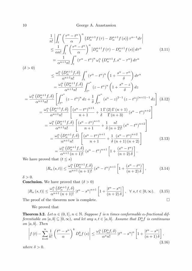
where δ > 0.2) case of t ≤ s: We have
|Rn (s, t)| ≤ 1
n!
∣∣∣∣∫ s
t
(tα − τα
α
)n (Dn+1α f (τ)−Dn+1
α f (s))τα−1dτ
∣∣∣∣
10 George A. Anastassiou
1
n!
∣∣∣∣∫ s
t
(τα − tα
α
)n (Dn+1α f (τ)−Dn+1
α f (s))τα−1dτ
∣∣∣∣≤ 1
αn!
∫ s
t
(τα − tα
α
)n ∣∣Dn+1α f (τ)−Dn+1
α f (s)∣∣ dτα (3.11)
=1
αn+1n!
∫ s
t
(τα − tα)nωα1(Dn+1α f, sα − τα
)dτα
(δ > 0)
≤ωα1(Dn+1α f, δ
)αn+1n!
∫ s
t
(τα − tα)n
(1 +
sα − τα
δ
)dτα
=ωα1(Dn+1α f, δ
)αn+1n!
∫ sα
tα(z − tα)
n
(1 +
sα − zδ
)dz
=ωα1(Dn+1α f, δ
)αn+1n!
[∫ sα
tα(z − tα)
ndz +
1
δ
∫ sα
tα(sα − z)2−1 (z − tα)
(n+1)−1dz
](3.12)
=ωα1(Dn+1α f, δ
)αn+1n!
[(sα − tα)
n+1
n+ 1+
1
δ
Γ (2) Γ (n+ 1)
Γ (n+ 3)(sα − tα)
n+2
]
=ωα1(Dn+1α f, δ
)αn+1n!
[(sα − tα)
n+1
n+ 1+
1
δ
n!
(n+ 2)!(sα − tα)
n+2
]
=ωα1(Dn+1α f, δ
)αn+1n!
[(sα − tα)
n+1
n+ 1+
1
δ
(sα − tα)n+2
(n+ 1) (n+ 2)
](3.13)
=ωα1(Dn+1α f, δ
)αn+1 (n+ 1)!
(sα − tα)n+1
[1 +
(sα − tα)
(n+ 2) δ
].
We have proved that (t ≤ s)
|Rn (s, t)| ≤ωα1(Dn+1α f, δ
)αn+1 (n+ 1)!
(sα − tα)n+1
[1 +
(sα − tα)
(n+ 2) δ
], (3.14)
δ > 0.Conclusion. We have proved that (δ > 0)
|Rn (s, t)| ≤ωα1(Dn+1α f, δ
)αn+1 (n+ 1)!
|tα − sα|n+1
[1 +|tα − sα|(n+ 2) δ
], ∀ s, t ∈ [0,∞). (3.15)
The proof of the theorem now is complete.
We proved that
Theorem 3.2. Let α ∈ (0, 1], n ∈ N. Suppose f is n times conformable α-fractional dif-ferentiable on [a, b] ⊆ [0,∞), and let any s, t ∈ [a, b]. Assume that Dn
αf is continuouson [a, b]. Then∣∣∣∣∣f (t)−
n∑k=0
1
k!
(tα − sα
α
)kDkαf (s)
∣∣∣∣∣ ≤ ωα1 (Dnαf, δ)
αnn!|tα − sα|n
[1 +|tα − sα|(n+ 1) δ
],
(3.16)where δ > 0.
Conformable fractional approximation by max-product operators 11
Proof. By Theorem 3.1.
Corollary 3.3. (n = 1 case of Theorem 3.2) Let α ∈ (0, 1]. Suppose f is α-conformablefractional differentiable on [a, b] ⊆ [0,∞), and let any s, t ∈ [a, b]. Assume that Dαfis continuous on [a, b]. Then∣∣∣∣f (t)− f (s)−
(tα − sα
α
)Dαf (s)
∣∣∣∣ ≤ ωα1 (Dαf, δ)
α|tα − sα|
[1 +|tα − sα|
2δ
], (3.17)
where δ > 0.
Corollary 3.4. (to Theorem 3.2) Same assumptions as in Theorem 3.2. For specifics ∈ [a, b] assume that Dk
αf (s) = 0, k = 1, ..., n. Then
|f (t)− f (s)| ≤ ωα1 (Dnαf, δ)
αnn!|tα − sα|n
[1 +|tα − sα|(n+ 1) δ
], δ > 0. (3.18)
The case n = 1 follows:
Corollary 3.5. (to Corollary 3.4) For specific s ∈ [a, b] assume that Dαf (s) = 0. Then
|f (t)− f (s)| ≤ ωα1 (Dαf, δ)
α|tα − sα|
[1 +|tα − sα|
2δ
], δ > 0. (3.19)
We make
Remark 3.6. For 0 < α ≤ 1, t, s ≥ 0, we have
2α−1 (xα + yα) ≤ (x+ y)α ≤ xα + yα. (3.20)
Assume that t > s, then
t = t− s+ s⇒ tα = (t− s+ s)α ≤ (t− s)α + sα,
hence tα − sα ≤ (t− s)α .Similarly, when s > t⇒ sα − tα ≤ (s− t)α.Therefore it holds
|tα − sα| ≤ |t− s|α , ∀ t, s ∈ [0,∞). (3.21)
Corollary 3.7. (to Theorem 3.2) Same assumptions as in Theorem 3.2. For specifics ∈ [a, b] assume that Dk
αf (s) = 0, k = 1, ..., n. Then
|f (t)− f (s)| ≤ ωα1 (Dnαf, δ)
αnn!|t− s|nα
[1 +
|t− s|α
(n+ 1) δ
], δ > 0, (3.22)
∀ t ∈ [a, b] ⊆ [0,∞).
Corollary 3.8. (to Corollary 3.3) Same assumptions as in Corollary 3.3. For specifics ∈ [a, b] assume that Dαf (s) = 0. Then
|f (t)− f (s)| ≤ ωα1 (Dαf, δ)
α|t− s|α
[1 +|t− s|α
2δ
], δ > 0, (3.23)
∀ t ∈ [a, b] ⊆ [0,∞).
We need
12 George A. Anastassiou
Definition 3.9. Here C+ ([a, b]) := f : [a, b] ⊆ [0,∞)→ R+, continuous functions .Let LN : C+ ([a, b])→ C+ ([a, b]), operators, ∀ N ∈ N, such that
(i)LN (αf) = αLN (f) , ∀α ≥ 0,∀f ∈ C+ ([a, b]) , (3.24)
(ii) if f, g ∈ C+ ([a, b]) : f ≤ g, then
LN (f) ≤ LN (g) , ∀N ∈ N, (3.25)
(iii)LN (f + g) ≤ LN (f) + LN (g) , ∀ f, g ∈ C+ ([a, b]) . (3.26)
We call LNN∈N positive sublinear operators.
We need a Holder’s type inequality, see next:
Theorem 3.10. (see [2]) Let L : C+ ([a, b]) → C+ ([a, b]), be a positive sublinear op-erator and f, g ∈ C+ ([a, b]), furthermore let p, q > 1 : 1
p + 1q = 1. Assume that
L ((f (·))p) (s∗) , L ((g (·))q) (s∗) > 0 for some s∗ ∈ [a, b]. Then
L (f (·) g (·)) (s∗) ≤ (L ((f (·))p) (s∗))1p (L ((g (·))q) (s∗))
1q . (3.27)
We make
Remark 3.11. By [4], p. 17, we get: let f, g ∈ C+ ([a, b]), then
|LN (f) (x)− LN (g) (x)| ≤ LN (|f − g|) (x) , ∀ x ∈ [a, b] ⊆ [0,∞). (3.28)
Furthermore, we also have that
|LN (f) (x)− f (x)| ≤ LN (|f (·)− f (x)|) (x) + |f (x)| |LN (e0) (x)− 1| , (3.29)
∀ x ∈ [a, b] ⊆ [0,∞); e0 (t) = 1.From now on we assume that LN (1) = 1. Hence it holds
|LN (f) (x)− f (x)| ≤ LN (|f (·)− f (x)|) (x) , ∀ x ∈ [a, b] ⊆ [0,∞). (3.30)
Next we use Corollary 3.8.Here Dαf (x) = 0 for a specific x ∈ [a, b] ⊆ [0,∞). We also assume that
LN
(|· − x|α+1
)(x) , LN
((· − x)
2(α+1))
(x) > 0. By (3.23) we have
|f (·)− f (x)| ≤ ωα1 (Dαf, δ)
α
[|· − x|α +
|· − x|2α
2δ
], δ > 0, (3.31)
true over [a, b] ⊆ [0,∞).By (3.30) we get
|LN (f) (x)− f (x)| ≤ ωα1 (Dαf, δ)
α
LN (|· − x|α) (x) +LN
(|· − x|2α
)(x)
2δ
(3.32)
(by (3.27))
≤ ωα1 (Dαf, δ)
α
(LN (|· − x|α+1)
(x)) αα+1
+
(LN
((· − x)
2(α+1))
(x)) αα+1
2δ
(3.33)
Conformable fractional approximation by max-product operators 13
(choose δ :=
((LN
((· − x)
2(α+1))
(x)) αα+1
) 12
> 0, hence
δ2 =(LN
((· − x)
2(α+1))
(x)) αα+1
)
=
ωα1
(Dαf,
(LN
((· − x)
2(α+1))
(x)) α
2(α+1)
)α
·[(LN
(|· − x|α+1
)(x)) αα+1
+1
2
(LN
((· − x)
2(α+1))
(x)) α
2(α+1)
]. (3.34)
We have proved:
Theorem 3.12. Let α ∈ (0, 1], [a, b] ⊆ [0,∞). Suppose f is α-conformable frac-tional differentiable on [a, b]. Dαf is continuous on [a, b]. Let an x ∈ [a, b] such thatDαf (x) = 0, and LN : C+ ([a, b]) into itself, positive sublinear operators. Assume
that LN (1) = 1 and LN
(|· − x|α+1
)(x) , LN
((· − x)
2(α+1))
(x) > 0, ∀ N ∈ N.
Then
|LN (f) (x)− f (x)| ≤ωα1
(Dαf,
(LN
((· − x)
2(α+1))
(x)) α
2(α+1)
)α
·[(LN
(|· − x|α+1
)(x)) αα+1
+1
2
(LN
((· − x)
2(α+1))
(x)) α
2(α+1)
], ∀ N ∈ N. (3.35)
We make
Remark 3.13. By Theorem 3.10, we get that
LN
(|· − x|α+1
)(x) ≤
(LN
((· − x)
2(α+1))
(x)) 1
2
. (3.36)
As N → +∞, by (3.35) and (3.36), and LN
((· − x)
2(α+1))
(x) → 0, we obtain that
LN (f) (x)→ f (x) .
We continue with
Remark 3.14. In the assumptions of Corollary 3.7 and (3.22) we can write over [a, b] ⊆[0,∞), that
|f (·)− f (x)| ≤ ωα1 (Dnαf, δ)
αnn!
[|· − x|nα +
|· − x|(n+1)α
(n+ 1) δ
], δ > 0. (3.37)
By (3.30) we get
|LN (f) (x)− f (x)| ≤ ωα1 (Dnαf, δ)
αnn!·[
LN (|· − x|nα) (x) +1
(n+ 1) δLN
(|· − x|(n+1)α
)(x)
](by (3.27))
≤ ωα1 (Dnαf, δ)
αnn!· (3.38)
14 George A. Anastassiou[(LN
(|· − x|n(α+1)
)(x)) αα+1
+1
(n+ 1) δ
(LN
((· − x)
(n+1)(α+1))
(x)) αα+1
][(here is assumed LN (1) = 1, and LN
(|· − x|n(α+1)
)(x) ,
LN
((· − x)
(n+1)(α+1))
(x) > 0, ∀ N ∈ N),
(we take δ :=(LN
((· − x)
(n+1)(α+1))
(x)) α
(n+1)(α+1)
> 0, then
δn+1 =(LN
((· − x)
(n+1)(α+1))
(x)) αα+1
)]
=
ωα1
(Dnαf,(LN
((· − x)
(n+1)(α+1))
(x)) α
(n+1)(α+1)
)αnn!
·
[(LN
(|· − x|n(α+1)
)(x)) αα+1
+1
(n+ 1)
(LN
((· − x)
(n+1)(α+1))
(x)) nα
(n+1)(α+1)
].
(3.39)
We have proved
Theorem 3.15. Let α ∈ (0, 1], n ∈ N. Suppose f is n times conformable α-fractionaldifferentiable on [a, b] ⊆ [0,∞), and Dn
αf is continuous on [a, b]. For a fixed x ∈ [a, b]we have Dk
αf (x) = 0, k = 1, ..., n. Let positive sublinear operators LNN∈Nfrom C+ ([a, b]) into itself, such that LN (1) = 1, and LN
(|· − x|n(α+1)
)(x) ,
LN
((· − x)
(n+1)(α+1))
(x) > 0, ∀ N ∈ N. Then
|LN (f) (x)− f (x)| ≤ωα1
(Dnαf,(LN
((· − x)
(n+1)(α+1))
(x)) α
(n+1)(α+1)
)αnn!
· (3.40)
[(LN
(|· − x|n(α+1)
)(x)) αα+1
+1
(n+ 1)
(LN
((· − x)
(n+1)(α+1))
(x)) nα
(n+1)(α+1)
],
∀ N ∈ N.
We make
Remark 3.16. By Theorem 3.10, we get that
LN
(|· − x|n(α+1)
)(x) ≤
(LN
((· − x)
(n+1)(α+1))
(x)) nn+1
. (3.41)
As N → +∞, by (3.40), (3.41), and LN
((· − x)
(n+1)(α+1))
(x) → 0, we derive that
LN (f) (x)→ f (x) .
Conformable fractional approximation by max-product operators 15
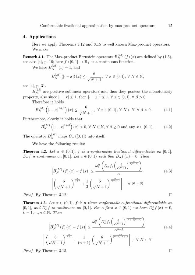
4. Applications
Here we apply Theorems 3.12 and 3.15 to well known Max-product operators.We make
Remark 4.1. The Max-product Bernstein operators B(M)N (f) (x) are defined by (1.5),
see also [4], p. 10; here f : [0, 1]→ R+ is a continuous function.
We have B(M)N (1) = 1, and
B(M)N (|· − x|) (x) ≤ 6√
N + 1, ∀ x ∈ [0, 1] , ∀ N ∈ N,
see [4], p. 31.
B(M)N are positive sublinear operators and thus they possess the monotonicity
property, also since |· − x| ≤ 1, then |· − x|β ≤ 1, ∀ x ∈ [0, 1], ∀ β > 0.Therefore it holds
B(M)N
(|· − x|1+β
)(x) ≤ 6√
N + 1, ∀ x ∈ [0, 1] , ∀ N ∈ N, ∀ β > 0. (4.1)
Furthermore, clearly it holds that
B(M)N
(|· − x|1+β
)(x) > 0, ∀ N ∈ N, ∀ β ≥ 0 and any x ∈ (0, 1) . (4.2)
The operator B(M)N maps C+ ([0, 1]) into itself.
We have the following results:
Theorem 4.2. Let α ∈ (0, 1], f is α-conformable fractional differentiable on [0, 1],Dαf is continuous on [0, 1]. Let x ∈ (0, 1) such that Dαf (x) = 0. Then
∣∣∣B(M)N (f) (x)− f (x)
∣∣∣ ≤ ωα1
(Dαf,
(6√N+1
) α2(α+1)
)α
· (4.3)[(6√N + 1
) αα+1
+1
2
(6√N + 1
) α2(α+1)
], ∀ N ∈ N.
Proof. By Theorem 3.12.
Theorem 4.3. Let α ∈ (0, 1], f is n times conformable α-fractional differentiable on[0, 1], and Dn
αf is continuous on [0, 1]. For a fixed x ∈ (0, 1) we have Dkαf (x) = 0,
k = 1, ..., n ∈ N. Then
∣∣∣B(M)N (f) (x)− f (x)
∣∣∣ ≤ ωα1
(Dnαf,(
6√N+1
) α(n+1)(α+1)
)αnn!
· (4.4)[(6√N + 1
) αα+1
+1
(n+ 1)
(6√N + 1
) nα(n+1)(α+1)
], ∀ N ∈ N.
Proof. By Theorem 3.15.
16 George A. Anastassiou
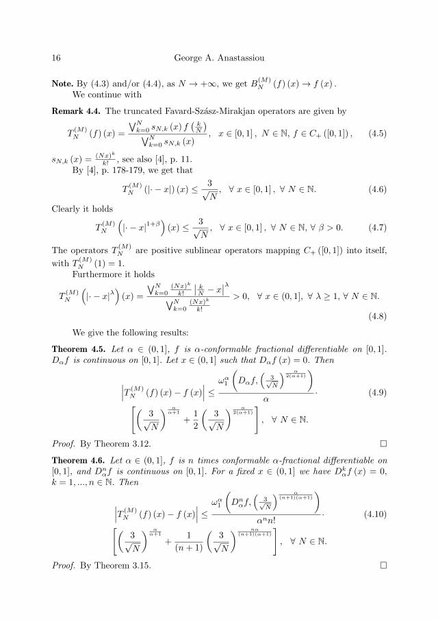
Note. By (4.3) and/or (4.4), as N → +∞, we get B(M)N (f) (x)→ f (x) .
We continue with
Remark 4.4. The truncated Favard-Szasz-Mirakjan operators are given by
T(M)N (f) (x) =
∨Nk=0 sN,k (x) f
(kN
)∨Nk=0 sN,k (x)
, x ∈ [0, 1] , N ∈ N, f ∈ C+ ([0, 1]) , (4.5)
sN,k (x) = (Nx)k
k! , see also [4], p. 11.By [4], p. 178-179, we get that
T(M)N (|· − x|) (x) ≤ 3√
N, ∀ x ∈ [0, 1] , ∀ N ∈ N. (4.6)
Clearly it holds
T(M)N
(|· − x|1+β
)(x) ≤ 3√
N, ∀ x ∈ [0, 1] , ∀ N ∈ N, ∀ β > 0. (4.7)
The operators T(M)N are positive sublinear operators mapping C+ ([0, 1]) into itself,
with T(M)N (1) = 1.
Furthermore it holds
T(M)N
(|· − x|λ
)(x) =
∨Nk=0
(Nx)k
k!
∣∣ kN − x
∣∣λ∨Nk=0
(Nx)k
k!
> 0, ∀ x ∈ (0, 1], ∀ λ ≥ 1, ∀ N ∈ N.
(4.8)
We give the following results:
Theorem 4.5. Let α ∈ (0, 1], f is α-conformable fractional differentiable on [0, 1].Dαf is continuous on [0, 1]. Let x ∈ (0, 1] such that Dαf (x) = 0. Then
∣∣∣T (M)N (f) (x)− f (x)
∣∣∣ ≤ ωα1
(Dαf,
(3√N
) α2(α+1)
)α
· (4.9)[(3√N
) αα+1
+1
2
(3√N
) α2(α+1)
], ∀ N ∈ N.
Proof. By Theorem 3.12.
Theorem 4.6. Let α ∈ (0, 1], f is n times conformable α-fractional differentiable on[0, 1], and Dn
αf is continuous on [0, 1]. For a fixed x ∈ (0, 1] we have Dkαf (x) = 0,
k = 1, ..., n ∈ N. Then
∣∣∣T (M)N (f) (x)− f (x)
∣∣∣ ≤ ωα1
(Dnαf,(
3√N
) α(n+1)(α+1)
)αnn!
· (4.10)[(3√N
) αα+1
+1
(n+ 1)
(3√N
) nα(n+1)(α+1)
], ∀ N ∈ N.
Proof. By Theorem 3.15.
Conformable fractional approximation by max-product operators 17
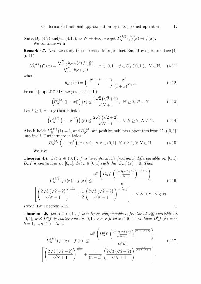
Note. By (4.9) and/or (4.10), as N → +∞, we get T(M)N (f) (x)→ f (x) .
We continue with
Remark 4.7. Next we study the truncated Max-product Baskakov operators (see [4],p. 11)
U(M)N (f) (x) =
∨Nk=0 bN,k (x) f
(kN
)∨Nk=0 bN,k (x)
, x ∈ [0, 1] , f ∈ C+ ([0, 1]) , N ∈ N, (4.11)
where
bN,k (x) =
(N + k − 1
k
)xk
(1 + x)N+k
. (4.12)
From [4], pp. 217-218, we get (x ∈ [0, 1])(U
(M)N (|· − x|)
)(x) ≤
2√
3(√
2 + 2)
√N + 1
, N ≥ 2, N ∈ N. (4.13)
Let λ ≥ 1, clearly then it holds(U
(M)N
(|· − x|λ
))(x) ≤
2√
3(√
2 + 2)
√N + 1
, ∀ N ≥ 2, N ∈ N. (4.14)
Also it holds U(M)N (1) = 1, and U
(M)N are positive sublinear operators from C+ ([0, 1])
into itself. Furthermore it holds
U(M)N
(|· − x|λ
)(x) > 0, ∀ x ∈ (0, 1], ∀ λ ≥ 1, ∀ N ∈ N. (4.15)
We give
Theorem 4.8. Let α ∈ (0, 1], f is α-conformable fractional differentiable on [0, 1].Dαf is continuous on [0, 1]. Let x ∈ (0, 1] such that Dαf (x) = 0. Then
∣∣∣U (M)N (f) (x)− f (x)
∣∣∣ ≤ ωα1
(Dαf,
(2√3(√2+2)√
N+1
) α2(α+1)
)α
· (4.16)(2√
3(√
2 + 2)
√N + 1
) αα+1
+1
2
(2√
3(√
2 + 2)
√N + 1
) α2(α+1)
, ∀ N ≥ 2, N ∈ N.
Proof. By Theorem 3.12.
Theorem 4.9. Let α ∈ (0, 1], f is n times conformable α-fractional differentiable on[0, 1], and Dn
αf is continuous on [0, 1]. For a fixed x ∈ (0, 1] we have Dkαf (x) = 0,
k = 1, ..., n ∈ N. Then
∣∣∣U (M)N (f) (x)− f (x)
∣∣∣ ≤ ωα1
(Dnαf,
(2√3(√2+2)√
N+1
) α(n+1)(α+1)
)αnn!
· (4.17)(2√
3(√
2 + 2)
√N + 1
) αα+1
+1
(n+ 1)
(2√
3(√
2 + 2)
√N + 1
) nα(n+1)(α+1)
,
18 George A. Anastassiou
∀ N ≥ 2, N ∈ N.
Proof. By Theorem 3.15.
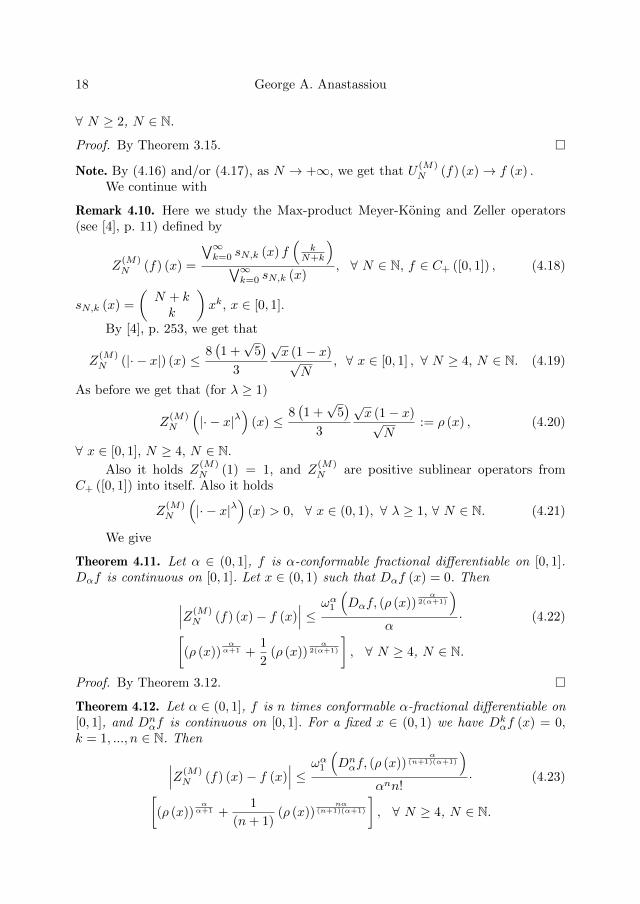
Note. By (4.16) and/or (4.17), as N → +∞, we get that U(M)N (f) (x)→ f (x) .
We continue with
Remark 4.10. Here we study the Max-product Meyer-Koning and Zeller operators(see [4], p. 11) defined by
Z(M)N (f) (x) =
∨∞k=0 sN,k (x) f
(k
N+k
)∨∞k=0 sN,k (x)
, ∀ N ∈ N, f ∈ C+ ([0, 1]) , (4.18)
sN,k (x) =
(N + kk
)xk, x ∈ [0, 1].
By [4], p. 253, we get that
Z(M)N (|· − x|) (x) ≤
8(1 +√
5)
3
√x (1− x)√
N, ∀ x ∈ [0, 1] , ∀ N ≥ 4, N ∈ N. (4.19)
As before we get that (for λ ≥ 1)
Z(M)N
(|· − x|λ
)(x) ≤
8(1 +√
5)
3
√x (1− x)√
N:= ρ (x) , (4.20)
∀ x ∈ [0, 1], N ≥ 4, N ∈ N.Also it holds Z
(M)N (1) = 1, and Z
(M)N are positive sublinear operators from
C+ ([0, 1]) into itself. Also it holds
Z(M)N
(|· − x|λ
)(x) > 0, ∀ x ∈ (0, 1), ∀ λ ≥ 1, ∀ N ∈ N. (4.21)
We give
Theorem 4.11. Let α ∈ (0, 1], f is α-conformable fractional differentiable on [0, 1].Dαf is continuous on [0, 1]. Let x ∈ (0, 1) such that Dαf (x) = 0. Then∣∣∣Z(M)
N (f) (x)− f (x)∣∣∣ ≤ ωα1
(Dαf, (ρ (x))
α2(α+1)
)α
· (4.22)[(ρ (x))
αα+1 +
1
2(ρ (x))
α2(α+1)
], ∀ N ≥ 4, N ∈ N.
Proof. By Theorem 3.12.
Theorem 4.12. Let α ∈ (0, 1], f is n times conformable α-fractional differentiable on[0, 1], and Dn
αf is continuous on [0, 1]. For a fixed x ∈ (0, 1) we have Dkαf (x) = 0,
k = 1, ..., n ∈ N. Then∣∣∣Z(M)N (f) (x)− f (x)
∣∣∣ ≤ ωα1
(Dnαf, (ρ (x))
α(n+1)(α+1)
)αnn!
· (4.23)[(ρ (x))
αα+1 +
1
(n+ 1)(ρ (x))
nα(n+1)(α+1)
], ∀ N ≥ 4, N ∈ N.
Conformable fractional approximation by max-product operators 19
Proof. By Theorem 3.15.
Note. By (4.22) and/or (4.23), as N → +∞, we get that Z(M)N (f) (x)→ f (x) .
We continue with
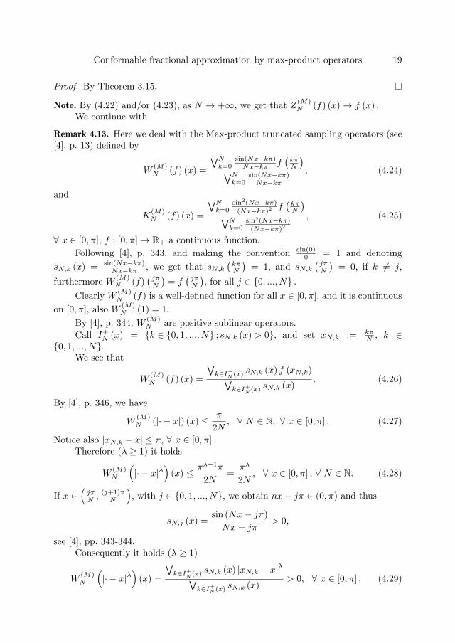
Remark 4.13. Here we deal with the Max-product truncated sampling operators (see[4], p. 13) defined by
W(M)N (f) (x) =
∨Nk=0
sin(Nx−kπ)Nx−kπ f
(kπN
)∨Nk=0
sin(Nx−kπ)Nx−kπ
, (4.24)
and
K(M)N (f) (x) =
∨Nk=0
sin2(Nx−kπ)(Nx−kπ)2 f
(kπN
)∨Nk=0
sin2(Nx−kπ)(Nx−kπ)2
, (4.25)
∀ x ∈ [0, π], f : [0, π]→ R+ a continuous function.
Following [4], p. 343, and making the convention sin(0)0 = 1 and denoting
sN,k (x) = sin(Nx−kπ)Nx−kπ , we get that sN,k
(kπN
)= 1, and sN,k
(jπN
)= 0, if k 6= j,
furthermore W(M)N (f)
(jπN
)= f
(jπN
), for all j ∈ 0, ..., N .
Clearly W(M)N (f) is a well-defined function for all x ∈ [0, π], and it is continuous
on [0, π], also W(M)N (1) = 1.
By [4], p. 344, W(M)N are positive sublinear operators.
Call I+N (x) = k ∈ 0, 1, ..., N ; sN,k (x) > 0, and set xN,k := kπN , k ∈
0, 1, ..., N.We see that
W(M)N (f) (x) =
∨k∈I+N (x) sN,k (x) f (xN,k)∨
k∈I+N (x) sN,k (x). (4.26)
By [4], p. 346, we have
W(M)N (|· − x|) (x) ≤ π
2N, ∀ N ∈ N, ∀ x ∈ [0, π] . (4.27)
Notice also |xN,k − x| ≤ π, ∀ x ∈ [0, π] .Therefore (λ ≥ 1) it holds
W(M)N
(|· − x|λ
)(x) ≤ πλ−1π
2N=
πλ
2N, ∀ x ∈ [0, π] , ∀ N ∈ N. (4.28)
If x ∈(jπN ,
(j+1)πN
), with j ∈ 0, 1, ..., N, we obtain nx− jπ ∈ (0, π) and thus
sN,j (x) =sin (Nx− jπ)
Nx− jπ> 0,
see [4], pp. 343-344.Consequently it holds (λ ≥ 1)
W(M)N
(|· − x|λ
)(x) =
∨k∈I+N (x) sN,k (x) |xN,k − x|λ∨
k∈I+N (x) sN,k (x)> 0, ∀ x ∈ [0, π] , (4.29)
20 George A. Anastassiou
such that x 6= xN,k, for any k ∈ 0, 1, ..., N .
We give
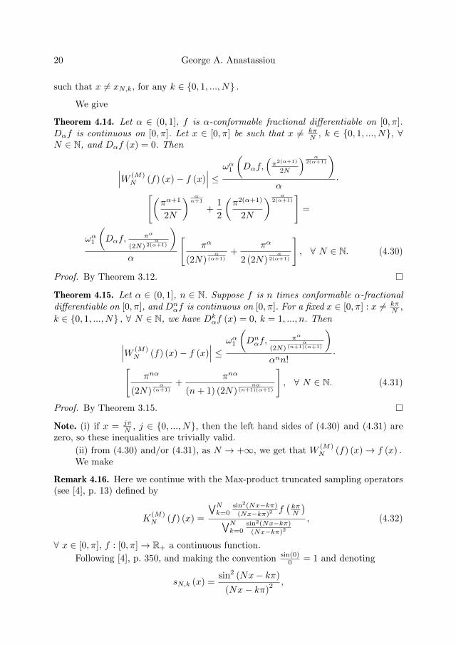
Theorem 4.14. Let α ∈ (0, 1], f is α-conformable fractional differentiable on [0, π].Dαf is continuous on [0, π]. Let x ∈ [0, π] be such that x 6= kπ
N , k ∈ 0, 1, ..., N, ∀N ∈ N, and Dαf (x) = 0. Then
∣∣∣W (M)N (f) (x)− f (x)
∣∣∣ ≤ ωα1
(Dαf,
(π2(α+1)
2N
) α2(α+1)
)α
·[(πα+1
2N
) αα+1
+1
2
(π2(α+1)
2N
) α2(α+1)
]=
ωα1
(Dαf,
πα
(2N)α
2(α+1)
)α
[πα
(2N)α
(α+1)+
πα
2 (2N)α
2(α+1)
], ∀ N ∈ N. (4.30)
Proof. By Theorem 3.12.
Theorem 4.15. Let α ∈ (0, 1], n ∈ N. Suppose f is n times conformable α-fractionaldifferentiable on [0, π], and Dn
αf is continuous on [0, π]. For a fixed x ∈ [0, π] : x 6= kπN ,
k ∈ 0, 1, ..., N , ∀ N ∈ N, we have Dkαf (x) = 0, k = 1, ..., n. Then
∣∣∣W (M)N (f) (x)− f (x)
∣∣∣ ≤ ωα1
(Dnαf,
πα
(2N)α
(n+1)(α+1)
)αnn!
·[πnα
(2N)α
(α+1)+
πnα
(n+ 1) (2N)nα
(n+1)(α+1)
], ∀ N ∈ N. (4.31)
Proof. By Theorem 3.15.
Note. (i) if x = jπN , j ∈ 0, ..., N, then the left hand sides of (4.30) and (4.31) are
zero, so these inequalities are trivially valid.
(ii) from (4.30) and/or (4.31), as N → +∞, we get that W(M)N (f) (x)→ f (x) .
We make
Remark 4.16. Here we continue with the Max-product truncated sampling operators(see [4], p. 13) defined by
K(M)N (f) (x) =
∨Nk=0
sin2(Nx−kπ)(Nx−kπ)2 f
(kπN
)∨Nk=0
sin2(Nx−kπ)(Nx−kπ)2
, (4.32)
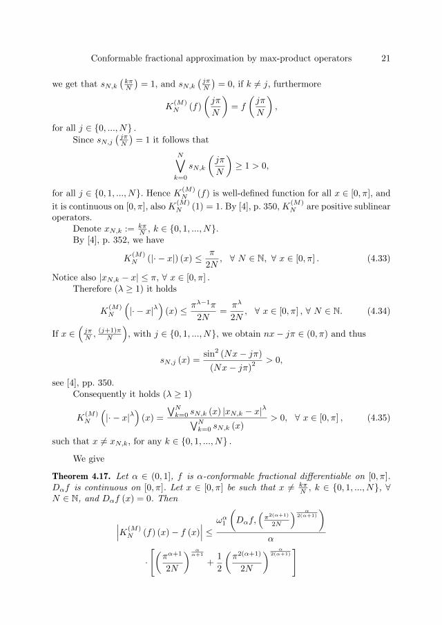
∀ x ∈ [0, π], f : [0, π]→ R+ a continuous function.
Following [4], p. 350, and making the convention sin(0)0 = 1 and denoting
sN,k (x) =sin2 (Nx− kπ)
(Nx− kπ)2 ,
Conformable fractional approximation by max-product operators 21
we get that sN,k(kπN
)= 1, and sN,k
(jπN
)= 0, if k 6= j, furthermore
K(M)N (f)
(jπ
N
)= f
(jπ
N
),
for all j ∈ 0, ..., N .Since sN,j
(jπN
)= 1 it follows that
N∨k=0
sN,k
(jπ
N
)≥ 1 > 0,
for all j ∈ 0, 1, ..., N. Hence K(M)N (f) is well-defined function for all x ∈ [0, π], and
it is continuous on [0, π], also K(M)N (1) = 1. By [4], p. 350, K
(M)N are positive sublinear
operators.Denote xN,k := kπ
N , k ∈ 0, 1, ..., N.By [4], p. 352, we have
K(M)N (|· − x|) (x) ≤ π
2N, ∀ N ∈ N, ∀ x ∈ [0, π] . (4.33)
Notice also |xN,k − x| ≤ π, ∀ x ∈ [0, π] .Therefore (λ ≥ 1) it holds
K(M)N
(|· − x|λ
)(x) ≤ πλ−1π
2N=
πλ
2N, ∀ x ∈ [0, π] , ∀ N ∈ N. (4.34)
If x ∈(jπN ,
(j+1)πN
), with j ∈ 0, 1, ..., N, we obtain nx− jπ ∈ (0, π) and thus
sN,j (x) =sin2 (Nx− jπ)
(Nx− jπ)2 > 0,
see [4], pp. 350.Consequently it holds (λ ≥ 1)
K(M)N
(|· − x|λ
)(x) =
∨Nk=0 sN,k (x) |xN,k − x|λ∨N
k=0 sN,k (x)> 0, ∀ x ∈ [0, π] , (4.35)
such that x 6= xN,k, for any k ∈ 0, 1, ..., N .
We give
Theorem 4.17. Let α ∈ (0, 1], f is α-conformable fractional differentiable on [0, π].Dαf is continuous on [0, π]. Let x ∈ [0, π] be such that x 6= kπ
N , k ∈ 0, 1, ..., N, ∀N ∈ N, and Dαf (x) = 0. Then
∣∣∣K(M)N (f) (x)− f (x)
∣∣∣ ≤ ωα1
(Dαf,
(π2(α+1)
2N
) α2(α+1)
)α
·
[(πα+1
2N
) αα+1
+1
2
(π2(α+1)
2N
) α2(α+1)
]
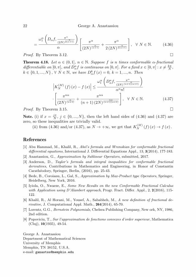
22 George A. Anastassiou
=
ωα1
(Dαf,
πα
(2N)α
2(α+1)
)α
[πα
(2N)α
(α+1)+
πα
2 (2N)α
2(α+1)
], ∀ N ∈ N. (4.36)
Proof. By Theorem 3.12.
Theorem 4.18. Let α ∈ (0, 1], n ∈ N. Suppose f is n times conformable α-fractionaldifferentiable on [0, π], and Dn
αf is continuous on [0, π]. For a fixed x ∈ [0, π] : x 6= kπN ,
k ∈ 0, 1, ..., N , ∀ N ∈ N, we have Dkαf (x) = 0, k = 1, ..., n. Then
∣∣∣K(M)N (f) (x)− f (x)
∣∣∣ ≤ ωα1
(Dnαf,
πα
(2N)α
(n+1)(α+1)
)αnn!
·
[πnα
(2N)α
(α+1)+
πnα
(n+ 1) (2N)nα
(n+1)(α+1)
], ∀ N ∈ N. (4.37)
Proof. By Theorem 3.15.
Note. (i) if x = jπN , j ∈ 0, ..., N, then the left hand sides of (4.36) and (4.37) are
zero, so these inequalities are trivially valid.
(ii) from (4.36) and/or (4.37), as N → +∞, we get that K(M)N (f) (x)→ f (x) .
References
[1] Abu Hammad, M., Khalil, R., Abel’s formula and Wronskian for conformable fractionaldifferential equations, International J. Differential Equations Appl., 13, 3(2014), 177-183.
[2] Anastassiou, G., Approximation by Sublinear Operators, submitted, 2017.
[3] Anderson, D., Taylor’s formula and integral inequalities for conformable fractionalderivatives, Contributions in Mathematics and Engineering, in Honor of ConstantinCaratheodory, Springer, Berlin, (2016), pp. 25-43.
[4] Bede, B., Coroianu, L., Gal, S., Approximation by Max-Product type Operators, Springer,Heidelberg, New York, 2016.
[5] Iyiola, O., Nwaeze, E., Some New Results on the new Conformable Fractional Calculuswith Application using D’Alambert approach, Progr. Fract. Differ. Appl., 2, 2(2016), 115-122.
[6] Khalil, R., Al Horani, M., Yousef, A., Sababheh, M., A new definition of fractional de-rivative, J. Computational Appl. Math., 264(2014), 65-70.
[7] Lorentz, G.G., Bernstein Polynomials, Chelsea Publishing Company, New ork, NY, 1986,2nd edition.
[8] Popoviciu, T., Sur l’approximation de fonctions convexes d’order superieur, Mathematica(Cluj), 10(1935), 49-54.
George A. AnastassiouDepartment of Mathematical SciencesUniversity of MemphisMemphis, TN 38152, U.S.A.e-mail: [email protected]
Stud. Univ. Babes-Bolyai Math. 63(2018), No. 1, 23–35DOI: 10.24193/subbmath.2018.1.02
Generalizations of some fractional integralinequalities for m-convex functions viageneralized Mittag-Leffler function
Ghulam Farid and Ghulam Abbas
Abstract. In this paper we are interested to present some general fractional in-tegral inequalities for m-convex functions by involving generalized Mittag-Lefflerfunction. In particular we produce inequalities for several kinds of fractional inte-grals. Also these inequalities have some connections with known integral inequal-ities.
Mathematics Subject Classification (2010): 26A51, 26A33, 33E12.
Keywords: m-convex function, Hadamard inequality, generalized Mittag-Lefflerfunction.
1. Introduction
Inequalities play an essential role in mathematical and other kinds of analysis,specially inequalities involving derivative and integral of functions are of great interestfor researchers.Convex functions are very special in the study of functions defined on real line, a lotof results, in particular inequalities in mathematical analysis based on their invention.A convex function f : I → R is also equivalently defined by the Hadamard inequality
f
(a+ b
2
)≤ 1
b− a
∫ b
a
f(t)dt ≤ f(a) + f(b)
2
where a, b ∈ I, a < b.A close generalized form of convex functions is m-convex functions introduced byToader [23].
Definition 1.1. A function f : [0, b]→ R, b > 0 is said to be m-convex function if forall x, y ∈ [0, b] and t ∈ [0, 1]
f(tx+m(1− t)y) ≤ tf(x) +m(1− t)f(y)
24 Ghulam Farid and Ghulam Abbas
holds for m ∈ [0, 1].
Every m-convex function is not convex function.
Example 1.2. [16] Let f : [0,∞]→ R be defined by
g(t) =1
12(x4 − 5x3 + 9x2 − 5x)
is 1617 -convex function but it is not convex function.
Form = 1 the above definition becomes the definition of convex functions definedon [0, b]. If we take m = 0, then we obtain the concept of starshaped functions on[0, b]. A function f : [0, b]→ R is said to be starshaped if f(tx) ≤ tf(x) for all t ∈ [0, 1]and x ∈ [0, b].If set of m-convex functions on [0, b] for which f(0) < 0 is denoted by Km(b), thenwe have
K1(b) ⊂ Km(b) ⊂ K0(b)
whenever m ∈ (0, 1). In the class K1(b) there are convex functions f : [0, b] → R forwhich f(0) ≤ 0 (see, [2]). There are a number of results and inequalities obtained viam-convex functions for detail (see [2, 4, 7, 10]).Recently, a number of authors are taking keen interest to obtain integral inequalitiesof the Hadamard type via fractional integral operators of different kinds in the variousfield of fractional calculus. For example one can see [5, 6, 11, 15, 17, 20, 22].
2. Preliminaries in fractional calculus and integral operators
Fractional calculus deals with the study of integral and differential operatorsof non-integral order. Many mathematicians like Liouville, Riemann and Weyl mademajor contributions to the theory of fractional calculus. The study on the fractionalcalculus continued with contributions from Fourier, Abel, Lacroix, Leibniz, Grun-wald and Letnikov. For detail (see, [11, 13, 15]). Riemann-Liouville fractional integraloperator is the first formulation of an integral operator of non-integral order.
Definition 2.1. [24] Let f ∈ L1[a, b]. Then Riemann-Liouville fractional integral of fof order ν is defined by
Iνa+f(x) =1
Γ(ν)
∫ x
a
(x− t)ν−1f(t)dt, x > a
and
Iνb−f(x) =1
Γ(ν)
∫ b
x
(t− x)ν−1f(t)dt, x < b.
In fact these formulations of fractional integral operators have been establisheddue to Letnikov [14], Sonin [21] and then by Laurent [12]. In these days a variety offractional integral operators have been produced and many are under discussion. Anumber of generalized fractional integral operators are also very useful in generalizingthe theory of fractional integral operators [1, 11, 15, 18, 22, 24].
Generalization of some fractional integral inequalities 25
Definition 2.2. [18] Let µ, ν, k, l, γ be positive real numbers and ω ∈ R. Then the
generalized fractional integral operators containing Mittag-Leffler function εγ,δ,kµ,ν,l,ω,a+
and εγ,δ,kµ,ν,l,ω,b−for a real valued continuous function f is defined by:(εγ,δ,kµ,ν,l,ω,a+f
)(x) =
∫ x
a
(x− t)ν−1Eγ,δ,kµ,ν,l (ω(x− t)µ)f(t)dt, (2.1)
and (εγ,δ,kµ,ν,l,ω,b−
f)
(x) =
∫ b
x
(t− x)ν−1Eγ,δ,kµ,ν,l (ω(t− x)µ)f(t)dt,
where the function Eγ,δ,kµ,ν,l is generalized Mittag-Leffler function defined as
Eγ,δ,kµ,ν,l (t) =
∞∑n=0
(γ)kntn
Γ(µn+ ν)(δ)ln, (2.2)
(a)n is the Pochhammer symbol, it defined as
(a)n = a(a+ 1)(a+ 2)...(a+ n− 1), (a)0 = 1.
If δ = l = 1 in (2.1), then integral operator εγ,δ,kµ,ν,l,ω,a+ reduces to an integral operator
εγ,1,kµ,ν,1,ω,a+ containing generalized Mittag-Leffler function Eγ,1,kµ,ν,1 introduced by Srivas-
tava and Tomovski in [22]. Along with δ = l = 1 in addition if k = 1 then (2.1) reducesto an integral operator defined by Prabhaker in [17] containing Mittag-Leffler function
Eγµ,ν . For ω = 0 in (2.1), integral operator εγ,δ,kµ,ν,l,ω,a+ reduces to the Riemann-Liouville
fractional integral operator [18].
In [18, 22] properties of generalized integral operator and generalized Mittag-
Leffler functions are studied in details. In [18] it is proved that Eγ,δ,kµ,ν,l (t) is absolutely
convergent for k < l + µ. Let S be the sum of series of absolute terms of Eγ,δ,kµ,ν,l (t).We will use this property of Mittag-Leffler function in sequal.
Now a days a number of authors are working on inequalities involving fractionalintegral operators and generalized fractional integral operators for example Riemann-Liouville, Caputo, Hilfer, Canvati etc [8, 20]. Actually, fractional integral inequalitiesare very useful to find the uniqueness of solutions for partial differential equationsof non-integral order. In this paper we give some fractional integral inequalities form-convex functions by involving generalized Mittag-Leffler function. Also we deducesome main results of [3, 9, 19].
3. Fractional integral inequalities
First we prove the following lemma which would be helpful to obtain the mainresults.
Lemma 3.1. Let f : I → R be a differentiable mapping on I, a, b ∈ I with 0 ≤ a < band also let g : [a,mb] → R be a continuous function on [a,mb]. If f ′, g ∈ L[a,mb],
26 Ghulam Farid and Ghulam Abbas
then the following equality holds for ν > 0(∫ mb
a
g(s)Eγ,δ,kµ,ν,l (ωsµ)ds
)ν[f(a) + f(mb)] (3.1)
− ν∫ mb
a
(∫ t
a
g(s)Eγ,δ,kµ,ν,l (ωsµ)ds
)ν−1g(t)Eγ,δ,kµ,ν,l (ωt
µ)f(t)dt
− ν∫ mb
a
(∫ mb
t
g(s)Eγ,δ,kµ,ν,l (ωsµ)ds
)ν−1g(t)Eγ,δ,kµ,ν,l (ωt
µ)f(t)dt
=
∫ mb
a
(∫ t
a
g(s)Eγ,δ,kµ,ν,l (ωsµ)ds
)νf ′(t)dt
−∫ mb
a
(∫ mb
t
g(s)Eγ,δ,kµ,ν,l (ωsα)ds
)νf ′(t)dt
where Eγ,δ,kµ,ν,l is generalized Mittag-Leffler function.
Proof. One can have on integrating by parts∫ mb
a
(∫ t
a
g(s)Eγ,δ,kµ,ν,l (ωsµ)ds
)νf ′(t)dt (3.2)
=
(∫ mb
a
g(s)Eγ,δ,kµ,ν,l (ωsµ)ds
)νf(mb)
− ν∫ mb
a
(∫ t
a
g(s)Eγ,δ,kµ,ν,l (ωsµ)ds
)ν−1g(t)Eγ,δ,kµ,ν,l (ωt
µ)f(t)dt.
And likewise∫ mb
a
(∫ mb
t
g(s)Eγ,δ,kµ,ν,l (ωsµ)ds
)νf ′(t)dt (3.3)
= −
(∫ mb
a
g(s)Eγ,δ,kµ,ν,l (ωsµ)ds
)νf(a)
+ ν
∫ mb
a
(∫ mb
t
g(s)Eγ,δ,kµ,ν,l (ωsµ)ds
)ν−1g(t)Eγ,δ,kµ,ν,l (ωt
µ)f(t)dt.
On substracting equation (3.3) from (3.2), we get the result.
We use Lemma 3.1 to establish the following fractional integral inequality.
Theorem 3.2. Let f : I → R be a differentiable mapping on I, a, b ∈ I with 0 ≤ a < band also let g : [a,mb] → R be a continuous function on [a,mb]. If |f ′| is m-convex
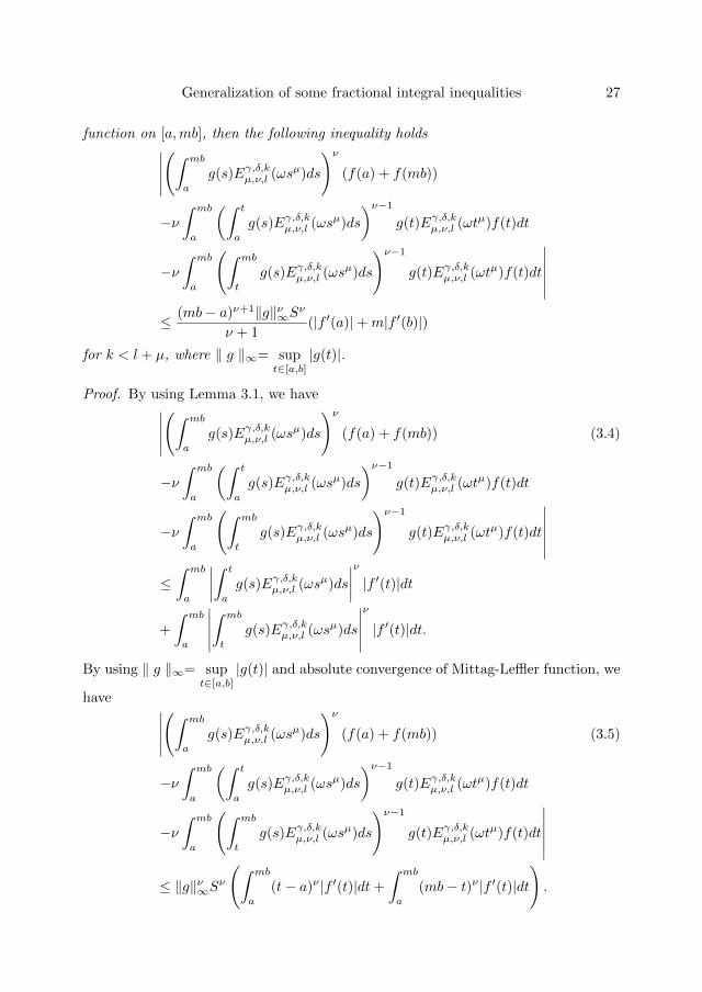
Generalization of some fractional integral inequalities 27
function on [a,mb], then the following inequality holds∣∣∣∣∣(∫ mb
a
g(s)Eγ,δ,kµ,ν,l (ωsµ)ds
)ν(f(a) + f(mb))
−ν∫ mb
a
(∫ t
a
g(s)Eγ,δ,kµ,ν,l (ωsµ)ds
)ν−1g(t)Eγ,δ,kµ,ν,l (ωt
µ)f(t)dt
−ν∫ mb
a
(∫ mb
t
g(s)Eγ,δ,kµ,ν,l (ωsµ)ds
)ν−1g(t)Eγ,δ,kµ,ν,l (ωt
µ)f(t)dt
∣∣∣∣∣∣≤ (mb− a)ν+1‖g‖ν∞Sν
ν + 1(|f ′(a)|+m|f ′(b)|)
for k < l + µ, where ‖ g ‖∞= supt∈[a,b]
|g(t)|.
Proof. By using Lemma 3.1, we have∣∣∣∣∣(∫ mb
a
g(s)Eγ,δ,kµ,ν,l (ωsµ)ds
)ν(f(a) + f(mb)) (3.4)
−ν∫ mb
a
(∫ t
a
g(s)Eγ,δ,kµ,ν,l (ωsµ)ds
)ν−1g(t)Eγ,δ,kµ,ν,l (ωt
µ)f(t)dt
−ν∫ mb
a
(∫ mb
t
g(s)Eγ,δ,kµ,ν,l (ωsµ)ds
)ν−1g(t)Eγ,δ,kµ,ν,l (ωt
µ)f(t)dt
∣∣∣∣∣∣≤∫ mb
a
∣∣∣∣∫ t
a
g(s)Eγ,δ,kµ,ν,l (ωsµ)ds
∣∣∣∣ν |f ′(t)|dt+
∫ mb
a
∣∣∣∣∣∫ mb
t
g(s)Eγ,δ,kµ,ν,l (ωsµ)ds
∣∣∣∣∣ν
|f ′(t)|dt.
By using ‖ g ‖∞= supt∈[a,b]
|g(t)| and absolute convergence of Mittag-Leffler function, we
have ∣∣∣∣∣(∫ mb
a
g(s)Eγ,δ,kµ,ν,l (ωsµ)ds
)ν(f(a) + f(mb)) (3.5)
−ν∫ mb
a
(∫ t
a
g(s)Eγ,δ,kµ,ν,l (ωsµ)ds
)ν−1g(t)Eγ,δ,kµ,ν,l (ωt
µ)f(t)dt
−ν∫ mb
a
(∫ mb
t
g(s)Eγ,δ,kµ,ν,l (ωsµ)ds
)ν−1g(t)Eγ,δ,kµ,ν,l (ωt
µ)f(t)dt
∣∣∣∣∣∣≤ ‖g‖ν∞Sν
(∫ mb
a
(t− a)ν |f ′(t)|dt+
∫ mb
a
(mb− t)ν |f ′(t)|dt
).
28 Ghulam Farid and Ghulam Abbas
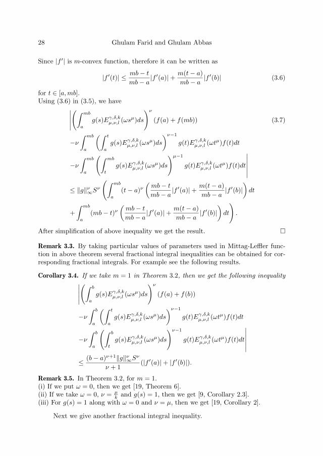
Since |f ′| is m-convex function, therefore it can be written as
|f ′(t)| ≤ mb− tmb− a
|f ′(a)|+ m(t− a)
mb− a|f ′(b)| (3.6)
for t ∈ [a,mb].Using (3.6) in (3.5), we have∣∣∣∣∣
(∫ mb
a
g(s)Eγ,δ,kµ,ν,l (ωsµ)ds
)ν(f(a) + f(mb)) (3.7)
−ν∫ mb
a
(∫ t
a
g(s)Eγ,δ,kµ,ν,l (ωsµ)ds
)ν−1g(t)Eγ,δ,kµ,ν,l (ωt
µ)f(t)dt
−ν∫ mb
a
(∫ mb
t
g(s)Eγ,δ,kµ,ν,l (ωsµ)ds
)µ−1g(t)Eγ,δ,kµ,ν,l (ωt
µ)f(t)dt
∣∣∣∣∣∣≤ ‖g‖ν∞Sν
(∫ mb
a
(t− a)ν(mb− tmb− a
|f ′(a)|+ m(t− a)
mb− a|f ′(b)|
)dt
+
∫ mb
a
(mb− t)ν(mb− tmb− a
|f ′(a)|+ m(t− a)
mb− a|f ′(b)|
)dt
).
After simplification of above inequality we get the result.
Remark 3.3. By taking particular values of parameters used in Mittag-Leffler func-tion in above theorem several fractional integral inequalities can be obtained for cor-responding fractional integrals. For example see the following results.
Corollary 3.4. If we take m = 1 in Theorem 3.2, then we get the following inequality∣∣∣∣∣(∫ b
a
g(s)Eγ,δ,kµ,ν,l (ωsµ)ds
)ν(f(a) + f(b))
−ν∫ b
a
(∫ t
a
g(s)Eγ,δ,kµ,ν,l (ωsµ)ds
)ν−1g(t)Eγ,δ,kµ,ν,l (ωt
µ)f(t)dt
−ν∫ b
a
(∫ b
t
g(s)Eγ,δ,kµ,ν,l (ωsµ)ds
)ν−1g(t)Eγ,δ,kµ,ν,l (ωt
µ)f(t)dt
∣∣∣∣∣∣≤ (b− a)ν+1‖g‖ν∞Sν
ν + 1(|f ′(a)|+ |f ′(b)|).
Remark 3.5. In Theorem 3.2, for m = 1.(i) If we put ω = 0, then we get [19, Theorem 6].(ii) If we take ω = 0, ν = µ
k and g(s) = 1, then we get [9, Corollary 2.3].(iii) For g(s) = 1 along with ω = 0 and ν = µ, then we get [19, Corollary 2].
Next we give another fractional integral inequality.
Generalization of some fractional integral inequalities 29
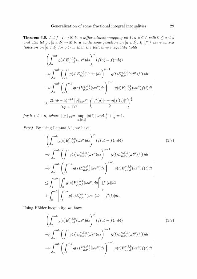
Theorem 3.6. Let f : I → R be a differentiable mapping on I, a, b ∈ I with 0 ≤ a < band also let g : [a,mb] → R be a continuous function on [a,mb]. If |f ′|q is m-convexfunction on [a,mb] for q > 1, then the following inequality holds∣∣∣∣∣
(∫ mb
a
g(s)Eγ,δ,kµ,ν,l (ωsµ)ds
)ν(f(a) + f(mb))
−ν∫ mb
a
(∫ t
a
g(s)Eγ,δ,kµ,ν,l (ωsµ)ds
)ν−1g(t)Eγ,δ,kµ,ν,l (ωt
µ)f(t)dt
−ν∫ mb
a
(∫ mb
t
g(s)Eγ,δ,kµ,ν,l (ωsµ)ds
)ν−1g(t)Eγ,δ,kµ,ν,l (ωt
µ)f(t)dt
∣∣∣∣∣∣≤ 2(mb− a)ν+1‖g‖ν∞Sν
(νp+ 1)1q
(|f ′(a)|q +m|f ′(b)|q
2
) 1q
for k < l + µ, where ‖ g ‖∞= supt∈[a,b]
|g(t)| and 1p + 1
q = 1.
Proof. By using Lemma 3.1, we have∣∣∣∣∣(∫ mb
a
g(s)Eγ,δ,kµ,ν,l (ωsµ)ds
)ν(f(a) + f(mb)) (3.8)
−ν∫ mb
a
(∫ t
a
g(s)Eγ,δ,kµ,ν,l (ωsµ)ds
)ν−1g(t)Eγ,δ,kµ,ν,l (ωt
µ)f(t)dt
−ν∫ mb
a
(∫ mb
t
g(s)Eγ,δ,kµ,ν,l (ωsµ)ds
)ν−1g(t)Eγ,δ,kµ,ν,l (ωt
µ)f(t)dt
∣∣∣∣∣∣≤∫ mb
a
∣∣∣∣∫ t
a
g(s)Eγ,δ,kµ,ν,l (ωsµ)ds
∣∣∣∣ν |f ′(t)|dt+
∫ mb
a
∣∣∣∣∣∫ mb
t
g(s)Eγ,δ,kµ,ν,l (ωsµ)ds
∣∣∣∣∣ν
|f ′(t)|dt.
Using Holder inequality, we have∣∣∣∣∣(∫ mb
a
g(s)Eγ,δ,kµ,ν,l (ωsµ)ds
)ν(f(a) + f(mb)) (3.9)
−ν∫ mb
a
(∫ t
a
g(s)Eγ,δ,kµ,ν,l (ωsµ)ds
)ν−1g(t)Eγ,δ,kµ,ν,l (ωt
µ)f(t)dt
−ν∫ mb
a
(∫ mb
t
g(s)Eγ,δ,kµ,ν,l (ωsµ)ds
)ν−1g(t)Eγ,δ,kµ,ν,l (ωt
µ)f(t)dt
∣∣∣∣∣∣
30 Ghulam Farid and Ghulam Abbas
≤
(∫ mb
a
∣∣∣∣∫ t
a
g(s)Eγ,δ,kµ,ν,l (ωsµ)ds
∣∣∣∣νp dt) 1p(∫ mb
a
|f ′(t)|qdt
) 1q
+
(∫ mb
a
∣∣∣∣∣∫ mb
t
g(s)Eγ,δ,kµ,ν,l (ωsµ)ds
∣∣∣∣∣νp
dt
) 1p(∫ mb
a
|f ′(t)|qdt
) 1q
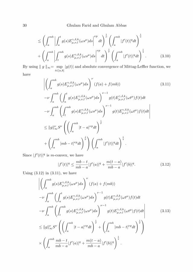
. (3.10)
By using ‖ g ‖∞= supt∈[a,b]
|g(t)| and absolute convergence of Mittag-Leffler function, we
have ∣∣∣∣∣(∫ mb
a
g(s)Eγ,δ,kµ,ν,l (ωsµ)ds
)ν(f(a) + f(mb)) (3.11)
−ν∫ mb
a
(∫ t
a
g(s)Eγ,δ,kµ,ν,l (ωsµ)ds
)ν−1g(t)Eγ,δ,kµ,ν,l (ωt
µ)f(t)dt
−ν∫ mb
a
(∫ mb
t
g(s)Eγ,δ,kµ,ν,l (ωsµ)ds
)ν−1g(t)Eγ,δ,kµ,ν,l (ωt
µ)f(t)dt
∣∣∣∣∣∣≤ ‖g‖ν∞Sν
(∫ mb
a
|t− a|νpdt
) 1p
+
(∫ mb
a
|mb− t|νpdt
) 1p
(∫ mb
a
|f ′(t)|qdt
) 1q
.
Since |f ′(t)|q is m-convex, we have
|f ′(t)|q ≤ mb− tmb− a
|f ′(a)|q +m(t− a)
mb− a|f ′(b)|q. (3.12)
Using (3.12) in (3.11), we have∣∣∣∣∣(∫ mb
a
g(s)Eγ,δ,kµ,ν,l (ωsµ)ds
)ν(f(a) + f(mb))
−ν∫ mb
a
(∫ t
a
g(s)Eγ,δ,kµ,ν,l (ωsµ)ds
)ν−1g(t)Eγ,δ,kµ,ν,l (ωt
µ)f(t)dt
−ν∫ mb
a
(∫ mb
t
g(s)Eγ,δ,kµ,ν,l (ωsµ)ds
)ν−1g(t)Eγ,δ,kµ,ν,l (ωt
µ)f(t)dt
∣∣∣∣∣∣ (3.13)
≤ ‖g‖ν∞Sν(∫ mb
a
|t− a|νpdt
) 1p
+
(∫ mb
a
|mb− t|νpdt
) 1p
×
(∫ mb
a
mb− tmb− a
|f ′(a)|q +m(t− a)
mb− a|f ′(b)|q
) 1q
.
Generalization of some fractional integral inequalities 31
After a simple calculation, we get the required result.
Remark 3.7. It is remarkable that by taking particular values of parameters of Mittag-Leffler function in above theorem several fractional integral inequalities can be ob-tained for corresponding fractional integrals. For example some results are given be-low.
Corollary 3.8. In Theorem 3.6 if we take m = 1, then we have the following integralinequality ∣∣∣∣∣
(∫ b
a
g(s)Eγ,δ,kµ,ν,l (ωsµ)ds
)ν(f(a) + f(b))
−ν∫ b
a
(∫ t
a
g(s)Eγ,δ,kµ,ν,l (ωsµ)ds
)ν−1g(t)Eγ,δ,kµ,ν,l (ωt
µ)f(t)dt
−ν∫ b
a
(∫ b
t
g(s)Eγ,δ,kµ,ν,l (ωsµ)ds
)ν−1g(t)Eγ,δ,kµ,ν,l (ωt
µ)f(t)dt
∣∣∣∣∣∣≤ 2(b− a)ν+1‖g‖ν∞Sν
(νp+ 1)1q
(|f ′(a)|q + |f ′(b)|q
2
) 1q
.
Remark 3.9. In Theorem 3.6, for m = 1.(i) If we put ω = 0, then we get [19, Theorem 7].(ii) If we take ω = 0 along with ν = µ
k , then we get [9, Theorem 2.5].(iii) If we take g(s) = 1 and ω = 0, then we get [3, Theorem 2.3].(iv) If we put ω = 0 and ν = 1, then we get [3, Corollary 3].
In the next result we give the Hadamard type inequalities for m-convex func-tions via generalized fractional integral operator containing generalized Mittag-Lefflerfunction.
Theorem 3.10. Let f : [a,mb] → R be a positive function with 0 ≤ a < b andf ∈ L[a,mb]. If f is m-convex function, then the following inequalities for generalizedfractional integral hold
f
(a+mb
2
)(εγ,δ,kµ,ν,l,ω′,( a+mb2 )+
1)
(mb)
≤(εγ,δ,kµ,ν,l,ω′,( a+mb2 )+
f)
(mb) +(εγ,δ,kµ,ν,l,mµω′,( a+mb2m )−
f)( a
m
)≤ 1
mb− a
[f(a)−mf
( a
m2
)](εγ,δ,kµ,ν+1,l,ω′,( a+mb2 )+
1)
(mb)
+mν+1(f(b) +mf
( a
m2
))(εγ,δ,kµ,ν,l,mµω′,( a+mb2m )+
1)( a
m
)where ω′ = 2µω
(mb−a)µ .
Proof. Using m-convexity of f , we have
f
(x+my
2
)≤ f(x) +mf(y)
2(3.14)
32 Ghulam Farid and Ghulam Abbas
for x, y ∈ [a,mb].By taking x = t
2a + 2−t2 mb, y = 2−t
2m a + t2b for t ∈ [0, 1] such that x, y ∈ [a,mb],
inequality (3.14) becomes
2f
(a+mb
2
)≤ f
(t
2a+
2− t2
mb
)+mf
(2− t2m
a+t
2b
). (3.15)
Multiplying both sides of (3.15) by tν−1Eγ,δ,kµ,ν,l (ωtµ) and integrating with respect to t
on [0, 1]
2f
(a+mb
2
)∫ 1
0
(tν−1)Eγ,δ,kµ,ν,l (ωtµ)dt (3.16)
≤∫ 1
0
(tν−1)Eγ,δ,kµ,ν,l (ωtµ)f
(t
2a+
2− t2
mb
)dt
+m
∫ 1
0
(tν−1)Eγ,δ,kµ,ν,l (ωtµ)f
(2− t2m
a+t
2b
)dt.
Setting u = t2a+ 2−t
2 mb and v = 2−t2m a+ t
2b in (3.16), we have
2f
(a+mb
2
)∫ mb
a+mb2
(mb− u)ν−1Eγ,δ,kµ,ν,l (ω′(mb− u)µ)du (3.17)
≤∫ mb
a+mb2
(mb− u)ν−1Eγ,δ,kµ,ν,l (ω′(mb− u)µ)f(u)du
+mν+1
∫ a+mb2m
am
(v − a
m
)ν−1Eγ,δ,kµ,ν,l
(mµω′(v − a
m)µ)f(v)dv
where ω′ = 2µω(mb−a)µ .
This implies
2f
(a+mb
2
)(εγ,δ,kµ,ν,l,ω′,( a+mb2 )+
1)
(mb) (3.18)
≤(εγ,δ,kµ,ν,l,ω′,( a+mb2 )+
f)
(mb) +(εγ,δ,kµ,ν,l,mµω′,( a+mb2m )−
f)( a
m
).
To prove the second inequality from m-convexity of f , we have
f
(t
2a+m
2− t2
b
)+mf
(2− t2m
a+t
2b
)(3.19)
≤ t
2
(f(a)−m2f
( a
m2
))+m
(f(b) +mf
( a
m2
)).
Generalization of some fractional integral inequalities 33
Multiplying both sides of (3.19) by tν−1Eγ,δ,kα,β,l(ωtα) and integrating with respect to t
over [0, 1], we have∫ 1
0
tν−1Eγ,δ,kµ,ν,l (ωtµ)f
(t
2a+m
2− t2
b
)dt (3.20)
+m
∫ 1
0
tν−1Eγ,δ,kµ,ν,l (ωtµ)f
(2− t2m
a+t
2b
)≤ 1
2
(f(a)−m2f
( a
m2
))∫ 1
0
tνEγ,δ,kµ,ν,l (ωtµ)dt
+m(f(b) +mf
( a
m2
))∫ 1
0
tν−1Eγ,δ,kµ,ν,l (ωtµ)dt.
Setting u = t2a+m 2−t
2 b and v = 2−t2m a+ t
2b in (3.20), we have∫ mb
a+mb2
(mb− u)ν−1Eγ,δ,kµ,ν,l (ω′(mb− u)µ)f(u)du (3.21)
+
∫ a+mb2m
am
(v − a
m
)ν−1Eγ,δ,kµ,ν,l
(mµω′
(v − a
m
)µ)f(v)dv
≤ 1
2
(f(a)−m2f
( a
m2
))∫ mb
a+mb2
(mb− u)νEγ,δ,kµ,ν,l (ω′(mb− u)µ) dt
+mν+1(f(b) +mf
( a
m2
))∫ a+mb2m
am
(v − a
m
)ν−1Eγ,δ,kµ,ν,l
(mµω′
(v − a
m
)µ)dt.
This implies(εγ,δ,kµ,ν,l,ω′,( a+mb2 )+
f)
(mb) +mν+1
(εγ,δ,kµ,ν,l,mµω′,( a+mb2m )−
f
)( am
)(3.22)
≤ 1
mb− a
(f(a)−m2f
( a
m2
))(εγ,δ,kµ,ν+1,l,ω′,( a+mb2 )+
1)
(mb)
+mν+1(f(b) +mf
( a
m2
))(εγ,δ,kµ,ν,l,mµω′,( a+mb2m )−
1)( a
m
).
Combining (3.18) and (3.22) we get the result.
Corollary 3.11. In Theorem 3.10 if we take ω = 0, then we get the following inequalityfor Riemann-Liouville fractional integral operator
f
(a+mb
2
)≤ 2ν−1Γ(ν + 1)
(mb− a)µ
(Iν( a+mb2 )+
f(mb) +mν+1Iν( a+mb2m )−
f( am
))(3.23)
≤ ν
4(ν + 1)
(f(a)−m2f
( a
m2
))+m
2
(f(b) +mf
( a
m2
)).
Remark 3.12. If we put ω = 0, m = 1 and ν = 1 in Theorem 3.10, then we get theclassical Hadamard inequality.
Acknowledgement. The research work of Ghulam Farid is supported by the HigherEducation Commission of Pakistan under NRPU 2016, Project No. 5421.
34 Ghulam Farid and Ghulam Abbas
References
[1] Dalir, M., Bashour, M., Applications of fractional calculus, Appl. Math. Sci., 4(2010),no. 21, 1021-1032.
[2] Dragomir, S.S., On some new inequalities of Hermite-Hadamard type for m-convex func-tions, Turkish J. Math., 33(2002), no. 1, 45-55.
[3] Dragomir, S.S., Agarwal, R.P., Two inequalities for differentiable mappings and appli-cations to special means of real numbers and trapezoidal formula, Appl. Math. Lett.,11(1998), no. 5, 91-95.
[4] Dragomir, S.S., Toader, G.H., some inequalities for m-convex functions, Stud. Univ.Babes-Bolyia. Math., 38(1993), no. 1, 21-28.
[5] Farid, G., A treatment of the Hadamard inequality due to m-convexity via generalizedfractional integrals, J. Fract. Calc. Appl. , 9(2018), no. 1, 8-14.
[6] Farid, G., Hadamard and Fejer-Hadamard inequalities for generalized fractional integralsinvolving special functions, Konuralp J. Math., 4(2016), no. 1, 108-113.
[7] Farid, G., Marwan, M., Rehman, A.U., New mean value theorems and generalization ofHadamard inequality via coordinated m-convex functions, J. Inequal. Appl., Article ID283, (2015), 11 pp.
[8] Farid, G., Pecaric, J., Tomovski, Z., Opial-type inequalities for fractional integral oper-ator involving Mittag-Leffler function, Fract. Differ. Calc., 5(2015), no. 1, 93-106.
[9] Farid, G., Rehman, A.U., Generalizations of some integral inequalities for fractionalintegrals, Ann. Math. Sil., to appear, https://doi.org/10.1515/amsil-2017-0010.
[10] Iscan, I., New estimates on generalization of some integral inequalities for (α,m)-convexfunctions, Contemp. Anal. Appl. Math., 1(2013), no. 2, 253-264.
[11] Kilbas, A.A., Srivastava, H.M., Trujillo, J.J., Theory and applications of fractional differ-ential equations, North-Holland Mathematics Studies, 204, Elsevier, New York-London,2006.
[12] Laurent, H., Sur le calcul des derivees a indices quelconques, Nouv. Annales de Mathe-matiques, 3(1884), no. 3, 240-252.
[13] Lazarevic, M., Advanced topics on applications of fractional calculus on control problems,System Stability and Modeling, WSEAS Press, 2014.
[14] Letnikov, A.V., Theory of differentiation with an arbitray index (Russian), Moscow,Matem. Sbornik, 3, 1-66, 1868.
[15] Miller, K., Ross, B., An introduction to the fractional differential equations, John, Wileyand Sons Inc., New York, 1993.
[16] Mocanu, P.T., Serb, I., Toader, G., Real star convex functions, Stud. Univ. Babes-BolyaiMath., 42(1997), no. 3, 65-80.
[17] Prabhakar, T.R., A singular integral equation with a generalized Mittag-Leffler functionin the kernel, Yokohama Math. J., 19(1971), 7-15.
[18] Salim, L.T.O., Faraj, A.W., A Generalization of Mittag-Leffler function and integraloperator associated with integral calculus, J. Frac. Calc. Appl., 3(2012), no. 5, 1-13.
[19] Sarikaya, M.Z., Erden, S., On the Hermite-Hadamard Fejer type integral inequality forconvex functions, Turkish Journal of Analysis and Number Theory, 2(2014), no. 3, 85-89.
[20] Sarikaya, M.Z., Set, E., Yaldiz, H., Basak, N., Hermite-Hadamard inequalities for frac-tional integrals and related fractional inequalities, J. Math. Comput. Model, 57(2013),2403-2407.
Generalization of some fractional integral inequalities 35
[21] Sonin, N.Y., On differentiation with arbitray index, Moscow Matem. Sbornik, 6(1869),no. 1, 1-38.
[22] Srivastava, H.M., Tomovski, Z., Fractional calculus with an integral operator containinggeneralized Mittag-Leffler function in the kernal, Appl. Math. Comput., 211(2009), no.1, 198-210.
[23] Toader, G., Some generaliztion of convexity, Proc. Colloq. Approx. Optim, Cluj Napoca(Romania), (1984), 329-338.
[24] Tomovski, Z., Hiller, R., Srivastava, H.M., Fractional and operational calculus with gen-eralized fractional derivative operators and Mittag-Leffler function, Integral TransformsSpec. Funct., 21(2011), no. 11, 797-814.
Ghulam FaridCOMSATS Institute of Information Technology, Attock CampusDepartment of MathematicsAttock, Pakistane-mail: [email protected], [email protected]
Ghulam AbbasUniversity of Sargodha, Department of MathematicsSargodha, PakistanandGovernment College Bhalwal, Department of MathematicsSargodha, Pakistane-mail: [email protected]

Stud. Univ. Babes-Bolyai Math. 63(2018), No. 1, 37–57DOI: 10.24193/subbmath.2018.1.03
Inequalities for the area balance of absolutelycontinuous functions
Sever S. Dragomir
Abstract. We introduce the area balance function associated to a Lebesgue inte-grable function f : [a, b]→ C by
ABf (a, b, ·) : [a, b]→ C, ABf (a, b, x) :=1
2
[∫ b
x
f (t) dt−∫ x
a
f (t) dt
].
We show amongst other that, if f : I → C is an absolutely continuous function
on the interval I and [a, b] ⊂ I , where I is the interior of I and such that f ′ is ofbounded variation on [a, b] , then we have the inequality∣∣∣∣∣ABf (a, b, x)−
(a + b
2− x
)f (x)− f ′ (a) + f ′ (b)
4
[(x− a + b
2
)2
+1
4(b− a)2
]∣∣∣∣∣≤ 1
4
[1
4(b− a)2 +
(x− a + b
2
)2]
b∨a
(f ′)
for any x ∈ [a, b] .
If there exists the real numbers m,M such that
m ≤ f ′ (t) ≤M for a.e. t ∈ [a, b] ,
then also∣∣∣∣∣ABf (a, b, x)−(a + b
2− x
)f (x)− m + M
4
[(x− a + b
2
)2
+1
4(b− a)2
]∣∣∣∣∣≤ 1
4
[1
4(b− a)2 +
(x− a + b
2
)2]
(M −m)
for any x ∈ [a, b] .
Mathematics Subject Classification (2010): 26D15, 25D10.
Keywords: Functions of bounded variation, Lipschitzian functions, convex func-tions, integral inequalities.
38 Sever S. Dragomir
1. Introduction
For a Lebesgue integrable function f : [a, b] → C and a number x ∈ (a, b) we
can naturally ask how far the integral∫ bxf (t) dt is from the integral
∫ xaf (t) dt. If f
is nonnegative and continuous on [a, b] , then the above question has the geometricalinterpretation of comparing the area under the curve generated by f at the right ofthe point x with the area at the left of x. The point x will be called a median point, if∫ b
x
f (t) dt =
∫ x
a
f (t) dt.
Due to the above geometrical interpretation, we can introduce the area balance func-tion associated to a Lebesgue integrable function f : [a, b]→ C defined as
ABf (a, b, ·) : [a, b]→ C, ABf (a, b, x) :=1
2
[∫ b
x
f (t) dt−∫ x
a
f (t) dt
].
Utilising the cumulative function notation F : [a, b]→ C given by
F (x) :=
∫ x
a
f (t) dt
then we observe that
ABf (a, b, x) =1
2F (b)− F (x) , x ∈ [a, b] .
If f is a probability density, i.e. f is nonnegative and
∫ b
a
f (t) dt = 1, then
ABf (a, b, x) =1
2− F (x) , x ∈ [a, b] .
In this paper we obtain some inequalities concerning the area balance for absolutelycontinuous. Applications for differentiable functions whose derivatives are Lipschitzianfunctions are provided. Bounds involving the Jensen difference
g (a) + g (b)
2− g
(a+ b
2
)are also established.
We notice that Jensen difference is closely related to the Hermite-Hadamardtype inequalities where various bounds for the quantities
f (a) + f (b)
2− 1
b− a
∫ b
a
f (t) dt
and
1
b− a
∫ b
a
f (t) dt− f(a+ b
2
)are provided, see [1]-[6] and [8]-[18].
Inequalities for the area balance 39
2. Preliminary results
The following representation result holds:
Theorem 2.1. Let f : [a, b] → C be an absolutely continuous function on [a, b]. Thenwe have the representation
ABf (a, b, x) =
(a+ b
2− x)f (x) (2.1)
+1
2
[∫ x
a
(t− a) f ′ (t) dt+
∫ b
x
(b− t) f ′ (t) dt
]and
ABf (a, b, x) =bf (b) + af (a)
2− f (b) + f (a)
2x (2.2)
− 1
2
∫ b
a
|t− x| f ′ (t) dt
for any x ∈ [a, b] , where the integrals in the right hand side are taken in the Lebesguesense.
Proof. Since f is absolutely continuous on [a, b] , then f is differentiable almost every-where (a.e.) on [a, b] and the Lebesgue integrals in the right hand side of the equations(2.1) and (2.2) exist.
Utilising the integration by parts formula for the Lebesgue integral, we have∫ x
a
(t− a) f ′ (t) dt+
∫ b
x
(b− t) f ′ (t) dt (2.3)
= (t− a) f (t)|xa −∫ x
a
f (t) dt+ (b− t) f (t)|bx +
∫ b
x
f (t) dt
= (x− a) f (x)−∫ x
a
f (t) dt− (b− x) f (x) +
∫ b
x
f (t) dt
= (2x− a− b) f (x) + 2ABf (a, b, x)
for any x ∈ [a, b] .Dividing (2.3) by 2 and rearranging the equation, we deduce (2.1).Integrating by parts, we also have∫ b
a
|t− x| f ′ (t) dt (2.4)
=
∫ x
a
(x− t) f ′ (t) dt+
∫ b
x
(t− x) f ′ (t) dt
= (x− t) f (t)|xa +
∫ x
a
f (t) dt+ (t− x) f (t)|bx −∫ b
x
f (t) dt
= − (x− a) f (a) + (b− x) f (b)− 2ABf (a, b, x)
= bf (b) + af (a)− [f (b) + f (a)]x− 2ABf (a, b, x)
40 Sever S. Dragomir
for any x ∈ [a, b] .
Dividing (2.4) by 2 and rearranging the equation, we deduce (2.2).
Corollary 2.2. Let f : [a, b]→ R be an absolutely continuous function on [a, b].If f ′ (t) ≥ 0 for a.e. t ∈ [a, b] , then
bf (b) + af (a)
2− f (b) + f (a)
2x ≥ ABf (a, b, x) (2.5)
≥(a+ b
2− x)f (x)
for any x ∈ [a, b] .
In particular,
1
4(b− a) [f (b)− f (a)] ≥ ABf
(a, b,
a+ b
2
)≥ 0. (2.6)
The constant 14 is a best possible constant in the sense that it cannot be replaced by a
smaller quantity.
Proof. The inequalities (2.5) follow from the representations (2.1) and (2.2) by takinginto account that f ′ (t) ≥ 0 for a.e. t ∈ [a, b].
The inequality (2.6) follows by (2.5) for x = a+b2 .
Assume that the first inequality in (2.6) holds for a constant C > 0, i.e.
C (b− a) [f (b)− f (a)] ≥ ABf(a, b,
a+ b
2
)(2.7)
Consider the function fn : [−1, 1]→ R given by
fn (t) =
0 if t ∈ [−1, 0]
nt if t ∈(0, 1
n
)1 if t ∈
[1n , 1]
where n ≥ 2, a natural number. This functions is absolutely continuous and f ′n (t) ≥ 0for any t ∈ (−1, 1) . We have for a = −1, b = 1
C (b− a) [fn (b)− fn (a)] = 2C
and
ABfn
(a, b,
a+ b
2
)=
1
2
[∫ 1
0
fn (t) dt−∫ 0
−1fn (t) dt
]=
1
2
(∫ 1n
0
ntdt+
∫ 1
1n
1dt
)
=1
2
(1
2n+ 1− 1
n
)=
1
2
(1− 1
2n
).
Inequalities for the area balance 41
Replacing these values in (2.7) we get
2C ≥ 1
2
(1− 1
2n
)(2.8)
for any n ≥ 2.Taking the limit for n→∞ in (2.8) we get C ≥ 1
4 , which proves that 14 is best
possible in the first inequality in (2.6)
Remark 2.3. Let f : [a, b] → R be an absolutely continuous function on [a, b]. Iff ′ (t) ≥ 0 for a.e. t ∈ [a, b] , then ABf (a, b, x) ≥ 0 for x ∈
[a, a+b2
] ([a+b2 , b
]).
Moreover, if f (b) 6= −f (a) and
bf (b) + af (a)
f (b) + f (a)∈ [a, b] (2.9)
then
ABf
(a, b,
bf (b) + af (a)
f (b) + f (a)
)≤ 0. (2.10)
Also, if f (a) , f (b) > 0, then (2.9) holds and the inequality (2.10) is valid.
Corollary 2.4. Let f : [a, b] → C be an absolutely continuous function on [a, b] andγ ∈ C. Then we have the representation
ABf (a, b, x) =1
2γ
[(x− a+ b
2
)2
+1
4(b− a)
2
]+
(a+ b
2− x)f (x) (2.11)
+1
2
[∫ x
a
(t− a) (f ′ (t)− γ) dt+
∫ b
x
(b− t) (f ′ (t)− γ) dt
]and
ABf (a, b, x) =bf (b) + af (a)
2− f (b) + f (a)
2x (2.12)
− 1
2γ
[(x− a+ b
2
)2
+1
4(b− a)
2
]
− 1
2
∫ b
a
|t− x| (f ′ (t)− γ) dt
for any x ∈ [a, b] .
Proof. Let e (t) = t, t ∈ [a, b] . If we write the equality (2.1) for the function f − γewe have
ABf−γe (a, b, x) =
(a+ b
2− x)
(f (x)− γx) (2.13)
+1
2
[∫ x
a
(t− a) (f ′ (t)− γ) dt+
∫ b
x
(b− t) (f ′ (t)− γ) dt
]for any x ∈ [a, b] .
42 Sever S. Dragomir
Observe that
ABf−γe (a, b, x) = ABf (a, b, x)− γABe (a, b, x)
and
ABe (a, b, x) =1
2
(∫ b
x
tdt−∫ x
a
tdt
)
=1
2
(b2 − x2
2− x2 − a2
2
)=
1
2
(a2 + b2
2− x2
).
From (2.13) we have
ABf (a, b, x) =
(a+ b
2− x)
(f (x)− γx) +1
2γ
(a2 + b2
2− x2
)(2.14)
+1
2
[∫ x
a
(t− a) (f ′ (t)− γ) dt+
∫ b
x
(b− t) (f ′ (t)− γ) dt
]
=
(a+ b
2− x)f (x) +
1
2γ
(a2 + b2
2− x2
)− γ
(a+ b
2− x)x
+1
2
[∫ x
a
(t− a) (f ′ (t)− γ) dt+
∫ b
x
(b− t) (f ′ (t)− γ) dt
](2.15)
=1
2γ
[x2 − (a+ b)x+
a2 + b2
2
]+
(a+ b
2− x)f (x)
+1
2
[∫ x
a
(t− a) (f ′ (t)− γ) dt+
∫ b
x
(b− t) (f ′ (t)− γ) dt
]
for any x ∈ [a, b] .
Since
x2 − (a+ b)x+a2 + b2
2=
(x− a+ b
2
)2
+1
4(b− a)
2
then from (2.14) we deduce the desired equality (2.11).
From (2.2) we have
ABf−γe (a, b, x) =bf (b) + af (a)
2− γ b
2 + a2
2− f (b) + f (a)
2x+ γ
a+ b
2x
− 1
2
∫ b
a
|t− x| (f ′ (t)− γ) dt
and since
ABf−γe (a, b, x) = ABf (a, b, x)− γABe (a, b, x)
Inequalities for the area balance 43
then
ABf (a, b, x) =1
2γ
(a2 + b2
2− x2
)+bf (b) + af (a)
2
− γ b2 + a2
2− f (b) + f (a)
2x+ γ
a+ b
2x
− 1
2
∫ b
a
|t− x| (f ′ (t)− γ) dt
=bf (b) + af (a)
2− f (b) + f (a)
2x
− 1
2γ
[x2 − (a+ b)x+
a2 + b2
2
]− 1
2
∫ b
a
|t− x| (f ′ (t)− γ) dt
which proves the desired equality (2.12).
Remark 2.5. We have the following equalities
ABf
(a, b,
a+ b
2
)=
1
8γ (b− a)
2(2.16)
+1
2
[∫ a+b2
a
(t− a) (f ′ (t)− γ) dt+
∫ b
a+b2
(b− t) (f ′ (t)− γ) dt
]and
ABf
(a, b,
a+ b
2
)=
1
4(b− a) [f (b)− f (a)]− 1
8γ (b− a)
2(2.17)
− 1
2
∫ b
a
∣∣∣∣t− a+ b
2
∣∣∣∣ (f ′ (t)− γ) dt
for any γ ∈ C.
3. Bounds for absolutely continuous functions
Now, for γ,Γ ∈ C and [a, b] an interval of real numbers, define the sets ofcomplex-valued functions
U[a,b] (γ,Γ) :=f : [a, b]→ C|Re
[(Γ− f (t))
(f (t)− γ
)]≥ 0 for each t ∈ [a, b]
and
∆[a,b] (γ,Γ) :=
f : [a, b]→ C|
∣∣∣∣f (t)− γ + Γ
2
∣∣∣∣ ≤ 1
2|Γ− γ| for each t ∈ [a, b]
.
The following representation result may be stated.
Proposition 3.1. For any γ,Γ ∈ C, γ 6= Γ, we have that U[a,b] (γ,Γ) and ∆[a,b] (γ,Γ)are nonempty, convex and closed sets and
U[a,b] (γ,Γ) = ∆[a,b] (γ,Γ) . (3.1)
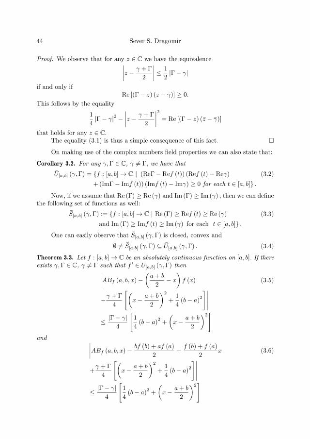
44 Sever S. Dragomir
Proof. We observe that for any z ∈ C we have the equivalence∣∣∣∣z − γ + Γ
2
∣∣∣∣ ≤ 1
2|Γ− γ|
if and only ifRe [(Γ− z) (z − γ)] ≥ 0.
This follows by the equality
1
4|Γ− γ|2 −
∣∣∣∣z − γ + Γ
2
∣∣∣∣2 = Re [(Γ− z) (z − γ)]
that holds for any z ∈ C.The equality (3.1) is thus a simple consequence of this fact.
On making use of the complex numbers field properties we can also state that:
Corollary 3.2. For any γ,Γ ∈ C, γ 6= Γ, we have that
U[a,b] (γ,Γ) = f : [a, b]→ C | (ReΓ− Ref (t)) (Ref (t)− Reγ) (3.2)
+ (ImΓ− Imf (t)) (Imf (t)− Imγ) ≥ 0 for each t ∈ [a, b] .
Now, if we assume that Re (Γ) ≥ Re (γ) and Im (Γ) ≥ Im (γ) , then we can definethe following set of functions as well:
S[a,b] (γ,Γ) := f : [a, b]→ C | Re (Γ) ≥ Ref (t) ≥ Re (γ) (3.3)
and Im (Γ) ≥ Imf (t) ≥ Im (γ) for each t ∈ [a, b] .
One can easily observe that S[a,b] (γ,Γ) is closed, convex and
∅ 6= S[a,b] (γ,Γ) ⊆ U[a,b] (γ,Γ) . (3.4)
Theorem 3.3. Let f : [a, b]→ C be an absolutely continuous function on [a, b]. If thereexists γ,Γ ∈ C, γ 6= Γ such that f ′ ∈ U[a,b] (γ,Γ) then∣∣∣∣ABf (a, b, x)−
(a+ b
2− x)f (x) (3.5)
−γ + Γ
4
[(x− a+ b
2
)2
+1
4(b− a)
2
]∣∣∣∣∣≤ |Γ− γ|
4
[1
4(b− a)
2+
(x− a+ b
2
)2]
and ∣∣∣∣ABf (a, b, x)− bf (b) + af (a)
2+f (b) + f (a)
2x (3.6)
+γ + Γ
4
[(x− a+ b
2
)2
+1
4(b− a)
2
]∣∣∣∣∣≤ |Γ− γ|
4
[1
4(b− a)
2+
(x− a+ b
2
)2]
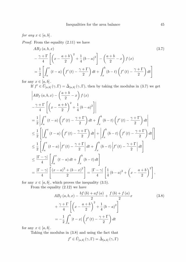
Inequalities for the area balance 45
for any x ∈ [a, b] .
Proof. From the equality (2.11) we have
ABf (a, b, x) (3.7)
− γ + Γ
4
[(x− a+ b
2
)2
+1
4(b− a)
2
]−(a+ b
2− x)f (x)
=1
2
[∫ x
a
(t− a)
(f ′ (t)− γ + Γ
2
)dt+
∫ b
x
(b− t)(f ′ (t)− γ + Γ
2
)dt
]for any x ∈ [a, b] .
If f ′ ∈ U[a,b] (γ,Γ) = ∆[a,b] (γ,Γ), then by taking the modulus in (3.7) we get∣∣∣∣ABf (a, b, x)−(a+ b
2− x)f (x)
−γ + Γ
4
[(x− a+ b
2
)2
+1
4(b− a)
2
]∣∣∣∣∣=
1
2
∣∣∣∣∣∫ x
a
(t− a)
(f ′ (t)− γ + Γ
2
)dt+
∫ b
x
(b− t)(f ′ (t)− γ + Γ
2
)dt
∣∣∣∣∣≤ 1
2
[∣∣∣∣∫ x
a
(t− a)
(f ′ (t)− γ + Γ
2
)dt
∣∣∣∣+
∣∣∣∣∣∫ b
x
(b− t)(f ′ (t)− γ + Γ
2
)dt
∣∣∣∣∣]
≤ 1
2
[∫ x
a
(t− a)
∣∣∣∣f ′ (t)− γ + Γ
2
∣∣∣∣ dt+
∫ b
x
(b− t)∣∣∣∣f ′ (t)− γ + Γ
2
∣∣∣∣ dt]
≤ |Γ− γ|4
[∫ x
a
(t− a) dt+
∫ b
x
(b− t) dt
]
=|Γ− γ|
4
[(x− a)
2+ (b− x)
2
2
]=|Γ− γ|
4
[1
4(b− a)
2+
(x− a+ b
2
)2],
for any x ∈ [a, b] , which proves the inequality (3.5).From the equality (2.12) we have
ABf (a, b, x)− bf (b) + af (a)
2+f (b) + f (a)
2x (3.8)
+γ + Γ
4
[(x− a+ b
2
)2
+1
4(b− a)
2
]
= −1
2
∫ b
a
|t− x|(f ′ (t)− γ + Γ
2
)dt
for any x ∈ [a, b] .Taking the modulus in (3.8) and using the fact that
f ′ ∈ U[a,b] (γ,Γ) = ∆[a,b] (γ,Γ)

46 Sever S. Dragomir
we have∣∣∣∣ABf (a, b, x)− bf (b) + af (a)
2+f (b) + f (a)
2x
+γ + Γ
4
[(x− a+ b
2
)2
+1
4(b− a)
2
]∣∣∣∣∣≤ 1
2
∫ b
a
|t− x|∣∣∣∣f ′ (t)− γ + Γ
2
∣∣∣∣ dt≤ |Γ− γ|
4
∫ b
a
|t− x| dt =|Γ− γ|
4
[∫ x
a
(x− t) dt+
∫ b
x
(t− x) dt
]
=|Γ− γ|
4
[(x− a)
2+ (b− x)
2
2
]=|Γ− γ|
4
[1
4(b− a)
2+
(x− a+ b
2
)2]
for any x ∈ [a, b] , which proves the desired inequality (3.6).
Remark 3.4. Let f : [a, b]→ R be an absolutely continuous function on [a, b]. If thereexists the real numbers m,M such that
m ≤ f ′ (t) ≤M for a.e. t ∈ [a, b] ,
then ∣∣∣∣ABf (a, b, x)−(a+ b
2− x)f (x) (3.9)
−m+M
4
[(x− a+ b
2
)2
+1
4(b− a)
2
]∣∣∣∣∣≤ M −m
4
[1
4(b− a)
2+
(x− a+ b
2
)2]
and ∣∣∣∣ABf (a, b, x)− bf (b) + af (a)
2+f (b) + f (a)
2x (3.10)
+m+M
4
[(x− a+ b
2
)2
+1
4(b− a)
2
]∣∣∣∣∣≤ M −m
4
[1
4(b− a)
2+
(x− a+ b
2
)2]
for any x ∈ [a, b] .
Corollary 3.5. With the assumptions of Theorem 3.3 we have∣∣∣∣ABf (a, b, a+ b
2
)− γ + Γ
16(b− a)
2
∣∣∣∣ ≤ |Γ− γ|16(b− a)
2(3.11)
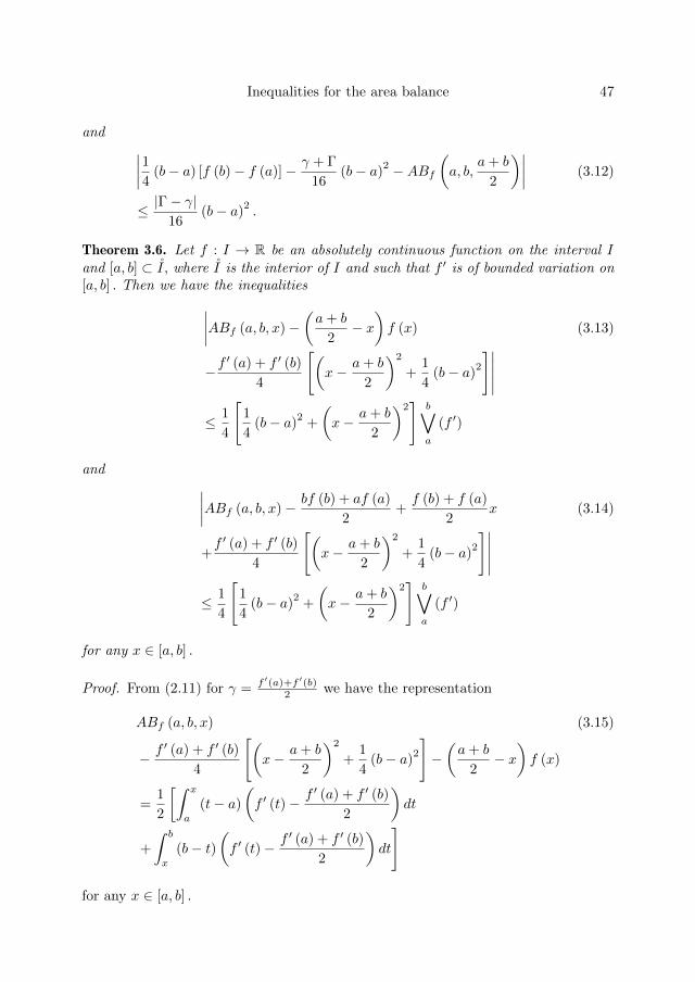
Inequalities for the area balance 47
and ∣∣∣∣14 (b− a) [f (b)− f (a)]− γ + Γ
16(b− a)
2 −ABf(a, b,
a+ b
2
)∣∣∣∣ (3.12)
≤ |Γ− γ|16
(b− a)2.
Theorem 3.6. Let f : I → R be an absolutely continuous function on the interval Iand [a, b] ⊂ I , where I is the interior of I and such that f ′ is of bounded variation on[a, b] . Then we have the inequalities∣∣∣∣ABf (a, b, x)−
(a+ b
2− x)f (x) (3.13)
−f′ (a) + f ′ (b)
4
[(x− a+ b
2
)2
+1
4(b− a)
2
]∣∣∣∣∣≤ 1
4
[1
4(b− a)
2+
(x− a+ b
2
)2]
b∨a
(f ′)
and ∣∣∣∣ABf (a, b, x)− bf (b) + af (a)
2+f (b) + f (a)
2x (3.14)
+f ′ (a) + f ′ (b)
4
[(x− a+ b
2
)2
+1
4(b− a)
2
]∣∣∣∣∣≤ 1
4
[1
4(b− a)
2+
(x− a+ b
2
)2]
b∨a
(f ′)
for any x ∈ [a, b] .
Proof. From (2.11) for γ = f ′(a)+f ′(b)2 we have the representation
ABf (a, b, x) (3.15)
− f ′ (a) + f ′ (b)
4
[(x− a+ b
2
)2
+1
4(b− a)
2
]−(a+ b
2− x)f (x)
=1
2
[∫ x
a
(t− a)
(f ′ (t)− f ′ (a) + f ′ (b)
2
)dt
+
∫ b
x
(b− t)(f ′ (t)− f ′ (a) + f ′ (b)
2
)dt
]
for any x ∈ [a, b] .
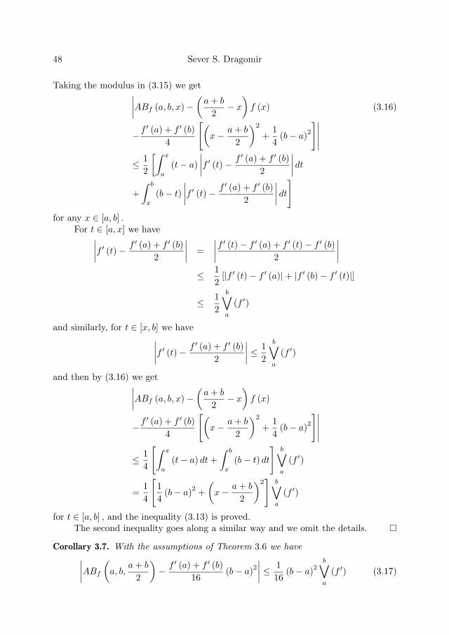
48 Sever S. Dragomir
Taking the modulus in (3.15) we get∣∣∣∣ABf (a, b, x)−(a+ b
2− x)f (x) (3.16)
−f′ (a) + f ′ (b)
4
[(x− a+ b
2
)2
+1
4(b− a)
2
]∣∣∣∣∣≤ 1
2
[∫ x
a
(t− a)
∣∣∣∣f ′ (t)− f ′ (a) + f ′ (b)
2
∣∣∣∣ dt+
∫ b
x
(b− t)∣∣∣∣f ′ (t)− f ′ (a) + f ′ (b)
2
∣∣∣∣ dt]
for any x ∈ [a, b] .For t ∈ [a, x] we have∣∣∣∣f ′ (t)− f ′ (a) + f ′ (b)
2
∣∣∣∣ =
∣∣∣∣f ′ (t)− f ′ (a) + f ′ (t)− f ′ (b)2
∣∣∣∣≤ 1
2[|f ′ (t)− f ′ (a)|+ |f ′ (b)− f ′ (t)|]
≤ 1
2
b∨a
(f ′)
and similarly, for t ∈ [x, b] we have∣∣∣∣f ′ (t)− f ′ (a) + f ′ (b)
2
∣∣∣∣ ≤ 1
2
b∨a
(f ′)
and then by (3.16) we get∣∣∣∣ABf (a, b, x)−(a+ b
2− x)f (x)
−f′ (a) + f ′ (b)
4
[(x− a+ b
2
)2
+1
4(b− a)
2
]∣∣∣∣∣≤ 1
4
[∫ x
a
(t− a) dt+
∫ b
x
(b− t) dt
]b∨a
(f ′)
=1
4
[1
4(b− a)
2+
(x− a+ b
2
)2]
b∨a
(f ′)
for t ∈ [a, b] , and the inequality (3.13) is proved.The second inequality goes along a similar way and we omit the details.
Corollary 3.7. With the assumptions of Theorem 3.6 we have∣∣∣∣ABf (a, b, a+ b
2
)− f ′ (a) + f ′ (b)
16(b− a)
2
∣∣∣∣ ≤ 1
16(b− a)
2b∨a
(f ′) (3.17)
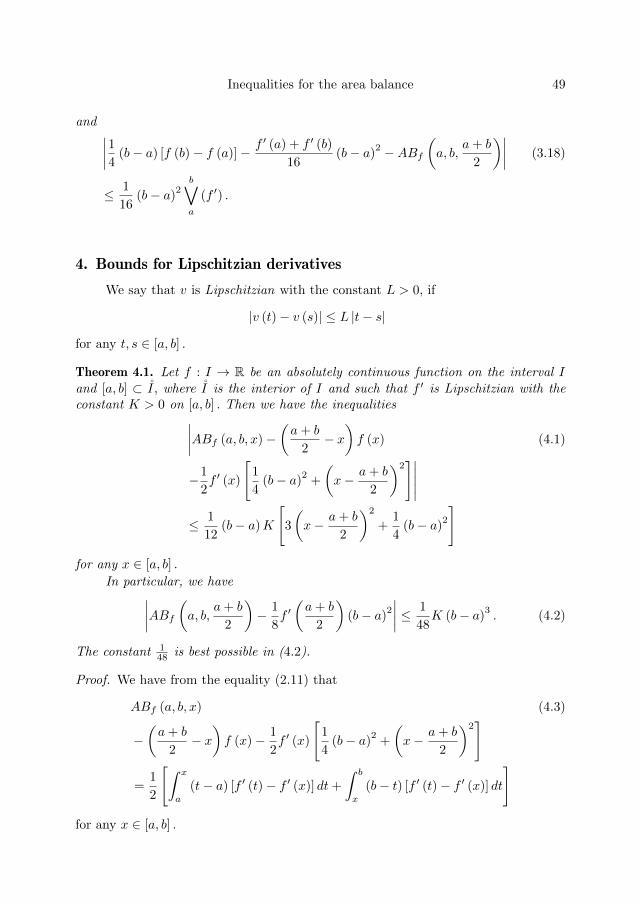
Inequalities for the area balance 49
and ∣∣∣∣14 (b− a) [f (b)− f (a)]− f ′ (a) + f ′ (b)
16(b− a)
2 −ABf(a, b,
a+ b
2
)∣∣∣∣ (3.18)
≤ 1
16(b− a)
2b∨a
(f ′) .
4. Bounds for Lipschitzian derivatives
We say that v is Lipschitzian with the constant L > 0, if
|v (t)− v (s)| ≤ L |t− s|
for any t, s ∈ [a, b] .
Theorem 4.1. Let f : I → R be an absolutely continuous function on the interval Iand [a, b] ⊂ I , where I is the interior of I and such that f ′ is Lipschitzian with theconstant K > 0 on [a, b] . Then we have the inequalities∣∣∣∣ABf (a, b, x)−
(a+ b
2− x)f (x) (4.1)
−1
2f ′ (x)
[1
4(b− a)
2+
(x− a+ b
2
)2]∣∣∣∣∣
≤ 1
12(b− a)K
[3
(x− a+ b
2
)2
+1
4(b− a)
2
]for any x ∈ [a, b] .
In particular, we have∣∣∣∣ABf (a, b, a+ b
2
)− 1
8f ′(a+ b
2
)(b− a)
2
∣∣∣∣ ≤ 1
48K (b− a)
3. (4.2)
The constant 148 is best possible in (4.2).
Proof. We have from the equality (2.11) that
ABf (a, b, x) (4.3)
−(a+ b
2− x)f (x)− 1
2f ′ (x)
[1
4(b− a)
2+
(x− a+ b
2
)2]
=1
2
[∫ x
a
(t− a) [f ′ (t)− f ′ (x)] dt+
∫ b
x
(b− t) [f ′ (t)− f ′ (x)] dt
]for any x ∈ [a, b] .
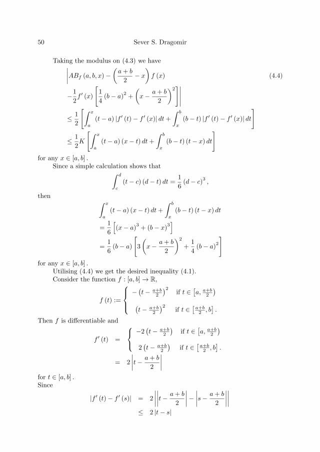
50 Sever S. Dragomir
Taking the modulus on (4.3) we have∣∣∣∣ABf (a, b, x)−(a+ b
2− x)f (x) (4.4)
−1
2f ′ (x)
[1
4(b− a)
2+
(x− a+ b
2
)2]∣∣∣∣∣
≤ 1
2
[∫ x
a
(t− a) |f ′ (t)− f ′ (x)| dt+
∫ b
x
(b− t) |f ′ (t)− f ′ (x)| dt
]
≤ 1
2K
[∫ x
a
(t− a) (x− t) dt+
∫ b
x
(b− t) (t− x) dt
]for any x ∈ [a, b] .
Since a simple calculation shows that∫ d
c
(t− c) (d− t) dt =1
6(d− c)3 ,
then ∫ x
a
(t− a) (x− t) dt+
∫ b
x
(b− t) (t− x) dt
=1
6
[(x− a)
3+ (b− x)
3]
=1
6(b− a)
[3
(x− a+ b
2
)2
+1
4(b− a)
2
]for any x ∈ [a, b] .
Utilising (4.4) we get the desired inequality (4.1).Consider the function f : [a, b]→ R,
f (t) :=
−(t− a+b
2
)2if t ∈
[a, a+b2
)(t− a+b
2
)2if t ∈
[a+b2 , b
].
Then f is differentiable and
f ′ (t) =
−2(t− a+b
2
)if t ∈
[a, a+b2
)2(t− a+b
2
)if t ∈
[a+b2 , b
].
= 2
∣∣∣∣t− a+ b
2
∣∣∣∣for t ∈ [a, b] .Since
|f ′ (t)− f ′ (s)| = 2
∣∣∣∣∣∣∣∣t− a+ b
2
∣∣∣∣− ∣∣∣∣s− a+ b
2
∣∣∣∣∣∣∣∣≤ 2 |t− s|
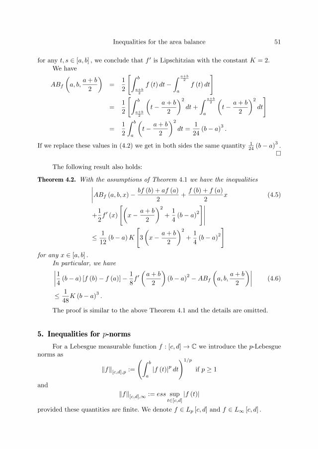
Inequalities for the area balance 51
for any t, s ∈ [a, b] , we conclude that f ′ is Lipschitzian with the constant K = 2.We have
ABf
(a, b,
a+ b
2
)=
1
2
[∫ b
a+b2
f (t) dt−∫ a+b
2
a
f (t) dt
]
=1
2
[∫ b
a+b2
(t− a+ b
2
)2
dt+
∫ a+b2
a
(t− a+ b
2
)2
dt
]
=1
2
∫ b
a
(t− a+ b
2
)2
dt =1
24(b− a)
3.
If we replace these values in (4.2) we get in both sides the same quantity 124 (b− a)
3.
The following result also holds:
Theorem 4.2. With the assumptions of Theorem 4.1 we have the inequalities∣∣∣∣ABf (a, b, x)− bf (b) + af (a)
2+f (b) + f (a)
2x (4.5)
+1
2f ′ (x)
[(x− a+ b
2
)2
+1
4(b− a)
2
]∣∣∣∣∣≤ 1
12(b− a)K
[3
(x− a+ b
2
)2
+1
4(b− a)
2
]for any x ∈ [a, b] .
In particular, we have∣∣∣∣14 (b− a) [f (b)− f (a)]− 1
8f ′(a+ b
2
)(b− a)
2 −ABf(a, b,
a+ b
2
)∣∣∣∣ (4.6)
≤ 1
48K (b− a)
3.
The proof is similar to the above Theorem 4.1 and the details are omitted.
5. Inequalities for p-norms
For a Lebesgue measurable function f : [c, d]→ C we introduce the p-Lebesguenorms as
‖f‖[c,d],p :=
(∫ b
a
|f (t)|p dt
)1/p
if p ≥ 1
and
‖f‖[c,d],∞ := ess supt∈[c,d]
|f (t)|
provided these quantities are finite. We denote f ∈ Lp [c, d] and f ∈ L∞ [c, d] .
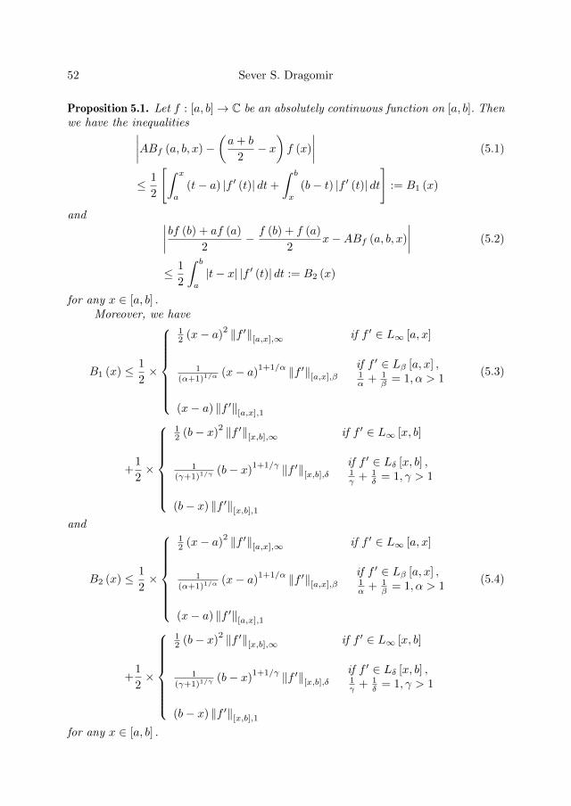
52 Sever S. Dragomir
Proposition 5.1. Let f : [a, b]→ C be an absolutely continuous function on [a, b]. Thenwe have the inequalities∣∣∣∣ABf (a, b, x)−
(a+ b
2− x)f (x)
∣∣∣∣ (5.1)
≤ 1
2
[∫ x
a
(t− a) |f ′ (t)| dt+
∫ b
x
(b− t) |f ′ (t)| dt
]:= B1 (x)
and ∣∣∣∣bf (b) + af (a)
2− f (b) + f (a)
2x−ABf (a, b, x)
∣∣∣∣ (5.2)
≤ 1
2
∫ b
a
|t− x| |f ′ (t)| dt := B2 (x)
for any x ∈ [a, b] .Moreover, we have
B1 (x) ≤ 1
2×
12 (x− a)
2 ‖f ′‖[a,x],∞ if f ′ ∈ L∞ [a, x]
1(α+1)1/α
(x− a)1+1/α ‖f ′‖[a,x],β
if f ′ ∈ Lβ [a, x] ,1α + 1
β = 1, α > 1
(x− a) ‖f ′‖[a,x],1
(5.3)
+1
2×
12 (b− x)
2 ‖f ′‖[x,b],∞ if f ′ ∈ L∞ [x, b]
1(γ+1)1/γ
(b− x)1+1/γ ‖f ′‖[x,b],δ
if f ′ ∈ Lδ [x, b] ,1γ + 1
δ = 1, γ > 1
(b− x) ‖f ′‖[x,b],1and
B2 (x) ≤ 1
2×
12 (x− a)
2 ‖f ′‖[a,x],∞ if f ′ ∈ L∞ [a, x]
1(α+1)1/α
(x− a)1+1/α ‖f ′‖[a,x],β
if f ′ ∈ Lβ [a, x] ,1α + 1
β = 1, α > 1
(x− a) ‖f ′‖[a,x],1
(5.4)
+1
2×
12 (b− x)
2 ‖f ′‖[x,b],∞ if f ′ ∈ L∞ [x, b]
1(γ+1)1/γ
(b− x)1+1/γ ‖f ′‖[x,b],δ
if f ′ ∈ Lδ [x, b] ,1γ + 1
δ = 1, γ > 1
(b− x) ‖f ′‖[x,b],1for any x ∈ [a, b] .
Inequalities for the area balance 53
Proof. From (2.1) and (2.2) we have by taking the modulus∣∣∣∣ABf (a, b, x)−(a+ b
2− x)f (x)
∣∣∣∣ (5.5)
≤ 1
2
[∣∣∣∣∫ x
a
(t− a) f ′ (t) dt
∣∣∣∣+
∣∣∣∣∣∫ b
x
(b− t) f ′ (t) dt
∣∣∣∣∣]
≤ 1
2
[∫ x
a
(t− a) |f ′ (t)| dt+
∫ b
x
(b− t) |f ′ (t)| dt
]and ∣∣∣∣bf (b) + af (a)
2− f (b) + f (a)
2x−ABf (a, b, x)
∣∣∣∣ (5.6)
≤ 1
2
∫ b
a
|t− x| |f ′ (t)| dt
=1
2
[∫ x
a
(x− t) |f ′ (t)| dt+
∫ b
x
(t− x) |f ′ (t)| dt
]for any x ∈ [a, b] .
Using the Holder inequality we have
B1 (x)
≤ 1
2×
12 (x− a)
2 ‖f ′‖[a,x],∞ if f ′ ∈ L∞ [a, x]
1(α+1)1/α
(x− a)1+1/α ‖f ′‖[a,x],β
if f ′ ∈ Lβ [a, x] ,1α + 1
β = 1, α > 1
(x− a) ‖f ′‖[a,x],1
+1
2×
12 (b− x)
2 ‖f ′‖[x,b],∞ if f ′ ∈ L∞ [x, b]
1(γ+1)1/γ
(b− x)1+1/γ ‖f ′‖[x,b],δ
if f ′ ∈ Lδ [x, b] ,1γ + 1
δ = 1, γ > 1
(b− x) ‖f ′‖[x,b],1and a similar inequality for B2.
Remark 5.2. We observe that
B1 (x) ≤ 1
4(x− a)
2 ‖f ′‖[a,x],∞ +1
4(b− x)
2 ‖f ′‖[x,b],∞ (5.7)
≤[
1
4(x− a)
2+
1
4(b− x)
2
]max
‖f ′‖[a,x],∞ , ‖f ′‖[x,b],∞
=
1
2
[1
4(b− a)
2+
(x− a+ b
2
)2]‖f ′‖[a,b],∞
54 Sever S. Dragomir
therefore ∣∣∣∣ABf (a, b, x)−(a+ b
2− x)f (x)
∣∣∣∣ (5.8)
≤ 1
2
[1
4(b− a)
2+
(x− a+ b
2
)2]‖f ′‖[a,b],∞
for any x ∈ [a, b] .Similarly, ∣∣∣∣bf (b) + af (a)
2− f (b) + f (a)
2x−ABf (a, b, x)
∣∣∣∣ (5.9)
≤ 1
2
[1
4(b− a)
2+
(x− a+ b
2
)2]‖f ′‖[a,b],∞
for any x ∈ [a, b] .In particular, we have∣∣∣∣ABf (a, b, a+ b
2
)∣∣∣∣ ≤ 1
8(b− a)
2 ‖f ′‖[a,b],∞ (5.10)
and ∣∣∣∣14 (b− a) [f (b)− f (a)]−ABf(a, b,
a+ b
2
)∣∣∣∣ ≤ 1
8(b− a)
2 ‖f ′‖[a,b],∞ . (5.11)
6. Applications for twice differentiable functions
If we write the equalities (2.11) and (2.12) for the function f = g′, where g :I → R is a differentiable function on the interior of the interval I with the derivativeabsolutely continuous on [a, b] ⊂ I , then we get
ABg′ (a, b, x) (6.1)
=1
2γ
[(x− a+ b
2
)2
+1
4(b− a)
2
]+
(a+ b
2− x)g′ (x)
+1
2
[∫ x
a
(t− a) (g′′ (t)− γ) dt+
∫ b
x
(b− t) (g′′ (t)− γ) dt
]and
ABg′ (a, b, x) =bg′ (b) + ag′ (a)
2− g′ (b) + g′ (a)
2x (6.2)
− 1
2γ
[(x− a+ b
2
)2
+1
4(b− a)
2
]
− 1
2
∫ b
a
|t− x| (g′′ (t)− γ) dt
Inequalities for the area balance 55
and since
ABf (a, b, x) =1
2F (b)− F (x) ,
where F (x) :=
∫ x
a
f (t) dt, then
ABg′ (a, b, x) =1
2[g (b)− g (a)]− g (x) + g (a)
=g (a) + g (b)
2− g (x)
and by (6.1) and (6.2) we get the representations
g (x) =g (a) + g (b)
2(6.3)
− 1
2γ
[(x− a+ b
2
)2
+1
4(b− a)
2
]−(a+ b
2− x)g′ (x)
− 1
2
[∫ x
a
(t− a) (g′′ (t)− γ) dt+
∫ b
x
(b− t) (g′′ (t)− γ) dt
]
and
g (x) =g (a) + g (b)
2− bg′ (b) + ag′ (a)
2+g′ (b) + g′ (a)
2x (6.4)
+1
2γ
[(x− a+ b
2
)2
+1
4(b− a)
2
]
+1
2
∫ b
a
|t− x| (g′′ (t)− γ) dt
for any x ∈ [a, b] .
If we assume that g′′ ∈ U[a,b] (ψ,Ψ) for some ψ,Ψ ∈ C, ψ 6= Ψ, then, as above,we have the inequalities∣∣∣∣g (x)− g (a) + g (b)
2(6.5)
+ψ + Ψ
4
[(x− a+ b
2
)2
+1
4(b− a)
2
]+
(a+ b
2− x)g′ (x)
∣∣∣∣∣≤ |Ψ− ψ|
4
[1
4(b− a)
2+
(x− a+ b
2
)2]
56 Sever S. Dragomir
and ∣∣∣∣g (x)− g (a) + g (b)
2+bg′ (b) + ag′ (a)
2− g′ (b) + g′ (a)
2x (6.6)
−ψ + Ψ
4
[(x− a+ b
2
)2
+1
4(b− a)
2
]∣∣∣∣∣≤ |Ψ− ψ|
4
[1
4(b− a)
2+
(x− a+ b
2
)2]
for any x ∈ [a, b] .We have the particular inequalities∣∣∣∣g(a+ b
2
)− g (a) + g (b)
2+ψ + Ψ
16(b− a)
2
∣∣∣∣ (6.7)
≤ |Ψ− ψ|16
(b− a)2
and ∣∣∣∣g(a+ b
2
)− g (a) + g (b)
2+
1
4(b− a) [g′ (b)− g′ (a)] (6.8)
−ψ + Ψ
16(b− a)
2
∣∣∣∣≤ |Ψ− ψ|
16(b− a)
2
Other similar results may be stated, however we do not present the details here.
Acknowledgement. The author would like to thank the anonymous referee for readingcarefully the manuscript and correcting some typos.
References
[1] Azpeitia, A.G., Convex functions and the Hadamard inequality, Rev. Colombiana Mat.,28(1994), no. 1, 7-12.
[2] Dragomir, S.S., A mapping in connection to Hadamard’s inequalities, An. Oster. Akad.Wiss. Math.-Natur., (Wien), 128(1991), 17-20.
[3] Dragomir, S.S., Two mappings in connection to Hadamard’s inequalities, J. Math. Anal.Appl., 167(1992), 49-56.
[4] Dragomir, S.S., On Hadamard’s inequalities for convex functions, Mat. Balkanica,6(1992), 215-222.
[5] Dragomir, S.S., An inequality improving the second Hermite-Hadamard inequality forconvex functions defined on linear spaces and applications for semi-inner products, J.Inequal. Pure & Appl. Math., 3(2002), no. 3, Art. 35.
[6] Dragomir, S.S., Bounds for the normalized Jensen functional, Bull. Austral. Math. Soc.,74(3)(2006), 471-476.
[7] Dragomir, S.S., Refinements of the generalised trapezoid and Ostrowski inequalities forfunctions of bounded variation, Arch. Math. (Basel), 91(2008), no. 5, 450–460.
Inequalities for the area balance 57
[8] Dragomir, S.S., Gomm, I., Bounds for two mappings associated to the Hermite-Hadamard inequality, Preprint, RGMIA Res. Rep. Coll., 14(2011), to appear.
[9] Dragomir, S.S., Milosevic, D.S., Sandor, J., On some refinements of Hadamard’s in-equalities and applications, Univ. Belgrad, Publ. Elek. Fak. Sci. Math., 4(1993), 21-24.
[10] Dragomir, S.S., Pearce, C.E.M., Selected Topics on Hermite-Hadamard Inequalities andApplications, RGMIA Monographs, 2000.
[11] Guessab, A., Schmeisser, G., Sharp integral inequalities of the Hermite-Hadamard type,J. Approx. Theory, 115(2002), no. 2, 260–288.
[12] Kilianty, E., Dragomir, S.S., Hermite-Hadamard’s inequality and the p-HH-norm on theCartesian product of two copies of a normed space, Math. Inequal. Appl., 13(2010), no.1, 1–32.
[13] Merkle, M., Remarks on Ostrowski’s and Hadamard’s inequality, Univ. Beograd. Publ.Elektrotehn. Fak. Ser. Mat., 10(1999), 113–117.
[14] Pearce, C.E.M., Rubinov, A.M., P-functions, quasi-convex functions, and Hadamardtype inequalities, J. Math. Anal. Appl., 240 (1999), no. 1, 92–104.
[15] Pecaric, J., Vukelic, A., Hadamard and Dragomir-Agarwal inequalities, the Euler formu-lae and convex functions, Functional Equations, Inequalities and Applications, 105–137,Kluwer Acad. Publ., Dordrecht, 2003.
[16] Toader, G., Superadditivity and Hermite-Hadamard’s inequalities, Studia Univ. Babes-Bolyai Math., 39(1994), no. 2, 27–32.
[17] Yang, G.-S., Hong, M.-C., A note on Hadamard’s inequality, Tamkang J. Math.,28(1997), no. 1, 33–37.
[18] Yang, G.-S., Tseng, K.-L., On certain integral inequalities related to Hermite-Hadamardinequalities, J. Math. Anal. Appl., 239(1999), no. 1, 180–187.
Sever S. DragomirMathematics, College of Engineering & ScienceVictoria University, PO Box 14428Melbourne City, MC 8001, Australiae-mail: [email protected]
DST-NRF Centre of Excellence in the Mathematical and Statistical SciencesSchool of Computer Science and Applied MathematicsUniversity of the WitwatersrandPrivate Bag 3, Johannesburg 2050, South Africa

Stud. Univ. Babes-Bolyai Math. 63(2018), No. 1, 59–69DOI: 10.24193/subbmath.2018.1.04
Applications of generalized fractional integraloperator to unified subclass of prestarlikefunctions with negative coefficients
Santosh B. Joshi, Sayali S. Joshi and Haridas Pawar
Abstract. In this paper, we have introduced and studied various properties ofunified class of prestarlike functions with negative coefficients in the unit disc U .Also distortion theorem involving a generalized fractional integral operator forfunctions in this class is established.
Mathematics Subject Classification (2010): 30C45.
Keywords: Univalent function, coefficient estimates, distortion theorem.
1. Introduction
Let A denote the class of functions of the form
f(z) = z +
∞∑n=2
an zn (1.1)
which are analytic in the unit disc U= z : |z| < 1. Let S denote the subclass of A,which consists of functions of the form (1.1) that are univalent in U.
A function f ∈ S is said to be starlike of order µ(0 ≤ µ < 1) if and only if
Re
zf′(z)
f(z)
> µ, z ∈ U
and convex of order µ(0 ≤ µ < 1) if and only if
Re
1 +
zf′′(z)
f ′(z)
> µ, z ∈ U.
Denote these classes respectively by S∗(µ) and K(µ).
60 Santosh B. Joshi, Sayali S. Joshi and Haridas Pawar
Let T denote subclass of S consisting of functions of the form
f(z) = z −∞∑n=2
an zn, an ≥ 0. (1.2)
The classes obtained by taking intersections of the classes S∗(µ) and K(µ)with T are denoted by T ∗(µ) and K∗(µ) respectively. The classes T ∗(µ), K∗(µ)were studied by Silverman [9].
The function
Sµ(z) = z(1− z)−2(1−µ) , 0 ≤ µ < 1 , (1.3)
is the familiar extremal function for the class S∗(µ), setting
C(µ, n) =
n∏i=2
(i− 2µ)
(n− 1)!, n ∈ N\1, N = 1, 2, 3, · · · , (1.4)
then
Sµ(z) = z +
∞∑n=2
C(µ, n) zn . (1.5)
We note that C(µ, n) is a decreasing function in µ, and that
limn→∞
C(µ, n) =
∞ , µ <
1
2
1 , µ =1
2
0 , µ >1
2.
If f(z) is given by (1.2) and g(z) defined by
g(z) = z −∞∑n=2
bn zn, bn ≥ 0 ,
belonging to T , then convolution or Hadamard product of f and g is defined by
(f ∗ g)(z) = z −∞∑n=2
an bn zn.
Let Rµ(α, β, γ) be the subclass of A consisting functions f(z) such that∣∣∣∣∣∣∣∣zh′(z)
h(z)− 1
γzh′(z)
h(z)+ 1− (1 + γ)α
∣∣∣∣∣∣∣∣ < β ,
where, h(z) = (f ∗ Sµ(z)), 0 ≤ α < 1, 0 < β ≤ 1, 0 ≤ γ ≤ 1, 0 ≤ µ < 1.Also let Cµ(α, β, γ) be the subclass of A consisting of functions f(z), which
satisfy the condition
zf ′(z) ∈ Rµ(α, β, γ).
Applications of generalized fractional integral operator 61
The classes Rµ(α, β, γ) and Cµ(α, β, γ) of prestarlike functions was investigated byJoshi [1]. In particular, the subclasses
Rµ[α, β, γ] = Rµ(α, β, γ) ∩ T, Cµ[α, β, γ] = Cµ(α, β, γ) ∩ T ,
were also studied by Joshi [1].The following results will be required for our investigation.
Lemma 1.1. [1]. A function f defined by (1.2) is in the class Rµ[α, β, γ] if and only if
∞∑n=2
C(µ, n) (n− 1) + β [γn+ 1− (1 + γ)α] an ≤ β(1 + γ)(1− α). (1.6)
The result (1.6) is sharp.
Lemma 1.2. [1]. A function f defined by (1.2) is in the class Cµ[α, β, γ] if and only if
∞∑n=2
C(µ, n) n (n− 1) + β [γn+ 1− (1 + γ)α] an ≤ β(1 + γ)(1− α). (1.7)
The result (1.7) is sharp.
Further we note that such type of classes were extensively studied by Sheil-Small et al. [8], Owa and Uralegaddi [4], Srivastava and Aouf [10] and Raina andSrivastava [7].
In view of Lemma 1.1 and Lemma 1.2, we present here a unified study of theclasses Rµ[α, β, γ] and Cµ[α, β, γ] by introducing a new subclass Pµ(α, β, γ, σ). Indeed,we say that a function f(z) defined by (1.2) is in the class Pµ(α, β, γ, σ) if and only if
∞∑n=2
(n− 1) + β [γn+ 1− (1 + γ)α] (1− σ + σn)
β(1 + γ)(1− α)C(µ, n)an ≤ 1 , (1.8)
where, 0 ≤ α < 1, 0 < β ≤ 1, 0 ≤ γ ≤ 1, 0 ≤ µ < 1, 0 ≤ σ ≤ 1.Then clearly we have,
Pµ(α, β, γ, σ) = (1− σ)Rµ[α, β, γ] + σCµ[α, β, γ] , (1.9)
where, 0 ≤ σ ≤ 1. So that
Pµ(α, β, γ, 0) = Rµ[α, β, γ], Pµ(α, β, γ, 1) = Cµ[α, β, γ]. (1.10)
The main object of this paper is to investigate various interesting properties andcharacterization of the general class Pµ(α, β, γ, σ). Also distortion theorem involvinga generalized fractional integral operator for functions in this class are obtained.
2. Main results
Theorem 2.1. A function f defined by (1.2) is in the class Pµ(α, β, γ, σ) then
an ≤β(1 + γ)(1− α)
C(µ, n) (n− 1) + β [γn+ 1− (1 + γ)α] (1− σ + σn), n ∈ N\1. (2.1)

62 Santosh B. Joshi, Sayali S. Joshi and Haridas Pawar
Equality holds true for the function f(z) given by
f(z) = z − β(1 + γ)(1− α)
C(µ, n) (n− 1) + β [γn+ 1− (1 + γ)α] (1− σ + σn)zn, n ∈ N\1.
(2.2)
Proof. The proof of Theorem 2.1 is straightforward and hence details are omitted.
A distortion theorem for function f in the class Pµ(α, β, γ, σ) is given as follows:
Theorem 2.2. If the function f defined by (1.2) is in the class Pµ(α, β, γ, σ) then
|z| − β(1 + γ)(1− α)
2 1 + β [2γ + 1− (1 + γ)α] (1− µ)(1 + σ)|z|2 ≤ |f(z)|
≤ |z|+ β(1 + γ)(1− α)
2 1 + β [2γ + 1− (1 + γ)α] (1− µ)(1 + σ)|z|2 , (2.3)
and
1− β(1 + γ)(1− α)
1 + β [2γ + 1− (1 + γ)α] (1− µ)(1 + σ)|z| ≤ |f ′(z)|
≤ 1 +β(1 + γ)(1− α)
1 + β [2γ + 1− (1 + γ)α] (1− µ)(1 + σ)|z| . (2.4)
Proof. Let
f(z) = z −∞∑n=2
anzn
Since f(z) ∈ Pµ(α, β, γ, σ) and clearly C(µ, n) defined by (1.4) is non-decreasing for0 ≤ µ ≤ 1
2 and using (1.8) we get
∞∑n=2
an ≤β(1 + γ)(1− α)
2 1 + β [2γ + 1− (1 + γ)α] (1− µ)(1 + σ), n ∈ N\1. (2.5)
Then using (1.2) and (2.5) we get (for z ∈ U),
|f(z)| ≤ |z|+ |z|2∞∑n=2
|an|
≤ |z|+ β(1 + γ)(1− α)
2 1 + β [2γ + 1− (1 + γ)α] (1− µ)(1 + σ)|z|2
and
|f(z)| ≥ |z| − |z|2∞∑n=2
|an|
≥ |z| − β(1 + γ)(1− α)
2 1 + β [2γ + 1− (1 + γ)α] (1− µ)(1 + σ)|z|2.
which proves the assertion (2.3) of Theorem 2.2.
Applications of generalized fractional integral operator 63
Also for z ∈ U , we find that
|f ′(z)| ≤ 1 + |z|∞∑n=2
n |an|
≤ 1 +β(1 + γ)(1− α)
1 + β [2γ + 1− (1 + γ)α] (1− µ)(1 + σ)|z|
and
|f ′(z)| ≥ 1− |z|∞∑n=2
n |an|
≥ 1− β(1 + γ)(1− α)
1 + β [2γ + 1− (1 + γ)α] (1− µ)(1 + σ)|z|.
which proves the assertion (2.4) of Theorem 2.2This completes the proof.
We note that results (2.3) and (2.4) is sharp for the function f(z) given by
f(z) = z − β(1 + γ)(1− α)
2 1 + β [2γ + 1− (1 + γ)α] (1− µ)(1 + σ)z2. (2.6)
3. Closure theorems
In this section, we shall prove that the class Pµ(α, β, γ, σ) is closed under linearcombination.
Theorem 3.1. The class Pµ(α, β, γ, σ) is closed under linear combination.
Proof. Suppose f(z), g(z) ∈ Pµ(α, β, γ, σ) and
f(z) = z −∞∑n=2
anzn
and
g(z) = z −∞∑n=2
bnzn .
It is sufficient to prove that the function H defined by
H(z) = λf(z) + (1− λ)g(z) , (0 ≤ λ ≤ 1)
is also in the class Pµ(α, β, γ, σ). Since
H(z) = z −∞∑n=2
[λan + (1− λ)bn]zn .
We observe that∞∑n=2
(n− 1) + β [γn+ 1− (1 + γ)α] (1− σ + σn)
β(1 + γ)(1− α)C(µ, n)[λan + (1− λ)bn] ≤ 1.
Thus H ∈ Pµ(α, β, γ, σ). This completes the proof.
64 Santosh B. Joshi, Sayali S. Joshi and Haridas Pawar
Theorem 3.2. If
f1(z) = z
and
fn(z) = z − β(1 + γ)(1− α)
(n− 1) + β [γn+ 1− (1 + γ)α] (1− σ + σn)C(µ, n)zn , (n ≥ 2).
Then f ∈ Pµ(α, β, γ, σ) if and only if it can be expressed in the form
f(z) =
∞∑n=1
λnfn(z)
where λn ≥ 0 and
∞∑n=1
λn = 1 .
Proof. Let
f(z) =
∞∑n=1
λnfn(z)
= z −∞∑n=2
β(1 + γ)(1− α)
(n− 1) + β [γn+ 1− (1 + γ)α] (1− σ + σn)C(µ, n)λnz
n
= z −∞∑n=2
an zn ,
where
an =β(1 + γ)(1− α)
(n− 1) + β [γn+ 1− (1 + γ)α] (1− σ + σn)C(µ, n)λn ≥ 0, (n ≥ 2).
Since,∞∑n=2
[β(1 + γ)(1− α)
(n− 1) + β [γn+ 1− (1 + γ)α] (1− σ + σn)C(µ, n)
(n− 1) + β [γn+ 1− (1 + γ)α] (1− σ + σn)C(µ, n)
β(1 + γ)(1− α)
]λn
=
∞∑n=2
λn =
∞∑n=1
λn − λ1 = 1− λ1 ≤ 1 .
Therefore f(z) ∈ Pµ(α, β, γ, σ).Conversely, suppose that f ∈ Pµ(α, β, γ, σ) and since
an =β(1 + γ)(1− α)
(n− 1) + β [γn+ 1− (1 + γ)α] (1− σ + σn)C(µ, n)λn ≥ 0, (n ≥ 2).
Setting
λn =(n− 1) + β [γn+ 1− (1 + γ)α] (1− σ + σn)C(µ, n)
β(1 + γ)(1− α), (n ≥ 2)
Applications of generalized fractional integral operator 65
and
λ1 = 1−∞∑n=2
λn .
We get
f(z) =
∞∑n=1
λnfn(z) .
This completes the proof.
4. Generalized fractional integral operator
In recent years the theory of fractional calculus operator have been fruitfullyapplied to analytic functions. Moreover generalized operator of fractional integrals(or derivatives) having kernels of different types of special functions (including Fox’sH-function) have generated keen interest in this area. For details one may refer toKiryakova [2], Raina and Saigo [6], Srivastava and Owa [11] and Raina and Bolia [5].Further we note that Riemann-Liouville fractional calculus operators have been usedto obtain basic results which include coefficient estimates, boundedness properties forvarious subclasses of analytic and univalent functions.
A generalized fractional integral operator involving the celebrated Fox’s H-function [2, 3] defined below.
Definition 4.1. Let m ∈ N, βk ∈ R and γk, δk ∈ C, ∀ k = 1, 2, · · · ,m. Then theintegral operator
I(γm),(δm)(βm);m f(z) = I
(γ1,··· ,γm),(δ1,··· ,δm)(β1,··· ,βm);m f(z)
=1
z
∫ z
0
Hm,0m,m
tz
(γk + δk + 1− 1
βk, 1βk
)1,m(
γk + 1− 1βk, 1βk
)1,m
f(t)dt,
for
m∑i
Re(δk) > 0, (4.1)
= f(z), for δ1 = · · · = δm = 0 ,
is said to be a multiple fractional integral operator of Riemann-Liouville type of mul-tiorder δ = (δ1, · · · , δm).
Following [2], let ∆ denote a complex domain starlike with respect to the originz = 0, and A(∆) denote the space of functions analytic in ∆. If Aρ(∆) denote theclass of functions
Aρ(∆) = f(z) = zρf(z) : f(z) ∈ A(∆), ρ ≥ 0; (4.2)
then clearly Aρ(∆) ⊆ Av(∆) ⊆ A(∆) for ρ ≥ v ≥ 0 .The fractional integral operator (4.1) includes various useful and important frac-
tional integral operators as special cases. For more details of these special cases, one
may refer to Raina and Saigo [6]. Throughout this paper (λ)k stands for Γ(λ+k)Γ(λ) .
66 Santosh B. Joshi, Sayali S. Joshi and Haridas Pawar
The following results will be required for our investigation.
Lemma 4.2. [2]. Let γk > − pβk− 1, δk ≤ 0 (∀ k = 1, · · · ,m). Then the operator
I(γm),(δm)(βm);m maps the class ∆p(G) into itself preserving the power functions f(z) = zp
(up to a constant multiplier):
I(γm),(δm)(βm);m zp =
m∏k=1
Γ(pβk
+ γk + 1)
Γ(pβk
+ γk + δk + 1) zp . (4.3)
Theorem 4.3. Let m ∈ N, hk ∈ R+, and γk, δk ∈ R such that 1 + γk + δk > 0(k = 1, · · · ,m), and
m∏k=1
(1 + γk + 2hk)hk
(1 + γk + δk + 2hk)hk
≤ 1 (4.4)
and f(z) defined by (1.2) be in the class Pµ(α, β, γ, σ) with 0 ≤ α < 1, 0 < β ≤1, 0 ≤ γ ≤ 1, 0 ≤ µ ≤ 1
2 , 0 ≤ σ ≤ 1. Then∣∣∣I(γm),(δm)
(h−1m );m
f(z)∣∣∣ ≥ m∏
k=1
(Γ (1 + γk + hk)
Γ (1 + γk + δk + hk)
).
[|z| − A∗β(1 + γ)(1− α)
2 1 + β [2γ + 1− (1 + γ)α] (1− µ)(1 + σ)|z|2]
,
(4.5)
and∣∣∣I(γm),(δm)
(h−1m );m
f(z)∣∣∣ ≤ m∏
k=1
(Γ (1 + γk + hk)
Γ (1 + γk + δk + hk)
).
[|z|+ A∗β(1 + γ)(1− α)
2 1 + β [2γ + 1− (1 + γ)α] (1− µ)(1 + σ)|z|2]
,
(4.6)
for z ∈ U . The inequalities in (4.5) and (4.6) are attained by the function f(z) givenby (2.6), where
A∗ =
m∏k=1
(1 + γk + hk)hk
(1 + γk + δk + hk)hk
. (4.7)
Proof. By using lemma 4.2, we get
I(γm),(δm)
(h−1m );m
f(z) =
m∏k=1
Γ (1 + γk + hk)
Γ (1 + γk + δk + hk)
z
−∞∑n=2
m∏k=1
Γ (1 + γk + n hk)
Γ (1 + γk + δk + n hk)
anz
n . (4.8)
Applications of generalized fractional integral operator 67
Letting
G(z) =
m∏k=1
Γ (1 + γk + δk + hk)
Γ (1 + γk + hk)
I
(γm),(δm)
(h−1m );m
f(z)
= z −∞∑n=2
φ(n) an zn , (4.9)
where,
φ(n) =
m∏k=1
(1 + γk + hk)hk(n−1)
(1 + γk + δk + hk)hk(n−1)
, (n ∈ N\1) . (4.10)
Under the hypothesis of Theorem 4.3 (along with the conditions (4.4)), we can seethat φ(n) is non-increasing for integers n (n ≥ 2), and we have
0 < φ(n) ≤ φ(2) =
m∏k=1
(1 + γk + hk)hk
(1 + γk + δk + hk)hk
= A∗ , (n ∈ N\1) . (4.11)
Now in view equation (1.8) and (4.11), we have
|G(z)| ≥ |z| − φ(2) |z|2∞∑n=2
an
≥
m∏k=1
(Γ (1 + γk + hk)
Γ (1 + γk + δk + hk)
).
[|z| − A∗β(1 + γ)(1− α)
2 1 + β [2γ + 1− (1 + γ)α] (1− µ)(1 + σ)|z|2]
.
and
|G(z)| ≤ |z|+ φ(2) |z|2∞∑n=2
an
≤
m∏k=1
(Γ (1 + γk + hk)
Γ (1 + γk + δk + hk)
).
[|z|+ A∗β(1 + γ)(1− α)
2 1 + β [2γ + 1− (1 + γ)α] (1− µ)(1 + σ)|z|2]
.
It can be easily verified that the following inequalities are attained by the functionf(z) given by (2.6).∣∣∣I(γm),(δm)
(h−1m );m
f(z)∣∣∣ ≥ m∏
k=1
(Γ (1 + γk + hk)
Γ (1 + γk + δk + hk)
).
[|z| − A∗β(1 + γ)(1− α)
2 1 + β [2γ + 1− (1 + γ)α] (1− µ)(1 + σ)|z|2]
,
68 Santosh B. Joshi, Sayali S. Joshi and Haridas Pawar
and∣∣∣I(γm),(δm)
(h−1m );m
f(z)∣∣∣ ≤ m∏
k=1
(Γ (1 + γk + hk)
Γ (1 + γk + δk + hk)
).
[|z|+ A∗β(1 + γ)(1− α)
2 1 + β [2γ + 1− (1 + γ)α] (1− µ)(1 + σ)|z|2]
.
Which are as desired in (4.5) and (4.6). This completes the proof of Theorem 4.3.
Acknowledgments. The work of second author (Sayali S. Joshi) is supported by NBHMresearch project (2/48(7)/2016/NBHM/RP/R and D II/14977). Also, the authorswish to express their sincere thanks to the referee of this paper for several usefulcomments and suggestions.
References
[1] Joshi, S.B., On subclasses of prestarlike functions with negative coefficients, Stud. Univ.Babes-Bolyai Math., 54(2009), no. 2, 65-74.
[2] Kiryakova, V.S., Generalized fractional calculus and applications, Pitman ResearchNotes in Math., Longman Publishers, London, 1993.
[3] Kiryakova, V.S., Srivastava, H.M., Generalized multiple Riemann-Liouville fractionaldifferintegrals and applications in univalent function theory, Analysis Geometry andGroups: A Riemann Legacy Volume, Hadronic Press, Palm Harbor, Florida, U.S.A.,1993, 191-226.
[4] Owa, S., Uralegaddi, B.A., A class of functions α prestarlike of order β, Bull. KoreanMath. Soc., 21(1984), 77-85.
[5] Raina, R.K., Bolia, M., On certain classes of distortion theorems involving generalizedfractional integral operators, Bull. Inst. Math. Acad. Sinica, 26(1998), no. 4, 301-307.
[6] Raina, R.K., Saigo, M., A note on fractional calculus operators involving Fox’s H-function on space Fp,µ and F ′
p,µ, Recent Advances in Fractional Calculus, 1993, 219-229.
[7] Raina, R.K., Srivastava, H.M., A unified presentation of certain subclasses of prestarlikefunctions with negative coefficients, Int. J. Comp. Math. Appl., 38(1999), 71-78.
[8] Sheil-Small, T., Silverman, H., M. Silvia, E.M., Convolutions multipliers and starlikefunctions, J. Anal. Math., 41(1982), 181-192.
[9] Silverman, H., Univalent functions with negative coefficients, Proc. Amer. Math. Soc.,51(1975), 109-116.
[10] Srivastava, H.M., Aouf, M.K., Some applications of fractional calculus operators to cer-tain subclasses of prestarlike functions with negative coefficients, Comp. Math. Appl.,30(1995), no. 1, 53-61.
[11] Srivastava, H.M., Owa, S., (Editors), Univalent Functions, Fractional Calculus and TheirApplications, Halsted Press, John Wiley and Sons, New York, 1989.
Applications of generalized fractional integral operator 69
Santosh B. JoshiDepartment of MathematicsWalchand College of EngineeringSangli 416415, Indiae-mail: [email protected] , [email protected]
Sayali S. JoshiDepartment of MathematicsSanjay Bhokare Group of Institutes, MirajMiraj 416410, Indiae-mail: [email protected]
Haridas PawarDepartment of MathematicsSVERI’s College of Engineering PandharpurPandharpur 413304, Indiae-mail: haridas [email protected]

Stud. Univ. Babes-Bolyai Math. 63(2018), No. 1, 71–78DOI: 10.24193/subbmath.2018.1.05
Starlike and convex properties for Poissondistribution series
Nanjundan Magesh, Saurabh Porwal and Chinnaswamy Abirami
Abstract. In this paper, we find the necessary and sufficient conditions, inclusionrelations for Poisson distribution series belonging to the classes S ∗(α, β) andC ∗(α, β). Further, we consider an integral operator related to Poisson Distribu-tion series.
Mathematics Subject Classification (2010): 30C45.
Keywords: Starlike functions, convex functions, Poisson distribution series.
1. Introduction
Let A denote the class of functions of the form
f(z) = z +
∞∑n=2
anzn (1.1)
which are analytic and univalent in the open disc U = z : z ∈ C |z| < 1. Let T bea subclass of A consisting of functions whose non-zero coefficients from second on isgive by
f(z) = z −∞∑n=2
|an|zn, z ∈ U. (1.2)
In 2014, Porwal [4] introduced a power series whose coefficients are probabilities ofPoisson distribution
K (m, z) := z +
∞∑n=2
mn−1
(n− 1)!e−mzn, z ∈ U,
where m > 0. By ratio test the radius of convergence of the above series is infinity.Further, Porwal [4] defined a series
F (m, z) = 2z −K (m, z) = z −∞∑n=2
mn−1
(n− 1)!e−mzn, z ∈ U.
72 Nanjundan Magesh, Saurabh Porwal and Chinnaswamy Abirami
Corresponding to the series K (m, z) using the Hadamard product for f ∈ A , Porwaland Kumar [5] introduced a new linear operator I (m) : A → A defined by
I (m)f(z) : = K (m, z) ∗ f(z)
= z +
∞∑n=2
mn−1
(n− 1)!e−manz
n, z ∈ U,
where ∗ denotes the convolution (or Hadamard product) of two series
f(z) =
∞∑n=0
anzn and g(z) =
∞∑n=0
bnzn
is defined by
(f ∗ g)(z) =
∞∑n=0
anbnzn.
Let S ∗(α, β) be the subclass of T consisting of functions which satisfy the condition:∣∣∣∣∣∣zf ′(z)f(z) − 1
zf ′(z)f(z) + 1− 2α
∣∣∣∣∣∣ < β, z ∈ U,
where 0 ≤ α < 1 and 0 < β ≤ 1.Also, let C ∗(α, β) be the subclass of T consisting of functions which satisfy the
condition: ∣∣∣∣∣∣zf ′′(z)f ′(z)
zf ′′(z)f ′(z) + 2(1− α)
∣∣∣∣∣∣ < β, z ∈ U,
where 0 ≤ α < 1 and 0 < β ≤ 1.The classes S ∗(α, β) and C ∗(α, β), were introduced and studied by Gupta and
Jain [2] (see [3]). Also, we note that for β = 1 the classes S ∗(α, β) and C ∗(α, β)reduce to the class of starlike and convex functions of order α(0 ≤ α < 1) (see [6]).
A function f ∈ A is said to be in the class Rτ (A,B), (τ ∈ C \ 0, −1 ≤ B <A ≤ 1), if it satisfies the inequality∣∣∣∣ f ′(z)− 1
(A−B)τ −B[f ′(z)− 1]
∣∣∣∣ < 1, z ∈ U.
This class was introduced by Dixit and Pal [1].
Lemma 1.1. [2] A function f(z) of the form (1.2) is in S ∗(α, β) if and only if∞∑n=2
[n(1 + β)− 1 + β(1− 2α)] |an| ≤ 2β(1− α). (1.3)
Lemma 1.2. [2] A function f(z) of the form (1.2) is in C ∗(α, β) if and only if∞∑n=2
n[n(1 + β)− 1 + β(1− 2α)] |an| ≤ 2β(1− α). (1.4)
To obtain our main results, we need the following lemmas:
Starlike and convex properties for Poisson distribution series 73
Lemma 1.3. [1] If f ∈ Rτ (A,B) is of the form (1.1), then
|an| ≤ (A−B)|τ |n, n ∈ N \ 1. (1.5)
In the present investigation, inspired by the works of Porwal [4] and Porwal andKumar [5], we find the necessary and sufficient conditions for F (m, z) belonging tothe classes S ∗(α, β) and C ∗(α, β). Also, we obtain inclusion relations for aforecitedclasses with Rτ (A,B).
2. Necessary and sufficient conditions
Theorem 2.1. If m > 0, 0 ≤ α < 1 and 0 < β ≤ 1, then F (m, z) ∈ S ∗(α, β) if andonly if
emm(1 + β) ≤ 2β(1− α). (2.1)
Proof. Since
F (m, z) = z −∞∑n=2
mn−1
(n− 1)!e−mzn,
in view of Lemma 1.1, it is enough to show that∞∑n=2
[n(1 + β)− 1 + β(1− 2α)]mn−1
(n− 1)!e−m ≤ 2β(1− α).
Let
T1 =
∞∑n=2
[n(1 + β)− 1 + β(1− 2α)]mn−1
(n− 1)!e−m.
Now,
T1 =
∞∑n=2
[n(1 + β)− 1 + β(1− 2α)]mn−1
(n− 1)!e−m
= e−m∞∑n=2
[(n− 1)(1 + β) + 2β(1− α)]mn−1
(n− 1)!
= e−m
[(1 + β)
∞∑n=2
mn−1
(n− 2)!+ 2β(1− α)
∞∑n=2
mn−1
(n− 1)!
]= e−m [(1 + β)mem + 2β(1− α)(em − 1)]
= (1 + β)m+ 2β(1− α)(1− e−m).
But this last expression is bounded by 2β(1 − α), if and only if (2.1) holds. Thiscompletes the proof of Theorem 2.1.
Theorem 2.2. If m > 0, 0 ≤ α < 1 and 0 < β ≤ 1, then F (m, z) ∈ C ∗(α, β) if andonly if
em[(1 + β)m2 + 2(1 + β(2− α))m
]≤ 2β(1− α). (2.2)
74 Nanjundan Magesh, Saurabh Porwal and Chinnaswamy Abirami
Proof. Since
F (m, z) = z −∞∑n=2
mn−1
(n− 1)!e−mzn,
in view of Lemma 1.2, it is enough to show that
∞∑n=2
n[n(1 + β)− 1 + β(1− 2α)]mn−1
(n− 1)!e−m ≤ 2β(1− α).
Let
T2 =
∞∑n=2
n[n(1 + β)− 1 + β(1− 2α)]mn−1
(n− 1)!e−m.
Therefore,
T2 = e−m
[ ∞∑n=2
(n− 1)(n− 2)(1 + β)mn−1
(n− 1)!
+
∞∑n=2
(n− 1)[3(1 + β)− 1 + β(1− 2α)]mn−1
(n− 1)!+
∞∑n=2
2β(1− α)mn−1
(n− 1)!
]
= e−m
[(1 + β)
∞∑n=3
mn−1
(n− 3)!
+2[1 + β(2− α)]
∞∑n=2
mn−1
(n− 2)!+ 2β(1− α)
∞∑n=2
mn−1
(n− 1)!
]= e−m
[(1 + β)m2em + 2(1 + β(2− α))mem + 2β(1− α)(em − 1)
]= (1 + β)m2 + 2(1 + β(2− α))m+ 2β(1− α)(1− e−m).
But this last expression is bounded by 2β(1 − α), if and only if (2.2) holds. Thiscompletes the proof of Theorem 2.2.
3. Inclusion results
Theorem 3.1. Let m > 0, 0 ≤ α < 1 and 0 < β ≤ 1. If f ∈ Rτ (A,B), thenI (m)f ∈ S ∗(α, β) if and only if
(A−B)|τ |[(1 + β)(1− e−m) +
(β(1− 2α)− 1)
m(1− e−m −me−m)
]≤ 2β(1− α).
(3.1)
Proof. In view of Lemma 1.1, it suffices to show that
P1 =
∞∑n=2
[n(1 + β)− 1 + β(1− 2α)]mn−1
(n− 1)!e−m|an| ≤ 2β(1− α).
Starlike and convex properties for Poisson distribution series 75
Since f ∈ Rτ (A,B), then by Lemma 1.3, we have
|an| ≤(A−B)|τ |
n.
Therefore,
P1 ≤∞∑n=2
[n(1 + β)− 1 + β(1− 2α)]mn−1
(n− 1)!e−m
(A−B)|τ |n
= (A−B)|τ |e−m∞∑n=2
[n(1 + β)− 1 + β(1− 2α)]mn−1
n!
= (A−B)|τ |e−m[
(1 + β)
∞∑n=2
mn−1
(n− 1)!+
(β(1− 2α)− 1)
m
∞∑n=2
mn
n!
]
= (A−B)|τ |e−m[(1 + β)(em − 1) +
(β(1− 2α)− 1)
m(em − 1−m)
]= (A−B)|τ |
[(1 + β)[1− e−m] +
(β(1− 2α)− 1)
m(1− e−m −me−m)
].
But this last expression is bounded by 2β(1 − α), if (3.1) holds. This completes theproof of Theorem 3.1.
Theorem 3.2. Let m > 0, 0 ≤ α < 1 and 0 < β ≤ 1. If f ∈ Rτ (A,B), thenI (m)f ∈ C ∗(α, β) if and only if
(A−B)|τ |[m(1 + β) + 2β(1− α)(1− e−m)
]≤ 2β(1− α). (3.2)
Proof. In view of Lemma 1.2, it suffices to show that
P2 =
∞∑n=2
n[n(1 + β)− 1 + β(1− 2α)]mn−1
(n− 1)!e−m|an| ≤ 2β(1− α).
Since f ∈ Rτ (A,B), then by Lemma 1.3, we have
|an| ≤(A−B)|τ |
n.
76 Nanjundan Magesh, Saurabh Porwal and Chinnaswamy Abirami
Therefore,
P2 ≤∞∑n=2
n[n(1 + β)− 1 + β(1− 2α)]mn−1
(n− 1)!e−m
(A−B)|τ |n
= (A−B)|τ |e−m∞∑n=2
[n(1 + β)− 1 + β(1− 2α)]mn−1
(n− 1)!
= (A−B)|τ |e−m∞∑n=2
[(n− 1)(1 + β) + 2β(1− α)]mn−1
(n− 1)!
= (A−B)|τ |e−m[ ∞∑n=2
(1 + β)mn−1
(n− 2)!+ 2β(1− α)
∞∑n=2
mn−1
(n− 1)!
]
= (A−B)|τ |e−m[
(1 + β)
∞∑n=2
mn−1
(n− 2)!+ 2β(1− α)
∞∑n=2
mn−1
(n− 1)!
]= (A−B)|τ |e−m [mem(1 + β) + 2β(1− α)(em − 1)] .
But this last expression is bounded by 2β(1 − α), if (3.2) holds. This completes theproof of Theorem 3.2.
4. An integral operator
Theorem 4.1. If m > 0, 0 ≤ α < 1 and 0 < β ≤ 1, then
G (m, z) =
z∫0
F (m, t)
tdt
is in C ∗(α, β) if and only if inequality (2.1) is satisfied.
Proof. Since
G (m, z) = z −∞∑n=2
e−mmn−1
(n− 1)!
zn
n= z −
∞∑n=2
e−mmn−1
n!zn
by Lemma 1.2, we need only to show that
∞∑n=2
n[n(1 + β)− 1 + β(1− 2α)]mn−1
n!e−m ≤ 2β(1− α).
Let
Q1 =
∞∑n=2
n[n(1 + β)− 1 + β(1− 2α)]mn−1
n!e−m.
Starlike and convex properties for Poisson distribution series 77
Now,
Q1 =
∞∑n=2
[n(1 + β)− 1 + β(1− 2α)]mn−1
(n− 1)!e−m
= e−m∞∑n=2
[(n− 1)(1 + β) + 2β(1− α)]mn−1
(n− 1)!
= e−m
[ ∞∑n=2
(n− 1)(1 + β)mn−1
(n− 1)!+
∞∑n=2
2β(1− α)mn−1
(n− 1)!
]
= e−m
[(1 + β)
∞∑n=2
mn−1
(n− 2)!+ 2β(1− α)
∞∑n=2
mn−1
(n− 1)!
]= e−m [(1 + β)mem + 2β(1− α)(em − 1)]
= (1 + β)m+ 2β(1− α)(1− e−m).
But this last expression is bounded by 2β(1 − α), if and only if (2.1) holds. Thiscompletes the proof of Theorem 4.1.
Theorem 4.2. If m > 0, 0 ≤ α < 1 and 0 < β ≤ 1, then
G (m, z) =
z∫0
F (m, t)
tdt
is in S ∗(α, β) if and only if
(1 + β)(1− e−m) +(β(1− 2α)− 1)
m(1− e−m −me−m) ≤ 2β(1− α).
The proof of Theorem 4.2 is lines similar to the proof of Theorem 4.1, so weomitted the proof of Theorem 4.2.
Acknowledgement. The authors are thankful to the referee for his/her valuable com-ments and observations which helped in improving the paper.
References
[1] Dixit, K.K., Pal, S.K., On a class of univalent functions related to complex order, IndianJ. Pure Appl. Math., 26(1995), no. 9, 889–896.
[2] Gupta, V.P., Jain, P.K., Certain classes of univalent functions with negative coefficients,Bull. Aust. Math. Soc., 14(1976), 409–416.
[3] Mostafa, A.O., Starlikeness and convexity results for hypergeometric functions, Comput.Math. Appl., 59(2010), 2821-2826.
[4] Porwal, S., An application of a Poisson distribution series on certain analytic functions,J. Complex Anal., 2014, Art. ID 984135, 3 pp.
[5] Porwal, S., Kumar, M., A unified study on starlike and convex functions associated withPoisson distribution series, Afr. Mat., 27(5)(2016), 1021–1027.
[6] Silverman, H., Univalent functions with negative coefficients, Proc. Amer. Math. Soc.,51(1975), 109–116.
78 Nanjundan Magesh, Saurabh Porwal and Chinnaswamy Abirami
Nanjundan MageshPost-Graduate and Research Department of MathematicsGovernment Arts College for MenKrishnagiri 635001, Tamilnadu, Indiae-mail: [email protected]
Saurabh PorwalDepartment of Mathematics, U.I.E.T., C.S.J.M. UniversityKanpur-208024, (U.P.), Indiae-mail: [email protected]
Chinnaswamy AbiramiFaculty of Engineering and Technology, SRM UniversityKattankulathur-603203, Tamilnadu, Indiae-mail: [email protected]
Stud. Univ. Babes-Bolyai Math. 63(2018), No. 1, 79–108DOI: 10.24193/subbmath.2018.1.06
Solvability of BVPs for impulsive fractionaldifferential equations involving theRiemann-Liouvile fractional derivatives
Yuji Liu
Abstract. In this paper, we study two classes of BVPs for impulsive fractionaldifferential equations. Some existence results for these boundary value problemsare established. Some comments on three published papers are made.
Mathematics Subject Classification (2010): 34K37, 34K45, 34B37, 34B15, 34B10,92D25, 34A37, 34K15.
Keywords: Impulsive fractional differential equation, boundary value problem,Riemann-Liouville fractional derivative.
1. Introduction
Impulsive fractional differential equations is an important area of study [1]. Inrecent years, boundary value problems (BVPs) or initial value problems (IVPs) forimpulsive fractional differential equations (IFDEs) have been studied by many au-thors. For example, in [2, 4, 3, 9, 11, 14, 15], the authors studied the existence oruniqueness of solutions of BVPs for IFDEs with Caputo type fractional derivativesand multiple starting points.
In [8], Kosmatov studied the following problem:Dα
0+x(t) = f(t, x(t)), t ∈ [0, 1] \ t1, t2, · · · , tm,
Dβ0+x(t+k )−Dβ
+x(t−k ) = Jk(x(tk)), i = 1, 2, · · · ,m, I1−α0+ x(0) = x0,
(1.1)
where α ∈ (0, 1), D∗0+ is the standard Riemann-Liouville fractional derivative of order∗, β ∈ (0, α), x0 ∈ R, 0 = t0 < t1 < · · · < tm < tm+1 = 1, Jk : R→ R, f : [0, 1]×R→R are suitable functions.
The author was supported by the Natural Science Foundation of Guangdong province(No: S2011010001900) and the Natural science research project for colleges and universities of Guang-
dong Province (No: 2014KTSCX126).
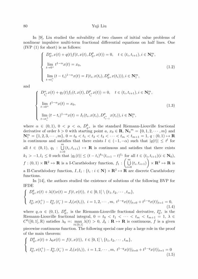
80 Yuji Liu
In [9], Liu studied the solvability of two classes of initial value problems ofnonlinear impulsive multi-term fractional differential equations on half lines. One(IVP (1) for short) is as follows:
Dα0+x(t) + q(t)f(t, x(t), Dp
0+x(t)) = 0, t ∈ (ti, ti+1), i ∈ Nm0 ,
limt→0+
t1−αx(t) = x0,
limt→t+i
(t− ti)1−αx(t) = I(ti, x(ti), Dp0+x(ti))), i ∈ Nm
1 ,
(1.2)
and
Dαt+ix(t) + q1(t)f1(t, x(t), Dp
t+ix(t)) = 0, t ∈ (ti, ti+1), i ∈ Nm
0 ,
limt→0+
t1−αx(t) = x0,
limt→t+i
(t− ti)1−αx(t) = I1(ti, x(ti), Dp
t+i−1
x(ti)), i ∈ Nm1 ,
(1.3)
where α ∈ (0, 1), 0 < p < α, Dba+ is the standard Riemann-Liouville fractional
derivative of order b > 0 with starting point a, x0 ∈ R, N0m = 0, 1, 2, · · · ,m and
Nm1 = 1, 2, 3, · · · ,m, 0 = t0 < t1 < t2 < t3 < · · · < tm < tm+1 = 1, q : (0, 1) 7→ R
is continuous and satisfies that there exists l ∈ (−1,−α) such that |q(t)| ≤ tl for
all t ∈ (0, 1), q1 :m⋃i=0
(ti, ti+1) 7→ R is continuous and satisfies that there exists
k1 > −1, l1 ≤ 0 such that |q1(t)| ≤ (t − ti)k1(ti+1 − t)l1 for all t ∈ (ti, ti+1)(i ∈ N0),
f : (0, 1) ×R2 7→ R is a I-Caratheodory function, f1 :
(m⋃i=0
(ti, ti+1)
)×R2 7→ R is
a II-Caratheodory function, I, I1 : ti : i ∈ N ×R2 7→ R are discrete Caratheodoryfunctions.
In [14], the authors studied the existence of solutions of the following BVP forIFDE
Dq0+x(t) + λ(t)x(t) = f(t, x(t)), t ∈ [0, 1] \ t1, t2, · · · , tm,
Iα0+x(t+i )− Iα0+(t−i ) = Ji(x(ti)), i = 1, 2, · · · ,m, t1−qx(t)|t=0 + t1−qx(t)|t=1 = 0,(1.4)
where q, α ∈ (0, 1), Dq0+ is the Riemann-Liouville fractional derivative, Iα0+ is the
Riemann-Liouville fractional integral, 0 = t0 < t1 < · · · < tm < tm+1 = 1, λ ∈C0([0, 1],R) satisfies λ0 =: max
t∈[0,1]λ(t) > 0, Jk : R 7→ R is continuous, f is a given
piecewise continuous function. The following special case play a large role in the proofof the main theorem:
Dq0+x(t) + λ0x(t) = f(t, x(t)), t ∈ [0, 1] \ t1, t2, · · · , tm,
Iα0+x(t+i )− Iα0+(t−i ) = Ji(x(ti)), i = 1, 2, · · · ,m, t1−qx(t)|t=0 + t1−qx(t)|t=1 = 0(1.5)
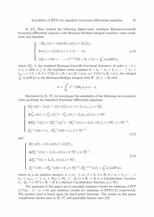
Solvability of BVPs for impulsive fractional differential equations 81
In [17], Zhao studied the following higher-order nonlinear Riemann-Liouvillefractional differential equation with Riemann-Stieltjes integral boundary value condi-tions and impulses
−Dα0+x(t) = λa(t)f(t, x(t)), t \ timi=1,
∆x(ti) = Ii(x(ti)), i = 1, 2, · · · ,m,
x(0) = x′(0) = · · · = x(n−2)(0) = 0, x′(1) =∫ 1
0x(s)dH(s),
(1.6)
where Dα0+ is the standard Riemann-Liouville fractional derivative of order n − 1 <
α ≤ n with n ≥ 3, the impulsive point sequence 0 = t0 < t1 < t2 < · · · < tm <tm+1 = 1,λ > 0, f ∈ C([0, 1]× [0,+∞), [0,+∞)), a ∈ C((0, 1), [0,+∞)), the integral∫ 1
0x(s)dH(s) is the Riemann-Stieltjes integral with H : [0, 1]→ R with
δ =:
∫ 1
0
sα−1dH(s) 6= α− 1.
Motivated by [8, 17], we investigate the solvability of the following two boundaryvalue problems for impulsive fractional differential equations
Dα0+x(t)− λx(t) = f(t, x(t)), a.e., t ∈ (ti, ti+1], i ∈ Nm0 ,
∆Iβ0+x(ti) =: Iβ0+x(t+i )− Iβ0+x(ti) = In(ti, x(ti)), i ∈ Nm1 ,
∆Dα−j0+ x(ti) =: Dα−j
0+ x(t+i )−Dα−j0+ x(ti) = Ij(ti, x(ti)), i ∈ Nm1 , j ∈ Nn−1
1 ,
In−α0+ x(0) = xn, Dα−j0+ x(0) = xj , j ∈ Nn−1
1 ,(1.7)
and
Dα0+x(t) = f(t, x(t)), t \ timi=1,
∆Dα−j0+ x(ti) = Ij(ti, x(ti)), i ∈ Nm1 , j ∈ Nn−1
1 ,
∆In−α0+ x(ti = In(ti, x(ti)), i ∈ Nm1 ,
In−α0+ x(0) = Dα−j0+ x(0) = 0, j ∈ Nn−2
1 , Dα−n+10+ x(1) =
∫ 1
0x(s)dH(s),
(1.8)
where m,n are positive integers, α ∈ (n − 1, n), β > 0, λ ∈ R, 0 = t0 < t1 < · · · <tm < tm+1 = 1, xj ∈ R(j ∈ Nn1 , f : (0, 1) × R → R is a Caratheodory fraction,Ij : ti : i ∈ Nm1 × R→ R is a discrete Caratheodory function (j ∈ Nn1 ).
The purposes of this paper are to establish existence results for solutions of IVP(1.7)(α − β − n = 0) and existence results for solutions of BVP(1.8) respectively.The method used is based upon the fixed point theorems. The results in this papercomplement known ones in [8, 17] and generalize known ones [10].
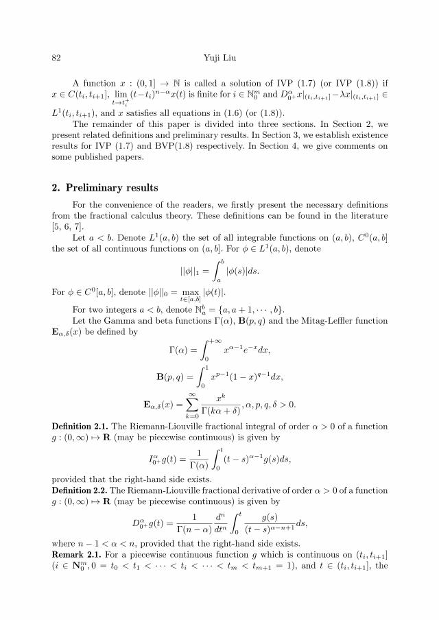
82 Yuji Liu
A function x : (0, 1] → N is called a solution of IVP (1.7) (or IVP (1.8)) ifx ∈ C(ti, ti+1], lim
t→t+i(t−ti)n−αx(t) is finite for i ∈ Nm0 and Dα
0+x|(ti,ti+1]−λx|(ti,ti+1] ∈
L1(ti, ti+1), and x satisfies all equations in (1.6) (or (1.8)).The remainder of this paper is divided into three sections. In Section 2, we
present related definitions and preliminary results. In Section 3, we establish existenceresults for IVP (1.7) and BVP(1.8) respectively. In Section 4, we give comments onsome published papers.
2. Preliminary results
For the convenience of the readers, we firstly present the necessary definitionsfrom the fractional calculus theory. These definitions can be found in the literature[5, 6, 7].
Let a < b. Denote L1(a, b) the set of all integrable functions on (a, b), C0(a, b]the set of all continuous functions on (a, b]. For φ ∈ L1(a, b), denote
||φ||1 =
∫ b
a
|φ(s)|ds.
For φ ∈ C0[a, b], denote ||φ||0 = maxt∈[a,b]
|φ(t)|.
For two integers a < b, denote Nba = a, a+ 1, · · · , b.Let the Gamma and beta functions Γ(α), B(p, q) and the Mitag-Leffler function
Eα,δ(x) be defined by
Γ(α) =
∫ +∞
0
xα−1e−xdx,
B(p, q) =
∫ 1
0
xp−1(1− x)q−1dx,
Eα,δ(x) =
∞∑k=0
xk
Γ(kα+ δ), α, p, q, δ > 0.
Definition 2.1. The Riemann-Liouville fractional integral of order α > 0 of a functiong : (0,∞) 7→ R (may be piecewise continuous) is given by
Iα0+g(t) =1
Γ(α)
∫ t
0
(t− s)α−1g(s)ds,
provided that the right-hand side exists.Definition 2.2. The Riemann-Liouville fractional derivative of order α > 0 of a functiong : (0,∞) 7→ R (may be piecewise continuous) is given by
Dα0+g(t) =
1
Γ(n− α)
dn
dtn
∫ t
0
g(s)
(t− s)α−n+1ds,
where n− 1 < α < n, provided that the right-hand side exists.Remark 2.1. For a piecewise continuous function g which is continuous on (ti, ti+1](i ∈ Nm
0 , 0 = t0 < t1 < · · · < ti < · · · < tm < tm+1 = 1), and t ∈ (ti, ti+1], the
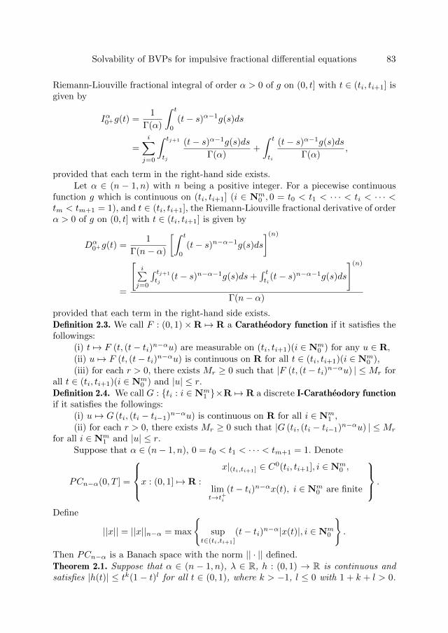
Solvability of BVPs for impulsive fractional differential equations 83
Riemann-Liouville fractional integral of order α > 0 of g on (0, t] with t ∈ (ti, ti+1] isgiven by
Iα0+g(t) =1
Γ(α)
∫ t
0
(t− s)α−1g(s)ds
=
i∑j=0
∫ tj+1
tj
(t− s)α−1g(s)ds
Γ(α)+
∫ t
ti
(t− s)α−1g(s)ds
Γ(α),
provided that each term in the right-hand side exists.Let α ∈ (n − 1, n) with n being a positive integer. For a piecewise continuous
function g which is continuous on (ti, ti+1] (i ∈ Nm0 , 0 = t0 < t1 < · · · < ti < · · · <
tm < tm+1 = 1), and t ∈ (ti, ti+1], the Riemann-Liouville fractional derivative of orderα > 0 of g on (0, t] with t ∈ (ti, ti+1] is given by
Dα0+g(t) =
1
Γ(n− α)
[∫ t
0
(t− s)n−α−1g(s)ds
](n)
=
[i∑
j=0
∫ tj+1
tj(t− s)n−α−1g(s)ds+
∫ tti
(t− s)n−α−1g(s)ds
](n)
Γ(n− α)
provided that each term in the right-hand side exists.Definition 2.3. We call F : (0, 1)×R 7→ R a Caratheodory function if it satisfies thefollowings:
(i) t 7→ F (t, (t− ti)n−αu) are measurable on (ti, ti+1)(i ∈ Nm0 ) for any u ∈ R,
(ii) u 7→ F (t, (t− ti)n−αu) is continuous on R for all t ∈ (ti, ti+1)(i ∈ Nm0 ),
(iii) for each r > 0, there exists Mr ≥ 0 such that |F (t, (t− ti)n−αu) | ≤Mr forall t ∈ (ti, ti+1)(i ∈ Nm
0 ) and |u| ≤ r.Definition 2.4. We call G : ti : i ∈ Nm
1 ×R 7→ R a discrete I-Caratheodory functionif it satisfies the followings:
(i) u 7→ G (ti, (ti − ti−1)n−αu) is continuous on R for all i ∈ Nm1 ,
(ii) for each r > 0, there exists Mr ≥ 0 such that |G (ti, (ti − ti−1)n−αu) | ≤Mr
for all i ∈ Nm1 and |u| ≤ r.
Suppose that α ∈ (n− 1, n), 0 = t0 < t1 < · · · < tm+1 = 1. Denote
PCn−α(0, T ] =
x : (0, 1] 7→ R :
x|(ti,ti+1] ∈ C0(ti, ti+1], i ∈ Nm0 ,
limt→t+i
(t− ti)n−αx(t), i ∈ Nm0 are finite
.
Define
||x|| = ||x||n−α = max
sup
t∈(ti,ti+1]
(t− ti)n−α|x(t)|, i ∈ Nm0
.
Then PCn−α is a Banach space with the norm || · || defined.Theorem 2.1. Suppose that α ∈ (n − 1, n), λ ∈ R, h : (0, 1) → R is continuous andsatisfies |h(t)| ≤ tk(1− t)l for all t ∈ (0, 1), where k > −1, l ≤ 0 with 1 + k + l > 0.
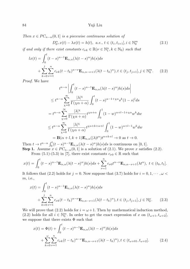
84 Yuji Liu
Then x ∈ PCn−α(0, 1] is a piecewise continuous solution of
Dα0+x(t)− λx(t) = h(t), a.e., t ∈ (ti, ti+1], i ∈ Nm0 (2.1)
if and only if there exist constants cνk ∈ R(ν ∈ Nn1 , k ∈ N0) such that
lx(t) =
∫ t
0
(t− s)α−1Eα,α(λ(t− s)α)h(s)ds
+
j∑k=0
n∑ν=1
cνk(t− tk)α−νEα,α−ν+1(λ(t− tk)α), t ∈ (tj , tj+1], j ∈ Nm0 . (2.2)
Proof. We have
tn−α∣∣∣∣∫ t
0
(t− s)α−1Eα,α(λ(t− s)α)h(s)ds
∣∣∣∣≤ tn−α
∞∑χ=0
|λ|χ
Γ(χα+ α)
∫ t
0
(t− s)α−1+χαsk(1− s)lds
= tn−α∞∑χ=0
|λ|χ
Γ(χα+ α)tχα+α
∫ 1
0
(1− w)α+l−1+χαwkdw
≤ tn−α∞∑χ=0
|λ|χ
Γ(χα+ α)tχα+k+α+l
∫ 1
0
(1− w)α+l−1wkdw
= B(α+ l, k + 1)Eα,α(|λ|tα)tn+k+l → 0 as t→ 0.
Then t→ tn−α∫ t
0(t− s)α−1Eα,α(λ(t− s)α)h(s)ds is continuous on [0, 1].
Step 1. Assume x ∈ PCn−α(0, 1] is a solution of (2.1). We prove x satisfies (2.2).From (5.1)-(5.3) in [7], there exist constants cν0 ∈ R such that
x(t) =
∫ t
0
(t− s)α−1Eα,α(λ(t− s)α)h(s)ds+
n∑ν=1
cν0tα−νEα,α−ν+1(λtα), t ∈ (t0, t1].
It follows that (2.2) holds for j = 0. Now suppose that (3.7) holds for i = 0, 1, · · · , ω <m, i.e.,
x(t) =
∫ t
0
(t− s)α−1Eα,α(λ(t− s)α)h(s)ds
+
j∑k=0
n∑ν=1
cνk(t− tk)α−νEα,α−ν+1(λ(t− tk)α), t ∈ (tj , tj+1], j ∈ Nω0 . (2.3)
We will prove that (2.2) holds for i = ω+1. Then by mathematical induction method,(2.2) holds for all i ∈ Nm0 . In order to get the exact expression of x on (tω+1, tω+2],we suppose that there exists Φ such that
x(t) = Φ(t) +
∫ t
0
(t− s)α−1Eα,α(λ(t− s)α)h(s)ds
+
ω∑k=0
n∑ν=1
cνk(t− tk)α−νEα,α−ν+1(λ(t− tk)α), t ∈ (tω+01, tω+2]. (2.4)
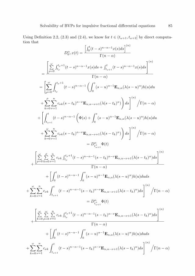
Solvability of BVPs for impulsive fractional differential equations 85
Using Definition 2.2, (2.3) and (2.4), we know for t ∈ (tω+1, tω+2] by direct computa-tion that
Dα0+x(t) =
[∫ t0(t− s)n−α−1x(s)ds
](n)
Γ(n− α)
=
[ω∑ρ=0
∫ tρ+1
tρ(t− s)n−α−1x(s)ds+
∫ ttω+1
(t− s)n−α−1x(s)ds
](n)
Γ(n− α)
=
[ω∑ρ=0
∫ tρ+1
tρ
(t− s)n−α−1
(∫ s
0
(s− u)α−1Eα,α(λ(s− u)α)h(u)du
+
ρ∑k=0
n∑ν=1
cνk(s− tk)α−νEα,α−ν+1(λ(s− tk)α)
)ds
](n)/Γ(n− α)
+
[∫ t
tω+1
(t− s)n−α−1
(Φ(s) +
∫ s
0
(s− u)α−1Eα,α(λ(s− u)α)h(u)du
+
ω∑k=0
n∑ν=1
cνk(s− tk)α−νEα,α−ν+1(λ(s− tk)α)
)ds
](n)/Γ(n− α)
= Dαt+ω+1
Φ(t)
+
[ω∑ρ=0
ρ∑k=0
n∑ν=1
cνk∫ tρ+1
tρ(t− s)n−α−1(s− tk)α−νEα,α−ν+1(λ(s− tk)α)ds
](n)
Γ(n− α)
+
[∫ t
0
(t− s)n−α−1
∫ s
0
(s− u)α−1Eα,α(λ(s− u)α)h(u)duds
+
ω∑k=0
n∑ν=1
cνk
∫ t
tω+1
(t− s)n−α−1(s− tk)α−νEα,α−ν+1(λ(s− tk)α)ds
](n)/Γ(n− α)
= Dαt+ω+1
Φ(t)
+
[ω∑k=0
ω∑ρ=k
n∑ν=1
cνk∫ tρ+1
tρ(t− s)n−α−1(s− tk)α−νEα,α−ν+1(λ(s− tk)α)ds
](n)
Γ(n− α)
+
[∫ t
0
(t− s)n−α−1
∫ s
0
(s− u)α−1Eα,α(λ(s− u)α)h(u)duds
+
ω∑k=0
n∑ν=1
cνk
∫ t
tω+1
(t− s)n−α−1(s− tk)α−νEα,α−ν+1(λ(s− tk)α)ds
](n)/Γ(n− α)
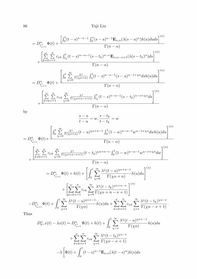
86 Yuji Liu
= Dαt+ω+1
Φ(t) +
[∫ t0(t− s)n−α−1
∫ s0
(s− u)α−1Eα,α(λ(s− u)α)h(u)duds](n)
Γ(n− α)
+
[ω∑k=0
n∑ν=1
cνk∫ ttk
(t− s)n−α−1(s− tk)α−νEα,α−ν+1(λ(s− tk)α)ds
](n)
Γ(n− α)
= Dαt+ω+1
Φ(t) +
[∫ t0
∞∑χ=0
λχ
Γ(χα+α)
∫ tu(t− s)n−α−1(s− u)α−1+χαdsh(u)du
](n)
Γ(n− α)
+
[ω∑k=0
n∑ν=1
cνk∞∑χ=0
λχ
Γ(χα+α−ν+1)
∫ ttk
(t− s)n−α−1(s− tk)α−ν+χαds
](n)
Γ(n− α)
bys− ut− u
= w,s− tkt− tk
= w
= Dαt+ω+1
Φ(t)+
[∫ t0
∞∑χ=0
λχ
Γ(χα+α) (t− u)χα+n−1∫ 1
0(1− w)n−α−1wα−1+χαdwh(u)du
](n)
Γ(n− α)
+
[ω∑k=0
n∑ν=1
cνk∞∑χ=0
λχ
Γ(χα+α−ν+1) (t− tk)χα+n−ν ∫ 1
0(1− w)n−α−1wα−ν+χαdw
](n)
Γ(n− α)
= Dαt+ω+1
Φ(t) + h(t) +
[∫ t
0
∞∑χ=0
λχ(t− u)χα+n−1
Γ(χα+ n)h(u)du
](n)
+
[ω∑k=0
n∑ν=1
cνk
∞∑χ=0
λχ(t− tk)χα+n−ν
Γ(χα+ n− ν + 1)
](n)
−Dαt+ω+1
Φ(t) +
∫ t
0
∞∑χ=1
λχ(t− u)χα+−1
Γ(χα)h(u)du+
ω∑k=0
n∑ν=1
cνk
∞∑χ=1
λχ(t− tk)χα−ν
Γ(χα− ν + 1).
Thus
Dα0+x(t)− λx(t) = Dα
t+ω+1
Φ(t) + h(t) +
∫ t
0
∞∑χ=1
λχ(t− u)χα+−1
Γ(χα)h(u)du
+
ω∑k=0
n∑ν=1
cνk
∞∑χ=1
λχ(t− tk)χα−ν
Γ(χα− ν + 1)
−λ[Φ(t) +
∫ t
0
(t− s)α−1Eα,α(λ(t− s)α)h(s)ds
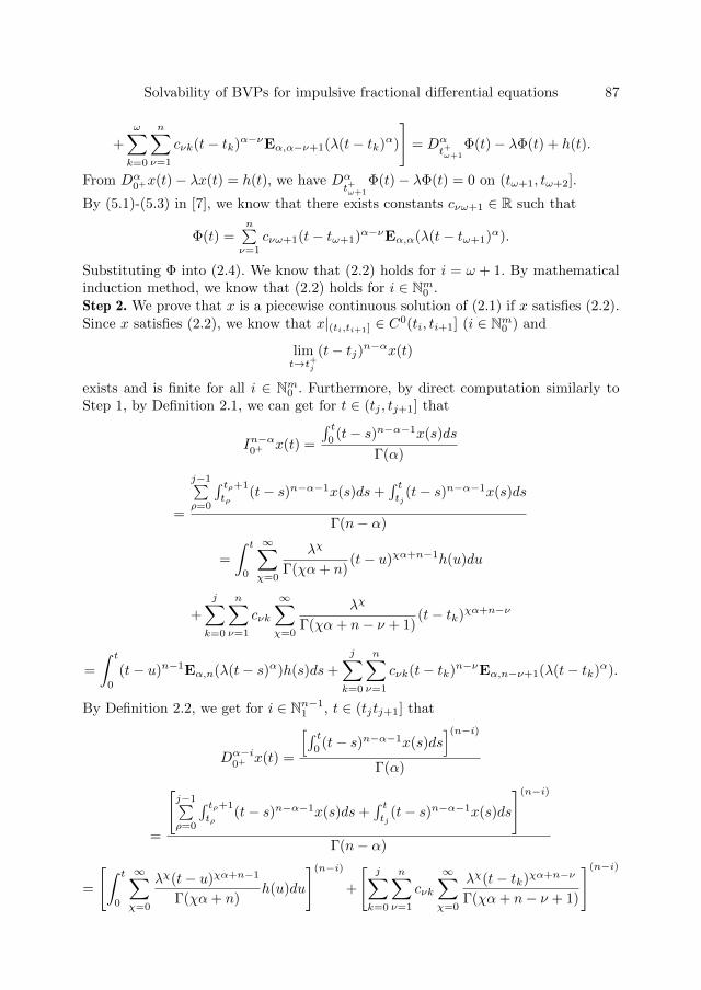
Solvability of BVPs for impulsive fractional differential equations 87
+
ω∑k=0
n∑ν=1
cνk(t− tk)α−νEα,α−ν+1(λ(t− tk)α)
]= Dα
t+ω+1
Φ(t)− λΦ(t) + h(t).
From Dα0+x(t)− λx(t) = h(t), we have Dα
t+ω+1
Φ(t)− λΦ(t) = 0 on (tω+1, tω+2].
By (5.1)-(5.3) in [7], we know that there exists constants cνω+1 ∈ R such that
Φ(t) =n∑ν=1
cνω+1(t− tω+1)α−νEα,α(λ(t− tω+1)α).
Substituting Φ into (2.4). We know that (2.2) holds for i = ω + 1. By mathematicalinduction method, we know that (2.2) holds for i ∈ Nm0 .Step 2. We prove that x is a piecewise continuous solution of (2.1) if x satisfies (2.2).Since x satisfies (2.2), we know that x|(ti,ti+1] ∈ C0(ti, ti+1] (i ∈ Nm0 ) and
limt→t+j
(t− tj)n−αx(t)
exists and is finite for all i ∈ Nm0 . Furthermore, by direct computation similarly toStep 1, by Definition 2.1, we can get for t ∈ (tj , tj+1] that
In−α0+ x(t) =
∫ t0(t− s)n−α−1x(s)ds
Γ(α)
=
j−1∑ρ=0
∫ tρ+1
tρ(t− s)n−α−1x(s)ds+
∫ ttj
(t− s)n−α−1x(s)ds
Γ(n− α)
=
∫ t
0
∞∑χ=0
λχ
Γ(χα+ n)(t− u)χα+n−1h(u)du
+
j∑k=0
n∑ν=1
cνk
∞∑χ=0
λχ
Γ(χα+ n− ν + 1)(t− tk)χα+n−ν
=
∫ t
0
(t− u)n−1Eα,n(λ(t− s)α)h(s)ds+
j∑k=0
n∑ν=1
cνk(t− tk)n−νEα,n−ν+1(λ(t− tk)α).
By Definition 2.2, we get for i ∈ Nn−11 , t ∈ (tjtj+1] that
Dα−i0+ x(t) =
[∫ t0(t− s)n−α−1x(s)ds
](n−i)Γ(α)
=
[j−1∑ρ=0
∫ tρ+1
tρ(t− s)n−α−1x(s)ds+
∫ ttj
(t− s)n−α−1x(s)ds
](n−i)
Γ(n− α)
=
[∫ t
0
∞∑χ=0
λχ(t− u)χα+n−1
Γ(χα+ n)h(u)du
](n−i)
+
[j∑
k=0
n∑ν=1
cνk
∞∑χ=0
λχ(t− tk)χα+n−ν
Γ(χα+ n− ν + 1)
](n−i)
88 Yuji Liu
=
∫ t
0
∞∑χ=0
λχ(t− u)χα+i−1
Γ(χα+ i)h(u)du
+
j∑k=0
n∑ν=1
cνk
∞∑χ=1
λχ(t− tk)χα+i−ν
Γ(χα+ i− ν + 1)+
j∑k=0
i∑ν=1
cνk(t− tk)i−ν
Γ(i− ν + 1)
=
∫ t
0
(t− u)i−1Eα,i(λ(t− u)α)h(u)du+
j∑k=0
i∑ν=1
cνk(t− tk)i−νEα,i−ν+1(λ(t− tk)α)
+λ
j∑k=0
n∑ν=i+1
cνk(t− tk)α+i−νEα,α+i−ν+1(λ(t− tk)α).
We see thatIn−α0+ x|(tj ,tj+1], D
α−i0+ x|(tj ,tj+1](i ∈ Nn−1
1 , j ∈ Nm0 )
are continuous and the limits
limt→t+j
In−α0+ x(t), limt→t+j
Dα−i0+ x(t) (i ∈ Nn−1
1 , j ∈ Nm0 )
are finite. By Definition 2.2, α ∈ (n− 1, n), for t ∈ (tj , tj+1], we have
Dα0+x(t) =
[∫ t0(t− s)n−α−1x(s)ds
](n−i)Γ(α)
=
[j−1∑ρ=0
∫ tρ+1
tρ(t− s)n−α−1x(s)ds+
∫ ttj
(t− s)n−α−1x(s)ds
](n−i)
Γ(n− α)
=
[∫ t
0
∞∑χ=0
λχ(t− u)χα+n−1
Γ(χα+ n)h(u)du
](n)
+
[j∑
k=0
n∑ν=1
cνk
∞∑χ=0
λχ(t− tk)χα+n−ν
Γ(χα+ n− ν + 1)
](n)
= h(t)+
∫ t
0
∞∑χ=1
λχ(t− u)χα−1
Γ(χα)h(u)du+
j∑k=0
n∑ν=1
cνk
∞∑χ=1
λχ(t− tk)χα+−ν
Γ(χα− ν + 1), t ∈ (tj , tj+1].
ThenDα
0+x(t)− λx(t) = h(t), t ∈ (tj , tj+1], j ∈ Nm0 .So x is a piecewise continuous solution of (2.1). The proof is completed. Remark 2.1. Lemma 2.1 (when λ = 0) is one of the main results in [10] (see Theorem3.2 in [10]). So our results generalizes the one in [10].Theorem 2.2. Suppose that x is a solution of (2.1) and is defined by (2.2). Then
Iβ0+x(t) =
∫ t
0
(t− s)α+β−1Eα,α+β(λ(t− s)α)h(s)ds
+
j∑k=0
n∑ν=1
cνk(t− tk)α+β−νEα,α+β−ν+1(λ(t− tk)α),
t ∈ (tj , tj+1], j ∈ Nm0 (2.5)
Solvability of BVPs for impulsive fractional differential equations 89
In−α0+ x(t) =
i∑k=0
n∑ν=1
cνk(t− tk)n−νEα,n−ν+1(λ(t− tk)α)
+
∫ t
0
(t− u)n−1Eα,n(λ(t− u)α)h(u)du,
t ∈ (ti, ti+1], i ∈ Nm0 , (2.6)
and
Dα−j0+ x(t) =
i∑k=0
j∑ν=1
cνk(t− tk)j−νEα,j−ν+1(λ(t− tk)α)
+ λ
i∑k=0
n∑ν=j+1
cνk(t− tk)α+j−νEα,α+j−ν+1(λ(t− tk)α)
+
∫ t
0
(t− u)j−1Eα,j(λ(t− u)α)h(u)du,
t ∈ (ti, ti+1], i ∈ Nm0 , j ∈ Nn−11 . (2.7)
Proof. We firstly prove (2.5). For t ∈ (ti, ti+1], by (2.2) and Definition 2.1, we get
Iβ0+x(t) =
i−1∑µ=0
∫ tµ+1
tµ(t− s)β−1x(s)ds+
∫ tti
(t− s)β−1x(s)ds
Γ(β)
=
i−1∑µ=0
∫ tµ+1
tµ
(t− s)β−1
(∫ s
0
(s− u)α−1Eα,α(λ(s− u)α)h(u)du
+
µ∑k=0
n∑ν=1
cνk(s− tk)α−νEα,α−ν+1(λ(s− tk)α)
)ds/
Γ(β)
+
∫ t
ti
(t− s)β−1
(∫ s
0
(s− u)α−1Eα,α(λ(s− u)α)h(u)du
+
i∑k=0
n∑ν=1
cνk(s− tk)α−νEα,α−ν+1(λ(s− tk)α)
)ds/
Γ(β)
=
i−1∑µ=0
∫ tµ+1
tµ(t− s)β−1
µ∑k=0
n∑ν=1
cνk(s− tk)α−νEα,α−ν+1(λ(s− tk)α)ds
Γ(β)
+
∫ tti
(t− s)β−1i∑
k=0
n∑ν=1
cνk(s− tk)α−νEα,α−ν+1(λ(s− tk)α)ds
Γ(β)
+
∫ t0(t− s)β−1
∫ s0
(s− u)α−1Eα,α(λ(s− u)α)h(u)duds
Γ(β)
90 Yuji Liu
=
i−1∑k=0
i−1∑µ=k
n∑ν=1
cνk∫ tµ+1
tµ(t− s)β−1(s− tk)α−ν
∞∑χ=0
λχ
Γ(χα+α−ν+1) (s− tk)χαds
Γ(β)
+
i∑k=0
n∑ν=1
cνk∫ tti
(t− s)β−1(s− tk)α−ν∞∑χ=0
λχ
Γ(χα+α−ν+1) (s− tk)χαds
Γ(β)
+
∫ t0
∫ tu(t− s)β−1(s− u)α−1
∞∑χ=0
λχ
Γ(χα+α) (s− u)χαdsh(u)du
Γ(β)
=
i−1∑k=0
i−1∑µ=k
n∑ν=1
cνk∞∑χ=0
λχ
Γ(χα+α−ν+1)
∫ tµ+1
tµ(t− s)β−1(s− tk)α−ν+χαds
Γ(β)
+
i∑k=0
n∑ν=1
cνk∞∑χ=0
λχ
Γ(χα+α−ν+1)
∫ tti
(t− s)β−1(s− tk)α−ν+χαds
Γ(β)
+
∞∑χ=0
λχ
Γ(χα+α)
∫ t0
∫ tu(t− s)β−1(s− u)α−1+χαdsh(u)du
Γ(β)
=
i−1∑k=0
i−1∑µ=k
n∑ν=1
cνk∞∑χ=0
λχ
Γ(χα+α−ν+1) t− tk)χα+α+β−ν ∫ tµ+1−tkt−tk
tµ−tKt−tk
(1− w)β−1wα−ν+χαdw
Γ(β)
+
i∑k=0
n∑ν=1
cνk∞∑χ=0
λχ
Γ(χα+α−ν+1) (t− tk)χα+α+β−ν ∫ 1ti−tkt−tk
(1− w)β−1wα−ν+χαdw
Γ(β)
+
∞∑χ=0
λχ
Γ(χα+α)
∫ t0(t− u)χα+α+β−1
∫ 1
0(1− w)β−1wα−1+χαdwh(u)du
Γ(β)
=
i∑k=0
n∑ν=1
cνk∞∑χ=0
λχ
Γ(χα+α−ν+1) (t− tk)χα+α+β−ν ∫ 1
0(1− w)β−1wα−ν+χαdw
Γ(β)
+
∞∑χ=0
λχ
Γ(χα+α)
∫ t0(t− u)χα+α+β−1
∫ 1
0(1− w)β−1wα−1+χαdwh(u)du
Γ(β)
=
i∑k=0
n∑ν=1
cνk
∞∑χ=0
λχ
Γ(χα+ α+ β − ν + 1)(t− tk)χα+α+β−ν
+
∞∑χ=0
λχ
Γ(χα+ α+ β)
∫ t
0
(t− u)χα+α+β−1h(u)du
Solvability of BVPs for impulsive fractional differential equations 91
=
∫ t
0
(t− s)α+β−1Eα,α+β(λ(t− s)α)h(s)ds
+
i∑k=0
n∑ν=1
cνk(t− tk)α+β−νEα,α+β−ν+1(λ(t− tk)α), t ∈ (ti, ti+1], i ∈ Nm0
Thus (2.5) is proved. Hence (2.6) holds by β = n− α.Now, we prove (2.7). In fact, for t ∈ (ti, ti+1], we have by using 2.2 and Definition 2.2that
Dα−j0+ x(t) =
[∫ t0(t− s)n−α−1x(s)ds
](n−j)Γ(n− α)
=
[i−1∑µ=0
(t− s)n−α−1x(s)ds+∫ tti
(t− s)n−α−1x(s)ds
](n−j)
Γ(n− α)
=
[i−1∑µ=0
∫ tµ+1
tµ
(t− s)n−α−1
(∫ s
0
(s− u)α−1Eα,α(λ(s− u)α)h(u)du
+
µ∑k=0
n∑ν=1
cνk(s− tk)α−νEα,α−ν+1(λ(s− tk)α)
)ds
](n−j)/Γ(n− α)
+
[∫ t
ti
(t− s)n−α−1
(∫ s
0
(s− u)α−1Eα,α(λ(s− u)α)h(u)du
+
i∑k=0
n∑ν=1
cνk(s− tk)α−νEα,α−ν+1(λ(s− tk)α)
)ds
](n−j)/Γ(n− α)
=
[i−1∑µ=0
∫ tµ+1
tµ(t− s)n−α−1
µ∑k=0
n∑ν=1
cνk(s− tk)α−νEα,α−ν+1(λ(s− tk)α)ds
](n−j)
Γ(n− α)
+
[∫ tti
(t− s)n−α−1i∑
k=0
n∑ν=1
cνk(s− tk)α−νEα,α−ν+1(λ(s− tk)α)ds
](n−j)
Γ(n− α)
+
[∫ t0(t− s)n−α−1
∫ s0
(s− u)α−1Eα,α(λ(s− u)α)h(u)duds](n−j)
Γ(n− α)
=
[i−1∑k=0
i−1∑µ=k
n∑ν=1
cνk∫ tµ+1
tµ(t− s)n−α−1(s− tk)α−ν
∞∑χ=0
λχ
Γ(χα+α−ν+1) (s− tk)χαds
](n−j)
Γ(n− α)
+
[i∑
k=0
n∑ν=1
cνk∫ tti
(t− s)n−α−1(s− tk)α−ν∞∑χ=0
λχ
Γ(χα+α−ν+1) (s− tk)χαds
](n−j)
Γ(n− α)
92 Yuji Liu
+
[∫ t0
∫ tu(t− s)n−α−1(s− u)α−1
∞∑χ=0
λχ
Γ(χα+α) (s− u)χαdsh(u)du
](n−j)
Γ(n− α)
=
[i−1∑k=0
i−1∑µ=k
n∑ν=1
cνk∞∑χ=0
λχ
Γ(χα+α−ν+1)
∫ tµ+1
tµ(t− s)n−α−1(s− tk)α−ν+χαds
](n−j)
Γ(n− α)
+
[i∑
k=0
n∑ν=1
cνk∞∑χ=0
λχ
Γ(χα+α−ν+1)
∫ tti
(t− s)n−α−1(s− tk)α−ν+χαds
](n−j)
Γ(n− α)
+
[∞∑χ=0
λχ
Γ(χα+α)
∫ t0
∫ tu(t− s)n−α−1(s− u)α−1+χαdsh(u)du
](n−j)
Γ(n− α)
=
i−1∑k=0
i−1∑µ=k
n∑ν=1
cνk
∞∑χ=0
λχ
Γ(χα+ α− ν + 1)(t− tk)χα+n−ν
×∫ tµ+1−tk
t−tk
tµ−tkt−tk
(1− w)n−α−1wα−ν+χαdw
(n−j)/Γ(n− α)
+
[i∑
k=0
n∑ν=1
cνk∞∑χ=0
λχ
Γ(χα+α−ν+1) (t− tk)χα+n−ν ∫ 1ti−tkt−tk
(1− w)n−α−1wα−ν+χαdw
](n−j)
Γ(n− α)
+
[∞∑χ=0
λχ
Γ(χα+α)
∫ t0(t− u)χα+n−1
∫ 1
0(1− w)n−α−1wα−1+χαdwh(u)du
](n−j)
Γ(n− α)
=
[i∑
k=0
n∑ν=1
cνk∞∑χ=0
λχ
Γ(χα+α−ν+1) (t− tk)χα+n−ν ∫ 1
0(1− w)n−α−1wα−ν+χαdw
](n−j)
Γ(n− α)
+
[∞∑χ=0
λχ
Γ(χα+α)
∫ t0(t− u)χα+n−1
∫ 1
0(1− w)n−α−1wα−1+χαdwh(u)du
](n−j)
Γ(n− α)
=
[i∑
k=0
n∑ν=1
cνk
∞∑χ=0
λχ
Γ(χα+ n− ν + 1)(t− tk)χα+n−ν
](n−j)
Solvability of BVPs for impulsive fractional differential equations 93
+
[ ∞∑χ=0
λχ
Γ(χα+ n)
∫ t
0
(t− u)χα+n−1h(u)du
](n−j)
=
i∑k=0
j∑ν=1
cνk1
Γ(j − ν + 1)(t−tk)j−ν+
i∑k=0
n∑ν=1
cνk
∞∑χ=1
λχ
Γ(χα+ j − ν + 1)(t−tk)χα+j−ν
+
∞∑χ=0
λχ
Γ(χα+ j)
∫ t
0
(t− u)χα+j−1h(u)du
=
i∑k=0
j∑ν=1
cνk
∞∑χ=0
λχ
Γ(χα+ j − ν + 1)(t− tk)χα+j−ν
+
i∑k=0
n∑ν=j+1
cνk
∞∑χ=1
λχ
Γ(χα+ j − ν + 1)(t− tk)χα+j−ν
+
∫ t
0
(t− u)j−1Eα,j(λ(t− u)α)h(u)du
=
i∑k=0
j∑ν=1
cνk(t− tk)j−νEα,j−ν+1(λ(t− tk)α)
+λ
i∑k=0
n∑ν=j+1
cνk(t− tk)α+j−νEα,α+j−ν+1(λ(t− tk)α)
+
∫ t
0
(t− u)j−1Eα,j(λ(t− u)α)h(u)du.
Banach space PCn−α(0, 1]. Let n be a positive integer, α ∈ (n − 1, n) and 0 = t0 <t1 < · · · < tm+1 = 1. Choose
PCn−α(0, 1] =
x : (0, 1] 7→ R :
x|(ti,ti+1] ∈ C0(ti, ti+1], i ∈ Nm0 ,
limt→t+i
(t− ti)n−αx(t), i ∈ Nm0 are finite
.
Define
||x|| = ||x||n−α = max
sup
t∈(ti,ti+1]
(t− ti)n−α|x(t)|, i ∈ Nm0
.
Then PCn−α(0, 1] is a Banach space with the norm || · || defined.
94 Yuji Liu
Theorem 2.3. Suppose that α+ β = n, h ∈ L1(0, 1] aji, bi ∈ R. Then x ∈ PCn−α(0, 1]is a solution of
Dα0+x(t)− λx(t), a.e., t ∈ (ti, ti+1], i ∈ Nm0
∆In−α0+ x(ti), i ∈ Nm1
∆Dα−j0+ x(ti), i ∈ Nm1 , j ∈ Nn−1
1
In−α0+ x(0)
Dα−j0+ x(0), j ∈ Nn−1
1
=
h(t), a.e., t ∈ (ti, ti+1], i ∈ Nm0
ani, i ∈ Nm1
aji, i ∈ Nm1 , j ∈ Nn−11
bn
bj , j ∈ Nn−11
(2.8)
if and only if
x(t) =
∫ t
0
(t− s)α−1Eα,α(λ(t− s)α)h(s)ds+
n∑ν=1
bνtα−νEα,α−ν+1(λtα)
+
j∑k=1
n∑ν=1
aνk(t− tk)α−νEα,α−ν+1(λ(t− tk)α), t ∈ (tj , tj+1], j ∈ Nm0 .
Proof. Suppose that x is a solution of (2.15). By Theorem 2.1, there exist constantscνk ∈ R(ν ∈ Nn1 , k ∈ N0) such that
x(t) =
∫ t
0
(t− s)α−1Eα,α(λ(t− s)α)h(s)ds
+
j∑k=0
n∑ν=1
cνk(t− tk)α−νEα,α−ν+1(λ(t− tk)α),
t ∈ (tj , tj+1], j ∈ Nm0 . (2.9)
Then Theorem 2.2 implies
Iβ0+x(t) =
∫ t
0
(t− s)α+β−1Eα,α+β(λ(t− s)α)h(s)ds
+
j∑k=0
n∑ν=1
cνk(t− tk)α+β−νEα,α+β−ν+1(λ(t− tk)α),
t ∈ (tj , tj+1], j ∈ Nm0 (2.10)
In−α0+ x(t) =
i∑k=0
n∑ν=1
cνk(t− tk)n−νEα,n−ν+1(λ(t− tk)α)
+
∫ t
0
(t− u)n−1Eα,n(λ(t− u)α)h(u)du,
t ∈ (ti, ti+1], i ∈ Nm0 , (2.11)
Solvability of BVPs for impulsive fractional differential equations 95
and
Dα−j0+ x(t) =
i∑k=0
j∑ν=1
cνk(t− tk)j−νEα,j−ν+1(λ(t− tk)α)
+ λ
i∑k=0
n∑ν=j+1
cνk(t− tk)α+j−νEα,α+j−ν+1(λ(t− tk)α)
+
∫ t
0
(t− u)j−1Eα,j(λ(t− u)α)h(u)du,
t ∈ (ti, ti+1], i ∈ Nm0 , j ∈ Nn−11 . (2.12)
By Dα−j0+ x(0) = bj and (2.12), we get cj0 = bj , j ∈ Nn−1
1 .
By In−α0+ x(0) = bn and (2.11), we get cn0 = bn.
By ∆Dα−j0+ x(ti) = aji, i ∈ Nm1 , j ∈ Nn−1
1 and (2.12), we get cji = aji for i ∈ Nm1 ,
j ∈ Nn−11 .
By ∆In−α0+ x(ti) = ani, i ∈ Nm1 and (2.11), we get cni = ani, i ∈ Nm1 .Hence
x(t) =
∫ t
0
(t− s)α−1Eα,α(λ(t− s)α)h(s)ds+
n∑ν=1
bνtα−νEα,α−ν+1(λtα)
+
j∑k=1
n∑ν=1
aνk(t− tk)α−νEα,α−ν+1(λ(t− tk)α), t ∈ (tj , tj+1], j ∈ Nm0 .
The proof is completed. Theorem 2.4. Suppose that
M =:1
Γ(α− n+ 2)+
m∑µ=0
∫ tµ+1
tµ
sα−n+1
Γ(α− n+ 2)dH(s) 6= 0, h ∈ L1(0, 1], aji, bi ∈ R.
Then x ∈ PCn−α(0, 1] is a solution of
Dα0+x(t), a.e., t ∈ (ti, ti+1], i ∈ Nm0
∆In−α0+ x(ti), i ∈ Nm1
∆Dα−j0+ x(ti), i ∈ Nm1 , j ∈ Nn−1
1 ,
In−α0+ x(0)
Dα−j0+ x(0) = 0, j ∈ Nn−2
1
Dα−n+10+ x(1)−
∫ 1
0x(s)dH(s)
=
h(t), a.e., t ∈ (ti, ti+1], i ∈ Nm0
ani, i ∈ Nm1
aji, i ∈ Nm1 , j ∈ Nn−11
0
0, j ∈ Nn−21
0
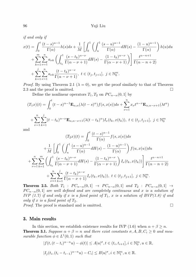
96 Yuji Liu
if and only if
x(t) =
∫ t
0
(t− s)α−1
Γ(α)h(s)ds+
1
M
[∫ 1
0
(∫ 1
u
(s− u)α−1
Γ(α)dH(s)− (1− u)α−1
Γ(α)
)h(u)du
+
m∑k=1
n∑ν=1
aνk
(∫ 1
tk
(s− tk)α−ν
Γ(α− ν + 1)dH(s)− (1− tk)α−ν
Γ(α− ν + 1)
)]tα−n+1
Γ(α− n+ 2)
+
j∑k=1
n∑ν=1
aνk(t− tk)α−ν
Γ(α− ν + 1), t ∈ (tj , tj+1], j ∈ Nm0 .
Proof. By using Theorem 2.1 (λ = 0), we get the proof similarly to that of Theorem2.3 and the proof is omitted.
Define the nonlinear operators T1, T2 on PCn−α(0, 1] by
(T1x)(t) =
∫ t
0
(t− s)α−1Eα,α(λ(t− s)α)f(s, x(s))ds+
n∑ν=1
xνtα−νEα,α−ν+1(λtα)
+
n∑ν=1
j∑k=1
(t− tk)α−νEα,α−ν+1(λ(t− tk)α)Iν(tk, x(tk)), t ∈ (tj , tj+1], j ∈ Nm0
and
(T2x)(t) =
∫ t
0
(t− s)α−1
Γ(α)f(s, x(s))ds
+1
M
[∫ 1
0
(∫ 1
u
(s− u)α−1
Γ(α)dH(s)− (1− u)α−1
Γ(α)
)f(u, x(u))du
+
n∑ν=1
m∑k=1
(∫ 1
tk
(s− tk)α−ν
Γ(α− ν + 1)dH(s)− (1− tk)α−ν
Γ(α− ν + 1)
)Iν(tk, x(tk))
]tα−n+1
Γ(α− n+ 2)
+
n∑ν=1
j∑k=1
(t− tk)α−ν
Γ(α− ν + 1)Iν(tk, x(tk)), t ∈ (tj , tj+1], j ∈ Nm0 .
Theorem 2.5. Both T1 : PCn−α(0, 1] → PCn−α(0, 1] and T2 : PCn−α(0, 1] →PCn−α(0, 1] are well defined and are completely continuous and x is a solution ofIVP (1.7) if and only if x is a fixed point of T1, x is a solution of BVP(1.8) if andonly if x is a fixed point of T2.Proof. The proof is standard and is omitted.
3. Main results
In this section, we establish existence results for IVP (1.6) when α+ β ≥ n.Theorem 3.1. Suppose α + β = n and there exist constants σ,A,B,Ci ≥ 0 and mea-surable function φ ∈ L1(0, 1) such that
|f(t, (t− ti)α−nu)− φ(t)| ≤ A|u|σ, t ∈ (ti, ti+1], i ∈ Nm0 , u ∈ R,
|Ij(ti, (ti − ti−1)α−nu)− Ci| ≤ B|u|σ, i ∈ Nm1 , u ∈ R.
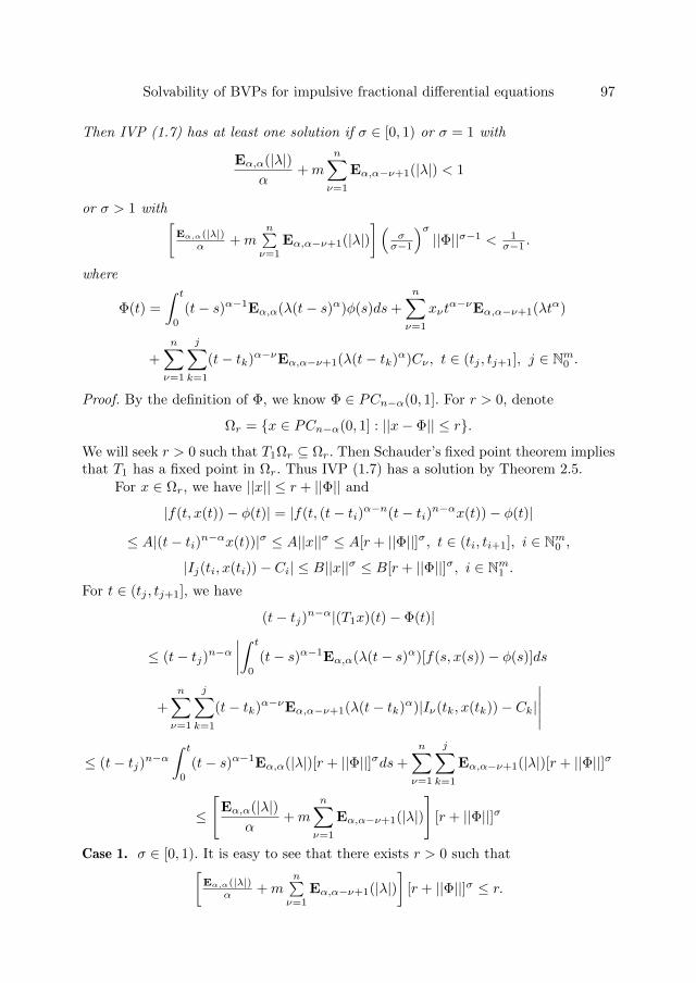
Solvability of BVPs for impulsive fractional differential equations 97
Then IVP (1.7) has at least one solution if σ ∈ [0, 1) or σ = 1 with
Eα,α(|λ|)α
+m
n∑ν=1
Eα,α−ν+1(|λ|) < 1
or σ > 1 with[Eα,α(|λ|)
α +mn∑ν=1
Eα,α−ν+1(|λ|)](
σσ−1
)σ||Φ||σ−1 < 1
σ−1 .
where
Φ(t) =
∫ t
0
(t− s)α−1Eα,α(λ(t− s)α)φ(s)ds+
n∑ν=1
xνtα−νEα,α−ν+1(λtα)
+
n∑ν=1
j∑k=1
(t− tk)α−νEα,α−ν+1(λ(t− tk)α)Cν , t ∈ (tj , tj+1], j ∈ Nm0 .
Proof. By the definition of Φ, we know Φ ∈ PCn−α(0, 1]. For r > 0, denote
Ωr = x ∈ PCn−α(0, 1] : ||x− Φ|| ≤ r.
We will seek r > 0 such that T1Ωr ⊆ Ωr. Then Schauder’s fixed point theorem impliesthat T1 has a fixed point in Ωr. Thus IVP (1.7) has a solution by Theorem 2.5.
For x ∈ Ωr, we have ||x|| ≤ r + ||Φ|| and
|f(t, x(t))− φ(t)| = |f(t, (t− ti)α−n(t− ti)n−αx(t))− φ(t)|
≤ A|(t− ti)n−αx(t))|σ ≤ A||x||σ ≤ A[r + ||Φ||]σ, t ∈ (ti, ti+1], i ∈ Nm0 ,
|Ij(ti, x(ti))− Ci| ≤ B||x||σ ≤ B[r + ||Φ||]σ, i ∈ Nm1 .For t ∈ (tj , tj+1], we have
(t− tj)n−α|(T1x)(t)− Φ(t)|
≤ (t− tj)n−α∣∣∣∣∫ t
0
(t− s)α−1Eα,α(λ(t− s)α)[f(s, x(s))− φ(s)]ds
+
n∑ν=1
j∑k=1
(t− tk)α−νEα,α−ν+1(λ(t− tk)α)|Iν(tk, x(tk))− Ck|
∣∣∣∣∣≤ (t− tj)n−α
∫ t
0
(t− s)α−1Eα,α(|λ|)[r + ||Φ||]σds+
n∑ν=1
j∑k=1
Eα,α−ν+1(|λ|)[r + ||Φ||]σ
≤
[Eα,α(|λ|)
α+m
n∑ν=1
Eα,α−ν+1(|λ|)
][r + ||Φ||]σ
Case 1. σ ∈ [0, 1). It is easy to see that there exists r > 0 such that[Eα,α(|λ|)
α +mn∑ν=1
Eα,α−ν+1(|λ|)]
[r + ||Φ||]σ ≤ r.
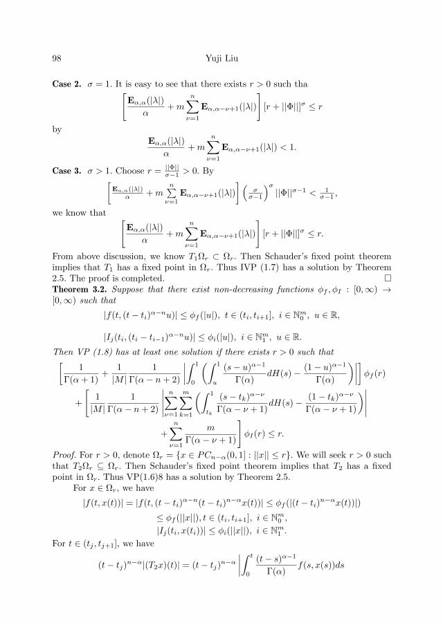
98 Yuji Liu
Case 2. σ = 1. It is easy to see that there exists r > 0 such tha[Eα,α(|λ|)
α+m
n∑ν=1
Eα,α−ν+1(|λ|)
][r + ||Φ||]σ ≤ r
by
Eα,α(|λ|)α
+m
n∑ν=1
Eα,α−ν+1(|λ|) < 1.
Case 3. σ > 1. Choose r = ||Φ||σ−1 > 0. By[
Eα,α(|λ|)α +m
n∑ν=1
Eα,α−ν+1(|λ|)](
σσ−1
)σ||Φ||σ−1 < 1
σ−1 ,
we know that [Eα,α(|λ|)
α+m
n∑ν=1
Eα,α−ν+1(|λ|)
][r + ||Φ||]σ ≤ r.
From above discussion, we know T1Ωr ⊂ Ωr. Then Schauder’s fixed point theoremimplies that T1 has a fixed point in Ωr. Thus IVP (1.7) has a solution by Theorem2.5. The proof is completed. Theorem 3.2. Suppose that there exist non-decreasing functions φf , φI : [0,∞) →[0,∞) such that
|f(t, (t− ti)α−nu)| ≤ φf (|u|), t ∈ (ti, ti+1], i ∈ Nm0 , u ∈ R,
|Ij(ti, (ti − ti−1)α−nu)| ≤ φi(|u|), i ∈ Nm1 , u ∈ R.Then VP (1.8) has at least one solution if there exists r > 0 such that[
1
Γ(α+ 1)+
1
|M |1
Γ(α− n+ 2)
∣∣∣∣∫ 1
0
(∫ 1
u
(s− u)α−1
Γ(α)dH(s)− (1− u)α−1
Γ(α)
)∣∣∣∣]φf (r)
+
[1
|M |1
Γ(α− n+ 2)
∣∣∣∣∣n∑ν=1
m∑k=1
(∫ 1
tk
(s− tk)α−ν
Γ(α− ν + 1)dH(s)− (1− tk)α−ν
Γ(α− ν + 1)
)∣∣∣∣∣+
n∑ν=1
m
Γ(α− ν + 1)
]φI(r) ≤ r.
Proof. For r > 0, denote Ωr = x ∈ PCn−α(0, 1] : ||x|| ≤ r. We will seek r > 0 suchthat T2Ωr ⊆ Ωr. Then Schauder’s fixed point theorem implies that T2 has a fixedpoint in Ωr. Thus VP(1.6)8 has a solution by Theorem 2.5.
For x ∈ Ωr, we have
|f(t, x(t))| = |f(t, (t− ti)α−n(t− ti)n−αx(t))| ≤ φf (|(t− ti)n−αx(t))|)≤ φf (||x||), t ∈ (ti, ti+1], i ∈ Nm0 ,|Ij(ti, x(ti))| ≤ φi(||x||), i ∈ Nm1 .
For t ∈ (tj , tj+1], we have
(t− tj)n−α|(T2x)(t)| = (t− tj)n−α∣∣∣∣∫ t
0
(t− s)α−1
Γ(α)f(s, x(s))ds
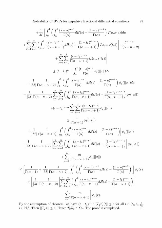
Solvability of BVPs for impulsive fractional differential equations 99
+1
M
[∫ 1
0
(∫ 1
u
(s− u)α−1
Γ(α)dH(s)− (1− u)α−1
Γ(α)
)f(u, x(u))du
+
n∑ν=1
m∑k=1
(∫ 1
tk
(s− tk)α−ν
Γ(α− ν + 1)dH(s)− (1− tk)α−ν
Γ(α− ν + 1)
)Iν(tk, x(tk))
]tα−n+1
Γ(α− n+ 2)
+
n∑ν=1
j∑k=1
(t− tk)α−ν
Γ(α− ν + 1)Iν(tk, x(tk))
∣∣∣∣∣≤ (t− tj)n−α
∫ t
0
(t− s)α−1
Γ(α)φf (||x||)ds
+1
|M |1
Γ(α− n+ 2)
∫ 1
0
(∫ 1
u
(s− u)α−1
Γ(α)dH(s)− (1− u)α−1
Γ(α)
)φf (||x||)du
+1
|M |1
Γ(α− n+ 2)
n∑ν=1
m∑k=1
(∫ 1
tk
(s− tk)α−ν
Γ(α− ν + 1)dH(s)− (1− tk)α−ν
Γ(α− ν + 1)
)φI(||x||)
+(t− tj)n−αn∑ν=1
j∑k=1
(t− tk)α−ν
Γ(α− ν + 1)φI(||x||)
≤ 1
Γ(α+ 1)φf (||x||)
+1
|M |1
Γ(α− n+ 2)
∣∣∣∣∫ 1
0
(∫ 1
u
(s− u)α−1
Γ(α)dH(s)− (1− u)α−1
Γ(α)
)∣∣∣∣φf (||x||)
+1
|M |1
Γ(α− n+ 2)
∣∣∣∣∣n∑ν=1
m∑k=1
(∫ 1
tk
(s− tk)α−ν
Γ(α− ν + 1)dH(s)− (1− tk)α−ν
Γ(α− ν + 1)
)∣∣∣∣∣φI(||x||)+
n∑ν=1
m
Γ(α− ν + 1)φI(||x||)
≤[
1
Γ(α+ 1)+
1
|M |1
Γ(α− n+ 2)
∣∣∣∣∫ 1
0
(∫ 1
u
(s− u)α−1
Γ(α)dH(s)− (1− u)α−1
Γ(α)
)∣∣∣∣]φf (r)
+
[1
|M |1
Γ(α− n+ 2)
∣∣∣∣∣n∑ν=1
m∑k=1
(∫ 1
tk
(s− tk)α−ν
Γ(α− ν + 1)dH(s)− (1− tk)α−ν
Γ(α− ν + 1)
)∣∣∣∣∣+
n∑ν=1
m
Γ(α− ν + 1)
]φI(r).
By the assumption of theorem, we have (t− tj)n−α|(T2x)(t)| ≤ r for all t ∈ (ti, ti+1],i ∈ Nm0 . Then ||T2x|| ≤ r. Hence T2Ωr ⊂ Ωr. The proof is completed.
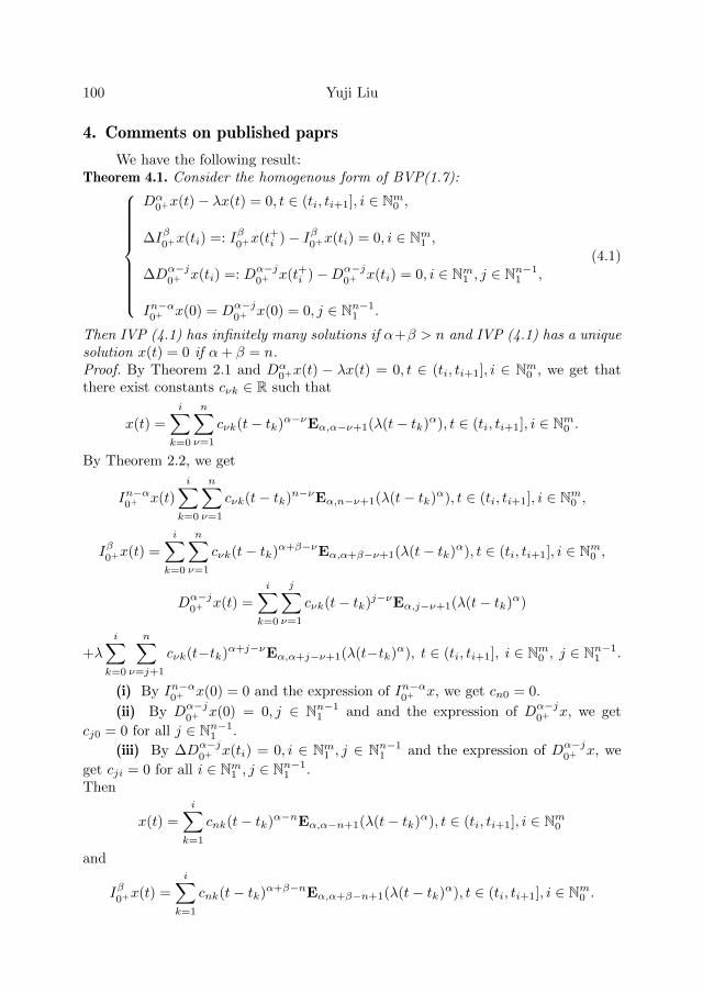
100 Yuji Liu
4. Comments on published paprs
We have the following result:Theorem 4.1. Consider the homogenous form of BVP(1.7):
Dα0+x(t)− λx(t) = 0, t ∈ (ti, ti+1], i ∈ Nm0 ,
∆Iβ0+x(ti) =: Iβ0+x(t+i )− Iβ0+x(ti) = 0, i ∈ Nm1 ,
∆Dα−j0+ x(ti) =: Dα−j
0+ x(t+i )−Dα−j0+ x(ti) = 0, i ∈ Nm1 , j ∈ Nn−1
1 ,
In−α0+ x(0) = Dα−j0+ x(0) = 0, j ∈ Nn−1
1 .
(4.1)
Then IVP (4.1) has infinitely many solutions if α+β > n and IVP (4.1) has a uniquesolution x(t) = 0 if α+ β = n.Proof. By Theorem 2.1 and Dα
0+x(t) − λx(t) = 0, t ∈ (ti, ti+1], i ∈ Nm0 , we get thatthere exist constants cνk ∈ R such that
x(t) =
i∑k=0
n∑ν=1
cνk(t− tk)α−νEα,α−ν+1(λ(t− tk)α), t ∈ (ti, ti+1], i ∈ Nm0 .
By Theorem 2.2, we get
In−α0+ x(t)
i∑k=0
n∑ν=1
cνk(t− tk)n−νEα,n−ν+1(λ(t− tk)α), t ∈ (ti, ti+1], i ∈ Nm0 ,
Iβ0+x(t) =
i∑k=0
n∑ν=1
cνk(t− tk)α+β−νEα,α+β−ν+1(λ(t− tk)α), t ∈ (ti, ti+1], i ∈ Nm0 ,
Dα−j0+ x(t) =
i∑k=0
j∑ν=1
cνk(t− tk)j−νEα,j−ν+1(λ(t− tk)α)
+λ
i∑k=0
n∑ν=j+1
cνk(t−tk)α+j−νEα,α+j−ν+1(λ(t−tk)α), t ∈ (ti, ti+1], i ∈ Nm0 , j ∈ Nn−11 .
(i) By In−α0+ x(0) = 0 and the expression of In−α0+ x, we get cn0 = 0.
(ii) By Dα−j0+ x(0) = 0, j ∈ Nn−1
1 and and the expression of Dα−j0+ x, we get
cj0 = 0 for all j ∈ Nn−11 .
(iii) By ∆Dα−j0+ x(ti) = 0, i ∈ Nm1 , j ∈ Nn−1
1 and the expression of Dα−j0+ x, we
get cji = 0 for all i ∈ Nm1 , j ∈ Nn−11 .
Then
x(t) =
i∑k=1
cnk(t− tk)α−nEα,α−n+1(λ(t− tk)α), t ∈ (ti, ti+1], i ∈ Nm0
and
Iβ0+x(t) =
i∑k=1
cnk(t− tk)α+β−nEα,α+β−n+1(λ(t− tk)α), t ∈ (ti, ti+1], i ∈ Nm0 .
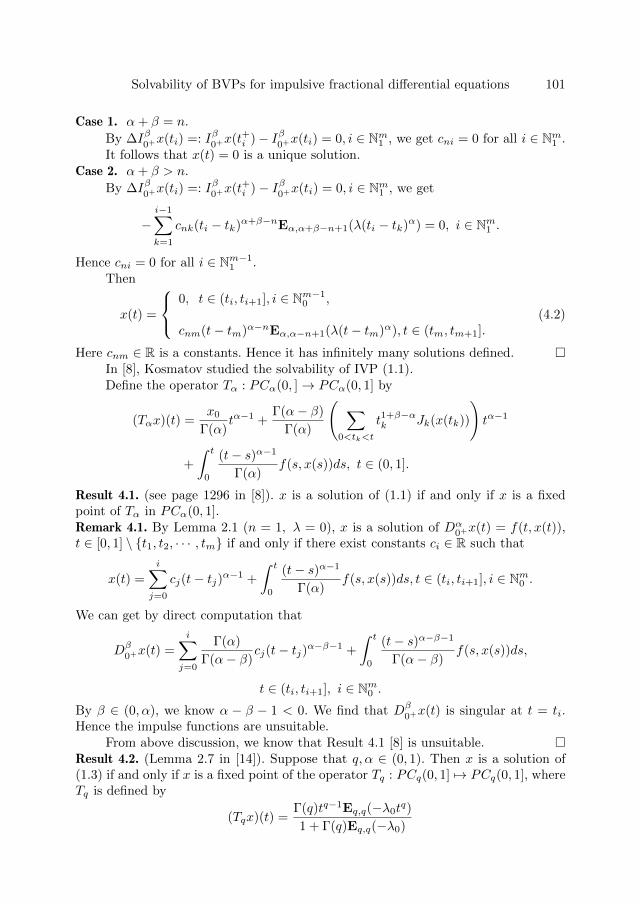
Solvability of BVPs for impulsive fractional differential equations 101
Case 1. α+ β = n.
By ∆Iβ0+x(ti) =: Iβ0+x(t+i )− Iβ0+x(ti) = 0, i ∈ Nm1 , we get cni = 0 for all i ∈ Nm1 .It follows that x(t) = 0 is a unique solution.
Case 2. α+ β > n.
By ∆Iβ0+x(ti) =: Iβ0+x(t+i )− Iβ0+x(ti) = 0, i ∈ Nm1 , we get
−i−1∑k=1
cnk(ti − tk)α+β−nEα,α+β−n+1(λ(ti − tk)α) = 0, i ∈ Nm1 .
Hence cni = 0 for all i ∈ Nm−11 .
Then
x(t) =
0, t ∈ (ti, ti+1], i ∈ Nm−10 ,
cnm(t− tm)α−nEα,α−n+1(λ(t− tm)α), t ∈ (tm, tm+1].(4.2)
Here cnm ∈ R is a constants. Hence it has infinitely many solutions defined. In [8], Kosmatov studied the solvability of IVP (1.1).Define the operator Tα : PCα(0, ]→ PCα(0, 1] by
(Tαx)(t) =x0
Γ(α)tα−1 +
Γ(α− β)
Γ(α)
( ∑0<tk<t
t1+β−αk Jk(x(tk))
)tα−1
+
∫ t
0
(t− s)α−1
Γ(α)f(s, x(s))ds, t ∈ (0, 1].
Result 4.1. (see page 1296 in [8]). x is a solution of (1.1) if and only if x is a fixedpoint of Tα in PCα(0, 1].Remark 4.1. By Lemma 2.1 (n = 1, λ = 0), x is a solution of Dα
0+x(t) = f(t, x(t)),t ∈ [0, 1] \ t1, t2, · · · , tm if and only if there exist constants ci ∈ R such that
x(t) =
i∑j=0
cj(t− tj)α−1 +
∫ t
0
(t− s)α−1
Γ(α)f(s, x(s))ds, t ∈ (ti, ti+1], i ∈ Nm0 .
We can get by direct computation that
Dβ0+x(t) =
i∑j=0
Γ(α)
Γ(α− β)cj(t− tj)α−β−1 +
∫ t
0
(t− s)α−β−1
Γ(α− β)f(s, x(s))ds,
t ∈ (ti, ti+1], i ∈ Nm0 .By β ∈ (0, α), we know α − β − 1 < 0. We find that Dβ
0+x(t) is singular at t = ti.Hence the impulse functions are unsuitable.
From above discussion, we know that Result 4.1 [8] is unsuitable. Result 4.2. (Lemma 2.7 in [14]). Suppose that q, α ∈ (0, 1). Then x is a solution of(1.3) if and only if x is a fixed point of the operator Tq : PCq(0, 1] 7→ PCq(0, 1], whereTq is defined by
(Tqx)(t) =Γ(q)tq−1Eq,q(−λ0t
q)
1 + Γ(q)Eq,q(−λ0)
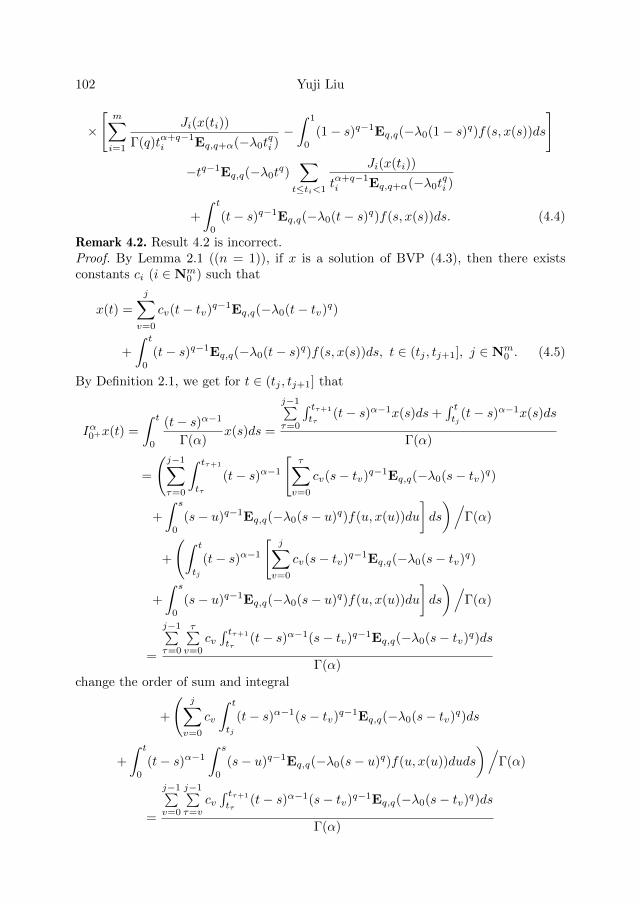
102 Yuji Liu
×
[m∑i=1
Ji(x(ti))
Γ(q)tα+q−1i Eq,q+α(−λ0t
qi )−∫ 1
0
(1− s)q−1Eq,q(−λ0(1− s)q)f(s, x(s))ds
]
−tq−1Eq,q(−λ0tq)∑
t≤ti<1
Ji(x(ti))
tα+q−1i Eq,q+α(−λ0t
qi )
+
∫ t
0
(t− s)q−1Eq,q(−λ0(t− s)q)f(s, x(s))ds. (4.4)
Remark 4.2. Result 4.2 is incorrect.Proof. By Lemma 2.1 ((n = 1)), if x is a solution of BVP (4.3), then there existsconstants ci (i ∈ Nm
0 ) such that
x(t) =
j∑v=0
cv(t− tv)q−1Eq,q(−λ0(t− tv)q)
+
∫ t
0
(t− s)q−1Eq,q(−λ0(t− s)q)f(s, x(s))ds, t ∈ (tj , tj+1], j ∈ Nm0 . (4.5)
By Definition 2.1, we get for t ∈ (tj , tj+1] that
Iα0+x(t) =
∫ t
0
(t− s)α−1
Γ(α)x(s)ds =
j−1∑τ=0
∫ tτ+1
tτ(t− s)α−1x(s)ds+
∫ ttj
(t− s)α−1x(s)ds
Γ(α)
=
(j−1∑τ=0
∫ tτ+1
tτ
(t− s)α−1
[τ∑v=0
cv(s− tv)q−1Eq,q(−λ0(s− tv)q)
+
∫ s
0
(s− u)q−1Eq,q(−λ0(s− u)q)f(u, x(u))du
]ds
)/Γ(α)
+
(∫ t
tj
(t− s)α−1
[j∑
v=0
cv(s− tv)q−1Eq,q(−λ0(s− tv)q)
+
∫ s
0
(s− u)q−1Eq,q(−λ0(s− u)q)f(u, x(u))du
]ds
)/Γ(α)
=
j−1∑τ=0
τ∑v=0
cv∫ tτ+1
tτ(t− s)α−1(s− tv)q−1Eq,q(−λ0(s− tv)q)ds
Γ(α)
change the order of sum and integral
+
(j∑
v=0
cv
∫ t
tj
(t− s)α−1(s− tv)q−1Eq,q(−λ0(s− tv)q)ds
+
∫ t
0
(t− s)α−1
∫ s
0
(s− u)q−1Eq,q(−λ0(s− u)q)f(u, x(u))duds
)/Γ(α)
=
j−1∑v=0
j−1∑τ=v
cv∫ tτ+1
tτ(t− s)α−1(s− tv)q−1Eq,q(−λ0(s− tv)q)ds
Γ(α)
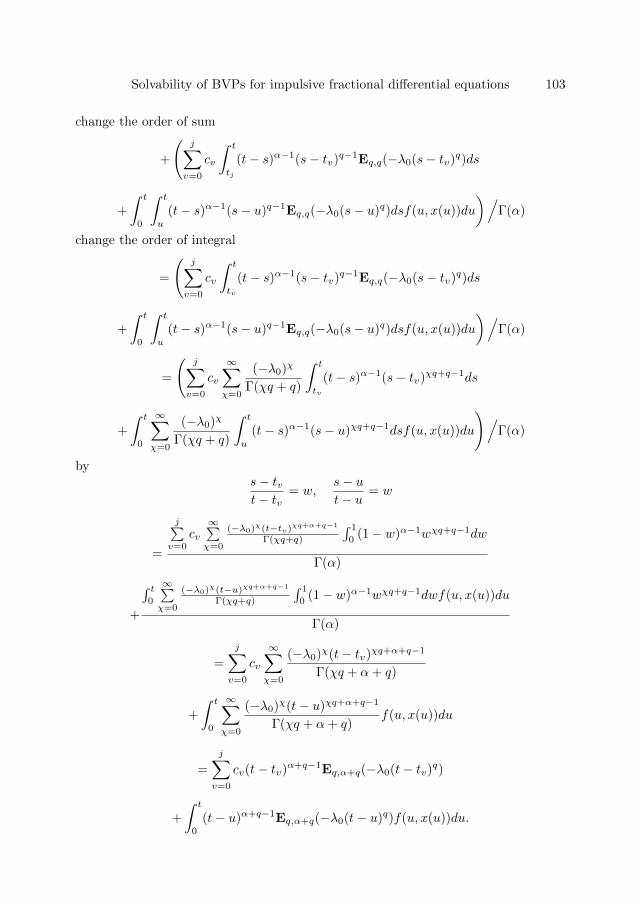
Solvability of BVPs for impulsive fractional differential equations 103
change the order of sum
+
(j∑
v=0
cv
∫ t
tj
(t− s)α−1(s− tv)q−1Eq,q(−λ0(s− tv)q)ds
+
∫ t
0
∫ t
u
(t− s)α−1(s− u)q−1Eq,q(−λ0(s− u)q)dsf(u, x(u))du
)/Γ(α)
change the order of integral
=
(j∑
v=0
cv
∫ t
tv
(t− s)α−1(s− tv)q−1Eq,q(−λ0(s− tv)q)ds
+
∫ t
0
∫ t
u
(t− s)α−1(s− u)q−1Eq,q(−λ0(s− u)q)dsf(u, x(u))du
)/Γ(α)
=
(j∑
v=0
cv
∞∑χ=0
(−λ0)χ
Γ(χq + q)
∫ t
tv
(t− s)α−1(s− tv)χq+q−1ds
+
∫ t
0
∞∑χ=0
(−λ0)χ
Γ(χq + q)
∫ t
u
(t− s)α−1(s− u)χq+q−1dsf(u, x(u))du
)/Γ(α)
bys− tvt− tv
= w,s− ut− u
= w
=
j∑v=0
cv∞∑χ=0
(−λ0)χ(t−tv)χq+α+q−1
Γ(χq+q)
∫ 1
0(1− w)α−1wχq+q−1dw
Γ(α)
+
∫ t0
∞∑χ=0
(−λ0)χ(t−u)χq+α+q−1
Γ(χq+q)
∫ 1
0(1− w)α−1wχq+q−1dwf(u, x(u))du
Γ(α)
=
j∑v=0
cv
∞∑χ=0
(−λ0)χ(t− tv)χq+α+q−1
Γ(χq + α+ q)
+
∫ t
0
∞∑χ=0
(−λ0)χ(t− u)χq+α+q−1
Γ(χq + α+ q)f(u, x(u))du
=
j∑v=0
cv(t− tv)α+q−1Eq,α+q(−λ0(t− tv)q)
+
∫ t
0
(t− u)α+q−1Eq,α+q(−λ0(t− u)q)f(u, x(u))du.
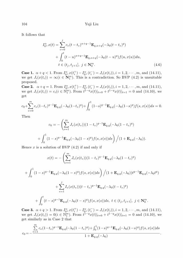
104 Yuji Liu
It follows that
Iα0+x(t) =
j∑v=0
cv(t− tv)α+q−1Eq,α+q(−λ0(t− tv)q)
+
∫ t
0
(t− u)α+q−1Eq,α+q(−λ0(t− u)q)f(u, x(u))du,
t ∈ (tj , tj+1], j ∈ Nm0 . (4.6)
Case 1. α+ q < 1. From Iα0+x(t+i )− Iα0+(t−i ) = Ji(x(ti)), i = 1, 2, · · · ,m, and (14.11),we get Ji(x(ti)) = ∞(i ∈ Nm
1 ). This is a contradiction. So BVP (4.2) is unsuitableproposed.
Case 2. α+ q = 1. From Iα0+x(t+i )− Iα0+(t−i ) = Ji(x(ti)), i = 1, 2, · · · ,m, and (14.11),we get Ji(x(ti)) = ci(i ∈ Nm1 ). From t1−qx(t)|t=0 + t1−qx(t)|t=1 = 0 and (14.10), weget
c0+
m∑v=0
cv(1−tv)q−1Eq,q(−λ0(1−tv)q)+∫ 1
0
(1−s)q−1Eq,q(−λ0(1−s)q)f(s, x(s))ds = 0.
Then
c0 = −
(m∑v=1
Jv(x(tv))(1− tv)q−1Eq,q(−λ0(1− tv)q)
+
∫ 1
0
(1− s)q−1Eq,q(−λ0(1− s)q)f(s, x(s))ds
)/(1 + Eq,q(−λ0)).
Hence x is a solution of BVP (4.2) if and only if
x(t) = −
(m∑v=1
Jv(x(tv))(1− tv)q−1Eq,q(−λ0(1− tv)q)
+
∫ 1
0
(1− s)q−1Eq,q(−λ0(1− s)q)f(s, x(s))ds
)/(1 + Eq,q(−λ0))tq−1Eq,q(−λ0t
q)
+
j∑v=1
Iv(x(tv))(t− tv)q−1Eq,q(−λ0(t− tv)q)
+
∫ t
0
(t− s)q−1Eq,q(−λ0(t− s)q)f(s, x(s))ds, t ∈ (tj , tj+1], j ∈ Nm0 .
Case 3. α+ q > 1. From Iα0+x(t+i )− Iα0+(t−i ) = Ji(x(ti)), i = 1, 2, · · · ,m, and (14.11),we get Ji(x(ti)) = 0(i ∈ Nm1 ). From t1−qx(t)|t=0 + t1−qx(t)|t=1 = 0 and (14.10), weget similarly as in Case 2 that
c0 =−
m∑v=1
cv(1−tv)q−1Eq,q(−λ0(1− tv)q)+∫ 1
0(1−s)q−1Eq,q(−λ0(1−s)q)f(s, x(s))ds
1 + Eq,q(−λ0).

Solvability of BVPs for impulsive fractional differential equations 105
Hence x is a solution of BVP (4.2) if and only if
x(t)=−
m∑v=1
cv(1−tv)q−1Eq,q(−λ0(1−tv)q)+∫ 1
0(1−s)q−1Eq,q(−λ0(1−s)q)f(s, x(s))ds
1 + Eq,q(−λ0)
×tq−1Eq,q(−λ0tq) +
j∑v=1
cv(t− tv)q−1Eq,q(−λ0(t− tv)q)
+
∫ t
0
(t− s)q−1Eq,q(−λ0(t− s)q)f(s, x(s))ds, t ∈ (tj , tj+1], j ∈ Nm0 .
Then x is a solution of BVP (4.2) if and only if
x(t)=−
m∑v=1
cv(t−tv)q−1Eq,q(−λ0(1−tv)q)+∫ 1
0(1−s)q−1Eq,q(−λ0(1−s)q)f(s, x(s))ds
1 + Eq,q(−λ0)
×tq−1Eq,q(−λ0tq) +
j∑v=1
cv(t− tv)q−1Eq,q(−λ0(t− tv)q)
+
∫ t
0
(t− s)q−1Eq,q(−λ0(t− s)q)f(s, x(s))ds, t ∈ (tj , tj+1], j ∈ Nm0
and Ji(x(ti)) = 0(i ∈ Nm1 ).
Hence from Case 1-Case 3 Result 4.2 is incorrect. In [17], Zhao studied the existence of solutions of BVP(1.7) for the higher-order
nonlinear Riemann-Liouville fractional differential equation with Riemann-Stieltjesintegral boundary value conditions and impulses Lemma 2.4 [17] claimed:Result 4.3. If H is a function of bounded variation
δ =
∫ 1
0
sα−1dH(s)α− 1
and h ∈ C([0, 1]), then the unique solution of
−Dα0+x(t) = h(t), t \ timi=1,
∆x(ti) = Ii(x(ti)), i = 1, 2, · · · ,m,
x(0) = x′(0) = · · · = x(n−2)0 = 0, x′(1) =
∫ 1
0
x(s)dH(s),
is
x(t) =
∫ 1
0
G(t, s)h(s)ds+ tα−1∑
t≤tk<1
t1−αk Ik(x(tk)), t ∈ [0, 1], (4.7)
where G(t, s) = G1(t, s) +G2(t, s) and
G1(t, s) =
tα−1(1−s)α−2−(t−s)α−1
Γ(α) , 0 ≤ s ≤ t ≤ 1,
tα−1(1−s)α−2
Γ(α) , 0 ≤ t ≤ s ≤ 1,
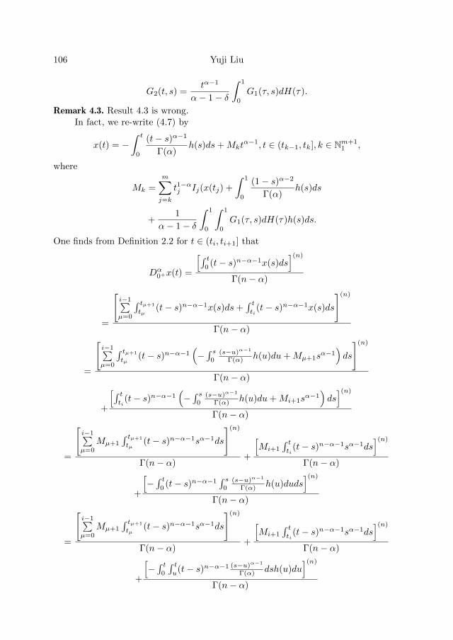
106 Yuji Liu
G2(t, s) =tα−1
α− 1− δ
∫ 1
0
G1(τ, s)dH(τ).
Remark 4.3. Result 4.3 is wrong.In fact, we re-write (4.7) by
x(t) = −∫ t
0
(t− s)α−1
Γ(α)h(s)ds+Mkt
α−1, t ∈ (tk−1, tk], k ∈ Nm+11 ,
where
Mk =
m∑j=k
t1−αj Ij(x(tj) +
∫ 1
0
(1− s)α−2
Γ(α)h(s)ds
+1
α− 1− δ
∫ 1
0
∫ 1
0
G1(τ, s)dH(τ)h(s)ds.
One finds from Definition 2.2 for t ∈ (ti, ti+1] that
Dα0+x(t) =
[∫ t0(t− s)n−α−1x(s)ds
](n)
Γ(n− α)
=
[i−1∑µ=0
∫ tµ+1
tµ(t− s)n−α−1x(s)ds+
∫ tti
(t− s)n−α−1x(s)ds
](n)
Γ(n− α)
=
[i−1∑µ=0
∫ tµ+1
tµ(t− s)n−α−1
(−∫ s
0(s−u)α−1
Γ(α) h(u)du+Mµ+1sα−1
)ds
](n)
Γ(n− α)
+
[∫ tti
(t− s)n−α−1(−∫ s
0(s−u)α−1
Γ(α) h(u)du+Mi+1sα−1
)ds](n)
Γ(n− α)
=
[i−1∑µ=0
Mµ+1
∫ tµ+1
tµ(t− s)n−α−1sα−1ds
](n)
Γ(n− α)+
[Mi+1
∫ tti
(t− s)n−α−1sα−1ds](n)
Γ(n− α)
+
[−∫ t
0(t− s)n−α−1
∫ s0
(s−u)α−1
Γ(α) h(u)duds](n)
Γ(n− α)
=
[i−1∑µ=0
Mµ+1
∫ tµ+1
tµ(t− s)n−α−1sα−1ds
](n)
Γ(n− α)+
[Mi+1
∫ tti
(t− s)n−α−1sα−1ds](n)
Γ(n− α)
+
[−∫ t
0
∫ tu(t− s)n−α−1 (s−u)α−1
Γ(α) dsh(u)du](n)
Γ(n− α)
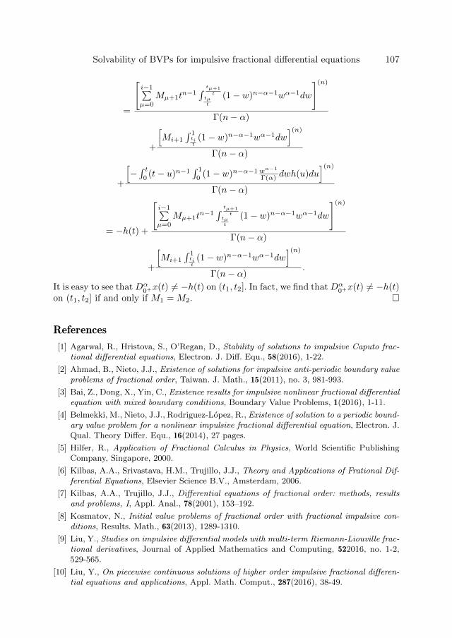
Solvability of BVPs for impulsive fractional differential equations 107
=
[i−1∑µ=0
Mµ+1tn−1
∫ tµ+1t
tµt
(1− w)n−α−1wα−1dw
](n)
Γ(n− α)
+
[Mi+1
∫ 1tit
(1− w)n−α−1wα−1dw](n)
Γ(n− α)
+
[−∫ t
0(t− u)n−1
∫ 1
0(1− w)n−α−1wα−1
Γ(α) dwh(u)du](n)
Γ(n− α)
= −h(t) +
[i−1∑µ=0
Mµ+1tn−1
∫ tµ+1t
tµt
(1− w)n−α−1wα−1dw
](n)
Γ(n− α)
+
[Mi+1
∫ 1tit
(1− w)n−α−1wα−1dw](n)
Γ(n− α).
It is easy to see that Dα0+x(t) 6= −h(t) on (t1, t2]. In fact, we find that Dα
0+x(t) 6= −h(t)on (t1, t2] if and only if M1 = M2.
References
[1] Agarwal, R., Hristova, S., O’Regan, D., Stability of solutions to impulsive Caputo frac-tional differential equations, Electron. J. Diff. Equ., 58(2016), 1-22.
[2] Ahmad, B., Nieto, J.J., Existence of solutions for impulsive anti-periodic boundary valueproblems of fractional order, Taiwan. J. Math., 15(2011), no. 3, 981-993.
[3] Bai, Z., Dong, X., Yin, C., Existence results for impulsive nonlinear fractional differentialequation with mixed boundary conditions, Boundary Value Problems, 1(2016), 1-11.
[4] Belmekki, M., Nieto, J.J., Rodriguez-Lopez, R., Existence of solution to a periodic bound-ary value problem for a nonlinear impulsive fractional differential equation, Electron. J.Qual. Theory Differ. Equ., 16(2014), 27 pages.
[5] Hilfer, R., Application of Fractional Calculus in Physics, World Scientific PublishingCompany, Singapore, 2000.
[6] Kilbas, A.A., Srivastava, H.M., Trujillo, J.J., Theory and Applications of Frational Dif-ferential Equations, Elsevier Science B.V., Amsterdam, 2006.
[7] Kilbas, A.A., Trujillo, J.J., Differential equations of fractional order: methods, resultsand problems, I, Appl. Anal., 78(2001), 153–192.
[8] Kosmatov, N., Initial value problems of fractional order with fractional impulsive con-ditions, Results. Math., 63(2013), 1289-1310.
[9] Liu, Y., Studies on impulsive differential models with multi-term Riemann-Liouville frac-tional derivatives, Journal of Applied Mathematics and Computing, 522016, no. 1-2,529-565.
[10] Liu, Y., On piecewise continuous solutions of higher order impulsive fractional differen-tial equations and applications, Appl. Math. Comput., 287(2016), 38-49.
108 Yuji Liu
[11] Liu, Y., Survey and new results on boundary-value problems of singular fractional dif-ferential equations with impulse effects, Electron. J. Differ. Equ, 16(2016), 296.
[12] Mawhin, J., Topological degree methods in nonlinear boundary value problems, in: NS-FCBMS Regional Conference Series in Math., American Math. Soc. Providence, RI,1979.
[13] Rehman, M., Eloe, P.W., Existence and uniqueness of solutions for impulsive fractionaldifferential equations, Appl. Math. Comput., 224(2013), 422-431.
[14] Wang, H., Lin, X., Anti-periodic BVP of fractional order with fractional impulsive con-ditions and variable parameter, J. Appl. Math. Comput.
[15] Wang, J., Zhang, Y., On the concept and existence of solutions for fractional impulsivesystems with Hadamard derivatives, Appl. Math. Letters, 39(2015), 85-90.
[16] Wang, J., Zhou, Y., Feckan, M., On recent developments in the theory of boundaryvalue problems for impulsive fractional differential equations, Comput. Math. Appl.,64(10)(2012), 3008-3020.
[17] Zhao, K., Impulsive fractional differential equation higher order problems of the higher-order fractional differential equation with eigenvalue arguments, Adv. Differ. Equ.,382(2015) 16 pages.
Yuji LiuDepartment of Mathematics and StatisticsGuangdong University of Finance and EconomicsGuangzhou 510320, P.R. Chinae-mail: [email protected]
Stud. Univ. Babes-Bolyai Math. 63(2018), No. 1, 109–124DOI: 10.24193/subbmath.2018.1.07
Generalizations of an asymptotic stabilitytheorem of Bahyrycz, Pales and Piszczekon Cauchy differences to generalized cocycles
Arpad Szaz
Abstract. We prove some straightforward analogues and generalizations of a re-cent asymptotic stability theorem of A. Bahyrycz, Zs. Pales and M. Piszczek onCauchy differences to semi-cocycles and pseudo-cocycles introduced in a formerpaper by the present author.
Mathematics Subject Classification (2010): 39B52, 39B82, 20K99, 22A99.
Keywords: Cauchy-differences, generalized cocycles, asymptotic and hyper stabil-ities.
1. Introduction
The first results on a certain stability property of the Cauchy functional equation
f(x+ y) = f(x) + f(y) (1.1)
were proved by Polya and Szego [63, p. 171 ] in 1925 and Hyers [38] in 1941.
In particular, Polya and Szego proved the following statement in two ratherdifficult ways.
Theorem 1.1. Suppose that the number sequence a1, a2, a3, . . . satisfies the condition
am + an − 1 < am+n < am + an + 1.
Then, there exists the limit
limn→∞
ann
= ω;
and even more ω is finite, and for all n = 1, 2, 3, . . . there holds
ωn− 1 < an < ωn+ 1.
110 Arpad Szaz
Remark 1.2. The significance of this theorem was not recognized either by Polya andSzego or the mathematical community for a long time. It was first cited by Kuczma[50, p. 424] in 1985 at the suggestion of R. Ger. However, in contrast to [5, 11], severalauthors have still not been mentioning it.
By R. Ger [34, p. 4] and some communications with Ger and M. Laczkovich, hisattention to this theorem was first drawn by Laczkovich, at an undetectable confer-ence, who indicated that the real-valued particular case of Hyers’s stability theoremcan be derived from it. His proof, reconstructed with the help of Ger and M. Sablik,can be found in [77, p. 633].
Hyers, giving a partial answer to a general problem proposed by S. M. Ulambefore the Mathematics Club of the University of Wisconsin in 1940, proved thefollowing fundamental theorem in a quite simple way.
An obvious generalization of his theorem to a function of a commutative semi-group to a Banach space [30, p. 216] already includes Theorem 1.1. Moreover, byRemark 1.2 and [30, Theorem 3], the two theorems are actually equivalent.
Theorem 1.3. Let E and E′ be Banach spaces and let f(x) be a δ-linear transformationof E into E′. Then the limit l(x) = limn→∞ f(2nx)/2n exists for each x in E, l(x) isa linear transformation, and the inequality ‖f(x)− l(x)‖ ≤ δ is true for all x in E.
Remark 1.4. Moreover, Hyers also stated that l(x) is the only linear transformationsatisfying this inequality.
Here, in contrast to the recent terminology, Hyers used the term ”linear” insteadof ”additive”. Thus, his δ–linearity of f(x) means only that
‖f(x+ y)− f(x)− f(y)‖ ≤ δ for all x, y ∈ E.
Now, because of l(nx) = nl(x), we also have
‖f(nx)/n− l(x)‖ = ‖f(nx)− l(nx)‖/n ≤ δ/n
for all n ∈ N and x ∈ E. Therefore, analogously to Theorem 1.1 of Polya and Szego,we can also state that l(x) = limn→∞ f(nx)/n for all x ∈ X.
The above basic Theorem 1.3 of Hyers has been generalized, in one direction, byAoki [6], Th. M. Rassias [65], J. M. Rassias [64], Gavruta [32] (see also [43]), and inother directions by several further mathematicians.
Moreover, some counterexamples, showing the necessity of certain extra assump-tions in the corresponding stability theorems, such as commutativity and completenessfor instance, have also been provided.
The interested reader can get a rapid overview on this enormous subject byconsulting some of the numerous survey papers [39, 34, 31, 66, 67, 68, 69, 82, 56, 70,71, 23, 21, 12, 17, 57] and the fundamental books [40, 44, 22, 49, 46].
The above works show that some local, restricted, asymptotic, super and hyperstability results have also been proved for the Cauchy equation. Moreover, some closerelationships with invariant means, sandwich and fixed point theorems have also beenestablished. And, quite early, some set-valued generalizations have also been given.
Stability theorems on generalized cocycles 111
These set-valued generalizations show that Hyers’s stability theorem is actuallyan additive selection theorem for a subadditive relation. Therefore, some of its gen-eralizations should be derived from those of the Hahn–Banach extension theorems.(For some ideas in this respect, see [22, Chapter 34] and [35, 77, 36].)
However, it is now more important to note that recently Bahyrycz, Pales andPiszczek [9] have proved a new type, asymptotic stability theorem for the Cauchyfunctional equation by using metric Abelian groups instead of normed spaces.
They called a triple (X,+, d) to be a metric abelian group if (X,+) is an abeliangroup and d is a translation invariant metric on X in the sense that
d(x+ z, y + z) = d(x, y) for all x, y, z ∈ X.
In this case, they defined ‖x‖d = d(x, 0) for all x ∈ X, and noticed that ‖ ‖d is aneven subadditive function function onX which is not, in general, even 2–homogeneous.
In [74, 83, 13, 48], metric groups and groupoids have been used in different senses.From Remarks 3.1 of [83, 13], we can see that a metric d on a group X is translationinvariant if and only if d(x+ y, z + w) ≤ d(x, z) + d(y, w) for all x, y, z, w ∈ X.
Thus, if in particular d is a translation invariant metric on a group X, then theaddition in X is continuous. Moreover, in this case we can also note that
d(−x,−y) = d(0, x− y) = d(y, x) = d(x, y) for all x, y ∈ X.
Thus, in particular the inversion in X is also continuous.In particular, in [9], Bahyrycz, Pales and Piszczek have proved the following
asymptotic stability theorem.
Theorem 1.5. Let (X,+, d) and (Y,+, ρ) be metric abelian groups such that X isunbounded by d. Let ε ≥ 0 and assume that f : X → Y possesses the asymptoticstability property
lim supmin(‖x‖d,‖y‖d)→∞
‖f(x+ y)− f(x)− f(y)‖ρ ≤ ε,
then
‖f(x+ y)− f(x)− f(y)‖ρ ≤ 5ε for all x, y ∈ X.
Remark 1.6. Moreover, by taking ε > 0 and x0 ∈ X \ 0, and defining
f(x0) = 3ε and f(x) = ε for x ∈ X \ x0,
they have also proved that 5 is the smallest possible constant in the above theorem.
The most closely related related results to Theorem 1.5 are [52, Theorem 1] ofLosonczi with the same constant 5, and the results of Jung, Moslehian, and Sahoo[45, 47] and Chung [18, 19, 20] with some other natural constants in the concludedestimates.
The origins of these investigations go back to Skof [72, 73], Hyers, Isac andRassias [41] and Gavruta [33]. (See also [54].) In the real-valued case, Volkmann [84]proved the best estimate.
From Theorem 1.5, by taking ε = 0, Bahyrycz, Pales and Piszczek could imme-diately derive the following asymptotic hyperstability result.
112 Arpad Szaz
Corollary 1.7. Let (X,+, d) and (Y,+, ρ) be metric abelian groups such that X isunbounded by d. If f : X → Y satisfies
lim supmin(‖x‖d,‖y‖d)→∞
‖f(x+ y)− f(x)− f(y)‖ρ = 0,
then
f(x+ y) = f(x) + f(y), x, y ∈ X.
Hyperstability results, for the Cauchy equation and its generalizations, have alsobeen proved by Maksa and Pales [53], Najati and Rassias [59], Alimohammady andSadeghi [3], and Brzdek [14, 15, 16], Piszczek [61, 62], Almahalebi, Charifi and Kabbaj[4], Bahyrycz and Olko [7, 8], Aiemsomboon and Sintunavarat [1, 2], Molaei, Najatiand Park [55, 58].
Moreover, several interesting asymptotic stability and hyperstability theoremsfor additive functions have also been proved by using some other functional equationsthan the Cauchy and generalized Cauchy ones.
In the present paper, we shall improve and generalize Theorem 1.5 of Bahyrycz,Pales and Piszczek. For this, we shall use preseminormed groups instead of the metricones. Moreover, we shall use generalized cocycles introduced in [78], instead of theCauchy difference
F (x, y) = f(x+ y)− f(x)− f(y). (1.2)
Some basic definitions and results on these fundamental objects, which are cer-tainly unfamiliar to the reader, will be briefly laid out in the next preparatory section.
2. A few basic facts on preseminorms and generalized cocycles
Motivated by the corresponding definitions of [76, 80] and the proofs of ourforthcoming theorems, an even subadditive function ‖ ‖ of a group X to R will becalled a preseminorm on X.
Thus, under the notation ‖x‖ = ‖ ‖(x), we have ‖0‖ = ‖0 + 0‖ ≤ ‖0‖+ ‖0‖, andthus 0 ≤ ‖0‖. And more generally, ‖0‖ = ‖x+(−x)‖ ≤ ‖x‖+‖−x‖ = 2‖x‖, and thus0 ≤ ‖x‖ for all x ∈ X.
Therefore, if ‖0‖ 6= 0, then by defining ‖x‖? = 0 for x = 0, and ‖x‖? = ‖x‖ forx ∈ X \ 0, we can obtain a new preseminorm ‖ ‖? on X such that ‖0‖? = 0 alreadyholds.
By using induction and the corresponding definitions, we can also easily see that‖nx‖ ≤ n‖x‖, and thus ‖(−n)x‖ = ‖n(−x)‖ ≤ n‖ − x‖ = n‖x‖ for all n ∈ N andx ∈ X.
Therefore, the preseminorm ‖ ‖ may be naturally called a seminorm if n‖x‖ ≤‖nx‖ for all x ∈ X. Namely, thus we have ‖kx‖ = |k|‖x‖ for all x ∈ X and k ∈ Z\0.(If ‖0‖ = 0, then this also holds for k = 0.)
Note that a nonzero seminorm cannot be bounded. While, if ‖ ‖ is a seminorm(preseminorm) on X, then for instance the function defined by ‖x‖∗ = min1, ‖x‖for all x ∈ X is a bounded preseminorm on X.
Stability theorems on generalized cocycles 113
Now, a seminorm (preseminorm) ‖ ‖ on X may be naturally called a norm(prenorm) if ‖x‖ = 0 implies x = 0 for all x ∈ X. If X = Zx for all x ∈ X \ 0, theneach nonzero preseminorm on X is a prenorm.
In [79, Remark 3.14], with the help of G. Horvath, it was proved that the lattercondition is equivalent to the requirement that the cardinality of X is prime, orequivalently X has no nontrival proper subgroup.
Now, for instance, an ordered pair X(‖ ‖) = (X, ‖ ‖) consisting a group X anda preseminorm ‖ ‖ on X, may be naturally called a preseminormed group. And, wemay simply write X instead of X(‖ ‖).
If X is a preseminormed group, then because of the subadditivity and evennessof the corresponding preseminorm, for any x, y ∈ X, we have
‖x‖ = ‖x+ y − y‖ ≤ ‖x+ y‖+ ‖ − y‖ = ‖x+ y‖+ ‖y‖and
‖y‖ = ‖ − x+ x+ y‖ ≤ ‖ − x‖+ ‖x+ y‖ = ‖x‖+ ‖x+ y‖.Therefore,∣∣‖x‖ − ‖y‖∣∣ ≤ ‖x+ y‖ and
∣∣‖x‖ − ‖y‖∣∣ =∣∣‖x‖ − ‖ − y‖∣∣ ≤ ‖x− y‖.
However, it is now more important to note that Bahyrycz, Pales and Piszczek,in the proof of their Theorem 1.5, have used, but not explicitly stated, the equality
f(x+ y)− f(x)− f(y) = f(x− u) + f(u)− f(x)
+ f(y − v) + f(v)− f(y) + f(x+ y − u− v)− f(x− u)− f(y − v)
+ f(u+ v)− f(u)− f(v) + f(x+ y)− f(x+ y − u− v)− f(u+ v). (2.1)
In a former paper [78], by using the Cauchy difference (1.2), we have noticedthat, instead of equation (2.1), it is more convenient to consider the equation
F (x, y) = F (u, v)− F (x− u, u)− F (y − v, v)
+ F (x− u, y − v) + F (x+ y − u− v, u+ v). (2.2)
Namely, thus Theorem 1.5 can be easily extended to the solutions of (2.2). More-over, we can prove that every symmetric cocycle F on X to Y is a solution of thisequation.
That is, if F is a function of X2 to Y such that F (x, y) = F (y, x) and
F (x, y) + F (x+ y, z) = F (x, y + z) + F (y, z) (2.3)
for all x, y, z ∈ X, then (2.2) also holds for all x, y, u, v ∈ X.It is well-known that every Cauchy–difference is a symmetric cocycle. Moreover,
Davison and Ebanks [24, Lemma 2] have proved that if F is a symmetric cocycle onX to Y , then
F (x+ y, u+ v) = F (x+ u, y + v) + F (x, u) + F (y, v)− F (x, y)− F (u, v) (2.4)
also holds for all x, y, u, v ∈ X.At first seeing, I considered equations (2.2) and (2.4) to be very similar, but still
quite independent. However, Gyula Maksa, my close colleague, has noticed that theyare actually equivalent.
114 Arpad Szaz
Namely, (2.4) can be immediately derived from (2.2) by replacing x by x+u andy by y + v. And conversely, (2.2) can be immediately derived from (2.4) by replacingx by x− u and y by y − v. Thus, equation (2.1) is a consequence of (2.4) too.
Inspired by the above observations, in our former paper [78], we have also con-sidered the more difficult equations
F (x, y) + F (u, y + v) + F (x+ y, u+ v)
= F (x, u) + F (y, u+ v) + F (x+ u, y + v) (2.5)
and
F (x, y) + F (x− u, u) + F (y − v, u) + F (y − v, v)
= F (u, v) + F (u, y − v) + F (x− u, y − v) + F (x+ y − u− v, u+ v). (2.6)
Note that if in particular F is symmetric, then equation (2.6) is equivalent to(2.2), which is in turn equivalent to (2.4). Moreover, it can be easily shown that if Fis additive in its second variable, then equations (2.5) and (2.6) are also equivalent.
In our former paper [78], by using some more difficult computations, we havealso proved that equations (2.5) and (2.6) are also natural generalizations of (2.3) too.Therefore, their solutions may be naturally called semi-cocycles and pseudo-cocycles,respectively.
In the light of the above observations, it seems to be a reasonable research pro-gram to extend some of the basic theorems on cocycles to these generalized cocycles.And, to establish some deeper relationships among the various generalizations of co-cycles mentioned in [78].
However, in the sequel, we shall only prove some straightforward analogues andgeneralizations of Theorem 1.5 to semi-cocycles and pseudo–cocycles.
3. Analogues of Theorem 1.5 for generalized cocycles
Notation 3.1. In the sequel, we shall assume that F is a function of an unbounded,commutative preseminormed group X to a commutative preseminormed group Y .
Remark 3.2. Note that now, by defining
(x, y) + (u, v) = (x+ u, y + v)
and
‖(x, y)‖ = ‖x‖ ∨ ‖y‖ = max‖x‖, ‖y‖
for all x, y, u, v ∈ X, the set X2 can also be turned into an unbounded commutativepreseminormed group.
Thus, by using a more simple argument than that used by Bahyrycz, Pales andPiszczek in [9], we can prove the following natural analogue of Theorem 1.5.
Theorem 3.3. If F is a semi-cocycle and
ε = lim‖z‖→+∞
‖F (z)‖,
Stability theorems on generalized cocycles 115
then‖F (z)‖ ≤ 5ε
for all z ∈ X2.
Proof. By the corresponding definitions, for any η > ε, we have
infr>0
sup‖z‖>r
‖F (z)‖ < η.
Therefore, there exists r > 0 such that sup‖z‖>r ‖F (z)‖ < η, and thus
‖F (z)‖ < η
for all z ∈ X2 with ‖z‖ > r.Hence, since ‖z‖ = ‖(z1, z2)‖ ≥ ‖zi‖ for i = 1, 2, it is clear that in particular
we have‖F (s, t)‖ < η
for all s, t ∈ X with either ‖s‖ > r or ‖t‖ > r.Now, by taking x, y ∈ X and using equation (2.5), we can see that
‖F (x, y)‖ = ‖F (x, u) + F (y, u+ v)− F (u, y + v)
+ F (x+ u, y + v)− F (x+ y, u+ v)‖≤ ‖F (x, u)‖+ ‖F (y, u+ v)‖+ ‖F (u, y + v)‖+ ‖F (x+ u, y + v)‖+ ‖F (x+ y, u+ v)‖ < 5η
whenever for instance u, v ∈ X such that
‖u‖ > r, ‖u+ v‖ > r, ‖x+ u‖ > r.
Therefore, if such u and v exist, then
‖F (x, y)‖ < 5η, and thus ‖F (x, y)‖ ≤ 5ε
Now, to complete the proof, it remains to show only that the required u and vexist. For this, we can note that, because of the assumed unboundedness of X, thereexist u, v ∈ X such that
‖u‖ > r + ‖x‖ and ‖v‖ > r + ‖u‖.Thus, we evidently have ‖u‖ > r. Moreover, by using the inequality ‖s+t‖ ≥ ‖t‖−‖s‖,we can also see that
‖x+ u‖ ≥ ‖u‖ − ‖x‖ > r + ‖x‖ − ‖x‖ = r
and‖u+ v‖ ≥ ‖v‖ − ‖u‖ > r + ‖u‖ − ‖u‖ = r.
From equation (2.6) and the proof of Theorem 3.3, it is clear that we also have
Theorem 3.4. If F is a pseudo-cocycle and
ε = lim‖z‖→+∞
‖F (z)‖,
then‖F (z)‖ ≤ 7ε
for all z ∈ X2.
116 Arpad Szaz
Now, as an immediate consequence of the above two theorems, we can also state
Corollary 3.5. If Y is prenormed, F is either a semi or pseudo cocycle, and
lim‖z‖→+∞
‖F (z)‖ = 0,
then F (z) = 0 for all z ∈ X2.
Remark 3.6. However, from Theorems 3.3 and 3.4 we cannot get proper generaliza-tions of Theorem 1.5. Therefore, in the next section we shall prove some modificationand improvement of Theorem 3.4.
4. Proper and partial generalizations of Theorem 1.5 topseudo-cocycles
Remark 4.1. Because of the condition of Theorem 1.5, in the sequel we shall also usethe quantity
∦ (x, y) ∦= ‖x‖ ∧ ‖y‖ = min‖x‖, ‖y‖
,
for all (x, y) ∈ X2 instead of the natural preseminorm considered in Remark 3.2.Thus, the function ∦ ∦ is not a preseminorm on X2. However, despite this, it can bewell used to measure the magnitude of the points of X2.
Moreover, it can as well be used to prove the following proper and partial gene-ralizations of Theorem 1.5 to pseudo-cocycles. The proof of the first one is quitesimilar to the second one. Therefore, it will be omitted.
Theorem 4.2. If F is a symmetric pseudo-cocycle and
ε = lim∦z∦→+∞
‖F (z)‖,
then
‖F (z)‖ ≤ 5ε
for all z ∈ X2.
The proof of the following theorem is again quite similar, but a little morereadable, than the one given by Bahyrycz, Pales and Piszczek in [9].
Theorem 4.3. If F is a pseudo-cocycle and
ε = lim∦z∦→+∞
‖F (z)‖,
then
‖F (z)‖ ≤ 7ε
for all z ∈ X2.
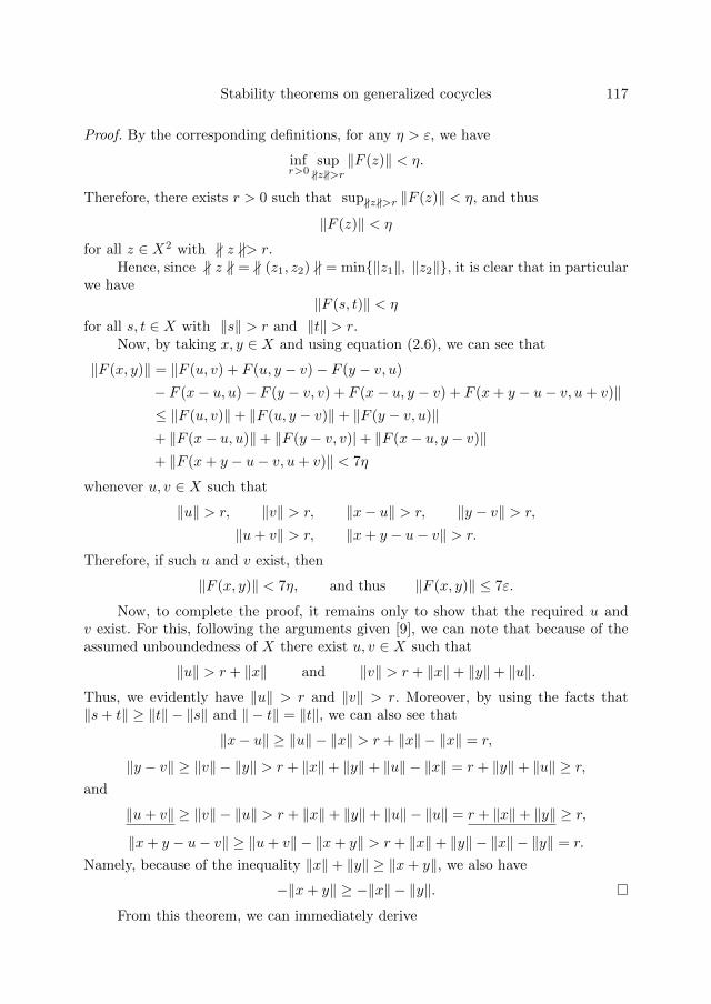
Stability theorems on generalized cocycles 117
Proof. By the corresponding definitions, for any η > ε, we have
infr>0
sup∦z∦>r
‖F (z)‖ < η.
Therefore, there exists r > 0 such that sup∦z∦>r ‖F (z)‖ < η, and thus
‖F (z)‖ < η
for all z ∈ X2 with ∦ z ∦> r.Hence, since ∦ z ∦ = ∦ (z1, z2) ∦ = min‖z1‖, ‖z2‖, it is clear that in particular
we have
‖F (s, t)‖ < η
for all s, t ∈ X with ‖s‖ > r and ‖t‖ > r.Now, by taking x, y ∈ X and using equation (2.6), we can see that
‖F (x, y)‖ = ‖F (u, v) + F (u, y − v)− F (y − v, u)
− F (x− u, u)− F (y − v, v) + F (x− u, y − v) + F (x+ y − u− v, u+ v)‖≤ ‖F (u, v)‖+ ‖F (u, y − v)‖+ ‖F (y − v, u)‖+ ‖F (x− u, u)‖+ ‖F (y − v, v)|+ ‖F (x− u, y − v)‖+ ‖F (x+ y − u− v, u+ v)‖ < 7η
whenever u, v ∈ X such that
‖u‖ > r, ‖v‖ > r, ‖x− u‖ > r, ‖y − v‖ > r,
‖u+ v‖ > r, ‖x+ y − u− v‖ > r.
Therefore, if such u and v exist, then
‖F (x, y)‖ < 7η, and thus ‖F (x, y)‖ ≤ 7ε.
Now, to complete the proof, it remains only to show that the required u andv exist. For this, following the arguments given [9], we can note that because of theassumed unboundedness of X there exist u, v ∈ X such that
‖u‖ > r + ‖x‖ and ‖v‖ > r + ‖x‖+ ‖y‖+ ‖u‖.
Thus, we evidently have ‖u‖ > r and ‖v‖ > r. Moreover, by using the facts that‖s+ t‖ ≥ ‖t‖ − ‖s‖ and ‖ − t‖ = ‖t‖, we can also see that
‖x− u‖ ≥ ‖u‖ − ‖x‖ > r + ‖x‖ − ‖x‖ = r,
‖y − v‖ ≥ ‖v‖ − ‖y‖ > r + ‖x‖+ ‖y‖+ ‖u‖ − ‖x‖ = r + ‖y‖+ ‖u‖ ≥ r,and
‖u+ v‖ ≥ ‖v‖ − ‖u‖ > r + ‖x‖+ ‖y‖+ ‖u‖ − ‖u‖ = r + ‖x‖+ ‖y‖ ≥ r,
‖x+ y − u− v‖ ≥ ‖u+ v‖ − ‖x+ y‖ > r + ‖x‖+ ‖y‖ − ‖x‖ − ‖y‖ = r.
Namely, because of the inequality ‖x‖+ ‖y‖ ≥ ‖x+ y‖, we also have
−‖x+ y‖ ≥ −‖x‖ − ‖y‖.
From this theorem, we can immediately derive
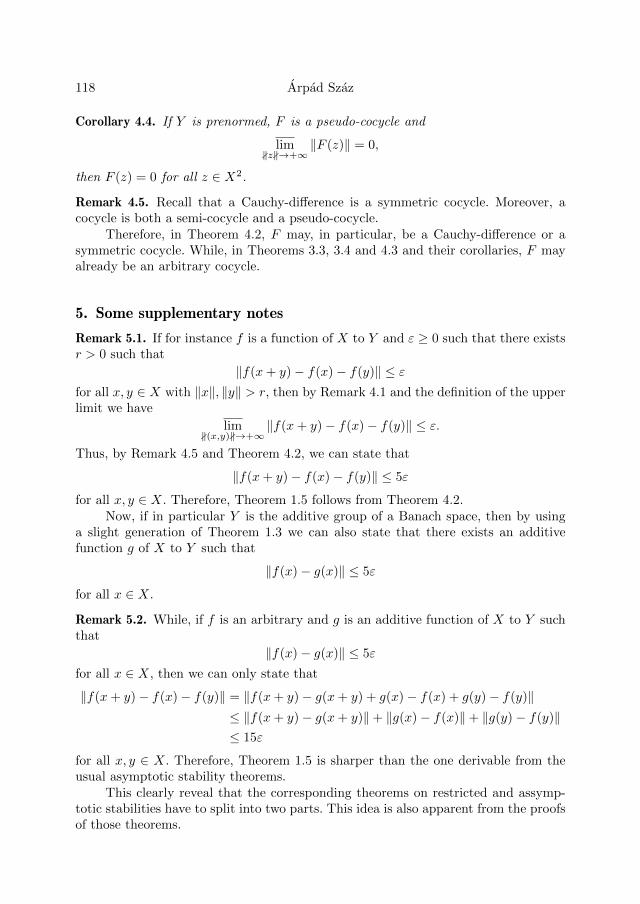
118 Arpad Szaz
Corollary 4.4. If Y is prenormed, F is a pseudo-cocycle and
lim∦z∦→+∞
‖F (z)‖ = 0,
then F (z) = 0 for all z ∈ X2.
Remark 4.5. Recall that a Cauchy-difference is a symmetric cocycle. Moreover, acocycle is both a semi-cocycle and a pseudo-cocycle.
Therefore, in Theorem 4.2, F may, in particular, be a Cauchy-difference or asymmetric cocycle. While, in Theorems 3.3, 3.4 and 4.3 and their corollaries, F mayalready be an arbitrary cocycle.
5. Some supplementary notes
Remark 5.1. If for instance f is a function of X to Y and ε ≥ 0 such that there existsr > 0 such that
‖f(x+ y)− f(x)− f(y)‖ ≤ εfor all x, y ∈ X with ‖x‖, ‖y‖ > r, then by Remark 4.1 and the definition of the upperlimit we have
lim∦(x,y)∦→+∞
‖f(x+ y)− f(x)− f(y)‖ ≤ ε.
Thus, by Remark 4.5 and Theorem 4.2, we can state that
‖f(x+ y)− f(x)− f(y)‖ ≤ 5ε
for all x, y ∈ X. Therefore, Theorem 1.5 follows from Theorem 4.2.Now, if in particular Y is the additive group of a Banach space, then by using
a slight generation of Theorem 1.3 we can also state that there exists an additivefunction g of X to Y such that
‖f(x)− g(x)‖ ≤ 5ε
for all x ∈ X.
Remark 5.2. While, if f is an arbitrary and g is an additive function of X to Y suchthat
‖f(x)− g(x)‖ ≤ 5ε
for all x ∈ X, then we can only state that
‖f(x+ y)− f(x)− f(y)‖ = ‖f(x+ y)− g(x+ y) + g(x)− f(x) + g(y)− f(y)‖≤ ‖f(x+ y)− g(x+ y)‖+ ‖g(x)− f(x)‖+ ‖g(y)− f(y)‖≤ 15ε
for all x, y ∈ X. Therefore, Theorem 1.5 is sharper than the one derivable from theusual asymptotic stability theorems.
This clearly reveal that the corresponding theorems on restricted and assymp-totic stabilities have to split into two parts. This idea is also apparent from the proofsof those theorems.
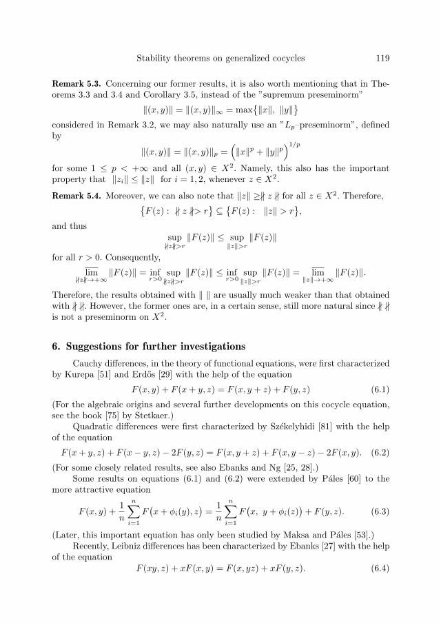
Stability theorems on generalized cocycles 119
Remark 5.3. Concerning our former results, it is also worth mentioning that in The-orems 3.3 and 3.4 and Corollary 3.5, instead of the ”supremum preseminorm”
‖(x, y)‖ = ‖(x, y)‖∞ = max‖x‖, ‖y‖
considered in Remark 3.2, we may also naturally use an ”Lp–preseminorm”, definedby
‖(x, y)‖ = ‖(x, y)‖p =(‖x‖p + ‖y‖p
)1/pfor some 1 ≤ p < +∞ and all (x, y) ∈ X2. Namely, this also has the importantproperty that ‖zi‖ ≤ ‖z‖ for i = 1, 2, whenever z ∈ X2.
Remark 5.4. Moreover, we can also note that ‖z‖ ≥∦ z ∦ for all z ∈ X2. Therefore,F (z) : ∦ z ∦> r
⊆F (z) : ‖z‖ > r
,
and thussup
∦z∦>r‖F (z)‖ ≤ sup
‖z‖>r‖F (z)‖
for all r > 0. Consequently,
lim∦z∦→+∞
‖F (z)‖ = infr>0
sup∦z∦>r
‖F (z)‖ ≤ infr>0
sup‖z‖>r
‖F (z)‖ = lim‖z‖→+∞
‖F (z)‖.
Therefore, the results obtained with ‖ ‖ are usually much weaker than that obtainedwith ∦ ∦. However, the former ones are, in a certain sense, still more natural since ∦ ∦is not a preseminorm on X2.
6. Suggestions for further investigations
Cauchy differences, in the theory of functional equations, were first characterizedby Kurepa [51] and Erdos [29] with the help of the equation
F (x, y) + F (x+ y, z) = F (x, y + z) + F (y, z) (6.1)
(For the algebraic origins and several further developments on this cocycle equation,see the book [75] by Stetkaer.)
Quadratic differences were first characterized by Szekelyhidi [81] with the helpof the equation
F (x+ y, z) + F (x− y, z)− 2F (y, z) = F (x, y + z) + F (x, y − z)− 2F (x, y). (6.2)
(For some closely related results, see also Ebanks and Ng [25, 28].)Some results on equations (6.1) and (6.2) were extended by Pales [60] to the
more attractive equation
F (x, y) +1
n
n∑i=1
F(x+ φi(y), z
)=
1
n
n∑i=1
F(x, y + φi(z)
)+ F (y, z). (6.3)
(Later, this important equation has only been studied by Maksa and Pales [53].)Recently, Leibniz differences has been characterized by Ebanks [27] with the help
of the equationF (xy, z) + xF (x, y) = F (x, yz) + xF (y, z). (6.4)
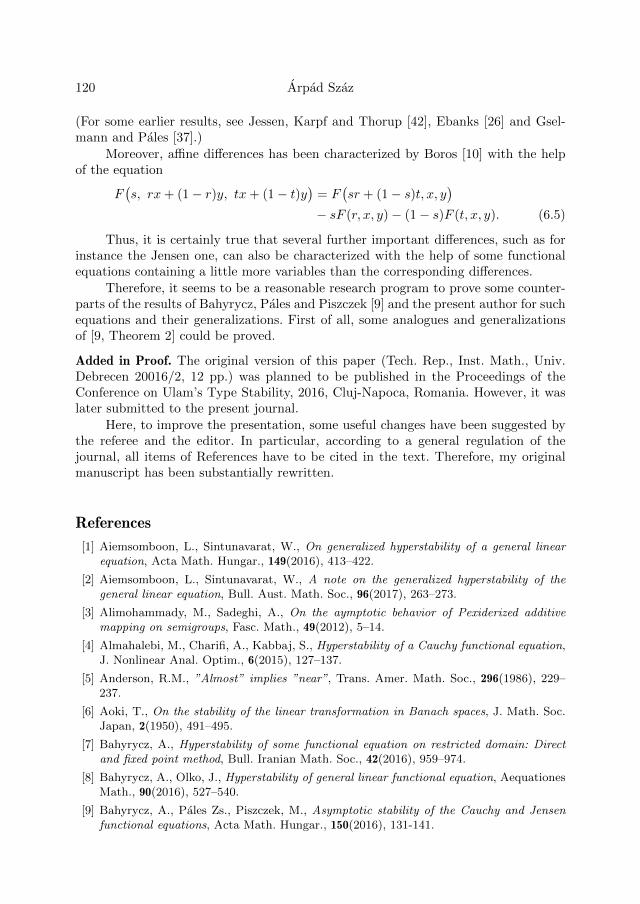
120 Arpad Szaz
(For some earlier results, see Jessen, Karpf and Thorup [42], Ebanks [26] and Gsel-mann and Pales [37].)
Moreover, affine differences has been characterized by Boros [10] with the helpof the equation
F(s, rx+ (1− r)y, tx+ (1− t)y
)= F
(sr + (1− s)t, x, y
)− sF (r, x, y)− (1− s)F (t, x, y). (6.5)
Thus, it is certainly true that several further important differences, such as forinstance the Jensen one, can also be characterized with the help of some functionalequations containing a little more variables than the corresponding differences.
Therefore, it seems to be a reasonable research program to prove some counter-parts of the results of Bahyrycz, Pales and Piszczek [9] and the present author for suchequations and their generalizations. First of all, some analogues and generalizationsof [9, Theorem 2] could be proved.
Added in Proof. The original version of this paper (Tech. Rep., Inst. Math., Univ.Debrecen 20016/2, 12 pp.) was planned to be published in the Proceedings of theConference on Ulam’s Type Stability, 2016, Cluj-Napoca, Romania. However, it waslater submitted to the present journal.
Here, to improve the presentation, some useful changes have been suggested bythe referee and the editor. In particular, according to a general regulation of thejournal, all items of References have to be cited in the text. Therefore, my originalmanuscript has been substantially rewritten.
References
[1] Aiemsomboon, L., Sintunavarat, W., On generalized hyperstability of a general linearequation, Acta Math. Hungar., 149(2016), 413–422.
[2] Aiemsomboon, L., Sintunavarat, W., A note on the generalized hyperstability of thegeneral linear equation, Bull. Aust. Math. Soc., 96(2017), 263–273.
[3] Alimohammady, M., Sadeghi, A., On the aymptotic behavior of Pexiderized additivemapping on semigroups, Fasc. Math., 49(2012), 5–14.
[4] Almahalebi, M., Charifi, A., Kabbaj, S., Hyperstability of a Cauchy functional equation,J. Nonlinear Anal. Optim., 6(2015), 127–137.
[5] Anderson, R.M., ”Almost” implies ”near”, Trans. Amer. Math. Soc., 296(1986), 229–237.
[6] Aoki, T., On the stability of the linear transformation in Banach spaces, J. Math. Soc.Japan, 2(1950), 491–495.
[7] Bahyrycz, A., Hyperstability of some functional equation on restricted domain: Directand fixed point method, Bull. Iranian Math. Soc., 42(2016), 959–974.
[8] Bahyrycz, A., Olko, J., Hyperstability of general linear functional equation, AequationesMath., 90(2016), 527–540.
[9] Bahyrycz, A., Pales Zs., Piszczek, M., Asymptotic stability of the Cauchy and Jensenfunctional equations, Acta Math. Hungar., 150(2016), 131-141.
Stability theorems on generalized cocycles 121
[10] Boros, Z., A characterization of affine differences on intervals, Report of Meeting, TheSeventeenth Katowice-Debrecen Winter Seminar, Zakopane (Poland), February 1-4,2017, Ann. Math. Sil., 31(2017), 188–189.
[11] Boualem, H., Brouzet, R., On what is the almost-near principle, Amer. Math. Monthly,119(2012), 381–397.
[12] Brillouet-Bellout, N., Brzdek, J., Cieplinski, K., On some recent developments in Ulam’stype stability, Abstr. Appl. Anal., 2012 (2012), 41 pp.
[13] Brzdek, J., On a method of proving the Hyers-Ulam stability of functional equations onrestricted domains, Aust. J. Math. Anal. Appl., 6(2009), 10 pp.
[14] Brzdek, J., Hyperstability of the Cauchy equation on restricted domains, Acta Math.Hungar., 141(2013), 58–67.
[15] Brzdek, J., Remarks on hyperstability of the Cauchy functional equation, AequationesMath., 86(2013), 255–267.
[16] Brzdek, J., A hyperstability result for Cauchy equation, Bull. Aust. Math. Soc., 89(2014),33–40.
[17] Brzdek, J., Cieplinski, K., Hyperstability and superstability, Abstr. Appl. Anal., Vol.2013, 13 pp.
[18] Chung, J.-Y., Stability of functional equations on restricted domains in a group and theirasymptotic behaviors, Comput. Appl. Math., 60(2010), 2653–2665.
[19] Chung, J.-Y., Stability of a conditional Cauchy equation, Aequationes Math., 83(2012),313–320.
[20] Chung, J.-Y., Stability of a conditional Cauchy equation on a set of measure zero, Ae-quationes Math., 87(2014), 391–400.
[21] Cieplinski, K., Applications of fixed point theorems to the Hyers–Ulam stability of func-tional equations – A survey Ann. Funct. Anal., 3(2012), 151–164.
[22] Czerwik, S., Functional Equations and Inequalities in Several Variables, World Scientific,London, 2002.
[23] Czerwik, S., Krol, K., Ulam stability of functional equations, Aust. J. Math. Anal. Appl.,6(2009), 15 pp.
[24] Davison, T.M.K., Ebanks, B.R., Cocycles on cancellative semigroups, Publ. Math. De-brecen, 46(1995), 137–147.
[25] Ebanks, B.R., Differentiable solutions of a functional equation of Szekelyhidi, Util.Math., 36(1989), 197–199.
[26] Ebanks, B.R., On some functional equations of Jessen, Karpf, and and Thorup, Math.Scand., 44(1979), 231–234.
[27] Ebanks, B.R., On Leibniz differences, Publ. Math. Debrecen, 91 (2017), 143–151.
[28] Ebanks, B.R., Ng, C.T., Characterizations of quadratic differences, Publ. Math. Debre-cen, 48(1996), 89–102.
[29] Erdos, J., A remark on the paper ”On some functional equations” by S. Kurepa, Glas.Mat. Ser. III, 14(1959), 3–5.
[30] Forti, G.L., The stability of homomorphisms and amenability, with applications to func-tional equations, Abh. Math. Semin. Univ. Hambg., 57(1987), 215–226.
[31] Forti, G.L., Hyers–Ulam stability of functional equations in several variables, Aequa-tiones Math., 50(1995), 143–190.
122 Arpad Szaz
[32] Gavruta, P., A generalization of the Hyers–Ulam–Rassias stability of approximately ad-ditive mappings, J. Math. Anal. Appl., 184(1994), 431–436
[33] Gavruta, P., On the Hyers-Ulam-Rassias asymptotic stability of mappings, Bul. Stiint.Univ. Politeh. Timis. Ser. Mat. Fiz., 41(1996), 48–51.
[34] Ger, R., A survey of recent results on stability of functional equations, Proceedings ofthe 4th International Conference on Functional Equations and Inequalities, PedagogicalUniversity of Cracow, 1994, 5–36.
[35] Glavosits, T., Szaz, A., A Hahn-Banach type generalization of the Hyers-Ulam theorem,An. Stiint. Univ. ”Ovidius” Constanta Ser. Mat., 19(2011), 139–144.
[36] Glavosits, T., Szaz, A., Constructions and extensions of free and controlled additiverelations, In: Th. M. Rassias (Ed.), Handbook of Functional Equations: Functional In-equalities, Springer Optim. Appl., 95(2014), 161–208.
[37] Gselmann E., Pales, Zs., Additive solvability and linear independence of the solutions ofa system of functional equations, Acta Sci. Math. (Szeged), 82(2016), 101–110.
[38] Hyers, D.H., On the stability of the linear functional equation, Proc. Natl. Acad. Sci.USA, 27(1941), 222–224.
[39] Hyers, D.H., Rassias, Th.M., Approximate homomorphisms, Aequationes Math.,44(1992), 125–153.
[40] Hyers, D.H., Isac, G., Rassias, Th.M., Stability of Functional Equations in Several Vari-ables, Birkhauser, Boston, 1998.
[41] Hyers, D.H., Isac, G., Rassias, Th.M., On the asymptotic aspect of Hyers–Ulam stabilityof mappings, Proc. Amer. Math. Soc., 126(1998), 425–430.
[42] Jessen, B., Karpf, J., Thorup, A., Some functional equations in groups and rings, Math.Scand., 22(1968), 257–265.
[43] Jun, K.-W., Shin, D.-S., Kim, B.-D., On the Hyers-Ulam-Rassias stability of the Pexiderequation, J. Math. Anal. Appl., 239(1999), 20–29.
[44] Jung, S.M., Hyers–Ulam–Rassias Stability of Functional Equations in MathematicalAnalysis, Hadronic Press, Palm Harbor, Fl, 2001.
[45] Jung, S.M., Local stability of the additive functional equation, Glas. Mat. Ser. III,38(2003), 45–55.
[46] Jung, S.M., Hyers-Ulam-Rassias Stability of Functional Equations in Nonlinear Analy-sis, Springer Optim. Appl. 48, New York, 2011.
[47] Jung, S.M., Moslehian, M.S., Sahoo, P.K., Stability of a generalized Jensen equation onrestricted domains, J. Math. Inaqual., 4(2010), 191–206.
[48] Jung, S.M., Popa, D., Rassias, M.Th., On the stability of the linear functional equationin a single variable on complete metric groups, J. Global. Optim., 59(2014), 165–171.
[49] Kannappan, Pl., Functional Equations and Inequalities with Applications, Springer, Dor-drecht, 2009.
[50] Kuczma, M., An Introduction to the Theory of Functional Equations and Inequalities,
Polish Sci. Publ. and Univ. Slaski, Warszawa, 1985.
[51] Kurepa, S., On some functional equations, Glas. Mat. Ser. III, 11(1956), 95–100.
[52] Losonczi, L., On the stability of Hossu’s functional equation, Results Math., 29(1996),305–310.
[53] Maksa, Gy., Pales, Zs., Hyperstability of a class of linear functional equations, ActaMath. Acad. Paedagog. Nyhazi. (N.S.), 17(2001), 107–112.
Stability theorems on generalized cocycles 123
[54] Manar, Y., Elqorachi, E., Rassias, Th.M., On the generalized Hyers-Ulam stability ofthe Pexider equation on restricted domains, In: Rassias, Th. M. (Ed.), Handbook ofFunctional Equations, Stability Theory, Springer Optim. Appl., 96(2014), 279–299.
[55] Molaei, D., Najati, A., Hyperstability of the general linear equation on restricted do-mains, Acta Math. Hungar., 149(2016), 238–253.
[56] Moszner, Z., On the stability of functional equations, Aequationes Math., 77(2009), 33–88.
[57] Moszner, Z., Stability has many names, Aequationes Math., 90(2016), 983–999.
[58] Najati, A., Molaee, D., Park, Ch., Hyperstability of a generalized Cauchy functionalequation, J. Comput. Anal. Appl., 22(2017), 1049–1054.
[59] Najati, A., Rassias, Th.M., Stability of the Pexiderized Cauchy and Jensen’s equationson restricted domains, Commun. Math. Anal., 8(2010), 125–135.
[60] Pales, Zs., Bounded solutions and stability of functional equations for two variable func-tions, Results Math., 26(1994), 360–365.
[61] Piszczek, M., Remark on hyperstability of the general linear equation, AequationesMath., 88(2014), 163–168.
[62] Piszczek, M., Hyperstability of the general linear functional equation, Bull. Korean Math.Soc., 52(2015), 1827–1838.
[63] Polya, Gy., Szego, G., Aufgaben und Lehrsatze aus der Analysis I, Verlag von JuliusSpringer, Berlin, 1925.
[64] Rassias, J.M., On approximation of approximately linear mappings by linear mappingsJ. Funct. Anal., 46(1982), 126–130.
[65] Rassias, Th. M. On the stability of the linear mapping in Banach spaces, Proc. Amer.Math. Soc., 72(1978), 279–300.
[66] Rassias, Th.M., Stability and set-valued functions, In: Analysis and Topology, World Sci.Publ., River Edge, NJ, 1998, 585–614.
[67] Rassias, Th.M., The problem of S. M. Ulam for approximately multiplicative mappings,J. Math. Anal. Appl., 246(2000), 352–378.
[68] Rassias, Th.M., On the stability of functional equations and a problem of Ulam, ActaAppl. Math., 62(2000), 23–130.
[69] Rassias, Th.M., On the stability of functional equations in Banach spaces J. Math. Anal.Appl., 251(2000), 264–284.
[70] Rassias, Th.M., On the stability of functional equations originated by a problem of Ulam,Mathematica (Cluj), 44(2002), 39–75.
[71] Sanchez, F.C., Castillo, J.M.F., Banach space techniques underpinning a theory fornearly additive mappings, Dissertationes Math. (Rozprawy Mat.), 404(2002), 73 pp.
[72] Skof, F., Sull’approssimazione delle applicazioni localmente δ-additive, Atti Accad. Sci.Torino, 117(1983), 377–389.
[73] Skof, F., Properieta locali e approssimazione di operatori, Rend. Semin. Mat. Fis. Milano,53(1983), 113–129.
[74] Spakula, J., Zlatos, P., Almost homomorphisms of compact groups, Illinois J. Math.,48(2004), 1183–1189.
[75] Stetkaer, H., Functional Equations on Groups, World Scientific, New Jersey, 2013.
[76] Szaz, A., Preseminormed spaces, Publ. Math. Debrecen, 30(1983), 217–224.
124 Arpad Szaz
[77] Szaz, A., The Hyers–Ulam and Hahn–Banach theorems and some elementary operationson relations motivated their set-valued generalizations, In: P. M. Pardalos, P. G. Georgievand H. M. Srivastava (Eds.), Stability, Approximations, and Inequalities, Springer Op-tim. Appl. 68(2012), 631–705.
[78] Szaz, A., Two natural generalizations of cocycles, J. Int. Math. Virtual Inst., 6(2016),66–86.
[79] Szaz, A., Remarks and problems at the conference on inequalities and applications,Hajduszoboszlo, Hungary, 2016, Tech. Rep., Inst. Math., Univ. Debrecen, 9(2016), 34pp.
[80] Szaz, A., A natural Galois connection between generalized norms and metrics, ActaUniv. Sapientiae Math., 9(2017), 353-366.
[81] Szekelyhidi, L., Stability properties of functional equations in several variables, Stochas-tica, 47(1995), 95–100.
[82] Szekelyhidi, L., Ulam’s problem, Hyers’s solution – and to where they led, In: Th. M.Rassias (Ed.), Functional Equations and Inequalities, Math. Appl., 518, Kluwer Acad.Publ., Dordrecht, 2000, 259–285.
[83] Tabor, J., Tabor, J., Stability of the Cauchy functional equation in metric groupoidsAequationes Math., 76(2008), 92–104.
[84] Volkmann, P., Zur Stabilitat der Cauchyschen und der Hosszuschen Funktionalgleichung,Seminar 40(1998), No. 1, 5 pp.
Arpad SzazUniversity of DebrecenInstitute of MathematicsH–4002 Debrecen, Pf. 400, Hungarye-mail: [email protected]
Stud. Univ. Babes-Bolyai Math. 63(2018), No. 1, 125–140DOI: 10.24193/subbmath.2018.1.08
Korovkin type approximation for doublesequences via statistical A-summation processon modular spaces
Sevda Orhan and Burcak Kolay
Abstract. In this work, we introduce the Korovkin type approximation theoremson modular spaces via statistical A-summation process for double sequences ofpositive linear operators and we construct an example satisfying our new approx-imation theorem but does not satisfy the classical one.
Mathematics Subject Classification (2010): 40B05, 41A36, 47B38, 46E30.
Keywords: Modular space, A-summation process, positive linear operators, Ko-rovkin theorem.
1. Introduction and preliminaries
Summability theory is the theory of the assignment of limits in the case of real orcomplex sequences which are divergent. There are many types of summability meth-ods especially regular summability methods, for example, Abel and Borel methods[6]. Another regular summability method introduced by Fast ([8]) and which is notequivalent to any regular matrix method is called statistical convergence which isalso known as (C, 1) statistical convergence. Furthermore, in recent years, variousstatistical approximation results and theorems have been proved via the concept ofstatistical convergence ([9, 11, 19]) and the motivation using this type of convergencecomes from that the obtained results are more powerful than the classical versionof the approximations. One of these frequently used approximation method is theKorovkin-type approximation theorems. As it is known Korovkin theorems allows usto check the convergence with a minimum of computations. In this paper, our mainpurpose is to study a further generalization of classical Korovkin theorem by consid-ering certain matrix summability process in the frame of statistical convergence inabstract spaces (namely, modular spaces) for double sequences. We also introduce anexample satisfying new approximation theorem but does not satisfy the classical one.
126 Sevda Orhan and Burcak Kolay
Now, let us mention the notion of statistical convergence for double sequencesintroduced by Moricz [15].
The double sequence x = xi,j is statistically convergent to L provided thatfor every ε > 0,
P − limm,n
1
mn|i ≤ m, j ≤ n : |xi,j − L| ≥ ε| = 0,
where P−convergent denotes Pringsheim limit ([22]). In that case we write
st2 − limi,jxi,j = L.
It can be easily seen that a P−convergent double sequence is statistically convergentto the same value but its converse is not always true. Also, it is crucial to state that aconvergent single sequence needs to be bounded even though this necessity does notexist always for the double sequences. A convergent double sequence does not needto be bounded. For example, take into consideration the double sequence x = xi,jdefined by
xi,j =
ij, i and j are squares1, otherwise.
.
Then, clearly st2 − limi,jxi,j = 1 but not P−convergent and also, it is not bounded.
The characterization for the statistical convergence for double sequences is given in[15] as indicated below :
A double sequence x = xi,j is statistically convergent to L if and only if thereexists a set S ⊂ N2 such that the natural density of S is 1 and
P − limi,j→∞
and (i,j)∈S
xi,j = L.
In [7] the concepts of statistical superior limit and inferior limit for double sequenceshave been introduced by Cakan and Altay. For any real double sequence x = xi,j ,the statistical limit superior of x is defined by
st2 − lim supi,j
xi,j =
supGx, if Gx 6= ∅,−∞, if Gx = ∅,
where Gx := C ∈ R : δ2 ((i, j) : xi,j > C) 6= 0 and ∅ denotes the empty set. Notethat, in general, by δ2 (K) 6= 0 we mean either δ2 (K) > 0 or K fails to have thedouble natural density. Similarly, the statistical limit inferior of x is given by
st2 − lim infi,j
xi,j =
inf Fx, if Fx 6= ∅,∞, if Fx = ∅,
where Fx := D ∈ R : δ2 ((i, j) : xi,j < D) 6= 0 . As in the ordinary superior orinferior limit, it was proved that
st2 − lim infi,j
xi,j ≤ st2 − lim supi,j
xi,j
and also that, for any double sequence x = xi,j satisfying
δ2 ((i, j) : |xi,j | > M) = 0
Statistical A-summation process 127
for some M > 0,
st2 − limi,jxi,j = L iff st2 − lim inf
i,jxi,j = st2 − lim sup
i,jxi,j = L.
Let A = [ak,l,i,j ], k, l, i, j ∈ N, be a four-dimensional infinite matrix.The A−transform of x = xi,j, denoted by Ax := (Ax)k,l, is defined by
(Ax)k,l =∑
(i,j)∈N2
ak,l,i,jxi,j , k, l ∈ N,
provided the double series converges in Pringsheim’s sense for every (k, l) ∈ N2. Then,a double sequence x is A−summable to L if the A−transform of x exists for all k, l ∈ Nand convergent in the Pringsheim’s sense i.e.,
P − limp,q
p∑i=1
q∑j=1
ak,l,i,jxi,j = yk,l and P − limk,l
yk,l = L.
Now letA :=A(m,n)
=a(m,n)k,l,i,j
be a sequence of four-dimensional infinite matrices
with non-negative real entries. For a given double sequence of real numbers, x = xi,jis said to be A−summable to L if
P − limk,l
∑(i,j)∈N2
a(m,n)k,l,i,jxi,j = L
uniformly in m and n. If A(m,n) = A, four-dimensional infinite matrix, thenA−summability is the A−summability for four-dimensional infinite matrix. Someresults concerning matrix summability method for double sequences may be attainedin [9], [21], [24].
Now, we recall some definitions and notations on modular spaces.
Let I = [a, b] be a bounded interval of the real line R provided with the Lebesguemeasure. Then, let X
(I2)
denote the space of all real-valued measurable functions
on I2 = [a, b]× [a, b] provided with equality a.e. As usual, let C(I2)
denote the space
of all continuous real-valued functions, and C∞(I2)
denote the space of all infinitely
differentiable functions on I2. A functional ρ : X(I2)→ [0,+∞] is called a modular
on X(I2)
if it satisfies the following conditions:
(i) ρ (f) = 0 if and only if f = 0 a.e. in I2,
(ii) ρ (−f) = ρ (f) for every f ∈ X(I2),
(iii) ρ (αf + βg) ≤ ρ (f) +ρ (g) for every f, g ∈ X(I2) and for any α, β ≥ 0 withα+ β = 1.
A modular ρ is said to be N−quasi convex if there exists a constant N ≥ 1 suchthat ρ (αf + βg) ≤ Nαρ (Nf) + Nβρ (Ng) holds for every f, g ∈ X
(I2), α, β ≥ 0
with α+ β = 1. In particular, if N = 1, then ρ is called convex.
A modular ρ is said to be N−quasi semiconvex if there exists a constant N ≥ 1such that ρ(af) ≤ Naρ(Nf) holds for every f ∈ X
(I2)
and a ∈ (0, 1].
It is clear that every N−quasi convex modular is N−quasi semiconvex. Bardaroet. al. introduced and worked through the above two concepts in [3, 5].
128 Sevda Orhan and Burcak Kolay
We now present some acquired vector subspaces of X(I2) via a modular ρ asfollows:
The modular space Lρ(I2)
generated by ρ is defined by
Lρ(I2)
:=
f ∈ X(I2) : lim
λ→0+ρ (λf) = 0
,
and the space of the finite elements of Lρ(I2)
is given by
Eρ(I2)
:=f ∈ Lρ
(I2)
: ρ (λf) < +∞ for all λ > 0.
Observe that if ρ is N−quasi semiconvex, then the spacef ∈ X
(I2)
: ρ (λf) < +∞ for some λ > 0
coincides with Lρ(I2). The notions about modulars are introduced in [16] and widely
discussed in [3] (see also [13, 17]).Bardaro and Mantellini [4] introduced some Korovkin type approximation the-
orems via the notions of modular convergence and strong convergence. AfterwardsKarakus et al. [11] investigated the modular Korovkin-type approximation theoremvia statistical convergence and then, Orhan and Demirci [20] extended these typeof approximations to the spaces of double sequences of positive linear operators asfollows:
Definition 1.1. [20] A function sequence fi,j in Lρ(I2)
is said to be statistically
modularly convergent to a function f ∈ Lρ(I2)
iff
st2 − limi,j
ρ (λ0 (fi,j − f)) = 0 for some λ0 > 0. (1.1)
Also, fi,j is statistically F−norm convergent (or, statistically strongly convergent)to f iff
st2 − limi,j
ρ (λ (fi,j − f)) = 0 for every λ > 0. (1.2)
It is known from [16] that (1.1) and (1.2) are equivalent if and only if the modular ρsatisfies the ∆2−condition, i.e.
there exists a constant M > 0 such that ρ (2f) ≤Mρ (f) for every f ∈ X(I2).
Recently, Orhan and Demirci [19] have introduced the notion of A−summationprocess on the one dimensional modular space X (I) . Now we introduce the notionof the A−summation process for double sequences as follows:
A sequence T := Ti,j of positive linear operators of D into X(I2)
is calledan A−summation process on D if Ti,j (f) is A−summable to f (with respect tomodular ρ) for every f ∈ D, i.e.,
P − limk,lρ[λ(ATk,l,m,n (f)− f
)]= 0, uniformly in m,n (1.3)
for some λ > 0, where for all k, l,m, n ∈ N, f ∈ D the series
ATk,l,m,n (f) :=
∑(i,j)∈N2
a(m,n)k,l,i,jTi,jf (1.4)
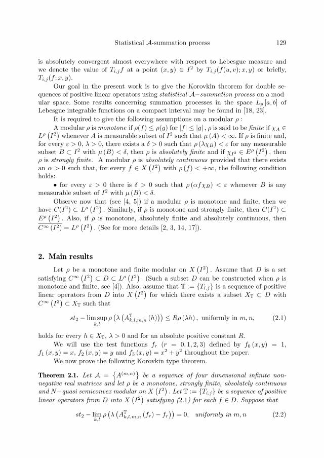
Statistical A-summation process 129
is absolutely convergent almost everywhere with respect to Lebesgue measure andwe denote the value of Ti,jf at a point (x, y) ∈ I2 by Ti,j(f(u, v);x, y) or briefly,Ti,j(f ;x, y).
Our goal in the present work is to give the Korovkin theorem for double se-quences of positive linear operators using statistical A−summation process on a mod-ular space. Some results concerning summation processes in the space Lp [a, b] ofLebesgue integrable functions on a compact interval may be found in [18, 23].
It is required to give the following assumptions on a modular ρ :
A modular ρ is monotone if ρ(f) ≤ ρ(g) for |f | ≤ |g| , ρ is said to be finite if χA ∈Lρ(I2)
whenever A is measurable subset of I2 such that µ (A) <∞. If ρ is finite and,for every ε > 0, λ > 0, there exists a δ > 0 such that ρ (λχB) < ε for any measurablesubset B ⊂ I2 with µ (B) < δ, then ρ is absolutely finite and if χI2 ∈ Eρ
(I2), then
ρ is strongly finite. A modular ρ is absolutely continuous provided that there existsan α > 0 such that, for every f ∈ X
(I2)
with ρ (f) < +∞, the following conditionholds:
• for every ε > 0 there is δ > 0 such that ρ (αfχB) < ε whenever B is anymeasurable subset of I2 with µ (B) < δ.
Observe now that (see [4, 5]) if a modular ρ is monotone and finite, then wehave C(I2) ⊂ Lρ
(I2). Similarly, if ρ is monotone and strongly finite, then C(I2) ⊂
Eρ(I2). Also, if ρ is monotone, absolutely finite and absolutely continuous, then
C∞ (I2) = Lρ(I2). (See for more details [2, 3, 14, 17]).
2. Main results
Let ρ be a monotone and finite modular on X(I2). Assume that D is a set
satisfying C∞(I2)⊂ D ⊂ Lρ
(I2). (Such a subset D can be constructed when ρ is
monotone and finite, see [4]). Also, assume that T := Ti,j is a sequence of positivelinear operators from D into X
(I2)
for which there exists a subset XT ⊂ D with
C∞(I2)⊂ XT such that
st2 − lim supk,l
ρ(λ(ATk,l,m,n (h)
))≤ Rρ (λh) , uniformly in m,n, (2.1)
holds for every h ∈ XT, λ > 0 and for an absolute positive constant R.
We will use the test functions fr (r = 0, 1, 2, 3) defined by f0 (x, y) = 1,f1 (x, y) = x, f2 (x, y) = y and f3 (x, y) = x2 + y2 throughout the paper.
We now prove the following Korovkin type theorem.
Theorem 2.1. Let A =A(m,n)
be a sequence of four dimensional infinite non-
negative real matrices and let ρ be a monotone, strongly finite, absolutely continuousand N−quasi semiconvex modular on X
(I2). Let T := Ti,j be a sequence of positive
linear operators from D into X(I2)
satisfying (2.1) for each f ∈ D. Suppose that
st2 − limk,l
ρ(λ(ATk,l,m,n (fr)− fr
))= 0, uniformly in m,n (2.2)
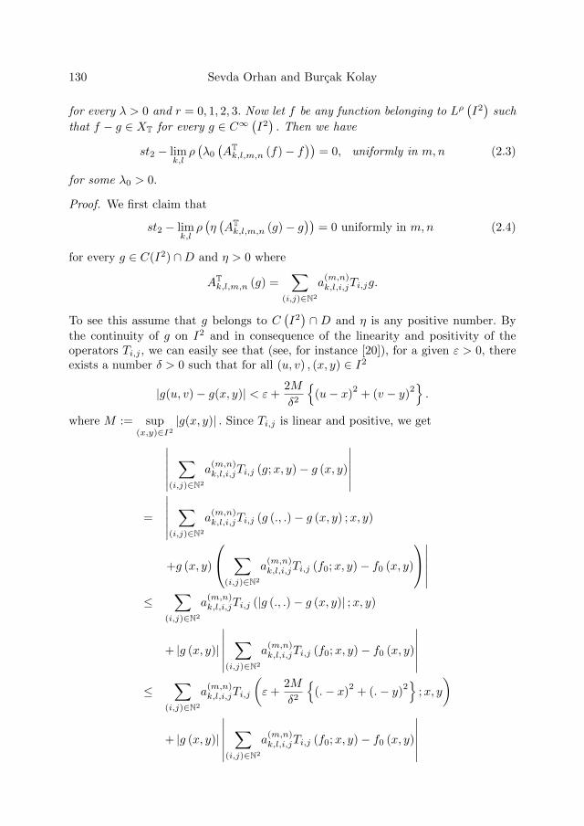
130 Sevda Orhan and Burcak Kolay
for every λ > 0 and r = 0, 1, 2, 3. Now let f be any function belonging to Lρ(I2)
such
that f − g ∈ XT for every g ∈ C∞(I2). Then we have
st2 − limk,l
ρ(λ0(ATk,l,m,n (f)− f
))= 0, uniformly in m,n (2.3)
for some λ0 > 0.
Proof. We first claim that
st2 − limk,l
ρ(η(ATk,l,m,n (g)− g
))= 0 uniformly in m,n (2.4)
for every g ∈ C(I2) ∩D and η > 0 where
ATk,l,m,n (g) =
∑(i,j)∈N2
a(m,n)k,l,i,jTi,jg.
To see this assume that g belongs to C(I2)∩ D and η is any positive number. By
the continuity of g on I2 and in consequence of the linearity and positivity of theoperators Ti,j , we can easily see that (see, for instance [20]), for a given ε > 0, thereexists a number δ > 0 such that for all (u, v) , (x, y) ∈ I2
|g(u, v)− g(x, y)| < ε+2M
δ2
(u− x)
2+ (v − y)
2.
where M := sup(x,y)∈I2
|g(x, y)| . Since Ti,j is linear and positive, we get
∣∣∣∣∣∣∑
(i,j)∈N2
a(m,n)k,l,i,jTi,j (g;x, y)− g (x, y)
∣∣∣∣∣∣=
∣∣∣∣∣∣∑
(i,j)∈N2
a(m,n)k,l,i,jTi,j (g (., .)− g (x, y) ;x, y)
+g (x, y)
∑(i,j)∈N2
a(m,n)k,l,i,jTi,j (f0;x, y)− f0 (x, y)
∣∣∣∣∣∣≤
∑(i,j)∈N2
a(m,n)k,l,i,jTi,j (|g (., .)− g (x, y)| ;x, y)
+ |g (x, y)|
∣∣∣∣∣∣∑
(i,j)∈N2
a(m,n)k,l,i,jTi,j (f0;x, y)− f0 (x, y)
∣∣∣∣∣∣≤
∑(i,j)∈N2
a(m,n)k,l,i,jTi,j
(ε+
2M
δ2
(.− x)
2+ (.− y)
2
;x, y
)
+ |g (x, y)|
∣∣∣∣∣∣∑
(i,j)∈N2
a(m,n)k,l,i,jTi,j (f0;x, y)− f0 (x, y)
∣∣∣∣∣∣
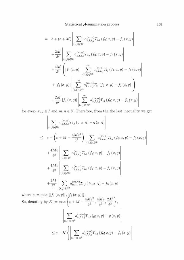
Statistical A-summation process 131
= ε+ (ε+M)
∣∣∣∣∣∣∑
(i,j)∈N2
a(m,n)k,l,i,jTi,j (f0;x, y)− f0 (x, y)
∣∣∣∣∣∣+
2M
δ2
∣∣∣∣∣∣∑
(i,j)∈N2
a(m,n)k,l,i,jTi,j (f3;x, y)− f3 (x, y)
∣∣∣∣∣∣+
4M
δ2
|f1 (x, y)|
∣∣∣∣∣∣∞∑
(i,j)∈N2
a(m,n)k,l,i,jTij (f1;x, y)− f1 (x, y)
∣∣∣∣∣∣+ |f2 (x, y)|
∣∣∣∣∣∣∞∑
(i,j)∈N2
a(m,n)k,l,i,jTij (f2;x, y)− f2 (x, y)
∣∣∣∣∣∣
+2M
δ2|f3 (x, y)|
∣∣∣∣∣∣∞∑
(i,j)∈N2
a(m,n)k,l,i,jTij (f0;x, y)− f0 (x, y)
∣∣∣∣∣∣for every x, y ∈ I and m,n ∈ N. Therefore, from the the last inequality we get∣∣∣∣∣∣
∑(i,j)∈N2
a(m,n)k,l,i,jTi,j (g;x, y)− g (x, y)
∣∣∣∣∣∣≤ ε+
(ε+M +
4Mc2
δ2
) ∣∣∣∣∣∣∑
(i,j)∈N2
a(m,n)k,l,i,jTi,j (f0;x, y)− f0 (x, y)
∣∣∣∣∣∣+
4Mc
δ2
∣∣∣∣∣∣∑
(i,j)∈N2
a(m,n)k,l,i,jTi,j (f1;x, y)− f1 (x, y)
∣∣∣∣∣∣+
4Mc
δ2
∣∣∣∣∣∣∑
(i,j)∈N2
a(m,n)k,l,i,jTi,j (f2;x, y)− f2 (x, y)
∣∣∣∣∣∣+
2M
δ2
∣∣∣∣∣∣∑
(i,j)∈N2
a(m,n)k,l,i,jTi,j (f3;x, y)− f3 (x, y)
∣∣∣∣∣∣where c := max |f1 (x, y)| , |f2 (x, y)| .
So, denoting by K := max
ε+M +
4Mc2
δ2,
4Mc
δ2,
2M
δ2
,∣∣∣∣∣∣
∑(i,j)∈N2
a(m,n)k,l,i,jTi,j (g;x, y)− g (x, y)
∣∣∣∣∣∣≤ ε+K
∣∣∣∣∣∣∑
(i,j)∈N2
a(m,n)k,l,i,jTi,j (f0;x, y)− f0 (x, y)
∣∣∣∣∣∣
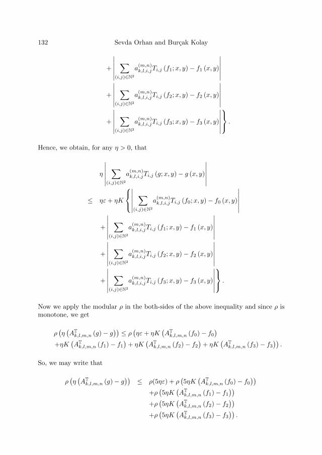
132 Sevda Orhan and Burcak Kolay
+
∣∣∣∣∣∣∑
(i,j)∈N2
a(m,n)k,l,i,jTi,j (f1;x, y)− f1 (x, y)
∣∣∣∣∣∣+
∣∣∣∣∣∣∑
(i,j)∈N2
a(m,n)k,l,i,jTi,j (f2;x, y)− f2 (x, y)
∣∣∣∣∣∣+
∣∣∣∣∣∣∑
(i,j)∈N2
a(m,n)k,l,i,jTi,j (f3;x, y)− f3 (x, y)
∣∣∣∣∣∣ .
Hence, we obtain, for any η > 0, that
η
∣∣∣∣∣∣∑
(i,j)∈N2
a(m,n)k,l,i,jTi,j (g;x, y)− g (x, y)
∣∣∣∣∣∣≤ ηε+ ηK
∣∣∣∣∣∣∑
(i,j)∈N2
a(m,n)k,l,i,jTi,j (f0;x, y)− f0 (x, y)
∣∣∣∣∣∣+
∣∣∣∣∣∣∑
(i,j)∈N2
a(m,n)k,l,i,jTi,j (f1;x, y)− f1 (x, y)
∣∣∣∣∣∣+
∣∣∣∣∣∣∑
(i,j)∈N2
a(m,n)k,l,i,jTi,j (f2;x, y)− f2 (x, y)
∣∣∣∣∣∣+
∣∣∣∣∣∣∑
(i,j)∈N2
a(m,n)k,l,i,jTi,j (f3;x, y)− f3 (x, y)
∣∣∣∣∣∣ .
Now we apply the modular ρ in the both-sides of the above inequality and since ρ ismonotone, we get
ρ(η(ATk,l,m,n (g)− g
))≤ ρ
(ηε+ ηK
(ATk,l,m,n (f0)− f0
)+ηK
(ATk,l,m,n (f1)− f1
)+ ηK
(ATk,l,m,n (f2)− f2
)+ ηK
(ATk,l,m,n (f3)− f3
)).
So, we may write that
ρ(η(ATk,l,m,n (g)− g
))≤ ρ(5ηε) + ρ
(5ηK
(ATk,l,m,n (f0)− f0
))+ρ(5ηK
(ATk,l,m,n (f1)− f1
))+ρ(5ηK
(ATk,l,m,n (f2)− f2
))+ρ(5ηK
(ATk,l,m,n (f3)− f3
)).
Statistical A-summation process 133
Since ρ is N−quasi semiconvex and strongly finite, we have, assuming 0 < ε ≤ 1
ρ(η(ATk,l,m,n (g)− g
))≤ Nερ (5ηN) + ρ
(5ηK
(ATk,l,m,n (f0)− f0
))+ρ(5ηK
(ATk,l,m,n (f1)− f1
))+ρ(5ηK
(ATk,l,m,n (f2)− f2
))+ρ(5ηK
(ATk,l,m,n (f3)− f3
)).
For a given ε∗ > 0, choose an ε ∈ (0, 1] such that Nερ (5ηN) < ε∗. Now we define thefollowing sets:
Gη : =
(k, l) : ρ(η(ATk,l,m,n (g)− g
))≥ ε∗
,
Gη,r : =
(k, l) : ρ
(5ηK
(ATk,l,m,n (fr)− fr
))≥ ε∗ −Nερ (5ηN)
4
,
r = 0, 1, 2, 3. Then, it is easy to see that Gη ⊆3⋃r=0
Gη,r. So, we can write that
δ2 (Gη) ≤3∑r=0
δ2 (Gη,r) .
Using the hypothesis (2.2), we get
δ2 (Gη) = 0,
which proves our claim (2.4). Obviously, (2.4) also holds for every g ∈ C∞(I2). Nowlet f ∈ Lρ
(I2)
satisfying f−g ∈ XT for every g ∈ C∞(I2). Since µ
(I2)<∞ and ρ is
strongly finite and absolutely continuous, it can be seen that ρ is also absolutely finiteon X(I2) (see [2]). So, it is known from [3, 14] that the space C∞(I2) is modularlydense in Lρ
(I2), i.e., there exists a sequence gk,l ⊂ C∞
(I2)
such that
P − limk,l
ρ (3λ∗0 (gk,l − f)) = 0 for some λ∗0 > 0,
which means, for every ε > 0, there is a positive number k0 = k0(ε) so that
ρ (3λ∗0 (gk,l − f)) < ε for every k, l ≥ k0. (2.5)
In addition to that, because the operators Ti,j are linear and positive, we can writethat
λ∗0
∣∣∣∣∣∣∑
(i,j)∈N2
a(m,n)k,l,i,jTi,j(f ;x, y)− f(x, y)
∣∣∣∣∣∣≤ λ∗0
∣∣∣∣∣∣∑
(i,j)∈N2
a(m,n)k,l,i,jTi,j(f − gk0,k0 ;x, y)
∣∣∣∣∣∣+λ∗0
∣∣∣∣∣∣∑
(i,j)∈N2
a(m,n)k,l,i,jTi,j(gk0,k0 ;x, y)− gk0,k0(x, y)
∣∣∣∣∣∣+λ∗0 |gk0,k0(x, y)− f(x, y)| ,
134 Sevda Orhan and Burcak Kolay
holds for every x, y ∈ I and m,n ∈ N. Applying the modular ρ and moreover consid-ering the monotonicity of ρ, we have
ρ(λ∗0(ATk,l,m,n (f)− f
))≤ ρ
(3λ∗0
(ATk,l,m,n (f − gk0,k0)
))+ρ(3λ∗0
(ATk,l,m,n (gk0,k0)− gk0,k0
))+ρ (3λ∗0 (gk0,k0 − f)) . (2.6)
Then, it follows from (2.5) and (2.6) that
ρ(λ∗0(ATk,l,m,n (f)− f
))≤ ε+ ρ
(3λ∗0
(ATk,l,m,n (f − gk0,k0)
))+ρ(3λ∗0
(ATk,l,m,n (gk0,k0)− gk0,k0
)). (2.7)
So, taking statistical limit superior as k, l → ∞ in the both-sides of (2.7) and alsousing the facts that gk0,k0 ∈ C∞(I2) and f − gk0,k0 ∈ XT, we obtain from (2.1) that
st2 − lim supk,l
ρ(λ∗0(ATk,l,m,n (f)− f
))≤ ε+Rρ (3λ∗0(f − gk0,k0))
+st2 − lim supk,l
ρ(3λ∗0
(ATk,l,m,n (gk0,k0)− gk0,k0
)),
which gives
st2 − lim supk,l
ρ(λ∗0(ATk,l,m,n (f)− f
))≤ ε(R+ 1) + st2 − lim sup
k,lρ(3λ∗0
(ATk,l,m,n (gk0,k0)− gk0,k0
)). (2.8)
By (2.4), since
st2 − limk,lρ(3λ∗0
(ATk,l,m,n (gk0,k0)− gk0,k0
))= 0, uniformly in m,n,
we get
st2 − lim supk,l
ρ(3λ∗0
(ATk,l,m,n (gk0,k0)− gk0,k0
))= 0, uniformly in m,n. (2.9)
From (2.8) and (2.9), we conclude that
st2 − lim supk,l
ρ(λ∗0(ATk,l,m,n (f)− f
))≤ ε(R+ 1).
Since ε > 0 was arbitrary, we find
st2 − lim supk,l
ρ(λ∗0(ATk,l,m,n (f)− f
))= 0 uniformly in m,n.
Furthermore, since ρ(λ∗0
(ATk,l,m,n (f)− f
))is non-negative for all k, l,m, n ∈ N, we
can easily see that
st2 − limk,l
ρ(λ∗0(ATk,l,m,n (f)− f
))= 0, uniformly in m,n,
which completes the proof.
If the modular ρ satisfies the ∆2−condition, then one can get immediately thefollowing result from Theorem 2.1.
Statistical A-summation process 135
Theorem 2.2. Let A =A(m,n)
be a sequence of four dimensional infinite non-
negative real matrices. Let ρ and T = Ti,j be the same as in Theorem 2.1. If ρsatisfies the ∆2−condition, then the statements (a) and (b) are equivalent:
(a) st2− limk,l
ρ(λ(ATk,l,m,n (fr)− fr
))= 0 uniformly in m,n, for every λ > 0 and
r = 0, 1, 2, 3,
(b) st2 − limk,l
ρ(λ(ATk,l,m,n (f)− f
))= 0 uniformly in m,n, for every λ > 0 pro-
vided that f is any function belonging to Lρ(I2) such that f − g ∈ XT for everyg ∈ C∞
(I2).
If one replaces the matrices A(m,n) by the identity matrix and taking P−limit,then the condition (2.1) reduces to
P − lim supi,j
ρ (λ (Ti,jh)) ≤ Rρ (λh) (2.10)
for every h ∈ XT, λ > 0 and for an absolute positive constant R. In this case, the nextresults which were obtained by Orhan and Demirci [20] immediately follows from ourTheorems 2.1 and 2.2.
Corollary 2.3. ([20]) Let ρ be a monotone, strongly finite, absolutely continuous and N -quasi semiconvex modular on X
(I2). Let T := Ti,j be a sequence of positive linear
operators from D into X(I2)
satisfying (2.10). If Ti,jfr is strongly convergent tofr for each r = 0, 1, 2, 3, then Ti,jf is modularly convergent to f provided that f isany function belonging to Lρ
(I2)
such that f − g ∈ XT for every g ∈ C∞(I2).
Corollary 2.4. ([20]) Let T = Ti,j and ρ be the same as in Corollary 2.3. If ρ satisfiesthe ∆2−condition, then the following statements are equivalent:
(a)Ti,jfr is strongly convergent to fr for each r = 0, 1, 2, 3,(b)Ti,jf is strongly convergent to f provided that f is any function belonging
to Lρ(I2) such that f − g ∈ XT for every g ∈ C∞(I2).
In the following, we construct an example of positive linear operators satisfyingthe conditions of Theorem 2.1.
Example 2.5. Take I = [0, 1] and let ϕ : [0,∞)→ [0,∞) be a continuous function forwhich the following conditions hold:
• ϕ is convex,• ϕ (0) = 0, ϕ (u) > 0 for u > 0 and lim
u→∞ϕ (u) =∞.
Hence, let us consider the functional ρϕ on X(I2) defined by
ρϕ(f) :=
1∫0
1∫0
ϕ (|f (x, y)|) dxdy for f ∈ X(I2). (2.11)
In this case, ρϕ is a convex modular on X(I2), which satisfies all assumptions listed
in Section 1 (see [4]). Let us consider the Orlicz space generated by ϕ as follows:
Lρϕ(I2) :=f ∈ X
(I2)
: ρϕ (λf) < +∞ for some λ > 0.
136 Sevda Orhan and Burcak Kolay
Then let us consider the following bivariate Bernstein-Kantorovich operator
U := Ui,j
on the space Lρϕ(I2)
which is defined by:
Ui,j(f ;x, y) =
i∑k=0
j∑l=0
p(i,j)k,l (x, y) (i+ 1) (j + 1)
(k+1)/(i+1)∫k/(i+1)
(l+1)/(j+1)∫l/(j+1)
f (t, s) dsdt
(2.12)
for x, y ∈ I, where p(i,j)k,l (x, y) defined by
p(i,j)k,l (x, y) =
(i
k
)(j
l
)xkyl (1− x)
i−k(1− y)
j−l.
Also, it is clear that,i∑
k=0
j∑l=0
p(i,j)k,l (x, y) = 1. (2.13)
Observe that the operators Ui,j map the Orlicz space Lρϕ(I2)
into itself. Because of(2.13), as in the proof of [4] Lemma 5.1 and similar to Example 1[20], we obtain thatfor every f ∈ Lρϕ
(I2)
and i, j ∈ N there is an absolute constant M > 0 such that
ρϕ(Ui,jf) ≤Mρϕ(f).
Then, we know that, for any function f ∈ Lρϕ(I2)
such that f − g ∈ XU for every
g ∈ C∞(I2), Ui,jf is modularly convergent to f, with the choice of XU := Lρϕ(I2).
Now define si,j by
si,j =
1, if i, j are squares0 otherwise.
(2.14)
Now observe that, st2 − limi,j si,j = 0. Also, assume that
A :=A(m,n)
=a(m,n)k,l,i,j
is a sequence of four dimensional infinite matrices defined by
a(m,n)k,l,i,j =
1
klif m ≤ i ≤ m+ k − 1, n ≤ j ≤ n+ l − 1, (m,n = 1, 2, ...)
and a(m,n)k,l,i,j = 0 otherwise. Then, using the operators Ui,j , we define the sequence of
positive linear operators V := Vi,j on Lρϕ(I2) as follows:
Vi,j(f ;x, y) = (1 + si,j)Ui,j (f ;x, y) for f ∈ Lρϕ(I2), x, y ∈ [0, 1] and i, j ∈ N.(2.15)
As in the proof of Lemma 5.1 [4] and using the convexity of ϕ we get, for everyh ∈ XV := Lρϕ(I2), λ > 0 and for positive constant M, that
st2 − lim supk,l
ρϕ(λ(AVk,l,m,n (h)
))≤Mρϕ (λh) , uniformly in m,n,
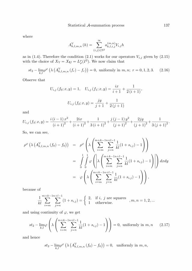
Statistical A-summation process 137
where
AVk,l,m,n (h) =
∞∑(i,j)∈N2
a(m,n)k,l,i,jVi,jh
as in (1.4). Therefore the condition (2.1) works for our operators Vi,j given by (2.15)with the choice of XV = XU = Lρϕ(I2). We now claim that
st2 − limk,lρϕ(λ(AVk,l,m,n (fr)− fr
))= 0, uniformly in m,n; r = 0, 1, 2, 3. (2.16)
Observe that
Ui,j (f0;x, y) = 1, Ui,j (f1;x, y) =ix
i+ 1+
1
2 (i+ 1),
Ui,j (f2;x, y) =jy
j + 1+
1
2 (j + 1)
and
Ui,j (f3;x, y) =i (i− 1)x2
(i+ 1)2 +
2ix
(i+ 1)2 +
1
3 (i+ 1)2 +
j (j − 1) y2
(j + 1)2 +
2jy
(j + 1)2 +
1
3 (j + 1)2 .
So, we can see,
ρϕ(λ(AVk,l,m,n (f0)− f0
))= ρϕ
λm+k−1∑
i=m
n+l−1∑j=n
1
kl(1 + si,j)− 1
=
1∫0
1∫0
ϕ
∣∣∣∣∣∣λm+k−1∑
i=m
n+l−1∑j=n
1
kl(1 + si,j)− 1
∣∣∣∣∣∣ dxdy
= ϕ
λm+k−1∑
i=m
n+l−1∑j=n
1
kl(1 + si,j)− 1
,
because of
1
kl
m+k−1∑i=m
n+l−1∑j=n
(1 + si,j) =
2, if i, j are squares1 otherwise.
,m, n = 1, 2, ...
and using continuity of ϕ, we get
st2 − limk,lϕ
λm+k−1∑
i=m
n+l−1∑j=n
1
kl(1 + si,j)− 1
= 0, uniformly in m,n (2.17)
and hence
st2 − limk,lρϕ(λ(AVk,l,m,n (f0)− f0
))= 0, uniformly in m,n,
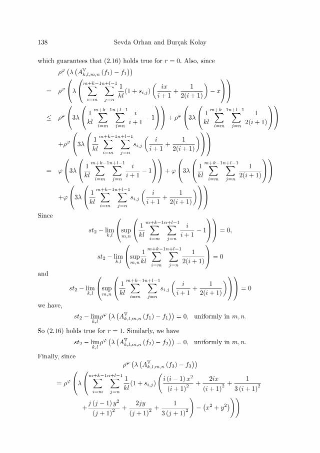
138 Sevda Orhan and Burcak Kolay
which guarantees that (2.16) holds true for r = 0. Also, since
ρϕ(λ(AVk,l,m,n (f1)− f1
))= ρϕ
λm+k−1∑
i=m
n+l−1∑j=n
1
kl(1 + si,j)
(ix
i+ 1+
1
2(i+ 1)
)− x
≤ ρϕ
3λ
1
kl
m+k−1∑i=m
n+l−1∑j=n
i
i+ 1− 1
+ ρϕ
3λ
1
kl
m+k−1∑i=m
n+l−1∑j=n
1
2(i+ 1)
+ρϕ
3λ
1
kl
m+k−1∑i=m
n+l−1∑j=n
si,j
(i
i+ 1+
1
2(i+ 1)
)= ϕ
3λ
1
kl
m+k−1∑i=m
n+l−1∑j=n
i
i+ 1− 1
+ ϕ
3λ
1
kl
m+k−1∑i=m
n+l−1∑j=n
1
2(i+ 1)
+ϕ
3λ
1
kl
m+k−1∑i=m
n+l−1∑j=n
si,j
(i
i+ 1+
1
2(i+ 1)
)Since
st2 − limk,l
supm,n
1
kl
m+k−1∑i=m
n+l−1∑j=n
i
i+ 1− 1
= 0,
st2 − limk,l
supm,n
1
kl
m+k−1∑i=m
n+l−1∑j=n
1
2(i+ 1)
= 0
and
st2 − limk,l
supm,n
1
kl
m+k−1∑i=m
n+l−1∑j=n
si,j
(i
i+ 1+
1
2(i+ 1)
) = 0
we have,
st2 − limk,lρϕ(λ(AVk,l,m,n (f1)− f1
))= 0, uniformly in m,n.
So (2.16) holds true for r = 1. Similarly, we have
st2 − limk,lρϕ(λ(AVk,l,m,n (f2)− f2
))= 0, uniformly in m,n.
Finally, sinceρϕ(λ(AVk,l,m,n (f3)− f3
))= ρϕ
λm+k−1∑
i=m
n+l−1∑j=n
1
kl(1 + si,j)
(i (i− 1)x2
(i+ 1)2 +
2ix
(i+ 1)2 +
1
3 (i+ 1)2
+j (j − 1) y2
(j + 1)2 +
2jy
(j + 1)2 +
1
3 (j + 1)2
)−(x2 + y2
)))
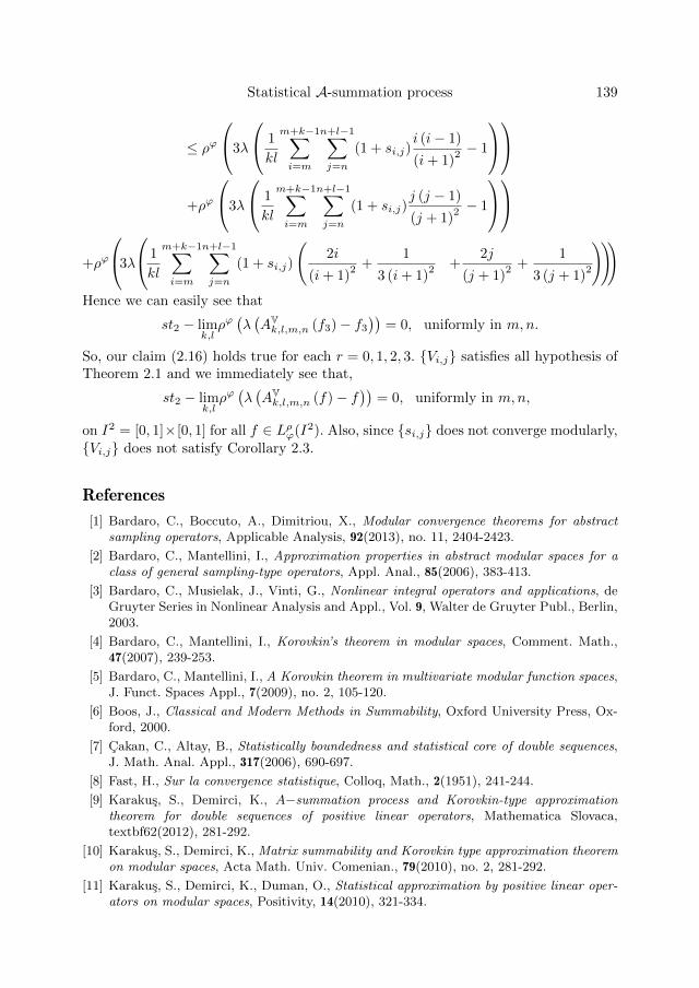
Statistical A-summation process 139
≤ ρϕ3λ
1
kl
m+k−1∑i=m
n+l−1∑j=n
(1 + si,j)i (i− 1)
(i+ 1)2 − 1
+ρϕ
3λ
1
kl
m+k−1∑i=m
n+l−1∑j=n
(1 + si,j)j (j − 1)
(j + 1)2 − 1
+ρϕ
3λ
1
kl
m+k−1∑i=m
n+l−1∑j=n
(1 + si,j)
(2i
(i+ 1)2 +
1
3 (i+ 1)2 +
2j
(j + 1)2 +
1
3 (j + 1)2
)))Hence we can easily see that
st2 − limk,lρϕ(λ(AVk,l,m,n (f3)− f3
))= 0, uniformly in m,n.
So, our claim (2.16) holds true for each r = 0, 1, 2, 3. Vi,j satisfies all hypothesis ofTheorem 2.1 and we immediately see that,
st2 − limk,lρϕ(λ(AVk,l,m,n (f)− f
))= 0, uniformly in m,n,
on I2 = [0, 1]×[0, 1] for all f ∈ Lρϕ(I2). Also, since si,j does not converge modularly,Vi,j does not satisfy Corollary 2.3.
References
[1] Bardaro, C., Boccuto, A., Dimitriou, X., Modular convergence theorems for abstractsampling operators, Applicable Analysis, 92(2013), no. 11, 2404-2423.
[2] Bardaro, C., Mantellini, I., Approximation properties in abstract modular spaces for aclass of general sampling-type operators, Appl. Anal., 85(2006), 383-413.
[3] Bardaro, C., Musielak, J., Vinti, G., Nonlinear integral operators and applications, deGruyter Series in Nonlinear Analysis and Appl., Vol. 9, Walter de Gruyter Publ., Berlin,2003.
[4] Bardaro, C., Mantellini, I., Korovkin’s theorem in modular spaces, Comment. Math.,47(2007), 239-253.
[5] Bardaro, C., Mantellini, I., A Korovkin theorem in multivariate modular function spaces,J. Funct. Spaces Appl., 7(2009), no. 2, 105-120.
[6] Boos, J., Classical and Modern Methods in Summability, Oxford University Press, Ox-ford, 2000.
[7] Cakan, C., Altay, B., Statistically boundedness and statistical core of double sequences,J. Math. Anal. Appl., 317(2006), 690-697.
[8] Fast, H., Sur la convergence statistique, Colloq, Math., 2(1951), 241-244.
[9] Karakus, S., Demirci, K., A−summation process and Korovkin-type approximationtheorem for double sequences of positive linear operators, Mathematica Slovaca,textbf62(2012), 281-292.
[10] Karakus, S., Demirci, K., Matrix summability and Korovkin type approximation theoremon modular spaces, Acta Math. Univ. Comenian., 79(2010), no. 2, 281-292.
[11] Karakus, S., Demirci, K., Duman, O., Statistical approximation by positive linear oper-ators on modular spaces, Positivity, 14(2010), 321-334.
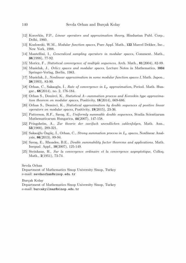
140 Sevda Orhan and Burcak Kolay
[12] Korovkin, P.P., Linear operators and approximation theory, Hindustan Publ. Corp.,Delhi, 1960.
[13] Kozlowski, W.M., Modular function spaces, Pure Appl. Math., 122 Marcel Dekker, Inc.,New York, 1988.
[14] Mantellini, I., Generalized sampling operators in modular spaces, Comment. Math.,38(1998), 77-92.
[15] Moricz, F., Statistical convergence of multiple sequences, Arch. Math., 81(2004), 82-89.
[16] Musielak, J., Orlicz spaces and modular spaces, Lecture Notes in Mathematics, 1034Springer-Verlag, Berlin, 1983.
[17] Musielak, J., Nonlinear approximation in some modular function spaces I, Math. Japon.,38(1993), 83-90.
[18] Orhan, C., Sakaoglu, I., Rate of convergence in Lp approximation, Period. Math. Hun-gar., 68(2014), no. 2, 176-184.
[19] Orhan S., Demirci, K., Statistical A−summation process and Korovkin type approxima-tion theorem on modular spaces, Positivity, 18(2014), 669-686.
[20] Orhan S., Demirci, K., Statistical approximation by double sequences of positive linearoperators on modular spaces, Positivity, 19(2015), 23-36.
[21] Patterson, R.F., Savas, E., Uniformly summable double sequences, Studia ScientiarumMathematicarum Hungarica, 44(2007), 147-158.
[22] Pringsheim, A., Zur theorie der zweifach unendlichen zahlenfolgen, Math. Ann.,53(1900), 289-321.
[23] Sakaoglu Ozguc, I., Orhan, C., Strong summation process in Lp spaces, Nonlinear Anal-ysis, 86(2013), 89-94.
[24] Savas, E., Rhoades, B.E., Double summability factor theorems and applications, Math.Inequal. Appl., 10(2007), 125-149.
[25] Steinhaus, H., Sur la convergence ordinaire et la convergence asymptotique, Colloq.Math., 2(1951), 73-74.
Sevda OrhanDepartment of Mathematics Sinop University Sinop, Turkeye-mail: [email protected]
Burcak KolayDepartment of Mathematics Sinop University Sinop, Turkeye-mail: [email protected]
Stud. Univ. Babes-Bolyai Math. 63(2018), No. 1, 141–151DOI: 10.24193/subbmath.2018.1.09
Quintic B-spline method for numerical solutionof fourth order singular perturbation boundaryvalue problems
Ram Kishun Lodhi and Hradyesh Kumar Mishra
Abstract. In this communication, we have studied an efficient numerical approachbased on uniform mesh for the numerical solutions of fourth order singular pertur-bation boundary value problems. Such type of problems arises in various fields ofscience and engineering, like electrical network and vibration problems with largePeclet numbers, Navier-Stokes flows with large Reynolds numbers in the theoryof hydrodynamics stability, reaction-diffusion process, quantum mechanics andoptimal control theory etc. In the present study, a quintic B-spline method hasbeen discussed for the approximate solution of the fourth order singular pertur-bation boundary value problems. The convergence analysis is also carried outand the method is shown to have convergence of second order. The performanceof present method is shown through some numerical tests. The numerical resultsare compared with other existing method available in the literature.
Mathematics Subject Classification (2010): 65L10.
Keywords: Fourth order singular perturbation boundary value problem, quinticB-spline, quasilinearization, uniform mesh, convergence analysis.
1. Introduction
We consider the fourth order singular perturbation boundary value problem
−εyiv (t)− p (t) y′′′ (t) + q (t) y′′ (t) + r (t) y (t) = f (t) , t ∈ [a, b] , (1.1)
y (a) = η1, y (b) = η2, y′′ (a) = η3, y′′ (b) = η4. (1.2)
where η1, η2, η3 and η4 are finite real constants and ε is a small positive parameter,such that 0 < ε 1. Moreover, we assume that the functions p (t) ,q (t) ,r (t) andf (t) are sufficiently smooth. Further, the problem (1.1) is called non-turning pointproblem if p (t) ≥ α > 0 throughout the interval [a, b], where α is some positiveconstant and boundary layer will be in the neighbourhood of t = a [9]. In the same
142 Ram Kishun Lodhi and Hradyesh Kumar Mishra
vein, if the p (t) vanishes at t = 0, then it becomes a turning point problem. In thatscenario, the boundary layer will be at both the end points t = a and t = b [2].
Singular perturbation problems are engendered by multiplication of a small pos-itive parameter ε to highest derivative term of differential equation with boundaryconditions. Many scholars have studied the analytical and numerical solutions of theseproblems, but sometimes they found that the classical numerical methods failed toget good approximate solutions of singular perturbation problems. That’s why theyhave gone for the non classical methods. In the last few decades, many researchershave discussed the numerical solutions of singular perturbation problems. Most ofthe researchers have studied the numerical solutions of second order singular pertur-bation problems [5, 10, 11, 12, 13, 17, 19, 20, 21, 22, 29]. Only a few researchershave focused the numerical solutions of higher order singular perturbation problems[3, 24, 23, 28, 27]. Lodhi and Mishra [14, 15] have suggested the computational tech-nique for numerical solutions of fourth order singular singularly perturbed and selfadjoint boundary value problems. Raja and Tamilselvan [23] have designed a shoot-ing method on a Shishkin mesh to solve reaction-diffusion type problems. Mishra andSaini [18] have used initial value technique for the numerical solution of fourth or-der singularly perturbed boundary value problems. Sarakhsi et al [25] have studiedthe existence of boundary layer problem. Parameter uniform numerical scheme tosolve fourth order singularly perturbed turning points problems have been presentedby Geetha and Tamilselvan [7]. Sharma et al. [26] have done the survey on singularlyperturbed turning point and interior layers problem. Geetha et al. [8] have applied pa-rameter uniform numerical method based on Shishkin mesh for third order singularlyperturbed turning point problems exhibiting boundary layers.
This paper describes a quintic B-spline approach for the numerical solution offourth order singular perturbation boundary value problems and it has been provedto be second order convergence. The paper is organized as follows: In section 2, wedescribe the quintic B-spline method. Convergence analysis is established in section3. Quasilinearization method is discussed in section 4. Section 5 gives the numericalresults which substantiate the theoretical aspects. Finally, we discuss the conclusionsin section 6.
2. Quintic B-spline Method
We divide the interval [a, b] into N equal subinterval and we choose piecewiseuniform mesh points represented by π = t0, t1, t2, ..., tN ,such that t0 = a, tN = band h = b−a
N is the piecewise uniform spacing. We define L2 [a, b] as a vector space ofall the integrable functions on [a, b] , and X be the linear subspace of L2 [a, b] . Nowwe define
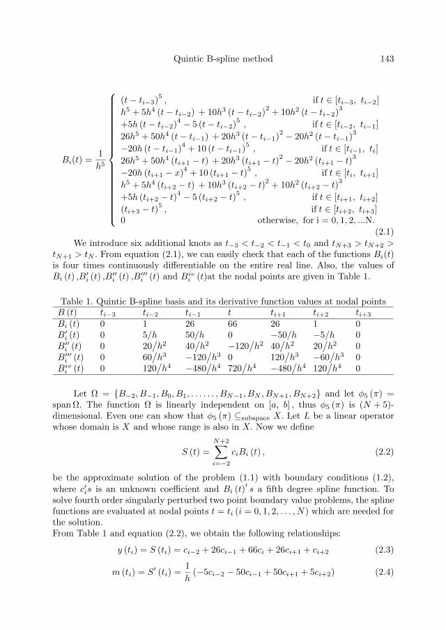
Quintic B-spline method 143
Bi(t) =1
h5
(t− ti−3)5, if t ∈ [ti−3, ti−2]
h5 + 5h4 (t− ti−2) + 10h3 (t− ti−2)2
+ 10h2 (t− ti−2)3
+5h (t− ti−2)4 − 5 (t− ti−2)
5, if t ∈ [ti−2, ti−1]
26h5 + 50h4 (t− ti−1) + 20h3 (t− ti−1)2 − 20h2 (t− ti−1)
3
−20h (t− ti−1)4
+ 10 (t− ti−1)5, if t ∈ [ti−1, ti]
26h5 + 50h4 (ti+1 − t) + 20h3 (ti+1 − t)2 − 20h2 (ti+1 − t)3
−20h (ti+1 − x)4
+ 10 (ti+1 − t)5 , if t ∈ [ti, ti+1]
h5 + 5h4 (ti+2 − t) + 10h3 (ti+2 − t)2 + 10h2 (ti+2 − t)3
+5h (ti+2 − t)4 − 5 (ti+2 − t)5 , if t ∈ [ti+1, ti+2]
(ti+3 − t)5 , if t ∈ [ti+2, ti+3]0 otherwise, for i = 0, 1, 2, ...N.
(2.1)We introduce six additional knots as t−3 < t−2 < t−1 < t0 and tN+3 > tN+2 >
tN+1 > tN . From equation (2.1), we can easily check that each of the functions Bi(t)is four times continuously differentiable on the entire real line. Also, the values ofBi (t) ,B′i (t) ,B′′i (t) ,B′′′i (t) and Bivi (t)at the nodal points are given in Table 1.
Table 1. Quintic B-spline basis and its derivative function values at nodal pointsB (t) ti−3 ti−2 ti−1 t ti+1 ti+2 ti+3
Bi (t) 0 1 26 66 26 1 0B′i (t) 0 5/h 50/h 0 −50/h −5/h 0B′′i (t) 0 20
/h2 40
/h2 −120
/h2 40
/h2 20
/h2 0
B′′′i (t) 0 60/h3 −120
/h3 0 120
/h3 −60
/h3 0
Bivi (t) 0 120/h4 −480
/h4 720
/h4 −480
/h4 120
/h4 0
Let Ω = B−2, B−1, B0, B1, . . . . . . , BN−1, BN , BN+1, BN+2 and let φ5 (π) =span Ω. The function Ω is linearly independent on [a, b] , thus φ5 (π) is (N + 5)-dimensional. Even one can show that φ5 (π) ⊆subspace X. Let L be a linear operatorwhose domain is X and whose range is also in X. Now we define
S (t) =
N+2∑i=−2
ciBi (t) , (2.2)
be the approximate solution of the problem (1.1) with boundary conditions (1.2),where c′is is an unknown coefficient and Bi (t)
′s a fifth degree spline function. To
solve fourth order singularly perturbed two point boundary value problems, the splinefunctions are evaluated at nodal points t = ti (i = 0, 1, 2, . . . , N) which are needed forthe solution.From Table 1 and equation (2.2), we obtain the following relationships:
y (ti) = S (ti) = ci−2 + 26ci−1 + 66ci + 26ci+1 + ci+2 (2.3)
m (ti) = S′ (ti) =1
h(−5ci−2 − 50ci−1 + 50ci+1 + 5ci+2) (2.4)
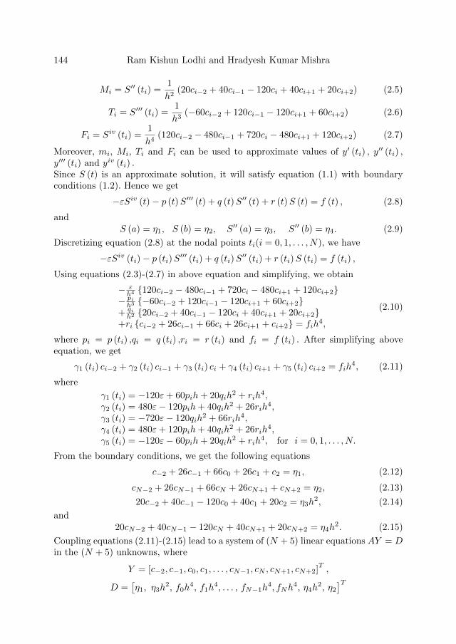
144 Ram Kishun Lodhi and Hradyesh Kumar Mishra
Mi = S′′ (ti) =1
h2(20ci−2 + 40ci−1 − 120ci + 40ci+1 + 20ci+2) (2.5)
Ti = S′′′ (ti) =1
h3(−60ci−2 + 120ci−1 − 120ci+1 + 60ci+2) (2.6)
Fi = Siv (ti) =1
h4(120ci−2 − 480ci−1 + 720ci − 480ci+1 + 120ci+2) (2.7)
Moreover, mi, Mi, Ti and Fi can be used to approximate values of y′ (ti) , y′′ (ti) ,
y′′′ (ti) and yiv (ti) .Since S (t) is an approximate solution, it will satisfy equation (1.1) with boundaryconditions (1.2). Hence we get
−εSiv (t)− p (t)S′′′ (t) + q (t)S′′ (t) + r (t)S (t) = f (t) , (2.8)
andS (a) = η1, S (b) = η2, S′′ (a) = η3, S′′ (b) = η4. (2.9)
Discretizing equation (2.8) at the nodal points ti(i = 0, 1, . . . , N), we have
−εSiv (ti)− p (ti)S′′′ (ti) + q (ti)S
′′ (ti) + r (ti)S (ti) = f (ti) ,
Using equations (2.3)-(2.7) in above equation and simplifying, we obtain
− εh4 120ci−2 − 480ci−1 + 720ci − 480ci+1 + 120ci+2− pih3 −60ci−2 + 120ci−1 − 120ci+1 + 60ci+2
+ qih2 20ci−2 + 40ci−1 − 120ci + 40ci+1 + 20ci+2
+ri ci−2 + 26ci−1 + 66ci + 26ci+1 + ci+2 = fih4,
(2.10)
where pi = p (ti) ,qi = q (ti) ,ri = r (ti) and fi = f (ti) . After simplifying aboveequation, we get
γ1 (ti) ci−2 + γ2 (ti) ci−1 + γ3 (ti) ci + γ4 (ti) ci+1 + γ5 (ti) ci+2 = fih4, (2.11)
where
γ1 (ti) = −120ε+ 60pih+ 20qih2 + rih
4,γ2 (ti) = 480ε− 120pih+ 40qih
2 + 26rih4,
γ3 (ti) = −720ε− 120qih2 + 66rih
4,γ4 (ti) = 480ε+ 120pih+ 40qih
2 + 26rih4,
γ5 (ti) = −120ε− 60pih+ 20qih2 + rih
4, for i = 0, 1, . . . , N.
From the boundary conditions, we get the following equations
c−2 + 26c−1 + 66c0 + 26c1 + c2 = η1, (2.12)
cN−2 + 26cN−1 + 66cN + 26cN+1 + cN+2 = η2, (2.13)
20c−2 + 40c−1 − 120c0 + 40c1 + 20c2 = η3h2, (2.14)
and20cN−2 + 40cN−1 − 120cN + 40cN+1 + 20cN+2 = η4h
2. (2.15)
Coupling equations (2.11)-(2.15) lead to a system of (N + 5) linear equations AY = Din the (N + 5) unknowns, where
Y = [c−2, c−1, c0, c1, . . . , cN−1, cN , cN+1, cN+2]T,
D =[η1, η3h
2, f0h4, f1h
4, . . . , fN−1h4, fNh
4, η4h2, η2
]T
Quintic B-spline method 145
and the coefficient matrix A is given by
A =
1 26 66 26 1 020 40 −120 40 20 0
γ1 (t0) γ2 (t0) γ3 (t0) γ4 (t0) γ5 (t0) 00 γ1 (t1) γ2 (t1) γ3 (t1) γ4 (t1) γ5 (t1)
0 0...
......
...0 0 0 γ1 (ti) γ2 (ti) γ3 (ti)...
......
......
...0 0 · · · 0 0 γ1 (tN−1)0 0 · · · 0 0 00 0 · · · 0 0 00 0 · · · 0 0 0
0 0 · · · 0 00 0 · · · 0 00 0 · · · 0 00 0 · · · 0 0...
......
......
γ4 (ti) γ5 (ti) 0 0 0...
...... 0 0
γ2 (tN−1) γ3 (tN−1) γ4 (tN−1) γ5 (tN−1) 0γ1 (tN ) γ2 (tN ) γ3 (tN ) γ4 (tN ) γ5 (tN )
20 40 −120 40 201 26 66 26 1
.
(2.16)Since A is a non-singular matrix, so we can solve the system AY = D for
c−2,c−1,c0,c1,c2,. . . ,cN−2,cN−1,cN ,cN+1,cN+2 substituting these values into equation(2.2), we get the required approximate solution.
3. Derivation for convergence
In this section, a technique is portrayed which will ascertain the truncation errorfor the quintic B-spline method over the whole range a ≤ t ≤ b. Here, we supposethat function y (t) has continuous derivatives in the whole range.
We calculate the following relationships by comparing the coefficients ofci (i = −2,−1, 0, 1, . . . , N,N + 1, N + 2) . From equations (2.3)-(2.7), we have
S′(ti−2) + 26S′(ti−1) + 66S′(ti) + 26S′(ti+1) + S′(ti+2)= 1
h −5y(ti−2)− 50y(ti−1) + 50y(ti+1) + 5y(ii+2) (3.1)
S′′(ti−2) + 26S′′(ti−1) + 66S′′(ti) + 26S′′(ti+1) + S′′(ti+2)= 1
h2 20y(ti−2) + 40y(ti−1)− 120y(ti) + 40y(ti+1) + 20y(ti+2) (3.2)
S′′′(ti−2) + 26S′′′(ti−1) + 66S′′′(ti) + 26S′′′(ti+1) + S′′′(ti+2)= 1
h3 −60y(ti−2) + 120y(ti−1)− 120y(ti+1) + 60y(ti+2) (3.3)
146 Ram Kishun Lodhi and Hradyesh Kumar Mishra
Siv(ti−2) + 26Siv(ti−1) + 66Siv(ti) + 26Siv(ti+1) + Siv(ti+2)= 1
h4 120y(ti−2)− 480y(ti−1) + 720y(ti)− 480y(ti+1) + 120y(ti+2) (3.4)
Using the operator notation [6, 16], the equations (3.1)-(3.4) can we written as
S′(ti) =1
h
(−5E−2 − 50E−1 + 50E + 5E2
E−2 + 26E−1 + 66I + 26E + E2
)y(ti) (3.5)
S′′(ti) =1
h2
(20E−2 + 40E−1 − 120I + 40E + 20E2
E−2 + 26E−1 + 66I + 26E + E2
)y(ti) (3.6)
S′′′(ti) =1
h3
(−60E−2 + 120E−1 − 120E + 60E2
E−2 + 26E−1 + 66I + 26E + E2
)y(ti) (3.7)
Siv(ti) =1
h4
(120E−2 − 480E−1 + 720I − 480E + 120E2
E−2 + 26E−1 + 66I + 26E + E2
)y(ti) (3.8)
where the operators are defined as Ey(ti) = y(ti + h), Dy(ti) = y′(ti) and Iy(ti) =y(ti). Let E = ehD and expand them in powers of hD, we get
S′(ti) = y′(ti) +1
5040h6y7(ti)−
1
21600h8y9(ti) +
1
1036800h10y11(ti) + 0(h11) (3.9)
S′′(ti) = y′′(ti) + 1720h
4y6(ti)− 13360h
6y8(ti) + 186400h
8y10(ti)+ 221
239500800h10y12(ti) + 0(h11)
(3.10)
S′′′(ti) = y′′′(ti)− 1240h
4y7(ti) + 1130240h
6y9(ti)− 128800h
8y11(ti)+ 37
11404800h10y13(ti) + 0(h11)
(3.11)
Siv(ti) = yiv(ti)− 112h
2y6(ti) + 1240h
4y8(ti)− 17560h
6y10(ti)− 13
907200h8y12(ti) + 643
159667200h10y14(ti) + 0(h11)
(3.12)
We now define e (t) = y (t) − S (t) and substitute equations (3.9)-(3.12) in theTaylor series expansion of e (ti + θh) we obtain
e (ti + θh) =(
θ2
1440 −5θ4
1440
)h6y6(ti) +
(θ
5040 −θ2
1440
)h7y7(ti)
+(− θ2
6720 + θ4
5760
)h8y8(ti) + 0(h9)
(3.13)
where a ≤ θ ≤ b. We abridge the above results in the following theorem:Theorem 3.1. Let y (t) be the exact solution and S (t) be the numerical solution ofthe singularly perturbed fourth order boundary value problem (1.1) with the boundaryconditions (1.2) for sufficiently small h which further gives the truncation error ofO(h6)
and method of convergence of O(h2).
4. Quasilinearization method
Let us consider the boundary value problem
−εyiv (t) = F (t, y, y′′, y′′′) , t = [a, b] , (4.1)
y (a) = η1, y (b) = η2, y′′ (a) = η3, y′′ (b) = η4, (4.2)
Quintic B-spline method 147
where F (t, y, y′′, y′′′) is a smooth function such that Fy′′′ (t, y, y′′, y′′′) ≥ α > 0,
Fy′′ (t, y, y′′, y′′′) ≥ β > 0, t ∈ [a, b] ,
0 ≥ Fy (t, y, y′′, y′′′) ≥ −λ, λ > 0.(4.3)
In order to obtain the numerical solution of the boundary value problem (4.1) and(4.2), Newton’s method of quasilinearization [1, 4] is applied to generate the sequenceof yk∞0 of successive approximations with a proper selection of initial guess y0. Wedefine yk+1, for each fixed non-negative integer k,to be solution of the following linearproblem:
−εyivk+1 (t)−pk (t) y′′′k+1 (t)+qk (t) y′′k+1 (t)+rk (t) yk+1 (t) = fk (t) , t ∈ [a, b] , (4.4)
yk+1 (a) = η1, yk+1 (b) = η2, y′′k+1 (a) = η3, y′′k+1 (b) = η4, (4.5)
where
pk (t) = Fy′′′ (t, yk, y′′k , y
′′′k ) , qk (t) = Fy′′ (t, yk, y
′′k , y
′′′k ) ,
rk (t) = Fy (t, yk, y′′k , y
′′′k ) , fk (t) = Fy (t, yk, y
′′k , y
′′′k )
−ykFy (t, yk, y′′k , y
′′′k )− y′′kFy′′ (t, yk, y′′k , y′′′k )
−y′′′k Fy′′′ (t, yk, y′′k , y′′′k ) .
We make the following observations:
i) If the initial guess y0 is sufficiently close to the solution y (t) of (4.1) and (4.5),then the sequence yk∞0 converges to y(x). One can see the proof given in [4].From (4.3), it follows that, for each fixed k,
pk (t) = Fy′′′ (t, y, y′′, y′′′) ≥ α > 0,
qk (t) = Fy′′ (t, y, y′′, y′′′) ≥ β > 0,
0 ≥ rk (t) = Fy (t, y, y′′, y′′′) ≥ −λ, λ > 0.(4.6)
ii) Problem (4.4) with the boundary conditions (4.5), for each fixed k,is a linearfourth order boundary value problem which is in the form of (1.1) and (1.2).Hence it can be solved by the method described in section 2.
iii) The following convergence criterion is used to terminate the iteration:
‖yk+1 (ti)− yk (ti)‖ ≤ ε, ti ∈ [a, b] , k ≥ 0. (4.7)
5. Numerical results
In the present section, we have presented numerical results of the consideredexamples with the help of MATLAB software which verifies theoretical estimates.When the exact solutions of the considered examples are available then the maximumabsolute errors EN are evaluated using the following formula for the present method,which is given by
EN = maxti∈[a, b]
∣∣yNε (ti)− SNε (ti)∣∣ , (5.1)
148 Ram Kishun Lodhi and Hradyesh Kumar Mishra
When the exact solutions of the considered examples are not available then the maxi-mum absolute errors ENd are evaluated using the double mesh principle for the presentmethod, which is given by
ENd = maxti∈[a, b]
∣∣SNε (ti)− S2Nε (ti)
∣∣ , (5.2)
The numerical order of convergence is computed using the following formula
OrdN =lnEN − lnE2N
ln 2. (5.3)
The exact and approximate solutions are denoted by yNε and SNε respectively.Example 5.1 Consider the following singular perturbation boundary value problem[27]:
−εyiv (t)− 4y′′′ (t) = 1, t ∈ [0, 1] ,
y (0) = 1, y (1) = 1, y′′ (0) = −1, y′′ (1) = −1.
The exact solution of Example 5.1 is given by
y (t) = 1
192(1−e−
4ε
) −3ε2e−4tε − 72t2 − 8t3 + 80t− 3tε2 + 192 + 3ε2
+ e−4ε
(−192 + 96t2 + 8t3 − 104t+ 3tε2
).
Table 2. Maximum absolute errors and order of convergence ofExample 5.1 for different values of ε and N.
N ε = 2−4 Ord ε = 2−5 Ord ε = 2−6 Ord ε = 2−7 Ord ε = 2−8 Ord64 9.5153E-06 2.0442 1.1597E-05 2.2186 9.3841E-06 1.6594 7.6100E-06 1.6904 1.0217E-05 2.4174128 2.3070E-06 2.0097 2.4916E-06 2.0418 2.9708E-06 2.2173 2.3579E-06 1.6494 1.9126E-06 1.6944256 5.7289E-07 2.0010 6.0512E-07 2.0095 6.3885E-07 2.0421 7.5163E-07 2.2142 5.9098E-07 1.6435512 1.4312E-07 2.1459 1.5029E-07 1.4799 1.5512E-07 2.0623 1.6198E-07 2.0885 1.8916E-07 2.20511024 3.2339E-08 5.3882E-08 3.7140E-08 3.8086E-08 4.1024E-08
Example 5.2. Consider the following singular perturbation boundary value problem[7]:
−εyiv (t) + 5ty′′′ (t) + 4y′′ (t) + 2y (t) = 0, t ∈ [−1, 1] ,
y (−1) = 1, y (1) = 1, y′′ (−1) = 1, y′′ (1) = 1.
Table 3. Comparison of maximum absolute error and order of convergence ofExample 5.2 for different values of N and ε = 2−4.
N Geetha and Tamilselvan [7] Present MethodENd Ord ENd Ord
64 3.9249E-2 0.9770 4.4948E-04 2.5794128 1.9940E-2 0.9886 7.5204E-05 2.0864256 1.0049E-2 0.9944 1.7708E-05 2.0177512 5.0440E-3 0.9972 4.3731E-06 2.30711024 2.5269E-3 8.8366E-07
Quintic B-spline method 149
Example 5.3. Consider the following singular perturbation boundary value problem[7]:
−εyiv (t) + 5ty′′′ (t) + (4 + t) y′′ (t) +(2 + t2
)y (t) = −et + 5, t ∈ [−1, 1] ,
y (−1) = 1, y (1) = 1, y′′ (−1) = 2, y′′ (1) = 2.
Table 4. Comparison of maximum absolute error and order of convergence ofExample 5.3 for different values of N and ε = 2−4
N Geetha and Tamilselvan [7] Present MethodENd Ord ENd Ord
64 3.3778E-2 0.9823 4.1824E-04 2.5806128 1.7097E-2 0.9913 6.9920E-05 2.0866256 8.6002E-3 0.9957 1.6462E-05 2.0306512 4.3130E-3 0.8693 4.0291E-06 2.10871024 2.3610E-3 9.3418E-07
Example 5.4. Consider the following singular perturbation boundary value problem[7]:
−εyiv (t) + 5ty′′′ (t) + (4 + t) y′′ (t) + 2y2 (t) = 0, t ∈ [−1, 1] ,
y (−1) = 1, y (1) = 1, y′′ (−1) = 2, y′′ (1) = 2.
Table 5. Comparison of maximum absolute error and order of convergence ofExample 5.4 for different values of N and ε = 2−4
N Geetha and Tamilselvan [7] Present MethodENd Ord ENd Ord
64 7.5762E-02 0.9731 1.1620e-03 2.5795128 3.8593E-02 0.9867 1.9440e-04 2.0863256 1.9475E-02 0.9934 4.5777e-05 2.0215512 9.7821E-03 0.9967 1.1275e-05 1.74491024 4.9021E-03 - 3.3639e-06 -
6. Conclusions
In this article, we have used the quintic B-spline method for finding the approx-imate solution of fourth order linear and non-linear singular perturbation boundaryvalue problems. We linearised the non-linear boundary value problem via quasilin-earization method and solved the problem. It is a computationally proficient tech-nique and the algorithm can easily be applied on a computer. The results obtainedthrough this method are better than the existing method [7] with the same numberof nodal points.
150 Ram Kishun Lodhi and Hradyesh Kumar Mishra
References
[1] Bellman, R.E., Kalaba, R.E., Quasilinearization and Nonlinear Boundary Value Prob-lems, American Elsevier, New York, 1965.
[2] Berger, A.E., Han, H., Kellogg, R.B., A priori estimates and analysis of a numericalmethod for a turning point problem, Mathematics of Computation, 42(1984), 465–492.
[3] Chen, S., Wang, Y., A rational spectral collocation method for third-order singularlyperturbed problems, Journal of Computational and Applied Mathematics, 307(2016),93–105.
[4] Doolan, E.P., Miller, J.J.H., Schildres, W.H.A., Uniform Numerical Method for Problemswith Initial and Boundary Layers, Dublin, Boole Press, 1980.
[5] Farrell, P.A., Hagarty, A.F., Miller, J.J.H., O’Riordan, E., Shishkin, G.I., Robust Compu-tational Techniques for Boundary Layers, Boca Raton, Chapman and Hall/CRC Press,2000.
[6] Fyfe, D.J., The use of the cubic spline in the solution of two point boundary valueproblems, Computing Journal, 12(1969), 188–192.
[7] Geetha, N., Tamilselvan, A., Parameter uniform numerical method for fourth ordersingularly perturbed turning point problems exhibiting boundary layers, Ain Shams En-gineering Journal, http://dx.doi.org/10.1016/j.asej.2016.04.018, 2016.
[8] Geetha, N., Tamilselvan, A., Subburayan, V., Parameter uniform numerical methodfor third order singularly perturbed turning point problems exhibiting boundary layers,International Journal of Applied and Computational Mathematics, 2(2016), 349–364.
[9] Howes, F.A., The asymptotic solution of a class of third-order boundary value problemarising in the theory of thin film flow, SIAM Journal of Applied Mathematics, 43(1983),993–1004.
[10] Kadalbajoo, M.K., Patidar, K.C., A survey of numerical techniques for solving singu-larly perturbed ordinary differential equations, Applied Mathematics and Computations,130(2002), 457–510.
[11] Kadalbajoo, M.K., Yadaw, A.S., Kumar, D., Comparative study of singularly perturbedtwo-point BVPs via: Fitted-mesh finite difference method, B-spline collocation methodand finite element method, Applied Mathematics and Computation, 204(2008), 713–725.
[12] Khan, A., Khan, I., Aziz, T., Sextic spline solution of a singularly perturbed boundary-value problems, Applied Mathematics and Computation, 181(2006), 432–439.
[13] Kumar, M., Singh, P., Mishra, H.K., A recent survey on computational techniques forsolving singularly perturbed boundary value problems, International Journal of ComputerMathematics, 84(2007), 1439–1463.
[14] Lodhi, R.K., Mishra, H.K., Computational approach for fourth-order self-adjoint sin-gularly perturbed boundary value problems via non-polynomial quintic spline, IranianJournal of Science and Technology, Transactions A: Science, DOI 10.1007/s40995-016-0116-6, 2016.
[15] Lodhi, R.K., Mishra, H.K., Solution of a class of fourth order singular singularly per-turbed boundary value problems by quintic B-spline method, Journal of the NigerianMathematical Society, 35(2016), 257–265.
[16] Lucas, T.R., Error bounds for interpolating cubic splines under various end conditions,SIAM Journal Numerical Analysis, 11(1974), 569–584.
Quintic B-spline method 151
[17] Miller, J.J.H., O’Riordan, E., Shishkin, G.I., Fitted numerical methods for singularlyperturbed problems. Error estimates in the maximum norm for linear problems in oneand two dimensions, Singapore: World Scientific Publishing Co. Pvt. Ltd., 2012.
[18] Mishra, H.K., Saini, S., Fourth order singularly perturbed boundary value problems viainitial value techniques, Applied Mathematical Sciences, 8(2014), 619–632.
[19] O’Malley, R.E., Introduction to Singular Perturbations, New York, Academic Press,1974.
[20] Pandit, S., Kumar, M., Haar wavelet approach for numerical solution of two parame-ters singularly perturbed boundary value problems, Applied Mathematics & InformationSciences, 6(2014), 2965–2974.
[21] Rai, P., Sharma, K.K., Numerical analysis of singularly perturbed delay differential turn-ing point problem, Applied Mathematics and Computation, 218(2011), 3486–3498.
[22] Rai, P., Sharma, K.K., Numerical study of singularly perturbed differential – differenceequation arising in the modeling of neuronal variability, Computers & Mathematics withApplications, 63(2012), 118–132.
[23] Roja, J.C., Tamilselvan,A., Shooting method for singularly perturbed fourth-order ordi-nary differential equations of reaction-diffusion type, International Journal of Compu-tational Methods, http://dx.doi.org/10.1142/S0219876213500412, Vol. 10, 1350041 (21pages), (2013).
[24] Roos, H.G., Stynes, M., Tobiska, L., Numerical Method for Singularly Perturbed Differ-ential Equation Convection-Diffusion and Flow Problems, Springer, 2006.
[25] Sarakhsi, A.R., Ashrafi, S., Jahanshahi, M., Sarakhsi, M., Investigation of boundarylayers in some singular perturbation problems including fourth order ordinary differentialequations, World Applied Sciences Journal, 22(2013), 1695–1701.
[26] Sharma, K.K., Rai, P., Patidar, K.C., A review on singularly perturbed differential equa-tions with turning points and interior layers, Applied Mathematics and Computation,219(2013), 10575–10609.
[27] Shanthi, V., Ramanujam, N., A boundary value technique for boundary value prob-lems for singularly perturbed fourth-order ordinary differential equations, Computersand Mathematics with Applications, 47(2004), 1673–1688.
[28] Valarmathi, S., Ramanujam, N., A computational method for solving third order singu-larly perturbed ordinary differential equations, Applied Mathematics and Computation,129(2002), 345–373.
[29] Zhang, Y., Naidu, D. S., Cai, C., Zou, Y., Singular perturbations and time scales incontrol theories and applications: An overview 2002-2012, International Journal of In-formation and Systems Sciences, 9(2014), 1–35.
Ram Kishun LodhiDepartment of Mathematics, Jaypee University of Engineering & TechnologyAB Road Raghogarh, Guna-473226 (M.P.), Indiae-mail: [email protected]
Hradyesh Kumar MishraCorresponding authorDepartment of Mathematics, Jaypee University of Engineering & TechnologyAB Road Raghogarh, Guna-473226 (M.P.), Indiae-mail: [email protected]