MATH7021 | Technological Maths 312 - J.P. McCarthy: Math Page | Last year's maths …€¦ · ·...
75
MATH7021 — Technological Maths 312 J.P. McCarthy October 4, 2012
Transcript of MATH7021 | Technological Maths 312 - J.P. McCarthy: Math Page | Last year's maths …€¦ · ·...

MATH7021 — Technological Maths 312
J.P. McCarthy
October 4, 2012
Contents
0.1 Introduction . . . . . . . . . . . . . . . . . . . . . . . . . . . . . . . . . . . . 2
1 Numerical Methods I 51.1 Finite-Difference Methods . . . . . . . . . . . . . . . . . . . . . . . . . . . . 51.2 Linear Systems . . . . . . . . . . . . . . . . . . . . . . . . . . . . . . . . . . 17
2 Laplace Methods 492.1 The Laplace Transform . . . . . . . . . . . . . . . . . . . . . . . . . . . . . . 492.2 The Inverse Laplace Transform . . . . . . . . . . . . . . . . . . . . . . . . . 612.3 First and Second Order Linear Differential Equations . . . . . . . . . . . . . 702.4 Systems of Linear Differential Equations . . . . . . . . . . . . . . . . . . . . 72
3 Numerical Methods II 733.1 Curve Fitting II . . . . . . . . . . . . . . . . . . . . . . . . . . . . . . . . . . 73
4 Multiple Integrals 744.1 Line Integrals . . . . . . . . . . . . . . . . . . . . . . . . . . . . . . . . . . . 744.2 Double Integrals . . . . . . . . . . . . . . . . . . . . . . . . . . . . . . . . . . 744.3 Jacobians . . . . . . . . . . . . . . . . . . . . . . . . . . . . . . . . . . . . . 744.4 Applications: Centroids and the Second Moment of Area . . . . . . . . . . . 744.5 Triple Integrals . . . . . . . . . . . . . . . . . . . . . . . . . . . . . . . . . . 74
1

MATH7021 — Technological Maths 312 2
0.1 Introduction
Lecturer
J.P. McCarthy
Office
Meetings before class by appointment via email only.
Email & Web:
[email protected] and http://jpmccarthymaths.wordpress.comThis page will comprise the webpage for this module and as such shall be the venue forcourse announcements including definitive dates for the tests. This page shall also housesuch resources as links (such as to exam papers), as well supplementary material. Please notethat not all items here are relevant to MATH7021; only those in the category ‘MATH7021’.Feel free to use the comment function therein as a point of contact.
Module Objective
This module covers numerical methods such as interpolation, Gaussian elimination and iter-ative methods for solving simultaneous linear equations; the method of Laplace transformsfor the solution of differential equations; further calculus in relation to line and multipleintegrals.
Module Content
Numerical Methods
Interpolation via finite difference tables. Newton-Gregory interpolation formulae. Deter-mination of a line of best-fit to a set of data points using the method of Least Squares.Non-linear laws. Fitting a curve such as a parabola to a set of points. The regression line.Pearson’s product-moment correlation coefficient r. Solutions of simultaneous linear equa-tions using Gaussian elimination without and with partial pivoting. Jacobi’s method andthe Gauss-Siedel method.
Laplace Transforms
Derivation of Laplace transforms. The inverse Laplace transform via table look-up andpartial fraction expansions. Solution of first and second order differential equations. Solutionof 2x2 systems of linear differential equations.
Multiple Integrals
Development and evaluation of line integrals along various paths including closed paths. De-velopment and evaluation of double integrals over various regions. Jacobians. Applicationsto include centroids and second moment of area about an axis. Development and evaluationof triple integrals.

MATH7021 — Technological Maths 312 3
Assessment
Total Marks 100: End of Year Written Examination 70 marks; Continuous Assessment 30marks.
Continuous Assessment
The Continuous Assessment will be divided between two in-class tests, each worth 15%, inweeks 6 & 11.Absence from a test will not be considered accept in truly extraordinary cases. Plenty ofnotice will be given of the test date. For example, routine medical and dental appointmentswill not be considered an adequate excuse for missing the test.
Lectures
It will be vital to attend all lectures as many of the examples, proofs, etc. will be completedby us in class.
Tutorials
The aim of the tutorials will be to help you achieve your best performance in the tests andexam.
Exercises
There are many ways to learn maths. Two methods which arent going to work are
1. reading your notes and hoping it will all sink in
2. learning off a few key examples, solutions, etc.
By far and away the best way to learn maths is by doing exercises, and there are two mainreasons for this. The best way to learn a mathematical fact/ theorem/ etc. is by using it inan exercise. Also the doing of maths is a skill as much as anything and requires practise.There are exercises in the notes for your consumption. The webpage may contain a link to aset of additional exercises. Past exam papers are fair game. Also during lectures there willbe some things that will be left as an exercise. How much time you can or should devote todoing exercises is a matter of personal taste but be certain that effort is rewarded in maths.

MATH7021 — Technological Maths 312 4
Reading
Your primary study material shall be the material presented in the lectures; i.e. the lecturenotes. Exercises done in tutorials may comprise further worked examples. While the lectureswill present everything you need to know about MATH7021, they will not detail all there isto know. Further references are to be found in the library. Good references include:
• Dennis G. Zill & Michael R. Cullen 2000, Advanced Engineering Mathematics, 2nd Ed.,Jones & Barlett
• S.C.Chapra & R.P.Canale 2005, Numerical Methods for Engineers, 5th Ed., McGrawHill
The webpage may contain supplementary material, and contains links and pieces abouttopics that are at or beyond the scope of the course. Finally the internet provides yetanother resource. Even Wikipedia isn’t too bad for this area of mathematics! You areencouraged to exploit these resources; they will also be useful for further maths modules.
Exam
The exam format will roughly follow last year’s. Acceding to the maxim that learning off afew key examples, solutions, etc. is bad and doing exercises is good, solutions to past papersshall not be made available (by me at least). Only by trying to do the exam papers yourselfcan you guarantee proficiency. If you are still stuck at this stage feel free to ask the questioncome tutorial time.
Chapter 1
Numerical Methods I
Although this may seem a paradox, all exact science is dominated by the idea ofapproximation.
Bertrand Russell
1.1 Finite-Difference Methods
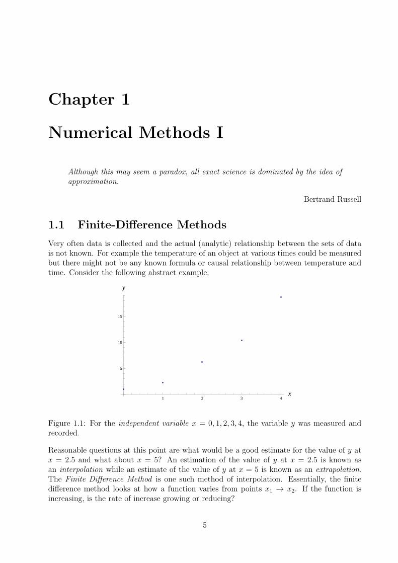
Very often data is collected and the actual (analytic) relationship between the sets of datais not known. For example the temperature of an object at various times could be measuredbut there might not be any known formula or causal relationship between temperature andtime. Consider the following abstract example:
1 2 3 4x
5
10
15
y
Figure 1.1: For the independent variable x = 0, 1, 2, 3, 4, the variable y was measured andrecorded.
Reasonable questions at this point are what would be a good estimate for the value of y atx = 2.5 and what about x = 5? An estimation of the value of y at x = 2.5 is known asan interpolation while an estimate of the value of y at x = 5 is known as an extrapolation.The Finite Difference Method is one such method of interpolation. Essentially, the finitedifference method looks at how a function varies from points x1 → x2. If the function isincreasing, is the rate of increase growing or reducing?
5

MATH7021 — Technological Maths 312 6
For the present we concentrate on problems where the values of x differ by the same amount.The first forward difference is the difference between consecutive values of y and is given by:
Similarly the second forward difference are the differences of the first differences, that is
A table should show what we mean:
x y ∆y ∆2y
x0 y0
∆y0 = y1 − y0x1 y1 ∆2y0 = ∆y1 −∆y0
∆y1 = y2 − y1
x2 y2 ∆2y1 = ∆y2 −∆y1
∆y2 = y3 − y2
x3 y3 ∆2y2 = ∆y3 −∆y2
Third and subsequent forward differences are defined in the obvious way. Note that youcan also do backward and central differences but we shall concentrate on these forwarddifferences.
Remark
There are a number of remarks that we can make about these forward differences. Firstly ifit is indeed the case that1 y = f(x), then the analysis will be greatly simplified if f(x) is apolynomial. That is a sum of powers of x:
f(x) = aNxN + aN−1x
N−1 + · · ·+ a2x2 + a1x+ a0, (1.1)
where the ai are real numbers and n is some natural number: the degree of f(x). For exampleif f(x) is a constant function, say f(x) = 2 then all of the forward differences will be zero.If f(x) is a linear function, that is of the form f(x) = mx + c for some real number m andc then it is not too difficult2 to show that the second forward differences will be zero and soon. Therefore if f(x) is a degree N then the (N + 1)-th forward differences will all be zero.Equivalently the N -th forward differences of a degree N polynomial will all be equal.
1y is a function of x — the value of x uniquely determines the value of x2Let f(x) = aNxN + · · · + a1x + a0 be a degree N polynomial and suppose the (x, y = f(x)) data has
the xs located h units apart. Now let ∆yn be the forward difference yn+1 − yn. In this notation yn = f(xn)

MATH7021 — Technological Maths 312 7
However, be careful. Mathematically at least, having, say, all the third forward differencesequal to zero does not necessarily imply that y = f(x) with f(x) a quadratic function.
1.1.1 Data Errors
The above remark shows that if we know that a set of data comes from a polynomial andthe forward differences do not converge that there must be an error. In past papers you cansee the following:
1. It is suspected that the table contains an error or
2. The table contains an error,
and you are supposed to find this error. In future I should prefer to state that this set ofdata comes from a polynomial function.
Summer 2012: Question 1 (a)
Attached to this examination paper is a table of corresponding values of x and y. It issuspected that the table contains an error.
(i) Form a table of forward differences. If it exists locate and correct the error. Submitthe completed table with your examination script.
(ii) Extend the table to find the values of y at x = 0 and x = 6.
Solution: See Sheet.
Autumn 2012: Question 1 (a)
At the rear of this examination paper there is a table of corresponding values of x and y.The table contains an error.
(i) Form a table of forward differences. Locate and correct the error. Submit the completedtable with your examination script.
(ii) Extend the table to find the values of y at x = 0 and x = 120.
Solution: See Sheet.
and also xn+1 = xn + h. Thence
∆yn = yn+1 − yn = f(xn + h)− f(xn)
=(aN (xn + h)N + aN−1(xn + h)N−1 + · · · a1(xn + h) + a0
)− (aNxn + · · ·+ a1x+ a0)
=(aNxN +O(xN−1)
)−(aNxN +O(xN−1)
)= O(xN−1)
where ‘O(xm)’ means of degreem or less. Roughly therefore, the forward differences of a degreeN polynomialare degree N − 1 and hence inductively the (N + 1)-th forward differences will be zero

MATH7021 — Technological Maths 312 8
Exercises
1. Form a forward difference table for the set of values below up as far as including secondforward differences:
x 0 1 2 3 4 5 6 7 8
y 5 2 1 2 5 10 17 26 37
2. For the set of values below form a forward difference table for up as far as and includingthird differences:
x 0 1 2 3 4 5 6 7 8
y -5 -8 -13 -14 -5 20 67 142 251
3. Form a forward difference table for the set of values below up as far as and includingsecond differences.
x 1.0 1.2 1.4 1.6 1.8 2.0 2.2
y 0.0000 0.1823 0.3365 0.4700 0.5878 0.6931 0.7885
4. Form a difference table for the set of values up as far as and including second differences.Expand the table to evaluate f(0), f(9) and f(10).
x 1 2 3 4 5 6 7 8
f(x) 0.03 0.5 1.1 2.1 3.5 5.3 7.5 10.1
Selected Solution: f(10) = 16.5.
5. Form a difference table for the set of values below up as far as and including thirddifferences and correct the error. Expand the table to evaluate f(0), f(9) and f(10).
x 1 2 3 4 5 6 7 8
f(x) -18 -19 -18 -15 -9 -3 6 17
Selected Solution: f(10) = 554.
6. Form a difference table for the set of values below up as far as and including seconddifferences. The data is from a polynomial and contains an error. Locate and correctthis error. Expand the table to show that f(0) = 20 and f(4.5) = 74.
x 0.5 1.0 1.5 2.0 2.5 3.0 3.5 4.0
f(x) 18 18 20 24 32 38 48 60
7. Form a difference table for the set of values below. The table of values of f(x) containstwo errors. Locate and correct these errors. Expand the table to evaluate f(0) andf(12).
x 1 2 3 4 5 6 7 8 9 10
f(x) 12 21 32 45 77 79 96 117 140 165

MATH7021 — Technological Maths 312 9
1.1.2 Curve Fitting I
How many lines pass through a given point P (x1, y1) on the plane? How about through Pand some other point Q(x2, y2)?
x
f HxL
Figure 1.2: An infinite number of lines pass through P ; only one of these, however, alsopasses through Q.
How about quadratics (degree-two polynomials)? Given points P , Q and R(x3, y3) is theremore than one quadratic through P and Q but only one through P , Q and R?
x
f HxL
Figure 1.3: 2 + 1 = 3 points defines a unique degree 2 polynomial. In other words giventhree points there is a unique quadratic q(x) whose graph goes through all three points.
A bit of heavy algebra shows that in fact we have the following:
The Polynomial Unisolvence Theorem
Given a set of d + 1 points on the plane there is a unique d-degree polynomial P thatpasses through all of these points.
But how do we find this interpolating polynomial? One way is to use finite differences.
MATH7021 — Technological Maths 312 10
1.1.3 Newton-Gregory Interpolation Formula
This is a formula that expresses the interpolating polynomial in terms of the forward differ-ences.
Newton-Gregory Interpolation Formula
Let the function f be known at n+1 equally h-spaced data points a = x0 < x1 < · · · <= xn = bin the interval [a, b] as f0, f1, · · · fn. Then the n degree polynomial approximation of f(x)can be given as
f(x) = f(x0 + rh) ≈ P (x) =n∑
i=0
(r
i
)∆if0 (1.2)
where(ri
)are the binomial coefficients defined as
(r0
)= 1, and(
r
i
)=
r(r − 1) · · · (r − i+ 1)
i!(1.3)
for any integer i > 0.
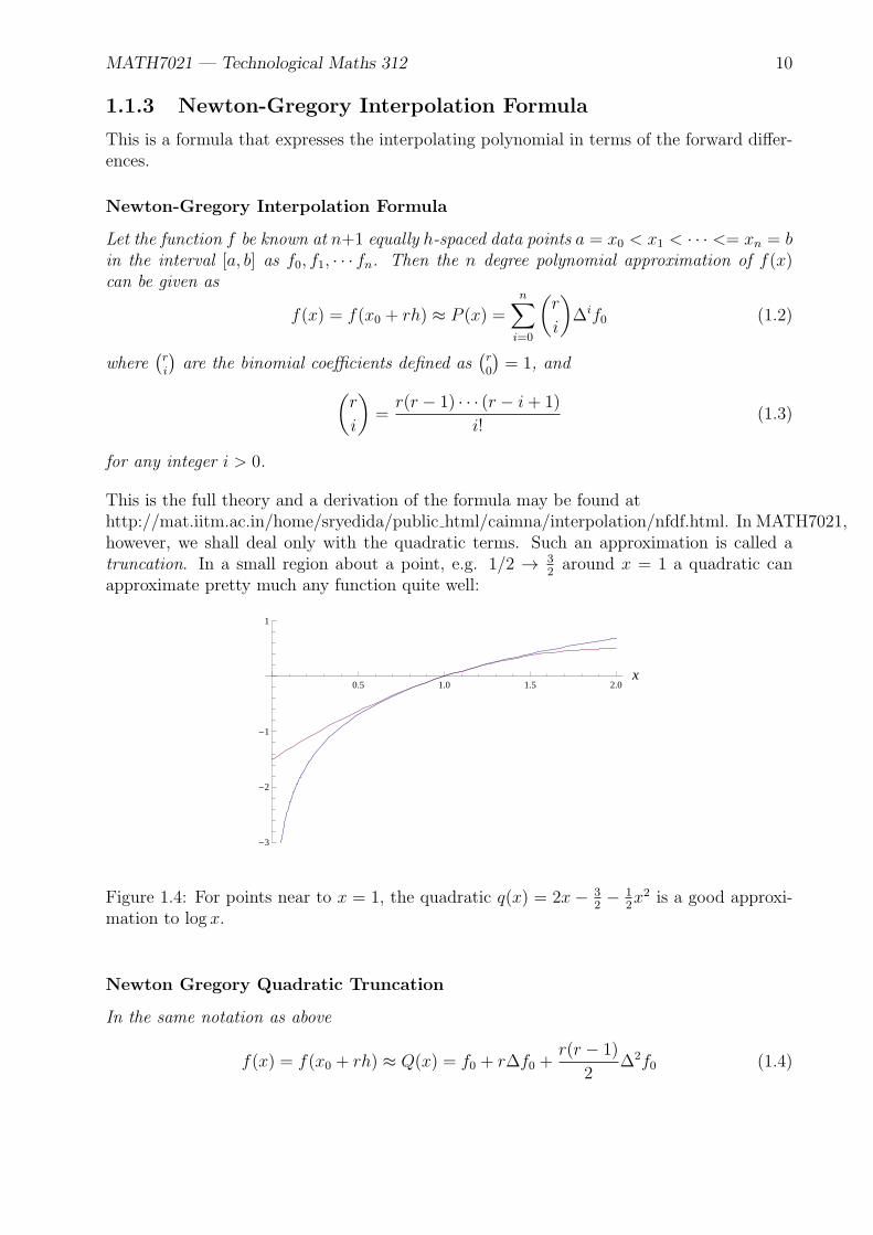
This is the full theory and a derivation of the formula may be found athttp://mat.iitm.ac.in/home/sryedida/public html/caimna/interpolation/nfdf.html. In MATH7021,however, we shall deal only with the quadratic terms. Such an approximation is called atruncation. In a small region about a point, e.g. 1/2 → 3
2around x = 1 a quadratic can
approximate pretty much any function quite well:
0.5 1.0 1.5 2.0x
-3
-2
-1
1
Figure 1.4: For points near to x = 1, the quadratic q(x) = 2x− 32− 1
2x2 is a good approxi-
mation to log x.
Newton Gregory Quadratic Truncation
In the same notation as above
f(x) = f(x0 + rh) ≈ Q(x) = f0 + r∆f0 +r(r − 1)
2∆2f0 (1.4)

MATH7021 — Technological Maths 312 11
Now that we have truncated to degree 2 quadratics we may as well go the whole hog andtruncate to degree 1 polynomials: lines!
Linear Interpolation
In the same notation as above
f(x) = f(x0 + rh) ≈ L(x) = f0 + r∆f0 (1.5)
Moving Estimates
These are the formulae that appear in the literature and indeed will appear on your exampapers. We can improve them slightly however:
1 2 3 4 5 6 7x
Data
Figure 1.5: Suppose that we want to approximate the value of y(5.5). With h = 1 here, ∆f0is the slope of the line segment connecting the x = 0 and x = 1 points. Wouldn’t it makemuch more sense to use the slope from the x = 5 to x = 6 points instead?
The ‘justification’ for this is that if we are approximating these sets of data by polynomials,then their slopes in turn are also polynomials which are continuous without sudden jumpsin slope: in general the slopes of polynomials change smoothly and hence not only is a ‘localapproximation’ better than a global one (∆f0), but also a good one.

MATH7021 — Technological Maths 312 12
This can be seen for the quadratic approximation also:
1 2 3 4 5 6 7x
Data
Figure 1.6: Again suppose that we want to approximate the value of y(5.5). With h = 1 here,∆2f0 is the difference between the slopes of the line segments x = 0 → 1 and x = 1 → 2.Wouldn’t it make much more sense to use the slopes closer to the x = 5, x = 6 and x = 7points instead?
Now we could adjust the formulae (first linear then quadratic):
We just see xn as are starting point analogous to x0.
Exercises
8. Form a difference table for the values below up and as far as second differences.
x 0 0.5 1 1.5 2 2.5 3 3.5 4 4.5
y 0 2 6 12 20 30 42 56 72 90
Using the interpolation formula above estimate the values of f(1.8) and f(2.25).
9. Form a difference table for the values below up and as far as second differences.
x 0 1 2 3 4 5 6 7 8
f(x) 2 0 0 2 6 12 20 30 42
Using the interpolation formula above estimate the values of f(3.5) and f(5.25).

MATH7021 — Technological Maths 312 13
10. Form a difference table for the values below up and as far as second differences.
x 2 4 6 8 10 12 14 16
f(x) 0.693 1.386 1.792 2.079 2.303 2.485 2.639 2.773
Using the interpolation formula above estimate the values of f(9) and f(8.2).
11. Form a difference table for the values below up and as far as second differences.
x 0 1 2 3 4 5 6 7
f(x) 1.000 1.105 1.221 1.350 1.492 1.649 1.822 2.014
Using the interpolation formula above estimate the values of f(3.5) and f(4.2).
12. Form a difference table for the values below up and as far as second differences.
x 0 1 2 3 4 5 6 7
f(x) 0 1 4 9 16 25 36 49
By expanding the table and by using the interpolating formula deduce the values off(−1), f(10), f(3.5) and f(5.25).
14. If y(5) = 10.0 and if y(5.5) = 10.2 use linear interpolation to estimate the value ofy(5.2).
15. If f(3) = 9.00 and if f(3.1) = 9.61 use linear interpolation to estimate f(3.4).
Derivatives
The derivative of a polynomial is another polynomial and hence the derivative (slope of thetangent) of the interpolating polynomial is another polynomial (which we can also derive).It can be shown that
f ′(x0 + rh) ≈ 1
h
[∆f0 +
2r − 1
2!∆2f0
](1.6)
This is another quadratic truncation.

MATH7021 — Technological Maths 312 14
Summer 2012: Question 1 (a)
Attached to this examination paper is a table of corresponding values of x and y.
(iii) Use the Newton-Gregory Interpolation Formula to estimate the value of y at x = 1.3.
(iv) By using linear interpolation estimate the value of y at x = 2.2.
(v) Estimate the slope of y at x = 2.2 and x = 2.
Solution: All the time using the sheet marked ‘Su ‘12’ with the corrections.
(iii) Our formula is
f(x0 + rh) = f0 + r∆f0 +r(r − 1)
2∆2f0 (1.7)
Looking at the formula above and working from x2 = 1 we have
In this case r = 35= 0.6, h = 0.5 and we also have
Thence
(iv) Very straightforwardly
f(x0 + rh) = f(x0) + r∆f0 (1.8)
(v) Just recall that slope is nothing but the derivative. Again just implement the relevantformula
f ′(x0 + rh) =1
h
[∆f0 +
2r − 1
2!∆2f0
](1.9)
MATH7021 — Technological Maths 312 15
and also
Autumn 2012: Question 1 (a)
Attached to this examination paper is a table of corresponding values of x and y.
(iii) Use the Newton-Gregory Interpolation Formula to estimate the value of y at x = 75.
(iv) By using linear interpolation estimate the value of y at x = 75.
(v) Estimate the value ofdy
dxat x = 82 and x = 80.
Solution: All the time using the sheet marked ‘Au ‘12’ with the corrections.
(iii) Our formula is
f(x0 + rh) = f0 + r∆f0 +r(r − 1)
2∆2f0 (1.10)
Looking at the formula above and working from x7 = 70 we have
In this case r = 510
= 12, h = 10 and we also have
Thence
(iv) Very straightforwardly
f(x0 + rh) = f(x0) + r∆f0 (1.11)

MATH7021 — Technological Maths 312 16
(v) Just recall that slope is nothing but the derivative which is denoted by both f ′(x) anddy
dx. Again just implement the relevant formula
f ′(x0 + rh) =1
h
[∆f0 +
2r − 1
2!∆2f0
](1.12)
and also
Exercises
16. For the values below form a difference table up to and including second differences.
x 0 0.5 1.0 1.5 2.0 2.5 3.0 3.5 4.0
f(x) 1 1 7 25 61 121 221 337 505
Estimate the value of y′(1.5) and y′(1.8).
17. Form a table of forward differences:
x 1 2 3 4 5 6 7
f(x) -2.8 -1.1 1.6 5.3 10.0 15.7 22.4
Estimate the value of y′(3.4) and y′(4)

MATH7021 — Technological Maths 312 17
1.2 Linear Systems
1.2.1 Review of Gaussian Elimination Methods
In this chapter we learn how to solve and analyse equations such as the those generated bynetwork flows. Such a set of equations is known as a system of linear equations. For nowa matrix is just a rectangular array of numbers in a bracket but later we will see their truenature.
Systems of Linear Equations
If two lines intersect they will do so at a single point; if two planes intersect their intersectionwill be a line, a line can intersect a plane at one point, lie in the plane, or not intersect itat all. Three planes can have one point in common or no points in common. Some of thesepossibilities are illustrated as follows:
Figure 1.7: Three planes can intersect at a point, a line, or nowhere.
We can show that the equation of a plane is given by:
What the hell is the equation of a plane? In essence it is a membership card:
Hence to find the intersection of three planes we find points that are on all three curves —that is the satisfy their equations, at the same time, simultaneously. For example, we mighthave to find the points (x, y, z) that satisfy all of
3x+ 4y − z = 7
2x− 6y + z = −2
x− y + z = 3
Definitions
A linear equation in n variables is an equation of the form:
a1x1 + a2x2 + a3x3 + · · ·+ anxn = b, (1.13)

MATH7021 — Technological Maths 312 18
where the variables are x1, x2, . . . , xn, the numbers a1, . . . , an are called the coefficients, andb is the constant. A system of m equations in n variables has the form
a11x1 + a12x2 + · · ·+ a1nxn = b1
a21x1 + a22x2 + · · ·+ a2nxn = b2......
...
am1x1 + am2x2 + · · ·+ amnxn = bm.
Row Operations and Gaussian Elimination
While it is possible to solve systems with small numbers of equations in a few variables by adhoc methods such as these, we would like a more systematic approach to solve more complexsystems, and would also like to be able to program computers to do the task. We will developan algorithmic method perfectly adapted to the task. First note that the variable names areirrelevant; the systems
4x− 8y = 1 and 4m− 9n = 1−3x+ y = −3 −3m+ n = −3
have the same solutions3. Consequently all we actually need to look at are the coefficientsand constants, which can be recorded in a rectangular array called a matrix :
x1 + 2x2 − 6x3 − x4 = 02x1 + 4x2 + 7x4 = 36x1 − 2x2 + x3 + 2x4 = −43x1 − 8x3 + 2x4 = 9
converts to
1 2 −6 −1 02 4 0 7 36 −2 1 2 −43 0 −8 2 9
Conversely, given such a matrix we can recover the corresponding system: 4 3 −7 1 0
2 9 1 −1 108 −2 0 5 0
converts to4x1 + 3x2 − 7x3 + x4 = 92x1 + 9x2 + x3 − x4 = 108x1 − 2x2 + 5x4 = 0
Elementary Row Operations
We want to transform a given system into one which is easier to solve. There are three thingswhich we can do to a linear system which will not change the solution, but possibly make iteasier to see the solution.
• Swap equations — clearly
4x− y = 7
2x+ 5y = −2
has the same solution as
2x+ 5y = −2
4x− y = 7
3namely x = m = 26/23 and y = n = 9/23.

MATH7021 — Technological Maths 312 19
• Multiply an equation by a constant — neither will this change the solution; say mul-tiplying the second equation by five:
2x+ 5y = −2
20x− 5y = 35
• Add the equations together — why would this not change the solution?
2x+ 5y = 1
(20x− 5y) + (2x+ 5y) = 35− 2
Now we would have 22x = 33 ⇒ x = 3/2. Note also that we could have put these lasttwo transformations into the single add a multiple of an equation to another.
If we go back into the augmented matrix picture we see:[4 −1 72 5 −2
]r1↔r2→
[2 5 −24 −1 7
]r2→r2×5→
[2 5 −220 −5 35
]r2→r2+r1→
[2 5 −222 0 33
],
and we can convert this into
2x+ 5y = −2
22x = 33
Note the row operations we enacted. Suppose we have a system of linear equations inaugmented matrix form [A|B]. From the discussions above we can show that the followingrow operations will leave the solution unchanged:
• swapping any two rows:
• multiplying any row by a constant:
• adding any row to any other:
• combining the last two: adding a multiple of a row to another row:
We call these the elementary row operations or EROs.

MATH7021 — Technological Maths 312 20
Example
Use the techniques above to simplify and hence solve the following simultaneous equation:
5x+ 7y = 0
−3x+ 4y = 2
Solution: First we write everything in augmented matrix form:
What I am going to do is try to use the EROs to get the augmented matrix in the form
Hence we now have
Using the three EROs we want to take the augmented matrix form of the linear system andapply the EROs until the coefficient matrix is in row-echelon form. This looks like

MATH7021 — Technological Maths 312 21
In words,
1. all rows containing zeros are on the bottom.
2. all the leading coefficients (of the non-zero rows) are 1 and above zeros.
The coefficient matrix is in reduced row-echelon form if, in addition
3. the leading coefficient or pivot is the only non-zero entry in its column.
The following matrices are in row-echelon form (where ⋆ denotes any number):
To be in reduced row-echelon form they must look like:
The following matrices are not in row-echelon form:
but can easily be brought into row-echelon form by applying EROs.
The Solution Space
As soon as the coefficient matrix is brought into row-echelon form we can tell if solutionsexist for the system, and if so whether there is just one solution, or infinitely many. Therewill be no solution if there is a row looking like
This follows because this particular row corresponds to the equation
which has no solution since the left-hand side is zero but the right-hand side is k ̸= 0.

MATH7021 — Technological Maths 312 22
If no such row appears then there is at least one solution. It is unique if every columncontains a pivot; if this is not so then the variables corresponding to the columns withoutpivots are not determined and become parameters/free variables in the solution leading toinfinitely many solutions.
Examples
The augmented matric for the three linear systems has been brought into reduced row-echelonform. Find the solutions:
(i)
1 0 0 −10 1 0 00 0 1 2
, (ii)
1 3 0 1 30 0 1 7 10 0 0 0 2
, (iii)
1 5 0 0 −2 30 0 1 0 4 −50 0 0 1 2 60 0 0 0 0 0
.
Solution:
(i) We simply have
(ii) Note the third row...
(iii) Rewrite this set of equations:
x1 + 5x2 − 2x5 = 3
x3 + 4x4 = 5
x4 + 2x5 = 6
0x5 = 0
No solve from the bottom. Firstly x5 could be anything. We write this by sayingx5 = t for t ∈ R. This means that x5 can take on any real number (R) value. In thiscase, x5 or t is called a parameter or free variable. For each value of the parameter(t), we get a different solution. As t can take on any value from minus to plus infinity,there are thus an infinite number of solutions. Now we look at the second last row:
Now at the third last:
Now look at the first equation:
Now for any fixed value of t, x1 = −5x1 + (3 + 2t) actually represents a line andthus there are an infinite number of pairs (x1, x2) that satisfy this equation. We needanother parameter/free variable. In this we could choose x1 or x2 but usually we will

MATH7021 — Technological Maths 312 23
be better off if we pick the x2 (e.g. the x5 over the x3 etc.) Hence now call x2 = s —where again s ∈ R:
Hence we have the solution(s):
x1 = 3 + 2t− 5s
x2 = s
x3 = −19 + 8t
x4 = 6− 2t
x5 = t
where t, s ∈ R. You might (not?) be interested to show that we have shown that threefive-dimensional (hyper) planes can intersect along a plane...
How did we know that x5 and x2 were parameters/free variables? Why did we need twoparameters? Why did we need any? The following theorem is useful in this case. We willnot provide a proof.
Theorem
Consider a linear system of m equations in n variables. Suppose that the coeffi-cient matrix has r non-zero rows when put in row-echelon form. Then if thereare solutions, the set of solutions has n − r parameters. In particular, if r < n, thenthere will be infinitely many solutions.
Remark
It follows that we have three possibilities:
(i) there is no solution (the system is inconsistent), or
(ii) there is exactly one solution (n = r), or
(iii) there are infinitely many solutions (n > r)
The number r represents the number of independent equations. Consider the three equations:
2x− y = 4
x− 6y = 1
2x− 12y = 2
Although there are three equations here, equations 2 and 3 are actually equivalent — in rowechelon form these would form a row of zeros.

MATH7021 — Technological Maths 312 24
Hence once we have the augmented matrix in row-echelon form we must see how manyparameters/free variables there are (in this module it will usually be zero, one (t) or two(t and s)). Usually we look at the augmented matrix and correspond rows to variables. Ifthere is no row for the last equation we can usually take that variable to be a parameter/freevariable.
Note that this will not always be possible. For example,
Here there is one parameter/free variable but we can’t say that x3 is a parameter/free variable— x3 = 1.
The coefficient matrix can always be brought into row-echelon form by using the followingGaussian Elimination algorithm.
1. If possible, swap rows such that the first entry of the first row is a ̸= 0.
2. Multiply the first row by 1/a in order to get a leading 1.
3. Subtract multiples of this row from those below to make each entry below this into azero.
4. Repeat steps 1-3 for the second entry in the second row, third entry in the third rowetc.
Examples
Solve the following systems of linear equations using row reduction.
1.
x+ 2y = 2
2x− y = 1
Solution:
MATH7021 — Technological Maths 312 25
2.
x+ 2y − z = 2
2x+ 5y + 2z = −1
7x+ 17y + 5z = −1
Solution:
3.
x+ 10z = 5
3x+ y − 4z = −1
4x+ y + 6z = 1
Solution:

MATH7021 — Technological Maths 312 26
4.
x+ 2y − 4z = 10
2x− y + 2z = 5
x+ y − 2z = 7
Solution:

MATH7021 — Technological Maths 312 27
Now the number of non-zero rows, r = 2; while the number of variables, n = 3. Hencethere is n− r = 1 parameter. Let z = t ∈ R:
Hence we have the solution x = 4− 8t, y = 3 + 2t and z = t for t ∈ R.
Winter 2011: Question 4(a) (i)
Use Gaussian Elimination to solve the set of simultaneous linear equations1 1 2 32 4 8 42 4 6 73 7 8 8
xyzw
=
2486
Solution:

MATH7021 — Technological Maths 312 28
Now we have the solutions
w = 2
z =
y =
x =
Autumn 2012: Question 4(a) (i)
Use Gaussian Elimination to solve the set of simultaneous linear equations1 1 1 12 4 5 43 5 5 35 7 9 3
xyzw
=
0006
Solution:
MATH7021 — Technological Maths 312 29
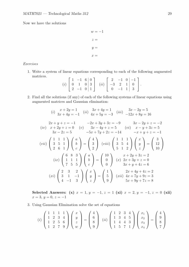
Now we have the solutions
w = −1
z =
y =
x =
Exercises
1. Write a system of linear equations corresponding to each of the following augmentedmatrices.
(i)
1 −1 6 00 1 0 32 −1 0 1
(ii)
2 −1 0 −1−3 2 1 00 −1 1 3
.
2. Find all the solutions (if any) of each of the following systems of linear equations usingaugmented matrices and Gaussian elimination:
(i)x+ 2y = 1
3x+ 4y = −1(ii)
3x+ 4y = 14x+ 5y = −3
(iii)3x− 2y = 5
−12x+ 8y = 16
(iv)2x+ y + z = −1x+ 2y + z = 03x− 2z = 5
(v)−2x+ 3y + 3z = −9
3x− 4y + z = 5−5x+ 7y + 2z = −14
(vi)3x− 2y + z = −2x− y + 3z = 5
−x+ y + z = −1
(vii)
1 1 13 5 12 6 1
abc
=
432
(viii)
1 1 13 5 45 1 2
xyz
=
31210
(ix)
6 8 31 1 17 5 5
abc
=
1000
(x)x+ 2y + 3z = 22x+ 3y + z = 03x+ y + 4z = 6
(xi)
2 3 23 1 −14 −1 3
xyz
=
159
(xii)2x+ 4y + 4z = 24x+ 7y + 9z = 35x+ 9y + 7z = 8
Selected Answers: (x) x = 1, y = −1, z = 1 (xi) x = 2, y = −1, z = 0 (xii)x = 3, y = 0, z = −1
3. Using Gaussian Elimination solve the set of equations
(i)
1 1 1 11 2 3 41 2 5 61 2 7 9
xyzw
=
4689
(ii)
1 2 3 41 3 4 51 4 4 31 5 7 1
x1
x2
x3
x4
=
4987
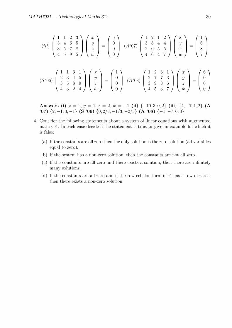
MATH7021 — Technological Maths 312 30
(iii)
1 1 2 33 4 6 53 5 7 84 5 9 5
xyzw
=
5000
(A ‘07)
1 2 1 23 8 4 42 6 5 54 6 4 7
xyzw
=
1687
(S ‘06)
1 1 3 12 3 4 53 5 8 94 3 2 4
xyzw
=
1000
(A ‘08)
1 2 3 12 7 7 33 9 8 64 5 3 7
xyzw
=
6000
Answers (i) x = 2, y = 1, z = 2, w = −1 (ii) {−10, 3, 0, 2} (iii) {4,−7, 1, 2} (A‘07) {2,−1, 3,−1} (S ‘06) {0, 2/3,−1/3,−2/3} (A ‘08) {−1,−7, 6, 3}
4. Consider the following statements about a system of linear equations with augmentedmatrix A. In each case decide if the statement is true, or give an example for which itis false:
(a) If the constants are all zero then the only solution is the zero solution (all variablesequal to zero).
(b) If the system has a non-zero solution, then the constants are not all zero.
(c) If the constants are all zero and there exists a solution, then there are infinitelymany solutions.
(d) If the constants are all zero and if the row-echelon form of A has a row of zeros,then there exists a non-zero solution.

MATH7021 — Technological Maths 312 31
1.2.2 Cramer’s Rule
Suppose that a linear system has the form
then the system can be rewritten in the form
where A is a square matrix, b is the vector of constants and x is the vector of variables:
Now introduce the idea of the inverse of a matrix. We might have encountered these beforebut again as an aid to understanding it might be fruitful to consider the geometry of thesituation. What does a 2 × 2 matrix do? Well it sends points (x, y) on the plane to otherpoints on the plane:
An inverse of a matrix sends the points back to where they came from so that hitting a pointwith A and then by ‘A−1’ will send it back from whence it came.
x
f HxL
Figure 1.8: The action of a matrix and its inverse.

MATH7021 — Technological Maths 312 32
If A is invertible4, then we can ‘hit’ both sides with A−1 to obtain the unique solution
That is if we have a square matrix of coefficients A and of if A is invertible then the solutionis unique.
There is a quantity related to square matrices called the determinant. You will have encoun-tered determinants before and may be able to calculate the determinants of 2× 2 and 3× 3matrices. For MATH7021 we only need to calculate determinants of 2 × 2 matrices. Whatare they geometrically though?
x
f HxL
Figure 1.9: If a 2× 2 matrix M1 is applied to a region of area A then the area of the imagewill be detM1 × A. This means that a matrix M1 with detM1 = 0 cannot be invertible asan infinite number of points will be sent to a single point or line — dimension argumentsshow that we cannot send these points back faithfully.
Definition & Formula
Let A be a square matrix with column vectors c1, c2, . . . , cn. The determinant of A, detAis the volume of the parallelepiped generated by the column vectors. The determinant of a2× 2 matrix is given by:
det
(a bc d
)=
∣∣∣∣ a bc d
∣∣∣∣ = ad− bc. (1.14)
|A| is another notation for the determinant of A. We have the following which we may havelearnt about in a previous module.
Theorem
A square matrix A is invertible if and only if detA is non-zero.
Proof. If detA = 0 then clearly A can not be invertible according to Figure 1.9. There is a
formula for the inverse of a square matrix: A−1 =1
detAC where C is a matrix defined in
terms of A. If detA ̸= 0 then this formula is valid and A is invertible •4if there exists a matrix A−1 such that AA−1 = A−1 = I where I is the identity matrix
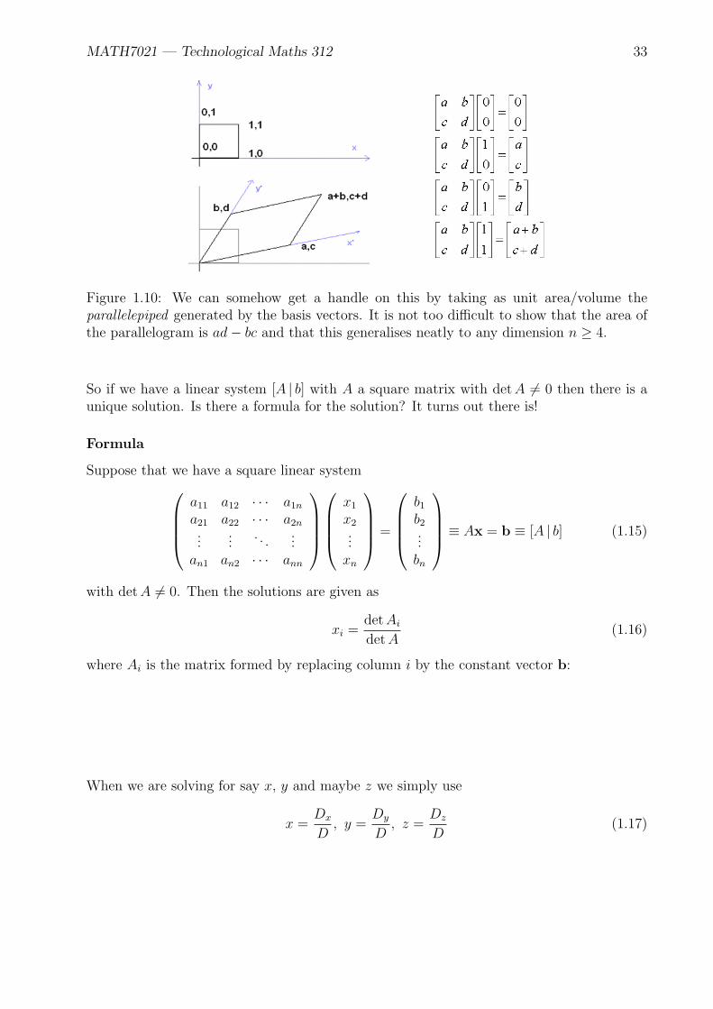
MATH7021 — Technological Maths 312 33
Figure 1.10: We can somehow get a handle on this by taking as unit area/volume theparallelepiped generated by the basis vectors. It is not too difficult to show that the area ofthe parallelogram is ad− bc and that this generalises neatly to any dimension n ≥ 4.
So if we have a linear system [A | b] with A a square matrix with detA ̸= 0 then there is aunique solution. Is there a formula for the solution? It turns out there is!
Formula
Suppose that we have a square linear systema11 a12 · · · a1na21 a22 · · · a2n...
.... . .
...an1 an2 · · · ann
x1
x2...xn
=
b1b2...bn
≡ Ax = b ≡ [A | b] (1.15)
with detA ̸= 0. Then the solutions are given as
xi =detAi
detA(1.16)
where Ai is the matrix formed by replacing column i by the constant vector b:
When we are solving for say x, y and maybe z we simply use
x =Dx
D, y =
Dy
D, z =
Dz
D(1.17)

MATH7021 — Technological Maths 312 34
Example
Use Cramer’s Rule to solve the linear system
4x+ 5y = 8
x− y = 11
Solution: First we find x =Dx
D:
Now we find y =Dy
D:
Remark
This seems too good to be true — such a simple formula for solving simultaneous equations.Much quicker than Gaussian elimination methods and even ad hoc methods... Don’t befooled. Cramer’s Rule only applies when the linear system is square and has a uniquesolution. The only way to know this in advance is to calculate the determinant of thecoefficient matrix. For 2 × 2 this is simple. For 3 × 3 a little harder but not impossible.However as the size of the system increases Cramer’s Rule takes comparatively longer andlonger to implement in comparison to Gaussian elimination methods because determinantsof larger matrices take an increasingly long time to compute.
Why the hell do we even use Cramer’s Rule so? Well suppose that you have a real physicallinear system (e.g. some kind of network flow) that you know must somehow have a uniquesolution. Sometimes you will not be interested in all of the variables but only one: this iswhere Cramer’s Rule’s strength lies. With Gaussian elimination methods you either havenone of the solutions or one of the solutions. With Cramer’s Rule you can find only onevariable if you want. IN MATH7021 we will be using it in an exam situation to check ananswer or approximation.
Also I have omitted the proof. It relies on a number of properties of determinants.Exercises: Check your answers to the previous Exercise 2. (i), (ii) & (iii) using Cramer’sRule.
MATH7021 — Technological Maths 312 35
1.2.3 Round-Off Error & Partial Pivoting
With exact arithmetic, Gaussian elimination is guaranteed to succeed. However this assur-ance does not help us when we do Gaussian elimination with rounded-off decimals. This isbecause matrix arithmetic is ill-conditioned. A lot of problems are well-conditioned whichmeans that their solutions are stable. This means a small variation in the parameters doesnot change the solution greatly, e.g.
However with matrices the situation is very different. Consider the two linear systems:
Ax = b.
(A+ εij)x = b.
where εij is a matrix of small perturbations/errors which changes the coefficients only veryslightly. It turns out that the solutions to these two systems, whose parameters are verysimilar, can be very different indeed.
This comes from the numerical analysis principle which says that
If any calculation if undefined when a certain quantity is zero, the same calcula-tion is likely to suffer numerical problems when the quantity is ‘small.
This applies to Gaussian elimination when a pivot is non-zero but ‘small’.
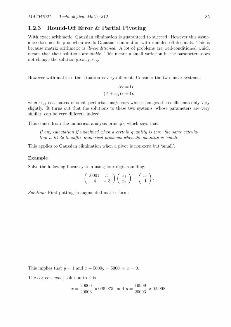
Example
Solve the following linear system using four-digit rounding:(.0001 .5.4 −.3
)(x1
x2
)=
(.5.1
).
Solution: First putting in augmented matrix form:
This implies that y = 1 and x+ 5000y = 5000 ⇒ x = 0.
The correct, exact solution to this
x =20000
20003≈ 0.99975, and y =
19999
20003≈ 0.9998.

MATH7021 — Technological Maths 312 36
You might say, well just do exact arithmetic. In reality if you have a complicated linearsystem you are going to use a computer programme to solve the system and can computershandle exact arithmetic morryah infinite precision... Hence we need a way of avoiding thesemassive errors. Note that in the above example we had a very small pivot 0.0001. Note howwe went from 0.4 and −0.3 to 0 and -2000: we multiplied the small pivot a11 = 0.0001 bythe large multiple m1 = 10, 000 and then took 0.4r1 from r2:
0.4 = a21 −→ a21 −m1a11
−0.3 = a22 −→ a22 −m1a12
A small pivot such as 0.0001 can be small with respect to other elements of the row, such asa12 = 0.5 and b1 = 0.5, and this causes the elements a22 and b2 to ‘disappear’ so we appearto be dealing with the system(
.0001 .5.4 0
)(x1
x2
)=
(.50
).
which is clearly very different to the original one. Note that according to the principle abovea21 −m1a11 ̸= 0 when a11 = 0 so this should result in a problem when a11 ≈ 0, as it is here.
Hence the problem is with small pivots. Based on this an obvious idea would be to avoidunnecessarily small pivots. The way we do this is via a method called partial pivoting.Briefly, we make sure that the largest pivot (in magnitude: −10 is larger in magnitude than0.4 say) in any column or sub-column is the primary pivot. If this is not the case we swaprows to achieve this. We will show this with an example.
Example
Use Gaussian elimination with partial pivoting and four-digit rounding to solve the linearsystem: (
.0001 .5.4 −.3
)(x1
x2
)=
(.5.1
).
Solution: First we put the system in augmented matrix form:
Now the the pivot in the first column is smaller than the other element(s) of that column sowe swap rows one and two and proceed:
Now we can turn .4999 into a 1 by multiplying by 1/.4999 ≈ 2.000:
Now we read off the solutions

MATH7021 — Technological Maths 312 37
Recall that without partial pivoting we got the answers x = 0 and y = 1 when the exactanswers are to four digits x = 0.9999 and y = 0.9998 .
An obvious question is whether a partial pivoting strategy will guarantee that round-off errorswill cause significantly different solutions. Unfortunately the answer to this question is “no”,however the cases when partial pivoting does not work well are extreme and pathological.
Summer 2012: Question 4(a) (ii)
Use Gaussian Elimination with partial pivoting to solve the set of simultaneous equations 2 3 76 15 94 15 9
xyz
=
143632
Solution: First we write in augmented form such that the leading pivot is the greatest inmagnitude:
Note that in the sub-column5−2
that the larger pivot is on top X:
Now we can read off the solutions:
Autumn 2012: Question 4(a) (ii)
By using Gaussian Elimination with and without partial pivoting solve the set of simultane-ous equations below. All calculations correct to two places of decimals. 1 1 1
2 3 14 8 1
xyz
=
61123
Solution: First we write in augmented form such that the leading pivot is the greatest inmagnitude:
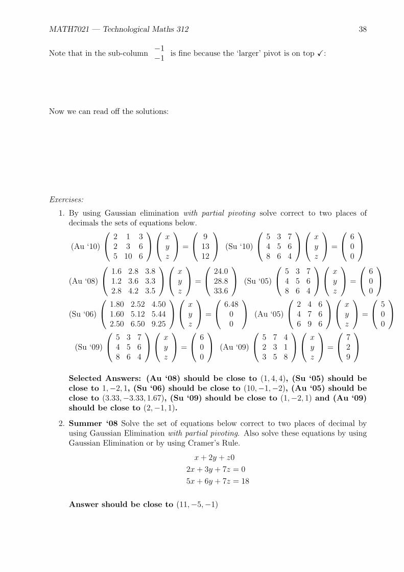
MATH7021 — Technological Maths 312 38
Note that in the sub-column−1−1
is fine because the ‘larger’ pivot is on top X:
Now we can read off the solutions:
Exercises:
1. By using Gaussian elimination with partial pivoting solve correct to two places ofdecimals the sets of equations below.
(Au ‘10)
2 1 32 3 65 10 6
xyz
=
91312
(Su ‘10)
5 3 74 5 68 6 4
xyz
=
600
(Au ‘08)
1.6 2.8 3.81.2 3.6 3.32.8 4.2 3.5
xyz
=
24.028.833.6
(Su ‘05)
5 3 74 5 68 6 4
xyz
=
600
(Su ‘06)
1.80 2.52 4.501.60 5.12 5.442.50 6.50 9.25
xyz
=
6.4800
(Au ‘05)
2 4 64 7 66 9 6
xyz
=
500
(Su ‘09)
5 3 74 5 68 6 4
xyz
=
600
(Au ‘09)
5 7 42 3 13 5 8
xyz
=
729
Selected Answers: (Au ‘08) should be close to (1, 4, 4), (Su ‘05) should beclose to 1,−2, 1, (Su ‘06) should be close to (10,−1,−2), (Au ‘05) should beclose to (3.33,−3.33, 1.67), (Su ‘09) should be close to (1,−2, 1) and (Au ‘09)should be close to (2,−1, 1).
2. Summer ‘08 Solve the set of equations below correct to two places of decimal byusing Gaussian Elimination with partial pivoting. Also solve these equations by usingGaussian Elimination or by using Cramer’s Rule.
x+ 2y + z0
2x+ 3y + 7z = 0
5x+ 6y + 7z = 18
Answer should be close to (11,−5,−1)

MATH7021 — Technological Maths 312 39
1.2.4 Jacobi’s Method
We have already seen examples of matrices that behave badly, that are ill-conditioned. Aclass of matrices that are particularly well-behaved in contrast are diagonally dominantmatrices. A diagonally dominant matrix is one whose diagonal element is the larger inmagnitude than all of the other row elements added together (in magnitude). For example,
The well-behaviour of a diagonally dominant matrix A is such that we can approximate wellthe solutions of a linear system Ax = b as follows. First we separate the diagonal part fromthe matrix:
For example,
Now because such matrices are well behaved we know that the solutions of
are well approximated by those of
Now these systems are very easy to solve.
Example
Solve the diagonal system 5 0 00 3 00 0 −8
xyz
=
12−64
Solution: Well if we multiply out we have
Now it is pretty obvious that this cannot be the correct solution.

MATH7021 — Technological Maths 312 40
Let us do some matrix arithmetic! Suppose that x solves the linear system Ax = b then
Now the funny thing about this formula is that when it is written out in full, e.g.
we can see that the solutions are given in terms of the other solutions. The interesting thingabout this is that if we have approximations for x, y and z then this method gives a valuefor say x in terms of the approximations to y and z. Suppose that x0 = (x0, y0, z0) is anapproximate solution, given by the diagonal system. If we use the y0 and z0 to calculatea new value for x, say x1; use x0 and z0 to calculate a new value for y, say y1; and finallyuse x0 and y0 to find a new value for z, say z1, it turns out that (x1, y1, z1) is a betterapproximation to the true value than (x1, y1, z1). Now we can use (x1, y1, z1) to produce aneven better approximation (x2, y2, z2), etc.
This method can still be applied if the matrix of coefficients is not diagonally dominantbut it can be shown that if we want to ensure that the series of approximations (xi, yi, zi)converges to the exact solution the matrix must be diagonally dominant. Let us write allthis down for 3× 3 systems (the theorem generalises neatly to n× n linear systems).
Theorem: Jacobi’s Method
Suppose that Ax = b is a diagonally dominant system d1 a12 a13a21 d2 a23a31 a32 d3
xyz
=
b1b2b3
with approximate solution (x0, y0, z0). Then the following is a better approximation
x1 =b1 − a12y0 − a13z0
d1
y1 =b2 − a21x0 − a23z0
d2
z1 =b3 − a31x0 − a32y0
d3
If we iterate this process to generate approximations (x2, y2, z2), (x3, y3, z3), . . . , thenthe sequence of approximations converge to the exaxt solution.
Proof. This can be extracted from the matrix equations above.

MATH7021 — Technological Maths 312 41
Remark
We shouldn’t have to remember formula. Can we get some kind of straightforward formulaout of this? The answer is yes. Take a linear system such as
Now solve the first equation for x, the second for y, and the last for z:
If you examine the above you will see that these are the same equations. To fix themremember that somehow the right-hand-side is the ‘old’ step k approximations, and theleft-hand-side is the ‘new’ step k + 1 approximation
These are our iterative equations and what we will use to answer questions.
The beauty of Jacobi’s method is that it is a quick, iterative method which is relativelyeasy to implement on a computer. We can show using the Gershgorin Circle Theorem thatdiagonally dominant matrices are invertible so that the solution of a diagonally dominantsystem will always be unique. Also the consideration of diagonal systems allows us to makea very quick estimate of the solution. We will one quick example here but more later whenwe see how to do the Gauss-Siedel Method.

MATH7021 — Technological Maths 312 42
Example
Use Jacobi’s Method to find correct to two decimal places the solution of
5x+ y = 10
2x+ 9y = 4
Solution: First we note that this is a diagonally dominant system and we extract the diagonalpart:
Hence we have the approximate solution (x0, y0) = (2, 0.44). Now we write the Jacobimethod equations:
Now iterate once:
Iterate again:
and again

MATH7021 — Technological Maths 312 43
While this is frustrating we know this method converges. So when we get two sets of answersin a row agreeing to two places of decimals we know we can stop. In an exam situation youwill be asked to perform a certain number of iterations. We’ll try once more:
Lovely we know that to two decimal places x = 2 and y = 0. A quick substitution showsthat this is in fact the exact solution.
1.2.5 The Gauss-Siedel Method
We can consider the Gauss-Siedel Method as an improvement of the Jacobi method. Supposethat we have approximated the solution of a 2× 2 linear system
7x+ 2y = 19
3x− y = 10
by x0 = 19/7 ≈ 2.71 and y0 = 10/3 ≈ 3.33. We then go off and write down the Jacobiequations for this system
Now we use y0 to find a better approximation for x, x1. Now if x1 is better approximationthan x0, then why do we use x0 to find y1. Would it not make more sense to use x1? Clearlyit would be better:
So the Gauss-Siedel method is the same as the Jacobi method but we use our very bestand latest approximations to generate new approximations to solutions. Like the Jacobimethod, the Gauss-Siedel method is guaranteed to converge to the exact solution if me havea diagonally dominant matrix — and we might want to make the solution of the diagonalsystem our first approximation to the solution. In an exam situation you might be promptedto use some other first approximation.

MATH7021 — Technological Maths 312 44
Summer 2012: Question 4(b)
Use the Gauss-Siedel Method twice with initial approximations x = 2.0 and y = 0.9 toestimate the solution of the set of simultaneous equations. Use two places of decimals inyour calculations.
9x+ 2y = 20
x+ 9y = 11
Also solve for x using Cramer’s Rule.
Solution: First we write down the Jacobi method equations:
Now we iterate to find a better approximation to x, x1:
Now we use this approximation to find one to y, y1.
Now repeat this process
Now to see how good this approximation is we can look at Cramer’s Rule which says that
x =Dx
D

MATH7021 — Technological Maths 312 45
Autumn 2012: Question 4(b)
(i) By using two iterations of Jacobi’s Method and two iterations of the Gauss-SiedelMethod estimate further approximations to the solution of the simultaneous equations.Use two places of decimals in your calculations.
10x+ 3y = 23
3x+ 10y = 15
with x0 = 2 and y0 = 1.
(ii) Use Cramer’s Rule to find the value of x.
Solution
(i) We have our first approximation (x0, y0) = (2, 1) so we write the Jacobi method equa-tions:
Now using Jacobi’s method we find our second approximation:
Now iterate a second time:
Now for the Gauss-Siedel method we remember to update our estimates constantly:
MATH7021 — Technological Maths 312 46
Now iterate a second time as requested:
(ii) Cramer’s Rule gives x =Dx
D:
Exercises:
1. Su ‘10 The solution of the below set of equations is close to x = 0.95, y = 1.60 andz = 1.10. Use one iteration of the Gauss-Siedel Method to find further approximationsto the correct solutions. Use two places of decimals in your calculations. 10 2 1
2 8 13 2 10
xyz
=
141618
2. Find an approximate solution to the set of simultaneous equations. Use Jacobi’s
Method twice to find further approximations. Use three places of decimals in yourcalculations.
8x+ y = 8.50
2x+ 9y = 2.90
3. The solutions of the below simultaneous equations are close to x = 1.95 and y = 0.05.By using Jacobi’s Method twice find further approximations. Use three places ofdecimals in your calculations.
5x+ y = 10
2x+ 9y = 4
Further approximations should yield (1.99, 0) and (2, 0).

MATH7021 — Technological Maths 312 47
4. Use Jacobi’s method to estimate the solution of the set of simultaneous equationscorrect to two decimal places.
x+ 9y = 11
9x+ 2y = 20
[HINT: Is this system diagonally dominant as written?]
5. Au ‘09 Consider the set of simultaneous equations
10x+ y + z = 1
x+ 10y + z = 2
x+ y + 10z = 9
The solution of this set of equations is close to x = 0, y = 0, z = 1. Use two iterationsof the Gauss-Siedel Method or of the Jacobi Method to find further approximations tothe solution of this set of equations. Use two places of decimals in your calculations.
6. By using Jacobi’s Method twice with an initial approximation x = 0.9, y = 0.1, z = 2.1estimate the solution of the set of simultaneous equations. Use three places of decimalsin your calculations.
18x+ 2y + z = 20
2x+ 11y + z = 4
x+ 3y + 9z = 19
Further approximations should yield (0.98, 0.01, 1.98) and (1.00, 0.00, 2.00).
7. Consider the set of simultaneous equations
10x+ y + z = 21
x+ 8y + z = 3
x+ y + 8z = 10
The solution of the set of simultaneous equations is close to (1.95, 0.05, 0.95). Use twoiterations of Jacobi’s Method to find further approximations to the solution of this setof simultaneous equations. Use two places of decimals in your calculations.
Further approximations should yield (2.00, 0.01, 1.00) and (2.00, 0.00, 1.00).
8. By using the Gauss-Siedel Method with an initial approximation x = 1.95, y = 0.05solve correct to two places of decimals the set of simultaneous equations
5x+ y = 10
2x+ 9y = 4

MATH7021 — Technological Maths 312 48
9. Find an approximate solution to the below set of simultaneous equations. Then use theGauss-Siedel Method twice to find further approximations. Use two places of decimalsin your calculations.
5x+ y = 10
2x+ 9y = 4
Answers should be close to (2, 0).
10. Use the Gauss-Siedel Method to estimate correct to three places of decimal the solutionof the set of simultaneous equations
18x+ 2y + z = 20
2x+ 11y + z = 4
x+ 3y + 9z = 19
Answer (1.000,0.000,2.000).
11. Consider the linear system
10x+ y + z = 21
x+ 8y + z = 3
x+ y + 8z = 10
The solution set of the linear system is close to (1.95, 0.05, 0.95). Use two iterationsof the Gauss-Siedel Method to find further approximations to the solution set of thisset of simultaneous equations. Use two places of decimals in your calculations.
Chapter 2
Laplace Methods
Whenever I meet in Laplace with the words ‘Thus it plainly appears’, I am surethat hours and perhaps days, of hard study will alone enable me to discover howit plainly appears.
Nathaniel Bowditch.
2.1 The Laplace Transform
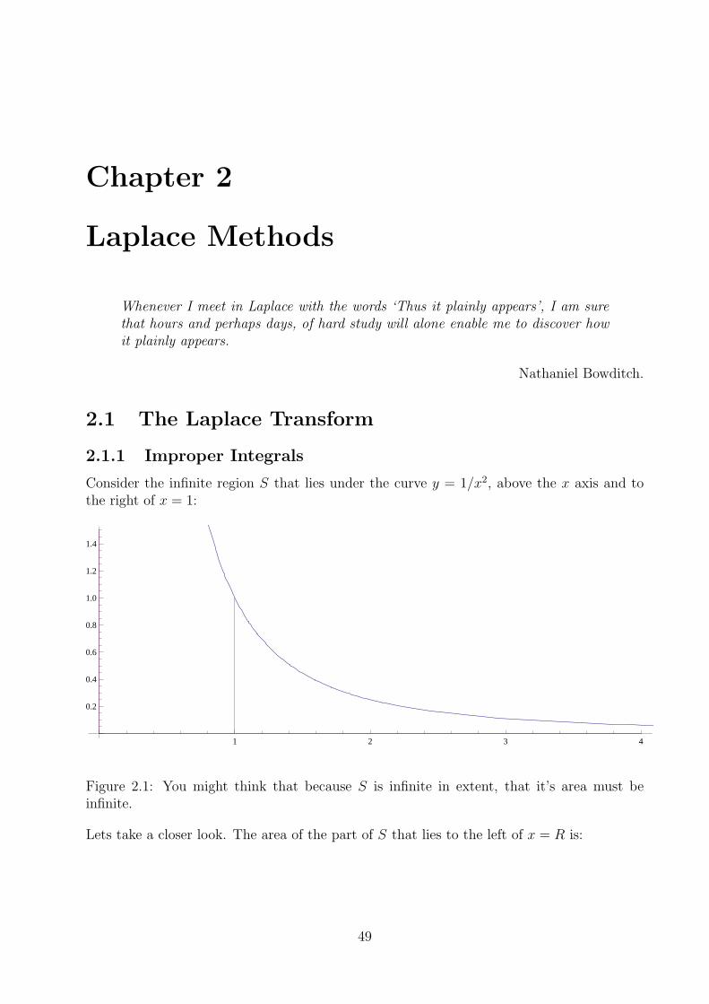
2.1.1 Improper Integrals
Consider the infinite region S that lies under the curve y = 1/x2, above the x axis and tothe right of x = 1:
1 2 3 4
0.2
0.4
0.6
0.8
1.0
1.2
1.4
Figure 2.1: You might think that because S is infinite in extent, that it’s area must beinfinite.
Lets take a closer look. The area of the part of S that lies to the left of x = R is:
49

MATH7021 — Technological Maths 312 50
We also observe that
The area A(R) approaches 1 as t → ∞, so we say that the area of the infinite region S equals1 and we write:
Using this example as a guide, we define the integral of f over an infinite interval as thelimit of integrals over finite intervals.
Definition
If∫ R
af(x) dx exists for every R ≥ a, then
The integral∫∞a
f(x) dx is called convergent if it exists; otherwise it is divergent.
Examples
1. Determine whether the integral∫∞1
1/x dx is convergent or divergent.
2. Evaluate ∫ ∞
0
xe−x dx.
MATH7021 — Technological Maths 312 51
3. Evaluate ∫ ∞
0
1
1 + x2dx
At the very roughest level, the Laplace Transform is a function:
The difference between functions of the type f(x) = x2 and the Laplace Transform is thatthe inputs are functions of a real variable — and the outputs are functions of a complexvariable (rather than real-number-inputs and real-number-outputs). By and large we will besuppressing the fact that L{f(t)} = F (s) is a function defined on the complex numbers, andwe will usually just treat s as a real number. An interpretation is that t is a time variableand s is a frequency variable.
2.1.2 Definition
Consider a function f(t) defined for t ≥ 0. Then, if the integral:
exists at s, it is called the Laplace transform of f(t) and we write:

MATH7021 — Technological Maths 312 52
Exercises
1. Determine whether the integrals are convergent or divergent. Evaluate those that areconvergent.
(i)
∫ ∞
1
1
(3x+ 1)2dx.
(ii)
∫ ∞
0
x
(x2 + 2)2dx.
(iii)
∫ ∞
4
e−y/2 dy.
(iv)
∫ ∞
2π
sin θ dθ.
(v)
∫ ∞
0
dz
z2 + 3z + 2.
2. Find the Laplace transform of the zero function f(t) = 0.
3. Find the Laplace transform of the following function, g(t):
g(t) :=
{1 if t ∈ [0, 1]0 otherwise.
(2.1)
2.1.3 The Laplace Transform of Elementary Functions
Analysis Fact
Let a, b > 0;
limx→∞
xa
ebx= 0.
Constant Function
Let f(t) = k, a constant. What about L{f(t)}?
In the region where s > 0:
MATH7021 — Technological Maths 312 53
In particular;
L{1} =1
s, for s > 0. (2.2)
Exponential Function
Let f(t) = eat where a ∈ R.
Now if s > a, then a− s < 0 hence e(a−s)R → 0:
So for s > a;
L{eat} =1
s− a, for s > a. (2.3)
Identity Function
Let f(t) = t.
Let I =∫te−st dt;

MATH7021 — Technological Maths 312 54
Now putting in the limits:
Now assume that s > 0. Now as R → ∞:
So for s > 0;
L{t} =1
s2, for s > 0. (2.4)
Powers
We can show by induction that for s > 0;
L{tn} =n!
sn+1, for s > 0. (2.5)
Polynomials and Trigonometric Functions
Let p(t) = antn + an−1t
n−1 + · · ·+ a1t+ a0 be a polynomial. What about L{p(t)}? How canwe do the Laplace transform of this sum?
Complex Analysis Fact
We have the following:
cosωt =
sinωt =
So to look at the Laplace Transform of say, cos 2t, we can consider the Laplace transform of:
The next section will show us how to do this.
MATH7021 — Technological Maths 312 55
Linearity
Suppose that a, b ∈ R and g, h : R → R are real functions. Define
f(t) = ag(t) + bh(t).
What can we say about L{f(t)} — i.e. about sums f + g and linear combinations f + λg?
Proposition
The Laplace transform is linear:
L{ag(t) + bh(t)} = aL{g(t)}+ bL{h(t)} = aG(s) + bH(s) (2.6)
Proof: This all hinges on the fact that integration is linear •
Examples
1. Find the Laplace transform of
q(t) = at2 + bt+ c.
Solution:
2. Find the Laplace transform of f(t) = 4e−t − 1t3.Solution:

MATH7021 — Technological Maths 312 56
2.1.4 Sine and Cosine
1. We have that
Hence, L{cosωt}:
2. Now looking at sinωt:

MATH7021 — Technological Maths 312 57
Example
Find L{cos 5t}.
2.1.5 First Shift Theorem
Proposition
Suppose that a ∈ R and L{f(t)} = F (s). Then
L{e−atf(t)} = F (s+ a).
Proof:
•
Examples
1. Find L{ett2}.
2. Find L{e−2t cos 3t}.

MATH7021 — Technological Maths 312 58
2.1.6 Differentiation
Can we say anything about the Laplace transform of a derivative? First we have to say alittle something about functions with a Laplace transform.
Integration Fact
Suppose that∫∞0
g(x) dx exists; then limx→∞ g(x) = 0.

MATH7021 — Technological Maths 312 59
Proposition
Suppose that f(t) has Laplace transform F (s). Then
L{f ′(t)} = sF (s)− f(0).
Proof
Do an integration by parts and use the above fact •
Example
Suppose that y(x) is the solution of the differential equation:
dy
dx− 5y = 5e−x,
and y(0) = 1. Find L{y}.
Proposition
Suppose that f(t) has Laplace transform F (s). Then
L{f ′′(t)} = s2F (s)− sf(0)− f ′(0).
Proof
Two integrations by parts •
MATH7021 — Technological Maths 312 60
Example
Find the Laplace transform of the door closer; i.e. the function x(t) satisfying the differentialequation:
md2x
dt2+ λ
dx
dt+ kx = 0.
You can assume that the initial displacement is A and initial speed is 0. m, λ and k areconstants.
Exercises
1. Find the Laplace Transform of the following functions:
(i) 6 cos 4t+ t3
(ii) 6t2 + 3t− 8
(iii) 3 sin 5t+ 4 cos 5t
(iv) 50t− 250(1− e−t/5)
(v) t2(1− t)
(vi) (t+ 1)2
(vii)(t2 + 3t)3
t

MATH7021 — Technological Maths 312 61
2. Find the Laplace transforms of the functions which satisfy the following differentialequations:
(i) 4dI
dt+ 12I = 60 , I(0) = 0.
(ii) y′′ + 2y′ + 4y = 0 , y(0) = 1, y′(0) = 0.
(iii) y′′ − 2y′ − 5y = 0 , y(0) = 0, y′(0) = 3.
(iv)dx2
dt2+ 4
dx
dt+ 5x(t) = 0 , x(0) = 1, x′(0) = 2
(v)d2θ
dt2− 4
dθ
dt+ 13θ(t) = 3e2x − 5e3x , θ(0) = θ′(0) = 1.
(vi)f ′′(t)− 3f ′(t) = 2e2x sin x , f(0) = 1 , f ′(0) = 2.
2.2 The Inverse Laplace Transform
A Review of Partial Fractions
1.
2.
3.

MATH7021 — Technological Maths 312 62
Example
Find the partial fraction expansion of
x2 + 2x− 1
2x3 + 3x2 − 2x
Now comparing the numerators:

MATH7021 — Technological Maths 312 63
The Cover Up Method
There is a cheeky little method for doing partial fractions when q(x) factors has two distinctlinear terms. Suppose we are trying to find the partial fraction decomposition of
5x+ 10
(x+ 1)(x+ 6).
1. Cover-up the x+ 6 with your hand and put x = −6 into what is left:
2. Cover-up the x+ 1 with your hand and put x = −1 into what is left:
3. These residues are the constants:
Theorem
When we have q(x) factorising into distinct linear terms the cover-up method always works.
Examples
Use the cover-up method to find the partial fraction expansion of:
1
(x− 8)(x− 6)
Use the cover-up method to find the partial fraction expansion of:
5x− 2
x2 − 4.
MATH7021 — Technological Maths 312 64
2.2.1 Definition
We have seen that the Laplace Transform takes functions from the t-domain to the s-domain.Is there an inverse transform, L−1 that can take us back (faithfully)? The answer is yes —we will not be examining this transform in detail but you can believe me that it does exist.Of course it has the special property that
Straight away looking at the table of Laplace transforms we can see the following (in allcases F (s) = L{f(t)} and G(s) = L{g(t)}):
Proposition
• Linearity: For any constants a, b ∈ R, L−1{aF (s) + bG(s)} = af(t) + bg(t).
• First Shift Theorem: L−1{F (s− a)} = eatf(t).
• Powers: L−1{1/sn} = tn−1/(n− 1)!.
• Linear Partial Fractions:
L−1
{1
s− a
}= eat.
• Quadratic Partial Fractions:
L−1
{s
s2 + k2
}= cos kt
and
L−1
{k
s2 + k2
}= sin kt
Loads of Examples
Find the inverse Laplace transforms of the following functions:
1.12s
(s+ 3)(s− 2)

MATH7021 — Technological Maths 312 65
2.4s
36s2 + 1
3.2
(s+ 3)5

MATH7021 — Technological Maths 312 66
4.3s2 + 2
(s− 2)(s+ 3)(s2 + 25)

MATH7021 — Technological Maths 312 67
5.(s+ 1)2
s4

MATH7021 — Technological Maths 312 68
6.2s+ 1
s2 + 6s+ 13

MATH7021 — Technological Maths 312 69
7.6s
s2 + 8s+ 25

MATH7021 — Technological Maths 312 70
Exercises
Find the Inverse Laplace transforms of the following functions:
(i)(s+ 1)3
s4
(ii)1
4s+ 1
(iii)4s
4s2 + 1
(iv)1
s2 + 3s
(v)2s+ 4
(s− 2)(s2 + 4s+ 3)
(vi)s
(s− 1)(s2 + 1)
(vii)s
(s2 − 4)(s+ 2)
(viii)4
s(s2 + 4)
(ix)s
s2 + 6s+ 13
(x)12
s(s+ 2)2
2.3 First and Second Order Linear Differential Equa-
tions
A differential equation is an equation involving an unknown function y(x) and it’s derivatives:
The aim is to solve for the function y(x). In this section we deal with ordinary differentialequations — that is differential equations involving a function of a single variable; e.g. y(x).

MATH7021 — Technological Maths 312 71
2.3.1 Solving Linear Differential Equations using Laplace Trans-forms
Consider a linear differential equation:
1. Take the Laplace transform of both sides.
2. Solve for L{y} =: Y (s), the transformed solution.
3. Find the solution y(t) by applying the inverse transform to Y (s).
All of our differential equations in MATH7021 will look like:
where a, b, c ∈ R. In many examples ϕ(t) will be zero. We will now present a number ofexamples of differential equations which can be solved using this method.
Examples
Solve the initial value problem:
y′′(x) + y′(x)− 6y(x) = 0
subject to the initial values y(0) = 1, y′(0) = 0.
Apply the boundary conditions:
Expand using partial fractions — we can use the cover-up method here:

MATH7021 — Technological Maths 312 72
Now applying the inverse transform:
Exercises
Solve the following differential equations:
(i)d2y
dt2+ 10
dy
dt+ 29y = 0 , y(0) = 1, y′(0) = 0.
(ii) y′′ − 4y′ + y = 0 , y(0) = 1, y′(0) = 0.
(iii) y′′ + 2y′ + 4y = 0 , y(0) = 3, y′(0) = 6.
(iv) y′′ + 4y = 0 , y(0) = −1, y′(0) = −8.
(v) y′′ − 16y = 0 , y(0) = 5, y′(0) = e.
2.4 Systems of Linear Differential Equations

Chapter 3
Numerical Methods II
People take the longest possible paths, digress to numerous dead ends, and makeall kinds of mistakes. Then historians come along and write summaries of thismessy, nonlinear process and make it appear like a simple, straight line.
Dean Kamen
3.1 Curve Fitting II
3.1.1 Lagrange Interpolation
3.1.2 The Method of Least Squares
3.1.3 Linear Regression
Pearson’s Product-Moment Correlation Coefficient
3.1.4 Non-Linear Laws
[Fitting a curve such as a parabola to a set of points]
73

Chapter 4
Multiple Integrals
I’m very good at integral and differential calculus, I know the scientific names ofbeings animalculous; in short, in matters vegetable, animal, and mineral, I amthe very model of the modern Major General.
W.S. Gilbert in the Pirates of Penzance.
4.1 Line Integrals
[Development and evaluation of line integrals along various paths including closed paths.]
4.2 Double Integrals
[Development and evaluation of double integrals over various regions.]
4.3 Jacobians
4.4 Applications: Centroids and the Second Moment
of Area
4.5 Triple Integrals
74


![Gauss-Siedel Method - Mathematics for College …mathforcollege.com/.../gen/04sle/mws_gen_sle_ppt_seidel.pdfGauss-Seidel Method Solve for the unknowns Assume an initial guess for [X]](https://static.fdocuments.net/doc/165x107/5ac15f6b7f8b9a357e8c99f8/gauss-siedel-method-mathematics-for-college-method-solve-for-the-unknowns.jpg)