Math Notes Full
51
MATH 10250 MATHS FOR ENGINEERS I DIFFERENTIAL CALCULUS Dr. Marius Ghergu School of Mathematical Sciences University College Dublin e-mail: [email protected] Contents 1 Sets and functions 3 1.1 Sets .............................................. 3 1.2 Functions ........................................... 4 1.3 The composite of two functions ............................... 9 1.4 Inverse functions ....................................... 10 2 Limits and Continuity 12 2.1 Infinite limits ......................................... 12 2.2 Continuity of functions .................................... 13 2.3 Some examples of continuous functions ........................... 13 2.4 Basic Limit Theorems .................................... 14 2.5 l’Hˆopital’sRule ........................................ 15 3 Differentiation 16 3.1 Mechanical Interpretation of Derivative .......................... 16 3.2 Tangent lines ......................................... 16 3.3 Basic Rules of Differentiation ................................ 17 3.4 Derivatives of some standard functions ........................... 17 3.5 Inverse trigonometric functions ............................... 18 3.6 Differentiation of inverse functions in general ....................... 19 3.7 Implicit differentiation .................................... 19 3.8 Appendix on trigonometry .................................. 20 4 The exponential and logarithm functions 21 4.1 Some properties of the exponential. ............................ 22 4.2 Properties of log ....................................... 22 4.3 Logs to other bases ...................................... 23 1
-
Upload
areq-mikolajczak -
Category
Documents
-
view
145 -
download
4
Transcript of Math Notes Full
MATH 10250
MATHS FOR ENGINEERS I DIFFERENTIAL CALCULUS
Dr. Marius GherguSchool of Mathematical Sciences
University College Dubline-mail: [email protected]
Contents
1 Sets and functions 3
1.1 Sets . . . . . . . . . . . . . . . . . . . . . . . . . . . . . . . . . . . . . . . . . . . . . . 3
1.2 Functions . . . . . . . . . . . . . . . . . . . . . . . . . . . . . . . . . . . . . . . . . . . 4
1.3 The composite of two functions . . . . . . . . . . . . . . . . . . . . . . . . . . . . . . . 9
1.4 Inverse functions . . . . . . . . . . . . . . . . . . . . . . . . . . . . . . . . . . . . . . . 10
2 Limits and Continuity 12
2.1 Infinite limits . . . . . . . . . . . . . . . . . . . . . . . . . . . . . . . . . . . . . . . . . 12
2.2 Continuity of functions . . . . . . . . . . . . . . . . . . . . . . . . . . . . . . . . . . . . 13
2.3 Some examples of continuous functions . . . . . . . . . . . . . . . . . . . . . . . . . . . 13
2.4 Basic Limit Theorems . . . . . . . . . . . . . . . . . . . . . . . . . . . . . . . . . . . . 14
2.5 l’Hopital’s Rule . . . . . . . . . . . . . . . . . . . . . . . . . . . . . . . . . . . . . . . . 15
3 Differentiation 16
3.1 Mechanical Interpretation of Derivative . . . . . . . . . . . . . . . . . . . . . . . . . . 16
3.2 Tangent lines . . . . . . . . . . . . . . . . . . . . . . . . . . . . . . . . . . . . . . . . . 16
3.3 Basic Rules of Differentiation . . . . . . . . . . . . . . . . . . . . . . . . . . . . . . . . 17
3.4 Derivatives of some standard functions . . . . . . . . . . . . . . . . . . . . . . . . . . . 17
3.5 Inverse trigonometric functions . . . . . . . . . . . . . . . . . . . . . . . . . . . . . . . 18
3.6 Differentiation of inverse functions in general . . . . . . . . . . . . . . . . . . . . . . . 19
3.7 Implicit differentiation . . . . . . . . . . . . . . . . . . . . . . . . . . . . . . . . . . . . 19
3.8 Appendix on trigonometry . . . . . . . . . . . . . . . . . . . . . . . . . . . . . . . . . . 20
4 The exponential and logarithm functions 21
4.1 Some properties of the exponential. . . . . . . . . . . . . . . . . . . . . . . . . . . . . 22
4.2 Properties of log . . . . . . . . . . . . . . . . . . . . . . . . . . . . . . . . . . . . . . . 22
4.3 Logs to other bases . . . . . . . . . . . . . . . . . . . . . . . . . . . . . . . . . . . . . . 23
1
4.4 The power function . . . . . . . . . . . . . . . . . . . . . . . . . . . . . . . . . . . . . . 23
4.5 Properties of the power function . . . . . . . . . . . . . . . . . . . . . . . . . . . . . . 23
4.6 Logarithmic differentiation . . . . . . . . . . . . . . . . . . . . . . . . . . . . . . . . . . 24
5 The hyperbolic functions 25
5.1 Standard formulae for hyperbolic functions . . . . . . . . . . . . . . . . . . . . . . . . 26
5.2 Osborn’s Rule . . . . . . . . . . . . . . . . . . . . . . . . . . . . . . . . . . . . . . . . . 27
5.3 Derivatives of hyperbolic functions . . . . . . . . . . . . . . . . . . . . . . . . . . . . . 27
5.4 Inverse hyperbolic functions . . . . . . . . . . . . . . . . . . . . . . . . . . . . . . . . . 27
5.5 Expression in log form . . . . . . . . . . . . . . . . . . . . . . . . . . . . . . . . . . . . 28
6 Extrema of functions 29
6.1 The Mean-Value Theorem . . . . . . . . . . . . . . . . . . . . . . . . . . . . . . . . . . 30
6.2 Consequences of the Mean-Value Theorem . . . . . . . . . . . . . . . . . . . . . . . . . 31
6.3 Regions of increase and decrease . . . . . . . . . . . . . . . . . . . . . . . . . . . . . . 31
6.4 Second Derivative Test . . . . . . . . . . . . . . . . . . . . . . . . . . . . . . . . . . . . 32
7 Integral Calculus 32
7.1 Methods of Integration . . . . . . . . . . . . . . . . . . . . . . . . . . . . . . . . . . . 34
8 Numerical Approximation of Definite Integrals 36
9 Applications of the Integral Calculus 37
9.1 Total Area . . . . . . . . . . . . . . . . . . . . . . . . . . . . . . . . . . . . . . . . . . . 37
9.2 Area bounded by two graphs . . . . . . . . . . . . . . . . . . . . . . . . . . . . . . . . 37
9.3 Volume of a Solid . . . . . . . . . . . . . . . . . . . . . . . . . . . . . . . . . . . . . . . 37
9.4 Length of a Graph . . . . . . . . . . . . . . . . . . . . . . . . . . . . . . . . . . . . . . 38
9.5 Area of a Surface . . . . . . . . . . . . . . . . . . . . . . . . . . . . . . . . . . . . . . . 38
9.6 Centres of Mass and Centroids . . . . . . . . . . . . . . . . . . . . . . . . . . . . . . . 38
10 Sequences and Series 39
10.1 Sequences . . . . . . . . . . . . . . . . . . . . . . . . . . . . . . . . . . . . . . . . . . . 39
10.2 Series . . . . . . . . . . . . . . . . . . . . . . . . . . . . . . . . . . . . . . . . . . . . . 39
10.3 Power Series . . . . . . . . . . . . . . . . . . . . . . . . . . . . . . . . . . . . . . . . . . 40
10.4 Representing functions by power series . . . . . . . . . . . . . . . . . . . . . . . . . . . 41
11 Differential Equations 42
11.1 First Order Differential Equations . . . . . . . . . . . . . . . . . . . . . . . . . . . . . 42
11.2 Linear First Order Differential Equations . . . . . . . . . . . . . . . . . . . . . . . . . 43
12 Linear Second Order Differential Equations 44
12.1 Homogeneous Linear Second Order Differential Equations . . . . . . . . . . . . . . . . 44
2
12.2 Nonhomogeneous Linear Second Order Differential Equations . . . . . . . . . . . . . . 45
13 Revision 47
13.1 The hyperbolic functions . . . . . . . . . . . . . . . . . . . . . . . . . . . . . . . . . . . 47
13.2 Numerical Approximation of Definite Integrals . . . . . . . . . . . . . . . . . . . . . . 47
13.3 Applications of the Integral Calculus . . . . . . . . . . . . . . . . . . . . . . . . . . . . 48
13.3.1 Total Area . . . . . . . . . . . . . . . . . . . . . . . . . . . . . . . . . . . . . . 48
13.3.2 Area bounded by two graphs . . . . . . . . . . . . . . . . . . . . . . . . . . . . 48
13.3.3 Volume of a Solid . . . . . . . . . . . . . . . . . . . . . . . . . . . . . . . . . . . 48
13.3.4 Length of a Graph . . . . . . . . . . . . . . . . . . . . . . . . . . . . . . . . . . 49
13.3.5 Area of a Surface . . . . . . . . . . . . . . . . . . . . . . . . . . . . . . . . . . . 49
13.3.6 Centres of Mass and Centroids . . . . . . . . . . . . . . . . . . . . . . . . . . . 49
13.4 Representing functions by power series . . . . . . . . . . . . . . . . . . . . . . . . . . . 49
13.5 Differential Equations . . . . . . . . . . . . . . . . . . . . . . . . . . . . . . . . . . . . 50
13.5.1 Linear First Order Differential Equations . . . . . . . . . . . . . . . . . . . . . 50
13.5.2 Linear Second Order Differential Equations . . . . . . . . . . . . . . . . . . . . 50
13.5.3 Homogeneous Linear Second Order Differential Equations . . . . . . . . . . . . 50
13.5.4 Nonhomogeneous Linear Second Order Differential Equations . . . . . . . . . . 50
1 Sets and functions
1.1 Sets
Set theory was introduced in the late 19th century by the German mathematician Georg Cantor(1845-1918). One of his motivations was his interest in comparing the magnitudes of infinite sets ofnumbers.
Definition 1.1 A set is a collection of elements.
A subset of a set is a subcollection of the elements of that set.
Sets will usually be labelled by capital letters and the elements of the set by small letters.
Important sets
• The set of the natural numbers N = {1, 2, · · · , n, n + 1, · · · } also known as the set of positiveintegers.
• The set of the integer numbers Z = {· · · ,−3,−2,−1, 0, 1, 2, 3, · · · }.• The set of the rational numbers Q =
{ab : a ∈ Z, b ∈ Z, b 6= 0
}.
• The set of the real numbers R. It is helpful to think of the real numbers as corresponding topoints on a straight line extending infinitely to both left and right. This line is called the realnumber line.
Remark 1.2 We always have N ⊂ Z ⊂ Q ⊂ RRemark 1.3
√2, π are not a rational number
The modulus of a real number
3
Definition 1.4 For any real number x we define the modulus of x, denoted | x | by
|x| ={
x if x ≥ 0−x if x < 0
Properties of the modulus of a real number
(i) |x| ≥ 0 for all x ∈ R and |x| = 0 if and only if x = 0.
(ii) |(−x)| = |x|∀x ∈ R
(iii) |xy| = |x||y|∀x, y ∈ R(iv) |x + y| ≤ |x|+ |y|∀x, y ∈ R (this is known as the triangle inequality.)
Exercise: Prove the above four properties of the modulus!
Note√
x2 = |x| ∀x ∈ R because ”square root sign” denotes the positive square root.
Intervals
Let a and b be real numbers with a < b, i.e. a is to the left of b on the real number line.
The open interval (a, b) = {x ∈ R : a < x < b}.The closed interval [a, b] = {x ∈ R : a ≤ x ≤ b}The half-open interval [a, b) = {x ∈ R : a ≤ x < b}.The half-open interval (a, b] = {x ∈ R : a < x ≤ b}.The interval (a,∞) = {x ∈ R : a < x}.The interval (−∞, b) = {x ∈ R : x < b}.
Remark Infinity is not a real number but is a convenient symbol usually written ∞.
Remark In this course the most important sets which we will use are the set R and the variousintervals on R.
1.2 Functions
Definition Let A and B be sets.
A function f from A to B is a rule of correspondence that assigns to each element x ∈ A a uniqueelement in B denoted f(x).
We write f : A → B.
A is called the domain of the function f.
B is called the range (or the codomain) of the function f .
The graph of a function
For functions f : R→ R a useful geometric device is the graph.
4
For some easy examples it can be sketched immediately.
Some examples of functions
Example 1
f : R→ R, f(x) = x
This is called the identity function or identity map.
Its graph is a slanting straight line of slope 1 and passing through the origin, i.e. the point (0, 0)
Ex 2
f : R→ R, f(x) = mx + c where m and c are constants, i.e. fixed real numbers.
Its graph is a slanting line of slope m.
When m = 0 the graph is a line of slope zero, i.e. a horizontal line.
Ex 3
f : R→ R, f(x) =| x |This is the modulus or absolute value function. See earlier for some of its properties.
Its graph has a sharp point at the origin.
Ex 4
f : R→ R, f(x) = x2
Its graph is a parabola with vertex at the origin and its axis of symmetry is the y-axis.
Quadratic functions
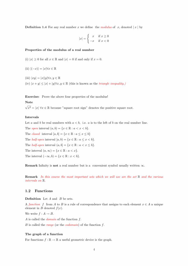
The simplest case of a quadratic function is f : R→ R, f(x) = x2.
y=x2
x
y
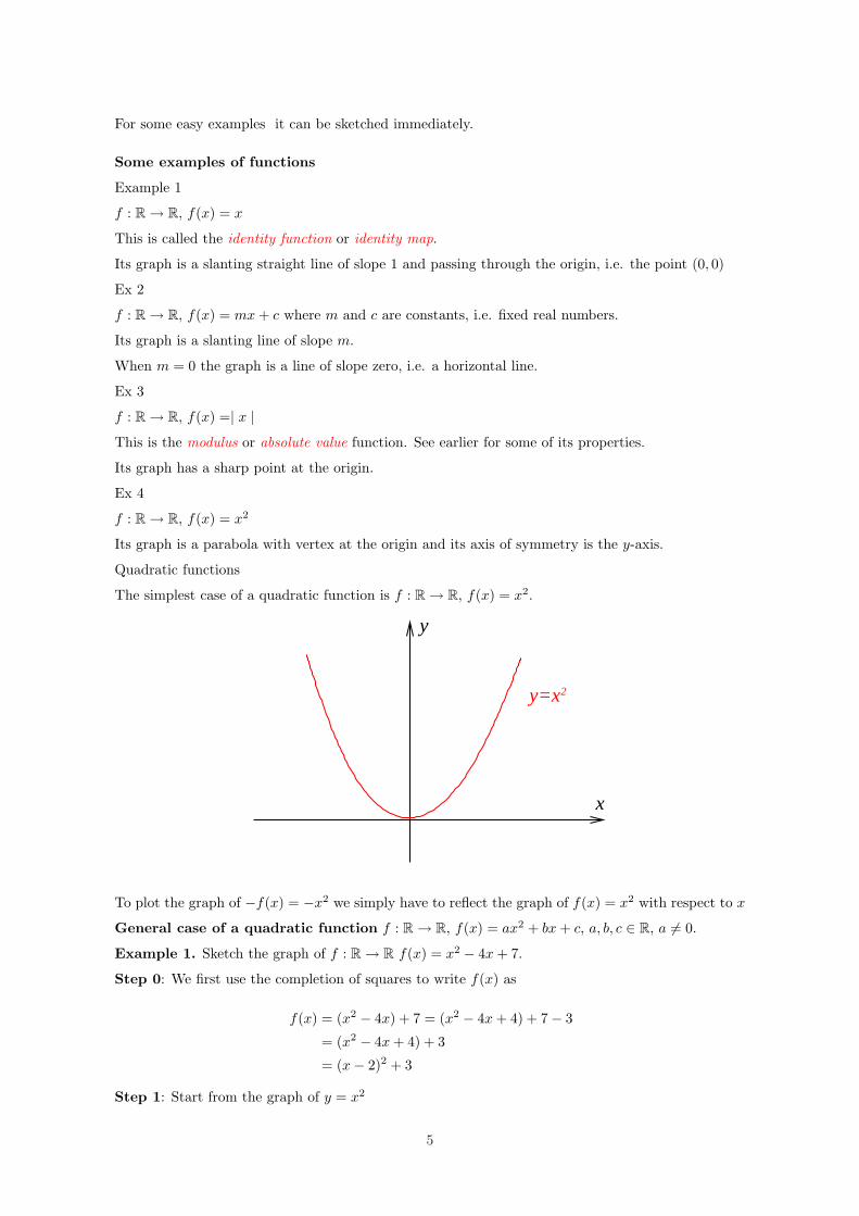
To plot the graph of −f(x) = −x2 we simply have to reflect the graph of f(x) = x2 with respect to x
General case of a quadratic function f : R→ R, f(x) = ax2 + bx + c, a, b, c ∈ R, a 6= 0.
Example 1. Sketch the graph of f : R→ R f(x) = x2 − 4x + 7.
Step 0: We first use the completion of squares to write f(x) as
f(x) = (x2 − 4x) + 7 = (x2 − 4x + 4) + 7− 3
= (x2 − 4x + 4) + 3
= (x− 2)2 + 3
Step 1: Start from the graph of y = x2
5
y
x
y=−x 2
y=x2
x
y
Step 2: Move the graph at Step 1 two units to the right to obtain the graph of y = (x− 2)2
x
y
(2,0)
y=(x−2)2
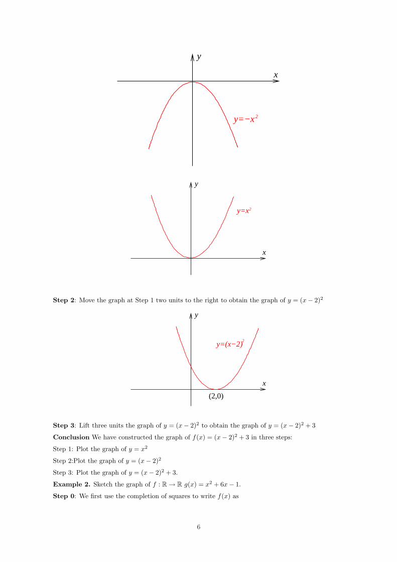
Step 3: Lift three units the graph of y = (x− 2)2 to obtain the graph of y = (x− 2)2 + 3
Conclusion We have constructed the graph of f(x) = (x− 2)2 + 3 in three steps:
Step 1: Plot the graph of y = x2
Step 2:Plot the graph of y = (x− 2)2
Step 3: Plot the graph of y = (x− 2)2 + 3.
Example 2. Sketch the graph of f : R→ R g(x) = x2 + 6x− 1.
Step 0: We first use the completion of squares to write f(x) as
6
x
y
(2,0)
y=(x−2) +3
3
2
f(x) = (x2 + 6x)− 1 = (x2 + 6x + 9)− 1− 9
= (x2 + 6x + 9)− 10
= (x + 3)2 − 10
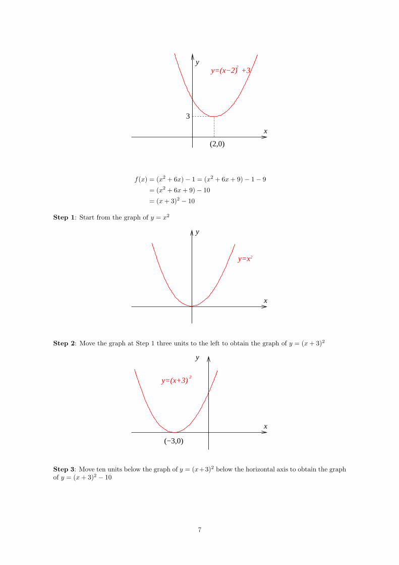
Step 1: Start from the graph of y = x2
y=x2
x
y
Step 2: Move the graph at Step 1 three units to the left to obtain the graph of y = (x + 3)2
x
y
y=(x+3)2
(−3,0)
Step 3: Move ten units below the graph of y = (x+3)2 below the horizontal axis to obtain the graphof y = (x + 3)2 − 10
7
y
x
2y=(x+3) −10
(−3,0)
−10
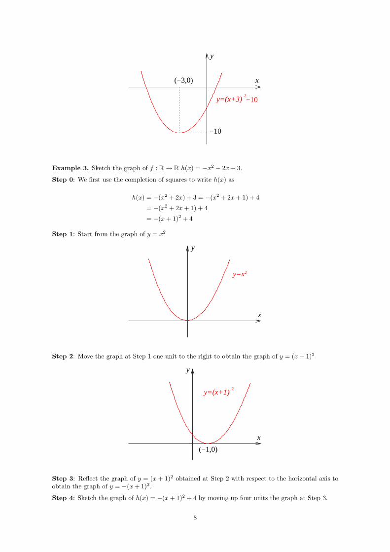
Example 3. Sketch the graph of f : R→ R h(x) = −x2 − 2x + 3.
Step 0: We first use the completion of squares to write h(x) as
h(x) = −(x2 + 2x) + 3 = −(x2 + 2x + 1) + 4
= −(x2 + 2x + 1) + 4
= −(x + 1)2 + 4
Step 1: Start from the graph of y = x2
y=x2
x
y
Step 2: Move the graph at Step 1 one unit to the right to obtain the graph of y = (x + 1)2
2
(−1,0)
y=(x+1)
x
y
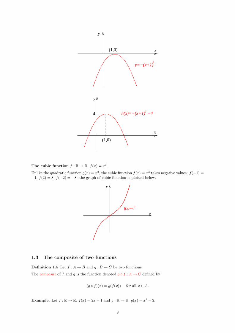
Step 3: Reflect the graph of y = (x + 1)2 obtained at Step 2 with respect to the horizontal axis toobtain the graph of y = −(x + 1)2.
Step 4: Sketch the graph of h(x) = −(x + 1)2 + 4 by moving up four units the graph at Step 3.
8
x
y
y=−(x+1)2
(1,0)
x
y
(1,0)
h(x)=−(x+1) +424
The cubic function f : R→ R, f(x) = x3.
Unlike the quadratic function g(x) = x2, the cubic function f(x) = x3 takes negative values: f(−1) =−1, f(2) = 8, f(−2) = −8. the graph of cubic function is plotted below.
x
f(x)=x3
y
1.3 The composite of two functions
Definition 1.5 Let f : A → B and g : B → C be two functions.
The composite of f and g is the function denoted g ◦ f : A → C defined by
(g ◦ f)(x) = g(f(x)) for all x ∈ A.
Example. Let f : R→ R, f(x) = 2x + 1 and g : R→ R, g(x) = x2 + 2.
9
Then(g ◦ f)(x) = g(f(x)) = f(x)2 + 2
= (2x + 1)2 + 2
= (2x2 + 4x + 1) + 2
= 4x2 + 4x + 3.
In the same manner(f ◦ g)(x) = f(g(x)) = 2g(x) + 1
= 2(x2 + 2) + 1
= 2x2 + 5.
Remark 1 To be able to define the composite g ◦ f we need the domain of f to be equal the rangeof g.
Remark 2 In general f ◦ g 6= g ◦ f .
Example. f(x) = 2x + 1 and g(x) = 3x− 4.
1.4 Inverse functions
Definition Let f : A → B be a function.
If there exists a function g : B → A such that
(g ◦ f)(x) = x for all x ∈ A
and also(f ◦ g)(x) = x for all x ∈ B,
then f is said to be the invertible.
The function g is called the inverse function of f and it is denoted by f−1 : B → A.
Remark 1 By the symmetry of this definition it follows also that f is the inverse function of g. Hencef and g are inverses of each other.
Remark 2
Many functions will not have inverses, but if an inverse function exists then it is unique.
Remark 3 Let f : A → B be an invertible function. Then its inverse is f−1 : B → A.
Hence,
• the domain of f−1 is the range of f
• the range of f−1 is the domain of f .
Question
When does a function have an inverse ?
To answer this question we need the following notions :
The function f : A → B is said to be injective if f(x1) = f(x2) implies x1 = x2, i.e. if f keepselements of A separate, i.e. f does not take two different elements of A to the same element of B.
The function f : A → B is said to be surjective if the image of f equals the whole of B, i.e. if y ∈ Bthen ∃ x ∈ X such that f(x) = y.
The function f : A → B is said to be bijective if it is both injective and surjective.
(Alternative terminology - one-one means injective, onto means surjective.)
10
Graphical criterion for injectivitity and surjectivity of real-valued functions
A function f : R→ R is injective if and only if each horizontal line, ( i.e. line parallel to the x-axis)cuts the graph of y = f(x) in at most one point.
A function f : R→ R is surjective if and only if each horizontal line cuts the graph of y = f(x) in atleast one point.
A function f : R → R is bijective if and only if each horizontal line cuts the graph of y = f(x) inexactly one point.
Theorem
A function f : A → B has an inverse if and only if f is bijective.
Remark 1
To calculate the inverse of a function given by a formula y = f(x) you solve this equation for x interms of y.
Example - f : R → R, f(x) = 5x + 8 is easily seen to be bijective, and solving y = f(x) = 5x + 8yields x = (y − 8)/5.
Hence the inverse of f is the function g : R→ R, g(x) = (x− 8)/5.
Comment
Inverse function provide some of the most useful functions in mathematics. Later in this course wewill meet
• the inverse trigonometric functions, i.e., inverses of sine, cosine, tangent;
• exponential and logarithmic functions, which are inverses of each other;
• hyperbolic functions and their inverses
Some terminology on functions
Even functions
The function f : R→ R is called an even function if f(−x) = f(x) ∀x ∈ RSymmetry feature - the graph of an even function will be symmetric about the y-axis
Standard examples of even functions are xn with n even, i.e. the even powers of x, and also thetrigonometric function cos x.
Odd functions
The function f : R→ R is called an odd function if f(−x) = −f(x) ∀x ∈ R.
Symmetry feature - the graph of an odd function will be symmetric about the origin, i.e. the graphequals its own reflection in the origin.
Standard examples of odd functions are xn with n odd, i.e. the odd powers of x, and also thetrigonometric function sinx.
Periodic functions
The function f : R → R is called a periodic function if there exists a positive real number p suchthat f(x + p) = f(x) ∀x ∈ R.
The least such positive integer p is called the period of the function f .
Symmetry feature - the graph repeats itself, i.e. once you know the graph on the interval [0, p] youcan draw the whole graph.
11
Standard examples are the trigonometric functions sine and cosine which are periodic of period 2π,and also the saw-tooth wave function f(x) = x− [x] which is periodic of period 1.
2 Limits and Continuity
The notion of limit is fundamental for any course in differential calculus because the derivative of afunction is defined as a limit.
Informal definition of a limit
Let f : U → R be a function with either U = R or else U is some open interval on R. Let x0 ∈ U.
We say that that the real number L is the limit of the function f(x) as x tends to the point x0
provided that the value of f(x) gets arbitrarily close to the value L as x gets closer and closer to thepoint x0 without actually reaching the value x0.
There is no guarantee that any such number L will exist. If no such real number L exists then wesay that the limit does not exist
Notation
We write limx→x0 f(x) = L or alternatively we write f(x) → L as x → x0 as short for the sentence”f(x) tends to the limit L as x tends to the point x0”.
It should be noted that the actual value of f at the point x0 is not relevant to determining the limit.It is the values of f(x) for x very close to x0 which matter. Indeed we can discuss limx→x0 f(x) evenwhen the function f is not defined at x0 as long as f(x) is defined for all other values of x in theneighbourhood of the point x0.
So, for example, if f(x) = sin x/x we can discuss limx→0 f(x) because f is defined for all x 6= 0. (thislimit is 1 as we shall see later).
Formal definition of a limit
Let f : U → R be a function with either U = R or else U is some open interval on R. Let x0 ∈ Uand let L ∈ R.
Then limx→x0 f(x) = L provided that, given any positive real number ε, however small, there existsa positive real number δ such that | f(x)− L |< ε for all x satisfying 0 <| x− x0 |< δ.
Remark 1
The value of δ will depend on ε. The smaller the value of ε that is chosen then the smaller the valueof δ that is needed.
Remark 2
This formal definition is the formulation into precise mathematical language of the informal definitiongiven above.
The use of this formal definition is often referred to as ε− δ technique.
ε is the Greek letter epsilon, δ is the Greek letter delta.
In this course you are not required to use ε− δ technique.
2.1 Infinite limits
Let f : U → R be a function with either U = R or else U is some open interval on R. Let x0 ∈ U .
12
We say that f has limit ∞ as x tends to x0 and write limx→x0 f(x) = ∞ provided that, given anypositive real number M , there exists a positive real number δ such that f(x) > M for all x ∈ Usatisfying 0 <| x− x0 |< δ.
We say that f has limit −∞ as x tends to x0 and write limx→x0 f(x) = −∞ provided that, given anypositive real number M , there exists a positive real number δ such that f(x) < −M for all x ∈ Usatisfying 0 <| x− x0 |< δ.
Remark
When the function f tends to a different values depending on whether you approach x0 from theright or from the left then the limit limx→x0 f(x) does not exist.
Some examples of limits
Ex 1
limx→3(2x + 7) = 13
Ex 2
limx→1x2−1x−1 = 2 because x2 − 1 = (x− 1)(x + 1) so that ∀x 6= 1, x2−1
x−1 = x + 1.
Ex 3
limx→33+√
x+63−x = 1
6 .
To see this multiply top and bottom by 3−√x + 6 so that the quotient simplifies to 13+√
x+6.
Ex 4
limx→0[x] does not exist, where [x] denotes the integral part of x(i.e. the greatest integer less thanor equal to x)
2.2 Continuity of functions
Let f : U → R be a function with either U = R or else U is some open interval on R and let x0 ∈ U.
Definition The function f is said to be continuous at the point x0 provided that limx→x0 f(x) =f(x0).
Definition The function f is said to be continuous provided that it is continuous at each point x0
in its domain U .
Intuitive picture
The function f will be continuous if and only if the graph of y = f(x) is unbroken, i..e it can bedrawn without lifting your pen from the paper.
While continuous functions are important for differential calculus there are some discontinous func-tions which are very useful in the mathematical modelling of some physical situations, e.g. squarewave function, saw-tooth wave function etc.
Note also that if the domain of a function f has a break in it then the graph of y = f(x) willnecessarily have a break in it. However the function may possibly be continuous at each point of itsdomain, e.g. f : R\0 → R, f(x) = 1/x is continuous at each point of its domain.
2.3 Some examples of continuous functions
Ex - all polynomials are continuous, e.g. f(x) = x3 + 3x2 + 3x + 1. The graph is an unbroken curve.
Ex - the trigonometric functions sine and cosine, f(x) = sin x and f(x) = cos x, are continuous. Thegraph of each one is an unbroken curve.
13
Some examples of non-continuous functions
Ex - f : R→ R, f(x) = [x], the integral part of x, i.e. the greatest integer less than or equal to x.We saw this as Ex 7 in chapter 1.
Its graph has breaks at each integer value of x, so that f fails to be continuous at each integer valueof x.
Ex - f : R→ R, f(x) = x − [x]. This is the saw-tooth wave function and fails to be continuous ateach integer value of x.
Inverse functions and continuity
If the function f : R→ R is bijective then it has an inverse g : R→ R.
If f is continuous then it is easily seen that g must also be continuous.
This follows from the fact that to obtain a formula for the inverse you solve the equation y = f(x)for x in terms of y. Hence the graph of g is obtained from that of f by swapping the x and y-axes.Thus if the graph of f is unbroken then the same is true of the graph of g.
2.4 Basic Limit Theorems
(1) limx→x0(f(x) + g(x)) = limx→x0 f(x) + limx→x0 g(x),
i.e. limit of sum = sum of limits
(2) limx→x0 kf(x) = k limx→x0 f(x) where k is any constant,
i.e. any constant multiplying a function can be taken outside of the limit.
(3) limx→x0(f(x)g(x)) = limx→x0 f(x) limx→x0 g(x),
i.e. limit of product = product of limits
(4) limx→x0(f(x)/g(x)) = (limx→x0 f(x))/(limx→x0 g(x)),
provided that limx→x0 g(x) 6= 0 and g(x) 6= 0 in the neighbourhood of x0
i.e. limit of quotient = quotient of limits provided that the quotients are well-defined, i..e providedthat the bottom line does not become zero.
(5) If f(x) ≤ g(x) for all x in the neighbourhood of x0 then limx→x0 f(x) ≤ limx→x0 g(x).
(6) The Sandwich Limit Theorem
Suppose that f(x) ≤ g(x) ≤ h(x) for all x in the neighbourhood of x0, and that limx→x0 f(x) =limx→x0 h(x) = L.
Then limx→x0 g(x) = L.
i.e. if the function g is sandwiched between two functions f and h which tend to the same limit Lthen g must also tend to L.
A famous limit
limx→x0
(sinx
x) = 1
This can be proved by some geometry and the Sandwich Limit Theorem.
14

2.5 l’Hopital’s Rule
This is a handy rule for evaluating limits involving quotients of functions.
Suppose that f(x0) = g(x0) = 0 and that the derivatives f ′(x) and g′(x) exist for all x in theneighbourhood of x0.∞
Then limx→x0
f(x)g(x)
= limx→x0
f ′(x)g′(x)
if this latter limit exists.
Note - Sometimes it may be necessary to use l’Hopital’s Rule twice or more to evaluate a limit.
Beware that it is only valid to use l’Hopital’s Rule if f(x0) = g(x0) = 0.
If the quotient f(x0)/g(x0) happens to be a finite real number then it is almost certainly the valueof the limit.
Limits as x tends to infinity
Informal definition
Let f : U → R be a function with either U = R or else U contains some interval (a,∞) on R, sothat it makes sense to talk about the values of f(x) as x tends to infinity.
We say that that the number L (real or ±∞) is the limit of the function f(x) as x tends to infinityprovided that the value of f(x) gets arbitrarily close to the value L as x gets larger and larger.
We write limx→∞ f(x) = L, or alternatively we write f(x) → L as x → ∞ as short for the sentence”f(x) tends to the limit L as x tends to infinity”.
Formal definition
Let f : U → R be a function where U is as in the informal definition above.
Then limx→∞ f(x) = L ∈ R provided that, given any positive real number ε, however small, thereexists a positive real number x0 such that | f(x)− L |< ε for all x satisfying x > x0.
Remark
The value of x0 will depend on ε. The smaller the value of ε that is chosen then the larger the valueof x0 that is needed.
Examples
Ex 1
limx→∞ 2x3+x2+x+17x3−x2−x+4 = 2
7
To see this divide top and bottom by x3.
Ex 2
limx→∞ x999+2x1000+5 = 0
To see this divide top and bottom by x1000
Ex 3
limx→∞ x4+1x3−1 = ∞.
To see this divide top and bottom by x4
(The general technique for these examples is to divide top and bottom by the highest power of xappearing.)
15
3 Differentiation
Definition 3.1 Let f : U → R be a function where either U = R or U is some open interval on R.Let x0 be a point in U . If
limh→0
f(x0 + h)− f(x0)
h
exists, it is called the derivative of f at x0
We will usually denote the derivative by f ′(x0).
Other common notation used is dfdx or dy
dx if we write y = f(x).
The quantityf(x0 + h)− f(x0)
h
is known as the Newton quotient.
In other notation we sometimes write y0 = f(x0), h = δx, y0 + δy = f(x0 + h). Then we have
dy
dx= lim
δx→0
δy
δx
Terminology
If f ′(x0) exists we say that the function f is differentiable at the point x0.
If f ′(x0) exists at all points x0 in the domain of f we say that the function f is differentiable.
Important remark
If the function f is differentiable at the point x0 then f is continuous at the point x0,
i.e. differentiable implies continuous.
This follows from the fact that the top line of the Newton quotient must tend to zero for the limit inthe definition of the derivative to exist, and top line tending to zero says exactly that the function iscontinuous.
Beware !! The converse implication is false (that is, continuous does not imply differentiable)
Example f : R→ R, f(x) =| x |, modulus of x. This function is continuous at the point x = 0 butnot differentiable at x = 0.
Geometric Interpretation of Derivative
The derivative f ′(x0) may be interpreted as the slope of the tangent at the point (x0, f(x0)) to thegraph of y = f(x).
The derivative exists if and only if the graph has a tangent of finite slope at the point (x0, f(x0)).
3.1 Mechanical Interpretation of Derivative
The derivative f ′(x0) may be interpreted as the instantaneous rate of change of y with respect to xwhere y = f(x).
If x represents time and y represents distance then the Newton quotient represents the average speedover a time interval of length h and the derivative represents the instantaneous speed at time x = x0.
3.2 Tangent lines
The equation of any tangent line to the curve y = f(x) is easily calculated.
16
Writing y0 = f(x0) and m = f ′(x0), the equation of the tangent at the point (x0, y0) is
y − y0 = m(x− x0).
Similarly the normal line at (x0, y0), i.e. the line perpendicular to the tangent line, is
y − y0 = (−1/m)(x− x0)
3.3 Basic Rules of Differentiation
(1)d
dx(f + g) =
df
dx+
dg
dx
(2)d(kf)
dx= k
df
dxwhere k is a constant
(3) PRODUCT RULEd
dx(fg) = f
dg
dx+ g
df
dx
(4) QUOTIENT RULEd
dx
(f
g
)=
g dfdx − f dg
dx
g2
(5) CHAIN RULE
Let u(x) be a differentiable function of x and g(u) be a differentiable function of u.
Then the composite function (g ◦ u)(x) is differentiable and, writing dgdx as short for d
dx ( g ◦ u), wehave the chain rule formula
dg
dx=
dg
du
du
dx
In composite notation we should really write
(g ◦ u)′(x0) = g′(u(x0)) u′(x0)
Remark
Differentiation from first principles is not required for the examination.
Differentiation using the above rules will most certainly be examined.
3.4 Derivatives of some standard functions
(1) f(x) = k:f ′(x) = 0 for any constant k.
(2) f(x) = xn:f ′(x) = nxn−1 for all integers n, both positive and negative.
(3) Trigonometric functions (also sometimes called the circular functions)
f(x) = sin x, f ′(x) = cos x
f(x) = cos x, f ′(x) = − sin x
17
f(x) = tan x, f ′(x) = sec2 x
f(x) = sec x, f ′(x) = sec x tan x
f(x) = cosecx, f ′(x) = −cosecx cot x
f(x) = cot x, f ′(x) = −cosec2x
Beware that tan and sec are undefined at all odd integer multiples of π2 since cos takes value zero at
these points.
Beware that cosec and cot are undefined at all integer multiples of π since sin takes value zero atthese points.
3.5 Inverse trigonometric functions
Inverse sine, denoted sin−1 or arcsin .
The function f : R→ R, f(x) = sin x is neither injective nor surjective. To make it injective werestrict the domain to be [−π
2 , π2 ], and to make it surjective we restrict the codomain to be [−1, 1].
Hence we define the inverse sine function as follows :
sin−1 : [−1, 1] → [−π2 , π
2 ] is defined to be the unique element y ∈ [−π2 , π
2 ] such that sin y = x.
The derivative of sin−1 x exists for all x ∈ (−1, 1) and
d
dx(sin−1 x) =
1√1− x2
Inverse cosine, denoted cos−1 or arccos .
The function f : R→ R, f(x) = cos x is neither injective nor surjective. To make it injective werestrict the domain to be [0, π], and to make it surjective we restrict the codomain to be [−1, 1].Hence we define the inverse cosine function as follows :
cos−1 : [−1, 1] → [0, π] is define to be the unique element y ∈ [0, π] such that cos y = x.
The derivative of cos−1 x exists for all x ∈ (−1, 1) and
d
dx(cos−1 x) = − 1√
1− x2
Inverse tangent, denoted tan−1 or arctan
The function f : R→ R, f(x) = tan x is not injective but is surjective. To make it injective werestrict the domain to be the open inerval (−π
2 , π2 ). Hence we define the inverse tangent function as
follows :
tan−1 : R→ (−π2 , π
2 ) is defined to be the unique element y ∈ (−π2 , π
2 ) such that tan y = x.
The derivative of tan−1 x exists for all x ∈ R and
d
dx(tan−1 x) =
11 + x2
The above are the three most important inverse trigonometric functions. Inverses of the other trigono-metric functions, i.e. sec, cosec and cot, can also be defined, with appropriate choices of domain andcodomain, and formulae for their derivatives obtained.
Equivalently we can define them as follows :
18
sec−1 x = cos−1 1x
cosec−1 x = sin−1 1x
cot−1 x = tan−1 1x
3.6 Differentiation of inverse functions in general
Let the function f(x) be differentiable and bijective. Let g be the inverse function of f so thatg(f(x)) = x and f(g(x)) = x for all x.
Then the function g is differentiable at all points f(x0) where f ′(x0) 6= 0 and
g′(f(x0) =1
f ′(x0)
Remark 1
Geometrically we can see why the condition f ′(x0) 6= 0 is necessary. The graph of y = g(x) isobtained from that of y = f(x) by swapping the roles of the x and y-axes. If f ′(x0) = 0 then thetangent to the graph of y = f(0x) has slope zero, i.e. it is horizontal, at the point x0. On swappingthe axes the tangent to the graph of y = g(x) will become vertical at the point f ′(x0), i.e. the slopebecomes infinite, so that the derivative g′ will not exist at the point f (x0).
Note that if f is bijective and differentiable with f ′(x) 6= 0 for all x in the domain of f then theinverse function g will be differentiable throughout its domain.
If you can differentiate f(x) then the following technique enables you to calculate the derivative of g.
Write y = g(x)
Then f(y) = f(g(x)) = x since f and g are inverses.
Differentiate each side of the equation f(y) = x with respect to x to obtain f ′(y) dydx = 1. (Chain
rule was used here !)
This yields the resultdy
dx=
1f ′(y)
This technique may be used in particular to obtain the derivatives of the inverse trigonometricfunctions mentioned above.
3.7 Implicit differentiation
The technique used above, of differentiating a whole equation with respect to x, is known as implicitdifferentiation.
We illustrate by an example.
Consider the equation x3 + y3 − 9xy = 0.
Implicit differentiation gives 3x2 + 3y2 dydx − 9y − 9x dy
dx = 0
Re-arranging yieldsdy
dx=
9y − 3x2
3y2 − 9x
The equation represents a certain curve in the plane, known as the folium of Descartes.
19
The point (2, 4) lies on the curve. (Check that x = 2, y = 4 satisfies the equation).
Then, substituting in the formula gives dydx = 4
5 at the point (2, 4) .
Hence the tangent line at this point has equation
y − 4 =45(x− 2)
3.8 Appendix on trigonometry
The two basic trigonometric functions are sine and cosine, written sin and cos for short.
We assume that you are familiar with functions f : R→ R, f(x) = sin x and f : R→ R, f(x) = cosx.
These are periodic functions of period 2π and their graphs are wave-shaped curves.
Note that −1 ≤ sin x ≤ 1 and −1 ≤ cosx ≤ 1 for all x ∈ R.
Also sin(−x) = − sin x and cos(−x) = cos x for all x ∈ R,, i.e. sin is an odd function while cos is aneven function.
The other trigometric functions are defined in terms of these :
tanx =sin x
cos x, called tangent
sec x =1
cos x, called secant
cos ecx =1
sin x, called cosecant
cot x =cosx
sin x, called cotangent
We will always use the shortened version of these names.
Note that tanx and sec x are undefined when cos x = 0, i.e. when x is an odd integer multiple of π/2.
Note that cos ecx and cot x are undefined when sin x = 0, i.e. when x is an integer multiple of π.
From triangle geometry you should be familiar with the following two rules for a triangle with anglesA,B,C at the vertices and the opposite sides of lengths a,b,c respectively :
Sine Rulea
sin A=
b
sin B=
c
sinC
Cosine rulea2 = b2 + c2 − 2bc cos A
More generally there are the following standard trigonometric identities :
Triangle identities
cos2 x + sin2 x = 11 + tan2 = sec2 x
1 + cot2 x = cos ec2x
20
Compound angle formulae
sin(x + y) = sin x cos y + cos x sin y
sin(x− y) = sin x cos y − cos x sin y
cos(x + y) = cos x cos y − sin x sin y
cos(x− y) = cos x cos y + sin x sin y
tan(x + y) =tan x + tan y
1− tan x tan y
tan(x− y) =tan x− tan y
1 + tan x tan y
Double angle formulae
sin 2x = 2 sin x cos x
cos 2x = 2 cos2 x− 1 = 1− 2 sin2 x
cos2 x =1 + cos 2x
2
sin2 x =1− cos 2x
2
tan 2x =2 tan x
1− tan2 x
Sum and product identities
sin x + sin y = 2 sin(x + y
2) cos(
x− y
2)
sin x− sin y = 2 cos(x + y
2) sin(
x− y
2)
cosx + cos y = 2 cos(x + y
2) cos(
x− y
2)
cosx− cos y = −2 sin(x + y
2) sin(
x− y
2)
Radian measure
In triangle geometry it is usual to measure angles in degrees. However in the calculus of trigonometricfunctions it is conventional to measure angles in radians. It is easy to translate from one scale ofmeasurement to the other.
2π radians = 360 degreesπ radians = 180 degreesπ
2radians = 90 degrees
etc.
4 The exponential and logarithm functions
Definition 4.1 The exponential function is the unique function f : R→ R such that
(1) f ′(x) = f(x) for all x ∈ R,
(2) f(0) = 1.
It can be proved that there exists a unique function f : R→ R satisfying properties (1) and (2).
We will write either f(x) = exp x or f(x) = ex as shorthand notation for the exponential function.
21
4.1 Some properties of the exponential.
(i)exp x > 0 for all x ∈ R. Also exp x →∞ as x →∞ while exp x → 0 as x → −∞.
(ii)(exp x)(exp y) = exp(x + y) for all x, y ∈ R
(iii)
exp(−x) =1
exp xfor all x ∈ R
Examination of the graph shows that the function f : R→ R, f(x) = exp x is injective but notsurjective. Its image is (0,∞).
Hence the function f : R→ (0,∞), f(x) = expx, is bijective.
Its inverse is a function (0,∞) → R called the natural logarithm function, denoted log x, or sometimesln x.
4.2 Properties of log
(i) The function log x is defined only for positive values of x. Also log x → ∞ as x → ∞ whilelog x → −∞ as x → 0.
(ii)
log x > 0 for all x > 1log x < 0 for all x < 1log 1 = 0
(iii)
log(exp x) = x for all x ∈ Rexp(log x) = x for all x ∈ (0,∞)
(iv)log(xy) = log x + log y for all x > 0, y > 0
(v)
log(1x
) = − log x for all x > 0
(vi)log(
x
y) = log x− log y for all x > 0, y > 0
The real number e
We define the real number e = exp 1, the value of the exponential function at x = 1.
It can be shown that e is an irrational number with an infinte non-recurring decimal expansion.
To three decimal places e = 2.718.
Observe that log e = 1 since log and exp are inverses, so that log(exp 1) = 1.
Differentiation of the logarithm function
22
We have seen that, as part of the definition, the exponential function equals its own derivative, i.e.if f(x) = exp x then f ′(x) = exp x.
Also, by property (i), exp x > 0 for all x ∈ R, so that the derivative of the exponential function isnever zero. It follows then, by our earlier proposition on the differentiation of inverse functions,that the logarithm function is differentiable at all points in its domain.
Indeedd
dx(log x) =
1x
for all x > 0
This follows easily from implicit differentiation of the equation exp y = x.
4.3 Logs to other bases
Let k be any positive real number, excluding k = 1.
We define a function logk : (0,∞) → R, called log to the base k, by
logk x =log x
log kfor all x > 0
Here log x and log k are the natural logs.
When k = e note that loge x = log x. Thus log to the base e coincides with the natural logarithmdefined earlier as the inverse of the exponential.
Note also that, for any fixed k, the function logk x is a constant multiple of log x, the constant being1/ log k.
k > 1: log k > 0: logk x is an increasing function of x.
k < 1: log k < 0: logk x is an decreasing function of x.
The special case k = 10 gives logs to the base 10. These were the logs commonly used for calculationsup until the last thirty or forty years. They appear in the old books of log tables. Calculators etchave now replaced log tables !
4.4 The power function
Let a be any positive real number. Let b be any real number. We will now define a to the power b asfollows:
ab = exp(b log a)
4.5 Properties of the power function
(i)a0 = 1
(ii)a1 = a
(iii)abac = ab+c
(iv)log(ab) = b log a
(v)(ab)c = abc
23
These properties follow easily from the properties of log and exp listed earlier.
Remark 1
The special case a = e, the real number we defined earlier as exp 1, shows that ex = exp(x log e) =expx since log e = 1.
This justifies the shorthand notation ex for the exponential function, because exp x actually is thereal number e raised to the power x.
Remark 2
Our definition can be seen to be consistent with previous conventions and notions about powers.
By our definition a2 = exp(2 log a) = exp(log a+ log a) = exp(log a) exp(log a) = a times a, usingproperty (ii) of exp.
Thus a2 under our definition equals a times a.
Similarly, for any positive integer n, we see that an under our definition equals the product of a withitself n times.
Also a−1 under our definition equals exp(− log a) = 1/ exp(log a) = 1/a, coinciding with our conven-tional notation of a−1 for 1/a.
Furthemore recall that a1//2 is used to denote the positive square root of a. This is consistent withour new definition of a1/2 = exp(1/2 log a) because exp(1/2 log a) exp(1/2 log a) = exp(1/2 log a +1/2 log a) = exp(log a) = a. So a1/2 is a positive real number whose square equals a.
For any positive real number k 6= 1 we have a function f : R→ (0,∞), f(x) = kx which is bijective.Its inverse can be checked to be the function g : (0,∞) → R, g(x) = logk x, i.e. the functions kx andlogk x are inverses of each other.. In the special case k = e this reduces to the fact that natural logand exponential are inverses of each other.
Derivative of kx
If f(x) = kx then f ′(x) = kx log k.
This is easily verified by using the chain rule.
Remark
For any x > 0 and any real number b the function f(x) = xb is meaningful.
The chain rule now easily yields that f ′(x) = bxb−1, i.e. the basic rule for differentiating powers ofx is valid for all powers, not just integer or rational powers.
4.6 Logarithmic differentiation
This is the technique to use whenever you need to differentiate a function involving a power whichis itself a function of x, for example functions such as xx, (cos2 x)x2+x+1. We illustrate the techniqueby doing these two examples.
Ex 1
Let y = xx.
Taking logs yields log y = log(xx) = x log x using property (iv) of the power function.
Now differentiate implicitly to get1y
dy
dx= log x + x(
1x
)
using the product rule for differentiation of the right hand side.
This simplifies to givedy
dx= xx(log x + 1)
24
Ex 2
Let y = (cos2 x)x2+x+1
Taking logs yields log y = log((cos2 x)x2+x+1) = (x2 + x + 1) log(cos2 x) using property (iv) of thepower function.
Now differentiate implicitly to get
1y
dy
dx= (2x + 1) log(cos2 x) + (x2 + x + 1)(
−2 cos x sin x
cos2 x)
using the product rule for differentiation of the right hand side.
This simplifies to give
dy
dx= (cos2 x)x2+x+1{(2x + 1) log(cos2 x)− 2(x2 + x + 1) tanx}
5 The hyperbolic functions
Definition 5.1 The hyperbolic sine function, denoted sinh x is a function R→ R defined by
sinhx =ex − e−x
2
The hyperbolic cosine function, denoted cosh x is a function R→ R defined by
cosh x =ex + e−x
2
Note
From the definitions we see easily that
(i) sinhx is an odd function of x because sinh(−x) = − sinhx for all x ∈ R(ii) cosh x is an even function of x because cosh(−x) = − cosh x for all x ∈ R(iii) sinh 0 = 0
(iv) cosh 0 = 1
(v) sinhx →∞ as x →∞ and sinh x → −∞ as x → −∞(vi) cosh x →∞ as x → ±∞To see (v) and (vi) observe that as x → ∞, e−x → 0 so that the graph of both y = sinh x andy = cosh x approach that of y = (1/2)ex.
Also as x → −∞, ex → 0 so that the graph of y = sinh x approaches that of y = −(1/2)e−x whilethe graph of y = cosh x approaches that of y = (1/2)e−x.
Remark
A basic formula for hyperbolic functions is
cosh2 x− sinh2 x = 1
This can be verified by using the definitions of cosh and sinh .
This formula is the analogue of the well-known formula in trigonometry
cos2 x + sin2 x = 1.
25
Recall that the trigonometric functions are sometimes known as the circular functions because theycan be used to parametrize the unit circle which has equation
x2 + y2 = 1
We put x = cos t, y = sin t where 0 ≤ t ≤ 2π.
The hyperbolic functions can be used to parametrize the hyperbola which has equation
x2 − y2 = 1
We put x = cosh t, y = sinh t where t ∈ R.
Thus the hyperbolic functions correspond to the geometry of the hyperbola in the same way as thetrigonometric functions correspond to the geometry of the circle.
The hyperbolic functions have many similarities to the trigonometric functions sinx and cos x buthave some important differences.
The trigonometric functions are periodic but the hyperbolic functions are not periodic.
The other hyperbolic functions
We define four more hyperbolic functions, the hyperbolic tangent,secant, cosecant, and cotangent,denoted tanh, sec h, cos ech, and coth respectively :
tanh x =sinhx
cosh x
sec hx =1
cosh x
cos echx =1
sinh x
cothx =cosh x
sinhx
The first two of these are defined for all x ∈ R since cosh x is never zero, while the last two are definedfor all x 6= 0 since sinh 0 = 0.
5.1 Standard formulae for hyperbolic functions
Dividing the formula
cosh2 x− sinh2 x = 1
by cosh2 x or by sinh2 x yields two more formulae
1− tanh2 x = sec h2x
coth2 x− 1 = cos ech2x
The usual formulae for trigonometric functions (see appendix to chapter 3), e.g. formulae such assin(x + y) = sin x cos y + cos x sin y, have analogues for hyperbolic functions. The following rule maybe used :
26
5.2 Osborn’s Rule
- Given any addition formula for trigonometric functions we may translate it into a formula valid forhyperbolic functions with the modification that whenever a product of two sines appears in the trig.formula we must change the sign in front of it to get the corresponding hyperbolic formula.
Here are some examples :
Ex 1
cos2 x + sin2 x = 1 becomes cosh2 x− sinh2 x = 1
(Note that sin2 x = sin x sin x is a product of two sines.)
Ex 2
cosx− cos y = −2 sin((x + y)/2) sin((x− y)/2) becomes cosh x− cosh y = 2 sinh((x + y)/2) sinh((x−y)/2)
Ex 3
sin(x + y) = sin x cos y + cosx sin y becomes sinh(x + y) = sinh x cosh y + cosh x sinh y
Ex 4
cos(x− y) = cos x cos y − sin x sin y becomes cosh(x− y) = cosh x cosh y + sinh x sinh y
5.3 Derivatives of hyperbolic functions
(i) f(x) = sinh x, f ′(x) = cosh x
(ii) f(x) = cosh x, f ′(x) = sinh x
(iii) f(x) = tanh x, f ′(x) = sec h2x
(iv) f(x) = sec hx, f ′(x) = − sec h x tanh x
(v) f(x) = cos ech x, f ′(x) = − cos ech x cothx
(vi) f(x) = coth x, f ′(x) = − cos ech2x
Proof
(i) and (ii) follow easily from the definitions of sinhx and cosh x
The other four follow from the quotient rule.
It suffices to remember (i) and (ii) only, since from them it is easy to determine the rest.
Beware - the above rule for translating addition formulae to hyperbolic formulae does not hold foranything involving derivatives.
5.4 Inverse hyperbolic functions
f : R→ R, f(x) = sinh x is a bijective function.
Its inverse, denoted sinh−1 : R→ R, is defined by
sinh−1 x equals the unique y ∈ R such that sinh y = x.
f : R→ R, f(x) = cosh x is not bijective but if we must restrict both domain and codomain weobtain the bijective function f : [0,∞)→[1,∞), f(x) = cosh x.
Its inverse is cosh−1 : [1,∞)→[0,∞) defined by cosh−1 x equals the unique y ∈ [1,∞) such thatcosh y = x.
Similarly, by restricting the codomain of tanh, we define the the inverse hyperbolic tangent.
27
It is the function tanh−1 : (−1, 1) → R defined by tanh−1 x equals the unique y ∈ R such thattanh y = x.
Also, in similar fashion to what we did for inverse trig. functions, we can define
sec h−1x = cosh−1 1x
cos ech−1x = sinh−1 1x
coth−1 x = tanh−1 1x
Derivatives
(i) f(x) = sinh−1 x, f ′(x) = 1√x2+1
(ii) f(x) = cosh−1 x, f ′(x) = 1√x2−1
(iii) f(x) = tanh−1 x, f ′(x) = 11−x2
(iv) f(x) = sec h−1x, f ′(x) = − 1x√
1−x2
(v) f(x) = cos ech−1x, f ′(x) = − 1|x|√x2+1
(vi) f(x) = coth−1 x, f ′(x) = 11−x2
These are verified using the standard method for derivatives of inverse functions. We illustrate bydoing (i).
y = sinh−1 x: sinh y = x: cosh y dydx = 1: dy
dx = 1cosh y = 1√
x2+1
Here we used cosh2 y− sinh2 y = 1 so that cosh y =√
sinh2 y + 1, the positive square root being usedbecause cosh always takers positive values.
It is unnecessary to remember the above formulae (i) -(vi), but you should be able to work them outif necessary.
5.5 Expression in log form
It is sometimes convenient to expresss the inverse hyperbolic functions in terms of logs :
(i) sinh−1 x = log(x +√
x2 + 1)
(ii) cosh−1 x = log(x +√
x2 − 1)
(iii) tanh−1 x = 12 log( 1+x
1−x )
We derive (i) as follows :
y = sinh−1 x: sinh y = x:ey − e−y = 2x using the definition of sinh .
Multiplying by ey yields the equation e2y − 1 = 2xey which can be re-arranged to
e2y − 2xey − 1 = 0
Properties of the power function show that e2y = (ey)2 so that the above equation is
(ey)2 − 2xey − 1 = 0
28
This can be viewed as a quadratic in ey and the standard formula for solving a quadratic gives
ey =2x±√4x2 + 4
2
This simplifies toey = x±
√x2 + 1
Since ey > 0 for all y we can discard the minus sign in this last formula. (Observe that x−√x2 + 1 < 0for all x.)
Taking logs now yields the desired formula
sinh−1 x = log(x +√
x2 + 1)
Formulae (ii) and (iii) are verified similarly.
6 Extrema of functions
Let f : U → R be a function where either U = R or U is some open interval on R. Let c be a pointin U .
Definition 6.1 The point c ∈ U is a called a local maximum of the function f provided that f(x) ≤f(c) for all x in the immediate neighbourhood of the point c, i.e. if there exists some open interval Icontaining c and such that f(x) ≤ f(c) for all x ∈ I.
Note - if you move far enough away from c then f may well take larger values than f(c).
The point c ∈ U is a called a local minimum of the function f provided that f(x) ≥ f(c) for all xin the immediate neighbourhood of the point c, i.e. if there exists some open interval I containing cand such that f(x) ≥ f(c) for all x ∈ I.
Note - if you move far enough away from c then f may well take smaller values than f(c).
Remark on terminology
Sometimes the term relative maximum and relative minimum are used instead of local maximum andlocal minimum.
Proposition
Suppose that f : (a, b) → R is differentiable at all points of (a, b) and that it has a local maximum orlocal minimum at a point c in (a, b).
Then f ′(c) = 0.
Proof
Examine the Newton quotientf(c + h)− f(c)
h
If c is a local maximum then the top line of this quotient must always be negative for all h sufficientlysmall in absolute value. Now since h can take both positive and negative values we see that the onlyway that the limit of this quotient can possibly exist is if its value is zero.
This shows that f ′(c) = 0 as desired.
A similar argument applies when c is a local minimum.
Geometric View
29
Geometricallly this proposition says that at a local maximium or minimum of the function f theslope of the tangent to the curve y = f(x) is zero, i.e the tangent line is horizontal.
Remark
The above proposition may fail if the function f is not differentiable at some point in the interval(a, b).
Example - f : (−1, 1) → R, f(x) =| x |, the modulus (or absolute value) function.
The point x = 0 is clearly a local minimum but there is no point on (−1, 1) where the derivative iszero.
As we have seen earlier this function is not differentiable at x = 0.
Also if f is defined on some closed interval and if one of the end-points of the interval is a localmaximum or minimum then the conclusion of the theorem need not hold.
Example - f : [−1, 1] → R, f(x) = x.
Then x = 1 is a local maximum, x = −1 is a local minimum, but there is no point where the derivativeis zero.
6.1 The Mean-Value Theorem
Suppose that the function f : [a, b] → R is continuous on [a, b] and differentiable on (a, b).
Then there exists at least one point c ∈ (a, b) such that
f ′(c) =f(b)− f(a)
b− a
Mechanical viewpoint
If x represents time and y = f(x) represents distance travellled then we have a mechanical viewpointof the Mean-Value Theorem.
The ratio f(b)−f(a)b−a is the average speed over the time interval (a, b) while the derivative f ′(c) is the
instantaneous speed at time t = c. Hence the Mean-Value Theorem says that there is some momentof time, x = c, in the time interval (a, b) at which the speed at that instant equals the average speedover the interval.
Remark
Geometrically the Mean-Value Theorem has the following interpretation :
Let P = (a, f(a) and Q = (b, f(b)) be points on the curve y = f(x). Now f ′(c) is the slope of thetangent at x = c while f(b)−f(a)
b−a is the slope of the line segment PQ. The theorem says that there issome point R = (c, f(c)) on the curve y = f(x) at which the slope of the tangent at R to the curveequals the slope of the line segment PQ.
Remark
The Mean-Value Theorem is an existence theorem. The fact that the point c exists can be veryimportant, even if you cannot easily determine an actual value for c. In some cases you obtain avalue by solving for c in the equation
f ′(c) =f(b)− f(a)
b− a
but in other cases it can be extremely difficult.
30
6.2 Consequences of the Mean-Value Theorem
Suppose that the function f : [a, b] → R is continuous on [a, b] and differentiable on (a, b).
(i) If f ′(x) > 0 for all x ∈ (a, b) then f is strictly increasing on (a, b),
i.e. for all x1 < x2 we ahve f(x1) < f(x2)
(ii) If f ′(x) < 0 for all x ∈ (a, b) then f is strictly decreasing on (a, b),
i.e. for all x1 < x2 we have f(x1) > f(x2).
(iii) If f ′(x) = 0 for all x ∈ (a, b) then f(x) is constant on (a, b).
6.3 Regions of increase and decrease
We have the following consequences of the Mean Value Theorem :
If f ′(x) > 0 on (a, b) then f is increasing on (a, b)If f ′(x) < 0 on (a, b) then f is increasing on (a, b)
Hence a detailed examination of the sign of f ′(x) will enable us to determine the regions of increaseand decrease of the function f(x).
Example
f(x) = x3 + 2x2 − 4x + 1
Then f ′(x) = 3x2 + 4x− 4 = (3x− 2)(x + 2)
Note - to determine the sign of f ′(x) it is helpful to factorize it as much as possible.
In this example we have a product of two factors and hence f ′(x) is positive whenever both factorshave the same sign and is negative when they have opposite signs.
Examining this we see that
f ′(x) > 0 for x ∈ (−∞,−2)
f ′(x) < 0 for x ∈ (−2, 2/3)
f ′(x) > 0 for x ∈ (2/3,∞).
Thus the function f(x) ↑ on (−∞,−2) ∪ (2/3,∞).and f(x) ↓ on (−2, 2/3).
Critical points
Let f(x) be a differentiable function.
Definition 6.2 A point c in the domain of f is called a critical point of f provided that f ′(c) = 0.
Alternative terminology - the terms stationary point or turning point are also used.
Points of inflection
Definition 6.3 Let c be a point in the domain of a twice differentiable function f(x).
Then c is called a point of inflexion provided that f ′′(x) changes sign as we pass through the pointc, i.e. f ′′ is positive on one side of c and negative on the other side.
Beware that f ′′(c) = 0 does not necessarily imply that c is a point of inflexion.
Example - If f(x) = x4 then f ′(x) = 4x3 and f ′′(x) = 12x2.
31
Now f ′′(0) = 0 but x = 0 is not a point of inflexion. Clearly f ′′(x) = 12x2 does not change sign atx = 0.
Indeed it is not hard to see that x = 0 is a local minimum for the function f(x) = x4.
Remark
While points of inflection often turn out to be critical points there can exist points of inflexion whichare not critical points
Example - If f(x) = sinh x then f ′(x) = cosh x and f ′′(x) = sinh x.
Then x = 0 is a point of inflexion because f ′(x) = cosh x changes sign at x = 0.
However x = 0 is not a critical point of f(x) because f ′(0) = cosh 0 = 1
6.4 Second Derivative Test
Let c be a critical point of the differentiable function f(x).
If f ′′(c) > 0 then x = c is a local minimum of the function f(x).
If f ′′(c) < 0 then x = c is a local maximum of the function f(x).
If f ′′(c) = 0 then the test yields no information.
7 Integral Calculus
Definition 7.1 Let f : I → R where I ⊆ R is an interval.
A function F : I → R is called an antiderivative of f if F ′(x) = f(x) for all x ∈ I. We write
F (x) =∫
f(x)dx.
Example
Let f : R→ R, f(x) = x2 + 1. Then F (x) = x3
3 + x is an antiderivative of F since F ′ = f . Note thatG(x) = x3
3 + x + 7 is also an antiderivative if f (since G′ = f).
Remark
The antiderivative of f if exists is not unique. Any two antiderivatives of f differ by a constant.
Example
Let f : R→ R, f(x) = x2 + 1. Then all the antiderivatives of f are of the form F (x) = x3
3 + x + C.That is why we write ∫
(x2 + 1)dx =x3
3+ x + C
and say that the indefinite integral of x2 + 1 is x3
3 + x + C.
Basic Examples
(1)∫
xkdx =1
k + 1xk+1 + C , k 6= −1.
(2)∫
1x
dx = ln |x|+ C.
(3)∫
cos xdx = sin x + C.
(4)∫
sin xdx = − cosx + C.
32
(5)∫
axdx =ax
ln a+ C , a > 0 , a 6= 1.
(6)∫
exdx = ex + C.
(7)∫
sinh xx = cosh x + C.
(8)∫
cosh xdx = sinh x + C.
Theorem 7.2 Let f, g : I → R be two continous functions. Then
(i)∫
[f(x)± g(x)]dx =∫
f(x)dx±∫
g(x)dx.
(ii)∫
cf(x)dx = c
∫f(x)dx for all real constant c.
(iii)∫
f(x)g(x)]dx 6=(∫
f(x)dx
)(∫g(x)dx
).
Definition 7.3 Let f : [a, b] → R be a continuous function such that f ≥ 0.
The definite integral of f on [a, b] is denoted by∫ b
af(x)dx and represents the area of the region
between the graph pof f and the horizontal axis.
Remark
Unlike the indefinite integral∫
f(x)dx which represents the whole (infinite) set of antiderivatives off (all difering by a constant), the definite integral
∫ b
af(x)dx is a number.
Theorem 7.4 (Fundamental theorem of Calculus)
Let f : [a, b] → R be a continuous function. Then∫ b
a
f(x)dx = F (x)∣∣∣b
a= F (b)− F (a),
where F is any antiderivative of f .
Example
Find∫ 2
−2
(4− x2)dx.
The above integral represents the area of the region bounded by the parabola y = 4 − x2 and thehorizontal axis. We have
∫ 2
−2
(4− x2)dx =(4x− x3
3
)∣∣∣2
−2=
643
.
Theorem 7.5 (Properties of the definite integral) Let f, g : [a, b] → R be two continous func-tions. Then
(i)∫ b
a
[f(x)± g(x)]dx =∫ b
a
f(x)dx±∫ b
a
g(x)dx.
(ii)∫ b
a
cf(x)dx = c
∫ b
a
f(x)dx for all real constant c.
(iii)∫ a
a
f(x)dx = 0.
(iv)∫ a
b
f(x)dx = −∫ b
a
f(x)dx.
33
(v) If a < c < b then∫ b
a
f(x)dx =∫ c
a
f(x)dx +∫ b
c
f(x)dx.
7.1 Methods of Integration
The most important methods of integration are:
1. Integration by parts
2. Substitution
3. The Method of Partial Fractions
1. Integration by Parts
This can be written as ∫udv = uv −
∫vdu.
Example
Find∫
x3 ln xdx.
Consider dv = x3dx and u = ln x. then v = x4/4 and du = 1/xdx. Therefore∫
x3 ln xdx =x4
4ln x− 1
4
∫x3dx =
x4
4ln x− 1
12x4 + C.
2. Integration by Substitution
Let u = g(x) be a diferentiable function and f be a continuous function. then∫
f(g(x))g′(x)dx =∫
f(u)du.
Example
Find∫
x2
x3 + 5dx.
Consider u = x3 + 5. Then du = 3x2dx so x2dx = 13du. Therefore
∫x2
x3 + 5dx =
13
∫1u
du =13
ln |u|+ C =13
ln |x3 + 5|+ C.
Remark (Substitution Method in the definite integral)
When we change the variable of integration we must convert the x−limits of integration to u−limitsof integration.
3. The Method of Partial Fractions
Let f(x) = p(x)q(x) be a rational function where
p(x) = αmxm + αm−1xm−1 + · · ·+ α1x + α0,
q(x) = βnxn + βn−1xn−1 + · · ·+ β1x + β0,
and m < n.
Case 1 (Distinct Linear Factors)
34
If the denominator q(x) consists of n distinct linear factors a1x + b1, a2x + b2, . . . anx + bn then
f(x) =C1
a1x + b1+
C2
a2x + b2+ · · ·+ Cn
anx + bn.
Example
Evaluate∫
2x + 1x2 + 2x− 3
dx.
In our case f(x) = p(x)q(x) where p(x) = 2x + 1 and q(x) = x2 + 2x − 3 = (x − 1)(x + 3). In this case
m = 1, n = 1 and q(x) is the product of two distinct linear factors. Thus,
f(x) =2x + 1
x2 + 2x− 3=
A
x− 1+
B
x + 3.
This yields2x + 1
x2 + 2x− 3=
A(x + 3) + B(x− 1)x2 + 2x− 3
,
so 2x + 1 = A(x + 3) + B(x− 1) which imples A = 3/4 and B = 5/4. We find∫
2x + 1x2 + 2x− 3
=34
1x− 1
dx +54
∫1
x + 3dx
=34
ln |x− 1|+ 54
ln |x + 3|+ C.
Case 2 (Repeated Linear Factors)
If the denominator q(x) contains a repeated linear factor (ax + b)n then
f(x) =C1
ax + b+
C2
(ax + b)2+ · · ·+ Cn
(ax + b)n.
Case 3 (Distinct Linear Factors)
If the denominator q(x) contains the repeated linear factor (ax + b)k and the distinct linear factorsa1x + b1, a2x + b2, . . . asx + bs then
f(x) =A1
ax + b+
A2
(ax + b)2+ · · ·+ Ak
(ax + b)k+
C1
a1x + b1+
C2
a2x + b2+ · · ·+ Cs
asx + bs.
35
8 Numerical Approximation of Definite Integrals
For many continuous functions f : [ b] → R we are not able to compute exactly∫ b
af(x)dx. The best
we can hope for is an approximation of the value of the definite integral∫ b
af(x)dx by the following
methods:
1. Midpoint Rule
2. Trapezoidal Rule
3. Simpson’s Rule
1. Midpoint Rule
One way to aproximate the definite integral∫ b
af(x)dx is to construct rectangular elements under the
graph of f and add their areas.
Let [x0, x1], x1, x2], . . . [xn−1, xn] be a division of the interval [a, b] into n subintervals of the samelength (b− a)/n. Then
∫ b
a
f(x)dx ≈b− a
n
[f(x0 + x1
2
)+ f
(x1 + x2
2
)+ · · ·+ f
(xn−1 + xn
2
)].
Example
Using the midpoint rule evaluate∫ 1
0x√
1− x2dx for n = 4.
We have ∫ 1
0
f(x)dx ≈14
[f(1
8
)+ f
(38
)+ f
(58
)+ f
(78
)]≈ 0.26723.
2. Trapezoidal Rule
Given a continuous function f : [a, b] → R we aproximate the definite integral∫ b
af(x)dx by adding
the areas of trapezoids instead of rectangles.
If [x0, x1], x1, x2], . . . [xn−1, xn] is a division of the interval [a, b] into n subintervals of the same length,then ∫ b
a
f(x)dx ≈b− a
2n
[f(x0) + 2f(x1) + 2f(x2) + · · ·+ f(xn−1) + f(xn)
]
Example
With n = 4 we have∫ 1
0
x√
1− x2dx ≈18
[f(0) + 2f
(14
)+ 2f
(12
)+ 2f
(34
)+ f(1)
]≈ 0.29279.
3. Simpson’s Rule
Let [x0, x1], x1, x2], . . . [xn−1, xn] is a division of the interval [a, b] into n subintervals of the samelength. Assume that n is even. Then
∫ b
a
f(x)dx ≈b− a
3n
[f(x0) + 4f(x1) + 2f(x2) + 4f(x3) + · · ·+ 4f(xn−1) + f(xn)
]
Example
With n = 4 we have∫ 1
0
x√
1− x2dx ≈112
[f(0) + 4f
(14
)+ 2f
(12
)+ 4f
(34
)+ f(1)
]≈ 0.31822.
36
9 Applications of the Integral Calculus
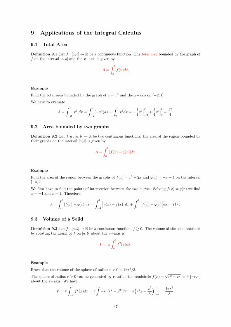
9.1 Total Area
Definition 9.1 Let f : [a, b] → R be a continuous function. The total area bounded by the graph off on the interval [a, b] and the x−axis is given by
A =∫ b
a
f(x)dx.
Example
Find the total area bounded by the graph of y = x3 and the x−axis on [−2, 1].
We have to evaluate
A =∫ 1
−2
|x3|dx =∫ 0
−2
(−x4)dx +∫ 1
0
x3dx = −14x3
∣∣∣0
−2+
14x4
∣∣∣1
0=
174
.
9.2 Area bounded by two graphs
Definition 9.2 Let f, g : [a, b] → R be two continuous functions. the area of the region bounded bytheir graphs on the interval [a, b] is given by
A =∫ b
a
|f(x)− g(x)|dx.
Example
Find the area of the region between the graphs of f(x) = x2 + 2x and g(x) = −x + 4 on the interval[−4, 2].
We first have to find the points of intersection between the two curves. Solving f(x) = g(x) we findx = −4 and x = 1. Therefore,
A =∫ b
a
|f(x)− g(x)|dx =∫ 1
−4
[g(x)− f(x)
]dx +
∫ 2
1
[f(x)− g(x)
]dx = 71/3.
9.3 Volume of a Solid
Definition 9.3 Let f : [a, b] → R be a continuous function, f ≥ 0. The volume of the solid obtainedby rotating the graph of f on [a, b] about the x−axis is
V = π
∫ b
a
f2(x)dx.
Example
Prove that the volume of the sphere of radius r > 0 is 4πr3/3.
The sphere of radius r > 0 can be generated by rotation the semicircle f(x) =√
r2 − x2, x ∈ [−r, r]about the x−axis. We have
V = π
∫ r
−r
f2(x)dx = π
∫−rr(r2 − x2)dx = π
(r2x− x3
3
)∣∣∣r
−r=
4πr3
3.
37
9.4 Length of a Graph
Definition 9.4 Let f : [a, b] → R be a differentiable function such that f ′ is continuous. Then, thelength L of the graph of y = f(x) on the interval [a, b] is given by
L =∫ b
a
√1 + [f ′(x)]2dx
9.5 Area of a Surface
Definition 9.5 Let f : [a, b] → R be a differentiable function such that f ≥ 0 and f ′ is continuous.the area S of the surface obtained by rotating the graph of f on the interval [a, b] about the x−axisis given by
S = π
∫ b
a
f(x)√
1 + [f ′(x)]2dx.
9.6 Centres of Mass and Centroids
Suppose we have n point masses m1, m2, . . . , mn on a horizontal line at distances x1, x2, . . . , xn
from the origin. Then
m = m1 + m2 + · · ·+ mn is called the total mass of the system.
M0 = m1x1 + m2x2 + · · ·+ mnxn is called the moment of the system about the origin.
The centre of mass (or centre of gravity) of the system is a point x on the x−axis whose coordinateis
x =M0
m=
m1x1 + m2x2 + · · ·+ mnxn
m1 + m2 + · · ·+ mn.
A similar situation occurs in the plane: If n point masses located in the plane at (x1, y1), (x2, y2),. . . , (xn, yn) are given, the centre of mass of the system is defined to be the point (x, y) where
x =My
m=
m1x1 + m2x2 + · · ·+ mnxn
m1 + m2 + · · ·+ mn.
y =Mx
m=
m1y1 + m2y2 + · · ·+ mnyn
m1 + m2 + · · ·+ mn.
Suppose we want to find the centre of mass of a thin two-dimensional lamina with constant densitythat occupies a region in the plane bounded by the graph of a continuous function f : [a, b] → R andthe horizontal axis. The coordinates of the centre of mass are defined by
x =My
A=
∫ b
axf(x)dx
∫ b
af(x)dx
.
y =Mx
A=
12
∫ b
af2(x)dx
∫ b
af(x)dx
.
Remark that the quantity on the bottom is A =∫ b
af(x)dx=the area of the region bounded by the
graph of f and the x−axis. From geometrical point of view, (x, y) is called the centroid of the regionbounded by the graph of f and the x axis.
38
10 Sequences and Series
10.1 Sequences
Definition 10.1 A sequence is the image of a real function whose domain of definition if the set ofpositive intereges N.
If f : N→ R is such a function, we write
a1 = f(1), a2 = f(2) , a3 = f(3) , . . . , an = f(n) , . . . .
Definition 10.2 We say that a sequence (an)∞n=1 converges to a real number L if an can be madearbitrarily close to L for n sufficiently large, that is, for all ε > 0 there exists N ≥ 1 such that|an − L| < ε for all n ≥ N .
The number L is called the limit of (an)∞n=1 and we write
limn→∞
an = L or simply an → L as n →∞.
10.2 Series
Definition 10.3 Let (an)∞n=1 be a sequence or real numbers. The sum of terms
a1 + a2 + a3 + · · ·+ an + . . .
is called the infinite series or simply the series of (an)∞n=1 and we write∑∞
n=1 an.
sn = a1 + a2 + · · ·+ an is called the nth partial sum of the series.
Remark One of the motivations for the study of series comes from decimal expansions. Take forexample
13
= 0.333333333333 =310
+3
102+
3103
+ · · ·+ 310n
+ . . .
The sequence of partial sums is
s1 =310
= 0.3
s2 =310
+3
102= 0.33
s3 =310
+3
102+
3103
= 0.333
. . . . . . . . .
Definition 10.4 We say that the series∑∞
n=1 an is convergent if the sequence of its partial sums(sn)∞n=1 is convergent. We write
∞∑n=1
an = limn→∞
sn.
A series∑∞
n=1 an which is not convergent is called divergent.
Theorem 10.5 (Geometric Series)
Let r be a real number. Then , the series∑∞
n=1 rn is convergent if and only if |r| < 1. In this case
∞∑n=1
rn =r
1− r.
Theorem 10.6 (The Harmonic Series)
The harmonic series∞∑
n=1
1n
is divergent.
39
Theorem 10.7 The series∞∑
n=1
1np
is convergent if and only if p > 1.
Theorem 10.8 (Ratio Test)
Let∞∑
n=1
an be a series of real numbers such that an 6= 0 for all n ≥ 1. Let
` = limn→∞
∣∣∣∣an+1
an
∣∣∣∣ .
If ` < 1 then the series∞∑
n=1
an is convergent
If ` > 1 then the series∞∑
n=1
an is divergent
If ` = 1 then the test is inconclusive.
Theorem 10.9 (Alternating Series Test)
Let (an)∞n=1 be a decreasing sequence of positive real numbers. Then, the series∑∞
n=1 an convergesif and only if limn→∞ an = 0.
Definition 10.10 We say that the series∞∑
n=1
an is absolute convergent if the series∞∑
n=1
|an| is con-
vergent
Remark
Any absolute convergent series is also convergent.
Remark
There are convergent series∞∑
n=1
an that are not absolute convergent.
10.3 Power Series
Definition 10.11 A series containg nonnegative integral powers of (x− a) in the form
∞∑n=1
cn(x− a)n = c0 + c1(x− a) + c2(x− a)2 + · · ·+ cn(x− a)n + . . . ,
is called a power series centred at a.
When a = 0 we obtain∞∑
n=1
cnxn = c0 + c1x + c2x2 + · · ·+ cnxn + . . . ,
which is called poower series of x.
Definition 10.12 The set of all values of x ∈ R for which the series∑∞
n=1 cn(x − a)n converges iscalled the interval of convergence. the centre of the interval of convergence is a. the radius of theinterval of convergence is called the radius of convergence.
Theorem 10.13 (Convergence of Power Series)
For a power series∑∞
n=1 cn(x− a)n exactly one of the following is true:
40
• the series converges only at the single number x = a
• the series converges absolutely for all x ∈ R;
• the series converges absolutely for the numbers x in a finite interval (a−R, a+R) and divergesfor numbers in the set (−∞, a−R) ∪ (a + R,∞)
10.4 Representing functions by power series
Theorem 10.14 (Differentiation of Power Series)
If f(x)∞∑
n=0
cn(x − a)n converges on an interval (a − R, a + R) then f is differentiable at each point
x ∈ (a−R, a + R) and
f ′(x) =∞∑
n=1
ncn(x− a)n−1
Theorem 10.15 (Integration of a Power Series)
If f(x)∞∑
n=0
cn(x− a)n converges on an interval (a−R, a + R) then
∫f(x)dx =
∞∑n=0
cn
n + 1(x− a)n+1 + C.
Theorem 10.16 (Taylor Series)
Let f : (a − R, a + R)ariR be a function that posseses derivatives of all orders on the interval(a−R, a + R). Then
f(x) =∞∑
n=0
f (n)(a)n!
(x− a)n.
Definition 10.17 The series
f(x) =∞∑
n=0
f (n)(a)n!
(x− a)n = f(a) +f ′(a)
1!(x− a) +
f ′′(a)2!
(x− a)2 +f ′′′(a)
3!(x− a)3 + . . . .
is called the Taylor Series of f at a.
Definition 10.18 The series
f(x) =∞∑
n=0
f (n)(0)n!
xn = f(0) +f ′(0)
1!x +
f ′′(0)2!
x2 +f ′′′(0)
3!x3 + . . . .
is called the Maclaurin Series of f .
Remark 10.19 The Maclaurin series corresponds to Taylor series for a = 0.
Theorem 10.20 (Binomial Series) If |x| < 1, then for any real number r, we have
(1 + x)r =∞∑
n=0
(rn
)xn,
where (r0
)= 1 and
(rn
)=
r(r − 1)(r − 2) . . . (r − n + 1)n!
, n ≥ 1.
41
11 Differential Equations
Definition 11.1 A differential equation is a mathematical equation that involves an unknown func-tion y and one or more of the derivatives of y.
Remark 11.2 Differential equations are classified by the order of the highest derivative.
11.1 First Order Differential Equations
Definition 11.3 Any differential equation that can be written in the form
dy
dx= F (x, y).
where F is a function of two variables x and y is called a first order differential equation
Definition 11.4 Any differential equation that can be written in the form
dy
dx= g(x)f(y)
is called separable first order differential equation.
Algorithm for solving separable first-order differential equations
Step 1: Determine whether the first-order differential equation can be written in the form
dy
dx= g(x)f(y).
Step 2: Rewrite the equation at step 1 in the form
1f(y)
= g(x)dx.
Step 3: Integrate both sides of the differential equation at Step 2. Integrate the left-hand side withrespect to y and the right-hand side with respect to x.
Example 11.5 Solve the differential equation
dy
dx+ 2x3y2
by using the separation of variables method.
Solution
First, we write the differential equation in the form
1y2
dy = −2x3dx.
Integrating both sides we find1y
=12(x4 + c),
for some constant c ∈ R. This gives y = 2x4+c .
Example 11.6 Solve the initial-value problem
dy
dx= y(1− y) , y(0) =
13.
42
Solution
The equation has separable variable. We first write it in the form
1y(y − 1)
dy = dx,
which by integration yieldsln |y| − ln |y − 1| = x + C1.
Hence
ln∣∣∣∣
y
y − 1
∣∣∣∣ = x + C1
and so ∣∣∣∣y
y − 1
∣∣∣∣ = ex+C1
Letting C = eC1 we find ∣∣∣∣y
y − 1
∣∣∣∣ = Cex.
Case 1:y
y − 1= Cex with the solution
y =−Cex
1− Cex.
Case 2:y
y − 1= −Cex with the solution
y =Cex
1Cex.
In bothe cases, the general form of solution is y = Cex
1Cex .. Since y(0) = 1/3 we find C = 1/2 and thesolution of the inivial-value problem is
y =ex
2 + ex.
11.2 Linear First Order Differential Equations
Definition 11.7 Any differential equation that can be writen in the form
dy
dx+ P (x)y = f(x)
is called a first-order differential equatiuon.
Remark 11.8 Not all first-order differential equations are linear.
Example
(1) xdy
dx+ y = cos x is linear
(2) xdy
dx= y2 is not linear.
Theorem 11.9 The general solution of the linear first-order differential equation
ady
dx+ P (x)y = f(x)
is given by
y =1
Q(x)
∫Q(x)f(x)dx, where Q(x) = e
RP (x)dx.
43

Example 11.10 Find the general solution of
xdy
dx− 4y = x6ex , x > 0.
Solution We first write the differential equation in the form
dy
dx− 4
xy = x5ex , x > 0.
In this case P (x) = − 4x and f(x) = x5ex. the general solution is
y =1
Q(x)
∫Q(x)f(x)dx, where Q(x) = e
RP (x)dx.
In our particular case ∫P (x)dx = −4
∫x−1dx = −4 ln x = ln(x−4)
soQ(x) = e
RP (x)dx = x−4.
It remains to evaluate ∫Q(x)f(x)dx =
∫xexdx = (x− 1)ex + C.
Hencey =
1Q(x)
∫Q(x)f(x)dx = x4
[(x− 1)ex + C
].
12 Linear Second Order Differential Equations
Definition 12.1 Any differential equation that can be written in the form
a(x)d2y
dx2+ b(x)
dy
dx+ c(x)y = g(x)
is called a linear second order diferential equation.
a(x), b(x), c(x) are called the coefficients of differential equation.
If g(x) = 0 for all x, the above equation is called homogeneous.
In this course we shall be convcerned with the case of constant coefficients, so we shll investigate theequation
ad2y
dx2+ b
dy
dx+ cy = g(x)
12.1 Homogeneous Linear Second Order Differential Equations
We study in this section the general solution of
ad2y
dx2+ b
dy
dx+ cy = 0
We associate the characteristic equation
aλ2 + bλ + c = 0.
Case 1: Distinct Real Roots
Assume that the solutions λ1, λ2 of the characteristic equation are distinct real numbers. Then, thegeneral solution of the homogeneous second-order differential equation is
y(x) = C1eλ1x + C2e
λ2x
44
Example 12.2 Solve the differential equation
d2y
dx2− 5
dy
dx+ 6y = 0
Solution. The characteristic equation is λ2 − 5λ + 6 = 0 with λ1 = 2 and λ2 = 3. Therefore, thegeneral solution is y(x) = C1e
2x + C2e3x.
Case 2: Equal Real Roots
Assume that the solutions λ1, λ2 of the characteristic equation are equal real numbers, that is λ1 =λ2 = λ. Then, the general solution of the homogeneous second-order differential equation is
y(x) = C1eλx + C2xeλx = eλx(C1 + C2x).
Case 3: Complex Conjugate Roots
Assume that the solutions λ1, λ2 of the characteristic equation are complex (and conjugate) numbers,that is
λ1 = α + iβ , λ2 = α− iβ.
Then, the general solution of the homogeneous second-order differential equation is
y(x) = eαx(C1 cosβx + C2 sin βx).
12.2 Nonhomogeneous Linear Second Order Differential Equations
To solve the nonhomogeneous second order differential equation
ad2y
dx2+ b
dy
dx+ cy = g(x)
we follow the following steps:
Step 1: Find the general solution yh(x) of the associated homogeneous equation
ad2y
dx2+ b
dy
dx+ cy = 0
according to the previous section.
Step 2: Find a particular solution yp(x) of the nonhomogeneous differential equation.
Step 3: Write the general solution y(x) in the form y(x) = yh(x) + yp(x).
We already know how to solve the homogeneous equation. The difficult part coms from Step 2, thatis, to find a particular solution of the nonhomogeneous differential equation. to this aim we shall givein the following two different methods
1. The Method of Undetermined Coefficients
2. The Method of Variation of Parameters
1. The Method of Undetermined Coefficients
Definition 12.3 We say that a function g(x) generates a finite family under differentiation if thereexists
h1(x), h2(x), . . . , hm(x) ,m ≥ 1
such that any derivative of g can be writtem as a linear combination of h1(x), h2(x), . . . , hm(x)
45
Example 12.4 Let g(x) = x2 + 3x− 4 and
h1(x) = x2 , h2(x) = x , h3(x) = 1.
Then g(x) generates under differentiation the family h(1), h2(x), h3(x) since
g(x) = 1 · h1(x) + 3 · h2(x)− 4 · h3(x)
g′(x) = 0 · h1(x) + 2 · h2(x) + 3 · h3(x)
g′′(x) = 0 · h1(x) + 0 · h2(x) + 2 · h3(x)
g′′′(x) = 0 · h1(x) + 0 · h2(x) + 0 · h3(x)
gIV (x) = 0 · h1(x) + 0 · h2(x) + 0 · h3(x)
Theorem 12.5 (Method of Undetermined Coefficients)
Consider the nonhomogeneous differential equation
ad2y
dx2+ b
dy
dx+ cy = g(x) (1)
Assume that g(x) generates a finite family under differentiation given by h1(x), h2(x), . . . , hm(x)and that none of these functions are solutions of the homogeneous differential equation
ad2y
dx2+ b
dy
dx+ cy = 0.
Then, a particular solution yp(x) having the form
yh(x) = A1h1(x) + A2h2(x) + . . . A + mhm(x)
can be found. To obtain the specific coefficients A1, A2, . . . , Am we substitute the expression of yp(x)in the nonhomogeneous differential equation (1). this will result in m−linear algebraic equations inthe m unknowns A1, A2, . . . , Am.
Example 12.6 Solve the differential equation
d2y
dx2+ 2
dy
dx− 3y = 28 sin 3x + 30x cos 3x.
Solution. The characteristic equation is λ2 +2λ− 3 = 0 with solutions λ1 = 1 and λ2 = −3. Hence,
yh(x) = C1ex + C2e
−3x.
to find a particular solution, let g(x) = 28 sin 3x + 30x cos 3x. Then g(x) generates under differentia-tion the finite family
h1(x) = cos 3x , h2(x) = sin 3x , h3(x) = x cos 3x , h4(x) = x sin 3x .
Thus, we will be looking for a particular solution yp(x) in the form
yp(x) = A cos 3x + B sin 3x + Cx cos 3x + Dx sin 3x .
Using this form of yp(x) in the original nonhomogeneous differential equation we find A = − 13 ,
B = −1, C = −2 and D = 1. Thus
yp(x) = −13
cos 3x− sin 3x− 2x cos 3x + x sin 3x .
and the general solution is
y(x) = yh(x) + yp(x) = C1ex + C2e
−3x 13
cos 3x− sin 3x− 2x cos 3x + x sin 3x .
46
2. The Method of Variation of Parameters
Theorem 12.7 We write the homogeneous differential equation in the form
d2y
dx2+ b
dy
dx+ cy = g(x)
and assume that the solution yh(x) of the homogeneous equation
d2y
dx2+ b
dy
dx+ cy = 0
isyh(x) = C1y1(x) + C2(x).
Then, a particular solution yp(x) having the form
yh(x) = u1(x)h1(x) + u2(x)h2(x)
can be found. Here u1 and u2 are functions of x that satisfy
u′1y1(x) + u2y2(x) = 0
u′1y′1(x) + u2y
′2(x) = g(x),
that is
u1(x) = −∫
y2(x)g(x)y1(x)y′2(x)− y2(x)y′1(x)
dx , u2(x) =∫
y1(x)g(x)y1(x)y′2(x)− y2(x)y′1(x)
dx.
13 Revision
13.1 The hyperbolic functions
Definition 13.1 The hyperbolic sine function, denoted sinh x is a function R→ R defined by
sinhx =ex − e−x
2
The hyperbolic cosine function, denoted cosh x is a function R→ R defined by
cosh x =ex + e−x
2
The formulae for the derivatives of hyperbolic sin, cosine and tangent are not required to be learnedby heart. Some exercises in the exam will require to prove the formulae for their differentiation.
13.2 Numerical Approximation of Definite Integrals
For many continuous functions f : [ b] → R we are not able to compute exactly∫ b
af(x)dx. The best
we can hope for is an approximation of the value of the definite integral∫ b
af(x)dx by the following
methods:
1. Midpoint Rule
2. Trapezoidal Rule
3. Simpson’s Rule
47
1. Midpoint Rule
One way to aproximate the definite integral∫ b
af(x)dx is to construct rectangular elements under the
graph of f and add their areas.
Let [x0, x1], x1, x2], . . . [xn−1, xn] be a division of the interval [a, b] into n subintervals of the samelength (b− a)/n. Then
∫ b
a
f(x)dx ≈b− a
n
[f(x0 + x1
2
)+ f
(x1 + x2
2
)+ · · ·+ f
(xn−1 + xn
2
)].
2. Trapezoidal Rule
Given a continuous function f : [a, b] → R we aproximate the definite integral∫ b
af(x)dx by adding
the areas of trapezoids instead of rectangles.
If [x0, x1], x1, x2], . . . [xn−1, xn] is a division of the interval [a, b] into n subintervals of the same length,then ∫ b
a
f(x)dx ≈b− a
2n
[f(x0) + 2f(x1) + 2f(x2) + · · ·+ f(xn−1) + f(xn)
]
3. Simpson’s Rule
Let [x0, x1], x1, x2], . . . [xn−1, xn] is a division of the interval [a, b] into n subintervals of the samelength. Assume that n is even. Then
∫ b
a
f(x)dx ≈b− a
3n
[f(x0) + 4f(x1) + 2f(x2) + 4f(x3) + · · ·+ 4f(xn−1) + f(xn)
]
13.3 Applications of the Integral Calculus
13.3.1 Total Area
Definition 13.2 Let f : [a, b] → R be a continuous function. The total area bounded by the graphof f on the interval [a, b] and the x−axis is given by
A =∫ b
a
f(x)dx.
13.3.2 Area bounded by two graphs
Definition 13.3 Let f, g : [a, b] → R be two continuous functions. the area of the region boundedby their graphs on the interval [a, b] is given by
A =∫ b
a
|f(x)− g(x)|dx.
13.3.3 Volume of a Solid
Definition 13.4 Let f : [a, b] → R be a continuous function, f ≥ 0. The volume of the solid obtainedby rotating the graph of f on [a, b] about the x−axis is
V = π
∫ b
a
f2(x)dx.
48
13.3.4 Length of a Graph
Definition 13.5 Let f : [a, b] → R be a differentiable function such that f ′ is continuous. Then, thelength L of the graph of y = f(x) on the interval [a, b] is given by
L =∫ b
a
√1 + [f ′(x)]2dx
13.3.5 Area of a Surface
Definition 13.6 Let f : [a, b] → R be a differentiable function such that f ≥ 0 and f ′ is continuous.The area S of the surface obtained by rotating the graph of f on the interval [a, b] about the x−axisis given by
S = 2π
∫ b
a
f(x)√
1 + [f ′(x)]2dx.
13.3.6 Centres of Mass and Centroids
The coordinates of the centre of mass(centroid) are defined by
x =My
A=
∫ b
axf(x)dx
∫ b
af(x)dx
.
y =Mx
A=
12
∫ b
af2(x)dx
∫ b
af(x)dx
.
Remark that the quantity on the bottom is A =∫ b
af(x)dx=the area of the region bounded by the
graph of f and the x−axis. From geometrical point of view, (x, y) is called the centroid of the regionbounded by the graph of f and the x axis.
13.4 Representing functions by power series
Theorem 13.7 (Taylor Series)
Let f : (a − R, a + R)ariR be a function that posseses derivatives of all orders on the interval(a−R, a + R). Then
f(x) =∞∑
n=0
f (n)(a)n!
(x− a)n.
Definition 13.8 The series
f(x) =∞∑
n=0
f (n)(a)n!
(x− a)n = f(a) +f ′(a)
1!(x− a) +
f ′′(a)2!
(x− a)2 +f ′′′(a)
3!(x− a)3 + . . . .
is called the Taylor Series of f at a.
Definition 13.9 The series
f(x) =∞∑
n=0
f (n)(0)n!
xn = f(0) +f ′(0)
1!x +
f ′′(0)2!
x2 +f ′′′(0)
3!x3 + . . . .
is called the Maclaurin Series of f .
Remark 13.10 The Maclaurin series corresponds to Taylor series for a = 0.
49
13.5 Differential Equations
13.5.1 Linear First Order Differential Equations
Theorem 13.11 The general solution of the linear first-order differential equation
ady
dx+ P (x)y = f(x)
is given by
y =1
Q(x)
∫Q(x)f(x)dx, where Q(x) = e
RP (x)dx.
13.5.2 Linear Second Order Differential Equations
13.5.3 Homogeneous Linear Second Order Differential Equations
ad2y
dx2+ b
dy
dx+ cy = 0
We associate the characteristic equation
aλ2 + bλ + c = 0.
Case 1: Distinct Real Roots
Assume that the solutions λ1, λ2 of the characteristic equation are distinct real numbers. Then, thegeneral solution of the homogeneous second-order differential equation is
y(x) = C1eλ1x + C2e
λ2x
Case 2: Equal Real Roots
Assume that the solutions λ1, λ2 of the characteristic equation are equal real numbers, that is λ1 =λ2 = λ. Then, the general solution of the homogeneous second-order differential equation is
y(x) = C1eλx + C2xeλx = eλx(C1 + C2x).
Case 3: Complex Conjugate Roots
Assume that the solutions λ1, λ2 of the characteristic equation are complex (and conjugate) numbers,that is
λ1 = α + iβ , λ2 = α− iβ.
Then, the general solution of the homogeneous second-order differential equation is
y(x) = eαx(C1 cosβx + C2 sin βx).
13.5.4 Nonhomogeneous Linear Second Order Differential Equations
To solve the nonhomogeneous second order differential equation
ad2y
dx2+ b
dy
dx+ cy = g(x)
we follow the following steps:
Step 1: Find the general solution yh(x) of the associated homogeneous equation
ad2y
dx2+ b
dy
dx+ cy = 0
50
according to the previous section.
Step 2: Find a particular solution yp(x) of the nonhomogeneous differential equation.
Step 3: Write the general solution y(x) in the form y(x) = yh(x) + yp(x).
We already know how to solve the homogeneous equation. The difficult part coms from Step 2, thatis, to find a particular solution of the nonhomogeneous differential equation. to this aim we shall givein the following two different methods
1. The Method of Undetermined Coefficients
2. The Method of Variation of Parameters
51