MATH 8210, FALL 2011 LECTURE NOTESalpha.math.uga.edu/~usher/8210-notes.pdfMATH 8210, FALL 2011...

MATH 8210, FALL 2011 LECTURE NOTES

MIKE USHER

1. Multivariable calculus without coordinates

The objects of study in this course are what are called “smooth manifolds.” For the time being I won’t givea precise definition of these (it will come later, or of courseyou can easily look it up), but for now suffice it tosay that these are topological spaces which locally resemble Euclidean space and in which, in particular, it ispossible to do something resembling calculus. The surface of the Earth is (to good approximation) an exampleof a two-dimensional smooth manifold. Of course, the Earth is notR2 but rather a closed surface (I was going tosay a sphere, but then it occurred to me that if one looks closely enough there are some rock formations whichcause the genus to be positive), yet locally it looks enough like R2 that it seems reasonable to speak for instanceof the directional derivatives of a function (the temperature, say) defined on the Earth.

So how can we formulate calculus in such spaces? Part of the definition will be that a manifoldM will havean open coverUα|α ∈ A by sets equipped with homeomorphisms (“charts”)φα : Uα → Vα whereVα ⊂ R

n isopen. So we can try to do calculus onM by, roughly speaking, doing standard multivariable calculus in the opensetsVα and then transporting the constructions back toM by the mapsφα (or their inverses). However, ifm ∈ M,thenm will typically belong to several of the setsUα in the open cover ofM, and one needs to make sure thatone’s constructions don’t depend on which of the charts one is using. To compare between theαth chart and theβth chart, one needs to look at the “transition function”

φβ φ−1α : φα(Uα ∩ Uβ)→ φβ(Uα ∩ Uβ).

This is a map between two open subsets ofRn, and part of the definition of a smooth manifold will ensure thatthe map is smooth (i.e., C∞) and invertible (with a smooth inverse), but there won’t be any restrictions on whatφβ φ

−1α other than that. So for example it doesn’t make sense to “takethe partial derivative of a function onM

with respect to the first coordinate,” since although we can differentiate a function onVα with respect to the firstcoordinate, or we can do the same for a function onVβ, these operations won’t be equivalent when we try to liftthem up toM using the mapsφα, φβ.

So this makes it important to understand how notions of multivariable calculus behave under the action ofdiffeomorphisms(i.e., smooth maps with smooth inverses)φ : U → U whereU andU are open subsets ofRn.You should think of the action of such a diffeomorphism as being the same as changing one’s coordinate system,e.g. from Cartesian coordinates to polar coordinates. In particular I want to first discuss various notions of whata tangent vector at a point p∈ U is. (And we’ll later generalize this to the notion of a tangent vector at a pointin a smooth manifold.) Visually you’re supposed to think of atangent vector atp as being a little arrow whosebase is atp, pointing in a possible direction of motion fromp. The set of these tangent vectors will form a vectorspace called thetangent space to U at pand denotedTpU. I’ll give three characterizations, from most concreteto most abstract.

(1) The way to describe this notion that is used in undergraduate multivariable calculus courses is just to saythat a tangent vectorv at p ∈ U is (or is represented by) an n-tuple of numbers (v1, . . . , vn) ∈ Rn. Onecan then draw the vector whose base is atp and whose first coordinate isv1, second coordinate isv2, andso on. (In somewhat more sophisticated language, the standard Cartesian coordinates onRn determine abasise1, . . . ,en of unit vectors, and one hasv =

∑viei .)

1

2 MIKE USHER

This characterization is very good for computational purposes, but when one is interested in howtangent vectors behave under coordinate changesφ : U → U it has some disadvantages. The tangentvectorv = (v1, . . . , vn) ∈ TpU should correspond under the coordinate changeφ to a tangent vectorφ∗v ∈ Tφ(p)U at φ(p). Perhaps you’ve learned how this correspondence works: one constructs theJacobian matrix atp of the mapφ (with (i, j) entry given by∂φi

∂x jwhereφi is the ith component ofφ),

and then the coordinates ofφ∗v are obtained by multiplying the Jacobian matrix by the vector consistingof the components ofv. This is a manageable computation, but it may not be very conceptually clearfrom this discussion what’s going on here. In particular if we then want to say what a tangent vectorto a pointm on a smooth manifold is we’d have to say something like “ann-tuple of numbers for eachchart containingm, such that then-tuples for different charts are related by the Jacobians of the transitionfunctions,” which is much more opaque and less natural-sounding than it really should be.

(2) A more natural characterization of tangent vectors is the following. The idea is that the tangent spaceTpU consists of all possible velocities of curves passing through p. If p ∈ U, consider allC∞ pathsγ : (−ǫ, ǫ) → U (for someǫ > 0) such thatγ(0) = p. I would like to declare two of these to beequivalent if they have the same velocity,i.e., γ1 ∼ γ2 iff γ′1(0) = γ′2(0) (or equivalently, and maybeless circularly,γ1 ∼ γ2 if lim t→0

γ1(t)−γ2(t)t = 0). Then simply define a “tangent vector” atp to be an

equivalence class [γ] of C∞ arcs throughp (and soTpU is just the set of equivalence classes). The waythis behaves under coordinate changes is extremely simple,since I’m not using coordinates to define thenotion: a tangent vectorv ∈ TpU has the formv = [γ] for someγ, and the corresponding tangent vectorφ∗v ∈ Tφ(p)U is just [φ γ]. We’ll see later that this adapts to general smooth manifolds very simply anddirectly—a tangent vector at a point on a smooth manifold willjust be a suitable equivalence class ofcurves passing through that point.

The one disadvantage of this characterization is that it’s not so intuitively obvious how to do algebraicoperations (like addition of tangent vectors) on equivalence classes of curves through a point (thoughyou can make a suitable definition if you put your mind to it).

It shouldn’t be hard to construct a natural correspondence between tangent vectors in this sense andtangent vectors in the sense of Definition (1) above, but again, the advantage of thinking about it thisway is that it’s less coordinate-dependent.

(3) Now for a characterization of tangent vectors that you almost certainly would not have thought of. Toattempt to motivate it, note that a given tangent vectorv ∈ TpU gives you the ability to differentiatesmooth functionsf : U → R at p—namely you take the directional derivative atp:

(Dv f )(p) = limt→0

f (p+ tv) − f (p)t

.

So we will definea tangent vector atp to be “a way of differentiating functions defined nearp,” i.e., wewill abstract some relevant properties of the operation of taking a directional derivative, and then definea tangent vector to be one of these operations.

To do this, first consider pairs (f ,V) whereV is an open neighborhood ofp and f : V → R isC∞, and declare two such pairs (f ,V) and (g,W) to be equivalent if there is a smaller neighborhoodZ ⊂ V ∩ W of p such thatf |Z = g|Z. Let Op be the set of equivalence classes. Since we can set,for instance [f ,V] · [g,W] = [ f g,V ∩W], Op is easily seen to be a commutativeR-algebra (i.e., it isboth a commutative ring and a vector space overR, with appropriately compatible operations), calledthe “algebra of germs of functions atp.” I’ll tend to denote a germ by justf rather than [f ,V]; itis to be understood thatf is defined not necessarily throughoutU but rather on some (varying) openneighborhood ofp. Of course one always has a well-defined valuef (p) for f ∈ Op.

A tangent vector atp will then be defined to be aderivation v: Op→ R, i.e. v is to satisfy• (R-linearity)v(c f + g) = cv( f ) + v(g) for c ∈ R and f ,g ∈ Op

• (Leibniz rule)v( f g) = f (p)v(g) + g(p)v( f ) for f ,g ∈ Op.

MATH 8210, FALL 2011 LECTURE NOTES 3

It’s standard that the directional derivative operationsDv alluded to above satisfy these properties. It’snot obvious that, conversely, any derivation onOp is given by a directional derivative in some direction,but we’ll prove this shortly.

Like the characterization of tangent vectors as equivalence classes curves, this formulation is com-pletely coordinate free, making it easy to extend the definition to manifolds when the time comes. Unlikethe situation with curve characterization, though, it’s quite obvious that derivations form a vector space,which is another advantage.

To see how this notion behaves under diffeomorphisms (or indeed under more general smooth maps)φ : U → U, if v ∈ TpU (i.e., if v is a derivation onOp), we need to construct a derivationφ∗v onOφ(p).Well, if f ∈ Oφ(p) (really we should write [f ,V]), so f is a smooth function defined nearφ(p), then f φwill be a smooth function defined nearp (specifically, it will be defined on the open setφ−1(V) aroundp), and so we can define

(φ∗v)( f ) = v( f φ)

So as with the curve formulation, it’s quite simple to see howderivations transform under coordinatechanges.

Among the three above characterizations of tangent vectors, it should be clear that (1) is equivalent to (2),under the correspondence which assigns to an equivalence class of curves [γ] the vectorγ′(0) (expressed incoordinates using the standard basis forRn). We now set about proving that (1) and (3) are also equivalent.Let TpU denote the space of tangent vectors as given by formulation (1) (i.e., as elements ofRn) and (for themoment)TpU that given by (3) (i.e., as derivations). Write the coordinates ofp ∈ U ⊂ Rn as (p1, . . . , pn). Nowwe have a linear mapα : TpU → TpU given by

α(v1, . . . , vn) =n∑

i=1

vi∂

∂xi,

i.e., α sends a vector (in the undergraduate multivariable calculus sense) to the operation given by directionaldifferentiation in the direction of that vector. We claim thatα is bijective, justifying our proposal to regard (3) asan equivalent definition of the tangent space atp. It should be clear thatα is injective. Indeed, for eachi we havean elementxi − pi ∈ Op, and we see that, whereβ : TpU → TpU is given by

β(v) = (v(x1 − p1), . . . , v(xn − pn)) ,

we haveβ α = 1 (as ∂∂xi

(x j − p j) = δi j ). Thusα is injective, andβ surjective. To see thatα is surjective, we notethe following, wheneverv ∈ TpU:

• v(1) = v(1 · 1) = 1v(1)+ 1v(1) = v(1)+ v(1). Hencev(1) = 0, and so byR-linearity v(c) = 0 for everyconstant functionc.• For anyi and j, if f ∈ Op we have

v((xi − pi)(x j − p j) f

)= (xi − pi)|pv((x j − p j) f ) + (x j − p j)|p f (p)v((xi − pi)) = 0.

• By the multivariable Taylor formula, any (germ of a) function g ∈ Op can be written (on some neighbor-hood ofp)

g(x) = g(p) +n∑

i=1

∂g∂xi

(p)(xi − pi) +n∑

i, j=1

(xi − pi)(x j − p j) fi j (x)

for somefi j ∈ Op. Hence by the first two items and the linearity ofv, we get

v(g) =n∑

i=1

∂g∂xi

(p)v(xi − pi).

4 MIKE USHER

Thus

v =∑

vi∂

∂xi= α(v1, . . . , vn),

where the numbersvi are equal tov(xi − pi).In view of the above correspondence, we can drop the tilde in the notationTpU, and always view tangent

vectors as derivations on spaces of germs of functions. Evenwhen we express a tangent vector in coordinates,we will often use notation consistent with the derivation interpretation and write the vector as

v1∂

∂x1+ · · · + vn

∂

∂xn

rather than (v1, . . . , vn).Of course, another familiar notion from multivariable calculus is that of avector fieldon an open setU, which

can be thought of as a smooth family of tangent vectors at all of the points ofU, or as a smooth vector-valuedfunctionX : U → Rn, expressible in coordinates asX(m) = (X1(m), . . . ,Xn(m)). There is also a coordinate-freeinterpretation of what a vector field is: it is a mapX : C∞(U) → C∞(U) which, as with tangent vectors, is aderivation, namely:

• X(c f + g) = cX( f ) + X(g) for all c ∈ R, f ,g ∈ C∞(U), and• X( f g) = f X(g) + gX( f ) for all f ,g ∈ C∞(M).

Note that while tangent vectors, when viewed as derivations, just take values inR, vector fields take values inthe space of smooth functions. Just as with tangent vectors,there’s a natural one-to-one correspondence betweenthe undergraduate versions of vector fields and the derivations onC∞(U): simply assign to (X1(·), . . . ,Xn(·)) thederivation

f 7→n∑

i=1

Xi∂ f∂xi

.

Again, the great advantage of the derivation interpretation is that it makes no direct reference to coordinates.So on a smooth manifoldM, once have defined the space of smooth functionsC∞(M), we will effortlessly beable to define a vector field onM as a derivationX : C∞(M)→ C∞(M).

Another nice feature of the derivation interpretation for vector fields (but not for tangent vectors) is that itpoints toward some additional structure on the space of vector fields that we wouldn’t have noticed if we justworked in coordinates. Namely, given that a vector field is a certain kind of functionX : C∞(U) → C∞(U), itbecomes natural to think about composing such functions. Now a slight hitch with this is that the composition oftwo derivations will not typically be a derivation. For example, ∂

∂x1is a derivation, but ∂

∂x1 ∂∂x1

certainly is not:namely we have

∂

∂x1

∂

∂x1(x1x1) = 2

but

x1∂

∂x1

∂

∂x1(x1) + x1

∂

∂x1

∂

∂x1(x1) = 0.

So while we can “compose” two vector fields the result won’t bea vector field. However:

Proposition 1.1. LetA be a commutativeR-algebra and let X,Y: A → A be two derivations onA. Then thecommutator [X,Y] := X Y− Y X is also a derivation onA.

Proof. The linearity of [X,Y] is trivial, so we just need to check the Leibniz rule. We find,for f ,g ∈ A:

[X,Y]( f g) = X (Y( f g)) − Y (X( f g)) = X ( f Yg+ gY f) − Y ( f Xg+ gX f)

= ( f XYg+ (X f)(Yg) + gXY f+ (Xg)(Y f)) − ( f YXg+ (Y f)(Xg) + gYX f+ (Yg)(X f))

= f (XY− YX)g+ g(XY− YX) f = f [X,Y](g) + g[Y,X]( f ),

which is precisely the Leibniz rule for [X,Y].


In local coordinates, ifX =∑

Xi∂∂xi

andY =∑

Yj∂∂x j

, then one finds

[X,Y]( f ) =n∑

i=1

Xi∂

∂xi

n∑

j=1

Yj∂ f∂x j

−n∑

i=1

Yi∂

∂xi

n∑

j=1

X j∂ f∂x j

=

n∑

i, j=1

(XiYj

∂2 f∂xi∂x j

+ Xi∂Yj

∂xi

∂ f∂x j

)−

n∑

i, j=1

(YiX j

∂2 f∂xi∂x j

+ Yi∂X j

∂xi

∂ f∂x j

)

=

n∑

j=1

n∑

i=1

Xi∂Yj

∂xi− Yi

∂X j

∂xi

∂ f∂x j

.

Thus [X,Y] is the vector field∑

Z j∂∂x j

whosejth component is given by

(1) Z j =

n∑

i=1

(Xi∂Yj

∂xi− Yi

∂X j

∂xi

)

This commutator operation on vector fields (also called theLie bracket) turns out to be a fairly important one.Of course, if one wanted to work entirely in coordinates without taking a more abstract point of view, it wouldhave been possible to just define the Lie bracket of two vectorfields X andY to be the vector field given byformula (1), but it’s not clear why one would be motivated to do so.

In general, the commutator operation [·, ·] on the space of linear maps from a vector space to itself satisfiestheJacobi identity:

(2) [X, [Y,Z]] + [Z, [X,Y]] + [Y, [Z,X]] = 0

Indeed, the left hand side is equal to

X(YZ− ZY) − (YZ− ZY)X + Z(XY− YX) − (XY− YX)Z + Y(XZ− ZX) − (ZX− XZ)Y

and (using associativity of function composition) you can see that each of the six three-letter words made up ofone each of the letters X,Y,Z appears above once positively and once negatively, so the sum is zero. Note that if[·, ·] were an associative operation we would instead have [X, [Y,Z]] + [Z, [X,Y]] = [X, [Y,Z]] − [[X,Y],Z] = 0;thus the Jacobi identity expresses a particular way for a binary operation to be non-associative. In general a vectorspaceL equipped with a binary operation [·, ·] : A× A→ A which is bilinear, which obeys [X,Y] = −[Y,X], andwhich satisfies the Jacobi identity is called aLie algebra; thus we have shown that, ifU ⊂ Rn is open, then thespaceX(U) of vector fields onU is naturally a Lie algebra.

Exercise1.2. a) Letφ : U → V be a diffeomorphism between two open subsets ofRn, and letX be a vector field

on U. Prove that ifφ∗X : C∞(V) → C∞(V) is defined by ((φ∗X)( f ))(φ(p)) = (X( f φ))(p), thenφ∗X is a vectorfield on V. Why did we have to assume thatφ was a diffeomorphism (or at least bijective) in order to do this(unlike the situation with tangent vectors, which can be pushed forward by any smooth map)?

b) Prove that ifX,Y are two vector fields onU and ifφ : U → V is a diffeomorphism then

φ∗[X,Y] = [φ∗X, φ∗Y].

6 MIKE USHER

Exercise1.3. Define the following three vector fields1 onR3:

I = z∂

∂y− y

∂

∂z

J = x∂

∂z− z

∂

∂x

K = y∂

∂x− x

∂

∂y

a) Compute [I , J], [ I ,K], and [J,K].b) Deduce as a formal consequence of part (a) that the cross product onR3 satisfies the Jacobi identity.

2. Bump functions and partitions of unity in Rn

In point-set topology one learns a result called Urysohn’s Lemma, which states that given inclusionsA ⊂U ⊂ X whereX is a normal topological space,U is open, andA is closed, there is a continuous functionχ : X → [0,1] identically equal to one onA and identically zero onX \ U. A version of this result is extremelyimportant in differential topology (perhaps more important than in point-set topology); unfortunately, since weneed our functions to beC∞ and not just continuous, we can’t just cite Urysohn’s Lemma but rather need to provea new, smooth, version of the result (of course, this smooth version will apply in a more limited context, if onlybecause it doesn’t make sense to speak of “smooth functions”on a general normal topological space). The goodnews is that the functions can be constructed in a more concrete fashion than one sees in the proof of Urysohn’sLemma.

We begin with a result in one-variable calculus.

Lemma 2.1. Define the function f: R→ R by

f (t) =

e−1/t t > 00 t ≤ 0

Then f ∈ C∞(R). Indeed, for all k∈ N there is a polynomial Pk ∈ R[t] with the property that the kth derivativef (k) exists and is given by

(3) f (k)(t) =

Pk(1/t)e−1/t t > 00 t ≤ 0

Proof. First note that if (3) holds, thenf (k) is continuous on all ofR: indeed continuity is obvious everywhereexcept zero, and at zero we have, by repeated applications ofL’H opital’s rule,

limt→0+

Pk(1/t)e−1/t = lim

s→∞

Pk(s)es= lim

s→∞

ck

es= 0

whereck is some constant (which results from differentiatingdegPk-many times the polynomialPk), from whichcontinuity at zero follows directly.

Thus we just need to prove (3), which we do by induction onk. So assume (3) holds fork; we prove it fork+ 1. Fort < 0 the formula is trivial. Fort = 0 we see

limt→0+

f (k)(t) − f (k)(0)t

= limt→0+

1tPk(1/t)e

−1/t = lims→∞

sPk(s)es

= 0

1Though it’s not necessary in order to do the problem, you might convince yourself that if one interprets these vector fields in the standardmultivariable calculus sense,I points in the direction of a rotation around thex-axis,J in the direction of a rotation around they-axis, andKin the direction of a rotation around thez-axis.


by L’Hopital’s rule, and so (since the left-hand limit is trivially zero) we havef (k+1)(t) = 0. Finally for t > 0 wehave, by the product and chain rules,

f (k+1)(t) =ddt

(Pk(1/t)e

−1/t)= −

1t2

P′k

(1t

)e−1/t +

1t2

Pk

(1t

)e−1/t,

and so the formula holds withPk+1(s) = s2(P′k(s) + Pk(s)).

Note that our functionf is a surjection to the half-open interval [0,1), with f −1(0) = (−∞,0]. Out of thisfunction we can build many other useful ones. For instance:

Corollary 2.2. There is a C∞ function g: R → [0,1] with the property that g−1(1) = [1,∞) and g−1(0) =(−∞,0].

Proof. Note that the functiont 7→ f (1− t) is smooth and nonnegative, and equals zero precisely on theinterval[1,∞). In particular f (t) + f (1− t) is positive everywhere. So we can let

g(t) =f (t)

f (t) + f (1− t).

I leave it to you to check that this has the desired properties.

Corollary 2.3. For any real numbers a< b there is a C∞ function ga,b : R→ [0,1] such that g−1a,b(0) = (−∞,a]

and g−1a,b(1) = [b,∞).

Proof. Let

ga,b(t) = g( t − ab− a

).

Corollary 2.4. For any real numbers a< b < c < d there is a smooth “bump” function h: R → [0,1] so thath−1(1) = [b, c] and h−1(0) = (−∞,a] ∪ [d,∞).

Proof. Leth(t) = ga,b(t)(1− gc,d(t)).

Corollary 2.5. For x ∈ Rn and r > 0 let Br (x) = y ∈ Rn|‖y− x‖ < r denote the open ball of radius r around x.Then for any0 < s< r there is a smooth functionβ : Rn→ [0,1] such thatβ−1(1) = Bs(x) and supp(β) = Br (x).

(Here bysupp(β) we mean thesupportof β, i.e., the closed sety ∈ Rn|β(y) , 0)

Proof. Letβ(y) = 1− gs2,r2(‖y− x‖2).

Our goal now is the following theorem:

Theorem 2.6. Let U ⊂ Rn be an open set, and letV = Vα|α ∈ A be an open cover of U. Then there are C∞

functionsχα : U → [0,1] obeying the following properties:

(i) supp(χα) ⊂ Vα

(ii) Any x∈ U has a neighborhood Wx with the property thatχα|Wx = 0 for all but finitely manyα.(iii) For all x ∈ U we have

∑α χα(x) = 1.

8 MIKE USHER

Note that property (ii) ensures that∑α χα is well-defined and smooth (even if there are infinitely many—

perhaps uncountably many—differentα), sinceU is then covered by open sets on each of which the sum∑α χα

is really a finite sum (all but finitely many terms are zero).

Definition 2.7. A collection of functionsχα|α ∈ A obeying properties (i)-(iii) of Theorem 2.6 is called apartitionof unity subordinate to the coverVα.

Theorem 2.6 has an analogue for general smooth manifolds (see Theorem 3.17); to make this more generalversion eventually easier to reach we present the proof for open sets inRn in a fairly general way (a proof morespecifically adapted toRn can be found in Appendix A of Madsen-Tornehave). In particular we bring in thefollowing definition from point-set topology:

Definition 2.8. A topological space X is calledsecond-countableif there is a countable basis for the topology ofX.

In other words, there should be a collectionOn|n ∈ N of open sets with the property that ifU is open andx ∈ U thenx ∈ On ⊂ U for somen. For exampleRn has this property (take the base to consist of open ballscentered at points with rational coordinates and having rational radius), as does any open subset ofRn (just usethose rational balls that are contained in the open subset).Part of our eventual definition will require that anysmooth manifold also has this property.

Lemma 2.9. Let X be a second-countable locally compact Hausdorff space. Then there is a sequence of compactsetsKi

∞i=1 and a sequence of open setsHi

∞i=1 such that

• Ki ⊂ Hi

• X = ∪∞i=1Ki = ∪∞i=1Hi

• If j ≥ i + 3 then Hi ∩ H j = ∅.

Proof. First note that a second-countable, locally compact space has a countable base for its topology whichconsists of open sets with compact closure. Indeed, given a countable baseB, by local compactness any pointx ∈ X has a neighborhoodOx with compact closure, and there will be someV ∈ B such thatx ∈ V ⊂ Ox;evidentlyV will be compact, and the set of allV that can be obtained in this fashion will still be a base for thetopology (and will be contained in the originalB, so will be countable).

So letUi∞i=0 be a base for the topology which is countable and such that each Ui is compact. In particular the

Ui coverX. We claim now that there is a sequenceGi∞i=0 of open sets with eachGi compact, such thatGi ⊂ Gi+1

and such that∪∞i=0Gi = X. Specifically, theGi will have the form

Gi = U0 ∪ · · · ∪ U j i

for a certain increasing sequence of natural numbers j i. To construct the sequence j i, we let j0 = 0 (soG0 = U0), and assuming that we have chosenjk, so thatGk = U1∪· · ·∪U jk, we note thatGk is compact since theUi are, and so since theUi coverX there must be somejk+1 > jk so thatGk ⊂ ∪

jk+1

i=1 Ui . Inductively choosing thejk in this fashion results in a sequenceGi satisfying the required properties (the fact that theGi coverX followsfrom the fact that theUi do, and the fact thatj i → ∞ since thej i are a strictly increasing sequence of naturalnumbers).

To constructKi andHi , let K1 = G1, W1 = G2, and, fori ≥ 2, let Ki = Gi \Gi−1 andHi = Gi+1 \Gi−2. Theseare easily seen to satisfy the required properties.

Proof of Theorem 2.6.Let Ki andHi be subsets ofU as in Lemma 2.9 (applied withX = U), and fix anyi. Forall x ∈ Ki we may chooseαx ∈ A andǫx > 0 so thatB2ǫx(x) ⊂ Vαx ∩ Hi . Then the collection of open ballsBǫx(x)|x ∈ Ki coversKi , so it has a finite subcover.

Now lettingi vary and taking the union of all of these finite subcovers, we have a countable collection of ballsBk

∞k=1 that coversX, and such that whereBk denotes the ball with the same center asBk but twice the radius,


there areαk and ik such thatBk ⊂ Vαk ∩ Hik. (While there may be more than one suchαk and ik—there mighteven be uncountably many possibleαk—we specifically choose oneαk andik for everyk. For convenience let ustakeik to be thei for which Bk was a member of the finite subcover ofKi , so that in particular for anyi there arejust finitely manyk with ik = i.)

I claim that the ballsBk form alocally finitecover ofU, i.e. that any pointx ∈ U has a neighborhoodOx whichmeets just finitely many of theBk. Indeed we could use forOx any neighborhood ofx with compact closure. ForthenOx is contained in the union of just finitely many of the setsHi , sayOx ⊂ H1∪ · · · ∪Hr . But theHi have theproperty thatHi ∩ Hm = ∅ wheneverm≥ i + 3, and soOx ∩ Hm = ∅ for m≥ r + 3. ConsequentlyBk ∩Ox = ∅

unlessk is one of the finitely many indices havingik ≤ r + 2.We can now construct the desired functions. First, for eachk, let ψk : U → [0,1] be a smooth function

identically equal to 1 onBk and such thatsupp(ψk) ⊂ Bk; suchψk exist by Corollary 2.5. By the previousparagraph, any point inU has a neighborhood which is disjoint from the supports of allbut finitely many of theψk; consequently

ψ =

∞∑

k=1

ψk

is a well-defined, smooth function. Moreoverψ > 0 everywhere, since the (smaller) ballsBk coverU. So for anyk we have a well-defined, smooth functionψk

ψ, and obviously

∑kψk

ψ= 1.

Now define

χα =∑

k:αk=α

ψk

ψ.

Since Bk ⊂ Vα wheneverα = αk, we havesupp(χα) ⊂ Vα for all α. Since any point has a neighborhoodintersecting the support ofψk for only finitely manyk, there will be just finitely manyχα whose supports intersectthis neighborhood (namely, just thoseα which equalαk for one of thesek). Finally, we clearly have

∑

α

χα =∑

α

∑

k:αk=α

ψk

ψ=

∑

k

ψk

ψ= 1.

As essentially a special case we get a direct analogue of Urysohn’s Lemma:

Corollary 2.10. If A ⊂ U ⊂ Rn with A closed and U open, there is a C∞ function f: Rn → [0,1] with f |A = 1and supp( f ) ⊂ U.

Proof. Let χ1, χ2 be a partition of unity subordinate to the coverU,Rn \ A of Rn, and let f = χ1. I leave it toyou to confirm the desired properties.

Exercise2.11. a) LetU ⊂ Rn be open, letp ∈ U, and letX be a vector field onU (use the interpretation ofXas a derivation fromC∞(U) to itself). Prove that one can obtain a well-defined tangentvector (in the sense ofa derivationOp → R) Xp by the following prescription: If [f ,V] ∈ Op, let f ∈ C∞(U) be a function such that[ f ,U] = [ f ,V]. ThenX f ∈ C∞(U), and we set

Xp([ f ,V]) = (X f )(p)

(Part of the problem is showing thatf exists, and moreover thatXp([ f ,V]) is independent of the choice of sucha f .)

b) If in coordinates we haveX =∑

i fi ∂∂xi

, prove thatXp =∑

i fi(p) ∂∂xi

.

10 MIKE USHER

3. Smooth manifolds

Definition 3.1. Let n ∈ N. An n-dimensional topological manifold(or “topological n-manifold”) is a second-countable Hausdorff space M with the property that, for all m∈ M, there is a neighborhood U⊂ M of m and ahomeomorphismφ : U → V where V⊂ Rn is an open subset.

Remark3.2. Of course, by replacingV with a small open ballB ⊂ V aroundφ(p) andU with φ−1(B), we couldjust as well require the image ofφ is an open ball inRn rather than an arbitrary open set. In turn, since any openball in Rn is homeomorphic (and indeed diffeomorphic) toRn, we could equally well require the images of themapsφ in Defnition 3.1 to all beRn—i.e., a topologicaln-manifold is a second-countable Hausdorff space inwhich every point has a neighborhood homeomorphic toRn.

Definition 3.3. Let M be a topological n-manifold, and let k be either a positive integer or∞. A Ck atlason Mis a collectionA = (Uα, φα)|α ∈ A where

• The Uα are open subsets of M, and∪α∈AUα = M.• Eachφα : Uα → R

n is a homeomorphism from Uα to the open subsetφα(Uα) ⊂ Rn, and• If α, β ∈ A are such that Uα ∩ Uβ , ∅, then

φβ φ−1α : φα(Uα ∩ Uβ)→ φβ(Uα ∩ Uβ)

is of class Ck.

The mapsφα : Uα → Rn are calledcoordinate charts(or sometimes “coordinate patches”) for the atlasA.

Exercise3.4. (a) IfA andB areCk atlases on a topologicaln-manifold, writeA ∼ B if A∪ B is also aCk

atlas. Prove that∼ defines an equivalence relation on the set of all atlases.(b) If A = (Uα, φα) is aCk atlas forM, letAmax denote the set of all pairs (U, φ) whereφ : U → Rn is

a homeomorphism from an open subsetU ⊂ M to an open subsetφ(U) ⊂ Rn, and such that wheneverU ∩ Uα , ∅ the mapφ φ−1

α : φα(U ∩ Uα) → φ(U ∩ Uα) is Ck and has inverse which isCk. Prove thatAmax is an atlas containingA, and is maximal in the sense that it contains every other atlas that containsA. Deduce that ifA ∼ B thenAmax= Bmax.

Definition 3.5. A Ck-differentiable structureon a topological n-manifold is a maximal atlasA on M (i.e., anatlas such that, in the notation of Exercise 3.4(b),A = Amax). An n-dimensionalCk manifold is a topologicaln-manifold M equipped with a Ck-differentiable structure. A C∞ manifold will also be called asmooth manifold,and a C∞-differentiable structure will also be called asmooth structure.

Remark3.6. We will almost exclusively discusssmooth(i.e., C∞) manifolds in this course. This is partly justifiedby the fact that, for 1≤ k < ∞, anyCk manifold isCk-diffeomorphic to aC∞ manifold (there is a proof inHirsch’s bookDifferential Topology). On the other hand there is some real loss of generality in looking atC∞

(or even justC1) manifolds rather than just topological (C0) manifolds, as there are topological manifolds whichare not homeomorphic to anyC1 manifold. Examples of such are rather complicated—Kervaireconstructed a10-dimensional one in 1960, and the lowest dimension in which any occur is 4, where there are examples due toFreedman in the early 1980s.

Remark3.7. The definition is that a smooth manifold is a certain kind of topological space equipped with amax-imal C∞ atlas. A maximal atlas is a rather unwieldy object—except in trivial cases it will consist of uncountablymany coordinate charts. But in view of Exercise 3.4 it is rarely if ever necessary to really work with a maximalatlas—you just have to specifyoneatlas (often with a small, finite number of charts), and then this canonicallydetermines a maximal atlas by the construction in Exercise 3.4(b). One could equally well define a smooth man-ifold as a topological manifold equipped with an equivalence class of atlases, where the equivalence relation isthe one from Exercise 3.4(a). One advantage of a maximal atlas is that “everything that could be a coordinatepatch is,” so that if you have to work in local coordinates youhave a great variety of possible coordinate systemsto work in and you can choose whichever works best for your purposes at the time.


Example3.8. As the simplest possible example, we note thatRn is canonically a smooth manifold: take an atlas

consisting of the single pair (1Rn,Rn) where 1Rn denotes the identity map. As noted in Remark 3.7 specifyingthis (very small!) atlas canonically determines a maximal atlas (i.e., a differentiable structure).

Of course we could just as well have replacedRn by any open subsetU of Rn, using the atlas(1U ,U) tomakeU into a smooth manifold. More generally, ifM is any smooth manifold with atlas(φα,Uα) and ifU ⊂ Mis an open subset then we naturally get an atlas onU, namely(φα|U∩Uα

,U ∩ Uα).

I promised at the outset that a smooth manifold would be the kind of space on which it is possible to dosomething resembling calculus. In particular ifM is a smoothm-manifold it should be possible to speak ofdifferentiable functions fromM to Rn, or vice versa, for anyn (and, more generally, ifM andN are two smoothmanifolds we should be able to speak of differentiable functions fromM to N). The principle is simple: onechecks the differentiability of a function by using coordinate charts to turn the function into one whose domainand range are open subsets of Euclidean space, where we already have a notion of differentiability.

Definition 3.9. Let M be an m-dimensional smooth manifold, with (maximal) atlas (φα,Uα)|α ∈ A.

• If f : M → Rn is a continuous function, we say f is of class Ck, and write f ∈ Ck(M,Rn), if for everyα ∈ A the function

f φ−1α : φα(Uα)→ Rn

is of class Ck (note that f φ−1α is a function from an open set inRm toRn, so the notion of f φ−1

α beingof class Ck is well-defined from multivariable calculus).• If V ⊂ Rm is an open subset and g: V → M is a continuous function we say that g is of class Ck, and

write Ck(V,M), if for all α ∈ A the function

φα g: g−1(Uα)→ Rm

is of class Ck.• Suppose that N is an n-dimensional smooth manifold, with (maximal) atlasψβ,Vβ)|β ∈ B. If f : M →

N is a continuous function, we say that f is of class Ck if, for all α, β such that f(Uα) ∩ Vβ , ∅, thefunction

ψβ f φ−1α : φα(Uα ∩ f −1(Vβ))→ R

n

is of class Ck (as a function from an open subset ofRm toRn).

The appropriate notion of isomorphism of smooth manifolds is the following:

Definition 3.10. Let M and N be Ck-manifolds. A Ck-diffeomorphismfrom M to N is a smooth, bijective mapf : M → N such that f−1 is also smooth.

As mentioned earlier, we will generally just consider theC∞ case—as such a “diffeomorphism” will, unlessotherwise indicated, mean aC∞ diffeomorphism.

Of course, it would be a pain to actually check that Definition3.9 is satisfied since maximal atlases are verylarge. But the following exercise shows that theCk property can be checked more easily (and also implies that,viewingRn as a smooth manifold, the third part of the above definition contains the first two as special cases).This exercise is intended in part to demonstrate the role of the assumption on the functionsφβ φ−1

α in thedefinition of an atlas.

Exercise3.11. Let M andN be smooth manifolds, and letf : M → N be a continuous function. Prove thatf ∈ Ck(M,N) if and only if the following holds: For eachx ∈ M, there exists a coordinate chartφ : U → Rm

from the atlas forM and a coordinate chartψ : V → Rn from the atlas forN such thatx ∈ U, f (x) ∈ V and

ψ f φ−1 : φ(U ∩ f −1(V))→ Rn

is of classCk.

12 MIKE USHER

Thus in practice to show that a map isCk we just need to find collections of charts covering the manifolds interms of which the map is aCk map between Euclidean spaces, rather than checking the condition on the entiremaximal atlas. Another way of saying this is that the two appearances of the word “(maximal)” in Definition 3.9are unnecessary—we can just use any atlases (possibly quite small) to check theCk condition.

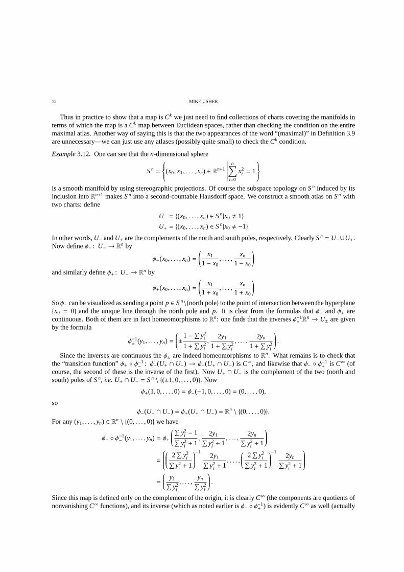
Example3.12. One can see that then-dimensional sphere

Sn =

(x0, x1, . . . , xn) ∈ Rn+1

∣∣∣∣∣∣∣

n∑

i=0

x2i = 1

is a smooth manifold by using stereographic projections. Ofcourse the subspace topology onSn induced by itsinclusion intoRn+1 makesSn into a second-countable Hausdorff space. We construct a smooth atlas onSn withtwo charts: define

U− = (x0, . . . , xn) ∈ Sn|x0 , 1

U+ = (x0, . . . , xn) ∈ Sn|x0 , −1

In other words,U− andU+ are the complements of the north and south poles, respectively. ClearlySn = U−∪U+.Now defineφ− : U− → Rn by

φ−(x0, . . . , xn) =

(x1

1− x0, . . . ,

xn

1− x0

)

and similarly defineφ+ : U+ → Rn by

φ+(x0, . . . , xn) =

(x1

1+ x0, . . . ,

xn

1+ x0

)

Soφ− can be visualized as sending a pointp ∈ Sn\north pole to the point of intersection between the hyperplanex0 = 0 and the unique line through the north pole andp. It is clear from the formulas thatφ− andφ+ arecontinuous. Both of them are in fact homeomorphisms toRn: one finds that the inversesφ−1

± Rn → U± are given

by the formula

φ−1± (y1, . . . , yn) =

±1−

∑y2

i

1+∑

y2i

,2y1

1+∑

y2i

, . . . ,2yn

1+∑

y2i

.

Since the inverses are continuous theφ± are indeed homeomorphisms toRn. What remains is to check thatthe “transition function”φ+ φ−1

− : φ−(U+ ∩ U−) → φ+(U+ ∩ U−) is C∞, and likewise thatφ− φ−1+ is C∞ (of

course, the second of these is the inverse of the first). NowU+ ∩ U− is the complement of the two (north andsouth) poles ofSn, i.e. U+ ∩ U− = Sn \ (±1,0, . . . ,0). Now

φ+(1,0, . . . ,0) = φ−(−1,0, . . . ,0) = (0, . . . ,0),

soφ−(U+ ∩ U−) = φ+(U+ ∩ U−) = R

n \ (0, . . . ,0).

For any (y1, . . . , yn) ∈ Rn \ (0, . . . ,0) we have

φ+ φ−1− (y1, . . . , yn) = φ+

∑

y2i − 1

∑y2

i + 1,

2y1∑y2

i + 1, . . . ,

2yn∑y2

i + 1

=

2∑

y2i∑

y2i + 1

−1

2y1∑y2

i + 1, . . . ,

2∑

y2i∑

y2i + 1

−1

2yn∑y2

i + 1

=

y1∑y2

i

, . . . ,yn∑y2

i

.

Since this map is defined only on the complement of the origin,it is clearlyC∞ (the components are quotients ofnonvanishingC∞ functions), and its inverse (which as noted earlier isφ− φ

−1+ ) is evidentlyC∞ as well (actually


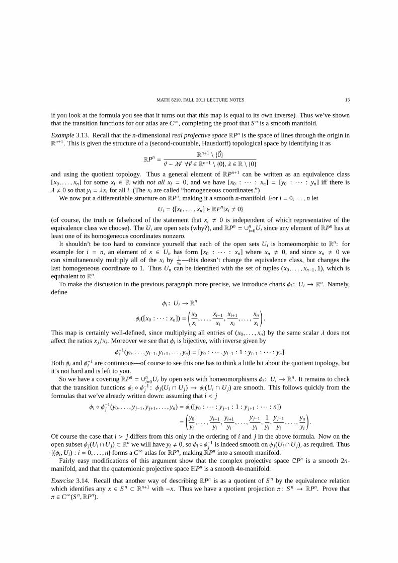
if you look at the formula you see that it turns out that this map is equal to its own inverse). Thus we’ve shownthat the transition functions for our atlas areC∞, completing the proof thatSn is a smooth manifold.

Example3.13. Recall that then-dimensionalreal projective spaceRPn is the space of lines through the origin inR

n+1. This is given the structure of a (second-countable, Hausdorff) topological space by identifying it as

RPn =R

n+1 \ ~0~v ∼ λ~v ∀~v ∈ Rn+1 \ 0, λ ∈ R \ 0

and using the quotient topology. Thus a general element ofRPn+1 can be written as an equivalence class[x0, . . . , xn] for somexi ∈ R with not all xi = 0, and we have [x0 : · · · : xn] = [y0 : · · · : yn] iff there isλ , 0 so thatyi = λxi for all i. (Thexi are called “homogeneous coordinates.”)

We now put a differentiable structure onRPn, making it a smoothn-manifold. Fori = 0, . . . ,n let

Ui = [x0, . . . , xn] ∈ RPn|xi , 0

(of course, the truth or falsehood of the statement thatxi , 0 is independent of which representative of theequivalence class we choose). TheUi are open sets (why?), andRPn = ∪n

i=0Ui since any element ofRPn has atleast one of its homogeneous coordinates nonzero.

It shouldn’t be too hard to convince yourself that each of theopen setsUi is homeomorphic toRn: forexample fori = n, an element ofx ∈ Un has form [x0 : · · · : xn] where xn , 0, and sincexn , 0 wecan simultaneously multiply all of thexi by 1

xn—this doesn’t change the equivalence class, but changes the

last homogeneous coordinate to 1. ThusUn can be identified with the set of tuples (x0, . . . , xn−1,1), which isequivalent toRn.

To make the discussion in the previous paragraph more precise, we introduce chartsφi : Ui → Rn. Namely,

define

φi : Ui → Rn

φi([x0 : · · · : xn]) =

(x0

xi, . . . ,

xi−1

xi,

xi+1

xi, . . . ,

xn

xi

).

This map is certainly well-defined, since multiplying all entries of (x0, . . . , xn) by the same scalarλ does notaffect the ratiosx j/xi . Moreover we see thatφi is bijective, with inverse given by

φ−1i (y0, . . . , yi−1, yi+1, . . . , yn) = [y0 : · · · , yi−1 : 1 : yi+1 : · · · : yn].

Bothφi andφ−1i are continuous—of course to see this one has to think a little bit about the quotient topology, but

it’s not hard and is left to you.So we have a coveringRPn = ∪n

i=0Ui by open sets with homeomorphismsφi : Ui → Rn. It remains to check

that the transition functionsφi φ−1j : φ j(Ui ∩ U j) → φi(Ui ∩ U j) are smooth. This follows quickly from the

formulas that we’ve already written down: assuming thati < j

φi φ−1j (y0, . . . , y j−1, y j+1, . . . , yn) = φi([y0 : · · · : y j−1 : 1 : y j+1 : · · · : n])

=

(y0

yi, . . . ,

yi−1

yi,yi+1

yi, . . . ,

y j−1

yi,

1yi,y j+1

yi, . . . ,

yn

yi

).

Of course the case thati > j differs from this only in the ordering ofi and j in the above formula. Now on theopen subsetφ j(Ui ∩U j) ⊂ Rn we will haveyi , 0, soφi φ

−1j is indeed smooth onφ j(Ui ∩U j), as required. Thus

(φi ,Ui) : i = 0, . . . ,n forms aC∞ atlas forRPn, makingRPn into a smooth manifold.Fairly easy modifications of this argument show that the complex projective spaceCPn is a smooth 2n-

manifold, and that the quaternionic projective spaceHPn is a smooth 4n-manifold.

Exercise3.14. Recall that another way of describingRPn is as a quotient ofSn by the equivalence relationwhich identifies anyx ∈ Sn ⊂ Rn+1 with −x. Thus we have a quotient projectionπ : Sn → RPn. Prove thatπ ∈ C∞(Sn,RPn).

14 MIKE USHER

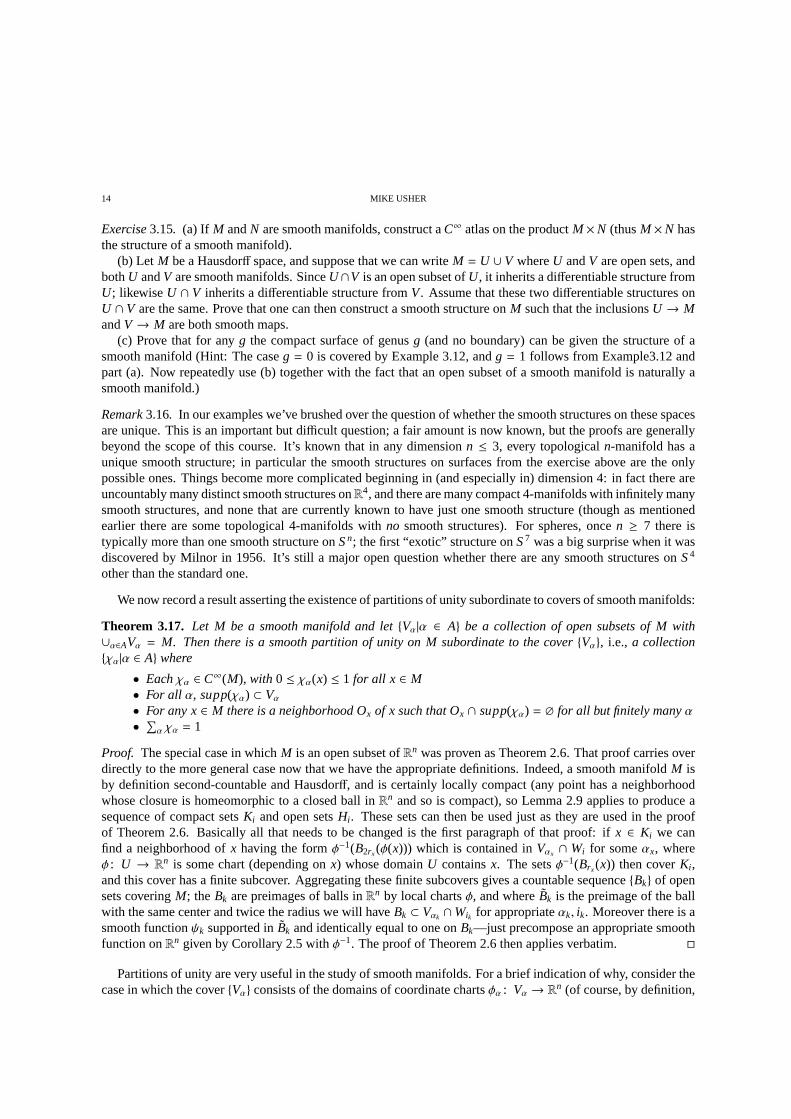
Exercise3.15. (a) If M andN are smooth manifolds, construct aC∞ atlas on the productM ×N (thusM ×N hasthe structure of a smooth manifold).

(b) Let M be a Hausdorff space, and suppose that we can writeM = U ∪ V whereU andV are open sets, andbothU andV are smooth manifolds. SinceU∩V is an open subset ofU, it inherits a differentiable structure fromU; likewiseU ∩ V inherits a differentiable structure fromV. Assume that these two differentiable structures onU ∩ V are the same. Prove that one can then construct a smooth structure onM such that the inclusionsU → MandV → M are both smooth maps.

(c) Prove that for anyg the compact surface of genusg (and no boundary) can be given the structure of asmooth manifold (Hint: The caseg = 0 is covered by Example 3.12, andg = 1 follows from Example3.12 andpart (a). Now repeatedly use (b) together with the fact that an open subset of a smooth manifold is naturally asmooth manifold.)

Remark3.16. In our examples we’ve brushed over the question of whether the smooth structures on these spacesare unique. This is an important but difficult question; a fair amount is now known, but the proofs are generallybeyond the scope of this course. It’s known that in any dimension n ≤ 3, every topologicaln-manifold has aunique smooth structure; in particular the smooth structures on surfaces from the exercise above are the onlypossible ones. Things become more complicated beginning in(and especially in) dimension 4: in fact there areuncountably many distinct smooth structures onR4, and there are many compact 4-manifolds with infinitely manysmooth structures, and none that are currently known to havejust one smooth structure (though as mentionedearlier there are some topological 4-manifolds withno smooth structures). For spheres, oncen ≥ 7 there istypically more than one smooth structure onSn; the first “exotic” structure onS7 was a big surprise when it wasdiscovered by Milnor in 1956. It’s still a major open question whether there are any smooth structures onS4

other than the standard one.

We now record a result asserting the existence of partitionsof unity subordinate to covers of smooth manifolds:

Theorem 3.17. Let M be a smooth manifold and letVα|α ∈ A be a collection of open subsets of M with∪α∈AVα = M. Then there is a smooth partition of unity on M subordinate to the coverVα, i.e., a collectionχα|α ∈ A where

• Eachχα ∈ C∞(M), with 0 ≤ χα(x) ≤ 1 for all x ∈ M• For all α, supp(χα) ⊂ Vα

• For any x∈ M there is a neighborhood Ox of x such that Ox ∩ supp(χα) = ∅ for all but finitely manyα•

∑α χα = 1

Proof. The special case in whichM is an open subset ofRn was proven as Theorem 2.6. That proof carries overdirectly to the more general case now that we have the appropriate definitions. Indeed, a smooth manifoldM isby definition second-countable and Hausdorff, and is certainly locally compact (any point has a neighborhoodwhose closure is homeomorphic to a closed ball inRn and so is compact), so Lemma 2.9 applies to produce asequence of compact setsKi and open setsHi . These sets can then be used just as they are used in the proofof Theorem 2.6. Basically all that needs to be changed is the first paragraph of that proof: ifx ∈ Ki we canfind a neighborhood ofx having the formφ−1(B2rx(φ(x))) which is contained inVαx ∩Wi for someαx, whereφ : U → Rn is some chart (depending onx) whose domainU containsx. The setsφ−1(Brx(x)) then coverKi ,and this cover has a finite subcover. Aggregating these finitesubcovers gives a countable sequenceBk of opensets coveringM; the Bk are preimages of balls inRn by local chartsφ, and whereBk is the preimage of the ballwith the same center and twice the radius we will haveBk ⊂ Vαk ∩Wik for appropriateαk, ik. Moreover there is asmooth functionψk supported inBk and identically equal to one onBk—just precompose an appropriate smoothfunction onRn given by Corollary 2.5 withφ−1. The proof of Theorem 2.6 then applies verbatim.

Partitions of unity are very useful in the study of smooth manifolds. For a brief indication of why, consider thecase in which the coverVα consists of the domains of coordinate chartsφα : Vα → R

n (of course, by definition,


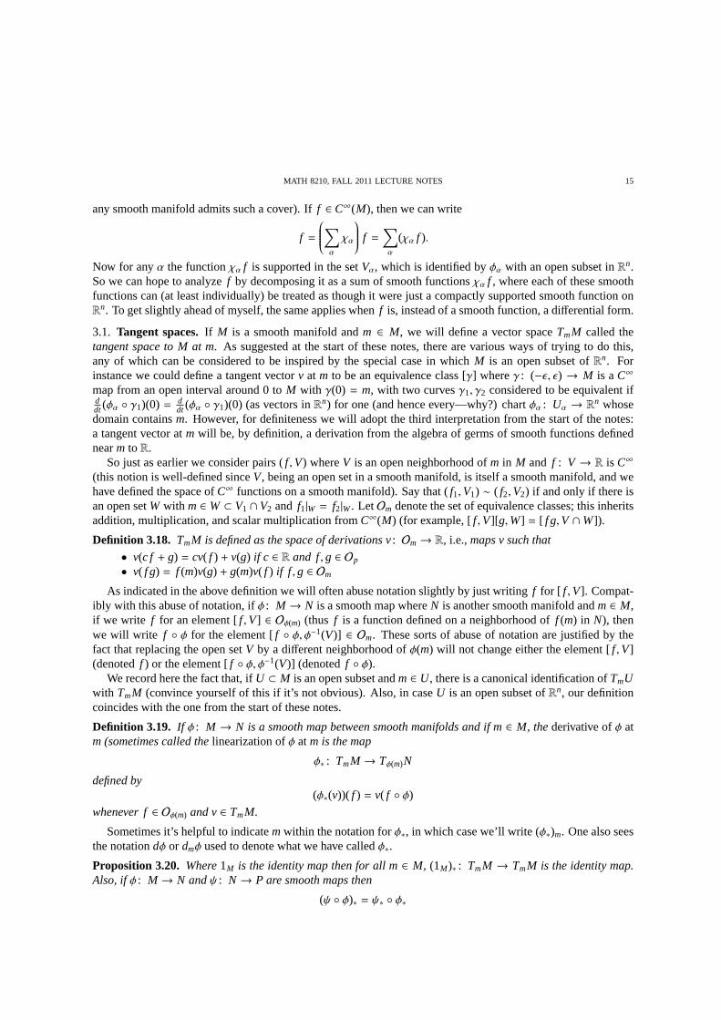
any smooth manifold admits such a cover). Iff ∈ C∞(M), then we can write

f =

∑

α

χα

f =∑

α

(χα f ).

Now for anyα the functionχα f is supported in the setVα, which is identified byφα with an open subset inRn.So we can hope to analyzef by decomposing it as a sum of smooth functionsχα f , where each of these smoothfunctions can (at least individually) be treated as though it were just a compactly supported smooth function onR

n. To get slightly ahead of myself, the same applies whenf is, instead of a smooth function, a differential form.

3.1. Tangent spaces.If M is a smooth manifold andm ∈ M, we will define a vector spaceTmM called thetangent space to M at m. As suggested at the start of these notes, there are various ways of trying to do this,any of which can be considered to be inspired by the special case in whichM is an open subset ofRn. Forinstance we could define a tangent vectorv at m to be an equivalence class [γ] whereγ : (−ǫ, ǫ) → M is aC∞

map from an open interval around 0 toM with γ(0) = m, with two curvesγ1, γ2 considered to be equivalent ifddt(φα γ1)(0) = d

dt(φα γ1)(0) (as vectors inRn) for one (and hence every—why?) chartφα : Uα → Rn whose

domain containsm. However, for definiteness we will adopt the third interpretation from the start of the notes:a tangent vector atm will be, by definition, a derivation from the algebra of germsof smooth functions definednearm toR.

So just as earlier we consider pairs (f ,V) whereV is an open neighborhood ofm in M and f : V → R is C∞

(this notion is well-defined sinceV, being an open set in a smooth manifold, is itself a smooth manifold, and wehave defined the space ofC∞ functions on a smooth manifold). Say that (f1,V1) ∼ ( f2,V2) if and only if there isan open setW with m ∈W ⊂ V1 ∩V2 and f1|W = f2|W. LetOm denote the set of equivalence classes; this inheritsaddition, multiplication, and scalar multiplication fromC∞(M) (for example, [f ,V][g,W] = [ f g,V ∩W]).

Definition 3.18. TmM is defined as the space of derivations v: Om→ R, i.e., maps v such that

• v(c f + g) = cv( f ) + v(g) if c ∈ R and f,g ∈ Op

• v( f g) = f (m)v(g) + g(m)v( f ) if f ,g ∈ Om

As indicated in the above definition we will often abuse notation slightly by just writing f for [ f ,V]. Compat-ibly with this abuse of notation, ifφ : M → N is a smooth map whereN is another smooth manifold andm ∈ M,if we write f for an element [f ,V] ∈ Oφ(m) (thus f is a function defined on a neighborhood off (m) in N), thenwe will write f φ for the element [f φ, φ−1(V)] ∈ Om. These sorts of abuse of notation are justified by thefact that replacing the open setV by a different neighborhood ofφ(m) will not change either the element [f ,V](denotedf ) or the element [f φ, φ−1(V)] (denotedf φ).

We record here the fact that, ifU ⊂ M is an open subset andm ∈ U, there is a canonical identification ofTmUwith TmM (convince yourself of this if it’s not obvious). Also, in case U is an open subset ofRn, our definitioncoincides with the one from the start of these notes.

Definition 3.19. If φ : M → N is a smooth map between smooth manifolds and if m∈ M, thederivative ofφ atm (sometimes called thelinearization ofφ atm is the map

φ∗ : TmM → Tφ(m)N

defined by(φ∗(v))( f ) = v( f φ)

whenever f∈ Oφ(m) and v∈ TmM.

Sometimes it’s helpful to indicatemwithin the notation forφ∗, in which case we’ll write (φ∗)m. One also seesthe notationdφ or dmφ used to denote what we have calledφ∗.

Proposition 3.20. Where1M is the identity map then for all m∈ M, (1M)∗ : TmM → TmM is the identity map.Also, ifφ : M → N andψ : N→ P are smooth maps then

(ψ φ)∗ = ψ∗ φ∗

16 MIKE USHER

Proof. The first statement (about the identity) is obvious from the definition. For the second, we have, iff ∈Oψφ(m),

((ψ φ)∗v)( f ) = v( f (ψ φ)) = v(( f ψ) φ) = (φ∗v)( f ψ) = (ψ∗φ∗v)( f ).

Corollary 3.21. If m ∈ M where M is a smooth n-manifold, thendimTmM = n.

Proof. We can choose a coordinate chartφ : U → φ(U) whereU is an open neighborhood ofm. As noted earlierwe haveTmM = TmU. By Proposition 3.20, (φ−1)∗ φ∗ = (φ−1 φ)∗ is the identity map fromTmU = TmM toitself, andφ∗ (φ−1)∗ = (φ φ−1)∗ is the identity map fromTφ(m)φ(U) to itself. Thusφ∗ is an isomorphism ofvector spaces fromTmM to Tφ(m)φ(U), with inverse (φ−1)∗. We showed in Section 1 that, sinceφ(U) is an opensubset ofRn, dimTφ(m)φ(U) = n, so the conclusion follows.

Expanding a bit on the above proof, recall that we showed thatTφ(m)φ(U) consists precisely of mapsOφ(m) → R

taking the formg 7→∑n

i=1 vi∂g∂xi|φ(m). So since (φ−1)∗ is an isomorphism, we conclude that, in the presence of a

chosen coordinate chartφ : U → Rn aroundm, a general elementv ∈ TmM will be given by the formula

v( f ) =n∑

i=1

vi∂

∂xi( f φ−1)|φ(m).

When this is the case, we will say something along the lines of,“v is given in the coordinate chartφ byv =

∑vi

∂∂xi

.” Of course, the coefficientsvi will depend on the coordinate chart, not just on the tangent vectorv.

Exercise3.22. Let φ, ψ : U → Rn be two coordinate charts whereU is an open subset of a smooth manifoldM,and letm ∈ U. If v is given in the coordinate chartφ by v =

∑vi

∂∂xi

, and is given in the coordinate chartψ by

v =∑

wi∂∂yi

, find, with proof, an expression for thewi in terms of thevi and the mapsφ ψ−1 and/or ψ φ−1.

So if M is a smoothn-manifold, we have associated to every pointm ∈ M an n-dimensional vector spaceTmM. A diffeomorphismφ : M → M′ induces an isomorphism of vector spacesφ∗ : TmM → Tφ(m)M′. Howeverthere is (in general) no canonical way of identifyingTm1 M with Tm2 M for distinct pointm1,m2 ∈ M (of course,since the two vector spaces have the same dimension, they areisomorphic as vector spaces, just not canonicallyso).

Relatedly, while choosing the pointm ∈ M canonically determines then-dimensional vector spaceTmM, itdoes not canonically determine a basis for this vector space. One way of choosing a basis forTmM is suggestedabove: choose a local coordinate chartφ : U → Rn aroundU; then a basis is given by the derivationsf 7→ ∂

∂xi( f

φ−1)(p) for i = 1, . . . ,n (the members of this basis are typically denoted by∂∂xi

. Different choices of coordinatechart of course give rise to different bases; the relationship between the bases is determined by Exercise 3.22.

Thetangent bundleof a smooth manifold is, as a set, defined to be the union

T M = ∪m∈Mm × M.

For any subsetS ∈ M (typically S will be open or closed) we define the “restriction of the tangent bundle toS”as

T M|S = ∪m∈Sm × TmM.

Given a coordinate chartφ : U → Rn whereU ⊂ M is open, we have a bijectionΦ : T M|U → φ(U) × Rn givenby

Φ

(m,

∑vi∂

∂xi

)= (φ(m), v1, . . . , vn).

We can then define a topology onT M by requiring that each of these bijections be homeomorphisms—moreprecisely, we take as a base for this topology the collectionof subsets of the formΦ−1(V) whereΦ : T M|U →φ(U) × Rn is a map as above constructed from a coordinate chartφ andV ⊂ φ(U) × Rn is open.


The various homeomorphismsΦ : T M|U → φ(U) × Rn associated to coordinate chartsφ : U → φ(U) in factform aC∞ atlas forT M. Indeed the domainsT M|U certainly coverT M (sinceM is covered by coordinate charts)and so we just need to check that the transition functions aresmooth. This latter fact follows from Exercise 3.22.Indeed, ifφα : Uα → R

n andφβ : Uβ : Uβ → Rn are two coordinate charts, then it should follow from your

computation in Exercise 3.22 that the transition function

Φβ Φ−1α : φα(Uα ∩ Uβ) × R

n→ φβ(Uα ∩ Uβ) × Rn

is given by

(4) Φβ Φ−1α (x,~v) = (φβ φ

−1α (x),gαβ(x)~v)

wheregαβ is a certain smooth function which takes values in the group of invertible n × n matrices. Thus thetransition functions are smooth, and so determine a smooth manifold structure onT M.

Of course, we have a projectionπ : T M→ M which sends (m, v) to m. In terms of the local coordinate chartsΦ onT M andφ on M, π just acts by the projection ofφ(U) × Rn onto its first factor; thusπ is a smooth map.

Summing up, out of ann-dimensional smooth manifoldM we have constructed a 2n-dimensional smoothmanifoldT M, equipped with a projectionπ : T M → M. The “fibers”π−1(m) of π are canonically identifiedwith the tangent spacesTmM, and thus aren-dimensional vector spaces. Moreover there is an atlas onT M suchthat the transition functions respect the vector space structures on the fibers in the sense that they are given bya formula of the shape (4) where eachgαβ(x) is a linear map.T M is thus an example of what is called avectorbundle; we will see more examples of vector bundles as the course proceeds.

3.2. Vector fields. Consistently with what was done in Section 1, we make the following definition:

Definition 3.23. Let M be a smooth manifold and U⊂ M an open subset. Avector field onU is a derivationX : C∞(U)→ C∞(U) (i.e., X obeys X(c f + g) = cX f + Xg and X( f g) = f Xg+ gX f if f,g ∈ C∞(U), c ∈ R). Wedenote the space of vector fields on U byX(U).

Just as in Section 1, we can scalar multiply, add, and take thecommutators of derivations fromC∞(U) toitself, soX(U) naturally has the structure of a Lie algebra.

A vector field onU should have another interpretation as a “smoothly-varying” choice of tangent vectorat m for eachm ∈ M. We now lay out how this works. ForU ⊂ M we have a (restricted) tangent bundleπ : T M|U → U.

Definition 3.24. A smooth sectionof T M over U is a smooth map s: U → T M|U such thatπ s is the identity.We writeΓ(U,T M) for the space of smooth sections of T M over U.

In other words,s(m) ∈ TmU for all p ∈ U; the notion that the tangent vectors should vary smoothly isencodedin the requirement thats should be a smooth map. SinceTmU is a vector space, we get vector space operationson Γ(U,T M) defined by (cs)(m) = c(s(m)) and (s1 + s2)(m) = s1(m) + s2(m) (there’s something to show here,namely that for instance the sum of two smooth sections is still smooth, but it’s not hard to check this). Oneimportant example of a section ofT M (or more generally of any vector bundle) is thezero section, defined bys(m) = 0 ∈ TmM for all p. (To see that this is smooth, just note that in the local coordinatesφ(U) × Rn ⊂ R2n

described earlier the map is given byx 7→ (x,0) which is obviously a smooth map fromRn toR2n).Recall Exercise 2.11, to which the following gives a solution:

Proposition 3.25. Let M be a smooth manifold, U⊂ M open, m∈ U, and X ∈ X(U). Then the followingprescription uniquely specifies an element Xm ∈ TmM. For any [ f ,V] ∈ Om, choose af ∈ C∞(U) such that[ f ,U] = [ f ,V], and define Xm([ f ,V]) = (X f )(m).

Proof. First of all we need to show that for any [f ,V] ∈ Om (in other words,V is an open set aroundm andf is a smooth function onV) there is a smooth functionf defined throughoutU and coinciding on withfon some neighborhoodG of m. To see this, note that we can find a coordinate chartφ : W → Rn aroundm and r > 0 so thatφ−1(B2r (φ(m))) ⊂ V. Take a partition of unityχ1, χ2 subordinate to the open cover

18 MIKE USHER

φ−1(B2r (φ(m))),M \ φ−1(Br (φ(m))) of M. Then let f = χ1 f ; initially this function is only defined onV, butsince it has support contained in a compact subset ofV we may extend it by zero to obtain a smooth function onall of M. Sinceχ1 + χ2 = 1 andχ2 vanishes onφ−1(Br (φ(m))), f coincides withf onφ−1(Br (φ(m))), as desired.

We now show that the value (X f )(m) is independent of the choice off with [ f ,U] = [ f ,V]. If g is anothersuch choice, there is a neighborhoodW of m such that f |W = g|W. Let O be a neighborhood ofm such thatm ∈ O ⊂ W (for instance takeO to be the preimage of a small ball in a coordinate chart, as in the previousparagraph). Just as in the previous paragraph we can find a smooth functionχ : M → R such thatχ|O = 1 andsupp(χ) ⊂ W. Let β = 1− χ, soβ vanishes identically on the neighborhoodO of m and is equal to 1 outsideW.Hence

(1− β2) f = (1− β2)g

(both sides are zero everywhere thatf , g). On the other hand(X(β2 f )

)(m) = β(m)

(X(β f )

)(m) + β(m) f (m) (Xβ) (m) = 0

and similarly (X(β2g)

)(m) = 0.

Hence

(X f )(m) =(X(β2 f )

)(m) +

(X((1− β2) f )

)(m)

=(X((1− β2) f )

)(m) =

(X((1− β2)g)

)(m)

=(X(β2g)

)(m) +

(X((1− β2)g)

)(m) = (Xg)(m).

This confirms that the prescription of the proposition givesa well-defined mapXm : Om → R. It remains tocheck thatXm is a derivation. But this follows easily from the derivationproperty forX. Given [f ,V], [g,W] ∈Om, if we use f ∈ C∞(U) to computeXm[ f ,V] = (X f )(m) andg ∈ C∞(U) to computeXm[g,V] = (Xg)(m) thenwe can usef g = f g to computeXm([ f ,V][g,W]) (of course we could make other choices forf g, but the start ofthe proof ensures that this would result in the same value forXm([ f ,V][g,W])). Then the derivation property forX shows

Xm([ f ,V][g,W]) =(X( f g)

)(m) = f (m)(Xg)(m) + g(m)(X f )(m)

= f (m)Xm[g,W] + g(m)Xm[ f ,V].

R-linearity is proved in essentially the same way, completing the proof thatXm ∈ TmM.

We now show that giving a vector field (in the sense of a derivation on the space of smooth functions) isexactly the same as giving a smooth section of the tangent bundle.

Theorem 3.26. Let U be an open subset of the smooth manifold M. A bijectionF : X(U) → Γ(U,T M) may bedefined as follows. For X∈ X(U), setF (X) equal to the map sX : M → T M defined by sX(m) = Xm (where Xm

is given by Proposition 3.25).

Proof. First we need to show thatF is well-defined—we certainly have a well-defined functionsX : M → T Mfor anyX ∈ X(U), andsX is a section in the sense thatπ sX = 1M, but we also need to check thatsX is smoothin order forF to take values in the spaceΓ(U,T M) of smooth sections.

To see this, note first of all that a functionf between two smooth manifolds is smooth if and only if the domaincan be covered by open sets to each of whichf restricts as a smooth function. Ifm ∈ M, let φ : V → Rn be acoordinate chart withm ∈ V ⊂ U, and forr > 0 small enough thatB2r (φ(m)) ⊂ φ(V) let Wm = φ

−1(Br (φ(m))).We will show thatsX|Wm is smooth, which suffices since any point inM has a neighborhood of the formWm.

In this direction, letχ : M → R be a smooth function withχ|Wm= 1 andsupp(χ) ⊂ V. For anyq ∈ Wm and

f ∈ Oq we have(sX(q))( f ) = Xq( f ) = Xq(χ f )


since f andχ f coincide on a neighborhood (namelyWm) of q.Now for eachj = 1, . . . ,n write g j = (x j ψ) ·χ ∈ C∞(M). Then onWm, g coincides with thejth coordinate of

the chartψ|Wm : Wm→ Rn. We know that, for eachq ∈Wm, sinceXq ∈ TqM we can expressXq in the coordinate

chartψ asXq =∑

i vi(q) ∂∂xi|q for somevi(q) ∈ R. Evaluating on the functionsg j we see that, for eachj,

v j(q) = (Xgj)(q).

Thus the functionsv j : Wm→ R are each smooth. Now in terms of the local coordinates for thetangent bundledescribed at the end of the previous subsection, the mapsX is given within Wm by the formula (wherex ∈ψ(Wm) ⊂ Rn)

x 7→(x, v1(ψ−1(x)), . . . , vn(ψ−1(x))

).

This map is smooth since thev j are smooth. ThussX|Wm is smooth, and sosX is smooth sinceU can be coveredby open sets of the formWm.

Now that we have shown the mapF : X(U) → Γ(U,T M) to be well-defined, we show that it is bijective.Suppose thatX,Y ∈ X(U) are two distinct vector fields onU. Then there isf ∈ C∞(U) andm ∈ U such that(X f)(m) , (Y f)(m). But then [f ,U] is a well-defined element ofOm with Xm([ f ,U]) , Ym([ f ,U]), and thusXm , Ym, i.e. sX(m) , sY(m). ThusF is injective.

Finally suppose thats ∈ Γ(U,T M); we must findX ∈ X(U) so thatsX = s. If f ∈ C∞(U) then for allm wehave an element [f ,U] ∈ Om and so a real number (s(m))([ f ,U]). This determines a functionX f : U → R bythe formula (X f)(m) = (s(m))([ f ,U]). The derivation propertiesX(c f + g) = cX f + XgandX( f g) = f Xg+ gX ffollow directly from the fact that eachs(m) is a derivation fromOm to R; however we still need to check thatX f ∈ C∞(U) for any f ∈ C∞(U). In a local coordinate chartψ : V → Rn, the tangent vectorss(m) for m ∈ Vare represented ass(m) =

∑vi(m) ∂

∂xi, where the functionsvi areC∞ by the fact thats is a smooth map. But then

X f |V =∑

vi∂ f∂xi

, which is a smooth function. ThusX f restricts to each coordinate chart as a smooth function, andso is smooth. It is clear from the definition thatsX = s.

So we have two equivalent characterizations of vector fieldson M: as derivationsC∞ → C∞, and as smoothsectionsM → T M (which in coordinate charts can be locally expressed in the form

∑vi

∂∂xi

for suitable smoothfunctionsvi). Both characterizations are often useful.

4. Differential forms

As the title of the course textbook suggests, a very important role will be played in the rest of the course bywhat are called thedifferential formson a smooth manifold. IfM is a smoothn-manifold, we will develop thenotion of a “p-form” on M for p = 0,1, . . . ,n (and also forp > n, but for algebraic reasons it turns out thatthe onlyp-forms with p > n will be zero). Thesep-forms will form a vector spaceΩp(M), and we will have avery important mapd, called theexterior derivative, which maps the space of all differential forms to itself andrestricts for eachp to a mapd: Ωp(M)→ Ωp+1(M).

To ease into this, let’s start withp = 0 andp = 1.

Definition 4.1. A 0-form on M is a smooth function f: M → R. In other wordsΩ0(M) = C∞(M).

The case of 1-forms is a bit more interesting. First we introduce the notion of thecotangent space:

Definition 4.2. • If M is a smooth manifold and m∈ M, thecotangent space atm, denoted by T∗mM, is thedual space to the tangent space TmM.• Thecotangent bundleof M is

T∗M = ∪m∈Mm × T∗mM.

In other words,T∗mM consists of linear functionalsα : TmM → R. Since a vector space and its dual have thesame dimension, ifM is ann-manifold then dimT∗pM = n for all m ∈ M.

Definition 4.2 identifies the cotangent bundleT∗M as a set. One can equip it with a topology and then witha smooth manifold structure, in such a way that the projection π : T∗M → M (sending (m, α) to m if α ∈ T∗mM)

20 MIKE USHER

makesT∗M into a vector bundle, just like the situation with the tangent bundle. At least for now we won’t reallyneed to use this fact, but note that we have (at least at a set-theoretic level) the notion of asection s: M → T∗M,i.e. a functions: M → T∗M such thatπ s= 1M. A sections: M → T∗M associates to eachm ∈ M an elementsm ∈ T∗pM.

Definition 4.3. A differential 1-formon a smooth manifold M is a sectionα : M → T∗M which satisfies thefollowing smoothness property: Whenever X∈ X(M) is a vector field on M, the function

α(X) : m 7→ αm(Xm)

is a C∞ function on M. We denote byΩ1(M) the vector space of differential1-forms.

To unpack the above, note that the sectionα of thecotangentbundle determinescovectorsαm ∈ T∗mM for allm, while the vector fieldX (which by Theorem 3.26) is equivalent to a section of thetangentbundle, determinesfor eachma tangent vectorXm ∈ TmM. Hence we can evaluateαm(Xm), and the smoothness requirement onα isthat (as long asX is smooth) the result of this evaluation varies smoothly with m. If we had gone ahead and puta smooth manifold structure onT∗M it turns out that this would be equivalent to requiringα : M → T∗M to bea smooth map.

As mentioned earlier, for allp we will define a mapd: Ωp(M)→ Ωp+1(M). I can now fulfill this promise forp = 0. Actually if one thinks of tangent vectors as derivations the definition may seem strangely simple:

To any f ∈ Ω0(M), i.e., any smooth functionf , we are to associate a sectiond f : M → T∗M. In other wordsfor eachm we should obtain (d f)m: TmM → R. Well, bearing in mind that an element ofTmM is a derivationfrom functions defined nearm toR, we use the formula

(5) (d f)m(v) = v( f ) if v ∈ TmM.

Suppose now thatφ : U → Rn is a coordinate chart, whereU ⊂ M is open. NowU is a smooth manifold inits own right, so we can considerΩ1(U). The coordinate chartφ distinguishes some special smooth functionson U, namely thecoordinate functions x1, . . . , xn (perhaps we should really writex1 φ, . . . , xn φ, or we couldjust agree that the decomposition ofφ into coordinates is given byφ(m) = (x1(m), . . . , xn(m))). Since thexi aresmooth functions (i.e., 0-forms) onU, we obtain 1-forms dx1, . . . ,dxn ∈ Ω

1(U). So for eachm ∈ U we havecovectors (dxi)m ∈ T∗mU = T∗mM.

On the other hand, recall that the tangent spaceTmM atm has basis given by∂∂x1|m, . . . ,

∂∂xn|m. We have

(dxi)m

(∂

∂x j|m

)=

∂

∂x j(xi) = δi j .

Thus the (dxi)m form adual basisto the cotangent spaceT∗mM with respect to the basis∂∂xi|m

for TpM.

Since the (dxi)m form a basis forT∗mM at allm, it follows that any 1-formα ∈ Ω1(U) can be written as

α =

n∑

i=1

αidxi

for some functionsαi ∈ C∞(U) (which may be recovered by evaluatingα on ∂∂xi

).

Exercise4.4. Suppose that we have two different coordinate charts

φ : m 7→ (x1(m), . . . , xn(m)) and ψ : m 7→ (y1(m), . . . , yn(m))

each with domain given by some open subsetU of a smooth manifold. Ifα ∈ Ω1(U) can be written as

α =

n∑

i=1

αidxi =

n∑

i=1

βidyi

find a general formula (in terms of the derivatives ofφ ψ−1 and/or ψ φ−1) for the relationship between thecoefficientsαi andβi .


The above exercise is designed to be compared to Exercise 3.22. A single coordinate chart aroundmproducesdistinguished bases

∂∂xi|m

for TmM and (dxi)m for T∗mM, allowing one to parametrizeTmM or T∗mM by Rn.Changing the coordinate chart changes the appropriate parametrization for eitherTmM or T∗mM, and you shouldhave found that the way in which the parametrization transforms under a coordinate change is different forTmMthan it is forT∗mM. This reflects the fact that vector fields and 1-forms really are fundamentally different kinds ofobjects.

If ( x1, . . . , xn) : U → Rn is a coordinate patch andm ∈ U, we see that

d fm

(∂

∂xi

)=∂ f∂xi

(m) =

n∑

j=1

∂ f∂x j

(dxj)m

(∂

∂xi

),

and thus, throughout the coordinate chartU, we have

(6) d f =n∑

j=1

∂ f∂x j

dxj .

In principle we could also have definedd: Ω0(M) → Ω1(M) by saying that if f ∈ Ω0(M) has support in acoordinate chart thend f is given by formula (6), and requiring thatd be linear overR—this would determined f for any f (not necessarily supported in a coordinate chart) since by using a partition of unity we can write anarbitrary function as a sum of functions each of which is supported in a coordinate chart. (Of course, with thisapproach one would need to make sure thatd f didn’t depend on the way in whichf is decomposed as such asum—our more natural and coordinate-free definition ofd evades this issue).

Having defined the mapd: Ω0(M) → Ω1(M), one could ask whether it is surjective. A little thought shouldconvince you that the answer must be no (if dimM ≥ 2)—indeed this may be familiar from multivariablecalculus. Consider just a 1-formα which is supported in a coordinate chartU, so in coordinatesα|U =

∑i αidxi

for some smooth functionsαi supported inU, andα vanishes elsewhere. Evidently ifα = d f then, onU, wewould haveαi =

∂ f∂xi

. Since f is assumedC∞, its mixed partials are equal and so if we hadα = d f we would

need∂αi

∂x j=

∂α j

∂xifor all i, j, and of course these equations have no reason to hold for a general collection of smooth

functionsαi supported inU.Thus we obtain anobstructionto a 1-formα being in the image ofd, which in local coordinates can be seen

as coming from the partial derivatives of the various components ofα. If α is in the image ofd it is calledexact.Once we define the space of 2-formsΩ2(M) and the exterior derivatived: Ω1(M) → Ω2(M), we will see thatthe above obstruction vanishes in the sense that the relevant partial derivatives coincide if and only ifdα = 0.Indeed,d d: Ω0(M) → Ω2(M) is zero (as, more generally, isd d: Ωp(M) → Ωp+2(M)). One can then askwhether everyα for which the obstruction vanishes (dα = 0) is indeed exact. We’ll see that the answer to thisquestion depends on the topology ofM (as measured by thede Rham cohomology groups). )

4.1. The alternating algebra.

Definition 4.5. Let V be a vector space overR, and let p be a positive integer. Analternatingp-form on V is afunctionη : Vp→ R with the following properties:

• η is p-linear: For any i, if c∈ R and v1, . . . , vp ∈ V and wi ∈ V then

η(v1, . . . , vi−1, cvi + wi , . . . , vp) = cη(v1, . . . , vi−1, vi , . . . , vp) + η(v1, . . . , vi−1,wi , . . . , vp).

• V is antisymmetric: if v,w ∈ V then, for any i< j and any u1, . . . ,ui−1,ui+1, . . . ,u j−1,u j+1, . . . ,up ∈ V

η(u1, . . . ,ui−1, v,ui+1, . . . ,u j−1,w,u j+1, . . . ,up) = −η(u1, . . . ,ui−1,w,ui+1, . . . ,u j−1, v,u j+1, . . . ,up).

We will denote the vector space of alternating p-forms on V byΛpV∗. We extend the notationΛpV∗ to p= 0 bysettingΛ0V∗ = R.

22 MIKE USHER

Implicit in the above is that the alternatingp-forms do indeed form a vector space, which should be clear. OurnotationΛpV∗ reflects a number of algebraic facts, not all of which we will need or use: for any vector spaceVthere is a certain standard vector spaceΛpV (“the pth graded part of the exterior algebra”), and (at least assumingthatV is finite-dimensional) what we denote byΛpV∗ can be canonically identified both with (ΛpV)∗ and withΛp(V∗) (so our lack of parentheses is in writingΛpV∗ is deliberate). There is an obvious identification ofΛ1V∗

with V∗.With this definition, there is for allp,q ≥ 0 a map

∧ : ΛpV∗ × ΛqV∗ → Λp+qV∗

(α, β) 7→ α ∧ β

called thewedge product, which satisfies various important properties. Let us give the definition gradually. Thefirst interesting case is whenp = q = 1: in this case we define the wedge product by, forα, β ∈ Λ1V∗, andv,w ∈ V,

(α ∧ β)(v,w) = α(v)β(w) − α(w)β(v).

It is not hard to see that, with this definition,α ∧ β does indeed belong toΛ2V∗ (the minus sign ensures that theantisymmetry condition holds). We then extend this to the case thatp = 1 butq is arbitrary by, forα ∈ Λ1V∗, β ∈ΛqV∗,

(α ∧ β)(v1, v2, . . . , vq+1) = α(v1)β(v2, . . . , vq+1) − α(v2)β(v1, v3, . . . , vq+1)

+ α(v3)β(v1, v2, v4, . . . , vq+1) + · · · + (−1)lα(vq+1)β(v1, . . . , vq)

=

q+1∑

j=1

(−1) j−1α(v j)β(v1, . . . , v j−1, v j+1, . . . , vq+1)

We introduce a notation for “omitting” inputs intok-forms as we often need to do: instead of writingβ(v1, . . . , v j−1, v j+1, . . . , vq+1) we will write β(v1, . . . , v j , . . . , vq+1); thus the hat signifies that thejth term hasbeen omitted.

We should check thatα∧β as defined above is actually an element ofΛq+1V∗. It’s fairly obvious from this def-inition thatα∧β is (q+1)-linear. As for antisymmetry, if we switchvk andvl with k < l then the antisymmetry ofβ shows that all terms in the sum change sign except for those with j = k, l. Meanwhile thekth term changes from(−1)k−1α(vk)β(v1, . . . , vk, . . . , vl , . . . , vq+1) to (−1)k−1α(vl)β(v1, . . . , vl , . . . , vk, . . . , vq+1), and thelth term changesfrom (−1)l−1α(vl)β(v1, . . . , vk, . . . , vl , . . . , vq+1) to (−1)l−1α(vk)β(v1, . . . , vl , . . . , vk, . . . , vq+1). I claim that the newlth term is the negative of the oldkth term, and vice versa. Indeed to convert the newlth term to something thatlooks like the oldkth term we can “move thevl pastvk+1, . . . , vl−1”—in other words we should switchvl with vk+1,then switchvl with vk+2, and so on, until we switchvl with vl−1. Sinceβ is antisymmetric each of these switchesproduces a factor of−1, and so since there are a total ofl − k−1 numbers fromk+1 to l −1 the whole procedureproduces a factor of (−1)l−k−1. So the newlth term is equal to (−1)l−1(−1)l−k−1α(vk)β(v1, . . . , vk, . . . , vq+1), whichis indeed equal to the negative of the oldkth term. Similarly, the newkth term can be equated with the negativeof the oldlth term by “movingvk l −k−1 slots to the left.” Summing up, switchingvk with vl causes all the termswith j < k, l to change signs, and also causes the sum of thekth andlth terms to change sign. This proves thatα ∧ β is alternating, so our mapΛ1V∗ × ΛqV∗ → Λq+1V∗ is well-defined.

Finally we extend the definition of the wedge product to general values ofp andq. One way of characterizingthis extension is that, given our definition for the casep = 1, there turns out to be a unique way of extending thedefinition to generalp so that the operation∧ will be bilinear and associative (for instance, ifα, β ∈ Λ1V∗, sothatα ∧ β ∈ Λ2V∗, we take the wedge product withα ∧ β (on the left) by insisting that (α ∧ β) ∧ γ = α ∧ (β ∧ γ)for γ ∈ ΛqV∗—since we’ve already decided how to take wedge product with 1-forms the right-hand side iswell-defined).

Instead of showing that this indirect argument gives a well-defined prescription, we give a formula. Givennonnegative integersp andq, let Sp,q denote the collection ofp-element subsets of1, . . . , p + q. Then for


S ∈ Sp,q let the positive integersiS1 < iS2 < · · · < iSp be the elements ofS, and let the positive integersjS1 < . . . < jSqbe the elements of1, . . . , p+ q \ S. DefineρS : 1, . . . , p+ q → 1, . . . , p+ q by, for 1≤ k ≤ p, ρS(k) = iSk ,and forp+ 1 ≤ k ≤ p+ q, ρS(k) = jSk−p. In other wordsρS is the permutation of1, . . . , p+ q gotten by writingall the elements ofS in increasing order, and then all the elements of1, . . . , p+ q \ S in increasing order. Let(−)S be 1 if the permutationρS is even and−1 if ρS is odd. The general formula for the wedge product is then

(7) (α ∧ β)(v1, . . . , vp+q) =∑

S∈Sp,q

(−)Sα(viS1, . . . , viSp )β(v jS1

, . . . , v jSq )

In other words, (α ∧ β)(v1, . . . , vp+q) is gotten by looking at all the different products gotten by plugging inp ofthevi into α andq of them intoβ, and summing these up with a naturally associated sign. It’snot hard to see thatthis coincides with our previous definition in casep = 1.

To help verify some other properties of the wedge product (inparticular the fact that the wedge productof alternating forms is alternating) we rewrite (7) as a sum over all permutations onp + q letters. LetSp+q

denote the group of permutations onp + q letters. IdentifySp × Sq with a subgroup ofSp+q by associating to(σ, τ) ∈ Sp×Sq with the permutation onp+q letters (still denoted (σ, τ)) such that (σ, τ)(i) = σ(i) for 1 ≤ i ≤ pand (σ, τ)(p+ j) = p+τ( j) for 1 ≤ j ≤ q (in other words,σ acts on the firstp letters andτ acts on the lastq). Anypermutation inη ∈ Sp+q can be written uniquely in the formη = ρS (σ, τ) whereρS is one of the permutationsfrom the previous paragraph: namely, letS = η(1), . . . , η(p); let σ send j to r if η( j) is therth largest elementof S; and letτ sendj to s if η(p+ j) is thesth largest element ofS \ η(1), . . . , η(p). If η = ρS (σ, τ) we see that

α(vη(1), . . . , vη(p)) = sgn(σ)α(vη(σ−1(1)), . . . , vη(σ−1(p))) = sgn(σ)α(viS1, . . . , viSp )

wheresgn(σ) is one ifσ is even and−1 if σ is odd, and similarly

β(vη(p+1), . . . , vη(p+q)) = sgn(τ)β(v jS1, . . . , v jSq ).

Now evidently ifη = ρS (σ, τ) thensgn(η) = (−)Ssgn(σ)sgn(τ), and so we deduce

sgn(η)α(vη(1), . . . , vη(p))β(vη(p+1), . . . , vη(p+q)) = (−)Sα(viS1, . . . , viSp )β(v jS1

, . . . , v jSq ) if η = ρS (σ, τ).

Now as mentioned earlier anyη ∈ Sp+q can be expressed uniquely asρS (σ, τ) for someS, σ, τ, and so sincethe pair (σ, τ) varies through the groupSp×Sq which has orderp!q!, we deduce the following (more symmetricand redundant) version of (7):

(8) (α ∧ β)(v1, . . . , vp+q) =1

p!q!

∑

η∈Sp+q

sgn(η)α(vη(1), . . . , vη(p))β(vη(p+1), . . . , vη(p+q))

From (8) it is not difficult to see thatα ∧ β (which is obviously (p + q)-linear) is antisymmetric and henceis an alternating (p + q)-form: indeed, letτk,l be the transposition which switches lettersk and l; of course anypermutation can be written uniquely in the formη τk,l , and so we have

(α ∧ β)(v1, . . . , vp+q) =1

p!q!

∑

η∈Sp+q

sgn(η τk,l)α(vητk,l (1), . . . , vητk,l (p))β(vητk,l (p+1), . . . , vητk,l (p+q))

=1

p!q!

∑

η∈Sp+q

(−1)sgn(η)α(vη(1), . . . , vη(p))β(vη(p+1), . . . , vη(p+q)) but with the places ofη(k) andη(l) switched

= −(α ∧ β)(v1, . . . , vk−1, vl , vk+1, . . . , vl−1, vk, vl+1, . . . , vp+q).

This proves that the map∧ : ΛpV∗×ΛqV∗ → Λp+qV∗ defined by the equivalent formulas (7,8) is well-defined.The definition is still valid whenp and/or q is zero (recalling thatΛ0V∗ = R by definition): wedge product witha 0-form is just multiplication by the corresponding number.

We define thealgebra of alternating forms on Vas the direct sum

Λ∗V∗ = ⊕∞p=0ΛpV∗.

24 MIKE USHER

This is equipped with the obvious vector space structure, and also with a multiplication operation∧ induced byextending bilinearly from the above-defined operations∧ : ΛpV∗ × ΛqV∗ → Λp+qV∗

Proposition 4.6. The wedge product obeys:

(a) For α ∈ ΛpV∗, β ∈ ΛqV∗,β ∧ α = (−1)pqα ∧ β.

(b) For all α, β, γ ∈ Λ∗V∗,α ∧ (β ∧ γ) = (α ∧ β) ∧ γ.

Proof. (a) Let ηp,q ∈ Sp+q be the permutation given byη(i) = q + i for 1 ≤ i ≤ p and η( j) = j − p forp+ 1 ≤ j ≤ p+ q. Note thatsgn(ηp,q) = (−1)pq (why?). Any permutation inSp+q can be written uniquely in theform η ηp,q, so we have

α ∧ β(v1, . . . , vp+q) =1

p!q!

∑

η∈Sp+q

sgn(η ηp,q)α(vηηp,q(1), . . . , vηηp,q(p))β(vηηp,q(p+1), . . . , vηηp,q(p+q))

=1

p!q!

∑

η∈Sp+q

(−1)pqsgn(η)β(vη(1), . . . , vη(q))α(vη(q+1), . . . , vη(p+q))

= (−1)pqβ ∧ α,

proving (a).(b) Using the bilinearity of∧ we may assume that, for somep,q, r, we haveα ∈ ΛpV∗, β ∈ ΛqV∗, and

γ ∈ ΛrV∗. Consider ways of writing1, . . . , p + q + r as a disjoint union1, . . . , p + q + r = S1∐

S2∐

S3

where #S1 = p, #S2 = q, #S3 = r. For any such decomposition, write the elements ofS1 in increasing orderasa1 < · · · < ap, those ofS2 asb1 < · · · < bq, and those ofS3 asc1 < · · · < cr . Also let (−)S1S2S3 for the signof the permutation obtained by sendingi to ai for 1 ≤ i ≤ p, to bi−p for p + 1 ≤ i ≤ p + q, and toci−p−q forp+ q+ 1 ≤ i ≤ p+ q+ r. Then after repeatedly applying our original formula (7) and unraveling the notation itis easy to check that both

(α ∧ (β ∧ γ)) (v1, . . . , vp+q+r ) and ((α ∧ β) ∧ γ) (v1, . . . , vp+q+r )

are equal to ∑

S1,S2,S3

(−)S1S2S3α(va1, . . . , vap)β(vb1, . . . , vbq)γ(vc1, . . . , vcr ).

Of course, one consequence of associativity is that ifα1, . . . , αm ∈ Λ∗V∗ we can unambiguously writeα1∧· · ·∧

αm. The results of Proposition 4.6 can be summarized as sayingthatΛ∗V∗ is an associative, graded commutativealgebra.

We now observe that the exterior algebra behaves nicely under linear maps. Suppose that we have two realvector spacesV,W and a linear mapA: V → W. For anyp, we obtain a linear mapA∗ : ΛpW∗ → ΛpV∗ (calledthepullback of A) by setting

(A∗α)(v1, . . . , vp) = α(Av1, . . . ,Avp).

Note that since we don’t assumeA to be invertible it is necessary forA∗ to “go in the opposite direction” to geta well-defined map. Extending by linearity produces a linearmap A∗ : Λ∗W∗ → Λ∗V∗ defined on the wholealternating algebra.

Proposition 4.7. If A : V →W is a linear map andα, β ∈ Λ∗W∗ then

A∗(α ∧ β) = (A∗α) ∧ (A∗β).

Proof. This is an immediate consequence of our formula (7) for the wedge product.


In other words, a linear mapA: V → W induces not just a linear map but in fact an algebra homomorphismΛ∗W∗ → Λ∗V∗. Looking at how compositions behave, one sees easily that the alternating algebra constructionV 7→ Λ∗V∗ defines a contravariant functor from the category of real vector spaces to the category of real associa-tive graded commutative algebras. (Given what we’ve proven, one just needs to check that 1∗V = 1Λ∗V∗ and that(A B)∗ = B∗ A∗.)

In the discussion of alternating forms so far, we have avoided choosing a basis for the vector spaceV (andwe haven’t even assumed thatV is finite-dimensional). This has been deliberate, as we intend to apply this withV equal to the tangent spaceTmM at a point on a smooth manifold, and as mentioned before although we canimpose a basis onTmM by choosing a coordinate chart aroundm, different coordinate charts yield different basesand so there is no canonical choice. However to actually do any computations on a specific vector space onetypically does eventually have to choose a basis, and so we now turn to discussing how a basis forV allows oneto do calculations inΛ∗V∗.

So letV be a real vector space with finite dimensionn and basise1, . . . ,en. Let e1, . . . ,en denote the dualbasis forV∗ (soei(ej) = δi j ), and recall thatV∗ is equal toΛ1V∗, so that theei can be viewed as elements of thealternating algebraΛ∗V∗.

Proposition 4.8. Letη ∈ ΛpV∗ and suppose that for all p-tuples of integers(i1, . . . , ip) with 1 ≤ i1 < · · · < ip ≤ nwe have

η(ei1, . . . ,eip) = 0.

Thenη = 0.

Proof. Suppose to the contrary thatη , 0. Then we can choose somev1, . . . , vp ∈ V with η(v1, . . . , vp) ,0. Now thevi can be written in the formv =

∑j v ji ej for some real numbersv ji . Repeatedly using thep-

linearity of η we then find that the nonzero numberη(v1, . . . , vp) can be written as a linear combination of thereal numbersη(ej1, . . . ,ejp) for variousk-tuples (j1, . . . , jp). So the fact thatη(v1, . . . , vp) , 0 implies that someη(ej1, . . . ,ejp) , 0 where j1, . . . , jp ∈ 1, . . . ,n. Now if two of the numbersj i are equal to each other then itfollows directly from the antisymmetry property ofη thatη(ej1, . . . ,ejp) would be zero, so the numbersj1, . . . , jp

makingη(ej1, . . . ,ejp) , 0 must all be distinct. But again using the antisymmetry property, any reordering of thenumbersj1, . . . , jp causesη(ej1, . . . ,ejp) to change only by multiplication by±1. So if we choosei1 < · · · < ip

to be the result of writingj1, . . . , jp (which we know to be distinct) in strictly increasing order it will hold thatη(ei1, . . . ,eip) , 0. This proves (the contrapositive of) the proposition.

Proposition 4.9. Suppose that1 ≤ p ≤ n and that1 ≤ i1 < · · · < ip ≤ n and1 ≤ j1 < · · · < jp ≤ n are twostrictly increasing sequences of integers from1 to n. Then

(ei1 ∧ · · · ∧ eip)(ej1, . . . ,ejp) =

1 if i l = j l for all l0 otherwise

Proof. We can use induction onp. For p = 1 this is just the definition of the dual basis, so assume the resultholds for p and consider increasing sequencesi1 < · · · < ip+1 and j1 < · · · < jp+1. If these sequences are notidentical to each other, then there is somer such thatjr < i1, . . . , ip+1. We have (usingˆto signify omission)

(9) (ei1 ∧ · · · ∧ eip+1)(ej1, . . . ,ejp+1) =p+1∑

s=1

(−1)s−1ei1(ejs)(ei2 ∧ · · · ∧ eip+1)(ej1, . . . , ejs, . . . ,ejp+1).

The rth term vanishes becausejr , i1, and all of the other terms vanish by the inductive hypothesis becausejr < i2, . . . , ik+1. This proves the “otherwise” part of the proposition.

On the other hand if eachi l coincides withj l , then since thei l form an increasing sequence it follows from theinductive hypothesis that, in (9), the first term (i.e. the one withs= 1) equals 1 and all others equal zero.

Corollary 4.10. If I = (i1, . . . , ip) is a p-tuple of integers with1 ≤ i1 < · · · < ip ≤ n = dimV, and if we write

eI = ei1 ∧ · · · ∧ eip,

26 MIKE USHER

then the various eI form a basis forΛpV∗. In particular dimΛpV∗ =(np

)= n!

p!(n−p)!

Proof. The variouseI are linearly independent: if some linear combination∑

I cI eI = 0 then, for anyJ =( j1, . . . , jp), evaluating both sides on the tuple (ej1, . . . ,ejp) shows thatcJ = 0 by Proposition 4.9.

To see that theeI spanΛpV∗, if η ∈ ΛkV∗ andI = (i1, . . . , ip) is an increasing sequence, letηI = η(ei1, . . . ,eip).Then by Proposition 4.9 we have η −

∑

I

ηI eI

(ej1, . . . ,ejp) = 0

for all increasing sequencesj1 < · · · < jp. So by Proposition 4.8 it follows thatη =∑

I ηI eI .The statement about dimΛpV∗ just follows from counting the number of increasing sequences of p-tuples

I drawn from the set1, . . . ,n, which is evidently the same as the number ofp-element subsets of1, . . . ,n,which of course is

(np

).

Of course, the formula dimΛpV∗ =(dimV

p

)continues to hold forp = 0 for trivial reasons. We note in particular

that, if dimV = n, ΛpV∗ is trivial for p > n, andone-dimensionalfor p = n. Evidently a generator for the one-dimensional vector spaceΛnV∗ is given bye1 ∧ . . . ∧ en where theei form a dual basis to a basisei for v. Forsome other basis fi the elementf 1 ∧ · · · ∧ f n will then be a multiple ofe1 ∧ · · · ∧ en; this multiple is given bythe determinant of a certain basis change matrix, as you may be able to see from the following exercise:

Exercise4.11. Let A: V → V be a linear map, whereV is ann-dimensional real vector space. We then have aninduced mapA∗ : ΛnV∗ → ΛnV∗, which is a linear map from a one-dimensional vector space toitself and henceis given by the formulaA∗x = cAx for all x wherecA is some number depending onA. Prove thatcA = detA.(Hint: Choose a basis in terms of whichA has Jordan normal form)

Exercise4.12. Let V be a finite-dimensional real vector space and letα ∈ ΛpV∗, with 2 ≤ p ≤ dimV. Let us saythatα is decomposableif there areα1, . . . , αp ∈ Λ

1V∗ so thatα = α1 ∧ · · · ∧ αp.(a) Prove that ifα is decomposable thenα ∧ α = 0.(b) Prove that if dimV = 2 or 3 then (for 2≤ p ≤ dimV) everyα ∈ ΛpV∗ is decomposable.(c) If dim V ≥ 4, construct (with proof, giving an explicit formula) someα ∈ Λ2V∗ such thatα is not

decomposable. (Hint: By (a) it is enough to arrange thatα ∧ α , 0.)

4.2. Higher-degree differential forms. If M is a smooth manifold andm ∈ M we letΛpT∗mM denote the spaceof alternatingp-forms on the tangent spaceTmM (strictly speaking in the notation of the previous subsection weshould instead writeΛpTmM∗, but we do not), and let

ΛpT∗M = ∪m∈Mm × ΛpT∗mM.

Thus projection onto the first factor gives a functionπ : ΛpT∗M → M, and so we can consider the notion of asections: M → ΛpT∗M, i.e. a maps obeyingπ s = 1M, and thus associating to eachm ∈ M an alternatingp-form sm on the tangent spaceTmM.

Definition 4.13. A differentialp-form on M is a sectionη : M → ΛpT∗M obeying the following smoothnessproperty: If X1, . . . ,Xp are any smooth vector fields on M, then the function

m 7→ ηm

((X1)m, . . . , (Xp)m

)

is of class C∞. We denote the vector space of differential p-forms on M byΩp(M).

Note that this coincides with the previous definition forp = 1, recalling the general fact thatΛ1V∗ = V∗. Wealso earlier definedΩ0(M) to be the space of smooth functions fromM toR; sinceΛ0V∗ = R this new definitionis equivalent (albeit slightly notationally different, but this shouldn’t cause a problem) to the previous one.


Assume that dimM = n. Choose a coordinate chart (x1, . . . , xn) : U → Rn with m ∈ U. Recall that, foreachm ∈ M, the covectors (dx1)m, . . . , (dxn)m form a basis forT∗mM, dual to the basis

∂∂xi|m

for TmM. ForI = (i1, . . . , ip) ∈ 1, . . . ,np with i1 < . . . < ip, write

dxIm = (dx1)m∧ · · · ∧ (dxn)m.

According to Corollary 4.10, the variousdxIm form a basis forΛpT∗mM. Consequently, for anyη ∈ Ωp(M), for

eachq in the coordinate patchU we can write

ηq =∑

I

fI (q)dxIq

for some functionsfI : U → R. Moreover, by evaluatingη on tuples of vector fields whose restrictions toUcoincide with some of the∂

∂xi, we see that the functionsfI are smooth. Thus, a differentialp-form restricts to a

coordinate chart (U, x1, . . . , xn) as an object of the form

η|U =∑

I

fI dxI where fI ∈ C∞(U).

In less abbreviated notation, we could write

η|U =∑

i1<···<ip

fi1···ipdxi1 ∧ · · · ∧ dxip.

Having defined the spaces ofp-formsΩp(M), we can letΩ∗(M) = ⊕∞p=0Ωp(M); a differential formon M is

then simply an element ofΩ∗(M).For eachm ∈ M and p,q ≥ 0 we have a wedge product operation∧ΛpT∗mM × ΛqT∗mM → Λp+qT∗mM. This

then induces a wedge productΩp(M) × Ωq(M) → Ωp+q(M) in an obvious way, setting (α ∧ β)m = αm ∧ βm. So,extending bilinearly, we get a wedge product∧ : Ω∗(M) × Ω∗(M) → Ω∗(M). In view of Proposition 4.6, thewedge product on differential forms is associative and graded commutative.

We now complete the definition of theexterior derivative d: Ω∗(M)→ Ω∗(M).

Theorem 4.14. There is a uniqueR-linear map d: Ω∗(M)→ Ω∗(M) obeying the following properties:

(i) For all p, the restriction d|Ωp(M) has image contained inΩp+1(M).(ii) d|Ω0(M) coincides with the map d: Ω0(M)→ Ω1(M) defined in (5).

(iii) If ω ∈ Ωp(M) andφ ∈ Ωq(M) we have

d(ω ∧ φ) = (dω) ∧ φ + (−1)pφ ∧ dω.

(iv) d d = 0.

For any coordinate chart(x1, . . . , xn) : U → Rn, if ω|U =∑

I fI dxI , then

(10) dω|U =n∑

j=1

∑

I

∂ fI∂x j

dxj ∧ dxI .

Proof. We start with the following lemma. Of course, thesupport supp(η) of a p-form η is by definition theclosure of the set ofm ∈ M for whichηm ∈ Λ

pT∗mM is nonzero.

Lemma 4.15. Assume that the linear map d: Ω∗(M) → Ω∗(M) satisfies properties (i)-(iv) and suppose thatω ∈ Ωp(M) has supp(η) equal to a closed subset of M which is contained in the domain Uof a coordinate chart(x1, . . . , xn) : U → Rn. If ω|U =

∑I fI dxI , then dω has support contained in U and dω|U =

∑nj=1

∑I∂ fI∂x j

dxj ∧dxI .The same conclusion continues to hold if we only assume that conditions (i)-(iv) hold for d when d is restrictedto forms whose supports are contained in U.

28 MIKE USHER

Proof. Let β : M → R be a smooth function such thatβ|supp(ω) = 1 andsupp(β) ⊂ U. Note then that for eachi the smooth functionβxi : U → Rn has closed support withinU, and therefore extends to a smooth functionon all of M by setting it equal to zero outside ofU. Also the functionsfI each have support contained in thesupport ofω (on whichβ = 1), so thefI also extend by zero to smooth functions on all ofM, and moreover ifI = (i1, . . . , ip) we have (at least onU, where both sides are defined)

fI dxI = fI d(βxi1) ∧ · · · ∧ d(βxip).

Thus

ω =∑

I=(i1,...,ip)

fI d(βxi1) ∧ · · · ∧ d(βxip)

(the two sides coincide onU, and are both zero outside ofU).Now by induction on the integerr it is easy to see from conditions (iii) and (iv) that, for any smooth functions

g1, . . . ,gr we have

d (dg1 ∧ dg2 ∧ · · · ∧ dgr ) = 0.

Applying this fact together with (iii) again (and the linearity of d) shows that

dω =∑

I

d fI ∧ d(βxi1) ∧ · · · ∧ d(βxip).

Sinceβ is identically 1 on the union of the supports of thefI (which is contained inU), and sinced fI =∑

j∂ fI∂x j

dxj

onU, the result follows.

Motivated by this lemma, choose once and for all a coverUα by domains of coordinate charts (xα1 , . . . , xαn) : Uα →

R, and letχα be a partition of unity subordinate to the coverUα. For I = (i1, . . . , ip) let dxIα = dxαi1 ∧ · · ·∧dxαip

.

Lemma 4.16. For anyα letΩ∗α(M) denote the space of differential forms on M whose support is contained inα.Define dα : Ω∗α(M)→ Ω∗α(M) by setting, ifω ∈ Ω∗α(M) withω|Uα

=∑

I fI dxIα,

dαω|Uα=

∑

I

d fI ∧ dxIα

(and dαω = 0 outside Uα). Then dα : Ω∗α(M) → Ω∗α(M) satisfies (i)-(iv) of Theorem 4.14 when restricted toΩ∗α(M), and is the unique such map with these properties.

Proof. Uniqueness is already proven in (the last sentence of) Lemma4.15, so we just need to check that (i)-(iv)are satisfied. (i) is obvious, and (ii) is given by Equation 6.The fact that (iii) holds outside ofUα is trivial (bothsides are zero); inside ofUα let us writeω|Uα

=∑

I fI dxIα andφ|Uα =

∑J gJdxJ

α (where the multi-indicesI havelengthp and the multi-indicesJ have lengthq). We then have, onUα,

dα(ω ∧ φ) = dα

∑

I ,J

fI gJdxIα ∧ dxJ

α

=∑

k,I ,J

∂( fI gJ)∂xαk

dxαk ∧ dxIα ∧ dxJ

α

=∑

k,I ,J

(∂ fI∂xαk

gJ + fI∂gJ

∂xαk

)dxαk ∧ dxI

α ∧ dxJα

=∑

k,I ,J

(∂ fI∂xαk

dxαk ∧ dxIα

)∧ (gJdxJ

α) +∑

k,I ,J

(−1)p( fI dxIα) ∧

(∂gJ

∂xαk

)dxαk ∧ dxJ

α

= (dαω) ∧ φ + (−1)pω ∧ dαφ


where the (−1)p comes from applying Proposition 4.6 (a) to the wedge productdxαk ∧ dxIα. This proves thatdα

satisfies (iii). As for (iv), ifω|Uα=

∑I fI dxI

α, then clearlydα(dαω) vanishes outsideUα, and onUα we have

dα(dαω) = dα

n∑

k=1

∑

I

∂ fI∂xαk

dxαk ∧ dxIα

=∑

I

n∑

l=1

n∑

k=1

∂2 fI∂xαl ∂xαk

dxαl ∧ dxαk

∧ dxIα

=∑

I

n∑

l=1

∑

k<l

(∂2 fI

∂xαl ∂xαk−

∂2 fI∂xαk∂xαl

)dxαl ∧ dxαk

∧ dxIα = 0

since the mixed partials of the smooth functionfI are equal (of course in the second-to-last equation we’veswitched the indicesk andl in the terms that initially hadk > l and used the fact thatdxαk ∧ dxαl = −dxαl ∧ dxαk ).This proves (iv) and so completes the proof of the lemma.

We now move from these local considerations to prove the global Theorem 4.14. We have fixed a (locallyfinite) partition of unityχα subordinate to a coverUα. Then ifω ∈ Ω∗(M) we have

ω =∑

α

(χαω) where each χαω ∈ Ω∗α(M).

So for eachα we have a well-defined differential formdα(χαω), whose support is contained in the support ofχα(in particular any point inM has a neighborhood meeting the supports of only finitely manyof thedα(χαω), sothe sum

∑α dα(χαω) is a well-defined differential form). So define

dω =∑

α

dα(χαω).

This is clearlyR-linear since each of thedα are, and conditions (i), (ii), and (iv) are each also manifestly inheritedfrom the corresponding facts fordα (together, in the case of (ii), with the fact that the mapd: Ω0(M) → Ω1(M)defined earlier in (5) is alsoR-linear). Condition (iii) (the form version of the Leibniz rule) takes just a littlemore work. For eachα letψα be a smooth function which is equal to one onsupp(χα) but such that we still havesupp(ψα) ⊂ Uα. If ω ∈ Ωp(M) andφ ∈ Ωq(M), we have by definition

d(ω ∧ φ) =∑

α

dα(χα(ω ∧ φ)).

Note thatχα(ω ∧ φ) = (χαω) ∧ (ψαφ) (both factors of which have support inUα), so

dα(χα(ω ∧ φ)) = dα(χαω) ∧ (ψαφ) + (−1)pχαω ∧ dα(ψαφ)

and so (freely using associativity and distributivity of the wedge product, as well as the fact thatψαφ = φ

whereverd(χαω) , 0)

d(ω ∧ φ) =∑

α

dα(χαω) ∧ φ + (−1)pω ∧

∑

α

χαdα(ψαφ)

= (dω) ∧ φ + (−1)pω ∧

∑

α

χαdα(ψαφ)

So evidently it remains only to show that

(11)∑

α

χαdα(ψαφ) =? dφ.

30 MIKE USHER

Note also thatχαψα = χα andψαdχα = dχα, so

dα(χαφ) = dα(χαψαφ)

= χαdα(ψαφ) + dχα ∧ (ψαφ) = χαdα(ψαφ) + dχα ∧ φ,

i.e.

χαdα(ψαφ) = dα(χαφ) − dχα ∧ φ.

Thus∑

α

χαdα(ψαφ) =∑

α

dα(χαφ) −∑

α

dχα ∧ φ

= dφ − d

∑

α

χα

∧ φ = dφ

since∑α dχα = 1 and sod

(∑α χα

)= 0.

This completes the proof thatd, as we have defined it, satisfies the desired properties. The formula (10) givenat the end of the theorem for the behavior ofd on an arbitrary coordinate chart then follows from Lemma 4.15:If m ∈ U choose a cutoff function β : M → R equal to 1 on a neighborhood ofm and with compact supportcontained inU; thenω = βω+ (1−β)ω and we have (d((1−β)ω))m = 0 while Lemma 4.15 ensures that (d(βω))m

is given by evaluating the right-hand side of (10) atm.

It is not initially obvious that the formula ford given in the proof, namelydω =∑α dα(χαω), would give an

answer which is independent of the partition of unityχα or of the open coverUα, but the uniqueness part ofthe theorem implies that this independence property holds.

In practice, one does not calculatedω by choosing a partition of unity; rather one covers the manifold bycoordinate chartsU and uses the formula (10) to expressdω in each of these coordinate charts. Again, it is notinitially obvious that, ifV is another coordinate chart withU ∩ V = ∅, the forms obtained by using (10) withreference to the two different coordinate charts would give both give the same answerwhen restricted toU ∩ V.However, the theorem ensures that this is in fact the case (one can also verify this somewhat tediously by a directcomputation).

Sinced d = 0, we can make the following definition:

Definition 4.17. Let M be a smooth manifold, and p a nonnegative integer. Thepth de Rham cohomologyof Mis the real vector space

HpdR(M) =

ker(d: Ωp(M)→ Ωp+1(M))Im(d: Ωp−1(M)→ Ωp(M))

.

(For the case p= 0, we regardΩ−1(M) as the trivial vector space, so that H0dR(M) = ker(d: Ω0(M)→ Ω1(M)).)

Remark4.18. A form ω such thatdω = 0 is calledclosed, and a formω such thatω = dφ for someφ is calledexact. Thus the fact thatd d = 0 expresses that every exact form is closed, and thepth de Rham cohomologygroup measures the extent to which it fails to be true that, conversely, every closedp-form is exact.

I would also like to record a fact which we will make use of shortly, and which basically was proven in theproof of Theorem 4.14:

Proposition 4.19. Letω ∈ Ωp(M). Then we can writeω as a locally finite sumω =∑γ ωγ (i.e., any point has

an open set intersecting only finitely many of the supp(ωγ)) such that eachωγ is given by

ωγ = fγdg1,γ ∧ · · · ∧ dgp,γ

for some functions fγ,g1,γ, . . . ,gp,γ ∈ C∞(M).


Proof. Let Uα be an open cover ofM by domains of coordinate charts (xα1 , . . . , xαn) andχα a (locally finite)

partition of unity subordinate toUα. We can then writeω =∑α(χαω) where eachχαω is supported inUα.

In turn, it was shown in the proof of Lemma 4.15 that eachχαω can be written as a finite sum of forms of thedesired typefα,I dg1,α,I ∧ · · · ∧ dgp,α,I (asI varies over multi-indicesI = (i1, . . . , ip)), namely one setsg j,α,I = βxαi j

whereβ is a smooth function supported inUα and equal to 1 onsupp(χα). So by having the indexγ vary overpairs (α, I ) the result follows.

To get a sense of what the exterior derivatived is measuring, it is instructive to consider the special caseswhere the smooth manifold is an open subsetU of R2 orR3. As mentioned earlier, for any open subset ofRn thedegree-zero part ofd acts byd f =

∑ni=1

∂ f∂xi

dxi . So if we use the standard basis ofRn to identify vector fields with

1-forms2, the exterior derivative of a function is essentially itsgradientin the sense of multivariable calculus.For open subsetsU ⊂ R2, the only remaining interesting part ofd is that acting on 1-forms. A general 1-form

onU has the shape

ω = P(x, y)dx+ Q(x, y)dy

for functionsP,Q ∈ C∞(U), and we see that

dω =∂P∂x

dx∧ dx+∂P∂y

dy∧ dx+∂Q∂x

dx∧ dy+∂Q∂y

dy∧ dy

=

(∂Q∂x−∂P∂y

)dx∧ dy.

So if we considerω as corresponding to the vector field with componentsP,Q, thendω is obtained by mul-tiplying the standard 2-formdx∧ dy by what is sometimes called thescalar curlof this vector field,∂Q

∂x −∂P∂y , a

function which is probably familiar from Green’s theorem inmultivariable calculus.Moving up a dimension to open subsetsU ⊂ R3, a general 1-form onU has the form

ω = Pdx+ Qdy+ Rdz,

and we find that in this case

dω =

(∂R∂y−∂Q∂z

)dy∧ dz+

(∂P∂z−∂R∂x

)dz∧ dx+

(∂Q∂x−∂P∂y

)dx∧ dy.

We see that the three coefficients above are the components of thecurl of the vector field〈P,Q,R〉.Meanwhile, a general 2-form onU can be writtenη = Pdy∧ dz+ Qdz∧ dx+ Rdx∧ dy and so (because we

are working inR3) also corresponds to a vector field〈P,Q,R〉. We see that

dη =

(∂P∂x+∂Q∂y+∂R∂z

)dx∧ dy∧ dz,

and recognize the coefficient from multivariable calculus as thedivergenceof the vector field〈P,Q,R〉.Thus in dimension 3 the mapsd: Ω0(U)→ Ω1(U), d: Ω1(U)→ Ω2(U), andd: Ω2(U)→ Ω3(U) correspond

respectively to the gradient, curl, and divergence operators from multivariable calculus. The fact thatd d = 0expresses the facts that the curl of a gradient is always zero, and that the divergence of a curl is always zero.

Again for open subsetsU ⊂ R3, the first de Rham cohomology groupH1dR(U) will be zero if and only if,

conversely, every vector field whose curl is equal to zero is in fact the gradient of a function. You probably learned

2As I’ve emphasized elsewhere, on a general smooth manifold vector fields and 1-forms are different kinds of objects and one shouldn’ttry to identify them since they transform differently under coordinate changes, but onRn one can decide to only ever work in the standardcoordinate chart and then there won’t be any harm in making this identification

32 MIKE USHER

in multivariable calculus that ifU is all of R3 then this statement holds. However ifU is more topologicallyinteresting it may not hold: for example there is the (misleadingly labeled) “dθ” form, given by

dθ =xdy− ydx

x2 + y2

defined onU = (x, y, z) ∈ R3|x2 + y2, 0, which you can verify to be closed, but which (despite the notation) is

not exact since it has nonzero integral around closed curveswhich enclose thez-axis (dθ wants to be the exteriorderivative of the polar coordinateθ, butθ is not a well-defined smooth function onU).

Similarly, the second de Rham cohomology group of an open subsetU ⊂ R3 vanishes if and only if everyvector field onU which has divergence equal to zero is in fact the curl of some other vector field. IfU = R3 thenthis is true (we’ll prove a much more general statement not too long from now), but this statement is false forU = R3 \ (0,0,0). A standard example illustrating this is the form

η =xdy∧ dz+ ydz∧ dx+ zdx∧ dy

(x2 + y2 + z2)3/2

Physically,η corresponds to the electric field onR3 \ (0,0,0) generated by a point charge located at the origin.The statement that this vector field is not the curl of anothervector field can be shown using Stokes’ theorem, bytaking the flux integral of the vector field over a sphere around the origin. Later we’ll develop language for thisthat generalizes such arguments substantially and stays within the realm of differential forms rather than vectorfields.

Exercise4.20. (A coordinate-free formula ford): Let M be a smooth manifold,ω ∈ Ωp(M), and letX(0), . . . ,X(p)

be vector fields onM. Prove that

(dω)(X(0), . . . ,X(p)) =p∑

i=0

(−1)iX(i)(ω(X(0), . . . , X(i), . . . ,X(p))

)+∑

i< j

(−1)i+ jω([X(i),X( j)],X(0), . . . , X(i), . . . , X( j), . . . ,X(p)

).

(To clarify the notation, if we have a differentialq-form α and vector fieldsY(1), . . . ,Y(q), the function

m 7→ αm(Y(1)m , . . . ,Y(q)

m )

is a smooth function, which we denote byα(Y(1), . . . ,Y(q)). In particular since vector fields are derivations on thespace of smooth functions, ifZ is another vector field we get another smooth function given by Z

(α(Y(1), . . . ,Y(q))

).

To do this problem, I would suggest first showing that the value of the function on the right-hand side at a pointmis unchanged if some (or all)X(i) are replaced by another vector fieldX(i) such thatX(i)

m = X(i)m , and then proving

the result when theX(i) are (at least on a neighborhood of a given point) equal to standard coordinate vectorfields.)

4.3. Pullbacks of differential forms and the naturality of d. Let φ : M → N be a smooth map between twosmooth manifolds. Recall then that for eachm ∈ M we have a derivative mapφ∗ : TmM → Tφ(m)N, defined interms of the derivation formalism by the simple formula

(φ∗v)( f ) = v( f φ)

wheneverf is a germ of aC∞ function defined nearφ(m) ∈ N. As described just before Proposition 4.7, thisinduces for allm ∈ N a pullback operation

φ∗ : ΛpT∗φ(m)N→ ΛpT∗mM

by setting, forα ∈ ΛpT∗φ(m)N andv1, . . . , vp ∈ TmM,

(φ∗α)(v1, . . . , vp) = α(φ∗v1, . . . , φ∗vp).

In particular, whenp = 1, so thatΛpT∗pM is just the cotangent spaceT∗pM, φ∗ coincides with the adjoint mapto φ∗ from linear algebra.


Theorem 4.21. Let φ : M → N be a smooth map and letω ∈ Ωp(M) be a differential form. Define a sectionφ∗ω ofΛpT∗M by

(φ∗ω)m = φ∗(ωφ(m)).

Thenφ∗ω is a differential form on M, and

(12) d(φ∗ω) = φ∗(dω).

The fact thatφ∗ω is a differential form requires proof, since there is a smoothness condition to check. In casep = 0 (so thatω ∈ C∞(M)) the definition above should be read as saying that

φ∗ω := ω φ (if ω ∈ Ω0(M)).

Proof. Step 1: We prove the theorem when p= 0. Let h ∈ Ω0(M) = C∞(N) be a 0-form. By definitionφ∗h = hφ,which is certainly a smooth function (i.e. a 0-form) onM since compositions of smooth functions are smooth.For all v ∈ TmM we have, by the definition ofd on 0-forms:

(d(φ∗h))m(v) = v(φ∗h) = v(h φ) = (φ∗v)(h) = (dh)φ(m)(φ∗v) = (φ∗dh)m(v).

This confirms thatd(φ∗h) = φ∗dh (It also confirms thatφ∗dh satisfies the smoothness condition required of a1-form, sinced(φ∗h) certainly does so.)

Step 2: We prove the theorem in caseω = f dg1 ∧ · · · ∧ dgp for some f,g1, . . . ,gp ∈ C∞(N). In this case, ifm ∈ M, we have (using Proposition 4.7 and Step 1)

(φ∗ω)m = f (φ(m))φ∗((dg1)φ(m) ∧ · · · ∧ (dgp)φ(m)

)

= ( f φ)(m)((φ∗dg1)m∧ · · · ∧ (φ∗dgp)m

)

= ( f φ)(m)(d(g1 φ)m∧ · · · ∧ d(gp φ)m

),

i.e.φ∗ω = ( f φ)d(g1 φ) ∧ · · · ∧ d(gp φ).

Now the space of differential forms is closed under wedge product (as the smoothness condition is easily seen tobe preserved), and the zero-formf φ and the 1-formsd(gi φ) are all differential forms by what we have alreadydone, so this proves thatφ∗ω is a differential form. Using the Leibniz rule and the fact thatd2 = 0 we see that

d(φ∗ω) = d(( f φ)d(g1 φ) ∧ · · · ∧ d(gp φ)

)

= d( f φ) ∧ d(g1 φ) ∧ · · · ∧ d(gp φ)

= (φ∗d f) ∧ (φ∗dg1) ∧ · · · ∧ φ∗(dgp)

= φ∗(d f ∧ dg1 ∧ · · · ∧ dgp

)

= d(f dg1 ∧ · · · ∧ dgp

)= dω.

Step 3: We prove the result in general.By Proposition 4.19, any differential formω ∈ Ωp(N) can be writtenas a locally finite sum of forms of the type considered in Step 2. Now the smoothness condition required of adifferential form is preserved under locally finite sums (since the smoothness of a function can be checked bylooking at its restriction to each member of an open cover, wecan reduce to the case of genuinely finite sums),so using the linearity ofφ∗ it follows thatφ∗ω is a differential form. Similarly theR-linearity of d, together withStep 2, implies thatdφ∗ω = φ∗dω

Corollary 4.22. A smooth mapφ : M → N between two smooth manifolds induces by the pullback operation amapφ∗ : Ω∗(N) → Ω∗(M). If ω ∈ Ω∗(N) is closed, thenφ∗ω ∈ Ω∗(M) is closed, and ifω ∈ Ω∗(N) is exact, thenφ∗ω ∈ Ω∗(M) is exact

Proof. The first sentence has already been proven. Ifω is closed,i.e. dω = 0, thend(φ∗ω) = φ∗dω = φ∗0 = 0. Ifω is exact,i.e.ω = dη for someη ∈ Ω∗(N), thenφ∗ω = φ∗dη = d(φ∗η).

34 MIKE USHER

Recall that we have defined thepth de Rham cohomology of a smooth manifoldM as the quotient vectorspace

HpdR(M) =

closedp-formsexactp-forms

.

If we write H∗dR(M) = ⊕∞p=0HpdR(M), the wedge-product induces aring structure onH∗dR(M): if a ∈ Hp

dR(M) andb ∈ Hq

dR(M), then we can find closed formsω ∈ Ωp(M), η ∈ Ωq(M), representing the classesa andb. Thend(ω∧η) = (dω)∧η+ (−1)pω∧ (dη) = 0, soω∧η represents some cohomology class (denoteda∪b) in Hp+q

dR (M).Moreover this cohomology class is independent of our particular choice of representativesω andη—for exampleif we replacedω by some other form ¯ω = ω + dα, then

ω ∧ η = (ω + dα) ∧ η = ω ∧ η + (dα) ∧ η = ω ∧ η + d(α ∧ η)

(we’ve used thatdη = 0), i.e. the de Rham cohomology class of ¯ω∧ η is the same as that ofω∧ η (they differ byan exact form).

Using Proposition 4.6, one easily checks that this multiplication onH∗dR(M) (called thecup product) givesH∗dR(M) the structure of an associative, graded commutativeR-algebra.

Corollary 4.23. If M and N are smooth manifolds andφ : M → N is a smooth map, we obtain a homomorphismof gradedR-algebras (in particular a ring homomorphism)φ∗ : H∗dR(N)→ H∗dR(M) by settingφ∗[ω] = [φ∗ω] forany closed formω on N. Ifφ is a diffeomorphism thenφ∗ is an isomorphism.

Proof. The first sentence follows directly from various things thatwe have already done (check this for yourselfif it’s not clear). For the second, note thatφ∗ (acting either on forms or on cohomology) satisfies the functorialityconditions (Id)∗ = (Id) and (φ ψ)∗ = ψ∗ φ∗ (note the order on the right hand side, reflecting thatφ∗ “goesin the opposite direction” toφ). From this it follows immediately that ifφ is a diffeomorphism thenφ∗ is anisomorphism with inverse (φ−1)∗.

Exercise4.24. If M is a smooth manifold, give an explicit formula, in terms of the point-set topology ofM,for the degree-zero de Rham cohomologyH0

dR(M). (As a point of convention, since there is no such thing as a(−1)-form, we regard the exact 0-forms onM to consist only of 0.)

MATH 8210, FALL 2011 LECTURE NOTESalpha.math.uga.edu/~usher/8210-notes.pdfMATH 8210, FALL 2011...

Documents

Transcript of MATH 8210, FALL 2011 LECTURE NOTESalpha.math.uga.edu/~usher/8210-notes.pdfMATH 8210, FALL 2011...