Math 408A Line Search Methods - University of Washington
29
Outline One Dimensional Optimization and Line Search Methods Math 408A Line Search Methods The Backtracking Line Search The Backtracking Line Search Math 408A Line Search Methods
Transcript of Math 408A Line Search Methods - University of Washington

Outline One Dimensional Optimization and Line Search Methods
Math 408ALine Search Methods
The Backtracking Line Search
The Backtracking Line Search
Math 408A Line Search Methods

Outline One Dimensional Optimization and Line Search Methods
One Dimensional Optimization and Line Search Methods
The Backtracking Line Search
Math 408A Line Search Methods

Outline One Dimensional Optimization and Line Search Methods
Line Search Methods
Let f : Rn → R be given and suppose that xc is our current bestestimate of a solution to
P minx∈Rn
f (x) .
Given d ∈ Rn, we construct the one dimensional function
φ(t) := f (xc + td) .
We can then try to approximately minimize φ.We call d a search direction and the approximate solution t̄ thestepsize or step length.The new estimate of a solution to P is
x+ = xc + t̄d .
How should the search direction and stepsize be chosen.
The Backtracking Line Search
Math 408A Line Search Methods

Outline One Dimensional Optimization and Line Search Methods
Line Search Methods
Let f : Rn → R be given and suppose that xc is our current bestestimate of a solution to
P minx∈Rn
f (x) .
Given d ∈ Rn, we construct the one dimensional function
φ(t) := f (xc + td) .
We can then try to approximately minimize φ.
We call d a search direction and the approximate solution t̄ thestepsize or step length.The new estimate of a solution to P is
x+ = xc + t̄d .
How should the search direction and stepsize be chosen.
The Backtracking Line Search
Math 408A Line Search Methods

Outline One Dimensional Optimization and Line Search Methods
Line Search Methods
Let f : Rn → R be given and suppose that xc is our current bestestimate of a solution to
P minx∈Rn
f (x) .
Given d ∈ Rn, we construct the one dimensional function
φ(t) := f (xc + td) .
We can then try to approximately minimize φ.We call d a search direction and the approximate solution t̄ thestepsize or step length.
The new estimate of a solution to P is
x+ = xc + t̄d .
How should the search direction and stepsize be chosen.
The Backtracking Line Search
Math 408A Line Search Methods

Outline One Dimensional Optimization and Line Search Methods
Line Search Methods
Let f : Rn → R be given and suppose that xc is our current bestestimate of a solution to
P minx∈Rn
f (x) .
Given d ∈ Rn, we construct the one dimensional function
φ(t) := f (xc + td) .
We can then try to approximately minimize φ.We call d a search direction and the approximate solution t̄ thestepsize or step length.The new estimate of a solution to P is
x+ = xc + t̄d .
How should the search direction and stepsize be chosen.
The Backtracking Line Search
Math 408A Line Search Methods

Outline One Dimensional Optimization and Line Search Methods
Line Search Methods
Let f : Rn → R be given and suppose that xc is our current bestestimate of a solution to
P minx∈Rn
f (x) .
Given d ∈ Rn, we construct the one dimensional function
φ(t) := f (xc + td) .
We can then try to approximately minimize φ.We call d a search direction and the approximate solution t̄ thestepsize or step length.The new estimate of a solution to P is
x+ = xc + t̄d .
How should the search direction and stepsize be chosen.The Backtracking Line Search
Math 408A Line Search Methods

Outline One Dimensional Optimization and Line Search Methods
The Basic Backtracking Algorithm
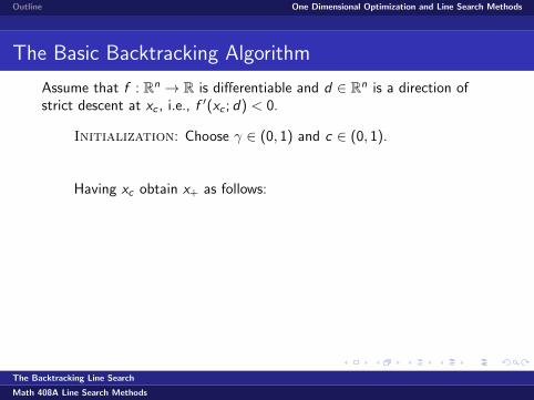
Assume that f : Rn → R is differentiable and d ∈ Rn is a direction ofstrict descent at xc , i.e., f ′(xc ; d) < 0.
Initialization: Choose γ ∈ (0, 1) and c ∈ (0, 1).
Having xc obtain x+ as follows:
Step 1: Compute the backtracking stepsize
t∗ := max γν
s.t. ν ∈ {0, 1, 2, . . .} andf (xc + γνd) ≤ f (xc) + cγν f ′(xc ; d).
Step 2: Set x+ = xc + t∗d .
The Backtracking Line Search
Math 408A Line Search Methods

Outline One Dimensional Optimization and Line Search Methods
The Basic Backtracking Algorithm
Assume that f : Rn → R is differentiable and d ∈ Rn is a direction ofstrict descent at xc , i.e., f ′(xc ; d) < 0.
Initialization: Choose γ ∈ (0, 1) and c ∈ (0, 1).
Having xc obtain x+ as follows:
Step 1: Compute the backtracking stepsize
t∗ := max γν
s.t. ν ∈ {0, 1, 2, . . .} andf (xc + γνd) ≤ f (xc) + cγν f ′(xc ; d).
Step 2: Set x+ = xc + t∗d .
The Backtracking Line Search
Math 408A Line Search Methods

Outline One Dimensional Optimization and Line Search Methods
The Basic Backtracking Algorithm
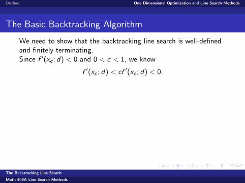
We need to show that the backtracking line search is well-definedand finitely terminating.
Since f ′(xc ; d) < 0 and 0 < c < 1, we know
f ′(xc ; d) < cf ′(xc ; d) < 0.
Hence
f ′(xc ; d) = limt↓0
f (xc + td)− f (xc)
t< cf ′(xc ; d) .
Therefore, there is a t > 0 such that
f (xc + td)− f (xc)
t< cf ′(xc ; d) ∀ t ∈ (0, t),
that is
f (xc + td) < f (xc) + ctf ′(xc ; d) ∀ t ∈ (0, t).
The Backtracking Line Search
Math 408A Line Search Methods
Outline One Dimensional Optimization and Line Search Methods
The Basic Backtracking Algorithm
We need to show that the backtracking line search is well-definedand finitely terminating.Since f ′(xc ; d) < 0 and 0 < c < 1, we know
f ′(xc ; d) < cf ′(xc ; d) < 0.
Hence
f ′(xc ; d) = limt↓0
f (xc + td)− f (xc)
t< cf ′(xc ; d) .
Therefore, there is a t > 0 such that
f (xc + td)− f (xc)
t< cf ′(xc ; d) ∀ t ∈ (0, t),
that is
f (xc + td) < f (xc) + ctf ′(xc ; d) ∀ t ∈ (0, t).
The Backtracking Line Search
Math 408A Line Search Methods

Outline One Dimensional Optimization and Line Search Methods
The Basic Backtracking Algorithm
Sof (xc + td) < f (xc) + ctf ′(xc ; d) ∀ t ∈ (0, t).
Since 0 < γ < 1, γν ↓ 0 as ν ↑ ∞, there is a ν0 such that γν < t̄for all ν ≥ ν0.Consequently,
f (xc + γνd) ≤ f (xc) + cγν f ′(xc ; d) ∀ ν ≥ ν0,
that is, the backtracking line search is finitely terminating.
The Backtracking Line Search
Math 408A Line Search Methods

Outline One Dimensional Optimization and Line Search Methods
The Basic Backtracking Algorithm
Sof (xc + td) < f (xc) + ctf ′(xc ; d) ∀ t ∈ (0, t).
Since 0 < γ < 1, γν ↓ 0 as ν ↑ ∞, there is a ν0 such that γν < t̄for all ν ≥ ν0.
Consequently,
f (xc + γνd) ≤ f (xc) + cγν f ′(xc ; d) ∀ ν ≥ ν0,
that is, the backtracking line search is finitely terminating.
The Backtracking Line Search
Math 408A Line Search Methods

Outline One Dimensional Optimization and Line Search Methods
The Basic Backtracking Algorithm
Sof (xc + td) < f (xc) + ctf ′(xc ; d) ∀ t ∈ (0, t).
Since 0 < γ < 1, γν ↓ 0 as ν ↑ ∞, there is a ν0 such that γν < t̄for all ν ≥ ν0.Consequently,
f (xc + γνd) ≤ f (xc) + cγν f ′(xc ; d) ∀ ν ≥ ν0,
that is, the backtracking line search is finitely terminating.
The Backtracking Line Search
Math 408A Line Search Methods

Outline One Dimensional Optimization and Line Search Methods
Programming the Backtracking Algorithm
Pseudo-Matlab code:
fc = f (xc)∆f = cf ′(xc ; d)
newf = f (xc + d)t = 1
while newf > fc + t∆ft = γt
newf = f (xc + td)endwhile
The Backtracking Line Search
Math 408A Line Search Methods

Outline One Dimensional Optimization and Line Search Methods
Direction Choices
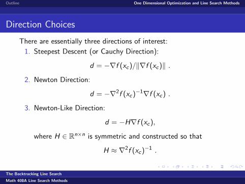
There are essentially three directions of interest:
1. Steepest Descent (or Cauchy Direction):
d = −∇f (xc)/‖∇f (xc)‖ .
2. Newton Direction:
d = −∇2f (xc)−1∇f (xc) .
3. Newton-Like Direction:
d = −H∇f (xc),
where H ∈ Rn×n is symmetric and constructed so that
H ≈ ∇2f (xc)−1 .
The Backtracking Line Search
Math 408A Line Search Methods

Outline One Dimensional Optimization and Line Search Methods
Direction Choices
There are essentially three directions of interest:
1. Steepest Descent (or Cauchy Direction):
d = −∇f (xc)/‖∇f (xc)‖ .
2. Newton Direction:
d = −∇2f (xc)−1∇f (xc) .
3. Newton-Like Direction:
d = −H∇f (xc),
where H ∈ Rn×n is symmetric and constructed so that
H ≈ ∇2f (xc)−1 .
The Backtracking Line Search
Math 408A Line Search Methods

Outline One Dimensional Optimization and Line Search Methods
Descent Condition
For all of these directions we have
f ′(xc ;−H∇f (xc)) = −∇f (xc)TH∇f (xc).
Thus, to obtain strict descent we need,
0 < ∇f (xc)TH∇f (xc) .
This holds, in particular, when H is positive definite.
In the case of steepest descent H = I and so
∇f (xc)TH∇f (xc) = ‖∇f (xc)‖22.
In all other cases, H ≈ ∇2f (xc)−1. The condition that H be pd isrelated to the second-order sufficient condition for optimality, alocal condition.
The Backtracking Line Search
Math 408A Line Search Methods