MATH 4030 Differential GeometryLecture Notes Part 1

last revised on September 28, 2015

The subject “Differential Geometry” can be vaguely defined as the area of mathematics which usesdifferential and integral calculus to study geometry. During the last century the field has expandedenormously into an intertwining subject between analysis, complex and algebraic geometry, represen-tation theory and mathematical physics etc. What we are going to cover in this course is the classicaldifferential geometry of curves and surfaces which dates back to the times of Euler and Gauss. We hopethis course can serve as an introduction to the field which opens a lot more doors into the fascinatingworld of geometry.

We will mainly follow the textbook written by Wolfgang Kuhnel but additional materials would beadded from other reference where appropriate. Students are advised to read the textbook with care asthere are some typos in the text.

Regular parametrized curves in Rn

We will be studying curves, surfaces (and submanifolds in general) in the n-dimensional Euclideanspace Rn. We think of Rn := x = (x1, · · · , xn) : xi ∈ R as an n-dimensional vector space over R which

is equipped with the standard inner product 〈x, y〉 :=∑n

i=1 xiyi and the norm ‖x‖ :=

(∑ni=1(xi)2

)1/2.

(In Riemannian geometry, one consider a differentiable manifold Mn equipped with an inner productgp on each tangent space TpM which varies smoothly in p. This notion is essential in Einstein’s generaltheory of relativity where the spacetime is described by a 4-dimensional Lorentzian manifold.)

Just like we learn calculus by first understanding single variable calculus, we will begin with thesimplest object - curves - a 1-dimensional object.

Definition 1. A (smooth) parametrized curve in Rn is a smooth map c : [a, b] → Rn given in coordi-nates by t 7→ (c1(t), · · · , cn(t)). The curve c is said to be regular if c′(t) 6= 0 for all t ∈ (a, b).

One can think of the parametrized curve c(t) as the trajectory of an object moving in Rn and c(t)is its position at time t. The condition c′(t) 6= 0 then just means that the object does not stop movingat any particular time. Let us first look at some basic examples.

1

1. Straight line in Rn: given a vector ~v ∈ Rn, c(t) = t~v for t ∈ (−∞,∞) is parametrizing the straightline through the origin parallel to the vector ~v.

Exercise: Give a parametrization of the line segment from a point p to another point q in Rn.

2. Circles: the parametrized curve c(θ) = r(cos θ, sin θ), θ ∈ [0, 2π], is a circle of radius r centeredat the origin. If L : R2 → Rn is an affine linear map, then L c is an ellipse in Rn.

Exercise: Can you give a parametrization of the unit circle centered at origin so that ‖c′(t)‖ = 1for all t?

3. Helix in R3: c(t) = (r cos t, r sin t, bt), t ∈ R.

4. Neil parabola: consider the parametrized curve c(t) = (t2, t3), t ∈ R, which lies on the set(x, y) ∈ R2 : x3 = y2. Note that even though the coordinate functions of c(t) are smooth,

2

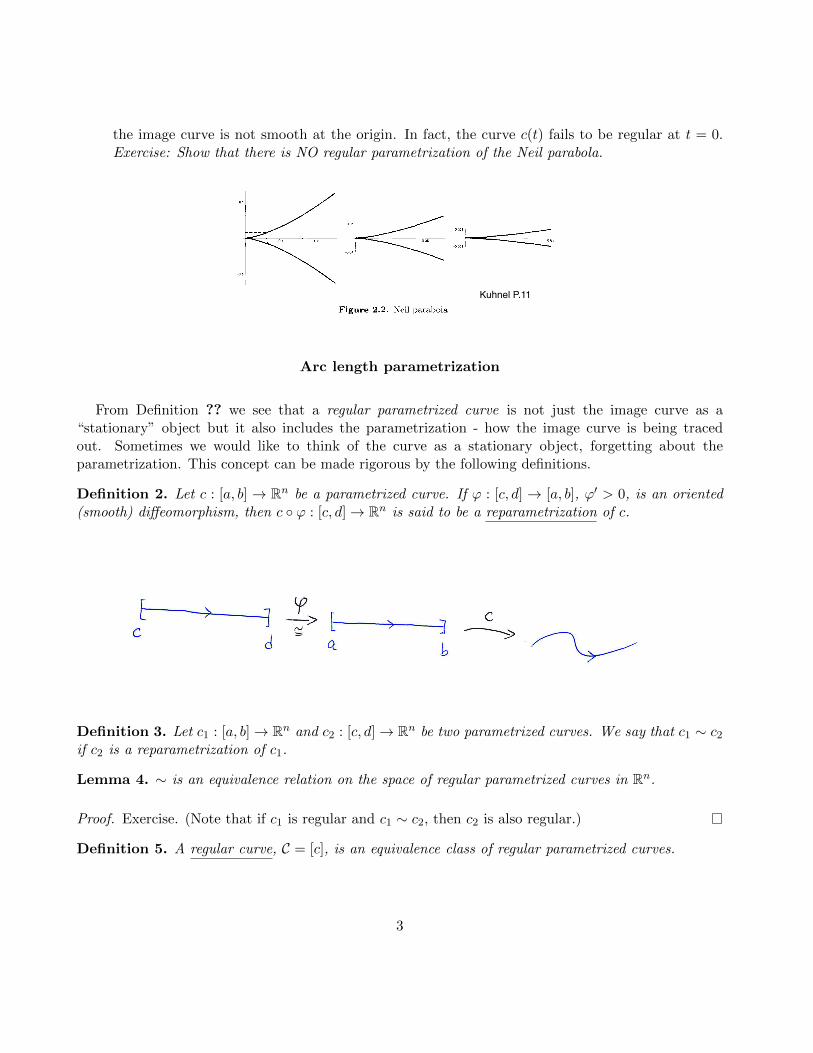
the image curve is not smooth at the origin. In fact, the curve c(t) fails to be regular at t = 0.Exercise: Show that there is NO regular parametrization of the Neil parabola.

Kuhnel P.11

Arc length parametrization

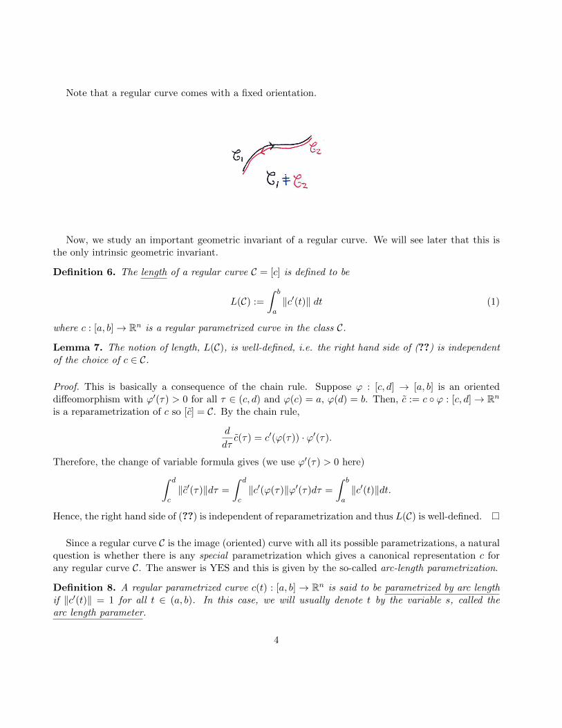
From Definition ?? we see that a regular parametrized curve is not just the image curve as a“stationary” object but it also includes the parametrization - how the image curve is being tracedout. Sometimes we would like to think of the curve as a stationary object, forgetting about theparametrization. This concept can be made rigorous by the following definitions.

Definition 2. Let c : [a, b] → Rn be a parametrized curve. If ϕ : [c, d] → [a, b], ϕ′ > 0, is an oriented(smooth) diffeomorphism, then c ϕ : [c, d]→ Rn is said to be a reparametrization of c.

Definition 3. Let c1 : [a, b]→ Rn and c2 : [c, d]→ Rn be two parametrized curves. We say that c1 ∼ c2

if c2 is a reparametrization of c1.

Lemma 4. ∼ is an equivalence relation on the space of regular parametrized curves in Rn.

Proof. Exercise. (Note that if c1 is regular and c1 ∼ c2, then c2 is also regular.)

Definition 5. A regular curve, C = [c], is an equivalence class of regular parametrized curves.

3

Note that a regular curve comes with a fixed orientation.

Now, we study an important geometric invariant of a regular curve. We will see later that this isthe only intrinsic geometric invariant.

Definition 6. The length of a regular curve C = [c] is defined to be

L(C) :=

∫ b

a‖c′(t)‖ dt (1)

where c : [a, b]→ Rn is a regular parametrized curve in the class C.

Lemma 7. The notion of length, L(C), is well-defined, i.e. the right hand side of (??) is independentof the choice of c ∈ C.

Proof. This is basically a consequence of the chain rule. Suppose ϕ : [c, d] → [a, b] is an orienteddiffeomorphism with ϕ′(τ) > 0 for all τ ∈ (c, d) and ϕ(c) = a, ϕ(d) = b. Then, c := c ϕ : [c, d]→ Rnis a reparametrization of c so [c] = C. By the chain rule,

d

dτc(τ) = c′(ϕ(τ)) · ϕ′(τ).

Therefore, the change of variable formula gives (we use ϕ′(τ) > 0 here)∫ d

c‖c′(τ)‖dτ =

∫ d

c‖c′(ϕ(τ)‖ϕ′(τ)dτ =

∫ b

a‖c′(t)‖dt.

Hence, the right hand side of (??) is independent of reparametrization and thus L(C) is well-defined.

Since a regular curve C is the image (oriented) curve with all its possible parametrizations, a naturalquestion is whether there is any special parametrization which gives a canonical representation c forany regular curve C. The answer is YES and this is given by the so-called arc-length parametrization.

Definition 8. A regular parametrized curve c(t) : [a, b] → Rn is said to be parametrized by arc lengthif ‖c′(t)‖ = 1 for all t ∈ (a, b). In this case, we will usually denote t by the variable s, called thearc length parameter.

4

The following lemma below says that any regular parametrized curve can be reparametrized by arclength. This implies that there is no intrinsic local invariant for a curve, and the only global invariantis given by the total arc length L(C).

Lemma 9. For any regular curve C, there exists an arc-length parametrization c ∈ C. Moreover, thearc-length parametrization is unique up to translations in the domain interval.

Proof. Take any regular parametrization c(t) : [a, b] → Rn for C. Define the arc-length functions : [a, b]→ [0, L], where L = L(C), by

s(t) :=

∫ t

a‖c′(τ)‖ dτ.

By the fundamental theorem of calculus, s′(t) = ‖c′(t)‖ > 0 for all t ∈ (a, b). (Note that c is regular.)Therefore, the inverse function theorem says that there is a smooth inverse t = t(s) : [0, L]→ [a, b] tothe function s = s(t) : [a, b] → [0, L]. Consider the reparametrization of c given by c(s) := c(t(s)) :[0, L]→ Rn, then by the chain rule,

d

dsc(s) = c′(t(s))

dt

ds= c′(t(s))

(ds

dt

)−1

=c′(t(s))

‖c′(t(s))‖,

which has unit length. Therefore, c is an arc-length parametrization of C. We leave the proof of theuniqueness as an exercise.

As an exercise, try to give the arc length parametrization of all the examples in the first section.

The method of moving frame

The idea of moving frames is a very useful tool in differential geometry which was promoted bythe great geometers Cartan and S.S. Chern in the 20th century. The standard coordinate basis ofRn provides a parallel global inertial frame. However, it is not always the most convenient frame inpractice. For example, image a car driving on a curvy road, the concept of “driving forward along theroad” makes sense to the driver (as long as the road is well-paved and there is no branching). However,

5

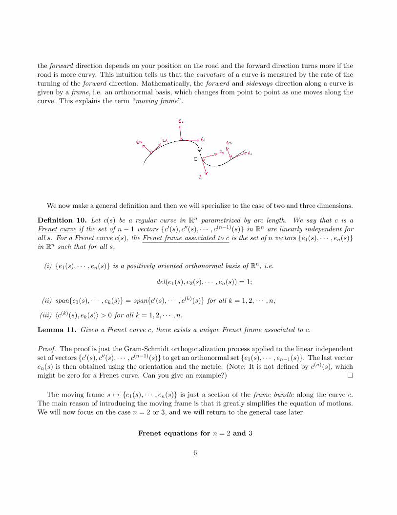
the forward direction depends on your position on the road and the forward direction turns more if theroad is more curvy. This intuition tells us that the curvature of a curve is measured by the rate of theturning of the forward direction. Mathematically, the forward and sideways direction along a curve isgiven by a frame, i.e. an orthonormal basis, which changes from point to point as one moves along thecurve. This explains the term “moving frame”.

We now make a general definition and then we will specialize to the case of two and three dimensions.

Definition 10. Let c(s) be a regular curve in Rn parametrized by arc length. We say that c is aFrenet curve if the set of n − 1 vectors c′(s), c′′(s), · · · , c(n−1)(s) in Rn are linearly independent forall s. For a Frenet curve c(s), the Frenet frame associated to c is the set of n vectors e1(s), · · · , en(s)in Rn such that for all s,

(i) e1(s), · · · , en(s) is a positively oriented orthonormal basis of Rn, i.e.

det(e1(s), e2(s), · · · , en(s)) = 1;

(ii) spane1(s), · · · , ek(s) = spanc′(s), · · · , c(k)(s) for all k = 1, 2, · · · , n;

(iii) 〈c(k)(s), ek(s)〉 > 0 for all k = 1, 2, · · · , n.

Lemma 11. Given a Frenet curve c, there exists a unique Frenet frame associated to c.

Proof. The proof is just the Gram-Schmidt orthogonalization process applied to the linear independentset of vectors c′(s), c′′(s), · · · , c(n−1)(s) to get an orthonormal set e1(s), · · · , en−1(s). The last vectoren(s) is then obtained using the orientation and the metric. (Note: It is not defined by c(n)(s), whichmight be zero for a Frenet curve. Can you give an example?)

The moving frame s 7→ e1(s), · · · , en(s) is just a section of the frame bundle along the curve c.The main reason of introducing the moving frame is that it greatly simplifies the equation of motions.We will now focus on the case n = 2 or 3, and we will return to the general case later.

Frenet equations for n = 2 and 3

6

First, we study plane curves, i.e. curves in R2.

Proposition 12. (1) Every regular curve parametrized by arc length is a Frenet curve.

(2) Let c(s) be a regular curve parametrized by arc length. Then the Frenet frame associated to c isgiven by

e1(s) := c′(s), e2(s) := Je1(s),

where J =

(0 −11 0

)is the counterclockwise rotation by π/2. Moreover, c′′(s) = κ(s)e2(s) for

all s and the function κ(s) ∈ R is called the (signed) curvature of the curve c.

Proof. When n = 2, an arc-length parametrized curve c(s) is Frenet if and only if c′(s) 6= 0 for alls, which holds automatically since ‖c′(s)‖ = 1 by the definition of arc length parametrization. Thisproves (1). For (2), notice that 〈c′(s), c′(s)〉 ≡ 1 for all s. Differentiating in s gives

2〈c′(s), c′′(s)〉 =d

ds〈c′(s), c′(s)〉 = 0.

Since e1(s) = c′(s), we must have c′′(s) parallel to e2(s). This proves (2).

Note that reversing the orientation of the curve flips the sign of the curvature (Exercise: Prove this!)

Remark: The notion of curvature κ is NOT an intrinsic property of the curve itself! In other words, anant walking on the curve whose world is just the 1-dimensional curve cannot detect κ. The “centrifugalforce” that one feels when traveling on a circle is always perpendicular to the curve, hence is somethingthe ant cannot feel if its world is only 1-dimensional along the curve. Therefore, the curvature κ is anextrinsic property that tells us how the 1-dimensional curve is sitting inside the 2-dimensional plane.The concept of intrinsic and extrinsic properties is an intriguing concept in differential geometry whichwould re-appear from time to time throughout this course.

As stated at the end of the previous section, the main reason for introducing the Frenet frame isthat the equation of motions simplifies substantially in this adapted frame (This is similar in spirit to

7

choosing a good coordinate system for a specific problem - however - there is some subtle differencesbetween a frame and a coordinate system, we will address this point later in the course).

Proposition 13. The Frenet frame e1(s), e2(s) of a Frenet curve in R2 satisfies the following systemof linear ODEs called the Frenet equations:(

e1(s)e2(s)

)′=

(0 κ(s)

−κ(s) 0

)(e1(s)e2(s)

),

where κ(s) is the (signed) curvature of the curve (defined in Proposition ?? (2)).

Proof. By definition of κ and e1, we have e′1(s) = c′′(s) = κ(s)e2(s). On the other hand, since〈e2(s), e2(s)〉 ≡ 1, we have 〈e′2(s), e2(s)〉 = 0 and thus e′2(s) is parallel to e1(s). Moreover,

〈e′2(s), e1(s)〉 = 〈e2(s), e1(s)〉′ − 〈e2(s), e′1(s)〉 = −κ(s).

Therefore, e′2(s) = −κ(s)e1(s) and we have proved the proposition.

Note that in the proof above, we have repeatedly used the fact that the metric 〈 , 〉 is constant andtherefore do not need to be differentiated. In Riemannian geometry, one needs the metric g to beparallel in the sense that ∇g = 0 where ∇ is a canonical connection determined by g.

Now, we go up one dimension to study space curves, i.e. curves in R3.

Proposition 14. Let c(s) be a regular curve in R3 parametrized by arc length.

(1) c is Frenet if and only if c′′(s) 6= 0 for all s.

(2) If c is Frenet, then the Frenet frame associated to c is given by

e1(s) = c′(s), e2(s) =c′′(s)

‖c′′(s)‖, e3(s) = e1(s)× e2(s).

Classically, e1, e2, e3 are called the tangent, principal normal and binormal vectors respectively.

Proof. Since c(s) is parametrized by arc length, 〈c′(s), c′(s)〉 ≡ 1 implies that 〈c′(s), c′′(s)〉 ≡ 0. There-fore, if c′′(s) 6= 0, then c′(s), c′′(s) is linearly independent. This proves (1). The statement (2) thenfollows from (1) and the definition of cross product in R3.

Definition 15. Given a Frenet curve in R3 with associated Frenet frame e1(s), e2(s), e3(s), we definethe curvature and torsion of c respectively as:

κ(s) := ‖c′′(s)‖ and τ(s) := 〈e′2(s), e3(s)〉.

8

Note that in contrast with plane curves, the curvature is always positive κ > 0 by definition, whilethe torsion τ can have a sign. Geometrically, the curvature κ measures how the tangent vector turnsand the torsion τ measures how the plane containing c′ and c′′ turns. We now derive the Frenetequations for a space curve.

Proposition 16. The Frenet frame e1(s), e2(s), e3(s) of a Frenet curve in R3 satisfies the followingFrenet equations: e1(s)

e2(s)e3(s)

′ = 0 κ(s) 0−κ(s) 0 τ(s)

0 −τ(s) 0

e1(s)e2(s)e3(s)

,

where κ(s) and τ(s) is the curvature and torsion of the curve.

Proof. For simplicity, we will omit the dependence of s in the proof. By definitions, we have e′1 =‖e′1‖e2 = κe2. Moreover, since e2 is parallel to e′1, we have

e′3 = e′1 × e2 + e1 × e′2 = e1 × e′2.

Therefore, 〈e′3, e1〉 = 0. Moreover, we have 〈e′3, e3〉 = 0 (as ‖e3‖ ≡ 1) and 〈e′3, e2〉 = −〈e3, e′2〉 = −τ (as

〈e2, e3〉 ≡ 0). As a result, we obtain the last equation e′3 = −τe2. For the second equation, by a similarargument we have 〈e′2, e2〉 = 0 and

〈e′2, e1〉 = −〈e2, e′1〉 = −κ,

〈e′2, e3〉 = −〈e2, e′3〉 = τ.

Therefore, e′2 = −κe1 + τe3, which proves the proposition.

Plane curves

From the Frenet equations of a plane curve, we see that there is only one (extrinsic) geometricinvariant given by the signed curvature κ. Geometrically, it measures quantitatively how fast is theunit tangent vector e1 = c′ turning towards the e2-direction. Let us look at two basic examples:

1. Straight line: Let c(s) = s~v, s ∈ R be the arc length parametrization of the line parallel to theunit vector ~v ∈ R2. Then c′′(s) = 0 and hence κ(s) ≡ 0.

2. Circles: Consider an arc length parametrization of the circle of radius r centered at p:

c(s) = p+ r(

coss

r, sin

s

r

), s ∈ R.

Then the Frenet frame is given by

e1(s) = c′(s) =(− sin

s

r, cos

s

r

), and e2(s) = Je1(s) = −

(cos

s

r, sin

s

r

).

Therefore, the curvature is given by κ(s) = 〈c′′(s), e2(s)〉 ≡ 1/r. (Note that if we parametrizedthe circle in the clockwise direction, we get κ ≡ −1/r instead.)

9

In fact, these are the only examples of plane curves with constant curvature.

Proposition 17. The lines and circles are the only plane curves with constant curvature κ.

The proposition above follows easily as a corollary of the following general theorem.

Theorem 18. The curvature κ(s) determines the curve c(s) uniquely up to translations and rotations(i.e. rigid motions of R2).

Proof. By the existence and uniqueness of the solution to linear ODE systems, the Frenet equations isuniquely solvable with any given initial data:

(e1(s)e2(s)

)′=

(0 κ(s)

−κ(s) 0

)(e1(s)e2(s)

)e1(0) = ~v, e2(0) = J~v.

where ~v ∈ R2 is a unit vector. Then, for any fixed p ∈ R2, the initial value problem below is uniquelysolvable for c(s):

c′(s) = e1(s),c(0) = p.

Therefore, given any initial data (p,~v), the curve c(s) is uniquely determined by the curvature κ(s).

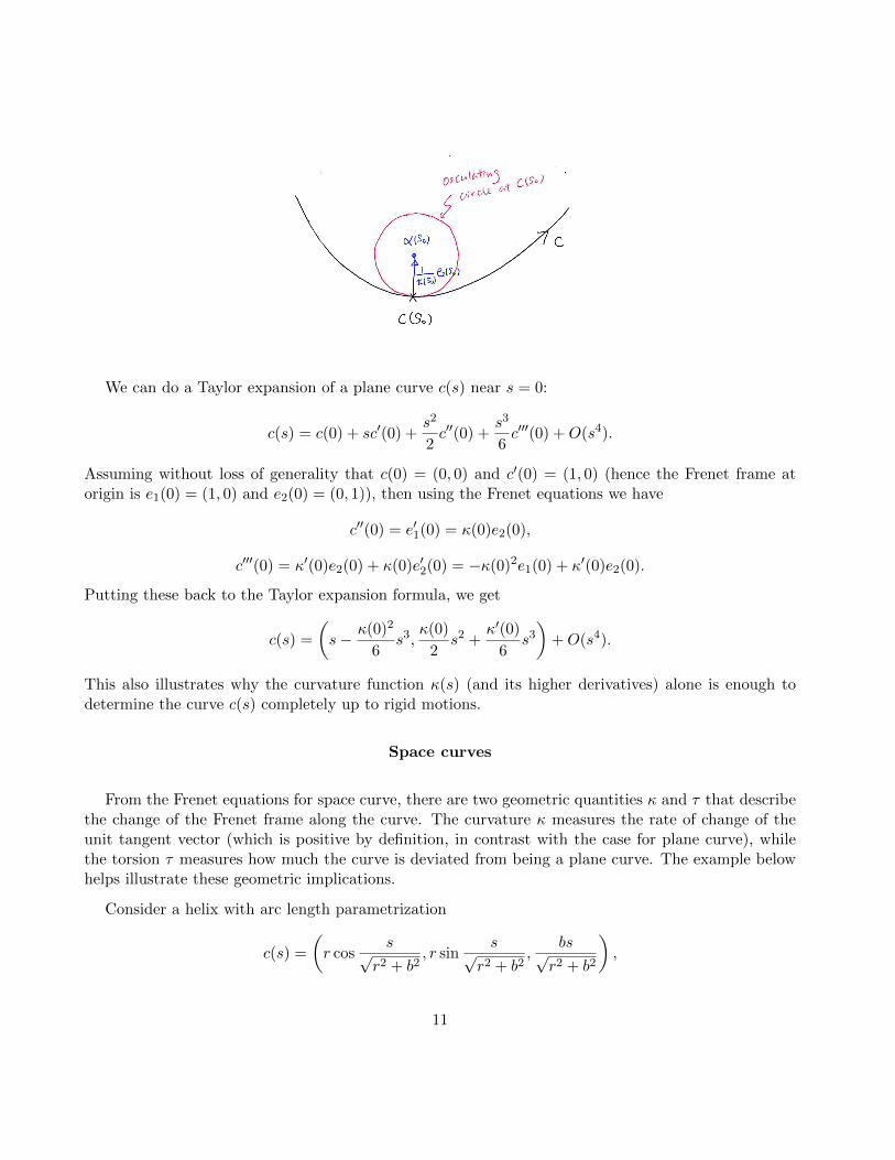
Recall that the tangent line to a curve at a point p is the linear approximation of the curve near p.We say that the tangent line has contact order 1 with the curve at p. If we want to approximate thecurve near p with something of contact order 2, it leads to the notion of osculating circle.

Definition 19. If c(s) is an arc-length parametrized plane curve with κ(s0) 6= 0 for some s0. Then, theosculating circle of c at s0 is the unique circle of radius 1/κ(s0) centered at α(s0) := c(s0)+ 1

κ(s0)e2(s0).

Proposition 20. The osculating circle of c at s0 has contact order 2 with c at s = s0, i.e.

d(k)

ds(k)

∣∣∣∣∣s=s0

‖c(s)− α(s0)‖ = 0, for k = 1, 2.

Proof. Note that ‖c(s)− α(s0)‖ > 0 for s ∼ s0 so the function above is smooth near s0. Moreover,

d

ds

∣∣∣∣s=s0

‖c(s)− α(s0)‖2 = 〈c′(s0), c(s0)− α(s0)〉 = 〈e1(s0),− 1

κ(s0)e2(s0)〉 = 0.

d2

ds2

∣∣∣s=s0‖c(s)− α(s0)‖2 = 〈c′′(s0), c(s0)− α(s0)〉+ 〈c′(s0), c′(s0)〉

= 〈κ(s0)e2(s0),− 1κ(s0)e2(s0)〉+ 〈e1(s0), e1(s0)〉

= (−1) + 1 = 0.

10

We can do a Taylor expansion of a plane curve c(s) near s = 0:

c(s) = c(0) + sc′(0) +s2

2c′′(0) +

s3

6c′′′(0) +O(s4).

Assuming without loss of generality that c(0) = (0, 0) and c′(0) = (1, 0) (hence the Frenet frame atorigin is e1(0) = (1, 0) and e2(0) = (0, 1)), then using the Frenet equations we have

c′′(0) = e′1(0) = κ(0)e2(0),

c′′′(0) = κ′(0)e2(0) + κ(0)e′2(0) = −κ(0)2e1(0) + κ′(0)e2(0).

Putting these back to the Taylor expansion formula, we get

c(s) =

(s− κ(0)2

6s3,

κ(0)

2s2 +

κ′(0)

6s3

)+O(s4).

This also illustrates why the curvature function κ(s) (and its higher derivatives) alone is enough todetermine the curve c(s) completely up to rigid motions.

Space curves

From the Frenet equations for space curve, there are two geometric quantities κ and τ that describethe change of the Frenet frame along the curve. The curvature κ measures the rate of change of theunit tangent vector (which is positive by definition, in contrast with the case for plane curve), whilethe torsion τ measures how much the curve is deviated from being a plane curve. The example belowhelps illustrate these geometric implications.

Consider a helix with arc length parametrization

c(s) =

(r cos

s√r2 + b2

, r sins√

r2 + b2,

bs√r2 + b2

),

11

differentiating in s gives

e1(s) = c′(s) =1√

r2 + b2

(−r sin

s√r2 + b2

, r coss√

r2 + b2, b

),

c′′(s) =r

r2 + b2

(− cos

s√r2 + b2

,− sins√

r2 + b2, 0

).

Therefore, the curvature is κ(s) = ‖c′′(s)‖ = rr2+b2

and

e2(s) =c′′(s)

‖c′′(s)‖=

(− cos

s√r2 + b2

,− sins√

r2 + b2, 0

).

Therefore,

e3(s) = e1(s)× e2(s) =1√

r2 + b2

(b sin

s√r2 + b2

,−b coss√

r2 + b2, r

).

Hence, the torsion is

τ(s) = −〈e′3(s), e2(s)〉 =b

r2 + b2.

As for the case of plane curve, we can do a Taylor expansion of a Frenet curve in R3 to study thelocal behavior of the curve (see Tutorial Notes 1):

Kuhnel P.18

Next, we introduce the Darboux rotation vector ~D in R3. Recall from the Frenet equations thatthe 3× 3 coefficient matrix A, sometimes called the Frenet matrix, is skew-symmetric, i.e. AT = −A.Therefore, A ∈ so(3) is an infinitesimal rotation in R3 and is therefore given by ~D× (·) for some vector

12

~D called the Darboux vector (which depends on s since A depends on s). We digress a little bit to seewhy skew-symmetric matrices correspond to infinitesimal rotations (in fact in any dimension, n = 3 isonly used to conclude that the infinitesimal rotation is given by the cross product with a vector ~D).

Let SO(n) be the special orthogonal group of Rn which is the group of orientation-preserving isome-tries of Rn:

SO(n) := A ∈ GL(n) : AAT = ATA = I, detA = 1.

This is a classical example of a Lie group, which is a differentiable manifold with a group structure.Therefore, we can look at the tangent space at the identity element I ∈ SO(n), which is called theLie algebra of the Lie group SO(n), denoted by so(n). To see that so(n) consists of skew-symmetricmatrices, suppose we have a smooth family A(t) ∈ SO(n), t ∈ (−ε, ε), such that A(0) = I. SinceA(t) ∈ SO(n) for all t, we have the identity

A(t)AT (t) ≡ I.

Differentiating at t = 0 and using the initial condition A(0) = AT (0) = I, we obtain

A′(0) + (A′)T (0) = O,

i.e. (A′)T (0) = −A′(0). In other words, any tangent vector to SO(n) at the identity I is given by askew-symmetric matrix A′(0), therefore,

so(n) = B ∈ gl(n) : BT = −B,

where gl(n) is the set of all n×n matrices, the Lie algebra of the Lie group GL(n) of all n×n invertiblematrices.

Now, we go back to find the Darboux vector ~D in terms of the Frenet frame e1, e2, e3. Suppose~D = ae1 + be2 + ce3, then using the definition of ~D and the Frenet equations, we have ~D × e1

~D × e2

~D × e3

=

e1

e2

e3

′ = 0 κ 0−κ 0 τ0 −τ 0

e1

e2

e3

.

Using that e1, e2, e3 is an oriented orthonormal frame and comparing coefficients, we get

~D = τe1 + κe2.

Note that ‖ ~D‖ =√τ2 + κ2 represents the speed of rotation of the Frenet frame. (As an exercise, show

that a helix has constant Darboux vector which is parallel to the “axis” of the helix.)

Recall that the only plane curves with constant curvature are circles. Similarly, in the case of spacecurves, we want to characterize those curves in R3 which lies on a sphere. Let

S2R(p) := x ∈ R3 : ‖x− p‖ = R

be the sphere of radius R > 0 centered at p ∈ R3.

13

Theorem 21. Let c(s) be a Frenet curve in R3 parametrized by arc length. Suppose that τ 6= 0everywhere. Then c lies on a sphere if and only if the following equation holds:

τ

κ=

(κ′

κ2τ

)′. (2)

Proof. Suppose we have an arc-length parametrized Frenet curve c(s) lying on a sphere S2R(p). We will

prove the conclusion assuming p = 0 (Exercise: Write the proof for an arbitrary p). By hypothesis,〈c, c〉 ≡ R2 = constant. Differentiating with respect to s, using e1 := c′,

0 =1

2〈c, c〉′ = 〈c′, c〉 = 〈e1, c〉.

Differentiating again and using the Frenet equation e′1 = κe2,

0 = 〈e1, c〉′ = 〈e′1, c〉+ 〈e1, c′〉 = 〈κe2, c〉+ 〈e1, e1〉,

which implies that 〈e2, c〉 = −1/κ. Differentiate once more and using Frenet equation e′2 = −κe1 + τe3,we have

〈−κe1 + τe3, c〉+ 〈e2, e1〉 = 〈e′2, c〉+ 〈e2, c′〉 = 〈e2, c〉′ =

κ′

κ2,

which implies that 〈e3, c〉 = κ′

κ2τ(recall that 〈e1, c〉 = 0). Combining all these results, we have

c = −1

κe2 +

κ′

κ2τe3.

In other words, for all s,

c+1

κe2 −

κ′

κ2τe3 = 0.

Differentiating one last time and using the Frenet equations,

0 = c′ − κ′

κ2e2 + 1

κe′2 −

(κ′

κ2τ

)′e3 − κ′

κ2τe′3

= e1 − κ′

κ2e2 + 1

κ(−κe1 + τe3)−(κ′

κ2τ

)′e3 − κ′

κ2τ(−τe2)

=

(τκ −

(κ′

κ2τ

)′)e3,

which implies the desired conclusion (??).

Suppose, on the other hand, (??) holds. Reversing the argument above implies that

c+1

κe2 −

κ′

κ2τe3 ≡ p,

for some constant p ∈ R3. We claim that c lies on a sphere S2R(p) centered at p for some radius R > 0.

It is equivalent to showing that ‖c− p‖2 ≡ constant, which follows from

1

2〈c− p, c− p〉′ = 〈c′, c− p〉 = 〈e1,−

1

κe2 +

κ′

κ2τe3〉 ≡ 0.

14

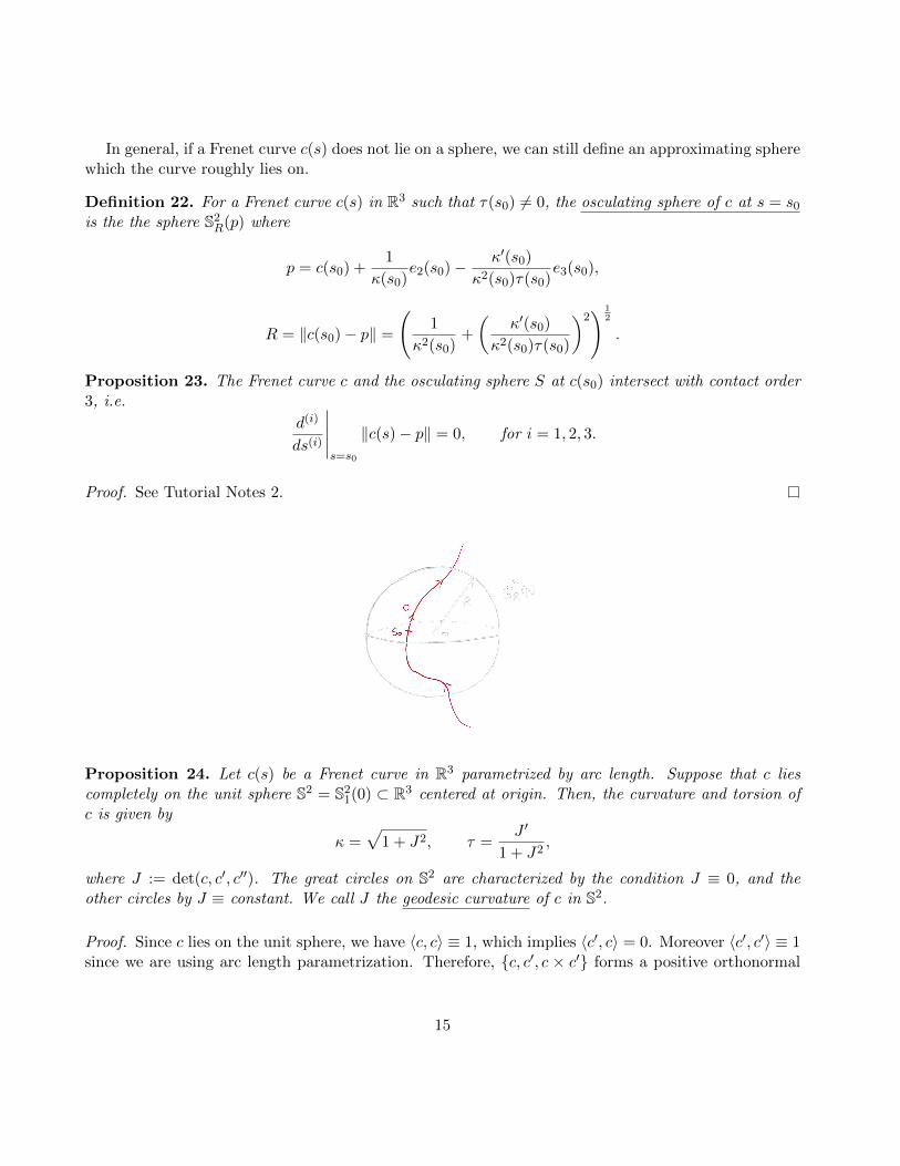
In general, if a Frenet curve c(s) does not lie on a sphere, we can still define an approximating spherewhich the curve roughly lies on.

Definition 22. For a Frenet curve c(s) in R3 such that τ(s0) 6= 0, the osculating sphere of c at s = s0

is the the sphere S2R(p) where

p = c(s0) +1

κ(s0)e2(s0)− κ′(s0)

κ2(s0)τ(s0)e3(s0),

R = ‖c(s0)− p‖ =

(1

κ2(s0)+

(κ′(s0)

κ2(s0)τ(s0)

)2) 1

2

.

Proposition 23. The Frenet curve c and the osculating sphere S at c(s0) intersect with contact order3, i.e.

d(i)

ds(i)

∣∣∣∣∣s=s0

‖c(s)− p‖ = 0, for i = 1, 2, 3.

Proof. See Tutorial Notes 2.

Proposition 24. Let c(s) be a Frenet curve in R3 parametrized by arc length. Suppose that c liescompletely on the unit sphere S2 = S2

1(0) ⊂ R3 centered at origin. Then, the curvature and torsion ofc is given by

κ =√

1 + J2, τ =J ′

1 + J2,

where J := det(c, c′, c′′). The great circles on S2 are characterized by the condition J ≡ 0, and theother circles by J ≡ constant. We call J the geodesic curvature of c in S2.

Proof. Since c lies on the unit sphere, we have 〈c, c〉 ≡ 1, which implies 〈c′, c〉 = 0. Moreover 〈c′, c′〉 ≡ 1since we are using arc length parametrization. Therefore, c, c′, c × c′ forms a positive orthonormal

15

basis (note: this is not the Frenet frame!) and thus we can decompose c′′ into components of such abasis. Note that

〈c′′, c〉 = −〈c′, c′〉 = −1,

〈c′′, c′〉 =1

2〈c′, c′〉′ = 0,

〈c′′, c× c′〉 = det(c, c′, c′′) =: J.

Therefore, κ = ‖c′′‖ =√

1 + J2. Next, we consider the vector c′′′, observe that

〈c′′′, c〉 = 〈c′′, c〉′ − 〈c′′, c′〉 = 0.

Moreover, by the definition of Frenet frame,

e1 = c′, e2 =1

κc′′, e3 = e1 × e2 =

1

κc′ × c′′.

Therefore, by the definition of τ ,

τ := −〈e′3, e2〉 = −〈( 1

κc′ × c′′)′, 1

κc′′〉 = − 1

κ2〈c′ × c′′′, c′′〉 = − 1

κ2〈c′ × c′′′,−c+ Jc× c′〉 =

1

κ2〈c′ × c′′′, c〉,

where the last equality uses the fact that 〈c′′′, c〉 = 0, which implies that 〈c′ × c′′′, c × c′〉 = 0. Theformula for τ then follows from the definition of J that

J ′ = 〈c′ × c′′, c〉′ = 〈c′ × c′′′, c〉.

The quantity J is in fact an interesting geometric quantity which measures the curvature of c as seenfrom the sphere S2. Note that c × c′ is the unit vector normal to the curve but tangent to the sphereS2, hence J = 〈c′′, c × c′〉 is the part of c′′ which is tangent to the sphere. From this the rest of theproposition follows easily. (Exercise: can you give a rigorous proof?)

It is a good exercise for the reader to derive the formulas of κ and τ if the curve lies on a sphere ofany radius R > 0. Does the center of the sphere matter?

Fundamental theorem of curves in Rn

In this section, we return to the general theory of curves inside Rn. We will derive the Frenetequations for general n and prove the fundamental theorem curves which says that the “curvatures” ofthe curve uniquely determines a curve in Rn up to rigid motions.

16

Proposition 25. Let e1, e2, · · · , en be the Frenet frame of a Frenet curve c in Rn. Then, they satisfythe Frenet equations below:

e1

e2

e3......

en−1

en

′

=

0 κ1 0 0 · · · 0

−κ1 0 κ2 0. . .

...

0 −κ2 0. . .

. . . 0

0 0. . .

. . .. . . 0

.... . .

. . .. . . 0 κn−1

0 · · · 0 0 −κn−1 0

e1

e2

e3......

en−1

en

,

where κi := 〈e′i, ei+1〉, i = 1, · · · , n − 1, are the i-th Frenet curvature of the curve c. When i = n − 1,κn−1 is called the torsion of the curve. Moreover, we have κi > 0 for i ≤ n− 2.

Proof. Recall from the definition of Frenet frame that for i = 1, 2, · · · , n− 1, ei ∈ spanc′, c′′, · · · , c(i)and thus e′i ∈ spanc′, c′′, · · · , c(i+1) = spane1, e2, · · · , ei+1. This explains the zeros in the upperright corner of the Frenet matrix. The rest of the entries follows from the definition of κi and theskew-symmetry: 〈e′i, ej〉 = −〈ei, e′j〉. The positivity of κi, i ≤ n − 2, follows from the construction of

the Frenet frame ei using Gram-Schmidt and that the condition 〈c(i), ei〉 > 0.

From above it is easy to see that a Frenet curve in Rn is contained in a hyperplane if and only ifκn−1 ≡ 0, which is equivalent to saying that en is a constant vector (perpendicular to the hyperplane).

As in the case for plane curves, where the curve is uniquely determined by the curvature κ up torigid motions. We have the same phenomenon in Rn. The lemma below says that the i-th curvaturesκi is invariant under rigid motions of Rn.

Lemma 26. Let c(s) be a Frenet curve in Rn. Suppose that T : Rn → Rn is a (orientation preserving)rigid motion of Rn. If we define the curve c = T c, then c is a Frenet curve and κi = κi for alli = 1, · · · , n− 1.

Proof. Since any rigid motion T of Rn can be written as a rotation followed by a translations, i.e.T (x) = Ax + b for some constant A ∈ SO(n) and b ∈ Rn. Since AT = A−1, it is clear that c := T cis still a Frenet curve parametrized by arc length provied c is. Moreover, if e1, · · · , en is the Frenetframe of c, then Ae1, · · · , Aen is the Frenet frame of c since c(i) = Ac(i) for all i (recall that A isconstant!). In addition, the curvatures are the same because

(Aei)′ = Ae′i = A(−κi−1ei−1 + κiei+1) = −κi−1(Aei−1) + κi(Aei+1).

The main theorem for local theory of curves says that we can arbitrarily prescribed the curvaturesκi of a curve and the curve is determined uniquely up to rigid motions in Rn. We will see later that

17

this is not the same for surfaces in R3, for example. In the latter case, the “curvatures” have to satisfysome compatibility/integrability conditions called constraint equations in order to guarantee existence.The situation is much simpler for curves because curves do not have any local intrinsic geometry (i.e.any two curves are locally isometric to each other).

Theorem 27 (Fundamental Theorem of Curves). Let κ1, κ2, · · · , κn−1 : (a, b) → R be given smoothfunctions on the interval (a, b) containing 0 and κ1, · · · , κn−2 > 0 are positive functions. Let q ∈ Rn bea given point and e0

1, · · · , e0n be a given n-frame (i.e. positively oriented orthonormal basis). Then,

there exists a smooth Frenet curve c(s) : (a, b)→ Rn parametrized by arc length such that

(i) c(0) = q,

(ii) e01, · · · , e0

n is the Frenet frame of c at the point q when s = 0,

(iii) κ1, κ2, · · · , κn−1 are the Frenet curvatures of c.

Proof. By the existence and uniqueness for linear system of ODEs, the Frenet equations in Proposition?? is uniquely solvable for all s given initial conditions (ii). Let

F = F (s) =

e1(s)e2(s)

...en(s)

be an n× n matrix of functions of s (we think of each ei as a row vector). Then, the Frenet equationcan be written in matrix form as F ′ = KF , where K is the Frenet matrix (depending on s). Notethat we get a unique solution to F ′ = KF with initial condition F (0) = F0 such that F0F

T0 = I since

e01, · · · , e0

n is a positively oriented orthonormal frame. Therefore, if we define G(s) = F (s)F (s)T ,then G′ = F ′F T + F (F ′)T = (KF )F T + F (KF )T = K(FF T ) + (FF T )KT = K(FF T ) − (FF T )K(where we have used the skew-symmetry of the Frenet matrix K). Therefore, G satisfies the followingODE

G′ = KG−GK,G(0) = I.

Since constant solution is a solution to the initial value problem, by uniqueness, we must have G(s) ≡ Iand thus FF T = I for all s. This tells us that the solution F (s) we got by solving the ODEs indeedgives an orthonormal frame for all s. Since detF 6= 0 for all s and detF (0) = 1, we have detF = 1 forall s, i.e. F (s) gives a positively oriented orthonormal basis. As before, we can integrate out the firstrow of F (s) to get c(s) with initial condition:

c′(s) = e1(s),c(0) = q.

It is then trivial to verify that e1(s), · · · , en(s) is the Frenet frame of the curve c(s) and thus κi arethe curvatures of c.

18

Global theory of curves

We now turn to the study of the global properties of curves. Much of what we have studied so farare local properties of curves. A “local property” is something which can be determined by informationon a small neighborhood of a certain point. For example, the derivative f ′(x0) of a function f(x) atx = x0 is a local quantity since you only need to know the function f near x0 to be able to find outits derivative at x0. Another example is that “a curve is regular” is a local property since it can bechecked locally (that c′ 6= 0) at any point. In contrast, “integration” is a global property since you needto know the function on the entire domain to evaluate the integral. It is very important to understandwhich properties are local and which are global, and the interplay between local and global quantities.

Every one of us have already learned an important example of such in calculus - the fundamentaltheorem of calculus: ∫ b

af ′(x) dx = f(b)− f(a),

which says that the integral of the derivative of a function depends only on the difference of the valuesof the function at the end points, regardless of what the function f is in the interior (assuming f is C1,say). The fundamental theorem of calculus has far reaching consequences in analysis and geometry. Inparticular, one can generalize the situation to the 2D case to obtain the Green’s theorem:∮

CP dx+Qdy =

∫∫Ω

(∂Q

∂x− ∂P

∂y

)dA

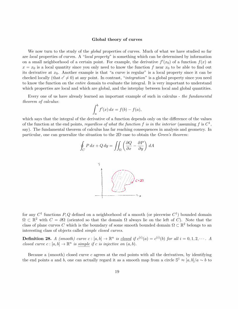
for any C1 functions P,Q defined on a neighborhood of a smooth (or piecewise C1) bounded domainΩ ⊂ R2 with C = ∂Ω (oriented so that the domain Ω always lie on the left of C). Note that theclass of plane curves C which is the boundary of some smooth bounded domain Ω ⊂ R2 belongs to aninteresting class of objects called simple closed curves.

Definition 28. A (smooth) curve c : [a, b] → Rn is closed if c(i)(a) = c(i)(b) for all i = 0, 1, 2, · · · . Aclosed curve c : [a, b]→ Rn is simple if c is injective on (a, b).

Because a (smooth) closed curve c agrees at the end points with all the derivatives, by identifyingthe end points a and b, one can actually regard it as a smooth map from a circle S1 ≈ [a, b]/a ∼ b to

19

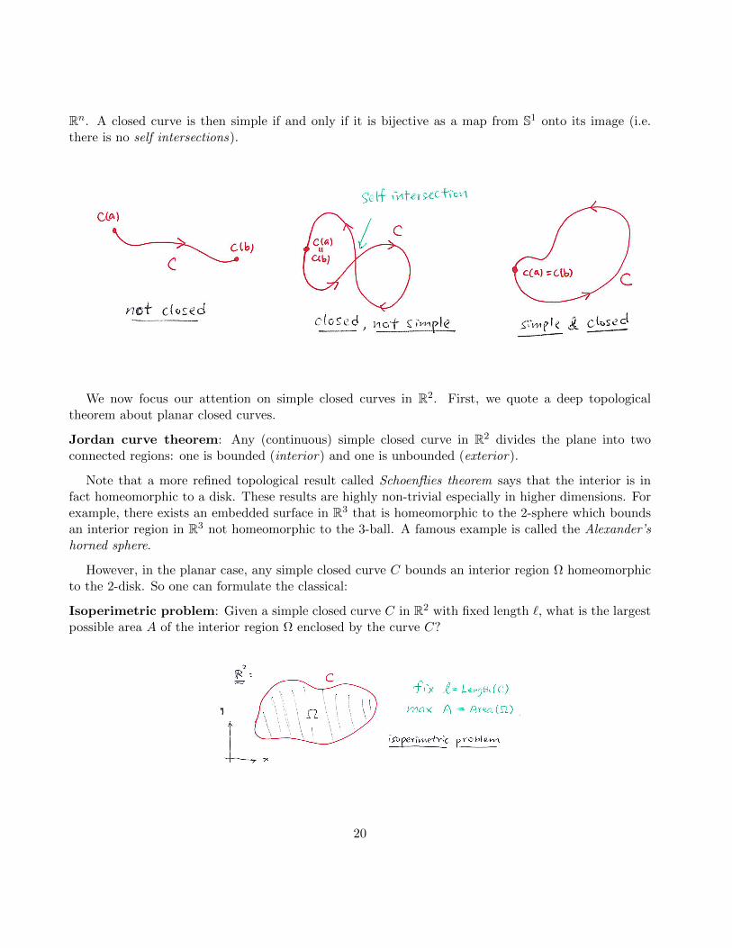
Rn. A closed curve is then simple if and only if it is bijective as a map from S1 onto its image (i.e.there is no self intersections).

We now focus our attention on simple closed curves in R2. First, we quote a deep topologicaltheorem about planar closed curves.

Jordan curve theorem: Any (continuous) simple closed curve in R2 divides the plane into twoconnected regions: one is bounded (interior) and one is unbounded (exterior).

Note that a more refined topological result called Schoenflies theorem says that the interior is infact homeomorphic to a disk. These results are highly non-trivial especially in higher dimensions. Forexample, there exists an embedded surface in R3 that is homeomorphic to the 2-sphere which boundsan interior region in R3 not homeomorphic to the 3-ball. A famous example is called the Alexander’shorned sphere.

However, in the planar case, any simple closed curve C bounds an interior region Ω homeomorphicto the 2-disk. So one can formulate the classical:

Isoperimetric problem: Given a simple closed curve C in R2 with fixed length `, what is the largestpossible area A of the interior region Ω enclosed by the curve C?

20

It turns out that the isoperimetric problem in R2 has a neat answer.

Theorem 29 (The Isoperimetric Inequality). Let C be a simple closed curve in R2 with length `, andlet A be the area of the interior region Ω bounded by C. Then

A ≤ `2

4π,

and equality holds if and only if C is a round circle.

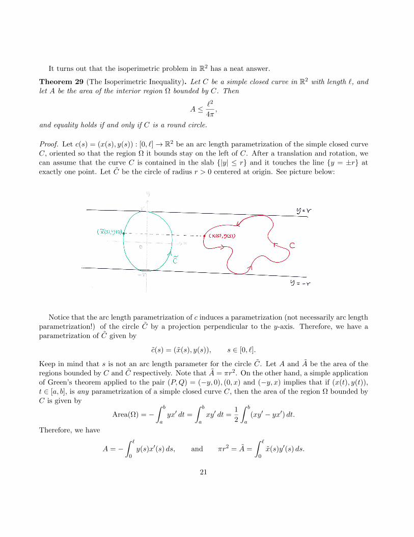
Proof. Let c(s) = (x(s), y(s)) : [0, `]→ R2 be an arc length parametrization of the simple closed curveC, oriented so that the region Ω it bounds stay on the left of C. After a translation and rotation, wecan assume that the curve C is contained in the slab |y| ≤ r and it touches the line y = ±r atexactly one point. Let C be the circle of radius r > 0 centered at origin. See picture below:

Notice that the arc length parametrization of c induces a parametrization (not necessarily arc lengthparametrization!) of the circle C by a projection perpendicular to the y-axis. Therefore, we have aparametrization of C given by

c(s) = (x(s), y(s)), s ∈ [0, `].

Keep in mind that s is not an arc length parameter for the circle C. Let A and A be the area of theregions bounded by C and C respectively. Note that A = πr2. On the other hand, a simple applicationof Green’s theorem applied to the pair (P,Q) = (−y, 0), (0, x) and (−y, x) implies that if (x(t), y(t)),t ∈ [a, b], is any parametrization of a simple closed curve C, then the area of the region Ω bounded byC is given by

Area(Ω) = −∫ b

ayx′ dt =

∫ b

axy′ dt =

1

2

∫ b

a(xy′ − yx′) dt.

Therefore, we have

A = −∫ `

0y(s)x′(s) ds, and πr2 = A =

∫ `

0x(s)y′(s) ds.

21

If we add these two equations (we are omitting the parameter s for simplicity and all the derivativeshere are taken with respect to s), we obtain

A+ πr2 =∫ `

0 (xy′ − yx′) ds≤

∫ `0 |〈(x,−y), (y′, x′)〉| ds

≤∫ `

0 ‖(x,−y)‖‖(y′, x′)‖ ds=

∫ `0 ‖(x,−y)‖ ds = r`.

(3)

where we have used Cauchy-Schwarz inequality and the facts that (x(s), y(s)) is an arc length parametriza-tion for C and that ((x)(s),−y(s)) lies on C, a circle of radius r centered at origin. By the AM-GMinequality, we obtain

√πr2A ≤ A+ πr2

2≤ r`

2.

Rearranging the inequality above yields the desired isoperimetric inequality A ≤ `2/4π.

It remains to study the equality case A = `2/4π. In this case all the inequalities above are infact equalities. In particular, the AM-GM inequality tells us that A = πr2, which them implies fromA = `2/4π that ` = 2πr. Hence the width of the slab we used to enclosed the curve C is independentof the directions of the slab. On the other hand, the equalities in (??) implies that for every s, we have

(x(s),−y(s)) = λ(s)(y′(s), x′(s)), where λ(s) ≥ 0.

Taking the length of the vectors on both sides, we actually have λ(s) ≡ r > 0. Therefore, y(s) ≡−rx′(s). By using instead the slabs |x− a| ≤ r for some a > 0 so that the lines x = a± r touchesC, we can similarly obtain x(s)− a ≡ −ry′(s) for the same constant r > 0. Therefore,

(x(s)− a)2 + y(s)2 = r2(x′(s)2 + y′(s)2) = r2,

which means that C is the circle of radius r > 0.

Remark 30. The isoperimetric inequality actually holds for piecewise C1 curves.

Next, we prove a classical result for planar convex curves regarding the number of “vertices”. Avertex of a curve c is a point on the curve at which κ′ = 0. A planar simple closed curve is said to beconvex if the (closed) region Ω it bounds is a convex subset of R2, in the sense that the line segmentpq joining any two points p, q ∈ Ω lies entirely inside Ω. One easily check that (Proof?) the followingstatements are equivalent:

1. The simple closed curve C is convex.

2. If a (infinite) line meets the curve C, the intersection is either a line segment (which could possiblydegenerate to a single point) or exactly two points.

3. The curve C always lie on one side of the tangent line at every point on C.

22

4. The curvature κ of the curve C does not change sign.

Theorem 31 (Four Vertex Theorem). A simple closed convex planar curve has at least four vertices.

Note that the number 4 is optimal as one can verify that an ellipse with unequal axes has exactly4 vertices, two of which are minima and two of which are maxima of κ.

Proof. Without loss of generality, we assume that κ 6≡ constant. Let c(s) = (x(s), y(s)) : [0, `] → R2

be an arc length parametrization of the curve. Since κ(s) is a continuous function on the compactset [0, `], it achieves its minimum and maximum so κ′ = 0 there. So there are at least two vertices.Suppose that κ(0) = minκ and κ(s0) = maxκ. Erect a coordinate system such that c(0) and c(s0)both lie on the x-axis. By the convexity of the curve, the curve meets the x-axis at no other points(unless κ(0) = κ(s0) = 0 which implies κ(s) ≡ 0, a contradiction to our assumption). In other words,y(s) changes sign only at s = 0 and s = s0.

Next, we argue by contradiction that there are more than two vertices. Suppose not, then there areonly two vertices, namely, c(0) and c(s0). Then, κ′(s) changes sign only at s = 0 and s = s0, but thenthe function κ′(s)y(s) doesn’t change sign at all along the curve. Notice that the Frenet frame is givenby

e1 = (x′, y′), e2 = (−y′, x′),and thus the Frenet equation e′1 = κe2 implies that x′′ = −κy′. Therefore, using this and the closenessof the curve, we get ∫ `

0κ′(s)y(s) ds = −

∫ `

0κ(s)y′(s) ds =

∫ `

0x′′(s) ds = 0.

23

However, we just showed that the integrand κ′(s)y(s) has a constant sign, and thus it must vanishidentically. This says κ′ ≡ 0, which contradicts our assumption that κ is non-constant. Therefore,there must be a third vertex and κ′ must change sign there (why?). But then since the curve is closed,there must be a fourth vertex with a change of sign, which proves the theorem.

Now, we want to study another global quantity which is the total curvature of a curve. Supposec(t) : [a, b]→ R2 is a regular closed plane curve, the total curvature of c is defined to be

TC(c) :=

∫ b

aκ(t)‖c′(t)‖ dt.

If s ∈ [0, `] is an arc length parameter for c, then we have the formula

TC(c) =

∫ `

0κ(s) ds.

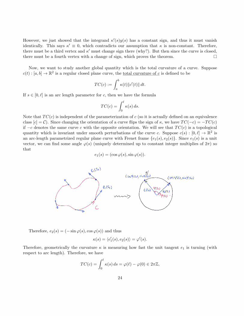
Note that TC(c) is independent of the parameterization of c (so it is actually defined on an equivalenceclass [c] = C). Since changing the orientation of a curve flips the sign of κ, we have TC(−c) = −TC(c)if −c denotes the same curve c with the opposite orientation. We will see that TC(c) is a topologicalquantity which is invariant under smooth perturbations of the curve c. Suppose c(s) : [0, `] → R2 isan arc-length parametrized regular plane curve with Frenet frame e1(s), e2(s). Since e1(s) is a unitvector, we can find some angle ϕ(s) (uniquely determined up to constant integer multiplies of 2π) sothat

e1(s) = (cosϕ(s), sinϕ(s)).

Therefore, e2(s) = (− sinϕ(s), cosϕ(s)) and thus

κ(s) = 〈e′1(s), e2(s)〉 = ϕ′(s).

Therefore, geometrically the curvature κ is measuring how fast the unit tangent e1 is turning (withrespect to arc length). Therefore, we have

TC(c) =

∫ `

0κ(s) ds = ϕ(`)− ϕ(0) ∈ 2πZ,

24

since e1(0) = e1(`) is the same point on S1. Hence, we define the rotation index of the closed curve cto be the integer

Uc :=1

2πTC(c) =

1

2π

∫ `

0κ(s) ds =

1

2π(ϕ(`)− ϕ(0)).

Note that even though the angle ϕ(s) is defined up to an addition constant multiple of 2π, the differenceϕ(`)− ϕ(0) is well-defined! Hence, geometrically, the rotation index Uc is measuring how many timeshave the unit tangent turned a complete circle after traveling along the closed curve c once (note thatc may not be simple!). In the case that c is simple, we have the following theorem.

Theorem 32 (Theorem of Turning Tangents). The rotation index Uc of a simple closed regular planecurve c is ±1.

The proof uses strongly the fact that the rotation index Uc is a homotopy invariant, i.e. if two closedregular curves c0 and c1 can be connected by a smooth family of closed regular curves ct, t ∈ [0, 1],then Uc0 = Uc1 . (See Tutorial Notes 3 for the details of the proof.)

25