Math 245 Notes

Spring 2011 offering of

MATH 245Advanced Linear Algebra 2

Professor: S. NewUniversity of Waterloo

LaTeXer: M. L. Baker <http://lambertw.wordpress.com>Updated: September 3, 2011

Contents1 Affine spaces 2

1.1 Affine spaces . . . . . . . . . . . . . . . . . . . . . . . . . . . . . . . . . . . . . . . . . . . . . . . . . . . . . . . . 21.2 Affine independence and span . . . . . . . . . . . . . . . . . . . . . . . . . . . . . . . . . . . . . . . . . . . . . . . 21.3 Convex sets . . . . . . . . . . . . . . . . . . . . . . . . . . . . . . . . . . . . . . . . . . . . . . . . . . . . . . . . . 31.4 Simplices . . . . . . . . . . . . . . . . . . . . . . . . . . . . . . . . . . . . . . . . . . . . . . . . . . . . . . . . . . 3

2 Orthogonality 52.1 Norms, distances, angles . . . . . . . . . . . . . . . . . . . . . . . . . . . . . . . . . . . . . . . . . . . . . . . . . . 52.2 Orthogonal complements . . . . . . . . . . . . . . . . . . . . . . . . . . . . . . . . . . . . . . . . . . . . . . . . . . 72.3 Orthogonal projection . . . . . . . . . . . . . . . . . . . . . . . . . . . . . . . . . . . . . . . . . . . . . . . . . . . 8

3 Applications of orthogonality 93.1 Circumcenter of a simplex . . . . . . . . . . . . . . . . . . . . . . . . . . . . . . . . . . . . . . . . . . . . . . . . . 93.2 Polynomial interpolation . . . . . . . . . . . . . . . . . . . . . . . . . . . . . . . . . . . . . . . . . . . . . . . . . . 103.3 Least-squares best fit polynomials . . . . . . . . . . . . . . . . . . . . . . . . . . . . . . . . . . . . . . . . . . . . 11

4 Cross product in Rn 134.1 Generalized cross product . . . . . . . . . . . . . . . . . . . . . . . . . . . . . . . . . . . . . . . . . . . . . . . . . 134.2 Parallelotope volume . . . . . . . . . . . . . . . . . . . . . . . . . . . . . . . . . . . . . . . . . . . . . . . . . . . . 14

5 Spherical geometry 16

6 Inner product spaces 166.1 Abstract inner products . . . . . . . . . . . . . . . . . . . . . . . . . . . . . . . . . . . . . . . . . . . . . . . . . . 166.2 Orthogonality and Gram-Schmidt . . . . . . . . . . . . . . . . . . . . . . . . . . . . . . . . . . . . . . . . . . . . . 206.3 Orthogonal complements . . . . . . . . . . . . . . . . . . . . . . . . . . . . . . . . . . . . . . . . . . . . . . . . . . 226.4 Orthogonal projections . . . . . . . . . . . . . . . . . . . . . . . . . . . . . . . . . . . . . . . . . . . . . . . . . . . 23

7 Linear operators 257.1 Eigenvalues and eigenvectors . . . . . . . . . . . . . . . . . . . . . . . . . . . . . . . . . . . . . . . . . . . . . . . 257.2 Dual spaces and quotient spaces . . . . . . . . . . . . . . . . . . . . . . . . . . . . . . . . . . . . . . . . . . . . . 29

8 Adjoint of a linear operator 318.1 Similarity and triangularizability . . . . . . . . . . . . . . . . . . . . . . . . . . . . . . . . . . . . . . . . . . . . . 328.2 Self-adjoint operators . . . . . . . . . . . . . . . . . . . . . . . . . . . . . . . . . . . . . . . . . . . . . . . . . . . . 348.3 Singular value decomposition . . . . . . . . . . . . . . . . . . . . . . . . . . . . . . . . . . . . . . . . . . . . . . . 36

9 Bilinear and quadratic forms 379.1 Bilinear forms . . . . . . . . . . . . . . . . . . . . . . . . . . . . . . . . . . . . . . . . . . . . . . . . . . . . . . . . 379.2 Quadratic forms . . . . . . . . . . . . . . . . . . . . . . . . . . . . . . . . . . . . . . . . . . . . . . . . . . . . . . 42

10 Jordan canonical form 44

These notes are provided “as-is”, without any guarantee of accuracy, in the hopes that they may be helpful.Note that Dr. New has a very useful set of notes on spherical geometry, so that section was omitted.I’ve reorganized the notes, so the section numbers no longer match with the textbook.

1

Administrative• Website: http://math.uwaterloo.ca/~snew.

• Office: MC 5163.

• Email: [email protected]

• Textbook: We will cover most of Chapters 6 and 7 from Linear Algebra by Friedberg, Insel and Spence (Sections 6.1 –6.8, 7.1 – 7.4).

• Midterm: Tuesday, June 7.

1 Affine spaces

1.1 Affine spacesThe set Rn is given by

Rn =

x =

x1

...xn

: xi ∈ R

A vector space in Rn is a set of the form U = span{v1, . . . , v`}.

Definition 1.1. An affine space in Rn is a set of the form p+ U = {p+u | u ∈ U} for some point p ∈ Rn and some vector spaceU in Rn.

Theorem 1.2. Let P = p+ U and Q = q + U be two affine spaces. We have p+ U ⊆ q + V if and only if q − p ∈ V and U ⊆ V.

Proof. Suppose that p+ U ⊆ q+ V. We have p = p+ 0 ∈ p+ U. Hence p ∈ q+ V. Hence p = q+ v for some v ∈ V, by definition.From that equation, q−p = −v ∈ V. Let u ∈ U. Consider p+u. This is an element of p+ U. But p+ U ⊆ q+ V. So we can writep+ u = q + v for some v ∈ V. Hence u = (q − p) + v, which is in V since q − p, v ∈ V. This finishes the proof of one direction.

Conversely, suppose q−p ∈ V and U ⊆ V. We will show p+U ⊆ q+V. Let u ∈ U. p+u = p+u+q−q = q+(u−(q−p)) ∈ q+V.

Corollary 1.3. p+ U = q + V if and only if q − p ∈ U and U = V.

Definition 1.4. The vector space U is called the vector space associated to the affine space p+ U. The dimension of an affinespace is the dimension of its associated vector space. A 0-dimensional affine space in Rn is a point. A 1-dimensional affine spacein Rn is called a line (this defines the word “line”). A 2-dimensional affine space in Rn is called a plane. An (n− 1)-dimensionalaffine space in Rn is called a hyperplane.

Remark 1.5. To calculate the dimension of a solution space, you count the number of parameters (columns with no pivots inthe row-reduced matrix).

Remark 1.6. A vector is the name given to an element of a vector space. In an affine space, they are called points.

1.2 Affine independence and spanDefinition 1.7. Let a0, . . . , a` be points in Rn. We let 〈a0, . . . , a`〉 denote the smallest affine space in Rn that contains thosepoints (that is, the intersection of all affine spaces in Rn which contain each ai). This is called the affine span of the points.

Remark 1.8. To be rigorous, we should prove that an intersection of countably many affine spaces is always an affine space.

Definition 1.9. We say that the points a0, . . . , a` are affinely independent if dim〈a0, . . . , a`〉 = `.

Theorem 1.10. Let a0, . . . , a` be points in Rn. Let uk = ak − a0 (for 1 ≤ k ≤ `). Then 〈a0, . . . , a`〉 = a0 + span{u1, . . . , u`}.

Proof. Let U = span{u1, . . . , u`}. We first show that a0 + U contains all the points ai. Note a0 = a0 + 0 ∈ a0 + U, and for therest we can write ak = a0 + ak − a0 = a0 + uk ∈ a0 + U. This proves that 〈a0, . . . , a`〉 ⊆ a0 + U.Next, we show that a0 + U ⊆ 〈a0, . . . , a`〉. So we need to show that a0 + U ⊆ q + V for every affine space q + V which containsa0, . . . , a`. So let q + V be such an affine space. We must show that q − a0 ∈ V and U is a subspace of V. Since a0 ∈ q + V wehave q − a0 ∈ V. Also, we have ak ∈ q + V for k ≥ 1. Say ak = q + vk for vk ∈ V. Now uk = ak − a0 = q + vk − a0. So uk ∈ Vsince q − a0, vk ∈ V. Hence U is a subspace of V.

2

a0

a1

u1

a2

u2

a3u3

Figure 1: The setup for l = 3

Corollary 1.11. We have the following:

(i) Note:

〈a0, . . . , a`〉 = a0 + span{u1, . . . , uk} =

{a0 +

∑i=1

tiui | ti ∈ R

}=

{∑i=0

siai | si ∈ R,∑i=0

si = 1

}

(ii) {a0, . . . , a`} is affinely independent if and only if {u1, . . . , u`} is linearly independent where uk = ak − a0.

1.3 Convex setsDefinition 1.12. Let a, b ∈ Rn. The line segment [a, b] is the set

{a+ t(b− a) | 0 ≤ t ≤ 1}.

A set C ⊆ Rn is called convex if for all a, b ∈ C, we have [a, b] ⊆ C.

Figure 2: Convex and non-convex subsets of the plane

Definition 1.13. For a set S ⊆ Rn, the convex hull of S, denoted by [S], is the smallest convex set in Rn containing S, that is,the intersection of all convex sets which contain S. (Should prove that the intersection of convex sets is convex for full rigour;this is left as an exercise).

Remark 1.14. When S = {a0, . . . , a`} we write [S] as [a0, . . . , a`]. Note that this agrees with the notation for the line segment(convex hull of two points).

1.4 SimplicesDefinition 1.15. An (ordered, non-degenerate) `-simplex consists of an ordered (l+ 1)-tuple (a0, . . . , a`) of points ai ∈ Rn with{a0, . . . , a`} affinely independent, together with the convex hull [a0, . . . , a`]. A 0-simplex is a point, a 1-simplex is an orderedline segment. A 2-simplex is an ordered triangle. A 3-simplex is an ordered tetrahedron.

Theorem 1.16. Let {a0, . . . , a`} be affinely independent points in Rn. Then [a0, . . . , a`] can be written{a0 +

n∑i=1

tiui | 0 ≤ ti ∈ R,∑i=1

ti ≤ 1

}=

{∑i=0

siai | 0 ≤ si ∈ R,∑i=0

si = 1

}

where uk = ak − a0.

Proof. Exercise. Check the statement of the theorem and then prove it.

3

Figure 3: The medial hyperplane M1,2 (shaded) in a 3-simplex.

Remark 1.17 (triangle facts). The medians of a triangle meet at a point called the centroid. The perpendicular bisectors meetat the circumcenter (the center of the circle in which the triangle is inscribed). The angle bisectors meet at the incenter (thecenter of the circle inscribed in the triangle). Furthermore, the altitudes meet at the orthocenter. The cleavers meet at thecleavance center. We will think about higher-dimensional generalizations of these notions.

Definition 1.18. Let [a0, . . . , a`] be an `-simplex in Rn. For 0 ≤ j < k ≤ `, the (j, k) medial hyperplane is defined to be theaffine space Mj,k which is the affine span of the points ai (for i 6= j, k) and the midpoint 1

2 (aj + ak).

Theorem 1.19. Let [a0, . . . , a`] be an `-simplex in Rn. The medial hyperplanes Mj,k with 0 ≤ j < k ≤ ` have a unique pointof intersection g. This point g is called the centroid of the `-simplex, and it is given by the the “average” of the points ai,

g =1

l + 1

∑i=0

ai.

Proof. We first claim that g lies in each Mj,k. We have

g =1

l + 1

∑i=0

ai =1

l + 1

∑i6=j,k

ai +1

l + 1(aj + ak) =

1l + 1

∑i6=j,k

ai +2

l + 1

(aj + ak

2

)and the sum of the coefficients is

(l − 1)1

1 + l+

2l + 1

=l + 1l + 1

= 1.

Hence g ∈Mj,k for all 0 ≤ j < k ≤ `, henceg ∈

⋂j,k

Mj,k.

Further, we claim g is unique; it is the only point of intersection. Note that each Mj,k really is a hyperplane. To see this, weshow that the points ai (i 6= j, k) and 1

2 (aj + ak) are affinely independent. Suppose∑i 6=j,k

siai + s

(aj + ak

2

)= 0

ands+

∑i 6=j,k

si = 0.

Thens0a0 + . . .+

s

2aj + . . .+

s

2ak + . . .+ s`a` = 0.

Also, the sum of these coefficients is zero, therefore each coefficient is zero since {a0, . . . , a`} is affinely independent. Thus{ai | i 6= j, k} ∪ { 1

2 (aj + ak)} is affinely independent. This shows that each Mj,k is indeed a hyperplane of dimension l − 1.

Note ak does not lie in the medial hyperplane M0,k = 〈 12 (a0 + ak), a1, . . . , ak−1, ak+1, . . . , a`〉. Suppose to the contrary thatak ∈M0,k, say

ak = s1a1 + . . .+ sk−1ak−1 + sk

(a0 + ak

2

)+ sk+1ak+1 + . . .+ s`a`

4

with∑`i=1 si = 1. Then

sk2a0 + s1a1 + . . .+ sk−1ak−1 +

(sk2− 1)ak + sk+1ak+1 + . . .+ s`a` = 0

and the sum of the coefficients is zero (since we moved ak to the other side). Since {a0, . . . , a`} is affinely independent, all of thecoefficients

sk2, s1, . . . , sk−1,

sk2− 1, sk+1, . . . , s`

must be zero. However, it is impossible that both sk2 and sk

2 − 1 are zero. So we have reached a contradiction, proving thatak /∈M0,k.

We now construct a sequence of affine spaces (formed by taking intersections of the medial hyperplanes) by putting Vk :=⋂ki=1M0,i for 1 ≤ k ≤ `. Hence V1 = M0,1, V2 = M0,1 ∩M0,2, and so on. To finish the proof, we note that because ak+1 ∈ Vk

but ak+1 /∈ Vk+1, it follows thatk+1⋂i=1

M0,i (k⋂i=1

M0,i

In other words, each Vk+1 is properly contained within Vk (for 1 ≤ k ≤ `− 1). We know dim(M0,1) = `− 1 and g ∈ V` (as waspreviously shown), so dim(V`) ≥ 0. By the above, dim(Vk) = ` − k and hence dim(V`) = 0. This hence demonstrates g is theunique point of intersection of the hyperplanes M0,k (1 ≤ k ≤ `). Thus g is the unique point of intersection of the hyperplanesMj,k for 1 ≤ j < k ≤ `.

2 Orthogonality

2.1 Norms, distances, anglesDefinition 2.1. Let u, v ∈ Rn. We define the dot product of u with v by

u • v := utv = vtu =n∑i=1

uivi.

Theorem 2.2 (Properties of Dot Product). The dot product satisfies, for all u, v, w ∈ Rn and t ∈ R:

1. [positive definite] u • u ≥ 0, holding with equality if and only if u = 0.

2. [symmetry] u • v = v • u.

3. [bilinearity] (tu) • v = t(u • v) = u • (tv), (u+ v) • w = u • w + v • w, and u • (v + w) = u • v + u • w.

Proof. Easy.

Definition 2.3. For u ∈ Rn we define the length (or norm) of u to be

|u| :=√u • u.

Theorem 2.4 (Properties of Length). Length satisfies, for all u, v, w ∈ Rn and t ∈ R:

1. [positive definite] |u| ≥ 0, holding with equality if and only if u = 0.

2. [homogeneous] |tu| = |t||u|.

3. [polarization identity] u • v = 12 (|u+ v|2 − |u|2 − |v|2) = 1

4 (|u+ v|2 − |u− v|2). (Law of Cosines)

4. [Cauchy-Schwarz inequality] |u • v| ≤ |u||v|, with equality if and only if {u, v} is linearly dependent.

5. [triangle inequality] |u+ v| ≤ |u|+ |v|, and also ||u| − |v|| ≤ |u+ v|.

Proof. The first two are trivial; we will prove properties 3 to 5.

3. Note that|u+ v|2 = (u+ v) • (u+ v) = u • u+ 2(u • v) + v • v = |u|2 − 2(u • v) + |v|2

whereby the first equality follows immediately. We also have

|u− v|2 = |u|2 − 2(u • v) + |v|2

Therefore |u+ v|2 − |u− v|2 = 4(u • v), and the second equality falls out.

5

4. Suppose {u, v} is linearly dependent, say v = tu. Then

|u • v| = |u • (tu)| = |t(u • u)| = |t||u • u| = |t||u|2 = |u||tu| = |u||v|.

Now suppose {u, v} is linearly independent. We will prove strict equality. Note that for all t ∈ R we have u + tv 6= 0 byindependence. Hence

0 < |u+ tv|2 = (u+ tv) • (u+ tv) = |u|2 + 2t(u • v) + t2|v|2

which is a quadratic in t with no real roots. Hence the discriminant must be negative, that is,

(2(u • v))2 − 4|v|2|u|2 < 0

whereby, taking square roots, we are done.

5. Note that|u+ v|2 = |u|2 + 2(u • v) + |v|2 ≤ |u|2 + 2|u • v|+ |v|2 ≤ |u|2 + 2|u||v|+ |v|2 = (|u|+ |v|)2

by applying Cauchy-Schwarz. Taking square roots, the proof follows. For the other equality, note

|u| = |(u+ v)− v| ≤ |u+ v|+ |v|

so that |u| − |v| ≤ |u+ v|. Similarly, |v| − |u| ≤ |u+ v|.

We are done.

Definition 2.5. For a, b ∈ Rn, the distance between a and b is defined to be

dist(a, b) := |b− a|.

Theorem 2.6 (Properties of Distance). Distance satisfies, for all a, b, c ∈ Rn:

1. [positive definite] dist(a, b) ≥ 0, holding with equality if and only if a = b.

2. [symmetric] dist(a, b) = dist(b, a).

3. [triangle inequality] dist(a, c) ≤ dist(a, b) + dist(b, c).

Proof. Exercise.

Definition 2.7. Let u ∈ Rn. We say u is a unit vector if it has length 1.

Definition 2.8. For 0 6= u, v ∈ Rn, we define the angle between them to be the angle

θ(u, v) := arccos(u • v|u||v|

)∈ [0, π].

Theorem 2.9 (Properties of Angle). Angle satisfies for all 0 6= u, v ∈ Rn:

1. The following:

• θ(u, v) ∈ [0, π].

• θ(u, v) = 0 if and only if u = tv for some 0 < t ∈ R.

• θ(u, v) = π if and only if u = tv for some 0 > t ∈ R.

• θ(u, v) = π2 if and only if u • v = 0.

2. θ(u, v) = θ(v, u).

3. θ(tu, v) = θ(u, tv) =

{θ(u, v) if 0 < t ∈ Rπ − θ(u, v) if 0 > t ∈ R.

4. The Law of Cosines holds. Put θ := θ(u, v). Then

|v − u|2 = |u|2 + |v|2 − 2|u||v| cos θ.

6

5. Trigonometric ratios. Put θ := θ(u, v) and suppose (v − u) • u = 0. Then

cos θ =|u||v|

and sin θ =|v − u||v|

.

Proof. Exercise.

Remark 2.10. We have the following:

1. For points a, b, c ∈ Rn with a 6= b and b 6= c, we define

∠abc := θ(a− b, c− b).

2. For 0 6= u, v ∈ R2 we can define the oriented angle from u to v to be the angle φ ∈ [0, 2π] with

cosφ =u • v|u||v|

and sinφ =det(u, v)|u||v|

=u1v2 − u2v1|u||v|

.

In this case it is understood thatdet(u, v) := det

[u1 v1u2 v2

].

Definition 2.11. For u, v ∈ Rn, we say that u and v are orthogonal (or perpendicular) when u • v = 0.

2.2 Orthogonal complementsDefinition 2.12. For a vector space U in Rn we define the orthogonal complement of U in Rn to be the vector space

U⊥ = {v ∈ Rn : v • u = 0 for all u ∈ U}.

Theorem 2.13 (Properties of Orthogonal Complement). We have the following:

1. U⊥ is a vector space in Rn.

2. If U = span{u1, . . . , u`} where each ui ∈ Rn, then

U⊥ = {v ∈ Rn : v • ui = 0 for all i}.

3. For A ∈ Mk×n(R), we have (RowA)⊥ = nullA. For

A =

rt1...rtk

RowA = span{r1, . . . , rk} ⊆ Rn. Note that

Ax =

rt1x...rtkx

=

r1 • x...rk • x

4. dim U + dim U⊥ = n, and U⊕ U⊥ = Rn.

5. (U⊥)⊥ = U.

6. (nullA)⊥ = RowA.

Proof. We will prove #5; the rest are left as exercise.

5. Let x ∈ U. By definition of U⊥, x • v = 0 for all v ∈ U⊥. By definition of (U⊥)⊥, we have x ∈ (U⊥)⊥ therefore U ⊆ (U⊥)⊥.

On the other hand by #4, dim U + dim(U⊥) = n. Also, dim U⊥ + dim(U⊥)⊥ = n. Therefore, dim U = dim(U⊥)⊥. Since Uis a subspace of (U⊥)⊥ and dim U = dim(U⊥)⊥, it follows that U = (U⊥)⊥.

7

2.3 Orthogonal projectionTheorem 2.14. Let A ∈ Mk×n(R). Then null(AtA) = null(A).

Proof. For x ∈ Rn, x ∈ null(A) implies Ax = 0, so AtAx = 0. Therefore x ∈ null(AtA).

If x ∈ null(AtA) then AtAx = 0, then xtAtAx = 0, so (Ax)t(Ax) = 0, so (Ax) • (Ax) = 0, so |Ax|2 = 0, so |Ax| = 0, so Ax = 0,so x ∈ null(A).

Remark 2.15. For A = (u1, . . . , un), we have

AtA =

ut1...utn

(u1, . . . , un) =

u1 • u1 u1 • u2 u1 • u3 . . .u2 • u1 u2 • u2 . . .

...

Theorem 2.16 (Orthogonal Projection Theorem). Let U be a subspace of Rn. Then for any x ∈ Rn there exist unique vectorsu, v ∈ Rn with u ∈ U and v ∈ U⊥ and u+ v = x.

Proof. (uniqueness) Let x ∈ Rn. Suppose u ∈ U, v ∈ U⊥, u + v = x. Let {u1, . . . , u`} be a basis for U. Let A be the matrixwith columns u1 up to u` (A ∈ Mn×`), so U = col(A). Since u ∈ U = col(A), we have u = At for some t ∈ R`. Sincev ∈ U⊥ = col(A)⊥ = nullAt, we have Atv = 0. We have

u+ v = x

At+ v = x

AtAt = Atx since Atv = 0

t = (AtA)−1Atx

since {u1, . . . , u`} is linearly independent, so rank(AtA) = rank(A) = ` and AtA ∈ M`×`(R). So

u = At = A(AtA)−1Atx

and v = x− u.

(existence) Again, let {u1, . . . , u`} be a basis for U and let A = (u1, . . . , u`), and let

u = A(AtA)−1Atx

Then clearly u ∈ col(A) = U and u+ v = x. We need to show that v ∈ U⊥ = (colA)⊥ = nullAt.

Atv = At(x− u) = Atx−AtA(AtA)−1Atx = Atx− (AtA)(AtA)−1Atx = Atx−Atx = 0.

So the proof is complete.

Definition 2.17. Let U be a vector space in Rn. Let x ∈ Rn. Let u and v be the vectors of the above theorem with u ∈ U,v ∈ U⊥, u+ v = x. Then u is called the orthogonal projection of x onto U and we write

u = ProjU(x).

Note that since U = (U⊥)⊥ it follows thatv = ProjU⊥(x)

Example 2.18. When U = span{u} with 0 6= u ∈ Rn, we can take A = u, hence

ProjU(x) = A(AtA)−1Atx = u(utu)−1utx = u(|u|2)−1utx =uutx

|u|2=u(u • x)|u|2

=u • x|u|2

u.

We also writeProju(x) = ProjU(x) =

u • x|u|2

u

Theorem 2.19. u := ProjU(x) is the unique point in U nearest to x.

Proof. Let w ∈ U with w 6= u. Note that (w− u) • (x− u) = 0 since u,w ∈ U so w− u ∈ U and v = x− u ∈ U⊥ by the definitionof u = ProjU(x). By Pythagoras’ theorem (special case of the Law of Cosines), we note that

|w − x|2 = |w − u|2 + |x− u|2 > |x− u|2

since |w − u|2 > 0 (because w 6= u).

8

Definition 2.20. Let U be a subspace of Rn and let x ∈ Rn. We define the reflection of x in U to be

ReflU(x) = ProjU(x)− ProjU⊥(x) = x− 2ProjU⊥(x) = 2ProjU(x)− x

For an affine space P = p+ U ⊆ Rn and a point x ∈ Rn we can also define

Projp+U(x) = p+ ProjU(x− p)

Reflp+U(x) = p+ ReflU(x− p).

3 Applications of orthogonalityWe started off by talking about affine spaces (when you solve systems of equations, the solution set is, in general, an affine space:a vector space translated by a point). We also defined `-simplices, and saw that we can apply the ideas of linear algebra totalk about geometry in higher dimensions. We then talked about inner products (the dot product in Rn and its relationship tolengths and angles, orthogonality, orthogonal complements of vector spaces, orthogonal projections). Geometric applications ofthese include finding the circumcenter of a simplex by finding an intersection of perpendicular bisectors, and finding best-fit andinterpolating polynomials.

3.1 Circumcenter of a simplexAside 3.1. In geometry, we study curves and surfaces and higher-dimensional versions of those. There are three main ways: agraph (draw a graph of a function of one variable, you get a curve; a graph of a function of two variables, you get a surface),you can do an implicit description, or you can do it parametrically.

For f : U ⊆ Rk → R`, the graph of f denoted Graph(f) = {(x, y) ∈ Rk+` | y = f(x)} ⊆ Rk+`; usually this is a k-dimensionalversion of a surface. The equation y = f(x) is known as an explicit equation (it can be thought of as ` equations, actually).The kernel of f is {x ∈ Rk | f(x) = 0}. Usually this is (k − `)-dimensional. We also define the image of f , which is the set{f(x) | x ∈ U} ⊆ R`. Usually this is k-dimensional. (It is described parametrically, by parameter x).

For example, the top half of a sphere can be described by z =√r2 − (x2 + y2). An implicit equation describing the whole sphere

would be x2 + y2 + z2 − r2 = 0. The sphere is the kernel of f(x, y, z) = x2 + y2 + z2 − r2.

Definition 3.2. Let P be an affine space in Rn and let a, b be points in Rn with a 6= b. The perpendicular bisector of [a, b] in Pis the set of all x ∈ P such that x− a+b

2 • (b− a) = 0.

Theorem 3.3. x is on the perpendicular bisector of [a, b] if and only if dist(x, a) = dist(x, b).

Proof. For x ∈ P, x lies on the perpendicular bisector of [a, b] if and only if (x− a+b2 )•(b−a) = 0 if and only if (2x−(a+b))•(b−a) =

0. This holds iff 2x • b− 2x • a− a • b+ a • a− b • b+ b • a = 0. This holds iff a • a− 2x • a = b • b− 2x • b. But this holds iffa • a− 2x • a+ x • x = b • b− 2x • b+ x • x iff |x− a|2 = |x− b|2 iff |x− a| = |x− b|.

Theorem 3.4 (Simplicial Circumcenter Theorem). Let [a0, a1, . . . , a`] be an `-simplex in Rn. For 0 ≤ j < k ≤ `, write Bj,k forthe perpendicular bisector of the [aj , ak]. Then the affine spaces Bj,k with 0 ≤ j < k ≤ ` have a unique point of intersection in〈a0, . . . , a`〉. This point is denoted by ζ and is called the circumcenter of the `-simplex.

By the above theorem, ζ is the unique point in 〈a0, . . . , a`〉 which is equidistant from each ai. There’s an (` − 1)-dimensionalsphere centered at ζ passing through each of the points ai.

Proof. (uniqueness) Suppose such a point ζ exists. Then ζ lies on each B0,k for 1 ≤ k ≤ `. We have ζ ∈ 〈a0, . . . , a`〉. Sayζ = a0 + t1u1 + . . .+ t`u` where uk = ak − a0 and tk ∈ R. That is,

ζ = a0 +At

where A is the matrix with the column vectors u1 to u`. Since ζ lies on B0,k, where 1 ≤ k ≤ `, we use the definition of B0,k andwrite the equation that ζ satisfies. (

ζ − a0 + ak2

)• (ak − a0) = 0

We rewrite this as((a0 +At)− (a0 +

ak − a0

2)) • (ak − a0) = 0

9

This gives

(At− 12uk) • uk = 0

(At) • uk =12|uk|2(At) • u1

...(At) • u`

=12

|u1|2...|u`|2

AtAt =

12

|u1|2...|u`|2

Where we note that At denotes the transpose and not A raised to the power of t (the letter t is being used in two different wayshere). Since [a0, . . . , a`] is a (non-degenerate) `-simplex, we know that {u1, . . . , u`} is linearly independent so that rank(AtA) =rank(A) = ` and AtA is an `× ` matrix, so it is invertible. Therefore,

t = (AtA)−1v

where

v =12

|u1|2...|u`|2

and therefore ζ = a0 +At = a0 +A(AtA)−1v.

(existence) We need to show that this point ζ = a0 +A(AtA)−1v lies on all the perpendicular bisectors Bj,k with 0 ≤ j < k ≤ `.So let 0 ≤ j < k ≤ `. Since ζ ∈ B0,j and ζ ∈ B0,k, we have

dist(ζ, a0) = dist(ζ, aj)dist(ζ, a0) = dist(ζ, ak)

hence dist(ζ, ak) = dist(ζ, aj) so that ζ lies on Bj,k.

3.2 Polynomial interpolationThe following theorem gives us information about the so-called “polynomial interpolation” of data points. This process producesa polynomial which actually passes through the points.

Theorem 3.5. Let (a0, b0), (a1, b1), . . . , (an, bn) be n+ 1 points with the ai distinct. Then there exists a unique polynomial ofdegree n with p(ai) = bi for all i.

Proof. For p(x) = c0 + c1x+ c2x2 + . . .+ cnx

n, then we have p(ai) = bi for all i if and only if

c0 + c1a0 + c2a20 + . . .+ cna

n0 = b1

...

c0 + c1an + c2a22 + . . .+ cna

nn = bn

if and only if Ac = b, where

A =

1 a0 a 2

0 . . . an01 a1 a 2

1 . . . an1...1 an a 2

n . . . ann

and

c =

c0c1...cn

, b =

b0b1...bn

10

This matrix A is called the Vandermonde matrix for a0, a1, . . . , an. We must show that A is invertible. We claim that

detA =∏

0≤j<k≤n

(ak − aj).

We prove this by induction. Let

Ak =

1 a0 a 2

0 . . . a k01 a1 a 2

1 . . . a k1...1 ak a 2

k . . . a kk

that is, Ak is the Vandermonde matrix for a0, a1, . . . , ak. We have

detA1 = det(

1 a0

1 a1

)= a1 − a0.

Fix k with 2 ≤ k ≤ n and suppose detAk−1 =∏

0≤i<j<k−1

(aj − ai). Write x = ak. Then

D(x) := detAk =

1 a0 a 2

0 . . . a k01 a1 a 2

1 . . . a k1...1 x x2 . . . xk

and we see that, expanding on the last row, D(x) is a polynomial of degree k in x, with leading coefficient C = detAk−1 whichby the induction hypothesis is ∏

0≤i<j≤k−1

(aj − ai).

For each 0 ≤ i ≤ k − 1, by subtracting the ith row from the last, we see that

D(x) = detAk = det

1 a0 a 2

0 . . . a k01 a1 a 2

1 . . . a k1...1 ak−1 a 2

k−1 . . . a kk−1

0 x− ai x2 − a2i . . . xk − aki

.

So (x− ai) is a factor of each term on the last row, so (x− ai) is a factor of D(x) for each 0 ≤ i ≤ k − 1. It follows that

D(x) = C(x− a0)(x− a1) · · · (x− ak−1)

=

∏0≤i<j≤k−1

(aj − ai)

(ak − a0)(ak − a1) · · · (ak − ak−1)

=∏

0≤i<j≤k

(aj − ai).

This completes the proof.

3.3 Least-squares best fit polynomialsNow we will look not at polynomial interpolation, but fitting polynomials, that is, finding a polynomial which is a “best fit”curve to some data points (not necessarily passing through those points).

Example 3.6. Given a positive integer ` and given n data points (a1, b1), (a2, b2), . . ., (an, bn). Find the best fit polynomial ofdegree ` for the data points.

The solution depends on what we mean by “best fit”. We could mean some function f which minimizes the distance of each datapoint to the graph of f :

n∑i=1

dist((ai, bi), graph of f).

11

Or we could mean a function f which minimizes the sum of the vertical distances between the data points and the graph:n∑i=1

bi − f(ai).

As our definition, we will take “best fit” to mean something that minimizesn∑i=1

(bi − f(ai))2

hence the name sum of squares. Equivalently, such a function minimizes√√√√ n∑i=1

(bi − f(ai))2 = dist

b1...bn

,

f(a1)...

f(an)

.

To help us with this task, we have the following theorem.

Theorem 3.7. Given a positive integer `, and n points (a1, b1), . . . , (an, bn) in R2 such that at least ` + 1 of the points ai aredistinct, there exists a unique polynomial f(x) of degree ` which minimizes the sum

n∑i=1

(bi − f(ai))2.

This polynomial is called the least-squares best fit polynomial of degree ` for the data points.

Proof. For f(x) = c0 + c1x+ . . .+ c`x`, we havef(a1)

...f(an)

=

c0 + c1a1 + c2a21 + . . .+ c`a

`1

...c0 + c1an + c2a

2n + . . .+ c`a

`n

= Ac,

where

A =

1 a1 a2

1 . . . a`11 a2 a2

2 . . . a`2...1 an a2

n . . . a`n

∈ Mn×(`+1)(R) and c =

c0c1...c`

To minimize the sum

n∑i=1

(bi − f(ai))2,

we must minimize

dist

b1...bn

,

f(a1)...

f(an)

= dist(b, Ac)

We must have that Ac is the (unique) point in col(A) which lies nearest to b. Thus

Ac = Projcol(A)(b).

Since `+ 1 of the ai are distinct, it follows that the corresponding `+ 1 rows of A form a Vandermonde matrix on `+ 1 distinctpoints. This (` + 1) × (` + 1) Vandermonde matrix is invertible by the previous theorem, so these ` + 1 rows are linearlyindependent. Therefore, the rank of the matrix A is ` + 1, which means the columns of A are linearly independent. ThereforeA is one-to-one, and hence there is a unique c.

We now seek a formula for c. We look for u, v ∈ R`+1 with u ∈ U = colA, v ∈ U⊥ = nullAt, and u+ v = b. Say u = Ac.

u+ v = b

Ac+ v = b

AtAc = Atb

c = (AtA)−1Atb.

Since c is the vector of coefficients, the proof is complete. Put f(x) = c0 + . . .+ c`x`.

12

4 Cross product in Rn

A familiar notion is the cross product of two vectors in R3. In this section, we generalize this to the cross product of n−1 vectorsin Rn, and see some results about the connections between cross products, determinants, and the volume of the parallelotopegenerated by vectors.

4.1 Generalized cross productDefinition 4.1. Let u1, . . . , un−1 be vectors in Rn. We define the cross product of these vectors to be

X(u1, . . . , un−1) = formal det

(u1 . . . un−1

e1...en

)

where ek is the kth standard basis vector. This is equal to

n∑i=1

(−1)i+n det(Ai)ei

where A = (u1, . . . , un−1) ∈ Mn×(n−1) and Ai is the (n− 1)× (n− 1) matrix obtained from A by removing the ith row.

Example 4.2. In R2, for u =(u1

u2

)∈ R2 we write uX = X(u) = formal det

(u1 e1u2 e2

). In R3, for u, v ∈ R3 we write

X(u, v) = formal det

u1 v1 e1u2 v2 e2u3 v3 e3

= det

(u2 v2u3 v3

)e1 − det

(u1 v1u3 v3

)e2 + det

(u1 v1u2 v2

)e3.

=

u2v3 − u3v2u3v1 − u1v3u1v2 − u2v1

.

This particular cross product gives the area of the parallelogram “generated” by the vectors u, v.

Theorem 4.3 (Properties of Cross Product). We have the following, for u1, . . . , un−1, v ∈ Rn, and t ∈ R:

1. X(u1, . . . , tuk, . . . , un−1) = tX(u1, . . . , uk, . . . , un−1).

2. X(u1, . . . , u`, . . . , uk, . . . , un−1) = −X(u1, . . . , uk, . . . , u`, . . . , un−1), that is, interchanging two vectors flips the sign of thecross product. (This means the cross product is skew-symmetric).

3. X(u1, . . . , uk + v, . . . , un−1) = X(u1, . . . , uk, . . . , un−1) + X(u1, . . . , v, . . . , un−1). This, together with property 1, says thatthe cross product is multilinear.

4. We haveX(u1, . . . , un−1) • v = det(u1, . . . , un−1, v)

hence for 1 ≤ i ≤ n− 1, we haveX(u1, . . . , un−1) • ui = 0.

5. X(u1, . . . , un−1) = 0 if and only if {u1, . . . , un−1} is linearly dependent. Furthermore, when X(u1, . . . , un−1) 6= 0, the set

{u1, . . . , un−1,X(u1, . . . , un−1)}

is what we would call a positively oriented basis for Rn which means

det(u1, . . . , un−1,X(u1, . . . , un−1)) > 0.

Proof. We prove 4 and 5.

13

4. Note that

X(u1, . . . , un−1) • v =

(n∑i=1

(−1)i+n det(Ai)ei

)• v

=n∑i=1

(−1)i+n det(Ai)(ei • v)

=n∑i=1

(−1)i+n det(Ai)vi

= det(u1, . . . , un−1, v)

5. {u1, . . . , un−1} is linearly independent if and only if A has rank n − 1, if and only if row space has dimension n − 1, ifand only if some n− 1 rows of A are linearly independent, if and only if one of the matrices Ai is invertible, if and only ifX(u1, . . . , un−1) 6= 0.

X(u1, . . . , un−1) =

+|A1|−|A2|+|A3|

...±|An−1|

6= 0.

Also,

det(u1, . . . , un−1,X(u1, . . . , un−1)) = X(u1, . . . , un−1) • X(u1, . . . , un−1)

= |X(u1, . . . , un)|2 > 0

whenever X(u1, . . . , un−1) 6= 0.

The proof is complete.

4.2 Parallelotope volumeDefinition 4.4. For vectors u1, . . . , uk we define the parallelotope (or parallelepiped) on the vectors u1, . . . , uk in Rn to be theset {

k∑i=1

tiui | 0 ≤ ti ≤ 1 for all i

}.

We define the k-volume of this parallelotope, written volk(u1, . . . , uk) inductively by vol1(u1) = |u1| and for k ≥ 2 we define

volk

(u1, . . . , uk) = volk−1

(u1, . . . , uk−1)|uk| sin θ,

where θ is the angle between the vector uk and the vector space U = span{u1, . . . , uk−1}, or alternatively

volk

(u1, . . . , uk) = volk−1

(u1, . . . , uk−1) |ProjU⊥(uk)| .

Theorem 4.5 (Parallelotope Volume Theorem). Let u1, . . . , uk ∈ Rn. Then

volk

(u1, . . . , uk) =√

det(AtA),

where A is the matrix with columns u1, . . . , uk.

Proof. To see the truth of the base case, note vol1(u1) = |u1| =√u1 • u1 =

√ut1u1 =

√det(ut1u1) =

√det(AtA), where A = u1.

Next, fix k ≥ 2, and suppose inductively that

volk−1

(u1, . . . , uk−1) =√

det(AtA)

where A = (u1, . . . , uk−1). Let B = (u1, . . . , uk) = (A, uk), that is, B is the matrix obtained from A by inserting the vector ukas its last column. Now, put U = span{u1, . . . , uk−1} and then define the projections

p := ProjU(uk) ∈ colA

q := ProjU⊥(uk) ∈ (colA)⊥ = null(At)

14

and hence p + q = uk. Then of course B = (A, p + q). Since p ∈ colA, the matrix B can be defined from the matrix (A, q) byperforming elementary column operations of type 3. Hence B = (A, p+ q) = (A, q)E where E is a product of type 3 elementarymatrices. Hence E is k × k, and det(E) = 1. It follows that

det(BtB) = det(Et(A, q)t(A, q)E) = det[(At

qt

)(A, q)

]since detE = 1. This then becomes

det(BtB) = det(AtA AtqqtA qtq

)= det

(AtA 0

0 |q|2)

= det(AtA)|q|2.

Therefore taking square roots, we apply the induction hypothesis to obtain√det(BtB) =

√det(AtA)|q| = vol

k−1(u1, . . . , uk−1) · |q| = vol

k(u1, . . . , uk)

hence completing the proof.

Theorem 4.6 (Dot Product of Two Cross Products). Let u1, . . . , un−1, v1, . . . , vn−1 ∈ Rn. Then

X(u1, . . . , un−1) • X(v1, . . . , vn−1) = det(AtB)

where A is the matrix with columns u1, . . . , un−1 and B is the matrix with columns v1, . . . , vn−1.

Proof. First, we define

x := X(u1, . . . , un−1)y := X(v1, . . . , vn−1).

We now calculate x • y twice:x • y = X(u1, . . . , un−1) • y = det(A, y)

and alsox • y = x • X(v1, . . . , vn−1) = X(v1, . . . , vn−1) • x = det(B, x).

Therefore, we see that

(x • y)2 = det(A, y) det(B, x) = det[(A, y)t(B, x)

]= det

[(At

yt

)(B, x)

]and this becomes

(x • y)2 = det(AtB AtxytB ytx

)= det

(AtB 0

0 x • y

).

To justify that Atx = 0, observe that since x = X(u1, . . . , un−1), it is the case that x • ui = 0 for all i. This means thatx ∈ (span{u1, . . . , un−1})⊥ = (colA)⊥ = nullAt. Also, y ∈ nullBt. It is now clear that either x • y = 0, or x • y = det(AtB).

Suppose that x • y = 0 with one of x or y being zero. If x = X(u1, . . . , un−1) = 0, then {u1, . . . , un−1} is linearly dependent, sorank(A) < n − 1 (the proof of this is an exercise). Therefore AtB is non-invertible, implying det(AtB) = 0. Similarly, if y = 0we also obtain det(AtB) = 0.

Suppose next that x • y = 0 with both x, y nonzero. Since

0 = x • y = X(u1, . . . , un−1) • y = det(A, y)

we have y ∈ col(A) (since x 6= 0 so the columns of A are linearly independent). Similarly, x ∈ col(B), say x = Bt. Note thatt 6= 0, since x 6= 0. Note that since x = X(u1, . . . , un−1), we know it’s perpendicular to col(A) which means x ∈ null(At),therefore AtBt = Atx = 0. Since t 6= 0 and (AtB)t = 0, we see that AtB has nontrivial nullspace, proving AtB cannot beinvertible. Hence det(AtB) = 0.

In all cases, we have obtained x • y = det(AtB). So the proof is complete.

Corollary 4.7. For u1, . . . , un−1 ∈ Rn,

|X(u1, . . . , un−1)| =√

det(AtA) = voln−1

(u1, . . . , un−1).

This is the end of the material that will be tested on the course midterm.

15

5 Spherical geometryIn this section we study some spherical geometry. A useful reference for this material is available at

http://www.math.uwaterloo.ca/~snew/math245spring2011/Notes/sphere.pdf.

In view of this, these notes do not themselves include information on spherical geometry.

6 Inner product spaces

6.1 Abstract inner productsDefinition 6.1. Let F be a field. We define the dot product of two vectors u, v ∈ Fn by

u • v :=

u1

...un

•v1...vn

=n∑i=1

uivi = vtu = utv.

Remark 6.2. Let u, v, w ∈ Fn and t ∈ F. The dot product is symmetric and bilinear, but it is not positive definite, that is, itis not the case that u • u ≥ 0.

For example, if F = Z5 then (12

)•(

12

)= 12 + 22 = 0

or on the other hand if F = C then (1i

)•(

1i

)= 12 + i2 = 0.

For A ∈ Mk×`(F) and x ∈ F`, if

A =

rt1...rtk

then we observe that

Ax =

r1 • x...rk • x

.

For u, v ∈ Cn, we could define

u ∗ v =

u1

...un

∗v1...vn

=

x1 + iy1...

xn + iyn

∗r1 + is1

...rn + isn

= x1r1 + y1s1 + x2r2 + y2s2 + . . .

Here we are identifying Cn with R2n and using the dot product in R2n. This dot product is symmetric and R-bilinear, but isnot C-bilinear. Note that for z ∈ C we have |z|2 = zz.

Definition 6.3. For u, v ∈ Cn, we define the (standard) inner product of u and v to be

〈u, v〉 =n∑i=1

uivi = vtu = v∗u

where v∗ = vt.

This product has the following properties:

• It is conjugate-symmetric.

• It is linear in the first variable, and conjugate linear in the second (we call this hermitian or sesquilinear). That is,

〈u+ v, w〉 = 〈u,w〉+ 〈v, w〉〈u, v + w〉 = 〈u, v〉+ 〈u,w〉〈tu, v〉 = t〈u, v〉〈u, tv〉 = t〈u, v〉

16

• It is positive definite: we have 〈u, u〉 ≥ 0 with 〈u, u〉 = 0 if and only if u = 0.

For A = (u1, . . . , u`) ∈ Mn×`(C), and x ∈ Cn, we have

A∗x = Atx =

ut1...ut`

x =

〈x, u1〉...

〈x, u`〉

and for B = (v1, . . . , v`) ∈ Mn×`(C) we have

B∗A =

vt1...vt`

(u1, . . . , u`) =

〈u1, v1〉 . . . 〈u`, v1〉...

. . ....

〈u1, v`〉 . . . 〈u`, v`〉

where A∗ = At = At, that is,

(A∗)ij = Aji.

When A ∈ Mn×`(R) then we simply have A∗ = At since complex conjugation, when restricted to the reals, is the identity map.

Definition 6.4. Let F be R or C. Let V be a vector space over the field F. Then we can define an inner product on V as a map〈 , 〉 : V × V→ F such that for all u, v, w ∈ V and all t ∈ F we have:

〈u, v〉 = 〈v, u〉〈u, v + w〉 = 〈u, v〉+ 〈u,w〉〈u+ v, w〉 = 〈u,w〉+ 〈v, w〉〈tu, v〉 = t〈u, v〉〈u, tv〉 = t〈u, v〉〈u, u〉 ≥ 0 with equality iff u = 0

A vector space V over F (R or C) together with an inner product is called an inner product space over F.

Example 6.5. We have the following:

• Rn is an inner product space using the dot product (also called the standard inner product) on Rn.

• Cn is an inner product space using its standard inner product.

• The standard inner product on Mk×`(F) is given by

〈A,B〉 =

⟨a11

. . .ak`

,

b11 . . .bk`

⟩ = a11b11 + a12b12 + . . .+ ak`bk` = tr(B∗A).

Example 6.6. Let F be R or C. Then F∞ is the vector space of sequences a = (a1, a2, . . .) with ai ∈ F, where ai 6= 0 for onlyfinitely many i. This vector space has the standard basis

{e1, e2, e3, . . .}

where ek = (ek1, ek2, . . .) with eki = δki (Kronecker delta notation). The standard inner product on F∞ is

〈a, b〉 =∞∑i=1

aibi

where we note that this sum is indeed finite since only finitely many ai, bi are nonzero.

Example 6.7. Let a < b be real. Then we define C([a, b],F) to be the vector space of continuous functions f : [a, b] → F. Thestandard inner product on C([a, b],F) is given by

〈f, g〉 =∫ b

a

fg

where we note that |f |2 = 〈f, f〉 =∫ baff =

∫ ba|f |2 ≥ 0.

17

Example 6.8. Let Pn(F) denote the vector space of polynomials with coefficients in F of degree at most n. Let P(F) denotethe vector space of all polynomials over F. In Pn(F) we have several inner products:

• We can define ⟨n∑i=0

aixi,

n∑j=0

bjxj

⟩=

n∑i=0

aibi.

• For a < b real, we can put

〈f, g〉 =∫ b

a

fg

• For distinct points a0, . . . , an ∈ F we can define

〈f, g〉 =n∑i=0

f(ai)g(ai).

Note that the first and second of these inner products generalize to inner products on P(F).

Definition 6.9. Let U be an inner product space over F (where F is R or C). For u, v ∈ U we say that u and v are orthogonalwhen 〈u, v〉 = 0. Also, for u ∈ U we define the norm (or length) of u to be

|u| =√〈u, u〉

noting that when |u| = 1 we call u a unit vector.

Definition 6.10. Let U be an inner product space. Let u, x ∈ U. We define the orthogonal projection of x onto u to be

Projux =〈x, u〉|u|2

u

(not the same as

〈u, x〉|u|2

u if F = C!)

Proposition 6.11. x− Projux is orthogonal to u.

Proof. This is an easy computation. Just expand 〈x− Projux, u〉 and use the properties of the inner product.

Theorem 6.12 (Properties of Norm). Let U be an inner product space over F, with F = R or F = C. Then for all u, v, w ∈ Uand t ∈ F we have

1. |tu| = |t||u| (note that these are 2 different norms).

2. |u| ≥ 0 with equality if and only if u = 0.

3. The Cauchy-Schwarz inequality holds, that is, |〈u, v〉| ≤ |u||v|.

4. The triangle inequality holds: ||u| − |v|| ≤ |u+ v| ≤ |u|+ |v|.

5. The polarization identity holds. If F = R then we have

〈u, v〉 =14(|u+ v|2 − |u− v|2

)whereas if F = C we have (?)

〈u, v〉 =14(|u+ v|2 + i|u+ iv|2 − |u− v|2 − i|u− iv|2

)6. Pythagoras’ theorem holds: if 〈u, v〉 = 0 then |u+ v|2 = |u|2 + |v|2. Note that in the complex setting, the converse is not

true!

Proof of Cauchy-Schwarz. If {u, v} is linearly dependent, then one of u and v is a multiple of the other, say v = tu with t ∈ F.Then

|〈u, v〉| = |〈u, tu〉| = |t〈u, u〉| = |t||u|2 = |u||tu| = |u||v|.

Next, suppose {u, v} is linearly independent. Consider

w = v − Projuv = v − 〈v, u〉|u|2

u = 1 · v − 〈v, u〉|u|2

u

18

Since {u, v} is linearly independent, we have w 6= 0, hence |w|2 > 0, hence 〈w,w〉 > 0⟨v − 〈v, u〉

|u|2u, v − 〈v, u〉

|u|2u

⟩> 0

hence

〈v, v〉 − 〈v, u〉|u|2

〈v, u〉 − 〈v, u〉|u|2

〈u, v〉+〈v, u〉|u|2

〈v, u〉|u|2

〈u, u〉 > 0

therefore

〈v, v〉 − 〈u, v〉〈u, v〉|u|2

− 〈u, v〉〈u, v〉|u|2

+〈u, v〉〈u, v〉|u|4

〈u, u〉 > 0

hence

|v|2 − 2|〈u, v〉|2

|u|2+|〈u, v〉|2

|u|4|u|2 > 0

therefore multiplying through by |u|2 we obtain|u|2|v|2 − |〈u, v〉|2 > 0

finally yielding|〈u, v〉|2 < |u|2|v|2

as required.

Proof of triangle inequality. We will prove that |u+ v| ≤ |u|+ |v|. Note that

|u+ v|2 = 〈u+ v, u+ v〉 = 〈u, u〉+ 〈u, v〉+ 〈v, u〉+ 〈v, v〉 = 〈u, u〉+ 〈u, v〉+ 〈u, v〉+ 〈v, v〉

and therefore this is equal to

|u|2 + 2 · Re〈u, v〉+ |v|2 ≤ |u|2 + 2|Re〈u, v〉|+ |v|2 ≤ |u|2 + 2|u||v|+ |v|2 = (|u|+ |v|)2.

So the proof is complete.

Proof of Pythagoras’ theorem. We will prove that if 〈u, v〉 = 0 then |u+ v|2 = |u|2 + |v|2. As above, we have

|u+ v|2 = |u|2 + 2 · Re〈u, v〉+ |v|2

We see that|u+ v|2 = |u|2 + |v|2

if and only if Re〈u, v〉 = 0.

Remark 6.13. Let F be R or C and U be a vector space over F. Then a norm on U is a map | · | : U → R such that for allu, v ∈ U and all t ∈ F,

1. |tu| = |t||u|.

2. |u+ v| ≤ |u|+ |v|.

3. |u| ≥ 0 with equality if and only if u = 0.

A vector space U over F with a norm is called a normed linear space.

Example 6.14. Some norms do not arise from inner products. In Rn for u ∈ Rn we can define the norm of u to be

|u| =n∑i=1

|ui|.

This is a norm on Rn (that is different from the standard one).

Definition 6.15. Let U be an inner product space (it could be a normed linear space) over F (R or C). For a, b ∈ U we definethe distance between them to be

dist(a, b) = |b− a|

The distance function has the following properties for all u, v, w ∈ U:

1. dist(a, b) = dist(b, a).

19

2. dist(a, c) ≤ dist(a, b) + dist(b, c).

3. dist(a, b) ≥ 0 with equality if and only if a = b.

Remark 6.16. A metric on a set X is a map dist : X ×X → R which satisfies properties 1, 2 and 3 above. A subset U ⊆ X isopen when for all a ∈ U , there exists r > 0 such that Br(a) ⊆ U , where

Br(a) := {x ∈ X : dist(a, x) < r}

It has the following properties:

1. ∅, X are open.

2. If U1, . . . , Un are open then so isn⋂i=1

Ui.

3. If Uα is open for all α ∈ A then so is ⋃α∈A

Uα.

A topology on a set X is a set T of subsets of X which we call the open sets in X such that 1, 2, and 3 hold. A topological spaceis a set X together with a topology T .

6.2 Orthogonality and Gram-SchmidtDefinition 6.17. Let W be an inner product space over F (R or C). Let U ⊆ W. We say U is orthogonal when 〈u, v〉 = 0 forall u 6= v ∈ U . We say U is orthonormal if it is orthogonal and furthermore |u| = 1 for all u ∈ U .

Example 6.18. For U = {u1, . . . , u`} ⊆ Rn, let A = (u1, . . . , u`), then U is orthogonal if and only if AtA is diagonal, since

AtA =

u1 • u1 . . . u` • u1

.... . .

...u1 • u` . . . u` • u`

and U is orthonormal if and only if AtA = I.

Example 6.19. Recall that if U is a basis for the vector space U, then for x ∈ U = span U , we can write

x = t1u1 + t2u2 + . . .+ tù`

with each ti ∈ F and ui distinct elements in U . When U = {u1, . . . , u`} and x = t1u1 + . . .+ tù` we write

[x]U = t =

t1...t`

∈ F`.

The map φ : U→ F` given by φ(x) =[x]U is a vector space isomorphism, so U ∼= F`.

Remark 6.20. For U = {u1, . . . , u`} ⊆ Rn, A = (u1, . . . , u`), and x ∈ U = span U = colA with x = t1u1 + . . .+ tù` = At, note[x]U = t. To find t =

[x]U we solve At = x. Hence

AtAt = Atx

and thus[x]U = t = (AtA)−1Atx. As a remark, note that (AtA)−1At is a left inverse for A. If U is orthonormal then AtA = I

so[x]U = Atx which gives

[x]U =

ut1...ut`

x =

x • u1

...x • u`

.

Also, for x ∈ Rn, we haveProjUx = A(AtA)−1Atx.

If U is orthonormal so that AtA = I, then ProjUx = AAtx, which is equal to

(u1 . . . u`

)x • u1

...x • u`

.

20

Theorem 6.21 (Gram-Schmidt Procedure). Let U be a finite (or countable) dimensional inner product space over F (R or C).Let U = {u1, . . . , u`} (or U = {u1, . . .}) be a basis for U. Let v1 = u1, and for k ≥ 1, let

vk = uk −k−1∑i=1

Projvi(uk) = uk −k−1∑i=1

〈uk, vi〉|vi|2

vi.

ThenV = {v1, . . . , v`} (or V = {v1, . . .})

is an orthogonal basis for U with span{v1, . . . , vk} = span{u1, . . . , uk} for all k ≥ 1.

Proof. We will prove inductively that {v1, . . . , vk} is an orthogonal basis for span{u1, . . . , uk}. The base case holds since v1 = u1.Fix k ≥ 2 and suppose that {v1, . . . , vk−1} is an orthogonal basis for span{u1, . . . , uk−1}. Let

vk = uk −k−1∑i=1

〈uk, vi〉|vi|2

vi.

Since vk is equal to uk plus a linear combination of v1, . . . , vk−1 and since span{v1, . . . , vk−1} = span{u1, . . . , uk−1}, it followsthat

span{v1, . . . , vk} = span{v1, . . . , vk−1, uk} = span{u1, . . . , uk−1, uk}

and hence {v1, . . . , vk} is a basis for span{u1, . . . , uk}. Next, we seek to show that {v1, . . . , vk} is orthogonal. By our inductionhypothesis, 〈vi, vj〉 = 0 for all i 6= j less than k. So it remains to show that 〈vk, vi〉 = 0 for 1 ≤ i ≤ k − 1. We have for1 ≤ j ≤ k − 1 that

〈vk, vj〉 =

⟨uk −

k−1∑i=1

〈uk, vi〉|vi|2

vi, vj

⟩= 〈uk, vj〉 −

k−1∑i=1

⟨〈uk, vi〉|vi|2

vi, vj

⟩= 〈uk, vj〉 −

k−1∑i=1

(〈uk, vi〉|vi|2

〈vi, vj〉)

but this is, since 〈vi, vj〉 = 0 for all i 6= j, becomes

〈uk, vj〉 −〈uk, vj〉|vj |2

〈vj , vj〉 = 0.


Corollary 6.22. Every finite (or countable) dimensional inner product space U over F (R or C) has an orthonormal basis.

Proof. Let U = {u1, . . . , u`} (or U = {u1, . . .}) be a basis for U. Apply the Gram-Schmidt procedure to U to obtain anorthonormal basis V = {v1, . . . , v`} (or V = {v1, . . .}) for U, then for all k ≥ 1 let

wk =vk|vk|

to obtain an orthonormal basis W = {w1, . . . , w`} (or W = {w1, . . .}).

Remark 6.23. The previous corollary does not hold for uncountable dimensional vector spaces.

Corollary 6.24. Let W be a finite (or countable) dimensional inner product space over R or C and let U be a finite dimensionalsubspace. Then any orthogonal (or orthonormal) basis U can be extended to an orthogonal (or orthonormal) basis W for W.

Proof. Extend a given orthogonal basis U = {u1, . . . , u`} to a basis {u1, . . . , u`+1, . . .} for W, then apply the Gram-Schmidtprocedure to obtain an orthogonal basis {v1, . . . , v`, v`+1, . . .} for W and verify that vi = ui for 1 ≤ i ≤ `.

Remark 6.25. This result does not always hold when U is countable dimensional.

Example 6.26. Let W be an inner product space. Let U = {u1, . . . , u`} ⊆W. If U is an orthogonal set of nonzero vectors, thenfor x ∈ span U , say

x = t1u1 + . . .+ t`u` =∑i=1

tiui

with each ti ∈ F (R or C), we have for each k (1 ≤ k ≤ `) that

〈x, uk〉 =

⟨∑i=1

tiui, uk

⟩=∑i=1

ti〈ui, uk〉 = tk〈uk, uk〉 = tk|uk|2.

21

Thus,

tk =〈x, uk〉|uk|2

so U is linearly independent and we have

[x]U =(〈x, u1〉|u1|2

. . .〈x, u`〉|u`|2

)tIf U is orthonormal, then

[x]U =(〈x, u1〉 . . . 〈x, u`〉

)t6.3 Orthogonal complementsDefinition 6.27. Let W be an inner product space. Let U be a subspace of W. The orthogonal complement of U in W is thevector space

U⊥ = {x ∈W : 〈x, u〉 = 0 for all u ∈ U}Note that if U = {u1, . . . , u`} is a basis for U, then

U⊥ = {x ∈W : 〈x, ui〉 = 0 for all i = 1, . . . , `}

and also if U is a (possibly infinite) basis for U, then

U⊥ = {x ∈W : 〈x, u〉 = 0 for all u ∈ U}.

Remark 6.28. Let W be a finite dimensional inner product space and let U be a subspace of W. Let U = {u1, . . . , u`} be anorthogonal (or orthonormal) basis for U. Extend U to an orthogonal (or orthonormal) basis

W = {u1, . . . , u`, v1, . . . , vm}

for W. Then V = {v1, . . . , vm} is an orthogonal (or orthonormal) basis for U⊥.

Proof. For x = t1u1 + . . .+ t`u` + s1v1 + . . .+ smvm, we have

tk =〈x, uk〉|uk|2

and sk =〈x, vk〉|vk|2

.

If x ∈ U⊥, then each tk = 0 so x ∈ spanV. If x ∈ spanV then x = s1v1 + . . .+ smvm, then for each k, 〈x, uk〉 = 〈∑sivi, uk〉 =∑

si〈vi, uk〉 = 0.

Remark 6.29. As a consequence, we see that in the case above,

1. U⊕ U⊥ = W.

2. dim U + dim U⊥ = dim W.

3. U = (U⊥)⊥.

Proof of #3. 〈x, v〉 = 0 for all v ∈ U⊥ (from the definition of U⊥), and so x ∈ (U⊥)⊥ (from the definition of (U⊥)⊥) thusU ⊆ (U⊥)⊥. Also dim U = dim W − dim U⊥ = dim W − (dim W − dim(U⊥)⊥) = dim(U⊥)⊥. Thus U = (U⊥)⊥.

Note carefully that the first part of the proof above does not use finite-dimensionality.

Remark 6.30. When U is infinite dimensional we still have U ⊆ (U⊥)⊥ but in general U 6= (U⊥)⊥.

Since U⊕ U⊥ = W , it follows that given x ∈W there exist unique vectors u, v with u ∈ U, v ∈ U⊥ such that u+ v = x.

Example 6.31. Consider the inner product space W = R∞. This is the set of sequences (a1, a2, . . .) with each ai ∈ R and onlyfinitely many ai are nonzero. W has basis {e1, e2, . . .}. Let U be the subspaces of sequences whose sum

∑∞i=1 ai = 0 (note that

this is a finite sum). U has basis{ek − e1 : k ≥ 2} = {e2 − e1, e3 − e1, . . .}

andU⊥ = {x ∈ R∞ : 〈x, a〉 = 0 for all a ∈ U}

Note that

〈x, a〉 = 〈(x1, x2, . . .), (a1, a2, . . .)〉 =∞∑i=1

xiai.

SoU⊥ = {x ∈ R∞ : 〈x, ek − e1〉 = 0 for all k ≥ 2} = {x = (x1, x1, x1, . . .) ∈ R∞} = {0}

since only finitely many xi are nonzero.

22

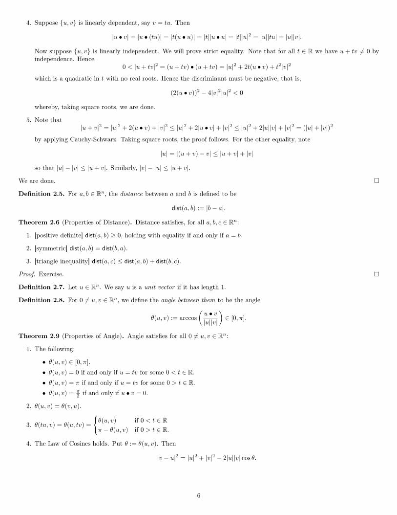
6.4 Orthogonal projectionsTheorem 6.32 (Orthogonal Projection Theorem). Let W be a (possibly infinite dimensional) inner product space. Let U be afinite dimensional subspace of W. Let U = {u1, . . . , u`} be an orthogonal basis for U. Given x ∈ W, there exist unique vectorsu, v ∈ W with u ∈ U, v ∈ U⊥ such that u + v = x. The vector u is called the orthogonal projection of x onto U and is denotedProjUx. The projection is given by

u = ProjUx =∑i=1

〈x, ui〉|ui|2

ui.

Also, u is the unique vector in U which is nearest to x.

Proof. (uniqueness) Suppose such u, v exist. So u ∈ U, v ∈ U⊥ and u+ v = x. Say

u =∑i=1

tiui, so that ti =〈u, ui〉|ui|2

.

We have〈x, ui〉 = 〈u+ v, ui〉 = 〈u, ui〉+ 〈v, ui〉 = 〈u, ui〉

since v ∈ U⊥ so 〈v, ui〉 = 0 therefore

u =∑i=1

〈u, ui〉|ui|2

ui =∑i=1

〈x, ui〉|ui|2

ui.

This completes the proof of uniqueness.

(existence) Given x ∈W, let

u =∑i=1

〈x, ui〉|ui|2

ui

so we have〈u, ui〉|ui|2

=〈x, ui〉|ui|2

then let v = x− u. Clearly u ∈ U = span{u1, . . . , u`} and u+ v = x. We must verify v ∈ U⊥. We have

〈v, ui〉 = 〈x− u, ui〉 = 〈x, ui〉 − 〈u, ui〉 = 0.

This completes the proof of existence.

We claim u is the unique point in U nearest to x. Let w ∈ U with w 6= u. Note w − u ∈ U, since w, u ∈ U. Also x− u = v ∈ U⊥

so 〈x− u,w − u〉 = 0. By Pythagoras’ theorem,

|(w − u)− (x− u)|2 = |w − x|2 = |x− u|2 + |w − u|2 > |x− u|2

since w 6= u.

Example 6.33. Let a0, . . . , an be n+ 1 distinct points in F (R or C). Consider Pn(F) with the inner product

〈f, g〉 =n∑i=0

f(ai)g(ai).

For 0 ≤ k ≤ n, letgk(x) =

∏i 6=k

x− aiak − ai

so that we havegk(ai) = δki

(Kronecker delta notation). Note that {g0, . . . , gn} is an orthonormal basis for Pn(F). For f ∈ Pn(F),

f =n∑k=0

〈f, gk〉|gk|2

gk

23

and

〈f, gk〉 =n∑i=0

f(ai)gk(ai) = f(ak), since gk(ai) = δki .

So then

f =n∑k=0

f(ak)gk.

Example 6.34. Find the polynomial of degree 2 (f ∈ P2(R)) which minimizes∫ 1

−1

(f(x)− |x|)2 dx

Solution. Consider the vector space C([−1, 1],R) with its standard inner product

〈f, g〉 =∫ 1

−1

fg.

We need to find the unique f ∈ P2(R) which minimizes dist(f, g) where g(x) = |x|. We must take

f = ProjP2g.

Let p0 = 1, p1 = x, p2 = x2. So {p0, p1, p2} is the standard basis for P2(R). Apply the Gram-Schmidt procedure:

q0 = p0 = 1.

q1 = p1 −〈p1, q0〉|q0|2

q0 = p1 = x.

q2 = p2 −〈p2, q0〉|q0|2

q0 −〈p2, q1〉|q1|2

q1 = x2 − 23· 1

2· 1− 0 = x2 − 1

3.

We now have an orthogonal basis {q0, q1, q2}. So we take

f = ProjP2g =〈g, q0〉|q0|2

q0 +〈g, q1〉|q1|2

q1 +〈g, q2〉|q2|2

q2 = . . . =1516x2 +

316.

We are done.

Definition 6.35. Let U and V be inner product spaces. An inner product space isomorphism from U to V is a bijective linearmap L : U→ V which preserves the inner product, that is, 〈L(x), L(y)〉 = 〈x, y〉 for all x, y ∈ U.

Proposition 6.36. Note that if U = {u1, . . . , u`} and V = {v1, . . . , v`} are orthonormal bases for U and V respectively, then thelinear map L : U→ V given by L(ui) = vi (that is, L(

∑tiui) =

∑tivi) is an inner product space isomorphism.

Proof. For x =∑siui, y =

∑tjuj we have

〈x, y〉 = 〈∑

siui,∑

tjuj〉 =∑i,j

sitj〈ui, uj〉 =∑i

siti =

⟨s1...s`

,

t1...t`

⟩ = 〈[x]U ,[y]U 〉

and we have

L(x) = L(∑

siui) =∑

siL(ui) =∑

sivi

L(y) =∑

tjvj

〈L(x), L(y)〉 =∑

sitj .


As a corollary to the Gram-Schmidt orthogonalization procedure, we see that every n-dimensional inner product space is iso-morphic to Fn. If you have any (infinite dimensional) vector space, it has a basis, and you can use that basis to construct aninner product. Say U is a basis. We define an inner product as follows: for

x =∑u∈U

suu and y =∑u∈U

tuu

we define〈x, y〉 =

∑u∈U

sutu.

Every vector space, we can construct an inner product such that a given basis is orthonormal in it. However, not all innerproduct spaces (namely, the infinite dimensional ones) furnish an orthogonal basis!

24

7 Linear operators

7.1 Eigenvalues and eigenvectorsWe now want to consider the following problem. Given a linear map L : U → V find bases U and V which are related to thegeometry of L so that

the matrix[L]UV is in some sense simple.

Example 7.1. Let U and V be finite-dimensional vector spaces over any field F. Let L be a linear map. Show that we canchoose bases U and V for U and V so that [

L]UV =

(I 00 0

).

Solution. Suppose r = rank(L). Choose a basis{ur+1, . . . , uk}

for ker(L) = null(L). Extend this to a basis{u1, . . . , ur, ur+1, . . . , uk} =: U

for U. Let vi = L(ui) (for i with 1 ≤ i ≤ r). Verify that

{v1, . . . , vr}

is linearly independent and hence forms a basis for the range of L. Extend this to a basis

V = {v1, . . . , vr, . . . , v`}.

Thus [L]UV =

([L(u1)

]V . . .

[L(uk)

]V)

=(Ir 00 0

)and we are done.

Remark 7.2.[L]UV is the matrix such that [

L(x)]V =

[L]UV

[x]U .

When U = V we sometimes simply write[L]U . Note that for U = {u1, . . . , uk} and V = {v1, . . . , v`} we have[

L(ui)]V =

[L]UV

[ui]U =

[L]UV ei = ith column of

[L]UV

therefore [L]UV =

([L(u1)

]V . . .

[L(uk)

]V)∈ M`×k.

Also, forU(U)

L−→ V(V)

M−→ W(W)

we have [ML]UW =

[M]VW

[L]UV .

Similarly, forU

(U1)

I−→ U(U2)

L−→ V(V2)

I−→ V(V1)

we have [L]U1

V1=[IV]V2

V1

[L]U2

V2

[IU]U1

U2

Warning. Some calculational examples follow. I’m not completely sure about the correctness of these calculations; sorry.

Example 7.3. Let u1 = (1, 1, 2)t, u2 = (2, 1, 3)t, U = {u1, u2}, and U = span(U). Let F = ReflU, that is, F : R3 → R3 is givenby

F(x) = ReflU(x) = x− 2ProjU(x) = ProjU(x)− ProjU⊥(x) = 2ProjU(x)− x.

We wish to find[F].

Solution. There are three methods.

25

1. Let A = (u1, u2). We have ProjU(x) = A(AtA)−1Atx. Therefore

F(x) = 2ProjU(x)− x = (2A(AtA)−1At − I)x

so that [F]

= 2A(AtA)−1At − I.Calculating, we see that

AtA =(

1 1 22 1 3

)1 21 12 3

=(

6 99 14

)and eventually we arrive at [

F]

=13

1 −2 2−2 1 2

2 2 1

.

2. Use Gram-Schmidt to construct an orthonormal basis and perform the projection this way.

3. We have F(u1) = u1, F(u2) = u2. Choose u3 = u2 × u1, so that u3 = (1, 1,−1)t. Then F(u3) = −u3. For V = {u1, u2, u3},

[F]V =

([F(u1)

]V

[F(u2)

]V

[F(u3)

]V)

=

1 0 00 1 00 0 −1

So

F(u1, u2, u3) = (u1, u2,−u3) = (u1, u2, u3)

1 0 00 1 00 0 −1

(u1, u2, u3)−1

and then we get [F]

= (u1, u2, u3)

1 0 00 1 00 0 1

(u1, u2, u3)−1.

We are done.

Example 7.4. Let R be the rotation in R3 about the vector u = (1, 0,−2)t by π/2 (with the direction given by the right handrule). We wish to find

[R].

Solution. Choose u2 = (2, 0, 1)t so that u • u2 = 0 and choose u3 = u1 × u2 = (0,−5, 0)t. Let

v1 =u1

|u1|=

1√5

10−2

v2 =

u2

|u2|=

1√5

201

v3 =

u3

|u3|=

010

and observe that V = {v1, v2, v3} is orthonormal. Then R(v1) = v1, R(v2) = v3, R(v3) = −v2, so we get

[R]V =

1 0 00 0 −10 1 0

.

Then [R]

(v1, v2, v3) = (v1, v2, v3)

1 0 00 0 −10 1 0

so that [

R]

= (v1, v2, v3)

1 0 00 0 −10 1 0

(v1, v2, v3)−1.

Note that (v1, v2, v3)−1 = (v1, v2, v3)t for orthonormal vectors.

26

Example 7.5. Let L : R3 → R3 be the linear map which scales by a factor of 2 in the direction of u1 := (1, 1, 2)t, fixes vectorsin the direction of u2 := (2, 1, 3)t, and annihilates vectors in the direction of u3 := (1, 1,−1)t. Find

[L]

=[L]S.

Solution. Let U = {u1, u2, u3}. Note L(u1) = 2u1, L(u2) = u2, and L(u3) = 0. Then

[L]U =

2 0 00 1 00 0 0

but note that [

L]S

=[I]US

[L]UU

[I]SU .

Since[I]US

= (u1, u2, u3) and[I]SU = (u1, u2, u3)−1, we calculate

[L]S

=13

−2 4 2−5 7 2−7 11 4

.

We are done.

Remark 7.6. Note that

[L]U = diag(λ1, . . . , λn) ⇐⇒

([L(u1)

]U . . .

[L(un)

]U)

=

λ1 . . . 0...

. . ....

0 . . . λn

which occurs if and only if L(ui) = λiui for all i (1 ≤ i ≤ n).

Definition 7.7. For a linear operator L : U → U, we say λ ∈ F is an eigenvalue of L and u is an eigenvector of L for λ when0 6= u and L(u) = λu.

Definition 7.8. For a linear operator L on a finite dimensional vector space U, the characteristic polynomial of L is the polynomial

f(t) = fL(t) = det(L− tI).

Definition 7.9. For λ ∈ F an eigenvalue, the eigenspace of λ is the space

Eλ := null(L− λI).

Remark 7.10 (eigenvalue characterizations). Let L be a linear operator on U. The following are equivalent:

1. λ is an eigenvalue of L.

2. L(u) = λu for some nonzero u ∈ U.

3. (L− λI)(u) = 0 for some nonzero u ∈ U.

4. L− λI has a nontrivial kernel (that is, Eλ is nontrivial).

If we assume further that U is finite dimensional then we can add the following to the list:

6. det(L− λI) = 0.

7. λ is a root of the characteristic polynomial, fL.

Note also that a nonzero u ∈ U is an eigenvector for λ if and only if u ∈ Eλ.

Remark 7.11. Suppose dim(U) = n. If L : U→ U is diagonalizable, say[L]U = diag(λ1, . . . , λn)

then we have

fL(t) = det(L− tI) = det([

L− tI]U

)= det(

[L]U − tI) = det

λ1 − t . . . 0...

. . ....

0 . . . λn − t

= (−1)nn∏i=1

(t− λi).

27

Note that the isomorphism ϕU : U→ Fn given by ϕU (x) =[x]U maps null(L) onto null(

[L]U ) and hence maps null(L− λI) onto

null

λ1 − λ . . . 0...

. . ....

0 . . . λn − λ

= span{ei | λi = λ}

Thus,null(L− λI) = span{ui | λi = λ}

so thatdimEλ = dim null(L− λI) = (# of i such that λi = λ) = multiplicity of λ in fL(t).

Theorem 7.12 (Eigenvector Independence). Let L be a linear operator on a vector space U. Let λ1, . . . , λk be distinct eigenvaluesof L. Let u1, . . . , uk be the corresponding eigenvectors. Then the set {u1, . . . , uk} is linearly independent.

Proof. We proceed by induction. Note that {u1} is linearly independent, since u1 6= 0 by definition of an eigenvector. Suppose{u1, . . . , uk−1} is linearly independent and assume

t1u1 + t2u2 + . . .+ tk−1uk−1 + tkuk = 0

where each ti ∈ F. Operate on both sides by the transformation (L− λkI). We obtain

t1(L(u1)− λku1) + . . .+ tk−1(L(uk−1)− λkuk−1) + tk(L(uk)− λkuk) = 0

and thereforet1(λ1 − λk)u1 + . . .+ tk−1(λk−1 − λk)uk−1 + tk(λk − λk)uk = 0.

Since the λi are distinct, and {u1, . . . , uk−1} is linearly independent, it follows that

t1 = t2 = . . . = tk−1 = 0

and hence tk = 0 as required.

Corollary 7.13. If λ1, . . . , λk are distinct eigenvalues for a linear operator L on a vector space U and if Ui = {ui,1, . . . , ui,`i} isa basis for Eλi then

k⋃i=1

Ui is a basis for Eλ1 + Eλ2 + . . .+ Eλk =k⊕i=1

Eλi .

Theorem 7.14 (Dimension of an Eigenspace). Let L be a linear operator on a finite dimensional vector space U. Let λ be aneigenvalue of L. Then

1 ≤ dimEλ ≤ multλ(fL).

Proof. Since λ is an eigenvalue, we haveEλ = null(L− λI) 6= {0}.

Hence dimEλ ≥ 1. Let {u1, . . . , u`} be a basis for Eλ (so that dimEλ = `). Extend this to a basis

U = {u1, . . . , un}

for U. Then[L]U has the block form [

L]U =

(λI`×` A

0 B

)where O is a zero matrix. So

fL(t) = det([L]U − tI) = det

(λI`×` A

0 B

)= (λ− t)` det(B − tI).

Hence (t− λ)` divides fL(t), therefore ` ≤ multλ(fL). This completes the proof.

Corollary 7.15. For a linear operator L on a finite dimensional vector space U, L is diagonalizable if and only if fL splits (factorscompletely into linear factors) and dim(Eλ) = multλ(fL) for each eigenvalue λ.

28

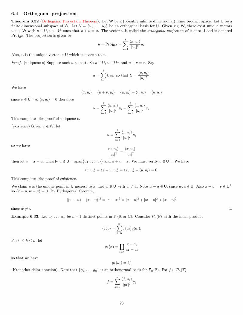
Example 7.16. Let L(x) = Ax, where

A =

−2 4 2−5 7 2−7 11 2

.

Diagonalize L.

Solution. Find the eigenvalues:

det(A− λI) = det

−2− λ 4 2−5 7− λ 2−7 11 4− λ

= (−2− λ)(7− λ)(4− λ)− 56− 110− 22(−2− λ) + 20(4− λ) + 14(7− λ)

which is equal to −λ(λ− 3)(λ− 6). Hence the eigenvalues are λ = 0, 3, 6. Find a basis for each eigenspace:

• (λ = 0): Note that

null(A− λI) = null

−2 4 2−5 7 2−7 11 4

= null

1 0 10 1 10 0 0

by a row reduction. So a basis is {(−1,−1, 1)t}.

• (λ = 3): Note that

null(A− λI) = null

−5 4 2−5 4 2−7 11 1

= null

1 0 −2/30 1 −1/30 0 0

hence a basis is {(2, 1, 3)t}.

And so on.

Aside 7.17. Defineθ(u, v) = cos−1 〈u, v〉

|u||v|∈ [0, π/2]

for 0 6= u, v ∈ Cn. Then in general we have to deal with the complex cos−1 function on the unit disk, so we get complex angles.

Remark 7.18. Read section 5.4.

Theorem 7.19 (Cayley-Hamilton Theorem). For a linear map L : U→ U of finite dimensional vector spaces, fL(L) = 0. (Aside:if fL(t) = a0 + a1t+ . . .+ ant

n then by definition fL(L) = a0I + a1L + a2L2 + . . .+ anLn so indeed fL is a linear operator on L).

7.2 Dual spaces and quotient spacesDefinition 7.20. Let W be a vector space over a field F and let U be a subspace of W. Then we define the quotient space W/Uto be the vector space

W/U = {x+ U : x ∈W}

with addition given by(x+ U) + (y + U) = (x+ y) + U

and the zero given by 0 + U = U.

Example 7.21. Show that if U is a basis for U and we extend this to a basis W = U ∪ V for W (where U and V are disjoint)then {v + U : v ∈ V} is a basis for W/U.

Corollary 7.22. We havedim U + dim(W/U) = dim W.

In the finite dimensional case, if W is an inner product space, we have an isomorphism

U⊥ ∼= W/U given by the map φ : W/U→ U⊥ defined by φ(x+ U) = ProjU⊥(x) = x− ProjU(x).

Definition 7.23. The codimension of U in W is defined to be dim(W/U).

29

Recall that for vector spaces U and V, the set L(U,V) = {linear maps from U to V} is a vector space. This space is also sometimesdenoted Hom(U,V) (due to the word “homomorphism”, since linear maps are technically vector space homomorphisms). In thefinite dimensional case, if we choose bases U and V for U and V we obtain an isomorphism

φ : L(U,V)→ Mk×`

where k = dim V, ` = dim U, given byφ(L) =

[L]UV .

Definition 7.24. For a vector space U over a field F, the dual space of U is

U∗ = Hom(U,F)

that is, the space of linear maps from the vector space to the underlying field (such maps are often called linear functionals onU).

Definition 7.25. Given a basis U = {u1, . . . , u`} for U, for each k = 1, . . . , ` define fk ∈ U∗ by

fk(ui) = δki

where δki is the Kronecker delta notation. Observe the effect of these maps:

fk

(∑i

tiui

)=∑i

tifk(ui) = tk.

Remark 7.26. Note that L = {f1, . . . , f`} is a basis for U∗. Indeed, if t1f1 + . . .+ t`f` = 0 in U∗, then

t1f1(x) + . . .+ t`f`(x) = 0

for all x ∈ U, so∑i tifi(uk) = 0 for all k. Hence tk = 0 for all k. Also, given L ∈ U∗ (that is, L : U → F linear), note that for

x =∑i tiui, we get

L(x) = L(∑i

tiui) =∑i

tiL(ui) =∑i

fi(x)L(ui) =

(∑i

L(ui)fi

)(x)

and hence L =∑i L(ui)fi. This basis L is called the dual basis to the basis U .

Remark 7.27. Note that for x ∈ U, say x =∑i tiui, we have tk = fk(x), so

[x]U =

f1(x)...

f`(x)

and for L ∈ U∗ we have [

L]L

=

L(u1)...

L(u`)

Definition 7.28. Define eval : U → U∗∗ by

(eval(x))(f) = f(x)

for x ∈ U, f ∈ U∗. This is called the evaluation map. This map is always a monomorphism (injective linear map), but in thefinite dimensional case is actually a vector space isomorphism.

Example 7.29. Show that in the case that U is finite dimensional, the evaluation map is an isomorphism.

Definition 7.30. Let W be a vector space over a field F and let U be a subspace of W. Then we define the annihilator of U inW∗ to be

U◦ = {g ∈W∗ : g(x) = 0, ∀x ∈ U}

Example 7.31. Show that when W is finite dimensional,

dim U∗ + dim U◦ = dim W∗

30

Definition 7.32. Let U,V be vector spaces over a field F. Let L : U→ V be a linear map. Then the transpose of L (or the dualmap) is the linear map Lt : V∗ → U∗ given by

Lt(g)(x) = g(L(x)) ∀g ∈ V∗, x ∈ U.

Hence in terms of linear maps,Lt(g) = (g ◦ L) ∀g ∈ V∗.

Theorem 7.33. Let U and V be finite dimensional vector spaces over F. Let L : U→ V be linear. Let U , V be bases for U andV respectively. Let F , G be the dual bases for U∗ and V∗. Then[

Lt]GF =

([L]UV

)tProof. We have

[Lt]GF =

([Lt(g1)

]F . . .

[Lt(g`)

]F)

=

Lt(g1)(u1) . . . Lt(g`)(u1)...

Lt(g1)(uk) . . . Lt(g`)(uk)

=

g1(L(u1)) . . . g`(L(u1))...

g1(L(uk)) . . . g`(L(uk))

and also [

L]UV =

([L(u1)

]V . . .

[L(uk)

]V)

=

g1(L(u1)) . . . g1(L(uk))...

g`(L(u1)) . . . g`(L(uk)).


8 Adjoint of a linear operator

V W

V∗ W∗

L

φV φW

Lt

L∗

Definition 8.1. Let U be an inner product space over F = R or C. We define a map

φ = φU : U→ U∗ given by φ(u) = 〈−, u〉

by which we mean, of course, thatφ(u)(x) = 〈x, u〉

for all u, x ∈ U.

Note that when F = R, φ is linear in u, however when F = C it is conjugate linear in u. However, in either case, any map φ(u)(u ∈ U) is linear, and also φ is injective, since for u ∈ U, φ(u) = 0 implies that

φ(u)(x) = 0 for all x ∴ 〈x, u〉 = 0 for all x

hence in particular 〈u, u〉 = 0, implying that u = 0. In the case that U is finite dimensional, the map φ is also surjective. To seethis, suppose U is finite dimensional, and choose an orthonormal basis U = {u1, . . . , u`} for U. Let L ∈ U∗ so L : U→ F. For

x =∑

tiui, L(x) = L(∑

tiui) =∑

tiL(ui).

For u =∑siui, we have

φ(u)(x) = 〈x, u〉 = 〈∑i

tiui,∑j

sjuj〉 =∑i,j

tisj〈ui, uj〉 =∑i

tisi.

To get φ(u) = L, that is φ(u)(x) = L(x) for all x, choose si = L(ui), so that

u =∑

L(ui)ui.

31

Definition 8.2. Let U and V be finite dimensional inner product spaces over F = R or C. Let L : U→ V be a linear map. Wedefine the adjoint (or conjugate transpose) of L to be the linear map L∗ : V→ U, defined by

L∗ = φ−1U LtφV,

where we note that φ−1U and φV are conjugate linear. Hence L∗ is linear, and we have

φUL∗ = LtφV

=⇒ (φUL∗)(y) = (LtφV)(y) ∀y ∈ V

=⇒ (φUL∗)(y)(x) = (LtφV)(y)(x) ∀x ∈ U

=⇒ φU(L∗(y))(x) = Lt(φV(y))(x) = φV(y)(L(x))=⇒ 〈x, L∗(y)〉 = 〈L(x), y〉 ∀x ∈ U, y ∈ V

L∗ is the unique linear map from V to U satisfying the last line above for all x ∈ U and y ∈ V.

Definition 8.3. More generally, for any (possibly infinite dimensional) vector spaces U and V and for a linear map L : U→ V,if there exists a map L∗ : V→ U such that

〈L(x), y〉 = 〈x, L∗(y)〉 ∀x ∈ U, y ∈ V

then L∗ is indeed unique and linear (prove this as an exercise) and we call it the adjoint of L.

Remark 8.4. For A ∈ Mk×`(C) that is, A : C` → Ck, we have for all x ∈ C` and y ∈ Ck,

〈Ax, y〉 = y∗Ax = y∗A∗∗x = (A∗y)∗x = 〈x,A∗y〉.

Theorem 8.5. Let U and V be finite dimensional inner product spaces over F = R or C. Let L : U→ V be linear. Let U and Vbe orthonormal bases for U and V respectively. Then [

L∗]VU =

([L]UV

)∗.

Proof. We simply calculate the matrices:

[L∗]VU =

([L∗(v1)

]U . . .

[L∗(v`)

]U)

=

〈L∗(v1), u1〉 . . . 〈L∗(v`), u1〉

.... . .

...〈L∗(v1), uk〉 . . . 〈L∗(v`), uk〉

=

〈u1, L∗(v1)〉 . . . 〈u1, L∗(v`)〉...

. . ....

〈uk, L∗(v1)〉 . . . 〈uk, L∗(v`)〉

which becomes 〈L(u1), v1〉 . . . 〈L(u1), v`〉

.... . .

...〈L(uk), v1〉 . . . 〈L(uk), v`〉

.

However, we have

[L]UV =

([L(u1)

]V . . .

[L(uk)

]V)

=

〈L(u1), v1〉 . . . 〈L(uk), v1〉...

. . ....

〈L(u1), v`〉 . . . 〈L(uk), v`〉

which completes the proof.

8.1 Similarity and triangularizabilityRemark 8.6. If L : U→ U is linear and we are given bases U , V for U, then[

L]VV =

[I]VU

[L]UU

[I]UV .

Definition 8.7. For A,B ∈ Mn×n(F), we say A and B are similar when B = P−1AP for some invertible matrix P ∈ Mn×n(F).Note that if U = {u1, . . . , un} is an orthonormal basis for an inner product space U, then ψU : U→ Fn given by

ψU (x) =[x]U

is an inner product space isomorphism. As a result, we see that the following are equivalent:

32

1. V = {v1, . . . , vn} is orthonormal.

2. {[v1]U , . . . ,

[vn]U} is orthonormal.

3. Q :=[I]VU satisfies Q∗Q = I, or in other words, Q∗ = Q−1.

4. P :=[I]UV satisfies P ∗P = I.

Definition 8.8. For P ∈ Mn×n(F) where F = R or C, we call P an orthonormal matrix if P ∗P = I. When F = C, we call P aunitary matrix. When F = R, P ∗ = P t, hence P ∗P = I if and only if P tP = I, and P is called orthogonal.

For A,B ∈ Mn×n(F) where F = R or C, we say A and B are orthonormally similar when B = P ∗AP (= P−1AP ) for someorthonormal matrix P .

Definition 8.9. For L : U→ U linear when U is a finite dimensional inner product space, we say L is orthonormally diagonalizablewhen there exists an orthonormal basis U for U such that

[L]U is diagonal.

For A ∈ Mn×n(F) where F = R or C, we say A is orthonormally diagonalizable when A is orthonormally similar to a diagonalmatrix, that is, when P ∗AP is diagonal for some orthonormal matrix P .

Theorem 8.10 (Schur’s Theorem). Let U be a finite dimensional inner product space over F = R or C. Let L : U→ U be linear.Then L is orthonormally triangularizable (i.e. there exists an orthonormal basis U for U such that

[L]U is upper triangular) if

and only if fL(t) splits over F.

We now recast the above theorem as an equivalent statement about square matrices over F = R or C, and then prove that.

Theorem 8.11 (Schur’s Theorem). For A ∈ Mn×n(F), F = R or C, A is orthonormally triangularizable if and only if fA(t)splits.

Proof. Suppose A is orthonormally triangularizable. Choose an orthonormal matrix P such that T = P ∗AP is upper triangular.Note that fA(t) = fT (t), which is equal to

det

t11 − t t12 . . . t1n

0 t22 − t . . . t2n...

. . . . . ....

0 . . . 0 tnn − t

=n∏i=1

(tii − t)

which shows that fT (t) and hence fA(t) splits.

Conversely, suppose fA(t) splits. Choose an eigenvalue λ1 of A with a corresponding unit eigenvector u1 for λ1. Then Au1 = λ1u1.Extend {u1} to an orthonormal basis {u1, . . . , un} for Fn. Define

P = (u1, . . . , un)

so that P is an orthonormal matrix. Also, let Q = (u2, . . . , un) so that P = (u1, Q). Then

P ∗AP =(u∗1Q∗

)A(u1, Q) =

(u∗1Q∗

)(λ1u1, AQ) =

(λ1u

∗1u1 u∗1AQ

λ1Q∗u1 Q∗AQ

)=(λ1 u∗1AQ0 B

)where the last equation is obtained by putting B = Q∗AQ and noting that Q∗u1 is a matrix of dot products which are all zerodue to orthonormality. Also u∗1u1 = 1 as remarked above so that λ1u

∗1u1 = λ1. Now note that fA(t) = (λ1 − t)fB(t), so fB(t)

splits. Assume inductively that B is orthonormally triangularizable. Choose R ∈ M(n−1)×(n−1)(F) with R∗R = I so that R∗BRis upper triangular. Then we have(

1 00 R

)∗P ∗AP

(1 00 R

)=(

1 00 R∗

)(λ1 u∗1AQ0 B

)(1 00 R

)=(λ1 u∗1AQR0 R∗BR

)which is upper triangular. Note that(

P

(1 00 R

))∗(P

(1 00 R

))=(

1 00 R∗

)P ∗P

(1 00 R

)=(

1 00 R∗R

)= I.

The proof is complete.

33

Definition 8.12. Let U be a finite-dimensional inner product space over F = R or C. Let L : U→ U be linear. Then L is callednormal when L commutes with L∗ (that is, L∗L = LL∗). Similarly, for A ∈ Mn×n(F), with F = R or C, A is called normal whenA∗A = AA∗.

Definition 8.13. The spectrum of a linear map L : U→ U is the set of eigenvalues of L.

Theorem 8.14 (Orthonormal Diagonalization of Normal Matrices). Let U be a finite-dimensional inner product space overF = R or C. Let L : U→ U be linear. Then L is orthonormally diagonalizable if and only if L is normal and fL(t) splits.

Proof. Suppose L is orthonormally diagonalizable. Then choose an orthonormal basis U so that[L]U = D = diag(λ1, . . . , λn).

Then L∗ commutes with L, since[L∗]U = D∗ = diag(λ1, . . . , λn) which commutes with D =

[L]U , and fL(t) splits since

fL(t) = fD(t) =n∏i=1

(λi − t).

Conversely, suppose that L∗L = LL∗ and fL(t) splits. Since fL(t) splits, L is orthonormally upper triangularizable by Schur’stheorem. Choose an orthonormal basis U for U so that T =

[L]U is upper triangular. Since L∗L = LL∗, we have T ∗T = TT ∗.

We shall show that this implies T is diagonal. Suppose

T =(T11 T12 T13 . . .0 T22 T23 . . .

)so that T ∗ =

T11 0 . . .T12 T22 . . .T13 T23 . . ....

.... . .

Note that since T ∗T = TT ∗, we clearly have (TT ∗)11 = (T ∗T )11 and so

|T11|2 + |T12|2 + |T13|2 + . . . = |T11|

and thus |T12|2 = |T13|2 = . . . = 0. Now (TT ∗)22 = (T ∗T )22 and hence

|T22|2 + |T23|2 + |T24|2 + . . . = |T12|2 + |T22|2 = |T22|2 by the previous equation

whereby T23 = T24 = . . . = 0 and so on. This completes the proof.

Definition 8.15. For 0 6= u ∈ R3 and θ ∈ R, extend { u|u|} to an orthonormal basis U = {u1, u2, u3}. Then Ru,θ : R3 → R3 isthe map [

Ru,θ]U =

1 0 00 cos θ − sin θ0 sin θ cos θ

Remark 8.16. Given

x0, x1, x2, and the recurrence xn+3 = 6xn + 5xn+1 − 2xn+2,

we have f(x) = 6 + 5x− 2x2 − x3 and we solve for the roots α, β, γ. The solution is of the form

Aαn +Bβn + Cγn.

8.2 Self-adjoint operatorsDefinition 8.17. Let U be a finite-dimensional inner product space over F = R or C. A linear operator L on U is calledHermitian or self-adjoint when L∗ = L. For A ∈ Mn×n(F) with F = R or C we say that A is Hermitian or self-adjoint whenA∗ = A and we say A is symmetric when At = A.

Theorem 8.18 (Spectral Theorem for Hermitian Maps). Let U be a finite dimensional inner product space over F = R or C.Let L be a linear operator on U. Then L is orthonormally diagonalizable and every eigenvalue of L is real if and only if L isHermitian.

Proof. Suppose L is orthonormally diagonalizable and every eigenvalue of L is real. Choose an orthonormal basis U for U so that[L]U = D = diag(λ1, . . . , λn)

where each λi ∈ R. We have D∗ = diag(λ1, . . . , λn), and so[L∗]U = D∗ = D =

[L]U . Therefore, L∗ = L.

Proof of other direction: Suppose L∗ = L. We claim every eigenvalue of L is real. To see this, proceed as follows. Choose

34

an orthonormal basis U for U and let A =[L]U . Note that A∗ = A, so A commutes with A∗. By previous theorem, A is

orthonormally diagonalizable over C. Choose a change of basis matrix P ∈ Mn×n(I) with P ∗P = I, such that

P ∗AP = D = diag(λ1, . . . , λn)

with each λi ∈ C. We haveD∗ = (P ∗AP )∗ = P ∗A∗P = P ∗AP = D.

Since D∗ = diag(λ1, . . . , λn) = diag(λ1, . . . , λn) = D we have λi = λi for all i, so each λi is real.

Alternate proof : Suppose L∗ = L. Let λ be any eigenvalue of L and let u be an eigenvector for λ. Then

λ〈u, u〉 = 〈λu, u〉 = 〈L(u), u〉 = 〈u, L∗u〉 = 〈u, L(u)〉 = 〈u, λu〉 = λ〈u, u〉

therefore λ = λ since 〈u, u〉 6= 0, therefore λ ∈ R.

Since the eigenvalues are all real, fL splits (even when F = R). Since L∗ = L, L commutes with L∗. Therefore L is normal.Therefore L is orthonormally diagonalizable.

Remark 8.19. Recall that for a linear operator L on a finite dimensional inner product space U, the following are equivalent:

1. L is an isometry.

2. L preserves norm.

3. L is an isomorphism of inner product spaces.

4. Given an orthonormal basis U = {u1, . . . , un} for U, the set {L(u1), . . . , L(un)} is an orthonormal basis.

5. The columns of A =[L]U are an orthonormal basis.

6. A∗A = I.

Definition 8.20. Let U be a (finite dimensional) inner product space over F = R or C. Let L be a linear operator on U. ThenL is called unitary, or orthonormal if it satisfies any of the (equivalent) conditions above.

For A ∈ Mn×n(F) where F is R or C, A is unitary if A∗A = I, and we say A is orthogonal when AtA = I.

Remark 8.21. Here is some notation not used in the course. For any field F,

• The general linear group, GL(n,F) = {A ∈ Mn×n(F) : detA 6= 0}.

• The special linear group, SL(n,F) = {A ∈ GL(n,F) : detA = 1}.

• The orthogonal group, O(n,F) = {A ∈ GL(n,F) : AtA = I}.

• The special orthogonal group, SO(n,F) = {A ∈ O(n,F) : detA = 1}.

• When F = C, we also have the unitary group, U(n) = {A ∈ GL(n,C) : A∗A = I}.

• And also the special unitary group, SU(n) = {A ∈ U(n) : detA = 1}.

Theorem 8.22 (Spectral Theorem for Unitary Maps). Let U be a finite dimensional inner product space over F = R or C. LetL be a linear operator on U. Then L is orthonormally diagonalizable and every eigenvalue of L has unit norm if and only if L isunitary and fL splits.

Proof. This is an immediate corollary to the Spectral Theorem for Normal Matrices since if L∗L = I so L−1 = L∗ thus L commuteswith L∗. Also for D = diag(λ1, . . . , λn), we have

D∗D = diag(λ1, . . . , λn) diag(λ1, . . . , λn) = diag(|λ1|2, . . . , |λn|2).

So D∗D = I which is equivalent to each |λi| = 1.

35

Remark 8.23. Suppose U is a finite dimensional inner product space, and V ⊆ U a subspace. Say {u1, . . . , uk} is an orthonormalbasis for V and we extend it to a basis U = {u1, . . . , un} for the bigger space. Then

[ProjV

]U =

(Ik 00 0

)and also

[ReflV

]U =

(Ik 00 −In−k

)Orthogonal scaling map: [

Scaleλ,V]

=(λIk 00 In−k

)For L : U→ U, if U = {u1, . . . , un} is an orthonormal basis for U such that

[L]U = D = diag(λ1, . . . , λn), then

L =n∑i=1

λi · Projui =∑

distincteigenvalues λ

λProjEλ =n∏i=1

Scaleλi,ui =∏

distincteigenvalues λ

Scaleλ,Eλ

Also, for L : U→ U where U is a finite-dimensional inner product space,

L is an orthogonal reflection (that is, L = ReflV for some subspace V ⊆ U)

if and only if L = L∗ and L∗L = I if and only if L = L∗ and L2 = I. Furthermore,

L is an orthogonal projection (that is, L = ProjV for some subspace V ⊆ U)

if and only if L = L∗ and L2 = L.

8.3 Singular value decompositionTheorem 8.24 (Singular Value Theorem). Let U and V be finite dimensional inner product spaces over F = R or C. LetL : U→ V be linear. Then there exist orthonormal bases U and V for U and V such that[

L]UV is in the form

(diag(σ1, . . . , σr) 0

0 0

)where the σi are real (r = rank L) with σ1 ≥ σ2 ≥ . . . ≥ σr > 0. The values σi are uniquely determined from L.

Proof. (uniqueness) Suppose that {u1, . . . , uk} and V = {v1, . . . , v`} are orthonormal bases for U and V such that

[L]UV =

(diag(σ1, . . . , σr) 0

0 0

)with σ1 ≥ σ2 ≥ . . . ≥ σr > 0. Then L(ui) = σivi for i ≤ r and L(ui) = 0 for i > r. Also,

[L∗]VU =

(diag(σ1, . . . , σr) 0

0 0

)so L∗(vi) = σiui for i ≤ r and also L∗(vi) = 0 for i > r, therefore L∗L(ui) = L∗σivi = σiL

∗(vi) = σ2i ui, so each σ2

i is an eigenvaluefor L∗L and each ui is an eigenvalue for σ2

i . This completes the proof for uniqueness.

(existence) Note that rank(L) = rank(L∗) = rank(L∗L). Indeed,

null(L∗) = null(L∗L) by your homework.

Note that the eigenvalues L∗L are all non-negative since if L∗L(u) = λu where 0 6= u ∈ U then

|L(u)|2 = 〈L(u), L(u)〉 = 〈u, L∗L(u)〉 = 〈u, λu〉 = λ〈u, u〉 = λ|u|2

therefore

λ =|L(u)|2

|u|2≥ 0

and hence λ ≥ 0. Also note that L∗L is self-adjoint, since (L∗L)∗ = L∗L∗∗ = L∗L. Thus we can orthonormally diagonalize L∗L, sochoose an orthonormal basis U for U so that [

L∗L]U = D = diag(λ1, . . . , λn)

36

with λ1 ≥ λ2 ≥ . . . ≥ λn > 0 and λi = 0 for i > r. For each i ≥ r, let

σi =√λi and vi =

L(ui)σi

.

Note that {v1, . . . , vr} is orthonormal since

〈vi, vj〉 = 〈L(ui)σi

,L(uj)σj〉 =

1σiσj

〈L(ui), L(uj)〉 =1

σiσj〈ui, L∗L(uj)〉 =

1σiσj

〈ui, σ2juj〉 =

σjσiδij = δij .

Extend {v1, . . . , vr} to an orthonormal basis V = {v1, . . . , vr, . . . , v`} for V. Then

[L]UV =

(diag(σ1, . . . , σr) 0

0 0

)since L(ui) = σivi for i ≤ r and L(ui) = 0 for i > r.

Remark 8.25. When we choose U and V to put[L]UV in the above form, the above proof shows the following:

• The σi are the positive square roots of the eigenvalues λi (which are non-negative) of L∗L.

• The vectors ui are eigenvectors of L∗L.

• For i = 1, . . . , r,

vi =L(ui)σi

and ui =L∗(vi)σi

– {ur+1, . . . , uk} is an orthonormal basis for null L

– {u1, . . . , ur} is an orthonormal basis for (null L)⊥

– {v1, . . . , vr} is an orthonormal basis for range(L)

– {vr+1, . . . , v`} is an orthonormal basis for range(L)⊥ = null L∗.

For A ∈ M`×k(F), F = R or C we can find unitary (or orthogonal when F = R) matrices P and Q where P = (u1, . . . , uk) andQ = (u1, . . . , u`) (for ui, vi are above) so that A = QΣP ∗ where

Σ =(

diag(σ1, . . . , σr) 00 0

)with σ1 ≥ σ2 ≥ . . . ≥ σr > 0. Such a factorization A = QΣP ∗ is called a singular value decomposition of A, and the numbers

σ1 ≥ σ2 ≥ . . . ≥ σr > 0

are called the singular values of A, or the singular values of L for L ∈ Hom(U,V).

9 Bilinear and quadratic forms

9.1 Bilinear formsDefinition 9.1. Let U,V,W be vector spaces over any field F. Then a map F : U×V→W is called bilinear when the followingare satisfied:

• F(u+ v, w) = F(u,w) + F(v, w)

• F(u, v + w) = F(u, v) + F(u,w)

• F(tu, v) = tF(u, v)

• F(u, tv) = tF(u, v)

for all u, v, w in the appropriate spaces (notational note – the small letters do not correspond to the large ones).

The set of bilinear mapsF : U× V→W

is a vector space, which we denote by Bilin(U× V,W).

37

Theorem 9.2. Let U and V be finite-dimensional vector spaces over F. Then for a bilinear map F : U × V → F, if we choosebases U and V then there is a unique matrix

[F]UV such that for all u ∈ U and v ∈ V we have

F(u, v) =[v]tV

[F]UV

[u]U

Moreover the map ΦU,V : Bilin(U× V,F)→ M`×k(F) where k = dimU , and ` = dimV given by

ΦU,V(F) =[F]UV

is an isomorphism.

Proof. (uniqueness) SupposeF(u, v) = ytAx

where y =[v]V , x =

[u]U for all u ∈ U, v ∈ V. Say U = {u1, . . . , uk} and V = {v1, . . . , v`}. Then

F(ui, vj) = etjAei = Aji.

(existence) Given F ∈ Bilin(U× V,F) let A be the matrix given by

Aji = F(ui, vj)

For u =∑xiui, v =

∑yjvj so that

[u]U = x,

[v]V = y we have

F(u, v) = F(∑

xiui,∑

yjvj

)=∑i,j

xiyjF(ui, vj) =∑i,j

xiyjAji = ytAx.

Verify that this map is indeed linear and bijective (vector space isomorphism).

Remark 9.3. U⊗ V = Bilin(U∗ × V∗,F) is called the tensor product of U and V.

Definition 9.4. Let U be a vector space over a field F. A bilinear form on U is a bilinear map F : U× U→ F. A bilinear formF : U × U → F is symmetric when

F (u, v) = F (v, u)

for all u, v ∈ U . It is skew-symmetric whenF (u, v) = −F (v, u)

When U is finite-dimensional and U is a basis for U we write[F]U =

[F]UU .

As an exercise, verify that symmetry (resp. skew-symmetry) of bilinear forms is equivalent to symmetry (resp. skew-symmetry)in their matrices.

Example 9.5. Let U be a finite dimensional vector space over a field F. Let

F : U× U→ F

be a bilinear form on U. For bases U and V for U, determine how[F]U and

[F]V are related.

Solution. For x, y ∈ U,

F(x, y) =[y]tV

[F]V

[x]V =

([I]UV

[y]U

)t [F]V

([I]UV

[x]U

)=[y]tU

([I]UV

t [F]V

[I]UV

)[x]U

therefore [F]U =

[I]UV

t [F]V

[I]UV

and we are done.

Definition 9.6. For A,B ∈ Mn×n(F) when A = P tBP for some invertible matrix P , we say A and B are congruent.

38

Remark 9.7. When A and B are congruent, they have the same rank, so we can define the rank of a bilinear form

F : U× U→ F

to be the rank of[F]U (this is independent of the choice of basis U). On the other hand, in general,

detA 6= detB

for congruent A,B. The spectra are not equal either, nor are the characteristic polynomials.

Example 9.8. Given a bilinear form F : U×U→ F on U, when can we diagonalize F, that is when can we find a basis for U sothat

[F]U is diagonal?

Theorem 9.9 (Diagonalization of Bilinear Forms). Let F be a field of characteristic not equal to 2. Let U be a finite dimensionalvector space over F. Let F : U× U→ F be a bilinear form on U. Then there exists a basis U for U such that

[F]U is diagonal if

and only if F is symmetric.

Proof. Note that if[F]U = D is diagonal, then D is symmetric, so F is symmetric.

Suppose F is symmetric. Choose a basis V for U and let A =[F]V . Note A is symmetric, since F is symmetric. We need to find

an invertible matrix P so that P tAP is diagonal. We shall put A into diagonal form using a sequence of column operations andcorresponding row operations so the elementary matrices for the row operations are the transposes of the elementary matricesfor the column operations. Here is an algorithm to do this.

1. If A11 6= 0, we use the operations

Ci 7→ Ci −A1i

A11C1

Ri 7→ Ri −Ai1A11

R1

(notice that the corresponding elementary matrices are transposes of each other) to eliminate the entries in the first rowand column.

If A11 = 0, then if Aii 6= 0 for some i ≥ 2 then use R1 ↔ Ri, C1 ↔ Ci to move Aii into the (1, 1) position. If Aii = 0 forall i ≥ 2, and some A1i 6= 0 for i ≥ 2, then do

C1 7→ C1 + Ci

R1 7→ R1 +Ri

to convert the (1,1) entry 2A1i 6= 0 then eliminate the other entries in the first row and column as above.

2. Note that A is symmetric, so is EtAE since (EtAE)t = EtAtEtt = EtAE. Repeat the above procedure on the lower-right(n− 1)× (n− 1) submatrix.


Corollary 9.10. When F = C, given a symmetric bilinear form F on U, we can choose a basis U so[F]U is in the form

[F]U =

(Ir

0

)where r = rank F.

Proof. Choose V so that [F]V =

(diag(z1, . . . , zr) 0

0 0

)= D

with each zi 6= 0. Choose wi with w2i = zi. Let

E =(

diag(1/w1, . . . , 1/wr) 00 0

)∴ EtDE =

(Ir 00 0

)We are done.

Corollary 9.11. When F = R we can choose U so that

[F]U =

Ik −Ir−k0n−r

39

Proof. Exercise. (Take wi =√|zi| above).

Theorem 9.12 (Sylvester’s Law of Inertia). Let U be an n-dimensional vector space over R. Let F : U×U→ R be a symmetricbilinear form on U. Let U and V be bases for U such that

[F]U =

Ik −Ir−k0n−r

and[F]V =

I` −Ir−`0n−r

then k = `. The number k is called the index of F.

Proof. Suppose k 6= `, say ` > k. Say U = {u1, . . . , un} and V = {v1, . . . , vn}. For w ∈ U, say

w =∑

xiui

so[w]U = x, where x = (x1, . . . , xn)t, we have

F(w, uj) = F(∑

xiui, uj) =∑

xiF(ui, uj) =

+xj if 1 ≤ j ≤ k−xj if k + 1 ≤ j ≤ r0 if r + 1 ≤ j ≤ n

and

F(w,w) = F(∑i

xiui,∑j

xjuj) =∑i,j

xixjF(ui, uj) =k∑i=1

x2i −

r∑j=k+1

x2j +

n∑p=r+1

0 =k∑i=1

x2i −

r∑j=k+1

x2j .

We claim that we can choose w ∈ U so that

F(w, ui) = 0 for 1 ≤ i ≤ kF (w, vj) = 0 for `+ 1 ≤ j ≤ rF (w, ui) 6= 0 for some k + 1 ≤ i ≤ r

If we can do this, we will be done (why?). We now prove the above claim. Define L : U→ Rk+r−` by

L(w) = (F(w, u1), . . . ,F(w, uk),F(w, v`+1), . . . ,F(w, vr))t

Note that rank(L) ≤ k + r − `, and nullity(L) ≥ n− (k + r − `) = (n− r) + (`− k) > n− r. Therefore,

span{ur+1, . . . , un} 6= null(L)

so we can choose w ∈ null(L) with w /∈ span{ur+1, . . . , un}. If we write

w =n∑i=1

xiui

then because F(w, ui) = 0 for 1 ≤ i ≤ k, it follows that xi = 0 (1 ≤ i ≤ k), and because w /∈ span{ur+1, . . . , un}, it follows thatF(w, ui) = xi 6= 0 for some k+1 ≤ i ≤ r. This proves the claim. Choose such a vector w ∈ U. Then writing w =

∑xiui =

∑yjvj ,

F(w,w) =k∑i=1

x2i −

r∑i=k+1

x2i = −

r∑i=k+1

x2i

since xi = F(w, ui) = 0 for 1 ≤ i ≤ k. But the above is strictly negative, since xi = F(w, ui) 6= 0 for some k + 1 ≤ i ≤ r, and

F(w,w) =∑i=1

y2i −

r∑i=k+1

y2i =

∑i=1

y2i

since y1 = F(w, vi) = 0 for ` + 1 ≤ i ≤ r. But the above is nonnegative, giving the desired contradiction. This completes theproof.

Definition 9.13. Let U be a vector space over R. Let F : U×U→ R be a symmetric bilinear form. Then we make the followingdefinitions:

40

1. F is called positive definite when F(u, u) ≥ 0, with equality if and only if u = 0, ∀u ∈ U.

2. F is called positive semidefinite when F(u, u) ≥ 0, ∀u ∈ U.

3. F is called negative definite when F(u, u) ≤ 0, with equality if and only if u = 0, ∀u ∈ U.

4. F is called negative semidefinite when F(u, u) ≤ 0, ∀u ∈ U.

5. F is called indefinite if it’s none of the above, that is, if F(u, u) > 0 for some u ∈ U, and F(v, v) < 0 for some v ∈ U.

When U is finite dimensional, and U is a basis for U and A =[F]U , then we have F is positive definite ⇐⇒ F(u, u) > 0 for all

0 6= u ∈ U ⇐⇒[u]tU

[F]U

[u]U > 0 for all 0 6= u ∈ U ⇐⇒ xtAx > 0 for all 0 6= x ∈ Rn.

For A ∈ Mn×n(R) symmetric, A is positive definite ⇐⇒ xtAx > 0 for all 0 6= x ∈ Rn. A is positive semidefinite ⇐⇒ xtAx ≥ 0for all x ∈ Rn.

In particular, an inner product is a positive-definite symmetric bilinear form.

Theorem 9.14. Let U be a finite dimensional vector space over R. Let F : U× U→ R be a symmetric bilinear form. Let U bea basis for U. Let A =

[F]U . Then F is positive definite (if and only if A is positive definite) if and only if all the eigenvalues of

A are positive. F is positive semidefinite if and only if all the eigenvalues of A are nonnegative, etc.

Proof. We know that F is positive definite if and only if A is positive definite, if and only if xtAx > 0 for all 0 6= x ∈ Rn. Hencesuppose that xtAx > 0 for all 0 6= x ∈ Rn. Let λ be an eigenvalue of A, and let x be an eigenvector (hence x 6= 0 by definition)of A for λ. Then

Ax = λx

xtAx = xtλx = λ|x|2

λ =xtAx

|x|2> 0.

Conversely, suppose that all the eigenvalues of A are positive. Since A is symmetric, we can orthogonally diagonalize A. Hence,choose an orthogonal matrix P so that

P ∗AP = D = diag(λ1, . . . , λn),

where the λi are the eigenvalues of A, which are assumed to all be positive. We have

A = PDP ∗ = PDP t since we’re in R.

For 0 6= x ∈ Rn,xtAx = xtPDP t = ytDy where y = P tx

noting that y 6= 0 since x 6= 0 and P is invertible. This becomes

(y1, . . . , yn) diag(λ1, . . . , λn)

y1...yn

=n∑i=1

λiy2i > 0,

since each λi > 0 and some yi 6= 0.

Theorem 9.15 (Characterization of Positive/Negative Definite Bilinear Forms over R). Let A ∈ Mn×n(R) be symmetric. ThenA is positive definite if and only if det(Ak×k) > 0 for all k = 1, . . . , n. A is negative definite if and only if

(−1)k det(Ak×k) > 0

for all k = 1, . . . , n where Ak×k is the upper-left k × k submatrix of A.

Remark 9.16. For A ∈ Mn×n(R), At = A, A is positive definite if and only if xtAx > 0 for 0 6= x ∈ Rn if and only if eigenvaluesof A are all positive.

Proof of theorem. We show that xtAx > 0 for all 0 6= x ∈ Rn if and only if det(Ak×k) > 0 for all k. Suppose xtAx > 0 for all0 6= x ∈ Rn. Then for all 0 6= x ∈ Rk we have(

x0

)tA

(x0

)= (xt, 0)

(Ak×k BC D

)(x0

)= (xt, 0)

(Ak×kxCx

)= xtAk×kx

41

and hence Ak×k is positive definite for all k. Hence the eigenvalues of Ak×k are all positive. Therefore the determinant of Ak×kis positive (since the determinant is the product of the eigenvalues). A different way of seeing this: since the k × k matrix issymmetric, we can orthogonally diagonalize it: we convert it to a diagonal matrix and look at the determinant of that matrix.

Now suppose detAk×k > 0 for all k (1 ≤ k ≤ n). Use our row/column operation algorithm to diagonalize A. We have

A11 = det(A1×1) > 0

so we useCi 7→ Ci −

A1i

A11C1, Ri 7→ Ri −

Ai1A11

R1

to convert A to the form (A11 00 B

)These same operations convert A(k+1)×(k+1) to (

A11 00 Bk×k

)These operations do not change the determinant so

detBk×k =detA(k+1)×(k+1)

A11> 0

for all k (1 ≤ k ≤ n−1). Continuing the algorithm we convert A to diagonal form and the resulting diagonal matrix has positiveentries. Therefore, the index of A is n. On the other hand, since A = At we can orthogonally diagonalize to convert A to theform D = diag(λ1, . . . , λn) where the λi are the eigenvalues of A. Since the index of A is n, every λi > 0 (we are using Sylvester’stheorem).

Part 2 follows from part 1 by replacing A by −A.

9.2 Quadratic formsDefinition 9.17. Let U be a vector space over a field F. A quadratic form if a map K : U→ F given by

K(u) = F(u, u)

for some symmetric bilinear form F on U.

Remark 9.18. When U is finite dimensional and U is a basis for U we write[K]U =

[F]U

so that forK(u) = F(u, u) =

[u]tU

[F]U

[u]U =

[u]tU

[K]U

[u]U = xtAx

where x =[u]U , A =

[K]U and

xtAx =∑i,j

xiAijxj =∑i

Aiix2i +

∑i<j

2Aijxixj

which is a homogeneous polynomial of degree 2. A polynomial (or power series) in x, y is of the form

p(x, y) = c00 + c10x+ c01y︸︷︷︸homog. of deg. 1

+ c20x2 + c11xy + c02y

2︸︷︷︸homog. of deg. 2(quadratic form)

+ c30x3 + c21x

2y + c12xy2 + c03y

3︸︷︷︸homog. of deg. 3

(cubic form)

+ . . .

For f(x, y) C∞, the Taylor series at (0, 0) is

T (x, y) = f(0, 0) +∂f

∂x(0, 0)x+

∂f

∂y(0, 0)y +

12∂2f

∂x2(0, 0)x2 +

∂2f

∂x∂y(0, 0)xy +

12∂2f

∂y2(0, 0)y2 +

13!∂3f

∂x3(0, 0)x3 + . . .

= f(0, 0) +D

(xy

)+ (x, y)H

(xy

)where

D =(∂f∂x (0, 0) ∂f

∂y (0, 0))

and H =

(∂2f∂x2 (0, 0) ∂2f

∂x∂y (0, 0)∂2f∂y∂x (0, 0) ∂2f

∂y2 (0, 0)

).

42

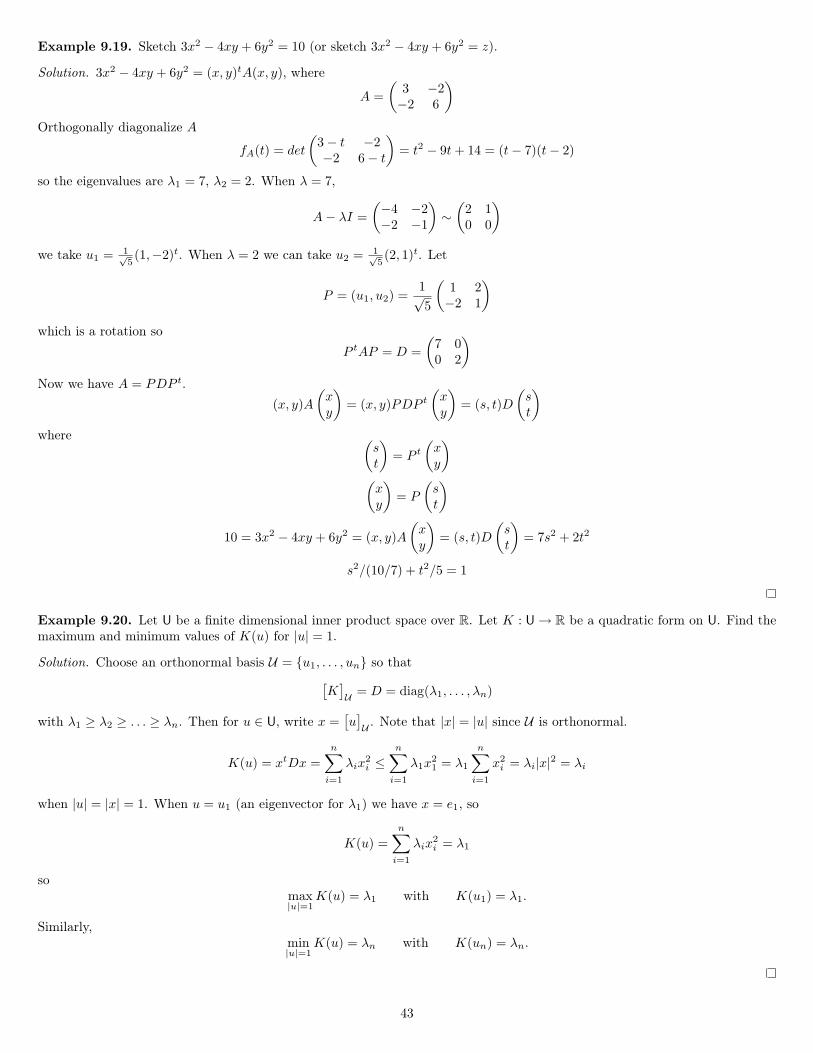
Example 9.19. Sketch 3x2 − 4xy + 6y2 = 10 (or sketch 3x2 − 4xy + 6y2 = z).

Solution. 3x2 − 4xy + 6y2 = (x, y)tA(x, y), where

A =(

3 −2−2 6

)Orthogonally diagonalize A

fA(t) = det

(3− t −2−2 6− t

)= t2 − 9t+ 14 = (t− 7)(t− 2)

so the eigenvalues are λ1 = 7, λ2 = 2. When λ = 7,

A− λI =(−4 −2−2 −1

)∼(

2 10 0

)we take u1 = 1√

5(1,−2)t. When λ = 2 we can take u2 = 1√

5(2, 1)t. Let

P = (u1, u2) =1√5

(1 2−2 1

)which is a rotation so

P tAP = D =(

7 00 2

)Now we have A = PDP t.

(x, y)A(xy

)= (x, y)PDP t

(xy

)= (s, t)D

(st

)where (

st

)= P t

(xy

)(xy

)= P

(st

)10 = 3x2 − 4xy + 6y2 = (x, y)A

(xy

)= (s, t)D

(st

)= 7s2 + 2t2

s2/(10/7) + t2/5 = 1

Example 9.20. Let U be a finite dimensional inner product space over R. Let K : U→ R be a quadratic form on U. Find themaximum and minimum values of K(u) for |u| = 1.

Solution. Choose an orthonormal basis U = {u1, . . . , un} so that[K]U = D = diag(λ1, . . . , λn)

with λ1 ≥ λ2 ≥ . . . ≥ λn. Then for u ∈ U, write x =[u]U . Note that |x| = |u| since U is orthonormal.

K(u) = xtDx =n∑i=1

λix2i ≤

n∑i=1

λ1x21 = λ1

n∑i=1

x2i = λi|x|2 = λi

when |u| = |x| = 1. When u = u1 (an eigenvector for λ1) we have x = e1, so

K(u) =n∑i=1

λix2i = λ1

somax|u|=1

K(u) = λ1 with K(u1) = λ1.

Similarly,min|u|=1

K(u) = λn with K(un) = λn.

43

Example 9.21. Let U and V be two finite dimensional vector spaces over R. Let L : U→ V be linear. Find

max|u|=1

|L(u)| and min|u|=1

|L(u)|

Solution. Choose an orthonormal basis U for U and V for V. Let A =[L]UV . For u ∈ U, write x =

[u]U . Then[

L(u)]V = Ax

and because V was orthonormal,|L(u)| = |Ax| =⇒ |L(u)|2 = |Ax|2 = xtAtAx

therefore,max|u|=1

|L(u)|2

is the maximum eigenvalue of AtA. Similarly,min|u|=1

|L(u)|2

is the minimum eigenvalue of AtA. Thus

max|u|=1

|L(u)| = σ1 =√λ1 min

|u|=1|L(u)| = σn =

√λn

where λ1 ≥ . . . ≥ λn are the eigenvalues of AtA.

This is the end of the material that will be tested on the course final exam.

10 Jordan canonical formTheorem 10.1 (Jordan Canonical Form). Let U be a finite dimensional vector space over any field F. Let L : U→ U be linear.Suppose fL(t) splits. There is a basis U for U such that

[L]U is of the block-diagonal formJk1λ1

. . .Jk`λ`

where

Jkλ =

λ 1 . . . 0... λ 1

...

λ 1...

. . . . . . 10 . . . 0 λ

and the blocks Jkiλi are unique (up to order).

44

Math 245 Notes

Documents

Transcript of Math 245 Notes