Math 224 Fall 2017 Homework 5 Drew Armstrong
12
Math 224 Fall 2017 Homework 5 Drew Armstrong Problems from 9th edition of Probability and Statistical Inference by Hogg, Tanis and Zim- merman: • Section 3.1, Exercises 3, 10. • Section 3.3, Exercises 2, 3, 10, 11. • Section 5.6, Exercises 2, 4. • Section 5.7, Exerciese 4, 14. Solutions to Book Problems. 3.1-3. Customers arrive randomly at a bank teller’s window. Given that a customer arrived in a certain 10-minute period, let X be the exact time within the 10 minutes that the customer arrived. We will assume that X is U (0, 10), i.e., that X is uniformly distributed on the real interval [0, 1] ⊆ R. (a) Find the pdf of X . Solution: f X (x)= ( 1/10 if 0 ≤ x ≤ 10 0 otherwise Here is a picture (not to scale): (b) Compute P (X ≥ 8). Solution: We could compute an integral: P (X ≥ 8) = Z 10 8 1/10 dx = x/10 10 8 = 10/10 - 8/10 = 2/10 = 1/5. Or we could just recognize that this is the area of a rectangle with height 1/10 and width 2: 1
Transcript of Math 224 Fall 2017 Homework 5 Drew Armstrong

Math 224 Fall 2017Homework 5 Drew Armstrong
Problems from 9th edition of Probability and Statistical Inference by Hogg, Tanis and Zim-merman:
• Section 3.1, Exercises 3, 10.• Section 3.3, Exercises 2, 3, 10, 11.• Section 5.6, Exercises 2, 4.• Section 5.7, Exerciese 4, 14.
Solutions to Book Problems.
3.1-3. Customers arrive randomly at a bank teller’s window. Given that a customer arrivedin a certain 10-minute period, let X be the exact time within the 10 minutes that the customerarrived. We will assume that X is U(0, 10), i.e., that X is uniformly distributed on the realinterval [0, 1] ⊆ R.
(a) Find the pdf of X. Solution:
fX(x) =
{1/10 if 0 ≤ x ≤ 10
0 otherwise
Here is a picture (not to scale):
(b) Compute P (X ≥ 8). Solution: We could compute an integral:
P (X ≥ 8) =
∫ 10
81/10 dx = x/10
∣∣∣108
= 10/10− 8/10 = 2/10 = 1/5.
Or we could just recognize that this is the area of a rectangle with height 1/10 andwidth 2:
1

2
(c) Compute P (2 ≤ X < 8). Solution: Skipping the integral, we’ll compute this as thearea of a rectangle with width 2 and height 1/10:
Remark: For general 0 ≤ a ≤ b ≤ 10 we will have P (a ≤ X ≤ b) = b− a.(d) Compute the expected value E[X]. Solution: We have
E[X] =
∫ ∞−∞
xfX(x) dx =
∫ 10
0x/10 = x2/20
∣∣∣100
= 100/20− 0/20 = 5.
Indeed, this agrees with our intuition that the distribution is symmetric about x = 5.(e) Compute the variance Var(X). Solution: We could first compute E[X2] first, but
instead we’ll go directly from the definition. Since µ = 5 we have
Var(X) = E[(X − µ)2] =
∫ ∞−∞
(x− µ)2fX(x) dx
=
∫ 10
0(x− 5)2/10 dx
=
∫ 10
0(x2 − 10x+ 25)/10 dx
= (x3/3− 10x2/2 + 25x)/10∣∣∣100
= (1000/3− 1000/2 + 250)/10
= (2000/6− 3000/6 + 1500/6)/10
= 50/6.
Indeed, if X ∼ U(a, b) then the front of the book says that Var(X) = (b − a)2/12,which agrees with our answer when a = 0 and b = 10.
3.1-10. The pdf1 of X is f(x) = c/x2 with support 1 < x < ∞. (This means that thefunction is zero outside of this range.)
1The textbook is lying here because we don’t know yet whether this really is a pdf.

3
(a) Calculate the value of c so that f(x) is a pdf. Solution: We must have
1 =
∫ ∞1
f(x) dx
=
∫ ∞1
c/x2 dx
= −c/x∣∣∣∞0
= 0− (−c/1)
= c.
(b) Show that E[X] is not finite. Solution: If the expected value existed then it wouldsatisfy the formula
E[X] =
∫ ∞1
xf(x) dx =
∫ ∞1
1/x dx.
But the antiderivative of 1/x is the natural logarithm log(x), so that∫ ∞1
1/x dx =[
limx→∞
log(x)]− log(1) =
[limx→∞
log(x)]
=∞.
If the random variable X represents some kind of waiting time, then we should expectto wait forever!
[Moral of the Story: The expected value and variance are useful tools. However: (1) Somecontinuous random variables X have an infinite expected value E[X] = ∞. (2) Some randomvariables with finite expected value E[X] < ∞ still have infinite variance Var(X) = ∞. So becareful.]
3.3-2. If Z ∼ N(0, 1) has a standard normal distribution, compute the following probabil-ities. We will use the general formulas
• P (a ≤ Z ≤ b) = Φ(b)− Φ(a)• Φ(−z) = 1− Φ(z)
and we will look up the values for Φ(z) in the table on page 494 of the textbook.
(a)
P (0 ≤ Z ≤ 0.87) = Φ(0.87)− Φ(0) = 0.8078− 0.5000 = 30.78%
(b)
P (−2.64 ≤ Z ≤ 0) = Φ(0)− Φ(−2.64)
= Φ(0)− [1− Φ(2.64)]
= Φ(2.64) + Φ(0)− 1
= 0.9959 + 0.5000− 1 = 49.59%.
(c)
P (−2.13 ≤ Z ≤ −0.56) = Φ(−0.56)− Φ(−2.13)
= [1− Φ(0.56)]− [1− Φ(2.13)]
= Φ(2.13)− Φ(0.56)
= 0.9834− 0.7123 = 27.11%.

4
(d)
P (|Z| > 1.39) = P (Z > 1.39) + P (Z < −1.39)
= 1− Φ(1.39) + Φ(−1.39)
= 1− Φ(1.39) + [1− Φ(1.39)]
= 2 [1− Φ(1.39)] = 2 [1− 0.9177] = 16.46%.
(e)
P (Z < −1.62) = Φ(−1.62) = 1− Φ(1.62) = 1− 0.9474 = 5.26%.
(f)
P (|Z| > 1) = P (Z > 1) + P (Z < −1)
= 1− Φ(1) + Φ(−1)
= 1− Φ(1) + [1− Φ(1)]
= 2 [1− Φ(1)] = 2 [1− 0.8413] = 31.74%.
(g) After parts (d) and (f) we observe the general pattern:
P (|Z| > z) = 2 [1− Φ(z)] .
Therefore we have
P (|Z| > 2) = 2 [1− Φ(2)] = 2 [1− 0.9772] = 4.56%
(h) and also
P (|Z| > 3) = 2 [1− Φ(3)] = 2 [1− 0.9987] = 2.6%.
3.3-3. Suppose Z ∼ N(0, 1). Find values of c to satisfy the following equations.
(a) P (Z ≥ c) = 0.025. Solution: We are looking for c such that
P (Z ≥ c) = 0.025
1− P (Z ≤ c) = 0.025
1− Φ(c) = 0.025
0.9750 = Φ(c).
My trusty table tells me that Φ(1.96) = 0.975, and hence c = 1.96.(b) P (|Z| ≤ c) = 0.95. Solution: We are looking for c such that
P (|Z| ≤ c) = 0.95
P (−c ≤ Z ≤ c) = 0.95
Φ(c)− Φ(−c) = 0.95
Φ(c)− [1− Φ(c)] = 0.95
2Φ(c)− 1 = 0.95
Φ(c) = 1.95/2 = 0.9750.
So the answer is the same as for part (a), i.e., c = 1.96.

5
(c) P (Z > c) = 0.05. Solution: Following the same steps as in part (a) gives
P (Z > c) = 0.05
1− P (Z > c) = 0.05
1− Φ(c) = 0.05
0.9500 = Φ(c).
We look up in the table that Φ(1.64) = 0.9495 and Φ(1.65) = 0.9505. Therefore wemust have Φ(1.645) ≈ 0.9500 and hence c ≈ 1.645.
(d) P (|Z| ≤ c) = 0.90. Solution: Following the same steps as in part (b) gives
P (|Z| ≤ c) = 0.90
P (−c ≤ Z ≤ c) = 0.90
Φ(c)− Φ(−c) = 0.90
Φ(c)− [1− Φ(c)] = 0.90
2Φ(c)− 1 = 0.90
Φ(c) = 1.90/2 = 0.9500.
So the answer is the same as for part (c), i.e., c ≈ 1.645.
3.3-10. Let X ∼ N(µ, σ2) be normal and for any real numbers a, b ∈ R with a 6= 0 definethe random variable
Y = aX + b.
By properties of expectation and variance we have
E[Y ] = E[aX + b] = aE[X] + b = aµ+ b
and
Var(Y ) = Var(aX + b) = Var(aX) = a2Var(X) = a2σ2.
I claim, furthermore thatn Y is also normal, i.e., that
Y ∼ N(aµ+ b, a2σ2).
Proof: To show that Y is normal, we want to show for any real numbers y1 ≤ y2 that
(?) P (y1 ≤ Y ≤ y2) =
∫ w=y2
w=y1
1√2πa2σ2
e−(w−aµ−b)2/2a2σ2
dw.
To show this, we can use the fact that X is normal to obtain2
P (y1 ≤ Y ≤ y2) = P (y1 ≤ aX + b ≤ y2)= P (y1 − b ≤ aX ≤ y2 − b)
= P
(y1 − ba≤ X ≤ y2 − b
a
)=
∫ x=(y1−b)/a
x=(y1−b)/a
1√2πσ2
e−(x−µ)2/2σ2
dx.(∗)
2In the third line here we will assume that a > 0. The proof for a < 0 is exactly the same except that it willswitch the limits of integration.
6
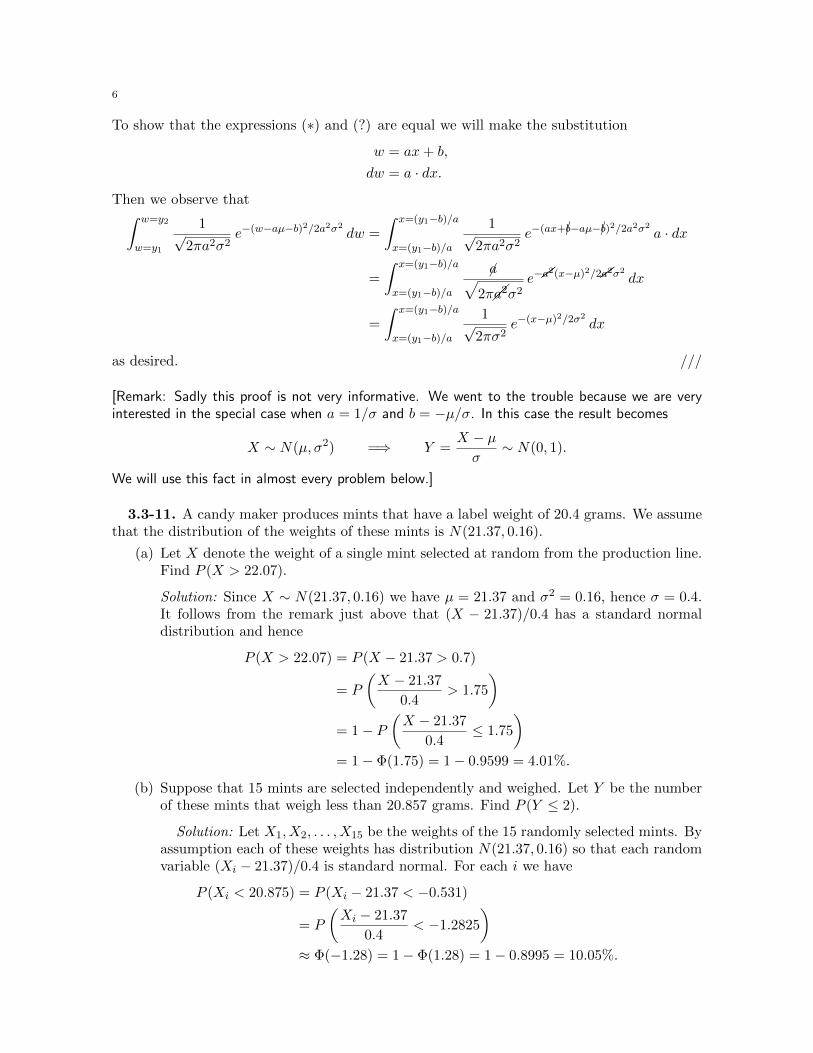
To show that the expressions (∗) and (?) are equal we will make the substitution
w = ax+ b,
dw = a · dx.
Then we observe that∫ w=y2
w=y1
1√2πa2σ2
e−(w−aµ−b)2/2a2σ2
dw =
∫ x=(y1−b)/a
x=(y1−b)/a
1√2πa2σ2
e−(ax+�b−aµ−�b)2/2a2σ2
a · dx
=
∫ x=(y1−b)/a
x=(y1−b)/a
�a√2π��a
2σ2e−��a
2(x−µ)2/2��a2σ2dx
=
∫ x=(y1−b)/a
x=(y1−b)/a
1√2πσ2
e−(x−µ)2/2σ2
dx
as desired. ///
[Remark: Sadly this proof is not very informative. We went to the trouble because we are veryinterested in the special case when a = 1/σ and b = −µ/σ. In this case the result becomes
X ∼ N(µ, σ2) =⇒ Y =X − µσ
∼ N(0, 1).
We will use this fact in almost every problem below.]
3.3-11. A candy maker produces mints that have a label weight of 20.4 grams. We assumethat the distribution of the weights of these mints is N(21.37, 0.16).
(a) Let X denote the weight of a single mint selected at random from the production line.Find P (X > 22.07).
Solution: Since X ∼ N(21.37, 0.16) we have µ = 21.37 and σ2 = 0.16, hence σ = 0.4.It follows from the remark just above that (X − 21.37)/0.4 has a standard normaldistribution and hence
P (X > 22.07) = P (X − 21.37 > 0.7)
= P
(X − 21.37
0.4> 1.75
)= 1− P
(X − 21.37
0.4≤ 1.75
)= 1− Φ(1.75) = 1− 0.9599 = 4.01%.
(b) Suppose that 15 mints are selected independently and weighed. Let Y be the numberof these mints that weigh less than 20.857 grams. Find P (Y ≤ 2).
Solution: Let X1, X2, . . . , X15 be the weights of the 15 randomly selected mints. Byassumption each of these weights has distribution N(21.37, 0.16) so that each randomvariable (Xi − 21.37)/0.4 is standard normal. For each i we have
P (Xi < 20.875) = P (Xi − 21.37 < −0.531)
= P
(Xi − 21.37
0.4< −1.2825
)≈ Φ(−1.28) = 1− Φ(1.28) = 1− 0.8995 = 10.05%.

7
In other words, we can think of each of the 15 selected mints as a coin flip where“heads” means “the weight is less than 20.857” and the probability of heads is ap-proximately 10%. Then Y is a binomial random variable with parameters n = 15 andp ≈ 0.1 and we conclude that
P (Y ≤ 2) ≈2∑
k=0
(15
k
)(0.1)k(0.9)15−k
= (0.9)15 + 15 · (0.1)(0.9)14 + 105 · (0.1)2(0.9)13 ≈ 81.59%.
In other words, there is an 80% chance that no more than 2 out of every 15 mints willweigh less than 20.857 grams. I don’t know if that’s good.
5.6-2. Let Y = X1 + X2 + · · · + X15 be the sum of a random sample of size 15 from adistribution whose pdf is f(x) = (3/2)x2 with support −1 < x < 1. Using this pdf, one canuse a computer to show that P (−0.3 ≤ Y ≤ 1.5) = 0.22788. On the other hand, we can usethe Central Limit Theorem to approximate this probability.
Solution: The distribution in question looks like this:
Since the distribution is symmetric about zero, we conclude without doing any work thatµ = E[Xi] = 0 for each i. To find σ, however, we need to compute an integral. For any i, thevariance of Xi is defined by
σ2 = Var(Xi) = E[(Xi − 0)2
]= E[X2
i ]
=
∫ 1
−1x2 · f(x) dx
=
∫ 1
−1x2 · 3
2x2 dx
=3
2
∫ 1
−1x4 dx
=3
2· x
5
5
∣∣∣∣1−1
=3
2· 1
5− 3
2· (−1)5
5=
6
10=
3
5.
It follows that Y has mean and variance given by
µYE[Y ] = E[X1] + E[X2] + · · ·+ E[X15] = 0 + 0 + · · ·+ 0 = 0

8
and
σ2Y = Var(Y ) = Var(X1) + Var(X2) + · · ·+ Var(X15) =3
5+
3
5+ · · ·+ 3
5= 15 · 3
5= 9,
By the Central Limit Theorem, the sum Y is approximately normal and hence (Y −µY )/σY =Y/3 is approximately standard normal. We conclude that
P (−0.3 ≤ Y ≤ 0.5) = P
(−0.3
3≤ Y
3≤ 1.5
3
)= P
(−0.1 ≤ Y
3≤ 0.5
)≈ Φ(0.5)− Φ(−0.1)
= Φ(0.5)− [1− Φ(0.1)]
= Φ(0.5) + Φ(0.1)− 1
= 0.6915 + 0.5398− 1 = 23.13%.
That’s reasonably close to the exact value 22.788%, I guess. We would get a more accurateresult by taking more than 15 samples.
5.6-4. Approximate P (39.75 ≤ X ≤ 41.25), where X is the mean of a random sample ofsize 32 from a distribution with mean µ = 40 and σ2 = 8.
Solution: In general the sample mean is defined by X = (X1 + X2 + · · · + Xn)/n, whereeach Xi has E[Xi] = µ and Var(Xi) = σ2. From this we compute that
E[X] =1
n(E[X1] + E[X2] + · · ·+ E[Xn]) =
1
n(µ+ µ+ · · ·+ µ) =
nµ
n= µ
and
Var(X) =1
n2(Var(X1) + · · ·+ Var(Xn)) =
1
n2(σ2 + · · ·+ σ2) =
nσ2
n2=σ2
n.
The Central Limit Theorem says that if n is large then X is approximately normal:
X ≈ N(µ, σ2/n).
In the case n = 32, µ = 40 and σ2 = 8 we obtain
X ≈ N(40, 8/32) = N(40, (1/2)2).
It follows that (X − 40)/(1/2) = 2(X − 40) is approximately N(0, 1) and hence
P (39.75 ≤ X ≤ 41.25) = P(−0.25 ≤ X − 40 ≤ 1.25
)= P
(−0.5 ≤ 2(X − 40) ≤ 2.5
)≈ Φ(2.5)− Φ(−0.5)
= Φ(2.5)− [1− Φ(0.5)]
= Φ(2.5) + Φ(0.5)− 1
= 0.9938 + 0.6915− 1 = 68.53%.
5.7-4. Let X equal the number out of n = 48 mature aster seeds that will germinate whenp = 0.75 is the probability that a particular seed germinates. Approximate P (35 ≤ X ≤ 40).
Solution: We observe that X is a binomial random variable with pmf
P (X = k) =
(48
k
)(0.75)k(0.25)48−k.

9
My laptop tells me that the exact probability is
P (35 ≤ X ≤ 40) =
40∑k=35
P (X = k) =
40∑k=35
(48
k
)(0.75)k(0.25)48−k = 63.74%.
If we want to compute an approximation by hand then we should use the de Moivre-LaplaceTheorem (a special case of the Central Limit Theorem), which says that X is approximatelynormal with mean np = 36 and variance σ2 = np(1 − p) = 9, i.e., standard deviation σ = 3.Let X ′ be a continuous random variable with X ′ ∼ N(36, 32). Here is a picture comparingthe probability mass function of the discrete variable X to the probability density functionof the continuous variable X ′:
The picture suggests that we should use the following continuity correction:3
P (35 ≤ X ≤ 40) ≈ P (34.5 ≤ X ′ ≤ 40.5).
And then because (X ′ − 36)/3 is standard normal we obtain
P (34.5 ≤ X ′ ≤ 40.5) = P (−1.5 ≤ X ′ − 36 ≤ 4.5)
= P
(−0.5 ≤ X ′ − 36
3≤ 1.5
)= Φ(1.5)− Φ(−0.5)
= Φ(1.5)− [1− Φ(0.5)]
= Φ(1.5) + Φ(0.5)− 1 = 0.9332 + 0.6915− 1 = 62.47%
Not too bad.
5.7-14. A (fair six-sided) die is rolled 24 independent times. Let Xi be the number thatappears on the ith roll and let Y = X1 + X2 + · · · + X24 be the sum of these numbers. Thepmf of each Xi is given by the following table
k 1 2 3 4 5 6P (Xi = k) 1/6 1/6 1/6 1/6 1/6 1/6
3If you don’t do this then you will still get a reasonable answer, it just won’t be as accurate.

10
So we find that:
E[Xi] = (1 + 2 + 3 + 4 + 5 + 6)/6 = 7/2,
E[X2i ] = (12 + 22 + 32 + 42 + 52 + 62)/6 = 91/6,
Var(Xi) = E[X2i ]− E[Xi]
2 = 91/6− (7/2)2 = 35/12.
Then the expected value and variance of Y are given by
E[Y ] = 24 · E[Xi] = 24 · 7
2= 84 and Var(Y ) = 24 ·Var(Xi) = 24 · 35
12= 70
and the Central Limit Theorem tells us that Y is approximately N(84, 70). Let Y ′ be acontinuous random variable that is exactly N(84, 70), so that (Y ′ − 84)/
√70 has a standard
normal distribution.
(a) Compute P (Y ≥ 86). Solution:
P (Y ≥ 86) ≈ P (Y ′ ≥ 85.5)
= P (Y ′ − 84 ≥ 1.5)
≈ P(Y ′ − 84√
70≥ 0.18
)= 1− Φ(0.18) = 1− 0.5714 = 42.86%.
(b) Compute (P < 86). Solution: This is the complement of part (a):
P (Y < 86) = 1− P (Y ≥ 86) ≈ 1− 0.4286 = 57.14%.
(c) Compute P (70 < Y ≤ 86). Solution:
P (70 < Y ≤ 86) ≈ P (70.5 ≤ Y ′ ≤ 86.5)
= P (−13.5 ≤ Y ′ − 84 ≤ 2.5)
≈ P(−1.61 ≤ Y ′ − 84√
70≤ 0.30
)= Φ(0.30)− Φ(−1.61)
= Φ(0.30)− [1− Φ(1.61)]
= Φ(0.30) + Φ(1.61)− 1 = 0.6179 + 0.9463− 1 = 56.42%.
Here is a picture explaining the continuity correction that we used in the first step:

11
Additional Problems.
1. The Normal Curve. Let µ, σ2 ∈ R be any real numbers (with σ2 > 0) and considerthe graph of the function
n(x) =1√
2πσ2e−(x−µ)
2/2σ2.
(a) Compute the first derivative n′(x) and show that n′(x) = 0 implies x = µ.(b) Compute the second derivative n′′(x) and show that n′′(µ) < 0, hence the curve has a
local maximum at x = µ.(c) Show that n′′(x) = 0 implies x = µ+σ or x = µ−σ, hence the curve has inflections at
these points. [The existence of inflections at µ+ σ and µ− σ was de Moivre’s originalmotivation for defining the standard deviation.]
Solution: The chain rule tells us that for any function f(x) we have
d
dxef(x) = ef(x) · d
dxf(x).
Applying this to the function n(x) gives
n′(x) =1√
2πσ2· e−(x−µ)2/2σ2 · −1
2σ22(x− µ) =
−1√8πσ6
· e−(x−µ)2/2σ2 · (x− µ).
We observe that the expression inside the box is never zero. In fact, it is always strictlynegative. Therefore we have n′(x) = 0 precisely when (x − µ) = 0, or, in other words, whenx = µ. This tells us that there is a horizontal tangent when x = µ. To determine whether thisis a maximum or a minimum we should compute the second derivative. Using the productrule gives
n′′(x) =d
dx
[−1√8πσ6
· e−(x−µ)2/2σ2 · (x− µ)
]=
−1√8πσ6
· ddx
[e−(x−µ)
2/2σ2 · (x− µ)]
=−1√8πσ6
·[e−(x−µ)
2/2σ2 · −1
2σ22(x− µ) · (x− µ) + e−(x−µ)
2/2σ2
]=
−1√8πσ6
· e−(x−µ)2/2σ2 ·[−(x− µ)2
σ2+ 1
].
Then plugging in x = µ gives
n′′(µ) =−1√8πσ6
< 0,
which implies that the graph of n(x) curves down at x = µ, so it must be a local maximum.Finally, we observe that the boxed formula in the following expression is always nonzero (infact it is always negative):
n′′(x) =−1√8πσ6
· e−(x−µ)2/2σ2 ·[−(x− µ)2
σ2+ 1
]

12
Therefore we have n′′(x) = 0 precisely when
−(x− µ)2
σ2+ 1 = 0
(x− µ)2
σ2= 1
(x− µ)2 = σ2
x− µ = ±σx = µ± σ.
In other words, the graph of n(x) has inflection points when x = µ ± σ. As we observed inthe course notes, the height of these inflection points is always around 60% of the height ofthe maximum. This gives the “bell curve” its distinctive shape: