University of British Columbia

Math 103 Syllabus

Contents

Version 1

Mission Statement 2

Prerequisites 3

1 Area, Volume and Sigma Notation 4

2 Riemann Sums and Integration 8

3 Fundamental Theorem of Calculus 11

4 Applications of Integrals (primarily to velocities and rates) 14

5 Applications of integrals to volume, mass and length 16

6 Integration Techniques 18

7 Improper Integrals 22

8 Continuous Probability Distributions 24

9 Differential Equations 27

10 Sequences 29

11 Series 32

12 Taylor Series 36

13 Summary 38

14 Solutions 39

Version

Version 1.0 This file was created by Carmen Bruni in 2013, a then graduate student at theUniversity of British Columbia.

Version 1.1 Updated by Carmen Bruni to correct numerous typos in the document. Updatedthe license and mission statement.

1

Mission Statement

The goal of this document is to provide a clear vision of Math 103 that can be utilized byboth instructors and students to gain a perspective on what will be covered during a term.Throughout, learning goals are presented to help make it clear what instructors should teachand what knowledge students should expect to obtain upon successful completion of the course.

The Math 102 and 103 sequence is very different from its two sister first year calculus se-quences offered at UBC. This sequence focuses heavily on biological applications and emphasizesunderstanding how these ideas play a role in real world situations. As such, many proofs aredeemphasized if not altogether omitted (the main exception being the content on series).

The document also makes extensive references to the Math Educational Resources wiki.This project began in 2012 out of a desire to create a free working resource for undergraduates.Graduate students volunteer their time towards the development of this project. The site canbe found at

http://wiki.ubc.ca/Science:Math_Educational_Resources

Here, students can find relevant exam questions by exam or by topic. Videos are alsoembedded on topic links to help reinforce concepts and aid in reminding students of the coreideas. The original author of this document, Carmen Bruni, included pencasts on the wiki whichwere created specifically for this course. Combining this with many of the examples present inthis document makes this not only a syllabus, but an extremely valuable resource for studentsto ensure that they are learning the correct material in order to excel in this course.

Solutions when provided are presented only in a minimalist form. Students working throughthe problems are encouraged to write out complete comprehensive solutions. These solutions areonly present as a time saving measure for students. Students are more than welcomed and evenencouraged to discuss questions found in this document with their instructors or fellow peers.Concerns or confusions found on the wiki should be discussed on the wiki itself.

Any comments about this current version are welcomed and can be sent to Carmen Bruni atcbruni@alumni.ubc.ca. The TeX file is also available upon request.

This document is licensed under the Creative Commons license CC-BY-SA

- Carmen Bruni, December 5th, 2013 (modified May 4th, 2014)

2

Prerequisites

The following is a base set of skills one needs in order to do well in this course. Any problemsin these areas should seek immediate rectification.

• Adding, subtracting, multiplying and dividing rational functions (that is, functions wherethe numerator and denominator are both polynomials and the denominator is nonzero).

• Solving for roots of quadratic polynomials using all of the following methods: factoring,completing the square, and the quadratic formula. This also includes finding commonfactors in expressions

• Solving systems of equations

• Manipulate exponents including but not limited to xaxb = xa+b, (xa)b = xab, xa

xb= xa−b,

y = ex ⇔ ln(y) = x.

• Derivatives and graphs of elementary functions including xa where a is a real number,trigonometric, inverse trigonometric, logarithmic and exponential functions.

• All rules of differentiation (power, product, quotient, chain rules).

• Understanding and being able to compute limits of functions.

• Basic familiarity with differential equations (what are they, how they are used).

• A working understanding of trigonometry, including but not limited to drawing the functionof sin(x),cos(x),tan(x) and values of these functions at 0,π/6,π/4,π/3,π/2 and these valuesadded with multiples of π/2.

Solutions are included here to help with solving problems. These are in general not intendedto be full solutions but are included to help you verify that your work is correct.

Learning goal sections roughly correspond to weeks of the course which also roughly corre-spond to chapters in the course notes.

Throughout this article, an implicit emphasis will be to apply many of these learning goalsin a variety of biological applications not explicitly given in the exercises. These will be a mixof WebWork problems as well as examples covered in class. The best way to practice is toattempt problems and make sure you’re familiar with examples covered in the notes (even ifyour instructor does not cover them in class).

3

1 Area, Volume and Sigma Notation

Learning Goal 1.1. Know formulas for the areas and perimeters of basic shapes, includingtriangles, squares, regular n-gons, parallelograms and circles. [Knowledge]

Learning Goal 1.2. Explain Archimedes method for computing the exact value of π.[Knowledge, Evaluation]

Learning Goal 1.3. Know formulas for the surface areas and volumes of basic shapes,include cubes, rectangular boxes, cylinders and spheres. [Knowledge]

Learning Goal 1.4. Convert between sigma notation and standard notation. [Comprehen-sion]

Exercise 1.1 Write out the summation5∑i=0

ei in standard notation

Exercise 1.2 Write out the sum 2 + 5 + 10 + 17 using sigma notation

Exercise 1.3 Write out the summation3∑i=1

f(i+ 2) in standard notation where f(x) = ln(2x)

Learning Goal 1.5. Calculate sums using the following identities: [Analysis]

n∑i=1

i =n(n+ 1)

2

n∑i=1

i2 =n(n+ 1)(2n+ 1)

6

n∑i=1

i3 =

(n(n+ 1)

2

)2

Exercise 1.4 Compute

10∑i=1

i2

Learning Goal 1.6. Using the above identities and the linearity of summations, manipulatesums into a form that can be evaluated using those formulas and then compute their sums.[Application and Analysis]

4

Exercise 1.5 Compute15∑i=5

(i− 1)2

Exercise 1.6 Compute10∑i=2

(i3 + 2i+ 1)

Exercise 1.7 Computen∑i=0

n where n is a positive integer.

Learning Goal 1.7. Evaluate why a given answer to a summation question cannot becorrect. [Evaluation]

Exercise 1.8 A student computes20∑i=4

i2 to be 19(20)(41)6 . Why is this not correct?

Learning Goal 1.8. Convert a summation using a change of variables. [Comprehension]

Exercise 1.9 Which of the following sums is equivalent to29∑i=7

(i− 1)3 + i?

(i)

23∑j=1

(j + 5)3 + j + 5

(ii)

22∑j=1

(j + 6)3 + j + 6

(iii)25∑j=3

(j + 4)3 + j + 5

(iv)32∑j=10

(j + 2)3 + j + 3

(v)

27∑j=5

(j + 1)3 + j + 2

Learning Goal 1.9. Convert expressions to closed forms (that is, a form that is in an easyto put into a calculator form).

5

Exercise 1.10 Convert −1 + 2− 3 + 4− 5 + 6− ...− (2n− 1) + 2n into a closed form.

Learning Goal 1.10. State the definition of a geometric series. [Knowledge]

Learning Goal 1.11. Compute sums usingN∑i=0

ari =a(1− rN+1)

1− r[Application]

Exercise 1.11 Compute9∑i=0

3 · 2i

Exercise 1.12 Compute9∑i=1

3 · 2i

Exercise 1.13 Compute13∑i=8

3 · 5i+1

22i

Learning Goal 1.12. Compute sums by expanding into standard notation and noticingpatterns [Analysis]

Exercise 1.14 SimplifyN∑n=1

(1

n− 1

n+ 1

)as a fraction

Exercise 1.15 Compute

50∑n=1

(−1)nn

Learning Goal 1.13. Define a partial sum [Knowledge]

Learning Goal 1.14. State what it means for an infinite series to converge [Knowledge]

Learning Goal 1.15. Compute sums using

∞∑i=0

ari =a

1− r[Application]

6

Exercise 1.16 Find the sum of the geometric series 5− 103 + 20

9 −4027 + 80

81 − ...

Exercise 1.17 Write 2.445353535353... as a fraction

Exercise 1.18 Determine if

∞∑n=1

(−3)n−1

4nconverges. If so, compute its value.

Exercise 1.19 Compute or state it diverges

∞∑i=0

5

(1

3

)i

Exercise 1.20 Compute or state it diverges∞∑i=0

5 · 2i

Exercise 1.21 Compute or state it diverges

∞∑i=2

3 · 2−i

Learning Goal 1.16. Use geometric series in biological applications to determine limitingbehaviours. [Application]

Exercise 1.22 Compute the maximum and minimum amount of a drug remaining in a patientin the limit (that is, as time tends to infinity) given that the patient takes an 80 milligram doseonce a day at the same time each day and the drug has a half life of 22 hours.

External Example. Check out section 1.7 in the notes (page 18) on bifurcating and trifurcatingtrees.

Relevant exam questions from previous years can be found at the following links

• wiki.ubc.ca/Category:MER Tag Geometric series

• wiki.ubc.ca/Category:MER Tag Summations

7

2 Riemann Sums and Integration

Learning Goal 2.1. Define a Riemann Sum. [Knowledge]

Learning Goal 2.2. Approximate the area under a function using left, right and midpointrules. Also, identify when an estimate is an overestimate or underestimate.[Analysis]

Exercise 2.1 Approximate the area under the curve f(x) = ln(x) between x = 1 and x = 5using the left, right and midpoint rules with n = 4 intervals (rectangles)

Learning Goal 2.3. Define a definite integral. Also, be able to sketch a region as given ina definite integral. [Knowledge]

Learning Goal 2.4. Using Riemann sums, compute the area under a function. Reworded,evaluate a definite integral using the definition of a definite integral. [Application]

Exercise 2.2 Compute the area under the curve y = x2 between x = 1 and x = 3 usingRiemann sums (that is, using the definition of a definite integral). No marks will be given tosolutions not using the definition directly.

Exercise 2.3 Compute the area under the curve y = 2x2 + x between x = 0 and x = 3 usingRiemann sums (that is, using the definition of a definite integral). No marks will be given tosolutions not using the definition directly.

Learning Goal 2.5. Convert between a Riemann sum and a definite integral and vice versa.[Comprehension]

Exercise 2.4 Write limn→∞

n∑i=1

((2in

)2+ 1)(

2n

)as a definite integral

Exercise 2.5 Write

∫ 5

2(ex

2+ x) dx as a Riemann sum.

Exercise 2.6 Write limn→∞

n∑i=1

( π8n

)tan

( iπ40n

)as a definite integral

8

Learning Goal 2.6. Compute integrals using high school geometry. That is, recognize anintegral as a signed area and compute it. [Application]

Exercise 2.7 Evaluate

∫ 2

−2f(x) dx where f(x) =

{3 if x ≤ −1

x if x > −1

Exercise 2.8 Evaluate

∫ 2

−2

√4− x2 + 1 dx

Learning Goal 2.7. Compute the area of objects given a defining equation using Riemannsums. [Application]

Exercise 2.9 Compute the area of a leaf given by the equation y2 = (x2 − 1)2 for −1 ≤ x ≤ 1using Riemann sums.

Learning Goal 2.8. State properties of a definite integral and give justification of theirtruth, including the following; in what follows, let f(x) and g(x) be integrable on [a, b] andlet c be a real number:

• Trivial integral

∫ a

af(x) dx = 0

• Linearity

∫ b

a(f(x)± g(x)) dx =

∫ b

af(x) dx±

∫ b

ag(x) dx and∫ b

acf(x) dx = c

∫ b

af(x) dx

• Area of a rectangle

∫ b

ac dx = c(b− a)

• Switching directions

∫ b

af(x) dx = −

∫ a

bf(x) dx

• Adding parts: If a ≤ c ≤ b, then

∫ b

af(x) dx =

∫ c

af(x) dx+

∫ b

cf(x) dx

• Positivity: If f(x) ≥ 0 for every value of x between a and b, then

∫ b

af(z) dz ≥ 0

• Boundedness: If h(x) ≤ f(x) ≤ g(x) for every value of x between a and b, then∫ b

ah(z) dz ≤

∫ b

af(z) dz ≤

∫ b

ag(z) dz

9

Relevant exam questions from previous years can be found at the following links

• wiki.ubc.ca/Category:MER Tag Riemann sum

• wiki.ubc.ca/Category:MER Tag Integral properties

10

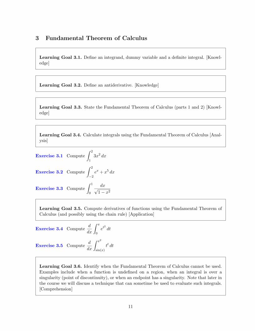
3 Fundamental Theorem of Calculus

Learning Goal 3.1. Define an integrand, dummy variable and a definite integral. [Knowl-edge]

Learning Goal 3.2. Define an antiderivative. [Knowledge]

Learning Goal 3.3. State the Fundamental Theorem of Calculus (parts 1 and 2) [Knowl-edge]

Learning Goal 3.4. Calculate integrals using the Fundamental Theorem of Calculus [Anal-ysis]

Exercise 3.1 Compute

∫ 2

13x2 dx

Exercise 3.2 Compute

∫ 2

−2ex + x5 dx

Exercise 3.3 Compute

∫ 1

0

dx√1− x2

Learning Goal 3.5. Compute derivatives of functions using the Fundamental Theorem ofCalculus (and possibly using the chain rule) [Application]

Exercise 3.4 Computed

dx

∫ x

0et

2dt

Exercise 3.5 Computed

dx

∫ x2

sin(x)tt dt

Learning Goal 3.6. Identify when the Fundamental Theorem of Calculus cannot be used.Examples include when a function is undefined on a region, when an integral is over asingularity (point of discontinuity), or when an endpoint has a singularity. Note that later inthe course we will discuss a technique that can sometime be used to evaluate such integrals.[Comprehension]

11

Exercise 3.6 Compute∫ 1−1

1x dx using the Fundamental Theorem of Calculus or state why this

is impossible.

Exercise 3.7 Compute∫ π0 tan(x) dx or state why this is impossible.

Learning Goal 3.7. Verify antiderivatives using differentiation. [Evaluation]

Exercise 3.8 A student computes an antiderivative of sec(x)−tan(x) sin(x) to be tan(x) cos(x).Is the student correct?

Learning Goal 3.8. Identify use of absolute values in the logarithmic integral. [Knowledge,Evaluation]

Exercise 3.9 A student computes

∫ −1−3

1

xdx to be ln(−1) − ln(−3). Explain why the answer

is incorrect and how to fix it.

Learning Goal 3.9. Define even and odd functions and use this property to computeintegrals. [Knowledge and Application]

Exercise 3.10 Compute

∫ 10

−10sin103(x) cos102(x11) dx

Learning Goal 3.10. Give an expression for the area function A(x) of a given function f(t)from a fixed endpoint and be able to draw this function. Reworded, be able to sketch thearea under a function given a picture of the function. [Knowledge, Analysis]

Learning Goal 3.11. Compute the area of objects given a defining equation. [Application]

Exercise 3.11 Compute the area of a leaf given by the equation y2 = (x2−1)2 for −1 ≤ x ≤ 1.

Learning Goal 3.12. Calculate the area between two curves [Analysis]

Exercise 3.12 Compute the area between y = x2 and y = x3.

Exercise 3.13 Compute the area of the region bounded by y = 2x2 + 10 and y = 4x+ 16

12

Exercise 3.14 Compute the area of the region bounded by y = x− 2 and y2 = x.

Relevant exam questions from previous years can be found at the following links

• wiki.ubc.ca/Category:MER Tag Fundamental theorem of calculus

• wiki.ubc.ca/Category:MER Tag Integration using symmetry

• wiki.ubc.ca/Category:MER Tag Antiderivative sketching

• wiki.ubc.ca/Category:MER Tag Area between two curves

13

4 Applications of Integrals (primarily to velocities and rates)

Learning Goal 4.1. Define distance, displacement, velocity and acceleration and explainthe relationship between these values using derivatives and integrals. [Knowledge]

Learning Goal 4.2. Compute the solution to the differential equation dvdt = g − kv where

g = 9.8m/s2 is the acceleration due to gravity and k is the drag coefficient and describeits terminal velocity (including the case when k = 0 and g is an arbitrary acceleration).[Knowledge, Application]

Learning Goal 4.3. Describe the difference between distance and displacement and knowhow to compute both given a velocity function (or an acceleration function). [Comprehension,Application]

Exercise 4.1 Compute the velocity as a function of time given the acceleration function a(t) =t+ 4 and v(0) = 5

Exercise 4.2 Compute the displacement and the total distance traveled of a particle given thatits velocity at time t is given by v(t) = 2t2 − 10t+ 8 from t = 1 to t = 4

Exercise 4.3 Compute the displacement and the total distance traveled of a particle given thatits velocity at time t is given by v(t) = t2 − t− 6 from t = 1 to t = 4

Learning Goal 4.4. Understand how rates of changes of functions relate to the originalfunction. This is referred to as the net change theorem. [Comprehension]

Exercise 4.4 A tree grows at a rate of g(t) = 10 + 15t2 cm/year. How tall is the tree after 10years?

Exercise 4.5 The rate of change of a cup of tea is given by f(t) = 50e−2t degrees Celsius perminute. Compute the total change in temperature of the coffee between t = 1 and t = 5.

External Example. For more examples, see 4.3, 4.4 and 4.6 in your notes (pages 72-85).

Learning Goal 4.5. State the formula for average value. [Knowledge]

14

Learning Goal 4.6. Compute average values of functions on bounded domains. [Applica-tion]

Exercise 4.6 Find the average value of f(x) = sin(x) on [−π2 ,

π2 ].

Relevant exam questions from previous years can be found at the following links

• wiki.ubc.ca/Category:MER Tag Average value

• wiki.ubc.ca/Category:MER Tag Net change theorem

15

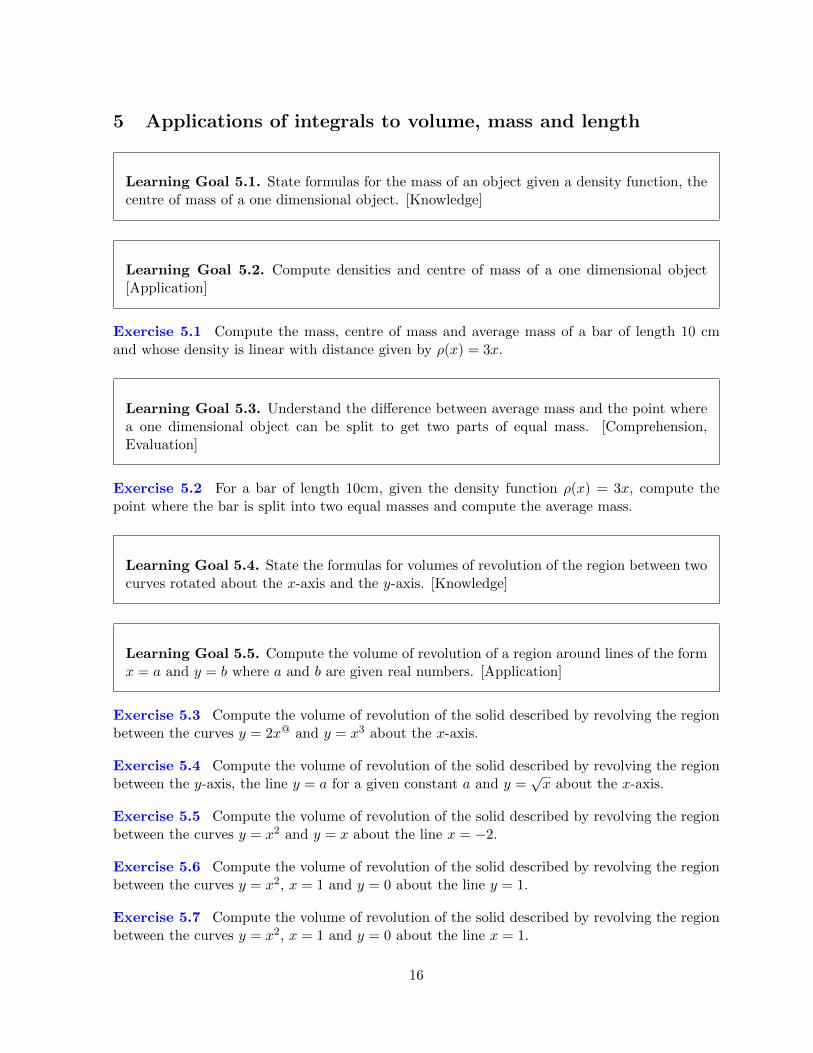
5 Applications of integrals to volume, mass and length

Learning Goal 5.1. State formulas for the mass of an object given a density function, thecentre of mass of a one dimensional object. [Knowledge]

Learning Goal 5.2. Compute densities and centre of mass of a one dimensional object[Application]

Exercise 5.1 Compute the mass, centre of mass and average mass of a bar of length 10 cmand whose density is linear with distance given by ρ(x) = 3x.

Learning Goal 5.3. Understand the difference between average mass and the point wherea one dimensional object can be split to get two parts of equal mass. [Comprehension,Evaluation]

Exercise 5.2 For a bar of length 10cm, given the density function ρ(x) = 3x, compute thepoint where the bar is split into two equal masses and compute the average mass.

Learning Goal 5.4. State the formulas for volumes of revolution of the region between twocurves rotated about the x-axis and the y-axis. [Knowledge]

Learning Goal 5.5. Compute the volume of revolution of a region around lines of the formx = a and y = b where a and b are given real numbers. [Application]

Exercise 5.3 Compute the volume of revolution of the solid described by revolving the regionbetween the curves y = 2x@ and y = x3 about the x-axis.

Exercise 5.4 Compute the volume of revolution of the solid described by revolving the regionbetween the y-axis, the line y = a for a given constant a and y =

√x about the x-axis.

Exercise 5.5 Compute the volume of revolution of the solid described by revolving the regionbetween the curves y = x2 and y = x about the line x = −2.

Exercise 5.6 Compute the volume of revolution of the solid described by revolving the regionbetween the curves y = x2, x = 1 and y = 0 about the line y = 1.

Exercise 5.7 Compute the volume of revolution of the solid described by revolving the regionbetween the curves y = x2, x = 1 and y = 0 about the line x = 1.

16

Exercise 5.8 Compute the volume of revolution of the solid described by revolving the regionbetween the x-axis and y = x2 − 1 about the x-axis.

Exercise 5.9 Compute the volume of revolution of the solid described by revolving the regionbetween the x-axis and y = x2 − 1 about the y-axis.

Exercise 5.10 Compute the volume of revolution of the solid described by revolving the regionbetween the x-axis and y = x2 − 1 about the line y = −1.

Exercise 5.11 Compute the volume of revolution of the solid described by revolving the regionbetween the x-axis and y = x2 − 1 about the line x = −1.

Learning Goal 5.6. State the formula for computing the arc length of a function. [Knowl-edge]

Learning Goal 5.7. Compute the arc length of an object. [Application]

Exercise 5.12 Find the arc length of y =∫ x1

√t− 1 dt between x = 1 and x = 4.

Exercise 5.13 Find the arc length of y = x3

3 + 14x between x = 1 and x = 2.

Exercise 5.14 Find the arc length of y = 1 + 6x3/2 between x = 0 and x = 1.

Relevant exam questions from previous years can be found at the following links

• wiki.ubc.ca/Category:MER Tag Center of mass

• wiki.ubc.ca/Category:MER Tag Solid of revolution

• wiki.ubc.ca/Category:MER Tag Arc length

• wiki.ubc.ca/Category:MER Tag Mass

17

6 Integration Techniques

Learning Goal 6.1. Understand the interpretation of dydx via the perspective of differentials.[Comprehension]

Learning Goal 6.2. Explain the difference between definite and indefinite integrals (forexample, explain why the latter has an arbitrary constant in their solution). [Evaluation]

Learning Goal 6.3. State the substitution rule for indefinite integrals. [Knowledge]

Learning Goal 6.4. State the substitution rule for definite integrals. [Knowledge]

Learning Goal 6.5. Using the substitution rule, compute definite and indefinite integrals.[Application]

Exercise 6.1 Compute

∫(x+ 1)102 dx.

Exercise 6.2 Compute

∫ π

0sin(x)(cos(x))2 dx.

Exercise 6.3 Compute

∫x√x+ 7 dx

Learning Goal 6.6. Using the substitution rule, compute definite and indefinite integralsusing a multiplication by one technique. [Application]

Exercise 6.4 Compute

∫sec(x) dx

Exercise 6.5 Compute

∫csc(x) dx (Hint: multiply top and bottom by −(csc(x) cot(x)) and

recall that ddx csc(x) = − csc(x) cot(x) and d

dx cot(x) = − csc(x)2)

18

Learning Goal 6.7. Using the substitution rule, compute definite and indefinite integralsby first factoring a perfect square in the denominator. [Application]

Exercise 6.6 Compute

∫dx

4x2 − 12x+ 9and

∫ 1

0

dx

4x2 − 12x+ 9

Learning Goal 6.8. Using the substitution rule, compute definite and indefinite integralsby first completing the square in the denominator. [Application]

Exercise 6.7 Compute

∫dx

x2 + 10x+ 50

Learning Goal 6.9. State formulas for the centroid (centre of mass) of an object of uniformdensity of a two dimensional object. [Knowledge]

Learning Goal 6.10. Using the substitution rule, compute definite and indefinite integralsof powers of sin(x) and cos(x) in the case when the powers are either odd or even and positivegiven certain formulas. See the introduction for given formulas. [Application]

Exercise 6.8 Compute

∫sin2(x) dx

Exercise 6.9 Compute

∫sin(x) cos3(x) dx

Exercise 6.10 Compute

∫cos3(x) dx

Exercise 6.11 Compute

∫cos3(x) dx

sin(x)

Learning Goal 6.11. Using the substitution rule, compute definite and indefinite integralsof powers of tan(x) and sec(x) in the case when the power of tan(x) is odd or when the powerof sec(x) is even and both of the degrees are nonzero (an exception is when the integral isjust sec(x)). See the introduction for given formulas. [Application]

Exercise 6.12 Compute

∫sec(x) dx

Exercise 6.13 Compute

∫tan(x) dx

19

Exercise 6.14 Compute

∫sec(x) tan3(x) dx

Exercise 6.15 Compute

∫sec2(x) tan2(x) dx

Learning Goal 6.12. Using the method of trigonometric substitution, solve integrals, bothdefinite and indefinite, of rational functions and radicals (polynomials divided by polynomialsand possibly multiplied by square roots) and solve. Techniques of completing the squaremight also be required. [Comprehension, Application]

Exercise 6.16 Compute∫ 11/2

dx√2x−x2

Exercise 6.17 Compute∫ √

9−x2x2

dx

Exercise 6.18 Compute∫

dxx2√x2+4

Exercise 6.19 Compute∫ √

x2−9x3

dx

Learning Goal 6.13. Using the method of partial fractions, compute integrals of rationalfunctions (polynomials divided by polynomials) where the degree of the numerator is lessthan the degree of the denominator and the degree of the denominator is at most two.[Comprehension, Application]

Exercise 6.20 Compute∫ 10

x−1x2+3x+2

dx

Exercise 6.21 Compute∫ 10

2x+3x2+2x+1

dx

Exercise 6.22 Compute∫

dxx√x+1

Learning Goal 6.14. Using integration by parts (possibly multiple times or in conjunctionwith other methods), compute definite and indefinite integrals. [Application]

Exercise 6.23 Compute

∫ ln(2)

1xex dx

Exercise 6.24 Compute

∫x ln(x) dx

Exercise 6.25 Compute

∫ln(x) dx

20

Exercise 6.26 Compute

∫ln(x)/x dx

Exercise 6.27 Compute

∫x2 cos(x) dx

Exercise 6.28 Compute

∫x sin(2x+ 3) dx

Learning Goal 6.15. Compute integrals using integration by parts where the integralcycles. [Application]

Exercise 6.29 Compute

∫ex sin(x) dx

Learning Goal 6.16. Identify which of the above techniques is appropriate and computeintegrals using a method of choice. [Comprehension, Application]

Relevant exam questions from previous years can be found at the following links

• wiki.ubc.ca/Category:MER Tag Substitution

• wiki.ubc.ca/Category:MER Tag Integration by parts

• wiki.ubc.ca/Category:MER Tag Trigonometric integral

• wiki.ubc.ca/Category:MER Tag Trigonometric substitution

• wiki.ubc.ca/Category:MER Tag Partial fractions

• wiki.ubc.ca/Category:MER Tag Integrals that cycle

21

7 Improper Integrals

Learning Goal 7.1. Describe the two types of improper integrals discussed in this course.[Knowledge]

Learning Goal 7.2. Show divergence of integrals for improper integrals even if notprompted that the integral is improper. [Application, Evaluation, Proof]

Exercise 7.1 Compute

∫ 1

−1

1

x2dx.

Learning Goal 7.3. Compute improper integrals when they exist (using proper notation,that is, breaking into one sided limits as necessary). [Application]

Exercise 7.2 Compute

∫ ∞0

e−4x dx

Exercise 7.3 Compute

∫ ∞1

1

xedx

Exercise 7.4 Compute

∫ 0

−1

e1/x

x3dx

Learning Goal 7.4. State the integral comparison test. [Knowledge]

Learning Goal 7.5. Use the integral comparison test to show that an integral converges.[Proof]

Exercise 7.5 Show that the following integral is convergent∫∞0

xx3+1

dx

Learning Goal 7.6. State l’Hopital’s rule. [Knowledge]

Learning Goal 7.7. Use l’Hopital’s rule to compute limits of functions. [Application]

22

Exercise 7.6 Compute limx→∞

ln(x)

x

Exercise 7.7 Compute limx→∞

ex

x2

Exercise 7.8 Compute limx→∞

ln lnx

lnx

Relevant exam questions from previous years can be found at the following links

• wiki.ubc.ca/Category:MER Tag Improper integral

• wiki.ubc.ca/Category:MER Tag Integral comparison test

• wiki.ubc.ca/Category:MER Tag L’Hopital’s rule

23

8 Continuous Probability Distributions

Learning Goal 8.1. Define a probability density function. [Knowledge]

Learning Goal 8.2. Define a cumulative distribution function. [Knowledge]

Learning Goal 8.3. Normalize functions so that they become probability density functions.[Comprehension, Application]

Exercise 8.1 Normalize f(x) = cos(πx/6) + 2 on 0 ≤ x ≤ 9 so that it is a probability densityfunction.

Learning Goal 8.4. Given a probability density function, compute a cumulative distribu-tion function and vice versa. [Application]

Exercise 8.2 In the previous example, compute the cumulative distribution function of theassociated probability density function.

Learning Goal 8.5. Given a probability density function or a cumulative density function,compute the probability that a random variable takes on a value between a and b. [Analysis]

Exercise 8.3 Let p(x) = x/2 be a probability density function defined on [0, 2]. Compute theprobability that 0.5 ≤ x ≤ 1.5.

Learning Goal 8.6. Define the median and the mean, also known as the average or expectedvalue, of a probability density function. [Knowledge]

Learning Goal 8.7. Compute the median x value and the mean of a probability densityfunction. [Application]

Exercise 8.4 Compute the mean and median of f(t) = 5e−5t given that this function definesa probability density function on [0,∞).

24

Learning Goal 8.8. Graphically understand the difference in position of the mean, median,variance and standard deviation in graphs of probability distribution functions. [Compre-hension]

External Example. See question 1.(b) on the Math 103 exam from 2011

External Example. See also Section 8.3.2 on page 162 of the course notes.

Learning Goal 8.9. Solve problems requiring the above techniques in an applied setting.[Application]

Learning Goal 8.10. Explain how change of variables affects probability density functionsand cumulative density functions. [Comprehension]

External Example. Raindrops in section 8.4 of your notes

External Example. See question 6 parts a through c on the Math 103 exam from 2013

Exercise 8.5 Suppose there is a mysterious fish species in the sea, where for each fish in thespecies its weight w in grams follows the probability density function

p(w) =2√πe−w

2

where 0 ≤ w < ∞ (there is no limit for the maximum weight). For some mysterious reason ,each fish has a concentration of radioactive material. Suppose that the amount of radioactivematerial m (in micro milligrams) in each fish in this species depends on the weight w of the fishas m = ln(1 + w). Find the probability density function of m.

Learning Goal 8.11. Define the n-th moment (for n = 0, 1, 2), variance and standarddeviation. [Knowledge]

Learning Goal 8.12. Describe how the formulas V = M2 − µ2 and V =∫ ba (x− µ)2p(x) dx

are related. [Proof]

25

Learning Goal 8.13. Compute the n-th moment (for n = 0, 1, 2), variance and standarddeviation of a given probability density function. [Application]

Exercise 8.6 Compute the n-th moment for n = 0, 1, 2, variance and standard deviation off(t) = e−t given that this function defines a probability density function on [0,∞).

Relevant exam questions from previous years can be found at the following links

• wiki.ubc.ca/Category:MER Tag Probability density function

• wiki.ubc.ca/Category:MER Tag Standard deviation (continuous)

• wiki.ubc.ca/Category:MER Tag Mean (continuous)

• wiki.ubc.ca/Category:MER Tag Median (continuous)

• wiki.ubc.ca/Category:MER Tag Cumulative distribution function

26

9 Differential Equations

Learning Goal 9.1. Define what a differential equation is. [Knowledge]

Learning Goal 9.2. Solve a (first order) differential equation using separation of variables.[Application]

Exercise 9.1 Solve dydt = ky

Exercise 9.2 Solve dydt = y

t

Learning Goal 9.3. Solve an initial value problem using separation of variables. [Applica-tion]

Exercise 9.3 Solve dydt = ky2 subject to y(0) = 7 and y(1) = −14/5

Exercise 9.4 Solve dydt = 3t2e−y subject to y(0) = 1

Learning Goal 9.4. Define a steady state. [Knowledge]

Learning Goal 9.5. Compute steady states (equilibria) of differential equations. [Applica-tion]

Exercise 9.5 Find the steady states of dydx = y2 + 3y + 2

Learning Goal 9.6. Given a graph of a derivative, be able to interpret the information andmake inferences about the original function. [Comprehension]

External Example. Check out question 5 (b) from the Math 103 exam from 2013.

Learning Goal 9.7. Construct differential equations from a given scenario and solve fortheir solution (ie understanding that rates of changed are measured by rate in minus rateout). [Application]

27

External Example. Blood alcohol and chemical kinetics found on page 187-190 in section 9.4of your notes

External Example. Torricelli’s law as stated on page 190 and 191 of the course notes (section9.5)

Exercise 9.6 Mixing problem. A tank contains 20kg of salt dissolved in 5000L of water. Brinethat contains 0.03kg or salt per litre enters the tank at a rate of 25L/min. The solution is keptthoroughly mixed and drains out at the same rate. How much salt remains in the tank after halfan hour?

External Example. Here is an example from the Math 102 differential calculus exam fromDecember 2012 Question C4a.

Learning Goal 9.8. Describe the logistic equation and explain why it is a better modelthan the naive population growth model dy

dx = ky. [Knowledge, Evaluation]

Relevant exam questions from previous years can be found at the following links

• wiki.ubc.ca/Category:MER Tag Differential equation

• wiki.ubc.ca/Category:MER Tag Separation of variables

• wiki.ubc.ca/Category:MER Tag Initial value problem

• wiki.ubc.ca/Category:MER Tag Steady states

28

10 Sequences

Learning Goal 10.1. Define a sequence (in the context of this course). Also, define thehead and tail of a sequence. [Knowledge]

External Example. A good exercise is to take the idea of Newton’s method from the previousterm and put it in the context of sequences.

Learning Goal 10.2. Compute the first terms of a sequence given a formula (includingrecursive formulas) or given the first few terms. [Comprehension]

Learning Goal 10.3. Be able to manipulate sequences and demonstrate an understandingof the sequence notation. Give examples of sequences, including the harmonic sequence andthe Fibonacci sequence. [Knowledge]

Learning Goal 10.4. Understand and define what it means for a sequence to converge(formal definition not required but a working understanding is required). [Knowledge, Com-prehension]

Learning Goal 10.5. Define what it means for a sequence to be bounded above, boundedbelow, bounded, monotonic, increasing, decreasing, non-increasing and non-decreasing.[Knowledge]

Learning Goal 10.6. Understand the sentence “the head of a sequence does not determineconvergence”. [Comprehension]

Learning Goal 10.7. Compute the convergence of sequences both formally and using knownfacts about growth rates of functions. [Application]

Exercise 10.1 Determine the convergence of(k!kk

)k≥0. If it converges, compute the limit.

Exercise 10.2 Determine the convergence of (1, 1, 1, 1, ...). If it converges, compute the limit.

29

Exercise 10.3 Determine the convergence of (1, 1/2, 1/3, 1/4, ...). If it converges, compute thelimit.

Exercise 10.4 Determine the convergence of(

kln(k)102

)k≥0

. If it converges, compute the limit.

Learning Goal 10.8. Use an = eln an to compute limits. [Application]

Exercise 10.5 Determine if the sequence defined by an =(1 + 1

n

)nconverges and if so compute

the limit.

Learning Goal 10.9. State l’Hopital’s rule (for sequences). [Knowledge]

Learning Goal 10.10. Use l’Hopital’s rule to compute limits of sequences. [Application]

External Example. See the section on improper integrals in this file for some examples.

Learning Goal 10.11. State the squeeze theorem. [Knowledge]

Learning Goal 10.12. Use the squeeze theorem to compute limits. [Application]

Exercise 10.6 Compute if the sequence { sin(n)n }∞n=1 converges.

Learning Goal 10.13. Use the fact that if f(x) is a continuous real valued function andlimk→∞ ak exists, then limk→∞ f(ak) = f(limk→∞ ak). Recognize examples where this failsbut we still have a limit. [Application]

Exercise 10.7 Compute if the sequence { sin(1/n)(1/n) }∞n=1 converges.

Exercise 10.8 Compute if the sequence {sin(nπ)}∞n=1 converges.

Learning Goal 10.14. Explain the process of cobwebbing and that the process computes.[Evaluation]

30

Learning Goal 10.15. Compute examples of a cobwebbing both numerically and graphi-cally given a function, an initial point and a number of iterations. [Application]

External Example. See the 2013 exam, question 5 part (a) on cobwebbing.

Learning Goal 10.16. Discuss and compute the fixed points (or equilibria or steady states)of a [recursive] sequence and be able to distinguish this from the steady states of a differentialequation. [Comprehension, Application, Evaluation]

External Example. See the 2013 exam question 5 problems (a) and (b) on steady states.

Learning Goal 10.17. Define what it means for fixed points of a recurrence sequence tobe stable or unstable both analytically and graphically. [Knowledge]

Learning Goal 10.18. Classify fixed points as stable or unstable. [Comprehension]

External Example. See the examples on the difference equation and logistic maps in section10.7-10.8 (pages 221-227) in the notes.

Learning Goal 10.19. Compare the logistic map to the logistic differential equation andevaluate their similarities and differences. [Evaluation]

Relevant exam questions from previous years can be found at the following links

• wiki.ubc.ca/Category:MER Tag Sequences

• wiki.ubc.ca/Category:MER Tag Steady states (sequences)

• wiki.ubc.ca/Category:MER Tag Cobwebbing

31

11 Series

Learning Goal 11.1. Define a series (in the context of this course). [Knowledge]

Learning Goal 11.2. Define a partial sum. [Knowledge]

Learning Goal 11.3. State what it means for an infinite series to converge. [Knowledge]

Learning Goal 11.4. State the harmonic series and justify why it diverges. [Knowledge,Evaluation]

Learning Goal 11.5. Give conditions for an infinite geometric series to converge and eval-uate such series. [Knowledge]

External Example. Refer to chapter 1 in this document for practice exercises.

Learning Goal 11.6. Use telescoping series to evaluate infinite series (you will likely needto apply a partial fractions technique as well). [Application]

Exercise 11.1 Compute∑∞

n=22

n2−1

Exercise 11.2 Compute∑∞

n=13

n(n+3)

Learning Goal 11.7. State the divergence test. [Knowledge]

Learning Goal 11.8. Know examples of sequences {an}∞n=1 where an converges to 0 but∞∑n=1

an still diverges. [Knowledge, Comprehension]

32

Learning Goal 11.9. Apply the divergence test to show a series diverges. [Application,Proof]

Exercise 11.3 Determine if∑∞

n=1en

n2 converges.

Exercise 11.4 Determine if∑∞

n=1n(n+2)n2+3

converges.

Learning Goal 11.10. State the integral test. [Knowledge]

Learning Goal 11.11. Apply the integral test to show a series converges or diverges.[Application, Proof]

Exercise 11.5 Determine if

∞∑n=2

1

n lnnconverges.

Exercise 11.6 Determine if∞∑n=1

1

n2 + 9converges.

Exercise 11.7 Determine for which values of p does the sum∞∑n=2

1

n(lnn)pconverge.

Learning Goal 11.12. State the p-series test. [Knowledge]

Learning Goal 11.13. Apply the p-series test to show a series converges or diverges. [Ap-plication, Proof]

Exercise 11.8 Determine if∞∑n=1

1

n1.000000001converges.

Learning Goal 11.14. State the comparison test. [Knowledge]

Learning Goal 11.15. Apply the comparison test to show a series converges or diverges.[Application, Proof]

33

Exercise 11.9 Determine if∞∑n=1

n4

n7 + 9converges.

Learning Goal 11.16. State the absolute comparison test. [Knowledge]

Learning Goal 11.17. Apply the absolute comparison test to show a series converges ordiverges. [Application, Proof]

Exercise 11.10 Determine if

∞∑n=1

n4

n7 + 9converges.

Learning Goal 11.18. Describe what the notation n! means for a nonnegative integer n.[Knowledge]

Learning Goal 11.19. State the ratio test. [Knowledge]

Learning Goal 11.20. Apply the ratio test to show a series converges or diverges. [Appli-cation, Proof]

Exercise 11.11 Determine if

∞∑n=1

n22n

n!converges.

Learning Goal 11.21. Determine the convergence of a series by using one of the previoustests (without prompt). [Application, Proof]

Exercise 11.12 Determine which of the following series converge or diverge.

(i)

∞∑n=2

1

n lnn.

(ii)

∞∑n=1

arctan(n)

(iii)

∞∑n=1

n2 − 1

3n4 + 1

34

(iv)∞∑n=1

(−1)n

n4

(v)∞∑n=3

n!

2n

(vi)∞∑n=3

n3 − 1

n3 + 1

(vii)∞∑n=4

1√n2 + 1

Learning Goal 11.22. Apply the ratio test to show the interval of convergence for a powerseries. [Application, Proof]

Exercise 11.13 Find the interval of convergence for∞∑n=3

n(x+ 2)n

3n+1.

Relevant exam questions from previous years can be found at the following links

• wiki.ubc.ca/Category:MER Tag Series

• wiki.ubc.ca/Category:MER Tag Power series

35

12 Taylor Series

Learning Goal 12.1. Define the nth degree Taylor polynomial and the Taylor series of afunction f(x) centred at a point x = a (typically a, our centre, will be 0). [Knowledge]

Learning Goal 12.2. Explain what Taylor series are used for. [Evaluation]

Learning Goal 12.3. Know the power series expansions for 1/(1−x), ln(1−x), ex, sin(x),cos(x), arctan(x). [Knowledge, Application]

Learning Goal 12.4. Compute the Taylor series expansion (either the first few terms or theentire series in sigma notation) of a function either directly using the definition or using theabove known Taylor series and combinations of differentiating or integrating. [Application]

Exercise 12.1 Compute the Taylor series for 1/(1− x)3 centred at 0.

External Example. Check out the final problem on the MATH 103 exam from 2013.

Learning Goal 12.5. Compute the Taylor series expansion (either the first few terms orthe entire series in sigma notation) of a function using the above known Taylor series and acombination of multiplying, composing and or adding Taylor series. [Application]

Exercise 12.2 Compute the first 3 nonzero terms for the Taylor series for x2 sin(x3) centredat 0.

Exercise 12.3 Compute the Taylor series for x3 cos(x2) using summation notation centred at0.

Learning Goal 12.6. Use Taylor series to evaluate limits. [Comprehension, Application]

Learning Goal 12.7. Use Taylor series to evaluate derivatives of functions. [Comprehen-sion, Application]

36

Exercise 12.4 Compute the 19th and 20th derivative of x arctan(x2) at the point x = 0.

Learning Goal 12.8. Use Taylor series to evaluate integrals of functions. [Comprehension,Application]

External Example. See question 7 part (b) from the 2011 exam in Math 103.

Exercise 12.5 Evaluate

∫ 1/2

0

∞∑n=0

nxn−1 dx

Exercise 12.6 Evaluate

∫ 1/2

0sin(t2) dt using Taylor series

Learning Goal 12.9. Use Taylor series to determine solutions to differential equations.[Comprehension, Application]

External Example. See question 2 part (c) from the 2011 exam in Math 103.

Exercise 12.7 Using a Taylor series centred at 0, solve dydx = 1 +xy subject to y(0) = 3. What

are the first four non-zero terms?

Relevant exam questions from previous years can be found at the following links

• wiki.ubc.ca/Category:MER Tag Taylor series

• wiki.ubc.ca/Category:MER Tag Power series

37

13 Summary

Knowledge (Total : 54). These types of question refer to rote memorization of informationand the ability to repeat the information exactly.

Comprehension (Total : 23). This involves the ability to demonstrate an understanding ofkey facts of gained knowledge.

Application (Total : 61). This involves taking the knowledge points and actually using theinformation to solve concrete problems.

Analysis (Total : 8). This involves breaking down complex parts into simple components andapplying skills learnt to each part.

Evaluation (Total : 13). This involves making judgements or offering explanations on certaincontent.

Proof (Total : 11). This could have been grouped with evaluation above but warrants a bitof extra emphasis. In problems with this flag, the process is far more valuable than the directanswer to a problem. With these problem, there is more of a focus on understand how parts fitstogether and being able to explain your answer with proper justification to another person.

38

14 Solutions

Solution to 1.1 1 + e+ e2 + e3 + e4 + e5

Solution to 1.2

4∑i=1

(i2 + 1) (there are many answers)

Solution to 1.3 ln(6) + ln(8) + ln(10)

Solution to 1.4 385

Solution to 1.5 1001

Solution to 1.6 3141

Solution to 1.7 n(n+ 1) (this is not a typo!)

Solution to 1.8 The answer can be reduced in lowest terms to 19(10)(41)3 which is not an

integer. Since we are adding integers, we need to get an integer answer. Thus the answer cannotbe correct.

Solution to 1.927∑j=5

(j + 1)3 + j + 2

Solution to 1.10 n

Solution to 1.11 3069

Solution to 1.12 3066

Solution to 1.1315(54

)8(1−(54

)6)1−5

4

Solution to 1.14 1− 1N+1 (Telescoping sum)

Solution to 1.15 25

Solution to 1.16 3

Solution to 1.17 24209/9900.

Solution to 1.18 1/7

Solution to 1.19 152

Solution to 1.20 This sum diverges.

Solution to 1.21 32

39

Solution to 1.22 Max: 80/(1− 2−12/11), Min: 80 · 2−12/11/(1− 2−12/11)

Solution to 2.1 Left: ln(2) + ln(3) + ln(4)

Right: ln(2) + ln(3) + ln(4) + ln(5)

Midpoint: ln(1.5) + ln(2.5) + ln(3.5) + ln(4.5)

Solution to 2.2 263

Solution to 2.3 452

Solution to 2.4

∫ 2

0(x2 + 1) dx (there are other answers)

Solution to 2.5 limn→∞

n∑i=1

(3n

)(e(2+3i/n)2 + (2 + 3i/n)

)

Solution to 2.6

∫ π/8

0tan(x/5) dx (there are other answers)

Solution to 2.7 9/2

Solution to 2.8 2π + 4

Solution to 2.9 8/3

Solution to 3.1 7

Solution to 3.2 e2 − e−2

Solution to 3.3 π2

Solution to 3.4 ex2

Solution to 3.5 2x(x2)x2 − cos(x)(sin(x))sin(x)

Solution to 3.6 The function has a discontinuity at x = 0 and so the Fundamental Theoremof Calculus cannot be used.

Solution to 3.7 This function has a singularity (point of discontinuity) at π/2 and so cannotbe integrated using techniques up to this point.

Solution to 3.8 Differentiating tan(x) cos(x) gives

sec2(x) cos(x)− tan(x) sin(x)

which is equivalent to the original function.

40

Solution to 3.9 Domains of logarithms are positive real numbers. Correct by recalling that∫ −1−3

1

xdx = ln | − 1| − ln | − 3|.

Solution to 3.10 0

Solution to 3.11 8/3

Solution to 3.12 1/12

Solution to 3.13 64/3

Solution to 3.14 9/2

Solution to 4.1 v(t) = t2/2 + 4t+ 5

Solution to 4.2 Displacement −9 and the distance traveled 9 (integrate |v(t)|).

Solution to 4.3 Displacement −9/2 and the distance traveled 61/6 (integrate |v(t)|).

Solution to 4.4 5100

Solution to 4.5 25/e2 − 25/e10

Solution to 4.6 0

Solution to 5.1 Mass is 150, average mass is 15, centre of mass is 20/3.

Solution to 5.2 Average mass is 15. Point to cut the bar in half to get two pieces of equalmass is x = 5

√2.

Solution to 5.3∫ 20 π(4x4 − x6) dx = 256π

35

Solution to 5.4

∫ a2

0π(a2 − x) dx = a4π/2

Solution to 5.5 5π/6

Solution to 5.6 7π/15

Solution to 5.7 π/6

Solution to 5.8

∫ 1

−1π(x2 − 1)2 dx = 16π/15

Solution to 5.9

∫ 0

−1π(√y + 1)2 dy = π/2

Solution to 5.10

∫ 1

−1π(12 − (x2 − 1 + 1)2) dx = 8π/5

41

Solution to 5.11

∫ 0

−1π((√y + 1 + 1)2 − (1−

√y + 1)2) dy = 8π/3

Solution to 5.12 14/3

Solution to 5.13 59/24

Solution to 5.14 −2/243 + 164/(243√

82)

Solution to 6.1 (x+ 1)103/103 + C

Solution to 6.2 2/3

Solution to 6.3 2(x+ 7)3/2(3x− 14)/15

Solution to 6.4 ln | sec(x) + tan(x)|+ C

Solution to 6.5 − ln | csc(x) + cot(x)|+ C

Solution to 6.6 −1/(2(2x− 3)) + C and 1/3

Solution to 6.7 arctan((x+ 5)/5)/5 + C

Solution to 6.8 x/2− sin(2x)/4 + C

Solution to 6.9 − cos4(x)/4 + C

Solution to 6.10 sin(x)− sin3(x)/3 + C

Solution to 6.11 ln | sin(x)| − sin2(x)2 + C

Solution to 6.12 ln | sec(x) + tan(x)|+ C

Solution to 6.13 − ln | cos(x)|+ C or ln | sec(x)|+ C

Solution to 6.14 sec3(x)/3− sec(x) + C

Solution to 6.15 tan3(x)/3 + C

Solution to 6.16 π/6

Solution to 6.17 −√9−x2x − arcsin(x/3) + C

Solution to 6.18 −√x2+44x + C

Solution to 6.19 arcsec(x/3)/6−√x2 − 9/(2x2) + C

Solution to 6.20 3 ln 3− 5 ln 2

Solution to 6.21 2 ln 2− 1/2

42

Solution to 6.22 ln |√x+ 1− 1| − ln |

√x+ 1 + 1|+ C

Solution to 6.23 ln(4)− 2

Solution to 6.24 x2 ln(x)2/2− x2/4 + C

Solution to 6.25 x ln(x)− x+ C

Solution to 6.26 ln(x)2/2 + C (you probably want to use a substitution here!)

Solution to 6.27 x2 sin(x)− 2 sin(x) + 2x cos(x) + C

Solution to 6.28 sin(2x+ 3)/4− (2x+ 3) cos(2x+ 3)/4 + 3 cos(2x+ 3)/4 + C

Solution to 6.29 −ex cos(x)/2 + ex sin(x)/2 + C.

Solution to 7.1 This integral is improper (there is a discontinuity at 0) and also the integraldiverges (don’t forget to show your work!).

Solution to 7.2 1/4

Solution to 7.3 1/(e− 1).

Solution to 7.4 −2/e.

Solution to 7.5 Briefly,∫∞0

xx3+1

dx <∫∞0

1x2dx which converges (you will need to justify these

claims on an exam for full marks).

Solution to 7.6 0

Solution to 7.7 ∞

Solution to 7.8 0

Solution to 8.1 π(cos(πx/6) + 2)/(−6 + 18π)

Solution to 8.2 (3 sin(πx/6) + πx)/(−3 + 9π)

Solution to 8.3 1/2

Solution to 8.4 Mean: 1/5. Median: (ln 2)/5.

Solution to 8.5 q(m) = 2√πem−(e

m−1)2

Solution to 8.6 The n-th moments are 1, 2, 4 for n = 0, 1, 2 (for a bonus problem, show thatthe n-th moment is n! for any n. Variance is 1 and so is the standard deviation.

Solution to 9.1 y = Cekt

Solution to 9.2 y = kt

43

Solution to 9.3 y = 142−7t2

Solution to 9.4 y = ln(t3 + e)

Solution to 9.5 y = −1,−2

Solution to 9.6 150− 130e−3/20

Solution to 10.1 0 since k!� kk (this is sufficient justification in this case).

Solution to 10.2 Converges to 1

Solution to 10.3 Converges to 0

Solution to 10.4 Diverges since k � ln(k)102.

Solution to 10.5 Converges to e.

Solution to 10.6 Yes converges to 0.

Solution to 10.7 Yes converges to 1 (think of this as a function and recognize this as thederivative of sin(x) after substituting x = 1/n or use l’Hopital’s rule.

Solution to 10.8 Yes converges to 0 (this is a constant sequence!)

Solution to 11.1 3/2

Solution to 11.2 11/6

Solution to 11.3 Diverges by the divergence test.

Solution to 11.4 Diverges by the divergence test.

Solution to 11.5 Diverges

Solution to 11.6 Converges

Solution to 11.7 p > 1

Solution to 11.8 Converges

Solution to 11.9 Converges

Solution to 11.10 Converges

Solution to 11.11 Converges

Solution to 11.12 Diverges (integral test), diverges (divergence test), converges (comparison+ p-series test), converges (absolute + p-series test), diverges (ratio test), diverges (divergencetest), diverges (comparison + p-series test).

44

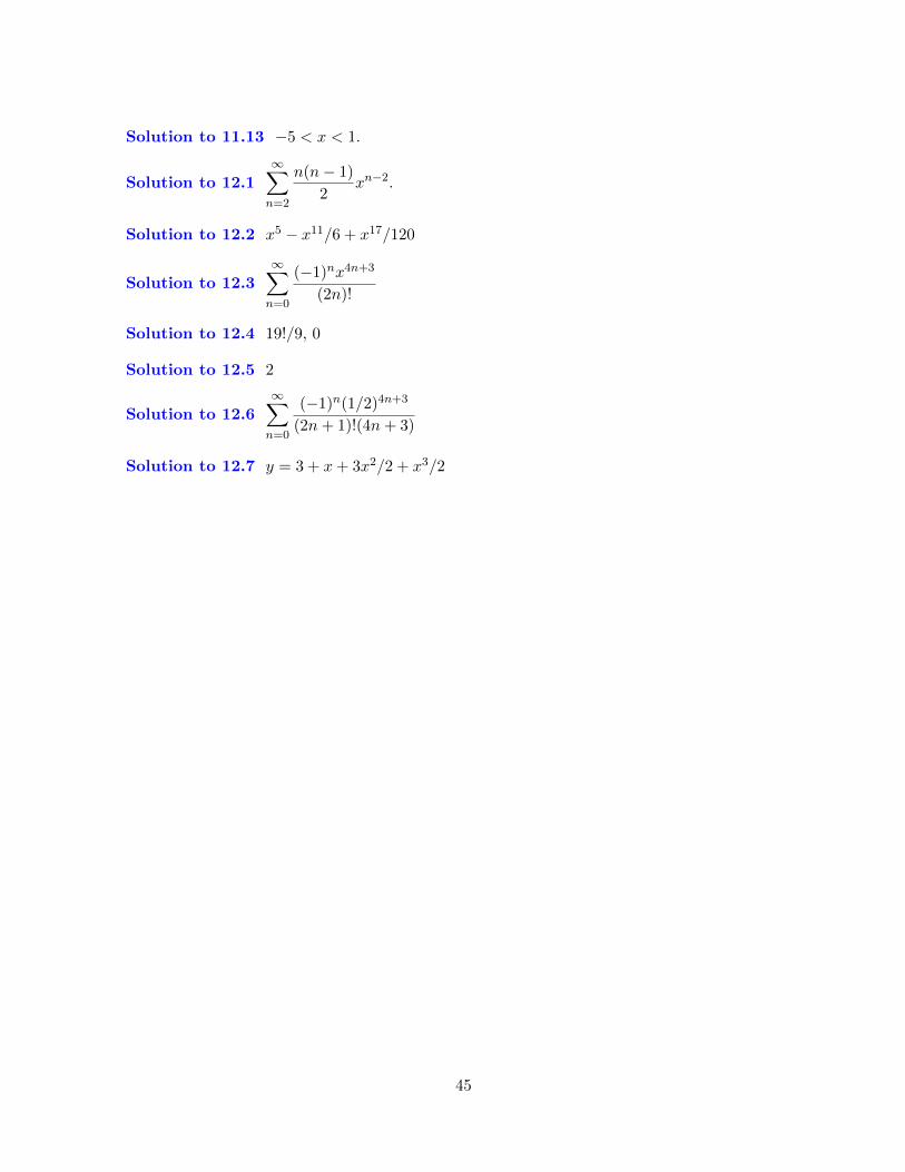
Solution to 11.13 −5 < x < 1.

Solution to 12.1

∞∑n=2

n(n− 1)

2xn−2.

Solution to 12.2 x5 − x11/6 + x17/120

Solution to 12.3∞∑n=0

(−1)nx4n+3

(2n)!

Solution to 12.4 19!/9, 0

Solution to 12.5 2

Solution to 12.6

∞∑n=0

(−1)n(1/2)4n+3

(2n+ 1)!(4n+ 3)

Solution to 12.7 y = 3 + x+ 3x2/2 + x3/2

45