Math 017 Lecture Notes

Math 017 Lecture Notes

(1.1) Preference Ballots and Schedules

Election ingredients:

- Set of choices/candidates to choose from

- Voters whom make these choices

- Ballots lets voters designate their choices

(vote on something): ski/snowboard/other (both ways)

- Say we only ask for one of the three choices. Define Linear Ballot

- We can also design ballots that rank the choices in order of most to least preferable (define

Preference Ballot)

- Naturally, since there are a limited number of choices for ranking these choices, we can

organize ballots by their respective rankings. Define Preference Ballot (draw it)

Link this vocabulary to the vote:

Preference ballot: voters are asked to rank candidates/choices

Linear Ballot: plain vote (disregard lesser choice candidates)

Preference Schedule: organize matching ballots

Transitivity of Elimination Candidates: preferring choices A over B and B over C implies A is preferred

over C

o This implies relative preference of a voter is not affected by the elimination of

candidate(s)

o Eg. Eliminate one of the activities we’ve voted on, show new schedule

(1.2) The Plurality Method

Plurality Method: Only choose first place votes (most votes wins = plurality candidate)

Principle of Majority Rule: In an election with 2 candidates, the candidate with the more than half the

votes wins (majority candidate). Harder to accomplish when more than 2 candidates. Plurality

candidate not necessarily a majority candidate

Democratic Criteria

Majority Criterion: If candidate X has majority (>half!) of first-place votes than X should win the election

- Majority => plurality but plurality ≠> majority!

- Let m = # of votes for majority, then if N = total number of votes, then m = ceil(N/2 +1)

- If a majority candidate does not win the election we say the Majority Criterion has been

violated (e.g. plurality method satisfies the majority criterion)


- e.g. ( show schedule st plurality not majority)

e.g. Do Plurality method homework example

Condorcet Criterion: Candidate X wins the election if preferred by other voters in “head to head”

comparison

- Considers all results of a preference schedule (not just the top votes)

- Better representation of the combined voters motives

- The plurality method violates the Condorcet Criterion (however specific plurality voting

schemes may not violate this criteria)

e.g. Condorcet Criterion Example

Insincere/strategic Voting: Instead of voting for a candidate doomed to loose, instead cast your vote

for the one of the “lesser of two evils” who are more likely to win (e.g. Democrat/Republican vs Green

Party)

e.g. Show how insincere voting could skew election (skiing example)

(1.3) The Borda-Count Method

Borda-Count Method: Voters rank top candidates as in a preference ballot. Each rank is assigned a

number of points. Winner is based on the total point accumulation. Usually base points on the number

of choices ,N, assigning a first place vote with N points, second with N-1 points and so on. (e.g. In

winter sport example there were 3 rankings so 1st place receives 3 points, 2nd place 2 pts, 3rd place 1 pt.

e.g. Using the Borda Count Method

- Advantage: Incorporates all information from a preference ballot. Takes candidate with

best average ranking. Preferable when comparing a large number of candidates.

- Disadvantage: Can violate both the Majority and Condorcet Criterion.

e.g. Show how Borda Count Method can violate both Majority and Condorcet

Borda Rebuttal

- Very useful for elections with many candidates

- When there are many candidates, violations of Majority or Condorcet criterion are rare

- Uses in the real world

o Sports awards (Heisman Trophy, NBA rookie of year, NFL MVP)

o College football polls, music industry awards

o Hiring of school principals, university presidents, corporate executives

Class work: Assign questions on board, allow them to work in groups


(1.4) Plurality-with-Elimination Method (Instant Runoff Voting)

- In municipal and local elections candidates generally need a majority of first place votes to

win.

- Usually the candidate with the fewest 1st place votes is eliminated and a runoff election is

held

- Runoff elections are inefficient and cumbersome, this is why we use preference ballots

- Instead of holding extra elections, eliminate the candidate with fewest first place votes one

at a time until one candidate wins the majority. (no extra elections)

- We will call this method the plurality-with-elimination method. Another name for this

method is called instant runoff voting (IRV)

Plurality-with-Elimination Method Steps

- Round 1: Count 1st place votes for each candidate. If a candidate has a majority of 1st place

votes, then the candidate wins. Otherwise, eliminate the candidate(/candidates if a tie)

with fewest 1st place votes

- Round 2: Cross the name of candidates eliminated from preference schedule and recount 1st

place votes. If a candidate has a majority of 1st place votes, then that candidate is wins

- Round 3,4,…: Repeat process until a candidate has a majority of 1st place votes

e.g. Plurality with elimination example

Monotonicity Criterion

- If candidate X is a winner of an election and, in a reelection, the only changes in the ballots

are changes that favor X (and only X), then X should remain the winner of the election.

Plurality-with-elimination Advantages/Disadvantages

- Designed to satisfy the majority criterion

- Used in International Olympic Committee to choose who hosts Olympics

- Used in various states to determine municipal elections (including Burlington, Vt -2005)

- Can violate both the monotonicity and Condorcet criterion

e.g. Olympic Problem violates monotonicity criterion


(1.5) Method of Pairwise Comparisons

- So far all methods presented can violate the Condorcet Criterion

- Method of Pairwise Comparisons (AKA Copeland’s method) constructed to satisfy the

Condorcet criterion

Method of Pairwise Comparisons

- Compare every candidate in a head to head comparison using a preference ballot

- In a comparison between candidates X and Y, the vote goes to whichever candidate is listed

higher on the ballot.

- Candidate with more votes wins a point and loser gets none. For a tie, both candidates get

half a point

- Tally all these points, candidate with the most points wins. In case of a tie use a

predetermined tie-breaker

e.g. Using Method of Pairwise Comparisons

Independence-of-Irrelevant Alternatives Criterion

- If candidate X is a winner of an election and in a recount one of the non-winning candidates

withdraws or is disqualified, then X should still be the winner of the election

e.g. Show method of Pairwise Comparisons that violates this rule (pg 18 gives a good example)

Advantage/Disadvantage

- ADV: Satisfies majority(usually since majority candidate � will win converse may not be

true) , monotonicity, and Condorcet criteria

- Dis: can violate the independence-of-irrelevant-alternatives criterion

Finding the sum of consecutive Integers: 1+2+…L = L(L+1)/2

- Gauss was in grade school when his teacher gave his students the task of adding up the

numbers 1…99 as busy work. He expected it would take the children the afternoon. Gauss

walked up in a few minutes and presented his teacher with the correct answer. HOW?

- Let S = 1+2+…99. Write out S = 99 + 98 + 97…+1 underneath. Notice each column adds up

to 100 and there are 99 columns so this would be 99x100 = 9900 = 2S => S = 4950.

- Generalize: Suppose S = 1+2+..L where L is positive integer. Write S = L + L-1 + L-2 +…+1

underneath. Each column adds to L+1 for a total of L columns. Thus 2S = L(L+1) or

equivalently S = L(L+1)/2 our formula! (show sum notation)

e.g. Show how to count #pairwise comparisons, using this formula

Classwork: if theres time assign a couple of the add em up questions from the book


(1.6) Rankings

So far we’ve only discussed methods that choose a particular winner for an election. What if we

wanted a rigorous definition for who finished 2nd ,3rd,… last. For this we have extended ranking systems

Consider the natural extension that can be used to rank candidates through the various methods:

We call these the extended method

Extended Method Ranking

Extended Plurality Rank by number of 1st place votes

Extended Borda Rank by total number of points

Extended Plurality

with Elimination

Rank candidates in reverse order of elimination (candidate eliminated first is

last, eliminated second is second to last…) If there was a majority before every

candidate was eliminated, continue to rank by order of elimination as if no

majority candidate

Extended Pairwise

Comparison

Rank by the number of points tallied from each pairwise comparison (1 for win,

0 for loss, ½ for tie)

e.g. Show a preference schedule and do each method and show the extended ranking (pg22)

We are skipping the recursive ranking methods (they are confusing and unnecessary)

Conclusion

This chapter has presented various methods that can be used to decide the winner of an election.

We’ve also discussed a number of fairness criteria that are used to determine the “fairness” of an

election

Arrow’s Impossibility Thm:

- It is mathematically impossible for a democratic voting method to satisfy all of the fairness

criteria


- Thus we can conclude making decisions in a consistently fair way is inherently impossible in

a democratic society

(2.1) An Introduction to Weighted Voting

We have a bunch of new notation to work with: Defn:

Weighted voting system: Any formal voting arrangement in which voters are not necessarily equal in

terms of # of votes they control

- Only consider yes-no voting decisions, known as motions.

- Elements of Weighted Voting Systems

o Players: the voters in the system. Use N to denote number of players. Generally

Denote players P1, P2, …Pn.

o Weights: each player controls a certain number of votes, called weights. Assume

weights are positive integers denoted w1, w2, .. wn. Use V = w1+w2+…+wn. to

denote total number of votes in the system.

o Quota: the quota is the minimum number of votes required to pass a motion,

denoted q.

We use a generic notation to organize the important aspects of a weighted voting system:

Generic Weighted Voting System with N Players: [q: w1, w2, ...wn] with w1>=w2…>=wn

e.g. Venture Capitalism

Problems we Want to Avoid

-Anarchy: when the number of both yay/nay votes are greater than the quota

- Gridlock: when the quota is greater than the number of votes in the system

e.g. Anarchy, Gridlock (PROBLEMS)

Solution to Problems

- Force the quota to fall between either a simple majority and unanimity of votes

- So we need q>V/2 and q<= V which can be expressed via the inequality

V/2 < q <= V (where V = w1+…+wn)

e.g. One-partner-one-vote (weights and quota s.t. a unanimity is needed to pass motion)


Other possible members of the weighted voting system

o Dictator: a player whose weight is bigger than or equal to the quota (so can make

the decision alone)

o Dummies: A player who does not have a say in the outcome of the voting (due to

such a low weight). (i.e if a dictator exists then all other players are dummies )

e.g. Dictators and dummies

e.g. Veto

Veto Power: a player whose vote will always decide whether a motion will pass or fail (not necessarily

due to having more votes than the quota)

- In general a player who is not a dictator has veto power if a motion cannot pass unless the

player votes in favor of the motion.

- Mathematically occurs when w<q (not a dictator) and V-w < q (other votes in the system are

not enough to pass motion)

- (i.e.) A player with weight,w, has veto power if and only if w<q and V-w<q where V = w1 + … +

wn

(2.2) The Banzhaf Power Index

We have seen that a player’s weights in this system of weighted voting can be deceiving

It’s possible for a player with few votes to have as much power as one with many votes.

e.g. Weirdness of Parliamentary Politics

Coalitions

- A coalition describes any set of players who join forces and vote the same way.

- If there is a coalition consisting of all players we call this a grand coalition.

- We will use set notation to describe coalitions, i.e. if players P1,P2,P3 form a coalition, the

coalition will be denoted { P1,P2,P3} where the order of players in the coalition is irrelevant

- Coalitions with enough votes to win will be designated winning coalitions, non-winning

called losing coalitions

- In a winning coalition a player is called a critical player for the coalition if the coalition must

have that player’s votes to win.


o i.e. subtracting a critical player’s weight from the total weight of the coalition the

number of remaining votes drops below the quota

o i.e. (math) A player P in a winning coalition is a critical player for the coalition � W-

w < q ( where W is the weight of the coalition and w denotes the weight of P)

o #critical players in a coalition can be : 0, 1, multiple, or all

e.g. continue Parliament example to give coalitions and critical players

John Banzhaf: “A player’s power should be measured by how often the player is a critical player.”

The Banzhaf Power Index

- In computing the Banzhaf power index of player P, first count the number of times P is a

critical player in a winning coalition. The critical count, B of player P is then defined as the

number of times P is a critical player.

- Next compute the critical counts B2,…Bn for all other players in the system

- Let T = B1+…+BN the Total critical count of the system

- Then the Banzhaf Power Index of Player P1, β1 = B1/T

- This ratio of P1’s share of the total power in the system

- The Banzhaf Power Distribution is the complete list of power indexes β1.. βn where the sum

of all Betas is 1 (the full power pie)

Computing Banzhaf Power Distribution of a Weighted Voting System

1 Make a list of all possible winning coalitions

2 Within each winning coalition determine which are the critical players (undlerline them).

3 Count the number of times P1 is critical, i.e. B1. Repeat for all other critical players

4 Add all the B’s in step 3, T = sum (i=1..n)Bi

5 Find the ratio β1 = B1/T of each critical players.

e.g. Compute a Banzhaf Power Index, maybe do two size 3 and 4

Classwork: Assign a couple of these out of the book

So how many coalitions can there be given a system of N players?


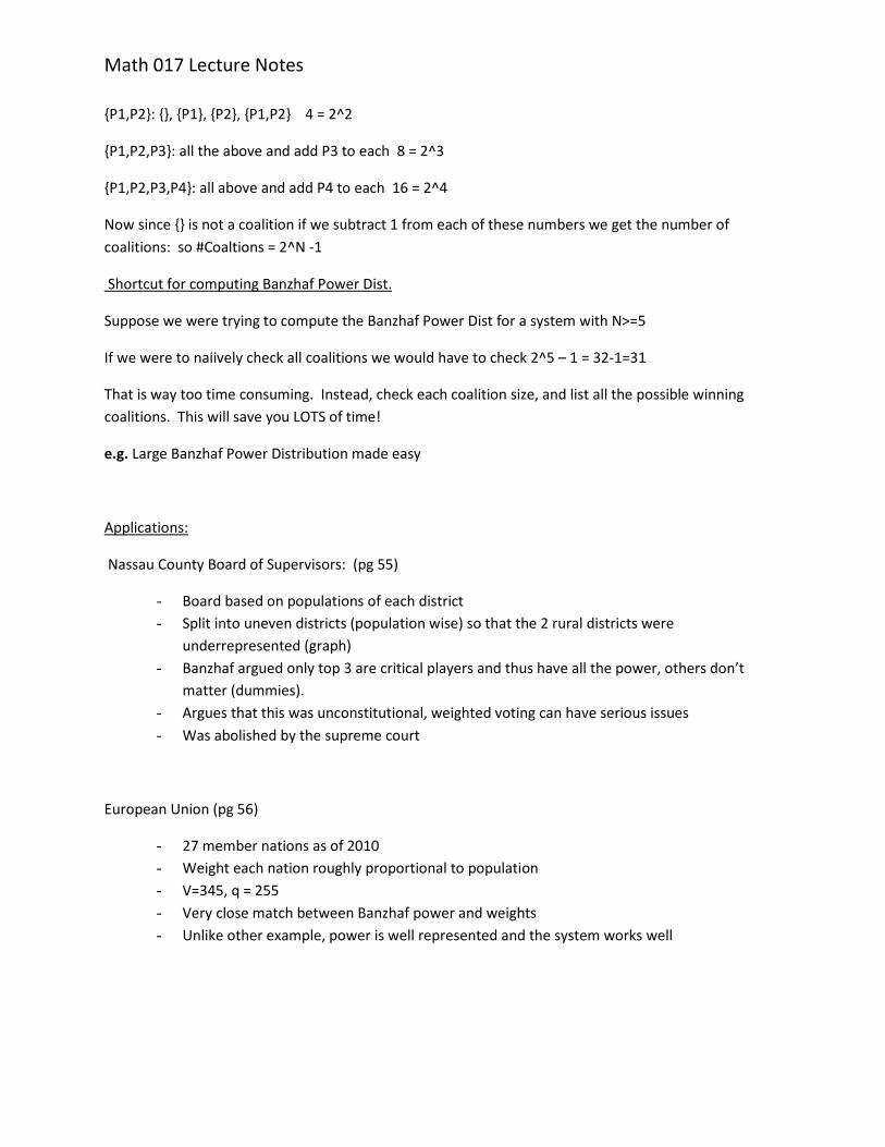
{P1,P2}: {}, {P1}, {P2}, {P1,P2} 4 = 2^2

{P1,P2,P3}: all the above and add P3 to each 8 = 2^3

{P1,P2,P3,P4}: all above and add P4 to each 16 = 2^4

Now since {} is not a coalition if we subtract 1 from each of these numbers we get the number of

coalitions: so #Coaltions = 2^N -1

Shortcut for computing Banzhaf Power Dist.

Suppose we were trying to compute the Banzhaf Power Dist for a system with N>=5

If we were to naiively check all coalitions we would have to check 2^5 – 1 = 32-1=31

That is way too time consuming. Instead, check each coalition size, and list all the possible winning

coalitions. This will save you LOTS of time!

e.g. Large Banzhaf Power Distribution made easy

Applications:

Nassau County Board of Supervisors: (pg 55)

- Board based on populations of each district

- Split into uneven districts (population wise) so that the 2 rural districts were

underrepresented (graph)

- Banzhaf argued only top 3 are critical players and thus have all the power, others don’t

matter (dummies).

- Argues that this was unconstitutional, weighted voting can have serious issues

- Was abolished by the supreme court

European Union (pg 56)

- 27 member nations as of 2010

- Weight each nation roughly proportional to population

- V=345, q = 255

- Very close match between Banzhaf power and weights

- Unlike other example, power is well represented and the system works well


(3.1) Fair Division Games

Basic Elements of Fair-Division Game

- Goods/Booty: Informal name of the item(s) being divided. Can be tangible/intangible

(pizza/chores). Denote booty by S

- Players: The set of parties with the right to share S. Can be people or institutions

- Value Systems: Assumption that each player has an internalized value system, giving the player

the ability to quantify the value of the booty or its parts. So each player can look at S or its

subsets and assign values based on its worth to the individual.

Basic Assumptions

- Rationality: Each player is a thinking rational entity trying to maximize his/her share of the

booty, S. A player’s move is based on reason alone (no mind games)

- Cooperation: Players follow the rules of the game. After a finite number of moves by players

the game ends with division of S. (no judges)

- Privacy: Players have no useful information on other players value system.

- Symmetry: Players have equal right in sharing the set S. At a minimum each player is entitled to

proportional share of S – i.e. for 2 players each is entitled to atleast ½ of S, for 3 entitled to 1/3

of S…

Fair Shares and Fair Division Methods

- Given booty S with players P1,…Pn each with his/her own value system the goal is to end up

with a fair division of S, i.e. divide S into N shares such that each person gets a fair share

- Fair Share: Suppose s is a share of booty S and P is a player in a fair division game with N players.

Then s is a fair share to player P if s is worth atleast 1/N of the total value of S in the opinion of

P. (proportional fair share)

- Note a share can be a fair share without being the most valuable share.

- Fair division method is the set of rules that define how the game is played. Considers the

players, booty, and the specific method of fair division.

Types of Fair Division Methods

- Continuous: Here S is divisible in infinitely many ways, shares increased or decreased by

arbitrarily small amounts (e.g. pizza,cake,land…)

- Discrete: Here S consists of indivisible objects. Integer units (i.e. cars, paintings)

- Mixed: S can be a mixture of continuous and discrete (dividing up a house containing stuff

jewelry etc)

e.g. PIZZA pg 104 #3 and cake


(3.2) 2 Players: The Divider-Chooser Method

- “You cut-I choose method”

- Continuous fair division method

- Under rationality and privacy assumptions each player will get at least 50% of the entire total

worth of booty, S. Since the divider doesn’t know the other player’s likes and dislikes, (s)he is

only guaranteed a 50% or better share of the booty.

- The chooser is guaranteed a 50% or better (value) share by choosing the piece (s)he likes best

- Always better to be the chooser than the divider. Chooser can end up with a share worth more

than 50% of the total booty.

- Both players should have an equal chance of being the chooser (i.e. coin toss)

- Will later discuss how to extend this method to more than 2 players

e.g. cake example

Damian likes chocolate and strawberry equally, Cleo is allergic to chocolate so the chocolate half is

worth absolutely nothing to her. They are splitting a half strawberry half chocolate cake with the divider

chooser method. Suppose Damian is the divider. They both may have ideas of what they want but we

assume this is unknown. Suppose Damian cuts a piece with mostly chocolate and piece with mostly

strawberry. Then naturally Cleo will choose the piece with more strawberry. However since strawberry

half is worth 100% of the booty, in her eyes, she comes out with a piece that’s worth about 2/3 of the

value of the entire cake. Also, Damian receives a piece worth half of the total value, so this was a fair

division.

e.g. book example


(3.3) The Lone Divider Method

Lone divider method generalizes Divider Chooser method for N-players developed by Hugo Steinhaus

First consider case when n = 3 players:

Lone Divider Method for 3 Players

- Preliminaries: One of 3 players is the divider, D. Other 2 players are choosers C1,C2. Since

better to be chooser than divider, random draw decides roles

- Step 1 Division: Divider, D, divides the cake into 3 shares (s1,s2,s3). Since D does not know

which share will be his/hers , this forces D to divide the cake into 3 shares of equal value

- Step 2 Bidding: C1, C2 independently list which of s1,s2,s3 are fair shares, called the bids. (must

list all fair shares, no mind games, no knowledge of other bids)

- Step 3 Distribution: 2 types of pieces: C-pieces (pieces chosen by choosers), U pieces (pieces

Unwanted by chooser). The U-piece is valued at less than 1/3 of the booty for choosers and C-

pieces at least 1/3 of the booty for choosers. Depending on number of C-pieces we have cases

to consider:

o Case 1: When there are 2 or more C-pieces there is always a possible, true fair division

of the booty. Can either randomly assign C-pieces to each chooser or preferably assign

C-pieces bases on their values to C1,C2. After division the final, informal step allows

choosers to swap their pieces if desired

o Case 2: There is only 1 C-piece, then both choosers are bidding for the same piece. First

assign the divider, D, one of the unwanted pieces either randomly or the least desirable

piece between C1,C2. Next combine the remaining two pieces into a single piece, call it

B piece. Now perform the divider-chooser method with players C1,C2 to ensure every

player is guaranteed a fair share

e.g. Performing 3 Player Lone-Divider Method

Lone Divider Method for >3 Players: Harold Kuhn

- Preliminaries: One of N players is Divider, D, chosen randomly. Other N-1 players are choosers,

C1..C(N-1)

- Step 1 Division: Divider, D, divides the cake into N shares (s1,…sN). D is guaranteed one of these

shares but doesn’t know which

- Step 2 Bidding: Each of N-1 choosers submits a bid-list consisting of all pieces (s1..sN) that are

fair shares (i.e. worth at least 1/N the booty)

- Step 3 Distribution: Break pieces into U-pieces (unwanted) and C-pieces (wanted).

o Case 1: If possible, assign different share to the N-1 choosers, that is fair for each

chooser. Divider gets last unassigned share. Afterward players can swap pieces if

necessary

o Case 2: There is a standoff- occurs when K choosers are bidding for less than K-shares.

Separate the standoff shares and players from the rest of the choosers. Assign fair


shares to each of the remaining players and divider. Now, recombine the rest of the

shares into a new booty, S to be divided among the players in the standoff. If K>2,

continue Lone Divider Method, until K = 2 then use Divider-Chooser Method

e.g. Lone-Divider Method for 5 players

(3.5) The Last-Diminisher Method

Another continuous division method that lets players continuously break up the booty

Per step there is a claimant who divides the booty into the C-piece and R-piece (remaining piece). As

each player makes their move per round, the C-piece may be reshaped and reclaimed.

Steps:

- Preliminaries: Players are randomly assigned an order of play. Assume P1 plays first…Pn plays

last. Game is played in rounds. At end of each round there is one fewer player and a smaller S to

be divided.

- Round 1:

o P1 cuts a share of S equal to (1/N)th the value of S. This is the current C-piece, P1 the

claimant. (P1 does not know if this piece is guaranteed, so doesn’t cut it too large or too

small)

o P2 now has a choice, either pass (remain nonclaimant) or diminish the C-Piece into a

share that is (1/N)th the share of S (i.e. P2 could be a diminisher only if he thinks the C-

piece is worth more than 1/N the value of S).

� If P2 diminishes, P2 becomes the new claimant (so P1 is a nonclaimant), the

diminished C-piece becomes the new C piece and the

“trimmed piece” is added to the old R-piece

o Now P3..PN-1 can pass or diminish just as P2

o PN can pass or diminish as well, however if chooses to diminish, there is no further

player who can diminish his claim. In this case if PN becomes the diminisher he will trim

the tiniest possible slice in order to maximize his share. Since the slice is continuous, he

can cut a piece so small that it is negligible to the total value of S. We call this “trimming

by 0”

o At the end of Round 1 the current claimant, aka Last Diminisher, gets to keep the C-

piece (a fair share) and is out of the game.

- Round 2…: The remaining players move to the next round to divide R-piece among themselves.

Continue this process until there are only 2 players left

- Last Round: The final 2 players decide the final piece with the divider-chooser method

e.g. pg 92, show diagram of castaways

e.g. close to hw question


(3.6) The Method of Sealed Bids

- Discrete division method

Method of Sealed Bids: (booty consists of different types of discrete items)

- Step 1 Bidding: Each player makes a bid (in dollars) for each item in the booty. Player gives

honest assessment of actual value of the item in the bid. To satisfy privacy assumption, bids are

done independently

- Step 2 Allocation: Each item goes to the highest bidder for that item. Ties can be broken with

predetermined tiebreaker. Note: its possible for a player to get anywhere between 0 up to all

the items depending on their bids.

- Step 3 First Settlement: Depending on the item(s) each player gets in step 2, he/she will either

owe money or is owed money from the group.

o First, calculate each players fair dollar share of the booty. The fair dollar share is given

by adding each of the player’s bids and dividing by the total number of players.

Calculate each fair dollar share of each player

o Now calculate what each player owes or is owed by the group. If the value of the

item(s) a player receives in the Allocation phase is greater than his/her fair dollar share

then the player pays the difference to the group. If the item is less than the fair dollar

share for that item, then the player gets the difference in cash.

- Step 4 Division of Surplus: After each player gets their share and is either paid money or gives

money to the group, there can be money left over, called a surplus. To find the surplus, S’: add

up the money that is owed by players whose item(s) are more than their fair share and subtract

from the amount that is given out to players whose items are less than their fairs shares. If

positive, this surplus is divided evenly among the players.

- Step 5 Final Settlement: The final settlement is simply adding the money from the surplus

(divided equally among the players) to what each player gets in the settlement.

-

e.g. 54 pg 114

Conditions

- Each player must have enough $$ to pay for their bids. Must be prepared to buy some or all of

the bids. If $$ not available player is at a serious disadvantage

- Each player must accept $$ as a substitute for any item (so no item can be priceless in the eyes

of the player)

e.g. 60 pg 115


(4.1) Apportionment Problems

Apportionment: Dividing and assigning indivisible objects/positions on a proportional basis and in a

planned, organized fashion. Primarily used in the allocation of seats in a legislature, weighted by the

population distribution of an area. Whenever were trying to assign items, weighted in some way, we

can use different methods of apportionment.

Elements of Apportionment Problems

- The states: Term to describe the parties/players having a stake in the apportionment. Unless

they have specific names, denoted A1,…An

- The seats: Term describes the M identical, indivisible objects, that are being divided among the

N states. Usually assume more seats than states ensuring every state can potentially get 1 seat.

(Note: Does not reply every state must get a seat!)

- The populations: This is the set of N positive numbers used as the basis for apportionment of

seats to the states. Use p1…pn to denote a state’s respective populations and the total

population is given by P = p1+...+pn

- The Standard Divisor: The ratio of the entire population to number of seats for apportionment

calculations. (SD people = 1 seat � SD = P/M)

- The Standard Quotas: The standard quota of a state is the exact fractional number of seats the

state would get, if fractional seats were allowed. Round to 2 or 3 decimal places. Let q1…qn

denote the standard quotas of the respective states. Then qi = state population/standard quota

= pi/SD

- Upper and Lower Quotas: Associated with each standard quota, the lower quota, Li, of state Ai

is the standard quota rounded down. The upper quota,Ui, is the standard quota rounded up. If

the quota is a whole number then Ui = Li

The whole idea of apportionment is how can we split up these discrete seats in a fair manner. The

problem is rounding. Each different Apportionment Method will explore the fairest way to round

standard quotas

e.g. pg 144 #4 Nurse Standard Quotas


(4.2) Hamilton Method and Quota Rule

-“Every state gets at least its lower quota. As many states as possible get their upper quota, with the

one with highest residue (fractional part) having first priority, the one with second highest residue

second priority, and so on…

Hamilton Method

- Step 1: Calculate each state’s standard quota

- Step 2: Give to each state its lower quota

- Step 3: Give the surplus seats (one at a time) to the states with the largest residues (fractional

parts) until there are no more surplus seats.

Quota Rule

- No state should be apportioned a number of seats smaller than its lower quota or larger than its

upper quota.

- A state that’s apportioned a number lower than its lower quota is called a lower-quota violation.

- If apportioned larger than its upper quota, called upper quota violation

Advantages/Disadvantages

- Advantage: 1) easy, 2) satisfies the quota rule

- Only considers the fractional residues and not a state’s population when assigning extra seats

- Called a systematic bias in favor of larger states over smaller ones. A good apportionment

method should be population neutral and not bias large states over smaller states.

e.g. Performing Hamilton Method: 14 pg 145


(4.3) Alabama and Other Paradoxes

Alabama Paradox: An increase in the total number of seats being apportioned, in and of itself, forces a

state to lose one of its seats.

e.g. pg 131 Real Alabama Paradox (1882)

Population Paradox: Under Hamilton’s method, its possible that a state could potentially lose some

seats because its population grew too large. Occurs when population of state A loses a seat to state B

even when population of A grows at a higher rate.

New States Paradox: The addition of a new state with its fair share of seats can, in and of itself, affect

the apportionments of other states

(4.3) Jefferson’s Method

-Similar to Hamilton’s Method, except here instead of using a fixed Standard Divisor, we modify a

divisor, D, (called a modified divisor). The idea is to choose D, so that every states modified standard

quota (Pi/D) can be rounded down and sum to the total number of seats. This takes some trial and error

Steps: Jefferson’s Method

- Step 1: Find a suitable divisor D

- Step 2: Using D as the divisor, compute each state’s modified quota (Pi/D)

- Step 3: Each state is apportioned its modified lower quota

Helpful: Draw flow chart from pg 136

Advantage/Disadvantage

- ADV: satisfies quota rule. Avoid fairness issues with Hamilton method since all are rounded

down.

- Dis: It can produce upper quota violations! Tend to consistently favor large states. Depending on

how divisor is chosen, its possible that states are apportioned more than the upper quota when

considering the standard divisor and standard quotas

Adams and Webster methods are similar, based on picking a divisor D and then different rules for

rounding.

e.g: Nurse Jefferson Method #26 pg 146


(10.1) Percentages %

- Expressing a fraction with a percentage can be an easy way to view different ratios and

proportions.

- Percentages are a “common yardstick” that are easy to interpret

- A percentage is just a fraction with denominator 100

- X % = X/100

e.g. Converting fractions/decimals to percentages (#1,3 pg 392)

e.g. Comparing Test Scores, Restaurant Tips

Often when trying to buy an item, you may see a shop offering a sale. This is a percent decrease on the

value of the item. Also, every item we buy has an associated tax, which can be thought of as a percent

increase on the item you buy.

e.g. shopping for an ipod

Formulas For Percentage Increase and Decrease:

1. If you start with quantity Q and increase that quantity by x%, you end up with the quantity:

I = (1 + (x/100))Q

2. If you start with quantity Q and decrease that quantity by x% you end up with quantity:

D = (1- (x/100))Q

3. If I is the quantity you get when you increase an unknown quantity Q by x% then

Q = (I) / (1 + (x/100) (note this can be obtained from 1)

e.g. percent increases and decreases (finding the baseline) (#17 pg 392)

CAUTION: be careful going from % increase to % decrease, make sure you have the right baseline!!!

e.g. Bogus 200% Decrease

e.g. Increasing wage tax issues: (data from Wikipedia)


(10.2) Simple Interest

- When investing your money in something, the goal is to receive a larger amount of cash than

what you initially invested, also known as the principal.

o The present value is the value of your initial investment, the value of the cash today.

o The future value is the value of your investment at some future date. Hopefully, the

future value of your investment is greater than the initial investment.

- When calculating the future value from the present value there are several variables involved. A

very important factor is the interest rate of the return

o The interest rate is the expected return of an initial investment per unit of time. ( i.e.

may expect 3% per month on an initial investment)

o Standard way to describe an interest rate is yearly, called the annual percentage rate

(APR)

- Also must ask how the interest is added up. It could be simple interest or compound interest.

Simple interest: Only the original money invested (aka the principal) or borrowed accumulates interest

e.g. simple interest defn

Simple Interest Formula

- The future value F of P dollars invested under simple interest for t years at an APR of R% is given

by:

F = P(1+rt) (where r denotes the R% written as a decimal i.e. r = R%/100

e.g. (#21 pg 393, Grandpa Jones #26, #27 loan)

e.g. Crazy Credit Cards


(10.3) Compound Interest

- Under simple interest only the principal (initial investment) generates interest.

- Compound Interest both the original principal and previously accumulated interest will generate

interest. Thus money invested under compound interest grows much faster than simple interest and

the difference is magnified over time. Much better for the investor

e.g. Trust fund pg 371

Annual Compounding Formula

The future value, F, of P dollars compounded annually for t years at an APR of R% is given by :

F = P ( 1+ r)t

General Compounding Formula

- Some investments may be compounded more than once a year (as we’ve seen).

- To compute the future value we must find the periodic interest rate which is the interest rate

that applies to each compounding period. This can be found by taking the yearly interest rate

and dividing by the total number of compounding periods (i.e. if compounded monthly we

divide the APR by 12)

- We also must find the total number of periods we are compounding per year. Then we can

write our general formula as:

F = P ( 1 + r/n)nt where n is the number of periods

- If we let T = nt (the number of times we compound) and p = r/n (the periodic interest rate) this

reduces to:

F = P(1+p)T

- (Continuous Compounding Formula) If we let n approach infinity we are continuously

compounding interest which can be calculated via the formula

F = Pert where r is the APR expressed as a decimal, and e = 2.718…

e.g. Computing different compound interests

Annual Percentage Yield(APY)

- The annual percentage yield (APY) of an investment is the percentage of profit that the

investment generates in a one year period.

- This is simply the percent change of your investment in a given year:

APY = (F-P) / P where P is the principal and F the future value (after 1 yr)

- With this you can easily calculate the percent increase (and hopefully not decrease) of your

investment per year.

e.g. Computing the APY of an investment


(10.4) Geometric Sequences and Series

- A sequence is a succession of entities that can be related by some formula.

- i.e. 5, 10, 20, 40, …

- Specifically we consider Geometric Sequences

o Start with initial term, P

o Every term after P can be found by multiplying the preceding term by a common ratio, c

o The common ratio c is simply a number that we must find that given a sequence of

numbers.

o So the sequence looks like: P, cP, c2P, …

- So 5, 10, 20, 40, 80 = 5, 2*5, 22*5, 23*5, …

- Thus this is a geometric sequence with common ratio c = 2, and initial term P = 5

e.g. Compound Interest: When we found the future value of an investment of P dollars compounded

annually for T years at APR of r = R%/100 we had:

F1 = P(1+r), F2 = P(1+r)2, … here we have a geometric sequence with c = (1+r)

Geometric Sequence Formulas

- A recursive formula tells you how to compute each term of the sequence from previous terms:

GN = cGN-1 ; G0 = P

- An explicit formula tells you how to find any member of the sequence without recursion:

GN = cNG0 ; G0 = P

e.g. #52 pg 395, # 56

Geometric Series

- Sometimes, we may want to add up the terms of a geometric series in order (called a geometric

sum)

- Deriving the formula is beyond the scope of this class, so I will give it to you for free: sum (n =

0 to N-1) cNP = P + cP + c2P + … cN-1P = P[ (cN – 1) / ( c-1)]

e.g. spread of infectious disease


(10.5) Deferred Annuities: Planned Savings for the Future

A fixed annuity is a sequence of equal payments made or received over regular (monthly, quarterly,

annually) time intervals.

- e.g. deposits to save for vacation, college; making payments on a car loan or home mortgage

- Types of annuities:

o Deferred annuity: payments made to produce a lump payout at a later date (i.e. college

trust fund)

o Installment Loan : (aka fixed immediate annuity) lump sum is paid to generate a series

of regular payments later ( i.e. car loan)

e.g. Setting up a college trust fund

Fixed Deferred Annuity Formula:

The future value F of a fixed deferred annuity consisting of T payments of $P having a periodic interest

rate of p is :

F = L [ ((1+p)T- 1) / p ] where L denotes the future value of the last payment

o Value of L is determined whether payments are made at the start or end of the period (

so it depends on whether the last payment generates interest or not

o If pay at the start of the period, then last payment generates interest so:

L = (1+p)P

o If paid at the end, last payment doesn’t generate interest so L = P

e.g. pg 395-396 #’s 64, 70

(10.6) Installment Loans: The Cost of Financing the Present

Installment Loan : (aka fixed immediate annuity) a series of equal payments made at equal time

intervals for the purpose of paying off a lump sum of money received up front

KEY DIFFERENCE between installment loan and deferred annuity: Installment loan has a present value

computed by adding the present value of each payment. A fixed deferred annuity has a future value

that is computed by adding the future value of each payment.

e.g. financing a red mustang (pg 383)

Amortization Formula

If an installment loan of P dollars is paid off in T payments of F dollars at a periodic interest rate of p :

P = Fq [ (qT – 1) / (q – 1) ] where q = 1/(1+p)

e.g. # 74A, #78 pg 396


(14.1) Graphical Descriptions of Data

A dataset is a collection of data value (aka data points) that are reported (i.e. each of your numerical

grades in the course can be considered data points)

A frequency table organizes a data set into bins or piles of data points with the same or similar values.

Very useful in finding outliers – extreme data points that don’t fit into the overall pattern of the data

e.g. LabMT data set binned by valence (each frequency is percentage of words with that reported

valence)

Types of Frequency Tables

- Bar Graphs: Represent the frequency of each individual (data point) by the length of a bar.

Can also represent the relative frequency which are the frequencies viewed as a percentage of the

entire population

- Pictograms: same as a bar graph but use picture icons as the bar to represent frequency in the

dataset

(14.2) Variables

A variable is any characteristic that varies with the members of the population

- Variable Types

o Quantitative Variable: a numerical or measureable quantity either continuous (differences

can be arbitrarily small) or discrete (fixed number differences)

� e.g. discrete: IQ, SAT score, shoe size,… continuous: height, weight, foot size (as

opposed to shoe size)

o Qualitative Variable: Can not be measured numerically (i.e. gender, nationality, hair color,

etc.)

A pie chart organizes the categories or classes of the population into slices whose size represent their

relative frequency in the population (rel. freq = freq / total freq)

- General rule in drawing pie charts is that a slice representing x% is given by an angle of (3.6)x

degrees. E.g. pie chart

Sometimes may want to organize (or bin) data by class intervals to see which intervals hold the most

data points.

For continuous variables it makes sense to make these class intervals that are connected. A bar graph

out of these connected class intervals is called a Histogram (e.g. labMT)


(14.3) Numerical Summaries of Data

Types of Numerical Summaries

- Measures of location: mean, average, quartiles; provide info about values of data

- Measure of spread: range, IQR, standard deviation; provide info about spread within the dataset

The average (aka mean) of a set of N numbers is found by adding each of the N numbers and dividing by

N.

- i.e. the average of the set of N numbers { d1, d2, d3, …dN} is : (d1 + d2 + d3 +

… dN ) / N

- When trying to find average value of data values depicted with a frequency distribution, where each

value di has some corresponding frequency fi then:

Avg = (d1*f1 + … + dN*fN) / (f1 + … + fN) e.g.: computing avg

Another type of numerical summary describes the percent of the data that fall at or below a certain

value. This is called the pth percentile of the dataset, the value such that p percent of the numbers fall at

or below this value and the rest fall at or above it

- First sort the dataset from smallest to largest , let d1 , … , dN represent the data

- Find the locator L = p/(100) * N

- If L is a whole number, the pth percentile is dL.5 = (dL + dL+1)/2

- If L is not a whole number, the pth percentile is dL+ where L+ is L rounded up

e.g. Computing percentiles, median

The 50th percentile is known as the median, denoted M. The median splits the data into 2 halves. To find

the median: (other than computing the 50th percentile)

- Sort the data set from smallest to largest, d1 , … , dN

- If N is odd, the median is d(N+1)/2

- If N is even the median is the average of dN/2 and d(N/2)+1

Other very common percentiles are called the first and third quartiles. The first quartile Q1 is the 25th

percentile and the 3rd quartile Q3 is the 75th percentile

The five number summary of a data set is given by (1) the min (smallest number) (2) the first quartile (3)

the median (4) the third quartile and (5) the max (largest number). The five number summary can be

organized into a box and whisker plot. The box represents the interquartile range (Q3 – Q1) with a

marker at the Median. The whiskers extend from the box to the min/max resp. of the data. (sometimes

use * to denote outliers)

e.g. 5 number summary, drawing a box plot


(14.4) Measures of Spread

The range of the data set, R, is the difference in lowest and highest values of the set (R = max – min).

Sometimes useful to discount outliers

The interquartile range, IQR, is the difference between the third and first quartile (IQR = Q3 – Q1 ).

Tells us how spread out the middle 50% of the data values are

Standard Deviation:

- Deviation from the mean: If A is the average of a data set and x is some arbitrary data point then the

deviation from the mean is simply (x-A). This is a measure of how “far” the data point is from the

average of the data points. These deviations can help us measure the spread of the data

- Variance, V: the variance of the data set is the average of the squares of each deviation from the

mean ( Average deviations from the mean (A-x)2 for all points, x, in the data set)

- Standard Deviation: This is the square root of the variance. σ = V1/2. This is a useful measure of

spread

- Steps in Finding σ:

o Let A denote the mean of the data set. For each number, x, in the dataset compute its

deviation from the mean (x – A) and square each of these numbers (called the squared

deviations)

o Find the variance, V, the average of the squared deviations

o The Standard deviation is the square root of the variance σ = V1/2

- Key Facts on the Standard Deviation

o The standard deviation of the data set is measured in the SAME units as the original data!

(measures the spread in terms of the same number of units as the data points)

o It is POINTLESS to compare standard deviations of data sets that are given in different

units!!!

o Comparing standard deviations for data sets based on the same underlying scale, can tell us

about the spread of the data. If σ is small then the data points are close together and there

is little spread. As σ increases we can conclude the points are spreading out. If the points

are exactly the same, σ = 0.

e.g. Computing standard deviations, LabMT example

Math 017 Lecture Notes

Documents

Transcript of Math 017 Lecture Notes