Maternal education, parental investment and non-cognitive

characteristics in rural China

Jessica Leight∗1 and Elaine M. Liu2

1Williams College Department of Economics2University of Houston Department of Economics and NBER

August 20, 2016

Abstract

This paper evaluates the parental response to non-cognitive variation across siblings in Gansu

province, China, employing a household fixed effects specification. The non-cognitive indices

are defined as the inverse of externalizing challenges (behavioral problems) and internalizing

challenges (anxiety and withdrawal). The results suggest that there is significant heterogeneity

with respect to maternal education; educated mothers compensate for differences between their

children, investing more in a child exhibiting greater non-cognitive deficits, while less educated

mothers reinforce these differences. Most importantly, there is evidence that these investments

lead to the narrowing of non-cognitive deficits over time for children of more educated mothers.

1 Introduction

In recent years, both research and policy debates have placed increasing emphasis on the importance

of non-cognitive skills in determining long-term economic outcomes. Data primarily from indus-

trialized countries has suggested that non-cognitive skills have a large impact on adult economic

welfare, measured as earnings and labor productivity (Heckman and Rubinstein, 2001; Heckman,

Stixrud and Urzua, 2006; Cunha, Heckman, Lochner and Masterov, 2006; Carneiro, Crawford and

Goodman, 2007). There are many causal pathways through which stronger non-cognitive skills

may lead to improved educational and economic outcomes. Individuals with enhanced skills may

∗Thanks to Doug Almond, Janet Currie, Flavio Cunha, Rebecca Dizon-Ross, Benjamin Feigenberg, Paul Frijters,Paul Glewwe, Lucie Schmidt, Kevin Schnepel, Chih-Ming Tan, and Andy Zuppann for helpful conversation and sug-gestions, and to seminar and conference participants at the University of Minnesota - Applied Economics, Williams,the ASSA meetings, the Chinese Economists’ Society conference, the Western Economic Association conference, theUniversity of North Dakota, the University of Montreal - CIREQ conference, and the Society of Labor Economists2016 meeting for feedback. Previous drafts were circulated under the title “Maternal bargaining power, parental com-pensation and non-cognitive skills in rural China.” Keywords: non-cognitive characteristics, parental investment,intrahousehold allocation. JEL codes: I24, O15, D13

1

be more likely to be persistent in achieving strong academic outcomes or building professional

expertise, may be more resilient in the face of setbacks, or may be better able to forge useful

professional relationships. One particularly important channel, however, is the relationship forged

much earlier in life between children and their parents.

Variation in non-cognitive characteristics may affect parental investments in several ways. First,

this variation could alter the weight that a parent places on a child’s welfare. Parents could favor

a child with more desirable characteristics with whom they forge a stronger relationship, or a child

who exhibits more behavioral challenges if he requires more nurturing. Second, even if the weights

parents place on their children’s welfare are unchanged, variation in non-cognitive characteristics

could affect children’s future income, and may affect the returns to human capital investment in a

given child. Depending on whether parents emphasize efficiency or equality, they may then invest

more or less in human capital development for a child who is struggling or flourishing.

Ultimately, we may observe investment that is compensatory, defined as a pattern in which

parents invest more in a relatively weaker child, or investment that is reinforcing, defined as a

pattern in which parents invest more in a stronger child. Needless to say, the question of whether

investment is in general compensatory or reinforcing is an important question in family economics

going back to Becker; Almond and Mazumder (2013) provide a recent review.

The objective of this paper is to analyze whether non-cognitive characteristics measured in child-

hood and adolescence have a significant impact on the within-household allocation of educational

expenditure in rural Gansu province, China. We employ a panel dataset that provides a detailed

set of outcome measures for a large cohort of children in one of the poorest provinces in China.

Non-cognitive characteristics are measured via direct surveys of the children, and defined as the in-

verse of externalizing challenges (behavioral problems and aggression) and internalizing challenges

(withdrawal and anxiety); accordingly, our measure effectively captures an absence of behavioral

or socio-emotional problems. Focusing on a sample of two-children families, our primary specifi-

cation examines how parents respond to differences in non-cognitive characteristics conditional on

household fixed effects, and whether this response varies based on parental education.

Our results suggest that while parents are not responsive to differences in non-cognitive charac-

teristics on average—neither reinforcing nor compensating for these differences—there is significant

heterogeneity with respect to characteristics of the parents, and particularly the mother. House-

holds with more educated mothers show evidence of significantly more compensatory investment

compared to households with less educated mothers. For a child who scores one standard devi-

ation lower on the non-cognitive index relative to his sibling (i.e., indicative of more behavioral

challenges), an increase in maternal education from the 25th to the 75th percentile, or from one

to six years of education, would ceteris paribus result in an increase in discretionary educational

expenditure directed to this child of nearly 35%. (Discretionary expenditure comprises all educa-

tional expenditure including tuition; there is no parallel effect observed for tuition.) There is very

2

little evidence of comparable heterogeneity with respect to the education of the father.

One potential challenge faced in this analysis is that non-cognitive characteristics may in fact

be partly an outcome of previous parental investment, rather than an endowment; if there is some

serial correlation in parental investment, this will generate bias toward the detection of a reinforcing

pattern of expenditure. We address this challenge in several ways. First, we demonstrate that bias

on the interaction effect including maternal education will only arise given specific assumptions

that do not seem to be supported by the empirical evidence. Second, we present evidence that the

results are robust to several alternate specifications, including the use of earlier measurements of

non-cognitive characteristics and the inclusion of control variables for past educational expenditure.

This observed pattern of heterogeneous response—more compensation in households with a

more educated mother—could be consistent with a number of possible channels. More educated

mothers may simply be better able to recognize the non-cognitive deficits in their children and

to compensate appropriately. Maternal education may be a proxy for income or other household

characteristics, and higher-income households may have a preference for intrahousehold compen-

sation. Alternatively, women (or more educated women in particular) may have a preference for

compensatory investment, and the ability to impose these preferences within the household.

Further exploration suggests that the first two channels are not particularly salient in this

context: there is little evidence consistent with parental learning or higher income leading to a

compensatory response by more educated mothers. However, it does seem that more educated

mothers may have both a greater preference for compensatory investment and higher bargaining

power, enabling them to exert more influence over the allocation of expenditure within a household.

In the final section of the paper, we analyze whether this variation in compensatory vis-a-

vis reinforcing behavior results in the reduction of non-cognitive deficits over time for children in

households with more educated mothers—where struggling children receive greater investment—

compared to children in households with less educated mothers. While the second-born child in this

data is observed only once, the first-born child is observed three times. Analyzing the longitudinal

data observed for the first-born child, we do find evidence of significantly greater catch-up for

children of more educated mothers.

As a result, the correlation between maternal education and non-cognitive characteristics be-

comes more pronounced as children age. In the first wave, the observed cross-household correlation

between a dummy variable for a mother of high maternal education and non-cognitive character-

istics is essentially zero. By the third wave, this correlation has increased in magnitude to .151.

This result highlights the role of maternal education in shaping the formation of non-cognitive

skills, consistent with the broader literature on the importance of maternal education in child de-

velopment (Carneiro et al., 2013; Currie, 2009). Moreover, if the economic returns to non-cognitive

skills are significant, differential parental compensation is a channel through which inequality across

households can widen over time.

3

Our paper contributes to several related literatures on intrahousehold allocation and human

capital investment. First, there is an extensive literature examining parental responses to differences

in children’s endowment, and the evidence has been mixed. Bharadwaj et al. (2013b), Royer (2009),

and Almond and Currie (2011) find little or no evidence of either compensatory or reinforcing

behavior. Akresh et al. (2012), Rosenzweig and Zhang (2009), Frijters et al. (2013), Almond et

al. (2009), Adhvaryu and Nyshadham (2014) and Aizer and Cunha (2012) find parents exhibit

reinforcing behavior in Burkina Faso, China, Sweden, Tanzania, and the United States, while

Del Bono et al. (2012) find evidence of compensatory behavior in breast-feeding decisions and

birth weight and Black et al. (2010) provide some indirect evidence of compensatory behavior

in a robustness check. Bharadwaj et al. (2013a) find compensatory investment with respect to

initial health comparing across siblings, but comparing across twins, there is no evidence of either

compensatory or reinforcing behaviors. Leight (2014) finds evidence of compensatory behavior

with respect to height-for-age using the same sample as this paper. This literature, however,

focuses primarily on parental responses to children’s health endowment and cognitive ability. Our

paper is one of the first papers that examines whether parents respond to children’s non-cognitive

characteristics in the allocation of human capital investment.1

Second, our paper finds that maternal education plays an important role in determining the al-

location of parental investment. This is similar to the results reported in Hsin (2012) and Restropo

(2016), who conclude that households with less educated mothers generally exhibit reinforcing in-

vestment behavior, while households with more educated mothers exhibit compensatory behavior.

However, neither of these papers examine the father’s education level; instead, they analyze ma-

ternal education as a proxy for household socioeconomic status. In light of these findings, a recent

review by Almond and Currie (2011) suggests that the observed pattern could be due to credit

constraints in low socioeconomic status households, or a high elasticity of substitution between

consumption and human capital investment in these households.

In our context, we are able to rule out these two channels given the absence of any evidence

of heterogeneity with respect to the father’s education and household income. Rather, we present

additional results that suggest differential preferences and bargaining power for more educated

women are the primary channels for the differential compensatory response in households with

more educated mothers.

Third, there is growing evidence that early intervention and investment can mitigate initial

deficits in children’s endowments (Bhalotra and Venkataramani, 2016; Adhvaryu et al., 2015; Bleak-

ley, 2010; Cunha and Heckman, 2007; Cunha et al., 2010; Gould et al., 2011; Almond et al., forth-

coming; Kling et al., 2007). However, this literature primarily focuses on catch-up in children’s

health and cognitive outcomes. To the best of our knowledge, we are the first to show evidence of

1The only other relevant paper is Gelber and Isen (2013). While it is not the focus of their work, they report intheir appendix that parents respond positively to a child with greater observed non-cognitive abilities, but they donot further investment the heterogeneity by mother’s education.

4

the narrowing of non-cognitive deficits as a result of parental investment, especially among more

educated mothers.

The remainder of the paper proceeds as follows. Section 2 describes the data. Section 3

describes the empirical strategy and the primary results, and Section 4 presents robustness checks

and evidence about the relevant channels. Section 5 examines the longitudinal evidence, and Section

6 concludes.

2 Data

The data set used in this paper is the Gansu Survey of Children and Families (GSCF), a panel

study of rural children conducted in Gansu province, China. Gansu, located in northwest China, is

one of the poorest and least developed provinces in China. The description of the data here draws

substantially on the description in Leight (2014).

The first wave of the GSCF was conducted in 2000, and surveyed a representative sample of

2,000 children aged 9–12 in 20 rural counties, supplementing these surveys with additional surveys

of mothers, household heads, teachers, principals, and village leaders. These children are denoted

the “index children.” All but one of the index children have complete information in the first wave.

The second wave, implemented in 2004, re-surveyed the first sample of children at age 13–16

and also added a survey of their fathers. 1,872 children, or 93.6% of the original sample, were

re-interviewed in the second wave. In addition, surveys were added of the eldest younger sibling of

the index child. These additional children are denoted “younger siblings.” Surveys are conducted

directly with the younger siblings, as well as with their homeroom teachers; in addition, mothers

and fathers report limited supplementary information about the younger siblings.

In early 2009, a third wave of surveying was conducted, re-interviewing the index children

during Spring Festival, a period at which many of them had returned to their natal villages. In

cases where the sampled individual was not available, parents were asked to provide information

about their child’s education and employment status. 1,437 individuals, or 72% of the original

sample, were interviewed directly in this wave, and information was collected in parental interviews

for an additional 426 sample children.

The household surveys in waves one (2000) and two (2004) included extensive questions about

schooling outcomes, household expenditure on education for each child, child time use, time in-

vestments in education by parents and teachers, and child and parental attitudes, as well as more

standard socioeconomic variables. The index children also completed a number of achievement and

cognitive tests. Younger siblings also completed these tests in wave two.

In addition, each wave of data collection included survey questions posed to the sample chil-

dren that were designed to measure their non-cognitive characteristics. In the first and second

waves, the survey measured both internalizing and externalizing behavioral challenges: the former

refers to intra-personal problems (e.g., withdrawal and anxiety), and the latter to inter-personal

5

problems (destructive behavior, aggression, and hyper-activity). Both measures of non-cognitive

characteristics are constructed by recording the respondent’s agreement or disagreement with a

series of statements and then applying item response theory (IRT) to generate internalizing and

externalizing scores. The measures are identical across waves one and two, and the scores are stan-

dardized to have a mean of zero and a standard deviation of one. In the third wave, a Rosenberg

self-esteem index and a depressive index were measured. Further detail about the construction of

the non-cognitive characteristics measures can be found in Glewwe, Huang and Park (2013).

It may be useful to briefly comment here on the measures of non-cognitive characteristics

employed (and the terminology used to describe these measures), and their relationship to the

previous literature. A number of other papers have employed variables capturing internalizing

and externalizing challenges, including Heckman et al. (2013) in analyzing the long-term effect of

the Perry preschool program and Neidell and Waldfogel (2010) in analyzing cognitive and non-

cognitive peer effects in preschool education. Similarly, Bertrand and Pan (2013) and Cornwell,

Mustard and Van Parys (2013) document gender differences in a number of non-cognitive measures

including internalizing and externalizing indices, and Juhn, Rubinstein and Zuppann (2015) employ

a behavioral problems index in analyzing quality-quantity trade-offs. The terminology used to

describe these measures varies, but given that we are not measuring a non-cognitive skill per se (e.g.,

self-esteem, or negotiating ability), we will follow the other authors noted here and preferentially

use the term non-cognitive characteristics.2

Non-cognitive characteristics of the younger siblings were measured only in wave two. For ease

of interpretation in the primary specifications, the primary non-cognitive measures employed here

(the externalizing and internalizing indices) have been inverted; in the original index, a higher value

indicates more challenges, but in our index a higher value indicates fewer challenges.

In this paper, we will focus on a subsample of the families in the survey: those with two children

in the household where both children have reported measurements for non-cognitive and cognitive

skills in the second-wave survey. If the index children and the younger sibling are the only children

in the household, then the surveys provide a complete overview of parental allocations and child

endowment. Complete data is available for 388 families drawn from 90 localities in 20 counties, and

these households constitute the relevant subsample. In our sample, only 6.5% of households have

one child. The remaining households are excluded because the index child has two or more siblings,

or has one older sibling for whom non-cognitive ability is not reported. In the robustness checks

reported in Section 4.1, we will also present results employing a larger sample including households

where these two children (the index child and the younger sibling) are part of a larger family.3

2Evidence in psychology suggests that positive attributes such as conscientiousness, agreeableness, and opennessto experience are negatively correlated with the internalizing and externalizing behaviors we analyze here Ehler etal. (1999).

3While China’s One-Child Policy was in effect during the period in which these children were born, many ruralhouseholds could nonetheless have two children legally under various exemptions to the policy (Gu et al., 2007). It isnot possible using this dataset to accurately identify for each household whether it was in technical compliance with

6

Figure 1 summarizes the structure of the sample, including the years in which data is collected, the

children that are observed in each wave, and their age at the point of data collection.

Panel A of Table 1 reports summary statistics for the subsample of two-children families and

the overall sample for key demographic indicators, as well as a t-test for equality between the two

means; the covariates reported are measured in the second wave of the survey, the wave in primary

use here. It is evident that there are no significant differences in income or parental education

between the sample and the subsample. However, households in the subsample are slightly younger

and have younger children. This primarily reflects the exclusion of larger families or families in

which the index child is the younger child; these families are generally headed by older parents.

We also report the total amount of time reported spent by each parent playing with children

or assisting them with homework in a week; and the number of parenting decisions (out of two,

choices about parenting style and choices about education) that each parent reports s/he is able

to make independently. Interestingly, reported time investment is 3.7 hours for the mother, and

only slightly lower (3.4 hours) for the father, and similarly each parent reports making around

one parenting decision alone on average. Time invested in children is significantly higher for the

subsample, consistent with the fact that households in which the index child is the older child (and

younger child requiring more care are present) are included in the subsample. However, there are

no significant differences in decision-making patterns, and importantly, there are also no significant

differences in reported non-cognitive and cognitive skills of the index children comparing across the

full sample and the subsample.

The dependent variable of interest is educational expenditure per child per semester, reported

by the head of household in six categories: tuition, educational supplies, food consumed in school,

transportation and housing, tutoring, and other fees.4 Each household separately reports expen-

diture for each child in each of these categories. Discretionary expenditure is defined as the sum

of all expenditures excluding tuition. Summary statistics for average expenditure per child for the

subsample of families analyzed can be found in Panel B of Table 1. Total educational expendi-

ture averages around 360 yuan per child per semester; an average of 20% of household income is

allocated to educational expenditure in total for both children.

We focus on educational expenditure given that it is the primary form of child-specific expendi-

ture reported in this dataset. The only other type of child-specific expenditure reported is medical

expenditure over the past year; only 25% of households report any positive medical expenditure

for either child over the past year, and unsurprisingly this expenditure is highly correlated with

reported illness (i.e., it is reasonable to assume that very little corresponds to preventive care).

Given that we are primarily interested in human capital investments with long-term returns, we do

not focus on medical expenditure.

the policy.4In China, textbook fees are mandatory and levied as part of the overall tuition, and here they are likewise reported

in the tuition category. Educational supplies is supplies other than textbooks.

7

3 Empirical strategy and results

3.1 Empirical strategy

Our empirical strategy entails evaluating whether parental expenditure on education for children is

correlated with measures of non-cognitive characteristics, conditional on household fixed effects.5

In other words, our primary specification identifies whether parents are more likely to invest in a

child who has more desirable non-cognitive characteristics, relative to a sibling.

The child’s observed non-cognitive characteristics will be denoted Ncogihct, for child i in house-

hold h, living in county c and born in year t; the non-cognitive variables employed will include

the externalizing and internalizing index, as well as a summary measure that is the mean of the

two indices. All non-cognitive variables have been standardized to have means equal to zero and

standard deviations equal to one, and in order to facilitate interpretation, the indices have been

inverted such that a higher value is indicative of fewer non-cognitive challenges.

The dependent variable, educational expenditure, is denoted Yihct. The specification includes

household fixed effects ηh, year-of-birth fixed effects νt, and a vector of child covariates Xihct,

yielding the following equation. Child covariates include gender, the sibling’s gender, birth parity

(i.e., whether a child is first-born or second-born), height-for-age, reported grades in school, and

scores on grade-specific achievement tests administered in math and Chinese. The inclusion of birth

parity is particularly important, given the evidence presented by Black et al. (2005a) suggests that

birth order is an important determinant of children’s outcomes. Our sample includes both male

and female children (60% boys and 40% girls).6

This specification is estimated with and without interactions with parental education Shct.

Standard errors will be clustered at the county level in all specifications.7

Yihct = β1Ncogihct + β2Ncogihct × Shct +Xihct + νt + ηh + εihct (1)

The identification assumption for this family of specifications requires that non-cognitive charac-

teristics are uncorrelated with other unobservable variables that determine parental allocations.

This assumption would be violated, for example, if parents invest more in a favored child, who is

subsequently observed to score highly on the non-cognitive indices employed.

In order to present some preliminary evidence about the relationship between non-cognitive

characteristics and child characteristics conditional on household fixed effects, the following speci-

fications can be estimated, regressing the internalizing and externalizing indices on child covariates

5Given that our primary interest is examining how parents allocate resources between children with differentnon-cognitive characteristics, it is necessary to include family fixed effects since we are examining within householdvariation. Also, the use of fixed effects addresses the challenge of unobserved household-level heterogeneity.

6For concision, we will employ male pronouns.7We regard clustering at the county level as a conservative strategy for inference. Our subsample includes 20

counties and 90 villages; our results are also consistent if we cluster at the village level.

8

Xihct, conditional on household fixed effects.

Ncogihct = β1Xihct + ηh + εihct (2)

The results can be found in Table 2: Panel A reports the correlations with sibling parity, age,

gender, and grade level, and Panel B reports the correlations with various measures of the child’s

endowment. Interestingly, in Panel A there is no evidence of any significant correlation between the

internalizing index and any child characteristic. However, for the externalizing index we observe

that non-cognitive measures are lower, suggestive of more behavioral challenges, for second-born

children, younger children, boys and children enrolled in lower grades in school. There is, of course,

a high degree of correlation among these covariates: second-born children are on average younger,

enrolled in lower grades, and more likely to be boys.8 Columns (9) and (10) show the results of a

multiple regression including all four covariates; there is some evidence here that the most robust

correlations are between gender and grade level and the externalizing index.

Panel B shows that there is little evidence of significant correlations between non-cognitive

characteristics and other measures of endowment: specifically, height-for-age, and various measures

of cognitive skills. This includes the child’s grades reported in the last academic year in math and

Chinese, and their score on a grade-specific achievement test. The only exception is a significant

correlation between the internalizing index and the achievement test score.

In light of these results, the primary specifications all include year-of-birth fixed effects as well as

controls for gender, sibling’s gender, sibling parity, height-for-age, and all three reported measures

of cognitive skills as measured in the second wave, contemporaneously with non-cognitive charac-

teristics. The inclusion of grade fixed effects is more complex; given that the primary dependent

variable of interest is educational expenditure, grade level can plausibly be considered an outcome.

However, the primary results will also be robust to the inclusion of grade fixed effects.

Given that the primary specifications are estimated conditional on household and year-of-birth

fixed effects, it is also useful to examine how much variation in the child characteristics of interest

is observed within a given household and within a given birth year. Table A1 in the Appendix

reports the R-squared in a simple regression including only the specified fixed effects as explanatory

variables and the specified child covariate as the dependent variable. In general, between 50%

and 60% of the variation in non-cognitive characteristics is explained by household fixed effects,

suggesting there is still considerable within-household variation.

3.2 Primary results

Table 3 shows the results of estimating equation (1) without the interaction terms with parental

education. The objective is to test whether parental allocations of educational expenditure are

8The implications of gender selection for this analysis will be explored in greater detail in Section 4.1.

9

responsive, on average, to variation in non-cognitive characteristics between siblings; the measures

of expenditure include total expenditure, discretionary expenditure (the sum of all expenditure

excluding tuition), and six individual categories. Enrollment is universal among the subsample of

interest, and thus school enrollment is not reported as an outcome. The results show coefficients that

are small in magnitude, varying in sign, and generally insignificant. This suggests that parents are

neither systematically compensating children characterized by more internalizing and externalizing

challenges, nor systematically reinforcing these differences. A similar pattern is observed if we

estimate this regression in the cross-section without household fixed effects.

In light of this pattern, we then examine whether parents who themselves have certain char-

acteristics are more likely to respond to measured differences in the non-cognitive traits of their

children. The most obvious relevant characteristic is education, particularly given that recent work

from Hsin (2012) and Restropo (2016) suggests that maternal education is an important deter-

minant of parental allocation of expenditure. While the average level of education reported is

relatively low—four years for mothers and seven years for fathers—there is considerable variation.

Around 75% of mothers report completing at least one year of formal schooling, and 17% report

completing junior high school. For fathers, around 90% report completing at least one year of

formal schooling, and 10% report completing senior high school.

Figure 2 shows histograms of the distribution of both maternal and paternal education. The

correlation between maternal and paternal education is positive, but low in magnitude (around .3).

Unsurprisingly, the education of both parents is also positively correlated with income and other

measures of household wealth.

In addition, Figures 3a and 3b show the distribution of intrahousehold (between-sibling) dif-

ferences in non-cognitive characteristics and in normalized expenditure residuals for households at

different levels of maternal education. We can observe that the mean absolute difference in non-

cognitive characteristics between siblings is around .75 standard deviations, and this is roughly

constant across households of different levels of maternal education. Normalized expenditure resid-

uals are calculated by regressing expenditure on child characteristics (gender, birth parity, cognitive

skills, and height-for-age), generating the residuals and standardizing them to have mean zero and

standard deviation one. The mean absolute difference is around .4 standard deviations, and this

seems to be larger at higher levels of maternal education.

To identify whether parents who are more educated respond differentially to differences in

non-cognitive characteristics, we then re-estimate equation (1) including interaction terms between

non-cognitive indices and parental education. Again, the specification includes controls for a wide

range of child characteristics including gender, sibling parity, and cognitive skills, and household

and year-of-birth fixed effects. We also include the interactions of gender, age, sibling parity,

height-for-age and the achievement test score with the specified measure of parental education.

The results are reported in Table 4. We observe a robust pattern in which households in which

10

mothers have low levels of education (roughly speaking, fewer than three years of schooling) provide

more expenditure to children with higher non-cognitive scores, reinforcing the pre-existing differ-

ences, while households with more educated mothers seem to engage in compensatory behavior,

providing more expenditure to children characterized by lower scores and thus by more behavioral

and socio-emotional challenges. This is evident in the negative coefficients on the interaction term

between non-cognitive indices and maternal education.9 The coefficients on the interaction terms

for other child characteristics are not reported in Table 4 for concision, but are reported in the on-

line appendix for a simple specification using a summary non-cognitive index.10 For cognitive skills

as captured by a summary achievement test score, β1 is positive though insignificant, suggestive

of a reinforcing allocation of investment, and there is no evidence of heterogeneity with respect to

maternal education; more discussion about this pattern is provided in Section 4.2.

In general, there is no compensatory effect observed for tuition, consistent with the intuition that

tuition is not easily manipulable; though the coefficients are negative, they are small in magnitude

and insignificant.11 Comparing the estimated coefficients for the interaction effect in Columns

(2) and (3) in Panel A, we can observe that relative to the mean of the dependent variable, the

magnitude of the coefficient on tuition in Column (3) is around 10% of the magnitude of the

coefficient on discretionary expenditure in Column (2). A similar pattern is observed in Panel C.

The interaction terms for paternal education, on the other hand, are smaller in magnitude,

heterogeneous in sign, and generally not statistically significant. Panels B and D report p-values

testing the equality of the estimated coefficients on the interaction terms for maternal and paternal

education for the two non-cognitive indices, respectively.12 These coefficients are denoted βm2 and

βf2 , where βm2 refers to the coefficient on the interaction term for maternal education, and βf2 refers to

the analogous coefficient for paternal education. We can reject the hypothesis that the coefficient on

the maternal and the parental education interaction terms is equal in both specifications employing

total and discretionary expenditure as the dependent variable, as well as in several additional

specifications. We also report results in both panels from a joint test of the hypotheses βm1 = βf1and βm2 = βf2 , and find parallel results.

These results may raise the question of how variation in maternal and paternal education

interact, and if we observe a different pattern if the parents’ educational levels are similar, or if one

is much more educated than the other. We explore this question in detail in Section 4.2.

Finally, the magnitudes of the implied effects are substantial. For example, consider a child

whose score on the internalizing index is one standard deviation lower than his sibling’s score,

9Aizer and Cunha (2012) find that the degree of parental reinforcing behaviors increases with family size. However,our finding cannot be explained by variation in family size since the sample is restricted to only two-child households.

10The on-line appendix can be found on both authors’ homepages.11Approximately 12% of students attend schools that are are private or publicly assisted private institutions;

accordingly, it is possible that there is some variation in tuition, and some potential for parents to select a higher-tuition school for their children.

12This test is implemented by estimating the two specifications simultaneously in a seemingly unrelated regressionframework.

11

suggestive of more behavioral or socio-emotional challenges. The coefficient on the interaction

term suggests that an increase in maternal education from the 25th to the 75th percentile, or

from one to six years — conditional on all other household characteristics — would result in an

increase in discretionary educational expenditure for this child compared to his sibling of 35%. The

magnitudes are similar for the coefficients estimated for the externalizing index in Panel C.

4 Robustness checks and channels

4.1 Robustness checks

Alternate specifications First, we verify the primary results are robust to a number of addi-

tional specifications. For concision, in the robustness checks we employ an average non-cognitive

index that is the mean of the internalizing and externalizing indices. The observed pattern is

consistent if grade fixed effects are included, if the non-cognitive variables are reformulated as per-

centile rank variables, and if log expenditure variables are employed as the dependent variables.13

Importantly, the results are also consistent in sign and magnitude if estimated unconditional on

cognitive skills and other endowment measures. There may be some concern that contemporane-

ous measures of cognitive skills are endogenous relative to parental investments, but there is no

evidence that including these cognitive measures as controls generates systematic bias; the results

from estimating a more parsimonious specification are reported in Panel A of Table A2.

We also re-estimate the results using two alternate samples. First, we employ the full sample of

all households where the number of children is greater than or equal to two, rather than restricting

to households in which the index child and his or her younger sibling are the only children.14

(Less than 10% of the sample of interest are households with only one child.) The estimation

results can be found in Panel B of Table A2, and the interaction terms on maternal education

are again negative and and of roughly equal magnitude, suggesting that the observed pattern of

compensation in households with more educated mothers is not limited to households of a particular

size. (Households in which the index child has an older sibling and no younger siblings are still

not observed in this sample due to the absence of data on the older sibling. However, the evidence

presented in Table 1 suggests that there is no significant difference in household characteristics or

the non-cognitive or cognitive skills of the index child when comparing index children observed in

the subsample to the full sample.)15

13These results are reported in the on-line appendix.14We preferentially employ the restricted sample in the primary results given that failing to observe the endowment

of the third sibling may lead to attenuation bias in the primary results if parents are compensating the unobservedsibling.

15We also explore whether there is evidence of a correlation between birth spacing (between the first- and second-born child) and maternal education that could be an alternate channel for the detected pattern. There is no evidenceof any correlation between birth spacing and maternal or paternal education, and no evidence that parents responddifferentially to non-cognitive characteristics in households with different spacing between the two siblings.

12

Second, it should be noted that gender cannot be considered to be exogenous in this sample;

nearly 70% of second-born children are boys. However, consistent with existing anthropological

evidence, there is little evidence of sex selection prior to the first birth (Gu et al., 2007). The

gender ratio for first-born children is not significantly different from .5, and the gender ratio for

second-born children who follow the birth of a son is also not significantly different from .5. Thus,

sex selection is a phenomenon primarily observed after the birth of a first-born girl. Accordingly, if

we restrict the sample to households reporting a first-born son, the distribution of gender in these

households can plausibly be considered quasi-exogenous. Re-estimating the primary specification

for this smaller sample generates the same pattern of results, reported in Panel C of Table A2.

Serial correlation in parental investment Parents may use various strategies to determine

investment between children: they may seek to maximize the returns on their educational invest-

ments, or they may allocate based on other criteria. Regardless of the allocation strategy, if there

is some serial correlation in investment, this may be a source of bias in our results.

Consider the following simple specification as an example, where the dependent variable is

educational expenditure and Yi,t−1 denotes previous parental investment.

Yit = β1Noncogit + β2Yi,t−1 (3)

If we assume that prior investment is unobserved and is positively correlated with expenditure today,

then Cov(Noncogit, Yi,t−1) > 0, generating upward bias on the coefficient β1. If β1 is positive (i.e.,

investment is higher for children with higher non-cognitive scores), then we will over-estimate β1

and over-estimate the degree of reinforcing investment. If β1 is negative (i.e., investment is higher

for children with lower non-cognitive scores), then the coefficient will be biased toward zero, and

we will under-estimate the degree of compensatory investment. The bias in the coefficient can be

captured by the familiar bias term for omitted variables,β2 Cov(Yi,t−1,Noncogit)

V ar(Noncogit). β2 captures the

degree of serial correlation in investment.

The question of primary interest for our specification is whether there will be bias in the

interaction term between non-cognitive indices and maternal education – and, if the bias does

exist, why do we observe this pattern only for maternal education, but not paternal education?16

If we estimated equation (3) separately for low-education and high-education mothers and then

calculated the difference in the estimated correlations β1 as a proxy for the interaction term, the

bias would cancel unlessβ2 Cov(Yi,t−1,Noncogit)

V ar(Noncogit)is different for the two samples. This could arise if

either the variance in non-cognitive scores or the degree of serial correlation in investment is different

for more and less educated mothers (i.e., β2 is not the same), or if the relationship between past

investment and current non-cognitive characteristics is different for more and less educated mothers

16We will also present results in Section 4.2 that there is no evidence of comparable heterogeneity with respect tohousehold income.

13

(i.e., the returns to investment are not the same).

We can present some evidence on these points using data reported on non-cognitive characteris-

tics and expenditure for the first-born child over time. In general, there is positive serial correlation

in investment that seems to be significantly larger in families with more educated mothers.17 How-

ever, there is no evidence that the dependence of current non-cognitive scores on past investment

differs significantly in households with more educated mothers, and there is also no evidence that

V ar(Noncogit) is statistically different between the two groups. Thus if anything, the upward bias

on β1 would be larger in the sample of more educated mothers, generating upward bias on the

interaction term of interest in the main specification; this is, of course, in the opposite direction of

the observed effect.

We can also perform an additional test to evaluate the potential for bias in the primary specifi-

cations due to serial correlation in investment. We presume that there is limited scope for parental

investment (via educational expenditure or other, correlated measures) to affect non-cognitive char-

acteristics prior to primary school. Accordingly, we construct a new variable Ncogprimihct that is

defined as non-cognitive characteristics at primary school age, as observed in wave one for the older

sibling or wave two for the younger. We similarly define expenditure at primary school age Y primihct .

We then estimate a specification parallel to the specification of interest, though rather than using

year-of-birth fixed effects, we employ fixed effects for the age of the child in the survey year, νage.

Y primihct = β1Ncog

primihct + β2Ncog

primihct × Shct + β3Xihct + νage + ηh + εihct (4)

The results from estimating equation (4) are reported in Panels A and B of Table A3. We

again observe evidence of greater compensation in households with more educated mothers, and

no systematic variation with respect to paternal education. While the coefficients are smaller in

magnitude, the mean levels of expenditure are also lower when we examine only children at primary

school age. The estimated coefficients suggest that a one standard deviation increase in maternal

education leads to an increase in discretionary expenditure directed to a child characterized by a

non-cognitive index that is one standard deviation lower of around 27%, compared to an effect

size of 35% using the original specification. This result is consistent with the hypothesis that the

observed pattern does not solely reflect bias introduced by differential prior investment.

It is also possible to re-estimate our primary specification controlling directly for lagged ex-

penditure; this is analogous to attempting to solve the omitted variable bias challenge captured

in equation (3) by directly including the omitted variable. The primary results, reported in Panel

C of Table A3, are all consistent in both magnitude and significance when re-estimated including

lagged measures of expenditure.

17More specifically, the correlation between Yi,t−1 and Yit is 0.22 for children with mothers above the median levelof education, and 0.11 for children with mothers below the median level of education.

14

Parental favoritism Parental favoritism may interact with non-cognitive characteristics in two

ways. First, if a child with fewer behavioral challenges is more likely to be the parental favorite and

thus receives more parental investment, favoritism could be interpreted as a channel through which

non-cognitive characteristics affect educational investment. Second, if parents choose a favorite child

early in life, invest more in this favored child, and he is then observed to have fewer challenges,

then parental favoritism could be the underlying reason for a pattern of serial correlation — and

if parental favoritism and the associated persistence in investment is more prevalent in certain

households, this could be a source of bias in our main specification.

We implement two tests to evaluate whether favoritism is relevant in this analysis. First, we

exploit questions in the survey of mothers in which she reports the identity of the children who

will provide more emotional and economic support in the future. We designate a child as a favorite

if he is identified as the primary source of both emotional and economic support, and examine

whether more educated mothers are more likely to provide more expenditure to their favorite

children, conditional on non-cognitive characteristics and the full set of child covariates already

reported. Importantly, there is no significant correlation between non-cognitive characteristics and

the identity of the favorite child, nor is there any heterogeneity in this correlation with respect to

maternal education, suggesting that it is not the case that children experiencing fewer non-cognitive

challenges are more likely to build relationships with parents and be identified as the favorite.

Second, we evaluate whether parents invest more in a favored child, and if this pattern is

different in households with more educated mothers. The specification of interest is as follows,

where Fihct denotes a dummy for favorite.

Yihct = β1Ncogihct + β2Ncogihct × Shct + β3Fihct + β4Fhct × Shct + β5Xihct + νt + ηh + εihct (5)

The results are reported in Table A4. In general, there is no systematic preference in expenditure

for the favored child; there is some evidence of greater preference for the favored child among more

educated mothers, but the difference is not significant.18 These results suggest that favoritism is

unlikely to be an important channel for the observed pattern of compensation.

Alternate measures of non-cognitive characteristics Our primary measure of non-cognitive

characteristics is based on children’s self-reported status. This may raise questions about noise in

the data, especially given that some children in the sample are relatively young. The other relevant

measure available is drawn from surveys of the children’s teachers, who are asked to report whether

a child possesses a series of eight characteristics, both positive and negative.19 Given the limited

variation in this measure, which has only eight unique values, we construct a dummy variable equal

18It is also useful to note that the favorite child is significantly more likely to be a boy, though there is no significantvariation in this relationship with respect to maternal education.

19This series includes whether the child is smart, conscientious, reasonable/well-mannered, clean, enjoys work, islively/imaginative, gets along with others, likes to cry, or lacks confidence.

15

to one if the teacher’s reports of the child’s characteristics places him or her in the top half of all

children, denoted TcogDihct. We then estimate a specification parallel to our primary specification

of interest, employing this dummy variable as a measure of non-cognitive skills.

Yihct = β1TcogDihct + β2Tcog

Dihct × Shct + β3Xihct + νt + ηh + εihct (6)

The results are reported in Table A5 and show the same pattern of greater compensation in

households with more educated mothers. The magnitude observed is similar to the magnitude in

a parallel specification using a dummy variable constructed from the original self-reported non-

cognitive characteristics measure.

This evidence suggests that the observed pattern of differential compensation for adverse non-

cognitive characteristics in households with more educated mothers is not an artifact of the non-

cognitive self-reports. However, we preferentially use the measures derived from self-reports given

that these measures have greater variation, and only self-reported measures can be employed in the

longitudinal analysis discussed in Section 5. Teacher reports are, clearly, no longer available for the

index children once they have completed secondary school.

4.2 Channels

There are several channels that would be consistent with the observed pattern of compensation

only in high maternal education households. First, more educated mothers may simply be better

able to learn about variation in non-cognitive characteristics among their children, while less edu-

cated mothers do not acquire this information. (By contrast, more educated fathers are no better

able to recognize differences in non-cognitive characteristics compared to less educated fathers.)

Second, maternal education may be a proxy for income or socioeconomic status, and higher-income

households may have a preference for compensatory investment.

Third, more educated women may have a greater preference for compensatory investment rel-

ative to less educated women; alternatively, all women may have a greater preference for com-

pensatory investment, while only educated women are able to impose this preference within the

household. A gender difference in preferences would be consistent with the finding from the ex-

perimental literature that women are in general more inequality-averse (Andreoni and Vesterlund,

2001; Dickinson and Tiefenthaler, 2002; Selten and Ockenfels, 1998; Dufwenberg and Muren, 2006),

with the caveat that we cannot rule out that compensatory investment in this context is a returns-

maximizing strategy if returns to investment are higher for children with greater non-cognitive

deficits.20 In addition, a large literature has presented evidence that women exhibit a preference

for greater investment in health and education for children, (Bobonis, 2009; Duflo, 2003; Fafchamps

20For example, Andreoni and Vesterlund (2001) find that women are more concerned about equalizing earningsduring experiments, while men are more focused on maximizing efficiency.

16

and Quisumbing, 2002; Quisumbing and Maluccio, 2003); women or more educated women may

also have a stronger preference for compensatory investment. We will explore each channel in turn.

Parental learning about child characteristics The first postulated channel is that more

educated mothers are better able to recognize non-cognitive deficits among their children and

respond appropriately, while less educated mothers do not recognize these deficits. It is also possible

that more educated mothers acquire information about the returns to investing in children with

weak non-cognitive skills that less educated mothers do not acquire. In either case, it is also

necessary to assume there is no correlation between paternal education and the relevant information

acquisition process.

If this channel is important, then ceteris paribus we would expect more compensation among

parents who spend more time with their children, and thus have the opportunity to learn more

about their child’s characteristics and/or how these characteristics affect the returns to investment

on that child. In this survey, parents report the time spent in a typical week either playing with or

talking to children. As previously noted, about 65% of both parents report that in a typical week

they spend any time on either of these activities, and the mean time spent is around three hours,

only slightly higher for mothers than fathers. (Importantly, parents do not report the division

of this time between children, and thus we cannot analyze the time spent with each child as a

dependent variable.) Similar to the evidence presented in Guryan et al. (2008), we find a positive,

albeit relatively weak, correlation between parental education and time spent with children.

In order to test whether the observed pattern reflects a process in which educated mothers spend

more time with their children and thus learn more about their characteristics, we estimate the

following specification including the original interaction term between non-cognitive characteristics

and parental education, and adding an interaction term between non-cognitive characteristics and

average hours spent per week with children Timehct for both the mother and the father. (In order

to enable comparison of the coefficients on the two variables, in each specification the time variable

is re-scaled to have the same mean as the parental education variable.) The same control variables

included in the primary specification are included.

Yihct = β1Ncogihct + β2Noncogihct × Shct + β3Noncogihct × Timehct + β4Xihct (7)

+ νt + ηh + εihct

The results can be found in Panels A and B of Table 5 for maternal and paternal education

respectively. We can observe that the coefficients β2 remain significant and negative for the mother.

While the estimated coefficients β3 are negative, indicating there is some evidence that mothers

who spend more time with their children do compensate more, they are small in magnitude and

generally insignificant.21

21However, it is also important to note that if the most important information educated mothers acquire is informa-

17

Maternal education as a proxy for income The second postulated channel that could be

consistent with the observed pattern of differential compensation is that maternal education is a

proxy for household income, and higher-income parents prefer compensatory investment whereas

lower-income households prefer reinforcing investment. As suggested by Almond and Currie (2011)

and Conley (2008), low socioeconomic status households could focus on better endowed children due

to credit constraints; alternatively, the elasticity of substitution between consumption and human

capital investment could be higher for low SES households. These hypotheses are somewhat less

plausible in our context given that there are no parallel effects for paternal education, and in the

sample of interest there is no evidence that maternal education is more closely correlated with

household income when compared to paternal education.

However, a simple test of this hypothesis can be implemented by adding an interaction term

between household income and non-cognitive characteristics to the primary specification. This

yields the following equations, where Ihct denotes household income; income and maternal education

are re-scaled to have the same mean in order to allow for comparison of the coefficient magnitudes.

Yihct = β1Ncogihct + β2Ncogihct × Shct + β3Inihct × Ihct + β4Xihct + νt + ηh + εihct (8)

The results of estimating equation (8) employing the education of the mother can be found in

Table 6. It is evident that the coefficients β3 on the income interaction terms are small in magni-

tude, inconsistent in sign, and generally insignificant. The coefficients on the maternal education

interaction terms, by contrast, remain consistently negative and significant. We also re-estimate

this specification employing indices of productive assets and durable household goods owned by

the household, rather than income. We observe some evidence of greater compensation among

higher-asset households; importantly, however, the coefficient β2 remains negative, significant, and

of consistent magnitude. This suggests it is unlikely the primary results reflect shifts in parental

preferences in higher-income households.

Maternal education and preferences for compensatory investment Finally, we seek to

evaluate whether there is evidence consistent with the hypothesis that maternal education is cor-

related with a greater preference for compensatory investment, or a greater ability to impose a

certain preference within the household (i.e., greater bargaining power). We do not have any data

that would enable us to identify variation in preferences for compensatory investment between more

and less educated mothers, or for mothers compared to fathers. However, we do have data on who

makes certain decisions within the household (as reported by mothers), and we employ this data to

construct two measures of household decision-making power. The first is a general decision-making

index ranging from zero to seven, corresponding to the number of decision-making categories in

tion about variation in the returns to investment with respect to child characteristics, rather than child characteristicsthemselves, this process may be orthogonal to time spent with the child. In that case, the test implemented herewould have limited power.

18

which the mother reports involvement.22 The second is an index capturing the number of parenting

decisions made by the mother, ranging from zero to two.

We then regress these decision-making variables, denoted Dechct, on both the mother’s edu-

cation and the difference in education in two simple specifications, including household control

variables (net income, per-capita income, and age of both parents) and county fixed effects.

Dechct = β1Smhct + κc +Xhct + εhct (9)

Dechct = β1Sdifhct + κc +Xhct + εhct (10)

The results are reported in Panel A of Table 7, and suggest that there is generally a positive

correlation between maternal education and the mother’s reported decision-making power.23 We

then test whether greater bargaining power is correlated with greater compensation by re-estimating

the primary specification, adding an interaction term between the non-cognitive index and a dummy

variable capturing the mother’s reported decision-making power around parenting decisions; the

dummy variable is defined equal to one if she reports any decision-making power. The specification

of interest can thus be written as follows, where DecDhct denotes the decision-making dummy.

Yihct = β1Noncogihct + β2Noncogihct × Shct + β3Noncogihct ×DecDhct + β4Xihct (11)

+ νt + ηh + εihct

The results are reported in Panel B of Table 7. While the coefficients β2 on maternal schooling

remain significant and similar in magnitude compared to the coefficients reported in Table 4, the

interpretation is somewhat different. For example, the results in Table 4 suggest we would ob-

serve compensatory behavior in a household where the mother has five years of education. Here,

the results suggest if the mother has five years of education but no decision-making power (the

decision-making dummy equals zero), we would observe a reinforcing allocation of expenditure. In

contrast, if the mother is educated and has some decision-making power, the allocation of edu-

cational expenditure would reverse, favoring the child with experiencing more non-cognitive chal-

lenges. This example illustrates the importance of the mother’s bargaining power in conjunction

with her education level in determining the intrahousehold allocation of investment.

Since the coefficients on maternal education remain relatively unchanged, this also suggests

that maternal education may affect investment through a channel other than bargaining power.

We interpret this as evidence that different preferences among more educated women are also

important. A differential preference for compensation may reflect a belief among more educated

22These include decisions about children’s schooling, purchase of durable goods, choice of crops, purchase of live-stock, managing family finances, parenting methods, and household management.

23Interestingly, the comparable correlation between paternal education and paternal bargaining power is insignifi-cant.

19

women that they have the ability to address non-cognitive deficits among their children, while

low-educated women may not believe they have this ability. This difference is in addition to the

implied difference in average preferences between mothers and fathers.

These results also raise the question of whether it is solely the level of maternal education

that affects observed decisions about child investment, or the difference between maternal and

paternal education. If we re-estimate the primary results restricting the sample to households

where parents are relatively close in education (i.e., excluding households falling in the top and

bottom 25% of the distribution of the within-household educational gap), we observe that more

educated women still report greater decision-making power, and households with more educated

women still show evidence of greater compensation. In other words, high-education women married

to high-education men exhibit more compensatory behavior than low-education women married to

low-education men. This suggests that the level of education is important, perhaps because it is

correlated with different maternal preferences.24

However, we can also re-estimate our primary specification replacing the interaction of maternal

education and non-cognitive characteristics with the interaction of the difference in education (ma-

ternal minus paternal) and the non-cognitive indices, and we also observe greater compensation in

households where the difference in education is more positive. In other words, low-education women

married to low-education men show more compensatory behavior than low-education women mar-

ried to high-education men, presumably because they can exert greater bargaining power within the

household. This evidence, in conjunction with the results presented in Panel A of Table 7, suggests

that the difference in education (relative bargaining power) is also relevant.25 Both the difference

in education and the level of education seem important in determining parents’ joint decisions.

It may also be useful at this point to briefly return to the evidence for the parental response

to cognitive skills. The results, though noisy, suggested that there was uniform reinforcement

with respect to cognitive skills, regardless of the level of maternal education.26 One hypothesis

that would be consistent with this pattern is that, as argued above, fathers generally have a

preference for reinforcing expenditure with respect to all dimensions of human capital for their

children, and mothers are primarily responsive to non-cognitive characteristics (and do not respond

to cognitive skills). Accordingly, we observe a pattern of reinforcing expenditure except with respect

to non-cognitive characteristics in households with more educated mothers, who have a stronger

24These results, as well as the results referred to below, are reported in the on-line appendix.25The fact that the difference in education is also correlated with greater compensation also suggests that it is

unlikely that greater compensation in higher maternal-education households reflects a pattern of assortative matingin which high-education women choose spouses whose preferences match their own. Even comparing across householdswhere the woman is relatively uneducated, and thus presumably commands less power in the marriage market, weobserve that a woman who is relatively more educated within her household is able to exert a preference for greatercompensation.

26If we estimate the parental response to a summary human capital variable including cognitive skills, non-cognitivecharacteristics and height-for-age, a proxy for overall health, the results are generally noisy, and show no uniformpattern of compensation or reinforcement.

20

preference for compensatory investment in this dimension, and/or the bargaining power to impose

this preference. However, given the imprecision in the estimated response to cognitive skills, this

hypothesis must be regarded as merely speculative.

5 Catch-up over time

Given the evidence about compensatory investment in households with educated mothers, it is

plausible to hypothesize that over time, children of educated mothers experiencing more non-

cognitive challenges should begin to catch up relative to their peers (assuming, of course, that

there are positive returns to educational expenditure). In other words, the persistence over time of

the internalizing and externalizing measures should be weaker for children of educated mothers.

In this data, the younger sibling is only observed once (in the second wave of the survey em-

ployed here), while the older sibling is observed in all three survey waves. Accordingly, to test

whether catch-up is more evident in more educated households, we examine whether the longitu-

dinal correlation in child characteristics for the older child is weaker in households with a more

educated mother.27 More specifically, we regress various measures of non-cognitive characteristics

observed in 2009 and 2004 on earlier measures for the same child. In 2009, the psychometric mea-

sures include a Rosenberg index of self-esteem, and an index of depression.28 In 2004, internalizing

and externalizing indices are reported as already noted; in 2000, the internalizing and externalizing

indices are reported, as well as a self-esteem measure.

In the psychology literature, it is also common to use rank-order measures for personality

traits (Shiner and Caspi, 2003; Roberts and DelVecchio, 2000). This is particularly relevant when

employing longitudinal data in which subjects are observed at very different ages. Accordingly, for

this analysis we convert all the non-cognitive measures into percentile measures ranking the child

with respect to children of the same gender and the same age group; the child with the strongest

non-cognitive characteristics is assigned the highest percentile of 1.29

These measures will be denoted Psychihct for child i in household h in county c born in year

t, and the superscript will indicate the year in which the data was observed. Thus the primary

equations of interest can be written as follows, regressing non-cognitive outcomes on outcomes from

the previous wave and the interaction of the previous outcome with a household-level input, Ihct.

Ihct can be a dummy variable for the mother or father having a high level of education (above the

median), or reported discretionary educational expenditure on the child in the previous wave. The

27Another test that could be implemented is to examine whether the absolute difference in human capital charac-teristics between the first-born and second-born children is narrower in wave two in households with more educatedmothers. This would be consistent with compensatory investment already successfully leading to “catch-up” by theweaker sibling. This test shows no significant differences in the absolute difference comparing across households withmore or less educated mothers. Results are reported in the on-line appendix.

28We invert the depression index, such that a higher depression index is indicative of a lower level of depression.29The primary results are similar when estimated employing the original variables, though more noisily estimated.

21

specifications of interest are written as follows.

Ncog2009ihct = β1Ncog2004ihct + β2Ncog

2004ihct × Ihct (12)

+ β4Xhct + νt + κc + εihct

Ncog2004ihct = β1Ncog2000ihct + β2Ncog

2000ihct × Ihct (13)

+ β4Xhct + νt + κc + εihct

Xihct denotes a vector of child- and household-level controls, and standard errors are clustered

at the county level. The control variables are drawn from the same set of covariates employed

in the earlier analysis: cognitive test scores as measured in 2000 and 2004, math and Chinese

test scores as measured in 2004, height-for-age as measured in 2004, household net income, fixed

capital and assets as measured in 2004, paternal and maternal education dummies, the number

of siblings in the family, gender, gender of the younger sibling, sibling gender interacted with the

number of siblings, and county and year-of-birth fixed effects. We also include an interaction term

with household net income as measured in 2004. In the specifications including an expenditure

interaction effect, additional controls include linear and quadratic terms for total and discretionary

educational expenditure, and a dummy for discretionary expenditure above the median.

The results of estimating equations (12) and (13) for maternal and paternal education dum-

mies and educational expenditure are reported in Table 8. Note a positive coefficient β1 can be

interpreted as evidence of persistence of non-cognitive characteristics over time, and a negative

coefficient β2 can be interpreted as catch-up in households with higher levels of parental education

or more educational expenditure. The interaction terms with maternal and paternal education are

included in the same specification.

First, it is useful to note that non-cognitive characteristics at ages 9–12 (measured in 2000) do

not seem to be particularly strongly correlated with the measures collected at ages 13–16 (measured

in 2004); β1 is positive, but not always statistically significant. There appears to be greater evidence

of persistence between ages 13–16 and young adulthood, or between 2004 and 2009.

Second, and more importantly, there is also evidence of catch-up for children of more educated

mothers (as reported in Columns 1, 3, 5, and 7), and for children who receive more educational

expenditure (as reported in Columns 2, 4, 6, and 8). This is observed both between 2000 and

2004 and between 2004 and 2009, and is consistent with compensatory investment by mothers

facilitating catch-up by children experiencing greater non-cognitive challenges.30 This pattern is

consistent with the existing literature suggesting non-cognitive skills are more malleable for a longer

period into adolescence and young adulthood than cognitive skills (Borghans et al., 2008). (It is,

30There is no evidence of comparable catch-up in cognitive skills. This is unsurprising, given that we did notobserve a compensatory response among households with more educated mothers in response to variation in children’scognitive skills.

22

however, important to be cautious in interpreting these results as evidence of returns to the specific

investments observed: more educated mothers may also make additional, unobserved investments

targeting children with greater non-cognitive challenges that lead to catch-up.)

The interaction terms with paternal education, by contrast, are generally positive and insignif-

icant. Given that there was little evidence that more educated fathers compensated children expe-

riencing more non-cognitive challenges with additional investment, this result is insurprising.

An alternate test that captures the same fundamental empirical pattern examines the cross-

household correlation between non-cognitive characteristics and a dummy variable for the household

being characterized by high maternal education, conditional on the same set of control variables.

This correlation is increasing in magnitude in each wave: in the first wave, it is essentially zero. In

the second wave, the correlation has increased in magnitude to .028, and by the third wave, .151.

The difference between the first- and third-wave coefficients is statistically significant at the five

percent level.31 There is no evidence of a comparable pattern for paternal education.

Given this pattern, it is also useful to briefly reconsider our primary results of heterogeneous

response to variation in non-cognitive characteristics with respect to parental education. The

longitudinal evidence suggests that in households with more educated mothers, compensatory in-

vestments may already have succeeded in generating some catch-up among first-born children with

greater non-cognitive deficits prior to wave two. However, we have already presented evidence in

section 4.1 (Table A3) that the primary results are robust to employing the initial, wave-one mea-

sure of non-cognitive characteristics for the older child. In addition, any catch-up prior to wave

two would lead to a narrowing of the gap in non-cognitive scores between children of an educated

mother, and thus lead us to underestimate the compensatory behavior engaged in by these moth-

ers. There is no obvious source of bias that would lead us to erroneously conclude that educated

mothers are compensating when in fact they are reinforcing.

Considering the long-term effect of the observed patterns, we can again compare a child with

a mother below the median level of education to a child with a mother above the median level of

education. For the former child, a one standard deviation decrease in the non-cognitive percentile

rank in adolescence leads to a .23 decrease in the Rosenberg percentile rank in young adulthood

(i.e., the child has lower self-esteem).32 For the latter child, however, the same decrease in the non-

cognitive index in adolescence does not lead to any statistically significant change in self-esteem

in adulthood. If there are positive returns in the labor market to non-cognitive skills such as

self-esteem, this pattern may have meaningful economic implications.

In addition, these results may raise the question of why parents may utilize educational expen-

diture as a tool to address non-cognitive deficits. We should note that we cannot rule out that

31The difference between the coefficients for the first and second wave is not significant, and the difference betweenthe coefficients for the second and third wave is narrowly insignificant at the ten percent level.

32We assume the father is also above the median level of education, and thus the relevant coefficient is the sum of.110 and .118 as reported in Column (5) of Table 8.

23

parents are simultaneously making other, targeted investments, in expenditure or in time, and

that the observed pattern represents primarily returns to these unobserved investments. As previ-

ously highlighted, educational expenditure is the only type of child-specific investment reported in

this survey other than medical care. However, given that these are relatively resource-constrained

households, forms of expenditure that might be considered appropriate for addressing non-cognitive

deficits in a developed county (e.g., therapeutic interventions, additional attention from teachers,

or intense supervision by parents) may be unavailable.

If we examine the evidence about categories of expenditure that respond to non-cognitive char-

acteristics, referring back to Table 3, we observe the largest effects for food at school, transportation

to school, and tutoring. Tutoring for children after school hours may be a viable strategy to ensure

that they engage in constructive activities when the parents are unavailable for supervision. Ex-

penditure on food at school and transportation to school may correspond to a decision to allow the

child to spend more time at school or attend a school that is farther away from home, enhancing

exposure to peers and teachers. Needless to say, we also cannot rule out that these investments

lead to simultaneous enhanced development of cognitive skills.

6 Conclusion

The decisions parents make about how to allocate educational investments among children have

major implications for policies targeting human capital accumulation. As greater emphasis is placed

on the development of non-cognitive skills as well as cognitive skills as a strategy for increasing

long-term welfare, it is even more important to understand how parents may respond to observed

differences in non-cognitive skills, and whether they seek to address any detectable deficits.

The evidence in this paper suggests that in a rural developing country context, households

with more educated mothers may engage in more compensatory behavior, targeting expenditure

to children with greater non-cognitive deficits, when compared to households with less educated

mothers. While the observed pattern would be consistent with many channels and we must be

cautious in interpreting our findings, we suggest that both greater bargaining power for more

educated mothers and a differential preference for compensation among more educated mothers

are relevant. Over time, this leads to greater persistence in non-cognitive challenges in households

with less educated mothers, while children with more educated mothers show evidence of catch-up.

There is an extensive literature that finds substantial intergenerational transmission linking

maternal educational attainment and children’s educational outcomes (Black et al., 2005b).33 Our

findings suggest that one potential channel for the intergenerational transmission of education may

be the impact of maternal education on children’s non-cognitive characteristics, which in turn affect

their educational outcomes. This pattern also may have implications for interventions targeted to

33See Bjorklund et al. (2011) for a review of this literature.

24

strengthen non-cognitive skills. Given that a number of evaluations have found that targeted early

intervention can affect these skills, understanding how parents respond when allocating household

resources may be a useful contribution to this policy debate.34 If more educated mothers respond to

such interventions by redirecting expenditure away from the child whose skills have been strength-

ened, this may be a mechanism that decreases the long-term benefits for the targeted child. There

may, however, be positive spillovers for other siblings.

It is important to note that our sample is relatively small and drawn from only one province

in China, and we cannot conclude that the observed phenomenon is a general one. Gansu is one

of the poorest regions of China; our sample is characterized by per capita income of only slightly

over $200 in 2004, comparable to the poorer regions of sub-Saharan Africa. Accordingly, while

this sample cannot plausibly be considered to be representative of all of China, our results suggest

that compensatory behavior by parents may be found even in resource-constrained settings in the

developing world. Accordingly, the question of whether differential household responses to child

variation in non-cognitive skills widen cross-household inequality in human capital over time may

merit further analysis.

34The results from the Perry preschool study as reported in Schweinhart et al. (2005) are among the best knownin this respect.

25

References

Adhvaryu, Achyuta and Anant Nyshadham, “Endowments at birth and parents’ investments

in children,” The Economic Journal, 2014.

, Teresa Molina, Anant Nyshadham, and Jorge Tamayo, “Helping Children Catch Up:

Early Life Shocks and the Progresa Experiment,” 2015.

Aizer, Anna and Flavio Cunha, “The production of human capital: Endowments, investments

and fertility,” Working Paper 18429, National Bureau of Economic Research September 2012.

Akresh, Richard, Emilie Bagby, Damien de Walque, and Harounan Kazianga, “Child

ability and household human capital investment in Burkina Faso,” Economic Development and

Cultural Change, 2012, 61 (1), 157–186.

Almond, Douglas and Bhashkar Mazumder, “Fetal origins and parental responses,” Annu.

Rev. Econ., 2013, 5 (1), 37–56.

and Janet Currie, “Human capital development before age five,” Handbook of Labor Eco-

nomics, 2011, 4, 1315–1486.

, Hilary Hoynes, and Diane Schanzenbach, “Childhood Exposure to the Food Stamp Pro-

gram: Long-run Health and Economic Outcomes,” American Economic Review, forthcoming.

, Lena Edlund, and Maarten Palme, “Chernobyl’s subclinical legacy: Prenatal exposure to

radioactive fallout and school outcomes in Sweden,” Quarterly Journal of Economics, 2009, 124

(4), 1729–1772.

Andreoni, James and Lise Vesterlund, “Which is the fair sex? Gender differences in altruism,”

Quarterly Journal of Economics, 2001, pp. 293–312.

Bertrand, Marianne and Jessica Pan, “The trouble with boys: Social influences and the

gender gap in disruptive behavior,” American Economic Journal: Applied Economics, 2013, 5

(1), 32–64.

Bhalotra, Sonia and Atheendar Venkataramani, “Shadows of the captain of the men of

death: Early life health, human capital investment and institutions.,” 2016. Mimeo.

Bharadwaj, Prashant, Juan Eberhard, and Christopher Neilson, “Health at birth, parental

investments and academic outcomes,” University of California at San Diego Working Paper

Series, 2013.

, Katrine Vellesen Løken, and Christopher Neilson, “Early life health interventions and

academic achievement,” American Economic Review, 2013, 103 (5), 1862–1891.

26

Bjorklund, Anders, Kjell G Salvanes et al., “Education and Family Background: Mechanisms

and Policies,” Handbook of the Economics of Education, 2011, 3, 201–247.

Black, Sandra E, Paul J Devereux, and Kjell G Salvanes, “The more the merrier? The

effect of family size and birth order on children’s education,” The Quarterly Journal of Economics,

2005, pp. 669–700.

, , and , “Why the apple doesn’t fall far: Understanding intergenerational transmission of

human capital,” The American economic review, 2005, 95 (1), 437–449.

, , and , “Small family, smart family? Family size and the IQ scores of young men,” Journal

of Human Resources, 2010, 45 (1), 33–58.

Bleakley, Hoyt, “Malaria Eradication in the Americas: A Retrospective Analysis of Childhood

Exposure,” American Economic Journal: Applied Economics, 2010, 122 (1), 73–117.

Bobonis, Gustavo, “Is the allocation of resources within the household efficient? New evidence

from a randomized experiment,” Journal of Political Economy, 2009, 117 (3), 453–503.

Bono, Emilia Del, John Ermisch, and Marco Francesconi, “Intrafamily resource allocations:

a dynamic structural model of birth weight,” Journal of Labor Economics, 2012, 30 (3), 657–706.

Borghans, Lex, Angela Duckworth, James Heckman, and Bas ter Weel, “The economics

and psychology of personality traits,” Journal of Human Resources, 2008, 43 (4), 972–1059.

Carneiro, Pedro, Claire Crawford, and Alissa Goodman, “The impact of early cognitive

and non-cognitive skills on later outcomes,” 2007.

, Costas Meghir, and Matthias Parey, “Maternal education, home environments, and the

development of children and adolescents,” Journal of the European Economic Association, 2013,

11 (s1), 123–160.

Conley, Dalton, “Bringing sibling differences in: Enlarging our understanding of transmission of

advantage in families,” Social Class: How Does It Work?, 2008, p. 179.

Cornwell, Christopher, David B Mustard, and Jessica Van Parys, “Noncognitive skills

and the gender disparities in test scores and teacher assessments: Evidence from primary school,”

Journal of Human Resources, 2013, 48 (1), 236–264.

Cunha, Flavio and James Heckman, “The technology of skill formation,” American Economic

Review P & P, 2007, 97 (2), 31–47.

, , and Suzanne Schennach, “Estimating the elasticity of intertemporal substitution in the

formation of cognitive and non-cognitive skills,” Econometrica, 2010, 78 (3), 883–931.

27

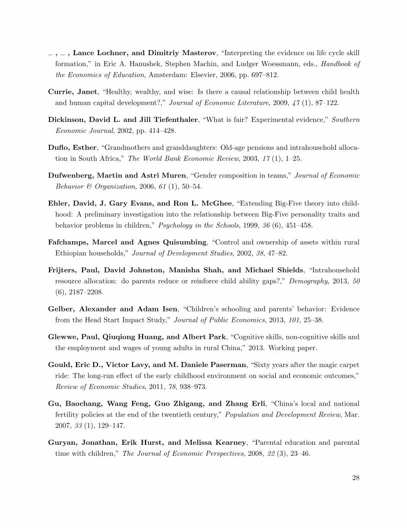
, , Lance Lochner, and Dimitriy Masterov, “Interpreting the evidence on life cycle skill

formation,” in Eric A. Hanushek, Stephen Machin, and Ludger Woessmann, eds., Handbook of

the Economics of Education, Amsterdam: Elsevier, 2006, pp. 697–812.

Currie, Janet, “Healthy, wealthy, and wise: Is there a causal relationship between child health

and human capital development?,” Journal of Economic Literature, 2009, 47 (1), 87–122.

Dickinson, David L. and Jill Tiefenthaler, “What is fair? Experimental evidence,” Southern

Economic Journal, 2002, pp. 414–428.

Duflo, Esther, “Grandmothers and granddaughters: Old-age pensions and intrahousehold alloca-

tion in South Africa,” The World Bank Economic Review, 2003, 17 (1), 1–25.

Dufwenberg, Martin and Astri Muren, “Gender composition in teams,” Journal of Economic

Behavior & Organization, 2006, 61 (1), 50–54.

Ehler, David, J. Gary Evans, and Ron L. McGhee, “Extending Big-Five theory into child-

hood: A preliminary investigation into the relationship between Big-Five personality traits and

behavior problems in children,” Psychology in the Schools, 1999, 36 (6), 451–458.

Fafchamps, Marcel and Agnes Quisumbing, “Control and ownership of assets within rural

Ethiopian households,” Journal of Development Studies, 2002, 38, 47–82.

Frijters, Paul, David Johnston, Manisha Shah, and Michael Shields, “Intrahousehold

resource allocation: do parents reduce or reinforce child ability gaps?,” Demography, 2013, 50

(6), 2187–2208.

Gelber, Alexander and Adam Isen, “Children’s schooling and parents’ behavior: Evidence

from the Head Start Impact Study,” Journal of Public Economics, 2013, 101, 25–38.

Glewwe, Paul, Qiuqiong Huang, and Albert Park, “Cognitive skills, non-cognitive skills and

the employment and wages of young adults in rural China,” 2013. Working paper.

Gould, Eric D., Victor Lavy, and M. Daniele Paserman, “Sixty years after the magic carpet

ride: The long-run effect of the early childhood environment on social and economic outcomes,”

Review of Economic Studies, 2011, 78, 938–973.

Gu, Baochang, Wang Feng, Guo Zhigang, and Zhang Erli, “China’s local and national

fertility policies at the end of the twentieth century,” Population and Development Review, Mar.

2007, 33 (1), 129–147.

Guryan, Jonathan, Erik Hurst, and Melissa Kearney, “Parental education and parental

time with children,” The Journal of Economic Perspectives, 2008, 22 (3), 23–46.

28

Heckman, James J and Yona Rubinstein, “The importance of noncognitive skills: Lessons

from the GED testing program,” American Economic Review, 2001, 91 (2), 145–149.

Heckman, James J., Jora Stixrud, and Sergio Urzua, “The effects of cognitive and noncog-

nitive abilities on labor market outcomes and social behavior,” Journal of Labor Economics,

2006, 24, 411–482.

Heckman, James, Rodrigo Pinto, and Peter Savelyev, “Understanding the mechanisms

through which an influential early childhood program boosted adult outcomes,” The American

economic review, 2013, 103 (6), 2052–2086.

Hsin, Amy, “Is biology destiny? Birth weight and differential parental treatment,” Demography,

2012, 49 (4), 1385–1405.

Juhn, Chinhui, Yona Rubinstein, and C Andrew Zuppann, “The Quantity-Quality Trade-

off and the Formation of Cognitive and Non-cognitive Skills,” Technical Report, National Bureau

of Economic Research 2015.

Kling, Jeffrey, Jeffrey Liebman, and Lawrence Katz, “Experimental analysis of neighbor-

hood effects,” Econometrica, 2007, 75, 83119.

Leight, Jessica, “Sibling rivalry: Ability and intrahousehold allocation in Gansu Province,

China,” 2014. Mimeo.

Neidell, Matthew and Jane Waldfogel, “Cognitive and noncognitive peer effects in early

education,” The Review of Economics and Statistics, 2010, 92 (3), 562–576.

Quisumbing, Agnes and John Maluccio, “Resources at marriage and intrahousehold allo-

cation: Evidence from Bangladesh, Ethiopia, Indonesia and South Africa,” Oxford Bulletin of

Economics and Statistics, 2003, 65, 283–327.

Restropo, Brandon, “Parental Investment Responses to a Low Birth Weight Outcome: Who

Compensates and Who Reinforces,” Forthcoming, Journal of Population Economics, 2016.

Roberts, Brent W. and Wendy F. DelVecchio, “The rank-order consistency of personality

traits from childhood to old age: a quantitative review of longitudinal studies,” Psychological

Bulletin, 2000, 126 (1), 3.

Rosenzweig, Mark and Junsen Zhang, “Do population control policies induce more human

capital investment? Twins, birth weight and China’s “One-Child” Policy,” Review of Economic

Studies, 2009, 76 (3), 1149–74.

Royer, Heather, “Separated at girth: US twin estimates of the effects of birth weight,” American

Economic Journal: Applied Economics, 2009, 1 (1), 49–85.

29

Schweinhart, Lawrence J., Jeanne Montie, Zongping Xiang, William S. Barnett,

Clive R. Belfield, and Milagros Nores, Lifetime effects: The HighScope Perry preschool

study through age 40, Ypsilanti, Michigan: Monographs of the HighScope Educational Research

Foundation, 2005.

Selten, Reinhard and Axel Ockenfels, “An experimental solidarity game,” Journal of Eco-

nomic Behavior and Organization, 1998, 34 (4), 517–539.

Shiner, Rebecca and Avshalom Caspi, “Personality differences in childhood and adolescence:

Measurement, development, and consequences,” Journal of Child Psychology and Psychiatry,

2003, 44 (1), 2–32.

30

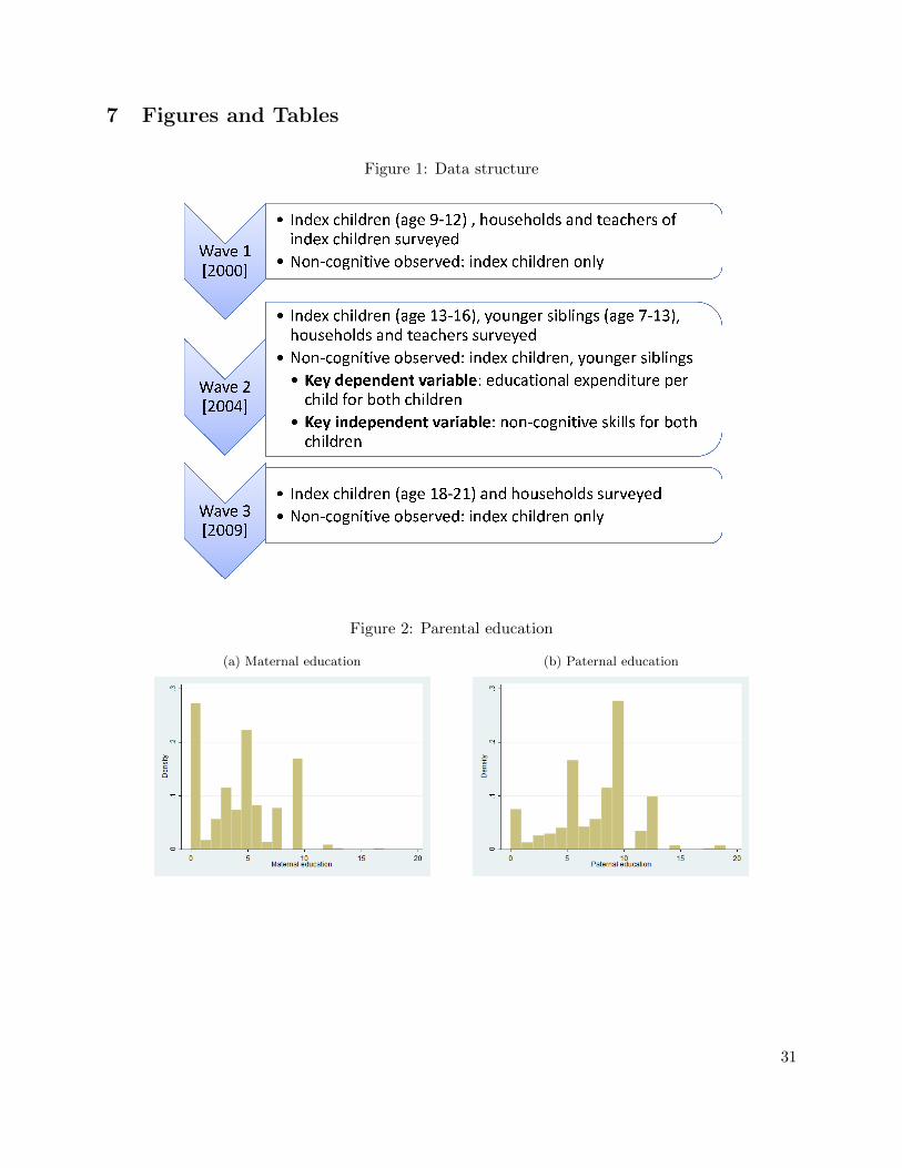
7 Figures and Tables

Figure 1: Data structure

Figure 2: Parental education

(a) Maternal education (b) Paternal education

31

Figure 3: Intra-household differences in non-cognitive characteristics and expenditure, by mother’seducation

(a) Non-cognitive characteristics (b) Expenditure

Notes: For each level of mother’s education in years, the bottom bar corresponds to the minimum value ofbetween-sibling absolute differences in non-cognitive characteristics (Figure 3a) or between-sibling absolutedifferences in normalized educational expenditure residuals (Figure 3b), while the top bar corresponds to themaximum value. The rectangle corresponds to the interquartile range, with the median value represented by thebold line bisecting the rectangle. Normalized expenditure residuals are calculated by regressing expenditure on childcharacteristics (gender, birth parity, cognitive skills, and height-for-age), generating the residuals and standardizingthem to have mean zero and standard deviation one.

32

Table 1: Summary statistics

Panel A: Demographic data Panel B: Educational expenditure per child

Sample Subsample p-value Mean Std. Dev. Max.

Net income 6848.56 6728.28 .863 Total 361.52 343.1 2900Income per capita 1717.76 1631.04 .581 Discretionary 149.03 215.65 1660Mother education 4.31 4.35 .805 Tuition 212.49 185.47 2000Father education 7.12 7.16 .837 Supplies 47.07 43.55 300Mother age 39.19 36.97 .000 Transportation 19.67 50.99 500Father age 42.57 38.89 .072 Food 59.12 139.08 1200Mother time investment 3.05 3.72 .002 Tutoring 9.66 21.42 110Father time investment 2.86 3.43 .001 Other fees 13.50 36.41 360Mother child-rearing decisions .86 .86 .816Father child-rearing decisions 1.08 1.1 .507Index child age 15.09 14.96 .013Internalizing index -.01 .01 .634Externalizing index .03 -.01 .280Achievement index 0 .06 .183

Obs. 1918 388

Notes: The sample encompasses the full sample of households that report income data; this is 1914 out of the fullsample of 2000 households in the survey. The subsample is households with two-children families in which bothchildren report data on non-cognitive characteristics as well as height-for-age. There are 388 households in thesubsample of interest, and 776 children. Income is reported in yuan; educational expenditure is reported in yuanper semester. The child-rearing decisions measure reports the average number of child-rearing decisions each parentreports making alone, out of a total of two (choices about parenting, and choices about the child’s schooling).Internalizing, externalizing and achievement indices have been standardized to have means equal to zero andstandard deviations equal to one. A higher internalizing or externalizing index is indicative of fewer non-cognitivechallenges. Column (3) reports the p-value for a test of equality of means across the sample and subsample.

33

Tab

le2:

Non

-cog

nit

ive

char

acte

rist

ics

and

chil

dch

arac

teri

stic

s

Inte

rnal

Exte

rnal

Inte

rnal

Exte

rnal

Inte

rnal

Exte

rnal

Inte

rnal

Exte

rnal

Inte

rnal

Exte

rnal

(1)

(2)

(3)

(4)

(5)

(6)

(7)

(8)

(9)

(10)

Panel

A:

Child

chara

cte

rist

ics

Sib

ling

pari

ty.0

03

-.118∗∗

.143

.131

(.058)

(.059)

(.140)

(.119)

Age

.008

.039∗∗

.007

-.076∗

(.017)

(.018)

(.051)

(.044)

Fem

ale

-.006

.315∗∗

∗-.

007

.289∗∗

∗

(.077)

(.083)

(.080)

(.074)

Gra

de

level

.015

.068∗∗

∗.0

46

.159∗∗

∗

(.019)

(.020)

(.045)

(.054)

Panel

B:

Cognit

ive

skills

and

healt

h

Hei

ght-

for-

age

.013

.042

.019

.045

(.030)

(.039)

(.029)

(.038)

Math

score

-.0007

.002

-.0005

-.0009

(.003)

(.005)

(.005)

(.006)

Chin

ese

score

.0009

.005

.004

.007

(.005)

(.005)

(.007)

(.007)

Ach

ievem

ent

score

-.006∗∗

-.005

-.006∗∗

-.005∗

(.003)

(.003)

(.003)

(.003)

Obs.

776

776

776

776

776

776

776

776

776

776

Note

s:T

he

dep

enden

tva

riable

sare

the

inte

rnalizi

ng

and

exte

rnalizi

ng

indic

es.

Ahig

her

inte

rnalizi

ng

or

exte

rnalizi

ng

index

isin

dic

ati

ve

of

few

ernon-c

ognit

ive

challen

ges

.T

he

indep

enden

tva

riable

isth

esp

ecifi

edch

ild

chara

cter

isti

c,all

mea

sure

din

the

seco

nd

wav

e;all

spec

ifica

tions

incl

ude

house

hold

fixed

effec

tsand

standard

erro

rscl

ust

ered

at

the

county

level

.A

ster

isks

indic

ate

signifi

cant

at

the

10,

5and

1p

erce

nt

level

s.

34

Table 3: Parental allocations and non-cognitive characteristics

Total Discretionary Tuition Supplies Transportation Food Tutoring Other(1) (2) (3) (4) (5) (6) (7) (8)

Panel A: Internalizing index

Index -8.010 -10.019 2.009 .591 -.617 -10.713∗ -1.056 1.776(10.770) (8.021) (4.065) (1.635) (1.247) (5.873) (.712) (1.437)

Panel B: Externalizing index

Index .028 -2.772 2.800 2.366∗ .252 -6.048 -.284 .941(11.850) (7.854) (5.576) (1.405) (1.348) (5.799) (.730) (.912)

Obs. 776 776 776 776 776 776 776 776

Mean (dep. var.) 276.748 104.052 172.696 38.164 12.011 37.679 6.218 9.98St. dev. (dep. var.) 286.515 174.218 161.381 38.785 40.065 109.107 17.357 28.532

Notes: The dependent variables are educational expenditure per semester per child in the specified category; totalexpenditure is the sum of all categories, and discretionary expenditure is the sum of all categories excluding tuition.The independent variable is the specified index of internalizing or externalizing behavior. A higher internalizing orexternalizing index is indicative of fewer non-cognitive challenges. All specifications include controls for siblingparity, gender, sibling gender, height-for-age and cognitive skills measured contemporaneously with non-cognitiveskills, year-of-birth and household fixed effects, and standard errors clustered at the county level. Asterisks indicatesignificance at the 10, 5 and 1 percent levels.

35

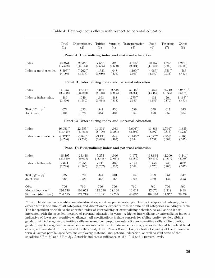
Table 4: Heterogeneous effects with respect to parental education

Total Discretionary Tuition Supplies Transportation Food Tutoring Other(1) (2) (3) (4) (5) (6) (7) (8)

Panel A: Internalizing index and maternal education

Index 27.973 20.386 7.588 .392 4.365∗ 10.157 1.253 4.219∗∗

(17.338) (14.144) (7.585) (1.600) (2.504) (11.232) (.829) (2.080)

Index x mother educ. -8.595∗∗ -7.262∗∗ -1.333 .048 -1.190∗∗ -4.985∗ -.551∗∗ -.583(4.186) (3.617) (1.686) (.426) (.606) (2.652) (.231) (.442)

Panel B: Internalizing index and paternal education

Index -11.252 -17.317 6.066 -2.838 5.045∗ -9.825 -2.712 -6.987∗∗∗

(20.718) (16.862) (8.148) (1.905) (2.664) (14.485) (1.725) (2.676)

Index x father educ. .286 .949 -.663 .488 -.775∗∗ -.131 .204 1.163∗∗

(2.329) (1.580) (1.414) (.314) (.340) (1.355) (.170) (.472)

Test βm2 = βf

2 .072 .023 .847 .430 .589 .070 .017 .013Joint test .184 .073 .857 .484 .084 .180 .052 .034

Panel C: Externalizing index and maternal education

Index 36.951∗∗ 22.555∗ 14.396∗ -.033 5.606∗∗ 13.883 1.764∗∗ 1.335(15.425) (11.563) (8.706) (1.281) (2.391) (8.492) (.813) (1.227)

Index x mother educ -9.971∗∗ -6.840∗ -3.131 .648 -1.446∗∗ -5.382∗∗ -.553∗ -.106(4.740) (3.531) (2.495) (.403) (.644) (2.531) (.309) (.325)

Panel D: Externalizing index and paternal education

Index -18.195 -23.448 5.253 -.946 1.977 -18.834 -2.200 -3.444∗

(26.820) (19.075) (11.498) (2.617) (2.666) (15.555) (1.857) (2.008)

Index x father educ 2.644 2.855 -.211 .408 -.197 1.758 .243 .643∗

(2.725) (1.983) (1.287) (.325) (.362) (1.570) (.203) (.347)

Test βm2 = βf

2 .027 .020 .344 .601 .064 .028 .051 .347Joint test .085 .058 .453 .168 .099 .089 .144 .473

Obs. 766 766 766 766 766 766 766 766Mean (dep. var.) 276.748 104.052 172.696 38.164 12.011 37.679 6.218 9.98St. dev. (dep. var.) 286.515 174.218 161.381 38.785 40.065 109.107 17.357 28.532

Notes: The dependent variables are educational expenditure per semester per child in the specified category; totalexpenditure is the sum of all categories, and discretionary expenditure is the sum of all categories excluding tuition.The independent variable is the specified index of internalizing or externalizing behavior, as well as the indexinteracted with the specified measure of parental education in years. A higher internalizing or externalizing index isindicative of fewer non-cognitive challenges. All specifications include controls for sibling parity, gender, siblinggender, height-for-age and cognitive skills measured contemporaneously with non-cognitive skills, sibling parity,gender, height-for-age and achievement scores interacted with maternal education, year-of-birth and household fixedeffects, and standard errors clustered at the county level. Panels B and D report tests of equality of the interactionterm β2 across parallel specifications employing maternal and paternal education, as well as joint tests of theequalities βm

1 = βf1 and βm

2 = βf2 . Asterisks indicate significance at the 10, 5 and 1 percent levels.

36

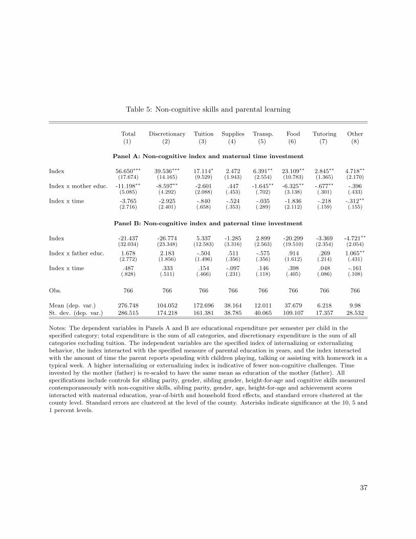
Table 5: Non-cognitive skills and parental learning

Total Discretionary Tuition Supplies Transp. Food Tutoring Other(1) (2) (3) (4) (5) (6) (7) (8)

Panel A: Non-cognitive index and maternal time investment

Index 56.650∗∗∗ 39.536∗∗∗ 17.114∗ 2.472 6.391∗∗ 23.109∗∗ 2.845∗∗ 4.718∗∗

(17.674) (14.165) (9.529) (1.943) (2.554) (10.783) (1.365) (2.170)

Index x mother educ. -11.198∗∗ -8.597∗∗ -2.601 .447 -1.645∗∗ -6.325∗∗ -.677∗∗ -.396(5.085) (4.292) (2.088) (.453) (.702) (3.138) (.301) (.433)

Index x time -3.765 -2.925 -.840 -.524 -.035 -1.836 -.218 -.312∗∗

(2.716) (2.401) (.658) (.353) (.289) (2.112) (.159) (.155)

Panel B: Non-cognitive index and paternal time investment

Index -21.437 -26.774 5.337 -1.285 2.899 -20.299 -3.369 -4.721∗∗

(32.034) (23.348) (12.583) (3.316) (2.563) (19.510) (2.354) (2.054)

Index x father educ. 1.678 2.183 -.504 .511 -.575 .914 .269 1.065∗∗

(2.772) (1.856) (1.496) (.356) (.356) (1.612) (.214) (.431)

Index x time .487 .333 .154 -.097 .146 .398 .048 -.161(.828) (.511) (.466) (.231) (.118) (.405) (.086) (.108)

Obs. 766 766 766 766 766 766 766 766

Mean (dep. var.) 276.748 104.052 172.696 38.164 12.011 37.679 6.218 9.98St. dev. (dep. var.) 286.515 174.218 161.381 38.785 40.065 109.107 17.357 28.532

Notes: The dependent variables in Panels A and B are educational expenditure per semester per child in thespecified category; total expenditure is the sum of all categories, and discretionary expenditure is the sum of allcategories excluding tuition. The independent variables are the specified index of internalizing or externalizingbehavior, the index interacted with the specified measure of parental education in years, and the index interactedwith the amount of time the parent reports spending with children playing, talking or assisting with homework in atypical week. A higher internalizing or externalizing index is indicative of fewer non-cognitive challenges. Timeinvested by the mother (father) is re-scaled to have the same mean as education of the mother (father). Allspecifications include controls for sibling parity, gender, sibling gender, height-for-age and cognitive skills measuredcontemporaneously with non-cognitive skills, sibling parity, gender, age, height-for-age and achievement scoresinteracted with maternal education, year-of-birth and household fixed effects, and standard errors clustered at thecounty level. Standard errors are clustered at the level of the county. Asterisks indicate significance at the 10, 5 and1 percent levels.

37

Table 6: Heterogeneous effects with respect to maternal education and income

Total Discretionary Tuition Supplies Transportation Food Tutoring Other(1) (2) (3) (4) (5) (6) (7) (8)

Index 42.020∗∗ 29.815∗ 12.204 .520 6.639∗∗ 16.680 2.264∗∗ 3.712∗∗

(19.792) (15.645) (8.968) (1.473) (3.053) (11.959) (.891) (1.841)

Index x educ. -11.308∗∗ -8.161∗∗ -3.146 .458 -1.524∗∗ -6.156∗∗ -.599∗ -.340(4.879) (4.124) (2.185) (.522) (.616) (3.030) (.307) (.465)

Index x income -.571 -1.243 .672 -.120 -.192 -.621 -.162∗ -.148(1.401) (.896) (.678) (.149) (.198) (.563) (.087) (.111)

Obs. 776 776 776 776 776 776 776 776

Mean (dep. var.) 276.748 104.052 172.696 38.164 12.011 37.679 6.218 9.98St. dev. (dep. var.) 286.515 174.218 161.381 38.785 40.065 109.107 17.357 28.532

Notes: The dependent variables are educational expenditure per semester per child in the specified category; totalexpenditure is the sum of all categories, and discretionary expenditure is the sum of all categories excluding tuition.The independent variable is the specified index of internalizing or externalizing behavior, the index interacted withthe specified measure of parental education in years, and the index interacted with household net income. A higherinternalizing or externalizing index is indicative of fewer non-cognitive challenges. Net income is re-scaled to havethe same mean as maternal education. All specifications include controls for sibling parity, gender, sibling gender,height-for-age and cognitive skills measured contemporaneously with non-cognitive skills, sibling parity, gender, age,height-for-age and achievement scores interacted with maternal education, year-of-birth and household fixed effects,and standard errors clustered at the county level. Asterisks indicate significance at the 10, 5 and 1 percent levels.

38

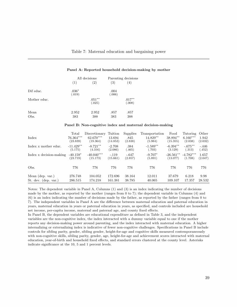
Table 7: Maternal education and bargaining power

Panel A: Reported household decision-making by mother

All decisions Parenting decisions(1) (2) (3) (4)

Dif educ. .036∗ .004(.019) (.006)

Mother educ. .051∗∗ .017∗∗

(.025) (.008)

Mean 2.952 2.952 .857 .857Obs. 383 388 383 388

Panel B: Non-cognitive index and maternal decision-making

Total Discretionary Tuition Supplies Transportation Food Tutoring OtherIndex 76.364∗∗∗ 62.670∗∗∗ 13.694 .845 14.829∗∗ 38.894∗∗ 6.160∗∗∗ 1.942

(23.839) (19.364) (14.853) (2.838) (5.984) (15.355) (2.038) (2.032)

Index x mother educ. -11.429∗∗ -8.721∗∗ -2.708 .384 -1.589∗∗ -6.394∗∗ -.675∗∗ -.446(5.175) (4.316) (2.086) (.465) (.703) (3.129) (.313) (.452)

Index x decision-making -40.159∗ -40.040∗∗∗ -.119 -.647 -9.707∗ -26.561∗∗ -4.782∗∗∗ 1.657(23.719) (15.173) (15.661) (2.857) (5.891) (13.077) (1.708) (2.047)

Obs. 776 776 776 776 776 776 776 776

Mean (dep. var.) 276.748 104.052 172.696 38.164 12.011 37.679 6.218 9.98St. dev. (dep. var.) 286.515 174.218 161.381 38.785 40.065 109.107 17.357 28.532

Notes: The dependent variable in Panel A, Columns (1) and (3) is an index indicating the number of decisionsmade by the mother, as reported by the mother (ranges from 0 to 7); the dependent variable in Columns (4) and(6) is an index indicating the number of decisions made by the father, as reported by the father (ranges from 0 to7). The independent variables in Panel A are the difference between maternal education and paternal education inyears, maternal education in years or paternal education in years, as specified, and controls included are householdnet income, per-capita income, maternal and paternal age, and county fixed effects.In Panel B, the dependent variables are educational expenditure as defined in Table 3, and the independentvariables are the non-cognitive index, the index interacted with a dummy variable equal to one if the motherreports any decision-making power around parenting, and the index interacted with maternal education. A higherinternalizing or externalizing index is indicative of fewer non-cognitive challenges. Specifications in Panel B includecontrols for sibling parity, gender, sibling gender, height-for-age and cognitive skills measured contemporaneouslywith non-cognitive skills, sibling parity, gender, age, height-for-age and achievement scores interacted with maternaleducation, year-of-birth and household fixed effects, and standard errors clustered at the county level. Asterisksindicate significance at the 10, 5 and 1 percent levels.

39

Table 8: Persistence of non-cognitive skills in percentile and parental education

Internal 2004 External 2004 Rosenberg 2009 Depression 2009(1) (2) (3) (4) (5) (6) (7) (8)

Psychometric index 2000 .001 .067 -.005 .046(.093) (.078) (.059) (.054)

Mother educ. 2000 int. -.143∗∗ -.083(.059) (.070)

Father educ. 2000 int. .159 .127(.121) (.106)

Exp. 2000 int. -.002∗∗∗ -.0009∗∗

(.0005) (.0004)

Psychometric index 2004 .110 .093 .131∗∗ .164∗∗∗

(.096) (.070) (.063) (.048)

Mother educ. 2004 int. -.181∗ -.004(.107) (.099)

Father educ. 2004 int. .118 -.025(.116) (.106)

Exp. 2004 int. -.00002 -.0004∗∗

(.0003) (.0002)

Obs. 550 550 550 550 408 408 410 410

Notes: The dependent variables are the specified measure of non-cognitive skills from waves two and three,calculated in percentile terms. A higher index in internalizing or externalizing behavior is indicative of fewernoncognitive challenges. A higher percentile in the Rosenberg index is associated with higher self-esteem. Thedepression index is inverted, and thus a higher percentile in the depression index is indicative of a lower level ofdepression. The independent variables include the psychometric index, the mean of internalizing and externalizingindices from waves one and two, calculated in percentile terms. The psychometric index is also interacted withdummy variables for the mother’s (father’s) education being above the median, and discretionary educationalexpenditure. All specifications include controls for cognitive skills measured in waves one and two, grades in mathand Chinese, height-for-age, the parental education dummy variables, net income, assets, and fixed capital in thehousehold, the number of siblings, sibling gender, and sibling gender interacted with the number of siblings, andcounty and year-of-birth fixed effects; the specifications including an interaction effect with expenditure also includelinear and quadratic terms for total and discretionary educational expenditure, and a dummy for discretionaryexpenditure above the median. Standard errors are clustered at the level of the county. Asterisks indicatesignificance at the 10, 5 and 1 percent levels.

40

Appendix

Table A1: Within-household and cross-household variation

Internal External Height-for-age Achievement score Grades(1) (2) (3) (4) (5) (6) (7) (8) (9) (10)

Fixed effects Household Year Household Year Household Year Household Year Household Year

Obs. 776 776 776 776 776 776 776 776 776 776R-squared .600 .021 .620 .016 .828 .067 .864 .054 .676 .034

Notes: Each column reports the R-squared for the regression of the specified child characteristic on the specified setof fixed effects.

41

Table A2: Parental allocations and non-cognitive characteristics: Alternate specifications

Total Discretionary Tuition Supplies Transportation Food Tutoring Other(1) (2) (3) (4) (5) (6) (7) (8)

Panel A: Results unconditional on child characteristics

Index 38.182∗∗ 24.918∗ 13.265 .520 5.902∗∗ 13.422 1.465∗∗ 3.609(15.827) (13.257) (8.286) (1.443) (2.552) (10.643) (.720) (2.584)

Index x mother educ. -11.467∗∗ -8.740∗∗ -2.727 .129 -1.534∗∗∗ -6.293∗∗ -.525∗ -.516(4.752) (3.939) (2.169) (.528) (.552) (2.829) (.284) (.519)

Obs. 776 776 776 776 776 776 776 776

Panel B: Households including two or more children

Index 29.733∗∗ 18.451∗ 11.282∗∗ .786 4.462∗ 9.526 1.042 2.635∗∗

(12.185) (9.588) (5.406) (.965) (2.334) (7.144) (.965) (1.119)

Index x mother educ. -8.238∗∗ -5.680∗∗ -2.558 .269 -.864 -3.756∗ -.999 -.330(3.554) (2.896) (1.576) (.335) (.540) (1.973) (.668) (.275)

Obs. 1132 1132 1132 1132 1132 1132 1132 1132

Panel C: Households including a first-born son

Index 48.862∗ 39.267∗∗ 9.595 1.790 6.373 27.235∗∗ 2.954∗∗ .915(25.905) (18.256) (11.187) (1.876) (3.928) (13.106) (1.444) (1.593)

Index x mother educ. -13.411∗ -11.645∗∗ -1.766 -.184 -1.674 -8.777∗∗ -1.022∗∗ .012(7.697) (5.729) (2.911) (.520) (1.077) (4.148) (.437) (.669)

Obs. 390 390 390 390 390 390 390 390

Mean (dep. var.) 261.867 94.244 167.622 36.22 10.658 31.111 7.025 9.23St. dev. (dep. var.) 273.416 168.236 148.407 37.226 37.467 102.985 33.987 30.367

Notes: The dependent variables are educational expenditure per semester per child in the specified category; totalexpenditure is the sum of all categories, and discretionary expenditure is the sum of all categories excluding tuition.The independent variable is a mean index of non-cognitive skills and the interaction of this index with maternaleducation. A higher internalizing or externalizing index is indicative of fewer non-cognitive challenges. In Panel A,the specifications include year-of-birth and household fixed effects, and standard errors clustered at the county level;the sample is households with two children. In Panel B, all specifications include controls for sibling parity, gender,sibling gender, height-for-age and cognitive skills, sibling parity, gender, age, height-for-age and achievement scoresinteracted with maternal education, year-of-birth and household fixed effects, and standard errors clustered at thecounty level; the sample is households with two or more children. Asterisks indicate significance at the 10, 5 and 1percent levels.

42

Table A3: Heterogeneous effects: Addressing bias due to serial correlation in expenditure

Total Discretionary Tuition Supplies Transp. and food Tutoring Other fees(1) (2) (3) (4) (5) (6) (7) (8)

Panel A: Maternal education and non-cognitive index

Index 9.480∗ 6.518∗ 2.962 1.455 1.611 .317 .069(5.508) (3.862) (3.558) (1.904) (1.090) (.286) (1.448)

Index x mother educ. -3.820∗∗ -2.643∗∗ -1.177 -.897∗∗ -1.045∗ -.115 -.054(1.829) (1.208) (1.061) (.420) (.582) (.082) (.464)

Obs. 756 756 756 756 756 756 756

Panel B: Paternal education and non-cognitive index

Index -17.016 3.775 -20.791 1.076 -2.584 -.781∗∗ 2.551(18.593) (7.605) (15.264) (2.487) (2.235) (.379) (2.340)

Index x father educ. 1.762 -1.017 2.779 -.423 .048 .096∗ -.445(2.450) (.770) (2.122) (.311) (.236) (.056) (.346)

Mean (dep. var.) 159.95 49.19 110.76 25.06 5.42 1.52 9.75St. dev. (dep. var.) 133.65 78.21 89.91 24.35 32.7 7.9 25.11Obs. 756 756 756 756 756 756 756

Panel C: Maternal education including controls for past expenditure

Total Discretionary Tuition Supplies Transportation Food Tutoring Other

Index 40.791∗∗ 27.190∗ 13.601 .267 6.230∗∗ 15.364 1.927∗∗ 3.402∗

(18.974) (15.689) (8.923) (1.399) (2.987) (12.149) (.955) (1.822)

Index x mother educ. -11.692∗∗ -8.987∗∗ -2.705 .378 -1.653∗∗ -6.569∗∗ -.706∗∗ -.437(5.004) (4.238) (2.105) (.463) (.707) (3.095) (.312) (.433)

Mean (dep. var.) 276.748 104.052 172.696 38.164 12.011 37.679 6.218 9.98St. dev. (dep. var.) 286.515 174.218 161.381 38.785 40.065 109.107 17.357 28.532Obs. 776 776 776 776 776 776 776 776

Notes: In Panel A and Panel B, the dependent variables are educational expenditure per semester per child in thespecified category at primary school age (as observed in wave one for the first-born child and in wave two for thesecond-born child); total expenditure is the sum of all categories, and discretionary expenditure is the sum of allcategories excluding tuition. The independent variables in Panels A and B include a non-cognitive index asmeasured at primary school age, as well as the index interacted with the specified measure of parental education. Ahigher internalizing or externalizing index is indicative of fewer non-cognitive challenges. All specifications includecontrols for sibling parity, gender, sibling gender, height-for-age and cognitive skills measured contemporaneouslywith non-cognitive skills, sibling parity, gender, age, height-for-age and achievement scores interacted with maternaleducation, year-of-birth and household fixed effects, and standard errors clustered at the county level. Specificationsin Panel C are similar to those in Table 4 and include an additional control for lagged educational expenditure (asreported in wave one). Asterisks indicate significance at the 10, 5 and 1 percent levels.

43

Table A4: Heterogeneous effects with respect to maternal favorite

Total Discretionary Tuition Supplies Transportation Food Tutoring Other

Index 40.644∗∗ 27.199∗ 13.445 .283 6.230∗∗ 15.348 1.902∗∗ 3.435∗

(18.599) (15.198) (8.873) (1.370) (2.845) (11.894) (.926) (1.846)

Index x mother educ. -11.693∗∗ -9.023∗∗ -2.670 .366 -1.653∗∗ -6.587∗∗ -.701∗∗ -.447(5.181) (4.352) (2.111) (.460) (.702) (3.163) (.320) (.448)

Favorite 11.545 -1.244 12.789 -1.940 .535 .839 2.113 -2.790(24.908) (19.064) (9.275) (6.472) (4.874) (13.812) (2.238) (1.912)

Favorite x mother educ. 6.370 7.054 -.684 1.222 .723 4.281 .293 .535(8.962) (5.643) (4.555) (1.476) (1.375) (4.232) (.490) (.520)

Obs. 776 776 776 776 776 776 776 776

Mean (dep. var.) 276.748 104.052 172.696 38.164 12.011 37.679 6.218 9.98St. dev. (dep. var.) 286.515 174.218 161.381 38.785 40.065 109.107 17.357 28.532

Notes: The dependent variable is educational expenditure in the specified category, and the independent variablesare the non-cognitive index and a dummy for the child being reported as the maternal favorite, and both variablesinteracted with maternal education. A higher internalizing or externalizing index is indicative of fewer non-cognitivechallenges. All specifications include controls for sibling parity, gender, sibling gender, height-for-age and cognitiveskills measured contemporaneously with non-cognitive skills, sibling parity, gender, age, height-for-age andachievement scores interacted with maternal education, year-of-birth and household fixed effects, and standarderrors clustered at the county level. Standard errors are clustered at the level of the county.

Table A5: Alternate measures of non-cognitive skills: teacher reports

Total Discretionary Tuition Supplies Transportation Food Tutoring Other(1) (2) (3) (4) (5) (6) (7) (8)

Teacher index 34.132 28.784∗ 5.348 8.086 4.973 13.544 .136 2.045(25.439) (16.150) (12.351) (5.030) (4.655) (8.644) (2.061) (2.044)

Index x mother educ. -14.294∗∗ -13.210∗∗∗ -1.085 -1.586∗∗ -2.785∗∗ -8.496∗∗∗ -.282 -.061(5.642) (4.078) (2.626) (.764) (1.121) (2.551) (.592) (.272)

Obs. 774 774 774 774 774 774 774 774

Mean (dep. var.) 276.748 104.052 172.696 38.164 12.011 37.679 6.218 9.98St. dev. (dep. var.) 286.515 174.218 161.381 38.785 40.065 109.107 17.357 28.532

Notes: The dependent variables are educational expenditure per semester per child in the specified category; totalexpenditure is the sum of all categories, and discretionary expenditure is the sum of all categories excluding tuition.The independent variables are a dummy variable equal to one if an index of non-cognitive skills based on teacherreports of the child’s behavior is above the mean, and the interaction of this dummy variable with maternaleducation. All specifications include controls for sibling parity, gender, sibling gender, height-for-age and cognitiveskills measured contemporaneously with non-cognitive skills, sibling parity, gender, age, height-for-age andachievement scores interacted with maternal education, year-of-birth and household fixed effects, and standarderrors clustered at the county level. Asterisks indicate significance at the 10, 5 and 1 percent levels.

44