Material Qualification and Equivalency for Polymer Matrix ... · 11. Contract or Grant No. 12....

DOT/FAA/AR-00/47 Office of Aviation Research Washington, D.C. 20591

Material Qualification and Equivalency for Polymer Matrix Composite Material Systems April 2001 Final Report This document is available to the U.S. public through the National Technical Information Service (NTIS), Springfield, Virginia 22161.

U.S. Department of Transportation Federal Aviation Administration

NOTICE

This document is disseminated under the sponsorship of the U.S. Department of Transportation in the interest of information exchange. The United States Government assumes no liability for the contents or use thereof. The United States Government does not endorse products or manufacturers. Trade or manufacturer’s names appear herein solely because they are considered essential to the objective of this report. This document does not constitute FAA certification policy. Consult your local FAA aircraft certification office as to its use. This report is available at the Federal Aviation Administration William J. Hughes Technical Center’s Full-Text Technical Reports page: actlibrary.tc.faa.gov in Adobe Acrobat portable document format (PDF).

Technical Report Documentation Page

1. Report No. DOT/FAA/AR-00/47

2. Government Accession No. 3. Recipient’s Catalog No.

4. Title and Subtitle MATERIAL QUALIFICATION AND EQUIVALENCY FOR POLYMER

5. Report Date April 2001

MATRIX COMPOSITE MATERIAL SYSTEMS 6. Performing Organization Code

7. Author(s)

John S. Tomblin, Yeow C. Ng, and K. Suresh Raju

8. Performing Organization Report No.

9. Performing Organization Name and Address

National Institute for Aviation Research Wichita State University

10. Work Unit No. (TRAIS)

1845 North Fairmount Wichita, KS 67260-0093

11. Contract or Grant No.

12. Sponsoring Agency Name and Address

U.S. Department of Transportation Federal Aviation Administration

13. Type of Report and Period Covered Final Report

Office of Aviation Research Washington, DC 20591

14. Sponsoring Agency Code

ACE-110 15. Supplementary Notes The FAA William J. Hughes Technical Monitor was Peter Shyprykevich. 16. Abstract This document presents a qualification plan that will provide the detailed background information and engineering practices to help ensure the control of repeatable base material properties and processes, which are applied to both primary and secondary structures for aircraft products using composite materials. This qualification plan includes recommendations for the original qualification as well as procedures to statistically establish equivalence to the original data set. The plan describes in detail the procedures to generate statistically based design allowables for both A- and B-basis applications. Specific test matrices are presented which produce lamina level composite material properties for various loading modes and environmental conditions for aircraft applications not exceeding 200oF. This plan only covers the initial material qualification at the lamina level and does not include procedures for laminate or higher-level building block tests. The general methodology, however, is applicable to a broader usage. 17. Key Words Composite material, Qualification, Equivalence, Acceptance, Criteria, A- and B-B-basis, aircraft structures

18. Distribution Statement This document is available to the public through the National Technical Information Service (NTIS), Springfield, Virginia 22161.

19. Security Classif. (of this report)

Unclassified

20. Security Classif. (of this page)

Unclassified

21. No. of Pages

119

22. Price

Form DOT F1700.7 (8-72) Reproduction of completed page authorized

iii/iv

ACKNOWLEDGEMENTS The following document was assembled with help from many individuals across many areas of expertise. The following people should be acknowledged for their individual contributions to this document:

K. Bowman, Scaled Composites L. Cheng, FAA M. Chris, Bell Helicopter Textron L. Dunham, Wichita State E. Hooper, Toyota Aircraft L. Ilcewicz, FAA J. McKenna, Wichita State D. Oplinger, FAA D. Ostrodka, FAA D. Showers, FAA P. Shyprykevich, FAA T. Smyth, FAA J. Soderquist, FAA (retired) D. Swartz, FAA M. Vangel, Dana Farber Cancer Institute S. Ward, SW Composites

v

TABLE OF CONTENTS

Page

EXECUTIVE SUMMARY xiii

1. INTRODUCTION 1

1.1 Scope 1 1.2 Field of Application 1 1.3 Applicable Documents 1

2. APPLICABLE FAA REGULATIONS AND RECOMMENDATIONS 2

2.1 Applicable Federal Regulations 2 2.2 Applicable Advisory Circular (AC) Recommendations 3

2.2.1 AC 20-107A Composite Aircraft Structures 3

2.2.2 AC 21-26 Quality Control for the Manufacture of Composite

Structures 3 3. COMPOSITE TEST METHODS AND SPECIMEN GEOMETRY 4

3.1 Specimen Manufacturing 4

3.1.1 Number of Specimens 5 3.1.2 Panel Sizes 5 3.1.3 Panel Manufacturing 5 3.1.4 Tabs 7 3.1.5 Specimen Machining 7 3.1.6 Specimen Selection 7 3.1.7 Specimen Naming 7 3.1.8 Strain Gage Bonding 8 3.1.9 Specimen Dimensioning and Inspection 9

3.2 Environmental Conditioning 9

3.2.1 Traveler Specimens 9 3.2.2 Equilibrium Criteria 10

3.3 Nonambient Testing 10

3.3.1 Temperature Chamber 10 3.3.2 Testing at Elevated Temperatures 10 3.3.3 Testing at Subzero Temperatures 11

vi

3.4 Specimen Geometry and Test Methods 11

3.4.1 General 11 3.4.2 References 11 3.4.3 Unidirectional Material Forms 12 3.4.4 Woven Fabric Material Forms 12 3.4.5 Mechanical Property Testing and Specimen Geometry 15 3.4.6 Additional Test Methods 28

4. QUALIFICATION PROGRAM 31

4.1 Introduction 31 4.2 General 31 4.3 Technical Requirements 31 4.4 Material Qualification Program for Uncured Prepreg 31 4.5 Material Qualification Program for Cured Lamina Main Properties 32

4.5.1 Reduced Sampling Requirements for B-Basis Allowables 34 4.5.2 Robust Sampling Requirements for A- and B-Basis Allowables 35 4.5.3 Fluid Sensitivity Screening 35

5. DESIGN ALLOWABLE GENERATION 36

5.1 Introduction 36 5.2 Normalization 37

5.2.1 Normalization Procedure 37 5.2.2 Application of Normalization 39

5.3 Statistical Analysis 40

5.3.1 Methodology 40 5.3.2 Example of B-Basis Calculation 50

5.4 Material Performance Envelope and Interpolation 55

6. MATERIAL EQUIVALENCY AND ACCEPTANCE TESTING 57

6.1 Material Equivalence 60 6.2 Acceptance Testing 64 6.3 Statistical Tests for Material Equivalency and Acceptance Testing 66

6.3.1 Failure for Decrease in Mean or Minimum Individual 67 6.3.2 Failure for Change in Mean 68 6.3.3 Failure for a High Mean 69 6.3.4 Criteria Specific to Material Equivalence 70

vii

6.3.5 Criteria Specific to Acceptance Testing 70 6.3.6 Statistical Testing Examples 71

6.4 Further Discussion 74

6.4.1 Effects of Coefficient of Variation 74 6.4.2 Type 1 and Type 2 Errors 74 6.4.3 Some Unaccounted Forms of Error 79 6.4.4 Assumptions 80 6.4.5 Generating a New Material Qualification Database 80 6.4.6 Qualification of an Alternate Material 81

7. CONCLUDING REMARKS AND FUTURE NEEDS 82 8. REFERENCES 83 9. GLOSSARY 84 APPENDICES A Robust Sampling Panel Requirements B Reduced Sampling Panel Requirements C Laminate Lay-Up and Bagging Guide

viii

LIST OF FIGURES Figure Page 1 Reduced Sampling 6

2 Robust Sampling 6

3 Skewed Lines Drawn Across Subpanel Used for Reconstruction 8

4 Unidirectional Tape With Defined Directions 12

5 Warp and Fill Directions for Woven Fabric Material 13

6 Plain Weave Fabric Construction 14

7 Satin Weave Fabric Construction 14

8 Example Satin Weave Showing Alternating Warp and Fill Faces Used for Lamination 15

9 Zero-Degree Unidirectional Tape Tension Specimen 16

10 Zero-Degree (Warp) Woven Fabric Tension Specimen 17

11 Ninety-Degree (Fill) Woven Fabric and Unidirectional Tension Specimens 17

12 Zero-Degree (Warp) Woven Fabric and Unidirectional Compression Strength Specimens 19

13 Zero-Degree (Warp) Woven Fabric and Unidirectional Compression Modulus Specimens 20

14 Ninety-Degree (Fill) Woven Fabric and Unidirectional Compression Strength Specimens 21

15 Ninety-Degree (Fill) Woven Fabric and Unidirectional Compression Modulus Specimens 22

16 In-Plane Shear Strength and Modulus Specimen 25

17 Short-Beam Shear Strength Specimen 26

18 Glass Transition Temperature Determination From Storage Modulus 30

19 Stepwise Data Reduction Procedure for Design Allowable Generation 43

20 Procedures to Obtain Design Allowables in the Case of Variance Inequality 50

ix

21 Normalized Fit of Experimental Data for Each Environment 53

22 Normalized Fit of Pooled Data 54

23 Material Performance Envelope 55

24 Example of 150°F Interpolation for B-Basis Values 57

25 An Example of Specimen Selection Methodology and Processing Traceability per Test Method and Environmental Condition Used to Establish Material Equivalence 62

26 A Normal Distribution, Two Specimens 75

27 A Normal Distribution, Ten Specimens 76

28 Two Normal Distributions With Equal Means but Unequal Standard Deviations 77

29 Two Normal Distributions of Equal Standard Deviations, Close but Unequal Means, Ten Specimens 78

30 Two Normal Distributions of Equal Standard Deviations, Unequal Means, Ten Specimens 78

31 Two Normal Distributions of Equal Standard Deviations, Unequal Means, Two Specimens 79

32 Flowchart Illustrating Procedures for Selecting and Demonstrating Equivalency for an Alternate Material 81

LIST OF TABLES Table Page 1 Recommended Physical and Chemical Property Tests to be Performed by

Material Vendor 32

2 Cured Lamina Physical Property Tests 33

3 Reduced Sampling Requirements for Cured Lamina Main Properties 34

4 Robust Sampling Requirements for Cured Lamina Main Properties 35

5 Fluid Types Used for Sensitivity Studies 36

6 Material Qualification Program for Fluid Resistance 36

x

7 Critical Values 45

8 Example Data Set for Each Testing Environment per Table 3 51

9 Calculated MNR Statistic for the Environmentally Grouped Data 52

10 Resulting Pooled Data After Normalization Procedure 53

11 Suitable Pass/Fail Criteria and Test Statistic for Each Property of Interest 59

12 Material Equivalence Testing Requirements for Physical, Chemical, and Thermal Properties 62

13 Material Equivalence Testing Requirements for Cured Lamina Physical Property Tests 63

14 Material Equivalence Testing Requirements for Cured Lamina Main Properties 63

15 Acceptance Test Matrix for Physical, Chemical, and Thermal Properties 64

16 Acceptance Test Matrix for Cured Lamina Physical Properties 65

17 Acceptance Testing for Cured Lamina Properties 65

18 Prepreg Visual Defects and Their Acceptable Levels 66

19 Test Frequency for Acceptance Testing 66

20 Constants 20 Tablenk for Test on Mean and Minimum Individual (Values for Mean) 67

21 Constants 21 Tablenk for Test on Mean and Minimum Individual (Values for

Minimum Individual) 68

22 Constants nat , 69

23 Compressive Strength Results of Carbon/Epoxy 71

24 Compressive Modulus Results of Carbon/Epoxy 72

xi/xii

ABBREVIATIONS AND ACRONYMS AC Advisory Circular ACO Aircraft Certification Office AMS Aerospace Material Specification ANOVA ANalysis Of Variance ASME American Society of Mechanical Engineers ASTM American Society for Testing and Materials CFR Code of Federal Regulations CLC Combined Loading Compression CPT Cured Ply Thickness CTD Cold Temperature Dry CV Coefficient of Variation DAR Designated Airworthiness Representative DER Designated Engineering Representative DMA Dynamic Mechanical Analysis DMIR Designated Manufacturing Inspection Representative DSC Differential Scanning Calorimetry ETD Elevated Temperature Dry ETW Elevated Temperature Wet FAA Federal Aviation Administration FAW Fiber Areal Weight FTIR Fourier Transform Infrared Spectroscopy FV Fiber Volume fraction HPLC High Performance Liquid Chromatography IR Infrared spectroscopy MIDO Manufacturing Inspection District Office MNR Maximum Normed Residual MOL Material Operational Limit MRB Material Review Board NDI Nondestructive Inspection NIST National Institute of Standards and Technology OEM Original Equipment Manufacturer OSL Observed Significance Level QA Quality Assurance QC Quality Control RTD Room Temperature Dry RTW Room Temperature Wet SACMA Suppliers of Advanced Composite Materials Association SAE Society of Automotive Engineers Tg Glass Transition Temperature

xiii/xiv

EXECUTIVE SUMMARY

This document presents a qualification plan that will provide the detailed background information and engineering practices to help ensure the control of repeatable base material properties and processes, which are applied to both primary and secondary structures for aircraft products using composite materials. This qualification plan includes recommendations for the original qualification as well as procedures to statistically establish equivalence to the original data set. The plan describes in detail the procedures to generate statistically based design allowables for both A- and B-basis applications. Specific test matrices are presented which produce lamina level composite material properties for various loading modes and environmental conditions for aircraft applications not exceeding 200°F. This plan only covers the initial material qualification at the lamina level and does not include procedures for laminate or higher-level building block tests. The general methodology, however, is applicable to a broader usage.

1

1. INTRODUCTION.

This document presents a qualification plan that will provide the detailed background information and engineering practices to help ensure the control of repeatable base composite material properties and processes for use in aircraft products. These engineering procedures apply to the original material qualification and provide a benchmark for subsequent material and process control. Over time, changes to the material, process, tooling, and/or facility require a review, and it may be required that some (or all) of these tests be repeated. 1.1 SCOPE.

This qualification plan includes recommendations for the original qualification as well as procedures to statistically establish equivalence to the original data set. The plan describes in detail the procedures to generate statistically-based, design allowables for both A and B basis applications. Specific test matrices are presented which produce lamina level composite material properties for various loading modes and environmental conditions. This plan only covers the initial material qualification at the lamina level and does not include procedures for laminate or higher level building block tests. Specifically, this plan covers qualification methodology for no-bleed prepreg systems manufactured using vacuum bagging techniques (autoclave or oven cure) only. However, the methodology described is this plan is applicable to broader usage. 1.2 FIELD OF APPLICATION.

The qualification plan describes material qualification methodology for epoxy-based carbon or fiberglass preimpregnated materials cured and processed at 240 degrees Fahrenheit or higher. Additionally, this plan establishes testing methods and process controls necessary to certify composite materials used for airframe components under 14 Code of Federal Regulations (CFR) Part 23 requirements. In some cases, unique characteristics of a material system or its application may require testing beyond that described in this document. In these situations, Aircraft Certification Offices (ACOs) may require additional testing to demonstrate compliance to the applicable Federal Aviation Regulations. 1.3 APPLICABLE DOCUMENTS.

MIL-HDBK-17-1E, 2E, 3E Military Handbook for Polymer Matrix Composites SAE AMS 2980/0-5 Technical Specification: Carbon Fiber Fabric Epoxy Resin Wet Lay-up Repair FAA Code of Federal Regulations (CFR) 14: Aeronautics and Space FAA Advisory Circular 20-107A: Composite Aircraft Structures FAA Advisory Circular 21-26: Quality Control for the Manufacture of Composite Materials

2

2. APPLICABLE FAA REGULATIONS AND RECOMMENDATIONS.

This qualification plan was developed as a means to show compliance with 14 CFR Part 23 requirements. Specifically, this document provides material qualification methodology to show compliance with the following 14 CFR Part 23 paragraphs. 2.1 APPLICABLE FEDERAL REGULATIONS.

• § 23.601 General The suitability of each questionable design detail and part having an important bearing on safety in operations must be established by tests. • § 23.603 Materials and Workmanship

(a) The suitability and durability of materials used for parts, the failure of which

could adversely affect safety, must -

(1) Be established by experience or tests;

(2) Meet approved specifications that ensure their having the strength and other properties assumed in the design data;

and

(3) Take into account the effects of environmental conditions such as temperature and humidity, expected in service.

(b) Workmanship must be of a high standard.

• § 23.605 Fabrication Methods

(a) The methods of fabrication used must produce consistently sound structures. If a fabrication process (such as gluing, spot welding, or heat-treating) requires close control to reach this objective, the process must be performed under an approved process specification.

(b) Each new aircraft fabrication method must be substantiated by a test program.

• § 23.613 Material Strength Properties and Design Values

(a) Material strength properties must be based on enough tests of material meeting specifications to establish design values on a statistical basis.

(b) Design values must be chosen to minimize the probability of structural failure due

to material variability. Except as provided in paragraph (e) of this section,

3

compliance with this paragraph must be shown by selecting design values that ensure material strength with the following probability:

(1) Where applied loads are eventually distributed through a single member

within an assembly, the failure of which would result in loss of structural integrity of the component; 99 percent probability with 95 percent confidence.

(2) For redundant structure, in which the failure of individual elements would

result in applied loads being safely distributed to other load carrying members; 90 percent probability with 95 percent confidence.

(c) The effects of temperature on allowable stresses used for design in an essential

component or structure must be considered where thermal effects are significant under normal operating conditions.

(d) The design of the structure must minimize the probability of catastrophic fatigue

failure, particularly at points of stress concentration. (e) Design values greater than the guaranteed minimums required by this section may

be used where only guaranteed minimum values are normally allowed if a “premium selection” of the material is made in which a specimen of each individual item is tested before use to determine that the actual strength properties of that particular item will equal or exceed those used in design.

2.2 APPLICABLE ADVISORY CIRCULAR RECOMMENDATIONS.

The following FAA advisory circulars present recommendations for showing compliance with FAA regulations associated with composite materials. These circulars are considered essential in certification process for composite aircraft components as well as for establishing quality control provisions for material receiving and manufacturing. 2.2.1 AC 20-107A Composite Aircraft Structures.

This advisory circular (AC) sets forth an acceptable, but not the only, means of showing compliance with the provisions of 14 CFR Parts 23, 25, 27, and 29 regarding airworthiness type certification requirements for composite aircraft structures, involving fiber reinforced materials, e.g., carbon (graphite), boron, aramid (Kevlar), and glass reinforced plastics. Guidance information is also presented on associated quality control and repair aspects. 2.2.2 AC 21-26 Quality Control for the Manufacture of Composite Structures.

This advisory circular provides information and guidance concerning an acceptable means, but not the only means, of demonstrating compliance with the requirements of 14 CFR Part 21, Certification Procedures for Products and Parts, regarding quality control (QC) systems for the manufacture of composite structures involving fiber reinforced materials, e.g., carbon (graphite), boron, aramid (Kevlar), and glass reinforced polymeric materials. This AC also provides

4

guidance regarding the essential features of QC systems for composites as mentioned in AC 20-107, Composite Aircraft Structure. Consideration will be given to any other method of compliance the applicant elects to present to the FAA. 3. COMPOSITE TEST METHODS AND SPECIMEN GEOMETRY.

This section specifies the composite test procedures, specimen manufacturing procedures, panel size recommendations, environmental conditioning, and specimen geometry to be used in a typical material qualification by referring to existing standards. Drawings for each specimen’s geometry are provided with dimensions and tolerances for conformity purposes. Any specific additions or changes to the referenced test standard were also summarized. Although Society of Automotive Engineers (SAE) Aerospace Material Specification (AMS) 2980/0-5 applies to field repair wet lay-up systems, the general format of that qualification program has been adopted for this document. All specimens shall be fabricated according to the appropriate process specification to the geometry defined in this section and FAA conformity established by an FAA Manufacturing Inspection District Office (MIDO) employee, or the FAA may delegate this to a Designated Airworthiness Representative (DAR) or a Designated Manufacturing Inspection Representative (DMIR). For the purposes of material properties qualification, each of the following paragraphs serves as the engineering definition of the specimen in the same way as would a drawing. 3.1 SPECIMEN MANUFACTURING.

This document describes recommendations for manufacturing test panels used for the development of design allowables for a specific preimpregnated material system. Whenever possible, the manufacturing methods to produce the test panel should be identical in process to those used on production parts to the greatest extent practical with the following exceptions: • Caul plates may be used during panel manufacturing to produce desired surface flatness

as required by appropriate American Society for Testing and Materials (ASTM) and/or Suppliers of Advanced Composite Material Association (SACMA) test methods. These caul plates may not be practical on actual part production but may be required to produce test panels of acceptable quality to yield material design properties.

• Peel-ply should not be used for the surface finish for bonding of tabs. It should be noted that the use of peel-ply might have a negative impact on the accuracy of test results. Peel-ply may absorb resin and change cured ply thickness, fiber volume fraction, and void content of the panel. If used, investigation to the effect of peel-ply should be conducted prior to beginning actual qualification testing.

• Each panel manufactured for testing should have a traceable reference edge to be used during specimen preparation. These reference edges should be used throughout the specimen preparation procedure.

Detailed guidelines for manufacturing test panels for qualification testing are given in appendix C.

5

3.1.1 Number of Specimens.

The number of specimens required for qualification is dependent on the purpose for the material system. If a redundant load path exists within the design, a B-basis number may be used to substantiate the design allowable. If a single load path exists, an A-basis number must be used. The number of specimens for basis allowable generation is dependent on the method of sampling; Robust Sampling or Reduced Sampling. Both sampling techniques are equally valid to generate A- and B-basis allowables, however, robust sampling will generally yield higher and more stable basis allowables. 3.1.2 Panel Sizes.

Recommended panel sizes are given in appendices A and B for robust and reduced sampling design allowables, respectively, for a typical unidirectional tape and/or fabric weave material system. These panel sizes are recommended to generate subpanels to be used for individual specimens as well as provide enough material for physical and humidity aged conditioning travelers. These panel sizes also allow for a limited number of extra specimens in the case of accidental errors. 3.1.2.1 Robust Sampling Panel Sizes and Quantity Requirement.

Appendix A lists the required panel sizes for each test method as well as the anticipated number of specimens for each batch of material for both unidirectional tape and fabric weave materials. Robust sampling generally requires five unique batches of prepreg material with a total of eleven specimens per loading condition (see section 4.5.2). 3.1.2.2 Reduced Sampling Panel Sizes and Quantity Requirement.

Appendix B lists the required panel sizes for each test method as well as the anticipated number of specimens for each batch of material for both unidirectional tape and fabric weave materials. Reduced sampling generally requires three unique batches of prepreg (see section 4.5.1) with a total of six specimens per loading condition. 3.1.3 Panel Manufacturing.

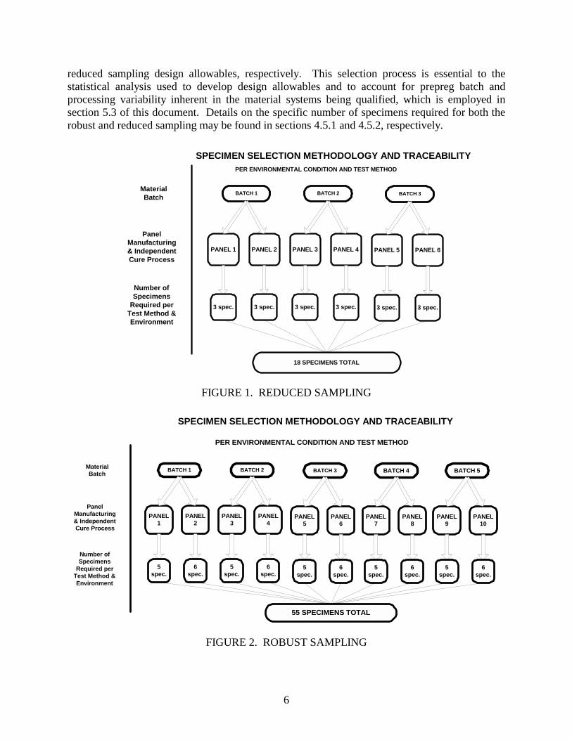
Each panel manufactured for testing should have a traceable reference edge to be used during subpanel and specimen preparation. Detailed guidelines for producing these reference edges are given in appendix C. The reference edge of the original panel should be maintained until individual specimens are produced. In order to include the effect of processing variability within the qualification data, the manufacturing process to produce the test panels should be representative of multiple process cycles. Panels manufactured for each loading condition, test method, and batch of qualification testing should be representative of a minimum of two independent processing cure cycles. For example, the B-basis hot-wet testing for in-plane shear strength is composed of three batches of material with six replicates from each batch. The replicates within these tests should be traceable to a minimum of two independent processing cycles. Figures 1 and 2 describe a typical methodology used for specimen selection as well as panel manufacturing for both robust and

6

reduced sampling design allowables, respectively. This selection process is essential to the statistical analysis used to develop design allowables and to account for prepreg batch and processing variability inherent in the material systems being qualified, which is employed in section 5.3 of this document. Details on the specific number of specimens required for both the robust and reduced sampling may be found in sections 4.5.1 and 4.5.2, respectively.

CPER ENVIRONMENTAL CONDITION AND TEST METHOD

MaterialBatch

PanelManufacturing& IndependentCure Process

Number ofSpecimens

Required perTest Method &Environment

BATCH 2

PANEL 4

3 spec.

PANEL 3

3 spec.

BATCH 3

PANEL 6

3 spec.

PANEL 5

3 spec.

BATCH 1

PANEL 2

3 spec.

PANEL 1

3 spec.

18 SPECIMENS TOTAL

FIGURE 1. REDUCED SAMPLING

FIGURE 2. ROBUST SAMPLING

PER ENVIRONMENTAL CONDITION AND TEST METHOD

MaterialBatch


Number ofSpecimens


BATCH 2

PANEL4

6spec.

PANEL3

5spec.

BATCH 3

PANEL6

6spec.

PANEL5

5spec.

BATCH 1

PANEL2

6spec.

PANEL1

5spec.

55 SPECIMENS TOTAL

BATCH 4

PANEL8

6spec.

PANEL7

5spec.

BATCH 5

PANEL10

6spec.

PANEL9

5spec.

SPECIMEN SELECTION METHODOLOGY AND TRACEABILITY

SPECIMEN SELECTION METHODOLOGY AND TRACEABILITY

7

3.1.4 Tabs.

Where tabs are added to the specimen for the purpose of introducing loads, they shall be bonded to the specimen using epoxy adhesive that cures at or below the panel cure temperature. If the epoxy adhesive cure temperature is at or near the panel cure temperature, the epoxy adhesive cure time should not be longer than the panel cure time. This is to avoid adding undesirable postcure to the panel. Strain compatible tabbing material should be used, which commonly consists of glass or graphite, woven fabric. Strain compatible tabbing material is defined as tabbing material that will yield acceptable specimen failure modes. In some cases, it is necessary to control adhesive bondline and tab thicknesses to achieve acceptable specimen failure modes within the specimens. The subpanel reference edge should be used during the tabbing process to insure proper tab alignment. 3.1.5 Specimen Machining.

Care should be used in cutting of subpanels to maintain fiber orientation with respect to the reference edges as defined in section 3.1.3 and appendix C. To insure that this is maintained, a subpanel cut should always be based upon the original manufacturing panel reference edge. This may be accomplished by using locator pins or test indicators during cutting. The subpanel reference edge should also be used as a reference for the sectioning of individual specimens. Precautions should be taken to insure that accumulation of fiber direction error does not exceed 0.25°. This error-accumulation effect is one of the main reasons for small panel sizes (as indicated in appendices A and B). In general, specimens are sectioned from subpanels using a water-cooled diamond saw, with care taken not to overheat the specimen that may result in matrix charring. Specimens are then generally surface ground to final dimensions to achieve desired dimensional tolerances and surface finish. All dimensional tolerances must be achieved according to the specifications provided in section 3.4 for each test method. In cases where dimensional tolerances are not met, the specimens may be reworked. 3.1.6 Specimen Selection.

For each material or property, batch replicates should be sampled from at least two different test panels covering at least two independent processing cycles per section 3.1.3. Guidelines for specimen selection from each batch/panel are presented in figures 1 and 2. Specimens taken from each individual panel should be selected randomly. Test specimens should not be extracted from panel areas having indications of questionable quality either visually or as determined from nondestructive inspection techniques. 3.1.7 Specimen Naming.

An individual specimen naming system should be devised to guarantee traceability to the original subpanel, panel, test method, test condition, batch, and processing cycle. Evidence of traceability should be established by a FAA MIDO representative, DAR, or DMIR. Skewed lines may be drawn across each subpanel with a permanent marker or paint pen before specimen

8

sectioning to allow subpanel or panel reconstruction after testing as shown in figure 3. These may be very important when tracking outliers within the material data after testing.

FIGURE 3. SKEWED LINES DRAWN ACROSS SUBPANEL USED FOR

RECONSTRUCTION 3.1.8 Strain Gage Bonding.

ASTM E1237 should be used as a general guide for strain gage installation with the following certain recommendations specific to composite materials: • Isopropyl alcohol should be used for any wet abrading or surface cleaning. • 280 to 600 grit sandpaper should be used for abrading the surface, taking care not to

sever or expose any fibers. • Specimens that are humidity conditioned prior to testing should be gaged after the

conditioning has taken place. Humidity-aged specimens may be exposed to ambient conditions for a maximum of 2 hours for application of the gages.

• If soldering lead wiring, care must be taken not to burn the matrix of the test coupon. • If possible, gage sizes should be selected such that the gage area is greater than three

times the repetitive pattern of the weave. This may not be possible with some test methods; however, the gage area must be greater than a single repetitive pattern of the weave.

Skewed Lines

9

3.1.9 Specimen Dimensioning and Inspection.

All dimensions to be used in the calculations of mechanical and physical properties should be recorded as specified in the respective figures. These dimensions must meet the dimensional requirements in appropriate drawing figures. All thickness measurements should be made with point or ball micrometers and all width measurements with calipers. The accuracy of all measuring instruments should be traceable to the National Institute for Standards and Technology (NIST) or the applicable national organization standards of that country. In the case of tabbed specimens, all measurements should be taken after the bonding of tabs and final specimen machining. For humidity-aged specimens, all dimensioning should be recorded prior to environmental conditioning process. A minimum of one randomly selected specimen from each subpanel must be inspected for every dimensional requirement stated in the appropriate figure. If the randomly selected specimen fails any one of the requirements, every specimen must be inspected for that dimensional requirement. The specimens that do not meet any dimensional requirement must be reinspected after rework has been accomplished. The FAA Form 8130-9 must be used to indicate any deviation to FAA-approved test plan. 3.2 ENVIRONMENTAL CONDITIONING.

Humidity-aged specimens typically use accelerated conditioning to simulate the long-term exposure to humid air and establish a moisture saturation of the material. Accelerated conditioning of the specimens at 85% ±5% relative humidity and 145° ±5°F will be used until moisture equilibrium is achieved. The environmental conditioning chamber must be calibrated using standards having traceability to the NIST or which have been derived from acceptable values of natural physical constants or through the use of the ratio method of self-calibration techniques. ASTM D5229 and SACMA SRM 11 provide general guidelines regarding environmental conditioning and moisture absorption. Specimens to be tested in the “dry,” as fabricated, condition should be exposed to ambient laboratory conditions until mechanical testing. Ambient laboratory conditions are defined as an ambient temperature range of 65°-75°F. Since moisture absorption or desorption rate of epoxy is very slow at ambient temperature, there is no requirement to maintain relative humidity levels in the mechanical test laboratory. 3.2.1 Traveler Specimens.

In order to establish the effect of moisture with respect to the mechanical properties, specimens should be environmentally conditioned, per section 3.2. Since the individual specimens may not be measured to determine the percentage of moisture content (due to size and tab effects), traveler coupons of approximately 1″ by 1″ by specimen thickness should be used to establish the weight gain measurements. Individual traveler specimens should be obtained from the representative panel from which the mechanical test specimens were obtained. One traveler specimen per qualification panel per batch is recommended.

10

3.2.2 Equilibrium Criteria.

Effective moisture equilibrium is achieved when the average moisture content of the traveler specimen changes by less than 0.05% for two consecutive readings within a span of 7 ±0.5 days and may be expressed by

0.0005 < WW - W

b

1 - ii

where: Wi = weight at current time Wi – 1 = weight at previous time Wb = baseline weight prior to conditioning If the traveler coupons pass the criteria for two consecutive readings which are 7 ±0.5 days apart, the specimens may be removed from the environmental chamber and placed in a sealed bag along with a moist paper towel for a maximum of 14 days until mechanical testing. Strain-gaged specimens may be removed from the controlled environment for a maximum of 2 hours for application of gages in ambient laboratory conditions, as defined in section 3.2. If the moisture diffusivity constant is not required, the samples do not require drying prior to conditioning. 3.3 NONAMBIENT TESTING.

In order to quantify the effect of temperature with respect to mechanical properties, increased and decreased temperature testing is recommended (see section 4.3). This increased and decreased temperature testing is usually accomplished using an environmental testing chamber attached to the load frame. 3.3.1 Temperature Chamber.

The temperature chamber used in the environmental testing should be capable of performing all required tests with an accuracy of ±3°F of the required temperature. The chamber must be calibrated using standards having traceability to the NIST or which have been derived from acceptable values of natural physical constants or through the use of the ratio method of self-calibration techniques. The chamber should be of adequate size that all test fixtures and load frame grips may be contained within the chamber. The chamber should also be capable of a heating rate as to reach the desired test temperature within the times specified in the following sections. 3.3.2 Testing at Elevated Temperatures.

Before beginning the testing, the temperature chamber and test fixture should be preheated to the specified temperature. Each specimen should be heated to the required test temperature as verified by a thermocouple in direct contact with the specimen gage section. The heat-up time of the specimen shall not exceed 5 minutes. The test should start 1

02 +− minutes after the specimen has reached the test

11

temperature. During the test, the temperature, as measured on the specimen, shall be within ±5°F of the required test temperature. 3.3.3 Testing at Subzero Temperatures.

Each specimen should be cooled to the required test temperature as verified by a thermocouple in direct contact with the specimen gage section. The test should start 1

0 5 +− minutes after the

specimen has reached the test temperature. During the test, the temperature, as measured on the specimen, shall be within ±5°F of the required test temperature. 3.4 SPECIMEN GEOMETRY AND TEST METHODS.

3.4.1 General.

The test methods and specimen geometry presented in the following sections refer to the actual qualification procedures and test methods used to establish design allowables for a given material system. The following referenced publications serve as the basis for this qualification plan. The applicable issue of the standard or recommendation at the time of publication of this qualification plan should be used. In the event a revision of the testing standard or recommendation occurs during the material qualification, the extent to which it affects this qualification plan should be investigated. The test methods described in the following sections are intended to provide basic composite properties essential to most methods of analysis. These properties are considered to provide the initial base of the “building block” approach. Additional coupon level tests and subelement tests may be required to fully substantiate the full-scale design. 3.4.2 References.

3.4.2.1 ASTM Standards.

D3039-95 Tensile Properties of Polymer Matrix Composite Materials

D5379-93 Shear Properties of Composite Materials by the V-Notched Beam Method

D2344-00 Apparent Interlaminar Shear Strength of Parallel Fiber Composites by Short-Beam Method

D792-91 Density and Specific Gravity (Relative Density) of Plastics by Displacement

D2584-94 Ignition Loss of Cured Reinforced Plastics

D2734-94 Void Content of Reinforced Plastics

D3171-90 Fiber Content of Resin – Matrix Composites by Matrix Digestion

12

3.4.2.2 SACMA Publications.

SRM 1-94 Compressive Properties of Oriented Fiber-Resin Composites SRM 8-94 Short-Beam Shear Strength of Oriented Fiber-Resin Composites SRM 18-94 Glass Transition Temperature (Tg) Determination by DMA of Oriented

Fiber-Resin Composites 3.4.3 Unidirectional Material Forms.

Unidirectional tape prepreg material consists of fibers arranged in the same direction. Figure 4 shows a typical unidirectional tape system with the associated defined directions. Unidirectional materials are commonly the most difficult to produce valid and reproducible results from mechanical tests. Extreme care must be maintained throughout the panel production, specimen preparation, and testing phases to produce viable results for design allowables.

FIGURE 4. UNIDIRECTIONAL TAPE WITH DEFINED DIRECTIONS 3.4.4 Woven Fabric Material Forms.

Woven fabric weaves are characterized by the manner in which the warp and fill (sometimes known as weft) yarns are interlaced to form the fabric. Typically, the warp direction runs parallel to the selvage of the fabric (along the length of the fabric as it comes off the roll). The weaving style of the yarns has a great influence on the properties of the woven fabric. In composite reinforcement applications, weave styles are almost always variations of plain or satin weaves and are described in detail in the following sections. Figure 5 shows a typical woven fabric with defined directions.

13

Warp Direction

Fill Direction

0o

90o

FIGURE 5. WARP AND FILL DIRECTIONS FOR WOVEN FABRIC MATERIAL (PLAIN WEAVE SHOWN)

Some controversy exists over the exact methodology that should be applied when qualifying a woven fabric material form. Since most weave patterns have approximately equal yarn counts in both the warp and fill directions, some qualifications have used a [0/90]ns lay-up to produce qualification panels. This type of procedure, although it may reduce the amount of testing required, may produce a nonconservative design allowable if manufacturing procedures are not in place to verify cross-ply lay-up during manufacturing at all times. In a [0]n lay-up sequence for woven fabric material, the mechanical properties in the fill direction are generally lower than the warp direction due to prepreg manufacturing. For these reasons, the warp and fill directions should be treated as independent directions in the qualification process similar to a unidirectional tape. If the warp and fill direction are not accurately tracked in the composite manufacturing process, the lower of both the warp and fill should be used for the design allowable. If procedures are in place to track the warp and fill directions, the designer may use both warp and fill properties for the design allowables. If the differences in strength and modulus are small between warp and fill, the strength and modulus values can be pooled (added together) and the basis value thus calculated can be used for strength and average pooled value can be used for modulus. 3.4.4.1 Plain Weaves.

In a plain weave fabric pattern, warp and fill yarns are interlaced over and under each other in an alternating pattern. Figure 6 shows a typical plain weave architecture of alternating yarns. Plain weave fabrics are ideally suited for flat laminates, where a high degree of drapeability is not required.

14

FIGURE 6. PLAIN WEAVE FABRIC CONSTRUCTION

3.4.4.2 Satin Weaves.

Satin weave construction consists of yarns that do not interlace at every yarn intersection. Instead, the yarns in both directions will cross over several intersections and interlace under one, as shown in figure 7. Satin weave fabrics have a higher degree of drapeability than plain weaves and are well suited for manufacturing parts with complex surfaces. Common satin weaves used in composite applications are four-harness satin, five-harness satin, and eight-harness satin.

FIGURE 7. SATIN WEAVE FABRIC CONSTRUCTION (FIVE HARNESS SHOWN)

15

Extreme care should be used when manufacturing the qualification panels using satin weave woven fabrics. Due to the unsymmetrical nature of the weave pattern, warpage may result during cure if strict lay-up practices are not followed. In the lay-up of a [0]n or [warp]n laminate, each corresponding ply should be rotated 180° about the warp axis to produce a lay-up of alternating the warp face and fill face, as depicted in figure 8.

warp

warp

fill

fill

warp reference

direction

lamination

process

alternating warp

and fill faces

Warp face

Fill face

FIGURE 8. EXAMPLE SATIN WEAVE SHOWING ALTERNATING WARP AND FILL FACES USED FOR LAMINATION

3.4.5 Mechanical Property Testing and Specimen Geometry.

This section describes the specific specimen geometry used to produce each individual mechanical property. Specific dimensions and tolerances are provided for each specimen taken from the referenced test method(s) as well as requirements on the parallelism and perpendicularity. Requirements for the thickness of each specimen are provided and should be adjusted based upon the nominal cured ply thickness of the material system being qualified. Specific changes and/or additions to the referenced test methods are also presented.

16

For general guidelines with respect to specimen dimensions and tolerances, the following reference provides guidelines for interpreting the specimen geometry, as shown for each test method and/or material type: Dimensioning and Tolerancing, American Society of Mechanical Engineers National Standard, Engineering Drawing and Related Document Practices, ASME Y14.5M-1994. The test methods described in this section have been used to generate data for this document. Other test methods that are acceptable by the MIL-HDBK-17 committee can be substituted if starting out on a qualification process. These may be such test methods as ASTM D3410 or the Combined Loading Compression (CLC) test method for compression and ASTM D3418 for shear. 3.4.5.1 Tensile Strength, Modulus, and Poisson’s Ratio.

ASTM D3039-95 Tensile Properties of Polymer Matrix Composite Materials a. Specimen Geometry

a.1 0° Tensile (Unidirectional Tape) Strength, Modulus, and Poisson’s Ratio (see figure 9)

FIGURE 9. ZERO-DEGREE UNIDIRECTIONAL TAPE TENSION SPECIMEN

17

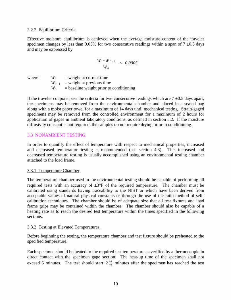
a.2 0° (warp) Tensile (Woven Fabric) Strength, Modulus, and Poisson’s Ratio (see figure 10)

FIGURE 10. ZERO-DEGREE (WARP) WOVEN FABRIC TENSION SPECIMEN

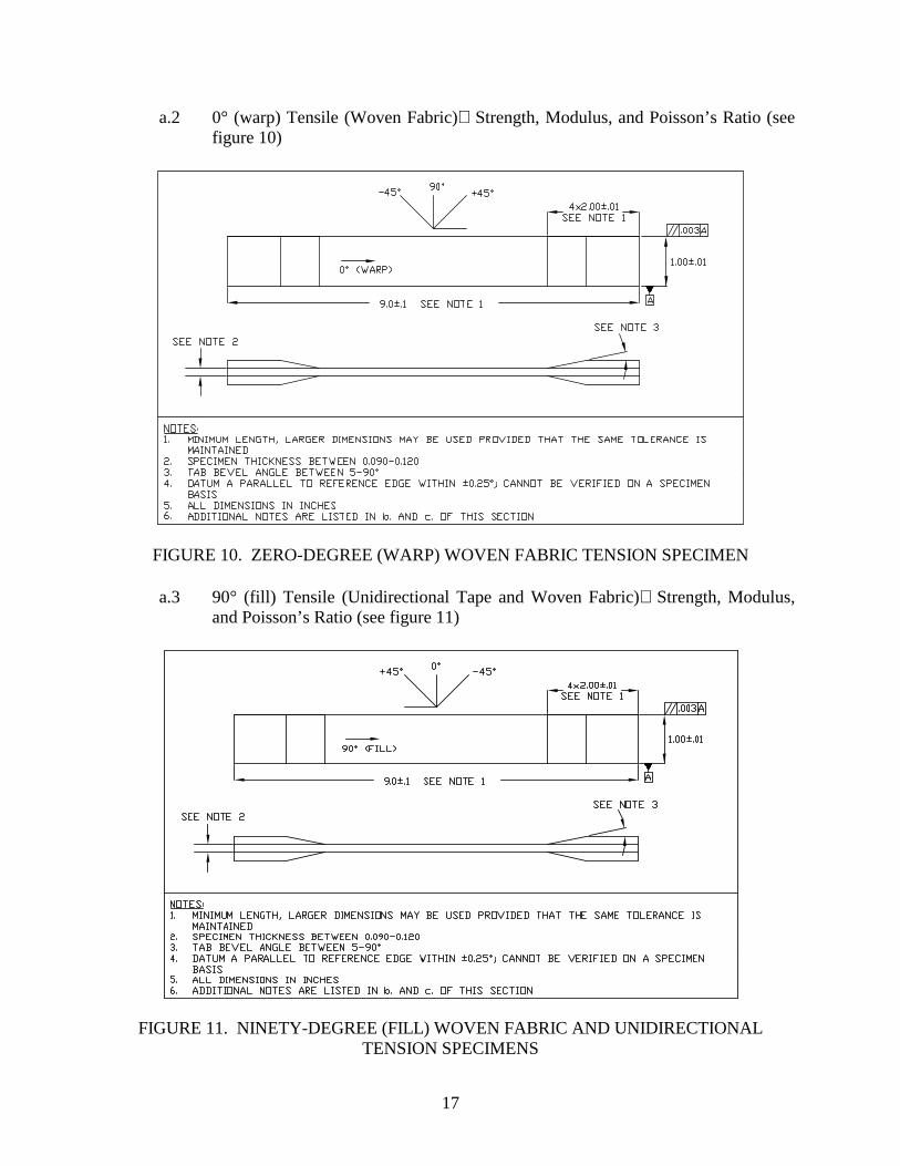
a.3 90° (fill) Tensile (Unidirectional Tape and Woven Fabric) Strength, Modulus, and Poisson’s Ratio (see figure 11)

FIGURE 11. NINETY-DEGREE (FILL) WOVEN FABRIC AND UNIDIRECTIONAL TENSION SPECIMENS

18

b. Laminate Lay-up and Recommended Thickness

b.1 0° Tensile (Unidirectional Tape)

[0]n where n is the number of plies Recommended Thickness: 0.040 inch

b.2 0° (warp) Tensile (Woven Fabric)


b.3 90° (Fill) Tensile (Unidirectional Tape and Woven Fabric)


c. Specific Additions and Changes to Referenced Test Method(s):

c.1 Quality Control and Documentation Requirements

At least one randomly selected specimen per subpanel should be checked for all dimensional tolerances detailed on the specimen geometry figures. If the randomly selected specimen fails any one of the requirements, all specimens from that subpanel should be individually inspected for that dimension. If the specimens cannot be corrected to fall within the required tolerances, the impact of such deviation(s) must be investigated. Specimens with deviation(s) that will affect the test results must be discarded. Specimens with deviation(s) that will not affect the test results may be used provided that such deviations are documented on FAA Form 8130-9. A minimum of two width and thickness measurements must be recorded within the gage section of each specimen. The average width and thickness should be used for the final material property calculations.

c.2 Strain Gage

Perform strain gage application, per section 3.1.8, as required by section 4 of this qualification plan. Upon testing system alignment verification, back-to-back strain gages are not required to verify percent bending.

c.3 Specimen Sampling

Specimen sampling should be randomly selected, based upon the panel requirements delineated in appendix A or B.

c.4 Recommended Calculation of Modulus of Elasticity and Poisson’s Ratio

Calculate the slope of a linear curve fit of the applicable data between the strain range given in table 3 of ASTM D3039-95.

19

c.5 Environmental Conditioning

Perform specimen conditioning as outlined in section 3.2. c.6 Tabs

Tab surfaces may be ground flat after tab bonding operations if there is evidence of uneven adhesive bondline thickness that will cause bending in the specimens during gripping.

3.4.5.2 Compressive Strength and Modulus.

SACMA SRM 1-94 Compressive Properties of Oriented Fiber-Resin Composites a. Specimen Geometry

a.1 0° (Warp) Compressive (Unidirectional Tape and Woven Fabric) Strength (see figure 12)

FIGURE 12. ZERO-DEGREE (WARP) WOVEN FABRIC AND UNIDIRECTIONAL COMPRESSION STRENGTH SPECIMENS

20

a.2 0° (warp) Compressive (Unidirectional Tape and Woven Fabric) Modulus (see figure 13)

FIGURE 13. ZERO-DEGREE (WARP) WOVEN FABRIC AND UNIDIRECTIONAL COMPRESSION MODULUS SPECIMENS

21

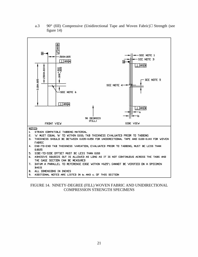
a.3 90° (fill) Compressive (Unidirectional Tape and Woven Fabric) Strength (see figure 14)

FIGURE 14. NINETY-DEGREE (FILL) WOVEN FABRIC AND UNIDIRECTIONAL COMPRESSION STRENGTH SPECIMENS

22

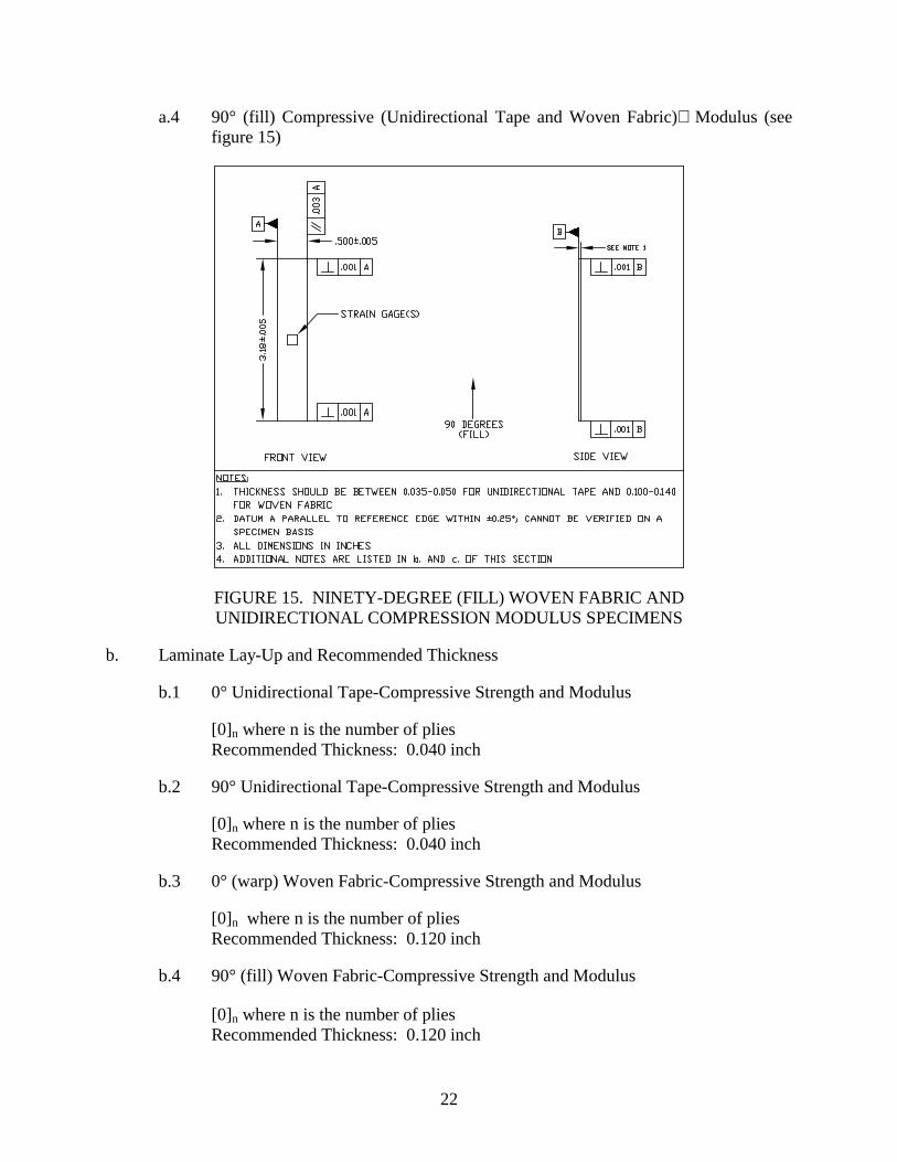
a.4 90° (fill) Compressive (Unidirectional Tape and Woven Fabric) Modulus (see figure 15)

FIGURE 15. NINETY-DEGREE (FILL) WOVEN FABRIC AND UNIDIRECTIONAL COMPRESSION MODULUS SPECIMENS

b. Laminate Lay-Up and Recommended Thickness

b.1 0° Unidirectional Tape-Compressive Strength and Modulus


b.2 90° Unidirectional Tape-Compressive Strength and Modulus


b.3 0° (warp) Woven Fabric-Compressive Strength and Modulus


b.4 90° (fill) Woven Fabric-Compressive Strength and Modulus


23

c. Specific Additions and Changes to Reference Test Method(s)

c1. Quality Control and Documentation Requirements

Due to the extreme sensitivity of this test method, all specimens for 0° unidirectional tape must be checked for all dimensional tolerances detailed on the specimen geometry figures. Particular attention should be addressed to parallelism and perpendicularity. In the case of woven fabric materials or 90° unidirectional tape, at least one randomly selected specimen per subpanel must be checked for all dimensional tolerances on the specimen geometry. If the randomly selected specimen fails any one of the requirements, all specimens from that subpanel must be individually inspected for that dimension. If the specimens cannot be corrected to fall within the required tolerances, the impact of such deviation(s) must be investigated. Specimens with deviation(s) that will affect the test results must be discarded. Specimens with deviation(s) that will not affect the test results may be used, provided that such deviations are documented on FAA Form 8130-9. A minimum of two width and two thickness measurements must be recorded within the gage section of each specimen. The average width and thickness must be used for the final material property calculations.

c.2 Strain Gage

Perform strain gage application, per section 3.1.8, as required by section 4 of this qualification plan. Back-to-back strain gages are not mandatory for modulus tests.

c.3 Sampling

Specimen sampling should be randomly selected, based upon the panel requirements delineated in appendix A or B.

c.4 Recommended Calculation of Modulus of Elasticity and Poisson’s Ratio

Calculate the slope of a linear curve fit of the applicable data between the 1000-3000 µε range as needed.

c.5 Environmental Conditioning

Perform specimen conditioning as outlined in section 3.2. c.6 Tabs

Tab surfaces may be ground flat after tab bonding operations if there is evidence of nonparallel tab surfaces that will cause the specimens to buckle prematurely.

24

3.4.5.3 In-Plane Shear Strength and Modulus.

ASTM D5379-93 Shear Properties of Composite Materials by the V-Notched Beam Method a. Specimen Geometry

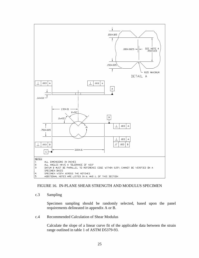
a.1 In-Plane Shear Strength and Modulus (Unidirectional Tape and Woven Fabric)

(see figure 16)

b. Laminate Lay-Up and Recommended Thickness b.1 In-Plane Shear Strength and Modulus (Unidirectional Tape and Woven Fabric)

[0/90]ns where n is the number of plies and s indicates a symmetric lay-up

configuration Recommended Thickness: 0.140 inch Note: 0.12-0.16 inch thickness recommendation allows for testing without

the use of tabs. c. Specific Additions and Changes to Referenced Test Method(s)


At least one randomly selected specimen per subpanel should be checked for all dimensional tolerances detailed on the specimen geometry figures. If the randomly selected specimen fails any one of the requirements, all specimens from that subpanel must be individually inspected for that dimension. If the specimens cannot be corrected to fall within the required tolerances, the impact of such deviation(s) must be investigated. Specimens with deviation(s) that will affect the test results must be discarded. Specimens with deviation(s) that will not affect the test results may be used, provided that such deviations are indicated in FAA Form 8130-9. A minimum of one width measurement across the notches (see figure 16, Detail A, Note 4) and two thickness measurements should be recorded within the gage section of each specimen. The average of these measurements should be used in the final material property calculations.

c.2 Strain Gage

Perform strain gage application, per section 3.1.8, as required by section 4 of this qualification plan. Back-to-back strain gages are not mandatory for modulus tests if specimen thickness is adequate to prevent twisting of the specimen during testing. Sample specimens should be verified prior to beginning test plan to be twist-free.

25

FIGURE 16. IN-PLANE SHEAR STRENGTH AND MODULUS SPECIMEN

c.3 Sampling Specimen sampling should be randomly selected, based upon the panel requirements delineated in appendix A or B.

c.4 Recommended Calculation of Shear Modulus

Calculate the slope of a linear curve fit of the applicable data between the strain range outlined in table 1 of ASTM D5379-93.

26

c.5 Environmental Conditioning Perform specimen conditioning as outlined in section 3.2.

c.6 Special Note

This method is not recommended for materials that may not demonstrate homogeneity with respect to the test section.

3.4.5.4 Short-Beam Shear Strength.

ASTM D2344-95 Apparent Interlaminar Shear Strength of Parallel Fiber Composites by Short-Beam Method

or

SACMA SRM 8-94 Short-Beam Shear Strength of Oriented Fiber-Resin Composites

Note: This test method is for quantitative quality control purposes only and should not be used for interlaminar shear strength values.

a. Specimen Geometry

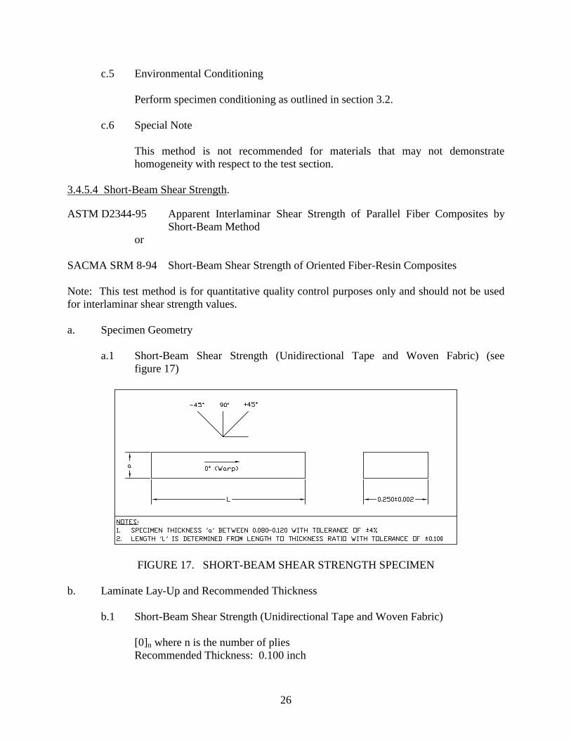
a.1 Short-Beam Shear Strength (Unidirectional Tape and Woven Fabric) (see figure 17)

FIGURE 17. SHORT-BEAM SHEAR STRENGTH SPECIMEN

b. Laminate Lay-Up and Recommended Thickness

b.1 Short-Beam Shear Strength (Unidirectional Tape and Woven Fabric)


27

c. Specific Additions and Changes


At least one randomly selected specimen per subpanel should be checked for all dimensional tolerances detailed on the specimen geometry figures. If the randomly selected specimen fails any one of the requirements, all specimens from that subpanel must be individually inspected for that dimension. If the specimens cannot be corrected to fall within the required tolerances, the impact of such deviation(s) must be investigated. Specimens with deviation(s) that will affect the test results must be discarded. Specimens with deviation(s) that will not affect the test results may be used, provided that such deviations are indicated in FAA Form 8130-9. A minimum of two width and two thickness measurements must be recorded for each specimen. These measurements must be taken at the center of the specimen. The average of these measurements must be used in the final material property calculations.

c.2 Sampling

Specimens used for this test method are not required to follow the processing requirements delineated in section 3.1.3. Specimen sampling should be randomly selected, based upon the requirements delineated in appendix A or B.

c.3 Span and Specimen Length

Recommendations for support span and specimen lengths are delineated in table 1 of ASTM D2344. However, these recommendations may be adjusted (and reported) to ensure proper failure modes.

Guidelines for the length are taken from ASTM D2344 in terms of the length-to-thickness ratio. For glass fibers, the length-to-thickness ratio should be 7 and for graphite fibers, the length-to-thickness ratio should be 6. The span may be adjusted to obtain proper failure modes.

c.4 Ply Orientation

Specimen should be sectioned such that the 0° or warp direction is along the length of the specimen.

28

3.4.6 Additional Test Methods.

3.4.6.1 Fiber Volume Fraction.

3.4.6.1.1 Fiberglass Laminates. a. Procedure

ASTM D2584-94 Ignition Loss of Cured Reinforced Resins b. Specific Additions or Changes

b.1 One sample should be tested per panel used for fabricating mechanical test coupons.

b.2 Specimens should be desiccated or oven-dried prior to taking initial weight

measurement, instead of being exposed to the standard laboratory atmosphere. 3.4.6.1.2 Carbon or Graphite Laminates. a. Procedure

ASTM D3171-90 Fiber Content of Resin Matrix Composites by Matrix Digestion, Procedure B

b. Specific Additions or Changes


b.2 Specimens should be desiccated or oven-dried prior to taking initial weight

measurement, instead of being exposed to the standard laboratory atmosphere. b.3 Procedure B is recommended due to the ease of process. Although procedures A

and C are recommended for epoxy matrices, both require a high capital investment in equipment. Assessment as to the degree of digestion by the proposed method should be investigated prior to beginning test program for each matrix system.

29

3.4.6.2 Void Volume Fraction.

3.4.6.2.1 Specimen Density. a. Procedure

ASTM D792-91 Density and Specific Gravity (Relative Density) of Plastics by Displacement, Procedure A



b.2 Optimum results will be obtained if samples tested for density are the same as

those utilized for fiber volume fraction tests (section 3.4.6.1). b.3 Specimens should be dried in a desiccated oven or vacuum-oven prior to taking

initial weight measurement, instead of being exposed to the standard laboratory atmosphere.

b.4 Upon immersing the specimens in water, the weight should be recorded

immediately, as the composite specimen will begin to absorb small amounts of water. If bubbles adhere to the sample, they should be removed immediately and the weight recorded soon thereafter.

3.4.6.2.2 Specimen Void Content. a. Procedure

ASTM D2734-94 Void Content of Reinforced Plastics, Procedure A b. Specific Additions or Changes

b.1 Although the test standard references only D2584-94, the void calculation is equally applicable to method D3171-90.

b.2 In order to avoid negative void content results, section 7.1 of D2734-94 should be

strictly followed. The material supplier should supply certified resin density measurements, or procedure D792-91 should be used on a representative sample of cured neat resin in order to obtain the resin density value that is used in the void calculation.

30

3.4.6.3 Glass Transition Temperature.

a. Procedure

SACMA SRM 18-94 Glass Transition Temperature (Tg) Determination by DMA of Oriented Fiber-Resin Composites


b.1 Fixture Type: Three-point bend b.2 Testing Frequency: 1 Hz b.3 Heating Rate: 5° ±0.2°C per minute

b.4 Temperature range: Test should begin from room temperature and end at a

temperature 50°C above Tg but below decomposition temperature. In the case of a lower curing material system (below 240oF), it may be necessary to begin the test below room temperature in order to obtain a sufficient slope at the beginning of the test.

b.5 Tg is determined from a logarithmic plot of the storage modulus as a function of

temperature. The Tg is determined to be the intersection of the two slopes from the storage modulus. Figure 18 depicts a typical plot and the Tg measurement.

FIGURE 18. GLASS TRANSITION TEMPERATURE DETERMINATION FROM STORAGE MODULUS

31

4. QUALIFICATION PROGRAM.

4.1 INTRODUCTION.

This section outlines the specific number of tests required at each condition to substantiate a statistically based design allowable for each material property. Unless noted, the following test procedures will be performed for each individual material system being qualified. 4.2 GENERAL.

For a composite material system design allowable, several batches of material must be characterized to establish the statistically based material property for each of the material systems. The definition of a batch of material for this qualification plan refers to a quantity of homogenous resin (base resin and curing agent) prepared in one operation with traceability to individual component batches as defined by the resin manufacturer. In order to account for processing and panel-to-panel variability, the material system being qualified must also be representative of multiple-processing cycles as delineated in section 3.1.3. For this qualification plan, each batch of prepreg material must be represented by a minimum of two independent processing/curing cycles. 4.3 TECHNICAL REQUIREMENTS.

In order to substantiate the environmental effects with respect to the material properties, several environmental conditions will be defined to represent extreme cases of exposure. The conditions defined as extreme cases in this qualification plan are listed as follows: Cold Temperature Dry (CTD) - 65°F with an “as-fabricated” moisture content Room Temperature Dry (RTD) ambient laboratory conditions with an as-fabricated

moisture content Elevated Temperature Dry (ETD) 180°F with an as-fabricated moisture content Elevated Temperature Wet (ETW) 180°F with an equilibrium moisture weight gain in a 85%

relative humidity environment, per section 3.2 4.4 MATERIAL QUALIFICATION PROGRAM FOR UNCURED PREPREG.

Table 1 describes the physical tests recommended for each batch of material received from the material vendor. These tests should be traceable to each referenced test. These test methods are for the purpose of quality control in addition to specific values used in the normalization of material data (described in section 5.2). Some of the tests must be repeated in an incoming receiving inspection. Usually this retesting provides a verification of shipping to the airframe manufacturer and to establish that an error did not occur during shipment. In general, it should be noted that most of these properties significantly influence the producibility of the material system and commonly do not influence the resulting mechanical properties.

32

TABLE 1. RECOMMENDED PHYSICAL AND CHEMICAL PROPERTY TESTS TO BE PERFORMED BY MATERIAL VENDOR

Test Method(s)

No. Test Property ASTM SACMA No. of Replicates

per Batch 1 RESIN CONTENT D 3529, C 613,

D 5300, D3171 RM 23, RM 24 3

2 Volatile Content D 3530 - - - 3 3 Gel Time D 3532 RM 19 3 4 Resin Flow D 3531 RM 22 3 5 Fiber Areal Weight D 3776 RM 23, RM 24 3 6 IR (Infrared Spectroscopy) E 1252, E 168 - - - 3 7 HPLC (High Performance

Liquid Chromatography)* - - - RM 20 3

8 DSC (Differential Scanning Calorimetry) E 1356 RM 25 3

* Sections 5.5.1 and 5.5.2 of MIL-HDBK-17-1E describe detailed procedures that will be used when extracting resin

from prepreg and performing HPLC tests. Listed in table 1 are suggestions taken from MIL-HDBK-17-1E for the acceptable test methods to produce each property. Both ASTM and SACMA test methods are shown. The material vendor should describe the exact test method used for each property and such methods must comply with the test methods described in table 1. These chemical and physical tests also represent the properties of the prepreg system with the fibers and resin combined. The quality control procedures of the material vendor should be reviewed to ensure that quality control programs are in place for both the raw fiber and neat resin. The material vendor should submit these quality procedures to each manufacturer and be on file as part of the original qualification as well as part of quality assurance documentation for the airframe manufacturer. 4.5 MATERIAL QUALIFICATION PROGRAM FOR CURED LAMINA MAIN PROPERTIES.

The required number of material batches and replicates per batch are presented in the following sections. For the purpose of presentation, the following format was adopted to represent the required number of batches and replicates per batch:

# x #

where the first # represents the required number of batches and the second # represents the required number of replicates per batch. For example, “3 x 6” refers to three batches of material and six specimens per batch for a total requirement of 18 test specimens.

33

MIL-HDBK-17 Working Group is in the process of revising the definition of prepreg batch at the time of this publication. As an interim, the definition of prepreg batch in section 1.5 may be used. Note that duplication of fiber or resin lot in any two prepreg batches within a material qualification program is not allowed. According to the definition, the prepreg produced after an interim run or a significant downtime should be considered as a separate prepreg batch but should not be used in a material qualification program together with the previous prepreg batch, because this would result in a duplication of the resin and/or fiber lot. In addition, minor changes in resin constituent lot(s) to produce a separate resin lot is undesirable. The objective is to ensure that the material qualification database accurately represents the population and the associated material variability. Table 2 shows the cured lamina physical properties required to support the maximum operational temperature limit of the material system as well as specific data to be used in the statistical design allowable generation. Typically, the maximum operational limit for the material should have a margin that is at least 50°F below the wet glass transition temperature. Fiber, resin, and void fraction specimens are taken from each subpanel used for qualification to verify quality and to establish ranges for acceptable production. The properties obtained from the tests in this section may be used to develop mature material specifications for material procurement as well as used to develop acceptable limits for incoming, receiving, and inspection.

TABLE 2. CURED LAMINA PHYSICAL PROPERTY TESTS

Physical Property Test Procedure No. of Replicates

per Batch Fiber Volume ASTM D 31711 or D 25842 See note 3 Resin Content ASTM D 31711 or D 25842 See note 3 Void Content ASTM D 27344 See note 3 Cured Neat Resin Density ASTM D 792 See note 5 Glass Transition Temperature (dry6) SACMA RM 18 3 Glass Transition Temperature (wet7) SACMA RM 18 3

Notes: 1. Test method used for carbon or graphite materials. 2. Test method used for fiberglass materials. 3. At least one test shall be performed on each panel manufactured for qualification (see appendices A and B). 4. Test method may also be applied to carbon or graphite materials. 5. Data or neat resin sample should be provided by material supplier for each batch of material. 6. Dry specimens are as-fabricated specimens that have been maintained at ambient conditions in an

environmentally controlled laboratory. 7. Wet specimens are humidity aged until an equilibrium moisture weight gain is achieved, per section 3.2.

34

4.5.1 Reduced Sampling Requirements for B-Basis Allowables.

Table 3 describes the number of tests required for each environmental condition along with the relevant test method for reduced sampling. The format shown in each matrix is described in section 4.5. The temperature for each environmental condition is described in section 4.3.

TABLE 3. REDUCED SAMPLING REQUIREMENTS FOR CURED LAMINA

MAIN PROPERTIES

No. of Specimens Per Test Condition Figure

No. Test Method

Reference CTD1 RTD2 ETW3 ETD4

9 or 10 0o (warp) Tensile Strength ASTM D 3039 1 x 4 3 x 4 3 x 4 1 x 4

9 or 10* 0o (warp) Tensile Modulus, Strength and Poisson’s Ratio

ASTM D 3039 1 x 2 3 x 2 3 x 2 1 x 2

11 90o (fill) Tensile Strength ASTM D 3039 1 x 4 3 x 4 3 x 4 1 x 4

11* 90o (fill) Tensile Modulus and Strength ASTM D 3039 1 x 2 3 x 2 3 x 2 1 x 2

12 0o (warp) Compressive Strength SACMA SRM 1 1 x 6 3 x 6 3 x 6 1 x 6

13* 0o (warp) Compressive Modulus SACMA SRM 1 1 x 2 3 x 2 3 x 2 1 x 2

14 90o (fill) Compressive Strength SACMA SRM 1 1 x 6 3 x 6 3 x 6 1 x 6

15* 90o (fill) Compressive Modulus SACMA SRM 1 1 x 2 3 x 2 3 x 2 1 x 2

16 In-Plane Shear Strength ASTM D 5379 1 x 4 3 x 4 3 x 4 1 x 4

16* IN-PLANE SHEAR MODULUS AND STRENGTH

ASTM D 5379 1 x 2 3 x 2 3 x 2 1 x 2

17 Short-Beam Shear ASTM D 2344 -- 3 x 6 -- -- * strain gages or extensometers used during testing Notes: 1. Only one batch of material is required (test temperature = -65 ±5°F, moisture content = as fabricated5). 2. Three batches of material are required (test temperature = 70 ±10°F, moisture content = as fabricated5). 3. Three batches of material are required (test temperature = 180 ±5°F, moisture content = per section 3.2). 4. Three batches of material are required (test temperature = 180 ±5°F, moisture content = as fabricated5). 5. Dry specimens are as-fabricated specimens that have been maintained at ambient conditions in an

environmentally controlled laboratory.

35

4.5.2 Robust Sampling Requirements for A- and B-Basis Allowables.

Table 4 describes the number of tests required for each environmental condition along with the relevant test method for robust sampling. The format shown in each matrix is described in section 4.5. The temperature for each environmental condition is described in section 4.3.

TABLE 4. ROBUST SAMPLING REQUIREMENTS FOR CURED LAMINA MAIN PROPERTIES

No. of Specimens Per Test Condition Figure

No. Test Method

Reference CTD1 RTD2 ETW3 ETD4

9 or 10 0o (warp) Tensile Strength ASTM D 3039 1 x 7 5 x 7 5 x 7 1 x 7

9* OR 10*

0o (warp) Tensile Modulus, Strength and Poisson’s Ratio ASTM D 3039 1 x 4 5 x 4

5 x 4 1 x 4

11 90o (fill) Tensile Strength ASTM D 3039 1 x 7 5 x 7 5 x 7 1 x 7

11* 90o (fill) Tensile Modulus and Strength ASTM D 3039 1 x 4 5 x 4

5 x 4 1 x 4

12 0o (warp) Compressive Strength SACMA SRM 1 1 x 11 5 x 11 5 x 11 1 x 11

13* 0o (warp) Compressive Modulus SACMA SRM 1 1 x 4 5 x 4

5 x 4 1 x 4

14 90o (fill) Compressive Strength SACMA SRM 1 1 x 11 5 x 11 5 x 11 1 x 11 15* 90o (fill) Compressive Modulus SACMA SRM 1 1 x 4 5 x 4 5 x 4 1 x 4 16 In-Plane Shear Strength ASTM D 5379 1 x 7 5 x 7 5 x 7 1 x 7

16* In-Plane Shear Modulus and Strength ASTM D 5379 1 x 4 5 x 4 5 x 4 1 x 4

17 Short-Beam Shear ASTM D 2344 -- 5 x 11 -- -- * strain gages or extensometers used during testing Notes: 1. Only one batch of material is required (test temperature = -65 ±5°F, moisture content = as fabricated5). 2. Five batches of material are required (test temperature = 70 ±10°F, moisture content = as fabricated5). 3. Five batches of material are required (test temperature = 180 ±5°F, moisture content = per section 3.2). 4. Five batches of material are required (test temperature = 180 ±5°F, moisture content = as fabricated5). 5. Dry specimens are as-fabricated specimens that have been maintained at ambient conditions in an

environmentally controlled laboratory. 4.5.3 Fluid Sensitivity Screening.

Although epoxy-based materials historically have not been shown to be sensitive to fluids other than water or moisture, the influence of fluids other than water or moisture on the mechanical properties should be characterized. These fluids usually fall into two exposure classifications. The first class is considered to be in contact with the material for an extended period of time and the second class is considered to be wiped on and off (or evaporate) with relatively short exposure times.

36

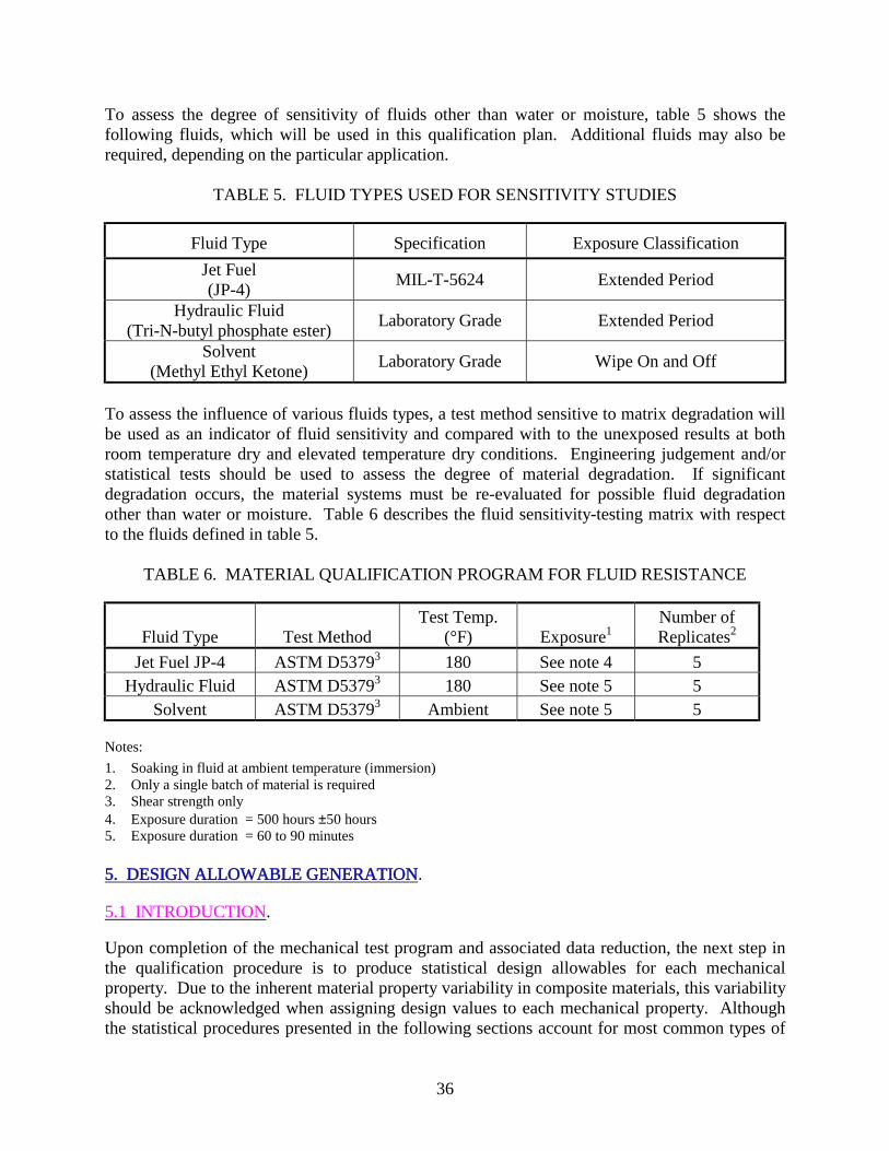
To assess the degree of sensitivity of fluids other than water or moisture, table 5 shows the following fluids, which will be used in this qualification plan. Additional fluids may also be required, depending on the particular application.

TABLE 5. FLUID TYPES USED FOR SENSITIVITY STUDIES

Fluid Type Specification Exposure Classification Jet Fuel (JP-4) MIL-T-5624 Extended Period

Hydraulic Fluid (Tri-N-butyl phosphate ester) Laboratory Grade Extended Period

Solvent (Methyl Ethyl Ketone) Laboratory Grade Wipe On and Off

To assess the influence of various fluids types, a test method sensitive to matrix degradation will be used as an indicator of fluid sensitivity and compared with to the unexposed results at both room temperature dry and elevated temperature dry conditions. Engineering judgement and/or statistical tests should be used to assess the degree of material degradation. If significant degradation occurs, the material systems must be re-evaluated for possible fluid degradation other than water or moisture. Table 6 describes the fluid sensitivity-testing matrix with respect to the fluids defined in table 5.

TABLE 6. MATERIAL QUALIFICATION PROGRAM FOR FLUID RESISTANCE

Fluid Type Test Method Test Temp.

(°F) Exposure1 Number of Replicates2

Jet Fuel JP-4 ASTM D53793 180 See note 4 5 Hydraulic Fluid ASTM D53793 180 See note 5 5

Solvent ASTM D53793 Ambient See note 5 5 Notes: 1. Soaking in fluid at ambient temperature (immersion) 2. Only a single batch of material is required 3. Shear strength only 4. Exposure duration = 500 hours ±50 hours 5. Exposure duration = 60 to 90 minutes

5. DESIGN ALLOWABLE GENERATION.

5.1 INTRODUCTION.

Upon completion of the mechanical test program and associated data reduction, the next step in the qualification procedure is to produce statistical design allowables for each mechanical property. Due to the inherent material property variability in composite materials, this variability should be acknowledged when assigning design values to each mechanical property. Although the statistical procedures presented in the following sections account for most common types of

37

variability, it should be noted that these procedures might not account for all sources of variability. B- and A-basis design allowables are determined for each strength property using the statistical procedures outlined in the following sections. In the case of modulus and Poisson’s ratio design values, the average value of all corresponding tests for each environmental condition should be used. If strain design allowables are required, simple one-dimensional linear stress-strain relationships may be used to obtain corresponding strain design values. However, it should be noted that this process should approximate tensile and compressive strain behavior relatively well but may produce extremely conservative strain values in shear due to the nonlinear behavior. These conservative shear allowables are appropriate if a linear analysis of the laminate is performed. If a nonlinear analysis is performed, then the nonlinear shear stress-strain curve may be used, with a maximum strain value of 5% used as the shear strain allowable (reference MIL-HDBK-17-1E, section 5.7.6). 5.2 NORMALIZATION.

5.2.1 Normalization Procedure.

This normalization method is performed for direct comparison of mechanical test results, adjusting raw test values to a specified fiber volume content. The process of data normalization attempts to reduce variability in fiber-dominated properties and is justified on the basis that most of the load is carried by the fibers. Excerpts and methodology taken from MIL-HDBK-17-1E, section 2.4.3.

5.2.1.1 Assumptions.

• The method is based on the assumption that the relationship between fiber volume fraction and ultimate laminate strength is linear over the entire range of fiber/resin ratios. (It neglects the effects of resin starvation at high fiber contents.)

• Fiber volume is not commonly measured for each test sample, so this method accounts

for the fiber volume variation between individual test specimens by using a relationship between fiber volume fraction and laminate-cured ply thickness. This relationship is virtually linear in the 0.45 to 0.65 fiber volume fraction range.

5.2.1.2 Methodology.

• Define an equivalent thickness of fiber which would result if the fiber material could be shaped into a solid sheet of uniform thickness with no air space between filaments

f

fFAWtρ

= (1)

38

where tf = equivalent thickness of a solid layer of fiber FAW = reinforcement fiber areal weight

ρf = fiber density • The fraction of fiber in a laminate is the thickness of this fiber layer divided by the total

laminate thickness

CPTt

FV f= (2)

where FV = fiber volume fraction CPT = laminate cured ply thickness • It follows that

CPT

FAWFVf ×

=ρ

(3)

and

gnormalizinf

nominalgnormalizin CPT

FAWFV×

=ρ (4)

and

specimenf

specimenspecimen CPT

FAWFV

×=

ρ (5)

where FVnormalizing = fiber volume fraction specified or chosen for normalizing

FVspecimen = fiber volume fraction of the specimen

FAWnominal = nominal fiber areal weight from a material specification or other source

FAWspecimen = specimen actual fiber areal weight

CPTnormalizing = cured ply thickness corresponding to normalizing fiber volume fraction

CPTspecimen = actual specimen ply thickness (specimen thickness divided by number of plies)

39

• Combining the previous two equations renders

gnormalizin

specimen

specimen

nominal

specimen

gnormalizin

CPTCPT

FAWFAW

FVFV

×= (6)

and since

specimen

gnormalizin

FVFV

Value TestValue Normalized ×= (7)

gnormalizin

specimen

specimen

nominal

CPTCPT

FAWFAW

Value TestValue Normalized ××= (8)

Assuming a negligible difference between the FAW, equation 8 may be rewritten as

gnormalizin

specimen

CPTCPT

TestValueValueNormalized ×= (9)

5.2.2 Application of Normalization.

The methodology for practical application of normalization has been adopted from MIL-HDBK-17-1E, section 2.4.3.3. Fiber-dominated properties shall be normalized according to the procedure outlined in the previous section, with specific examples cited below. Normalize:

• 0° (warp) tensile strength and modulus (fabric weave and unidirectional tape) • 90° (fill) tensile strength and modulus (fabric weave only) • 0° (warp) compressive strength and modulus (fabric weave and unidirectional tape) • 90° (fill) compressive strength and modulus (fabric weave only)

Do not normalize:

• 90° tensile strength and modulus (unidirectional only) • 90° compressive strength and modulus (unidirectional only) • Interlaminar shear • In-plane shear strength and modulus • Short-beam strength • Poisson’s ratio

After normalizing, data scatter should reduce or remain the same. However, if data scatter increases significantly after normalizing, the reason should be investigated.

40

5.3 STATISTICAL ANALYSIS.

When compared to metallic materials, the base material properties for fiber-reinforced composite materials exhibit a high degree of variability. This variability is due to many factors including, but not limited to, raw material and prepreg manufacture, material handling, part fabrication techniques, ply-stacking sequence, environmental conditions, and testing techniques. In some cases, the variation in the defects or flaws associated with these factors is the apparent cause. The variability, which is directly related to the test procedures, has been minimized over the years through research and standardization. Nevertheless, the cost of composite testing is relatively high. This, combined with additional testing due to the orthotropic nature of composite materials, has led to smaller data sets for a particular property than those produced for metallic materials. This necessitates the usage of advanced statistical techniques for determining reasonable design allowables for composites. 5.3.1 Methodology.

The statistical analyses and design allowable generation for both A- and B-basis values may be performed using the methodology presented by Shyprykevich [1]. In this data reduction method, the data from all environments, batches, and panels are used jointly to obtain statistical information about the corresponding test condition and failure mode. This approach uses essentially small data sets to generate test condition statistics such as population variability factors and corresponding basis values for pooling of test results for a specific failure mode across all test environments. This section describes an overview of this methodology as applied to a design allowable generated using the testing procedures presented in the qualification plan. For additional information regarding this methodology or statistical analyses in general, the reader is referred to either Shyprykevich or MIL-HDBK-17-1E, chapter 8. The data reduction methodology presented in this section requires several underlying assumptions in order to generate a valid design allowable. By pooling the data sets in the analysis method, the variability across environments should be comparable and the failure modes for each environment should not significantly change. The methodology presented here uses a normal distribution to analyze the data. If the assumption of normality is not acceptable, the Weibull distribution can be used as outlined by Shyprykevich. It generally produces the most conservative basis values. If the variability or failure modes significantly change or if the assumption of normality is violated, the traditional methods of MIL-HDBK-17 should be used. The methodology to produce a design allowable (based upon testing completed via section 4.5 of this document) is presented through a stepwise process, which assumes that all testing data for each condition and testing environment has been reduced and is in terms of failure stress. An assumption of normality is used in the method to reduce and model the behavior. The stepwise process then proceeds to determine a basis design allowable value (A or B) as follows: a. Normalize all relevant fiber-dominated data via the procedures presented in MIL-HDBK-

17-1E, section 2.4.3 (which is also given in section 5.2 of this document). This normalization procedure will account for variations in the fiber volume fraction between individual specimens, panels, and/or batches of material.

41

b. For a single test condition (such as 0° compression strength), collect the data for each environment being tested. The number of observations in each environmental condition is nj where the subscript j represents the total number of environments beings pooled. Calculate the sample mean x and sample standard deviation s for each environment via

∑=

=n

iix

nx

1

1 (10)

2

1

2 )(1

1 ∑=

−−

=n

ii xx

ns (11)

For each environment, the environmental groupings must be checked for any outliers, per

section 5.3.1.1, as well as for the assumption of normality, per section 5.3.1.2. In addition, the variances of each environmental grouping should be checked for equality, per section 5.3.1.3. If any outliers exist within each environmental grouping, the disposition of each outlier should be investigated via the procedures given in section 5.3.1.1.1. For the check of population normality, engineering judgement should be applied to verify that the assumption of normality is not significantly violated. If the assumption of normality is significantly violated, other statistical models should be investigated to fit the data. As stated above, the Weibull distribution provides the most conservative basis values. If the variance of each environmental grouping is significantly different as determined by the procedure described in section 5.3.1.3, traditional statistical methods of MIL-HDBK-17 should be used.

c. Normalize the data in each environment by dividing the individual strength by the mean

strength for the corresponding environment. Normalizing will result in all data having a mean of 1.0. Pool all the normalized data together from each environment into one data set.

d. For the pooled, normalized data set, calculate the number of samples N, the sample mean

x and sample standard deviation s via equations 10 and 11. For the pooled data set, a visual comparison of the best normal fit should be conducted, per section 5.3.1.2. For the distributional check of normality, engineering judgement should be applied to verify that the assumption of normality is not significantly violated. If the assumption of normality is significantly violated, the other statistical models should be investigated to fit the data. In general, the Weibull distribution provides the most conservative basis value.

e. Calculate the one-sided B- and A-basis tolerance factors for the normal distribution for

each environment j that is based upon the number of samples in the pooled data set N and the number of samples in each environment nj. The B-basis tolerance factor (number of standard deviations) (kB)j may be approximated by [2]

B

B

B

B

jBBjB c

b2cb

ncQfz(k

21)

2

−

++= (12)

42

where nj is the number of observations of the selected environment (a subset of N, the number of total pooled observations) and zB is the standard normal random variable. In the case of a B-basis calculation, zB is taken as 1.28115 (90% probability). The subscript j is used to indicate the tolerance factor for that specific environment. The coefficients bB and cB are given by the following relationships:

( )ffff

fbB118612.0149162.011372.1 +−= (13)

( )ffff

fcB119693.0171750.010040342.036961.0 +−+= (14)

where f = N-2 is the degrees of freedom for the variance. In the case f ≥ 3, Q may be approximated by

ffffQ 13287.016057.0138.1327.2 −++−= (15)

For f = 2, the exact value of Q may be used as Q = 0.05129. The above approximations are accurate within 1.2% of the tabulated values for B-basis calculations. The A-basis tolerance factor, kA may be approximated by

A

A

A

A

jAAjA c

b2cb

ncQfz(k

21)

2

−

++= (16)

where nj is the number of observations of the selected environment (a subset of N, the number of total pooled observations) and zA is the standard normal random variable. In the case of an A-basis calculation, zA is taken as 2.32635 (99% probability). The subscript j is used to indicate the tolerance factor for that specific environment. The coefficients bA and cA are given by the following relationships:

( )ffff

fbA151251.0195145.010643.2 +−= (17)

( )ffff

fcA1011320.0165201.010026958.036961.0 +−+= (18)

where f = N-2 is the degrees of freedom for the variance. In the case f ≥ 3, Q may be approximated by

ffffQ 13287.016057.0138.1327.2 −++−= (19)

For f = 2, the exact value of Q may be used as Q = 0.05129. The above approximations are accurate within 0.9% of the tabulated values for A-basis calculations.

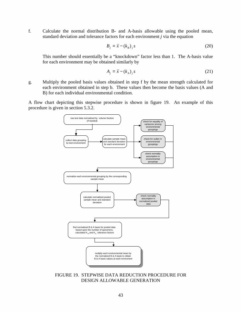
43

f. Calculate the normal distribution B- and A-basis allowable using the pooled mean, standard deviation and tolerance factors for each environment j via the equation

skxB jBj )(−= (20)

This number should essentially be a “knockdown” factor less than 1. The A-basis value for each environment may be obtained similarly by

skxA jAj )(−= (21)

g. Multiply the pooled basis values obtained in step f by the mean strength calculated for each environment obtained in step b. These values then become the basis values (A and B) for each individual environmental condition.

A flow chart depicting this stepwise procedure is shown in figure 19. An example of this procedure is given in section 5.3.2.

raw test data normalized by volume fraction(if needed)

collect data groupingby test environment

calculate sample meanand standard deviationfor each environment

check for outlier inenvironmental

groupings

check normalityassumption inenvironmental

groupings

normalize each environmental grouping by the correspondingsample mean

find normalized B & A basis for pooled databased upon the number of specimens,calculated K B and KA tolerance factors

multiply each environmental mean bythe normalized B & A basis to obtain

B & A basis values at each enviroment

check for equality ofvariances among

environmentalgroupings

check normalityassumption in

normalized pooleddata

calculate normalized pooledsample mean and standard

deviation

FIGURE 19. STEPWISE DATA REDUCTION PROCEDURE FOR DESIGN ALLOWABLE GENERATION

44

5.3.1.1 Test for Outliers.

Once the strength data is generated for each testing condition, the data should be screened for outliers since these values can have a substantial influence on the statistical analysis. This screening may be done visually using graphical plots of the data as well as the quantitative procedure outlined below, which is taken from MIL-HDBK-17, section 8.3.3. The data used for the screening should be checked for outliers in both raw-grouped data (by environment) as well as the normalized pooled data set. The Maximum Normed Residual (MNR) method, as suggested by MIL-HDBK-17, is used for detecting outliers. The MNR test declares a value to be an outlier if it has an absolute deviation from the sample mean which, when compared to the sample standard deviation, is too large to be due to chance. This method can only detect one outlier at a time from a selected group or subgroup, hence, once an outlier is detected, the outlier must be dispositioned (see section 5.3.1.1.1) and the analysis rerun to check for additional outliers. Let x1, x2, … xn denote the data values in the sample of size n, and let x and s be the sample mean and standard deviation defined previously for the normal distribution. The MNR statistic is the maximum absolute deviation, from the sample mean, divided by the sample deviation

n1,2,...,i ,s

xx

imax

MNR i =−

= (22)

The value obtained from this equation is compared to the critical value for the sample size n taken from table 7. If the calculated MNR is smaller than the critical value, then no outliers are detected in the sample. If the MNR value is greater than the critical value, the data value associated with the largest value of xxi − is declared to be an outlier. If an outlier is detected, the disposition of the outlier should be investigated via the procedure described in section 5.3.1.1.1. 5.3.1.1.1 Dispositioning of Outliers. The rationale for dispositioning of outliers detected in the data set is taken from MIL-HDBK-17, section 2.4.4 and is primarily based upon engineering judgement so that outliers that should be retained are not casually discarded and those that should be deleted are not retained. The rationale presented attempts to separate variability apparent in the data that does not exist from material, processing parameter, or environmental variability. These types of variability should be reflected in the data set and should be represented in the finalized basis value. Variability, which exists from other sources such as inferior specimen fabrication, processing parameters, which fall outside the control limits, test fixture or machine deficiencies, or a number of other factors both detectable and undetectable, may produce outliers in the data set and cause an unnecessary statistical penalty in the basis value. The purpose of this section is to provide some guidance to retain or delete the detected outliers.

45

TABLE 7. CRITICAL VALUES

n CV n CV n CV n CV n CV- - 41 3.047 81 3.311 121 3.448 161 3.539- - 42 3.057 82 3.315 122 3.451 162 3.5413 1.154 43 3.067 83 3.319 123 3.453 163 3.5434 1.481 44 3.076 84 3.323 124 3.456 164 3.5455 1.715 45 3.085 85 3.328 125 3.459 165 3.5476 1.887 46 3.094 86 3.332 126 3.461 166 3.5497 2.020 47 3.103 87 3.336 127 3.464 167 3.5518 2.127 48 3.112 88 3.340 128 3.466 168 3.5529 2.215 49 3.120 89 3.344 129 3.469 169 3.55410 2.290 50 3.128 90 3.348 130 3.471 170 3.55611 2.355 51 3.136 91 3.352 131 3.474 171 3.55812 2.412 52 3.144 92 3.355 132 3.476 172 3.56013 2.462 53 3.151 93 3.359 133 3.479 173 3.56114 2.507 54 3.159 94 3.363 134 3.481 174 3.56315 2.548 55 3.166 95 3.366 135 3.483 175 3.56516 2.586 56 3.173 96 3.370 136 3.486 176 3.56717 2.620 57 3.180 97 3.374 137 3.488 177 3.56818 2.652 58 3.187 98 3.377 138 3.491 178 3.57019 2.681 59 3.193 99 3.381 139 3.493 179 3.57220 2.708 60 3.200 100 3.384 140 3.495 180 3.57421 2.734 61 3.206 101 3.387 141 3.497 181 3.57522 2.758 62 3.212 102 3.391 142 3.500 182 3.57723 2.780 63 3.218 103 3.394 143 3.502 183 3.57924 2.802 64 3.224 104 3.397 144 3.504 184 3.58025 2.822 65 3.230 105 3.401 145 3.506 185 3.58226 2.841 66 3.236 106 3.404 146 3.508 186 3.58427 2.859 67 3.241 107 3.407 147 3.511 187 3.58528 2.876 68 3.247 108 3.410 148 3.513 188 3.58729 2.893 69 3.252 109 3.413 149 3.515 189 3.58830 2.908 70 3.258 110 3.416 150 3.517 190 3.59031 2.924 71 3.263 111 3.419 151 3.519 191 3.59232 2.938 72 3.268 112 3.422 152 3.521 192 3.59333 2.952 73 3.273 113 3.425 153 3.523 193 3.59534 2.965 74 3.278 114 3.428 154 3.525 194 3.56635 2.978 75 3.283 115 3.431 155 3.527 195 3.59836 2.991 76 3.288 116 3.434 156 3.529 196 3.59937 3.003 77 3.292 117 3.437 157 3.531 197 3.60138 3.014 78 3.297 118 3.440 158 3.533 198 3.60339 3.025 79 3.302 119 3.442 159 3.535 199 3.60440 3.036 80 3.306 120 3.445 160 3.537 200 3.606

When an outlier is detected, the first action should be to identify the cause through physical evidence. The following list is taken from MIL-HDBK-17 to give some examples of conditions that could be used as the basis for discarding outlier data. a. The material was out of specification.

b. One or more panel or specimen fabrication parameters were outside the specified tolerances.

46

c. Test specimen dimensions or orientation were outside the specified tolerance range.

d. A defect was detected in the test specimen.

e. An error was made in the specimen preconditioning (or conditioning parameters were out of specified tolerance ranges).

f. The test machine and/or test fixture was improperly set up in some specific and identifiable manner.

g. The test specimen was improperly installed in the test fixture in some specific and identifiable manner.

h. Test parameters (speed, temperature, etc.) were outside the specified range.

i. The test specimen slipped in the grips during the test.

j. The test specimen failed in a mode other than the mode under test (loss of tabs, unintended bending, failure outside the gage section, etc.).

k. A test was purposely run to verify conditions suspected to have produced outlier data.

l. Data were improperly normalized.

m. A different failure mode that is still in the gage section (most specimens failed in interlaminar shear but one failed due to fiber matrix interface).

If the search for physical causes has been completed without success, engineering judgement should be used in assessing the outlier data. This section provides some guidelines in case no physical determination exists but is not meant to provide rulings when data should be retained or deleted. In most cases, if the outlier’s inclusion in the data set does not significantly affect calculated basis values, the outlier should simply be retained without further consideration. In the case of a detected outlier, given the stepwise process presented in section 5.3.1, two possibilities exist with respect to the corresponding data set (either environmentally grouped or pooled data): the outlier may be “high” or the outlier may be “low.” In the case in which an outlier (high or low) is detected with respect to the environmental grouping of the data as described in section 5.3.1, engineering judgement should be used to disposition the outlier. Clearly, the easiest case to examine is the case in which a high outlier is detected. In the case of a high outlier, engineering judgement should be used to consider whether the outlier is within the range of material capability. If the outlier is clearly outside the range of the material capability, the outlier should be deleted from the data set (particularly in the case of pooled data). In the case where the high outlier is within the range of material capability, the outlier should be retained. In the case of a low outlier without physical evidence, in general, the data should be retained. If the low outlier is seen to penalize the basis value severely, the FAA Aircraft Certification Office

47

should be consulted to discuss deletion of the outlier and possible causes for the outlier. In this case, additional testing may be required in order to substantiate this outlier deletion. The original equipment manufacturer (OEM) must take the responsibility to take real root cause corrective action to prevent the detected occurrence from affecting future production runs (i.e., if, as a result of the investigation of outliers, it is determined that the fiber sizing was out of date, the OEM must insure that the problem will not reoccur in production). This may require changes in the quality control requirements or in the material specifications. 5.3.1.2 Normality Check.

The normality of a given set of data may be verified visually by comparing the data distribution with the best-fit normal curve and using engineering judgement to check the fit of the distribution. The normality of the grouped data (data from different batches for same test environment) is checked as follows: The data from different batches are grouped together and sorted in an ascending order. The probability of survival at each value of the data is

11

+−=

nix at survivalofy Probabilit i (23)

where n: total number of data points i : rank of the xi data value in the sorted/ordered list

xi: data value of rank “i” in the sorted/ordered list The mean and standard deviation for the grouped data are then computed using rudimentary statistical techniques presented previously. The mean and the standard deviation are the parameters that define the normal distribution. Using this value of the mean and standard deviation, the probability of survival is computed at each data value using a standard normal distribution. The data values are then plotted against the respective probability of survival obtained using equation 23 and the normal distribution. The data are compared visually and the normality of the data is evaluated using engineering judgement. The grouped data are then normalized with respect to the mean of the individual groups. The normalized groups are then pooled together and sorted and arranged in an ascending order. The probability of survival at each pooled normalized data value is computed using equation 23. The mean and the standard deviation of the pooled normalized data are then used to compute the probability of survival using the standard normal distribution. The normalized data values are then plotted against their respective probability of survival obtained using equation 23 and the normal distribution. The data is compared visually and the normality of the data is evaluated using engineering judgement. Another check for normality may be performed using the Anderson-Darling test (see MIL-HDBK-17-1E, section 8.3.4.2). This test generates an observed significance level (OSL), which measures the probability of observing an Anderson-Darling statistic at least as extreme as the

48

value calculated if in fact the data are from a normal distribution. If the OSL ≤ 0.05, one may conclude (at a 5 percent risk of being in error) that the population is not normally distributed. Otherwise, the hypothesis that the population is normally distributed is not rejected. 5.3.1.3 Equality of Variance.

The equality of variances between the different grouped data must also be checked using Levene’s test MIL-HDBK-17-1E, section 8.3.5.2.1. This test determines whether the sample variances for “k” groups differ significantly, which is an important assumption that must be validated to substantiate the pooling across environments. The following steps are involved in performing this test. a. The data is transformed according to

|~| iijij xxw −= (24) where: wij is the transformed value of the jth data point in the ith group xij is the original jth data point in the ith group

ix~ is the median of the ith group b. Perform an F-test (MIL-HDBK-17-1E, section 8.3.5.2.2) and compute the “F” statistic.

The F statistic is given by

( ) ( )

( ) ( )∑∑

∑

= =

=

−−

−−=

k

i

n

jiij

k

iii

i

knww

kwwnF

1 1

1

2 1 (25)

where iw is the average of the ni values in the ith group

w is the average of all the n observations ( i.e., of the pooled data) k is the number of groups ni is the number of observations in the ith group n is the total number of observations

c. The F statistic obtained above is compared with the (1-α) quantile of the F-distribution

having k-1 numerator and n-k denominator degrees of freedom. A typical value of α = 0.05 is used. This statistic from the F-distribution is termed as Fcritical. The value for Fcritical may be obtained using an approximate formula:

( )

−++

−−+= 6

31 2 3

43

11 2 exp2222 zzzFcritical

σσσδ (26)

49

where:

−−

−=

11

11 5.0

12 γγδ (27)

−+

−=

11

11 5.0

12

2

γγσ (28)

z = 1.645 1γ numerator degrees of freedom (k-1) 2γ denominator degrees of freedom (n-k) d. If the computed F-statistic is less than Fcritical, the variances of the groups are not

significantly different. e. It should be noted that other α values less than 0.05 may also be used to assess equality

of variances at different environments (see step c.). These different values of α can be useful in establishing engineering judgement as to the degree of variance inequality and suggest possible problems with obtaining a representative pooled data set. In the case when the variances are not equal at the 0.05 level, engineering judgement should be used to determine the degree of inequality. Figure 20 provides guidance in the situation of unequal variances and describes procedures to obtain a conservative design allowable. Note that these procedures must be combined with engineering judgement and that the failure modes must remain the same across environments. In general, if variances are significantly different at the 0.01 level, the reason should be investigated and some corrective action may be required.

In general, a coefficient of variation between 4% to 10% is typical of composite materials. Experiences with large data sets have shown that this range is representative of most composite material systems. Lower coefficients of variation may be caused by the specimen fabrication and testing by a single laboratory, while higher coefficients may point to lack of material and processing control. In cases where the coefficients of variation of the pooled data set are higher or lower than this range, the reason for the higher or lower coefficient of variation should be investigated before determining design allowable values from the pooled data set. For the coefficient of variation lower than 4%, an assigned value of 4% may be considered as an alternative engineering solution.

50

Check Equality of Variance persection 5.3.1.3

VarianceEqual ?NO

YESUsing "engineering judgement",assess the degree of inequality using

α = 0.05, 0.025 and 0.01

QUESTIONABLE

ACCEPTABLE

Identify dataset problem looking atCoefficients of Variations (CV)

LOW CV

HIGH CV

delete low CV environmental datasetfrom analysis

Proceed with analysis as presented insection 5.3.1

If an environmental dataset set wasdeleted, use the pooled variability for

the A and B basis multipled by themean of the deleted data set togenerate the allowable for that

environment

Was a datasetdeleted for the

analysis?YES

NO

Use A and B basis allowables asgenerated

FIGURE 20. PROCUDURES TO OBTAIN DESIGN ALLOWABLES IN THE CASE OF VARIANCE INEQUALITY

5.3.2 Example of B-Basis Calculation.

This section illustrates the calculation of basis values according to the stepwise procedure presented in section 5.3.1 using example mechanical property data (in this specific example, for compression) that was generated according to the procedures outlined in this document. The example data represent testing at all environments, per table 3, and already have

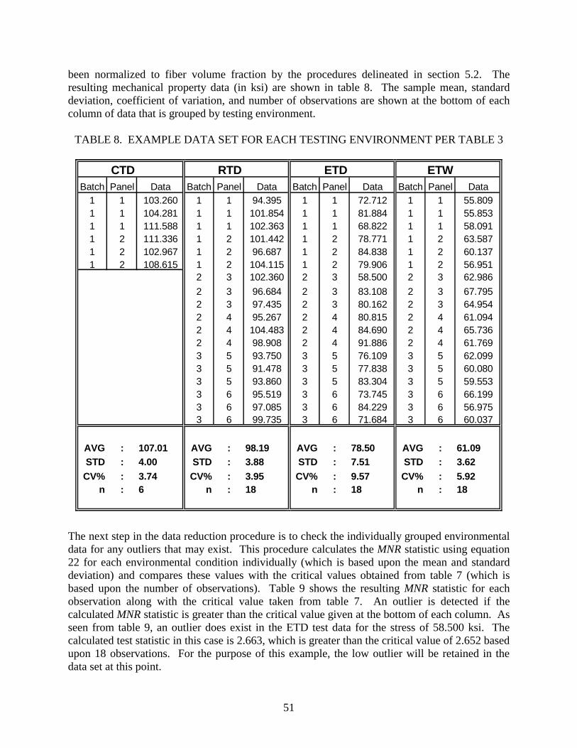
51

been normalized to fiber volume fraction by the procedures delineated in section 5.2. The resulting mechanical property data (in ksi) are shown in table 8. The sample mean, standard deviation, coefficient of variation, and number of observations are shown at the bottom of each column of data that is grouped by testing environment.

TABLE 8. EXAMPLE DATA SET FOR EACH TESTING ENVIRONMENT PER TABLE 3

CTD RTD ETD ETWBatch Panel Data Batch Panel Data Batch Panel Data Batch Panel Data

1 1 103.260 1 1 94.395 1 1 72.712 1 1 55.8091 1 104.281 1 1 101.854 1 1 81.884 1 1 55.8531 1 111.588 1 1 102.363 1 1 68.822 1 1 58.0911 2 111.336 1 2 101.442 1 2 78.771 1 2 63.5871 2 102.967 1 2 96.687 1 2 84.838 1 2 60.1371 2 108.615 1 2 104.115 1 2 79.906 1 2 56.951

2 3 102.360 2 3 58.500 2 3 62.9862 3 96.684 2 3 83.108 2 3 67.7952 3 97.435 2 3 80.162 2 3 64.9542 4 95.267 2 4 80.815 2 4 61.0942 4 104.483 2 4 84.690 2 4 65.7362 4 98.908 2 4 91.886 2 4 61.7693 5 93.750 3 5 76.109 3 5 62.0993 5 91.478 3 5 77.838 3 5 60.0803 5 93.860 3 5 83.304 3 5 59.5533 6 95.519 3 6 73.745 3 6 66.1993 6 97.085 3 6 84.229 3 6 56.9753 6 99.735 3 6 71.684 3 6 60.037

AVG : 107.01 AVG : 98.19 AVG : 78.50 AVG : 61.09STD : 4.00 STD : 3.88 STD : 7.51 STD : 3.62

CV% : 3.74 CV% : 3.95 CV% : 9.57 CV% : 5.92n : 6 n : 18 n : 18 n : 18

The next step in the data reduction procedure is to check the individually grouped environmental data for any outliers that may exist. This procedure calculates the MNR statistic using equation 22 for each environmental condition individually (which is based upon the mean and standard deviation) and compares these values with the critical values obtained from table 7 (which is based upon the number of observations). Table 9 shows the resulting MNR statistic for each observation along with the critical value taken from table 7. An outlier is detected if the calculated MNR statistic is greater than the critical value given at the bottom of each column. As seen from table 9, an outlier does exist in the ETD test data for the stress of 58.500 ksi. The calculated test statistic in this case is 2.663, which is greater than the critical value of 2.652 based upon 18 observations. For the purpose of this example, the low outlier will be retained in the data set at this point.

52

TABLE 9. CALCULATED MNR STATISTIC FOR THE ENVIRONMENTALLY GROUPED DATA

Raw Data MNR Raw Data MNR Raw Data MNR Raw Data MNR103.260 0.936 94.395 0.977 72.712 0.771 55.809 1.460104.281 0.681 101.854 0.944 81.884 0.451 55.853 1.448111.588 1.144 102.363 1.075 68.822 1.289 58.091 0.830111.336 1.081 101.442 0.838 78.771 0.036 63.587 0.689102.967 1.010 96.687 0.387 84.838 0.844 60.137 0.265108.615 0.402 104.115 1.526 79.906 0.187 56.951 1.145

102.360 1.074 58.500 2.663 62.986 0.52396.684 0.388 83.108 0.614 67.795 1.85197.435 0.194 80.162 0.221 64.954 1.06695.267 0.753 80.815 0.308 61.094 0.000

104.483 1.621 84.690 0.824 65.736 1.28298.908 0.185 91.886 1.782 61.769 0.18693.750 1.143 76.109 0.318 62.099 0.27791.478 1.729 77.838 0.088 60.080 0.28093.860 1.115 83.304 0.640 59.553 0.42695.519 0.688 73.745 0.633 66.199 1.41197.085 0.285 84.229 0.763 56.975 1.13899.735 0.398 71.684 0.908 60.037 0.292

CTD

Critical Value Critical Value Critical Value Critical Value1.887 2.652 2.652 2.652

RTD ETD ETW

After the data is checked for outliers, a visual check should be performed on the environmentally grouped data to validate the assumption of normality following the procedures outlined in section 5.3.1.2. Figure 21 shows the data from table 8 plotted against the standard normal curves for each environment tested. As seen in the figure, the normal model appears to closely represent the data across all represented environments and does not appear to cause any significant engineering concerns. This plot may also be graphically represented on a probability scale, which reduces the distribution to a straight line. Probability plotting is a graphical method for determining whether sample data conforms to a hypothesized normal distribution based on a subjective visual examination of the data. If the normal distribution adequately describes the data, the plotted points will fall approximately on a straight line. The next step in the data reduction process is the pooling of data across environments. The data from each environment is normalized using the sample mean from each environmental condition. Table 10 shows the resulting normalized data, pooling all environments together. As seen from this method, all strength values then take on a normalized value in the neighborhood of one. Also shown in table 10 are the resulting mean, standard deviation, coefficient of variation, and number of observations.

53

0 40 80 120 160Failure Stress (ksi)

0

0.2

0.4

0.6

0.8

1

Prob

abili

ty o

f Sur

viva

l

CTDRTDETDETWNormal Fit

FIGURE 21. NORMALIZED FIT OF EXPERIMENTAL DATA FOR EACH ENVIRONMENT

TABLE 10. RESULTING POOLED DATA AFTER NORMALIZATION PROCEDURE

CTD RTD ETD ETWBatch Panel Data Batch Panel Data Batch Panel Data Batch Panel Data

1 1 0.965 1 1 0.961 1 1 0.926 1 1 0.9131 1 0.975 1 1 1.037 1 1 1.043 1 1 0.9141 1 1.043 1 1 1.042 1 1 0.877 1 1 0.9511 2 1.040 1 2 1.033 1 2 1.003 1 2 1.0411 2 0.962 1 2 0.985 1 2 1.081 1 2 0.9841 2 1.015 1 2 1.060 1 2 1.018 1 2 0.932

2 3 1.042 2 3 0.745 2 3 1.0312 3 0.985 2 3 1.059 2 3 1.1102 3 0.992 2 3 1.021 2 3 1.0632 4 0.970 2 4 1.029 2 4 1.0002 4 1.064 2 4 1.079 2 4 1.0762 4 1.007 2 4 1.171 2 4 1.0113 5 0.955 3 5 0.970 3 5 1.0163 5 0.932 3 5 0.992 3 5 0.9833 5 0.956 3 5 1.061 3 5 0.9753 6 0.973 3 6 0.939 3 6 1.0843 6 0.989 3 6 1.073 3 6 0.9333 6 1.016 3 6 0.913 3 6 0.983

Pooled Average : 1.000Pooled Standard Dev. : 0.0649

Coeff. of Variation : 6.494Number of Observations : 60

54

Using the pooled data, figure 22 shows the visual check of the normal distribution with respect to the pooled data. As seen from figure 22, the normal model appears to closely represent the data across all pooled data and does not appear to cause any significant engineering concerns.

0.6 0.8 1 1.2 1.4Normalized Pooled Data

0

0.2

0.4

0.6

0.8

1

Prob

abili

ty o

f Sur

viva

lNormal FitPooled Data

FIGURE 22. NORMALIZED FIT OF POOLED DATA After the pooled data has been collected, the pooled sample mean and standard deviation may be computed (see table 10). Using these values, the B- and A-basis values may be calculated for the pooled data. Using equations 12 through 19, the one-sided tolerance limits may be calculated for each environmental condition. The values of these tolerance limits for each environment are

Statistic CTD RTD ETD ETW

kB 2.0281 1.7585 1.7585 1.7585 kA 3.1632 2.9250 2.9250 2.9250

which, combined with the pooled normal sample mean and standard deviation, yield B and A knockdown values for each of via equations 20 and 21


Bnormal 0.8683 0.8858 0.8858 0.8858 Anormal 0.7946 0.8100 0.8100 0.8100

55

Once these values are obtained, the B and A basis for each environmental condition may be obtained using the mean of each environment and the pooled B- and A-basis values. Simple multiplication yields the B- and A-basis values for each environment as


B-basis value 92.914 86.977 69.536 54.118 A-basis value 85.026 79.538 63.589 49.489

It should be noted that even though A-basis numbers were calculated for this example, the number of specimens was more in accordance with the number recommended for B-basis calculations. For a more robust A-basis allowable, the number of specimens can be increased to those given in table 4. 5.4 MATERIAL PERFORMANCE ENVELOPE AND INTERPOLATION.

Using the B-basis numbers generated in the previous example, a material performance envelope may be generated for the example material system by plotting these values as a function of temperature. Figure 23 shows the material performance envelope using the B-basis values generated in the previous example.

��

-100 -50 0 50 100 150 200Temperature (o F)

20

40

60

80

100

120

B-B

asis

Str

engt

h Va

lues

(ksi

)

Actual Basis ValueEstimated Value

CTDRTD

ETD

ETW

RTW

MaterialPerformanceEnvelope

FIGURE 23. MATERIAL PERFORMANCE ENVELOPE

56

Since each specific aircraft application of the qualified material may have different material operational limits (MOL) than those tested in the material qualification (which is usually the upper limit), some applications may require a reduced MOL. In this case, simple linear interpolation may be used to obtain the corresponding basis values at the new application MOL. This interpolation may be accomplished using the following simple relationships assuming TRTD < TMOL < TETD : For the corresponding MOL “dry” basis value, the “interpolated” basis value using the qualification data is

( )( )( )ETDRTD

MOLRTDETDRTDRTDMOL TT

TTBBBB−

−−−=

(29)

where: BMOL = new application basis value interpolated to TMOL BRTD = basis RTD strength value BETD = basis ETD strength value TRTD = RTD test temperature

TETD = ETD test temperature TMOL = new application MOL temperature

For the corresponding MOL “wet” basis value, an estimated room temperature wet (RTW) value must be calculated. This may be accomplished by the simple relation

)( ETWETDRTDRTW BBBB −−= (30) The interpolated wet basis value using the qualification data may then be obtained by

( )( )( )ETWRTW

MOLRTWETWRTWRTWMOL TT

TTBBBB−

−−−= (31)

where: BMOL = new application basis value interpolated to TMOL BRTW = estimated basis RTW strength value BETW = basis ETW strength value TRTW = RTW (i.e., RTD) test temperature

TETW = ETW test temperature TMOL = new application MOL temperature

These equations may also be used for interpolated mean strengths as well as A-basis values with the appropriate substitutions. It should be noted that because unforeseen material property drop-offs with respect to temperature and environment can occur, extrapolation to a higher MOL should not be attempted without additional testing and verification. In addition, the interpolation equations shown above are practical for materials obeying typical mechanical behavior. In most cases, some minimal amount of testing may also be required to verify the interpolated values.

57

Using the basis values obtained in the previous example, presented in section 5.3.2, this section provides an example of linear interpolations to a specific application environment less than the tested upper material limit used in qualification. Assuming a specific application environment of 150°F, figure 24 depicts the linear interpolation of the B-basis design allowable to this environment. Using equations 29 and 31 along with the nominal testing temperatures (see table 3), the interpolated basis values at 150°F become ETD : BMOL = 75.765 ksi ETW : BMOL = 58.875 ksi

��

-100 -50 0 50 100 150 200Temperature (o F)

20

40

60

80

100

120

B-B

asis

Str

engt

h Va

lues

(ksi

)

Actual Basis ValueEstimated Value

CTD

RTD

ETD

ETW

RTW

FIGURE 24. EXAMPLE OF 150°F INTERPOLATION FOR B-BASIS VALUES 6. MATERIAL EQUIVALENCY AND ACCEPTANCE TESTING.

This section describes the methodology to demonstrate material equivalency and establish acceptance testing criteria. Material equivalency programs are specified to assure that a “follow-on” material and/or follow-on process will produce material properties equivalent to those of the original qualification. Acceptance testing is a quality control procedure designed to detect large property variations or undesirably high or low properties in an incoming prepreg lot.

58

In general, the properties that are normalized (see section 5.2.2) in the “original” qualification should be compared with normalized properties of the follow-on material for statistical testing purposes, particularly in the case of unidirectional tape. The data normalization method of the two sets of data should be identical. If data scatter increases significantly either in the original or follow-on material properties after the normalization process, the reason should be investigated. The properties that are not normalized (see section 5.2.2) from the original qualification should be compared with unnormalized properties of the follow-on material. No clear model is currently available to accurately normalize matrix-dominated properties, although the effects of fiber volume fraction on these properties have been observed. This form of error may hamper the effectiveness and validity of the statistical tests. Rejection by statistical tests on these properties may be justified by significant differences in cured-ply thickness, fiber volume fraction, and/or void content, however, the reason for such differences should be investigated. In general, engineering judgement must be exercised to determine the significance of these properties that fail the criteria and may override the statistical tests. A major part of the criterion adopted in this document is based on a statistical test commonly known as test of hypotheses. For strength properties, both the means and the minimum individuals are considered. This is a joint/combined α for one-sided test, hence, a low mean or low minimum individual or both will constitute a rejection. For modulus properties, only the means are considered. Table 11 provides the suitable criteria and test statistic for each property of interest. When one embarks on the path of showing equivalency, engineering judgment should not be left behind. If some mechanical property at one temperature does not show statistical equivalence, the importance of that property and the size of the discrepancy should be investigated before declaring that the materials are not the same or equivalent. For example, tensile strength and modulus and ETW compression strength and modulus are examples of properties which are usually design critical and more importance should be placed on the statistical test results. The criteria described in this section are applicable only when between-batch variability is assumed insignificant. MIL-HDBK-17-1E, section 8.4.2 provides guidance for the case where between-batch variability is significant.

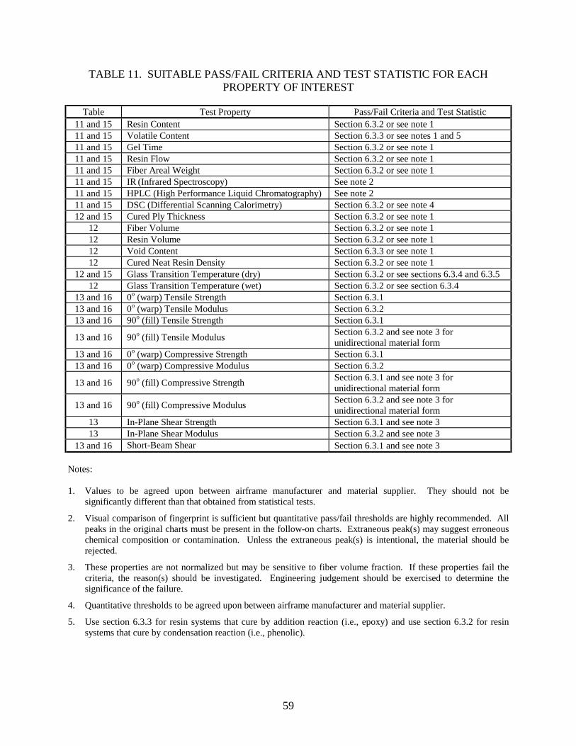
59

TABLE 11. SUITABLE PASS/FAIL CRITERIA AND TEST STATISTIC FOR EACH PROPERTY OF INTEREST

Table Test Property Pass/Fail Criteria and Test Statistic 11 and 15 Resin Content Section 6.3.2 or see note 1 11 and 15 Volatile Content Section 6.3.3 or see notes 1 and 5 11 and 15 Gel Time Section 6.3.2 or see note 1 11 and 15 Resin Flow Section 6.3.2 or see note 1 11 and 15 Fiber Areal Weight Section 6.3.2 or see note 1 11 and 15 IR (Infrared Spectroscopy) See note 2 11 and 15 HPLC (High Performance Liquid Chromatography) See note 2 11 and 15 DSC (Differential Scanning Calorimetry) Section 6.3.2 or see note 4 12 and 15 Cured Ply Thickness Section 6.3.2 or see note 1

12 Fiber Volume Section 6.3.2 or see note 1 12 Resin Volume Section 6.3.2 or see note 1 12 Void Content Section 6.3.3 or see note 1 12 Cured Neat Resin Density Section 6.3.2 or see note 1

12 and 15 Glass Transition Temperature (dry) Section 6.3.2 or see sections 6.3.4 and 6.3.5 12 Glass Transition Temperature (wet) Section 6.3.2 or see section 6.3.4

13 and 16 0o (warp) Tensile Strength Section 6.3.1 13 and 16 0o (warp) Tensile Modulus Section 6.3.2 13 and 16 90o (fill) Tensile Strength Section 6.3.1

13 and 16 90o (fill) Tensile Modulus Section 6.3.2 and see note 3 for unidirectional material form

13 and 16 0o (warp) Compressive Strength Section 6.3.1 13 and 16 0o (warp) Compressive Modulus Section 6.3.2

13 and 16 90o (fill) Compressive Strength Section 6.3.1 and see note 3 for unidirectional material form

13 and 16 90o (fill) Compressive Modulus Section 6.3.2 and see note 3 for unidirectional material form

13 In-Plane Shear Strength Section 6.3.1 and see note 3 13 In-Plane Shear Modulus Section 6.3.2 and see note 3

13 and 16 Short-Beam Shear Section 6.3.1 and see note 3 Notes: 1. Values to be agreed upon between airframe manufacturer and material supplier. They should not be

significantly different than that obtained from statistical tests.

2. Visual comparison of fingerprint is sufficient but quantitative pass/fail thresholds are highly recommended. All peaks in the original charts must be present in the follow-on charts. Extraneous peak(s) may suggest erroneous chemical composition or contamination. Unless the extraneous peak(s) is intentional, the material should be rejected.

3. These properties are not normalized but may be sensitive to fiber volume fraction. If these properties fail the criteria, the reason(s) should be investigated. Engineering judgement should be exercised to determine the significance of the failure.

4. Quantitative thresholds to be agreed upon between airframe manufacturer and material supplier.

5. Use section 6.3.3 for resin systems that cure by addition reaction (i.e., epoxy) and use section 6.3.2 for resin systems that cure by condensation reaction (i.e., phenolic).

60

6.1 MATERIAL EQUIVALENCE.

The procedures for material equivalency described in this document are only applicable to the following specific types of changes:

a. Identical material fabricated by the same airframe manufacturer using identical fabrication process at a different location,

b. Identical material fabricated by a different airframe manufacturer using a follow-on process that is equivalent to the original process,

c. Identical material fabricated by the same airframe manufacturer using a follow-on process that is slightly different from the original process,

d. Minor changes in the prepreg constituent(s) and/or constituent manufacturing process, or

e. Combinations of the above.

The above-mentioned changes are subject to the following limitations:

a. All critical prepreg constituent(s) and/or constituent manufacturing process must remain unchanged.

b. All critical steps in the process specifications used to fabricate the original and follow-on material systems must be equivalent. The process specification for the follow-on material system may not include any information which might degrade the performance of the follow-on material system below that of the originally qualified system.

c. The fabrication of the follow-on material system must meet the applicable CFR requirements including, but are not limited to:

- § 23.603 (a) and (b) - § 23.605 (a) and (b) In all cases of material equivalence, an original database should exist that contains material properties of the original material system. The types of changes to the follow-on material system that are considered as major changes which are not covered by this document include, but are not limited to:

a. Change of fiber (for example, changing from AS4 to T300 fibers)

b. Change of resin (for example, changing from 3501-6 to E7K8 resin)

c. Change of fabric weave style (for example, changing from eight-harness satin weave to plain weave)

d. Change of tow dimension of fabric (for example, changing from 6K tow to 3K tow)

61

e. Significant change in resin content of prepreg

f. Change of sizing or coupling agent type The specific types of changes to the follow-on material system and/or process which may be considered as minor changes include, but are not limited to: a. Increasing the cure pressure or vacuum level for the follow-on process. This includes

changing from oven curing (vacuum only) to autoclave curing. Decreasing the cure pressure or vacuum level for the follow-on process, however, is generally not allowed.

b. Cure parameters such as dwell time and heat-up rate

c. Prepreg tackiness

Further evaluation or testing may be required depending on the extent of the changes. For example, increasing the prepreg tackiness may result in higher volatile content. Higher volatile content has been known to cause higher void content and lower glass transition temperature in cured laminate. MIL-HDBK-17-1E, sections 2.3.4, 2.3.7, 2.5.3.4, and 8.4.3 provide further guidance to this subject. Although outlined in MIL-HDBK-17-1E, in particular cases, engineering judgement must assess the degree of similarity between different materials or manufacturing process changes and the significance of these changes. In the case where a material supplier decides to modify the material system, even for the purpose of improving the material properties, airframe manufacturers which have been approved to use the material system may be required to perform the material equivalency exercise to demonstrate that the change(s) is compatible with individual manufacturers’ processing parameters. A successful material equivalency demonstration does not imply that the follow-on material and/or follow-on process will also yield equal properties at laminate, element, and subcomponent levels, as the manufacturing complexity of a particular application may result in different properties. To ascertain if there will be any divergence of properties for more complex shapes and configurations, some simple laminate-notched tension and compression tests should be performed before investing in tooling, etc. If successful, further tests, such as elements and components are typically needed to fulfill the remaining parts of the structural substantiation requirement. The material equivalency procedures outlined herein are not intended for use in determining the effect of cocuring the prepreg onto honeycomb or foam, as this level of testing should be conducted at the laminate level. The statistical method described in this document was chosen for its simplicity in application. Other methods can be found in MIL-HDBK-17-1E that can perform similar equivalency evaluations. Material equivalence testing should be conducted to incorporate the processing or panel-to-panel variability. Specimen sampling and selection should be based upon at least two independent processing or cure cycles, as depicted in figure 25.

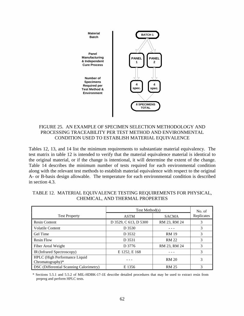
62

FIGURE 25. AN EXAMPLE OF SPECIMEN SELECTION METHODOLOGY AND PROCESSING TRACEABILITY PER TEST METHOD AND ENVIRONMENTAL

CONDITION USED TO ESTABLISH MATERIAL EQUIVALENCE Tables 12, 13, and 14 list the minimum requirements to substantiate material equivalency. The test matrix in table 12 is intended to verify that the material equivalence material is identical to the original material, or if the change is intentional, it will determine the extent of the change. Table 14 describes the minimum number of tests required for each environmental condition along with the relevant test methods to establish material equivalence with respect to the original A- or B-basis design allowable. The temperature for each environmental condition is described in section 4.3.

TABLE 12. MATERIAL EQUIVALENCE TESTING REQUIREMENTS FOR PHYSICAL, CHEMICAL, AND THERMAL PROPERTIES

Test Method(s) Test Property ASTM SACMA

No. of Replicates

Resin Content D 3529, C 613, D 5300 RM 23, RM 24 3 Volatile Content D 3530 - - - 3 Gel Time D 3532 RM 19 3 Resin Flow D 3531 RM 22 3 Fiber Areal Weight D 3776 RM 23, RM 24 3 IR (Infrared Spectroscopy) E 1252, E 168 - - - 3 HPLC (High Performance Liquid Chromatography)* - - - RM 20 3

DSC (Differential Scanning Calorimetry) E 1356 RM 25 3

* Sections 5.5.1 and 5.5.2 of MIL-HDBK-17-1E describe detailed procedures that may be used to extract resin from prepreg and perform HPLC tests.

BATCH 1

PANEL2

4spec.

PANEL1

4spec.

8 SPECIMENSTOTAL

MaterialBatch


Number ofSpecimens


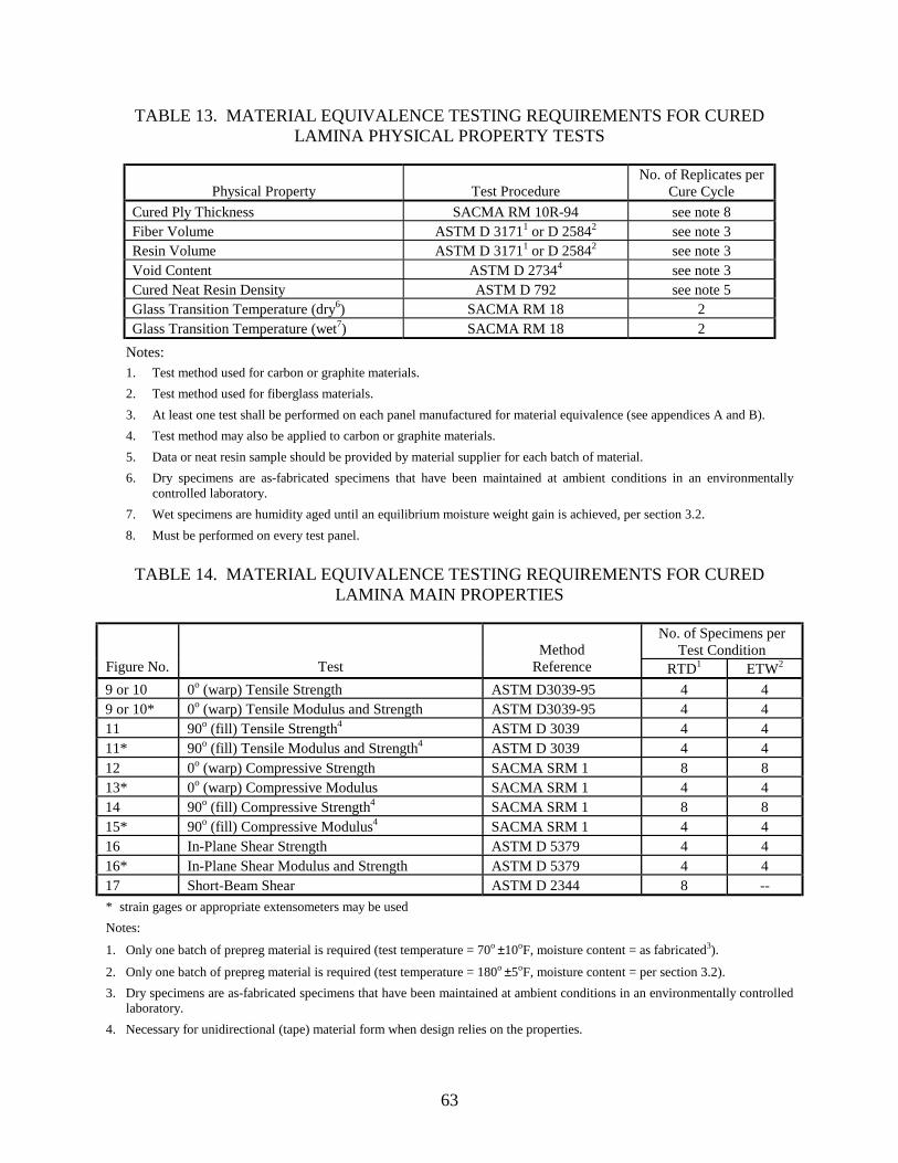
63

TABLE 13. MATERIAL EQUIVALENCE TESTING REQUIREMENTS FOR CURED LAMINA PHYSICAL PROPERTY TESTS

Physical Property Test Procedure No. of Replicates per

Cure Cycle Cured Ply Thickness SACMA RM 10R-94 see note 8 Fiber Volume ASTM D 31711 or D 25842 see note 3 Resin Volume ASTM D 31711 or D 25842 see note 3 Void Content ASTM D 27344 see note 3 Cured Neat Resin Density ASTM D 792 see note 5 Glass Transition Temperature (dry6) SACMA RM 18 2 Glass Transition Temperature (wet7) SACMA RM 18 2

Notes: 1. Test method used for carbon or graphite materials. 2. Test method used for fiberglass materials. 3. At least one test shall be performed on each panel manufactured for material equivalence (see appendices A and B). 4. Test method may also be applied to carbon or graphite materials. 5. Data or neat resin sample should be provided by material supplier for each batch of material. 6. Dry specimens are as-fabricated specimens that have been maintained at ambient conditions in an environmentally

controlled laboratory. 7. Wet specimens are humidity aged until an equilibrium moisture weight gain is achieved, per section 3.2. 8. Must be performed on every test panel.

TABLE 14. MATERIAL EQUIVALENCE TESTING REQUIREMENTS FOR CURED

LAMINA MAIN PROPERTIES

No. of Specimens per Test Condition

Figure No. Test Method

Reference RTD1 ETW2

9 or 10 0o (warp) Tensile Strength ASTM D3039-95 4 4 9 or 10* 0o (warp) Tensile Modulus and Strength ASTM D3039-95 4 4 11 90o (fill) Tensile Strength4 ASTM D 3039 4 4 11* 90o (fill) Tensile Modulus and Strength4 ASTM D 3039 4 4 12 0o (warp) Compressive Strength SACMA SRM 1 8 8 13* 0o (warp) Compressive Modulus SACMA SRM 1 4 4 14 90o (fill) Compressive Strength4 SACMA SRM 1 8 8 15* 90o (fill) Compressive Modulus4 SACMA SRM 1 4 4 16 In-Plane Shear Strength ASTM D 5379 4 4 16* In-Plane Shear Modulus and Strength ASTM D 5379 4 4 17 Short-Beam Shear ASTM D 2344 8 -- * strain gages or appropriate extensometers may be used Notes:

1. Only one batch of prepreg material is required (test temperature = 70o ±10oF, moisture content = as fabricated3).

2. Only one batch of prepreg material is required (test temperature = 180o ±5oF, moisture content = per section 3.2). 3. Dry specimens are as-fabricated specimens that have been maintained at ambient conditions in an environmentally controlled

laboratory. 4. Necessary for unidirectional (tape) material form when design relies on the properties.

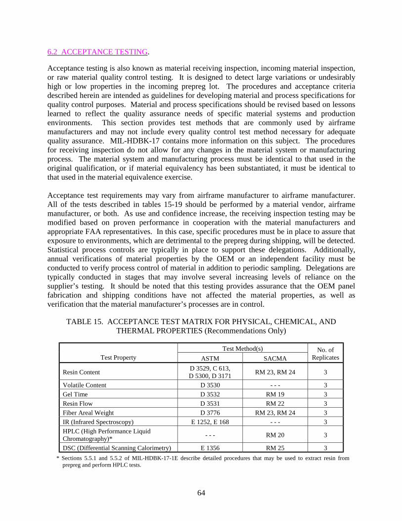
64

6.2 ACCEPTANCE TESTING.

Acceptance testing is also known as material receiving inspection, incoming material inspection, or raw material quality control testing. It is designed to detect large variations or undesirably high or low properties in the incoming prepreg lot. The procedures and acceptance criteria described herein are intended as guidelines for developing material and process specifications for quality control purposes. Material and process specifications should be revised based on lessons learned to reflect the quality assurance needs of specific material systems and production environments. This section provides test methods that are commonly used by airframe manufacturers and may not include every quality control test method necessary for adequate quality assurance. MIL-HDBK-17 contains more information on this subject. The procedures for receiving inspection do not allow for any changes in the material system or manufacturing process. The material system and manufacturing process must be identical to that used in the original qualification, or if material equivalency has been substantiated, it must be identical to that used in the material equivalence exercise. Acceptance test requirements may vary from airframe manufacturer to airframe manufacturer. All of the tests described in tables 15-19 should be performed by a material vendor, airframe manufacturer, or both. As use and confidence increase, the receiving inspection testing may be modified based on proven performance in cooperation with the material manufacturers and appropriate FAA representatives. In this case, specific procedures must be in place to assure that exposure to environments, which are detrimental to the prepreg during shipping, will be detected. Statistical process controls are typically in place to support these delegations. Additionally, annual verifications of material properties by the OEM or an independent facility must be conducted to verify process control of material in addition to periodic sampling. Delegations are typically conducted in stages that may involve several increasing levels of reliance on the supplier’s testing. It should be noted that this testing provides assurance that the OEM panel fabrication and shipping conditions have not affected the material properties, as well as verification that the material manufacturer’s processes are in control.

TABLE 15. ACCEPTANCE TEST MATRIX FOR PHYSICAL, CHEMICAL, AND THERMAL PROPERTIES (Recommendations Only)

Test Method(s) Test Property ASTM SACMA

No. of Replicates

Resin Content D 3529, C 613, D 5300, D 3171 RM 23, RM 24 3

Volatile Content D 3530 - - - 3 Gel Time D 3532 RM 19 3 Resin Flow D 3531 RM 22 3 Fiber Areal Weight D 3776 RM 23, RM 24 3 IR (Infrared Spectroscopy) E 1252, E 168 - - - 3 HPLC (High Performance Liquid Chromatography)* - - - RM 20 3

DSC (Differential Scanning Calorimetry) E 1356 RM 25 3 * Sections 5.5.1 and 5.5.2 of MIL-HDBK-17-1E describe detailed procedures that may be used to extract resin from

prepreg and perform HPLC tests.

65

TABLE 16. ACCEPTANCE TEST MATRIX FOR CURED LAMINA PHYSICAL PROPERTIES (Recommendations Only)

Physical Property Test Procedure No. of Replicates Cured Ply Thickness SACMA RM 10R See notes 2 and 3 Glass Transition Temperature (dry1) SACMA RM 18 1

Notes: 1. Dry specimens are as-fabricated specimens that have been maintained at ambient conditions in an environmentally

controlled laboratory.

2. Must be performed on every test panel.

3. Type of measuring surface should be identical to the one used in original material qualification, or the amount of difference introduced by the measuring surface should be taken into account.

TABLE 17. ACCEPTANCE TESTING FOR CURED LAMINA PROPERTIES

(Recommendations Only)

No. of Specimens Figure No. Test

Method Reference RTD1, 2 ETD1, 2

9 or 10 0o (warp) Tensile Strength ASTM D 3039 0-2 - 9 or 10* 0o (warp) Tensile Modulus and Strength ASTM D 3039 3 - 11 90o (fill) Tensile Strength3 ASTM D 3039 0-2 - 11* 90o (fill) Tensile Modulus and Strength3 ASTM D 3039 3 - 12 0o (warp) Compressive Strength SACMA SRM 1 - 3-5 13* 0o (warp) Compressive Modulus SACMA SRM 1 3 - 14 90o (fill) Compressive Strength3 SACMA SRM 1 - 3-5 15* 90o (fill) Compressive Modulus3 SACMA SRM 1 3 - 17 Short-Beam Shear ASTM D 2344 3-5 -

* strain gages or appropriate extensometers may be used

Notes:

1. Only one lot of material is required (test temperature = 70o ±10oF, moisture content = as fabricated2).

2. Dry specimens are as fabricated specimens that have been maintained at ambient conditions in an environmentally controlled laboratory.

3. Necessary for unidirectional (tape) material form when design relies on these properties. For acceptance testing, it is not necessary to incorporate processing cycle or panel-to-panel variability, as shown in figure 25. All of the test panels for the test matrix in table 17 may be processed in a single cure cycle. Material and process specifications often define acceptable levels for visual defects; however, they are rather ineffective when incorporated into acceptance testing since it is impractical to unroll every roll of prepreg for the purpose of quality assurance. This inspection process is often left to individuals in charge of prepreg cutting and lay-up. These individuals must be trained and be familiar with prepreg visual inspection techniques. Table 18 lists some common types of defects and their corresponding acceptable levels.

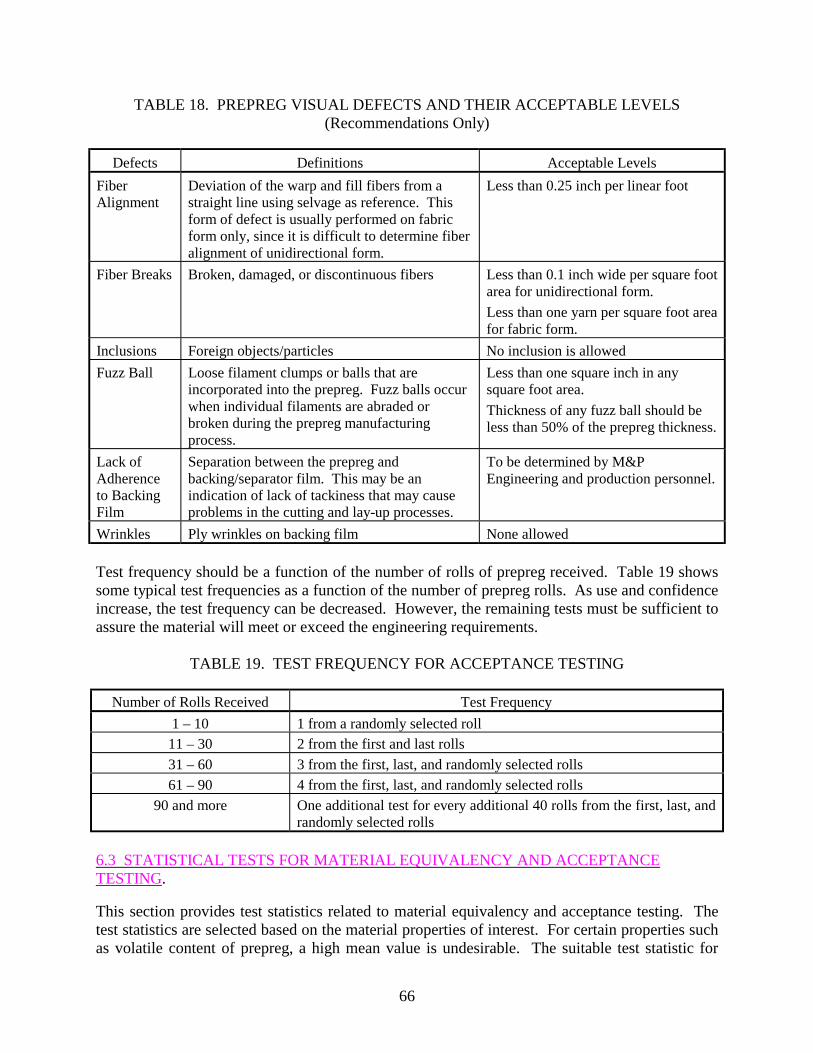
66

TABLE 18. PREPREG VISUAL DEFECTS AND THEIR ACCEPTABLE LEVELS (Recommendations Only)

Defects Definitions Acceptable Levels Fiber Alignment

Deviation of the warp and fill fibers from a straight line using selvage as reference. This form of defect is usually performed on fabric form only, since it is difficult to determine fiber alignment of unidirectional form.

Less than 0.25 inch per linear foot

Fiber Breaks Broken, damaged, or discontinuous fibers Less than 0.1 inch wide per square foot area for unidirectional form. Less than one yarn per square foot area for fabric form.

Inclusions Foreign objects/particles No inclusion is allowed Fuzz Ball Loose filament clumps or balls that are

incorporated into the prepreg. Fuzz balls occur when individual filaments are abraded or broken during the prepreg manufacturing process.

Less than one square inch in any square foot area. Thickness of any fuzz ball should be less than 50% of the prepreg thickness.

Lack of Adherence to Backing Film

Separation between the prepreg and backing/separator film. This may be an indication of lack of tackiness that may cause problems in the cutting and lay-up processes.

To be determined by M&P Engineering and production personnel.

Wrinkles Ply wrinkles on backing film None allowed Test frequency should be a function of the number of rolls of prepreg received. Table 19 shows some typical test frequencies as a function of the number of prepreg rolls. As use and confidence increase, the test frequency can be decreased. However, the remaining tests must be sufficient to assure the material will meet or exceed the engineering requirements.

TABLE 19. TEST FREQUENCY FOR ACCEPTANCE TESTING

Number of Rolls Received Test Frequency 1 – 10 1 from a randomly selected roll

11 – 30 2 from the first and last rolls 31 – 60 3 from the first, last, and randomly selected rolls 61 – 90 4 from the first, last, and randomly selected rolls

90 and more One additional test for every additional 40 rolls from the first, last, and randomly selected rolls

6.3 STATISTICAL TESTS FOR MATERIAL EQUIVALENCY AND ACCEPTANCE TESTING.

This section provides test statistics related to material equivalency and acceptance testing. The test statistics are selected based on the material properties of interest. For certain properties such as volatile content of prepreg, a high mean value is undesirable. The suitable test statistic for

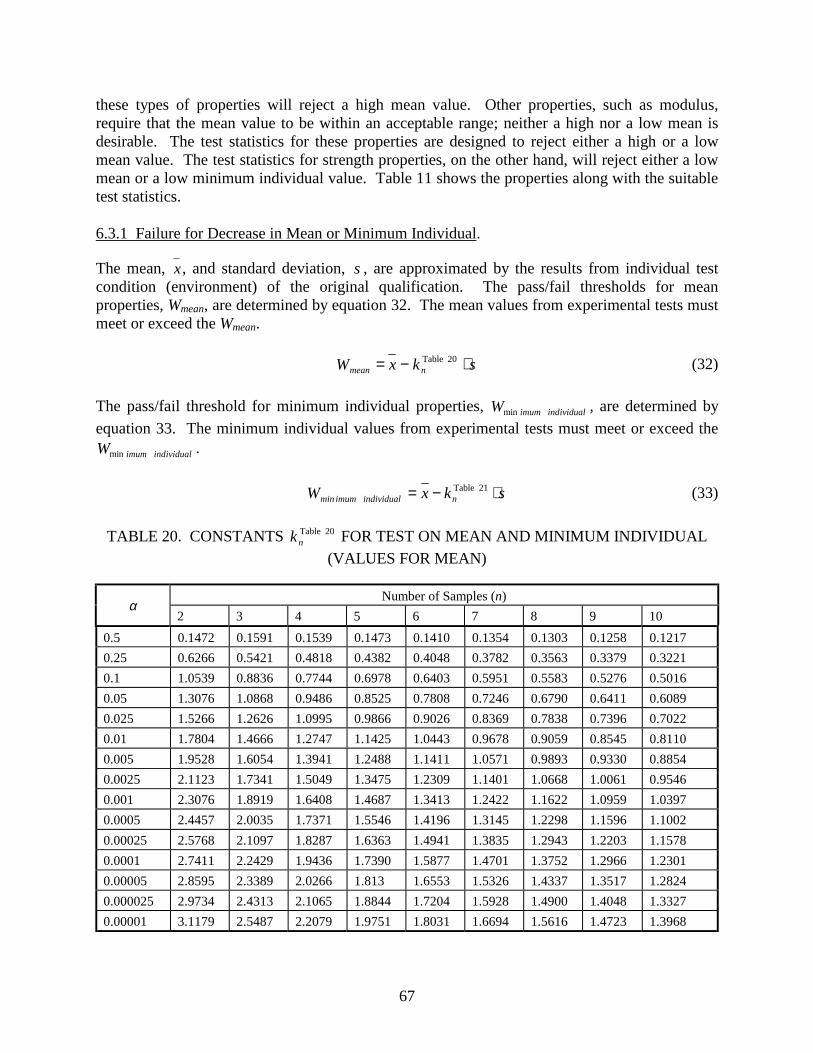
67

these types of properties will reject a high mean value. Other properties, such as modulus, require that the mean value to be within an acceptable range; neither a high nor a low mean is desirable. The test statistics for these properties are designed to reject either a high or a low mean value. The test statistics for strength properties, on the other hand, will reject either a low mean or a low minimum individual value. Table 11 shows the properties along with the suitable test statistics. 6.3.1 Failure for Decrease in Mean or Minimum Individual.

The mean, x , and standard deviation, s , are approximated by the results from individual test condition (environment) of the original qualification. The pass/fail thresholds for mean properties, Wmean, are determined by equation 32. The mean values from experimental tests must meet or exceed the Wmean. skxW nmean ⋅−= 20 Table (32) The pass/fail threshold for minimum individual properties, ividualimum indWmin , are determined by equation 33. The minimum individual values from experimental tests must meet or exceed the

ividualimum indWmin . skxW nividualimum indmin ⋅−= 21 Table (33)

TABLE 20. CONSTANTS 20 Tablenk FOR TEST ON MEAN AND MINIMUM INDIVIDUAL

(VALUES FOR MEAN)

Number of Samples (n) α

2 3 4 5 6 7 8 9 10 0.5 0.1472 0.1591 0.1539 0.1473 0.1410 0.1354 0.1303 0.1258 0.1217 0.25 0.6266 0.5421 0.4818 0.4382 0.4048 0.3782 0.3563 0.3379 0.3221 0.1 1.0539 0.8836 0.7744 0.6978 0.6403 0.5951 0.5583 0.5276 0.5016 0.05 1.3076 1.0868 0.9486 0.8525 0.7808 0.7246 0.6790 0.6411 0.6089 0.025 1.5266 1.2626 1.0995 0.9866 0.9026 0.8369 0.7838 0.7396 0.7022 0.01 1.7804 1.4666 1.2747 1.1425 1.0443 0.9678 0.9059 0.8545 0.8110 0.005 1.9528 1.6054 1.3941 1.2488 1.1411 1.0571 0.9893 0.9330 0.8854 0.0025 2.1123 1.7341 1.5049 1.3475 1.2309 1.1401 1.0668 1.0061 0.9546 0.001 2.3076 1.8919 1.6408 1.4687 1.3413 1.2422 1.1622 1.0959 1.0397 0.0005 2.4457 2.0035 1.7371 1.5546 1.4196 1.3145 1.2298 1.1596 1.1002 0.00025 2.5768 2.1097 1.8287 1.6363 1.4941 1.3835 1.2943 1.2203 1.1578 0.0001 2.7411 2.2429 1.9436 1.7390 1.5877 1.4701 1.3752 1.2966 1.2301 0.00005 2.8595 2.3389 2.0266 1.813 1.6553 1.5326 1.4337 1.3517 1.2824 0.000025 2.9734 2.4313 2.1065 1.8844 1.7204 1.5928 1.4900 1.4048 1.3327 0.00001 3.1179 2.5487 2.2079 1.9751 1.8031 1.6694 1.5616 1.4723 1.3968

68

TABLE 21. CONSTANTS 21 Tablenk FOR TEST ON MEAN AND MINIMUM INDIVIDUAL

(VALUES FOR MINIMUM INDIVIDUAL)

Number of Samples (n) α

2 3 4 5 6 7 8 9 10 0.5 0.7166 1.0254 1.2142 1.3498 1.4548 1.5400 1.6113 1.6724 1.7258 0.25 1.2887 1.5407 1.6972 1.8106 1.8990 1.9711 2.0317 2.0838 2.1295 0.1 1.8167 2.0249 2.1561 2.2520 2.3272 2.3887 2.4407 2.4856 2.525 0.05 2.1385 2.3239 2.4420 2.5286 2.5967 2.6527 2.7000 2.7411 2.7772 0.025 2.4208 2.5888 2.6965 2.7758 2.8384 2.8900 2.9337 2.9717 3.0052 0.01 2.7526 2.9027 2.9997 3.0715 3.1283 3.1753 3.2153 3.25 3.2807 0.005 2.9805 3.1198 3.2103 3.2775 3.3309 3.3751 3.4127 3.4455 3.4745 0.0025 3.1930 3.3232 3.4082 3.4716 3.5220 3.5638 3.5995 3.6307 3.6582 0.001 3.4549 3.5751 3.6541 3.7132 3.7603 3.7995 3.8331 3.8623 3.8883 0.0005 3.6412 3.7550 3.8301 3.8864 3.9314 3.9690 4.0011 4.0292 4.0541 0.00025 3.8188 3.9270 3.9987 4.0526 4.0958 4.1319 4.1628 4.1898 4.2138 0.0001 4.0421 4.1439 4.2117 4.2629 4.304 4.3384 4.3678 4.3936 4.4166 0.00005 4.2035 4.3011 4.3664 4.4157 4.4554 4.4886 4.5172 4.5422 4.5644 0.000025 4.3592 4.4530 4.5160 4.5637 4.6022 4.6344 4.6620 4.6863 4.7079 0.00001 4.5573 4.6466 4.7069 4.7527 4.7897 4.8206 4.8473 4.8707 4.8915

6.3.2 Failure for Change in Mean.

This statistical test assumes that the standard deviations of the original and follow-on data are equal but unknown. The pooled standard deviation, Sp, is used as an estimator of common population standard deviation.

2)1()1(

21

222

211

−+⋅−+⋅−

=nn

SnSnS p (34)

21

210 11

nnS

xxt

p +⋅

−= (35)

The test statistic is t0 and n is the number of specimens. Subscripts 1 and 2 denote follow-on and original, respectively. Since this is a two-sided t-test, 2,2/, 21 −+= nnna tt α . Note that 2a α= for the two-sided test. nat , is obtained from table 22. The passing range is between 2,2/ 21 −+− nntα and

2,2/ 21 −+nntα . In other words, t0 must be smaller than 2,2/ 21 −+nntα but larger than 2,2/ 21 −+− nntα to pass the criteria.

69

TABLE 22. CONSTANTS nat ,

a n 0.4 0.25 0.1 0.05 0.025 0.01 0.005 0.0025 0.001 0.0005

1 0.325 1 3.078 6.314 12.706 31.821 63.657 127.32 318.31 636.62 2 0.289 0.816 1.886 2.920 4.303 6.965 9.925 14.089 23.326 31.598 3 0.277 0.765 1.638 2.353 3.182 4.541 5.841 7.453 10.213 12.924 4 0.271 0.741 1.533 2.132 2.776 3.747 4.604 5.598 7.173 8.610 5 0.267 0.727 1.476 2.015 2.571 3.365 4.032 4.773 5.893 6.869 6 0.265 0.718 1.440 1.943 2.447 3.143 3.707 4.317 5.208 5.959 7 0.263 0.711 1.415 1.895 2.365 2.998 3.499 4.029 4.785 5.408 8 0.262 0.706 1.397 1.860 2.306 2.896 3.355 3.833 4.501 5.041 9 0.261 0.703 1.383 1.833 2.262 2.821 3.250 3.690 4.297 4.781 10 0.260 0.700 1.372 1.812 2.228 2.764 3.169 3.581 4.144 4.587 11 0.260 0.697 1.363 1.796 2.201 2.718 3.106 3.497 4.025 4.437 12 0.259 0.695 1.356 1.782 2.179 2.681 3.055 3.428 3.930 4.318 13 0.259 0.694 1.350 1.771 2.160 2.650 3.012 3.372 3.852 4.221 14 0.258 0.692 1.345 1.761 2.145 2.624 2.977 3.326 3.787 4.140 15 0.258 0.691 1.341 1.753 2.131 2.602 2.947 3.286 3.733 4.073 16 0.258 0.690 1.337 1.746 2.120 2.583 2.921 3.252 3.686 4.015 17 0.257 0.689 1.333 1.740 2.110 2.567 2.898 3.222 3.646 3.965 18 0.257 0.688 1.330 1.734 2.101 2.552 2.878 3.197 3.610 3.922 19 0.257 0.688 1.328 1.729 2.093 2.539 2.861 3.174 3.579 3.883 20 0.257 0.687 1.325 1.725 2.086 2.528 2.845 3.153 3.552 3.850 21 0.257 0.686 1.323 1.721 2.080 2.518 2.831 3.135 3.527 3.819 22 0.256 0.686 1.321 1.717 2.074 2.508 2.819 3.119 3.505 3.792 23 0.256 0.685 1.319 1.714 2.069 2.500 2.807 3.104 3.485 3.767 24 0.256 0.685 1.318 1.711 2.064 2.492 2.797 3.091 3.467 3.745 25 0.256 0.684 1.316 1.708 2.060 2.485 2.787 3.078 3.450 3.725 26 0.256 0.684 1.315 1.706 2.056 2.479 2.779 3.067 3.435 3.707 27 0.256 0.684 1.314 1.703 2.052 2.473 2.771 3.057 3.421 3.690 28 0.256 0.683 1.313 1.701 2.048 2.467 2.763 3.047 3.408 3.674 29 0.256 0.683 1.311 1.699 2.045 2.462 2.756 3.038 3.396 3.659 ∞ 0.253 0.674 1.282 1.645 1.960 2.326 2.576 2.807 3.090 3.291

For stiffness properties, modulus and Poisson’s ratio, variations of ±5%-7% from the base material mean can be an acceptable practice if difficulties are encountered with the t-test. 6.3.3 Failure for a High Mean.

The test statistic, t0, is obtained from equation 35. This test is designed to detect undesirably high mean values such as in the case of volatile content of prepreg. The mean of the follow-on property is said to be higher than the mean of the original property if equation 36 is satisfied, an

70

indication of bad material and/or process. This is a one-sided t-test so 2,, 21 −+= nnna tt α . Note that a α= for the one-sided test. nat , is obtained from table 22.

2,0 21 −+> nntt α (36) 6.3.4 Criteria Specific to Material Equivalence.

As of now, there are no fixed criteria for establishment of the MOL. One commonly used method uses wet glass transition temperature, reduced by some temperature margin ∆T, to establish the MOL. If this method is used, the MOL must exceed the maximum operating temperature. In addition, the average glass transition temperature (dry and wet) results in table 12 should not be significantly lower or higher than the results obtained from original material qualification. Section 6.3.2 may be used to determine the acceptable range. If the test method, equipment, or fixture are not identical to the ones used in the original qualification, the t-test may be invalid. It is recommended that a test method, equipment, or test fixture study be performed to investigate the amount of error due to the new test parameter. If a study cannot be performed, a variation of less than ±18°F from the base material mean can be an acceptable practice. For determining material equivalency, it is recommended to set the probability of rejecting a good property (α) to 0.05 or 5% for all test methods that use the test statistics in sections 6.3.1, 6.3.2, and 6.3.3. One retest is allowed for each property, reducing the actual probability to 0.0025 or 0.25%. As depicted in table 13, a minimum of eight specimens is required for strength properties comparison (typically four specimens from each processing cycle). A minimum of four specimens is required for modulus comparisons (typically two specimens from each processing cycle). In the case where one or more properties fail the criteria, one may choose to test only those properties that failed the criteria. However, it is recommended that the entire material equivalence test matrix be repeated if more than half of the properties in table 13 fail the criteria, so that a new qualification database may be generated. See section 6.4.5 for discussions on generating a new original qualification from material equivalence. 6.3.5 Criteria Specific to Acceptance Testing.

The determination of glass transition via onset of storage modulus requires drawing of two tangent lines. Since this is somewhat operator dependent, the peak of tangent delta or the peak of loss modulus may be a more desirable interpretation method for this quality control purpose. Section 6.3.2 may be used to determine the acceptable range. If the test method, equipment, or fixture are not identical to the ones used in the original qualification, the t-test may be invalid. It is recommended that a test method, equipment, or test fixture study be performed to investigate the amount of error due to the new test parameter. If a study cannot be performed, a variation of less than ±18°F from the base material mean can be an acceptable practice. For determining material acceptance, it is recommended to set the probability of rejecting a good property to 0.01 or 1% for all the test methods that use the test statistics in sections 6.3.1, 6.3.2, and 6.3.3. Since one retest is allowed for acceptance testing, the actual probability of rejecting a good property is reduced to 0.0001 or 0.01%. Only those properties that fail the criteria need to be repeated. Note that the minimum number of specimens required for strength results in

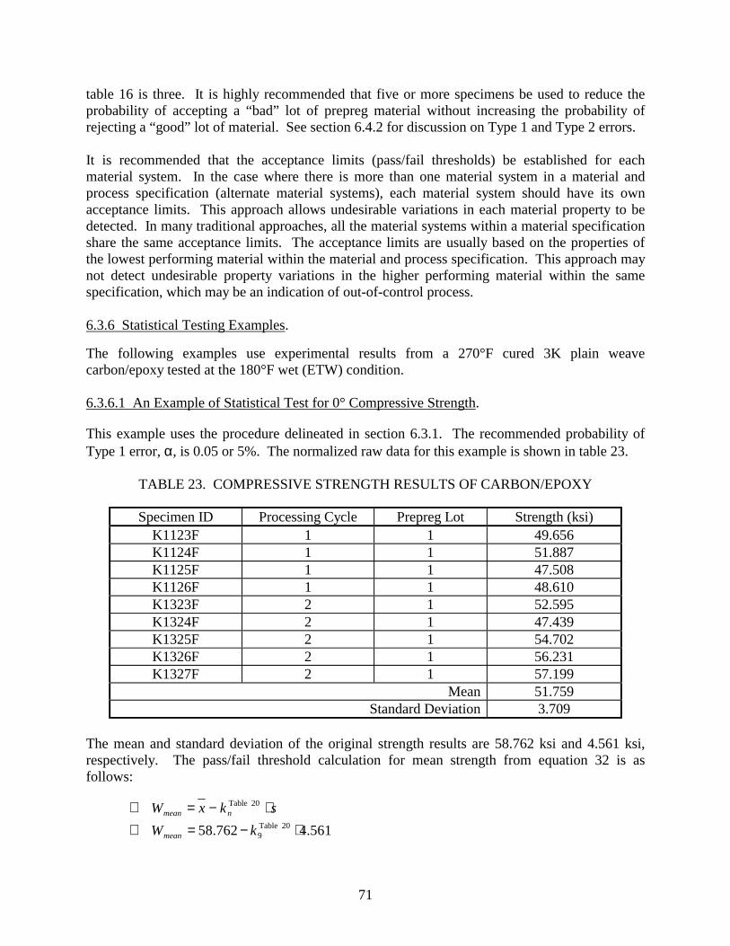
71

table 16 is three. It is highly recommended that five or more specimens be used to reduce the probability of accepting a “bad” lot of prepreg material without increasing the probability of rejecting a “good” lot of material. See section 6.4.2 for discussion on Type 1 and Type 2 errors. It is recommended that the acceptance limits (pass/fail thresholds) be established for each material system. In the case where there is more than one material system in a material and process specification (alternate material systems), each material system should have its own acceptance limits. This approach allows undesirable variations in each material property to be detected. In many traditional approaches, all the material systems within a material specification share the same acceptance limits. The acceptance limits are usually based on the properties of the lowest performing material within the material and process specification. This approach may not detect undesirable property variations in the higher performing material within the same specification, which may be an indication of out-of-control process. 6.3.6 Statistical Testing Examples.

The following examples use experimental results from a 270°F cured 3K plain weave carbon/epoxy tested at the 180°F wet (ETW) condition. 6.3.6.1 An Example of Statistical Test for 0° Compressive Strength.

This example uses the procedure delineated in section 6.3.1. The recommended probability of Type 1 error, α, is 0.05 or 5%. The normalized raw data for this example is shown in table 23.

TABLE 23. COMPRESSIVE STRENGTH RESULTS OF CARBON/EPOXY

Specimen ID Processing Cycle Prepreg Lot Strength (ksi) K1123F 1 1 49.656 K1124F 1 1 51.887 K1125F 1 1 47.508 K1126F 1 1 48.610 K1323F 2 1 52.595 K1324F 2 1 47.439 K1325F 2 1 54.702 K1326F 2 1 56.231 K1327F 2 1 57.199

Mean 51.759 Standard Deviation 3.709

The mean and standard deviation of the original strength results are 58.762 ksi and 4.561 ksi, respectively. The pass/fail threshold calculation for mean strength from equation 32 is as follows:

⇒ skxW nmean ⋅−= 20 Table ⇒ 561.4762.58 20 Table

9 ⋅−= kWmean

72

⇒ 561.46411.0762.58 ⋅−=meanW

⇒ 838.55=meanW ksi Since the follow-on mean (51.759 ksi) is lower than the Wmean (55.838 ksi), the follow-on material fails the test. It is concluded that the mean compressive strength of the follow-on material is lower than 58.762 ksi based on α = 0.05 level. The pass/fail threshold calculation for minimum individual strength from equation 33 is as follows:

⇒ skxW nindividual minimum ⋅−= 21 Table

⇒ 561476258 21 Table9 .k.W individual minimum ⋅−=

⇒ 561.47411.2762.58 ⋅−=individual minimumW

⇒ 26.46=individual minimumW ksi

All the individual strength values exceed the individual minimumW , but since the mean failed the requirement, the follow-on material is said to have failed the test. The test for this property will need to be repeated. 6.3.6.2 An Example of Statistical Test for 0° Compressive Modulus.

This example uses the procedure delineated in section 6.3.2. The normalized data for this example is shown in table 24.

TABLE 24. COMPRESSIVE MODULUS RESULTS OF CARBON/EPOXY

Specimen ID Processing Cycle Prepreg Lot Modulus (ksi) L1121F 1 1 7.761 L1321F 2 1 7.960 L1139F 3 1 7.999 L1339F 4 1 7.610

Mean 7.833 Standard Deviation 0.181

The mean and standard deviation of the original modulus results are 7.506 Msi and 0.306 Msi, respectively. The original qualification used a total of six modulus specimens. As in the previous example, the recommended α is 0.05 or 5%, and α/2 is 0.025. The pass/fail threshold calculation for mean modulus from equations 34 and 35 is as follows:

73

⇒ 2

)1()1(

21

222

211

−+⋅−+⋅−

=nn

SnSnS p

⇒ 264

306.0)16(181.0)14( 22

−+⋅−+⋅−=pS

⇒ 266.0=pS

⇒

21

210 11

nnS

xxt

p +⋅

−=

⇒

61

41266.0

506.7833.70

+⋅

−=t

⇒ 904.10 =t

From table 22, for a two-sided test, ta,n = 2,2/ 21 −+nntα = 264,2/05.0 −+t = 8,025.0t = 2.306. Since 1.904 is within the range of -2.306 and 2.306, the ETW compressive modulus passes the criteria. 6.3.6.3 An Example of Statistical Test for Volatile Content.

This example uses the procedure delineated in section 6.3.3. The original qualification used nine volatile content test specimens from three batches of prepreg. The mean and standard deviation are 0.263% and 0.106%, respectively. The follow-on test results have mean of 0.258% and standard deviation 0.0108%.

⇒ 2

)1()1(

21

222

211

−+⋅−+⋅−

=nn

SnSnS p

⇒ 293

106.0)19(0108.0)13( 22

−+⋅−+⋅−=pS

⇒ %0949.0=pS

⇒

21

210 11

nnS

xxt

p +⋅

−=

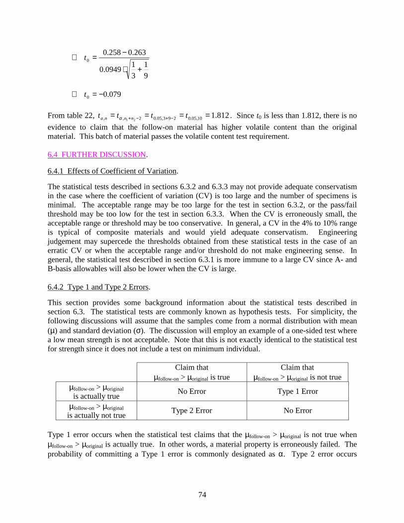
74

⇒

91

310949.0

263.0258.00

+⋅

−=t

⇒ 079.00 −=t

From table 22, 812.110,05.0293,05.02,, 21

==== −+−+ tttt nnna α . Since t0 is less than 1.812, there is no evidence to claim that the follow-on material has higher volatile content than the original material. This batch of material passes the volatile content test requirement. 6.4 FURTHER DISCUSSION.

6.4.1 Effects of Coefficient of Variation.

The statistical tests described in sections 6.3.2 and 6.3.3 may not provide adequate conservatism in the case where the coefficient of variation (CV) is too large and the number of specimens is minimal. The acceptable range may be too large for the test in section 6.3.2, or the pass/fail threshold may be too low for the test in section 6.3.3. When the CV is erroneously small, the acceptable range or threshold may be too conservative. In general, a CV in the 4% to 10% range is typical of composite materials and would yield adequate conservatism. Engineering judgement may supercede the thresholds obtained from these statistical tests in the case of an erratic CV or when the acceptable range and/or threshold do not make engineering sense. In general, the statistical test described in section 6.3.1 is more immune to a large CV since A- and B-basis allowables will also be lower when the CV is large. 6.4.2 Type 1 and Type 2 Errors.

This section provides some background information about the statistical tests described in section 6.3. The statistical tests are commonly known as hypothesis tests. For simplicity, the following discussions will assume that the samples come from a normal distribution with mean (µ) and standard deviation (σ). The discussion will employ an example of a one-sided test where a low mean strength is not acceptable. Note that this is not exactly identical to the statistical test for strength since it does not include a test on minimum individual.

Claim that µfollow-on > µoriginal is true

Claim that µfollow-on > µoriginal is not true

µfollow-on > µoriginal is actually true No Error Type 1 Error

µfollow-on > µoriginal is actually not true Type 2 Error No Error

Type 1 error occurs when the statistical test claims that the µfollow-on > µoriginal is not true when µfollow-on > µoriginal is actually true. In other words, a material property is erroneously failed. The probability of committing a Type 1 error is commonly designated as α. Type 2 error occurs

75

when the statistical test fails to claim that µfollow-on > µoriginal is not true when µfollow-on > µoriginal is actually true. The probability of committing a Type 2 error is commonly known as β. The figures in the following section are intended to provide engineers with some background knowledge of hypothesis tests. They are for illustration purposes only. Due to their simplicity, these figures contain some subtle technical errors, however, the observations that are made from these figures are valid statistical facts. 6.4.2.1 Effects of Number of Specimens on Pass/Fail Threshold.

Figures 26 and 27 show one-sided tests where a low mean strength is unacceptable. The standard deviations of both figures are equal. The probability of rejecting a good follow-on property, α, for both cases is 0.01 or 1%. Note that the pass/fail thresholds are unequal for both cases. In figure 26, the number of specimens tested, n, is 2. The threshold is 60.04 ksi. The number of specimens in figure 27, n, is 10. The threshold is 62.57 ksi. The shift in the threshold is purely due to the number of specimens tested. When only two specimens are tested, the probability of the average value to appear different from the original qualification data is higher. When the number of specimens tested is ten, the probability of the average to appear different from the original qualification data is lower. Since the Type 1 error probability is defined in the statistical test, the threshold must be lower for fewer specimens and higher for more specimens. This also means that if the threshold is maintained at the same level (60.04 ksi) when the number of specimens is increased from two to ten, the probability of Type 1 error will decrease. In order to remain at the same α level, the threshold must be increased when the number of specimens is increased. Note that this is true only for the case where a low mean is unacceptable.

40 45 50 55 60 65 70 75 800

2

4

6

8

10

12

mean=64.939ksi, std.dev=2.242ksi

type 1 error α = 0.01 = 1%, n=2. This means that 1% ofgood materials will be wrongly rejected

Strength (ksi)

Den

sity

60.04

Original Qualification

FIGURE 26. A NORMAL DISTRIBUTION, TWO SPECIMENS

76

40 45 50 55 60 65 70 75 800

2

4

6

8

10

12

type 1 error α = 0.01 = 1%, n=10 This means that 1% ofgood materials will be wrongly rejected

Strength (ksi)

Den

sity

62.57

Original Qualificationmean=64.939ksi, std.dev=2.242ksi

FIGURE 27. A NORMAL DISTRIBUTION, TEN SPECIMENS 6.4.2.2 Specifics About the Test on Minimum Individual.

This section attempts to explain the purpose of the test on minimum individual (section 6.3.1). The actual purpose of this test is not known, however, it is evident that engineers from various companies and organizations have decided that minimum individual is an important indicator of a bad material. To explain in statistical terms, a test on minimum individual may be viewed as analogous to a test on standard deviation. Figure 28 shows two normal distributions with equal means but unequal standard deviations. It is assumed that the minimum individual value will fail the statistical test if the standard deviation of the follow-on property is greater than the standard deviation of the original property. If the true purpose of this test is to detect a large standard deviation, then the test on standard deviation is certainly a more adequate test. However, this test usually requires substantially more specimens (about 20 or more) to achieve the desired accuracy, which may be impractical for most material equivalence or acceptance testing applications.

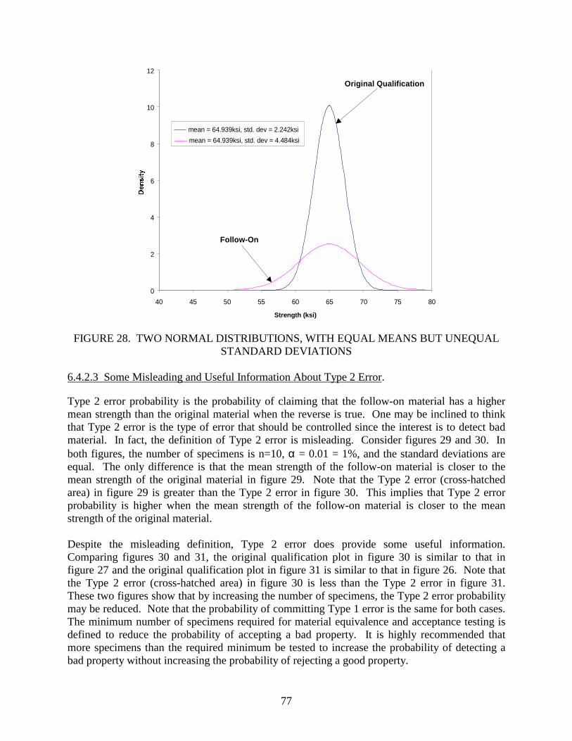
77

0

2

4

6

8

10

12

40 45 50 55 60 65 70 75 80

Strength (ksi)

mean = 64.939ksi, std. dev = 2.242ksimean = 64.939ksi, std. dev = 4.484ksi


Follow-On

FIGURE 28. TWO NORMAL DISTRIBUTIONS, WITH EQUAL MEANS BUT UNEQUAL STANDARD DEVIATIONS

6.4.2.3 Some Misleading and Useful Information About Type 2 Error.

Type 2 error probability is the probability of claiming that the follow-on material has a higher mean strength than the original material when the reverse is true. One may be inclined to think that Type 2 error is the type of error that should be controlled since the interest is to detect bad material. In fact, the definition of Type 2 error is misleading. Consider figures 29 and 30. In both figures, the number of specimens is n=10, α = 0.01 = 1%, and the standard deviations are equal. The only difference is that the mean strength of the follow-on material is closer to the mean strength of the original material in figure 29. Note that the Type 2 error (cross-hatched area) in figure 29 is greater than the Type 2 error in figure 30. This implies that Type 2 error probability is higher when the mean strength of the follow-on material is closer to the mean strength of the original material. Despite the misleading definition, Type 2 error does provide some useful information. Comparing figures 30 and 31, the original qualification plot in figure 30 is similar to that in figure 27 and the original qualification plot in figure 31 is similar to that in figure 26. Note that the Type 2 error (cross-hatched area) in figure 30 is less than the Type 2 error in figure 31. These two figures show that by increasing the number of specimens, the Type 2 error probability may be reduced. Note that the probability of committing Type 1 error is the same for both cases. The minimum number of specimens required for material equivalence and acceptance testing is defined to reduce the probability of accepting a bad property. It is highly recommended that more specimens than the required minimum be tested to increase the probability of detecting a bad property without increasing the probability of rejecting a good property.

78

0

2

4

6

8

10

12

40 45 50 55 60 65 70 75 80


62.57


type 2 error


Follow-OnD

ensi

ty

Strength (ksi)

FIGURE 29. TWO NORMAL DISTRIBUTIONS OF EQUAL STANDARD DEVIATIONS, CLOSE BUT UNEQUAL MEANS, TEN SPECIMENS

0

2

4

6

8

10

12

40 45 50 55 60 65 70 75 80


62.57

type 2 errortype 1 error α = 0.01 = 1%, n=10. This means that 1% ofgood materials will be wrongly rejected


Follow-On

Den

sity

Strength (ksi)

FIGURE 30. TWO NORMAL DISTRIBUTIONS OF EQUAL STANDARD DEVIATIONS, UNEQUAL MEANS, TEN SPECIMENS

79

0

2

4

6

8

10

12

40 45 50 55 60 65 70 75 80


60.04

type 2 error



Follow-OnD

ensi

ty

Strength (ksi)

FIGURE 31. TWO NORMAL DISTRIBUTIONS OF EQUAL STANDARD DEVIATIONS, UNEQUAL MEANS, TWO SPECIMENS

Note that the selection of α is for each material property; the actual probability of committing a Type 1 error for a set of material equivalence tests or a set of acceptance tests is higher than α since several properties are considered in a test matrix. In reality, it is impossible to commit a Type 1 error when the follow-on actually has a lower mean strength than the original (see the table in section 6.4.2). The actual distribution of the follow-on is not usually known due to the limited number of specimens typically tested in material equivalence and acceptance testing. Also, Type 1 error probability for this case of one-sided test is maximum and equal to the selected value (α=0.01=1%) when the mean of the follow-on is actually equal to the mean of the original. Type 1 error probability will be smaller than the selected value when the mean of the follow-on is actually higher than the mean of the original. 6.4.3 Some Unaccounted Forms of Error.

It is highly recommended that the specific specimen preparation and testing procedures used in the original material qualification be documented and followed during material equivalence and acceptance testing. The procedures described in this section do not take into account the between-laboratory error. Every attempt should be made to document the specific procedures used in the original qualification to minimize the between-laboratory error. The actual probability of rejecting good property may be higher or lower than specified (α=0.05 for material equivalence and α=0.01 for acceptance testing), if unaccounted errors such as those introduced by between-laboratory exist.

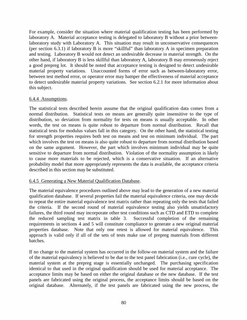
80

For example, consider the situation where material qualification testing has been performed by laboratory A. Material acceptance testing is delegated to laboratory B without a prior between-laboratory study with Laboratory A. This situation may result in unconservative consequences (per section 6.3.1) if laboratory B is more “skillful” than laboratory A in specimen preparation and testing. Laboratory B would not detect an undesirable decrease in material strength. On the other hand, if laboratory B is less skillful than laboratory A, laboratory B may erroneously reject a good prepreg lot. It should be noted that acceptance testing is designed to detect undesirable material property variations. Unaccounted forms of error such as between-laboratory error, between test method error, or operator error may hamper the effectiveness of material acceptance to detect undesirable material property variations. See section 6.2.1 for more information about this subject. 6.4.4 Assumptions.

The statistical tests described herein assume that the original qualification data comes from a normal distribution. Statistical tests on means are generally quite insensitive to the type of distribution, so deviation from normality for tests on means is usually acceptable. In other words, the test on means is quite robust to departure from normal distribution. Recall that statistical tests for modulus values fall in this category. On the other hand, the statistical testing for strength properties requires both test on means and test on minimum individual. The part which involves the test on means is also quite robust to departure from normal distribution based on the same argument. However, the part which involves minimum individual may be quite sensitive to departure from normal distribution. Violation of the normality assumption is likely to cause more materials to be rejected, which is a conservative situation. If an alternative probability model that more appropriately represents the data is available, the acceptance criteria described in this section may be substituted. 6.4.5 Generating a New Material Qualification Database.

The material equivalence procedures outlined above may lead to the generation of a new material qualification database. If several properties fail the material equivalence criteria, one may decide to repeat the entire material equivalence test matrix rather than repeating only the tests that failed the criteria. If the second round of material equivalence testing also yields unsatisfactory failures, the third round may incorporate other test conditions such as CTD and ETD to complete the reduced sampling test matrix in table 3. Successful completion of the remaining requirements in sections 4 and 5 will constitute compliance to generate a new original material properties database. Note that only one retest is allowed for material equivalence. This approach is valid only if all of the sets of tests make use of prepreg materials from different batches. If no change to the material system has occurred in the follow-on material system and the failure of the material equivalency is believed to be due to the test panel fabrication (i.e., cure cycle), the material system at the prepreg stage is essentially unchanged. The purchasing specification identical to that used in the original qualification should be used for material acceptance. The acceptance limits may be based on either the original database or the new database. If the test panels are fabricated using the original process, the acceptance limits should be based on the original database. Alternately, if the test panels are fabricated using the new process, the

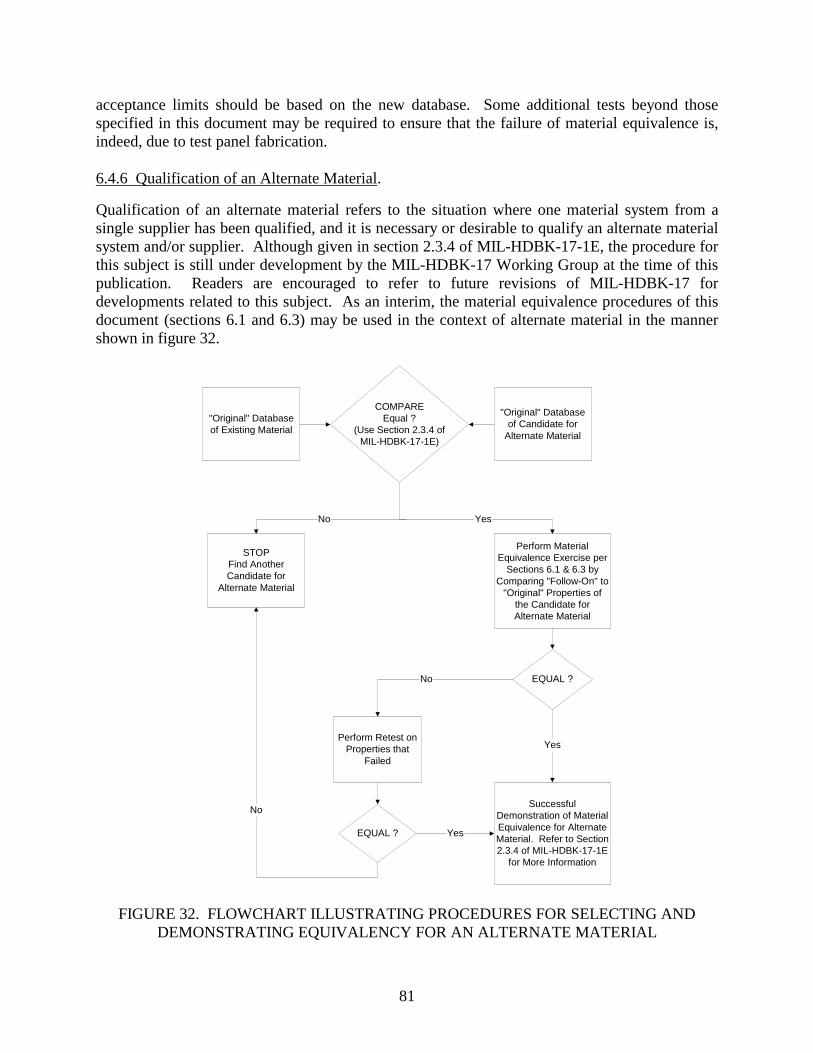
81

acceptance limits should be based on the new database. Some additional tests beyond those specified in this document may be required to ensure that the failure of material equivalence is, indeed, due to test panel fabrication. 6.4.6 Qualification of an Alternate Material.

Qualification of an alternate material refers to the situation where one material system from a single supplier has been qualified, and it is necessary or desirable to qualify an alternate material system and/or supplier. Although given in section 2.3.4 of MIL-HDBK-17-1E, the procedure for this subject is still under development by the MIL-HDBK-17 Working Group at the time of this publication. Readers are encouraged to refer to future revisions of MIL-HDBK-17 for developments related to this subject. As an interim, the material equivalence procedures of this document (sections 6.1 and 6.3) may be used in the context of alternate material in the manner shown in figure 32.

"Original" Databaseof Existing Material

"Original" Databaseof Candidate for

Alternate Material

COMPAREEqual ?

(Use Section 2.3.4 ofMIL-HDBK-17-1E)

Perform MaterialEquivalence Exercise per

Sections 6.1 & 6.3 byComparing "Follow-On" to

"Original" Properties ofthe Candidate forAlternate Material

STOPFind AnotherCandidate for

Alternate Material

Perform Retest onProperties that

Failed

EQUAL ?

SuccessfulDemonstration of MaterialEquivalence for AlternateMaterial. Refer to Section2.3.4 of MIL-HDBK-17-1E

for More Information

YesNo

Yes

No

EQUAL ? Yes

No

FIGURE 32. FLOWCHART ILLUSTRATING PROCEDURES FOR SELECTING AND DEMONSTRATING EQUIVALENCY FOR AN ALTERNATE MATERIAL

82

Due to the rather simple test matrix, the material equivalency procedures outlined earlier are rather narrow in scope. The limitations delineated in section 6.1 do not allow the material equivalency methodology of this document to be applied directly to qualification of an alternate material system. However, the material equivalency procedures delineated in this document may be used to demonstrate equivalency to an alternate material system if an original database of the candidate for alternate material exists. If this approach is to be used, prior comparisons between the two original material databases must reveal that the two material systems are equal, or the alternate material is desirably superior to the existing material. An FAA representative(s) is typically involved in such decision-making processes. Section 2.3.4 of MIL-HDBK-17-1E may be used as a guideline for this comparison. The material equivalence procedures of this document (sections 6.1 and 6.3) may be adapted to compare the degree of similarities between the two original databases. This determination of equivalency only deals with lamina level properties. Additional tests at higher levels (laminate, element, and subcomponent) may be required to demonstrate acceptable equivalency between two material systems. These higher level tests are required to validate equivalency for material properties that account for such effects as holes, bolted and bonded joints, impact damage, and large notches. In general, the modulus values of the alternate and existing materials must be almost identical. The average strength properties of the alternate material should be equal or slightly higher than that of the existing material. The A- and B-basis properties of the alternate material should also be equal or slightly higher than that of the existing material. All material systems within the same material and process specification will share the same material design allowables (A-, B-basis, modulus, and Poisson’s ratio). The prepreg lot acceptance thresholds and ranges should be based on the original qualification of individual material systems. All laminate, element, component, or full-scale tests should use the material with the lowest strengths. 7. CONCLUDING REMARKS AND FUTURE NEEDS.

The qualification plan in this report documents engineering practices for base composite material qualification databases and equivalency testing. Equivalence testing demonstrates that a given material processed by a new user can achieve the properties documented in the original database. This qualification plan provides a good starting point for protocol needed to share composite databases between multiple users. The practice of shared databases is routinely used within the metals industry for numerous materials used in aircraft products (e.g., aluminum alloys). To achieve the same status for composites, the accepted engineering practices must realize that a user advances the material to a finished state in fabricating a composite structure. As a result, equivalency testing is needed to ensure sufficient understanding of the materials and process controls behind a shared composite database. A number of other advances within the industry could further stabilize composite materials to support the engineering community in the safe and efficient deployment of composite materials to aircraft products. This section provides some recommendations in this area. Well-defined material and process specifications are needed to support shared composite material databases. Such specifications should be documented and provided to all candidate users as a means of transferring the technology behind a given qualification database. This suggests a mechanism such as the SAE Aerospace Materials Specification process currently used for metallic materials used in aircraft products. Some composite materials have successfully

83

pursued this path, but a more rigorous national or international effort is needed. A new working group within MIL-Handbook-17, called Data Utilization, is pursuing such direction. Without the material and process insights, composite qualification databases have little benefit to new users. The specifications are also needed to ensure a high level of success in users demonstrating equivalency. In order to evolve consistent and mature specifications, composite materials and processes must be rigorously studied to identify the key characteristics that will ensure invariance over time. Concerns over changes in the raw material processes traditionally led to a need for multiple batches used in original material qualification, as well as continuous monitoring by receiving inspections currently used by the industry. Both the upper and lower bounds of properties need to be more closely controlled to avoid issues of property drift over time. A more complete assessment of the final composite processing parameters is also needed. For example, the effects of composite processing windows should be incorporated into the supporting databases. The current engineering practices documented in this report have made some advances in this direction by including multiple process runs as a variable in the qualification database. However, more rigorous assessment of the complete processing space may be needed to capture the full variation in properties allowed within the specifications. Additional levels of building block tests are also candidates for shared databases. To be useful for a wide range of applications, shared databases should be limited to information that is non-product-specific. Such data might include some standard joints and notched material testing that can be helpful in design. Some data on the effects of defects and damage would also serve multiple users. Similarly, the basic data used for the repair of a composite material would help smaller users who are in dire need of such shared databases. Not only would the higher levels of building block data provide engineering efficiency through shared databases, but it would promote its use in controlling material and process invariance over time. Such a practice is currently not routinely followed within the industry (i.e., tests used to control material and processes often do not include some of the higher level data thought to be essential to structural applications). In summary, the qualification plan, material database, and equivalency to the original database presented in this report is the first step in development of shared databases. Higher-level tests and database will be needed for complete interchange of data and its usefulness in the design and manufacturing process. 8. REFERENCES.

1. Shyprykevich, P., “The Role of Statistical Data Reduction in the Development of Design Allowables for Composites,” Test Methods for Design Allowables for Fibrous Composites: 2nd Volume, ASTM STP 1003, C.C. Chamis, ed., American Society for Testing and Materials, Philadelphia, PA, 1989, pp. 111-135.

2. Scholz, Fritz, “Approximation for Allowable k-Factors, Boeing Computer Services, The

Boeing Company, Seattle, WA (internal paper).

84

9. GLOSSARY.

A-Basis 95% lower confidence limit on the first population percentile. Acceptance Testing The testing of incoming material to ensure that it meets requirements. B-Basis 95% lower confidence limit on the tenth population percentile.

Follow-on The applicant, material, process, or testing of material equivalence or acceptance testing. Material Equivalence The testing of a material to ensure that the follow-on applicant, material, or process will produce material properties equal to those of original material qualification/certification. Prepreg Batch A production run of prepreg material that is preimpregnated using one batch of resin and fiber form under one set of operating conditions. Scheduled interruptions (e.g., overnight plant shutdowns) or short maintenance downtimes in the production run to create material in this batch are permitted, provided there is no interim run. When defined in a material qualification program, no fiber or resin lot duplication is allowed in any two prepreg batches. Prepreg Lot One batch of prepreg material or a portion of one batch that is shipped to a purchaser for acceptance at one time. Scheduled interruptions (e.g., overnight plant shutdowns) or short maintenance downtimes in the production run to create material in this lot are permitted, provided there is no interim run. Reduced Sampling Specimen sampling technique that requires three prepreg batches. Robust Sampling Specimen sampling technique that requires five prepreg batches.

A-1

APPENDIX A ROBUST SAMPLING PANEL REQUIREMENTS

ASTM D3039-95 0o Unidirectional Tape Tensile Strength, Modulus, and Poisson’s Ratio For robust sampling, the required specimens are:

CTD RTD ETW ETD

Strength 1 x 7 5 x 7 5 x 7 1 x 7

Strength, Modulus, and Poisson’s Ratio

1 x 4 5 x 4 5 x 4 1 x 4

Recommended panel size:

12″

12″

90°

0°

Preferred Reference Edge

Physical Test Strip

Subpanel

Panel Dimensions

Lay-Up Configuration: [0]n with a recommended thickness of 0.040″

Required Thickness: 0.035″ - 0.060″

Minimum Number of Panels per Batch:

Batch 1 2 3 4 5 Panels 5 4 4 4 4

Number of Subpanels per Panel: 1

A-2

ASTM D3039-95 90o Unidirectional Tape Tensile Strength and Modulus

For robust sampling, the required specimens are:

CTD RTD ETW ETD

Strength 1 x 7 5 x 7 5 x 7 1 x 7

Strength and Modulus

1 x 4 5 x 4 5 x 4 1 x 4


12″

12″

0°

90°


Physical Test Strip

Subpanel

Panel Dimensions




Batch 1 2 3 4 5 Panels 8 6 6 6 6


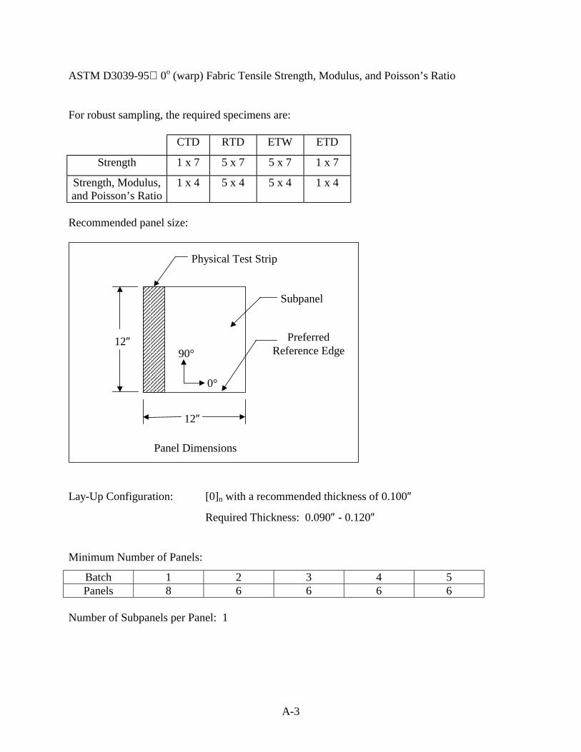
A-3

ASTM D3039-95 0o (warp) Fabric Tensile Strength, Modulus, and Poisson’s Ratio


CTD RTD ETW ETD

Strength 1 x 7 5 x 7 5 x 7 1 x 7


1 x 4 5 x 4 5 x 4 1 x 4


12″

12″

90°

0°


Physical Test Strip

Subpanel

Panel Dimensions



Minimum Number of Panels:

Batch 1 2 3 4 5 Panels 8 6 6 6 6


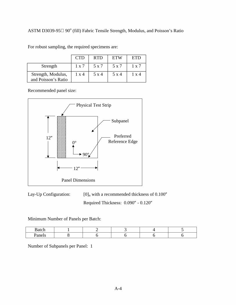
A-4

ASTM D3039-95 90o (fill) Fabric Tensile Strength, Modulus, and Poisson’s Ratio


CTD RTD ETW ETD

Strength 1 x 7 5 x 7 5 x 7 1 x 7


1 x 4 5 x 4 5 x 4 1 x 4


12″

12″

0°

90°


Physical Test Strip

Subpanel

Panel Dimensions




Batch 1 2 3 4 5 Panels 8 6 6 6 6


A-5

SACMA SRM 1-94 0o Unidirectional Tape Compressive Strength and Modulus


CTD RTD ETW ETD

Strength 1 x 11 5 x 11 5 x 11 1 x 11

Modulus 1 x 4 5 x 4 5 x 4 1 x 4

Recommended Panel Size:

Physical Test Strip

0°

90°

Subpanels

12″

12″

Preferred

Reference Edge

Panel Dimensions



Minimum Number of Panels per Batch: 3


A-6

SACMA SRM 1-94 90o Unidirectional Tape Compressive Strength and Modulus


CTD RTD ETW ETD

Strength 1 x 11 5 x 11 5 x 11 1 x 11

Modulus 1 x 4 5 x 4 5 x 4 1 x 4


Physical Test Strip

90°

0°

Subpanels

12″

12″


Panel Dimensions





A-7

SACMA SRM 1-94 0o (warp) Fabric Compressive Strength and Modulus


CTD RTD ETW ETD

Strength 1 x 11 5 x 11 5 x 11 1 x 11

Modulus 1 x 4 5 x 4 5 x 4 1 x 4


Physical Test Strip

0°

90°

Subpanels

12″

12″

Preferred

Reference Edge

Panel Dimensions





A-8

SACMA SRM 1-94 90o (fill) Fabric Compressive Strength and Modulus


CTD RTD ETW ETD

Strength 1 x 11 5 x 11 5 x 11 1 x 11

Modulus 1 x 4 5 x 4 5 x 4 1 x 4


Physical Test Strip

90°

0°

Subpanels

12″

12″


Panel Dimensions





A-9

ASTM D5379-93 In-Plane Shear Strength and Modulus (Unidirectional Tape and Fabric) For robust sampling, the required specimens are:

CTD RTD ETW ETD

Strength 1 x 7 5 x 7 5 x 7 1 x 7


1 x 4 5 x 4 5 x 4 1 x 4


Physical Test Strip

0°

90°

Subpanels

12″

12″

Preferred

Reference Edge

Panel Dimensions

Lay-Up Configuration: [0/90]ns with a recommended thickness of 0.140″




A-10

ASTM D2344-89 or SACMA SRM 8-94 Short-Beam Shear Strength (Unidirectional Tape and Fabric) For robust sampling, the required specimens are:

CTD RTD ETW ETD

Strength 5 x 11



Physical Test Strip

8″

8″


Panel Dimensions



Minimum Number of Panels per batch: 1


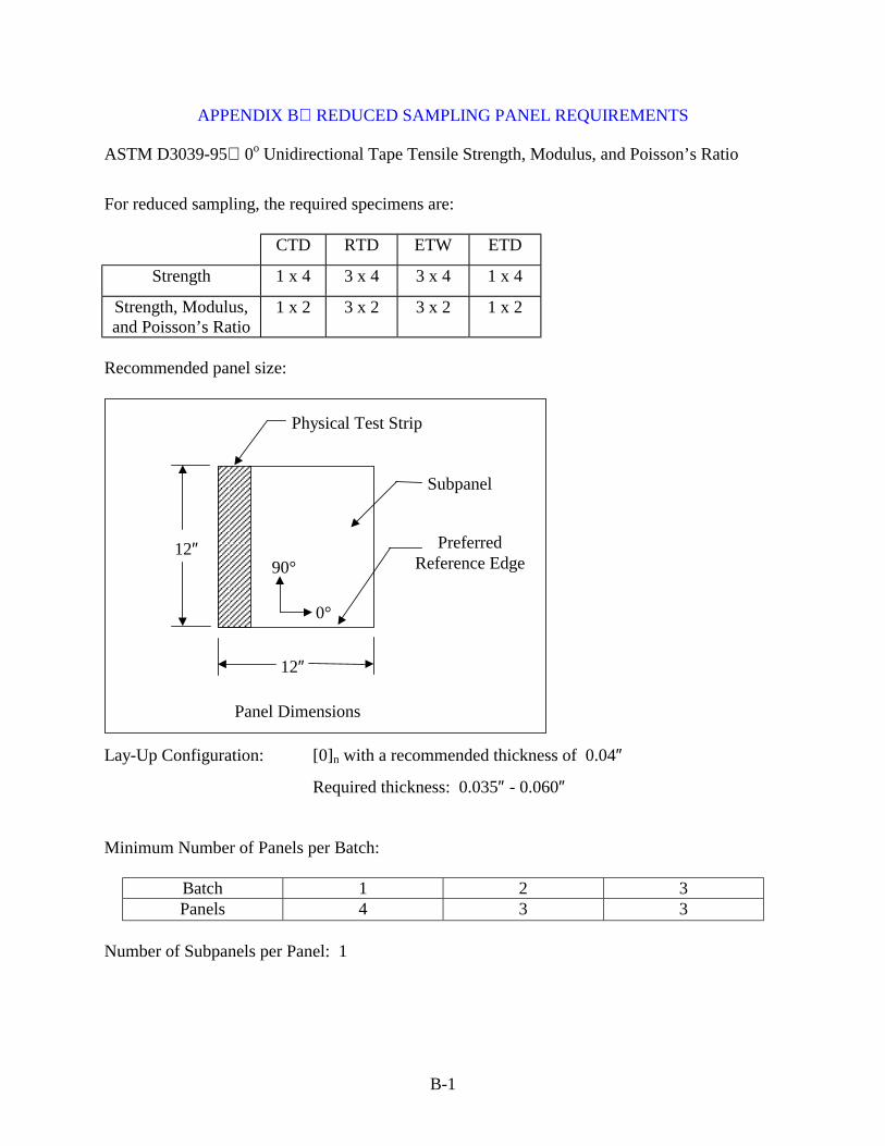
B-1

APPENDIX B REDUCED SAMPLING PANEL REQUIREMENTS

ASTM D3039-95 0o Unidirectional Tape Tensile Strength, Modulus, and Poisson’s Ratio

For reduced sampling, the required specimens are:

CTD RTD ETW ETD

Strength 1 x 4 3 x 4 3 x 4 1 x 4


1 x 2 3 x 2 3 x 2 1 x 2


12″

12″

90°

0°


Physical Test Strip

Subpanel

Panel Dimensions


Required thickness: 0.035″ - 0.060″


Batch 1 2 3 Panels 4 3 3


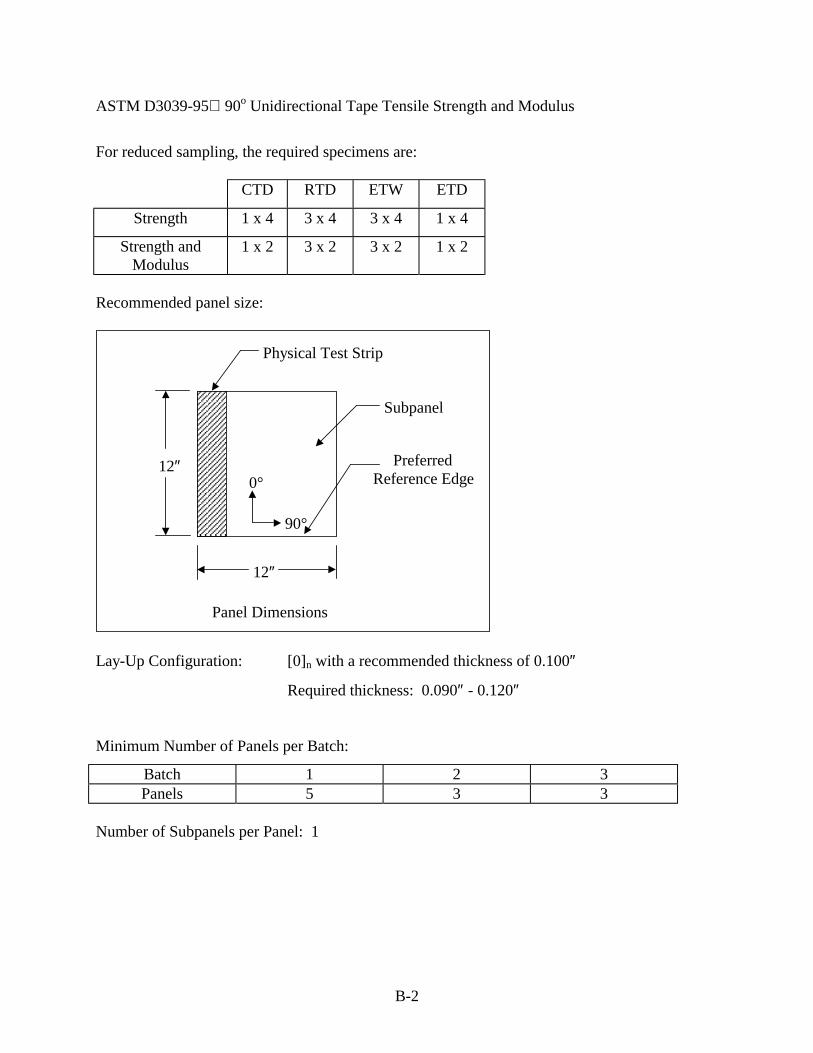
B-2

ASTM D3039-95 90o Unidirectional Tape Tensile Strength and Modulus


CTD RTD ETW ETD

Strength 1 x 4 3 x 4 3 x 4 1 x 4


1 x 2 3 x 2 3 x 2 1 x 2


12″

12″

0°

90°


Physical Test Strip

Subpanel

Panel Dimensions


Required thickness: 0.090″ - 0.120″




B-3

ASTM D3039-95 0o (warp) Fabric Tensile Strength, Modulus, and Poisson’s Ratio


CTD RTD ETW ETD

Strength 1 x 4 3 x 4 3 x 4 1 x 4


1 x 2 3 x 2 3 x 2 1 x 2


12″

12″

90°

0°


Physical Test Strip

Subpanel

Panel Dimensions






B-4

ASTM D3039-95 90o (fill) Fabric Tensile Strength, Modulus, and Poisson’s Ratio


CTD RTD ETW ETD

Strength 1 x 4 3 x 4 3 x 4 1 x 4


1 x 2 3 x 2 3 x 2 1 x 2


12″

12″

0°

90°


Physical Test Strip

Subpanel

Panel Dimensions






B-5

SACMA SRM 1-94 0° Unidirectional Tape Compressive Strength and Modulus


CTD RTD ETW ETD

Strength 1 x 6 3 x 6 3 x 6 1 x 6

Modulus 1 x 2 3 x 2 3 x 2 1 x 2


Physical Test Strip

0°

90°

Subpanels

12″

12″

Preferred

Reference Edge

Panel Dimensions





B-6

SACMA SRM 1-94 90° Unidirectional Tape Compressive Strength and Modulus


CTD RTD ETW ETD

Strength 1 x 6 3 x 6 3 x 6 1 x 6

Modulus 1 x 2 3 x 2 3 x 2 1 x 2


Physical Test Strip

90°

0°

Subpanels

12″

12″


Panel Dimensions





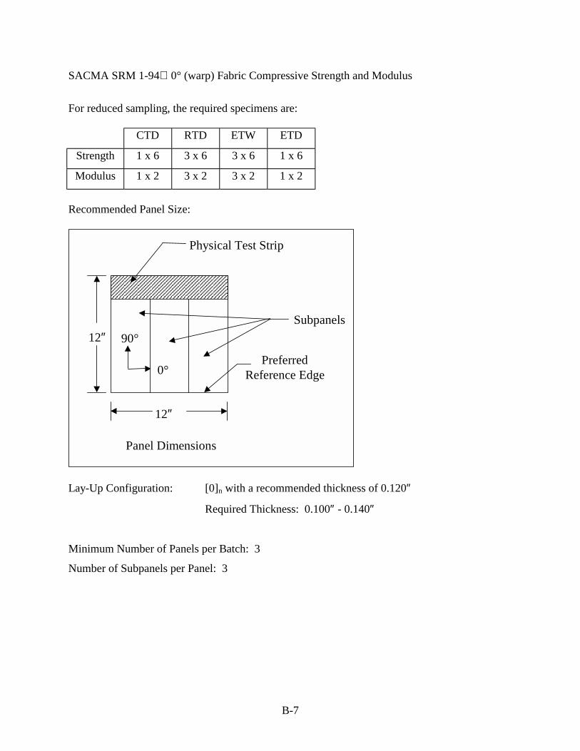
B-7

SACMA SRM 1-94 0° (warp) Fabric Compressive Strength and Modulus


CTD RTD ETW ETD

Strength 1 x 6 3 x 6 3 x 6 1 x 6

Modulus 1 x 2 3 x 2 3 x 2 1 x 2


Physical Test Strip

0°

90°

Subpanels

12″

12″

Preferred

Reference Edge

Panel Dimensions





B-8

SACMA SRM 1-94 90o (fill) Fabric Compressive Strength and Modulus


CTD RTD ETW ETD

Strength 1 x 6 3 x 6 3 x 6 1 x 6

Modulus 1 x 2 3 x 2 3 x 2 1 x 2


Physical Test Strip

90°

0°

Subpanels

12″

12″


Panel Dimensions





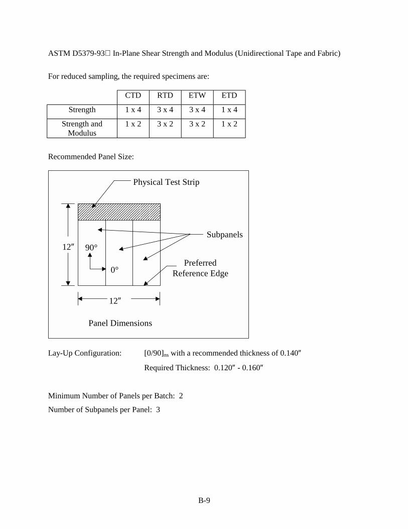
B-9

ASTM D5379-93 In-Plane Shear Strength and Modulus (Unidirectional Tape and Fabric)


CTD RTD ETW ETD

Strength 1 x 4 3 x 4 3 x 4 1 x 4


1 x 2 3 x 2 3 x 2 1 x 2


Physical Test Strip

0°

90°

Subpanels

12″

12″

Preferred

Reference Edge

Panel Dimensions

Lay-Up Configuration: [0/90]ns with a recommended thickness of 0.140″




B-10

ASTM D2344-89 or SACMA SRM 8-94 Short-Beam Shear Strength (Unidirectional Tape and Fabric) For reduced sampling, the required specimens are:

CTD RTD ETW ETD

Strength 3 x 6



Physical Test Strip

8″

8″


Panel Dimensions



Minimum Number of Panels per batch: 1


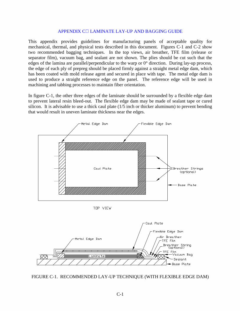
C-1

APPENDIX C LAMINATE LAY-UP AND BAGGING GUIDE

This appendix provides guidelines for manufacturing panels of acceptable quality for mechanical, thermal, and physical tests described in this document. Figures C-1 and C-2 show two recommended bagging techniques. In the top views, air breather, TFE film (release or separator film), vacuum bag, and sealant are not shown. The plies should be cut such that the edges of the lamina are parallel/perpendicular to the warp or 0° direction. During lay-up process, the edge of each ply of prepreg should be placed firmly against a straight metal edge dam, which has been coated with mold release agent and secured in place with tape. The metal edge dam is used to produce a straight reference edge on the panel. The reference edge will be used in machining and tabbing processes to maintain fiber orientation. In figure C-1, the other three edges of the laminate should be surrounded by a flexible edge dam to prevent lateral resin bleed-out. The flexible edge dam may be made of sealant tape or cured silicon. It is advisable to use a thick caul plate (1/5 inch or thicker aluminum) to prevent bending that would result in uneven laminate thickness near the edges.

FIGURE C-1. RECOMMENDED LAY-UP TECHNIQUE (WITH FLEXIBLE EDGE DAM)

C-2

In figure C-2, the caul plate is shown with respect to the lay-up assembly. Note that the caul plate is smaller than the lay-up with approximately 1 inch of the lay-up exposed on three edges. If this technique is used, the panel size recommendations described appendices A and B refer to the size of the caul plate. The caul plate may be made of aluminum sheet as thin as 0.040 inch since this technique is not prone to produce laminate with uneven thickness near the edges.

FIGURE C-2. RECOMMENDED LAY-UP TECHNIQUE (WITHOUT FLEXIBLE EDGE DAM)

For fabrics without tracer yarns, the warp/fill direction should be clearly marked on the lay-up before the bagging process. Two methods of marking direction are: 1. Use an engraved caul plate to indicate the warp/fill direction. 2. Place a small piece of tape with indication of warp/fill direction. Make sure that the mark

will remain visible after the curing process.

C-3/C-4

In either method, the direction marks should be placed on the laminate. It is also advisable to label the lay-up with its unique panel identification number or name as soon as the lay-up process is completed. The panel identification number or name should allow traceability to prepreg name, prepreg lot number, cure or processing cycle number, test method, stacking sequence, and number of plies. Extreme care should be used when laying up panels using satin weave fabrics (i.e., eight harness and 7781 style) due to the unsymmetrical nature of the weave pattern. See section 3.4.4.2 for more details. The use of breather strings is optional. Breather strings, if used, should be limited for the purpose of releasing the entrapped air only and should not be used for the purpose of releasing volatile of prepreg. Note that breather strings will absorb resin, cause waviness in the fibers, and may affect the mechanical properties. For these reasons, breather strings, if used, should be as fine as possible. Fiberglass strands/ends of 1581 or 7781 style that have been pretreated with a release agent have been shown to be successful in releasing entrapped air without releasing volatile and are quite easily removed after the curing process. The ends of breather strings should be in direct contact with air breather in the vacuum bag. If breather strings are used on unidirectional lamina, they should be placed 90° to the fiber direction. Breather strings should be removed after the curing process. An alternate method to using breather strings is making tiny holes (perforations) in the TFE film along the edges of the lay-up/laminate. The use of peel-ply (also known as release fabric) should be avoided. See section 3.1 for more details. Vacuum ports should not be placed on the laminate unless the caul plate is rigid enough to avoid marking the laminate. Thermocouple wires should be used to measure the laminate temperature. One method is to place the thermocouple junctions at the mid-plane and near the edge of the laminate, where they will be trimmed off after the panels have been cured. An alternative method is to place the thermocouple junctions in between the air breather and caul plate and at the center of the laminate, but such method will require that the caul plate be very thin and has good thermal conductivity (such as a 0.040-inch-thick aluminum sheet). The latter method allows the thermocouples wires to be reused.

Material Qualification and Equivalency for Polymer Matrix ... · 11. Contract or Grant No. 12....

Documents

Transcript of Material Qualification and Equivalency for Polymer Matrix ... · 11. Contract or Grant No. 12....