doi.org/10.26434/chemrxiv.12923558.v1

Material Informatics with PoreBlazer v4.0 and CSD MOF DatabaseLev Sarkisov, Rocio Bueno-Perez, Mythili Sutharson, David Fairen-jimenez

Submitted date: 06/09/2020 • Posted date: 07/09/2020Licence: CC BY-NC-ND 4.0Citation information: Sarkisov, Lev; Bueno-Perez, Rocio; Sutharson, Mythili; Fairen-jimenez, David (2020):Material Informatics with PoreBlazer v4.0 and CSD MOF Database. ChemRxiv. Preprint.https://doi.org/10.26434/chemrxiv.12923558.v1

In this article, we present an updated version of the PoreBlazer code, an open access, open source Fortran 90programme to calculate structural properties of porous materials. The article describes the propertiescalculated by the code, their physical meaning and their relationship to the properties that can be measuredexperimentally. We reflect on the progress of the code over the years and discuss features of the most recentversion. The results of these calculations, along with the PoreBlazer code, documentation, and case studiesare available online from https://github.com/SarkisovGroup/PoreBlazer.

File list (2)

download fileview on ChemRxivSarkisov_et_al_final.pdf (2.08 MiB)

download fileview on ChemRxivSarkisov_et_al_SI_final.pdf (2.41 MiB)

1

Materials informatics with PoreBlazer v4.0 and CSD MOF database

Lev Sarkisov1*, Rocio Bueno-Perez2, Mythili Sutharson2, and David Fairen-Jimenez2

1 The Department of Chemical Engineering and Analytical Science| Office C56 The Mill | The

University of Manchester | Sackville Street, Manchester, M13 9PL, UK

2The Adsorption & Advanced Materials Laboratory (A2ML), Department of Chemical Engineering &

Biotechnology, University of Cambridge, Philippa Fawcett Drive, Cambridge, CB3 0AS, UK

Abstract

The development of computational methods to explore crystalline materials has received significant

attention in the last decades. Different codes have been reported to help researchers to evaluate and

learn about the structure of materials and to understand and predict their properties. Here, we

present an updated version of PoreBlazer, an open-access, open-source Fortran 90 code to calculate

structural properties of porous materials. The article describes the properties calculated by the code,

their physical meaning and their relationship to the properties that can be measured experimentally.

Here, we reflect on the methods in the code and discuss features of the most recent version. First,

we demonstarte the capabilities of PoreBlazer on the prototypical metal-organic framework (MOF)

materials, HKUST-1, IRMOF-1 and ZIF-8, and compare the results to those obtained with other codes,

Zeo++ and RASPA. Second, we apply PoreBlazer to the recently assembled database of MOF materials

– the CSD MOF subset – and compare properties such as accessible surface area and pore volume

from PoreBlazer and the two other codes, and reflect on the possible sources of the differences.

Finally, we use PoreBlazer to illustrate how correlations between various structural characteristics can

be mined using interactive, dynamic data visualization and how material informatics approaches –

including principal component analysis and machine learning – can accelerate the discovery of new

materials and new functionalities. The results of these calculations, along with the PoreBlazer code,

documentation, and case studies are available online from

https://github.com/SarkisovGroup/PoreBlazer. The data visualization tool is available at https://aaml-

explorer-geo-prop.herokuapp.com), and the principal component analysis is available at https://aaml-

pca-geo-prop.herokuapp.com.

1. Introduction

Structure determines property. This simple and powerful concept in chemistry has been the

cornerstone of modern computational approaches to drug discovery, where millions of candidate

small organic molecules are screened based on their ability to bind to the therapeutic target. Organic

chemistry provides the building blocks for metal-organic frameworks (MOFs)1. Combined with the

large number of topologies into which these building blocks can be arranged, this implies a virtually

infinite number of possible MOF structures. As a result, computational screening has become a new,

essential tool for porous, crystalline material discovery and optimization, and in particular, for MOFs,

zeolitic imidazolate frameworks (ZIFs)2, covalent organic frameworks (COFs)3, and other classes of

materials.

The first example of a virtual MOF designed for a specific application was provided by Duren et al.4

They explored how adsorption of methane at 35 bar and room temperature (conditions relevant for

2

the adsorbed natural gas vehicle technology) depended on the properties of porous materials, such

as the specific surface area and MOF-methane interaction strength. Using insights obtained from

computer simulations, the authors proposed new, hypothetical MOFs, with enhanced methane

storage capabilities. In the study, the authors also posed a question on how various structural

characteristics of a MOF, such as surface area and pore volume, define their functionality in a

particular application. Other characteristics of the porous morphology of a MOF include the shape and

size of the pores, shape and size of the windows between the pores, access to specific active sites, and

so on. Some of these properties have also a particular importance as they can be measured

experimentally (e.g. surface area, pore volume, and window size). Collectively, these characteristics –

the textural properties of materials – form a geometric identity of a MOF, its unique fingerprint.

The tinker-toy nature of MOFs, i.e. the fact that they are assembled from basic building blocks, led

to a new, profound idea: we can build databases of virtual MOF materials, following some assembly

algorithms, and explore their properties in silico with a view of identifying the most promising

candidates for a particular application. These ideas were put together by Wilmer et al.5, who

constructed a database of 137,953 hypothetical MOFs and investigated their capability to store

methane at the target conditions (35 bar, room temperature) as a function of their surface area, void

fraction, largest pore diameter, etc. Later, this led to a burgeoning area of computational material

screening in application to a number of problems, from carbon capture to toxic gas and warfare

chemical detection6.

For systematic comparison of the materials in computational screening, for their classification and

to reveal structure-property relations it is important to have computational tools, which would

produce the geometric identity of a MOF. The development of these tools to obtain structural

characteristics of porous materials has been a result of many contributions scattered over the years.

For example, the algorithms adopted by Duren et al.4, 7, have been originally applied to characterize

molecular models of porous glasses by Gelb and Gubbins8-10, which in their turn originate from the

methods developed in the field of stereology. Application of Voronoi tessellation in the context of

random heterogeneous media can be tracked down to the early eighties11. In the last 10 years, several

software packages and web platforms have emerged that, given coordinates of the atoms or particles

constituting the material, produce a comprehensive set of geometric characteristics. Let us briefly

review these codes here before we formulate the objectives of the article.

Chronologically, PoreBlazer, developed by Sarkisov, was the first simulation package of this kind

for computational characterization of crystalline and amorphous materials12, 13. The code, written in

Fortran 90, is based on the grid (or lattice) representation of the porous space and calculates pore

volume, accessible surface area, largest pore diameter, pore limiting diameter, pore size distribution

and other properties. ZEOMICS and MOFomics, by Floudas and co-workers, represent an alternative

approach.14, 15 There, the porous space of the material is parsed into geometric objects (portals,

channels, cages) using Delaunay triangulation and complementary geometric methods. Then, the

connectivity between these objects is determined and the properties of the structure (accessible

surface area, accessible volume) are calculated. These tools are presented in the form of a web portal,

where users can submit their structure files and receive the final results by email. Zeo++, developed

by Haranczyk and co-workers, is a C++ package for high-throughput analysis of porous materials based

on Voronoi tessellation16-18. With Voronoi network being a dual graph of the Delaunay network, this

approach is closely related to that of Foster et al.19. The program is downloadable from the website of

3

the developers, with the source code available upon request. RASPA simulation package, developed

by Dubbeldam and co-workers, is a powerful, open-source suite of classical simulation tools (e.g.

molecular dynamics, Monte Carlo simulations)20. Within RASPA, there are options to obtain the

surface area and pore volume of the material, using the computational helium porosimetry approach,

as well as a pore size distribution.

These software programs differ in their methodology, accessibility, operation, and performance,

and we encourage the readers to use a program suited for their specific research needs. However, we

believe what is important to do, is to compare properties calculated by these packages to each other.

This would ensure consistency across various calculations and methods and would allow us to reflect

on the differences in the obtained values as a result of different algorithms and definitions employed.

This is prompted by the aspirations of the computational scientific community to improve the

consistency of the simulations and reproducibility of the published results21. Hence, the objectives of

the article can be formulated as follows:

1) To provide a review of the most recent version of PoreBlazer (from now on, PB v4.0), including setup

examples, input files, properties it calculates and the algorithms behind these calculations.

This objective is dealt with in Sections 2 on the Properties and Algorithms. We also use this section as

an opportunity to establish a clear link between the geometric properties and the actual properties of

materials that can be directly or indirectly inferred from the experiments.

2) To establish consistency of the properties calculated across various codes, PB v4.0, Zeo++, and

RASPA*.

For this, we first consider three specific cases of well-known MOFs (HKUST-1, IRMOF-1 and ZIF-8) to

provide a detailed comparison of the properties produced by different codes. We guide the reader on

how to set up PB v4.0 simulations and interpret them and also provide the reader with the complete

setups used to obtain this data in PB v4.0, Zeo++ and RASPA. We then focus on the recently developed

database of MOF structures, the Cambridge Structural Database (CSD) MOF subset. To assemble this

database, Moghadam et al. sieved through the CSD to identify entries that satisfy certain criteria

characteristic for MOFs22. Using this set of MOFs (see additional details below in Section 3), we apply

PB v4.0, Zeo++ and RASPA to obtain key structural characteristics, compare the data produced by the

codes and provide an interpretation of the trends. The complete database of the geometric properties

obtained for CDS MOF using PB v4.0 is also available for download from

https://github.com/SarkisovGroup/PoreBlazer.

3) Provide the reader with a case study of how geometric characterization tools and data can be used

in the context of material informatics.

The data produced by PoreBlazer for CSD MOF subset structures form a multidimensional space of

values, with the dimensions being the geometric properties. Although interesting functional and

topological relations may exist between structures, they are not often easy to reveal and visualize due

to the complexity of the space. The set of python codes developed in the Fairen-Jimenez group

provides an interactive way to visualize these properties and relations between them23-25. In the final

*Unfortunately, at the time of writing this article, the MOFomics and ZEOMICs platforms were not available for use.

4

part of this article, we consider how the application of these visualization tools can reveal trends,

which help to accelerate the discovery and design of materials with specific adsorptive behavior.

2. Properties and algorithms

In this section, we define the geometric properties of interest and their connection to experimentally

measured characteristics. We then provide additional details on the algorithms to calculate these

properties and how these algorithms have been implemented in PB v4.0.

2.1 Surface area and pore volume

Consider the schematic illustration in Figure 1A. The system consists of a porous material, shown as

the grey area, and a channel spanning the system from left to right. Atoms of the structure forming

the channel are shown as striped circles. Consider now a probe particle of zero size (a point) moving

on the surface of the atoms of the structure. In a three-dimensional system, this will create the so-

called van der Waals surface, delineating the boundary of the spherical atoms. In the two-dimensional

schematic we use, this property is represented by the red line (Figure 1B). The volume enclosed by

this surface is called the geometric pore volume, 𝑉𝐺, which is the volume accessible to a point probe,

and it is shown as the light red shaded area in Figure 1B.

Figure 1. Schematic depiction of a porous material and its properties. (A) A model system consists of a

material, shown as the area shaded in grey, and a pore spanning the system in the horizontal direction. Atoms

of the material at the boundary between the shaded area and the pore are shown as striped circles. (B) The

geometric pore volume is defined as the region of the system not occupied by atoms (shown in light red). The

boundary between the occupied and empty space is the van der Waals surface, shown in B as the red line.

(C) Schematic depiction of the accessible surface: it is the surface formed by the center of the probe particle

rolling over the surface of the atoms of the structure, shown as the green line. A region of space enclosed by

the accessible surface corresponds to the probe-center accessible probe volume, shown as the green shaded

5

area. (D) Schematic depiction of the Connolly surface: it is the surface formed by the tip of the probe particle

rolling over atoms of the structure, shown as the dark blue line. A region of space enclosed by the Connolly

surface corresponds to the probe-occupiable volume, shown as the blue shaded area. The difference between

the geometric volume and the probe-occupiable volume is shown as residual red-shaded areas in panel D (see

the inset for more details).

In Figures 1C, D we consider the same process for a probe of finite size. In this case, we generate

two surfaces (again, in the case of the 2D schematic, it is two lines): one by the center of the particle,

shown as the green line in Figure 1C, and the one by the tip of the particle, shown as the blue line in

Figure 1D. The first property has been traditionally called solvent-accessible, or accessible surface in

biomolecular studies. The second surface is called the solvent-excluded surface in the biomolecular

community, or the Connolly surface. In this article, we are going to use subindex AC for the solvent-

accessible definition of the surface area (𝑆𝐴𝐶) and subindex C for the Connolly surface area (𝑆𝐶).

The physical meaning of the first property, 𝑆𝐴𝐶, is that it is most closely related to the nitrogen or

argon adsorption surface area if we use a probe particle representing properties of these molecules.

Indeed, gas-adsorption experimental methods for the determination of the surface area, such as BET,

are based on the notion of a layer of molecules forming on the surface (where the capacity of this

layer can be extracted from the adsorption isotherms depending on the method) and, given the cross-

sectional area of the probe molecule, the specific surface area of the material can be determined.

Multiple studies have been published on the correlation between the computed areas of a porous

material and surface areas extracted from experimental data on real crystals or simulation data on

perfect crystals7, 26-28. Correspondingly, the volume enclosed by this accessible surface is the volume

accessible to the probe of a specific size. Following the terminology of Ongari and co-workers29, we

call this property the probe-center accessible volume, 𝑉𝑃𝐶. In Figure 1C, this is shown schematically as

the green-shaded area.

The second property, the Connolly surface, is important for yet another definition of the pore

volume. Indeed, in this definition, the pore volume is the volume enclosed by the Connolly surface,

shown the blue area in Figure 1D. The physical meaning of this volume is that any point that belongs

to any part of the probe atom (not just the center) constitutes the pore volume. It has been argued,

that it is this volume that is most consistent with the volume obtained from the experimental nitrogen

and argon adsorption and the Gurvich rule, which assumes that the density of the confined liquid in

the porous material is equal to the density of the bulk liquid at the same temperature29. To distinguish

it from the probe-center accessible volume enclosed by the accessible surface, we need to give it a

separate name. In the study by Ongari and co-workers and in Zeo++ this volume is called the probe-

occupiable (PO) pore volume, 𝑉𝑃𝑂29. For consistency, we will use the same terminology.

The next property we wish to introduce is the helium pore volume. To understand the nature of

this property and its relevance, it is useful to take a brief detour into experimental measurements of

adsorption. The property that is determined and, typically, reported in experiments is the excess

amount adsorbed (𝑛𝑒𝑥):

𝑛𝑒𝑥 = 𝑛𝑎 − 𝑉𝑑𝑒𝑎𝑑∙𝜌𝑏𝑢𝑙𝑘 (1)

which is the difference between the actual amount of adsorbing species present in the system 𝑛𝑎 and

the amount of gas that would occupy the available space 𝑉𝑑𝑒𝑎𝑑, as if there was no effect of adsorption.

6

Here, 𝜌𝑏𝑢𝑙𝑘 is the bulk gas density at the temperature and pressure of the experiment. This available

space, traditionally called dead volume, consists of the volume of the pores (𝑉𝑝𝑜𝑟𝑒) in the material and

the volume external to the material sample (𝑉𝑒𝑥𝑡𝑒𝑟𝑛𝑎𝑙):

𝑉𝑑𝑒𝑎𝑑 = 𝑉𝑝𝑜𝑟𝑒 + 𝑉𝑒𝑥𝑡𝑒𝑟𝑛𝑎𝑙 (2)

To obtain (1), in experiments, the dead volume of the system is determined using a preliminary

calibration step based on the helium expansion. For this, helium is introduced in the system at ambient

temperature and low pressure. Using the ideal equation of state and the amount of helium in the

system, 𝑉𝑑𝑒𝑎𝑑 is determined. The absolute amount adsorbed (𝑛𝑎𝑏𝑠) is the total number of adsorbing

species present in the porous material:

𝑛𝑎𝑏𝑠 = 𝑛𝑒𝑥 + 𝑉𝑝𝑜𝑟𝑒 ∙ 𝜌𝑏𝑢𝑙𝑘 (3)

It has been argued on a number of occasions that the absolute amount adsorbed provides a rigorous

basis for the adsorption thermodynamics30, 31. Moreover, this is also the property used in the process

modeling of adsorption and calculated in molecular simulations31. Hence, comparison between

experimental and simulation studies requires consistent conversion between the excess and absolute

properties and the definition of the pore volume, 𝑉𝑝𝑜𝑟𝑒, of the sample. So far, in this section, our

definition of pore volume has been based on purely geometric considerations and on some rational

way to draw the boundary between what, colloquially speaking, belongs to the solid structure and the

remaining empty space. The helium expansion experiment offers another definition of the pore

volume:

𝑉𝑝𝑜𝑟𝑒 =𝑛𝐻𝑒

𝜌𝐻𝑒,𝑏𝑢𝑙𝑘 (4)

where 𝑛𝐻𝑒 is the amount of helium present in the pores and 𝜌𝐻𝑒,𝑏𝑢𝑙𝑘 is the density of the bulk helium

gas at ambient temperature and pressure. Let us hypothesize that helium is weakly interacting with

the porous material and therefore it is not adsorbing. Therefore, inside the pores of the material, it

behaves as an ideal gas; applying the ideal gas equation of state to the amount of helium present in

𝑉𝑝𝑜𝑟𝑒 will give us a value that is reasonably consistent with our expectation of what pore volume

should be as outlined by some boundary between the solid and the pore space. This is, however, not

the case, and particularly in materials with very narrow porosity: several studies have demonstrated

that helium does interact with the porous material, although weakly (for a review and discussion of

this issue see Brandani et al.31). As a result, the volume obtained according to Eq. 4 will likely have

values not consistent with the alternative definitions of the pore volumes based, for example, on the

geometric methods. Ongari et al.29, demonstrated that depending on the interactions with the pores

of the material, the value of the pore volume estimated in this fashion may be lower or higher than

the values of the pore volume defined using the geometric methods.

Hence, as has been argued by Neimark and Ravikovitch32, consistent conversion between the

experimental and simulation studies requires a consistent definition of the pore volume, regardless of

its true physical meaning. In other words, if the calibration with helium expansion was used to obtain

𝑛𝑒𝑥 in experiments (Eq. 1), then Eq. 3 to obtain absolute amount adsorbed requires 𝑉𝑝𝑜𝑟𝑒 also

obtained according to the helium porosimetry and Eq. 4. Similarly, conversion of the simulation values

for absolute amount adsorbed to the excess amount adsorbed would require some computational

analog of helium porosimetry:

7

𝑛𝑠𝑖𝑚𝑒𝑥 = 𝑛𝑠𝑖𝑚

𝑎𝑏𝑠 + 𝑉𝐻𝑒,𝑠𝑖𝑚 ∙ 𝜌𝑏𝑢𝑙𝑘 (5)

where 𝑛𝑠𝑖𝑚𝑎𝑏𝑠 is the absolute amount adsorbed in the simulations and 𝑉𝐻𝑒,𝑠𝑖𝑚 is the simulated helium

pore volume. Indeed, this approach to obtain and report simulated excess adsorption isotherms has

been adopted in many previous publications33, 34.

The essence of the computational helium porosimetry is to obtain 𝑉𝐻𝑒,𝑠𝑖𝑚 in simulations. In

principle, we could use the standard grand canonical Monte Carlo simulation to obtain the amount of

helium adsorbed at the specified temperature and pressure of the bulk phase. However, the fact that

at ambient temperature and low pressure we are located in the Henry’s regime of adsorption for

helium simplifies the analysis. In the Henry’s law regime, the amount adsorbed is:

𝑛𝐻𝑒 = 𝜌𝐻𝑒,𝑏𝑢𝑙𝑘 ∫ 𝑒−𝑈(𝒓)

𝑘𝑇 𝑑𝒓𝑉

(6)

where 𝑈(𝒓) is the interaction potential experienced by a helium atom at location 𝒓 within the system

and the integration takes place over the volume of the simulation cell. From Eqs. 4 and 6, the 𝑉𝐻𝑒,𝑠𝑖𝑚

becomes:

𝑉𝑝𝑜𝑟𝑒 = ∫ 𝑒−𝑈(𝒓)

𝑘𝑇 𝑑𝒓𝑉

= 𝑉 ∙ ⟨𝑒−𝑈(𝒓)

𝑘𝑇 ⟩ (7)

where 𝑉 is the volume of the system. The property in the angle brackets is the average Boltzmann

factor, which is estimated by placing a probe helium atom in random locations throughout the system

and estimating its interactions with the material. From this analysis, it is clear that the helium pore

volume estimated according to Eq. 7 will depend on temperature (although weakly when close to the

ambient range), and on the interaction parameters of the helium atom used and the atoms of the

material. It is also important to note that the Eqs. 6 and 7 can be also easily linked to the Henry’s

constant of adsorption. Using ideal gas equation of state for helium, one obtains:

𝑛𝐻𝑒

𝑉=

𝑃

𝑅𝑇⟨𝑒−

𝑈(𝒓)

𝑘𝑇 ⟩ (8)

leading to the Henry’s constant:

𝐾𝐻 =⟨𝑒

−𝑈(𝒓)𝑘𝑇 ⟩

𝑅𝑇 (9)

From the expressions above it is clear, that the calculation invoved in obtaining the helium pore

volume can be equally used to obtain the Henry’s constant of adsorption for other gases of interest,

using appropriate interaction parameters.

The final property we wish to introduce is the pore size distribution (PSD). Crystalline and

disordered porous materials (such activated carbons) can be seen as a system of pores of different

sizes. The total volume of all pores is equal to the cumulative pore volume of the system. PSD and how

pores are topologically arranged governs adsorption and transport properties of a porous material,

and it is vital in the characterization of their structure. In experiments, a PSD is obtained by

interpreting the nitrogen or argon adsorption isotherms measured at cryogenic conditions as a

cumulative result of adsorption in a system of independent cylindrical, slit, or spherical pores of

different sizes. In the modern approaches to characterization, the classical Density Functional Theory

(DFT) is employed to generate a kernel of isotherms for individual pores of specific width or diameter.

This kernel of the isotherms, combined with the experimental adsorption isotherm, is then used to

8

obtain the frequency with which pore of each size is present in the system, or, in other words, the

pore size distribution. Although it is now a standard approach in the characterization of porous

materials using physical adsorption experiments, it comes with several challenges. Firstly, the link

between adsorption in the whole sample and adsorption in individual pores is established through the

so-called Adsorption Integral Equation (AIE). The AIE corresponds to a Fredholm integral equation of

the first kind, commonly known to be both an ill-posed and ill-conditioned problem. This leads to

either no solution or to an infinite number of possible solutions which in turn are extremely sensitive

to small changes in the input. Therefore, to obtain reliable PSD by solving the AIE, advanced

techniques, based for example on regularization, need to be employed. Secondly, the current kernels

have been derived predominantly for the systems reflecting chemistry and properties of activated

carbons and certain zeolites. Direct application of these kernels to other classes of materials such as

MOFs should be approached with caution and the development of more specialized kernels for MOFs

is an ongoing area of research35. Finally, only for a few materials, a picture of independent pores of

simple geometry is realistic, and most of the materials would feature a network of pores.

Interpretation of adsorption isotherms and in particular adsorption hysteresis in terms of network

connectivity of pores is still an ongoing area of research, although significant progress has been

achieved in recent twenty years. For a more comprehensive review of the adsorption characterization

methods and application of DFT, we refer the reader to the excellent articles by Neimark and co-

workers36 and by Thommes and co-workers37.

For modeling porous materials we have two options to obtain PSD. We can simulate a nitrogen or

argon adsorption isotherm and interpret the results using the existing methods based on the AIE

inversion (using either DFT kernels or bespoke kernels from additional molecular simulations).

Alternatively, we can use geometric methods, which will attempt to allocate each point of the porous

space to a pore of a particular size. One particular method implemented in PB v4.0 has been originally

employed by Gelb and Gubbins in the characterization of model porous glasses8-10. We will describe

the method in more detail in section 2.3 on the algorithms. Here, it suffices to say that for the case of

mesoporous materials, Gelb and Gubbins observed surprisingly reasonable correlation between the

geometric PSDs and the PSDs from the physical adsorption characterization, although, clearly, the

methods are based on completely different principles.

In the case of MOF and other crystalline materials, the geometric methods are expected to identify

pores of a specific well-defined size and the PSD should look like a collection of discrete peaks. This

information is useful to understand the dimensions of the existing channels and cages and as a part

of the digital identity of a MOF – we can envision that selection and screening of MOFs within a

database can be done to identify MOFs with a profile of cages and channels of a certain size. Attempts

to connect geometric PSDs to specific adsorption behavior (for example, presence of cages of a certain

size should lead to the corresponding number of steps in the adsorption isotherm) proved to be,

however, difficult for microporous materials and it is still research in progress38. In section 2.3, we will

illustrate how geometric methods would tend to interpret cage-like porous space of MOFs, and in the

results section, we will provide several examples of this function for materials in the case studies.

2.2 Network accessible and network non-accessible properties

Consider a model network of pores shown in Figure 2. It consists of a single pore spanning the system

in the horizontal direction and also two spherical cavities. One cavity is completely isolated from the

outside space (i.e. closed porosity) and another one is connected to the main pore via a narrow

9

channel. This simple pore network allows us to introduce the notion of network accessibility and

several other related concepts. Indeed, depending on the size of the probe, various subregions of the

pore space shown in Figure 2 will be available for the probe to explore. A point-size probe entering

the system on the left through the main pore will be able to traverse the system from left to right and

also explore the side channel and the spherical pore connected to it. The pore in the top left corner of

the system cannot be reached via a continuous, physically meaningful walk by a probe of any size. A

probe of small size may be able to go to the side cavity in the top right corner via the channel if the

channel is wide enough. The region of space accessible to the center of the probe via physically

connected space is shown in yellow in Figure 2A. For a probe of a larger size, as shown in Figure 2B,

the side channel may be too narrow to pass and the side pore is not accessible for it to explore. The

regions that the center of the blue particle can reach via a physically meaningful walk are shown as

the light blue shaded areas in Figure 2B. The largest probe that can cross the simulation cell in at least

one dimension via a diffusive pathway is said to correspond to the Pore Limiting Diameter (PLD), as

illustrated in Figure 2D. Hence, we can define regions of porous space as network-accessible to a probe

of a particular size if they form a percolated network spanning the system in at least one dimension.

In other words, network-accessible space is formed by all pores inside the material, which a probe

molecule can reach and diffuse through if it was an actual experiment.

Figure 2. Schematic illustration of the network-accessible and non-accessible properties. (A) For a small

probe particle, shown as the yellow sphere, the area shaded light yellow is network-accessible to the center

of the probe. The spherical cavity in the top left corner of the system is not network-accessible to the probe.

(B) For a probe of a different (in this case, larger) size, the network-accessible regions will be different, here

shown as the light blue shaded area. (C) This panel illustrates the total probe-center accessible volume for

the blue particle. (D) This schematic illustrates the concepts of the Pore Limiting Diameter (PLD) and Largest

Cavity Diameter (LCD).

10

Each of the properties defined in 2.1 can be calculated considering either all the pores in the

system, even the ones that are isolated or inaccessible to a probe of a particular size, or only using the

percolated network – in other words, network-accessible regions. For example, consider the

accessible surface area, 𝑆𝐴𝐶. For this property, we use a molecular probe corresponding to an atom of

nitrogen. As has been discussed before, this is the surface enclosing the probe-center accessible

volume. If we take network accessibility of the porous space into account, it is the blue shaded area

in Figure 2B as discussed before. However, if the network accessibility is not taken into account, it

leads to a different picture: the volume accessible to the center of the probe, in this case, is shown in

Figure 2C. It includes regions within the two spherical cavities, which are large enough to

accommodate the blue particle, but are not reachable by a diffusive pathway. The surface area will

correspond to the boundaries between the blue regions and the white regions in the two schematics

and it will have different values depending on the approach (network-accessible vs. not network-

accessible).

In experiments, obviously, all properties measured via gas adsorption correspond to the network-

accessible regions of the porous space. Therefore, for consistent comparison of the properties, we

need to distinguish between network-accessible and not network-accessible properties. Often, these

have been referred to as open and closed porosity, respectively. We note that in defining these

properties, it is important to state with respect to what probe the accessibility is considered. Not all

combinations of properties actually are physically relevant or can be compared to the experimental

counterparts. For example, for the surface area, it makes sense to define 𝑆𝐴𝐶,𝐴(𝑁2) as accessible

surface area obtained specifically for a nitrogen-accessible network (Figure 2B), as this is what would

be measured in the actual gas adsorption experiments, and 𝑆𝐴𝐶,𝑇(𝑁2) as the total accessible surface

area (Figure 2C).

Table 1 summarizes the properties reported by PB v4.0. Each property can be either of the total

(second subindex T) or network-accessible type (second subindex, A). In these definitions, we use a

specific combination of the property and the probe, and therefore additional information on the

nature of the probe is not needed: for example, 𝑆𝐴𝐶,𝐴(𝑁2) is simply 𝑆𝐴𝐶,𝐴. To avoid cumbersome full

name for “network-accessible accessible surface area”, we make a convention here that, unless

specified otherwise, the surface area term describes the accessible surface area. This convention

allows us to call 𝑆𝐴𝐶,𝐴 property the network-accessible surface area and 𝑆𝐴𝐶,𝑇 the total surface area,

respectively.

Table 1. Properties reported by PB v4.0.

Property Probe Network Notation

Accessible surface area Nitrogen Nitrogen 𝑆𝐴𝐶,𝐴; 𝑆𝐴𝐶,𝑇

Geometric volume Point Point 𝑉𝐺,𝐴; 𝑉𝐺,𝑇

Probe-occupiable volume Nitrogen Nitrogen 𝑉𝑃𝑂,𝐴; 𝑉𝑃𝑂,𝑇

Helium pore volume Helium Helium 𝑉𝐻𝑒,𝐴; 𝑉𝐻𝑒,𝑇

In addition to the properties in Table 1, PB v4.0 also reports the PLD, the number of dimensions in

which the system is percolated and the PSD. If the PLD is smaller than the size of the nitrogen probe,

naturally the code will deem this material is not accessible to nitrogen and report zero values for 𝑆𝐴𝐶,𝐴

and 𝑉𝑃𝑂,𝐴. Similarly to the properties in Table 1, the PSD is reported for the network-accessible

11

subvolume of the system and for the total volume accessible to the center of the nitrogen probe.

Finally, the largest pore in the structure can be characterized by the largest cavity diameter (LCD), also

illustrated in Figure 2D. In Zeo++, this property is called the largest included sphere (LIS). Also, in

Zeo++, an additional property is identified, which is the largest included sphere along the percolated

pathway. The LCD should be consistent with the largest pore size reported in PSD.

2.3 Methods and algorithms

In this section, we turn our attention to the methods and algorithms involved in the calculation of the

properties defined above. In the first step of the PB v4.0 code, the system is divided into small cubelets

and, in the preliminary calculation, the distance between the centers of all cubelets and centers of the

atoms of the structure is calculated and stored for later use. Using this lattice of cubelets, we can

explore pore volume accessible to a center of a particular probe. For this, we first identify all the

cubelets, such that if the probe particle is placed in the center of the cube, it does not overlap with

any atoms of the structure. Mathematically, this condition can be expressed as:

|𝑟𝑖 − �⃗�𝑗| > 𝜎𝑖𝑗/2 for ∀ 𝑗 ∈ 𝐉 (10)

where 𝑟𝑖 is the coordinate of the center of cube i, �⃗�𝑗 is the location of atom j, J is a set of all atoms in

the system, and 𝜎𝑖𝑗 is the collision diameter between the probe i and atom j of the structure. Within

the same lattice subroutine, the code also calculates and stores the distance between the center of

the cube and the surface of the atoms: 𝑟𝑖𝑗,𝑆 = |𝑟𝑖 − �⃗�𝑗| + 𝜎𝑗/2. This property will be employed later

in the section.

Using a lattice representation of the porous space, PB v4.0 invokes the Hoshen-Kopelman

algorithm39 to explore the percolation of the porous space with respect to the probes of different

types (e.g. point probe, nitrogen atom, helium atom). This is schematically depicted in Figure 3. In

panel B, the system shown in panel A is divided into a lattice of small cubelets. Cubelets shaded in grey

are accessible to the blue probe particle as this leads to no overlaps with the atoms of the structure,

shown as the striped grey particles. The cluster of lattice sites in the middle of the system in panel B

forms a percolated pathway for the blue probe particle in the vertical direction – this cluster

corresponds to the network-accessible probe-center volume 𝑉𝑃𝐶,𝐴, whereas the whole set of cubelets

shaded grey forms the total probe-center volume 𝑉𝑃𝐶,𝑇. Pore limiting diameter is identified as the

largest probe for which a percolating lattice cluster exists, spanning the system in at least one

dimension. Along with the PLD, PB v4.0 will also return in how many dimensions percolation with the

current PLD has been detected (1, 2 or 3). If in Figure 3B the blue particle is the largest probe that can

traverse across the system, it is the size of this probe that corresponds to the PLD. In the case of the

model material shown in Figure 2D, it is the constriction of the main pore that defines the PLD. The

fortran maxval function applied to the array storing the distances between the centers of the cubelets

and the surfaces of the atoms identifies the site corresponding to the largest value of the distance

stored. This value corresponds to the Largest Cavity Diameter (LCD), also shown in Figure 2D,

schematically.

To calculate the accessible surface area, typically, a Monte-Carlo algorithm is invoked. This is

schematically depicted in Figure 3C, with the probe particle shown as a dashed green circle and the

atoms of the structure shown as grey striped circles as before. Points are generated randomly on a

12

surface of a sphere of radius 𝑟 = 𝑘 (𝜎𝑖+𝜎𝑝

2), shown in Figure 3C as the green circle, where 𝜎𝑖 is the

diameter of atom i, 𝜎𝑝 is the diameter of the probe particle and 𝑘 is a coefficient which by default is

equal 21/6 in PB v4.0 . This value of the coefficient makes the distance 𝑟 correspond to the location of

the Lennard-Jones potential minimum. Although other conventions are possible (e.g., 𝑘 = 1,

corresponding to the location where the Lennard-Jones potential between the two particles is equal

to zero), however, we believe the approach adopted here more accurately reflects the physical

location of a monolayer adsorbed on the surface of the material. For each point, the test is then

performed to check whether it is within the collision distance 𝑟 with any other atoms of the structure,

and if it is not, it counts as a point on the accessible surface, shown in Figure 3C as green dots. Points

that fail this test are shown in red. The accessible surface area associated with the adsorbent atom i

under consideration is then given by: 𝑎𝑖 = 𝑓 ∙ (4𝜋𝑟2) where 𝑓 is the fraction of green points in the

trial. Schematically, the proportion of the surface area that is not accessible to the probe particle is

shown as the red arc in Figure 3C. This is indeed the algorithm implemented within PB v4.0. The lattice

site representation of the space offers two additional functionalities: firstly, the check on whether a

point on the test sphere belongs to an accessible surface does not require an additional distance

calculation, just a look-up in the table for the cubelet to which the generated point belongs.

Furthermore, as we discussed before, the accessible surface is the boundary between the probe-

center accessible volume and the rest of the space. In principle, the area of this boundary can be

simply estimated from the surface area of the cubelets belonging to the probe-center volume. For

this, one simply needs to count all the faces of the cubelets within 𝑉𝑃𝐶 that are not shared with other

cubelets within 𝑉𝑃𝐶 (i.e., they are exposed, as the cubelet sits on the boundary). This should provide

a significant speed-up of the code, however, this has not been implemented yet.

Figure 3. Schematic illustration of some of the concepts involved in the PB v4.0 algorithms. (A, B) A model

system consisting of atoms, represented as striped circles (A), is divided into cubelets (B), with the grey

13

cubelets representing accessible cubelets to the center of the probe. Percolation algorithms are then used to

identify a set of cubelets forming a continuous pathway across the system, as shown in (B) for the blue

particle. (C) Illustration of the Monte Carlo algorithm to calculate the surface area of the structure. For each

atom, the algorithm obtains the proportion of the points sitting on the accessible surface of the atom (green

circle), without overlapping with other atoms of the structure. (D) Geometric PSD calculation. A point “a”

belongs to the pore shown as the red dashed circle: this is the largest pore containing the point without an

overlap with the atoms of the structure.

Calculation of the Connolly-surface enclosed volume 𝑉𝑃𝑂 is closely related to the calculation of the

pore size distribution, and therefore it would be logical to introduce this property and the algorithm

first. The algorithm effectively consists of two nested loops of random trials. First, a random point in

space not overlapping with the atoms of the structure is generated (point “a”, in Figure 3D). In the

second cycle, another set of random points space is generated. Each of these points is the center of a

sphere, which is assigned the maximum diameter possible without overlapping with the structure of

the atoms. Figure 3D shows two dashed circles as examples of this trial. The largest diameter identified

in the second trial that contains the first random point corresponds to the largest pore to which the

point belongs (the red dashed circle in Figure 3D). All pores of this and smaller diameter contain this

point, which upon completion of the cycle produces the cumulative pore size distribution. The

derivative of this function with respect to the radius or diameter of the pore produces the

conventional pore size distribution.

The lattice representation of the space offers few simplifications of this algorithm. A cubelet is

selected at random from the geometrical subset, 𝑉𝐺, this is equivalent to randomly choosing a point

in space in the off-lattice version. The distance between this cubelet and all other cubelets has been

already pre-calculated (or can be easily looked up simply using the lattice indices). As has been already

mentioned, in the preliminary calculations, we also computed the distances between the lattice sites

and the positions of the atoms constituting the structure of the material. Therefore, using a simple

sorting algorithm, it is easy to find the cubelet, the center of which is also the center of the largest

sphere that contains the center of the original cubelet from the 𝑉𝐺 lattice. The total volume of the

pores identified in this fashion corresponds to the volume included by the Connolly surface formed by

the tip of the nitrogen probe, as we defined earlier, the probe-occupiable volume, 𝑉𝑃𝑂. If we restrict

the sorting algorithm to only cubelets belonging to the network-accessible probe-center accessible

volume, 𝑉𝑃𝐶,𝐴, then the pore size distribution will also correspond to the network-accessible region of

the porous space and the total volume of these pores will correspond to the network-accessible,

probe-occupiable volume, 𝑉𝑃𝑂,𝐴.

What are then the PSDs one might expect for the MOF materials? To understand this, it is useful

to explore the structure of the PSDs that the algorithms described above would generate for simple

pore geometries such as a spherical cage, a slit, or a square pore. This is schematically depicted in

Figure 4. Indeed, the PSDs for the spherical cage and the slit pre would produce an expected δ-function

located at the diameter of the pore. A square pore represents a more interesting case. An intuitive

guess would suggest also a PSD with a single peak corresponding to the largest pore that can be

inscribed in a square. This however neglects the existence of the regions in the corners of the pore,

which according to the algorithms described above would be assigned to pores of a smaller size. The

corner of a square represents a wedge geometry and this should give rise to a continuous tail of

diminishing pore sizes in the PSD. Many of the MOF materials feature cube-like and square like pores

14

(e.g., IRMOF series of materials) and therefore similar trends for PSDs would be observed for these

MOFs as well.

Figure 4. Schematic illustration of the geometric Pore Size Distribution in model structures.

3. Analysis of the textural properties of MOFs

3.1 Case studies: HKUST-1, IRMOF-1, ZIF-8

Let us now consider the application of PB v4.0, Zeo++ and RASPA to three quintessential and well-

known MOF materials: HKUST-1, IRMOF-1 and ZIF-8. In the S1 section of the Electronic Supplementary

Information (ESI) file prvide complete description of the files and parameters required to setup PB

v4.0 simulations. Figure 5 shows molecular structures of the materials under consideration. Table 2

summarizes the results for PB v4.0 and Zeo++. Overall, they exhibit a high level of agreement and

consistency with each other. This is very reassuring for the community working on the material

informatics and computational screening studies and do rely on these two codes.

15

Figure 5. Molecular visualizations of HKUST-1 (left), IRMOF-1 (center), and ZIF-8 (right). This image was

made with VMD software40.

Table 2. Comparison of the results from PB v4.0 and Zeo++ for HKUST-1, IRMOF1, and ZIF-8. Showing

density, pore-limiting diameter (PLD), largest cavity diameter (LCD), network-accessible surface area (𝑆𝐴𝐶,𝐴),

total surface area, (𝑆𝐴𝐶,𝑇), network-accessible probe-occupiable volume, (𝑉𝑃𝑂,𝐴), total probe-occupiable

volume, (𝑉𝑃𝑂,𝑇) and CPU time.

HKUST-1 IRMOF-1 ZIF-8

Property PB Zeo++ PB Zeo++ PB Zeo++

Density [g/cm3] 0.884 0.884 0.593 0.593 0.923 0.924

PLD [Å] 6.380 6.337 7.800 7.773 2.860 3.073

LCD [Å] 12.86 12.99 15.03 15.03 11.42 11.40

𝑆𝐴𝐶,𝐴 [m2/g] 1808.09 1801.02 3400.07 3448.82 0.00 0.00

𝑆𝐴𝐶,𝑇 [m2/g] 1860.87 1853.46 3459.99 3448.82 1168.58 1156.51

𝑉𝑃𝑂,𝐴 [cm3/g] 0.759 0.72 1.30 1.27 0.00 0.00

𝑉𝑃𝑂,𝑇 [cm3/g] 0.762 0.722 1.304 1.270 0.517 0.501

CPU time [s] 116.847 683.857 92.104 672.437 347.058 2714.391

In addition, Table 3 compares the results from PB v4.0 and RASPA. Using RASPA, it is possible to

calculate the accessible surface area and helium pore volume fraction, 𝐹𝐻𝑒,𝑇 = 𝑉𝐻𝑒,𝑇/𝑉. Network

connectivity analysis is not performed in RASPA and, therefore, all the properties reported are total

properties, and not network-accessible properties. On a further note, in the case of Zeo++, the helium

pore volume is not calculated according to Eq. 7. Instead, it is based on the hard-sphere helium atom

probe, making this volume helium probe-center volume in our definition (either total or network-

accessible). Hence, we do not provide a comparison of this property between PB v4.0, RASPA, and

Zeo++, as it should not be expected to produce an agreement. We will, however, return to this

comparison in the next section for the complete set of MOF materials in this study. In the case of CPU

time, the results provided for RASPA correspond to the summative time required to obtain properties

listed in Table 3. It is important to emphasize that the CPU times listed in Tables 2 and 3 are setup-

specific, and they depend on the actual size of the unit cell used and the number of cycles involved for

sampling the properties. On https://github.com/SarkisovGroup/PoreBlazer, we provide complete

setups used to obtain the results in Tables 2 and 3, so the reader knows precisely under what

conditions this performance is observed. Section S2 in the ESI provides a more additional analysis of

the performance of the code and the sensitivity of the PB v4.0 results to the size of the grid.

Table 3. Comparison of the results from PB v4.0 and RASPA for HKUST-1, IRMOF1, and ZIF-8. Showing

density, Helium pore volume fraction (𝐹𝐻𝑒,𝑇), Total surface area (𝑆𝐴𝐶,𝑇) and CPU time.

HKUST-1 IRMOF-1 ZIF-8

Property PB RASPA PB RASPA PB RASPA

Density [g/cm3] 0.884 0.884 0.593 0.593 0.923 0.924

𝐹𝐻𝑒,𝑇 [-] 0.739 0.751 0.820 0.831 0.527 0.538

𝑆𝐴𝐶,𝑇 [m2/g] 1860.87 1857.54 3459.99 3435.09 1168.58 1166.09

CPU time [s] 116.847 420.33 92.104 202.12 347.058 5183.21

16

Figure 6 shows the PSDs for three structures. Although there are some variations in the details of

the curves, the three codes return the same number of peaks and the same location of peaks within

0.2 Å, the lattice precision of PB v4.0. These PSDs show the expected profiles of distinct peaks, with a

tail at lower pore sizes.

Figure 6. PSDs for HKUST-1 (left), IRMOF-1 (center),and ZIF-8 (right). Red lines are the Zeo++ results; black

lines are the PB v4.0 results. For HKUST-1 and IRMOF-1, PSD is the network-accessible property; for ZIF-8

the network-accessible probe-occupiable volume is zero, and therefore PSD is calculated on the whole

porous space (total property).

3.2 Geometric analysis of the CDS MOF database

We now turn our attention to the calculation of MOFs stored within the CSD MOF subset. The non-

disordered CSD MOF subset v5.40 (May 2019) contains ca. 70,000 MOFs22. From this subset, we

filtered out MOFs with structural disorder, partial occupancy issues or missing framework hydrogens,

using the bash script and methodology provided by Fairen-Jimenez and co-workers.25, 41 For the

complete tutorial about how to use the CSD MOF subset, we refer the reader to the work from Li et

al.38 The filtering step produced ca. 57,000 structures. In the next step, we removed the non-bonded

solvent molecules as well as those bonded to open metal sites using the CSD Python API, according to

the procedure by Li et al.41 Calculations on these ca. 57,000 structures revealed that only ca. 12,000

MOFs have non-zero surface area (in other words, they are porous). Therefore, the structure analysis

presented here was performed on this subset of structures – 12,052 MOFs for PB v4.0 vs. Zeo++

comparison, and 12,081 MOFs for PB v4.0 vs. RASPA comparison. The difference in numbers is due to

the fact that 29 MOFs from the larger set of 12,081 structures had technical issues/errors in Zeo++.

When comparing the results from PB v4.0, Zeo++ and RASPA, we did expect the existence of a

subgroup of MOFs for which these codes do not produce a consistent picture. Our philosophy in this

section is to first present the results for all the properties of interest (section 3.3.1) in the same way

they emerged from our calculations, giving some preliminary comments on the observed trends,

distribution of properties and differences in the predictions; then, to provide a more in-depth analysis

on what properties exhibit the most significant deviations, possible scenarios that may lead to the

disagreements in the predictions, further investigation of the characteristics of the MOFs in the set

for which the agreement is acceptable and in the set of MOFs for which results are not consistent.

17

3.2.1 Results and comparison for ca. 12,000 MOFs

Figure 7 shows the parity plots for the different textural properties – pore limiting diameter, PLD;

largest cavity diameter, LCD; total and network-accessible surface area, 𝑆𝐴𝐶,𝑇 and 𝑆𝐴𝐶,𝐴; and the and

network-accessible total probe-occupiable volume, 𝑉𝑃𝑂,𝑇 and 𝑉𝑃𝑂,𝐴 calculated from PB v4.0 and Zeo++

and they distribution from PB v4.0. Figure S3 in the ESI shows a similar comparison between PB v4.0

and RASPA. With the color bar, we indicate the population of the properties in the different range of

values. First, for PLD and LCD, overall, the results show a high level of consistency across the database

of materials. From the color bars and from the distribution of the properties, it is evident that only a

few materials exhibit PLDs and LCDs above 20 Å (not shown), while the majority of the materials

exhibit both PLDs and LCDs below 10 Å (Figs. 7a-b).

When looking at the total surface area, there is again a high level of consistency between the three

codes (Fig. 7c and Fig. S3 in the ESI). A different picture, however, emerges for the network-accessible

surface area (Fig. 7d). This property depends on how the accessibility of the pore network is calculated

and, given the differences in the algorithms between Zeo++ and PB v4.0, it is not surprising that this

property is more sensitive to the code used. Interestingly, there is a set of MOFs (~2,000) showing

zero network-accessible surface area in Zeo++ and non-zero values in PB v4.0; it manifests itself as a

horizontal line of points in the figure. We will return to a more comprehensive analysis for the reasons

for these deviations in section 3.2.2 once we present the results on the remaining properties (pore

volumes and their distributions). The differences in the distribution of the total and network-

accessible surface areas obtained from PB v4.0 is remarkable. The most striking feature is the large

number of MOFs that have a surface area close to zero (they are not strictly zero as materials with

strictly zero surface area have been already eliminated in the preliminary screening of the 57,000

MOFs). This implies that the CSD MOF subset, i.e. the database compiling all the reported MOFs from

the literature, is dominated by materials with low surface areas and porosities. Even within this smaller

subset of 12,052 porous MOFs, more than 3,000 have total surface areas below 50 m2/g, and only

2,455 MOFs have total surface areas above 1000 m2/g – i.e. only about 20% of ca. 12,000 MOFs.

However, we also need to be aware that some materials will appear in this analysis as non-porous,

whereas in reality, they are porous, with windows close to the size of the nitrogen molecules. A certain

degree of structural flexibility, not considered in the methods based on the assumption of the rigid

framework, allows nitrogen to adsorb in the actual experiments. ZIF-8 is one of the most prominent

examples of the materials belonging to this category42.

18

Figure 7. Comparison between results obtained from Zeo++ and PB v4.0. a. The pore limiting diameter, PLD; b. largest cavity diameter, LCD; c. total surface area, 𝑆𝐴𝐶,𝑇;

d. network-accessible surface area, 𝑆𝐴𝐶,𝐴; e. total probe-occupiable volume, 𝑉𝑃𝑂,𝑇; f. network-accessible probe-occupiable volume and 𝑉𝑃𝑂,𝐴. Left panels show the parity

plots, right panels show data distribution within 12,052 MOFs.

19

We now turn our attention to the comparison of the pore volumes obtained using the three codes.

Specifically, we focus our discussion on the network-accessible probe-occupiable 𝑉𝑃𝑂,𝐴 and the total

probe-occupiable volume 𝑉𝑃𝑂,𝑇. In the case of the total probe-occupiable volume, PB v4.0 and Zeo++

are in a reasonable agreement with each other. At the same time, for the network-accessible probe-

occupiable volume, we see again more scattering, particularly in the region of very dense materials

with very small pore volumes (Fig. 7e-f). When looking at the the data distribution within the set of

12,052 porous MOFs, it is clear that the vast majority of structures is very microporous. In fact, more

than 7,000 structures out of 12,052 have 𝑉𝑃𝑂,𝑇 below 0.25 cm3/g. In the case of the network-accessible

volume, 𝑉𝑃𝑂,𝐴, we notice a large number of structures having near-zero values. This subset of materials

contains some materials with very low porosity and surface areas, in general, but also some materials,

with appreciable total pore volume and surface area, but with PLDs smaller than the size of the probe

nitrogen particle. These materials can be promising candidates for kinetic gas separations, based on

the fine differences in sizes of the diffusing molecules.

In the case of RASPA, we can also obtain the helium pore volume and, therefore, we also explore

this property using the helium volume fraction 𝐹𝐻𝑒,𝑇 = 𝑉𝐻𝑒,𝑇/𝑉 (for a more convenient

representation). Figure 8 shows the parity graphs. There is a very good agreement between PB v4.0

and RASPA, as this property is calculated consistently between these two codes. As has been already

discussed, in our definition and in the case of Zeo++, this property corresponds to the helium probe-

center volume. Not surprisingly, there is a significant amount of scattering in the parity graph between

PB v4.0 and Zeo++ (Fig. 8, right). In their study, Ongari et al. outlined several scenarios under which

Eq. 7 underestimates, overestimates and agrees with the geometric pore volume and we refer the

reader to that publication29.

Figure 8. Parity graphs for helium pore volume fraction 𝑭𝑯𝒆,𝑻. Resultsfor PB v4.0 and RASPA are shown on

the left; and for PB v4.0 and Zeo++ on the right.

3.2.2 Error analysis

We then moved to study the error analysis for the different textural parameters analyzed, i.e. the total

and network-accessible probe-occupiable volume, 𝑉𝑃𝑂,𝑇 and 𝑉𝑃𝑂,𝐴, the total and network-accessible

surface area, 𝑆𝐴𝐶,𝑇 and 𝑆𝐴𝐶,𝐴, and the pore limiting diameter, PLD. Here, the relative error is deifned

as 𝐸𝑅𝑅 = 100% ∙|𝑃𝑃𝐵 𝑣4.0−𝑃𝑍𝑒𝑜++|

𝑃𝑃𝐵 𝑣4.0, where 𝑃 is a property of interest. The largest cavity diameter does

20

not feature materials for which predictions from PB v4.0 and Zeo++ deviate by more than 10%.. Figure

9 shows the parity plots, correlations and error distributions for the different parameters. For for

𝑉𝑃𝑂,𝑇, there are have 4,824 (40.03%) MOFs with an error exceeding 10% and with values from PB v4.0

systematically exceeding those from Zeo++ (Figure 9, first row). It is also clear that the vast majority

of these MOFs correspond to low pore volumes (below 0.25 cm3/g). For the network-accessible probe-

occupiable volume 𝑉𝑃𝑂,𝐴, we observe 986 (8.18%) MOFs with an error exceeding 10% (Figure 9, second

row). Out of them, 574 MOFs have 𝑉𝑃𝑂,𝐴 values from PB v4.0 larger than Zeo++. The errors occur

predominantly for MOFs with 𝑉𝑃𝑂,𝐴 values in the range 0-0.75 cm3/g; errors exceeding 25% occur only

for materials with 𝑉𝑃𝑂,𝐴 values around 0-0.5 cm3/g. Several structures (ca. 100) have 100% error: in

this case, the structure is considered non-accessible in Zeo++, but accessible on PB v4.0. Also, a small

number of structures has errors much higher than 100% (e.g. 1000%): these are the cases where,

according to PB v4.0, the MOFs have very low 𝑉𝑃𝑂,𝐴; however, these structures are deemed more

accessible and therefore with much larger 𝑉𝑃𝑂,𝐴 in Zeo++.

In the case of the total surface area, 𝑆𝐴𝐶,𝑇, we have a total number of 2,261 (18.76%) MOFs with

errors exceeding 10% (Figure 9, 3rd row); importantly, the maximum values found for MOFs having

these discrepancies are below 500 m2/g. Out of the 2,261 MOFs, 1,488 show Zeo++ 𝑆𝐴𝐶,𝑇 values larger

than PB v4.0. Similar to the previous properties, MOFs with significant errors are concentrated in the

low surface area regime: errors exceeding 100% correspond to the materials with surface areas below

5 m2/g. When looking at the network-accessible surface area, 𝑆𝐴𝐶,𝐴, we found 2,396 MOFs (19.88%)

with errors exceeding 10% (Figure 9, 4th row). 2,210 MOFs show an error of 100%; these MOFs have

zero network-accessible surface areas according to Zeo++ but non-zero values in PV v4.0 – this is

observed as the straight horizontal line of points (Figure 9, 4th row, left). Seven MOFs also feature zero

values of this property according to PB v4.0 and non-zero values in Zeo++ in the range of 90-600 m2/g.

We finally consider PLD, where there are 1,524 (10.40%) MOFs with errors exceeding 10% (Figure 9,

5th row). Within this group, Zeo++ systematically predicts higher values. We also note that the majority

of these MOFs are grouped around very low values of the PLD (below 2.5 Å). According to the error

distribution, from 1,524 MOFs with an error exceeding 10%, 1,142 show an error between 10 and 20%

and 264 between 20 and 30%.

21

Figure 9. Error analysis of the structural properties. From top down: the total and network-accessible probe-

occupiable volume, 𝑉𝑃𝑂,𝑇 and 𝑉𝑃𝑂,𝐴, the total and network-accessible surface area, 𝑆𝐴𝐶,𝑇 and 𝑆𝐴𝐶,𝐴, and the pore

limiting diameter, PLD. Parity plots of the 4,824 structures with the error exceeding 10% (left), the correlation

22

between the different properties and the magnitude of the error (center), and error distribution for each

property.

From the results presented above in the comparison of PB v4.0 and Zeo++, it is clear that the total

properties (i.e. volume and surface area) exhibit relatively limited scattering in the parity plots – the

main differences between both codes are observed, predominantly, for those materials that feature

low porosity. On the other hand, the network-accessible properties show higher scattering and

therefore the reasons for the differences must be associated with how the network accessibility is

obtained and to what factors this property is sensitive to. Let us outline three possible scenarios for

when the results are expected to deviate significantly for PB v4.0 and Zeo++:

Scenario 1. This is associated with what probe molecules are used to assess the accessibility of the

porous structure and to obtain the surface area. In PB v4.0, we effectively use two different probes:

the accessibility is obtained using a nitrogen probe and the collision diameter value for its size; for the

surface area we use nitrogen probe with the collision diameter multiplied by a factor 1.122 to account

for the likely position of the adsorbed atoms at the distance of the energy minimum, rather than at

the collision distance. To make Zeo++ calculation consistent with the PB v4.0, we invoked a setup,

provided in the github depository, that is based on the two different probe sizes. This is not however

the default protocol in Zeo++: in fact, it is recommended that the size of the probe used for the surface

sampling is equal or smaller than the size of the probe employed for the accessibility analysis. In the

majority of the cases, and as we observed for the results in Table 7, it does not present a problem,

giving consistent results between the two programs. However, it is a problem for the MOFs where the

PLD is very close to 3.72 Å. In the case of PB v4.0, it treats these materials as nitrogen accessible.

However, in Zeo++, these materials are not identified as accessible, leading to zero network-accessible

surface area. This is the reason for the string of 2,210 materials (flat line) with zero Zeo++ surface area

and non-zero PB v4.0 surface area in Figure 9. To test this hypothesis, we calculated the PLD

distribution for this set of materials (see ESI, section S4), showing that, indeed, all these materials

feature PLDs very close to 4 Å, where we expect the two codes to become sensitive to the details of

how connectivity in the porous space is calculated.

Scenario 2. The second scenario is similar to the first one. If compartments of the porous space are

separated by very narrow windows leading to side pores, comparable in size to the probe particle, the

resulting properties become sensitive to sizes of the probes and the algorithms employed to assess

accessibility. If PB v4.0 “sees” these side pores and Zeo++ does not, it would lead to the values of the

accessible properties being higher in PB v4.0 compared to Zeo++ and vice-versa.

For both scenarios 1 and 2, we need to be aware that Zeo++ and PB v4.0 use different algorithms to

assess percolation of the porous space across the periodic boundaries, and this may also be the source

of disagreement.

Scenario 3. Scenario 3 is a rather general shortcoming of the lattice representation of the porous

space: as the pores become smaller, and hence the surface area and porosity, their values become

more sensitive to the resolution of the lattice grid.

3.2.3 Analysis of a reduced set of MOFs with practical porosity and surface area values

Not all porous materials are useful for adsorption applications. Typically, for gas storage, we are

interested in high pore volume and high surface area materials. Surface areas of typical industrial

adsorbents are in the hundreds of m2/g, whereas pore volumes of most of MOFs and zeolites exceed

0.25 cm3/g (for zeolites, see First et al.15). Specifically, within the considered set of 12,052 MOFs, 3,598

23

MOFs have a total surface area below 50 m2/g, 7,094 MOFs have a total pore volume below 0.25 cm3/g

and 7,252 MOFs have low surface area or/and porosity according to the criteria above. In section, we

exclude these MOFs from consideration and focus on the remaining structures.

Within this reduced set of MOFs (ca. 4,800 structures) the errors (i.e. the differences in structural

properties from PB v4.0 and Zeo++) can be summarized as follows. For the total pore volume, 542

structures have outliers with errors larger than 10%; most of these errors are around 10-20%. For the

network-accessible volume, 449 structures have errors larger than 10%. These subgroups can be

separated into two subcategories: those that have errors within 25% and those with around 100%.

The latter category is associated with one of the codes considering the structure as accessible and

highly porous, whereas the other code does not consider it as accessible. For the total surface area

within the reduced dataset, only 70 structures have an error larger than 10%, and most of the

structures are with 10-15 % error. For the network-accessible surface area, 1,122 structures show

errors larger than 10%. Within this group, 995 structures show errors of 100% and 993 are structures

with a non-zero value for PB v4.0 and zero value for Zeo++. The rest of the structures show error values

between 10-30%. The complete set of figures and error analysis for this reduced set is provided in the

ESI file, sections S5 and S6.

In our analysis, by removing low porosity systems, we have eliminated the potential errors

associated with Scenario 3. The remaining disagreement between PB v4.0 and Zeo++ must be now

strictly associated with percolation and network accessibility analysis. While the actual detection of

the difference would require a more detailed analysis of the individual structures, a reasonable initial

support for this hypothesis would be provided by the analysis of the PLD in the outlier MOFs. Indeed,

Figure S10 in the ESI shows the distribution of the PLD for the set of 449 MOFs that show >10%

deviation in the network-accessible pore volume. This figure clearly demonstrates that the vast

majority of these materials feature PLDs below 4 Å. This is the regime where we expect higher

sensitivity in the percolation algorithms, according to Scenarios 1 and 2.

3.3 Material informatics with PB v4.0 and MOF/PCA Explorer

In section 3.2 we assembled a database of geometric properties of materials within the experimental

CSD MOF subset and explored the prediction of geometric properties from several available

computational tools. What type of questions can we ask using this data? In principle, one would hope

to use this data to explore current limits in the geometrical properties of materials, correlations

between various properties and clustering of the properties together, and to engineer advanced

features to be explored in the Machine Learning algorithms43. This, on its own, may guide the design

of new materials or help with the search for a material with particular structural characteristics, such

as a given PLD for kinetic separations. Combined with the functional properties of the materials, such

as the adsorption characteristics, this forms a platform for material discovery and process

optimization. An example of such a discovery platform is provided at the Materials Cloud44.

A discovery platform requires material informatics tools. The data we deal with is intrinsically

multidimensional, and therefore the tools required to reveal the trends and correlations within the

data generally aim to reduce the dimensionality of the space. Based on our previous work23-25, we have

developed two sets of tools available for interactive, dynamic exploration: the Metal-Organic

Framework Data Visualisation tool (https://aaml-explorer-geo-prop.herokuapp.com) and the

Principal Component Analysis Data Visualisation tool (https://aaml-pca-geo-prop.herokuapp.com),

24

which can be used without any prior programming knowledge. The MOF explorer allows the user to

filter the data according to a selection of various criteria, such as the values of the selected geometric

properties within certain intervals. It also visualizes and animates the data using 2D and 3D plots. The

data on these plots can be further augmented using color and the size of the symbols, expanding the

number of properties that can be simultaneously visualized to 5. Finally, it can provide statistics on

the distribution of properties within the dataset. The second tool, the Principle Component Analysis

(PCA) Explorer, allows one to explore of the data set through feature correlation analysis and PCA

obtaining biplots, loading plots, squared cosine and contribution plots. Using these tools, we have

explored some of the features of the CSD MOF subset obtained with PB v4.0.

Figure 10 shows an example of representing 4-dimensional space of values: pore volume, surface

area, PLD and LCD/PLD ratio using 2D plots. One particular question one may ask using this analysis is

the nature and properties of the materials sitting on the edge of the cloud of points shown in Figure

10. The MOFs on the top right of the plot corresponds to materials with 1D or 2D framework

dimensionalities; this is, metal-organic chains or sheets, respectively. For now, we do not consider

them, as they are more unlikely to find practical adsorption applications. We labeled other structures

with 3D pores on the edge (or close to) of the cloud in Figure 10 and provided their data in Table 4.

Table 4. Materials close to the edge of the cloud of properties in Figure 14 and their properties.

Showing the CSD refcode, density, total helium volume (𝐹𝐻𝑒,𝑇) fraction, total surface area (𝑆𝐴𝐶,𝑇),

total probe-occupiable volume (𝑉𝑃𝑂,𝑇), por limiting diameter (PLD), largest cavity diameter (LCD),

LCD/PLD ratio and pore dimensionality.

Refcode Density

(g/cm3) 𝑭𝑯𝒆,𝑻

𝑺𝑨𝑪,𝑻

(m2/g)

𝑽𝑷𝑶,𝑻

(cm3/g)

PLD

(Å)

LCD

(Å) LCD/PLD Porosity

NIHWIN 0.193 0.929 6358.6 4.671 12.98 32.34 2.49 3D

RAVXOD 0.179 0.875 3190.2 4.778 71.08 71.20 1.0 1D

RAVXIX 0.228 0.864 3061.5 3.654 52.79 53.13 1.0 1D

TOCJEC 0.253 0.900 3187.1 3.457 25.57 30.94 1.21 3D

FOTNIN 0.270 0.900 2901.1 3.284 28.18 33.41 1.18 2D

Figure 10. 4-dimensional analysis in a 2D plot. Total probe-occupiable pore volume 𝑉𝑃𝑂,𝑇 vs. total accessible

surface area 𝑆𝐴𝐶,𝑇. Color bar indicates the value of the LCD/PLD ratio and the size of the circles indicates the

value of the PLD.

25

What are these materials listed in Table 4? As the CSD MOF subset reports experimental structures,

the reference codes in Figure 10 and Table 4 correspond to the actual synthesized and reported

materials. RAVXOD and RAVXIX are IRMOF-74-IX and -XI, respectively45. These MOFs belong to a

series of MOFs isoreticular to CPO-27/MOF-74 (eth topology) and are made of Mg-clusters and

derivatives of dioxidoterephathalate with 9 (IRMOF-74-IX) or 11 (-XI) aromatic rings. NIWHIN is known

as DUT-6046. This MOF, isoreticular to DUT-6 (ith-d topology) with elongated linkers, was designed in

silico, its mechanical properties were studied computationally, and it was synthesized successfully. It

is built from Zn4O(CO2)6 clusters connected by bbc3- and bcpbd2- linkers, generating a pore system with

large mesopores surrounded by 8 smaller mesopores. TOCJEC is bio-MOF-247. This MOF was

synthesized from bio-MOF-100, a Zn-based MOF with mesoporous interconnected channels48. For the

synthesis of bio-MOF-2, they followed a stepwise ligand exchanged strategy, replacing the shorter

ligands of bio-MOF-100 with longer ligands to transform the crystal in a new one with the same

topology and bigger pores. FOTNIN is PCN-77749. This zirconium MOF is a highly stable MOF with β-

cristobalite topology and big cages.

Figure 11. 4-dimensional analysis in 2D. LCD/PLD ratio vs PLD, Å. Color bar indicates the value of LCD and

size of the point indicates the value of the total accessible surface area, 𝑆𝐴𝐶,𝑇.

In the ESI, section S8, we provide PCA of the geometric properties of MOFs. Interestingly, the ratio

of the LCD/PLD emerged as a property not strongly correlated with other properties under

consideration. The PCA showed that three principal components can explain 90.27% of the variance

within the dataset, and these three principal components are highly correlated with the ratio of the

LCD/PLD, the total pore volume (VPO,T) and the density. Therefore, although the geometrical properties

calculated with PB v4.0 are highly correlated, these three mostly independent properties can widely

explain the distribution of the data.

From the application point of few, we were curious whether we could identify materials with very

large values of LCD/PLD, as large pores connected by narrow windows could be promising materials

for kinetic separations, switch-on/switch-off or stimuli-responsive gas storage applications. For most

of the MOFs, the LCD/PLD ratio sits around a value of 1.5 and this corresponds to slightly different

pore diameters within the same channel. When the value of this property increases, we will find

26

structures with very small PLDs. Many MOFs are showing large values for LCD/PLD that are worth

exploring in more detail, such NIWHIN, already mentioned in Figure 10 and Table 4.

Figure 11 shows the LCD/PLD ratio as a function of PLD, with the color bar and the size of the circles

giving information about the LCD and the total accessible surface area, respectively. The structures

that clearly sit at the edge of the distribution are QOYYOU, with very high ratio LCD/PLD and relatively

low PLD, NIHWIN (DUT-60) and OCUNAC (known as MIL-101), that show the opposite trend (large

PLD, small LCD/PLD ratio). In the range of medium values, YEYCUC (PCN-58), IZEPAF (MIL-hypo-1) and

IZEPAF (MIL-hypo-2) show both large PLDs and LCD/PLD ratios as well as high surface areas. In

addition, there are two groups of structures near these ones. The first group, highlighted in grey, show

high LCD/PLD value but small PLD and correspond to structures with rho or sod type of topologies.

These topologies have big cages with narrow windows connecting them. The second group,

highlighted in blue, shows a large PLD and LCDs three times higher than the previous group; REWNEO

(NU-125) and GUPDEB (CdIF-9) belong here. Table 5 shows the geometrical properties of these MOFs,

except for NIHWIN, which was already reported above.

Table 5. Materials close to the edge of the cloud of properties in Figure 11 and their properties. Showing the

CSD refcode, density, total helium volume (𝐹𝐻𝑒,𝑇) fraction, total surface area (𝑆𝐴𝐶,𝑇), Total probe-occupiable

volume (𝑉𝑃𝑂,𝑇), pore limiting diameter (PLD), largest cavity diameter (LCD), LCD/PLD ratio and pore

dimensionality.

Refcode Density

(g/cm3) 𝑭𝑯𝒆,𝑻

𝑺𝑨𝑪,𝑻

(m2/g)

𝑽𝑷𝑶,𝑻

(cm3/g)

PLD

(Å)

LCD

(Å) LCD/PLD Porosity

QOYYOU 0.945 0.701 1247.0 0.642 3.31 20.93 6.32 3D

OCUNAC 0.450 0.803 2893.0 1.762 13.50 33.48 2.48 3D

IZEPEJ 0.585 0.763 2741.4 1.253 6.51 22.19 3.41 3D

IZEPAF 0.612 0.755 2727.2 1.173 7.30 22.05 3.02 3D

YEYCUC 0.554 0.768 2862.7 1.282 5.06 17.25 3.41 3D

REWNEO 0.578 0.833 3483.8 1.308 6.36 19.23 3.02 2D

GUPDEB 0.945 0.644 1448.7 0.635 7.07 19.98 2.82 3D

Again, the CSD reference codes in Table 5 correspond to real structures. QOYYOU is a structure

designed computationally and synthesized successfully by Bai et al. based on Zn4O-7 clusters50. Its pore

system comprises three types of cages with sizes ranging from the micro to the mesoporous scales.

The largest cage is connected to another 6 large-size cages, 8 medium-size cages and 12 small-size

cages. OCUNAC is MIL-101 from Ferey and co-workers, which was “tailor-made” by assembling its

building blocks using computational strategies51. The synthesized framework is characterized by two

types of mesoporous cages with pentagonal and hexagonal windows. YEYCUC is PCN-58 from Jiang

and co-workers52. This MOF belongs to an isoreticular series of MOFs similar to UiO-type, Zr-based

MOFs, and was designed with appended azide groups to control post-synthetic functionalization. The

resulting MOF shows two polyhedral microporous cages: one tetrahedral and one octahedral. IZEPAF

and IZEPEJ are MIL-hypo-1 and -2, two hypothetical MOFs designed computationally by Mellot-

Draznieks and co-workers53. IZEPAF has three types of cages, cubic, spherical and

rhombicuboactahedral in the range of micro- and mesopores. IZEPEJ has also three types of cages:

tetrahedral, cubic and a spherical one constructed by the combination of the other two. REWNEO is

NU-125 by Wilmer et al.54, a MOF with rht topology, Cu-Cu paddle-wheels as metal clusters and

27

characterized by four different types of cages with sizes ranging from 11 Å to 24 Å. GUPDEB is CdIF-9

by Tian et al.55, a MOF with rho topology that belongs to a group of cadmium imidazolate frameworks,

known as CdIFs, which are regarded as more open than their Zn- or Co-based analogs. In section S9 of

the ESI we provide computer visualizations of the structures within Table 5.

We emphasize here that the main objective of this section was not to identify the best MOF for a

specific application, but simply to illustrate how the available tools can be used to reduce the

dimensionality of the space of MOF geometric properties and to reveal some interesting, hidden

correlations between them. We encourage the reader to explore these tools, by using their own data

and their own derived features.

4. Outlook

The objective of this paper was to introduce the new version of the PoreBlazer code for structural

characterization of porous materials. We provided a comprehensive review of the geometric

properties that can be obtained for crystal structure given coordinates of its atoms, the algorithms

behind the calculation of these properties, and elaborated on the links between the geometric

properties of porous materials and the properties that can be actually measured experimentally.

There are now several codes available to obtain these geometric properties, differing in the algorithms

employed, efficiency, availability of the source code, platforms etc. In general, having several

alternative codes for the same computational task it generally a very positive thing scientific

advancement. For example, healthy competition between several coexisting molecular dynamic codes

(LAMMS, GROMOS etc.) has been driving efforts to improve performance of the codes, to provide

accurate and comprehensive documentation, and ultimately, to provide alternative platforms to

validate the algorithms and to ensure reproducibility of the data. Sarkisov group has recently made

the first step towards similar transparency and cross-validation in the domain of the Monte Carlo

codes, particularly in application to the adsorption problems.

To address this issue here we provided comprehensive comparison of the properties obtained from

the currently available codes, PB v4.0, Zeo++ and RASPA. While writing this article we became aware

of another code PorosityPlus56, however we have not tested its capabilities here. Overall, the codes

are predominantly consistent with each other, which is definitely reassuring. The most sensitive

properties that exhibit a significant degree of scattering are the properties that require analysis of the

accessibility of different region of the porous structure. This scattering is exacerbated where

structures have low porosity and surface area or/and feature channels of sizes comparable to the size

of the probe used to explore connectivity of the porous space. Identifying what properties are

sensitive to the algorithms employed is also an important outcome of the study.

This article should not be considered as a promotion of a specific code – likely the codes will find

different scopes and niches complementing each other. The significant advantage of Zeo++ is the fact

that it works with small asymmetric unit cells and cif files, leading to a substantial computational

efficiency (see a more complete analysis in the SI). However, for the expanded unit cell such as

presented in the section 3.1, PB v4.0 seems to be more efficient (this is without yet taking any

advantage of the lattice structure of the code, such GPU and parallelization using MPI and OpenMP.

This suggests that the possible area of PB v4.0 application is the disordered materials (model activated

carbons, MOFs with defects, polymers) based on unit cells of significant size to operate on the length

28

scales compatible with the disorder features. We further note that the fact that PB v4.0 uses lattice

representation and effectively pre-calculates the distances between possible location of the adsorbate

molecules and atoms of the adsorbent structure, allows PB v4.0 to go beyond purely geometric

features and explore properties that now depend on the intermolecular interactions. An obvious

example of this is the helium volume fraction obtained by default in PB v4.0. However, with the

interaction parameters changed to the spherical molecule of interest (e.g. methane, noble gases), the

same simulation can be used to obtain the Henry’s constants of adsorption (Eq. 9). Lattice

representation of the porous space then opens an opportunity to explore adsorption in Henry’s regime

and free energy landscapes within the porous materials57-59.

Using PB v4.0, Zeo++ and RASPA we obtained geometric properties of ca. 12,000 porous MOFs within

CDS MOF database and made the data available on the github depository. The analysis of this data

indicates that within this set of materials still a very significant proportion (close to 60%) of MOFs have

very low porosity and surface area and are unlikely candidates for any adsorptive applications. This is

in contrast to the hypothetical MOF and ZIF databases featuring hundreds of thousands of structures:

it seems only a small fraction of this proper porous MOF universe has been realized experimentally

and it is an interesting philosophical question on why it is so.

The data is available online and it opens an opportunity for readers explore this data and mine it for

some interesting correlations. Here, we presented a case study where visualization of the

multidimensional data, combined with some statistical analysis such as PCA, was used to efficiently

discover MOFs with interesting characteristics (e.g. large LPD/PLD ratio values). MOF databases have

been now assembled by several groups for both real and hypothetical structures and it is an ongoing

scientific quest to understand what kind of scientific questions we can pose to these databases. For

example, a recent study by Moosavi et al.60, asked whether the possible parameter space of MOFs is

uniformly sampled and what clusters form within the current universe of MOFs. We believe, however,

we are just at the beginning of the realization of the full potential of the material informatics tools in

discovery of new materials and new applications.

5. Acknowledgements

LS would like to thank Prof. Shane Telfer of Massey University and his group for early tests of the code,

Drs. Senja Barthel and Deniele Ongari for helpful comments and clarifications; and many scientists

around the world who provided feedback and pointed out to the bugs in the code.

6. References

1. Furukawa, H.; Cordova, K. E.; O'Keeffe, M.; Yaghi, O. M., The chemistry and applications of metal-organic frameworks. Science 2013, 341 (6149), 1230444. 2. Pimentel, B. R.; Parulkar, A.; Zhou, E. K.; Brunelli, N. A.; Lively, R. P., Zeolitic imidazolate frameworks: next-generation materials for energy-efficient gas separations. ChemSusChem 2014, 7 (12), 3202-40. 3. Ding, S. Y.; Wang, W., Covalent organic frameworks (COFs): from design to applications. Chem Soc Rev 2013, 42 (2), 548-68. 4. Düren, T.; Sarkisov, L.; Yaghi, O. M.; Snurr, R. Q., Design of New Materials for Methane Storage. Langmuir 2004, 20 (7), 2683-2689. 5. Wilmer, C. E.; Leaf, M.; Lee, C. Y.; Farha, O. K.; Hauser, B. G.; Hupp, J. T.; Snurr, R. Q., Large-scale screening of hypothetical metal–organic frameworks. Nature Chemistry 2012, 4 (2), 83-89.

29

6. Colón, Y. J.; Snurr, R. Q., High-throughput computational screening of metal–organic frameworks. Chemical Society Reviews 2014, 43 (16), 5735-5749. 7. Düren, T.; Millange, F.; Férey, G.; Walton, K. S.; Snurr, R. Q., Calculating Geometric Surface Areas as a Characterization Tool for Metal−Organic Frameworks. The Journal of Physical Chemistry C 2007, 111 (42), 15350-15356. 8. Figueroa-Gerstenmaier, S.; Avalos, J. B.; Gelb, L. D.; Gubbins, K. E.; Vega, L. F., Pore size distribution of porous glasses: A test of the independent pore model. Langmuir 2003, 19 (20), 8592-8604. 9. Gelb, L. D.; Gubbins, K. E., Characterization of porous glasses: Simulation models, adsorption isotherms, and the Brunauer-Emmett-Teller analysis method. Langmuir 1998, 14 (8), 2097-2111. 10. Gelb, L. D.; Gubbins, K. E., Pore size distributions in porous glasses: A computer simulation study. Langmuir 1999, 15 (2), 305-308. 11. Winterfeld, P. H.; Scriven, L. E.; Davis, H. T., Percolation and conductivity of random two-dimensional composites. Journal of Physics C: Solid State Physics 1981, 14 (17), 2361-2376. 12. Sarkisov, L.; Harrison, A., Computational structure characterisation tools in application to ordered and disordered porous materials. Molecular Simulation 2011, 37 (15), 1248-1257. 13. Sarkisov, L.; Kim, J., Computational structure characterization tools for the era of material informatics. Chemical Engineering Science 2015, 121, 322-330. 14. First, E. L.; Floudas, C. A., MOFomics: Computational pore characterization of metal–organic frameworks. Microporous and Mesoporous Materials 2013, 165, 32-39. 15. First, E. L.; Gounaris, C. E.; Wei, J.; Floudas, C. A., Computational characterization of zeolite porous networks: an automated approach. Physical Chemistry Chemical Physics 2011, 13 (38), 17339-17358. 16. Pinheiro, M.; Martin, R. L.; Rycroft, C. H.; Haranczyk, M., High accuracy geometric analysis of crystalline porous materials. CrystEngComm 2013, 15 (37), 7531-7538. 17. Pinheiro, M.; Martin, R. L.; Rycroft, C. H.; Jones, A.; Iglesia, E.; Haranczyk, M., Characterization and comparison of pore landscapes in crystalline porous materials. Journal of Molecular Graphics and Modelling 2013, 44, 208-219. 18. Willems, T. F.; Rycroft, C. H.; Kazi, M.; Meza, J. C.; Haranczyk, M., Algorithms and tools for high-throughput geometry-based analysis of crystalline porous materials. Microporous and Mesoporous Materials 2012, 149 (1), 134-141. 19. Foster, M. D.; Rivin, I.; Treacy, M. M. J.; Delgado Friedrichs, O., A geometric solution to the largest-free-sphere problem in zeolite frameworks. Microporous and Mesoporous Materials 2006, 90 (1), 32-38. 20. Dubbeldam, D.; Calero, S.; Ellis, D. E.; Snurr, R. Q., RASPA: molecular simulation software for adsorption and diffusion in flexible nanoporous materials. Molecular Simulation 2016, 42 (2), 81-101. 21. Coudert, F.-X., Reproducible Research in Computational Chemistry of Materials. Chemistry of Materials 2017, 29 (7), 2615-2617. 22. Moghadam, P. Z.; Li, A.; Wiggin, S. B.; Tao, A.; Maloney, A. G. P.; Wood, P. A.; Ward, S. C.; Fairen-Jimenez, D., Development of a Cambridge Structural Database Subset: A Collection of Metal–Organic Frameworks for Past, Present, and Future. Chemistry of Materials 2017, 29 (7), 2618-2625. 23. Moghadam, P. Z.; Islamoglu, T.; Goswami, S.; Exley, J.; Fantham, M.; Kaminski, C. F.; Snurr, R. Q.; Farha, O. K.; Fairen-Jimenez, D., Computer-aided discovery of a metal–organic framework with superior oxygen uptake. Nature Communications 2018, 9 (1), 1378. 24. Matito-Martos, I.; Moghadam, P. Z.; Li, A.; Colombo, V.; Navarro, J. A. R.; Calero, S.; Fairen-Jimenez, D., Discovery of an Optimal Porous Crystalline Material for the Capture of Chemical Warfare Agents. Chemistry of Materials 2018, 30 (14), 4571-4579. 25. Moghadam, P. Z.; Li, A.; Liu, X.-W.; Bueno-Perez, R.; Wang, S.-D.; Wiggin, S. B.; Wood, P. A.; Fairen-Jimenez, D., Targeted classification of metal–organic frameworks in the Cambridge structural database (CSD). Chemical Science 2020, 11 (32), 8373-8387.

30

26. Walton, K. S.; Snurr, R. Q., Applicability of the BET Method for Determining Surface Areas of Microporous Metal−Organic Frameworks. Journal of the American Chemical Society 2007, 129 (27), 8552-8556. 27. Ambroz, F.; Macdonald, T. J.; Martis, V.; Parkin, I. P., Evaluation of the BET Theory for the Characterization of Meso and Microporous MOFs. Small Methods 2018, 2 (11), 1800173. 28. Gómez-Gualdrón, D. A.; Moghadam, P. Z.; Hupp, J. T.; Farha, O. K.; Snurr, R. Q., Application of Consistency Criteria To Calculate BET Areas of Micro- And Mesoporous Metal–Organic Frameworks. Journal of the American Chemical Society 2016, 138 (1), 215-224. 29. Ongari, D.; Boyd, P. G.; Barthel, S.; Witman, M.; Haranczyk, M.; Smit, B., Accurate Characterization of the Pore Volume in Microporous Crystalline Materials. Langmuir 2017, 33 (51), 14529-14538. 30. Myers, A. L.; Monson, P. A., Physical adsorption of gases: the case for absolute adsorption as the basis for thermodynamic analysis. Adsorption 2014, 20 (4), 591-622. 31. Brandani, S.; Mangano, E.; Sarkisov, L., Net, excess and absolute adsorption and adsorption of helium. Adsorption 2016, 22 (2), 261-276. 32. Neimark, A. V.; Ravikovitch, P. I., Calibration of Pore Volume in Adsorption Experiments and Theoretical Models. Langmuir 1997, 13 (19), 5148-5160. 33. Düren, T.; Bae, Y.-S.; Snurr, R. Q., Using molecular simulation to characterise metal–organic frameworks for adsorption applications. Chemical Society Reviews 2009, 38 (5), 1237-1247. 34. Yang, Q.; Liu, D.; Zhong, C.; Li, J.-R., Development of Computational Methodologies for Metal–Organic Frameworks and Their Application in Gas Separations. Chemical Reviews 2013, 113 (10), 8261-8323. 35. Dantas, S.; Neimark, A. V., Coupling Structural and Adsorption Properties of Metal–Organic Frameworks: From Pore Size Distribution to Pore Type Distribution. ACS Applied Materials & Interfaces 2020, 12 (13), 15595-15605. 36. Landers, J.; Gor, G. Y.; Neimark, A. V., Density functional theory methods for characterization of porous materials. Colloids and Surfaces A: Physicochemical and Engineering Aspects 2013, 437, 3-32. 37. Cychosz, K. A.; Guillet-Nicolas, R.; García-Martínez, J.; Thommes, M., Recent advances in the textural characterization of hierarchically structured nanoporous materials. Chemical Society Reviews 2017, 46 (2), 389-414. 38. Dantas, S.; Sarkisov, L.; Neimark, A. V., Deciphering the Relations between Pore Structure and Adsorption Behavior in Metal–Organic Frameworks: Unexpected Lessons from Argon Adsorption on Copper–Benzene-1,3,5-tricarboxylate. Journal of the American Chemical Society 2019, 141 (21), 8397-8401. 39. Hoshen, J.; Kopelman, R., PERCOLATION AND CLUSTER DISTRIBUTION .1. CLUSTER MULTIPLE LABELING TECHNIQUE AND CRITICAL CONCENTRATION ALGORITHM. Physical Review B 1976, 14 (8), 3438-3445. 40. Humphrey, W.; Dalke, A.; Schulten, K., VMD: Visual molecular dynamics. Journal of Molecular Graphics 1996, 14 (1), 33-38. 41. Li, A.; Bueno-Perez, R.; Wiggin, S.; Fairen-Jimenez, D., Enabling efficient exploration of metal–organic frameworks in the Cambridge Structural Database. CrystEngComm 2020. 42. Fairen-Jimenez, D.; Moggach, S. A.; Wharmby, M. T.; Wright, P. A.; Parsons, S.; Düren, T., Opening the Gate: Framework Flexibility in ZIF-8 Explored by Experiments and Simulations. Journal of the American Chemical Society 2011, 133 (23), 8900-8902. 43. Jablonka, K. M.; Ongari, D.; Moosavi, S. M.; Smit, B., Big-Data Science in Porous Materials: Materials Genomics and Machine Learning. Chemical Reviews 2020. 44. Leopold Talirz, S. K., Elsa Passaro, Aliaksandr V. Yakutovich, Valeria Granata, Fernando Gargiulo, Marco Borelli, Martin Uhrin, Sebastiaan P. Huber, Spyros Zoupanos, Carl S. Adorf, Casper W. Andersen, Ole Schütt, Carlo A. Pignedoli, Daniele Passerone, Joost VandeVondele, Thomas C.

31

Schulthess, Berend Smit, Giovanni Pizzi, Nicola Marzari, Materials Cloud, a platform for open computational science. 2020. 45. Deng, H.; Grunder, S.; Cordova, K. E.; Valente, C.; Furukawa, H.; Hmadeh, M.; Gándara, F.; Whalley, A. C.; Liu, Z.; Asahina, S.; Kazumori, H.; O’Keeffe, M.; Terasaki, O.; Stoddart, J. F.; Yaghi, O. M., Large-Pore Apertures in a Series of Metal-Organic Frameworks. Science 2012, 336 (6084), 1018-1023. 46. Hönicke, I. M.; Senkovska, I.; Bon, V.; Baburin, I. A.; Bönisch, N.; Raschke, S.; Evans, J. D.; Kaskel, S., Balancing Mechanical Stability and Ultrahigh Porosity in Crystalline Framework Materials. Angewandte Chemie International Edition 2018, 57 (42), 13780-13783. 47. Li, T.; Kozlowski, M. T.; Doud, E. A.; Blakely, M. N.; Rosi, N. L., Stepwise Ligand Exchange for the Preparation of a Family of Mesoporous MOFs. Journal of the American Chemical Society 2013, 135 (32), 11688-11691. 48. An, J.; Farha, O. K.; Hupp, J. T.; Pohl, E.; Yeh, J. I.; Rosi, N. L., Metal-adeninate vertices for the construction of an exceptionally porous metal-organic framework. Nature Communications 2012, 3 (1), 604. 49. Feng, D.; Wang, K.; Su, J.; Liu, T.-F.; Park, J.; Wei, Z.; Bosch, M.; Yakovenko, A.; Zou, X.; Zhou, H.-C., A Highly Stable Zeotype Mesoporous Zirconium Metal–Organic Framework with Ultralarge Pores. Angewandte Chemie International Edition 2015, 54 (1), 149-154. 50. Bai, S.; Zhang, W.; Ling, Y.; Yang, F.; Deng, M.; Chen, Z.; Weng, L.; Zhou, Y., Predicting and creating 7-connected Zn4O vertices for the construction of an exceptional metal–organic framework with nanoscale cages. CrystEngComm 2015, 17 (9), 1923-1926. 51. Férey, G.; Mellot-Draznieks, C.; Serre, C.; Millange, F.; Dutour, J.; Surblé, S.; Margiolaki, I., A Chromium Terephthalate-Based Solid with Unusually Large Pore Volumes and Surface Area. Science 2005, 309 (5743), 2040-2042. 52. Jiang, H.-L.; Feng, D.; Liu, T.-F.; Li, J.-R.; Zhou, H.-C., Pore Surface Engineering with Controlled Loadings of Functional Groups via Click Chemistry in Highly Stable Metal–Organic Frameworks. Journal of the American Chemical Society 2012, 134 (36), 14690-14693. 53. Mellot-Draznieks, C.; Dutour, J.; Férey, G., Computational Design of Hybrid Frameworks: Structure and Energetics of Two Me3OF3{-O2C-C6H4-CO2-}3 Metal-Dicarboxylate Polymorphs, MIL-hypo-1 and MIL-hypo-2. Zeitschrift für anorganische und allgemeine Chemie 2004, 630 (15), 2599-2604. 54. Wilmer, C. E.; Farha, O. K.; Yildirim, T.; Eryazici, I.; Krungleviciute, V.; Sarjeant, A. A.; Snurr, R. Q.; Hupp, J. T., Gram-scale, high-yield synthesis of a robust metal–organic framework for storing methane and other gases. Energy & Environmental Science 2013, 6 (4), 1158-1163. 55. Tian, Y.-Q.; Yao, S.-Y.; Gu, D.; Cui, K.-H.; Guo, D.-W.; Zhang, G.; Chen, Z.-X.; Zhao, D.-Y., Cadmium Imidazolate Frameworks with Polymorphism, High Thermal Stability, and a Large Surface Area. Chemistry – A European Journal 2010, 16 (4), 1137-1141. 56. Opletal, G.; Petersen, T. C.; Russo, S. P.; Barnard, A. S., PorosityPlus: characterisation of defective, nanoporous and amorphous materials. Journal of Physics: Materials 2018, 1 (1), 016002. 57. Sarkisov, L., Calculation and visualization of free energy barriers for several VOCs and TNT in HKUST-1. Physical Chemistry Chemical Physics 2012, 14 (44), 15438-15444. 58. Sarkisov, L., Toward Rational Design of Metal–Organic Frameworks for Sensing Applications: Efficient Calculation of Adsorption Characteristics in Zero Loading Regime. The Journal of Physical Chemistry C 2012, 116 (4), 3025-3033. 59. Mace, A.; Barthel, S.; Smit, B., Automated Multiscale Approach To Predict Self-Diffusion from a Potential Energy Field. Journal of Chemical Theory and Computation 2019, 15 (4), 2127-2141. 60. Moosavi, S. M.; Nandy, A.; Jablonka, K. M.; Ongari, D.; Janet, J. P.; Boyd, P. G.; Lee, Y.; Smit, B.; Kulik, H. J., Understanding the diversity of the metal-organic framework ecosystem. Nature Communications 2020, 11 (1), 4068.

download fileview on ChemRxivSarkisov_et_al_final.pdf (2.08 MiB)

1

Material informatics with PoreBlazer v4.0 and CSD MOF database

Lev Sarkisov1*, Rocio Bueno-Perez2, Mythili Sutharson2, David Fairen-Jimenez2

1 The Department of Chemical Engineering and Analytical Science|Office C56 The Mill | The

University of Manchester | Sackville Street, Manchester, M13 9PL

2 Department of Chemical Engineering & Biotechnology, University of Cambridge, Philippa Fawcett

Drive, Cambridge, CB3 0AS

Abstract

The development of computational methods to explore crystalline materials has received significant

attention in the last decades. Different codes have been reported to help researchers to evaluate and

learn about the structure of materials and to understand and predict their properties. Here, we

present an updated version of PoreBlazer, an open-access, open-source Fortran 90 code to calculate

structural properties of porous materials. The article describes the properties calculated by the code,

their physical meaning and their relationship to the properties that can be measured experimentally.

Here, we reflect on the methods in the code and discuss features of the most recent version. First,

we demonstarte the capabilities of PoreBlazer on the prototypical metal-organic framework (MOF)

materials, HKUST-1, IRMOF-1 and ZIF-8, and compare the results to those obtained with other codes,

Zeo++ and RASPA. Second, we apply PoreBlazer to the recently assembled database of MOF materials

– the CSD MOF subset – and compare properties such as accessible surface area and pore volume

from PoreBlazer and the two other codes, and reflect on the possible sources of the differences.

Finally, we use PoreBlazer to illustrate how correlations between various structural characteristics can

be mined using interactive, dynamic data visualization and how material informatics approaches –

including principal component analysis and machine learning – can accelerate the discovery of new

materials and new functionalities. The results of these calculations, along with the PoreBlazer code,

documentation, and case studies are available online from

https://github.com/SarkisovGroup/PoreBlazer. The data visualization tool is available at https://aaml-

explorer-geo-prop.herokuapp.com), and the principal component analysis is available at https://aaml-

pca-geo-prop.herokuapp.com.

Contents S1. Setting up PB v4.0 simulations .......................................................................................................... 2

S2. Computational performance of the PB v4.0 ..................................................................................... 4

S2.1 CPU time as a function of the system volume ............................................................................ 4

S2.2 Sensitivity of the results to the grid size ..................................................................................... 5

S3. PB v4.0 vs RASPA results: total surface area ..................................................................................... 6

S4. PLD analysis of 2,210 materials with zero Zeo++ surface area and non-zero PB v4.0 surface area . 6

S5. Properties of the MOF set with low surface and low porosity structures excluded ........................ 6

S6. Error analysis in the reduced subset of ~4800 materials .................................................................. 8

S6.1 Total surface area ........................................................................................................................ 8

2

S6.2 Network-accessible surface area ................................................................................................ 8

S6.3 Total probe-occupiable pore volume .......................................................................................... 9

S6.4 Network-accessible probe-occupiable pore volume ................................................................ 10

S6.5 PLD ............................................................................................................................................ 10

S6.6 Summary of the observed errors within the subset of ~4800 MOFs ........................................ 11

S7. Histograms of properties from Zeo++. ............................................................................................ 12

S8. Principal component analysis .......................................................................................................... 13

S9. Computer visualization of interesting structures ........................................................................... 16

S10. References ..................................................................................................................................... 17

S1. Setting up PB v4.0 simulations Here we illustrate how to set up the PB v4.0 simulations and what information they provide. As an

example, we consider a well-known HKUST-1 material. The PB v4.0 takes as input four files. First, the

input.dat file deals with the details of the material under consideration, including the unit cell

parameters (Table S1). Second, the defaults.dat file specifies the parameters employed by the PB v4.0

simulations (Table S2), such as the interaction parameters for the helium and nitrogen probe atoms,

source of the force field and parameters for the atoms of the structure (the UFF force field1 is the

default setting; however, the user can change this setting to the force field their preference). All the

simulations presented in this article have been carried out using the default values. The users of PB

v4.0 have the freedom to change these parameters (e.g., the force field employed), however, it will

be important to state the exact values of the parameters used for any published data and results. The

remaining two files are pertaining to the details of the force field employed, where the UFF

parameters are stored in the UFF.atoms file (Table S3); and the coordinates of the atoms of the

structure, for this case, HKUST1.xyz.

Table S1. Structure of the input.dat file.

HKUST1.xyz Name of the file containing the coordinates of atoms of the structure in

xyz format

26.28791 26.28791 26.28791

Lengths of edges (a, b, c) of the simulation cell (Å)

90.0 90. 90.0 Angles between the edges of the unit cell, bc, ac, ab

Table S2. Structure of the defaults.dat file.

UFF.atoms Default forcefield: UFF

2.58, 10.22, 298, 12.8 Parameters for the helium atom probe σ (Å) and ε(K), temperature T (K),

required for the Helium porosimetry, and cut-off distance (Å), required for the

Helium porosimetry

3.314 Nitrogen atom probe σ (Å)

500 Number of trials per atom for the surface area calculation

0.2 Cubelet size (Å)

20.0, 0.25 Largest anticipated pore diameter (Å), size of the bin for PSD (Å)

3

21908391 Random number generator seed

0 Network-accessible nitrogen probe-center visualization options: 0 – no network

visualization files; 1 – xyz format; 2 – grd format; 3 – both xyz and grd format

Table S3. Fragment of the UFF.atoms file.

98

C 3.431 52.8 12.0

O 3.118 30.2 16.0

H 2.571 22.14 1.0

N 3.261 34.70 14.0

The first four lines of the UFF.atoms file. It contains in total 98 atom types. For

each type, the line contains the symbol of the element, σ (Å), ε(K) and atomic

weight.

Table S4 shows the results from this run (the summary.dat file). On the left side of the table, we show

the output of the PB v4.0 and, on the right, we provide additional comments on the correspondence

of the properties to the analogous properties reported by Zeo++. In Table S5, we also provide a brief

description of other files produced by the run. The optional visualization files may be large in size and

their generation will depend on the settings in the default.dat.

Table S4. Results in summary.dat file from PB v4.0 run on HKUST-1.

HKUST1.xyz Name of the structure, file

V_A^3 18166.371 Volume of the system, V, Å

M _g/mol 9674.208 Molecular weight of the unit cell, g/mol

RHO_g/cm^3 0.884 Density, g/cm3

PLD_A 6.38 Pore limiting diameter, Å

LCD_A 12.86 Largest cavity diameter, Å

D 3 Number of directions the system is percolated in

Total The next properties are total properties

S_AC_A^2 2989.37 Accessible surface area, 𝑆𝐴𝐶,𝑇, Å2

S_AC_ m^2/cm^3 1645.55 Accessible surface area, 𝑆𝐴𝐶,𝑇, m2/cm3

S_AC_m^2/g 1860.87 Accessible surface area, 𝑆𝐴𝐶,𝑇, m2/g

Total The next properties are total properties

V_He_A^3 13419.839 Helium pore volume, 𝑉𝐻𝑒,𝑇, Å3

V_He_cm^3/g 0.835 Helium pore volume, 𝑉𝐻𝑒,𝑇, cm3/g

V_G_A^3 12757.117 Geometric pore volume, 𝑉𝐺,𝑇, Å3

V_G cm^3/g: 0.794 Geometric pore volume, 𝑉𝐺,𝑇, cm3/g

V_PO A^3: 12243.005 Probe-occupiable pore volume, 𝑉𝑃𝑂,𝑇, Å3

V_PO cm^3/g: 0.762 Probe-occupiable volume, 𝑉𝑃𝑂,𝑇, cm3/g

FV_PO: 0.67394 Volume fraction, 𝑉𝑃𝑂,𝑇/𝑉

Network-accessible The next properties are network-accessible properties

S_AC_A^2 2904.59 Accessible surface area, 𝑆𝐴𝐶,𝐴, Å2

S_AC_m^2/cm^3 1598.88 Accessible surface area, 𝑆𝐴𝐶,𝐴, m2/cm3

S_AC_m^2/g 1808.09 Accessible surface area, 𝑆𝐴𝐶,𝐴, m2/g

Network-accessible The next properties are network-accessible properties

V_He_A^3 13419.839 Helium pore volume, 𝑉𝐻𝑒,𝐴, Å3

V_He_cm^3/g 0.835 Helium pore volume, 𝑉𝐻𝑒,𝐴, cm3/g

4

V_G_A^3 12755.759 Geometric pore volume, 𝑉𝐺,𝐴, Å3

V_G cm^3/g: 0.794 Geometric pore volume, 𝑉𝐺,𝐴, cm3/g

V_PO A^3: 12186.852 Probe-occupiable pore volume, 𝑉𝑃𝑂,𝐴, Å3

V_PO cm^3/g: 0.759 Probe-occupiable volume, 𝑉𝑃𝑂,𝐴, cm3/g

FV_PO: 0.67085 Volume fraction, 𝑉𝑃𝑂,𝐴/𝑉

Table S5. Additional files produced by PB v4.0 run.

PB output for HKUST-1: files Comment

Total_psd_cumulative.txt Total cumulative Pore Size Distribution

Total_psd.txt Total pore size distribution

Network-accessible_psd_cumulative.txt Network-accessible cumulative PSD

Network-accessible_psd.txt Network-accessible PSD

probe_occupialbe_volume.xyz Points sampled within the network-accessible probe-

occupiable volume

Optional files:

nitrogen_network.xyz Network-accessible nitrogen probe-center visualization in

xyz format (requires correct option in defaults.dat)

nitrogen_network.grd Network-accessible nitrogen probe-center visualization in

grd format (requires correct option in defaults.dat)

S2. Computational performance of the PB v4.0

S2.1 CPU time as a function of the system volume

Figure S1 summarizes the performance of the codes. Zeo++ works with the asymmetric unit cells (using

cif files as input), whereas PB v4.0 works with the expanded cells (using the xyz format). As a result,

the volume of the simulation cells in PB v4.0 is shifted to much higher values, as seen in Figure S1.

The expanded unit cells are, however, important for the accurate calculation of the Helium pore

volume, as defined in the paper.

Figure S1: CPU time for PB v4.0 (black symbols) and Zeo++ (red symbols) as a function of time at with the graphs from left to right progressively increasing in the resolution.

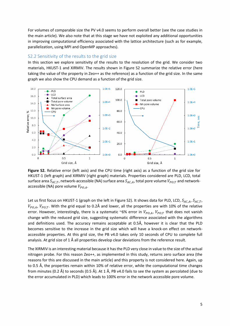
5

For volumes of comparable size the PV v4.0 seems to perform overall better (see the case studies in

the main article). We also note that at this stage we have not exploited any additional opportunities

in improving computational efficiency associated with the lattice architecture (such as for example,

parallelization, using MPI and OpenMP approaches).

S2.2 Sensitivity of the results to the grid size In this section we explore sensitivity of the results to the resolution of the grid. We consider two

materials, HKUST-1 and XIRMIV. The results shown in Figure S2 summarize the relative error (here

taking the value of the property in Zeo++ as the reference) as a function of the grid size. In the same

graph we also show the CPU demand as a function of the grid size.

Figure S2. Relative error (left axis) and the CPU time (right axis) as a function of the grid size for HKUST-1 (left graph) and XIRMIV (right graph) materials. Properties considered are PLD, LCD, total surface area 𝑆𝐴𝐶,𝑇, network-accessible (NA) surface area 𝑆𝐴𝐶,𝐴, total pore volume 𝑉𝑃𝑂,𝑇 and network-accessible (NA) pore volume 𝑉𝑃𝑂,𝐴.

Let us first focus on HKUST-1 (graph on the left in Figure S2). It shows data for PLD, LCD, 𝑆𝐴𝐶,𝐴, 𝑆𝐴𝐶,𝑇,

𝑉𝑃𝑂,𝐴, 𝑉𝑃𝑂,𝑇. With the grid equal to 0.2Å and lower, all the properties are with 10% of the relative

error. However, interestingly, there is a systematic ~6% error in 𝑉𝑃𝑂,𝐴, 𝑉𝑃𝑂,𝑇 that does not vanish

change with the reduced grid size, suggesting systematic difference associated with the algorithms

and definitions used. The accuracy remains acceptable at 0.5Å, however it is clear that the PLD

becomes sensitive to the increase in the grid size which will have a knock-on effect on network-

accessible properties. At this grid size, the PB v4.0 takes only 10 seconds of CPU to complete full

analysis. At grid size of 1 Å all properties develop clear deviations from the reference result.

The XIRMIV is an interesting material because it has the PLD very close in value to the size of the actual

nitrogen probe. For this reason Zeo++, as implemented in this study, returns zero surface area (the

reasons for this are discussed in the main article) and this property is not considered here. Again, up

to 0.5 Å, the properties remain within 10% of relative error, while the computational time changes

from minutes (0.2 Å) to seconds (0.5 Å). At 1 Å, PB v4.0 fails to see the system as percolated (due to

the error accumulated in PLD) which leads to 100% error in the network accessible pore volume.

6

S3. PB v4.0 vs RASPA results: total surface area In this section we provide comparison of the total surface area 𝑆𝐴𝐶,𝑇 for 12,081 MOFs obtained from

PB v4.0 and RASPA. As seen from Figure S3, there is a high level of consistency between the two codes.

Figure S3. Total surface area, 𝑆𝐴𝐶,𝑇, from PB v4.0 and RASPA. On the left, the data is for the complete set of

MOFs, and on the right, it is focusing on the region up to 2500 m2/g. Color bars indicate the population of the

properties in the different range of values.

S4. PLD analysis of 2,210 materials with zero Zeo++ surface area and

non-zero PB v4.0 surface area

Figure S4. PLD analysis of the 2,210 materials with zero Zeo++ surface area and non-zero PB v4.0 surface area. The parity plot on the left; and the distribution of the PLD within this set of materials on the right.

S5. Properties of the MOF set with low surface and low porosity

structures excluded Here we consider structures with 𝑆𝐴𝐶,𝑇, >=50 m2/g and 𝑉𝑃𝑂,𝑇 >=0.25 cm3/g, and plot the parity plots

and histograms following the same approach as in the main article. This subset has ~4800 MOFs.

Statistics of the results within these plots is discussed in the main article.

7

Figure S5. Parity plots for surface area from PB v4.0 and Zeo++ for a subset of ~4800 materials. Top panels: total surface area 𝑆𝐴𝐶,𝑇. Bottom panels: network-accessible surface area 𝑆𝐴𝐶,𝐴. Panels on the left show the complete range of values and panels on the right focus on the expanded region up to 2500 m2/g. Color bars indicate the population of the properties in the different range of values.

8

Figure S6. Parity graphs for pore volume from PB v4.0 and Zeo++ for a subset of ~4800 materials. Top panels: total probe-occupiable volume 𝑉𝑃𝑂,𝑇. Bottom panels: network-accessible probe-

occupiable volume 𝑉𝑃𝑂,𝐴. Panels on the left show the complete range of values and panels on the right focus on the expanded region up to 1.5 cm3/g. Color bars indicate the population of the properties in the different range of values.

S6. Error analysis in the reduced subset of ~4800 materials Here we provide error analysis for the subset of ~4800 materials with 𝑆𝐴𝐶,𝑇, >=50 m2/g and 𝑉𝑃𝑂,𝑇

>=0.25 cm3/g. In this analysis, values of properties (P) from PB v4.0 are taken as the reference: 𝐸𝑅𝑅 =

100% ∙|𝑃𝑃𝐵 𝑣4.0−𝑃𝑍𝑒𝑜++|

𝑃𝑃𝐵 𝑣4.0.

S6.1 Total surface area

There are only 70 structures with an error larger than 10%, and most of the structures are between

10-15 % error.

Figure S7. Error analysis of the total surface area, 𝑆𝐴𝐶,𝑇 in the subset of 70 MOFs. Top panels: parity

plot of the 70 structures with the error exceeding 10% (on the left); and the correlation between the value of 𝑆𝐴𝐶,𝑇 and the magnitude of the error (on the right). Bottom panel: error distribution

for 𝑆𝐴𝐶,𝑇 within 70 structures.

S6.2 Network-accessible surface area There are 1122 structures that show errors larger than 10%. Within this group, 995 structures show

errors of 100% and 993 are structures with some value for PB v4.0 and zero value for Zeo++. The rest

of structures show values between 10-30%.

9

Figure S8. Error analysis of the total surface area, 𝑆𝐴𝐶,𝐴 in the subset of 995 MOFs. Top panels: parity plot of the 995 structures with the error exceeding 10% (on the left); and the correlation between the value of 𝑆𝐴𝐶,𝐴 and the magnitude of the error (on the right). Bottom panel: error distribution for 𝑆𝐴𝐶,𝐴 within 995 structures.

It is clear that 995 MOFs have structures considered to be accessible in PB v4.0, but not in Zeo++. See

the discussion for the plausible reasons for this in the main article.

S6.3 Total probe-occupiable pore volume For this property, there are 542 structures that have outliers with errors larger than 10%. Most of

these errors are around 10-20%. It is important to emphasize however that PB v4.0 volume is

systematically lower than the Zeo++ volume and as we have discussed in section S2 it is independent

of the grid size for grids below 0.5 Å.

10

Figure S9. Error analysis of the total probe-occupiable pore volume 𝑉𝑃𝑂,𝑇 in the subset of 995 MOFs. Top panels: parity plot of the 995 structures with the error exceeding 10% (on the left); and the correlation between the value of 𝑉𝑃𝑂,𝑇 and the magnitude of the error (on the right). Bottom panel: error distribution for 𝑉𝑃𝑂,𝑇 within 995 structures.

S6.4 Network-accessible probe-occupiable pore volume For this property, there are 449 structures with errors larger than 10% within the set of ~4800

materials. For many of these structures the errors are below 25%, or around 100% (resulting from PB

v4.0 and Zeo++ not agreeing on whether the structure is accessible).

Figure S10. Error analysis of the network-accessible probe-occupiable pore volume 𝑉𝑃𝑂,𝐴 in the subset of 449 MOFs. Top panels: parity plot of the 449 structures with the error exceeding 10% (on the left); and the correlation between the value of 𝑉𝑃𝑂,𝐴 and the magnitude of the error (on the right). Bottom panel: error distribution for 𝑉𝑃𝑂,𝑇 within 449 structures (up to 120% error).

S6.5 PLD For PLD, we have 205 MOFs showing a systematic deviation larger than 10%. Most of them show

values of PLD around 2.5-5 Å, and below 20% percent error.

11

Figure S11. Error analysis of PLD in the subset of 205 MOFs. Top panels: parity plot of the 205 structures with the error exceeding 10% (on the left); and the correlation between the value of PLD and the magnitude of the error (on the right). Bottom panel: error distribution for PLD within 205 structures.

S6.6 Summary of the observed errors within the subset of ~4800 MOFs From the summary in Table S6 it is clear that the most sensitive properties with the largest percentage

of errors > 10% is the network accessible surface area. However, within this property the majority of

problematic structures is associated with the technical differences in how the probes are used in

Zeo++ and PB v4.0 for accessibility analysis and the surface area analysis. In the main article we

elaborated on the specific reasons for this.

Below in Figure S12 we show that the majority of issues for the network-accessible properties emerge

when the PLD is close to the size of the probe molecule, where the percolation analysis becomes

sensitive to the resolution of the grid and to algorithms employed.

Table S6. Summary of the observed errors within the subset of ~4800 MOfs

Total SA, 𝑆𝐴𝐶,𝑇

Network-accessible SA,

𝑆𝐴𝐶,𝐴

Total probe-occupiable PV, 𝑉𝑃𝑂,𝑇

Network-accessible,

probe occupiable PV,

𝑉𝑃𝑂,𝐴

PLD

Number 70 1122 542 449 205

% (4809) 1.46 23.33 11.27 9.33 4.26

12

Figure S12. Error analysis of PLD in the subset of 449 MOFs, which have error of more than 10% for the network-accessible pore occupiable volume, 𝑉𝑃𝑂,𝐴. Top panels: parity plot of the 449 structures

with the error exceeding 10% (on the left); distribution of the PLD within the set of 449 structures. Bottom panel: distribution of the PLD within the set of ~4800 structures.

According to Figure S12, there are 366 MOFs with PLD < 4.0 Å, 33 with 4 Å <= PLD < 4.5 Å, 18 with 4.5

Å <= PLD < 5.0 Å. This can be contrasted with the complete distribution of the PLD in the ~4800 porous

MOFs (bottom panel of Figure S12).

S7. Histograms of properties from Zeo++. In this section we present the distribution of properties within the set of ~12,000 structures from

Zeo++ for completeness.

13

Figure S13. Distribution of total surface area 𝑆𝐴𝐶,𝑇, network-accessible surface area 𝑆𝐴𝐶,𝐴, total probe-occupiable pore volume 𝑉𝑃𝑂,𝑇 and network-accessible probe-occupiable pore volume 𝑉𝑃𝑂,𝐴 within the set of ~12000 MOFs from Zeo++.

S8. Principal component analysis We have performed a Principal Component Analysis using the data for the main set of ~12000

materials, and considered the following properties: helium void fraction, 𝐹𝐻𝑒,𝑇, total surface area,

𝑆𝐴𝐶,𝑇, total pore volume, 𝑉𝑃𝑂,𝑇, pore limiting diameter, PLD, largest cavity diameter, LCD, and the ratio

LCD/PLD. For this we have used the package “stats” within R software environment (https://www.r-

project.org/) and the Principal Component Analysis Visualisation tool (https://aaml-pca-geo-

prop.herokuapp.com). We first analyse the correlation between these properties as summarized in

Figure S13.

Figure S14. Correlation plot for selected structural properties of the set of ~12000 MOFs. Figure downloaded from the Principal Component Analysis Visualisation tool.

This correlation plot shows that most of the properties calculated and studied are correlated. It is not

very surprising as these geometrical properties are different ways of measuring and characterizing the

pore space available within a framework. As a consequence, pore volume 𝑉𝑃𝑂,𝑇, surface area 𝑆𝐴𝐶,𝑇

14

and void fraction 𝐹𝐻𝑒,𝑇, which describe the total space within the pores without accounting for how

this space is distributed, are highly correlated. Pore limiting diameter (PLD) and largest cavity diameter

(LCD) relate to some particular features in the distribution of the pore space instead of the total space.

A high LCD can be paired with a high value of 𝐹𝐻𝑒,𝑇, but not necessarily. Thus, LCD and PLD are highly

correlated between them, but not with the rest of the properties. Interestingly, density and ratio

LCD/PLD are not correlated with the rest of the properties, although density shows a higher R2 with

some properties than ratio LCD/PLD. The density of a MOF accounts for the pore space within a

framework and the volume that framework atom occupy. The ratio LCD/PLD, although derived from

the properties that highly correlated to each other, is not strongly correlated with them, suggesting

that this measure can be a good feature to describe the arrangement of cages and channels.

We can also use the tool to see how many principal components we should use to have a significant

explanation of the variance in the dataset. The “Scree plot” tab in the tool generates a figure showing

the cumulative explained variance as a function of the number of principal components chosen. This

figure shows that a 79.94% of the variance in the dataset is explained by two principal components,

while using a third one would increase this value to 90.27%. Thus, we are choosing three principal

components to describe our dataset.

Figure S15. Cumulative scree plot of the explained variance a function of the number of principle components used. Figure downloaded from the Principal Component Analysis Visualisation tool.

The correspondence between properties and principal components can be measured through

loadings, contributions and squared cosines, and the Principal Component Analysis Visualisation tool

allows for exploring this through interactive plots and provide the data to export them to different

software. When performing a principal component analysis the data is represented by a new set of

orthogonal variables called principal components. The information extracted in this representation

retains a high percentage of the variance found in the original dataset. Loadings are the correlation

between the variables in the original dataset and the principal components in the new representation.

Contributions explain the proportion in which each variable in the original dataset contributes to the

principal components. Squared cosine shows the importance of a principal component for a given

variable, i.e. how well represented a variable is in a given principal component. To generate statistics

15

plots for the squared cosine, we have used the “stats” and “factoextra” packages in R to run a parallel

principal component analysis. Here we select the squared cosine (cos2), which shows values between

0 and 1, to illustrate this correspondence between properties and principal components. In the

figures, the color scale is the sum of the cos2 values of the two principal components shown. The

length of the arrow is the sum of the loadings. According to this, the ratio LCD/PLD, pore volume (VPO,T)

and density are the properties with the highest correlation with the principal components chosen.

16

Figure S16. Variable correlation plots showing the relationships between all variables for the projections of PC1 and PC2 (top), PC2 and PC3 (middle), and PC1 and PC3 (bottom). The colormap represents the squared cosine value for each of the variables. The arrows represent the sum of the loadings.

We also have extracted the data from the tool, and summarised the important values in the following

table. The cos2 values of the principal components towards the pore volume show that this property

is well represented, and mostly by PC1. Similarly, LCD/PLD is well represented by PC1-PC3, but the

highest proportion belongs to PC2. Density is also well represented by these principal components,

but mostly by PC1 and PC2. Regarding the values of contribution, the highest values are obtained for

the three mentioned properties. Therefore, pore volume contributes 18.334% to the PC1 and a

81.759% of PC2 is due to LCD/PLD. In the case of density, although it is better represented by PC1, it

contributes more to the PC3 (41.9%) than to the PC1 (11.0%).

Cos2 Contribution

PC1 PC2 PC3 PC1 PC2 PC3

Pore volume, VPO,T 0.863 0.036 0.007 18.334 4.012 0.958 LCD/PLD 0.261 0.727 0.001 5.540 81.759 0.084 Density 0.518 0.003 0.303 11.003 0.384 41.900

In the correlation plots we observed four independent groups of properties: 1) ratio LCD/PLD; 2) LCD

and PLD; 3) void fraction, pore volume and surface area; and 4) density. From the PCA analysis, we

have found that the properties that weight more to explain the dataset are pore volume, LCD/PLD and

density.

S9. Computer visualization of interesting structures Below we provide computer visualizations of the structures explored within the “3.3 Material

informatics with PB v4.0 and MOF/PCA Explorer” section of the main article. These visualizations were

produced using iRASPA software2.

17

S10. References 1. Rappe, A. K.; Casewit, C. J.; Colwell, K. S.; Goddard, W. A.; Skiff, W. M., UFF, a full periodic table force field for molecular mechanics and molecular dynamics simulations. Journal of the American Chemical Society 1992, 114 (25), 10024-10035. 2. Dubbeldam, D.; Calero, S.; Vlugt, T. J. H., iRASPA: GPU-accelerated visualization software for materials scientists. Molecular Simulation 2018, 44 (8), 653-676.

download fileview on ChemRxivSarkisov_et_al_SI_final.pdf (2.41 MiB)