Masters Thesis Possibilities - Worcester Polytechnic Institute

ANALYSIS OF DISTRIBUTED RESOURCES POTENTIAL IMPACTS ON ELECTRIC SYSTEM EFFICACY

By

Paul Robinson

A Thesis

Submitted to the Faculty

of the

WORCESTER POLYTECHNIC INSTITUTE

In partial fulfillment of the requirements for the

Degree of Master of Science

in

Electrical and Computer Engineering

By

________________________________

December 2009

Approved by:

_______________________________________ Professor Alexander E. Emanuel, Major Advisor

________________________________________ Slobodan Pajic, Review Committee

1

Abstract

The intent of this Thesis is to study the potential of distributed resources to

increase the efficacy of the electric system without decreasing the efficiency of the

system. Distributed resources (DR) are technologies that provide an increase in power or

a decrease in load on the distribution system. An example of DR is a storage device that

uses electricity during low use periods to store energy and then converts the stored energy

to power during high use periods.

The energy storage being studied is for the purpose of peak shaving or the ability

to shift small amounts of load to a more optimum time. In particular the concept of load

curve leveling is explored. DR options are studied to determine how size, location, and

storage losses impact the overall system efficacy and efficiency. This includes impacts

on system losses, capacity utilization, and energy costs.

2

Acknowledgements

I would like to thank my wife Mara and my children Kyle and Marissa for their

support and understanding during this endeavor. Also, I would like to thank Prof. A.

Emanuel and other WPI faculty for their guidance and encouragement throughout this

process. Lastly, I would like to thank National Grid for the educational reimbursement

program that made funding this research possible.

3

Contents 1 Introduction...................................................................................................................... 4 2 Background.................................................................................................................... 11 3 Design Elements ............................................................................................................ 17

3.1 Simple radial electric system .................................................................................. 17 3.2 Power Flow Methodology....................................................................................... 19 3.3 Multi-circuit system model ..................................................................................... 23 3.4 End use device based storage.................................................................................. 25

4 Simulation Results ......................................................................................................... 27 4.1 Simple radial electric system with DR supply........................................................ 27 4.2 Simple radial electric system with DR storage ....................................................... 37 4.3 Multi-circuit system model with DR storage.......................................................... 42

6 Conclusion .................................................................................................................... 58 References......................................................................................................................... 61 Appendices........................................................................................................................ 62

Appendix A: Impedance calculations .......................................................................... 62 Appendix B: Matlab program to solve Gauss-Seidel .................................................. 64 Appendix C: Modified Matpower program ................................................................. 68 Appendix D: Matlab model used for simple radial analysis........................................ 73 Appendix E: Matlab model used for multi-circuit analysis ......................................... 75 Appendix F: Sample Matlab power flow output........................................................... 77 Appendix G: Cost calculation input data ..................................................................... 80 Appendix H: Plant factor data...................................................................................... 87

4

1 Introduction

The intent of this Thesis is to study the potential of distributed resources to

increase the efficacy of the electric system, while not decreasing the efficiency of the

system. The system should have enough capacity to reliably supply the varying demand

for electricity 100% of the time, with the least amount of equipment and energy input.

Having higher efficacy may not be desirable if the system efficiency is lowered as a

result. The ability to decrease system losses during peak periods to offset increased

losses from energy storage used to increase the efficacy of the system will be explored.

For the purposes of this analysis, the efficacy of the system can be determined by

the capacity utilization factor. The capacity utilization factor is the capacity factor times

the load factor. The load factor is the ratio of the average load over a designated time

period to the peak load occurring during that time period. The capacity factor is the ratio

of the total energy served over a designated time period to the energy that would have

been served if the system had operated continuously at its maximum rating.

To provide some context on what distributed resources are, the following is a

simplified overview of the major topology categories of the electric system, as shown in

Figure 1.1. First, there is generation which uses some form of energy to produce

electricity. Next, there is transmission which delivers electricity at high voltage from the

large generators to the rest of the system. Then, there is distribution which is connected to

transmission and supplies the electricity to the consumer. The amount of electricity

required by the consumer is also referred to as the electric load or demand. To satisfy

5

electric demand the electricity must be produced by the generators and delivered to the

load when it is needed.

Figure 1.1 – Diagram of electric system topology

Most of the energy generated in the system is provided by large units, (hundreds

of MWs), connected to the transmission system. The concept of also having multiple

6

small generation sources distributed along the distribution system has been referred to as

distributed generation (DG). If energy storage devices are included with DG it has been

known as dispersed storage and generation (DSG). If other technologies to provide an

increase in power or a decrease in load are also included, then it is being collectively

referred to as distributed resources (DR).

Inherent in the system is a varying level of power being produced and delivered as

the amount of load changes. In other words, the electricity needed by the system

increases as electric consuming devices are turned on, and conversely, the amount of

electricity decreases as electric consuming devices are turned off. For the system to be

stable there must be a match between the amount of electricity being consumed,

including losses, and the amount of electricity being produced. This leads to a system

that must have the capacity to meet the highest level of demand even if that level is only

reached for a short time. Also, the amount of electric loss in the system is greater at the

higher load levels then it is at lower load levels.

For most of its history, the electric system was designed to reliably supply the

load requirements of the electricity consumers. This has led to a system that is built to

have the capacity necessary to satisfy the highest, or peak, amount of demand even if that

demand is only reached for a few hours. Parts of the system can be strained to their

capacity limits for a short time, but they may sit idle or under utilized for the majority of

time. The amount of load usually varies by time of day, day of week, and weather

conditions. A plot of the amount of electric load on the system over time is called a load

curve. An example load curve for one day normalized to the peak demand is shown in

Figure 1.2.

7

0%

10%

20%

30%

40%

50%

60%

70%

80%

90%

100%

1 2 3 4 5 6 7 8 9 10 11 12 13 14 15 16 17 18 19 20 21 22 23 24

Hour

Perc

ent o

f Pea

k Lo

ad

Figure 1.2 – Example of a 24 hour Load Curve

From an asset utilization view, it would be desirable to have a more constant level

of load. Reducing the peak amount of load and shifting it to times of lower load would

flatten the load curve. The total amount of energy delivered would be the same but the

capacity utilization factor would decrease. The result is the ability to deliver the same

amount of energy with less or smaller capacity infrastructure. It could also allow for more

energy to be delivered without increasing the capacity infrastructure. An example of load

shifting is shown in Figure 1.3.

8

0%

10%

20%

30%

40%

50%

60%

70%

80%

90%

100%

1 2 3 4 5 6 7 8 9 10 11 12 13 14 15 16 17 18 19 20 21 22 23 24

Hour

Perc

ent o

f Pea

k Lo

ad

Shifted LoadLoad

Load Shift

Figure 1.3 – Example of Load Shifting

There are a few factors in the electric system that makes load shifting or peak

shaving advantageous. One factor is that usually not all generation has the same

efficiency or costs. If load can be shifted to a time when the generation is more efficient

then the overall efficiency is improved. Another factor is that the delivery system needs

to be sized so the highest level or peak power usage can be delivered. Infrastructure must

be built to handle the highest load levels, so if this level is only reached occasionally then

its capacity is being under utilized.

A more subtle factor is that system losses are proportional to the current squared.

An electric system with twice as much current has four times as much loss. If the load

cycle for a 24 hour period is examined it is typical that there is a curve that has valleys

9

and peaks. If the overall energy load was spread out with same amount being used each

hour then the curve would be a straight line. The amount of energy used is the same for

the load cycle with the valleys and peaks as for the straight line cycle. However, the

system loss is higher for the cycle with valleys and peaks. This is due to the nonlinear

relation between the power loss and current.

From and electric system standpoint there are several benefits to having DR: 1) it

can provide voltage support and reduce system losses by having the supply source closer

to the load, 2) the ability to reduce system peaks which reduces capacity needs, and 3) the

ability to maximize the use of the most efficient supplies through storage. These features

can help lead to a more efficacious system. To maximize the benefit obtained from these

resources requires the integration of DR into the system. The size and location of the DR

has an impact on the overall efficacy of the system.

An example of DR is a storage device that uses electricity during low use periods

to store energy and then converts the stored energy to power during high use periods.

This can be accomplished by such techniques as charging batteries, pumping water,

compressing air or creating hydrogen from electrolysis. For the purpose of this analysis,

DR consists of resources of less than 10 MW and usually around 1 MW on the

distribution system.

The energy storage being studied is for the purpose of peak shaving or the ability

to shift small amounts of load to a more optimum time. Usually the shift is from a period

of high electric use or system constrained time to a lower use period. Energy storage

options are studied to determine how storage losses compare to system loss reduction. In

particular the concept of load curve leveling is explored.

10

The DR generation being studied could be from co-generation or from renewable

resources such as wind and solar. In the current environment the ability to utilize

renewable energy sources has taken on greater importance than in the past. The

integration of small generation sources onto the electric distribution system poses a

number of technical implications. These can range from system stability and control to

protection schemes and metering. This analysis will focus on the impact that a distributed

resource can have on capacity utilization and system efficacy.

Most of the focus of energy efficiency efforts has been on having devices use less

energy. A device is more efficient if it uses less energy to produce work than a device

that uses more energy to produce the same amount of work. The amount of energy is

usually measured at the terminals of the device and does not include the system that

provides the energy. The reference point can be broadened beyond the terminal of the

device to also consider the system that provides the energy. If we think of the consuming

devices as part of the system then it can change how we view efficiency and the supply

and demand relationship.

One area of interest is the idea of distributed end user device storage to flatten the

load curve. Local storage could allow for charging during low use periods and drain

during higher use periods. If devices that utilize AC/DC power supplies could also store

small amounts of energy then additional charging losses would be minimized. The stored

energy of hundreds of thousands of devices could be utilized randomly or controlled over

the projected peak period to reduce it. The consumer would get the benefit of the work

produced by the device during the peak period and the system would benefit from the

reduced peak load.

11

2 Background

The AC electric system in the United States can be traced back to 1885 in Great

Barrington Massachusetts. George Westinghouse had bought American patents covering

the AC transmission system developed by L. Gaulard and J. D. Gibbs of Paris. An

associate of Westinghouse, William Stanley tested single phase transformers in his

laboratory and supplied 150 lamps in the town. In 1888, Nikola Tesla presented a paper

on two-phase induction and synchronous motors. In 1893 Tesla demonstrated a two-

phase AC distribution system at the Columbian Exposition in Chicago. The advantages of

polyphase AC and especially three-phase AC over DC became apparent. By January

1894 there were five polyphase generating plants in the United States. [1]

The ability to step-up or step-down the voltages with the transformer was the

biggest reason that AC was adopted over DC early on in the industry. The ability to

transmit electricity at high voltages allows for transmission lines to deliver more power

than at lower voltages. This allowed for large amounts of power to be transmitted at high

voltages and then stepped-down to lower voltages for use.

The modern transmission system is operated at very high voltage levels in the

range of 115 kV – 765kV. The system is configured as a network with multiple

connection points, so the loss of one element in the system will not interrupt the supply.

Large generating facilities in the range of 100 MW – 1200 MW are connected to the

transmission system.

Distribution systems are usually operated at voltage levels in the range of 13kV –

34 kV. Some distribution systems in cities are connected in a network but most

12

distribution systems are radial with one normal supply point and backup connections that

are normally open. The distribution system is supplied from substations that have the

bulk power transformers that are supplied at a transmission voltage level and then supply

the distribution system at a lower distribution voltage level. The distribution system is

used to supply point of use transformers, or distribution transformers, to convert the

voltage to levels used by consumers. The voltages used by consumers are usually

120/240 V or 120/208 V for residential and small commercial users and 277/480V three

phase for larger commercial users.

The demand for electricity has continued to grow throughout the history of the

electric system. The system has been built to have adequate capacity to meet the peak

demand of the load. The total net summer generation capacity in the U.S. from 1971 to

2007 is shown in Figure 2.1.[2] The increase in capacity is not only due to population

growth it is also due to increasing usage per person. In 1982 the average power usage per

person in the U.S. was 1.1 kW [3], in 1996 it was 1.3 kW [4], and in 2007 it was 1.6 kW.

13

0

200,000

400,000

600,000

800,000

1,000,000

1,200,000

1971

1973

1975

1977

1979

1981

1983

1985

1987

1989

1991

1993

1995

1997

1999

2001

2003

2005

2007

Year

MW

Figure 2.1 – Total U.S. summer generation capacity [2]

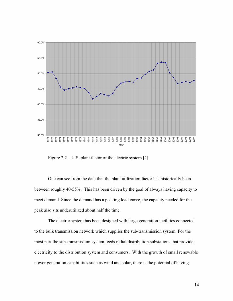
The plant or use factor of the system is the ratio of the total actual energy

produced over a designated time period to the energy that would have been produced if

the plant had operated continuously at its maximum rating [6]. A diagram of the plant

factor of the U.S. system derived from DOE data, included in appendix H, is shown in

Figure 2.2

14

30.0%

35.0%

40.0%

45.0%

50.0%

55.0%

60.0%

1971

1972

1973

1974

1975

1976

1977

1978

1979

1980

1981

1982

1983

1984

1985

1986

1987

1988

1989

1990

1991

1992

1993

1994

1995

1996

1997

1998

1999

2000

2001

2002

2003

2004

2005

2006

2007

Year

Figure 2.2 – U.S. plant factor of the electric system [2]

One can see from the data that the plant utilization factor has historically been

between roughly 40-55%. This has been driven by the goal of always having capacity to

meet demand. Since the demand has a peaking load curve, the capacity needed for the

peak also sits underutilized about half the time.

The electric system has been designed with large generation facilities connected

to the bulk transmission network which supplies the sub-transmission system. For the

most part the sub-transmission system feeds radial distribution substations that provide

electricity to the distribution system and consumers. With the growth of small renewable

power generation capabilities such as wind and solar, there is the potential of having

15

many smaller sources of power on the distribution system. This poses both opportunities

and challenges for the electric industry.

A basic premise of the power system is to have the generation available to meet

the load of the system. As the load of the system changes, the power required to be

generated changes along with it. For the most part the load changes as the devices using

the power are utilized. With most devices the benefit derived from the electricity being

used is obtained when the device is using the electricity from the system supplying it. So

if you want to use the electricity from the system when it is most efficient, then the

benefit of the device must be used when the supply is the most efficient. However, if the

device could store the energy when it is supplied most efficiently and use it during less

efficient supply times then the system overall is more efficient.

The vast majority of electric systems utilize AC to generate and supply electricity.

One drawback to AC is that it can not be directly stored for later use; it must be generated

and used at the same time. To store the electricity it must be converted from AC to

another form of energy, however energy is lost during this conversion process. If more

energy is lost when storing electricity than would be in direct use, then any efficiency

benefit is reduced. A device that converts electricity into useful work is deemed more

efficient if it requires less energy while producing the same amount of work. The electric

system can be deemed more efficacious if it requires less energy and equipment to supply

the electricity to the end users.

Over the past several decades the utilization of power electronics has grown

significantly. The advances in semiconductor fabrication technology have enabled higher

voltage and current handling and switching speeds of power semiconductor devices. This

16

has enabled electronic controllers to improve the efficiency of devices that utilize power

electronics. It has been estimated by electric utilities that since 2000, over half of the

electrical load is supplied through power electronics. [5]

The result of the change in a large portion of the load utilizing power electronics

is that the system has become increasingly an AC/DC hybrid system. The bulk of the

power is generated and delivered as AC and then the majority of end use devices convert

it to DC. The system now has a large amount of AC/DC conversion happening at the end

use device location. One of the ideas presented in this paper is the untapped potential of

this DC power to be harnessed as a distributed resource.

17

3 Design Elements

3.1 Simple radial electric system

A model of a simple radial electric system was created to study the potential

impacts of DR on the efficacy of the system, shown in Figure 3.1. The model has one

large generator, one transmission line and one substation transformer feeding a

distribution feeder, or circuit. The feeder has 10 loads and 10 DR locations positioned at

different points along the feeder. The DR points are modeled as small generators that can

be either on or off, depending on the analysis scenario.

This model provides the ability to measure the impact that different levels of load

and DR size and location has on the electric system. Parameters such as the amount of

power flowing through an element of the system or total losses can measured and

compared to reference measurements. It also provides the ability to determine if there is

an optimum location and size of DR for a given system arrangement. Multiple power

flow simulations of different combinations of load levels and DR locations and size were

performed.

18

Figure 3.1 - Diagram of radial feeder model used for simulations

19

The electrically equivalent parameters of the proposed system were derived to be

consistent with typical values found in the industry. The distribution line impedances

were calculated assuming a typical open air overhead cross-arm construction as shown in

Figure 3.2. The phase spacing was 44” and 336 AL wire was used.

Figure 3.2 – Distribution feeder geometry used to calculate impedance

The inductance of the distribution feeder was calculated using geometric mean

radius (GMR) [1]. The details of the calculation are shown in Appendix A. For the

model feeder each segment is about 2750’ which gives a segment impedance of .08+j.17.

The impedance of transformer was taken from typical values in the industry, .035+j.57 on

a per unit basis.

3.2 Power Flow Methodology

To solve the power flow or “load flow” of the electric system a nodal analysis is

performed. Each node, usually referred to as a “bus”, has four variables; voltage (V),

20

voltage angle (θ), real power (P), and reactive power (Q). The buses are assigned a type

depending on which variables are defined and which are to be calculated. The system has

one reference bus or “slack bus” which has a specified V and θ. A load bus has known

or specified P and Q values. A voltage controlled or generator bus has known or specified

P and V values. The line data is represented in a matrix form with from and to bus,

resistance and reactance per unit. The data is defined in an admittance matrix (Y).

For a total of N buses the calculated voltage at any bus k, where n ≠ k, and where

Pk and Qk are specified is: [1]

⎟⎠

⎞⎜⎝

⎛−

−= ∑

=

N

nnkn

k

kk

kk

k VYV

jQPY

V1*

1 (3.1)

For a bus where voltage magnitude rather than reactive power is specified, the

components of the voltage for n ≠ k are found from:

*1

k

N

nnknkkkkk VVYVYjQP ⎟⎠

⎞⎜⎝

⎛+=− ∑

=

(3.2)

For n=k

⎟⎠

⎞⎜⎝

⎛=− ∑

=

N

nnknkkk VYVjQP

1*

(3.3)

⎟⎠

⎞⎜⎝

⎛−= ∑

=

N

nnknkk VYVQ

1*Im

(3.4)

The nonlinear equations for the nodal analysis can be solved with an iterative

solution as shown in Figure 3.3.

21

Figure 3.3 – Power flow methodology

22

The Gauss-Seidel method uses the admittance matrix representation of the line

data to solve the I=YV equation, where I is the current, Y is the admittance, and V is the

voltage. An iterative solution method starts with an initial guess of values to solve the

unknowns. For the power flow equations the initial guess for voltages are 1 per unit and 0

for angles. The calculated values are compared to find the mismatch. If the mismatch is

greater than the set tolerance, then the calculated values are used as the guesses to solve

the equations again. This is repeated until the mismatch is within the tolerance or the max

number of iterations is reached.

For a load bus guesses for the V and α are entered into the equation to calculate

values for P and Q. These calculated values are compared to the known values of P and

Q. If the mismatch between the calculated values and known values are within a set

tolerance the iterations can stop. If the mismatch is greater than the tolerance the newly

calculated values for V and θ are used and the process is repeated. For a generator or

voltage controlled bus guesses for the Q and θ are entered into the equation to calculate

values for P. The calculated value is compared to the known values of P.

A basic Gauss-Seidel load flow program was created in Matlab and is included in

Appendix B. A more robust load flow program, Matpower V3.2,

(http://www.pserc.cornell.edu/matpower/), was used for the majority of the analysis. The

program was modified to provide the ability to scale the loads based on a scaling factor

entered at program execution. The portion of modified code is included in Appendix C.

This modification enabled a much more efficient program execution cycle for the

multiple simulations required.

http://www.pserc.cornell.edu/matpower/�

23

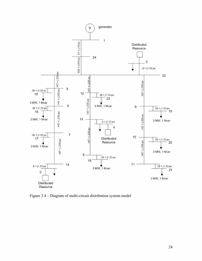
3.3 Multi-circuit system model

A second model of a small distribution system was created to study impacts on

overall system efficacy beyond a simple feeder. The multi-circuit model used in this

analysis is shown in figure 3.4. The model consists of a generator, transmission line, a

substation bus supplied by a transformer, and three feeders. The bus has a peak shaving

battery unit and two of the feeders have a peak shaving battery units at different

locations. The feeders are segmented into three sections with 8 - 3MW 95% pf loads

supplied by distribution transformers. Simulations were run comparing the losses with

the different peak shaving unit locations and methods.

24

Figure 3.4 – Diagram of multi-circuit distribution system model

25

3.4 End use device based storage

For DR that utilizes charging from the system, the charging losses are a major

factor in limiting efficacy. The biggest source of losses from battery storage is in the

conversion of power from AC to DC and then from DC to AC. An approach introduced

in this paper is to have the storage based at end use devices that already utilize AC/DC

power supplies. This eliminates the need for extra conversion processes and their

associated losses. This approach is also inherently scalable to the load since it is based in

the load.

The concept is to have a small amount of energy stored in the end use device that

would enable the device to use this energy to function for a short time. The device would

charge during a low use period and would then use the stored energy during a high use

period. If there are hundreds of thousands of these devices on a system then the amount

of load that could be shifted is significant. The devices would operate randomly over the

projected high and low use periods.

The impact that DR based on end use device storage has on system efficacy will

be analyzed along side distribution based DR. Since the end use device DR is part of the

load, it will be modeled as load. The result is a lower load during a peak period and a

higher load during an off peak period. The concept of end use device storage is shown in

Figure 3.5.

26

Figure 3.5 – Diagram of base case, distribution DR and end use device DR

27

4 Simulation Results

4.1 Simple radial electric system with DR supply

Load flow simulations were run on the distribution feeder model, shown in Figure

3.1. For the first set of simulations the feeder had a total load of 10 MW and 3 MVar

with 1 MW and .3 MVar at each load point. The system losses were recorded with no DR

and used for the normalized base line. Simulations were run with different DR locations

and sizes to compare the effect they have on system efficacy and efficiency.

The load factor of the feeder is increased by having a lower peak load seen at the

substation bus. For the case of having a 1 MW DR, the peak load on the feeder is 9 MW

instead of 10 MW, but the total energy of the load has not changed. The result is the

feeder now has extra capacity for load growth. The same goes for the other cases with

their respective levels of DR. A graph showing the system losses versus DR location

compared to the base case without DR is shown in Figure 4.1.

28

0.0%

10.0%

20.0%

30.0%

40.0%

50.0%

60.0%

70.0%

80.0%

90.0%

100.0%

1 2 3 4 5 6 7 8 9 10

DR location

Nor

mal

ized

loss

es

1 MW DR2 MW DR3 MW DR4 MW DR5 MW DR6 MW DR7 MW DR

Figure 4.1 – Normalized system losses versus DR location for different DR sizes

It can be seen from Figure 4.1 that the size and location of the DR has an impact

on the system losses. In all cases the overall system losses were reduced and the closer

the DR was to the beginning of the feeder the less of a reduction there was. For the lower

capacity DR the most system loss reduction is for locations at the end of the line. As the

DR capacity increases the greater loss reduction moves from the end to the middle of the

line.

If we assume no or minimal voltage drop, then the line losses can be expressed in

generic terms with the following equations. [7]

The line loss without any DR present is defined as:

LossB 2

22

3)(

P

LL

VQPrL +

= (4.1) [7]

29

The line loss from the source to the DR location can be expressed as:

LossASD 2

2222

3)22(

P

DLDLDDLL

VQQPPQPQPrD −−+++

= (4.2) [7]

The line loss form the DR location to the load can be expressed as:

LossADL 2

22

3))((

P

LL

VQPDLr +−

= (4.3) [7]

The total line loss can be expressed as:

LossAT 2

2222

3

)))(22((

P

DLDLDDLL

VLDQQPPQPQP

rL−−+++

=

(4.4) [7]

Where

LossB = Line loss without any DR LossASD = Line loss from source to DR LossADL = Line loss from DR to load LossAT = total line loss with DR PL = Real power of load QL = Reactive power of load PD = Real power of DR QD = Reactive power of DR r = line resistance per phase, ohm/mile L = Distance of distribution line, miles D = Distance from source to DR location, miles Vp = RMS phase voltage of the distribution line and load

Simulations were also run for equivalent amounts of demand reduction, for

example 1 MW of DR supply was compared to 1 MW of DR demand reduction. A graph

showing the system losses with DR supply normalized to the equivalent DR demand

reduction is shown in Figure 4.2.

30

80.0%

100.0%

120.0%

140.0%

160.0%

180.0%

200.0%

1 2 3 4 5 6 7 8 9 10

DR location

loss

es n

orm

aliz

ed to

load

redu

ctio

n lo

sses

1 MW DR2 MW DR3 MW DR4 MW DR5 MW DR6 MW DR

Figure 4.2 – System losses with DR supply normalized to losses from peak load reduction versus DR location

It can be seen from Figure 4.2 that the size and location of the DR supply has an

impact on the system losses compared to equivalent amounts of load reduction. In all

cases the overall system losses were higher for DR supply closer to the beginning of the

feeder compared to equivalent amounts of load reduction. For the lower capacity DR

supply, the system losses for locations at the end of the line are lower than equivalent

load reduction. As the DR capacity increases the system losses are greater for DR supply

compared to equivalent amounts of load reduction.

Since it was determined that the location and size of the DR source has an impact

on system losses, it was of interest to see the effect of adding another variable to the

analysis. It was decided to also look at the concentration of the DR source. For example,

31

if the 1 MW source was now made up of two 0.5 MW sources located at different

positions on the feeder. Having multiple DR supply sources also has significant

implications when it comes to capacity planning. For planning purposes it is standard to

consider the capacity of the system with an N-1 condition. If there are two DR sources

then capacity credit could still be claimed for one of them.

Multiple simulations were run with two different DR locations providing a supply

source. Figure 4.3 shows the percent of normalized losses for two 0.5 MW DR supply

points for 3 combinations of locations. Positions 10, 8, and 6 plus each of the 10 points

individually are shown. For example, a case with a 0.5 MW source at location 10 and 1

was solved. This looks like a 9 MW feeder load at the substation bus. The losses on the

system were recorded and normalized to a percentage of the base line loss level. Next,

another simulation was run with sources at position 10 and 2. The process was repeated

for each of the other combinations listed. The results were summarized in a graph and a

line showing the percent of normalized loss for a 9 MW feeder load is shown for

comparison.

32

65.0%

70.0%

75.0%

80.0%

85.0%

90.0%

1 2 3 4 5 6 7 8 9 10

Second DR location

Nor

mal

ized

loss

es

DR 10DR 8DR 69 MW load

Figure 4.3 – Normalized system losses versus DR locations for two 0.5 MW DRs

Again it can be seen from the results that system losses are reduced with the

presence of the DR and the reduction is dependent on the location of the DR. The system

losses for the equivalent 9MW feeder load are lower than the DR source when the DR is

close to the feeder’s beginning. The system loss reduction is greater when the DR is at

the end of the feeder and is lower than the system losses with the equivalent 9MW feeder

load.

Figure 4.4 shows the percent of normalized losses for two 1.0 MW DR supply

points for 3 combinations of locations. Positions 10, 8, and 6 with each of the 10 points

are shown. A line showing the percent of normalized loss for an 8 MW feeder load is

shown for comparison.

33

45.0%

50.0%

55.0%

60.0%

65.0%

70.0%

75.0%

1 2 3 4 5 6 7 8 9 10

Second DR location

Nor

mal

ized

loss

es



It can be seen in Figure 4.4, that when the DR sources are located at the same

location, there is less of a system loss reduction. This shows that from a system loss

reduction perspective having multiple DR locations is more beneficial than having one

DR location. It can also be seen that the system loss reduction is greater for locations near

the end of the feeder.



are shown. A line showing the percent of normalized loss for a 6 MW feeder load is


34

15.0%

20.0%

25.0%

30.0%

35.0%

40.0%

45.0%

50.0%

55.0%

1 2 3 4 5 6 7 8 9 10

Second DR location

Nor

mal

ized

loss

es



Again it can be seen in Figure 4.5, that when the DR sources are located at the

same location, there is less of a system loss reduction. It can also be seen that the system

loss reduction is greater for locations separated near the end of the feeder.



are shown. A line showing the percent of normalized loss for a 4 MW feeder load is


35

5.0%

10.0%

15.0%

20.0%

25.0%

30.0%

35.0%

40.0%

1 2 3 4 5 6 7 8 9 10

Second DR location

Nor

mal

ized

loss

es



The results show that as the capacity of the DR sources increase compared to the

feeder load, the lowest system losses are obtained when the DR are located between the

middle and end of the feeder. Also, it can be seen that the equivalent amount of load

reduction has about the same amount of system losses as the lowest DR locations.

In all cases the peak load seen at the substation bus is decreased. From a capacity

standpoint this is equivalent to increasing the unused capacity of the system by the

amount of the DR plus the reduced losses. In the case of existing equipment, this can

defer the need for system upgrades such as a larger substation transformer or feeder

upgrade. By reducing the peak load and keeping the total amount of energy the same

over a given period, the load factor is increased. This in turn increases the capacity

36

utilization factor and frees up system capacity and allows for additional load to be served,

which is more efficacious.

In the case of planning new equipment, the reduced peak can allow for a smaller

amount of capacity installation. This enables the ability to obtain a higher capacity

utilization factor than could be obtained with a lower load factor. The amount of DR can

be added to capacity calculations or subtracted from peak load projections. The same

amount of energy can be delivered over a given time with less installed capacity.

37

4.2 Simple radial electric system with DR storage

Simulations were run to also capture the system losses due to charging the DR in

an off peak period. The feeder load was assumed to be 40% of peak and the charging was

set to be 100% efficient. The combined losses of the peak supply and the off peak charge

are shown in Fig 4.7.

70.0%

80.0%

90.0%

100.0%

110.0%

120.0%

130.0%

1 2 3 4 5 6 7 8 9 10

DR location

Nor

mal

ized

loss

es

1 MW DR2 MW DR3 MW DR4 MW DR5 MW DR6 MW DR7 MW DR

Figure 4.7 – Normalized system losses including system losses from charging (100% efficient) versus DR location for different DR sizes


on the system losses. It can be seen that when system losses from charging are included

the overall loss reduction is reduced and highly dependent on DR size and location. For

38

the lower capacity DR the most system loss reduction is for locations at the end of the

line. As the DR capacity increases the greater loss reduction moves from the end to the

middle of the line.

Simulations were run to also capture the system losses due to charging the DR in

an off peak period. The equivalent amount of load reduction was also charged in the off

peak period. The feeder load was assumed to be 40% of peak and the charging was set to

be 100% efficient. The combined losses of the peak supply and the off peak charge are

shown in Fig 4.8.

80.0%

90.0%

100.0%

110.0%

120.0%

130.0%

140.0%

150.0%

1 2 3 4 5 6 7 8 9 10

DR location

loss

es n

orm

aliz

ed to

load

redu

ctio

n lo

sses

1 MW DR2 MW DR3 MW DR4 MW DR5 MW DR6 MW DR

Figure 4.8 – System losses with DR supply including losses from charging (100% efficient) normalized to losses from load shifting versus DR location


on the system losses. It can be seen that when system losses from charging are included

39

the overall loss reduction is reduced and highly dependent on DR size and location. For

the lower capacity DR the most system loss reduction is for locations at the end of the

line. As the DR capacity increases the greater loss reduction moves from the end to the

middle of the line.

Next simulations were run were the feeder load was assumed to be 40% of peak

and the charging of the distribution DR was set to be 80% efficient. The load shifting DR

was set to be 90% efficient. This was done since the load based DR has less conversion

losses since it eliminates an AC to DC and DC to AC conversion. The combined losses

of the peak supply and the off peak charge are shown in Fig 4.8.

80.0%

90.0%

100.0%

110.0%

120.0%

130.0%

140.0%

1 2 3 4 5 6 7 8 9 10

Second DR location

Nor

mal

ized

loss

es

DR 10DR 8DR 61 MW load shift

Figure 4.9 – Normalized system losses with charging versus DR locations for two 0.5 MW 80% efficient DRs and 90% efficient load shift.

40

It can be seen from Figure 4.9 that for smaller amounts of DR, the locations near

the end of the feeder have lower losses than DR at the beginning. It can be seen that

when system losses from charging are included the overall loss reduction is reduced and

in this case the overall losses are increased. The end use device based DR has lower

overall losses than the distribution based DR.

100.0%

110.0%

120.0%

130.0%

140.0%

150.0%

160.0%

170.0%

180.0%

1 2 3 4 5 6 7 8 9 10

Second DR location

Nor

mal

ized

loss

es



It can be seen from Figure 4.10 that for moderate amounts of DR, the locations

near the middle and end of the feeder have lower losses than DR at the beginning. It can

be seen that when system losses from charging are included the overall loss reduction is

41

reduced and in this case the overall losses are increased. The end use device based DR

has lower overall losses than the distribution based DR.

100.0%

120.0%

140.0%

160.0%

180.0%

200.0%

220.0%

240.0%

260.0%

280.0%

300.0%

1 2 3 4 5 6 7 8 9 10

Second DR location

Nor

mal

ized

loss

es



It can be seen from Figure 4.11 that for larger amounts of DR, the locations near

the beginning of the feeder have lower losses than DR at the end. It can be seen that

when system losses from charging are included the overall loss reduction is reduced and

in this case the overall losses are increased. The end use device based DR has lower

overall losses than the distribution based DR.

42

4.3 Multi-circuit system model with DR storage

Simulations were run on the second model which is a representation of a simple

distribution system. The model was shown in Figure 3.4; it has one large generator, one

transmission line, one substation transformer, one substation bus, three distribution

feeders, and three DR locations. The DR locations were picked to be at the substation

bus, near the beginning of a feeder, and near the end of a feeder. The distribution load

was modeled as large 3 MW loads located at several points along the feeders. The

impedances of the distribution transformers were also included in the model, shown in

figure 3.4.

The system was analyzed with a 24MW peak load and with the base load shape

shown in Figure 4.7. All loads were scaled to the percent of peak load for the

corresponding hour. The system load flow was solved for each hour and the system

losses for each hour were recorded. This was used as the base for losses and was

normalized to 100% for comparison to different load shapes and DR impacts.

43

0.0%

20.0%

40.0%

60.0%

80.0%

100.0%

120.0%

1 2 3 4 5 6 7 8 9 10 11 12 13 14 15 16 17 18 19 20 21 22 23 24

Hour

Load

Pea

k (%

)

Hourly Demand

Figure 4.7 – Hourly demands used for base case 3 feeder system analyses

The impact that DR used for load shifting or peak shaving has on system efficacy

was determined through load flow analysis. The DR locations were modeled as small

generators connected to the distribution feeders. The size and on/off status was varied to

simulate different combinations of DR on the system. To determine the losses associated

with charging a battery, the DR location was replaced with a load. The results of varying

DR locations and capacities on the system were recorded.

The total kWh delivered to the load in the 24 hour period was kept the same for

all the simulations. However the total energy generated varied by a little due to the

different amount of system losses. In other words, the 24 hour load curve as seen from

the substation bus varied but the total energy delivered to the consumer remained the

44

same. This was done to show that how energy is used over the time period has an impact

on the system efficacy and efficiency.

For the first set of simulations 3 MWh was shifted from the highest load level to

the lowest load level assuming 100% efficiency of load shifting. In other words it takes 3

MWh to charge a storage device that delivers 3 MWh. This was done system wide by

reducing each of the highest 3 hours by 1.0 MW in aggregate and increasing each of the

lowest 5 hours by 0.6 MW in aggregate.

The 3 MWh was also shifted using DR in different locations on the system. A DR

of 1 MW was supplied to the system for the highest 3 hours. It was charged from the

system by serving as a load of 0.6 MW for the lowest 5 hours. This was done individually

for each DR location in the model and for all the locations simultaneously.

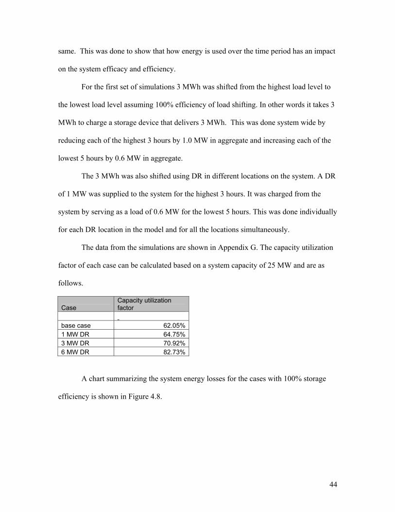
The data from the simulations are shown in Appendix G. The capacity utilization

factor of each case can be calculated based on a system capacity of 25 MW and are as

follows.

Case Capacity utilization factor

base case 62.05%1 MW DR 64.75%3 MW DR 70.92%6 MW DR 82.73%

A chart summarizing the system energy losses for the cases with 100% storage

efficiency is shown in Figure 4.8.

45

90.0%

92.0%

94.0%

96.0%

98.0%

100.0%

102.0%

104.0%

106.0%

108.0%

load shift loc 2 DR loc 3 DR loc 4 DR all DR

DR size & location

% o

f bas

e ca

se lo

sses

3hr 1MW 100% eff3 hr 3MW 100% eff3 hr 6 MW 100% eff

Figure 4.8 – Normalized system losses with different 100% efficient DR locations

It can be discerned that with a 100% efficient shift, the system wide load shift has

the most decrease in overall system losses. The reduced system losses with the DR

locations during peak usage is offset by increased system losses during off peak charging.

As the size of the charging and distance from the substation increases, the greater the

contribution of system losses is from charging. It can also be discerned that as the DR is

spread out amongst multiple locations the overall system losses are lower. The more

concentrated the DR is, the higher the system losses are due to the DR. There is also a

trade off between the benefit of a storage DR at the end of a feeder for supply and the

greater losses with having to charge the DR at the end of the feeder.

46

For the next set of simulations 3 MWh was shifted from the highest load level to

the lowest load level assuming 90% efficiency of load shifting. This was done system

wide by reducing each of the highest 3 hours by 1.0 MW in aggregate and increasing

each of the lowest 5 hours by 0.667 MW in aggregate. The 3 MWh was also shifted using

DR in different locations on the system. A DR of 1 MW was supplied to the system for

the highest 3 hours. It was charged from the system by serving as a load of 0.667 MW for

the lowest 5 hours. This was done individually for each DR location in the model and for

all the locations simultaneously.

90.0%

95.0%

100.0%

105.0%

110.0%

115.0%

120.0%

load shift loc 2 DR loc 3 DR loc 4 DR all DR

DR size & location

% o

f bas

e ca

se lo

sses

3hr 1MW 90% eff3 hr 3MW 90% eff3 hr 6 MW 90% eff

Figure 4.9 – Normalized system losses with different 90% efficient DR locations

47

It can be discerned that for DR storage with 90% storage efficiency, it is still

possible to decrease overall system losses. The impact on overall system losses is highly

dependent on the DR size and location. The overall losses associated with the DR are

lower for smaller multi location applications than for larger single applications of DR. It

is possible to lower overall system losses with DR storage even when the storage is not

100% efficient.

System losses are often expressed as a fraction of the system load in terms of

percent of demand or percent of delivered energy. Defining the ratio of the total saved

system losses to the peak load can be expressed by: [8]

))/(1)/1()/(1(2

2 ηηαηα

dGddGk

LoadPeakLL s

++−−

=− (4.5)

[8]

Where

L = system losses without any DR Ls = system losses with DR η = net AC energy efficiency of the DR storage system Ro, Rp are the equivalent T&D resistances during peak and off-peak periods, respectively Io, Ip are the load current during peak and off-peak periods, respectively Is current provided locally by the DR storage device d = Ro/Rp G = Io/Ip α = Is/Ip k= system losses (L)/Peak Load

For each system configuration and load characteristics, there is a maximum

storage size of DR when the losses due to charging equal the reduced system losses with

the DR. This size is a function of the location of the DR and the ratio of peak to off-peak

load. The results have been from analyzing actual load flow simulations, but general

equations can also be used for an approximation of maximum storage size.

48

))/(1)(1()/(1η

ηdG

dGGapMax

pop

ss

+−−

= (4.6) [8]

Where

Maxss = Maximum storage size Gappop = Gap between peak and off-peak η = net AC energy efficiency of the storage system d = Ro/Rp G = Io/Ip Ro, Rp are the equivalent T&D resistances during peak and off-peak periods, respectively Io, Ip are the load current during peak and off-peak periods, respectively The saved losses can be expressed as a fraction of the storage size as follows:

))/(1)/1()/(1(2

2 ηηαη

dGddGk

SizeStorageLL s

++−−

=− (4.7)

[8]

Where

L = system losses without any DR Ls = system losses with DR η = net AC energy efficiency of the DR storage system Ro, Rp are the equivalent T&D resistances during peak and off-peak periods, respectively Io, Ip are the load current during peak and off-peak periods, respectively Is current provided locally by the DR storage device d = Ro/Rp G = Io/Ip α = Is/Ip k= system losses (L)/Peak Load So far the analysis has focused on system losses, to determine if DR can be

implemented to increase the system capacity utilization factor without decreasing the

system efficiency. There are other benefits to obtaining a flatter load curve and increasing

the capacity utilization factor. The ability to reduce system capacity requirements has

enormous economic implications. The capacity of the system is sized to meet the peak

49

demand of the system, which includes generation, transmission, and distribution. A

lower system peak can also lower the cost of power by lowering the incremental costs.

More detailed cost implications will be examined in the next section.

50

5 Impact on System Costs

The impact that DR can have on distribution costs goes beyond just reduced

losses. It also includes investment cost of the feeders and system capacity. By lowering

the peak load of the feeder, extra capacity is freed up to allow for additional load which

can delay the need for upgrades. If there is wide spread use of DR on the system, then

the overall system peak load can also be lowered. This has a ripple effect to all parts of

the system, distribution feeders, substations, transmission lines and generation. When

DR is used to shift load from peak periods to off peak periods it can help flatten the load

curve.

A flatter load curve can lower the overall cost of power. This is mainly due to the

fact that not all generating units have the same efficiency or cost structure. Usually very

large plants require a huge capital investment to build. These large costs can be offset by

lower costs of fuel to produce power, such as coal and nuclear plants. These plants can

not start quickly and are most economical when they are run continuously and are

referred to as base load units. Other plants may require less capital to build but have a

higher fuel cost such as oil and natural gas. These plants can usually start quicker and

can be dispatched to follow load.

In a power market where generation suppliers bid for supplying power, the bids

are accepted from lowest to highest. However, all of the suppliers receive the price set by

the highest accepted bidder. Figure 4.10 and 4.11 show example graphs of costs

associated with a portfolio of generating plants. The units that can operate profitably for

$10/MWh, run continuously but never receive less than $15/MWh and can receive as

51

much as $70/MHh. The units that can only operate profitably at $70/MWh, run only

during the peak period and receive $70/MWh. This is pricing model is used to reward

the most cost efficient units and encourage new units to be more cost efficient to

maximize profits.

0.0%

10.0%

20.0%

30.0%

40.0%

50.0%

60.0%

70.0%

80.0%

90.0%

100.0%

1 2 3 4 5 6 7 8 9 10 11 12 13 14 15 16 17 18 19 20 21 22 23 24

Hour

Perc

ent o

f pea

k lo

ad

$70/MWH$40/MWH$25/MWH$15/MWH$10/MWH

Figure 5.1 – Example graph of generation portfolio cost without DR

For example, a system needs 100 MW for its peak hour to meet its load demand.

There are 30 MW at $10/MWH, 20 MW at $15/MWH, 20 MW at $25/MWH, 20 MW at

$40/MWH and 10 MW at $70/MWH. Since the price for all the power used is set by the

highest bid accepted, the price of all 100 MWh is $70/MWH, totaling $7000 for that

hour. The same analysis is done for each hour and the total cost for the day is $71,095.

52

If DR is used to shift 10 MW of load from the peak hour to an off peak time, then the

system only needs 90 MWh for the peak. Now there is no need for the $70/MWH

generation and the highest price is $40/MWH, totaling $3600 for that hour. The off peak

load has increased as a result but the price of this load is $25/MWH. The total energy

cost for the day is now $57,738, an almost 19% reduction. This simplified example

illustrates the ability a small amount of peak load has to dramatically impact price.

0.0%

10.0%

20.0%

30.0%

40.0%

50.0%

60.0%

70.0%

80.0%

90.0%

100.0%

1 2 3 4 5 6 7 8 9 10 11 12 13 14 15 16 17 18 19 20 21 22 23 24

hour

perc

ent o

f pea

k

$40/MWH$25/MWH$15/MWH$10/MWH

Figure 5.2 - Example graph of generation portfolio cost with DR peak shave/shift

As mentioned previously, the cost of the generation to produce the electricity is

only one piece of the total cost to the consumer. The cost of the infrastructure capacity

needed to deliver the electricity must also be considered. There are different methods for

53

analyzing the cost of electric system elements. One method to analyze distribution costs

is the total annual equivalent cost method. [6]

TAC = AIC + AEC + ADC $/mi

TAC is the total annual equivalent cost of the feeder AIC is the annual equivalent cost of the investment cost of the feeder AEC is the annual equivalent cost of the I2R losses ADC is the annual equivalent cost of the system capacity to supply I2R losses of the feeder

AIC = ICF x iF $/mi

ICF is the annual equivalent investment cost of a given size feeder iF is the annual fixed charge rate or carrying rate of the feeder

AEC = 3 I2R x EC x FLL x FLS x FLSA x 8760 $/mi

EC is the cost of energy $/kWh FLL is the load location factor FLS is the loss factor defined as the ratio of the average annual power loss to the peak annual power loss FLSA is the loss allowance factor, which is an allocation factor that allows for additional losses due to transmission from generating plants to distribution substations

FLL = S/L

S is the point on the feeder for an assumed lumped feeder load L is the distance in miles

FLS = 0.3 FLD + 0.7 F2LD , for urban areas

FLS = 0.16 FLD + 0.84 F2LD , for rural areas

FLD is the load factor, which is the ratio of the average load over a designated period of time to the peak load occurring in that period

ADC = 3 I2R x FLL x FPR x FR x FLSA [(CG x iG) + (CT x iT) + (CS x iS)] $/mi

FLL is the load location factor

54

FPR is the peak responsibility factor, which is a per unit value of the peak feeder losses that are coincident with the system peak demand FR is the reserve factor, which is the ratio of total generation capability to the total load and losses to be supplied FLSA is the loss allowance factor CG is the cost of peaking generation ($/KVA) iG is the annual fixed charge rate applicable to the generation system CT is the cost of transmission ($/KVA) iT is the annual fixed charge rate applicable to the transmission system CS is the cost of the distribution substation ($/KVA) iS is the annual fixed charge rate applicable to the distribution substation

The analysis presented in this paper focuses on how DR can impact the efficacy

of the system which directly affects the cost of the system. The TAC equation for

calculating distribution feeder costs can be used as a basis for analyzing how changes in

the equation variables affect the costs. The equation can be modified and augmented to

accommodate given or calculated data values such as the system energy costs (CE).

Central to this approach is the notion that the cost of energy changes with its time of use

(TOU). There has been an increasing emphasis in the industry to implement TOU rates

to send better pricing signals to consumers. TOU cost structures can be used to modify

TAC analysis to include the total cost of energy.

For this modified TAC analysis 24 hourly load flow simulations were run and the

energy plus losses for each hour were calculated and recorded. The cost of energy for

each hour was assigned and summed for the daily cost of energy. If the annual cost of DR

is included then the TAC equation can be expressed as the following.

TAC = [ICF x iF] + [CE x 365] + [FPR x FR [(CG x iG) + (CT x iT) + (CS x iS)]] + [ICDR x iDR] $/kVA

55

The equation was solved for the base case with no DR and the cost was used as

the basis for comparison with the DR options. The cost of energy per MW for a day was

calculated based on each hour of the load shape and assigned values as shown in the

Appendix. The peak responsibility factor was calculated from the losses at the peak hour

normalized to the equivalent system load at that hour. Figure 5.3 and 5.4 show the TAC

costs for a 1 MW load shift with 100% and 90 % efficiency respectively.

1 MW 1 MW 1 MW 1 MW 1 MW base shift #2 DR #3 DR #4 DR all DR Icf 50 50 50 50 50 50if 0.12 0.12 0.12 0.12 0.12 0.12CE 984.79 980.17 981.08 980.58 980.88 980.58Fpr 1.070 1.021 1.027 1.023 1.025 1.023Fr 1.15 1.15 1.15 1.15 1.15 1.15Cg 200 200 200 200 200 200ig 0.14 0.14 0.14 0.14 0.14 0.14Ct 150 150 150 150 150 150it 0.1 0.1 0.1 0.1 0.1 0.1Cs 130 130 130 130 130 130is 0.12 0.12 0.12 0.12 0.12 0.12Icdr 0 0 400 400 400 400idr 0.14 0.14 0.14 0.14 0.14 0.14 TAC $359,527 $357,836 $358,227 $358,044 $358,150 $358,044 Savings 0.47% 0.36% 0.41% 0.38% 0.41%

Figure 5.3 – Table of TAC for 1 MW load shift with 100% efficiency 1 MW 1 MW 1 MW 1 MW 1 MW base shift #2 DR #3 DR #4 DR all DR Icf 50 50 50 50 50 50if 0.12 0.12 0.12 0.12 0.12 0.12CE 984.79 980.75 981.63 981.17 981.42 981.13Fpr 1.070 1.021 1.027 1.023 1.025 1.023Fr 1.15 1.15 1.15 1.15 1.15 1.15Cg 200 200 200 200 200 200

56

ig 0.14 0.14 0.14 0.14 0.14 0.14Ct 150 150 150 150 150 150it 0.1 0.1 0.1 0.1 0.1 0.1Cs 130 130 130 130 130 130is 0.12 0.12 0.12 0.12 0.12 0.12Icdr 0 0 400 400 400 400idr 0.14 0.14 0.14 0.14 0.14 0.14 TAC $359,527 $358,049 $358,424 $358,257 $358,348 $358,242 Savings 0.41% 0.31% 0.35% 0.33% 0.36%

Figure 5.4 – Table of TAC for 1 MW load shift with 90% efficiency

Figure 5.5 and 5.6 show the TAC costs for a 3 MW load shift with 100% and 90

% efficiency respectively.

3 MW 3 MW 3 MW 3 MW 3 MW base shift #2 DR #3 DR #4 DR all DR Icf 50 50 50 50 50 50 if 0.12 0.12 0.12 0.12 0.12 0.12 CE 984.79 971.50 974.13 973.54 973.88 973.04 Fpr 1.070 0.924 0.942 0.935 0.939 0.935 Fr 1.15 1.15 1.15 1.15 1.15 1.15 Cg 200 200 200 200 200 200 ig 0.14 0.14 0.14 0.14 0.14 0.14 Ct 150 150 150 150 150 150 it 0.1 0.1 0.1 0.1 0.1 0.1 Cs 130 130 130 130 130 130 is 0.12 0.12 0.12 0.12 0.12 0.12 Icdr 0 0 1200 1200 1200 1200 idr 0.14 0.14 0.14 0.14 0.14 0.14 TAC $359,527 $354,666 $355,793 $355,580 $355,702 $355,397 Savings 1.35% 1.04% 1.10% 1.06% 1.15%


3 MW 3 MW 3 MW 3 MW 3 MW base shift #2 DR #3 DR #4 DR all DR Icf 50 50 50 50 50 50 if 0.12 0.12 0.12 0.12 0.12 0.12

57

CE 984.79 973.17 975.75 975.29 975.50 974.67 Fpr 1.070 0.924 0.942 0.935 0.939 0.935 Fr 1.15 1.15 1.15 1.15 1.15 1.15 Cg 200 200 200 200 200 200 ig 0.14 0.14 0.14 0.14 0.14 0.14 Ct 150 150 150 150 150 150 it 0.1 0.1 0.1 0.1 0.1 0.1 Cs 130 130 130 130 130 130 is 0.12 0.12 0.12 0.12 0.12 0.12 Icdr 0 0 1200 1200 1200 1200 idr 0.14 0.14 0.14 0.14 0.14 0.14 TAC $359,527 $355,274 $356,386 $356,218 $356,295 $355,990 Savings 1.18% 0.87% 0.92% 0.90% 0.98%


The results show that when the total cost of energy is included in the analysis it is

possible to have a lower TAC with DR implemented on the feeder, even when the DR is

not 100% efficient. The major driver for the decreased costs is the replacement of high

cost electricity with lower cost electricity. The replacement of peak system losses with

off peak system losses also contribute a little to the savings. The ratio of peak load to off

peak load and the ratio of peak electricity cost to off peak electricity cost will be the

limiting factors in the ability of DR to lower the TAC.

58

6 Conclusion

The ability of DR, used for peak shaving, to improve system efficacy was explored.

Models representing the basic elements of electric systems were created. Load flow

analysis was used on the models to obtain simulation results of the system performance.

Base case simulations were run without DRs in the models and used as the basis to

compare to system configurations with DR. The amount of system losses was analyzed

with different sizes and locations of DR to determine impact on efficiency. The ability of

DR to impact the load factor and capacity utilization factor were explored. The ability of

DR to impact the cost of energy and infrastructure was examined.

The capacity utilization factor was used as a gage to measure changes in system

efficacy. DR can improve the capacity utilization factor of an existing system while the

total energy delivered remains the same. This enables the system to have an increase in

unused capacity to serve future increases in load. DR can be used in analysis of future

system expansion to allow for higher capacity utilization projections. Therefore, capacity

requirements are smaller for projected energy delivery needs.

It was shown that the type, size, and location of the DR have an impact on system

losses and hence efficiency. DR applications that are supplying power, such as

distributed generation, have the greatest ability to reduce system losses. For sizes up to

about 50% of a uniformly distributed feeder load, locations at the end of the feeder

reduce the losses the most. For sizes over 50%, the greatest loss reduction is seen as the

location is moved from the end to the middle of the feeder.

It was shown that having more than one DR location reduces the losses more than

having one location of an equivalent size. This is due to the ability of having more of the

59

current produced closer to the varied load locations. The closer the source is to the load

the less the line losses are compared to the base case. Also, having more than one DR on

a feeder allows for N-1 firm capacity to include the remaining DR in calculations.

For DR that stores energy for peak shaving, the charging or storage losses becomes

the driving factor in its ability to reduce overall system losses. It was shown that peak

shaving can shift the load and losses to an off peak time. For DR with close to 100%

efficiency the savings in peak system losses makes the devices a lossless storage device

to the system. For DR with lower storage efficiency the reduction in peak load also has

benefits beyond a loss analysis. If the differential between the cost of energy during the

peak and off peak is enough, then overall cost can still be lowered.

The advantages of load based DR verse distribution based DR were presented. Load

based DR provides the ability to partially decouple the devices electric use from the

system use. This gives the consumer the ability to obtain the benefit of the device when

desired instead of going without at peak times. Storage losses are greatly reduced

compared to other techniques where the storage requires energy conversion to store and

energy conversion to supply. There are no system protection implications since the

storage is load based with no additional supply points. The amount of DR is inherently

scalable with the load since it is part of the load.

The analysis in this paper has shown that there are several benefits to having DR: 1) it

can provide voltage support and reduce system losses by having the supply source closer

to the load, 2) the ability to reduce system peaks which reduces capacity needs and peak

losses, 3) the ability to maximize the use of the most efficient supplies through storage,

and 4) small amounts of off peak storage losses can be offset by reduced peak losses.

60

These features can help lead to a more efficacious system. To maximize the benefit

obtained from these resources requires the integration of DR into the system. The size

and location of the DR has an impact on the overall efficacy and efficiency of the system.

The ability to obtain a flatter load curve without increasing system losses is an enabling

factor in obtaining a more efficacious electric system.

61

References

1. Stevenson, William D. Jr., “Elements of Power Systems Analysis”, Fourth

Edition, McGraw-Hill Book Co., New York 1982, pg. 2, 54-60 2. U.S. Department of Energy, “Annual Energy Review, 2008”, June 2009. 3. Bergen, Arthur R., “Power Systems Analysis”, Prentice-Hall, Inc., New Jersey

1986, Pg. 3-5 4. Bergen, Arthur R., Vittal, Vijay, “Power Systems Analysis”, Second Edition,

Prentice-Hall, Inc., New Jersey 1986, Pg. 3-5 5. Mohan, Ned, Undeland, Tore M., Robbins, William P., “Power Electronics,

Converters, Applications, and Design”, Third Edition, John Wiley & Sons, Inc., United States 2003, pg. 3

6. Gönen, Turan, “Electric Power Distribution System Engineering”, Second Edition, CRC Press, Florida 2008, Pg. 357

7. Chiradeja, P., “Benefit of Distributed Generation: A Line Loss Reduction Analysis”, IEEE/PES Transmission and Distribution Conference & Exhibition: Asia and Pacific Dalina, China, 2005

8. Nourai, Ali, et al, “Load Leveling Reduces T&D Line Losses”, IEEE transactions on power delivery, Vol 23, No. 4, October 2008

62

Appendices

Appendix A: Impedance calculations The distribution line impedances were calculated assuming a typical overhead cross-arm construction as shown in Figure 2. The phase spacing was 44” and 336 AL wire was used.

Figure 2 – Distribution feeder geometry The inductance of the feeder was calculated using geometric mean radius (GMR), designated as Ds (Stevenson, p54). For 336 kcmil conductor the geometric mean radius Ds = .0243’, from Stevenson Table A.1. Since the feeder has three phases the average inductance (La) is used. The average inductance is calculated by the following equation.

DsDeqxLa ln102 7−= H/m [Stevenson

p60] Deq is derived from the following equation.

3 cDabxDbcxDaDeq = [Stevenson p60]

For the model feeder

ftinxxDeq 62.444.558844443 ===

77 105.100243.

62.4ln102 −− == xxLa H/m

This can be converted to inductive reactance (X) and English units with the following.

ftmixxxfLX 1000/121./636.105.1016096022 7 Ω=Ω=== −ππ The resistance (R) for 336 AL conductor is

63

ftmiR 1000/053./2737. Ω=Ω= This can be represented in impedance form (Z).

ftjjXRZ 1000/121.053. Ω+=+= In order to use these values in the power flow model, they must be converted to per unit values. For the model a base of 100 MVA and 13.8kV was chosen. This gives a base impedance.

9044.1100

8.13===

MVAkV

VAbaseVbaseZbase

puftjjZpu 1000/3353.0278.9044.1

121.053.Ω+=

+=

For the model feeder each segment is about 2750 ft which gives a segment impedance of .08+j.17. The impedances of transformer were taken from typical values in the industry, .035+j.57 on a per unit basis.

64

Appendix B: Matlab program to solve Gauss-Seidel Matlab program to solve power flow of feeder model clear %Paul Robinson %Gauss-Seidel power flow program %This program solves a power flow with Gauss-Seidel solution % %bus data: bus num, type, voltage, angle , Pl, Ql, Pg, Qg %bus type: 0=load P&Q, 1=Gen Q hold V limit,2=hold V Var limit, %3=hold V&ang swing or slack % bus data in pu at 100 MVA busd =... [1 3 1 0 0 0 0 0; 2 0 1 0 0 0 0 0; 3 0 1 0 0.010 0.003 0 0; 4 0 1 0 0.010 0.003 0 0; 5 0 1 0 0.010 0.003 0 0; 6 0 1 0 0.010 0.003 0 0; 7 0 1 0 0.010 0.003 0 0; 8 0 1 0 0.010 0.003 0 0; 9 0 1 0 0.010 0.003 0 0; 10 0 1 0 0.010 0.003 0 0; 11 0 1 0 0.010 0.003 0 0; 12 0 1 0 0.010 0.003 0 0]; %line format: from bus, to bus, Rpu Xpu lined =... [1 2 .035+0.57j; 2 3 .08+0.17j; 3 4 .08+0.17j; 4 5 .08+0.17j; 5 6 .08+0.17j; 6 7 .08+0.17j; 7 8 .08+0.17j; 8 9 .08+0.17j; 9 10 .08+0.17j; 10 11 .08+0.17j; 11 12 .08+0.17j]; % bus count and lines nbuses = 12; nlines = size(lined,1); fbus = lined(:,1); tbus = lined(:,2); Rpu = real(lined(:,3)); Xpu = imag(lined(:,3)); ybr = 1./lined(:,3); % calc admitance matrix Ymat = zeros(nbuses); for line = 1:nlines yline = ybr(line); f = fbus(line); t = tbus(line);

65

Ymat(f,f) = Ymat(f,f) + yline; if( t ~= 0) Ymat(t,t) = Ymat(t,t) + yline; Ymat(f,t) = Ymat(f,t) - yline; Ymat(t,f) = Ymat(t,f) - yline; end end tol = 0.00001; iter = 0; % Calc the real and reactive power supplied to buses for i = 1:nbuses busp(i) = busd(i,7) - busd(i,5); busq(i) = busd(i,8) - busd(i,6); end % voltage at bus for i= 1:nbuses busv(i) = busd(i,3); end %perform iterations to solve all matrix values while (iter < 5000) iter = iter + 1; busvo = busv; %calc the updated bus voltage for i = 1:nbuses if busd(i,2)~= 3 % If gen bus, calc updated reactive if busd(i,2)== 2 reac = 0; for k = 1:nbuses reac = reac + Ymat(i,k) * busd(k,3); end reac = conj(busd(i,3)) * reac; busq(i) = -imag(reac); end % Calculate updated voltage at bus from all buses svi = 0; for k = 1:nbuses if i ~= k svi = svi - Ymat(i,k) * busd(k,3); end end svi = (busp(i) - j*busq(i)) / conj(busd(i,3)) + svi; busd(i,3) = 1/Ymat(i,i) * svi; % If gen bus, update the volt mag if busd(i,2)== 2 busd(i,3) = busd(i,3) * abs(busvo(i)) / abs(busd(i,3)); end end end for i= 1:nbuses

66

busv(i)= busd(i,3); end % check if within tolerence mism = busv - busvo; if max(abs(mism)) < tol break; end end %end of while statement for i=1:nbuses % if slack bus update the power if busd(i,2)==3 slk = 0; for k = 1:nbuses slk = slk + Ymat(i,k)*busd(k,3); end slk = conj(busd(i,3))*slk; busp(i) = real(slk); busq(i) = -imag(slk); end end % reformat data for output for i = 1:nbuses % pu voltage mag = abs(busd(i,3)); phase = angle(busd(i,3))*180/pi; busd(i,3)=mag; busd(i,4)=phase; % Power load busd(i,5)=busd(i,5)*100; busd(i,6)=busd(i,6)*100; % Power gen % P = (busp(i) +bus(i,7))*100; % Q = (busq(i) +bus(i,8))*100; P = (busp(i))*100; Q = (busq(i))*100; if busd(i,2)==0 P=0; Q=0; end busd(i,7)=P; busd(i,8)=Q; end % print out bus matrix and iterations fprintf('------------------------------------------------------------------------------\n'); fprintf(' Bus# Type Volt angle Pld Qld Pgen Qgen\n'); fprintf('==============================================================================\n'); busd fprintf('------------------------------------------------------------------------------\n'); iter

67

% Calc and print losses header fprintf('\n'); fprintf(' Losses \n'); fprintf('-------------------------------------------------------\n'); fprintf(' Line From To Loss Loss \n'); fprintf(' # Bus Bus (MW) (MVAR) \n'); fprintf('=======================================================\n'); % Initialize total loss Pltot = 0; Qltot = 0; for i = 1:nlines; fb = fbus(i); tb = tbus(i); il = (busv(fb) - busv(tb)) * Ymat(fb,tb); Pl = abs(il)^2 * Rpu(i)*100; Ql = abs(il)^2 * Xpu(i)*100; Pltot = Pltot + Pl; Qltot = Qltot + Ql; % print losses fprintf(' %4d',i); fprintf(' %10d',fbus(i)); fprintf(' %10d',tbus(i)); fprintf(' %7.3f', Pl ); fprintf(' %7.3f\n', Ql ); end % print total losses fprintf('-------------------------------------------------------\n'); fprintf(' Totals:'); fprintf(' %7.3f', Pltot ); fprintf(' %7.3f\n', Qltot );

68

Appendix C: Modified Matpower program Modified Matpower Matlab program to scale loads from program input function [MVAbase, bus, gen, branch, success, et] = ... runspf(casename, mpopt, fname, scale, solvedcase) %RUNSPF Runs a power flow. % % [baseMVA, bus, gen, branch, success, et] = ... % runspf(casename, mpopt, fname, scale, solvedcase) % % Modified to read in scale factor to scale loads PER 03/29/09 % % Runs a power flow (full AC Newton's method by default) and optionally % returns the solved values in the data matrices, a flag which is true if % the algorithm was successful in finding a solution, and the elapsed time % in seconds. All input arguments are optional. If casename is provided it % specifies the name of the input data file or struct (see also 'help % caseformat' and 'help loadcase') containing the power flow data. The % default value is 'case9'. If the mpopt is provided it overrides the % default MATPOWER options vector and can be used to specify the solution % algorithm and output options among other things (see 'help mpoption' for % details). If the 3rd argument is given the pretty printed output will be % appended to the file whose name is given in fname. If solvedcase is % specified the solved case will be written to a case file in MATPOWER % format with the specified name. If solvedcase ends with '.mat' it saves % the case as a MAT-file otherwise it saves it as an M-file. % % If the ENFORCE_Q_LIMS options is set to true (default is false) then if % any generator reactive power limit is violated after running the AC power % flow, the corresponding bus is converted to a PQ bus, with Qg at the % limit, and the case is re-run. The voltage magnitude at the bus will % deviate from the specified value in order to satisfy the reactive power % limit. If the reference bus is converted to PQ, the first remaining PV % bus will be used as the slack bus for the next iteration. This may % result in the real power output at this generator being slightly off % from the specified values. % MATPOWER % $Id: runpf.m,v 1.14 2006/09/29 19:23:07 ray Exp $ % by Ray Zimmerman, PSERC Cornell % Enforcing of generator Q limits inspired by contributions % from Mu Lin, Lincoln University, New Zealand (1/14/05). % Copyright (c) 1996-2005 by Power System Engineering Research Center (PSERC) % See http://www.pserc.cornell.edu/matpower/ for more info. %%----- initialize ----- %% define named indices into bus, gen, branch matrices [PQ, PV, REF, NONE, BUS_I, BUS_TYPE, PD, QD, GS, BS, BUS_AREA, VM, ... VA, BASE_KV, ZONE, VMAX, VMIN, LAM_P, LAM_Q, MU_VMAX, MU_VMIN] = idx_bus; [F_BUS, T_BUS, BR_R, BR_X, BR_B, RATE_A, RATE_B, RATE_C, ... TAP, SHIFT, BR_STATUS, PF, QF, PT, QT, MU_SF, MU_ST, ... ANGMIN, ANGMAX, MU_ANGMIN, MU_ANGMAX] = idx_brch;

69

[GEN_BUS, PG, QG, QMAX, QMIN, VG, MBASE, GEN_STATUS, PMAX, PMIN, ... MU_PMAX, MU_PMIN, MU_QMAX, MU_QMIN, PC1, PC2, QC1MIN, QC1MAX, ... QC2MIN, QC2MAX, RAMP_AGC, RAMP_10, RAMP_30, RAMP_Q, APF] = idx_gen; %% default arguments if nargin < 5 solvedcase = ''; %% don't save solved case if nargin < 4 scale = 1.0; %% don't scale loads if nargin < 3 fname = ''; %% don't print results to a file if nargin < 2 mpopt = mpoption; %% use default options if nargin < 1 casename = 'case9'; %% default data file is 'case9.m' end end end end end %% options verbose = mpopt(31); qlim = mpopt(6); %% enforce Q limits on gens? dc = mpopt(10); %% use DC formulation? %% read data & convert to internal bus numbering [baseMVA, bus, gen, branch] = loadcase(casename); [i2e, bus, gen, branch] = ext2int(bus, gen, branch); %% scale PD and QD ldbs = find(bus(:, BUS_TYPE)==1); bus(ldbs, PD) = bus(ldbs, PD)*scale; bus(ldbs, QD) = bus(ldbs, QD)*scale; %bus(:, PD) = bus(:, PD)*scale; %bus(:, QD) = bus(:, QD)*scale; %% get bus index lists of each type of bus [ref, pv, pq] = bustypes(bus, gen); %% generator info on = find(gen(:, GEN_STATUS) > 0); %% which generators are on? gbus = gen(on, GEN_BUS); %% what buses are they at? %%----- run the power flow ----- t0 = clock; if dc %% DC formulation %% initial state Va0 = bus(:, VA) * (pi/180); %% build B matrices and phase shift injections [B, Bf, Pbusinj, Pfinj] = makeBdc(baseMVA, bus, branch); %% compute complex bus power injections (generation - load) %% adjusted for phase shifters and real shunts Pbus = real(makeSbus(baseMVA, bus, gen)) - Pbusinj - bus(:, GS) / baseMVA;

70

%% "run" the power flow Va = dcpf(B, Pbus, Va0, ref, pv, pq); %% update data matrices with solution branch(:, [QF, QT]) = zeros(size(branch, 1), 2); branch(:, PF) = (Bf * Va + Pfinj) * baseMVA; branch(:, PT) = -branch(:, PF); bus(:, VM) = ones(size(bus, 1), 1); bus(:, VA) = Va * (180/pi); %% update Pg for swing generator (note: other gens at ref bus are accounted for in Pbus) %% Pg = Pinj + Pload + Gs %% newPg = oldPg + newPinj - oldPinj refgen = find(gbus == ref); %% which is(are) the reference gen(s)? gen(on(refgen(1)), PG) = gen(on(refgen(1)), PG) + (B(ref, :) * Va - Pbus(ref)) * baseMVA; success = 1; else %% AC formulation %% initial state % V0 = ones(size(bus, 1), 1); %% flat start V0 = bus(:, VM) .* exp(sqrt(-1) * pi/180 * bus(:, VA)); V0(gbus) = gen(on, VG) ./ abs(V0(gbus)).* V0(gbus); if qlim ref0 = ref; %% save index and angle of Varef0 = bus(ref0, VA); %% original reference bus limited = []; %% list of indices of gens @ Q lims fixedQg = zeros(size(gen, 1), 1); %% Qg of gens at Q limits end repeat = 1; while (repeat) %% build admittance matrices [Ybus, Yf, Yt] = makeYbus(baseMVA, bus, branch); %% compute complex bus power injections (generation - load) Sbus = makeSbus(baseMVA, bus, gen); %% run the power flow alg = mpopt(1); if alg == 1 [V, success, iterations] = newtonpf(Ybus, Sbus, V0, ref, pv, pq, mpopt); elseif alg == 2 | alg == 3 [Bp, Bpp] = makeB(baseMVA, bus, branch, alg); [V, success, iterations] = fdpf(Ybus, Sbus, V0, Bp, Bpp, ref, pv, pq, mpopt); elseif alg == 4 [V, success, iterations] = gausspf(Ybus, Sbus, V0, ref, pv, pq, mpopt); else error('Only Newton''s method, fast-decoupled, and Gauss-Seidel power flow algorithms currently implemented.');

71

end %% update data matrices with solution [bus, gen, branch] = pfsoln(baseMVA, bus, gen, branch, Ybus, Yf, Yt, V, ref, pv, pq); if qlim %% enforce generator Q limits %% find gens with violated Q constraints mx = find( gen(:, GEN_STATUS) > 0 & gen(:, QG) > gen(:, QMAX) ); mn = find( gen(:, GEN_STATUS) > 0 & gen(:, QG) < gen(:, QMIN) ); if ~isempty(mx) | ~isempty(mn) %% we have some Q limit violations if isempty(pv) if verbose if ~isempty(mx) fprintf('Gen %d (only one left) exceeds upper Q limit : INFEASIBLE PROBLEM\n', mx); else fprintf('Gen %d (only one left) exceeds lower Q limit : INFEASIBLE PROBLEM\n', mn); end end success = 0; break; end if verbose & ~isempty(mx) fprintf('Gen %d at upper Q limit, converting to PQ bus\n', mx); end if verbose & ~isempty(mn) fprintf('Gen %d at lower Q limit, converting to PQ bus\n', mn); end %% save corresponding limit values fixedQg(mx) = gen(mx, QMAX); fixedQg(mn) = gen(mn, QMIN); mx = [mx;mn]; %% convert to PQ bus gen(mx, QG) = fixedQg(mx); %% set Qg to binding limit gen(mx, GEN_STATUS) = 0; %% temporarily turn off gen, for i = 1:length(mx) %% (one at a time, since bi = gen(mx(i), GEN_BUS); %% they may be at same bus) bus(bi, [PD,QD]) = ... %% adjust load accordingly, bus(bi, [PD,QD]) - gen(mx(i), [PG,QG]); end bus(gen(mx, GEN_BUS), BUS_TYPE) = PQ; %% & set bus type to PQ %% update bus index lists of each type of bus ref_temp = ref; [ref, pv, pq] = bustypes(bus, gen); if verbose & ref ~= ref_temp fprintf('Bus %d is new slack bus\n', ref);

72

end limited = [limited; mx]; else repeat = 0; %% no more generator Q limits violated end else repeat = 0; %% don't enforce generator Q limits, once is enough end end if qlim & ~isempty(limited) %% restore injections from limited gens (those at Q limits) gen(limited, QG) = fixedQg(limited); %% restore Qg value, for i = 1:length(limited) %% (one at a time, since bi = gen(limited(i), GEN_BUS); %% they may be at same bus) bus(bi, [PD,QD]) = ... %% re-adjust load, bus(bi, [PD,QD]) + gen(limited(i), [PG,QG]); end gen(limited, GEN_STATUS) = 1; %% and turn gen back on if ref ~= ref0 %% adjust voltage angles to make original ref bus correct bus(:, VA) = bus(:, VA) - bus(ref0, VA) + Varef0; end end end et = etime(clock, t0); %%----- output results ----- %% convert back to original bus numbering & print results [bus, gen, branch] = int2ext(i2e, bus, gen, branch); if fname [fd, msg] = fopen(fname, 'at'); if fd == -1 error(msg); else printpf(baseMVA, bus, gen, branch, [], success, et, fd, mpopt); fclose(fd); end end printpf(baseMVA, bus, gen, branch, [], success, et, 1, mpopt); %% save solved case if solvedcase savecase(solvedcase, baseMVA, bus, gen, branch); end %% this is just to prevent it from printing baseMVA %% when called with no output arguments if nargout, MVAbase = baseMVA; end return;

73

Appendix D: Matlab model used for simple radial analysis function [baseMVA, bus, gen, branch] = case1 %CASE1 Power flow data for 12 bus, 11 gen case for thesis. % Please see 'help caseformat' for details on the case file format. % % This is the 12 bus example for thesis % MATPOWER %%----- Power Flow Data -----%% %% system MVA base baseMVA = 100; %% bus data % bus_i type Pd Qd Gs Bs area Vm Va baseKV zone Vmax Vmin bus = [ 1 3 0 0 0 0 1 1 0 115 1 1.1 0.9; 2 1 0 0 0 0 1 1 0 13.8 1 1.1 0.9; 3 2 1.0 .30 0 0 1 1 0 13.8 1 1.1 0.9; 4 2 1.0 .30 0 0 1 1 0 13.8 1 1.1 0.9; 5 2 1.0 .30 0 0 1 1 0 13.8 1 1.1 0.9; 6 2 1.0 .30 0 0 1 1 0 13.8 1 1.1 0.9; 7 2 1.0 .30 0 0 1 1 0 13.8 1 1.1 0.9; 8 2 1.0 .30 0 0 1 1 0 13.8 1 1.1 0.9; 9 2 1.0 .30 0 0 1 1 0 13.8 1 1.1 0.9; 10 2 1.0 .30 0 0 1 1 0 13.8 1 1.1 0.9; 11 2 1.0 .30 0 0 1 1 0 13.8 1 1.1 0.9; 12 2 1.0 .30 0 0 1 1 0 13.8 1 1.1 0.9; ]; %% generator data % bus Pg Qg Qmax Qmin Vg mBase status Pmax Pmin gen = [ 12 5 0 .2 -.2 1 100 01 1.1 0; 11 5 0 .2 -.2 1 100 0 1.1 0; 10 5 0 .2 -.2 1 100 0 1.1 0; 9 5 0 .2 -.2 1 100 0 1.1 0; 8 5 0 .2 -.2 1 100 0 1.1 0; 7 5 0 .2 -.2 1 100 0 1.1 0; 6 5 0 .2 -.2 1 100 0 1.1 0; 5 5 0 .2 -.2 1 100 0 1.1 0; 4 5 0 .2 -.2 1 100 0 1.1 0; 3 5 0 .2 -.2 1 100 0 1.1 0; 1 0 0 100 -100 1 100 1 0 0; ]; %% branch data % fbus tbus r x b rateA rateB rateC ratio angle status

74

branch = [ 1 2 0.035 0.57 0.0000 250 250 250 0 0 1; 2 3 0.08 0.17 0.0000 250 250 250 0 0 1; 3 4 0.08 0.17 0.0000 250 250 250 0 0 1; 4 5 0.08 0.17 0.0000 250 250 250 0 0 1; 5 6 0.08 0.17 0.0000 250 250 250 0 0 1; 6 7 0.08 0.17 0.0000 250 250 250 0 0 1; 7 8 0.08 0.17 0.0000 250 250 250 0 0 1; 8 9 0.08 0.17 0.0000 250 250 250 0 0 1; 9 10 0.08 0.17 0.0000 250 250 250 0 0 1; 10 11 0.08 0.17 0.0000 250 250 250 0 0 1; 11 12 0.08 0.17 0.0000 250 250 250 0 0 1; ]; return;

75

Appendix E: Matlab model used for multi-circuit analysis function [baseMVA, bus, gen, branch] = case2 %CASE2 Power flow data for 24 bus, 4 gen case for thesis. % Please see 'help caseformat' for details on the case file format. % % This is the 24 bus example for thesis % MATPOWER %%----- Power Flow Data -----%% %% system MVA base baseMVA = 100; %% bus data % bus_i type Pd Qd Gs Bs area Vm Va baseKV zone Vmax Vmin bus = [ 1 3 0 0 0 0 1 1 0 115 1 1.1 0.9; 2 2 0 0 0 0 1 1 0 13.8 1 1.1 0.9; 3 2 0 0 0 0 1 1 0 13.8 1 1.1 0.9; 4 2 0 0 0 0 1 1 0 13.8 1 1.1 0.9; 5 1 0 0 0 0 1 1 0 13.8 1 1.1 0.9; 6 1 0 0 0 0 1 1 0 13.8 1 1.1 0.9; 7 1 0 0 0 0 1 1 0 13.8 1 1.1 0.9; 8 1 0 0 0 0 1 1 0 13.8 1 1.1 0.9; 9 1 0 0 0 0 1 1 0 13.8 1 1.1 0.9; 10 1 0 0 0 0 1 1 0 13.8 1 1.1 0.9; 11 1 0 0 0 0 1 1 0 13.8 1 1.1 0.9; 12 1 0 0 0 0 1 1 0 13.8 1 1.1 0.9; 13 1 0 0 0 0 1 1 0 13.8 1 1.1 0.9; 14 1 0 0 0 0 1 1 0 13.8 1 1.1 0.9; 15 1 3.000 1.000 0 0 1 1 0 13.8 1 1.1 0.9; 16 1 3.000 1.000 0 0 1 1 0 13.8 1 1.1 0.9; 17 1 3.000 1.000 0 0 1 1 0 13.8 1 1.1 0.9; 18 1 3.000 1.000 0 0 1 1 0 13.8 1 1.1 0.9; 19 1 3.000 1.000 0 0 1 1 0 13.8 1 1.1 0.9; 20 1 3.000 1.000 0 0 1 1 0 13.8 1 1.1 0.9; 21 1 3.000 1.000 0 0 1 1 0 13.8 1 1.1 0.9; 22 1 3.000 1.000 0 0 1 1 0 13.8 1 1.1 0.9; 23 1 0 0 0 0 1 1 0 13.8 1 1.1 0.9; 24 1 0 0 0 0 1 1 0 115 1 1.1 0.9; ]; %% generator data % bus Pg Qg Qmax Qmin Vg mBase status Pmax Pmin gen = [ 4 1 0 .2 -.2 1 100 0 1.1 0; 3 6 0 .2 -.2 1 100 1 1.1 0; 2 1 0 .2 -.2 1 100 0 1.1 0; 1 0 0 100 -100 1 100 1 0 0; ]; %% branch data

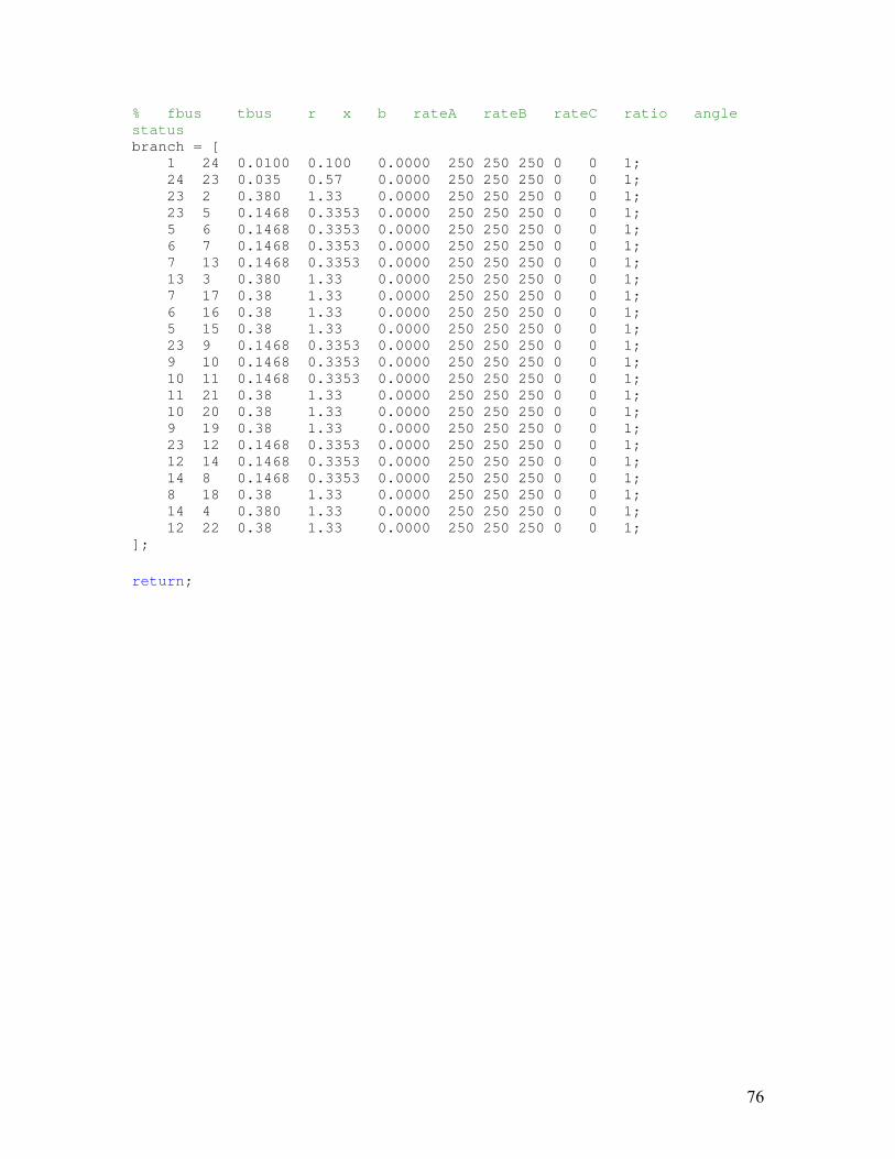
76

% fbus tbus r x b rateA rateB rateC ratio angle status branch = [ 1 24 0.0100 0.100 0.0000 250 250 250 0 0 1; 24 23 0.035 0.57 0.0000 250 250 250 0 0 1; 23 2 0.380 1.33 0.0000 250 250 250 0 0 1; 23 5 0.1468 0.3353 0.0000 250 250 250 0 0 1; 5 6 0.1468 0.3353 0.0000 250 250 250 0 0 1; 6 7 0.1468 0.3353 0.0000 250 250 250 0 0 1; 7 13 0.1468 0.3353 0.0000 250 250 250 0 0 1; 13 3 0.380 1.33 0.0000 250 250 250 0 0 1; 7 17 0.38 1.33 0.0000 250 250 250 0 0 1; 6 16 0.38 1.33 0.0000 250 250 250 0 0 1; 5 15 0.38 1.33 0.0000 250 250 250 0 0 1; 23 9 0.1468 0.3353 0.0000 250 250 250 0 0 1; 9 10 0.1468 0.3353 0.0000 250 250 250 0 0 1; 10 11 0.1468 0.3353 0.0000 250 250 250 0 0 1; 11 21 0.38 1.33 0.0000 250 250 250 0 0 1; 10 20 0.38 1.33 0.0000 250 250 250 0 0 1; 9 19 0.38 1.33 0.0000 250 250 250 0 0 1; 23 12 0.1468 0.3353 0.0000 250 250 250 0 0 1; 12 14 0.1468 0.3353 0.0000 250 250 250 0 0 1; 14 8 0.1468 0.3353 0.0000 250 250 250 0 0 1; 8 18 0.38 1.33 0.0000 250 250 250 0 0 1; 14 4 0.380 1.33 0.0000 250 250 250 0 0 1; 12 22 0.38 1.33 0.0000 250 250 250 0 0 1; ]; return;

77

Appendix F: Sample Matlab power flow output =============================================================== | System Summary | =============================================================== How many? How much? P (MW) Q (MVAr) --------------------- ------------------- ------------- ----------------- Buses 12 Total Gen Capacity 11.0 -102.0 to 102.0 Generators 11 On-line Capacity 1.1 -100.2 to 100.2 Committed Gens 2 Generation (actual) 10.3 3.9 Loads 10 Load 10.0 3.0 Fixed 10 Fixed 10.0 3.0 Dispatchable 0 Dispatchable 0.0 of 0.0 0.0 Shunts 0 Shunt (inj) 0.0 0.0 Branches 11 Losses (I^2 * Z) 0.35 0.95 Transformers 0 Branch Charging (inj) - 0.0 Inter-ties 0 Total Inter-tie Flow 0.0 0.0 Areas 1 Minimum Maximum ------------------------- -------------------------------- Voltage Magnitude 0.900 p.u. @ bus 12 1.000 p.u. @ bus 1 Voltage Angle -6.42 deg @ bus 12 0.00 deg @ bus 1 P Losses (I^2*R) - 0.08 MW @ line 3-4 Q Losses (I^2*X) - 0.24 MVAr @ line 1-2 =============================================================== | Bus Data | =============================================================== Bus Voltage Generation Load # Mag(pu) Ang(deg) P (MW) Q (MVAr) P (MW) Q (MVAr) ----- ------- -------- -------- -------- -------- -------- 1 1.000 0.000 5.35 3.75 - - 2 0.977 -1.710 - - - - 3 0.967 -2.090 5.00 0.20 1.00 0.30 4 0.953 -2.907 - - 1.00 0.30 5 0.941 -3.653 - - 1.00 0.30 6 0.931 -4.321 - - 1.00 0.30 7 0.922 -4.905 - - 1.00 0.30 8 0.915 -5.401 - - 1.00 0.30 9 0.909 -5.804 - - 1.00 0.30 10 0.905 -6.109 - - 1.00 0.30 11 0.902 -6.314 - - 1.00 0.30 12 0.900 -6.417 - - 1.00 0.30

78

-------- -------- -------- -------- Total: 10.35 3.95 10.00 3.00 =============================================================== | Branch Data | =============================================================== Brnch From To From Bus Injection To Bus Injection Loss (I^2 * Z) # Bus Bus P (MW) Q (MVAr) P (MW) Q (MVAr) P (MW) Q (MVAr) ----- ----- ----- -------- -------- -------- -------- -------- -------- 1 1 2 5.35 3.75 -5.33 -3.51 0.015 0.24 2 2 3 5.33 3.51 -5.30 -3.43 0.034 0.07 3 3 4 9.30 3.33 -9.21 -3.16 0.084 0.18 4 4 5 8.21 2.86 -8.15 -2.71 0.067 0.14 5 5 6 7.15 2.41 -7.10 -2.31 0.051 0.11 6 6 7 6.10 2.01 -6.06 -1.92 0.038 0.08 7 7 8 5.06 1.62 -5.03 -1.57 0.027 0.06 8 8 9 4.03 1.27 -4.02 -1.23 0.017 0.04 9 9 10 3.02 0.93 -3.01 -0.91 0.010 0.02 10 10 11 2.01 0.61 -2.00 -0.60 0.004 0.01 11 11 12 1.00 0.30 -1.00 -0.30 0.001 0.00 -------- -------- Total: 0.347 0.95 =============================================================== | System Summary | =============================================================== How many? How much? P (MW) Q (MVAr) --------------------- ------------------- ------------- ----------------- Buses 12 Total Gen Capacity 11.0 -102.0 to 102.0 Generators 11 On-line Capacity 0.0 -100.0 to 100.0 Committed Gens 1 Generation (actual) 9.1 1.9 Loads 10 Load 9.0 1.2 Fixed 10 Fixed 9.0 1.2 Dispatchable 0 Dispatchable 0.0 of 0.0 0.0 Shunts 0 Shunt (inj) 0.0 0.0 Branches 11 Losses (I^2 * Z) 0.14 0.74 Transformers 0 Branch Charging (inj) - 0.0 Inter-ties 0 Total Inter-tie Flow 0.0 0.0 Areas 1 Minimum Maximum ------------------------- -------------------------------- Voltage Magnitude 0.954 p.u. @ bus 12 1.000 p.u. @ bus 1 Voltage Angle -5.50 deg @ bus 12 0.00 deg @ bus 1

79

P Losses (I^2*R) - 0.07 MW @ line 2-3 Q Losses (I^2*X) - 0.50 MVAr @ line 1-2 =============================================================== | Bus Data | =============================================================== Bus Voltage Generation Load # Mag(pu) Ang(deg) P (MW) Q (MVAr) P (MW) Q (MVAr) ----- ------- -------- -------- -------- -------- -------- 1 1.000 0.000 9.14 1.94 - - 2 0.987 -2.987 - - - - 3 0.977 -3.839 - - 5.40 0.30 4 0.973 -4.164 - - 0.40 0.10 5 0.969 -4.456 - - 0.40 0.10 6 0.965 -4.713 - - 0.40 0.10 7 0.962 -4.936 - - 0.40 0.10 8 0.959 -5.122 - - 0.40 0.10 9 0.957 -5.272 - - 0.40 0.10 10 0.956 -5.385 - - 0.40 0.10 11 0.955 -5.460 - - 0.40 0.10 12 0.954 -5.498 - - 0.40 0.10 -------- -------- -------- -------- Total: 9.14 1.94 9.00 1.20 =============================================================== | Branch Data | =============================================================== Brnch From To From Bus Injection To Bus Injection Loss (I^2 * Z) # Bus Bus P (MW) Q (MVAr) P (MW) Q (MVAr) P (MW) Q (MVAr) ----- ----- ----- -------- -------- -------- -------- -------- -------- 1 1 2 9.14 1.94 -9.11 -1.44 0.031 0.50 2 2 3 9.11 1.44 -9.04 -1.29 0.070 0.15 3 3 4 3.64 0.99 -3.63 -0.96 0.012 0.03 4 4 5 3.23 0.86 -3.22 -0.84 0.009 0.02 5 5 6 2.82 0.74 -2.81 -0.73 0.007 0.02 6 6 7 2.41 0.63 -2.41 -0.62 0.005 0.01 7 7 8 2.01 0.52 -2.00 -0.51 0.004 0.01 8 8 9 1.60 0.41 -1.60 -0.40 0.002 0.01 9 9 10 1.20 0.30 -1.20 -0.30 0.001 0.00 10 10 11 0.80 0.20 -0.80 -0.20 0.001 0.00 11 11 12 0.40 0.10 -0.40 -0.10 0.000 0.00 -------- -------- Total: 0.143 0.74

80

Appendix G: Cost calculation input data 24 hour load loss and energy costs used in cost examples Base load shape % Pk load loss run loss $/Mwh load $ loss $

1 0.675 16.20 626 626 38 $615.60 $23.79 2 0.610 14.64 496 1122 37 $541.68 $18.35 3 0.598 14.35 475 1597 37 $531.02 $17.58 4 0.594 14.26 467 2064 36 $513.22 $16.81 5 0.615 14.76 506 2570 37 $546.12 $18.72 6 0.689 16.54 657 3227 37 $611.83 $24.31 7 0.721 17.30 731 3958 40 $692.16 $29.24 8 0.746 17.90 793 4751 41 $734.06 $32.51 9 0.786 18.86 900 5651 41 $773.42 $36.90

10 0.811 19.46 972 6623 44 $856.42 $42.77 11 0.826 19.82 1017 7640 44 $872.26 $44.75 12 0.829 19.90 1027 8667 45 $895.32 $46.22 13 0.842 20.21 1068 9735 47 $949.78 $50.20 14 0.867 20.81 1150 10885 47 $977.98 $54.05 15 0.898 21.55 1259 12144 52 $1,120.70 $65.47 16 0.931 22.34 1386 13530 53 $1,184.23 $73.46 17 0.960 23.04 1506 15036 60 $1,382.40 $90.36 18 0.982 23.57 1604 16640 61 $1,437.65 $97.84 19 1.000 24.00 1688 18328 67 $1,608.00 $113.10 20 0.985 23.64 1617 19945 67 $1,583.88 $108.34 21 0.957 22.97 1493 21438 63 $1,446.98 $94.06 22 0.884 21.22 1209 22647 52 $1,103.69 $62.87 23 0.791 18.98 914 23561 41 $778.08 $37.47 24 0.698 16.75 677 24238 39 $653.33 $26.40

Tot $ Total 463.08 24.238 22409.81 1225.56 $23,635.37 Avg 19.2951 1.009917 shift 1 mw for 3 hours, 5 hr .6 mw charge 100% eff % Pk load loss run loss $/Mwh load $ loss $

1 0.700 16.80 682 682 38 $638.40 $25.92 2 0.635 15.24 544 1226 37 $563.88 $20.13 3 0.623 14.95 521 1747 37 $553.15 $19.28 4 0.619 14.86 513 2260 36 $534.96 $18.47 5 0.640 15.36 554 2814 37 $568.32 $20.50 6 0.689 16.54 657 3471 37 $611.83 $24.31 7 0.721 17.30 731 4202 40 $692.16 $29.24 8 0.746 17.90 793 4995 41 $734.06 $32.51 9 0.786 18.86 900 5895 41 $773.42 $36.90

10 0.811 19.46 972 6867 44 $856.42 $42.77 11 0.826 19.82 1017 7884 44 $872.26 $44.75 12 0.829 19.90 1027 8911 45 $895.32 $46.22

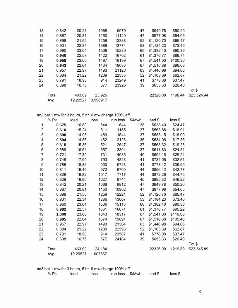
81

13 0.842 20.21 1068 9979 47 $949.78 $50.20 14 0.867 20.81 1150 11129 47 $977.98 $54.05 15 0.898 21.55 1259 12388 52 $1,120.70 $65.47 16 0.931 22.34 1386 13774 53 $1,184.23 $73.46 17 0.960 23.04 1506 15280 60 $1,382.40 $90.36 18 0.940 22.57 1422 16702 61 $1,376.77 $86.74 19 0.958 23.00 1497 18199 67 $1,541.00 $100.30 20 0.943 22.64 1434 19633 67 $1,516.88 $96.08 21 0.957 22.97 1493 21126 63 $1,446.98 $94.06 22 0.884 21.22 1209 22335 52 $1,103.69 $62.87 23 0.791 18.98 914 23249 41 $778.08 $37.47 24 0.698 16.75 677 23926 39 $653.33 $26.40

Tot $ Total 463.09 23.926 22326.00 1198.44 $23,524.44 Avg 19.29527 0.996917 no2 bat 1 mw for 3 hours, 5 hr .6 mw charge 100% eff % Pk load loss run loss $/Mwh load $ loss $

1 0.675 16.80 644 644 38 $638.40 $24.47 2 0.610 15.24 511 1155 37 $563.88 $18.91 3 0.598 14.95 489 1644 37 $553.15 $18.09 4 0.594 14.86 482 2126 36 $534.96 $17.35 5 0.615 15.36 521 2647 37 $568.32 $19.28 6 0.689 16.54 657 3304 37 $611.83 $24.31 7 0.721 17.30 731 4035 40 $692.16 $29.24 8 0.746 17.90 793 4828 41 $734.06 $32.51 9 0.786 18.86 900 5728 41 $773.42 $36.90

10 0.811 19.46 972 6700 44 $856.42 $42.77 11 0.826 19.82 1017 7717 44 $872.26 $44.75 12 0.829 19.90 1027 8744 45 $895.32 $46.22 13 0.842 20.21 1068 9812 47 $949.78 $50.20 14 0.867 20.81 1150 10962 47 $977.98 $54.05 15 0.898 21.55 1259 12221 52 $1,120.70 $65.47 16 0.931 22.34 1386 13607 53 $1,184.23 $73.46 17 0.960 23.04 1506 15113 60 $1,382.40 $90.36 18 0.982 22.57 1561 16674 61 $1,376.77 $95.22 19 1.000 23.00 1643 18317 67 $1,541.00 $110.08 20 0.985 22.64 1574 19891 67 $1,516.88 $105.46 21 0.957 22.97 1493 21384 63 $1,446.98 $94.06 22 0.884 21.22 1209 22593 52 $1,103.69 $62.87 23 0.791 18.98 914 23507 41 $778.08 $37.47 24 0.698 16.75 677 24184 39 $653.33 $26.40


82

1 0.675 16.80 682 682 38 $638.40 $25.92 2 0.610 15.24 544 1226 37 $563.88 $20.13 3 0.598 14.95 521 1747 37 $553.15 $19.28 4 0.594 14.86 513 2260 36 $534.96 $18.47 5 0.615 15.36 554 2814 37 $568.32 $20.50 6 0.689 16.54 657 3471 37 $611.83 $24.31 7 0.721 17.30 731 4202 40 $692.16 $29.24 8 0.746 17.90 793 4995 41 $734.06 $32.51 9 0.786 18.86 900 5895 41 $773.42 $36.90

10 0.811 19.46 972 6867 44 $856.42 $42.77 11 0.826 19.82 1017 7884 44 $872.26 $44.75 12 0.829 19.90 1027 8911 45 $895.32 $46.22 13 0.842 20.21 1068 9979 47 $949.78 $50.20 14 0.867 20.81 1150 11129 47 $977.98 $54.05 15 0.898 21.55 1259 12388 52 $1,120.70 $65.47 16 0.931 22.34 1386 13774 53 $1,184.23 $73.46 17 0.960 23.04 1506 15280 60 $1,382.40 $90.36 18 0.982 22.57 1471 16751 61 $1,376.77 $89.73 19 1.000 23.00 1549 18300 67 $1,541.00 $103.78 20 0.985 22.64 1484 19784 67 $1,516.88 $99.43 21 0.957 22.97 1493 21277 63 $1,446.98 $94.06 22 0.884 21.22 1209 22486 52 $1,103.69 $62.87 23 0.791 18.98 914 23400 41 $778.08 $37.47 24 0.698 16.75 677 24077 39 $653.33 $26.40


1 0.675 16.80 662 662 38 $638.40 $25.16 2 0.610 15.24 527 1189 37 $563.88 $19.50 3 0.598 14.95 504 1693 37 $553.15 $18.65 4 0.594 14.86 497 2190 36 $534.96 $17.89 5 0.615 15.36 537 2727 37 $568.32 $19.87 6 0.689 16.54 657 3384 37 $611.83 $24.31 7 0.721 17.30 731 4115 40 $692.16 $29.24 8 0.746 17.90 793 4908 41 $734.06 $32.51 9 0.786 18.86 900 5808 41 $773.42 $36.90

10 0.811 19.46 972 6780 44 $856.42 $42.77 11 0.826 19.82 1017 7797 44 $872.26 $44.75 12 0.829 19.90 1027 8824 45 $895.32 $46.22 13 0.842 20.21 1068 9892 47 $949.78 $50.20 14 0.867 20.81 1150 11042 47 $977.98 $54.05 15 0.898 21.55 1259 12301 52 $1,120.70 $65.47 16 0.931 22.34 1386 13687 53 $1,184.23 $73.46 17 0.960 23.04 1506 15193 60 $1,382.40 $90.36 18 0.982 22.57 1520 16713 61 $1,376.77 $92.72 19 1.000 23.00 1600 18313 67 $1,541.00 $107.20

83

20 0.985 22.64 1533 19846 67 $1,516.88 $102.71 21 0.957 22.97 1493 21339 63 $1,446.98 $94.06 22 0.884 21.22 1209 22548 52 $1,103.69 $62.87 23 0.791 18.98 914 23462 41 $778.08 $37.47 24 0.698 16.75 677 24139 39 $653.33 $26.40

Tot $ Total 463.09 24.139 22326.00 1214.72 $23,540.73 Avg 19.29527 1.005792 all bat .33 mw each for 3 hours, 5 hr .2 mw charge 100% eff % Pk load loss run loss $/Mwh load $ loss $

1 0.675 16.80 663 663 38 $638.40 $25.19 2 0.610 15.24 528 1191 37 $563.88 $19.54 3 0.598 14.95 505 1696 37 $553.15 $18.69 4 0.594 14.86 498 2194 36 $534.96 $17.93 5 0.615 15.36 537 2731 37 $568.32 $19.87 6 0.689 16.54 657 3388 37 $611.83 $24.31 7 0.721 17.30 731 4119 40 $692.16 $29.24 8 0.746 17.90 793 4912 41 $734.06 $32.51 9 0.786 18.86 900 5812 41 $773.42 $36.90

10 0.811 19.46 972 6784 44 $856.42 $42.77 11 0.826 19.82 1017 7801 44 $872.26 $44.75 12 0.829 19.90 1027 8828 45 $895.32 $46.22 13 0.842 20.21 1068 9896 47 $949.78 $50.20 14 0.867 20.81 1150 11046 47 $977.98 $54.05 15 0.898 21.55 1259 12305 52 $1,120.70 $65.47 16 0.931 22.34 1386 13691 53 $1,184.23 $73.46 17 0.960 23.04 1506 15197 60 $1,382.40 $90.36 18 0.982 22.57 1484 16681 61 $1,376.77 $90.52 19 1.000 23.00 1562 18243 67 $1,541.00 $104.65 20 0.985 22.64 1497 19740 67 $1,516.88 $100.30 21 0.957 22.97 1493 21233 63 $1,446.98 $94.06 22 0.884 21.22 1209 22442 52 $1,103.69 $62.87 23 0.791 18.98 914 23356 41 $778.08 $37.47 24 0.698 16.75 677 24033 39 $653.33 $26.40

Tot $ Total 463.09 24.033 22326.00 1207.72 $23,533.72 Avg 19.29527 1.001375

shift 3 mw for 3 hours, 5 hr 1.8 mw charge 100% eff % Pk load loss run loss $/Mwh load $ loss $

1 0.750 18.00 803 803 38 $684.00 $30.51 2 0.685 16.44 648 1451 37 $608.28 $23.98 3 0.673 16.15 622 2073 37 $597.55 $23.01 4 0.669 16.06 614 2687 36 $578.16 $22.10 5 0.690 16.56 659 3346 37 $612.72 $24.38

84

6 0.689 16.54 657 4003 37 $611.83 $24.31 7 0.721 17.30 731 4734 40 $692.16 $29.24 8 0.746 17.90 793 5527 41 $734.06 $32.51 9 0.786 18.86 900 6427 41 $773.42 $36.90

10 0.811 19.46 972 7399 44 $856.42 $42.77 11 0.826 19.82 1017 8416 44 $872.26 $44.75 12 0.829 19.90 1027 9443 45 $895.32 $46.22 13 0.842 20.21 1068 10511 47 $949.78 $50.20 14 0.867 20.81 1150 11661 47 $977.98 $54.05 15 0.898 21.55 1259 12920 52 $1,120.70 $65.47 16 0.931 22.34 1386 14306 53 $1,184.23 $73.46 17 0.960 23.04 1506 15812 60 $1,382.40 $90.36 18 0.857 20.57 1117 16929 61 $1,254.77 $68.14 19 0.875 21.00 1178 18107 67 $1,407.00 $78.93 20 0.860 20.64 1126 19233 67 $1,382.88 $75.44 21 0.957 22.97 1493 20726 63 $1,446.98 $94.06 22 0.884 21.22 1209 21935 52 $1,103.69 $62.87 23 0.791 18.98 914 22849 41 $778.08 $37.47 24 0.698 16.75 677 23526 39 $653.33 $26.40 Tot $ Total 463.09 23.526 22158.00 1157.53 $23,315.53 Avg 19.29527 0.98025 no2 bat 3 mw for 3 hours, 5 hr 1.8 mw charge 100% eff % Pk load loss run loss $/Mwh load $ loss $

1 0.675 18.00 682 682 38 $684.00 $25.92 2 0.610 16.44 546 1228 37 $608.28 $20.20 3 0.598 16.15 523 1751 37 $597.55 $19.35 4 0.594 16.06 516 2267 36 $578.16 $18.58 5 0.615 16.56 556 2823 37 $612.72 $20.57 6 0.689 16.54 657 3480 37 $611.83 $24.31 7 0.721 17.30 731 4211 40 $692.16 $29.24 8 0.746 17.90 793 5004 41 $734.06 $32.51 9 0.786 18.86 900 5904 41 $773.42 $36.90

10 0.811 19.46 972 6876 44 $856.42 $42.77 11 0.826 19.82 1017 7893 44 $872.26 $44.75 12 0.829 19.90 1027 8920 45 $895.32 $46.22 13 0.842 20.21 1068 9988 47 $949.78 $50.20 14 0.867 20.81 1150 11138 47 $977.98 $54.05 15 0.898 21.55 1259 12397 52 $1,120.70 $65.47 16 0.931 22.34 1386 13783 53 $1,184.23 $73.46 17 0.960 23.04 1506 15289 60 $1,382.40 $90.36 18 0.982 20.57 1535 16824 61 $1,254.77 $93.64 19 1.000 21.00 1615 18439 67 $1,407.00 $108.21 20 0.985 20.64 1548 19987 67 $1,382.88 $103.72 21 0.957 22.97 1493 21480 63 $1,446.98 $94.06 22 0.884 21.22 1209 22689 52 $1,103.69 $62.87 23 0.791 18.98 914 23603 41 $778.08 $37.47 24 0.698 16.75 677 24280 39 $653.33 $26.40

85

Tot $ Total 463.09 24.280 22158.00 1221.20 $23,379.20 Avg 19.29527 1.011667 no3 bat 3 mw for 3 hours, 5 hr 1.8 mw charge 100% eff % Pk load loss run loss $/Mwh load $ loss $

1 0.675 18.00 809 809 38 $684.00 $30.74 2 0.610 16.44 658 1467 37 $608.28 $24.35 3 0.598 16.15 633 2100 37 $597.55 $23.42 4 0.594 16.06 624 2724 36 $578.16 $22.46 5 0.615 16.56 669 3393 37 $612.72 $24.75 6 0.689 16.54 657 4050 37 $611.83 $24.31 7 0.721 17.30 731 4781 40 $692.16 $29.24 8 0.746 17.90 793 5574 41 $734.06 $32.51 9 0.786 18.86 900 6474 41 $773.42 $36.90

10 0.811 19.46 972 7446 44 $856.42 $42.77 11 0.826 19.82 1017 8463 44 $872.26 $44.75 12 0.829 19.90 1027 9490 45 $895.32 $46.22 13 0.842 20.21 1068 10558 47 $949.78 $50.20 14 0.867 20.81 1150 11708 47 $977.98 $54.05 15 0.898 21.55 1259 12967 52 $1,120.70 $65.47 16 0.931 22.34 1386 14353 53 $1,184.23 $73.46 17 0.960 23.04 1506 15859 60 $1,382.40 $90.36 18 0.982 20.57 1359 17218 61 $1,254.77 $82.90 19 1.000 21.00 1430 18648 67 $1,407.00 $95.81 20 0.985 20.64 1371 20019 67 $1,382.88 $91.86 21 0.957 22.97 1493 21512 63 $1,446.98 $94.06 22 0.884 21.22 1209 22721 52 $1,103.69 $62.87 23 0.791 18.98 914 23635 41 $778.08 $37.47 24 0.698 16.75 677 24312 39 $653.33 $26.40 Tot $ Total 463.09 24.312 22158.00 1207.32 $23,365.32 Avg 19.29527 1.013 no4 bat 3 mw for 3 hours, 5 hr 1.8 mw charge 100% eff % Pk load loss run loss $/Mwh load $ loss $

1 0.675 18.00 741 741 38 $684.00 $28.16 2 0.610 16.44 599 1340 37 $608.28 $22.16 3 0.598 16.15 575 1915 37 $597.55 $21.28 4 0.594 16.06 567 2482 36 $578.16 $20.41 5 0.615 16.56 609 3091 37 $612.72 $22.53 6 0.689 16.54 657 3748 37 $611.83 $24.31 7 0.721 17.30 731 4479 40 $692.16 $29.24 8 0.746 17.90 793 5272 41 $734.06 $32.51 9 0.786 18.86 900 6172 41 $773.42 $36.90

10 0.811 19.46 972 7144 44 $856.42 $42.77 11 0.826 19.82 1017 8161 44 $872.26 $44.75 12 0.829 19.90 1027 9188 45 $895.32 $46.22

86

13 0.842 20.21 1068 10256 47 $949.78 $50.20 14 0.867 20.81 1150 11406 47 $977.98 $54.05 15 0.898 21.55 1259 12665 52 $1,120.70 $65.47 16 0.931 22.34 1386 14051 53 $1,184.23 $73.46 17 0.960 23.04 1506 15557 60 $1,382.40 $90.36 18 0.982 20.57 1452 17009 61 $1,254.77 $88.57 19 1.000 21.00 1528 18537 67 $1,407.00 $102.38 20 0.985 20.64 1465 20002 67 $1,382.88 $98.16 21 0.957 22.97 1493 21495 63 $1,446.98 $94.06 22 0.884 21.22 1209 22704 52 $1,103.69 $62.87 23 0.791 18.98 914 23618 41 $778.08 $37.47 24 0.698 16.75 677 24295 39 $653.33 $26.40 Tot $ Total 463.09 24.295 22158.00 1214.67 $23,372.68 Avg 19.29527 1.012292 all bat 1 mw each for 3 hours, 5 hr .6 mw charge 100% eff % Pk load loss run loss $/Mwh load $ loss $

1 0.675 18.00 726 726 38 $684.00 $27.59 2 0.610 16.44 584 1310 37 $608.28 $21.61 3 0.598 16.15 559 1869 37 $597.55 $20.68 4 0.594 16.06 552 2421 36 $578.16 $19.87 5 0.615 16.56 594 3015 37 $612.72 $21.98 6 0.689 16.54 657 3672 37 $611.83 $24.31 7 0.721 17.30 731 4403 40 $692.16 $29.24 8 0.746 17.90 793 5196 41 $734.06 $32.51 9 0.786 18.86 900 6096 41 $773.42 $36.90

10 0.811 19.46 972 7068 44 $856.42 $42.77 11 0.826 19.82 1017 8085 44 $872.26 $44.75 12 0.829 19.90 1027 9112 45 $895.32 $46.22 13 0.842 20.21 1068 10180 47 $949.78 $50.20 14 0.867 20.81 1150 11330 47 $977.98 $54.05 15 0.898 21.55 1259 12589 52 $1,120.70 $65.47 16 0.931 22.34 1386 13975 53 $1,184.23 $73.46 17 0.960 23.04 1506 15481 60 $1,382.40 $90.36 18 0.982 20.57 1369 16850 61 $1,254.77 $83.51 19 1.000 21.00 1441 18291 67 $1,407.00 $96.55 20 0.985 20.64 1381 19672 67 $1,382.88 $92.53 21 0.957 22.97 1493 21165 63 $1,446.98 $94.06 22 0.884 21.22 1209 22374 52 $1,103.69 $62.87 23 0.791 18.98 914 23288 41 $778.08 $37.47 24 0.698 16.75 677 23965 39 $653.33 $26.40 Tot $ Total 463.09 23.965 22158.00 1195.34 $23,353.34 Avg 19.29527 0.998542

87

Appendix H: Plant factor data U.S. Electric net summer generating capacity [2] kw mwh MW MWh Plant year capacity generated capacity capacity factor 1949 63,400,000 296,124,289 63,400 555,384,000 53.3%1950 69,200,000 334,087,601 69,200 606,192,000 55.1%1951 75,500,000 375,298,355 75,500 661,380,000 56.7%1952 83,200,000 403,829,413 83,200 728,832,000 55.4%1953 93,300,000 447,048,563 93,300 817,308,000 54.7%1954 100,000,000 476,257,618 100,000 876,000,000 54.4%1955 114,200,000 550,298,862 114,200 1,000,392,000 55.0%1956 119,700,000 603,875,763 119,700 1,048,572,000 57.6%1957 131,100,000 634,642,367 131,100 1,148,436,000 55.3%1958 143,300,000 648,450,862 143,300 1,255,308,000 51.7%1959 155,900,000 713,378,831 155,900 1,365,684,000 52.2%1960 167,100,000 759,155,788 167,100 1,463,796,000 51.9%1961 179,000,000 797,124,391 179,000 1,568,040,000 50.8%1962 192,100,000 857,943,656 192,100 1,682,796,000 51.0%1963 209,700,000 920,028,271 209,700 1,836,972,000 50.1%1964 223,700,000 987,218,326 223,700 1,959,612,000 50.4%1965 234,800,000 1058385671 234,800 2,056,848,000 51.5%1966 247,500,000 1147531895 247,500 2,168,100,000 52.9%1967 266,700,000 1217795688 266,700 2,336,292,000 52.1%1968 284,000,000 1332825601 284,000 2,487,840,000 53.6%1969 309,800,000 1445458056 309,800 2,713,848,000 53.3%1970 336,400,000 1535111467 336,400 2,946,864,000 52.1%1971 366,400,000 1615853616 366,400 3,209,664,000 50.3%1972 396,000,000 1752978413 396,000 3,468,960,000 50.5%1973 439,800,000 1864056631 439,800 3,852,648,000 48.4%1974 468,500,000 1870319405 468,500 4,104,060,000 45.6%1975 491,300,000 1920754569 491,300 4,303,788,000 44.6%1976 517,200,000 2040913681 517,200 4,530,672,000 45.0%1977 535,900,000 2127447487 535,900 4,694,484,000 45.3%1978 552,100,000 2209376911 552,100 4,836,396,000 45.7%1979 565,500,000 2250665025 565,500 4,953,780,000 45.4%1980 578,600,000 2289600364 578,600 5,068,536,000 45.2%1981 598,300,000 2297973339 598,300 5,241,108,000 43.8%1982 613,700,000 2244372488 613,700 5,376,012,000 41.7%1983 621,100,000 2313445685 621,100 5,440,836,000 42.5%1984 635,100,000 2419465368 635,100 5,563,476,000 43.5%1985 655,200,000 2473002122 655,200 5,739,552,000 43.1%1986 664,800,000 2490470952 664,800 5,823,648,000 42.8%1987 674,100,000 2575287666 674,100 5,905,116,000 43.6%

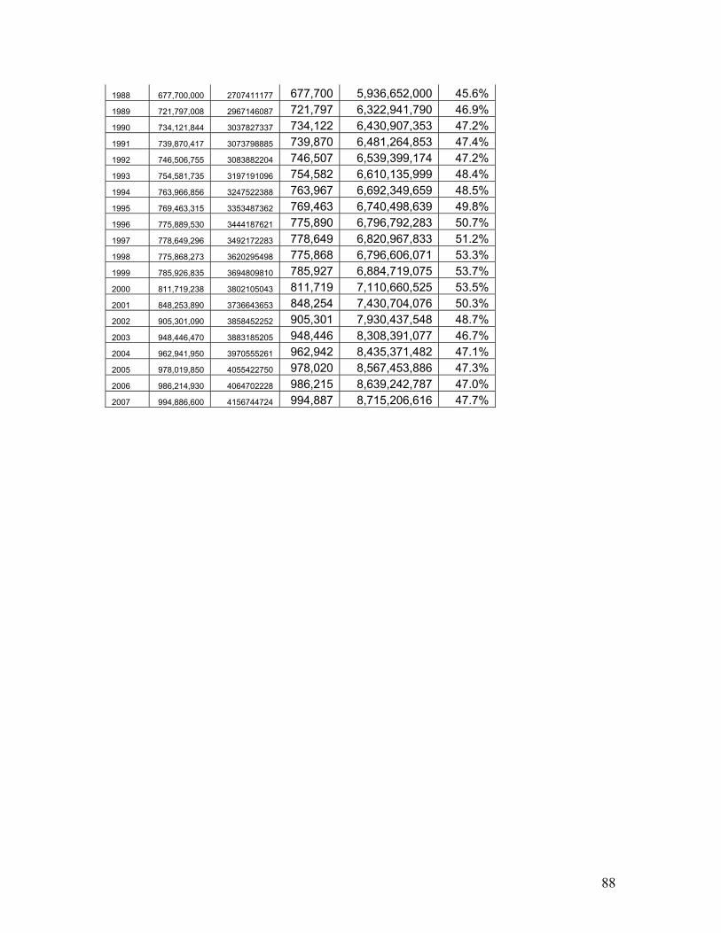
88

1988 677,700,000 2707411177 677,700 5,936,652,000 45.6%1989 721,797,008 2967146087 721,797 6,322,941,790 46.9%1990 734,121,844 3037827337 734,122 6,430,907,353 47.2%1991 739,870,417 3073798885 739,870 6,481,264,853 47.4%1992 746,506,755 3083882204 746,507 6,539,399,174 47.2%1993 754,581,735 3197191096 754,582 6,610,135,999 48.4%1994 763,966,856 3247522388 763,967 6,692,349,659 48.5%1995 769,463,315 3353487362 769,463 6,740,498,639 49.8%1996 775,889,530 3444187621 775,890 6,796,792,283 50.7%1997 778,649,296 3492172283 778,649 6,820,967,833 51.2%1998 775,868,273 3620295498 775,868 6,796,606,071 53.3%1999 785,926,835 3694809810 785,927 6,884,719,075 53.7%2000 811,719,238 3802105043 811,719 7,110,660,525 53.5%2001 848,253,890 3736643653 848,254 7,430,704,076 50.3%2002 905,301,090 3858452252 905,301 7,930,437,548 48.7%2003 948,446,470 3883185205 948,446 8,308,391,077 46.7%2004 962,941,950 3970555261 962,942 8,435,371,482 47.1%2005 978,019,850 4055422750 978,020 8,567,453,886 47.3%2006 986,214,930 4064702228 986,215 8,639,242,787 47.0%2007 994,886,600 4156744724 994,887 8,715,206,616 47.7%

Masters Thesis Possibilities - Worcester Polytechnic Institute

Documents

Transcript of Masters Thesis Possibilities - Worcester Polytechnic Institute