Masters Thesis: Optimal Control of Autonomous Greenhouses
86
Delft Center for Systems and Control Optimal Control of Autonomous Greenhouses A Data-Driven Approach L.G.J. Kerkhof Master of Science Thesis
Transcript of Masters Thesis: Optimal Control of Autonomous Greenhouses
Delft Center for Systems and Control
Optimal Control of AutonomousGreenhousesA Data-Driven Approach
L.G.J. Kerkhof
Mas
tero
fScie
nce
Thes
is

Optimal Control of AutonomousGreenhouses
A Data-Driven Approach
Master of Science Thesis
For the degree of Master of Science in Systems and Control at DelftUniversity of Technology
L.G.J. Kerkhof
July 13, 2020
Faculty of Mechanical, Maritime and Materials Engineering (3mE) · Delft University ofTechnology

The work in this thesis was supported by Hoogendoorn Growth Management. Their cooper-ation is hereby gratefully acknowledged.
Cover image by Erwan Hesry (https://unsplash.com/@erwanhesry).
Copyright c© Delft Center for Systems and Control (DCSC)All rights reserved.

Delft University of TechnologyDepartment of
Delft Center for Systems and Control (DCSC)
The undersigned hereby certify that they have read and recommend to the Faculty ofMechanical, Maritime and Materials Engineering (3mE) for acceptance a thesis
entitledOptimal Control of Autonomous Greenhouses
byL.G.J. Kerkhof
in partial fulfillment of the requirements for the degree ofMaster of Science Systems and Control
Dated: July 13, 2020
Supervisor(s):Prof.dr.ir. T. Keviczky
Reader(s):Dr.ir. S. Wahls
Dr.ir. K. Batselier
Ir. L. Baart de la Faille


Abstract
The world population is growing rapidly and the demand for healthy food grows with it.Greenhouse cultivation provides an efficient way to grow crops in a protected and controlledenvironment. In the past, many greenhouse control algorithms have been developed. How-ever, the majority of these algorithms rely on an explicit parametric model description of thegreenhouse. These models are often based on physical laws such as conservation of mass andenergy and contain many parameters which should be identified. Due to the complex andhighly non-linear dynamics of greenhouses, these models might not be applicable to controlgreenhouses other than the one for which the model has been designed and identified. Hence,in current horticultural practice these control algorithms are scarcely used. Therefore, theneed rises for a control algorithm which does not rely on a parametric system representa-tion but rather on input/output data of the greenhouse system, hereby establishing a wayto control the system with unknown or unmodeled dynamics. A recently proposed algo-rithm, Data-Enabled Predictive Control (DeePC), is able to replace system identification,state estimation and future trajectory prediction by one single optimization framework. Thealgorithm exploits a non-parametric model constructed solely from input/output data of thesystem. This algorithm is employed in order to control the greenhouse climate. It is shownthat in numerical simulation the DeePC algorithm is able to control the greenhouse climate.A comparison is made with the conventional Nonlinear Model Predictive Control (NMPC)algorithm in order to show the differences between a predictive control algorithm that hasdirect access to the non-linear greenhouse simulation model and a purely data-driven predic-tive control algorithm. Both algorithms are compared based on reference tracking accuracyand computational time. Furthermore, it is shown in numerical simulation that the DeePCalgorithm is able to cope with changing dynamics within the greenhouse system throughoutthe crop cycle.
Master of Science Thesis L.G.J. Kerkhof

ii
L.G.J. Kerkhof Master of Science Thesis

Table of Contents
Acknowledgements ix
1 Introduction 11-1 Motivation . . . . . . . . . . . . . . . . . . . . . . . . . . . . . . . . . . . . . . 11-2 Research Question . . . . . . . . . . . . . . . . . . . . . . . . . . . . . . . . . . 21-3 Thesis Outline . . . . . . . . . . . . . . . . . . . . . . . . . . . . . . . . . . . . 3
2 The Greenhouse System 52-1 Introduction . . . . . . . . . . . . . . . . . . . . . . . . . . . . . . . . . . . . . 52-2 The Greenhouse Climate System . . . . . . . . . . . . . . . . . . . . . . . . . . 7
2-2-1 Schematic Description of the Greenhouse Climate . . . . . . . . . . . . . 72-2-2 Greenhouse Climate Mathematical Model . . . . . . . . . . . . . . . . . 8
2-3 The Greenhouse Crop System . . . . . . . . . . . . . . . . . . . . . . . . . . . . 132-3-1 Schematic Description of the Greenhouse Crop . . . . . . . . . . . . . . 132-3-2 Greenhouse Crop Mathematical Model . . . . . . . . . . . . . . . . . . . 13
2-4 Greenhouse Simulation . . . . . . . . . . . . . . . . . . . . . . . . . . . . . . . 172-4-1 Discretization and Implementation . . . . . . . . . . . . . . . . . . . . . 172-4-2 Simulation Example . . . . . . . . . . . . . . . . . . . . . . . . . . . . . 18
3 Non-Linear Model Predictive Control 213-1 Introduction . . . . . . . . . . . . . . . . . . . . . . . . . . . . . . . . . . . . . 213-2 Non-Linear Model Predictive Control . . . . . . . . . . . . . . . . . . . . . . . . 233-3 Greenhouse Controlled by NMPC . . . . . . . . . . . . . . . . . . . . . . . . . . 24
3-3-1 Weather Conditions . . . . . . . . . . . . . . . . . . . . . . . . . . . . . 243-3-2 Reference Tracking . . . . . . . . . . . . . . . . . . . . . . . . . . . . . 253-3-3 Yield Maximization . . . . . . . . . . . . . . . . . . . . . . . . . . . . . 27
Master of Science Thesis L.G.J. Kerkhof

iv Table of Contents
4 Data-Enabled Predictive Control 314-1 Introduction . . . . . . . . . . . . . . . . . . . . . . . . . . . . . . . . . . . . . 314-2 Behavioural Systems Theory . . . . . . . . . . . . . . . . . . . . . . . . . . . . 314-3 Data-Enabled Predictive Control . . . . . . . . . . . . . . . . . . . . . . . . . . 334-4 Greenhouse Controlled by DeePC . . . . . . . . . . . . . . . . . . . . . . . . . . 35
4-4-1 Including Exogenous Signals . . . . . . . . . . . . . . . . . . . . . . . . 354-4-2 Extension to Non-Linear Systems . . . . . . . . . . . . . . . . . . . . . . 364-4-3 Window Constraint . . . . . . . . . . . . . . . . . . . . . . . . . . . . . 364-4-4 Regularized DeePC . . . . . . . . . . . . . . . . . . . . . . . . . . . . . 374-4-5 Reference Tracking with DeePC . . . . . . . . . . . . . . . . . . . . . . 37
5 Case Study: NMPC vs DeePC 415-1 Introduction Case-Study . . . . . . . . . . . . . . . . . . . . . . . . . . . . . . . 41
5-1-1 Weather Profile . . . . . . . . . . . . . . . . . . . . . . . . . . . . . . . 425-1-2 Control Input Signal . . . . . . . . . . . . . . . . . . . . . . . . . . . . . 42
5-2 Controlling the Greenhouse . . . . . . . . . . . . . . . . . . . . . . . . . . . . . 435-3 Comparison of Algorithm Performance . . . . . . . . . . . . . . . . . . . . . . . 455-4 Adjusted Greenhouse Dynamics . . . . . . . . . . . . . . . . . . . . . . . . . . . 46
6 Irrigation Control 496-1 Introduction . . . . . . . . . . . . . . . . . . . . . . . . . . . . . . . . . . . . . 496-2 Strategy . . . . . . . . . . . . . . . . . . . . . . . . . . . . . . . . . . . . . . . 496-3 Control Algorithm . . . . . . . . . . . . . . . . . . . . . . . . . . . . . . . . . . 50
7 Conclusions and Recommendations 537-1 Conclusion . . . . . . . . . . . . . . . . . . . . . . . . . . . . . . . . . . . . . . 53
7-1-1 Summary . . . . . . . . . . . . . . . . . . . . . . . . . . . . . . . . . . 537-1-2 Answers to Research Questions . . . . . . . . . . . . . . . . . . . . . . . 547-1-3 Autonomous Greenhouse Challenge . . . . . . . . . . . . . . . . . . . . . 55
7-2 Recommendations for Future Work . . . . . . . . . . . . . . . . . . . . . . . . . 57
A Notation 59
B Greenhouse Simulation Model Constants 61
Bibliography 65
Glossary 69List of Acronyms . . . . . . . . . . . . . . . . . . . . . . . . . . . . . . . . . . . 69List of Symbols . . . . . . . . . . . . . . . . . . . . . . . . . . . . . . . . . . . 69
L.G.J. Kerkhof Master of Science Thesis

List of Figures
2-1 Typical multi-span Venlo type greenhouse [19]. . . . . . . . . . . . . . . . . . . 5
2-2 Block scheme of the greenhouse climate system [3]. . . . . . . . . . . . . . . . . 7
2-3 Block scheme of the greenhouse tomato crop system [24]. . . . . . . . . . . . . 132-4 The control inputs that are used in both numerical simulations. . . . . . . . . . . 182-5 Greenhouse climate states that show the effect of a young crop and a fully devel-
oped crop on the greenhouse climate. . . . . . . . . . . . . . . . . . . . . . . . 192-6 Greenhouse crop states that show the states of a young crop (left) and a fully
developed crop (right). . . . . . . . . . . . . . . . . . . . . . . . . . . . . . . . 19
3-1 Model Predictive Control (MPC) scheme [29]. . . . . . . . . . . . . . . . . . . . 223-2 Weather conditions used in the NMPC simulations. . . . . . . . . . . . . . . . . 243-3 Greenhouse air (top) and heating pipe (bottom) temperatures controlled by NMPC
for r∆ = 10 and r∆ = 1. . . . . . . . . . . . . . . . . . . . . . . . . . . . . . . 263-4 Control inputs computed by NMPC for different values of r∆. The top plot shows
the heating water temperature for r∆ = 10 and r∆ = 1, respectively. The middleplot shows the lee and wind side window openings for r∆ = 10 and the bottomplot shows the lee and wind side opening for r∆ = 1. . . . . . . . . . . . . . . . 26
3-5 Greenhouse air and heating pipe temperatures (top) and greenhouse air CO2 con-centration (bottom) controlled by NMPC for rCO2 = 100 and rCO2 = 500. . . . . 28
3-6 Assimilate buffer dry weight (top) and fruit dry weight (bottom) controlled byNMPC for rCO2 = 100 and rCO2 = 500. . . . . . . . . . . . . . . . . . . . . . . 29
3-7 Control inputs computed by NMPC for different values of rCO2 . The top plotshows the heating water temperature for both rCO2 = 100 and rCO2 = 500. Themiddle plot shows the window positions on lee and wind side for both rCO2 = 100and rCO2 = 500. The bottom plot shows the CO2 injection for both rCO2 = 100and rCO2 = 500. . . . . . . . . . . . . . . . . . . . . . . . . . . . . . . . . . . 29
4-1 DeePC scheme . . . . . . . . . . . . . . . . . . . . . . . . . . . . . . . . . . . . 35
Master of Science Thesis L.G.J. Kerkhof
vi List of Figures
4-2 Random generated control inputs (bottom) and corresponding outputs (top). Thegreen dashed lines and arrows indicate which part of the data is stored in Up andUf (similar for Yp and Yf ). . . . . . . . . . . . . . . . . . . . . . . . . . . . . . 38
4-3 Model temperature and predicted temperature for different values of λy and Q. . 39
5-1 Measured weather conditions used in the DeePC algorithm. . . . . . . . . . . . . 425-2 Generated NMPC input signals used in the DeePC algorithm. . . . . . . . . . . . 435-3 Greenhouse air and heating pipe temperatures controlled by both DeePC and NMPC. 445-4 Heating water temperature and window positions computed by both DeePC and
NMPC. . . . . . . . . . . . . . . . . . . . . . . . . . . . . . . . . . . . . . . . . 445-5 Computation time per iteration for both DeePC and NMPC. . . . . . . . . . . . 455-6 Greenhouse air and heating pipe temperatures controlled by DeePC based on both
the old and updated data. . . . . . . . . . . . . . . . . . . . . . . . . . . . . . . 475-7 Heating water temperature and window positions computed by DeePC based on
both the old and updated data. . . . . . . . . . . . . . . . . . . . . . . . . . . . 47
6-1 Linear regression fit between the radiation sum received and dry-down rate duringthe light period ∆L with the dry-back rate prediction for 1500 J/cm2 superimposed. 51
6-2 Water content measurements during a particular day with the gradients ∆L and∆D superimposed. . . . . . . . . . . . . . . . . . . . . . . . . . . . . . . . . . . 51
7-1 Final results of the Autonomous Greenhouse Challenge based on net profit, sus-tainability and Artificial Intelligence (AI) strategy. Team Automatoes ranked firstin all categories [36]. . . . . . . . . . . . . . . . . . . . . . . . . . . . . . . . . 56
7-2 The net profit realized by all teams. Team Automatoes controlled compartment 306(green). The reference team controlled compartment 303 (gray). The remainingcolors are the other AI teams [36]. . . . . . . . . . . . . . . . . . . . . . . . . . 56
L.G.J. Kerkhof Master of Science Thesis
List of Tables
5-1 Comparison of DeePC and NMPC on tracking accuracy and computation time. . 455-2 Comparison of the two DeePC simulations on tracking accuracy and computation
time. . . . . . . . . . . . . . . . . . . . . . . . . . . . . . . . . . . . . . . . . . 46
B-1 Greenhouse model parameters . . . . . . . . . . . . . . . . . . . . . . . . . . . . 61B-2 Greenhouse model parameters, continued . . . . . . . . . . . . . . . . . . . . . . 62B-3 Greenhouse model parameters, continued . . . . . . . . . . . . . . . . . . . . . . 63
Master of Science Thesis L.G.J. Kerkhof

viii List of Tables
L.G.J. Kerkhof Master of Science Thesis

Acknowledgements
This thesis in front of you is the result of the project I worked on for the past year andconcludes my studies in Systems and Control. Also, it marks the end of my time as a studentat the Delft University of Technology after six years. Working on this project has been quitea journey during which I learnt a tremendous amount, not only on professional but also onpersonal level.
Of course, this journey would not have been possible without the help of many people. Firstand foremost, I would like to thank my supervisor prof.dr.ir. Tamás Keviczky for his advice,time and inspiration. Your constructive feedback has been crucial during the process of thisthesis project.
Furthermore, I would like to thank my fellow team members of team Automatoes: Evripidis,Rene, Gerdine, Leonard, Neil, Niek and Godfrey. Without them, this project would not havebeen such joyful as it has been now.
Finally, I would like to thank my friends and family who supported me throughout the pastsix years of my studies. Without all of you, I think it would have been nearly impossible forme to finish my studies. Especially, I would like to thank my parents for always supportingme and the decisions I made during my studies. Lastly, I would like to thank Gabrielle forher unconditional love, support and patience during this project.
Delft, University of Technology L.G.J. KerkhofJuly 13, 2020
Master of Science Thesis L.G.J. Kerkhof

x Acknowledgements
L.G.J. Kerkhof Master of Science Thesis

Chapter 1
Introduction
1-1 Motivation
The world population is increasing rapidly. According to the United Nations, the worldpopulation will increase to nearly 10 billion people in 2050 [1]. Currently an estimatedamount of 821 million people is undernourished worldwide and this amount has been growingsince 2014 [2]. Hence, as the world population is growing, the demand for healthy and freshfood grows as well.
Greenhouse cultivation plays an important role in providing fresh and healthy foods, such asfruits and vegetables. Due to their enclosure, greenhouses enable the control of climate con-ditions inside the greenhouse. Hence, this controlled indoor climate enables the manipulationof crop production by improving crop quality and decreasing the crop cultivation period [3].Furthermore, the greenhouse provides a protection against insects, pests and diseases.
An important concern within the greenhouse industry is sustainability. According to theEuropean Union, the share of energy consumption of agriculture with respect to the finalenergy consumption was 8.2% in 2017 in the Netherlands [4]. In addition, according to theDutch government, the 2020 target CO2 emission for the Dutch greenhouse industry that wasagreed upon in 2014 is probably not going to be reached [5]. Hence, advanced greenhousecontrol algorithms could play an important role in reaching higher resource use efficiency andhence decrease the total energy and CO2 consumption in the greenhouse industry, leading toa more sustainable horticultural sector.
Besides the food shortage and sustainability issues, one of the biggest problems within thegreenhouse industry nowadays is finding sufficient experienced labor to manage crop produc-tion because the amount of experienced growers worldwide is declining [6]. A solution toovercome the shortfall of experienced labor is to increase the level of autonomy in greenhousecrop production. Hence, since the worldwide greenhouse vegetable production is increasing[7] and the greenhouse equipment is becoming more advanced [8], the necessity for advancedgreenhouse control algorithms grows.
Master of Science Thesis L.G.J. Kerkhof

2 Introduction
In order to increase the level of autonomy in the greenhouse industry, various model based con-trol algorithms have been developed [9]. However, these algorithms usually exploit an explicitparametric model of the system dynamics. Difficulties in modelling the greenhouse dynam-ics arise in the fact that greenhouses exhibit complex and highly nonlinear behaviour [10].Therefore, data-driven control algorithms, e.g. Data-Enabled Predictive Control (DeePC)[11], could provide a solution to this problem since such algorithms do not rely on an explicitparametric system representation but rather on input-output data of the system.
Furthermore, recent advancements in the field of Artificial Intelligence (AI) have led to majorbreakthroughs in fields such as autonomous driving [12], healthcare [13] and robotics [14].Within the greenhouse industry, AI has been applied to yield prediction, disease detection,weed detection, crop quality classification and species recognition [15]. However, AI is stillscarcely used in greenhouse climate and irrigation control and in making crop managementdecisions. Therefore, AI could contribute to a fully autonomous greenhouse cultivation periodwith yield levels compared to commercial practice [9]. For this reason, Wageningen Univer-sity and Research and Tencent organise the Autonomous Greenhouse Challenge. During thisChallenge, 5 teams get the opportunity to grow cherry tomatoes in a remotely controlledgreenhouse compartment for six months. Since the greenhouse compartments are being re-motely controlled, the teams are not allowed to enter their compartments and are ought to useadvanced greenhouse control and/or AI algorithms which determine optimal settings for thegreenhouse climate based on sensor measurements and weather predictions. The goal of thisChallenge is to produce high quality tomatoes at a high level of production and with a highresource use efficiency. Together with researchers from Delft University of Technology andemployees from Hoogendoorn Growth Management, Van der Hoeven Horticultural Projectsand Keygene we will team up and participate during this Challenge.
1-2 Research Question
This thesis aims to develop a data-driven way to control greenhouses. This is done by employ-ing the DeePC algorithm. This algorithm will be used to control the greenhouse model from[16] and its performance will be compared to the Nonlinear Model Predictive Control (NMPC)algorithm. Hence, the research question is stated as follows:
How does Data-Enabled Predictive Control perform compared to Nonlinear Model PredictiveControl when controlling an autonomous greenhouse?
In order to support the research question, several sub-research questions with a more limitedscope are formulated next:
• Which model should be used to include in the NMPC algorithm and to generate data forthe DeePC algorithm?
• Which of the available actuators are going to be controlled and which inputs could beretrieved from auxiliary controllers or forecasts?
• How can feedback of the crop status be included in the control loop?
• How is the performance of the DeePC algorithm going to be bench-marked against theNMPC algorithm?
L.G.J. Kerkhof Master of Science Thesis

1-3 Thesis Outline 3
1-3 Thesis Outline
This thesis is organized as follows: in Chapter 2 an introduction is given to the greenhousesystem in general and the dynamical greenhouse/crop models that are used in this thesis. InChapter 3, the NMPC algorithm is introduced together with its application to the greenhousesystem. In Chapter 4, the DeePC algorithm is introduced together with the mathematicalbackground from behavioural systems theory on which the algorithm is relies. Thereafter,this algorithm will be applied to the greenhouse system. In Chapter 5, both the NMPCand DeePC algorithms will be used in a case-study where a reference is tracked during aparticular day of which the outside conditions are available. Afterwards, both algorithms willbe compared on their reference tracking accuracy and computation time. Furthermore, in thisChapter a comparison is made in the case that the DeePC algorithm controls the greenhousewhile using data from the beginning of the crop cycle and data from when the crop is fullydeveloped in order to show the relevance of the data that is used in the DeePC algorithm. InChapter 6 an algorithm is proposed that controls the irrigation based on the water content inthe substrate and the total daily solar radiation sum. Finally, in Chapter 7 a conclusion fromthe results will be drawn, the aforementioned research questions will be answered, the resultsof the Autonomous Greenhouse Challenge are discussed and recommendations for future workwill be made.
Master of Science Thesis L.G.J. Kerkhof

4 Introduction
L.G.J. Kerkhof Master of Science Thesis

Chapter 2
The Greenhouse System
2-1 Introduction
Worldwide, many different types and designs of greenhouses exist. Essential differences areseen in the greenhouse shape, cover material (e.g., glass or polyethylene) and the principles ofoperation [17]. For this thesis, the Venlo type greenhouse will be considered, which is shownin Figure 2-1. This glass covered, multi-span greenhouse is the most common greenhousetype in the Netherlands. Due to its transparent cover, solar radiation is allowed to enter thegreenhouse in order to stimulate photosynthesis. Photosynthesis is the driving factor for plantand fruit growth and hence increasing the photosynthesis rate of plants will increase the cropyield [18]. Photosynthesis is the process where a crop converts solar radiation, CO2, waterand nutrients into assimilates such as carbohydrates which are used for plant maintenanceand growth of fruits and leaves. Hence, modern greenhouse equipment allows the injection ofCO2 and additional heating in order to create the ideal plant growth climate. Furthermore,artificial lighting allows to add supplementary light when the solar radiation does not sufficeand irrigation and nutrients could be provided as desired through an irrigation system. Evenmore advanced greenhouses contain shading screens, fogging systems or cooling pads as well.
Figure 2-1: Typical multi-span Venlo type greenhouse [19].
Master of Science Thesis L.G.J. Kerkhof

6 The Greenhouse System
Besides the variations in greenhouse types and designs and control equipment, there is a largediversity of crops which can be grown in a greenhouse as well; ranging from bulk crops suchas tomato, cucumber and sweet pepper to ornamental crops such as pot plants or flowers andmedicinal plants [20]. Since all these different crops exhibit different dynamics due to theirdifferent growing processes, there exists a large variety of control inputs and objectives whenit comes to controlling a greenhouse.
Within the greenhouse, many physical, biological and chemical processes take place simul-taneously [21]. This results in the fact that the greenhouse system is a complex non-lineardynamical system that mainly consists of two subsystems: the greenhouse climate and thegreenhouse crop. The greenhouse crop mainly reacts to the surrounding greenhouse climate,e.g., temperature, humidity and CO2 concentration of the greenhouse air and light intensity.The greenhouse climate is mainly influenced by the control inputs such as heating, CO2 in-jection and artificial lighting and exogenous inputs such as solar radiation, wind speed andoutside temperature. Furthermore, the crop influences the climate as well due to e.g., tran-spiration, evaporation and CO2 uptake. Another complexity arises due to the fact that thegreenhouse crop dynamics are rather slow compared to the greenhouse climate dynamics.This difference in time scales makes it difficult to determine what the long term benefits ofthe yield will be when making short term decisions on resource usage.
Often, rejecting exogenous inputs is of major importance when controlling a system [22].However, one of the exogenous signals that acts on the greenhouse system is solar radiation.This radiation is also the main driving force behind photosynthesis and on cold days it couldbe used to heat up the greenhouse. Furthermore, it might occasionally be necessary to usethe cold outside air to cool down the greenhouse. Therefore, the exogenous signals shouldbe exploited instead of rejected. Especially since the greenhouse has a transparent cover,the goal is to exploit the energy from the sun as much as possible. Hence, the optimal wayto obtain high yield with a high resource use efficiency is by providing minimum heat andkeeping the windows closed as much as possible in order to keep the heat, humidity and CO2inside the greenhouse.
In order to validate and benchmark the results of a greenhouse control algorithm, a greenhousesimulation model is required. Therefore, this chapter describes both the greenhouse climateand greenhouse crop subsystems in a schematic and mathematical way. For the greenhouseclimate, a general description is given that includes common characteristics that hold formany greenhouse designs and crop varieties. For the greenhouse crop, a description of atomato crop is given. Many different publications arise in which a mathematical model ofthe greenhouse climate is developed. For an extensive survey on these models, the reader isreferred to [23] and the references therein. For this thesis, the greenhouse climate and cropmodel from [16] is used since it is developed for control purposes and describes processes suchas ventilation and crop evaporation in a non-linear way while many climate models assume alinear relationship for these processes.
L.G.J. Kerkhof Master of Science Thesis

2-2 The Greenhouse Climate System 7
2-2 The Greenhouse Climate System
2-2-1 Schematic Description of the Greenhouse Climate
In this section, a description of the greenhouse climate system is given. In Figure 2-2 isschematically shown how the greenhouse climate interacts with the control inputs, the externalenvironment and the greenhouse crop. In this scheme, the greenhouse and crop are consideredas two separate subsystems: Sg and Sc , with states xg and xc , respectively.
The solid arrows in this figure represent the mass and energy fluxes whereas the dashed arrowsrepresent the variables that influence these fluxes. These variables are the control inputs, thegreenhouse states, the crop states and the disturbances acting on the greenhouse and will becalled ’information flows’ for conciseness as is done in [3].
Figure 2-2: Block scheme of the greenhouse climate system [3].
Mass and energy fluxes between four different parts are distinguished: the fluxes between thecontrol equipment and the greenhouse, the fluxes between the greenhouse and the outsideenvironment, the fluxes between the greenhouse and the crop and the fluxes between the cropand output, denoted by je_g, jg_o, jg_c and jc_o, respectively. Mass fluxes are e.g., the waterand CO2 fluxes from and to the crops and energy fluxes are e.g., the heating and solar energyfluxes from and to the greenhouse.
The information flows, denoted by (1), ... , (10) are described below:
• (1) The control inputs that are used for active climate control, e.g., heating, irrigationand CO2 supply.
Master of Science Thesis L.G.J. Kerkhof
8 The Greenhouse System
• (2), (5), (6) The greenhouse climate states, e.g., the greenhouse air temperature andhumidity, the soil temperature, the temperature of the heating pipes and the CO2concentration of the greenhouse air.
• (3) The control inputs that steer the window opening on both the lee and wind sidewindows of the greenhouse (passive climate control).
• (4) The exogenous signals, i.e., all signals that come from the outside environmentsuch as the outside air temperature and humidity, wind speed, wind direction and solarradiation.
• (7), (9) The states of the crop e.g., the mass content of the assimilate buffer, the weightof fruits and leafs on the crop and the growth stage of the crop.
• (8) The solar radiation input to the crop. The only external input that directly influ-ences the crop since solar radiation is directly involved in the photosynthesis process.Hence, the solar radiation influences e.g., CO2 uptake and transpiration of the crop andtherefore the jg_c flux.
• (10) The decision actions that influence the crop, e.g., picking leafs, pruning and har-vesting fruits. In commercial practice, these actions are usually determined by thegrower.
Hence, the greenhouse climate and crop subsystems interact in a complex process with eachother, with the control inputs and with the external signals. This causes the entire greenhouseclimate system to be a complex and highly non-linear dynamical system. Therefore, modelingof the entire greenhouse climate system is a difficult task in which many factors should betaken into account. The next section describes the greenhouse climate model developed in[16].
2-2-2 Greenhouse Climate Mathematical Model
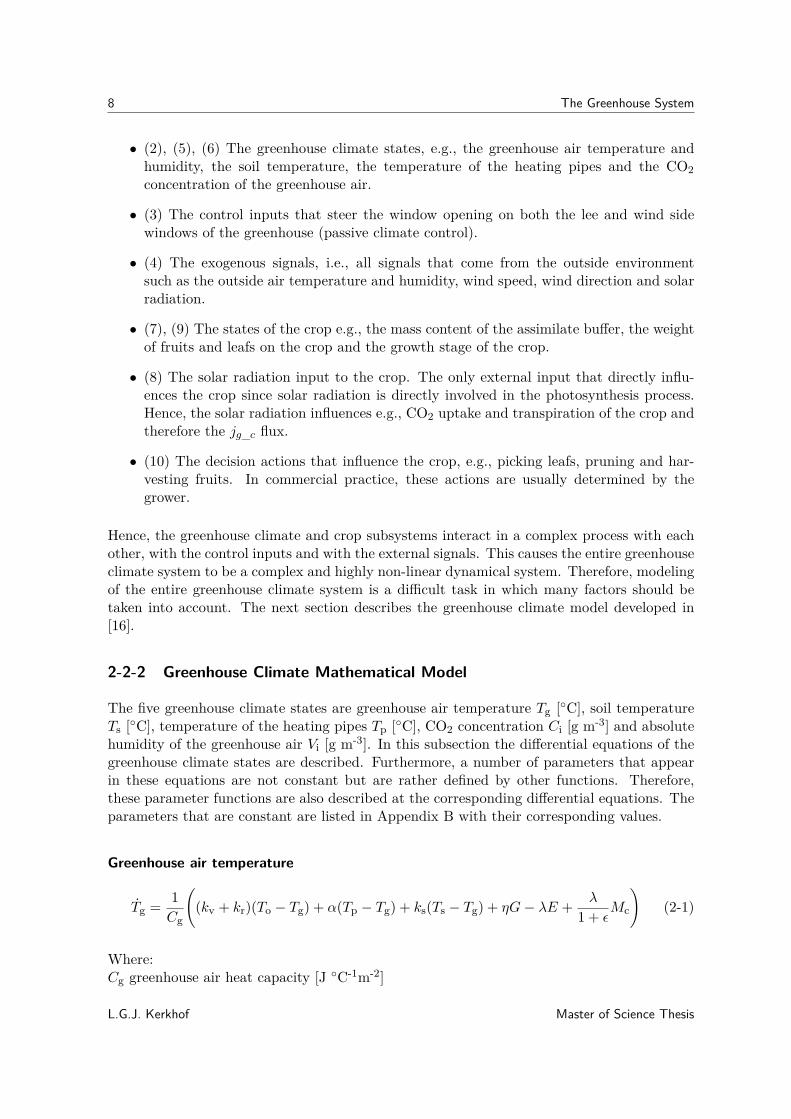
The five greenhouse climate states are greenhouse air temperature Tg [◦C], soil temperatureTs [◦C], temperature of the heating pipes Tp [◦C], CO2 concentration Ci [g m-3] and absolutehumidity of the greenhouse air Vi [g m-3]. In this subsection the differential equations of thegreenhouse climate states are described. Furthermore, a number of parameters that appearin these equations are not constant but are rather defined by other functions. Therefore,these parameter functions are also described at the corresponding differential equations. Theparameters that are constant are listed in Appendix B with their corresponding values.
Greenhouse air temperature
Tg = 1Cg
((kv + kr)(To − Tg) + α(Tp − Tg) + ks(Ts − Tg) + ηG− λE + λ
1 + εMc
)(2-1)
Where:Cg greenhouse air heat capacity [J ◦C-1m-2]
L.G.J. Kerkhof Master of Science Thesis

2-2 The Greenhouse Climate System 9
kv ventilation heat transfer coefficient [W ◦C-1m-2]kr cover heat transfer coefficient [W ◦C-1m-2]To outside temperature [◦C]α pipe heat transfer coefficient [W ◦C-1m-2]ks soil heat transfer coefficient [W ◦C-1m-2]η greenhouse transmission [-]G solar radiation [W m-2]λ evaporation energy water [J g-1]E transpiration rate crop [g s-1m-2]Mc condensation mass flow [g s-1m-2]ε greenhouse cover heat resistance [-]
The parameters listed above which are not constant but defined by a function instead aredescribed below:
The ventilation heat transfer coefficient kv is defined by the following function:
kv = ρacpΦv (2-2)
Where, ρa is the air density [g m-3], cp is the air specific heat at constant pressure [J◦C-1m-2]and Φv is the ventilation flux which on its turn is defined by:
Φv =(
σφlee1 + χφlee
+ ζ + ξφwind
)w + ψ (2-3)
Where, φlee is the lee side opening [%], φlee is the wind side opening [%], w is the wind speed[ms-1] and σ, χ, ζ, ξ and ψ are ventilation rate parameters.
The heat transfer coefficient of the pipes α is defined by:
α = ν
√τ +
√|Tg − Tp| (2-4)
Where, ν and τ are heat transfer coefficient parameters of the heating pipes.
The vaporisation energy of water is defined by:
λ = l1 − l2Tg (2-5)
Where, l1 and l2 are vaporisation energy coefficients.
The crop transpiration rate is defined by:
E = sηG+ ρacpDggb
λ(s+ γ(1 + gb
g )) (2-6)
Master of Science Thesis L.G.J. Kerkhof

10 The Greenhouse System
Where, s is the slope of the saturated water vapour pressure curve [kPa◦C-1], Dg is the airvapour pressure deficit [kPa], gb is the leaf boundary layer conductance [ms-1], γ is the ap-parent psychometric constant [kPa◦C-1] and g is the leaf conductance [ms-1].
The slope of the saturated water vapour pressure curve is defined by:
s = s1T2g + s2Tg + s3 (2-7)
Where, s1, s2 and s3 are saturated water vapour pressure curve slope coefficients.
The air vapour pressure deficit is defined by:
Dg = p∗g − pg (2-8)
Where, p∗g is the greenhouse air saturated vapour pressure [kPa] and pg is the greenhouse air
vapour pressure [kPa] which on their turn are defined by:
p∗g = a1e
a2Tga3+Tg (2-9)
pg = ΛTgVi (2-10)
Where, a1, a2 and a3 are saturation vapour pressure parameters and Λ is a pressure constantderived from the ideal gas law [Nm◦C-1g-1].
The leaf conductance is defined by:
g = g1(1− g2e
−g3G)e−g4Ci (2-11)
Where, g1, g2, g3 and g4 are leaf conductance parameters.
Finally, the greenhouse cover condensation mass flow is defined by:
Mc ={m1|Tg − Tc|m2(Wg −W ∗
c ), if Wg > W ∗c
0, if Wg ≤W ∗c
(2-12)
Where, m1 and m2 are mass transfer parameters. Tc is the temperature at the greenhousecover [◦C]. Wg is the greenhouse air humidity ratio [-] at vapour pressure pg and W ∗
c isthe greenhouse air humidity ratio [-] at saturated vapour pressure p∗
g at the cover and arecalculated by:
W (p) = ωp
patm − p(2-13)
Where, ω is a humidity ratio parameter and patm is the atmospheric pressure [kPa]. Tc isapproximated by:
Tc = ε
ε+ 1To + 1εTg (2-14)
L.G.J. Kerkhof Master of Science Thesis

2-2 The Greenhouse Climate System 11
Heating pipe temperature
Tp = 1Vp
(φh(Th − Tp) + Ap
ρwCp
(βG− α(Tp − Tg)
))(2-15)
Where:Vp heating pipe volume [m3]φh opening heating valve [-]Th heating water temperature [◦C]Ap heating pipe surface [m2]ρw density water [g m-3]Cp specific heat of water at constant pressure [J◦C-1m-2]β heat absorption coefficient [-]
Soil temperature
Ts = 1Cs
(ks(Tg − Ts) + kd(Td − Ts)
)(2-16)
Where:Cs greenhouse soil heat capacity [J ◦C-1m-2]kd deep soil heat transfer coefficient [W ◦C-1m-2]Td deep soil temperature [◦C]
Greenhouse air CO2 concentration
Ci =(VgAg
)−1(Φv(Co − Ci) + φinj +R− µP
)(2-17)
Where:VgAg
average greenhouse height [m]Φv ventilation flux [m s-1]Co outside CO2 concentration [kg m-3]φc CO2 injection flux [g s-1 m-2]R crop respiration [g s-1m-2]µ fraction molar weight CO2 and CH2O [-]P crop photosynthesis [g s-1m-2]
Master of Science Thesis L.G.J. Kerkhof

12 The Greenhouse System
Greenhouse air absolute humidity
Vi =(VgAg
)−1(E − Φv(Vi − Vo)−Mc
)(2-18)
Where:Vo outside humidity [kg m-3]
Combining (2-1), (2-16), (2-15), (2-17) and (2-18) we obtain the following dynamical modelfor the greenhouse climate:
xg = f(xg, u, v) (2-19)
Where xg denotes the greenhouse climate state vector, u denotes the vector with controlinputs and v denotes the vector with external signals:
xg =
TgTpTsCiVi
, u =
Thφleeφwindφc
, v =
ToTdCoVowG
(2-20)
L.G.J. Kerkhof Master of Science Thesis

2-3 The Greenhouse Crop System 13
2-3 The Greenhouse Crop System
2-3-1 Schematic Description of the Greenhouse Crop
Figure 2-3: Block scheme of the greenhouse tomato crop system [24].
In Figure 2-3, a block scheme is shown which shows the main processes involved in the growthof a tomato crop. The diagram start with photosynthesis (1) where solar radiation is usedto produce assimilates. The assimilates produced by photosynthesis are transferred (p) tothe assimilate buffer (4) where accumulation of assimilates takes place. From this bufferassimilates are again transferred (gr, g) in order to be used for growth respiration (2) anddistribution (5) among the fruits, stems, leafs and roots as the crop grows. Growth respirationis the process where assimilates are combined with oxygen and converted to energy requiredfor crop growth. After distribution, the assimilates are converted into biomass (6) or used formaintenance respiration (3, m). Finally, the resulting biomass can be harvested in the formof fruits (7, h1) or leafs (8, h2).
Obviously, the model here is a simplified version of the real crop growth process. The as-sumption is done that irrigation is done properly and the influence of fertigation is left outdue to the complex, and partly unknown, chemical interaction between different fertilizersand the greenhouse crop. Furthermore, other processes such as pollination and diseases areomitted and assumed to cause no limitations in the growth of the crop.
2-3-2 Greenhouse Crop Mathematical Model
The greenhouse crop model used in this thesis is obtained from [16]. This model is a so calledbig-fruit big-leaf model, i.e., it considers the total fruit and leaf weight in single states insteadof considering every fruit or leaf in a separate state. This approach is convenient for use incontrol algorithms since it limits the number of states substantially. For example, the tomatocrop model developed in [25] uses 2 states per truss, 6 states per fruit, 4 for each vegetativeunit (part of the stem and leaf corresponding to a truss) and 4 for the overall plant. Hence,
Master of Science Thesis L.G.J. Kerkhof

14 The Greenhouse System
for a full-grown tomato crop with 6 trusses and 8 fruits per truss, the total number of stateswould be 328 states. This is in clear contrast with the model from [16], which only uses atotal of four states to describe the crop.The states described in this model are the assimilate buffer dry weight per ground area mB [gm-2], the weight of the fruits per ground area mF [g m-2], the weight of the leafs per groundarea mL [g m-2] and the crop development stage D [-]. The crop states are represented bydifferential equations. Similar to the greenhouse climate states, there are parameters whichappear in these equations which are not constant but rather depend on other functions. Again,these parameter functions are described at the corresponding differential equations and theparameters that are constant are listed in Appendix B with their corresponding values.Each state is influenced by processes such as photosynthesis or fruit/leaf harvesting whichare in their turn determined by equations.
Assimilate buffer dry weight
mB = P − b(fgFmF + vgL
mLz
)− b(rFmF + rL
mLz
)(2-21)
Where:P crop photosynthesis [g s-1m-2]b buffer switching function [-]f is the fruit assimilate requirement quotient [-]gF relative fruit growth rate [s-1]v is the vegetative requirement quotient [-]gL is the relative leaf growth rate [s-1]z is the leaf fraction of vegetative dry weight [-]rF is the relative fruit respiration rate [s-1]rL is the relative leaf respiration rate [s-1].
The first term on the right hand side in (2-21) represents the assimilate production by pho-tosynthesis. The middle term on the right hand side in (2-21) represents the assimilatesto biomass conversion and distribution where constant distribution parameters are assumed.The right term on the right hand side in (2-21) represents the respiration for both the fruitsand the vegetative part of the crop. The parameters listed above which are not constant butdefined by a function instead are described below:The crop photosynthesis is defined by the following function:
P = PmlI
p1 + I
C
p2 + C(2-22)
Where Pm is the maximum photosynthesis rate [g s-1m-2], l is the LAI correction function [-],I is the PAR [µmol s-1-2], C is the CO2 concentration [ppm] and p1, p2 are photosynthesisparameters.
The PAR is defined by:I = ηmpG (2-23)
L.G.J. Kerkhof Master of Science Thesis

2-3 The Greenhouse Crop System 15
Where mp is the Watt to µmol conversion factor.
The CO2 in ppm is calculated by:
C = 106RgMCO2patm
(Tg + T0)Ci (2-24)
Where Rg is the gas constant [Jmol-1K-1], MCO2 is the molar mass of CO2 [kg] and T0 is afactor to convert the temperature from Celsius to Kelvin.
The LAI correction function is defined by:
l =
(WLwR
)m1 +
(WLwR
)m (2-25)
Where wR and m are LAI correction function coefficients.
The buffer switching function is defined by:
b = 1− e−b1B (2-26)
This function tends to zero when the assimilate buffer is empty and tends to one when theassimilate buffer is full; hence the name switching function. b1 is a buffer switching parameter.
The relative fruit and leaf growth rates, respectively, are defined by:
gF = (f1 − f2DP)QTg−TG
10G (2-27)
gL = gFv1ev2(Tg−v3) (2-28)
Where f1 and f2 are fruit growth rate coefficients, QG is the Q10-value for the temperatureeffect on fruit growth rate, TG is the growth rate reference temperature and v1, v2 and v3 arevegetative fruit growth ratio coefficients.
The relative fruit and leaf respiration rates, respectively, are defined by:
rF = MFQTg−TG
10R (2-29)
rL = MLQTg−TG
10R (2-30)
Where QR is the Q10-value for the temperature effect on the maintenance respiration andMFand ML are the fruit and leaf maintenance respiration coefficients, respectively.
Master of Science Thesis L.G.J. Kerkhof

16 The Greenhouse System
Fruit weightmF =
(bgF − (1− b)rF − hF
)mF (2-31)
Where:hF fruit harvest rate [s-1]
Here, the first term on the right hand side represents the growth of the fruit. The middleterm on the right hand side represents the respiration necessary for fruit growth and the rightterm on the right hand side represents the harvest of the fruits.
Leaf weightmL =
(bgL − (1− b)rL − hL
)mL (2-32)
Where:hL leaf harvest rate [s-1]
Here, the first term on the right hand side represents the growth of the leafs. The middleterm on the right hand side represents the respiration necessary for leaf growth and the rightterm on the right hand side represents the harvest of the leafs.
The harvest coefficient is defined by:
h =
0, if 0 < D < 1d1 + d2ln
(Tgd3
)+ d4t, if D = 1
(2-33)
Then, the fruit and leaf harvest coefficients are defined by:
hF = yFh (2-34)
hL = yLh (2-35)
Here, yF and yL are the fruit harvest coefficient parameters.
Crop development stage
D = d1 + d2 + ln(Tgd3
)+ d4t− h (2-36)
Where:d1, d2, d3 and d4 are plant development rate parameterst is the timeh is the harvest coefficient [s-1].
The crop development stage starts at zero and increases to one while the crop develops. Themoment when D becomes one means that the crop has developed in such a way that the firstfruits can be harvested. At that moment, D remains constant, i.e., D = 0.
L.G.J. Kerkhof Master of Science Thesis

2-4 Greenhouse Simulation 17
Finally, for a given period from t0 until tf the total harvest of fruits and leaves is computedas follows:
WHF =∫ tf
t0hFWFdt (2-37)
WHL =∫ tf
t0hLWLdt (2-38)
Combining (2-21), (2-31), (2-32) and (2-36) we obtain the following dynamical model for thegreenhouse crop:
xc = f(xc, xg, t, v) (2-39)
Where xg and v are as defined in (2-20), t is the time and xc denotes the vector that containsthe greenhouse crop states:
xc =
mBmFmLD
(2-40)
2-4 Greenhouse Simulation
2-4-1 Discretization and Implementation
By combining both the greenhouse climate and greenhouse crop models, the complete green-house model is obtained:
x = fgh(x, u, v, t) (2-41)
Where x = [xTg , xTc ]T and fgh contains the state transition equations: (2-1), (2-16), (2-15),(2-17), (2-18) (2-21), (2-31), (2-32) and (2-36).
Now, for implementation purposes, the continuous time model (2-41) is discretized usingEuler’s method. Hence, the states are updated in the following discrete way:
x(t+ 1) = x(t) + h ∗ fgh(x(t), u(t), v(t), t) (2-42)
where h is the sampling time.
Using this discretization method, the following non-linear discrete time model is obtained:
x(t+ 1) = fgh(x(t), u(t), v(t), t) (2-43)
Since the dynamics of the greenhouse are relatively slow, the sampling time h is chosen to be300 seconds throughout this thesis. Furthermore, this is also convenient due to the fact thatthe weather condition measurements are also sampled every 5 minutes. The discrete timegreenhouse simulation model (2-41) is subsequently implemented in Matlab.
Master of Science Thesis L.G.J. Kerkhof
18 The Greenhouse System
2-4-2 Simulation Example
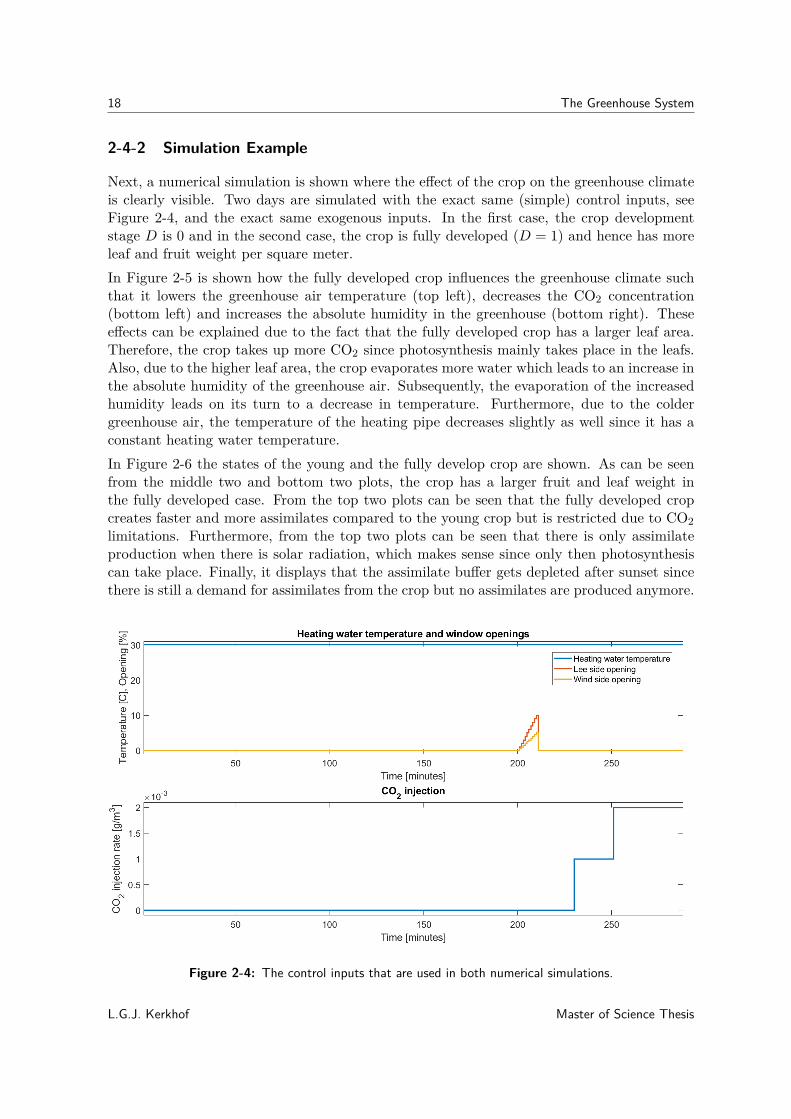
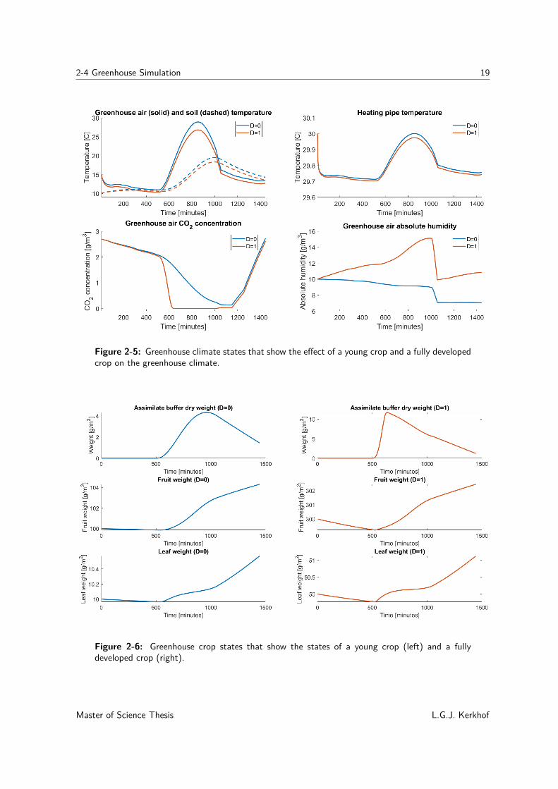
Next, a numerical simulation is shown where the effect of the crop on the greenhouse climateis clearly visible. Two days are simulated with the exact same (simple) control inputs, seeFigure 2-4, and the exact same exogenous inputs. In the first case, the crop developmentstage D is 0 and in the second case, the crop is fully developed (D = 1) and hence has moreleaf and fruit weight per square meter.In Figure 2-5 is shown how the fully developed crop influences the greenhouse climate suchthat it lowers the greenhouse air temperature (top left), decreases the CO2 concentration(bottom left) and increases the absolute humidity in the greenhouse (bottom right). Theseeffects can be explained due to the fact that the fully developed crop has a larger leaf area.Therefore, the crop takes up more CO2 since photosynthesis mainly takes place in the leafs.Also, due to the higher leaf area, the crop evaporates more water which leads to an increase inthe absolute humidity of the greenhouse air. Subsequently, the evaporation of the increasedhumidity leads on its turn to a decrease in temperature. Furthermore, due to the coldergreenhouse air, the temperature of the heating pipe decreases slightly as well since it has aconstant heating water temperature.In Figure 2-6 the states of the young and the fully develop crop are shown. As can be seenfrom the middle two and bottom two plots, the crop has a larger fruit and leaf weight inthe fully developed case. From the top two plots can be seen that the fully developed cropcreates faster and more assimilates compared to the young crop but is restricted due to CO2limitations. Furthermore, from the top two plots can be seen that there is only assimilateproduction when there is solar radiation, which makes sense since only then photosynthesiscan take place. Finally, it displays that the assimilate buffer gets depleted after sunset sincethere is still a demand for assimilates from the crop but no assimilates are produced anymore.
Figure 2-4: The control inputs that are used in both numerical simulations.
L.G.J. Kerkhof Master of Science Thesis
2-4 Greenhouse Simulation 19
Figure 2-5: Greenhouse climate states that show the effect of a young crop and a fully developedcrop on the greenhouse climate.
Figure 2-6: Greenhouse crop states that show the states of a young crop (left) and a fullydeveloped crop (right).
Master of Science Thesis L.G.J. Kerkhof

20 The Greenhouse System
L.G.J. Kerkhof Master of Science Thesis

Chapter 3
Non-Linear Model Predictive Control
3-1 Introduction
Model Predictive Control (MPC) is a predictive control algorithm that makes use of an explicitmodel of the system it aims to control. At each time step the algorithm computes the optimalcontrol input signal over a prediction horizon in order to reach a certain objective [26]. Afrequently appearing objective in MPC is reference tracking, see Figure 3-1 for a graphicalrepresentation. Furthermore, a typical example of an explicit dynamical system model is thediscrete time linear state space system:
x(t+ 1) = Ax(t) +Bu(t)y(t) = Cx(t) +Du(t)
(3-1)
Here x(t) ∈ Rn denotes the system state, u(t) ∈ Rm denotes the control input and y(t) ∈ Rpdenotes the system output at time t ∈ Z+. Furthermore, A ∈ Rn×n, B ∈ Rn×m, C ∈ Rp×n
and D ∈ Rp×m are the system matrices.
Hence, when an explicit model of a system such as (3-1) is available, an optimization problemcan be formulated where a cost function is minimized while the problem is subject to thesystem dynamics, control input constraints and state constraints [11]. Therefore, in (3-2) ageneral linear MPC optimization framework is shown, which is solved at every time step [27].Then, in Algorithm 1 the outline of the, in this case linear, MPC algorithm is shown [28].
minu
VN(x, u, r) =N−1∑k=0
`(xk, uk, rk) + Vf(xN , rN )
subject to xk+1 = Axk +Buk, ∀k ∈ {0, ..., N − 1},yk = Cxk +Duk, ∀k ∈ {0, ..., N − 1},x0 = x(t),uk ∈ U , ∀k ∈ {0, ..., N − 1},xk ∈ X , ∀k ∈ {0, ..., N − 1}.
(3-2)
Master of Science Thesis L.G.J. Kerkhof

22 Non-Linear Model Predictive Control
Figure 3-1: MPC scheme [29].
In (3-2), VN(x, u, r) is the cost function which is minimized. In this cost function, `(xk, uk, rk)is the stage cost computed at each time index k ∈ Z+ and Vf(xN , rN ) is the terminal costcomputed at the end of the prediction horizon k = N .
Furthermore, N ∈ Z++ denotes the prediction horizon horizon, u = (u0, ..., uN−1) denote thecontrol inputs which are the optimization variables, x = (x0, ..., xN ) denote the system statesas predicted by the model, y = (y0, ..., yN−1) denote the predicted system output as predictedby the model and r = (r0, ...rN ) is the desired state or output reference trajectory.
Besides, x(t) denotes the state estimate at time t where t ∈ Z+ is the time step at whichthe optimization problem is solved. Hence, if full state measurement is available, x(t) = x(t).Else, in case full state measurement is not available and the system is observable, an observeris typically used to estimate the state.
Finally, U ⊆ Rm and X ⊆ Rn denote the sets of input and state constraints, respectively.
Algorithm 1: MPCInput: System matrices (A,B,C,D), prediction horizon N , constraint sets U and X ;1) Obtain initial state estimate x(t).2) Solve (3-2) for the optimal input sequence u? = (u?0, ..., u?N−1).3) Apply only the first input u(t) = (u?0).4) Set t to t+ 1.5) Return to 1.
L.G.J. Kerkhof Master of Science Thesis

3-2 Non-Linear Model Predictive Control 23
3-2 Non-Linear Model Predictive Control
Essentially all systems are inherently stochastic and non-linear. Therefore, using (3-1) mightnot give a sufficient accurate representation of the true system dynamics. Especially in thecase of the highly non-linear dynamics of the greenhouse system, a non-linear system repre-sentation (3-3) is inevitable. Therefore, the classic non-linear discrete time system descriptionis given here:
x(t+ 1) = f(x(t), u(t), v(t))y(t) = h(x(t), u(t), v(t))
(3-3)
Here, f : Rn × Rm × Rq → Rn and h : Rn × Rm × Rq → Rp denote the nonlinear functionswhich map the current state and input to the next state and current output, respectively.Furthermore, v(t) denote the exogenous inputs at time t. With this nonlinear system repre-sentation, we arrive at the following Nonlinear Model Predictive Control (NMPC) framework[30]:
minu
VN(x, u) =N−1∑k=0
`(xk, uk, rk) + Vf(xN )
subject to xk+1 = f(xk, uk), ∀k ∈ {0, ..., N − 1},yk = h(xk, uk), ∀k ∈ {0, ..., N − 1},x0 = x(t),uk ∈ U , ∀k ∈ {0, ..., N − 1},xk ∈ X , ∀k ∈ {0, ..., N − 1}.
(3-4)
which is solved at every time step t ∈ Z+. Now, the algorithm for NMPC is shown inAlgorithm 2.
Algorithm 2: NMPCInput: Non-linear system equations f(x(t), u(t), v(t)) and h(x(t), u(t), v(t)), prediction
horizon N , constraint sets U and X ;1) Obtain initial state estimate x(t).2) Solve (3-4) for the optimal input sequence u? = (u?0, ..., u?N−1).3) Apply only the first input u(t) = (u?0).4) Set t to t+ 1.5) Return to 1.
Master of Science Thesis L.G.J. Kerkhof
24 Non-Linear Model Predictive Control
3-3 Greenhouse Controlled by NMPC
In this section, two numerical simulations will be shown where the NMPC algorithm is usedto control the greenhouse system. In the first example, NMPC will be used for trackinga reference temperature with the greenhouse air temperature. In the second example, thegoal will be to maximize the yield of the greenhouse crop while keeping the greenhouse airtemperature between a minimum and a maximum bound. In both the reference trackingand yield maximization simulations, (2-19) and (2-39) will be used as the non-linear systemequations which are required in the NMPC optimization framework (3-4). Furthermore, inboth simulations (and the remainder of this thesis) the SNOPT solver from the TOMLABOptimization Environment is used to solve the non-linear optimization problems [31].
3-3-1 Weather Conditions
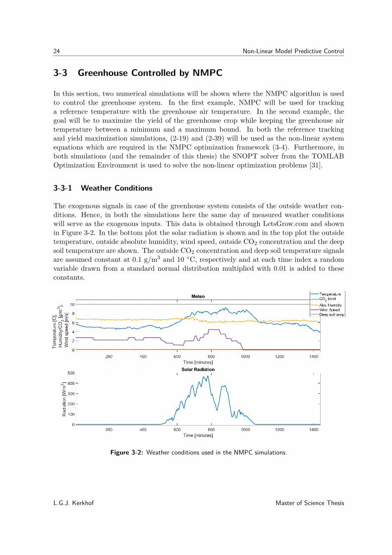
The exogenous signals in case of the greenhouse system consists of the outside weather con-ditions. Hence, in both the simulations here the same day of measured weather conditionswill serve as the exogenous inputs. This data is obtained through LetsGrow.com and shownin Figure 3-2. In the bottom plot the solar radiation is shown and in the top plot the outsidetemperature, outside absolute humidity, wind speed, outside CO2 concentration and the deepsoil temperature are shown. The outside CO2 concentration and deep soil temperature signalsare assumed constant at 0.1 g/m3 and 10 ◦C, respectively and at each time index a randomvariable drawn from a standard normal distribution multiplied with 0.01 is added to theseconstants.
Figure 3-2: Weather conditions used in the NMPC simulations.
L.G.J. Kerkhof Master of Science Thesis

3-3 Greenhouse Controlled by NMPC 25
3-3-2 Reference Tracking
In this numerical simulation, the objective will be to track a reference with the greenhouseair temperature while minimizing the control input. Furthermore, a penalty is given to thechange of in control inputs in order to avoid rapid changes in window position or heatingpipe temperatures since this could lead to breakdown of the actuators due to fatigue. Thecontrol inputs will be constrained due to the physical limitations of the actuators. This meansthat the heating water temperature will be constrained between 10◦C and 80 ◦C, the windowopening will be constrained between 0% and 100%. The CO2 injection will be constrainedbetween 0 g s-1m-2 and 2*10-3 g s-1m-2. Hence, the optimization problem for reference trackingbecomes:
minu
N−1∑k=0‖Tg,k − rk‖2Q + ‖uk‖2R + ‖uk − uk−1‖2R∆
subject to xk+1 = fg(xk, uk), ∀k ∈ {0, ..., N − 1},x0 = x(t),ul ≤ uk ≤ uu, ∀k ∈ {0, ..., N − 1}.
(3-5)
Here, Q � 0, R � 0 and R∆ � 0 are positive semi-definite matrices that represent the coston reference deviation, control input and change of control input, respectively. Furthermore,Tg,k denotes the temperature of the greenhouse air at time k and ul and uu are the lower andupper bounds of the set U , respectively. For this numerical simulation, full state measurementis assumed, no terminal cost is used and the parameters are chosen as follows:N = 12Q = diag(500, 0, ..., 0)R = 0.1I4R∆ = r∆I4ul = [10, 0, 0, 0]Tuu = [80, 100, 100, 2 ∗ 10−3]T
Two different simulations are done for r∆ = 10 and r∆ = 1 in order to show the differenceswhen the penalty on change of control is larger.
In Figure 3-3 and Figure 3-4 the results of the reference tracking simulations are shown.As can be seen from Figure 3-3, the greenhouse air temperature is driven to the referenceas desired. Furthermore, the control input signals are smoother for r∆ = 10 while betterreference tracking is achieved while using r∆ = 1. Hence, a trade-off needs to be madebetween the accuracy of the reference tracking and the aggressiveness of the control inputs.
Master of Science Thesis L.G.J. Kerkhof

26 Non-Linear Model Predictive Control
Figure 3-3: Greenhouse air (top) and heating pipe (bottom) temperatures controlled by NMPCfor r∆ = 10 and r∆ = 1.
Figure 3-4: Control inputs computed by NMPC for different values of r∆. The top plot showsthe heating water temperature for r∆ = 10 and r∆ = 1, respectively. The middle plot shows thelee and wind side window openings for r∆ = 10 and the bottom plot shows the lee and wind sideopening for r∆ = 1.
L.G.J. Kerkhof Master of Science Thesis

3-3 Greenhouse Controlled by NMPC 27
3-3-3 Yield Maximization
Besides reference tracking to maintain an optimal temperature, another goal of NMPC mightbe to maximize the yield. Since we have access to both a climate and a crop model, thesemodels might be used together to maintain an optimal growth climate while balancing thecosts of resources and the gains of yield. Furthermore, the goal will be to keep the temper-ature within desired bounds. Hence, constraints will be placed such that the greenhouse airtemperature state is constraint within those bounds. However, due to exogenous signals thesystem can be driven out of the desired range, which will result in a region where the NMPCproblem is infeasible. Therefore, in order to avoid infeasibility problems, these constraintswill be softened by using slack variables [32].
Therefore, the optimization problem becomes:
minu
N−1∑k=0−mF,k + ‖uk‖2R + λε‖ε‖1
subject to xk+1 = fg(xk, uk), ∀k ∈ {0, ..., N − 1},x0 = x(t),ul ≤ uk ≤ uu, ∀k ∈ {0, ..., N − 1},
xl − ε ≤ xTempk ≤ xu + ε ∀k ∈ {0, ..., N − 1},
ε ≥ 0
(3-6)
Where mF,k denotes the fruit weight state at time index k. Furthermore, ε ∈ R denotesa slack variable that represents the temperature constraint violation. Hence, if ε = 0, thetemperature constraints are satisfied. λε ∈ R denotes the penalty on the slack variable.
For this numerical result, the parameters are chosen as follows:N = 12R = diag(0.01, 0.01, 0.01, rCO2)λε = 105
xl = 15xu = 22ul = [10, 0, 0, 0]Tuu = [80, 100, 100, 2 ∗ 10−3]T
In the variables above, xl and xu are the lower and upper bounds on the states, respectively.Furthermore, rCO2 denotes the penalty on the CO2 injection control input. Two differentnumerical simulations are performed for both rCO2 = 100 and rCO2 = 500 in order to showthe differences when the penalty on CO2 injection is larger.
Master of Science Thesis L.G.J. Kerkhof

28 Non-Linear Model Predictive Control
In Figure 3-5, Figure 3-6 and Figure 3-7 the results of the yield maximization simulationare shown. As can be seen from Figure 3-5, the temperature of the greenhouse air is keptbetween the desired bounds of 15 ◦C and 22◦C. Since the CO2 concentration and injectiononly effect the greenhouse crop and not the greenhouse temperature, the same greenhouseair temperature, heating pipe temperature, heating water temperature and window openingswere realized for both cases of rCO2 = 100 and rCO2 = 500. Therefore, these are only shownonce since they are similar for both cases of rCO2 .
In Figure 3-6 can be seen that with higher CO2 levels, more assimilates are produced, which isa logical cause since a higher CO2 level enables a higher photosynthesis capacity. Furthermore,at the end of the day when the light levels decrease, the photosynthesis decreases as well. Thiscauses in its turn a depletion of the assimilate buffer as all assimilates are used in order tofrom new biomass for the fruits, stems, leafs or for respiration. From the fruit weight plotcan be seen that at the end of the day, the fruit weight is higher with a lower penalty on theCO2 injection compared to the higher penalty.
Furthermore, from Figure 3-7 can be seen that CO2 is dosed only in presence of solar radia-tion. Obviously, this makes sense since without solar radiation no photosynthesis is realized.However, from this figure can also bee seen that at the middle of the day when the light levelsare high, the CO2 dosage decreases. This can be clarified due to the fact that the CO2 willgo directly out of the window when the windows are open. The windows open in order toprevent too high temperatures when there is high radiation, therefore making it too costly todose CO2 when only a small part is used by the crop and a large part goes out of the window.
Figure 3-5: Greenhouse air and heating pipe temperatures (top) and greenhouse air CO2 con-centration (bottom) controlled by NMPC for rCO2 = 100 and rCO2 = 500.
L.G.J. Kerkhof Master of Science Thesis

3-3 Greenhouse Controlled by NMPC 29
Figure 3-6: Assimilate buffer dry weight (top) and fruit dry weight (bottom) controlled by NMPCfor rCO2 = 100 and rCO2 = 500.
Figure 3-7: Control inputs computed by NMPC for different values of rCO2 . The top plot showsthe heating water temperature for both rCO2 = 100 and rCO2 = 500. The middle plot shows thewindow positions on lee and wind side for both rCO2 = 100 and rCO2 = 500. The bottom plotshows the CO2 injection for both rCO2 = 100 and rCO2 = 500.
Master of Science Thesis L.G.J. Kerkhof

30 Non-Linear Model Predictive Control
L.G.J. Kerkhof Master of Science Thesis
Chapter 4
Data-Enabled Predictive Control
4-1 Introduction
Data-Enabled Predictive Control (DeePC) is a predictive control algorithm that computesoptimal control policies using real-time feedback driving the unknown system along a desiredtrajectory while satisfying system constraints [11]. The algorithm uses a finite number of datasamples from the unknown system to learn a non-parametric system model that represents thedynamics of the system. This non-parametric system model is subsequently used to implicitlyestimate the state and to predict future input/output trajectories of the unknown system.
Therefore, the DeePC algorithm replaces system identification, state estimation and trajectoryprediction by one single optimization framework that determines the non-parametric model,implicitly estimates the state and optimizes the system trajectory over a future horizon.
The theory on exploiting a non-parametric model arises from behavioural systems theory.Therefore, the next section introduces a few preliminaries from behavioural systems theoryon which the DeePC algorithm relies.
4-2 Behavioural Systems Theory
Within behavioural systems theory a dynamical system is described by its behaviour, i.e. thedynamical systems are defined by the subspace of the signal space in which trajectories ofthe system live. This is different from classical systems theory where a particular parametricsystem representation is used to describe the system. Often, system properties are definedon representation level and therefore these properties might be dependent on their particularrepresentation. Hence, viewing a system from the behavioural systems theory perspective isa more general way in the sense that system properties can be defined in terms of the systemsbehaviour, independent of any representation. The following definitions describe a dynamicalsystem and its properties from a behavioural systems theory perspective [11][33]:
Master of Science Thesis L.G.J. Kerkhof

32 Data-Enabled Predictive Control
Definition 4.1: A dynamical system is a 3-tuple Σ = (Z+,W,B) where Z+ is the discrete-time axis, W is the signal space and B ⊆WZ+ is the behaviour.
Definition 4.2: Let Σ = (Z+,W,B) be a dynamical system.
(i) A system Σ = (Z+,W,B) is said to be linear if the signal space W is a vector spaceand B is a linear subspace of WZ+ .
(ii) A system Σ = (Z+,W,B) is said to be time-invariant if B ⊆ σB where σ is the forwardshift operator: (σw)(t) := w(t+ 1) and σB = {σw | w ∈ B}.
(iii) A system Σ = (Z+,W,B) is said to be complete if:w |[t0,t1]∈ B |[t0,t1], ∀ t0, t1 ∈ Z+, t0 ≤ t1 ⇒ w ∈ B
The class of systems (Z+,Rm+p,B) satisfying (i)-(iii) is denoted by Lm+p, with m, p ∈ Z+.Any trajectory w ∈ B can be written as w = col(u, y), where col(u, y) := (uT , yT )T [11].
Definition 4.3: A system B ∈ Lm+p is controllable if for any two trajectories w1, w2 ∈ B,there is a third trajectory w ∈ B, such that w1(t) = w(t), ∀ t < 0, and w2(t) = w(t), ∀ t ≥ 0.
Definition 4.4: Let L, T ∈ Z++ such that T −L+ 1 ≥ mL. The signal u = col(u1, ..., uT ) ∈RmT is persistently exciting of order L if the Hankel matrix
HL(u) :=
u1 · · · uT−L+1... . . . ...uL · · · uT
is full row rank.
The definitions above describe the non-parametric system representation. Multiple equivalentways exist to represent a behavioural system in a parametric representation. One of them isthe discrete time state space system (3-1) where B ∈ Lm+p is represented by B(A,B,C,D) ={col(u, y) ∈ (Rm+p)(Z+) | ∃ x ∈ (Rn)(Z+) s.t. x(t + 1) = Ax(t) + Bu(t), y(t) = Cx(t) +Du(t)}. The state space representation of smallest order is called a minimal representationof the system and the minimal order is denoted by n(B). Furthermore, denote the lag of asystem B ∈ Lm+p by l(B). The lag is defined as the smallest integer l ∈ Z++ such that theobservability matrix Ol(A,C) := col(C,CA, ..., CAl−1) has rank n(B). Finally, define thelower triangular Toeplitz matrix, denoted by T , as follows:
TN (A,B,C,D) :=
D 0 · · · 0CB D · · · 0... . . . . . . ...
CAN−2B · · · CB D
(4-1)
L.G.J. Kerkhof Master of Science Thesis

4-3 Data-Enabled Predictive Control 33
Now, two useful lemmas can be presented:
Lemma 4.1 ([34], Lemma 1): Let B(A,B,C,D) be a minimal state space representationof B ∈ Lm+p and let Tini, Tf ∈ Z++ with Tini ≥ l(B) and col(uini, u, yini, y) ∈ BTini+Tf
. Thenthere exists a unique xini ∈ Rn(B) such that:
yf = OTf(A,C)xini + TTf
(A,B,C,D)uf (4-2)
Hence, if the window of initial system data col(uini, yini) is sufficiently long, the state xini towhich the system is driven by the sequence of inputs uini is unique.
Lemma 4.2 ([35], Theorem 1): Consider a controllable system B ∈ Lm+p and let T, t ∈Z++ and w = col(u, y) ∈ BT . Furthermore, let u to be persistently exciting of order t+n(B).Then colspan(Ht(w)) = Bt.
Hence, the Hankel matrix, consisting of a finite amount of data samples, provides a way toreplace the required model or the preliminary system identification procedure.
4-3 Data-Enabled Predictive Control
Data Collection DeePC is a data-driven control algorithm. Hence, the first step is to collectdata. First there is assumed that the data is generated by an unknown controllable LTI systemB ∈ Lm+p. Let T, Tini, Tf ∈ Z++ such that T ≥ (m + 1)(Tini + Tf + n(B))− 1. Then in anoffline procedure a sequence of T inputs ud = col(ud1, ..., udT ) ∈ RmT is applied to the unknownsystem and the corresponding outputs yd = col(yd1 , ..., ydT ) ∈ RpT are collected. Here, thesuperscript d is used to denote the offline collected data. Next the data is separated into apast and future part:
(UpUf
):= HTini+Tf
(ud),(YpYf
):= HTini+Tf
(yd) (4-3)
where Up consists of the first Tini block rows of HTini+Tf(ud) and Uf consists of the last Tf
block rows of HTini+Tf(ud) (similar for Yp and Yf ). The past data matrices Up and Yp will
be used to implicitly estimate the initial state whereas the future data matrices Uf and Yfwill be used to predict the future trajectories of the system. Below is shown in detail how theHankel matrix HTini+Tf
(ud) is divided in Up and Uf (similar division holds for HTini+Tf(yd)):
(UpUf
)=
u1 u2 . . . uT−Tini−Tf +1...
... . . . ...uTini uTini+1 . . . uT−Tf
uTini+1 uTini+2 . . . uT−Tf +1...
... . . . ...uTini+Tf
uTini+Tf +1 . . . uT
(4-4)
Master of Science Thesis L.G.J. Kerkhof

34 Data-Enabled Predictive Control
Now using the result of Lemma 4.2: with the collected data, any trajectory of BTini+Tfof
length Tini +Tf could be constructed. It follows that a trajectory col(uini, uf , yini, yf ) belongsto BTini+Tf
if and only if there exists g ∈ RT−Tini−Tf +1 such that:UpYpUfYf
g =
uiniyiniufyf
(4-5)
Now using the result of Lemma 4.1: if Tini ≥ l(B), Lemma 4.1 implies that there exists aunique xini ∈ Rn(B) such that yf is uniquely determined by (4-2). Hence, when solving thefirst three block rows of (4-5) for g, a unique output yf can be computed based on inputs ufand the initial trajectory col(uini, yini).
Data-Enabled Predictive Control Next, the DeePC algorithm will be formulated. Considerthe following optimal control problem:
ming
Tf −1∑k=0
(‖yf,k − rt+k‖2Q + ‖uf,k‖2R)
subject to
UpYpUfYf
g =
uiniyiniufyf
,uk ∈ U , ∀k ∈ {0, ..., Tf − 1},yk ∈ Y, ∀k ∈ {0, ..., Tf − 1}.
(4-6)
Where Tf ∈ Z++ is the time horizon, r = (r0, r1, ...) ∈ RpTf is the output reference trajectory,col(uini, yini) ∈ BTini is the past input and output data, U ⊆ Rm is the input constraint set,Y ⊆ Rp is the output constraint set. Furthermore, ‖uk‖2R denotes uTkRuk (similar for ‖.‖Q),where R ∈ Rm×m denotes the positive semi-definite control cost matrix and Q ∈ Rp×p denotesthe positive semi-definite output cost matrix.
The optimization problem in (4-6) is solved at every time step t ∈ Z+. Furthermore, inAlgorithm 3 the DeePC algorithm is shown.
Algorithm 3: DeePCInput: col(ud, yd) ∈ BT , reference trajectory r ∈ RpTf , past input/output data
col(uini, yini) ∈ BTini , constraint sets U and Y and cost matrices Q and R;1) Solve (4-6) for g?.2) Compute the optimal input sequence u? = Ufg
?.3) Apply input u(t), ..., u(t+ s) = (u?0, ..., u?s) for some s ≤ N − 1.4) Set t to t+ s and update uini and yini to the Tini most recent input/outputmeasurements.5) Return to 1.
L.G.J. Kerkhof Master of Science Thesis

4-4 Greenhouse Controlled by DeePC 35
In Figure 4-1, a graphical representation is shown on how the data of the different input/out-put trajectories is used. First, the data which captures the system dynamics is collectedduring a trajectory of length T . Then, a trajectory of length Tini is measured to implicitlyestimate the initial state of the system. This is done by solving the equality constraintsUpg = uini and Ypg = yini. Finally, an input/output trajectory of length Tf is predicted byuf = Ufg and yf = Yfg, respectively. Hence, the vector g contains the optimization variableswhich are used to fix the system dynamics, the state estimation and trajectory prediction.
Figure 4-1: DeePC scheme
4-4 Greenhouse Controlled by DeePC
4-4-1 Including Exogenous Signals
In this section, the DeePC algorithm is used to control the greenhouse system. Since theexogenous inputs such as solar radiation and outside temperature have large effects on thestates of the greenhouse, theses exogenous input signals need to be taken into account as wellbesides only the control input and output signals. Hence, the DeePC algorithm in (4-6) needsto be extended in order to include these exogenous signals. In case of the greenhouse system,the exogenous inputs are the outside weather conditions. Hence, these are measured in thepast and forecast are available for the future. Therefore, a Hankel matrix is constructed inthe same way as is done in (4-3) but it is build from the exogenous signal data. Hence, giventhe recorded data vd = col(v1, ..., vT ) ∈ RqT a Hankel matrix is constructed such that:
HTini+Tf(v) :=
v1 · · · vT−Tini−Tf +1... . . . ...
vTini+Tf· · · vT
(4-7)
Subsequently, this matrix is separated into a past and a future part similar to (4-3):(VpVf
):= HTini+Tf
(vd) (4-8)
Master of Science Thesis L.G.J. Kerkhof

36 Data-Enabled Predictive Control
where Vp consists of the first Tini block rows of HTini+Tf(vd) and Vf consists of the last Tf
block rows of HTini+Tf(vd). In the same way as is done in (4-5), the past Tini measurements of
the external signals are stored in col(vini) ∈ RqTini and the future Tf forecasts of the externalsignals are stored in vf ∈ RqTf . The equality constraints in (4-5) are then augmented withthe aforementioned data matrices and vectors such that:
UpVpYpUfVfYf
g =
uiniviniyiniufvfyf
(4-9)
4-4-2 Extension to Non-Linear Systems
Furthermore, since the dynamics of the greenhouse system are non-linear, the equation Ypg =yini might become infeasible in non-linear regions of the system dynamics. Therefore, theconstraint is softened by using a slack variable to allow constraint violation. Besides, dueto the stochastic nature of the exogenous signals, the equations VP g = vini and Vfg = vfmight become infeasible as well. Therefore, these equations are relaxed with a slack variablein the same way in order to avoid possible infeasibilities. Hence, the constraints in (4-9) areextended with auxiliary slack variables σy ∈ RpTini , σv1 ∈ RqTini and σv2 ∈ RqTf :
UpVpYpUfVfYf
g =
uiniviniyiniufvfyf
+
0σv1
σy0σv2
0
(4-10)
4-4-3 Window Constraint
When cooling the greenhouse, the wind side window has a larger effect on the ventilationrate compared to the lee side window. Hence, it might be desirable to keep the wind sidewindow opening at a relative lower opening compared to the lee side window. Therefore, aninequality constraint will be added in order to preserve the difference between the lee sideand wind side window openings:
Uf,leeg ≥ 2Uf,windg (4-11)
Here, Uf,lee and Uf,wind denote the rows of the Uf Hankel matrix that correspond to the leeside and wind side window openings, respectively. Furthermore, this additional constraintalso decreases the computation time since it limits the search space when optimizing over g.
L.G.J. Kerkhof Master of Science Thesis

4-4 Greenhouse Controlled by DeePC 37
4-4-4 Regularized DeePC
Now, including the constraints formulated in (4-10) and (4-11), we arrive at the followingoptimization problem:
ming
Tf −1∑k=0
(‖yf,k − rt+k‖2Q + ‖uf,k‖2R) + λy‖σy‖1 + λv‖σv‖1
subject to
UpVpYpUfVfYf
g =
uiniviniyiniuvy
+
0σv1
σy0σv2
0
,
Uf,leeg ≥ 2Uf,windg,
σv1 ≥ 0,σv2 ≥ 0,σy ≥ 0,uk ∈ U , ∀k ∈ {0, ..., Tf − 1}.
(4-12)
Here, λy ∈ R+ and λv ∈ R+ are regularization parameters on the constraint violations andσv = [σTv1 , σ
Tv2 ]T .
The optimization problem in (4-12) is subsequently solved at each time step t ∈ Z+. Further-more, in Algorithm 4 the extended regularized DeePC algorithm is shown.
Algorithm 4: Extended regularized DeePCInput: col(ud, vd, yd) ∈ BT , reference trajectory r ∈ RpTf , past input/output data
col(uini, vini, yini) ∈ BTini , constraint sets U and Y and output cost matrix Q andcontrol cost matrix R;
1) Solve (4-12) for g?.2) Compute the optimal input sequence u? = Ufg
?.3) Apply input u(t), ..., u(t+ s) = (u?0, ..., u?s) for some s ≤ Tf − 1.4) Set t to t+ s and update uini, vini and yini to the Tini most recent input/outputmeasurements.5) Return to 1.
4-4-5 Reference Tracking with DeePC
Here, a numerical simulation is shown where the DeePC algorithm is used to control thegreenhouse system (2-43).
As described above, first data needs to be collected in order to construct the Hankel matrices.In order to ensure the control input data to be persistently exciting the system, the controlinputs will be sampled as random variables from a uniform distribution, see Figure 4-2. Theheating water temperature and the window openings are drawn from a uniform distributions
Master of Science Thesis L.G.J. Kerkhof

38 Data-Enabled Predictive Control
with a minimum and maximum values of [20,80] and [0,20], respectively. The input/outputtrajectory that was collected is of length T = 144, i.e., 12 hours of data in this case.
Furthermore, Tini = 5 and Tf = 12, i.e., the past 5 data samples are used to implicitlyestimate the state and a prediction horizon of 12 samples (1 hour) is used. Within Figure 4-2is indicated which part of the data is used in the Hankel matrix Up and which data is usedin the Hankel matrix Uf . Furthermore, R is fixed at diag(0.1, 5, 5) and λv is fixed at = 104.
In Figure 4-3 the results of the simulations are shown for different values of λy and Q. Withinthis plots, the temperatures predicted by the DeePC algorithm and the realized temperaturesby the model are compared together with the reference that needs to be tracked. Here, thepredicted temperature is the first step ahead prediction computed by the DeePC algorithm,i.e., the first entry of the vector Yfg? ∈ RpTf . The simulated temperature is the output fromthe model after applying the first predicted control input computed by the DeePC algorithm,i.e., the first m entries of the vector Ufg? ∈ RmTf .
From this figures can be seen that a high value for Q (bottom) results in good referencetracking for the model but a large mismatch in the model and prediction outputs. For a highvalue of λini is shown that there is a low mismatch between the model and prediction outputsbut the reference tracking accuracy is low. Hence, a trade-off needs to be made between areliable match of the predicted and model outputs and desirable reference tracking by varyingλy and Q.
Figure 4-2: Random generated control inputs (bottom) and corresponding outputs (top). Thegreen dashed lines and arrows indicate which part of the data is stored in Up and Uf (similar forYp and Yf ).
L.G.J. Kerkhof Master of Science Thesis

4-4 Greenhouse Controlled by DeePC 39
Figure 4-3: Model temperature and predicted temperature for different values of λy and Q.
Master of Science Thesis L.G.J. Kerkhof

40 Data-Enabled Predictive Control
L.G.J. Kerkhof Master of Science Thesis
Chapter 5
Case Study: NMPC vs DeePC
5-1 Introduction Case-Study
In this chapter a case study will be performed in order to compare the Nonlinear ModelPredictive Control (NMPC) and Data-Enabled Predictive Control (DeePC) algorithms. Theobjective for both algorithms will be to track a temperature reference with the greenhouse airtemperature on a similar day. From this day, the recorded weather conditions will be used asexogenous inputs. Afterwards, both algorithms will be compared on tracking accuracy andcomputational time.
In the previous chapter, the input/output data that is used in the Hankel matrices (4-5) inthe DeePC algorithm is randomly generated. However, in practice it is often not desired oreven impossible to apply a random generated control input signal to a system. In case ofthe greenhouse system, the greenhouse crop is sensitive to rapid changes in greenhouse airtemperature which occur by applying a random control inputs, see Figure 4-2. Therefore, acontrol input sequence will be generated using NMPC such that a ’safe’ input can be appliedto the greenhouse in order to capture its dynamics.
Furthermore, the importance of the representativeness of this data will be shown in this chap-ter. In another example, the DeePC algorithm will be leveraged twice in order to control thegreenhouse system. In the first case, the Hankel matrices will be constructed from input/out-put data where the crop is still young. In the second case, the control input and exogenoussignals will be the same, however, the system will be initialized such that the output rep-resents the dynamics of the greenhouse with a full grown crop. For both cases, a referencetracking example will be given. Afterwards, the tracking accuracy and computational timeof both these simulations will be shown as well.
The next two subsections show the recorded weather conditions and NMPC control inputdata that is used within this case-study.
Master of Science Thesis L.G.J. Kerkhof

42 Case Study: NMPC vs DeePC
5-1-1 Weather Profile
Similar recorded weather conditions will be used in order to compare both algorithms. Theseweather conditions are shown in Figure 5-1. This data will be used to construct the matricesVp and Vf in (4-5). Besides, in this figure is indicated which part of the data is used toconstruct the data matrices.
Figure 5-1: Measured weather conditions used in the DeePC algorithm.
5-1-2 Control Input Signal
In Figure 5-2 the NMPC control input signal is shown that is used to construct the Hankelmatrices Up and Uf . In this figure is indicated which part is used in the Up matrix (usedfor capturing the dynamics of the system) and which part is used in the Uf matrix (used forpredictions of the future trajectory). This control input signal is constructed while using therecorded weather data shown in Figure 3-2. Besides, in this figure is indicated which partof the data is used to construct the data matrices. A necessary condition for (4-12) to befeasible is that Up has full rank. After checking it’s rank using Matlab it turned out to be fullrank. Hence, the control input data in Figure 5-2 seems to be appropriate as control inputdata for the DeePC algorithm.
Now with both the recorded weather data shown in Figure 5-1 and the control input signalshown in Figure 5-2, the data is available to generate the output data signals (not shownhere) to construct the final two Hankel matrices Yp and Yf .
L.G.J. Kerkhof Master of Science Thesis

5-2 Controlling the Greenhouse 43
Figure 5-2: Generated NMPC input signals used in the DeePC algorithm.
5-2 Controlling the Greenhouse
Now all the data necessary is available, both algorithms can be used to track a temperaturereference. The reference is constructed in such a way that the 24 hour average temperature isapproximately 21 ◦C, which is an average also occurring in commercial practice. Furthermore,the minimum and maximum temperatures are chosen such that they are safe for the crop andthe energy of the sun can be exploited by using a higher temperature in the middle of theday and lower temperature at the start and end of the day.
Since a half day of measurements with 5 minute sampling is used to construct the Hankelmatrices T = 144. Furthermore, Tini = 5, i.e., the last 5 samples are used to implicitlyestimate the system state and Tf = 12, i.e., the prediction horizon over which the futuretrajectory of the system is predicted is 12 samples (1 hour). Other parameters that are usedin the DeePC algorithm are: Q = diag(105, 0, ..., 0), R = diag(0.1, 5, 5), λv = 104, λε = 105,ul = [10, 0, 0]T and uu = [80, 100, 100]T .
For the NMPC algorithm, the following parameters are used: N = 12, Q = diag(500, 0, ...0, ),R = 0.1I3, ∆R = I3, ul = [10, 0, 0]T and uu = [80, 100, 100]T .
In Figure 5-3 and Figure 5-4, the states and control inputs controlled and computed by bothNMPC and DeePC are shown. From this figures can be seen that both algorithms are able toaccurately track the desired reference. Furthermore, a noticeable difference is that the NMPCalgorithm returned smoother control inputs signals compared to the DeePC algorithm.
Master of Science Thesis L.G.J. Kerkhof

44 Case Study: NMPC vs DeePC
Figure 5-3: Greenhouse air and heating pipe temperatures controlled by both DeePC and NMPC.
Figure 5-4: Heating water temperature and window positions computed by both DeePC andNMPC.
L.G.J. Kerkhof Master of Science Thesis

5-3 Comparison of Algorithm Performance 45
5-3 Comparison of Algorithm Performance
In Table 5-1 the tracking accuracy, average computation time and total computation time areshown for both the NMPC and DeePC algorithms. The Root Mean Squared Error (RMSE)is used in order to make a comparison on tracking accuracy. From this table can be seenthat the NMPC algorithm has a higher reference tracking accuracy compared to the DeePCalgorithm. Furthermore, the average computation time for NMPC is approximately 30 timessmaller. However, since the sampling time is 5 minutes in this case, the DeePC algorithmwould still be able to control the greenhouse in real-time.
Table 5-1: Comparison of DeePC and NMPC on tracking accuracy and computation time.
NMPC DeePCTracking accuracy [RMSE] 0.0461 0.2572Average computation time [seconds] 0.5347 15.425Total computation time [minutes] 160.42 4642.9
Figure 5-5: Computation time per iteration for both DeePC and NMPC.
Master of Science Thesis L.G.J. Kerkhof

46 Case Study: NMPC vs DeePC
5-4 Adjusted Greenhouse Dynamics
Here, another example will be given where two numerical simulations will be performed. Inthe first simulation the input/output data in the Hankel matrices will be the same as inthe previous example. This data was obtained in a period where the crop was still young.However, within this simulation the initial state of the crop will be adapted in such a waythat it represents a full grown crop; similar to the simulation example in Chapter 1. Hence,this will influence the dynamics of the greenhouse climate while these effects are not presentin the data stored in the Hankel matrices. This will be done in order to show the sensitivityof the DeePC algorithm when data is used that is less representative for the current dynamicsof the system. Subsequently, in the second simulation the Hankel matrices will be updatedwith data from the greenhouse where the crop is fully developed. With these updated datamatrices the algorithm is used again to control the greenhouse climate in order to show thatthe DeePC algorithm is again able to control the system while the dynamics have changed.Within these examples, the same values as in Section 5-2 are used.
In Table 5-2, the tracking accuracy, average and total computation time of both simulationsare shown. From this table can be seen that the tracking accuracy of the simulation withthe new data is comparable with the tracking accuracy from the simulation in the previousexample. However, the RMSE in case of the simulation with the old data has almost doubledcompared to the case with the simulation with the new data. Hence, this shows the effectof using the old data matrices instead of the updated data matrices. The old data does notaccurately represent the dynamics of the system anymore whereas the updated data does.The computation time of both numerical simulations here is roughly equal.
In Figure 5-6 and Figure 5-7 the results from these numerical simulations are shown. As canbe seen from this figures the DeePC algorithm is sensitive to time-varying systems when thedata in the Hankel matrices becomes less representative for the current greenhouse dynamics.However, when the data is updated with more recent input/output data, the algorithm isable to recover from this and control the system accordingly. In these figures the simulationof the DeePC algorithm with the data of the young crop is indicated as ’DeePC; Old data’and the simulation with the updated data is indicated as ’DeePC; New data’.
Table 5-2: Comparison of the two DeePC simulations on tracking accuracy and computationtime.
DeePC; Old data DeePC; New dataTracking accuracy [RMSE] 0.8045 0.3800Average computation time [seconds] 9.2296 9.7268Total computation time [minutes] 46.1479 48.6340
L.G.J. Kerkhof Master of Science Thesis

5-4 Adjusted Greenhouse Dynamics 47
Figure 5-6: Greenhouse air and heating pipe temperatures controlled by DeePC based on boththe old and updated data.
Figure 5-7: Heating water temperature and window positions computed by DeePC based onboth the old and updated data.
Master of Science Thesis L.G.J. Kerkhof

48 Case Study: NMPC vs DeePC
L.G.J. Kerkhof Master of Science Thesis

Chapter 6
Irrigation Control
6-1 Introduction
The greenhouse model used in this thesis assumes that the crop is irrigated properly. This isa common assumption in many crop models. In commercial practice, irrigation if often doneby an experienced grower who irrigates the crop based on their own strategy and experience.
Nowadays, greenhouses are often equipped with sensors which measure characteristics in thesubstrate slab such as the Water Content (WC), Electrical Conductivity (EC) and tempera-ture of the slab. Hence, this data contains a lot of information about the water uptake of thecrop, e.g., when the WC decreases. Therefore, in this chapter an irrigation control algorithmis proposed. This algorithm relies on these WC measurements and on the total solar radiationsum received on a daily base. Since solar radiation has a major influence on the water uptakeof the crop, solar radiation was chosen as the quantity to relate with the WC measurements.Based on these measurements, a relation is derived between the total radiation sum and thegradient of the water content graph after the last irrigation.
6-2 Strategy
In this section, an irrigation strategy that is applied in commercial growing practice will beexplained. First, at sunrise, irrigation is provided until the slab reaches its saturation point,i.e., when drain is realized. After this point this saturation level is maintained by applying aconstant interval time such that the WC level remains constant at the saturation level. Then,the goal is to dry-down the slab a certain percentage. This is done since during the night thecrop does not use the water. Therefore, drying down the slab prevents rotting in the rootzone and it allows the slab to refill with oxygen again. However, growers determine whento stop the irrigation based on their experience. In order to automatize the irrigation, it isnecessary to predict what the dry-down is going to be during the remaining part of the dayand during the night, which will be explained in the next section.
Master of Science Thesis L.G.J. Kerkhof

50 Irrigation Control
6-3 Control Algorithm
Now, let ∆L denote the dry-down rate during the remaining part of the day when it is lightand let ∆D denote the dry-down rate when it is dark, see Figure 6-2. In order to makepredictions for these dry-down rates, historical data is collected from which dry-down ratesof previous days are derived. Furthermore, for each day the corresponding total radiationsum was collected as well. Now, with both the dry-down rates and radiation sum available,a correlation can be made between dry-down rate and amount of radiation received. Thecorrelation with radiation is made since radiation has a major influence on the water uptakeof the crop.
Now, with the necessary collected data, predictions for the dry-down rates ∆L and ∆D canbe made. This is done by fitting a linear relationship between the radiation sums and thedry-back rates to the data such that with the forecast of radiation sum, the correspondingprediction can be computed, see Figure 6-1. When fitting the linear regression, only the datapoints of the latest τ days are taken into account. This is done in order to account for thegrowth stage of the crop. Since a young crop takes up far less water compared to a full growncrop, the water uptake rate is much lower for young crops. Hence, if only the latest e.g., 14days are taken into account, the data will implicitly account for the growth stage of the crop.
Now let ∆L and ∆D denote the predictions of the dry-down rate during the light and darkperiod, respectively, and let ξdd denote the total desired dry-down [%] that needs to beachieved to maintain optimal substrate slab conditions. Furthermore, let tL and tD denotethe time in hours of the remaining light part of the day and the dark part, respectively. Thetotal dry-down of a day is then be computed by:
Total dry-down = ∆LtL + ∆DtD (6-1)
The time during the dark period tD is often known in advance since the sunrise/sunset timesand the time the lights switch on/off are available. Hence, when the estimates for the dry-down are available, the desired dry-down can be calculated as follows:
ξdd = ∆LtL + ∆DtD (6-2)
In (6-2), the only unknown quantity is now the time length of the light period. Hence,re-arranging terms yields:
tL = 1∆L
(ξdd − ∆ttD) (6-3)
Now both tL and tD are available, the total time that is necessary to dry-down the desiredamount of WC can be calculated as the sum of tL and tD. With this information, let Tstopdenote the time to stop the irrigation. Then in algorithm 5, the irrigation algorithm is shown.
L.G.J. Kerkhof Master of Science Thesis

6-3 Control Algorithm 51
Figure 6-1: Linear regression fit between the radiation sum received and dry-down rate duringthe light period ∆L with the dry-back rate prediction for 1500 J/cm2 superimposed.
Figure 6-2: Water content measurements during a particular day with the gradients ∆L and ∆D
superimposed.
Master of Science Thesis L.G.J. Kerkhof

52 Irrigation Control
Algorithm 5: Irrigation algorithmData: Dry-down target ξdd, τ data points of [Radiation sum, ∆L] and [Radiation sum,
∆D], drain and WC measurements.while Drain ≤ 0% do
Irrigate every hour;if Drain > 0% then
Set: Setpoint = Saturation level;while Time < Tstop do
Calculate Tstop using (6-3);if Measured WC < Setpoint then
Supply irrigation shot
L.G.J. Kerkhof Master of Science Thesis

Chapter 7
Conclusions and Recommendations
7-1 Conclusion
7-1-1 Summary
In this thesis, a data-driven predictive control algorithm, Data-Enabled Predictive Control(DeePC), was employed in order to control a greenhouse system. The greenhouse systemconsisted of both a greenhouse climate and a greenhouse crop model, implemented in Matlab.The performance of the DeePC algorithm was compared to a model based control algorithm(Nonlinear Model Predictive Control (NMPC)), in a case-study where the greenhouse climateneeded to be controlled. The NMPC algorithm had direct access to a greenhouse simulationmodel whereas the DeePC algorithm only relied on a non-parametric model which was builtfrom data from this greenhouse simulation. The goal for both algorithms was to control thegreenhouse air temperature by following a temperature reference.In numerical simulation it was shown that the DeePC algorithm was able to follow the refer-ence temperature. The performance in terms of tracking accuracy was lower for the DeePCalgorithm, which is not surprising since the NMPC algorithm had direct access to the green-house simulation model. Hence, NMPC could directly see the effects of the control inputs overwhich it optimized whereas DeePC could only rely on the dynamics of the greenhouse cap-tured in the data that was used to construct the Hankel matrices. Although the computationtime of DeePC was on average 30 time larger compared to NMPC, it is in simulation still ableto control the greenhouse system in real-time. Besides, DeePC replaces system identification,state estimation and trajectory prediction with one single optimization framework, making(usually time consuming) system identification and state observer design superfluous.Furthermore, it has been shown that the DeePC algorithm would automatically adapt tothe changing behaviour of the greenhouse climate through a growing cycle. This was done innumerical simulation by providing two simulations with the exact same control and exogenousinput data but with different output data due to a different crop stage. The simulation whichused the most recent data in the Hankel matrices showed that it accounted for the adaptedbehaviour and controlled the system accordingly.
Master of Science Thesis L.G.J. Kerkhof

54 Conclusions and Recommendations
7-1-2 Answers to Research Questions
The research questions as stated in Chapter 1 are answered in this subsection. The followingsub-research questions are listed and answered below:
Which model should be used to include in the NMPC algorithm and to generate data for theDeePC algorithm?
• The model from [16] was used in this thesis. It concerns a 9-state time-varying non-linear greenhouse climate and crop model. The continuous time model was discretizedand subsequently implemented in Matlab. This model was used as simulator in order togenerate data for the DeePC algorithm and included as model in the NMPC algorithm.
Which of the available actuators are going to be controlled and which inputs could be retrievedfrom auxiliary controllers or forecasts?
• The control inputs that were used are the heating water temperature, the window open-ings on both the lee and wind side and the CO2 injection. Furthermore, the exogenoussignals were retrieved through LetsGrow.com and consisted of recorded weather data.
How can feedback of the crop status be included in the control loop?
• In the NMPC yield maximization case, the weight of the crop was directly taken intoaccount in the cost function. Hence, the algorithm optimized the yield while takinginto account the resource usage. In the case of DeePC the growth stage of the crop wasimplicitly taken into account since it was captured in the data used by this algorithm.
How is the performance of the DeePC algorithm going to be bench-marked against the NMPCalgorithm?
• Both algorithms were compared on reference tracking accuracy in terms of Root MeanSquared Error (RMSE) and on computation time. This gave an indication on howaccurate both algorithms were able to control the greenhouse climate with respect toeach other and how computationally demanding both algorithms are.
Below, the main research question is answered:
How does Data-Enabled Predictive Control perform compared to Nonlinear Model PredictiveControl when controlling an (autonomous) greenhouse?
• In numerical simulation has been shown that the DeePC algorithm is able to control thegreenhouse climate by learning the dynamics of the greenhouse solely from input/out-put data. Furthermore, it was shown in numerical simulation that the DeePC algorithmwas able to adapt to the changing behaviour through the growing cycle. The NMPCalgorithm performed better in terms of reference tracking accuracy since it had directaccess to the greenhouse model whereas the DeePC algorithm only relied on input/out-put data from this model. The DeePC algorithm has larger computation time comparedto the NMPC algorithm but could still control the greenhouse simulation in real-time.
L.G.J. Kerkhof Master of Science Thesis

7-1 Conclusion 55
7-1-3 Autonomous Greenhouse Challenge
As mentioned in the introduction, the Autonomous Greenhouse Challenge, organized by Wa-geningen University and Research and Tencent, was a challenge where a greenhouse compart-ment needed to be remotely controlled for a growing period of 6 months. After a 24 hourhackathon in which 21 teams participated, 5 teams were selected to participate in the realChallenge. These 5 teams were given the opportunity to take part in the growing experimentto remotely control one of the greenhouse compartments for 6 months. Furthermore, a sixthreference team consisting of experienced growers got access to a compartment as well such thata comparison could be made between the remotely controlled greenhouses and ’commercialpractice’. The goal of this Challenge was to produce a cherry tomato crop with a high levelproduction and a high resource use efficiency. Furthermore, the quality of the tomatoes playedan important role as well. Together with fellow team members from the Technical Univer-sity of Delft, Hoogendoorn Growth Management, Van der Hoeven Horticultural Projects andKeygene we formed team Automatoes and participated during this international Challenge.
The participating teams in the Challenge were evaluated based on three factors: the obtainednet profit (50%), sustainability (20%) and their Artificial Intelligence (AI) strategy (30%).The net profit factor was calculated by multiplying the weight of the harvested fruits witha price based on fruit quality and subtracting the costs of electricity, heating, CO2 usage,labour and the plants itself. The sustainability factor was based on CO2, water, nutrients,heat and electricity usage per kilogram of production. Finally, the AI strategy was presentedfor an international jury consisting of experts from both the horticultural and computerscience domain. This jury reviewed the presentation on four components: novelty, robustness,scalability and functionality and combined those elements into one score for the AI strategy.
During this Challenge it was attempted to use the DeePC algorithm for control of the green-house climate. Unfortunately, due to the time-varying delays in input/output data andweather forecasts it was not feasible to test it for a long period during the real Challenge.Furthermore, the developed irrigation algorithm explained in Chapter 6 was used for severalconsecutive days in the Challenge. Also, its predictions were used as guideline on other dayswhen the algorithm was not running and the stopping time of the irrigation needed to be de-termined. It proved that it was able to outperform a highly experienced world-class grower.Furthermore, in this Challenge I was responsible for drafting slides for the final presentationthat accounted for 30% of the final score, participating in the weekly discussions on strategicchoices and hacking our way through the 24 hour hackathon at the beginning of the Challenge.
Finally, with this multidisciplinary team we managed to maintain a high level of productionof excellent quality tomatoes throughout the Challenge while having a high resource useefficiency. Furthermore, the Challenge was approached in a modular way, i.e., for differentparts of the climate control, separate AI strategies were developed. Besides an innovativeapproach in control, some unprecedented choices concerning crop handling and stem densitywere made as well. Combining all these innovative algorithms and strategies with excellentteamwork, resulted in the first place for team Automatoes in the Autonomous GreenhouseChallenge, see Figure 7-1 and Figure 7-2. Our team managed to finish with the highest scorepossible in all three categories, which maximally displayed our great efforts and teamwork!
Master of Science Thesis L.G.J. Kerkhof
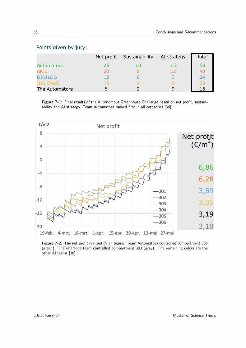
56 Conclusions and Recommendations
Figure 7-1: Final results of the Autonomous Greenhouse Challenge based on net profit, sustain-ability and AI strategy. Team Automatoes ranked first in all categories [36].
Figure 7-2: The net profit realized by all teams. Team Automatoes controlled compartment 306(green). The reference team controlled compartment 303 (gray). The remaining colors are theother AI teams [36].
L.G.J. Kerkhof Master of Science Thesis

7-2 Recommendations for Future Work 57
7-2 Recommendations for Future Work
Some points that are addressed for future work are listed below:
Time-Varying Systems The DeePC algorithm as used in this thesis exploits a fixed periodof measured input/output data to represent the system dynamics. However, when a systemexhibits time-varying dynamics, the recorded data that is used to construct the Hankel ma-trices should be updated regularly in order to ensure the representative of the current systemdynamics. During this thesis, a method to account for time-varying dynamics, Online DeePC,was proposed in [37]. Hence, a topic for future work could be to use the method from [37] inorder to account for time-varying system dynamics.
Persistence of Excitation The quality of the solution of the optimization problem (4-12)largely depends on the data that is used to construct the Hankel matrices. Hence, the in-put/output data collected during regular operation might not be persistently exciting thesystem or it might even be impossible to collect persistently exciting control input data dur-ing regular operation due to physical limitations. Therefore, a topic for future research wouldbe to investigate how well a sequence of control input data excites the system and how wellthis captures the system dynamics, especially for non-linear systems.
Tuning of Parameters The DeePC algorithm has many different tuning and decision pa-rameters. Within this thesis values for these parameters are used which proved to work forthe these data sets and this simulation model. Due to long computational times it was notsuitable to test a wide range of possible combinations of parameters. Hence, it might berecommended to develop some sort of automated tuning algorithm that is able to find a setof the most suitable tuning parameters according to a certain metric, e.g., RMSE.
Greenhouse Model The greenhouse model used in this thesis describes the main processesthat happen in almost every modern greenhouse. However, even more state-of-the-art green-houses nowadays are also equipped with more advanced tools such as a fogging system, activecooling and multiple screens. Hence, this increases the complexity of the greenhouse dynam-ics. Therefore, a topic for future work could be to improve the greenhouse model in such away that more advanced equipment is modeled. Furthermore, a more advanced crop modelthat would for example have daily state updates based on e.g., daily radiation sums or dailyaverage temperatures would be more suitable when controlling the crop states with DeePC.
Irrigation Now, the irrigation algorithm correlates the dry-down rates with the daily radi-ation sum. By taking only the most recent data points, the growth stage is implicitly takeninto account as well. However, a point for future work could be to improve the algorithm byinvestigating the influence of other factors on the dry-down rate such as substrate slab tem-perature, greenhouse air temperature, radiation intensity, plant load or evaporation energyon the dry-down rate. In this way, more reliable predictions of the dry-down rates could beaccomplished, leading to an improved performance of the irrigation control and a reductionin water usage.
Master of Science Thesis L.G.J. Kerkhof

58 Conclusions and Recommendations
L.G.J. Kerkhof Master of Science Thesis

Appendix A
Notation
This Appendix gives a description of the notation used in this thesis.
The following notation is used for the (sub-)sets of real numbers: R denotes the set of realnumbers, R+ denotes the set of non-negative real numbers and R++ denotes the set of positivereal numbers.
Similar, the following notation is used for the (sub-)sets of integers: Z denotes the set ofintegers, Z+ denotes the set of non-negative integers and Z++ denote the set of positiveintegers.
Furthermore, Rn denotes the real numbered n-dimensional vector (similar for Z) and Rn×n
denotes the real numbered n-by-nmatrix (similar for Z). The transpose of a matrix A ∈ Rm×n
is denoted by AT ∈ Rn×m.
Moreover, ‖x‖2 denotes the 2-norm on a vector x ∈ Rn. ‖x‖2Q denotes the scalar xTQx for avector x ∈ Rn and a matrix Q ∈ Rn×n. The inequalities Q � 0 and Q � 0 indicate that amatrix Q ∈ Rn×n is positive semi-definite and positive definite, respectively.
Finally, In denotes the n-by-n identity matrix and diag(1, 2, ...n) ∈ Rn×n denotes the followingdiagonal matrix:
1 0 . . . 00 2 . . . 0...
... . . . ...0 0 . . . n
(A-1)
Master of Science Thesis L.G.J. Kerkhof

60 Notation
L.G.J. Kerkhof Master of Science Thesis

Appendix B
Greenhouse Simulation ModelConstants
Table B-1: Greenhouse model parameters
Symbol Description Value Unitβ Heat absorption efficiency 0.01 [-]γ Apparent psychometric constant 0.067 kPa ◦Cε Cover heat resistance ration 3 [-]ζ Ventilation rate parameter 2.7060*10-5 [-]η Radiation conversion factor 0.7 [-]θ Ventilation rate parameter 4.02*10-5 [-]κ Ventilation rate parameter 5.03*10-5 [-]Λ Pressure constant 0.46153 Nm◦C -1g -1
µ Molar weight fraction CO2 CH2O 1.4667 [-]v Ventilation rate parameter 3.68*10-5 %-1
ξ Ventilation rate parameter 6.3233*10-5 %-1
ρw Density of water 998 kg m-3
ρa Density mass of air 1.29 kg m-3
σ Ventilation rate parameter 7.1708*10-5 % -1
τ Pipe heat transfer coefficient 3 ◦C-1/2
ν Pipe heat transfer coefficient 0.74783 Wm-2◦C-3/4
χ Ventilation rate parameter 0.0156 %-1
ψ Ventilation rate parameter 7.4*10-5 m s-1
ω Humidity ratio parameter 0.622 [-]a1 Saturated vapour pressure parameter 0.611 kPaa2 Saturated vapour pressure parameter 17.27 [-]a3 Saturated vapour pressure parameter 239 ◦CAp Heating pipe outer surface area 314.16 m2
Master of Science Thesis L.G.J. Kerkhof

62 Greenhouse Simulation Model Constants
Table B-2: Greenhouse model parameters, continued
Symbol Description Value Unitb1 Buffer switching function coefficient 2.7 m2g-1
Cg Greenhouse heat capacity 32*103 J◦C-1m-2
Cp Specific heat of water at constant pressure 1010 J◦C-1kg-1
Cs Greenhouse soil heat capacity 120*103 J◦C-1m-2
cp Air specific heat of water at constant pressure 1010 J◦C-1kg-1
d1 Plant development rate parameter 2.1332*10-7 s-1
d2 Plant development rate parameter 2.4664*10-1 s-1
d3 Plant development rate parameter 20 ◦Cd4 Plant development rate parameter 7.4966*10-11 [-]f Fruit assimilate requirement coefficient 1.2 [-]f1 Fruit growth rate coefficient 8.1019*10-7 s-1
f2 Fruit growth rate coefficient 4.6296*10-6 s-1
g1 Leaf conductance parameter 20.3 mm s-1
g2 Leaf conductance parameter 0.44 [-]g3 Leaf conductance parameter 2.5*10-3 s m2µmol-1g4 Leaf conductance parameter 3.1*10-4 m3g-1
gb Boundary layer conductance 10 mm s-1
kd Soil to soil heat transfer coefficient 2.0 W◦C-1m-2
kr Roof heat transfer coefficient 7.9 W◦C-1m-2
ks Soil to air heat transfer coefficient 5.75 W◦C-1m-2
l1 Vaporisation energy coefficient 2.501*106 J g-1
l2 vaporisation energy coefficient 2.381*103 J g-1◦C-1
m1 Mass transfer parameter 1.0183*10-3 g s-1m-2
m2 Mass transfer parameter 0.33 [-]MCO2 Molar mass CO2 0.0044 kg mol-1MF Fruit maintenance respiration coefficient 1.157*10-7 s-1
ML Vegetative maintenance respiration coefficient 2.894*10-7 s-1
mp Watt to µmol conversion factor 4.57 µmol J-1
p1 Net-photosynthesis parameter 577 µmol s-1m-2
p2 Net-photosynthesis parameter 221 ppmpatm Atmospheric pressure 101.0 kPaPm Maximum photosynthesis rate 2.2538*10-3 g s-1 m -2
QG Fruit growth rate parameter Q10-value 2.0 [-]QR Maintenance respiration Q10-value 2.0 [-]Rg Gas constant 8.3144 J mol-1K-1
L.G.J. Kerkhof Master of Science Thesis
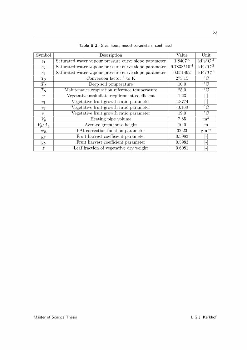
63
Table B-3: Greenhouse model parameters, continued
Symbol Description Value Units1 Saturated water vapour pressure curve slope parameter 1.8407-4 kPa◦C-3
s2 Saturated water vapour pressure curve slope parameter 9.7838*10-4 kPa◦C-2
s3 Saturated water vapour pressure curve slope parameter 0.051492 kPa◦C-1
T0 Conversion factor ◦ to K 273.15 ◦CTd Deep soil temperature 10.0 ◦CTR Maintenance respiration reference temperature 25.0 ◦Cv Vegetative assimilate requirement coefficient 1.23 [-]v1 Vegetative fruit growth ratio parameter 1.3774 [-]v2 Vegetative fruit growth ratio parameter -0.168 ◦Cv3 Vegetative fruit growth ratio parameter 19.0 ◦CVp Heating pipe volume 7.85 m3
Vg/Ag Average greenhouse height 10.0 mwR LAI correction function parameter 32.23 g m-2
yF Fruit harvest coefficient parameter 0.5983 [-]yL Fruit harvest coefficient parameter 0.5983 [-]z Leaf fraction of vegetative dry weight 0.6081 [-]
Master of Science Thesis L.G.J. Kerkhof

64 Greenhouse Simulation Model Constants
L.G.J. Kerkhof Master of Science Thesis

Bibliography
[1] United Nations, “World urbanization prospects: The 2018 revision,” tech. rep., UnitedNations, Department of Economic and Social Affairs, Population Division, New York,2019.
[2] FAO, IFAD, UNICEF, WFP, and WHO, “The state of food security and nutrition in theworld 2018,” tech. rep., FAO, Rome, 2018.
[3] G. van Straten and E. J. van Henten, “Optimal greenhouse cultivation control: Surveyand perspectives,” IFAC Proceedings Volumes, vol. 43, no. 26, pp. 18 – 33, 2010.
[4] Eurostat, “Agri-environmental indicator - energy use.” https://ec.europa.eu/eurostat/statistics-explained/index.php/Agri-environmental_indicator_-_energy_use, January 2018. [Online; accessed 19-Sep-2019].
[5] M. van Eerdt, “Doel co2-emissie meerjarenafspraak glastuinbouw(2020) waarschijnlijk niet binnen bereik.” https://themasites.pbl.nl/balansvandeleefomgeving/jaargang-2018/themas/landbouw-en-voedsel/emissie-broeikasgassen-glastuinbouw-2020, January 2018. [Online; accessed13-Nov-2019].
[6] D. Brian, “What is the current state of labor in the green-house industry?.” https://www.greenhousegrower.com/management/what-is-the-current-state-of-labor-in-the-greenhouse-industry/, November2018. [Online; accessed 17-Sep-2019].
[7] C. Van Rijswijk, “World vegetable map 2018. raboresearch food agribusiness.”https://research.rabobank.com/far/en/sectors/regional-food-agri/world_vegetable_map_2018.html, January 2018. [Online; accessed 17-Sep-2019].
[8] R. Shamshiri, F. Kalantari, K. Ting, K. Thorp, I. Hameed, C. Weltzien, et al., “Advancesin greenhouse automation and controlled environment agriculture: A transition to plantfactories and urban agriculture,” International Journal of Agricultural and BiologicalEngineering, vol. 11, no. 1, pp. 1–22, 2018.
Master of Science Thesis L.G.J. Kerkhof

66 Bibliography
[9] S. Hemming, F. Zwart, A. Elings, I. Righini, and A. S. Petropoulou, “Remote control ofgreenhouse vegetable production with artificial intelligence - greenhouse climate, irriga-tion, and crop production,” Sensors, vol. 19, no. 8, pp. 1–22, 2019.
[10] S. Zeng, H. Hu, L. Xu, and G. Li, “Nonlinear adaptive PID control for greenhouseenvironment based on rbf network,” Sensors, vol. 12, no. 5, pp. 5328–5348, 2012.
[11] J. Coulson, J. Lygeros, and F. Dörfler, “Data-Enabled Predictive Control: In the Shal-lows of the DeePC,” arXiv e-prints, p. arXiv:1811.05890, Nov 2018.
[12] M. Waldrop, “Autonomous vehicles: No drivers required,” Nature, vol. 518, pp. 20–23,Feb 2015.
[13] F. Jiang, Y. Jiang, H. Zhi, Y. Dong, H. Li, S. Ma, Y. Wang, Q. Dong, H. Shen, andY. Wang, “Artificial intelligence in healthcare: past, present and future,” Stroke andVascular Neurology, vol. 2, no. 4, pp. 230–243, 2017.
[14] K. Goldberg, “Robots and the return to collaborative intelligence,” Nature MachineIntelligence, pp. 2–4, Jan 2019.
[15] K. Liakos, P. Busato, D. Moshou, S. Pearson, and D. Bochtis, “Machine learning inagriculture: A review,” Sensors, vol. 18, no. 8, pp. 2674–2703, 2018.
[16] F. Tap, Economics-based Optimal Control of Greenhouse Tomato Crop Production. PhDthesis, Wageningen Agricultural University, 2000.
[17] B. Vanthoor, C. Stanghellini, E. Van Henten, and P. Visser, “A methodology for model-based greenhouse design: Part 1, a greenhouse climate model for a broad range of designsand climates,” Biosystems Engineering, vol. 110, no. 4, pp. 363–377, 2012.
[18] T. R. Sinclair, T. W. Rufty, and R. S. Lewis, “Increasing photosynthesis: Unlikely solu-tion for world food problem,” Trends in Plant Science, vol. 24, no. 11, pp. 1032–1039,2019.
[19] Quistnix, “Westland_kassen.jpg.” https://commons.wikimedia.org/wiki/File:Westland_kassen.jpg, May 2005. [Online; accessed 07-Oct-2019].
[20] G. van Straten, “Optimal greenhouse cultivation control: Quo vadis?,” IFAC ProceedingsVolumes, vol. 46, no. 4, pp. 11 – 16, 2013.
[21] A. Ramírez-Arias, F. Rodríguez, J. Guzmán, and M. Berenguel, “Multiobjective hier-archical control architecture for greenhouse crop growth,” Automatica, vol. 48, no. 3,pp. 490 – 498, 2012.
[22] Z. Gao, “On the centrality of disturbance rejection in automatic control,” ISA transac-tions, vol. 53, no. 4, pp. 850–857, 2013.
[23] I. Lopez-Cruz, E. Fitz-Rodríguez, S. Raquel, A. Rojano-Aguilar, and M. Kacira, “De-velopment and analysis of dynamical mathematical models of greenhouse climate: Areview,” European Journal of Horticultural Science, vol. 83, no. 5, pp. 269–279, 2018.
L.G.J. Kerkhof Master of Science Thesis

67
[24] W. J. Kuijpers, M. J. van de Molengraft, S. van Mourik, A. van ’t Ooster, S. Hemming,and E. J. van Henten, “Model selection with a common structure: Tomato crop growthmodels,” Biosystems Engineering, vol. 187, pp. 247 – 257, Nov 2019.
[25] A. de Koning, Development and dry matter distribution in glasshouse tomato : a quan-titative approach. PhD thesis, Landbouwuniversiteit Wageningen, 1994.
[26] S. Qin and T. A. Badgwell, “A survey of industrial model predictive control technology,”Control Engineering Practice, vol. 11, no. 7, pp. 733 – 764, 2003.
[27] R. Amrit, J. B. Rawlings, and D. Angeli, “Economic optimization using model predictivecontrol with a terminal cost,” Annual Reviews in Control, vol. 35, no. 2, pp. 178 – 186,2011.
[28] A. Bemporad and M. Morari, “Robust model predictive control: A survey,” in Robustnessin identification and control (A. Garulli and A. Tesi, eds.), pp. 207–226, Springer London,1999.
[29] M. Behrendt, “A basic working principle of model predictive control.” https://commons.wikimedia.org/wiki/File:MPC_scheme_basic.svg, October 2009. [Online; accessed24-Sep-2019].
[30] J. Rawlings, E. Meadows, and K. Muske, “Nonlinear model predictive control: A tutorialand survey,” IFAC Proceedings Volumes, vol. 27, no. 2, pp. 185 – 197, 1994.
[31] TomLab, “Tomlab optimization environment.” https://tomopt.com/tomlab/.
[32] E. C. Kerrigan and J. M. Maciejowski, “Soft constraints and exact penalty functions inmodel predictive control,” in Proceedings UKACC International Conference on Control,Sep 2000.
[33] I. Markovsky, J. C. Willems, S. van Huffel, and B. de Moor, Exact and ApproximateModeling of Linear Systems: A Behavioral Approach. Society for Industrial & AppliedMathematics (SIAM), 2006.
[34] I. Markovsky and P. Rapisarda, “Data-driven simulation and control,” InternationalJournal of Control, vol. 81, no. 12, pp. 1946–1959, 2008.
[35] J. C. Willems, P. Rapisarda, I. Markovsky, and B. de Moor, “A note on persistency ofexcitation,” Systems & Control Letters, vol. 54, no. 4, pp. 325 – 329, 2005.
[36] S. Hemming, F. Zwart, A. Elings, I. Righini, and A. S. Petropoulou, “Analysis of results.”Final Presentation Autonomous Greenhouse Challenge; Unpublished, 2020.
[37] S. Baros, C.-Y. Chang, G. E. Colon-Reyes, and A. Bernstein, “Online data-enabledpredictive control,” arXiv e-prints, p. arXiv:2003.03866, Mar 2020.
Master of Science Thesis L.G.J. Kerkhof

68 Bibliography
L.G.J. Kerkhof Master of Science Thesis

Glossary
List of Acronyms
MPC Model Predictive Control
NMPC Nonlinear Model Predictive Control
WC Water Content
EC Electrical Conductivity
DeePC Data-Enabled Predictive Control
AI Artificial Intelligence
RMSE Root Mean Squared Error
List of Symbols
∆D Dry-Down Rate Dark Period∆L Dry-Down Rate Light Period∆D Prediction Dry-Down Rate Dark Period∆L Prediction Dry-Down Rate Light PeriodW Signal SpaceZ+ Discrete Time AxisU Control Input Constraint SetX State Constraint SetB System BehaviourHt Hankel Matrix of Order tξdd Total Dry-DownCi Greenhouse Air CO2 Concentration
Master of Science Thesis L.G.J. Kerkhof

70 Glossary
D Crop Development Stagejc_o Flux between Crop and Outside Environmentje_g Flux between Equipment and Greenhousejg_c Flux between Greenhouse and Cropjg_o Flux between Greenhouse and Outside EnvironmentmB Dry Weight Assimilate BuffermF Fruit WeightmL Leaf WeightN Prediction HorizonR∆ Change of Control Cost MatrixSc Greenhouse Crop SubsystemSg Greenhouse Climate SubsystemT Trajectory Length to Capture System DynamicsTg Greenhouse Air TemperatureTp Heating Pipe TemperatureTs Greenhouse Soil TemperaturetD Length Dark PeriodTf Trajectory Length for Future Trajectory PredictiontL Length Light PeriodTini Trajectory Length for Implicit State EstimationTstop Stop Time IrrigationUf Input Data Hankel Matrixul Lower Bound Control InputUp Input Data Hankel Matrixuu Upper Bound Control InputsVi Greenhouse Air Absolute HumidityVf Exogenous Data Hankel MatrixVp Exogenous Data Hankel Matrixxl Lower Bound System Statesxu Upper Bound System Statesxc Greenhouse Crop Statesxg Greenhouse Climate StatesYf Output Data Hankel MatrixYp Output Data Hankel Matrix
L.G.J. Kerkhof Master of Science Thesis