Master's Thesis: Evaluate and develop high-performance GPS...
132
Evaluate and develop high-performance GPS navigation using free GPS software Master’s Thesis in Engineering Physics R onny Videkull Department of Earth and Space Sciences Chalmers University of Technology Gothenburg, Sweden 2015
Transcript of Master's Thesis: Evaluate and develop high-performance GPS...

Evaluate and develop high-performanceGPS navigation using free GPS softwareMaster’s Thesis in Engineering Physics
Ronny Videkull
Department of Earth and Space SciencesChalmers University of TechnologyGothenburg, Sweden 2015


THESIS FOR THE DEGREE IN MASTER OF SCIENCE
Evaluate and develop high-performance GPS navigation using free GPSsoftware
Ronny Videkull
Department of Earth and Space SciencesCHALMERS UNIVERSITY OF TECHNOLOGY
Gothenburg, Sweden 2015

Evaluate and develop high-performance GPS navigation using free GPS software
Ronny Videkull
© Ronny Videkull, 2015
Master of Science Thesis in cooperation with Saab ABDepartment of Earth and Space SciencesChalmers University of TechnologySE-412 96 GöteborgSwedenTelephone: + 46 (0)31-772 1000
Cover:SAR image created using positions produced by RTKLIB
Chalmers ReproserviceGothenburg, Sweden 2015

Abstract
Synthetic Aperture Radar (SAR) mounted on an aircraft allows us to create high resolutionimages of landscapes. In order to obtain such images it is crucial to accurately determinethe flight-path of the instrument’s platform. For centimeter-level accurate positioning of theaircraft, a differential positioning technique based on Global Navigation Satellite Systems(GNSS) is used. This method, also known as Real-Time Kinematic (RTK) positioning,utilizes carrier phase signals and relies on a second (fixed) "base station" with well knowncoordinates. In this thesis the accuracy of the open-source GNSS library RTKLIB wasevaluated. A comparison with results from a commercial software has shown that RTKLIBis able to provide similar positioning performance. In general it could be concluded that theaccuracy of RTKLIB is sufficient for the given SAR application. Moreover, a batch-drivenprocessing chain utilizing RTKLIB was realized in order to minimize manual interactions.The thesis was conducted at Saab AB.

Sammanfattning
Syntetisk aperturradar (SAR) monterat på ett flygplan kan användas för att skapa högupp-lösta bilder av landskap. För att skapa sådana bilder är det nödvändigt att noggrant be-stämma instrumentplattformens flygbana. Centimeternivå på noggrannheten uppnås ge-nom att använda en differentiell positioneringsteknik baserat på Global Navigation Satel-lite Systems (GNSS). Denna metod, känd som Real-Time Kinematic (RTK) positionering,använder bärvågsmätning och behöver en annan (fixerad) basstation vars position är välkänd position. I denna avhandling utvärderas noggrannheten hos den öppna GNSS pro-gramvaran RTKLIB. Genom att jämföra med resultat från en kommersiell programvara hardet visats att RTKLIB klarar av att ge liknande positioneringsprestanda. I allmänhet kanslutsatsen dras att noggrannheten hos RTKLIB är tillräcklig för den angivna SAR tillämp-ningen. Dessutom har en processeringskedja som använder RTKLIB realiserats i syfte attminimera manuella interaktioner. Avhandlingen genomfördes vid Saab AB.

AcknowledgmentsFirst I would like to thank Saab AB for giving me the opportunity to carry out this thesis.Thanks to all people at Saab I have come in contact with for answering all my questions,especially my supervisors Anders Åhlander and Patrik Dammert. I would also like to thankmy examiner Thomas Hobiger for his support and ability to always point me in the rightdirection when I needed it. A special thanks goes to Tomoji Takasu for answering all myquestions regarding RTKLIB and fixing the baseline bug so fast.
Ronny Videkull, Gothenburg 2015-05-21
i

List of symbols and abbreviations
C/A Coarse Acquisition
CDMA Code Division Multiple Access
DGPS Differential GPS
DOP Dilution Of Precision
ECEF Earth-Centered Earth-Fixed
EKF Extended Kalman Filter
ENU East, North, Up
GDOP Geometric Dilution Of Precision
GLONASS Globalnaja nawigazionnaja sputnikowaja sistema
GNSS Global Navigation Satellite System
GPS Global Positioning System
GPST GPS Time
GRS Geodetic Reference System
HDOP Horizontal Dilution Of Precision
IMU Inertial Measurement Unit
LAMBDA Least-squares AMBiguity Decorrelation Adjustment
LLI Loss of Lock Indicator
MEMS Micro-Electro-Mechanical Systems
NTRIP Networked Transport of RTCM via Internet Protocol
PRN Pseudo Random Noise
RINEX Receiver INdependent EXchange Format
RMS Root Mean Square
ii

RTCM Radio Technical Commission for Maritime Services
RTK Real-Time Kinematic
SAR Synthetic-Aperture Radar
TAI International Atomic Time
TDOP Time Dilution Of Precision
UERE User Equivalent Range Error
UT1 Universal Time
UTC Coordinated Universal Time
VDOP Vertical Dilution Of Precision
VHF Very High Frequency
WGS World Geodetic System
iii

Contents
1 Introduction 11.1 Background . . . . . . . . . . . . . . . . . . . . . . . . . . . . . . . . . . 11.2 Purpose . . . . . . . . . . . . . . . . . . . . . . . . . . . . . . . . . . . . 21.3 Objective . . . . . . . . . . . . . . . . . . . . . . . . . . . . . . . . . . . 2
2 Global Positioning System (GPS) 32.1 Operation principle . . . . . . . . . . . . . . . . . . . . . . . . . . . . . . 42.2 Signals . . . . . . . . . . . . . . . . . . . . . . . . . . . . . . . . . . . . . 52.3 GPS observables . . . . . . . . . . . . . . . . . . . . . . . . . . . . . . . 6
2.3.1 Code pseudorange . . . . . . . . . . . . . . . . . . . . . . . . . . 62.3.2 Carrier phase . . . . . . . . . . . . . . . . . . . . . . . . . . . . . 82.3.3 Doppler measurements . . . . . . . . . . . . . . . . . . . . . . . . 10
2.4 Reference systems . . . . . . . . . . . . . . . . . . . . . . . . . . . . . . 102.4.1 Time systems . . . . . . . . . . . . . . . . . . . . . . . . . . . . . 102.4.2 Coordinate systems . . . . . . . . . . . . . . . . . . . . . . . . . . 11
2.5 Differential positioning . . . . . . . . . . . . . . . . . . . . . . . . . . . . 132.5.1 Single difference formation . . . . . . . . . . . . . . . . . . . . . . 142.5.2 Double difference formation . . . . . . . . . . . . . . . . . . . . . 14
2.6 DOP . . . . . . . . . . . . . . . . . . . . . . . . . . . . . . . . . . . . . . 162.7 RTKLIB algorithms . . . . . . . . . . . . . . . . . . . . . . . . . . . . . . 18
2.7.1 Extended Kalman Filter . . . . . . . . . . . . . . . . . . . . . . . 182.7.2 Integer Ambiguity Resolution . . . . . . . . . . . . . . . . . . . . 192.7.3 Cycle slip . . . . . . . . . . . . . . . . . . . . . . . . . . . . . . . 20
3 GPS processing software 213.1 RTKLIB . . . . . . . . . . . . . . . . . . . . . . . . . . . . . . . . . . . . 213.2 Waypoint . . . . . . . . . . . . . . . . . . . . . . . . . . . . . . . . . . . 21
4 SAR image acquisition 224.1 SAR principle . . . . . . . . . . . . . . . . . . . . . . . . . . . . . . . . . 23
iv
5 Method 255.1 Data collection . . . . . . . . . . . . . . . . . . . . . . . . . . . . . . . . 25
5.1.1 Flight path . . . . . . . . . . . . . . . . . . . . . . . . . . . . . . 255.1.2 Orientation . . . . . . . . . . . . . . . . . . . . . . . . . . . . . . 26
5.2 Receivers . . . . . . . . . . . . . . . . . . . . . . . . . . . . . . . . . . . 275.3 Measurements . . . . . . . . . . . . . . . . . . . . . . . . . . . . . . . . . 285.4 Statistics . . . . . . . . . . . . . . . . . . . . . . . . . . . . . . . . . . . . 28
6 Results 306.1 Flight paths . . . . . . . . . . . . . . . . . . . . . . . . . . . . . . . . . . 30
6.1.1 2014-10-03 . . . . . . . . . . . . . . . . . . . . . . . . . . . . . . 326.1.2 2014-10-06 . . . . . . . . . . . . . . . . . . . . . . . . . . . . . . 34
6.2 Individual test runs, flight paths . . . . . . . . . . . . . . . . . . . . . . . . 366.2.1 2014-10-01, AFT1001a . . . . . . . . . . . . . . . . . . . . . . . . 366.2.2 2014-10-06, FWD1006c . . . . . . . . . . . . . . . . . . . . . . . 38
6.3 Orientation . . . . . . . . . . . . . . . . . . . . . . . . . . . . . . . . . . 416.3.1 2014-10-03 . . . . . . . . . . . . . . . . . . . . . . . . . . . . . . 426.3.2 2014-10-06 . . . . . . . . . . . . . . . . . . . . . . . . . . . . . . 44
6.4 Individual test runs, orientation . . . . . . . . . . . . . . . . . . . . . . . . 466.4.1 2014-10-01, BASELINE1001a . . . . . . . . . . . . . . . . . . . . 466.4.2 2014-10-06, BASELINE1006c . . . . . . . . . . . . . . . . . . . . 47
6.5 Summary of test runs . . . . . . . . . . . . . . . . . . . . . . . . . . . . . 486.6 Quality flag . . . . . . . . . . . . . . . . . . . . . . . . . . . . . . . . . . 486.7 Final image . . . . . . . . . . . . . . . . . . . . . . . . . . . . . . . . . . 52
7 Summary 55
8 Conclusions and outlook 57
A Additional results 63A.1 Flight paths . . . . . . . . . . . . . . . . . . . . . . . . . . . . . . . . . . 63
A.1.1 2014-10-01 . . . . . . . . . . . . . . . . . . . . . . . . . . . . . . 63A.1.2 2014-10-03 . . . . . . . . . . . . . . . . . . . . . . . . . . . . . . 69A.1.3 2014-10-06 . . . . . . . . . . . . . . . . . . . . . . . . . . . . . . 72A.1.4 2014-10-07 . . . . . . . . . . . . . . . . . . . . . . . . . . . . . . 73
A.2 Individual test runs, flight paths . . . . . . . . . . . . . . . . . . . . . . . . 77A.2.1 2014-10-01, AFT1001a . . . . . . . . . . . . . . . . . . . . . . . . 77A.2.2 2014-10-06, FWD1006c . . . . . . . . . . . . . . . . . . . . . . . 80
A.3 Orientation . . . . . . . . . . . . . . . . . . . . . . . . . . . . . . . . . . 90A.3.1 2014-10-01 . . . . . . . . . . . . . . . . . . . . . . . . . . . . . . 90
v

A.3.2 2014-10-03 . . . . . . . . . . . . . . . . . . . . . . . . . . . . . . 92A.3.3 2014-10-07 . . . . . . . . . . . . . . . . . . . . . . . . . . . . . . 93
A.4 Individual test runs, orientation . . . . . . . . . . . . . . . . . . . . . . . . 95A.4.1 2014-10-01, BASELINE1001a . . . . . . . . . . . . . . . . . . . . 95A.4.2 2014-10-06, BASELINE1006c . . . . . . . . . . . . . . . . . . . . 99
B Script overview 109B.1 Main files . . . . . . . . . . . . . . . . . . . . . . . . . . . . . . . . . . . 110B.2 Minor files . . . . . . . . . . . . . . . . . . . . . . . . . . . . . . . . . . . 111
C Configuration files 112C.1 flightpath.conf . . . . . . . . . . . . . . . . . . . . . . . . . . . . . . 112C.2 flightpath_single.conf . . . . . . . . . . . . . . . . . . . . . . . . . 114C.3 baseline.conf . . . . . . . . . . . . . . . . . . . . . . . . . . . . . . . 116C.4 static.conf . . . . . . . . . . . . . . . . . . . . . . . . . . . . . . . . . 118
vi

Chapter 1
Introduction
This thesis was conducted at the Airborne Surveillance Systems business unit in the busi-ness area Electronic Defence Systems at Saab AB. Saab is one of the world’s premieresuppliers of solutions for surveillance, threat detection and location, platform and forceprotection, as well as avionics. Centre for this knowledge is the business area ElectronicDefence Systems.
1.1 BackgroundOne of the projects the division works on is a product called CARABAS[40]. In CARABASa Synthetic-aperture radar (SAR), a form of radar, is used to create images of landscapes.SAR can be mounted on a moving platform and the distance the SAR device travels overa target creates a large synthetic antenna aperture. The radar under consideration operatesin the VHF band, using wavelengths of 1-15 m, as opposed to traditional microwave SAR.Thanks to the long wavelengths it is possible for the radar to penetrate leaves and branchesof a forest and see what lies underneath. In doing so, larger objects placed in a forest canbe seen, for example cars and trucks, which would be hidden by the forest if microwaveswould be used.
In order to obtain high resolution images it is very important to accurately determinethe flight-path of the instrument’s platform. To achieve the needed accuracy a differentialpositioning technique known as Real-Time Kinematic (RTK) positioning is used. RTKpositioning is a technique based on Global Navigation Satellite Systems (GNSS). It utilizesthe carrier phase signals and relies on a second (fixed) "base station" with well knowncoordinates [22]. This can increase the positioning accuracy of ordinary GPS positioningfrom meters to centimeters [7].
RTK can be used both in real-time applications and in post-processing. In real-timeapplications a data link must be set up between the base station and the rover. For post-
1

processing the link is not needed, only the collected data. The latter is being studied in thisthesis.
1.2 PurposeCurrently a commercial software is used to perform the differential GPS processing. It hasgood accuracy but it requires a lot of manual interactions, which is undesirable. Since itis a commercial software there is a cost attached to it, meaning that if Saab sells a productutilizing that software the customer would have to buy the software as well. The purposeof this thesis is to find another processing solution which reduces the manual interactionswhile fulfilling the accuracy requirements.
1.3 ObjectiveThe goal of this thesis is
• Evaluate the accuracy of the open source program package for GNSS positioningcalled RTKLIB.
• Produce a batch-driven, stand-alone processing chain of RTKLIB which has a mini-mum of manual interactions.
The stated requirements for producing high resolution SAR images are a positioning accu-racy of 5 cm (RMS) and an angular accuracy of 1◦ (RMS) [27] for the aircraft position andorientation. The requirement for the vertical positioning is not explicitly stated, but it is notas tightly defined as the horizontal.
2

Chapter 2
Global Positioning System (GPS)
GPS, which stands for Global Positioning System, has its origin in radio navigation sys-tems. The main application of GPS is to be able to find location and time informationanywhere on Earth where there is a free line of sight to four or more GPS satellites underall weather conditions. It originated in the United States military in the 1960s and the de-cision to make it free for civilan purposes was made after the incident with the Korean AirLines Flight 007 [23, p. 248].
The first satellite was launched in 1978 and the system was fully operational in the mid1990s [38]. The satellites orbit at an altitude of approximately 20200 km and are arrangedinto six equally-spaced orbital planes inclined 55◦ from the equator, see Figure 2.1. Thisconstellation ensures that at least four satellites are visible at least 15◦ above the horizonanywhere in the world at any given time [11]. Originally the GPS constellation consistedof 24 satellites, but expansions have been made and as of January 2015 there were 30 activeGPS satellites in orbit. Each satellite circles the Earth twice a day [9].
GPS consists of three segments, the space segment, control segment, and user segment:
• The space segment consists of the satellites. They broadcast radio signals to usersand receive commands from the control segment.
• The control segment monitors the space segment and sends commands and data tothe satellites.
• The user segment consists of the receivers that record and interpret the radio signalsbroadcasted by the satellites.
The satellites are monitored by five base stations which transmit ephemerides and clockadjustments [41, p. 2]. Ephemeris data are used to calculate the position of the satellite.The location of a receiver is determined by measuring the ranges between the receiver andat least four simultaneously observed satellites.
3

Figure 2.1: GPS constellation [39].
The term Global Navigation Satellite System (GNSS) can be used for a satellite sys-tem with global coverage, and is often used when talking about satellite navigation withoutspecifying the system. GPS was the first GNSS. The Russian counterpart, Globalnaja naw-igazionnaja sputnikowaja sistema (GLONASS), was the second. Other systems that donot yet have full global coverage and are in various states of completion are the EuropeanGalileo and the Chinese BeiDou/COMPASS. This thesis will only consider GPS.
2.1 Operation principleThe GPS system is based on time. A broadcasted GPS satellite signal consists of, amongother things, a message with the time of transmission and a pseudorandom noise (PRN)code. The PRN code is a sequence of ones and zeros. When a receiver receives the signalit will compare the received code with an identical coded signal generated internally. Thereplica code is shifted in time until it achieves correlation with the received code. The timeshift corresponds to the propagation time of the signal. This is illustrated in Figure 2.2,where te is the signal emission time, tr is the signal reception time and τ is the propagationtime. The receiver also keeps track of the phase of the signal, and measures the frequencyshift of the signal caused by the Doppler effect.
By multiplying the propagation time with the speed of light the distance between thesatellite and user can be computed. This is not the complete story as the signal does not
4

Figure 2.2: Use of replica code to determine signal propagation time [31].
travel through vacuum, and a more complete model is presented in Section 2.3.1.
2.2 SignalsThe satellites use up to three frequencies to transmit data, all located in the L-band. Thefrequencies are known as L1, L2 and L5 and they are 1575.42 MHz, 1227.60 MHz and1176.45 MHz respectively. Usually the word "carrier" is used when talking about the GPSsignals, which comes from that the signals are modulated with some data in order to carryinformation. The three different carrier frequencies are generated by multiplying the fun-damental frequency 10.23 MHz by 154, 120 and 115. The fundamental L-band frequencyis produced by atomic clocks aboard the satellite. The carrier frequency and clock rates onthe satellites are offset to compensate for relativistic effects [8]. For an observer on a satel-lite the fundamental frequency would appear to be 10.2299999954326 MHz. Without theoffset of the clock rate the atomic clocks aboard the satellites would tick faster than iden-tical clocks on the ground by 38 microseconds per day. This would lead to accumulatingpositioning errors of about 10 kilometers per day [2].
Superimposed on the carrier frequencies are pseudo random noise (PRN) codes andnavigation data. The latter in the form of satellite ephemerides, ionospheric modelingcoefficients, status information, system time and satellite clock corrections.
All satellites transmit three PRN ranging codes [8] known as the C/A-code, P-code andY-code:
Coarse/Acquisition (C/A) code is a relatively short code and it is modulated onto the L1carrier. The length of the code is 1 millisecond at a chipping rate of 1.023 millionchips per second. The broadcast of the C/A-code is known as the Standard Posi-tioning Service (SPS) and it is available to civilian users. Because the C/A-code isrelatively short it is used for acquisition of the P-code.
5
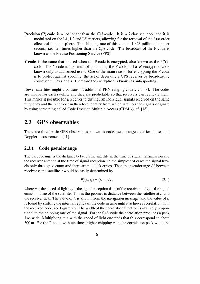
Precision (P) code is a lot longer than the C/A-code. It is a 7-day sequence and it ismodulated on the L1, L2 and L5 carriers, allowing for the removal of the first ordereffects of the ionosphere. The chipping rate of this code is 10.23 million chips persecond, i.e. ten times higher than the C/A code. The broadcast of the P-code isknown as the Precise Positioning Service (PPS).
Y-code is the name that is used when the P-code is encrypted, also known as the P(Y)-code. The Y-code is the result of combining the P-code and a W encryption codeknown only to authorized users. One of the main reason for encrypting the P-codeis to protect against spoofing, the act of deceiving a GPS receiver by broadcastingcounterfeit GPS signals. Therefore the encryption is known as anti-spoofing.
Newer satellites might also transmit additional PRN ranging codes, cf. [8]. The codesare unique for each satellite and they are predictable so that receivers can replicate them.This makes it possible for a receiver to distinguish individual signals received on the samefrequency and the receiver can therefore identify from which satellites the signals originateby using something called Code Division Multiple Access (CDMA), cf. [18].
2.3 GPS observablesThere are three basic GPS observables known as code pseudoranges, carrier phases andDoppler measurements [41].
2.3.1 Code pseudorangeThe pseudorange is the distance between the satellite at the time of signal transmission andthe receiver antenna at the time of signal reception. In the simplest of cases the signal trav-els only through vacuum and there are no clock errors. Then the pseudorange Ps
r betweenreceiver r and satellite s would be easily determined by
Psr(tr, te) = (tr − te)c, (2.1)
where c is the speed of light, tr is the signal reception time of the receiver and te is the signalemission time of the satellite. This is the geometric distance between the satellite at te andthe receiver at tr. The value of te is known from the navigation message, and the value of tr
is found by shifting the internal replica of the code in time until it achieves correlation withthe received code, see Figure 2.2. The width of the correlation function is inversely propor-tional to the chipping rate of the signal. For the C/A code the correlation produces a peak1 µs wide. Multiplying this with the speed of light one finds that this correspond to about300 m. For the P-code, with ten times higher chipping rate, the correlation peak would be
6

ten times shorter and therefore the corresponding distance would be about 30 meters. Thepeak of the correlation function can be determined to about 1% of the width [41, p. 39],this gives ranging accuracy of 3 m and 0.3 m for the C/A and P-code, respectively.
Denoting the satellite vector rs(t) = (xs(t), ys(t), zs(t)) and the receiver vector rr(t) =
(xr(t), yr(t), zr(t)), the pseudorange can be expressed as the distance between their vectors,
Psr(tr, te) = ‖rs(te) − rr(tr)‖
=√
(xs(te) − xr(tr))2 + (ys(te) − yr(tr))2 + (zs(te) − zr(tr))2,(2.2)
This geometric distance will be denoted ρsr(tr, te).
However we will never experience the simple case as the signals will travel througha medium which is not vacuum and both the satellite and receiver clock will have errors.Introducing clock errors the pseudorange can be represented as
Psr(tr, te) = ((tr + δtr) − (te + δts))c
= (tr − te)c + (δtr − δts)c= ρs
r(tr, te) + (δtr − δts)c,(2.3)
where δtr and δts denotes the clock offsets of the receiver and satellite, respectively.Adding ionospheric and tropospheric delay and other errors, denoted by I, T and εp,
the pseudorange model can be written as
Psr(tr, te) = ρs
r(tr, te) + (δtr − δts)c + I sr + T s
r + εp. (2.4)
Among the errors hidden in εp are earth tide effects, loading tide effects, multipath andrelativistic effects [41]. This is the pseudorange model used in RTKLIB [32].
To calculate the position of one receiver at least four visible GPS satellites are needed.This is because the receiver clock bias needs to be estimated along with the three dimen-sional position. The rest of the parameters are modeled. The tropospheric delay T s
r willbe modeled using the Saastamoinen model [26]. The ionospheric delay I s
r will be modeledusing Klobuchar model [15] which uses the broadcasted ionospheric parameters.
The need of at least four satellites can be illustrated using the pseudo range equation.For simplicity the tropospheric and ionospheric delay terms are ignored, and similarly theadditional errors are ignored. Expanding ρs
r the pseudo range can be written
Psr =√
(xs − xr)2 + (ys − yr)2 + (zs − zr)2 + (δtr − δts)c. (2.5)
The satellite position (xs, ys, zs) and satellite clock error (δts) are stated in the navigationmessage and therefore known. The other four terms, three position components and oneclock error, are unknown. The system of equations for a receiver denoted r and the satellites
7

1, 2, 3 and 4 can be written
P1r =√
(x1 − xr)2 + (y1 − yr)2 + (z1 − zr)2 + (δtr − δt1)c
P2r =√
(x2 − xr)2 + (y2 − yr)2 + (z2 − zr)2 + (δtr − δt2)c
P3r =√
(x3 − xr)2 + (y3 − yr)2 + (z3 − zr)2 + (δtr − δt3)c
P4r =√
(x4 − xr)2 + (y4 − yr)2 + (z4 − zr)2 + (δtr − δt4)c.
(2.6)
This system of nonlinear equations can be solved iteratively.
2.3.2 Carrier phaseIt is not possible to measure the exact number of carrier cycles between a satellite anda receiver. It is however possible to keep track of the change in cycles since the start of ameasurement. When a receiver initially locks on to a satellite the number of cycles betweenthe satellite and the receiver is not known, but as long as the receiver maintains a lock onthe signal that number stays constant. Then the fractional phase is measured continuouslyand the phase difference for each measurement is added to a tally keeping track of thechange in cycles. This kind of measurement will have the correct fractional phase, but willhave an ambiguous amount of full cycles wrong. To find the correct number of full cyclesthe ambiguity parameters can be modeled. The phase measurement can be made on all thecarrier frequencies as it completely disregards the information contained within the signal,only the phase of the signal is needed.
The phase can be measured with a precision better than 1% of the wavelength [41, p.39], meaning the positioning accuracy significantly improves from using only the code.For the L1 carrier, whose wavelength is about 19 cm, this corresponds to an accuracy ofabout 1.9 mm and 2.4 mm for L2 whose wavelength is about 24 cm. To fully exploit thephase measurements one must correct for propagation effects of the signal which is whythe carrier phase is not usually used in standard navigation systems.
Once again starting in the simple and unrealistic case of the signal travelling throughvacuum and no clock errors we can write the measured phase φs
r between receiver r andsatellite s as
φsr(tr, te) = φr(tr) − φs(te) + N s
r . (2.7)
Here tr is the signal reception time of the receiver, te is the signal emission time of thesatellite, φr is the phase of the receiver’s oscillator and φs is the phase of the emitted signalfrom the satellite. N s
r denotes the number of full cycles between satellite s and receiver r,and that is the parameter which should be determined.
Assuming the received satellite signal and the reference carrier of the receiver have thefrequency f , the phases can be written as
φr(tr) = f (tr − t0) + φr,0 (2.8)
8

andφs(te) = f (te − t0) + φs,0, (2.9)
where t0 is the initial time, φr,0 and φs,0 are the initial phases of the receiver oscillator andthe initial satellite carrier phase of the emitted signal respectively.
In a more realistic case both the receiver and satellite clock has errors. Using the samenotation for those errors as used for the pseudorange the phases can be written
φr(tr) = f (tr + δtr − t0) + φr,0 (2.10)
andφs(te) = f (te + δts − t0) + φs,0. (2.11)
Using this the carrier phase becomes
φsr(tr, te) = ( f (tr + δtr − t0) + φr,0) − ( f (te + δts − t0) + φs,0) + N s
r
= f (tr − te) + f (δtr − δts) + (φr,0 − φs,0) + N s
r .(2.12)
To express the carrier phase using the wavelength instead of the frequency the relation
c = fλ ⇒ f = c/λ (2.13)
is used, resulting in
φsr(tr, te) =
cλ
(tr − te) +cλ
(δtr − δts) + (φr,0 − φs,0) + N s
r . (2.14)
Defining the phase range, Φsr, as the carrier phase multiplied by the carrier wavelength
we get
Φsr(tr, te) = λφs
r(tr, te)
= c(tr − te) + c(δtr − δts) + λ(φr,0 − φs,0) + λN s
r
= ρsr(tr, te) + c(δtr − δts) + λ(φr,0 − φ
s,0) + λN sr .
(2.15)
So far only the clock errors have been introduced, but there are also other error sources.As for the pseudorange there is a delay because of the ionosphere and troposphere. Uniqueerrors for the carrier phase are hidden in a term denoted dΦs
r, which includes the receiverand satellite antenna phase offsets, receiver and satellite antenna phase center variations,station displacement, phase wind-up effect and relativity correction on the satellite clock.Once again other errors will be stored in a separate term, this time denoted εΦ for the phaserange. Putting all of this together Equation (2.15) becomes
Φsr(tr, te) = ρs
r(tr, te) + c(δtr − δts) + λ(φr,0 − φs,0) + λN s
r − I sr + T s
r + dΦsr + εΦ, (2.16)
which is the model used in RTKLIB [32]. Note that the sign of the error from the ionosphereis opposite of that used in the pseudo range model. This is because the ionosphere delaysthe code signal transmission and advances the phase signal transmission [21].
9
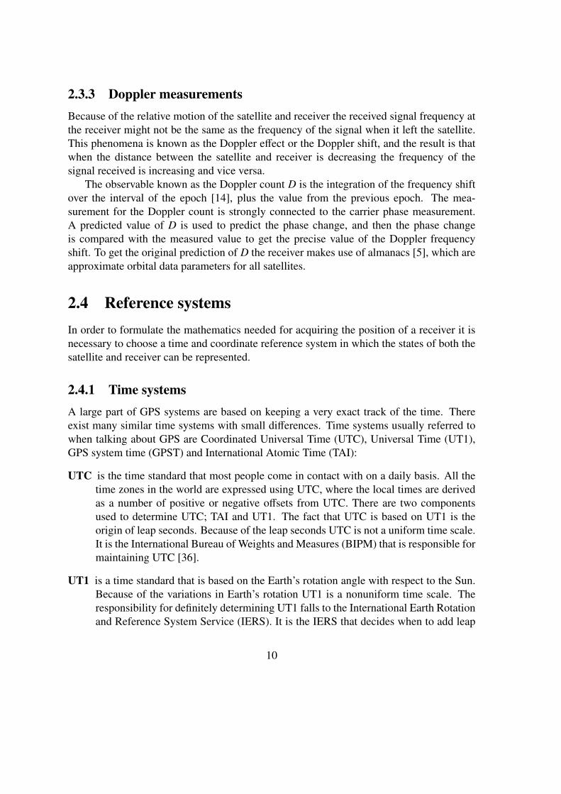
2.3.3 Doppler measurementsBecause of the relative motion of the satellite and receiver the received signal frequency atthe receiver might not be the same as the frequency of the signal when it left the satellite.This phenomena is known as the Doppler effect or the Doppler shift, and the result is thatwhen the distance between the satellite and receiver is decreasing the frequency of thesignal received is increasing and vice versa.
The observable known as the Doppler count D is the integration of the frequency shiftover the interval of the epoch [14], plus the value from the previous epoch. The mea-surement for the Doppler count is strongly connected to the carrier phase measurement.A predicted value of D is used to predict the phase change, and then the phase changeis compared with the measured value to get the precise value of the Doppler frequencyshift. To get the original prediction of D the receiver makes use of almanacs [5], which areapproximate orbital data parameters for all satellites.
2.4 Reference systemsIn order to formulate the mathematics needed for acquiring the position of a receiver it isnecessary to choose a time and coordinate reference system in which the states of both thesatellite and receiver can be represented.
2.4.1 Time systemsA large part of GPS systems are based on keeping a very exact track of the time. Thereexist many similar time systems with small differences. Time systems usually referred towhen talking about GPS are Coordinated Universal Time (UTC), Universal Time (UT1),GPS system time (GPST) and International Atomic Time (TAI):
UTC is the time standard that most people come in contact with on a daily basis. All thetime zones in the world are expressed using UTC, where the local times are derivedas a number of positive or negative offsets from UTC. There are two componentsused to determine UTC; TAI and UT1. The fact that UTC is based on UT1 is theorigin of leap seconds. Because of the leap seconds UTC is not a uniform time scale.It is the International Bureau of Weights and Measures (BIPM) that is responsible formaintaining UTC [36].
UT1 is a time standard that is based on the Earth’s rotation angle with respect to the Sun.Because of the variations in Earth’s rotation UT1 is a nonuniform time scale. Theresponsibility for definitely determining UT1 falls to the International Earth Rotationand Reference System Service (IERS). It is the IERS that decides when to add leap
10
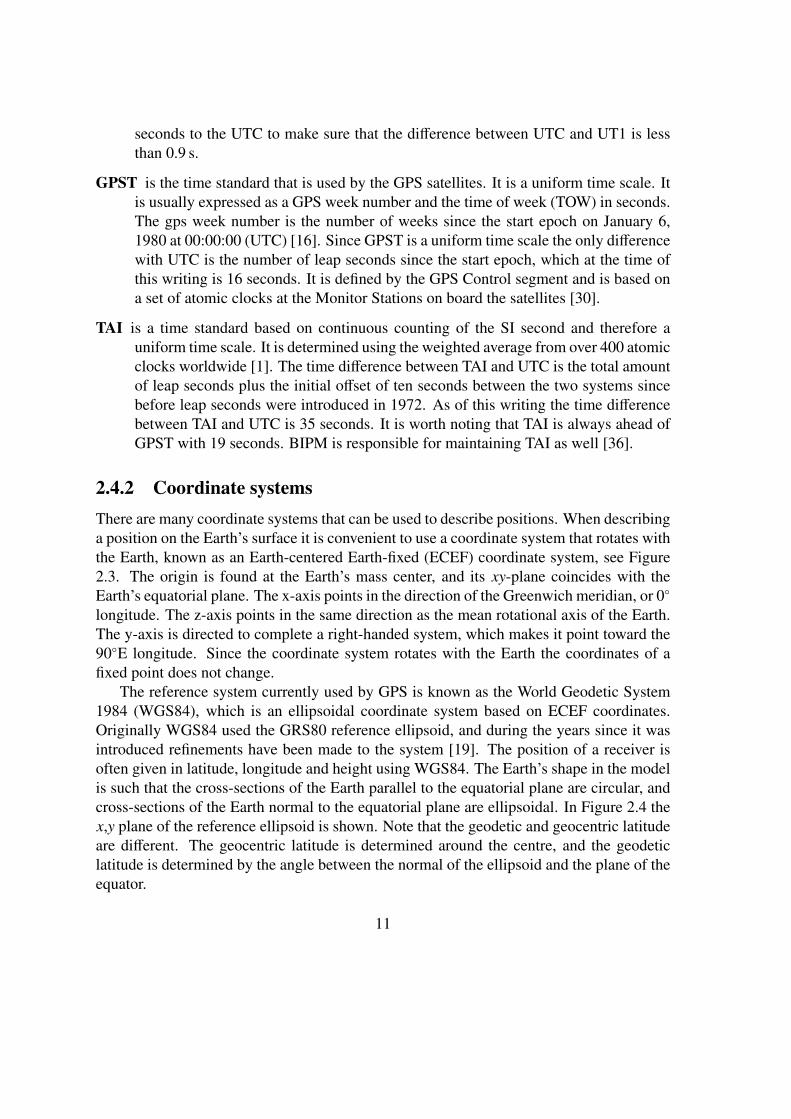
seconds to the UTC to make sure that the difference between UTC and UT1 is lessthan 0.9 s.
GPST is the time standard that is used by the GPS satellites. It is a uniform time scale. Itis usually expressed as a GPS week number and the time of week (TOW) in seconds.The gps week number is the number of weeks since the start epoch on January 6,1980 at 00:00:00 (UTC) [16]. Since GPST is a uniform time scale the only differencewith UTC is the number of leap seconds since the start epoch, which at the time ofthis writing is 16 seconds. It is defined by the GPS Control segment and is based ona set of atomic clocks at the Monitor Stations on board the satellites [30].
TAI is a time standard based on continuous counting of the SI second and therefore auniform time scale. It is determined using the weighted average from over 400 atomicclocks worldwide [1]. The time difference between TAI and UTC is the total amountof leap seconds plus the initial offset of ten seconds between the two systems sincebefore leap seconds were introduced in 1972. As of this writing the time differencebetween TAI and UTC is 35 seconds. It is worth noting that TAI is always ahead ofGPST with 19 seconds. BIPM is responsible for maintaining TAI as well [36].
2.4.2 Coordinate systemsThere are many coordinate systems that can be used to describe positions. When describinga position on the Earth’s surface it is convenient to use a coordinate system that rotates withthe Earth, known as an Earth-centered Earth-fixed (ECEF) coordinate system, see Figure2.3. The origin is found at the Earth’s mass center, and its xy-plane coincides with theEarth’s equatorial plane. The x-axis points in the direction of the Greenwich meridian, or 0◦
longitude. The z-axis points in the same direction as the mean rotational axis of the Earth.The y-axis is directed to complete a right-handed system, which makes it point toward the90◦E longitude. Since the coordinate system rotates with the Earth the coordinates of afixed point does not change.
The reference system currently used by GPS is known as the World Geodetic System1984 (WGS84), which is an ellipsoidal coordinate system based on ECEF coordinates.Originally WGS84 used the GRS80 reference ellipsoid, and during the years since it wasintroduced refinements have been made to the system [19]. The position of a receiver isoften given in latitude, longitude and height using WGS84. The Earth’s shape in the modelis such that the cross-sections of the Earth parallel to the equatorial plane are circular, andcross-sections of the Earth normal to the equatorial plane are ellipsoidal. In Figure 2.4 thex,y plane of the reference ellipsoid is shown. Note that the geodetic and geocentric latitudeare different. The geocentric latitude is determined around the centre, and the geodeticlatitude is determined by the angle between the normal of the ellipsoid and the plane of theequator.
11

Figure 2.3: ECEF coordinate system [4].
Figure 2.4: Reference ellipsoid, cross-section normal to equatorial plane [32]. a is the semi-majoraxis, b is the semi-minor axis and e is the eccentricity.
For some applications it is sufficient to use a simpler coordinate system such as localeast, north, up (ENU) coordinates. In such a system the coordinates are formed by pro-
12

jecting positions to a plane which is tangential to the surface of the Earth in a referencepoint. Usually the x-axis points in the east direction, y in the north direction and z straightup. Because of the shape of the earth this type of coordinate system is only valid for shortdistances from the reference point. In Figure 2.5 a ENU coordinate system is presentedtogether with an ECEF system.
Figure 2.5: ECEF and ENU coordinates [32].
2.5 Differential positioningIn order to improve the positioning accuracy of ordinary GPS a differential positioningtechnique called Real-Time Kinematic, abbreviated RTK, can be used. RTK is based onthe use of the carrier phase. Two GPS receivers are needed, one which is fixed on a knownlocation and the other which might be moving around. The two receivers are called basestation and rover, respectively. If the two receivers are close to each other it is possible toeliminate most errors that are common to both receivers. This is done by forming linearcombinations of the measurements, i.e. forming differences of measurements from tworeceivers observing the same satellite. That process is referred to as a single difference.Using a pair of single differences one can form the double difference. Using double dif-ference most of the error sources are removed [24], except for the multipath which can bemitigated but not eliminated [14].
There are no exact numbers for how close the receivers should be to each other for
13
eliminating errors. A good rule of thumb is that they should be no further apart than 20 km[25], but the number varies with atmosphere conditions.
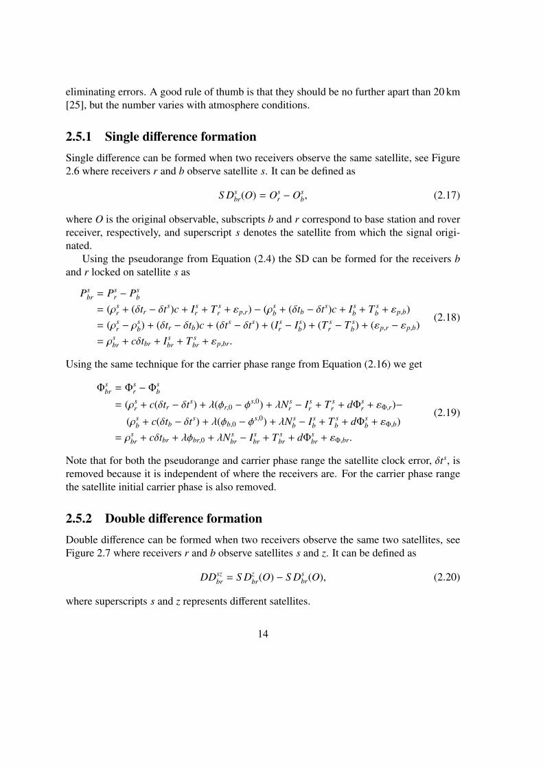
2.5.1 Single difference formationSingle difference can be formed when two receivers observe the same satellite, see Figure2.6 where receivers r and b observe satellite s. It can be defined as
S Dsbr(O) = Os
r − Osb, (2.17)
where O is the original observable, subscripts b and r correspond to base station and roverreceiver, respectively, and superscript s denotes the satellite from which the signal origi-nated.
Using the pseudorange from Equation (2.4) the SD can be formed for the receivers band r locked on satellite s as
Psbr = Ps
r − Psb
= (ρsr + (δtr − δts)c + I s
r + T sr + εp,r) − (ρs
b + (δtb − δts)c + I sb + T s
b + εp,b)= (ρs
r − ρsb) + (δtr − δtb)c + (δts − δts) + (I s
r − I sb) + (T s
r − T sb) + (εp,r − εp,b)
= ρsbr + cδtbr + I s
br + T sbr + εp,br.
(2.18)
Using the same technique for the carrier phase range from Equation (2.16) we get
Φsbr = Φs
r − Φsb
= (ρsr + c(δtr − δts) + λ(φr,0 − φ
s,0) + λN sr − I s
r + T sr + dΦs
r + εΦ,r)−
(ρsb + c(δtb − δts) + λ(φb,0 − φ
s,0) + λN sb − I s
b + T sb + dΦs
b + εΦ,b)= ρs
br + cδtbr + λφbr,0 + λN sbr − I s
br + T sbr + dΦs
br + εΦ,br.
(2.19)
Note that for both the pseudorange and carrier phase range the satellite clock error, δts, isremoved because it is independent of where the receivers are. For the carrier phase rangethe satellite initial carrier phase is also removed.
2.5.2 Double difference formationDouble difference can be formed when two receivers observe the same two satellites, seeFigure 2.7 where receivers r and b observe satellites s and z. It can be defined as
DDszbr = S Dz
br(O) − S Dsbr(O), (2.20)
where superscripts s and z represents different satellites.
14

Φrs Φb
s
s
r b
Baseline
Figure 2.6: Single differencing.
r b
Φrs
Φbs
s z
Φrz
Φbz
Baseline
Figure 2.7: Double differencing.
Using the same technique as for the single differencing the double difference of the
15

pseudoranges and carrier phase ranges can be formed as
Pszbr = Pz
br − Psbr = ρsz
br + cδtszbr + I sz
br + T szbr + εsz
pbr(2.21)
Φszbr = Φsz
r − Φszb = ρsz
br + cδtszbr + λφsz
br,0 + λN szbr − I sz
br + T szbr + dΦsz
br + εΦbr (2.22)
Some of the terms can be canceled out. First off the receiver clock offsets are constant andindependent of satellites, thus we can write
δtszbr = δtz
br − δtsbr = (δtz
r − δtzb) − (δts
r − δtsb) = (δtz
r − δtsr) + (δts
b − δtzb) = 0. (2.23)
The same goes for the initial carrier phases of the receivers:
φszbr,0 = φz
br,0 − φsbr,0 = (φz
r,0 − φzb,0) − (φs
r,0 − φsb,0) = (φz
r,0 − φsr,0) + (φs
b,0 − φzb,0) = 0. (2.24)
For short baselines the base station and rover are close enough to each other that theweather conditions are very similar. In such cases the ionospheric and tropospheric errorsare highly correlated and one assumes that they are eliminated in the double differencingprocess,
I szrb = Iz
rb − I srb ≈ 0 (2.25)
andT sz
rb = T zrb − T s
rb ≈ 0. (2.26)
That means that for a short baseline the double difference pseudorange and carrier phaserange can be written as
Pszbr = ρsz
br + εszpbr, (2.27)
Φszbr = ρsz
br + λN szbr + dΦsz
br + εszΦbr. (2.28)
This is the double difference measurement model used in RTKLIB for baselines shorterthan 10 km [32], and this is the category all flights in this thesis will fall under. For longerbaselines the ionospheric and tropospheric errors would not cancel out and the double dif-ference pseudorange and carrier phase range would then be
Pszbr = ρsz
br + I szbr + T sz
br + εszpbr, (2.29)
Φszbr = ρsz
br + λN szbr + dΦsz
br − I szbr + T sz
br + εszΦbr. (2.30)
2.6 DOPA set of satellites which are more spread out in the sky will provide a more accurate posi-tion than a set of satellites that are close to each other. This concept is known as dilution
16
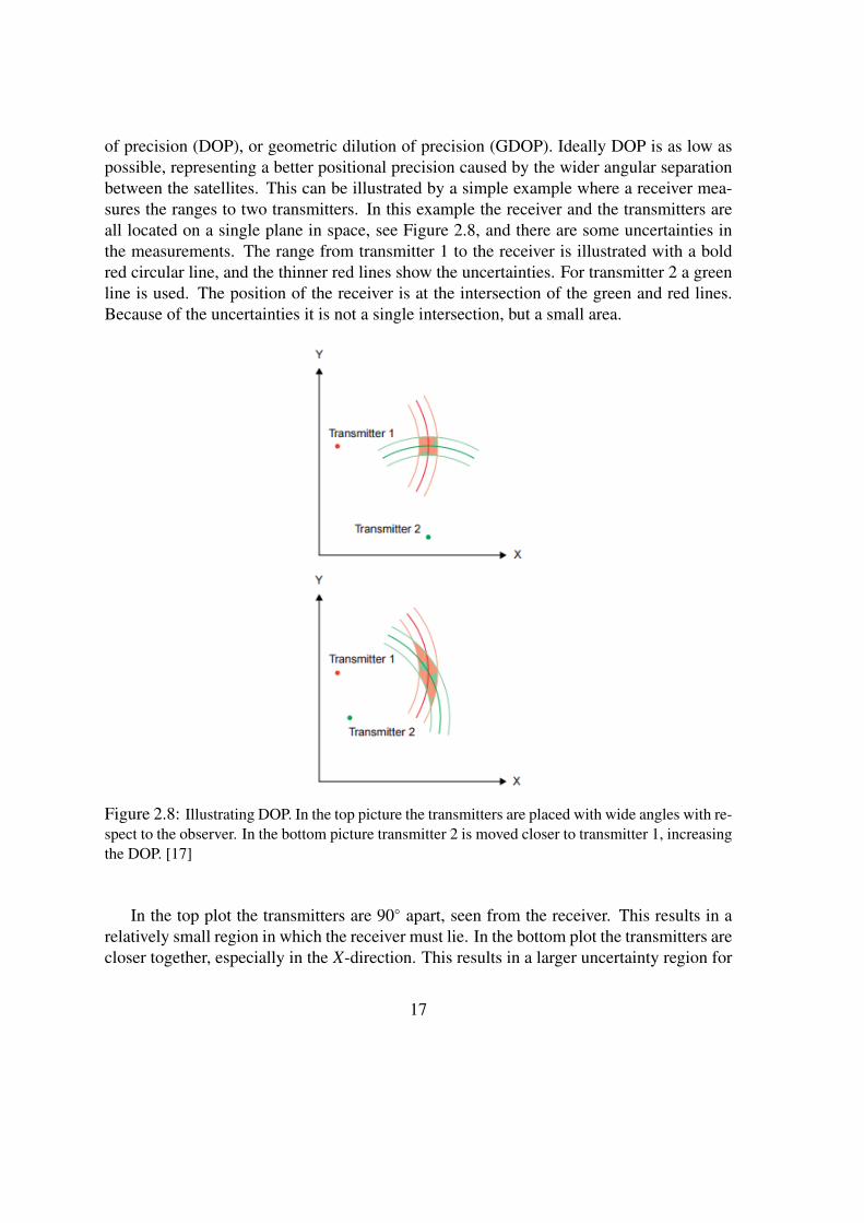
of precision (DOP), or geometric dilution of precision (GDOP). Ideally DOP is as low aspossible, representing a better positional precision caused by the wider angular separationbetween the satellites. This can be illustrated by a simple example where a receiver mea-sures the ranges to two transmitters. In this example the receiver and the transmitters areall located on a single plane in space, see Figure 2.8, and there are some uncertainties inthe measurements. The range from transmitter 1 to the receiver is illustrated with a boldred circular line, and the thinner red lines show the uncertainties. For transmitter 2 a greenline is used. The position of the receiver is at the intersection of the green and red lines.Because of the uncertainties it is not a single intersection, but a small area.
Figure 2.8: Illustrating DOP. In the top picture the transmitters are placed with wide angles with re-spect to the observer. In the bottom picture transmitter 2 is moved closer to transmitter 1, increasingthe DOP. [17]
In the top plot the transmitters are 90◦ apart, seen from the receiver. This results in arelatively small region in which the receiver must lie. In the bottom plot the transmitters arecloser together, especially in the X-direction. This results in a larger uncertainty region for
17

the receiver, with the largest uncertainty in the Y-direction, and this shows that the precisionin the bottom plot is diluted in comparison to that of the top plot.
This is a simple case in two dimensions, but the same concept is applicable for posi-tioning of a receiver in three dimensions using satellites, where there are both positioningand timing errors. Generally the DOP value gets smaller when more satellites are used fora solution. Instead of examining the quality of the overall solution it is possible to look atspecific components, such as the horizontal coordinate, vertical coordinate or the clock off-set. They are known as the HDOP, VDOP and TDOP respectively. They can be expressedas
HDOP =
√σ2
E + σ2N
σ
VDOP =σU
σ
T DOP =σT
σ,
(2.31)
and they are related to the GDOP according to
GDOP2 = HDOP2 + VDOP2 + T DOP2. (2.32)
In the equations σE, σN and σU are the standard deviations of the receiver position in theeast, north and up components. σT is the standard deviation of the receiver clock offsetestimate and σ is the total user equivalent range error (UERE) which can be around 5 m forthe standard positioning service [17].
2.7 RTKLIB algorithms
2.7.1 Extended Kalman FilterRTKLIB employs the Extended Kalman filter (EKF) for obtaining position solutions. EKFis the nonlinear version of the Kalman filter, meaning that it works on nonlinear systems asopposed to the regular Kalman filter which only works on linear systems.
The regular Kalman filter can be broken into three basic steps:
Prediction Using a process noise model, the filter "predicts" parameters at next data epoch.A state transition matrix projects state vector (parameters) forward to the next epoch.
Kalman gain The Kalman Gain is the matrix that allocates the differences between theobservations at time t + 1 and their predicted value at this time based on the currentvalues of the state vector according to the noise in the measurements and the statevector noise.
18

Update This is the step in which the new observations are "blended" into the filter andthe covariance matrix of the state vector is updated. The filter has now been updatedto time t + 1 and measurements from t + 2 can be added and so on until all theobservations have been added.
In order to initiate the filter it starts with an apriori state vector and covariance matrix.The EKF works in much the same way as the Kalman filter. As stated above the state
model does not have to be a linear function, instead it is enough that is differentiable. Themodel will for each time step be linearized using a Taylor expansion. For the details pleaserefer to the RTKLIB manual [32] and [33].
In a standard Kalman filter the stochastic parameters obtained during the filter run arenot optimum because they do not contain information about the deterministic parametersobtained from future data. A smoothing Kalman filter runs the filter forward and backwardsin time, taking the full average of the forward filter at the update step with the backwardsfilter at the prediction step.
2.7.2 Integer Ambiguity ResolutionIf the initial integer ambiguity value for each satellite-receiver pair could be determined thecarrier phase measurements could be corrected to create a very precise receiver-satellitedistance measurement. A solution using the corrected carrier phase observation is knownas an "ambiguity-fixed" solution. In RTKLIB those are identified by the value of the qualityflag Q. For a fixed solution the value of Q would be 1.
By using EKF the estimated rover position and the single-differenced carrier-phaseambiguities are obtained. The next step in order to improve the accuracy is to resolve thefloat carrier-phase ambiguities into integer values, refer to [33]. Eventually the integerambiguity can be found by solving the integer least square (ILS) problem
N = minN∈Z
((N − N)T C−1N (N − N)), (2.33)
where N is the best integer vector, N is the double-differenced carrier-phase ambiguities.C is the covariance matrix of the system noise.
To solve this ILS problem RTKLIB employs LAMBDA [34] and MLAMBDA [3].Then the improved rover position is obtained by solving
r = r − CRNC−1N (N − N). (2.34)
For more details please refer to the RTKLIB manual [32] and [33].
19

2.7.3 Cycle slipOnce a receiver has found and locked on to a signal from a satellite the unknown numberof full wavelengths, ambiguity, between the satellite and the receiver stays constant. Ifthere is a signal blockage, causing the receiver to temporarily lose the lock on a signalfrom a satellite, a cycle slip occurs. Once the receiver re-establishes the signal lock a newambiguity will exist and must be solved for separately from the original ambiguity.
In RTKLIB cycle slips are detected by loss of lock indicator (LLI) in the input mea-surement data [10]. If dual-frequency measurements are available cycle slips can alsobe detected by monitoring jumps of the geometry-free linear combination of L1 and L2carrier-phase.
One effect of cycle slips is that the position of the receiver might be offset by one ormore wavelengths, corresponding to about 20 cm for L1, once the new ambiguity is found.This is a large jump when compared to the restrictions for the creation of high resolutionSAR images and therefore it is crucial to identify and try to prevent cycle slips.
20

Chapter 3
GPS processing software
In this chapter the software products used to process GPS data for this thesis will be givena brief introduction.
3.1 RTKLIBRTKLIB is a set of open source programs written by Tomoji Takasu. It is written in ANSI C(C89) and can be run on multiple OS environments. It can be used for logging, converting,downloading, streaming and processing GNSS data. RTKLIB supports data communica-tion via serial I/O, TCP/IP connection and Networked Transport of RTCM via InternetProtocol (NTRIP). Various data formats are supported including RTCM 3.1 [29] and rawdata from common GPS receivers. The parts of RTKLIB used in this work are the onesused for post-processing RTK and converting raw GPS data to the Receiver IndependentExchange Format (RINEX).
From the version 2.2.0 RTKLIB has been distributed under the GPLv3 license.
3.2 WaypointThe software originally used in the CARABAS system is GrafNav and GrafMov fromWaypoint Software [12]. GrafNav is used for flight paths and GrafMov for baselines.Instead of using RINEX files Waypoint uses their own observation format.
21

Chapter 4
SAR image acquisition
The main steps involved in creating an image using CARABAS is presented in Figure 4.1.This thesis focuses on the steps which has to do with GPS processing, shown on the toprow.
Pre-processing
GPS/Gyro-processing
SAR-processing SAR image
Radar data
GPS data
Gyroscope data
Figure 4.1: Processing steps for creation of a CARABAS III image.
GPS data from three antennas are used during the process. Two of the antennas aremounted on a helicopter and the third antenna is placed on the ground at a known position.The GPS data is the starting point of the processing together with the radar data and thegyroscope data. After acquiring GPS data they are passed through a software in order todetermine the flight path and orientation of the aircraft. This is where RTKLIB is used. Inthe SAR-processing step a so called pass file is used to determine what data should be used.One piece of information found in the pass files is the time for each pass made during theflight, i.e. the start and stop times for each synthetic aperture.
22

4.1 SAR principleDuring data collection for a single SAR image radar pulses are emitted in order to illumi-nate a target scene, and the echo of each pulse is recorded. CARABAS makes use of a radarthat operates in the VHF band where the wavelengths are about 1-15 m. The radar antennamoves relative to the target scene as the data is collected and it is possible to distinguishthe different pulses and identify them. The collected data basically shows a recording frommultiple antenna locations which is what forms the synthetic antenna aperture. The finalresolution of an image created using this technique is finer than what would be possiblewith the given physical antenna aperture [28, p. 3].
Consider the case when the radar pulses are sent from an antenna located on an airplaneflying in a straight line over a target scene with three stationary objects. This is illustrated inFigure 4.2. The blue, red and green squares represents three objects at different locations.
Figure 4.2: Illustration of radar data collection for one SAR image. Image courtesy Anders Åh-lander.
As the plane passes the target scene the relative distance to the objects changes. This leadsto each object creating a unique path in the radar data, as seen in the rectangle on the bottomright of the Figure.
23

In order to combine the radar data from all the pulses to create the final image a tech-nique called Fast Factorized Backprojection[35] is used. Briefly described two neighbour-ing pulses are combined to create a sub-aperture, then two neighbouring sub-apertures arecombined to create a bigger sub-aperture and so on until the all sub-apertures have beencombined to create the final aperture.
As an example of how it might look Figure 4.3 presents one recording and the resultingimage from a flight over Linköping.
Figure 4.3: Recording to the left and resulting image to the right.
24

Chapter 5
Method
In this chapter the measurement and setup used will be described, together with the statis-tics used for comparing the two softwares.
5.1 Data collectionA small helicopter is used for collecting data in the CARABAS system, see Figure 5.1.Two GPS antennas are attached to the tail boom of the helicopter with a distance of ap-proximately 1.2 m. From now on they will be referred to as the front and rear antennas.
A third GPS antenna is positioned stationary on the ground and functions as a basestation. The base station updates at 5 Hz, and the front and rear antennas at 10 Hz. Af-ter a flight the flight path and orientation of the helicopter should be determined by postprocessing the collected GPS data from all antennas.
5.1.1 Flight pathThe data from the front and rear antennas can be used to determine their positions during theflight. This is made by combining their data with that from the base station using RTK. Thepositions of one antenna are given in latitude, longitude and height based on the WGS84datum. The most crucial part of the flight path is the part flown when creating the SARimages which is mostly made on somewhat straight lines. Obviously only position datafrom those parts are the ones that are used in the SAR image processing, but in this thesispositions from the whole flight path will be used as well for evaluating the performance ofRTKLIB.
25

Figure 5.1: Picture of the helicopter used for collecting data. The placement of the high band andlow band radar antennas are shown, as well as the GPS antennas. Image courtesy Saab AB.
5.1.2 OrientationTo find the orientation of the helicopter the moving baseline between the front and rearantennas should be determined as well. It is called a moving baseline since both of theantennas might be moving, and therefore the baseline between them will not be the samefor all epochs during the flight. Note that for regular RTK positioning one of the antennasare placed on a fixed location.
The coordinate system used is a local ENU defined such that the origin is found at thestart of the vector which in this thesis will be the rear antenna. The y-axis coincides withtrue north and the x-axis coincides with true east. The z-axis is defined vertically. As forthe flight path only parts of the data are actually used in the SAR image processing, butbaseline data from the whole flight will be used for evaluating RTKLIB.
Describing the rotation of an aircraft one usually uses the terms roll, pitch and yaw.They refer to rotations about certain axes of the aircraft, see Figure 5.2. The roll axis passesthrough the aircraft from the nose to the tail, the pitch axis passes through the aircraft from
26

Figure 5.2: Roll, pitch and yaw axes [20].
the left side to the right side of the aircraft perpendicular to the roll axis. The yaw axis isperpendicular to the plane created by the roll and pitch axes.
Since only two antennas are attached to the helicopter in the CARABAS system thefull orientation can not be determined without extra inputs. Therefore a MEMS IMU gy-roscope is used for the third unknown angle. The gyroscope is calibrated during flightsby performing "calibration manoeuvres", which are done by changing the heading of thehelicopter at regular intervals [27].
5.2 ReceiversTwo Javad Delta receivers were mounted on the tail boom of the helicopter. They canreceive and process multiple signal types [13]. For the flights they provide measurementdata for post processing at 10 Hz. For the flights compared in this thesis the only recordeddata comes from GPS satellites, but they could be used to receive signals from GLONASSand Galileo as well.
The base station used is a dual-frequency Novatel receiver. It provides measurementdata for post processing at 5 Hz. Both the receivers mounted on the helicopter and the basestation provide data from the L1 and L2 frequencies.
27

5.3 MeasurementsIn order to evaluate RTKLIB data from flights made in October 2014 will be used. Duringaquisition of SAR data the helicopter flew at heights of 30, 250, 350 and 800 m respectively.The data will be processed using the command line tool rnx2rtkp with settings that arepresented in Appendix C. Since the true flight path and moving baselines are not knownthe output from the currently used software will be taken as a reference. This means thatit will be impossible to know if the results are completely valid, only how the result fromRTKLIB differs from that of the other software. It should be noted that the result fromRTKLIB could be closer to the correct value, or it could be further away from the correctvalue than the reference.
5.4 StatisticsTo compare the different positioning results the mean difference, standard deviation ofthe difference, root mean square error of the difference, weighted mean difference andmaximum difference will be studied. Assume there are N values, and the reference valuesand RTKLIB values are denoted yi and yi (i ∈ 1,N), respectively. Then the mean difference,d, is simply defined as
d =1N
N∑i=1
(yi − yi). (5.1)
The standard deviation of the differences, σd is defined as
σd =
√√1N
N∑i=1
((yi − yi) − d)2. (5.2)
The root mean square error (RMSE) of the difference is defined as
(RMS E) =
√√1N
N∑i=1
(yi − yi)2, (5.3)
or equivalently(RMS E)2 = d
2+ σ2
d. (5.4)
The mean difference gives information about how much the result differ from the ref-erence on average, and the standard deviation gives information about the amount of varia-tion about the mean difference. The RMSE of the difference instead describes the variationabout 0.
28

The weighted mean difference uses the formal errors corresponding to each output po-sition value. This way output values which are more uncertain, i.e. the ones with a largeformal error, will not contribute the same amount to the result as values with smaller formalerrors. It can be defined according to
dw =
∑Ni=1 wi(yi − yi)∑N
i=1 wi, (5.5)
wherewi =
1σ2
i
(5.6)
andσi =
√σ2
yi+ σ2
yi. (5.7)
Here σyi is the formal error corresponding to yi and σyi is the formal error corresponding toyi.
29

Chapter 6
Results
In this chapter the results from the comparisons of flight paths and moving baselines be-tween RTKLIB and Waypoint will be presented. The accuracy of RTKLIB is evaluatedusing the result from Waypoint as a reference. The same input GPS data was used by bothsoftwares. Since some settings of Waypoint are hidden a perfect comparison is impossibleto do. The value of the quality flag, Q, which describes whether the integer ambiguities areresolved or not in RTKLIB and Waypoint was also studied. The value of Q can be either1 or 2, where 1 means that the integer ambiguities are properly resolved and 2 means thatthey are not. The value of Q is determined in both programs using a statistic test.
In order to keep this chapter from overflowing with tables and plots most results canbe found in Appendix A. The tables and figures in this chapter are chosen by how theyrepresent the general results.
6.1 Flight pathsA typical flight path is presented in Figure 6.1. The color of the marker corresponds todifferent values of the quality flag Q. Green parts of the plot correspond to where the integerambiguities are properly resolved, and the yellow parts where they are not resolved but thesolution is still found by carrier-based relative positioning. The straight lines making upthe square show where the helicopter flew when collecting radar data for the SAR images.Those parts of the flight path are known as test runs. It is for the test runs that the accuracyof RTKLIB needs to fulfill the stated requirements. The rest of the flight path consists ofthe helicopter repositioning itself for the test runs, and making some calibration movementsfor the gyroscopes on board.
The output from RTKLIB and GrafNav was converted from geodetic coordinates (lati-tude, longitude and height) to Cartesian coordinates with origin in 58◦ 15′ 0.324′′N 15◦ 34′
57.468′′E 151.5 m. That is a point close to where all flights are made (mostly within 5 km),
30

Figure 6.1: Example of a flight path.
ensuring that the local coordinate system is valid. Conversions were made using providedMATLAB functions from the CARABAS project signal processing chain.
The results from the comparisons will be presented using tables and plots. Each tablewill contain columns for mean difference, standard deviation of the difference, RMS of thedifference, weighted mean difference and maximum difference. In the caption of each tableadditional information is found:
qRatR is the fix ratio of the RTKLIB positioning results, i.e. the ratio between the numberof epochs where the integer ambiguity is fixed, and the total number of epochs.
qRatG is the corresponding fix ratio of the GrafNav positioning results.
nValues is the total number of values compared.
At the beginning of each caption is a string used for identifying from where the data origi-nates. The first three characters describe the antenna, which can be either "AFT" or "FWD".The following four numbers describe the date of the flight. The final letter describes theflight number of the day, starting at "a" for the first flight and then "b" for the second and
31

so on. From "AFT1001a" one can see that the antenna used was the "AFT"-antenna, thedate flown was October 1st , and that it was the first flight of the day.
6.1.1 2014-10-03The results for the second flight of October 3rd can be found in Table 6.1, and the corre-sponding Figure 6.2. RTKLIB has a slightly higher fix ratio than GrafNav for the comparedvalues. The mean difference is less than one centimeter in both the x and y-direction, andas expected the difference is a bit larger for the z-direction. Note that the positioning re-quirement is fulfilled.
Table 6.1: FWD1003b, qRatR = 0.988, qRatG = 0.944, nValues = 19865
Variable Mean diff. Std. of diff. RMS of diff. W.Mean diff. Max diff.X (mm) 6.3 16.6 17.8 5.3 52.5Y (mm) -5.9 24.0 24.7 -2.5 83.1Z (mm) -36.5 34.7 50.4 -36.3 171.6
In the plots on can see that the differences in the horizontal directions are almost cen-tered around 0 m. The histograms shows that there is an offset of about 0.05 m in thevertical direction. All in all this represents a good result as the differences are small andRTKLIB had a high fix ratio.
32

Figure 6.2: Plot and histogram displaying differences in x-, y- and z-directions for FWD1003b.
33

6.1.2 2014-10-06The results for the third flight of October 6th can be found in Table 6.2 and Figure 6.3. Forthis flight RTKLIB has a significantly lower fix ratio than GrafNav. This is caused by somecycle slips, which GrafNav has a certain algorithm [12, p. 4] for correcting that RTKLIBdoes not have a counterpart for.
As expected the vertical direction is the one with the largest differences again. The re-sulting positions in the x-directions are a little bit better than the positions in the y-direction.
Table 6.2: FWD1006c, qRatR = 0.695, qRatG = 0.942, nValues = 13745
Variable Mean diff. Std. of diff. RMS of diff. W.Mean diff. Max diff.X (mm) 4.2 63.7 63.7 5.2 190.7Y (mm) 21.7 84.5 87.3 20.3 315.4Z (mm) -0.6 172.1 172.1 -6.7 528.7
The result of the cycle slips can easily be seen in the plot where the differences jumpat different times. In the histograms this is seen by the smaller peaks that are not centeredaround 0 m. Note that the accuracy requirements are not fulfilled for this flight.
34

Figure 6.3: Plot and histogram displaying differences in x-, y- and z-directions for FWD1006c.
35

6.2 Individual test runs, flight pathsThe positioning data used for creating SAR images will be extracted using external infor-mation where time tags are used for setting the start and stop time of the radar collection.The part of the flight where data is collected for one image is called a test run. In this sec-tion the results from a few test runs will be presented to give a better understanding of howthe positioning of RTKLIB performs during the crucial radar data collection. The captionof the tables contains additional information:
h is the height above the ground flown by the helicopter.
l is the distance flown while collecting radar data.
At the beginning of each caption is a string used for identifying the test run.
6.2.1 2014-10-01, AFT1001aIn Table 6.3 and Figure 6.4 the results from one of the test runs from October 1st are pre-sented. The data comes from the AFT-antenna on the first flight of the day. The helicopterflew at 250 m above the ground and both RTKLIB and GrafNav fixed the integer ambiguityresolution during the whole test run. Once again the largest differences are found in thevertical direction. It is worth noting that the maximum difference is still very small, only58.9 mm.
Table 6.3: 15_E0904211, qRatR = 1.00, qRatG = 1.00, nValues = 209, h = 250 m, l = 1015 m
Variable Mean diff. Std. of diff. RMS of diff. W.Mean diff. Max diff.X (mm) -6.5 3.5 7.4 -6.5 15.2Y (mm) -22.8 7.7 24.1 -22.9 37.2Z (mm) -15.3 20.5 25.5 -15.3 58.9
Looking at the histograms it is obvious there is a small offset between the solutions,and the offset is the smallest for the x-direction.
This test run illustrates well the behaviour for most test runs compared to full flights.The differences between RTKLIB and GrafNav is generally smaller during the test runs,and the fix ratio is usually very high for RTKLIB, cf. Table A.1.
36

Figure 6.4: Plot and histogram displaying differences in x-, y- and z-directions for AFT1001a testrun 15_E0904211.
37

6.2.2 2014-10-06, FWD1006cIn Table 6.4 and Figure 6.5 the results from one of the test runs from October 6th arepresented. In this test run a cycle slip occurred which caused the integer ambiguity to bereinitialized by RTKLIB. After the reinitialization the position relative to that produced byGrafNav was shifted which can be seen by the jump at about 12:44:18 in the plot. A shortwhile later RTKLIB corrects the integer ambiguity and the differences jump back to smallervalues.
Table 6.4: 13_E0915508, qRatR = 0.721, qRatG = 0.446, nValues = 258, h = 250 m, l = 492 m
Variable Mean diff. Std. of diff. RMS of diff. W.Mean diff. Max diff.X (mm) -37.8 60.0 70.9 -34.6 153.3Y (mm) 58.2 74.8 94.8 55.3 194.0Z (mm) 102.1 166.0 194.9 91.9 406.7
By studying the position file produced by RTKLIB it can be seen that one satellite is thecause of the loss of the integer ambiguity. Using the solution status file, which is output byRTKLIB if the corresponding parameter is set, the satellite could be identified. It was foundto be a satellite at a low elevation angle, slightly above 15◦. Note that all this information isindependent of the GrafNav results, meaning it is possible to identify the cause of similarproblems without reference data.
By excluding the satellite from the processing the result significantly improved forthe studied test run, see Figure 6.6. After excluding the satellite this test run fulfills therequirements on the accuracy. This is however not a perfect way of solving this kind ofproblems that can occur. By removing one satellite from the processing other test runswere affected, and even though most of the test runs improved there were two for whichthe result degraded. But it is a technique that can be used if no other solution is found forfixing the cycle slips.
38

Figure 6.5: Plot and histogram displaying differences in x-, y- and z-directions for FWD1006c testrun 13_E0915508.
39

Figure 6.6: Plot and histogram displaying differences in x-, y- and z-directions for FWD1006c testrun 13_E0915508, with satellite G15 excluded from the solution.
40

6.3 OrientationA typical set of moving baselines from one flight is presented in Figure 6.7, where thehorizontal projections of the baseline vectors are shown. The plot consists of one markerfor the x and y coordinates at each epoch. It looks like a circle because the helicopter isrotating around more than 360◦ during the flight. The origin of the moving baselines wasset to be the AFT-antenna, meaning that each marker corresponds to the relative positionof the FWD-antenna with respect to the AFT-antenna. From the plot it can be found thatthe baseline lengths is approximately 1.18 m.
Figure 6.7: Set of moving baselines from all the epochs in one flight.
The results from the comparisons will be presented using tables and plots for the mov-ing baselines as well, with basically the same information as the flight paths. The outputused as a reference does not provide formal error, meaning the weighted mean differencewill not be presented in the tables regarding moving baselines. Additionally there are twoangles compared. The first angle is the azimuth which is defined as the angle between thetrue north and the projection of the baseline onto the horizontal plane. The second angle,θ, is the actual angle between the reference baseline and the new baseline. Also, note onceagain that the values used as a reference does not have to be the true positions.
41

6.3.1 2014-10-03In Table 6.5 and Figure 6.8 the moving baseline results for the second flight of October 3rdare presented. These are the moving baselines corresponding to the flight path presentedabove for October 3rd. As for the flight path the fix rate is slightly higher for RTKLIB.The mean differences is on the millimeter scale, and the largest difference is 64.4 mm. Thestandard deviation of the compared moving baseline angles is lower than 1◦, thus fulfillingthe stated requirement.
Table 6.5: Baseline1003b, qRatR = 0.999, qRatG = 0.996, nValues = 39719
Variable Mean diff. Std. of diff. RMS of diff. Max diff.X (mm) 1.2 3.0 3.2 19.7Y (mm) 0.5 5.3 5.3 35.0Z (mm) -1.2 9.3 9.4 64.4Az (◦) -0.008 0.185 0.185 1.611θ (◦) 0.394 0.293 0.491 3.286
In the plots we can see the difference in x-, y- and z-directions for the different epochs,all of which are centered around 0 m. The angle differences are also presented. When thereare spikes in one of the three Cartesian coordinates a corresponding spike is found in theangle differences.
42

Figure 6.8: Plots displaying differences in x-, y-, z-directions and angles 1003b.
43

6.3.2 2014-10-06In Table 6.6 and Figure 6.9 the moving baseline results for the third flight of October 6thare presented. These are the moving baselines corresponding to the flight path presentedabove for October 6th. As opposed to the flight path RTKLIB does not have a significantlylower fix rate. It is in fact slightly higher than that of GrafMov. Note though that the RMSand standard deviation of the differences between the angles are large, above 2◦.
Table 6.6: Baseline1006c, qRatR = 0.979, qRatG = 0.952, nValues = 27328
Variable Mean diff. Std. of diff. RMS of diff. Max diff.X (mm) -1.4 34.0 34.0 3769.9Y (mm) 0.2 14.6 14.6 415.2Z (mm) -1.1 91.2 91.2 7821.4Az (◦) 0.174 0.666 0.688 26.195θ (◦) 1.052 2.244 2.479 73.453
Figure 6.9: Plot displaying differences in x-, y-, z-directions and angles for 1006c.
A large spike can be seen early on in the flight. By comparing the east and north
44

components of the moving baselines it is clearly seen that the spike is caused by a largejump in the position by GrafMov, see Figure 6.10. This illustrates that it is not alwaysRTKLIB that is the cause of large differences, sometimes it is the reference positions thatare off.
Figure 6.10: Plot displaying in east and north components for BASELINE1006c.
45

6.4 Individual test runs, orientation
6.4.1 2014-10-01, BASELINE1001aIn Table 6.7 and Figure 6.11 the results from one of the test runs from October 1st are pre-sented. These are the moving baselines corresponding to the flight path test run presentedearlier. The stated accuracy requirements for the baselines are clearly fulfilled for this testrun.
Table 6.7: 15_E0904211, qRatR = 1.00, qRatG = 1.00, nValues = 418, h = 250 m, l = 1015 m
Variable Mean diff. Std. of diff. RMS of diff. Max diff.X (mm) -5.1 2.4 5.7 12.6Y (mm) 6.9 3.8 7.8 16.3Z (mm) 5.5 8.0 9.7 29.3Az (◦) -0.196 0.098 0.219 0.501θ (◦) 0.366 0.234 0.434 1.278
Figure 6.11: Plot displaying differences in x-, y-, z-directions and angles for 1001a test run15_E0904211.
46

6.4.2 2014-10-06, BASELINE1006cIn Table 6.8 and Figure 6.12 the results from one of the test runs from October 6th are pre-sented. These are the moving baselines corresponding to the flight path test run presentedearlier where there was a cycle slip present. Note that the fix ratio is 1 for RTKLIB, a clearindication that the cycle slip did not affect the baselines.
Table 6.8: 13_E0915508, qRatR = 1.00, qRatG = 0.907, nValues = 516, h = 250 m, l = 492 m
Variable Mean diff. Std. of diff. RMS of diff. Max diff.X (mm) 4.7 4.7 6.7 29.0Y (mm) -1.9 7.5 7.8 22.2Z (mm) -9.9 15.8 18.6 75.2Az (◦) -0.013 0.293 0.293 1.130θ (◦) 0.736 0.529 0.906 3.819
Figure 6.12: Plot displaying differences in x-, y-, z-directions and angles for 1006c test run13_E0915508.
47

6.5 Summary of test runsThere are a total of 26 test runs presented in this thesis. For the flight path data 23 of themfulfill the stated requirements and 3 did not fulfill them. This is for the data created usingthe default configuration files presented in Appendix C. For those that failed it was possibleto modify the settings to fix individual test runs, however as stated earlier this affected othertest runs as well. The standard deviation between the reference position and RTKLIB wasused for judging the test runs as a small global shift of the flight path does not affect theSAR images significantly. This means that a small offset in positions would not really alterthe images, but that offset would make the values of the RMS in the tables increase.
For the orientation there were 22 test runs that fulfilled the requirements, and 2 thatdid not fulfill the requirements. This leaves 2 test runs, A.48 and A.49, where it dependson whether the azimuth (horizontal projection) or actual angle of the moving baselinesaffects the image quality. This depends on how the calibration maneuver for the gyroscopecalibration is made, and since the calibration is usually made by turning the helicopter theazimuth is the more important angle. Then 24 test runs fulfilled the requirements, and 2failed. Whereas for the full angle 22 fulfilled the requirements and 4 failed.
6.6 Quality flagThe goal of studying the quality flag was to find out whether the helicopter movementssomehow affected the value of Q. Therefore the relation between the velocity of the heli-copter and the quality flag was analysed. The values of Q for the first flight of October 7thusing the FWD-antenna are presented in Figure 6.13. For this flight the fix ratio was 96 %,i.e. for 96 % of the epochs the integer ambiguities were fixed, and for the rest they werenot.
The absolute velocities for that flight are presented in Figure 6.14, and the correspond-ing velocity components in Figure 6.15. Apart from the outlier in the y component of thevelocity around 09:40 the solution looks good. Comparing the epochs where the value ofthe quality flag is 2 with the velocities no discernible pattern can be seen. It does not seemlike a high velocity would affect the Q-value, at least not for the velocities reached by thehelicopter.
The relation between the length of the baseline from base station to the helicopter wasalso studied, see Figure 6.16. At first glance it might seem like a short baseline causeproblems here, but the reason for the large amount of Q=2 values is simply that for most ofthe flight the helicopter was close to the base station. I.e. there are a lot more data pointsin the region 100-400 m than in other regions.
In most of the data available from other flights the distance between the reference sta-tion and the helicopter is below 10 km, and the maximum length was 20 km. For these
48

09:15 09:30 09:45 10:00 10:15 10:300
0.5
1
1.5
2
2.5
3
Q
UTC
Figure 6.13: Plot displaying the values of the quality flag Q for FWD1007a.
relatively short distances no clear signs were found that the quality flag was affected.
49

09:30 09:45 10:00 10:15
5
10
15
20
25
30
35
40
45
50
55
UTC
|v|[m/s]
Figure 6.14: Plot displaying the absolute velocities for FWD1007a.
09:15 09:30 09:45 10:00 10:15 10:300
20
40
v x[m/s]
UTC
09:15 09:30 09:45 10:00 10:15 10:300
50
100
v y[m/s]
UTC
09:15 09:30 09:45 10:00 10:15 10:300
0.05
0.1
v z[m/s]
UTC
Figure 6.15: Plot displaying the velocity components for FWD1007a.
50

0 0.2 0.4 0.6 0.8 1 1.2 1.4 1.6 1.8 2
x 104
0
0.5
1
1.5
2
2.5
3
Baseline length [m]
Q
Figure 6.16: Plot displaying the Q values for different baseline lengths for FWD1007A.
51

6.7 Final imageThe absolute comparison between RTKLIB and the Waypoint software is made by com-paring the resulting CARABAS images created using the positioning data from both soft-wares. For this flight data from Febraury 8th 2013 was used. This particular flight waschosen since the image would contain an artificial calibration reflector.
In Figure 6.17 the SAR image created using the original software is presented. Thecorresponding image created using RTKLIB is found in Figure 6.18. The color of thepixels follows a logarithmic scale which describes the intensity of each pixel relative toother pixels. A logarithmic scale is used since otherwise large part of the picture would becompletely black. The x-axis corresponds to the east direction, and the y-axis to the northdirection. Comparing the two images they are close to identical. No information is lostusing RKTLIB, and there is even a small improvement on the image in the area close tothe reflector as it appears slightly sharper. The reflector can be found in the center of theimages.
Figure 6.17: CARABAS image created using positioning data from Waypoint.
52

Figure 6.18: CARABAS image created using positioning data from RKTLIB.
In Figure 6.19 the area around the reflector has been enlarged. This image is madeusing the Waypoint output. In Figure 6.20 the same area can be seen where the positioningdata comes from RTKLIB. Note the area to the right and left of the reflector where theoutput using RTKLIB improved upon that from Waypoint.
These images serve as a final proof that the accuracy of RTKLIB satisfies the require-ments for the CARABAS system. Since the true positions are not known and the accuracyof the reference software is not known either one should keep in mind that the numbersin the tables presented in this report might not reflect the actual positions. However, asthe final images are almost identical when using positions from RTKLIB and Waypoint wehave shown that RTKLIB is accurate enough.
53

East
North
2400 2420 2440 2460 2480 2500 2520 2540 2560 2580 2600
2400
2420
2440
2460
2480
2500
2520
2540
2560
2580
2600
60
70
80
90
100
110
Figure 6.19: Closer look on the reflector in the CARABAS image created using positioning datafrom Waypoint.
East
North
2400 2420 2440 2460 2480 2500 2520 2540 2560 2580 2600
2400
2420
2440
2460
2480
2500
2520
2540
2560
2580
2600
60
70
80
90
100
110
Figure 6.20: Closer look on the reflector in the CARABAS image created using positioning datafrom RTKLIB.
54

Chapter 7
Summary
One of the major objectives of this thesis was to create a batch-driven processing chain uti-lizing RTKLIB with minimum manual interaction. This was realized using the command-line interface of RTKLIB together with scripts written in C-shell and MATLAB-functions.The main script takes two arguments, the folder where to find raw rover data and the folderwhere to find the raw base station data. If all files are available the output from the scriptwill be position files in a format that can be used by the rest of the processing chain forcreating a SAR image. Once the program is started no further input is required which is agreat improvement from using Waypoint Software where one operator had to actively sitin front of the program during the GPS processing which could take about one hour. Therequirement for running the scripts is that all files are placed in the correct folders, andthat SWEPOS data is available if needed. The machine on which the scripts are run alsoobviously need C-shell, MATLAB and RTKLIB. For more information see Appendix B
All results in this thesis where generated using the above mentioned scripts. A demon-stration was made on the computer used in the field for creating CARABAS images. Thisdemonstration proved that the scripts worked as intended, and showed the ease of installingRTKLIB as well as setting up everything needed.
The version 2.4.2 of RTKLIB was used in this thesis, and it was compiled without link-ing to LAPACK of Intel MKL libraries. By recompiling RTKLIB and linking to eitherlibrary the time for processing GPS data will decrease if the computer used for the process-ing has more than one core. For time critical applications this provides a great and simpleway speeding up the application.
For the flights studied in this thesis RTKLIB was generally on the same level of accu-racy as the Waypoint software. There were however some drawbacks that have not yet beenmentioned. In order to determine the base station position one must often use data fromfixed reference stations. In Sweden it is possible to utilize the SWEPOS network whichconsists of about 300 fixed reference stations. Both softwares used are able to do this.However the processing options for GrafNav fits this type of positioning better than the
55
counterpart in RTKLIB. Using GrafNav it is possible to provide data from multiple refer-ence stations, something that is not possible in RTKLIB. Another drawback using RTKLIBfor this kind of processing is that the data available from SWEPOS consists of RINEXfiles with data for one hour. There is no utility in RTKLIB for merging multiple RINEXobservation files into one file. Because of this the processing of the base station positionwill have to be done one time for every hour that it collected data. If the base stationstarted collecting data at 09:00 and stopped at 13:00 this would result in having to do thesame processing four times in order to accurately determine the base station position. Thismeans that the Kalman filter used for each processed hour has no information about theother states at the other hours. A simple remedy for this can be found. There exist freelyavailable software for performing the merging of RINEX observation files, for exampleGPSTk [37] and TEQC [6]. Both GPSTk and TEQC could easily be implemented in thebatch-driven processing chain created during this thesis for processing the GPS data usingRTKLIB.
In the process of evaluating RTKLIB a bug was discovered when studying the baselinedata. The bug caused the baselines to be several kilometers long, even though the baselinein reality was around 1.2 m. The creator of RTKLIB was then contacted and he found andfixed the bug a short time thereafter.
A good indication that the processing worked well is the fix ratio. For a good flightthe ratio percentage is in the upper 90s. Adjusting the parameters in the configuration fileswill modify the behaviour of RTKLIB and therefore alter the ratio. For most flights theconfiguration files presented in Appendix C is sufficient. For certain flights where the fixratio is lower one might need to adjust the values to better accommodate the environment atthe measurements and the receivers used. This was used for the flight on October 6th in thisthesis where there were cycle slips in some of the test runs. By modifying the parametersthe cycle slips were repaired for some test runs. Though no perfect solution was foundwhich fixed all cycle slips this could be used in the CARABAS system for improving theimage quality of specific images.
56

Chapter 8
Conclusions and outlook
It has been shown that RKTLIB satisfies the accuracy requirements stated for creating high-resolution SAR images in the CARABAS system. The positioning accuracy was found tobe within 5 cm and the moving baseline vectors within 1◦ when compared to reference data.SAR images were created using the output from RTKLIB for an absolute confirmation thatthe positioning accuracy was fulfilled. Using an image with a reflector at a known positionit was shown that RTKLIB improved on the result with the compared Waypoint software.Assuming that the commercial software has an accuracy of 5 cm, RTKLIB should be onthe same level or better.
A processing chain utilizing RTKLIB to create the position files used by the CARABASsystem was created using C-shell and MATLAB, where the only required input from a useris information about where raw receiver data can be found on the computer where theprocessing will take place.
By studying how the quality flag was affected by the movements of the helicopter itwas found that the speeds reached by the helicopter did not affect the integer ambiguity.Neither did the distances between the helicopter and the reference station, which for theprovided flights always were less than 20 km.
Moving onwards there is still much that might be worth studying regarding the GPSprocessing for the CARABAS system. First and foremost the real-time performance ofRTKLIB should be analyzed. This would be a natural step in the process of moving onfrom creating SAR images after a flight to create them while flying. Although no clearindications were found that the helicopter cabin affected one of the antennas more thanthe other it might be a good idea to study further. Modifying the filters used for updatingpositions in the single positioning mode of RTKLIB to use the characteristics of an aircraftwould be a good start to see if it would be possible to eventually get rid of the referencestation in the CARABAS system.
It should also be kept in mind that the future support of RTKLIB is not guaranteedto keep the same level at all times since it is a free software. For example if a bug is
57

found it will probably only be fixed for the next release, which might be months away.The continuity aspect is also worth considering, it is always a risk that RTKLIB will notbe maintained in 5-10 years. However, being open source makes it possible for users tofix bugs themselves, since modifications can be made as long as the conditions for thedistribution conditions are met.
58

Bibliography
[1] Elisa Felicitas Arias. "Bureau International des Poids et Mesures (BIPM) - Time De-partment -". http://iag.dgfi.badw.de/fileadmin/IAG-docs/Travaux2013/08_BIPM.pdf, 2013. Accessed: 2015-05-11.
[2] Neil Ashby. Relativistic effects in the global positioning system. In Gravitation andRelativity: At the Turn of the Millenium. 15th International Conference on GeneralRelativity and Gravitation, pages 231–258, 1997.
[3] X-W Chang, X Yang, and T Zhou. MLAMBDA: a modified LAMBDA method forinteger least-squares estimation. Journal of Geodesy, 79(9):552–565, 2005.
[4] Peter H. Dana. "Earth Centered, Earth Fixed X,Y,Z". http://www.colorado.edu/geography/gcraft/notes/coordsys/gif/ecefxyz.gif, 1994. Accessed:2015-05-12.
[5] Peter H. Dana. "Global Positioning System Overview". http://www.colorado.edu/geography/gcraft/notes/gps/gps.html, 1994. Accessed: 2015-03-17.
[6] Louis H Estey and Charles M Meertens. TEQC: the multi-purpose toolkit for GPS/-GLONASS data. GPS solutions, 3(1):42–49, 1999.
[7] Yanming Feng, Jinling Wang, et al. GPS RTK performance characteristics and anal-ysis. Positioning, 1(13), 2008.
[8] United States Government. "GLOBAL POSITIONING SYSTEM WING(GPSW) SYSTEMS ENGINEERING & INTEGRATION". http://www.gps.gov/technical/icwg/IS-GPS-200E.pdf, June 2010. Revision E.
[9] United States Government. "Constellation Arrangement". http://www.gps.gov/systems/gps/space/, January 2015. Accessed: 2015-03-04.
[10] Werner Gurtner and Lou Estey. RINEX: The Receiver Independent Exchange FormatVersion 2.11, 2007.
59

[11] Elizabeth Howell. "Navstar: GPS Satellite Network". http://www.space.com/19794-navstar.html, February 2013. Accessed: 2015-05-07.
[12] Waypoint Consulting Inc. GrafNav/GrafNet, GrafNav Lite, GrafMov, Inertial Ex-plorer, September 2004.
[13] "JAVAD GNSS, Inc". Delta GNSS Receiver, Operator’s Manual, version 1.4, May2009.
[14] Elliott D. Kaplan. Understanding GPS: Principles and Applications. Artech House,second edition, 2005.
[15] John A Klobuchar. Ionospheric time-delay algorithm for single-frequency gps users.Aerospace and Electronic Systems, IEEE Transactions on, (3):325–331, 1987.
[16] Richard B Langley. Time, clocks, and gps. GPS World, 2(10):38–42, 1991.
[17] Richard B Langley. Dilution of precision. GPS world, 10(5):52–59, 1999.
[18] Jhong Sam Lee and Leonard E. Miller. CDMA Systems Engineering Handbook.Artech House Publishers, 1998.
[19] FG Lemoine, DE Smith, L Kunz, R Smith, EC Pavlis, NK Pavlis, SM Klosko,DS Chinn, MH Torrence, RG Williamson, et al. The Development of the Joint NASAGSFC and NIMA Geopotential Model. In Gravity, geoid and marine geodesy, pages461–469. Springer, 1997.
[20] Tech mp website. http://www.www.tech-mp.com/vtol.sw.htm/. Accessed:2015-05-21.
[21] Navipedia. Ionospheric Delay — Navipedia, 2013. Accessed 2015-05-28.
[22] Navipedia. Real Time Kinematics — Navipedia, 2014. Accessed 2015-05-20.
[23] Scott Pace et al. Global Positioning System: Assessing National Policies. RandPublishing, 1996.
[24] Benjamin W. Remondi. Using the Global Positioning System (GPS) phase observablefor relative geodesy: Modelling, processing, and results. PhD thesis, University ofTexas at Austin, Center for Space Research, Austin, TX, 1984.
[25] Anette RietDorf, Christopher Daub, and Peter Loef. Precise positioning in real-timeusing navigation satellites and telecommunication. In Proceedings of The 3rd Work-shop on Positioning and Communication (WPNC’06), 2006.
60

[26] J Saastamoinen. Atmospheric correction for the troposphere and stratosphere in radioranging satellites. The use of artificial satellites for geodesy, pages 247–251, 1972.
[27] Gary Smith-Jonforsen. Carabas 3 generation 1 motion compensation performanceevaluation. Unpublished, August 2013.
[28] Mehrdad Soumekh. Synthetic aperture radar signal processing. New York: Wiley,1999.
[29] RTCM Standard. 10403.1 for Differential GNSS (Global Navigation Satellite Sys-tems) Services-Version 3. Radio Technical Commission for Matitime Services, 2006.
[30] J. Sanz Subirana et al. "Time Reference in GNSS — Navipedia". www.navipedia.net/index.php/Time_Reference_in_GNSS, 2011. Accessed: 2015-05-11.
[31] Tomoji Takasu. "GNSS Precise Point Positioning with RTKLIB Part 1", 2011.
[32] Tomoji Takasu. RTKLIB ver. 2.4.2 Manual, April 2013.
[33] Tomoji Takasu and Akio Yasuda. Development of the low-cost RTK-GPS receiverwith an open source program package RTKLIB. In International Symposium on GP-S/GNSS, pages 4–6. International Convention Centre Jeju, Korea, 2009.
[34] Peter JG Teunissen. A new method for fast carrier phase ambiguity estimation. InPosition Location and Navigation Symposium, 1994., IEEE, pages 562–573. IEEE,1994.
[35] Lars MH Ulander, Hans Hellsten, and Gunnar Stenstrom. Synthetic-aperture radarprocessing using fast factorized back-projection. Aerospace and Electronic Systems,IEEE Transactions on, 39(3):760–776, 2003.
[36] BIPM website. "BIPM work programme: Time". http://www.bipm.org/en/bipm/tai. Accessed: 2015-05-11.
[37] GPSTk website. http://www.gpstk.org/. Accessed: 2015-05-21.
[38] NASA website. "Global Positioning System History". https://www.nasa.gov/directorates/heo/scan/communications/policy/GPS_History.html#.VVyUHfmqpBc, August 2013. Accessed: 2015-05-20.
[39] NASA website. "Global Positioning System". https://www.nasa.gov/directorates/heo/scan/communications/policy/GPS.html#.VUthGvmqpBd, April 2014. Accessed: 2015-05-07.
61

[40] Saab website. "CARABAS". saab.com/air/sensor-systems/ground-imaging-sensors/carabas. Accessed: 2015-05-07.
[41] Guochang Xu. GPS: Theory, Algorithms and Applications. Springer, second edition,2007.
62

Appendix A
Additional results
Here additional results from the comparison between RTKLIB and GrafNav/GrafMov willbe presented.
A.1 Flight paths
A.1.1 2014-10-01
Table A.1: AFT1001a, qRatR = 0.987, qRatG = 0.930, nValues = 25689
Variable Mean diff. Std. of diff. RMS of diff. W.Mean diff. Max diff.X (mm) -4.9 17.1 17.8 -4.9 299.4Y (mm) -27.5 28.6 39.7 -27.4 614.4Z (mm) -1.3 65.7 65.7 -8.6 1931.0
Table A.2: AFT1001b, qRatR = 0.999, qRatG = 0.964, nValues = 3902
Variable Mean diff. Std. of diff. RMS of diff. W.Mean diff. Max diff.X (mm) 0.4 16.3 16.3 0.9 58.3Y (mm) 14.7 18.6 23.7 13.6 84.4Z (mm) -27.2 31.6 41.7 -23.7 146.6
Note on A.2 the output from RTKLIB is split up into b and c for the correspondingoutput b from GrafNav. This is because GrafNav merges two observation files into one,whereas RTKLIB creates one solution for each file.
63

Figure A.1: Plot and histogram displaying differences in x-, y- and z-directions for AFT1001a.
Table A.3: AFT1001b (the rest), qRatR = 0.763, qRatG = 0.831, nValues = 10571
Variable Mean diff. Std. of diff. RMS of diff. W.Mean diff. Max diff.X (mm) 31.2 87.7 93.1 24.5 443.8Y (mm) 39.9 67.3 78.2 36.0 448.4Z (mm) -53.2 153.7 162.6 -44.8 806.9
Table A.4: FWD1001a, qRatR = 0.897, qRatG = 0.765, nValues = 25466
Variable Mean diff. Std. of diff. RMS of diff. W.Mean diff. Max diff.X (mm) 12.3 43.3 45.1 4.6 422.5Y (mm) -40.4 44.3 59.9 -34.6 231.8Z (mm) 44.5 103.2 112.4 11.6 1076.0
64

Figure A.2: Plot and histogram displaying differences in x-, y- and z-directions for AFT1001b.
Table A.5: FWD1001b, qRatR = 0.995, qRatG = 0.888, nValues = 3859
Variable Mean diff. Std. of diff. RMS of diff. W.Mean diff. Max diff.X (mm) -0.8 18.8 18.8 -1.1 52.9Y (mm) 13.8 23.3 27.0 12.6 65.4Z (mm) -26.1 20.2 32.9 -25.5 97.2
65
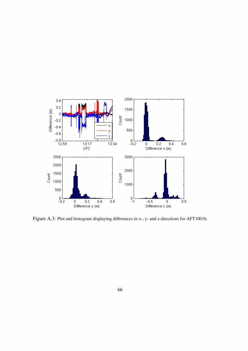
Figure A.3: Plot and histogram displaying differences in x-, y- and z-directions for AFT1001b.
66

Figure A.4: Plot and histogram displaying differences in x-, y- and z-directions for FWD1001a.
67

Figure A.5: Plot and histogram displaying differences in x-, y- and z-directions for FWD1001b.
68

A.1.2 2014-10-03
Table A.6: AFT1003a, qRatR = 0.660, qRatG = 0.940, nValues = 20667
Variable Mean diff. Std. of diff. RMS of diff. W.Mean diff. Max diff.X (mm) 13.8 24.6 28.2 14.3 118.7Y (mm) -15.9 35.4 38.8 -16.0 200.5Z (mm) -87.7 52.9 102.4 -85.2 298.0
Figure A.6: Plot and histogram displaying differences in x-, y- and z-directions for AFT1003a.
69

Table A.7: AFT1003b, qRatR = 0.961, qRatG = 0.925, nValues = 19976
Variable Mean diff. Std. of diff. RMS of diff. W.Mean diff. Max diff.X (mm) 6.4 140.6 14.1 1.8 4432.7Y (mm) 8.1 64.1 6.5 8.5 1901.8Z (mm) 4.5 703.9 70.4 -15.9 22275.3
Figure A.7: Plot and histogram displaying differences in x-, y- and z-directions for AFT1003b.
Table A.8: FWD1003a, qRatR = 0.643, qRatG = 0.965, nValues = 20126
Variable Mean diff. Std. of diff. RMS of diff. W.Mean diff. Max diff.X (mm) 24.3 39.7 46.5 25.4 143.2Y (mm) -24.5 64.6 69.1 -24.9 258.9Z (mm) -45.5 133.7 141.2 -57.7 387.6
70
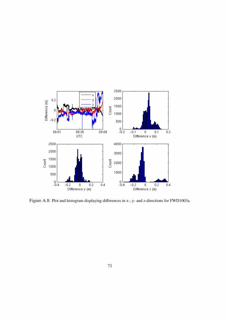
Figure A.8: Plot and histogram displaying differences in x-, y- and z-directions for FWD1003a.
71

A.1.3 2014-10-06
Table A.9: AFT1006c, qRatR = 0.513, qRatG = 0.852, nValues = 13746
Variable Mean diff. Std. of diff. RMS of diff. W.Mean diff. Max diff.X (mm) 41.2 55.0 68.7 35.1 161.8Y (mm) 12.4 54.9 56.2 17.8 689.0Z (mm) 229.0 372.5 437.3 180.2 1166.1
Figure A.9: Plot and histogram displaying differences in x-, y- and z-directions for AFT1006c.
72

A.1.4 2014-10-07
Table A.10: AFT1007a, qRatR = 0.533, qRatG = 0.923, nValues = 19867
Variable Mean diff. Std. of diff. RMS of diff. W.Mean diff. Max diff.X (mm) -121.4 176.0 213.8 -106.6 642.2Y (mm) -106.3 176.5 206.1 -85.8 963.8Z (mm) -66.4 442.6 447.6 24.9 2478.7
Figure A.10: Plot and histogram displaying differences in x-, y- and z-directions for AFT1007a.
73
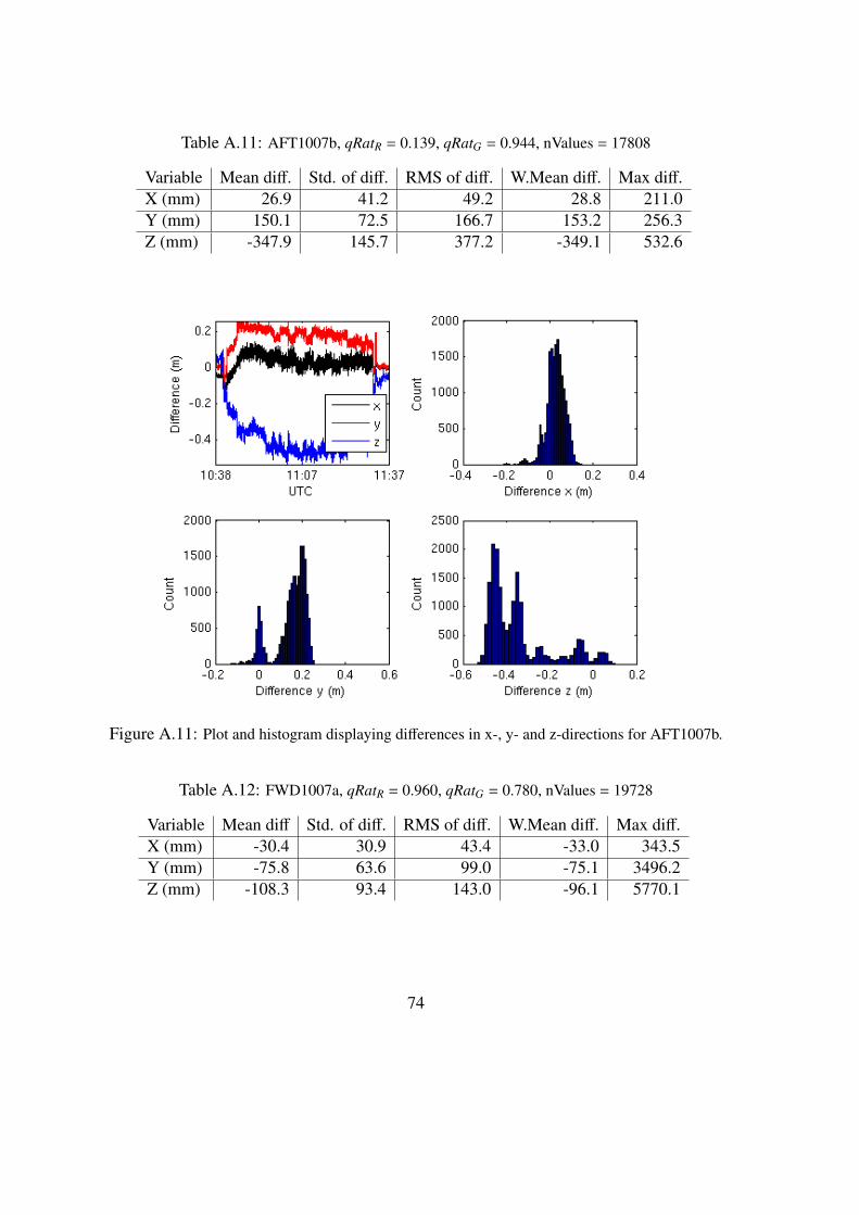
Table A.11: AFT1007b, qRatR = 0.139, qRatG = 0.944, nValues = 17808
Variable Mean diff. Std. of diff. RMS of diff. W.Mean diff. Max diff.X (mm) 26.9 41.2 49.2 28.8 211.0Y (mm) 150.1 72.5 166.7 153.2 256.3Z (mm) -347.9 145.7 377.2 -349.1 532.6
Figure A.11: Plot and histogram displaying differences in x-, y- and z-directions for AFT1007b.
Table A.12: FWD1007a, qRatR = 0.960, qRatG = 0.780, nValues = 19728
Variable Mean diff Std. of diff. RMS of diff. W.Mean diff. Max diff.X (mm) -30.4 30.9 43.4 -33.0 343.5Y (mm) -75.8 63.6 99.0 -75.1 3496.2Z (mm) -108.3 93.4 143.0 -96.1 5770.1
74

Figure A.12: Plot and histogram displaying differences in x-, y- and z-directions for FWD1007a.
Table A.13: FWD1007b, qRatR = 0.973, qRatG = 0.833, nValues = 17306
Variable Mean diff. Std. of diff. RMS of diff. W.Mean diff. Max diff.X (mm) 3.1 20.4 20.7 4.1 79.2Y (mm) -23.8 23.3 33.3 -24.5 90.3Z (mm) -54.2 26.9 60.5 -54.0 195.8
75

Figure A.13: Plot and histogram displaying differences in x-, y- and z-directions for FWD1007b.
76

A.2 Individual test runs, flight paths
A.2.1 2014-10-01, AFT1001a
Table A.14: 16_E0904212, qRatR = 1.00, qRatG = 0.908, nValues = 173, h = 250 m, l = 1015 m
Variable Mean diff. Std. of diff. RMS of diff. W.Mean diff. Max diff.X (mm) 2.8 2.6 3.8 2.8 11.4Y (mm) -30.9 7.7 31.9 -30.9 54.7Z (mm) 4.5 16.8 17.4 4.4 41.4
Figure A.14: Plot and histogram displaying differences in x-, y- and z-directions for AFT1001atest run 16 E0904212.
77

Table A.15: 17_E0904213, qRatR = 1.00, qRatG = 1.00, nValues = 216, h = 250 m, l = 1013 m
Variable Mean diff. Std. of diff. RMS of diff. W.Mean diff. Max diff.X (mm) 10.7 8.9 13.9 10.7 31.3Y (mm) -43.7 8.2 44.5 -43.7 60.2Z (mm) -3.3 27.1 27.3 -3.2 63.6
Table A.16: 18_E0904214, qRatR = 1.00, qRatG = 0.394, nValues = 160, h = 250 m, l = 973 m
Variable Mean diff. Std. of diff. RMS of diff. W.Mean diff. Max diff.X (mm) 11.5 3.5 12.0 11.5 23.5Y (mm) -58.5 13.1 59.9 -58.5 85.7Z (mm) 15.6 38.8 41.8 15.6 91.0
Table A.17: 19_E0904215, qRatR = 1.00, qRatG = 0.963, nValues = 215, h = 250 m, l = 1038 m
Variable Mean diff. Std. of diff. RMS of diff. W.Mean diff. Max diff.X (mm) -26.3 8.8 27.8 -2.6 46.8Y (mm) -30.8 5.6 31.3 -3.1 44.5Z (mm) 76.6 17.8 78.6 76.2 118.4
Table A.18: 26_E0904218, qRatR = 1.00, qRatG = 0.965, nValues = 57, h = 30 m, l = 353 m
Variable Mean diff. Std. of diff. RMS of diff. W.Mean diff. Max diff.X (mm) 1.9 4.6 5.0 1.9 15.5Y (mm) -60.9 15.0 62.7 -60.9 87.8Z (mm) 38.0 34.3 51.2 38.0 83.5
Table A.19: 27_E0904219, qRatR = 1.00, qRatG = 1.00, nValues = 103, h = 30 m, l = 469 m
Variable Mean diff. Std. of diff. RMS of diff. W.Mean diff. Max diff.X (mm) -28.6 5.8 29.2 -28.6 38.8Y (mm) -21.5 7.4 22.7 -21.5 38.8Z (mm) 102.1 16.7 103.4 102.1 126.4
78

Table A.20: 28_E0904220, qRatR = 1.00, qRatG = 1.00, nValues = 57, h = 30 m, l = 323 m
Variable Mean diff. Std. of diff. RMS of diff. W.Mean diff. Max diff.X (mm) 1.5 3.5 3.8 1.5 8.1Y (mm) -73.5 7.4 73.9 -73.5 90.0Z (mm) 72.7 14.8 74.2 72.7 94.6
Figure A.15: Plot and histogram displaying differences in x-, y- and z-directions for AFT1001atest run 28 E0904220.
Table A.21: 29_E0904221, qRatR = 1.00, qRatG = 1.00, nValues = 76, h = 30 m, l = 368 m
Variable Mean diff. Std. of diff. RMS of diff. W.Mean diff. Max diff.X (mm) -5.7 6.1 8.4 -5.7 16.0Y (mm) -56.2 7.3 56.7 -56.2 74.0Z (mm) 67.8 15.9 69.7 67.9 98.3
79

A.2.2 2014-10-06, FWD1006c
Table A.22: 10_E0914220, qRatR = 1.00, qRatG = 1.00, nValues = 40, h = 30 m, l = 242 m
Variable Mean diff. Std. of diff. RMS of diff. W.Mean diff. Max diff.X (mm) 13.6 2.9 13.9 13.6 19.7Y (mm) 4.6 4.8 6.7 4.6 14.9Z (mm) -11.5 10.2 15.4 -11.5 30.8
Table A.23: 11_E0914221, qRatR = 1.00, qRatG = 1.00, nValues = 51, h = 30 m, l = 240 m
Variable Mean diff. Std. of diff. RMS of diff. W.Mean diff. Max diff.X (mm) -14.1 4.5 14.8 -14.1 24.7Y (mm) 23.9 6.3 24.7 23.9 37.1Z (mm) -17.5 9.6 20.0 -17.5 39.0
Table A.24: 12_E0914222, qRatR = 1.00, qRatG = 1.00, nValues = 46, h = 30 m, l = 239 m
Variable Mean diff. Std. of diff. RMS of diff. W.Mean diff. Max diff.X (mm) 11.6 3.7 12.2 11.6 17.9Y (mm) -16.4 5.2 17.2 -16.4 25.6Z (mm) -38.4 10.8 39.9 -38.4 57.9
Table A.25: 13_E0914223, qRatR = 1.00, qRatG = 1.00, nValues = 51, h = 30 m, l = 238 m
Variable Mean diff. Std. of diff. RMS of diff. W.Mean diff. Max diff.X (mm) -10.4 3.5 11.0 -10.4 19.7Y (mm) 13.7 5.4 14.7 13.7 23.2Z (mm) -45.7 14.3 47.9 -45.7 67.
80

Table A.26: 14_E0914218, qRatR = 1.00, qRatG = 0.674, nValues = 43, h = 30 m, l = 239 m
Variable Mean diff. Std. of diff. RMS of diff. W.Mean diff. Max diff.X (mm) 11.7 4.0 12.4 11.7 18.6Y (mm) -5.8 4.1 7.1 -5.8 14.1Z (mm) -39.1 7.8 39.9 -39.1 51.7
Table A.27: 15_E0914219, qRatR = 1.00, qRatG = 1.00, nValues = 51, h = 30 m, l = 235 m
Variable Mean diff. Std. of diff. RMS of diff. W.Mean diff. Max diff.X (mm) -11.3 3.6 11.9 -11.3 20.6Y (mm) 10.8 7.0 12.9 10.8 23.6Z (mm) -38.5 7.7 39.2 -38.5 54.1
Table A.28: 8_E0914218, qRatR = 0.00, qRatG = 1.00, nValues = 40, h = 30 m, l = 249 m
Variable Mean diff. Std. of diff. RMS of diff. W.Mean diff. Max diff.X (mm) -108.8 7.0 109.1 -108.8 123.9Y (mm) 129.1 4.9 129.2 129.1 139.1Z (mm) 384.1 9.9 384.2 384.1 413.8
Table A.29: 10_E0915505, qRatR = 1.00, qRatG = 1.00, nValues = 248, h = 250 m, l = 1781 m
Variable Mean diff. Std. of diff. RMS of diff. W.Mean diff. Max diff.X (mm) 27.1 4.2 27.5 27.1 37.8Y (mm) 25.6 7.3 26.6 25.6 43.4Z (mm) -56.0 14.0 57.7 -56.0 87.8
Table A.30: 11_E0915506, qRatR = 0.949, qRatG = 1.00, nValues = 276, h = 250 m, l = 1576 m
Variable Mean diff. Std. of diff. RMS of diff. W.Mean diff. Max diff.X (mm) -11.6 26.8 29.2 -9.5 129.5Y (mm) -21.7 46.3 51.1 -25.7 220.2Z (mm) -31.9 64.7 72.1 -37.9 290.2
81

Figure A.16: Plot and histogram displaying differences in x-, y- and z-directions for FWD1006ctest run 8 E0914218.
Table A.31: 12_E0915507, qRatR = 0.00, qRatG = 0.984, nValues = 252, h = 250 m, l = 841 m
Variable Mean diff. Std. of diff. RMS of diff. W.Mean diff. Max diff.X (mm) -101.2 17.8 102.7 -100.6 140.2Y (mm) 178.4 24.9 180.1 179.6 221.0Z (mm) 336.1 14.0 336.4 335.7 367.6
Table A.32: 14_E0915509, qRatR = 0.00, qRatG = 0.981, nValues = 257, h = 250 m, l = 132 m
Variable Mean diff. Std. of diff. RMS of diff. W.Mean diff. Max diff.X (mm) -117.5 14.1 118.3 -117.9 155.8Y (mm) 147.0 17.9 148.1 146.0 208.3Z (mm) 359.2 27.1 360.2 358.2 431.8
82

Figure A.17: Plot and histogram displaying differences in x-, y- and z-directions for FWD1006ctest run 10 E0915505.
Table A.33: 15_E0915510, qRatR = 0.371, qRatG = 1.00, nValues = 245, h = 250 m, l = 394 m
Variable Mean diff. Std. of diff. RMS of diff. W.Mean diff. Max diff.X (mm) -61.2 56.0 83.0 -61.3 127.4Y (mm) 57.6 43.0 71.9 58.1 114.6Z (mm) 171.6 140.0 221.5 174.0 309.8
83
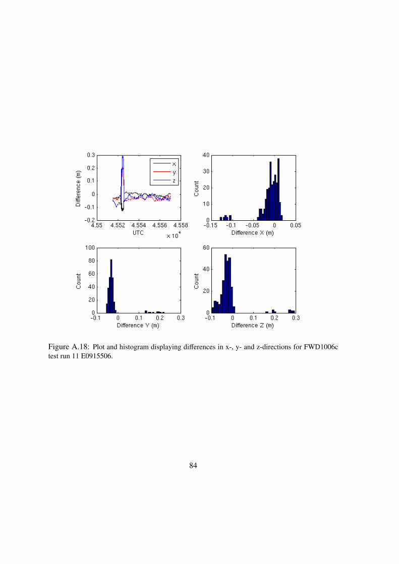
Figure A.18: Plot and histogram displaying differences in x-, y- and z-directions for FWD1006ctest run 11 E0915506.
84

Figure A.19: Plot and histogram displaying differences in x-, y- and z-directions for FWD1006ctest run 12 E095507.
85

Figure A.20: Plot and histogram displaying differences in x-, y- and z-directions for FWD1006ctest run 14 E0915509.
86

Figure A.21: Plot and histogram displaying differences in x-, y- and z-directions for FWD1006ctest run 15 E0915510.
Table A.34: 16_E0915511, qRatR = 1.00, qRatG = 1.00, nValues = 256, h = 250 m, l = 1065 m
Variable Mean diff. Std. of diff. RMS of diff. W.Mean diff. Max diff.X (mm) 4.6 12.2 13.0 4.6 28.3Y (mm) -13.2 9.9 16.6 -13.2 43.2Z (mm) -35.5 17.9 39.7 -35.5 88.8
87

Table A.35: 17_E0915512, qRatR = 0.971, qRatG = 0.543, nValues = 280, h = 250 m, l = 1377 m
Variable Mean diff. Std. of diff. RMS of diff. W.Mean diff. Max diff.X (mm) 8.4 15.0 17.2 8.0 87.0Y (mm) -11.6 18.9 22.2 -11.5 119.2Z (mm) -49.9 47.7 69.0 -47.6 345.4
Table A.36: 8_E0915503, qRatR = 1.00, qRatG = 0.992, nValues = 262, h = 250 m, l = 1483 m
Variable Mean diff. Std. of diff. RMS of diff. W.Mean diff. Max diff.X (mm) 18.9 4.6 19.5 18.9 28.6Y (mm) 48.7 10.1 49.7 48.7 77.4Z (mm) -43.2 13.0 45.1 -43.2 72.7
Table A.37: 9_E0915504, qRatR = 1.00, qRatG = 1.00, nValues = 284, h = 250 m, l = 1931 m
Variable Mean diff. Std. of diff. RMS of diff. W.Mean diff. Max diff.X (mm) 36.0 9.1 37.1 36.0 49.8Y (mm) 53.0 7.5 53.5 53.0 71.3Z (mm) -13.9 7.9 16.0 -13.9 29.5
88

Figure A.22: Plot and histogram displaying differences in x-, y- and z-directions for FWD1006ctest run 9 E0915504.
89

A.3 Orientation
A.3.1 2014-10-01
Table A.38: Baseline1001a, qRatR = 0.999, qRatG = 0.995, nValues = 49546
Variable Mean diff. Std. of diff. RMS of diff. Max diff.X (mm) -0.0 7.0 7.0 157.5Y (mm) 1.0 10.6 10.6 130.4Z (mm) 1.7 29.7 29.8 388.3Az (◦) -0.053 0.453 10.456 5.444θ (◦) 0.782 1.280 1.500 16.032
Figure A.23: Plot displaying differences in x-, y-, z-directions and angles for 1001a.
90
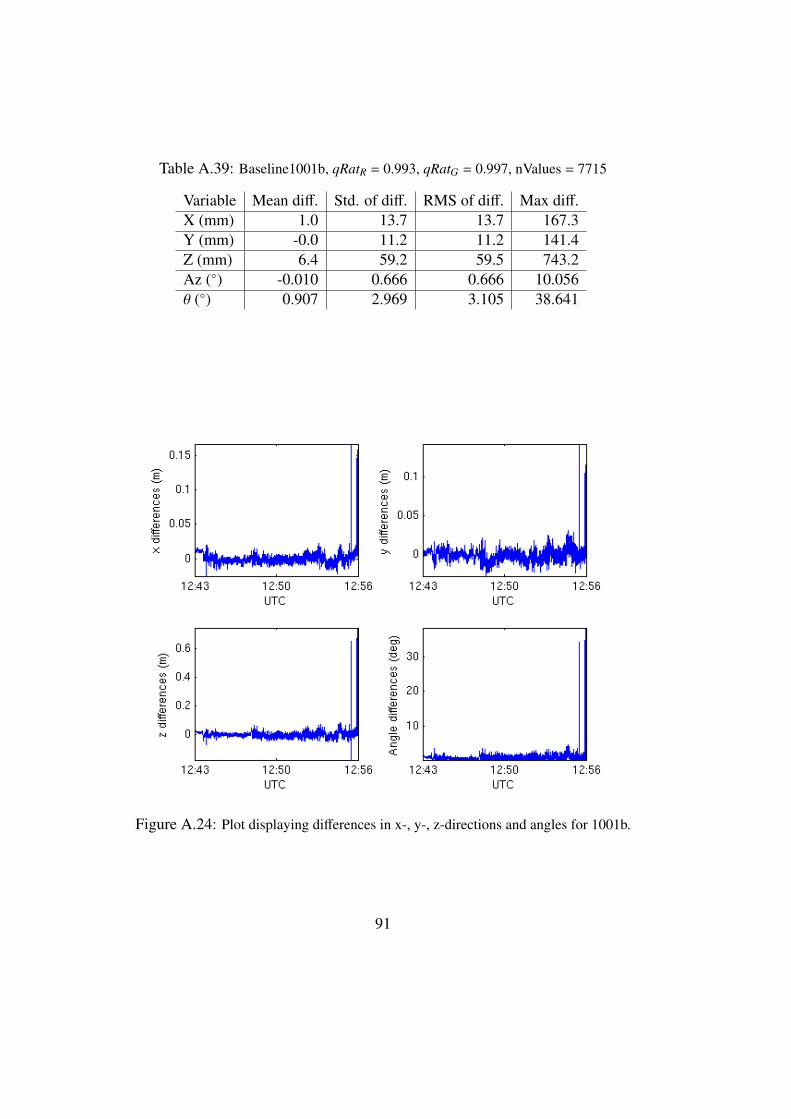
Table A.39: Baseline1001b, qRatR = 0.993, qRatG = 0.997, nValues = 7715
Variable Mean diff. Std. of diff. RMS of diff. Max diff.X (mm) 1.0 13.7 13.7 167.3Y (mm) -0.0 11.2 11.2 141.4Z (mm) 6.4 59.2 59.5 743.2Az (◦) -0.010 0.666 0.666 10.056θ (◦) 0.907 2.969 3.105 38.641
Figure A.24: Plot displaying differences in x-, y-, z-directions and angles for 1001b.
91

A.3.2 2014-10-03
Table A.40: Baseline1003a, qRatR = 0.978, qRatG = 0.992, nValues = 36660
Variable Mean diff. Std. of diff. RMS of diff. Max diff.X (mm) 2.3 21.6 21.7 405.0Y (mm) -0.1 21.9 21.9 313.4Z (mm) 4.0 35.3 35.5 394.2Az (◦) -0.003 1.370 1.370 24.071θ (◦) 0.779 2.047 2.190 25.377
Figure A.25: Plot displaying differences in x-, y-, z-directions and angles for for 1003a.
92

A.3.3 2014-10-07
Table A.41: Baseline1007a, qRatR = 0.937, qRatG = 0.991, nValues = 27591
Variable Mean diff. Std. of diff. RMS of diff. Max diff.X (mm) 3.3 35.9 36.0 402.2Y (mm) 2.9 50.1 50.2 977.6Z (mm) 32.1 199.5 202.0 4262.1Az (◦) 0.311 2.117 2.140 61.178θ (◦) 2.400 8.504 8.837 100.115
Figure A.26: Plot displaying differences in x-, y-, z-directions and angles for 1007a.
93

Table A.42: Baseline1007b, qRatR = 1.00, qRatG = 0.973, nValues = 34584
Variable Mean diff. Std. of diff. RMS of diff. Max diff.X (mm) 0.5 6.0 6.0 779.1Y (mm) 1.2 6.0 6.1 55.0Z (mm) -1.7 18.8 18.8 2175.3Az (◦) 0.012 0.347 0.347 41.578θ (◦) 0.584 0.592 0.831 69.513
Figure A.27: Plot displaying differences in x-, y-, z-directions and angles for 1006b.
94

A.4 Individual test runs, orientation
A.4.1 2014-10-01, BASELINE1001a
Table A.43: 16_E0904212, qRatR = 1.00, qRatG = 1.00, nValues = 347, h = 250 m, l = 1015 m
Variable Mean diff. Std. of diff. RMS of diff. Max diff.X (mm) -0.8 1.8 1.9 6.1Y (mm) -3.7 2.7 4.6 11.0Z (mm) 7.0 5.3 8.8 20.9Az (◦) 0.042 0.090 0.100 0.290θ (◦) 0.353 0.219 0.415 0.975
Figure A.28: Plot displaying differences in x-, y-, z-directions and angles for 1001a test run 16E0904212.
95
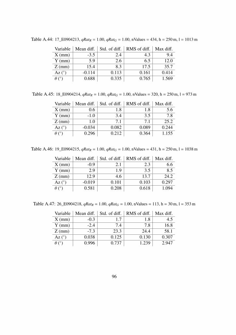
Table A.44: 17_E0904213, qRatR = 1.00, qRatG = 1.00, nValues = 434, h = 250 m, l = 1013 m
Variable Mean diff. Std. of diff. RMS of diff. Max diff.X (mm) -3.5 2.4 4.3 9.4Y (mm) 5.9 2.6 6.5 12.0Z (mm) 15.4 8.3 17.5 35.7Az (◦) -0.114 0.113 0.161 0.414θ (◦) 0.688 0.335 0.765 1.569
Table A.45: 18_E0904214, qRatR = 1.00, qRatG = 1.00, nValues = 320, h = 250 m, l = 973 m
Variable Mean diff. Std. of diff. RMS of diff. Max diff.X (mm) 0.6 1.8 1.8 5.6Y (mm) -1.0 3.4 3.5 7.8Z (mm) 1.0 7.1 7.1 25.2Az (◦) -0.034 0.082 0.089 0.244θ (◦) 0.296 0.212 0.364 1.155
Table A.46: 19_E0904215, qRatR = 1.00, qRatG = 1.00, nValues = 431, h = 250 m, l = 1038 m
Variable Mean diff. Std. of diff. RMS of diff. Max diff.X (mm) -0.9 2.1 2.3 6.6Y (mm) 2.9 1.9 3.5 8.5Z (mm) 12.9 4.6 13.7 24.2Az (◦) -0.019 0.101 0.103 0.297θ (◦) 0.581 0.208 0.618 1.094
Table A.47: 26_E0904218, qRatR = 1.00, qRatG = 1.00, nValues = 113, h = 30 m, l = 353 m
Variable Mean diff. Std. of diff. RMS of diff. Max diff.X (mm) -0.3 1.7 1.8 4.5Y (mm) -2.4 7.4 7.8 16.8Z (mm) -7.3 23.3 24.4 58.1Az (◦) 0.038 0.125 0.130 0.307θ (◦) 0.996 0.737 1.239 2.947
96

Table A.48: 27_E0904219, qRatR = 1.00, qRatG = 1.00, nValues = 205, h = 30 m, l = 469 m
Variable Mean diff. Std. of diff. RMS of diff. Max diff.X (mm) 2.7 3.5 4.4 10.7Y (mm) 6.8 13.8 15.3 37.1Z (mm) 19.7 45.0 49.2 121.2Az (◦) 0.264 0.449 0.521 1.226θ (◦) 1.916 1.191 2.256 5.748
Table A.49: 28_E0904220, qRatR = 1.00, qRatG = 1.00, nValues = 113, h = 30 m, l = 323 m
Variable Mean diff. Std. of diff. RMS of diff. Max diff.X (mm) -3.6 1.9 4.1 9.3Y (mm) -11.8 7.3 13.9 29.3Z (mm) -33.6 22.6 40.5 96.7Az (◦) 0.146 0.093 0.174 0.415θ (◦) 1.805 1.056 2.091 4.947
Table A.50: 29_E0904221, qRatR = 1.00, qRatG = 1.00, nValues = 153, h = 30 m, l = 368 m
Variable Mean diff. Std. of diff. RMS of diff. Max diff.X (mm) -8.2 2.3 8.5 17.0Y (mm) -12.4 7.5 14.5 38.4Z (mm) -50.2 23.5 55.4 123.6Az (◦) -0.472 0.144 0.494 0.935θ (◦) 2.214 0.964 2.415 5.063
97

Figure A.29: Plot displaying differences in x-, y- and z-directions for 1001a test run 28 E0904220.
98

A.4.2 2014-10-06, BASELINE1006c
Table A.51: 10_E0914220, qRatR = 1.00, qRatG = 1.00, nValues = 97, h = 30 m, l = 242 m
Variable Mean diff. Std. of diff. RMS of diff. Max diff.X (mm) 3.4 1.2 3.6 6.1Y (mm) -8.4 3.4 9.0 18.8Z (mm) -8.9 4.7 10.1 18.6Az (◦) 0.045 0.091 0.101 0.356θ (◦) 0.538 0.241 0.589 1.027
Table A.52: 11_E0914221, qRatR = 1.00, qRatG = 1.00, nValues = 153, h = 30 m, l = 240 m
Variable Mean diff. Std. of diff. RMS of diff. Max diff.X (mm) -1.5 1.4 2.0 4.8Y (mm) 7.0 3.3 7.8 15.1Z (mm) 7.9 5.1 9.4 19.4Az (◦) 0.187 0.106 0.215 0.475θ (◦) 0.405 0.172 0.440 0.890
Table A.53: 12_E0914222, qRatR = 1.00, qRatG = 1.00, nValues = 93, h = 30 m, l = 239 m
Variable Mean diff. Std. of diff. RMS of diff. Max diff.X (mm) -0.0 1.8 1.8 4.9Y (mm) -2.9 4.7 5.5 15.1Z (mm) -0.7 5.0 5.1 13.1Az (◦) 0.066 0.074 0.099 0.206θ (◦) 0.243 0.160 0.291 0.742
99

Table A.54: 13_E0914223, qRatR = 1.00, qRatG = 1.00, nValues = 102, h = 30 m, l = 238 m
Variable Mean diff. Std. of diff. RMS of diff. Max diff.X (mm) 1.3 1.6 2.0 5.2Y (mm) 1.9 4.3 4.7 12.8Z (mm) 6.5 6.8 9.4 23.3Az (◦) 0.113 0.119 0.164 0.415θ (◦) 0.384 0.235 0.450 1.074
Table A.55: 14_E0914218, qRatR = 1.00, qRatG = 1.00, nValues = 85, h = 30 m, l = 239 m
Variable Mean diff. Std. of diff. RMS of diff. Max diff.X (mm) 1.4 2.3 2.7 6.1Y (mm) -6.3 4.4 7.7 16.7Z (mm) -5.9 5.9 8.4 16.9Az (◦) 0.086 0.107 0.137 0.320θ (◦) 0.445 0.196 0.487 0.961
Table A.56: 15_E0914219, qRatR = 1.00, qRatG = 0.990, nValues = 102, h = 30 m, l = 235 m
Variable Mean diff. Std. of diff. RMS of diff. Max diff.X (mm) -2.5 2.1 3.3 8.9Y (mm) 1.3 5.2 5.3 11.3Z (mm) -14.5 8.0 16.5 34.9Az (◦) -0.046 0.155 0.162 0.409θ (◦) 0.731 0.324 0.800 1.604
Table A.57: 8_E0914218, qRatR = 1.00, qRatG = 1.00, nValues = 79, h = 30 m, l = 249 m
Variable Mean diff. Std. of diff. RMS of diff. Max diff.X (mm) 1.1 1.4 1.8 4.2Y (mm) -6.3 5.4 8.3 17.4Z (mm) -5.0 6.4 8.1 21.1Az (◦) 0.095 0.104 0.141 0.398θ (◦) 0.379 0.309 0.489 1.235
100

Figure A.30: Plot displaying differences in x-, y- and z-directions for 1006c test run 8 E0914218.
101

Table A.58: 10_E0915505, qRatR = 1.00, qRatG = 1.00, nValues = 497, h = 250 m, l = 1781 m
Variable Mean diff. Std. of diff. RMS of diff. Max diff.X (mm) 4.6 10.5 11.5 26.5Y (mm) -4.5 10.8 11.7 33.3Z (mm) 0.6 35.9 35.9 97.0Az (◦) 0.345 0.165 0.382 0.758θ (◦) 1.337 0.817 1.567 3.963
Figure A.31: Plot displaying differences in x-, y- and z-directions for 1006c test run 10 E0915505.
102

Table A.59: 11_E0915506, qRatR = 0.202, qRatG = 0.885, nValues = 494, h = 250 m, l = 1576 m
Variable Mean diff. Std. of diff. RMS of diff. Max diff.X (mm) -29.4 56.2 63.4 323.6Y (mm) -29.2 62.9 69.4 395.5Z (mm) -21.4 224.9 225.9 1696.7Az (◦) 1.448 3.552 3.836 26.195θ (◦) 7.059 8.333 10.921 53.012
Figure A.32: Plot displaying differences in x-, y-, z-directions and angles for 1006c test run 11E0915506.
103
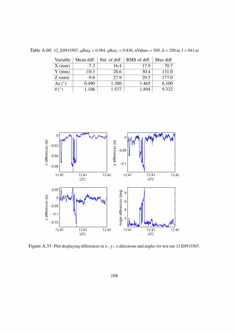
Table A.60: 12_E0915507, qRatR = 0.584, qRatG = 0.836, nValues = 505, h = 250 m, l = 841 m
Variable Mean diff. Std. of diff. RMS of diff. Max diff.X (mm) -7.3 16.4 17.9 70.7Y (mm) -10.3 28.6 30.4 131.0Z (mm) -9.6 27.9 29.5 177.0Az (◦) 0.490 1.380 1.465 6.100θ (◦) 1.106 1.537 1.894 9.332
Figure A.33: Plot displaying differences in x-, y-, z-directions and angles for test run 12 E0915507.
104

Table A.61: 14_E0915509, qRatR = 1.00, qRatG = 0.984, nValues = 514, h = 250 m, l = 132 m
Variable Mean diff. Std. of diff. RMS of diff. Max diff.X (mm) -0.2 3.2 3.2 11.0Y (mm) -2.7 8.8 9.2 27.9Z (mm) -5.2 10.9 12.1 30.0Az (◦) 0.039 0.226 0.229 0.868θ (◦) 0.545 0.336 0.640 1.780
Figure A.34: Plot displaying differences in x-, y-, z-directions and angles for 1006c test run 14E0915509.
105

Table A.62: 15_E0915510, qRatR = 1.00, qRatG = .998, nValues = 489, h = 250 m, l = 394 m
Variable Mean diff. Std. of diff. RMS of diff. Max diff.X (mm) -1.4 2.8 3.2 8.7Y (mm) -0.1 8.3 8.3 23.2Z (mm) -3.3 10.3 10.8 37.0Az (◦) 0.115 0.248 0.273 1.216θ (◦) 0.516 0.311 0.603 1.697
Figure A.35: Plot displaying differences in x-, y- and z-directions for 1006c test run 15 E0915510.
106

Table A.63: 16_E0915511, qRatR = 1.00, qRatG = 1.00, nValues = 511, h = 250 m, l = 1065 m
Variable Mean diff. Std. of diff. RMS of diff. Max diff.X (mm) 0.0 2.0 2.0 8.6Y (mm) -2.5 6.7 7.1 21.4Z (mm) 0.9 8.7 8.7 23.2Az (◦) 0.030 0.183 0.186 1.060θ (◦) 0.397 0.260 0.475 1.151
Table A.64: 17_E0915512, qRatR = 1.00, qRatG = 0.928, nValues = 559, h = 250 m, l = 1377 m
Variable Mean diff. Std. of diff. RMS of diff. Max diff.X (mm) 1.3 2.5 2.8 11.8Y (mm) -7.2 6.2 9.5 22.1Z (mm) -3.7 9.2 10.0 50.5Az (◦) 0.008 0.170 0.170 0.739θ (◦) 0.472 0.316 0.568 2.597
Table A.65: 8_E0915503, qRatR = 1.00, qRatG = 1.00, nValues = 524, h = 250 m, l = 1483 m
Variable Mean diff. Std. of diff. RMS of diff. Max diff.X (mm) 3.2 5.5 6.3 17.2Y (mm) 9.7 6.4 11.6 24.5Z (mm) 14.4 21.5 25.9 69.5Az (◦) 0.284 0.302 0.415 1.109θ (◦) 1.015 0.706 1.236 3.389
Table A.66: 9_E0915504, qRatR = 1.00, qRatG = 0.996, nValues = 569, h = 250 m, l = 1931 m
Variable Mean diff. Std. of diff. RMS of diff. Max diff.X (mm) 1.8 8.5 8.7 28.1Y (mm) -0.2 9.9 9.9 33.2Z (mm) -3.5 30.9 31.1 119.3Az (◦) 0.052 0.284 0.289 1.054θ (◦) 1.114 0.832 1.390 5.272
107

Figure A.36: Plot displaying differences in x-, y-, z-directions and angles for test run 9 E0915504.
108

Appendix B
Script overview
In this chapter the scripts created for the processing chain utilizing RTKLIB will be brieflypresented. Raw data from three antennas are needed in order to be able to create the fileswith flight path and moving baseline data for the SAR image processing. If the base stationposition is known that information should be put in a txt-file. If the base station positionis not known data from the SWEPOS network can be used to determine the position andcreate the corresponding txt-file. For this the SWEOPOS data should placed in the correctfolder and the main script will then find out how it should proceed.
In Figure B.1 a short overview of the main steps in the processing chain are presented.Script files written in C-shell and MATLAB function files are used in the processing. The
main.csh
baseline.csh pos2txt.cshflightpath.cshconverter.csh
Raw rover data Raw base station data
1 2 3 4
Figure B.1: Main steps in the GPS processing chain.
processing is started by providing the folders with raw rover and raw base station data tothe main script. From there the main script will call converter.csh for converting theraw data into RINEX. For this convbin from RTKLIB is used.
109

The next step is to create position files with flight path data which is done in the scriptcalled fligthpath.csh. Then the base station position is needed. If there exists a filenamed basePosition.txt the position therein will be used. Otherwise the behaviour iscontrolled by setting the corresponding variables in the main script. The default behaviouris to use SWEPOS data for determining the base station position, but it is also possible touse the approximate position stated in the RINEX header, or use the average of the singlepoint solutions by RTKLIB.
Once the flight path files are created it is time to create the moving baseline files usingthe script baseline.csh. Then information is needed about how far apart the antennas onthe helicopter are mounted. This information should be placed in a file named inst.txt.If this file does not exist the moving baseline files will be created once without constraintsfor the baseline. Those files will be used to determine the baseline constraint and create theneeded file. Once the setup file exists the baseline files will be created using the baselineconstraint. For creating both the flight path and baseline files rnx2rtkp from RTKLIB isused.
The last step is to convert the pos-files created by RTKLIB into txt-files with the formatthat is used be the rest of the SAR processing. This is done using pos2txt.csh
By modularizing the code as have been done it is easy for users to execute only partof the processing if needed. For example if it is needed to recreate the baseline data withdifferent settings this can be done without starting from scratch and converting the raw dataand creating flight path files.
B.1 Main filesmain.csh
Sets all major variables needed by other scripts.
converter.cshConverts raw GPS data to RINEX.
baseposition.cshCreates a file with information about the base station position. Needs SWEPOS data.
flightpath.cshCreates AFT/FWD.pos-files.
baseline.cshCreates BASELINE.pos-files.
pos2txt.csh"Wrapper" for corresponding m-file.
110

B.2 Minor filescheckObsTimes.csh
"Wrapper" for m-file.
checkObsTimes.mChecks whether 2 observation files match in time.
pos2txt.mConverts the format of the files created by RTKLIB to the format needed by the SARprocessing.
readPos.mReads data from pos-files produced by RTKLIB.
readHeader.mReads header information from file produced by RTKLIB.
setupBaselineConstraints.mCreates baseline constraint file.
setupBasePosition.mCreates base station position file.
111

Appendix C
Configuration files
In this chapter the configuration files used for the different modes of rnx2rtkp are presented.For explanation of the configuration file refer to [32].
C.1 flightpath.conf
This configuration file is used to create position files for the flightpaths. When the basestation position is used the variable "ant2-postype" is overriden by using the flag "-l".
1 # rtkpost options (2015/02/12 07:17:01, v.2.4.2)23 pos1-posmode =kinematic # (0:single ,1:dgps,2:kinematic ,3:static ,4:movingbase ,5:←↩
fixed ,6:ppp-kine,7:ppp-static)4 pos1-frequency =l1+l2 # (1:l1,2:l1+l2,3:l1+l2+l5,4:l1+l2+l5+l6,5:l1+l2+l5+l6+l7←↩
)5 pos1-soltype =combined # (0:forward ,1:backward ,2:combined)6 pos1-elmask =15 # (deg)7 pos1-snrmask_r =off # (0:off,1:on)8 pos1-snrmask_b =off # (0:off,1:on)9 pos1-snrmask_L1 =0,0,0,0,0,0,0,0,0
10 pos1-snrmask_L2 =0,0,0,0,0,0,0,0,011 pos1-snrmask_L5 =0,0,0,0,0,0,0,0,012 pos1-dynamics =off # (0:off,1:on)13 pos1-tidecorr =off # (0:off,1:on,2:otl)14 pos1-ionoopt =brdc # (0:off,1:brdc,2:sbas,3:dual-freq,4:est-stec,5:ionex-tec←↩
,6:qzs-brdc,7:qzs-lex,8:vtec_sf ,9:vtec_ef ,10:gtec)15 pos1-tropopt =saas # (0:off,1:saas,2:sbas,3:est-ztd,4:est-ztdgrad)16 pos1-sateph =brdc # (0:brdc,1:precise ,2:brdc+sbas,3:brdc+ssrapc ,4:brdc+←↩
ssrcom)17 pos1-posopt1 =on # (0:off,1:on)18 pos1-posopt2 =on # (0:off,1:on)19 pos1-posopt3 =off # (0:off,1:on)20 pos1-posopt4 =off # (0:off,1:on)21 pos1-posopt5 =on # (0:off,1:on)22 pos1-exclsats = # (prn ...)23 pos1-navsys =1 # (1:gps+2:sbas+4:glo+8:gal+16:qzs+32:comp)
112

24 pos2-armode =fix-and-hold # (0:off,1:continuous ,2:instantaneous ,3:fix-and-hold)25 pos2-gloarmode =on # (0:off,1:on,2:autocal)26 pos2-bdsarmode =on # (0:off,1:on)27 pos2-arthres =328 pos2-arlockcnt =029 pos2-arelmask =0 # (deg)30 pos2-arminfix =1031 pos2-elmaskhold =0 # (deg)32 pos2-aroutcnt =533 pos2-maxage =30 # (s)34 pos2-syncsol =off # (0:off,1:on)35 pos2-slipthres =0.05 # (m)36 pos2-rejionno =30 # (m)37 pos2-rejgdop =3038 pos2-niter =139 pos2-baselen =0 # (m)40 pos2-basesig =0 # (m)41 out-solformat =llh # (0:llh,1:xyz,2:enu,3:nmea)42 out-outhead =on # (0:off,1:on)43 out-outopt =on # (0:off,1:on)44 out-timesys =gpst # (0:gpst,1:utc,2:jst)45 out-timeform =tow # (0:tow,1:hms)46 out-timendec =547 out-degform =deg # (0:deg,1:dms)48 out-fieldsep =49 out-height =ellipsoidal # (0:ellipsoidal ,1:geodetic)50 out-geoid =internal # (0:internal ,1:egm96 ,2:egm08_2.5,3:egm08_1 ,4:gsi2000)51 out-solstatic =all # (0:all,1:single)52 out-nmeaintv1 =0 # (s)53 out-nmeaintv2 =0 # (s)54 out-outstat =off # (0:off,1:state ,2:residual)55 stats-eratio1 =10056 stats-eratio2 =10057 stats-errphase =0.003 # (m)58 stats-errphaseel =0.003 # (m)59 stats-errphasebl =0 # (m/10km)60 stats-errdoppler =10 # (Hz)61 stats-stdbias =30 # (m)62 stats-stdiono =0.03 # (m)63 stats-stdtrop =0.3 # (m)64 stats-prnaccelh =10 # (m/s^2)65 stats-prnaccelv =10 # (m/s^2)66 stats-prnbias =0.0001 # (m)67 stats-prniono =0.001 # (m)68 stats-prntrop =0.0001 # (m)69 stats-clkstab =5e-12 # (s/s)70 ant1-postype =llh # (0:llh,1:xyz,2:single ,3:posfile ,4:rinexhead ,5:rtcm)71 ant1-pos1 =90 # (deg|m)72 ant1-pos2 =0 # (deg|m)73 ant1-pos3 =-6335367.6285 # (m|m)74 ant1-anttype =ACC53G1215A_XT175 ant1-antdele =0 # (m)76 ant1-antdeln =0 # (m)77 ant1-antdelu =0 # (m)78 ant2-postype =rinexhead # (0:llh,1:xyz,2:single ,3:posfile ,4:rinexhead ,5:rtcm)79 ant2-pos1 =0 # (deg|m) Note these values will be overriden80 ant2-pos2 =0 # (deg|m) during call to rnx2rtkp using flag -l81 ant2-pos3 =0 # (m|m)82 ant2-anttype =ASH701975.01B83 ant2-antdele =0 # (m)
113

84 ant2-antdeln =0 # (m)85 ant2-antdelu =0 # (m)86 misc-timeinterp =off # (0:off,1:on)87 misc-sbasatsel =0 # (0:all)88 misc-rnxopt1 =89 misc-rnxopt2 =90 file-satantfile =/proj/Carabas_PDF2/Personal/u025078_Ronny/training/pcv/ngs08.atx91 file-rcvantfile =/proj/Carabas_PDF2/Personal/u025078_Ronny/training/pcv/ngs08.atx92 file-staposfile =93 file-geoidfile =94 file-ionofile =95 file-dcbfile =96 file-eopfile =97 file-blqfile =98 file-tempdir =99 file-geexefile =
100 file-solstatfile =101 file-tracefile =
C.2 flightpath_single.conf
This configuration file is used to create position files for the flightpaths where the base sta-tion position is set as the average of single point solutions. When the base station positionis used the variable "ant2-postype" is overriden by using the flag "-l". The only differencebetween this file and the one shown above is the value of "ant2-postype".
1 # rtkpost options (2015/02/12 07:17:01, v.2.4.2)23 pos1-posmode =kinematic # (0:single ,1:dgps,2:kinematic ,3:static ,4:movingbase ,5:←↩
fixed ,6:ppp-kine,7:ppp-static)4 pos1-frequency =l1+l2 # (1:l1,2:l1+l2,3:l1+l2+l5,4:l1+l2+l5+l6,5:l1+l2+l5+l6+l7←↩
)5 pos1-soltype =combined # (0:forward ,1:backward ,2:combined)6 pos1-elmask =15 # (deg)7 pos1-snrmask_r =off # (0:off,1:on)8 pos1-snrmask_b =off # (0:off,1:on)9 pos1-snrmask_L1 =0,0,0,0,0,0,0,0,0
10 pos1-snrmask_L2 =0,0,0,0,0,0,0,0,011 pos1-snrmask_L5 =0,0,0,0,0,0,0,0,012 pos1-dynamics =off # (0:off,1:on)13 pos1-tidecorr =off # (0:off,1:on,2:otl)14 pos1-ionoopt =brdc # (0:off,1:brdc,2:sbas,3:dual-freq,4:est-stec,5:ionex-tec←↩
,6:qzs-brdc,7:qzs-lex,8:vtec_sf ,9:vtec_ef ,10:gtec)15 pos1-tropopt =saas # (0:off,1:saas,2:sbas,3:est-ztd,4:est-ztdgrad)16 pos1-sateph =brdc # (0:brdc,1:precise ,2:brdc+sbas,3:brdc+ssrapc ,4:brdc+←↩
ssrcom)17 pos1-posopt1 =on # (0:off,1:on)18 pos1-posopt2 =on # (0:off,1:on)19 pos1-posopt3 =off # (0:off,1:on)20 pos1-posopt4 =off # (0:off,1:on)21 pos1-posopt5 =off # (0:off,1:on)22 pos1-exclsats = # (prn ...)23 pos1-navsys =1 # (1:gps+2:sbas+4:glo+8:gal+16:qzs+32:comp)
114

24 pos2-armode =fix-and-hold # (0:off,1:continuous ,2:instantaneous ,3:fix-and-hold)25 pos2-gloarmode =on # (0:off,1:on,2:autocal)26 pos2-bdsarmode =on # (0:off,1:on)27 pos2-arthres =328 pos2-arlockcnt =029 pos2-arelmask =0 # (deg)30 pos2-arminfix =1031 pos2-elmaskhold =0 # (deg)32 pos2-aroutcnt =533 pos2-maxage =30 # (s)34 pos2-syncsol =off # (0:off,1:on)35 pos2-slipthres =0.05 # (m)36 pos2-rejionno =30 # (m)37 pos2-rejgdop =3038 pos2-niter =139 pos2-baselen =0 # (m)40 pos2-basesig =0 # (m)41 out-solformat =llh # (0:llh,1:xyz,2:enu,3:nmea)42 out-outhead =on # (0:off,1:on)43 out-outopt =on # (0:off,1:on)44 out-timesys =gpst # (0:gpst,1:utc,2:jst)45 out-timeform =tow # (0:tow,1:hms)46 out-timendec =547 out-degform =deg # (0:deg,1:dms)48 out-fieldsep =49 out-height =ellipsoidal # (0:ellipsoidal ,1:geodetic)50 out-geoid =internal # (0:internal ,1:egm96 ,2:egm08_2.5,3:egm08_1 ,4:gsi2000)51 out-solstatic =all # (0:all,1:single)52 out-nmeaintv1 =0 # (s)53 out-nmeaintv2 =0 # (s)54 out-outstat =off # (0:off,1:state ,2:residual)55 stats-eratio1 =10056 stats-eratio2 =10057 stats-errphase =0.003 # (m)58 stats-errphaseel =0.003 # (m)59 stats-errphasebl =0 # (m/10km)60 stats-errdoppler =10 # (Hz)61 stats-stdbias =30 # (m)62 stats-stdiono =0.03 # (m)63 stats-stdtrop =0.3 # (m)64 stats-prnaccelh =10 # (m/s^2)65 stats-prnaccelv =10 # (m/s^2)66 stats-prnbias =0.0001 # (m)67 stats-prniono =0.001 # (m)68 stats-prntrop =0.0001 # (m)69 stats-clkstab =5e-12 # (s/s)70 ant1-postype =llh # (0:llh,1:xyz,2:single ,3:posfile ,4:rinexhead ,5:rtcm)71 ant1-pos1 =90 # (deg|m)72 ant1-pos2 =0 # (deg|m)73 ant1-pos3 =-6335367.6285 # (m|m)74 ant1-anttype =ACC53G1215A_XT175 ant1-antdele =0 # (m)76 ant1-antdeln =0 # (m)77 ant1-antdelu =0 # (m)78 ant2-postype =single # (0:llh,1:xyz,2:single ,3:posfile ,4:rinexhead ,5:rtcm)79 ant2-pos1 =0 # (deg|m) Note these values will be overriden80 ant2-pos2 =0 # (deg|m) during call to rnx2rtkp using flag -l81 ant2-pos3 =0 # (m|m)82 ant2-anttype =ASH701975.01B83 ant2-antdele =0 # (m)
115

84 ant2-antdeln =0 # (m)85 ant2-antdelu =0 # (m)86 misc-timeinterp =off # (0:off,1:on)87 misc-sbasatsel =0 # (0:all)88 misc-rnxopt1 =89 misc-rnxopt2 =90 file-satantfile =/proj/Carabas_PDF2/Personal/u025078_Ronny/training/pcv/ngs08.atx91 file-rcvantfile =/proj/Carabas_PDF2/Personal/u025078_Ronny/training/pcv/ngs08.atx92 file-staposfile =93 file-geoidfile =94 file-ionofile =95 file-dcbfile =96 file-eopfile =97 file-blqfile =98 file-tempdir =99 file-geexefile =
100 file-solstatfile =101 file-tracefile =
C.3 baseline.conf
This configuration file is used to create the position files for the baselines without con-straints. To set baseline constraints the value of the variables "pos2-baselen" and "pos2-basesig" are changed to appropriate values.
1 # rtkpost options (2015/02/27 12:42:04, v.2.4.3)23 pos1-posmode =movingbase # (0:single ,1:dgps,2:kinematic ,3:static ,4:movingbase ,5:←↩
fixed ,6:ppp-kine,7:ppp-static)4 pos1-frequency =l1+l2 # (1:l1,2:l1+l2,3:l1+l2+l5,4:l1+l2+l5+l6,5:l1+l2+l5+l6+l7←↩
)5 pos1-soltype =combined # (0:forward ,1:backward ,2:combined)6 pos1-elmask =20 # (deg)7 pos1-snrmask_r =off # (0:off,1:on)8 pos1-snrmask_b =off # (0:off,1:on)9 pos1-snrmask_L1 =0,0,0,0,0,0,0,0,0
10 pos1-snrmask_L2 =0,0,0,0,0,0,0,0,011 pos1-snrmask_L5 =0,0,0,0,0,0,0,0,012 pos1-dynamics =off # (0:off,1:on)13 pos1-tidecorr =off # (0:off,1:on,2:otl)14 pos1-ionoopt =brdc # (0:off,1:brdc,2:sbas,3:dual-freq,4:est-stec,5:ionex-tec←↩
,6:qzs-brdc,7:qzs-lex,8:vtec_sf ,9:vtec_ef ,10:gtec)15 pos1-tropopt =saas # (0:off,1:saas,2:sbas,3:est-ztd,4:est-ztdgrad)16 pos1-sateph =brdc # (0:brdc,1:precise ,2:brdc+sbas,3:brdc+ssrapc ,4:brdc+←↩
ssrcom)17 pos1-posopt1 =off # (0:off,1:on)18 pos1-posopt2 =off # (0:off,1:on)19 pos1-posopt3 =off # (0:off,1:on)20 pos1-posopt4 =off # (0:off,1:on)21 pos1-posopt5 =off # (0:off,1:on)22 pos1-exclsats = # (prn ...)23 pos1-navsys =1 # (1:gps+2:sbas+4:glo+8:gal+16:qzs+32:comp)24 pos2-armode =continuous # (0:off,1:continuous ,2:instantaneous ,3:fix-and-hold)25 pos2-gloarmode =off # (0:off,1:on,2:autocal)
116

26 pos2-bdsarmode =off # (0:off,1:on)27 pos2-arthres =328 pos2-arlockcnt =029 pos2-arelmask =0 # (deg)30 pos2-arminfix =1031 pos2-elmaskhold =0 # (deg)32 pos2-aroutcnt =533 pos2-maxage =30 # (s)34 pos2-syncsol =off # (0:off,1:on)35 pos2-slipthres =0.05 # (m)36 pos2-rejionno =30 # (m)37 pos2-rejgdop =3038 pos2-niter =239 pos2-baselen =0 # (m)40 pos2-basesig =0 # (m)41 out-solformat =enu # (0:llh,1:xyz,2:enu,3:nmea)42 out-outhead =on # (0:off,1:on)43 out-outopt =on # (0:off,1:on)44 out-timesys =gpst # (0:gpst,1:utc,2:jst)45 out-timeform =tow # (0:tow,1:hms)46 out-timendec =247 out-degform =deg # (0:deg,1:dms)48 out-fieldsep =49 out-height =ellipsoidal # (0:ellipsoidal ,1:geodetic)50 out-geoid =internal # (0:internal ,1:egm96 ,2:egm08_2.5,3:egm08_1 ,4:gsi2000)51 out-solstatic =all # (0:all,1:single)52 out-nmeaintv1 =0 # (s)53 out-nmeaintv2 =0 # (s)54 out-outstat =off # (0:off,1:state ,2:residual)55 stats-eratio1 =10056 stats-eratio2 =10057 stats-errphase =0.003 # (m)58 stats-errphaseel =0.003 # (m)59 stats-errphasebl =0 # (m/10km)60 stats-errdoppler =10 # (Hz)61 stats-stdbias =30 # (m)62 stats-stdiono =0.03 # (m)63 stats-stdtrop =0.3 # (m)64 stats-prnaccelh =10 # (m/s^2)65 stats-prnaccelv =10 # (m/s^2)66 stats-prnbias =0.0001 # (m)67 stats-prniono =0.001 # (m)68 stats-prntrop =0.0001 # (m)69 stats-clkstab =5e-12 # (s/s)70 ant1-postype =llh # (0:llh,1:xyz,2:single ,3:posfile ,4:rinexhead ,5:rtcm)71 ant1-pos1 =90 # (deg|m)72 ant1-pos2 =0 # (deg|m)73 ant1-pos3 =-6335367.6285 # (m|m)74 ant1-anttype =ACC53G1215A_XT175 ant1-antdele =0 # (m)76 ant1-antdeln =0 # (m)77 ant1-antdelu =0 # (m)78 ant2-postype =single # (0:llh,1:xyz,2:single ,3:posfile ,4:rinexhead ,5:rtcm)79 ant2-pos1 =0 # (deg|m)80 ant2-pos2 =0 # (deg|m)81 ant2-pos3 =0 # (m|m)82 ant2-anttype =ACC53G1215A_XT183 ant2-antdele =0 # (m)84 ant2-antdeln =0 # (m)85 ant2-antdelu =0 # (m)
117
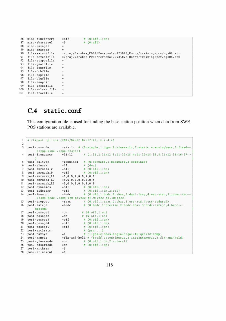
86 misc-timeinterp =off # (0:off,1:on)87 misc-sbasatsel =0 # (0:all)88 misc-rnxopt1 =89 misc-rnxopt2 =90 file-satantfile =/proj/Carabas_PDF2/Personal/u025078_Ronny/training/pcv/ngs08.atx91 file-rcvantfile =/proj/Carabas_PDF2/Personal/u025078_Ronny/training/pcv/ngs08.atx92 file-staposfile =93 file-geoidfile =94 file-ionofile =95 file-dcbfile =96 file-eopfile =97 file-blqfile =98 file-tempdir =99 file-geexefile =
100 file-solstatfile =101 file-tracefile =
C.4 static.conf
This configuration file is used for finding the base station position when data from SWE-POS stations are available.
1 # rtkpost options (2015/02/12 07:17:01, v.2.4.2)23 pos1-posmode =static # (0:single ,1:dgps,2:kinematic ,3:static ,4:movingbase ,5:fixed←↩
,6:ppp-kine,7:ppp-static)4 pos1-frequency =l1+l2 # (1:l1,2:l1+l2,3:l1+l2+l5,4:l1+l2+l5+l6,5:l1+l2+l5+l6+l7←↩
)5 pos1-soltype =combined # (0:forward ,1:backward ,2:combined)6 pos1-elmask =15 # (deg)7 pos1-snrmask_r =off # (0:off,1:on)8 pos1-snrmask_b =off # (0:off,1:on)9 pos1-snrmask_L1 =0,0,0,0,0,0,0,0,0
10 pos1-snrmask_L2 =0,0,0,0,0,0,0,0,011 pos1-snrmask_L5 =0,0,0,0,0,0,0,0,012 pos1-dynamics =off # (0:off,1:on)13 pos1-tidecorr =off # (0:off,1:on,2:otl)14 pos1-ionoopt =brdc # (0:off,1:brdc,2:sbas,3:dual-freq,4:est-stec,5:ionex-tec←↩
,6:qzs-brdc,7:qzs-lex,8:vtec_sf ,9:vtec_ef ,10:gtec)15 pos1-tropopt =saas # (0:off,1:saas,2:sbas,3:est-ztd,4:est-ztdgrad)16 pos1-sateph =brdc # (0:brdc,1:precise ,2:brdc+sbas,3:brdc+ssrapc ,4:brdc+←↩
ssrcom)17 pos1-posopt1 =on # (0:off,1:on)18 pos1-posopt2 =on # (0:off,1:on)19 pos1-posopt3 =off # (0:off,1:on)20 pos1-posopt4 =off # (0:off,1:on)21 pos1-posopt5 =off # (0:off,1:on)22 pos1-exclsats = # (prn ...)23 pos1-navsys =1 # (1:gps+2:sbas+4:glo+8:gal+16:qzs+32:comp)24 pos2-armode =fix-and-hold # (0:off,1:continuous ,2:instantaneous ,3:fix-and-hold)25 pos2-gloarmode =on # (0:off,1:on,2:autocal)26 pos2-bdsarmode =on # (0:off,1:on)27 pos2-arthres =328 pos2-arlockcnt =0
118

29 pos2-arelmask =0 # (deg)30 pos2-arminfix =1031 pos2-elmaskhold =0 # (deg)32 pos2-aroutcnt =533 pos2-maxage =30 # (s)34 pos2-syncsol =off # (0:off,1:on)35 pos2-slipthres =0.05 # (m)36 pos2-rejionno =30 # (m)37 pos2-rejgdop =3038 pos2-niter =139 pos2-baselen =0 # (m)40 pos2-basesig =0 # (m)41 out-solformat =llh # (0:llh,1:xyz,2:enu,3:nmea)42 out-outhead =on # (0:off,1:on)43 out-outopt =on # (0:off,1:on)44 out-timesys =gpst # (0:gpst,1:utc,2:jst)45 out-timeform =tow # (0:tow,1:hms)46 out-timendec =547 out-degform =deg # (0:deg,1:dms)48 out-fieldsep =49 out-height =ellipsoidal # (0:ellipsoidal ,1:geodetic)50 out-geoid =internal # (0:internal ,1:egm96 ,2:egm08_2.5,3:egm08_1 ,4:gsi2000)51 out-solstatic =all # (0:all,1:single)52 out-nmeaintv1 =0 # (s)53 out-nmeaintv2 =0 # (s)54 out-outstat =off # (0:off,1:state ,2:residual)55 stats-eratio1 =10056 stats-eratio2 =10057 stats-errphase =0.003 # (m)58 stats-errphaseel =0.003 # (m)59 stats-errphasebl =0 # (m/10km)60 stats-errdoppler =10 # (Hz)61 stats-stdbias =30 # (m)62 stats-stdiono =0.03 # (m)63 stats-stdtrop =0.3 # (m)64 stats-prnaccelh =10 # (m/s^2)65 stats-prnaccelv =10 # (m/s^2)66 stats-prnbias =0.0001 # (m)67 stats-prniono =0.001 # (m)68 stats-prntrop =0.0001 # (m)69 stats-clkstab =5e-12 # (s/s)70 ant1-postype =llh # (0:llh,1:xyz,2:single ,3:posfile ,4:rinexhead ,5:rtcm)71 ant1-pos1 =90 # (deg|m)72 ant1-pos2 =0 # (deg|m)73 ant1-pos3 =-6335367.6285 # (m|m)74 ant1-anttype =ASH701975.01B75 ant1-antdele =0 # (m)76 ant1-antdeln =0 # (m)77 ant1-antdelu =0 # (m)78 ant2-postype =rinexhead # (0:llh,1:xyz,2:single ,3:posfile ,4:rinexhead ,5:rtcm)79 ant2-pos1 =0 # (deg|m) Note these values will be overriden80 ant2-pos2 =0 # (deg|m) during call to rnx2rtkp using flag -l81 ant2-pos3 =0 # (m|m)82 ant2-anttype =*83 ant2-antdele =0 # (m)84 ant2-antdeln =0 # (m)85 ant2-antdelu =0 # (m)86 misc-timeinterp =off # (0:off,1:on)87 misc-sbasatsel =0 # (0:all)88 misc-rnxopt1 =
119

89 misc-rnxopt2 =90 file-satantfile =/proj/Carabas_PDF2/Personal/u025078_Ronny/training/pcv/ngs08.atx91 file-rcvantfile =/proj/Carabas_PDF2/Personal/u025078_Ronny/training/pcv/ngs08.atx92 file-staposfile =93 file-geoidfile =94 file-ionofile =95 file-dcbfile =96 file-eopfile =97 file-blqfile =98 file-tempdir =99 file-geexefile =
100 file-solstatfile =101 file-tracefile =
120