An Honors Thesis in Physics submitted by stephen Omohundro ...

Department of Physics and Astronomy
University of Heidelberg
Master Thesis in Physics
submitted by
Christian Mohler
2014

D-meson production at ultra-low transverse momentum in
proton-proton collisions with ALICE at the LHC
This Master Thesis has been carried out by
Christian Mohler
at the
University of Heidelberg
under the supervision of
PD Dr. Kai Schweda

Abstract
The measurement of charm production provides valuable insights into the properties of
the Quark-Gluon Plasma, which is expected to be formed in ultra-relativistic heavy-ion
collisions at the Large Hadron Collider (LHC) at CERN. The high-precision tracking and
particle identification capabilities of A Large Ion Collider Experiment (ALICE) allow for
the measurement of D mesons in hadronic decay channels, based on the reconstruction
of secondary decay vertices. For weakly decaying D mesons, these are typically displaced
from the primary vertex by a few hundred µm. However, this topological approach will
inevitably fail at low transverse momentum (pT), where the Lorentz boost is not strong
enough to be resolved. Current ALICE results of D-meson production using this analysis
strategy are therefore limited to pT > 1 GeV/c.
This thesis presents a new measurement of the pT-differential cross section of prompt
D0 production in the decay channel D0 → K−π+ at mid-rapidity in proton-proton
collisions at√s = 7 TeV. By giving up the topological selection, the presented analysis
extends the measurable pT range down to zero. The extraction of a stable signal at low
pT is made possible by using the like-sign background subtraction technique. In the
overlapping pT range, the results of this work are consistent with those obtained using
the standard topological approach. The pT-integrated charm production cross section at
mid-rapidity can be given without extrapolation for the first time at the LHC, resulting
in dσcc/dy = (879± 135) µb, which represents an increase in precision by about a factor
two over the previous topological measurement.

Zusammenfassung
Die Messung der Produktion von Charm-Quarks gewahrt einen wertvollen experimentellen
Zugang zu den Eigenschaften des Quark-Gluon-Plasmas, welches wahrscheinlich in ultra-
relativistischen Schwerionenkollisionen am LHC (Large Hadron Collider) am CERN
erzeugt wird. Dank praziser Teilchenspurrekonstruktion und Teilchenidentifikation konnen
mit dem ALICE-Detektor D-Mesonen uber ihre hadronischen Zerfallskanalen gemessen
werden. Hierbei wird ausgenutzt, dass abhangig von der Lebensdauer eines D-Mesons der
Zerfallsvertex typischerweise um einige hundert Mikrometer vom primaren Vertex entfernt
ist. Dieser topologische Ansatz kann allerdings nicht fur die Messung von D-Mesonen
mit niedrigem Transversalimpuls (pT) verwendet werden, da die geringe Zerfallslange
nicht im Detektor aufgelost werden kann. Alle gegenwartig veroffentlichten Ergebnisse
der ALICE-Kollaboration zur Messung von D-Mesonen beschranken sich daher notwendi-
gerweise auf Transversalimpulse pT > 1 GeV/c.
In der vorliegenden Arbeit wird eine neue Messung des pT-differentiellen Wirkungsquer-
schnitts der Produktion von D-Mesonen bei mittlerer Rapiditat vorgestellt. Hierbei
wurde der Zerfallskanal D0 → K−π+ in Protonenkollisionen bei einer Schwerpunktsen-
ergie von√s = 7 TeV analysiert. Durch Verzicht auf eine topologische Selektion konnte
der gemessene Transversalimpulsbereich bis hin zu 0 GeV/c erweitert werden. Die Sig-
nalextraktion wurde dabei durch die Verwendung der ”Like-Sign”-Methode stabilisiert.
In dem Transversalimpulsbereich, der von beiden Analysen abgedeckt wird, stimmen die
Resultate der hier vorgestellten Messung mit denen der topologischen Messung uberein.
Zum ersten Mal am LHC ist es nun moglich, den pT-integrierten Wirkungsquerschnitt der
Charm-Produktion bei mittlerer Rapiditat in Protonenkollisionen ohne eine Extrapolation
in pT anzugeben. Der ermittelte Wirkungsquerschnitt betragt dσcc/dy = (879± 135) µb.
Im Vergleich zur topologischen Analyse konnte der Messfehler auf die Halfte reduziert
werden.
Contents
1 Introduction 1
2 D-Meson Production in Hadronic Collisions 5
2.1 Key Features of Quantum Chromodynamics . . . . . . . . . . . . . . . . . 5
2.2 Exploring the QCD Phase Diagram . . . . . . . . . . . . . . . . . . . . . . 7
2.3 Heavy Quarks in the QGP . . . . . . . . . . . . . . . . . . . . . . . . . . . 9
2.4 Open Charm and Charmonium . . . . . . . . . . . . . . . . . . . . . . . . 13
2.5 Theoretical Predictions for Heavy-Flavour Production . . . . . . . . . . . 15
3 ALICE at the LHC 19
3.1 LHC Experiments and Physics Programme . . . . . . . . . . . . . . . . . 19
3.2 ALICE Detector Overview . . . . . . . . . . . . . . . . . . . . . . . . . . . 20
3.3 Inner Tracking System . . . . . . . . . . . . . . . . . . . . . . . . . . . . . 21
3.4 Time Projection Chamber . . . . . . . . . . . . . . . . . . . . . . . . . . . 22
3.5 Time of Flight . . . . . . . . . . . . . . . . . . . . . . . . . . . . . . . . . 23
3.6 T0 . . . . . . . . . . . . . . . . . . . . . . . . . . . . . . . . . . . . . . . . 23
3.7 V0 . . . . . . . . . . . . . . . . . . . . . . . . . . . . . . . . . . . . . . . . 24
4 The D0 Decay 25
4.1 D0 Decay Modes . . . . . . . . . . . . . . . . . . . . . . . . . . . . . . . . 25
4.2 D0 Decay Kinematics . . . . . . . . . . . . . . . . . . . . . . . . . . . . . . 27
4.2.1 Momentum-Space Variables . . . . . . . . . . . . . . . . . . . . . . 27
4.2.2 Invariant Mass . . . . . . . . . . . . . . . . . . . . . . . . . . . . . 29
4.2.3 Decay Length . . . . . . . . . . . . . . . . . . . . . . . . . . . . . . 29
4.2.4 Kinematics of a Two-Body Decay . . . . . . . . . . . . . . . . . . . 31
4.2.5 A Toy Monte Carlo for Decay Kinematics . . . . . . . . . . . . . . 31
i

5 Data Analysis 34
5.1 Strategy and Overview . . . . . . . . . . . . . . . . . . . . . . . . . . . . . 34
5.2 Computational Analysis . . . . . . . . . . . . . . . . . . . . . . . . . . . . 36
5.3 Data Sets and Event Selection . . . . . . . . . . . . . . . . . . . . . . . . 37
5.4 Track Reconstruction and Selection . . . . . . . . . . . . . . . . . . . . . . 38
5.5 Particle Identification . . . . . . . . . . . . . . . . . . . . . . . . . . . . . 42
5.5.1 PID Information from TPC and TOF . . . . . . . . . . . . . . . . 42
5.5.2 PID Strategy . . . . . . . . . . . . . . . . . . . . . . . . . . . . . . 44
5.6 Signal Extraction . . . . . . . . . . . . . . . . . . . . . . . . . . . . . . . . 46
5.6.1 Overview and Preliminary Considerations . . . . . . . . . . . . . . 46
5.6.2 Background Subtraction . . . . . . . . . . . . . . . . . . . . . . . . 49
5.6.3 Fitting Procedure . . . . . . . . . . . . . . . . . . . . . . . . . . . 54
5.6.4 Randomised Multi-Trial Approach . . . . . . . . . . . . . . . . . . 56
5.7 Efficiency Correction . . . . . . . . . . . . . . . . . . . . . . . . . . . . . . 57
5.8 Feed-Down Correction . . . . . . . . . . . . . . . . . . . . . . . . . . . . . 59
5.9 Calculation of the Cross Section . . . . . . . . . . . . . . . . . . . . . . . 61
6 Uncertainties 63
6.1 Statistical Uncertainties . . . . . . . . . . . . . . . . . . . . . . . . . . . . 63
6.2 Systematic Uncertainties . . . . . . . . . . . . . . . . . . . . . . . . . . . . 64
7 Results 67
7.1 D0 Production Cross Section . . . . . . . . . . . . . . . . . . . . . . . . . 67
7.2 Total Charm Production Cross Section . . . . . . . . . . . . . . . . . . . . 70
8 Summary and Outlook 74
ii
List of Figures
2.1 The ‘running’ of the strong coupling constant αs as a function of the
energy scale Q . . . . . . . . . . . . . . . . . . . . . . . . . . . . . . . . . 6
2.2 Sketch of a possible QCD phase diagram. . . . . . . . . . . . . . . . . . . 8
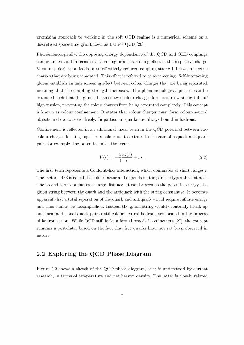
2.3 Generation mechanisms of quark masses . . . . . . . . . . . . . . . . . . . 10
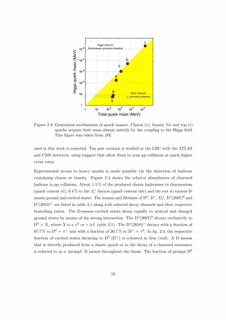
2.4 Relative abundances of charmed hadrons in pp collisions . . . . . . . . . . 11
2.6 Feynman diagrams of the leading-order (LO) processes of heavy-flavour
pair production. . . . . . . . . . . . . . . . . . . . . . . . . . . . . . . . . 16
2.7 Feynman diagrams of two contributions to the heavy-quark pair production
cross section at next-to-leading order (NLO). . . . . . . . . . . . . . . . . 16
2.8 FONLL predictions of the D0 pT spectrum . . . . . . . . . . . . . . . . . . 18
3.1 Sketch of ALICE with labels for the different subsystems . . . . . . . . . 20
4.1 Feynman diagrams of the Cabibbo-favoured decay D0 → K−π+ (left) and
the doubly Cabibbo-suppressed decay D0 → K+π− (right). . . . . . . . . 25
4.2 Average D0 decay length in the lab frame as a function of the D0 transverse
momentum and rapidity. . . . . . . . . . . . . . . . . . . . . . . . . . . . . 30
4.3 Simulated kinematics of the D0 → K−π+ decay. . . . . . . . . . . . . . . . 33
5.1 Distribution of the z position of reconstructed vertices in pp and Pb-Pb
collisions. . . . . . . . . . . . . . . . . . . . . . . . . . . . . . . . . . . . . 37
5.2 Flow chart for the different stages of the tracking procedure. . . . . . . . 39
5.3 ITS-TPC matching efficiency in pp collisions with different requirements
of ITS and SPD clusters. . . . . . . . . . . . . . . . . . . . . . . . . . . . . 41
5.4 TPC dE/dx signal (left) and Lorentz β from TOF information (right) as
a function of the reconstructed track momentum p. . . . . . . . . . . . . . 43
iii
5.5 The PID nσ variable for the kaon (top) and pion (bottom) mass hypotheses
in TPC (left) and TOF (right). . . . . . . . . . . . . . . . . . . . . . . . . 45
5.6 Overview of the structure of the Kπ invariant mass distribution for D0
candidates in two selected pT intervals. . . . . . . . . . . . . . . . . . . . . 47
5.7 Invariant mass distribution for D0 candidates, as well as like-sign, track-
rotation and event-mixing background. . . . . . . . . . . . . . . . . . . . . 51
5.8 Signal to background ratio before and after like-sign subtraction (left) and
the remaining residual background in percent (right). . . . . . . . . . . . . 54
5.9 Invariant mass distribution after like-sign subtraction for all analysed pT
intervals. . . . . . . . . . . . . . . . . . . . . . . . . . . . . . . . . . . . . . 55
5.10 Comparison between data and Monte Carlo of the position µ and the
width σ of the D0 peak. . . . . . . . . . . . . . . . . . . . . . . . . . . . . 56
5.11 Distribution of the extracted raw yield, using the multi-trial approach
with one thousand random parameter configurations. . . . . . . . . . . . . 57
5.12 Acceptance and efficiency for the selections specified in previous chapters. 59
5.13 Prompt fraction fprompt. . . . . . . . . . . . . . . . . . . . . . . . . . . . . 60
7.1 Transverse momentum dependence of the D0 production cross section at
mid-rapidity in pp collisions at√s = 7 TeV. . . . . . . . . . . . . . . . . . 68
7.2 LHC measurements of the total charm production cross section in pp
collisions at√s = 7 TeV. . . . . . . . . . . . . . . . . . . . . . . . . . . . . 72
7.3 Total charm cross section in nucleon-nucleon collisions as a function of the
centre-of-mass energy. . . . . . . . . . . . . . . . . . . . . . . . . . . . . . 73
iv
List of Tables
2.1 Properties of charmed mesons and their most important resonances . . . . 12
2.2 Parameters included in FONLL calculations of heavy-flavour production. . 17
5.1 Selection cuts for single tracks used in this analysis. The cuts are labelled
for reference in the text. . . . . . . . . . . . . . . . . . . . . . . . . . . . . 40
5.2 Raw yield, efficiency correction and prompt fraction as an input to D0
production cross section. . . . . . . . . . . . . . . . . . . . . . . . . . . . . 62
6.1 Summary of the statistical uncertainties of the D0 production cross section
in percent. . . . . . . . . . . . . . . . . . . . . . . . . . . . . . . . . . . . . 64
6.2 Summary of the systematic uncertainties on the D0 production cross section. 66
7.1 D0 production cross section at mid-rapidity in pp collisions at√s = 7 TeV,
as obtained with this analysis (left) and with the topological analysis (right). 69
7.2 LHC measurements of the total charm production cross section in pp
collisions at√s = 7 TeV. . . . . . . . . . . . . . . . . . . . . . . . . . . . . 72
v
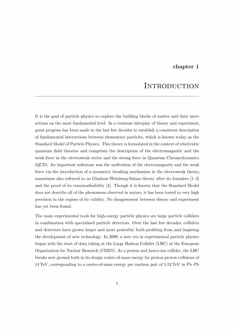
chapter 1
Introduction
It is the goal of particle physics to explore the building blocks of matter and their inter-
actions on the most fundamental level. In a constant interplay of theory and experiment,
great progress has been made in the last few decades to establish a consistent description
of fundamental interactions between elementary particles, which is known today as the
Standard Model of Particle Physics. This theory is formulated in the context of relativistic
quantum field theories and comprises the description of the electromagnetic and the
weak force in the electroweak sector and the strong force in Quantum Chromodynamics
(QCD). An important milestone was the unification of the electromagnetic and the weak
force via the introduction of a symmetry breaking mechanism in the electroweak theory,
sometimes also referred to as Glashow-Weinberg-Salam theory after its founders [1–3]
and the proof of its renormalisability [4]. Though it is known that the Standard Model
does not describe all of the phenomena observed in nature, it has been tested to very high
precision in the regime of its validity. No disagreement between theory and experiment
has yet been found.
The main experimental tools for high-energy particle physics are large particle colliders
in combination with specialised particle detectors. Over the last few decades, colliders
and detectors have grown larger and more powerful, both profiting from and inspiring
the development of new technology. In 2009, a new era in experimental particle physics
began with the start of data taking at the Large Hadron Collider (LHC) at the European
Organization for Nuclear Research (CERN). As a proton and heavy-ion collider, the LHC
breaks new ground both in its design centre-of-mass energy for proton-proton collisions of
14 TeV, corresponding to a centre-of-mass energy per nucleon pair of 5.52 TeV in Pb–Pb
1

collisions, and in its design luminosity of 1034 cm−2s−1. Currently, as of the end of 2014,
the LHC is in a maintenance period, the Long Shutdown I, and is being prepared for
its second period of operation and data taking (Run II). In Run I from 2009 until 2013,
the LHC provided extensive data sets for proton-proton (pp) collisions at a centre-of-
mass energy of 0.9 TeV, 2.76 TeV, 7 TeV and 8 TeV; lead-lead (Pb–Pb) collisions with a
centre-of-mass energy per nucleon pair of 2.76 TeV; and proton-lead (p–Pb) collisions at
a centre-of-mass energy per nucleon pair of 5.02 TeV. The most prominent LHC result
so far was the discovery of a new resonance with a mass of 125 GeV/c2 in 2012 by A
Toroidal LHC Apparatus (ATLAS) and the Compact Muon Solenoid (CMS) [5,6]. Up
until now, the properties of this resonance are compatible with the Standard Model Higgs
boson and are currently under further investigation. Already predicted in 1964 [7, 8], the
Higgs boson was the last missing particle in the Standard Model to be experimentally
confirmed.
Besides the rich physics programme related to the electroweak theory and its symmetry
breaking mechanism or to the search for ‘new physics’ beyond the Standard Model, the
LHC provides an excellent environment for the study of strongly interacting matter
under extreme conditions. In ultra-relativistic nucleus-nucleus collisions, a deconfined,
thermalised state of strongly interacting matter, the Quark-Gluon Plasma (QGP), is
expected to be formed [9, 10]. This hot and dense phase of QCD matter permeated
the early universe in the first few microseconds, according to the standard Big Bang
model. Among the four major experiments at the LHC, A Large Ion Collider Experiment
(ALICE) is dedicated to the study of heavy-ion collisions. A variety of rare probes is
investigated, including quarkonia, heavy-flavour hadrons, photons and jets. Heavy quarks
(charm, beauty) are produced at an early stage in heavy-ion collisions and thus provide
access to the QGP properties through their interaction with the medium. The study
of heavy-quark production at low momentum is of particular importance to address
the question, to which extent heavy quarks might be thermalised and take part in the
collective behaviour of the strongly interacting medium.
Experimental access to heavy quarks is given via the detection of hadrons containing
charm or beauty. A large fraction of the produced charm hadronises into various D meson
species, which consist of one charm quark and one of the light quarks up, down or strange.
D mesons decay before reaching active detector material and must be reconstructed via
their decay products. When an invariant mass analysis in hadronic decay channels is
2
performed, the full kinematic information of the heavy-flavour hadron is retained. The
high spatial resolution provided by the combined tracking of the ALICE Inner Tracking
System and the Time Projection Chamber enable the reconstruction of secondary decay
vertices of D mesons with intermediate-to-high momenta, which are typically displaced
from the primary vertex by a few hundred µm. D mesons can thus be very efficiently
distinguished from background by a selection on the decay topology. Using this analysis
strategy, the ALICE collaboration published a series of results for D-meson production
at central rapidity. These include the transverse momentum (pT) spectra for different
D-meson species in pp collisions at√s = 7 TeV and
√s = 2.76 TeV [11–13] and D-meson
suppression and flow in Pb–Pb collisions at√sNN = 2.76 TeV [14–16].
While performing efficiently at high pT, the topological selection of D mesons is bound to
fail at low pT, where the small Lorentz boost can no longer be resolved with the detector
and, consequently, the selection efficiency drops very sharply. All of the D meson results
currently published by the ALICE collaboration are therefore limited to pT > 1 GeV/c in
pp collisions and pT > 2 GeV/c in Pb–Pb collisions with increasing uncertainty towards
this low-pT limit.
Despite the experimental challenge, it is of great interest to extend the measurements
to zero transverse momentum. Fixed Order plus Next-to-Leading Logarithms (FONLL)
calculations [17] predict that over 50 % of the D0 yield lies below 2 GeV/c in pp collisions.
The low-pT region is therefore crucial for a precise determination of the total charm
production cross section at mid-rapidity, which is of substantial importance for the
interpretation of charmonium production in QGP studies at the LHC [18,19]. Up until
now, the best ALICE measurement of the charm production cross section at mid-rapidity
still relies on an extrapolation to zero transverse momentum based on theory input with
rather large uncertainties [12]. Moreover, the low-pT measurement of charm production
in pp collisions is important as a baseline to study the low-momentum phenomenology of
charm quarks in nucleus-nucleus collisions.
This thesis presents the first measurement of D-meson production in pp collisions down
to zero transverse momentum with ALICE. The studied system comprises D0 mesons
and their antiparticles by means of the reconstructed decay D0 → K−π+ and its charge
conjugate. In order to keep a high efficiency in the low-pT region, it is necessary to give
up the topological selection. The challenge of how to deal with the large combinatorial
3
background from primary pion and kaon production then arises. This background peaks
in a similar kinematic region to that populated by kaons and pions originating from D0
decays in the low-pT regime. After exploiting the excellent particle identification (PID)
capabilities of ALICE, the remaining signal-to-background ratio is still 10−3 in the pT
interval 0 < pT < 1 GeV/c, impeding the extraction of a stable signal in the invariant
mass. The subtraction of an estimate of the combinatorial background improves the
stability of the signal extraction. Background estimates are obtained from data, using
the like-sign technique. After background subtraction, the D0 signal can be extracted
down to zero transverse momentum.
The analysis strategy applied in this work is similar to that used by the Solenoidal Tracker
at RHIC (STAR) collaboration at the Relativistic Heavy-Ion Collider (RHIC) for their
measurement of D0 and D∗ production in pp collisions at√s = 200 GeV [20] and gold-gold
(Au-Au) collisions at√sNN = 200 GeV [21]. Due to the lack of a high-precision vertex
detector at the time of the STAR measurement, the topological approach to D-meson
reconstruction was not available. The measurements are therefore based on background-
subtraction techniques, such as like sign, track rotation and event mixing. The recent
installation of a Heavy Flavor Tracker will allow for the topological reconstruction of
heavy-flavour hadrons with STAR in the near future [22].
This thesis is structured as follows. Chapter 2 presents the theoretical and experimental
background of D-meson production in hadronic collisions. After a short description of
ALICE in chapter 3, chapter 4 offers details on the D0 decay. Chapter 5 presents the
data analysis in detail. A discussion of the uncertainties in chapter 6 is followed by the
results in chapter 7. The thesis concludes in chapter 8.
4
chapter 2
D-Meson Production in Hadronic
Collisions
This chapter introduces the basic theoretical and experimental concepts in order to put
D-meson production in proton-proton and heavy-ion collisions into context.
2.1 Key Features of Quantum Chromodynamics
Quantum Chromodynamics (QCD) is one of the pillars of the Standard Model of Particle
Physics. It describes the strong interaction between colour-charged quarks and gluons,
with the latter being the gauge bosons of the theory. Unlike in Quantum Electrodynamics
(QED), where the force carrier is a neutral photon, gluons carry colour charge and are thus
subject to interactions with one another. This gauge boson self-interaction is manifest in
the non-abelian nature of the underlying symmetry group, which is the SU(3) component
of the Standard Model gauge group SU(3) × SU(2) × U(1). Non-zero commutators of
the 8 generators of SU(3) in the fundamental representation lead to terms in the gluon
field kinematic part of the Lagrangian that correspond to vertices with three or four
gluons. This particular structure is responsible for some characteristic features of QCD,
which are described in the following.
Figure 2.1 shows the energy dependence of the renormalised ‘running’ coupling constant αs.
Data points from various experiments at different energy scales or momentum transfer Q
are displayed. At low Q, corresponding to a large spatial range of the interaction, the
5
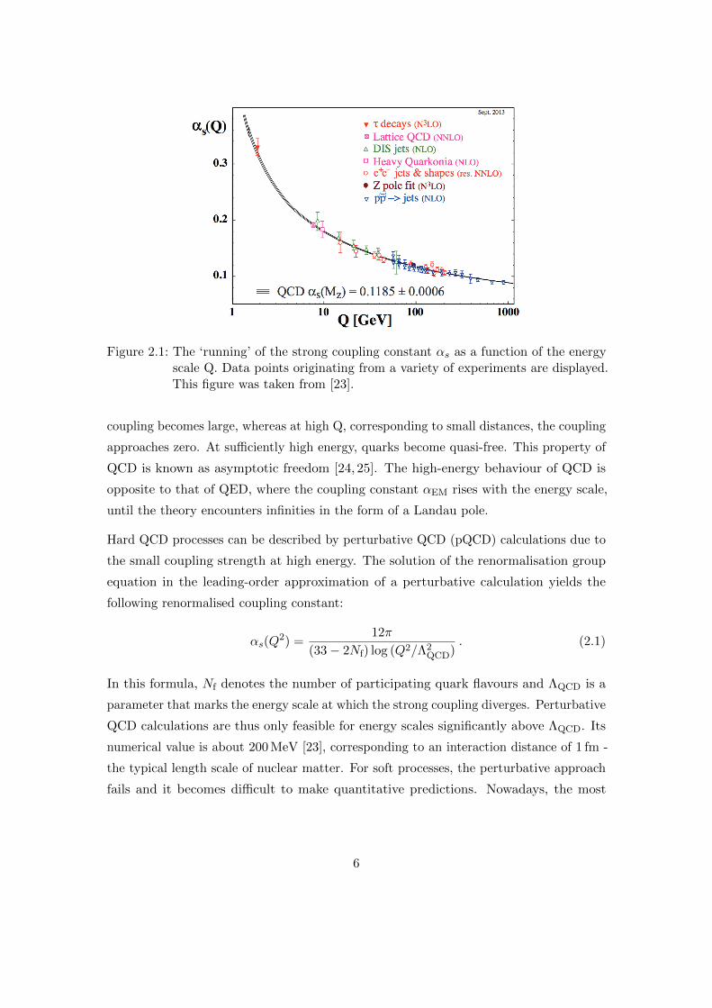
Figure 2.1: The ‘running’ of the strong coupling constant αs as a function of the energyscale Q. Data points originating from a variety of experiments are displayed.This figure was taken from [23].
coupling becomes large, whereas at high Q, corresponding to small distances, the coupling
approaches zero. At sufficiently high energy, quarks become quasi-free. This property of
QCD is known as asymptotic freedom [24, 25]. The high-energy behaviour of QCD is
opposite to that of QED, where the coupling constant αEM rises with the energy scale,
until the theory encounters infinities in the form of a Landau pole.
Hard QCD processes can be described by perturbative QCD (pQCD) calculations due to
the small coupling strength at high energy. The solution of the renormalisation group
equation in the leading-order approximation of a perturbative calculation yields the
following renormalised coupling constant:
αs(Q2) =
12π
(33− 2Nf) log (Q2/Λ2QCD)
. (2.1)
In this formula, Nf denotes the number of participating quark flavours and ΛQCD is a
parameter that marks the energy scale at which the strong coupling diverges. Perturbative
QCD calculations are thus only feasible for energy scales significantly above ΛQCD. Its
numerical value is about 200 MeV [23], corresponding to an interaction distance of 1 fm -
the typical length scale of nuclear matter. For soft processes, the perturbative approach
fails and it becomes difficult to make quantitative predictions. Nowadays, the most
6
promising approach to working in the soft QCD regime is a numerical scheme on a
discretised space-time grid known as Lattice QCD [26].
Phenomenologically, the opposing energy dependence of the QCD and QED couplings
can be understood in terms of a screening or anti-screening effect of the respective charge.
Vacuum polarisation leads to an effectively reduced coupling strength between electric
charges that are being separated. This effect is referred to as as screening. Self-interacting
gluons establish an anti-screening effect between colour charges that are being separated,
meaning that the coupling strength increases. The phenomenological picture can be
extended such that the gluons between two colour charges form a narrow string tube of
high tension, preventing the colour charges from being separated completely. This concept
is known as colour confinement. It states that colour charges must form colour-neutral
objects and do not exist freely. In particular, quarks are always bound in hadrons.
Confinement is reflected in an additional linear term in the QCD potential between two
colour charges forming together a colour-neutral state. In the case of a quark-antiquark
pair, for example, the potential takes the form:
V (r) = −4
3
αs(r)
r+ κr . (2.2)
The first term represents a Coulomb-like interaction, which dominates at short ranges r.
The factor −4/3 is called the colour factor and depends on the particle types that interact.
The second term dominates at large distance. It can be seen as the potential energy of a
gluon string between the quark and the antiquark with the string constant κ. It becomes
apparent that a total separation of the quark and antiquark would require infinite energy
and thus cannot be accomplished. Instead the gluon string would eventually break up
and form additional quark pairs until colour-neutral hadrons are formed in the process
of hadronisation. While QCD still lacks a formal proof of confinement [27], the concept
remains a postulate, based on the fact that free quarks have not yet been observed in
nature.
2.2 Exploring the QCD Phase Diagram
Figure 2.2 shows a sketch of the QCD phase diagram, as it is understood by current
research, in terms of temperature and net baryon density. The latter is closely related
7

Figure 2.2: Sketch of a possible QCD phase diagram, as illustrated by the CompressedBaryonic Matter (CBM) collaboration [28].
to the baryochemical potential. Two main regimes can be identified: ordinary hadronic
matter at low temperature or low baryon density; and the Quark Gluon Plasma (QGP)
at high temperature or high baryon density. The QGP is a deconfined state of matter,
the properties of which are determined by the degrees of freedom of single quarks
and gluons [9, 10]. Moreover, the QGP is characterised by the restoration of chiral
symmetry [29]. The critical temperature Tc marks the transition between the two
phases at zero baryochemical potential. Its value is currently estimated to be about
Tc = 160 MeV [9, 10]. At low temperature and high density, a new phase of colour
superconductivity is predicted [30]. However, this region of the phase diagram is not yet
covered by experiments and predictions are very difficult to make.
It is one of the goals of heavy-ion physics to explore the different phases and transitions
of the QCD phase diagram. Different experiments are hereby sensitive to different paths,
such as those indicated by arrows in fig. 2.2. High-energy particle colliders like the
RHIC and the LHC explore the regime of low baryochemical potential, while the future
experiments at the Facility for Antiproton and Ion Research (FAIR), which is currently
being built at the GSI Helmholtz Centre for Heavy Ion Research, are designed to explore
the regions of higher baryochemical potential at lower energy.
The QGP phase of strongly interacting matter is expected to be created in high-energy
nucleus-nucleus collisions. In the standard picture, an ultra-relativistic heavy-ion collision
8

experiences the following stages. The pre-equilibrium phase immediately after the
collision is characterised by hard scatterings of partons in the colliding nuclei. After
a thermalisation time of about τ = 1 fm/c = 3.3× 10⁻²⁴ s, the QGP is formed. High
pressure gradients subsequently drive a collective expansion of the medium, which can
be described by hydrodynamical modelling [31]. During the expansion, the fireball cools
down until the medium undergoes a phase transition and hadrons are formed. At chemical
freeze-out, the relative abundances of the created particle species are fixed. Afterwards,
hadrons are allowed to re-scatter, until particle momenta are fixed by the time of the
kinetic freeze-out. The free streaming particles then reach the detector.
2.3 Heavy Quarks in the QGP
Throughout this thesis, the term ‘heavy quark’ encompasses the charm and the beauty
quarks, which have masses of mc ≈ 1.3 GeV/c2 and mb ≈ 4.2 GeV/c2 [23]. The top
quark, with a mass of mt ≈ 173 GeV/c2, is not considered for reasons explained further
down.
Heavy quarks are produced at an early stage in heavy-ion collisions, before the QGP is
formed. The production time scale is of the order of 12m , where m is the mass of the heavy
quark. In contrast to the light quarks, their total mass is dominated by the coupling to
the Higgs field, as illustrated in fig. 2.3. Consequently, heavy quarks keep their large
mass even when chiral symmetry is restored. Since the charm and beauty masses are
much larger than the QGP temperature, mc,mb � TQGP, the thermal production of
heavy quarks in the medium can be neglected at LHC energies. The annihilation rate of
heavy-quark pairs is also negligible [32]. In summary, it can be stated that heavy flavour
is approximately conserved during the evolution of the system, which makes heavy quarks
calibrated probes of the QGP medium properties.
In contrast to charm and beauty quarks, top quarks decay on a very short time scale of
1.3× 10⁻²⁴ s [23] due to the large available phase space. All produced top quarks have
therefore already decayed before they can interact with the equilibrated medium (cf.
previous section). Consequently, they can not be used to probe the QGP. Furthermore,
top pair production is very rare. With a production cross section of about 200 pb in pp
collisions at√s = 7 TeV [34,35], only one top event in the entire data set of 5.25 nb−1
9
1
10
10 2
10 3
10 4
10 5
1 10 102
103
104
105
1
10
10 2
10 3
10 4
10 5
1 10 102
103
104
105
Total quark mass (MeV)
Higg
s qu
ark
mas
s (M
eV)
t
bc
s
d
u
QCD Vacuum!c symmetry breaking
Higgs VacuumElectroweak symmetry breaking
Figure 2.3: Generation mechanisms of quark masses. Charm (c), beauty (b) and top (t)quarks acquire their mass almost entirely by the coupling to the Higgs field.This figure was taken from [33].
used in this work is expected. Top pair creation is studied at the LHC with the ATLAS
and CMS detectors, using triggers that allow them to scan pp collisions at much higher
event rates.
Experimental access to heavy quarks is made possible via the detection of hadrons
containing charm or beauty. Figure 2.4 shows the relative abundances of charmed
hadrons in pp collisions. About 1.5 % of the produced charm hadronises to charmonium
(quark content cc), 9.4 % to the Λ+c baryon (quark content udc) and the rest to various D-
meson ground and excited states. The masses and lifetimes of D0, D+, D+s , D∗(2007)0 and
D∗(2010)+ are listed in table 2.1 along with selected decay channels and their respective
branching ratios. The D-meson excited states decay rapidly to neutral and charged
ground states by means of the strong interaction. The D∗(2007)0 decays exclusively to
D0 + X, where X is a π0 or γ (cf. table 2.1). The D∗(2010)+ decays with a fraction of
67.7 % to D0 + π+ and with a fraction of 30.7 % to D+ + π0. In fig. 2.4, the respective
fraction of excited states decaying to D0 (D+) is coloured in blue (red). A D meson
that is directly produced from a charm quark or in the decay of a charmed resonance
is referred to as a ‘prompt’ D meson throughout the thesis. The fraction of prompt D0
10
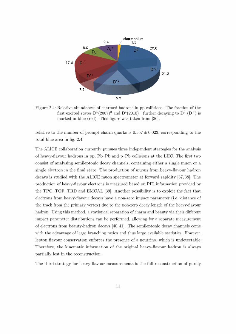
Figure 2.4: Relative abundances of charmed hadrons in pp collisions. The fraction of thefirst excited states D∗(2007)0 and D∗(2010)+ further decaying to D0 (D+) ismarked in blue (red). This figure was taken from [36].
relative to the number of prompt charm quarks is 0.557± 0.023, corresponding to the
total blue area in fig. 2.4.
The ALICE collaboration currently pursues three independent strategies for the analysis
of heavy-flavour hadrons in pp, Pb–Pb and p–Pb collisions at the LHC. The first two
consist of analysing semileptonic decay channels, containing either a single muon or a
single electron in the final state. The production of muons from heavy-flavour hadron
decays is studied with the ALICE muon spectrometer at forward rapidity [37,38]. The
production of heavy-flavour electrons is measured based on PID information provided by
the TPC, TOF, TRD and EMCAL [39]. Another possibility is to exploit the fact that
electrons from heavy-flavour decays have a non-zero impact parameter (i.e. distance of
the track from the primary vertex) due to the non-zero decay length of the heavy-flavour
hadron. Using this method, a statistical separation of charm and beauty via their different
impact parameter distributions can be performed, allowing for a separate measurement
of electrons from beauty-hadron decays [40,41]. The semileptonic decay channels come
with the advantage of large branching ratios and thus large available statistics. However,
lepton flavour conservation enforces the presence of a neutrino, which is undetectable.
Therefore, the kinematic information of the original heavy-flavour hadron is always
partially lost in the reconstruction.
The third strategy for heavy-flavour measurements is the full reconstruction of purely
11
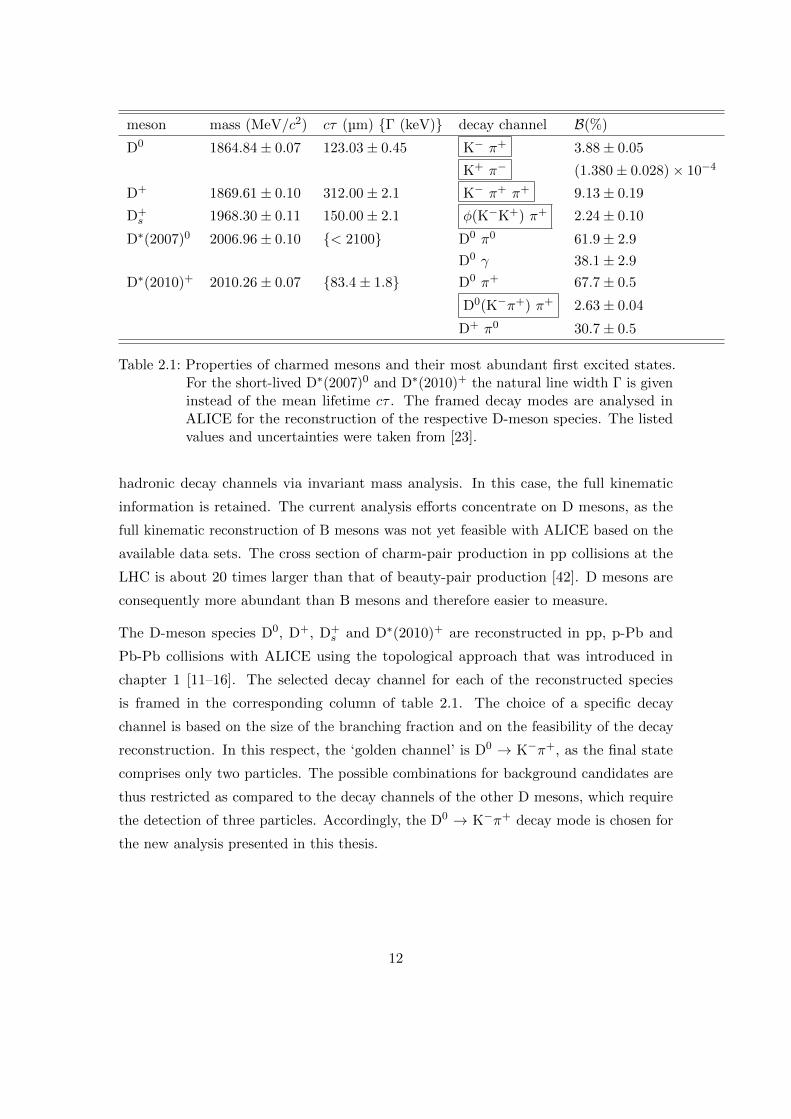
meson mass (MeV/c2) cτ (µm) {Γ (keV)} decay channel B(%)
D0 1864.84± 0.07 123.03± 0.45 K− π+ 3.88± 0.05
K+ π− (1.380± 0.028)× 10−4
D+ 1869.61± 0.10 312.00± 2.1 K− π+ π+ 9.13± 0.19
D+s 1968.30± 0.11 150.00± 2.1 φ(K−K+) π+ 2.24± 0.10
D∗(2007)0 2006.96± 0.10 {< 2100} D0 π0 61.9± 2.9
D0 γ 38.1± 2.9
D∗(2010)+ 2010.26± 0.07 {83.4± 1.8} D0 π+ 67.7± 0.5
D0(K−π+) π+ 2.63± 0.04
D+ π0 30.7± 0.5
Table 2.1: Properties of charmed mesons and their most abundant first excited states.For the short-lived D∗(2007)0 and D∗(2010)+ the natural line width Γ is giveninstead of the mean lifetime cτ . The framed decay modes are analysed inALICE for the reconstruction of the respective D-meson species. The listedvalues and uncertainties were taken from [23].
hadronic decay channels via invariant mass analysis. In this case, the full kinematic
information is retained. The current analysis efforts concentrate on D mesons, as the
full kinematic reconstruction of B mesons was not yet feasible with ALICE based on the
available data sets. The cross section of charm-pair production in pp collisions at the
LHC is about 20 times larger than that of beauty-pair production [42]. D mesons are
consequently more abundant than B mesons and therefore easier to measure.
The D-meson species D0, D+, D+s and D∗(2010)+ are reconstructed in pp, p-Pb and
Pb-Pb collisions with ALICE using the topological approach that was introduced in
chapter 1 [11–16]. The selected decay channel for each of the reconstructed species
is framed in the corresponding column of table 2.1. The choice of a specific decay
channel is based on the size of the branching fraction and on the feasibility of the decay
reconstruction. In this respect, the ‘golden channel’ is D0 → K−π+, as the final state
comprises only two particles. The possible combinations for background candidates are
thus restricted as compared to the decay channels of the other D mesons, which require
the detection of three particles. Accordingly, the D0 → K−π+ decay mode is chosen for
the new analysis presented in this thesis.
12

2.4 Open Charm and Charmonium
Charmed hadrons that contain exactly one charm or anti-charm quark, i.e. mainly D
mesons and the Λ+c baryon, are often referred to as ‘open charm’. In contrast, bound
states of one charm and one anti-charm quark are known as charmonium. A variety of
charmonium states exist that differ in quantum numbers and binding energy. For an
extensive review of the physics of charmonium spectroscopy see [43] or [44]. For the
field of ultra-relativistic heavy-ion physics, the most relevant charmonium state is the
vector ground state, J/ψ, as it is produced in relatively large abundance and can be
directly measured via its decay into e+e− or µ+µ− with a branching ratio of about 6 %
each [23].
The detection of charmonium has played a central role in heavy-ion physics since its
possible suppression in heavy-ion collisions was proposed as a direct observable for
deconfinement [45]. The original concept assumes that charmonium is produced in initial
hard scattering processes and is subsequently destroyed in the possibly deconfined medium
via a process known as colour screening. It is assumed that this ‘melting’ of charmonium
occurs above the Debye temperature TD, which depends on the binding energy of the
respective state. This implies that excited states are melted at lower temperatures than
the ground state. The possible observation of a hierarchy in the suppression of different
charmonium states, also referred to as ‘sequential melting’, was therefore proposed as a
proxy for the QGP temperature [46].
The modern picture of charmonium production in ultra-relativistic heavy-ion collisions is
more refined and takes into account non-primordial production during the evolution of
the medium or at the phase boundary. In the Statistical Hadronisation Model [18], it
is assumed that charmonium is exclusively produced at the phase boundary. In such a
scenario, the production of charmonium is then governed by the total number of charm
quarks available for thermal hadron formation. An important premise is that charm
quarks are formed in initial hard scatterings and their total number is approximately
conserved during the evolution of the system [32]. Transport models comprise the second
main scenario for charmonium production in relativistic heavy-ion collisions [19]. These
models account for a continuous generation and destruction of charmonium throughout
the evolution of the system.
13

⟩part
N⟨0 50 100 150 200 250 300 350 400
AA
R
0
0.2
0.4
0.6
0.8
1
1.2
1.4
Stat. Hadronization model (A. Andronic & al., JPG 38 (2011) 124081)
Transport model (Y.P. Liu & al, PLB 678 (2009) 72)
Transport model (X. Zhao & al., NPA 859 (2011) 114)
Shadowing+comovers+recombination (E. Ferreiro, PLB 731 (2014) 57)
= 2.76 TeVNN
s, PbPb µ+µ → ψInclusive J/
15%± global syst.= c<8 GeV/T
p<4, 0<yALICE (PLB 734 (2014) 314), 2.5<
ALI−DER−65278
Figure 2.5: J/ψ suppression in Pb–Pb collisions at√sNN = 2.76 TeV vs. Npart. A recent
ALICE measurement in the µ+µ− decay channel [47] is displayed along withtheoretical predictions from different models [48–50]. The large uncertaintiesof the models are due to the uncertainty on the charm production crosssection, which enters quadratically as a model parameter. This figure wasderived from [47].
The experimental observable to quantify medium effects like suppression or enhancement
is the nuclear modification factor RJ/ψAA . It is defined as the ratio of the J/ψ yield in
nucleus-nucleus (AA) collisions to the yield in pp collisions, scaled up by the average
number of binary collisions 〈Ncoll〉:
RJ/ψAA =
dNAAJ/ψ/dy
〈Ncoll〉 · dNppJ/ψ/dy
. (2.3)
Figure 2.5 presents the J/ψ nuclear modification factor in Pb–Pb collisions at√sNN =
2.76 TeV as a function of the number of nucleons participating in the collision, Npart. A
recent measurement in the µ+µ− decay channel with the ALICE muon spectrometer
at forward rapidity [47] is displayed along with the theoretical predictions from the
Statistical Hadronisation Model [48] and two transport models [49,50].
From this example, it can be seen that the measurement is considerably more precise than
the theory. The large uncertainties in the models are due to the large uncertainties of
14
the total charm cross section, dσcc/dy, which is required as an input parameter for both
types of models. In the case of the Statistical Hadronisation Model, dσcc/dy is actually
the only free parameter. Furthermore, as two charm quarks are needed to form a J/ψ
meson, dσcc/dy enters quadratically into the J/ψ yield calculation. A better precision of
the measurement of dσcc/dy will therefore significantly contribute to the understanding
of charmonium production in nucleus-nucleus collisions.
2.5 Theoretical Predictions for Heavy-Flavour Production
The production cross section of a heavy-flavour meson in pp collisions can be calculated by
splitting the calculation into a perturbative and a non-perturbative part. This technique
is known as the factorisation approach. It consists of a convolution of the perturbative
cross section of heavy-quark pair production with a non-perturbative fragmentation
function that parameterises the relative abundance and momentum distribution of the
heavy-flavour hadron:
dσpp→HQX = dσpp→QQX ⊗DNPQ→HQ
. (2.4)
Here, HQ is the produced heavy-flavour meson and heavy (anti)quarks are denoted as
Q (Q). The cross section for heavy-quark pair production from two colliding protons,
i.e. the first term in eq. (2.4), can be reduced to a sum of elementary processes as
follows:
dσpp→QQX =∑i,j
∫dx1
∫dx2 F
i(x1, µ2F)F j(x2, µ
2F) dσij→QQX(p1, p2, µ
2R, µ
2F) . (2.5)
This formula involves the cross sections dσij→QQX for the interaction of single partons
i and j that can be computed by the means of a perturbative series in the strong
coupling constant. The formula further includes the parton distribution functions (PDFs),
F i(xk, µ2F) with k ∈ 1, 2, which denote the probability density of the parton i to carry
the momentum pk = xkPk, where Pk is the respective proton momentum. The parton
distribution functions and the partonic cross sections depend on the factorisation and
renormalisation scale parameters µF and µR.
The lowest order in the perturbative expansion for the calculation of the elementary
15
Q
Q
Q
Q
QQq
q
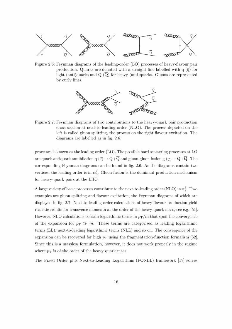
Figure 2.6: Feynman diagrams of the leading-order (LO) processes of heavy-flavour pairproduction. Quarks are denoted with a straight line labelled with q (q) forlight (anti)quarks and Q (Q) for heavy (anti)quarks. Gluons are representedby curly lines.
Q
Q
Q
Q
Figure 2.7: Feynman diagrams of two contributions to the heavy-quark pair productioncross section at next-to-leading order (NLO). The process depicted on theleft is called gluon splitting, the process on the right flavour excitation. Thediagrams are labelled as in fig. 2.6.
processes is known as the leading order (LO). The possible hard scattering processes at LO
are quark-antiquark annihilation q+q→ Q+Q and gluon-gluon fusion g+g→ Q+Q. The
corresponding Feynman diagrams can be found in fig. 2.6. As the diagrams contain two
vertices, the leading order is in α2s. Gluon fusion is the dominant production mechanism
for heavy-quark pairs at the LHC.
A large variety of basic processes contribute to the next-to-leading order (NLO) in α3s. Two
examples are gluon splitting and flavour excitation, the Feynman diagrams of which are
displayed in fig. 2.7. Next-to-leading order calculations of heavy-flavour production yield
realistic results for transverse momenta at the order of the heavy-quark mass, see e.g. [51].
However, NLO calculations contain logarithmic terms in pT/m that spoil the convergence
of the expansion for pT � m. These terms are categorised as leading logarithmic
terms (LL), next-to-leading logarithmic terms (NLL) and so on. The convergence of the
expansion can be recovered for high pT using the fragmentation-function formalism [52].
Since this is a massless formulation, however, it does not work properly in the regime
where pT is of the order of the heavy quark mass.
The Fixed Order plus Next-to-Leading Logarithms (FONLL) framework [17] solves
16
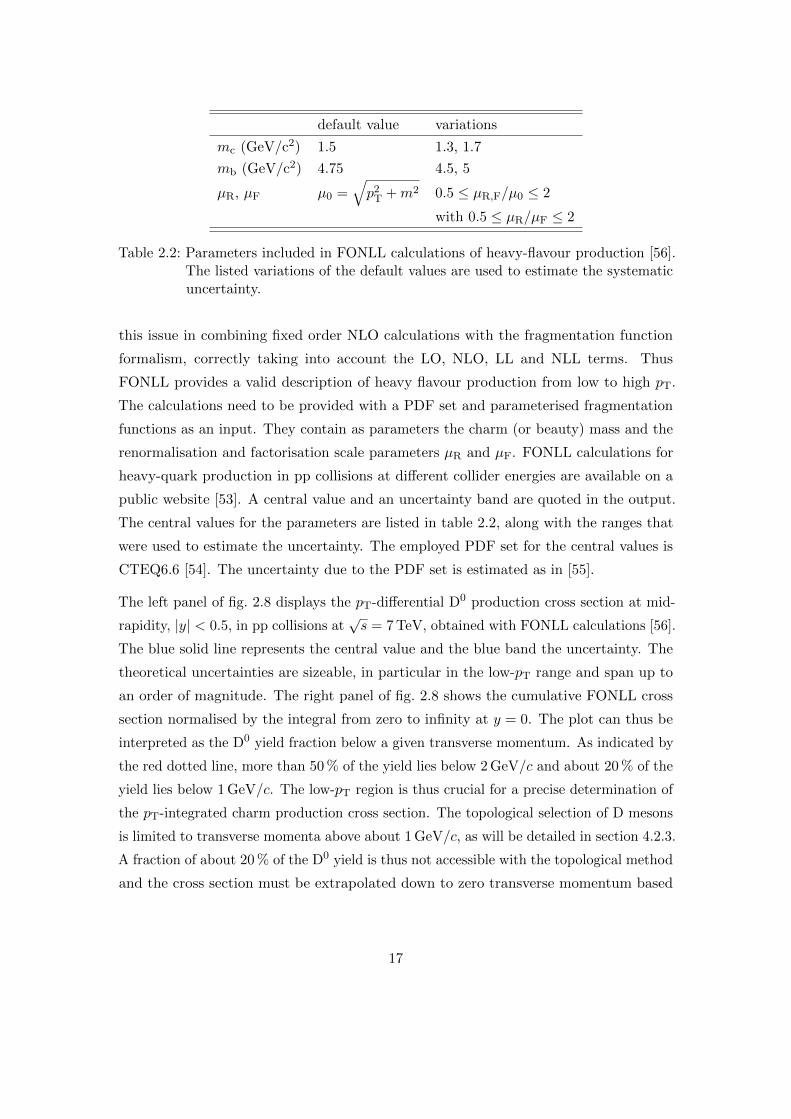
default value variations
mc (GeV/c2) 1.5 1.3, 1.7
mb (GeV/c2) 4.75 4.5, 5
µR, µF µ0 =√p2T +m2 0.5 ≤ µR,F/µ0 ≤ 2
with 0.5 ≤ µR/µF ≤ 2
Table 2.2: Parameters included in FONLL calculations of heavy-flavour production [56].The listed variations of the default values are used to estimate the systematicuncertainty.
this issue in combining fixed order NLO calculations with the fragmentation function
formalism, correctly taking into account the LO, NLO, LL and NLL terms. Thus
FONLL provides a valid description of heavy flavour production from low to high pT.
The calculations need to be provided with a PDF set and parameterised fragmentation
functions as an input. They contain as parameters the charm (or beauty) mass and the
renormalisation and factorisation scale parameters µR and µF. FONLL calculations for
heavy-quark production in pp collisions at different collider energies are available on a
public website [53]. A central value and an uncertainty band are quoted in the output.
The central values for the parameters are listed in table 2.2, along with the ranges that
were used to estimate the uncertainty. The employed PDF set for the central values is
CTEQ6.6 [54]. The uncertainty due to the PDF set is estimated as in [55].
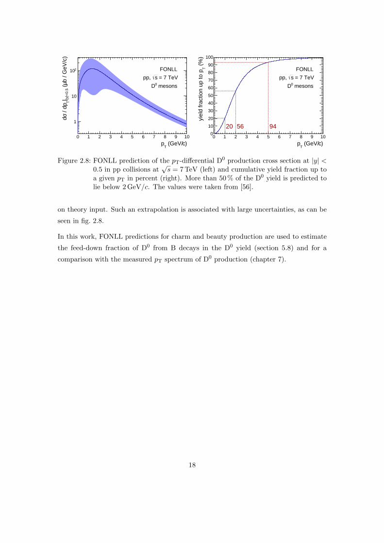
The left panel of fig. 2.8 displays the pT-differential D0 production cross section at mid-
rapidity, |y| < 0.5, in pp collisions at√s = 7 TeV, obtained with FONLL calculations [56].
The blue solid line represents the central value and the blue band the uncertainty. The
theoretical uncertainties are sizeable, in particular in the low-pT range and span up to
an order of magnitude. The right panel of fig. 2.8 shows the cumulative FONLL cross
section normalised by the integral from zero to infinity at y = 0. The plot can thus be
interpreted as the D0 yield fraction below a given transverse momentum. As indicated by
the red dotted line, more than 50 % of the yield lies below 2 GeV/c and about 20 % of the
yield lies below 1 GeV/c. The low-pT region is thus crucial for a precise determination of
the pT-integrated charm production cross section. The topological selection of D mesons
is limited to transverse momenta above about 1 GeV/c, as will be detailed in section 4.2.3.
A fraction of about 20 % of the D0 yield is thus not accessible with the topological method
and the cross section must be extrapolated down to zero transverse momentum based
17
)c (GeV/T
p0 1 2 3 4 5 6 7 8 9 10
b / G
eV/c
)µ
(|y
|<0.
5|
T /
dpσd
1
10
210 FONLL
= 7 TeVspp,
mesons0D
)c (GeV/T
p0 1 2 3 4 5 6 7 8 9 10
(%
)Tp
yiel
d fr
actio
n up
to
0
10
20
30
40
50
60
70
80
90
100
FONLL
= 7 TeVspp,
mesons0D
20 56 94
Figure 2.8: FONLL prediction of the pT-differential D0 production cross section at |y| <0.5 in pp collisions at
√s = 7 TeV (left) and cumulative yield fraction up to
a given pT in percent (right). More than 50 % of the D0 yield is predicted tolie below 2 GeV/c. The values were taken from [56].
on theory input. Such an extrapolation is associated with large uncertainties, as can be
seen in fig. 2.8.
In this work, FONLL predictions for charm and beauty production are used to estimate
the feed-down fraction of D0 from B decays in the D0 yield (section 5.8) and for a
comparison with the measured pT spectrum of D0 production (chapter 7).
18

chapter 3
ALICE at the LHC
This chapter introduces ALICE in the context of the physics programme of the Large
Hadron Collider (LHC) and describes the detectors of ALICE that are important for this
thesis.
3.1 LHC Experiments and Physics Programme
The LHC [57] provides hadron collisions to four major experiments. A Toroidal LHC
Apparatus (ATLAS) [58] and the Compact Muon Solenoid (CMS) [59] are two general
purpose detectors, currently focussing on the investigation of the Higgs boson and the
search for new physics beyond the Standard Model, mainly in pp collisions. ATLAS
and CMS essentially share the same physics programme, allowing for the cross check
of important results by two independent collaborations – a concept that has already
been proven successful for the Higgs discovery. The Large Hadron Collider Beauty
(LHCb) experiment [60] is specialised in physics involving beauty quarks, for example
the investigation of CP violation in B meson oscillations.
Whereas ATLAS, CMS and LHCb primarily focus on the investigation of pp collisions,
A Large Ion Collider Experiment (ALICE) [61] is dedicated to the heavy-ion programme
at the LHC. The detector is therefore optimised to meet the specific challenges that arise
from the high multiplicity environment created in central Pb-Pb collisions. The Time
Projection Chamber, which is the main tracking device of ALICE, can handle particle
densities up to dN/dy = 8000 [61]. A low material budget, a moderate magnetic field of
19
TPC
TRD
TOF
EMCal
ACORDE
absorberL3 solenoid dipole
MCH
MTR
ZDC
ZDC
HMPID
SPD SDD SSD T0C V0C
PMD
T0A, V0A
PHOS
FMD
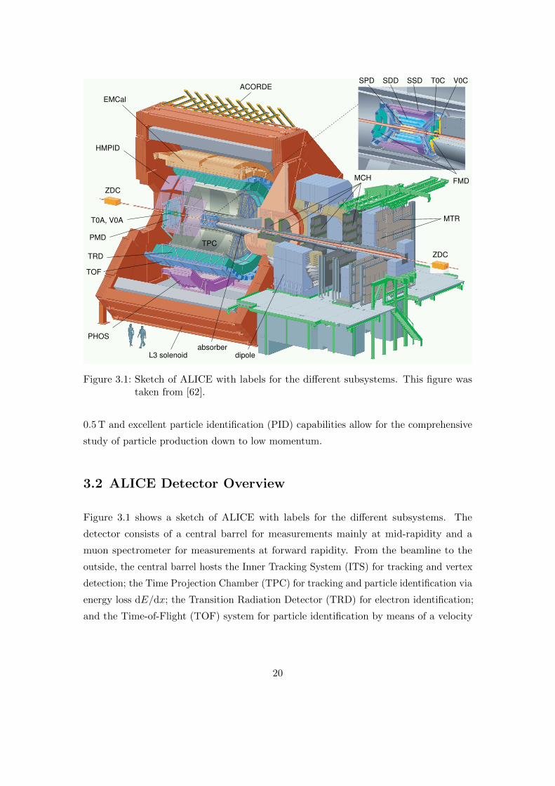
Figure 3.1: Sketch of ALICE with labels for the different subsystems. This figure wastaken from [62].
0.5 T and excellent particle identification (PID) capabilities allow for the comprehensive
study of particle production down to low momentum.
3.2 ALICE Detector Overview
Figure 3.1 shows a sketch of ALICE with labels for the different subsystems. The
detector consists of a central barrel for measurements mainly at mid-rapidity and a
muon spectrometer for measurements at forward rapidity. From the beamline to the
outside, the central barrel hosts the Inner Tracking System (ITS) for tracking and vertex
detection; the Time Projection Chamber (TPC) for tracking and particle identification via
energy loss dE/dx; the Transition Radiation Detector (TRD) for electron identification;
and the Time-of-Flight (TOF) system for particle identification by means of a velocity
20
measurement. ITS, TPC and TOF cover full azimuth and a pseudo-rapidity range of
about |η| < 0.9, apart from the first two layers of the ITS that have an extended η coverage.
The TRD is currently completed with the missing modules and will be established in full
azimuthal coverage in Run II. The Electromagnetic Calorimeter (EMCAL), the Photon
Calorimeter (PHOS) and the High Momentum Particle IDentification Detector (HMPID)
cover only a part in azimuth and in pseudo-rapidity.
A magnetic field of 0.5 T is provided by a solenoidal magnet that was inherited from the
L3 experiment at the Large Electron Positron (LEP) collider. Some smaller detectors for
event characterisation and triggering are located in the forward rapidity region, close
to the beam pipe. In the central barrel, these are the V0 and T0 detectors, the Photon
Multiplicity Detector (PMD) and the Forward Multiplicity Detector (FMD). The Zero
Degree Calorimeters (ZDC) are located outside the detector at a distance of 116 m at
each side of the central interaction point.
Throughout this thesis, the standard ALICE coordinate system is used, if not otherwise
stated. The central interaction point in the detector defines the origin of the cartesian
coordinate system. The z axis points along the beamline. Accordingly, the xy plane is
oriented transverse to the beamline and sometimes denoted as the transverse plane. The
muon system defines the ‘C-side’ of the detector, the opposite side is called ’A-side’.
The subsystems of ALICE that are relevant for this work are described in detail in the
following sections. A comprehensive description of layout and performance of the detector
is given in the Technical Design Report [61] and a recent performance paper [62].
3.3 Inner Tracking System
The Inner Tracking System (ITS) provides tracking and identification of charged particles
in six cylindrical layers of silicon semiconductor detectors at radii between 3.9 cm and
43.0 cm in coaxial arrangement around the beam pipe. The two innermost layers with
a pseudo-rapidity coverage of |η| < 1.98 constitute the Silicon Pixel Detector (SPD).
With a granularity of 50 µm (rφ) x 425 µm (z), it provides a high spatial resolution of
12 µm in rφ and of 100 µm in z. The SPD is followed by two layers of the Silicon Drift
Detector (SDD) and two layers of the Silicon Strip Detector (SSD) with a pseudo-rapidity
acceptance of |η| < 0.9. The total material budget for a track traversing each layer of
21
the ITS is only about 8% of a radiation length.
In this analysis, the ITS is used to improve the momentum resolution of particles
reconstructed with the TPC and for the precise localisation of primary vertices. Moreover,
the SPD contributes a signal to the minimum bias trigger that is used in this analysis.
The contribution of the ITS to the combined ITS-TPC tracking system is crucial for
the reconstruction of secondary decay vertices and thus for the topological selection
of D mesons. This particular functionality of the ITS, however, is not needed in this
work, where D mesons are measured without the reconstruction of secondary vertices.
Furthermore, the SSD and SDD layers provide energy loss information that can be used
for the identification of charged particles. This feature is particularly useful to identify
low momentum particles that do not reach the TPC. However, in this analysis, the PID
information from the ITS is not used, since the corresponding dE/dx information from
the TPC is more precise and thus preferred.
3.4 Time Projection Chamber
The Time Projection Chamber (TPC) is the heart of the central barrel with an essential
contribution to most of the ALICE physics analyses. With an inner radius of 85 cm, an
outer radius of 250 cm and a length of 500 cm, it is the largest TPC ever built. The TPC
provides tracking in a large transverse momentum range, as well as PID information by
measuring the specific energy loss of charged particles in the TPC gas. In the period of
data taking that is relevant for this thesis, it was operated with a gas mixture of neon,
carbon dioxide and nitrogen in the proportions 90/10/5. The drift field is provided by a
central electrode at a negative voltage of 100 kV. The produced ionisation electrons are
collected at read-out plates on either side of the chamber. The drift time for electrons
traversing the full chamber is of about 90 µs. The read-out panels are organised in 18
sectors at each side in azimuthal direction and 159 pad rows in radial direction.
For tracks with full radial length that have possible matches in ITS, TOF and TRD,
the acceptance is about |η| < 0.9. Tracks with a pseudo-rapidity outside this range are
still reconstructed, but suffer from reduced momentum resolution since the track only
partially traverses the active volume and the lever arm is shortened. The TPC is designed
for the high occupancies that occur in central Pb–Pb collisions. The fast read-out can
22
manage primary charged particle multiplicities up to dN/dη = 8000, mounting up to
about 20000 tracks in the acceptance. The relative dE/dx resolution in the data set used
in this work was measured to be about 5.5 % [63], enabling a kaon-pion separation of
2σ up to a momentum of about 0.8 GeV/c and a proton-pion separation of 2σ up to a
momentum of about 1.6 GeV/c [62].
The current analysis strongly relies on both the tracking and the particle identification
capacities of the TPC.
3.5 Time of Flight
The Time-of-Flight (TOF) system provides particle identification via flight-time measure-
ments in an acceptance range of |η| < 0.88. It consists of 1593 Multi-gap Resistive-Plate
Chambers (MRPCs), arranged in 18 segments in φ and 5 segments in z direction with a
radial distance between 3.7 m and 3.99 m from the beamline. The flight time of a particle
is evaluated by taking the difference of the measured arrival time in the TOF system and
a reference start time for each event that is provided by the T0 detector. In combination
with the track length and the track momentum measured in the TPC, a mass hypothesis
for the particle can be calculated. The resolution of particle arrival times in the TOF
detector is about 80 ps [64], enabling a kaon-pion separation of 2σ up to a momentum of
3 GeV/c and a proton-pion separation of 2σ up to a momentum of 5 GeV/c. [62].
In this analysis, the TOF information is used in conjunction with the PID information
provided by the TPC.
3.6 T0
The T0 detector consists of two small arrays of Cherenkov detectors placed at forward
rapidity on either side of the interaction point, very close to the beam pipe. The
part on the A-side (T0A) covers a pseudo-rapidity of 4.61 ≤ η ≤ 4.92. Due to space
constraints on the C-side, T0C had to be placed in front of the muon absorber. It is
hence located closer to the nominal interaction point and covers a pseudo-rapidity range
of −3.28 ≤ η ≤ −2.97.
23

The T0 detector is primarily used to provide a common start time per event to the
TOF system. Besides, it contributes the earliest signal to the lowest-level trigger and
participates in the luminosity measurement.
3.7 V0
The V0 detector consists of two arrays of scintillator counters, V0A and V0C, placed
on both sides of the interaction point, close to the T0 detectors. V0A and V0C cover a
pseudo-rapidity of 2.8 ≤ η ≤ 5.1 and −3.7 ≤ η ≤ −1.7 respectively.
The V0 detector is used to define various minimum bias (MB) triggers in combination
with other sub-detectors. The monotonic increase of the V0 signal amplitudes with the
event multiplicity are exploited to classify the multiplicity and, in the case of nucleus-
nucleus collisions, the centrality of events. With this functionality, the V0 detector is
also employed as a centrality trigger. Furthermore, the combined timing information of
V0A and V0C is exploited for the rejection of beam-gas events. The V0 detector is also
used as a luminometer.
24
chapter 4
The D0 Decay
The first part of this chapter presents details about the D0 decay modes that are relevant
for the analysis presented in this thesis. In particular, the notion of Cabibbo suppression
is introduced in the context of the decay mode D0 → K+π−. In the second part of this
chapter, the D0 decay kinematics is studied, which is essential for various aspects of this
thesis.
4.1 D0 Decay Modes
In this analysis, D0 mesons are reconstructed in the D0 → K−π+ decay channel and
its charge conjugate D0 → K+π−. The specific choice among the many possible decay
modes was motivated in chapter 2. All opposite-signed Kπ pairs are thus considered
for the invariant mass analysis. Naturally, also the decay mode D0 → K+π− and its
c
u
u
s
d
u
D0
π−
K+W+ W+
c
u
u
d
s
u
D0
K−
π+
Figure 4.1: Feynman diagrams of the Cabibbo-favoured decay D0 → K−π+ (left) with abranching ratio of (3.88± 0.05) % and the doubly Cabibbo-suppressed decayD0 → K+π− (right) with a branching ratio of (1.380± 0.028)× 10−2 %.
25

charge conjugate D0 → K−π+ contribute to the measured D0 signal, though they are
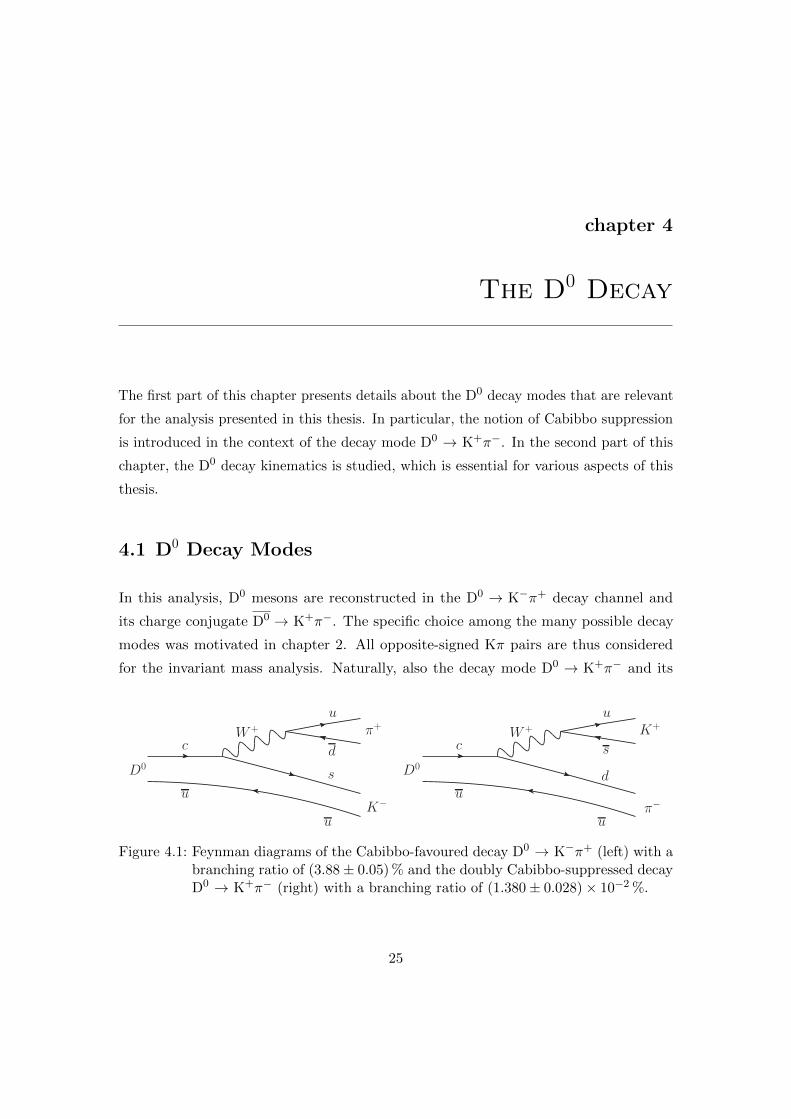
strongly suppressed. Figure 4.1 shows Feynman diagrams of the two processes. During
the D0 → K−π+ decay (left diagram in fig. 4.1), the charm quark from the original D0
splits into a strange quark and a W+ that subsequently decays to a ud quark pair forming
a π+. The two flavour changes involved are either within the first or within the second
quark family. The transition amplitude consequently contains only diagonal elements of
the Cabibbo-Kobayashi-Maskawa (CKM) matrix [65, 66]. In the D0 → K+π− decay, the
charm quark changes its flavour to a down quark radiating a W+ that decays further to a
us quark pair, constituting a K+ in the final state. A cross-over between different quark-
families now occurs in both of these flavour changes. The transition amplitude accordingly
contains two off-diagonal elements of the CKM matrix, which are much smaller than the
diagonal entries. This effect is known as Cabibbo suppression. D0 → K+π− is doubly
Cabibbo-suppressed, whereas D0 → K−π+ is Cabibbo-favoured.
The Particle Data Group (PDG) currently lists the branching fractions (3.88± 0.05) %
for D0 → K−π+ and (1.380± 0.028)× 10−4 for D0 → K+π− as world average [23]. The
ratio of the branching fractions of the Cabibbo-suppressed to the Cabibbo-favoured decay
is (3.56± 0.06)× 10−3. Though it is hence of little relevance to the analysis results
whether the doubly Cabibbo-suppressed decay is taken into account or not, it is straight
forward to add the branching ratios of the two contributing decay channels. A total
branching ratio of B = (3.89± 0.05) % is consequently used for the calculation of the D0
cross section (cf. section 5.9).
The PDG values of the branching fractions are subject to small fluctuations due to
regular updates from recent measurements. By the time the topological D0 analysis
was published, the PDG value for the branching ratio of D0 → K−π+ was 3.87 % [11].
Furthermore, the doubly-Cabibbo suppressed decay channel was not taken into account.
The branching ratio used in this analysis is therefore 0.02 % larger than that used in
the topological analysis. The relative difference of about 0.5 % should be kept in mind,
even though it is negligible compared to the uncertainties of the measurements. The
inconsistency could in principle be avoided by quoting the branching ratio times cross
section as the final result. Meanwhile, the current PDG value of the branching fraction
B(D0 → K−π+) is likely to be adjusted again soon, as the CLEO collaboration recently
updated their measurement of several D-meson branching ratios in electron-positron
collisions at the Cornell Electron Storage Ring (CESR) [67]. They reported an updated
26
result of 3.934±0.021(stat.)±0.061(syst.) % for D0 → K−π+, which constitutes now the
most precise single measurement of this particular branching ratio.
In a rare process, known as oscillation, a D0 can transform to its antiparticle D0
and vice versa before it decays. Such D0-D0 oscillations were observed recently with
the LHCb experiment via a precise decay time dependent measurement of the ratio
B(D0 → K+π−)/B(D0 → K−π+) [68]. This measurement is the first significant observa-
tion of D-meson oscillations with a single experiment and contains interesting physics of
its own. For this analysis, however, possible influences of D-meson oscillations on the
invariant mass distributions can be completely neglected.
4.2 D0 Decay Kinematics
4.2.1 Momentum-Space Variables
This section is intended to provide a collection of important definitions and equations
for the kinematic variables that are used in this thesis. In equations in this chapter and
throughout the thesis, natural units with c = 1 are used, where c denotes the speed of
light.
In this thesis, the momentum-space variables (pT, y, φ) are used, where pT is the transverse
momentum, i.e. the momentum projected to the transverse plane, φ the azimuthal angle
in the transverse plane, and y the rapidity defined as
y = tanh−1 βz =1
2lnE + pzE − pz
. (4.1)
Here, E denotes the energy of the particle and βz and pz the relativistic velocity and the
momentum along the z direction, which corresponds to the beam axis (cf. section 3.2).
As defined according to eq. (4.1), rapidity is an additive quantity under Lorentz transfor-
mations along the z direction. For massive particles, the rapidity depends on the mass
m of the particle. Rapidity is thus only a meaningful quantity if the particle type is
known. For some applications, it is therefore more convenient to use the pseudo-rapidity
27
η instead, which is independent of the particle species. It is defined as
η = − ln tan
(θ
2
), (4.2)
where θ is the polar angle between the z axis and the momentum vector. A flight direction
of a particle transverse to the beam axis corresponds to η = 0; a flight direction at
θ = 45◦ corresponds to |η| ≈ 0.88; and a flight direction along the beam axis corresponds
to |η| =∞. The transformation from pseudo-rapidity to rapidity is
y = ln
√m2 + p2T cosh2 η + pT sinh η√
m2 + p2T
. (4.3)
Rapidity coincides with pseudo-rapidity for massless particles or in the ultra-relativistic
limit E � m for a massive particle. The following inequality for rapidity y and pseudo-
rapidity η always holds:
|y| ≤ |η| . (4.4)
The transformation of the momentum coordinates (pT, y, φ) to cartesian momentum
coordinates (px, py, pz) is given by
px = pT cosφ , (4.5)
py = pT sinφ , (4.6)
pz = pT sinh η = mT sinh y . (4.7)
Here, the transverse mass mT is defined as
mT =√m2 + p2T . (4.8)
The following expressions for the energy and the absolute value of the momentum as a
function of pT and y are also useful:
E = mT cosh y , (4.9)
|~p| = pT cosh η =√
(m2 + p2T) sinh2 y + p2T . (4.10)
28
4.2.2 Invariant Mass
The invariant mass M of a system of N particles with four-momenta pi = (Ei, ~pi) is
defined as
M2 =
(N∑i=0
pi
)2
. (4.11)
For two particles, the invariant mass can be written in the form
M2 = (p1 + p2)2 = m2
1 +m22 + 2(E1E2 − |~p1||~p2| cos θ) . (4.12)
Using the (pT, y, φ) momentum-space variables, the formula translates to
M2 = m21 +m2
2 + 2mT,1mT,2 cosh ∆y − 2pT,1pT,2 cos ∆φ (4.13)
with the differences in rapidity, ∆y = y1 − y2, and in the azimuthal angle, ∆φ = φ1 − φ2,
of the two particles and the transverse mass mT as defined in eq. (4.8).
4.2.3 Decay Length
The decay length is defined as the distance between the production point of a particle,
i.e. the primary vertex, and the location where it decays, i.e. the secondary vertex.
The decay length of D mesons is the determining parameter for the performance of the
measurement of D-meson production via the reconstruction of the decay topology. The
efficiency of the background rejection decreases with decreasing decay length. If the
decay length is too small, the secondary vertex can no longer be distinguished from the
primary vertex and the topological approach for D-meson reconstruction fails. For an
evaluation of the experimental limit of the topological approach for the measurement of
D mesons towards low pT, it is therefore instructive to analyse the dependence of the
decay length on kinematic variables and to compare it to the detector resolution.
The average lifetime of a D0 in its rest frame is about τ0 = 123 µm/c [23]. Performing a
Lorentz boost to the lab frame yields for the average decay length
L = βγτ0 =p
mτ0 , (4.14)
29
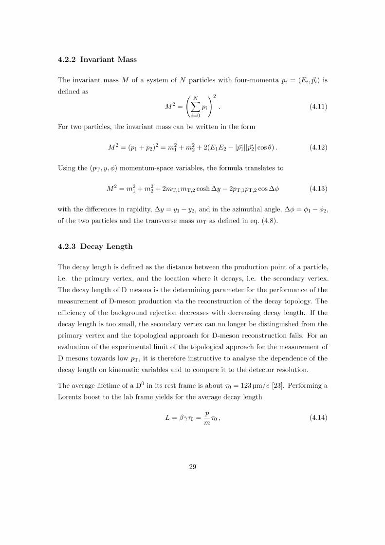
Figure 4.2: Average D0 decay length in the lab frame as a function of the D0 transversemomentum and rapidity. The white line marks the resolution limit of about80 µm for the separation of the secondary from the primary vertex.
where p is the absolute value of the momentum and m = 1.865 GeV/c2 the D0 mass. The
average decay length can be expressed as a function of the D0 rapidity and transverse
momentum using eq. (4.10):
L =τ0m
√(m2 + p2T) sinh2 y + p2T . (4.15)
A plot of this formula in the rapidity range |y| < 1 and in the pT range 0 < pT < 2 GeV/c
is shown in fig. 4.2. The resolution of the separation of the secondary vertex from the
primary vertex is about 80 µm for a D0 at zero transverse momentum [11]. The white
contour line in fig. 4.2 encloses the phase space region, for which the average D0 decay
length is below this resolution limit of 80 µm. As this area covers almost the entire
phase space for a D0 with pT < 1 GeV/c at mid-rapidity |y| < 0.8, the topological
reconstruction of D mesons with ALICE is limited to about pT > 1 GeV/c.
Figure 4.2 also demonstrates that, profiting from the boost in rapidity, the topolog-
ical approach can still be applied down to zero transverse momentum using a for-
ward detector. With the LHCb experiment, D-meson production in pp collisions at√s = 7 TeV was measured at forward rapidity in 2.0 < y < 4.5 and in the pT range
0 < pT < 8 GeV/c [69].
30
4.2.4 Kinematics of a Two-Body Decay
Consider a general two-body decay, where a mother particle with mass M decays to two
daughter particles with masses m1 and m2, where M ≥ m1 +m2. The centre-of-mass
frame (CMS) of the system corresponds to the rest frame of the decaying particle. In the
CMS, the four-momenta of the involved particles can be written as p = (M, 0, 0, 0) for
the mother particle and pi = (Ei, ~pi), with i ∈ {1, 2}, for the daughter particles. Starting
from four-momentum conservation
p = p1 + p2 , (4.16)
the energies and momenta of the daughter particles in the CMS can be expressed as
E1 =1
2M(M2 +m2
1 −m22) , (4.17)
E2 =1
2M(M2 +m2
2 −m21) , (4.18)
|~p1| = |~p2| =1
2M
√M4 +m4
1 +m42 − 2(M2m2
1 +M2m22 +m2
1m22) . (4.19)
These expressions are symmetric under the exchange of the two particles, as expected. For
the D0 → K−π+ decay, with the masses of the involved particles, mD0 = 1.865 GeV/c2,
mK− = 0.494 GeV/c2 and mπ+ = 0.140 GeV/c2, eqs. (4.18) - (4.19) yield for the energies
and momenta of the decay products:
|~pK− | = |~pπ+ | = 0.861 GeV/c , (4.20)
EK− = 0.993 GeV , (4.21)
Eπ+ = 0.873 GeV . (4.22)
In the CMS, the energy and momentum spectra of the daughter particles are discrete.
Boosting the decay kinematics to the lab frame results in continuous spectra for the case
of a moving mother particle.
4.2.5 A Toy Monte Carlo for Decay Kinematics
Based on the equations of the last section, the two-body decay D0 → K−π+ can be
simulated using four-vector relativistic kinematics and random generators. In the course
31

of this work, a toy Monte Carlo (MC) was developed for the use in several parts of this
thesis.
The decay routine is described in the following. In the centre-of-mass frame of the D0,
the four-momentum of the kaon is initialised with the three-momentum pointing in a
random direction on a sphere with radius 861.06 MeV/c (cf. section 4.2.4). In a second
step, the four-momentum of the pion is initialised with the three-momentum pointing
in the opposite direction. The three-momentum of the corresponding mother particle
is then randomly generated in (pT, y, φ) space. According to both FONLL [17] and
PYTHIA [70, 71] predictions, the rapidity distribution of D0 mesons in pp collisions
is flat within 1 % in |y| < 1. The rapidity for generated D0 mesons is thus drawn
from a uniform distribution in a given interval around mid-rapidity. The underlying pT
distribution can be chosen flat, or realistic, e.g. using the FONLL pT distribution. For
the φ angle, a flat distribution in [0, 2π] is used. Once the mother and daughter particles
are initialised, the four-momenta of the daughter particles are boosted to the lab frame
with a Lorentz transformation based on the three-momentum of the mother particle.
The entire kinematic information of a particular decay is thus contained in the resulting
three-momenta of the kaon and the pion (six numbers). Depending on the goal of the
specific simulation, this information is then processed further.
In fig. 4.3, the momentum and transverse momentum spectra of the decay daughters
are displayed, along with their angular distance in the transverse plane, ∆φ. Ten
million D0 mesons with |y| < 0.8 were generated with the toy MC in four pT bins in
0 < pT < 4 GeV/c (top to bottom in fig. 4.3). The daughter particles were additionally
restricted to |η| < 0.8 to mimic the corresponding track selection cut applied in this
analysis (cf. section 5.4). A minimum transverse momentum was not required.
32
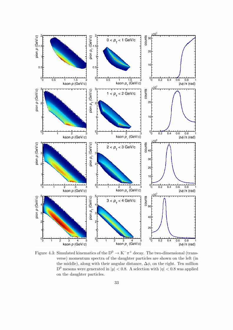
Figure 4.3: Simulated kinematics of the D0 → K−π+ decay. The two-dimensional (trans-verse) momentum spectra of the daughter particles are shown on the left (inthe middle), along with their angular distance, ∆φ, on the right. Ten millionD0 mesons were generated in |y| < 0.8. A selection with |η| < 0.8 was appliedon the daughter particles.
33
chapter 5
Data Analysis
In this chapter, the different steps of the analysis of low-pT D0 production are described
in detail. The chapter starts with a general overview of the analysis strategy. After some
remarks on computational aspects and workflow, further details about each analysis stage
can be found in a dedicated subsequent section.
5.1 Strategy and Overview
D0 mesons and their antiparticles D0 mesons are reconstructed in the decay channel
D0 → K−π+ and its charge conjugate with a small contribution of about 0.4 % from
the doubly Cabibbo-suppressed decay D0 → K+π−, as pointed out in section 4.1. The
analysis is run on selected events in a data set of pp collisions recorded with ALICE in
2010 at a centre-of-mass energy√s = 7 TeV. The data samples and the event selection
are described in section 5.3. Within the reconstructed events, charged particles are
represented by tracks that have been reconstructed from detector signals in the ITS and
the TPC. A quality and kinematic selection is applied on the tracks that are present
in each event, as detailed in section 5.4. The selected tracks are then processed further
in the analysis. Without any assumption on the particle type, each combination of
a negative and a positive track within the same event is accepted as a D0 candidate.
The D0 signature is a peak in the invariant mass distribution of all such candidates at
the nominal D0 mass. It is intrinsic to the procedure of combining tracks to implicate
a large combinatorial background of track pairs not originating from a D0 decay, of
34
which the invariant mass falls in the D0 peak region by coincidence. A priori, the signal-
to-background ratio (S/B) is thus only about 2.5× 10⁻⁴ in the low-pT region, where
the combinatorial background is particularly large due to the production of soft pions
and kaons. The stable extraction of the signal in such a high background environment
constitutes the major challenge to this analysis.
The excellent particle identification (PID) capabilities of ALICE contribute significantly
to the reduction of background, while retaining a high efficiency for the signal. The
specific energy loss per unit of path length dE/dx of charged particles in the TPC gas
is used in conjunction with the time-of-flight information provided by the TOF system.
Details of the PID strategy are discussed in section 5.5. After PID selection, the S/B
ratio is about 10−3 in the pT interval 0 < pT < 1 GeV/c. At this scale, signal extraction
is still very sensitive to the unknown background shape and thus highly unstable. An
estimate of the combinatorial background is therefore subtracted from the invariant
mass spectrum, as part of the signal extraction, using the like-sign technique. After
subtraction of the combinatorial background, the D0 yield is extracted in the full pT
range 0 < pT < 16 GeV/c by fitting with a parameterisation of the signal and the small
residual background that survived the background subtraction. Section 5.6 is dedicated
to the signal extraction procedure.
The extracted raw yield is corrected by the efficiency of the reconstruction and the selec-
tions applied in the analysis. The efficiency correction is determined by analysing Monte
Carlo (MC) events that were generated in a realistic simulated detector environment,
applying the identical reconstruction algorithm and the same selections as for real data.
In the standard topological D-meson analysis, the efficiency quickly drops to zero for
small pT. In this work, however, the efficiency flattens off at about 20 % going towards
zero transverse momentum of the D0. Signal extraction thus becomes possible in the
entire momentum space, assuming that the background is under control. Section 5.7
contains details about the efficiency correction. D0 mesons from B decays are denoted
as feed-down. Their contribution to the measured D0 yield must be subtracted, relying
on theory input, in order to derive the cross section of prompt D0 production. The
analysis step of feed-down subtraction is described in section 5.8. With all the input
gathered, the chapter concludes section 5.9 with the calculation of the D0 production
cross section.
35
5.2 Computational Analysis
For a variety of programming tasks including data processing, Monte Carlo simulation
and data visualisation, the ALICE collaboration uses the C++ based object oriented
data analysis framework ROOT [72]. Libraries that are specific to the ALICE experiment
are collected and maintained in a derived package known as AliRoot [73]. The code used
for data analysis with a specific physics goal is called an analysis task and is typically im-
plemented as an AliRoot class. Analysis tasks share a common global structure, the most
important parts being a function for the definition of output objects, which are mainly
histograms, and a function that is executed for each analysed event. The task developed
for the analysis of D mesons without topological selection is AliAnalysisTaskCombinHF
and can currently be found in the AliRoot directory PWGHF/vertexingHF. Certain config-
urations like the track selection cuts or the specific method for particle identification can
be inserted as parameters by the user. Thus, it becomes possible to run multiple versions
of the same task with different setups in order to compare different selections. Due to the
rather large data files, the analysis is computationally expensive and the infrastructure of
a world-wide computing grid [74] was used. The average CPU time to process one event
was of the order of 10 ms. With parallelisation, the typical duration for processing the
entire data set of about 380 million events before selection was about six hours.
Analysis tasks operate on preprocessed data sets that contain fully reconstructed events,
providing a convenient interface for the end user. The first step towards these sets after
data taking is the reconstruction of physical objects from raw detector signals. In a
tracking detector, for example, the procedure consists of reconstructing charged particle
tracks by fitting neighbouring clusters of energy loss to curved lines (cf. section 5.4).
The reconstructed events containing the reconstructed objects for the different detector
systems are initially stored in a structure called Event Summary Data (ESD). The data
sets can then be processed further into a final format called Analysis Object Data (AOD).
Different filters can be applied in this last processing step from ESDs to AODs, in order
to reduce the large data amount and to provide easier access to the end user.
Once the output of an analysis task is available, a series of ‘post-processing’ steps is
performed, including signal extraction, the calculation of the cross section with the
respective corrections and finally data visualisation.
36
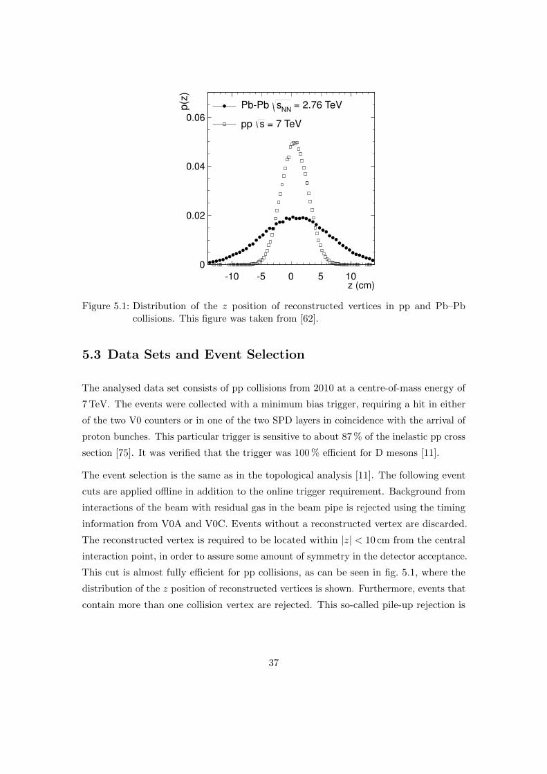
z (cm)10 5 0 5 10
p(z
)
0
0.02
0.04
0.06
= 2.76 TeVNN
sPbPb
= 7 TeVspp
Figure 5.1: Distribution of the z position of reconstructed vertices in pp and Pb–Pbcollisions. This figure was taken from [62].
5.3 Data Sets and Event Selection
The analysed data set consists of pp collisions from 2010 at a centre-of-mass energy of
7 TeV. The events were collected with a minimum bias trigger, requiring a hit in either
of the two V0 counters or in one of the two SPD layers in coincidence with the arrival of
proton bunches. This particular trigger is sensitive to about 87 % of the inelastic pp cross
section [75]. It was verified that the trigger was 100 % efficient for D mesons [11].
The event selection is the same as in the topological analysis [11]. The following event
cuts are applied offline in addition to the online trigger requirement. Background from
interactions of the beam with residual gas in the beam pipe is rejected using the timing
information from V0A and V0C. Events without a reconstructed vertex are discarded.
The reconstructed vertex is required to be located within |z| < 10 cm from the central
interaction point, in order to assure some amount of symmetry in the detector acceptance.
This cut is almost fully efficient for pp collisions, as can be seen in fig. 5.1, where the
distribution of the z position of reconstructed vertices is shown. Furthermore, events that
contain more than one collision vertex are rejected. This so-called pile-up rejection is
37

performed on the basis of vertices reconstructed from SPD tracklets, which are correlated
hit pairs in the two SPD layers. An event is classified as a pile-up event and consequently
rejected if it contains more than one SPD vertex with a minimum number of three
contributing tracklets and a minimum distance of 0.8 cm in z direction between the
vertices. A total number of about 280 million selected events is then processed in the
analysis task.
In addition to the number of analysed events, the number of events with a non-
reconstructed vertex in |z| < 10 cm has to be accounted for in the calculation of the cross
section. Under the assumption that the z distribution is the same for events with and
without a reconstructed vertex, the number of events with a non-reconstructed vertex
in |z| < 10 cm can be estimated from the number of events with a reconstructed vertex
using
N(w/o vert., |z| < 10 cm) = N(w/o vert., |z| <∞)× N(w/ vert., |z| < 10 cm)
N(w/ vert., |z| <∞). (5.1)
In this formula, N(...) denotes the number of events with (w/) or without (w/o) a
reconstructed vertex, within the specified z range. The total number of events, Nevents,
considered for the calculation of the D0 production cross section is then
Nevents = N(w/ vert., |z| < 10 cm) +N(w/o vert., |z| < 10 cm) = 327 million . (5.2)
The first term corresponds to the number of analysed events having passed the selection;
the second term is estimated using eq. (5.1) above. With the minimum bias cross section,
σMB = 62.3 mb [75], this number of events corresponds to the following integrated
luminosity for the analysed data sample:
Lint =Nevents
σMB= 5.25 nb−1 . (5.3)
5.4 Track Reconstruction and Selection
A track represents the flight path of a charged particle traversing active detector volume.
The procedure of combining single detector signals to global tracks in the course of event
reconstruction is called tracking. Several central barrel detectors of ALICE are involved
38
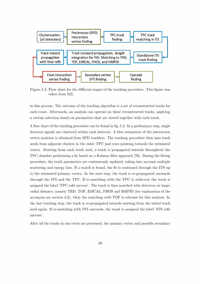
Figure 5.2: Flow chart for the different stages of the tracking procedure. This figure wastaken from [62].
in this process. The outcome of the tracking algorithm is a set of reconstructed tracks for
each event. Afterwards, an analysis can operate on these reconstructed tracks, applying
a certain selection based on parameters that are stored together with each track.
A flow chart of the tracking procedure can be found in fig. 5.2. In a preliminary step, single
detector signals are clustered within each detector. A first estimation of the interaction
vertex position is obtained from SPD tracklets. The tracking procedure then uses track
seeds from adjacent clusters in the outer TPC pad rows pointing towards the estimated
vertex. Starting from each track seed, a track is propagated inwards throughout the
TPC chamber performing a fit based on a Kalman filter approach [76]. During the fitting
procedure, the track parameters are continuously updated, taking into account multiple
scattering and energy loss. If a match is found, the fit is continued through the ITS up
to the estimated primary vertex. In the next step, the track is re-propagated outwards
through the ITS and the TPC. If re-matching with the TPC is achieved, the track is
assigned the label ‘TPC refit success’. The track is then matched with detectors at larger
radial distance, namely TRD, TOF, EMCAL, PHOS and HMPID (for explanation of the
acronyms see section 3.2). Only the matching with TOF is relevant for this analysis. In
the last tracking step, the track is re-propagated inwards starting from the initial track
seed again. If re-matching with ITS succeeds, the track is assigned the label ‘ITS refit
success’.
After all the tracks in one event are processed, the primary vertex and possible secondary
39

label description cut value
TS1 no. of crossed rows in the TPC ≥ 70
TS2 no. of crossed rows / no. of findable clusters ≥ 0.8
TS3 no. of clusters in the TPC ≥ 50
TS4 χ2 per no. of clusters in the TPC ≤ 4
TS5 TPC refit success yes
TS6 ITS refit success yes
TS7 reject kink daughters yes
TS8a DCA to vertex in transverse plane < 2.4 cm
TS8b DCA to vertex in z direction < 3.2 cm
TS9 pseudo-rapidity |η| < 0.8
TS10 transverse momentum pT > 0.3 GeV/c
Table 5.1: Selection cuts for single tracks used in this analysis. The cuts are labelled forreference in the text.
vertices are recomputed using the full information from the reconstructed tracks. This
results in a better precision on the position of primary and secondary vertices. The
reconstruction of secondary vertices with high precision is not relevant to the analysis
presented here, in contrast to the topological analysis, where it is an essential part of the
analysis strategy.
A quality selection of tracks has to be applied in order to assure sufficient momentum
and dE/dx resolution and a high reconstruction efficiency. The applied single track cuts
are listed in table 5.1. The cuts are labelled for referencing in the text. The cuts TS1
to TS6 are pure quality cuts; TS7 to TS8b partially serve as background rejection; TS9
and TS10 are kinematic cuts. A minimum of 70 crossed pad rows in the TPC (TS1)
out of a possible 159 is required in order to assure a minimum track length. This has
the most direct impact on the momentum resolution. An additional cut on the ratio of
the number of crossed rows in the TPC and the number of findable TPC clusters of 0.8
(TS2) is applied. The number of findable clusters is defined as the maximum number of
clusters that could be assigned to a track with a given geometry provided full efficiency
in the reconstruction. The minimum requirement of 50 clusters in the TPC (TS3), is an
artefact of the AOD-filtering stage of the used data set (cf. section 5.2). However, TS3
has no effect, since all tracks rejected by TS3 are also rejected by TS1 and TS2.
40
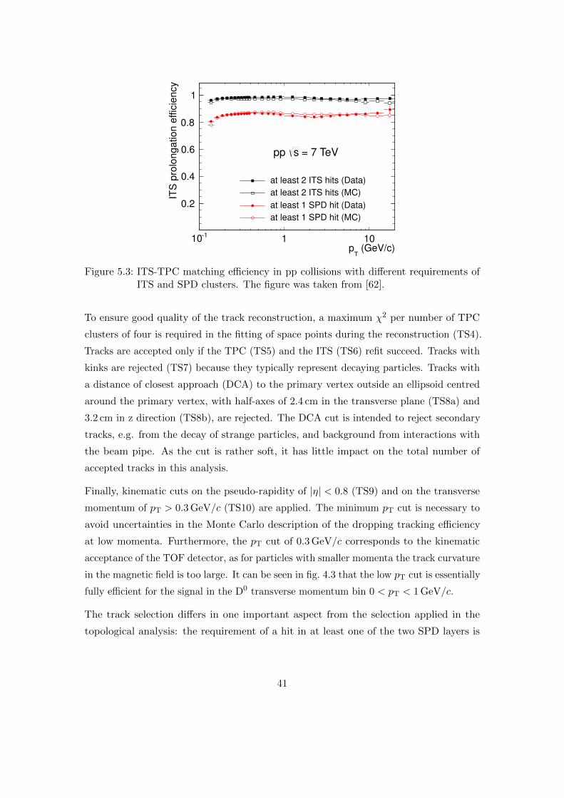
(GeV/c)T
p
110 1 10
ITS
pro
lon
ga
tio
n e
ffic
ien
cy
0.2
0.4
0.6
0.8
1
= 7 TeVspp
at least 2 ITS hits (Data)
at least 2 ITS hits (MC)
at least 1 SPD hit (Data)
at least 1 SPD hit (MC)
Figure 5.3: ITS-TPC matching efficiency in pp collisions with different requirements ofITS and SPD clusters. The figure was taken from [62].
To ensure good quality of the track reconstruction, a maximum χ2 per number of TPC
clusters of four is required in the fitting of space points during the reconstruction (TS4).
Tracks are accepted only if the TPC (TS5) and the ITS (TS6) refit succeed. Tracks with
kinks are rejected (TS7) because they typically represent decaying particles. Tracks with
a distance of closest approach (DCA) to the primary vertex outside an ellipsoid centred
around the primary vertex, with half-axes of 2.4 cm in the transverse plane (TS8a) and
3.2 cm in z direction (TS8b), are rejected. The DCA cut is intended to reject secondary
tracks, e.g. from the decay of strange particles, and background from interactions with
the beam pipe. As the cut is rather soft, it has little impact on the total number of
accepted tracks in this analysis.
Finally, kinematic cuts on the pseudo-rapidity of |η| < 0.8 (TS9) and on the transverse
momentum of pT > 0.3 GeV/c (TS10) are applied. The minimum pT cut is necessary to
avoid uncertainties in the Monte Carlo description of the dropping tracking efficiency
at low momenta. Furthermore, the pT cut of 0.3 GeV/c corresponds to the kinematic
acceptance of the TOF detector, as for particles with smaller momenta the track curvature
in the magnetic field is too large. It can be seen in fig. 4.3 that the low pT cut is essentially
fully efficient for the signal in the D0 transverse momentum bin 0 < pT < 1 GeV/c.
The track selection differs in one important aspect from the selection applied in the
topological analysis: the requirement of a hit in at least one of the two SPD layers is
41
crucial for the topological D-meson analysis to assure high precision in the reconstruction
of the decay topology. This requirement results, however, in a relatively large decrease
of the ITS prolongation efficiency from close to 100 % down to around 85 %, as can be
observed in fig. 5.3. This decrease is due to cooling problems in the SPD during the pp
data runs from 2010, which lead to a high dead channel rate and thus reduced acceptance.
For this analysis, it is considered fully sufficient to require at least two hits in any of the
ITS layers, which is implicitly contained in the selection cuts TS5 and TS6. For this looser
selection, the ITS prolongation efficiency is close to one. Since two tracks are involved
in the analysis, the absence of the requirement of an SPD hit yields an excess of about
30 % on the number of D0 candidates for this analysis as compared to the topological
analysis. It is reasonable to assume that signal and background scale in the same way, as
no topological selection is involved, which would require high-precision pointing of the
track. The increase in statistics is consequently associated with an increase in significance
of about a factor√
1.3 = 1.14. This increase in significance is an important benefit for
the signal extraction at low pT.
In addition to the single track selection, a rapidity cut of |y| < 0.8 was applied on D0
candidates constructed by combining track pairs. This corresponds to the maximum
rapidity range for D0 mesons that is kinematically accessible due to the selection |η| < 0.8
on the single tracks (TS9). Apart from the rapidity cut, no further selection was applied
on D0 candidates.
5.5 Particle Identification
A powerful tool at hand for the rejection of background is particle identification (PID).
For the identification of kaons and pions, the specific energy loss dE/dx in the TPC and
the time of flight measured with the TOF system are used.
5.5.1 PID Information from TPC and TOF
A charged particle propagating in the active volume in the TPC loses energy via ionisation
of gas atoms (cf. section 3.4). The number of generated electrons and ions is proportional
to the specific energy loss per unit of path length, dE/dx, of the ionising particle.
The created charge is collected with the TPC readout panels and transformed into a
42
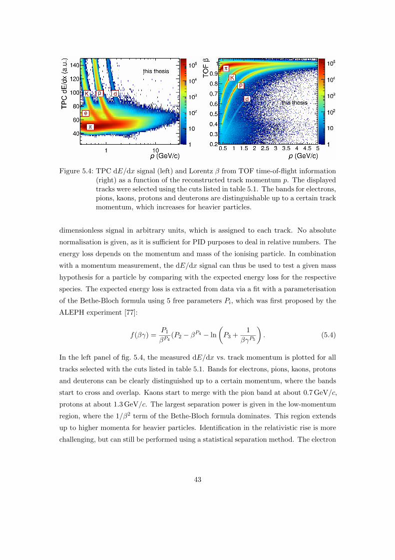
Figure 5.4: TPC dE/dx signal (left) and Lorentz β from TOF time-of-flight information(right) as a function of the reconstructed track momentum p. The displayedtracks were selected using the cuts listed in table 5.1. The bands for electrons,pions, kaons, protons and deuterons are distinguishable up to a certain trackmomentum, which increases for heavier particles.
dimensionless signal in arbitrary units, which is assigned to each track. No absolute
normalisation is given, as it is sufficient for PID purposes to deal in relative numbers. The
energy loss depends on the momentum and mass of the ionising particle. In combination
with a momentum measurement, the dE/dx signal can thus be used to test a given mass
hypothesis for a particle by comparing with the expected energy loss for the respective
species. The expected energy loss is extracted from data via a fit with a parameterisation
of the Bethe-Bloch formula using 5 free parameters Pi, which was first proposed by the
ALEPH experiment [77]:
f(βγ) =P1
βP4(P2 − βP4 − ln
(P3 +
1
βγP5
). (5.4)
In the left panel of fig. 5.4, the measured dE/dx vs. track momentum is plotted for all
tracks selected with the cuts listed in table 5.1. Bands for electrons, pions, kaons, protons
and deuterons can be clearly distinguished up to a certain momentum, where the bands
start to cross and overlap. Kaons start to merge with the pion band at about 0.7 GeV/c,
protons at about 1.3 GeV/c. The largest separation power is given in the low-momentum
region, where the 1/β2 term of the Bethe-Bloch formula dominates. This region extends
up to higher momenta for heavier particles. Identification in the relativistic rise is more
challenging, but can still be performed using a statistical separation method. The electron
43
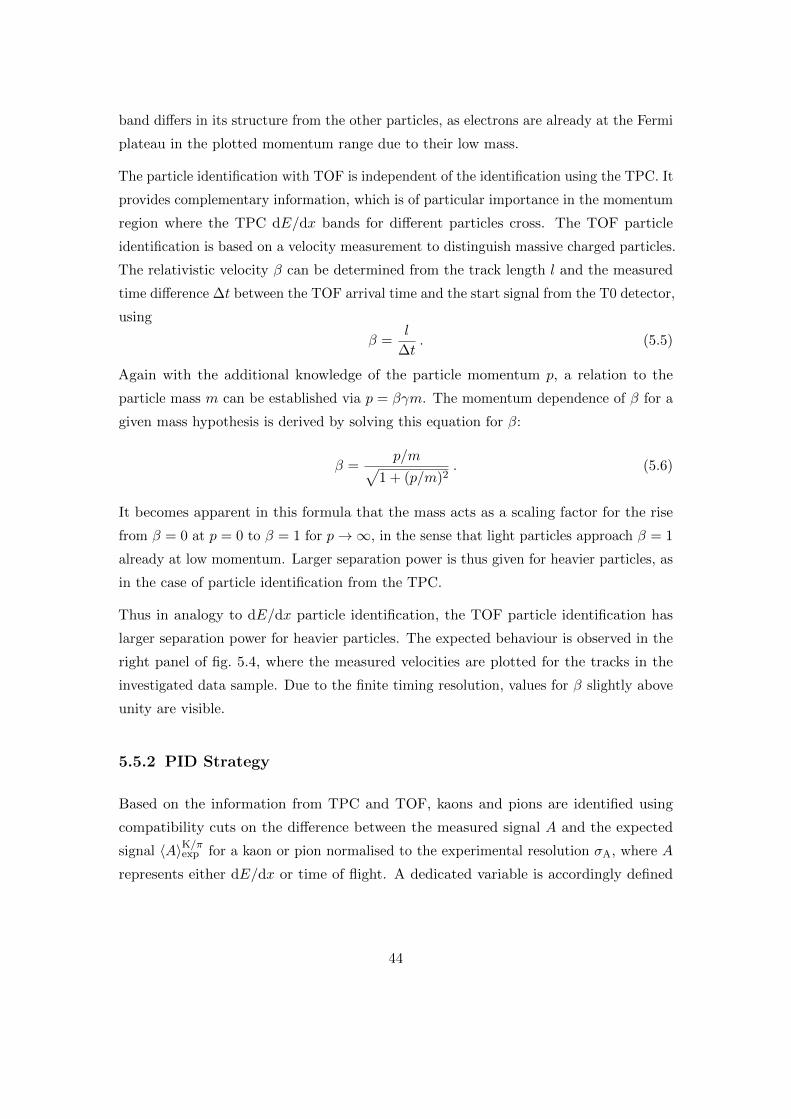
band differs in its structure from the other particles, as electrons are already at the Fermi
plateau in the plotted momentum range due to their low mass.
The particle identification with TOF is independent of the identification using the TPC. It
provides complementary information, which is of particular importance in the momentum
region where the TPC dE/dx bands for different particles cross. The TOF particle
identification is based on a velocity measurement to distinguish massive charged particles.
The relativistic velocity β can be determined from the track length l and the measured
time difference ∆t between the TOF arrival time and the start signal from the T0 detector,
using
β =l
∆t. (5.5)
Again with the additional knowledge of the particle momentum p, a relation to the
particle mass m can be established via p = βγm. The momentum dependence of β for a
given mass hypothesis is derived by solving this equation for β:
β =p/m√
1 + (p/m)2. (5.6)
It becomes apparent in this formula that the mass acts as a scaling factor for the rise
from β = 0 at p = 0 to β = 1 for p→∞, in the sense that light particles approach β = 1
already at low momentum. Larger separation power is thus given for heavier particles, as
in the case of particle identification from the TPC.
Thus in analogy to dE/dx particle identification, the TOF particle identification has
larger separation power for heavier particles. The expected behaviour is observed in the
right panel of fig. 5.4, where the measured velocities are plotted for the tracks in the
investigated data sample. Due to the finite timing resolution, values for β slightly above
unity are visible.
5.5.2 PID Strategy
Based on the information from TPC and TOF, kaons and pions are identified using
compatibility cuts on the difference between the measured signal A and the expected
signal 〈A〉K/πexp for a kaon or pion normalised to the experimental resolution σA, where A
represents either dE/dx or time of flight. A dedicated variable is accordingly defined
44

Figure 5.5: The PID nσ variable for the kaon (top) and pion (bottom) hypothesis inTPC (left) and TOF (right). The dashed lines indicate the 3σ cut used inthe analysis. Contaminations from different species are labelled.
as
nTPC/TOFσ,K/π =
A− 〈A〉K/πexp
σA. (5.7)
The TPC information is available for every track used in the analysis. This does not
hold for the TOF information, which can be absent, if the matching of the track from
TPC to TOF fails, for example if the particle is absorbed after traversing the TPC.
If TOF information is missing, the particle is identified using only the TPC with a
cut of nTPCσ < 3 for both kaons and pions. If the TOF information is present, the
requirement nTOFσ < 3 is applied in addition. The efficiency of this strategy is thus close
to 100 %. PID cuts of this type are also referred to as ‘nσ cuts’ and the corresponding
strategy as ‘nσ’ PID. In fig. 5.5, nσ is plotted for the TPC (left) and the TOF system
(right) with a kaon hypothesis (top) or a pion hypothesis (bottom), respectively. The
upper and lower 3σ cut is indicated by the dotted red lines. Daughter particles from
45
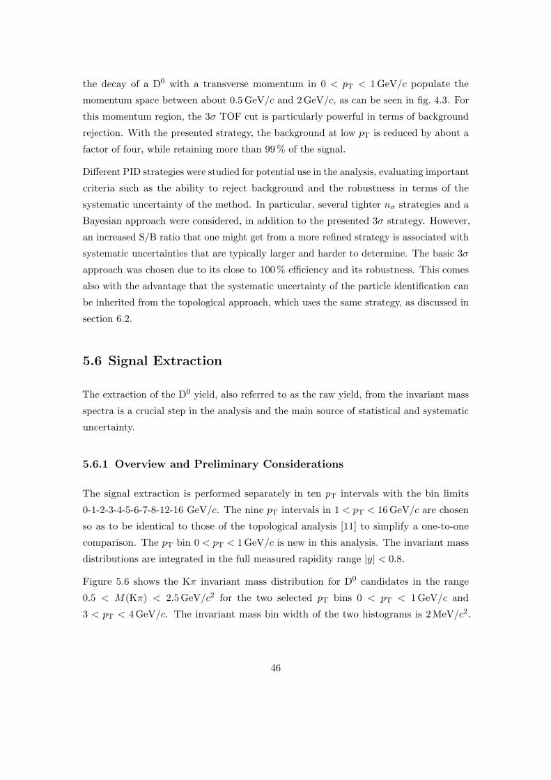
the decay of a D0 with a transverse momentum in 0 < pT < 1 GeV/c populate the
momentum space between about 0.5 GeV/c and 2 GeV/c, as can be seen in fig. 4.3. For
this momentum region, the 3σ TOF cut is particularly powerful in terms of background
rejection. With the presented strategy, the background at low pT is reduced by about a
factor of four, while retaining more than 99 % of the signal.
Different PID strategies were studied for potential use in the analysis, evaluating important
criteria such as the ability to reject background and the robustness in terms of the
systematic uncertainty of the method. In particular, several tighter nσ strategies and a
Bayesian approach were considered, in addition to the presented 3σ strategy. However,
an increased S/B ratio that one might get from a more refined strategy is associated with
systematic uncertainties that are typically larger and harder to determine. The basic 3σ
approach was chosen due to its close to 100 % efficiency and its robustness. This comes
also with the advantage that the systematic uncertainty of the particle identification can
be inherited from the topological approach, which uses the same strategy, as discussed in
section 6.2.
5.6 Signal Extraction
The extraction of the D0 yield, also referred to as the raw yield, from the invariant mass
spectra is a crucial step in the analysis and the main source of statistical and systematic
uncertainty.
5.6.1 Overview and Preliminary Considerations
The signal extraction is performed separately in ten pT intervals with the bin limits
0-1-2-3-4-5-6-7-8-12-16 GeV/c. The nine pT intervals in 1 < pT < 16 GeV/c are chosen
so as to be identical to those of the topological analysis [11] to simplify a one-to-one
comparison. The pT bin 0 < pT < 1 GeV/c is new in this analysis. The invariant mass
distributions are integrated in the full measured rapidity range |y| < 0.8.
Figure 5.6 shows the Kπ invariant mass distribution for D0 candidates in the range
0.5 < M(Kπ) < 2.5 GeV/c2 for the two selected pT bins 0 < pT < 1 GeV/c and
3 < pT < 4 GeV/c. The invariant mass bin width of the two histograms is 2 MeV/c2.
46

)2c) (GeV/π(KM1 1.5 2 2.5
)2 cE
ntrie
s / (
2 M
eV/
0
500
1000
310×
< 1 GeV/cT
p0 <
K*(892)
)2c) (GeV/π(KM1 1.5 2 2.5
)2 cE
ntrie
s / (
2 M
eV/
0
50
100
310×
< 4 GeV/cT
p3 <
K*(892) K*(1430) 0D
Figure 5.6: Overview of the structure of the Kπ invariant mass distribution for D0 can-didates in the pT intervals 0 < pT < 1 GeV/c (left) and 3 < pT < 4 GeV/c(right). In the first pT bin, only the K*(892) peak can be distinguished fromthe large background by the eye. The D0 peak apparently vanishes due toa low signal-to-background ratio of about 10−3. For 3 < pT < 4 GeV/c, theK*(1430) peak and the D0 peak also become visible.
The observed invariant mass threshold coincides well with the theoretical value of
Mmin = 0.633 GeV/c2, which is the sum of the kaon and pion mass, as can be seen from
eq. (4.12). Starting from this kinematic boundary, the invariant mass distribution rises
up to a maximum and then falls again, where the rise is steeper than the decrease. This
global structure is similar for those transverse momentum intervals not displayed in
fig. 5.6.
The bin entries of the invariant mass distribution follow a Poisson distribution. The
associated relative uncertainty thus decreases with 1/√N , where N is the bin content.
The shape of the D0 candidate distribution in 0 < pT < 1 GeV/c is therefore rather
smooth due to the large number of candidates per invariant mass bin. A peak is visible
in the structure at M(Kπ) = 892 MeV/c2, which results from the K*(892) decay to a Kπ
pair. In this lowest pT interval, the D0 peak, expected at M(Kπ) = 1865 MeV/c2, remains
hidden to the naked eye due to a low signal-to-background (S/B) ratio of about 10−3. In
the pT interval 3 < pT < 4 GeV/c, the background scale is decreased by about an order
of magnitude and the D0 peak can be identified. In addition, another kaon resonance,
the K*(1430), becomes visible. Statistical fluctuations in the invariant mass distribution
are more pronounced than for 0 < pT < 1 GeV/c due to the lower background.
47
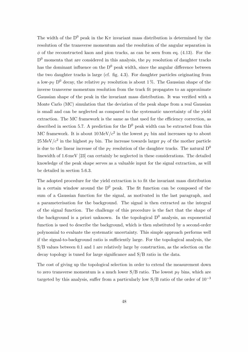
The width of the D0 peak in the Kπ invariant mass distribution is determined by the
resolution of the transverse momentum and the resolution of the angular separation in
φ of the reconstructed kaon and pion tracks, as can be seen from eq. (4.13). For the
D0 momenta that are considered in this analysis, the pT resolution of daughter tracks
has the dominant influence on the D0 peak width, since the angular difference between
the two daughter tracks is large (cf. fig. 4.3). For daughter particles originating from
a low-pT D0 decay, the relative pT resolution is about 1 %. The Gaussian shape of the
inverse transverse momentum resolution from the track fit propagates to an approximate
Gaussian shape of the peak in the invariant mass distribution. It was verified with a
Monte Carlo (MC) simulation that the deviation of the peak shape from a real Gaussian
is small and can be neglected as compared to the systematic uncertainty of the yield
extraction. The MC framework is the same as that used for the efficiency correction, as
described in section 5.7. A prediction for the D0 peak width can be extracted from this
MC framework. It is about 10 MeV/c2 in the lowest pT bin and increases up to about
25 MeV/c2 in the highest pT bin. The increase towards larger pT of the mother particle
is due to the linear increase of the pT resolution of the daughter tracks. The natural D0
linewidth of 1.6 meV [23] can certainly be neglected in these considerations. The detailed
knowledge of the peak shape serves as a valuable input for the signal extraction, as will
be detailed in section 5.6.3.
The adopted procedure for the yield extraction is to fit the invariant mass distribution
in a certain window around the D0 peak. The fit function can be composed of the
sum of a Gaussian function for the signal, as motivated in the last paragraph, and
a parameterisation for the background. The signal is then extracted as the integral
of the signal function. The challenge of this procedure is the fact that the shape of
the background is a priori unknown. In the topological D0 analysis, an exponential
function is used to describe the background, which is then substituted by a second-order
polynomial to evaluate the systematic uncertainty. This simple approach performs well
if the signal-to-background ratio is sufficiently large. For the topological analysis, the
S/B values between 0.1 and 1 are relatively large by construction, as the selection on the
decay topology is tuned for large significance and S/B ratio in the data.
The cost of giving up the topological selection in order to extend the measurement down
to zero transverse momentum is a much lower S/B ratio. The lowest pT bins, which are
targeted by this analysis, suffer from a particularly low S/B ratio of the order of 10−3
48
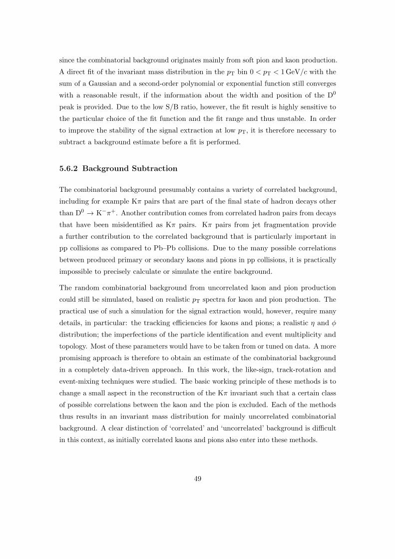
since the combinatorial background originates mainly from soft pion and kaon production.
A direct fit of the invariant mass distribution in the pT bin 0 < pT < 1 GeV/c with the
sum of a Gaussian and a second-order polynomial or exponential function still converges
with a reasonable result, if the information about the width and position of the D0
peak is provided. Due to the low S/B ratio, however, the fit result is highly sensitive to
the particular choice of the fit function and the fit range and thus unstable. In order
to improve the stability of the signal extraction at low pT, it is therefore necessary to
subtract a background estimate before a fit is performed.
5.6.2 Background Subtraction
The combinatorial background presumably contains a variety of correlated background,
including for example Kπ pairs that are part of the final state of hadron decays other
than D0 → K−π+. Another contribution comes from correlated hadron pairs from decays
that have been misidentified as Kπ pairs. Kπ pairs from jet fragmentation provide
a further contribution to the correlated background that is particularly important in
pp collisions as compared to Pb–Pb collisions. Due to the many possible correlations
between produced primary or secondary kaons and pions in pp collisions, it is practically
impossible to precisely calculate or simulate the entire background.
The random combinatorial background from uncorrelated kaon and pion production
could still be simulated, based on realistic pT spectra for kaon and pion production. The
practical use of such a simulation for the signal extraction would, however, require many
details, in particular: the tracking efficiencies for kaons and pions; a realistic η and φ
distribution; the imperfections of the particle identification and event multiplicity and
topology. Most of these parameters would have to be taken from or tuned on data. A more
promising approach is therefore to obtain an estimate of the combinatorial background
in a completely data-driven approach. In this work, the like-sign, track-rotation and
event-mixing techniques were studied. The basic working principle of these methods is to
change a small aspect in the reconstruction of the Kπ invariant such that a certain class
of possible correlations between the kaon and the pion is excluded. Each of the methods
thus results in an invariant mass distribution for mainly uncorrelated combinatorial
background. A clear distinction of ‘correlated’ and ‘uncorrelated’ background is difficult
in this context, as initially correlated kaons and pions also enter into these methods.
49
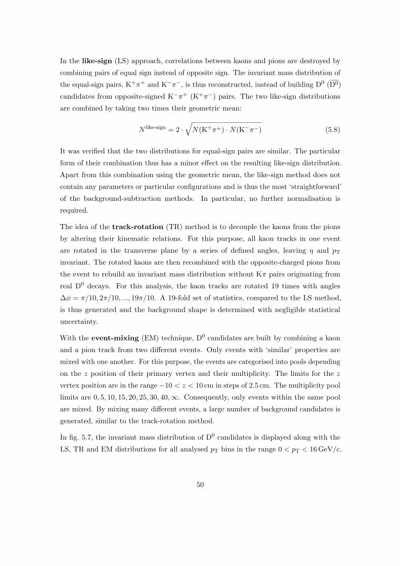
In the like-sign (LS) approach, correlations between kaons and pions are destroyed by
combining pairs of equal sign instead of opposite sign. The invariant mass distribution of
the equal-sign pairs, K+π+ and K−π−, is thus reconstructed, instead of building D0 (D0)
candidates from opposite-signed K−π+ (K+π−) pairs. The two like-sign distributions
are combined by taking two times their geometric mean:
N like-sign = 2 ·√N(K+π+) ·N(K−π−) (5.8)
It was verified that the two distributions for equal-sign pairs are similar. The particular
form of their combination thus has a minor effect on the resulting like-sign distribution.
Apart from this combination using the geometric mean, the like-sign method does not
contain any parameters or particular configurations and is thus the most ‘straightforward’
of the background-subtraction methods. In particular, no further normalisation is
required.
The idea of the track-rotation (TR) method is to decouple the kaons from the pions
by altering their kinematic relations. For this purpose, all kaon tracks in one event
are rotated in the transverse plane by a series of defined angles, leaving η and pT
invariant. The rotated kaons are then recombined with the opposite-charged pions from
the event to rebuild an invariant mass distribution without Kπ pairs originating from
real D0 decays. For this analysis, the kaon tracks are rotated 19 times with angles
∆φ = π/10, 2π/10, ..., 19π/10. A 19-fold set of statistics, compared to the LS method,
is thus generated and the background shape is determined with negligible statistical
uncertainty.
With the event-mixing (EM) technique, D0 candidates are built by combining a kaon
and a pion track from two different events. Only events with ‘similar’ properties are
mixed with one another. For this purpose, the events are categorised into pools depending
on the z position of their primary vertex and their multiplicity. The limits for the z
vertex position are in the range −10 < z < 10 cm in steps of 2.5 cm. The multiplicity pool
limits are 0, 5, 10, 15, 20, 25, 30, 40,∞. Consequently, only events within the same pool
are mixed. By mixing many different events, a large number of background candidates is
generated, similar to the track-rotation method.
In fig. 5.7, the invariant mass distribution of D0 candidates is displayed along with the
LS, TR and EM distributions for all analysed pT bins in the range 0 < pT < 16 GeV/c.
50
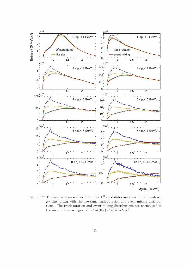
1 1.5 20
1
2
3
610×
< 1 GeV/cT
p0 <
candidates0D
like sign
1 1.5 20
1
2
3
4
610×
< 2 GeV/cT
p1 <
track rotation
event mixing
1 1.5 20
0.5
1
610×
< 3 GeV/cT
p2 <
1 1.5 20
0.1
0.2
0.3
610×
< 4 GeV/cT
p3 <
1 1.5 20
50
100310×
< 5 GeV/cT
p4 <
1 1.5 20
10
20
30
310×
< 6 GeV/cT
p5 <
1 1.5 20
5
10
15
310×
< 7 GeV/cT
p6 <
1 1.5 20
2
4
6
310×
< 8 GeV/cT
p7 <
1 1.5 20
2
4
6
8310×
< 12 GeV/cT
p8 <
1 1.5 20
0.5
1
310×
< 16 GeV/cT
p12 <
)2 cE
ntrie
s / (
5 M
eV/
)2c) (GeV/π(KM
Figure 5.7: The invariant mass distribution for D0 candidates are shown in all analysedpT bins, along with the like-sign, track-rotation and event-mixing distribu-tions. The track-rotation and event-mixing distributions are normalised inthe invariant mass region 2.0 < M(Kπ) < 2.05 GeV/c2.
51
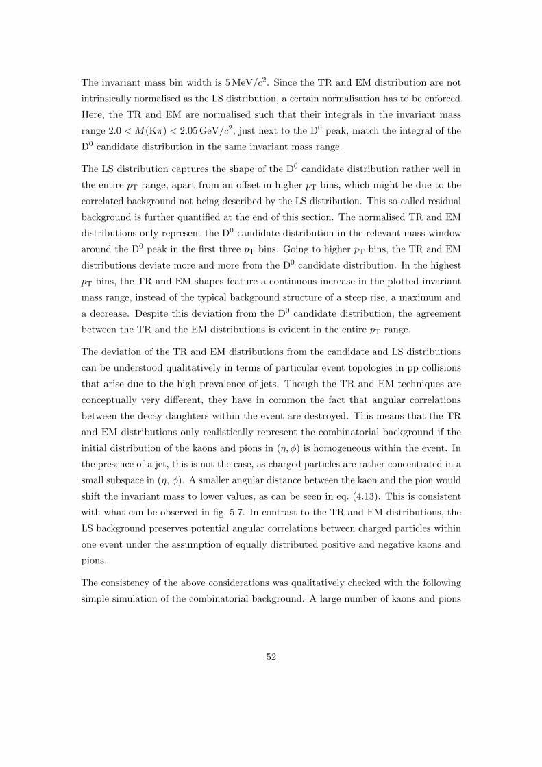
The invariant mass bin width is 5 MeV/c2. Since the TR and EM distribution are not
intrinsically normalised as the LS distribution, a certain normalisation has to be enforced.
Here, the TR and EM are normalised such that their integrals in the invariant mass
range 2.0 < M(Kπ) < 2.05 GeV/c2, just next to the D0 peak, match the integral of the
D0 candidate distribution in the same invariant mass range.
The LS distribution captures the shape of the D0 candidate distribution rather well in
the entire pT range, apart from an offset in higher pT bins, which might be due to the
correlated background not being described by the LS distribution. This so-called residual
background is further quantified at the end of this section. The normalised TR and EM
distributions only represent the D0 candidate distribution in the relevant mass window
around the D0 peak in the first three pT bins. Going to higher pT bins, the TR and EM
distributions deviate more and more from the D0 candidate distribution. In the highest
pT bins, the TR and EM shapes feature a continuous increase in the plotted invariant
mass range, instead of the typical background structure of a steep rise, a maximum and
a decrease. Despite this deviation from the D0 candidate distribution, the agreement
between the TR and the EM distributions is evident in the entire pT range.
The deviation of the TR and EM distributions from the candidate and LS distributions
can be understood qualitatively in terms of particular event topologies in pp collisions
that arise due to the high prevalence of jets. Though the TR and EM techniques are
conceptually very different, they have in common the fact that angular correlations
between the decay daughters within the event are destroyed. This means that the TR
and EM distributions only realistically represent the combinatorial background if the
initial distribution of the kaons and pions in (η, φ) is homogeneous within the event. In
the presence of a jet, this is not the case, as charged particles are rather concentrated in a
small subspace in (η, φ). A smaller angular distance between the kaon and the pion would
shift the invariant mass to lower values, as can be seen in eq. (4.13). This is consistent
with what can be observed in fig. 5.7. In contrast to the TR and EM distributions, the
LS background preserves potential angular correlations between charged particles within
one event under the assumption of equally distributed positive and negative kaons and
pions.
The consistency of the above considerations was qualitatively checked with the following
simple simulation of the combinatorial background. A large number of kaons and pions
52
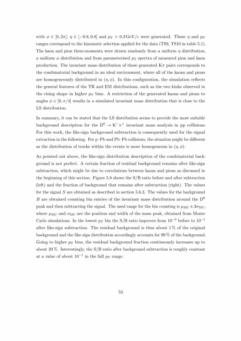
with φ ∈ [0, 2π[, η ∈ [−0.8, 0.8] and pT > 0.3 GeV/c were generated. These η and pT
ranges correspond to the kinematic selection applied for the data (TS9, TS10 in table 5.1).
The kaon and pion three-momenta were drawn randomly from a uniform η distribution,
a uniform φ distribution and from parameterised pT spectra of measured pion and kaon
production. The invariant mass distribution of these generated Kπ pairs corresponds to
the combinatorial background in an ideal environment, where all of the kaons and pions
are homogeneously distributed in (η, φ). In this configuration, the simulation reflects
the general features of the TR and EM distributions, such as the two kinks observed in
the rising shape in higher pT bins. A restriction of the generated kaons and pions to
angles φ ∈ [0, π/4] results in a simulated invariant mass distribution that is close to the
LS distribution.
In summary, it can be stated that the LS distribution seems to provide the most suitable
background description for the D0 → K−π+ invariant mass analysis in pp collisions.
For this work, the like-sign background subtraction is consequently used for the signal
extraction in the following. For p–Pb and Pb–Pb collisions, the situation might be different
as the distribution of tracks within the events is more homogeneous in (η, φ).
As pointed out above, the like-sign distribution description of the combinatorial back-
ground is not perfect. A certain fraction of residual background remains after like-sign
subtraction, which might be due to correlations between kaons and pions as discussed in
the beginning of this section. Figure 5.8 shows the S/B ratio before and after subtraction
(left) and the fraction of background that remains after subtraction (right). The values
for the signal S are obtained as described in section 5.6.3. The values for the background
B are obtained counting bin entries of the invariant mass distribution around the D0
peak and then subtracting the signal. The used range for the bin counting is µMC±3σMC,
where µMC and σMC are the position and width of the mass peak, obtained from Monte
Carlo simulations. In the lowest pT bin the S/B ratio improves from 10−3 before to 10−1
after like-sign subtraction. The residual background is thus about 1 % of the original
background and the like-sign distribution accordingly accounts for 99 % of the background.
Going to higher pT bins, the residual background fraction continuously increases up to
about 20 %. Interestingly, the S/B ratio after background subtraction is roughly constant
at a value of about 10−1 in the full pT range.
53
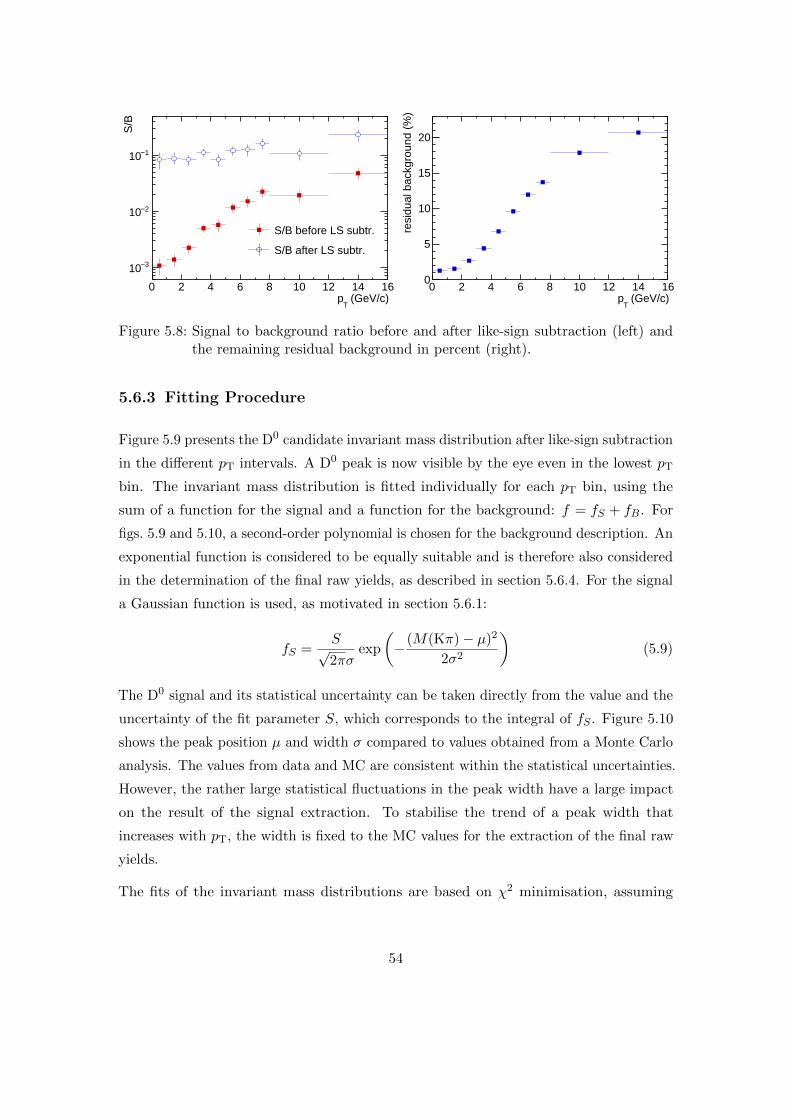
(GeV/c)T
p0 2 4 6 8 10 12 14 16
S/B
3−10
2−10
1−10
S/B before LS subtr.
S/B after LS subtr.
(GeV/c)T
p0 2 4 6 8 10 12 14 16
resi
dual
bac
kgro
und
(%)
0
5
10
15
20
Figure 5.8: Signal to background ratio before and after like-sign subtraction (left) andthe remaining residual background in percent (right).
5.6.3 Fitting Procedure
Figure 5.9 presents the D0 candidate invariant mass distribution after like-sign subtraction
in the different pT intervals. A D0 peak is now visible by the eye even in the lowest pT
bin. The invariant mass distribution is fitted individually for each pT bin, using the
sum of a function for the signal and a function for the background: f = fS + fB. For
figs. 5.9 and 5.10, a second-order polynomial is chosen for the background description. An
exponential function is considered to be equally suitable and is therefore also considered
in the determination of the final raw yields, as described in section 5.6.4. For the signal
a Gaussian function is used, as motivated in section 5.6.1:
fS =S√2πσ
exp
(−(M(Kπ)− µ)2
2σ2
)(5.9)
The D0 signal and its statistical uncertainty can be taken directly from the value and the
uncertainty of the fit parameter S, which corresponds to the integral of fS . Figure 5.10
shows the peak position µ and width σ compared to values obtained from a Monte Carlo
analysis. The values from data and MC are consistent within the statistical uncertainties.
However, the rather large statistical fluctuations in the peak width have a large impact
on the result of the signal extraction. To stabilise the trend of a peak width that
increases with pT, the width is fixed to the MC values for the extraction of the final raw
yields.
The fits of the invariant mass distributions are based on χ2 minimisation, assuming
54

1.8 1.85 1.9 1.95
)2 cE
ntrie
s / (
7 M
eV/
15
20
25
30
310×
< 1 GeV/cT
p0 <
= 9.5MCσ 2.9± = 1859.5 µ
1.8 1.85 1.9 1.95
)2 cE
ntrie
s / (
8 M
eV/
20
30
40
310×
< 2 GeV/cT
p1 <
= 11.1MCσ 3.5± = 1867.9 µ
1.8 1.9
)2 cE
ntrie
s / (
9 M
eV/
20
25
30
35
310×
< 3 GeV/cT
p2 <
= 12.9MCσ 2.7± = 1862.0 µ
1.8 1.9 2
)2 cE
ntrie
s / (
10 M
eV/
10
15
20
310×
< 4 GeV/cT
p3 <
= 14.9MCσ 2.6± = 1866.5 µ
1.7 1.8 1.9 2
)2 cE
ntrie
s / (
12 M
eV/
6
8
10
12
310×
< 5 GeV/cT
p4 <
= 16.7MCσ 4.2± = 1862.3 µ
1.7 1.8 1.9 2
)2 cE
ntrie
s / (
13 M
eV/
3
4
5
6310×
< 6 GeV/cT
p5 <
= 18.0MCσ 3.8± = 1862.7 µ
1.7 1.8 1.9 2
)2 cE
ntrie
s / (
14 M
eV/
1.5
2
2.5
3
310×
< 7 GeV/cT
p6 <
= 19.3MCσ 5.8± = 1865.4 µ
1.7 1.8 1.9 2
)2 cE
ntrie
s / (
15 M
eV/
1
1.5
2
310×
< 8 GeV/cT
p7 <
= 20.7MCσ 5.3± = 1865.1 µ
1.7 1.8 1.9 2
)2 cE
ntrie
s / (
16 M
eV/
1
1.5
2
2.5
3310×
< 12 GeV/cT
p8 <
= 22.7MCσ 7.5± = 1873.4 µ
1.6 1.8 2
)2 cE
ntrie
s / (
18 M
eV/
200
400
600
800 < 16 GeV/c
Tp12 <
= 26.3MCσ 8.9± = 1878.1 µ
)2c) (GeV/π(KM
Figure 5.9: Invariant mass distribution after like-sign subtraction for all analysed pTintervals. The distributions are fitted with the sum of a Gaussian functionfor the signal and a second-order polynomial for the background (red curve).For each pT bin, the width of the Gaussian is fixed with the value obtainedfrom Monte Carlo, µMC. The numerical values of µMC are indicated on theplots, along with those of the peak positions µ, which are treated as a freeparameter in the fits.
55

(GeV/c)T
p0 2 4 6 8 10 12 14 16
)2 c (
MeV
/µ
peak
pos
ition
1850
1860
1870
1880
1890
1900
Monte Carlo
like-sign subtr.
(GeV/c)T
p0 2 4 6 8 10 12 14 16
)2 c (
MeV
/σ
peak
wid
th
0
10
20
30
40
50
60
Figure 5.10: Comparison between data and Monte Carlo of the position µ and the widthσ of the D0 peak.
Gaussian uncertainties on the bin entries. This assumption is justified as the statistics of
the bin entries is large, even for the higher pT bins. The invariant mass bin widths are
7, 8, 9, 10, 12, 13, 14, 15, 16, 18 MeV/c2 for the different pT bins. This particular binning
is chosen such that the bin width corresponds to about 0.7σMC in the respective pT bin.
The fit range has to be chosen such that it contains the mass peak and reasonably large
side-bands. As the actual form of the background is unknown, it is favourable to choose
as small a range as possible. There is no interest in describing the background far from
the mass peak. Decreasing the fit range too much, on the other hand, causes the fit to
become more sensitive to background fluctuations. For figs. 5.9 and 5.10, the invariant
mass is fitted in a range that corresponds to 10σMC. For each pT bin in fig. 5.9, the
plotted range corresponds to the fit range.
5.6.4 Randomised Multi-Trial Approach
To determine the central value for the D0 signal and the associated statistical and
systematic uncertainties, the following method was developed. The fit is performed
one thousand times in each pT bin, with a different parameter set for each trial. The
parameters for each fit are drawn randomly from a pre-defined distribution. The fit
function for the background is randomly chosen as either a second-order polynomial
or an exponential function. The binning of the invariant mass distributions is drawn
from a uniform distribution in the range of ±20 % around the central values defined
in section 5.6.3. The values are rounded to the nearest integer. The lower value of
56
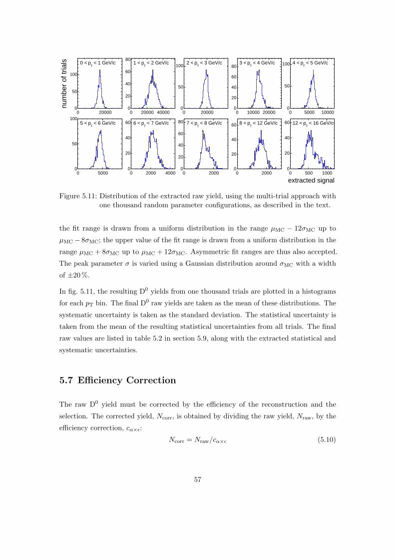
0 200000
50
100
< 1 GeV/cT
p0 <
0 20000 400000
20
40
60
80 < 2 GeV/c
Tp1 <
0 200000
50
100 < 3 GeV/c
Tp2 <
0 10000 200000
20
40
60
80 < 4 GeV/c
Tp3 <
0 5000 100000
50
100 < 5 GeV/cT
p4 <
0 50000
50
100 < 6 GeV/c
Tp5 <
0 2000 40000
20
40
60 < 7 GeV/cT
p6 <
0 20000
20
40
60
80 < 8 GeV/cT
p7 <
0 20000
20
40
60 < 12 GeV/cT
p8 <
0 500 10000
20
40
60 < 16 GeV/cT
p12 <
num
ber
of tr
ials
extracted signal
Figure 5.11: Distribution of the extracted raw yield, using the multi-trial approach withone thousand random parameter configurations, as described in the text.
the fit range is drawn from a uniform distribution in the range µMC − 12σMC up to
µMC− 8σMC; the upper value of the fit range is drawn from a uniform distribution in the
range µMC + 8σMC up to µMC + 12σMC. Asymmetric fit ranges are thus also accepted.
The peak parameter σ is varied using a Gaussian distribution around σMC with a width
of ±20 %.
In fig. 5.11, the resulting D0 yields from one thousand trials are plotted in a histograms
for each pT bin. The final D0 raw yields are taken as the mean of these distributions. The
systematic uncertainty is taken as the standard deviation. The statistical uncertainty is
taken from the mean of the resulting statistical uncertainties from all trials. The final
raw values are listed in table 5.2 in section 5.9, along with the extracted statistical and
systematic uncertainties.
5.7 Efficiency Correction
The raw D0 yield must be corrected by the efficiency of the reconstruction and the
selection. The corrected yield, Ncorr, is obtained by dividing the raw yield, Nraw, by the
efficiency correction, cα×ε:
Ncorr = Nraw/cα×ε (5.10)
57

The efficiency correction is a number between zero and one. It can be viewed as the
probability for a D0 that is created in the collision to be actually reconstructed in the
detector and selected in the analysis. In this analysis, the efficiency correction is factorised
into a purely geometric acceptance and a reconstruction and selection efficiency. A D0
decay daughter is called ‘accepted’ if it survives the kinematic cuts (TS9 and TS10 in
table 5.1). The term ‘acceptance’ can then be defined as the probability for a kinematic
configuration such that both decay daughters are accepted. The ‘reconstruction and
selection efficiency’ then refers to the probability that a D0 with two accepted decay
daughters is actually reconstructed and selected in the analysis. The efficiency correction
can be determined to a certain precision in a simulation with high statistics using ratios
of total numbers of D0 mesons:
cα×ε =N1
gen, acc
N1gen
× N2reco
N2gen, acc
(5.11)
Here, Ngen and Nreco refer to the number of generated and reconstructed D0 mesons
in a certain region of phase space and Ngen, acc denotes the number of generated D0
mesons the daughters of which are accepted. The indices 1 and 2 indicate that different
frameworks are used for the two factors of the efficiency correction. The acceptance
is a purely kinematic quantity and can as such be simulated using simple four-vector
kinematics. In this thesis, the toy MC, described in section 4.2.5, is used for this purpose.
The results were checked with those from the Monte Carlo simulation described below
and were found to agree within the statistical uncertainty of the MC simulation. The
advantage of the toy MC is a higher precision due to the much larger number of generated
D0 mesons. Furthermore, the simulation provides a cross check for the more complicated
MC framework.
In contrast to the case of the kinematic acceptance, a full detector description is needed
to determine the reconstruction and selection efficiency. Events are simulated using
PYTHIA [70, 71]. The generated particles are then propagated through the detector
using the GEANT3 package [78]. The same analysis task is run on MC as in real data in
order to ensure that the same cuts and PID are applied. A charm enriched MC sample
is used in order to enhance statistics.
Figure 5.12 shows the acceptance, the reconstruction and selection efficiency and the
total correction factor. The efficiency rises from about 0.2 at low pT to about 0.65 at
58
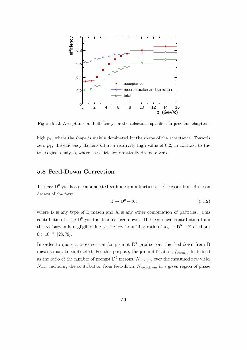
(GeV/c)T
p0 2 4 6 8 10 12 14 16
effic
ienc
y
0
0.2
0.4
0.6
0.8
1
acceptance
reconstruction and selection
total
Figure 5.12: Acceptance and efficiency for the selections specified in previous chapters.
high pT, where the shape is mainly dominated by the shape of the acceptance. Towards
zero pT, the efficiency flattens off at a relatively high value of 0.2, in contrast to the
topological analysis, where the efficiency drastically drops to zero.
5.8 Feed-Down Correction
The raw D0 yields are contaminated with a certain fraction of D0 mesons from B meson
decays of the form
B→ D0 + X , (5.12)
where B is any type of B meson and X is any other combination of particles. This
contribution to the D0 yield is denoted feed-down. The feed-down contribution from
the Λb baryon is negligible due to the low branching ratio of Λb → D0 + X of about
6× 10⁻⁴ [23, 79].
In order to quote a cross section for prompt D0 production, the feed-down from B
mesons must be subtracted. For this purpose, the prompt fraction, fprompt, is defined
as the ratio of the number of prompt D0 mesons, Nprompt, over the measured raw yield,
Nraw, including the contribution from feed-down, Nfeed-down, in a given region of phase
59

(GeV/c)T
p0 2 4 6 8 10 12 14 16
prom
ptf
0.8
0.85
0.9
0.95
1
Figure 5.13: The fraction of prompt D0 production over the total D0 production. Thefeed-down component of the raw yield is determined using FONLL calcula-tions with the full theoretical uncertainty included.
space:
fprompt =Nprompt
Nraw= 1− Nfeed-down
Nraw. (5.13)
The prompt fraction enters into the cross section as a correction factor between zero and
one, where a value of one signifies no contamination from feed-down and a value of zero
signifies full contamination.
As no direct mid-rapidity measurement of the bb cross section at low momentum for
pp collisions at√s = 7 TeV is available, FONLL predictions [17] are used to determine
Nfeed-down.
Nfeed-down = 2 · 2Y ·∆pT · cα×ε · B · Lint ·dσD
0from BFONLL
dpT
∣∣∣∣∣|y|<0.5
(5.14)
This formula is obtained by taking eq. (5.15) and substituting Nraw by Nfeed-down and the
D0 cross section by the FONLL cross section for D0 from B; and solving for Nfeed-down.
The involved symbols are explained in section 5.9.
Figure 5.13 presents the prompt fraction in the full analysed pT range. The horizontal
lines indicate the pT bin width and the boxes the systematic uncertainty. The prompt
fraction decreases from about 0.96 in the lowest pT bin to around 0.9 for higher pT bins.
60
The decrease is explained by the fact that the B meson pT spectra are harder than the D0
spectrum, meaning they are shifted towards higher transverse momenta. The fluctuations
in the prompt fraction are due to the fluctuations in the raw yield, which is involved in
the definition of fprompt in eq. (5.13).
A distinct advantage as compared to the topological analysis are the equal efficiencies for
prompt and feed-down D0 mesons. In the topological analysis, the feed-down efficiency
is considerably higher than the prompt efficiency due to the longer lifetimes of B mesons
in comparison to D0 mesons. The feed-down is consequently enhanced by the topological
selection and the prompt fraction resides in a lower range between about 0.8 and 0.9.
A higher feed-down efficiency as compared to the prompt efficiency translates linearly
into a higher uncertainties of the prompt fraction. In the lowest pT bin of the topological
analysis, pT 1 < pT < 2 GeV/c, the efficiencies differ by a factor of three. With the new
analysis approach presented in this thesis, the uncertainty is thus decreased by a factor
of three at low pT.
5.9 Calculation of the Cross Section
With the output from the different analysis steps described in the previous sections, the
pT-differential D0 production cross section at central rapidity, |y| < 0.5, is calculated
using the following formula:
dσD0
dpT
∣∣∣∣∣|y|<0.5
=1
2
1
2Y∆pT(pT)
fprompt ·Nraw
cα×ε(pT)
∣∣∣∣|y|<Y
1
B · Lint. (5.15)
The factor of one half accounts for the fact that, according to an ALICE convention,
the cross section is quoted for particles only, whereas the raw yield contains both D0
and D0, making the assumption of equal yields for particles and antiparticles at the high
LHC energies. The transverse momentum bin width is denoted by ∆pT. Following a
convention of ALICE results for D-meson production, the cross section is given in the
rapidity interval |y| < 0.5. It must therefore be scaled down by the measured rapidity
window 2Y , where Y = 0.8 is the rapidity cut applied on D0 candidates in the analysis
(cf. section 5.4). The simple rapidity scaling is justified since the rapidity distribution of
D0 mesons in pp collisions at√s = 7 TeV is considered flat within 1 % (cf. section 4.2.5).
61
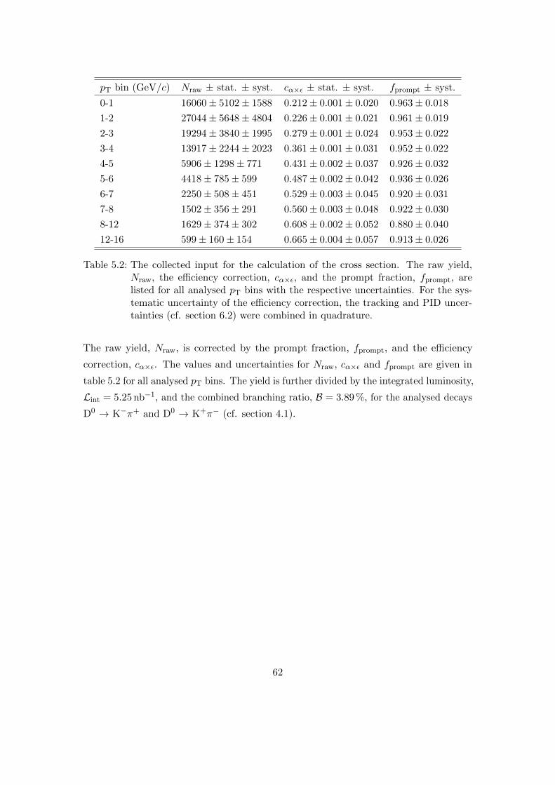
pT bin (GeV/c) Nraw ± stat. ± syst. cα×ε ± stat. ± syst. fprompt ± syst.
0-1 16060± 5102± 1588 0.212± 0.001± 0.020 0.963± 0.018
1-2 27044± 5648± 4804 0.226± 0.001± 0.021 0.961± 0.019
2-3 19294± 3840± 1995 0.279± 0.001± 0.024 0.953± 0.022
3-4 13917± 2244± 2023 0.361± 0.001± 0.031 0.952± 0.022
4-5 5906± 1298± 771 0.431± 0.002± 0.037 0.926± 0.032
5-6 4418± 785± 599 0.487± 0.002± 0.042 0.936± 0.026
6-7 2250± 508± 451 0.529± 0.003± 0.045 0.920± 0.031
7-8 1502± 356± 291 0.560± 0.003± 0.048 0.922± 0.030
8-12 1629± 374± 302 0.608± 0.002± 0.052 0.880± 0.040
12-16 599± 160± 154 0.665± 0.004± 0.057 0.913± 0.026
Table 5.2: The collected input for the calculation of the cross section. The raw yield,Nraw, the efficiency correction, cα×ε, and the prompt fraction, fprompt, arelisted for all analysed pT bins with the respective uncertainties. For the sys-tematic uncertainty of the efficiency correction, the tracking and PID uncer-tainties (cf. section 6.2) were combined in quadrature.
The raw yield, Nraw, is corrected by the prompt fraction, fprompt, and the efficiency
correction, cα×ε. The values and uncertainties for Nraw, cα×ε and fprompt are given in
table 5.2 for all analysed pT bins. The yield is further divided by the integrated luminosity,
Lint = 5.25 nb−1, and the combined branching ratio, B = 3.89 %, for the analysed decays
D0 → K−π+ and D0 → K+π− (cf. section 4.1).
62

chapter 6
Uncertainties
This chapter presents an exhaustive summary of the considered statistical and systematic
uncertainties on the D0 production cross section. For practical reasons, most of the
contributions to the statistical and systematic uncertainties were already described in the
previous chapter. For these cases, a short summary is given and the respective section is
referenced.
6.1 Statistical Uncertainties
The following sources of statistical uncertainty for the D0 production cross section were
considered. The corresponding quantity from eq. (5.15) is given in parentheses.
• signal extraction (Nraw)
• efficiency correction (cα×ε)
The statistical uncertainties on the extracted raw yields were determined from the invariant
mass fits, using the randomised multi-trial approach described in section 5.6.4.
The statistical uncertainty in the efficiency correction is due to the limited available
statistics in the Monte Carlo sample that was used to determine the reconstruction
and selection efficiency (cf. section 5.7). It was determined by propagating the bi-
nomial uncertainties in the ratio of the reconstructed to the generated D0 mesons in
eq. (5.11).
63

pT(GeV/c) 0-1 1-2 2-3 3-4 4-5 5-6 6-7 7-8 8-12 12-16
signal extraction 31.8 20.9 19.9 16.1 22.0 17.8 22.6 23.7 22.9 26.6
efficiency correction 0.3 0.3 0.3 0.3 0.4 0.4 0.5 0.6 0.4 0.6
overall 31.8 20.9 19.9 16.1 22.0 17.8 22.6 23.7 23.0 26.6
Table 6.1: Summary of the statistical uncertainties of the D0 production cross section inpercent.
The overall statistical uncertainty of the D0 production cross section was obtained by
summing the two contributions in quadrature. The resulting values are given in table 6.1,
along with those of the single contributions. The statistical uncertainty of the efficiency
correction is completely negligible for all of the analysed pT bins.
6.2 Systematic Uncertainties
The following sources of systematic uncertainty on the D0 production cross section were
studied. The corresponding quantity from eq. (5.15) is given in parentheses.
• signal extraction (Nraw)
• efficiency correction (cα×ε):
– track reconstruction and selection
– particle identification
– MC input pT shape
• feed-down from B (fprompt)
• branching ratio (B)
• integrated luminosity (Lint)
The systematic uncertainty related to the signal extraction was evaluated varying
the relevant fit parameters in a randomised multi-trial approach, as described in sec-
tion 5.6.4.
For the systematic uncertainty of the efficiency correction, the following three sources
were considered: the track reconstruction and selection; the particle identification; and
the initially unknown D0 meson pT spectrum that has to be provided as an input to the
MC simulations. The systematic uncertainty related to the track reconstruction, also
referred to as the tracking uncertainty, is inherited from the topological analysis, where
64
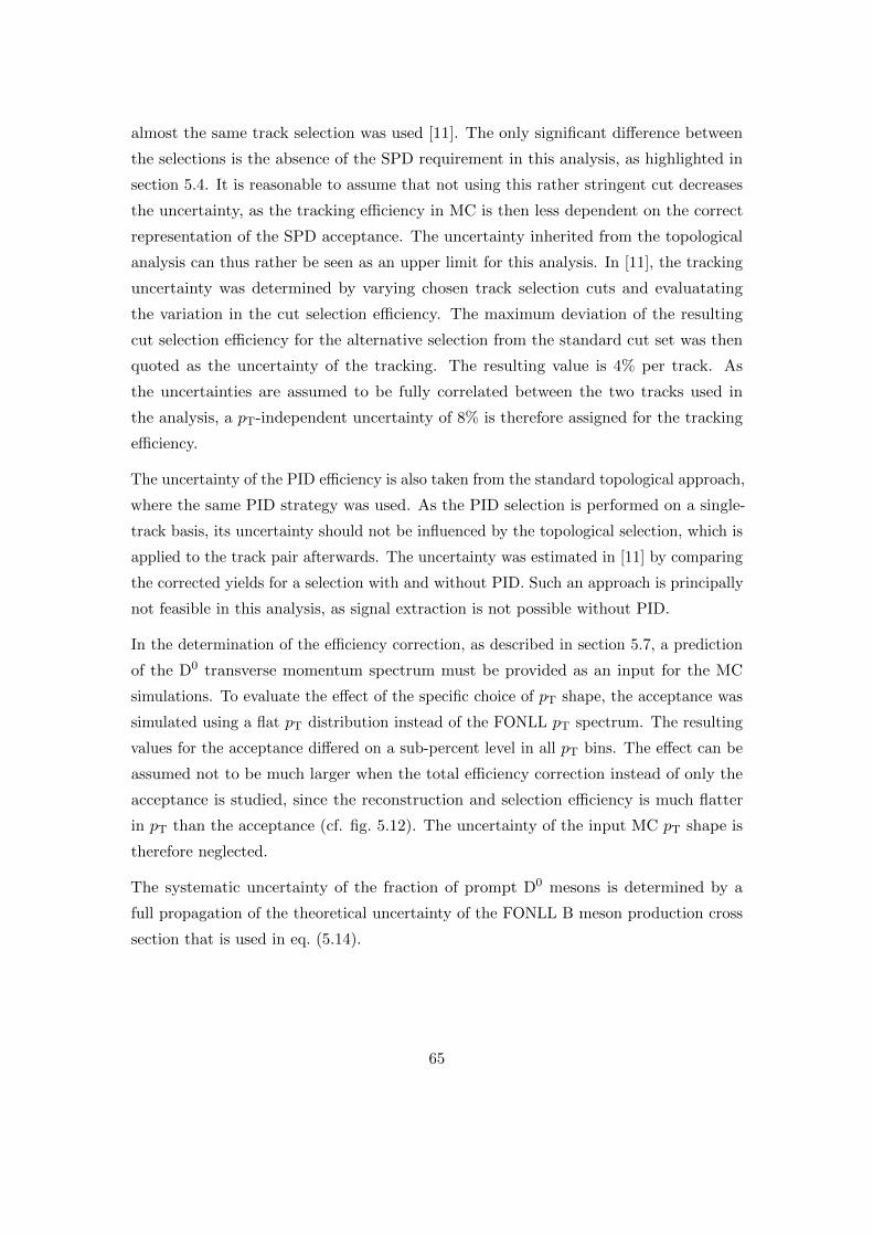
almost the same track selection was used [11]. The only significant difference between
the selections is the absence of the SPD requirement in this analysis, as highlighted in
section 5.4. It is reasonable to assume that not using this rather stringent cut decreases
the uncertainty, as the tracking efficiency in MC is then less dependent on the correct
representation of the SPD acceptance. The uncertainty inherited from the topological
analysis can thus rather be seen as an upper limit for this analysis. In [11], the tracking
uncertainty was determined by varying chosen track selection cuts and evaluatating
the variation in the cut selection efficiency. The maximum deviation of the resulting
cut selection efficiency for the alternative selection from the standard cut set was then
quoted as the uncertainty of the tracking. The resulting value is 4% per track. As
the uncertainties are assumed to be fully correlated between the two tracks used in
the analysis, a pT-independent uncertainty of 8% is therefore assigned for the tracking
efficiency.
The uncertainty of the PID efficiency is also taken from the standard topological approach,
where the same PID strategy was used. As the PID selection is performed on a single-
track basis, its uncertainty should not be influenced by the topological selection, which is
applied to the track pair afterwards. The uncertainty was estimated in [11] by comparing
the corrected yields for a selection with and without PID. Such an approach is principally
not feasible in this analysis, as signal extraction is not possible without PID.
In the determination of the efficiency correction, as described in section 5.7, a prediction
of the D0 transverse momentum spectrum must be provided as an input for the MC
simulations. To evaluate the effect of the specific choice of pT shape, the acceptance was
simulated using a flat pT distribution instead of the FONLL pT spectrum. The resulting
values for the acceptance differed on a sub-percent level in all pT bins. The effect can be
assumed not to be much larger when the total efficiency correction instead of only the
acceptance is studied, since the reconstruction and selection efficiency is much flatter
in pT than the acceptance (cf. fig. 5.12). The uncertainty of the input MC pT shape is
therefore neglected.
The systematic uncertainty of the fraction of prompt D0 mesons is determined by a
full propagation of the theoretical uncertainty of the FONLL B meson production cross
section that is used in eq. (5.14).
65
pT(GeV/c) 0-1 1-2 2-3 3-4 4-5 5-6 6-7 7-8 8-12 12-16
signal extraction 9.9 17.8 10.3 14.5 13.0 13.6 20.1 19.4 18.5 25.6
tracking 8.0 8.0 8.0 8.0 8.0 8.0 8.0 8.0 8.0 8.0
PID 5.0 5.0 3.0 3.0 3.0 3.0 3.0 3.0 3.0 3.0
feed-down 1.9 2.0 2.3 2.3 3.4 2.8 3.4 3.2 4.6 2.9
overall 13.8 20.2 13.6 17.0 16.0 16.3 22.1 21.4 20.9 27.2
Table 6.2: Summary of the systematic uncertainties on the D0 production cross section.
The relative uncertainty of the branching ratio is 1.3 % [23] and the relative uncertainty
of the integrated luminosity 3.5 % [75]. The uncertainties of the branching ratio and of
the integrated luminosity are global uncertainties that are fully correlated between the
pT bins. They are therefore treated separately.
The signal extraction, tracking, PID and feed-down uncertainties are possibly partially
correlated between the pT bins, but are assumed to be uncorrelated with each other.
They are thus summed in quadrature to obtain the overall systematic uncertainty for
each pT bin. The systematic uncertainties are summarised in table 6.2. The overall
uncertainties range from about 14 % to 28 %. The signal extraction uncertainty is the
dominant contribution in all pT bins.
66
chapter 7
Results
In this chapter, the results for D0 production in pp collisions obtained in this thesis are
discussed. The pT-differential cross section is shown and compared with the results from
the topological approach. In the second part of the chapter, the pT-integrated cross
section is presented and compared with different measurements.
7.1 D0 Production Cross Section
Figure 7.1 presents the D0 production cross section for pp collisions at√s = 7 TeV.
The new values obtained in this work without topological selection (blue) are plotted
along with those from the topological analysis (orange) [11]. The lower panel shows the
ratio of the two measurements for pT > 1 GeV/c. The horizontal bars indicate the pT
bin width. The vertical bars represent the overall statistical uncertainty and the open
boxes the overall systematic uncertainty. The fully correlated systematic uncertainties
are not included in the plot, following the convention of ALICE publications of D
meson production [11–13]. The shaded yellow boxes represent the uncertainty band of
the FONLL theory prediction for D0 production [56], which are shown for comparison
with the measurements. The values of the plotted cross sections from both analyses
are given in table 7.1 along with the absolute and relative statistical and systematic
uncertainties.
The new data point for pT < 1 GeV/c closes the gap towards zero transverse momentum.
It conforms well into the trend observed for pT > 1 GeV/c, lying in the upper part of
67
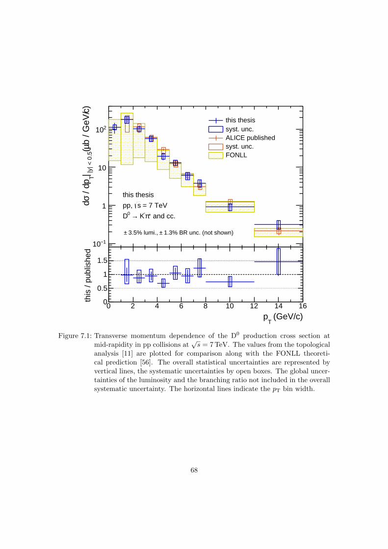
)c (GeV/T
p
0 2 4 6 8 10 12 14 16
)cb
/ GeV
/µ (
|y| <
0.5
| Tp /
dσd
1−10
1
10
210this thesissyst. unc.ALICE publishedsyst. unc.FONLL
this thesis
= 7 TeVspp,
and cc.+π- K→ 0D
1.3% BR unc. (not shown)± 3.5% lumi., ±
)c (GeV/T
p0 2 4 6 8 10 12 14 16
this
/ pu
blis
hed
0
0.5
1
1.5
Figure 7.1: Transverse momentum dependence of the D0 production cross section atmid-rapidity in pp collisions at
√s = 7 TeV. The values from the topological
analysis [11] are plotted for comparison along with the FONLL theoreti-cal prediction [56]. The overall statistical uncertainties are represented byvertical lines, the systematic uncertainties by open boxes. The global uncer-tainties of the luminosity and the branching ratio not included in the overallsystematic uncertainty. The horizontal lines indicate the pT bin width.
68

pT interval dσ/dpT||y|<0.5 ± stat.± syst. (µb/GeV/c)
(GeV/c) this analysis topological analysis
0-1 112± 36 (32%)± 15 (14%) -
1-2 177± 37 (21%)± 36 (20%) 180± 30 (17%)+48 (27%)−98 (54%)
2-3 101± 20 (20%)± 14 (14%) 115± 11 (10%)+20 (17%)−33 (29%)
3-4 56.3± 9.1 (16%)± 9.6 (17%) 59.7± 4.3 (7%)+8.5 (14%)−12.6 (21%)
4-5 19.5± 4.3 (22%)± 3.1 (16%) 29.1± 2.1 (7%)+4.2 (14%)−5.8 (20%)
5-6 13.0± 2.3 (18%)± 2.1 (16%) 12.5± 1.1 (9%)+1.8 (14%)−2.3 (18%)
6-7 6.00± 1.36 (23%)± 1.32 (22%) 6.37± 0.70 (11%)+0.94 (15%)−1.08 (17%)
7-8 3.79± 0.90 (24%)± 0.81 (21%) 3.07± 0.47 (15%)+0.50 (16%)−0.53 (17%)
8-12 0.90± 0.21 (23%)± 0.19 (21%) 1.23± 0.13 (11%)+0.19 (15%)−0.21 (17%)
12-16 0.316± 0.084 (27%)± 0.086 (27%) 0.215± 0.050 (23%)+0.037 (17%)−0.038 (18%)
Table 7.1: D0 production cross section in pp collisions at√s = 7 TeV, as obtained with
this analysis (left) and with the topological analysis [11] (right). The relativestatistical and systematic uncertainties are given in parentheses.
the FONLL uncertainty range. The new measurement is consistent with the topological
measurement within their respective total uncertainties. In this context, it is important
to notice that the measurements can be regarded as only partially correlated, as the
raw D0 yields in this analysis are larger by about a factor of ten at low pT and a factor
of five at high pT, thus resulting only in a small overlap between the analyses. The
systematic difference of 0.5 % due to the different branching ratios in use (cf. section 4.1) is
evidently negligible. The mean relative deviation of the two measurements of about 18 %
compares well with the order of magnitude of the statistical and systematic uncertainties.
In summary, this also provides an excellent verification of the topological D-meson
measurements with ALICE.
For the new analysis, the statistical uncertainty is larger in all pT bins by up to about a
factor of two, whereas the systematic uncertainty is significantly lower for pT < 3 GeV/c
and of comparable size up to pT < 6 GeV/c. This corresponds to the behaviour expected
‘by design’ of the two methods. The topological approach is clearly limited by the
systematics of the topological selection, the feed-down and the signal extraction. The
new approach is limited by the statistical uncertainty, which becomes particularly clear
in the new pT bin 0 < pT < 1 GeV/c, where the statistical uncertainty is more than
69
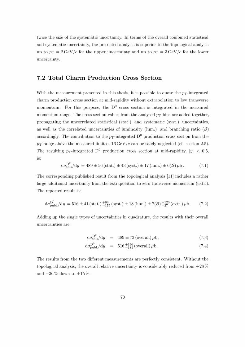
twice the size of the systematic uncertainty. In terms of the overall combined statistical
and systematic uncertainty, the presented analysis is superior to the topological analysis
up to pT = 2 GeV/c for the upper uncertainty and up to pT = 3 GeV/c for the lower
uncertainty.
7.2 Total Charm Production Cross Section
With the measurement presented in this thesis, it is possible to quote the pT-integrated
charm production cross section at mid-rapidity without extrapolation to low transverse
momentum. For this purpose, the D0 cross section is integrated in the measured
momentum range. The cross section values from the analysed pT bins are added together,
propagating the uncorrelated statistical (stat.) and systematic (syst.) uncertainties,
as well as the correlated uncertainties of luminosity (lum.) and branching ratio (B)
accordingly. The contribution to the pT-integrated D0 production cross section from the
pT range above the measured limit of 16 GeV/c can be safely neglected (cf. section 2.5).
The resulting pT-integrated D0 production cross section at mid-rapidity, |y| < 0.5,
is:
dσD0
this/dy = 489± 56 (stat.)± 43 (syst.)± 17 (lum.)± 6(B)µb . (7.1)
The corresponding published result from the topological analysis [11] includes a rather
large additional uncertainty from the extrapolation to zero transverse momentum (extr.).
The reported result is:
dσD0
publ./dy = 516± 41 (stat.) +69−175 (syst.)± 18 (lum.)± 7(B) +120
−37 (extr.)µb . (7.2)
Adding up the single types of uncertainties in quadrature, the results with their overall
uncertainties are:
dσD0
this/dy = 489± 73 (overall)µb , (7.3)
dσD0
publ./dy = 516 +146−185 (overall)µb . (7.4)
The results from the two different measurements are perfectly consistent. Without the
topological analysis, the overall relative uncertainty is considerably reduced from +28 %
and −36 % down to ±15 %.
70

The pT-integrated charm production cross section at mid-rapidity can be derived by
dividing the D0 result by the fragmentation fraction of charm to D0, f(c → D0) =
0.557± 0.023 (cf. section 2.3). The uncertainty of this fraction has to be added as an
additional source of uncertainty on the cross section (FF). The resulting charm cross
section at mid-rapidity is:
dσccthis/dy =879± 101 (stat.)± 76 (syst.)± 31 (lum.)± 11 (B)± 36 (FF)µb
=879 ± 135 (overall)µb . (7.5)
The pT-integrated result is further extrapolated to the full phase space. For this purpose,
the same extrapolation method as in [12] is applied. An extrapolation factor of 8.56+2.51−0.42
is obtained as the ratio of the FONLL prediction for D0 production in the full phase
space to the prediction for the measured central rapidity region. The uncertainty of
the extrapolation factor is determined by varying the renormalisation and factorisation
scale parameters, the charm quark mass and the PDFs as described in section 2.5. The
resulting total charm cross section for the measurement presented in this thesis is:
σccthis =7.5± 0.9 (stat.)± 0.7 (syst.)± 0.3 (lum.)± 0.1 (B)± 0.3 (FF) +2.2−0.4 (extr.) mb
=7.5 +2.5−1.2 (overall) mb . (7.6)
In fig. 7.2 and table 7.2, the measurement is compared with the ALICE result using
the topological approach [12] and results from the LHCb [69] and ATLAS [80, 81]
collaborations. The total charm cross section was determined measuring the production
of charmed hadrons in different pT and y (η) ranges, as indicated in table 7.2. For
the results involving more than one species, the charm cross section is quoted as the
average of the measurements. The LHCb measurement in the visible cross section was
extrapolated using the extrapolation factor from [42]. When considering the result of
this thesis, the overall uncertainties of the total charm production cross section measured
with ALICE are halved as compared to the topological analysis The data point moves
down, yielding a better consistency with the results of LHCb and ATLAS.
The energy dependence of the total nucleon-nucleon charm cross section is shown in fig. 7.3.
Data points from various experiments are plotted [12,20,69,80–83]. The measurements
of the charm cross section conform well to the trend of a next-to-leading order (NLO)
calculation [84] over a wide energy range.
71
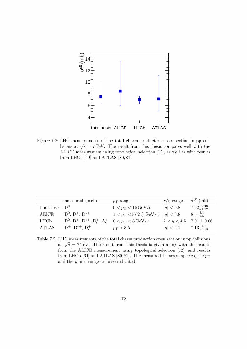
this thesis ALICE LHCb ATLAS
(m
b)cc σ
4
6
8
10
12
14
Figure 7.2: LHC measurements of the total charm production cross section in pp col-lisions at
√s = 7 TeV. The result from this thesis compares well with the
ALICE measurement using topological selection [12], as well as with resultsfrom LHCb [69] and ATLAS [80,81].
measured species pT range y/η range σcc (mb)
this thesis D0 0 < pT < 16 GeV/c |y| < 0.8 7.52+2.49−1.22
ALICE D0, D+, D∗+ 1 < pT <16(24) GeV/c |y| < 0.8 8.5+5.1−2.5
LHCb D0, D+, D∗+, D+s , Λ+
c 0 < pT < 8 GeV/c 2 < y < 4.5 7.01± 0.66
ATLAS D+, D∗+, D+s pT > 3.5 |η| < 2.1 7.13+4.01
−2.18
Table 7.2: LHC measurements of the total charm production cross section in pp collisionsat√s = 7 TeV. The result from this thesis is given along with the results
from the ALICE measurement using topological selection [12], and resultsfrom LHCb [69] and ATLAS [80,81]. The measured D meson species, the pTand the y or η range are also indicated.
72

(GeV)s10 210 310 410
b)µ ( ccσ
10
210
310
410
this thesis (total unc.)this thesis extr. unc.ALICE (total unc.)ALICE extr. unc.ATLAS Preliminary (total unc.)ATLAS extr. unc.LHCb (total unc.)PHENIXSTARHERA-B (pA)E653 (pA)E743 (pA)NA27 (pA)NA16 (pA)E769 (pA)NLO (MNR)
Figure 7.3: Total charm cross section in nucleon-nucleon collisions as a function of thecentre-of-mass energy. The result obtained in this thesis is shown along withdata points from various experiments [12, 20, 69, 80–83]. For measurementsusing proton-nucleus (pA) collisions, the cross section was scaled down bythe number of binary collisions. The four LHC data points at
√s = 7 TeV
are horizontally displaced with respect to each other for better visibility. Thenext-to-leading order MNR calculation is shown [84] with the solid (dashed)black line(s) indicating the central value and the uncertainty band. Thisfigure is adapted from [12].
73
chapter 8
Summary and Outlook
The cross section of prompt D0 production at mid-rapidity in proton-proton collisions was
measured down to zero transverse momentum for the first time at the LHC, providing an
important baseline for the study of the low-momentum phenomenology of heavy quarks
in the quark-gluon plasma as well as for the investigation of charmonium production
in heavy-ion collisions. The full kinematic reconstruction of D mesons at low pT is
particularly challenging as a topological approach can not be adopted due to the small
Lorentz boost of a low-momentum D meson. An alternative analysis strategy was thus
developed in this thesis to extend the measurement of D0 production down to zero
transverse momentum.
D0 mesons were reconstructed with an invariant mass analysis in the D0 → K−π+ decay
channel using a data sample of pp collisions at√s = 7 TeV with an integrated luminosity
Lint = 5.25 nb−1, collected with a minimum-bias trigger in 2010. Particle identification in
the TPC and TOF detectors was exploited in order to improve the signal-to-background
ratio. Large parts of the combinatorial background could then be subtracted using the
like-sign technique.
The pT-differential cross section for prompt D0 production was found to be consistent
with the topological analysis in the overlapping pT region. The new data point for
pT < 1 GeV/c lies in the upper range of the FONLL prediction, supporting the trend
observed in the higher pT intervals. It is intrinsic to the different methods that the
topological analysis is rather limited by the systematic uncertainty, whereas the new
analysis is limited in the statistical uncertainty. Combining the statistical and systematic
74
uncertainties in quadrature, the results from the analysis presented in this thesis are more
precise than those of the topological measurement for pT < 3 GeV/c (pT < 2 GeV/c) in
terms of the lower (upper) uncertainty. For pT < 1 GeV/c it is obviously superior, as no
data is available for the topological analysis.
Based on the presented D0 measurement, the pT-integrated charm production cross
section at mid-rapidity can be given without extrapolation. The cross section and
its overall uncertainty were determined to be dσcc/dy = (879± 135) µb. The relative
overall uncertainty of 15 % signifies an increase in precision by about a factor of two,
as compared to the previous measurement [12]. Models of charmonium production in
heavy-ion collisions [18, 19], for which dσcc/dy is an important input parameter, will
benefit greatly from this increase in precision. The pT-integrated charm cross section
at mid-rapidity was extrapolated to the full phase space and compared to other LHC
experiments, where good agreement was found.
An analysis using the same strategy as in this thesis is currently being performed in the
p–Pb collision system. A comparison of the pp and the p–Pb measurements down to zero
transverse momentum will thus soon become possible, providing important information
to disentangle experimental observations in Pb–Pb collisions that are due to the hot and
dense matter from those arising from initial-state effects. Meanwhile, the measurement
of D mesons in Pb–Pb collisions without topological selection is probably not feasible
using the currently available data sets due to the large background. With the tenfold
statistics expected for the LHC Run II starting in 2015, the measurement of D mesons
at low pT in Pb–Pb collisions without topological selection may become possible.
In the long term, the logical follow-up of D-meson measurements would be the direct
kinematic reconstruction of B mesons. Currently, this is foreseen as part of the ALICE
physics programme for Run III, scheduled for 2020. With the upgrade of the Inner
Tracking System [85], a significantly improved precision of the vertex separation is
expected. The topological selection might thus be extended to much lower pT values
than are currently possible. In the meantime, it would be worth attempting a direct
reconstruction of B mesons in the upcoming Run II, both with the topological approach
and with the alternative approach presented in this thesis. The direct measurement of
low-momentum B meson production at mid-rapidity would signify a major leap forward
in the study of heavy-quark production in the Quark-Gluon Plasma.
75
Bibliography
[1] S. Glashow. Partial-symmetries of weak interactions. Nucl. Phys., 22(4):579–588,1961. doi:10.1016/0029-5582(61)90469-2.
[2] S. Weinberg. A model of leptons. Phys. Rev. Lett., 19(1264), 1967. doi:10.1103/
PhysRevLett.19.1264.
[3] A. Salam. Weak and electromagnetic interactions. In N. Svartholm, editor, Ele-mentary particle physics: relativistic groups and analyticity, page 367. Almqvist andWiskell, 1968.
[4] G. ’t Hooft and M. Veltman. Regularization and renormalization of gauge fields.Nucl. Phys. B, 44(1):189–213, 1972. doi:10.1016/0550-3213(72)90279-9.
[5] ATLAS Collaboration. Observation of a new particle in the search for the standardmodel higgs boson with the ATLAS detector at the LHC. Phys. Lett. B, 716:1–29,2012. arXiv:1207.7214, doi:10.1016/j.physletb.2012.08.020.
[6] CMS Collaboration. Observation of a new boson at a mass of 125 GeV with theCMS experiment at the LHC. Phys. Lett. B, 716:30, 2012. arXiv:1207.7235,doi:10.1016/j.physletb.2012.08.021.
[7] F. Englert and R. Brout. Broken symmetry and the mass of gauge vector mesons.Phys. Rev. Lett., 13:321, 1964. doi:10.1103/PhysRevLett.13.321.
[8] P. W. Higgs. Broken symmetries, massless particles and gauge fields. Phys. Lett.,12:132, 1964. doi:10.1016/0031-9163(64)91136-9.
[9] Borsanyi et al. Full result for the QCD equation of state with 2+1 flavors. Phys. Lett.B, 370:99–104, 2014. arXiv:1309.5258, doi:10.1016/j.physletb.2014.01.007.
[10] A. Bazavov et al. The equation of state in (2+1)-flavor QCD. 2014. arXiv:1407.
6387.
[11] ALICE Collaboration. Measurement of charm production at central rapidity inproton-proton collisions at
√s = 7 TeV. JHEP, 01(128), 2012. arXiv:1111.1553,
doi:10.1007/JHEP01(2012)128.
76

[12] ALICE Collaboration. Measurement of charm production at central rapidity inproton-proton collisions at
√s = 2.76 TeV. JHEP, 07(191), 2012. arXiv:1205.
4007, doi:10.1007/JHEP07(2012)191.
[13] ALICE Collaboration. D+s meson production at central rapidity in proton–proton
collisions at√s = 7 TeV. Physics Letters B, 718(2):279–294, October 2012. arXiv:
1208.1948, doi:10.1016/j.physletb.2012.10.049.
[14] ALICE Collaboration. Suppression of high transverse momentum D mesons incentral Pb-Pb collisions at
√sNN = 2.76 TeV. Journal of high energy physics,
09(112), 2012. arXiv:1203.2160, doi:10.1007/JHEP09(2012)112.
[15] ALICE Collaboration. D meson elliptic flow in noncentral Pb-Pb collisions at√sNN = 2.76 TeV. Phys. Rev. Lett., 111(102301), 2013. arXiv:1305.2707,
doi:10.1103/PhysRevLett.111.102301.
[16] ALICE Collaboration. Azimuthal anisotropy of D meson production in Pb-Pbcollisions at
√sNN = 2.76 TeV. Phys. Rev. C, 90(034904), 2014. arXiv:1405.2001,
doi:10.1103/PhysRevC.90.034904.
[17] M. Cacciari, M. Greco, and P. Nason. The pT spectrum in heavy-flavourhadroproduction. JHEP, 9805(007), 1998. arXiv:hep-ph/9803400, doi:10.1088/1126-6708/2001/03/006.
[18] P. Braun-Munzinger and J. Stachel. (Non)Thermal aspects of charmonium pro-duction and a new look at J/ψ suppression. Phys. Lett. B, 490:196–202, 2000.arXiv:nucl-th/0007059, doi:10.1016/S0370-2693(00)00991-6.
[19] R. L. Thews, M. Schroedter, and J. Rafelski. Enhanced J/ψ production in de-confined quark matter. Phys. Rev. C, 63(054905), 2001. arXiv:hep-ph/0007323,doi:10.1103/PhysRevC.63.054905.
[20] STAR Collaboration. Measurements of D0 and D∗ production in p+p collisions at√s = 200 GeV. Phys. Rev. D, 86(072013), 2012. arXiv:1204.4244, doi:10.1103/
PhysRevD.86.072013.
[21] STAR Collaboration. Observation of D0 meson nuclear modifications in Au+Aucollisions at
√sNN = 200 GeV. Phys. Rev. Lett., 113(142301), 2014. arXiv:1404.
6185, doi:10.1103/PhysRevLett.113.142301.
[22] H. Qiu. STAR heavy flavor tracker. Nucl. Phys. A, 2014. doi:doi:10.1016/j.
nuclphysa.2014.08.056.
[23] K.A. Olive et al. (Particle Data Group). The review of particle physics. Chin. Phys.C, 38(090001), 2014.
[24] D. J. Gross and F. Wilczek. Ultraviolet behavior of non-abelian gauge theories.Phys. Rev. Lett., 30(1343), 1973. doi:10.1103/PhysRevLett.30.1343.
77
[25] H. D. Politzer. Reliable perturbative results for strong interactions? Phys. Rev.Lett., 30(1346), 1973. doi:10.1103/PhysRevLett.30.1346.
[26] K. Wilson. Confinement of quarks. Phys. Rev. D, 10(2445), 1974. doi:10.1103/
PhysRevD.10.2445.
[27] R. Alkofer and J. Greensite. Quark confinement: The hard problem of hadronphysics. J. Phys. G, 34(S3), 2007. arXiv:hep-ph/0610365, doi:10.1088/
0954-3899/34/7/S02.
[28] CBM Collaboration. CBM progress report. 2013. URL: http://www.fair-center.eu/for-users/experiments/cbm/cbm-documents.html.
[29] V. Koch. Aspects of chiral symmetry. Int. J. Mod. Phys. E, 6:203–250, 1997.arXiv:nucl-th/9706075, doi:10.1142/S0218301397000147.
[30] K. Rajagopal and F. Wilczek. The condensed matter physics of QCD. Ann. Rev.Nucl. Part. Sci., 51(131), 2001.
[31] J.-Y. Ollitrault. Relativistic hydrodynamics for heavy-ion collisions. Eur. J. Phys.,29:275–302, 2008. arXiv:0708.2433, doi:10.1088/0143-0807/29/2/010.
[32] K. Redlich A. Andronic, P. Braun-Munzinger and J. Stachel. Statistical hadroniza-tion of heavy quarks in ultra-relativistic nucleus-nucleus collisions. Nucl. Phys. A,789:334–356, 2007. arXiv:nucl-th/0611023.
[33] X. Zhu, M. Bleicher, S.L. Huang, K. Schweda, H. Stoecker, N. Xu, and P. Zhuang.DD correlations as a sensitive probe for thermalization in high energy nuclearcollisions. Phys. Lett. B, 647:366–370, 2007. arXiv:hep-ph/0604178v2, doi:
10.1016/j.physletb.2007.01.072.
[34] CMS Collaboration. First measurement of the cross section for top-quark pairproduction in proton-proton collisions at
√s = 7 TeV. Phys. Lett. B, 695:424–443,
2011. arXiv:1010.5994, doi:10.1016/j.physletb.2010.11.058.
[35] ATLAS Collaboration. Measurement of the top quark-pair production cross sectionwith ATLAS in pp collisions at
√s = 7 TeV. Eur. Phys. J. C, 71(1577), 2011.
arXiv:1012.1792, doi:10.1140/epjc/s10052-011-1577-6.
[36] K. Schweda. Prompt production of D mesons with ALICE at the LHC. Habilitationthesis, Heidelberg University, 2013. arXiv:1402.1370.
[37] ALICE Collaboration. Heavy flavour decay muon production at forward rapidityin proton–proton collisions at
√s = 7 TeV. Phys. Lett. B, 708(3–5):265–275, 2012.
arXiv:1201.3791, doi:10.1016/j.physletb.2012.01.063.
[38] ALICE Collaboration. Production of muons from heavy flavour decays at for-ward rapidity in pp and Pb-Pb collisions at
√sNN = 2.76 TeV. Phys. Rev. Lett.,
109(112301), 2012. arXiv:1205.6443, doi:10.1103/PhysRevLett.109.112301.
78

[39] ALICE Collaboration. Measurement of electrons from semileptonic heavy-flavourhadron decays in pp collisions at
√s = 7 TeV. Phys. Rev. D, 86(112007), 2012.
arXiv:1205.5423, doi:10.1103/PhysRevD.86.112007.
[40] ALICE Collaboration. Measurement of electrons from beauty hadron decays in ppcollisions at
√s = 7 TeV. Phys. Lett. B, 721(1–3):13–23, 2013. arXiv:1208.1902,
doi:10.1016/j.physletb.2013.01.069.
[41] ALICE Collaboration. Beauty production in pp collisions at√s = 2.76 TeV,
measured via semi-electronic decays. Phys. Lett. B, 738:97–108, November 2014.arXiv:1405.4144, doi:DOI:10.1016/j.physletb.2014.09.026.
[42] LHCb Collaboration. Prompt charm production in pp collisions at√s = 7 TeV.
LHCb-CONF-2010-013, 2010.
[43] N. Brambilla et al. Heavy quarkonium: progress, puzzles, and opportuni-ties. Eur. Phys. J. C, 71(1534), 2011. arXiv:1010.5827, doi:10.1140/epjc/
s10052-010-1534-9.
[44] M.B. Voloshin. Charmonium. Prog. Part. Nucl. Phys., 61:455–511, 2008. arXiv:
0711.4556, doi:10.1016/j.ppnp.2008.02.001.
[45] T. Matsui and H. Satz. J/ψ suppression by quark-gluon plasma formation. Phys.Lett. B, 178(4):416–422, 1986. doi:10.1016/0370-2693(86)91404-8.
[46] F. Karsch and H. Satz. The spectral analysis of strongly interacting matter. Z.Phys. C, 51(2):209–224, 1991. doi:10.1007/BF01475790.
[47] ALICE Collaboration. Centrality, rapidity and transverse momentum dependenceof J/ψ suppression in Pb–Pb collisions at
√sNN = 2.76 TeV. Phys. Lett. B, 734:314–
327, 2014. arXiv:1311.0214, doi:10.1016/j.physletb.2014.05.064.
[48] A. Andronic, P. Braun-Munzinger, K. Redlich, and J. Stachel. The thermalmodel on the verge of the ultimate test: particle production in Pb—Pb colli-sions at the LHC. J. Phys. G, 38(124081), 2011. arXiv:1106.6321, doi:doi:
10.1088/0954-3899/38/12/124081.
[49] Y. Liu, Z. Qu, N. Xu, and P. Zhuang. J/ψ transverse momentum distribution inhigh energy nuclear collisions. Phys. Lett. B, 678:72–76, 2009. doi:doi:10.1016/
j.physletb.2009.06.006.
[50] X. Zhao and R. Rapp. Medium modifications and production of charmonia at LHC.Nucl. Phys. A, 859(1):114–125, 2011. doi:10.1016/j.nuclphysa.2011.05.001.
[51] P. Nason, S. Dawson, and R.K. Ellis. The total cross section for the productionof heavy quarks in hadronic collisions. Nuclear Physics B, 303(4):607–633, 1988.doi:10.1016/0550-3213(88)90422-1.
[52] M. Cacciari and M. Greco. Large pT hadroproduction of heavy quarks. Nucl. Phys.
79

B, 421:530–544, 1994. arXiv:hep-ph/9311260, doi:10.1016/0550-3213(94)
90515-0.
[53] FONLL heavy quark production [online]. 2014. URL: http://www.lpthe.jussieu.fr/~cacciari/fonll/fonllform.html.
[54] P. M. Nadolsky, H.-L. Lai, Q.-H. Cao, J. Huston, J. Pumplin, D. Stump, W.-K.Tung, and C.-P. Yuan. Implications of CTEQ global analysis for collider observables.Phys. Rev. D, 78(013004), 2008. doi:10.1103/PhysRevD.78.013004.
[55] P.M. Nadolsky and Z. Sullivan. PDF uncertainties in WH production at tevatron.In N. Graf, editor, Proceedings of APS / DPF / DPB Summer Study on the Futureof Particle Physics (Snowmass 2001), Snowmass, Colorado, 30 Jun - 21 Jul 2001,pp P510, 2001. arXiv:hep-ph/0110378.
[56] M. Cacciari, S. Frixione, N. Houdeau, M. L. Mangano, P. Nason, and G. Ridolfi.Theoretical predictions for charm and bottom production at the LHC. JHEP,1210(137), 2012. doi:10.1007/JHEP10(2012)137.
[57] L. Evans and P. Bryant. LHC machine. Journal of Instrumentation, 3(S08001),2008. doi:10.1088/1748-0221/3/08/S08001.
[58] ATLAS Collaboration. The ATLAS experiment at the CERN Large Hadron Col-lider. Journal of Instrumentation, 3(S08003), 2008. doi:10.1088/1748-0221/3/
08/S08003.
[59] CMS Collaboration. The CMS experiment at the CERN LHC. Journal of Instru-mentation, 3(S08004), 2008. doi:10.1088/1748-0221/3/08/S08004.
[60] LHCb Collaboration. The LHCb detector at the LHC. Journal of Instrumentation,3(S08005), 2008. doi:10.1088/1748-0221/3/08/S08005.
[61] ALICE Collaboration. The ALICE experiment at the CERN LHC. Journal ofInstrumentation, 3(S08002), 2008. doi:10.1088/1748-0221/3/08/S08002.
[62] ALICE Collaboration. Performance of the ALICE experiment at the CERNLHC. Int. J. Mod. Phys. A, 29(1430044), 2014. arXiv:1402.4476, doi:10.1142/S0217751X14300440.
[63] J. Alme et al. The ALICE TPC, a large 3-dimensional tracking device with fastreadout for ultra-high multiplicity events. Nucl. Instrum. Meth. A, 622(1):316–367,2010. arXiv:1001.1950, doi:10.1016/j.nima.2010.04.042.
[64] A. Akindinov et al. Performance of the ALICE time-of-flight detector at the LHC.Eur. Phys. J. Plus, 128(44), 2013. doi:10.1140/epjp/i2013-13044-x.
[65] N. Cabibbo. Unitary symmetry and leptonic decays. Phys. Rev. Lett., 10(531),1963. doi:10.1103/PhysRevLett.10.531.
[66] M. Kobayashi and T. Maskawa. Cp-violation in the renormalizable theory of weakinteraction. Prog. Theor. Phys., 49(2):652–657, 1973. doi:10.1143/PTP.49.652.
80
[67] CLEO Collaboration. Updated measurements of absolute D+ and D0 hadronicbranching fractions and σ(e+e− → DD) at Ecm = 3774 MeV. Phys. Rev. D,89(072002), 2014. arXiv:1312.6775, doi:10.1103/PhysRevD.89.072002.
[68] LHCb Collaboration. Observation of D0 - D0 oscillations. Phys. Rev. Lett.,110(101802), 2013. arXiv:1211.1230, doi:10.1103/PhysRevLett.110.101802.
[69] LHCb Collaboration. Prompt charm production in pp collisions at√s = 7 TeV.
Nucl. Phys. B, 871:1–20, 2013. arXiv:1302.2864, doi:10.1016/j.nuclphysb.
2013.02.010.
[70] T. Sjostrand, S. Mrenna, and P. Skands. PYTHIA 6.4 physics and manual. JHEP,05:026, 2006. arXiv:hep-ph/0603175, doi:10.1088/1126-6708/2006/05/026.
[71] P. Z. Skands. The Perugia tunes, 2009. arXiv:0905.3418.
[72] R. Brun and F. Rademakers. Root - an object oriented data analysis framework.In Phys. Res. A, editor, AIHENP’96 Workshop, Lausanne, Sep. 1996, Nucl. Inst.& Meth., volume 389, pages 81–86, 1997.
[73] AliRoot reference manual [online]. 2014. URL: http://aliweb.cern.ch/Offline/AliRoot/Reference.html.
[74] ALICE Collaboration. ALICE computing: Technical Design Report. CERN-LHCC-2005-018, 2005. URL: https://cds.cern.ch/record/832753?ln=en.
[75] ALICE Collaboration. Measurement of inelastic, single- and double-diffraction crosssections in proton–proton collisions at the lhc with alice. Eur. Phys. C, 73:2456,2013. arXiv:1208.4968, doi:10.1140/epjc/s10052-013-2456-0.
[76] R. Fruhwirth. Application of Kalman filtering to track and vertex fitting. Nucl. Instr.and Meth. A, 262(2-3):444–450, 1987. doi:10.1016/0168-9002(87)90887-4.
[77] W. Blum and L. Rolandi. Particle detection with drift chambers, Springer, 1998.
[78] R. Brun et al. GEANT detector description and simulation tool. CERN Pro-gram Library Long Write-up W5013, 1994. URL: http://wwwasdoc.web.cern.
ch/wwwasdoc/pdfdir/geant.pdf.
[79] LHCb Collaboration. Studies of beauty baryon decays to D0ph− and Λ+c h− final
states. Phys. Rev. D, 89(032001), 2014. arXiv:1311.4823, doi:10.1103/PhysRevD.89.032001.
[80] ATLAS Collaboration. Comparison of D(∗) meson production cross sections withFONLL and GM-VFNS predictions. ATL-PHYS-PUB-2011-012, 2011. URL: http://cds.cern.ch/record/1378479.
[81] ATLAS Collaboration. Measurement of D(∗) meson production cross sections in ppcollisions at
√s = 7 TeV with the ATLAS detector. ATLAS-CONF-2011-017, 2011.
URL: http://cds.cern.ch/record/1336746.
81
[82] C. Lourenco and H. K. Wohri. Heavy flavour hadro-production from fixed-targetto collider energies. Phys. Rept., 433:127–180, 2006. arXiv:hep-ph/0609101, doi:10.1016/j.physrep.2006.05.005.
[83] PHENIX Collaboration. Heavy quark production in p+p and energy loss and flow ofheavy quarks in Au+Au collisions at
√sNN = 200 GeV. Phys. Rev. C, 84(044905),
2011. arXiv:1005.1627, doi:10.1103/PhysRevC.84.044905.
[84] M. L. Mangano, P. Nason, and G. Ridolfi. Heavy-quark correlations in hadroncollisions at next-to-leading order. Nucl. Phys. B, 373(2):295–345, 1992. doi:10.
1016/0550-3213(92)90435-E.
[85] ALICE Collaboration. Technical design report for the upgrade of the ALICE InnerTracking System. J. Phys. G: Nucl. Part. Phys., 41(087002), 2014. doi:10.1088/0954-3899/41/8/087002.
82

Acknowledgements
First and foremost, I would like to thank Kai Schweda for providing the exciting topicof my master thesis and for his great encouragement and support during the last year.I would like to express my gratitude to Ulrich Uwer for reading and evaluating thisthesis.Furthermore, I am grateful to Johanna Stachel for giving me the opportunity to jointhe ALICE group at the PI in Heidelberg. I would like to thank my office colleaguesMichael and Martin and everybody in the working group for the pleasant atmosphereand the inspiring environment that I enjoyed during the last year. A big thanks goes toMichael Winn for his continuous interest in the progress of my work and for his answersto numerous questions. I am thankful to Martin Volkl for interesting discussions onstatistical methods and on the determination of systematic uncertainties. I would alsolike to thank Jeremy Wilkinson for his support with computing issues and for helpingme to significantly improve my English skills.I wish to thank Zaida Conesa del Valle, Davide Caffari, Francesco Prino, Andrea Rossi,Chitrasen Jena, Massimo Venaruzzo and Andrea Dainese for many helpful discussionsduring meetings and via email. I am thankful to the conveners for the possibility topresent and discuss my work in the D2H group and PWGHF.Last but not least, I wish to express my gratitude to Michael Winn, Jeremy Wilkinson,Yvonne Pachmayer and Martin Volkl for proofreading my thesis.
This work was supported by the Cusanuswerk and by the Federal Ministry of Educationand Research under promotional reference 06HD197D.

Erklarung
Ich versichere, dass ich diese Arbeit selbststandig verfasst und keine anderen als dieangegebenen Quellen und Hilfsmittel benutzt habe.
Heidelberg, den 1. Dezember 2014,