MASTER OF SCIENCE IN ANALYTICS 2014 EMPLOYMENT REPORTslrace/LinearAlgebra.pdf · MASTER OF SCIENCE...

!

North&Carolina&State&University&•&920&Main&Campus&Drive,&Suite&530&•&Raleigh,&NC&27606&•&http://analytics.ncsu.edu&

MASTER OF SCIENCE IN ANALYTICS 2014 EMPLOYMENT REPORT

Results at graduation, May 2014

Number of graduates: 79

Number of graduates seeking new employment: 75

Percent with one or more offers of employment by graduation: 100

Percent placed by graduation: 100

Number of employers interviewing: 138

Average number of initial job interviews per student: 13

Percent of all interviews arranged by Institute: 92

Percent of graduates with 2 or more job offers: 90



Average base salary offer ($): 96,600

Median base salary offer ($): 95,000

Average base salary offers – candidates with job experience ($): 100,600

Range of base salary offers – candidates with job experience ($): 80,000-135,000

Percent of graduates with prior professional work experience: 50

Average base salary offers – candidates without experience ($): 89,000

Range of base salary offers – candidates without experience ($): 75,000-110,000

Percent of graduates receiving a signing bonus: 65

Average amount of signing bonus ($): 12,200

Percent remaining in NC: 59

Percent of graduates sharing salary data: 95

Number of reported job offers: 246

Percent of reported job offers based in U.S.: 100

MSA 2015

Linear Algebra

Author:Shaina Race

© 2014

1

CONTENTS

1 The Basics 11.1 Conventional Notation . . . . . . . . . . . . . . . . . . . . . . . . . 1

1.1.1 Matrix Partitions . . . . . . . . . . . . . . . . . . . . . . . 21.1.2 Special Matrices and Vectors . . . . . . . . . . . . . . . . 31.1.3 n-space . . . . . . . . . . . . . . . . . . . . . . . . . . . . . 4

1.2 Vector Addition and Scalar Multiplication . . . . . . . . . . . . 41.3 Exercises . . . . . . . . . . . . . . . . . . . . . . . . . . . . . . . . 7

2 Norms, Inner Products and Orthogonality 92.1 Norms and Distances . . . . . . . . . . . . . . . . . . . . . . . . . 92.2 Inner Products . . . . . . . . . . . . . . . . . . . . . . . . . . . . . 13

2.2.1 Covariance . . . . . . . . . . . . . . . . . . . . . . . . . . . 132.2.2 Mahalanobis Distance . . . . . . . . . . . . . . . . . . . . 152.2.3 Angular Distance . . . . . . . . . . . . . . . . . . . . . . . 162.2.4 Correlation . . . . . . . . . . . . . . . . . . . . . . . . . . 16

2.3 Orthogonality . . . . . . . . . . . . . . . . . . . . . . . . . . . . . 172.4 Outer Products . . . . . . . . . . . . . . . . . . . . . . . . . . . . 19

3 Linear Combinations and Linear Independence 233.1 Linear Combinations . . . . . . . . . . . . . . . . . . . . . . . . . 233.2 Linear Independence . . . . . . . . . . . . . . . . . . . . . . . . . 26

3.2.1 Determining Linear Independence . . . . . . . . . . . . . 273.3 Span of Vectors . . . . . . . . . . . . . . . . . . . . . . . . . . . . 28

4 Basis and Change of Basis 32

5 Least Squares 38

CONTENTS 2

6 Eigenvalues and Eigenvectors 436.1 Diagonalization . . . . . . . . . . . . . . . . . . . . . . . . . . . . 476.2 Geometric Interpretation of Eigenvalues and Eigenvectors . . . 49

7 Principal Components Analysis 517.1 Comparison with Least Squares . . . . . . . . . . . . . . . . . . 577.2 Covariance or Correlation Matrix? . . . . . . . . . . . . . . . . . 577.3 Applications of Principal Components . . . . . . . . . . . . . . . 58

7.3.1 PCA for dimension reduction . . . . . . . . . . . . . . . . 58

8 Singular Value Decomposition (SVD) 628.1 Resolving a Matrix into Components . . . . . . . . . . . . . . . 63

8.1.1 Data Compression . . . . . . . . . . . . . . . . . . . . . . 648.1.2 Noise Reduction . . . . . . . . . . . . . . . . . . . . . . . 648.1.3 Latent Semantic Indexing . . . . . . . . . . . . . . . . . . 65

9 Advanced Regression Techniques 689.1 Biased Regression . . . . . . . . . . . . . . . . . . . . . . . . . . . 68

9.1.1 Principal Components Regression (PCR) . . . . . . . . . 699.1.2 Ridge Regression . . . . . . . . . . . . . . . . . . . . . . . 72

1

CHAPTER 1

THE BASICS

1.1 Conventional Notation

Linear Algebra has some conventional ways of representing certain types ofnumerical objects. Throughout this course, we will stick to the following basicconventions:

• Bold and uppercase letters like A, X, and U will be used to refer tomatrices.

• Occasionally, the size of the matrix will be specified by subscripts, likeAm×n, which means that A is a matrix with m rows and n columns.

• Bold and lowercase letters like x and y will be used to reference vectors.Unless otherwise specified, these vectors will be thought of as columns,with xT and yT referring to the row equivalent.

• The individual elements of a vector or matrix will often be referred towith subscripts, so that Aij (or sometimes aij) denotes the element inthe ith row and jth column of the matrix A. Similarly, xk denotes the kth

element of the vector x. These references to individual elements are notgenerally bolded because they refer to scalar quantities.

• Scalar quantities are written as unbolded greek letters like α, δ, and λ.

• The trace of a square matrix An×n, denoted Tr(A) or Trace(A), is thesum of the diagonal elements of A,

Tr(A) =n

∑i=1

Aii.

1.1. Conventional Notation 2

Beyond these basic conventions, there are other common notational tricksthat we will become familiar with. The first of these is writing a partitionedmatrix.

1.1.1 Matrix Partitions

We will often want to consider a matrix as a collection of either rows or columnsrather than individual elements. As we will see in the next chapter, when wepartition matrices in this form, we can view their multiplication in simplifiedform. This often leads us to a new view of the data which can be helpful forinterpretation.

When we write A = (A1|A2| . . . |An) we are viewing the matrix A ascollection of column vectors, Ai, in the following way:

A = (A1|A2| . . . |An) =

↑ ↑ ↑ . . . ↑A1 A2 A3 . . . Ap↓ ↓ ↓ . . . ↓

Similarly, we can write A as a collection of row vectors:

A =

A1A2...

Am

=

←− A1 −→←− A2 −→

......

...←− Am −→

Sometimes, we will want to refer to both rows and columns in the same

context. The above notation is not sufficient for this as we have Aj referring toeither a column or a row. In these situations, we may use A?j to reference thejth column and Ai? to reference the ith row:

A?1 A?2 . . . . . . A?n

a11 a12 . . . . . . a1n...

......

ai1 . . . aij . . . ain...

......

am1 . . . . . . . . . amn

A1? a11 a12 . . . . . . a1n...

......

...Ai? ai1 . . . aij . . . ain...

......

...Am? am1 . . . . . . . . . amn

1.1. Conventional Notation 3

1.1.2 Special Matrices and Vectors

The bold capital letter I is used to denote the identity matrix. Sometimes thismatrix has a single subscript to specify the size of the matrix. More often, thesize of the identity is implied by the matrix equation in which it appears.

I4 =

1 0 0 00 1 0 00 0 1 00 0 0 1

The bold lowercase ej is used to refer to the jth column of I. It is simply a

vector of zeros with a one in the jth position. We do not often specify the sizeof the vector ej, the number of elements is generally assumed from the contextof the problem.

ej =

0...0

jthrow→ 10...0

The vector e with no subscript refers to a vector of all ones.

e =

111...1

A diagonal matrix is a matrix for which off-diagonal elements, Aij, i 6= j

are zero. For example:

D =

σ1 0 0 00 σ2 0 00 0 σ3 00 0 0 σ4

Since the off diagonal elements are 0, we need only define the diagonal elementsfor such a matrix. Thus, we will frequently write

D = diag{σ1, σ2, σ3, σ4}

or simplyDii = σi.

1.2. Vector Addition and Scalar Multiplication 4

1.1.3 n-space

You are already familiar with the concept of “ordered pairs" or coordinates(x1, x2) on the two-dimensional plane (in Linear Algebra, we call this plane"2-space"). Fortunately, we do not live in a two-dimensional world! Our datawill more often consist of measurements on a number (lets call that numbern) of variables. Thus, our data points belong to what is known as n-space.They are represented by n-tuples which are nothing more than ordered lists ofnumbers:

(x1, x2, x3, . . . , xn).

An n-tuple defines a vector with the same n elements, and so these two conceptsshould be thought of interchangeably. The only difference is that the vectorhas a direction, away from the origin and toward the n-tuple.

You will recall that the symbol R is used to denote the set of real numbers.R is simply 1-space. It is a set of vectors with a single element. In this senseany real number, x, has a direction: if it is positive, it is to one side of theorigin, if it is negative it is to the opposite side. That number, x, also has amagnitude: |x| is the distance between x and the origin, 0.

n-space (the set of real n-tuples) is denoted Rn. In set notation, the formalmathematical definition is simply:

Rn = {(x1, x2, . . . , xn) : xi ∈ R, i = 1, . . . , n} .

We will often use this notation to define the size of an arbitrary vector.For example, x ∈ Rp simply means that x is a vector with p entries: x =(x1, x2, . . . , xp).

Many (all, really) of the concepts we have previously considered in 2- or3-space extend naturally to n-space and a few new concepts become useful aswell. One very important concept is that of a norm or distance metric, as wewill see in Chapter 2. Before discussing norms, let’s revisit the basics of vectoraddition and scalar multiplication.

1.2 Vector Addition and Scalar Multiplication

You’ve already learned how vector addition works algebraically: it occurselement-wise between two vectors of the same length:

a + b =

a1a2a3...

an

+

b1b2b3...

bn

=

a1 + b1a2 + b2a3 + b3

...an + bn


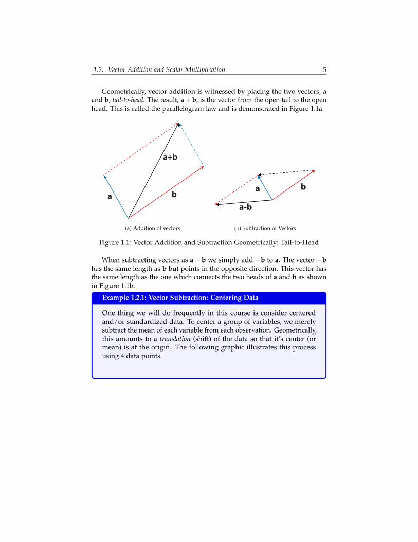
Geometrically, vector addition is witnessed by placing the two vectors, aand b, tail-to-head. The result, a + b, is the vector from the open tail to the openhead. This is called the parallelogram law and is demonstrated in Figure 1.1a.

a b

a+b

(a) Addition of vectors

a b

a-b

(b) Subtraction of Vectors

Figure 1.1: Vector Addition and Subtraction Geometrically: Tail-to-Head

When subtracting vectors as a− b we simply add −b to a. The vector −bhas the same length as b but points in the opposite direction. This vector hasthe same length as the one which connects the two heads of a and b as shownin Figure 1.1b.

Example 1.2.1: Vector Subtraction: Centering Data

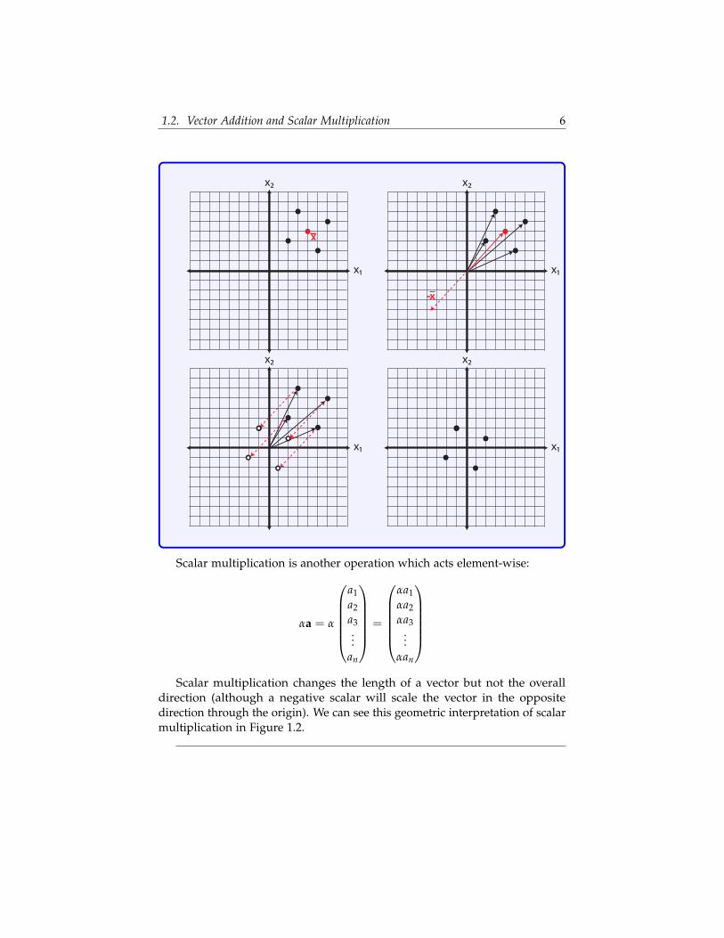
One thing we will do frequently in this course is consider centeredand/or standardized data. To center a group of variables, we merelysubtract the mean of each variable from each observation. Geometrically,this amounts to a translation (shift) of the data so that it’s center (ormean) is at the origin. The following graphic illustrates this processusing 4 data points.


x2

x1

x

x2

x1

-x

x2

x1

x2

x1

Scalar multiplication is another operation which acts element-wise:

αa = α

a1a2a3...

an

=

αa1αa2αa3

...αan

Scalar multiplication changes the length of a vector but not the overall

direction (although a negative scalar will scale the vector in the oppositedirection through the origin). We can see this geometric interpretation of scalarmultiplication in Figure 1.2.

1.3. Exercises 7

a

2a

-.5a

Figure 1.2: Geometric Effect of Scalar Multiplication

1.3 Exercises

1. For a general matrix Am×n describe what the following products willprovide. Also give the size of the result (i.e. "n× 1 vector" or "scalar").

a. Aej

b. eTi A

c. eTi Aej

d. Ae

e. eTA

f. 1n eTA

2. Let Dn×n be a diagonal matrix with diagonal elements Dii. What effectdoes multiplying a matrix Am×n on the left by D have? What effect doesmultiplying a matrix An×m on the right by D have? If you cannot seethis effect in a general sense, try writing out a simple 3× 3 matrix as anexample first.

3. What is the inverse of a diagonal matrix, D = diag{d11, d22, . . . , dnn}?

4. Suppose you have a matrix of data, An×p, containing n observationson p variables. Suppose the standard deviations of these variables areσ1, σ2, . . . , σp. Give a formula for a matrix that contains the same data butwith each variable divided by its standard deviation. Hint: you should useexercises 2 and 3.

5. Suppose we have a network/graph as shown in Figure 1.3. This particularnetwork has 6 numbered vertices (the circles) and edges which connectthe vertices. Each edge has a certain weight (perhaps reflecting some levelof association between the vertices) which is given as a number.

1.3. Exercises 8

1

2

3

4

5

6

12

10

9

53

2

Figure 1.3: An example of a graph or network

a. The adjacency matrix of a graph is defined to be the matrix A suchthat element Aij reflects the the weight of the edge connecting vertexi and vertex j. Write out the adjacency matrix for this graph.

b. The degree of a vertex is defined as the sum of the weights of theedges connected to that vertex. Create a vector d such that di is thedegree of node i.

c. Write d as a matrix-vector product in two different ways using theadjacency matrix, A, and e.

9

CHAPTER 2

NORMS, INNER PRODUCTS ANDORTHOGONALITY

2.1 Norms and Distances

In applied mathematics, Norms are functions which measure the magnitude orlength of a vector. They are commonly used to determine similarities betweenobservations by measuring the distance between them. As we will see, thereare many ways to define distance between two points.

Definition 2.1.1: Vector Norms and Distance Metrics

A Norm, or distance metric, is a function that takes a vector as inputand returns a scalar quantity ( f : Rn → R). A vector norm is typicallydenoted by two vertical bars surrounding the input vector, ‖x‖, tosignify that it is not just any function, but one that satisfies the followingcriteria:

1. If c is a scalar, then‖cx‖ = |c|‖x‖

2. The triangle inequality:

‖x + y‖ ≤ ‖x‖+ ‖y‖

3. ‖x‖ = 0 if and only if x = 0.

4. ‖x‖ ≥ 0 for any vector x

We will not spend any time on these axioms or on the theoretical aspects of

2.1. Norms and Distances 10

norms, but we will put a couple of these functions to good use in our studies,the first of which is the Euclidean norm or 2-norm.

Definition 2.1.2: Euclidean Norm, ‖ ? ‖2

The Euclidean Norm, also known as the 2-norm simply measures theEuclidean length of a vector (i.e. a point’s distance from the origin). Letx = (x1, x2, . . . , xn). Then,

‖x‖2 =√

x21 + x2

2 + · · ·+ x2n

If x is a column vector, then

‖x‖2 =√

xTx.

Often we will simply write ‖ ? ‖ rather than ‖ ? ‖2 to denote the 2-norm,as it is by far the most commonly used norm.

This is merely the distance formula from undergraduate mathematics,measuring the distance between the point x and the origin. To compute thedistance between two different points, say x and y, we’d calculate

‖x− y‖2 =√(x1 − y1)2 + (x2 − y2)2 + · · ·+ (xn − yn)2

Example 2.1.1: Euclidean Norm and Distance

Suppose I have two vectors in 3-space:

x = (1, 1, 1) and y = (1, 0, 0)

Then the magnitude of x (i.e. its length or distance from the origin) is

‖x‖2 =√

12 + 12 + 12 =√

3

and the magnitude of y is

‖y‖2 =√

12 + 02 + 02 = 1

and the distance between point x and point y is

‖x− y‖2 =√(1− 1)2 + (1− 0)2 + (1− 0)2 =

√2.

The Euclidean norm is crucial to many methods in data analysis as itmeasures the closeness of two data points.


Thus, to turn any vector into a unit vector, a vector with a length of 1, weneed only to divide each of the entries in the vector by its Euclidean norm.This is a simple form of standardization used in many areas of data analysis.For a unit vector x, xTx = 1.

Perhaps without knowing it, we’ve already seen many formulas involvingthe norm of a vector. Examples 2.1.2 and 2.1.3 show how some of the mostimportant concepts in statistics can be represented using vector norms.

Example 2.1.2: Standard Deviation and Variance

Suppose a group of individuals has the following heights, measured ininches: (60, 70, 65, 50, 55). The mean height for this group is 60 inches.The formula for the sample standard deviation is typically given as

s =

√∑n

i=1(xi − x)2

√n− 1

We want to subtract the mean from each observation, square the num-bers, sum the result, take the square root and divide by

√n− 1.

If we let x = xe = (60, 60, 60, 60, 60) be a vector containing the mean,and x = (60, 70, 65, 50, 55) be the vector of data then the standarddeviation in matrix notation is:

s =1√

n− 1‖x− x‖2 = 7.9

The sample variance of this data is merely the square of the samplestandard deviation:

s2 =1

n− 1‖x− x‖2

2

Example 2.1.3: Residual Sums of Squares

Another place we’ve seen a similar calculation is in linear regression.You’ll recall the objective of our regression line is to minimize the sumof squared residuals between the predicted value y and the observedvalue y:

n

∑i=1

(yi − yi)2.

In vector notation, we’d let y be a vector containing the observed dataand y be a vector containing the corresponding predictions and writethis summation as

‖y− y‖22


In fact, any situation where the phrase "sum of squares" is encountered,the 2-norm is generally implicated.

Example 2.1.4: Coefficient of Determination, R2

Since variance can be expressed using the Euclidean norm, so can thecoefficient of determination or R2.

R2 =SSreg

SStot=

∑ni=1(yi − y)2

∑ni=1(yi − y)2 =

‖y− y‖2

‖y− y‖2

Other useful norms and distances

1-norm, ‖ ? ‖1. If x =(

x1 x2 . . . xn)

then the 1-norm of X is

‖x‖1 =n

∑i=1|xi|.

This metric is often referred to as Manhattan distance, city block distance, or taxicabdistance because it measures the distance between points along a rectangulargrid (as a taxicab must travel on the streets of Manhattan, for example). Whenx and y are binary vectors, the 1-norm is called the Hamming Distance, andsimply measures the number of elements that are different between the twovectors.

Figure 2.1: The lengths of the red, yellow, and blue paths represent the 1-norm distance between the two points. The green line shows the Euclideanmeasurement (2-norm).

2.2. Inner Products 13

∞-norm, ‖ ? ‖∞. The infinity norm, also called the Supremum, or Max dis-tance, is:

‖x‖∞ = max{|x1|, |x2|, . . . , |xp|}

2.2 Inner Products

The inner product of vectors is a notion that you’ve already seen, it is what’scalled the dot product in most physics and calculus text books.

Definition 2.2.1: Vector Inner Product

The inner product of two n × 1 vectors x and y is written xTy (orsometimes as 〈x, y〉) and is the sum of the product of correspondingelements.

xTy =(

x1 x2 . . . xn)

y1y2...

yn

= x1y1 + x2y2 + · · ·+ xnyn =n

∑i=1

xiyi.

When we take the inner product of a vector with itself, we get the squareof the 2-norm:

xTx = ‖x‖22.

Inner products are at the heart of every matrix product. When we multiplytwo matrices, Xm×n and Yn×p, we can represent the individual elements of theresult as inner products of rows of X and columns of Y as follows:

XY =

X1?X2?

...Xm?

(Y?1 Y?2 . . . Y?p)=

X1?Y?1 X1?Y?2 . . . X1?Y?pX2?Y?1 X2?Y?2 . . . X2?Y?pX3?Y?1 X3?Y?2 . . . X3?Y?p

......

. . ....

Xm?Y?1 . . .. . . Xm?Y?p

2.2.1 Covariance

Another important statistical measurement that is represented by an innerproduct is covariance. Covariance is a measure of how much two randomvariables change together. The statistical formula for covariance is given as

Covariance(x, y) = E[(x− E[x])(y− E[y])] (2.1)

where E[?] is the expected value of the variable. If larger values of one variablecorrespond to larger values of the other variable and at the same time smaller


values of one correspond to smaller values of the other, then the covariancebetween the two variables is positive. In the opposite case, if larger values ofone variable correspond to smaller values of the other and vice versa, then thecovariance is negative. Thus, the sign of the covariance shows the tendencyof the linear relationship between variables, however the magnitude of thecovariance is not easy to interpret. Covariance is a population parameter - it isa property of the joint distribution of the random variables x and y. Definition2.2.2 provides the mathematical formulation for the sample covariance. This isour best estimate for the population parameter when we have data sampledfrom a population.

Definition 2.2.2: Sample Covariance

If x and y are n× 1 vectors containing n observations for two differentvariables, then the sample covariance of x and y is given by

1n− 1

n

∑i=1

(xi − x)(yi − y) =1

n− 1(x− x)T(y− y)

Where again x and y are vectors that contain x and y repeated n times.It should be clear from this formulation that

cov(x, y) = cov(y, x).

When we have p vectors, v1, v2, . . . , vp, each containing n observationsfor p different variables, the sample covariances are most commonlygiven by the sample covariance matrix, Σ, where

Σij = cov(vi, vj).

This matrix is symmetric, since Σij = Σji. If we create a matrix V whosecolumns are the vectors v1, v2, . . . vp once the variables have been centeredto have mean 0, then the covariance matrix is given by:

cov(V) = Σ =1

n− 1VTV.

The jth diagonal element of this matrix gives the variance vj since

Σjj = cov(vj, vj) =1

n− 1(vj − vj)

T(vj − vj) (2.2)

=1

n− 1‖vj − vj‖2

2 (2.3)

= var(vj) (2.4)

When two variables are completely uncorrelated, their covariance is zero.


This lack of correlation would be seen in a covariance matrix with a diagonalstructure. That is, if v1, v2, . . . , vp are uncorrelated with individual variancesσ2

1 , σ22 , . . . , σ2

p respectively then the corresponding covariance matrix is:

Σ =

σ21 0 0 . . . 0

0 σ22 0 . . . 0

0 0. . .

... 0...

......

. . ....

0 0 0 0 σ2p

Furthermore, for variables which are independent and identically distributed(take for instance the error terms in a linear regression model, which areassumed to independent and normally distributed with mean 0 and constantvariance σ), the covariance matrix is a multiple of the identity matrix:

Σ =

σ2 0 0 . . . 00 σ2 0 . . . 0

0 0. . .

... 0...

......

. . ....

0 0 0 0 σ2

= σ2I

Transforming our variables in a such a way that their covariance matrixbecomes diagonal will be our goal in Chapter 7.

Theorem 2.2.1: Properties of Covariance Matrices

The following mathematical properties stem from Equation 2.1. LetXn×p be a matrix of data containing n observations on p variables. If Ais a constant matrix (or vector, in the first case) then

cov(XA) = ATcov(X)A and cov(X + A) = cov(X)

2.2.2 Mahalanobis Distance

Mahalanobis Distance is similar to Euclidean distance, but takes into accountthe correlation of the variables. This metric is relatively common in datamining applications like classification. Suppose we have p variables whichhave some covariance matrix, Σ. Then the Mahalanobis distance between twoobservations, x =

(x1 x2 . . . xp

)T and y =(y1 y2 . . . yp

)T is givenby

d(x, y) =√(x− y)TΣ−1(x− y).


If the covariance matrix is diagonal (meaning the variables are uncorrelated)then the Mahalanobis distance reduces to Euclidean distance normalized bythe variance of each variable:

d(x, y) =

√√√√ p

∑i=1

(xi − yi)2

s2i

= ‖Σ−1/2(x− y)‖2.

2.2.3 Angular Distance

The inner product between two vectors can provide useful information abouttheir relative orientation in space and about their similarity. For example, tofind the cosine of the angle between two vectors in n-space, the inner productof their corresponding unit vectors will provide the result. This cosine is oftenused as a measure of similarity or correlation between two vectors.

Definition 2.2.3: Cosine of Angle between Vectors

The cosine of the angle between two vectors in n-space is given by

cos(θ) =xTy

‖x‖2‖y‖2

θ x

y

This angular distance is at the heart of Pearson’s correlation coefficient.

2.2.4 Correlation

Pearson’s correlation is a normalized version of the covariance, so that notonly the sign of the coefficient is meaningful, but its magnitude is meaningful inmeasuring the strength of the linear association.

2.3. Orthogonality 17

Example 2.2.1: Pearson’s Correlation and Cosine Distance

You may recall the formula for Pearson’s correlation between variable xand y with a sample size of n to be as follows:

r = ∑ni=1(xi − x)(yi − y)√

∑ni=1(xi − x)2

√∑n

i=1(yi − y)2

If we let x be a vector that contains x repeated n times, like we didin Example 2.1.2, and let y be a vector that contains y then Pearson’scoefficient can be written as:

r =(x− x)T(y− y)‖x− x‖‖y− y‖

In other words, it is just the cosine of the angle between the two vectorsonce they have been centered to have mean 0.This makes sense: correlation is a measure of the extent to which thetwo variables share a line in space. If the cosine of the angle is positiveor negative one, this means the angle between the two vectors is 0◦ or180◦, thus, the two vectors are perfectly correlated or collinear.

It is difficult to visualize the angle between two variable vectors becausethey exist in n-space, where n is the number of observations in the dataset.Unless we have fewer than 3 observations, we cannot draw these vectors oreven picture them in our minds. As it turns out, this angular measurementdoes translate into something we can conceptualize: Pearson’s correlationcoefficient is the angle formed between the two possible regression lines usingthe centered data: y regressed on x and x regressed on y. This is illustrated inFigure 2.2.

To compute the matrix of pairwise correlations between variables x1, x2, x3, . . . , xp(columns containing n observations for each variable), we’d first center themto have mean zero, then normalize them to have length ‖xi‖ = 1 and thencompose the matrix

X = [x1|x2|x3| . . . |xp].

Using this centered and normalized data, the correlation matrix is simply

C = XTX.

2.3 Orthogonality

Orthogonal (or perpendicular) vectors have an angle between them of 90◦,meaning that their cosine (and subsequently their inner product) is zero.

2.3. Orthogonality 18

θ

x=f(y)

y=f(x)

r=cos(θ)

Figure 2.2: Correlation Coefficient r and Angle between Regression Lines

Definition 2.3.1: Orthogonality

Two vectors, x and y, are orthogonal in n-space if their inner product iszero:

xTy = 0

Combining the notion of orthogonality and unit vectors we can define anorthonormal set of vectors, or an orthonormal matrix. Remember, for a unitvector, xTx = 1.

Definition 2.3.2: Orthonormal Sets

The n × 1 vectors {x1, x2, x3, . . . , xp} form an orthonormal set if andonly if

1. xTi xj = 0 when i 6= j and

2. xTi xi = 1 (equivalently ‖xi‖ = 1)

In other words, an orthonormal set is a collection of unit vectors whichare mutually orthogonal.

If we form a matrix, X = (x1|x2|x3| . . . |xp), having an orthonormal set ofvectors as columns, we will find that multiplying the matrix by its transposeprovides a nice result:

2.4. Outer Products 19

XTX =

xT

1xT

2xT

3...

xTp

(x1 x2 x3 . . . xp

)=

xT1 x1 xT

1 x2 xT1 x3 . . . xT

1 xpxT

2 x1 xT2 x2 xT

2 x3 . . . xT2 xp

xT3 x1 xT

3 x2 xT3 x3 . . . xT

3 xp...

.... . . . . .

...

xTp x1 . . . . . .

. . . xTp xp

=

1 0 0 . . . 00 1 0 . . . 00 0 1 . . . 0...

.... . . . . .

...0 0 0 . . . 1

= Ip

We will be particularly interested in these types of matrices when they aresquare. If X is a square matrix with orthonormal columns, the arithmetic abovemeans that the inverse of X is XT (i.e. X also has orthonormal rows):

XTX = XXT = I.

Square matrices with orthonormal columns are called orthogonal matrices.

Definition 2.3.3: Orthogonal (or Orthonormal) Matrix

A square matrix, U with orthonormal columns also has orthonormalrows and is called an orthogonal matrix. Such a matrix has an inversewhich is equal to it’s transpose,

UTU = UUT = I

2.4 Outer Products

The outer product of two vectors x ∈ Rm and y ∈ Rn, written xyT , is an m× nmatrix with rank 1. To see this basic fact, lets just look at an example.


Example 2.4.1: Outer Product

Let x =

1234

and let y =

213

. Then the outer product of x and y is:

xyT =

1234

(2 1 3)=

2 1 34 2 66 3 98 4 12

which clearly has rank 1. It should be clear from this example thatcomputing an outer product will always result in a matrix whose rowsand columns are multiples of each other.

Example 2.4.2: Centering Data with an Outer Product

As we’ve seen in previous examples, many statistical formulas involvethe centered data, that is, data from which the mean has been subtractedso that the new mean is zero. Suppose we have a matrix of datacontaining observations of individuals’ heights (h) in inches, weights(w), in pounds and wrist sizes (s), in inches:

A =

h w sperson1 60 102 5.5person2 72 170 7.5person3 66 110 6.0person4 69 128 6.5person5 63 130 7.0

The average values for height, weight, and wrist size are as follows:

h = 66 (2.5)

w = 128 (2.6)

s = 6.5 (2.7)

To center all of the variables in this data set simultaneously, we couldcompute an outer product using a vector containing the means and avector of all ones:


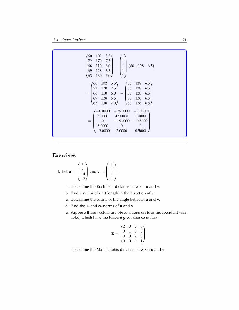
60 102 5.572 170 7.566 110 6.069 128 6.563 130 7.0

−

11111

(66 128 6.5)

=

60 102 5.572 170 7.566 110 6.069 128 6.563 130 7.0

−

66 128 6.566 128 6.566 128 6.566 128 6.566 128 6.5

=

−6.0000 −26.0000 −1.00006.0000 42.0000 1.0000

0 −18.0000 −0.50003.0000 0 0−3.0000 2.0000 0.5000

Exercises

1. Let u =

12−4−2

and v =

1−11−1

.

a. Determine the Euclidean distance between u and v.

b. Find a vector of unit length in the direction of u.

c. Determine the cosine of the angle between u and v.

d. Find the 1- and ∞-norms of u and v.

c. Suppose these vectors are observations on four independent vari-ables, which have the following covariance matrix:

Σ =

2 0 0 00 1 0 00 0 2 00 0 0 1

Determine the Mahalanobis distance between u and v.


2. Let

U =13

−1 2 0 −22 2 0 10 0 3 0−2 1 0 2

a. Show that U is an orthogonal matrix.

b. Let b =

1111

. Solve the equation Ux = b.

3. Write a matrix expression for the correlation matrix, C, for a matrix ofcentered data, X, where Cij = rij is Pearson’s correlation measure betweenvariables xi and xj. To do this, we need more than an inner product, weneed to normalize the rows and columns by the norms ‖xi‖. For a hint,see Exercise 2 in Chapter 1.

4. Suppose you have a matrix of data, An×p, containing n observations onp variables. Develop a matrix formula for the standardized data (wherethe mean of each variable should be subtracted from the correspondingcolumn before dividing by the standard deviation). Hint: use Exercises 1(f)and 4 from Chapter 1 along with Example 2.4.2.

5. Explain why, for any norm or distance metric,

‖x− y‖ = ‖y− x‖

6. Find two vectors which are orthogonal to x =

111

7. Pythagorean Theorem. Show that x and y are orthogonal if and only if

‖x + y‖22 = ‖x‖2

2 + ‖y‖22

(Hint: Recall that ‖x‖22 = xTx)

23

CHAPTER 3

LINEAR COMBINATIONS AND LINEARINDEPENDENCE

One of the most central ideas in all of Linear Algebra is that of linear indepen-dence. For regression problems, it is repeatedly stressed that multicollinearity isproblematic. Multicollinearity is simply a statistical term for linear dependence.It’s bad. We will see the reason for this shortly, but first we have to develop thenotion of a linear combination.

3.1 Linear Combinations

Definition 3.1.1: Linear Combination

A linear combination is constructed from a set of terms v1, v2, . . . , vnby multiplying each term by a constant and adding the result:

c = α1v1 + α2v2 + · · ·+ αnvn =n

∑i=1

αivn

The coefficients αi are scalar constants and the terms, {vi} can be scalars,vectors, or matrices.

If we dissect our formula for a system of linear equations, Ax = b, we willfind that the right-hand side vector b can be expressed as a linear combinationof the columns in the coefficient matrix, A.

3.1. Linear Combinations 24

b = Ax (3.1)

b = (A1|A2| . . . |An)

x1x2...

x3

(3.2)

b = x1A1 + x2A2 + · · ·+ xnAn (3.3)

A concrete example of this expression is given in Example 3.1.1.

Example 3.1.1: Systems of Equations as Linear Combinations

Consider the following system of equations:

3x1 + 2x2 + 9x3 = 1 (3.4)

4x1 + 2x2 + 3x3 = 5 (3.5)

2x1 + 7x2 + x3 = 0 (3.6)

We can write this as a matrix vector product Ax = b where

A =

3 2 94 2 32 7 1

x =

x1x2x3

and b =

150

We can also write b as a linear combination of columns of A:

x1

342

+ x2

227

+ x3

931

=

150

Similarly, if we have a matrix-matrix product, we can write each column

of the result as a linear combination of columns of the first matrix. Let Am×n,Xn×p, and Bm×p be matrices. If we have AX = B then

(A1|A2| . . . |An)

x11 x12 . . . x1px21 x22 . . . x2n

......

. . ....

xn1 xn2 . . . xnp

= (B1|B2| . . . |Bn)

and we can write

Bj = AXj = x1jA1 + x2jA2 + x3jA3 + · · ·+ xnjAn.

A concrete example of this expression is given in Example 3.1.2.

3.1. Linear Combinations 25

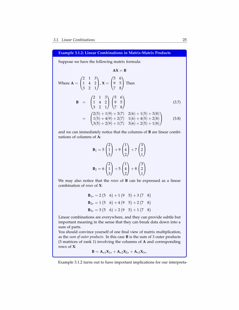
Example 3.1.2: Linear Combinations in Matrix-Matrix Products

Suppose we have the following matrix formula:

AX = B

Where A =

2 1 31 4 23 2 1

, X =

5 69 57 8

Then

B =

2 1 31 4 23 2 1

5 69 57 8

(3.7)

=

2(5) + 1(9) + 3(7) 2(6) + 1(5) + 3(8)1(5) + 4(9) + 2(7) 1(6) + 4(5) + 2(8)3(5) + 2(9) + 1(7) 3(6) + 2(5) + 1(8)

(3.8)

and we can immediately notice that the columns of B are linear combi-nations of columns of A:

B1 = 5

213

+ 9

142

+ 7

321

B2 = 6

213

+ 5

142

+ 8

321

We may also notice that the rows of B can be expressed as a linearcombination of rows of X:

B1? = 2(5 6

)+ 1

(9 5

)+ 3

(7 8

)B2? = 1

(5 6

)+ 4

(9 5

)+ 2

(7 8

)B3? = 3

(5 6

)+ 2

(9 5

)+ 1

(7 8

)Linear combinations are everywhere, and they can provide subtle butimportant meaning in the sense that they can break data down into asum of parts.You should convince yourself of one final view of matrix multiplication,as the sum of outer products. In this case B is the sum of 3 outer products(3 matrices of rank 1) involving the columns of A and correspondingrows of X:

B = A?1X1? + A?2X2? + A?3X3?.

Example 3.1.2 turns out to have important implications for our interpreta-

3.2. Linear Independence 26

tion of matrix factorizations. In this context we’d call AX a factorization of thematrix B. We will see how to use these expressions to our advantage in laterchapters.

We don’t necessarily have to use vectors as the terms for a linear combi-nation. Example 3.1.3 shows how we can write any m× n matrix as a linearcombination of nm matrices with rank 1.

Example 3.1.3: Linear Combination of Matrices

Write the matrix A =

(1 34 2

)as a linear combination of the following

matrices: {(1 00 0

),(

0 10 0

),(

0 01 0

),(

0 00 1

)}Solution:

A =

(1 34 2

)= 1

(1 00 0

)+ 3

(0 10 0

)+ 4

(0 01 0

)+ 2

(0 00 1

)

Now that we understand the concept of Linear Combination, we can de-velop the important concept of Linear Independence.

3.2 Linear Independence

Definition 3.2.1: Linear Dependence and Linear Independence

A set of vectors {v1, v2, . . . , vn} is linearly dependent if we can expressthe zero vector, 0, as non-trivial linear combination of the vectors. Inother words there exist some constants α1, α2, . . . αn (non-trivial meansthat these constants are not all zero) for which

α1v1 + α2v2 + · · ·+ αnvn = 0. (3.9)

A set of terms is linearly independent if Equation 3.9 has only thetrivial solution (α1 = α2 = · · · = αn = 0).

Another way to express linear dependence is to say that we can write oneof the vectors as a linear combination of the others. If there exists a non-trivialset of coefficients α1, α2, . . . , αn for which

α1v1 + α2v2 + · · ·+ αnvn = 0

3.2. Linear Independence 27

then for αj 6= 0 we could write

vj = −1αj

n

∑i=1i 6=j

αivi

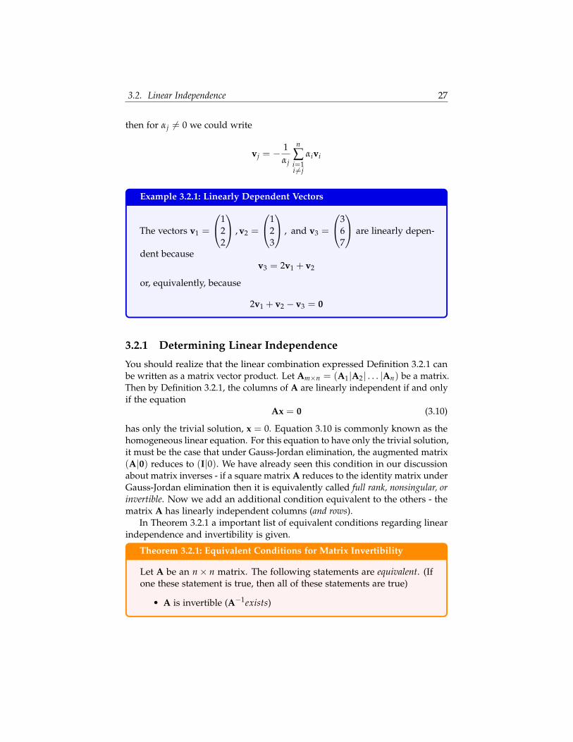
Example 3.2.1: Linearly Dependent Vectors

The vectors v1 =

122

, v2 =

123

, and v3 =

367

are linearly depen-

dent becausev3 = 2v1 + v2

or, equivalently, because

2v1 + v2 − v3 = 0

3.2.1 Determining Linear Independence

You should realize that the linear combination expressed Definition 3.2.1 canbe written as a matrix vector product. Let Am×n = (A1|A2| . . . |An) be a matrix.Then by Definition 3.2.1, the columns of A are linearly independent if and onlyif the equation

Ax = 0 (3.10)

has only the trivial solution, x = 0. Equation 3.10 is commonly known as thehomogeneous linear equation. For this equation to have only the trivial solution,it must be the case that under Gauss-Jordan elimination, the augmented matrix(A|0) reduces to (I|0). We have already seen this condition in our discussionabout matrix inverses - if a square matrix A reduces to the identity matrix underGauss-Jordan elimination then it is equivalently called full rank, nonsingular, orinvertible. Now we add an additional condition equivalent to the others - thematrix A has linearly independent columns (and rows).

In Theorem 3.2.1 a important list of equivalent conditions regarding linearindependence and invertibility is given.

Theorem 3.2.1: Equivalent Conditions for Matrix Invertibility

Let A be an n× n matrix. The following statements are equivalent. (Ifone these statement is true, then all of these statements are true)

• A is invertible (A−1exists)

3.3. Span of Vectors 28

• A has full rank (rank(A) = n)

• The columns of A are linearly independent

• The rows of A are linearly independent

• The system Ax = b, b 6= 0 has a unique solution

• Ax = 0 =⇒ x = 0

• A is nonsingular

• AGauss−Jordan−−−−−−−−→ I

3.3 Span of Vectors

Definition 3.3.1: Vector Span

The span of a single vector v is the set of all scalar multiples of v:

span(v) = {αv for any constant α}

The span of a collection of vectors, V = {v1, v2, . . . , vn} is the set of alllinear combinations of these vectors:

span(V) = {α1v1 + α2v2 + · · ·+ αnvn for any constants α1, . . . , αn}

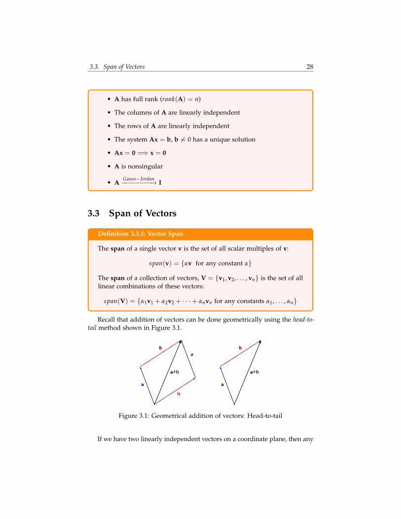
Recall that addition of vectors can be done geometrically using the head-to-tail method shown in Figure 3.1.

Figure 3.1: Geometrical addition of vectors: Head-to-tail

If we have two linearly independent vectors on a coordinate plane, then any


third vector can be written as a linear combination of them. This is becausetwo vectors is sufficient to span the entire 2-dimensional plane. You shouldtake a moment to convince yourself of this geometrically.

In 3-space, two linearly independent vectors can still only span a plane.Figure 3.2 depicts this situation. The set of all linearly combinations of thetwo vectors a and b (i.e. the span(a, b)) carves out a plane. We call this atwo-dimensional collection of vectors a subspace of R3. A subspace is formallydefined in Definition 3.3.2.

Figure 3.2: The span(a, b) in R3 creates a plane (a 2-dimensional subspace)

Definition 3.3.2: Subspace

A subspace, S of Rn is thought of as a “flat” (having no curvature)surface within Rn. It is a collection of vectors which satisfies thefollowing conditions:

1. The origin (0 vector) is contained in S

2. If x and y are in S then the sum x + y is also in S

3. If x is in S and α is a constant then αx is also in S

The span of two vectors a and b is a subspace because it satisfies these threeconditions. (Can you prove it? See exercise 4).


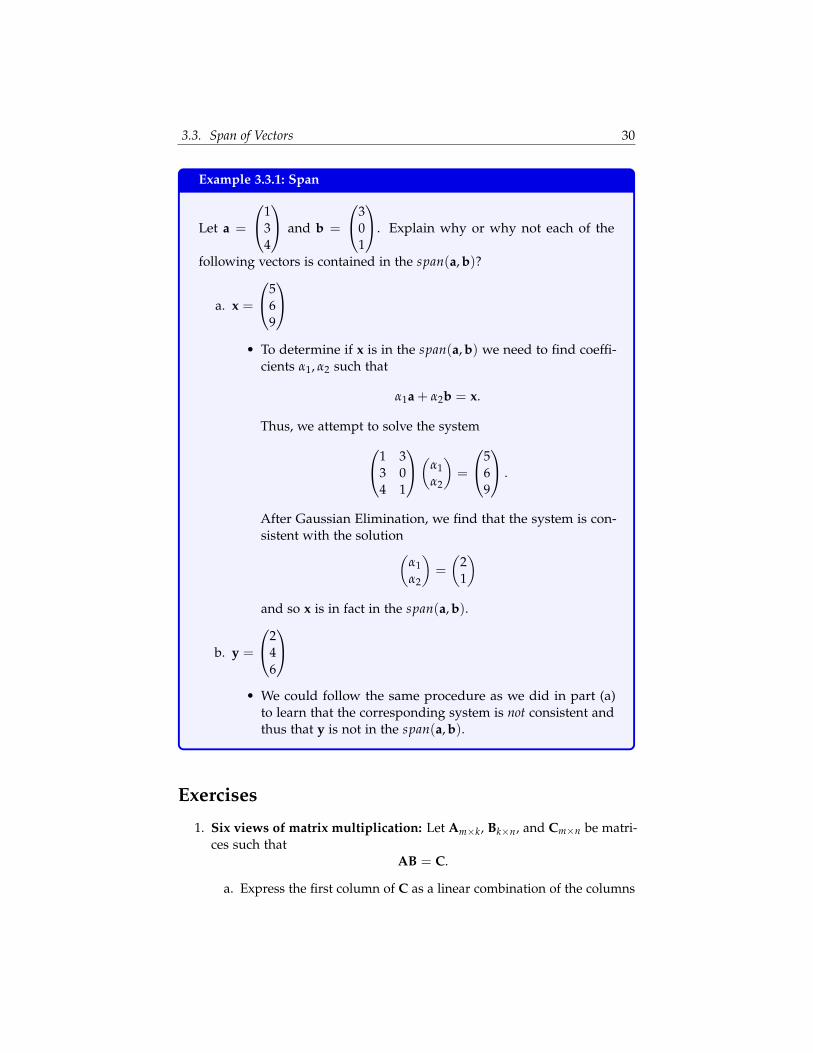
Example 3.3.1: Span

Let a =

134

and b =

301

. Explain why or why not each of the

following vectors is contained in the span(a, b)?

a. x =

569

• To determine if x is in the span(a, b) we need to find coeffi-

cients α1, α2 such that

α1a + α2b = x.

Thus, we attempt to solve the system1 33 04 1

(α1α2

)=

569

.

After Gaussian Elimination, we find that the system is con-sistent with the solution(

α1α2

)=

(21

)and so x is in fact in the span(a, b).

b. y =

246

• We could follow the same procedure as we did in part (a)

to learn that the corresponding system is not consistent andthus that y is not in the span(a, b).

Exercises

1. Six views of matrix multiplication: Let Am×k, Bk×n, and Cm×n be matri-ces such that

AB = C.

a. Express the first column of C as a linear combination of the columns


of A.

b. Express the first column of C as a matrix-vector product.

c. Express C as a sum of outer products.

d. Express the first row of C as a linear combination of the rows of B.

e. Express the first row of C as a matrix-vector product.

d. Express the element Cij as an inner product of row or column vectorsfrom A and B.

2. Determine whether or not the vectors

x1 =

131

, x2 =

011

, x3 =

210

are linearly independent.

3. Let a =

134

and b =

301

.

a. Show that the zero vector,

000

is in the span(a, b).

b. Determine whether or not the vector

101

is in the span(a, b).

4. Prove that the span of vectors is a subspace by showing that it satisfiesthe three conditions from Definition 3.3.1. You can simply show this factfor the span of two vectors and notice how the concept will hold for morethan two vectors.

5. True/False Mark each statement as true or false. Justify your response.

• If Ax = b has a solution then b can be written as a linear combina-tion of the columns of A.

• If Ax = b has a solution then b is in the span of the columns of A.

• If the vectors v1, v2, and , v3 form a linearly dependent set, then v1is in the span(v2, v3).

32

CHAPTER 4

BASIS AND CHANGE OF BASIS

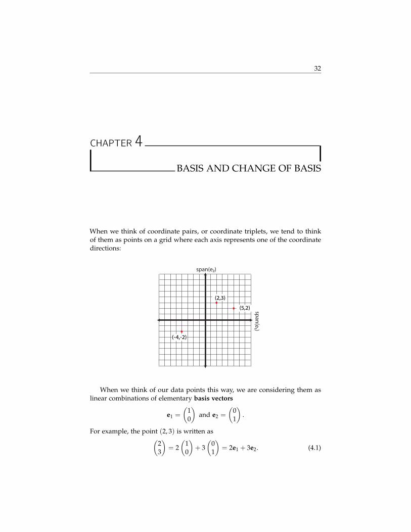
When we think of coordinate pairs, or coordinate triplets, we tend to thinkof them as points on a grid where each axis represents one of the coordinatedirections:

span(e2)

span(e1)

(2,3)(5,2)

(-4,-2)

When we think of our data points this way, we are considering them aslinear combinations of elementary basis vectors

e1 =

(10

)and e2 =

(01

).

For example, the point (2, 3) is written as(23

)= 2

(10

)+ 3

(01

)= 2e1 + 3e2. (4.1)

33

We consider the coefficients (the scalars 2 and 3) in this linear combinationas coordinates in the basis B1 = {e1, e2}. The coordinates, in essence, tell ushow much “information” from the vector/point (2, 3) lies along each basisdirection: to create this point, we must travel 2 units along the direction of e1and then 3 units along the direction of e2.

We can also view Equation 4.1 as a way to separate the vector (2, 3) intoorthogonal components. Each component is an orthogonal projection ofthe vector onto the span of the corresponding basis vector. The orthogonalprojection of vector a onto the span another vector v is simply the closest pointto a contained on the span(v), found by “projecting” a toward v at a 90◦ angle.Figure 4.1 shows this explicitly for a = (2, 3).

span(e2)

span(e1)

orthogonal projection ofa onto e1

orthogonal projection ofa onto e2 a

Figure 4.1: Orthogonal Projections onto basis vectors.

Definition 4.0.3: Elementary Basis

For any vector a = (a1, a2, . . . , an), the basis B = {e1, e2, . . . , en} (recallei is the ith column of the identity matrix In) is the elementary basisand a can be written in this basis using the coordinates a1, a2, . . . , an asfollows:

a = a1e1 + a2e2 + . . . anen.

The elementary basis B1 is convenient for many reasons, one being itsorthonormality:

eT1 e1 = eT

2 e2 = 1

eT1 e2 = eT

2 e1 = 0

However, there are many (infinitely many, in fact) ways to represent thedata points on different axes. If I wanted to view this data in a different

34

way, I could use a different basis. Let’s consider, for example, the followingorthonormal basis, drawn in green over the original grid in Figure 4.2:

B2 = {v1, v2} ={√

22

(11

),√

22

(1−1

)}

span(e2)

span(e1)

span(v2)

span(v1)

Figure 4.2: New basis vectors, v1 and v2, shown on original plane

The scalar multipliers√

22 are simply normalizing factors so that the basis

vectors have unit length. You can convince yourself that this is an orthonormalbasis by confirming that

vT1 v1 = vT

2 v2 = 1

vT1 v2 = vT

2 v1 = 0

If we want to change the basis from the elementary B1 to the new green basisvectors in B2, we need to determine a new set of coordinates that direct us tothe point using the green basis vectors as a frame of reference. In other wordswe need to determine (α1, α2) such that travelling α1 units along the directionv1 and then α2 units along the direction v2 will lead us to the point in question.For the point (2, 3) that means(

23

)= α1v1 + α2v2 = α1

(√2

2√2

2

)+ α2

( √2

2

−√

22

).

This is merely a system of equations Va = b:

√2

2

(1 11 −1

)(α1α2

)=

(23

)

35

The 2× 2 matrix V on the left-hand side has linearly independent columnsand thus has an inverse. In fact, V is an orthonormal matrix which means itsinverse is its transpose. Multiplying both sides of the equation by V−1 = VT

yields the solution

a =

(α1α2

)= VTb =

(5√

22

−√

22

)This result tells us that in order to reach the red point (formerly known

as (2,3) in our previous basis), we should travel 5√

22 units along the direction

of v1 and then −√

22 units along the direction v2 (Note that v2 points toward

the southeast corner and we want to move northwest, hence the coordinateis negative). Another way (a more mathematical way) to say this is that thelength of the orthogonal projection of a onto the span of v1 is 5

√2

2 , and the length of

the orthogonal projection of a onto the span of v2 is −√

22 . While it may seem that

these are difficult distances to plot, they work out quite well if we examine ourdrawing in Figure 4.2, because the diagonal of each square is

√2.

In the same fashion, we can re-write all 3 of the red points on our graphin the new basis by solving the same system simultaneously for all the points.Let B be a matrix containing the original coordinates of the points and let A bea matrix containing the new coordinates:

B =

(−4 2 5−2 3 2

)A =

(α11 α12 α13α21 α22 α23

)Then the new data coordinates on the rotated plane can be found by solving:

VA = B

And thus

A = VTB =

√2

2

(−6 5 7−2 −1 3

)Using our new basis vectors, our alternative view of the data is that in

Figure 4.3.In the above example, we changed our basis from the original elementary

basis to a new orthogonal basis which provides a different view of the data. Allof this amounts to a rotation of the data around the origin. No real informationhas been lost - the points maintain their distances from each other in nearlyevery distance metric. Our new variables, v1 and v2 are linear combinationsof our original variables e1 and e2, thus we can transform the data back to itsoriginal coordinate system by again solving a linear system (in this example,we’d simply multiply the new coordinates again by V).

In general, we can change bases using the procedure outlined in Theorem4.0.1.

36

span(v1)

span(v2)+

+

Figure 4.3: Points plotted in the new basis, B

Theorem 4.0.1: Changing Bases

Given a matrix of coordinates (in columns), A, in some basis, B1 ={x1, x2, . . . , xn}, we can change the basis to B2 = {v1, v2, . . . , vn} withthe new set of coordinates in a matrix B by solving the system

XA = VB

where X and V are matrices containing (as columns) the basis vectorsfrom B1 and B2 respectively.Note that when our original basis is the elementary basis, X = I, oursystem reduces to

A = VB.

When our new basis vectors are orthonormal, the solution to this systemis simply

B = VTA.

Definition 4.0.4: Basis Terminology

A basis for the vector space Rn can be any collection of n linearlyindependent vectors in Rn; n is said to be the dimension of the vectorspace Rn. When the basis vectors are orthonormal (as they were in our

37

example), the collection is called an orthonormal basis.

The preceding discussion dealt entirely with bases for Rn (our examplewas for points in R2). However, we will need to consider bases for subspaces ofRn. Recall that the span of two linearly independent vectors in R3 is a plane.This plane is a 2-dimensional subspace of R3. Its dimension is 2 because 2basis vectors are required to represent this space. However, not all points fromR3 can be written in this basis - only those points which exist on the plane.In the next chapter, we will discuss how to proceed in a situation where thepoint we’d like to represent does not actually belong to the subspace we areinterested in. This is the foundation for Least Squares.

Exercises

1. Show that the vectors v1 =

(31

)and v2 =

(−26

)are orthogonal. Create

an orthonormal basis for R2 using these two direction vectors.

2. Consider a1 = (1, 1) and a2 = (0, 1) as coordinates for points in theelementary basis. Write the coordinates of a1 and a2 in the orthonormalbasis found in exercise 1. Draw a picture which reflects the old and newbasis vectors.

3. Write the orthonormal basis vectors from exercise 1 as linear combinationsof the original elementary basis vectors.

4. What is the length of the orthogonal projection of a1 onto v1?

38

CHAPTER 5

LEAST SQUARES

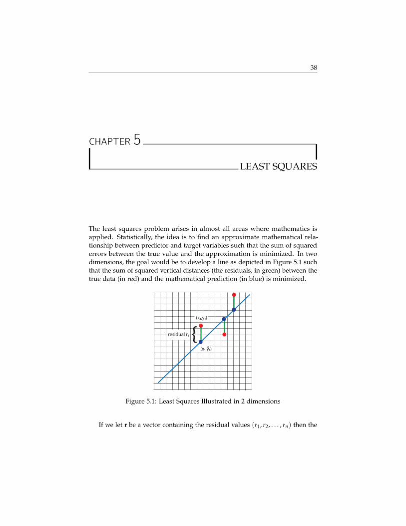
The least squares problem arises in almost all areas where mathematics isapplied. Statistically, the idea is to find an approximate mathematical rela-tionship between predictor and target variables such that the sum of squarederrors between the true value and the approximation is minimized. In twodimensions, the goal would be to develop a line as depicted in Figure 5.1 suchthat the sum of squared vertical distances (the residuals, in green) between thetrue data (in red) and the mathematical prediction (in blue) is minimized.

(x1,y1)

(x1,y1)^

{residual r1

Figure 5.1: Least Squares Illustrated in 2 dimensions

If we let r be a vector containing the residual values (r1, r2, . . . , rn) then the

39

sum of squared residuals can be written in linear algebraic notation as

n

∑i=1

r2i = rTr = (y− y)T(y− y) = ‖y− y‖2

Suppose we want to regress our target variable y on p predictor variables,x1, x2, . . . , xp. If we have n observations, then the ideal situation would be tofind a vector of parameters β containing an intercept, β0 along with p slopeparameters, β1, . . . , βp such that

x1 x2 . . . xp

obs1 1 x11 x12 . . . x1pobs2 1 x21 x22 . . . x2p...

......

......

...obsn 1 xn1 xn2 . . . xnp

︸︷︷︸

X

β0β1...

βp

︸︷︷︸

β

=

y0y1...

yn

︸︷︷︸

y

(5.1)

With many more observations than variables, this system of equations willnot, in practice, have a solution. Thus, our goal becomes finding a vector ofparameters β such that Xβ = y comes as close to y as possible. Using thedesign matrix, X, the least squares solution β is the one for which

‖y− Xβ‖2 = ‖y− y‖2

is minimized. Theorem 5.0.2 characterizes the solution to the least squaresproblem.

Theorem 5.0.2: Least Squares Problem and Solution

For an n× m matrix X and n× 1 vector y, let r = Xβ− y. The leastsquares problem is to find a vector β that minimizes the quantity

n

∑i=1

r2i = ‖y− Xβ‖2.

Any vector β which provides a minimum value for this expression iscalled a least-squares solution.

• The set of all least squares solutions is precisely the set of solutionsto the so-called normal equations,

XTXβ = XTy.

40

• There is a unique least squares solution if and only if rank(X) = m(i.e. linear independence of variables or no perfect multicollinear-ity!), in which case XTX is invertible and the solution is givenby

β = (XTX)−1XTy

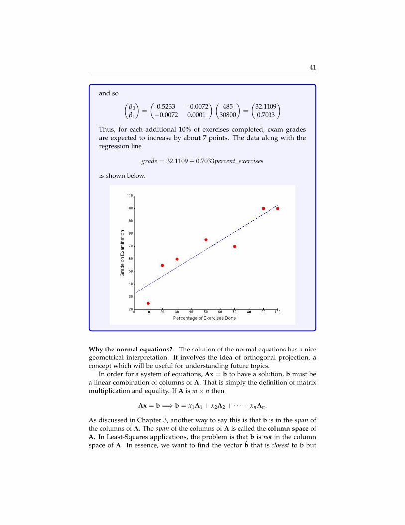
Example 5.0.2: Solving a Least Squares Problem

In 2014, data was collected regarding the percentage of linearalgebra exercises done by students and the grade they received ontheir examination. Based on this data, what is the expected effect ofcompleting an additional 10% of the exercises on a students exam grade?

ID % of Exercises Exam Grade1 20 552 100 1003 90 1004 70 705 50 756 10 257 30 60

To find the least squares regression line, we want to solve the equationXβ = y:

1 201 1001 901 701 501 101 30

(

β0β1

)=

5510010070752560

This system is obviously inconsistent. Thus, we want to find the leastsquares solution β by solving XTXβ = XTy:(

7 370370 26900

)(β0β1

)=

(485

30800

)Now, since multicollinearity was not a problem, we can simply find theinverse of XTX and multiply it on both sides of the equation:(

7 370370 26900

)−1

=

(0.5233 −0.0072−0.0072 0.0001

)

41

and so (β0β1

)=

(0.5233 −0.0072−0.0072 0.0001

)(485

30800

)=

(32.11090.7033

)Thus, for each additional 10% of exercises completed, exam gradesare expected to increase by about 7 points. The data along with theregression line

grade = 32.1109 + 0.7033percent_exercises

is shown below.

Why the normal equations? The solution of the normal equations has a nicegeometrical interpretation. It involves the idea of orthogonal projection, aconcept which will be useful for understanding future topics.

In order for a system of equations, Ax = b to have a solution, b must bea linear combination of columns of A. That is simply the definition of matrixmultiplication and equality. If A is m× n then

Ax = b =⇒ b = x1A1 + x2A2 + · · ·+ xnAn.

As discussed in Chapter 3, another way to say this is that b is in the span ofthe columns of A. The span of the columns of A is called the column space ofA. In Least-Squares applications, the problem is that b is not in the columnspace of A. In essence, we want to find the vector b that is closest to b but

42

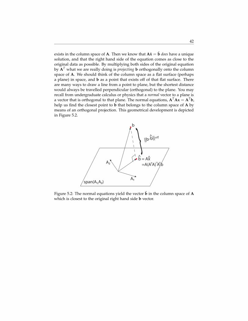
exists in the column space of A. Then we know that Ax = b does have a uniquesolution, and that the right hand side of the equation comes as close to theoriginal data as possible. By multiplying both sides of the original equationby AT what we are really doing is projecting b orthogonally onto the columnspace of A. We should think of the column space as a flat surface (perhapsa plane) in space, and b as a point that exists off of that flat surface. Thereare many ways to draw a line from a point to plane, but the shortest distancewould always be travelled perpendicular (orthogonal) to the plane. You mayrecall from undergraduate calculus or physics that a normal vector to a plane isa vector that is orthogonal to that plane. The normal equations, ATAx = ATb,help us find the closest point to b that belongs to the column space of A bymeans of an orthogonal projection. This geometrical development is depictedin Figure 5.2.

A1

A2

span(A1,A2)

b

b = Ax

} ||b-b||=r

=A(A A) A b T T -1

^

^

^

Figure 5.2: The normal equations yield the vector b in the column space of Awhich is closest to the original right hand side b vector.

43

CHAPTER 6

EIGENVALUES AND EIGENVECTORS

Definition 6.0.5: Eigenvalues and Eigenvectors

For a square matrix An×n, a scalar λ is called an eigenvalue of A ifthere is a nonzero vector x such that

Ax = λx.

Such a vector, x is called an eigenvector of A corresponding to theeigenvalue λ. We sometimes refer to the pair (λ, x) as an eigenpair.

Eigenvalues and eigenvectors have numerous applications throughout math-ematics, statistics and other fields. First, we must get a handle on the definitionwhich we will do through some examples.

Example 6.0.3: Eigenvalues and Eigenvectors

Determine whether x =

(11

)is an eigenvector of A =

(3 11 3

)and if

so, find the corresponding eigenvalue.To determine whether x is an eigenvector, we want to compute Ax andobserve whether the result is a multiple of x. If this is the case, then themultiplication factor is the corresponding eigenvalue:

Ax =

(3 11 3

)(11

)=

(44

)= 4

(11

)From this it follows that x is an eigenvector of A and the corresponding

44

eigenvalue is λ = 4.

Is the vector y =

(22

)an eigenvector?

Ay =

(3 11 3

)(22

)=

(88

)= 4

(22

)= 4y

Yes, it is and it corresponds to the same eigenvalue, λ = 4

Example 6.0.3 shows a very important property of eigenvalue-eigenvectorpairs. If (λ, x) is an eigenpair then any scalar multiple of x is also an eigenvectorcorresponding to λ. To see this, let (λ, x) be an eigenpair for a matrix A (whichmeans that Ax = λx) and let y = αx be any scalar multiple of x. Then we have,

Ay = A(αx) = α(Ax) = α(λx) = λ(αx) = λy

which shows that y (or any scalar multiple of x) is also an eigenvector associatedwith the eigenvalue λ.

Thus, for each eigenvalue we have infinitely many eigenvectors. In thepreceding example, the eigenvectors associated with λ = 4 will be scalar

multiples of x =

(11

). You may recall from Chapter 3 that the set of all scalar

multiples of x is denoted span(x). The span(x) in this example represents theeigenspace of λ. Note: when using software to compute eigenvectors, it is standardpractice for the software to provide the normalized/unit eigenvector.

In some situations, an eigenvalue can have multiple eigenvectors which arelinearly independent. The number of linearly independent eigenvectors associ-ated with an eigenvalue is called the geometric multiplicity of the eigenvalue.Example 6.0.4 clarifies this concept.

Example 6.0.4: Geometric Multiplicity

Consider the matrix A =

(3 00 3

). It should be straightforward to see

that x1 =

(10

)and x2 =

(01

)are both eigenvectors corresponding to

the eigenvalue λ = 3. x1 and x2 are linearly independent, therefore thegeometric multiplicity of λ = 3 is 2.

What happens if we take a linear combination of x1 and x2? Is that also

45

an eigenvector? Consider y =

(23

)= 2x1 + 3x2. Then

Ay =

(3 00 3

)(23

)=

(69

)= 3

(23

)= 3y

shows that y is also an eigenvector associated with λ = 3.The eigenspace corresponding to λ = 3 is the set of all linear combina-tions of x1 and x2, i.e. the span(x1, x2).

We can generalize the result that we saw in Example 6.0.4 for any squarematrix and any geometric multiplicity. Let An×n have an eigenvalue λ withgeometric multiplicity k. This means there are k linearly independent eigenvec-tors, x1, x2, . . . , xk such that Axi = λxi for each eigenvector xi. Now if we let ybe a vector in the span(x1, x2, . . . , xk) then y is some linear combination of thexi’s:

y = α1x2 + α2x2 + · · ·+ αkxk

Observe what happens when we multiply y by A:

Ay = A(α1x2 + α2x2 + · · ·+ αkxk)

= α1(Ax1) + α2(Ax2) + · · ·+ αk(Axk)

= α1(λx1) + α2(λx2) + · · ·+ αk(λxk)

= λ(α1x2 + α2x2 + · · ·+ αkxk)

= λy

which shows that y (or any vector in the span(x1, x2, . . . , xk)) is an eigenvectorof A corresponding to λ.

This proof allows us to formally define the concept of an eigenspace.

Definition 6.0.6: Eigenspace

Let A be a square matrix and let λ be an eigenvalue of A. The set of alleigenvectors corresponding to λ, together with the zero vector, is calledthe eigenspace of λ. The number of basis vectors required to form theeigenspace is called the geometric multiplicity of λ.

Now, let’s attempt the eigenvalue problem from the other side. Given aneigenvalue, we will find the corresponding eigenspace in Example 6.0.5.

46

Example 6.0.5: Eigenvalues and Eigenvectors

Show that λ = 5 is an eigenvalue of A =

(1 24 3

)and determine the

eigenspace of λ = 5.

Attempting the problem from this angle requires slightly more work.We want to find a vector x such that Ax = 5x. Setting this up, we have:

Ax = 5x.

What we want to do is move both terms to one side and factor out thevector x. In order to do this, we must use an identity matrix, otherwisethe equation wouldn’t make sense (we’d be subtracting a constant froma matrix).

Ax− 5x = 0

(A− 5I)x = 0((1 24 3

)−(

5 00 5

))(x1x2

)=

(00

)(−4 24 −2

)(x1x2

)=

(00

)

Clearly, the matrix A− λI is singular (i.e. does not have linearly inde-pendent rows/columns). This will always be the case by the definitionAx = λx, and is often used as an alternative definition.In order to solve this homogeneous system of equations, we use Gaus-sian elimination: (

−4 2 04 −2 0

)−→

(1 − 1

2 00 0 0

)This implies that any vector x for which x1 − 1

2 x2 = 0 satisfies theeigenvector equation. We can pick any such vector, for example x =(

12

), and say that the eigenspace of λ = 5 is

span{(

12

)}

If we didn’t know either an eigenvalue or eigenvector of A and insteadwanted to find both, we would first find eigenvalues by determining all possibleλ such that A− λI is singular and then find the associated eigenvectors. There

6.1. Diagonalization 47

are some tricks which allow us to do this by hand for 2× 2 and 3× 3 matrices,but after that the computation time is unworthy of the effort. Now that wehave a good understanding of how to interpret eigenvalues and eigenvectorsalgebraically, let’s take a look at some of the things that they can do, startingwith one important fact.

Theorem 6.0.3: Eigenvalues and the Trace of a Matrix

Let A be an n× n matrix with eigenvalues λ1, λ2, . . . , λn. Then the sumof the eigenvalues is equal to the trace of the matrix (recall that the traceof a matrix is the sum of its diagonal elements).

Trace(A) =n

∑i=1

λi.

Example 6.0.6: Trace of Covariance Matrix

Suppose that we had a collection of n observations on p variables,x1, x2, . . . , xp. After centering the data to have zero mean, we can com-pute the sample variances as:

var(xi) =1

n− 1xT

i xi = ‖xi‖2

These variances form the diagonal elements of the sample covariancematrix,

Σ =1

n− 1XTX

Thus, the total variance of this data is

1n− 1

n

∑i=1‖xi‖2 = Trace(Σ) =

n

∑i=1

λi.

In other words, the sum of the eigenvalues of a covariance matrixprovides the total variance in the variables x1, . . . , xp.

6.1 Diagonalization

Let’s take another look at Example 6.0.5. We already showed that λ1 = 5 and

v1 =

(12

)is an eigenpair for the matrix A =

(1 24 3

). You may verify that

λ2 = −1 and v2 =

(1−1

)is another eigenpair. Suppose we create a matrix of

6.1. Diagonalization 48

eigenvectors:

V = (v1, v2) =

(1 12 −1

)and a diagonal matrix containing the corresponding eigenvalues:

D =

(5 00 −1

)Then it is easy to verify that AV = VD:

AV =

(1 24 3

)(1 12 −1

)=

(5 −1

10 1

)=

(1 12 −1

)(5 00 −1

)= VD

If the columns of V are linearly independent, which they are in this case, wecan write:

V−1AV = D

What we have just done is develop a way to transform a matrix A into adiagonal matrix D. This is known as diagonalization.

Definition 6.1.1: Diagonalizable

An n× n matrix A is said to be diagonalizable if there exists an invert-ible matrix P and a diagonal matrix D such that

P−1AP = D

This is possible if and only if the matrix A has n linearly independenteigenvectors (known as a complete set of eigenvectors). The matrixP is then the matrix of eigenvectors and the matrix D contains thecorresponding eigenvalues on the diagonal.

Determining whether or not a matrix An×n is diagonalizable is a littletricky. Having rank(A) = n is not a sufficient condition for having n linearlyindependent eigenvectors. The following matrix stands as a counter example:

A =

−3 1 −320 3 102 −2 4

This matrix has full rank but only two linearly independent eigenvectors. For-tunately, for our primary application of diagonalization, we will be dealing

6.2. Geometric Interpretation of Eigenvalues and Eigenvectors 49

with a symmetric matrix, which can always be diagonalized. In fact, symmet-ric matrices have an additional property which makes this diagonalizationparticularly nice, as we will see in Chapter 7.

6.2 Geometric Interpretation ofEigenvalues and Eigenvectors

Since any scalar multiple of an eigenvector is still an eigenvector, let’s considerfor the present discussion unit eigenvectors x of a square matrix A - those withlength ‖x‖ = 1. By the definition, we know that

Ax = λx

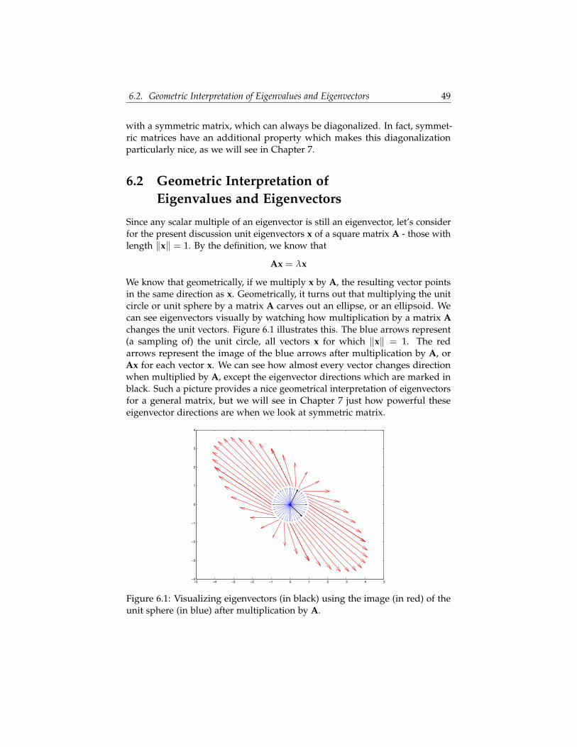
We know that geometrically, if we multiply x by A, the resulting vector pointsin the same direction as x. Geometrically, it turns out that multiplying the unitcircle or unit sphere by a matrix A carves out an ellipse, or an ellipsoid. Wecan see eigenvectors visually by watching how multiplication by a matrix Achanges the unit vectors. Figure 6.1 illustrates this. The blue arrows represent(a sampling of) the unit circle, all vectors x for which ‖x‖ = 1. The redarrows represent the image of the blue arrows after multiplication by A, orAx for each vector x. We can see how almost every vector changes directionwhen multiplied by A, except the eigenvector directions which are marked inblack. Such a picture provides a nice geometrical interpretation of eigenvectorsfor a general matrix, but we will see in Chapter 7 just how powerful theseeigenvector directions are when we look at symmetric matrix.

−5 −4 −3 −2 −1 0 1 2 3 4 5−4

−3

−2

−1

0

1

2

3

4

Figure 6.1: Visualizing eigenvectors (in black) using the image (in red) of theunit sphere (in blue) after multiplication by A.

6.2. Geometric Interpretation of Eigenvalues and Eigenvectors 50

Exercises

1. Show that v is an eigenvector of A and find the corresponding eigenvalue:

a. A =

(1 22 1

)v =

(3−3

)b. A =

(−1 16 0

)v =

(1−2

)c. A =

(4 −25 −7

)v =

(42

)2. Show that λ is an eigenvalue of A and list two eigenvectors corresponding

to this eigenvalue:

a. A =

(0 4−1 5

)λ = 4

b. A =

(0 4−1 5

)λ = 1

3. Based on the eigenvectors you found in exercises 2, can the matrix A bediagonalized? Why or why not? If diagonalization is possible, explainhow it would be done.

51

CHAPTER 7

PRINCIPAL COMPONENTS ANALYSIS

We now have the tools necessary to discuss one of the most important con-cepts in mathematical statistics: Principal Components Analysis (PCA). PCAinvolves the analysis of eigenvalues and eigenvectors of the covariance orcorrelation matrix. Its development relies on the following important facts:

Theorem 7.0.1: Diagonalization of Symmetric Matrices

All n× n real valued symmetric matrices (like the covariance and corre-lation matrix) have two very important properties:

1. They have a complete set of n linearly independent eigenvectors,{v1, . . . , vn}, corresponding to eigenvalues

λ1 ≥ λ2 ≥ · · · ≥ λn.

2. Furthermore, these eigenvectors can be chosen to be orthonormalso that if V = [v1| . . . |vn] then

VTV = I

or equivalently, V−1 = VT .

Letting D be a diagonal matrix with Dii = λi, by the definition ofeigenvalues and eigenvectors we have for any symmetric matrix S,

SV = VD

Thus, any symmetric matrix S can be diagonalized in the followingway:

VTSV = D

52

Covariance and Correlation matrices (when there is no perfect multi-collinearity in variables) have the additional property that all of theireigenvalues are positive (nonzero). They are positive definite matrices.

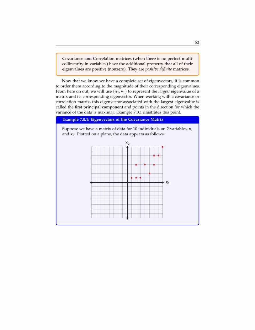
Now that we know we have a complete set of eigenvectors, it is commonto order them according to the magnitude of their corresponding eigenvalues.From here on out, we will use (λ1, v1) to represent the largest eigenvalue of amatrix and its corresponding eigenvector. When working with a covariance orcorrelation matrix, this eigenvector associated with the largest eigenvalue iscalled the first principal component and points in the direction for which thevariance of the data is maximal. Example 7.0.1 illustrates this point.

Example 7.0.1: Eigenvectors of the Covariance Matrix

Suppose we have a matrix of data for 10 individuals on 2 variables, x1and x2. Plotted on a plane, the data appears as follows:

x2

x1

53

Our data matrix for these points is:

X =

1 12 12 43 14 45 26 46 67 68 8

the means of the variables in X are:

x =

(4.43.7

).

When thinking about variance directions, our first step should be tocenter the data so that it has mean zero. Eigenvectors measure thespread of data around the origin. Variance measures spread of dataaround the mean. Thus, we need to equate the mean with the origin.To center the data, we simply compute

Xc = X− exT =

1 12 12 43 14 45 26 46 67 68 8

−

4.4 3.74.4 3.74.4 3.74.4 3.74.4 3.74.4 3.74.4 3.74.4 3.74.4 3.74.4 3.7

=

−3.4 −2.7−2.4 −2.7−2.4 0.3−1.4 −2.7−0.4 0.30.6 −1.71.6 0.31.6 2.32.6 2.33.6 4.3

.

Examining the new centered data, we find that we’ve only translatedour data in the plane - we haven’t distorted it in any fashion.

54

x2

x1

Thus the covariance matrix is:

Σ =19(XT

c Xc) =

(5.6 4.84.8 6.0111

)The eigenvalue and eigenvector pairs of Σ are (rounded to 2 decimalplaces) as follows:

(λ1, v1) =

(10.6100,

[0.690.72

])and (λ2, v2) =

(1.0012,

[−0.720.69

])Let’s plot the eigenvector directions on the same graph:

x2

x1

v1

v2

55

The eigenvector v1 is called the first principal component. It is the di-rection along which the variance of the data is maximal. The eigenvectorv2 is the second principal component. In general, the second principalcomponent is the direction, orthogonal to the first, along which thevariance of the data is maximal (in two dimensions, there is only onedirection possible.)

Why is this important? Let’s consider what we’ve just done. We startedwith two variables, x1 and x2, which appeared to be correlated. We thenderived new variables, v1 and v2, which are linear combinations of the originalvariables:

v1 = 0.69x1 + 0.72x2 (7.1)

v2 = −0.72x1 + 0.69x2 (7.2)

These new variables are completely uncorrelated. To see this, let’s representour data according to the new variables - i.e. let’s change the basis fromB1 = [x1, x2] to B2 = [v1, v2].

Example 7.0.2: The Principal Component Basis

Let’s express our data in the basis defined by the principal components.We want to find coordinates (in a 2× 10 matrix A) such that our original(centered) data can be expressed in terms of principal components. Thisis done by solving for A in the following equation (see Chapter 4 andnote that the rows of X define the points rather than the columns):

Xc = AVT (7.3)

−3.4 −2.7−2.4 −2.7−2.4 0.3−1.4 −2.7−0.4 0.30.6 −1.71.6 0.31.6 2.32.6 2.33.6 4.3

=

a11 a12a21 a22a31 a32a41 a42a51 a52a61 a62a71 a72a81 a82a91 a92

a10,1 a10,2

(vT

1vT

2

)(7.4)

Conveniently, our new basis is orthonormal meaning that V is anorthogonal matrix, so

A = XV.

56

The new data coordinates reflect a simple rotation of the data aroundthe origin:

v1

v2

Visually, we can see that the new variables are uncorrelated. You maywish to confirm this by calculating the covariance. In fact, we can dothis in a general sense. If A = XcV is our new data, then the covariancematrix is diagonal:

ΣA =1

n− 1ATA

=1

n− 1(XcV)T(XcV)

=1

n− 1VT((XT

c Xc)V

=1

n− 1VT((n− 1)ΣX)V

= VT(ΣX)V

= VT(VDVT)V

= D

Where ΣX = VDVT comes from the diagonalization in Theorem 7.0.1.By changing our variables to principal components, we have managedto “hide” the correlation between x1 and x2 while keeping the spa-cial relationships between data points in tact. Transformation back tovariables x1 and x2 is easily done by using the linear relationships inEquations 7.1 and 7.2.

7.1. Comparison with Least Squares 57

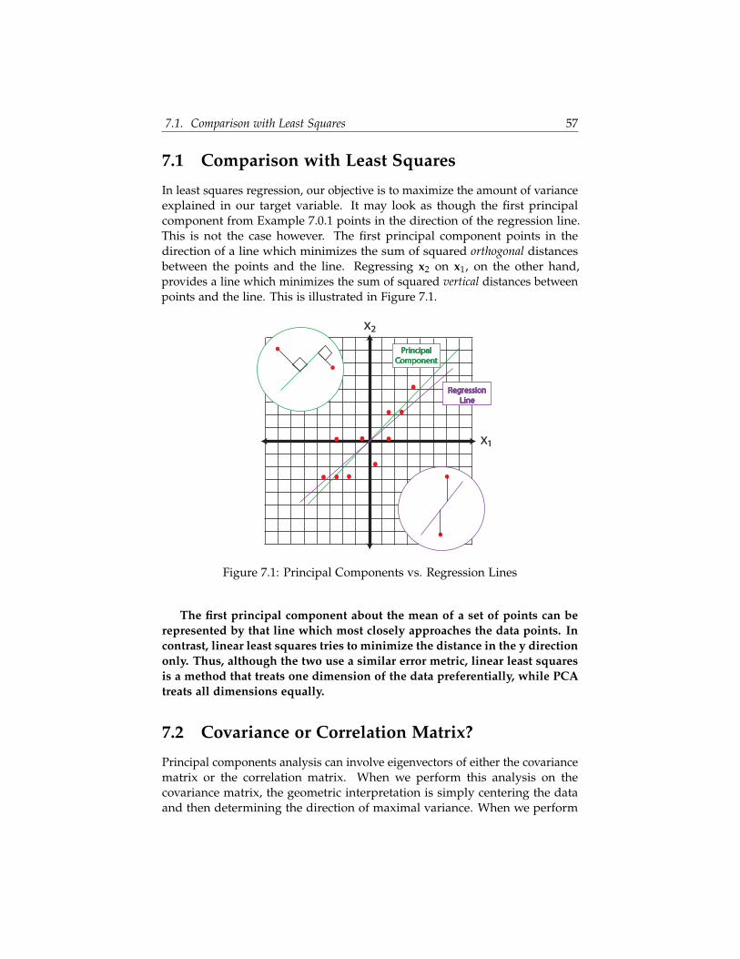
7.1 Comparison with Least Squares

In least squares regression, our objective is to maximize the amount of varianceexplained in our target variable. It may look as though the first principalcomponent from Example 7.0.1 points in the direction of the regression line.This is not the case however. The first principal component points in thedirection of a line which minimizes the sum of squared orthogonal distancesbetween the points and the line. Regressing x2 on x1, on the other hand,provides a line which minimizes the sum of squared vertical distances betweenpoints and the line. This is illustrated in Figure 7.1.

x2

x1

Principal Component

RegressionLine

Figure 7.1: Principal Components vs. Regression Lines

The first principal component about the mean of a set of points can berepresented by that line which most closely approaches the data points. Incontrast, linear least squares tries to minimize the distance in the y directiononly. Thus, although the two use a similar error metric, linear least squaresis a method that treats one dimension of the data preferentially, while PCAtreats all dimensions equally.

7.2 Covariance or Correlation Matrix?

Principal components analysis can involve eigenvectors of either the covariancematrix or the correlation matrix. When we perform this analysis on thecovariance matrix, the geometric interpretation is simply centering the dataand then determining the direction of maximal variance. When we perform

7.3. Applications of Principal Components 58

this analysis on the correlation matrix, the interpretation is standardizing thedata and then determining the direction of maximal variance. The correlationmatrix is simply a scaled form of the covariance matrix. In general, these twomethods give different results, especially when the scales of the variables aredifferent.

The covariance matrix is the default for R. The correlation matrix is thedefault in SAS. The covariance matrix method is invoked by the option:

proc princomp data=X cov;var x1--x10;run;

Choosing between the covariance and correlation matrix can sometimespose problems. The rule of thumb is that the correlation matrix should be usedwhen the scales of the variables vary greatly. In this case, the variables with thehighest variance will dominate the first principal component. The argumentagainst automatically using correlation matrices is that it is quite a brutal wayof standardizing your data.

7.3 Applications of Principal Components

Principal components have a number of applications across many areas ofstatistics. In the next sections, we will explore their usefulness in the context ofdimension reduction. In Chapter 9 we will look at how PCA is used to solvethe issue of multicollinearity in biased regression.

7.3.1 PCA for dimension reduction

It is quite common for an analyst to have too many variables. There are twodifferent solutions to this problem:

1. Feature Selection: Choose a subset of existing variables to be used in amodel.

2. Feature Extraction: Create a new set of features which are combinationsof original variables.

Feature Selection

Let’s think for a minute about feature selection. What are we really doing whenwe consider a subset of our existing variables? Take the two dimensional datain Example 7.0.2 (while two-dimensions rarely necessitate dimension reduction,the geometrical interpretation extends to higher dimensions as usual!). Thecentered data appears as follows:


x2

x1

Now say we perform some kind of feature selection (there are a number ofways to do this, chi-square tests for instances) and we determine that thevariable x2 is more important than x1. So we throw out x2 and we’ve reducedthe dimensions from p = 2 to k = 1. Geometrically, what does our new datalook like? By dropping x1 we set all of those horizontal coordinates to zero. Inother words, we project the data orthogonally onto the x2 axis:

x2

x1

(a) Projecting Data Orthogonally

x2

x1

(b) New One-Dimensional Data

Figure 7.2: Geometrical Interpretation of Feature Selection

Now, how much information (variance) did we lose with this projection?The total variance in the original data is

‖x1‖2 + ‖x2‖2.

The variance of our data reduction is

‖x2‖2.


Thus, the proportion of the total information (variance) we’ve kept is

‖x2‖2

‖x1‖2 + ‖x2‖2 =6.01

5.6 + 6.01= 51.7%.

Our reduced dimensional data contains only 51.7% of the variance of theoriginal data. We’ve lost a lot of information!

The fact that feature selection omits variance in our predictor variablesdoes not make it a bad thing! Obviously, getting rid of variables which haveno relationship to a target variable (in the case of supervised modeling likeprediction and classification) is a good thing. But, in the case of unsupervisedlearning techniques, where there is no target variable involved, we must beextra careful when it comes to feature selection. In summary,

• Feature Selection is important. Examples include:

– Removing variables which have little to no impact on a target vari-able in supervised modeling (forward/backward/stepwise selec-tion).

– Removing variables which have obvious strong correlation withother predictors.

– Removing variables that are not interesting in unsupervised learning(For example, you may not want to use the words “th” and “of”when clustering text).

• Feature Selection is an orthogonal projection of the original data onto thespan of the variables you choose to keep.

• Feature selection should always be done with care and justification.

– In regression, could create problems of endogeneity (errors corre-lated with predictors - omitted variable bias).

– For unsupervised modelling, could lose important information.

Feature Extraction

PCA is the most common form of feature extraction. The rotation of the spaceshown in Example 7.0.2 represents the creation of new features which arelinear combinations of the original features. If we have p potential variablesfor a model and want to reduce that number to k, then the first k principalcomponents combine the individual variables in such a way that is guaranteedto capture as much “information” (variance) as possible. Again, take ourtwo-dimensional data as an example. When we reduce our data down to one-dimension using principal components, we essentially do the same orthogonalprojection that we did in Feature Selection, only in this case we conduct that


projection in the new basis of principal components. Recall that for this data,our first principal component v1 was

v1 =

(0.690.73

).

Projecting the data onto the first principal component is illustrated in Figure7.3 How much variance do we keep with k principal components? The pro-

x2

x1

v1

(a) Projecting Data Orthogonally

x2

x1

v1

(b) New One-Dimensional Data

Figure 7.3: Illustration of Feature Extraction via PCA

portion of variance explained by each principal component is the ratio of thecorresponding eigenvalue to the sum of the eigenvalues (which gives the totalamount of variance in the data).

Theorem 7.3.1: Proportion of Variance Explained

The proportion of variance explained by the projection of the data ontoprincipal component vi is

λi

∑pj=1 λj

.

Similarly, the proportion of variance explained by the projection of thedata onto the first k principal components (k < j) is

∑ki=1 λi

∑pj=1 λj

In our simple 2 dimensional example we were able to keep

λ1

λ1 + λ2=

10.6110.61 + 1.00

= 91.38%

of our variance in one dimension.

62

CHAPTER 8

SINGULAR VALUE DECOMPOSITION (SVD)

The Singular Value Decomposition (SVD) is one of the most important conceptsin applied mathematics. It is used for a number of application includingdimension reduction and data analysis. Principal Components Analysis (PCA)is a special case of the SVD. Let’s start with the formal definition, and then seehow PCA relates to that definition.

Definition 8.0.1: Singular Value Decomposition

For any m× n matrix A with rank(A) = r, there are orthogonal matricesUm×m and Vn×n and a diagonal matrix Dr×r = diag(σ1, σ2, . . . , σr) suchthat

A = U(

D 00 0

)︸︷︷︸

m× n

VT with σ1 ≥ σ2 ≥ · · · ≥ σr ≥ 0 (8.1)

The σi’s are called the nonzero singular values of A. (Whenr < p = min{m, n} (i.e. when A is not full-rank), A is said to havean additional p− r zero singular values). This factorization is calleda singular value decomposition of A, and the columns of U andV are called the left- and right-hand singular vectors for A, respectively.

Properties of the SVD

• The left-hand singular vectors are a set of orthonormal eigenvec-tors for AAT .

• The right-hand singular vectors are a set of orthonormal eigenvec-tors for ATA.

8.1. Resolving a Matrix into Components 63

• The singular values are the square roots of the eigenvalues forATA and AAT , as these matrices have the same eigenvalues.

When we studied PCA, one of the goals was to find the new coordinates, orscores, of the data in the principal components basis. If our original (centeredor standardized) data was contained in the matrix X and the eigenvectors ofthe covariance/correlation matrix (XTX) were columns of a matrix V, then tofind the scores (call these S) of the observations on the eigenvectors we usedthe following equation:

X = SVT .

This equation mimics Equation 8.1 because the matrix VT in Equation 8.1 isalso a matrix of eigenvectors for ATA. This means that the principal componentscores S are a set of unit eigenvectors for AAT scaled by the singular values inD:

S = U(

D 00 0

).

8.1 Resolving a Matrix into Components

One of the primary goals of the singular value decomposition is to resolvethe data in A into r mutually orthogonal components by writing the matrixfactorization as a sum of outer products using the corresponding columns ofU and rows of VT :

A = U(

D 00 0

)VT =

(u1 u2 . . . um

)

σ1 0 . . . 0 0

0. . . 0

... 0... 0 σr 0

...0 0 0 0 0...

......

......

0 0 0 0 0

vT

1vT

2...

vTn

= σ1u1vT1 + σ2u2vT

2 + · · ·+ σrurvTr .

σ1 ≥ σ2 ≥ . . . σr

For simplicity, let Zi = uivTi act as basis matrices for this expansion, so we have

A =r

∑i=1

σiZi. (8.2)

This representation can be regarded as a Fourier expansion. The coefficient(singular value) σi can be interpreted as the proportion of A lying in the


“direction" of Zi. When σi is small, omitting that term from the expansion willcause only a small amount of the information in A to be lost. This fact hasimportant consequences for compression and noise reduction.

8.1.1 Data Compression

We’ve already seen how PCA can be used to reduce the dimensions of ourdata while keeping the most amount of variance. The way this is done is bysimply ignoring those components for which the proportion of variance issmall. Supposing we keep k principal components, this amounts to truncatingthe sum in Equation 8.2 after k terms:

A ≈k

∑i=1

σiZi. (8.3)

As it turns out, this truncation has important consequences in many applica-tions. One example is that of image compression. An image is simply an arrayof pixels. Supposing the image size is m pixels tall by n pixels wide, we cancapture this information in an m× n matrix if the image is in grayscale, or anm× 3n matrix for a [r,g,b] color image (we’d need 3 values for each pixel torecreate the pixel’s color). These matrices can get very large (a 6 megapixelphoto is 6 million pixels).

Rather than store the entire matrix, we can store an approximation to thematrix using only a few (well, more than a few) singular values and singularvectors.

This is the basis of image compression. An approximated photo will not beas crisp as the original - some information will be lost - but most of the timewe can store much less than the original matrix and still get a good depictionof the image.

8.1.2 Noise Reduction

Many applications arise where the relevant information contained in a matrixis contaminated by a certain level of noise. This is particularly common withvideo and audio signals, but also arises in text data and other types of (usuallyhigh dimensional) data. The truncated SVD (Equation 8.3) can actually reducethe amount of noise in data and increase the overall signal-to-noise ratio undercertain conditions.

Let’s suppose, for instance, that our matrix Am×n contains data which iscontaminated by noise. If that noise is assumed to be random (or nondirec-tional) in the sense that the noise is distributed more or less uniformly acrossthe components Zi, then there is just as much noise “in the direction” of one Zias there is in the other. If the amount of noise along each direction is approx-imately the same, and the σi’s tell us how much (relevant) information in A


is directed along each component Zi, then it must be that the ratio of “signal”(relevant information) to noise is decreasing across the ordered components,since

σ1 ≥ σ2 ≥ · · · ≥ σr

implies that the signal is greater in earlier components. So letting SNR(σiZi)denote the signal-to-noise ratio of each component, we have

SNR(σ1Z1) ≥ SNR(σ2Z2) ≥ · · · ≥ SNR(σrZr)

This explains why the truncated SVD,

A ≈k

∑i=1

σiZi where k < r

can, in many scenarios, filter out some of the noise without losing much of thesignificant information in A.

8.1.3 Latent Semantic Indexing

Text mining is another area where the SVD is used heavily. In text mining, ourdata structure is generally known as a Term-Document Matrix. The documentsare any individual pieces of text that we wish to analyze, cluster, summarize ordiscover topics from. They could be sentences, abstracts, webpages, or socialmedia updates. The terms are the words contained in these documents. Theterm-document matrix represents what’s called the “bag-of-words” approach -the order of the words is removed and the data becomes unstructured in thesense that each document is represented by the words it contains, not the orderor context in which they appear. The (i, j) entry in this matrix is the number oftimes term j appears in document i.

Definition 8.1.1: Term-Document Matrix

Let m be the number of documents in a collection and n be the numberof terms appearing in that collection, then we create our term-document


matrix A as follows:

term 1 term j term n

Am×n =

Doc 1

Doc i

Doc m

|||

− − fij

where fij is the frequency of term j in document i. A binary term-document matrix will simply have Aij = 1 if term j is contained indocument i.

Term-document matrices tend to be large and sparse. Term-weightingschemes are often used to downplay the effect of commonly used words andbolster the effect of rare but semantically important words. The most popularweighting method is known as “Term Frequency-Inverse Document Frequency”(TF-IDF). For this method, the raw term-frequencies fij in the matrix A aremultiplied by global weights (inverse document frequencies), wj, for each term.These weights reflect the commonality of each term across the entire collection.The inverse document frequency of term i is:

wj = log(

total # of documents# documents containing term j

)To put this weight in perspective for a collection of n = 10, 000 documentswe have 0 ≤ wj ≤ 9.2, where wj = 0 means the word is contained in everydocument (i.e. it’s not important semantically) and wj = 9.2 means the wordis contained in only 1 document (i.e. it’s quite important). The documentvectors are often normalized to have unit 2-norm, since their directions (nottheir lengths) in the term-space is what characterizes them semantically.

The noise-reduction property of the SVD was extended to text processing in1990 by Susan Dumais et al, who named the effect Latent Semantic Indexing (LSI).LSI involves the singular value decomposition of the term-document matrixdefined in Definition 8.1.1. In other words, it is like a principal componentsanalysis using the unscaled, uncentered inner-product matrix ATA. If thedocuments are normalized to have unit length, this is a matrix of cosinesimilarities (see Chapter 2). In text-mining, the cosine similarity is the mostcommon measure of similarity between documents. If the term-documentmatrix is binary, this is often called the co-occurrence matrix because eachentry gives the number of times two words occur in the same document.

It certainly seems logical to view text data in this context as it containsboth an informative signal and semantic noise. LSI quickly grew roots in the


information retrieval community, where it is often used for query process-ing. The idea is to remove semantic noise, due to variation and ambiguityin vocabulary and presentation style, without losing significant amounts ofinformation. For example, a human may not differentiate between the words“car” and “automobile”, but indeed the words will become two separate entitiesin the raw term-document matrix. The main idea in LSI is that the realignmentof the data into fewer directions should force related documents (like thosecontaining “car” and “automobile”) closer together in an angular sense, thusrevealing latent semantic connections.

Purveyors of LSI suggest that the use of the Singular Value Decomposition toproject the documents into a lower-dimensional space results in a representationwhich reflects the major associative patterns of the data while ignoring lessimportant influences. This projection is done with the simple truncation of theSVD shown in Equation 8.3.

As we have seen with other types of data, the very nature of dimensionreduction makes possible for two documents with similar semantic propertiesto be mapped closer together. Unfortunately, the mixture of signs (positiveand negative) in the singular vectors (think principal components) makesthe decomposition difficult to interpret. While the major claims of LSI arelegitimate, this lack of interpretability is still conceptually problematic forsome folks. In order to make this point as clear as possible, consider theoriginal “term basis” representation for the data, where each document (froma collection containing m total terms in the dictionary) could be written as:

Aj =m

∑i=1

fijei

where fij is the frequency of term i in the document, and ei is the ith column ofthe m×m identity matrix. The truncated SVD gives us a new set of coordinates(scores) and basis vectors (principal component features):

Aj ≈r

∑i=1

αiui

but the features ui live in the term space, and thus ought to be interpretableas a linear combination of the original “term basis.” However the linearcombination, having both positive and negative coefficients, is semanticallymeaningless in context - These new features cannot, generally, be thought of asmeaningful topics.

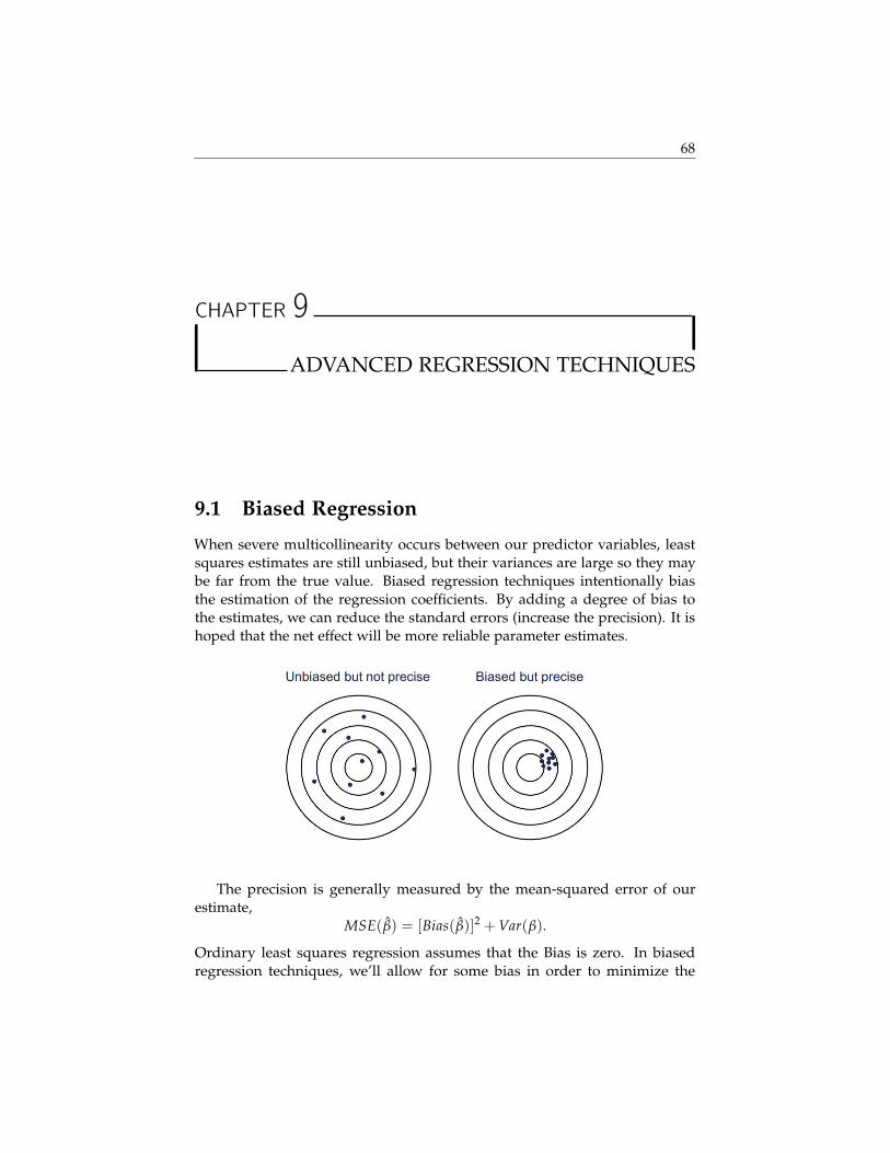
68

CHAPTER 9

ADVANCED REGRESSION TECHNIQUES

9.1 Biased Regression

When severe multicollinearity occurs between our predictor variables, leastsquares estimates are still unbiased, but their variances are large so they maybe far from the true value. Biased regression techniques intentionally biasthe estimation of the regression coefficients. By adding a degree of bias tothe estimates, we can reduce the standard errors (increase the precision). It ishoped that the net effect will be more reliable parameter estimates.

The precision is generally measured by the mean-squared error of ourestimate,

MSE(β) = [Bias(β)]2 + Var(β).

Ordinary least squares regression assumes that the Bias is zero. In biasedregression techniques, we’ll allow for some bias in order to minimize the

9.1. Biased Regression 69

variance of our estimate.Ideally, the criteria for deciding when biased regression techniques are

better than OLS depends on the true values of the parameters (i.e. we cannoteven estimate the bias in our parameter estimates). Since this is not possible,there is no completely objective way to decide. Principal Components Regres-sion (PCR) and Ridge Regression are two such techniques. Ridge regressiontends to be the more popular of the two methods, but PCR is a little morestraightforward.

9.1.1 Principal Components Regression (PCR)

As we saw in Chapter 7, every linear regression model can be restated in termsof a new set of orthogonal predictor variables that are a linear combination ofthe original variables - principal components. Let x1, x2, . . . xp be our predictorvariables. Then the principal components (PCs) are just linear combinationsof these predictor variables with coefficients from the rows of the eigenvectormatrix:

PCj = v1jx1 + v2jx2 + · · ·+ vpjxp

The variance-covariance matrix of the principal components is diagonal(diag(λ1, . . . , λp)) because the principal components are orthogonal. If λj = 0then the corresponding PC has no variance (i.e. constant). This reveals linearstructure in variables. For example, suppose one of our principal componentsis

PC2 = −0.5x1 + 2x2 with corresponding eigenvalue λ2 = 0

This means that when we subtract 2x2 − 0.5x1 in the original data, the resulthas zero variability. It is constant for every observation. Thus, it must be thatfor all observations x2 is completely determined by x1 and vice-versa. The twovariables are perfectly correlated. When λj is nearly zero, we are very close tothe same situation, which violates the assumptions of our regression model.Let’s look at an applied example.

Example: French Economy

We are going to examine data from the French economy reported by Malinvaud(1968).

• The Variables:

1. Imports (Target)

2. Domestic Production

3. Stock Formation

4. Domestic Consumption


• All measured in billions of French francs between 1949 and 1966.

Lets try to run a simple linear regression to predict Imports using the 3predictor variables above. We are assuming there is some underlying insistenceto understand the relationship of all three variables on Imports - we do notwant to drop any variables from the analysis. When we run the regression, weshould always pay attention the the Variance Inflation Factors (VIFs) to see ifany multicollinearity is affecting the variability in our parameter estimates.

proc reg data=advanced.french;model Import = DoProd Stock Consum / vif;

run;quit;

proc princomp data=advanced.french out=frenchPC;var DoProd Stock Consum;

run;

The VIF output from the regression model clearly indicates strong multi-collinearity. The principal component output in Figure 9.1 makes it clear thatthe difference between two of our variables is essentially constant or has novariability, illuminating the exact source of that multicollinearity.

Figure 9.1: SAS Output

Domestic Consumption is essentially equal to Domestic Production. Thisis something that matches with realistic expectations. Now there is a “new”set of variables (the PCs) that are orthogonal to each other. Does this newset of variables eliminate multicollinearity concerns? No! In the first modellisted in the next block of code (PC Model 1), we have not really changed


anything! We’ve just rotated our data. Using all 3 principal components we arenot incorporating bias into the model or removing the multicollinearity - weare just hiding it! It isn’t until we drop some of the PCs (the second model) thatwe are able to introduce bias and eliminate the underlying multicollinearity.

/* First must standardize our dependent variable. *//* be aware on covariance vs. correlation PCA! *//* what would be the difference? */

proc standard data=frenchPC mean=0 std=1 out=frenchPC2;var Import;

run;

proc reg data=frenchPC2;PC Model 1: model Import = Prin1 Prin2 Prin3 /vif;PC Model 2: model Import = Prin1 Prin2 /vif;

run;quit;

In order to compute meaningful coefficients we have to do some algebraand take into account the standard errors of our variables (because both theindependent variables and the dependent variables were centered and scaledwhen forming the principal components - there is a difference here if you usethe covariance matrix, so understand and be careful!):

Y = α1PC1 + α2PC2 + · · ·+ αpPCp + ε

PCj = v1jx1 + v2jx2 + · · ·+ vpjxp

Y = β0 + β1x1 + · · ·+ βpxp + ε

Where

β j =sy

sxj

(vj1α1 + vj2α2 + · · ·+ vjpαp)

β0 = Y− β1 x1 − · · · − βp xp

SAS can actually do this in PROC PLS (Partial Least Squares) as demon-strated in the next block of code. The caveat is that this procedure can onlydrop the later PCs keeping the first nfac=n components. Usually this is infact what you want to accomplish unless you have a principal component thatis being driven by some variable that is not significant in your model andyou wish to drop that component but keep others after it. In such cases, thecoefficients will have to be computed by hand.

proc pls data=advanced.french method=pcr nfac=2;model Import= DoProd Stock Consum /solution;

run;quit;


PCR - Cautions

PCR may not always work, in the sense that it may have trouble explainingvariability in the response variable. You should never blindly drop PCs - youshould always be using the justifications set forth above. Outliers / influentialobservations can severely distort the principal components because they alterthe variance-covariance matrix - you should be aware of this fact and alwaysexamine your principal components.

9.1.2 Ridge Regression

Ridge regression is a biased regression technique to use in the presence ofmulticollinearity. Produces estimates that tends to have lower MSE (but higherbias) than OLS estimates. Works with standardized values for each of thevariables in the model (similar to PCR):

Y = θ1 x1 + θ2 x2 + · · ·+ θp xp

where Y, x represent the standardized values. Recall that solving for OLSestimates involves the normal equations:

ZTZθ = ZTY

Rearranging the normal equations leads to the following way to solve for theOLS estimates.

θ1 + r12θ2 + · · ·+ r1pθp = r1y

r21θ1 + θ2 + · · ·+ r2pθp = r2y

. . . = . . .

rp1θ1 + rp2θ2 + · · ·+ θp = rpy

where rij is the correlation between predictors i and j (so rij = rji) and rjy isthe correlation between the response and predictor j.

Ridge Adjustments Solving for ridge estimates involves changing the normalequations to

ZTZθ = ZTY −→ (ZTZ + kI)θR = ZTY

Rearranging the changed normal equations leads to the following way to solvefor the ridge estimates:

(1 + k)θ1 + r12θ2 + · · ·+ r1pθp = r1y

r21θ1 + (1 + k)θ2 + · · ·+ r2pθp = r2y

. . . = . . .

rp1θ1 + rp2θ2 + · · ·+ (1 + k)θp = rpy


The higher the value of k, the more bias is introduced in the estimates of themodel. The hardest part about ridge regression is choosing the appropriatevalue of k because many different ways have been proposed over the years:

• Fixed Point (1975 by Hoerl, Kennard, Baldwin)

k =pσ2

∑pi=1 θ2

i,OLS

where σ2 is the MSE for the model. This is one of the most popularestimates, sometimes referred to as HKB estimate.

• Iterative Method (1976 by Hoerl, Kennard)

k0 =pσ2

∑pi=1 θ2

i,OLS

k1 =pσ2

∑pi=1 θ2

i,k0

kn =pσ2

∑pi=1 θ2

i,kn−1

This is repeated until the change is negligible. In practice, we expecttaking very few iterations.

• Ridge Trace

– Plot of many different estimates of θi across a series of k values.

– Use the plot to approximate when the estimates become stable.

Example: Fixed Point Method

The code below highlights the method for implementing the Fixed Pointmethod in SAS. Here we create macro variables to represent the MSE of themodel and the value for k. The MSE of the model will be used for implementingthe Iterative Method. The last PROC REG statement outputs the VIFs, thestandard errors for the betas (SEB) and the parameter estimates to the outputdata set ’B’. The reason we must output these parameters to a dataset is thatthe SAS output will not show the VIF values for the ridge regression, onlyfrom the ordinary OLS model. The RIDGE option allows us to use our macrovariable for the parameter k.

proc standard data=advanced.french mean=0 std=1 out=frenchstd;var Import DoProd Stock Consum;

run;


proc reg data=frenchstd outest=B;model Import = DoProd Stock Consum / vif;

run;quit;

data _null_;set B;call symput(’MSE’ , RMSE**2);call symput(’k’, 3*RMSE**2/(DoProd**2+Stock**2+Consum**2));

run;

proc reg data=frenchstd outvif outseb outest=B ridge=&k;model Import = DoProd Stock Consum / vif;

run;quit;

Example: Iterative Method

The code for the iterative method simply extends the code for the fixed pointmethod. We again create macro variables to represent the MSE of the modeland the resulting value for k.


run;quit;

proc print data=B;run;

data _null_;set B;where _TYPE_=’RIDGE’;call symput(’k’, 3*&MSE / (DoProd**2+Stock**2+Consum**2));

run;


run;quit;



This code would be repeated using the latest ridge model. In practice, wedon’t often need to go beyond a few iterations before witnessing convergence.In this example, the VIF values drop below 1 in the second iteration which issomething we have to be careful about - we probably do not want to use thisiteration.

Example: Ridge Trace Method

The Ridge Trace method is implemented by simply inputting the RIDGEparameter as a sequence as shown below:

proc reg data=frenchstd outvif outest=B ridge=0 to 0.08 by 0.002;model Import = DoProd Stock Consum / vif;

run;quit;

proc reg data=frenchstd outvif outseb outest=B ridge=0.04;model Import = DoProd Stock Consum / vif;

run;quit;


The code above will output the VIF values and the standardized coefficientsfor each variable in the model for a range of values of k. These values are givenin the output plots shown in Figure 9.2. The goal is to choose a value for kwhere the lines on the graph become approximately horizontal.

Ridge Regression- Cautions

Due to the uncertainty of how to calculate k, there are some that dislike theuse of ridge regression (or any other bias regression technique). Both PrincipleComponents regression and Ridge regression should be used as a last casescenario. Deleting or combining variables is preferred because it doesn’tintroduce bias. These methods, however, should not be shunned.


Figure 9.2: SAS Output: Ridge Regression with Ridge Trace Method

MASTER OF SCIENCE IN ANALYTICS 2014 EMPLOYMENT REPORTslrace/LinearAlgebra.pdf · MASTER OF SCIENCE...

Documents

Transcript of MASTER OF SCIENCE IN ANALYTICS 2014 EMPLOYMENT REPORTslrace/LinearAlgebra.pdf · MASTER OF SCIENCE...