Master Erasmus Mundus in Computational Mechanics …€¦ · Master Erasmus Mundus in Computational...

Master Erasmus Mundus in Computational Mechanics

Institut de Recherche en Génie Civil et Mécanique

Prediction of

Laminates

Loadings



Prediction of

Laminates under

Loadings

Damage Evolution


2008/2010

Ecole Centrale de Nantes


MASTER

Prediction of Delamination

under Quasi

Loadings with

Damage Evolution

Presented &

Pubudu Sampath Ranaweera

Thesis Advis

Prof. Laurent Gornet


Nantes, June 2010


2008/2010



MASTER THESIS

Delamination

Quasi-

with Local

Damage Evolution

Presented & Submitted By


Thesis Advised By



Nantes, June 2010


2008/2010



THESIS

Delamination in

-Static

Local / Non

Damage Evolution

Submitted By


ed By



Nantes, June 2010



in Composite

Static and Fatigue

Non-local

Damage Evolution



Composite

Fatigue

local

Composite

Fatigue

II

Abstract

Composites are materials that are composed of two or more distinct phases. Importantly, these phases shall not dissolve or blend with each other and remain distinct on a macroscopic level. However, mechanical and physical properties of each phase would differ from each other. Here, the challenge is to combine properties of each phase in a systematic manner to form the most efficient material for the intended application. Among many classes of advanced composite materials, fibrous composite laminates have been the most preferred option for structural applications. The inherent anisotropy and the brittle characteristics of composite laminates result in failure mechanisms that are very different from those of homogeneous monolithic materials. Among all different failure mechanisms, ‘Delamination’ is considered to be the most prominent mode of failure in fiber-reinforced laminates as a result of their relatively weak inter-laminar strength. When laminated composites are subjected to static, dynamic or cyclic loadings, the inter-laminar adhesion strength between individual plies tends to deteriorate significantly and act as the origin of the final failure. Therefore, an efficient and reliable design tool capable of predicting delamination would certainly improve the designs based on composite laminates. The present study is focused on taking a step forward in this respect.

The main objectives of this thesis work is to study an existing design tool [Allix O. and Ladevèze P., 1994; Gornet L., 1996; Ijaz H., 2009] and then to enhance it further to predict initiation and propagation of delamination under both quasi-static (i.e., monotonic) and fatigue (i.e., cyclic) loading conditions. The existing tool has been orginally formulated within the framework of Damage Mechanics Therefore, in the present work much attention has been devoted to improve its functionality and versatility by studying Damage Mechanics formulations. However, Fracture Mechanics also play a key role in determining the damage model.The key idea here is to use Fracture Mechanics test results to determine parameters of the Damage Mechanics model. Therefore, these damage models basically link Fracture Mechanics to Damage Mechanics.

The work presented in this report is organized in to four main parts. PART-I, also called ‘Preamble’ comprises two main chapters, Chapter 1 and Chapter 2. In Chapter 1, at first, a general introduction is given on Composites, focusing especially on their advantages and applications. Next, information on general failure mechanisms associated to composites laminates is also presented. In additon, a brief discussion is made on the delamination phenomena in laminated composites. Next, a synopsis of state-of-the-art modelling tools (based on Fracture and/or Damage Mechanics) for predicting delamination is also presented. In Chapter 2, a review has been made on the existing interface damage model which is based on meso-modelling concept. In addition, a detailed description of the constitutive equation and the methodology adopted for FE implementation is also included.

PART-II is dedicated for the study performed on ‘Delamination under Quasi-static Loading’. It is also comprised of two major chapters, Chapter 3 and Chapter 4. Chapter 3 mainly contains formulations of the static damage model. Note that, the existing model is inherently local, meaning that it is mesh dependent. Therefore, to overcome such spurious localizations, existing theories on regularization methodologies were studied and reported. Chapter 4 includes detailed descriptions on FE simulations performed using static damage models (i.e., local and proposed nonlocal). At first, the local model’s effectiveness was tested in all dimensional spaces with appropriate modifications for static loading condition. Identification of model parameters and preliminary investigation results followed by main investigation results are detailed out comprehensively. Next, a nonlocal integral-type regularization scheme was introduced to overcome the spurious localization problem associated to the existing local model. Special attention was devoted to improve the FE formulation of the nonlocal model to reduce computational cost. Details of complete formulation, simulations procedures and all investigations results with accompanying conclusions are included.

PART-III of the report is dedicated for the study on ‘Delamination under Fatigue Loading’. Once more, it is comprised of two chapters, Chapter 5 and Chapter 6. Chapter 5 starts with an overview of fatigue and related theories associated to composite laminates. Then after, it includes an introduction of a new fatigue damage evolution law, its derivation and implementation. The existing local model was used as a platform to build the new fatigue model. Chapter 6 includes details of FE simulations performed to validate the proposed fatigue damage model. Versatility of the fatigue model was also checked for different mode-ratios. Procedure of identification of model parameters, simulation results and accompaying conclusions are also deatiled out completely. Finally, a summary of conclusions of the present work is included in Chapter 7 under PART-IV, titled as ‘Closure’.

III

Acknowledgements

The subject of this thesis started from the ideas of my thesis advisor, Prof. Laurent Gornet. His excellent ideas, advice and guidance were invaluable for the completion of this work and I render special thanks to him. In addition, I am also grateful for his continuous support and encouragements throughout my Master's degree.

I would like to express my gratitude to Dr. Hassan Ijaz for his support, comments and valuable contributions that were very constructive. In addition, I am also grateful to Mr. Kamran-Ali Syed for his continuous interest and valuable suggestions rendered at crucial stages of the thesis work.

A special token of appreciation is also extended towards the organizers of the Erasmus Mundus masters program and in particular the consortium of Erasmus Mundus Computational Mechanics for rendering me the opportunity to begin my postgraduate studies in Europe. In addition, I would also like to express my thanks to European Commission for awarding financial assistance for my stay and studies.

I am very thankful to all the lecturers in University of Swansea, Wales and Ecole Centrale de Nantes for their invaluable efforts and guidance to enhance my knowledge in the field of Computational Mechanics. It was very instrumental in helping me to successfully complete my thesis work. Special thanks to both Prof. Nicolas Möes and Prof. Chevaugeon Nicolas for their tremendous dedication and efforts in coordinating all the activities of the Masters program at Ecole Centrale. I am also thankful to the GEM laboratory for the technical support given throughout the thesis work.

I would also like to thank Dr. Pierre Charrier and Eng. Denis Taveau for their invaluable advice and guidance given to me during my internship at Trelleborg MODYN in Nantes.

It is with great pleasure and gratitude I thank all the international officers headed by Anne-Laure Frémondière at Ecole Centrale de Nantes for their tremendous continuing support to make my stay in France a memorable one. I equally thank all the administrative staff of Swansea University, Wales for their support and guidance during first part of the Masters degree in United-Kingdom.

Life in Europe became more wonderful by the friendships I've developed with people all over the world. Khalid, Hasnat, Shiyee, Jianhui, Sudarshan, Rehan, Sebastian, Dibakar, Saeid, Violette, Jacobo, Fazik, Prabu, Amith, Shoapu and many others whom I express my gratitude and my apologies for not being able to mention here.

Last but not least, I am very grateful to my parents, my sister Dinusha and my lovely wife Piumanthi for their continuous support and encouragements.

This thesis is dedicated to my parents, Mrs. Jayanthi Ranaweera and late Mr. Hemachandra Ranaweera.

IV

Contents

Abstract .................................................................................................................................................. II

Acknowledgements ............................................................................................................................. III

Contents ................................................................................................................................................ IV

List of Figures ...................................................................................................................................... VI

List of Tables ...................................................................................................................................... VIII

Nomenclature ....................................................................................................................................... IX

PART – I : Preamble ........................................................................................................................... 1

Chapter 1 : General Introduction ......................................................................................................... 2 1.1 Composites and their Applications ............................................................................................. 2 1.2 Failure Modes of Composite Laminates .................................................................................... 4 1.3 Delamination of Composite Laminates ...................................................................................... 4 1.4 Delamination Modelling with Fracture / Damage Mechanics ..................................................... 5 1.5 Objectives and Scope of Study .................................................................................................. 6

Chapter 2 : Interface Damage Model ................................................................................................... 7 2.1 Meso-Modelling Concept ........................................................................................................... 7 2.2 Constitutive equation for the Interface ....................................................................................... 8 2.3 FE Implementation of Damage Models ...................................................................................... 9

PART – II : Delamination under Quasi-Static Loading ........................................................... 10

Chapter 3 : Static Damage Evolution ............................................................................................... 11 3.1 Energy Formulation .................................................................................................................. 11 3.2 Local Damage Evolution .......................................................................................................... 14 3.3 Regularization Damage Evolution ............................................................................................ 15

3.3.1 Rate-Dependent Damage Evolution ............................................................................ 15 3.3.2 Non-Local Integral-Type Damage Evolution ................................................................ 16

Chapter 4 : Analysis of Static Simulations ....................................................................................... 17 4.1 Analysis Procedure .................................................................................................................. 17 4.2 Identification of Static Damage Model Parameters ................................................................. 18

4.2.1 Identification of Parameter - α .................................................................................... 18

4.2.2 Identification of Initial Interface Rigidities ..................................................................... 19 4.3 Overview of Fracture Mechanics Tests for Delamination ........................................................ 25 4.4 Validation of Static Damage Models ........................................................................................ 26 4.5 Validation of Local Static Damage Model ................................................................................ 27

4.5.1 FE Simulation Details ................................................................................................... 27 4.5.2 Simulation Results for DCB Test ................................................................................. 28 4.5.3 Simulation Results for 3ENF Test ................................................................................ 33

4.6 Validation of Nonlocal Static Damage Model ........................................................................... 37 4.6.1 FE Implementation of Nonlocal Model ......................................................................... 37 4.6.2 Simulation Results on DCB and 3ENF Tests .............................................................. 40 4.6.3 Influence of the Internal Length Scale ......................................................................... 42 4.6.4 Comparison of different Modelling ............................................................................... 43 4.6.5 Comparison of Evolution of Damage Variable ............................................................. 44 4.6.6 Size Effect Prediction using Nonlocal Model ............................................................... 45

V

PART – III : Delamination under Fatigue Loading ................................................................... 46

Chapter 5 : Fatigue Damage Evolution ............................................................................................. 47 5.1 Overview of Fatigue and related Theories ............................................................................... 47 5.2 Proposed Fatigue Damage Evolution Law............................................................................... 49

5.2.1. Static Part of Cyclic Damage Evolution ...................................................................... 49 5.2.2. Fatigue Part of Cyclic Damage Evolution ................................................................... 50 5.2.3. Complete Fatigue Damage Evolution Law ................................................................. 52

Chapter 6 : Analysis of Fatigue Simulations .................................................................................... 53 6.1 Analysis Procedure .................................................................................................................. 53 6.2 Identification of Fatigue Damage Model Parameters ............................................................... 55 6.3 Validation of Proposed Fatigue Damage Model ...................................................................... 55

6.3.1 Experimental Methods ................................................................................................. 55 6.3.2 Finite Element Model ................................................................................................... 57 6.3.3 Simulation Results for DCB Fatigue Test .................................................................... 58 6.3.4 Simulation Results for 3ENF Fatigue Test ................................................................... 60 6.3.5 Simulation Results for MMB Fatigue Test ................................................................... 63 6.3.6 Mixed-Mode Fatigue Failure Prediction ....................................................................... 65

6.4 Effects of Fatigue Model Parameters ....................................................................................... 69

6.4.1 Influence of Parameter - N∆ ...................................................................................... 69

6.4.2 Influence of Parameters - C & β ............................................................................... 70

PART – IV : Closure ......................................................................................................................... 71

Chapter 7 : General Conclusions ...................................................................................................... 72 7.1 Delamination under Quasi-Static Loading ............................................................................... 72 7.2 Delamination under Fatigue Loading ....................................................................................... 73

Bibliography ........................................................................................................................................ 75

VI

List of Figures

Figure 1.01 : Statistics on use of carbon-fiber composites in the industrial sector…………………….. 3

Figure 1.02 : Statistics on usage of composites by weight on major aircraft programs……………….. 3

Figure 1.03 : Crack propagation modes…………………………………………………………………….. 4

Figure 2.01 : Meso-model of a laminate...………………………………………………………………….. 7

Figure 2.02 : Basic building blocks of the interface model………………………………………………... 8

Figure 3.01 : Steady-state delamination process………………………………………………………….. 12

Figure 3.02 : Graphical representation of critical energy release rate for Mode-I and Mode-II………. 13

Figure 3.03 : Graphical representation of numerical problems of local damage model………………. 15

Figure 4.01 : Normalized Mode-I / Mode-II plane for HTA/6376C……………………………………….. 18

Figure 4.02 : Test-piece geometry and loading/boundary conditions…………………………………… 21

Figure 4.03 : Pictorial views of interface elements for 1D and 2D cases……………………………….. 22

Figure 4.04 : Comparison of G-Global and G-Local………………………………………………………. 23

Figure 4.05 : DCB test with loaded and unloaded conditions……………………………………………. 25

Figure 4.06 : 3ENF test with loaded and unloaded conditions…………………………………………… 25

Figure 4.07 : Schematic of MMB test rig……………………………………………………………………. 26

Figure 4.08 : Overlapping of the arms when contact condition not specified………………………….. 28

Figure 4.09 : Force vs. Displacement for DCB – simulated results for 1D, 2D and 3D models……… 29

Figure 4.10 : Crack length vs. Displacement for DCB – simulated results for 1D, 2D and 3D models………………………………………………………………………………………………………….. 29

Figure 4.11 : Crack paths monitored for plotting…………………………………………………………… 30

Figure 4.13 : Principal stress fields of the laminate arms for DCB test………………………………….. 31

Figure 4.14 : Force & Crack length vs. Displacement for DCB – simulated results in 1D for different element sizes………………………………………………………………………………………... 31

Figure 4.15 : Force & Crack length vs. Displacement for DCB – simulated results in 2D for different element sizes………………………………………………………………………………………... 32

Figure 4.16 : Force & Crack length vs. Displacement for DCB – simulated results in 1D for different FTOL and MTOL values……………………………………………………………………………. 32

Figure 4.17 : Force vs. Displacement for 3ENF – simulated results for 1D, 2D and 3D models…….. 33

Figure 4.18 : Crack length vs. Displacement for 3ENF – simulated results for 1D, 2D and 3D models………………………………………………………………………………………………………….. 34

Figure 4.19 : Shear stress filed at the crack front for 3ENF test…………………………………………. 35

Figure 4.20 : Force & Crack length vs. Displacement for 3ENF – simulated results in 1D for different element sizes………………………………………………………………………………………... 36

Figure 4.21 : Force & Crack length vs. Displacement for 3ENF – simulated results in 2D for different element sizes………………………………………………………………………………………... 36

Figure 4.22 : Force & Crack length vs. Displacement for 3ENF – simulated results in 2D for different FTOL and MTOL values……………………………………………………………………………. 36

Figure 4.23 : Effect of internal length scale on weighing function……………………………………….. 38

Figure 4.24 : Level of contributions received from left and right………………………………………… 39

Figure 4.25 : Criterion for selecting neighbourhood points for averaging………………………………. 39

Figure 4.26 : Influence of element size on nonlocal model’s behaviour for DCB and 3ENF tests...... 41

Figure 4.27 : Influence of increment size on nonlocal model’s behaviour for DCB and 3ENF tests... 41

Figure 4.28 : Comparison of local and nonlocal results for DCB test................................................. 42

Figure 4.29 : Comparison of local and nonlocal results for 3ENF test................................................ 42

VII

Figure 4.30 : Influence of internal length scale on nonlocal model’s behaviour for DCB and 3ENF test....................................................................................................................................................... 43

Figure 4.31 : Influence of taking average or maximum as a common value over an element............ 43

Figure 4.32 : Model responses on averaging over entire domain and averaging over a limited range................................................................................................................................................... 44

Figure 4.33 : Evolutions of damage variables for local and nonlocal models..................................... 44

Figure 4.34 : Predictions made on size effect using nonlocal model.................................................. 45

Figure 5.01 : Fatigue crack growth characteristic curve…………………………………………………... 48

Figure 6.01 : Numerically applied fatigue load and actual fatigue load…………………………………. 53

Figure 6.02 : Schematic of the specimen geometry used for fatigue test………………………………. 56

Figure 6.03 : Schematic of the fatigue test rig……………………………………………………………… 56

Figure 6.04 : Normalized Paris Plots for DCB, ENF and MMB tests…………………………………….. 56

Figure 6.05 : Dimensions of the model geometry used for fatigue simulations………………………… 57

Figure 6.06 : Mesh used for fatigue simulations…………………………………………………………… 57

Figure 6.07 : Boundary and loading conditions for DCB fatigue test……………………………………. 58

Figure 6.08 : Normalized Paris Plot for simulated and experimental results of DCB fatigue tests….. 58

Figure 6.09 : Evolution of crack extension for different max ICG G ratios in DCB fatigue test………… 59

Figure 6.10 : Evolution of max

G for different max ICG G ratios in DCB fatigue test…………………….. 59

Figure 6.11 : Evolution of crack growth rate with max

G in DCB fatigue test…………………………… 60

Figure 6.12 : Boundary and loading conditions for 3ENF fatigue test…………………………………… 60

Figure 6.13 : Normalized Paris Plot for simulated and experimental results of 3ENF fatigue tests…. 61

Figure 6.14 : Evolution of crack extension for different max IICG G ratios in 3ENF fatigue test………. 61


G for different max IICG G ratios in 3ENF fatigue test………………….. 62


G in 3ENF fatigue test………………………….. 62

Figure 6.17 : Boundary and loading conditions for MMB fatigue test…………………………………… 63

Figure 6.18 : Superposition of Mode-I and Mode-II loadings for Mixed-Mode case…………………… 63

Figure 6.19 : Normalized Paris Plot for simulated and experimental results of MMB fatigue tests…. 64

Figure 6.20 : Evolution of crack extension for different max 0.5TOT CG G −

ratios in MMB fatigue test… 64


G in MMB fatigue test………………………….. 65

Figure 6.22 : Monotonic and non-monotonic relations for Paris law coefficient……………………….. 65

Figure 6.23 : Monotonic and non-monotonic relations for Paris law exponent…………………………. 66

Figure 6.24 : Evolution of C vs. φ …………………………………………………………………………. 67

Figure 6.25 : Evolution of β vs. φ …………………………………………………………………………. 67

Figure 6.26 : Normalized Paris Plot for mode-ratios 0.25 , 0.50 and 0.75 …………………………… 67

Figure 6.27 : Comparison of experimental / simulated results of B for different mode-ratios………. 68

Figure 6.28 : Comparison of experimental / simulated results of m for different mode-ratios………. 68

Figure 6.29 : Evolution of delamination length for different jump cycles in 3ENF fatigue test……….. 69

Figure 6.30 : Evolution of delamination length for different jump cycles in MMB fatigue test………… 69

Figure 6.31 : Influence of C in 3ENF fatigue test…………………………………………………………. 70

Figure 6.32 : Influence of β in 3ENF fatigue test…………………………………………………………. 70

VIII

List of Tables

Table 1.01 : Failure mechanisms in fiber-reinforced composites………………………………………… 4

Table 4.01 : FE implementation of static damage model…………………………………………………. 17

Table 4.02 : Critical energy release rates of HTA/6376C for different failure modes………………… 18

Table 4.03 : Elastic properties of HTA/6376C unidirectional prepregs reported by Rikard B. et al…. 21

Table 4.04 : Damage model parameters and 2D mesh details for simulations of test case…………. 21

Table 4.05 : Evolution of force, damage and strain energy with displacement for the test case…….. 22

Table 4.06 : 3D mesh details for simulation of test case………………………………………………….. 23

Table 4.07 : Evolution of force with displacement for different n and critical stress values…………… 24

Table 4.08 : Types of FE used for 1D, 2D and 3D models of DCB and 3ENF tests…………………… 27

Table 4.09 : Mechanical variables associated to solid and shell elements……………………………... 27

Table 4.10 : Boundary and loading conditions for DCB static test………………………………………. 28

Table 4.11 : Boundary and loading conditions for 3ENF static test……………………………………… 33

Table 4.12 : FE implementations of nonlocal static damage models……………………………………. 37

Table 6.01 : FE implementation of static load scheme of fatigue damage model……………………… 54

Table 6.02 : FE implementation of fatigue load scheme of fatigue damage model……………………. 54

Table 6.03 : Elastic properties of HTA/6376C unidirectional prepregs reported by Leif E. Asp. et al.. 55

Table 6.04 : Finite elements for arms and interface for fatigue simulations…………………………….. 57

Table 6.05 : General fatigue damage model parameters…………………………………………………. 57

Table 6.06 : List of values of C , β , λ , B and m for mode-ratios 0 , 0.5 and 1…………………… 67

Table 6.07 : List of values of C , β , λ , B and m for mode-ratios 0.25 and 0.75…………………. 68

Table 6.08 : Comparison of fracture toughness calculated by analytical and numerical methods…… 68

IX

Nomenclature

1U , 2U , 3U Interfacial displacements in orthotropic directions [ ]mm

13σ , 23σ , 33σ Shear and normal interfacial stresses [ ]MPa or2

N mm

0

1k , 0

2k , 0

3k Shear and normal interfacial stiffnesses [ ]MPa mm

1d , 2d , 3d Damage variables for Mode-II, Mode-III & Mode-I failures

DE Elastic strain energy of inter-laminar inerface [ ]N mm

1d

Y , 2

dY ,

3d

Y Damage energy release rates for Mode-II, Mode-III & Mode-I failures [ ]N mm

Y Equivalent damage energy release rate [ ]N mm

1γ ,

2γ Coupling parameters in Mixed-Mode case for Mode-II and Mode-III failures

α Material parameter for damage evolution is Mixed-Mode case

n Power of static damage evolution function

( )w Y Static damage function

0Y Threhold damage energy release rate [ ]N mm

CY Critical damage energy release rate [ ]N mm

ICG ,

IICG ,

IIICG Critical energy release rates for Mode-I, Mode-II & Mode-III failures [ ]N mm

IG ,

IIG ,

IIIG Energy release rates for Mode-I, Mode-II & Mode-III failure modes [ ]N mm

U Averaged interfacial displacement [ ]mm

Y Averaged equivalent damage energy release rate [ ]N mm

d Averaged damage variable

0α , l Weighing function and internal length scale

2L ,b , 2h Span, width and height of specimen [ ]mm

a Crack length [ ]mm

da Crack extension [ ]mm

IP ,

IIP Force at load point for Mode-I & Mode-II failures

IU ,

IIU Displacement at load point for Mode-I & Mode-II failures

φ Mode-ratio (w.r.t, Mode-II)

λ , C , β Fatigue damage model parameters

( ),F

G d N Fatigue damage function for single cycle

N , N∆ Total number of fatigue cycles and number of Jump cycles

maxG Strain energy release rate at max. of cyclic load envelope (

maxU ) [ ]N mm

B , m Coefficient and exponent of Paris law for composites

1

PART – I

Preamble

Section comprises two main chapters, Chapter 1 and Chapter 2. In Chapter 1, at first, a general introduction is given on Composites, focusing especially on their advantages and applications. Next, information on general failure mechanisms of composites laminates is also presented. In particular, a discussion is made on the delamination phenomena in laminated composites. Next, a synopsis of state-of-the-art modelling tools (based on Fracture and/or Damage Mechanics) for predicting delamination is also presented. In Chapter 2, a review has been made on the existing interface damage model which is based on meso-modelling concept. In addition, a detailed description of the constitutive equation and the methodology adopted for FE implementation is also included.

2

Chapter 1 – General Introduction

Chapter 1

General Introduction

1.1 Composites and their Applications

A Composite is a material which is composed of two or more distinct phases. Unlike monolithic materials, one can easily distinguish these phases as they do not dissolve or blend with each other and remain distinct on a macroscopic level. They are merely connected with each other by means of interfacial bonding. Therefore, Composites are said to be ‘Heterogeneous’ by nature. Note that, the mechanical, physical and chemical properties of each phase would differ from one to the other. Here, the challenge is to combine properties of each phase in a systematic manner to form the most efficient material for the intended application. It is this particular characteristic which makes Composites as one of the most lucrative materials for engineering applications in the 21

st century.

Composites are materials in which one phase acts as ‘reinforcement’ for the second phase, where the second phase is known as the ‘matrix’ [Herakovich C. T., 1997]. In other words, the matrix surrounds and binds together a cluster of reinforcing fibers or particles having a preferred orientation. Note that, reinforcements are much stronger / stiffer, and are responsible for composite’s high structural properties. They mainly act as the primary load carrying component. On the other hand, matrix is responsible in transferring stresses between reinforcing fibers. Although fibers are strong, they can be brittle. The matrix is capable of absorbing energy by deforming under stress. In other words, the matrix adds toughness to the composite. In addition, matrix gives compression strength and thereby ensuring structural integrity upon compression.

Composites appeared in nature for a long time. A piece of Wood can be considered as a composite since it is composed of fibers of cellulose (reinforcement) held together by a weak binding substance called lignin (matrix). Human or animal bones are another good example for naturally occurring composites. Bones are mainly composed of fiber like osteons embedded in an interstitial bone matrix. A bird’s wing, fins of a fish, etc. are few other examples of natural composites. The first man-made composite; straw-reinforced clay, were used to produce bricks, pottery, etc. and is still in use today.

At present, engineered composites are made up of metal, ceramic or polymer binders reinforced with different fibers (glass, carbon, polymer, etc) or particles (metal, ceramic, etc). By combining different matrix materials with different reinforcing materials it is possible to obtain a wide range of composites having different mechanical properties. More importantly, one can change the design parameters of the material during its manufacture to tailor its properties for the intended purpose. For example, during fabrication, the reinforcing fibers can be placed in the most preferred orientation to obtain desired properties in specified direction without overdesigning in other directions. In addition, the ratio between the fiber volume-fraction to matrix volume-fraction can be altered to change strength of the material according to design specifications of the structure. One can also instill desired physical properties (resistance to heat, thermal expansion, corrosion, etc.) into the composite by selecting an appropriate matrix material. Composite also exhibit high strength to weight ratios and high stiffness weight ratios, which make them ideal for structural applications. They can merely be fabricated in to the net-shape of the final desired product. As a result, composite materials find many applications compared to any other conventional materials.

Among many classes of advanced composite materials, fiber-reinforced polymer-matrix composites (Fibrous Composites) have been the most preferred option for structural applications. These fibrous composites can be found in many different forms, such as laminates, woven fabrics, etc. Laminated composites can be broadly classified under unidirectional laminates and multidirectional laminates. Unidirectional laminates are composed of layers of material having fibers in the same direction, where as multidirectional laminates are made of stacking unidirectional layers at different fiber orientations. The effective mechanical properties (i.e., strength, stiffness, etc) of the laminate vary with the orientation, thickness and stacking sequence of the individual layers.

Chapter 1

The use of composite materials in our daydecadesin aerospace and aeronautics industry, automotive industry, etc. Here, processing costs of composites compared to their counterparts.and subsequent of applications. boats, automotive parts, given belowreinforced composites for the period from 1985 to 2005. use of composites in the industrial sector.

Fiber composite structures are finding increasing use in the upcoming generation of aircrafts. The primary their reduced weight compared to equivalent metal structures. In addition, composites also exhibit greater specific strength and stiffness, aerodynamic smoothcorrosion that is required for such applications. In terms of airliners, the Boeing 787 Dreamliner, Airbus A380 and A350XWB programs contain a large percentage (by weight) of composites, including many key structural comComposite market reports), illustrates the use of composites (percentage by weight) on major aircraft programs for the period from 1975 to 2010.

% Weight

Chapter 1 – General

The use of composite materials in our daydecades. Initially, composites were exclusively used in technologically advanced applications, such as in aerospace and aeronautics industry, automotive industry, etc. Here, processing costs of composites compared to their counterparts.

subsequent reduction of manufacturing costsof applications. Theboats, automotive parts, given below (Source reinforced composites for the period from 1985 to 2005. use of composites in the industrial sector.

Figure 1.0

Fiber composite structures are finding increasing use in the upcoming generation of aircrafts. The primary reason that has driven the increased use of composites in aircraft, particularly in airliners, is their reduced weight compared to equivalent metal structures. In addition, composites also exhibit greater specific strength and stiffness, aerodynamic smoothcorrosion that is required for such applications. In terms of airliners, the Boeing 787 Dreamliner, Airbus A380 and A350XWB programs contain a large percentage (by weight) of composites, including many key structural comComposite market reports), illustrates the use of composites (percentage by weight) on major aircraft programs for the period from 1975 to 2010.

Figure 1.02

Weight

General Introduction

The use of composite materials in our day. Initially, composites were exclusively used in technologically advanced applications, such as

in aerospace and aeronautics industry, automotive industry, etc. Here, processing costs of composites compared to their counterparts.

reduction of manufacturing costsThese applications range from advanced

boats, automotive parts, sportive items, household items to biomedical implants.(Source - Toray Industries, Tokyo)

reinforced composites for the period from 1985 to 2005. use of composites in the industrial sector.

Figure 1.01 : Statistics on use of carbon

Fiber composite structures are finding increasing use in the upcoming generation of aircrafts. The reason that has driven the increased use of composites in aircraft, particularly in airliners, is

their reduced weight compared to equivalent metal structures. In addition, composites also exhibit greater specific strength and stiffness, aerodynamic smoothcorrosion that is required for such applications. In terms of airliners, the Boeing 787 Dreamliner, Airbus A380 and A350XWB programs contain a large percentage (by weight) of composites, including many key structural components. Figure 1.02 given below (Source Composite market reports), illustrates the use of composites (percentage by weight) on major aircraft programs for the period from 1975 to 2010.

2 : Statistics on usage of composites by weight on major aircraft programs

Introduction

The use of composite materials in our day-to. Initially, composites were exclusively used in technologically advanced applications, such as


reduction of manufacturing costsapplications range from advanced

sportive items, household items to biomedical implants.Toray Industries, Tokyo)

reinforced composites for the period from 1985 to 2005. use of composites in the industrial sector.

Statistics on use of carbon


their reduced weight compared to equivalent metal structures. In addition, composites also exhibit greater specific strength and stiffness, aerodynamic smoothcorrosion that is required for such applications. In terms of airliners, the Boeing 787 Dreamliner, Airbus A380 and A350XWB programs contain a large percentage (by weight) of composites, including

ponents. Figure 1.02 given below (Source Composite market reports), illustrates the use of composites (percentage by weight) on major aircraft programs for the period from 1975 to 2010.

Statistics on usage of composites by weight on major aircraft programs

to-day life has increased dramatically. Initially, composites were exclusively used in technologically advanced applications, such as


reduction of manufacturing costs, has allowed composites to be used in wide range applications range from advanced

sportive items, household items to biomedical implants.Toray Industries, Tokyo) illustrates statistics of the use of carbon

reinforced composites for the period from 1985 to 2005.

Statistics on use of carbon-fiber composites in the industrial sector


their reduced weight compared to equivalent metal structures. In addition, composites also exhibit greater specific strength and stiffness, aerodynamic smoothcorrosion that is required for such applications. In terms of airliners, the Boeing 787 Dreamliner, Airbus A380 and A350XWB programs contain a large percentage (by weight) of composites, including

ponents. Figure 1.02 given below (Source Composite market reports), illustrates the use of composites (percentage by weight) on major aircraft


Year of Introduction

day life has increased dramatically. Initially, composites were exclusively used in technologically advanced applications, such as

in aerospace and aeronautics industry, automotive industry, etc. Here, processing costs of composites compared to their counterparts. However

has allowed composites to be used in wide range applications range from advanced aerospace

sportive items, household items to biomedical implants.illustrates statistics of the use of carbon

reinforced composites for the period from 1985 to 2005. Here one can note the significa

fiber composites in the industrial sector


their reduced weight compared to equivalent metal structures. In addition, composites also exhibit greater specific strength and stiffness, aerodynamic smoothness, and resistance to fatigue and corrosion that is required for such applications. In terms of airliners, the Boeing 787 Dreamliner, Airbus A380 and A350XWB programs contain a large percentage (by weight) of composites, including

ponents. Figure 1.02 given below (Source Composite market reports), illustrates the use of composites (percentage by weight) on major aircraft


Year of Introduction

day life has increased dramatically. Initially, composites were exclusively used in technologically advanced applications, such as

in aerospace and aeronautics industry, automotive industry, etc. Here, the main However, technological development

has allowed composites to be used in wide range aerospace and aircraft

sportive items, household items to biomedical implants.illustrates statistics of the use of carbon

Here one can note the significa



their reduced weight compared to equivalent metal structures. In addition, composites also exhibit ness, and resistance to fatigue and

corrosion that is required for such applications. In terms of airliners, the Boeing 787 Dreamliner, Airbus A380 and A350XWB programs contain a large percentage (by weight) of composites, including

ponents. Figure 1.02 given below (Source - Teal Group, Boeing, Airbus, Composite market reports), illustrates the use of composites (percentage by weight) on major aircraft


day life has increased dramatically over the last three. Initially, composites were exclusively used in technologically advanced applications, such as

main reason being , technological development

has allowed composites to be used in wide range aircraft vehicles, bridges,

sportive items, household items to biomedical implants. The Figure 1.0illustrates statistics of the use of carbon

Here one can note the significant increase in





Teal Group, Boeing, Airbus, Composite market reports), illustrates the use of composites (percentage by weight) on major aircraft


3

over the last three . Initially, composites were exclusively used in technologically advanced applications, such as

reason being high , technological development

has allowed composites to be used in wide range vehicles, bridges, The Figure 1.01

illustrates statistics of the use of carbon-fiber nt increase in




Teal Group, Boeing, Airbus, Composite market reports), illustrates the use of composites (percentage by weight) on major aircraft


4


1.2 Failure Modes of Composite Laminates

The inherent anisotropy and the brittle characteristics in fiber direction of composite laminates result in macroscopic failure mechanisms that are very different from those of homogeneous monolithic materials. Therefore, it is important to understand the factors influencing failure of fibrous composites (i.e., damage development) under various environmental and mechanical loading conditions. By gaining a proper understanding of the failure phenomena of the composite, one can then use it to further optimize the final design. The present study also focuses in achieving those objectives.

Failure of laminated composites is a complicated phenomenon and requires the understanding of its behavior at all scales. These heterogeneous, laminated materials typically exhibit many local failures prior to rupture into two or more distinct pieces. The local (initiation) failures are referred to as, ‘damage’, and the development of additional local failures with increasing load or time is called ‘damage accumulation’ [Herakovich C. T., 1997]. The accumulation of damage has a direct impact on material’s stiffness. As the damage grows the stiffness of the structure also degrades gradually. The ‘final failure’ or ‘final fracture’ of the composite takes place when the structure is no more capable of withstanding the service load due to the reduction of its stiffness. Fiber composite materials fail in a variety of mechanisms at both micro and macro levels. Table 1.01 given below includes a comprehensive list of those failure mechanisms.

Mechanism Description

Fiber failure Fiber fracture, fiber pullout, fiber splitting, fiber buckling (kinking)

Matrix failure Matrix cracking, degradation caused by radiation or moisture

Fiber/Matrix interface failure Debonding at the fiber-matrix interface, radial interface cracking

Inter-laminar interface failure (Delamination)

Progressive debonding or separation of two adjacent laminae (plies/layers)

Table 1.01 : Failure mechanisms in fiber-reinforced composites

1.3 Delamination of Composite Laminates

Among all different failure mechanisms, ‘Delamination’ is considered to be the most prominent mode of failure in fiber-reinforced laminates due to their relatively weak inter-laminar properties (i.e., strength, energy release rate, etc). When laminated composites are subjected to static, dynamic or cyclic loadings, the inter-laminar adhesion strength between individual plies tends to deteriorate significantly. Ultimately, the laminate reaches a point where it can no longer sustain the loading, causing separation of the plies. However, recent researches have shown that delamination is a much more complex phenomena involving degradation of both the layers (brittle fracture of fibers, progressive transverse matrix cracking, debonding of fiber-matrix interface) and inter-laminar adhesion. At the microscopic level, the growth of an inter-laminar crack is preceded by the formation of a damage zone ahead of the crack tip. The size and shape of the damage zone will depend on matrix’s toughness and more importantly, upon state of the stress (i.e., Mode-I, Mode-II, Mode-III or Mixed-Mode). The Figure 1.03 given below illustrates each of these crack propagation modes.

Figure 1.03 : Crack propagation modes

MODE-I MODE-III MODE-II

5


The size of the damage zone ahead of crack tip for Mode-II and Mode-III (shear) loadings is greater than for Mode-I (opening) loading. This is because; the stress field tends to decay much slowly for shear loadings. On the other hand, a brittle matrix material has a much smaller damage zone compared to a ductile matrix material.

Delamination may take place in the interior (inner delamination) as well on the exterior (near-surface delamination) of the composite laminates. Inner delamination, significantly reduce the load carrying capacity of the material. However, unlike in near-surface delamination, the delaminated laminae are within the composite. Hence, upon flexure all laminae deflect in a similar manner. On the other hand, when dealing with near-surface delamination one has to take into account not only the debonding of lamina but also its local stability. Delamination may arise in various circumstances. For example, they may originate from abrupt changes in the laminate (such as; ply drop-offs, free edges/ flanges, stiffener terminations, holes or bonded/ bolted joints). Curved sections (such as; tubular or spherical segments) may also promote delamination. In addition, temperature effects, moisture effects, impact events and fabrication defects (such as, incomplete wetting, air entrapment) would also act as possible sources.

The study of delamination is of great importance since it significantly affects the global stability of the structure. Delamination can cause local buckling and drastic reduction of the bending stiffness. It could also facilitate a direct way for the moisture or air to seep into the laminate. In addition, it may cause excessive vibrations, reduction of fatigue life, etc. As this failure mechanism forms inside the laminates one would find it extremely difficult to detect them during service conditions to take necessary actions. Therefore, an efficient and reliable design tool capable of predicting initiation of delamination would certainly improve the design based on strength criteria. Despite of many research studies and publications on this topic, delamination failure mechanisms in composites are still not well understood. It is this fact that has limited the use of fibrous laminated composites to its full potential.

1.4 Delamination Modelling with Fracture / Damage Mechanics

Delamination prediction is still considered to be a formidable challenge both from scientific and industrial point of view. This is because the analysts have to take into account a large number of parameters that are involved in design of composite laminates. In addition, the state of stress which is responsible for initiation and growth of delamination tends to be much more complicated as in the case of conventional monolithic materials. A notable effort has been devoted to the numerical and theoretical modelling of delamination in the last few decades but a number of issues still need to be further investigated [Allix O. and Ladevèze P., 1992/4; Corigliano A., 1993; Gornet L., 1996; Alfano G. and Crisfield M.A., 2001; Ijaz H., 2009].

The formation of a delamination in a flawless structure can be divided into two parts; delamination onset (initiation) and delamination growth (propagation). Traditionally, for initiation of delamination, the tolerance prediction was based on ‘semi-empirical’ criteria, such as point stress or average stress. Here, the inter-laminar stress state is computed and a strength criterion is utilized to predict onset of delamination. This criterion essentially requires a large number of experimental tests to certify the tolerance. Recently a novel method known as First Ply Failure criterion has also been introduced considering delamination as a special mode of ply failure.

For the simulation of delamination propagation, methods employing ‘Fracture Mechanics', have been extensively used by many researchers throughout last several decades. Linear Elastic Fracture Mechanics (LEFM) has proven to be a suitable choice for predicting delamination growth when material non–linearity can be neglected. This is true in case of composite laminates since laminae are very stiff in the laminate plane and behave as linear elastic materials in their gross deformation. Therefore, LEFM serves as a very useful tool for the analysis of inter-laminar toughness. The core idea here is to express inter-laminar toughness in terms of ‘Energy Release Rate’. Here, delamination is set to propagate when the energy release rate reaches its critical value. In addition, for the prediction of delamination growth, methods like, ‘Virtual Crack Closure Technique’ (VCCT), ‘J–integral’, and ‘Virtual Crack Extension Technique’ (VCET) have also been used successfully. The VCCT technique is based on the assumption that when a crack extends by a small amount, the energy released in the process is equal to the work required to close the crack to its original length. This approach is said to be computationally effective since the energy release rates can be obtained

6


from only one analysis. However, all these techniques can only be applied when a starting crack exists. In other words, they require the knowledge of initial delamination pattern. To make matters worse for certain geometries and load cases, the location of the delamination front might well be difficult to determine. In addition, even for 2D applications, difficulties may arise when more than one crack propagate simultaneously.

Another approach for numerical simulation of delamination is the ‘Cohesive Zone Method’ (CZM). Main advantage of CZM is the capability to predict both onset and growth of delamination without previous knowledge of the crack location and propagation direction. The technique is based on the framework of ‘Damage Mechanics’ and ‘Strain Softening’. Here, a thin layer of matrix material is assumed to exist between plies. Delamination is interpreted as creation of a cohesive damage zone in front of the delamination-front, separating adjacent plies. Here, traction–separation laws for the interface can be defined within Finite Element (FE) Method. On the flip side, CZM is considered to be numerically expensive since it requires a fine mesh in order to represent damaged zone accurately. However, the growing power of computers and damage mechanics formulation, offer the possibility of avoiding many experimental tests and other prerequisites (i.e., initial delamination pattern). In recent times, XFEM methods along with levels sets has also been successfully used to predict initiation and propagation of cracks in metals/ concrete using cohesive zone approach and is a good candidate for prediction of delamination in composite laminates.

1.5 Objectives and Scope of Study

The most severe limitation to the application of composites is the lack of engineering knowledge to design with these materials. As the understanding of their behavior improves, the number and range of applications will grow rapidly. This requires a continuous development in the analysis and design procedures of composites. Present study is focused on taking a step forward in this respect.

The usual methodology for the determination of composites reliability involves large number of mechanical tests. This would ultimately lead to high design costs. Moreover, existing tests are not sufficient to reproduce all possible circumstances encountered during material’s service life. These circumstances include environmental conditions (temperatures effects, moisture effects, etc), loading conditions (static, dynamic, fatigue, etc) or a combination of both. As a result, a reliable, robust and efficient design tool is required to predict the behaviour of composites, especially their failure mechanisms (i.e., delamination). When designing advanced composites one can resort to either to a strength verification approach or damage-tolerance verification approach. Here, ‘damage-tolerance’ verification uses a more realistic approach in appreciating the material’s degradation of mechanical properties and reduction of its functionality. The methodology takes into account the formation of subcritical cracks that will continue to grow and cause the final rupture. Therefore, it may prove useful in analyzing composite structures loaded under fatigue load conditions, where the growth of subcritical cracks is the main cause of failure. In addition, this approach could provide a quantitative guidance to repair or replace a damage component of a structure before any catastrophic structural failure. Based on all these facts, a design tool based on damage-tolerance approach is considered to be the most logical option to study failure mechanisms. Therefore, the present study mainly focuses on predicting delamination failure using the Damage Mechanics frame work.

The main objectives of this thesis work is to study an existing design tool [Allix O. and Ladevèze P., 1994; Gornet L., 1996; Ijaz H., 2009] and then to enhance it further to predict initiation and propagation of delamination under both quasi-static (i.e., monotonic) and fatigue (i.e., cyclic) loading conditions. At first, an existing damage model was exhaustively studied. Then after, effort was put in to improving its functionality and versatility in simulating delamination initiation and growth for different loading conditions. In the first part of the work, model’s effectiveness was tested in all dimensions with appropriate modifications for static loading condition. Next, a regularization scheme (i.e., nonlocal integral-type) was introduced to overcome the spurious localization problem associated to the existing local model. Special attention was devoted to improve the FE formulation of the nonlocal model to reduce computational cost. The second part of the work focuses on delamination due to fatigue loading condition. It includes an introduction to a new fatigue damage evolution law, its derivation and implementation. The existing local model was used as a platform to build the new fatigue model. Fracture Mechanics test results were used to validate and verify the effectiveness of both static (local/ nonlocal) and fatigue models.

7

Chapter 2 – Interface Damage Model

Chapter 2

Interface Damage Model

2.1 Meso-Modelling Concept

The failure of composites has been investigated extensively from the micro-mechanical and macro-mechanical points of view. On the micro-mechanical scale, failure mechanisms and processes vary widely with type of loading and are intimately related to the properties of the constituent phases, i.e., matrix, reinforcement, and interface-interphase. Failure predictions based on micro-mechanics, even when they are accurate with regard to failure initiation at critical points, are only approximate with regard to global failure of a lamina and failure progression to ultimate failure of a multi-directional laminate [Issac M. Daniel, 2005]. Although, macro-mechanical approach could provide a better understanding of composite’s behavior, it may not be sufficient enough to appreciate the progressive degradation effect or the influence of various parameters that contribute to ultimate failure of the material. As a result of these inherent limitations encountered at both micro and macro scales, researchers have turned their focus on predicting failure characteristics at a more intermediate scale known as the ‘meso-scale’ [Allix O. and Ladevèze P., 1992/4; Corigliano A., 1993; Gornet L., 1996].

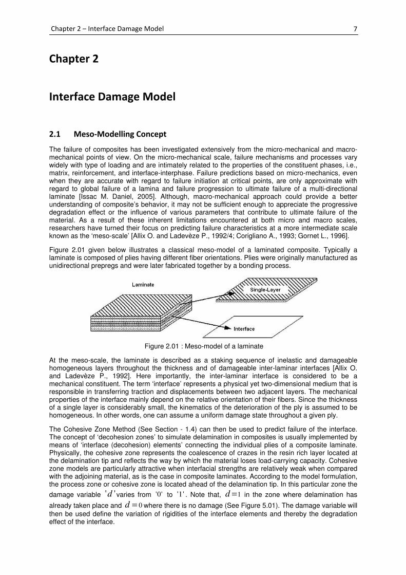
Figure 2.01 given below illustrates a classical meso-model of a laminated composite. Typically a laminate is composed of plies having different fiber orientations. Plies were originally manufactured as unidirectional prepregs and were later fabricated together by a bonding process.

Figure 2.01 : Meso-model of a laminate

At the meso-scale, the laminate is described as a staking sequence of inelastic and damageable homogeneous layers throughout the thickness and of damageable inter-laminar interfaces [Allix O. and Ladevèze P., 1992]. Here importantly, the inter-laminar interface is considered to be a mechanical constituent. The term ‘interface’ represents a physical yet two-dimensional medium that is responsible in transferring traction and displacements between two adjacent layers. The mechanical properties of the interface mainly depend on the relative orientation of their fibers. Since the thickness of a single layer is considerably small, the kinematics of the deterioration of the ply is assumed to be homogeneous. In other words, one can assume a uniform damage state throughout a given ply.

The Cohesive Zone Method (See Section - 1.4) can then be used to predict failure of the interface. The concept of ‘decohesion zones’ to simulate delamination in composites is usually implemented by means of ‘interface (decohesion) elements’ connecting the individual plies of a composite laminate. Physically, the cohesive zone represents the coalescence of crazes in the resin rich layer located at the delamination tip and reflects the way by which the material loses load-carrying capacity. Cohesive zone models are particularly attractive when interfacial strengths are relatively weak when compared with the adjoining material, as is the case in composite laminates. According to the model formulation, the process zone or cohesive zone is located ahead of the delamination tip. In this particular zone the

damage variable ' 'd varies from '0' to '1' . Note that, 1d = in the zone where delamination has

already taken place and 0d = where there is no damage (See Figure 5.01). The damage variable will

then be used define the variation of rigidities of the interface elements and thereby the degradation effect of the interface.

8


2.2 Constitutive equation for the Interface

The need for an appropriate constitutive equation in the formulation of the interface modelling is fundamental for an accurate simulation of the inter-laminar debonding process. The constitutive equations for the interface are phenomenological mechanical relations between the tractions (stresses) and interfacial separations (displacement discontinuities). With increasing interfacial separation, the tractions across the interface reach a maximum (i.e., interfacial normal or shear tractions attain their respective inter-laminar tensile or shear strengths), decrease, and vanish when complete debonding occurs. The work of normal and tangential separation can be related to the critical values of energy release rates. It is this particular characteristic that allows one to link fracture mechanics with damage mechanics.

The displacement discontinuity or jump of one layer to the other layer can be written as,

11 2 2 3 3[ ] [ ] [ ] [ ]U U U U N U N U N+ −

= − = + +��

(2.01)

Figure 2.02 : Basic building blocks of the interface model

Let the bisectors of the fiber direction be 1N��

and 2N��

. The direction of 3N��

is normal to the interface.

Essentially, all are ‘orthotropic’ directions of the interface. Here, U+��

and U−��

are displacement

vectors of the top and bottom layers respectively. See Figure 2.02 given above.

Let 0

1k , 0

2k and 0

3k are initial interface rigidities (stiffness) associated to damage variables 1d , 2d

and 3d along the orthotropic directions 1N��

, 2N��

and 3N��

respectively. Here, 3d is associated to the

opening mode (Mode-I) of the inter-laminar connections, where 1d and 2d are associated to in-plane

and out-of-plane shearing modes (Mode-II and Mode-III) respectively.

The relation between the stresses and displacement jumps along the orthotropic axes can then be expressed as follows (for simplicity displacement jumps in each orthogonal direction is written without square brackets),

(2.02)

0

13 1 1 1

0

23 2 2 2

0

33 3 3 3

(1 ) 0 0

0 (1 ) 0

0 0 (1 )

k d U

k d U

k d U

σ

σ

σ

−

= − −

9


2.3 FE Implementation of Damage Models

The constitutive behaviour laws presented in the present study are implemented in a finite element code called CAST3M via a user-subroutine known as UMAT.

CAST3M is a system designed and developed so as to overcome the hurdles of adaptability provided by conventional codes. It has been developed by the Dèpartement Mècanique et Technologie (DMT) du Commissariat Français à l’Energie Atomique (ECA). CAST3M can be used as support for design, dimensioning and analysis of structures and components. It presents a complete system, integrating; tools for calculation, tools for model construction (pre-processor) and tools for processing results (post-processor). On the contrary of other systems, made to solve some defined problems, CAST3M is a program the user can adapt to his own needs. In practice, the program is made of a set of elementary operators (written in GIBIANE) and objects. Each operator is attributed to the execution of one unique operation. The user can manipulate the objects and operators to build a new application or customize an existing application. CAST3M enables the processing of linear and nonlinear problems in static, dynamic or cyclic fields. In addition, CAST3M is equipped with interface or joint elements that can be readily used for model construction (i.e., interface model of laminates). Therefore, all these facts make CAST3M an ideal research tool for the present study under consideration.

UMAT user-subroutine (written in FORTRAN) merely allows researchers to work on material response modelling. The subroutine can be used to introduce a new constitutive law (i.e., with damage effects) in to finite element code of CAST3M. In addition, the subroutine can also be used to define solution-dependent state variables. During a nonlinear calculation, the subroutine will be called at all material calculation points of elements for which the material definition includes a user-defined material behavior. It will also update the stresses and solution-dependent state variables to their values at the end of each increment for which it is called. The smaller the time increment the greater the accuracy of the result, but at the expense of high computational cost.

10

PART – II

Delamination under Quasi-Static Loading

Section comprises two chapters, Chapter 3 and Chapter 4. Chapter 3 mainly contains formulations of the static damage model. In additon, to overcome spurious localizations of local models, existing theories on regularization methodologies were studied and reported. Chapter 4 includes detailed descriptions on FE simulations performed using static damage models (i.e., local and proposed nonlocal). At first, the local model’s effectiveness was tested in all dimensional spaces with appropriate modifications for static loading condition. Identification of model parameters, preliminary investigation results and main investigation results are detailed out comprehensively. Next, a nonlocal integral-type regularization scheme was introduced to overcome the spurious localization problem of the existing local model. Special attention was devoted to improve the FE formulation of the nonlocal model to reduce computational cost. Details of complete formulation, simulations precedures, investigations results and conclusions are also included.

11

Chapter 3 – Static Damage Evolution

Chapter 3

Static Damage Evolution

3.1 Energy Formulation

In Chapter 2 under Section 2.2 a constitutive relation for the interface was introduced. Here, the effect of deterioration of the inter-laminar connection on its mechanical behaviour is taken into account by means of three internal damage variables which are associated to Mode-I, Mode-II and Mode-III failure modes. The total strain energy [Ladevèze P., 1986; Allix O. and Ladevèze P., 1992; Gornet L. et al 1997] in the system can now be expressed as,

2 22 2

33 33 23 13

0 0 0 0

3 3 3 2 2 1 1

1

2 (1 ) (1 ) (1 )DE

k k d k d k d

σ σ σ σ− + = + + +

− − −

(3.01)

Note that, different types of damageable behaviour in ‘tension’ and in ‘compression’ are distinguished

by splitting the strain energy into ‘tension energy’ and ‘compression energy’. For example, X+

and

X−

represents the tension and compression parts of X .

The thermodynamic model is built by taking into account the three possible modes of delaminations. The thermodynamic forces associated to each damage variable can be defined as,

11 2 3

2 3

D D D

d d d

E E EY Y Y

d d dσ σ σ

∂ ∂ ∂= − = − = −

∂ ∂ ∂ (3.02)

Now, using equations 3.01 and 3.02, the following relations can be derived,

[ ]

[ ]

[ ]

22013

1 10 21

1 1

22023

2 20 22

2 2

2

233 0

3 30 23

3 3

1 1

2 (1 ) 2

1 1

2 (1 ) 2

1 1

2 (1 ) 2

d

d

d

Y k Uk d

Y k Uk d

Y k Uk d

σ

σ

σ+

+

= =

−

= = −

= =−

(3.03)

The total energy dissipated from the system can be expressed as,

1 2 31 2 3

d d dY d Y d Y d

• • •

Φ = + + Where, ( 0)Φ ≥ (3.04)

One may also use classical Fracture Mechanics theory to determine the critical energy characteristics of the interface damage model. As explained in Section – 1.4, LEFM is a proven approach for dealing with propagation of delamination. In that respect, LEFM serves as a reference to compare and contrast any new modelling of delamination propagation. Since delamination is a dissipative phenomenon [Allix O. et al., 1995] a simple way to compare LEFM with the presented model is to compare their mechanical dissipations.

12


In LEFM, the total energy dissipated from a single crack whose area given by S is written as,

a a

LEFM

a

G S•

+∆

Φ = ∫ (3.05)

If one consider a specimen having a constant width equaling to b, then S b a• •

= , where a is the

length of the crack. Here, G is the ‘Energy Release Rate’ and it depends only on the material

properties. In order to explicitly integrate equation 3.05, ‘steady-state’ propagation of the crack is

assumed. In other words, crack length is assumed to increase by a∆ over a time increment of t∆ .

The Figure 3.01 given below illustrates the propagation of the crack tip along with the cohesive zone in a steady-state delamination process.

Figure 3.01 : Steady-state delamination process

Similarly, from equation 3.04, the total energy dissipated from the interface according to damage mechanics formulation can be written as,

3

1

( )dIDM ii

i

Y d d•

=Γ

Φ = Γ∑∫ (3.06)

Where, Γ represents the cohesive zone of the interface.

Since, the energy dissipated for propagation of delamination in LEFM should be equal to energy

dissipated in interface damage model, LEFM IDM

=Φ Φ .

Then integration of equations 3.05 and 3.06 for a given time increment, leads to the equations [Allix O. and Ladevèze P., 1996] given below,

1

2

I CC

CIIC

CIIIC

G Y

YG

YG

γ

γ

=

= =

(3.07)

,I IIC C

G G and IIIC

G are critical energy release rates associated to Mode-I, Mode-II and Mode-III

failure modes respectively. Here, C

Y is the critical ‘Damage Energy Release Rate’ and 1γ and 2γ are

‘Coupling Parameters’ for IIC

G and IIIC

G respectively.

1d = 0d =

0 1d≤ ≤

time t−

crack length a= cohesive zone undamaged zone

time t t− +∆

crack length a a= +∆ cohesive zone .undam zone

1d = 0 1d≤ ≤ 0d =

Chapter 3

In order to satisfy the energy balance principle, the area under the stress vs. displacement for the ‘Debonding Process’ (DP) should be equal to critical energy release rate (i.e.

, &I II IIIC C C

G G G

2000]. The resulting equations can be written as

ICDP

IIC

IIIC

G dU

G dU

G dU

=

=

=

Notice that, delamination doesn’t tSee Figure 3.

Figure

For the Mixed

C I II IIIG G G G=

In addition, one can also write a relation

I II III

I II IIIC C C

G G G

G G G

α

Therefore



, &I II IIIC C C

G G G


33 3

13 1

23 2

DP

DP

DP

G dU

G dU

G dU

σ

σ

σ

+

=

=

=

∫

∫

∫

Notice that, delamination doesn’t tSee Figure 3.02 given below.

Figure 3.02 : Graphical representation of critical energy release rate for

Mixed-Mode

C I II IIIG G G G+ +


I II III

I II IIIC C C

G G G

G G G

α + + =

Therefore, parameter



C C C) for each failure mode


33 3

13 1

23 2

G dU

G dU

Notice that, delamination doesn’t tgiven below.

Graphical representation of critical energy release rate for

Mode failure case, critical energy release rate for the system can be

C I II III


I II III

I II IIIC C C

G G G

G G G

α α + + =

parameter α governs



) for each failure mode


Notice that, delamination doesn’t take place when the laminate is


failure case, critical energy release rate for the system can be

In addition, one can also write a relation for the

1I II III

C C C

α α + + =

governs the damage evolution in


) for each failure mode [Ladevèze

2000]. The resulting equations can be written as follows,

ake place when the laminate is



for the Mixed-Mode

damage evolution in


P. et al., 1998;

ake place when the laminate is subjected to compressive stresses.



Mode failure as

damage evolution in Mixed-Mode


et al., 1998; Corigliano A. and Allix O.,

subjected to compressive stresses.

Graphical representation of critical energy release rate for Mode


failure as given below,

Mode.

In order to satisfy the energy balance principle, the area under the stress vs. displacement jumpfor the ‘Debonding Process’ (DP) should be equal to critical energy release rate (i.e.

Corigliano A. and Allix O.,


Mode-I and Mode

failure case, critical energy release rate for the system can be expressed as,

given below,

13

jump-curve for the ‘Debonding Process’ (DP) should be equal to critical energy release rate (i.e.,

Corigliano A. and Allix O.,

(3.08)


Mode-II

expressed as,

(3.09)

(3.10)

14


3.2 Local Damage Evolution

The damage evolution law explained hereunder is based on the assumption that the evolutions of the different damage variables are driven by a single variable known as ‘Equivalent Damage Energy Release Rate’ [Allix O. et al., 1995]. The expression for ‘Equivalent Damage Energy Release Rate’ is written as,

( ) ( ) ( ) ( )1

1 23 1 2d d dtY t Max Y Y Y

α αα α

τγ γ

≤

= + +

(3.11)

Note that, the first, second and third terms in the expression are associated to the Mode-I, Mode-II and Mode-III failure modes respectively.

Some important characteristics of this technique can be listed as follows,

I. Evolution of the damage variables are assumed to strongly coupled (i.e., ‘ISOTROPIC’ damage evolution)

II. Damage taken place within a given time period will depend on the maximum value of the equivalent damage energy release rate.

The damage or material function [Allix O. and Ladevèze P., 1996] is selected in the form,

0

0

( )1

n

C

Y Ynw Y

n Y Y

+

− = + −

(3.12)

Where, n is called the characteristic function of the material and C

Y and 0

Y are critical and

threshold damage energy release rates. 0

Y is introduced to enlarge the possibility to describe both

initiation and propagation of delamination (usually, 0

Y =0).

The damage evolution procedure can then be defined as follows,

13

( )1 2 3

11 2 3

d Y

d d d w Y

d d d

f and YR

else

endif

i < <

= = =

= = =

Where,

( )0 0

1R C C

n

nY Y d Y Y+

+= − (3.13)

Here, R

Y is the damage energy corresponding to rupture, and C

d is the critical damage value, which

is usually taken as equal to one ( 1C

d = ). In general, 0,1C

d ∈ .

15


3.3 Regularization Damage Evolution

The interface damage model presented in Section – 3.2 is called a local damage model as it does not account for ‘spurious localizations’. The classical damage models lead inevitably to strain softening response and the numerical solutions obtained with such models tend to exhibit severe mesh dependence in the presence of ‘strain-softening’. The problem is much more evident in three-dimensional (3D) problems rather than in two-dimensional (2D) problems [Gornet L. et al., 1997]. In addition, classical damage models tend to produce multiple solutions when the tangent operator becomes negative. This phenomenon is presented pictorially in Figure 3.03.

Figure 3.03 : Graphical representation of numerical problems of local damage models Thus, to avoid spurious localization and other undesired effects one may need to regularize the damage evolution. Regularized evolution laws current available falls in to two major categories; namely, Rate-dependent damage evolution laws and Non-local (differential/ integral -type) damage evolution laws.

3.3.1 Rate-Dependent Damage Evolution

The core idea here is to introduce a delay effect into the classical damage model. The variant damage

model ensures that physical variation of deriving force (Y ) does not lead to an instantaneous

variation of damage variable ( d ). In other words, the ‘damage-rate’ is kept bounded. An example of a

damage law with delay effect [Ladevèze P., 1995] is given below.

13

( ) , ( ) 13 3

1 2 3

11 2 3

d and

m

d k w Y d w Y

d d d

d d d

f Y YR

else

endif

i

•

• • •

< <

+ = − ≤

= =

= = =

Note that, parameters mand k need to be determined experimentally. Here, an implicit Euler

algorithm can be employed and the nonlinear discretized damage equation can be solved by Newton method. Damage models with delay effects have been successfully used to predict delamination process [Gornet L. et al., 1997, Marguet S. et al., 2006]. Simulated results were in well agreement with the experimental results. However, rate dependent models suffer from some limitations. For example, in case of fatigue loadings it is not logical to use rate dependent models as the load is inherently varying between the maximum and minimum values.

16


3.3.2 Non-Local Integral-Type Damage Evolution

The models are formulated by introducing a length scale into the governing equations to avoid the pathological mesh sensitivity. They have been successfully used to eliminate the effect of localization in civil engineering work by many researchers but domain is still open to implement them in interface damage modelling for delamination of composite laminates [Borino G. et al., 2007; Milan Jirásek, 2007].

In integral-type non-local damage models, the equivalent strain (eq

ε ) is made non-local by means of

spatial averaging over the surrounding volume (V ) with respect to a ‘weight function’ (0

α ) (i.e., a

Gaussian distribution function) [Zdeněk P. Bažant et al., 1988]. Now, the resulting average equivalent strain can be defined as follows.

0

0

( ) ( )

( )( )

eq

Veq

V

x d

xx d

α ζ ε ζ ζ

α ζ ζε

−

=−

∫

∫ (3.14)

Where,

2

0 2( ) exp

2

rr

lα

=

(3.15)

Here, r x ζ= − and, l is the internal length scale.

The same idea can be applied for interface damage modelling by the following ways.

Method-1 Averaging relative displacement :

[ ]( ) ( )eq Uζ ζε → ⇒ ( ) ( )eq x U xε → ⇒ ( )( )( )d d Y U x =

Method-2 Averaging damage energy release rate :

( ) ( )eq

Yζ ζε → ⇒ ( ) ( )eq x Y xε → ⇒ ( )( )d d Y x=

Method-3 Averaging damage variable :

( ) ( )eq dζ ζε → ⇒ ( ) ( )eq x d xε → ⇒ ( )d d x=

Here, Method-1 is considered to be the most effective approach compared to Method-2 and Method-

3. This is mainly because, Y is a function of [ ]U and d is a function of Y .

The computed damage variable will be non-local in nature due to its dependence on averaged variables. Now, the relation between the stresses and displacement jumps along the orthotropic axes can be re-written in terms of the nonlocal damage variables as follows (for simplicity displacement jumps in each orthogonal direction is written without square brackets),

(3.16)

0

1 113 1

0

23 2 2 2

033 33 3

(1 ) 0 0

0 (1 ) 0

0 0 (1 )

k d U

k d U

Uk d

σ

σ

σ

−

= − −

17

Chapter 4 – Analysis of Static Simulations

Chapter 4

Analysis of Static Simulations

4.1 Analysis Procedure

Given hereunder is the routine of a finite element simulation procedure and subsequent post treatments carried out for validation of the interface damage model.

Pre-processing

Define type of analysis(1D / 2D-plane stress/ 3D) Define geometry & mesh Define material parameters for arms Define ‘static damage model’ parameters for interface Define boundary, contact & loading conditions

Define convergence criteria

Solution

Launch nonlinear calculation

Post-processing

Plot evolution of force vs. displacement, crack length vs. displacement, damage variable vs. displacement, etc.

Produce stress & strain field plots on un-deformed / deformed meshes

Analysis Compare and contrast simulated results with experimental data and investigate the effect of static model parameters

The finite element implementation of the ‘static damage model’ for the interface in 3D is summarized in the Table 4.01 given below.

Step-1 Compute damage energy release rate,

i.e., ( )Y t using 1 2,

d dY Y &

3d

Y

Step-2 Compute isotropic damage function,

i.e., ( )w Y using ,C

Y Y & 0

Y

Step-3 Compute damage variables,

i.e., ( )1 2 3

d d d w Y= = =

Step-4 Compute stresses for the interface,

i.e., 0 0 0

13 1 1 1 23 2 2 2 33 3 3 3(1 ) , (1 ) , (1 )k d U k d U k d Uσ σ σ= − = − = −

Table 4.01 : FE implementation of static damage model

The constitutive law for the inter-laminar interface will be introduced in to the finite element formulation of CAST3M via UMAT.

One of the useful advantages of the sub-routine is its capability to print STATE VARIABLE values (i.e., stress, strain, damage variable, energy release rate, etc) at end of each loading increment during nonlinear calculation process. This option helps the user to properly calibrate the damage model with relative ease.

18


4.2 Identification of Static Damage Model Parameters

Prior to the commencement of simulations one needs to identify the model parameters of the damage

evolution law. Parameters, C

Y , 0

Y , 1γ , 2

γ and α are computed based on values of the critical

energy release rates of each failure mode. Thus they are strongly depended on the mechanical

behaviour of the material and therefore called ‘material parameters’. In addition, 0

1k , 0

2k (initial shear

stiffness) and 0

3k (initial normal stiffness) are computed using maximum admissible stresses of the

inter-laminar interface [Ladevèze P. et al., 1998; Ijaz H., 2009]. The parameter n has a significant

influence on initiation of delamination and subsequent evolution of damage variable. In Section 3.1,

the formulas for computing C

Y , 1

γ and 2

γ are presented. In cases where inter-laminar fracture

toughness for Mode-III is not available, one can take 2 1

γ γ= [Ladevèze P. et al., 1998] for 3D

analyses.

4.2.1 Identification of Parameter - α

Procedure for identification of α is explained hereafter. Let us consider a state of stress, where

Mode-III fracture toughness is considerably negligible. Now, the reduced equation can be written as,

1I II

I IIC C

G G

G G

αα

+ =

(4.01)

The value of α can be obtained using the normalized Mode-I / Mode-II plane. Experimental results

on critical energy release rate for pure Mode-I, pure Mode-II and Mixed-Mode (at least one data point) are used in the identification process. The example given hereunder considers the data reported [Rikard Borg et al., 2003] on a unidirectional composite laminate - HTA/6376C. The critical energy release rate (fracture toughness) for each failure mode is listed in the Table 4.02. Failure Mode (Test Method) [ / ]G N mm

C

Mode-I (DCB) 0.259

Mixed-Mode (MMB)

/ ( ) 0.5II I II

G G G+ = 0.447

Mode-II (3ENF) 1.008

Table 4.02 : Critical energy release rates of HTA/6376C for different failure modes

Figure 4.01 - Normalized Mode-I / Mode-II plane for HTA/6376C

19


Figure 4.01 given above shows the normalized Mode-I / Mode-II plane, developed using the available

experimental results included in Table 4.01. The best fit of plot can be obtained when 1.4α = . The

good value of α is usually identified by using several experimental results obtained for different mode

mixtures. Note that, α governs the shape of the failure locus in Mixed-Mode and has no influence on

the evolution of the damage variable in either pure Mode-I or Mode-II cases. Typically, value of α for

most fibrous composites is in between 1 and 2 (i.e.,1 2α≤ ≤ ) [Harper P. W., 2008].

4.2.2 Identification of Initial Interface Rigidities

An ‘instability criteria’ [Gornet L., 1997; Ijaz H., 2009] has been derived to find the relationship

between the maximum admissible stress (i.e.,3

1,2th

iiσ = and 3) at the interface and the damage

model parameters. Through this formulation one can determine the initial rigidities (i.e.,0 1,2i

k i = and

3) of the interface.

For each failure mode the instability criteria can be expressed as follows,

Mode-I : 33 0σ•

= for 3 0U

•

≠

Mode-II : 31 0σ•

= for 1 0U

•

≠

Mode-III : 32 0σ•

= for 2 0U

•

≠

For Mode-I, differentiating normal stress; ( )0

33 3 3 31k d Uσ = − with respect to 3U we have,

( ) ( )0333 3 3 3

3 3

1 1d d

k d U ddU dU

σ = − + −

Next by considering equations 3.03 and 3.12

( ) ( ) ( )0333 3 3

3 33 3

3

1d d

d

d d dk d U W Y Y

dU dY dU

σ = − − ⋅

( ) ( )0333 3

33 3

3

1 2d d

d

d dk d Y W Y

dU dY

σ = − −

(4.02)

According to instability criteria: 33

3

0d

dU

σ= , which leads to the following expression,

( ) ( )3 3 33

1 2 0d d

d

dd Y W Y

dY− − = (4.03)

Now, one can re-write equation 4.03 in a more general form considering all failure modes.

( ) ( )1 2 0d

d Y W YdY

− − = (4.04)

20


Mode-I : 3d d= and 3d

Y Y=

Mode-II : 1d d= and 1 1dY Yγ=

Mode-III : 2d d= and 2 2dY Yγ=

By considering equation 3.12 one can further expand equation 4.04 as follows,

0 0

0 0

1 2 01 1

n n

C C

Y Y Y Yn d nY

n Y Y n Y YdY

− − − − = + − + −

1

0

ˆ ˆ1 2 01 1

n nn n

C

n Y nY n Y

n Y Y n

− − − =

+ − + where,

0

0

ˆ

C

Y YY

Y Y

−=

−

( ) 10

0

1ˆ ˆ2 1 2 0

nn n

C

Y nn Y n Y

Y Y n

− + + + − =

− (4.05)

Analytical relation for initial interface rigidities in each direction can be derived from the above

equation by taking, 0

0Y = .

For Mode-I, considering equation 4.05 we have,

( ) 3 12 1 0

n nd

C

Y nn

Y n

+ + − =

(4.06)

Now substituting equation 3.12 in ( )0

33 3 3 31k d Uσ = − with 0

0Y = ,

0

33 3 331

1

n

d

C

Ynk U

n Yσ

= −

+

(4.07)

Considering equations 4.06 and 4.07 one can derive,

0

33 3 3

2

2 1

nk U

nσ =

+ (4.08)

Now by considering equations 3.03, 4.06 and 4.08 the initial interface rigidity in the out-of-plane direction (i.e., Mode-I) can be expressed as follows,

( )

( )0 2

3 33

2 12 1

8 1

nn

C

nk

n n Yσ

++

=+

(4.09)

Similarly, the initial interface rigidities in the in-plane directions (i.e., Mode-II and Mode-III, respectively) can be expressed as follows,

( )

( )10 2

1 31

2 12 1

8 1

nn

C

nk

n n Y

γσ

++

=+

(4.10) , ( )

( )20 2

2 32

2 12 1

8 1

nn

C

nk

n n Y

γσ

++

=+

(4.11)

21


The initial interface rigidities can then be computed using above equations, if experimental data on maximum admissible stresses for the interface and critical energy release rate for Mode-I are

available.. Note that, the value of ' 'n will be assumed based on the brittleness of the interface.

Usually, 1n< is used for brittle interfaces.

For a unidirectional composite laminate - HTA/6376C, maximum admissible stresses for the interface were reported [Robinson P. et al., 2005] to be approximately equal to 30 MPa (i.e.

[ ]33 13 30C MPaσ σ σ= = = ). By using the above equations and assuming 0.5n = , the normal

and shear rigidities can be found [ ]0

3 9265 /k MPa mm= and [ ]0

1 2380 /k MPa mm= .

The results given hereunder illustrate the model response for both Mode-I and Mode-II failure modes

for simple test-cases. The laminate material is considered to be HTA/6376C with [ ]0 / 0 interface.

Reported mechanical properties [Rikard Borg et al., 2003] of the lamina are included in Table 4.03.

11E - 146,000 [ ]MPa 22E

- 10,500 [ ]MPa 33E

- 10,500 [ ]MPa

12ν - 0.3 23ν

- 0.51

13ν

- 0.3

12G - 5,250 [ ]MPa 23G - 3,480 [ ]MPa

13G - 5,250 [ ]MPa

Table 4.03 : Elastic properties of HTA/6376C unidirectional prepregs reported by Rikard B. et al.

Figure 4.02 given below illustrate the geometry of the test-piece, loading schemes i.e., imposed

displacements; 3U for Mode-I and 1U for Mode-II, and boundary conditions.

Figure 4.02 : Test-piece geometry and loading/boundary conditions

Simulations were performed considering a state of ‘PLANE STRESS’ in 2D. Values of the material parameters and FEs used are given in Table 4.04.

[ ]/C

Y N mm 0.259 Body (2D)

Geo. Support / Finite Element : QUA4 / QUA4

Deg. of Interpolation : 1

1γ 0.2569

α 1.4 Interface(1D)

Geo. Support / Finite Element : RAC2 /


JOI2

n 0.5

Table 4.04 : Damage model parameters and 2D mesh details for simulations of test case

The mechanical behaviour of the ‘Body’ will be simulated with the classical constitutive law (i.e.,

kσ ε= ) using solid elements. At the same time, the interface elements are used simulate the

degradation of the interface using the modified constitutive law (i.e., ( )1 d kσ ε= − ) formulated

according to damage mechanics. The damage model is simply responsible for computing the damage

variable (i.e., d ) at the end of each increment (i.e., force or imposed displacement). Note that,

interface elements are zero thickness elements having same size of the solid elements (length and width directions) adjacent to them. Figure 4.03 illustrates the relative location of the interface elements for 1D and 2D cases.

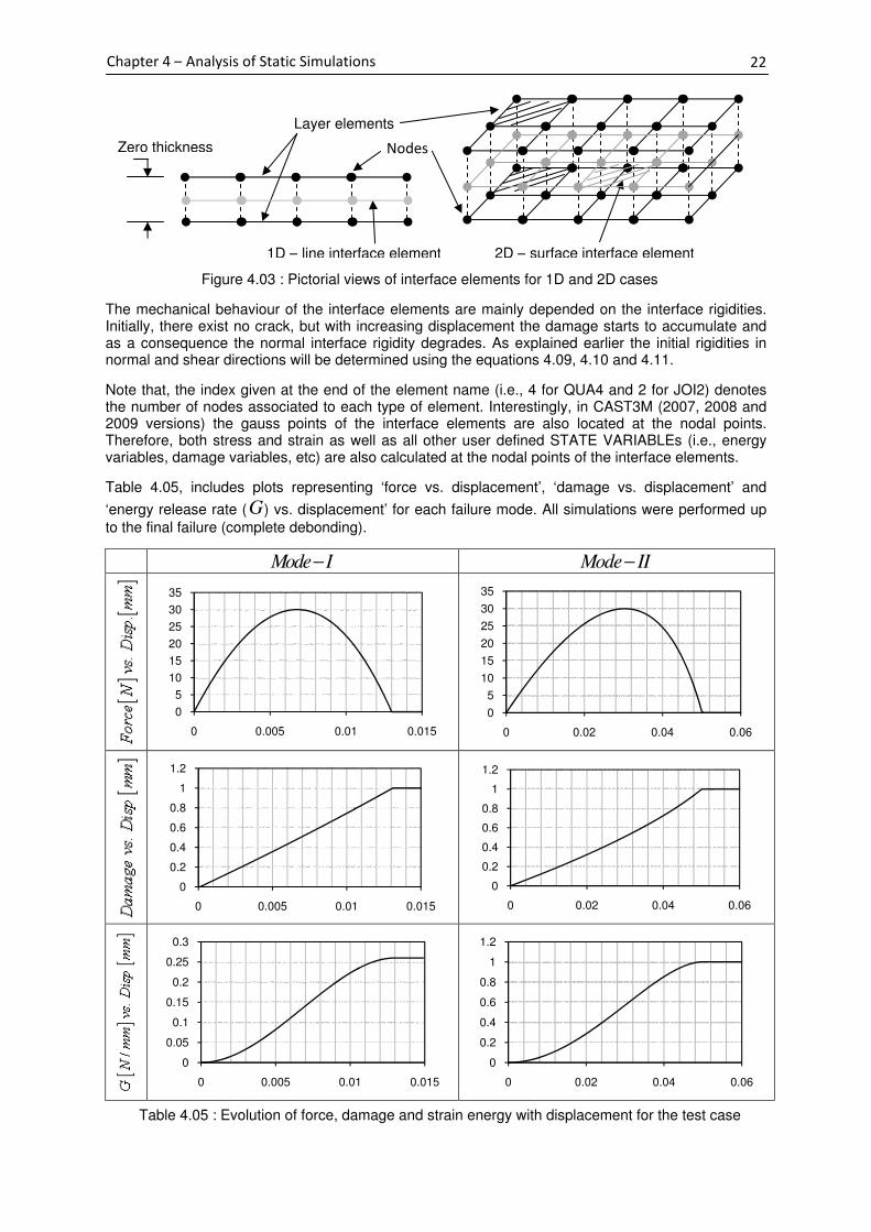
22


The mechanical behaviour of the interface elements are mainly depended on the interface rigidities. Initially, there exist no crack, but with increasing displacement the damage starts to accumulate and as a consequence the normal interface rigidity degrades. As explained earlier the initial rigidities in normal and shear directions will be determined using the equations 4.09, 4.10 and 4.11.

Note that, the index given at the end of the element name (i.e., 4 for QUA4 and 2 for JOI2) denotes the number of nodes associated to each type of element. Interestingly, in CAST3M (2007, 2008 and 2009 versions) the gauss points of the interface elements are also located at the nodal points. Therefore, both stress and strain as well as all other user defined STATE VARIABLEs (i.e., energy variables, damage variables, etc) are also calculated at the nodal points of the interface elements.

Table 4.05, includes plots representing ‘force vs. displacement’, ‘damage vs. displacement’ and

‘energy release rate (G) vs. displacement’ for each failure mode. All simulations were performed up

to the final failure (complete debonding).

Mode I− Mode II−

Table 4.05 : Evolution of force, damage and strain energy with displacement for the test case

0

5

10

15

20

25

30

35

0 0.005 0.01 0.015

0

5

10

15

20

25

30

35

0 0.02 0.04 0.06

0

0.2

0.4

0.6

0.8

1

1.2

0 0.005 0.01 0.015

0

0.2

0.4

0.6

0.8

1

1.2

0 0.02 0.04 0.06

0

0.05

0.1

0.15

0.2

0.25

0.3

0 0.005 0.01 0.015

0

0.2

0.4

0.6

0.8

1

1.2

0 0.02 0.04 0.06

Figure 4.03 : Pictorial views of interface elements for 1D and 2D cases

Nodes

Layer elements

2D – surface interface element 1D – line interface element

Zero thickness

23


Numerical simulations were also carried out in 3D with same material parameters. The types of FEs used are included in Table 4.06.

Body (3D) Geo. Support / Finite Element : CUB8 / CUB8


Interface(2D) Geo. Support / Finite Element : LIA4 / JOI4


Table 4.06 : 3D mesh details for simulation of test case

3D simulation results were identical to the ones obtained from 2D analysis. 3D model did not exhibit any spurious localization as a result of its simple geometry. However, the computational cost increased notably.

During the debonding process the damage variable increases from '0' to '1 ' and energy release rate

from '0' to 'C

G ( =0.259 for Mode-I and =1.008 for Mode-II) simultaneously. Here, the evolution of

energy release rate has been determined using global force and displacement variables. Note that, the area under the force vs. displacement curve is equal to the critical energy release rate for each failure mode. However, for analysis purposes it would be useful to determine the strain energy released in terms of local variables (i.e., stress and strain) during the calculation process. This is achieved by using the trapezoidal rule to compute the area under the ‘stress vs. strain' curve at each increment and adding them progressively. Here, the computations are performed at each gauss points of the interface elements (in CAST3M the gauss points and nodal points are located at the same position).

Note that, classically energy release rate is defined in terms of failed surface area; therefore it can attributed as an area parameter. On the other hand, when strain energy release rate is calculated at the gauss points it is no more a physical quantity but a mere representation of this area parameter by numerical means. It is the responsibility of the user to properly appreciate the correlation between this numerical variable and the physical quantity. When the relation is established it serves as a useful numerical tool in determining the energy variation in the system. Theory associated to this methodology for determining the energy release rate was discussed earlier in Section 3.1.

Figure 4.04 given below illustrates the evolution of the energy release rate at the interface for Mode-I failure using both global and local variables. Note that, for the considered test-case, degradation of the entire interface takes place homogeneously and delamination happens all at once. In other words, crack front is not a point but a line. Hence, any selected gauss point of a given interface element can be indirectly used to determine the evolution of the energy release rate variable.

Figure 4.04 : Comparison of G-Global and G-Local

As it can be seen from the above figure, the variation of this numerical quantity can be directly mapped on to the evolution of the energy release rate obtained by the global variables. Therefore, this information justifies the applicability of the assumption for determination of energy release rate in terms of local variables.

0

0.05

0.1

0.15

0.2

0.25

0.3

0 0.005 0.01 0.015 0.02 0.025

G-Local

G-Global

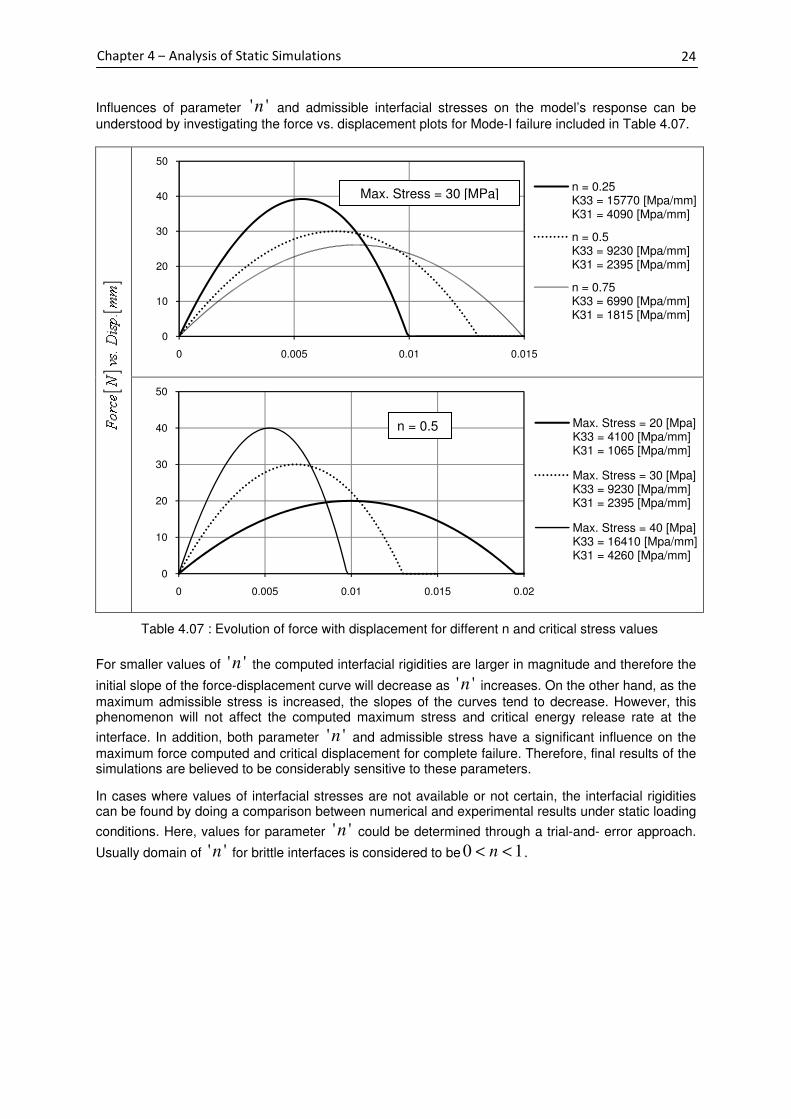
24


Influences of parameter ' 'n and admissible interfacial stresses on the model’s response can be

understood by investigating the force vs. displacement plots for Mode-I failure included in Table 4.07.

Table 4.07 : Evolution of force with displacement for different n and critical stress values

For smaller values of ' 'n the computed interfacial rigidities are larger in magnitude and therefore the

initial slope of the force-displacement curve will decrease as ' 'n increases. On the other hand, as the

maximum admissible stress is increased, the slopes of the curves tend to decrease. However, this phenomenon will not affect the computed maximum stress and critical energy release rate at the

interface. In addition, both parameter ' 'n and admissible stress have a significant influence on the

maximum force computed and critical displacement for complete failure. Therefore, final results of the simulations are believed to be considerably sensitive to these parameters.

In cases where values of interfacial stresses are not available or not certain, the interfacial rigidities can be found by doing a comparison between numerical and experimental results under static loading

conditions. Here, values for parameter ' 'n could be determined through a trial-and- error approach.

Usually domain of ' 'n for brittle interfaces is considered to be 0 1n< < .

0

10

20

30

40

50

0 0.005 0.01 0.015

n = 0.25K33 = 15770 [Mpa/mm]K31 = 4090 [Mpa/mm]

n = 0.5K33 = 9230 [Mpa/mm]K31 = 2395 [Mpa/mm]

n = 0.75K33 = 6990 [Mpa/mm]K31 = 1815 [Mpa/mm]

0

10

20

30

40

50

0 0.005 0.01 0.015 0.02

Max. Stress = 20 [Mpa]K33 = 4100 [Mpa/mm]K31 = 1065 [Mpa/mm]



Max. Stress = 30 [MPa]

n = 0.5

25


4.3 Overview of Fracture Mechanics Tests for Delamination

Fracture toughness of fiber reinforced composites is classically determined using test methods developed for unidirectional laminates. This is mainly due to intra ply damage, undesired edge effects and crack plane migration effects associated to multidirectional laminates. Although inter-laminar fracture toughness can be measured in any combination of three fracture modes, the most commonly used ones are Mode-I (opening), Mode-II (shearing) or combination of both [ASTM standards; Brunner A. J., et al, 2001a/2001b]. Note that, Mode-III (tearing) fracture toughness is relatively larger in magnitude and contribution to delamination is comparatively low.

Usually the fracture toughness is measured using a beam-type composite specimen with an initial crack between central plies. The initial delamination is introduced into the laminate by a thin non-stick film, usually made of polymer. Therefore, upon application of loading, delamination grows parallel to the plies in the mid-plane of the beam. Interestingly, during the propagation stage one can observe a non-straight crack front. This is mainly due to the variation of the energy release rate across the width of the specimen. While performing the test, both applied load and corresponding displacement are measured and are correlated to the delamination length. From correlated data, the inter-laminar fracture toughness will be obtained using simple beam theory principles or other empirical formulations.

Typically ‘Double Cantilever Beam (DCB)’ test method is used to obtain experimental inter-laminar fracture toughness for Mode-I. Note that, the initial delamination is introduced in the mid-plane of the beam at one end and the other end will be fixed. The initial delamination is then forced to grow by pulling the two beams at the free end in opposite directions (opening). A schematic illustration of the DCB test with loaded and unloaded conditions is given below in Figure 4.05.

Figure 4.05 : DCB test with loaded and unloaded conditions

‘Three-point End Notched Flexure (3ENF)’ test is one of the most commonly used experimental methods for obtaining Mode-II inter-laminar fracture toughness. Here, initial delamination is forced to grow in the mid-plane by making crack faces slide (shearing) relative to each other. This is achieved by simply supporting the beam at the two ends and applying a compressive force at the mid span of the beam. Figure 4.06 given below shows a schematic of a 3ENF test with loaded and unloaded conditions.

Figure 4.06 : 3ENF test with loaded and unloaded conditions

Mixed-Mode I/II inter-laminar fracture toughness is commonly evaluated using a ‘Mixed Mode Bending (MMB)’ test apparatus [Crews J. H. and Reeder J.R., 1988]. Here, initial delamination is forced to propagate by both opening and shearing actions. The test allows the determination of fracture toughness with a Mixed-Mode ratio ranging from pure Mode-I to pure Mode-II. Figure 4.07 given below illustrates a schematic of the test rig (source - Blanco Villaverde N., 2004). Usually different Mixed-Mode ratios are achieved by varying the position of the load point ( c ) along the lever arm.

Chapter 4

4.4

The following sectiodamage modelexperimental results.

I. II.

Previous studies 1997] showsfailure mode. The purpose of the ongoing investigation is to check its validity2D or 3D) spaces and to provide a synopsis of its limitations and advantages.

Next, the FE implementation of the proposed nonlocal model the model will include determination of influence of different parameters, such as element size, incretc. However

Note that, the will be used to perform

The investigationsand 3ENF tests respectively.carbon/epo

dimensions

and nominal thickness

and initial delamination length,

illustrated in Figure 4.0failure modrigidities are

value is believed to be in the range of

taken equal to

test-case considering Modeobtain a broader understanding, it is necessary to compare simulated results for different critical stress values with actual experimental results.

Since the investigation is twofold, the validations will be local model and another one on the nonlocal model.


Validation of Static Damage Models

The following sectiodamage models. Verifications will be experimental results.

Local static damage modelNonlocal static damage model (integral

Previous studies [Allix 1997] shows that local failure mode. The purpose of the ongoing investigation is to check its validity2D or 3D) spaces and to provide a synopsis of its limitations and advantages.

he FE implementation of the proposed nonlocal model he model will also be subjected to a thorough investigation will include determination of influence of different parameters, such as element size, incr

owever, the nonlocal model will

Note that, the experimental results reported by Rikard Bwill be used to perform

The investigations will be carried outand 3ENF tests respectively.carbon/epoxy unidirectional prepregs and

dimensions of the rectangular shaped specimens a

and nominal thickness

and initial delamination length,

illustrated in Figure 4.0failure mode is tabulated in Table 4.02rigidities are determined as explained

is believed to be in the range of

taken equal to [30 MPa

case considering Modeobtain a broader understanding, it is necessary to compare simulated results for different critical

alues with actual experimental results.



Figure


The following sections are dedicated for analyzing. Verifications will be

experimental results. The two static damag

Local static damage modelNonlocal static damage model (integral

[Allix O. and Ladevlocal damage

failure mode. The purpose of the ongoing investigation is to check its validity2D or 3D) spaces and to provide a synopsis of its limitations and advantages.

he FE implementation of the proposed nonlocal model will also be subjected to a thorough investigation

will include determination of influence of different parameters, such as element size, incr, the nonlocal model will

experimental results reported by Rikard Bwill be used to perform all verifications

will be carried outand 3ENF tests respectively. All specimens

xy unidirectional prepregs and

rectangular shaped specimens a

and nominal thickness 2 3.1h mm=

and initial delamination length, a mm

illustrated in Figure 4.05 (DCB) and e is tabulated in Table 4.02

determined as explained

is believed to be in the range of

]MPa . Previously, in Section 4.2

case considering Mode-I failure to understand model's behaviour for different values. However, to obtain a broader understanding, it is necessary to compare simulated results for different critical




Figure 4.07 : Schematic of


dedicated for analyzing. Verifications will be done

he two static damage models will be referred from hereafter as,

Local static damage model Nonlocal static damage model (integral

Ladevèze P.,damage model has a high potential for determining delamination



will include determination of influence of different parameters, such as element size, incr, the nonlocal model will only be tested for 2D applications.

experimental results reported by Rikard Bverifications.

will be carried out considering pure ModeAll specimens

xy unidirectional prepregs and

rectangular shaped specimens a

[ ]2 3.1h mm . In addition

[ ]35a mm=

(DCB) and Figure e is tabulated in Table 4.02. Finally

determined as explained in Section

is believed to be in the range of 20 to

Previously, in Section 4.2

I failure to understand model's behaviour for different values. However, to obtain a broader understanding, it is necessary to compare simulated results for different critical



Schematic of


dedicated for analyzing the applicability and effectiveness of thedone by closely examining the simulated results e models will be referred from hereafter as,

Nonlocal static damage model (integral-type)

, 1992; Corigliano A. and Allix O., 1996; model has a high potential for determining delamination



will include determination of influence of different parameters, such as element size, incrbe tested for 2D applications.

experimental results reported by Rikard B

considering pure ModeAll specimens experimented

xy unidirectional prepregs and their elastic properties

rectangular shaped specimens are; width

In addition, the testing s

]a mm . Schematics of the specimens and their dimensions are

Figure 4.06 (3ENF)Finally, values of the material parameters

in Section 4.2. Typically, for CFRP composites the critical stress

to [ ]40 MPa

Previously, in Section 4.2.2 few computations were performed on a simple




Schematic of MMB test rig

the applicability and effectiveness of theby closely examining the simulated results

e models will be referred from hereafter as,

Corigliano A. and Allix O., 1996; model has a high potential for determining delamination


he FE implementation of the proposed nonlocal model will be discwill also be subjected to a thorough investigation to understand its behaviour.


experimental results reported by Rikard Borg and coworkers [Rikard Borg et al

considering pure Mode-I and Modeexperimented were

stic properties

re; width 20b mm=

testing span of the specimen,

Schematics of the specimens and their dimensions are

(3ENF). In addition, fracture toughness for, values of the material parameters

Typically, for CFRP composites the critical stress

MPa . Note that,

few computations were performed on a simple


Since the investigation is twofold, the validations will be done in two different sections; one

MMB test rig



Corigliano A. and Allix O., 1996; model has a high potential for determining delamination

failure mode. The purpose of the ongoing investigation is to check its validity in all dimensional (1D, 2D or 3D) spaces and to provide a synopsis of its limitations and advantages.

will be discussed in details. to understand its behaviour.


org and coworkers [Rikard Borg et al

I and Mode-II failure modes manufactured from HTA/6376C are given in Table 4

[ ]20b mm , length

pan of the specimen,


In addition, fracture toughness for, values of the material parameters


, for the present study



done in two different sections; one



Corigliano A. and Allix O., 1996; Gornet L. et al model has a high potential for determining delamination in any given

in all dimensional (1D,

ussed in details. In addition, to understand its behaviour. The analysis

will include determination of influence of different parameters, such as element size, increment size,

org and coworkers [Rikard Borg et al

II failure modes with DCB manufactured from HTA/6376C

in Table 4.0

, length 150Sl mm=

pan of the specimen, 2 100L mm=


In addition, fracture toughness for, values of the material parameters and initial interface


present study σ



done in two different sections; one

26

the applicability and effectiveness of the static by closely examining the simulated results with

Gornet L. et al in any given

in all dimensional (1D,

In addition, The analysis ement size,

org and coworkers [Rikard Borg et al, 2003]

with DCB manufactured from HTA/6376C

.03. The

[ ]150l mm ,

[ ]2 100L mm


In addition, fracture toughness for each and initial interface


Cσ

will be



done in two different sections; one on the

27


4.5 Validation of Local Static Damage Model

4.5.1 FE Simulation Details

The local damage model was tested systematically in 1D, 2D and 3D spaces. The types of FEs used in each space are given in Table 4.08.

Laminate arms Inter-laminar interface

1D Geo. Support / Finite Element : SEG2 / COQ2




JOI2

2D Geo. Support / Finite Element : QUA4 / QUA4




JOI2

3D Geo. Support / Finite Element : QUA4 / COQ4


Geo. Support / Finite Element : LIA4 / JOI4


Table 4.08 : Types of FE used for 1D, 2D and 3D models of DCB and 3ENF tests

Note that, in CAST3M the degree of the interpolation function associated to both ‘RACCORD’ (1D) and ‘LIAISON’ (2D) type interface elements are limited to '1' . As a consequence, laminate arms were also needed to be meshed with elements having interpolation functions of the same degree. In other words, compatibility of the elements used for the interface and laminate arms should be ascertained prior to the commencement of the simulations. Usually, for the case of simple beam bending, a coarse mesh with elements having degree-2 interpolation functions (i.e., QUA8 for 2D and CU20 for 3D) will be sufficient for simulating the bending behaviour accurately. However, to obtain a prediction using degree-1 elements (i.e., QUA4 for 2D and CUB8 for 3D) with similar accuracy, the mesh size needs to be reduced significantly.

In all models the laminate arms were formulated with ‘ELASTIC ORTHOTROPIC’ material behaviour. Note that, in previous studies some authors had introduced isotropic behaviour to obtain satisfactory results. However, the unidirectional composites are orthotropic by nature (see Table 4.03); therefore it is necessary to consider orthotropic behaviour for laminate arms to properly model the delamination characteristics. Although delamination is a phenomenon happening at the interface it is affected by the behaviour of the arms connected to the interface.

Here, both COQ2 and COQ4 belong to the ‘SHELL’ elements category and were found to be tailor-made for the problem in hand. For the ID case, COQ2 elements allow the user to define elastic properties in both longitudinal and thickness directions, along with Poisson ratio and shear modulus. On the other hand, for the 3D case, COQ4 elements allow the user to define additional transverse shear components. The 2D simulations were performed considering a state of ‘PLANE STRESS’ (‘PLANE STRAIN’ also possible) along with a more comprehensive list of orthotropic material definitions. Table 4.09 given below includes a complete list of mechanical variables taken in to account by each type of elements.

Thin-Shell(1D) : COQ2 Solid(2D) : QUA4 Thin-Shell(3D) : COQ4

11E , 22E

12ν

12G

11E , 22E , 33E

12ν , 23ν , 13ν

12G , 23G , 13G

11E , 22E

12ν

12G , 23G , 13G

Table 4.09 : Mechanical variables associated to solid and shell elements

Note that, all computations were performed with imposed displacement loading condition as it was the case with the two experimental tests.

Chapter 4

Since the two laminate arms are modeled separately i'contact' action taking place between them. Note that, in reality the laminate layers will not penetrate each other upon compression. If the contact condition is not properly defined the meshes of the two arms will

This issue has a significant effect on the 3ENF test compared to DCB test, because for 3ENF the loading direction is compressive by nature.

In general, interface elements are designed to handle only tensile and shearing forces. Therefore, from a modelling point of view it is mandatory to restrain the motion of the surfaces in 3D) of the top and bottom arms in therelation can be defined with the operator named, 'RELA'. The command allows the user to define the minimum distance between two entitieCAST3M, the 'PASAPAS' process. The model definitions, material definitions, element rigidities, boundary conditions and loading conditions are given as input to tconvergence criteria are also defined explicitly with PASAPAS.

The two main variables associated to t

(FTOL)' and

However for the present study, conlarger tolerance level. As it will be revealed in the Fatigue are required to calibrate the fatigue model and if the convergence tolerance is too severe then the computational cost (time) will become very expensive. Therefore, for a given type of test (i.e., DCB, 3ENF) with aconvergence analysis performed on this regard are included in the later part

4.5.2

Application of the boundary conditand 3D DCB test

1D

2D

3D


Since the two laminate arms are modeled separately i'contact' action taking place between them. Note that, in reality the laminate layers will not penetrate each other upon compression. If the contact condition is not properly defined the meshes of the two arms will move freely and overlap ea


Figure

In general, interface elements are designed to handle only tensile and shearing forces. Therefore, from a modelling point of view it is mandatory to restrain the motion of the surfaces in 3D) of the top and bottom arms in therelation can be defined with the operator named, 'RELA'. The command allows the user to define the minimum distance between two entitie

M, the 'PASAPAS' process. The model definitions, material definitions, element rigidities, boundary conditions and

g conditions are given as input to tconvergence criteria are also defined explicitly with PASAPAS.


(FTOL)' and 'Moment

However for the present study, conlarger tolerance level. As it will be revealed in the Fatigue are required to calibrate the fatigue model and if the convergence tolerance is too severe then the computational cost (time) will become very expensive. Therefore, for a given type of test (i.e., DCB, 3ENF) with a fixed mesh the optimum convergence limits needs to be identified. The details of the convergence analysis performed on this regard are included in the later part

Simulation Results for DCB Test

Application of the boundary conditDCB test simulations

Table 4.10


Since the two laminate arms are modeled separately i'contact' action taking place between them. Note that, in reality the laminate layers will not penetrate each other upon compression. If the contact condition is not properly defined the meshes of the two

move freely and overlap ea


Figure 4.08 : Overlapping of the arms

In general, interface elements are designed to handle only tensile and shearing forces. Therefore, from a modelling point of view it is mandatory to restrain the motion of the surfaces in 3D) of the top and bottom arms in therelation can be defined with the operator named, 'RELA'. The command allows the user to define the minimum distance between two entitie

M, the 'PASAPAS' (meaning ‘stepprocess. The model definitions, material definitions, element rigidities, boundary conditions and



'Moment Tolerance

However for the present study, conlarger tolerance level. As it will be revealed in the Fatigue are required to calibrate the fatigue model and if the convergence tolerance is too severe then the computational cost (time) will become very expensive. Therefore, for a given type of test (i.e., DCB,

fixed mesh the optimum convergence limits needs to be identified. The details of the convergence analysis performed on this regard are included in the later part


Application of the boundary conditsimulations are

Table 4.10 : Boundary and loading conditions for DCB



move freely and overlap each other as shown in Figure 4.08


Overlapping of the arms

In general, interface elements are designed to handle only tensile and shearing forces. Therefore, from a modelling point of view it is mandatory to restrain the motion of the surfaces in 3D) of the top and bottom arms in therelation can be defined with the operator named, 'RELA'. The command allows the user to define the minimum distance between two entities that is to be maintained at any given loading condition.

(meaning ‘stepprocess. The model definitions, material definitions, element rigidities, boundary conditions and


The two main variables associated to the convergence criteria in CAST3

Tolerance (MTOL)'. By default both of these values are set to

However for the present study, convergence of the numerical solutionlarger tolerance level. As it will be revealed in the Fatigue are required to calibrate the fatigue model and if the convergence tolerance is too severe then the computational cost (time) will become very expensive. Therefore, for a given type of test (i.e., DCB,



Application of the boundary conditions and loading conditions (i.e.are shown in Table

: Boundary and loading conditions for DCB


ch other as shown in Figure 4.08

This issue has a significant effect on the 3ENF test compared to DCB test, because for 3ENF the

Overlapping of the arms when contact condition not specified

In general, interface elements are designed to handle only tensile and shearing forces. Therefore, from a modelling point of view it is mandatory to restrain the motion of the surfaces in 3D) of the top and bottom arms in the compression direction. In CAST3relation can be defined with the operator named, 'RELA'. The command allows the user to define the

s that is to be maintained at any given loading condition.(meaning ‘step-by-step’) operator handles the nonlinear calculation

process. The model definitions, material definitions, element rigidities, boundary conditions and g conditions are given as input to this command. In addition

convergence criteria are also defined explicitly with PASAPAS.

he convergence criteria in CAST3

'. By default both of these values are set to

vergence of the numerical solutionlarger tolerance level. As it will be revealed in the Fatigue are required to calibrate the fatigue model and if the convergence tolerance is too severe then the computational cost (time) will become very expensive. Therefore, for a given type of test (i.e., DCB,



ions and loading conditions (i.e.shown in Table 4.10.


Since the two laminate arms are modeled separately it was necessary to take in to account the 'contact' action taking place between them. Note that, in reality the laminate layers will not penetrate each other upon compression. If the contact condition is not properly defined the meshes of the two

ch other as shown in Figure 4.08


when contact condition not specified

In general, interface elements are designed to handle only tensile and shearing forces. Therefore, from a modelling point of view it is mandatory to restrain the motion of the

compression direction. In CAST3relation can be defined with the operator named, 'RELA'. The command allows the user to define the

s that is to be maintained at any given loading condition.operator handles the nonlinear calculation

process. The model definitions, material definitions, element rigidities, boundary conditions and his command. In addition

convergence criteria are also defined explicitly with PASAPAS.

he convergence criteria in CAST3


vergence of the numerical solutionlarger tolerance level. As it will be revealed in the Fatigue study section, many number of simulations are required to calibrate the fatigue model and if the convergence tolerance is too severe then the computational cost (time) will become very expensive. Therefore, for a given type of test (i.e., DCB,


ions and loading conditions (i.e., imposed displacement) for


t was necessary to take in to account the 'contact' action taking place between them. Note that, in reality the laminate layers will not penetrate each other upon compression. If the contact condition is not properly defined the meshes of the two

ch other as shown in Figure 4.08 (mesh with



In general, interface elements are designed to handle only tensile and shearing forces. Therefore, from a modelling point of view it is mandatory to restrain the motion of the bottom and top edges

compression direction. In CAST3relation can be defined with the operator named, 'RELA'. The command allows the user to define the


process. The model definitions, material definitions, element rigidities, boundary conditions and his command. In addition, parameters relating to

he convergence criteria in CAST3M are 'Force Tolerance


vergence of the numerical solutions can be achieved at a much study section, many number of simulations

are required to calibrate the fatigue model and if the convergence tolerance is too severe then the computational cost (time) will become very expensive. Therefore, for a given type of test (i.e., DCB,

fixed mesh the optimum convergence limits needs to be identified. The details of the convergence analysis performed on this regard are included in the later part of the

, imposed displacement) for

: Boundary and loading conditions for DCB static test


(mesh with QUA4 elements)



In general, interface elements are designed to handle only tensile and shearing forces. Therefore, bottom and top edges

compression direction. In CAST3M, the contact relation can be defined with the operator named, 'RELA'. The command allows the user to define the


process. The model definitions, material definitions, element rigidities, boundary conditions and , parameters relating to

M are 'Force Tolerance

'. By default both of these values are set to 1.0 5s can be achieved at a much

study section, many number of simulations are required to calibrate the fatigue model and if the convergence tolerance is too severe then the computational cost (time) will become very expensive. Therefore, for a given type of test (i.e., DCB,

fixed mesh the optimum convergence limits needs to be identified. The details of the of the upcoming

, imposed displacement) for

test

28


elements).


In general, interface elements are designed to handle only tensile and shearing forces. Therefore, bottom and top edges (or

M, the contact relation can be defined with the operator named, 'RELA'. The command allows the user to define the

s that is to be maintained at any given loading condition. In operator handles the nonlinear calculation

process. The model definitions, material definitions, element rigidities, boundary conditions and , parameters relating to

M are 'Force Tolerance

1.0 5E − .

s can be achieved at a much study section, many number of simulations

are required to calibrate the fatigue model and if the convergence tolerance is too severe then the computational cost (time) will become very expensive. Therefore, for a given type of test (i.e., DCB,

fixed mesh the optimum convergence limits needs to be identified. The details of the upcoming sections.

, imposed displacement) for 1D, 2D

IU

IU

IU

IU

IU

IU

29


In order to determine the most optimum mesh size, a convergence analysis was also performed. In

general, numerical solutions converged for element sizes smaller than [ ]0.2 mm (in the longitudinal

direction). Details of the convergence analysis are presented at the end. Figure 4.09 given below shows a comparison of experimental and simulated results. Note that, all simulations were done with

displacement increments equal to [ ]0.02 mm . Convergence limits were set to 1.0 2E − .

Figure 4.09 : Force vs. Displacement for DCB – simulated results for 1D, 2D and 3D models

Simulated results for 2D and 3D are in good agreement with the experimental results. However, for 1D, simulated result shows a small increase of the stiffness prior to crack propagation. All simulated curves attain their maximum values approximately at a similar displacement level (see vertical dotted

line on figure drawn at [ ]2.3 mm ). Here, percentage errors for 1D, 2D and 3D are 4.4% , 1.7% and

1.7% respectively. Similarly, the maximum value of the force was also predicted well within an

acceptable range. Percentage errors of prediction for 1D, 2D and 3D are 7.5% , 4.9% and 1.7%

respectively. Although, 1D result shows some deviation at first, the propagation stage has been predicted with good accuracy compared to 2D and 3D results.

Figure 4.10 : Crack length vs. Displacement for DCB – simulated results for 1D, 2D and 3D models

Figure 4.10 given above illustrates the evolution of crack length against displacement for all simulations. The predictions seem to be satisfactorily when compared to experimental result. Interestingly, the experimental result shows some erratic variations which may probably be caused by vibration of the test piece during measurement. For all simulations, the prediction of initiation of crack

30


growth seems to be within an acceptable accuracy. In general, the initiation points directly correspond to the points at which the force vs. displacement curves starts to change direction. However, in 3D simulations the crack initiation seems to take place with a small delay. As it has been pointed out earlier, in 3D, crack front is a line. Therefore, crack growth in both center and outer edges of the model need to be determined. Two curves, named 3DSHELL and 3DSHELL-M given in the above figure refer to the crack growth at the outer edges and middle of the specimen. Figure 4.11 given below can be used to visualize the crack growth paths considered for plotting.

Figure 4.11 : Crack paths monitored for plotting

From these results it can be deduced that crack growth in the center of the specimen happens earlier than the outer edges. Notice that, the two evolution remains roughly parallel to each other. This suggests that the crack front moves forward with a curvature and the shape of the curvature remains roughly the same throughout the test. The stress field plots given in Figure 4.12 can be used to visualize this phenomenon. The stress fields given below have been produced using normal stress component (i.e., SMN) of the interface elements. Note that, the shear stress components are negligible because the tests were performed specifically to achieve Mode-I or Opening Mode failure.

Just before crack initiation During crack propagation

Figure 4.12 : Normal stress filed at the crack front for DCB test

These stress fields also provide an insight to the shape of the process zone ahead of the crack front. Even before crack initiation, the intensity of stress fields close to the outer edges tends to be lesser than the central region. At the same time, evolution of the damage variable at the center happens at a faster rate compared to the outer edges. As the displacement of the arms increases the stress field also changes gradually. When the propagation stage is reached the stress field remains roughly the same until the end of the test. Note that, intensity of the stress field is a good representation of the shape of the crack front. Here, experimental result used for the comparison has been obtained by examining the delamination growth at the outer edges of the specimen. The predicted initiation point

at the outer edge of the model has a percentage error of 8%.

Crack growth at

the edges

(3DSHELL)

Crack growth in

the middle

(3DSHELL-M)

Crack front

31


The principal stress fields of the laminate arms of the 2D model are shown in Figure 4.13. Note that,

plots have been made at a prescribed displacement of [ ]2.6 mm .

SMXX

SMYY

Figure 4.13 : Principal stress fields of the laminate arms for DCB test

As expected, the regions close to the inner edges of the laminate arms are in tension and the regions close to the outer edges are in compression (See SMXX stress field). The pricipal stress in Y-direction shows high stress concentration surrouding the crack tip. Note that, weaker objects in the FE model are interface elements. The deformation and stress distribution of the laminate arms are effected by the bahaviour of these interface elements. Stress fields plots shown above justify the fact that contunity between solid elements and interface elements are mainteined at all time.

Details of the convergence analysis for determination of the optimum mesh size are discussed hereunder. The investigation was performed on both 1D and 2D models.

Figure 4.14 : Force & Crack length vs. Displacement for DCB – simulated results in 1D for different element sizes

32


Figure 4.15 : Force & Crack length vs. Displacement for DCB – simulated results in 2D for different element sizes

Investigation results for 1D and 2D models are illustrated in Figure 4.14 and Figure 4.15 respectively.

Note that, all simulations were done with a constant displacement increment, equal to [ ]0.04 mm . As

it can been seen from each plot for both models, the conergence of the results were achieved for

element sizes less than [ ]0.2 mm .

In case of 1D model, when the selement size increases over the optimum value, undulation of the curve becomes more severe. Similar observations were also made for the 2D model. Interestingly in

2D, when the element size increases over [ ]0.2 mm the simulation tends to stop abruptly as a

consequence of non-convergence. This may probably be associated to the severity of the erratic evolution of the variables. For example, the force-displacement curve for element size equals to

[ ]0.4 mm shows a dramatic increase of the evolution and sudden collapse of the calculation

process.

However, even at larger element sizes the behaviour of the model was observed to be intact. In other words, the predicted evolutions still follow the experimental results. Therefore, the damage model seems to be well reliable.

The results of the converegence analysis for determination of the of optimum limits of ‘Force Tolerance’ and ‘Moment Tolerance’ are given in Figure 4.16.

Figure 4.16 : Force & Crack length vs. Displacement for DCB – simulated results in 1D for different FTOL and MTOL values

The analysis was carried out considering the 1D model. Element size was selected equal to

[ ]0.2 mm . Note that, for simplicity both FTOL and MTOL values were taken equal to each other.

According to plots given in above figure, FTOL (or MTOL) values smaller than 1.0 2E − produce

converged results. Another convergence analysis was also perfomed considering the 2D model and simillar conlucsions can be made based on its results.

33


4.5.3 Simulation Results for 3ENF Test

Application of the boundary conditions and loading conditions (i.e., imposed displacement) for the 1D, 2D and 3D 3ENF test simulations are shown in Table 4.11.

1D

2D

3D

Table 4.11 : Boundary and loading conditions for 3ENF static test

Note that, both 1D and 3D models were meshed with SHELL elements. Mid-planes of the shell elements for the two arms were located on either side at a distance equal to half the thickness of an arm. However, it’s purely a virtual definition. Therefore, to define a compressive load on the shell mesh it then necessary to include an addition block (a line in 1D and a surface in 3D) at the location where the load it to be applied. The blocks were defined with same material properties used for the arms. Importantly, these entities (i.e., new mesh blocks) are only connected to the top laminate arm. Finally, the compressive loads were applied on each block as shown in above figures.

The optimum mesh size was once more identified by performing a convergence analysis. Interestingly, the optimum mesh size for 3ENF is larger than for DCB. For example, convergence of

the numerical results was even achieved at element size equal to [ ]0.4 mm . However, to be

consistent with DCB test conditions, element size equal to [ ]0.2 mm was selected for simulations.

Figure 4.17 given below shows a comparison of experimental and simulated results. Simulations were

done with displacement increment equal to [ ]0.01 mm . Convergence limits were set to 1.0 2E − .

Figure 4.17 : Force vs. Displacement for 3ENF – simulated results for 1D, 2D and 3D models

IU

IU

IU

34


Simulated results obtained for all 1D, 2D and 3D models seem to be acceptable in comparison to the experimental results. Interestingly, all 3ENF models have produced similar force-displacement evolutions. Note that, in DCB tests some difference was noted for the results obtained with 1D model.

In figure above, experimental curve shows a sudden dip in the beginning of the test. This uncharacteristic behaviour may probably be associated to some problematic issues encountered during testing. One possible reason is crushing of the laminate top surface during initial application of the loading. The static damage model does not consider this phenomenon and the laminate surface is considered to be a stiff body. The maximum value of the force was predicted within an acceptable

range. Percentage errors of prediction for 1D, 2D and 3D are 2.8% , 2.8% and 3.1% respectively.

In addition, a sudden drop in the experimental curve can be seen just after maximum force value. At

this point, the laminates have been deformed roughly up to [ ]2.5 mm . Since, the laminate arms are

manufactured by bonding several unidirectional layers; it is more or less susceptible for compression failure at some point. It is probable that, when the interface starts to fail by shear, laminate arms also start failing by compression. In this particular case, the force value seems to reduce dramatically and the drop is almost vertical. Once more, the static damage model is not designed to take in to account the failure of the arms. Coupled failures, such as the one discussed here may pose many numerical difficulties (i.e., snap back phenomenon), and require much more rigorous investigation.

As expected, the simulation results shows a drop of the force with increasing displacement up to

[ ]3.0 mm . Note that, experimental results are not available beyond this value. However, simulation

was continued further and an interesting phenomenon was observed. As the prescribed displacement

goes beyond approximately [ ]3.25 mm , the global force starts to increase gradually. This

phenomenon may probably be associated to the position of the crack tip relative to the load point position. This argument will be verified by investigating the evolution of the crack length.

Figure 4.18 given above illustrate the evolution of crack length obtained for each model. The initiation of the crack has been predicted satisfactorily by all models. As explained above, the propagation of the crack may not be accurately captured by the static model as a result of the probable coupled failure mechanism that has taken place during the test.

Figure 4.18 : Crack length vs. Displacement for 3ENF – simulated results for 1D, 2D and 3D models

As previously mentioned, the simulations were performed beyond the experimental range. When the

prescribed displacement reaches [ ]3.25 mm the crack extension increases up to [ ]15 mm . Note

that, the initial crack length is [ ]35 mm , therefore, total length of the crack is equal to [ ]50 mm . This

means that, at this instant the crack tip is directly underneath the loading point. As a result, the global force tends to increase with further increase of the prescribed displacement. At the same time shearing action also continues and the crack length will keep on growing gradually without showing any abrupt changes.

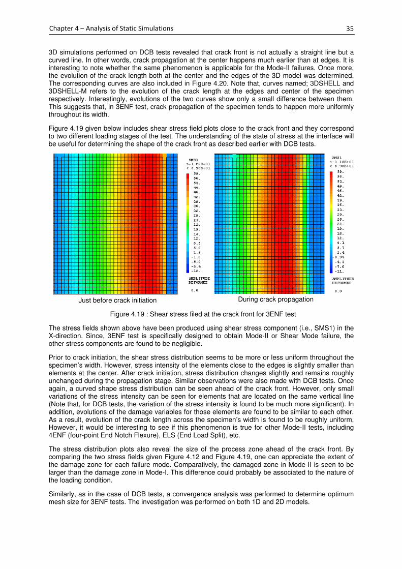
35


3D simulations performed on DCB tests revealed that crack front is not actually a straight line but a curved line. In other words, crack propagation at the center happens much earlier than at edges. It is interesting to note whether the same phenomenon is applicable for the Mode-II failures. Once more, the evolution of the crack length both at the center and the edges of the 3D model was determined. The corresponding curves are also included in Figure 4.20. Note that, curves named; 3DSHELL and 3DSHELL-M refers to the evolution of the crack length at the edges and center of the specimen respectively. Interestingly, evolutions of the two curves show only a small difference between them. This suggests that, in 3ENF test, crack propagation of the specimen tends to happen more uniformly throughout its width.

Figure 4.19 given below includes shear stress field plots close to the crack front and they correspond to two different loading stages of the test. The understanding of the state of stress at the interface will be useful for determining the shape of the crack front as described earlier with DCB tests.

Just before crack initiation During crack propagation

Figure 4.19 : Shear stress filed at the crack front for 3ENF test

The stress fields shown above have been produced using shear stress component (i.e., SMS1) in the X-direction. Since, 3ENF test is specifically designed to obtain Mode-II or Shear Mode failure, the other stress components are found to be negligible.

Prior to crack initiation, the shear stress distribution seems to be more or less uniform throughout the specimen’s width. However, stress intensity of the elements close to the edges is slightly smaller than elements at the center. After crack initiation, stress distribution changes slightly and remains roughly unchanged during the propagation stage. Similar observations were also made with DCB tests. Once again, a curved shape stress distribution can be seen ahead of the crack front. However, only small variations of the stress intensity can be seen for elements that are located on the same vertical line (Note that, for DCB tests, the variation of the stress intensity is found to be much more significant). In addition, evolutions of the damage variables for those elements are found to be similar to each other. As a result, evolution of the crack length across the specimen’s width is found to be roughly uniform, However, it would be interesting to see if this phenomenon is true for other Mode-II tests, including 4ENF (four-point End Notch Flexure), ELS (End Load Split), etc.

The stress distribution plots also reveal the size of the process zone ahead of the crack front. By comparing the two stress fields given Figure 4.12 and Figure 4.19, one can appreciate the extent of the damage zone for each failure mode. Comparatively, the damaged zone in Mode-II is seen to be larger than the damage zone in Mode-I. This difference could probably be associated to the nature of the loading condition.

Similarly, as in the case of DCB tests, a convergence analysis was performed to determine optimum mesh size for 3ENF tests. The investigation was performed on both 1D and 2D models.

36


Figure 4.20 : Force & Crack length vs. Displacement for 3ENF – simulated results in 1D for different element sizes

Figure 4.21 : Force & Crack length vs. Displacement for 3ENF – simulated results in 2D for different element sizes

Investigation results for 1D and 2D models are illustrated in Figure 4.20 and Figure 4.21 respectively.

Note that, all simulations were done with a constant displacement increment, equal to [ ]0.02 mm .

Interestingly, the conergence of the results were even achieved with element sizes equal to

[ ]0.4 mm . Note that for DCB, the optimum mesh size was found to be [ ]0.2 mm . For element sizes

over the optimum limit the undulations of the curve becomes more and more prominent, but the prediction of the general behaviour was found to be satifactorily.

Figure 4.22 : Force & Crack length vs. Displacement for 3ENF – simulated results in 2D for different FTOL and MTOL values

Figure 4.22 given above illustrate the results of the convergence analysis performed for determination of optimum FTOL and MTOL limits. The analysis was performed considering 1D model with an

element size equal to [ ]0.2 mm . Similarly, to DCB tests, the optimum FTOL and MTOL limits were

found to be equal to 1.0 2E − . Converegence analysis performed on the 2D model also produced

similar results.

37


4.6 Validation of Nonlocal Static Damage Model

4.6.1 FE Implementation of Nonlocal Model

The nonlocal damage model is basically formulated by introducing some intermediate steps in the finite element implementation of the local model. Note that, in the present study an integral-type nonlocal damage evolution law has been considered for implementation. Table 4.12 given below includes the two different approaches that were considered for simulations. As it was discussed earlier in Section 3.3.2, the regularization of the computed solution can easily be achieved by either directly averaging the damage variables or averaging the damage energy release rate variables.

Averaging damage energy release rate Averaging damage variable

Step-1 Compute damage energy release rate variables,

i.e., ( )Y t using 1 2,

d dY Y &

3d

Y

Compute damage energy release rate variables,

i.e., ( )Y t using 1 2,

d dY Y &

3d

Y

Step-2 Average damage energy release rate variables,

i.e., Y Y→ using Eq. 3.14 & 3.15

Compute isotropic damage function,


Y Y & 0

Y



Y Y & 0

Y

Compute damage variables,

i.e., ( )1 2 3

d d d w Y= = =


i.e., 1 2 3 ( )wd d d Y= = =

Average damage variables

i.e., d d→ using Eq. 3.14 & 3.15


i.e.,

0

13 1 1 1

0

23 2 2 2

0

33 3 3 3

(1 ) ,

(1 ) ,

(1 )

k d U

k d U

k d U

σ

σ

σ

= −

= −

= −

Compute stresses for the interface,

i.e.,

0

13 1 1 1

0

23 2 2 2

0

33 3 3 3

(1 ) ,

(1 ) ,

(1 )

k d U

k d U

k d U

σ

σ

σ

= −

= −

= −

Table 4.12 : FE implementations of nonlocal static damage models

Note that, all simulations were performed in 2D considering the same DCB and 3ENF test cases. Therefore, all material properties and values of damage model parameters are same as given before. In each approach, averaging of the variables needs to be performed at each gauss point of the all the interface elements. Usually, averaging of the variables is performed starting from the second increment. If the increment size is sufficiently small, the effect of this delay is believed to have a negligible influence on the final result.

In CAST3M, averaging of the variables was achieved using a personal procedure; named PERSO1, available in the PASAPAS operator. As explained before, the modified damage model is once again introduced in to CAST3M using the UMAT sub-routine. Initially, for the first increment, values of all the STATE VARIABLES (damage variables, damage energy release rate variables, stress, strain, etc) will be computed at every gauss point in each element. When the convergence is achieved, the PASAPAS PROCEDURE will then launch the PERSO1 sub-procedure. At first, the procedure will call for the STATE VARIABLE data saved in the ‘VARI’ (i.e., initial internal variables) table. Each variable will then be saved in different tables for subsequent processing. Next, X and Y coordinates of all the gauss points (or nodal points) are also obtained and saved in two different tables. As explained in Section 3.3.2, a Gaussian distribution is used for the averaging of the selected variable (damage variable or damage energy release rate variable). The coordinates along with an internal length scale

(i.e., l ) is then used to compute the weight of each variable value for every node in the interface.

Chapter 4

Figure 4.2distribution

The Gaussian function is also referred as the weighing function, because it is usedcontributionlocated at the origin. other pointsdepend on the distance between the point of interest and the point from where the contribution is coming from.variable value. In generalfurther. separately. The nonlocal value at the poincontributions with their weights.

As it can be seen from the above figure, the internal length scale is typically used to modify the shape

of the weighing function.

contribution coming from each variable value which are responsible for making plots given above, the smaller ones.

In order to the relatioabove, let us consider a mesh with elements ofthe element length (i.e.,

points in the neighborhood of the interested point (i.e., origin).half the size of the element length

and the number ocoming fromreduce the internal length scale further (i.e.,

coming from any pointsa local model.localizations.element size of the FE model.determined by fitting the simulated data with exp

One of the major limitations of the presented model is its high computational cost. Note that, averaging of the variables is performed at each gauss point of all the elemeelements increase, the number of variables that is to be averaged would also increase.averaging of variables at each point is normally performed by considering all the points in the interface. When the number points increase, taveraging process will automaticallythe notable increase of the computational time.simple strategy was introduced.


4.23 given hereunderdistribution. Note that, the

Figure 4.2

The Gaussian function is also referred as the weighing function, because it is usedcontributions of variable valuelocated at the origin. other points will be taken in depend on the distance between the point of interest and the point from where the contribution is coming from. Contributions are simply computed by multiplying the weight at a givvariable value. In general

In the next stepseparately. The nonlocal value at the poincontributions with their weights.


of the weighing function.

contribution coming from each variable value which are responsible for making plots given above, the smaller ones.

In order to completely understandthe relation between element size and

e, let us consider a mesh with elements ofthe element length (i.e.,


and the number of significant contributions can be seencoming from some of the points that are located outside the zone (see figurreduce the internal length scale further (i.e.,

coming from any pointsa local model. Thereforelocalizations. In conclusion, the selection of the internal length scale element size of the FE model.determined by fitting the simulated data with exp

One of the major limitations of the presented model is its high computational cost. Note that, averaging of the variables is performed at each gauss point of all the elemeelements increase, the number of variables that is to be averaged would also increase.averaging of variables at each point is normally performed by considering all the points in the interface. When the number points increase, taveraging process will automaticallythe notable increase of the computational time.

strategy was introduced.


given hereunder illustrateNote that, the selected Gaussian function has the form given in Equation 3.15.

Figure 4.23 :

The Gaussian function is also referred as the weighing function, because it is usedof variable values of every gauss point.

located at the origin. In order to find the nonlocal value at this point, the variable values located at the be taken in to ac

depend on the distance between the point of interest and the point from where the contribution is Contributions are simply computed by multiplying the weight at a giv

variable value. In general, as the distance increase, the contribution tends to decrease further and In the next step, all the contributions

separately. The nonlocal value at the poincontributions with their weights.


of the weighing function. For higher values of

contribution coming from each variable value which are responsible for making plots given above, the plots made with the higher length scales cover

completely understandn between element size and

e, let us consider a mesh with elements ofthe element length (i.e., 1l = ), we can


f significant contributions can be seensome of the points that are located outside the zone (see figur

reduce the internal length scale further (i.e.,

coming from any points that are located outside. ATherefore, the

In conclusion, the selection of the internal length scale element size of the FE model. determined by fitting the simulated data with exp

One of the major limitations of the presented model is its high computational cost. Note that, averaging of the variables is performed at each gauss point of all the elemeelements increase, the number of variables that is to be averaged would also increase.averaging of variables at each point is normally performed by considering all the points in the interface. When the number points increase, taveraging process will automaticallythe notable increase of the computational time.

strategy was introduced.

0( ) exprα =

r x= −


illustrates the effect of the internal length scale on theselected Gaussian function has the form given in Equation 3.15.

: Effect of internal length scale on weighing function

The Gaussian function is also referred as the weighing function, because it is usedof every gauss point.

In order to find the nonlocal value at this point, the variable values located at the to account. However, the level of contribution


, as the distance increase, the contribution tends to decrease further and ll the contributions

separately. The nonlocal value at the point of interest will then be computed by taking the ratio of


For higher values of

contribution coming from each variable value which are responsible for making significant contributions would also inc

plots made with the higher length scales cover

completely understand the behaviour of the nonlocal model, it is necessary to investigate n between element size and the

e, let us consider a mesh with elements of, we can clear observe some major contributions coming from

points in the neighborhood of the interested point (i.e., origin).half the size of the element length (i.e., 0.5l =

f significant contributions can be seensome of the points that are located outside the zone (see figur

reduce the internal length scale further (i.e.,

that are located outside. Athe nonlocal model is now incapable of regularizing the spurious

In conclusion, the selection of the internal length scale In the present study, a good value for the internal length

determined by fitting the simulated data with exp

One of the major limitations of the presented model is its high computational cost. Note that, averaging of the variables is performed at each gauss point of all the elemeelements increase, the number of variables that is to be averaged would also increase.averaging of variables at each point is normally performed by considering all the points in the interface. When the number points increase, taveraging process will automatically increase.the notable increase of the computational time.

2

2( ) exp

2

r

l

ζ= −

the effect of the internal length scale on theselected Gaussian function has the form given in Equation 3.15.

Effect of internal length scale on weighing function

The Gaussian function is also referred as the weighing function, because it is usedof every gauss point. For example, let us consider

In order to find the nonlocal value at this point, the variable values located at the count. However, the level of contribution


, as the distance increase, the contribution tends to decrease further and ll the contributions and weights considered will be added

t of interest will then be computed by taking the ratio of


For higher values of l , bell shape tends to expand further. As a result, the

contribution coming from each variable value will also increase. In addition, the domain of the significant contributions would also inc


the behaviour of the nonlocal model, it is necessary to investigate the internal length scale.

e, let us consider a mesh with elements of unit length. Whenclear observe some major contributions coming from

points in the neighborhood of the interested point (i.e., origin).0.5= ), a considerable drop

f significant contributions can be seen. However, some notable contributions are still some of the points that are located outside the zone (see figur

reduce the internal length scale further (i.e., 0.25l = )

that are located outside. At this point, the nonlocal model nonlocal model is now incapable of regularizing the spurious


determined by fitting the simulated data with experimental result

One of the major limitations of the presented model is its high computational cost. Note that, averaging of the variables is performed at each gauss point of all the elemeelements increase, the number of variables that is to be averaged would also increase.averaging of variables at each point is normally performed by considering all the points in the interface. When the number points increase, the number of points that is to be considere

increase. In fact, this is the main reason which is responsible for the notable increase of the computational time. In order to overcome this problem

unit length



The Gaussian function is also referred as the weighing function, because it is usedFor example, let us consider

In order to find the nonlocal value at this point, the variable values located at the count. However, the level of contribution


, as the distance increase, the contribution tends to decrease further and and weights considered will be added



, bell shape tends to expand further. As a result, the

also increase. In addition, the domain of the significant contributions would also inc


the behaviour of the nonlocal model, it is necessary to investigate internal length scale. Corresponding to the figure given

unit length. When internal length scaleclear observe some major contributions coming from

points in the neighborhood of the interested point (i.e., origin). When the internal length scale isa considerable drop

. However, some notable contributions are still some of the points that are located outside the zone (see figur

0.25 ), we clearly see no significant contribution

t this point, the nonlocal model nonlocal model is now incapable of regularizing the spurious


erimental result.

One of the major limitations of the presented model is its high computational cost. Note that, averaging of the variables is performed at each gauss point of all the elemeelements increase, the number of variables that is to be averaged would also increase.averaging of variables at each point is normally performed by considering all the points in the

he number of points that is to be considerethis is the main reason which is responsible for

In order to overcome this problem

unit length



The Gaussian function is also referred as the weighing function, because it is usedFor example, let us consider

In order to find the nonlocal value at this point, the variable values located at the count. However, the level of contribution of those variable values will






also increase. In addition, the domain of the significant contributions would also increase. If we consider

plots made with the higher length scales cover more points compared to the

the behaviour of the nonlocal model, it is necessary to investigate Corresponding to the figure given internal length scale

clear observe some major contributions coming from

When the internal length scale isa considerable drop of both level of the contribution

. However, some notable contributions are still some of the points that are located outside the zone (see figure) of interest

we clearly see no significant contribution

t this point, the nonlocal model nonlocal model is now incapable of regularizing the spurious

In conclusion, the selection of the internal length scale is mainly connected to the In the present study, a good value for the internal length

One of the major limitations of the presented model is its high computational cost. Note that, averaging of the variables is performed at each gauss point of all the elements. Aselements increase, the number of variables that is to be averaged would also increase.averaging of variables at each point is normally performed by considering all the points in the


In order to overcome this problem

the effect of the internal length scale on the Gaussian selected Gaussian function has the form given in Equation 3.15.


The Gaussian function is also referred as the weighing function, because it is used to determineFor example, let us consider the variable value

In order to find the nonlocal value at this point, the variable values located at the of those variable values will

depend on the distance between the point of interest and the point from where the contribution is Contributions are simply computed by multiplying the weight at a given point with its





also increase. In addition, the domain of the f we consider

more points compared to the

the behaviour of the nonlocal model, it is necessary to investigate Corresponding to the figure given internal length scale is taken

clear observe some major contributions coming from

When the internal length scale islevel of the contribution

. However, some notable contributions are still e) of interest. When we


t this point, the nonlocal model starts to behavenonlocal model is now incapable of regularizing the spurious

mainly connected to the In the present study, a good value for the internal length

One of the major limitations of the presented model is its high computational cost. Note that, nts. As the number of

elements increase, the number of variables that is to be averaged would also increase. In addition, averaging of variables at each point is normally performed by considering all the points in the


In order to overcome this problem, an innovative

38

Gaussian

to determine the variable value

In order to find the nonlocal value at this point, the variable values located at the of those variable values will

depend on the distance between the point of interest and the point from where the contribution is en point with its

, as the distance increase, the contribution tends to decrease further and and weights considered will be added together

t of interest will then be computed by taking the ratio of total



also increase. In addition, the domain of the points f we consider the bell

more points compared to the

the behaviour of the nonlocal model, it is necessary to investigate Corresponding to the figure given

taken equal clear observe some major contributions coming from many

When the internal length scale is taken level of the contribution

. However, some notable contributions are still When we


starts to behave as nonlocal model is now incapable of regularizing the spurious

mainly connected to the In the present study, a good value for the internal length scale is

One of the major limitations of the presented model is its high computational cost. Note that, the number of

In addition, averaging of variables at each point is normally performed by considering all the points in the

d for the this is the main reason which is responsible for

, an innovative but

39


As it was discussed earlier, only some points are providing major contributions for the averaging process. Figure 4.24 given below can be used to describe the magnitude of contributions coming from both left and right side of the point in interest.

`

Figure 4.24 : Level of contributions received from left and right

As we move along in either direction, the magnitude of the weights determined by the weighing function will decrease gradually. With increasing distance, the values of the weights will decrease towards zero. As a result, contributions corresponding to those weights would automatically become very small. Therefore, averaging of the variables needs only be done with points that are in the neighbourhood. In fact, when we do averaging considering all the points in the whole domain, we perform unnecessary amount of computations without any useful gain. The idea was to eliminate redundant computations as much as possible. At the same care was taken to ensure the integrity of the nonlocal model.

Next, a criterion was introduced to estimate the number of points that should be considered for the averaging process. In accordance to Figure 4.25, the criterion should also necessarily consider the effect of the internal length scale. Thus, to reduce complexity a simple approach was adopted to identify the size of the neighbourhood points. Figure 4.25 given below illustrate the selected criterion in a graphical form.

`

Figure 4.25 : Criterion for selecting neighbourhood points for averaging

As shown above, the points that are lying in between the two limits corresponding to 0 1.0 3Eα = −

are selected for the averaging process. The neighbourhood of these points is referred as the ‘Averaging Zone’. These limits have been identified by performing a simple investigation between the original model and the modified model. Note that, the limits are inherently related to the problem in hand. In other words geometry of the model, mesh size, evolution of the variables, etc needs to be closely analyzed before making a decision. For test-cases where influence of parameters is not well

understood, a limit corresponding to 0 1.0 6Eα = − should at least be considered.

In addition, few other attempts were made to further optimize the computation process. Generally (except at the two ends of the domain), at each nodal point there are two gauss points belonging to the two elements connected to it. The evolution of the STATE VARIABLES at these two gauss points will essentially be equal to each other at every stage of the solution process. This is mainly because of the continuity relation that exists between elements connected to each other. However, when it comes to averaging of the variables, it is not necessary to perform the same computation twice for the two gauss points located at the same node. We only need to perform a single computation and then store the averaged values for the two gauss points separately. By adopting this method we can effectively reduce the total number of computations required for averaging by half. Therefore, it was possible to reduce the computational time significantly. Interestingly, a notable reduction of the computation cost was observed with all proposed modifications. The ratio of the computational time between the original and the modified model is in the range between 4 and 6.

Weighing function

Very small contributions Very small contributions

Significant contributions

Averaging Zone

( )0 rα

0 1.0 3Eα = − 0 1.0 3Eα = −

40


Afterwards, the averaged variables need to be defined at each gauss point systematically. Note that, during the averaging process averaged values were written in separate tables. Now, all the STATE VARIABLES need to be redefined in the ‘VARF’ (i.e., final internal variables) table in PASAPAS PROCEDURE. In CAST3M, the user is only limited to define a common value over an element. The following choices were considered for determining a common or a representative value for each element using the values of the averaged variables at the two gauss points.

I. Taking the average of the variable values at the two gauss points II. Taking the maximum value of the variable values at the two gauss points

Both approaches were tested methodically and comparisons were made for subsequent analysis. Results of the investigation are included in the next section. Interestingly, the two approaches present two different conceptual arguments. In CASE-I, when you do averaging on the already averaged variables, this new value will make the model more nonlocal in comparison. On the other hand, in CASE-II, when you assign the maximum value of the two averaged values, comparatively you are making the model more local.

However, when we perform further averaging on the already averaged values, we ultimately delay the evolution of the variables. As a consequence, the computational time tend to increase significantly. On the other hand, excessive averaging would also hinder accuracy of the computed value. It adds more viscosity in to the models behaviour. As a result, the STATE VARIABLES take more time to converge on to the realistic values. In comparison, taking the maximum value would help to reduce the computational time effectively. However, the lost information would obviously have a negative impact on the model's outcome. The details of the investigation comparing the two approaches are included in a later section. In general, the second approach seems to produce better results compared to the first one.

Efforts were also made to further expand the nonlocal model from 2D to 3D environment. In fact, spurious localization issues are more associated to 3D models in comparison to 2D models. As it was observed during the study, 2D FE models with uniform mesh do not give rise to any numerical localization. In fact, models with varying mesh sizes also produced localization free results. In 3D, the Gaussian function is no longer line but a three-dimensional surface having a ‘bell shape’. As a result, in three-dimensions the computational time increases heavily and the investigation of the model’s behaviour becomes more inflexible. Therefore, as mentioned earlier, all investigations of the present study are performed on 2D models.

4.6.2 Simulation Results on DCB and 3ENF Tests

According to preliminary analysis, the approach based on ‘averaging of damage energy release rate’ was found to be more favourable in predicting the experimental results. Therefore, much attention was devoted to appreciate the behaviour of that model. Investigations was carried out on both DCB and 3ENF test models. Classically, for any given nonlocal model, the convergence of model’s response should be verified. Experimental results used for verfication of the local model will once again be used to validate the proposed nonlocal model. Note that, a choice should be made for selecting a representative value for each element using the averaged values. Simulation results given hereunder are based on the approach of taking the maximum value of the two gauss points belonging to each element.

At first, an investigation was carried out to identiy a suitable value for the internal length scale. The results of this invetigation is inluded in later section. The value for the inernal length scale selected for

the simulations equals to 0.25 . Efforts were also made to identity correlations between the internal

length scale and model parameters (i.e., dimensions of the geometry, element size, etc). The size of the averaging zone selected for the following simulations corresponds to the range of points

enveloped by 0 5.0 3Eα = − . For simplicity, a linear correlation was developed between the internal

length scale and number nodes that should be considered for averaging (i.e, NAN). In addition, this relation is inherently depended on the selected element size. For example, for an element size of

0.1ES = the corresponding relation reads as, 32 1NAN l= + . Note that, in the developed program

code the user needs to enter the value of NAN along with the value of internal length scale.

Chapter 4

Given hernonlocal modeldiplacement

value were taken equal to

Figure

In additionwere made on the behaviour of the evolutionselement size the forcevisible with the DCB tests simulations

already ach

achieved roughly at an element size of

Interestinglythe case of DCBautomatically promts a question on the influence of the increment size on the nonlocal model’s behaviourand the re

Figure 4.2

Here, the simulations were p

value was kept unchangedachieved with decreasing increment sizeDCB and experimental resultscase than for

size of INC

to perform the final s

selected element and increment sizes are

selected to simulate the


Given hereunder are the results and conclusions madenonlocal model. Figure diplacement for different element sizes

value were taken equal to

Figure 4.26 : Influence of

tion, same simulations were performed with different increment sizes and similar observations were made on the behaviour of the evolutionselement size the forcevisible with the DCB tests simulations

already achieved with a


Interestingly, we can note that evolutions are moving away from the experimental the case of DCB, in fact nonlocal results on automatically promts a question on the influence of the increment size on the nonlocal model’s behaviour. Thereforeand the results of this


the simulations were p

value was kept unchangedachieved with decreasing increment sizeDCB and 3ENF test experimental results

than for 3ENF test case

0.01INC = .

to perform the final s


selected to simulate the


under are the results and conclusions madeFigure 4.26 given below

different element sizes

value were taken equal to [0.01

Influence of element size on

same simulations were performed with different increment sizes and similar observations were made on the behaviour of the evolutionselement size the force-displacement evolutions seems to converge towards each othervisible with the DCB tests simulations

ieved with a larger element size


we can note that evolutions are moving away from the experimental in fact nonlocal results on

automatically promts a question on the influence of the increment size on the nonlocal model’s Therefore, a seperate analysis was performed to understand the effect of

his analysis is

Influence of increment

the simulations were performed with an element size equal to

value was kept unchanged. Similarlyachieved with decreasing increment size

ENF test results. Interesetiexperimental results. Once more

ENF test case. In case of DCB

0.01 . By considering the facts of the two analysis discussed earlier

to perform the final simulations to obatin the conver


selected to simulate the 3ENF test


under are the results and conclusions madegiven below

different element sizes. Here

[ ]0.01 mm and 1.0 2

element size on

same simulations were performed with different increment sizes and similar observations were made on the behaviour of the evolutions

displacement evolutions seems to converge towards each othervisible with the DCB tests simulations, where as for

element size

achieved roughly at an element size of ES =

we can note that evolutions are moving away from the experimental in fact nonlocal results on 3

automatically promts a question on the influence of the increment size on the nonlocal model’s a seperate analysis was performed to understand the effect of

is shown in Figure

increment size on

rformed with an element size equal to

Similarly, as with the case ofachieved with decreasing increment size. As it can be seen from the above plots

Interesetingly, Once more, as expected

In case of DCB

By considering the facts of the two analysis discussed earlier

imulations to obatin the conver


ENF test.

under are the results and conclusions made on the convergiven below, illustrate the evolution of the

Here, for both DCB and

1.0 2E − respectively

element size on nonlocal model’s behaviour for DCB

same simulations were performed with different increment sizes and similar observations were made on the behaviour of the evolutions. As it can be seen from each plot

displacement evolutions seems to converge towards each otherwhere as for 3

element size (i.e., ES =0.05= .

we can note that evolutions are moving away from the experimental 3ENF are very close to the local results


Figure 4.27 given below

size on nonlocal model’s behaviour for DCB


as with the case ofAs it can be seen from the above plots, force-displacement evolutions are moving towards the

as expected, this phenomenon is In case of DCB, the converegence is achieved roughly


imulations to obatin the converged solutions

0.05ES =

on the converillustrate the evolution of the for both DCB and 3ENF tests

respectively.

nonlocal model’s behaviour for DCB

same simulations were performed with different increment sizes and similar observations As it can be seen from each plot

displacement evolutions seems to converge towards each other3ENF the convergence seems to have been

0.2= ). In case of DCB

we can note that evolutions are moving away from the experimental ENF are very close to the local results


given below.



as with the case of element sizeAs it can be seen from the above plots

displacement evolutions are moving towards the this phenomenon is

the converegence is achieved roughly


ged solutions.

and INC =

on the convergence analysis ofillustrate the evolution of the force

ENF tests, increment size and FTOL


same simulations were performed with different increment sizes and similar observations As it can be seen from each plot

displacement evolutions seems to converge towards each otherENF the convergence seems to have been

In case of DCB,

we can note that evolutions are moving away from the experimental ENF are very close to the local results



rformed with an element size equal to 0.1ES =element size, convergence is normally

As it can be seen from the above plotsdisplacement evolutions are moving towards the this phenomenon is more visible for the DCB

the converegence is achieved roughly


Therefore, for the DCB test

0.005= . Similar values were also

gence analysis of the proposed force against

increment size and FTOL

nonlocal model’s behaviour for DCB and 3ENF tests

same simulations were performed with different increment sizes and similar observations As it can be seen from each plot, with decreasing

displacement evolutions seems to converge towards each other. This is clealry ENF the convergence seems to have been

, the converegence is

we can note that evolutions are moving away from the experimental result (especially in ENF are very close to the local results). This observation

automatically promts a question on the influence of the increment size on the nonlocal model’s a seperate analysis was performed to understand the effect of increment size

nonlocal model’s behaviour for DCB and 3ENF tests

0.1 for both tests

convergence is normally As it can be seen from the above plots, this is true for both

displacement evolutions are moving towards the visible for the DCB

the converegence is achieved roughly at an increment

By considering the facts of the two analysis discussed earlier, it is now possible

for the DCB test

Similar values were also

41

the proposed imposed

increment size and FTOL

ENF tests

same simulations were performed with different increment sizes and similar observations with decreasing This is clealry

ENF the convergence seems to have been

the converegence is

especially in This observation

automatically promts a question on the influence of the increment size on the nonlocal model’s increment size

ENF tests

for both tests. FTOL

convergence is normally this is true for both

displacement evolutions are moving towards the visible for the DCB test

increment

it is now possible

for the DCB test, the

Similar values were also

Chapter 4

Plots included in the Figure nonlocal

As it can be seen from forcelocal and nonlocal model seems to over predict the maximum value of the forcethe initiatiwith increasing displacement the curve strarts dropplot with a sudden increase of the crack lengthevolution tSame is true for evolution of the crack lengthrelated to the numerical viscosityproblem

Figure 4local and nonlocalNote thatvalues. Interesinglysimulations convergence was also achieved with larger element sizes

4.6.3

In order to identify a suitable candidate foby comparing model’s response for few arbitarary valuesvalues were done in relation to the element size of the FE modelinternal length scale should not be too small compared to the element sizevalue, then the nonlocal model will nolonger be capable of regularizing the evolutions of the variablesIf the value is too largeconsequenceconsider the element size to make a good prediction for the internal length scale


Plots included in the Figure nonlocal models for DCB test

Figure 4.

As it can be seen from forcelocal and nonlocal models are in good agreement with the experimental resultsnonlocal model seems to over predict the maximum value of the force

ation of the crackwith increasing displacement the curve strarts dropplot with a sudden increase of the crack lengthevolution tend to settle down gradually and seem to follow the experimental result with good accuracySame is true for evolution of the crack lengthrelated to the numerical viscosityproblem associated to integral

Figure 4.

4.29 given above shows a similar comparison made betweenlocal and nonlocal modelsNote that, convergence of the nonlocal results were eve

Interesingly, simulations convergence was also achieved with larger element sizes

Influence of the Internal Length Scale

In order to identify a suitable candidate foby comparing model’s response for few arbitarary valuesvalues were done in relation to the element size of the FE modelinternal length scale should not be too small compared to the element size

then the nonlocal model will nolonger be capable of regularizing the evolutions of the variablesIf the value is too largeconsequence, the maximum force value will increase unrealisticallyconsider the element size to make a good prediction for the internal length scale


Plots included in the Figure 4.28for DCB test.

Figure 4.28 : Comparison of local and nonlocal results

As it can be seen from force- and crack extensionnonlocal models are in good agreement with the experimental results

nonlocal model seems to over predict the maximum value of the forceon of the crack happens with a little delay

with increasing displacement the curve strarts dropplot with a sudden increase of the crack length

end to settle down gradually and seem to follow the experimental result with good accuracySame is true for evolution of the crack lengthrelated to the numerical viscosity

associated to integral-type regularization schemes

Figure 4.29 : Comparison of local and nonlocal results

given above shows a similar comparison made betweenmodels. As explained before

convergence of the nonlocal results were eve, the local model a

simulations convergence was also achieved with larger element sizes


In order to identify a suitable candidate foby comparing model’s response for few arbitarary valuesvalues were done in relation to the element size of the FE modelinternal length scale should not be too small compared to the element size

then the nonlocal model will nolonger be capable of regularizing the evolutions of the variablesIf the value is too large, then we wi

the maximum force value will increase unrealisticallyconsider the element size to make a good prediction for the internal length scale


28 given hereunder

Comparison of local and nonlocal results

and crack extensionnonlocal models are in good agreement with the experimental results

nonlocal model seems to over predict the maximum value of the forcehappens with a little delay

with increasing displacement the curve strarts dropplot with a sudden increase of the crack length

end to settle down gradually and seem to follow the experimental result with good accuracySame is true for evolution of the crack lengthrelated to the numerical viscosity induced by the nonlocal m

type regularization schemes


given above shows a similar comparison made betweenAs explained before

convergence of the nonlocal results were evethe local model also behaved in a similar manner



In order to identify a suitable candidate for the internal length scaleby comparing model’s response for few arbitarary valuesvalues were done in relation to the element size of the FE modelinternal length scale should not be too small compared to the element size

then the nonlocal model will nolonger be capable of regularizing the evolutions of the variablesthen we will be intro


hereunder, shows


and crack extension-displacement plotsnonlocal models are in good agreement with the experimental results

nonlocal model seems to over predict the maximum value of the forcehappens with a little delay. After the force has reached its maximum val

with increasing displacement the curve strarts drop steeplyplot with a sudden increase of the crack length. When displacement is further increased

end to settle down gradually and seem to follow the experimental result with good accuracySame is true for evolution of the crack length. The reason for the nonphysical increase of the force is

induced by the nonlocal mtype regularization schemes


given above shows a similar comparison made betweenAs explained before, nonlocal model’

convergence of the nonlocal results were evelso behaved in a similar manner



r the internal length scaleby comparing model’s response for few arbitarary valuesvalues were done in relation to the element size of the FE modelinternal length scale should not be too small compared to the element size

then the nonlocal model will nolonger be capable of regularizing the evolutions of the variablesoducing more viscosity in to the model’s behaviour


shows the converged


displacement plotsnonlocal models are in good agreement with the experimental results

nonlocal model seems to over predict the maximum value of the forceAfter the force has reached its maximum valsteeply. This is reflected on the crack extension When displacement is further increased

end to settle down gradually and seem to follow the experimental result with good accuracyThe reason for the nonphysical increase of the force is

induced by the nonlocal model. This is considered to betype regularization schemes.


given above shows a similar comparison made betweennonlocal model’s behaviour is closer to

convergence of the nonlocal results were even achieved with larger lso behaved in a similar manner


r the internal length scale, by comparing model’s response for few arbitarary values. However, values were done in relation to the element size of the FE model. internal length scale should not be too small compared to the element size

then the nonlocal model will nolonger be capable of regularizing the evolutions of the variablesducing more viscosity in to the model’s behaviour


converged results

Comparison of local and nonlocal results for DCB

displacement plots, the results produced by both nonlocal models are in good agreement with the experimental results

nonlocal model seems to over predict the maximum value of the force. At the same timeAfter the force has reached its maximum val

This is reflected on the crack extension When displacement is further increased


This is considered to be

Comparison of local and nonlocal results for 3ENF

given above shows a similar comparison made between 3ENF test reuslts obatined froms behaviour is closer to

n achieved with larger lso behaved in a similar manner and in comparison to DCB test

simulations convergence was also achieved with larger element sizes.

, a simple analysis was performed , initial selection of these arbitrary . As it was discussed earlie

internal length scale should not be too small compared to the element size. If it goes below the crtitical then the nonlocal model will nolonger be capable of regularizing the evolutions of the variables

ducing more viscosity in to the model’s behaviourthe maximum force value will increase unrealistically. Therefore

consider the element size to make a good prediction for the internal length scale.

results of both local and

test

the results produced by both nonlocal models are in good agreement with the experimental results. However

At the same time, prediction of After the force has reached its maximum val

This is reflected on the crack extension When displacement is further increased


This is considered to be an inherent

test

reuslts obatined froms behaviour is closer to local model

n achieved with larger element/incrementand in comparison to DCB test

a simple analysis was performed initial selection of these arbitrary As it was discussed earlie

If it goes below the crtitical then the nonlocal model will nolonger be capable of regularizing the evolutions of the variables

ducing more viscosity in to the model’s behaviourTherefore, it is necessary to

42

both local and

the results produced by both However, the prediction of

After the force has reached its maximum value, This is reflected on the crack extension

When displacement is further increased, force end to settle down gradually and seem to follow the experimental result with good accuracy.

The reason for the nonphysical increase of the force is an inherent

reuslts obatined from local model. increment

and in comparison to DCB test

a simple analysis was performed initial selection of these arbitrary As it was discussed earlier, the

If it goes below the crtitical then the nonlocal model will nolonger be capable of regularizing the evolutions of the variables.

ducing more viscosity in to the model’s behaviour. As a it is necessary to

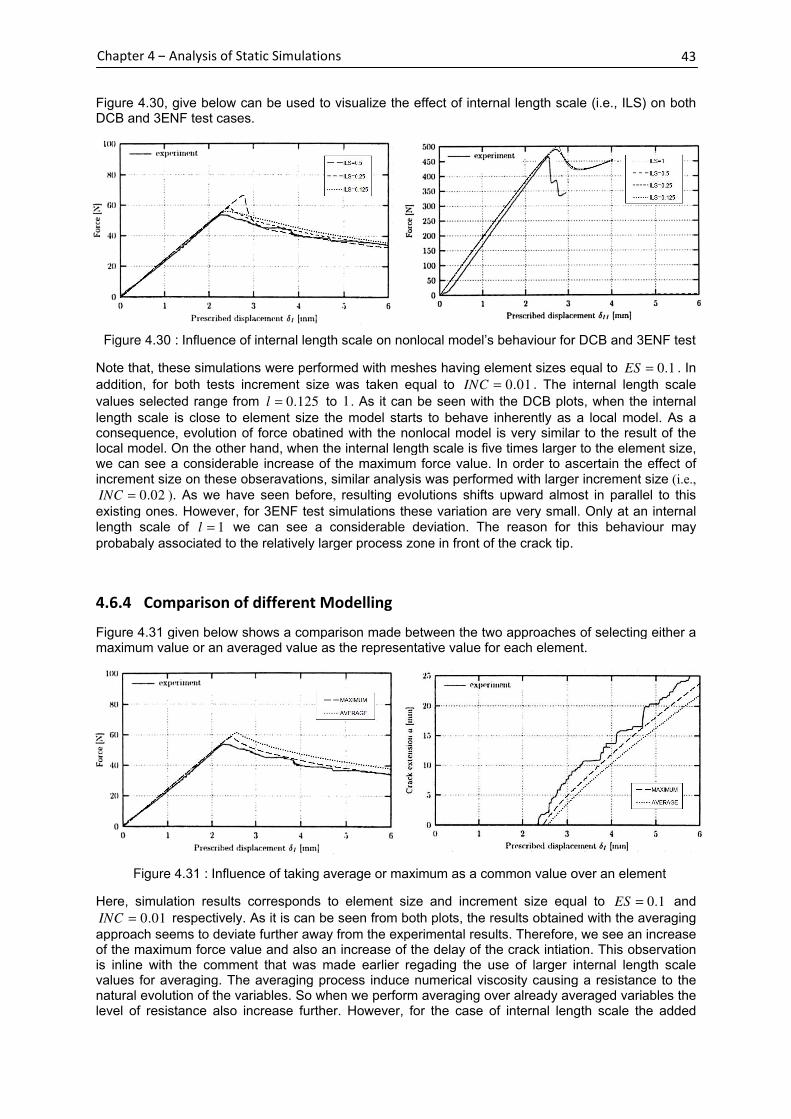
Chapter 4

Figure 4DCB and

Figure 4.

Note that

addition,

values selected

length scale is close to element size the model starts to behave inherently as a local modelconsequencelocal modelwe can see a considerable increase of the maximum force valueincrement size on these obseravations

0.02INC =existing ones

length scale of

probabaly associated to the relatively larger process

4.6.4

Figure 4maximum value or an

Figure 4.

Here, simulation results corresponds to element size and increment size equal to

0.01INC =approach seems to deviate further away from the experimental resultsof the maximum force valueis inline with the comment that was made earlier regading the use of larger internal length scale values for averagingnatural evolution of the variableslevel of resistance also incre


4.30, give below can be used to visualize the effect of internal length scaleDCB and 3ENF test cases


Note that, these simulations were performed with meshes having element size

, for both tests increment size was taken equal to

selected rang

length scale is close to element size the model starts to behave inherently as a local modelconsequence, evolution of force obatined local model. On the other handwe can see a considerable increase of the maximum force valueincrement size on these obseravations

0.02= ). As we have seen before

existing ones. However

length scale of l =probabaly associated to the relatively larger process

Comparison of different Modelling

4.31 given below shows a comparison made between the two approaches of selectimaximum value or an


simulation results corresponds to element size and increment size equal to

0.01= respectivelyapproach seems to deviate further away from the experimental resultsof the maximum force valueis inline with the comment that was made earlier regading the use of larger internal length scale values for averagingnatural evolution of the variableslevel of resistance also incre


give below can be used to visualize the effect of internal length scaleENF test cases.

Influence of internal length scale

simulations were performed with meshes having element size

for both tests increment size was taken equal to

range from l =length scale is close to element size the model starts to behave inherently as a local model

evolution of force obatined On the other hand,

we can see a considerable increase of the maximum force valueincrement size on these obseravations

As we have seen before

However, for 3ENF test simulations these variation are

1= we can see a considerable deviation



given below shows a comparison made between the two approaches of selectimaximum value or an averaged value as the representative value for each element

Influence of taki


respectively. As it is can

approach seems to deviate further away from the experimental resultsof the maximum force value and also an increase of the delay of the crack intiationis inline with the comment that was made earlier regading the use of larger internal length scale values for averaging. The averaging process induce numerical viscosity causing a resistance to the natural evolution of the variableslevel of resistance also increase fu


give below can be used to visualize the effect of internal length scale

internal length scale



0.125= to 1.

length scale is close to element size the model starts to behave inherently as a local modelevolution of force obatined with the nonlocal model is very similar to the result of the

, when the internal length scale is five times larger to the element sizewe can see a considerable increase of the maximum force valueincrement size on these obseravations, similar analysis was performed with larger increment size

As we have seen before, resulting

ENF test simulations these variation are

we can see a considerable deviation



given below shows a comparison made between the two approaches of selectiaveraged value as the representative value for each element

taking average or maximum


As it is can be seen from both plots

approach seems to deviate further away from the experimental resultsand also an increase of the delay of the crack intiation

is inline with the comment that was made earlier regading the use of larger internal length scale The averaging process induce numerical viscosity causing a resistance to the

natural evolution of the variables. So when we pse further. However


internal length scale on nonlocal model’s behaviour for DCB



As it can be seen with the DCB plots

length scale is close to element size the model starts to behave inherently as a local modelwith the nonlocal model is very similar to the result of the

when the internal length scale is five times larger to the element sizewe can see a considerable increase of the maximum force value

similar analysis was performed with larger increment size

resulting evolution


we can see a considerable deviation

probabaly associated to the relatively larger process zone in front of the crack tip



average or maximum


be seen from both plots



So when we perform averaging over already averaged variables the However, for the case of internal length scale




for both tests increment size was taken equal to INC =As it can be seen with the DCB plots


when the internal length scale is five times larger to the element sizewe can see a considerable increase of the maximum force value. In order to asce


evolutions shifts upward almost in parallel to this


we can see a considerable deviation. The reason for this behaviour may

zone in front of the crack tip


average or maximum as a common value over an element


be seen from both plots, the results obtained with the averaging



erform averaging over already averaged variables the for the case of internal length scale



simulations were performed with meshes having element sizes equal to

0.01= . The

As it can be seen with the DCB plots


when the internal length scale is five times larger to the element sizeIn order to asce


upward almost in parallel to this

ENF test simulations these variation are very small

The reason for this behaviour may

zone in front of the crack tip.


as a common value over an element


the results obtained with the averaging

approach seems to deviate further away from the experimental results. Thereforeand also an increase of the delay of the crack intiation


erform averaging over already averaged variables the for the case of internal length scale

give below can be used to visualize the effect of internal length scale (i.e., ILS)

nonlocal model’s behaviour for DCB and 3

equal to ES

The internal length scale

As it can be seen with the DCB plots, when the internal


when the internal length scale is five times larger to the element sizeIn order to ascertain the e



very small. Only at an internal


.

given below shows a comparison made between the two approaches of selecting either a averaged value as the representative value for each element.


simulation results corresponds to element size and increment size equal to ES =the results obtained with the averaging

Therefore, we see an increase and also an increase of the delay of the crack intiation. This observation


erform averaging over already averaged variables the for the case of internal length scale the added

43

) on both

3ENF test

0.1ES = . In

internal length scale

when the internal

length scale is close to element size the model starts to behave inherently as a local model. As a with the nonlocal model is very similar to the result of the

when the internal length scale is five times larger to the element size, the effect of

similar analysis was performed with larger increment size (i.e.,


Only at an internal


ng either a


0.1= and

the results obtained with the averaging

we see an increase bservation


erform averaging over already averaged variables the the added

Chapter 4

resistance seems to settle down gradually with increasing crack length and the phenomenon tends to balance out internallyresult, the corresponding evolution remains parallel and over the evolution of the(which was

Figure 4modification to the nonlocamain objective of the propsed modifcations was to reduce com

Figure 4.

Selected element size and increment size f

it is evident from averaging overyield same resultsthe same computer and care was taken to impose same tesing conditionssimulation time between averaging over the whole domain and averaging over a limited range was

found to approximately equal to

significant

4.6.5

In order to appreciate the behaviour of each damage variable


resistance seems to settle down gradually with increasing crack length and the phenomenon tends to nce out internally

the corresponding evolution remains parallel and over the evolution of thewhich was obtained by

4.32 given hereunder are the results of an invetigation modification to the nonlocamain objective of the propsed modifcations was to reduce com

Figure 4.32 : Model

elected element size and increment size f

it is evident from each plotaveraging over the en

d same results. Cthe same computer and care was taken to impose same tesing conditionssimulation time between averaging over the whole domain and averaging over a limited range was


significant. In case of

Comparison of Evolution of Damage Variable

In order to appreciate the behaviour of each e variable at different gauss points along the interface starting from the crack tip

Figure 4.


resistance seems to settle down gradually with increasing crack length and the phenomenon tends to nce out internally. On the other hand

the corresponding evolution remains parallel and over the evolution of theobtained by taking the maximum value

iven hereunder are the results of an invetigation modification to the nonlocal model does not effect the outcome of the original model’s responsemain objective of the propsed modifcations was to reduce com

odel responses on averaging over entire domain

elected element size and increment size f

each plot, both force anthe entire domain or over a limited range

Computation timethe same computer and care was taken to impose same tesing conditionssimulation time between averaging over the whole domain and averaging over a limited range was


In case of 3D modelling


In order to appreciate the behaviour of each at different gauss points along the interface starting from the crack tip

Figure 4.33 : Evolutions of damage variables for local and nonlocal models


resistance seems to settle down gradually with increasing crack length and the phenomenon tends to On the other hand, averaging over the element is an external process

the corresponding evolution remains parallel and over the evolution of thetaking the maximum value

iven hereunder are the results of an invetigation l model does not effect the outcome of the original model’s response

main objective of the propsed modifcations was to reduce com

responses on averaging over entire domain

elected element size and increment size for

both force and crackdomain or over a limited range

on times were the same computer and care was taken to impose same tesing conditionssimulation time between averaging over the whole domain and averaging over a limited range was

found to approximately equal to 6 . Therefore

D modelling, these modification


In order to appreciate the behaviour of each at different gauss points along the interface starting from the crack tip

Evolutions of damage variables for local and nonlocal models

resistance seems to settle down gradually with increasing crack length and the phenomenon tends to averaging over the element is an external process

the corresponding evolution remains parallel and over the evolution of thetaking the maximum value).

iven hereunder are the results of an invetigation l model does not effect the outcome of the original model’s response

main objective of the propsed modifcations was to reduce com

responses on averaging over entire domain

or analysis are

crack length evolutions are almost identicaldomain or over a limited range

noted for both simulationsthe same computer and care was taken to impose same tesing conditionssimulation time between averaging over the whole domain and averaging over a limited range was

Therefore, the time saved by the proposed modifications is fai

these modifications may prove to be very useful


In order to appreciate the behaviour of each model it would be useful to compare the evolution of at different gauss points along the interface starting from the crack tip



the corresponding evolution remains parallel and over the evolution of the

iven hereunder are the results of an invetigation performedl model does not effect the outcome of the original model’s response

main objective of the propsed modifcations was to reduce compuational time effectively

responses on averaging over entire domain and

analysis are 0.2ES = andlength evolutions are almost identical

domain or over a limited range (i.e., averagingnoted for both simulations

the same computer and care was taken to impose same tesing conditionssimulation time between averaging over the whole domain and averaging over a limited range was

the time saved by the proposed modifications is fai

may prove to be very useful


model it would be useful to compare the evolution of at different gauss points along the interface starting from the crack tip



the corresponding evolution remains parallel and over the evolution of the

performed to justify that the proposed l model does not effect the outcome of the original model’s response

puational time effectively

and averaging over a limited range

and 0.02INC =length evolutions are almost identical

averaging-zone as seen on Figure noted for both simulations. Here, the

the same computer and care was taken to impose same tesing conditions. Finallysimulation time between averaging over the whole domain and averaging over a limited range was


may prove to be very useful

model it would be useful to compare the evolution of at different gauss points along the interface starting from the crack tip



the corresponding evolution remains parallel and over the evolution of the second approa

to justify that the proposed l model does not effect the outcome of the original model’s response

puational time effectively.

averaging over a limited range

0.02= respectivelylength evolutions are almost identical. In other wor

zone as seen on Figure the tests were done on Finally, the ratio of the

simulation time between averaging over the whole domain and averaging over a limited range was


may prove to be very useful.

model it would be useful to compare the evolution of at different gauss points along the interface starting from the crack tip.


44

resistance seems to settle down gradually with increasing crack length and the phenomenon tends to averaging over the element is an external process. As a

second approach

to justify that the proposed l model does not effect the outcome of the original model’s response. The

averaging over a limited range

respectively. As

In other words, zone as seen on Figure 4.25)

were done on the ratio of the

simulation time between averaging over the whole domain and averaging over a limited range was

the time saved by the proposed modifications is fairly

model it would be useful to compare the evolution of

Chapter 4

Figure 4the visinity of the crack tip

simulations are

starting from the left and nonlocal models

at gauss points located at

Interestinglygradually and with increasing displacement the evolution rate increase rapidlybecomes more severe as we move along the interface from the crack tipwhen the first element gets debondedalso begins to get damagedvariables at these gauss points

increasing crack length

The main difference between the two evolutions are the starting point of the damage for gauss points that are located internallyinternal gauss points also happens at the begining of the

4.6.6

In solid mechanics[Zdeněk P. Bažantcomposite materials to decrease with increasing specimen sizephenomenonsmall test coupons or specimensone needs to take account the size effect correctlyrandomness of material propertiesnot introduce an internal length [Zdeněk P. Bažantdeveoping nonlinear fracture modelspredict effect of structure size on the nominal strengthinvestigation

The DCB test case was considered for the analysigeometries with different sizes

dimension with the

representative

0.25 . Element size and increment size were taken equal to

Figure 4other handsize. Therefore


4.33 given above shows the variations of damage variables associated to the gauss points in the visinity of the crack tip

simulations are ES =starting from the left and nonlocal models

at gauss points located at

Interestingly, for both models the evolution of damage gradually and with increasing displacement the evolution rate increase rapidlybecomes more severe as we move along the interface from the crack tip

the first element gets debondedbegins to get damaged

variables at these gauss points

increasing crack length

The main difference between the two evolutions are the starting point of the damage for gauss points that are located internallyinternal gauss points also happens at the begining of the

Size Effect Prediction using Nonlocal Model

In solid mechanics, the scaling problem of main ěk P. Bažant,

composite materials to decrease with increasing specimen sizephenomenon. Note thatsmall test coupons or specimensone needs to take account the size effect correctlyrandomness of material propertiesnot introduce an internal length

ěk P. Bažant, 2005;deveoping nonlinear fracture modelspredict effect of structure size on the nominal strengthinvestigation performed to predic

The DCB test case was considered for the analysigeometries with different sizes

dimension with the

representative dimen

Element size and increment size were taken equal to

Figure 4.

4.34 given above shows an increase of the maximum force value with increasing scaleother hand, the maximum b

Therefore, the nonlocal model seems to capture the size effect as expected


given above shows the variations of damage variables associated to the gauss points in the visinity of the crack tip for the DCB test

0.1ES = and INC

starting from the left correspond to the the evolutions of the damage variables at the crack tip for local and nonlocal models respectively

at gauss points located at [ ]1 mm

for both models the evolution of damage gradually and with increasing displacement the evolution rate increase rapidlybecomes more severe as we move along the interface from the crack tip

the first element gets debondedbegins to get damaged. Interestingly

variables at these gauss points

increasing crack length. Note that

The main difference between the two evolutions are the starting point of the damage for gauss points that are located internally. From the plots we can clearly see that internal gauss points also happens at the begining of the


the scaling problem of main 2005]. It is well known that there is a tendancy for the strength of laminated

composite materials to decrease with increasing specimen sizeNote that, at laboratory we determine the design allowables of a given c

small test coupons or specimensone needs to take account the size effect correctlyrandomness of material propertiesnot introduce an internal length

, 2005; Fréddeveoping nonlinear fracture modelspredict effect of structure size on the nominal strength

performed to predic

The DCB test case was considered for the analysigeometries with different sizes.

dimension with the coefficients;

dimension for each scale


Figure 4.34 : Predictions made on size effect using nonlocal model

given above shows an increase of the maximum force value with increasing scaleximum bending stress

the nonlocal model seems to capture the size effect as expected


given above shows the variations of damage variables associated to the gauss points in for the DCB test

0.01INC = correspond to the the evolutions of the damage variables at the crack tip for local respectively. The other curves correspond to the evolution of

]mm away from each other one after the other


the first element gets debonded, undamaged Interestingly, we can see a

variables at these gauss points. This behaviour then seems to continue in a similar fashion with

Note that, the nonlocal results correpond to an intenal length scale of

The main difference between the two evolutions are the starting point of the damage for gauss points From the plots we can clearly see that

internal gauss points also happens at the begining of the


the scaling problem of main It is well known that there is a tendancy for the strength of laminated

composite materials to decrease with increasing specimen sizeat laboratory we determine the design allowables of a given c

small test coupons or specimens. Thereforeone needs to take account the size effect correctlyrandomness of material properties. Howevernot introduce an internal length scale that is necessary to reproduce experimental measurements

déric D., 2007deveoping nonlinear fracture models and nonlocal damage modelspredict effect of structure size on the nominal strength

performed to predict scaling effect using the the proposed nonlocal model

The DCB test case was considered for the analysi. The scaling of the geometries were achieved by multiplying each

; 0.5 , 1 and

ion for each scale. Once more


Predictions made on size effect using nonlocal model

given above shows an increase of the maximum force value with increasing scaleending stress (obatined by simulations


given above shows the variations of damage variables associated to the gauss points in for the DCB test. Note that

0.01 respectively.correspond to the the evolutions of the damage variables at the crack tip for local

The other curves correspond to the evolution of

away from each other one after the other


undamaged gauss pointswe can see a

This behaviour then seems to continue in a similar fashion with

he nonlocal results correpond to an intenal length scale of


internal gauss points also happens at the begining of the


the scaling problem of main interest is the effect of size of structure on its strengthIt is well known that there is a tendancy for the strength of laminated

composite materials to decrease with increasing specimen sizeat laboratory we determine the design allowables of a given c

Therefore, when it comes to one needs to take account the size effect correctly. For a long time

However, the probabilistic aspectthat is necessary to reproduce experimental measurements

2007]. Last two decadesnonlocal damage models

predict effect of structure size on the nominal strengthscaling effect using the the proposed nonlocal model

The DCB test case was considered for the analysis. Simulations wereThe scaling of the geometries were achieved by multiplying each

and 2 . The height of the laminate arm will be taken as the

Once more, the internal length scale was selected equal to



given above shows an increase of the maximum force value with increasing scaleobatined by simulations


given above shows the variations of damage variables associated to the gauss points in Note that, element size and increment size used for

. The first continuous line and the dotted line

correspond to the the evolutions of the damage variables at the crack tip for local The other curves correspond to the evolution of

away from each other one after the other

for both models the evolution of damage variable at the crack tip gradually and with increasing displacement the evolution rate increase rapidlybecomes more severe as we move along the interface from the crack tip

gauss points located futher inside the interface we can see a sudden increse of the




test for the nonlocal model


interest is the effect of size of structure on its strengthIt is well known that there is a tendancy for the strength of laminated

composite materials to decrease with increasing specimen size. This is the so called ‘size effect’ at laboratory we determine the design allowables of a given c

hen it comes to design of large composite structuresFor a long time

the probabilistic aspectthat is necessary to reproduce experimental measurements

Last two decadesnonlocal damage models [Zden

predict effect of structure size on the nominal strength. Given hereunder are the results oscaling effect using the the proposed nonlocal model

Simulations wereThe scaling of the geometries were achieved by multiplying each

The height of the laminate arm will be taken as the

the internal length scale was selected equal to

Element size and increment size were taken equal to 0.1ES =


given above shows an increase of the maximum force value with increasing scaleobatined by simulations)


given above shows the variations of damage variables associated to the gauss points in element size and increment size used for

The first continuous line and the dotted line

correspond to the the evolutions of the damage variables at the crack tip for local The other curves correspond to the evolution of

away from each other one after the other.

at the crack tip gradually and with increasing displacement the evolution rate increase rapidlybecomes more severe as we move along the interface from the crack tip. For the case of local model

located futher inside the interface sudden increse of the



The main difference between the two evolutions are the starting point of the damage for gauss points From the plots we can clearly see that the starting

for the nonlocal model


This is the so called ‘size effect’ at laboratory we determine the design allowables of a given c

design of large composite structuresFor a long time, size effect was explained by

the probabilistic aspect in statistical approachesthat is necessary to reproduce experimental measurements

Last two decades, much attention was given on Zdeněk P. Bažant

Given hereunder are the results oscaling effect using the the proposed nonlocal model

Simulations were performed on The scaling of the geometries were achieved by multiplying each



0.1 and INC


given above shows an increase of the maximum force value with increasing scale) tend to decrease with

the nonlocal model seems to capture the size effect as expected.



correspond to the the evolutions of the damage variables at the crack tip for local The other curves correspond to the evolution of damage variable

at the crack tip starts to take placegradually and with increasing displacement the evolution rate increase rapidly. This behaviour

For the case of local modellocated futher inside the interface

evolution of This behaviour then seems to continue in a similar fashion with


The main difference between the two evolutions are the starting point of the damage for gauss points the starting of the damage for

for the nonlocal model.


This is the so called ‘size effect’ at laboratory we determine the design allowables of a given composite using

design of large composite structuressize effect was explained by in statistical approaches

that is necessary to reproduce experimental measurementsmuch attention was given on

k P. Bažant et al., 1996]Given hereunder are the results o

scaling effect using the the proposed nonlocal model.

performed on threeThe scaling of the geometries were achieved by multiplying each



0.01INC = respectively


given above shows an increase of the maximum force value with increasing scaletend to decrease with increasing

.

45



correspond to the the evolutions of the damage variables at the crack tip for local damage variable

starts to take place This behaviour

For the case of local model, located futher inside the interface

evolution of damage This behaviour then seems to continue in a similar fashion with

he nonlocal results correpond to an intenal length scale of 0.25 .

The main difference between the two evolutions are the starting point of the damage for gauss points of the damage for

interest is the effect of size of structure on its strength It is well known that there is a tendancy for the strength of laminated

This is the so called ‘size effect’ omposite using

design of large composite structures size effect was explained by in statistical approaches does

that is necessary to reproduce experimental measurements much attention was given on

et al., 1996] to Given hereunder are the results of an

three similar The scaling of the geometries were achieved by multiplying each



respectively.

given above shows an increase of the maximum force value with increasing scale. On the increasing

46

PART – III

Delamination under Fatigue Loading

Section comprises two chapters, Chapter 5 and Chapter 6. Chapter 5 starts with an overview of fatigue and related theories associated to metal and composite laminates. Then after, includes an introduction to a new fatigue damage evolution law, its derivation and implementation. The existing local model was used as a platform to build the new fatigue model. Chapter 6 includes details of FE simulations performed to validate the proposed fatigue damage model. Versatility of the fatigue model was also checked for different mode-ratios. Procedure of identification of model parameters, simulation results and accompaying conclusions are also deatiled out completely.

47

Chapter 5 – Fatigue Damage Evolution

Chapter 5

Fatigue Damage Evolution

5.1 Overview of Fatigue and related Theories

The understanding of the phenomenon of ‘fatigue’ is crucial for designing structures made of any given material (i.e., single-phase or composite). The ‘fatigue life’ is basically responsible for the durability of the structure and hence considered as the most important design criterion. Fatigue is a state in which a material fails under repetitive loading generating stresses lower than the initial static strength or rather yielding limit of the material. In a scientific point of view, fatigue can be defined as a permanent, localized, and progressive structural change (i.e., damage) that occurs in a material subjected to cyclic or fluctuating strains. The fatigue life of a material or a component is defined as the total number of stress cycles required to cause the critical failure, where failure being understood as a state in which the structure no longer functions for the purpose it is designed.

The ability of predicting the life of laminates is important for designing, operation, and safety analysis of a composite structure under specific conditions. In laminated composite materials, the fatigue process also involves several damage mechanisms that result in the degradation of the structure. Once more, the most important fatigue damage mechanism is considered to be inter-laminar damage or delamination. Unlike in the case of delamination under static loadings, the number of research work devoted in appreciating damage evolution (i.e., for delamination) under fatigue lading seems to be significantly scarce [Leif E. Asp et al., 2001; Robinson P. et al., 2005; Ijaz H, 2009].

The determination of fatigue characteristics for metals is based on a well known theory called ‘Paris Law’ [Paris P., 1964]. Simply, the theory made it possible to make a quantitative prediction of the residual life for a crack of a certain size. In more details, Paris theory suggests that, for metals, there is a threshold level in the stress intensity amplitude below which no crack growth will take place. Above this threshold value, fatigue crack propagation is governed by the expression given below.

( )rK

dAE

dN= ∆ (5.01)

Here, A is the surface area of crack and N is the number of loading cycles. Therefore, dAdN

is the

fatigue crack growth rate and K∆

is the magnitude of the stress intensity factor variation (i.e.,

max minK K K∆ = − ). Note that, the constants E and r are evaluated using the Paris Plot.

However, evaluation of stress intensity factors is problematic for composite materials. Therefore, a relationship similar to that in Equation 5.01, based on strain energy release rate was proposed [Wilkins D. J. et al., 1982]. The equation has the form,

( )sG

dAD

dN= ∆ (5.02)

Here, max min

G G G∆ = − , is the cyclic variation of energy release rate and depends on the loading

conditions. Here, max

G and min

G are directly associated with max max

( )F or U and min min

( )F or U

respectively. For a composite laminate specimen having a constant width, b and a crack length, a;

then A ab= . Now, if one consider the minimum energy release rate, min

G to be zero, then

maxG G∆ = .

48


Therefore, Paris Law for composite material can be rewritten in the form,

( )max

mdaB G

dN= (5.03)

Parameters B and m depends on the material and fracture mode, which is typically quantified with a

parameter known as ‘mode-ratio’ ( 1 / ( )I I II IIIG G G Gφ = + + for MODE-I or

2 / ( )II I II IIIG G G Gφ = + + for MODE-II or 3 / ( )III I II IIIG G G Gφ = + + for MODE-III in 3-

dimensions) . Note that, In the Fracture Mechanics approach for predicting delamination, the fatigue crack growth rate is assumed to be intimately related to the amplitude of the critical energy release

rate (i.e., C

G ) and therefore one could write the above formulation in a normalized form as

expressed below.

max

q

C

GdaP

dN G

=

(5.04)

This correlation can then be plotted on a log-log diagram as shown in Figure 5.01.

Figure 5.01 : Fatigue crack growth characteristic curve As depicted in the figure, the diagram can be divided into three main regions depending upon the differences of the slopes of the curve. In Region I; there exists a threshold value of the energy release

rate (th

G ) below which no crack growth will take place. Beyond the threshold limit the crack starts to

propagate non-linearly with increasing max

G (actually G∆ ). Next, in Region II; the crack growth rate is

linearly related to the normalized energy release rate and, slope of the curve is equal to exponent, q of Paris law. Finally, in Region III; the crack growth rate increases non-linearly to a point that

corresponds to the fracture toughness (C

G ) of the material.

In literature, Damage Mechanics approaches are available for predicting fatigue damage evolution in both metals and laminated composites [Daudeville L. et al., 2002; Robinson P. et al., 2005; Turon A. et al., 2007]. There are several models that extend cohesive laws for monotonic loading into forms suitable for cyclic loading. Here, the total damage in the interface is considered to be sum of the damage caused by quasi-static load and the damage that results from the cyclic loads. Most of these extended cohesive models determine the accumulated damage on a cycle-by-cycle basis and as the number of cycles grows the computation becomes much more intractable. Therefore, for high-cycle fatigue, the damage evolution that results from cyclic loads needs to be formulated as a function of the number of cycles and displacement jumps.

49


5.2 Proposed Fatigue Damage Evolution Law

The approach is based on the cohesive zone model concept. A constitutive damage model previously developed for quasi-static loads is enhanced to incorporate a damage evolution law for high-cycle fatigue. For different problems, the damage law needs to be calibrated by adjusting several parameters through trial-and-error analysis. The key idea here is to use results of Fracture Mechanics tests to determine parameters of the Damage Mechanics model. Therefore, the proposed model basically links Fracture Mechanics to Damage Mechanics. The model relates damage accumulation to number of load cycles while taking into account different loading conditions (i.e., Pure-/ Mixed-Mode).

In the proposed model, the delamination growth under high-cycle fatigue is considered to be a combination of delamination due to quasi-static loading and cyclic variation of the loading [Robinson P. et al., 2005, Ijaz H., 2009]. Therefore, total damage evolution in rate format is expressed as,

iT iS iFd d d• • •

= + (5.05)

Here, subscript 1,2,3i = , corresponds to failure modes; Mode-I, Mode-II and Mode-III respectively.

The terms, iSd•

and iFd•

are associated to static and fatigue delamination respectively. Therefore, the

formulation of the fatigue damage model is performed in two steps. Note that hereafter, subscript i is

eliminated for the sake of simplicity.

5.2.1. Static Part of Cyclic Damage Evolution

If the ‘material function’ describing the static damage evolution is written as,

0

01

n

SC

Y Ynd

n Y Y

•

•+

− = + −

(5.06)

Then by integrating Equation 5.08 with time,

0

1

nt t t t

SC ot t

Y Ynd dt dt

n Y Y

•

•+

+∆ +∆ − = + −

∫ ∫

1

00

1

1

nt t t t

SCt t

nd dt n Y Y Y dt

n Y Y

••

+

−+∆ +∆ = − + −

∫ ∫ (5.07)

Let t and t t+∆ are times corresponding to end of load cycles N and N N+∆ respectively,

( ) ( )1

( ) ( )

00( ) ( )

1

1

nnd N N Y N Ns

SCd N Y NS

nd d n Y Y d Y

n Y Y +

−+∆ +∆

= − + − ∫ ∫

��

��

(5.08)

Here, ( )S

d N N+ ∆ & ( )Y N N+ ∆ correspond to end of cycle N N+∆ and, ( )S

d N & ( )Y N

correspond to end of cycle N .

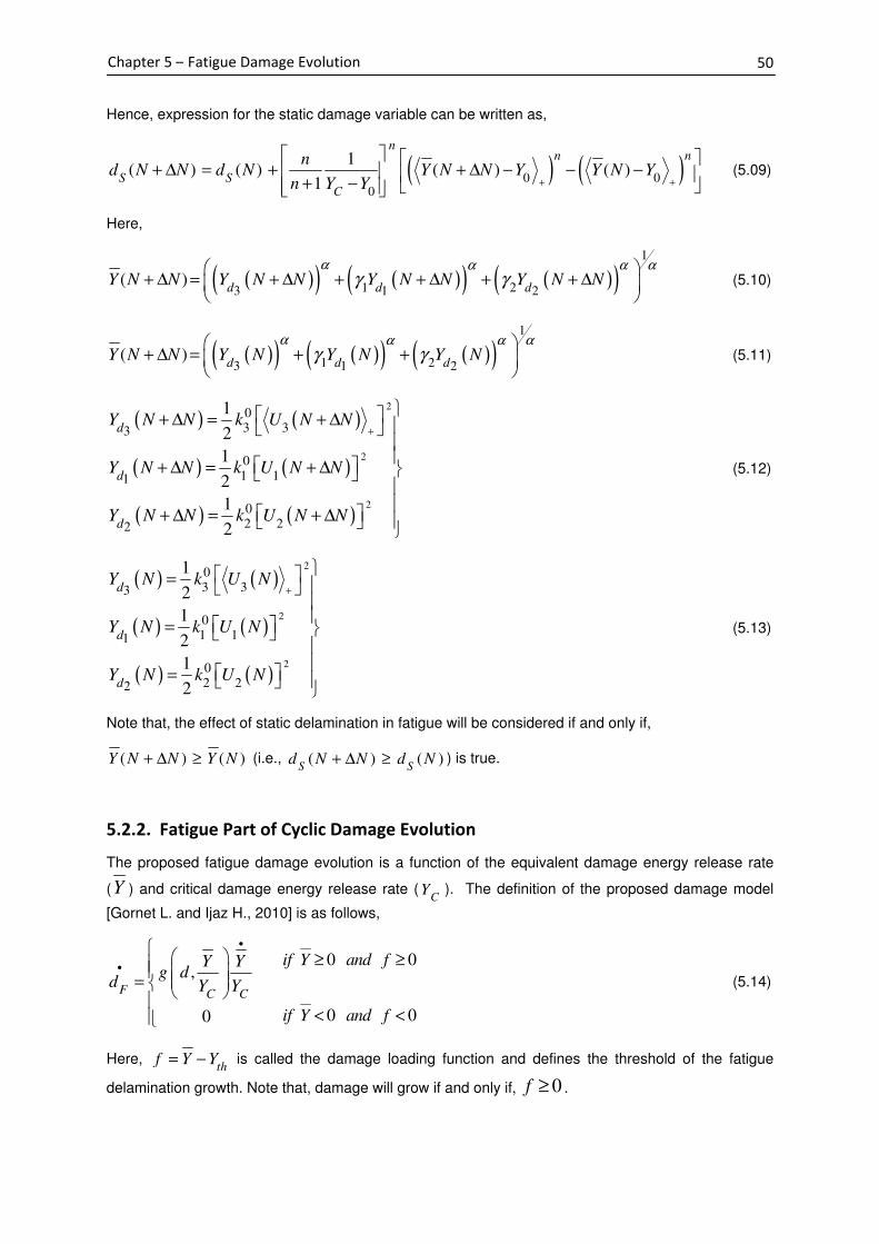
50


0 0

0 0

if Y and f

if Y and f

≥ ≥

< <

��

��

Hence, expression for the static damage variable can be written as,

( ) ( )0 00

1( ) ( ) ( ) ( )

1

nn n

S SC

nd N N d N Y N N Y Y N Y

n Y Y + +

+ ∆ = + + ∆ − − − + −

(5.09)

Here,

( )( ) ( )( ) ( )( )1

1 23 1 2( )

d d dY N N Y N N Y N N Y N N

α αα αγ γ

+ ∆ = + ∆ + + ∆ + + ∆

(5.10)

( )( ) ( )( ) ( )( )1

1 23 1 2( )

d d dY N N Y N Y N Y N

α αα αγ γ

+ ∆ = + +

(5.11)

( ) ( )

( ) ( )

( ) ( )

2

2

2

03 33

01 11

02 22

1

2

1

2

1

2

d

d

d

Y N N k U N N

Y N N k U N N

Y N N k U N N

+

+ ∆ = + ∆

+ ∆ = + ∆

+ ∆ = + ∆

(5.12)

( ) ( )

( ) ( )

( ) ( )

2

2

2

03 33

01 11

02 22

1

2

1

2

1

2

d

d

d

Y N k U N

Y N k U N

Y N k U N

+

=

=

=

(5.13)

Note that, the effect of static delamination in fatigue will be considered if and only if,

( ) ( )Y N N Y N+ ∆ ≥ (i.e., ( ) ( )S S

d N N d N+ ∆ ≥ ) is true.

5.2.2. Fatigue Part of Cyclic Damage Evolution

The proposed fatigue damage evolution is a function of the equivalent damage energy release rate

(Y ) and critical damage energy release rate (C

Y ). The definition of the proposed damage model

[Gornet L. and Ijaz H., 2010] is as follows,

,

0

F C C

Y Yg d

d Y Y

•

•

=

(5.14)

Here, th

f Y Y= − is called the damage loading function and defines the threshold of the fatigue

delamination growth. Note that, damage will grow if and only if, 0f ≥ .

0 0

0 0

if Y and f

if Y and f

≥ ≥

< <

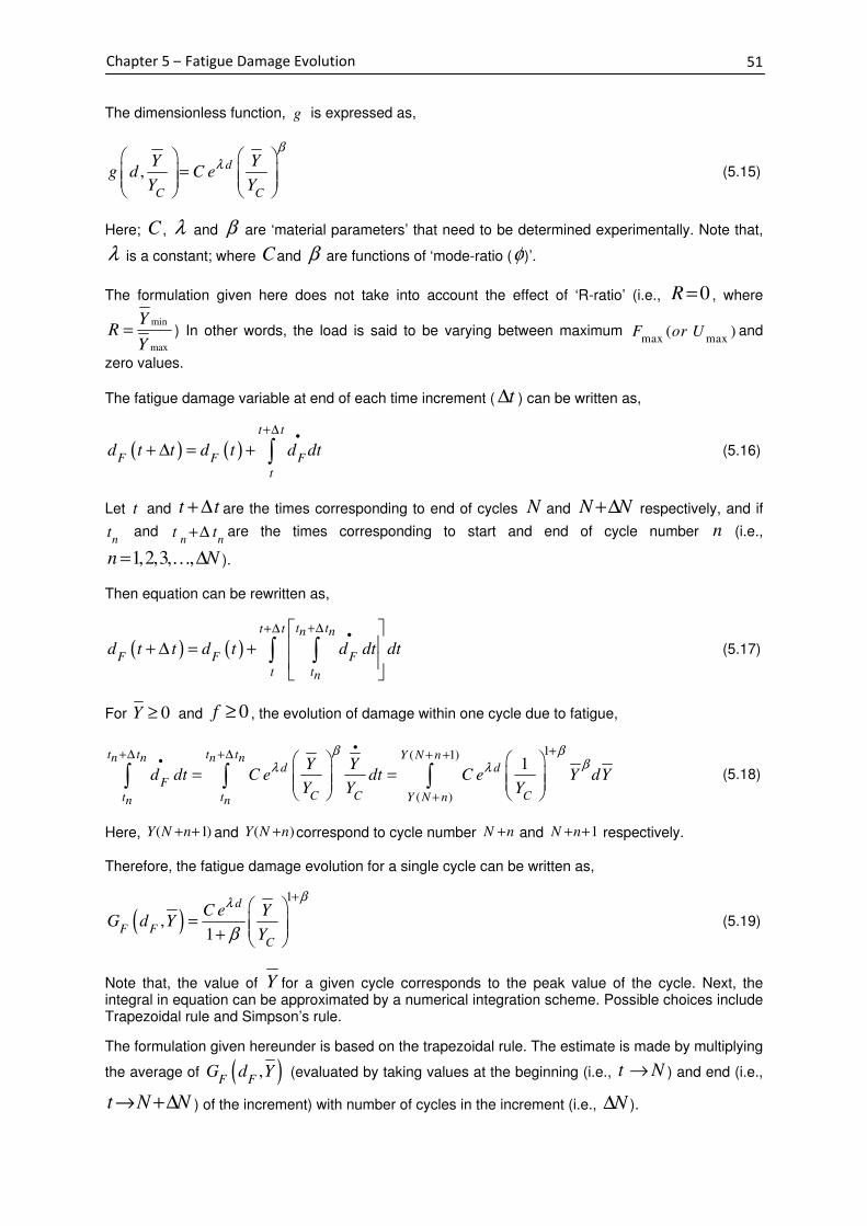
51


The dimensionless function, g is expressed as,

,d

C C

Y Yg d C e

Y Y

β

λ =

(5.15)

Here; C , λ and β are ‘material parameters’ that need to be determined experimentally. Note that,

λ is a constant; where Cand β are functions of ‘mode-ratio (φ)’.

The formulation given here does not take into account the effect of ‘R-ratio’ (i.e., 0R = , where

min

max

YR

Y= ) In other words, the load is said to be varying between maximum

max max( )F or U and

zero values.

The fatigue damage variable at end of each time increment ( t∆ ) can be written as,

( ) ( )t t

F F F

t

d t t d t d dt•

+∆

+ ∆ = + ∫ (5.16)

Let t and t t+ ∆ are the times corresponding to end of cycles N and N N+∆ respectively, and if

nt and

n nt t+∆ are the times corresponding to start and end of cycle number n (i.e.,

1,2,3, ,n N= ∆… ).

Then equation can be rewritten as,

( ) ( )t tt t n n

F F F

t tn

d t t d t d dt dt•

+∆+∆ + ∆ = +

∫ ∫ (5.17)

For 0Y ≥ and 0f ≥ , the evolution of damage within one cycle due to fatigue,

1( 1)

( )

1t t t t Y N nn n n n

d d

FC C Ct t Y N nn n

Y Yd dt C e dt C e Y dY

Y Y Y

β ββλ λ

•

•++∆ +∆ + +

+

= =

∫ ∫ ∫ (5.18)

Here, ( 1)Y N n+ + and ( )Y N n+ correspond to cycle number N n+ and 1N n+ + respectively.

Therefore, the fatigue damage evolution for a single cycle can be written as,

( )1

,1

d

F FC

C e YG d Y

Y

βλ

β

+

= + (5.19)

Note that, the value of Y for a given cycle corresponds to the peak value of the cycle. Next, the integral in equation can be approximated by a numerical integration scheme. Possible choices include Trapezoidal rule and Simpson’s rule.

The formulation given hereunder is based on the trapezoidal rule. The estimate is made by multiplying

the average of ( ),F F

G d Y (evaluated by taking values at the beginning (i.e., t N→ ) and end (i.e.,

t N N→ +∆ ) of the increment) with number of cycles in the increment (i.e., N∆ ).

52


Now, expression for the fatigue damage variable can be written as,

( ) ( ) ( ) ( )( ) ( ) ( )( )1, ,

2F F F F F Fd N N d N G d N N Y N N G d N Y N N + ∆ = + + ∆ + ∆ + ∆

(5.20)

Note that, equation is an implicit equation. For example, the fatigue damage variable ( )Fd N N+ ∆ ,

appears on both side of the relation. To solve the equation, one can replace ( )Fd N N+ ∆ on the

right-hand side with a ‘predictor’ (i.e., PF

d ) based on Forward Euler Technique [Ijaz H., 2009; and

other]. The expression used for the predictor is as follows,

( ) ( )( )( ) ,PF F F F

d d N G d N Y N N= + ∆ (5.21)

Therefore, the modified expression for the fatigue damage variable reads as,

( ) ( ) ( )( ) ( ) ( )( )1, ,

2

PF F F F F F

d N N d N G d Y N N G d N Y N N + ∆ = + + ∆ + ∆

(5.22)

5.2.3. Complete Fatigue Damage Evolution Law

Finally, the expression for the complete fatigue damage evolution law is as follows,

( ) ( ) ( ) ( )

( )( ) ( ) ( )( )

0 00

1( ) ( )

1

1, ,

2

nn n

C

PF F F F

nd N N d N Y N N Y Y N Y

n Y Y

G d Y N N G d N Y N N

+ +

+ ∆ = + + ∆ − − − + −

+ + ∆ + ∆

(5.23)

Here,

( ) ( ) ( )S Fd N N d N N d N N+ ∆ = + ∆ + + ∆ and ( ) ( ) ( )S F

d N d N d N= + .

53

Chapter 6 – Analysis of Fatigue Simulations

Chapter 6

Analysis of Fatigue Simulations

6.1 Analysis Procedure

The analysis procedure is similar to the description given for static case with the following exceptions.

Pre-processing

Define type of analysis (2D-plane stress) Define geometry & mesh Define material parameters for arms Define ‘fatigue damage model’ parameters for interface Define boundary, contact & loading conditions

Define convergence criteria

Solution

Launch nonlinear calculation

Post-processing

Plot evolution of crack length vs. number of loading cycles, damage variable vs. number of loading cycles, energy release rate vs. crack length, etc.

Analysis Compare and contrast simulated results with experimental data and investigate the effect of fatigue model parameters

Note that, for simulation purposes a static load increasing from ‘zero’ to ‘peak of the cyclic load’ will precede the start of the envelope of the cyclic (fatigue) load. A pictorial representation of the actual applied load and the numerically applied load are shown in Figure 6.01 given below.

Figure 6.01 : Numerically applied fatigue load and actual fatigue load

In addition, an assumption is made with regard to the numerically applied loading to simplify the nonlinear calculation process [Robinson P. et al., 2005; Ijaz H., 2009]. Note that, in this particular study the actual load is taken to be oscillating between zero and a maximum value as illustrated in the above figure. For high cyclic fatigue the numerically applied load will be taken as a constant and will be equal to the maximum value of the actual load. The cyclic nature of the loading scheme will be taken in to account by the formulas governing the evolution of the fatigue damage variable. Interestingly this means that fatigue damage evolution should be independent of the number of loading cycles specified for a given increment. This aspect will be validated in a later section. The finite element implementation of the ‘fatigue damage model’ for the interface in 3D is summarized in the two tables given hereafter.

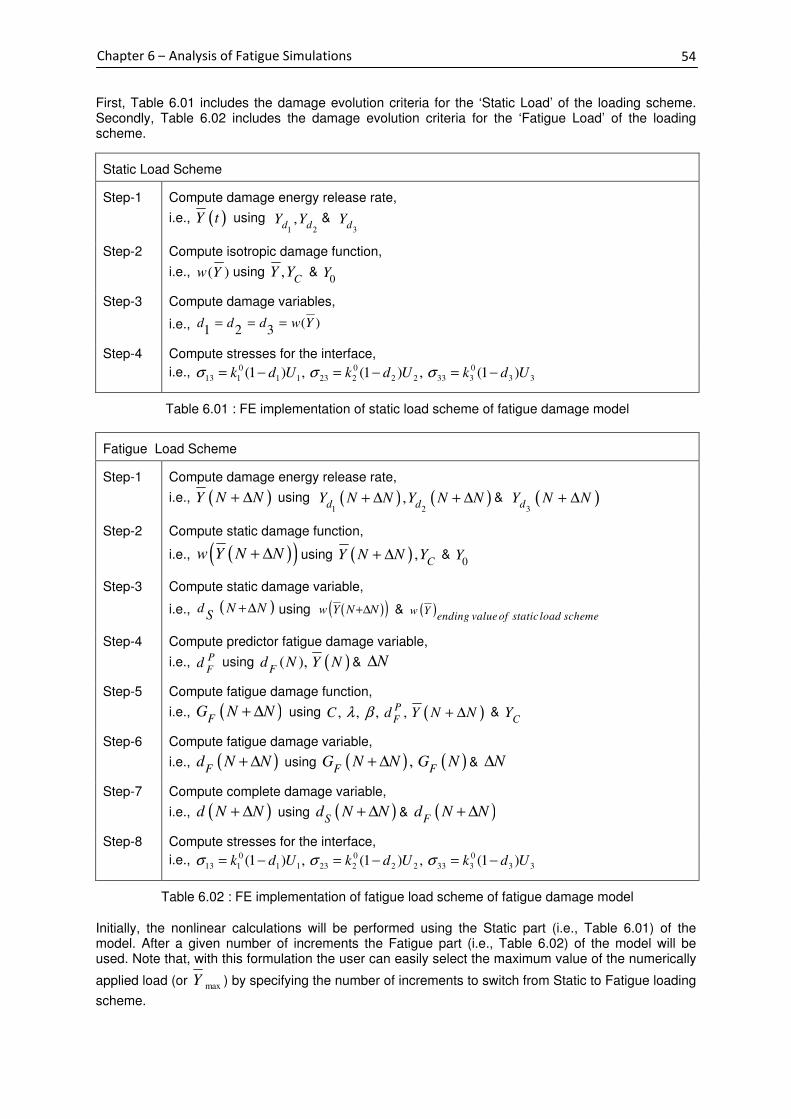
54


First, Table 6.01 includes the damage evolution criteria for the ‘Static Load’ of the loading scheme. Secondly, Table 6.02 includes the damage evolution criteria for the ‘Fatigue Load’ of the loading scheme.

Static Load Scheme


i.e., ( )Y t using 1 2,

d dY Y &

3d

Y



Y Y & 0

Y


i.e., ( )1 2 3

d d d w Y= = =


i.e., 0 0 0

13 1 1 1 23 2 2 2 33 3 3 3(1 ) , (1 ) , (1 )k d U k d U k d Uσ σ σ= − = − = −

Table 6.01 : FE implementation of static load scheme of fatigue damage model

Fatigue Load Scheme


i.e., ( )Y N N+ ∆ using ( ) ( )1 2

,d d

Y N N Y N N+ ∆ + ∆ & ( )3

dY N N+ ∆

Step-2 Compute static damage function,

i.e., ( )( )w Y N N+ ∆ using ( ) ,C

Y N N Y+ ∆ & 0

Y

Step-3 Compute static damage variable,

i.e., ( )d N NS

+∆ using ( )( )w Y N N+∆ & ( )w Yending valueof static load scheme

Step-4 Compute predictor fatigue damage variable,

i.e., PF

d using ( )( ),F

d N Y N & N∆

Step-5 Compute fatigue damage function,

i.e., ( )FG N N+ ∆

using ( ), , , ,PF

C d Y N Nλ β + ∆ & C

Y

Step-6 Compute fatigue damage variable,

i.e., ( )Fd N N+ ∆

using ( ) ( ),F F

G N N G N+ ∆ & N∆

Step-7 Compute complete damage variable,

i.e., ( )d N N+ ∆

using ( )Sd N N+ ∆ & ( )F

d N N+ ∆


i.e., 0 0 0

13 1 1 1 23 2 2 2 33 3 3 3(1 ) , (1 ) , (1 )k d U k d U k d Uσ σ σ= − = − = −

Table 6.02 : FE implementation of fatigue load scheme of fatigue damage model

Initially, the nonlinear calculations will be performed using the Static part (i.e., Table 6.01) of the model. After a given number of increments the Fatigue part (i.e., Table 6.02) of the model will be used. Note that, with this formulation the user can easily select the maximum value of the numerically

applied load (or maxY ) by specifying the number of increments to switch from Static to Fatigue loading

scheme.

55


6.2 Identification of Fatigue Damage Model Parameters

Similarly as explained in Chapter 4, the damage model parameters of the fatigue damage evolution law needs to be determined beforehand. There are number of parameters to be determined for both

static part and also fatigue part of the damage evolution. Identification of parameters such as, C

Y , 0

Y

, 1

γ , 2

γ , α and interface rigidities ( 0 0

1 2,k k and 0

3k ) have already been discussed in Section 4.2.

For the fatigue part, one needs to identify four key parameters, namely C , λ , β and N∆ . The

choice of the number of increment cycles does not affect the final result of the computation.

Therefore, the user is free to select a value for N∆ . Note that, if N∆ is too large for a given time

increment several elements may fail together and the delamination process will be rapid. On the other

hand, if N∆ is too small, the computational time would increase significantly. Generally, a good value

for N∆ is selected depending on the problem in hand.

The identification of parameter values for C , λ and β are based on a trial-and-error approach. In

other words, the user has to calibrate the fatigue damage model for a given problem using the available experimental data. However, FE inverse-optimization procedure may also be considered for future studies. Identification of these parameters without the aid of any experimental data for any given Mixed-Mode delamination will also be discussed in a later section. Here, a non-monotonic relation between each parameter is established using results of three different Fracture Mechanics tests.

6.3 Validation of Proposed Fatigue Damage Model

6.3.1 Experimental Methods

To validate and verify the effectiveness of the proposed fatigue damage model, simulation results need to be compared with experimental results. In the present study, experimental results reported by Leif E. Asp. et al., 2001 will be used and details of test methods are explained hereunder. As reported, they studied the effects on the inter-laminar toughness in fatigue with three different test methods. For pure Mode-I and Mode-II, the DCB and 3ENF tests were utilized, respectively. For

Mixed-Mode load case (i.e., / 0.5II TotalG G = ) the MMB test was employed. All tests were

performed on a modified version of the Mixed-Mode bending test rig [Crews J. H. and Reeder J.R., 1988].

All specimens had been manufactured from HTA/6376C carbon/epoxy unidirectional prepregs and the cured plies have the elastic properties given in Table 6.03.

11E - 120,000 [ ]MPa 22E

- 10,500 [ ]MPa 33E

- 10,500 [ ]MPa

12ν - 0.3 23ν

- 0.51

13ν

- 0.3

12G - 5, 250 [ ]MPa 23G - 3,480 [ ]MPa

13G - 5, 250 [ ]MPa

Table 6.03 : Elastic properties of HTA/6376C unidirectional prepregs reported by Leif Asp. et al.

The ply thickness was [ ]130 mµ and the specimen lay-up was ( )12 40 / / 5 / 0S

± , where sign '/ / '

refers to the plane of the artificial delamination. The dimensions of the rectangular shaped specimens

were; width [ ]20b mm= , length [ ]150Sl mm= , and nominal thickness [ ]2 3.1h mm= .

Chapter 6

A schematic of the specimen g

A schematic of the test rig and the applied load is (i.e.,

the testing length

All tests were performed at a frequency of

in fatigue at a R

seven specimens were tested.‘normalized


A schematic of the specimen g

Figure 6.


the testing length 2 100L mm


in fatigue at a R-value of

specimens were tested.normalized Paris plots’ as

Figure 6.


A schematic of the specimen geometry is shown in Figure 6.02

Figure 6.02 : Schematic of the specimen geometry


[2 100L mm=

Figure 6.


value of 0.1 , at a constant displacement amplitude. For each test method, at least

specimens were tested.lots’ as shown in Figure 6.04

Figure 6.04 : Normalized Paris


eometry is shown in Figure 6.02

: Schematic of the specimen geometry


]L mm .

Figure 6.03 : Schematic of the

All tests were performed at a frequency of 5

, at a constant displacement amplitude. For each test method, at least

specimens were tested. The experimental resultsshown in Figure 6.04

: Normalized Paris

eometry is shown in Figure 6.02

: Schematic of the specimen geometry

A schematic of the test rig and the applied load is (i.e., P

: Schematic of the

[ ]5 Hz , at ambient conditions. The specimens were tested


The experimental resultsshown in Figure 6.04 given below.

: Normalized Paris Plots for DCB, ENF and MMB tests

eometry is shown in Figure 6.02.

: Schematic of the specimen geometry used for fatigue test

P ) is presented in

: Schematic of the fatigue test rig

, at ambient conditions. The specimens were tested


The experimental results were then presented in the form of given below.

for DCB, ENF and MMB tests

used for fatigue test

) is presented in Figure 6.03

test rig



were then presented in the form of


used for fatigue test

Figure 6.03. Here, span of





56

Here, span of




57


6.3.2 Finite Element Model

The geometry of the finite element model used for all three tests, namely DCB (pure MODE-I), 3ENF

(pure MODE-II) and MMB (Mixed-Mode; / 0.5II TotalG G = ) is given below in Figure 6.05.

Figure 6.05 : Dimensions of the model geometry used for fatigue simulations Simulations were performed considering a state of ‘PLANE STRESS’ condition in 2D. Values of some model parameters and FEs used are given in Table 6.04.

Laminate arms (2D) Geo. Support / Finite Element : QUA4 / QUA4


Interface(1D) Geo. Support / Finite Element : RAC2 /


JOI2

Table 6.04 : Finite elements for arms and interface for fatigue simulations

In addition, a FE mesh having a constant element size, i.e., 0.1ES = was used to carry out all

simulations for each test campaign. An example of a mesh for a DCB test is given in Figure 6.06.

Figure 6.06 : Mesh used for fatigue simulations The model parameters that were commonly used in all simulation are listed in Table 6.05 given below. Note that, the identification of these parameters was carried out earlier under the static part of the study.

[ ]/C

Y N mm - 0.26 α - 1.4 0

1k - [ ]2395 /MPa mm

1γ - 0.2595 n - 0.5 0

3k - [ ]9230 /MPa mm

Table 6.05 : General fatigue damage model parameters

The simulations were performed at different values of max CG G for each type of mode of failure. The

additional data plots describing the evolution of max

' 'G with crack length ' 'a were also used

determine the potential number of loading cycles elapsed for the extension of the cracks. Note that,

the selected ratios of max CG G correspond to the crack extension data given in those plots (also

included in the upcoming Sections).

Here, for tests at 0.1R = , min

G is considerably small compared to max

G , hence the proposed

fatigue damage model can be used to simulate the above mentioned tests. In all simulations evolution of energy release rate at the crack tip (i.e., using gauss point) was monitored by local means. It was

then used to determine the max CG G ratio corresponding to each increment of the loading condition.

Now, depending on the test data simulations were performed for different max CG G ratios by simply

changing the prescribed displacement limit for the static loading scheme accordingly. At the end of the static loading scheme the fatigue model will take over the computation process.

Chapter 6

6.3.3

Application of the boundary conditions and loading conditions (i.e.DCB test is as shown in Figure 6.

The parameters

below. Note that,

Figure 6.08

Figure 6.

The normalized Paris Plot obtained

the experimental

0.66

nonlinear regions of the Paris plot

Figure 6.09

a comparison has been made between simulated results for each

better understand of the delamination growth for


Simulation Results for DCB

pplication of the boundary conditions and loading conditions (i.e.DCB test is as shown in Figure 6.

Figure 6.

parameters C ,

Note that, Mode

C

Figure 6.08 given below illustrate the simulated results plotted over the experimental results.

Figure 6.08 : Normalized Paris Plot for

normalized Paris Plot obtained

the experimental data. Interestingly

have retained their linear relationship with


Figure 6.09 given below includes evolution of crack ext




Simulation Results for DCB

pplication of the boundary conditions and loading conditions (i.e.DCB test is as shown in Figure 6.

Figure 6.07 : Boundary and loading conditions for DCB

C , β and λ were calibrated carefully and were found to

Mode-I fracture toughness of the specimen was reported equal to

= 2.0 2E

given below illustrate the simulated results plotted over the experimental results.

Normalized Paris Plot for

normalized Paris Plot obtained

data. Interestingly



given below includes evolution of crack ext




Simulation Results for DCB Fatigue

pplication of the boundary conditions and loading conditions (i.e.DCB test is as shown in Figure 6.07.


were calibrated carefully and were found to

I fracture toughness of the specimen was reported equal to

2.0 2E − β


Normalized Paris Plot for simulated and e

normalized Paris Plot obtained from the simulated results is found to be in good agreement with

data. Interestingly, the simulated result


nonlinear regions of the Paris plot.

given below includes evolution of crack ext



Fatigue Test

pplication of the boundary conditions and loading conditions (i.e.




β =


simulated and e

from the simulated results is found to be in good agreement with

, the simulated result

have retained their linear relationship with rest of the points

given below includes evolution of crack extension against number of loading


better understand of the delamination growth for Mode-I.

pplication of the boundary conditions and loading conditions (i.e.




3.5 λ


simulated and experimental results of


, the simulated results for maxG G

rest of the points

ension against number of loading


.

pplication of the boundary conditions and loading conditions (i.e., imposed displacement) for the

: Boundary and loading conditions for DCB fatigue

were calibrated carefully and were found to be equal


λ = 1


xperimental results of


max ICG G ratio

rest of the points although they close to the

ension against number of loading

a comparison has been made between simulated results for each max ICG G

, imposed displacement) for the

fatigue test

equal to values given

I fracture toughness of the specimen was reported equal to [0.26 /N mm

1


DCB fatigue


ratio equal to 0.23

although they close to the

ension against number of loading cycles. Here

ratio and provides a

58

, imposed displacement) for the

to values given

]0.26 /N mm .

fatigue tests


0.23 and

although they close to the

cycles. Here,

and provides a

( )I IU or P

( )I IU or P

)I IU or P

)I IU or P

59


Figure 6.09 : Evolution of crack extension for different max ICG G ratios in DCB fatigue test

Note that, simulations were only performed in the range as specified in experiments. From figure it can be seen that, crack growth becomes non-liner with increasing number of cycles. This

phenomenon seems to become gradually severe with increasing max ICG G ratio. As a result the crack

growth rate seems to vary with number of loading cycles. Here, a simple assumption is made and crack growth rate is considered to be constant. In practice, it is determined by taking the ratio of total crack extension with number of cycles elapsed. However, the final results as illustrated in Figure 6.08 are satisfactory.

A comparison between experimental and simulated results was made to investigate the variation of strain energy release rate with crack growth. See Figure 6.10.


G for different max ICG G ratios in DCB fatigue test

60


Equation of plot,

( )max

mdaB G

dN=

here,

3.91 15B E= −

4.84m =

Variations of strain energy release rate with crack length are found to be in good agreement with the

experimental data. Note that, numerical result obtained for the highest max ICG G ratio does not

correspond to the experimental result (here, lack of information on actual start point of the experimental result made it difficult to do a proper analysis). The additional simulation was performed

to appreciate the evolution of the crack length and energy release rate for max 0.66ICG G = . In

general, the decrease of the energy release rate with increasing crack length seems to be satisfactorily captured by the proposed model.

Identification of B and m of the Paris Law was carried out by plotting max

G against da dN and

obtaining the equation of the best fit for the data points as given below in Figure 6.11.

6.3.4 Simulation Results for 3ENF Fatigue Test

Application of the boundary conditions and loading conditions (i.e., imposed displacement) for the 3ENF test is illustrated in Figure 6.12.

Figure 6.12 : Boundary and loading conditions for 3ENF fatigue test

The parameters C , β and λ were calibrated once more and were found to be equal to values given

below. Note that, Mode-II fracture toughness of the specimen was reported equal to [ ]1.002 /N mm .

C = 7.0 3E − β = 2.2 λ = 1


G in DCB fatigue test

( )II IIU or P

Chapter 6

Figure 6.1

Figure 6.1 The simulated results are in good agreement with the experimental model successfully the fatigue behaviour of the linear region in the Paris Plot.

corresponding to

the points. However, the corresponding numerical result has predicted the linear behaviour much more accurately.

In addition, an analysis out and the results are given in Figure 6.1

Figure 6.1


Figure 6.13 given below illustrate the simulated results plotted over the experimental results.

Figure 6.13 : Normalized Paris Plot for simulated and experimental results of

The simulated results are in good agreement with the experimental model successfully rethe fatigue behaviour of the linear region in the Paris Plot.

corresponding to maxG G

the points. However, the corresponding numerical result has predicted the linear behaviour much accurately.

In addition, an analysis out and the results are given in Figure 6.1

Figure 6.14 : Evolution of crack extension for different



Normalized Paris Plot for simulated and experimental results of

The simulated results are in good agreement with the experimental reproduces the expected linear behaviour.

the fatigue behaviour of the linear region in the Paris Plot.

max 0.27IICG G =

the points. However, the corresponding numerical result has predicted the linear behaviour much

In addition, an analysis on the evolution of out and the results are given in Figure 6.1

: Evolution of crack extension for different




The simulated results are in good agreement with the experimental produces the expected linear behaviour.


0.27

seem to be lying slightly outside of the linear trend of the rest of


volution of crack extensionout and the results are given in Figure 6.14.




The simulated results are in good agreement with the experimental produces the expected linear behaviour.




crack extension.




The simulated results are in good agreement with the experimental produces the expected linear behaviour. Note that, this test

the fatigue behaviour of the linear region in the Paris Plot. The cluster of experimental data points



crack extension with number of loading

: Evolution of crack extension for different max IICG G


Normalized Paris Plot for simulated and experimental results of 3ENF

The simulated results are in good agreement with the experimental results. Once more, the fatigue Note that, this test he cluster of experimental data points



number of loading

IICG G ratios in 3ENF


3ENF fatigue

Once more, the fatigue Note that, this test case only considers he cluster of experimental data points



number of loading cycles was

3ENF fatigue

61

fatigue tests

Once more, the fatigue case only considers

he cluster of experimental data points



was carried

test

62


Equation of plot,

( )max

mdaB G

dN=

here,

1.36 14B E= −

4.23m =

Unlike in the case of DCB test, crack growth seems to take place in a linear manner and the phenomenon is unaffected by for different ratio values. Therefore, computation of crack growth rate becomes trivial.

Evolution of strain energy release rate with crack growth was monitored for each max IICG G ratio and

comparisons of simulated against experimental results are given in Figure 6.15.


G for different max IICG G ratios in 3ENF fatigue test

Evolutions of strain energy release rate predicted by the simulations are in very good agreement with experimental results, except for the highest ratio where the result can only be considered satisfactorily. It is interesting to note that, for 3ENF test, reduction of strain energy release rate is considerably smaller than for DCB test.

Once more, the identification of B and m of the Paris law was performed by plotting max

G against

da dN and obtaining the equation of its best fit as given in Figure 6.16.


G in 3ENF fatigue test

Chapter 6

6.3.5

Application of the boundary conditions and loading conditions (i.e., imMMB test is illustrated in Figure 6.1

Although evaluation of loads in the DCB and 3ENF tests were trivial, for the MMB test, however, the

Mode-I and

equilibrium considera

P ) as shown

For FE simulations, the

(1

4IP c L= −

(IIP c L= +

Here, c

applied load i

Under the assumption of cylindrical bending and mid

release rate (i.e.,

MMB test is,

TOT I IIG G G= +

The Mixed

[0.447 /

simulations were first carried out to identify the value

0.5 and found to be equal to

Mode were then carried out on that basis.selected instead of imposed displacem


Simulation Results for MMB

Application of the boundary conditions and loading conditions (i.e., imtest is illustrated in Figure 6.1

Figure 6.1


I and Mode-

equilibrium considera

) as shown in Figure 6.1

Figure 6.1

For FE simulations, the

( )1

34

PP c L

L= −

)P

P c LL

= +

c is the distance from the center of the span of the testing length (i.e.,

applied load in the horizontal direction. Note that, both


release rate (i.e., IIIG

MMB test is,

TOT I IIG G G= +

Mixed-Mode fracture toughness with a mode mixity of

]0.447 /N mm . Note that, here mode


and found to be equal to

were then carried out on that basis.selected instead of imposed displacem


Simulation Results for MMB

Application of the boundary conditions and loading conditions (i.e., imtest is illustrated in Figure 6.1

Figure 6.17 : Boundary and loading conditions for MMB


-II load components (i.e.,

equilibrium considerations [Crews J. H. and Reeder J.R., 1988]

in Figure 6.18 given below.

Figure 6.18 : Superposition of

For FE simulations, the expressions used for the load components are as follows,

P

L

is the distance from the center of the span of the testing length (i.e.,

n the horizontal direction. Note that, both


IIIG ) in the MMB specimen is

fracture toughness with a mode mixity of

Note that, here mode


and found to be equal to 37

were then carried out on that basis.selected instead of imposed displacem


Simulation Results for MMB Fatigue

Application of the boundary conditions and loading conditions (i.e., imtest is illustrated in Figure 6.17.

: Boundary and loading conditions for MMB


II load components (i.e.,

[Crews J. H. and Reeder J.R., 1988]

given below.

8 : Superposition of Mode

expressions used for the load components are as follows,


n the horizontal direction. Note that, both


) in the MMB specimen is


Note that, here mode-ratio


[ ]37 mm . Subsequently, the fatigue simulations for the selected

were then carried out on that basis. Note that, for the MMB test a force loading condition was selected instead of imposed displacement condition.

Fatigue Test

Application of the boundary conditions and loading conditions (i.e., im



II load components (i.e., IP and

[Crews J. H. and Reeder J.R., 1988]

Mode-I and Mode



n the horizontal direction. Note that, both cUnder the assumption of cylindrical bending and mid-

) in the MMB specimen is zero, and the total strain energy release rate for the


ratio (i.e., φ ) is taken with respect to

simulations were first carried out to identify the value ' 'c

. Subsequently, the fatigue simulations for the selected

Note that, for the MMB test a force loading condition was ent condition.

IIP

Test

Application of the boundary conditions and loading conditions (i.e., im



and IIP respectively) must be obtained from

[Crews J. H. and Reeder J.R., 1988] and depend on the applied load (i.e.,

Mode-II loadings



c and L are illustrated clearly in Figure 6.03.

-plane symmetry, the

zero, and the total strain energy release rate for the

fracture toughness with a mode mixity of / 0.5II TOTG Gφ = =

is taken with respect to

' 'c which corresponds to the mode


Note that, for the MMB test a force loading condition was

IIP

Application of the boundary conditions and loading conditions (i.e., imposed displacement) for the

: Boundary and loading conditions for MMB fatigue


espectively) must be obtained from

and depend on the applied load (i.e.,

II loadings for Mixed-


is the distance from the center of the span of the testing length (i.e., 2L

are illustrated clearly in Figure 6.03.

plane symmetry, the Mode


/ 0.5II TOTG G= = was reported equal to

is taken with respect to Mode

which corresponds to the mode



posed displacement) for the

fatigue test




-Mode case


2L ) to the point of the


Mode-III strain energy


was reported equal to

Mode-II. Several FE

which corresponds to the mode-mixture of



63

posed displacement) for the




(6.01)

(6.02)

) to the point of the


III strain energy


(6.03)

was reported equal to

Several FE

mixture of

. Subsequently, the fatigue simulations for the selected Mixed-


IP

Chapter 6

Parameters

Figure 6.19 shown hereunder includes

Figure 6.1 The simulated results in the normalized Paris Plot results. the Paris Plot. loading cycles are illustrated in Figure 6.20.

Figure 6.20


arameters C , β and

C

6.19 shown hereunder includes

Figure 6.19 : Normalized Paris Plot for simulated and experimental results of

he simulated results in the normalized Paris Plot results. Once more, the the Paris Plot. In additionloading cycles are illustrated in Figure 6.20.

Figure 6.20 : Evolution of crack extension for different


and λ were calibrated

= 1.5 1E

6.19 shown hereunder includes


he simulated results in the normalized Paris Plot Once more, the Mixed-Mode

In addition, results of the analysis on loading cycles are illustrated in Figure 6.20.



were calibrated for the new test

1.5 1E − β

6.19 shown hereunder includes the simulated results


he simulated results in the normalized Paris Plot Mode test case is also intended for

results of the analysis on loading cycles are illustrated in Figure 6.20.


for the new test

β =

the simulated results


he simulated results in the normalized Paris Plot are incase is also intended for

results of the analysis on evolution of crack extension with number of


for the new test and equal to values given below

3.7 λ

the simulated results with experimental results.


are in good agreement with the experimental case is also intended for analyzing only the linear region of

evolution of crack extension with number of

: Evolution of crack extension for different max 0.5TOT CG G −

al to values given below

λ = 1

experimental results.

Normalized Paris Plot for simulated and experimental results of MMB

good agreement with the experimental analyzing only the linear region of


max 0.5TOT C−

ratios in MMB

al to values given below.

1

experimental results.

MMB fatigue



ratios in MMB fatigue

64

fatigue tests



fatigue test

65


Equation of plot,

( )max

mdaB G

dN=

here,

7.83 18B E= −

6.20m =

From above figure, it can be concluded that, crack growth take place in linear manner with increasing number of loading cycles for the MMB test. Similar to 3ENF test, computation of crack growth rate becomes straight forward. The values of the constants; B and m of the Paris Law are found using

the same method as explained earlier and the plot is given in Figure 6.21. The results obtained are also given below.

6.3.6 Mixed-Mode Fatigue Failure Prediction

The results of all numerical simulations performed for each mode of failure are found to be in good agreement with corresponding experimental data. Therefore, it proves the effectiveness of the proposed fatigue damage model in predicting delamination due to fatigue. Now, next task would be to propose a methodology to determine the parameters for the fatigue model for any given mode-ratio.

In order to achieve this goal one needs to develop a relationship between parameters B and m of

the Paris law with mode-ratio, φ . The idea here would be to use the known values of the parameters

to interpolate the unknown values for a given mode-ratio. Many researchers have worked on this problem for decades and have proposed both monotonic and non-monotonic relationships with varying degree of accuracy with respect to their particular case studies. The mode-ratio is intimately related to type of the material and therefore the parameter relationship with mode-ratio differs significantly from GFRP to CFRP materials. Note that, the material HTA/6376C under consideration in this case study is a CFRP composite. Figure 6.22 and Figure 6.23 given below illustrate a compendium of the both monotonic and non-monotonic relations developed for CFRP materials [Blanco N. et al, 2004].

Figure 6.22 : Monotonic and non-monotonic relations for Paris law coefficient

Figure 6.21 : Evolution of crack growth rate with

maxG in MMB fatigue test

66


Figure 6.23 : Monotonic and non-monotonic relations for Paris law exponent From the two figures, it is evident that the non-monotonic relation provides a better approximation to predict the evolution of parameters compared to the monotonic approaches. Therefore, present study focuses on application of non-monotonic relations to obtain new values for parameters of Paris law.

Recently in literature, a non-monotonic equation was reported [Tumino D. and Cappello F., 2007] to relate fatigue damage parameters and mode-ratio. To establish this non-monotonic relation, the suggested procedure requires at least three fatigue tests; fatigue in pure Mode-I, in pure Mode-II and

in Mixed-Mode with a fixed value of φ (i.e.,

mixφ ). The fatigue tests shall provide values of

IB ,

IIB ,

mixB ,

Im ,

IIm and

mixm for the calibrated fatigue parameters

IC ,

IIC ,

mixC ,

Iβ ,

IIβ and

mixβ .

Thereafter, the following equations will be used to compute the new values of B and m for any given

mode-ratio. Note that, here fatigue damage parameter, λ will be taken as a fixed constant for all

three failure modes to reduce the complexity of the formulation.

21 2 3

A A Aβ β ββ φ φ= + + (6.04)

( ) 21 2 3

lnC C C

C A A Aφ φ= + + (6.05)

Where,

( )1 2

II mix II I mix

mix mix

Aβ

β β β β φ

φ φ

− + −=

− (6.06)

21

2

mix I mix

mix

AA

ββ

β β φ

φ

− −= (6.07)

3 IA

ββ= (6.08)

( ) ( ) ( ) ( )( )1 2

ln ln ln lnI mix II I mix

C

mix mix

C C C CA

φ

φ φ

− + −=

− (6.09)

( ) ( ) 1

2

ln lnmix I C mix

Cmix

C C AA

φ

φ

− −= (6.10)

( )3ln

C IA C= (6.11)

Chapter 6

Finally, the new values of

values of the Paris law. In this study the same approach will be used to evaluate the performance of the proposed fatigue damage model for available.

Fracture Mode (Test)

MODE

Mixed

MODE

Now, evolution

given in

Mode-ratios;

illustrate the normalized Paris plots

Note that, the new curvesMMB-0.5 curve. This suggestresults shown above give an insight to the change of the fatigue behaviour for different mode ratiosThe curves tend to translate in the upward direction with increasing modebetween each translation has also increased


Finally, the new values of

values of the Paris law. In this study the same approach will be used to evaluate the performance of the proposed fatigue damage model for available. Table 6.06 given below


MODE-I (DCB)

Mixed-Mode (MMB)

MODE-II (3ENF)

Table 6.06 : List of values of

volutions of the fatigue model parameters,

Figure 6.24

Figure 6.24

ratios; 0.25


Figure 6.2

Note that, the new curves0.5 curve. This suggest

results shown above give an insight to the change of the fatigue behaviour for different mode ratiosThe curves tend to translate in the upward direction with increasing modebetween each translation has also increased


Finally, the new values of C and

values of the Paris law. In this study the same approach will be used to evaluate the performance of the proposed fatigue damage model for

Table 6.06 given below


I (DCB)

(MMB) 0.5

II (3ENF)

Table 6.06 : List of values of

the fatigue model parameters,

and 6.25 respectively.

4 : Evolution of

and 0.75 were the selected


Figure 6.26 : Normalized Paris Plot for mode

Note that, the new curves for MMB0.5 curve. This suggests that, t



and β for a given mode

values of the Paris law. In this study the same approach will be used to evaluate the performance of the proposed fatigue damage model for different

Table 6.06 given below provides a summary of the

φ

0 2.0 2

0.5 1.2 1

1 7.0 3

Table 6.06 : List of values of C ,

the fatigue model parameters,

respectively.

: Evolution of C vs. φ

were the selected

illustrate the normalized Paris plots developed using the

: Normalized Paris Plot for mode

for MMB-0.25 and MMBs that, the fatigue model


for a given mode-ratio will be used to find respective

values of the Paris law. In this study the same approach will be used to evaluate the performance of different mode-

provides a summary of the

C

2.0 2E − 3.5

1.2 1E − 3.35

7.0 3E − 2.2

β , λ , B and

the fatigue model parameters, C and

φ

were the selected for the

developed using the predicted

: Normalized Paris Plot for mode

0.25 and MMB-0.75 are also rectilinear and are roughly parallel to he fatigue model is

results shown above give an insight to the change of the fatigue behaviour for different mode ratiosThe curves tend to translate in the upward direction with increasing modebetween each translation has also increased when the mode

ratio will be used to find respective

values of the Paris law. In this study the same approach will be used to evaluate the performance of -ratios where experimental data is no longer

provides a summary of the data and results of the study

β

λ

3.5 1

3.35 1

2.2 1

and m for mode

and β ; with the mode

Figure 6.

for the investigation

predicted C

: Normalized Paris Plot for mode-ratios 0.25

are also rectilinear and are roughly parallel to is working in a robu

results shown above give an insight to the change of the fatigue behaviour for different mode ratiosThe curves tend to translate in the upward direction with increasing mode

when the mode-ratio is doubled

ratio will be used to find respective

values of the Paris law. In this study the same approach will be used to evaluate the performance of where experimental data is no longer

data and results of the study

λ

1 3.91 15

1 7.83 18

1 1.36 14

for mode-ratios 0,

with the mode-ratio can be illustrated

Figure 6.25 : Evolution of

investigation. Figure 6.2

C , β and λ

0.25 , 0.50 and

are also rectilinear and are roughly parallel to working in a robust manner. In addition, the

results shown above give an insight to the change of the fatigue behaviour for different mode ratiosThe curves tend to translate in the upward direction with increasing mode-ratio and interestingly, gap

is doubled.

ratio will be used to find respective B


data and results of the study.

B

3.91 15E −

7.83 18E −

1.36 14E −

0 , 0.5 and 1

ratio can be illustrated

: Evolution of β vs.

Figure 6.26 given below

λ values.

and 0.75

are also rectilinear and are roughly parallel to st manner. In addition, the

results shown above give an insight to the change of the fatigue behaviour for different mode ratiosratio and interestingly, gap

67

B and m


m

4.84 6.20 4.23

ratio can be illustrated as

vs. φ

given below

are also rectilinear and are roughly parallel to st manner. In addition, the

results shown above give an insight to the change of the fatigue behaviour for different mode ratios. ratio and interestingly, gap

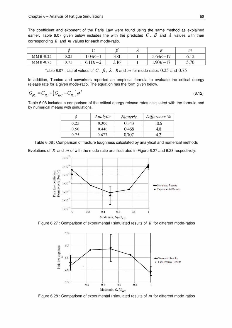
68


The coefficient and exponent of the Paris Law were found using the same method as explained

earlier. Table 6.07 given below includes the with the predicted C , β and λ values with their

corresponding B and m values for each mode-ratio.

In addition, Tumino and coworkers reported an empirical formula to evaluate the critical energy release rate for a given mode-ratio. The equation has the form given below.

( ) 2

C IC IIC ICG G G Gφ φ= + − (6.12)

Table 6.08 includes a comparison of the critical energy release rates calculated with the formula and by numerical means with simulations.

Evolutions of B and m of with the mode-ratio are illustrated in Figure 6.27 and 6.28 respectively.

Figure 6.27 : Comparison of experimental / simulated results of B for different mode-ratios

Figure 6.28 : Comparison of experimental / simulated results of m for different mode-ratios

φ C

β

λ

B m

MMB-0.25 0.25 1.03 1E − 3.81 1 5.63 17E − 6.12 MMB-0.75 0.75 6.11 2E − 3.16 1 1.90 17E − 5.70

Table 6.07 : List of values of C , β , λ , B and m for mode-ratios 0.25 and 0.75

φ Analytic

Numeric

%Difference

0.25 0.306 0.343 10.6

0.50 0.446 0.468 4.8

0.75 0.677 0.707 4.2

Table 6.08 : Comparison of fracture toughness calculated by analytical and numerical methods

69


As illustrated by the two figures; B and m values corresponding to mode-ratios 0.25 and 0.75 are

in good agreement with the experimental data reported by Blanco N. et al, 2004. Note that, C , β

and λ values for the fatigue damage model were derived using a non-monotonic relation and

therefore the results expected should also be non-monotonic. The key idea behind the investigation was to verify the effectiveness of the methodology. Note that, after calibrating the fatigue model (with three fatigue tests: pure Mode-I, pure Mode-II and a Mixed-Mode) it can be used to evaluate fatigue characteristics for any given mode-ratio. In practice, most composite structure experience Mixed-Mode failure loads more often than not. Moreover, there are situations where amplitude of the Mixed-Mode load would also vary with time. Therefore, the fatigue damage model needs to be versatile to handle such loading conditions. Importantly, the proposed model could easily be adapted for a given situation without many complications and has proven to be a robust tool.

6.4 Effects of Fatigue Model Parameters

Since affect of parameters, 0

1k , 0

2k and α has already been already discussed under the static part

of the study, the following sections are devoted to understanding the affect of parameters; N∆ , C

and β of fatigue model.

6.4.1 Influence of Parameter - N∆

To justify the fact that increment of number of cycles (i.e., jump cycles) has no effect on the final

result, an investigation was carried out for different N∆ values for each failure mode. Some selected

results of the investigation are given hereunder. Figure 6.29 and Figure 6.30 illustrate evolutions of

delamination length for 3ENF and MMB-0.75 tests with max

0.2C

G G= .

Figure 6.29 : Evolution of delamination length for different jump cycles in 3ENF fatigue test

Figure 6.30 : Evolution of delamination length for different jump cycles in MMB fatigue test

By analyzing the results, it can be concluded that, evolution of the delamination length is independent

of the selection of the jump cycles. Importantly, as N∆ decreases computation time increases

significantly. For higher values of N∆ the delamination rate grow rapidly and proper analysis of the

evolution of energy release rate and other parameters would be difficult. Therefore, a compromise should be made between the accuracy and computational cost. Here, the simulation results were

obtained with element size equal to 0.1 . Note that, element sizes lesser or equal to 0.2 produced

converging results.

70


6.4.2 Influence of Parameters - C & β

As for the fatigue model, C and β are the key parameters that influence the numerical results. The

model was calibrated accordingly by adjusting the values of the two parameters with the aid of

experimental results. For simplicity, λ was taken as a constant throughout the study. Given

hereunder are the results of the investigation carried out by varying one parameter while keeping the

other one constant. Figure 6.31 and Figure 6.32 given below illustrate the influence of parameter, C

for 2.2β = and parameter, β for 7.0 3C E= − respectively considering the 3ENF test.

Figure 6.31 : Influence of C in 3ENF

fatigue test

Figure 6.32 : Influence of β in 3ENF fatigue

test

Here in Figure 6.30, as C increase the Paris plot curves tend to translate in the upward direction

without exhibiting any rotation. It is also interesting to observe that when the value of C is doubled

the translation distance of the curve is roughly similar. Next, in Figure 6.31 much more complicated behviour was observed. In this case Paris plot curves tend to not only translate but also rotate at the

same time for increasing value of β . On the contrary to parameter, C both translation and rotation

takes place in the downward direction.

Prior to the beginning of the simulation campaign the user needs to first appreciate the probable values for each parameter through a trial-and-error analysis (FE inverse-optimization also possible). When the approximate values are known, the aforementioned behavioural pattern of the parameter can be taken in to account for fine tuning and arrive at a good approximation.

71

PART – IV

Closure

Section include one chapter, Chapter 7. Contains remarks regarding the work carried out on static and fatigue delamination modelling and simulations.

72

Chapter 7 – General Conclusions

Chapter 7

General Conclusions

Failure simulation of a laminate structure, taking into account all the progressive degradation phenomena, leads to a time dependant three-dimensional non-linear problem. Especially in the past three decades many researchers have been working towards in solving this problem with different types of mathematical tools. In this respect, both Fracture and Damage Mechanics have grown from strength to strength in recent times in successfully predicting delamination phenomenon in laminated composites. In present study, efforts have been made to further enhance an existing damage model to predict delamination of unidirectional composite laminates at both static and fatigue loading conditions. The damage model is formulated within the framework of Damage Mechanics, but is also essentially linked to Fracture Mechanics, as the damage model parameters (both of static and fatigue models) are determined using Fracture mechanics test results. Discussed hereunder are some of the key findings of the present study. The conclusions are based on the results obtained from the FE modelling(s) presented earlier. Note that, all the simulations in the present work have been performed in CAST3M finite element software developed by CEA/DMT. The non-linear material models were introduced in to the finite element frame work of CAST3M using the user-defined subroutine, known as UMAT (Source - ABAQUS).

7.1 Delamination under Quasi-Static Loading

The work performed under static study consists two major parts. At first, the existing local damage model was thoroughly studied and effort was put into FE implementation of the model in all dimensional spaces. A complete description on identification of model parameters and their influence on model's behaviour were presented. Secondly, a nonlocal damage model was proposed. Here, the proposed model is based on existing theories on nonlocal modelling for homogeneous monolithic materials. Inherent problem in nonlocal modelling is their high computational cost. Therefore, the proposed FE implementation procedure was further optimized to reduce the computational time significantly.

Under the study performed on the local model, much attention was given on identification of model parameters. Many parameters were basically identified by Fracture Mechanics test results. However, some parameters such as exponent of material function ( n ) and interface rigidities were based on

previous work published on similar studies. Therefore, a separate analysis was performed on appreciating their influence on damage model's behaviour. Here, it was found that parameter n has a

notable influence on the maximum stress attained. With increasing n , both stiffness and maximum

stress value seem to increase further. The interface rigidities are determined by formulas derived using the instability criteria. Finally, the initial rigidities are expressed in terms of critical stress for the interface. Generally, in most publications attention devoted to correct identification of critical stress is given less importance. However, investigation results show that simulation results are considerably sensitive to this parameter.

Simulation results corresponding to local damage model for all dimensional spaces were found to be in good agreement with the experimental results. For both Mode-I (DCB) and Mode-II (3ENF) simulations, it was necessary to consider the contact condition between laminate arms. Note that, interface elements (i.e., in CAST3M) are not modelled to bear compressive forces, hence upon compression or even flexure the two meshes tend to overlap each other and give erroneous numerical results. Results on convergence analysis also helped to identify the optimum parameters for the simulations. Through, 3D modelling it was possible to identify the actual shape of the crack front. In addition, the stress field over the 2D interface provided an insight on the size of the process zone associated to each failure mode. For DCB test it was observed that crack initiation in the center

73


of the specimen happens much earlier than close to outer edges. Therefore, crack front is no longer a straight line but a curved one. In case of 3ENF test, the crack growth at both center and edges happen relatively at the same time. However, it was noted that initiation of the crack still happens at the center of the specimen. As it was evident from the stress field plots, the process zone ahead of crack front in 3ENF test is much larger than the process zone in DCB test. This phenomenon can be explained by the slow decay of the stress field associated to Mode-II failure mode. Thus, it partly explains the reason for the uniform crack extension observed over the width of 3ENF test specimens.

Under the study performed on nonlocal model, a detailed analysis was made on understanding its behaviour. Here, the implmentation of the proposed model was done using the PERSO1 personal procedure in CAST3M. In the present study, the damage energy variable was used to regularize the evolution of all the other variables (i.e., damage variables, stress, strain, etc). In the original formulation of the nonlocal model, averaging of the variables is performed at each gauss point of all the elements. As the number of elements increase, the number of variables that is to be averaged would also increase. In addition, averaging of variables at each point is normally performed by considering all the points in the interface. When the number points increase, the number of points that is to be considered for the averaging process will automatically increase. In fact, this is the main reason which is responsible for the notable increase of the computational time. However, in the analysis it was noted that only some points in the neighbourrhood of the interested point are responsible for making a significant contribution to the averaging process. Similalry, few other redundant computations were also identified. Finally, by considering all these facts several modifications were introduced to the orginal formulation to reduce computatinal cost. Interestingly, the ratio of the computational time between the original and the modified model was found to be in the range between 4 and 6. Here, results obatined from both models were essentially the same. Therefore, this proves the effectiveness of the simulation methodology introduced with the proposed nonlocal model.

Note that, simulated results are in good agreement with the experimental results. Interestingly, the convergence of the simulated results needed to be checked with both element size and increment size. Here, converged results of both local and nonlocal models are close to each other. However, in case of nonlocal model, an increase of the maximum force can be seen. This is mainly, due to the added viscosity introduced by the nonlocal model. By performing averaging we ultimately delay the evolution of the variables. As a consequence we see an increase of the maximum force value. This phenomenon becomes more and more severe as we continue to increase the magnitude of the internal length scale. This is obviously true because by increasing the internal length scale we are ultimately increasing the size of the averaging zone. Importantly, the internal length scale should not be too small compared to the element size. If it goes below the crtitical value, then the nonlocal model will nolonger be capable of regularizing the evolutions of the variables. Identification of the internal length scale is still an open question and needs rigrous analysis with more experimental data. Some effort was also put into predict size effect phenomenon using the proposed nonlocal model. As expected, the model was able to capture the decrease of the laminate strength with increasing size.

7.2 Delamination under Fatigue Loading

The work perofrmed under fatigue study includes FE implementation of a newly proposed fatigue damage law. At first, an overview was made on existing fatigue theories for isotropic materials (i.e., metals). Fatigue behaviour of metals is usually characterized by the Paris law based on stress intensity factor. However, evaluation of stress intensity factors is problematic for composite materials. Therefore, the Paris law based on strain energy release rate was considered in the present study.

Here, the existing local model was used as a platform to build the new fatigue model. The derivation and FE implmentation of this model was explained in details in Chapter 7. The new fatigue model is capable of carrying out FE simulations on composite materials undergoing different types of loading conditions. Range of loading conditions which it can handle include pure Mode-I, pue Mode-II and any given Mixed-Mode loading condition. In literature, there are several models that extend cohesive laws for monotonic loading into forms suitable for cyclic loading. But, most of these extended cohesive models determine the accumulated damage on a cycle-by-cycle basis and as the number of cycles grows the computation becomes much more intractable. Therefore, for high-cycle fatigue, the damage

74


evolution that results from cyclic loads needs to be formulated as a function of the number of cycles and displacement jumps. The newly proposed model is basically based on this concept.

Here in the fatigue damage law, the total damage in the interface is considered to be sum of the damage caused by quasi-static load and the damage that results from the cyclic loads. The existing damage model was systematcally modified to incoporate these damage effects coming from both static and cyclic parts of the loading. Similarly to the case static damage model, the fatigue model parameters were also needed to be identified using Fracture Mechanics test results. The four main

parameters of the fatigue model are C , λ , β and N∆ . As it was shown later, the choice of the

number of increment cycles does not affect the final result of the computation. Therefore, the user is

free to select a value for N∆ . But it was noted that, for large N∆ the delamination process will be

rapid and proper idetification of evolution of certain parameters (i.e., energy release rate) may

become difficult. However, if N∆ is too small, the computational time would increase significantly. An

optimum value for N∆ was selected depending on the problem in hand (i.e., type of loading condition,

maximum value of the cyclic load envelope, etc). In the present study, identification of parameter

values for C , λ and β was acheved through a trial-and-error approach. However, for future studies

parameter identification through FE inverse-optimization approach is recommended.

The simulated results were found to be in good agreement with the experimental results. Importantly the fatigue model was able to reproduce the linear part of the Paris plot with good accuracy. Note that, in the present study more focus was given to identifying the behaviour of the composite material in

cyclic load ranges corresponding to the linear region of the Paris plot. For simplicity, parameter λ

was kept constant while parameters C and β were used as variables. To help the identfication

process, a seperate analysis was performed on understanding the influnce of parameters C and β .

According to investigation results, it was seen that as C increase the Paris plot curves tend to

translate in the upward direction without exhibiting any rotation. However, in case of increasing value

of β the Paris plot curves tend to not only translate but also rotate at the same time. On the contrary

to parameter C both translation and rotation takes place in the downward direction for parameter β .

Finally, identified behavioural pattern of these parameters were taken in to account to calibrate the fatigue damage model using the available experimental data (i.e., data corresponding to pure Mode-I and Mode-II).

Evolution of the energy release rate with increasing crack length was also determined for each pure mode case (i.e., Mode-I and Mode-II). This was achieved by performing numerical integration over the local stress and strain variables at each gauss point of the interface elements. All evolutions corresponding to medium to small cyclic load levels were in good agreement with the experimental results. However, for high cyclic load levels the simulated results show small deviation from the experimental results. The cause here is believed to be associated to the large deformations of the laminate arms at high cyclic load levels.

In the final part of the study, fatigue model was tested for different Mixed-Mode ratios. The idea was to develop a methodology to identify model parameters without the aid of any experimental data. Here, a non-monotonic relation between each parameter was established using results of three different Fracture Mechanics tests. The parameters identified by this approach were then used to develop the Paris plot for for different mode-ratios. Importantly, the simulated results were in good agreement with the reported expermental results.

In conclusion, the fatigue model seems to be operating effectively and proves to be a versatile model in determining delamination phenomena for different loading conditions.

75

Bibliography

Alfano G., Crisfield M.A. (2001). Finite element interface models for the delamination analysis of laminated composites: mechanical and computational issues. International Journal for Numerical Methods in Engineering, Vol. 50, 1701-1736.

Allix O., Ladevèze P. (1992). Interlaminar interface modelling for the prediction of delamination. Composite Structures, Vol. 22, 235-242.

Allix O., Ladevèze P. (1994). A meso-modelling approach for delamination prediction. Fracture and Damage in quasi-brittle Structures, 606-615.

Allix O., Ladevèze P. (1996). Damage mechanics of interfacial media: basic aspects identification and application to delamination. Damage and interfacial debonding in Composites.

Allix O., Ladevèze P., Corigliano A. (1995). A damage analysis of interlaminar fracture specimens. Composite Structures, Vol. 31, 66-74.

ASTM Standards. Standard test method for Mode I Fatigue Delamination Growth Onset of Unidirectional Fiber-reinforced Polymer Matrix Composites. D6115-97.

ASTM Standards. Standard test method for Mode I Interlaminar Fracture Toughness of Unidirectional Fiber-reinforced Polymer Matrix Composites. D5528-94a.

Blanco Villaverde N. (2004). Variable mixed-mode delamination in composite laminates under fatigue conditions: testing and analysis. PhD Thesis, Universitat de Girona, Escola Politècnica Superior, ISBN 8468909904.

Blanco N., Gamstedt E.K., Leif E. Asp, Costa J. (2004). Mixed-mode delamination growth in carbon-fibre composite laminates under cyclic loading. Elsevier Ltd., International Journal of Solids and Structures 41 (2004) 4219-4235.

Borino G., Failla B., Parrinello F. (2003). A symmetric nonlocal damage theory. International Jouranal of Solids and Structures, Vol. 40, 38, 7359-7380.

Brunner A.J., Blackman B.R.K., Davis P. (2001a). Mode I delamination. ESIS publication, Vol. 28, 277-305.

Brunner A.J., Blackman B.R.K., Davis P. (2001b). Mode II delamination. ESIS publication, Vol. 28, 307-333.

CAST3M software and tutorials. Dèpartement Mècanique et Technologie (DMT) du Commissariat Français à l’Energie Atomique (ECA).

Corigliano A. (1993). Formulation, identification and use of interface models in the numerical analysis of composite delamination. Int. J. Solids Structures, Vol. 30, 2779-2811.

Corigliano A., Allix O. (2000). Some aspects of interlaminar degradation in composites. Computer Methods in Applied Mechanics and Engineering, Vol. 185, 203-224.

Crews J. H., Reeder J.R. (1988). A Mixed-mode bending apparatus for delamination testing. Langley Research Center, NASA.

Daudeville L., Ladevèze P. (2002). A damage mechanics tool for Laminate delamination, Laboratoire de Mécanique et Technologie, ENS de Cachan / CNRS / Univ. P. et M. Curie.

Ferhun C. Caner, Zdeněk P. Bažant (2009). Size effect on strength of laminate-foam sandwich plates: Finite element analysis with interface fracture. Elsevier Ltd., Composites: Part B 40 (2009) 337-348.

Frédéric D. (2007). Size effect in geomaterials. Damage and Fracture in geomaterials, 963-975.

76

Gornet L. (1996). Simulations des endommagements et de la rupture dans le composites stratifies. PhD Thesis, Université Pierre et Marie Curie Paris 6/LMT/ENS-Cachan, ISBN 2110889705.

Gornet L., Hochard C., Ladevèze P., Perret L. (1997). Examples of delamination predictions by a damage computational approach. Damage and Fracture of Interfaces, ISBN 9054108991.

Harper P.W., Hallet S.R. (2008). Cohesive zone length in numerical simulations of composite delamination. Engineering Fracture Mechanics, Vol. 75, 4774-4792.

Herakovich C. T. (1997). Mechanics of fibrous composites. John Willey & sons Inc. ISBN 0471106364.

Ijaz H. (2009). Prediction of delamination crack growth in composite laminates under static and fatigue loadings using cohesive zone model. PhD Thesis. GeM, Ecole Centrale de Nantes.

Jean P. Lemaitre, Jean Louis Chaboche (1994). Mechanics of solid materials. Cambridge University press. ISBN 9780521477581.

Ladevèze P., Allix O., Gornet L., Léveque D., Perret L. (1998). A computational damage mechanics approach for laminates: identification and comparison with experimental results. Damage mechanics in engineering materials.

Leif E. Asp, Sjogren A., Greenhalgh E.S. (2001). Delamination growth and thresholds in a carbon/epoxy composite under fatigue loading. Journal of Composite Technology and Research, Vol. 23, Num. 2, 55-68.

Marguet S., Rozycki P., Gornet L. (2007). A rate dependent constitutive model for glass fiber epoxy matrix woven fabrics. Mechanics of Advanced Materials and Structures, 14:8, 619-631.

Milan Jirásek (2007). Nonlocal damage mechanics. Damage and fracture in geomaterials, 993-1021.

Revuelta D., Miravete A. (2002). Fatigue damage in composite materials, International Applied Mechanics, Vol. 38, No. 2.

Rikard Borg, Larsgunnar Nilsson, Kjell Simonsson (2004). Simulating DCB, ENF and MMB experiments using shell elements and a cohesive zone model. Elsevier Ltd., Composites Science and Technology 64 (2004) 269-278.

Robinson P., Galvanetto U., Tumino D., Bellucci G., Violeau D. (2005). Numerical simulation of fatigue-driven delamination using interface elements. Int. J. Numer. Meth. Engineing, Vol. 63, 1824-1848.

Tumino D., Cappello F. (2007). Simulation of fatigue delamination growth in composites with different mode mixtures. Journal of Composite Materials, Vol. 41, Num. 20, 2415-2441.

Turon Travesa A. (2007). Simulation of delamination in composites under quasi-static and fatigue loading using cohesive zone models. PhD Thesis, Universitat de Girona, Escola Politècnica Superior, ISBN 9788469043721.

Turon A., Costa J., Camanho P.P., Dávila C.G. (2007). Simulation of delamination in composites under high-cycle fatigue. Elsevier Ltd., Composites: Part A 38 (2007) 2270–2282.

Wilkins D. J., Eisenmann J.R., Camin R.A., Margolis W. S., Benson R.A. (1982). Characteristic delamination growth in Graphite-Epoxy. ASTM STP 775, 168-183.

Zdeněk P. Bažant (2005). Scaling of Structural Strength, Second Edition. Elsevier Ltd., ISBN 0750668490.

Zdeněk P. Bažant, Gilles Pijaudier-Cabot (1988). Nonlocal continuum damage, localization instability, and convergence. Journal of Applied Mechaincs, Vol. 14, Num. 3, 261-276.

Zdeněk P. Bažant, Issac M. Daniel, Zhengzhi Li (1996). Size effect and fracture characteristics of composite laminates. Journal of Engineering Materials and Technology, Vol. 118 317-324.

Master Erasmus Mundus in Computational Mechanics …€¦ · Master Erasmus Mundus in Computational...

Documents

Transcript of Master Erasmus Mundus in Computational Mechanics …€¦ · Master Erasmus Mundus in Computational...