Master Computer Science

An Exploration of Multiple Unsupervised Algorithms in aFinancial Auditing Context

Name: Alban BastiaanStudent ID: s1695495Date: 01/10/2019Specialisation: Data Science

1st supervisor: Dr. Wojtek Kowalczyk2nd supervisor: Dr. Bas van Stein

Master’s Thesis in Computer Science

Leiden Institute of Advanced Computer Science (LIACS)Leiden UniversityNiels Bohrweg 12333 CA LeidenThe Netherlands

Contents

1 Introduction 41.1 Research Questions and contributions . . . . . . . . . . . . . . . . . . . . . . . . . . . . . . 51.2 Research Setup . . . . . . . . . . . . . . . . . . . . . . . . . . . . . . . . . . . . . . . . . . 51.3 Structure Paper . . . . . . . . . . . . . . . . . . . . . . . . . . . . . . . . . . . . . . . . . . 6

2 Context Auditor and Problem Statement 72.1 Regular Audit Process . . . . . . . . . . . . . . . . . . . . . . . . . . . . . . . . . . . . . . . 72.2 Data Driven Auditing . . . . . . . . . . . . . . . . . . . . . . . . . . . . . . . . . . . . . . . 72.3 Global Comparison Between Audit Approaches . . . . . . . . . . . . . . . . . . . . . . . . . . 8

3 Theoretical Related Work 103.1 Existing Literature on Financial Auditing and Data Science . . . . . . . . . . . . . . . . . . . 103.2 Unsupervised or Supervised Learning . . . . . . . . . . . . . . . . . . . . . . . . . . . . . . . 103.3 Type of Anomalies . . . . . . . . . . . . . . . . . . . . . . . . . . . . . . . . . . . . . . . . . 103.4 Algorithms Selected and Formalized Descriptions . . . . . . . . . . . . . . . . . . . . . . . . 11

3.4.1 Neural Network Architecture Algorithms . . . . . . . . . . . . . . . . . . . . . . . . . 113.4.2 Autoencoders . . . . . . . . . . . . . . . . . . . . . . . . . . . . . . . . . . . . . . . 113.4.3 Restricted Boltzmann Machines . . . . . . . . . . . . . . . . . . . . . . . . . . . . . 153.4.4 Isolation Forests . . . . . . . . . . . . . . . . . . . . . . . . . . . . . . . . . . . . . . 163.4.5 Ensembling Algorithms . . . . . . . . . . . . . . . . . . . . . . . . . . . . . . . . . . 16

4 Research Approach 184.1 The Audit Client: Digital Simulation . . . . . . . . . . . . . . . . . . . . . . . . . . . . . . . 184.2 Feature Construction . . . . . . . . . . . . . . . . . . . . . . . . . . . . . . . . . . . . . . . 184.3 Datasets . . . . . . . . . . . . . . . . . . . . . . . . . . . . . . . . . . . . . . . . . . . . . . 194.4 Optimization of Parameters Algorithms . . . . . . . . . . . . . . . . . . . . . . . . . . . . . . 20

4.4.1 Train, Test and Validation Methods . . . . . . . . . . . . . . . . . . . . . . . . . . . 204.4.2 Threshold Reconstruction Error: Post-Processing . . . . . . . . . . . . . . . . . . . . 20

4.5 Distributions Fraud vs. non Fraud . . . . . . . . . . . . . . . . . . . . . . . . . . . . . . . . 214.5.1 Parameters Unsupervised Algorithms . . . . . . . . . . . . . . . . . . . . . . . . . . . 21

4.6 Programming Library . . . . . . . . . . . . . . . . . . . . . . . . . . . . . . . . . . . . . . . 224.6.1 Scikit-Learn . . . . . . . . . . . . . . . . . . . . . . . . . . . . . . . . . . . . . . . . 224.6.2 Pandas . . . . . . . . . . . . . . . . . . . . . . . . . . . . . . . . . . . . . . . . . . . 224.6.3 TensorFlow . . . . . . . . . . . . . . . . . . . . . . . . . . . . . . . . . . . . . . . . 224.6.4 Keras . . . . . . . . . . . . . . . . . . . . . . . . . . . . . . . . . . . . . . . . . . . 23

4.7 Evaluation Metrics . . . . . . . . . . . . . . . . . . . . . . . . . . . . . . . . . . . . . . . . . 23

5 Results 235.1 Small Dataset . . . . . . . . . . . . . . . . . . . . . . . . . . . . . . . . . . . . . . . . . . . 245.2 Big Dataset Less Frauds and Errors . . . . . . . . . . . . . . . . . . . . . . . . . . . . . . . . 265.3 Big Dataset More Frauds . . . . . . . . . . . . . . . . . . . . . . . . . . . . . . . . . . . . . 285.4 Overall Observations and Conclusions . . . . . . . . . . . . . . . . . . . . . . . . . . . . . . 28

5.4.1 Features . . . . . . . . . . . . . . . . . . . . . . . . . . . . . . . . . . . . . . . . . . 285.4.2 Anomaly Detection . . . . . . . . . . . . . . . . . . . . . . . . . . . . . . . . . . . . 28

6 Conclusion & Discussion 316.1 Summary and Conclusions . . . . . . . . . . . . . . . . . . . . . . . . . . . . . . . . . . . . . 31

6.1.1 Which algorithms can be taken into consideration to use, and why? . . . . . . . . . . 316.1.2 How do the algorithms perform across multiple evaluation measures? . . . . . . . . . 316.1.3 Can a robustness of results be found per algorithm using different fraud and error

contexts? . . . . . . . . . . . . . . . . . . . . . . . . . . . . . . . . . . . . . . . . . 316.2 Limitations . . . . . . . . . . . . . . . . . . . . . . . . . . . . . . . . . . . . . . . . . . . . . 326.3 Future Work and Suggestions . . . . . . . . . . . . . . . . . . . . . . . . . . . . . . . . . . . 33

Appendices 35

2

A Plots for Small Dataset 36A.1 Distributions Fraud vs. non Fraud . . . . . . . . . . . . . . . . . . . . . . . . . . . . . . . . 36A.2 Visual Threshold . . . . . . . . . . . . . . . . . . . . . . . . . . . . . . . . . . . . . . . . . . 39

B Plots for Large Dataset and Relatively Small number of Frauds 42B.1 Distributions Fraud vs. non Fraud . . . . . . . . . . . . . . . . . . . . . . . . . . . . . . . . 42B.2 Visual Threshold . . . . . . . . . . . . . . . . . . . . . . . . . . . . . . . . . . . . . . . . . . 45

C Plots for Large Dataset and Relatively More Frauds and Errors 48C.1 Distributions Fraud vs. non Fraud . . . . . . . . . . . . . . . . . . . . . . . . . . . . . . . . 48C.2 Visual Threshold . . . . . . . . . . . . . . . . . . . . . . . . . . . . . . . . . . . . . . . . . . 51

3

An Exploration of Multiple Unsupervised Algorithms in a Financial

Auditing Context

October 30, 2019

Abstract

This paper concerns an exploration of the combination of two distinct fields: accounting and datascience. The focus of this paper is the usage of unsupervised outlier detection for frauds and errorswithin an accounting context. Unique synthetic data are used from a digital simulation which simulates acompany with many business transactions. The simulation creates the possibility to verify thefunctioning of the unsupervised techniques with a ground truth target variable containing the real errorand fraud cases inserted in the simulation. Two distinct situations are used: a simulation case where arelatively lower number of errors or fraud are present, and a simulation case where there are relativelymore instances of error and/or fraud. Multiple unsupervised algorithms are explored. The results showthe Vanilla Autoencoder and Contractive Autoencoder obtain the best performance over the differentdatasets and imbalance settings. Additional work is identified, among other aspects, in finding methodsto overcome imbalancing problems with unsupervised learning.

1 Introduction

Providing assurance to the correctness and reliability of a companies financial statements is a central aspectof the work of a financial auditor. The goal of a financial auditor is to provide a judgement whether thefinancial statements are free of material errors or frauds. The financial auditor is, in a sense, the human formof an anomaly detector. The goal of this paper is to do a first exploration into multiple unsupervisedalgorithms within a financial auditing context.

The current procedures withing the auditing context used so far have had relatively lower amounts ofinnovation in the past 100 years. It is characterized by using basic sampling methods and manual work.Besides these observations it is a trivial fact that the bookkeeping which makes up the financial statements ischaracterized by highly structured data and larger numbers of records. Transactions of companies are labeledwithin a general ledger. This provides a rich number of categories to be exploited for algorithms. With therising possibilities of more advanced data science possibilities, combined with all of the precedingobservations, the usage of algorithms gives the opportunity to explore the usage of more modern innovationsof unsupervised algorithms within a financial auditing context.

The problem which largely exists with exploring algorithms within a financial auditing context is that theconfirmation of the performance is hard to do. This is due to two problems: (1) the unavailability of groundtruths concerning the existence of frauds or not in real life data, (2) the unavailability of public data ingeneral. To elaborate on (1): if real data are collected from a company there is no ground truth available onwhich transactions are true frauds or errors. These are almost never available for all transactions and/or ittakes a large effort to confirm the anomalies (note: frauds and errors) found. To elaborate on (2) anotherproblem which exists is that public data are not available, since businesses don’t want to provide this data forprivacy reasons. This blocks the possibility of doing strong research. For the purposes of this paper a uniquedataset is provided, which provides synthetic data from an audit simulator. This dataset simulates a real lifecompany, and also provides ground truths for which transactions are frauds and errors. Related research isconducted in financially related fields such as credit card fraud or is conducted with supervised models[7].This provides a unique opportunity to apply algorithms within a financial auditing context.

4

1.1 Research Questions and contributions

Using unsupervised algorithms within a financial auditing environment is challenging. This is mainly relatedto the intersection of regulation between for instance the ”International Auditing Standards” (IAS), externalreporting such as ”International Financial Reporting Standards” (IFRS) and multiple fiscal considerations.Knowledge about these regulations is necessary to (1) be able to know what transaction are consideredfraudulous or errors, (2) but also sets up the limitations of the financial auditor in what kind of naturalauthorizations the auditor has to perform his work. Exploring the usage of unsupervised algorithms must takethe previous aspects into consideration. The main research question of this paper is:

”To what extent can unsupervised algorithms detect financial frauds or errors in a financial auditingcontext?”

The sub questions of this paper are:

1. Which algorithms can be taken into consideration to use, and why?

2. How do the algorithms perform across multiple evaluation measures?

3. Can a robustness of results be found per algorithm using different fraud and error contexts? Note that thethird question pertains to have more errors or frauds in the same type of digital simulation or case anddifferent dataset sizes.

The contribution of this paper is threefold:

1. To do an exploration of applying unsupervised algorithms in a financial auditing context. In order to do sostrong domain knowledge is required of financial auditing, as well as the understanding of unsupervisedalgorithms.2. To provide additional benchmarking of the performance the different types of algorithms different datasetsacross multiple evaluation metrics. The emerging literature on anomaly detection, combined with new typesof algorithms, will give additional insight in how new types of algorithms perform.3. To formulate research directions which have relevance for the data science community as well as theauditing community. The set of problems encountered for further implementation within the audit professionis formulated.

1.2 Research Setup

This is a paper which is an exploration of multiple unsupervised algorithms within a financial auditingcontext. The consequence of this explorative nature is that no central hypothesis is formulated. The stepswithin this research are the following:

1. Understanding the different characteristics of the Financial Auditing Problem.

2. Reframing the auditing problem within a data scientific approach.

3. Literature review to identify different types of relevant algorithms.

4. Feature Construction from the data using Financial Auditing knowledge.

5. Evaluate the performance of different algorithms using multiple evaluation metrics.

6. Discussion of findings for further suggestions.

The focus of this paper is to do a strong exploration of the usage of algorithms within an auditing context.In order to perform research a special audit simulation is used. This audit simulation is provided by NyenrodeBusiness University and simulates a real life client who trades in laptops on a large scale. Multiple frauds anderrors are inserted into the dataset. It is possible to change certain aspects of this audit case and thus insertmore errors and more frauds. Two main settings will be explored using this simulation as input data for thealgorithms. One dataset where there are relatively lower number of errors in the auditing simulation and onedataset where there are around three times as much as the lower one. In addition a smaller dataset is alsoexplored. All the settings and datasets are realistic representations of real situations which might occur. Theperformance of the algorithms will be explored for all settings.

5

1.3 Structure Paper

The structure of this paper is set out as follows: In section 2 a description is given of the auditor process andwhere the data scientific approach is relevant. It explains the context and the problem to be solved from adata scientific point of view. Section 3 is dedicated to a literature study and finding relevant algorithms.Section 4 describes the (context of) the datasets, evaluation measures and feature construction. Section 5contains the reporting of the experiments and discussing the results. Lastly section 6 contains theconclusions and the summary and some discussion for the relevance to the auditing profession. In addition adiscussion is added for further suggested work.

6

2 Context Auditor and Problem Statement

Part of this paper is to explore how an effective usage of unsupervised algorithms might be used. Thissection is used to explain the professional context of the financial auditor. Figure 8 in the Appendices showsthe context of the regular audit process on a higher abstraction level. On the right of Figure 8 contains thenew procedures which are executed within this paper.

2.1 Regular Audit Process

The (yearly) financial statements of a company show the financial consequences which the activities of thatyear have had. The financial statements are an important document, showing for instance the profits of thatparticular year, for stakeholders such as stockholders and banks. These stakeholders rely on the reliability ofthe figures presented in the financial statements. For example, it may not become the case that the profitsshown in the financial statements are 40 million euro’s, when in reality the profits of the company are 30million euro’s. The task of the auditor is to audit the bookkeeping of a company to make sure that all thefigures in the financial statements are an accurate description of the financial reality. In order to providecontext to a highly regularized profession as the auditor Figure 8 in the appendix shows the ”Regular AuditProcess” on a higher abstraction level. Each step in the process is described here below.

The steps refer to Figure 8 in the Appendix

1. Step 1. The auditor performs a qualitative analysis for each balance sheet item and profit-and-lossitem. Using the business algorithm, type of company and context the greatness of the risk for errors orfrauds is determined for each type of data stream within the company.

2. Step 2. In order to perform the task the auditor obtains the bookkeeping which contains multipledatasets which are related to each other. A basic bookkeeping contains a data structure for recordingssales, costs, stock and bank transactions. These transactions are almost always fully stored digitally. Allthese together make up the bookkeeping which underlies the financial statements.

3. Step 3.The auditor uses sampling methods to randomly sample transactions from the bookkeeping inStep 2, from the datastream area’s which are considered a possible risk for misstatements as specifiedin Step 1 (within most procedures of the auditor). Possible datastreams are for example sales,personnel costs, stock transactions. These transactions are then, within the sample, ordered and madeready for evaluation. Usually tools such as Excel or other general data softwares are used.

4. Step 4. Evaluation of every transaction using invoices, bank statements, orders, receipts etc. todetermine if frauds or errors have occurred. If the sample contains too many errors or frauds then it isdecided to repeat step 3 and obtain more samples to evaluate more transactions.

5. Step 5. A conclusion is formulated for the subsection of the data for the financial statements. Are therereal material misstatements? Then a negative conclusion is formulated on the financial statements. Ifno (large) misstatements due to fraud or error are present, then a positive formulation is used.

2.2 Data Driven Auditing

This section explains in a more abstract fashion which new steps are generated for increasing the chances ofobtaining an effective procedure detecting errors and frauds. The right side of Figure 2.1 in the appendices isexplained.The steps refer to Figure 2.1.

1. Step 1. The auditor performs a qualitative analysis for each balance sheet item and profit-and-lossitem. The auditor determines which types of datastreams are viable for using unsupervised algorithms,and which are not. All assertions and risks are determined for those datastreams.

2. Step 2. In order to perform the task the auditor obtains the bookkeeping which contains multipledatasets which are related to each other. The auditor identifies the risks relevant for the currentdatastream using domain knowledge. These risks require that certain features should be created (thecombination between multiple general ledger accounts). A general and very simple example might be

7

to combine the existing feature ”invoice date” with ”shipping date” to ensure that no shipping date isafter the invoice date (which in a financial auditing context would lead to incorrect recognition offinancial item statements). The features should be (1) related to a specific risk, (2) using a qualitativejudgement giving enough discriminative strength to be used within unsupervised algorithms. Seesection 4.2 for more information.

3. Step 3. Select unsupervised algorithms which are suitable for the auditing task and are suitable to thetypes of features constructed. Then use the entire dataset to train and test the unsupervised algorithmand thus detect frauds or errors for each transaction in the dataset. Multiple parameter settings for thesame algorithm might be applied. See Section 3 for information on the types of algorithms used.

4. Step 4. The anomalies found by the algorithm are evaluated manually (if they truly are errors). Noresampling is performed since the entire dataset is already included in Step 3.

5. Step 5. A conclusion is formulated for the subsection of the data for the financial statements. Are therereal material misstatements? Then a negative conclusion is formulated on the financial statements. Ifno (large) misstatements due to fraud or error are present, then a positive formulation is used.

Figure 1 from Brandas et al. [5] shows the different type of data sources which can be used and what kind ofalgorithmic methods are used. The proposed shift and explored methods from section 2.1 and section 2.2 area movement from, in Figure 2, A to B. This paper will focus on using traditional data sources of financialauditing from the auditing environment. So the traditional data sources like cost transactions and salestransactions are used for an unsupervised learning context.

Figure 1: Table Audit Approach Frameworks

2.3 Global Comparison Between Audit Approaches

The previous two sections, section 2.1 and section 2.2, provide a general overview of the regular auditingapproach and data driven auditing approach. Table 1 contains the different characteristics which are relevantfor Financial Auditing Purposes. A short description is given for each of the audit approaches explained insection 2.1 and in section 2.2. A small explanation for each of the left column of Table 1 is given here.

1. Qualification of work refers to the way the audit approach is executed. From a regular auditingperspective a lot of the work is done manually where the Data Driven Auditing is done with algorithms.

2. Data Selection refers to in which way the data are selected. The Regular Auditing Approach usessampling methods to sample small sets of an entire datastream and to check for anomalies. WhereasData Driven Auditing uses the entire dataset to generate anomalies.

3. Type of Judgement refers to in what manner the anomalies are determined. With the regular auditingprocess this is done subjectively, going through each transaction manually and subjectively decide if a

8

transaction is fraudulous or an error. For Data Driven Auditing this process is done objectively by theunsupervised algorithm.

4. Height of Auditing Effort refers to the amount of resources which are necessary to finalize an audit.For Regular Auditing this requires more individuals to perform the work, whereas for Data DrivenAuditing this requires a relatively smaller amount (if compared to the amount of data which is verifiedand looked at).

5. Formatting of data refers to in what manner the data should be structured to adequately perform theaudit process. The Regular Auditing Process is able to take on multiple formats, whereas the DataDriven Auditing Approach requires the data are formatted in a precise way.

6. Speed of Auditing refers to the time needed to complete the audit of a transaction stream.

Table 1 gives an overview of the comparison between the two audit approaches. Note the final results of thispaper will indicate the general performance (for instance accuracy and recall) of the algorithms and istherefore not included as one of the characteristics compared in this table.

Overview: Global Comparison Audit Approaches

Important Aspects of AuditingRegularAuditing

(See section 2.1)

Data Driven Audit-ing (See section 2.2)

1. Qualification ofWork

Largely Manual Largely Automatic

2. Data Selection Sampling of Data Full Dataset3. Type of Judge-ment

(More) Subjective (More) Objective

4. Height of Audit-ing Effort

Relatively Higher Relatively Lower

5.Formattingofdata

Can take multipleforms

Enforces correct for-matting (for Algo-rithm input)

6. Speed of Auditing Slow Fast

Table 1: Global Comparison of the Regular Audit Approach and the Data Driven Audit Approach

9

3 Theoretical Related Work

This section is to provide an overview of the related theoretical work on data science and auditing. Section3.1 discusses the existing literature on data scientific techniques in a financial auditing context and whatcurrent progress is made within science and practice. Relevant theoretical considerations, in relation to thefinancial auditing environment, are discussed in the following sections. In section 3.2 the considerations forunsupervised and supervised learning are discussed. In section 3.3 the types of anomalies relevant to theaudit problem are discussed. Then in section 3.4 the algorithms are selected which meet the criteria in theprevious sections and the application to the dataset.

3.1 Existing Literature on Financial Auditing and Data Science

As mentioned in the introduction of this paper, this paper is a new exploration of using unsupervisedalgorithms within a financial auditing context. Some relevant research have been done on the subject offinancial accounting. Such as [4], which demonstrates that a lot of work in the financial domain is performed.Credit card frauds and money laundering type of contexts has been researched. This research, as shown intable 6 of [4], uses supervised models. No unsupervised models are used within a financial auditingcontext.More recently some limited amount of research is performed on unsupervised context. More basic clusteringapproaches, such as K-Means, are explored in [16] and [5]. The methods are promising and signal a firstmovement into using unsupervised learning. The methods are however quite rudimentary. The relatively smallamount of research in (financial) auditing has been noted by Geppa et al. stating that the ” the use of bigdata techniques in auditing, and (...) the practice is not as widespread as it is in other related fields. [1]. It isobserved that many scholars have noted the lack of the usage of big data in auditing [1]. Reasons for this arealso introduced in the introduction of this paper.

3.2 Unsupervised or Supervised Learning

The nature of the financial auditing context is such that the auditor never knows beforehand what types oferrors or frauds might be present in the data. This paper assumes the auditor has only a single year to audit,and uses the approach in section 2.2 for the entire approach. The consequence is no supervised orsemi-supervised methods are possible (see also section 6.3 for further suggestions on future work) since thereare no pre-labeled target variables present. Therefore only unsupervised algorithms are used.

3.3 Type of Anomalies

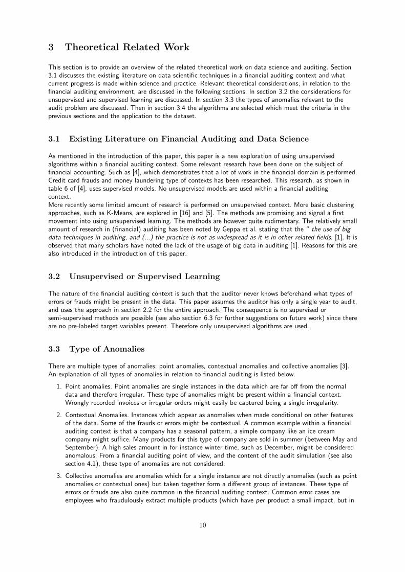
There are multiple types of anomalies: point anomalies, contextual anomalies and collective anomalies [3].An explanation of all types of anomalies in relation to financial auditing is listed below.

1. Point anomalies. Point anomalies are single instances in the data which are far off from the normaldata and therefore irregular. These type of anomalies might be present within a financial context.Wrongly recorded invoices or irregular orders might easily be captured being a single irregularity.

2. Contextual Anomalies. Instances which appear as anomalies when made conditional on other featuresof the data. Some of the frauds or errors might be contextual. A common example within a financialauditing context is that a company has a seasonal pattern, a simple company like an ice creamcompany might suffice. Many products for this type of company are sold in summer (between May andSeptember). A high sales amount in for instance winter time, such as December, might be consideredanomalous. From a financial auditing point of view, and the content of the audit simulation (see alsosection 4.1), these type of anomalies are not considered.

3. Collective anomalies are anomalies which for a single instance are not directly anomalies (such as pointanomalies or contextual ones) but taken together form a different group of instances. These type oferrors or frauds are also quite common in the financial auditing context. Common error cases areemployees who fraudulously extract multiple products (which have per product a small impact, but in

10

total a higher one) or an administrative system used for bookkeeping which doesn’t work properly andtherefore larger portions of invoices which are given wrong dates could be such an error. These datesare important within a financial auditing context.

In summary: in the exploration of unsupervised algorithms, the algorithms must be able to both detect pointanomalies and collective anomalies since these types of anomalies are most common within a financialauditing context.

3.4 Algorithms Selected and Formalized Descriptions

This section shortly describes the selected algorithms used for exploration. Most algorithms explored areneural network algorithms. The general strength of neural network algorithms are explained in section 3.4.1.Then section 3.4.2 explores different types of Autoencoders used in this paper. In addition in sectionRestricted Boltzmann Machines are formalized in section 3.4.3. Lastly the Isolation Forest is described insection 3.4.4.

3.4.1 Neural Network Architecture Algorithms

Unsupervised neural network algorithms are effective algorithms for the financial auditing environment. Thefinancial auditing has no ground truth and it uses non-sequential data, which have a regular point anomaliesbut also collective anomalies. neural network algorithms are effective tools for this setting, since unsupervisedneural network algorithms learn inherent characteristics of the data. The assumptions the neural networkalgorithms make for anomaly detection are: (1) the regular sections in the dataset or compressed variablesare different from the anomaly, (2) the normal data has a (much) larger presence than the anomalies, (3) theneural network algorithms are able to produce an anomaly score which are the result of learning intrinsicproperties of the dataset [14].

Assumptions (1) and (2) are both relevant within the financial auditing context. Frauds, besides generalerrors, are a special case since these are transactions which are meant to be ”normal”. However with enoughdomain knowledge it is possible to detect also frauds.

3.4.2 Autoencoders

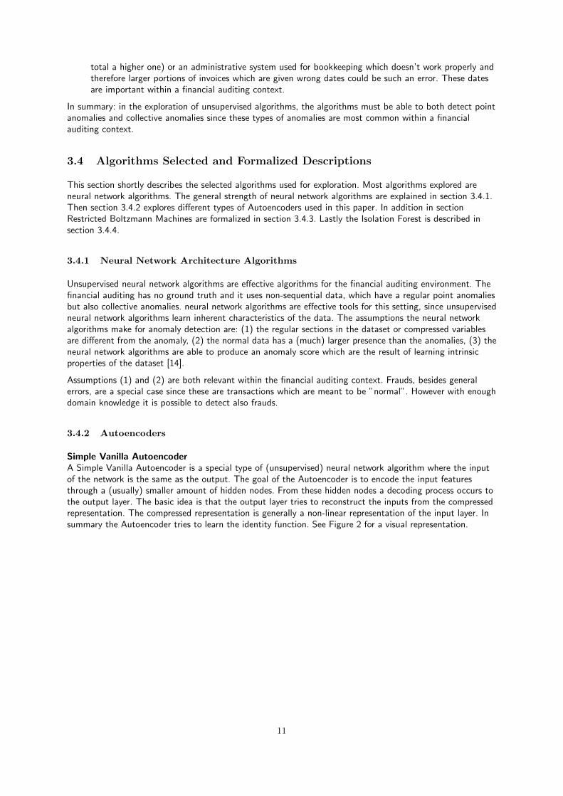
Simple Vanilla AutoencoderA Simple Vanilla Autoencoder is a special type of (unsupervised) neural network algorithm where the inputof the network is the same as the output. The goal of the Autoencoder is to encode the input featuresthrough a (usually) smaller amount of hidden nodes. From these hidden nodes a decoding process occurs tothe output layer. The basic idea is that the output layer tries to reconstruct the inputs from the compressedrepresentation. The compressed representation is generally a non-linear representation of the input layer. Insummary the Autoencoder tries to learn the identity function. See Figure 2 for a visual representation.

11

Figure 2: Simple Autoencoder

As displayed in Figure 2 the left side represents the input layer or the features which the dataset contains.The input vector is described by xi and contains n features (n corresponds with the count of input nodes onthe left side of Figure 2). This input is put through a set of weights (described by W in Figure 2 called theEncoder (or E) and results in a compressed representation described by the hidden nodes h(xi). The set ofnodes described by h(xi) in Figure 2 is the latent representation in a lower dimension than the input nodes.From latent representation the decoder (or D) decodes the hidden layer to the output layer. As noted theinput layer has the same number of n nodes as the output layer. The output layer on the right side of Figure2 is described by x̃i and contains n nodes. x̃i is a reconstruction of xi. x̃i can be described byx̃i = D(E(xi)).

The function which is optimized is given in Equation 1. The optimization function demonstrates theAutoencoder tries to learn the input data with the least amount of distortion.

Reconstruction Error = (∑

x̃i −∑

xi)2 (1)

The Reconstruction Error in Equation 1 is a way to measure the so called reconstruction error. The generalidea is that the Autoencoder learns the deeper structure in the dataset from the latent features and then isable to use this to detect the anomalies. The compressed representation describes the normal transactionswithin the dataset well and will be less prone to learning the anomalies. Transactions which are fraudulenttransactions would have a significant larger reconstruction error for that particular set of transactions, this iscaused due to the fact that anomalies do not contribute to the latent hidden layer as much. The anomalytransaction(s) will have a higher reconstruction error which is the basis for the anomaly detection.

Exploration Advantage for Financial AuditingThe Vanilla Autoencoder is a basic structure from which other variations of Autoencoders are built (see alsoContractive Autoencoder and Variational Autoencoder in this paper). The combination of the basicAutoencoder structure combined with the different variations might provide insight into the workings ofthese specific types of neural networks in a financial auditing context.

Contractive AutoencoderMultiple Regularized Autoencoders, which add some form of regularization on top of the ContractiveAutoencoder (CAE). The central characteristic of the CAE is that the learned representation is less sensitiveto minor variations of the training records. The main difference with the Vanilla Autoencoder is that theCAE has an added penalty term which make sure there is a higher robustness to the training of the CAE.The CAE uses the Frobenius norm of the Jacobian matrix of the mapping of the encoding as a way forregulation of the sensitivity [15].

12

L = ||X̃ −X||22 + λ||Jh(X)||2F (2)

||Jh(X)||2F =∑ij

(∂hj(X)

∂X2i

) (3)

The loss function in the CAE is similar to the Vanilla Autoencoder but a penalty term is added as shown inEquation 1. The penalty term is the Frobenius Norm of the Jacobian Matrix (as shown in Equation 3). TheJacobian Matrix contains the first-order partial derivatives for the hidden layer (h) with j nodes and iscomputed with respect to the input layer nodes (X) with i nodes of the CAE. The Frobenius norm of theJacobian Matrix is calculated by summing up all the elements in the Jacobian Matrix. Where the rows of theJacobian Matrix are i and represented by the input nodes of CAE and the columns of the Jacobian Matrixare j.

The consequence of this penalty term is that there appears a trade-off between the reconstruction error andthe Frobenius norm of the Jacobian Matrix. More simply stated, it means that the CAE (compared to aVanilla Autoencoder), will learn the larger variations the dataset contains and are less prone to changes tosmaller variations. The Equation 3 is added to the loss function in Equation 1.

Exploration Advantage for Financial AuditingBecause frauds and errors in Financial auditing can be of different qualitative kinds, and the amount of thefrauds and errors can differ the CAE is an algorithm which can provide robust results to differing variations inthe data across multiple features.

Variational Autoencoder

The Variational Autoencoder is a generative algorithm. Variational Autoencoder (VAE) is described byKingma et al. [12]. Just like the Vanilla Autoencoder it has an encoder, decoder and a loss function. Theinput of the VAE is compressed into a (hidden) latent representation (noted by z) which reduces thedimensionality of the input layer. A main difference with the Vanilla Autoencoder is that the VAE has a lowerdimensional space which is of a stochastic nature. The encoder computes a set of parameters of qθ(z|x)where x is the input of the VAE and z the latent representation. This represents a Gaussian probabilitydensity. The z is a stochastic variable. The VAE therefore converts the input to a continuous distributionwith a mean and a standard deviation. The decoder of the VAE converts the latent representation to anoutput. The decoder is described by pφ(x|z). Where φ represents the weights of the decoder from the latentrepresentation z to the output layer. Figure 3 shows the general structure of a Variational Autoencoder asdescribed in this paragraph.

Figure 3: Variational Autoencoder

The loss function of this model is shown in Equation 4. It has two components: a negative log likelihood ofthe reconstruction error using the aforementioned decoder and encoder and also a Kullback-LeiblerDivergence term. The loss function of a VAE does not contain general representation which are relevant forall the contents of the dataset. The first term can be described as the true reconstruction error. The E iscomputed in relation to the distribution of the encoder over the input. The first term basically states that ifthe decoder isn’t able to create a good parametrization of the distribution of the input data then a largerloss will occur. Since there are no general representations for all datapoints the loss function is using single

13

data points li for the calculation of the total loss. The total loss is then computed by summing all Ninstances. The loss function for each input datapoint is then described by Equation 4. As mentioned above: θand φ are respectively the weights and biases of the encoder and the decoder of the VAE.The second part of Equation 4 is the Kullback-Leibler divergence between the two mappings of encoder anddecoder. It gives the opportunity to measure how well the term q represents p. In a VAE, the term p isdescribed with a normal distribution of the latent representation with a mean of 0 and a standard deviationof 1. This penalty term is necessary to make sure that the latent space z is kept a decent uniqueness. Thesmaller differences between common datapoints are then kept in a certain place within a Eucledian space ofa Gaussian distribution.

li(θ, φ) = −Ez∼qθ(z|xi)(log pφ(xi | z)) + KL(qθ(z | xi) || p(z)) (4)

An important aspect of a VAE is the usage of the reparametrization trick. Autoencoders use abackpropagation structure to optimize the identity function. However the latent representation z is a fixedrepresentation of the distribution of q. Causing the derivative to be zero (but this derivative should of coursenot be zero). The reparametrization trick formulates the calculation of z = µ+ σ } ε provides theopportunity to allocate the stochasticity of a Gaussian latent variable z to the ε. Then ε is calculated using aGaussian normal distribution. Making it possible to calculate the derivatives of functions taking z as input.Figure 4 shows the difference, where the circled symbols represent the parameters which are stochastic, andthe squared symbols which are deterministic. The deterministic quality allows backpropagation to functionnormally.

Figure 4: Reparametrization Trick for Variational Autoencoder

Exploration Advantage for Financial Auditing

The main advantage this type of algorithm has is that the output of the algorithm provides disentanglement.Disentanglement means that the factors try to differentiate themselves as strongly as possible from eachother. [12] [10]. Being able to produce (in reduced dimensionality) the new variables ensure that one getsmore independent latent variables. Each latent factor is then able to algorithm an independent underlyingstructure. It can be stated on a higher conceptual level that this is similar to the Varimax Rotation inPrincipled Component Analysis (which can be considered an Autoencoder with linear activation functions),where variables are loaded as much as possible on a single factor. Obtaining larger independence between thedifferent factors [2].

Important consideration is that the dataset, see section 4.3, has mixed types of data. Categorical as well ascontinuous. Categorical data provide some complication in using variational autoencoders, since theautoencoder is trying to learn a distribution with a mean and a standard deviation for categorical data. Inorder to correct this a reparametrization is applied to categorical data called the Gumbal-Softmaxtransformation [11]. This results in data being more qualified to be effectively used by the VAE.

Transactions within a company have different groupings and underlying reasons. Each of the transactionstreams have a different underlying structure (type of products, type of clients, discounts etc.). Multiple

14

features can work together in a certain way, in light of the different type of transactions. It might provide alarge advantage to learn independent latent features which are used for anomaly detection, taking intoconsideration these different independent distributions. The VAE provides this advantage over the normalVanilla Autoencoder.

3.4.3 Restricted Boltzmann Machines

A Restricted Boltzmann Machine (RBM) [10] is a certain form of a (stochastic) neural network. The mainarchitectural difference with Autoencoders is that the RBM lacks an output layer, and only has an input layer(usually called the visible layer) and one hidden layer, see Figure 5.

Figure 5: Restricted Boltzmann Machines

The RBM has weighted undirected edges between the different sets of nodes. RBM is a bipartite graph, sono edges exist between a single layer (a single layer is either the hidden nodes or the input nodes). Thehidden nodes only takes on the binary positions of zero and one. The RBM uses uses an underlying jointprobability of input and hidden nodes. The joint probability tries to match a strongly as possible the datasuch that the nodes match the input data. The joint probability is described by the following formula:

p(v) =1

Z

∑h

e−E(v,h) (5)

where Z is a partition function ensuring that∑p(v) = 1,

Z =∑v,h

e−E(v,h), (6)

And E is the energy function,

E(v, h) = −∑

i∈visible

aivi −∑

j∈hidden

bjhj −∑i,j

wijvihj , (7)

The equation in 8 is a probability distribution and can be called a Boltzmann distribution. When optimizingthe RBM the parameters are found by maximizing the product of probabilities using the input data of atraining set V .

arg maxai,bi,wij∏V p(v) (8)

15

Optimization is usually performed using the Contrastive Divergence algorithm. When the algorithmconverges the output of the RBM algorithm is a Boltzmann distribution calculated using the features asinput. This probability distribution can then be ordered from low to high on a record level. Transposing thisgives a value for outlier detection.

Advantage for Exploration for the Financial Auditing ContextRBM’s have a similar architecture to Autoencoders, but have a different approach. RBM’s have aprobabilistic approach and are energy based algorithms. It may be expected, due to the different architectureand the undirected graph structure that the RBM is able to learn more freely the patterns in the dataset. Atleast learning other types of structures.

3.4.4 Isolation Forests

Isolation forest is, in contrast to the other models in this paper, a non-neural network algorithm to identifyanomalies. The Isolation Forest has a similar structure as the random forest algorithm [13]. Whereas thegeneral structure is to combine several decision trees and uses an averaging mechanism to decide on theoutliers in the dataset. Instead of trying to learn the general structure of the dataset, Isolation forestshowever are focused on detecting anomalies. The general idea of Isolation Forests is shown in Figure 6.Anomalies have a different structure, or different values for each of the features in the dataset. As Figure 6shows, the anomalies will be on a less deeper level when calculated from the root compared to very commonrecords. Many trees are constructed with a random amount of features, and every transaction is averaged onwhich level the transaction is a leaf in the tree. The anomalies will most likely be more often at a moreshallow level (so in Figure 6 the red leaves in the tree) than the more common ones.

Figure 6: Isolation Forest

Advantage for Exploration for the Financial Auditing ContextIsolation Forest is a different type of architecture than the neural network algorithms formalized in section3.4.1. The architecture of Isolation Forest might be stronger for detecting point anomalies since theuniqueness of these type of anomalies might be better captured by the leaves of the trees in theensembling.

3.4.5 Ensembling Algorithms

Ensembling is a way to combine the results of trained algorithms to obtain more effective results [6].Ensembling has taken more interest in the context of unsupervised learning [17]. Ensembling combines theresults of single algorithms in multiple ways. Most common ways are ranking methods, stacking and boosting[17].

Ensembling is a cheap method in which one can combine the outlier detection strength of multiple methods.The different algorithms described in section 3.4 have different characteristics and as a consequence othertypes of anomalies can be detected. The method used for ensembling in this paper is the ”rank-aggregation”

16

method which is a common and effective method [17]. This method normalizes the outlier scores for eachalgorithm, ranks every record for every independent model. This ranking is then averaged for eachtransaction across all used algorithms. This new average is the new ensembled anomaly score.

17

4 Research Approach

This section is dedicated to the research approach. Section 4.1 provides some background to the financialauditing case which is used to run the algorithms on. Section 4.3 gives a description of the datasets used.Section 4.2 provides some guidance on the general framework used to construct features for fraud and errordetection. Section 4.6 describes the programming library’s which are used to perform the experimentation.Finally Section 4.7 discusses the evaluation metrics used.

4.1 The Audit Client: Digital Simulation

The experiments for the algorithms are performed within an audit simulator. The Audit Simulator is used inmany accounting eduactational contexts, mainly Nyenrode Business University. The general website of thesimulator is: https://www.auditgaming.nl/. As mentioned, the data are owned by Nyenrode BusinessUniversity.

The company which is used from the audit simulator replicates a real life medium or large sized company.The company that is used in the Audit Simulator is a company called ”Laptopworld.nl”. The company sellslaptops using an online platform (website) to individual customers and to businesses. All kinds of transactionssuch as cost of sales, sales, invoices, orders, bank transactions, client information etc. are included within.The audit simulator is accredited by the “Nederlandse Beroepsorganisatie Accountants”, meaning it is usedto train financial auditors. The simulation provides a unique opportunity to also include a ground-truth.Meaning it can be checked what the output of the algorithms is. So the output of the unsupervisedalgorithms can be verified (see also Section 4.3). It is possible to manipulate the data in such a way thatmore frauds and errors occur within the data. This makes additional experimentation possible.

Laptopworld’s strategy is based upon buying large bulk purchases of laptops which gives large discounts. Thisgives the opportunity to sell laptops for a low price. The company has a CEO which is also 100% shareholderin the company. The company has a vision for the coming years that growth (in revenues) is highlyimportant. The sales totally used for the ”larger dataset” contains about 380.000 records and 300 millioneuro’s in revenue and the ”smaller dataset” have 40.000 records and 40 million euro’s in revenue.

4.2 Feature Construction

The audit simulator provides multiple options to extract structured datasets from the simulator. The digitalsimulator has a large variety of different aspects such as salary of employees, cost of sales, other costs andother special transactions. In the context of this paper it is decided to focus on the sales of the company.The two reasons for this choice are: (1) sales is one of the richest contexts to have fraud risks from afinancial auditing point of view, (2) sales have larger volumes which provide the opportunity to experimentwith the selected algorithms. The amount of records can be changed manually. Two different sizes ofdatasets are used within the context of this paper, see section 4.3.

In order to obtain relevant features to be used in algorithms a short description is given of the contents ofthe digital simulator for the sales section. The sales process of the digital simulator has 15 differentdatasheets (such as: a price sheet with 8 features which holds information about the products an pricesgiven, or an invoice datasheet with 19 features about the invoices sent to customers). The 15 datasheetscontain in total 181 unique features. Not all features are directly relevant for detecting frauds or errors andneed to be processed to be effectively used for the chosen algorithms in section 3.4.

The author of this paper is an experienced auditor. In order to obtain relevant features, creatingcombinations between the existing features or removing irrelevant ones, expert knowledge is used. The firsttwo steps as discussed in section 2.2 are performed to construct features which are indicative of frauds orerrors. This is a relatively challenging task to perform. It is to find a cross link between auditing methodologyand data science. Note that the author of this paper was unaware of the ground truth of the true frauds anderrors, but only at end of this research this was made available. This is mainly for the exploration purposes ofthis paper, in order to discover what process one has to go through if a financial auditor does not have theground truth and tries to go through the process described in section 2.2.

18

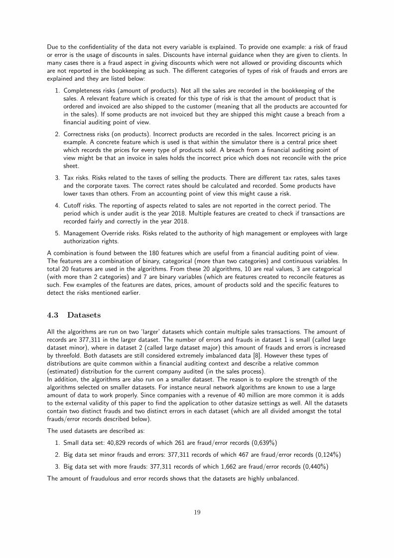
Due to the confidentiality of the data not every variable is explained. To provide one example: a risk of fraudor error is the usage of discounts in sales. Discounts have internal guidance when they are given to clients. Inmany cases there is a fraud aspect in giving discounts which were not allowed or providing discounts whichare not reported in the bookkeeping as such. The different categories of types of risk of frauds and errors areexplained and they are listed below:

1. Completeness risks (amount of products). Not all the sales are recorded in the bookkeeping of thesales. A relevant feature which is created for this type of risk is that the amount of product that isordered and invoiced are also shipped to the customer (meaning that all the products are accounted forin the sales). If some products are not invoiced but they are shipped this might cause a breach from afinancial auditing point of view.

2. Correctness risks (on products). Incorrect products are recorded in the sales. Incorrect pricing is anexample. A concrete feature which is used is that within the simulator there is a central price sheetwhich records the prices for every type of products sold. A breach from a financial auditing point ofview might be that an invoice in sales holds the incorrect price which does not reconcile with the pricesheet.

3. Tax risks. Risks related to the taxes of selling the products. There are different tax rates, sales taxesand the corporate taxes. The correct rates should be calculated and recorded. Some products havelower taxes than others. From an accounting point of view this might cause a risk.

4. Cutoff risks. The reporting of aspects related to sales are not reported in the correct period. Theperiod which is under audit is the year 2018. Multiple features are created to check if transactions arerecorded fairly and correctly in the year 2018.

5. Management Override risks. Risks related to the authority of high management or employees with largeauthorization rights.

A combination is found between the 180 features which are useful from a financial auditing point of view.The features are a combination of binary, categorical (more than two categories) and continuous variables. Intotal 20 features are used in the algorithms. From these 20 algorithms, 10 are real values, 3 are categorical(with more than 2 categories) and 7 are binary variables (which are features created to reconcile features assuch. Few examples of the features are dates, prices, amount of products sold and the specific features todetect the risks mentioned earlier.

4.3 Datasets

All the algorithms are run on two ’larger’ datasets which contain multiple sales transactions. The amount ofrecords are 377,311 in the larger dataset. The number of errors and frauds in dataset 1 is small (called largedataset minor), where in dataset 2 (called large dataset major) this amount of frauds and errors is increasedby threefold. Both datasets are still considered extremely imbalanced data [8]. However these types ofdistributions are quite common within a financial auditing context and describe a relative common(estimated) distribution for the current company audited (in the sales process).In addition, the algorithms are also run on a smaller dataset. The reason is to explore the strength of thealgorithms selected on smaller datasets. For instance neural network algorithms are known to use a largeamount of data to work properly. Since companies with a revenue of 40 million are more common it is addsto the external validity of this paper to find the application to other datasize settings as well. All the datasetscontain two distinct frauds and two distinct errors in each dataset (which are all divided amongst the totalfrauds/error records described below).

The used datasets are described as:

1. Small data set: 40,829 records of which 261 are fraud/error records (0,639%)

2. Big data set minor frauds and errors: 377,311 records of which 467 are fraud/error records (0,124%)

3. Big data set with more frauds: 377,311 records of which 1,662 are fraud/error records (0,440%)

The amount of fraudulous and error records shows that the datasets are highly unbalanced.

19

4.4 Optimization of Parameters Algorithms

4.4.1 Train, Test and Validation Methods

In order to obtain the reconstruction error the entire dataset is used for the determination of thereconstruction error. The task performed is a unsupervised learning task and the training and test data arenot separated [9]. In addition no validation methods (such as Cross-Validation) are applied, due to theunsupervised learning task.

4.4.2 Threshold Reconstruction Error: Post-Processing

One of the more important parameters to validate is the threshold for the reconstruction error (for theAutoencoders). The Autoencoders use the reconstruction error to optimize for the replication strength of thealgorithm. The higher the reconstruction error for each transaction the higher the probability this particulartransaction is an anomaly. A threshold needs to be selected to determine the boundary for anomaly. Eachtransaction higher or lower than this boundary might be considered an anomaly. The main problem is there isan extreme imbalance in the anomalies and non-anomalies in the dataset. Determining the threshold isrelatively challenging by a standard metric. No research has provided a robust heuristic to the knowledge ofthe author of this paper. Selecting the correct threshold is an important post-processing step to determinewhich transactions are considered anomalies.

A method to be used might be for instance using a standard percentile from the anomaly scores from thealgorithms. A concrete example is to calculate the mean from the anomaly scores from an algorithm andconsider everything above the three standard deviation from the mean as anomalous. This method ishowever often quite inaccurate and quite general.

The approach selected is to plot the reconstruction error for each transaction and see visually what aneffective threshold might be. This method is not algorithmic, but provides enough basis for determining in avisual approach what the anomaly threshold should be. See figure 7 for an example on the subset of the datain determining a correct threshold. The red line shows what threshold is chosen for this specific dataset. Thisis done by using the plot, which is ordered by time stamps of the transactions in the dataset. Note thethreshold is determined without a legenda fraud vs non fraud, meaning that all the data points are blue. Thismethod gives a decent amount enough to determine what amount of anomalies to select (and thedistinctness of the anomalies). This method has its limitation due to the subjective nature of selecting thethreshold.

20

4.5 Distributions Fraud vs. non Fraud

Figure 7: Visual Method of Selecting Anomalies

4.5.1 Parameters Unsupervised Algorithms

The parameters used within the unsupervised algorithms are not optimized in a strong fashion. The way themodels are selected, at least the autoencoders, using a method of trial and error. It is demonstrated thatusing 1 hidden (intermediate) layer between the input layer (with 20 input nodes) and a latent layer (with 6nodes) has the most robust and strong performance across all algorithms. Note that in a real life case thefinancial auditor would not be able to do this similar type of optimization described here since the realground truth for frauds and errors is not present. Therefore relatively standard parameters and settings areused and are showed in table 2. The loss function, the activation function, the learning rates and epochs areall kept standard.

21

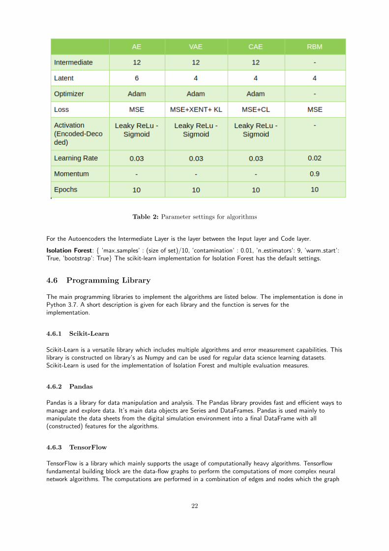
Table 2: Parameter settings for algorithms

For the Autoencoders the Intermediate Layer is the layer between the Input layer and Code layer.

Isolation Forest: { ’max samples’ : (size of set)/10, ’contamination’ : 0.01, ’n estimators’: 9, ’warm start’:True, ’bootstrap’: True} The scikit-learn implementation for Isolation Forest has the default settings.

4.6 Programming Library

The main programming libraries to implement the algorithms are listed below. The implementation is done inPython 3.7. A short description is given for each library and the function is serves for theimplementation.

4.6.1 Scikit-Learn

Scikit-Learn is a versatile library which includes multiple algorithms and error measurement capabilities. Thislibrary is constructed on library’s as Numpy and can be used for regular data science learning datasets.Scikit-Learn is used for the implementation of Isolation Forest and multiple evaluation measures.

4.6.2 Pandas

Pandas is a library for data manipulation and analysis. The Pandas library provides fast and efficient ways tomanage and explore data. It’s main data objects are Series and DataFrames. Pandas is used mainly tomanipulate the data sheets from the digital simulation environment into a final DataFrame with all(constructed) features for the algorithms.

4.6.3 TensorFlow

TensorFlow is a library which mainly supports the usage of computationally heavy algorithms. Tensorflowfundamental building block are the data-flow graphs to perform the computations of more complex neuralnetwork algorithms. The computations are performed in a combination of edges and nodes which the graph

22

consist out of. Tensorflow is (partly) used to implement all the neural network algorithms as described insection 3.4.

4.6.4 Keras

From the Keras website: Keras is a high-level neural networks API, written in Python and capable of runningon top of TensorFlow, CNTK, or Theano. It was developed with a focus on enabling fast experimentation.Also aspects of Keras are used for implementing the algorithms in section 3.4.

4.7 Evaluation Metrics

In order to evaluate the performance of the different algorithms multiple evaluation measures are used. Adiverse number of evaluation measures are selected in order to capture multiple dimensions of performancemeasures. Here below the different evaluation measures are mentioned, the corresponding formula’s (usingthe True Positive (TP), False Positive (FP), True Negative (TN), False Negative (FN)) and a shortdescription of the evaluation measure.These measures are also captured in confusion matrices.

1. Accuracy. Formula: TN+TPTP+FP+FN+TN . Accuracy is described as the percentage of the instances which

received a good classification.

2. Precision. Formula: TPTP+FP . A figure that describes the instances which are predicted to be frauds or

errors, and truly are frauds or errors.

3. Recall. Formula: TPTP+FN . This measure describes how effective an algorithm is able to identify frauds

or errors.

4. Specificity. Formula: TNTN+FP . Measures the effectiveness that an algorithm is able to identify regular

instances.

5. False Positive Rate. Formula: FPFP+TN . The amount of misclassified instances in the data.

6. ROC. Graph where True Positive Rate is plotted against the False Positive Rate.

7. F1-Measure. Formula: 2∗(Precision∗Recall)Precision+Recall . Is the weighted average of the precision and the recall.

8. Mathews Correlation Coefficient. Formula: TP∗TN−FP∗FN[(TP+FP )∗(FN+TN)∗(FP+TN)∗(TP+FN)](1/2)

. Another

balanced measure, such as the F1-Measure. Is noted to work well on strongly imbalanced datasets.

From a financial auditing point of view, recall is the most important measure. As described in section 2.1,the goal of the auditor is to make sure the final financial statements of the year are free of material errors orfrauds. In addition precision is important from an efficiency perspective. The auditor cannot audit manually adisproportional amount of false positive instances extracted from the unsupervised algorithms. For thepresentation of the results the simple Vanilla Autoencoder in section 3.4.2 is used as a baseline and the otheralgorithms are compared with it.

5 Results

This section concerns the reporting of the results. The reporting is split up in three subsections,corresponding to the different datasets in section 4.3. Section 5.1 reports on the results found with thesmaller dataset (40.000 records). Section 5.2 reports on the larger dataset which contains less frauds (alarger imbalance) (377.000 records). Section 5.3 reports on a dataset with the same records as in section 5.2( 377.000 records), but where the imbalance of the classes is less prevalent.

23

5.1 Small Dataset

Relevant for the discussion and the presentation of the results is Table 3, the distribution plots of the errorfunctions of each algorithm in the Appendix in section A.1 and the plots in the Appendix in section A.2which show the chosen threshold for each of the algorithms as explained in section 4.4.2.

In general it can be stated that the Autoencoder algorithms outperform the RBM and the IF on all theimportant metrics as displayed in table 3. The F1 (0.00066 for RBM and 0.2969 for IF) and the MCC (-0.0005 for RBM and 0.2950 for IF) measures are of a weak performance for RBM and IF and can beconsidered not useful for financial auditing contexts. F1 and MCC are heavily influenced by a low precisionand recall for RBM and IF algorithms. RBM has the worst performance. This is counter intuitive to thegeneral performance of the model in previous papers (see 3.4.3). The hypothesis is that RBM’s are not fullyfunctional on using a diverse amount of data types. The features, as described in section 4.2, are mostly realvalued features. These are the types of features which the RBM has more trouble working with. The absenceof stronger discriminative power of the RBM algorithm is also made visible in Figure 19 of section A.2 wherealmost all true anomalies are assigned a lower error value compared to the other parts of thetransactions.

For IF it might additionally be the case that the IF is able to not detect anomalies very strongly due to thefact there are four types of frauds/errors in the dataset. These are anomalies which have a recurringcharacter throughout the time period of this dataset. If an anomaly can be discovered due to a ”feature A”,but it is a type of anomaly which occurs with some intervals, it means the anomaly can be seperated byanother feature A and feature B. This means the probability these anomalies will have a deeper ’leaf’ level inthe IF algorithm is relatively high. Also the probability that normal transactions are split in a (set of)feature(s) in a certain way, making them anomalies by this algorithm is also higher from this point of view.This is visually supported by Figure 18 in section A.2, where fraudulous and normal transactions are at thetop all scatter relatively evenly. It is visible the algorithm is able to assign a higher error to all the ”orange”fraudulous dots (since none of these transactions are below the error rate of 0.450).

The Autoencoders perform relatively well. The VAE has a MCC of 0.65 and an F1 of 0.63. The results are ofa decent value but lower than AE and CAE. Recall of the VAE is of a similar order of magnitude with the AEand CAE. The precision is of a lower quality. This might be due to the probabilistic nature of the algorithmand the problems that VAE might still have with using binary types of variables. The Gumbel-Softmaxtransformation [11] might assist in the conversion to a usable input for the VAE. But trying to obtainsampled Gaussian Distributions from binary features on which the Gumbel-Softmax [11] transformation hastaken place might not fully solve all problems related to this.

The AE and the CAE both perform strongly on the dataset. AE has a F1 of 0.8933 and MCC of 0.8934 andCAE has a F1 of 0.9196 and MCC of 0.9193. Of the 261 frauds (or anomalies) which are in the dataset thealgorithms had a True Positive count of 243 and 246 for AE and CAE respectively. This is a very strongperformance for financial auditing contexts. The amount of work a financial auditor still needs to performhas reduced dramatically after using these algorithms. A financial auditor would in normal circumstancesneed to setup a large amount of manual procedures for detecting these types of anomalies. The algorithmsgive an almost full proof and more objective output on the entire dataset. Using a more qualitativejudgement from the author, obtaining the same amount of assurance on the absence of anomalies or fraudwould take four auditors and around ten manual procedures to obtain similar results. In auditing the types ofanomalies are more closely.

Lastly the performance of the ensemble where every algorithm (AE, CAE, VAE, RBM, IF) is combined. It isclear the recall at 0.96 outperforms the recall of all other algorithms. The precision is of a worse quality at0.54. Average Ranking Ensembling ensures a higher recall which can be useful within a financial auditingcontext, since the probability that Ensembling will have a more complete picture of what the anomalies trulyare is useful within financial auditing contexts (since one wants to find all the possible anomalies affectingthe financial statements. The precision however is not very strong, this is due to the fact that the precisionof the VAE, RBM and IF are all lower than 0.5 this is a logical consequence.

24

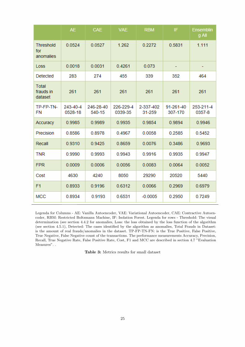
Legenda for Columns - AE: Vanilla Autoencoder, VAE: Variational Autoencoder, CAE: Contractive Autoen-coder, RBM: Restricted Boltzmann Machine, IF: Isolation Forest. Legenda for rows - Threshold: The visualdetermination (see section 4.4.2 for anomalies, Loss: the loss obtained by the loss function of the algorithm(see section 4.5.1), Detected: The cases identified by the algorithm as anomalies, Total Frauds in Dataset:is the amount of real frauds/anomalies in the dataset. TP-FP-TN-FN: is the True Positive, False Positive,True Negative, False Negative count of the transactions. The performance measurements Accuracy, Precision,Recall, True Negative Rate, False Positive Rate, Cost, F1 and MCC are described in section 4.7 ”EvaluationMeasures”. .

Table 3: Metrics results for small dataset

25

5.2 Big Dataset Less Frauds and Errors

Relevant for the discussion and the presentation of the results is Table 4, the distribution plots of the errorfunctions of each algorithm in the Appendix in section B.1 and the plots in the Appendix in section B.2which show the chosen threshold for each of the algorithms as explained in section 4.4.2. Note that the sametype of frauds and errors are present in this larger dataset compared to the smaller dataset in section 5.1,but the frequency of the anomalies has increased in the absolute sense.

When compared with the results for the smaller dataset in section 5.1 the overall performance of allalgorithms have decreased. However the Precision metric has stayed relatively the same for the AE and theCAE. It can be noticed in Table 4 that RBM still has a low performance as already described with thesmaller dataset in section 5.1 with a F1 of 0.0023 and MCC of 0.0006. The ensemble model is also heavilyinfluenced by the low performance of RBM and VAE.

The VAE algorithm also has drastically reduced its performance compared to the smaller dataset, with a F1measure of 0.0085 (0.6312 for the smaller dataset), MCC of 0.0072 (0.6531 for the smaller dataset). Whenlooking at the reconstruction error plot in section B.2 Figure 28 there are multiple ”layers” of errors presentin the Varational Autoencoder. This might be due to the already discussed binary variables in the dataset,the VAE most likely has a harder time differentiating between transaction using binary variables. A largernumber of the frauds and errors in this dataset can be detected using binary variables (in combination withreal valued features as well).

Similar results are found in Table 4 compared to the smaller dataset is the IF algorithm which has a F1measure of 0.3304 (for the smaller dataset 0.2969) and MCC of 0.3416 (for the smaller dataset 0.2950). Theperformance of the IF therefore has stayed relatively the same. It confers with the capacity for IF to be ableto shift and adapt to new distributions [13].

The algorithms AE and CAE have a reduced recall, but have a good retained precision compared to the smalldataset. It can be seen in the Appendix in section B.2 Figure 27 and Figure 29, the discrimination forrespectively AE and CAE are quite strong and even have some uniformity (as in the smaller dataset) for theanomalies detected (with a few datapoints which have a larger error). The uniformity of the results may bedescribed by the fact that many transactions might be considered an anomaly by the usage of binaryfeatures. In addition the dataset contains certain types of fraud, such as a ”caroussel” fraud, which occursmonthly at a regular basis. This combined brings the conclusion that the results are plausible and also usefulfor financial auditing contexts.

26

Legenda for Columns - AE: Vanilla Autoencoder, VAE: Variational Autoencoder, CAE: Contractive Autoen-coder, RBM: Restricted Boltzmann Machine, IF: Isolation Forest. Legenda for rows - Threshold: The visualdetermination (see section 4.4.2 for anomalies, Loss: the loss obtained by the loss function of the algorithm(see section 4.5.1), Detected: The cases identified by the algorithm as anomalies, Total Frauds in Dataset:is the number of real frauds/anomalies in the dataset. TP-FP-TN-FN: is the True Positive, False Positive,True Negative, False Negative count of the transactions. The performance measurements Accuracy, Precision,Recall, True Negative Rate, False Positive Rate, Cost, F1 and MCC are described in section 4.7 ”EvaluationMeasures”.

Table 4: Metrics results for large dataset relative smaller number of frauds and errors

27

5.3 Big Dataset More Frauds

Relevant for the discussion and the presentation of the results is table ,. Furthermore relevantinformation are the distribution plots of the error functions of each algorithm in the Appendix in section B.1and the plots in the Appendix in section B.2 which show the chosen threshold for each of the algorithms asexplained in section 4.4.2. Note that the same type of frauds and errors are present in this dataset comparedto the larger dataset and relatively less anomalies in section 5.2, but the frequency of the anomalies hasincreased in an absolute sense (for each of the type of fraud). The only difference is the ”Total Frauds indataset” in Table 4 and Table 5, all other parameters and settings are similar.

The main differences found are that in table 5 compared to table 4 the Recall for AE and CAE has increasedsignificantly with respectively 0.8104 (for the large dataset with relatively less anomalies 0.4239) 0.8104 (forthe large dataset with relatively less anomalies 0.5203). The main cause is the lesser imbalance in thedataset and the possibility for these types of algorithms to consistently assign larger errors to the anomaliesof this type.

An extremely weak performance is found for the Ensembling. The F1 Measure is 0.0311 and MCC 0.0299. Itshows ensembling is not always a strong method to try to detect anomalies. It seems the individual modelsall have found different anomalies, which do not overlap in the rank averaging.

5.4 Overall Observations and Conclusions

This section contains more general observations on the results found in section 5.1, section 5.2 and section5.3. This section is to provide additional insight in the results of the experiments.

5.4.1 Features

Important further experimentation shows that model selection is important as the different resultsdemonstrate. But most important is the correct selection of features (see also step 2 in section 2.2. Asmentioned 20 features are created or selected in order to cover a wide range of different frauds and errors.Four types of anomalies are contained in the dataset, three fraudulous transactions and one error type. Bysome trial and error six features are the most relevant to detect anomalies. If these features are not includedall algorithms, including the Vanilla Autoencoder and the Contractive Autoencoder have a very lowperformance. So selecting and creating correct features is crucial to detecting anomalies within a financialauditing context.

The amount of features relevant for the sales transactions are in total 180 features (see also section 4.2). Itrequires a large amount of effort to obtain 20 relevant features using professional judgement to cover a widerange of frauds and errors. As mentioned in section 3.1, there is a lack of knowledge of data scientificmethods in financial auditing and also thus the conversion of the qualitative risk judgements to a (set of)feature(s). The time the researcher of this paper invested into feature construction and creation wassubstantial and removed any speed advantages of using automation. This feature selection and creationhowever can be improved if more financial auditors obtain data science knowledge and best practices arecreated. Best practices in which combinations of features are useful to detect certain specific frauds anderrors.

It can be observed that the Variational Autoencoder (VAE), the Restricted Boltzmann Machines (RBM) andthe Isolation Forest (IF) algorithms are performing not as strong. Some discussion on the possible reasons forthis are given in section 5.1. It indicates the Vanilla Autoencoder and the Contractive Autoencoder seem tohave a more general purpose characteristic to observe anomalies than the other algorithms with respect tothe different types of input.

5.4.2 Anomaly Detection

Another important aspect in financial auditing is the concept of materiality. This is governed in theregulations of the ”International Standards Auditing” (ISA 320 specifically). This in an overgeneralized sense

28

means the financial auditor needs to detect larger frauds and errors. In the results found for VanillaAutoencoder (AE) and Contractive Autoencoder (CAE) the algorithms both are consistently able to obtainthe larger frauds and errors. The other algorithms, for the larger dataset, are not necessarily able to obtain alllarger frauds and errors.

Not all anomalies, frauds or errors, are detected for each algorithm. From a financial auditing perspective itis important that at least every type of anomaly in the dataset is detected. There are four anomaly types,three frauds and one error. When evaluating the types of anomalies found for the Vanilla Autoencoder (AE)and Contractive Autoencoder (CAE) all types of frauds and the error are all detected at least once in theanomalies. This is important for financial auditing purposes, since the auditor can evaluate the foundanomalies by the algorithm and evaluate every found fraud and error and then perform a more extensivesearch for the type of anomaly found by the algorithm (if considered necessary).

Lastly there is a substantive qualitative advantage of using a data driven auditing approach. At least with theAE and CAE algorithms a higher completeness of fraud and error detection is evient. As mentioned in theparagraph above, every type of fraud and error is detected at least once (with the AE and CAE algorithm).One type of fraud: the so called ”Carroussel Fraud” is more strongly present within this dataset (with theamount of transactions related to it and the size of each transaction). Within a normal audit this type offraud would likely be detected. The error, which concerns multiple transactions are not booked in the correctyear, would also be most likely detected by the auditor. The procedure for checking this error is quitesimplistic and easily done within every single audit. However the two other frauds (so three frauds and oneerror is four types of anomalies) are most likely not detected (an employee fraud and uncommon transactionswith foreign countries such as Saudi Aurabia). This is due to the fact that the type of transactions are veryuncommon and not thought of by the qualitative risk judgement of the financial auditor, but do come upusing the AE and CAE algorithms over different dataset contexts.

29

Legenda for Columns - AE: Vanilla Autoencoder, VAE: Variational Autoencoder, CAE: Contractive Autoen-coder, RBM: Restricted Boltzmann Machine, IF: Isolation Forest. Legenda for rows - Threshold: The visualdetermination (see section 4.4.2 for anomalies, Loss: the loss obtained by the loss function of the algorithm(see section 4.5.1), Detected: The cases identified by the algorithm as anomalies, Total Frauds in Dataset:is the number of real frauds/anomalies in the dataset. TP-FP-TN-FN: is the True Positive, False Positive,True Negative, False Negative count of the transactions. The performance measurements Accuracy, Precision,Recall, True Negative Rate, False Positive Rate, Cost, F1 and MCC are described in section 4.7 ”EvaluationMeasures”.

Table 5: Metrics results for large dataset with more frauds and errors

30

6 Conclusion & Discussion

6.1 Summary and Conclusions

A first exploration in combining data science and (financial) auditing is made within this paper. Differentunsupervised algorithms are explored and applied within an audit simulation which provide real-life syntheticdata which simulate a real company. This is highly unique data make it possible to research the possibility ofusing data scientific methods within an auditing setting. The absence of usable data are the main reason whyalmost no research exists in the financial auditing literature combined with data science [1]. Theunsupervised algorithms explored are (multiple) Autoencoders, Restricted Boltzmann Machines and IsolationForest. These algorithms are also combined within an ensemble by using an average ranking technique. Thestrongest results are found using a Vanilla Autoencoder and Contractive Autoencoder across differentdatasizes and anomaly/normal distributions. The main question posed in this paper is:

”To what extent can unsupervised algorithms detect (material) financial frauds or errors in a financialauditing context?”

The main question is answered by first answering the subquestions formulated in section 1.1.

6.1.1 Which algorithms can be taken into consideration to use, and why?

An important consideration in selecting algorithms is understanding the financial auditing environment. Thefinancial auditor has to perform a task in detecting material frauds and errors in the financial statements of acompany. The financial auditor has no existing labels providing a ground truth. In addition, the types ofanomalies most common for the auditor are point anomalies (unique and extreme anomalies) and groupanomalies (transactions which together are anomalous). Effective fitting types of algorithms are unsupervisedneural network algorithms to perform within this context. The selected unsupervised neural networkalgorithms are the Vanilla Autoencoder (AE), the Variational Autoencoder (VAE), the ContractiveAutoencoder (CAE) and the Restricted Boltzmann Machine (RBM). Besides these algorithms, IsolationForest (IF) is explored. Using a different type of algorithm also provides additional insight to the performanceof the algorithms.

6.1.2 How do the algorithms perform across multiple evaluation measures?

The best performing algorithms are the CAE and the AE. These algorithms have a relatively high F1Measure and higher Matthews Correlation Coefficient compared to the other algorithms. The VAE has amixed result pattern but in general is not a strong model and scores low on precision and recall. RBMconsistently has a low performance for recall, precision. This is due to the nature of the fit of the real valuedinput features and the way the RBM functions. The IF algorithm provides a minimum performance but notstrong enough to detect anomalies from all the different types of frauds and errors in the dataset. Mixedresults (high and low performance) are found using average ranking Ensembling in which all algorithms arecombined. In summary: the CAE and AE perform best on the important evaluation measures as Precision,Recall, Matthews Correlation Coefficient and the F1 Measure making these algorithms the most generalpurpose algorithms best fitted for the financial auditing context.

6.1.3 Can a robustness of results be found per algorithm using different fraud and errorcontexts?

The results for the dataset of 40,829 records with 0,639% of frauds and/or errors. The performance of thealgorithms is overall stronger than the larger datasets. On evalation measures as Precision, Recall, F1 andMatthew Correlation Coefficient the algorithms perform better than the larger datasets. The strongestperforming models on the smaller dataset are the AE (with a F1 Measure of 0.8933 and Matthew CorrelationCoefficient of 0.8934), the CAE (a F1 Measure of 0.9196 and Matthew Correlation Coefficient of 0.9193)and the Ensembling of all algorithms together (an F1 Measure of 0.6979 and Matthew CorrelationCoefficient of 0.7249).

31

The results on the larger datasets are of a lower performance than on the smaller dataset. There are twolarger datasets, which are identical, but they have a different mix of anomalies, one larger dataset of 377,311with a fraud/error percentage of 0,124%, and a larger dataset of 377,311 percentage of 0,440%. On thelarger dataset the best performing algorithms are AE (F1 measure of 0.5849 and Matthew CorrelationCoefficient of 0.6319) and CAE (F1 measure of 0.6287 and Matthew Correlation Coefficient of 0.6424). Allother algorithms have a very low performance on this dataset. For the larger dataset with more anomaliesthe AE (a F1 measure of 0.8908 and Matthew Correlation Coefficient of 0.8948) and CAE (a F1 measure of0.8873 and Matthew Correlation Coefficient of 0.8909).

It is noted that the performance of the AE and CAE decline with the larger dataset which has an anomalypercentage of 0,124%. For a financial auditing context, it is not specifically worrying since the total amountof fraud and error is already not that high. Whereas the extremity of the imbalance of frauds and errorsbecomes less then the algorithms of AE and CAE work well.

It is an interesting observation that the IF algorithm performs structurally consistent over all differentdataset contexts (within all context provides a F1 measure and Matthew Correlation Coefficient of around0,30). Ensembling performs decently well on the smaller dataset, but has the worst performance when usedon the larger dataset. Demonstrating that using ensembling is not always a safe method to use to detectanomalies to combine the strength of different algorithms.

To answer the main question:

”To what extent can unsupervised algorithms detect (material) financial frauds or errors in a financialauditing context?”

The first indications in implementing known unsupervised algorithms demonstrate the ability to detect fraudsor errors is strongly possible. Overall the Vanilla Simple Autoencoder is able to outperform all otheralgorithms on mostly all evaluation metrics. Unsupervised neural network algorithms in general seem to beable to take over subtasks of a financial auditor and perform strongly by integrally audit the entire (sales)dataset. If features are constructed in alignment with a decent qualitative risk analysis by a financial auditor,the chances are that the unsupervised neural network algorithms will be able to extract useful information forthe auditor.

In addition, the results seem to indicate the lower the number of frauds/errors are the lower the precisionand recall is. This is however not of a large consequence for the auditor. Since it is the case that the numberof frauds and errors are not significant enough to be considered a problematic misstatement for the financialstatements of the company.

The practical implications for the financial auditing are substantive. A first exploration for using unsupervisedalgorithms in auditing is made with satisfying results. This paper can be a first step in the direction ofcreating a new subfield within the financial auditing profession where individuals with financial auditingdomain knowledge and understanding of data science can perform audits over much larger amounts of data.As a consequence it provides a more complete analysis of possible frauds and errors. Multiple practicalaspects within related aspects of the profession, such as the standardization of the general ledger structureover multiple bookkeeping systems (twinfield, exact, oracle etc.), feature construction can also standardized.Creating features of interest for the audit can then be made much easier and be inputted faster in theunsupervised algorithm. This could all mean a new future where the called ’4th industrial revolution’ can alsobe feasibly and effectively start to happen within the financial auditing profession.

6.2 Limitations

While researching this subject some limitations to the conclusions must be made.

An audit simulator is used. Even though it is one of the more reliable methods to truly do research with, onehas to take into consideration the audit simulator always has some limitations in comparison with the realworld applications. In addition, some type of frauds (not implemented in the audit simulator) might still beharder to detect using the unsupervised algorithms proposed.

The audit case used is called laptop world and is a company which has the typology of ’trade’. From afinancial auditing point of view, when classifying the company to it’s type, it is the most simple form which a

32

company can take, since products come in and products go out. It does not for instance provide services orproduces goods. Different type of frauds and errors can occur which are different and sometimes harder todetect.

Not all class imbalance settings are tried due to time and budget constraints. An interesting case to try tosee is how the unsupervised algorithms perform by using a larger percentage of frauds or errors. Even thoughit is quite rare to see many frauds, it is the type of context a financial auditor would need in order to be ableto work the unsupervised algorithms.

6.3 Future Work and Suggestions

An aspect for further research might be solving the extreme imbalance class problem for unsupervisedsettings. For instance multiple oversampling and undersampling methods exist for supervised settings. Notrue heuristic or method is developed which can reliably counter the extreme imbalance problem. Furtherresearch might devise methods for solving that problem.

Another interesting research angle might be looking at methods of combining the algorithms which areexplored in this paper. This might be through pre-training methods, or creating larger ensembles. The resultsshow the way the algorithms learn are different from each other. The combined power might provide morestrength to the unsupervised methods.

As mentioned in the limitations, this research focuses on a single sector called ’trading’. Also the sales processis mainly evaluated. Different types of frauds, errors, datastreams and company sectors can be explored in asimilar fashion in order to see what the results might be for the financial auditing context.

It might be argued that some form of semi-supervised learning might be possible. By using the errors andfrauds detected (by hand) in the previous years, it can be a way of obtaining stronger results for the currentyear under audit. Looking at the possibility of using semi-supervised learning withing the context of financialauditing can be beneficial.

The explainabilty of the (true) positive cases which the unsupervised algorithms predict. One aspect whichcan help drastically in the work of the financial auditor, using the output of the data, is some indication whythe unsupervised algorithms exported the specified cases as a fraud or an error. Central to the work of afinancial auditor is to be able to report on why mistakes are selected, and be judged in light of the prevailingregulations. It might be time consuming if the auditor needs to manually check every output of theunsupervised algorithm.

References

[1] T. J. O. T. S. A. Geppa, M. K. Linnenlueckeb. Big data techniques in auditing research and practice:Current trends and future opportunities. Journal of Accounting Literature, 40:102 – 115, 2018.

[2] H. Abdi. Factor rotations in factor analyses. encyclopedia for research methods for the social sciences.Sage: Thousands Oaks, pages 792–795, 2003.

[3] S. Agrawal. Survey on anomaly detection using data mining techniques. Procedia Computer Science,60(10):708–713, 2015.

[4] M. Albashrawi. Detecting financial fraud using data mining techniques: A decade review from 2004 to2015. Journal of Data Science, 14:553 – 570, 2016.

[5] M. D. O. Brandas, C. Muntean. Intelligent decision support in auditing: Big data and machine learningapproach. 2019.

[6] T. G. Dietterich. Ensemble methods in machine learning. in international workshop on multiple classifiersystems. In International workshop on multiple classifier systems, pages 1–15, 2000.

[7] D. S. . R. B. Dutta, I. Detecting financial restatements using data mining techniques. Expert Systemswith Applications, 90:374 – 393, 2017.

33

[8] N. T. G Menardi. Training and assessing classification rules with imbalanced data. Data Mining andKnowledge Discovery, 28(1):92, 2014.

[9] . U. S. Goldstein, M. A comparative evaluation of unsupervised anomaly detection algorithms formultivariate data. PloS one, 11(4), 2016.

[10] X. G. A. P. B. U. C. B. S. M. A. L. I. Higgins, L. Matthey. Early visual concept learning withunsupervised deep learning. Procedia Computer Science, 2016.

[11] S. G. Jang, E and B. Poole. Categorical reparameterization with gumbel-softmax. preprint arXiv, 2016.

[12] M. W. Kingma, D.P. Auto-encoding variational bayes. arXiv preprint, 2013.

[13] T. K. M. . Z. Z. H. Liu, F. T. Isolation-based anomaly detection. Transactions on Knowledge Discoveryfrom Data, 6(1):1, 2012.

[14] S. R. Chalapathy. Deep learning for anomaly detection: A survey. 2019.

[15] X. M. X. G. Y. B. S. Rifai, P. Vincent. Contractive auto-encoders: Explicit invariance during featureextraction. Proceedings of the 28th International Conference on International Conference on MachineLearning, pages 833–840, 2011.

[16] . V. M. A. Thiprungsri, S. Cluster analysis for anomaly detection in accounting data: An auditapproach. The International Journal of Digital Accounting Research, 11:69 – 84, 2011.

[17] C. R. J. . S. J. Zimek, A. Ensembles for unsupervised outlier detection: challenges and researchquestions a position paper. ACM Sigkdd Explorations Newsletter, 15(1):11–22, 2014.

34

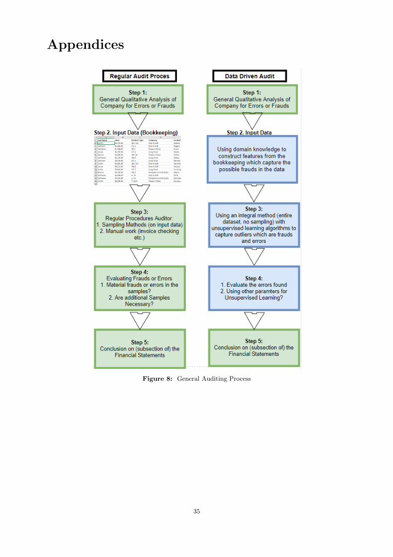
Appendices

Figure 8: General Auditing Process

35

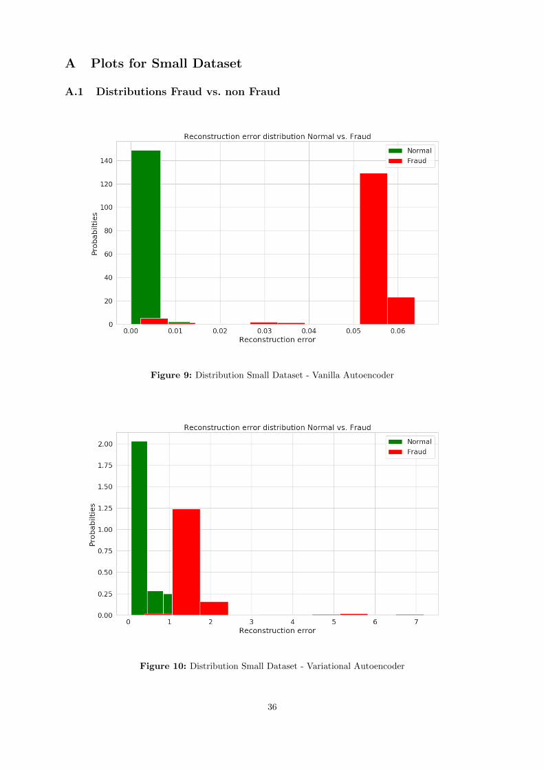
A Plots for Small Dataset

A.1 Distributions Fraud vs. non Fraud

Figure 9: Distribution Small Dataset - Vanilla Autoencoder

Figure 10: Distribution Small Dataset - Variational Autoencoder

36

Figure 11: Distribution Small Dataset - Contractive Autoencoder

Figure 12: Distribution Small Dataset - Restricted Boltzmann Machines

37

Figure 13: Distribution Small Dataset - Isolation Forest

Figure 14: Distribution Small Dataset - Ensemble

38

A.2 Visual Threshold

Figure 15: Threshold Determination Small Dataset - Vanilla Autoencoder

Figure 16: Threshold Determination Small Dataset - Variational Autoencoder

39

Figure 17: Threshold Determination Small Dataset - Contractive Autoencoder

Figure 18: Threshold Determination Small Dataset - Isolation Forest

40

Figure 19: Threshold Determination Small Dataset - Restricted Boltzmann Machines

Figure 20: Threshold Determination Small Dataset - Ensemble Modelling

41

B Plots for Large Dataset and Relatively Small number ofFrauds

B.1 Distributions Fraud vs. non Fraud

Figure 21: Distribution large Dataset - Vanilla Autoencoder

42

Figure 22: Distribution large Dataset - Variational Autoencoder

Figure 23: Distribution large Dataset - Contractive Autoencoder

43

Figure 24: Distribution large Dataset - Restricted Boltzmann Machines

Figure 25: Distribution large Dataset - Isolation Forest

44

Figure 26: Distribution large Dataset - Ensemble

B.2 Visual Threshold

Figure 27: Threshold Determination large Dataset - Vanilla Autoencoder

45

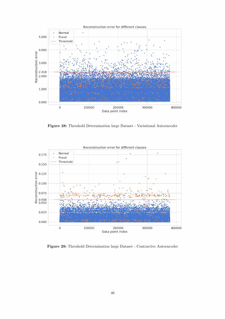
Figure 28: Threshold Determination large Dataset - Variational Autoencoder

Figure 29: Threshold Determination large Dataset - Contractive Autoencoder

46

Figure 30: Threshold Determination large Dataset - Isolation Forest

Figure 31: Threshold Determination large Dataset - Restricted Boltzmann Machines

47

Figure 32: Threshold Determination large Dataset - Ensemble Modelling

C Plots for Large Dataset and Relatively More Frauds andErrors

C.1 Distributions Fraud vs. non Fraud

Figure 33: Distribution large Dataset - Vanilla Autoencoder

48

Figure 34: Distribution large Dataset - Variational Autoencoder

Figure 35: Distribution large Dataset - Contractive Autoencoder

49

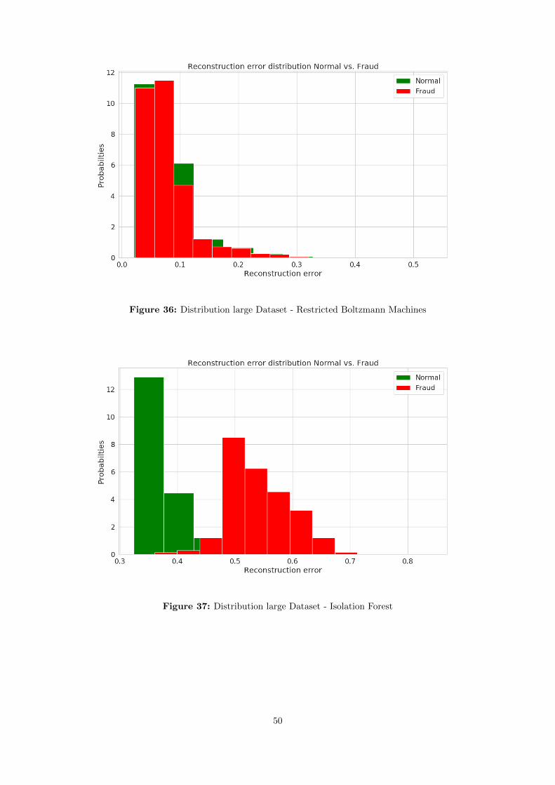
Figure 36: Distribution large Dataset - Restricted Boltzmann Machines

Figure 37: Distribution large Dataset - Isolation Forest

50

Figure 38: Distribution large Dataset - Ensemble

C.2 Visual Threshold

Figure 39: Threshold Determination large Dataset - Vanilla Autoencoder

51

Figure 40: Threshold Determination large Dataset - Variational Autoencoder

Figure 41: Threshold Determination large Dataset - Contractive Autoencoder

52

Figure 42: Threshold Determination large Dataset - Isolation Forest

Figure 43: Threshold Determination large Dataset - Restricted Boltzmann Machines

53

Figure 44: Threshold Determination large Dataset - Ensemble Modelling

54