MASTE R ¶6 T HESIS - Unit
101
Faculty of Science and Technology MASTER’S THESIS Study program: MSc. Petroleum Engineering Specialization: Well Engineering Spring semester, 2016 Open access Writer: Daniel S. Jacobsen ………………………………………… (Writer’s signature) Faculty supervisor: Bernt S. Aadnøy Thesis title: Study of Slug Flow in Undulated Horizontal Wells Credits (ECTS): 30 Key words: Multiphase flow Slug Flow Terrain induced slugging Mitigation techniques Experimental investigation Pages: 92 + Enclosure: 9 Stavanger, 15 th June, 2016
Transcript of MASTE R ¶6 T HESIS - Unit

Faculty of Science and Technology
MASTER’S THESIS
Study program:
MSc. Petroleum Engineering
Specialization:
Well Engineering
Spring semester, 2016
Open access
Writer:
Daniel S. Jacobsen
…………………………………………
(Writer’s signature)
Faculty supervisor:
Bernt S. Aadnøy
Thesis title:
Study of Slug Flow in Undulated Horizontal Wells
Credits (ECTS): 30
Key words:
Multiphase flow
Slug Flow
Terrain induced slugging
Mitigation techniques
Experimental investigation
Pages: 92
+ Enclosure: 9
Stavanger, 15th June, 2016


Study of Slug Flow in
Undulated Horizontal Wells
Daniel S. Jacobsen
Department of Petroleum Engineering
University of Stavanger
Thesis submitted for the degree of
Master of Science
June 2016


Acknowledgements
I would like to express my sincere appreciation to my supervisor, Professor Bernt S.
Aadnøy, for his invaluable guidance and encouragement throughout the work of this
thesis.
I would also like to give my thanks to Mehmed Nazecic for his work in the laboratory,
discussions, input and introducing me to AutoCAD.
I would also like to give my thanks to Mesfin A. Belayneh for discussing topics in this
thesis and sharing his ideas.
Lastly, I would like to thank my family for support and encouragement during my studies
at the University of Stavanger.


Abstract
Terrain induced slugging have become more common as the petroleum
industry matures. Late-life fields, deepwater fields and marginal subsea
tiebacks to existing facilities are prone to terrain induced slugging. Extended
reach wellbore, including snake wells, fish-hook wells and undulated wells are
relative new technologies used to drain otherwise not economically feasible
hydrocarbon zones. These well trajectories are, however, prone to terrain
induced slugging since they can resemble a pipeline-riser system containing
low spots over large distances to accumulate large liquid slugs. Conventional
methods of handling slug flow includes choking, gas injection at the riser
base or installation of a slug catcher. These methods have drawbacks of
reducing production rates, requiring large amounts of gas or high cost. Lately,
automatic slug control based on feedback control systems can suppress the
slugs, but becomes unstable when operating conditions change.
This study attempts to assess the potential of a rotating device to mechan-
ically break down liquid slugs in the gas-liquid interface and/or influence
multiphase flow in any significant and beneficial way. Experiments were
performed by placing the device in vertical, inclined and horizontal sections.
It was seen that the device in some cases influenced the slug flow behaviour,
especially in horizontal flow direction. The frequency increased while the av-
erage slug length decreased significantly over a short distance. It was further
seen that the impact in vertical direction and bend sections were insignificant
for the test conditions in this study.


Table of contents
List of figures xi
List of tables xiii
Nomenclature xv
1 Introduction 1
1.1 Background . . . . . . . . . . . . . . . . . . . . . . . . . . . . . . . . . . . . . . . . . . . . . 1
1.2 Problem formulation . . . . . . . . . . . . . . . . . . . . . . . . . . . . . . . . . . . . . . 1
1.3 Scope and objectives . . . . . . . . . . . . . . . . . . . . . . . . . . . . . . . . . . . . . . . 2
1.4 Outline . . . . . . . . . . . . . . . . . . . . . . . . . . . . . . . . . . . . . . . . . . . . . . . . . 2
2 Multiphase Flow 5
2.1 Concepts of multiphase flow . . . . . . . . . . . . . . . . . . . . . . . . . . . . . . . . . 6
2.1.1 Velocity . . . . . . . . . . . . . . . . . . . . . . . . . . . . . . . . . . . . . . . . . . . 6
2.1.2 Fluid fractions . . . . . . . . . . . . . . . . . . . . . . . . . . . . . . . . . . . . . . 7
2.1.3 Pressure gradients . . . . . . . . . . . . . . . . . . . . . . . . . . . . . . . . . . . 7
2.2 Flow regimes . . . . . . . . . . . . . . . . . . . . . . . . . . . . . . . . . . . . . . . . . . . . 8
2.2.1 Vertical Flow . . . . . . . . . . . . . . . . . . . . . . . . . . . . . . . . . . . . . . . 9
2.2.2 Horizontal Flow . . . . . . . . . . . . . . . . . . . . . . . . . . . . . . . . . . . . . 10
2.3 Flow Regime maps . . . . . . . . . . . . . . . . . . . . . . . . . . . . . . . . . . . . . . . . 11
2.3.1 Baker horizontal flow regime map . . . . . . . . . . . . . . . . . . . . . . . . 12
2.3.2 Mandhane horizontal flow regime map . . . . . . . . . . . . . . . . . . . . 13
2.3.3 Taitel and Dukler horizontal flow regime map . . . . . . . . . . . . . . . 14
2.3.4 Taitel, Bornea and Dukler vertical flow regime map . . . . . . . . . . . 15
3 Slug Flow 17
3.1 Slug flow related problems . . . . . . . . . . . . . . . . . . . . . . . . . . . . . . . . . . 17
viii Table of contents
3.2 Hydrodynamic slugging . . . . . . . . . . . . . . . . . . . . . . . . . . . . . . . . . . . . 18
3.2.1 Slug unit cell . . . . . . . . . . . . . . . . . . . . . . . . . . . . . . . . . . . . . . . 18
3.2.2 Pressure drop . . . . . . . . . . . . . . . . . . . . . . . . . . . . . . . . . . . . . . . 19
3.2.3 Slug frequency . . . . . . . . . . . . . . . . . . . . . . . . . . . . . . . . . . . . . . 20
3.3 Operational induced slugs . . . . . . . . . . . . . . . . . . . . . . . . . . . . . . . . . . . 22
3.4 Terrain induced slugging . . . . . . . . . . . . . . . . . . . . . . . . . . . . . . . . . . . . 22
3.4.1 Slugging in the well . . . . . . . . . . . . . . . . . . . . . . . . . . . . . . . . . . 23
3.4.2 Severe slugging . . . . . . . . . . . . . . . . . . . . . . . . . . . . . . . . . . . . . 25
3.4.3 Severe slug criteria . . . . . . . . . . . . . . . . . . . . . . . . . . . . . . . . . . . 26
3.5 Mitigation techniques . . . . . . . . . . . . . . . . . . . . . . . . . . . . . . . . . . . . . . 30
3.5.1 Slug catcher . . . . . . . . . . . . . . . . . . . . . . . . . . . . . . . . . . . . . . . . 31
3.5.2 Topside choking . . . . . . . . . . . . . . . . . . . . . . . . . . . . . . . . . . . . . 31
3.5.3 Gas injection at riser base . . . . . . . . . . . . . . . . . . . . . . . . . . . . . . 32
3.5.4 Combination of topside choking and gas injection . . . . . . . . . . . . 32
3.5.5 Controllers . . . . . . . . . . . . . . . . . . . . . . . . . . . . . . . . . . . . . . . . . 33
3.5.6 Subsea processing . . . . . . . . . . . . . . . . . . . . . . . . . . . . . . . . . . . 33
3.6 Case reviews . . . . . . . . . . . . . . . . . . . . . . . . . . . . . . . . . . . . . . . . . . . . . 34
3.6.1 Yme, marginal field with subsea tieback . . . . . . . . . . . . . . . . . . . 34
3.6.2 Åsgard Q, subsea tieback . . . . . . . . . . . . . . . . . . . . . . . . . . . . . . 36
4 Experimental Work 37
4.1 Introduction . . . . . . . . . . . . . . . . . . . . . . . . . . . . . . . . . . . . . . . . . . . . . 37
4.2 Experimental setup . . . . . . . . . . . . . . . . . . . . . . . . . . . . . . . . . . . . . . . . 37
4.2.1 Configuration 1 . . . . . . . . . . . . . . . . . . . . . . . . . . . . . . . . . . . . . 37
4.2.2 Configuration 2 . . . . . . . . . . . . . . . . . . . . . . . . . . . . . . . . . . . . . 39
4.2.3 Configuration 3 . . . . . . . . . . . . . . . . . . . . . . . . . . . . . . . . . . . . . 41
4.3 Equipment . . . . . . . . . . . . . . . . . . . . . . . . . . . . . . . . . . . . . . . . . . . . . . 42
4.3.1 Turbine . . . . . . . . . . . . . . . . . . . . . . . . . . . . . . . . . . . . . . . . . . . 42
4.3.2 Pipes . . . . . . . . . . . . . . . . . . . . . . . . . . . . . . . . . . . . . . . . . . . . . 44
4.4 Test conditions . . . . . . . . . . . . . . . . . . . . . . . . . . . . . . . . . . . . . . . . . . . 45
4.4.1 Liquid flow rate and superficial velocity . . . . . . . . . . . . . . . . . . . 45
4.4.2 Gas flow rate . . . . . . . . . . . . . . . . . . . . . . . . . . . . . . . . . . . . . . . 45
4.4.3 Flow regimes . . . . . . . . . . . . . . . . . . . . . . . . . . . . . . . . . . . . . . . 46
4.5 Testing procedure . . . . . . . . . . . . . . . . . . . . . . . . . . . . . . . . . . . . . . . . . 46

Table of contents ix
5 Results 47
5.1 Experiment 1 . . . . . . . . . . . . . . . . . . . . . . . . . . . . . . . . . . . . . . . . . . . . 48
5.2 Experiment 2 . . . . . . . . . . . . . . . . . . . . . . . . . . . . . . . . . . . . . . . . . . . . 49
5.3 Experiment 3 . . . . . . . . . . . . . . . . . . . . . . . . . . . . . . . . . . . . . . . . . . . . 51
5.4 Experiment 4 . . . . . . . . . . . . . . . . . . . . . . . . . . . . . . . . . . . . . . . . . . . . 52
5.5 Experiment 5 . . . . . . . . . . . . . . . . . . . . . . . . . . . . . . . . . . . . . . . . . . . . 53
5.6 Experiment 6 . . . . . . . . . . . . . . . . . . . . . . . . . . . . . . . . . . . . . . . . . . . . 56
5.7 Summary . . . . . . . . . . . . . . . . . . . . . . . . . . . . . . . . . . . . . . . . . . . . . . . 62
6 Discussion 65
7 Conclusion 69
7.1 Concluding remarks . . . . . . . . . . . . . . . . . . . . . . . . . . . . . . . . . . . . . . . 69
7.2 Future work . . . . . . . . . . . . . . . . . . . . . . . . . . . . . . . . . . . . . . . . . . . . . 70
References 71
Appendix A Experiments 75
A.1 Experiment 1 . . . . . . . . . . . . . . . . . . . . . . . . . . . . . . . . . . . . . . . . . . . . 75
A.2 Experiment 2 . . . . . . . . . . . . . . . . . . . . . . . . . . . . . . . . . . . . . . . . . . . . 76
A.3 Experiment 3 . . . . . . . . . . . . . . . . . . . . . . . . . . . . . . . . . . . . . . . . . . . . 77
A.4 Experiment 4 . . . . . . . . . . . . . . . . . . . . . . . . . . . . . . . . . . . . . . . . . . . . 78
A.5 Experiment 5 . . . . . . . . . . . . . . . . . . . . . . . . . . . . . . . . . . . . . . . . . . . . 79
A.6 Experiment 6 . . . . . . . . . . . . . . . . . . . . . . . . . . . . . . . . . . . . . . . . . . . . 80

List of figures
2.1 Typical phase diagram for hydrocarbons . . . . . . . . . . . . . . . . . . . . . . . . 5
2.2 Flow regimes in upward flow direction in a vertical pipe . . . . . . . . . . . . . 9
2.3 Flow regimes in horizontal pipe flow . . . . . . . . . . . . . . . . . . . . . . . . . . . 10
2.4 Baker flow regime map . . . . . . . . . . . . . . . . . . . . . . . . . . . . . . . . . . . . . 12
2.5 Mandhane flow regime map . . . . . . . . . . . . . . . . . . . . . . . . . . . . . . . . . 13
2.6 Taitel and Dukler horizontal flow regime map . . . . . . . . . . . . . . . . . . . . 15
2.7 Bornea, Taitel and Dukler vertical flow regime map . . . . . . . . . . . . . . . . 16
3.1 Formation of hydrodynamic slug . . . . . . . . . . . . . . . . . . . . . . . . . . . . . . 18
3.2 Slug unit cell for horizontal flow . . . . . . . . . . . . . . . . . . . . . . . . . . . . . . 19
3.3 Pressure drop in slug flow . . . . . . . . . . . . . . . . . . . . . . . . . . . . . . . . . . . 19
3.4 Slug frequency models . . . . . . . . . . . . . . . . . . . . . . . . . . . . . . . . . . . . . 21
3.5 Variations of pressure and flow rates in terrain induced slug cycle . . . . . . 23
3.6 Fish-hook well geometry and application . . . . . . . . . . . . . . . . . . . . . . . . 23
3.7 Slugging from undulations . . . . . . . . . . . . . . . . . . . . . . . . . . . . . . . . . . 24
3.8 Riser configurations . . . . . . . . . . . . . . . . . . . . . . . . . . . . . . . . . . . . . . . 25
3.9 Severe slugging in a riser . . . . . . . . . . . . . . . . . . . . . . . . . . . . . . . . . . . . 27
3.10 Choking effect on severe slugging . . . . . . . . . . . . . . . . . . . . . . . . . . . . . 30
3.11 Pressure drop in riser . . . . . . . . . . . . . . . . . . . . . . . . . . . . . . . . . . . . . . 32
3.12 Subsea processing . . . . . . . . . . . . . . . . . . . . . . . . . . . . . . . . . . . . . . . . 34
3.13 Yme B pipeline topography . . . . . . . . . . . . . . . . . . . . . . . . . . . . . . . . . . 35
3.14 Gas lift rate on slug length . . . . . . . . . . . . . . . . . . . . . . . . . . . . . . . . . . . 35
4.1 Flow loop 1 . . . . . . . . . . . . . . . . . . . . . . . . . . . . . . . . . . . . . . . . . . . . . . 38
4.2 Picture of flow loop 1 . . . . . . . . . . . . . . . . . . . . . . . . . . . . . . . . . . . . . . 38
4.3 Flow loop 2 . . . . . . . . . . . . . . . . . . . . . . . . . . . . . . . . . . . . . . . . . . . . . . 39
4.4 Picture of flow loop 3 . . . . . . . . . . . . . . . . . . . . . . . . . . . . . . . . . . . . . . 39

xii List of figures
4.5 Illustration of bend section flow in configuration 2 . . . . . . . . . . . . . . . . . 40
4.6 Flow in bend sections of configuration 2 . . . . . . . . . . . . . . . . . . . . . . . . 40
4.7 Flow loop 3 . . . . . . . . . . . . . . . . . . . . . . . . . . . . . . . . . . . . . . . . . . . . . . 41
4.8 Picture of flow loop 3 . . . . . . . . . . . . . . . . . . . . . . . . . . . . . . . . . . . . . . 41
4.9 Picture of the turbine . . . . . . . . . . . . . . . . . . . . . . . . . . . . . . . . . . . . . . 42
4.10 Propeller design . . . . . . . . . . . . . . . . . . . . . . . . . . . . . . . . . . . . . . . . . . 42
4.11 Bearings . . . . . . . . . . . . . . . . . . . . . . . . . . . . . . . . . . . . . . . . . . . . . . . . 43
4.12 Mixing part of the turbine . . . . . . . . . . . . . . . . . . . . . . . . . . . . . . . . . . . 43
4.13 Area occupied by turbine . . . . . . . . . . . . . . . . . . . . . . . . . . . . . . . . . . . 44
4.14 Pipes used in the experiments . . . . . . . . . . . . . . . . . . . . . . . . . . . . . . . . 44
4.15 Pipe connections . . . . . . . . . . . . . . . . . . . . . . . . . . . . . . . . . . . . . . . . . 45
4.16 High gas flow rate at the inlet . . . . . . . . . . . . . . . . . . . . . . . . . . . . . . . . . 46
5.1 Size distributions, turbine 120 cm from inlet . . . . . . . . . . . . . . . . . . . . . 48
5.2 Size distributions, turbine 195 cm from inlet . . . . . . . . . . . . . . . . . . . . . 49
5.3 Slug length, comparison between 120 cm and 195 cm from inlet . . . . . . . 50
5.4 Slug length over bend section . . . . . . . . . . . . . . . . . . . . . . . . . . . . . . . . 51
5.5 Slug length over two bend sections . . . . . . . . . . . . . . . . . . . . . . . . . . . . 52
5.6 Comparison with and without turbine in bend section . . . . . . . . . . . . . . 53
5.7 Slug lengths with turbine in vertical flow direction . . . . . . . . . . . . . . . . . 54
5.8 Breakdown of small gas bubble in vertical flow direction . . . . . . . . . . . . . 54
5.9 Slug flow over turbine in vertical flow direction . . . . . . . . . . . . . . . . . . . 55
5.10 Slug lengths without the turbine . . . . . . . . . . . . . . . . . . . . . . . . . . . . . . 56
5.11 Impact of turbine on slug sizes . . . . . . . . . . . . . . . . . . . . . . . . . . . . . . . 57
5.12 All graphs from experiment 6 . . . . . . . . . . . . . . . . . . . . . . . . . . . . . . . . 58
5.13 Comparing average values from experiment 6 . . . . . . . . . . . . . . . . . . . . 58
5.14 Effect of placement of turbine . . . . . . . . . . . . . . . . . . . . . . . . . . . . . . . . 59
5.15 Formation of slug over turbine in horizontal direction . . . . . . . . . . . . . . 60
5.16 Slug flow over turbine in horizontal flow direction . . . . . . . . . . . . . . . . . 61

List of tables
3.1 Pressure and variations in the production system at Åsgard . . . . . . . . . . 36
3.2 Terrain induced slugging from Åsgard Q . . . . . . . . . . . . . . . . . . . . . . . . . 36
5.1 Test results summarized from all experiments . . . . . . . . . . . . . . . . . . . . 63
A.1 Results with turbine 120 cm from inlet . . . . . . . . . . . . . . . . . . . . . . . . . . 75
A.2 Results with turbine 195 cm from inlet . . . . . . . . . . . . . . . . . . . . . . . . . . 76
A.3 Results with turbine in bend section . . . . . . . . . . . . . . . . . . . . . . . . . . . 77
A.4 Results with turbine in two bend sections . . . . . . . . . . . . . . . . . . . . . . . 78
A.5 Results with turbine in vertical section . . . . . . . . . . . . . . . . . . . . . . . . . . 79
A.6 Results without turbine and turbine 80 cm from inlet . . . . . . . . . . . . . . . 80
A.7 Results with turbine 100 cm and 120 cm from inlet . . . . . . . . . . . . . . . . . 81
A.8 Results with turbine 140 cm and 160 cm from inlet . . . . . . . . . . . . . . . . . 82
A.9 Results with turbine 200 cm from inlet and without turbine . . . . . . . . . . 83


Nomenclature
Symbols
α Phase fraction
β Inclination
µ Viscosity
σ Surface tension
C Choke coefficient
D Pipe diameter
F Force
fs Slug Frequency
g Gravitational acceleration
h Height
L Length
P Pressure
t Time
u Flow velocity
w Mass flow rate
α′
Gas holdup in gas cap
m Mass velocity
ρ Density
fL Liquid friction factor
K Proportionality constant
Re Reynolds number
S Perimeter over which stress acts
s Jeffreys’ sheltering coefficient
v Kinematic viscosity
Subscripts
f Film
G Gas
i Any phase within flow system, also
interface
L Liquid
m Mixture
P Pipeline
s Slug
t Total
u unit
B Back
E Entrance
sep Separator
SG Superficial gas
SL Superficial liquid
Abbreviations
PI Proportional and integral
PID Proportional, integral and derivative
PIG Pipeline inspection gauge
PT Pressure and temperature
RPM Rounds per minute

Chapter 1
Introduction
1.1 Background
Slug flow is considered a major flow assurance challenge characterized by alternation
of liquid and gas flow. Large variations in flow rates and pressure is a concern for
the reservoir integrity alongside corrosion, damage to pipelines and flooding of first
stage separator. Terrain induced slugs can originate from complex well geometries,
pipeline topography and low spots in flexible risers. In addition, slugs are created from
hydrodynamic instability caused by flowing conditions. Terrain induced slugging have
become more common as the petroleum industry matures. Late-life fields, deepwater
fields and marginal subsea tiebacks to existing facilities are prone to terrain induced
slugging. Extended reach wellbore, including snake wells, fish-hook wells and undulated
wells are relative new technologies used to drain otherwise non-profitable reservoirs.
These well trajectories are, however, prone to terrain induced slugging since they can
resemble a pipeline-riser system containing low spots over large distances to accumulate
large liquid slugs.
1.2 Problem formulation
Controller systems used to suppress slugs rely heavily on correct field data and models
to function properly and suppress the slugs. After some time the operating conditions
change and the control system becomes unstable. The operators, instead of tuning
the controller system, often change to the manual choke when the controller becomes
unstable (Jahanshahi, 2013). Other ways of mitigating effects of slugging are slug catch-

2 Introduction
ers, topside choking, gas injection at the riser base and subsea processing. Individual
drawbacks of these mitigation techniques are discussed in Section 3.5. In this thesis,
the potential of a device to mechanically break down or alter the slug flow behaviour is
tested in six experiments.
1.3 Scope and objectives
Scope of this thesis is study of multiphase flow, slug flow and experimental investigation
of a rotating device to mechanically break down slugs and/or alter the slug behaviour in
any way.
Objectives for this thesis are;
• Review literature to get fundamental understanding of multiphase flow and slug
flow in particular.
• Study flow in small scale flow loop and identify flow conditions for slug flow.
• Assess impact from device on slug flow behaviour in experiments.
– Bend, vertical and horizontal sections
– Identify optimal placements
1.4 Outline
• Chapter 2 reviews literature of multiphase flow focusing on concepts used in
multiphase flow, flow regimes encountered in horizontal and vertical flow direction
and flow regime maps for horizontal and vertical flow.
• Chapter 3 reviews slug flow focusing on why slug flow is encountered in various
industrial applications, models describing slug flow and special emphasis on
terrain induced slugging, considered to be largest slugs encountered. Several
mitigation techniques are discussed as well as two cases from the North Sea are
reviewed.
• Chapter 4 summarizes the experimental work. Three flow loops were used to
evaluate the use of a turbine in horizontal section, inclined section and vertical
section.
• Chapter 5 Summarizes the results from the experimental study.

1.4 Outline 3
• Chapter 6 discusses the experimental results.
• Chapter 7 concludes the work of the experimental study and suggests future work.

Chapter 2
Multiphase Flow
Multiphase flow is simultaneous flow of materials in different phases, either as gas, liquid
or solid with presence of minimum two phases. For petroleum production, presence
of oil and gas at the same time is a common multiphase flow system. This is the case
when gas-lift is used in oil wells or when the conditions are such that the produced
hydrocarbons are gas and liquid.
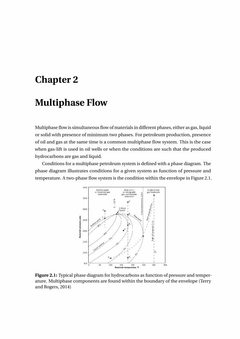
Conditions for a multiphase petroleum system is defined with a phase diagram. The
phase diagram illustrates conditions for a given system as function of pressure and
temperature. A two-phase flow system is the condition within the envelope in Figure 2.1.
Figure 2.1: Typical phase diagram for hydrocarbons as function of pressure and temper-ature. Multiphase components are found within the boundary of the envelope (Terryand Rogers, 2014)

6 Multiphase Flow
As the pressure decreases while transporting hydrocarbons from reservoir to surface,
single-phase systems can become two-phase flow system as the pressure depletes below
the bubble or dew point. This is the case when pressure depletes in an oil reservoir,
when pressure and temperature depletes in a wet gas reservoir or when pressure de-
pletes in gas-condensate reservoirs. Gas can be dry in the reservoir with high pressure
and temperature conditions, but saturated with oil or water in gas phase. When the
gas is transported, the temperature and pressure decrease and saturated oil or water
condensates. Reservoir pressure depletes over time resulting in multiphase flow systems
at new reservoir conditions that initially were single-phase flow systems.
2.1 Concepts of multiphase flow
2.1.1 Velocity
The phase velocity expresses the real velocity of each phase in the flow system. Determi-
nation of the phase velocity requires knowledge of area occupied by the specific phase,
which can change throughout the system. The expression for the phase velocity is:
ui =Qi
Ai(2.1)
As determination of the phase velocity requires detailed information about the flow
at a specific point, the superficial velocity is introduced as it only requires knowledge
about the pipe size and the volumetric flow rate of the phase. This makes the superficial
velocity recommended for multiphase flow. The superficial velocity is expressed as:
us i =Qi
A=αi ui (2.2)
The mixture velocity is the average flow velocity and can be expressed with the superficial
velocities in the following way:
um =∑
N
uN s i (2.3)

2.1 Concepts of multiphase flow 7
2.1.2 Fluid fractions
Void fraction
Void fraction is the fraction occupied by gas in the flow system defined geometrically ei-
ther by relative length, cross-sectional area or volume. The common method to quantify
the void fraction is with the cross-sectional void fraction (Thome, 2004) expressed as:
αG =AG
A(2.4)
Liquid holdup
Liquid holdup is the fraction occupied by liquid in the flow system. The heavier liquid
usually flows at a lower speed than the lighter gas and is for that reason more held up,
hence liquid holdup. The liquid holdup is expressed as:
αL =AL
A(2.5)
The void fraction and liquid holdup are linked by the fundamental relation in air-water
flow:
αL +αG =1 (2.6)
The fractions changes along the flow due to geometrical configurations, flow regime,
pipe size and fluid properties.
2.1.3 Pressure gradients
The homogeneous flow model (Thome, 2004) states that the total pressure drop gradient
in multiphase flow is expressed as:
d p
d x=�
d p
d x
�
f+�
d p
d x
�
h+�
d p
d x
�
a(2.7)
This means that the total pressure drop is caused by friction, head loss and acceleration.
The friction term is expressed by (Thome, 2004):
�
d p
d x
�
f=
2
DC (Rem )
−nρm u 2m (2.8)

8 Multiphase Flow
Where C and n are dependent of the Reynolds number in the following way (Filip et al.,
2014):
Re=
<2000, C =16 n =1
2000≤Re≤20 000, C =0.079 n =0.25
≥20000, C =0.046 n =0.2
The mixture density is expressed as:
ρm =ρLαL +(1−αL )ρG (2.9)
Further, the hydrostatic head is expressed as (Thome, 2004):
�
d p
d x
�
h=ρm g sinβ (2.10)
The inclination β is given with respect to horizontal. Furthermore, the acceleration term
is expressed as (Thome, 2004):
�
d p
d x
�
a=
d (mt /ρm )d x
(2.11)
The model is a generalisation of a single phase flow model to a multiphase flow model
by assuming completely homogeneous flow. Other correlations have been found for
flow regimes where homogeneous flow is not the case.
2.2 Flow regimes
Interaction between phases in multiphase flow results in various flow patterns with
different characteristics. Flow regimes are these patterns of flow and vary depending
on operating conditions, such as flow rates, fluid properties, geometry of pipe and
pressure differentials. Prediction of flow regime can be difficult and several methods are
used including analytical, empirical and numerical solutions (Li, 2007). As the physical
models behind flow transitions are not completely understood, predictions include high
uncertainty. Transition between flow regimes have no sharp boundaries but instead
changes smoothly between the regimes (Corneliussen et al., 2005).
2.2 Flow regimes 9
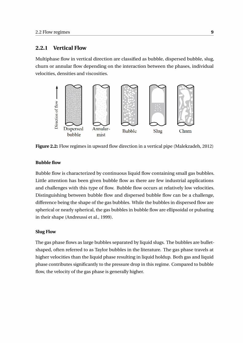
2.2.1 Vertical Flow
Multiphase flow in vertical direction are classified as bubble, dispersed bubble, slug,
churn or annular flow depending on the interaction between the phases, individual
velocities, densities and viscosities.
Figure 2.2: Flow regimes in upward flow direction in a vertical pipe (Malekzadeh, 2012)
Bubble flow
Bubble flow is characterized by continuous liquid flow containing small gas bubbles.
Little attention has been given bubble flow as there are few industrial applications
and challenges with this type of flow. Bubble flow occurs at relatively low velocities.
Distinguishing between bubble flow and dispersed bubble flow can be a challenge,
difference being the shape of the gas bubbles. While the bubbles in dispersed flow are
spherical or nearly spherical, the gas bubbles in bubble flow are ellipsoidal or pulsating
in their shape (Andreussi et al., 1999).
Slug Flow
The gas phase flows as large bubbles separated by liquid slugs. The bubbles are bullet-
shaped, often referred to as Taylor bubbles in the literature. The gas phase travels at
higher velocities than the liquid phase resulting in liquid holdup. Both gas and liquid
phase contributes significantly to the pressure drop in this regime. Compared to bubble
flow, the velocity of the gas phase is generally higher.

10 Multiphase Flow
Churn Flow
Churn flow is considered to be the result of transition between slug and annular flow.
The liquid slugs between the gas bubbles can be discontinuous or disappear, while the
gas phase becomes continuous. The pressure drop becomes more dependent on the gas
phase, rather than the liquid phase (Bai and Bai, 2012). Compared to slug flow, churn is
more chaotic and disordered as well as gas phase velocity is increased.
Annular-mist flow
Annular flow is characterized by the gas phase flowing in the middle of the pipe with
small droplets of liquid in the stream. The rest of the liquid flows at the pipe wall as
a liquid film. This flow regime is desired because of the flow stability. Mist flow is the
regime encountered when the gas velocity becomes very high. The liquid film is thinned
by the shear of the gas, until eventually all the liquid is entrained as droplets in the
continuous gas phase (Thome, 2004).
2.2.2 Horizontal Flow
Opposed to vertical flow, multiphase flow in the horizontal direction are classified as
either dispersed bubble, annular, stratified, slug and elongated bubble flow as illustrated
in Figure 2.3.
Figure 2.3: Flow regimes in horizontal pipe flow (Malekzadeh, 2012)
2.3 Flow Regime maps 11
Dispersed bubble flow
Dispersed bubble flow is characterized by small dispersed gas bubbles moving along the
flow in otherwise continuous flow of liquid. The size of the dispersed bubbles subside
with increasing velocity of the continuous liquid phase (Bai and Bai, 2012).
Stratified flow
The gas and liquid phase in stratified flow are separated with an interface between
the phases. Smooth stratified flow is characterized with a smooth interface, whereas
stratified wavy flow is characterized by waves moving in the flow direction. Waves arise
as the result of greater gas velocity creating instabilities in the interface.
Slug flow
Slug flow in horizontal direction is characterized by bullet-shaped gas bubbles travelling
along the flow direction separated by liquid slugs. Gas bubbles travel at the top of the
pipe due to low density of the gas bubbles.
Elongated bubble flow
Elongated bubble flow contain small dispersed gas bubbles moving through a continuous
liquid phase. The flow pattern is similar to the flow pattern of slug flow, but the size of
the bubbles are generally smaller with lower velocity. Elongated bubbles are formed
when smaller bubbles coalesce, often referred to as plug flow in the literature.
Annular flow
Similar to annular flow in vertical direction, the gas phase moves along the flow direction
in the centre of the pipe with some liquid entrained as small droplets. The rest of the
liquid flows along the pipe wall as a liquid film.
2.3 Flow Regime maps
Flow regime maps are used to predict flow regime for a multiphase flow system. The
maps are often based on experimental results in laboratory resulting in poor agreement
or high uncertainty when used for other system configurations. The map by Baker (Baker,
1953) was used for designing pipelines, while the data was gathered from experiments

12 Multiphase Flow
in laboratories. This made for high uncertainty when used. Later developments used
data from flow data banks to develop flow regime maps, although the data sets were in
most cases results of visual observations.
2.3.1 Baker horizontal flow regime map
The flow regime map proposed by Baker (Baker, 1953) was based on correction factors
and utilizing the available data at the time. The correction factors were necessary as
most of the available data at the time was for air-water flow at atmospheric conditions
and the flow regime map was used for designing pipelines containing oil and gas flow.
Bakers fluid property correction factors were written as:
λ=��
ρG
ρa i r
��
ρL
ρw a t e r
��1/2
(2.12)
and
ψ=�σw a t e r
σ
�
�
�
µL
µw a t e r
��
ρw a t e r
ρL
�2�1/3
(2.13)
Bakers work resulted in the following flow regime map for horizontal flow:
Figure 2.4: Baker flow regime map (Baker, 1953)
It is important to know that the transitional zones were rather broad and the map suffered
from not having a basis in mechanisms causing transitions as the map was made from
observations by Baker.

2.3 Flow Regime maps 13
2.3.2 Mandhane horizontal flow regime map
Mandhane et al.(Mandhane et al., 1974) tested several proposed models against flow pat-
tern observations gathered from the UC multiphase Pipe Flow Data Bank. Observations
in the data bank were results of visual inspections and the observers own interpretation
of the flow, possibly resulting in some error. After comparison with experimental data,
they proposed their own flow pattern map which represented an extension of the work
by Govier and Aziz (Aziz and Govier, 1972) in better agreement with experimental data.
The proposed flow pattern map was based on air-water flow data following attempts
to apply physical properties for correction purposes. Their approach was new, but with
the extensive amount of data available, it was possible. The base for the diagram is a
log-log plot with the superficial phase velocities as coordinate axes, thereby avoiding
complex parameters in the map.
Figure 2.5: Mandhane flow regime map (Mandhane et al., 1974)
Flow pattern observations were basis for the transitions in the air-water system. The
diagram is an average compromise of the variety of combinations of pipe diameters
and physical properties. The model was better than any of the other models examined
when considering air-water data. The proposed map tends to be more accurate when
the diameter is less than 2 inches because most of the observations in the data bank
were within this range.

14 Multiphase Flow
2.3.3 Taitel and Dukler horizontal flow regime map
The published model by Taitel and Dukler (Taitel and Dukler, 1976) is a combination
of experiment and theory to a model without having to be completely empirical, thus
removing the need for correlations of pure curve fit type. Their model was fairly simplified
with the choice of specific assumptions.
Their approach was to use a theoretical model based on physical concepts to predict
the transitions between flow regimes. The variables influencing transitions were believed
to be gas and liquid mass flow rates, the properties of the fluids, pipe diameter and
the inclination. The considered flow regimes were smooth stratified, wavy stratified,
intermittent(Elongated bubble flow and slug flow), annular and dispersed bubble flow
with emphasizes on transitions between the regimes. Analysis starts from the condition
of stratified flow, followed by determining the mechanism causing transition. Starting
from stratified smooth flow, they found transition to stratified wavy to take place when:
uG ≥
�
4vL
�
ρL −ρG
�
g cosβ
sρG uL
�1/2
(2.14)
Further, they expressed the transition from stratified to intermittent or annular dispersed
as:
uG =�
1−hL
D
�
��
ρL −ρG
�
g cosβAG
ρG Si
�1/2
(2.15)
Distinguishing between transition intermittent flow and annular dispersed flow was
found to be affected by the hL/D -ratio. In the paper it was suggested transition to
intermittent flow when hL/D <0.5, otherwise transition to annular dispersed flow. A
modified criterion of hL/D <0.35 was later suggested to account for gas holdup in the
liquid slug (Barnea et al., 1982). Further, they found transition between intermittent
flow and dispersed bubble flow to happen when:
uL >
�
4AG g cosβ�
ρL −ρG
�
SiρL fL
�1/2
(2.16)
Figure 2.6 illustrates the resulting flow regime map from the study, including a compari-
son with the Mandhane plot from Figure 2.5, indicating good agreement between the
flow regime maps.
2.3 Flow Regime maps 15
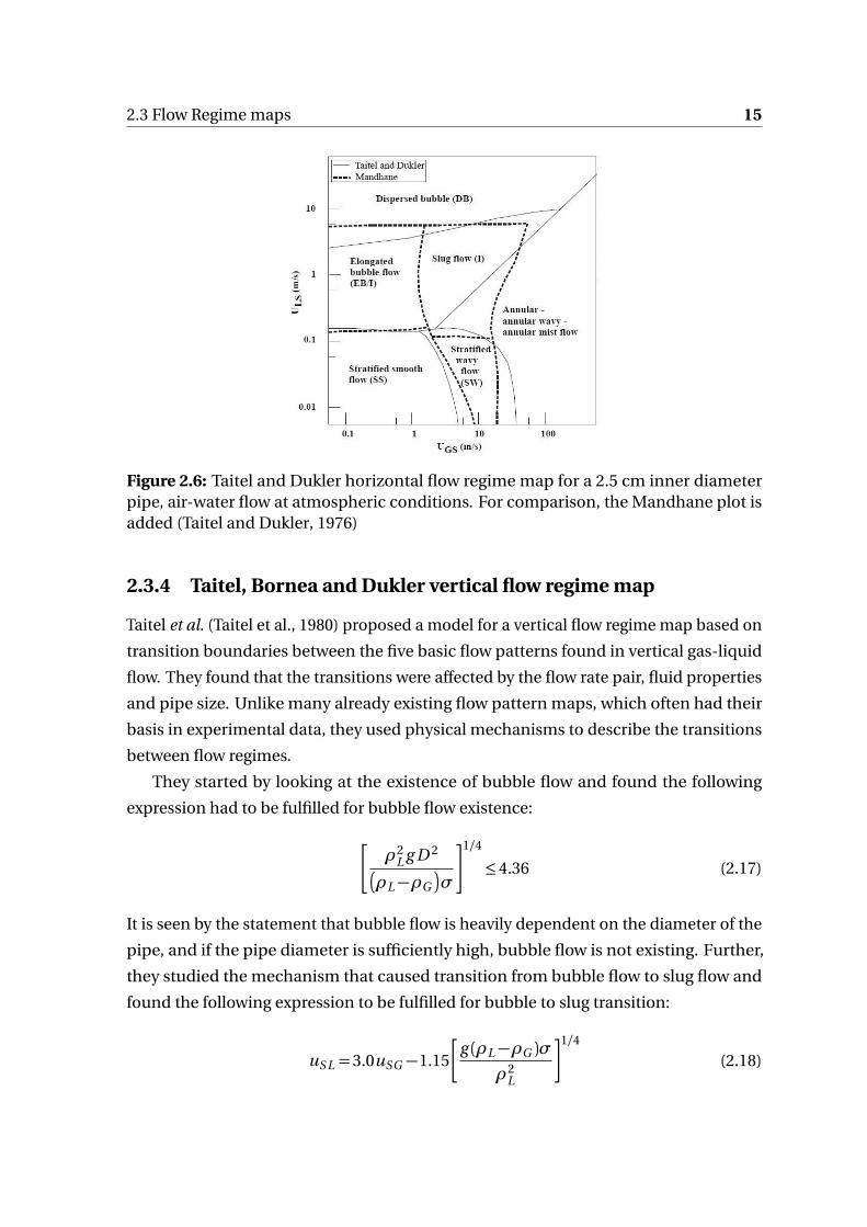
Figure 2.6: Taitel and Dukler horizontal flow regime map for a 2.5 cm inner diameterpipe, air-water flow at atmospheric conditions. For comparison, the Mandhane plot isadded (Taitel and Dukler, 1976)
2.3.4 Taitel, Bornea and Dukler vertical flow regime map
Taitel et al. (Taitel et al., 1980) proposed a model for a vertical flow regime map based on
transition boundaries between the five basic flow patterns found in vertical gas-liquid
flow. They found that the transitions were affected by the flow rate pair, fluid properties
and pipe size. Unlike many already existing flow pattern maps, which often had their
basis in experimental data, they used physical mechanisms to describe the transitions
between flow regimes.
They started by looking at the existence of bubble flow and found the following
expression had to be fulfilled for bubble flow existence:
�
ρ2L g D 2
�
ρL −ρG
�
σ
�1/4
≤4.36 (2.17)
It is seen by the statement that bubble flow is heavily dependent on the diameter of the
pipe, and if the pipe diameter is sufficiently high, bubble flow is not existing. Further,
they studied the mechanism that caused transition from bubble flow to slug flow and
found the following expression to be fulfilled for bubble to slug transition:
uS L =3.0uSG −1.15
�
g (ρL −ρG )σρ2
L
�1/4
(2.18)

16 Multiphase Flow
Further, they found that the transition from bubble flow to dispersed bubble flow was
expressed with the following equation:
uS L +uSG =4.0
�
D 0.492(σ/ρL )0.089
v 0.072L
�
g (ρL −ρG )ρL
�0.446�
(2.19)
Transition from slug flow to churn flow was found to be expressed as:
lE
D=40.6
�
ump
g D+0.22
�
(2.20)
The transition boundary to annular flow was found to be expressed as:
uSGρ1/2G
�
g (ρL −ρG )σ�1/4=3.1 (2.21)
Equation 2.21 shows that annular flow is independent of the liquid flow rate and pipe
diameter. The equations above was used to make the flow regime map illustrated in
Figure 2.7.
Figure 2.7: Bornea, Taitel and Dukler vertical flow regime map for a 5.0 cm inner diameterpipe, air-water flow at atmospheric conditions,σ=10N/cm2 and varying lE /D for Slug-Churn transition (Taitel et al., 1980)

Chapter 3
Slug Flow
Slug flow is a multiphase flow regime characterized by alternating flow of gas and liquid
slugs. Slug flow in the well and pipelines are undesirable because of large fluctuations in
both pressure and flow rates, ultimately leading to decrease in the overall production.
As the behaviour of slug flow is complex in nature, accurate predictions are challenging,
especially as there are several parameters affecting the flow behaviour. Slug flow in wells
and pipelines are common because of hydrodynamic instability, complex well geometry,
topography and flexible riser configurations. As the current mitigation techniques reduce
overall production rates or require additional equipment taking up large spaces, new
mitigation techniques are desired. Developments of deepwater and marginal subsea
tiebacks increase the likelihood of slug flow as the terrain becomes more complex and
the distance to processing facility increases.
3.1 Slug flow related problems
Slug flow is associated with problems at the receiving end in the transport of hydrocar-
bons from the reservoir to processing facility along with damage to pipes and equipment
in the wells. Flooding of the separator at the receiving can happen when model predic-
tions are wrong or slugging potential not properly studied in the design phase resulting
in bigger slugs than the processing equipment can handle. As a consequence, the wells
can get shut in, resulting in no production. Relatively large pressure variations are nor-
mal in slug flow as the flow alternates between gas and liquid. Terrain induced slugs
increases the pressure as the slug grows, but the pressure is quickly reduced when the
slug is produced. Long periods of low production leads to temperature decrease in the
pipelines leading to wax formation and ultimately hydrates (Skofteland et al., 2007).

18 Slug Flow
3.2 Hydrodynamic slugging
Hydrodynamic slugs are generated in horizontal pipelines due to instabilities of the
waves in the gas-liquid interface. The flow must be stratified at certain flowing conditions
for hydrodynamic slugs to occur. The growth of the wave is result of Kelvin-Helmholtz
instability lifting the interface between the gas-liquid phase upwards in the pipe. The
instability condition takes place because of differences in gas and liquid velocities. Fig-
ure 3.1 illustrates the formation of hydrodynamic slugs from an unstable wave growing
to a liquid slug.
Figure 3.1: Formation of hydrodynamic slug (Feesa, 2003)
The Kelvin-Helmholtz instability criterion is mathematically expressed as (Taitel and
Dukler, 1976):
uG >
�
g (ρL −ρG )hG
ρG
�1/2
(3.1)
Equation 3.1 shows that when the gas flow velocity is sufficiently high, waves will grow
and slugs can be formed.
3.2.1 Slug unit cell
The concept of slug unit cell is used to predict slug flow characteristics starting with one
unit cell and then generalize for a pipe section. The slug unit cell is an idealized slug
that has been fully established. The assumption of a fully established slug simplifies
the ls -term as the velocity of the liquid slug will move at a speed close to the mixing
velocity (Dukler and Hubbard, 1975).
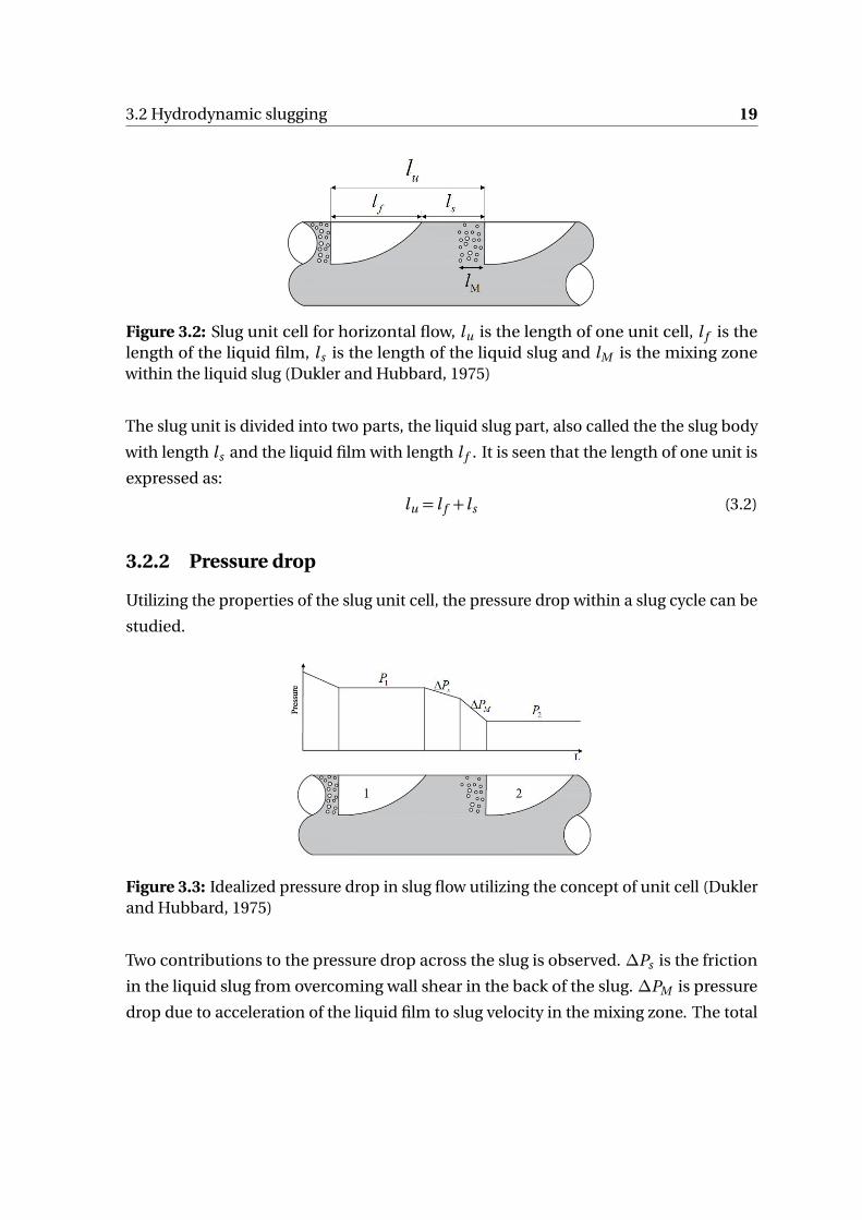
3.2 Hydrodynamic slugging 19
Figure 3.2: Slug unit cell for horizontal flow, lu is the length of one unit cell, l f is thelength of the liquid film, ls is the length of the liquid slug and lM is the mixing zonewithin the liquid slug (Dukler and Hubbard, 1975)
The slug unit is divided into two parts, the liquid slug part, also called the the slug body
with length ls and the liquid film with length l f . It is seen that the length of one unit is
expressed as:
lu = l f + ls (3.2)
3.2.2 Pressure drop
Utilizing the properties of the slug unit cell, the pressure drop within a slug cycle can be
studied.
Figure 3.3: Idealized pressure drop in slug flow utilizing the concept of unit cell (Duklerand Hubbard, 1975)
Two contributions to the pressure drop across the slug is observed. ∆Ps is the friction
in the liquid slug from overcoming wall shear in the back of the slug. ∆PM is pressure
drop due to acceleration of the liquid film to slug velocity in the mixing zone. The total

20 Slug Flow
pressure drop over the slug is expressed as (Dukler and Hubbard, 1975):
∆Pt =∆Ps +∆PM (3.3)
3.2.3 Slug frequency
Knowledge of slug frequency is essential for the design of the processing equipment,
especially separator design (Zabaras et al., 1999). Knowledge of the slug frequency
gives insight to the characteristics of the slug flow, such as slug length, pressure drop
and the velocity. The various models developed are based on empirical correlations or
mechanistic models. Most available empirical correlations are derived from air-water
systems in flow loops with pipe diameter usually smaller than 2 inches. As slug frequency
is influenced by several flow variables, the empirical models lack accuracy over a broad
range of flowing conditions as they usually only accounts for a few variables in the
models. The slug frequency defines the number of slugs passing through a specific point
in the pipe within a period of time.
Gregory and Scott (Gregory and Scott, 1969) conducted measurements of slug fre-
quency in a 3/4" pipe for CO2-water system. Their correlation resulted in the following
equation for slug frequency:
fs =0.0226�
uS L
g D
�
19.75
um+um
��1.2
(3.4)
Heywood and Richardson (Heywood and Richardson, 1979) measured instantaneous
values of liquid holdup for air-water flow in a 1.65" horizontal pipe by utilizing gamma-
ray techniques. Their work resulted in the following correlation:
fs =0.0434
�
uS L
um
�
2.02
D+
u 2m
g D
��1.02
(3.5)
Shell Slug Frequency Correlation (Stapelberg and Mewes, 1994) was derived by curve-
fitting the data of Heywood and Richardson, getting the following relation for the slug
frequency:
fs =0.048�
uS Lpg D
�0.81
+0.73�
uS Lpg D
�2.34�
�
uS Lpg D+ uSGp
g D
�0.1
−1.17�
uS Lpg D
�0.064�2
Ç
Dg
(3.6)
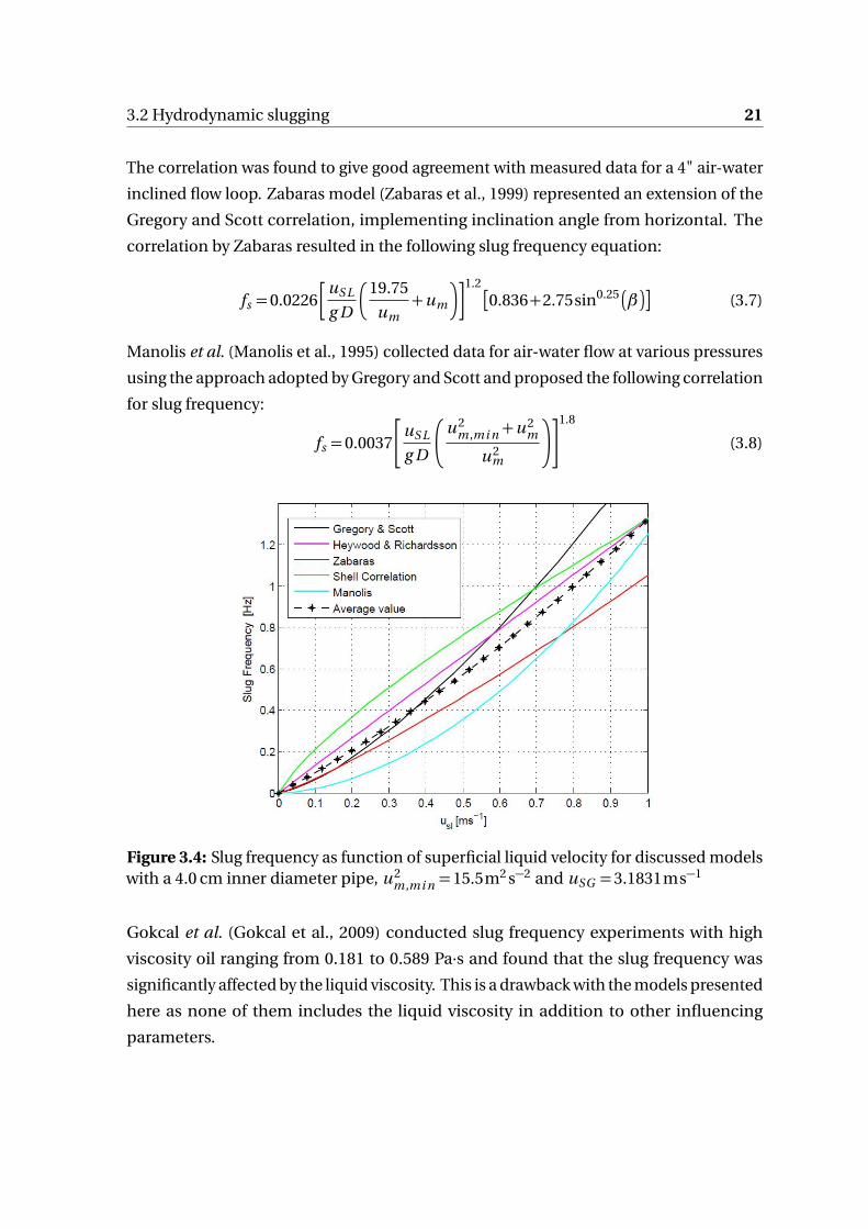
3.2 Hydrodynamic slugging 21
The correlation was found to give good agreement with measured data for a 4" air-water
inclined flow loop. Zabaras model (Zabaras et al., 1999) represented an extension of the
Gregory and Scott correlation, implementing inclination angle from horizontal. The
correlation by Zabaras resulted in the following slug frequency equation:
fs =0.0226�
uS L
g D
�
19.75
um+um
��1.2�
0.836+2.75sin0.25�
�
(3.7)
Manolis et al. (Manolis et al., 1995) collected data for air-water flow at various pressures
using the approach adopted by Gregory and Scott and proposed the following correlation
for slug frequency:
fs =0.0037
�
uS L
g D
�
u 2m ,mi n +u 2
m
u 2m
��1.8
(3.8)
Figure 3.4: Slug frequency as function of superficial liquid velocity for discussed modelswith a 4.0 cm inner diameter pipe, u 2
m ,mi n =15.5m2 s−2 and uSG =3.1831ms−1
Gokcal et al. (Gokcal et al., 2009) conducted slug frequency experiments with high
viscosity oil ranging from 0.181 to 0.589 Pa·s and found that the slug frequency was
significantly affected by the liquid viscosity. This is a drawback with the models presented
here as none of them includes the liquid viscosity in addition to other influencing
parameters.

22 Slug Flow
3.3 Operational induced slugs
Operational induced slugs are created when flow transforms from steady state to tran-
sient state. These slugs occur in Start-up of wells, when the flow rates are changed and
during pigging operations. The slugs develop because the liquid velocity is increased
which accumulates more liquid and the slugs grow.
A PIG is sent through the pipelines to remove debris and wax formation at the inner
wall of the pipeline. The PIG pushes all the liquid in front to the outlet, a process where
a large liquid slug is accumulated in front of the PIG.
3.4 Terrain induced slugging
Terrain induced slugging occurs when the geometry allows for blockage of gas in a low
spot and liquid accumulation. Gas blockage can happen when gas-liquid flow enters a
riser from the pipeline, in fish-hook wells, in complex in snake wells, undulating wells,
due to pipeline topography, in the riser, and in extended reach wells. Terrain induced
slugging is considered most critical in the case where gas-liquid flow enters a vertical
riser, called severe slugging. The size, in terms of diameter, is considerably larger for the
pipelines and riser compared to downhole equipment, thereby making the conditions
for severe slugging to occur. Terrain induced slugging occurs at relatively low gas and
liquid flow rates as the liquid has the tendency to accumulate at a low spot and blocking
free passage for the gas phase (Malekzadeh, 2012). The characteristics of terrain induced
slugs depend on many parameters such as wellbore geometry, pipeline topography,
reservoir fluid properties, pressures, production rate and fluid dynamics.
Terrain induced slugs create large variations in both pressure and flow rates. Fig-
ure 3.5 illustrates how the pressure, liquid flow rate and gas flow rate vary over one slug
cycle in a pipeline-riser configuration. It is seen that the pressure increases when the
slug builds in the riser. When the slug reaches the top of the riser, the pressure is stable
until the gas penetrates the riser base and starts flowing into the riser. When the gas
enters the riser, the pressure is quickly reduced and the gas and liquid flow rates within
the riser are quickly reduced. The cycle is complete and a new slug can be formed.

3.4 Terrain induced slugging 23
Figure 3.5: Variations of pressure and flow rates in terrain induced slug cycle
3.4.1 Slugging in the well
New technology give opportunities for more complex well trajectories to exploit the
reservoir section or exploit otherwise non-economical hydrocarbon zone with optimal
placement. With complex geometry, however, can slugging become a problem. In this
section, some complex geometries will be discussed with focus on how the slugs are
created from the geometries or reservoir properties.
Fish-hook well trajectory
Fish-hook wells have well geometry like a fish-hook, drilled downwards followed by an
uphill trajectory. Low spots are created where liquid slugs can accumulate.
Figure 3.6: Application of fish-hook well geometry. First drilled reservoir section locateddeeper than the reservoirs drilled at the end (Malekzadeh, 2012)

24 Slug Flow
Fish-hook wells drain hydrocarbon zones located shallower and a distance away from
the reservoir first drilled through. Marginal hydrocarbon zones can be exploited to
enhance the overall production from a field. Low spots are naturally generated because
the well is drilled upwards and liquid accumulation can take place.
Undulations
Undulations create low spots for slugs to accumulate. When stratified flow is encountered
in the downward flow direction, slug flow can be present in the upward flow direction.
The same effect is seen in pipelines as the topography changes.
Figure 3.7: Slugging due to undulations in the well, flow from left to right (Feesa, 2003)
Undulations are also found in snake wells. These wells are characterized by drainage
from several vertically stacked layers with a well trajectory that is laterally weaving to
reach all the zones (Obendrauf et al., 2006). The benefit is drainage from several zones
with lower costs than multilateral wells. Geosteering utilizes logging tools to navigate
horizontal layers in the reservoir. Optimal placement of the well can result in undulations
with low spots for slug accumulation. Horizontal wells can have undulations caused by
disturbances while drilling the horizontal.
Low producing horizontal wells
Hydraulic fractured horizontal shale oil wells with extremely low permeability and pro-
ductivity index are prone to slugging. Since the drainage radius is limited, the reservoir
pressure will deplete rapidly below the bubble point and multiphase flow is the result.
Fracturing techniques used in horizontal shale wells require liners to be of a certain
size, normally 4 or 6 inches, thereby resulting in low flow velocity within the pipe and
unstable flow (Norris, 2012).
Since the well path is rarely truly horizontal, it is reasonable to assume some small
inclinations from the horizontal in long reservoir sections making low spots for liquid
3.4 Terrain induced slugging 25
accumulation. This was studied by H. Lee Norris (Norris, 2012) by performing simula-
tions on a typical hydraulic fractured shale well with toe-up of +0.5°, creating a low spot
at the heel. The results were periodic liquid production and fluctuations as expected
from terrain induced slug flow. The slugging cycle was found to be long because of low
gas production rate and long horizontal section, thus the pressure build-up by the gas
was slow.
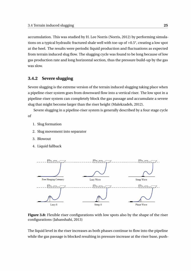
3.4.2 Severe slugging
Severe slugging is the extreme version of the terrain induced slugging taking place when
a pipeline-riser system goes from downward flow into a vertical riser. The low spot in a
pipeline-riser system can completely block the gas passage and accumulate a severe
slug that might become larger than the riser height (Malekzadeh, 2012).
Severe slugging in a pipeline-riser system is generally described by a four stage cycle
of
1. Slug formation
2. Slug movement into separator
3. Blowout
4. Liquid fallback
Figure 3.8: Flexible riser configurations with low spots also by the shape of the riserconfigurations (Jahanshahi, 2013)
The liquid level in the riser increases as both phases continue to flow into the pipeline
while the gas passage is blocked resulting in pressure increase at the riser base, push-

26 Slug Flow
ing the gas-liquid interface in the pipeline even further away from the riser base and
compressing the gas in the pipeline. The liquid slug grows larger within the riser. The
pressure at the riser base reaches its maximum when the liquid level reaches the riser
top, and the pressure of the gas in the pipeline eventually becomes higher than the
hydrostatic head of the of the liquid in the riser. Liquid starts to flow out at the top of
the riser while the slug tail pushes towards the riser base. When gas enters the riser, the
hydrostatic head in the riser decreases, the gas expands and the liquid column flushes
out of the riser. The gas flows through the riser and the liquid slug is produced. The gas
in the riser is produced rapidly, causing quick de-pressurization of the system. When all
the gas is produced, the pressure reaches its minimum. The cycle is finished and new
blockage can yet again take place at the riser base to start a new slug cycle (Malekzadeh
et al., 2012). Figure 3.5 illustrates the typical flow rate and pressure variations in a slug
cycle of this type.
3.4.3 Severe slug criteria
Throughout the years of studying slug flow in pipelines, several attempts to combine
mathematical models and behaviour of slug flow have been attempted to be able to
predict under which conditions severe slugging can occur.
The first condition for severe slugging to occur is effective blocking of the gas at the
bottom of the riser. The flow in the pipeline must then be stratified as other flow regimes
can transport the gas around the lowest point, thus not having effective blockage. Strati-
fied flow in the pipeline is encountered when the gas and liquid flow rates are relatively
low. Stratified flow in downward inclined flow moves faster than for the horizontal case
and decreases the liquid height level in the pipe, requiring higher gas and liquid rates to
cause transition from stratified flow to annular or intermittent (Barnea et al., 1982).
The second condition for severe slugging is that the hydrostatic pressure of the liquid
in the riser must increase faster than the pressure increase of the compressed gas in the
pipeline. Mathematical models and expressions for this condition have been developed
by several authors and will be discussed in the following parts.
Bøe criterion for severe slugging
The Bøe criterion (Bøe, 1981) is based on force balance applied to the liquid slug blocking
the entrance into the riser. The considered forces are the pressure build-up of gas as it is
blocked from entering the riser, seen as compressed gas and the hydrostatic head of the

3.4 Terrain induced slugging 27
liquid inside the riser. The Bøe criterion is given by the following equation (Bøe, 1981):
uS L ≥Pp
ρL gαG LuSG (3.9)
or as
uS L ≥ρG 0RT
ρL gαG LuSG (3.10)
When the statement is valid, severe slugging can occur. Drawing from Equation 3.9 and
Equation 3.10, we see that the chance of severe slugging to occur is reduced by adjusting
key variables in a beneficial way;
• Decreasing superficial liquid velocity, liquid density, average void fraction and
pipeline length
• Increasing superficial gas velocity, pipeline pressure and temperature
Taitel stability criterion
The stability criterion by Taitel (Taitel, 1986) is based on force balance. Severe slugging
occurs because gas is compressed until it overcomes the gravitational head of the liquid
in the riser resulting in a long liquid slug that is pushed in front as the gas enters the
upstream riser and expands. Assume that the slug tail has just entered the riser and the
riser is now filled with liquid and a small disturbance y may carry the liquid somewhat
higher. The disturbance is fast enough to not affect the flow rates of liquid and gas (Taitel,
1986). This condition is illustrated in Figure 3.9.
Figure 3.9: Severe slugging in a riser (Taitel, 1986)
28 Slug Flow
Drawing from Figure 3.9, the net force per unit acting on the liquid film in the riser is
expressed as (Taitel, 1986):
∆F =
�
�
Ps e p +ρL g h� αG L
αG L+α ′G y
�
−�
Ps e p +ρL g�
h− y��
(3.11)
If ∆F increases with y , the liquid column will be blown out of the pipe. Thus, the
condition for stability is satisfied for:
∂ (∆F )∂ y
<0, wheny =0 (3.12)
Applying the stability condition to the net force in the riser, the criterion for stability is
expressed as:Ps e p
P0>(αG /α
′
G )L−h
P0/ρL g(3.13)
Here, αG is the gas holdup and α′
G is the gas holdup in the gas cap penetrating the liquid
column. Drawing from Equation 3.13, we see that the stability of severe slugging can be
altered by adjusting key variables in a beneficial way;
• Decreasing the length of the pipeline and gas holdup
• Increasing separator pressure, height of the riser, liquid density and gas holdup in
the gas cape penetrating the liquid column.
Pots criterion
The criterion by Pots et al. (Pots et al., 1987) is based on force balance where the rate of
the hydrostatic pressure build-up in the riser must exceed the pressure build-up rate
of the gas in the pipeline. With these conditions satisfied, the liquid fills the riser faster
than gas pressure drives the flow.
Πs s =z RT /M
g LαG
wg
wL(3.14)
Equation 3.14 expresses the ratio between the pressure build-ups and severe slugging
can occur when Πs s <1. Drawing from Equation 3.14, we see that the severe slugging
can be avoided by adjusting key variables in a beneficial way;
• Decreasing pipeline length, average gas holdup in the pipeline and liquid mass
flow rate

3.4 Terrain induced slugging 29
• Increasing temperature and gas mass flow rate
Jansen et al. model
The model proposed by Jansen et al. (Jansen et al., 1996) includes elimination of severe
slugging to the criterion proposed by Taitel (Taitel, 1986) as back pressure increases
with implementation of choking at the riser top. They assumed that the two-phase time
averaged pressure drop across the choke could be approximated by (Malekzadeh, 2012):
∆Pc ho k e =C u 2S L (3.15)
The increase in pressure upstream of the choke was written as (Jansen et al., 1996):
PB −�
Ps e p +C u 2S L
�
=K y (3.16)
The net force on the interface between the end of the liquid slug and the front of the
penetrating gas phase was expressed as (Jansen et al., 1996):
∆F =
�
�
Ps e p +C u 2S L +ρL g h� αG L
αG L+α ′G L
�
−�
Ps e p +C u 2S L +K y +ρL g�
h− y��
(3.17)
The left part of the right hand side represents expansion of gas while the right part is the
resulting back pressure caused by liquid column(h− y ), separator pressure and choking.
Utilizing that severe slugging is not possible when
∂ (∆F )∂ y
<0, when y =0
By differentiating, the stability criterion is expressed as (Jansen et al., 1996):
Ps e p +C u 2S L
P0≥
αG L
α′G
�
1− KρL g
�
−h
P0ρL g
(3.18)
When there is no methods of eliminating severe slugging, the criterion overlaps the Bøe
criterion for severe slugging at the top as seen in Figure 3.10a. Drawing from the stability
criterion in Equation 3.18, we see that the severe slugging can be avoided by adjusting
key variables in a beneficial way;

30 Slug Flow
• Decreasing gas holdup in the gas cape penetrating the liquid column and liquid
density
• Increasing separator pressure, choke coefficient, superficial liquid velocity, height
of the riser and gas holdup
(a) No elimination (b) Choking, C =120,000 Pas2 m2
Figure 3.10: Choking effect on severe slugging. It is seen that choking reduce the enve-lope where severe slugging can occur (Jansen et al., 1996)
It was identified in the work of Yula Tang et al. (Tang et al., 2007) and the work of
Malekzadeh and Mudde (Malekzadeh and Mudde, 2012) that severe slugging could occur
in wells caused by undulations and complex well trajectories by performing dynamic
wellbore simulations using OLGA. The models mentioned in this section assumes flow
going from downward inclined to vertical as seen in pipeline-riser systems, but this is
not the case for reservoir sections and the inclination should be included. Seen from
Equation 2.10, the inclination is affecting the hydrostatic pressure drop. Further, the Bøe
criterion of Equation 3.9 can be modified to include the inclination as follows (Ogazi,
2011):
uS L ≥Pp
ρL gαG sinβLuSG (3.19)
Where the inclination is given with respect to horizontal for the upward flow direction.
3.5 Mitigation techniques
Several methods are used to mitigate effects from slug flow from the pipeline-system or
well. These techniques vary in the handling of the liquid slugs. The slug catcher handles
the liquid volumes from the slugs on the processing facility, while other slug control

3.5 Mitigation techniques 31
measures can utilize the choking possibilities with an active controller to suppress the
slugs.
3.5.1 Slug catcher
Slug catchers are designed to handle the largest expected slug volumes. Located on the
processing facility, slug catchers are space demanding, which is a problem for offshore
production facilities with space restrictions. Slug catchers are located between the riser
outlet and the processing facility as a buffer system to handle the large volumes from
liquid slugs. Proper sizing requires knowledge of the largest expected liquid slugs in
the system, considered the most difficult part of slug catcher design. Other factors to
consider while designing a slug catcher is capital cost, installation cost, available space,
performance and transportation. The high capital cost associated with implementation
of slug catchers might be economically unacceptable for some late life fields.
Slug catchers are classified in three main categories, vessel type, multi-pipe type
and parking loop type. A vessel type slug catcher is suitable for offshore facilities with
limited space. Moreover, with vessel type slug catcher comes simplicity in design and
maintainability. The drawback is reduced buffer capabilities compared to other configu-
rations. A multi-pipe slug catcher contains several long pieces of pipe to handle large
slug volumes. However, the multi-pipe slug catcher requires much space, and is for that
reason not suitable for many offshore facilities. Parking loop type slug catcher combines
the features of vessel type and multi-pipe type. The particular geometry of parking loop
design makes is suitable for offshore operations. The drawback of parking loop design it
the dependence on strict operational conditions (Cadei et al., 2015).
3.5.2 Topside choking
Topside choking is a measure of increasing the pressure at the receiving end to obtain
more stable production. The choke acts as both a pressure and flow regulator. The
limitation with use of a choke as mitigation technique is reduction in production due to
the topside flow restrictions through the choke, considered commercially unacceptable
by several operators (Enilari et al., 2015). The choke dramatically increases the pres-
sure drop at high flow rates. At low flow rates, however, the influence of the choke is
significantly reduced.

32 Slug Flow
Figure 3.11: Pressure drop in a riser with choke as mitigation technique for severeslugging with uS L = 2.0ft/s. It is seen that Riser + Choke reduces the superficial gasvelocity needed to obtain stable flow, opposed to not having a choke (Schmidt et al.,1985)
Assume a flow rate in the region of stable flow. An increase in gas flow rate results in in-
creased pressure drop in the riser, which in turn requires higher pipeline pressure. Higher
pipeline pressure can only be achieved by reducing the flow rate out of the pipeline since
the inflow is assumed constant (Schmidt et al., 1985). Studying the statement above with
the Bøe criterion from Equation 3.9, we see that increasing pipeline pressure increases
the right hand side of the Bøe criterion, thus reducing the likelihood of severe slugging
in the riser.
3.5.3 Gas injection at riser base
Gas injection at the riser base works like gas lift works in a well by reducing the hydrostatic
head in the riser. Other effects from gas injection are reduced pipeline pressure and
slug cycle time resulting in more continuous liquid flow. However, for gas injection to
be effective, large amounts of injected gas are required. The system is not completely
stabilized if the gas injection rate is not sufficiently high. The flow within the riser must
approach annular flow conditions to achieve stable flow (Hill, 1990). The gas to oil ratio
is increased and severe slugging can be reduced or avoided.
3.5.4 Combination of topside choking and gas injection
The synergy effect of using a combination of topside choking and gas injection at the riser
base is drastically reduced gas injection rate for optimum operating conditions as well as

3.5 Mitigation techniques 33
requiring less degree of choking. The choking stabilizes the flow by increasing the liquid
velocity while the gas injection stabilizes the flow by increasing the gas velocity (Jansen
et al., 1994). Cost savings can be achieved because less available gas are required.
3.5.5 Controllers
Dynamic measurements from the well or production system is fed to controller systems
that stabilize the flow and suppress the slugs. Correct field data and models are crucial for
the controllers to function as intended to ensure optimized production. Main drawback
with controllers is the lack of robustness as the system becomes unstable after some time
when operating conditions change. The operators, instead of tuning the controller again,
often switch over to manual choking when the controller becomes unstable (Jahanshahi,
2013). The control system is dependent on the operating conditions of each field and
must be tuned in order operate correctly for a specific field and operating conditions.
PI-controller and PID-controller uses the feedback from monitoring to adjust the
flow conditions to obtain stable flow. A PID-controller has the advantage of reducing the
oscillations compared to PI-control and process response time can be reduced. On the
other hand, tuning is harder than for PI-control as there are more parameters involved.
A Shell development (Yaw et al., 2014) for handling slugs in pipeline-riser systems
is the Smart Choke based on a single control valve installed between the riser top and
first stage separator. The Smart Choke is compact and cost efficient compared to other
measures to mitigate slug flow. Pressure readings are used as information about incom-
ing flow which then are used in the control algorithm for the Smart Choke. The control
mechanism aims to maintain constant volumetric flow rate at the outlet via a fast acting
flow controller.
3.5.6 Subsea processing
With subsea processing comes the possibility of separation of oil, gas and water at the
seafloor. By separating oil, gas and water at the seabed comes possibility of utilizing
several flowlines for the transportation to the production facility, thereby avoiding the
possibility of slug generation in the pipeline-riser system.

34 Slug Flow
Figure 3.12: Subsea processing with separation of gas and liquid on the seafloor beforetransportation to processing facility utilizing two flowlines (Haheim et al., 2009)
Although pipeline-riser slugging can be avoided by utilizing two flowlines, slugging from
the wells are not avoided. Another benefit from subsea processing is the possibility of
boosting to increase the pressure in the pipeline, making it possible to produce from
low-pressure reservoirs. The increased pipeline pressure increases the right hand side
of the Bøe criterion from Equation 3.9, thus reducing the possibility of severe slugging
in the pipeline-riser system. Subsea processing can also increase the recovery rate from
a field.
3.6 Case reviews
In this section two cases from the North Sea will be studied focusing on the experiences.
The first case was a subsea tieback at Yme with topography resulting in terrain induced
slugging. The second case experienced terrain induced slugging originating from three
places, the S-shaped riser, riser base and from the well.
3.6.1 Yme, marginal field with subsea tieback
The paper by Øverland and Ramstad (Øverland and Ramstad, 2001) is used for the
review in this section. Yme was a marginal oil field in the southern part of the North
Sea with low GOR and slightly over pressurised reservoir requiring artificial lift in early
stages of production. The subsea tieback, Yme B, located approximately 12 km from the
processing facility, experienced heavy slugging immediately after gas lift was utilized

3.6 Case reviews 35
as artificial lift. The topography caused terrain induced slugging in the pipeline 8-9km
from the subsea template as seen in Figure 3.13.
Figure 3.13: Yme B pipeline topography causing terrain induced slugging 8-9 km fromthe Yme B subsea template (Øverland and Ramstad, 2001)
Topside choking was implemented to reduce the heavy slugging at the expense of
production rates. The slug catcher at the processing facility was not designed to handle
heavy slugging and did not reduce the pressure fluctuations and production rate peaks
sufficiently to avoid shut downs. Production losses were significant as all the wells were
affected in a shut down scenario. Upgrade of the slug catcher was considered, but was
not found economically acceptable due to the production losses during installation
period and the high cost. This aspect shows the importance of designing the slug catcher
correctly and how it must be able to handle the largest anticipated slugs in the production
system. The instabilities increased with increasing gas lift rate as seen in Figure 3.14.
(a) 150 kSm3/d (b) 250 kSm3/d
Figure 3.14: Effect of gas lift rate on slug length from Yme Beta Øst. (a ) Gas lift rate of150 kSm3/d, lower frequency and slug length. (b ) Gas lift rate of 250 kSm3/d, higherfrequency and slug length (Øverland and Ramstad, 2001)

36 Slug Flow
3.6.2 Åsgard Q, subsea tieback
Skofteland et al. (Skofteland et al., 2007) published a paper about a control system
implemented at Åsgard Q to suppress the liquid slugs. Åsgard Q, a subsea tieback located
13 km away from the production ship Åsgard A, experienced heavy slugging shortly
after production had started. The slugs did not cause major problems at the processing
end, but during low liquid flow periods the temperature in the pipelines were reduces
significantly. The main concern was hydrate formation as the temperature decreased.
Table 3.1: Pressure and variations in the production system at Åsgard
Location Pressure Variaton
In the well 220-260 bar 40 bar
Subsea choke 85-98 bar 13 bar
Topside choke 58-74 bar 16 bar
Three possibilities of terrain induced slugging was identified, from the S-shaped riser,
the riser base and the well. It was identified that the heavy slugging originated from the
well with long slugging cycle and high pressure variations.
Table 3.2: Terrain induced slugging from Åsgard Q
Location Slug cycle time Pressure variation
S-shaped riser 5 minutes 1 bar
Riser base 30 minutes 5-10 bar
In the well 6-7 hours 20-40 bar
Decision was made that active controllers should be utilized to stabilize the flow using
feedback from downhole pressure measurements. The topside choke was controlled
by the pressure measurements in the well. The flow was effectively stabilized, but the
topside choke only had the possibility of controlling one well. Use of the subsea choke
instead of the topside choke was proposed and was found to stabilize the flow oscillations
from the well effectively. The control system for the subsea choke used pressure reading
downhole, just as for the topside choke.

Chapter 4
Experimental Work
4.1 Introduction
Experiments have been conducted in a 40 mm inner diameter pipe with air-water flow.
The experiments have been conducted to evaluate the potential use of a rotating device
with propeller and mixer to alter the flow behaviour in the pipe in a significant and
beneficial way. Three geometrical configurations have been made to study the impacts
of placing the turbine in horizontal, vertical and inclined sections.
4.2 Experimental setup
Three flow loop configurations have been studied. The first flow loop contained two
bend sections to simulate undulations found in well sections. The second flow loop
had a longer bend section with flow going directly to the vertical at the lowest point to
simulate a pipeline-riser system. The third flow loop had two horizontal sections in
order to study hydrodynamic slugging.
4.2.1 Configuration 1
This configuration was made to simulate the geometry of undulations to study terrain
induced slugging. The problem was short distance of the bend sections and dimensions
of the flow loop, not allowing pressure build-up and continuously transported gas. Slug
formation happened in the loop, but the characteristics were small slug lengths with low
frequency. Chaotic behaviour was observed at the base of each bend section.
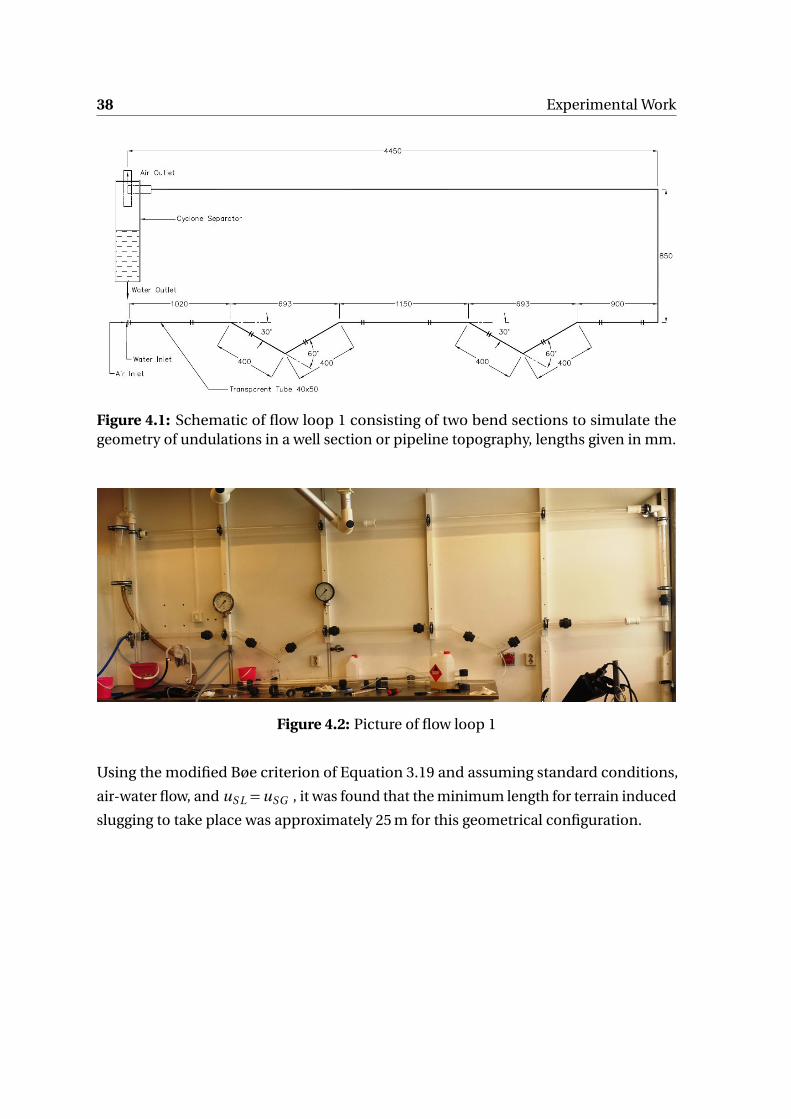
38 Experimental Work
Figure 4.1: Schematic of flow loop 1 consisting of two bend sections to simulate thegeometry of undulations in a well section or pipeline topography, lengths given in mm.
Figure 4.2: Picture of flow loop 1
Using the modified Bøe criterion of Equation 3.19 and assuming standard conditions,
air-water flow, and uS L =uSG , it was found that the minimum length for terrain induced
slugging to take place was approximately 25 m for this geometrical configuration.

4.2 Experimental setup 39
4.2.2 Configuration 2
Configuration 2 was made because of drawbacks with configuration 1 as it did not create
large slugs that the turbine could break down, but instead continuously transported gas
as small bubbles. The same problems took place in configuration 2 as pressure build-ups
were not possible and gas was continuously transported along the flow. By studying the
loop with the Bøe criterion of Equation 3.9, it was seen that the bend section required at
least 12-13 m length to accumulate terrain induced liquid slugs at the base.
Figure 4.3: Schematic of flow loop 2 consisting of a longer bend section, lengths givenin mm.
Figure 4.4: Picture of flow loop 2
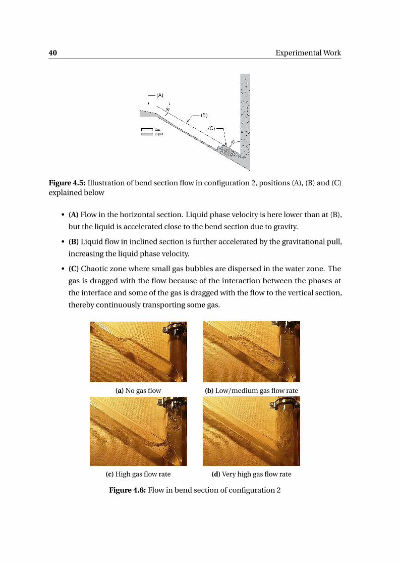
40 Experimental Work
Figure 4.5: Illustration of bend section flow in configuration 2, positions (A), (B) and (C)explained below
• (A) Flow in the horizontal section. Liquid phase velocity is here lower than at (B),
but the liquid is accelerated close to the bend section due to gravity.
• (B) Liquid flow in inclined section is further accelerated by the gravitational pull,
increasing the liquid phase velocity.
• (C) Chaotic zone where small gas bubbles are dispersed in the water zone. The
gas is dragged with the flow because of the interaction between the phases at
the interface and some of the gas is dragged with the flow to the vertical section,
thereby continuously transporting some gas.
(a) No gas flow (b) Low/medium gas flow rate
(c) High gas flow rate (d) Very high gas flow rate
Figure 4.6: Flow in bend section of configuration 2

4.2 Experimental setup 41
From Figure 4.5 and Figure 4.6, it was seen that gas was transported efficiently with the
liquid flow, thus not blocking the free gas passage and no terrain induced slugging took
place.
4.2.3 Configuration 3
Configuration 3 was made to study hydrodynamic slugging as described in Section 3.2.
Hydrodynamic slugs quickly occurred close to the inlet and grew in size along the flow.
The nature of hydrodynamic slugs differs a lot from the nature of the terrain induced
slugging
Figure 4.7: Schematic of flow loop 3 consisting of horizontal section to study the effectof hydrodynamic slugging, lengths given in mm.
Figure 4.8: Picture of flow loop 3

42 Experimental Work
4.3 Equipment
4.3.1 Turbine
Figure 4.9: Picture of the turbine used in the experiments
Propeller
Two propellers were considered for the experiments consisting of three and six blades,
respectively. The six bladed propeller was found to function best in the experiments
for this thesis because the impulse from the water was the driving mechanism that
resulted in rotation. The function of the propeller was to rotate the turbine and it was
seen through testing that the water had the biggest impact.
(a) Three bladed propeller (b) Six bladed propeller
Figure 4.10: Propeller designs used in the experiments (Raboesch®, 2016)
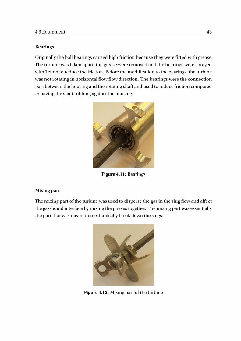
4.3 Equipment 43
Bearings
Originally the ball bearings caused high friction because they were fitted with grease.
The turbine was taken apart, the grease were removed and the bearings were sprayed
with Teflon to reduce the friction. Before the modification to the bearings, the turbine
was not rotating in horizontal flow flow direction. The bearings were the connection
part between the housing and the rotating shaft and used to reduce friction compared
to having the shaft rubbing against the housing.
Figure 4.11: Bearings
Mixing part
The mixing part of the turbine was used to disperse the gas in the slug flow and affect
the gas-liquid interface by mixing the phases together. The mixing part was essentially
the part that was meant to mechanically break down the slugs.
Figure 4.12: Mixing part of the turbine

44 Experimental Work
Housing
The housing part was the connection point between the turbine and the pipes used to
lock the turbine in place with a screw. It was found that the surface area occupied by
the housing was approximately 470 mm2. Further, the reduction of flow area over the
turbine because of the housing was approximately 37.5 %.
Figure 4.13: Illustration of surface area occupied by the turbine in the flow systems
4.3.2 Pipes
Figure 4.14: Pipes used in the experiments
Transparent acrylic glass pipes Ø50x40 mm were used in the experiments. In Figure 4.14
two different connections are used. The pipe at the bottom had the connections used
in experiment 1 to 5, but for experiment 6 it was decided to use white union muffs to
connect each pipe because the other connections seemed to affect the flow behaviour
with small local disturbances. Bend sections and the original connections were glued
together using acrifix.

4.4 Test conditions 45
(a) PVC union muff with O-ring to seal (b) White PVC double muff
Figure 4.15: Pipe connections used in the experiments. (a) Connection in experiment1-5 (b) Connection in experiment 6 (Dahl, 2015a,b)
4.4 Test conditions
4.4.1 Liquid flow rate and superficial velocity
The maximum liquid flow rate was found by measuring the time of filling a bucket of
20 litres with the water taps fully opened. By conducting several measurements, it was
found that the average time to fill the bucket was 79.5 s. It followed that the average
maximum liquid flow rate was:
QL =20l
79.5s=0.25ls−1 (4.1)
Further, the superficial liquid velocity was calculated by using Equation 2.2 as follows:
uS L =QL
A=
0.25 ·10−3m3 s−1
π4 (0.04m)2
=0.20ms−1 (4.2)
The low superficial liquid velocity limited the range of the experimental study substan-
tially. However, it is important to identify that slug flow was expected in flow loop 3 with
horizontal flow according to the flow regime maps from Figure 2.6. The liquid flow rate
was kept constant at the maximum rate in the experiments.
4.4.2 Gas flow rate
The gas flow rate was regulated by using two ball valves, one to regulate the flow, the
other for on/off-control. Between tests, the on/off-control valve was used so the other
valve could be kept at a fixed value. The gas pressure at the outlet from the laboratory
was varying between 7 and 8 bar between each day. Since the pressure was varying, each
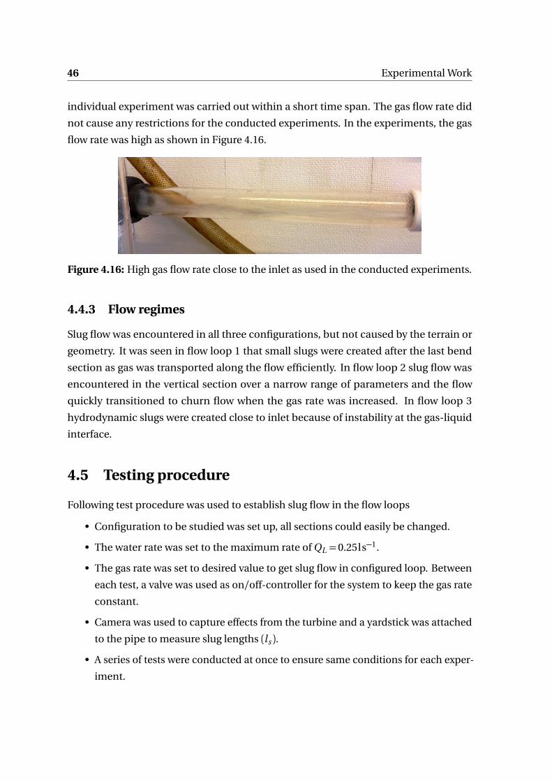
46 Experimental Work
individual experiment was carried out within a short time span. The gas flow rate did
not cause any restrictions for the conducted experiments. In the experiments, the gas
flow rate was high as shown in Figure 4.16.
Figure 4.16: High gas flow rate close to the inlet as used in the conducted experiments.
4.4.3 Flow regimes
Slug flow was encountered in all three configurations, but not caused by the terrain or
geometry. It was seen in flow loop 1 that small slugs were created after the last bend
section as gas was transported along the flow efficiently. In flow loop 2 slug flow was
encountered in the vertical section over a narrow range of parameters and the flow
quickly transitioned to churn flow when the gas rate was increased. In flow loop 3
hydrodynamic slugs were created close to inlet because of instability at the gas-liquid
interface.
4.5 Testing procedure
Following test procedure was used to establish slug flow in the flow loops
• Configuration to be studied was set up, all sections could easily be changed.
• The water rate was set to the maximum rate of QL =0.25ls−1.
• The gas rate was set to desired value to get slug flow in configured loop. Between
each test, a valve was used as on/off-controller for the system to keep the gas rate
constant.
• Camera was used to capture effects from the turbine and a yardstick was attached
to the pipe to measure slug lengths (ls ).
• A series of tests were conducted at once to ensure same conditions for each exper-
iment.
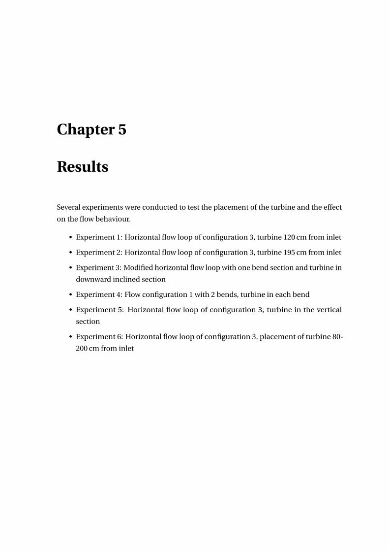
Chapter 5
Results
Several experiments were conducted to test the placement of the turbine and the effect
on the flow behaviour.
• Experiment 1: Horizontal flow loop of configuration 3, turbine 120 cm from inlet
• Experiment 2: Horizontal flow loop of configuration 3, turbine 195 cm from inlet
• Experiment 3: Modified horizontal flow loop with one bend section and turbine in
downward inclined section
• Experiment 4: Flow configuration 1 with 2 bends, turbine in each bend
• Experiment 5: Horizontal flow loop of configuration 3, turbine in the vertical
section
• Experiment 6: Horizontal flow loop of configuration 3, placement of turbine 80-
200 cm from inlet
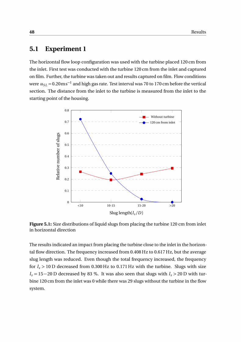
48 Results
5.1 Experiment 1
The horizontal flow loop configuration was used with the turbine placed 120 cm from
the inlet. First test was conducted with the turbine 120 cm from the inlet and captured
on film. Further, the turbine was taken out and results captured on film. Flow conditions
were uS L =0.20ms−1 and high gas rate. Test interval was 70 to 170 cm before the vertical
section. The distance from the inlet to the turbine is measured from the inlet to the
starting point of the housing.
<10 10-15 15-20 >200
0.1
0.2
0.3
0.4
0.5
0.6
0.7
0.8
Slug length(ls /D )
Rel
ativ
en
um
ber
ofs
lugs
Without turbine
120 cm from inlet
Figure 5.1: Size distributions of liquid slugs from placing the turbine 120 cm from inletin horizontal direction
The results indicated an impact from placing the turbine close to the inlet in the horizon-
tal flow direction. The frequency increased from 0.408 Hz to 0.617 Hz, but the average
slug length was reduced. Even though the total frequency increased, the frequency
for ls > 10 D decreased from 0.300 Hz to 0.171 Hz with the turbine. Slugs with size
ls = 15−20 D decreased by 83 %. It was also seen that slugs with ls > 20 D with tur-
bine 120 cm from the inlet was 0 while there was 29 slugs without the turbine in the flow
system.
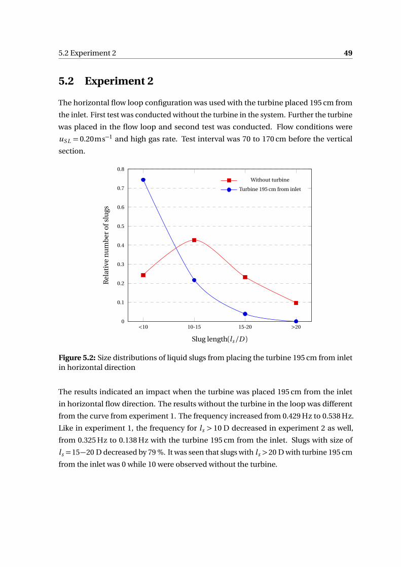
5.2 Experiment 2 49
5.2 Experiment 2
The horizontal flow loop configuration was used with the turbine placed 195 cm from
the inlet. First test was conducted without the turbine in the system. Further the turbine
was placed in the flow loop and second test was conducted. Flow conditions were
uS L = 0.20ms−1 and high gas rate. Test interval was 70 to 170 cm before the vertical
section.
<10 10-15 15-20 >200
0.1
0.2
0.3
0.4
0.5
0.6
0.7
0.8
Slug length(ls /D )
Rel
ativ
en
um
ber
ofs
lugs
Without turbine
Turbine 195 cm from inlet
Figure 5.2: Size distributions of liquid slugs from placing the turbine 195 cm from inletin horizontal direction
The results indicated an impact when the turbine was placed 195 cm from the inlet
in horizontal flow direction. The results without the turbine in the loop was different
from the curve from experiment 1. The frequency increased from 0.429 Hz to 0.538 Hz.
Like in experiment 1, the frequency for ls > 10 D decreased in experiment 2 as well,
from 0.325 Hz to 0.138 Hz with the turbine 195 cm from the inlet. Slugs with size of
ls =15−20 D decreased by 79 %. It was seen that slugs with ls >20 D with turbine 195 cm
from the inlet was 0 while 10 were observed without the turbine.
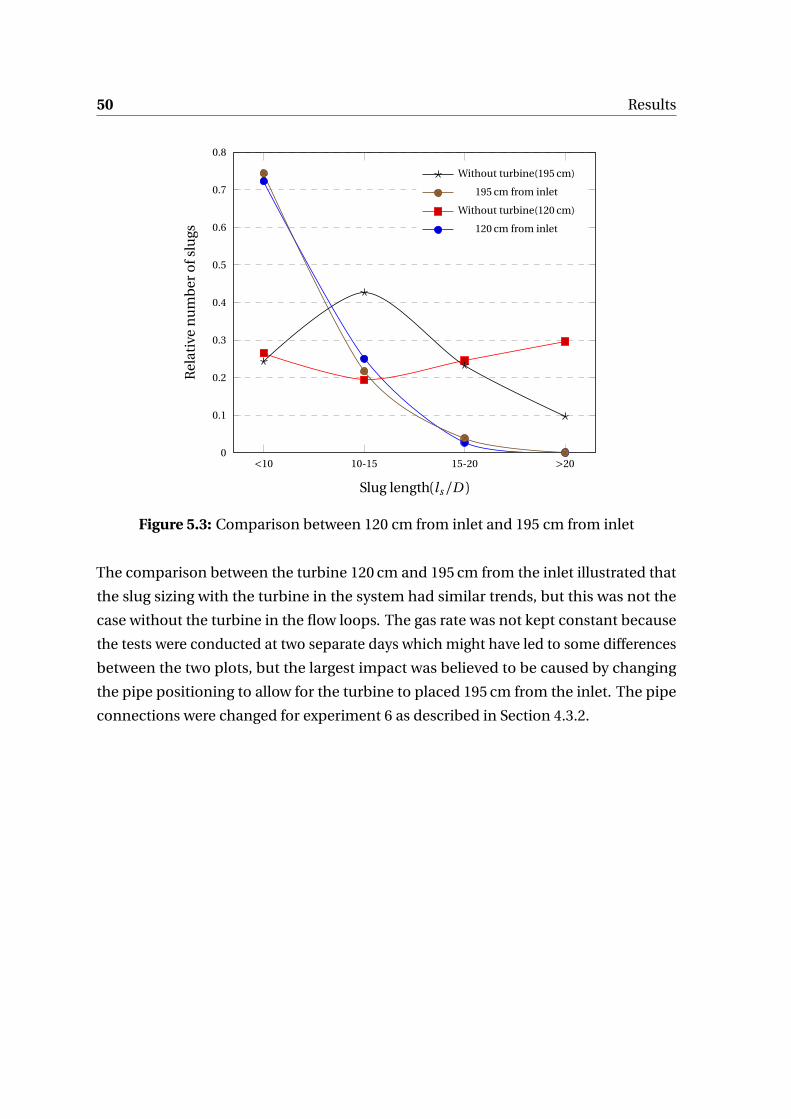
50 Results
<10 10-15 15-20 >200
0.1
0.2
0.3
0.4
0.5
0.6
0.7
0.8
Slug length(ls /D )
Rel
ativ
en
um
ber
ofs
lugs
Without turbine(195 cm)
195 cm from inlet
Without turbine(120 cm)
120 cm from inlet
Figure 5.3: Comparison between 120 cm from inlet and 195 cm from inlet
The comparison between the turbine 120 cm and 195 cm from the inlet illustrated that
the slug sizing with the turbine in the system had similar trends, but this was not the
case without the turbine in the flow loops. The gas rate was not kept constant because
the tests were conducted at two separate days which might have led to some differences
between the two plots, but the largest impact was believed to be caused by changing
the pipe positioning to allow for the turbine to placed 195 cm from the inlet. The pipe
connections were changed for experiment 6 as described in Section 4.3.2.

5.3 Experiment 3 51
5.3 Experiment 3
The horizontal flow loop was modified to have one bend section in the middle. The
turbine was placed in the inclined section in the downward flow direction with the
mixing part close to the base point of the bend section. The first test was conducted
with the turbine and the second test was conducted without. Flow conditions were
uS L = 0.20ms−1 and high gas rate. The test interval was closer to the vertical section
because of short distance from the bend section to the original test interval. The results
indicated no significant impacts from placing the turbine in flow loop with one bend
section. No slugs of size ls >20 D were observed for both tests.
<10 10-15 15-20 >200
0.1
0.2
0.3
0.4
0.5
0.6
0.7
0.8
Slug length(ls /D )
Rel
ativ
en
um
ber
ofs
lugs
Without turbine
With turbine
Figure 5.4: Slug lengths from placing turbine in bend section in modified flow loopcontaining one bend

52 Results
5.4 Experiment 4
The configuration of flow loop 1 was used with two turbines, one in each bend section.
The first test was conducted without the turbines and the second test was conducted
with. Flow conditions were uS L =0.20ms−1 and high gas rate. The test interval for this
experiment was at the top horizontal section because of short length from second bend
section to vertical section, 90 to 190 cm from the vertical section. The results indicated
no significant impacts from placing two turbines in flow loop with two bend sections.
No slugs of size ls >20 D were observed for both tests. Compared to Experiment 3, which
had one bend section, the frequency was drastically reduced with two bend sections,
probably caused by the gas accumulating at the top between the bend sections.
<10 10-15 15-20 >200
0.1
0.2
0.3
0.4
0.5
0.6
0.7
0.8
Slug length(ls /D )
Rel
ativ
en
um
ber
ofs
lugs
Without turbine
With turbine
Figure 5.5: Slug lengths from placing turbines in bend sections of flow loop 1
Figure 5.6 illustrates how the gas was efficiently transported with the flow in the case
of flow in bend section. No difference between the two cases was seen supporting the
results from experiment 3 and 4.

5.5 Experiment 5 53
t =0.00s t =0.00s
t =0.10s t =0.10s
t =0.20s t =0.20s
t =0.30s t =0.30s
Figure 5.6: Comparison with and without turbine in bend section. Left: with turbine,right: without turbine
5.5 Experiment 5
The horizontal flow loop was used in this experiment. The turbine was placed in the
vertical section with the propeller at the top and mixing part at the bottom. The first
test was conducted without the turbine and the second test was conducted with. Flow
conditions were uS L = 0.20ms−1 and high gas rate. The test interval was at the top
horizontal section, 90 to 190 cm from the vertical section. The results indicated minor
impacts from placing the turbine in the vertical section of the horizontal flow loop. The
frequency decreased from 0.321 Hz to 0.313 Hz, considered insignificant. Frequency for
ls >10 D decreased from 0.300 Hz to 0.171 Hz. Slugs with size of ls =15−20 D decreased
by 29 % and slugs with size of ls >20 D decreased by 19 %.
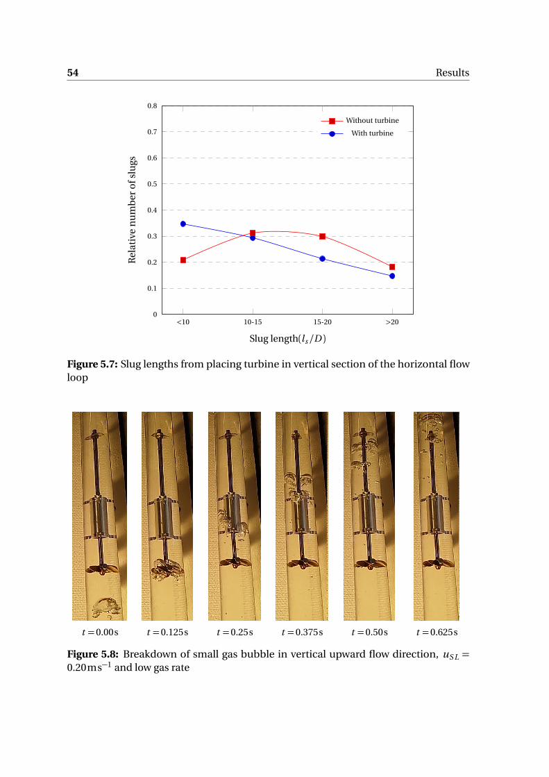
54 Results
<10 10-15 15-20 >200
0.1
0.2
0.3
0.4
0.5
0.6
0.7
0.8
Slug length(ls /D )
Rel
ativ
en
um
ber
ofs
lugs
Without turbine
With turbine
Figure 5.7: Slug lengths from placing turbine in vertical section of the horizontal flowloop
t =0.00s t =0.125s t =0.25s t =0.375s t =0.50s t =0.625s
Figure 5.8: Breakdown of small gas bubble in vertical upward flow direction, uS L =0.20ms−1 and low gas rate
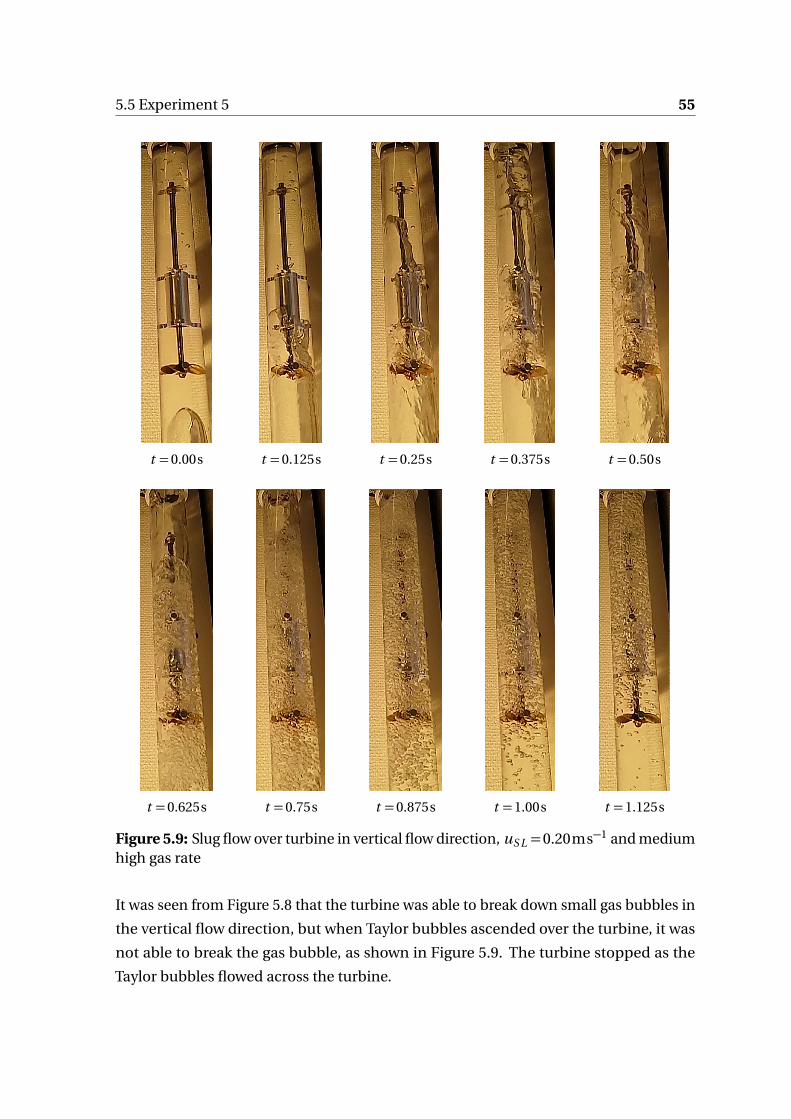
5.5 Experiment 5 55
t =0.00s t =0.125s t =0.25s t =0.375s t =0.50s
t =0.625s t =0.75s t =0.875s t =1.00s t =1.125s
Figure 5.9: Slug flow over turbine in vertical flow direction, uS L =0.20ms−1 and mediumhigh gas rate
It was seen from Figure 5.8 that the turbine was able to break down small gas bubbles in
the vertical flow direction, but when Taylor bubbles ascended over the turbine, it was
not able to break the gas bubble, as shown in Figure 5.9. The turbine stopped as the
Taylor bubbles flowed across the turbine.

56 Results
5.6 Experiment 6
The horizontal flow loop from previous experiments were modified slightly by changing
the connections to remove small disturbances caused by the original connections. First
test was conducted without turbine, followed by tests with the turbine 80, 100, 120, 140,
160 and 200 cm from the inlet. The last test was conducted without the turbine in the
flow loop. Flow conditions were uS L =0.20ms−1 and high gas rate. Test interval was 70
to 170 cm before the vertical section.
It was seen from Figure 5.10 some differences for the values ls =10−15D and ls =
15−20D for the two cases without the turbine. The difference was small enough to be
caused by the randomness in slug lengths for hydrodynamic slugs. The plot indicated
that large slugs were occurring without the turbine in the flow system.
<10 10-15 15-20 >200
0.1
0.2
0.3
0.4
0.5
0.6
0.7
0.8
Slug length(ls /D )
Rel
ativ
en
um
ber
ofs
lugs
Test 8 - Without
Test 1 - Without
Figure 5.10: Slug lengths without the turbine in experiment 6
Further it was seen from Figure 5.11 impacts of placing the turbine in various positions
from the inlet. The plot indicated that the amount of larger slugs decreased as the turbine
was placed closer to the test interval. This could be caused by the distance from the
turbine to the test interval being shorter and not enough distance for the slugs to grow. It
was identified, however, that all the trends with the turbine had reduced relative number

5.6 Experiment 6 57
of large slugs, while without the turbine the relative number of slugs were highest for
slugs with size ls >20 D.
<10 10-15 15-20 >200
0.1
0.2
0.3
0.4
0.5
0.6
0.7
0.8
Slug length(ls /D )
Rel
ativ
en
um
ber
ofs
lugs
Test 2 - 80 cm from inlet
Test 3 - 100 cm from inlet
Test 4 - 120 cm from inlet
Test 5 - 140 cm from inlet
Test 6 - 160 cm from inlet
Test 7 - 200 cm from inlet
Figure 5.11: Impact of turbine on slug sizes with the turbine at various positions fromthe inlet
It was seen by the comparisons in Figure 5.12 and Figure 5.13 that the turbine reduced
the slug length effectively over short distances. The results revealed that the number
of slugs with ls > 20 D with the turbine in the system were 11 over six tests, while 79
slugs with ls > 20 D were recorded in the two tests without the turbine in the system.
The average overall frequency increased with the turbine from 0.360 Hz to 0.481 Hz,
while the average frequency when excluding the slugs with size ls <10 D decreased from
0.308 Hz to 0.177 Hz with the turbine. Slugs with size of ls =15−20 D decreased by 31 %
and slugs with size of ls >20 D decreased by 95 %.

58 Results
<10 10-15 15-20 >200
0.1
0.2
0.3
0.4
0.5
0.6
0.7
0.8
Slug length(ls /D )
Rel
ativ
en
um
ber
ofs
lugs
Test 1 (without) Test 2(80 cm)
Test 3(100 cm) Test 4(120 cm)
Test 5(140 cm) Test 6 (160 cm)
Test 7 (200 cm) Test 8 (Without)
Figure 5.12: all graphs from experiment 6
<10 10-15 15-20 >200
0.1
0.2
0.3
0.4
0.5
0.6
0.7
0.8
Slug length(ls /D )
Rel
ativ
en
um
ber
ofs
lugs
Average value without turbine
Average value with turbine
Figure 5.13: Comparison of average values with and without turbine from experiment 6

5.6 Experiment 6 59
80 100 120 140 160 2000
0.1
0.2
0.3
0.4
0.5
0.6
0.7
0.8
0.9
Distance from inlet (cm)
Rel
ativ
en
um
ber
ofs
lugs
>20 (ls /D ) 15−20 (ls /D )
10−15 (ls /D ) <10 (ls /D )
Figure 5.14: Effect of turbine placement on slug sizes and relative number of slugs
Seen from Figure 5.14 above, slugs with size ls >20 D were not observed for placement
140-200 cm from the inlet. For slugs with size ls =15−20 D, it was seen that the relative
number of slugs decreased as the turbine was placed longer distance from the inlet. The
opposite was the case for slugs with ls <10 D as the relative number increased as the
turbine was place longer distance from the inlet.
From Figure 5.15 on the next page, it was seen that the liquid height increased close to
the propeller which seemed to accumulate a large number of slugs, possibly explaining
the increased frequency. Further, from Figure 5.16, as the liquid slug flowed across the
turbine, it was seen from t =0.25s and t =0.375s that cavitation happened, probably
caused by Bernoulli effect as the flow area decreased.

60 Results
t =0.00s
t =0.10s
t =0.20s
t =0.30s
t =0.40s
t =0.50s
t =0.60s
t =0.70s
t =0.80s
Figure 5.15: Formation of small slug over turbine in horizontal direction with rotation,uS L =0.20ms−1 and medium gas rate

5.6 Experiment 6 61
t =0.00s
t =0.125s
t =0.25s
t =0.375s
t =0.50s
t =0.625s
Figure 5.16: Slug flow over turbine in horizontal flow direction, uS L = 0.20ms−1 andhigh gas rate

62 Results
5.7 Summary
To summarize the experimental results, key findings are listed as bullet points below
and in Table 5.1;
• From experiments 1 and 2 in the horizontal flow direction it was identified;
– Slug frequency with turbine increased
– Number of large slugs decreased drastically with the turbine
– Frequency for slugs with ls >10 D decreased with the turbine
• From experiments 3 and 4 with bend sections it was identified;
– Insignificant difference with the turbine
– Two bend sections as opposed to one had 45 % lower slug frequency.
• From experiment 5 in the vertical flow direction it was identified;
– Small impact with the turbine
– Frequency was not affected
– Turbine stopped as large Taylor bubbles ascended through the turbine
• From experiment 6 in the horizontal flow direction it was identified;
– Slug frequency with turbine increased
– Number of large slugs decreased drastically with the turbine
– Frequency for slugs with ls >10 D decreased with the turbine
– Placement further away from the inlet reduced number of large slugs com-
pared to placement close to the inlet

5.7 Summary 63
Table 5.1: Test results summarized from all experiments. Extended information inAppendix A
Number of slugs by size
Experiment Test <10 D 10−15 D 15−20 D >20 D
Experiment 1With turbine 107 37 4 0
Without turbine 26 19 24 29
Experiment 2With turbine 96 28 5 0
Without turbine 25 44 24 10
Experiment 3With turbine 77 43 23 0
Without turbine 80 37 24 0
Experiment 4With turbine 55 24 3 0
Without turbine 51 23 2 0
Experiment 5With turbine 26 22 16 11
Without turbine 16 24 23 14
Experiment 6
Test 1 10 21 13 43
Test 2 59 35 23 3
Test 3 63 33 16 6
Test 4 78 27 12 2
Test 5 66 31 9 0
Test 6 96 24 3 0
Test 7 75 30 1 0
Test 8 15 16 18 36


Chapter 6
Discussion
The objective of this thesis was to review multiphase flow with special emphasis on
slug phenomena, followed by experiments to evaluate the use of a rotating device to
mechanically break down slugs in the gas-liquid interface and/or influence multiphase
flow in any significant and beneficial way. The results indicated varying impacts from
the turbine depending on flow configuration and placement. The largest impacts on the
flow behaviour was found in experiments 1, 2 and 6 as all these experiments studied the
impacts of the turbine when placed in the horizontal flow direction. The hydrodynamic
instability at the gas-liquid interface created slugs early in the flow loop, thus making it
possible to study the impacts of the turbine without the vertical section affecting the
flow.
The dimensions of the flow loop configurations limited the experimental study sub-
stantially. Terrain induced slugging required greater pressure build-ups than the di-
mensions in the experimental study would allow. This was caused by short lengths and
relatively low liquid flow rate. The horizontal flow loop was not as much limited by these
factors as hydrodynamic slugs developed over a broader range of parameters.
Terrain induces slugging and hydrodynamic slugging are very different in nature.
Terrain induced slugs occurs because of geometry allowing for liquid accumulation
at low spots and pressure build-ups while hydrodynamic slugs occurs because of flow
conditions and interaction between gas and liquid phase. Terrain induced slugs are
considered more harsh than hydrodynamic slugs because of large pressure and flow rate
fluctuations.
Terrain induced slugging did not occur in the flow loops containing bend sections
because of the dimensions and flow conditions. The turbine did not have any impact on
the flow because there was nothing to fix at the low points of the bend sections since gas

66 Discussion
was transported efficiently with the liquid flow as seen in Figure 5.6. Slug flow occurred
in the flow loops containing bend section, but the formation of the slugs took place at
other places of the flow loops rather than the base of the bend sections. It was discussed
briefly in Section 4.2 why terrain induced slugging did not occur and found to be caused
by the short length of the inclined sections not allowing for pressure build-ups. It was
mentioned that the lengths of the bend section should have been at least 12-13 m and
25 m using the Bøe criterion, but the assumptions for the calculations made the perfect
conditions for terrain induced slugging occurring and the length should probably been
even longer.
It was identified that the turbine was able to break down small gas bubbles ascending
over the turbine in the vertical direction as seen from snapshots in Figure 5.8, but was
not able to break down Taylor bubbles as seen from snapshots in Figure 5.9. When Taylor
bubbles ascended over the turbine, rotation stopped because of a vortex at the point
right above the propeller probably caused by the change of flow direction by the propeller.
The liquid velocity upwards was reduced and further accelerated downwards by the
gravitation. It was believed that this phenomenon stopped the device from rotating.
The horizontal flow loop with the test conditions resulted in hydrodynamic slugging.
These hydrodynamic slugs were caused by instabilities at the gas-liquid interface and the
slugs increased in size along the flow. The turbine altered the flow by increasing the slug
frequency and reducing the size of the slugs. From the slow motion footage in Figure 5.15,
it was seen that the liquid height at the position of the propeller increased which reduced
the height of the gas at the same position. Studying the Kelvin-Helmholtz instability
criterion of Equation 3.1 when the gas height is reduced, revealed that instability were
more likely to occur and create slugs, explaining the increase of frequency with the
turbine. In the experiments in this study, local effects were studied, but larger scale and
different test intervals might have led to other results because of interaction between
slugs along the flow. The amount of large slugs were drastically reduced, but Figure 5.14
illustrated that short distance from turbine to test interval might have caused these
results. It was, however, evident that under these experimental conditions that the
turbine reduced the size of the slugs over a short distance.
It was mentioned briefly in Section 4.3 that the device reduced the surface area by
approximately 37.5 %. This constriction of flow area would affect the production rate in
a negative way. From Figure 5.16, it was seen that cavitation happened as the already
created slug flowed through the turbine. Cavitation is associated with fast formation and
67
breakdown of gas bubbles due to Bernoulli effect, here created as the result of reducing
the flow area.
Slug lengths are associated with uncertainty because of random flow behaviour since
slugs interact with each other over large distances and might coalesce to larger slugs
as well as slugs might break down. Even at the small scale of the experiments in this
study, slugs grew and broke down in the test interval which is why large increments
were used for the size distributions. The flow loops in this study were short and only
local effects were studied. By studying Figure 5.14, it was seen that the number of
large slugs decreased significantly when the device was placed further away from the
inlet. The device placement very close to the test interval, so that slugs did not have
the opportunity to accumulate to larger slugs, might have caused this. It could also be
caused by the impacts of the device on the flow behaviour, but yet again not allowing
for accumulation of larger slugs before the test interval. It was, however, evident that
there was an impact from the device on this scale despite the large uncertainties of
these experiments. Uncertainty also related to the method used to gather the results as
impacts have been captured on film and further results from visual inspections of the
films.


Chapter 7
Conclusion
This study was set out to explore the possibilities of utilizing a turbine to mechanically
affect the slug flow behaviour in undulated horizontal wells and pipeliner-riser systems.
As terrain induced slugging did not occur in any of the flow loops, it was decided to
study the impacts from the turbine on hydrodynamic generated slugs. The nature of
hydrodynamic slugs are very different from the nature of terrain induced slugs. hydrody-
namic slugs are caused by flow instability and interaction between gas and liquid phase
whereas terrain induced slugs are created from liquid accumulation at low spots. This
means that the turbine is not expected to have the same outcome on terrain induced
slugging as the results in this study. New experiments should be conducted with a flow
loop where terrain induced slugging occurs to study the impacts of the turbine on this
flow.
7.1 Concluding remarks
The findings of this study are summarized below;
• Slug flow occurred in the flow loops caused by hydrodynamic instability as a result
of flowing conditions, but terrain induced slugging did not occur in any of the flow
loops likely because to the dimensions.
• Based on the results in experiment 5, it was indicated that the impact of the turbine
in the vertical flow direction was small, probably because the turbine stopped
rotating when large Taylor bubbles ascended over the turbine and the liquid phase
velocity was reduced.

70 Conclusion
• Based on the results from experiments 3 and 4, there was no impact from the
turbine on the flow behaviour in the bend sections.
• Based on the results from experiments 1, 2 and 6 in the flow loop consisting of
horizontal flow sections, slug flow tended to occur at the same spot in the pipe
with the test conditions. It was believed that placing the turbine around this
region would yield results as the turbine could break down the slugs as they were
generated. It was seen that the frequency increased while the size of each individual
slug was reduced. It was found that slugs tended to form over the turbine as the
liquid height was locally increased and waves grew due to flow instabilities. Further,
it was seen that placement of the turbine closer to the test interval resulted in the
lowest number of with size ls >15 D as the slugs did not have the opportunity to
grow in the short distance.
7.2 Future work
The experiences from this study has identified some improvement areas with the original
configurations and my suggestions for changes in future work are;
• First, To evaluate the use of the turbine for terrain induced slugging, the dimensions
must be scaled much larger so that liquid slugs can accumulate at low points. With
larger dimensions comes possibilities of studying placement of turbine in inclined
section to evaluate optimal positioning. As discussed in Section 3.4.3, the flow
in the downward flow direction have to be effectively stratified. Investigation on
whether or not the turbine could affect this criterion could be feasible.
• Further, to evaluate the impact of the rotational speed, implement a motor to
control RPM of the turbine. This would also affect the vertical section as the
turbine would no longer stop when Taylor bubbles ascends across the turbine.
• The use of a capacitance sensor or digital manometer connected to a computer
would extend the study to larger time scales in addition to less processing time
before the data analysis.
• Identify the possibility of a new device to transport the gas in inclined section
down to the base point or modifying the device in this study to the extent that it is
used for transportation of gas in the downward inclined section.
References
Andreussi, P., Paglianti, A. and Silva, F. S. (1999), ‘Dispersed bubble flow in horizontalpipes’, Chemical Engineering Science 54(8), 1101 – 1107.
Aziz, K. and Govier, G. W. (1972), The Flow of Complex Mixtures in Pipes, New York: VanNostrand Reinhold Company.
Bai, Y. and Bai, Q. (2012), Subsea Engineering Handbook, Gulf Publishing Company.
Baker, O. (1953), Design of pipelines for the simultaneous flow of oil and gas, in ‘FallMeeting of the Petroleum Branch of AIME’, Society of Petroleum Engineers.
Barnea, D., Shoham, O. and Taitel, Y. (1982), ‘Flow pattern transition for downward in-clined two phase flow; horizontal to vertical’, Chemical Engineering Science 37(5), 735–740.
Bøe, A. (1981), ‘Severe slugging characteristics; part i: flow regime for severe slugging; partii: Point model simulation study’, Selected Topics in Two-Phase Flow, NTH, Trondheim,Norway .
Cadei, L., Montenegro, G., Scaramellini, S., Di Sarra, A., Cerri, P., Bianco, A., Masi, S. et al.(2015), Slug catcher multiphase cfd modelling: Optimization and comparison withindustrial standards, in ‘Offshore Mediterranean Conference and Exhibition’, OffshoreMediterranean Conference.
Corneliussen, S., Couput, J.-P., Dahl, E., Dykesteen, E., Frøysa, K.-E., Malde, E., Moestue,H., Moksnes, P. O., Scheers, L. and Tunheim, H. (2005), ‘Handbook of multiphase flowmetering’, Norwegian Society for Oil and Gas Measurement (NFOGM), Revision 2.
Dahl, B. (2015a), ‘Katalog 2015 teknisk vvs’. Retrieved fromhttp://dahl.no/Documents/Kataloger/VVS/KATALOG_Teknisk_2015.pdf.
Dahl, B. (2015b), ‘Prisbok 2015 industri’. Retrieved fromhttp://www.dahl.no/Documents/Kataloger/Industri/Produktbok_Industri_2015.pdf.
Dukler, A. E. and Hubbard, M. G. (1975), ‘A model for gas-liquid slug flow in horizontal andnear horizontal tubes’, Industrial & Engineering Chemistry Fundamentals 14(4), 337–347.
Enilari, B., Kara, F. et al. (2015), Slug flow and it’s mitigation techniques in the oil and gasindustry, in ‘SPE Nigeria Annual International Conference and Exhibition’, Society ofPetroleum Engineers.
Feesa, L. (2003), ‘Hydrodynamic slug size in multiphase flowlines’. Retrieved fromhttp://www.feesa.net./case-studies/.
72 References
Filip, A., Baltaretu, F. and Damian, R.-M. (2014), ‘Comparison of two-phase pressuredrop models for condensing flows in horizontal tubes’, Mathematical Modelling inCivil Engineering 10(4), 19–27.
Gokcal, B., Al-Sarkhi, A., Sarica, C., Alsafran, E. M. et al. (2009), Prediction of slug fre-quency for high viscosity oils in horizontal pipes, in ‘SPE Annual Technical Conferenceand Exhibition’, Society of Petroleum Engineers.
Gregory, G. and Scott, D. (1969), ‘Correlation of liquid slug velocity and frequency inhorizontal cocurrent gas-liquid slug flow’, AIChE Journal 15(6), 933–935.
Haheim, S., Gaillard, X. et al. (2009), A simplified subsea separation and pumping system,in ‘SPE Annual Technical Conference and Exhibition’, Society of Petroleum Engineers.
Heywood, N. and Richardson, J. (1979), ‘Slug flow of air—water mixtures in a horizontalpipe: Determination of liquid holdup by γ-ray absorption’, Chemical EngineeringScience 34(1), 17–30.
Hill, T. (1990), ‘Gas injection at riser base solves slugging flow problems’, Oil and GasJournal;(USA) 88(9).
Jahanshahi, E. (2013), ‘Control solutions for multiphase flow: Linear and nonlinearapproaches to anti-slug control’.
Jansen, F., Shoham, O. and Taitel, Y. (1996), ‘The elimination of severe slug-ging—experiments and modeling’, International journal of multiphase flow22(6), 1055–1072.
Jansen, F., Shoham, O. et al. (1994), Methods for eliminating pipeline-riser flow instabili-ties, in ‘SPE Western Regional Meeting’, Society of Petroleum Engineers.
Li, S.-M. (2007), Mean-Field Free-Energy Lattice Boltzmann Method For Liquid-VaporInterfacial Flows, PhD thesis, Virginia Polytechnic Institue and State University.
Malekzadeh, R. (2012), Severe slugging in gas-liquid two-phase pipe flow, TU Delft, DelftUniversity of Technology.
Malekzadeh, R., Henkes, R. and Mudde, R. (2012), ‘Severe slugging in a long pipeline–riser system: experiments and predictions’, International journal of multiphase flow46, 9–21.
Malekzadeh, R. and Mudde, R. F. (2012), A modelling study of severe slugging in wellbore,in ‘North Africa Technical Conference and Exhibition’, Society of Petroleum Engineers.
Mandhane, J., Gregory, G. and Aziz, K. (1974), ‘A flow pattern map for gas—liquid flow inhorizontal pipes’, International Journal of Multiphase Flow 1(4), 537–553.
Manolis, I., Mendes-Tatsis, M. and Hewitt, G. (1995), The effect of pressure on slugfrequency on two-phase horizontal flow, in ‘The 2nd conference on multiphase flow,Kyoto, Japan’.
Norris, H. L. (2012), The use of a transient multiphase simulator to predict and suppressflow instabilities in a horizontal shale oil well, in ‘SPE Annual Technical Conferenceand Exhibition’, Society of Petroleum Engineers.

References 73
Obendrauf, W., Schrader, K., Al-Farsi, N., White, A. et al. (2006), Smart snake wells inchampion west-expected and unexpected benefits from smart completions, in ‘SPEAsia Pacific Oil & Gas Conference and Exhibition’, Society of Petroleum Engineers.
Ogazi, A. I. (2011), Multiphase severe slug flow control, Cranfield University.
Øverland, A. M. and Ramstad, H. J. (2001), Yme marginal field, 12 km subsea gas liftexperience, in ‘SPE Annual Technical Conference and Exhibition’, Society of PetroleumEngineers.
Pots, B. F., Bromilow, I. G., Konijn, M. J. et al. (1987), ‘Severe slug flow in offshore flow-line/riser systems’, SPE Production Engineering 2(04), 319–324.
Raboesch® (2016), ‘Raboesch ® Models’. Retrieved fromhttp://www.raboeschmodels.com/downloads/documents/catalog/RABOESCH-CATALOGUS-2016.pdf.
Schmidt, Z., Doty, D. R., Dutta-Roy, K. et al. (1985), ‘Severe slugging in offshore pipelineriser-pipe systems’, Society of Petroleum Engineers Journal 25(01), 27–38.
Skofteland, G., Godhavn, J.-M., Kulset, T. et al. (2007), Implementation of a slug controlsystem for subsea wells in an integrated operation environment, in ‘13th InternationalConference on Multiphase Production Technology’, BHR Group.
Stapelberg, H. H. and Mewes, D. (1994), ‘The pressure loss and slug frequency of liquid-liquid-gas slug flow in horizontal pipes’, International journal of multiphase flow20(2), 285–303.
Taitel, Y. (1986), ‘Stability of severe slugging’, International journal of multiphase flow12(2), 203–217.
Taitel, Y., Bornea, D. and Dukler, A. (1980), ‘Modelling flow pattern transitions for steadyupward gas-liquid flow in vertical tubes’, AIChE Journal 26(3), 345–354.
Taitel, Y. and Dukler, A. (1976), ‘A model for predicting flow regime transitions in hori-zontal and near horizontal gas-liquid flow’, AIChE Journal 22(1), 47–55.
Tang, Y., Wolff, M., Condon, P. and Ogden, K. A. (2007), A dynamic wellbore modeling forsinusoidal horizontal well performance with high water cut, in ‘SPE Annual TechnicalConference and Exhibition’, Society of Petroleum Engineers.
Terry, R. E. and Rogers, J. B. (2014), Applied Petroleum Reservoir Engineering, 3rd Edition,Prentice Hall.
Thome, J. R. (2004), ‘Engineering data book iii’, Wolverine Tube Inc .
Yaw, S. Y., Lee, C. Y., Haandrikman, G., Groote, G., Asokan, S., Malonzo, M. E. et al.(2014), Smart choke-a simple and effective slug control technology to extend fieldlife, in ‘International Petroleum Technology Conference’, International PetroleumTechnology Conference.
Zabaras, G. et al. (1999), Prediction of slug frequency for gas-liquid flows, in ‘SPE AnnualTechnical Conference and Exhibition’, Society of Petroleum Engineers.


Appendix A
Experiments
A.1 Experiment 1
Table A.1: Results with turbine 120 cm from inlet resulting from a period of 4 minutes.uS L =0.20ms−1 & high gas rate.
With turbine Without turbine
Number of slugs by size
<10D 107 26
10−15D 37 19
15−20D 4 24
>20D 0 29
Total number of slugs 148 98
Relative number of slugs (ls /D )
<10 0.723 0.265
10−15 0.250 0.194
15−20 0.027 0.245
>20 0.000 0.296
Relative number of slugs for ls >10D
10−15D 0.902 0.264
15−20D 0.098 0.333
>20D 0.000 0.403
Frequency, fs 0.617 0.408
Frequency, fs for ls >10D 0.171 0.300
Reduction 0.446 0.108

76 Experiments
A.2 Experiment 2
Table A.2: Results with turbine 195 cm from inlet resulting from a period of 4 minutes.uS L =0.20ms−1 & high gas rate.
With turbine Without turbine
Number of slugs by size
<10D 96 25
10−15D 28 44
15−20D 5 24
>20D 0 10
Total number of slugs 129 103
Relative number of slugs (ls /D )
<10 0.744 0.243
10−15 0.217 0.427
15−20 0.039 0.233
>20 0.000 0.097
Relative number of slugs for ls >10D
10−15D 0.848 0.564
15−20D 0.152 0.308
>20D 0.000 0.128
Frequency, fs 0.538 0.429
Frequency, fs for ls >10D 0.138 0.325
Reduction 0.400 0.104
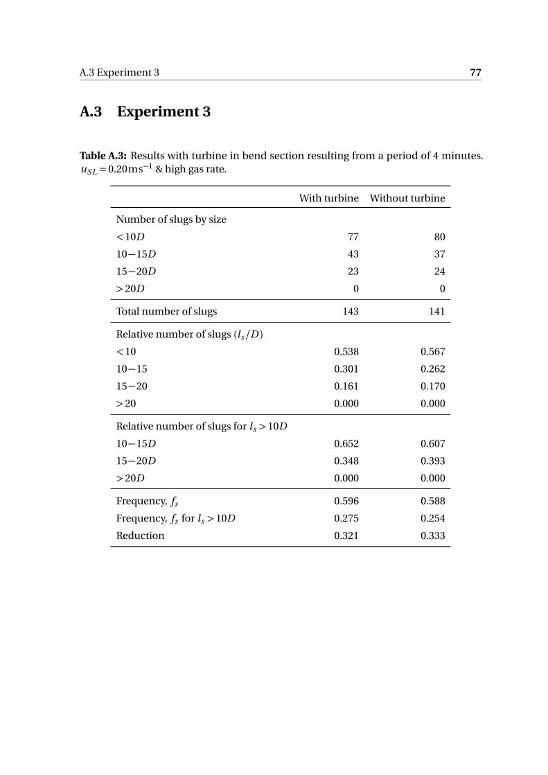
A.3 Experiment 3 77
A.3 Experiment 3
Table A.3: Results with turbine in bend section resulting from a period of 4 minutes.uS L =0.20ms−1 & high gas rate.
With turbine Without turbine
Number of slugs by size
<10D 77 80
10−15D 43 37
15−20D 23 24
>20D 0 0
Total number of slugs 143 141
Relative number of slugs (ls /D )
<10 0.538 0.567
10−15 0.301 0.262
15−20 0.161 0.170
>20 0.000 0.000
Relative number of slugs for ls >10D
10−15D 0.652 0.607
15−20D 0.348 0.393
>20D 0.000 0.000
Frequency, fs 0.596 0.588
Frequency, fs for ls >10D 0.275 0.254
Reduction 0.321 0.333

78 Experiments
A.4 Experiment 4
Table A.4: Results with turbine in two bend sections resulting from a period of 4 minutes.uS L =0.20ms−1 & high gas rate.
With turbine Without turbine
Number of slugs by size
<10D 55 51
10−15D 24 23
15−20D 3 2
>20D 0 0
Total number of slugs 82 76
Relative number of slugs (ls /D )
<10 0.671 0.671
10−15 0.293 0.303
15−20 0.037 0.026
>20 0.000 0.000
Relative number of slugs for ls >10D
10−15D 0.889 0.920
15−20D 0.111 0.080
>20D 0.000 0.000
Frequency, fs 0.342 0.317
Frequency, fs for ls >10D 0.113 0.104
Reduction 0.229 0.213
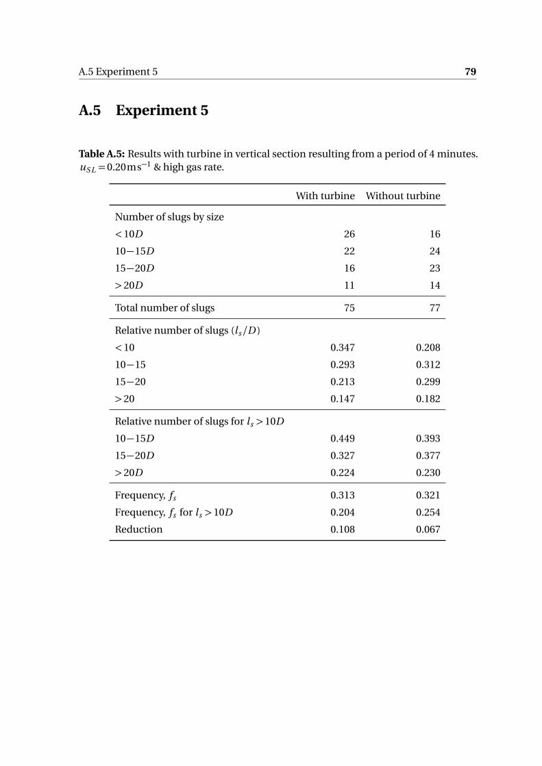
A.5 Experiment 5 79
A.5 Experiment 5
Table A.5: Results with turbine in vertical section resulting from a period of 4 minutes.uS L =0.20ms−1 & high gas rate.
With turbine Without turbine
Number of slugs by size
<10D 26 16
10−15D 22 24
15−20D 16 23
>20D 11 14
Total number of slugs 75 77
Relative number of slugs (ls /D )
<10 0.347 0.208
10−15 0.293 0.312
15−20 0.213 0.299
>20 0.147 0.182
Relative number of slugs for ls >10D
10−15D 0.449 0.393
15−20D 0.327 0.377
>20D 0.224 0.230
Frequency, fs 0.313 0.321
Frequency, fs for ls >10D 0.204 0.254
Reduction 0.108 0.067

80 Experiments
A.6 Experiment 6
Table A.6: Results without turbine and turbine 80 cm from inlet resulting from a periodof 4 minutes. uS L =0.20ms−1 & high gas rate.
Test #1 Test #2
Without turbine 80 cm from inlet
Number of slugs by size
<10D 10 59
10−15D 21 35
15−20D 13 23
>20D 43 3
Total number of slugs 87 120
Relative number of slugs (ls /D )
<10 0.115 0.492
10−15 0.241 0.292
15−20 0.149 0.192
>20 0.494 0.025
Relative number of slugs for ls >10D
10−15D 0.279 0.574
15−20D 0.169 0.377
>20D 0.558 0.049
Frequency, fs 0.363 0.500
Frequency, fs for ls >10D 0.321 0.254
Reduction 0.042 0.246

A.6 Experiment 6 81
Table A.7: Results with turbine 100 cm and 120 cm from inlet resulting from a period of4 minutes. uS L =0.20ms−1 & high gas rate.
Test #3 Test #4
100 cm from inlet 120 cm from inlet
Number of slugs by size
<10D 63 78
10−15D 33 27
15−20D 16 12
>20D 6 2
Total number of slugs 118 119
Relative number of slugs (ls /D )
<10 0.534 0.655
10−15 0.280 0.227
15−20 0.136 0.101
>20 0.051 0.017
Relative number of slugs for ls >10D
10−15D 0.600 0.659
15−20D 0.291 0.293
>20D 0.109 0.049
Frequency, fs 0.492 0.496
Frequency, fs for ls >10D 0.229 0.171
Reduction 0.263 0.325

82 Experiments
Table A.8: Results with turbine 140 cm and 160 cm from inlet resulting from a period of4 minutes. uS L =0.20ms−1 & high gas rate.
Test #5 Test #6
140 cm from inlet 160 cm from inlet
Number of slugs by size
<10D 66 96
10−15D 31 24
15−20D 9 3
>20D 0 0
Total number of slugs 106 123
Relative number of slugs (ls /D )
<10 0.623 0.780
10−15 0.292 0.195
15−20 0.085 0.024
>20 0.000 0.000
Relative number of slugs for ls >10D
10−15D 0.775 0.889
15−20D 0.225 0.111
>20D 0.000 0.000
Frequency, fs 0.442 0.513
Frequency, fs for ls >10D 0.167 0.113
Reduction 0.275 0.400

A.6 Experiment 6 83
Table A.9: Results with turbine 200 cm from inlet and without turbine resulting from aperiod of 4 minutes. uS L =0.20ms−1 & high gas rate.
Test #7 Test #8
200 cm from inlet Without turbine
Number of slugs by size
<10D 75 15
10−15D 30 16
15−20D 1 18
>20D 0 36
Total number of slugs 106 86
Relative number of slugs (ls /D )
<10 0.708 0.174
10−15 0.283 0.186
15−20 0.009 0.209
>20 0.000 0.419
Relative number of slugs for ls >10D
10−15D 0.968 0.225
15−20D 0.032 0.254
>20D 0.000 0.507
Frequency, fs 0.442 0.358
Frequency, fs for ls >10D 0.129 0.296
Reduction 0.313 0.063