Mass-conserving and positive-definite semi-Lagrangian advection … · 2016-01-26 · November 4,...

November 4, 2008 13th on the use of hpc in meteorology

1

Mass-conserving and positive-definite semi-Lagrangian advection in NCEP GFS:

Decomposition for massively parallel computing without halo

Hann-Ming Henry JuangEnvironmental Modeling Center, NCEP

NWS,NOAA,DOC,USA


2

Introduction• The common elements for traditional semi-

Lagrangian method are– Iteration to find departure and/or mid-point values– Interpolation from regular grid points to departure

and/or mid-points– Require halo grids in MPP

• Advantage of semi-Lagrangian Method– Allowable larger time step, saving time– Use linear grid in spectral model; same grid-point

with higher resolution of spectral truncation


3

A

M

D

∂q∂t

+ u∂q∂x

+ v ∂q∂y

= 0

DqDt

= 0

qAn +1 = qD

n−1


4

A

D

M

Starting from mid-point

No guessing and no iteration

but one 2-D interpolation and one 2-D remapping


5

Proposed Method• Splitting semi-Lagrangian advection

– advection in one direction first– then advection in another direction– temporal and spatial splitting

• Advantage– no guessing and no iteration– 1-D interpolation and remapping– possible no halo (with transpose)– incremental implementation

• Possible to add mass conservation and positive definite advection


6

∂q∂t

+ u∂q∂x

+ v ∂q∂y

= 0

∂q∂t

⎛ ⎝ ⎜

⎞ ⎠ ⎟

X −direction

+∂q∂t

⎛ ⎝ ⎜

⎞ ⎠ ⎟

Y −direction

+ u∂q∂x

+ v ∂q∂y

= 0

∂q∂t

⎛ ⎝ ⎜

⎞ ⎠ ⎟

X −direction

+ u∂q∂x

+∂q∂t

⎛ ⎝ ⎜

⎞ ⎠ ⎟

Y −direction

+ v ∂q∂y

= 0

DqDt

⎛ ⎝ ⎜

⎞ ⎠ ⎟

X −direction

+DqDt

⎛ ⎝ ⎜

⎞ ⎠ ⎟

Y −direction

= 0


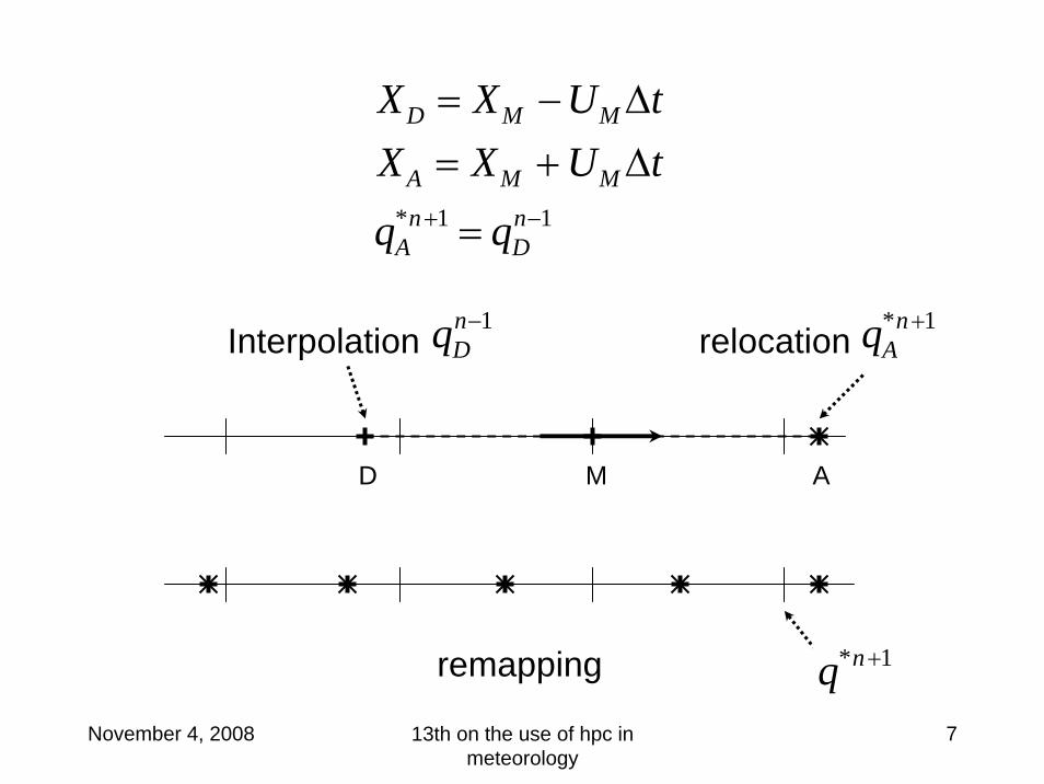
7

AD M

XD = XM −UM ΔtXA = XM + UM ΔtqA

*n +1 = qDn−1

Interpolation

remapping

qDn−1

relocation qA*n +1

q*n +1


8

YD = YM −VM ΔtYA = YM + VM ΔtqA

n +1 = qD*n +1

rem

appi

ng

qn +1A

D

M

Interpolation qD*n +1

relocation qAn +1


9

Ay

Dy

Mx AxDx

My

Dy

My

Ay

Dx Mx Ax


10

Gaussian 256 x 128 with time step of 1800 sec


11

Gaussian 256 x 128 with time step of 1800 secAcross north pole


12

Gaussian 256 x 128 with time step of 1800 secAcross south pole


13

at north pole


14

at equator


15

at south pole


16

one complete revolution


17

L2 =I q − qT( )2[ ]

12

I qT( )2[ ]12

whereI[A] =

14πa2 Acosφdφdλ

φλ∫∫Max[A] = global_max_of _ AMin[A] = global_min_of _ A

L∞ =Max | q − qT |[ ]

Max | qT |[ ]

L1 =I | q − qT |[ ]

I | qT |[ ]

max =Max q[ ]− Max qT[ ]Max qT[ ]− Min qT[ ]

min =Min q[ ]− Min qT[ ]

Max qT[ ]− Min qT[ ]


18

Compare Errorsmin max L1 L2 L∞

FFSL-5128x64

-1.3E-3 -0.053 0.047 0.041 0.053

NISL256x128

-7.67E-5 -0.0021 0.018 0.013 0.014

FFSL-3256x128

-5.82E-4 0.040 0.020 0.020 0.040

NISL128x64

-2.26E-4 -0.017 0.037 0.050 0.052

NISL512x256

-2.72E-5 -0.00026 0.0053 0.0046 0.0070


19

∂ρ∂t

+∂ρu∂x

+∂ρv∂y

+∂ρζ

•

∂ζ= 0

∂ρ∂t

⎛ ⎝ ⎜

⎞ ⎠ ⎟

(X )

+∂ρu∂x

+∂ρ∂t

⎛ ⎝ ⎜

⎞ ⎠ ⎟

(Y )

+∂ρv∂y

+∂ρ∂t

⎛ ⎝ ⎜

⎞ ⎠ ⎟

(Z )

+∂ρζ

•

∂ζ= 0

For mass conservation, let’s start from continuity equation

Consider 1-D and rewrite it in advection form, we have

∂ρ∂t

⎛ ⎝ ⎜

⎞ ⎠ ⎟

(X −direction )

+ u∂ρ∂x

= −ρ ∂u∂x

Advection form is for semi-Lagrangian,but it is not conserved if divergence is treated as force at mid-point,So divergence term should be treated with advection


20

Divergence term in Lagrangian sense is the change of the volumeif mass is conserved, so we can write divergence form as

∂u∂x

⎛ ⎝ ⎜

⎞ ⎠ ⎟

Lagrangian _ sense

=1

Δ x

dΔ x

dt

dρΔ x

dt⎛ ⎝ ⎜

⎞ ⎠ ⎟

X −direction

= 0

∂ρΔ x

∂t⎛ ⎝ ⎜

⎞ ⎠ ⎟

X −direction

+ u∂ρΔ x

∂x= 0

Put it into the previous continuity equation, we have

which can be seen as ρΔ x( )departure = ρΔ x( )arrival


21

∂q∂t

+ u∂q∂x

+ v ∂q∂y

+ ζ• ∂q

∂ζ= 0

∂ρ∂t

+∂ρu∂x

+∂ρv∂y

+∂ρζ

•

∂ζ= 0

∂ρq∂t

+∂ρqu

∂x+

∂ρqv∂y

+∂ρqζ

•

∂ζ= 0

dρqΔdt

= 0 dρΔdt

= 0

How about mass conservation for tracer ?

If we use tracer and continuity equation as following together

Then density weighted tracer can be treated as conservation as

Combine it with continuity equation, we can have conserved tracer advection


22

ALDL M

XLD = XL

M −ULM Δt

XRD = XR

M −URM Δt

ΔD = XRD − XL

D

Interpolation ρDn−1

relocation ρA*n +1

We do

X

DRAR

ρDn−1ΔD = ρA

n +1ΔA

ΔD ΔA

ML MR

XLA = XL

M + ULM Δt

XRA = XR

M + URM Δt

ΔA = XRA − XL

A


23

ALAR

ρDn−1ΔD = ρA

n +1ΔA

ΔA

DL DR

n-1

n

n+1

ΔD

X


24

The given value can be presented piece-wisely by

SDn−1(x)dx

DL

DR∫ = SAn +1(x)dx

AL

A R∫

ρ = S(x)so the previous mass equality can be replaced as following

Also we want to make sure that total mass is conserved as

SRn−1(x)dx∫ = SD

n−1(x)dx∫ = SAn +1(x)dx∫ = SR

n +1(x)dx∫

This implies that mass conservation should be used during interpolationfrom regular cell to departure cell and from arrival cell to regular cell.thus, we apply monotonic PPM for S(x).

where subscript R is regular gridD is departure gridA is arrival grid for


25

total mass( )− initial total mass( )initial total mass( )

≈10−15


26

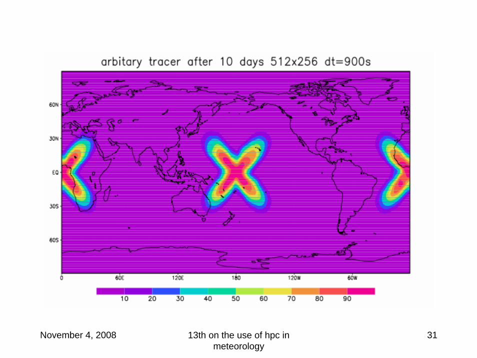
Isochronal flow• Any given point will return to its original

location after a given period of time.• Gaussian grid dimensioned 512 x 256.• Rotate coordinates so “equator” goes through

(39N,77W), thus giving flow over real poles.• Apply non-divergent global wave number 4-

20 perturbation displacement (of standard deviation size 0.1-0.2 non-dimensional vorticity) using a random number generator.

• Set return period to 10 days.


27


28


29


30


31


32

Decomposition in NCEP GFS• Current NCEP GFS uses 1D decomposition with MPI

and thread with OpenMP.• Transpose with MPI_AllToAllv is used to move

between two sub-domains for spectral transform.• First sub-domain has some given latitudes with all

longitudes grids, which is for FFT in longitudinal direction.

• Second sub-domain has some given zonal wave numbers with all meridian wave numbers, which is for Legendre transform in meridian direction.

• Transpose between two sub-domains, thus there is no halo required.


33

Implement into NCEP GFS• The same first sub-domain is used to compute semi-

Lagrangian advection in any given latitudinal global circle. All departure and arrival points are in the same circle, so no halo is needed.

• Then transpose first sub-domain to another grid-point sub-domain, which has all Gaussian latitude points but some longitude points. Therefore semi-Lagrangian advection can be computed in any given longitude with all latitude points, so, again, no halo is required.

• The PPM mass conserving between reduced grid and full grid in any given latitude is also applied.


34

np

sp

np

0 360

0 . . . . 180

<=>

Transpose

No halo is requiredNo increasing memory with

Increasing number of PE(cpu)

np.

sp

..


35

0 360

Halo Exchange

Extra memory is required,which may be as huge

as computing grid while number ofMPP cpu increases.

1D

2D

halo


36

Case test in NCEP GFS• Arbitrary date is selected.• Modify NCEP GFS IO into grid-point data.• Negative tracers are replaced with zero value

at the initial time.• T126 L64 resolution is tested.• Model physics is included.• Two runs are compared;

– control: Spectral advection in horizontal, finite difference in vertical asoperational GFS.

– nislfv: Non-iteration mass conserving positive definite semi-Lagrangian on tracers.


37

24h

72h controlnislfv


38

24 h

72 hcontrolnislfv


39

06h fcst specific humidityat model layer 40

control

nislfv


40


control

nislfv


41


control

nislfv


42


control

nislfv


43

6hr fcst cloud waterat model layer 35

control

nislfv


44


control

nislfv


45


control

nislfv


46


control

nislfv


47

6hr fcst precipitation

control

nislfv


48


control

nislfv


49


control

nislfv


50

Conclusion & Future Work• Modified traditional semi-Lagrangian without iteration to

locate mid-/departure-points, but require interpolation and remapping with temporal and spatial split computation.

• Mass conserving is included with consideration of semi-Lagrangian for divergence.

• Positive definite is applied with monotone piecewise parabolic method (PPM) for interpolation/remapping.

• Due to spatial split, no halo is required since all required data for computation are all in the partial domain through transpose. Since no halo, there is no extra memory request, but it may have more data in communication than the method with halo and small number of cpu.

• Implement all prognostic variable, not only tracers, to have larger model time step to save integration cost.

Mass-conserving and positive-definite semi-Lagrangian advection … · 2016-01-26 · November 4,...

Documents

Transcript of Mass-conserving and positive-definite semi-Lagrangian advection … · 2016-01-26 · November 4,...