Maryam Siddiqa and Muhammad Khalid Pervaiz 14.pdf · health issue of Pakistan. ... Maryam Siddiqa...
38
ISSN 1684-8403 Journal of Statistics Volume 22, 2015. pp. 219-256 ____________________________________________________________________ Identification of Significant Prognostic Factors of Dialysis Population Maryam Siddiqa 1 and Muhammad Khalid Pervaiz 2 Abstract Chronic Kidney Disease (CKD) is becoming a dreaded disease by increasing at alarming rate every year, worldwide. Globally, incidence of treated End Stage Renal Disease (ESRD) is rising at annual growth rate of 8% and one of ten individuals has any stage of Chronic Kidney Disease. The annual mortality rate in hemodialysis patients fluctuates within 10% to 25% globally and it is a critical health issue of Pakistan. In this study, combined Prognostic influence of demographic and biochemical variables was investigated to determine the best and worst prognosis for survival of dialysis receiving patients. Variety of Survival methods, Non-parametric and Semi-parametric techniques on the questionnaire based collected data has been employed in this research. Significant Prognostic factors were derived by fitting a Cox model in both Univariate and Multivariate Analysis. After checking the Adequacy of Fitted Cox model, the prediction model has been obtained with interactions of Prognostic factors at low, medium and high levels. Hazard Ratios confirmed the overall survival benefit at high level of serum albumin, high hemoglobin, low or medium inter-dialytic weight gain and low or medium potassium simultaneous reduces Hazard Rate by 99.34%. Combined effect of low level of serum albumin and hemoglobin, high level of inter-dialytic weight gain and potassium proved as more hazardous for concerned population. Complete set of interactions of main Prognostic factors has been presented that would become more beneficial to provide insight to clinicians for better survival of dialysis population. Keywords Chronic kidney disease, End stage renal disease, Hazard ratio, Dialysis therapy, Inter-dialytic weight gain ______________________________________ 1 Department of Statistics, GC University, Lahore, Pakistan. 2 Dean, Faculty of Management and Social Sciences, Hajvery University Business School, Lahore, Pakistan.
-
Upload
trinhduong -
Category
Documents
-
view
228 -
download
3
Transcript of Maryam Siddiqa and Muhammad Khalid Pervaiz 14.pdf · health issue of Pakistan. ... Maryam Siddiqa...
ISSN 1684-8403
Journal of Statistics
Volume 22, 2015. pp. 219-256
____________________________________________________________________
Identification of Significant Prognostic Factors of Dialysis Population
Maryam Siddiqa1and Muhammad Khalid Pervaiz
2
Abstract
Chronic Kidney Disease (CKD) is becoming a dreaded disease by increasing at
alarming rate every year, worldwide. Globally, incidence of treated End Stage
Renal Disease (ESRD) is rising at annual growth rate of 8% and one of ten
individuals has any stage of Chronic Kidney Disease. The annual mortality rate in
hemodialysis patients fluctuates within 10% to 25% globally and it is a critical
health issue of Pakistan. In this study, combined Prognostic influence of
demographic and biochemical variables was investigated to determine the best
and worst prognosis for survival of dialysis receiving patients. Variety of Survival
methods, Non-parametric and Semi-parametric techniques on the questionnaire
based collected data has been employed in this research. Significant Prognostic
factors were derived by fitting a Cox model in both Univariate and Multivariate
Analysis. After checking the Adequacy of Fitted Cox model, the prediction model
has been obtained with interactions of Prognostic factors at low, medium and high
levels. Hazard Ratios confirmed the overall survival benefit at high level of serum
albumin, high hemoglobin, low or medium inter-dialytic weight gain and low or
medium potassium simultaneous reduces Hazard Rate by 99.34%. Combined
effect of low level of serum albumin and hemoglobin, high level of inter-dialytic
weight gain and potassium proved as more hazardous for concerned population.
Complete set of interactions of main Prognostic factors has been presented that
would become more beneficial to provide insight to clinicians for better survival
of dialysis population.
Keywords
Chronic kidney disease, End stage renal disease, Hazard ratio, Dialysis therapy,
Inter-dialytic weight gain
______________________________________ 1 Department of Statistics, GC University, Lahore, Pakistan.
2 Dean, Faculty of Management and Social Sciences, Hajvery University Business School,
Lahore, Pakistan.
Maryam Siddiqa and Muhammad Khalid Pervaiz
______________________________________________________________________________
220
1. Introduction
The Chronic Kidney Disease (CKD) has turn into a common disorder and there is
growing number of CKD patients with worldwide rising prevalence. Researchers
documented the high prevalence of CKD in European, Australian and Asian
studies (Chadban et al., 2003; Chen et al., 2005; De Zeeuw et al., 2005 and Hallan
et al., 2006). Coresh et al. (2007) reported thatthe number of End Stage Kidney
failure patients maintained on Renal Replacement Therapy either by dialysis or
transplantation has raised a lot in USA from 209,000 in 1991 to 472,000 in 2004.
CKD is a burden because of Renal Replacement Therapy demands as well as for
overall population health.At the moment world widely, CKD is at the 12th
topmost cause of mortality and 17th
topmost cause of disability (Codreanu et al.,
2006). All over the world, incidence of treated ESRD (annual counts of new
patients/million population) is continuously increasing at annual growth rate of
8% while population growth rate is 1.3% (Schieppati and Remuzzi, 2005). The
increasing number of patients of treated ESRD is connected with the “globally
aging, multi-morbid population, the growing admission of the young population
of patients in developing countries and the higher life-expectancy of currently
treated ESRD patients” (Lysaght, 2002).
Pakistan is a developing country which does not have such policies to cure End
Stage Renal Disease due to lack of technical, human and economic resources.
Jafar (2006) reported that out of every three Pakistanis; one is suffering from any
stage of kidney disease. Effective policies to prevent the progression of Chronic
Renal Disease in developing countries have faced more challenges in
implementations (Barsoum, 2006). In Pakistan Chronic Renal failure has emerged
as a crucial medical, social and economic problem for the people suffering from
this disease. CKD preventive programs including management and control of
main prevalent risk factors of diabetes and hypertension are relatively
nonexistent. Unawareness of common people or poor symptomatic medical
practice leads Chronic Kidney Disease towards End Stage Renal Disease and
consequently patients have to bear the costly Renal Replacement Therapy.
According to the Dialysis Registry of Pakistan (2008) 6351 patients in 175
Centres are being dialyzed in Pakistan (Naqvi, 2009).
Hemodialysis (HD) is the mainstay of Renal Replacement Therapy all over the
world. In spite of the use of some other methods, above 1.7 million patients are
treated with HD in about 28, 500 dialysis units globally. The HD population was
estimated to grow to 2.0 million in 2010 (Floege et al., 2010). In economically

Identification of Significant Prognostic Factors of Dialysis Population
_______________________________________________________________________________ 221
privileged patients of CKD, only 10% can meet the expenses of dialysis.
insufficient dialysis, infections and malnutrition are the major causes of high
mortality among CKD patients globally (Barsoum, 2006).
In spite of significant advances in dialysis technology, the annual death rate in HD
patients fluctuates within 10% to 25% globally, might be a result of
demographic, geographic, cultural, economic and genetic factors differences
(Floege et al., 2010). High prevalence of CKD and costly treatment of dialysis
therapy made Chronic Kidney Disease a critical health issue of Pakistan. The
growing Burdon of Chronic Kidney Disease patients need dialysis, and still their
poor Survival Rateare signs of importance of statistical inferential research in the
field of nephrology. Thus importance is evident of identifying the significant
Prognostic factors for the better survival of this vital public health problem of
those patients who somehow made it possible to access the costly dialysis
sessions as Renal Replacement Therapy. Up till now, physicians have done few
descriptive researches related to causes of kidney failure and quality of life of
dialysis patients, but there is rare chance of any documented statistical inferential
work, regarding exploration of Prognostic factors, done by statisticians in
Pakistan. The intent of the present study is to clarify Prognostic factors for
adverse outcomes while accounting for the time varying covariates by
usingSurvival techniques. In this research, variety of Survival methods Non-
parametric and Semi-parametric techniques applied on the questionnaire based
collected data. The Proportional Hazard model is establishedas the standard
approach for Regression Analysis of survival time in various applied
settings.Significant Prognostic factors derived by fitting a Cox model in both
Univariate and MultivariateAnalysis. After assessing the adequacy of fitted Cox
model the prediction model has been obtained with interactions of Prognostic
factors at low, medium and high levels. Complete set of interactions of
marginalPrognostic factors has been presented that would be more beneficial to
provide insight to clinicians for better survival of dialysis population.
2. Patients and methods
2.1 Study population: For this research work the focused area was Punjab and
population consisted of all patients, undergoing dialysis, admitted in all hospitals
of Punjab, province of Pakistan. Target population consisted of all the patients of
dialysis, admitted in the dialysis units of 2 divisions of Punjab, during the clinical
study time of five years.
Maryam Siddiqa and Muhammad Khalid Pervaiz
______________________________________________________________________________
222
2.2 Outcome of interest and sample size: Outcome variable of interest is survival
time until an event occurs. In Cohort studies one can either, fix study time or the
number of events. Sample size depends on the availability of data that how many
individuals are included in the study during the fixed time period. For this
research, the total study time was fixed to be 5 years and data was collected
retrospectively. In order to obtain reliable estimates of Survival and Hazard
functions and their standard errors at each time interval, a feasible sample size of
dialysis patients was taken from public sector hospitals of 2 divisions of Punjab
province. Dialysis patients of 25 districts of Punjab out of 36, and combined 12
districts of Khyber Pakhtunkhwa (KPK), Northern areas and Azad Kashmir were
covered by the dialysis units of hospitals of Rawalpindi and Lahore divisions of
Punjab. These two divisions (Rawalpindi and Lahore) have well equipped tertiary
care centres in comparison with other divisions of Punjab, easily accessible to
nearby remote areas with trained staff and equipment to treat dialysis patients.
That is why even patients from other cities prefer to come here weekly (once or
twice) to attend dialysis sessions instead of undergoing treatment in newly
established medical units in nearby districts due to lack of up to mark staff and
equipment. For these reasons hospitals of these two divisions for data collection
was covered. Various researchers such as (Abbott et al., 2004; Chandna et al.,
1999; From et al., 2008; Herzog et al., 2005; Holland and Lam, 2000 and Pastan
et al., 2002) have used hospital based data from dialysis units of Chronic Kidney
Disease patients by fixed time period of study.
2.3 Retrospective / Historical Cohort study: Generally, study design comprises of
two types; studies wherein subjects are kept under observation and studies where
the outcomes of an intervention (treatment) are observed. The type of study
design where the subjects are scrutinized is described as observational studies.
Cohort study is a “forward-looking” (starting from a risk factor to an outcome)
observational study where a cluster of patients are followed longitudinally over a
period of time. In medical studies the patients of Cohort are chosen by some
significant distinctiveness supposed of being a sign of a disease or health
consequence. Numerous Cohort studies are also carried out by using previous
particulars saved in records and annals. Validity of these studies is frequently
dependent on medical records and memory. Several investigators such as, (Abbott
et al., 2004; Chandna et al., 1999; From et al., 2008; Herzog et al., 2005; Holland
and Lam, 2000; Huang et al.,2006; Pastan et al., 2002 and Slinin et al., 2005)
named this type of study a Historical Cohortstudy or Retrospective Cohortstudy,
due to the reason that information from previous studies is utilized in these studies
and the events become apparent earlier than at the beginning of study. However in
Identification of Significant Prognostic Factors of Dialysis Population
_______________________________________________________________________________ 223
the Historical Cohortstudy the tendency of the query is further survival time, from
a probable ground or risk factor to the outcome (Dawson and Trapp, 2004).
2.4 Data inclusion criteria: All patients with Chronic Renal failure who are
treated with maintenance hemodialysis at the various dialysis centers of Punjab,
and have been on Hemodialysis for at least 3 months were eligible for inclusion in
the present study. The Analysis was performed upon only those patients who
survived for at least 90 days after undergoing hemodialysis. This study is a
Retrospective follow-up study and the clinical patients were followed through the
medical charts until death or 30th December 2012, whichever came earlier.
2.5 Potential Prognostic factors: Values of the studied clinical variables such as,
hemoglobin, serum phosphate, serum potassium, serum albumin, serum
creatinine, inter-dialytic fluid weight gain for each patient were updated every 3rd
month in order to minimize the measurement variability and reduce bulk of data
(Kalantar-Zadeh et al., 2009).Collected data included age, gender, date of start of
dialysis, age at start of dialysis, and duration of dialysis at entry of study/months,
collected by reviewing the medical records. Laboratory and clinical data included
serum albumin, pre dialysis creatinine, pre dialysis urea, serum potassium, serum
phosphate, hemoglobin, inter-dialytic weight gain, post dialysis weight. Also, the
type of dialysis membrane, duration of dialysis hours per session and frequency of
dialysis were incorporated in the dialysis prescription data. Variables, covariates
and Prognostic factors are interchangeably used in this document.
3. Statistical methods
Descriptive Analysis of Prognostic factors is based on Kaplan Meier Survival
functions (1958) and related computations that provide insight for demographic
and clinical covariates. Continuous Prognostic factors were analysed by Cox
(1975)Regression and Categorical Prognostic factors were explored by
performing the Kaplan Meier and the log-rank methods for Univariate Analysis.
The Cox (1975) Proportional Hazards model or Cox Regression is a renowned
Regression technique and extensively applied approach to analyze the time to
event data, and to study the impact of numerous risk factors on survival
concurrently. Cox (1972) proposed this approach by using an expression he
referred as partial Likelihood function that means, model depends only on the
parameter of interest. Cox (1972) made the supposition that yielded parameter
Estimators from Partial Likelihood function hold the same Distributional
properties as that of Maximum Likelihood Estimators. Foremost characteristics of
Maryam Siddiqa and Muhammad Khalid Pervaiz
______________________________________________________________________________
224
Cox (1975) modeling consists of, measure of association by the relative risk,
refusal parametric assumptions, the utilization of the Partial Likelihood function,
obtaining of Survival function estimates and deriving effects of numerous
covariates (Collett, 2003 and Hosmer et al., 2008). Another aspect of Cox (1975)
Regression is, it does not have to go for the density function of a Parametric
Distribution, which implies that Cox’s (1972) Semi-parametric modeling has no
need for assumptions to be made about the Parametric Distribution of the survival
times, which confirms that technique is obviously more robust and flexible.
Instead of Parametric assumptions, the researchers have required to only confirm
the assumption that the Hazards are proportional over time and the Hazard Ratio
remains constant over time. The Proportional Hazards assumptions support the
fact that the Hazard functions are multiplicatively related, that is the effect of a
unit increase in a covariate is multiplicative with respect to the Hazard Rate. The
probability of the endpoint, whatever death or recurrence of disease, is described
in terms of hazard. The implementation of this modeling technique is referred by
CoxProportional Hazards model, Cox Regression model,Proportional Hazards
model and Semi-parametric Hazard model. Hence, Semi-parametric Regression
models have fully Parametric Regression structure with unspecified time
dependence (Hosmer et al., 2008).
Model based inferences completely rely on the fitted statistical model. After
completion of steps of fitting the model, the adequacy and validation of that
model should be assessed as an essential part of modeling process as well as
careful development of model. Cox (1975) Proportional Hazard model is most
extensively performed popular procedure for conducting Analysis of time to event
data in clinical research. Visual inspection of data would not be informative due
to several explanatory variables, and the scenario has become more complicated
due to the presence of censoring and the use of the Partial Maximum Likelihood
function for Proportional Hazard models. As for as, presence of censored survival
times make it slightly more complex to identify features of model adequacy than
analogous methods employed in Linear Regression modeling (Collett, 2003 and
Wilson, 2013). Residual based diagnostics generally applied to check the
adequacy of fitted Cox (1975) Model. All statistical Analysis was performed by
using STATA 12 and SPSS statistical package version 17.
4. Results and discussion
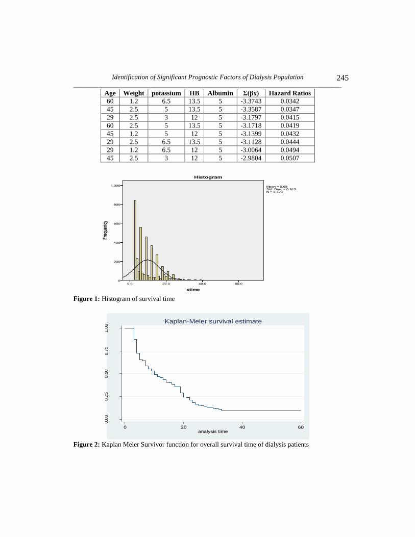
4.1 Patients characteristics: To acquire the graphical display of Distribution of
survival time, Histogram was plotted along with survival time and frequencies in
Identification of Significant Prognostic Factors of Dialysis Population
_______________________________________________________________________________ 225
Figure 1. The pattern shows unimodality with positive Skewness. High peaks
show the majority of events (death) occurring in starting 20 months of the total
follow up time. Maximum number of deaths occurred at 3rd
month after initiation
of dialysis treatment.
The overall survivor function for the 5 years of survival time by using Kaplan
Meier Survival Estimates is presented in Figure 2. In dialysis therapy, patient
survival is undeniably the most important question. From Non-parametric
Survival curve the sample median survival time for the target population is
estimated approximately 11 months.
Graphs of Kaplan Meier Survival Estimates are plotted for different categorical
covariates with their levels, to have understanding about their survival pattern,
and proportionality. The upper survival curve shows long survival time for that
particular level while the lower curve shows short survival time for corresponding
level.
Comparison of the both gender groups, using Kaplan Meier Estimates is provided
by a graph of Survival function. The plot of the survival probabilities is referred
to as a step function. Horizontal lines show the probability of survival stay at the
same point in time period, and long horizontal lines show no change in survival
probability for a long period. The graph shows that the Survivor function for the
females group lies above the males from 5th
month of follow up to onward. This
difference indicates that Females group has better survival at those follow-up
times. Though, in the first 5 months of follow-up, the two Survival functions are
closer together, but thereafter relatively spread apart. This widening gap suggests
that the survival of females group improved later during follow-up than that of
beginning point. From plot of Survival function, median survival time for female
is 15 months while for male is 10 months.
Among all categories of age at start of dialysis, 2 categories “age greater than 50”
and “age 40-49” exposed short survival time than other age categories. Frequency
of dialysis “once” a week has shorter survival time and thrice dialysis sessions per
week showed increase in survival time. It is logical that patients with no exposure
of incidence of hepatitis would achieve more survival time among rest of
categories but it is important finding that patients with B+ hepatitis had lower
survival in comparison to C+ hepatitis. “No” hospital acquired hepatitis gave
higher survival as well as both other categories B+ and C+ showed almost same
survival time. “None” co-morbidity had advantage of survival for patients under
dialysis and patients with “Cardio vascular diseases” had less chances of survival
Maryam Siddiqa and Muhammad Khalid Pervaiz
______________________________________________________________________________
226
as compare to other categories. Dialysis duration of greater than 24 months at
entry of study revealed higher survival time for patients as compared to less than
6 months, 7 – 12 months and 13 -24 months. It shows more rapid decline of
survival on the beginning of survival therapy and improvement in condition of
patients later on as duration on being dialysis increased with no worsening effect
of survival on increased duration of dialysis. Some major “causes of kidney
failures” are summarized in one variable and it is notable that “drug induced
(including Hikmatand peers prescriptions)” patients have lowest chances of
survival than rest of causes upsetting the functions of kidney.
Graphical representation of Product Limit Estimate established that survival time
is varying within the levels of factors. A statistical test would be useful to confirm
whether Survival curves are statistically differing with each other or just due to by
chance variation. Log Rank test (Nathan, 1966) is a Non-parametric test and can
be used to compareSurvival curves.It is a formal method for testing hypotheses
about survival, in two or more groups. By Log Rank test of categorical variables,
incidence of hepatitis and gender, age at start of dialysis, frequency of dialysis,
hospital acquired hepatitis, co-morbidity, causes of dialysis and dialysis duration
differ significantly within their categories. It is indication of significant
fluctuation of survival time among levels of categorical variables.
4.2 Univariate Analysis: Cox (1975) Regression model is used to determine the
impact of potential covariates on survival time of patients by Univariate Analysis
primarily given in Table 1.Univariate Analysis depicts that all variables have
significant effect on survival time of patients after being dialyzed except age at
start of dialysis (category 2), frequency of dialysis, incidence of hepatitis, causes
of ESRD (except drug induced), Co-morbidities and serum urea. Female gender
group expressed more chances of survival over male group. Younger group of
patients showed greater survival than, older age patients and those who delayed to
switch over to dialysis therapy. Those patients who dialysed thrice a week showed
more Survival Rates as compared to those undergoing dialysis twice a week.
Instead of exposure to hepatitis, hospital acquired hepatitis proved to be more
hazardous for survival of patients for both B+ and C+ hepatitis. Greater dialysis
duration (months) has also shown better survival than initial months of therapy.
Increase in inter-dialytic weight gain, urea, potassium and phosphate cause
decrease in survival time and high rate of early death, whereas increase in
hemoglobin and serum albumin would reflect in increased survival.
Identification of Significant Prognostic Factors of Dialysis Population
_______________________________________________________________________________ 227
Ours were the same findings from Univariate Analysis of each variable in relation
to survival time (in years) alike with Descriptive Analysis and Kaplan Meier
Survival Analysis. Univariate Analysis provided the understanding of association
of survival time and each of the covariate under consideration. Simultaneous
study of variables through Multivariate Analysis would clarify the consequences
of significant variables that have influenced survival. Cox (1975) Proportional
Hazard Regression Analysis is performed for Multivariable model building.
4.3 Assessment of adequacy of fitted Cox model: As for concern of Proportional
Hazards (PH) Regression model, there are two important assumptions that need
the satisfaction to allow one to trust on the statistical inferences and predictions of
established model. The first assumption is called PH assumption that is, the ratio
of the Hazard function for two individuals with different explanatory variables,
does not differ with time, in other terms, the Hazard Ratio remains constant over
time. The second assumption is about the relationship between log cumulative
hazard and a continuous predictor variable (covariate), should be linear (Collett,
2003; Hosmer et al., 2008 and Wilson, 2013). Residual based diagnostics are
particularly used for Cox (1975) model. Residuals are the central part of
evaluation of model adequacy in all settings of Regression models. The values of
residuals are calculated for each individual in the data set. Several residuals have
been proposed related to Cox Regression model for evaluating specific aspect of
model adequacy.
4.3.1 Test of proportionality assumption of Proportional Hazard model:
Schoenfeld residuals are generally applied to discover departures from the
Proportional Hazards assumption. If there exists a pattern in the plot of residuals
versus survival time, then Proportional Hazard assumption will be questionable.
Tests and graphical display for Proportional Hazards based on the scaled
Schoenfeld residuals were proposed by Schoenfeld (1982). He proposed the initial
set of residuals to check the fitted Proportional Hazard model. Grambsch and
Therneau (1994) proposed that scaling the Schoenfeld residuals by an Estimator
of its variance provides a residual having superior diagnostic power in
comparison of unscaled residuals. As Schoenfeld residuals are based on the
effects of the covariates that are supposed to be independent of time, consequently
plot of these residuals opposed to time is a visually assessing method to see the
effect of the covariates varying over the follow-up span. Number of procedures
are found in literature to check the Proportionality assumption but Grambsch and
Thernue (1994) and simulations by Ng’andu (1997) suggested an easily employed
test and associated graphical representation which is a useful evaluation of this
Maryam Siddiqa and Muhammad Khalid Pervaiz
______________________________________________________________________________
228
vital assumption (Collett, 2003 and Hosmer et al., 2008). The result of test is
summarized in Table 2.
The null hypothesis tests whether the Log-Hazard Ratio remains constant over
time. Accordingly rejection of null hypothesis indicates deviations from the
Proportional Hazard assumption. It’s obvious that global 12 degrees of freedom
test = 0.1868 is not significant. There is no evidence of violation of Proportional
Hazard assumption. Moreover, the covariate specific test provides the details of
proportionality of each covariate so that there is no chance to miss out non-
proportionality of any covariate summarized in Figure 3-7. Even though the
graphical method of assessment of the validity of assumption is subjective
approach, still it is a supportive tool. Graphical assessment of violation of PH
assumption yield the same information like statistical test, implying that PH
assumption has not been violated. Appropriateness of Cox (1975) Proportional
Hazard model for current data is confirmed by both test and graphical method.
4.3.2 Test of linearity assumption of Proportional Hazard model: The
Martingale residuals have been recommended as promising diagnostics for the
correct functional form (Therneau et al., 1990). Nonlinearity is actually
incorrectly specified functional form in the Parametric part of the model and a
probable difficulty in Cox (1975) Regression as it is in linear and generalized
linear models. The martingale residuals are plotted versus each covariate to detect
nonlinearity and functional form of that covariate. Generally the resulting graph
seems to be very noisy and to ease the interpretation a loess or lowess smoothed
line proposed by Cleveland (1979) has been superimposed to the plot and the
form of the smoothed line indicates an Estimate of the functional form of the
covariate in the model. If the smoothed line is reasonably linear, then the chosen
scale considered appropriately linear in the Log-Hazard. If considerably departure
of smoothed line from a linear trend exists, then the shape can give idea to correct
the scale of covariate in the model (Hosmer et al., 2008 and Wilson, 2013).
Nearly flat and horizontal Lowess smoothing line is considered sufficient for the
fulfillment of linearity assumption.
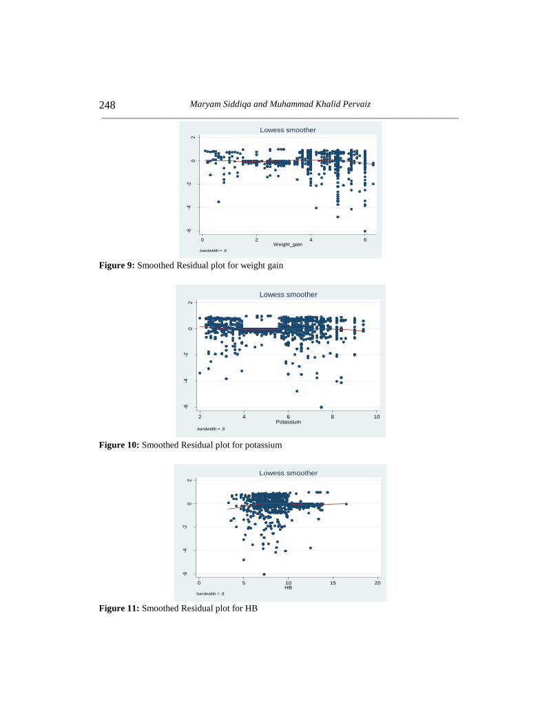
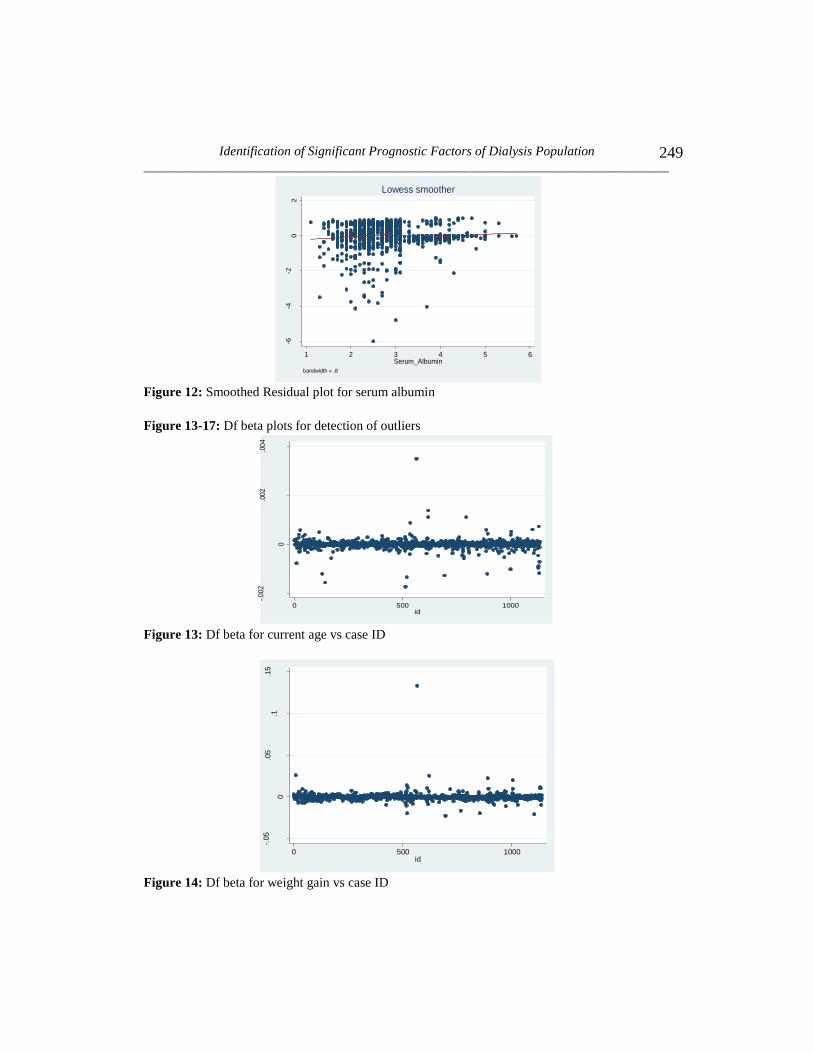
Smoothed Residual Plots for Linearity of covariates are given in Figure 8-12.
Martingale residuals are useful in assessing the functional form of a covariate to
be included into Cox(1975) model. The smoothing lines appear in all figures
almost log linear for each covariate, supporting the inclusion of untransformed
version of covariates into Cox model.

Identification of Significant Prognostic Factors of Dialysis Population
_______________________________________________________________________________ 229
4.3.3 Influential diagnostics of Cox Proportional Hazard model: Identification
of unusual impact of particular observations, on inferences based on fitted model,
needs to be assessed. These kinds of observations are referred as influential
observations. There is approach of delta-betas for assessment of these suspicious
observations. First the model estimated with full data set, then after omitting the
effect of ith
observation, model is refitted to assess the effect on estimates by
comparing the original measures of that full data set. Cain and Lange (1984)
presented an approximation based on scale residuals. Plots of delta-betas for each
covariate would provide better description of those observations which have
substantial impact on Parameter Estimates for any particular covariate. Moreover,
Plots of delta-betas versus rank order of survival time can present the information
which has concern about influence (Collett, 2003).
From Figure 13-17 of the Df beta, Plots it can be identified that the observations
maybe, are the influential values. We can see these observations are far away
from most of the other observations and these points need particular attention.
From all graphs, no influential observation is found which exceeds cut-off
criterion. By examining theses values in more detail, none of the observations
appeared as terribly influential individual, even though they are large values
compared with others. Observation of ID 565 stands out away from all other
points shown in the graphical presentation. It contains high values explained in
descriptive statistics. After removal of the ID 565 the ID 620, 37 and 796
appeared as influential observations in graphs of Df beta. That’s happened due to
widening of the gap of vertical lines that some other observations appeared as
influential observations. In fact these observations are not influential
observations, might be shown as, due to unusual or unexpected survival behavior.
For instance, in spite of better survival condition based upon clinical and
laboratory tests suddenly death occurred for that patient or in reasonably bad
condition prolonged life of patient, might be the reason of lying far away of these
observations. It is common behavior in survival data and didn’t cause much
concern. Even though the removal of these kinds of observations especially in
survival data is not considered a good practice, we obtained the Cox model’s
standard errors for the sake of comparison of with and without influential
observations. The resulting differences were very small, that had no practical
importance, and consequently those suspicious observations were retained in the
data set.
4.3.4 Multicollinearity: Multicollinearity is also verified through method of
Variance Inflation Factor (VIF). None of VIF value goes above 10, so we can
conclude that no severe multicollinearity was present there between covariates.
Maryam Siddiqa and Muhammad Khalid Pervaiz
______________________________________________________________________________
230
4.3.5 Goodness of fit of final Cox Model: Goodness of Fit of Cox(1975) model
is verified by the Cox-Snell (1968) residuals. The Nelson Aalen cumulative
Hazard function was graphed with the calculated Cox-Snell variable, so that
Hazard function to the diagonal line can be compare. If Hazard function follows
the 45 degree line, then it approximately has an Exponential Distribution with a
Hazard Rate of one and that model is considered appropriately fit to data. In
Figure18 it could be seen that Cox model does not fit the data too badly.
4.4 Multivariate Analysis: Approach of purposeful selection of covariates to a
Proportional Hazard model has been followed to search out a set of statistically
and clinically significant covariates. At earliest step of fitting a Multivariable
model all covariates were included, that appeared significant in the Univariate
Analysis as well as those variables that have clinical importance nevertheless of
their significance (Hosmer et al., 2008). Except urea, causes of ESRD and
incidence of hepatitis all other variables are included in the model at this step.
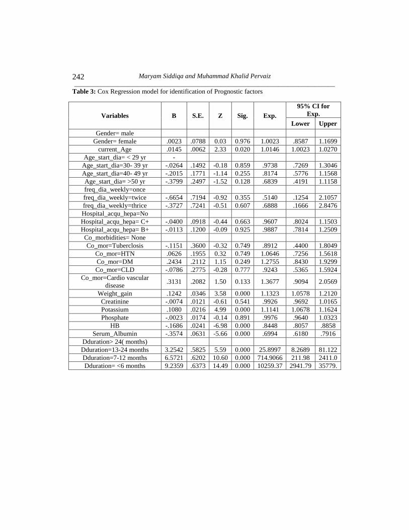
Results of this Multivariable model are summarized in the Table 3.
By performing Multivariate analysis, age at start of dialysis, frequency of dialysis,
hospital acquired hepatitis and co-morbidities are clearly not significant and are
dropped from the model step by step based on their significance level.
Hence current age, weight gain, potassium, hemoglobin, serum albumin and
dialysis duration were potential candidates for being included in main effect
model given in Table 6. In recent years, researchers gave attention to these
clinical covariates in their studies as important Prognostic factors. Hatakeyama et
al. (2013) had evaluated prognosis in Japanese hemodialysis patients aged ≥80
years. In his study, large differences of survival time also clarify the picture as
low risk group had 63 months, while other groups had 23-24 months survival
time. They concluded that theold age is no more considered as contraindication
for initiation of hemodialysis therapy. Hatakeyama et al. (2013) findings are in
line with the previous several reports by (Faller et al., 2013; Joly et al., 2003;
Neves et al., 1994; Rohrich et al., 1998; Schaefer and Rohrich, 1999 and Vandelli
et al., 1996) had studied indications and survival behavior of maintenance dialysis
in elderly patients. Hemodialysis therapy in elder age group is now considered an
established reality from recent decade. Earlier outcomes of different studies lead
towards conflicting conclusions. Vandelli et al. (1996) stated that by maintenance
on dialysis therapy, patients would be able to avoid the death from uraemia, but
Survival Rate for such patients is substantially low in comparison to general
population. The mean expected life time would remain only 9.3 years for those

Identification of Significant Prognostic Factors of Dialysis Population
_______________________________________________________________________________ 231
who started dialysis at age of 40, and 4.3 years for those who started at age 59,
compared with those of 37.4 and 20.4 years for general population for the same
age. Although Survival Rate of elder patients found in some studies less than the
general population, Vandelli et al. (1996) concluded that old aged patients can
attain improved Survival Rate and their quality of life can be improved by taking
under consideration main determinants of survival like, cardiovascular diseases,
nutritional status and adequacy of dialysis treatment. Joly et al. (2003) supported
the outcomes of earlier studies in favor of initiation of dialysis treatment for elder
patients, like younger patients. Although patient’s individual refusal, late referral,
social isolation, low functional capacity, and diabetes affect the survival of elder
patients but it is established reality that majority of such patients experienced a
extensively prolonger life. Contradictory concluding had been made by Munshi et
al. (2001) by suggesting that very old aged patients on dialysis therapy contained
poor prognosis might be because of late referral to Renal Replacement Therapy
(RRT) as an emergency admission, possibly could be a significant predictor for
poor prognosis of RRT, suggested by also (Byrne et al., 1994; Eadington,1996;
Jungers et al., 1993 and Ratcliffe et al.,1984).
Naves et al. (2011)concluded on the basis of Multivariable-adjusted Hazard Ratio
that low level of serum albumin was associated with increased mortality rate.
Iseki et al. (1993) also presented the similar type of relationship for serum
albumin as predictor variable and the impact on survival of chronic hemodialysis
patients. He identified serum albumin as strong predictor of mortality among
chronic hemodialysis patients and suggested that low level of serum albumin
should be cautiously treated.
For inter-dialytic weight gain Kalantar-Zadeh et al. (2009) chose Cut-off level of
1.5 kg, supported by Rodriguez et al. (2005) who suggested an inter-dialytic fluid
gain less than 1.5 to 2.0 kg as the most favorable target beneficial for survival of
patients. Kalantar-Zadeh et al. (2009) concluded that higher Inter-dialytic weight
gain proved to be related with higher risk of death. He categorized different
subgroups of dialysis patients and on the basis of outcomes suggested that inter-
dialytic weight gain >1.5 kg is associated with mortality and minimum inter-
dialytic fluid retention <1.0 kg had a considerable survival benefit. Researcher
proposed these findings on basis of 2-year period of the Cohort instead of a
longitudinal follow-up of several years, this limitation of study may have the
consideration. Kalantar-Zadeh et al. (2009) concluded results by using
Univariateanalysis that elevated Inter Dialetic Weight Gain (IDWG) linked with
better survival, but findings of MultivariateAnalysis no longer supported the
earlier findings of Descriptive Analysis. Increase in Inter-dialytic weight gain
Maryam Siddiqa and Muhammad Khalid Pervaiz
______________________________________________________________________________
232
showed association with high risk of mortality. Kimmel et al. (2000) had also
found similar type of relationship between Inter-dialytic weight gain and survival.
Kimmel et al. (2000) conducted an observational longitudinal study to determine
the relationship of IDWG and survival, with adjustments of several medical and
dialytic risk factors. Assessment of the relative death risk of higher IDWG
resulted in association of higher mortality risk with higher IWG (De-Nour and
Czaczkes.,1972; Manley and Sweeney., 1986; Leggat et al., 1998 and Agashua et
al., 1981) employed diverse ways for defining IDWG and the level of IDWG had
been reported in different studies. Kimmel et al. (2000) adopted more precise
method to measure IDWG with continuously updated dry weight.Percentage of
IDWG for each day in thrice a week sessions over every month was computed
and average of measurements for three-month period was calculated. None of the
previous study had identified the relationship between IDWG and mortality
among HD patients, adjusted for numerous medical risk factors. The effect of
IDWG on survival was not obvious in preceding studies. Leggat et al. (1998)
stated that HD patients with more than 5.7% IDWG had a 35% higher risk of
mortality, in case of missing or shortening HD sessions risk of mortality would be
higher. Koch et al. (1993) in a multicenter European study did not find and
documented any association of IDWG and higher mortality risk in ESRD patients
who had diabetes. Lopez et al. (2005) also explored the Prognostic effect of inter-
dialytic weight gain and its consequences on nutritional status. Findings of
Univariate Analysis suggested that excessive IDWG related with better nutritional
status and higher percentage of IDWG may be predictor of better long term
prognosis of patients. Lopez et al. (2005) concluded that, higher pre dialysis
IDWG had negative aspect, even though beneficial impact of IDWG upon
nutritional status and prognosis is more valuable and cannot be ignored.
Kovesdy et al. (2007) examined the association between predialysis serum
potassium levels and mortality. Predialysis serum potassium between 4.6 to 5.3
mEq/L was reported to be associatedwith the higher survival of patients, while
potassium <4.0 or >5.6 mEq/L resulted in association with increased mortality.
After adjustments results remained consistent and did not show any difference for
higher serum potassium >5.6 mEq/L on death risk, consistent with the results of
Bleyer et al. (1999) and Bleyer et al. (2006).
Gilbertson et al. (2008) verified the associations between the degrees of
hemoglobin level variability in hemodialysis patients receiving erythropoietin
therapy. Levels of hemoglobin were calcified as low L= < 11 g/dl, intermediate I
= 11 to 12.5 g/dl, and high H = >12.5 g/dl. Patients whose hemoglobin levels
Identification of Significant Prognostic Factors of Dialysis Population
_______________________________________________________________________________ 233
were constantly placed within the target range of 11 to 12.5 g/dl had lowest
chances of mortality. Also the longer time duration with a hemoglobin level < 11
g/dl, resulted in higher risk of death. Furthermore, the time duration of the low
hemoglobin value within the 6 months period was strongly linked with higher
mortality risk. Along with, patients experiencing the least numbers of months
with hemoglobin levels below the recommended range of 11 to 12.5 g/dl had
chances of lowest mortality risk. The results of current study elaborated that there
is significant association between particular hemoglobin variability patterns and
increased risk of death. Gilbertson et al. (2008) concluded that particular exposure
measurement period to be precise, number of months with values of hemoglobin
below the target range, instead of hemoglobin variability itself, probably be the
primary driver of improved risk of mortality. Regidor et al. (2006) explored
associations between baseline hemoglobin values and survival accounted
longitudinal variations in clinical and laboratory measures of maintenance
hemodialysis patients. Hemoglobin levels stable at 12 to 13 g/dl were shown to be
associated with greatest survival and the lower range of the hemoglobin range (11
to 11.5 g/dl) suggested by Kidney Disease Quality Outcomes Initiative was found
to be associated with a higher death risk compared with the 11.5- to 12-g/dl range.
Additionally independent of baseline hemoglobin, rise or drop in hemoglobin
with time was proved to be associated with increased or decreased death risk
respectively. In spite of, in previous studies (Collins, 2002; Collins et al., 2000
and Locatelli et al., 1998 and Locatelli et al., 2004) had examined the associations
between baseline hemoglobin levels and survival in patients of CKD, without
bothering about the changes in hemoglobin levels over time. Ofsthun et al. (2003)
reported the association of higher hemoglobin level more than the current Kidney
Dialysis Outcomes Quality Initiative (K/DOQI) recommendations with increased
risk of death. They examined both extremely low and high levels of hemoglobin
to discover any negative effect for any case. Patients with hemoglobin< 9 g/dL
showed the lowest proportion of patients surviving, and patients group with
hemoglobin>13 g/dL showed the highest proportion of patients surviving over
time. On basis of these results Ofsthun et al. (2003) established the findings that
hemoglobin higher than the current recommended values is not associated with
increased risk of death. Also Positive link between survival and high hemoglobin
level reported by Collins et al. (2001), Ma et al. (1999) and Xia et al. (1999),
supported the results of Ofsthun et al. (2003).
The final step of variable selection process is consideration of interaction terms in
to the main effect model. To check the effects of interactions without prior
knowledge of important interactions, the selection process started by forming a set
of all plausible interactions, including all marginal variables and just one

Maryam Siddiqa and Muhammad Khalid Pervaiz
______________________________________________________________________________
234
interaction in the model at one time. After that resulting significant interactions at
5% level of significance were added simultaneously to the marginal effect model.
Selected interaction terms for the final model were based on p-values of statistical
significance. Most of the time with insertion of interaction term in the model, it is
quite possible that any marginal effect variable of that interaction appears with an
insignificant Wald test due to the reason that estimates of effect required the
marginal effects and interaction effect simultaneously. Though insertion of
interaction terms made model more difficult to interpret but on the other hand
provides improved inferences, more realistic and informative model. Subsequent
to evaluation of model diagnostics and assessment of overall goodness of fit
model, it is referred to as final model. Results of the final model with significant
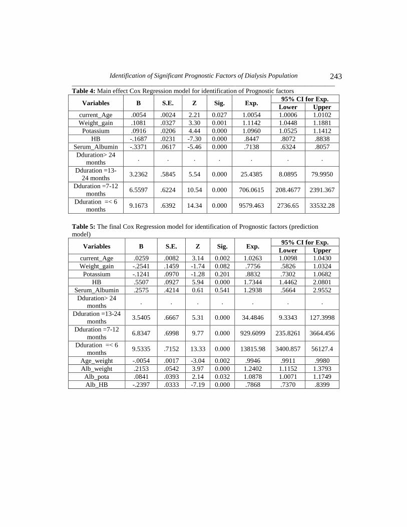
predictors would be useful for prediction purpose presented in Table 5.
Comparison of the model with interaction, to the model without interactions can
be made by Likelihood Ratio testwith assumption that models are nested.The
significant p-value = 0.00 with 4 degree of freedom supported the rejection of null
hypothesis that the two models fit the data equally well and concluding that the
bigger model with interactions fits the data better than the smaller model which
did not include the interactions.
Cox (1975) Proportional Hazard Regression technique was applied to explore the
impact of fixed and time varying covariates on survival of dialysis patients.
Current age, inter-dialytic weight gain, serum potassium, hemoglobin, serum
albumin and duration of dialysis proved to be significant variables with respect to
death. As Likelihood Ratio test referred the model without interactions to be
incorrect Model. Since, it is pointless to interpret the non-informative modeland
marginal effects of covariates which are already included in the interaction terms.
4.4.1 Interpretation of final model (prediction model) in terms of Hazard
Ratios: Duration of dialysis in months is an only variable which in not included in
interaction terms. For this variable all categories are significantly associated with
risk of death. Dialysis duration time category 2 “13 – 24 months” has (1-
34.4846=-33.4846) 33 times more chance of death of patients during this interval
than interval of “greater than 24 months”. Dialysis duration time category 3 “7 –
12 months” has (1-929.6099=- 928.6099) 928 times more chance of death of
patients during this interval than interval of “greater than 24 months”. While
duration of “less than 6 months” exposed out with (1-13815.98=- 13814.98)
13814 times more chance of death of patients during this interval than interval of
reference category “more than 24 months”.

Identification of Significant Prognostic Factors of Dialysis Population
_______________________________________________________________________________ 235
In this model, 4 interaction terms of main variables were proved significant.
Interaction of Age*ID weight gain showed .53% (1- .9946083= .0053917) chance
of decrease in death risk with one percent increase in combined effect of age and
ID weight gain from low range to high range. Similar trend can be seen for
interaction of serum albumin*HB. One percent increase from low range to high
range of combined effect of Serum albumin and HB has 21.32% (1-
.7868289=.213171) chance of decrease in death risk for dialysis patients.
Interaction of serum albumin and ID weight gain showed 24% (1-
1.240298=.240298) increase in Hazard Risk. Moreover, simultaneous increase in
combined effect of serum albumin and potassium have 8.78% (1-
1.087844=.087844) more chance of death for the current dialysis population.
Here, marginal effect is an approximation of how much the survival time is
expected to increase or decrease for a unit change in any covariate, by ignoring
the effect of all other covariates. Occasionally, we are also interested in that how
the variation in one covariate changes the effects of another covariate, or change
in one covariate effects the results of another covariate, that is, the interaction
effect. In statistical perspective, it can be described as deviation from conditional
independence. For instance, we all know that exercise is always better than
sedentary lifestyle for overall health as well as for weight reducing purpose, and
in the same way diet selection is always better than unhealthy food. These are the
established marginal effects, but diet selection and exercise coming together
would be particularly more effective than either diet selection or exercise only.
To study possible interaction effects, it was assessed whether the different
conditions for a covariate produce results that vary, depending on the conditions
that were considered for a second covariate. Another way to find out is to check if
the effect of a clinical covariate on disease risk differs among individuals with
different levels of clinical covariate. We have to look forward for the combined
effects of covariates, as there is more to consider than simply the marginal effect
of each covariate. The effect of one independent covariate depends on the level of
the other independent covariate and different levels of covariates yield different
interaction effects leaving the marginal effects not interpretable individually.
In order to explain the interaction effects of covariates at different levels 35
factorial design was applied, in which the five independent covariates are crossed
with one another with the intention that there are observations at every
combination of levels of the five independent covariates. To obtain numerical
value of different interaction combinations at low, medium and high level of five
Maryam Siddiqa and Muhammad Khalid Pervaiz
______________________________________________________________________________
236
variable’s meaningful values were taken at random from their low, medium and
high ranges.
4.4.2 Interaction effects of covariates at low, medium and high levels in Cox
model: Following Table 6 and Table 7 represents only highest 10% and lowest
10% (respectively) of Hazard Ratios in ascending order to have an idea about the
effects of covariates at different levels.
In this study, we inspected the joint Prognostic influence of demographic and
biochemical variables, to ascertain the Prognostic information for best and worst
survival of dialysis receiving patients. Significant interaction effects at low,
medium and high levels of covariates made the picture clearer. Hazard Ratios
explained some of the survival advantage (low Hazard Risk) at high level of
albumin, medium or high hemoglobin, low or medium ID weight gain and low or
medium potassium at the same time. Simultaneous effect of low level of serum
albumin and hemoglobin, high level of ID weight gain and potassium proved to
be more hazardous for concerned population.
Lowest Hazard Ratio 0.0066 explained (1-0.0066=0.9933) 99.34% reduction in
Hazard Risk for the patient who achieved lower level of weight, lower level of
potassium, higher level of hemoglobin and higher level of albumin with less age.
Such a 99.34% lower Hazard Risk would be a best ever possible condition for
current population under study. Possible worst condition of a patient under
dialysis would be with highest Hazard Ratio (1-7.7496=6.7496) of 6.74 times
more Hazard Risk with higher weight gain, higher potassium level, lower
hemoglobin level and lower albumin level irrespective of age. On the whole at
high level of serum albumin and hemoglobin, low level of ID Weight gain and
potassium, all together, with three age group of patient (low, med, and high)
demonstrated better survival condition and good prognosis for such patients,
reducing Hazard Risk by (99.34%, 99.09%, 98.80% resp.)
Furthermore, it’s noticeable that there are some specific conditions which
breached the typical trend. At high level of serum albumin and hemoglobin, low
level of potassium and lower age group and lower ID Weight gain, all together,
reduced Hazard Rate by 99.34%, compared to those patients with transformation
of level of low ID weight gain to medium ID weight gain showing reduction in
Hazard Rate by 98.42%. Besides this high level of serum albumin and
hemoglobin, low level of potassium and medium age group and medium ID
weight gain showed 98.07% decreased Hazard Risk and joint effect of high level

Identification of Significant Prognostic Factors of Dialysis Population
_______________________________________________________________________________ 237
of serum albumin and hemoglobin, low level of potassium and higher age group
and medium ID weight gain showed 97.68% decreased Hazard Risk, which is
slightly increased Hazard Risk as compared to low level of age group and ID
weight gain. On the other hand its worth mentioning, with lower hemoglobin level
and lower albumin level, higher potassium level and higher weight gain, there is
increased Hazard Risk for older age groups (6.50 times) as compared to medium
(6.61 times) and low age groups (6.74 times). These results suggested that
increase in levels of weight gain will be more harmful than that of older age of
patients, and will yield more increase in Hazard Risk.
To illustrate the mix effect of weight gain and albumin, we have particular
situations in that, low age group, higher potassium, lower hemoglobin level and
higher weight gain with rise in levels of albumin from low to medium level
increased Hazard Risk 6.64 times and 5.56 times respectively. Moreover, low age
group, lower potassium, higher hemoglobin level and higher albumin with rise in
levels of weight gain from low to medium level represented reduction in Hazard
Risk by 99.34% and 98.42% respectively. So that low reduction in Hazard Rate at
higher level of weight gain showed harmful effects on survival of patients.
As reported earlier with high level of serum albumin, high level of hemoglobin,
lower age group, lower ID weight gain and low level of potassium all together
reduced Hazard Ratio by 99.34%. Keeping constant levels of other covariates and
rise in levels of potassium up to medium and high level proposed decline in
Hazard Risk by 98.80% and 98.12% respectively. It’s clear that decline in Hazard
Risk goes on decreasing further by increasing the levels of potassium. Similarly,
at higher ID weight gain, low level of hemoglobin, any of three age groups, low
level of serum albumin and higher level of potassium gave about 6 times greater
Hazard Risk. In another case, with low level of hemoglobin, lower age group,
higher ID weight gain and higher level of potassium with low and medium level
of serum albumin revealed 6.74 times and 5.56 times increased Hazard Risk,
respectively. Increase in Hazard Risk is low where albumin is at medium level
instead of low, even in the company of the high potassium level, shows a slight
benefit for survival of patients. On the whole, it comes out that shift towards high
levels of potassium irrespective of albumin increased the Hazard Risk.
In the best possible combination of covariates high level of serum albumin, high
level of hemoglobin, lower age group, lower ID weight gain and low level of
potassium reduced Hazard Rate by 99.34%. In that condition by turning down the
hemoglobin level from high to medium will decrease the reduction in Hazard Risk
by 98.23% from 99.34%. In opposite situation, with low age group, higher weight
Maryam Siddiqa and Muhammad Khalid Pervaiz
______________________________________________________________________________
238
gain, higher potassium, lower hemoglobin level and with rise in levels of albumin
from low to medium level increased Hazard Risk by 6.64 times and 5.56 times
respectively. Therefore, it is understandable that increased levels of both albumin
and hemoglobin resulted in lower Hazard Risk for the maintenance dialysis
patients.
5. Conclusion
In this study, joint Prognostic influence of demographic and biochemical
variables was studied, to determine the Prognostic information for best and worst
survival of dialysis receiving patients. Combinations of significant interaction
effects at low, medium and high levels of covariates made the picture clearer.
Hazard Ratios clarified the overall survival advantage at high level of albumin,
medium or high hemoglobin; low or medium inter-dialytic weight gain and low or
medium potassium at the same time. Simultaneous effect of low level of serum
albumin and hemoglobin, high level of inter-dialytic weight gain and potassium
appeared as more hazardous for concerned population.
On the whole, at high level of serum albumin and hemoglobin, low level of inter-
dialytic weight gain and potassium, simultaneously, with three age group of
patient (low, med, and high) provided better survival condition and good
prognosis for dialysis patients, reducing Hazard Risk by approximately 99.34%,
99.09%, and 98.80%, respectively. The results of detailed combinations of weight
gain and age proposed that increase in levels of weight gain will be more harmful
than that of older age of patients, and will be resulted of more increase in the
Hazard Risk. Moreover, increased levels of both albumin and hemoglobin
provided lower Hazard Risk for the maintenance dialysis patients. The best
possible combination of covariates at high level of serum albumin, high level of
hemoglobin, lower age group, lower inter-dialytic weight gain and low level of
potassium decreased Hazard Rate by 99.34%.
6. Limitations of study and recommendations
a) Lack of availability of data was major limitation from all over the Punjab
hospitals. Among 15 teaching hospitals of both divisions of Lahore and
Rawalpindi, it was hardly possible to obtain data from just 7 teaching
hospitals. Some, among rest of those refused to give the access to data
files and others had no record keeping system of dialysis units.

Identification of Significant Prognostic Factors of Dialysis Population
_______________________________________________________________________________ 239
b) The number of dialysis patients who were referred from other hospitals or
who changed the dialysis units on their own choice and feasibility after the
onset of their treatment, were dropped to avoid the problem of duplication
of patients registered in two or more dialysis units, resulted in reduced
sample size of patients than actual, because of being dropped from both
dialysis units.
c) Records were not kept well and up to date even in Lahore and Rawalpindi
division for those patients who came from faraway places and other cities
for dialysis sessions. Either these patients had not available dialysis units
in their own cities or they were not satisfied with the treatment, which was
provided in their own city’s dialysis units.
d) Cox Proportional Hazard model is Semi-parametric approach fitted in this
study. Besides this full parametric approach should perform for
identification of Prognostic factors and also for comparison purpose. As
Parametric approaches have less standard errors and also applicable to
handle all type of censoring and are accountable for time dependent
covariates too. Parametric Regression models such as Accelerated Failure
Time Regression models represents results in terms of time ratios instead
of Hazard Ratios, possibly be easy to understand for clinical investigators.
Acknowledgements
The work on this paper was completed under the supervision of Dr. A. C. Kimber
and with the financial support of Higher Education Commission (HEC), Pakistan
under the scheme: International Research Support Initiative Program.
Table 1: Cox Proportional Hazard model for individual demographic variables and clinical
variables
Factors/
Covariates ID Level B S.E. Sig. Exp(B)
95% C.I. for
Exp(B)
Lower Upper
Gender gender Male - - - - - -
Female -.1495 .0757 0.048 0.8610 0.7422 .9989
Current age Current_
age
None .0075 .0024 0.002 1.0076 1.0027 1.0125
Age at start
of dialysis
Age_start_
dialysis
Less than 29 yr - - - - - -
30- 39 yr .0485 .1309 0.711 1.0497 .8122 1.3568
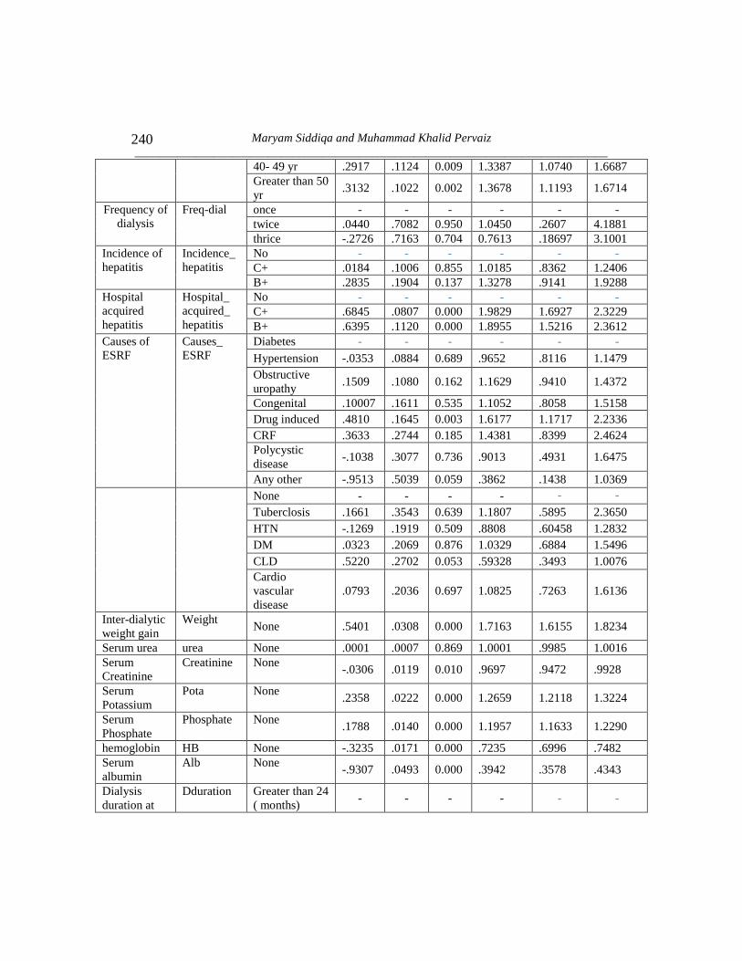
Maryam Siddiqa and Muhammad Khalid Pervaiz
______________________________________________________________________________
240
40- 49 yr .2917 .1124 0.009 1.3387 1.0740 1.6687
Greater than 50
yr .3132 .1022 0.002 1.3678 1.1193 1.6714
Frequency of
dialysis
Freq-dial once - - - - - -
twice .0440 .7082 0.950 1.0450 .2607 4.1881
thrice -.2726 .7163 0.704 0.7613 .18697 3.1001
Incidence of
hepatitis
Incidence_
hepatitis
No - - - - - -
C+ .0184 .1006 0.855 1.0185 .8362 1.2406
B+ .2835 .1904 0.137 1.3278 .9141 1.9288
Hospital
acquired
hepatitis
Hospital_
acquired_
hepatitis
No - - - - - -
C+ .6845 .0807 0.000 1.9829 1.6927 2.3229
B+ .6395 .1120 0.000 1.8955 1.5216 2.3612
Causes of
ESRF
Causes_
ESRF
Diabetes - - - - - -
Hypertension -.0353 .0884 0.689 .9652 .8116 1.1479
Obstructive
uropathy .1509 .1080 0.162 1.1629 .9410 1.4372
Congenital .10007 .1611 0.535 1.1052 .8058 1.5158
Drug induced .4810 .1645 0.003 1.6177 1.1717 2.2336
CRF .3633 .2744 0.185 1.4381 .8399 2.4624
Polycystic
disease -.1038 .3077 0.736 .9013 .4931 1.6475
Any other -.9513 .5039 0.059 .3862 .1438 1.0369
None - - - - - -
Tuberclosis .1661 .3543 0.639 1.1807 .5895 2.3650
HTN -.1269 .1919 0.509 .8808 .60458 1.2832
DM .0323 .2069 0.876 1.0329 .6884 1.5496
CLD .5220 .2702 0.053 .59328 .3493 1.0076
Cardio
vascular
disease
.0793 .2036 0.697 1.0825 .7263 1.6136
Inter-dialytic
weight gain
Weight None .5401 .0308 0.000 1.7163 1.6155 1.8234
Serum urea urea None .0001 .0007 0.869 1.0001 .9985 1.0016
Serum
Creatinine
Creatinine None -.0306 .0119 0.010 .9697 .9472 .9928
Serum
Potassium
Pota None .2358 .0222 0.000 1.2659 1.2118 1.3224
Serum
Phosphate
Phosphate None .1788 .0140 0.000 1.1957 1.1633 1.2290
hemoglobin HB None -.3235 .0171 0.000 .7235 .6996 .7482
Serum
albumin
Alb None -.9307 .0493 0.000 .3942 .3578 .4343
Dialysis
duration at
Dduration Greater than 24
( months) - - - - - -

Identification of Significant Prognostic Factors of Dialysis Population
_______________________________________________________________________________ 241
entry of
study 13-24 months 3.1931 .5210 0.000 24.364 8.7741 67.656
7-12 months 6.7637 .5635 0.000 865.91 286.94 2613.128
Less than 6
(months) 9.693 .5828 0.000 16213.54 5172.81 50819.29
Table 2: Overall test of proportionality
Covariates Chi-
square
d.f. Sig.
current_Age 0.84 1 0.3606
Weight_gain 0.35 1 0.5537
Potassium 0.03 1 0.8632
HB 1.21 1 0.2709
Serum_Albu 0.01 1 0.9252
1.dduration - 1 -
2.dduration 0.11 1 0.7425
3.dduration 0.49 1 0.4817
4.dduration 1.10 1 0.2952
Age_weight 0.71 1 0.3990
Alb_weight 1.99 1 0.1583
Alb_pota 0.03 1 0.8535
Alb_HB 1.91 1 0.1665
global test 16.10 12 0.1868
Maryam Siddiqa and Muhammad Khalid Pervaiz
______________________________________________________________________________
242
Table 3: Cox Regression model for identification of Prognostic factors
Variables B S.E. Z Sig. Exp.
95% CI for
Exp.
Lower Upper
Gender= male
Gender= female .0023 .0788 0.03 0.976 1.0023 .8587 1.1699
current_Age .0145 .0062 2.33 0.020 1.0146 1.0023 1.0270
Age_start_dia= < 29 yr -
Age_start_dia=30- 39 yr -.0264 .1492 -0.18 0.859 .9738 .7269 1.3046
Age_start_dia=40- 49 yr -.2015 .1771 -1.14 0.255 .8174 .5776 1.1568
Age_start_dia= >50 yr -.3799 .2497 -1.52 0.128 .6839 .4191 1.1158
freq_dia_weekly=once
freq_dia_weekly=twice -.6654 .7194 -0.92 0.355 .5140 .1254 2.1057
freq_dia_weekly=thrice -.3727 .7241 -0.51 0.607 .6888 .1666 2.8476
Hospital_acqu_hepa=No
Hospital_acqu_hepa= C+ -.0400 .0918 -0.44 0.663 .9607 .8024 1.1503
Hospital_acqu_hepa= B+ -.0113 .1200 -0.09 0.925 .9887 .7814 1.2509
Co_morbidities= None
Co_mor=Tuberclosis -.1151 .3600 -0.32 0.749 .8912 .4400 1.8049
Co_mor=HTN .0626 .1955 0.32 0.749 1.0646 .7256 1.5618
Co_mor=DM .2434 .2112 1.15 0.249 1.2755 .8430 1.9299
Co_mor=CLD -.0786 .2775 -0.28 0.777 .9243 .5365 1.5924
Co_mor=Cardio vascular
disease .3131 .2082 1.50 0.133 1.3677 .9094 2.0569
Weight_gain .1242 .0346 3.58 0.000 1.1323 1.0578 1.2120
Creatinine -.0074 .0121 -0.61 0.541 .9926 .9692 1.0165
Potassium .1080 .0216 4.99 0.000 1.1141 1.0678 1.1624
Phosphate -.0023 .0174 -0.14 0.891 .9976 .9640 1.0323
HB -.1686 .0241 -6.98 0.000 .8448 .8057 .8858
Serum_Albumin -.3574 .0631 -5.66 0.000 .6994 .6180 .7916
Dduration> 24( months)
Dduration=13-24 months 3.2542 .5825 5.59 0.000 25.8997 8.2689 81.122
Dduration=7-12 months 6.5721 .6202 10.60 0.000 714.9066 211.98 2411.0
Dduration= <6 months 9.2359 .6373 14.49 0.000 10259.37 2941.79 35779.
Identification of Significant Prognostic Factors of Dialysis Population
_______________________________________________________________________________ 243
Table 4: Main effect Cox Regression model for identification of Prognostic factors
Variables B S.E. Z Sig. Exp. 95% CI for Exp.
Lower Upper
current_Age .0054 .0024 2.21 0.027 1.0054 1.0006 1.0102
Weight_gain .1081 .0327 3.30 0.001 1.1142 1.0448 1.1881
Potassium .0916 .0206 4.44 0.000 1.0960 1.0525 1.1412
HB -.1687 .0231 -7.30 0.000 .8447 .8072 .8838
Serum_Albumin -.3371 .0617 -5.46 0.000 .7138 .6324 .8057
Dduration> 24
months . . . . . . .
Dduration =13-
24 months 3.2362 .5845 5.54 0.000 25.4385 8.0895 79.9950
Dduration =7-12
months 6.5597 .6224 10.54 0.000 706.0615 208.4677 2391.367
Dduration =< 6
months 9.1673 .6392 14.34 0.000 9579.463 2736.65 33532.28
Table 5: The final Cox Regression model for identification of Prognostic factors (prediction
model)
Variables B S.E. Z Sig. Exp. 95% CI for Exp.
Lower Upper
current_Age .0259 .0082 3.14 0.002 1.0263 1.0098 1.0430
Weight_gain -.2541 .1459 -1.74 0.082 .7756 .5826 1.0324
Potassium -.1241 .0970 -1.28 0.201 .8832 .7302 1.0682
HB .5507 .0927 5.94 0.000 1.7344 1.4462 2.0801
Serum_Albumin .2575 .4214 0.61 0.541 1.2938 .5664 2.9552
Dduration> 24
months . . . . . . .
Dduration =13-24
months 3.5405 .6667 5.31 0.000 34.4846 9.3343 127.3998
Dduration =7-12
months 6.8347 .6998 9.77 0.000 929.6099 235.8261 3664.456
Dduration =< 6
months 9.5335 .7152 13.33 0.000 13815.98 3400.857 56127.4
Age_weight -.0054 .0017 -3.04 0.002 .9946 .9911 .9980
Alb_weight .2153 .0542 3.97 0.000 1.2402 1.1152 1.3793
Alb_pota .0841 .0393 2.14 0.032 1.0878 1.0071 1.1749
Alb_HB -.2397 .0333 -7.19 0.000 .7868 .7370 .8399
Maryam Siddiqa and Muhammad Khalid Pervaiz
______________________________________________________________________________
244
Table 6: Highest 10% of Hazard Ratios
Age Weight potassium HB Albumin Ʃ(βx) Hazard Ratios
60 5 6.5 12 2.9 1.5812 4.8610
60 5 5 9 3.5 1.5934 4.9207
60 5 3 9 2.9 1.5948 4.9274
45 5 6.5 12 2.9 1.5970 4.9386
45 5 5 9 3.5 1.6093 4.9993
45 5 3 9 2.9 1.6106 5.0061
29 5 6.5 12 2.9 1.6139 5.0227
29 5 5 9 3.5 1.6261 5.0844
29 5 3 9 2.9 1.6275 5.0913
60 1.2 5 9 2.9 1.6599 5.2590
45 2.5 6.5 9 2.9 1.7129 5.5452
60 2.5 5 9 2.9 1.7197 5.5833
60 5 5 9 2.9 1.8348 6.2644
60 1.2 6.5 9 2.9 1.8399 6.2964
60 5 6.5 9 3.5 1.8492 6.3552
45 5 5 9 2.9 1.8507 6.3643
45 5 6.5 9 3.5 1.8651 6.4567
29 5 5 9 2.9 1.8676 6.4727
29 5 6.5 9 3.5 1.8820 6.5666
60 2.5 6.5 9 2.9 1.8998 6.6848
60 5 6.5 9 2.9 2.0149 7.5001
45 5 6.5 9 2.9 2.0307 7.6198
29 5 6.5 9 2.9 2.0476 7.7496
Table 7: Lowest 10% of Hazard Ratios
Age Weight potassium HB Albumin Ʃ(βx) Hazard Ratios
29 1.2 3 13.5 5 -5.017 0.0066
45 1.2 3 13.5 5 -4.7056 0.0090
29 1.2 5 13.5 5 -4.4237 0.0119
60 1.2 3 13.5 5 -4.4132 0.0121
29 2.5 3 13.5 5 -4.1518 0.0157
45 1.2 5 13.5 5 -4.1119 0.0163
29 1.2 3 12 5 -4.0453 0.0175
29 1.2 6.5 13.5 5 -3.9784 0.0187
45 2.5 3 13.5 5 -3.9524 0.0192
60 1.2 5 13.5 5 -3.8196 0.0219
60 2.5 3 13.5 5 -3.7655 0.0231
45 1.2 3 12 5 -3.7335 0.0239
45 1.2 6.5 13.5 5 -3.6666 0.0255
29 2.5 5 13.5 5 -3.5581 0.0284
29 1.2 5 12 5 -3.4517 0.0316
60 1.2 3 12 5 -3.4412 0.0320
Identification of Significant Prognostic Factors of Dialysis Population
_______________________________________________________________________________ 245
Age Weight potassium HB Albumin Ʃ(βx) Hazard Ratios
60 1.2 6.5 13.5 5 -3.3743 0.0342
45 2.5 5 13.5 5 -3.3587 0.0347
29 2.5 3 12 5 -3.1797 0.0415
60 2.5 5 13.5 5 -3.1718 0.0419
45 1.2 5 12 5 -3.1399 0.0432
29 2.5 6.5 13.5 5 -3.1128 0.0444
29 1.2 6.5 12 5 -3.0064 0.0494
45 2.5 3 12 5 -2.9804 0.0507
Figure 1: Histogram of survival time
Figure 2: Kaplan Meier Survivor function for overall survival time of dialysis patients
0.0
00.2
50.5
00.7
51.0
0
0 20 40 60analysis time
Kaplan-Meier survival estimate

Maryam Siddiqa and Muhammad Khalid Pervaiz
______________________________________________________________________________
246
Figure 3-7: Graphical assessment of PH assumptions
Figure 3: Scaled Schoenfeld residual plot for current age
Figure 4: Scaled Schoenfeld residual plot for ID weight gain
Figure 5: Scaled Schoenfeld residual plot for potassium
-1.5
-1-.
50
.51
sca
led S
cho
en
feld
- c
urr
ent_
Ag
e
0 10 20 30 40Time
bandwidth = .8
Test of PH Assumption
-30
-20
-10
01
02
0
sca
led S
cho
en
feld
- W
eig
ht_
gain
0 10 20 30 40Time
bandwidth = .8
Test of PH Assumption
-15
-10
-50
51
0
sca
led S
cho
en
feld
- P
ota
ssiu
m
0 10 20 30 40Time
bandwidth = .8
Test of PH Assumption

Identification of Significant Prognostic Factors of Dialysis Population
_______________________________________________________________________________ 247
Figure 6: Scaled Schoenfeld residual plot for HB
Figure 7: ScaledSchoenfeld residual plot for serum albumin
Figure 8-12: Smoothed residual plots for Linearity
Figure 8: Smoothed Residual plot for current age
-20
-10
01
0
sca
led S
cho
en
feld
- H
B
0 10 20 30 40Time
bandwidth = .8
Test of PH Assumption
-50
05
0
sca
led S
cho
en
feld
- S
eru
m_A
lbu
min
0 10 20 30 40Time
bandwidth = .8
Test of PH Assumption
-6-4
-20
2
ma
rtin
gal
e re
sidu
al
0 20 40 60 80current_Age
bandwidth = .8
Lowess smoother
Maryam Siddiqa and Muhammad Khalid Pervaiz
______________________________________________________________________________
248
Figure 9: Smoothed Residual plot for weight gain
Figure 10: Smoothed Residual plot for potassium
Figure 11: Smoothed Residual plot for HB
-6-4
-20
2
ma
rtin
gale
resi
du
al
0 2 4 6Weight_gain
bandwidth = .8
Lowess smoother
-6-4
-20
2
ma
rtin
gale
resid
ual
2 4 6 8 10Potassium
bandwidth = .8
Lowess smoother
-6-4
-20
2
ma
rtin
gale
resi
du
al
0 5 10 15 20HB
bandwidth = .8
Lowess smoother
Identification of Significant Prognostic Factors of Dialysis Population
_______________________________________________________________________________ 249
Figure 12: Smoothed Residual plot for serum albumin
Figure 13-17: Df beta plots for detection of outliers
Figure 13: Df beta for current age vs case ID
Figure 14: Df beta for weight gain vs case ID
-6-4
-20
2
ma
rtin
gale
resid
ual
1 2 3 4 5 6Serum_Albumin
bandwidth = .8
Lowess smoother
-.00
2
0
.00
2.0
04
DF
BE
TA
- c
urr
ent_
Ag
e
0 500 1000id
-.05
0
.05
.1.1
5
DF
BE
TA
- W
eig
ht_
gain
0 500 1000id
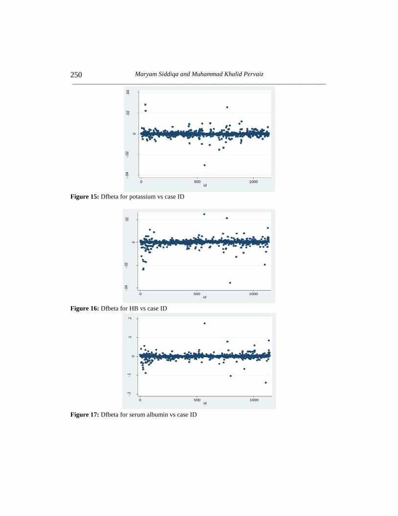
Maryam Siddiqa and Muhammad Khalid Pervaiz
______________________________________________________________________________
250
Figure 15: Dfbeta for potassium vs case ID
Figure 16: Dfbeta for HB vs case ID
Figure 17: Dfbeta for serum albumin vs case ID
-.04
-.02
0
.02
.04
DF
BE
TA
- P
ota
ssiu
m
0 500 1000id
-.04
-.02
0
.02
DF
BE
TA
- H
B
0 500 1000id
-.2
-.1
0.1
.2
DF
BE
TA
- S
eru
m_A
lbu
min
0 500 1000id

Identification of Significant Prognostic Factors of Dialysis Population
_______________________________________________________________________________ 251
Figure 18: Graph of Goodness of Fit of final Cox model
References
1. Abbott, C. K., Glanton, W. C., Trespalacios, C, F., Oliver, K. D., Ortiz, I. M.,
Agodoa, Y. L., Cruess, F. D. and Kimmel, L. P. (2004). Body mass index,
dialysis modality, and survival: Analysis of the United States Renal Data
System Dialysis Morbidity and Mortality Wave II Study. Kidney
International, 65, 597–605.
2. Agashua, P. A., Lyle, R. C., Livesley, W. J., Slade, P. D., Winney, R. J. and
Irwin, M. (1981). Predicting dietary non-compliance of patients on
intermittent hemodialysis. Journal of Psychosomatic Research, 25(4), 289-
301.
3. Barsoum, R. S. (2006). Chronic kidney disease in the developing world. New
England Journal of Medicine, 354(10), 997-999.
4. Bleyer, A. J., Hartman, J., Brannon, P. C., Reeves-Daniel, A., Satko, S. G. and
Russell, G. (2006). Characteristics of sudden death in hemodialysis patients.
Kidney international, 69(12), 2268-2273.
5. Bleyer, A. J., Russell, G. B. and Satko, S. G. (1999). Sudden and cardiac
death rates in hemodialysis patients. Kidney international, 55(4), 1553-1559.
6. Byrne, C., Vernon, P. and Cohen, J. J. (1994). Effect of age and diagnosis on
survival of older patients beginning chronic dialysis. Jama, 271(1), 34-36.
7. Cain, K. C. and Lange, N. T. (1984). Approximate case influence for the
Proportional Hazards Regression model with censored data. Biometrics, 40(2),
493-499.
02
46
8
0 2 4 6 8Cox-Snell residual
Nelson-Aalen cumulative hazard
Cox-Snell residual

Maryam Siddiqa and Muhammad Khalid Pervaiz
______________________________________________________________________________
252
8. Chandna, M. S., Schultz, J., Lawrence, C., Greenwood, N. R. and Farrington,
K. (1999). Is there a rationale for rationing chronic dialysis? A hospital based
Cohort study of factors affecting survival and morbidity. British Medical
Journal, 318(7178), 217-223.
9. Chadban, S. J., Briganti, E. M., Kerr, P. G., Dunstan, D. W., Welborn, T. A.,
Zimmet, P. Z. and Atkins, R. C. (2003). Prevalence of kidney damage in
Australian adults: The AusDiab kidney study. Journal of the American Society
of Nephrology, 14(2), 131-138.
10. Chen, J., Wildman, R. P., Gu, D., Kusek, J. W., Spruill, M., Reynolds, K. and
He, J. (2005). Prevalence of decreased kidney function in Chinese adults aged
35 to 74 years. Kidney International, 68(6), 2837-2845.
11. Cleveland, W. S. (1979). Robust locally weighted Regression and smoothing
scatter plots. Journal of the American Statistical Association, 74(368), 829-
836.
12. Codreanu, I., Perico, N., Sharma, S. K., Schieppati, A. and Remuzzi, G.
(2006). Prevention programmes of progressive renal disease in developing
nations (Review Article). Nephrology, 11(4), 321-328.
13. Collett, D. (2003). Modeling Survival Data in Medical Research II. CRC
Press, Boca Raton.
14. Collins, A. J. (2002). Influence of target hemoglobin in dialysis patients on
morbidity and mortality. Kidney International, 61, 44-48.
15. Collins, A. J., Li, S., Peter, W. S., Ebben, J., Roberts, T., Ma, J. Z. and
Manning, W. (2001). Death, hospitalization, and economic associations
among incident hemodialysis patients with hematocrit values of 36% to
39%. Journal of the American Society of Nephrology, 12(11), 2465-2473.
16. Collins, A. J., Ma, J. Z. and Ebben, J. (2000). Impact of hematocrit on
morbidity and mortality. Nephrology, 20(4), 345-349.
17. Coresh, J., Selvin, E., Stevens, L. A., Manzi, J., Kusek, J. W., Eggers, P. and
Levey, A. S. (2007). Prevalence of Chronic Kidney Disease in the
U.S. Jama, 298(17), 2038-2047.
18. Cox, D. R. (1972). Regression models and life table. Journal of the Royal
Statistical Society, 34(2), 187-220.
19. Cox, D. R. (1975). A note on data-splitting for the evaluation of significance
levels. Biometrika, 62(2), 441-444.
20. Cox, D. R. and Snell, E. J. (1968). A general definition of residuals. Journal
of the Royal Statistical Society-Series B (Methodological), 30(2), 248-275.
21. Dawson, B. and Trapp, R. G. (2004). Basic and Clinical Biostatistics. 4th
edition. McGraw-Hill, New York.
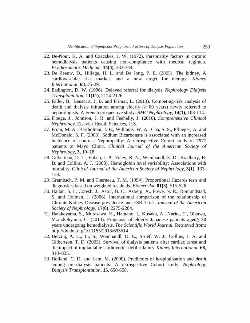
Identification of Significant Prognostic Factors of Dialysis Population
_______________________________________________________________________________ 253
22. De-Nour, K. A. and Czaczkes, J. W. (1972). Personality factors in chronic
hemodialysis patients causing non-compliance with medical regimen.
Psychosomatic Medicine, 34(4), 333-344.
23. De Zeeuw, D., Hillege, H. L. and De Jong, P. E. (2005). The kidney, A
cardiovascular risk marker, and a new target for therapy. Kidney
International, 68, 25-29.
24. Eadington, D. W. (1996). Delayed referral for dialysis. Nephrology Dialysis
Transplantation, 11(11), 2124-2126.
25. Faller, B., Beuscart, J. B. and Frimat, L. (2013). Competing-risk analysis of
death and dialysis initiation among elderly (≥ 80 years) newly referred to
nephrologists: A French prospective study. BMC Nephrology, 14(1), 103-114.
26. Floege, J., Johnson, J. R. and Feehally, J. (2010). Comprehensive Clinical
Nephrology. Elsevier Health Sciences, U.S.
27. From, M. A., Bartholmai, J. B., Williams, W. A., Cha, S. S., Pflueger, A. and
McDonald, S. F. (2008). Sodium Bicarbonate is associated with an increased
incidence of contrast Nephropathy: A retrospective Cohort study of 7977
patients at Mayo Clinic. Clinical Journal of the American Society of
Nephrology, 3, 10–18.
28. Gilbertson, D. T., Ebben, J. P., Foley, R. N., Weinhandl, E. D., Bradbury, B.
D. and Collins, A. J. (2008). Hemoglobin level variability: Associations with
mortality. Clinical Journal of the American Society of Nephrology, 3(1), 133-
138.
29. Grambsch, P. M. and Therneau, T. M. (1994). Proportional Hazards tests and
diagnostics based on weighted residuals. Biometrika, 81(3), 515-526.
30. Hallan, S. I., Coresh, J., Astor, B. C., Asberg, A., Powe, N. R., Romundstad,
S. and Holmen, J. (2006). International comparison of the relationship of
Chronic Kidney Disease prevalence and ESRD risk. Journal of the American
Society of Nephrology, 17(8), 2275-2284.
31. Hatakeyama, S., Murasawa, H., Hamano, I., Kusaka, A., Narita, T., Oikawa,
M.andOhyama, C. (2013). Prognosis of elderly Japanese patients aged≥ 80
years undergoing hemodialysis. The Scientific World Journal. Retrieved from:
http://dx.doi.org/10.1155/2013/693514
32. Herzog, A. C., Li, S., Weinhandl, D. E., Strief, W. J., Collins, J. A. and
Gilbertson, T. D. (2005). Survival of dialysis patients after cardiac arrest and
the impact of implantable cardioverter defibrillators. Kidney International, 68,
818–825.
33. Holland, C. D. and Lam, M. (2000). Predictors of hospitalization and death
among pre-dialysis patients: A retrospective Cohort study. Nephrology
Dialysis Transplantation, 15, 650-658.

Maryam Siddiqa and Muhammad Khalid Pervaiz
______________________________________________________________________________
254
34. Hosmer, D. W., Lemeshow, S. and May, S. (2008) Applied Survival Analysis
Regression Modeling of Time to Event Data. 2nd
edition, John Wiley and
Sons, Inc, New Jersey.
35. Huang, C. W., Levey, S. A., Serio, M. A., Snyder, M., Vickers, J. A., Raj, V.
J., Peter, T., Scardino, T. P. and Russo, P. (2006). Chronic Kidney Disease
after nephrectomy in patients with renal cortical tumors: A retrospective
Cohort study. The Lancet Oncology, 7(9), 735–740.
36. Iseki, K., Kawazoe, N. and Fukiyama, K. (1993). Serum albumin is a strong
predictor of death in chronic dialysis patients. Kidney International, 44, 115-
119.
37. Jafar, T. H. (2006). The growing burden of Chronic Kidney Disease in
Pakistan. New England Journal of Medicine, 354(10), 995-997.
38. Joly, D., Anglicheau, D., Alberti, C., Nguyen, A. T., Touam, M., Grunfeld, J.
P. and Jungers, P. (2003). Octogenarians reaching end-stage renal disease:
Cohort study of decision-making and clinical outcomes. Journal of the
American Society of Nephrology, 14(4), 1012-1021.
39. Jungers, P., Zingraff, J., Albouze, G., Chauveau, P., Page, B., Hannedouche,
T.and Man, N. K. (1993). Late referral to maintenance dialysis: Detrimental
consequences. Nephrology Dialysis Transplantation, 8(10), 1089-1093.
40. Kalantar-Zadeh, K., Regidor, D. L., Kovesdy, C. P., Van Wyck, D.,
Bunnapradist, S., Horwich, T. B. and Fonarow, G. C. (2009). Fluid retention
is associated with cardiovascular mortality in patients undergoing long-term
hemodialysis. Circulation, 119(5), 671-679.
41. Kaplan, E. L. and Meier, P. (1958). Nonparametric Estimation from
Incomplete Observations. Journal of the American Statistical Association, 53,
457–481.
42. Kimmel, P. L., Peterson, R. A., Weihs, K. L., Simmens, S. J., Alleyne, S.,
Cruz, I. and Veis, J. H. (2000). Psychosocial factors, behavioral compliance
and survival in urban hemodialysis patients. Kidney International, 54(1), 245-
254.
43. Koch, M., Thomas, B., Tschope, W. and Ritz, E. (1993). Survival and
predictors of death in dialysed diabetic patients. Diabetologia, 36(10), 1113-
1117.
44. Kovesdy, C. P., Regidor, D. L., Mehrotra, R., Jing, J., McAllister, C. J.,
Greenland, S. and Kalantar-Zadeh, K. (2007). Serum and dialysate potassium
concentrations and survival in hemodialysis patients. Clinical Journal of the
American Society of Nephrology, 2(5), 999-1007.
45. Leggat, J. E., Orzol, S. M., Hulbert-Shearon, T. E., Golper, T. A., Jones, C.
A., Held, P. J. chand Port, F. K. (1998). Noncompliance in hemodialysis:

Identification of Significant Prognostic Factors of Dialysis Population
_______________________________________________________________________________ 255
Predictors and survival analysis. American Journal of Kidney Diseases, 32(1),
139-145.
46. Locatelli, F., Conte, F. and Marcelli, D. (1998). The impact of hematocrit
levels and erythropoietin treatment on overall and cardiovascular mortality
and morbidity-the experience of the Lombardy Dialysis Registry. Nephrology
Dialysis Transplantation, 13(7), 1642-1644.
47. Locatelli, F., Pisoni, R. L., Akizawa, T., Cruz, J. M., DeOreo, P. B., Lameire,
N. H. and Held, P. J. (2004). Anemia management for hemodialysis patients:
Kidney disease outcomes quality initiative (K/DOQI) guidelines and dialysis
outcomes and practice patterns study (DOPPS) findings. American Journal of
Kidney Diseases, 44, 27-33.
48. Lopez-Gomez, J. M., Villaverde, M., Jofre, R., Rodriguez-Benitez, P. and
Perez-Garcia, R. (2005). Inter-dialytic weight gain as a marker of blood
pressure, nutrition, and survival in hemodialysis patients. Kidney
International, 67, 63-68.
49. Lysaght, M. J. (2002). Maintenance dialysis population dynamics: Current
trends and long-term implications. Journal of the American Society of
Nephrology, 13(1), 37-40.
50. Ma, J. Z., Ebben, J., Xia, H. and Collins, A. J. (1999). Hematocrit level and
associated mortality in hemodialysis patients. Journal of the American Society
of Nephrology, 10(3), 610-619.
51. Manley, M. and Sweeney, J. (1986). Assessment of compliance in
hemodialysis adaptation. Journal of Psychosomatic Research, 30(2), 153-161.
52. Munshi, S. K., Vijayakumar, N., Taub, N. A., Bhullar, H., Lo, T. N. and
Warwick, G. (2001). Outcome of Renal Replacement Therapy in the very
elderly. Nephrology Dialysis Transplantation, 16(1), 128-133.
53. Naqvi, S. A. J. (2009). Renal Diseases in Pakistan-Time to act. Journal of
Nephrology and Renal Transplantation, 2(1), 133-135.
54. Nathan, M. (1966). Evaluation of survival data and two new rank order
statistics arising in its consideration. Cancer Chemotherapy Reports, 50(3),
163–170.
55. Neves, P. L., Sousa, A., Bernardo, I., Anunciada, A. I., Pinto, I., Bexiga, I.
and Amorim, J. P. (1994). Chronic hemodialysis for very old patients. Age
and Ageing, 23(5), 356-359.
56. Ng’andu, N. H. (1997). An empirical comparison of statistical tests for
assessing the Proportional Hazards assumption of Cox's model. Statistics in
Medicine, 16(6), 611-626.
57. Ofsthun, N., Labrecque, J., Lacson, E., Keen, M. and Lazarus, J. M. (2003).
The effects of higher hemoglobin levels on mortality and hospitalization in
hemodialysis patients. Kidney International, 63(5), 1908-1914.

Maryam Siddiqa and Muhammad Khalid Pervaiz
______________________________________________________________________________
256
58. Pastan, S., Souchie, M. and McClellan, W. M. (2002). Vascular access and
increased risk of death among hemodialysis patients. Kidney International, 62,
620-626.
59. Ratcliffe, P. J., Phillips, R. E. and Oliver, D. O. (1984). Late referral for
maintenance dialysis. British Medical Journal, 288(6415), 441-443.
60. Regidor, D. L., Kopple, J. D., Kovesdy, C. P., Kilpatrick, R. D., McAllister,
C. J., Aronovitz, J. and Kalantar-Zadeh, K. (2006). Associations between
changes in hemoglobin and administered erythropoiesis-stimulating agent and
survival in hemodialysis patients. Journal of the American Society of
Nephrology, 17(4), 1181-1191.
61. Rodriguez, H. J., Domenici, R., Diroll, A. and Goykhman, I. (2005).
Assessment of dry weight by monitoring changes in blood volume during
hemodialysis using Crit-Line. Kidney International, 68(2), 854-861.
62. Rohrich, B., Von Herrath, D., Asmus, G. and Schaefer, K. (1998). The elderly
dialysis patient: management of the hospital stay. Nephrology Dialysis
Transplantation, 13(7), 69-72.
63. Schaefer, K. and Rohrich, B. (1999). The dilemma of Renal Replacement
Therapy in patients over 80 years of age: Dialysis should not be
withheld. Nephrology Dialysis Transplantation, 14(1), 35-36.
64. Schieppati, A. and Remuzzi, G. (2005). Chronic Renal Diseases as a public
health problem: Epidemiology, social, and economic implications. Kidney
International, 68, 7-10.
65. Schoenfeld, D. (1982). Partial residuals for the Proportional Hazards
Regression model. Biometrika, 69(1), 239-241.
66. Slinin, Y., Foley, N. R. and Collins, J. A. (2005). Calcium, phosphorus,
parathyroid hormone, and cardiovascular disease in hemodialysis patients:
The USRDS Waves 1, 3, and 4 Study. Journal of the American Society of
Nephrology, 16, 1788-1793.
67. Therneau, T. M., Grambsch, P. M. and Fleming, T. R. (1990). Martingale-
based residuals for survival models. Biometrika, 77(1), 147-160.
68. Vandelli, L., Medici, G., Perrone, S. and Lusvarghi, E. (1996). Hemodialysis
therapy in the elderly. Nephrology Dialysis Transplantation, 11(supp9), 89-
94.
69. Wilson, M. G. (2013). Assessing Model Adequacy in Proportional Hazards
Regression. SAS Global Forum 2013-Statistics and Data Analysis, 431, 1-36.
70. Xia, H., Ebben, J., Ma, J. Z. and Collins, A. J. (1999). Hematocrit levels and
hospitalization risks in hemodialysis patients. Journal of the American Society
of Nephrology, 10(6), 1309-1316.