Geological Fluid Mechanics Models at Various Scales

by

Martin Oliver Saar

M.S. (University of Oregon) 1998

A dissertation submitted in partial satisfactionof the requirements for the degree of

Doctor of Philosophy

in

Earth and Planetary Science

in the

GRADUATE DIVISION

of the

UNIVERSITY OF CALIFORNIA, BERKELEY

Committee in charge:

Professor Michael Manga, ChairProfessor James RectorProfessor Steven Glaser

Fall 2003

The dissertation of Martin Oliver Saar is approved.

Chair Date

Date

Date

University of California, Berkeley

Fall 2003

Geological Fluid Mechanics Models at Various Scales

Copyright c© 2003

by

Martin Oliver Saar

Abstract

Geological Fluid Mechanics Models at Various Scales

by

Martin Oliver Saar

Doctor of Philosophy in Earth and Planetary Science

University of California, Berkeley

Professor Michael Manga, Chair

In this dissertation, I employ concepts from fluid mechanics to quantitatively in-

vestigate geological processes in hydrogeology and volcanology. These research topics

are addressed by utilizing numerical and analytical models but also by conducting

field and lab work.

Percolation theory is of interest to a wide range of physical sciences and thus war-

rants research in itself. Therefore, I developed a computer code to study percolation

thresholds of soft-core polyhedra. Results from this research are applied to study the

onset of yield strength in crystal-melt suspensions such as magmas. Implications of

yield strength development in suspensions, marking the transition from Newtonian

to Bingham fluid, include the pahoehoe-’a’a transition and the occurrence of effusive

versus explosive eruptions.

I also study interactions between volcanic processes and groundwater as well as

between groundwater and seismicity (hydroseismicity). In the former case, I develop

numerical and analytical models of coupled groundwater and heat transfer. Here, per-

1

turbations from a linear temperature-depth profile are used to determine groundwater

flow patterns and rates. For the hydroseismicity project I investigate if seasonal ele-

vated levels of seismicity at Mt. Hood, Oregon, are triggered by groundwater recharge.

Both hydroseismicity and hydrothermal springs occur on the southern flanks of Mt.

Hood. This suggests that both phenomena are related while also providing a connec-

tion between the research projects involving groundwater, heat flow, and seismicity.

Indeed, seismicity may be necessary to keep faults from clogging thus allowing for

sustained activity of hydrothermal springs.

Finally, I present research on hydrologically induced volcanism, where a process

similar to the one suggested for hydroseismicity is invoked. Here, melting of glaciers,

or draining of lakes, during interglacial periods reduce the confining pressure in the

subsurface which may promote dike formation and result in increased rates of volcan-

ism.

In general, problems discussed in this dissertation involve interactions among pro-

cesses that are traditionally associated with separate research disciplines. However,

numerous problems in the geosciences require a multidisciplinary approach, as demon-

strated here. In addition, employing several analytical and numerical methods, such

as signal processing, inverse theory, computer modeling, and percolation theory, al-

lows me to study such diverse processes in a quantitative way.

Professor Michael MangaDissertation Committee Chair

2

Contents

Contents i

List of Figures iv

List of Tables vii

1 Introduction 1

2 Continuum percolation theory 5

2.1 Introduction . . . . . . . . . . . . . . . . . . . . . . . . . . . . . . . . 5

2.2 Method . . . . . . . . . . . . . . . . . . . . . . . . . . . . . . . . . . 8

2.3 Average number of bonds per object, Bc . . . . . . . . . . . . . . . . 11

2.4 Normalized average excluded volume, 〈vex〉 . . . . . . . . . . . . . . 12

2.5 Critical total average excluded volume, 〈Vex〉 . . . . . . . . . . . . . 14

2.6 Critical volume fraction, φc . . . . . . . . . . . . . . . . . . . . . . . 16

2.7 Conclusions . . . . . . . . . . . . . . . . . . . . . . . . . . . . . . . . 19

3 Yield strength development in crystal-melt suspensions 21

3.1 Introduction . . . . . . . . . . . . . . . . . . . . . . . . . . . . . . . . 21

3.2 Rheology of magmatic suspensions . . . . . . . . . . . . . . . . . . . 23

3.2.1 Fluid behavior - region A . . . . . . . . . . . . . . . . . . . . 23

3.2.2 Onset and development of yield strength - region A” . . . . . 25

3.3 Methods . . . . . . . . . . . . . . . . . . . . . . . . . . . . . . . . . . 26

3.4 Results . . . . . . . . . . . . . . . . . . . . . . . . . . . . . . . . . . . 30

i

3.5 Discussion . . . . . . . . . . . . . . . . . . . . . . . . . . . . . . . . . 33

3.5.1 Onset of yield strength . . . . . . . . . . . . . . . . . . . . . . 34

3.5.2 Scaling relation for τy(φ) curves of differing particle shapes, andother generalizations . . . . . . . . . . . . . . . . . . . . . . . 38

3.5.3 Implications . . . . . . . . . . . . . . . . . . . . . . . . . . . . 42

3.6 Conclusions . . . . . . . . . . . . . . . . . . . . . . . . . . . . . . . . 44

4 Hydroseismicity 46

4.1 Introduction . . . . . . . . . . . . . . . . . . . . . . . . . . . . . . . . 46

4.2 Data and analysis . . . . . . . . . . . . . . . . . . . . . . . . . . . . . 48

4.3 Discussion . . . . . . . . . . . . . . . . . . . . . . . . . . . . . . . . . 55

4.3.1 Causes of hydroseismicity . . . . . . . . . . . . . . . . . . . . 56

4.3.2 Analytic model . . . . . . . . . . . . . . . . . . . . . . . . . . 60

4.3.3 Hydraulic diffusivity . . . . . . . . . . . . . . . . . . . . . . . 62

4.3.4 Critical pore-fluid pressure change . . . . . . . . . . . . . . . . 64

4.3.5 Hydraulic conductivity and permeability . . . . . . . . . . . . 67

4.4 Conclusions . . . . . . . . . . . . . . . . . . . . . . . . . . . . . . . . 69

5 Permeability-depth curve 70

5.1 Introduction . . . . . . . . . . . . . . . . . . . . . . . . . . . . . . . . 70

5.2 Four depth scales of k . . . . . . . . . . . . . . . . . . . . . . . . . . 72

5.2.1 Spring discharge model: k(z <0.1 km) . . . . . . . . . . . . . 74

5.2.2 Coupled heat and groundwater transfer model:k(z <1 km) . . . . . . . . . . . . . . . . . . . . . . . . . . . . 76

5.2.3 Groundwater-recharge-induced seismicity model:k(z <5 km) . . . . . . . . . . . . . . . . . . . . . . . . . . . . 88

5.2.4 Magma intrusion and degassing model: k(z <15 km) . . . . . 90

5.3 Conversions between κ, K, and k . . . . . . . . . . . . . . . . . . . . 93

5.4 Discussion . . . . . . . . . . . . . . . . . . . . . . . . . . . . . . . . . 95

5.4.1 Heterogeneity and anisotropy of permeability . . . . . . . . . 95

5.4.2 Basal heat-flow, Hb . . . . . . . . . . . . . . . . . . . . . . . . 106

5.5 Conclusions . . . . . . . . . . . . . . . . . . . . . . . . . . . . . . . . 107

ii

6 Glacier-induced volcanism 109

6.1 Introduction . . . . . . . . . . . . . . . . . . . . . . . . . . . . . . . . 109

6.2 Data analysis . . . . . . . . . . . . . . . . . . . . . . . . . . . . . . . 111

6.3 Discussion . . . . . . . . . . . . . . . . . . . . . . . . . . . . . . . . . 115

6.4 Conclusions . . . . . . . . . . . . . . . . . . . . . . . . . . . . . . . . 121

7 Conclusions 122

7.1 Continuum percolation theory . . . . . . . . . . . . . . . . . . . . . . 122

7.2 Yield strength development in crystal-melt suspensions . . . . . . . . 123

7.3 Hydroseismicity . . . . . . . . . . . . . . . . . . . . . . . . . . . . . . 124

7.4 Permeability-depth curve . . . . . . . . . . . . . . . . . . . . . . . . . 125

7.5 Glacier-induced volcanism . . . . . . . . . . . . . . . . . . . . . . . . 126

A Appendix to Chapter 4: Hydroseismicity 128

A.1 Seismometer information . . . . . . . . . . . . . . . . . . . . . . . . . 128

A.2 Box-Jenkins method . . . . . . . . . . . . . . . . . . . . . . . . . . . 129

A.3 Moving polynomial interpolation . . . . . . . . . . . . . . . . . . . . 129

A.4 Correlation coefficients . . . . . . . . . . . . . . . . . . . . . . . . . . 130

B Appendix to Chapter 5: Permeability-depth curve 131

B.1 Definition of symbols . . . . . . . . . . . . . . . . . . . . . . . . . . . 131

B.2 Derivation of the equation for a T (z)-profile with an exponential de-crease in permeability . . . . . . . . . . . . . . . . . . . . . . . . . . . 132

B.3 Derivation of the equation for a T (z)-profile with constant hydraulicconductivity . . . . . . . . . . . . . . . . . . . . . . . . . . . . . . . . 133

B.4 Finite difference method . . . . . . . . . . . . . . . . . . . . . . . . . 134

B.5 Axisymmetric flow . . . . . . . . . . . . . . . . . . . . . . . . . . . . 136

Bibliography 153

iii

List of Figures

2.1 Visualization of a simplified simulation of large biaxial oblate and pro-late prisms . . . . . . . . . . . . . . . . . . . . . . . . . . . . . . . . . 10

2.2 Illustration of the overlap of two objects in a 2D system with parallel-aligned objects . . . . . . . . . . . . . . . . . . . . . . . . . . . . . . 11

2.3 Normalized average excluded volume as a function of object aspectratio and shape anisotropy . . . . . . . . . . . . . . . . . . . . . . . . 13

2.4 Critical total average excluded volume and critical volume fraction atthe percolation threshold . . . . . . . . . . . . . . . . . . . . . . . . . 17

3.1 Sketch of the development of effective shear viscosity and yield strengthas a function of crystal fraction . . . . . . . . . . . . . . . . . . . . . 24

3.2 Simulation of crystal intergrowth . . . . . . . . . . . . . . . . . . . . 27

3.3 Resolution requirements . . . . . . . . . . . . . . . . . . . . . . . . . 28

3.4 Visualizations of a simulation of randomly oriented elongated rectan-gular biaxial soft-core prisms . . . . . . . . . . . . . . . . . . . . . . . 30

3.5 Simulation results of the critical volume fraction for randomly orientedsoft-core prisms and ellipsoids . . . . . . . . . . . . . . . . . . . . . . 31

3.6 Simulation results of critical volume fraction versus aspect ratio forrandomly oriented triaxial soft-core prisms . . . . . . . . . . . . . . . 32

3.7 Size effects on critical crystal volume fraction . . . . . . . . . . . . . 33

3.8 Image of a pahoehoe sample close to the percolation threshold . . . . 37

3.9 “Quasi” invariant for scaling purposes . . . . . . . . . . . . . . . . . . 41

3.10 Scaling of yield strength curves from prisms to spheres . . . . . . . . 43

4.1 Seismicity at Mt. Hood, Oregon . . . . . . . . . . . . . . . . . . . . . 48

iv

4.2 Gutenberg-Richter plot . . . . . . . . . . . . . . . . . . . . . . . . . . 49

4.3 Stream discharge of Salmon River, Oregon . . . . . . . . . . . . . . . 50

4.4 Histograms of seismicity and stream discharge . . . . . . . . . . . . . 51

4.5 Period content of time series . . . . . . . . . . . . . . . . . . . . . . . 52

4.6 Original and interpolated time series . . . . . . . . . . . . . . . . . . 54

4.7 Interpolated time series . . . . . . . . . . . . . . . . . . . . . . . . . . 55

4.8 Time lag versus cross-correlation coefficients . . . . . . . . . . . . . . 56

4.9 Time lag versus mean moving cross-correlation coefficients . . . . . . 57

4.10 Relationship between stresses (Mohr-circle) . . . . . . . . . . . . . . . 58

4.11 Periodic pore-fluid pressure fluctuations . . . . . . . . . . . . . . . . . 61

4.12 Hydrostatic pressure with superimposed periodic pore-fluid pressurefluctuations . . . . . . . . . . . . . . . . . . . . . . . . . . . . . . . . 63

5.1 Study region . . . . . . . . . . . . . . . . . . . . . . . . . . . . . . . . 73

5.2 Spring discharge model . . . . . . . . . . . . . . . . . . . . . . . . . . 76

5.3 Schematic illustration of 1D groundwater recharge area . . . . . . . . 78

5.4 Radius of curvature of the Earth’s surface near Santiam Pass, Oregon 80

5.5 Groundwater flow streamlines at a (mostly vertical 1D-flow) rechargeregion . . . . . . . . . . . . . . . . . . . . . . . . . . . . . . . . . . . 81

5.6 Shaded relief map of Mt. Hood, Oregon, and subsurface temperaturedistribution . . . . . . . . . . . . . . . . . . . . . . . . . . . . . . . . 84

5.7 Temperature, vertical groundwater flow velocity, and hydraulic con-ductivity versus depth in a 1D-flow recharge region . . . . . . . . . . 86

5.8 Geotherm measurements and models for Mt. Hood . . . . . . . . . . 89

5.9 Magma intrusion underneath the Cascades range volcanic arc. . . . . 91

5.10 Near-surface heat-flow map . . . . . . . . . . . . . . . . . . . . . . . 97

5.11 Permeability, k, as a function of depth, z . . . . . . . . . . . . . . . . 101

6.1 Shaded relief map with locations of basaltic and silicic eruptions inLong Valley and Owens Valley volcanic fields, eastern California . . . 110

6.2 Original, binned, interpolated, differentiated, and cross-correlated datafor basaltic and silicic volcanic eruptions, as well as for glaciation . . 112

6.3 Mean cross-correlation coefficients from Figure 6.2c,d . . . . . . . . . 113

v

6.4 Power spectra for δ18O and volcanic eruptions . . . . . . . . . . . . . 114

6.5 Conceptual model of a magmatic system in the Sierras . . . . . . . . 119

6.6 Phase lag and amplitude of the transfer function relating glacial un-loading to volcanisms . . . . . . . . . . . . . . . . . . . . . . . . . . . 120

B.1 Schematic illustration of the computational grid in cylindrical coordi-nates used for heat and groundwater transfer modeling . . . . . . . . 137

vi

List of Tables

5.1 Spring model input and results . . . . . . . . . . . . . . . . . . . . . 77

5.2 Parameters for coupled groundwater and heat-flow models . . . . . . 88

5.3 Conversions from hydraulic conductivity, K, to permeability, k . . . . 96

vii

Acknowledgements

Numerous people have contributed in various ways to my completion of this disser-

tation. I would like to thank my adviser, Michael Manga, for his continuous support,

motivation, and encouragement during my Ph.D. studies and for introducing me to

research. I am also very grateful to have had the opportunity to discuss science,

and work with researchers from the University of Oregon, University of California -

Berkeley, Lawrence Berkeley National Laboratory, and the U.S. Geological Survey.

Some of these colleagues, friends, and mentors include Kathy Cashman, Dana John-

ston, Eugene Humphreys, Steve Ingebritsen, Jamie Rector, and Chi-Yuen Wang. In

addition, I would like to thank fellow graduate and undergraduate students as well

as postdocs with whom I shared lab and office spaces, had many stimulating research

discussions, and participated in inspiring field trips. Here, I would like to thank

Dayanthie Weeraratne, Chad Dorsey, Adam Soule, Rebecca and Cliff Ambers, Alison

Rust, Jason Crosswhite, Derek Schutt, Helge Gonnermann, Dave Stegman, David

Schmidt, Ingrid Johanson, Mark Wenzel, Mark Jellinek, Emily Brodsky, and Mike

Singer. Funding for the research presented in this dissertation was generously pro-

vided by the National Science Foundation, the American Chemical Society (Petroleum

Research Fund), the Sloan Foundation, and Lawrence Berkeley National Laboratory.

I am grateful to my parents, Karin and Rudiger Saar, and my brother, Bernd Saar,

for their belief in me and their support and encouragement in all my endeavours. Di-

ane, Cap, Amy, and Rob Tibbitts are thanked for making me feel at home and being

part of their family. Finally, I am very thankful to my wife, Amy Saar, for her love,

companionship, support, and encouragement without which this dissertation would

not have been possible.

viii

Chapter 1

Introduction

In this dissertation, I investigate processes in hydrogeology and volcanology, as

well as in rheology of suspensions in general. These investigations have in common

the application of fluid mechanics and the use of numerical and analytical modeling

techniques. The importance of applying concepts from fluid mechanics to geological

problems is nicely summarized by H.E. Huppert [74] in his classic paper entitled

“The intrusion of fluid mechanics into geology.” The objective in this dissertation

is to gain quantitative insight into processes governing the flow of subsurface water

on the one hand, and magma and lava flow on the other hand. For the latter two

(hereafter collectively referred to as magma), an understanding of the complex and

time-dependent rheology of crystal-melt suspensions is critical. Thus, I also conduct

research investigating the rheology of suspensions, employing a percolation theory

approach.

Percolation theory describes the transport properties of random, multiphase sys-

tems and materials and can thus be applied to numerous problems in the physical

sciences, warranting research in itself. As a result, I first present a more general

1

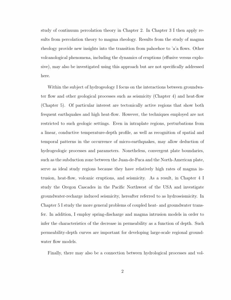
study of continuum percolation theory in Chapter 2. In Chapter 3 I then apply re-

sults from percolation theory to magma rheology. Results from the study of magma

rheology provide new insights into the transition from pahoehoe to ’a’a flows. Other

volcanological phenomena, including the dynamics of eruptions (effusive versus explo-

sive), may also be investigated using this approach but are not specifically addressed

here.

Within the subject of hydrogeology I focus on the interactions between groundwa-

ter flow and other geological processes such as seismicity (Chapter 4) and heat-flow

(Chapter 5). Of particular interest are tectonically active regions that show both

frequent earthquakes and high heat-flow. However, the techniques employed are not

restricted to such geologic settings. Even in intraplate regions, perturbations from

a linear, conductive temperature-depth profile, as well as recognition of spatial and

temporal patterns in the occurrence of micro-earthquakes, may allow deduction of

hydrogeologic processes and parameters. Nonetheless, convergent plate boundaries,

such as the subduction zone between the Juan-de-Fuca and the North-American plate,

serve as ideal study regions because they have relatively high rates of magma in-

trusion, heat-flow, volcanic eruptions, and seismicity. As a result, in Chapter 4 I

study the Oregon Cascades in the Pacific Northwest of the USA and investigate

groundwater-recharge induced seismicity, hereafter referred to as hydroseismicity. In

Chapter 5 I study the more general problems of coupled heat- and groundwater trans-

fer. In addition, I employ spring-discharge and magma intrusion models in order to

infer the characteristics of the decrease in permeability as a function of depth. Such

permeability-depth curves are important for developing large-scale regional ground-

water flow models.

Finally, there may also be a connection between hydrological processes and vol-

2

canic eruptions. In Chapter 6 I show that similar to the effects of reservoirs on

hydroseismicity, stress changes, caused by variations in the load exerted by surface

water or ice, can affect the frequency of eruptions.

Large-scale flow models in porous media are generally underconstrained. It is

thus desirable to use multiple direct and indirect observations, such as standard hy-

drogeologic boundary conditions and parameters as well as temperature distributions,

heat-flow, and hydroseismicity data to improve such simulations. Other implications

of utilizing multiple processes and constraints, as well as developing large-scale models

of mass and energy transfer, lie in the areas of water management, geothermal energy

resources, and assessment of volcanic and (hydro-) seismic hazards. Further implica-

tions include basic geological and geophysical research concerning water and magma

transport, interactions between fluids, heat, and earthquakes, and the effects of a

material’s rheology on transport processes. The latter subject also has implications

in material science.

To investigate geological processes quantitatively, I employ numerical and ana-

lytical methods at various temporal and spatial scales. Scales considered range from

particle interactions in suspensions to flow phenomena in mountain ranges. Methods

employed include percolation theory, signal processing, inverse theory, statistics, and

fluid flow simulations. Data used for calculations and models are obtained from field

work (e.g., on Hawai’i and in the Oregon Cascades), laboratory measurements (e.g.,

permeability of rock cores), and from third parties (e.g., temperature-depth profiles

from the US Geological Survey, Menlo Park).

Because of the wide range of topics covered, each following chapter includes a

separate introduction and conclusion section and is largely based either on previous

3

publications (Saar and Manga [158]1 for Chapter 2, Saar et al. [160]2 for Chapter 3,

and Saar and Manga [159]3 for Chapter 4) or on manuscripts that are in review at

the time this dissertation is being written (Chapters 5 and 6). Some details not

provided in these publications and manuscripts have been included in the chapters

or are provided in additional appendices. Definitions of symbols are unique to each

chapter. A conclusion chapter summarizes the main findings of this dissertation.

1Saar, M. O., and M. Manga, Physical Review E, Vol. 65, Art. No. 056131, 2002. Copyright(2002) by the American Physical Society.

2Reprinted from Earth and Planetary Science Letters, Vol. 187, Saar, M. O., M. Manga, K.V. Cashman, and S. Fremouw, Numerical models of the onset of yield strength in crystal-meltsuspensions, 367-379, Copyright (2001), with permission from Elsevier.

3Reprinted from Earth and Planetary Science Letters, Vol. 214, Saar, M. O., and M. Manga,Seismicity induced by seasonal groundwater recharge at Mt. Hood, Oregon, 605-618, Copyright(2003), with permission from Elsevier.

4

Chapter 2

Continuum percolation theory

This chapter is largely based on Saar and Manga [158]1.

2.1 Introduction

The transport properties of multiphase materials may either reflect the deforma-

tion of the material as a whole under applied stress (rheology) or the transfer of some

medium, such as electrons or fluids, within the material (conductivity). Both types of

transport are fundamentally different and depend on the relevant material properties

in different ways. However, rheology and conductivity of composite materials are both

determined in part by the interconnectivity of their individual elements (objects) that

constitute their phases.

Percolation theory describes interconnectivity of objects in a random multiphase

system as a function of the geometry, distribution, volume fraction, and orientation

1Saar, M. O., and M. Manga, Physical Review E, Vol. 65, Art. No. 056131, 2002. Copyright(2002) by the American Physical Society.

5

of the objects. The structure of the composite material may evolve with time due

to chemical reactions or temperature changes. A critical threshold may be passed

during the structural evolution and as a result some material properties such as yield

strength or conductivity can change abruptly and may exhibit a power-law behavior

above, and close to, the so-called percolation threshold.

Examples of composite materials that show time-dependent rheology include ce-

ments [15], gels [20], and magmas [160] (see also Chapter 3). Similarly, the conduc-

tivity of a medium for fluids (permeability) or electrons may change with time. For

example the permeability of a material changes with the formation or closure of pores

and fractures in solids [78] or with growth and coalescence or degassing of bubbles

in liquids [156, 157]. Similarly, electrical conductivity depends on the amount, ge-

ometry, and interconnectivity of the conductor [44, 176, 209]. In general, multiple

processes [191] in the Physical, Chemical, Biological, and Earth Sciences appear to

show power-law, i.e., fractal, properties above a certain threshold and may thus be

described by percolation theory.

Several soft-core (interpenetrating objects) continuum (randomly positioned) per-

colation studies have been conducted in three-dimensional (3D) systems. Investigated

3D percolating objects include spheres [61, 105, 141, 167], parallel-aligned [176] or

randomly oriented [50] ellipsoids, parallel-aligned cubes [176], and randomly oriented

hemispherically capped cylinders [8, 9]. In some studies randomly oriented 2D el-

lipses [31] and 2D polygons [78] are placed in a 3D system to simulate fractures

where the third object dimension may be neglected.

In this chapter I investigate continuum percolation for randomly oriented 3D

soft-core prisms. The objective is to point out similarities between prisms and other

percolation systems studied previously, to expand on explanations for differences using

6

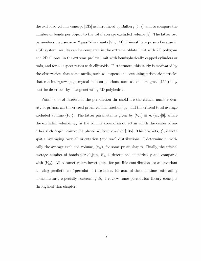
the excluded volume concept [135] as introduced by Balberg [5, 8], and to compare the

number of bonds per object to the total average excluded volume [8]. The latter two

parameters may serve as “quasi”-invariants [5, 8, 41]. I investigate prisms because in

a 3D system, results can be compared in the extreme oblate limit with 2D polygons

and 2D ellipses, in the extreme prolate limit with hemispherically capped cylinders or

rods, and for all aspect ratios with ellipsoids. Furthermore, this study is motivated by

the observation that some media, such as suspensions containing prismatic particles

that can intergrow (e.g., crystal-melt suspensions, such as some magmas [160]) may

best be described by interpenetrating 3D polyhedra.

Parameters of interest at the percolation threshold are the critical number den-

sity of prisms, nc, the critical prism volume fraction, φc, and the critical total average

excluded volume 〈Vex〉. The latter parameter is given by 〈Vex〉 ≡ nc 〈vex〉[8], where

the excluded volume, vex, is the volume around an object in which the center of an-

other such object cannot be placed without overlap [135]. The brackets, 〈〉, denote

spatial averaging over all orientation (and size) distributions. I determine numeri-

cally the average excluded volume, 〈vex〉, for some prism shapes. Finally, the critical

average number of bonds per object, Bc, is determined numerically and compared

with 〈Vex〉. All parameters are investigated for possible contributions to an invariant

allowing predictions of percolation thresholds. Because of the sometimes misleading

nomenclature, especially concerning Bc, I review some percolation theory concepts

throughout this chapter.

7

2.2 Method

In a soft-core system the percolation threshold is reached when a continuous path-

way of overlapping objects exists connecting opposing sides of a bounding box. The

computer code developed determines the percolation threshold and related parame-

ters for convex 3D soft-core polyhedra of any shape, size, and orientation distribution

that are randomly positioned (continuum percolation). Here, I focus on randomly

oriented biaxial and triaxial soft-core prisms of uniform size. In soft-core continuum

percolation, size distribution of objects does not appear to affect φc [160] and results

for parallel-aligned objects are independent of object shape [5].

Overlap of objects is determined analytically. The volume fraction of a phase is

determined by the number density of objects, n, that constitute the phase and the

object’s unit volume, V , by [51]

φ = 1 − exp(−nV ). (2.1)

Results for φ using Eq. (2.1) can be verified through comparison with numerical

volume fraction calculations using a space discretization method [160]. In order to

reduce finite size effects and the possibility of imposing large-scale structure I place

objects within a large unit bounding box whose volume typically is 8 to 64 times larger

than the volume of an inner bounding box used to determine connection between

opposing sides (Fig. 2.1). The more common approach is to perform calculations

with periodic boundary conditions [31, 50, 78]. In all simulations, the largest object

side length is one tenth or less of the side length of the inner bounding box. Fig. 2.1

shows visualizations of simplified simulations for randomly oriented biaxial oblate and

prolate prisms.

The computational method is tested by comparing results with well-established

8

values, such as φc and 〈vex〉 for spheres and parallel-aligned objects [8, 176], and

by visualizations of simulations at low nc. Moreover, the critical number density of

clusters per unit volume, nsc, at percolation scales as nsc ∝ s−τ over more than 4

orders of magnitude of s, where s is the number of objects in a cluster and τ ≈ 2.2.

Thus, the cluster size distribution follows the power-law relationship expected between

nsc and s close to the percolation threshold [7, 181], suggesting that finite size effects

are minimal.

For two continuous convex objects the average excluded volume 〈vex〉 can be

determined analytically by

〈vex〉 = Va + Vb + (AaRa + AbRb)/4π, (2.2)

where V is the volume, A the area, and R the mean radius of curvature of the objects

a and b [86]. The prisms in this study, however, have corners so that R, and thus

〈vex〉, cannot be determined analytically using Eq. (2.2). Instead I employ a method

analogous to Garboczi et al. [50] and de la Torre et al. [32], and determine 〈vex〉

numerically by randomly placing two objects of random orientation within a box and

testing for overlap. This is repeated typically 106 times and the ratio of the number

of overlaps over the total number of trials times the volume of the box is 〈vex〉. To

obtain a mean and a standard error, I repeat the above procedure ten times. I test

this method for the case of parallel-aligned objects of volume V , where in 3D for any

convex object shape 〈vex〉 = 8 × V . This is also a test of the contact function for

objects [50].

All simulations are repeated 10 times to calculate a mean and its standard error

for φc, nc, and Bc. Error bars in all figures indicate 95 % confidence intervals. Biaxial

object aspect ratios are given as small over large and as large over small axis length

for oblate and prolate objects, respectively. The shape anisotropy, ξ, of an object is

9

a

c

b

d

Figure 2.1. Visualization of a simplified simulation of large biaxial oblate (a, b) andprolate (c, d) prisms with aspect ratios 1:10 (short over long axis) and 10:1 (long overshort axis), respectively. The critical number densities are nc = 1060 and nc = 7025for the oblate and prolate prism simulations, respectively. In actual simulations objectside lengths are about 1/10 or less than the side length of the inner bounding box.nc increases with object elongation up to nc = 7 × 105 for prolate prisms of aspectratio 1000:1. The inner bounding box is used to determine if a continuous phase,or backbone (b, d) exists (percolation threshold). Objects are placed throughoutthe inner and outer bounding box and within a fringe around the outer box so thatobjects can protrude into the box (a, c). The average number of bonds per object,Bc, and the number density, nc, are determined using all object overlaps and objectcenters, respectively, that fall within the large bounding box.

10

object A

object B

excluded area of object B

excluded area of object A

connection

bond B

bond A

center Acenter B

Figure 2.2. Illustration of the overlap of two objects in a 2D parallel-aligned system(for easier visualization). The center of each object A and B falls within the otherobject’s excluded area, each resulting in an overlap, or bond. The number of bondsis 2. In contrast, the number of connections per object is the total number of bonds(2) divided by the total number of objects (2), here resulting in one connection. In3D-systems, randomly oriented objects have average excluded volumes, rather thanexcluded areas.

defined here as the ratio of large over short axis length for both oblate and prolate

objects.

2.3 Average number of bonds per object, Bc

Objects in soft-core continuum percolation can interpenetrate each other. The

average excluded volume, 〈vex〉, is always defined for 2 objects (A and B). When

placed within a unit volume 〈vex〉 describes the probability of each center, A and B,

being within the other object’s excluded volume, each causing an overlap, or bond

(Fig. 2.2).

Therefore, in a unit volume, n 〈vex〉 describes the probability of n object centers

being within n excluded volumes each causing an overlap, or bond, for each individual

object, or two bonds per connection (Fig. 2.2). This method of counting each bond is

11

commonly referred to as counting “bonds per object,” which has to be distinguished

from the more intuitive average number of connections per object,

C =total number of bonds

total number of objects, (2.3)

denoted Cc at percolation. The critical average number of bonds per object at per-

colation is given by [8]

Bc = nc 〈vex〉 (2.4)

and thus [137]

Cc =nc 〈vex〉

2=Bc

2. (2.5)

For example Bc = 1.4 indicates a 140 % probability per object to have a bond, or on

average each object has 1.4 bonds, or 0.70 connections.

I determine Bc (and thus Cc), nc, and 〈vex〉 numerically and can thus confirm

Eqs. (2.4, 2.5) for randomly oriented prisms. For example, for an aspect ratio of 3:1

I obtain 〈vex〉 = 〈vex〉 /V = 13.1 and 〈vex〉 = Bc/(ncV ) = 13.3. Hereafter, I use

Eq. (2.4) to calculate 〈vex〉 from Bc and nc for randomly oriented prisms. In general,

the larger number of overlaps in my simulation results in a more rapid and accurate

estimate of 〈vex〉 using Eq. (2.4) than the method described in Section 2.2.

2.4 Normalized average excluded volume, 〈vex〉

The normalized average excluded volume,

〈vex〉 = 〈vex〉 /V, (2.6)

is the factor by which the excluded volume is larger than the actual volume, V , of an

object. Fig. 2.3 shows 〈vex〉 as a function of aspect ratio for randomly oriented (solid

12

10−4

10−3

10−2

10−1

100

101

102

103

aspect ratio

104

103

102

101

100

101

102

103

shape anisotropy, ξ

ex⟨v

⟩

oblate prolate

100

101

102

103

104

ellipsoids [14]

prisms

parallel-aligned prisms

randomly oriented

[this study]

[this study]

Figure 2.3. Normalized average excluded volume 〈vex〉 as a function of object aspectratio (and shape anisotropy, ξ) for biaxial (squares) and triaxial (triangles) prisms(this study) and rotational (biaxial) ellipsoids (circles, from [50]). Solid and dashedlines indicate random and parallel orientation, respectively. Error bars for prismsindicate 95 % confidence intervals. Short over medium axis aspect ratios for triaxialprisms are 1/2 (upward pointing triangle), 1/5 (leftward pointing triangle), and 1/10(downward pointing triangle). Long over medium axis aspect ratios are as indicatedby the figure axis. 〈vex〉 is calculated using Bc and nc in Eq. (2.4) for randomlyoriented prisms (squares along solid line). Squares along the dashed line show 〈vex〉 forparallel-aligned biaxial prisms, determined using the method described in Section 2.2.

line) biaxial (squares) and triaxial (triangles) prisms and for parallel-aligned biaxial

prisms (squares along dashed line).

As indicated in Section 2.2, 〈vex〉 = 8 for any parallel-aligned convex 3D object.

In contrast, randomly oriented biaxial prisms exhibit an increase in 〈vex〉 with in-

creasing shape anisotropy, ξ, due to flattening or elongation. The combined effect of

3 different axis lengths of randomly oriented triaxial prisms increases 〈vex〉 further.

This dependency of 〈vex〉 on shape anisotropy is expected because randomly oriented

objects with eccentric shapes have a higher probability to overlap than objects of

13

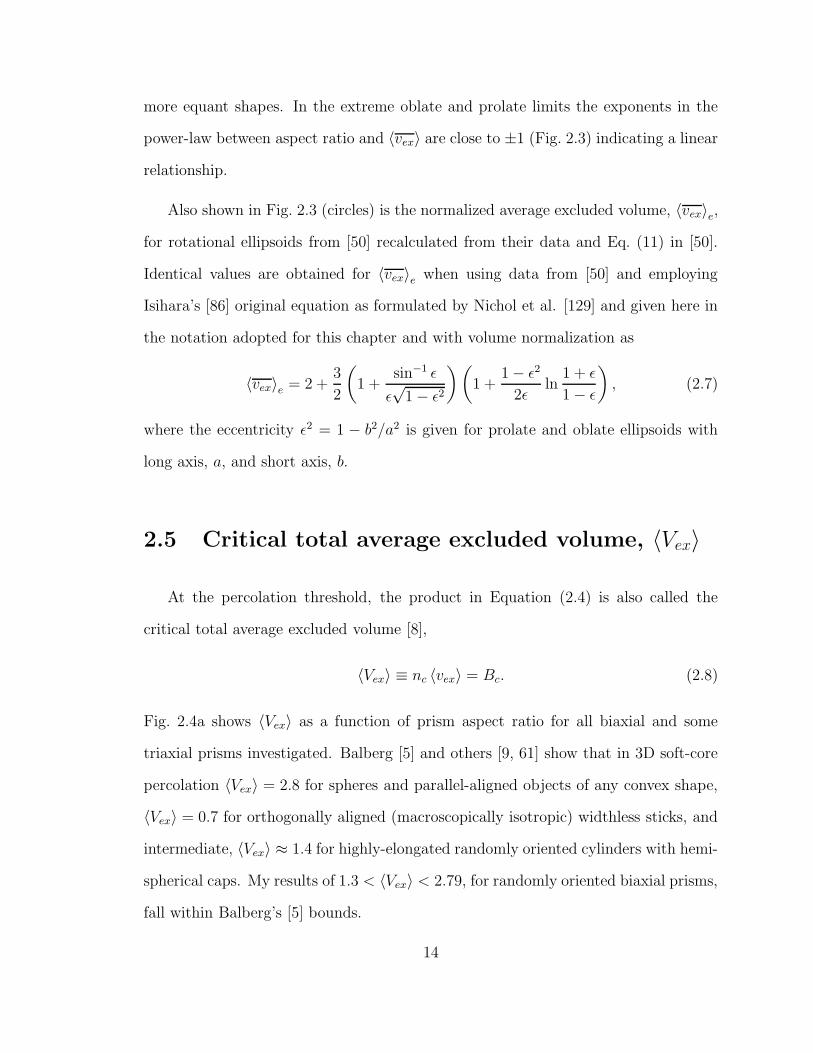
more equant shapes. In the extreme oblate and prolate limits the exponents in the

power-law between aspect ratio and 〈vex〉 are close to ±1 (Fig. 2.3) indicating a linear

relationship.

Also shown in Fig. 2.3 (circles) is the normalized average excluded volume, 〈vex〉e,

for rotational ellipsoids from [50] recalculated from their data and Eq. (11) in [50].

Identical values are obtained for 〈vex〉e when using data from [50] and employing

Isihara’s [86] original equation as formulated by Nichol et al. [129] and given here in

the notation adopted for this chapter and with volume normalization as

〈vex〉e = 2 +3

2

(

1 +sin−1 ε

ε√

1 − ε2

)(

1 +1 − ε2

2εln

1 + ε

1 − ε

)

, (2.7)

where the eccentricity ε2 = 1 − b2/a2 is given for prolate and oblate ellipsoids with

long axis, a, and short axis, b.

2.5 Critical total average excluded volume, 〈Vex〉

At the percolation threshold, the product in Equation (2.4) is also called the

critical total average excluded volume [8],

〈Vex〉 ≡ nc 〈vex〉 = Bc. (2.8)

Fig. 2.4a shows 〈Vex〉 as a function of prism aspect ratio for all biaxial and some

triaxial prisms investigated. Balberg [5] and others [9, 61] show that in 3D soft-core

percolation 〈Vex〉 = 2.8 for spheres and parallel-aligned objects of any convex shape,

〈Vex〉 = 0.7 for orthogonally aligned (macroscopically isotropic) widthless sticks, and

intermediate, 〈Vex〉 ≈ 1.4 for highly-elongated randomly oriented cylinders with hemi-

spherical caps. My results of 1.3 < 〈Vex〉 < 2.79, for randomly oriented biaxial prisms,

fall within Balberg’s [5] bounds.

14

In the extreme oblate biaxial prism limit my simulations yield

〈Vex〉 ≈ 2.3 (extreme oblate prism limit). (2.9)

This result is in close agreement with studies of similar object shapes (Fig. 2.4a)

such as 2D polygons [78] and 2D ellipses [31] placed in a 3D system where 2.22 ≤

〈Vex〉 ≤ 2.30 and 〈Vex〉 = 2.2, respectively (my definition of 〈Vex〉 is based on a unit

volume bounding box and thus already normalized). The 2D shapes may be viewed

as the extreme oblate limit of 3D objects. Garboczi et al. [50] report 〈Vex〉 = 3.0

for randomly oriented oblate rotational (biaxial) ellipsoids, a value higher than the

one introduced here and above the upper bound of 2.8 suggested by Balberg [5].

This discrepancy has been noted by Garboczi et al. [50] and others [31, 78]. Results

presented in Section 2.6 also suggest that for rotational ellipsoids values of 〈Vex〉 are

lower and possibly equal to values for biaxial prisms.

For an extreme prolate biaxial prism of aspect ratio 1000:1 I observe

〈Vex〉 ≈ 1.3 (extreme prolate prism limit) (2.10)

(Fig. 2.4a). Balberg [5] finds 〈Vex〉 ≈ 1.4 for extremely elongated randomly oriented

cylinders with hemispherical caps.

In general, maximum values of 〈Vex〉 = 2.8 occur for parallel-aligned objects of

any convex shape [9, 176], where the most equant shape possible, a sphere, is always

aligned. Therefore, it may be expected that I find a maximum of

〈Vex〉 ≈ 2.79 (cubes) (2.11)

for the most equant prism shape, a cube (Fig. 2.4a), where the effect of randomness

in orientation is at a minimum.

It has been argued [5, 39, 41, 50] that the total average excluded volume 〈Vex〉

is not a true invariant but may be viewed as an approximate invariant that is less

15

sensitive to object shapes than φc. My results confirm this reduced variability of

〈Vex〉 as a function of shape aspect ratio (Fig. 2.4). At the same time 〈Vex〉 ≈ 2.3

shows good agreement between extremely oblate prisms, 2D polygons, and 2D ellipses,

where the 2D-shapes are the extreme oblate 3D limits. Similarly, 〈Vex〉 ≈ 1.3 applies

to extremely prolate prisms, ellipsoids, and rods (hemispherically capped cylinders).

2.6 Critical volume fraction, φc

Fig. 2.4b shows φc as a function of aspect ratio for randomly oriented soft-core

biaxial (squares) and triaxial (triangles) prisms. The maximum value of φc is reached

for the most equant prism shape (cube with aspect ratio 1:1:1). Increasing shape

anisotropies due to flattening or elongation decrease φc for biaxial prisms. The

combined effect of flattening and elongation of triaxial prisms decreases φc further

(Fig. 2.4b). The larger the shape anisotropy of an object the greater its normalized

excluded volume, 〈vex〉 (Fig. 2.3) and probability of overlap. As a result, percolation

occurs at lower number densities, nc. Lower nc values for different object shapes re-

sult in reduced φc in Eq. (2.1), where differences in object volume have already been

accounted for by the volume normalization in 〈vex〉.

The circles in Fig. 2.4b are results from Garboczi et al. [50] for randomly oriented

soft-core rotational (biaxial) ellipsoids. Curves of φc, as a function of aspect ratio, for

ellipsoids and prisms have similar shapes but are offset for the most equant shapes

and converge in the extreme oblate and prolate limits. The offset between the curves

for prisms and ellipsoids may be a function of the ratio

R =〈vex〉e〈vex〉p

(2.12)

16

b

oblate prolate

φc

10−4

10−3

10−2

10−1

100

0.290.22

ellipsoids [50]

prisms[this study]

shape anisotropy, ξ10

410

310

210

110

010

110

210

3

aspect ratio10

−410

−310

−210

−110

010

110

210

3

0.5

1

1.5

2

2.5

3

3.5

a

spheres and parallel-aligned

orthogonal sticks [5]

randompolygons [78]and ellipses [31]

convex objects [5, 9, 61]

⟨V

⟩ = B

cex

2.8

prisms [this study] [5]

randomsticks

ellipsoids[50]

Figure 2.4. Critical total average excluded volume, 〈Vex〉 (panel a), and critical volumefraction, φc (panel b), at the percolation threshold versus aspect ratio (and shapeanisotropy, ξ) for biaxial (squares) and triaxial (triangles) prisms (this study) androtational (biaxial) ellipsoids (circles, from [50]). Short over medium axis aspectratios for triaxial prisms are 1/2 (upward pointing triangle), 1/5 (leftward pointingtriangle), 1/10 (downward pointing triangle), and 1/20 (rightward pointing triangle).Long over medium axis aspect ratios are as indicated by the figure axis. Error barsfor prisms indicate 95 % confidence intervals.

for a given aspect ratio. If I assume that for a given aspect ratio

〈Vex〉p ∼= 〈Vex〉e (2.13)

then by Eq. (2.8)

np 〈vex〉p = ne 〈vex〉e , (2.14)

where here and in all following equations the subscripts e and p denote parameters

17

for ellipsoids and prisms, respectively. All parameters are defined as before with

np, ne, 〈Vex〉p, 〈Vex〉e, φp, and φe being critical values at the percolation threshold.

Substituting Eq. (2.1) into Eq. (2.14) yields

〈vex〉pVp

ln(1 − φp) =〈vex〉eVe

ln(1 − φe). (2.15)

Applying Eq. (2.6) to the appropriate terms for prisms and ellipsoids in Eq. (2.15),

then substituting Eq. (2.12), and rearranging yields the critical prism volume fraction,

φp = 1 − (1 − φe)R. (2.16)

In the extreme oblate and prolate limits, the ratio in the exponent, R, approaches

one (Fig. 2.3) and thus Eq. (2.16) reduces to φp = φe as expected from Fig. 2.4b. For

the most equant shape (cube and sphere) the ratio is at its minimum of

R =8.00

10.56= 0.758, (2.17)

indicating that the normalized average excluded volume for a sphere is 75.8 % of

the one for a cube. The larger excluded volume of a cube with respect to a sphere

causes percolation at a lower volume fraction for cubes than for spheres. With the

result from Eq. (2.17) and φe = 0.2896 [50, 105, 141, 167] for spheres Eq. (2.16) yields

φp = 0.23 for cubes, agreeing, to within the uncertainty, with my numerical results of

φp = 0.22. The agreement between results from Eq. (2.16) and numerical results (Fig.

2.4b) for the most equant shapes as well as for the extreme aspect ratio limits suggest

that 〈Vex〉 may be invariant for a given aspect ratio as postulated by Eq. (2.13). Thus,

the curves in Fig. 2.4a are expected to converge for a given aspect ratio, possibly to

〈Vex〉p for prisms which agrees with results for 2D objects (Fig. 2.4a).

In the extreme oblate and prolate limits, the exponents of the power-law relat-

ing aspect ratio (or shape anisotropy, ξ) to φc are close to ±1 (line of slope ±1 in

18

Fig. 2.4b), indicating a linear relationship. Indeed, because φc is comparable for

ellipsoids and prisms for ξ > 50, in this limit, the linear relationships

φc =

0.6/ξ (prolate)

1.27/ξ (oblate)(2.18)

hold true for both biaxial prisms (this study) and rotational ellipsoids [50], where the

shape anisotropy, ξ, is the ratio of large over small axis for both prolate and oblate

objects.

2.7 Conclusions

The percolation system of randomly oriented 3D soft-core prisms serves as a link

combining characteristics between other systems such as 3D ellipsoids, 3D cylinders

with hemispherical caps (rods), 2D polygons, and 2D ellipses. All objects are ran-

domly oriented and randomly placed in the 3D continuum. The 2D shapes are the

extreme oblate limit of 3D objects.

Percolation parameters such as the critical volume fraction, φc, the critical total

average excluded volume, 〈Vex〉 ≡ nc 〈vex〉, or equivalently the average number of

bonds per object, Bc = nc 〈vex〉, can be related in most of the above mentioned

systems. Here, in the extreme oblate and prolate limits Bc ≈ 2.3 and Bc ≈ 1.3,

respectively. The minimum shape anisotropy of prisms is matched for cubes where

Bc = 2.79 reaches the prism maximum, close to Bc = 2.8 for spheres.

With respect to biaxial prisms, triaxial prisms have increased normalized average

excluded volumes, 〈vex〉, due to increased shape anisotropies. As a result, φc for

triaxial prisms is lower than φc for biaxial prisms.

An offset in the critical object volume fraction, φc, occurs between prisms and el-

19

lipsoids with low shape anisotropy. This offset appears to be a function of the ratio of

the normalized average excluded volume for ellipsoids, 〈vex〉e, over 〈vex〉p for prisms.

Prisms and ellipsoids yield converging values for 〈vex〉, and thus also for φc, in the

extreme oblate and prolate limits. In these limits both parameters exhibit a linear

relationship with respect to aspect ratio.

20

Chapter 3

Yield strength development in

crystal-melt suspensions

This chapter is largely based on Saar et al. [160]1.

3.1 Introduction

Magmas and lavas typically contain crystals, and often bubbles, suspended in a

liquid. These crystal-melt suspensions vary considerably in crystal volume fraction,

φ, and range from crystal-free in some volcanic eruptions, to melt-free in portions of

the Earth’s mantle. Moreover, the concentration of suspended crystals often changes

with time due to cooling or degassing, which causes crystallization, or due to heating,

adiabatic decompression, or hydration, which causes melting. Such variations in φ

can cause continuous or abrupt modifications in rheological properties such as yield

1Reprinted from Earth and Planetary Science Letters, Vol. 187, Saar, M. O., M. Manga, K.V. Cashman, and S. Fremouw, Numerical models of the onset of yield strength in crystal-meltsuspensions, 367-379, Copyright (2001), with permission from Elsevier.

21

strength, viscosity, and fluid-solid transitions. Thus the mechanical properties of geo-

logic materials vary as a result of the large range of crystal fractions present in geologic

systems. The rheology of crystal-melt suspensions affects geological processes, such

as ascent of magma through volcanic conduits, flow of lava across the Earth’s sur-

face, convection in magmatic reservoirs, and shear wave propagation through zones

of partial melting.

One example of a change in rheological properties that may influence a number of

magmatic processes is the onset of yield strength in a suspension once φ exceeds some

critical value, φc. The onset of yield strength has been proposed as a possible cause

for morphological transitions in surface textures of basaltic lava flows [26]. Yield

strength development may also be a necessary condition for melt extraction from

crystal mushes under compression, as in flood basalts, or in the partial melting zone

beneath mid ocean ridges [140]. Furthermore, increase of viscosity and development

of yield strength in magmatic suspensions may cause volcanic conduit plug formation

and the transition from effusive to explosive volcanism [35]. Indeed, Philpotts et

al. [140] state that the development of a load-bearing crystalline network is “one of

the most important steps in the solidification of magma.”

In this chapter I employ three-dimensional numerical percolation theory models

of crystal-melt suspensions to investigate the onset of yield strength, τy. The simu-

lations are based on results from Chapter 2 and the corresponding publication (Saar

and Manga [158]), where the occurence of a percolation threshold is investigated for

3D soft-core prisms in the continuum. Yield strength development due to vesicles

[155, 182] is not considered in this study. The objective is to understand the geomet-

rical properties of the crystals in suspension that determine the critical crystal volume

fraction, φc, at which a crystal network first forms. My simulations suggest that the

22

onset of yield strength in crystal-melt suspensions may occur at crystal fractions that

are lower than the 0.35-0.5 commonly assumed [95, 103, 142] in static (zero-shear)

environments. I demonstrate that yield strength can develop at significantly lower φ

when crystals have high shape anisotropy and are randomly oriented, and that an up-

per bound should be given by φc = 0.29 for parallel-aligned objects. Because particle

orientation is a function of the stress tensor, I expect increasing particle alignment

with increasing shear stress and perfect alignment in pure shear only [110]. Further-

more, I suggest a scaling relation between τy and φ for suspensions of different particle

shapes. The numerical models complement the experimental studies presented in a

paper by Hoover et al. [70].

3.2 Rheology of magmatic suspensions

In this section I provide an overview of the conceptual framework in which I

interpret results later. Fig. 3.1 illustrates schematically the relationship between

effective shear viscosity, µeff , yield strength, τy, and particle volume fraction, φ. I

make a distinction between fluid and solid (regions A and B respectively in Fig. 3.1).

The subcategories A’ and A” are used for suspensions with τy = 0 (Newtonian) and

τy > 0 (Bingham), respectively. I assume here that the suspensions are not influenced

by non-hydrodynamic (e.g., colloidal) forces, Brownian motion, or bubbles. First I

discuss viscosity (region A) then yield strength (subregion A”).

3.2.1 Fluid behavior - region A

Einstein [42] found an analytical solution,

µeff = µs(1 + 2.5φ), (3.1)

23

10

Newtonianfluid

Binghamfluid solid

particle volume fraction,0

fluid solid

effe

ctiv

e sh

ear

visc

osity

,yi

eld

stre

ngth

,

Figure 3.1. Sketch of the development of effective shear viscosity, µeff , and yieldstrength, τy, as a function of crystal fraction, φ. The critical crystal fractions φc andφm depend on the total shear stress, τ , and particle attributes, ξ, such as particleshape, size, and orientation distribution. A first minimum yield strength develops atφc ≡ φc(ξ, τy = 0) and increases with increasing φ. The fields A, A’, A”, and B areexplained in the text.

describing the effective shear viscosity, µeff , of a dilute (φ ≤ 0.03) suspension (left

hand side of field A) of spheres for very low Reynolds numbers (Stokes flow). The

viscosity of the suspending liquid is µs. The particle concentration, φ, has to be

sufficiently low that hydrodynamic interactions of the particles can be neglected.

At higher φ (right hand side of field A) the so-called Einstein-Roscoe equation [88,

152, 168] is often employed to incorporate effects of hydrodynamically interacting,

non-colloidal particles,

µr = µeff/µs = (1 − φ/φm)−2.5 , (3.2)

where φm is the maximum packing fraction. The form of Eq. (3.2) allows the relative

24

viscosity µr to diverge as φ → φm. Eq. (3.2) is commonly used to calculate the

viscosity of magmas [142]. However, the value of φm, which determines the transition

to a solid, is uncertain; suggested values range from φm = 0.74 [168] to φm = 0.60

[115]. φm = 0.74 corresponds to the maximum packing fraction of uniform spheres,

so φm might be expected to be different if non-spherical particles are considered

[115, 142]. An additional complication is the tendency of crystals to form aggregates

or networks. Jeffrey and Acrivos [88] argue that a suspension that forms aggregates

can be viewed as a suspension of single particles of new shapes (and sizes) and thus

possessing different rheological properties.

3.2.2 Onset and development of yield strength - region A”

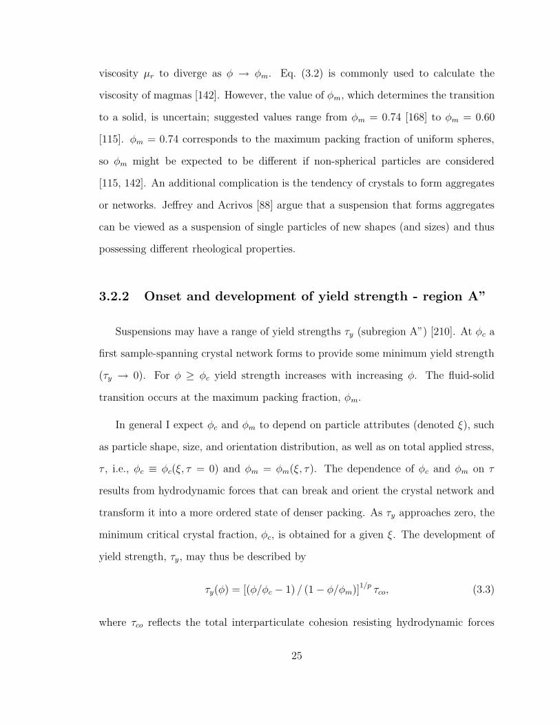
Suspensions may have a range of yield strengths τy (subregion A”) [210]. At φc a

first sample-spanning crystal network forms to provide some minimum yield strength

(τy → 0). For φ ≥ φc yield strength increases with increasing φ. The fluid-solid

transition occurs at the maximum packing fraction, φm.

In general I expect φc and φm to depend on particle attributes (denoted ξ), such

as particle shape, size, and orientation distribution, as well as on total applied stress,

τ , i.e., φc ≡ φc(ξ, τ = 0) and φm = φm(ξ, τ). The dependence of φc and φm on τ

results from hydrodynamic forces that can break and orient the crystal network and

transform it into a more ordered state of denser packing. As τy approaches zero, the

minimum critical crystal fraction, φc, is obtained for a given ξ. The development of

yield strength, τy, may thus be described by

τy(φ) = [(φ/φc − 1) / (1 − φ/φm)]1/p τco, (3.3)

where τco reflects the total interparticulate cohesion resisting hydrodynamic forces

25

and p may reflect the response of the aggregate state to shearing [202, 203, 210].

In this study I investigate the influence of ξ on φc as τ → 0, with the implication

that the onset of zero-shear yield strength is a lower bound for the onset of yield

strength in shear environments. Thus, φc may be viewed as the lowest crystal volume

fraction at which τy could possibly form under the given assumptions (e.g., no non-

hydrodynamic forces, bubbles, or Brownian motion).

3.3 Methods

In contrast to natural and analog experiments, computer models permit investiga-

tion of the formation of a continuous crystal network at low φ under static conditions

(zero strain rate). As experimental and in situ measurements of yield strength may

disrupt the fragile network that first forms at φc, it has been argued [10, 95] that

incorrect extrapolation of stress versus strain rate measurements towards zero strain

rate can lead to fictitious yield strength values when in actuality the suspension is

shear-thinning. Moreover, simulations allow intergrowth of crystals, which is impor-

tant for systems where crystal growth rate, G, is significantly larger than shear rate,

γ·, as is the case in some natural systems [139, 140]. In this study I assume a zero-shear

environment, thus

γ·

G→ 0. (3.4)

I employ continuum percolation models (Chapter 2 and Saar and Manga [158])

to study the possible development of τy as a function of φ and ξ. Percolation theory

describes the interconnectivity of individual elements in disordered (random) systems

26

I

IIa IIb

III

a

"backbone"

bounding box

crystal

"dead end"

cluster(2 crystals)

b

Figure 3.2. a) Simulation of crystal intergrowth. I) crystals touch; IIa) in naturalsystems under high growth rate to shear rate ratios, touching crystals grow together;IIb) in the computer model crystals overlap; III) same end result. b) Schematic 2-dimensional illustration of crystals forming clusters. One cluster connects oppositesides of the bounding box and forms the backbone. It is necessary that some crystalsare positioned outside the bounding box, so that they can protrude into it. Actualsimulations are 3-dimensional (Fig. 3.4).

and suggests a power law relationship of the form [181]

τy ∼

0 φ < φc

(φ− φc)η φ ≥ φc,

(3.5)

where φc is the percolation threshold which is reached when crystals first form a con-

tinuous phase across the suspending fluid. The exponent η describes the development

of τy for φ ≥ φc close to φc. Although phenomenological, I determine a geometrical

percolation threshold, pc, and assume that it is related to φc [50]. With this approach,

I can investigate the dependence of pc on crystal shape, size, and orientation distri-

bution and draw conclusions about the effects of these geometric properties on the

development of yield strength.

The crystals in the simulations can be approximated as convex polyhedra of any

shape, size, and orientation distribution in 3-dimensional space. Crystals are posi-

27

10−2 10−1 1000.25

0.30

0.35

0.40

0.45

0.50

0 10 20 30 40 50

0.20

0.24

0.28

Figure 3.3. Critical crystal volume fraction, φc, versus ratio of cube side length, lc,over bounding box side length, lb = 1, for parallel-aligned cubes. Inset: φc versusnumber of resolution grains, θ, per distance from the crystal center to the farthestvertex, d, for randomly oriented cubes. Symbols are the mean and shaded areasindicate standard deviations. Circle (light gray area): lc/lb = 0.1; square (mediumgray area): lc/lb = 0.05; diamond (dark gray area): lc/lb = 0.025. The total numberof grains is θt ≈ (θ/d)3, where for a cube d = (3l2c)

1/2.

tioned randomly and interpenetrate each other (soft-core continuum percolation). In

soft-core percolation the concept of maximum packing fraction, φm, does not apply.

Fig. 3.2a shows that overlapping crystals of finite size may simulate crystal inter-

growth in a zero-shear environment. Crystal orientation distribution is pre-assigned

so that, for example, parallel-aligned or randomly oriented distributions can be sim-

ulated. Crystals are positioned inside and outside a bounding unit cube (Fig. 3.2b).

To avoid finite size effects, the maximum length of the largest crystal in a given sim-

ulation is never longer than 1/10, and typically 1/20 to 1/40, of the bounding cube

side length. Fig. 3.3 shows the decrease in standard deviation and mean of φc for

decreasing particle side length for parallel-aligned cubes.

28

I determine crystal overlaps analytically. Volume fractions, φ, are determined

numerically by discretizing the bounding cube into subcubes (grains). The inset of

Fig. 3.3 illustrates, that while crystal size influences the standard deviation of φc (gray

shaded areas), “grain resolution,” θ, is relatively uncritical for calculations of φ. This

insensitivity could be due to the angular crystal shapes that may be approximated

well by a few angular grains. I also determine φ by using the number of crystals

per unit volume, n, and the volume of a crystal, v, in φ = 1 − exp(−nv) [6, 51] as

previously introduced in Chapter 2 [Eq. (2.1)].

Crystals that overlap are part of a “cluster.” Overlapping crystals of different

clusters cause the two clusters to merge into one. The percolation threshold is reached

when a continuous crystal chain (hereafter referred to as the “backbone”) exists,

connecting one face of the bounding cube with the opposing face (Figs. 3.2b, 3.4a). A

backbone in this study includes the “dead-end branches” which may not be considered

part of the backbone in other studies [181] (Fig. 3.2b).

All simulations are repeated at least 10 times to determine a mean and a standard

deviation of φc. Standard deviations of φc are about 0.01. The typical number of

crystals in each simulation ranges from 103 to 3×105, depending on particle attributes

ξ.

I test the computational method by running simulations for which percolation

theory results are well-established [61, 141, 167, 176], such as for parallel-aligned

cubes, where φc = 0.29. Furthermore, I use visualizations of crystal configurations at

low crystal numbers to confirm calculations of simulation parameters (Fig. 3.4).

29

b c

fd e

a

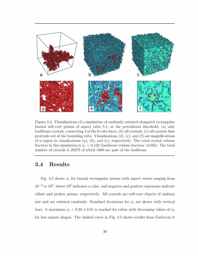
Figure 3.4. Visualizations of a simulation of randomly oriented elongated rectangularbiaxial soft-core prisms of aspect ratio 5:1, at the percolation threshold; (a) onlybackbone crystals, connecting 4 of the 6 cube faces, (b) all crystals, (c) all crystals thatprotrude out of the bounding cube. Visualizations (d), (e), and (f) are magnificationsof a region in visualizations (a), (b), and (c), respectively. The total crystal volumefraction in this simulation is φc = 0.132 (backbone volume fraction: 0.016). The totalnumber of crystals is 28373 of which 3400 are part of the backbone.

3.4 Results

Fig. 3.5 shows φc for biaxial rectangular prisms with aspect ratios ranging from

10−2 to 102, where 100 indicates a cube, and negative and positive exponents indicate

oblate and prolate prisms, respectively. All crystals are soft-core objects of uniform

size and are oriented randomly. Standard deviations for φc are shown with vertical

bars. A maximum φc = 0.22 ± 0.01 is reached for cubes with decreasing values of φc

for less equant shapes. The dashed curve in Fig. 3.5 shows results from Garboczi et

30

10−2

10−1

100

101

102

aspect ratio

0.22 ± 0.010.285

a = b > c a = b < c

a = b = c

−210

−110

100

a = b = c

a = b > c a = b < c

5

0.13 ± 0.01

3 4

prolateoblate

Figure 3.5. Simulation results of φc versus aspect ratio for randomly oriented biax-ial soft-core rectangular prisms (solid curve, this study), compared with values forrandomly oriented rotational soft-core ellipsoids (dashed curve) determined by [50].Maximum values of φc = 0.22± 0.01 and φc = 0.285 are reached for the most equantshapes, i.e., for cubes and spheres respectively. The number of crystals per simula-tion ranges from 4× 102 to 8× 104 (extreme prolate case). The standard deviation isshown with vertical bars. Two simulations, with 10 repetitions each, are performedfor cubes, first with 401 ± 49 cubes and second with 2597 ± 128 cubes. Both simu-lations yield the same result, indicating that the larger cube size is sufficiently smallto avoid finite size effects. The large and small shaded areas represent experimentalresults from Hoover et al. [70] and Philpotts et al. [140], respectively. This figure isequivalent to parts of Figure 2.4b

al. [50] for overlapping, randomly placed and randomly oriented, rotational ellipsoids.

The general form of the two curves in Fig. 3.5 is the same, but the curves are offset

for the more equant shapes. Both curves converge at the extreme prolate and oblate

limits.

Results for triaxial soft-core rectangular prisms at random positions and orienta-

tions are shown in Fig. 3.6. Aspect ratios are given as short over medium and as long

over medium axis for oblate and prolate prisms, respectively. Again, the uniaxial limit

31

100

10110

−1

100

10−2

10−1

prolateoblate

0.03

6 0.058

0.12

0.08

0.05

0.04

0.15

0.02

0.22 cube

0.00

4

0.29 sphere

long axis length

medium axis lengthshort axis length

medium axis length

0.10

0.07

0.04

0.200.19

0.13

Figure 3.6. Simulation results of φc versus aspect ratio for randomly oriented triaxialsoft-core rectangular prisms. A maximum value of φc = 0.22± 0.01 is reached for themost equant shape (cube). The gray shaded area indicates the range of aspect ratiosfor typical tabular plagioclase crystals [70, 140, 208].

and thus most equant shape (cube) provides the maximum value of φc = 0.22± 0.01.

Deviation from an equant shape by either elongation or flattening causes a decrease

in φc, with the largest combined decrease when all three axes have different lengths.

The effect of crystal size on the percolation threshold was examined by simulations

involving bimodal size distributions. Fig. 3.7 shows φc versus occurrence fraction of

large crystals in a bimodal size distribution of soft-core cubes. The volume of a

large crystal is Vlarge = 8Vsmall, where Vsmall is the volume of a small crystal. For

both parallel-aligned (solid line) and randomly oriented (dashed line) crystals, φc is

32

0.1 0.3 0.5 0.7 0.90.20

0.25

0.30

0.35

Figure 3.7. Critical crystal volume fraction, φc, versus occurrence fraction of largecrystals in a bimodal size distribution. Crystals are parallel-aligned (solid line) andrandomly oriented (dashed line) soft-core cubes. Open circles and error bars indicatenumerical crystal volume fraction calculations using a space discretization method.Also shown are calculations of crystal volume fraction using the number of crystals,n, and the mean volume of the crystals, Vm, in φ = 1 − exp(−nVm) (filled squares).Error bars for the latter calculation of φ are comparable in size to the ones shown.

invariant (to within the standard deviation) of bimodal size distribution. Fig. 3.7

also shows good agreement between calculations of crystal volume fraction using the

discretization approach (open circles) and using φ = 1 − exp(−nVm) [6, 51], where n

is the number and Vm the mean volume of the crystals (solid squares).

3.5 Discussion

The onset of yield strength, τy, can be related to the formation of a continuous

particle (or bubble) network that provides some resistance to applied stress [95, 210].

This particle network first forms at the percolation threshold, φc. No yield strength

33

is expected to exist for crystal volume fractions of φ < φc. Transitions in magmatic

processes controlled by τy may thus not be expected to occur before φ has reached

or exceeded φc. Therefore, the percolation threshold, φc, may be a crucial parameter

in understanding the occurrence of transitions in magmatic flow and emplacement

behavior.

Gueguen et al. [59] emphasize a necessary distinction between mechanical and

transport percolation properties. They suggest that the effective elastic moduli of

a material that contains pores and cracks is explained by “mechanical percolation.”

In contrast, elastic moduli for media that contain particles with bond-bending inter-

particle forces are probably described by the same percolation models that describe

transport properties (permeability, conductivity) [59, 161]. Therefore, while rheolog-

ical properties at critical melt fractions [147] probably belong to mechanical perco-

lation that describes solid behavior, the networks of crystals that form solid bonds

investigated in this study appear to be transport percolation problems.

In suspensions, τy may be created by friction, lubrication forces, or electrostatic

repulsion between individual particles [101]. In addition, crystal-melt suspensions

may provide τy by solid connections of intergrown crystals. I expect the latter to

occur at lower φ and provide larger τy than friction. Therefore, I consider only the

contribution of crystal network formation to τy.

3.5.1 Onset of yield strength

For randomly oriented biaxial soft-core prisms I obtain 0.01 < φc < 0.22 for oblate

crystals with aspect ratios ranging from 0.01 to 1, and 0.006 < φc < 0.22 for prolate

crystals with aspect ratios of 100 to 1, respectively (Fig. 3.5). Deviation from the

uniaxial shape, a sphere for ellipsoids, or a cube for rectangular prisms, leads to a

34

decrease of φc (Fig. 3.5). The percolation threshold for spheres and parallel-aligned

convex objects of any shape is φc ≈ 0.29 [61, 141, 167, 176]. When anisotropic

particles are not perfectly aligned, φc depends on the orientation distribution of the

objects [5, 8]. Randomly oriented cubes yield φc = 0.22 ± 0.01 in my simulations,

a result that supports the predictions of Balberg et al. [5, 8]. Thus, the onset of

yield strength is a function of both shape (Fig. 3.5) and the degree of randomness in

the particle orientation, with τy occurring at lower φ for more elongated or flattened

shapes, as well as for more randomly oriented objects. While it is well-established that

size heterogeneity of non-overlapping particles, for example in sediments, increases

the maximum packing fraction, size heterogeneity of overlapping objects does not

appear to influence φc, as shown in Fig. 3.7. Therefore, onset of yield strength should

not change with size variations of crystals.

Philpotts et al. [139, 140] observe a crystal network in the Holyoke flood basalt at

total crystal volume fractions of about 0.25. Based on 3D imaging of the crystals us-

ing CT scan data, they conclude that plagioclase (aspect ratio 5:1) forms the crystal

network, although it comprises only half of the total crystal volume fraction (≈ 0.13).

My results show that the formation of a continuous network of randomly oriented pla-

gioclase crystals of aspect ratio 5:1 at φc ≈ 0.13 is expected on a purely geometrical

basis and thus show good agreement with the experimental results (dashed line at as-

pect ratio 5 in Figure 3.5). Because the elongated plagioclase crystals form a network

at lower φc than the more equant (cube-like) pyroxenes, it may be reasonable, as a

first approximation, to model crystal-network formation in this plagioclase-pyroxene

system with plagioclase crystals only.

Typical plagioclase shapes may be approximated as triaxial polyhedra that are

elongated and flattened (tablets). Fig. 3.6 shows that, for random orientations, the

35

combined effect of three independent axis lengths in rectangular prisms reduces φc

further with respect to biaxial prisms. The shaded area in Fig. 3.6 indicates the

range of rectangular prism shapes that best approximate typical plagioclase crystals

[70, 140, 208]. These plagioclase tablets of aspect ratios (short:medium:long) 1:4:16

to 1:1:2 yield 0.08 < φc < 0.20, respectively, in my simulations. Therefore, under the

condition of random crystal orientation, i.e., in a zero-shear environment, I expect

typical plagioclase tablets to form a first fragile crystal network at crystal volume

fractions as low as 0.08 to 0.20, where the particular values depend on the crystal

aspect ratios.

My results also agree reasonably well with Hoover et al.’s [70] analog experiments

with prismatic fibers in corn-syrup, in which 0.10 < φc < 0.20 for aspect ratios 3

to 4 (gray shaded area in Fig. 3.5). However, the particles in the experiment are

non-overlapping, not soft-core as in my simulations, and thus I expect some devia-

tion from the numerical results. In the same study Hoover et al. [70] conduct partial

melting experiments with pahoehoe and ‘a‘a samples from Hawai‘i and Lava Butte,

Oregon, respectively. Partially melted pahoehoe samples with subequal amounts of

plagioclase and pyroxene show some finite yield strength, and thus the sample main-

tains its cubical shape, at volume fractions of 0.35 at a temperature of 1155 ◦C. At

1160 ◦C and volume fractions of 0.18, the sample collapses, indicating that the yield

strength dropped below the total stress of about 5 × 102 Pa applied by gravitational

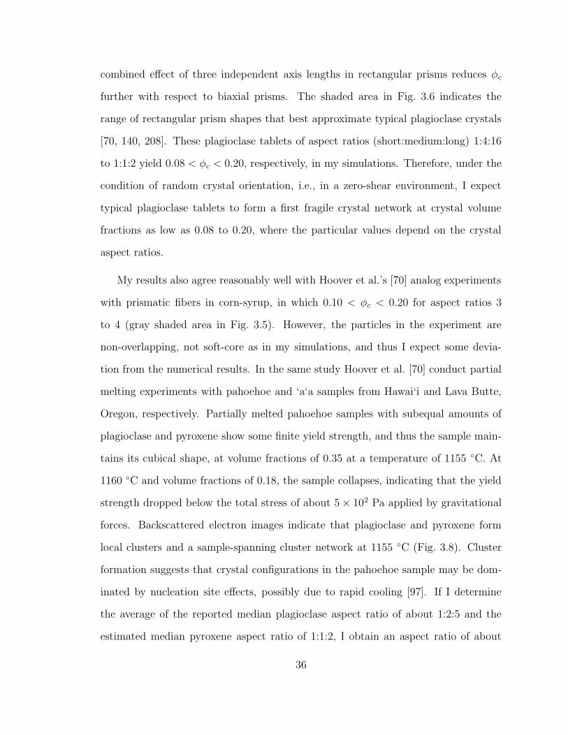
forces. Backscattered electron images indicate that plagioclase and pyroxene form

local clusters and a sample-spanning cluster network at 1155 ◦C (Fig. 3.8). Cluster

formation suggests that crystal configurations in the pahoehoe sample may be dom-

inated by nucleation site effects, possibly due to rapid cooling [97]. If I determine

the average of the reported median plagioclase aspect ratio of about 1:2:5 and the

estimated median pyroxene aspect ratio of 1:1:2, I obtain an aspect ratio of about

36

200 microns1155° C

Figure 3.8. Backscattered electron image of a pahoehoe sample from Hawai‘i close tothe percolation threshold after partial melting experiments [70]. An image-spanningcrystal pathway (arrows) formed of plagioclase (black) and pyroxene (gray) crystalscan be observed.

1:1.5:3.5 (volume fractions are about equal). For this aspect ratio and random orien-

tation, neglecting clustering effects visible in the experiments, my simulations suggest

φc ≈ 0.18 (Fig. 3.6).

Hoover et al. [70] also carried out melting experiments with ‘a‘a samples from Lava

Butte in Oregon, containing mainly plagioclase, with only minor pyroxene (volume

fraction < 0.05). The plagioclase crystals show some local alignment and exhibit a

small τy for a plagioclase volume fraction of 0.31 at 1142 ◦C, where the sample shape

is preserved, but not at 0.26 at 1150 ◦C, where the sample collapses. The plagioclase

aspect ratio is about 1:2:5 for which my simulations suggest φc ≈ 0.16. However, as

discussed previously, alignment of crystals causes an increase of φc, where the upper

bound φc = 0.29 is reached for parallel-aligned objects of any convex shape.

The general trend of my simulations and other percolation threshold studies ap-

37

pears to be consistent with experiments presented by Hoover et al. [70] and agrees

well with experiments presented by Philpotts et al. [139, 140] (Fig. 3.5). The dras-

tic decrease in φc I observe with increasing particle shape anisotropy and increasing

randomness in particle orientation is consistent with other numerical, experimetal,

and theoretical studies [6, 27, 59, 124, 156, 157] that investigate the formation of

continuous object networks.

3.5.2 Scaling relation for τy(φ) curves of differing particle

shapes, and other generalizations

To develop general rules that explain the dependence of the geometrical percola-

tion threshold, pc, on object geometries I consider two percolation theory concepts

(Chapter 2 and Saar and Manga [158]). First is the average critical number of bonds

per site at pc, Bc. Second is the excluded volume, vex, which is defined as the volume

around an object in which the center of another such object cannot be placed without

overlap. If the objects have an orientation or size distribution, the average excluded

volume of an object is averaged over these distributions and denoted by 〈vex〉 and the

average critical total excluded volume is given by 〈Vex〉 = nc 〈vex〉 [8], where nc is the

number of soft-core particles at the percolation threshold. Balberg et al. [8] find that

Bc is equal to 〈Vex〉, i.e.,

Bc = nc 〈vex〉 = 〈Vex〉 , (3.6)

equivalent to Eq. (2.8), and suggest that 〈Vex〉 is invariant for a given shape and

orientation distribution and thus independent of size distribution [5]. Values of 〈Vex〉

are highest for spheres and parallel-aligned convex objects of any shape, where 〈Vex〉 =

2.8, lowest for orthogonally-aligned (macroscopically isotropic) widthless sticks where

〈Vex〉 = 0.7, and intermediate for randomly oriented cylinders, for which 〈Vex〉 =

38

1.4 [5]. In natural systems particles can be oriented between random and parallel,

depending on the shear stress tensor and particle shapes [110, 194], and thus I expect

〈Vex〉 to fall within the bounds of 1.4 and 2.8. Therefore, 〈Vex〉 probably varies by a

factor of 2 in natural systems.

Shante and Kirkpatrick [167] found pc = 1 − exp(−Bc/8) for parallel-aligned

convex objects in continuum percolation. Using Eq. (3.6) and 〈vex〉 = 8v for spheres

(and parallel-aligned convex objects in general), where v is the volume of the sphere,

it is possible to make further generalizations. At the percolation threshold, where

n = nc, B = Bc, and φ = pc, Eq. (3.6) is substituted into φ = 1 − exp(−nv) [6, 51]

to yield

pc = 1 − exp(−Bcv/ 〈vex〉) (3.7)

for systems containing interpenetrating objects of any convex shape. Eq. (3.7) and

Bc = 〈Vex〉 = 2.8 for spheres agree well with the established percolation threshold

pc = 0.29 for soft-core spheres [141]. Soft-core parallel-aligned convex shapes also

yield pc = 0.29 [61]. Because the ratio of v/ 〈vex〉 is constant for objects of different

sizes and identical shape and orientation distributions, pc may be expected to be

invariant if only the size distribution changes. This expectation is confirmed in my

simulations (Fig. 3.7).

Generalization of a relationship between pc, 〈Vex〉, nc, and v to include variations

in object shapes have been less successful. Garboczi et al. [50] investigate a number

of possible shape functionals for randomly oriented soft-core rotational ellipsoids,

including 〈Vex〉. They find that nc 〈vex〉 ≈ 1.5 and 3.0 for extremely prolate and

oblate rotational ellipsoids, respectively, which agrees reasonably well with the range

of 1.4 (randomly oriented widthless sticks) to 2.8 (spheres) suggested by Balberg [5].

Similar results for the other shape functionals lead Garboczi et al. [50] to conclude

39

that simple shape functionals do not produce invariants and thus cannot predict pc

for overlapping rotational ellipsoids.

Drory [39] also concluded that the total average excluded volume is not truly

universal, but is influenced instead by the shape of objects “in a complicated way.”

However, Drory et al. [41] point out that 〈Vex〉 “seemed to be relatively insensitive to

the shape of particles” when compared with pc and that “it was therefore considered

an approximately universal quantity.” A more rigorous theoretical model is developed

to explain values of Bc = 〈Vex〉 for interacting objects of different shapes [39, 40, 41].

While this theory predicts Bc well it does not provide an alternative to Bc that would

be a true invariant.

Based on the above studies, I have to content myself with 〈Vex〉 as an approximate

invariant that varies by a factor of 2. Predictions of φc to within a factor of 2 should

thus be possible for a large range of particle shapes [27]. In geological applications,

a factor of 2 uncertainty in φc may be too large to interpret some observations, but

may still be a valuable constraint for developing models and predictions.

For the case of randomly oriented rods with hemispherical caps of length L +W

and width W [8],

〈vex〉 = (4π/3)W 3 + 2πW 2L + (π/2)WL2. (3.8)

For L�W , Eq. (3.8) reduces to that of Onsager [135],

〈vex〉 ≈ (π/2)WL2. (3.9)

Because the calculation of an average excluded volume for randomly oriented

rectangular prisms is difficult, I define a volume v∗ = (4/3)πr1r22 that scales in a

similar manner to Eq. (3.9). Here, r1 is the distance from the center to the closest

40

Figure 3.9. The volume v∗ = (4/3)πr1r22 scales in a similar manner to the average

excluded volume (Eq. 3.9). I normalize v∗ by the number of particles, nc, at thepercolation threshold.

edge and r2 is the distance to a vertex (Fig. 3.9). When I normalize v∗ by the critical

number of crystals per unit volume, nc, I obtain a quasi-invariant, ncv∗. In the

asymptotic limits of large and small aspect ratios ncv∗ varies by about a factor of

3 (Fig. 3.9). The relatively small variations of ncv∗ compared with φc suggests that

ncv∗ may be considered a reasonable estimate of a characteristic normalized volume.

If n 〈vex〉 were truly invariant, and could be applied to conditions of φ 6= φc and

non-overlapping (hard-core) particles, I could relate the volume fraction for particles

of general shape and volume, V , to the volume fraction, φeq, of an equivalent object

(here a sphere) by

φeq =φg 〈vex〉g

8Vg, (3.10)

where the subscript g denotes values for general particle shapes. For Eq. (3.10), I

41

use φ = nV (for hard-core particles). Similarly, for soft-core particles, where φ =

1 − exp(−nV ), I obtain the relationship

φeq = 1 − (1 − φg)〈vex〉g8Vg . (3.11)

Because nc 〈vex〉 varies by a factor of about 2, scaling in Eqs. (3.10-3.11) is accurate

to a factor of about 2.

As an example, I use Eqs. (3.8) and (3.10), and L = 2.5W for hard-core fibers of

mean aspect ratio 3.4:1 [70] to calculate that φeq = 1.5φg. I may then use this scaling

relation of 1.5 to scale experimentally measured τy(φ) curves for these fibers to the

values of the equivalent object (sphere). The two curves shown in Fig. 3.10 can be

superimposed using φeq = 2.2φg. The factor 2.2 is greater than my estimated value

of 1.5 by a factor of 1.5, and within the anticipated uncertainty range of a factor of

2.

An equivalent way of interpreting the experimental results is to determine the

average excluded volume, 〈vex〉. My result of φeq = 1.5φg implies that 〈vex〉 = 12Vg

for the hard-core fibers. I now use 〈vex〉 = 12Vg together with the computed number

of crystals at the percolation threshold, nc. For biaxial randomly oriented prisms of

aspect ratio 3:1 and a normalized particle volume of 1.7 × 10−6, simulations yield

nc = 113 × 103 which results in nc 〈vex〉 = 2.3. The average total excluded volume

thus falls within the expected range of 1.4 to 2.8 for particle shape and orientation

distributions in natural systems.

3.5.3 Implications

Possible implications of the development of yield strength in crystal-melt suspen-

sions include transitions in surface textures of basaltic lava flows [26], melt extrac-

42

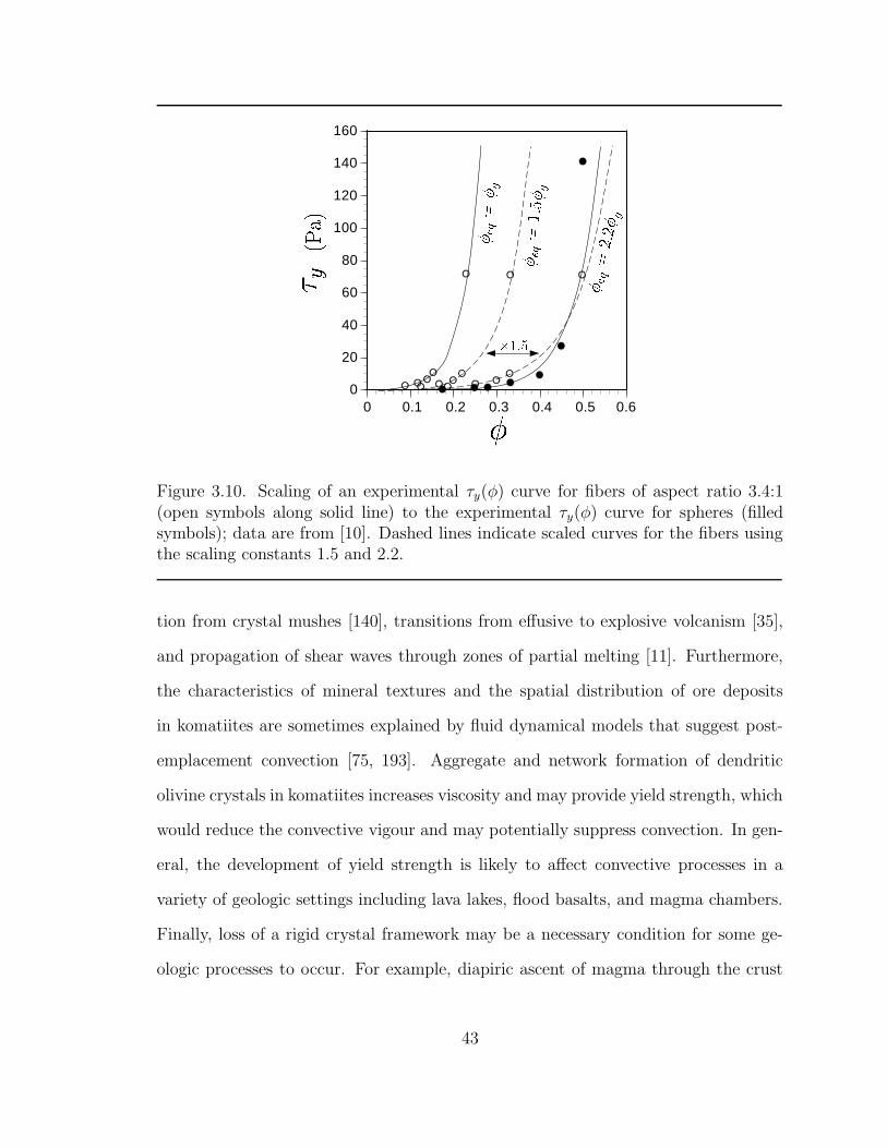
20

40

60

80

100

120

140

160

0 0.1 0.2 0.3 0.4 0.5 0.6

0

Figure 3.10. Scaling of an experimental τy(φ) curve for fibers of aspect ratio 3.4:1(open symbols along solid line) to the experimental τy(φ) curve for spheres (filledsymbols); data are from [10]. Dashed lines indicate scaled curves for the fibers usingthe scaling constants 1.5 and 2.2.

tion from crystal mushes [140], transitions from effusive to explosive volcanism [35],

and propagation of shear waves through zones of partial melting [11]. Furthermore,

the characteristics of mineral textures and the spatial distribution of ore deposits

in komatiites are sometimes explained by fluid dynamical models that suggest post-

emplacement convection [75, 193]. Aggregate and network formation of dendritic

olivine crystals in komatiites increases viscosity and may provide yield strength, which

would reduce the convective vigour and may potentially suppress convection. In gen-

eral, the development of yield strength is likely to affect convective processes in a

variety of geologic settings including lava lakes, flood basalts, and magma chambers.

Finally, loss of a rigid crystal framework may be a necessary condition for some ge-

ologic processes to occur. For example, diapiric ascent of magma through the crust

43

[116] or thorough mixing of partially solidified material into an intruding melt [125]

may require loss of continuous crystal networks.

3.6 Conclusions

I employ numerical simulations for soft-core (overlapping) rectangular prisms to

determine the critical crystal volume fraction, φc, at which a suspension may develop

a finite yield strength, τy. My results indicate that φc is a function of both shape and

the degree of randomness in particle orientations. In general, the onset of τy should

occur at lower crystal volume fractions for larger shape anisotropy, as well as for more

randomly oriented objects.

Formation of a sample-spanning network of randomly oriented plagioclase crys-

tals of aspect ratio 5:1 is expected at φc ≈ 0.13 and thus confirms experimental

observations [139, 140]. In general, under random orientations, for typical plagio-

clase aspect ratios ranging from 1:4:16 to 1:1:2 I expect 0.08 < φc < 0.20, respec-

tively. Randomly oriented crystals that have larger aspect ratios may exhibit yield

strength at even lower crystal volume fractions. Therefore, the development of yield

strength may occur at lower crystal volume fractions than the 0.35-0.5 commonly

assumed [95, 103, 142], provided the crystals are anisotropic in shape and exhibit

random orientations, as can be the case in low-shear environments.

For overlapping (soft-core) particles, φc increases with the degree of alignment and

reaches a maximum of φc = 0.29, the value for spheres, for parallel-aligned particles

of any convex shape. This dependence of φc on the particle orientation distribution

suggests that the flow regime, and therefore the resulting particle ordering, of a

suspension is an important parameter in defining φc and hence the onset of yield

44

strength. In contrast, crystal size distributions are not expected to influence φc unless

crystal overlap is inhibited. The presented results of φc in a zero-shear environment

may be viewed as a lower bound for the onset of yield strength in shear environments.

Phenocryst volume fractions larger than 0.30 [195] and even 0.50 [115] have been

reported for dikes. My results suggest that a first minimum yield strength (τy → 0)

may develop at much lower volume fractions and potentially impede magma flow.

Suppression of flow under high shear stresses, however, requires φ larger than about

0.5 [96]. Thus, it should be emphasized that even for φ > φc, flow can occur if stresses

exceed the yield strength.

Finally, I confirm that the average total excluded volume n 〈vex〉 is a quasi-

invariant that varies by only a factor of about 2 over a large range of shapes and

I suggest that it provides a reasonable means to define an equivalent volume fraction,

φeq. φeq captures the characteristic particle geometry that determines onset of φc

and may also be applied to φ 6= φc. Using φeq for all φ appears to allow scaling of

experimental τy(φ) curves [70] for suspensions of different particle shapes to within a

factor of 2.

45

Chapter 4

Hydroseismicity

This chapter is largely based on Saar and Manga [159]1.

4.1 Introduction

Natural or artificial changes in pore-fluid pressure may trigger earthquakes, a

process hereafter referred to as hydroseismicity. Examples include hydroseismicity

induced by reservoirs [60, 173, 187], by fluid injection into [67, 71, 144, 145, 150], or

withdrawal from [163, 164, 213] aquifers or oil reservoirs, or by pore-fluid pressure

changes induced by other earthquakes [72, 133]. It has also been suggested that

hydroseismicity may be caused by changes in groundwater recharge rates [30, 153, 205]

which can be the result of seasonal snow melt or variations in precipitation [90, 100,

134, 205]. In this study I use signal processing techniques to investigate whether

natural groundwater recharge variations trigger some earthquakes in the Cascade

1Reprinted from Earth and Planetary Science Letters, Vol. 214, Saar, M. O., and M. Manga,Seismicity induced by seasonal groundwater recharge at Mt. Hood, Oregon, 605-618, Copyright(2003), with permission from Elsevier.

46

volcanic arc, U.S.A.

The Cascade arc is located on a tectonically active, and in parts densely populated,

convergent plate boundary. Thus, for both seismic and volcanic hazard assessment it

is important to discern triggers of earthquakes as tectonic, magmatic, or hydrologic.

Moreover, rapid groundwater recharge may initiate larger (local magnitude, Ml > 3)

earthquakes on critically stressed faults [212]. More generally, understanding the

causes of hydroseismicity may provide additional insight into seismic hazards associ-

ated with reservoir impoundment or injection of fluids into the subsurface for example

during waste fluid injection, carbon sequestration, and geothermal energy exploration.

Detection of natural groundwater-recharge-induced earthquakes also provides a base-

line against which reservoir- or fluid-injection-induced seismicity can be measured to

evaluate the actual extent of human-caused hydroseismicity. Moreover, natural hy-

drologic triggering of earthquakes provides insight into the state of stress in the crust.

In addition to tectonic information, the time lag between groundwater recharge and

earthquakes allows me to determine hydraulic properties of the upper crust on spatial

and temporal scales that are relevant for studies of regional hydrogeology.

Figure 4.1a shows seismicity at Mt. Hood, Oregon, a Quaternary stratovolcano,

for the period from February 4th 1980 through July 11th 2002. Earthquakes oc-

cur preferentially on the southern flanks of the volcano. The offaxis concentration

suggests the possibility that earthquakes are not all caused directly by magma flow

although offcentered magma-related seismicity can occur when volcanic conduits are

inclined. Instead, I hypothesize that at least some seismicity could be triggered by

seasonal groundwater recharge that changes pore-fluid pressures on preexisting crit-

ically stressed faults. I select a region of concentrated off-axis seismicity (large open

square in Figure 4.1a) to test this hypothesis.

47

0 2 4 6 8 10

10

20

30

0

1020

1018

1022

depth (km)

num

ber

Mo (

dyne

)

mean depth = 4.5 +- 2 km

b

c

45°20’

45°30’-121°50’ -121°40’ -121°30’

✩

OR

10 km

a

Figure 4.1. a) Shaded relief map of Mt. Hood, Oregon indicating all earthquakes(pink circles and red squares) and selected (for criteria see text) earthquakes (redsquares), stream discharge gauging station on Salmon River (blue star), summit ofMt. Hood (large white triangle), and hydrothermal Swim Warm Springs (westernwhite diamond) and Meadows Spring (eastern white diamond). Three (small yellowtriangles) out of fourteen relevant seismometers (Appendix A.1) are located withinthe map region. b) Seismic moment, Mo, versus earthquake depth. c) Histogramof earthquake depths, mean earthquake depth (4.5 km), and range of 1σ-standarddeviation (2 km).

4.2 Data and analysis

The 1980 Mount St. Helens eruption increased monitoring efforts at volcanos in

the Cascade range. As a result, the Pacific Northwest Seismic Network (PNSN) has

maintained short-period vertical-motion seismometers around Mt. Hood since the

mid-1980s (Appendix A.1). To reduce instrumentation bias I only use earthquakes

with a minimum local magnitude of Ml = 1 (Figure 4.2), above which b ≈ −1 holds

48

−2 −1 0 1 2 3 4 5

occu

rren

ce

1

10

100

1000

magnitudeM -magnitudel

slope b = -1

wintersum

mer

total

Figure 4.2. Earthquake magnitude, Ml, binned in half-magnitude increments, versuslogarithmic frequency of occurrence (Gutenberg-Richter relationship) for all earth-quakes displayed in Figure 4.1. Open circles, squares, and solid circles indicate seis-micity during the summer (15 ≤ week ≤ 40, open circles) and winter(week ≥ 41 orweek ≤ 14, open squares), and total years, respectively. Above the cut-off magnitudeof Ml = 1 the decrease in seismicity with increasing magnitude follows approximatelythe expected slope of b = −1. This suggests that the data set is complete for Ml ≥ 1.

in the Gutenberg-Richter [102] relationship,

log10 N = a + bMl, (4.1)

where N is the number of earthquakes of magnitude Ml and a is the production of

seismicity. Seismic moment, Mo, is approximated by [102]

Mo = 101.5(Mw+10.73), (4.2)

where I assume Mw ≈Ml due to the small earthquake magnitudes of Ml ≤ 4.5.

Groundwater recharge at Mt. Hood is largely due to spring snow melt which

provides a natural pore-fluid pressure signal of narrow temporal width and poten-

tially relatively large amplitude. Groundwater recharge may be approximated by

49

stre

am d

isch

arge

(m

3 /s)

0 1000 2000 3000 4000 5000 6000 7000

0

1

2

3

4

5

6

7

8

1980 1982 1984 1986 1988 1990 1992 1994 1996 1998 2000

days since 01-01-1980

estimation period evaluation period prediction period

interval IIinterval I

Figure 4.3. Stream discharge of Salmon River, Oregon, measured at USGS gaugingstation 14134000 (red curve) located at an elevation of 1050 m. During the estimationperiod, a transfer function between Hood River and Salmon River is determined usinga Box-Jenkins [21] method (Appendix A.2). The evaluation period shows the fitbetween predicted (black) and actual (red) data. The prediction period shows theestimated discharge for Salmon River. Intervals I and I+II are used in the analysisand are discussed in the main text.

hydrographs of surface-runoff dominated streams at high elevations, such as Salmon

River, that show a peak in discharge during snow melt [108] (Figure 4.3). Ground-

water recharge may be delayed from stream discharge due to flow in the unsaturated

zone. This possible delay is not considered here but may be neglected considering the

uncertainty in earthquake depth discussed later.

Salmon River at USGS gauge 14134000 (blue star in Figure 4.1) has a 21 km2

drainage area. Gauge elevation is 1050 m. Stream discharge for Salmon River is only

available through September 30th 1995. Thus, I determine a transfer function between

stream discharge of Hood River (USGS gauge 14120000) and Salmon River using

a Box-Jenkins [21] method (Appendix A.2). Discharge at Hood River is available

until September 30th 2001 and is convolved with the transfer function to extend the

50

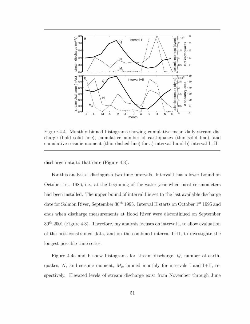
100

5

10

15

20

25

0.5

1

1.5

2

x 1021

seis

mic

mom

ent (

dyne

)

200

300

400

500

600

stre

am d

isch

arge

(m

/s)

3

# of

ear

thqu

akes

Q

N

Mo

a interval I

00

0.5

1.5

2

2.5

x 1021

seis

mic

mom

ent (

dyne

)

J F M A M J J A S O N D

stre

am d

isch

arge

(m

/s)

3

# of

ear

thqu

akes

Q

N

Mo

month

60

10

50

40

30

201

800

700

600

500

400

300

200

b interval I+II

Figure 4.4. Monthly binned histograms showing cumulative mean daily stream dis-charge (bold solid line), cumulative number of earthquakes (thin solid line), andcumulative seismic moment (thin dashed line) for a) interval I and b) interval I+II.

discharge data to that date (Figure 4.3).

For this analysis I distinguish two time intervals. Interval I has a lower bound on

October 1st, 1986, i.e., at the beginning of the water year when most seismometers

had been installed. The upper bound of interval I is set to the last available discharge

date for Salmon River, September 30th 1995. Interval II starts on October 1st 1995 and

ends when discharge measurements at Hood River were discontinued on September

30th 2001 (Figure 4.3). Therefore, my analysis focuses on interval I, to allow evaluation

of the best-constrained data, and on the combined interval I+II, to investigate the

longest possible time series.

Figure 4.4a and b show histograms for stream discharge, Q, number of earth-

quakes, N , and seismic moment, Mo, binned monthly for intervals I and I+II, re-

spectively. Elevated levels of stream discharge exist from November through June

51

period (days) period (days)

0

0.2

0.4

0.6

0.8

1

norm

aliz

ed p

ower

0 200 400 600

a

1 ye

ar

interval I

0 200 400 600

b

1 ye

ar

interval I+II

N

Q

Mo

N

Q

Mo

Figure 4.5. Period content of time series. Ten-day running average power spectra,normalized by their respective maximum power, of stream discharge, Q (bold solidline), number of earthquakes, N (thin solid line), and seismic moment, Mo (thindashed line). Dominant periods around one year occur for both interval I (a) andinterval I+II (b).

with a peak in May due to snow melt. Number of earthquakes and total seismic

moment show a peak during September and October for both intervals I and I+II.

In addition, interval I+II shows seismicity in January and February. For interval I,

the time lag between peak stream discharge, a proxy for groundwater recharge, and

seismicity is about 5 months. To test whether Q, N , and Mo have yearly periodicity,

I determine their power spectra which indeed show dominant periods of about one

year (Figure 4.5) for both intervals I and I+II.

Rather than using monthly-binned data averaged over all years from Figure 4.4

to determine cross correlation coefficients, I use the actual time series at a resolution

of one day. Seismicity is binned to yield daily number of earthquakes, N , and total

daily seismic moment, Mo. Next, I apply moving least-squares polynomial fits (Ap-

pendix A.3) of order ≤ 5 to Q, N , and Mo (Figure 4.6), resulting in the interpolated

52

time series denoted Q, N , and Mo, respectively. This type of interpolation assures

that the data is optimally matched in a least-squares sense and that later determi-

nation of cross-correlation coefficients between time series are based on equivalent

frequency bands. Moreover, interpolation of N and Mo provides evenly-spaced data

allowing for standard spectral analysis techniques. For better temporal comparison,

the interpolated data from Figure 4.6 (black curves) are shown normalized by their

respective maximum values in Figure 4.7.

For a lead channel f and a lag channel g, the normalized cross (f 6= g) and auto

(f = g) correlation coefficients, Φfg(t), at a time lag of t, are given by

−1 ≤ Φfg(t) =φfg(t)

√

φff(0)√

φgg(0)≤ 1, (4.3)

where

φfg =

∫

∞

−∞

f(τ)g(t+ τ)dτ. (4.4)

The normalization assures that perfect correlation, no correlation, and perfect anti-

correlation, are indicated by values of 1, 0, and -1, respectively.

I determine normalized unbiased cross-correlation coefficients, ΦQN and ΦQMo

(Figure 4.8) for the time series. Cross-correlations show statistically significant peaks

at 151 days that are distinct from 99% confidence intervals for random earthquake

distributions (Appendix A.4).

To reduce possible dominance by a year with exceptionally high seismicity, I also

determine moving normalized unbiased cross-correlation coefficients, Φfg, on overlap-

ping segments within each time series (Appendix A.4). The segment width is 3 years

with 30 days shift after each cross-correlation calculation resulting in 75 and 109

segments for intervals I and I+II, respectively. For each segment 20 repetitions are

performed so that a total of over 1000 and 2000 iterations are used to determine the

53

x 1021

0 1000 2000 3000 4000 5000

0

1

2

0

10

20

30

0

2

4

6

a

b

c

interval I interval II

seis

mic

mom

ent (

dyne

)nu

mbe

r of

ear

thqu

akes

stre

am d

isch

arge

(m

/s)

3

days since 10-01-1986

10-01-1986 09-30-1995 09-30-2001

Q

N

Mo

Figure 4.6. Original (gray) and interpolated (black) time series of a) seismic moment,b) number of earthquakes, and c) stream discharge of Salmon River at Mt. Hood.Stream discharge includes predicted data from Figure 4.3 for interval II. Interpolationis performed using a moving least-squares polynomial fit method of order ≤ 5 persegment as described in the text and in Appendix A.3. This assures that the datais optimally matched in a least-squares sense and that the series can be compared atequivalent frequency bands (Figure 4.7).

54

1

0.8

0.6

0.4

0.2

00 1000 2000 3000 4000 5000

10-01-1986 09-30-200109-30-1995interval I interval II

Q

N

Mo

Figure 4.7. Interpolated time series from Figure 4.6, normalized by each series’ abso-lute maximum value. Local maxima of number of earthquakes (thin solid line) andseismic moment (thin dashed line) typically follow local maxima of stream discharge(bold solid line) after a time lag of about 151 days.

confidence intervals for intervals I and I+II, respectively (Appendix A.4). Figure 4.9

shows statistically significant moving cross-correlation coefficients for ΦQN and ΦQMo

that are always distinct from the 90%, and in 3/4 of the cases even from the 99%,

confidence limits for random earthquake distributions. Results from all segments are

averaged for each time lag (bold lines in Figure 4.9). For both ΦQN and ΦQMoa

maximum is reached for a time lag of about Γ ≈ 151 days.

4.3 Discussion

In the following I describe processes that can cause hydroseismicity and provide a

model that allows me to determine both hydraulic diffusivity, κ, and critical pressure

change, P ′. From κ I then estimate hydraulic conductivity, Kh, and permeability, k.

Throughout the discussion I compare my results with other studies.

55

0 50 100 150 200 2500.2

0.4

0.6

0.8

time lag (days)

cros

s co

rrel

atio

n co

effic

ient

0.99

0.99

interval I

ΦQMo

ΦQN

Figure 4.8. Time lag versus unbiased normalized cross-correlation coefficients ΦQN

(bold solid line) and ΦQMo(bold dashed line) for interval I. Thin horizontal lines

indicate the respective upper bounds of the 99% confidence intervals of 1000 cross-correlations for randomly-assigned phases for each lag channel (Appendix A.4). Lowerbounds are comparable to the negative of the upper bounds. Both curves suggest atime lag of about 151 days.

4.3.1 Causes of hydroseismicity

Principal mechanisms involved in triggering hydroseismicity may be explained by

combining concepts from linear poroelasticity [198] with the Coulomb failure criterion,

τs = τ0 + µσ′

n, (4.5)

where τs, τ0, µ are the fault’s shear strength, cohesion, and coefficient of friction,

respectively, and σ′

n is the effective normal stress across the fault. Throughout this

chapter compressive stresses are positive. σ′

n, is given by

σ′

n =σ′

1 + σ′

3

2+σ′

1 − σ′

3

2cos(2θ), (4.6)

56

0 50 100 150 200 2500.3

0.4

0.5

0.6

0.7

0.8

time lag (days)

mea

n m

ovin

g cr

oss

corr

. coe

ff.

thick solid line: cross(Q,N): 157 +- 23 days

thick dashed line: cross(Q,Mo): 152 +- 18 days

thin solid line: 99% +2std from 2189 iterations

thin dashed line: 99% +2std from 2189 iterations

0.99

0.99

ΦQMo

ΦQN

a

0 50 100 150 200 250time lag (days)

b

0.99

0.99

0.90

0.90

ΦQMo

ΦQN

interval I interval I+IIthick solid line: moving_cross(Q,N): 155+-43 days (std) from 109 iterationsthick dashed line: moving_crossc(Q,Mo): 139+-41 days (std) from 109 iterationsthin black solid line: 99% +2std from 2189 iterations for moving_cross(Q,N)thin white solid line: 90% +2std from 2189 iterations for moving_cross(Q,N)thin black dashed line: 99% +2std from 2189 iterations for moving_cross(Q,Mo)thin white dashed line: 90%+2std from 2189 iterations for moving_cross(Q,Mo)

thick solid line: moving_cross(Q,N): 157 +- 23 days (std) from 75 iterationsthick dashed line: moving_cross(Q,Mo): 152 +- 18 days (std) from 75 iterationsthin solid line: 99% +2std from ... iterations for moving_cross(Q,N)thin dashed line: 99% +2std from ... iterations for moving_cross(Q,Mo)

Figure 4.9. Time lag versus the mean of the unbiased normalized moving cross-correlation coefficients ΦQN (bold solid line) and ΦQMo

(bold dashed line). Thin hori-zontal lines indicate the respective upper bounds of the 99% (black) and 90% (white)confidence intervals of over 2000 cross-correlations for randomly-assigned phases foreach lag channel (Appendix A.4). Lower bounds are comparable to the negative ofthe upper bounds. Vertical lines at maximum coefficient values indicate mean (cen-ter line) and mean ± 1-σ standard deviation (outer lines) for the respective timelags determined from 75 (a) and 109 (b) moving windows of 3-year width. The fourmean time lags and respective standard errors are (in days): a) 157±2.7 (solid line),152±2.1 (dashed line); b) 155±4.1 (solid line), 139±3.9 (dashed line), resulting in atotal mean and standard error of 151±6.6 days.

where σ′

1 and σ′

3 are the effective principal maximum and minimum compressive

stresses, respectively, and θ is the angle between σ ′

1 and the normal to the failure

plane (Figure 4.10a). σ′

n clamps the fault requiring larger shear stresses, τ , to induce

failure (Figure 4.10). The three effective principal stresses, σ ′

1, σ′

2, and σ′

3 are the

diagonal elements of the effective principal stress tensor given by

σ�

= σ − αPδij, (4.7)

57

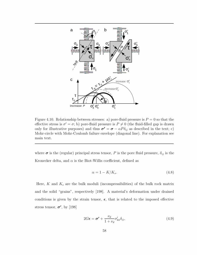
σ1

σ3

σn

τ

faul

t

θ

a

σ1

σ3

τ = τ

+ µσ ’n

s0

τ

increase P

τ0

’σ3 ’σ1’σn

increase ’σ1c

2θ

decrease ’σ3

Pσ3’ σ3’

’σ1

’σ1

τ

b

σn’

Figure 4.10. Relationship between stresses: a) pore-fluid pressure is P = 0 so that theeffective stress is σ′ = σ; b) pore-fluid pressure is P 6= 0 (the fluid-filled gap is drawnonly for illustrative purposes) and thus σ

�

= σ − αPδij as described in the text; c)Mohr-circle with Mohr-Coulomb failure envelope (diagonal line). For explanation seemain text.

where σ is the (regular) principal stress tensor, P is the pore fluid pressure, δij is the

Kronecker delta, and α is the Biot-Willis coefficient, defined as

α = 1 −K/Ks. (4.8)

Here, K and Ks are the bulk moduli (incompressibilities) of the bulk rock matrix

and the solid “grains”, respectively [198]. A material’s deformation under drained

conditions is given by the strain tensor, ε, that is related to the imposed effective

stress tensor, σ�

, by [198]

2Gε = σ�

+νd

1 + νd

σ′

kkδij, (4.9)

58

where σ′

kk = σ′

xx + σ′

yy + σ′

zz is the trace of σ�

, G is the shear modulus, and

νd =

(

∂εjj∂εii

)

∂P=0; ∂σjj=0

(4.10)

is the drained poisson’s ratio. Deformation can lead to failure, when the shear stress,

τ =

∣

∣

∣

∣

σ′

1 − σ′

3

2sin(2θ)

∣

∣

∣

∣

, (4.11)

exceeds the material’s shear strength, τs, in Eq. (4.5), for a given effective normal

stress σ′

n. Because σ′

n and τ depend on both orientation of the fault within a stress

field and on the magnitude of the stresses [Eqs. (4.6,4.11)], failure can be triggered by

changes in both θ and σ�

(Figure 4.10). The latter mechanism may induce earthquakes

by causing 1) an increase in σ′

1, 2) a decrease in σ′

3, or 3) an equal decrease in all

effective principal stresses, for example due to an increase in P [Eq. (4.7)]. The first

two mechanisms cause failure by increasing the effective differential stress, σ ′

1−σ′

3, and

thus shear stress, τ , in Eq. (4.11). The third mechanism induces failure by decreasing

the effective strength of the material caused by a decrease in σ ′

n which unclamps the

fault and moves the Mohr-circle closer to the Mohr-Coulomb failure envelope, while

leaving τ unchanged (Figure 4.10).

Fluctuations in pore-fluid pressure, P , denoted P ′, on faults due to an increase

in σ′

1 (e.g., by the weight of a filling reservoir that contracts the pore space) occur

immediately. In contrast, a local increase in hydrostatic pore-fluid pressure, Ph =

ρwgh, (e.g., by groundwater recharge, reservoir impoundment, or injection of fluids at

depth), may trigger earthquakes after a time lag, Γ, that is related to pressure diffusion

to the fault. Here, ρw is the density of water, g is acceleration due to the Earth’s

gravity, and h is the height of the water column above the point of interest. Reservoirs

exhibit both processes and thus typically cause earthquakes both concurrent with,

and delayed from, their filling [150, 173]. In this study I am interested in seismicity

59

induced by groundwater recharge and am thus focusing on earthquakes delayed from

recharge by pore-fluid pressure diffusion. Here, the load of the additional groundwater

is small and thus triggered seismicity due to a (small) increase in σ ′

1 is neglected.

Nonetheless, because only the connected pore space is fluid-filled, relatively high

hydrostatic pore-fluid pressure changes, P ′, may be reached that may be sufficient to

induce earthquakes.

4.3.2 Analytic model

I can approximate the effect of seasonal groundwater recharge with periodic yearly

(ψ = 1 year) pore-fluid pressure variations of amplitude P0 at the surface (z = 0 m)

as

P ′(t, z = 0) = P0 cos

(

2πt

ψ

)

. (4.12)

Pore-fluid pressure evolution below the water table is governed by the (pressure)

diffusion equation. In a 1-dimensional half-space the (pressure) diffusion equation is

given by

κ∂2P ′

∂z2=dP ′

dt, (4.13)

where the hydraulic diffusivity,

κ =Kh

Ss=

gk

νSs, (4.14)

is assumed constant. Here, Kh, Ss, k, and ν are the hydraulic conductivity, specific

storage, permeability, and kinematic viscosity, respectively. The solution to Eq. (4.13)

with boundary condition (4.12) is [192]

P ′

P0

= exp

(

−z√

π

ψκ

)

cos

(

2πt

ψ− z

√

π

ψκ

)

(4.15)

and is graphed in Figure 4.11 for ψ = 1 year and hydraulic diffusivity κ = 0.3 m2/s as

determined later in Eq. (4.18) for the study region. The exponential term in Eq. (4.15)

60

Figure 4.11. Periodic pore-fluid pressure fluctuations, P ′/P0, at various depths, z(in km), for hydraulic diffusivity κ = 0.3 m2/s and surface pressure perturbationperiodicity ψ = 1 year. With increasing depth, the amplitude of the pore-fluidpressure perturbation decreases and the phase lag increases. At a depth of 4.5 km,approximately 10% of the original pressure amplitude, P0, remains and the delay ofthe peak is about 151 days (dashed line), i.e., a phase lag of about 0.8 π.

describes the decrease in the time-dependent pressure amplitude with depth, z, to

P ′/P0 = 1/e at a characteristic length scale (skin depth) of

zc =

√

ψκ

π. (4.16)

The cosine term in Eq. (4.15) describes the periodic variations of the pressure signal

as a function of both depth, z, and time, t. In addition, both terms in Eq. (4.15) are

a function of κ and ψ.

The actual pore-fluid pressure at depth is P = Ph +P ′, i.e., the hydrostatic pore-

fluid pressure, Ph, with superimposed periodic pore-fluid pressure fluctuations, P ′

(Figure 4.12). The argument in the cosine in Eq. (4.15) is expected to be zero (or a

multiple of 2π) so that the cosine reaches its maximum, one, during failure (e.g., point

61

C in Figure 4.12). It may be reasonable to assume that if a critical pore-fluid pressure,

Pc, had been reached before the cosine maximum (e.g., point B in Figure 4.12) then

failure should have occurred at shallower depths where a cosine maximum reaches

the same critical pore-fluid pressure, Pc, earlier in time (e.g., point A in Figure 4.12).

Here, I assume that the subsurface has a pervasive system of at least one fault along

which failure can occur at any depth given appropriate stress conditions. Thus, from

the condition that the argument of the cosine term in Eq. (4.15) has to be zero, I can

determine κ from

κ =ψz2

4πt2. (4.17)

4.3.3 Hydraulic diffusivity

In this study the proposed period of pressure perturbation is ψ = 1 year and

the time lag, Γ, between groundwater recharge and seismicity at Mt. Hood is Γ =

t = 151 with a standard error of ±7 days (Figure 4.9). Earthquake phase data for

earthquake relocation was not readily available. Thus, I could not resolve whether

the 1σ-standard deviation in the earthquake depth distribution, z = 4.5 ± 2 km

(Figure 4.1c), reflects error in determining earthquake locations. Hurwitz et al. [77]

suggest that ice caps on many Cascade range volcanos may restrict recharge on their

summits and uppermost flanks and that the water table below stratovolcanos may

thus be relatively deep. Consequently, pore-fluid pressure diffusion distances to mean

seismic depths may be shorter than the 4.5 km assumed here, while relatively slow

flow through the unsaturated zone above the water table could delay fluctuations of

water table levels. Furthermore, isotopic contents of water discharged for example

at hydrothermal Meadows Spring suggest a recharge elevation of 2700 - 2900 m, i.e.,

62

0 200 400 600 800days

~de

pth,

z (

km)

10

20

30

0

1

2

3

0

100 days

A BCP

+ 1

0P (

MP

a)h

~’

Figure 4.12. Hydrostatic pressure, Ph, (at depths from 0 to 3 km) with superimposed(for better visibility) 10-fold exaggerated periodic pore-fluid pressure fluctuations,P = Ph + 10P ′, versus time for κ = 0.3 m2/s and periodicity of ψ = 1 year. Thecritical pore-fluid pressure for failure should be reached at the maximum of the cosineterm and a minimum possible depth (point A) as explained in the main text. At adepth of 3 km, the peak of the pressure perturbation is delayed (with respect to thesurface) by 100 days (vertical line). Thus, at the mean earthquake depth of about4.5 km the peak is delayed by the determined time lag of about 151 days. The upperhalves of the sinusoids are filled to better visualize the decrease in amplitude andincrease in phase lag of the pore-fluid pressure perturbation with increasing depth.

about 600 m below the summit of Mt. Hood [127]. However, lowering of the water

table not only reduces the available diffusion time, t, in the saturated zone but also

decreases the diffusion depth, z, to the earthquakes. Lower values of t and z in

Eq. (4.17) tend to cancel each other. In addition, earthquake depths are determined

relative to a horizontal plane that is approximately at the mean elevation (∼1 km)

of the relevant seismometers in the region. As a result, z and t assumed here are

probably both somewhat smaller than may be expected. Due to the large uncertainty

63

in earthquake depth (±2 km) already considered and due to the cancelling effects of

reducing both z and t, I neglect the effects of water table reduction by a possible 0.5

to 1 km relative to the surface.

Using ψ = 1 year, t ≈ 151 days, and z ≈ 4.5 km in Eq. (4.17) yields a hydraulic

diffusivity of

κ = 0.30 ± 0.22 m2/s. (4.18)

This value of κ agrees with other crustal hydraulic diffusivities compiled by Talwani

and Acree [187] and is in the upper range for fractured igneous rocks [149]. Gao et

al. [49] suggest a value as high as 1 m2/s for some fractured volcanic systems.

4.3.4 Critical pore-fluid pressure change

The step-function characteristics of a pore-fluid pressure increase due to initial

reservoir impoundment and its error function solution [2, 187] does not allow for eval-

uation of the critical value of P ′/P0 at which failure occurs [187]. In contrast, the

additional temporal information provided here by the periodicity of the surface pres-

sure perturbation in the case of seasonal groundwater recharge allows for estimation

of critical P ′/P0. Because failure is likely to occur when the cosine term in Eq. (4.15)

is one, I can determine P ′/P0 for the above calculated value of κ = 0.3 m2/s at a

mean depth of about 4 ≤ z ≤ 4.5 km and period ψ = 1 year as

P ′

P0

= exp

(

−z√

π

ψκ

)

≈ 0.1. (4.19)

Thus, about 10% of the estimated amplitude of near-surface pressure variations ap-

pears to be sufficient to trigger hydroseismicity at Mt. Hood.

Average annual precipitation in the (Oregon) Cascades, and particularly at Mt.

Hood, is about 3 m [165] of which approximately 50% infiltrates the ground [85, 109]

64

mostly during spring snow melt. This leads to infiltration rates of about 1.5 m per year

concentrated during a few months. Lava flows in the region typically have near-surface

porosities of about 15 % [81] that decrease with depth. Thus, groundwater levels

may fluctuate annually by approximately 10 m resulting in seasonal fluid pressure

variations that may exceed P0 = 0.1 MPa. Therefore, according to Eq. (4.19), the

critical pore-fluid pressure increase at depth z ≈ 4.5 km may be as low as P ′ ≈ 0.01

MPa, and possibly lower, at Mt. Hood.

While several authors mentioned in the introduction, as well as this study, suggest

that some earthquakes are triggered by pore-fluid pressure perturbations, the neces-

sary critical pore-fluid pressure increase, P ′, is uncertain [187]. However, it is often

argued that many faults are near critically-stressed [190]. Therefore, small stress

changes invoked by a variety of different mechanisms may be sufficient to cause seis-

micity on some preexisting faults. Examples include earthquake triggering by solid

Earth and ocean tides [94, 188, 201], seasonal modulations of seismicity by the load

of snow [68], precipitation and snow melt induced seismicity [100, 205] and general

fluid-driven seismicity [4]. Lockner and Beeler [104] conduct laboratory studies of

rock failure along preexisting faults induced by periodic axial stress changes superim-

posed on a confining pressure of 50 MPa. They find a transition from weak to strong

correlation between periodic stress and failure at an amplitude of 0.05 to 0.1 MPa

shear stress. Roeloffs [149, 150] suggests that an increase of P ′ ≈ 0.1 MPa can cause

reservoir-induced seismicity. Similarly, possible triggering of earthquakes by static

stress changes of about 0.1 MPa and less has been proposed by King et al. [98] and

Stein et al. [183, 184, 185]. Harris [65] summarizes the work of several authors and

states that “It appears that static stress changes as low as 0.01 MPa (0.1 bar) can

affect the locations of aftershocks.”

65

The examples cited previously as well as my results suggest that the necessary

stress change for earthquake initiation on preexisting faults may be as low as 0.01 to

0.1 MPa which is only a fraction of the coseismic stress drop. Therefore, Harris [65]

points out that Coulomb stress changes are said to “enhance” the occurrence of

an earthquake, as opposed to generating it. I support this view and suggest that

pore-fluid pressure changes due to groundwater recharge at Mt. Hood increase the

probability of seasonal earthquake occurrences.

Heki [68] states that seasonal seismicity is not expected if the rate of secular

(long-term) regional stress increase is much larger than the annual superimposed

disturbance. For the case of the Cascades subduction zone, and assuming the validity

of a characteristic earthquake model [169], the annual secular stress increase may be

estimated by the (approximately constant) coseismic stress drop, ∆σ ≈ 10 MPa,

divided by the average recurrence interval, tr ≈ 300 years, of large earthquakes.

Estimated annual pore-fluid pressure fluctuations of 0.01 MPa/year at Mt. Hood at

a mean earthquake depth of z = 4.5 km are comparable to ∆σ/tr ≈ 0.03 MPa/year.

Therefore, the pore-fluid pressure fluctuations below Mt. Hood at depths of about

4.5 km caused by groundwater recharge may be large enough to induce seasonal

hydroseismicity.

The concentration of (hydro-) seismicity south of Mt. Hood may be due to prefer-

ential occurrences of active faults in this region [92, 127, 200]. Jones and Malone [92]

performed earthquake relocations and determined focal mechanisms of events from

the June-July 2002 swarm which reveal distinct clusters along normal faults (e.g.,

White River fault) located south of Mt. Hood as well as events located beneath the

summit that appear to be magma-related. This relation between snow melt, ground-

water recharge, and seismicity on faults that are kept relatively permeable, may

66

also be reflected by the occurrence of the only hydrothermal springs (Swim Warm

Springs, Meadows Spring) at Mt. Hood [77, 127] in the region south of the volcano

(Figure 4.1a).

4.3.5 Hydraulic conductivity and permeability

Once the hydraulic diffusivity, κ, is known, the hydraulic conductivity, Kh, per-

meability, k, or specific storage, Ss, can be determined by Eq. (4.14). The specific

storage is given by

SS = ρg(α + nβ), (4.20)

where α is the bulk aquifer compressibility (at constant vertical stress and zero lateral

strain), n is the pore fraction, and β = 4.8 × 10−10 m2/N is the compressibility of

water. If I assume a mean n ≈ 0.05 for the study region [85] and α = 10−10 m2/N for

fractured rock [37, 150], then, for the hydraulic diffusivity range given in Eq. (4.18),

the hydraulic conductivity is

8 × 10−8 ≤ Kh = κSS ≤ 5 × 10−7 m/s (4.21)

which, from Eq. (4.14) and for a kinematic water viscosity of ν ≈ 10−7 m2/s at 80◦C,

corresponds to a permeability range of

8 × 10−16 ≤ k ≤ 5 × 10−15 m2 (4.22)

for the upper ∼6 km of the crust at Mt. Hood.

The suggested permeabilities are relatively high compared with a maximum of

k ≈ 10−16 m2 required for mostly conductive heat transfer [114] as suggested for

the Oregon Cascades at depths below about 2 km. However, I suggest two possible

arguments that potentially explain why k is higher than may be expected.

67

First, a reasonable assumption is that permeability is much higher at shallower

depths and decreases with depth due to compaction. Therefore, pore fluid diffusion

is much faster in the shallower section and most of the observed time delay probably

occurs at deeper portions of the profile. Reducing z for example by a factor of two

in Eq. (4.17) would decrease κ, Kh, and k by a factor of four.

Second, I suggest that the region south of Mt. Hood is anomalous with respect

to conductive heat transfer because it hosts the only two hot-springs observed on

the flanks of Mt. Hood to date [127]. The presence of hot springs suggests that

geothermal fluids rise relatively quickly along higher-k paths (e.g., faults) so that

time scales for complete conductive thermal equilibration between hot fluids and

colder surrounding rock are larger than the travel times of fluids. Indeed, Forster and

Smith [46] suggest that hot springs can only be expected for a permeability window

of 10−17 ≤ k ≤ 10−15 m2. My permeability values from Eq. (4.22) fall in the upper

range suggested for hot springs by Forster and Smith [46]. Here, high permeabilities

lead to increased water fluxes that result in lower geothermal spring temperatures

that are consistent with those (5◦C to about 25◦C [127]) observed at Meadows Spring

and Swim Warm Springs.

The magnitudes for (mostly vertical) permeability, k, calculated here, reflect val-

ues for a large spatial scale that includes Mt. Hood and its nearby active (normal)

faults that are kept permeable by rupture and appear to provide fluid pathways. That

the magnitudes of hydraulic diffusivity, κ, and permeability, k, are plausible further

supports the hypothesis of seasonal elevated seismicity levels due to groundwater

recharge in this region.

68

4.4 Conclusions

Several arguments support the hypothesis that some seismicity at Mt. Hood,

Oregon, is triggered by pore-fluid pressure diffusion as a result of rapid groundwater

recharge due to seasonal snow melt. Statistically significant cross-correlation coeffi-

cients between groundwater recharge and seismicity suggest a time lag of about 151

days. The values of the correlation coefficients are distinct from those for random

temporal earthquake distributions determined by Monte Carlo simulations. The time

lag and mean earthquake depth provide a reasonable (mostly) vertical hydraulic dif-

fusivity (κ ≈ 10−1 m2/s), hydraulic conductivity (Kh ≈ 10−7 m/s), and permeability

(k ≈ 10−15 m2) that agree with other studies [46, 187, 190]. Finally, I determine

the critical fraction (P ′/P0 = 0.1 MPa) of the periodic near-surface pore-fluid pres-

sure fluctuations (P0 ≈ 0.1 MPa) that reach the mean earthquake depth, suggesting

that P ′ ≈ 0.01 MPa can trigger seismicity. This value of P ′ ≈ 0.01 MPa is at the

lower end of the range of critical pore-fluid pressure changes of 0.01 ≤ P ′ ≤ 0.1

MPa suggested in previous studies [65, 98, 149, 150]. Therefore, while seismicity is

distributed throughout the year at Mt. Hood, I conclude that some earthquakes are

hydrologically induced by a reduction in effective stress due to a seasonal increase in

hydrostatic pore-fluid pressure, Ph, by a small amount P ′. In fact, elevated seismicity

levels due to such small effective stress changes suggest that the state of stress in the

crust at Mt. Hood, Oregon, could be near critical for failure.

69

Chapter 5

Permeability-depth curve

5.1 Introduction

Permeability, k, describes a material’s ability to transmit fluids. It is thus a crit-

ical material property that is relevant to numerous geological processes that depend

on mass and/or energy transfer as for example described by Ingebritsen and San-

ford [82]. Examples include transfer of water, steam, hydrocarbons, pore fluid pres-

sure, and heat. Permeability is a second rank tensor that can be highly anisotropic and

heterogeneous, varying over more than 15 orders of magnitude in geological materi-

als [47]. Because fluid driving forces and viscosities vary much less, permeability is the

most important parameter in geological porous media flow, largely determining fluid

fluxes. Measuring the permeability of rock cores in laboratory settings [22, 23, 157]

is done routinely. However, such rock core permeabilities may not reflect field-scale

values [28, 79, 162] where larger representative elementary volumes [12] may have to

be considered that include large-scale fractures or layers [37]. At intermediate field

scales, from tens to hundreds of meters, it is frequently possible to conduct pumping

70

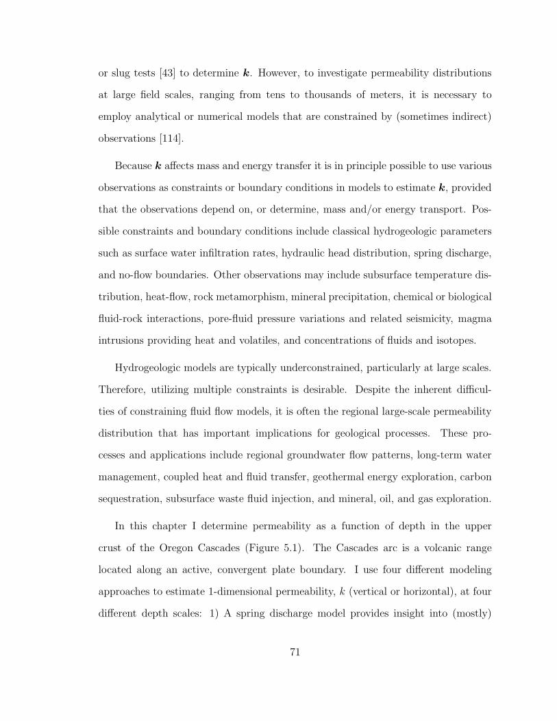
or slug tests [43] to determine k. However, to investigate permeability distributions

at large field scales, ranging from tens to thousands of meters, it is necessary to

employ analytical or numerical models that are constrained by (sometimes indirect)

observations [114].

Because k affects mass and energy transfer it is in principle possible to use various

observations as constraints or boundary conditions in models to estimate k, provided

that the observations depend on, or determine, mass and/or energy transport. Pos-

sible constraints and boundary conditions include classical hydrogeologic parameters

such as surface water infiltration rates, hydraulic head distribution, spring discharge,

and no-flow boundaries. Other observations may include subsurface temperature dis-

tribution, heat-flow, rock metamorphism, mineral precipitation, chemical or biological

fluid-rock interactions, pore-fluid pressure variations and related seismicity, magma

intrusions providing heat and volatiles, and concentrations of fluids and isotopes.

Hydrogeologic models are typically underconstrained, particularly at large scales.

Therefore, utilizing multiple constraints is desirable. Despite the inherent difficul-

ties of constraining fluid flow models, it is often the regional large-scale permeability

distribution that has important implications for geological processes. These pro-

cesses and applications include regional groundwater flow patterns, long-term water

management, coupled heat and fluid transfer, geothermal energy exploration, carbon

sequestration, subsurface waste fluid injection, and mineral, oil, and gas exploration.

In this chapter I determine permeability as a function of depth in the upper

crust of the Oregon Cascades (Figure 5.1). The Cascades arc is a volcanic range

located along an active, convergent plate boundary. I use four different modeling

approaches to estimate 1-dimensional permeability, k (vertical or horizontal), at four

different depth scales: 1) A spring discharge model provides insight into (mostly)

71

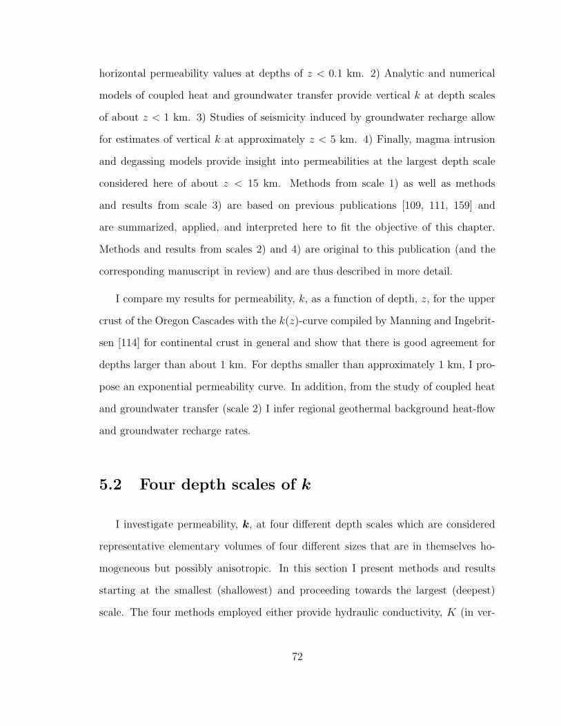
horizontal permeability values at depths of z < 0.1 km. 2) Analytic and numerical

models of coupled heat and groundwater transfer provide vertical k at depth scales

of about z < 1 km. 3) Studies of seismicity induced by groundwater recharge allow

for estimates of vertical k at approximately z < 5 km. 4) Finally, magma intrusion

and degassing models provide insight into permeabilities at the largest depth scale

considered here of about z < 15 km. Methods from scale 1) as well as methods

and results from scale 3) are based on previous publications [109, 111, 159] and

are summarized, applied, and interpreted here to fit the objective of this chapter.

Methods and results from scales 2) and 4) are original to this publication (and the

corresponding manuscript in review) and are thus described in more detail.

I compare my results for permeability, k, as a function of depth, z, for the upper

crust of the Oregon Cascades with the k(z)-curve compiled by Manning and Ingebrit-

sen [114] for continental crust in general and show that there is good agreement for

depths larger than about 1 km. For depths smaller than approximately 1 km, I pro-

pose an exponential permeability curve. In addition, from the study of coupled heat

and groundwater transfer (scale 2) I infer regional geothermal background heat-flow

and groundwater recharge rates.

5.2 Four depth scales of k

I investigate permeability, k, at four different depth scales which are considered

representative elementary volumes of four different sizes that are in themselves ho-

mogeneous but possibly anisotropic. In this section I present methods and results

starting at the smallest (shallowest) and proceeding towards the largest (deepest)

scale. The four methods employed either provide hydraulic conductivity, K (in ver-

72

Mt. Hood

Cultus RiverQuinn River

elevation (m)

longitude

latit

ude

Santiam Pass

A

B

C

E

D

Figure 5.1. Shaded relief map of the study region in Oregon, USA. Red boxes indicateparticular study regions used for the four methods and scales described in Section 5.2:A) spring discharge model, B) coupled heat and groundwater flow model in a 1-dimensional recharge area, C) radial coupled heat and groundwater flow model, D)magma intrusion model, E) region for heat-flow interpolation based on 209 geothermprofiles (white circles).

73

tical, Kz, or horizontal, Kx, direction) or vertical hydraulic diffusivity, κz. Both

hydraulic conductivity, K, and hydraulic diffusivity, κ, are converted to permeabil-

ity, k, as described in Section 5.3, so that the change in k as a function of depth can

be discussed in Section 5.4. Appendix B.1 lists symbols used in this chapter, their

units, and their definitions.

5.2.1 Spring discharge model: k(z <0.1 km)

Manga [109, 111, 112] shows that discharge at springs can be used to estimate

large-scale near-surface horizontal hydraulic conductivity, Kx, and horizontal perme-

ability, kx. I briefly describe the general approach and apply the method to discharge

data from springs in the study region. I reserve interpretation for the discussion

section.

Method

Stacked lava flows form aquifers that typically show high horizontal hydraulic

conductivities within the upper blocky parts of each flow [23, 122]. The dense but

jointed interior of a solidified lava flow shows predominantly vertical groundwater flow

along cooling joints. Manga [112] suggests that the horizontal blocky layer may be

approximated as a confined aquifer of mean constant thickness, b, and high horizontal

hydraulic conductivity, Kx, and the dense interior as an unconfined aquifer providing

water from storage according to its specific yield, SY . As a result, hydraulic head

distribution is governed by a (1-dimensional) confined aquifer equation

∂h

∂t=Kx b

SY

∂2h

∂x2+uR (x, t)

SY, (5.1)

74

where specific storage, SS, has been substituted by SY /b. Here, t, x, uR, Kx, and

SY are time, horizontal dimension, recharge rate, horizontal hydraulic conductivity,

and specific yield, respectively. The (variable) hydraulic head in the dense interior

layer is denoted h. Eq. (5.1) is equivalent to a linearized Boussinesq equation for

unconfined aquifer flow, in which case b and h denote mean constant hydraulic head

and small (variable) head, respectively. Eq. (5.1) is a linear diffusion equation where

the hydraulic diffusivity is given by

κx =Kx b

SY. (5.2)

As usual in a diffusive system, the diffusion time scale, τ , is characterized by τ =

L2/κx, where L is the aquifer length (Figure 5.2). Therefore, Eq. (5.2) becomes

Kx =SY L

2

bτ . (5.3)

The aquifer thickness, b, is related to the mean residence time of water in the aquifer,

tr, by

tr =AbSY

Qs

=bSY

uR

, (5.4)

where A, Qs, and uR = Qs/A are the surface area (exposed to recharge) of the un-

confined aquifer, the mean spring discharge flux, and the mean groundwater recharge

rate, respectively (Figure 5.2). Substituting Eq. (5.4) into Eq. (5.3) yields

Kx =S2

Y L2

τ tr uR

. (5.5)

I determine horizontal hydraulic conductivity, Kx, from Eq. (5.5). Hydraulic diffu-

sivity, κx, and other parameters can be estimated from baseflow recession curves of

streams [1, 62, 174, 186]. The aquifer length, L, is given by the watershed geometry

and κx is adjusted until good agreement between measured and calculated stream

discharge is achieved [109, 111]. Mean groundwater recharge, uR, can be approxi-

mated by discharge in runoff-dominated streams [108]. Specific yield, SY , may be

75

n

Qs

uRA

L b

Figure 5.2. Spring discharge model of a simplified aquifer. Symbols are defined inthe main text.

approximated by connected pore fraction, n. The mean residence time, tr, for these

springs is determined from radiogenic tracers [87].

Results

I apply Eq. (5.5) to two spring-fed streams, Cultus River and Quinn River, in the

Oregon Cascades (study region A in Figure 5.1). The input data from both streams

and results for horizontal hydraulic conductivity, Kx, are given in Table 5.1. For the

assumed range of specific yield, 0.05 ≤ SY ≤ 0.15, the range of horizontal hydraulic

conductivity is about

10−3 ≤ Kx ≤ 10−2 m/s. (5.6)

5.2.2 Coupled heat and groundwater transfer model:

k(z <1 km)

Several studies have discussed heat and groundwater transfer in the subsurface [25,

36, 46, 52, 76, 179, 206, 207]. Similar to the work presented in this section, Dem-

76

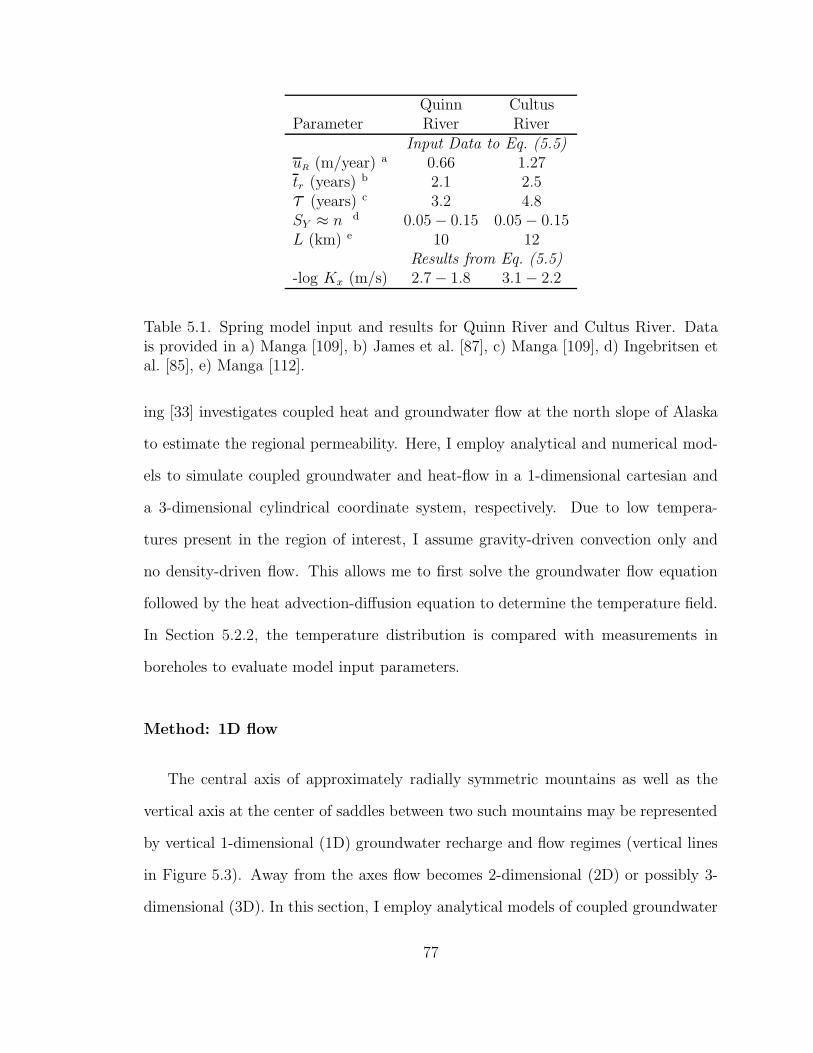
Quinn CultusParameter River River

Input Data to Eq. (5.5)uR (m/year) a 0.66 1.27tr (years) b 2.1 2.5τ (years) c 3.2 4.8SY ≈ n d 0.05 − 0.15 0.05 − 0.15L (km) e 10 12

Results from Eq. (5.5)-log Kx (m/s) 2.7 − 1.8 3.1 − 2.2

Table 5.1. Spring model input and results for Quinn River and Cultus River. Datais provided in a) Manga [109], b) James et al. [87], c) Manga [109], d) Ingebritsen etal. [85], e) Manga [112].

ing [33] investigates coupled heat and groundwater flow at the north slope of Alaska

to estimate the regional permeability. Here, I employ analytical and numerical mod-

els to simulate coupled groundwater and heat-flow in a 1-dimensional cartesian and

a 3-dimensional cylindrical coordinate system, respectively. Due to low tempera-

tures present in the region of interest, I assume gravity-driven convection only and

no density-driven flow. This allows me to first solve the groundwater flow equation

followed by the heat advection-diffusion equation to determine the temperature field.

In Section 5.2.2, the temperature distribution is compared with measurements in

boreholes to evaluate model input parameters.

Method: 1D flow

The central axis of approximately radially symmetric mountains as well as the

vertical axis at the center of saddles between two such mountains may be represented

by vertical 1-dimensional (1D) groundwater recharge and flow regimes (vertical lines

in Figure 5.3). Away from the axes flow becomes 2-dimensional (2D) or possibly 3-

dimensional (3D). In this section, I employ analytical models of coupled groundwater

77

A

A’

a

b

b

h=x /R2

A A’

x

z

q(x,z)

Figure 5.3. a) Schematic peaks (e.g., Three Fingered Jack and Mt. Washington, Ore-gon) and a saddle (e.g., Santiam Pass, Oregon) may represent groundwater rechargeregimes with 1-dimensional (1D) vertical groundwater flow. The saddle can also con-stitute a (local) groundwater discharge regime. b) Schematic cross section A-A’ (seepanel a) showing a typical recharge geometry. Parameters are defined in the maintext.

and heat transfer in a 1D recharge region.

Phillips [138] derives a solution for the advection-diffusion equation, providing

temperature as a function of depth, T (z), in a 1D groundwater recharge area. The

solution assumes a constant mean horizontal permeability and a linear decrease in

vertical groundwater flow (Darcy) velocity, uz, from a recharge (Darcy) velocity at the

surface to uz = 0 at the bottom of the aquifer. Here, I provide an equivalent solution

for T (z), Eq. (5.16), however with inverted z-axis so that z is positive-downwards, con-

sistent with the reference frame adopted for this chapter (Figure 5.3b). In addition, I

introduce a solution to the 1D heat advection-diffusion equation where permeability

decreases exponentially with depth, Eq. (5.15). More detailed derivations of the equa-

78

tions can be found in Appendices B.2 and B.3. For the remainder of this section I will

refer to Darcy velocity, u, as velocity, with the understanding that the actual inter-

stitial (seepage) velocity is given by v = u/n, where n is the connected pore fraction.

The vertical mean recharge velocity at the surface, z = 0, is uR = uz(z = 0) = ΦΨ,

where Φ is the fraction of the precipitation, Ψ, that infiltrates the ground. In the

Oregon Cascades, Φ ≈ 0.5 and Ψ ≈ 2 m/year [81] so that uR ≈ 1 m/year.

In a recharge zone (Figure 5.3), the vertical velocity, uz, at depth, z, is given by

the divergence in the horizontal directions, x = (x, y), of the volume flux per unit

width, q, i.e., [138]

uz(z) = ∇x · q. (5.7)

For an exponential decrease in hydraulic conductivity with depth, q is given by

q = Ks(b− z)e−z/δ ∇xh(x). (5.8)

Therefore,

uz(z) = ∇x

[

Ks(b− z)e−z/δ]

· ∇xh(x) (5.9)

+ Ks(b− z)e−z/δ ∇2xh(x),

where ∇x and ∇x· are the respective gradient and divergence operators in the hor-

izontal directions, x = (x, y), and h is the hydraulic head, Ks is the near-surface

hydraulic conductivity, and b is the total vertical thickness of the saturated zone.

The skin depth, δ, in the exponential term determines the decrease in K (from a

near-surface value, Ks) as a function of depth, z. In the case of constant hydraulic

conductivity and linearly decreasing uz to uz(z = b) = 0, the skin depth is given

by δ = ∞ and thus the exponential terms in Eqs. (5.8) and (5.9) vanish. At the

vertical symmetry axis in Figure 5.3b, the water table is at a maximum, and thus

79

Mt. Washington

FingeredJack

Three➪N

800

1000

1200

1400

1600

1800

2000 2 km

b

a

−122 −121.9 −121.8 −121.70

500

1000

1500

2000

R = 80 km

R = 120 km

longitude

elev

atio

n (m

)el

evat

ion

(m)

Figure 5.4. Radius of curvature of the Earth’s surface at Santiam Pass, Oregon. a)Shaded relief map between longitudes 44.25 and 44.55, color coded to elevation. Blacklines indicate locations of the 12 cross sections shown in b. The geotherm boreholelocation is indicated by the gray arrow. Weather station 357559 (U.S. Departmentof Commerce, National Oceanic & Atmospheric Administration, NOAA) is given bythe white arrow. b) East-west cross sections (thin black lines) used to estimate theminimum (R=80 km) and maximum (R=120 km) radius of curvature (red curves).The geotherm borehole is shown as the gray vertical line.

∇xh(x) = (0, 0) so that Eq. (5.9) reduces to

uz =Ks(b− z)

Re−z/δ, (5.10)

where R = −(∂2h/∂x2)−1 is the radius of curvature of the water table (in x-direction)

and is assumed constant near the symmetry axis where ‖x‖ ≈ 0. I use topography

(Figure 5.4) to obtain R ≈ 100 km. For an incompressible fluid, ∇ ·u = 0. Thus, for

uz given by Eq. (5.10) the 1D horizontal velocity is

ux =Ks

R

(

b− z

δ+ 1

)

x e−z/δ. (5.11)

80

x (m)

z (m

)

0

200

400

600

800

1000 -100 0 100

Figure 5.5. Groundwater flow streamlines near a 1D recharge region for exponentiallydecreasing hydraulic conductivity, Eqs. (5.10) and (5.11) with δ = 270 (bold curves),and constant hydraulic conductivity, Eqs. (5.12) and (5.13) (thin curves). The ex-ponential K model, leads to a recharge velocity of uR ≈ 0.9 m/year compared withuR ≈ 0.1 m/year for the constant K model (Figure 5.7a).

As before, δ = ∞ for constant hydraulic conductivity, reducing Eqs. (5.10) and (5.11)

to

uz =Ks

R(b− z) (5.12)

and

ux =Ks

Rx, (5.13)

respectively, which are equivalent to the solutions presented by Phillips [138] with

inverted z-axis. Figure 5.5 shows groundwater flow streamlines based on Eqs. (5.10-

5.13) for both constant and exponentially decreasing hydraulic conductivity. Substi-

tuting Eq. (5.10) into the steady-state 1D vertical heat advection-diffusion equation,

γuz∂T

∂z= κm

∂2T

∂z2, (5.14)

81

and integrating with respect to z, yields (Appendix B.2)

∂T

∂z= −

(

∂T

∂z

)

b

exp

[

γKsδ

κmRe−z/δ

(

z − b + δ − δez−b

δ

)

]

(5.15)

for exponentially decreasing hydraulic conductivity. To obtain T (z), I integrate

Eq. (5.15) numerically with respect to z and with boundary condition T (z = 0) = TR,

where TR is the (near-surface) recharge temperature.

In contrast to Eq. (5.15), for the case of constant hydraulic conductivity, i.e.,

linearly decreasing uz, Eq. (5.12) is substituted into Eq. (5.14) and integrated twice

with respect to z resulting in (Appendix B.3)

T = TR −(

∂T

∂z

)

b

√

πκmR

2γKs

erfc

[

(b− z)

√

γKs

2κmR

]

. (5.16)

Here, erfc is the complementary error function, (∂T/∂z)b is the (conductive) back-

ground temperature gradient at the bottom of the aquifer, and

γ =ρwcwρmcm

. (5.17)

For a given pore fraction, n, mixed properties, ξm, of the water-rock complex are

approximated by

ξm = nξw + (1 − n)ξr, (5.18)

where ξw and ξr are the properties in question of pure water and pure rock, re-

spectively. Water-rock complex properties to be substituted into Eq. (5.18), where

subscripts remain as given in Eq. (5.18), are mixed density, ξ = ρ, mixed specific

heat, ξ = c, and mixed thermal conductivity, ξ = kT . Mixed thermal diffusivity is

then given by

κm =kTm

ρmcm. (5.19)

Throughout this analysis I assume local thermal equilibrium between water and rock

and that n is sufficiently small so that Eq. (5.18) applies.

82

In Section (5.2.2) I compare results from the exponential-k [integral of Eq. (5.15)]

and constant-k [Eq. (5.16)] solutions and estimate groundwater recharge rates, uR,

characteristic depth scale, δ, aquifer thickness, b, and background heat flux,

Hb = −kTr

(

∂T

∂z

)

b

. (5.20)

Here, kTris the thermal conductivity of the rock alone, assumed to be on average

about kTr≈ 2 Wm−1◦C−1, based on measurements on cores and cuttings from the

Cascades [18, 81].

Method: Radial flow

As described previously, owing to relatively low temperatures, I assume only

gravity-driven convection and no density-driven flow. This allows me to first solve

the steady-state groundwater flow (hydraulic head diffusion) equation,

∂

∂r

(

Kr∂h

∂r

)

+Kr

r

∂h

∂r+

∂

∂z

(

Kz∂h

∂z

)

= 0, (5.21)

for anisotropic (and possibly heterogeneous) hydraulic conductivities, K, in a 3D-

cylindrical coordinate system using only hydrogeologic and no thermal boundary

conditions. Here, h is the variable hydraulic head and Kr and Kz are the hydraulic

conductivities in the radial, r, and vertical, z, directions, respectively. This coordi-

nate system is chosen because of the radial symmetry of Mt. Hood (Fig. 5.6). The

outer no-flow boundary is chosen based on the occurrence of apparent groundwater-

recharge induced earthquakes (Section 5.2.3 and [159]) and on the existence of a bore-

hole geotherm that shows a concave-down temperature profile (triangles in Fig. 5.8)

suggesting upward flow of warmer water [25].

I solve Eq. (5.21) numerically by employing a finite difference algorithm with

successively under-relaxed iterations (Appendix B.4). The obtained hydraulic head

83

1 km

offs

et

10

30

50

70T (°C)

latitudelongitude

Figure 5.6. Shaded relief map of Mt. Hood, Oregon, and subsurface temperature dis-tribution (color coded) based on a multiquadratic interpolation of thirteen geotherms(black bars) in study region C in Figure 5.1. The relief map is vertically offset by3 km from the temperature map for better visualization of the temperature data.Elevated temperatures beneath Mt. Hood appear to be offset towards the south (seevertical bar through the summit for comparison), consistent with the occurrence ofthe only two hot spring areas, Meadows Spring and Swim Warm Springs (yellow barson contour plot) observed to date at Mt. Hood [127]. Most earthquakes also occurbeneath the southern flanks of the volcano (see projection of earthquakes onto map)and show mostly normal-fault focal mechanisms (Section 5.2.3 and [92, 159]).

field, h(r, z), in the rz-plane is then converted into a Darcy velocity field, u(r, z),

using a finite difference approach (Appendix B.4).

I determine the temperature distribution by solving the steady-state heat-advection-

84

diffusion equation (without heat sources or sinks) in cylindrical coordinate form,

κm

γ

(

∂2T

∂r2+

1

r

∂T

∂r+∂2T

∂z2

)

= −ur∂T

∂r− uz

∂T

∂z, (5.22)

where T , ur, and uz are temperature and Darcy velocities in the radial and vertical

directions, respectively.

Eq. (5.22) is also solved using a finite difference approximation and successively

under-relaxed iterations (Appendix B.4). Boundary conditions (Appendix B.5) for

Eqs. (5.21) and (5.22) are no groundwater- and heat-flow (Dirichlet) boundary condi-

tions, ∂h/∂r = 0 and ∂T/∂r = 0, at the central axis and at the outer boundary. The

lower boundary has mixed boundary conditions with no groundwater flow, ∂h/∂z = 0,

but constant heat-flow (Neumann) boundary condition, ∂T/∂z = constant. Hy-

draulic head and temperature distribution along the upper boundary are a function

of elevation, where the water table is assumed to be similar to the topography and

temperature is approximated by the mean adiabatic lapse rate (MALR).

Hurwitz et al. [77] suggest that water tables in volcanos with ice-caps may be much

lower than the surface. However, for the approximate radial model the uncertainty

associated with the unknown position of the water table is small compared with the

overall model dimensions.

Results for 1D and radial flow

Figure 5.7a shows measured [16] and modeled temperature-depth profiles for the

groundwater recharge region at Santiam Pass, Oregon. Solutions to both the con-

stant, Eq. (5.16), and the exponentially decreasing, integral of Eq. (5.15), hydraulic

conductivity model are provided. Both models suggest a very similar aquifer thick-

ness, b ≈ 1000 m, and background heat flux, Hb ≈ 0.080 W/m2 (Table 5.2). However,

85

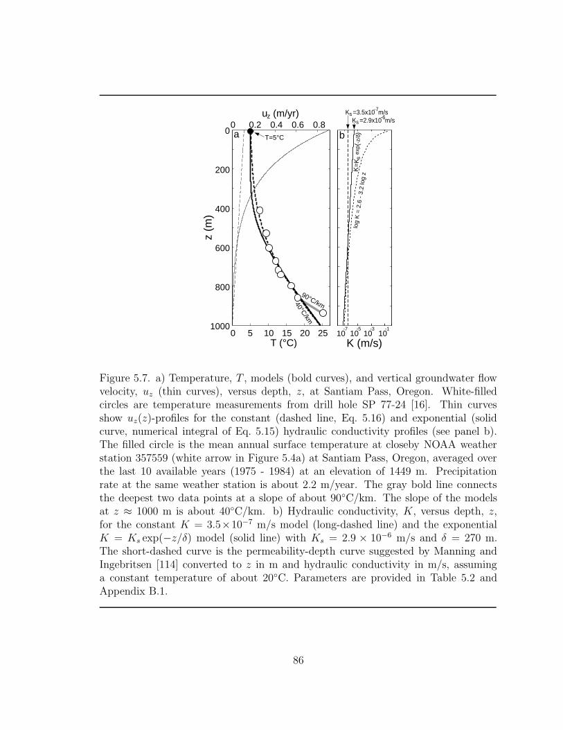
0 5 10 15 20 251000

800

600

400

200

00 0.2 0.4 0.6 0.8

T (°C)

u (m/yr)z

z (m

)

a

90°C/km

T=5°C

K (m/s)10

-510

-710

-310

-1

b

log

K =

2.6

- 3

.2 lo

g z

K =2.9x10 m/s-6s

K=

Ks

exp(

-z/δ

)

40°C/km

K =3.5x10 m/s-7s

Figure 5.7. a) Temperature, T , models (bold curves), and vertical groundwater flowvelocity, uz (thin curves), versus depth, z, at Santiam Pass, Oregon. White-filledcircles are temperature measurements from drill hole SP 77-24 [16]. Thin curvesshow uz(z)-profiles for the constant (dashed line, Eq. 5.16) and exponential (solidcurve, numerical integral of Eq. 5.15) hydraulic conductivity profiles (see panel b).The filled circle is the mean annual surface temperature at closeby NOAA weatherstation 357559 (white arrow in Figure 5.4a) at Santiam Pass, Oregon, averaged overthe last 10 available years (1975 - 1984) at an elevation of 1449 m. Precipitationrate at the same weather station is about 2.2 m/year. The gray bold line connectsthe deepest two data points at a slope of about 90◦C/km. The slope of the modelsat z ≈ 1000 m is about 40◦C/km. b) Hydraulic conductivity, K, versus depth, z,for the constant K = 3.5×10−7 m/s model (long-dashed line) and the exponentialK = Ks exp(−z/δ) model (solid line) with Ks = 2.9 × 10−6 m/s and δ = 270 m.The short-dashed curve is the permeability-depth curve suggested by Manning andIngebritsen [114] converted to z in m and hydraulic conductivity in m/s, assuminga constant temperature of about 20◦C. Parameters are provided in Table 5.2 andAppendix B.1.

86

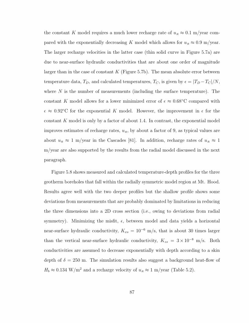
the constant K model requires a much lower recharge rate of uR ≈ 0.1 m/year com-

pared with the exponentially decreasing K model which allows for uR ≈ 0.9 m/year.

The larger recharge velocities in the latter case (thin solid curve in Figure 5.7a) are

due to near-surface hydraulic conductivities that are about one order of magnitude

larger than in the case of constant K (Figure 5.7b). The mean absolute error between

temperature data, TD, and calculated temperatures, TC , is given by ε = |TD−TC |/N ,

where N is the number of measurements (including the surface temperature). The

constant K model allows for a lower minimized error of ε ≈ 0.68◦C compared with

ε ≈ 0.92◦C for the exponential K model. However, the improvement in ε for the

constant K model is only by a factor of about 1.4. In contrast, the exponential model

improves estimates of recharge rates, uR, by about a factor of 9, as typical values are

about uR ≈ 1 m/year in the Cascades [81]. In addition, recharge rates of uR ≈ 1

m/year are also supported by the results from the radial model discussed in the next

paragraph.

Figure 5.8 shows measured and calculated temperature-depth profiles for the three

geotherm boreholes that fall within the radially symmetric model region at Mt. Hood.

Results agree well with the two deeper profiles but the shallow profile shows some

deviations from measurements that are probably dominated by limitations in reducing

the three dimensions into a 2D cross section (i.e., owing to deviations from radial

symmetry). Minimizing the misfit, ε, between model and data yields a horizontal

near-surface hydraulic conductivity, Kxs = 10−6 m/s, that is about 30 times larger

than the vertical near-surface hydraulic conductivity, Kzs = 3× 10−8 m/s. Both

conductivities are assumed to decrease exponentially with depth according to a skin

depth of δ = 250 m. The simulation results also suggest a background heat-flow of

Hb ≈ 0.134 W/m2 and a recharge velocity of uR ≈ 1 m/year (Table 5.2).

87

Symbol Units 1D 1D 3D-radial

Kx(z) (m/s) Kzs Kzse−z/δ ηKzse

−z/δ

Kzs (m/s) 3.4×10−7 2.9×10−6 3.3×10−8

δ (m) ∞ 270 250η 1 1 30b (m) 1000 1000 1200h (m) x2/R x2/R TOPOuR (m/yr) 0.1 0.9 1TR (◦C) 5 5 MALR(

∂T∂z

)

b(◦C/m) 0.042 0.040 0.067

H (W/m2) 0.84 0.080 0.134ε (◦C) 0.68 0.92 ∼1

Table 5.2. Parameters for coupled groundwater and heat-flow models. The anisotropyratio of horizontal to vertical hydraulic conductivity is given by η = Kx/Kz. For theradial model the recharge temperature is determined by the mean adiabatic lapserate (MALR) and the hydraulic head, h, is approximated by topography (TOPO).For the 1D models, h is determined by the radius of curvature of the water table,R = 105 ± 2×104 m (Figure 5.4), and the horizontal distance, x, from the maximumh in the recharge region.

5.2.3 Groundwater-recharge-induced seismicity model:

k(z <5 km)

Saar and Manga [159] (see also Chapter 4) suggest that an increase in seismicity

in late summer at Mt. Hood, Oregon, is caused by seasonal groundwater recharge

during spring due to snow melt on the flanks of the volcano. They show that a sta-

tistically significant correlation exists between groundwater recharge and seismicity.

Groundwater recharge is approximated by discharge in runoff-dominated streams.

The recharge in this region provides a natural pore-fluid pressure signal of narrow

temporal width and potentially relatively large amplitude. The pore fluid pressure

pulse diffuses and can cause an effective stress decrease on preexisting faults at depth,

effectively “unclamping” the fault and triggering earthquakes. Saar and Manga [159]

use the time lag between groundwater recharge and increased seismicity at a mean

88

0 20 40 60 80

0

200

400

600

800

1000

1200

T (°C)

dept

h be

low

res

pect

ive

surf

ace

(m)

67°C/km

Figure 5.8. Temperature, T , versus depth, measured from the surface at eachgeotherm at Mt. Hood, Oregon. The solid, dashed, and dotted curves are resultsfrom the 3D-radial simulation. Measurements are indicated by triangles, circles, andsquares. Two geotherms (circles and squares) show typical recharge dominated pro-files with isothermal upper section, similar to the one shown in Figure 5.7a. Thegeotherm depicted by the triangles shows a mostly linear (conductive) profile witha slight concave-downward bend at shallower depths, suggesting a groundwater dis-charge region.

depth of 4.5 km to estimate (vertical) hydraulic diffusivity, κz, for the depth range

of 0 < z < 5×103 m, assumed to be homogeneous.

Method

The solution to the 1-dimensional (pressure) diffusion equation for periodic sinu-

soidal boundary conditions,

P ′(t, z = 0) = P0 cos

(

2πt

ψ

)

, (5.23)

89

in a half-space is given by [192]

P ′

P0= exp

(

−z√

π

ψκz

)

cos

(

2πt

ψ− z

√

π

ψκz

)

, (5.24)

where P0, P′, ψ, t, and z are near-surface pore fluid pressure amplitude, pore fluid

pressure amplitude at depth (in excess to hydrostatic pressure), period, time, and

depth, respectively. The cosine term in Eq. (5.24) describes the phase lag of the

pressure peak as a function of depth. Saar and Manga [159] (see also Chapter 4)

show that the argument in the cosine-term is likely to be zero (or a multiple of 2π)

and can thus be used to determine vertical hydraulic diffusivity,

κz =ψz2

4πt2. (5.25)

Results

I use Eq. (5.25) to determine the large-scale vertical hydraulic diffusivity, κz,

for the upper 5 km of crust at Mt. Hood, Oregon. The periodicity of groundwater

recharge due to snow melt in spring is ψ = 1 year. The mean earthquake depth,

z = 4.5 km, and time lag, t = 151 days (determined by cross correlations), provide

the remaining parameters for Eq. (5.25), resulting in a hydraulic diffusivity of [159]

κz = 0.30 ± 0.22 m2/s. (5.26)

5.2.4 Magma intrusion and degassing model: k(z <15 km)

The Cascades range is a volcanic arc located at the convergent plate boundary

between the Juan de Fuca plate and the North American plate. Subduction zone

related magmas intrude into the crust where they may (partially) solidify, assimilate

crustal material, and/or erupt. Devolatilization of (mostly) water from solidifying

90

W=20 km

d ≈1

5 km

L

qM

N

h(z=d) = h p ρr

ρwd /=

h(z=0) = h e = dz

Figure 5.9. Schematic illustration of magma intrusion underneath the Cascades rangevolcanic arc (not drawn to scale), after Hildreth [69]. Symbols are defined in the maintext.

magma provides a fluid source in the crust that, due to conservation of mass, is

transmitted to the Earth’s surface, unless consumed in metamorphic reactions. This

volumetric fluid flux, Q, can be used to estimate vertical hydraulic conductivity, Kz,

on a depth scale of about 15 km, i.e., from the estimated main magma intrusion depth

to the surface (Figure 5.9). As before, within this region, Kz is assumed homogeneous.

Method

The volumetric magma flux is given by

QM = qMW, (5.27)

where qM is the volumetric magma intrusion rate per kilometer arc length andW is the

estimated arc width (Figure 5.9). I assume that only water devolatilizes. Therefore,

the volume flux of water, Qw, released by the solidifying magma is given by

Qw =qMWρMφw

ρw

, (5.28)

91

where φw, ρM , and ρw are weight fraction of water content in the magma, and the

densities of magma and water, respectively. In one (vertical) dimension, Darcy’s law

reduces to

qz =Qw

A= −Kz

∂h

∂z, (5.29)

where A and z are the total cross-sectional area perpendicular to the fluid flow direc-

tion and depth, respectively. Here, A = WL, where L = 1 km is the arc length con-

sidered for the magma intrusion rate, qM , described previously. The hydraulic head,

h = he +hp, is the sum of elevation head, he, and pressure head, hp ≈ Pρ−1w g−1, where

P is the pore fluid pressure. At depth, z, the magma and its exsolved volatiles are

under lithostatic pressure so that P = P` ≈ ρrgz, where ρr is the mean rock density.

At the surface (z = 0), P is given by the hydrostatic pressure, P = Ph = ρwgz = 0.

Therefore, if I set the arbitrary reference elevation to the magma intrusion depth, d,

then h(z = d) = hp ≈ ρrd/ρw and h(z = 0) = he = d. As a result, if I approximate

the density ratio between rock and water to be ρr/ρw ≈ 3, then for any intrusion

depth the hydraulic gradient is

∂h

∂z=hp − he

d=

3d− d

d= 2. (5.30)

Substituting Eqs. (5.28) and (5.30) into Eq. (5.29) and recognizing that A = WL,

yields the vertical hydraulic conductivity,

Kz =Qw

2A=qMρMφw

2ρwL. (5.31)

Therefore, Kz is independent of the assumed arc width, W . Applying L = 1 km, used

for the magma intrusion rate, and approximating the density ratio between magma

and water to be ρM/ρw ≈ 3/1 reduces Eq. (5.31) to

Kz = 1.5 qMφw km−1. (5.32)

92

Eq. (5.32) is independent of intrusion depth, d, because as depth increases, so does

the lithostatic pressure, P`. However, d determines the depth scale for which Kz is

determined. As before, within this depth scale, Kz is assumed homogeneous.

Results

I use Eq. (5.32) to determine overall (assumed homogeneous) vertical hydraulic

conductivity for the upper 15 km of the crust in the Cascades. As input data I assume

a range of magma intrusion rates of 9 ≤ qM ≤ 50 km3 Ma−1 km−1 [19, 84]. Sisson

and Layne [175] and other authors [58] suggest a magma water content of about 0.2

to over 3 wt.-% and up to 7 wt.-% for the Cascades arc and the nearby Mt. Shasta

region in northern California. Here, I pick 1.5 wt.-% (i.e., φw = 0.015). Substituting

these values into Eq. (5.32) results in a range of vertical hydraulic conductivities of

approximately

6×10−12 ≤ Kz ≤ 4×10−11 m/s. (5.33)

5.3 Conversions between κ, K, and k

In order to compare results from the four methods employed in this study I convert

hydraulic diffusivity, κ, and hydraulic conductivity, K, to permeability, k. Transfer-

ring κ to hydraulic conductivity,

K = κSS (5.34)

requires assuming a value for specific storage,

SS = ρwg(α+ nβ), (5.35)

93

where n is pore fraction, β = 4.8×10−10 m2/N is the compressibility of water, and α is

the bulk aquifer compressibility at constant vertical stress and zero lateral strain [198].

Further assumptions about temperature (and pressure) dependent (dynamic) viscos-

ity, µ, and water density, ρw, have to be made when converting hydraulic conductivity,

K, to permeability, k, using

k =νK

g, (5.36)

where the kinematic viscosity is given by ν = µ/ρw. Estimating α, ρw, and µ is not

trivial and can lead to large uncertainties in inferred permeability values, particularly

when converting from hydraulic diffusivity to permeability, where, in addition to ν,

SS has to be estimated. I assume α ≈ 10−10 m2/N for fractured igneous rock [37, 150]

and n ≈ 0.01 [77, 85] yielding Ss ≈ 10−6 m−1.

Similar to Germanovich et al. [53], I approximate kinematic viscosity as a function

of depth-dependent mean temperature, Tm, for Eq. (5.36) by

ν(Tm) ≈ 0.032 Pa · s ◦C

ρw[1 − αwTm][15.4 ◦C + Tm], (5.37)

where αw = 10−3 ◦C−1 is the coefficient of thermal expansion of water and ρw = 103

kg/m3 and ρw = 0.5×103 kg/m3 are the water density for mean depths (and associated

pressures and temperatures) zm ≤ 3 km and zm ≈ 10 km, respectively. For calculation

of zm and depth ranges (z-ranges) over which the permeability results from the pre-

vious section are applicable, I refer to Section 5.4 in conjunction with Table 5.3. The

mean temperature for Eq. (5.37) is then given by Tm ≈ TR+zm(∂T/∂z)b with a typical

recharge temperature of TR ≈ 5 ◦C (Figures 5.7 and 5.8) and a background temper-

ature gradient of (∂T/∂z)b ≈ 50 ◦C/km (Figure 5.7 and Section 5.4.2). Resulting

kinematic viscosities, ν, agree to within the implicit uncertainties with compilations

by Grigull et al. [57]. As I will show later, the depth ranges over which calculated per-

meabilities are applicable are independent of the actual permeability values. However,

94

the z-ranges do depend on the characteristics of the assumed decrease in permeability

with depth (exponential versus power-law relationship) and on the calculation of the

mean (arithmetic versus harmonic). Table 5.3 summarizes the hydraulic conductivi-

ties discussed in the previous section and the resulting permeabilities for the different

depth scales.

5.4 Discussion

In Section 5.4.1 I discuss results from the previous two sections and suggest a

curve describing permeability as a function of depth. In Section 5.4.2 I address mean

background heat-flow values determined in Section 5.2.2.

5.4.1 Heterogeneity and anisotropy of permeability

Permeability typically decreases with depth due to compaction, metamorphism,

and/or filling of pore spaces and fractures by precipitating minerals, particularly

in hydrothermal regions [17, 45, 82, 130]. In some cases, however, fractures can

remain open due to earthquakes providing long-term (10s to 100s of years) high-k

pathways [151]. The characteristics of the reduction of k with depth, z, are difficult to

determine and are controversial [22, 23, 33, 48, 54, 73, 123]. Several publications [14,

77, 114, 136, 170, 171, 204] as well as this study suggest a non-linear decrease of k with

z in the Cascades region and for continental crust in general. Non-linear k(z)-profiles

allow for high near-surface permeabilities and related high groundwater recharge rates

so that the observed near-surface isothermal and inverted temperature-depth profiles

are possible (Figures 5.7, 5.8, and 5.10). At the same time, a non-linear k(z)-profile

can reduce permeabilities to k ≤ 10−16 m2 at z ≥ 4 km, thus allowing for conduction-

95

Symbol Units 1 2 3 4 5 6Method spring dis. heat-flow heat-flow heat-flow hydroseis. magma intr.

Section # 5.2.1 5.2.2 5.2.2 5.2.2 5.2.3 5.2.4x, z x x z z z z

Study Area A C1 B C2 C3 DEA, EH, PH EA EA EH EH PH PHδmin, δmax km 0.2, 0.3 0.2, 0.3 0.2, 0.3 0.2, 0.3 - -λmin, λmax - - - - 1, 10 1, 10b± 0.25b km 0.05 ± 0.0125 1 ± 0.25 1.2 ± 0.3 1.2 ± 0.3 4.5 ± 1.125 15 ± 3.75z-range, zm km 0.02 - 0.03, 0.025 0.3 - 0.5, 0.4 0.4 - 0.9, 0.65 0.6 - 1.1, 0.85 1.7 - 4.4, 3 5.6 - 14.8, 10(∂T/∂z)b

◦C/km 50 50 50 50 50 50Tm

◦C 6 25 38 48 155 505Pm MPa 0.25 4 6.5 8.5 30 100ρm kg/m3 103 103 103 103 103 0.5×103

µm Pa · s 1.5×10−3 8×10−4 6×10−4 5×10−4 2×10−4 5×10−5

νm m2/s 1.5×10−6 8×10−7 6×10−7 5×10−7 2×10−7 1×10−7

Kmin m/s 10−3 10−6 3×10−7 3×10−8 8×10−8 6×10−12

Kmax m/s 10−2 10−6 3×10−6 3×10−8 5×10−7 4×10−11

kmin m2 1.5×10−10 8.2×10−14 1.8×10−14 1.5×10−15 1.6×10−15 6×10−20

kmax m2 1.5×10−9 8.2×10−14 1.8×10−13 1.5×10−15 1.0×10−14 4×10−19

Table 5.3. Conversions from hydraulic conductivity, K, to permeability, k, in horizontal, x, and vertical, z, directions, based on

Eqs. (5.36) and (5.37). The average of the z-range, zm, is calculated using combinations of min/max values for the aquifer depths,

b±25 %, skin depths, δ, and/or exponents, λ, for exponential, E, or power-law, P, functions, respectively. The exponential solution,

E, for the z-range is used for b ≤ 2 km, both for subhorizontal (parallel) pathways (Eq. 5.48) and for subvertical (serial) pathways

(Eq. 5.45) that are calculated using the arithmetic mean, A, and the harmonic mean, H, permeability expressions, respectively. The

power-law solution, P, is reserved for mean depths zm > 1 km and is determined only for subvertical (serial) pathways (Eq. 5.46)

that are characterized by harmonic mean, H, permeability values. Hydraulic conductivity for column 5 (Section 5.2.3) is based on

results for vertical hydraulic diffusivity, κz, and assuming SS ≈ 10−6 m−1 in Eq. (5.34) as discussed in Section 5.3. Uncertainties

in K and k (columns 2 and 4) are based on uncertainties calculated for k in columns 1, 3, 5, and 6.

96

surface gradT

43.6

43.8

44

44.2

44.4

44.6

44.8

45

45.2

45.4

latit

ude

20 km

Mt. Hood

Mt. Jefferson

Three Sisters

Newberry

122.5 122 121.5 121longitude

− − − −

dT/dz (°C/km)120 80 40 0 -40 -80

Figure 5.10. Map of near-surface temperature gradients in study region E (Figure 5.1),based on interpolation of geotherm data from drill holes (circles). Isothermal andinverted temperature gradients exist in high precipitation and groundwater rechargeareas such as the high-relief volcanos. Cold groundwater is heated at depth, the heatis advected and discharged at hot springs [84, 85].

dominated heat transfer at these depths, as also required by observations [85]. A

transition from advection- to conduction-dominated heat transfer at k ≈ 10−16 m2

has been suggested by numerous authors [29, 66, 73, 77, 113, 114, 132, 178].

In Section 5.2.2, I invoked non-linearity by decreasing permeability exponentially

with depth. Figure 5.5 shows streamlines for constant (thin curves) and exponentially

decreasing (bold curves) k, where recharge rates for the latter are about nine times

larger than for constant k (Figure 5.7a). The exponential k(z)-curve results in larger

horizontal groundwater flow components at smaller depths, rapidly reducing vertical

97

groundwater flow velocities and allowing for conduction-dominated heat transfer at

relatively shallow depths.

However, while exponential functions of (vertical) permeability, such as

kz(z) = kzse−z/δ, (5.38)

provide reasonable near-surface (denoted with the subscript “s”) values, including

kz(z = 0) = kzs, they also reduce permeability to unrealistically low magnitudes at

depths greater than about 2 km (Figure 5.11). In contrast, power laws, such as

kz(z) = kzD

( z

D

)−λ

, (5.39)

provide larger, and thus more realistic, permeabilities at greater depths, but approach

infinity for z → 0 and result in a singularity for z = 0. They are thus defined for a

finite depth, D, i.e., kz(z = D) = kzD.

Due to these advantages and limitations of either function, I suggest Eq. (5.38)

for 0 ≤ z ≤ 0.8 km and Eq. (5.39) for z > 0.8 km. Eq. (5.39) is equivalent to the

curve suggested by Manning and Ingebritsen [114] if λ = 3.2 and kzD = 10−14 m2 at

D = 1 km are chosen. In general, units of z and D have to be identical (e.g., both m

or both km). My results from Section 5.2.2 suggest δ ≈ 250 m and kzs ≈ 5 × 10−13

m2 for Eq. (5.38). For these values of λ, kzD, δ, and kzs, as well as depth z ≈ 0.8 km,

the vertical permeabilities and their gradients,

−kzs

δe−z/δ ≈ −kzDλD

λ

zλ+1, (5.40)

are similar, thus enabling the suggested transition from Eq. (5.38) to Eq. (5.39) at

z = 0.8 km (Figure 5.11).

The methods employed and conversions discussed in Sections 5.2 and 5.3 provide

estimates of mean permeability, k, at four depth scales, mostly in vertical, but in

98

two cases also in approximately horizontal, directions. The spring discharge model

(Section 5.2.1) of study region A (Figure 5.1) yields an estimate of mean horizontal

permeability, kx, because the method considers individual near-surface aquifers that

consist of slope-parallel, and thus roughly horizontally-layered, lava flows. Within

such solidified lava flows (or aquifers), water can flow primarily through the (about

parallel and horizontal) pathways of highest permeability. Thus, the mean horizontal

permeability is given by the arithmetic mean [106],

kx =1

b

N∑

i=1

kxibi, (5.41)

where the subscript i denotes the ith layer or pathway, bi is the thickness of layer i,

and b is the total thickness of all layers.

In contrast, vertical groundwater flow across horizontal lava flows (or aquifers)

is passing through sections of varying permeability in series, so that mean vertical

permeabilities are typically determined by the harmonic mean [106],

kz = b

(

N∑

i=1

bikzi

)−1

, (5.42)

where kz is dominated by the lowest permeabilities along that path. Hence, in volcanic

or sedimentary settings, where slope-parallel, and thus approximately horizontal, lay-

ers, pathways, and aquifers are common, typically 10 ≤ kx/kz ≤ 1000, at least near

the surface [33].

A further consequence of kz being determined by the harmonic mean (Eq. 5.42)

and kz(z) generally decreasing with depth is that my kz results from Section 5.2 apply

predominantly towards the lower portions of the considered depth ranges. Replacing

the discrete layer formulation in Eq. (5.42) with the definite integral from zero to

b of the continuous functions, Eqs. (5.38) and (5.39), results in the harmonic mean

99

vertical permeabilities

kz =bkzs

δ (eb/δ − 1)(5.43)

and

kz = kzD

(

D

b

)λ

(λ+ 1) (5.44)

suggested for 0 ≤ z ≤ 0.8 km and z > 0.8 km, respectively. Setting Eq. (5.38) equal

to Eq. (5.43) and Eq. (5.39) equal to Eq. (5.44) provides the depths

zz = −δ ln

[

b

δ (eb/δ − 1)

]

(5.45)

and

zz = b(λ+ 1)−1/λ, (5.46)

where kz and kz are reached, respectively. Here, over- and underbars denote functions

applicable to shallow (based on Eq. 5.38) and deeper (based on Eq. 5.39) depths,

respectively. As before, b is the considered depth scale. Eqs. (5.45) and (5.46) are

independent of the actual permeability value but depend on the characteristics of the

decrease in permeability with depth (exponential versus power-law relationship). I use

Eq. (5.45) for depths shallower than about 1 km, Eq. (5.46) for depths greater than

approximately 1 km, and ranges of 200 ≤ δ ≤ 300 m, 1 ≤ λ ≤ 10, and b ± 0.25 b to

determine the applicable depth ranges (Table 5.3 and Figure 5.11) for the respective

values of kz and kz, determined in Section 5.2.

For the shallow-most model (Section 5.2.1 and study region A in Figure 5.1) the

arithmetic mean horizontal permeability is determined. Here, each horizontal layer’s

permeability is assumed to decrease with depth according to Eq. (5.38). As before, I

replace the discrete formulation of the arithmetic mean (Eq. 5.41) with the definite

vertical integral from zero to b of the continuous function (Eq. 5.38) resulting in the

100

−20 −15 −10 −5

10−2

10−1

100

101

dept

h, z

(km

)

log k (m )2

Exp

Exp

Exp

Exp

Pwr

Pwr

PwrPw

r

A

C1

B

C2

C3

D

gravelsand

karst, limestonepermeable basalt

fractured igneous rocksilt, loess

sandstoneshale

unfractured metamorphic and igneous rock

a

b

0.8 km

Figure 5.11. a) Approximate (near-surface) range of permeability values (after Freezeand Cherry [47]). The (Oregon) Cascades primarily consist of basalt and basalticandesite where youngest (< 2.3 Ma) rock units show high near-surface permeabilitiesof k ≈ 10−14 m2 [81, 85], consistent with the k-range indicated for permeable basalts.b) Permeability, k, as a function of depth, z. Shown are the results for study regionsA,B,C, and D (Figure 5.1 and Table 5.3) for horizontal (thin boxes) and vertical(bold boxes) permeabilities. The depth ranges are determined as described in themain text and in the caption to Table 5.3. Box widths reflect approximate variationsin permeability. Superimposed is the exponential profile of Eq. (5.38), denoted Exp,with δ = 250 m and kzs = 5× 10−13 m2 for vertical (bold curve) and kxs = 5× 10−10

m2 for horizontal (thin curve) permeabilities. Also shown is the power law profile ofEq. (5.39), denoted Pwr, with λ = 3.2 and kzD = 10−14 m2 at D = 1 km as suggestedby Manning and Ingebritsen [114] for vertical (bold line) permeability. kzD = 10−11 m2

is used for horizontal (thin line) permeabilities. Solid lines indicate the permeability-depth curves suggested with a transition from exponential to power-law profile at adepth of 0.8 km (dashed horizontal line). The doted area indicates the expected rangebetween vertical and horizontal permeability. At depth this range between kx and kz

may be expected to reduce (not shown here).

101

arithmetic mean horizontal permeability given by

kx =δkzs

b

(

1 − e−b/δ)

. (5.47)

Setting Eq. (5.38) and Eq. (5.47) equal yields the depth,

zx = −δ ln

[

δ

b

(

1 − e−b/δ)

]

, (5.48)

where kx is reached, based on the suggested ranges of maximum near-surface aquifer

depths (thicknesses), b = 50 m ±25 %, and skin depths 200 ≤ δ ≤ 300 m (Table 5.3).

The values for δ are inferred from my heat-flow model (Section 5.2.2). As before, the

overbars denote functions applicable to shallower depths.

Figure 5.11b shows the results for kx, kz, and kz from Section 5.2 at depths zx, zz,

and zz determined using Eqs. (5.48), (5.45), and (5.46), respectively. This approach

allows me to base depths, for which the permeability results are applicable, on the

shape of the k(z)-curve (exponential versus power-law) and the method of calculating

the mean (arithmetic versus harmonic). Therefore, while this technique does not use

the actual (near-surface) permeability values, it requires assuming a model describing

the change of permeability with depth (Eqs. 5.38 and 5.39). While the equations

appear to describe kz(z)-profiles in principle, the appropriate parameters are not

well-constrained and depend largely on the local geology. I thus use a wide range of

values for δ, λ, and particularly b, as suggested previously, to calculate depth ranges

(i.e., uncertainties) over which the mean permeabilities are applicable (Table 5.3).

I recognize that my depth ranges are partially based on assuming that Eq. (5.39)

applies for mean depths zm > 1 km and are thus dependent on the curve suggested

by Manning and Ingebritsen [114], with λ = 3.2. However, I can use a wide range of

1 ≤ λ ≤ 10 values to calculate a range of zz using Eq. (5.46). For shallower mean

depths of 0 ≤ zm ≤ 1 km, I employ my suggested Eqs. (5.45) and (5.48) that are

102

instead based on Eq. (5.38) and use 200 ≤ δ ≤ 300 m to determine ranges of zz

and zx. For either method I estimate independently a large uncertainty range in b ±

25 %. Thus, while zz is not completely decoupled from λ = 3.2, the depth range is

nonetheless based on an independent estimate of maximum depth b, a wide range of λ,

and the reasonable assumption that the mean horizontal and vertical permeabilities

are given by the arithmetic and the harmonic means, respectively, if approximately

horizontal layers are present.

Given the previous considerations, I suggest that my results for kz(z) and kx(z) in

the Oregon Cascades are largely independent from, but comparable to, the permeability-

depth profile suggested by Manning and Ingebritsen [114] for the continental crust.

However, I propose that for depths smaller than about 0.8 km, Eq. (5.38) with

kzs ≈ 5 × 10−13 m2 and δ ≈ 250 m is more appropriate at least for the Cascades

and possibly for continental crust in general.

For example, Shmonov et al. [170] suggest a near-surface permeability of ap-

proximately ks ≈ 2.75 × 10−13±1.9 m2 that decreases to 1.67 × 10−20±1.5 at 40 km

depth based on experimental data on the permeability of samples of amphibolite and

gneiss from the Kola Ultradeep Borehole. Furthermore, Patriarche et al. [136] invoke

an exponential relationship between depth and hydraulic conductivity analogous to

Eq. (5.38) with δ ≈ 0.28 km to satisfy both hydraulic head model calibration and

measured 4He concentrations in the sedimentary Carrizo aquifer in Texas. Because

of the similarity of their δ value to the one introduced here, their K(z)-curve (con-

verted to k(z) = Kν/g ≈ 10−7K) has a similar shape as my exponential k(z)-curve.

Their zero-depth permeability of 2 × 10−11 m2 is based on a near-surface hydraulic

conductivity of the aquifer of about 2 × 10−4 m/s. Finally, measurements from the

German Continental Deep Drilling Program (KTB) [73] show even lower near-surface

103

permeabilities of 5×10−18 to 3×10−16 m2, however, with no clear depth-dependence.

A further advantage of using Eq. (5.38) for shallow depths is that the function

provides a finite near-surface permeability of kzs as depth approaches zero. In con-

trast, Eq. (5.39) diverges towards infinity for z → 0 and results in a singularity at

z = 0. This limitation of Eq. (5.39) may not be critical for global studies of perme-

ability, where overall estimates over larger depth scales (z > 0.5 km) may be desired.

In fact, for z > 2 km, Eq. (5.39) is preferred because at greater depths its perme-

ability gradient is smaller than the one for Eq. (5.38), providing more realistic deeper

permeabilities. Therefore, I propose a transition from Eq. (5.38) to Eq. (5.39) at

z = 0.8 km. This transition is relatively smooth as permeabilities and their gradients

(Eq. 5.40) are comparable at z = 0.8 km (Figure 5.11b) for the suggested values of

kzs ≈ 5 × 10−13 m2, δ ≈ 250 m, kzD ≈ 10−14 m2, and λ = 3.2 (the latter two values

are adopted from Manning and Ingebritsen [114] and corroborated by this study).

Of course there are large variations in permeability as a function of lithology [47]

particularly at zero depth (Figure 5.11a). However a maximum value may be reached

at about k ≈ 10−7 m2 for gravel (Figure 5.11a). A more typical upper limit for

continental crust in general may be k ≈ 10−12 m2 (Table 1 and Figure 8 in Man-

ning and Ingebritsen [114]) at least in the vertical direction across horizontal layers.

Such a low maximum average permeability further supports the exponential kz(z)-

relationship with the suggested finite near-surface value of about kzs ≈ 5 × 10−13

m2 (Figure 5.11b) for vertical groundwater flow across sub-horizontal lava flows or

sedimentary layers and in the absence of near-vertical fractures.

However, if sub-vertical fractures and faults are present, high-kz pathways can

alter the relationship between depth and permeability. Hence, I suggest that my

elevated values of kz ≈ 10−15 m2 at zm ≈ 3 km (Table 5.3 and Figure 5.11), deter-

104

mined by the hydroseismicity method (Section 5.2.3), are due to faults located on

the southern flanks of Mt. Hood, such as the White River fault. These faults, that

are located away from the volcano’s central axis, show predominantly normal-fault

focal mechanisms [92] and thus suggest tectonically-driven (possibly hydrologically-

triggered [159]) earthquakes, rather than magma-flow-induced seismicity that is typ-

ically characterized by non-double couple focal mechanisms [38]. High values of k

allow for advective heat transfer and hot springs, where water can reach the sur-

face faster than heat diffusion time scales required for thermal equilibration with

the surrounding rock. Indeed, the only two off-centered hot spring areas (Meadows

Spring and Swim Warm Springs) observed at Mt. Hood to date [127] are located on

the southern flanks of the volcano close to the earthquakes’ epicenters (Figure 5.6).

Therefore, I suggest that the slightly elevated kz values inferred for mean applicable

depths of about zm = 3 km in study region C3 (Figure 5.1 and Table 5.3) reflect the

permeability of a large representative elementary volume that is dominated by normal

faults that are being kept permeable by hydroseismicity [151, 190]. In addition, ver-

tical faults are approximately parallel to each other, thus providing parallel pathways

whose combined mean permeability is dominated by the highest-k pathways which

is determined by the larger arithmetic mean (Eq. 5.41), rather than by the smaller

harmonic mean (Eq. 5.42) [154].

Scale-dependence of permeability is controversial [13, 22, 23, 28, 79, 148, 154, 162,

190, 211]. In general, permeability tends to increase, as the representative elementary

volume increases from laboratory rock-core measurements, over in-situ field measure-

ments, to large-scale regional models, as those considered in this study. This rela-

tionship may be the case because large-scale heterogeneities, that may include high

permeability pathways, are more likely to be sampled if larger volumes are considered.

For example this appears to be the case in the hydroseismicity model described in the

105

previous paragraph. However, an upper bound appears to be reached at the upper

field and regional modeling scale [28, 162], possibly because most heterogeneities have

been included [148].

5.4.2 Basal heat-flow, Hb

Figure 5.10 shows a map of vertical near-surface heat-flow for study region E in

Figure 5.1. The near-surface results are based on a multi-quadratic interpolation tech-

nique [131] applied to 209 geotherm boreholes and KTr= 2 W◦C−1m−1 [16, 80, 83].

High precipitation (∼2 m/year) and infiltration rates (∼1 m/year) in the Oregon

Cascades cause isothermal (and sometimes inverted) near-surface geotherm profiles

(Figures 5.7a, 5.8, and 5.10) effectively masking the background heat-flow [84, 85].

I minimize the mean absolute error, ε, between data and calculated temperature

values and infer a thermal gradient of about (∂T/∂z)b ≈ 40◦C/km at Santiam

Pass, located between two volcanos, Three-Fingered Jack and Mt. Washington (Fig-

ure 5.7a). Connecting the deepest two data points yields (∂T/∂z)b ≈ 90 ◦C/km.

However, the last data point was taken as drilling progressed [16]. Deeper portions

of the linear temperature-depth profiles at Mt. Hood volcano (Figure 5.8) yield

(∂T/∂z)b ≈ 65◦C/km. Therefore, I infer a mean background heat-flow, Hb, for the

study region of approximately

0.080 ≤ Hb ≈ kTR

(

∂T

∂z

)

b

≤ 0.130 W/m2, (5.49)

where the lower and upper heat-flow values are inferred from the study of Santiam

Pass and Mt. Hood, respectively (Table 5.2). These values are consistent with the

more extensive studies of Blackwell et al. [18] and Ingebritsen et al. [81]. As expected

for a region showing active volcanism, heat-flow is elevated with respect to global

average values for continents of about 0.065 W/m2 [143].

106

5.5 Conclusions

I employ analytical and numerical modeling techniques to estimate permeability

at different depth scales for the Oregon Cascades. My results suggest that for depths

shallower than about 0.8 km, permeability decreases exponentially with depth, with

a skin depth of δ ≈ 250 m, from a near-surface value of kzs ≈ 5 × 10−13 m2.

For depths larger than about 1 km, permeability appears to decrease according

to a power law as suggested by Manning and Ingebritsen [114] with an exponent of

λ ≈ 3.2 and a permeability of kzD ≈ 10−14 m2 at depth z = 1 km. Therefore, I

propose

kz(z) =

5 × 10−13 m2 exp(

−z0.25 km

)

for 0 ≤ z ≤ 0.8 km

10−14 m2(

z1 km

)−3.2for z > 0.8 km,

(5.50)

where the parameters for z > 0.8 km are adopted from Manning and Ingebritsen [114].

The advantage of using two functions in Eq. (5.50) is that they provide realistic

vertical permeabilities for both small (z < 0.5 km) and large (z > 2 km) depths

which neither function alone could both achieve, as discussed in Section 5.4.1. In

addition, the functions in Eq. (5.50) yield a relatively smooth transition at z = 0.8

km, where their permeabilities and their permeability gradients are similar.

I also determine horizontal permeabilities at depths shallower than about 1 km. At

least near the surface, and in the absence of vertical fractures, horizontal permeabil-

ities are typically one to three orders of magnitude larger in volcanic or sedimentary

settings where slope-parallel, and thus approximately horizontal, layers, pathways,

and aquifers are common.

I note a divergence from Eq. (5.50) for my hydroseismicity model that suggests

about one order of magnitude higher permeability values. However, higher perme-

107

abilities in this region may be consistent with advective heat transfer along active

faults causing observed hot springs.

Finally, the coupled heat and groundwater transfer models suggest mean back-

ground heat-flow values of about Hb ≈ 0.080 to Hb ≈ 0.134 W/m2 for the investigated

region in the Oregon Cascades. The higher background heat-flow values are associated

with volcanic centers that may have magma sources at shallower depths.

Because large-scale hydrogeologic models are generally underconstrained, it is

desirable to utilize multiple direct and indirect observations to improve simulations, as

described in the introduction to this chapter. In this study, I use classic hydrogeologic

boundary conditions and parameters as well as temperature and seismic data, and

estimates of magma intrusion rates. Further improvements in future work may include

additional constraints such as water chemistry and multi-phase fluid flow, particularly

at greater depths.

Lithological variations can cause a wide range of permeabilities. Therefore, it is

important to emphasize that the general relationship between depth and permeability

suggested here provides only a large-scale average estimate. This estimate was devel-

oped for the volcanic (Oregon) Cascades but may also apply to continental crust in

general including sedimentary basins where near-horizontal layers are present. How-

ever, the suggested k(z)-relationship is not a substitute for more lithologically-specific

measurements of k for a given region of interest. Frequently such direct permeability

measurements are, however, technically or economically not feasible at greater depths

or over large regional scales. In such cases, estimates of the depth dependence of per-

meability, as presented here, can be useful.

108

Chapter 6

Glacier-induced volcanism

6.1 Introduction

Similar to hydroseismicity discussed in Chapter 4, a decrease in confining pres-

sure in the subsurface, due to a reduction in the load exerted by surface water or ice,

can cause dike propagation and volcanism. In fact, volcanic activity may be mod-

ulated by several external physical processes affecting the stress regime and acting

over a wide range of time scales. At short time scales volcanic eruptions may be

triggered by Earth tides [64, 91, 118, 180]), short term climatic effects [146] and daily

variations in atmospheric pressure and temperature[128]. Annual periodicity is also

sometimes observed [121]. At long periods (i.e., greater than hundreds of years) it

has been suggested that volcanism is influenced by changes in sea level [119, 197] and

by ice loading [56, 63, 93, 126, 172]. In addition, at long periods, both changes in

hydrothermal circulation [117] and melt productivity [107, 177] have been invoked.

Glazner et al. [56] suggest that glacial ice thickness and volcanism are anticorre-

lated in eastern California over the past 800 kyr. While this relationship appears to

109

38° 30’

37° 30’

36° 30’

35° 30’-119° -118° -117°

40 km

latit

ude

longitute

CACA

Figure 6.1. Shaded relief map with locations of basaltic (dark circles) and silicic(white circles) eruptions in Long Valley and Owens Valley volcanic fields in easternCalifornia during the past 400 kyr.

hold true, a stronger correlation between the rate of change of glaciation and volcanic

eruptions is suggested here. The hypothesis is that the volcanism in Long Valley and

Owens Valley volcanic fields (Figure 6.1) is a response controlled by the dynamics of

dike formation, which in turn is influenced by the rate of change of ice volume rather

than the total ice volume. Moreover, the responses for basaltic and silicic systems

is distinctive. The difference in response time allows for constraining critical magma

chamber overpressures required for volcanic eruptions as well as mechanical prop-

erties of the wall rock governing rhyolitic and basaltic dike formation. The results

are consistent with basaltic magmas being generated at greater depths than rhyolitic

110

(hereafter referred to as silicic) magmas, in accord with geochemical observations.

6.2 Data analysis

I employ signal processing techniques on time series of volcanic eruptions and

glaciation (Figure 6.2a). Eruption data is provided by Glazner et al. [56] and

Glazner [55] and is divided into basaltic and silicic categories (Figure 6.1). Glaciation

is assumed here to be proportional to ice thickness and is approximated by oxygen

isotopic data, δ18O, from the SPECMAP time series [120, 166]. Here, peaks in δ18O

correspond to glacial times. Figure 6.2a shows the original time series for basaltic and

silicic eruptions as well as for δ18O for the past 400 kyr. The sparse data available

for eruptions before 400 kyr is not used because individual eruptions would dominate

the analysis. Also shown in Figure 6.2a are binned eruption numbers where the bin

width is 1 kyr. In order to be able to compare the data at equivalent frequency bands,

I smooth the time series by convolving them with a Gaussian kernel with a width of

23 kyr. As a test, I also smooth the data using a moving polynomial interpolation

(Appendix A.3), where the polynomial order used in each segment is ≤ 5. The latter

method is equivalent to the one employed in Chapter 4 and by Saar and Manga [159]

and ensures that no artificial frequencies are introduced. Both techniques yield similar

results. Therefore, in the following I present results based on the convolution method

because it is similar to the approach reported by Glazner et al. [56] and thus allows

for easier comparison. Interpolating the binned data also provides the continuous

functions B and S for basaltic and silicic eruptions, respectively, on which standard

spectral analyses can be performed.

Figure 6.4 shows power spectra for the interpolated and smoothed time series

111

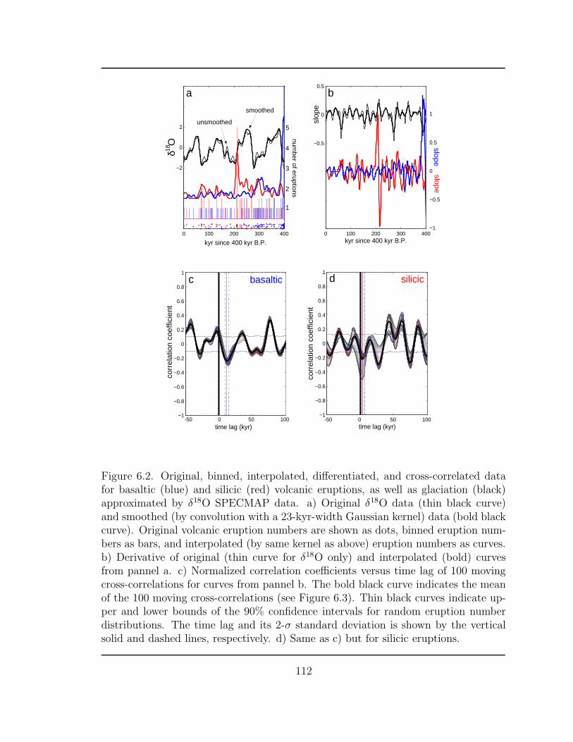
−1

−0.8

−0.6

−0.4

−0.2

0

0.2

0.4

0.6

0.8

1

time lag (kyr)0 50 100-50

−1

−0.8

−0.6

−0.4

−0.2

0

0.2

0.4

0.6

0.8

1

time lag (kyr)0 50 100-50

0 100 200 300 400

−2

0

2

kyr since 400 kyr B.P.

δ O18

number of eruptions

1

2

3

4

5

smoothed

unsmoothed

corr

elat

ion

coef

ficie

nt

0 100 200 300 400

−0.5

0

0.5

kyr since 400 kyr B.P.

slop

e

−1

−0.5

0

0.5

1

slopeslope

a b

c d

corr

elat

ion

coef

ficie

nt

basaltic silicic

Figure 6.2. Original, binned, interpolated, differentiated, and cross-correlated datafor basaltic (blue) and silicic (red) volcanic eruptions, as well as glaciation (black)approximated by δ18O SPECMAP data. a) Original δ18O data (thin black curve)and smoothed (by convolution with a 23-kyr-width Gaussian kernel) data (bold blackcurve). Original volcanic eruption numbers are shown as dots, binned eruption num-bers as bars, and interpolated (by same kernel as above) eruption numbers as curves.b) Derivative of original (thin curve for δ18O only) and interpolated (bold) curvesfrom pannel a. c) Normalized correlation coefficients versus time lag of 100 movingcross-correlations for curves from pannel b. The bold black curve indicates the meanof the 100 moving cross-correlations (see Figure 6.3). Thin black curves indicate up-per and lower bounds of the 90% confidence intervals for random eruption numberdistributions. The time lag and its 2-σ standard deviation is shown by the verticalsolid and dashed lines, respectively. d) Same as c) but for silicic eruptions.

112

cros

s co

rrel

atio

n co

effic

ient

, φ

time lag (kyr)

90%

90%

silicic basaltic

Figure 6.3. Mean correlation coefficients from Figure 6.2c,d for cross-correlationsbetween derivatives of δ18O and derivatives of basaltic (solid) and silicic (dashed)eruption numbers. Statistically significant anticorrelations, that are distinct from the90% confidence limits for random occurences of basaltic (solid) and silicic (dashed)eruptions are given at time lags of 11.3 and 3.3 kyr, respectively.

from Figure 6.2a. A distinctive peak is observed in all three data sets at a period of

about 40 kyr, suggesting that the characteristic time scale for a full glacial cycle (i.e.,

advance and retreat) is reflected in the volcanic record. Hence, melting glaciers do

indeed appear to cause volcanic eruptions in eastern California.

In order to compare quantitatively the rate of change in the time series, I compute

moving normalized unbiased cross-correlations, Φfg(t) (Eqs. 4.3 and 4.4 in Chapter 4),

between the derivative of the SPECMAP time series, f = δ18O′= dδ18O/dt, and the

derivatives of the basaltic, g = B ′ = dB/dt, and silicic, g = S ′ = dS/dt, time series

(Figure 6.2b) on overlapping segments. The segment width is 300 kyr and the step size

is 1 kyr resulting in 100 segments. 90% confidence intervals are determined for cross-

correlations of random distributions of B ′ or S ′. This is achieved by performing 10

113

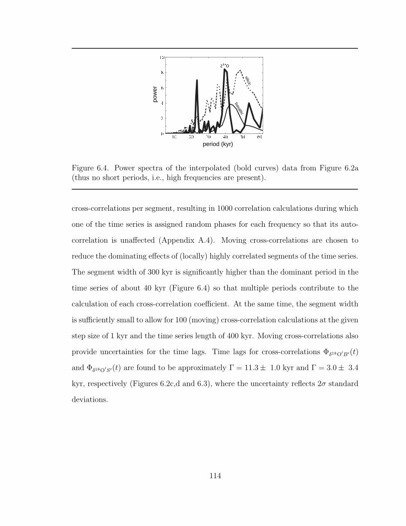
silicic

basaltic

pow

er

period (kyr)

Figure 6.4. Power spectra of the interpolated (bold curves) data from Figure 6.2a(thus no short periods, i.e., high frequencies are present).

cross-correlations per segment, resulting in 1000 correlation calculations during which

one of the time series is assigned random phases for each frequency so that its auto-

correlation is unaffected (Appendix A.4). Moving cross-correlations are chosen to

reduce the dominating effects of (locally) highly correlated segments of the time series.

The segment width of 300 kyr is significantly higher than the dominant period in the

time series of about 40 kyr (Figure 6.4) so that multiple periods contribute to the

calculation of each cross-correlation coefficient. At the same time, the segment width

is sufficiently small to allow for 100 (moving) cross-correlation calculations at the given

step size of 1 kyr and the time series length of 400 kyr. Moving cross-correlations also

provide uncertainties for the time lags. Time lags for cross-correlations Φδ18O′B′(t)

and Φδ18O′S′(t) are found to be approximately Γ = 11.3± 1.0 kyr and Γ = 3.0± 3.4

kyr, respectively (Figures 6.2c,d and 6.3), where the uncertainty reflects 2σ standard

deviations.

114

6.3 Discussion

In a model developed by Jellinek and DePaolo [89] the evolution of overpressure,

∆pch = (pch−σr), within a shallow (5 km depth) spherical magma chamber contained

in a Maxwell viscoelastic wall rock is given by

d∆pch

dt=

E

µwr(∆pmax − ∆pch), (6.1)

where ∆pch is the pressure in the chamber, σr is the remote lithostatic stress, and E

and µwr are the elastic modulus and the effective viscosity of the wall rock, respec-

tively. Here, ∆pmax is the maximum sustainable magma chamber overpressure. For a

given magma supply rate, effective wall rock viscosity, and magma chamber volume,

∆pch is approximately constant. Dike formation is expected to lead to volcanic erup-

tions if ∆pmax > ∆pcrit, where ∆pcrit is the critical overpressure required to propagate

a dike from the chamber to the surface, resulting in an eruption. In principal, glacial

unloading can influence both the confining lithostatic stress retarding dike formation

as well as the rate of decompression melting in the mantle, which governs the long

term magma supply [93]. However, the time lags identified in Figure 6.3 show that

glacial unloading affects rhyolitic and basaltic volcanism differently. This observa-

tion is inconsistent with volcanism being caused by a uniform increase in the magma

supply resulting from enhanced decompression melting. Moreover, mantle-derived

basalts are likely to form at depths greater than about 50 km [34], which is compara-

ble to the order 100 km width of Sierra ice sheets, hence, is an approximately linear

surface load, where the lateral extend may be neglected. Stresses resulting from such

loads fall off as 1/r3, where r is the radial distance from the center [189]. Thus the

effect of glacial loading and unloading in the Sierras on underlying mantle melting is

expected to be small.

115

In contrast to changing the magma supply, the influence of glacial unloading on the

stresses retarding dike formation from a shallow (5 km deep) magma chamber may

be sufficiently large to influence eruption frequency. To investigate this possibility

the constant source term in Eq. (6.1) is replaced with the rate of change of glacial

unloading, i.e.,

E

µwr∆pch = −d∆pf

dt, (6.2)

resulting in a new equation for the evolution of magma chamber overpressure,

d∆pch

dt+

E

µwr∆pch = −d∆pf

dt. (6.3)

Nondimensionalizing Eq. (6.3) by making the substitutions pch = ∆pch/∆pcrit, Pf =

∆pf/∆crit, and τ = t/τm, where

τm =µwr

E(6.4)

is the Maxwell relaxation time [192], reduces Eq. (6.3) to

dpch

dτ+ pch = −dpf

dτ. (6.5)

To further compare the model with data it is useful to look at the solution to Eq. (6.5)

in the frequency domain given by

iωPch + Pch = −iωPf , (6.6)

where P is the fourier transform of p, the complex number i is given by i2 = −1,

and ω is frequency. The transfer function, H(ω), relating the glacial forcing pressure,

Pf (input signal), to the chamber pressure, Pch (output signal), is thus given by the

spectral division (deconvolution in the time domain)

H(ω) =Pch

Pf= − iω

iω + 1. (6.7)

116

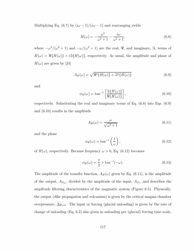
Multiplying Eq. (6.7) by (iω − 1)/(iω − 1) and rearranging yields

H(ω) = − ω2

ω2 + 1− iω

ω2 + 1, (6.8)

where −ω2/(ω2 + 1) and −ω/(ω2 + 1) are the real, <, and imaginary, =, terms of

H(ω) = <{H(ω)} + i={H(ω)}, respectively. As usual, the amplitude and phase of

H(ω) are given by [24]

AH(ω) =√

<2{H(ω)} + =2{H(ω)} (6.9)

and

φH(ω) = tan−1

[={H(ω)}<{H(ω)}

]

, (6.10)

respectively. Substituting the real and imaginary terms of Eq. (6.8) into Eqs. (6.9)

and (6.10) results in the amplitude

AH(ω) =ω√

ω2 + 1(6.11)

and the phase

φH(ω) = tan−1

(

1

ω

)

, (6.12)

of H(ω), respectively. Because frequency ω > 0, Eq. (6.12) becomes

φH(ω) =π

2+ tan−1(−ω). (6.13)

The amplitude of the transfer function, AH(ω) given by Eq. (6.11), is the amplitude

of the output, APch, divided by the amplitude of the input, APf

, and describes the

amplitude filtering characteristics of the magmatic system (Figure 6.5). Physically,

the output (dike propagation and volcanism) is given by the critical magma chamber

overpressure, ∆pcrit. The input or forcing (glacial unloading) is given by the rate of

change of unloading (Eq. 6.2) also given as unloading per (glacial) forcing time scale,

117

∆Pcrit/τf . Figure 6.6 shows this physical interpretation of the transfer function,

H(ω) = output/input, normalized by the Maxwell time scale, i.e.,

H(ω) =∆Pcritτf∆Pfτm

, (6.14)

versus forcing frequency, 1/τf , also normalized by τm, resulting in τm/τf .

Physically, a phase lag of φH(ω) = 2π radians in Eq. (6.13) corresponds to a full

glacial cycle (i.e., growth and retreat) with a forcing period of τf ≈ 40 kyr (Fig-

ure 6.4). Consequently, the phase lag, φH(ω), or equivalently the time lag, Γ, provide

information about the temporal response of the magmatic system as a function of

forcing frequency 1/τf . Time lags between the rate of glacial retreat, approximated

by δ18O′, and the increase in the frequency of both basaltic, B ′, and silicic, S ′, erup-

tions are determined in Section 6.2. Time lags, Γ, and phase lags, φH(ω), are related

by

φH(ω) =2πΓ

τf. (6.15)

Figure 6.6 shows φH(ω), determined from time lags, Γ, using Eq. (6.15), versus forc-

ing frequency normalized by the Maxwell time scale, i.e., τm/τf , for basaltic and

silicic eruptions. Each of these phase lags, along with their uncertainties, may be

projected onto the theoretical curve for the phase, which, in turn, identifies a range

of values for the normalized frequency, τm/τf , and the normalized amplitude of the

transfer function, AH(ω) = (∆pcrit/∆Pf )/(τf/τm). Consequently the time lags de-

termined from the data analysis constrain ∆pcrit/∆pf ≈ 0.8 for silicic volcanism and

∆pcrit/∆pf < 2×10−2 for basaltic volcanism. In principle, with additional constraints

on ∆pcrit or ∆pf , values for either parameter may be obtained.

Glazner et al. [56] suggest that a plausible estimate for the mean ice thickness and

lake depth in this region is around 300 m which corresponds to ∆pf ≈ 3 MPa. Thus,

from Figure 6.6, for silicic and basaltic volcanism, this loading constrains ∆pcrit ≈ 3

118

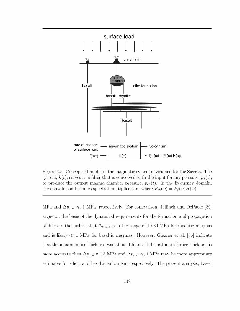
surface load

volcanism

dike formationbasalt

basalt

basalt rhyolite

P (ω)f

H(ω) P (ω) = P (ω) H(ω)fch

volcanismmagmatic systemrate of changeof surface load

silicicmagma

Figure 6.5. Conceptual model of the magmatic system envisioned for the Sierras. Thesystem, h(t), serves as a filter that is convolved with the input forcing pressure, pf (t),to produce the output magma chamber pressure, pch(t). In the frequency domain,the convolution becomes spectral multiplication, where Pch(ω) = Pf(ω)H(ω)

MPa and ∆pcrit � 1 MPa, respectively. For comparison, Jellinek and DePaolo [89]

argue on the basis of the dynamical requirements for the formation and propagation

of dikes to the surface that ∆pcrit is in the range of 10-30 MPa for rhyolitic magmas

and is likely � 1 MPa for basaltic magmas. However, Glazner et al. [56] indicate

that the maximum ice thickness was about 1.5 km. If this estimate for ice thickness is

more accurate then ∆pcrit ≈ 15 MPa and ∆pcrit � 1 MPa may be more appropriate

estimates for silicic and basaltic volcanism, respectively. The present analysis, based

119

τ τf mA

(ω

) =

Hcr f

∆P

∆

P

τfτm

basaltic eruptions

silicic eruptions

mean

mean 2σ-stdv

2σ-stdv 2πΓ τ

Hφ (

ω)

=f

1.78

0.47

π

Figure 6.6. Phase lag (i.e., time lag) and amplitude normalized by the Maxwell timescale, τm, versus glacial forcing frequency, 1/τf , also normalized by τm. Shown arethe phase lags for the basaltic and silicic time lags determined in Section 6.2.

on data, thus provides an additional independent constraint on ∆pcrit.

Figure 6.6 also shows that the estimate for τf ≈ 40 kyr constrains the Maxwell

time to 32 ≤ τm ≤ 400 kyr and τm < 2.4 kyr for rhyolitic and basaltic volcan-

ism, respectively. Taking E = 1010 Pa in Eq. (6.4) to be typical for all rocks, these

Maxwell times imply that the average effective wall rock viscosities governing silicic

and basaltic volcanism are 1022 ≤ µwr ≤ 1023 Pa·s and µwr < 8 × 1020 Pa·s, respec-

tively. Assuming that crustal rheology is thermally-activated [99] and that temper-

ature increases monotonically with depth, these results are consistent with basaltic

magmas originating at greater depths than silicic magmas (Figure 6.5). Geochemical

and petrological observations suggest that, while rhyolite magmas may erupt from

120

depths of 5-8 km [3, 196], basaltic magmas appear to erupt from the base of the litho-

sphere [34]. Finally, these wall rock viscosities agree with Jellinek and DePaolo [89]

who conclude that under most plausible conditions for silicic magma chambers in

intracontinental settings, the dynamics governing dike formation are likely to lead to

volcanism if µwr ≥ 1020 Pa·s.

6.4 Conclusions

Magmatic and volcanic systems involve processes that operate over a wide range

of time and length scales. In the example investigated here, glacial forcing at the

kiloyear time scale appears to modulate volcanic eruption frequency and provides

insight into crustal dynamics (e.g., the Maxwell time scale and wall rock viscosity).

In particular, I propose that statistically significant anticorrelations exist between

the rate of change of ice thickness (approximated by the derivative of the δ18O time

series) and the change in volcanic eruption frequency. The time lags between maxima

and minima of the derivatives of glaciation and basaltic and silicic eruption frequency

are about 11.3 ± 1.0 kyr and 3.0 ± 3.4 kyr, respectively. These results suggest a

wall rock viscosity of µwr < 8 × 1020 Pa·s and 1022 ≤ µwr ≤ 1023 Pa·s for basaltic

and silicic volcanism, respectively, which implies that basaltic magmas originate from

greater depths than silic magmas.

121

Chapter 7

Conclusions

In the following I summarize the findings of this dissertation by providing the

abstracts of the original publications (Sections 7.1, 7.2, and 7.3) or manuscripts in

review (Sections 7.4 and 7.5).

7.1 Continuum percolation theory

In Chapter 2, I study continuum percolation of three-dimensional randomly ori-

ented soft-core polyhedra (prisms). The prisms are biaxial or triaxial and range in

aspect ratio over 6 orders of magnitude. Results for prisms are compared with studies

for ellipsoids, rods, ellipses, and polygons and differences are explained using the con-

cept of the average excluded volume, 〈vex〉. For large shape anisotropies I find close

agreement between prisms and most of the above mentioned shapes for the critical

total average excluded volume, nc 〈vex〉, where nc is the critical number density of

objects at the percolation threshold. In the extreme oblate and prolate limits simu-

lations yield nc 〈vex〉 ≈ 2.3 and nc 〈vex〉 ≈ 1.3, respectively. Cubes exhibit the lowest

122

shape anisotropy of prisms minimizing the importance of randomness in orientation.

As a result, the maximum prism value, nc 〈vex〉 ≈ 2.79, is reached for cubes, a value

close to nc 〈vex〉 = 2.8 for the most equant shape, a sphere. Similarly, cubes yield a

maximum critical object volume fraction of φc = 0.22. φc decreases for more prolate

and oblate prisms and reaches a linear relationship with respect to aspect ratio for as-

pect ratios greater than about 50. Curves of φc as a function of aspect ratio for prisms

and ellipsoids are offset at low shape anisotropies but converge in the extreme oblate

and prolate limits. The offset appears to be a function of the ratio of the normalized

average excluded volume for ellipsoids over that for prisms, R = 〈vex〉e / 〈vex〉p. This

ratio is at its minimum of R = 0.758 for spheres and cubes, where φc(sphere) = 0.2896

may be related to φc(cube) = 0.22 by φc(cube) = 1 − [1 − φc(sphere)]R = 0.23. With

respect to biaxial prisms, triaxial prisms show increased normalized average excluded

volumes, 〈vex〉, due to increased shape anisotropies, resulting in reduced values of

φc. I confirm that Bc = nc 〈vex〉 = 2Cc applies to prisms, where Bc and Cc are the

average number of bonds per object and average number of connections per object,

respectively.

7.2 Yield strength development in crystal-melt sus-

pensions

In Chapter 3, I investigate the formation of a continuous crystal network in mag-

mas and lavas. Network formation in crystal-melt suspensions can provide finite yield

strength, τy, and can thus cause a change from Newtonian to Bingham rheology. The

rheology of crystal-melt suspensions affects geological processes, such as ascent of

magma through volcanic conduits, flow of lava across the Earth’s surface, melt extrac-

123

tion from crystal mushes under compression, convection in magmatic bodies, or shear

wave propagation through partial melting zones. Here, three-dimensional numerical

models are used to investigate the onset of ‘static’ yield strength in a zero-shear en-

vironment. Crystals are positioned randomly in space and can be approximated as

convex polyhedra of any shape, size, and orientation. I determine the critical crys-

tal volume fraction, φc, at which a crystal network first forms. The value of φc is

a function of object shape and orientation distribution, and decreases with increas-

ing randomness in object orientation and increasing shape anisotropy. For example,

while parallel-aligned convex objects yield φc = 0.29, randomly oriented cubes exhibit

a maximum φc of 0.22 as discussed in Chapter 2. Approximations of plagioclase crys-

tals as randomly oriented elongated and flattened prisms (tablets) with aspect ratios

between 1:4:16 and 1:1:2 yield 0.08 < φc < 0.20, respectively. The dependence of φc

on particle orientation implies that the flow regime and resulting particle ordering

may affect the onset of yield strength. φc in zero-shear environments is a lower bound

for φc. Finally the average total excluded volume is used, within its limitation of

being a “quasi-invariant” (Chapter 2), to develop a scaling relation between τy and φ

for suspensions of different particle shapes.

7.3 Hydroseismicity

Groundwater recharge at Mt. Hood, Oregon, is dominated by spring snow melt

which provides a natural large-amplitude and narrow-width pore-fluid pressure signal.

Time delays between this seasonal groundwater recharge and seismicity triggered by

groundwater recharge can thus be used to estimate large-scale hydraulic diffusivities

and the state of stress in the crust. I approximate seasonal variations in groundwater

recharge with discharge in runoff-dominated streams at high elevations. I interpolate

124

the time series of number of earthquakes, N , seismic moment, Mo, and stream dis-

charge, Q, and determine cross correlation coefficients at equivalent frequency bands

between Q and both N and Mo. I find statistically significant correlation coefficients

at a mean time lag of about 151 days. This time lag and a mean earthquake depth

of about 4.5 km are used in the solution to the pressure diffusion equation, under

periodic (1 year) boundary conditions, to estimate a hydraulic diffusivity of κ ≈ 10−1

m2/s, a hydraulic conductivity of about Kh ≈ 10−7 m/s, and a permeability of about

k ≈ 10−15 m2. Periodic boundary conditions also allow me to determine a critical

pore-fluid pressure fraction, P ′/P0 ≈ 0.1, of the applied near-surface pore-fluid pres-

sure perturbation, P0 ≈ 0.1 MPa, that has to be reached at the mean earthquake

depth to cause hydroseismicity. The low magnitude of P ′ ≈ 0.01 MPa is consistent

with other studies that propose 0.01 ≤ P ′ ≤ 0.1 MPa and suggests that the state

of stress in the crust near Mt. Hood could be near critical for failure. Therefore, I

conclude that, while earthquakes occur throughout the year at Mt. Hood, elevated

seismicity levels along preexisting faults south of Mt. Hood during summer months

are hydrologically induced by a reduction in effective stress.

7.4 Permeability-depth curve

Permeability is often considered the most important parameter in geological porous

media flow, largely determining fluid fluxes. Here, I investigate the decrease in 1-

dimensional permeability, k (in square meters), with depth, z (in kilometers), in

the tectonically and volcanically active Oregon Cascades employing four different

techniques. Each technique provides insight into the overall average permeability ap-

plicable to a different depth scale. Spring discharge models are used to infer shallow

(z < 0.1 km) horizontal permeability values. Coupled heat and groundwater flow

125

simulations provide vertical k for z < 1 km. Statistical investigations of the occur-

rences of earthquakes that are probably triggered by seasonal groundwater recharge

yield vertical k for z < 5 km. Finally, considerations of magma intrusion rates and

devolatilization of water from the magma provide estimates of vertical k for z < 15

km. For depths greater than about 0.8 km, my results agree with the power-law

permeability-depth relationship, k = 10−14 m2 (z/1 km)−3.2, suggested by Manning

and Ingebritsen (Rev. Geophys., 1999) for continental crust in general. However, for

shallower depths (z ≤ 0.8 km) I propose an exponential relationship, k = 5 × 10−13

m2 exp(−z/0.25 km), that both fits data better (at least for the Cascades) and al-

lows for a finite permeability near the surface and no singularity at zero depth. In

addition, the two suggested functions yield a relatively smooth transition at z = 0.8

km, where their permeabilities and their permeability gradients are similar. Perme-

ability values inferred from the hydroseismicity model at Mt. Hood are about one

order of magnitude larger than expected from the above k(z)-relationship. However,

higher permeabilities in this region may be consistent with advective heat transfer

along active faults causing observed hot springs. The coupled heat and groundwater

transfer models suggest mean background heat-flow values of about Hb ≈ 0.080 to

Hb ≈ 0.134 W/m2 for the investigated region in the Oregon Cascades.

7.5 Glacier-induced volcanism

A comparison of time series of basaltic and silicic eruptions in eastern California

over the last 400 kyr with the contemporaneous global record of glaciation suggests

that this volcanism is influenced by the growth and retreat of glaciers occurring

over periods of about 40 kyr. In addition, statistically significant cross correlations

between eruption data and the first derivative of the glacial time series imply that

126

the temporal pattern of volcanism is influenced by the rate of change in ice volume.

Moreover, calculated time lags for the effects of glacial unloading on basaltic and

rhyolitic volcanism are distinctive and are 11.3 and 3.0 kyr, respectively. A theoretical

model is developed to investigate whether the increase in eruption frequency following

periods of glacial unloading is a response ultimately controlled by the dynamics of

dike formation. Applying results from the time series analysis leads, in turn, to

estimates for the critical magma chamber overpressure required for eruption as well

as constraints on the average mechanical properties of the wall rocks governing dike

propagation.

127

Appendix A

Appendix to Chapter 4:Hydroseismicity

A.1 Seismometer information

The following information about the short-period vertical-motion seismometers inthe vicinity of Mt. Hood was provided by the Pacific Northwest Seismograph Net-work. The date-column refers to the seismometer installation date.

key latitude longitude elevation date(◦ ’ ”) (◦ ’ ”) (km) (mm/yy)

KMO 45 38 07.80 -123 29 22.20 0.975 09/82SSO 44 51 21.60 -122 27 37.80 1.242 09/91TDH 45 17 23.40 -121 47 25.20 1.541 09/82VBE 45 03 37.20 -121 35 12.60 1.544 10/79VCR 44 58 58.18 -120 59 17.35 1.015 08/83VFP 45 19 05.00 -121 27 54.30 1.716 10/80VG2 45 09 20.00 -122 16 15.00 0.823 09/85VGB 45 30 56.40 -120 46 39.00 0.729 04/80VLL 45 27 48.00 -121 40 45.00 1.195 10/80VLM 45 32 18.60 -122 02 21.00 1.150 06/80PGO 45 27 42.60 -122 27 11.50 0.253 06/82AUG 45 44 10.00 -121 40 50.00 0.865 10/81GUL 45 55 27.00 -121 35 44.00 1.189 07/86MTM 46 01 31.80 -122 12 42.00 1.121 03/80

128

A.2 Box-Jenkins method

The stream discharge of Salmon River is predicted beyond its last measurementby employing a transfer function between Hood River and Salmon River. The transferfunction is determined using a Box-Jenkins [21] method. In the case of a single inputchannel, Xt, investigated here, the output (or lag) channel, Yt, can depend on bothcurrent (t = 0) and previous (t < 0) input, Xt, as well as on previous output, Yt.Thus, input and output are related by

Yt =ω(B)

δ(B)Xt−b +Nt, (A.1)

whereω(B)

δ(B)=ω0 + ω1B + ω2B

2 + ... + ωnBη

δ0 + δ1B + δ2B2 + ...+ δnBγ(A.2)

is the transfer function with coefficients ω and δ. Because coefficients in ω act oncurrent and previous input and coefficients in γ act on previous output, they may bedenoted as moving average (MA) and auto-regressive (AR) processes and the transferfunction as a so-called ARMA model. In the previous equations, t is a time index, Bis the backshift operator such that BbXt = Xt−b, η and γ are the number of delaysfor input and output, respectively, and Nt is noise assumed unrelated to the input.Therefore, if the noise, Nt, is neglected and (in my case) η = 4 and γ = 1 is selectedthen the output, Yt, at time, t, is given by

δ0Yt = δ1Yt−1 + ω0Xt + ω1Xt−1 + ω2Xt−2 + ω3Xt−3 + ω4Xt−4, (A.3)

where δ0 = 1 is commonly assumed (or else Eq. (A.3) is divided by δ0). Therefore,in this example, the current output depends on one (b = 1) previous output (SalmonRiver discharge) as well as on the current (b = 0) and previous four (1 ≤ b ≤ 4)inputs (Hood River discharge).

A.3 Moving polynomial interpolation

The daily binned seismic data has to be interpolated so that continuous timeseries are obtained on which standard spectral analyses can be performed. I apply amoving polynomial interpolation, rather than convolution of the data with a Gaussiannormal curve, so that no artificial frequency is introduced by a convolution kernel. Inaddition, the moving polynomial approach allows interpolation with low-order (≤ 5)polynomials while assuring that the data is optimally matched in a least squares sense.For all three series, Q, N , and Mo, the width of the moving window is 1/12th of thetotal series length and the step width is 1/10th of the window width. The polynomialcoefficients, mLS, are found using the standard least-squares solution from inverse

129

theory given as mLS = [GTG]−1GTd, where G is the (up to) 5th order polynomialmodel matrix and d is the data vector. Multiple interpolation values for a given timestep result from the overlap of the moving window and are averaged.

A.4 Correlation coefficients

I determine auto (f = g) and cross (f 6= g) correlation coefficients for time seriesf and g as described in principal by Eqs. (4.3) and (4.4). In practice, correlationcoefficients, φfg, for positive time lags, l, are calculated by

φfg(l) =1

M − l

M−l−1∑

m=0

fm+l gm, (A.4)

where m and M are the index and the length of the (zero-padded) time series, respec-tively. Dividing by (M − l) provides so-called unbiased cross correlations where thereduced overlap length of the series for large time lags is accounted for. Correlationcoefficients are then normalized as described by Eq. (4.3).

I determine confidence intervals for the case where one of the two time series isassigned random phases for each frequency so that its auto-correlation is unaffected.Typically 500 iterations (each assigning new random phases for each frequency) ofcross correlations, φfg(t), at lag t, are performed by spectral multiplication directlyin the frequency domain as

φfg(t) = F−1{F{f}F ∗{g}}, (A.5)

where F , F−1, and F ∗ denote the Fourier transform, its inverse, and its complexconjugate, respectively. The range of values that contain 90% of the data for a giventime lag is the 90%-confidence interval for that time lag.

To reduce the effect of years with unusually high seismicity, moving cross correla-tion coefficients within overlapping subsections (windows) of the time series are alsodetermined. Here, based on all windows that provide output for a given time lag, themean coefficient per time lag is determined. Each window has to be short enough sothat the years with dominant seismicity do not fall in all windows but large enough sothat cross correlations are performed over several periods (I chose 3 years). Further-more, the time lags of coefficients that are distinct from the confidence interval forrandom phase distributions, are used to calculate a mean and a standard deviationfor the (positive) time lag around the first local maximum coefficient.

130

Appendix B

Appendix to Chapter 5:Permeability-depth curve

B.1 Definition of symbols

The following table provides definitions for symbols used in Chapter 5. Also shownare units and typical values used where appropriate.

Symbol Units Value Definitionα (m2/N) 10−10 vertical compressibility of bulk aquiferβ (m2/N) 4.8×10−10 compressibility of waterb (m) thickness of aquifer or saturated zonecw (J/kg/◦C) 4180 specific heat of watercr (J/kg/◦C) 1000 specific heat of rockd (m) magma intrusion depthδ (m) characteristic depth scale (skin depth)ε (◦C) mean absolute temperature errorg (m/s2) 9.81 gravitational constantH (W/m2) heat-flowh (m) hydraulic headk (m2) permeability tensorK (m/s) hydraulic conductivity tensorκ (m2/s) hydraulic diffusivity tensorκm (m2/s) mixed thermal diffusivity (as scalar)kTw

(W/m/◦C) 0.6 thermal conductivity of waterkTr

(W/m/◦C) 2 thermal conductivity of rock (as scalar)L (m) length of aquifer or volcanic arc

Table is continued on next page.

131

Symbol Units Value Definitionµ (Pa·s) dynamic viscosityν (m2/s) kinematic viscosityn (−) 0.01 connected pore fractionP (Pa) pressureΨ (m/s) precipitation rateψ (s) periodφ (−) weight fractionQ (m3/s) volumetric fluxq (m2/s) volumetric flux per unit width or lengthρw (kg/m3) 1000 density of waterρr (kg/m3) 2700 density of rockSS (1/m) specific storageSY (−) specific yieldT (◦C) temperaturet (s) timeτ (s) diffusion time scaleu (m/s) Darcy velocity vectorv (m/s) interstitial or seepage velocity vectorW (m) width of aquifer or volcanic arc

Subscripts Definition Subscripts Definitione elevation s (near) surface or springM magma T thermalm mixed w waterp pressure x = (x, y) horizontal dimensionsr rock or radial distance z vertical dimensionR recharge

B.2 Derivation of the equation for a T (z)-profile

with an exponential decrease in permeability

Substituting Eq. (5.10) into Eq. (5.14) yields

γKs

κmR(b− z)e−z/δ ∂T

∂z=∂2T

∂z2. (B.1)

In Eq. (B.1), set A = (γKs)/(κmR), D = ∂T/∂z, and D′ = ∂2T/∂z2, so that itbecomes

D′ + A(z − b)e−z/δD = 0, (B.2)

132

where the integration factor is now given as

D = exp

[∫

A(z − b)e−z/δdz

]

= exp[

Ae−z/δ(δb− δ2 − δz)]

. (B.3)

Eq. (B.2) times the integration factor (Eq. B.3),

[

D′ + A(z − b)e−z/δD]

exp[

Ae−z/δ(δb− δ2 − δz)]

= 0, (B.4)

is rewritten asd

dz

{

D exp[

Ae−z/δ(

δb− δ2 − δz)]}

= 0. (B.5)

Integration of Eq. (B.5) with respect to z results in

∂T

∂zexp[

Ae−z/δ(

δb− δ2 − δz)]

= c, (B.6)

where c is the integration constant and D = ∂T/∂z has been resubstituted. For theboundary condition

∂T

∂z= − qb

kTr

at z = b (B.7)

and after resubstituting A = (γKs)/(κmR), Eq. (B.6) becomes Eq. (5.15) which hasto be integrated numerically to yield temperature as a function of depth, T (z).

B.3 Derivation of the equation for a T (z)-profile

with constant hydraulic conductivity

Substituting Eq. (5.12) into Eq. (5.14) yields

γKs

κmR(b− z)

∂T

∂z=∂2T

∂z2. (B.8)

In Eq. (B.8), set A = (γKs)/(κmR), D = ∂T/∂z, and D′ = ∂2T/∂z2, so that itbecomes

D′ + A(z − b)D = 0, (B.9)

where the integration factor is now given as

D = exp

[∫

A(z − b)dz

]

= exp

(

A

2z2 − Abz

)

. (B.10)

Eq. (B.9) times the integration factor (Eq. B.10),

[D′ + A(z − b)D] exp

(

A

2z2 − Abz

)

= 0, (B.11)

133

is rewritten asd

dz

[

D exp

(

A

2z2 − Abz

)]

= 0. (B.12)

Integration of Eq. (B.12) with respect to z results in

∂T

∂z= c exp

(

Abz − A

2z2

)

, (B.13)

where c is the integration constant and D = ∂T/∂z has been resubstituted. Applyingthe boundary condition

∂T

∂z= − qb

kTr

at z = b (B.14)

to Eq. (B.13) yields

c = −(

∂T

∂z

)

b

exp

(

A

2b2 − Ab2

)

(B.15)

Integrating Eq. (B.13) with respect to z and with the boundary condition T (z = 0) =TR, where TR is the recharge temperature at the surface, yields

T (z) = TR + c

√

π

2Aexp

(

Ab2

2

)

erfc

[

(b− z)

√

A

2

]

. (B.16)

Here, c is given by Eq. (B.15) and erfc is the complimentary error function. Substi-tuting Eq. (B.15) into Eq. (B.16) and resubstituting A = (γKs)/(κmR) results inEq. (5.16).

B.4 Finite difference method

Eqs. (5.21) and (5.22) as well as Darcy’s law are approximated by replacing thecontinuous partial derivatives with finite differences. The grid points are regularlyspaced at distances of ∆r and ∆z in horizontal, r, and vertical, z, directions, re-spectively. Hydraulic conductivity can be anisotropic and heterogeneous so thatKr(r, z) 6= Kz(r, z).

The solution to the groundwater flow equation (5.21) is determined by iterativemethods and is given in finite difference form with succesive over/under relaxationby

hm+1ij = (1 − ω)hm

ij + ωhm+1ij , (B.17)

where i and j are the grid indeces in horizontal and vertical directions, respectively,m+1 and m indicate results from the current and the previous iteration, respectively,and ω is the relaxation factor. For ω = 1, ω > 1, and 0 < ω < 1 the current hydraulic

134

head, hm+1ij , is given by a standard Gauss-Seidel method, is over relaxed, and is under

relaxed, respectively [199]. I apply the chain rule

∂

∂w

(

Kw∂h

∂w

)

=∂Kw

∂w

∂h

∂w+Kw

∂2h

∂w2(B.18)

to Eq. (5.21), where w = r and w = z for the first and the third terms, respectively.Then, for any ω I compute the hydraulic head by

hm+1ij =

Ar +Krij

(∆r)2(hm+1

i−1,j + hmi+1,j) +Rhr

+ Az +Kzij

(∆z)2(hm+1

i,j−1 + hmi,j+1)

2(

Krij

(∆r)2+

Kzij

(∆z)2

) , (B.19)

where

Ar =

(

Kri+1,j−Kri−1,j

2∆r

)

(

hmi+1,j − hm+1

i−1,j

2∆r

)

, (B.20)

Az =

(

Kzi,j+1−Kzi,j−1

2∆z

)

(

hmi,j+1 − hm+1

i,j−1

2∆z

)

, (B.21)

and

Rhr=Krij

r

(

hmi+1,j − hm+1

i−1,j

2∆r

)

. (B.22)

Here, r = i∆r is the radial distance from the central axis in the cylindrical coordinatesystem. For a 2D-cartesian coordinate system, Rhr

= 0.

The solution to the heat advection-diffusion equation (5.22) is computed analo-gously to Eq. (B.17) where hm+1

ij and hmij are replaced with Tm+1

ij and Tmij , respectively.

I determine the temperature field iteratively on a grid with horizontal, i, and vertical,j, indices and horizontal, ∆r, and vertical, ∆z, grid point spacing by

Tm+1ij =

1

2κm

(

κm(B +RTr) − γqrij

Cr − γqzijCz

(∆r)−2 + (∆z)−2

)

, (B.23)

where

B =Tm+1

i−1,j + Tmi+1,j

(∆r)2+Tm+1

i,j−1 + Tmi,j+1

(∆z)2, (B.24)

Cr =Tm

i+1,j − Tm+1i−1,j

2∆r, (B.25)

Cz =Tm

i,j+1 − Tm+1i,j−1

2∆z, (B.26)

and

RTr=

1

r

(

Tmi+1,j − Tm+1

i−1,j

2∆r

)

. (B.27)

135

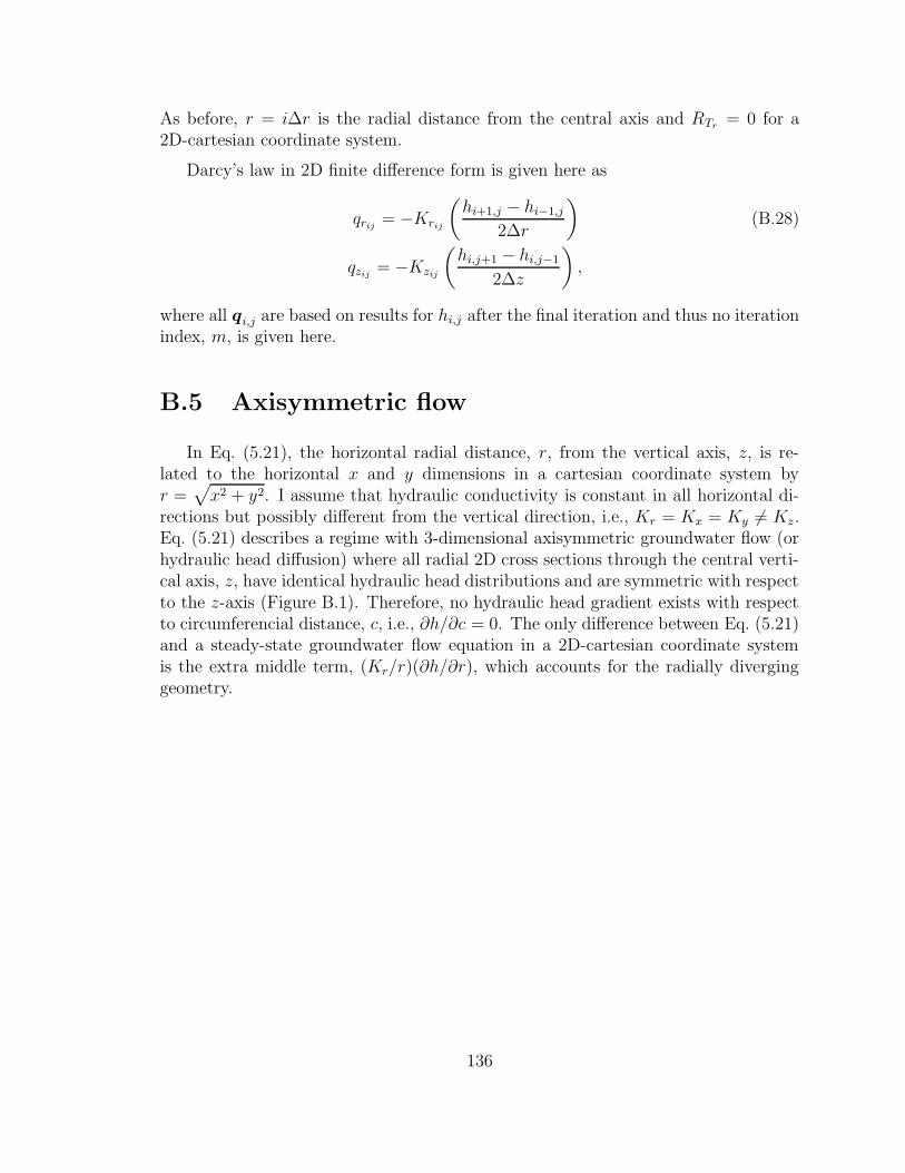
As before, r = i∆r is the radial distance from the central axis and RTr= 0 for a

2D-cartesian coordinate system.

Darcy’s law in 2D finite difference form is given here as

qrij= −Krij

(

hi+1,j − hi−1,j

2∆r

)

(B.28)

qzij= −Kzij

(

hi,j+1 − hi,j−1

2∆z

)

,

where all qi,j are based on results for hi,j after the final iteration and thus no iterationindex, m, is given here.

B.5 Axisymmetric flow

In Eq. (5.21), the horizontal radial distance, r, from the vertical axis, z, is re-lated to the horizontal x and y dimensions in a cartesian coordinate system byr =

√

x2 + y2. I assume that hydraulic conductivity is constant in all horizontal di-rections but possibly different from the vertical direction, i.e., Kr = Kx = Ky 6= Kz.Eq. (5.21) describes a regime with 3-dimensional axisymmetric groundwater flow (orhydraulic head diffusion) where all radial 2D cross sections through the central verti-cal axis, z, have identical hydraulic head distributions and are symmetric with respectto the z-axis (Figure B.1). Therefore, no hydraulic head gradient exists with respectto circumferencial distance, c, i.e., ∂h/∂c = 0. The only difference between Eq. (5.21)and a steady-state groundwater flow equation in a 2D-cartesian coordinate systemis the extra middle term, (Kr/r)(∂h/∂r), which accounts for the radially diverginggeometry.

136

r0z0

h(r,z ) = E0T(r,z ) = ALR0

r1z0 r2z0 r3z0

r0z1

r0z2

r0z3

r0z0 r1z0 r2z0 r3z0

r0z1

r0z2

r0z3

∂ h∂ r

=0

∂ T∂ r

=0

∂ h∂ r

=0

∂ T∂ r

=0

∂ h∂ z

= 0 ∂ T∂ z

= const.

z

z

r

r

r1z0

r2z0

r2z1

r2z2

r2z3

r3z0

r1z0

r2z0

Figure B.1. Schematic illustration of the computational grid in cylindrical coordinatesused for heat and groundwater transfer modeling. All cross sections through thecentral vertical axis, z, are identical and each cross section is symmetric with respectto the z-axis. Thus, while calculations are based on this 3D-cylindrical coordinatesystem, all information is given in the (pull-out) rectangle with coordinates (0 ≤r ≤ Nr, 0 ≤ z ≤ Nz), where Nr and Nz are the maximum number of grid pointsin the r- and z-direction, respectively. The symmetry axis, z, and the outer verticalboundary (r = Nr) are no-flow boundaries for both groundwater (∂h/∂r = 0) andheat (∂T/∂r = 0). The bottom boundary is a no-flow boundary for groundwater(∂h/∂z = 0) and a constant heat flux boundary (∂T/∂z = constant). Hydraulic headdistribution at the surface, which is approximated as being horizontal, is given bymean radial elevation, E, and temperature is given by the mean adiabatic lapse rate,ALR.

137

Bibliography

[1] H. Amit, V. Lyakhovsky, A. Katz, A. Starinsky, and A. Burg. Interpretationof spring recession curves. Ground Water, 40(5):543–551, 2002.

[2] H.S. Carslaw an d J.C. Jaeger. Conduction of Heat in Solids. Oxford Univ.Press, New York, 2nd edition, 1959.

[3] A.T. Anderson, S. Newman, S.N. Williams, T.H. Druitt, C. Skirius, andE. Stolper. H2O, CO2, Cl, and gas in plinian and ash-flow Bishop rhyolite.Geology, 17(3):221–225, 1989.

[4] L. Audin, J.-P. Avouac, M. Flouzat, and J.-L. Plantet. Fluid-driven seismicity ina stable tectonic context: The Remirmont fault zone, Vosges, France. Geophys.Res. Lett., 29(6):art. no. 1091, 2002.

[5] I. Balberg. “Universal” percolation-threshold limits in the continuum. Phys.Rev. B, 31(6):4053–4055, 1985.

[6] I. Balberg. Excluded-volume explanation of Archie’s law. Phys. Rev. B,33(5):3618–3620, 1986.

[7] I. Balberg. Nonuniversal behavior of the cluster properties in continuum sys-tems. Phys. Rev. B, 37(4):2391–2394, 1988.

[8] I. Balberg, C.H. Anderson, S. Alexander, and N. Wagner. Excluded volume andits relation to the onset of percolation. Phys. Rev. B, 30(7):3933–3943, 1984.

[9] I. Balberg, N. Binenbaum, and N. Wagner. Percolation thresholds. Phys. Rev.Lett., 52(17):1465–1468, 1984.

[10] H.A. Barnes and K. Walters. The yield strength myth. Rheol. Acta, 24(4):323–326, 1985.

[11] G.A. Barth, M.C. Kleinrock, and R.T. Helz. The magma body at Kilauea Ikilava lake: Potential insights into mid-ocean ridge magma chambers. J. Geophys.Res., 99:7199–7217, 1994.

138

[12] J. Bear. Dynamics of Fluids in Porous Media. Dover, New York, 1988.

[13] K. Becker and E. E. Davis. New evidence for age variation and scale effectsof permeabilities of young oceanic crust from borehole thermal and pressuremeasurements. Earth Planet. Sci. Lett., 210:499–508, May 2003.

[14] K. Belitz and J.D. Bredehoeft. Hydrodynamics of the Denver basin - explana-tion of subnormal fluid pressures. AAPG Bull., 72:1334–1359, 1988.

[15] D.P. Bentz and E.J. Garboczi. Percolation of phases in a 3-dimensional cementpaste microstructural model. Cem. Concr. Res., 21(2–3):325–344, 1991.

[16] D.D. Blackwell. Thermal results of the Santiam Pass 77-24 drill hole. In B.E.Hill, editor, Geology and Geothermal Resources of the Santiam Pass Area ofthe Oregon Cascade Range, Deschutes, Jefferson, and Linn Counties, Oregon,volume Open-File Report O-92-3, page 61. Oregon Department of Geology andMineral Industries, 1992.

[17] D.D. Blackwell and S.L. Baker. Geology and Geothermal Resources of theBreitenbush-Austin Hot Springs Area, Clackamas and Marion Counties, Ore-gon, volume O-88-5, chapter Thermal Analysis of the Austin and Breitenbushgeothermal systems, Western Cascades, Oregon, pages 47–62. Oregon Depart-ment of Geology and Mineral Industries Open-File Report, 1988.

[18] D.D. Blackwell, R.G. Bowen, D.A. Hull, J. Riccio, and J.L. Steele. Heat-flow, arc volcanism, and subduction in northern Oregon. J. Geophys. Res.,87(10):8735–8754, 1982.

[19] D.D. Blackwell, J.L. Steele, S. Kelley, and M.A. Korosec. Heat-flow in the stateof Washington and thermal conditions in the Cascade range. J. Geophys. Res.,95(B12):19,495–19,516, 1990.

[20] W. Borchard and M. Lechtenfeld. Time dependent properties of thermore-versible gels. Mater. Res. Innov., 4(5–6):381–387, 2001.

[21] G.E.P. Box, G.M. Jenkins, and G.C. Reinsel. Time Series Analysis : Forecastingand Control. Prentice Hall, Englewood Cliffs, N. J., 1994.

[22] W.F. Brace. Permeability of crystalline and argillaceous rocks. Int. J. Rock.Mech. Min., 17(5):241–251, 1980.

[23] W.F. Brace. Permeability of crystalline rocks - new in situ measurements. J.Geophys. Res., 89(6):4327–4330, 1984.

[24] R.N. Bracewell. The Fourier Transform and its Applications. McGraw Hill,New York, 3rd edition, 2000.

139

[25] J. Bredehoeft and I.S. Papadopulos. Rates of vertical groundwater movementestimated from the Earth’s thermal profile. Water Resour. Res., 1(2):325–328,1965.

[26] K.V. Cashman, C. Thornber, and J.P. Kauahikaua. Cooling and crystallizationof lava in open channels, and the transition of pahoehoe lava to ’a’a. Bull.Volcanol., 61(5):306–323, 1999.

[27] A. Celzard, E. McRae, C. Deleuze, M. Dufort, G. Furdin, and J.F. Mareche.Critical concentration in percolating systems containing a high-aspect-ratiofiller. Phys. Rev. B, 53(10):6209–6214, 1996.

[28] C. Clauser. Permeability of crystalline rocks. Eos Trans. AGU, 73:233–238,1992.

[29] C. Clauser, E. Griesshaber, and H.J. Neugebauer. Decoupled thermal andmantle helium anomalies: Implications for the transport regime in continentalrift zones. J. Geophys. Res., 107:doi:10.1029/2001JB000675, 2002.

[30] J.K. Costain, G.A. Bollinger, and J.A. Speer. Hydroseismicity: A hypothesisfor the role of water in the generation of intraplate seismicity. Seismological.Res. Lett., 58:41–64, 1987.

[31] J.-R. de Dreuzy, P. Davy, and O. Bour. Percolation parameter and percolation-threshold estimates for three-dimensional random ellipses with widely scattereddistributions of eccentricity and size. Phys. Rev. E, 62(5):5948–5952, 2000.

[32] J.G. de la Torre, S.E. Harding, and B. Carrasco. Calculation of NMR relax-ation, covolume, and scattering-related properties of bead models using solprocomputer program. Eur. Biophys. J., 28(2):119–132, 1999.

[33] D. Deming. Regional permeability estimates from investigations of coupledheat and groundwater flow, north slope of Alaska. J. Geophys. Res., 98:16,271–16,286, 1993.

[34] D.J. DePaolo and E.E. Daley. Neodymium isotopes in basalts of the southwestBasin and Range and lithospheric thinning during continental extension. Chem.Geol., 169(1–2):157–185, 2000.

[35] D.B. Dingwell. Volcanic dilemma: Flow or blow? Science, 273:1054–1055, 1996.

[36] P.A. Domenico and V.V. Palciauskas. Theoretical analysis of forced convectiveheat transfer in regional ground-water flow. Geol. Soc. Am. Bull, 84:3803–3814,1973.

[37] P.A. Domenico and F.W. Schwartz. Physical and Chemical Hydrogeology. JohnWiley and Sons, New York, 2nd edition, 1998.

140

[38] D.S. Dreger, H. Tkalcic, and M. Johnston. Dilational processes accompanyingearthquakes in the Long Valley caldera. Science, 288(5463):122–125, 2000.

[39] A. Drory. Theory of continuum percolation. I. general formalism. Phys. Rev.E, 54(6):5992–6002, 1996.

[40] A. Drory. Theory of continuum percolation. II. mean field theory. Phys. Rev.E, 54(6):6003–6013, 1996.

[41] A. Drory, B. Berkowitz, G. Parisi, and I. Balberg. Theory of continuum perco-lation. III. low-density expansion. Phys. Rev. E, 56(2):1379–1395, 1997.

[42] A. Einstein. Eine neue Bestimmung der Molekuldimensionen. Ann. Phys.,19:289–306, 1906.

[43] C.W. Fetter. Applied Hydrogeology. Prentice Hall, Upper Saddle River, N. J.,3rd edition, 1994.

[44] A. Fizazi, J. Moulton, K. Pakbaz, S.D. Rughooputh, P. Smith, and A.J. Heeger.Percolation on a self-assembled network-decoration of polyethylene gels withconducting polymer. Phys. Rev. Lett., 64(18):2180–2183, 1990.

[45] F. Jh. Fontaine, M. Rabinowicz, and J. Boulegue. Permeability changes due tomineral diagenisis in fractured crust: Implications for hydrothermal circulationat mid-ocean ridges. Earth Planet. Sci. Lett., 184:407–425, 2001.

[46] C. Forster and L. Smith. The influence of groundwater flow on thermal regimesin mountainous terrain: A model study. J. Geophys. Res., 94:9439–9451, 1989.

[47] R.A. Freeze and J.A. Cherry. Groundwater. Prentice Hall, Englewood Cliffs,N. J., 1979.

[48] A.F. Gangi. Variation of whole and fractured porous rock permeability withconfining pressure. Int. J. Rock Mech. Min., 15(5):249–257, 1978.

[49] S.S. Gao, P.G. Silver, A.T. Linde, and I.S. Sacks. Annual modulation of trig-gered seismicity following the 1992 Landers earthquake in California. Nature,406:500–504, 2000.

[50] E.J. Garboczi, K.A. Snyder, J.F. Douglas, and M.F. Thorpe. Geometricalpercolation threshold of overlapping ellipsoids. Phys. Rev. E, 52:819–828, 1995.

[51] E.J. Garboczi, M.F. Thorpe, M. DeVries, and A.R. Day. Universal conductivitycurve for a plane containing random holes. Phys. Rev. A, 43(12):6473–6482,1991.

[52] S. Ge. Estimation of groundwater velocity in localized fracture zones from welltemperature profiles. J. Volcanol. Geotherm. Res., 84:93–101, 1998.

141

[53] L.N. Germanovich, R.P. Lowell, and D.K. Astakhov. Stress-dependent perme-ability and the formation of seafloor event plumes. J. Geophys. Res., 105:8341–8354, 2000.

[54] L.N. Germanovich, R.P. Lowell, and D.K. Astakhov. Temperature-dependentpermeability and bifurcations in hydrothermal flow. J. Geophys. Res., 106:473–495, 2001.

[55] A.F. Glazner. Volcanic eruption ages in eastern California. unpublished.

[56] A.F. Glazner, C.R. Manley, and J.S. Marron. Fire or ice: Anticorrelation ofvolcanism and glaciation in California over the past 800,000 years. Geophys.Res. Lett., 26(12):1759–1762, 1999.

[57] U. Grigull, J. Straub, and P. Schiebener. Steam Tables in SI-Units. Springer-Verlag, Berlin, New York, 3rd edition, 1990.

[58] T.L. Grove, S.W. Parman, S.A. Bowring, R.C. Price, and M.B. Baker. Therole of an H2O-rich fluid component in the generation of primitive basalticandesites and andesites from the Mt. Shasta region, N. California. Contrib.Mineral. Petr., 142(4):375–396, 2002.

[59] Y. Gueguen, Chelidze T, and M. Le Ravalec. Microstructures, percolationthresholds, and rock physical properties. Tectonophysics, 279:23–35, 1997.

[60] H.K. Gupta. Reservoir-Induced Earthquakes. Elsevier Science, New York, 1992.

[61] S.W. Haan and R. Zwanzig. Series expansion in a continuum percolation prob-lem. J. Phys. A, 10:1547–1555, 1977.

[62] F.R. Hall. Base-flow recessions - a review. Water Resour. Res., 4(5):973–983,1968.

[63] K. Hall. Rapid deglaciation as an initiator of volcanic activity - an hypothesis.Earth Surf. Proc. Land, 7(1):45–51, 1982.

[64] W.L. Hamilton. Tidal cycles of volcanic eruptions - fortnightly to 19 yearlyperiods. J. Geophys. Res., 78(17):3363–3375, 1973.

[65] R.A. Harris. Introduction to special section: Stress triggers, stress shadows,and implications for seismic hazards. J. Geophys. Res., 103(B10):24,347–24,358,1998.

[66] D.O. Hayba and S.E. Ingebritsen. Multiphase groundwater flow near coolingplutons. J. Geophys. Res., 102:12,235–12,252, 1997.

[67] J.H. Healy, W.W. Rubey, D.T. Griggs, and C.B. Raleigh. The Denver earth-quakes. Science, 161:1301–1310, 1968.

142

[68] K. Heki. Snow load and seasonal variation of earthquake occurrence in Japan.Earth Planet. Sci. Lett., 207:159–164, 2003.

[69] W. Hildreth. Gradients in silicic magma chambers: Implications for lithosphericmagmatism. J. Geophys. Res., 86:10,153–10,192, 1981.

[70] S. Hoover, K.V. Cashman, and M. Manga. The yield strength of subliquidusbasalts - experimental results. J. Volc. and Geoth. Res., 107:1–18, 2001.

[71] P.A. Hsieh and J.D. Bredehoeft. A reservoir analysis of the Denver earthquakes:A case of induced seismicity. J. Geophys. Res., 86:903–920, 1981.

[72] K.W. Hudnut, L. Seeber, and J. Pacheco. Cross-fault triggering in the November1987 Superstition Hills earthquake sequence, southern California. Geophys. Res.Lett., 16:199–202, 1989.

[73] E. Huenges, J. Erzinger, J. Kuck, B. Engeser, and W. Kessels. The perme-able crust: Geohydraulic properties down to 9101 m depth. J. Geophys. Res.,102:18,255–18,265, 1997.

[74] H.E. Huppert. The intrusion of fluid mechanics into geology. J. Fluid Mech.,173:557–594, 1986.

[75] H.E. Huppert, R.S.J. Sparks, J.S. Turner, and N.T. Arndt. Emplacement andcooling of komatiite lavas. Nature, 309(5963):19–22, 1984.

[76] S. Hurwitz, S.E. Ingebritsen, and M.L. Sorey. Episodic thermal perturbationsassociated with groundwater flow: An example from Kilauea volcano, Hawaii.J. Geophys. Res., 107:art. no. 2297, 2002.

[77] S. Hurwitz, K.L. Kipp, S.E. Ingebritsen, and M.E. Reid. Groundwaterflow, heat transport, and water table position within volcanic edifices: Im-plications for volcanic processes in the Cascade range. J. Geophys. Res.,108:doi:10.1029/2003JB002565, 2003.

[78] O. Huseby, J.-F. Thovert, and P. M. Adler. Geometry and topology of fracturesystems. J. Phys. A, 30:1415–1444, 1997.

[79] Y. Hyun, S.P. Neuman, V.V. Vesselinov, W.A. Illman, D.M. Tartakovsky, andV. Di Federico. Theoretical interpretation of a pronounced permeability scaleeffect in unsaturated fractured tuff. Water Resour. Res., 38(6):art. no. 1092,2002.

[80] S.E. Ingebritsen, R.H. Mariner, D.E. Cassidy, L.D. Shepherd, T.S. Presser,M.K. Pringle, and L.D. White. Heat-flow and water-chemistry data from theCascade range and adjacent areas in north-central Oregon. Open-File Report88-702, page 205, 1988.

143

[81] S.E. Ingebritsen, R.H. Mariner, and D.R. Sherrod. Hydrothermal systems ofthe Cascades range, north-central Oregon. U.S. Geological Survey ProfessionalPaper 1044-L, 1994.

[82] S.E. Ingebritsen and W.E. Sanford. Groundwater in Geologic Processes. Cam-bridge University Press, Cambridge, New York, 1st edition, 1998.

[83] S.E. Ingebritsen, M.A. Scholl, and D.R. Sherrod. Heat flow from four newresearch drill holes in the western Cascades, Oregon, U.S.A. Geothermics,22(3):151–163, 1993.

[84] S.E. Ingebritsen, D.R. Sherrod, and R.H. Mariner. Heat-flow and hy-drothermal circulation in the Cascade range, north-central Oregon. Science,243(4897):1458–1462, 1989.

[85] S.E. Ingebritsen, D.R. Sherrod, and R.H. Mariner. Rates and patterns ofgroundwater flow in the Cascade range volcanic arc, and the effect of subsurfacetemperatures. J. Geophys. Res., 97:4599–4627, 1992.

[86] A. Isihara. Determination of molecular shape by osmotic measurement. J.Chem. Phys., 18(11):1446–1449, 1950.

[87] E.W. James, M. Manga, T.P. Rose, and G.B. Hudson. The use of temperatureand the isotopes of O, H, C, and noble gases to determine the pattern andspatial extent of groundwater flow. J. Hydrol., 237:100–112, 2000.

[88] D.J. Jeffrey and A. Acrivos. The rheological properties of suspensions of rigidparticles. AIChE J., 22:417–432, 1976.

[89] A.M. Jellinek and D.J. DePaolo. A model for the origin of large silicic magmachambers: Precursors of caldera-forming eruptions. Bull. of Volcanol., publishedonline, May 6, 2003.

[90] M.-J. Jimenez and M. Garcia-Fernandez. Occurrence of shallow earthquakesfollowing periods of intense rainfall in Tenerife, Canary Islands. J. Volc. andGeoth. Res., 103:463–468, 2000.

[91] M.J. Johnston and F.J. Mauk. Earth tides and triggering of eruptions from Mt.Stromboli, Italy. Nature, 239(5370):266, 1972.

[92] J. Jones and S.D. Malone. Mount Hood earthquake activity: Volcanic or tec-tonic origins? Eos. Trans. AGU, 83(47), Fall Meet. Suppl., Abstract S12A-1179,2002.

[93] M. Jull and D. McKenzie. The effect of deglaciation on mantle melting beneathIceland. J. Geophys. Res., 101(B10):21,815–21,828, 1996.

144

[94] J. Kasahara. Tides, earthquakes, and volcanoes. Science, 297:348–349, 2002.

[95] R.C. Kerr and J.R. Lister. The effects of shape on crystal settling and on therheology of magmas. J. Geology, 99:457–467, 1991.

[96] R.C. Kerr and J.R. Lister. Comment on ”on the relationship between dikewidth and magma viscosity” by Yutaka Wada. J. Geophys. Res., 100:15,541,1995.

[97] L. Keszthelyi and R. Denlinger. The initial cooling of pahoehoe flow lobes. Bull.Volcanol., 58(1):5–18, 1996.

[98] G.C.P. King, R.S. Stein, and J. Lin. Static stress changes and the triggering ofearthquakes. Bull. Seismol. Soc. Am., 84:935–953, 1994.

[99] S.H. Kirby. Rock mechanics observations pertinent to the rheology of the con-tinental lithosphere and the localization of strain along shear zones. Tectono-physics, 119(1–4):1–27, 1985.

[100] V. Leonardi, F. Arthaud, A. Tovmassian, and A. Karakhanian. Tectonic andseismic conditions for changes in spring discharge along the Garni right lateralstrike slip fault (Armenian upland). Geodinamica Acta, 11(2-3):85–103, 1998.

[101] R.G. Larson. The Structure and Rheology of Complex Fluids. Oxford UniversityPress, Oxford, New York, 1999.

[102] T. Lay and T.C. Wallace. Modern Global Seismology. Academic Press, SanDiego, 1995.

[103] A.-M. Lejeune and P. Richet. Rheology of crystal-bearing silicate melts: Anexperimental study at high viscosities. J. Geophys. Res., 100:4215–4229, 1995.

[104] D.A. Lockner and N.M. Beeler. Premonitory slip and tidal triggering of earth-quakes. J. Geophys. Res., 104(B9):20,133–20,151, 1999.

[105] C.D. Lorenz and R.M. Ziff. Precise determination of the critical percolationthreshold for the three-dimensional ”swiss cheese” model using a growth algo-rithm. J. Chem. Phys., 114(8):3659–3661, 2001.

[106] M. Maasland. Drainage of Agricultural Lands, in Soil Anisotropy and SoilDrainage, pages 216–285. Am. Soc. of Agron., Madison, Wis., 1957.

[107] J. Maclennan, M. Jull, D. McKenzie, L. Slater, and K. Gronvold. The linkbetween volcanism and deglaciation in Iceland. Geochem. Geophys. Geosys.,3:art. no. 1062, 2002.

[108] M. Manga. Hydrology of spring-dominated streams in the Oregon Cascades,.Water Resour. Res., 32:2435–2439, 1996.

145

[109] M. Manga. A model for discharge in spring-dominated streams and implica-tions for the transmissivity and recharge of Quaternary volcanics in the OregonCascades. Water Resour. Res., 33:1813–1822, 1997.

[110] M. Manga. Orientation distribution of microlites in obsidian. J. Volc. andGeoth. Res., 86:107–115, 1998.

[111] M. Manga. On the timescales characterizing groundwater discharge at springs.J. Hydrol., 219:56–69, 1999.

[112] M. Manga. Using springs to study groundwater flow and active geologic pro-cesses. Annu. Rev. Earth Planet. Sci., 29:201–28, 2001.

[113] C.E. Manning and S.E. Ingebritsen. Missing mineral zones in contact metamor-phosed basalts. Amer. J. Sci., 293:894–938, 1993.

[114] C.E. Manning and S.E. Ingebritsen. Permeability of the continental crust: Im-plications of geothermal data and metamorphic systems. Rev. Geophys., 37:127–150, 1999.

[115] B. Marsh. On the crystallinity, probability of occurrence, and rheology of lavaand magma. Contrib. Min. Pet., 78:85–98, 1981.

[116] B.D. Marsh. On the mechanism of igneous diapirism, stoping, and zone melting.Am. J. Sci., 282:808–855, 1982.

[117] L.G. Mastin. Explosive tephra emissions at Mount St.-Helens, 1989-1991 -the violent escape of magmatic gas following storms. Geol. Soc. Am. Bull.,106(2):175–185, 1994.

[118] F.J. Mauk and M.J. Johnston. Triggering of volcanic eruptions by Earth tides.J. Geophys. Res., 78(17):3356–3362, 1973.

[119] W.J. McGuire, R.J. Howarth, C.R. Firth, A.R. Solow, A.D. Pullen, S.J. Saun-ders, I.S. Stewart, and C. VitaFinzi. Correlation between rate of sea-levelchange and frequency of explosive volcanism in the Mediterranean. Nature,389(6650):473–476, 1997.

[120] A. McIntyre, W.F. Ruddiman, K. Karlin, and A.C. Mix. Surface water responseof the equatorial Atlantic ocean to orbital forcing. Paleoceanography, 4:19–55,1989.

[121] S.R. McNutt and R.J. Beavan. Eruptions of Pavlof volcano and their pos-sible modulation by ocean load and tectonic stresses. J. Geophys. Res.,92(B11):11,509–11,523, 1987.

146

[122] O.E. Meinzer. Large springs in the United States. U.S. Geol. Surv. Water Supp.Pap., 557:94, 1927.

[123] C. Morrow, D. Lockner, S. Hickman, M. Rusanov, and T. Rockel. Effects oflithology and depth on the permeability of core samples from the Kola andKTB drill holes. J. Geophys. Res., 99:7263–7274, 1994.

[124] S. H. Munson-McGee. Estimation of the critical concentration in an anisotropicpercolation network. Phys. Rev. B, 43(4):3331–3336, 1991.

[125] M.D. Murphy, R.S.J. Sparks, J. Barclay, M.R. Carroll, and T.S. Brewer. Re-mobilization of andesite magma by intrusion of mafic magma at the SoufriereHills volcano, Montserrat, West Indies. J. Petrol., 41:21–42, 2000.

[126] M. Nakada and H. Yokose. Ice-age as a trigger of active Quaternary volcanismand tectonism. Tectonophysics, 212(3–4):321–329, 1992.

[127] M. Nathenson. Springs on and in the vicinity of Mount Hood, Oregon. USGSOpen-File Report, in review, 2003.

[128] J. Neuberg. External modulation of volcanic activity. Geophys. J. Int.,142(1):232–240, 2000.

[129] L.W. Nichol, P.D. Jeffrey, and D.J. Winzor. Molecular covolumes of sphere andellipsoid of revolution coombinations. J. Phys. Chem., 80(6):648–649, 1976.

[130] K. Nicholson. Geothermal Fluids: Chemistry and Exploration Techniques.Springer-Verlag, Berlin, Heidelberg, 1993.

[131] G.M. Nielson. Scattered data modeling. IEEE Comput. Graph., 13(1):60–70,1993.

[132] D. Norton and J.E. Knight. Transport phenomena in hydrothermal systems:Cooling plutons. Amer. J. Science, 277:937–981, 1977.

[133] A. Nur and J.R. Booker. Aftershocks caused by pore fluid flow? Science,175:885–887, 1972.

[134] H. Ogasawara, K. Fujimori, N. Koizumi, N. Hirano, S. Fujiwara, S. Otsuka,S. Nakao, K. Nishigami, K. Taniguchi, Y. Iio, R. Nishida, K. Oike, andY. Tanaka. Microseismicity induced by heavy rainfall around flooded verticalore veins. PAGEOPH, 159:91–109, 2002.

[135] L. Onsager. The effects of shapes on the interactions of colloidal particles. Ann.N.Y. Acad. Sci., 51:627–659, 1949.

[136] D. Patriarche, M.C. Castro, and P. Goblet. Manuscript in preparation, 2003.

147

[137] A.P. Philipse. The random contact equation and its implications for (colloidal)rods in packings, suspensions, and anisotropic powders. Langmuir, 12:1127–1133, 1996.

[138] O.M. Phillips. Flow and Reactions in Permeable Rocks. Cambridge UniversityPress, Cambridge, New York, 1991.

[139] A.R. Philpotts and L. D. Dickson. The formation of plagioclase chains duringconvective transfer in basaltic magma. Nature, 406:59–61, 2000.

[140] A.R. Philpotts, J. Shi, and C. Brustman. Role of plagioclase crystal chains inthe differentiation of partly crystallized basaltic magma. Nature, 395(6700):343–346, 1998.

[141] G.E. Pike and C.H. Seager. Percolation and conductivity: A computer study.I. Phys. Rev. B, 10(4):1421–1434, 1974.

[142] H. Pinkerton and R.J. Stevenson. Methods of determining the rheologicalproperties of magmas at sub-liquidus temperatures. J. Volc. and Geoth. Res.,56:108–120, 1992.

[143] H.N. Pollack, S.J. Hurter, and J.R. Johnson. Heat-flow from the Earth’s interior- analysis of the global data set. Rev. Geophys., 31(3):267–280, 1993.

[144] C.B. Raleigh, J.H. Healy, and J.D. Bredehoeft. Faulting and crustal stress atRangely, Colorado, in Flow and Fracture of Rocks. Geophys. Monogr. Ser.,16:275–284, 1972.

[145] C.B. Raleigh, J.H. Healy, and J.D. Bredehoeft. An experiment in earthquakecontrol at Rangely, Colorado. Science, 191:1230–1237, 1976.

[146] M.R. Rampino and S. Self. Can rapid climate change cause volcanic eruptions?Science, 106(4420):826–829, 1979.

[147] J. Renner, B. Evans, and G. Hirth. On the rheologically critical melt fraction.Earth Planet. Sci. Lett., 181:585–594, 2000.

[148] C. E. Renshaw. Sample bias and the scaling of hydraulic conductivity in frac-tured rock. Geophys. Res. Lett., 25:121–124, January 1998.

[149] E. Roeloffs. Poroelastic techniques in the study of earthquake-related hydrologicphenomena. Adv. Geophys., 37:135–195, 1996.

[150] E. A. Roeloffs. Fault stability changes induced beneath a reservoir with cyclicvariations in water level. J. Geophys. Res., 93:2107–2124, 1988.

148

[151] S. Rojstaczer and S. Wolf. Permeability changes associated with large earth-quakes - an example from Loma-Prieta, California. Geology, 20(3):211–214,1992.

[152] R. Roscoe. Suspensions. In Flow Properties of Disperse Systems. J.J. Hermans,North Holland, Amsterdam, Netherlands, 1953.

[153] P. Roth, N. Pavoni, and N. Deichmann. Seismotectonics of the easternSwiss Alps and evidence for precipitation-induced variations of seismic activity.Tectonophysics, 207:183–197, 1992.

[154] C.W. Rovey. Digital simulation of the scale effect in hydraulic conductivity.Hydrogeology Journal, 6(2):216–225, 1998.

[155] F.J. Ryerson, H.C. Weed, and A.J. Piwinskii. Rheology of subliquidus magmas,1, picritic compositions. J. Geophys. Res., 93:3421–3436, 1988.

[156] M.O. Saar. The relationship between permeability, porosity and microstructurein vesicular basalts. Master’s thesis, University of Oregon, 1998.

[157] M.O. Saar and M. Manga. Permeability-porosity relationship in vesicularbasalts. Geophys. Res. Lett., 26(1):111–114, 1999.

[158] M.O. Saar and M. Manga. Continuum percolation for randomly oriented soft-core prisms. Phys. Rev. E, 65(5):art. no. 056131, 2002.

[159] M.O. Saar and M. Manga. Seismicity induced by seasonal groundwater rechargeat Mt. Hood, Oregon. Earth Planet. Sci. Lett., 214:605–618, 2003.

[160] M.O. Saar, M. Manga, K.V. Cashman, and S. Fremouw. Numerical models ofthe onset of yield strength in crystal- melt suspensions. Earth Planet. Sci. Lett.,187:367–379, 2001.

[161] M. Sahimi and S. Arabi. Mechanics of disorderd solids II. Phys. Rev. B, 47:703–712, 1993.

[162] X. Sanchez-Vila, J. Carrera, and J.P. Girardi. Scale effects in transmissivity.Journal of Hydrology, 183:1–22, 1996.

[163] P. Segall. Stress and subsidence resulting from subsurface fluid withdrawalin the epicentral region of the 1983 Coalinga earthquake. J. Geophys. Res.,90:6801–6816, 1985.

[164] P. Segall. Earthquakes triggered by fluid extraction. Geology, 17(10):942–946,1989.

[165] Spatial Climate Analysis Service. Average annual precipitation of Oregon. On-line, 2002.

149

[166] N.J. Shackleton. Oxygen isotopes, ice volume and sea-level. Quaternary Sci.Rev., 6(3–4):183–190, 1987.

[167] K.S. Shante and S. Kirkpatrick. An introduction to percolation theory. Adv.Phys., 20:325–367, 1971.

[168] H.R. Shaw. Comments on viscosity, crystal settling, and convection in graniticmagmas. Am. J. Sci., 263:120–152, 1965.

[169] K. Shimazaki and T. Nakata. Time-predictable recurrence model for largeearthquakes. Geophys. Res. Lett., 7(4):279–282, 1980.

[170] V.M. Shmonov, V.M. Vitiovtova, A.V. Zharikov, and A.A. Grafchikov. Perme-ability of the continental crust: Implications of experimental data. J. Geochem.Explor., 78–79:697–699, 2003.

[171] V.M. Shmonov, V.M. Vitovtova, A.V. Zharikov, and A.A. Grafchikov. Fluidpermeability of the continental crust: Estimation from experimental data.Geochem. Int., 40, Suppl. 1:S3–S13, 2002.

[172] G.E. Sigvaldason, K. Annertz, and M. Nilsson. Effect of glacier load-ing/deloading on volcanism - postglacial volcanic production-rate of the Dyn-gjufjoll area, central Iceland. B. Volcanol., 54(5):385–392, 1992.

[173] D.W. Simpson, W.S. Leith, and C.H. Scholz. Two types of reservoir-inducedseismicity. Bull. Seismol. Soc. Am., 78:2025–2040, 1988.

[174] K.P. Singh and J.B. Stall. Derivation of base flow recession curves and param-eters. Water Resour. Res., 7(2):292–303, 1971.

[175] T.W. Sisson and G.D. Layne. H2O in basalt and basaltic andesite glass inclu-sions from 4 subduction-related volcanos. Earth Planet. Sci. Lett., 117:619–635,1993.

[176] A.S. Skal and B.I. Shklovskii. Influence of the impurity concentration on thehopping conduction in semiconductors. Sov. Phys. Semicond., 7(8):1058–1061,1974.

[177] L. Slater, M. Jull, D. McKenzie, and K. Gronvold. Deglaciation effects onmantle melting under Iceland: Results from the northern volcanic zone. EarthPlanet. Sci. Lett., 164(1–2):151–164, 1998.

[178] L. Smith and D.S. Chapman. On the thermal effects of groundwater flow. J.Geophys. Res., 88:593–608, 1983.

[179] M.L. Sorey. Measurement of vertical groundwater velocity from temperatureprofiles in wells. Water Resour. Res., 7(4):963–970, 1971.

150

[180] R.S.J. Sparks. Triggering of volcanic eruptions by Earth tides. Nature,290(5806):448–448, 1981.

[181] D. Stauffer and A. Aharony. Introduction to Percolation Theory. Taylor andFrancis, London, Washington D.C., 1992.

[182] D.J. Stein and F.J. Spera. Rheology and microstructure of magmatic emulsions:Theory and experiments. J. Volcanol. Geotherm. Res., 49:157–174, 1992.

[183] R.S. Stein. The role of stress transfer in earthquake occurrence. Nature,402:605–609, 1999.

[184] R.S. Stein, G.C.P. King, and J. Lin. Change in failure stress on the southern SanAndreas fault system caused by the 1992 magnitude = 7.4 Landers earthquake.Science, 258:1328–1332, 1992.

[185] R.S. Stein, G.C.P. King, and J. Lin. Stress triggering of the 1994 M = 6.7Northridge, California, earthquake by its predecessors. Science, 265:1432–1435,1994.

[186] L.M. Tallaksen. A review of baseflow recession analysis. J. Hydrol., 165:349–370,1995.

[187] P. Talwani and S. Acree. Pore pressure diffusion and the mechanism of reservoir-induced seismicity. PAGEOPH, 122:947–965, 1984/85.

[188] S. Tanaka, M. Ohtake, and H. Sato. Spatio-temporal variation of the tidaltriggering effect on earthquake occurrence associated with the 1982 South Tongaearthquake of Mw 7.5. Geophys. Res. Lett., 29(16):art. no. 1756, 2002.

[189] S. Timoshenko and J.N. Goodier. Theory of Elasticity. McGraw Hill, NewYork, 1970.

[190] J. Townend and M.D. Zoback. How faulting keeps the crust strong. Geology,28(5):399–402, 2000.

[191] D.L. Turcotte. Self-organized criticality. Rep. Prog. Phys., 62:1377–1429, 1999.

[192] D.L. Turcotte and G. Schubert. Geodynamics. Cambridge University Press,Cambridge, New York, 2nd edition, 2002.

[193] J.S. Turner, H.E. Huppert, and R.S.J. Sparks. Komatiites II; experimental andtheoretical investigations of post-emplacement cooling and crystallization. J.Petrol., 27(2):397–437, 1986.

[194] Y. Wada. Magma flow directions inferred from preferred orientations ofphynocrysts in a composite feeder dike, Mikaye-Jima, Japan. J. Volcanol.Geotherm. Res., 49:119–126, 1992.

151

[195] Y. Wada. On the relationship between dike width and magma viscosity. J.Geophys. Res., 99:17,743–17,755, 1994.

[196] P.J. Wallace, A.T. Anderson, and A.M. Davis. Quantification of pre-eruptiveexsolved gas contents in silicic magmas. Nature, 377(6550):612–616, 1995.

[197] P.C. Wallmann, G.A. Mahood, and D.D. Pollard. Mechanical models for cor-relation of ring-fracture eruptions at Pantelleria, strait of Sicily, with glacialsea-level drawdown. B. Volcanol., 50(5):327–339, 1988.

[198] H.F. Wang. Theory of Linear Poroelasticity. Princeton University Press, Prince-ton, 2000.

[199] H.F. Wang and M.P. Anderson. Introduction to Groundwater Modeling : FiniteDifference and Finite Element Methods. Academic Press, San Francisco, 1982.

[200] C.S. Weaver, R.D. Norris, and C. Trisler-Jonientz. Results of seismological mon-itoring in the Cascades range 1962-1989: Earthquakes, eruptions, avalanches,and other curiosities. Geosci. Can., 17:158–162, 1990.

[201] W.S.D. Wilcock. Tidal triggering of micro earthquakes on the Juan de Fucaridge. Geophys. Res. Lett., 28(20):3999–4002, 2001.

[202] C.R. Wildemuth and M.C. Williams. Viscosity of suspensions modeled with ashear-dependent maximum packing fraction. Rheol. Acta, 23:627–635, 1984.

[203] C.R. Wildemuth and M.C. Williams. A new interpretation of viscosity andyield stress in dense slurries: Coal and other irregular particles. Rheol. Acta,24:75–91, 1985.

[204] C.F. Williams and T.N. Narasimhan. Hydrogeologic constraints on heat-flowalong the San-Andreas fault - a testing of hypotheses. Earth Planet. Sci. Lett.,92(2):131–143, 1989.

[205] L.W. Wolf, C.A. Rowe, and R.B. Horner. Periodic seismicity near Mt. Ogdenon the Alaska - British Columbia border: A case for hydrologically triggeredearthquakes? Bull. Seismol. Soc. Am., 87:1473–1483, 1997.

[206] A.D. Woodbury and L. Smith. Simultaneous inversion of hydrogeologic andthermal data: 2. incorporation of thermal data. Water Resour. Res., 24(3):356–372, 1988.

[207] A.D. Woodbury, L. Smith, and W.S. Dunbar. Simultaneous inversion of hy-drogeologic and thermal data: 1. theory and application using hydraulic headdata. Water Resour. Res., 23(8):1586–1606, 1987.

152

[208] T.L. Wright and R.T. Okamura. Cooling and crystallization of tholeiitic basalt,1965 Makaopuhi lava lake, Hawai’i. U.S. Geological Survey Prof. Paper 1004,page 77, 1977.

[209] J.Y. Yi and G.M. Choi. Percolation behavior of conductor-insulator compositeswith varying aspect ratio of conductive fiber. J. Electroceram., 3(4):361–369,1999.

[210] Z.Q. Zhou, F. Tunman, G. Luo, and P.H.T. Uhlherr. Yield stress and maximumpacking fraction of concentrated suspensions. Rheol. Acta, 34:544–561, 1995.

[211] G. Zimmermann, H. Burkhardt, and L. Engelhard. Scale dependence of hy-draulic and structural parameters in the crystalline rock of the KTB. Pure andAppl. Geophys., 160:1067–1085, 2003.

[212] M.D. Zoback and J.H. Healy. Friction, faulting, and in-situ stress. Ann. Geo-phys., 2:689–698, 1984.

[213] M.D. Zoback and J.C. Zinke. Production-induced normal faulting in the Valhalland Ekofisk oil fileds. Pure and Appl. Geophys., 159(1–3):403–420, 2002.

153