Marriage, Cohabitation, andCharitable Giving

by

Matthew Yorkilous

Submitted to the Distinguished Majors Program

Department of Economics

University of Virginia

April 19, 2021

Advisor: Leora Friedberg

Acknowledgements

First and foremost, I would like to thank my advisor Professor Leora Friedberg—likely

more than she knows, her expectations for me were much higher than my own, and it was

them that made this paper possible. She gave me the most helpful advice I’ve received in

my academic career, without which I certainly could not have finished this biggest project

I’ve ever attempted.

Thanks must also go to Professor Amalia Miller, who, despite the circumstances that

made teaching rather difficult this year, with great honesty and intention provided rich

opportunities for us to learn and improve. I also wish to thank the other members of the

DMP cohort, and particularly Cameron Scalera and Craig Epstein, who on several occasions

helped ground me in reality when the stress of this project was overwhelming.

On that subject, the stress of this thesis was often too much for me to handle on my

own. As such I’m extremely grateful for my loved ones whose support got me through

it—especially my parents and of course my friend Blair Smith. Pierina Rossini, you make

all of my days better, but especially the tougher ones over the course of this process—I can’t

thank you enough. I’m looking forward to this summer, when (according to my results) we’ll

suddenly start giving more to charity.

Marriage, Cohabitation, and Charitable Giving

Matt Yorkilous

University of Virginia

April 19, 2021

Abstract

I examine charitable giving behaviors by married and permanently cohabiting cou-ples. Looking first at differences between married, cohabiting, and single households,I find that married couples are more likely to give and to give more than other groups,especially to religious organizations. I then look at specific couples over time, exam-ining particularly those who transition from cohabitation to marriage, and find thatthough couples who will eventually get married are predisposed to giving even beforetheir marriage, their giving increases after marriage in a way not explained by changesin income or other relevant independent variables. This change is explained in largepart by differences in households’ income elasticities of giving across couple groups andover time. I also check the responsiveness of permanently cohabiting couples’ givingto changes in the tax-price of both household members, and show that their givingresponds only to changes in the higher earner’s marginal tax rate. The results suggesta connection between the commitment mechanism of marriage and investment in thehousehold public good of charitable giving.

1 Introduction

As long ago as Becker (1981), economists have been interested in analysis of the struc-

tures of families, as well as the ways in which these structures affect their spending decisions.

Among the most important is marriage. Obviously, a common reason people enter into a

marriage relationship is to express love and demonstrate commitment, as these contribute

to utility in and of themselves. But economists often consider marriage in another way as

well: as a mechanism that exploits the increased returns to consumption and production of

household goods that accompany a two-person family structure, relative to being single. In-

creasingly in recent decades, however, many people have been choosing to cohabit with their

romantic partners, either in advance of or in place of a legal marriage (Lundberg and Pollak

2015). Since many of the production benefits (i.e. division of labor) and consumption benefits

(i.e. shared household public goods) of a two-person household apply to cohabiting as well

as married couples, the fact that people still choose to get married (and indeed, often choose

to get married after first cohabiting) suggests some additional benefits to marriage—benefits

distinct from those enjoyed by multi-person households.

One potential explanation in the rational-choice framework for the decision to marry

rather than cohabit has to do with commitment. In particular, the social and legal costs of

exiting a marriage relationship (divorce) are significantly higher than the costs of exiting a

cohabiting or roommate relationship. Marriage, then, can act as a mechanism for commit-

ment, decreasing the probability of the dissolution of the union by increasing the costs of

exiting it. Lundberg and Pollak (2013) argue that couples choose marriage as a commitment

device in order to “foster cooperation and encourage marriage-specific investments.” Specif-

ically, they emphasize investment in children and children’s consumption goods, which are

considered household public goods.

Children and their consumption, though, are not the only examples of household public

goods, and it is of interest to know whether the commitment mechanism of marriage facil-

itates the same kind of increased investment in these other goods as well. One particular

1

example of a good that may be a household public good is a household’s charitable giving.

Charitable giving is of special interest because it is also a public good by the general defini-

tion, and increased levels of charity are of benefit (directly and indirectly) not only to donors

and beneficiaries but also the public (Yoruk 2015). As such, governments have often sought

and adopted policies to encourage charitable giving. It becomes natural, then, to inquire

about the relationship between the commitment mechanism of marriage, charitable giving,

and related government policies that influence both spending on all kinds of public goods

and the marriage decision itself.

In this paper, I explore marriage, cohabitation, and charitable giving. I first examine

whether the intertemporal commitment mechanism of marriage leads to an increase in giving.

I follow the rich literature on estimation of charitable giving by households as a function

of their incomes, tax rates, and other characteristics and directly compare married and

cohabiting couples (Andreoni, Brown, and Rischall 2003; Yoruk 2010; Wiepking and Bekkers

2012). In the interest of identifying the effect of the commitment mechanism of marriage, I

look especially closely at giving by couples who first cohabit and then later get married. In

addition, I examine other factors that affect the decision of how much and to whom to give,

again comparing married and cohabiting couples. Specifically, I explore the responsiveness

of giving to taxes and income by and between these two categories of couples. Taxation

is of special interest in the context of this topic, since married and cohabiting couples are

treated differently by United States tax law, and charitable giving is tax-deductible. Thus,

tax policies will likely influence simultaneously the decision to marry and the decision to

give.

I use data from eight biennial waves of the Center on Philanthropy Panel Study (COPPS)

supplement to the Panel Study of Income Dynamics (PSID) from 2001-2015 to examine

differences in charitable giving by married and permanently cohabiting couples. I use an

instrumental-variables approach to account for the endogenous tax-price of giving, and

present evidence that married couples are more likely to give and give in greater amounts

2

than cohabiting couples, holding other variables constant. I find that when households tran-

sition between couple categories, they give most when they are married, and in particular

once-cohabiting couples give more after they get married. These differences seem to be ex-

plained by a greater income elasticity of giving for married couples. Singles appear more

responsive to the tax-price of giving than other kinds of households, and before getting

married, cohabiting couples respond only to the tax-price faced by the higher earner in the

household.

In section 2 I review the literature on marriage and cohabitation, charitable giving by

households, and estimates for the tax-price elasticity of giving. In section 3 I develop a

simple theoretical model to motivate the idea that the commitment mechanism of marriage

increases investment in charitable gifts. In sections 4 and 5 I describe my data and present

my results. Conclusions are in section 6.

2 Literature Review

In much of the early literature on the economics of the family, “marriage” is essentially

synonymous with “two-person household,” such that the feasible set contains only two el-

ements: marriage and living alone (Becker 1973, 1981; Weiss 1997; Bergstrom 1997). The

gains from marriage often described by economists—namely, joint production and consump-

tion—are really just gains from living together (Weiss, 2008; Lam, 1988). Among the first to

explicitly study the marriage contract as a commitment device, rather than simply a decision

to form a union, were Matouschek and Rasul (2008). They provide evidence that commit-

ment is the most plausible reason couples enter a marriage relationship, compared with

alternative hypotheses of marriage as a signaling device or a method of providing exogenous

payoff. Several other authors followed in demonstrating a possible theoretical relationship

between such commitment and efficiency in household production and consumption, linking

the higher costs of divorce to an increase in intra-couple cooperation (Iyigun 2009, Gemici

3

and Laufer 2010, Cigno 2011). Lundberg and Pollak (2013, 2015) emphasize the importance

of this growing theoretical literature in explaining trends of increased cohabitation in the

United States. They draw particular attention to the effects of marital commitment on in-

vestment in children, as well as the disproportionate adoption of this family structure by

the poor and less educated, since parents seeking to invest more highly in their children get

married in order to better facilitate that investment.

While marriage and charitable giving have been studied extensively by economists, few

have analyzed the differences between cohabiting couples and married couples in this area;

indeed, few have even considered the existence of cohabiting couples. In Andreoni and

Payne’s (2013) overview of the charitable giving literature, they speak of giving by households

as synonymous with giving by married couples. Andreoni, Brown, and Rischall’s (2003)

seminal paper specifically examines such giving by married couples, finding differences in

the preferences over giving of single men and women, and showing that these differences

continue into marriage by analyzing giving broken down by who was the decision maker in

the household (the husband, the wife, or the couple jointly). They also observe costs of

bargaining over charitable gifts by couples, in that couples who decide together give less

than they would be predicted to give if they had decided independently and unilaterally.

However, Wilhelm (2007) shows that the quality of the data used by Andreoni, Brown, and

Rischall (the Survey of Giving and Volunteering) is lower than that available in the PSID.

Yoruk (2010) attempts to replicate their results using the PSID, but finds instead positive

returns to bargaining over charitable giving by legally married couples.

Other studies have followed Andreoni, Brown, and Rischall (2003) and Yoruk (2010)

in examining giving by married couples, but none have yet sufficiently analyzed the effects

of marriage relative to permanent cohabitation. Wiepking and Bekkers (2012) show that

legal marriage is correlated with more and bigger charitable gifts, but only relative to non-

marriage, rather than explicitly permanent cohabitation. Wiepking and Maas (2009) find

positive effects on charitable giving from having a partner of any kind, though they do

4

not separate cohabiting couples from married ones. Eagle, Keister, and Read (2018) look at

giving at various intersections of gender, marital status, and religion using the 2006 portraits

of American life study and find households headed by never-married females have lower giving

levels compared with those headed by divorced and widowed women, but do not find the

same association for households headed by single males. While this study briefly considers

cohabiting couples, their preliminary analyses find no differences between their giving and

that of single, never married people and therefore do not report them as a distinct category.

Further, their analysis was cross sectional and so could not look at the over-time effect of

getting married on giving.

Economists have used the PSID to look at both 1) cohabitation, marriage, and taxes,

and 2) the tax-price elasticity of giving; however, none have studied the two simultaneously.

Alm and Whittington (2003) find that tax policy affects the decision of already-cohabiting

couples to get married, though they do not look at charitable giving since the COPPS data

was not available at the time of their study. Brooks (2007) and Backus and Grant (2018) each

use the COPPS to estimate the tax-price of giving utilizing slightly different methodologies,

though neither study seeks to estimate separate elasticities by couple status. Meer and

Priday (2020), in an attempt to anticipate the effects of the Tax Cuts and Jobs Act (TCJA)

on charitable giving, estimate the tax-price of giving in a different way than most of the

preceding literature. For my own estimates, I follow this method and describe it explicitly

in section 4.

This paper contributes to the already-existing literature by explicitly seeking a causal

relationship between the commitment device of marriage and charitable giving, by studying

the giving of permanently cohabiting couples as well as married couples. In addition, I seek

to discern differences in the tax-price elasticity of giving between married and cohabiting

couples. Before empirically testing for these relationships, I first provide a brief theoretical

motivation.

5

3 Theoretical Motivation

3.1 How does commitment affect giving?

Households can consume two kinds of goods—private goods and household public goods.

If a private good is consumed by one member of the household, it cannot be consumed by

another. Public goods (e.g. living space, heating, the well-being of a couple’s children), on

the other hand, are non-rivalrous, and can be consumed jointly by members of the household.

Since a household’s charitable donations often provide benefit to all of its members, charitable

giving can be modeled as a household public good.

I present a simple model to motivate the idea that the increased exit costs (and therefore,

increased commitment) of marriage would increase the amounts of household public goods

consumed by a household, relative to a non-legal romantic union. In particular, marriage

should increase a household’s charitable donations. The model extends the simple explana-

tion of household giving presented in Andreoni, Brown, and Rischall (2003) to account for

the effects of intertemporal commitment.

Consider a two-person household with members i ∈ {h,w}. The members of the house-

hold are not necessarily married, but they participate in a romantic union such that they

each derive utility Ui from the consumption of relational capital (such as trust, love, social

preferences, and actions that take effort). Let g be the vector of household public goods

including relational capital and shared consumption goods, let xi be the vector of private

goods consumed by household member i, and suppose that Ui = Ui(xi, g). The household

budget set S restricts the possible choices of allocations, so that (xh, xw, g) ∈ S (Bergstrom

1997). Assume further that there is sufficient overlap between household members in their

preferences over different charities, such that each member’s utility function is increasing and

monotone in the level of donations, and that the act of donating contributes to the stock of

relational capital. Then donations are a household public good and an entry in the vector

6

g.1

In order to understand the effect of the intertemporal commitment mechanism of marriage

on charitable giving, now consider a linear, intertemporal utility function for a member

i of the two-person household in two periods t ∈ {1, 2}. Assume that goods consumed

in period 1 also provide utility in period 2, but that their value deteriorates such that

Ui2(xi1, g1) = λ · Ui1(xi1, g1)) for λ ∈ [0, 1]. This deterioration occurs in part because some

goods are literally used up, and in part because some goods (such as those composing the

stock of relational capital) are worth less as time goes on. Household public goods (and

particularly those composing the stock of relational capital) can be consumed and provide

benefit only if the household union remains intact.2 Then, if the union remains intact in

period 2, we have the expected utility:

Ui = xi1 + g1 + δ · (λ · (xi1 + g1) + xui2 + gu2 ) (1)

where δ ∈ [0, 1] is the discount factor, and xui2 and gu2 are the levels of private and public

goods chosen by the household in period 2. If instead the union dissolves in period 2:

Ui = xi1 + g1 + δ · (λ · (xi1) + xsi2) (2)

where xsi2 is the level of private goods chosen by the single individual i in period 2.

The two-person household can be either married (m) or cohabiting (c). Let the prob-

abilities that the union remains intact, given that the couple is married or cohabiting, be

ρm, ρc ∈ [0, 1] respectively. Since the costs of exiting a marriage are higher than those of

exiting a cohabiting relationship, let ρm > ρc. Clearly under this assumption, and as long as

1It is not totally obvious that warm-glow giving, where the act of giving itself provides utility ratherthan simply the amount of the donation, is a household public good (Andreoni 1990). This model insteadconsiders only the utility provided directly by the amount of giving.

2Some household public goods may possibly continue to provide benefit even after the union dissolves—butcertainly the stock of relational capital disappears with the dissolution of the union, and g decreases. I makethe simplifying assumption that g decreases to zero. Without this assumption, the conclusions of the modeldo not change as long as the act of giving contributes to the stock of relational capital.

7

δ, λ > 0, the expected utility obtained from consuming the household public good in period

1 for a married couple is greater than that for a cohabiting couple:

Umi (g1) = g1 · (1 + (ρm · δ · λ)) > g1 · (1 + (ρc · δ · λ)) = U c

i (g1) (3)

since (1 + (ρm · δ · λ)) > (1 + (ρc · δ · λ)). That is, the expected future value of consuming

g1 in period 1 is higher for a person in a married household compared with a cohabiting

household, since the likelihood that g1 will continue to provide utility in period 2 is higher.

For a utility-maximizing household, then, consumption of g (and in particular, charitable

giving) would be higher for a married rather than cohabiting couple, holding all else constant.

This is first hypothesis I will test empirically in this paper.

It is also possible that commitment increases charitable giving in a way not directly

connected to its status as a household public good. Namely, giving is a function of income,

and because of risk-sharing and income-pooling associated with marriage, married couples

may be the most secure in projecting their future income. This could make married couples

“richer” given the same amount of income compared to other kinds of households, and

ultimately result in higher levels of giving. If this were the case, we would expect to observe

a greater income elasticity of giving for married couples compared with other households.

This is the second hypothesis I test in this paper.

3.2 The tax-price of giving for cohabiting couples

In the United States, tax filers who itemize deductions can claim charitable donations as

a deduction, reducing their taxable income. Hence, if τ is the marginal tax rate, a household

that itemizes deductions only forgoes 1− τ dollars of other consumption to give 1 dollar to

charity, effectively making p ≡ 1− τ the price of giving (Andreoni and Payne 2013).

I expect cohabiting couples to respond only to changes in the tax-price faced by the

household member with higher marginal tax rate. To see why, suppose there is a two-

8

person, unmarried household in which household member 1 faces a higher marginal tax rate

than household member 2, that is, τ1 > τ2. Then p1 < p2, and the couple would assign all

charitable deductions to household member 1 in order to face the lowest price. Then if p2

increases or decreases by less than p2 − p1, the household’s giving will not respond to this

change. This is the third hypothesis I test empirically in this paper. Before reporting the

results, I describe the dataset I use.

4 Description of Data

I use data from the 2001-2015 biennial waves of the Panel Study of Income Dynamics

(PSID), a national panel survey that has been collected annually or biennially since 1968. In

addition to the PSID’s detailed information on employment, income, wealth, and expendi-

tures, I draw on the Center on Philanthropy Panel Study (COPPS). This supplement to the

PSID began in 2001 and asks respondents questions about the amounts of their charitable

contributions, broken down into several classes.

The unit of analysis is the household, which I specify by following the “head” of each

family (the male in a heterosexual married/cohabiting couple or a single adult of either sex),

as well as all individuals associated to the head, for as long as they remain in the survey.

Across the eight waves of data that I use (beginning in 2001 and continuing biennially until

2015), the total number of household-year observations is 67,227. I combine the household

level information with individual level information, of which there are 188,744 unique records.

Following Wilhelm (2006) and much of the charitable giving literature studying the PSID,

I remove the low-income Survey of Economic Opportunity (SEO) over-sample. In addition,

I remove observations of families who were not asked the charitable giving questions in a

given year, as well as same sex couples (n = 311), couples in which the “head” is a married

woman (n = 91), and families with negative income (n = 45).3 My final sample is of 41,277

3Same sex couples were not identified by the PSID until 2015. Married women are heads only if theirhusband is incapacitated or completely uncooperative. I remove these few observations in order to have a

9

total observations, representing 8,943 unique households.

The “status” of a couple (married, permanently cohabiting, or single), while not explicitly

reported by the PSID, can be determined by a combination of the marital status of the head

and the “relationship to head” variable recorded in the individual file. Here, the PSID

distinguishes between wives and “wives” (the latter referring to partners who have lived in

the family unit for more than one year). The survey also identifies partners who have lived in

the family unit for less than a year. However, since relatively little information is reported

about these “first-year cohabiting” partners, I consider these families a distinct category

from permanently-cohabiting families.

The PSID breaks down a household’s yearly giving into 11 charity “classes”. Follow-

ing Andreoni, Brown, and Rischall (2003) I construct a measure based on the Herfindahl-

Hirschman Index (HHI) to examine whether there are differences in the distribution of cat-

egories of gifts between various types of households. In particular,

HHI =11∑j=1

s2j (4)

where sj is the amount given to charity class j divided by the total amount given. Hence,

0 ≤ HHI ≤ 1, with a household’s HHI in a given year equal to 1 if the household gave to

only one class of charity in that year, and equal to 0.091 if the household gave equally to all

11 classes of charity in that year.

In table 1, I report the mean values of key PSID variables broken down by couple status.

On average, married couples give much more (∼700%) and are about 37.5% more likely

to give when compared with permanently cohabiting couples. In figure 1, I present the

distribution of the natural logarithm of (1 + total giving), again broken down by couple

status. Married couples concentrate their giving at higher amounts and give zero dollars

less frequently when compared with other couple types. It is important to note, however,

more uniform sample.

10

that married couples also face lower prices, have higher incomes, and are more religious than

permanently cohabiting couples—all factors which are often associated with higher levels of

charitable giving.

Table 1: Summary statistics

(1) (2) (3) (4)

Married Permanent First-year Single

Cohabiting Cohabiting

Gives to charity .7756 .3993 .3652 .5318

Total giving 2,144.86 309.76 297.31 744.39

(Giving | Giving > 0) 2,765.27 775.68 814.09 1,399.87

Price .9066 .9622 .9772 .9622

Itemizer (estimated) .4062 .0903 .1089 .1782

Income (in 2000 dollars) 86,517.97 54,801.89 42,030.33 35,064.81

Age of head 47.81 36.80 29.94 46.79

Head HS grad .8665 .7276 .8240 .8330

Head attended college .5895 .3918 .5168 .5262

Head college grad .3554 .1622 .2279 .2583

Child number .9199 .8544 .6053 .3800

Catholic .2136 .1651 .1536 .1782

Jewish .0297 .0183 .0193 .0256

Protestant .5794 .4230 .4578 .5761

Other non-Christian .0072 .0121 .0142 .0098

Greek/Russian Orthodox .0017 .0021 0 .0026

Other .0073 .0092 .0214 .0156

Atheist/Agnostic .1274 .2920 .3032 .1678

Religious giving 1,340.88 92.63 60.13 367.79

Secular giving 803.98 217.13 237.18 376.60

n 23,122 2,331 979 14,579

Notes: the sample includes participants from the PSID waves 2001-2015. I excludethe SEO low-income oversample, same-sex couples, couples in which the “head” isa married woman, and families with negative income.

One of the key variables studied in the literature on charitable giving is the tax-price of

giving. However, The PSID does not report the marginal tax rates of the families in the

11

Figure 1: Distribution of giving by couple status

sample. In order to compute the tax-price of giving, then, I first use the National Bureau of

Economic Research’s Taxsim program (Feenberg and Coutts 1993) as well as the information

provided in the PSID about marital status, number of children, labor and interest income,

and various deductions.4 Typically, the tax-price of giving is defined to be equal to 1 if the

household does not itemize deductions and 1− τit if they do, with τit equal to the marginal

tax rate of household i in time t. However, many families receive credits from the Earned

Income Tax Credit (EITC) and the Child Tax Credit (CTC), which have phase-in and phase-

out rates dependent on income and thus affect the family’s marginal tax rate as reported by

4While the PSID does not directly report mortgage interest paid (which is tax deductible) it does reportremaining principle amount, monthly mortgage payment, current interest rate, year obtained, and years topay for up to two of each family’s mortgages. I use the method described in Kimberlin, Kim, and Shaefer(2015) and these variables to calculate mortgage interest paid.

12

Taxsim. Since both of these credits are based solely on earned income, they do not affect the

tax-price of giving. To account for this disparity between the reported marginal tax rate and

the actual rate that affects the tax-price of giving, as well as any other similar complications

in the tax code, I follow Meer and Priday (2020) and estimate the tax-price of giving as

Priceit = 1 +T ′it − Tit100

(5)

where Tit is the tax liability of household i in time t and T ′it is the tax liability of household i

in time t if they were to have given $100 more to charity in the previous year. This captures

the actual effect of giving on taxes paid and thus acts as a more accurate measure of the

tax-price of giving, compared with simply using the marginal tax rate reported by Taxsim.

For a small number of households, donating $100 more to charity would cause them to begin

itemizing—again following Meer and Priday (2020), I set the price for these households equal

to 1.

For permanently cohabiting couples, who may not file as married under the U.S. system

of household taxation, I estimate the tax-price of giving separately for the head and the

“wife,” assuming that all child care expenses and children are assigned to the higher earner.

Assuming similarly that families maximize their tax benefits from giving, I set the tax-price

for these households equal to the minimum of the price faced by the head and that faced by

the wife. For first-year cohabiting couples, little information is reported about the cohabiting

partner of the head, and thus I calculate the price for the household in the same way as I

would for a single person.

13

5 Empirical Analysis

5.1 Empirical strategy

The basic model I estimate is the following:

Givingit = β1 · Cohabitingit + β2 · Singleit

+ γ1 · Cohabitingit × Priceit

+ γ2 · Singleit × Priceit

+ θ · Priceit + π ·Xit + αt + εit

(6)

where Givingit is the probability or amount of giving by household i in year t, Cohabitingit

and Singleit are dummy variables, Xit is a vector of demographic controls, αt represents

year-level fixed effects, and εit is a random error term. Often addressed in the literature

on charitable giving is the problem of the endogeneity of the tax-price of giving. Namely,

since households can donate enough to move into a lower tax bracket, giving will have a

negative effect on tax rates (and a positive effect on price) and the estimates for the tax-

price elasticity of giving will be biased downwards. To account for this, I again follow Meer

and Priday (2020) and construct the “first-dollar” tax-price of giving (that is, the marginal

tax rate a family would face if they were to give zero dollars to charity) in the same way as

the “last-dollar” price above, but with Tit = 0 and T ′it = 100. I use this constructed variable

to instrument for price, since it is highly correlated with the actual price, but affected only

by the tax code and not by a household’s charitable giving decisions.

I use the estimates for β1 and β2 to calculate average marginal effects, and while I gener-

ally interpret them as the effects of cohabiting or being single on charitable giving outcomes

relative to being married, the marriage decision is also likely endogenous. Unobservable

factors, unrelated to commitment, may simultaneously influence the decision to be married

and the decision to give, and thus it is with caution that I argue a causal relationship in the

14

absence of a strong instrument for marriage. Nevertheless, I proceed with the analysis and

use fixed effects and over-time variation to provide some evidence for a causal link.

5.2 Comparison of giving by categories of couples

My first objective is to investigate whether there are differences in charitable giving be-

tween married couples, cohabiting couples, and single people, on both the extensive and

intensive margins of giving. In anticipation of results from two-stage least squares (2SLS)

regressions, in table 2 I present the results from the first-stage regressions explaining the

endogenous tax-price of giving (and its interaction terms) with their respective instruments.

The coefficient estimates for each endogenous variable’s instrument are statistically signifi-

cant and close to 1, indicating high levels of correlation and suggesting that the instruments

are strong. In later sections of my analysis, I work with different sub-samples of the data

and re-estimate these first stage regressions, with similar strong results.

The first column of table 3 contains the results of a 2SLS estimation of the probability of

making a charitable gift for a given household in a given year, while the second column of ta-

ble 3 reports the same regression with the natural logarithm of total charitable contributions

as the dependent variable.5 In addition to a set of demographic controls, income, and year

fixed effects, both regressions contain a set of dummy variables that indicate the household’s

“couple status”: married, permanently cohabiting, first-year cohabiting, and single. I also

include the instrumented variables from the first stage: the natural logarithm of the last-

dollar tax-price of giving, as well as the couple status dummies interacted with this variable.

Standard errors are clustered at the household level and reported in parentheses.

The results suggest that permanently cohabiting, first-year cohabiting, and single house-

holds are all significantly less likely to make a gift than married couples, and that their gifts

are significantly smaller than those of married couples, holding other relevant explanatory

variables constant. A permanently cohabiting household is about 17% less likely to give to

5I add the constant one to the contribution amount before taking the natural logarithm.

15

Table 2: First-stage results

(1) (2) (3) (4)

Log(price) Perm. Coh. × 1st Y. Coh. × Single ×Log(price) Log(price) Log(price)

Log(first-dollar price) .8213*** -.0007** -.0002* -.0129***

(.0072) (.0004) (.0001) (.0014)

Perm. Coh × Log(1st price) .0741*** .9957*** -.0001 -.0038***

(.0059) (.0027) (.0001) (.0008)

1st Y. Coh. × Log(1st price) .0733*** -.0002 .9935*** -.0069***

(.0077) (.0003) (.0030) (.0012)

Single × Log(1st price) .0579*** -.0001 -.0001* .9625***

(.0051) (.0001) (.0001) (.0029)

Log(income) -.0180*** -.0000 .0001** .0065***

(.0040) (.0001) (.0001) (.0007)

Log(income)2 .0048*** .0000 -.0000** -.0010***

(.0008) (.0000) (.0000) (.0001)

Log(income)3 -.0003*** .0000* .0000** .0000***

(.0000) (.0000) (.0000) (.0000)

n 41,273 41,273 41,273 41,273

Unique households 8,943 8,943 8,943 8,943

***p < 0.01 **p < 0.05 *p < 0.1

Notes: In addition to the variables listed, I include age of the head of household and its quadratic, dummyvariables for education of the head, dummy variables for race, dummy variables for religious preference,number of children, and year fixed effects in each first-stage regression.

charity than a married household with the similar income and demographics. A represen-

tative married couple is predicted to give greater than four times more than a cohabiting

couple ($175.47 vs. $40.82).6 Additionally, in terms of both the probability and amount of

giving, the hypothesis that permanently cohabiting couples and singles behave in the same

way is rejected (χ2(1) = 43.51, p = 0.0000; χ2(1) = 64.77, p = 0.0000, respectively), with

singles predicted as more likely to give and to give more than permanent cohabitors. Singles

6The representative household from which these predictions are based is a white, protestant, family withone child and a 46 year old head of household who attended some college. They have an income of $77,963and face a tax price of .9312.

16

Table 3: Couple status and giving

(1) (2) (3) (4)

Pr(gives) Log(giving) LPM w/ FE OLS w/ FE

Perm. cohabiting -.1715*** -1.453*** -.0787*** -.5867***

(.0135) (.0869) (.0164) (.0991)

1st-year cohabiting -.1492*** -1.181*** -.0871*** -.5636***

(.0183) (.1230) (.0198) (.1269)

Single -.0803*** -.7400*** -.0925*** -.6103***

(.0081) (.0603) (.0140) (.0907)

Married (omitted) – – – –

Log(price) -.3419*** -2.567*** -.0653*** -.8639***

(.0283) (.2242) (.0239) (.1697)

PC × Log(price) -.3558*** -.6959 -.1101 -.2298

(.1079) (.7237) (.1171) (.7442)

1YC × Log(price) -.2791 -.7194 -.2639* -1.416

(.1787) (1.284) (.1503) (1.051)

Single × Log(price) -.2591*** -1.450*** -.1415*** -.8792**

(.0500) (.3979) (.0521) (.3550)

Log(income) -.1926*** -.8089*** -.0656*** -.2496**

(.0190) (.1362) (.0184) (.1191)

Log(income)2 .0337*** .1124*** .0117*** .0387*

(.0032) (.0239) (.0032) (.0214)

Log(income)3 -.0012*** -.0020* -.0004*** -.0006

(.0001) (.0011) (.0001) (.0010)

H0 : Single = PC 43.51*** 64.32*** 0.62 0.05

n 41,273 41,273 41,273 41,273

Unique households 8,943 8,943 8,943 8,943

***p < 0.01 **p < 0.05 *p < 0.1

Notes: results are derived from the PSID bienniel waves 2001-2015. In addition to thevariables listed, I also include age of the head of household and its quadratic, dummyvariables for education of the head, dummy variables for race, dummy variables forreligious preference, number of children, and year fixed effects. Reported are the two-stage least squares estimates and OLS regressions including the same independentvariables and household fixed effects. The values reported for the couple dummyvariables and log of price are average marginal effects; I also report the χ2(1) teststatistics for the null hypothesis that these average marginal effects are equal forsingles and permanent cohabitors. Standard errors are clustered at the householdlevel and in parentheses.

17

seem to react differently to a change in the tax-price than do married couples—they are

significantly more responsive in terms of both probabilities and amounts. The model pre-

dicts that a one-percent increase in the tax-price of giving would, on average, decrease the

probability that a single person gives by about 0.60% compared with a married couple’s

0.34%; the same increase in price would decrease a married couple’s giving by about 2.57%

on average, but a single person’s giving by just more than 4%. While permanently cohabiting

couples are also significantly more responsive to the tax-price than married couples in terms

of probabilities of giving, the difference is not significant in terms of amounts. When com-

paring singles and cohabiting couples, this difference is neither significant on the extensive

nor intensive margin (χ2(1) = 0.72, p = 0.3961; χ2(1) = 0.94, p = 0.3310, respectively).

In column 3 of table 3 I report the results of a linear probability model (LPM) explaining

the decision to give with the same set of explanatory variables as the 2SLS regression, as well

as household-level fixed effects. In column 4 I report the results of an ordinary least squares

(OLS) regression with those same explanatory variables and fixed effects. Household level

fixed effects are usually included in empirical estimations of the tax-price of giving to control

for the time-invariant features of households that are correlated both with the household’s

marginal tax rate and charitable giving. Indeed, estimating the amount-of-giving equation

with household fixed effects results in a smaller estimate for the tax-price elasticity of giving

(-1.08 if the interaction terms are not included), which is more consistent with the typical

estimates in the literature that are close to −1 (Meer and Priday 2020). However, these fixed

effects limit the observable variation in giving by different categories of couples. In particular,

the regression coefficients capture only the effects of changing couple status within a given

household—for example, from starting a relationship, getting divorced, or transitioning from

cohabitation to marriage. While the inclusion of household fixed effects does not change the

fact that cohabiting and single households appear to give significantly less often and less than

do married couples, the effects are diminished—cohabiting couples are expected to give about

7.9% less often and 58.7% less than similar married couples. Further, the difference between

18

singles and permanently cohabiting couples is not robust to this change in specification: it is

no longer significant (χ2(1) = 0.62, p = 0.4322 for probabilities; χ2(1) = 0.05, p = 0.8246 for

amounts), and singles are instead predicted to give both less often and less than permanently

cohabiting couples. Singles again appear to be more responsive to tax-prices than married

couples, but the difference in responsiveness between permanent cohabitors and married

couples disappears. Hence, while we can confidently say that permanently cohabiting couples

are less likely to give and give less than married couples, and that giving by singles is more

responsive to changes in the tax-price than giving by married couples, the existence of other

differences is less clear.

Also of interest is whether there are differences in the preferred destinations of giving

between households with different couple status. In table 4, I present the results of several

regressions to investigate this question. In column 1, I estimate the same 2SLS regressions

as those reported in columns 1 and 2 of table 3 in order to predict the HHI of a couple

in a given year, where HHI is constructed as described earlier. Though the results of two-

sample t-tests suggest differences in the mean levels of HHI for permanently cohabiting and

married couples—and in particular that the giving of permanently cohabiting couples is more

concentrated—when controlling for relevant independent variables, permanently cohabiting

couples are actually predicted to concentrate their giving less than married couples. However,

this difference is not statistically significant.

In columns 2 through 12 of table 4, I estimate the same regressions but with the probabil-

ities and amounts of giving to specific charity classes as the dependent variables. I report the

coefficient estimates for each couple status, as well as the χ2(1) statistic comparing perma-

nently cohabiting couples and singles. In most cases, the relative probabilities and amounts

of giving restricted to specific classes are the same as the probabilities and amounts for all

giving, i.e., married couples give more often and more than singles, who give more often and

more than permanently cohabiting couples. Exceptions to this rule are in environmental and

international giving, where singles are expected to give more often and more than all other

19

Table 4: Couple status and giving by charity class

(1) (2) (3) (4) (5) (6) (7) (8) (9) (10) (11) (12)

HHI Rel. Youth Env. Comb. Need Health Edu. Art Neigh. Int. Other

Probability of giving

Perm. coh. – -.212*** -.032*** -.006 -.072*** -.065*** -.054*** -.048*** .005 -.010*** -.006 -.016***

(.013) (.007) (.007) (.010) (.011) (.009) (.007) (.006) (.004) (.005) (.005)

1st-year coh. – -.182*** -.021*** -.006 -.045*** -.056*** -.030*** -.011 .002 -.004 -.006 .001

(.014) (.008) (.008) (.012) (.013) (.011) (.009) (.006) (.005) (.005) (.007)

Single – -.130*** -.022*** .002 -.042*** -.024*** -.021*** -.008 .008 -.005 .003 -.000

(.010) (.005) (.005) (.008) (.008) (.007) (.006) (.005) (.003) (.004) (.004)

Mar. (omitted) – – – – – – – – – – – –

H0 : single = PC – 42.2*** 2.43 1.0 8.3*** 14.7*** 13.3*** 30.3*** 0.3 1.9 3.0* 9.4**

Amount of giving

Perm. coh. -.001 -1.56*** -.123*** -.028 -.386*** -.335*** -.219*** -.221*** .016 -.044*** -.028 -.082***

(.011) (.080) (.029) (.031) (.053) (.057) (.042) (.034) (.028) (.015) (.020) (.024)

1st-year coh. -.018 -1.32*** -.072** -.023 -.299*** -.274*** -.086 -.036 .018 -.012 -.024 .014

(.015) (.084) (.034) (.035) (.064) (.068) (.052) (.042) (.030) (.021) (.025) (.036)

Single -.017*** -1.03*** -.087 .016 -.226*** -.116*** -.065** -.025 .047** -.017 .009 .003

(.006) (.072) (.023) (.024) (.042) (.042) (.035) (.032) (.025) (.014) (.009) (.021)

Mar. (omitted) – – – – – – – – – – – –

H0 : single = PC 2.1 46.6*** 1.5 1.9 8.9*** 14.4*** 13.0*** 29.4 1.1 2.8* 2.7* 12.13***

n 26,718 41,273 41,273 41,273 41,273 41,273 41,273 41,273 41,273 41,273 41,273 41,273

Unique households 6,748 8,943 8,943 8,943 8,943 8,943 8,943 8,943 8,943 8,943 8,943 8,943

***p < 0.01 **p < 0.05 *p < 0.1

Notes: all regressions also include the instrumented log(price); log(income), its quadratic, and cubic; the demographic variables as in table 3; andyear fixed effects. Reported are the coefficient estimates as well as χ2(1) statistics for the given null hypothesis. The sample size and number of uniquehouseholds are smaller in the HHI regression because I restrict the sample to families who gave > $0. Standard errors clustered at the householdlevel are in parentheses.

20

groups, as well as in art, where married couples are expected to give least among all cat-

egories of households. However, none of these “unexpected” differences are statistically

significant. The most dramatic differences are in religious giving, where married couples

dominate all other household categories, especially permanently cohabiting couples—a per-

manently cohabiting household is predicted 21.2% less likely to make a religious donation,

and the representative married household is predicted to give 4.78 times more to religious

organizations than if they were cohabiting.

One possible explanation for the disparity in giving by cohabiting couples relative to

married couples is that the survey respondent in a cohabiting couple might not be aware of

their partner’s giving, leading to under-reporting by cohabiting couples relative to married

couples. However, in the 2003 and 2005 waves of the PSID, survey respondents were asked

the question, “who in your family was responsible for decisions on how much support to give

individual charities in the previous year?” Possible answers were: the husband decides, the

wife decides, the couple decides jointly, or the couple decides separately. When I restrict my

analysis to these years and remove all couples who decide separately, I achieve similar results,

again showing that married couples give more than permanently cohabiting couples—thus,

this alternative explanation does not seem consistent with the data.

5.3 The effects of marriage on giving

In order to more explicitly identify the effect of the commitment mechanism of marriage

on charitable giving, I reduce my sample to include only three groups: households who were

married for the entire duration of their appearance in the sample, households who were

permanently cohabiting for this entire duration, and households who started by cohabiting

and then later got married. I remove observations of families after the couple I originally

observe splits up and a new couple forms (n = 2,551). I compare the probabilities and

amounts of giving across these groups, further subdividing the couples who “switched” and

looking at their giving both before and after getting married. Since I now restrict my

21

sample only to household-year observations that contain both a head of household and a

wife or “wife,” I am able to estimate the same 2SLS regressions as in table 3, but also

including demographic variables for the wife or “wife”. Additionally, I replace the couple

status dummies with “subcouple status” dummies, one for each of the subcategories of

couples I identified, and report my results in table 5.

As might be expected from the previous results, couples who are always cohabiting tend

to give less often and less than married couples. The difference between couples who are

always cohabiting and couples who are currently cohabiting but will later get married is

positive, though not significant (χ2(1) = 2.01, p = 0.1561 for probabilities and χ2(1) = 2.17,

p = 0.1404 for amounts), such that those who will eventually marry give more than those who

never will. This possibly indicates that there are some unobserved characteristics of couples

who are inclined to get married that increase their charitable giving. Additionally, the over-

time difference between couples who got married and those who will eventually get married

is positive and significant (χ2(1) = 7.47, p = 0.0063 for probabilities and χ2(1) = 6.24,

p = 0.0125 for amounts), so that once-cohabiting couples are, on average, 7.3% more likely

to give when they get married, and are expected to give 43% more. This suggests that

couples’ levels of unobserved, non-legal commitment may grow leading up to their marriage,

thereby increasing their charitable giving, with the binding, legal marriage increasing giving

dramatically and further still. These results also provide evidence for greater responsiveness

to the tax-price on the extensive margin by always-cohabiting couples and couples who have

gotten married, relative to couples who were always married. The evidence, however, is not

so conclusive for any subcouple on the intensive margin.

I also test whether there are differences between these four subcategories of couples over

the distribution of their charitable gifts, to investigate whether concentration and/or destina-

tion of giving changes when couples transition from permanent cohabitation to marriage. In

column 1 of table 6, I again estimate the regressions in columns 1 and 2 of table 5, but with

HHI as the dependent variable. While cohabiting couples who will eventually get married

22

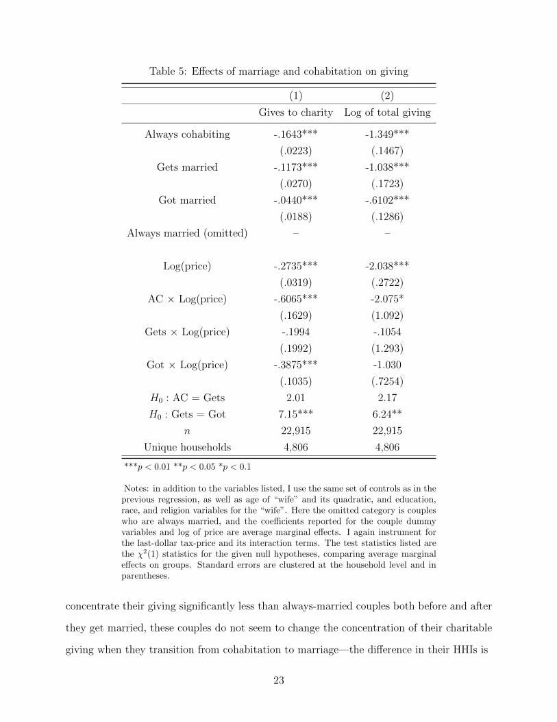
Table 5: Effects of marriage and cohabitation on giving

(1) (2)

Gives to charity Log of total giving

Always cohabiting -.1643*** -1.349***

(.0223) (.1467)

Gets married -.1173*** -1.038***

(.0270) (.1723)

Got married -.0440*** -.6102***

(.0188) (.1286)

Always married (omitted) – –

Log(price) -.2735*** -2.038***

(.0319) (.2722)

AC × Log(price) -.6065*** -2.075*

(.1629) (1.092)

Gets × Log(price) -.1994 -.1054

(.1992) (1.293)

Got × Log(price) -.3875*** -1.030

(.1035) (.7254)

H0 : AC = Gets 2.01 2.17

H0 : Gets = Got 7.15*** 6.24**

n 22,915 22,915

Unique households 4,806 4,806

***p < 0.01 **p < 0.05 *p < 0.1

Notes: in addition to the variables listed, I use the same set of controls as in theprevious regression, as well as age of “wife” and its quadratic, and education,race, and religion variables for the “wife”. Here the omitted category is coupleswho are always married, and the coefficients reported for the couple dummyvariables and log of price are average marginal effects. I again instrument forthe last-dollar tax-price and its interaction terms. The test statistics listed arethe χ2(1) statistics for the given null hypotheses, comparing average marginaleffects on groups. Standard errors are clustered at the household level and inparentheses.

concentrate their giving significantly less than always-married couples both before and after

they get married, these couples do not seem to change the concentration of their charitable

giving when they transition from cohabitation to marriage—the difference in their HHIs is

23

Table 6: Effects of marriage on giving by charity class

(1) (2) (3) (4) (5) (6) (7) (8) (9) (10) (11) (12)

HHI Rel. Youth Env. Comb. Need Health Edu. Art Neigh. Int. Other

Probability of giving

Always coh. – -.216*** -.015 .004 -.059*** -.064*** -.043*** -.024** .013 -.004 -.007 -.020***

(.185) (.010) (.012) (.014) (.015) (.013) (.010) (.010) (.005) (.006) (.007)

Gets married – -.172*** -.026** .000 -.027 -.015 -.013 -.006 .017 -.002 -.002 -.018*

(.026) (.013) (.015) (.023) (.022) (.020) (.017) (.012) (.008) (.009) (.010)

Got married – -.149*** -.033*** .011 -.016 .014 .009 -.022 -.011 -.003 -.016** -.005

(.022) (.012) (.133) (.019) (.019) (.017) (.015) (.010) (.006) (.004) (.009)

Always m. (om.) – – – – – – – – – – – –

H0 : AC = Gets – 2.4 0.6 0.1 1.6 4.0** 1.8 1.0 0.1 0.1 0.2 0.0

H0 : Gets = Got 0.8 0.2 0.5 0.3 1.7 1.1 0.7 4.8** 0.0 1.8 1.2

Amount of giving

Always coh. -.001 -1.47*** -.054 -.005 -.268*** -.323*** -.279*** -.090* .044 -.019 -.039 -.100***

(.016) (.121) (.043) (.048) (.077) (.084) (.062) (.053) (.044) (.022) (.028) (.036)

Gets married -.039* -1.29*** -.095** .000 -.143 -.106 -.073 -.029 .042 -.027 .005 -.058

(.022) (.157) (.054) (.065) (.118) (.114) (.097) (.077) (.051) (.028) (.043) (.044)

Got married -.029** -1.22*** -.159*** .015 -.084 .010 .014 -.101 -.083* -.025 -.093*** -.031

(.015) (.145) (.058) (.060) (.105) (.104) (.083) (.078) (.045) (.029) (.035) (.049)

Always m. (om.) – – – – – – – – – – – –

H0 : AC = Gets 2.3 1.0 0.4 0.0 0.9 2.8* 1.0 0.5 0.0 0.1 0.8 0.7

H0 : Gets = Got 0.2 0.2 0.9 0.1 0.2 0.9 0.7 0.7 4.8** 0.0 4.0** 0.2

n 17,117 22,915 22,915 22,915 22,915 22,915 22,915 22,915 22,915 22,915 22,915 22,915

Unique households 3,870 4,806 4,806 4,806 4,806 4,806 4,806 4,806 4,806 4,806 4,806 4,806

***p < 0.01 **p < 0.05 *p < 0.1

Notes: all regressions also include the instrumented log(price); log(income), its quadratic, and cubic; the demographic variables as in table 5; andyear fixed effects. Reported are the coefficient estimates as well as χ2(1) statistics for the given null hypothesis. The sample size and number ofunique households are smaller in the HHI regression because I restrict the sample to families who gave > $0. Standard errors clustered at thehousehold level are in parentheses.

24

not significant.

In columns 2 through 12 of table 6, I investigate how the destination of gifts is affected

by transitions from permanent cohabitation to marriage, using the probability or amount

of giving to a particular charitable class as the outcome variable in the 2SLS regression.

Compared with couples who are always married, couples who are always cohabiting are not

significantly more likely to make a gift, and their expected gift is not significantly higher

in any category. Cohabiting couples who will eventually get married give significantly more

often and more than other cohabiting couples only to need-based organizations. When these

couples get married, though they give more overall, they do not give significantly more to any

particular category (and in fact give significantly less often and less to arts and international

charities). However, these couples appear distinct from those who were always married with

regard to certain classes, as the giving of always-married couples to religious and need based

organizations is still more frequent and greater than that of couples who were cohabiting

and later got married.

5.4 Tests for different income elasticities of giving

In my analysis thus far, I have assumed that charitable giving is a household public good

and investigated the effects of intertemporal commitment on the consumption of this good.

I now consider another reason, also related to commitment, why giving might be greater

among married couples relative to permanently cohabiting households. Recall the hypothesis

that, since giving is a function of income, and married couples (because of risk-sharing and

income-pooling) are more secure than other categories of households in projecting their future

income, giving by married couples would be greater than giving by other households. If this

were the case, not only would we observe differences in probabilities and amounts of giving

by married and cohabiting people, but we would also observe different income elasticities for

the different couple groups.

This is exactly what I find. In table 7, I report the results of four 2SLS regressions.

25

Table 7: Giving explained by income and couple status

Effects of couple status and income on giving Over-time effects of marriage and income on giving

(1) (2) (3) (4)

Pr(gives) Log(giving) Pr(gives) Log(giving)

Perm. Coh. -.1704*** -1.388*** Always Coh. -.1757*** -1.481***

(.0137) (.0882) (.0227) (.1500)

1st-year coh. -.1599*** -1.248*** Gets mar. -.1158*** -1.064***

(.0186) (.1261) (.0281) (.1802)

Single -.0990*** -.9082*** Got mar. -.0516*** -.6349***

(.0082) (.0609) (.0194) (.1289)

Mar. (omitted) – – Always m. (om.) – –

Log(income) .0734*** .6660*** Log(income) .0767*** .7771***

(.0044) (.0342) (.0072) (.0579)

PC × Log(inc) -.0123 -.4026*** AC × Log(inc) -.0353** -.5917***

(.0149) (.1064) (.0171) (.1143)

1YC × Log(inc) -.0408*** -.6072*** Gets × Log(inc) .0207 -.2519

(.0118) (.0814) (.0294) (.2029)

Sing. × Log(inc) -.0208*** -.4228*** Got × Log(inc) .0657** .2645

(.0078) (.0610) (.0273) (.1818)

H0 : PC = Sing. 26.70*** 26.70*** H0 : AC × Log(inc) = Gets × Log(inc) 3.01* 2.45

H0 : PC × Log(inc) = S. × Log(inc) 0.38 0.05 H0 : Gets × Log(inc) = Got × Log(inc) 1.53 4.38**

n 41,273 41,273 n 22,915 22,915

Unique households 8,943 8,943 Unique households 4,806 4,806

***p < 0.01 **p < 0.05 *p < 0.1

Notes: in addition to the variables listed, I also include the (instrumented) log of price and its interactions with the couple/subcoupledummies; age and its quadratic; education, race, and religious preference dummy variables for the head and for the “wife” when possible;and year fixed effects. The coefficients reported for the couple and subcouple dummies and log of income are average marginal effects.Also reported are χ2(1) statistics for the given null hypotheses, comparing average marginal effects when relevant. Standard errors areclustered at the household level and in parentheses.

26

Similarly to the previous models in this paper, I estimate giving (in terms of probabilities or

amounts) as a function of the instrumented natural logarithm of price, the natural logarithm

of income, various household demographics, year fixed effects, and either couple status or

subcouple status. Now, however, I interact the income variable with the couple or subcouple

indicator variables, testing for differences in income elasticity.

Like the previous models, these results suggest that, on average, married couples are

more likely to give and give more than cohabiting and single households. Again, while

there is a tendency for cohabiting couples who eventually get married to give more than

other cohabiting couples, there is a further significant increase in their giving upon getting

married. The magnitudes of these effects are largely similar to what I have already estimated.

This model gives additional insight, however, into the mechanism by which commitment

increases giving. Namely, the coefficients on several of the interactions between couple status

or subcouple status and income are significant, indicating varying income elasticities across

groups. Following a 1% increase in income, permanently cohabiting couples and singles are

each predicted to increase their giving by about .4% less than similar married couples; this

same change in income would increase a married couple’s probability of giving by around

.07% compared with a permanently cohabiting couple’s .06% and a single household’s .05%.

Though these results are not extremely dramatic, they are statistically significant (with they

exception of the difference for permanent cohabitors on the extensive margin). Thus the data

suggest that an additional dollar earned by a married couple makes them relatively “richer”

than other kinds of households, and they are therefore able to give more often and make

larger charitable contributions.

Considering the effects of transitions from cohabitation to marriage on income elasticity

over time, I also look at regressions interacting income with subcouple status. Cohabiting

couples who eventually get married appear to respond more to a change in income than do

other cohabiting couples: a 1% increase in income is predicted to increase their probability of

giving by about .1% compared with .04%, and their amounts of giving by about .5% compared

27

with .2%. When these couples get married, they become significantly more responsive to

income on the intensive margin—their income elasticity of giving increases by about half a

percent. While there is also an increase on the extensive margin, it is not large or significant.

Together, these results suggest that, like giving itself, responsiveness of giving to income

changes with commitment; in particular, couples are more responsive as they approach

marriage, and dramatically more responsive when the binding legal commitment occurs.

Thus there is evidence that the differences between giving by married and cohabiting couples

owes in particular to the fact that giving is a function of income, and commitment allows

married couples to be more secure in projecting their income in subsequent periods.

5.5 The tax-price of giving for cohabiting couples

Finally, I use the detailed information on labor and interest income, various deductions,

and spending by each member of a two-person household provided by the PSID to briefly

investigate whether giving by cohabiting couples is influenced by the marginal tax rate faced

by both partners, or simply that of the higher earner. Using Meer and Priday’s (2020) method

described earlier, I separately estimate the (first and last-dollar) tax-price of giving for both

the head of the household and the “wife” of the household for each cohabiting couple. I then

estimate two 2SLS regressions similar to those referenced earlier in this paper, explaining

the decision to give and the size of charitable gifts with demographic variables for the head

and “wife,” household income, and the tax-price of both the primary and secondary earner

of the household (I instrument for each with the respective first-dollar price). Results are

reported in table 8, along with the first-stage regressions explaining each tax-price.

On both the extensive and intensive margins, the coefficient on each household member’s

tax-price is negative, but only the primary earner’s is significant. This is consistent with

the idea that cohabiting couples maximize the benefits they receive from charitable giving

by paying the lowest possible price—if this were the case, changes in the higher price would

not affect the couple’s giving.

28

Table 8: Effects of tax-prices on giving in cohabiting couples

(1) (2) (3) (4)

Gives to charity Log(total giving) 1st stage (pri.) 1st stage (sec.)

Log(price) pri. -.4962*** -2.865*** – –

(.1514) (.9683)

Log(price) sec. .0244 -.2571 – –

(.9683) (1.565)

Log(1st price) pri. – – .9509*** .0073

(.0215) (.0076)

Log(1st price) sec. – – .0485 .9691***

(.0333) (.0115)

***p < 0.01 **p < 0.05 *p < 0.1

Notes: in addition to the tax-price variables, I also include the natural logarithm of income and its quadraticand cubic; age and its quadratic for both head and “wife;” education, race, and religious preference dummyvariables for head and “wife”; and year fixed effects. I instrument for the last-dollar tax-price of the primaryand secondary earner with their respective first-dollar tax-prices; the results of the first stage regressionsexplaining each endogenous variable are reported in columns (3) and (4). Standard errors are clustered atthe household level.

6 Conclusion

In this paper, I investigate charitable giving by married and permanently cohabiting

couples. I find evidence that, holding other variables constant, married people both give

more and are more likely to give than cohabiting couples, particularly to religious charities.

Contrary to the few previous studies that have examined cohabitation and giving, I also find

differences between singles and permanently cohabiting couples, namely, that permanently

cohabiting couples give less than singles holding other variables constant. There is evidence

to support a causal link between the commitment mechanism of marriage and increased

giving; when people change marital or couple status over time, their giving is greatest when

they are married. This same causal link does not appear when comparing permanent co-

habiting couples and singles—that is, there is not evidence that picking up a non-marital

partner decreases one’s giving. These results appear to be closely related to the varying

responsiveness of giving to changes in income by married couples and other households.

29

In addition, I find that the giving of singles is more responsive to changes in the tax-price

than giving of married couples. While there is some evidence that permanently cohabiting

couples are more responsive than married couples to this change as well, the results are not

statistically significant in all specifications of my models. Permanently cohabiting couples

respond only to changes in the tax-price of the household’s primary earner.

These results could imply a greater motivation for governments to implement policies

that encourage legal marriage, as these may increase the private provision of the public good

that is charitable giving. For example, providing tax breaks to married couples may induce

marriage, as couples are responsive to these rates when they transition from cohabitation to

marriage (Alm and Whittington 2003). My results show that there is no significant difference

between the responsiveness of a couple’s giving to tax rates before and after marriage—and

indeed, if anything marriage makes giving less responsive to tax changes. Thus, if a perma-

nently cohabiting couple is encouraged to get married by facing a lower tax rate, that same

lower tax rate would increase their price of giving, and possibly decrease their giving by less

when they are married than it would have when they were permanently cohabiting.

Several limitations of my study leave open various avenues for further research. Though,

in preliminary analyses, I briefly consider higher bargaining costs as a cause of the lower

levels of giving by permanently cohabiting couples, my sample size is likely not large enough

to make any definitive claims on this topic. Another study with a larger sample of perma-

nently cohabiting couples and detailed information about the decision-making member of

the household could clarify this question.

Further, though I interpret many of my results as causal, it is difficult to say for certain

that the commitment mechanism of marriage induces charitable giving, since the marriage

decision is likely endogenous. Replicating my results, but using a strong instrument for

marriage or the variation of a natural experiment could solidify the evidence for such a

causal link. In particular, an examination of giving by same-sex couples who get married

shortly after the legalization of same-sex marriage could shed light on the issue, as well

30

as study the giving of same-sex couples in general—something I was unable to do as a

result of limitations of my sample. Finally, charitable giving is just a single example of a

household public good. Testing explicitly for the effects of commitment on investment in

other household public goods remains an important area for expansion of further research.

31

References

[1] Alm, James, and Leslie A. Whittington. ”Shacking up or shelling out: Income taxes,

marriage, and cohabitation.” Review of Economics of the Household 1, no. 3 (2003): 169-

186.

[2] Andreoni, James, and A. Abigail Payne. ”Charitable giving.” In Handbook of public

economics, vol. 5, pp. 1-50. Elsevier, 2013.

[3] Andreoni, James, Eleanor Brown, and Isaac Rischall. 2015. “Charitable Giving by Mar-

ried Couples: Who Decides and Why Does It Matter?” In The Economics of Philanthropy

and Fundraising. Volume 1., edited by James Andreoni, 526–48. Elgar Research Collec-

tion. International Library of Critical Writings in Economics, vol. 305. Cheltenham, UK

and Northampton, MA: Elgar.

[4] Andreoni, James. ”Impure altruism and donations to public goods: A theory of warm-

glow giving.” The economic journal 100, no. 401 (1990): 464-477.

[5] Backus, Peter G., and Nicky L. Grant. ”How sensitive is the average taxpayer to changes

in the tax-price of giving?.” International Tax and Public Finance 26, no. 2 (2019): 317-

356.

[6] Becker, Gary S. 1981. A treatise on the family. Cambridge, Mass: Harvard University

Press.

[7] Becker, Gary S. ”A Theory of Marriage: Part I.” Journal of Political Economy 81, no. 4

(1973): 813-46.

[8] Bekkers, Rene and Pamala Wiepking. 2012. ”Who Gives? A Literature Review of Pre-

dictors of Charitable Giving II – Gender, Family Composition and Income.” Voluntary

Sector Review 3 (2).

32

[9] Bergstrom, Theodore C. 1997. “A Survey of Theories of the Family.” In Handbook of

Population and Family Economics. Volume 1A, edited by Mark R. Rosenzweig and Oded

Stark, 21–79. Handbooks in Economics, vol. 14.

[10] Brooks, Arthur C. ”Income tax policy and charitable giving.” Journal of Policy Analysis

and Management 26, no. 3 (2007): 599-612.

[11] Cigno, Alessandro. “Marriage as a Commitment Device.” Review of Economics of the

Household 10, no. 2 (June 2012): 193–213.

[12] Eagle, David, Lisa A. Keister, and Jen’nan Ghazal Read. ”Household charitable giving

at the intersection of gender, marital status, and religion.” Nonprofit and Voluntary Sector

Quarterly 47, no. 1 (2018): 185-205.

[13] Feenberg, Daniel, and Elisabeth Coutts. ”An introduction to the TAXSIM model.”

Journal of Policy Analysis and management 12, no. 1 (1993): 189-194.

[14] Gemici, Ahu, and Steve Laufer. ”Marriage and cohabitation.” New York University,

mimeo (2011).

[15] Hirschman, A. 0. 1964. ”The Paternity of an Index.” American Economic Review 54

(5): 761.

[16] Iyigun, Murat. 2009. ”Marriage, Cohabitation and Commitment,” IZA Discussion Pa-

pers No. 4341. Institute for the Study of Labor (IZA), Bonn.

[17] Lam, David. 1988. “Marriage Markets and Assortative Mating with Household Public

Goods: Theoretical Results and Empirical Implications.” Journal of Human Resources 23

(4): 462–87.

[18] Kimberlin, Sara, Jiyoun Kim, and Luke Shaefer. ”An updated method for calculating

income and payroll taxes from PSID data using the NBER’s TAXSIM, for PSID survey

33

years 1999 through 2011.” Unpublished manuscript, University of Michigan. Accessed May

6 (2014): 2016.

[19] Lundberg, Shelly, and Robert A. Pollak. ”The Evolving Role of Marriage: 1950-2010.”

The Future of Children 25, no. 2 (2015): 29-50.

[20] Lundberg, Shelly, and Robert A. Pollak. 2013. “Cohabitation and the Uneven Retreat

from Marriage in the U.S., 1950-2010.”

[21] Matouschek, Niko, and Imran Rasul. 2008. “The Economics of the Marriage Contract:

Theories and Evidence.” Journal of Law and Economics 51 (1): 59–110.

[22] Meer, Jonathan, and Benjamin A. Priday. ”Tax Prices and Charitable Giving: Pro-

jected Changes in Donations under the 2017 Tax Cuts and Jobs Act.” Tax Policy and the

Economy 34, no. 1 (2020): 113-138.

[23] Weiss, Yoram. 2008. “Marriage and Divorce,” In The New Palgrave Dictionary of Eco-

nomics edited by Lawrence Blume and Steven N. Durlauf.

[24] Weiss, Yoram. 1997. “The Formation and Dissolution of Families: Why Marry? Who

Marries Whom? And What Happens upon Divorce.” In Handbook of Population and

Family Economics. Volume 1A, edited by Mark R. Rosenzweig and Oded Stark, 81–123.

Handbooks in Economics, vol. 14.

[25] Wiepking, Pamala, and Ineke Maas. ”Resources that make you generous: Effects of

social and human resources on charitable giving.” Social Forces 87, no. 4 (2009): 1973-

1995.

[26] Wilhelm, Mark O., Eleanor Brown, Patrick M. Rooney, and Richard Steinberg. 2001-

2015. The Center on Philanthropy Panel Study [machine-readable data file] / Director

and Principal Investigator, Mark O. Wilhelm; Co-Principal Investigators, Eleanor Brown,

Patrick M. Rooney, and Richard Steinberg; Sponsored by Atlantic Philanthropies. In the

34

Panel Study of Income Dynamics Wave XXXII-XXXIX [machine-readable data file] /

Director and Principal Investigator, Frank P. Stafford; Associate Director and Principal

Investigator Robert F. Schoeni; Co-Principal Investigators, Jacquelynne S. Eccles, Kather-

ine McGonagle, Wei-Jun Jean Yeung, and Robert B. Wallace. Ann Arbor: Institute for

Social Research, The University of Michigan.

[27] Wilhelm, Mark O. ”New data on charitable giving in the PSID.” Economics Letters 92,

no. 1 (2006): 26-31.

[28] Wilhelm, Mark O. ”The quality and comparability of survey data on charitable giving.”

Nonprofit and voluntary sector quarterly 36, no. 1 (2007): 65-84.

[29] Yoruk, Baris K. 2015. “Are Generous People More Likely to Vote? Tax Price Effects

of Charitable Giving on Voting Behavior.” Annals of Economics and Statistics/Annales

d’Economie et de Statistique, no. 119–120 (December): 345–73.

[30] Yoruk, Baris K. 2010. “Charitable Giving by Married Couples Revisited.” Journal of

Human Resources 45 (2): 497–516.

35