Markovianity of Trabecular Networks Dissertation

Markovianityof Trabecular Networks

Dissertation

zur Erlangung des akademischen GradesDoktor der Ingenieurwissenschaften

(Dr.-Ing.)der Technischen Fakultat

der Christian-Albrechts-Universitat zu Kiel

Wolfram Timm

Kiel

2006

1. Gutachter: Prof. Dr. G. Sommer

2. Gutachter: Prof. Dr. C.-C. Gluer

3. Gutachter: Prof. Dr. G. Pfister

Datum der mundlichen Prufung: 6. Oktober 2006

To my wife Susanne

Abstract

Clinically established methods to diagnose osteoporosis, a systemic disease with multipleimplications to the human’s well being are bound to the bone mineral density. Sinceit is well known, that the bone structure changes under osteoporosis, this thesis inves-tigates, whether structural changes represent information independent of bone mineraldensity, and whether this structural information, obtained by innovative mathematicaltechniques improves first the ability to distinguish between osteoporotic and healthy struc-tures, second the measurement of a risk to belong to the osteoporotic group, and third theprediction of a biomechanical measure, the failure load, compared to existing standardstructural measures. This in vitro study utilised mainly Micro-Computer Tomography(µ-CT) and for some proof of concept High-Resolution Computer Tomography (HRCT)to obtain digital datasets of trabecular structures. Having the aim to preserve and exploitthe complexity inherent to trabecular structures, the following methods of the theory ofMarkov processes were investigated: Markov random fields, Markov point processes, aMarkov graph based method of conditional entropy as well as Hidden Markov Models.These techniques allowed both to focus on the investigation of simpler, non-complex sub-structures and at the same time keep structural information of the whole structure byinvestigating these substructures in parallel. The study confirmed the independency ofstructural information from bone mineral density. Moreover, both a measure of clusteringbased on Markov point processes and the Markov graph based conditional entropy im-proved the discrimination of osteoporotic and healthy trabecular networks compared tostandard structural variables. Furthermore, the explanation of failure load was improvedbeyond bone mineral density by the application of entropy. Additionally, the standardisedodds ratios were higher again for the Markov graph based conditional entropy than forthe standard variables and the bone mineral density. Summarising, by building a bridgebetween natural patterns of human cancellous bone to mathematical and stochastic algo-rithms capable of modeling complex structures this in vitro study proposed a successfulway to catch the specifics of these natural patterns and to improve the current structuralanalysis methods.

Contents

1 Introduction 1

1.1 Osteoporosis: a medical perspective . . . . . . . . . . . . . . . . . . . . . . 1

1.1.1 Bone density . . . . . . . . . . . . . . . . . . . . . . . . . . . . . . 4

1.1.2 Bone quality . . . . . . . . . . . . . . . . . . . . . . . . . . . . . . . 5

1.1.3 Bone as a structure . . . . . . . . . . . . . . . . . . . . . . . . . . . 6

1.1.4 Osteoporotic changes of trabecular networks . . . . . . . . . . . . . 7

1.2 Osteoporosis: a perspective of computer science . . . . . . . . . . . . . . . 8

1.2.1 Simultaneous equality and inequality . . . . . . . . . . . . . . . . . 11

1.2.2 Information preservation . . . . . . . . . . . . . . . . . . . . . . . . 12

1.2.2.1 Loss of information by integration . . . . . . . . . . . . . 12

1.2.2.2 Information specification: Families of structures . . . . . . 12

1.2.3 Structures as realisations of stochastic processes . . . . . . . . . . . 14

1.2.4 The expected benefit of Markov-based structural characterisations . 17

1.3 Hypothesis . . . . . . . . . . . . . . . . . . . . . . . . . . . . . . . . . . . . 19

1.4 Presentation of research . . . . . . . . . . . . . . . . . . . . . . . . . . . . 19

2 Materials and Methods 21

2.1 Data set . . . . . . . . . . . . . . . . . . . . . . . . . . . . . . . . . . . . . 21

2.1.1 Study population and study groups . . . . . . . . . . . . . . . . . . 21

2.1.2 Preparation of bone specimens . . . . . . . . . . . . . . . . . . . . . 23

i

ii CONTENTS

2.1.3 Overview of study data utilisation . . . . . . . . . . . . . . . . . . . 23

2.2 Measurement procedures . . . . . . . . . . . . . . . . . . . . . . . . . . . . 23

2.2.1 High Resolution Computer Tomography (HRCT) . . . . . . . . . . 23

2.2.2 Micro-CT measurements . . . . . . . . . . . . . . . . . . . . . . . . 25

2.2.2.1 Reconstructions: High- and very high resolution . . . . . . 25

2.2.2.2 Voxel sizes in HRCT and Micro-CT . . . . . . . . . . . . . 27

2.2.3 Preprocessing: binarisation . . . . . . . . . . . . . . . . . . . . . . . 27

2.3 Standard structural variables for trabecular networks . . . . . . . . . . . . 32

2.4 Markov techniques . . . . . . . . . . . . . . . . . . . . . . . . . . . . . . . 33

2.4.1 What is the Markov property? . . . . . . . . . . . . . . . . . . . . . 34

2.4.2 Why Markov techniques? . . . . . . . . . . . . . . . . . . . . . . . . 34

2.4.2.1 Decomposition of complexity . . . . . . . . . . . . . . . . 35

2.4.2.2 Information preservation . . . . . . . . . . . . . . . . . . . 35

2.4.2.3 Regeneration of a realisation . . . . . . . . . . . . . . . . . 36

2.4.3 Markov Random Fields . . . . . . . . . . . . . . . . . . . . . . . . . 36

2.4.3.1 Introduction . . . . . . . . . . . . . . . . . . . . . . . . . 36

2.4.3.2 Topology and Markov random fields . . . . . . . . . . . . 39

2.4.4 Markov point processes . . . . . . . . . . . . . . . . . . . . . . . . . 41

2.4.4.1 Introduction . . . . . . . . . . . . . . . . . . . . . . . . . 41

2.4.4.2 Cluster Type Index and Ripley’s-K functions . . . . . . . 42

2.4.4.3 From trabecular networks to point processes . . . . . . . . 46

2.4.4.4 Trabecular Junctions as Markov point process . . . . . . . 47

2.4.4.4.1 Restriction to voxels of a local dimension of three 49

2.4.4.4.2 Opening and closing . . . . . . . . . . . . . . . . 49

2.4.4.4.3 Extraction of the Markov point process realisations 49

2.4.4.4.4 Estimation of CTI and Ripley′sK . . . . . . . . 50

2.4.5 Markov graphs . . . . . . . . . . . . . . . . . . . . . . . . . . . . . 50

CONTENTS iii

2.4.5.1 Information measures on graphs . . . . . . . . . . . . . . . 52

2.4.5.1.1 Probabilities on nodes of a DAG . . . . . . . . . 52

2.4.5.1.2 Conditional Entropy on edges of a DAG . . . . . 54

2.4.5.1.3 Nondeterminism and order: two extremes in thespace of predictability . . . . . . . . . . . . . . . 55

2.4.5.1.4 Entropy as a measure of information . . . . . . . 56

2.4.5.2 Application to trabecular networks . . . . . . . . . . . . . 56

2.4.5.2.1 Mapping the voxel space to a symbolic space . . . 58

2.4.5.2.2 Binarisation . . . . . . . . . . . . . . . . . . . . . 58

2.4.5.2.3 Decomposition by local dimension . . . . . . . . . 58

2.4.5.2.4 Removal of ambiguities . . . . . . . . . . . . . . . 59

2.4.5.2.5 Symbolic sequences of a 3D-structure . . . . . . . 59

2.4.5.2.6 Tree of transition probabilities . . . . . . . . . . . 62

2.4.6 Hidden Markov Models (HMM) . . . . . . . . . . . . . . . . . . . . 62

2.4.6.1 Introduction . . . . . . . . . . . . . . . . . . . . . . . . . 63

2.4.6.2 Three standard learning tasks of HMM . . . . . . . . . . . 64

2.4.6.3 Detection of Trabeculae by HMM - Proof of Concept . . . 64

2.4.6.3.1 Training a HMM by a HRCT measurement . . . 64

2.4.6.3.2 Bone or noise? Classification by HMM . . . . . . 65

3 Results 67

3.1 Reference variables . . . . . . . . . . . . . . . . . . . . . . . . . . . . . . . 67

3.1.1 BMD, BV/TV and AGE . . . . . . . . . . . . . . . . . . . . . . . . 68

3.1.1.1 Normal distribution property . . . . . . . . . . . . . . . . 68

3.1.1.2 Descriptive statistics of BMD, BV/TV and AGE . . . . . 68

3.1.1.3 Fracture discrimination of BMD, BV/TV and AGE . . . . 69

3.1.2 Standard structural variables . . . . . . . . . . . . . . . . . . . . . 70

3.1.2.1 Normal distribution property . . . . . . . . . . . . . . . . 71

iv CONTENTS

3.1.2.2 Descriptive statistics of TbN, TbTh and TbSp . . . . . . . 71

3.1.2.3 Fracture discrimination of TbN . . . . . . . . . . . . . . . 71

3.1.3 A combined model of the standard variables . . . . . . . . . . . . . 72

3.2 The Markovian variables . . . . . . . . . . . . . . . . . . . . . . . . . . . . 73

3.2.1 Node probabilities of a Markov graph . . . . . . . . . . . . . . . . . 73

3.2.2 Visual samples of entropy . . . . . . . . . . . . . . . . . . . . . . . 74

3.2.3 Cluster type index . . . . . . . . . . . . . . . . . . . . . . . . . . . 74

3.2.4 Ripley’s K-function . . . . . . . . . . . . . . . . . . . . . . . . . . . 78

3.2.5 Conditional entropy . . . . . . . . . . . . . . . . . . . . . . . . . . . 79

3.2.6 A mapping of Markovian vectors to a single measurement . . . . . . 80

3.2.7 Normal distribution property . . . . . . . . . . . . . . . . . . . . . 80

3.3 Standard and Markov variables combined . . . . . . . . . . . . . . . . . . . 82

3.3.1 Investigating redundancy . . . . . . . . . . . . . . . . . . . . . . . . 82

3.3.2 A combined model of standard and Markovian variables . . . . . . 83

3.3.3 Explanation of failure load . . . . . . . . . . . . . . . . . . . . . . . 83

3.4 Risk estimation by standardised odds ratios . . . . . . . . . . . . . . . . . 85

3.5 Testing for subgroups . . . . . . . . . . . . . . . . . . . . . . . . . . . . . . 86

3.5.1 Sets of two subgroups . . . . . . . . . . . . . . . . . . . . . . . . . . 87

3.5.1.1 Nominal logistic fit . . . . . . . . . . . . . . . . . . . . . . 88

3.5.1.2 t-test . . . . . . . . . . . . . . . . . . . . . . . . . . . . . 89

3.5.2 Differences of any two values . . . . . . . . . . . . . . . . . . . . . . 89

3.6 Dimensional network composition . . . . . . . . . . . . . . . . . . . . . . . 89

3.6.1 Fracture discrimination . . . . . . . . . . . . . . . . . . . . . . . . . 90

3.6.2 Correlation to structural variables . . . . . . . . . . . . . . . . . . . 90

3.7 Results in an overview . . . . . . . . . . . . . . . . . . . . . . . . . . . . . 91

3.8 HMM-based detection of trabeculae - Proof of concept . . . . . . . . . . . 91

CONTENTS v

4 Discussion 97

4.1 Relevance and method of structural analysis . . . . . . . . . . . . . . . . . 97

4.2 Catching complexity: the study hypothesis . . . . . . . . . . . . . . . . . . 98

4.3 Fracture discrimination . . . . . . . . . . . . . . . . . . . . . . . . . . . . . 98

4.3.1 Basic conditions: age and bone mineral density . . . . . . . . . . . 99

4.3.2 Standard structural variables . . . . . . . . . . . . . . . . . . . . . 99

4.3.3 Markovian variables . . . . . . . . . . . . . . . . . . . . . . . . . . 100

4.3.3.1 Node probabilities of a trabecular network . . . . . . . . . 100

4.3.3.2 Simplifying Markovian functionals to variables . . . . . . . 101

4.3.3.3 Cluster type index . . . . . . . . . . . . . . . . . . . . . . 101

4.3.3.4 Ripley’s K-function . . . . . . . . . . . . . . . . . . . . . . 103

4.3.3.5 Conditional entropy . . . . . . . . . . . . . . . . . . . . . 103

4.3.3.6 Combined models . . . . . . . . . . . . . . . . . . . . . . . 105

4.3.3.7 Risk estimation . . . . . . . . . . . . . . . . . . . . . . . . 105

4.3.3.8 Testing for subgroups . . . . . . . . . . . . . . . . . . . . 106

4.4 Explanation of failure load . . . . . . . . . . . . . . . . . . . . . . . . . . . 107

4.4.1 Reference variables . . . . . . . . . . . . . . . . . . . . . . . . . . . 107

4.4.2 Markovian variables . . . . . . . . . . . . . . . . . . . . . . . . . . 107

4.4.3 Combined models . . . . . . . . . . . . . . . . . . . . . . . . . . . . 108

4.5 Local dimension . . . . . . . . . . . . . . . . . . . . . . . . . . . . . . . . . 108

4.6 Testing redundancy . . . . . . . . . . . . . . . . . . . . . . . . . . . . . . . 109

4.7 Hidden Markov Model for noise detection . . . . . . . . . . . . . . . . . . . 109

4.8 Related studies . . . . . . . . . . . . . . . . . . . . . . . . . . . . . . . . . 110

4.9 Limitations . . . . . . . . . . . . . . . . . . . . . . . . . . . . . . . . . . . 113

4.9.1 Data acquisition . . . . . . . . . . . . . . . . . . . . . . . . . . . . . 114

4.9.2 Data analysis . . . . . . . . . . . . . . . . . . . . . . . . . . . . . . 114

4.9.3 Conceptual limitations . . . . . . . . . . . . . . . . . . . . . . . . . 114

4.10 Summary . . . . . . . . . . . . . . . . . . . . . . . . . . . . . . . . . . . . 115

vi CONTENTS

5 Future perspectives 119

5.1 Markov techniques applied to HRCT . . . . . . . . . . . . . . . . . . . . . 119

5.1.1 Do Markov techniques still work with HRCT? . . . . . . . . . . . . 120

5.1.1.1 Markov graphs on HRCT Measurements . . . . . . . . . . 120

5.1.1.2 Point process based measures applied to HRCT . . . . . . 120

5.1.1.3 Conditional entropy applied to HRCT . . . . . . . . . . . 121

5.1.2 Further application of Markov techniques . . . . . . . . . . . . . . . 122

5.1.2.1 Noise as a Markov point process . . . . . . . . . . . . . . 122

5.1.2.2 Simulating osteoporosis by Markov techniques . . . . . . . 125

5.2 Summary of outlook . . . . . . . . . . . . . . . . . . . . . . . . . . . . . . 127

References 135

Chapter 1

Introduction

Osteoporosis, a disease of bone, can be viewed from different perspectives: medicine,biomechanics, physics, computer science and more fields of research related. The medicalperspective is clearly given by the need of diagnostics and prevention of osteoporosis.The attempt to describe the changes of osteoporosis on bone by utilisation of computerscience, specifically statistical motivated pattern recognition is subject of investigationof this work. Thus, after a short introduction to the medical aspects of osteoporosis, anintroduction to characterisations of natural structures and the relationship between osteo-porosis and structural descriptions is given. Additionally, the basic idea of the statisticaltechnique of Markov processes which are central to this work is given informally. A formalintroduction to the Markov theory can be found in section 2.4.

1.1 Osteoporosis: a medical perspective

Osteoporosis is responsible for more than 1.5 million fractures per year in the UnitedStates including vertebral and non-vertebral fractures of the hip and wrist [1]. In Germanybetween four an six million people suffer from osteoporosis; this skeletal disease and itsaftereffects are one of the most frequent reasons for medical consultations [2].

Approximately 30% of postmenopausal white women in the United States have osteo-porosis, and 16% show osteoporotic characteristics at the lumbar spine in particular [3].The strength of the spinal trabecular bone declines by a factor of 4-5 from the age of 20to 80[4]. The lifetime incidence of hip fracture for a person at age 50 is 17 to 22.7 percentin women and 6 to 11 percent in men [5, 6].

Osteoporosis specifically because of resulting fractures has an impact on mortality [7],quality of life [8], and of course increases the costs of the health system [1, 9].

1

2 CHAPTER 1. INTRODUCTION

network

trabecular network

non−osteoporotic

osteoporotic trabecular

Figure 1.1: Upper row: Biopsy of a healthy vertebra showing a dense trabecular network.Lower row: Biopsy of a vertebra characterised by osteoporotic changes like a sparse, thinnedand perforated trabecular network, lowered bone volume (per total volume) and a higherportion of rod like trabeculae (red bone connections). Left column: A grey value renderingof the biopsies obtained from a human female vertebra reconstructed with a Micro-CT witha high resolution of (25µm)3 voxel size. Middle column: Topological map colour-coding thelocal dimension of each part of the network: rods (red), plate-like (green) and junction-like (blue) trabeculae build the network which is subject to change under osteoporosis.Right column: Horizontal slice through the volume showing differences in the thickness ofthe trabeculae.

Since this disease is preventable when diagnosed early enough or its progress can bedecelerated, diagnostic techniques are of major importance. Standard techniques clini-

1.1. OSTEOPOROSIS: A MEDICAL PERSPECTIVE 3

cally established determine the bone mineral density, while some of the newer techniquesinvestigate the inner structure of the bone: the trabecular network [10] (see figure 1.1).

Since osteoporosis changes not only the bone mass but also the organisation of this mass,the structure, this study investigates standard structural measures applied to osteoporoticand healthy trabecular networks and proposes the application of new techniques borrowedfrom mathematics, more precisely from the Markov theory.

The National Institutes of Health (NIH) sponsored a Consensus Development Conference,where the following statement about the definition of osteoporosis was given [11]:

Osteoporosis is defined as a skeletal disorder characterised by compromisedbone strength predisposing to an increased risk of fracture. Bone strengthreflects the integration of two main features: bone density and bone quality.Bone density is expressed as grams of mineral per area or volume and inany given individual is determined by peak bone mass and amount of boneloss. Bone quality refers to architecture, turnover, damage accumulation (e.g.,micro-fractures) and mineralisation.

According to this definition, two main aspects are important when diagnosing osteoporo-sis: Bone density and bone quality. The results from research are in agreement withthis definition: the bone fragility of osteoporosis is not fully explained by a deficit in bonemass [12]. In order to diagnose osteoporosis measures of these two aspects have beendeveloped and are still subject to investigation:

Some measures of bone integrity

• Mechanical testing (a biomechanical test method which reaches a failure load andtries to quantify stress/strain curves. Non-destructive methods using loads belowthe failure load are available, too.)

• Vibration analysis (determination of elasticity)

• Finite Element Modelling (FEM, integrity test by material properties and structure)

• Histomorphometry (gold standard for determining several aspects like two-dimensionalstructural analysis and degree of mineralisation)

• Quantitative Computed Tomography (determination of bone mineral density, firstattempts to extract structural properties in vivo)

• pQCT (high-resolution method for density and/or structural analysis)


• Micro-CT (structural analysis at the level of 10-30µm)

• Radiogrammetry (quantification of bone mineral density)

• Magnetic Resonance Imaging (structural evaluations in vivo)

• Quantitative Ultrasound (mechanical bone properties reflecting material and struc-tural properties)

• etc.

This list, which is not exhaustive, depicts some of the variety of bone measurements.Since bone integrity is determined by its density and quality, some measures combineboth aspects to some extend.

This study investigates measures which allow pure structural evaluations based on Micro-CT-generated digital models of the inner bone structure, the trabecular networks.

After discussing measures of bone density in the next section structural evaluations arethe objective of the subsequent section 1.1.2.

1.1.1 Bone density

The World Health Organisation defined osteoporosis in terms of bone density: a patient’sbone mineral density is referenced to that of a young adult’s (30 years) normal value(mean of normal population). This so called T-Score defines the degree of osteoporosisin terms of the number of standard deviations below the reference value mentioned above(see table 1.1).

T-Score Range

0 normal status-1 Osteopenia

-2.5 Osteoporosis

Fracture Osteoporosis

Table 1.1: Definition of osteoporosis according to the WHO

As outlined in the last row of table 1.1, a prevalent vertebral fracture is sufficient todiagnose osteoporosis.

Clinically established measures of bone density are [13]


• Dual Energy X-ray Absorptiometry (DXA)The basic principle of DXA is the attenuation of X-rays applied in a planar fashion.The attenuation is caused by soft tissue and bone mineral in the hard tissue. Lowdose X-rays of two different energies are used to distinguish between bone and softtissue, giving a very accurate measurement of bone density.

• QCT (Quantitative Computer Tomography)While DXA is a planar measure, QCT combines the capabilities of the three-dimensional reconstruction of the object investigated with the principle of atten-uation. Since for Quantitative Computer Tomographies a calibration phantom isused, the bone mineral density is determined directly from the phantom and thegrey values measured.

The outcome of bone densitometry measurements are always integrated scalar values,although bone is a complex organised structure.

1.1.2 Bone quality

According to the National Osteoporosis Foundation bone quality is covering the architec-ture, the bone turnover, the damage accumulation (e.g., micro-fractures) and the miner-alisation of bone.

The architecture can be viewed as the organisation of bone mass, i.e. the structural designof a trabecular network. This architecture is steadily modified in terms of breaking downand building up parts of the bone, i.e. by the bone turnover. In a healthy system, thisprocess of breaking down and building up bone by cells called osteoclasts and osteoblastsis a nearly perfectly coupled system, with one phase stimulating the other. Under Osteo-porosis (or osteopenia, which is a pre-stage of osteoporosis) these two processes becomeout of sync, the breakdown of bone eventually overtakes the build up.

While bone and thus trabecular networks are exposed to both physiological and non-physiological forces, small damages like single cracked trabeculae may occur while theoverall architecture still remains functional. These micro-cracks [14] may be repaired oradd up cumulatively while compromising bone strength up to a state where the overallstructure may be vulnerable.

The mineralisation of bone is an aspect of bone quality which deals with the amount ofcalcium and phosphor crystals embedded in the collagen structure, while the type andquality of collagen again may differ and thus impacts the quality of bone [15].

Bone quality in general is an issue of bone integrity. That is the ability of bone to with-stand those loads which defined its Gestalt. Unusual loads, i.e. loads which the bone


is not trained to withstand may lead to fractures. These fractures can be detected by aclinically established method to diagnose osteoporotic fractures and thus osteoporosis it-self: the application of semiquantitative and quantitative morphometric assessment whichallows to assess prevalent and/or incident vertebral fractures [16].

The focus of this study is on another aspect of bone quality: its bone structure andits measures. Imaging techniques applied to the assessment of trabecular bone structureinclude conventional radiography, magnification radiography, high-resolution CT (HRCT)and high-resolution MR imaging (HRMRI). The best results were obtained using high-resolution tomographic techniques [10].

Most of the studies evaluating structure analysis show that structural parameters1 andbone mineral density both predict bone strength and osteoporotic fractures, and thatcombining both techniques yields the best results in the diagnosis of osteoporosis [10].

In consequence, a new structural measure (also called structural variable) has to be provento represent information independent of bone mineral density. Statistically, tests have tobe performed which are adjusted by bone mineral density to assess the discriminativepower of the structural variables investigated.

Subsequently, bone is introduced as a structural object, which is subject to change underosteoporosis.

1.1.3 Bone as a structure

The macroscopic structure of bone can be divided into the corticalis, a thin compactosseus surface and the spongious inner part, which is surrounded by the corticalis.

Trabecular bone, also called cancellous bone or spongiosa, consists of delicate bars andsheets of bone, the trabeculae, which branch and intersect to form a sponge-like network.It is found at the end of long bones, in vertebrae and in flat bones like the pelvis.

This network built of osseus rods, plates and junctions is called trabecular network. Asdepicted in figure 1.1 and described in the next section, this structure is subject to changeunder osteoporosis. The subject of this work is to define a quantitative, comprehensivemeasure of the complex, interactive elements of the trabecular network.

1The scientific community often uses the term structural parameter to describe a measurement ofstructural characteristics. However, since formally a parameter specifies a system in terms of adjusting itby selecting a certain value for that parameter, the correct term is variable, since a measurement obtainssome quantified characteristics stored in a variable instead of adjusting a parameter. Although in thiswork the identifier structural variable is used, the user should keep in mind that most authors speakabout structural parameters.


1.1.4 Osteoporotic changes of trabecular networks

Investigations of changes of the trabecular network are done longitudinal in animal studies[17] as well as cross-sectional in human cadaver or in in-vivo biopsy studies [12].

Much of the cancellous bone deficit found in post-menopausal women with establishedosteoporosis can be attributed to loss of entire trabecular elements rather than to gener-alised thinning of trabeculae [12].

Under ovariectomy, for example, which causes a menopause with decrease of oestrogen andthus induces osteoporosis, the bone volume per total volume (BV/TV) decreases (togetherwith the bone mineral density), the separation of trabeculae increases (Tb.Sp), and thenumber of trabeculae decreases (Tb.N). Additionally, the more plate like trabeculae of ahealthy trabecular network perforate and migrate to rod like trabeculae as measured bythe Structure Model Index (SMI) [18].

Osteoporotic changes may go hand in hand with age related changes: it is known [4] thatwith age

• There is a loss of connectivity because of osteoclastic perforations of horizontalstruts

• There is an increase in anisotropy - again due to a loss of horizontal struts

• The changes in the network can lead to the slenderness ratio between vertical andhorizontal struts reaching a certain magnitude and thereby inducing buckling undercompression.

• Micro-damage and micro-fractures will occur - mainly in these very loaded verticalstruts. Micro-fractures will be repaired by micro-callus formation, and these calluseswill later be removed by the remodelling process.

• Bone material quality will slightly change, leading to a decrease in collagen contentand a relative increase in the degree of mineralisation.

Structural changes are the subject of investigation of this thesis. While numerous possi-bilities exist to quantify structural aspects (see next chapter), a key questions may be notonly to define a set of measures which are orthogonal in terms of minimal redundancy. Akey question may be the informational content a structural measure carries expressed inthe ability to recreate a similar structure based on the structural variable itself.

These and further structural aspects are discussed in the next chapter.


1.2 Osteoporosis: a perspective of computer science

Structural variables, often called structural parameters in the scientific literature, havebeen the subject of investigation for years now and are measured with many modali-ties like synchrotron Micro-Computer Tomography (Micro-CT) [19], High-Resolution CT(HRCT) [10, 20, 21, 22], Micro-Magnet Resonance Tomography (Micro-MR) [23], andHigh-Resolution-MR [24, 25].

There are many different fields of structural descriptions (see figure 1.2) which partly over-lap, and which partly provide orthogonal information to each other. Some possibilities tocharacterise a structure concentrate on specifying aspects of Gestalt, distribution, topol-ogy, (dis-)order, complexity, texture and fractal properties. Although a comprehensivecomparison of multiple structural variables available in the scientific community wouldbe of interest, the numerous possibilities make it difficult to bring all these approachestogether.

On many Micro-CT devices variables describing the Gestalt of trabecular networks aresupported by the software provided with the device. In this study, a Micro-CT fromStratec (Pforzheim, Germany) was used, which was not delivered with software for struc-tural characterisations. Hence, the author of this study created a structural evaluationsoftware which is capable of measuring the established standard variables described insection 2.3. These standard variables [26] serve as the reference structural descriptionagainst which all methods newly investigated within the context of cancellous bone arecompared to.

During the course of this chapter, some general considerations about the standard ap-proaches applied to trabecular networks are discussed which lead to the question whetherthese established measures provide comprehensive information or if they lack the poten-tial to include the central aspects important for structures exposed to mechanical forces(see section 2.3).

After discussing the standard structural variables, the different theoretical fields utilisedin this work are reviewed as far as needed to position the main hypothesis (see section1.3) in its context. Two basic methods are borrowed from statistics which are utilised inthis study: first, the probability theory interprets structures as realisation of a stochasticprocess. The Markov methods applied to these realisations are bound to the probabilitytheory, too, since the Markov property discussed in section 2.4.1 is a formulation of localprobabilities. Since the new techniques introduced are to be compared to establishedmethods, statistics again provides methods for this task. Hence, the second method is theuse of variance analysis to compare the discriminative power of the Markov approachesbetween the groups investigated. Each method provides one or more structural measures,which are random variables in theory and structural variables in practise (see figure 1.3).

1.2. OSTEOPOROSIS: A PERSPECTIVE OF COMPUTER SCIENCE 9

Gestalt

Dis

trib

utio

n Topology

Tra

be

cu

lar

me

as.

Connectivit

y

Complexity

Fra

cta

ls

Texture

Mark

ov te

chniq

ues

Hara

lick meas.

Co−occurrence

Bo

ne

vo

lum

e

Fractal dimension

Homogeneity

Anisotropy

Ord

er

Entropy

Figure 1.2: A selection of structural characterisations used in the field of structural relatedresearch of osteoporosis. The Markov techniques applied to trabecular networks are investi-gated in this study (including the entropy approach which is related to the Markov property)and compared to the established Gestalt parameters.


Random variable

processesMarkov Random

Fields

TrabecularNetworks

Probability theory

Markov Models Stochastic processes

Thesis

Realisations

Markov Graphs

Structural variable

Variance analysis

Statistics

Markov point

Figure 1.3: Statistics serves for both the incorporation of new techniques into the fieldof structural characterisation of stochastic realisations and the statistical evaluation of theability of these methods to characterise structure. The probability theory is the frameworkwhich motivates the interpretation of trabecular networks as realisations of a stochasticprocess. Markov techniques allow to model overall probabilities in terms of local charac-teristics found in trabecular networks. Additionally, quantitative measurements based onMarkov properties serve as innovative structural features for the characterisation of trabec-ular networks. These structural evaluations are called structural variables in the context oftrabecular networks and at the same time are random variables of a stochastic process (seesection 1.2.3). The discriminative power of the structural variables defined within this workis tested by statistical techniques of the variance analysis. The latter built the second armof the graph.


Figure 1.4: Two examples of realisations of natural stochastic processes showing commonconcepts while being individually different: Left: Striped patterns of zebras. Right: Humanfingerprints. Both examples look similar in a global sense but show local differences.

1.2.1 Simultaneous equality and inequality

Investigating the question what is typical of a structure, common concepts or equality is tobe formalised. When looking for the individual, on the same time subtle differences allowfor differentiation. The concepts of equality (on a coarser level) and inequality (on a finerlevel) are concurrent as can be found in biology: prominent examples are zebras (see figure1.4). The typical striped pattern is a common concept shared by all zebras, while eachindividual shows a different realisation of this pattern. This phenomenon is frequentlyobservable: a group of natural objects shares typical common aspects but differ withrespect to local characteristics. Another example is a human fingerprint. Of the millionsof fingerprints collected and compared since the onset of maintaining fingerprint files bythe FBI in 1924 till the year 1984, no two fingerprints were considered to be identical [27].The palm print is one of the most reliable physiological characteristics that distinguishesindividuals[28]. The individuality of human beings determined by genetics (and otherfactors) is in line with the individuality of the genetically determined fingerprints [29]although sharing concepts as mostly parallel lines and junctions of lines, etc. exist. Thereason for the omnipresent differences between fingerprints or, more general, skin ridgesis the number of variables modifying the structure during its development [30].

Trabecular networks as given in figure 1.1 which are in the centre of investigation inthis study, are natural examples of similar but different structures for which structuralmeasures are needed to describe them.


1.2.2 Information preservation

If an integral sums up the area under a curve, the shape of the area is not preserved underthe operation of the integral. The loss of information of a measure may lower its powerwhen conclusions are based on it. An indication of the amount of information preservedby a certain measure can be extracted from the variability of the set of structures whichleads to the same result when applied to this measure. The problem of the loss of basicstructural properties under the representation of integrative measures and the idea ofstructural regeneration of measures is discussed within the next two sections:

1.2.2.1 Loss of information by integration

Since the standard measures introduced in the previous section are integrative scoresaveraging quantifications of characteristics over the whole volume of interest, the questionmay arise, whether non-integrative aspects of structures are modelled sufficiently. Toclarify this point, see figure 1.5. In this visualisation the scenario is given that twostructures consisting of vertical trabeculae like struts are exposed to a load in verticaldirection. Although the integrative measures bone volume to total volume (BV/TV )and trabecular number (Tb.N) for the above, regular structure and the bottom, irregularstructure respond with the same value when horizontal test lines are provided, the loadapplied to the trabeculae may differ considerably. Although this is a simplified modelof structures neglecting several factors like horizontal trabeculae and non-horizontal testlines it may exemplify that the integration of characteristics over a whole volume is notsufficient to model the difference of these two structures.

A hypothesis of this work is that the main deficit of the integrative structural approachesdefined in section 2.3 above is the lack of modelling local relationships, or, in other words,the informational content of a measure increases and leads to a better discrimination be-tween the structures if local relationships are included into the measure. For example,the increased load of the middle trabeculae of the bottom structure in figure 1.5 existsas locally there are no neighbouring supportive trabeculae to the middle one. A mea-sure which would have incorporated a distance between the trabeculae would successfullydiscriminate these two simple structures.

1.2.2.2 Information specification: Families of structures

As discussed, a loss of information when applying an integrative measure to a structuremay have the consequence, that the structure is not specified well by the measure, i.e. thatdifferent structured patterns belong to the same measurement result. An ideal measurewould preserve all information necessary to reconstruct the typical characteristics from


Figure 1.5: Top: structures (white), evaluated in one direction (arrow) with the same numberof phase changes (black 7→ white, white 7→ black) and the same fraction of structure (white)versus background (black): a) regular pattern, b) irregular pattern. The standard structuralvariables principally do not take into account the differences of the regular and the irregularpattern. Thus, the regular and the irregular pattern result in the same structural values ifevaluated one dimensional. Bottom: qualitative visualisation of an estimated load appliedfrom above (and below) to the regular and irregular structure. The distance a structure haswith regard to its nearest neighbour is positively correlated with the load it has to withstand(highest load on middle, red column).


its measure. In this case, the structure is described by a measurement exactly. But astructural characterisation of a complex structure is a complex problem, since the spaceof structural measures is high-dimensional. In practise, for complex patterns structuralcharacterisations may not preserve all information contained in a structure. Nevertheless,when a high amount of information is preserved, a reconstructed structure s1 shouldshow similar structural characteristics to a second structure s2 reconstructed on the samemeasurement result with regard to some similarity measure.

Since it may be impossible to describe complex structural characteristics completely, thereis no inverse mapping from a result of a structural measurement to a unique structure;repeated inverse mappings will result in similar, but in detail different structural samples:A family of structures.

Summarising, a structural measurement describing the typical structural characteristicswill map only similar structures to almost the same result and generate only similarstructures from a specific measurement value by an appropriate method. In other words,an optimal structural measure could be described as being robust.

The concept described above supports both the partition of trabecular networks into twogroups of in each case similarly looking healthy and osteoporotic structures and the needto minimise overlaps of structural measures (see figure 1.7).

1.2.3 Structures as realisations of stochastic processes

The interpretation of natural structures as realisations of stochastic processes (and thusmembers of similarly looking structure families) is exemplified in terms of biological in-stances of structures first. As discussed in the following section this leads to a math-ematical theory which may be appropriate to model similarities expressed in terms ofprobability.

A natural structure ω ∈ Ω thus may be interpreted as realisation of a stochastical processX [31], i.e. it is drawn from the probability distribution of X. If structural characteristicsare of interest, a certain measure is evaluated over the set of realisations. Each of thesestructural measurements is indexed by a set I, thus for a sample ω of the sample space Ωwe are interested in certain features t ∈ I (or derived features like structural parametersD(t), t ∈ I) when investigating the stochastic process:

X(ω, t) : Ω × I 7→ R (1.1)

Thus, x(ω, ·) as a realisation of the stochastic process X is the object under investigationwith regard to structural characteristics t ∈ I. Here, I shares the dimension of the


ωt

.

. ωω2

.

ω1

.

m

.

random variable x( , )



ωi

tt t tj

ωi

1 2 n

jX( , t )

realisation X( ,t )1

nrealisation X( ,t )

Figure 1.6: A stochastic process given by a set of natural structures (here: slices of trabecularbone networks) organised in rows, and a set of structural variables, stored in columns,allowing to investigate the property tj (or computed/derived features of tj: D(tj)) of therealisation ωi: X(ωi, tj)

structure. Thus, for two-dimensional structures, I is two-dimensional, too, like I = IR2.Additionally, X(·, t) represents a random variable, i.e. a structural variable of X evaluatedover the set of realisations ωi (see figure 1.6).

The variability of a structural variable may lead to the situation that a group of subjectswhich is rated as pathologic is not separated well from another group which was classifiedas healthy (see figure 1.7) with regard to a certain structural characteristic. Thus, forsome subjects a structural measurement may result in a value which is shared by thepathologic and by the healthy cluster. To analyse whether there is a difference betweenthese two groups, the variance of the groups is investigated.

Thus, from a statistical point of view, the amount of variance is to be determined whichexplains the difference of a structural variable found in both groups of subjects.


a

bc

d

yes no

Figure 1.7: Two clusters in a one dimensional feature space of Bone Volume per TotalVolume (BV/TV), i.e. the feature BV/TV derived from X(·, tij) investigated is the sumof voxels tij classified as bone by thresholding (S 7→ 0, 1, S(t) = 1 iff t > threshold)divided by all voxels evaluated. Variances a and d are not explained by the structural variableBV/TV, while variances b and c are explained by BV/TV


1.2.4 The expected benefit of Markov-based structural charac-

terisations

The application of Markov techniques to the field of structural characterisations of tra-becular networks has two main advantages:

• Breakdown of complexity: A trabecular network is composed by numerous con-nections of different topological elements. Thus, multiple interactions have to bemodelled to characterise a trabecular network comprehensively instead of measuringglobal characteristics.

• Preservation of structural information: By modelling local interactions, Markovmethods allow to regenerate realisations similar to the original structure and hencecarry structural information not captured by simple standard structural measures.

A structure may show a certain degree of complexity which makes it difficult to describethis structure in a comprehensive way. One possibility to find a description which triesto catch as most features as possible is to combine simple characterisations to a vector ofobservations assigned to a structure. This spans a multidimensional space of characteri-sations, while the redundancy between the single dimensions is needed to be investigated.Although an orthogonal subspace cannot be defined since the concept of linear combi-nations of measures known from vector spaces is difficult to apply to the heterogeneousset of structural measures, one is interested in defining a comprehensive set of structuralcharacterisations while on the same time lowering the redundancy and thus the cardinalityof this set.

Instead of collecting different measures of structure to increase the comprehensiveness ofthe combined measure, Markov techniques handle complexity by not assessing a wholestructure at once, but characterising local parts of a structure in parallel. Thus, a Markovtechnique investigates a limited view of the structure multiple times and combines theresults. Since structures often can be described as repeated and modified features over aspace, the idea of looking at local features at all positions or subsets of positions at thesame time reduces the complexity of the measure to the complexity of the local feature.The parallelism of this approach ensures to capture the information typical of the structureinvestigated although the spatial range of the measure was decreased.

Modelling local interactions allows to reconstruct families of structures based on a Markov-based characterisation using a Metropolis-Hastings algorithm [32], for example. Theamount of structural information captured is appropriate to describe the structure interms of typical structural concepts shared by the family of similar structures while atthe same time allowing for small differences of the structures.


1 2 nS S ... S M1

Figure 1.8: Left: The whole structure is evaluated with respect to a certain measure S1.To increase the comprehensiveness of the measure, further measures are performed andthe results are collected to a descriptive vector < S1, . . . , Sn >. Right: The scale of theMarkov-based investigation is smaller compared to the conventional structural evaluationpresented on the left side. Due to the local range the measure itself can be evaluated at acertain position and in parallel at neighboured locations. The relationship between a Markovmeasure at a certain position and at its neighbour positions is central to the approach. Forexample, a measure detecting a black area inside usually is neighboured to a measure whichcontains a non-black region with a higher probability for a certain distance. By specifyingthe spatial relationship between black and non-black areas a powerful description for thepattern can be given which is not possible with a measure integrating over a whole structureas given on the left side. Of course, a combination of different Markov measures is possible,too.

1.3. HYPOTHESIS 19

Hence, Markov methods are expected to capture the typical properties of the stochasticrealisations given by trabecular networks of the two families of healthy and osteoporotic

samples.

1.3 Hypothesis

The considerations of this chapter are condensed into the following hypothesis:

• Within the mathematical framework of Markov-based methods certain concepts,specifically Markov point processes, Markov graphs, Hidden Markov Models andthe conditional entropy are applicable to the structural characterisation of humantrabecular networks. Thus the benefits of Markov theory, that is the breakdown ofcomplexity and the capture of essential structural information can be utilised forthe investigation of structural changes of osteoporotic networks.

• With regard to the integrative standard structural measures based on bone mineraldensity (BMD), bone volume to total volume fraction (BV/TV ) and trabecularnumber (Tb.N), the use of Markov based measures leads to

– a better explanation of the variance between the two groups of osteoporoticand healthy trabecular networks.

– an improvement of the explanation of the failure load of neighboured vertebrae.

1.4 Presentation of research

Different parts of this research were presented at several scientific congresses on an ongoingbasis:


Year Conference

2000 High Resolution imaging by a new micro-CT for the assessment of novel shape-based structural and geometrical parameters at periheral sites. W Timm,RBarkmann, R Scheffczyk, E-M Lochmuller,C Glaser, M Heller, C-C Gluer, 14thInternational Bone Densitometry Workshop, Warnemunde, in OsteoporosisInternational, Vol 11, Supplement 3, pp. s9-s10

2000 3D Assessment of Bone Structure of Whole Vertebra Bodies by a New Micro-CT. W Timm, R Barkmann, B Stampa, E M Lochmueller, M Heller, C-CGlueer, Journal of Bone and Mineral Research, Vol. 15, Suppl. 1, p. S522,ASBMR 22nd Annual Meeting

2000 Young Investigators Award, sponsored by Synarc, Project title: Classificationof Structures by Markov Random Fields: Application to Osteoporotic Bone,14th International Bone Densitometry Workshop, Warnemunde

2001 Frakturdiskriminierung durch neu entwickelte geometrische und konturbasierteStrukturparameter und ein neues Mikro-CT an Phalangen in vitro. W Timm,R Barkmann, R Scheffczyk, A Mohr, E-M Lochmuller, C Glaser, M Heller,C-C Gluer, 82. Deutscher Rontgenkongress, Wiesbaden, in RoFo, Band 173,S. s23

2002 Stochastic Modelling of Trabecular Networks. W Timm, C-C Gluer, Proceed-ings of 15th International Bone Densitometry Workshop, Monterey, CA

2002 Fracture discrimination by structural parameters is superior to bone density:an in vitro study. W. Timm, C. Sieber, F. Eckstein, E-M Lochmuller, M.Heller, C-C. Gluer,4th Baltic Bone and Cartilage, Binz, Rugen, in Acta Or-thopadica Scandinavica, Vol. 73, Supplementum 304, S. 25

2003 Vergleich der sequentiellen und sprialen hochauflosenden Computertomogra-phie zur Strukturanalyse von trabekularen Knochenstrukturen. W Timm, MHeller, C-C Gluer, 84. Deutscher Rontgenkongress, Wiesbaden, RoFo, Band175, Supplement 1, S. S262

2003 Umfassende Strukturcharakterisierung trabekularer Netzwerke durchStochastische Modellierung zur Frakturdiskriminierung. W Timm, C-CGluer, M Heller, Osteologie 2003, Gottingen, 2003, Osteologie, Band 12,Supplement 1, p. 38

2004 Degree of order determined by local conditional entropy: a new technique toassess osteoporotic changes of trabecular networks, W Timm, C.-C. Gluer,G. Sommer, Medical Imaging 2004, San Diego, CA, USA, Proceedings of theSPIE, Volume 5370, pp. 1292-1303, (Poster Award)

Chapter 2

Materials and Methods

In this chapter, first the set of study data is described. After discussing the modalitiesutilised in this study, the generation of the computerised representations of the studypopulation is given. Subsequently, the standard structural variables are given as referencemethods, followed by an introduction and discussion of the innovative Markov measuresused in this study. These are threefold: Node probabilities as well as measures of entropyare based on Markov graphs, while configuration patterns of trabecular networks are buildon Markov point processes. Finally, Hidden Markov Models were introduced to give amethod for the detection of structures.

2.1 Data set

The data set investigated in this study is subsequently described in terms of the vertebraeused, the characterisation of the osteoporotic status of the donors and the preparation ofthe bones.

2.1.1 Study population and study groups

The Anatomical Institute of the Ludwigs-Maximilians-University Munchen provided 209human vertebra T12 excised in anatomical courses. The aim was to identify two sets ofvertebra:

1. An osteoporotic group FX

2. A non-osteoporotic group Non-FX

21

22 CHAPTER 2. MATERIALS AND METHODS

Grade Deformity Height Reduction

0 no 01 mild < 20%2 medium 20% − 40%3 severe > 40%

Table 2.1: Grading of severity of fractures based on a spine radiography assessment.

Group Number Mean Age StdDev Age

FX 14 83.29 ±6.24Non-FX 25 80.68 ±7.19

All 39 81.62 ±6.9

Table 2.2: The groups of vertebra used in this study.

Every vertebra included in the finale measurement suite had to fulfil the following condi-tions

• The vertebra had to stem from a female donor (in order to exclude sexual differencesfrom the investigation and focus on structural differences).

• For the donor no disease was known for the point of time when the vertebra wasexcised.

• The vertebra itself was not fractured (although a fracture in the same spine atanother vertebra is allowed and leads to an assignment to the fracture group, seetable 2.1)

To decide whether a vertebra had to be assigned to one of these groups (or not to fit to anyof these groups), an experienced radiologist assessed radiographs taken from the donorsand graded each vertebra into one of the following groups: grade 0 (no fracture), grade 1(mild deformity), grade 2 (medium deformity), grade 3 (severe deformity). Quantitativedeformity levels are given in table 2.1.

Thus, the osteoporotic group (also called fracture group) consisted of vertebrae which werethemselves non-fractured, but stemmed from a spine which included a fractured vertebra.For a vertebra assigned to the Non-FX group (also called healthy group), all vertebrae ofthis spine were assessed fracture-free. To clearly separate the fracture from the healthygroup, all vertebrae with fracture grade 1 were excluded. The resulting groups are listedin table 2.2.

Finally, a dataset of 14 fractured vertebrae (FX group) and 25 non-fractured vertebrae(Non-FX group) was defined for the investigations of this study.

2.2. MEASUREMENT PROCEDURES 23

2.1.2 Preparation of bone specimens

Each vertebra was cut entirely from the spine through the intervertebral discs and storedin a formaldehyde atmosphere. After completion of the first whole vertebra-measurement(see section 2.2.2.1) by the µCT, all vertebrae were frozen by −18C to increase sta-bility and subsequently a cylindrical biopsy from the centre of the vertebral body wasobtained with a diamond saw. The diameter of the biopsies was 8mm while the heightwas determined by the height of the vertebral body.

2.1.3 Overview of study data utilisation

The further study data utilisation during the study can be retrieved from figure 2.1. Thedata set retrieved with a voxel side length of 156µm provided a basis for the investiga-tion of node probabilities in chapter 2.4.5.1.1. On the data set obtained with an evenhigher resolution (25µm voxel side length) the approach of local conditional entropy wasbuilt in chapter 2.4.5.1.4. For this approach a classification of each voxel into its mem-bership to one, two or three-dimensional trabecular structures was performed, describedin section 2.4.5.2.3. A restriction of the same dataset to the set of voxels classified asthree-dimensional built the data basis for the point process based measures explored inchapter 2.4.4.4.

2.2 Measurement procedures

During the last years techniques became available capable of obtaining vertebral mea-surements with a resolution showing details of the trabecular network: High ResolutionComputer Tomography provides high resolution measurements both in vitro and in vivo.However, in vitro techniques work with small objects and are conceptional capable ofproducing a better quality compared to in vivo techniques. Both techniques were used inthis study and are introduced in the following two sections.

2.2.1 High Resolution Computer Tomography (HRCT)

Since during the last years modern Computer Tomographs were installed into the clinicalroutine which are capable of measuring in vivo voxel sizes around 150µm [33], the reso-lution obtained in vivo overlaps the range of thicknesses found for trabecular networks.Although voxel sizes of below (150µm)3 are obtainable since the field of view of a re-construction can be adjusted to define smaller voxels, the possibility to reconstruct smallvoxels does not mean that the corresponding optical resolution is actually reached.


Σ Σ Σ ΣΣ

Σ

Σ

Σ

Σ

Node probabilities

on a Markov Graph

Voxel classification

by local dimension

Kdist16

Ripley’s K−function

Entropydist16

Local conditional

entropy

CLIdist16 Point Process estimations:

J−function

K−function

Biopsy

Image stack

Ma

rk

ov G

ra

ph

Micro−CT Micro−CT

Markov Point Processes

156µm voxelsize 25µm voxelsize

Image stack

1−dim 2−dim 3−dim

Cluster Index

Symbolic

representation

Σ

ΣΣ

Σ

Σ

Σ

Σ

Σ

ΣΣ Σ

Σ

Σ

Σ

Σ

Σ

Σ

Σ

Σ

Σ

Σ

Σ

ΣΣ

Σ

Σ

Σ

ΣΣΣ

Σ

ΣΣΣ

ΣΣ

ΣΣ

Σ

ΣΣ

Σ

Σ

Σ

Σ

ΣΣΣ

Σ

ΣΣ

Σ Σ Σ Σ

Σ

Figure 2.1: Flow of data and investigation during the study


The High Resolution Computer Tomography (HRCT) protocol applied in vivo to a fe-male’s patient vertebra T12 during a different study resulted in a dataset depicted infigure 2.2. The parameters used of the protocol performed on a Sensation 16 (Siemens,Erlangen, Germany) were: 120kVp, 360mAs, slice thickness of 0.3mm, voxel size of150µm× 150µm × 300µm, and a reconstruction kernel B80s using a helical scan.

Without quantification figure 2.2 depicts the main task to be solved when investigatingin vivo HRCT measurements: the differentiation of peaks induced by noise from peaksinduced by (trabecular) bone. Markov techniques utilising stochastic principles may beadequate to discriminate bone structures to be evaluated from noise structures to beneglected as introduced in section 2.4.6.1 and investigated in section 2.4.6.3 as proof ofconcept. A further possibility to handle noise as a random point process is discussed inthe outlook (section 5.1.1.2).

2.2.2 Micro-CT measurements

The facility of the micro-CT to measure objects up to 8cm diameter was exploited bymeasuring the vertebra twice: first, a high resolution reconstruction was obtained togenerate a dataset depicting the trabecular network at a coarser scale. Second, a very highresolution scan with biopsies taken from the vertebrae allowed to exhibit the trabecularnetwork at the highest level of detail available with this Micro-CT device.

2.2.2.1 Reconstructions: High- and very high resolution

The Micro-CT device FanBeam µ-Scope (Stratec, Pforzheim, Germany, see figure 2.3)were used to generate the digital datasets of the study samples. This is a desktop Com-puter Tomograph capable of measuring small specimens with diameters of up to 8cm,allowing to obtain two scales of resolution from the study sample set:

• A low resolution scan of the whole vertebra with a voxel size of 156µm. The scanof each vertebra resulted in a dataset of 512 × 512 × 400 voxels.

• A high resolution scan of a biopsy taken from the vertebra with a voxel size of25µm. From each vertebra a central biopsy of 8mm diameter and 10 mm lengthwas obtained. Scanning each biopsy resulted in a dataset of 512 x 512 x 1000isotropic voxels of 25 micrometres side length.

These measurements assigned to each voxel a continuous representation of the correspond-ing density of the biopsy. For subsequent investigations the proprietary 4 byte float format


Figure 2.2: HRCT reconstruction of a human vertebra T12. Upper half: binarisation oforiginal dataset visualised in the lower half of the larger figure. Bottom left: surface plotof the rectangular area of the grey value reconstruction. Bottom right: three-dimensionalrendering of the half vertebra shown above (processes virtually cut off). The correspondingviewing angles are depicted by the arrows.

of the Micro-CT device was transformed into a grey value range of 256 shades. Since theanalogue to digital processing of the device used 10 bits only, a 8 bit representation were


Figure 2.3: Micro-CT FanBeam µ-Scope used in the study.

estimated as appropriate to represent binary structures like bone.

All measurements were performed with a voltage of 40kV , a current of 200mA, an ex-posure period of 0.2 seconds per profile obtained, and 250 profiles per slice. A beamhardening correction was active.

2.2.2.2 Voxel sizes in HRCT and Micro-CT

Although the voxel sizes for HRCT (150µm) and Micro-CT (156µm) are comparable, thecorresponding resolution is showing a certain difference due to technical reasons: First,the HRCT protocol was obtained in vivo, which means that the vertebra of interest wassurrounded by soft tissue absorbing x-rays and modifying the x-ray spectrum. During thein vitro measurements of the Micro-CT the vertebrae investigated were excised and freefrom most of their soft tissue. Second, a clinical scanner typically scans in the time frameof a few seconds to at maximum a minute or two, while a Micro-CT device scans the sameobject in vitro in several hours. Hence, the nominal values of voxel sizes correspond todifferent corresponding resolutions.

2.2.3 Preprocessing: binarisation

A binarised representation of the trabecular architecture is used for the further investiga-tions. While the binarisation of the Micro-CT representations of the trabecular networksis performed using simple thresholding, the Hidden-Markov approach presented in chapter2.4.6 for HRCT measurements is following a different approach based on prior knowledge


Figure 2.4: Left: Scout View of a vertebra measured in the FanBeam µ-Scope. The orangebox marks the measurement range, the black box indicates where slices were evaluated.Right: Horizontal slice through the whole vertebra with a voxel size of (156µm)3 ((156µm)2

in plane and a slice distance of 156µm). The white box depicts the area delimiting theevaluation within the plane by excluding any cortical or abnormal parts of the vertebra. Therubber bands fixating the vertebra on its base plate in the micro-CT are visible around thevertebra.

2.3. STANDARD STRUCTURAL VARIABLES FOR TRABECULAR NETWORKS29

Figure 2.5: Left: Scout View of the biopsy placed on plastic tube. Right: Slice through thebiopsy. Red markers: Limiting the cylinder which was evaluated.

combined statistically with the grey values of the measurement to judge the status ofa voxel under investigation of being bone or not bone. Hence, in this subsection, thethresholding binarisation is presented only.

Although the coarser digital representation obtained with 156µm was assumed to showonly the bigger part of the trabeculae available in a human trabecular network while beingimpacted by partial volume effects, the contrast was observed as sufficient to perform asimple thresholding by selection of a threshold of 120 (the grey value range first was trans-formed to a range of 0, . . . , 255). This threshold was chosen by comparing the binarisedstructures with the original measurements while changing the threshold and optimisingthe visual equality between them (see figures 2.4 to 2.6). For the measurement obtainedwith 25µm the same threshold were found to be a valid.

All selections of the volumes of interest as well as the binarisation were performed with thein-house developed software Structural Insight written by the author of this study duringhis employment at the Medical Physics Research Group at the Department of DiagnosticRadiology of the University Hospital Schleswig-Holstein.


Figure 2.6: Top: Slice through a vertebra. Bottom: Binarisation.

Figure 2.7: Top: Slice through the biopsy of a vertebra. Bottom: Binarisation.

2.3. STANDARD STRUCTURAL VARIABLES FOR TRABECULAR NETWORKS31

Phase change

Figure 2.8: Test lines (grey) for which the phase changes (see circles in the left image)between marrow and bone as well as bone and marrow are counted are laid over the binarisedstructure (black/white). Afterwards, the parallel test lines are rotated (altogether a fewhundred rotations are taken into account) and the phase changes are computed again.After repeating the rotation - evaluation sequence, the overall phase changes are dividedby the overall length of all test lines. This gives a basic parameter which together with thebone volume fraction provides access to all standard measurements.


2.3 Standard structural variables for trabecular net-

works

Standard structural variables describe the Gestalt of the trabecular network. These areaspects of the thickness, the separation, the number of the bony connections in thisnetwork called trabeculae as well as the amount of bone found in the volume of interest.

Following, a list of these structural variables is given with their identifiers used in thescientific community:

1. The number of bone voxels divided by the number of voxels in the whole volume ofinterest (Bone Volume over Total Volume, BV/TV)

2. The mean number of trabeculae detected along different directions through thevolume of interest (Trabecular Number, Tb.N)

3. The mean thickness of trabeculae (Trabecular Thickness, Tb.Th)

4. The mean separation of trabeculae (Trabecular Separation, Tb.Sp)

5. The mean surface of bone voxels over the volume of interest (Bone Surface overTotal Volume, BS/TV)

To determine the above variables, the continuous dataset of grey values has to be binarised.Due to a sufficient contrast provided by the modality Micro-CT this is done by simplethresholding in this study. This procedure delivers the voxels classified as bone. Hence,the fraction bone volume over total volume (BV/TV) can be determined. Subsequently,the number of phase changes between bone and marrow and marrow and bone over a setof equally spaced but randomly orientated test lines (see figure 2.8) through the volumeof interest are counted. The process of choosing a random rotation α and subsequentlyadding the number of phase changes pcα is repeated N = 256 times, resulting in α1, . . . , αN

angles. Finally, for each angle αi the number of phase changes pcαiis accumulated as well

as the overall length of the test lines lαifor the angle chosen:

pc =

N∑

i=1

pcαi(2.1)

l =

N∑

i=1

lαi(2.2)

2.4. MARKOV TECHNIQUES 33

From these values, the following structural variables are determined:

Tb.N =pc

l(2.3)

Tb.Th =BV/TV

Tb.N(2.4)

Tb.Sp =1 − BV/TV

Tb.N(2.5)

BS/TV =2 ∗ Tb.N

BV/TV(2.6)

All angles αi define a three-dimensional vector through the volume of interest, i.e. αi ∈(−π

2, π

2) × (0, 2π).

From a statistical point of view, two independent variables out of the set BV/TV , Tb.N ,Tb.Sp, Tb.Th, BS/TV are sufficient to investigate this approach, since all the others canbe calculated from the two given ones. In this study, BV/TV and Tb.N are chosen.

2.4 Markov techniques

When investigating a set of structures, each structure is observed with a certain probabil-ity. The higher the number of elements building a structure and the higher the numberof possible combinations, the more difficult a calculation of the probability of a givenstructure can be.

The typical measurement procedures usually induce a grid, thus establishing a processwith discrete positions of its elements. Examples are voxels or pixels of two or three-dimensional structural images. Hence, a structure is decomposable in terms of its elementsor small groups of interacting elements, the so called cliques. Moreover, the probabilitymay be determined based on the neighbour relationships of these element groups. If twoelements are unlikely to be combined, a structure containing this combination may havea low probability to occur, too.

The decomposition of the probability into potentials based on cliques of interacting ele-ments or other local relationships is a strategy common to all Markov techniques listedin this chapter.


The three Markov techniques introduced in this chapter are related to each other in termsof building a chain of derived techniques: a Markov point process will be defined in termsof a Markov random field, and a Markov graph can be viewed as marked Markov pointprocess coding father-son-relationships.

2.4.1 What is the Markov property?

Informally, the Markov property specifies the lack of unlimited memory of a stochasticprocess. In case of a realisation of a one-dimensional process, which is a sequence Xnn≥0,we define the Markov property as following:

Definition 2.4.1 (Markov Property). Let n be a site, Xn the value of the process atthe site n and the set n− 1, n + 1 the neighbourhood of site n. If Xn is independent ofXk, k /∈ n− 1, n + 1 the underlying stochastic process generating Xn fulfils the Markovproperty1.

The approach of limited memory can be generalised to Markov fields, Markov point pro-cesses as well as Markov graphs, as shown in the subsequent sections.

2.4.2 Why Markov techniques?

When investigating which stochastic process models a (stochastic) structure best, severalaspects have to be taken into account:

• How does the technique handle complex structures, i.e. structures composed ofmultiple realisations of basic structural elements?

• Is a regeneration of a structure similar to the original one possible?

• How much information is preserved by the mapping of a structure to a parameterset of the technique chosen?

The Markov techniques introduced and summarised in the next sections all share a com-mon answer to the questions mentioned above, as explained in the following sections.

1When discussing the lack of memory of a stochastic process a formulation handling the past may bemore appropriate: P (Xn = xn|X0 = x0, . . . , Xn−1 = xn−1) = P (Xn = xn|Xn−1 = xn−1). However, thenatural ordering of time has no natural spatial analogue, thus it may be more convenient to work withthe symmetric formulation of definition 2.4.1.


Markov technique Partitioning/Factorisation Method

Markov random fields potential functions partitioning the energy functionMarkov point processes factorisation by interaction functions

Markov graph conditional probabilities for parental interactions

Table 2.3: Markov techniques and their methods of partitioning the overall probability of arealisation / configuration.

2.4.2.1 Decomposition of complexity

Complex structures can be decomposed into small subsets of structural elements which areinteracting. In detail, the probability for an overall structure to appear as a realisation ofa stochastic process is factorised in terms of these subsets, the cliques. This factorisationdecomposes the structural complexity into simple basic elements and groups of elementswhich interact with each other (see sections 2.4.3.1, 2.4.4.1 and 2.4.11). An overview ofthe partitioning concepts for the Markov techniques discussed in the next sections is givenin table 2.3.

2.4.2.2 Information preservation

When dealing with the task of generating a structure from a factorisation obtained by anoriginal structure, the parameters of the factorisation are the key to a simple estimationof the probability of a proposed realisation.

The first step to retrieve the values of parameters describing a stochastic model from agiven structure often is accomplished by the application of analytic or stochastic approx-imations of the maximum likelihood estimates of the factorisation [34]. Once, a structureis mapped to the vector of values of the model’s parameter set, the amount of informationof the structure preserved in this parameter set can be used to extract similar structures.Thus, a representation of a structure by the parameter set of the model applied can beviewed as representation of a family of similar structures.

An iterative approach to assimilate a proposed realisation to a given structure by modi-fying it step by step and subsequently measuring the increase (or decrease) of its overallprobability to occur based on the factorisation of the original structure is available bythe Metropolis-Hastings algorithm [35, 36], which was originally introduced in statisticalphysics [32, 37]:

The Metropolis-Hastings algorithm generates a discrete time Markov process [36] X0, X1, . . . ,where the transitions usually let the process (Xn)n≥0 converge to a given limit distributionP (·) but allow a temporarily decrease of the likelihood to avoid local minima:


1. A proposal Xpropi+1 for a new state is made by typically modifying, adding or deleting

(depending on the kind of the process) one element of the current structure Xi.

2. The proposal is accepted or rejected based on the likelihood of the proposed statecompared to the old one:If P (Xprop

i+1 ) ≥ P (Xi), then the proposal is accepted, since the increased likelihoodindicates that the Markov process (Xn)n≥0 converges to the limit distribution P (·).If the probability decreases, that is P (Xprop

i+1 ) < P (Xi) than the proposal is accepted

only with probabilityP (Xprop

i+1)

P (Xi)< 1.

2.4.2.3 Regeneration of a realisation

The application of the two steps summarised in the above two sections defines the inherentpower of the Markov approach: A structure can be Leander in terms of the parameters ofan underlying stochastic model. These parameters are strongly related to the factorisationof the model (by the Hammersley-Clifford theorem, see section 2.4.4.1), which enables anon-complex access to the overall probability of complex structures. Examples of theapplication of the Metropolis-Hastings algorithm on a parameter set of a given structurelearned can be viewed in [34] and, reproduced, in section 2.4.3.2.

A simple visualisation of the learning and reproduction techniques of Markov point pro-cesses is given in figure 2.9. The two point processes show similar characteristics: thevarying trend of the number of points per area along the vertical direction and the con-stant number of points per area along the horizontal direction. The second lower pointprocess is a Metropolis-Hastings based realisation of the first point process.

2.4.3 Markov Random Fields

The first technique taken from the set of Markov processes is the Markov random field,which was the first approach investigated in this work and serves as a generalisation ofthe Markov point processes introduced later on.

2.4.3.1 Introduction

In case the sites s ∈ S of a random process are arranged as a grid, the correspondingrandom variable can be interpreted as Markov random field, based on a neighbourhoodsystem:

Definition 2.4.2 (Neighbourhood system). A neighbourhood system on the set ofsites S is a family Nss∈S such that for all s ∈ S,


XX

2

Generation ofHastings:

new realisation

Metropolis−

Stochastic process

Realisation

estimationParameter

X

Tren

d

Figure 2.9: Top: a Poisson point process with a varying number of points per unit-area(intensity). Mid: trend of the intensity fitted to the Poisson process. Bottom: a Metropolis-Hastings generated point process showing a new realisation which is different but shows asimilar pattern compared to the original process (top figure).


1. s /∈ Ns

2. t ∈ Ns ⇒ s ∈ Nt

This definition states, that the interactions or neighbourhood relations of a Markov ran-dom field are bidirectional. The integration of the Markov property is done by the fol-lowing definition:

Definition 2.4.3 (Markov random field). Let ∆ be a set of possible values a config-uration x can take at site s ∈ S. Given the configuration space x ∈ ∆S, a configurationis given by x = (x(s), s ∈ S). For a neighbourhood system N and for all sites s ∈ S

P (X(s) = x(s)|X(S\s) = x(S\s)) = P (X(s) = x(s)|X(Ns) = x(Ns)) (2.7)

In other words, the dependence of a site s ∈ S is restricted to and sufficiently describedby the members of its neighbourhood Ns. The notation of the probability distribution ofa Markov random field recruited from physics is given by

P (x) =1

Ze−

1

Tε(x) (2.8)

with Z called partition function [38] and ε(x) named as energy of the configuration x. Apossibility to partition the energy function is given by the introduction of cliques [39]. Thisdecomposition of the neighbourhood allows to compute the probability of the realisationa Markov random field has (see figure 2.10):

Definition 2.4.4 (Clique). A singleton s ∈ S is a clique. A subset C ⊂ S with |C| > 1is called a clique of the graph (S, N) if and only if any two distinct sites si, sj ∈ C, i 6= jare mutual neighbours.

To derive the energy function ε(x) in terms of cliques, the following definition is given:

Definition 2.4.5 (Potential function). A set of potential functions VC , C ⊂ S isdefined as

1. VC = 0 if C is not a clique

2. for all x,x′ ∈ ∆S and all C ⊂ S,(x(C) = x′(C)) ⇒ (VC(x) = VC(x′)),

with x(C) is the restriction of the configuration x to the subset of sites C ⊂ S.


cliques

Neighbourhood

Singleton

Figure 2.10: Cliques (up to a rotation) with respect to a given neighbourhood

.

This allows to determine the energy function of the Markov random field in terms ofpotential functions of the cliques with respect to the neighbourhood system [35]:

ε(x) =∑

C

VC(x) (2.9)

(A remaining problem is the estimation of the partition function Z.)

2.4.3.2 Topology and Markov random fields

Markov random fields are used to extract the typical interaction for a texture and subse-quently generate a new but similar structure based on the interaction between the pixels.Pairwise interactions were used in figures 2.11 and 2.13 (taken from [34]) to model spatialdependence between pixels.

The nature of the textures in figures 2.11 and 2.13 seems to be reproduced adequatelyin the corresponding right textures 2.12 and 2.14. In contrast, figures 2.15 and 2.17show textures with topological elements. Comparing these original textures with thereproduced ones (figures 2.16 and 2.18), the topological characteristics seem to be notcatched in the pairwise interactions and thus did not show up in the regeneration of thetextures.


Figure 2.11:Texture withgrainy char-acter

Figure 2.12:Gibbs realisa-tion of figure2.11

Figure 2.13:Texture withcoarse grainycharacter

Figure 2.14:Gibbs realisa-tion of figure2.13

Figure 2.15:Regular tex-ture showingtopologicalconcepts.

Figure 2.16:Gibbs realisa-tion of figure2.15 with dif-ferent topo-logical con-cepts

Figure 2.17:Irregular tex-ture showingtopologicalconcepts.

Figure 2.18:Gibbs realisa-tion of figure2.17 with dif-ferent topo-logical con-cepts

All figures 2.11-2.18 taken from [34]

Since this work is investigating structures for which topological elements are typical,there are (at least) two possibilities: the first is to choose a model which does capturethe topological character of the texture to be learned, the second is a restriction of thetextural elements to a subset the model is able to store, like junctions of lines or originsof lines and their direction.

The first approach is introduced in section 2.4.5 (especially in section 2.4.5.1.2), while thesecond strategy is presented in the following section.


Figure 2.19: A Markov point process as (sparse) Markov random field.

2.4.4 Markov point processes


A Markov point process can be derived from the definition of Markov random fields [35].This is achieved by restricting (at first)2 the set of possible values ∆ at a site s ∈ S to theset 0, 1 (see figure 2.19). The neighbourhood system of a Markov point process is notany longer bound to the underlying grid, although discrete measurement spaces usuallyinduce a grid on which the sites are arranged. The direct neighbourhood relations arereplaced by distances in a metric space [36].

As in the case of Markov random fields, the overall probability distribution can be fac-torised: for a probability distribution on ∆S = 0, 1S there exists a function φ : 0, 1S →(0, 1] such that

P (x) =∏

cliques y⊂x

φ(y) (2.10)

and(φ(y) < 1) ⇒ ((s, t ∈ x ⇒ s ∈ Nt) ∨ y = ∅) (2.11)

which is a rephrasing of the Hammersley-Clifford theorem [36, 41]. An example of apairwise interaction process with φ : S×S → (0, 1] (realised as γ(·, ·) modelling interactionof cliques with two elements) is

2When more information than the state s ∈ 0, 1 has to be stored to model the underlying stochasticprocess appropriately, marked point processes allow to do this. By extension of the dimension of a pointprocess they were shown to be equivalent to non-marked point processes [36, 40].


P (x) = α∏

xi∈x

β(x)∏

xj ,xk∈x:xj xk

γ(xj , xk) (2.12)

(with α being a normalisation constant and β(x) is the intensity function). In order tomodel a point process consisting of discs of radius r not being allowed to overlap, theinteraction function

γ(xj , xk) =

1 if ||xj − xk|| > 2r0 otherwise

(2.13)

models this process. Another example would be given by setting γ ≡ 1 yielding a Poissonprocess.

The Hammersley-Clifford theorem can be used to design new Markov point processes:instead of defining a joint density P (x) for all point patterns x, it is sufficient to definethe interaction functions φ(·). The combination of interaction functions in formula 2.10in terms of multiplications can be interpreted as AND-relation: a single zero interactionwill decrease the overall probability to zero.

2.4.4.2 Cluster Type Index and Ripley’s-K functions

To facilitate the investigation and utilisation of structural characterisations assumed to beapplicable to natural structures like trabecular networks, known point process measuresare introduced and described in the following section. Their applicability is investigatedin chapter 2.4.4.4.

A Palm distribution builds the basis for the first point process measure investigated inthis work: the nearest-neighbour distance distribution function. This function representsthe probability that the point process X places at least one point within distance r of agiven point y:

Definition 2.4.6 (nearest-neighbour distance distribution function).

G(r) = Py( d(y, Xy) ≤ r), r ≥ 0 (2.14)

with d : IR2 → IR is the euclidian distance, and r ∈ IR is the distance argument of thenearest-neighbour function.

Since the number of points of the realisation N(X) is assumed to be non-zero, and thedistance is estimated from a representative point y (which implies stationarity of the un-derlying stochastic process), the Palm distribution Py(·) can be interpreted as conditionaldistribution and does not depend on the choice of y.


Replacing the palm distribution in 2.14 by the distribution of the Markov point processX, the empty space function is yielded:

Definition 2.4.7 (empty space function).

F (r) = P ( d(y, Xy) ≤ r), r ≥ 0 (2.15)

Hence, by exchanging the Palm distribution Py(·) by P·(·) (which is the normal probabilityP (·)) the set of sites taken as basis for the estimation of the nearest neighbour is extendedfrom the set of points s ∈ ∆S|s ∈ X to the set of all sites s ∈ ∆S of the point process.Thus, F (·) is the distribution function of the distance from an arbitrary point y ∈ ∆S

to the nearest point of the process. Again, the definition of F(r) does not depend on thechoice of y.

These two structural measures, F and G, can be combined to a single measure indicat-ing the tendency of a point process to build clusters or to build more regular patternsalternatively [36]:

Definition 2.4.8 (Cluster Type Index / J-function).

CTI(r) := J(r) =1 − G(r)

1 − F (r), F (r) < 1 (2.16)

with r ∈ IR is the distance argument of the cluster type index.

While in the scientific community the identifier J-Function has been established, the nameCluster Type Index is used during this work to make clear, what purpose this functionhas.

A limitation of the nearest neighbour function G is that by definition it uses only thenearest distance to a neighbour available. Hence, it considers only the shortest scalesof variation. An alternative when investigating the change of number of points withrespect to an increase of the area under observation is Ripley’s K-function, which is calledreduced second moment function alternatively [42, 43, 44, 45, 46, 47]. This characterisationprovides an estimate of spatial dependence over a wider range of scales compared to theG-function. The application of the K-function requires a point process which is isotropic.

Definition 2.4.9 (Ripley’s K-function). Ripley′sK-function of a stationary point pro-cess X is defined so that λK(r) equals the expected number of additional random pointswithin a distance r of a typical random point of X. Here λ is the intensity of the process,i.e. the expected number of points of X per unit area.


0 2 4 6

0.0

0.2

0.4

0.6

0.8

1.0

r

J(r)

pp

Distance

CTI−function

Figure 2.20: A Matern II cluster process (window size 100 × 100) and its CTI-functiondropping below 1.0 and thus indicating clustering. The dotted line represents a referencePoisson process.


0 2 4 6

12

34

5

r

J(r)

swedishpines

CTI−function

Distance

Figure 2.21: Swedish pine point process (window size 100×100) obtained from the Spatstatlibrary and its CTI-function indicating a more regular pattern (inhibitance between thepoints/pines). The dotted line represents a reference Poisson process.


Function Poisson point process reference value

F -function F (r) = 1 − exp(−λ ∗ π ∗ r2)G-function G(r) = 1 − exp(−λ ∗ π ∗ r2)

CTI-function CTI(r) := J(r) = 1Ripley′sK-function K(r) = πr2

Table 2.4: Structural variables of point processes with intensity λ and their reference valuesfor Poisson point processes showing complete spatial randomness (CSR). Complete spatialrandomness induces the equality of F and G: F (r) = G(r) ∀r ∈ IR>0

An estimate of K derived from a spatial point pattern dataset is useful in exploratorydata analysis and formal inference about the pattern [48, 49, 50]. In exploratory analyses,the estimate of K is a useful statistic summarising aspects of inter-point “dependence”and “clustering”. For inferential purposes, the estimate of K is usually compared to thetrue value of K for a completely random (Poisson) point process, which is K(r) = π ∗ r2.Deviations between the empirical and theoretical K curves may suggest spatial clusteringor spatial regularity.

The expected number of additional random points within a distance r of a random pointequals to λK(r). Here lambda is the intensity of the process, i.e. the expected number ofpoints per unit area. The K function is determined by the second order moment propertiesof X.

2.4.4.3 From trabecular networks to point processes

Trabecular networks are structures build of multiple bony connections (see figure 2.22,left). These connections, the trabeculae, can be classified to three discrete states: one-dimensional trabecular rods, two- dimensional trabecular plates and three-dimensionaltrabecular junctions. A network constructed only by one-dimensional trabeculae of three-dimensional junctions can be described easily with the tools of graph theory, namely anadjacency matrix. A network which shows two-dimensional, plate like structures is moredifficult to describe. Under the hypothesis, that the number of elements connecting oneor two-dimensional trabeculae may be of importance to the stability of the trabecular net-work, the investigation of these three-dimensional elements, the junctions, may be helpfulfor estimating the trabecular network’s integrity. Without quantifying the relationshipbetween the number of junctions between trabeculae and the stability of the network, it isobvious, that a set of unconnected trabeculae does not resist any force applied to it, whilethe same set of trabeculae connected by junctions shows increased stability. Junctionsconnecting trabeculae allow forces to interact, hence, the distribution of junctions mayplay an important role, too.


Figure 2.22: Left: Trabecular network as obtained as dataset from micro-CT.Middle:Classification of each voxel to its membership to a rod-like (red), plate-like (green)or junction-type (blue) trabeculae. Right: Restriction to junctions coded blue. All: Verticalprojections through whole bone volume.

The hypothesis of this approach is based on the assumption that a relationship between thenumber and position of junctions and the integrity of the whole network exists: Structuralmeasures which characterise the number and position of junctions with respect to eachother are able to discriminate osteoporotic and healthy trabecular networks.

Having all junctions extracted from the trabecular network, a technique is needed tocharacterise the distribution of these connecting elements in order to find meaningfulmeasures which can describe osteoporotic changes of trabecular networks.

Since the theory of point processes deals with multiple structures placed in a n-dimensionalspace, this framework can be utilised to describe distributions of junctions within the bone.Although the distribution of junctions is given in a three-dimensional space, we use twodimensional point process techniques in order to limit complexity of the problem andutilise fast, available estimation techniques for point processes [51].

2.4.4.4 Trabecular Junctions as Markov point process

The Micro-CT measurements used for this approach are described in section 2.2.2: thevery high resolution dataset with a voxel size of (25µm)3 was used in binarised represen-tation.

For each volume data set of a vertebra a certain sequence of steps generated a model ofthe bone structure, a projection onto the subset of trabecular junctions (i.e. the voxel setclassified as three-dimensional) and subsequently a set of point processes representing thecentres of the trabecular junctions within horizontal planes (see figure 2.23):

1. Binarisation to extract bone voxels


a)

e)d)

c)b)

Figure 2.23: From a high resolution scan of a continuous network to a set of point processrealisations and related measures: a) binarised volume, b) voxel set classified into one, twoand three-dimensional types, c) projection to 3D elements, d) opening of the dataset toexclude small groups of voxels not belonging to a junction, e) fitted ellipsoids mark thelocations of junctions and thus form a (marked) point process, from which measures likeJ and K-functions can be calculated. A stack of slice based realisations is retrieved byrepeating b)-e) for different slices.


2. Calculation of the local dimension of each voxel

3. Restriction to voxel subset with assigned local dimension of three

4. Morphologically opening and closing the data set

5. Extracting two dimensional realisations of the point process given in 11 equidistantlyspaced horizontal planes

6. Estimation of the point process measures F , G, CTI, and K

7. Calculation of the mean of CTI, and Ripley′sK over the slices extracted for allrealisations of a vertebra

The binarisation, the selection of 3D-typed voxels, the opening and closing of the dataset as well as the extraction and subsequent superposition of realisations of the pointprocess were performed using the software ImageJ (National Institutes of Health (NIH),Maryland, USA). The calculation of the local dimension of each voxel was done by in-house developed software tools, written by the author of this study, while the estimation ofthe characterising functions F , G, CTIand Ripley′sK was achieved by using the spatstat-package of A. Baddeley [51] under the statistical software system R [52].

Since the binarisation and calculation of the local dimension are already described insection 2.1, the steps performed subsequently are discussed in the following subsections:

2.4.4.4.1 Restriction to voxels of a local dimension of three After classifyingthe voxel space into the types 0 (no bone), 1 (rod like, one-dimensional structure), 2(plate like, two-dimensional structure), and 3 (junction type) a simple threshold of t > 2allowed to extract the junctions of the three-dimensional network (see figure 2.23 b,c).The calculation of the local dimension is described in section 2.4.5.2.3.

2.4.4.4.2 Opening and closing A morphological opening and closing of the set ofvoxels of type 3 allowed to eliminate voxels which were found at the curved margins oftrabeculae and thus were correctly classified as type 3 but did not belong to a junction.Since only margins of trabeculae showed such voxels, they were sorted out by performingan opening and closing of the dataset (see figure 2.23d).

2.4.4.4.3 Extraction of the Markov point process realisations A point processrealisation from the binary slice pattern (see figure 2.23c) is obtained by fitting ellipses toeach continuous pattern found in the slice extracted. The pattern of ellipses represents amarked point process. Finally, the centres of the ellipses are used as points.


A sequence of eleven point processes were extracted equidistantly from the stack of voxelsrestricted to three-dimensional junctions. Since the stack of voxels had a height of 10 mm,the distance between the eleven slices generating the eleven point processes were 1 mm.For the case that a biopsy was not measured exactly vertically adjusted, a potential slopeof the axis of the biopsy will not have an impact on the result if the point measures J andK are computed from each point process realisation and subsequently averaged instead ofsuper positioning the realisations and subsequently calculating the point process measuresfrom the super positioned point process.

2.4.4.4.4 Estimation of CTI and Ripley′sK The statistical software system R wasused together with the package spatstat in order to map the realisations of point pro-cesses obtained by and exported from ImageJ to estimates of the distributions CTI, andRipley′sK by the R/spatstat-functions Jest (J estimator)3 and Kest (K estimator) [51].

2.4.5 Markov graphs

While Markov random fields are based on predefined, local neighbourhoods, and sparseMarkov random fields defined as Markov point processes use local neighbourhoods witha coarser scale, Markov graphs are able to specify neighbourhoods completely uncoupledfrom metrics: two nodes are neighbours if they are connected by an edge, independent oftheir distance with regard to any metrics.

Definition 2.4.10 (Markov graph, Part 1). A Markov graph consists of

• an undirected Graph G = (V, E), where each vertex v ∈ V represents a randomvariable in X and each edge u, v ∈ E represents a dependency between the randomvariables u and v,

• a set of potential functions φk, one fore each clique k in G. Each potential functionφk is a mapping from possible joint assignments to non-negative real numbers.

The joint distribution of the Markov graph is defined by:

P (X = x) =1

Z

∏

k

φk(xk) (2.17)

where xk is the state of the random variables in the kth clique, and the normalizationconstant (or partition function) Z, where

3The Cluster Type Index CTI was defined as point process function J


Z =∑

x∈X

∏

k

φk(xk). (2.18)

Every node v in a Markov graph is conditionally independent of any other node w, whichis not connected by an edge to v, i.e. v, w /∈ E.

Practically, the partition function Z is difficult to calculate. But there is a special caseof Markov graphs, for which the calculation of the joint distribution simplyfies: Directed,acyclic graphs. In this study we were interested in neighbourhoods starting from a certainpoint in the voxel space and subsequently increasing the distance from this starting point.Looking at two points xi, xj ∈ X neighboured in the voxel space X, the pair (xi, xj) wereadded to the Markov graph if it fulfils dist(xj , s) > dist(xi, s) with s is the graph’s root,otherwise the pair (xj, xi) were added. Hence, the Markov graph constructed consists ofpairs of points in the voxel space which lead away from the graph’s root s.

Definition 2.4.11 (Markov graph, Part 2). In the special case the Markov graph G isa directed acyclic graph (DAG), each clique represents a single directed conditional depen-dency. More precisely, the factorisation of the overall probability simplifies to conditionalprobabilities given by the node relationships:

P (x) =∏

v∈V

P (xv|xpa(v)) (2.19)

for each node v ∈ V and the set of parents pa(v), which is the set of all nodes w whichshow a directed edge to v. P (xv|xpa(v)) is the probability of xv, given that the parents ofv and their values are known. The joint distribution thus requires as numerical input theconditional distribution of each node for any given configuration of its parents.

Hence, the overall probability of a realisation of a Markov graph can be factorised [53]similar to the Markov random fields and Markov point processes.

This approach allowed to define a topological object representing the typical behaviourof a structure with regard to their neighbourhood. In other words, Markov graphs wereexploited to model transition probabilities from a typical point of the structure swarmingin all directions. Having an anisotropic structure, these transition probabilities wouldreflect this anisotropy with regard to its direction. Moreover, the directed relationshipsimplicate the graph being acyclic and directed, which simplifies the computation of itsprobability, as shown in the next section.


2.4.5.1 Information measures on graphs

For both approaches presented here, a Directed Acyclic Graph (DAG) is assumed. Inconsequence, some simplifications can be used, e.g. the reduction from observing cliquesof nodes to observing simple father-son-relationships between nodes, coded as transitionprobabilities.

After coding structural characteristics of a given stochastic realisation as a Markov graphrepresenting transition probabilities of the original structure, the question is how to makeuse of this graph. The most direct possibility of investigating this graph is to investigatethe transition probabilities itself. For example, for two groups of structures which have tobe discriminated, a subset of all transition probabilities may differ between these groups.The aim is to identify this subset to obtain a measure which successfully discriminatesthe two groups of structures.

A more comprehensive measure is that of investigating the degree of determinism inherentto the graph and thus to the structure. In other words, a structure which is mostly ofrandom nature should show less determinism than a regular structure.

In this work the degree of determinism or randomness is investigated in terms of measuringinformation. Although a structure is, once measured and given as a dataset, static it isof interest to observe the step of extension when a structure is known partly and thenenlarged. The extension of a known part to an unknown, expanded graph introducesa dynamic moment and thus allows to apply techniques taken from information theorywhich deal typically with sequences representing a timely dimension.

In the following sections, the mathematical background of both approaches will be pre-sented:

2.4.5.1.1 Probabilities on nodes of a DAG For a given binary texture, a possibil-ity to characterise this structure is to store the structure into a (directed acyclic) graph byassigning a grey value to the nodes and voxel neighbourhoods to the edges while ensuringthat the edges are always directed away from the origin4. The edges simply represent therectangular grid of a voxel space (see two-dimensional example in figure 2.24).

For a given set of random positions rk,l ∈ S inside the binary structure S which are non-zero, that is I(rk,l) > 0 with I is the grey value function, at each random origin rk,l ∈ Sthe surrounding substructure is added to the graph. Hence, each random position knownto be non-zero builds the origin for which each node in the graph relative to this originstores the probability to find a voxel which is non-zero with respect to the random origin:

4The directness of edges actually is needed for the second approach measuring entropy, not necessarilyin the first approach investigating grey value probabilities, but is introduced in terms of consistency.


Pixel representing a node of the graphand a probability to be set at the same time

Transition between nodes (edge)

Origin

Figure 2.24: When several binary subimages are integrated with respect to different randomlychosen origins, the resulting directed acyclic graph represents grey value probabilities anddirected neighbourhoods


For a given set of random origins |rk,l ∈ S|I(rk,l) 6= 0| = n with cardinality n, theprobability of finding a non-zero voxel at a relative position rk,l + xi,j is defined as:

P (I(xi,j)|I(x0,0) = 1) :=1

n

∑

rk,l∈S,I(rk,l)=1,

I(xi,j + rk,l) (2.20)

By definition, for anisotropic structures, e.g. textures which show mainly vertical sub-structures, the probability of nodes in the vertical direction should be higher than that ofnodes in the horizontal direction. For isotropic structures the probabilities in these twodirections should assimilate to each other.

The graph utilised here modelled a three dimensional grid of 11 × 11 × 11. The size of avoxel was (156µm)3. It has been taken into account, that the number of voxels is growingwith x3 for a three dimensional volume. Hence, the corresponding neighbourhood had avolume of ca. 1.7mm3. Connections existed to the direct six neighbours. The size of theneighbourhood chosen was a trade off between a volume to be maximised and the numberof nodes to be limited in terms of avoiding complexity.

Each vertebral data set was binarised as described in section 2.2.3. For each vertebra aset of 50 random positions was identified for which the corresponding voxel was insidethe binary structure S

∣

∣

s∈S|I(s)6=0 . In other words, the centres of the local volumes wereset into the bone phase of the measurement, not the marrow phase. For each randomorigin, a neighbourhood graph starting at this origin was determined coding the voxelneighbourhoods inside the bone phase. All 50 resulting neighbourhood graphs were thenintegrated by overlaying them with respect to their origins. At each node at a certainposition of the resulting graph a mean probability were obtained by dividing the numberof nodes in the local graphs found at this position by the number of graphs investigated,which was 50 in this investigation.

To evaluate whether there existed nodes showing probabilities typical of the FX group orthe Non-FX group, each node’s probability was subject to investigation. This resulted in11×11×11 = 1, 331 different variables potentially reflecting a difference between the twosample groups.

2.4.5.1.2 Conditional Entropy on edges of a DAG Mathematical theories ofcommunication were introduced to describe the procedure of transmitting data in the firstquarter of the 20th century [54, 55, 56, 57]. The aim was the definition of a measure forthe syntactic content of information. The concept of information describes the reductionof uncertainty due to a message c ∈ An received, based on existing knowledge about thesource of messages observed. A message is a series of letters c = (c1, . . . , cn) built froman alphabet A.


The basic idea is to ask whether a given structure (c1, ..., cn), consisting of letters ci ofan alphabet A gives some hint for the extension (cn+1, cn+2, ...) of this sequence, or if thisextension is independent of the prefix (c1, ..., cn).

2.4.5.1.3 Nondeterminism and order: two extremes in the space of pre-dictability A system which shows nondeterministic characteristics can be assigned toa state between the two extremes of a random or an ordered system. Now two sim-ple examples of these two extremes are given: the first one consists of a purely randomstructure, where each subsequence is independent from its prefix, the one-dimensionalBernoulli sequence (see figure 2.25):

Example 2.4.1 (Bernoulli sequence).Each letter ci of the sequence (c1, ..., cn) is drawn independently with regard to certainprobability distributions p(c1), ..., p(cn) and subsequently concatenated to each other. Forexample the sequence 010101110010100101 is an example for such a Bernoulli sequence.The probability for a letter ck+1 as an extension of the sequence (c1, . . . , ck) is given bythe equation

p(ck+1|(c1, . . . , ck)) = p(ck+1) (2.21)

Hence, the knowledge of the prefix (c1, . . . , ck) does not reduce the uncertainty about theletter ck+1 to follow. The information gained is maximal at each step for this system.

The second example is the opposite of a random structure:

Example 2.4.2 (Deterministic sequence).A completely ordered, periodic sequence of letters (c1, ..., cn) with the condition ci =cj , j = i + t for some fixed period length t is given. A trivial example with a periodof t = 3 is abcabcabc... (see figure 2.25). Within this sequence, all future extensionsof a prefix are determined, if at least three letters are known: from any subsequence(ci, ci+1, ci+1) ∈ A3 the letter ci+3 is known as letter ci with probability

p(ci+3 = ci|(ci, ci+1, ci+2)) = 1 . (2.22)

Thus, the knowledge of the prefix (ci, ci+1, ci+2) does completely reduce any uncertaintyabout the suffix ci+3. Since no uncertainty exists after a period was observed, the amountof information gained is zero for this system.


This conditional probability can be interpreted as the degree of predictability of an ex-tension of a known structure. To extend this predictability to the conditional entropyas a measure of uncertainty of extension, the term entropy is introduced now within thecontext of symbolic sequences.

2.4.5.1.4 Entropy as a measure of information Based on a set of structures ofdifferent sizes, for example sequences of symbolic elements, a probability density can bedefined. Furthermore, a measure of information of these substructures can be definedbased on this probability density. In fact, the block entropy, which can be interpreted asmean uncertainty for a set of sequences (strings) c ∈ An of length n of an alphabet A withλ elements is defined as a functional H of p [40]:

Hn = −∑

(c1,...,cn)∈An

p(c1, ..., cn) logλ p(c1, ..., cn) (2.23)

To extend this approach to the problem of measuring the informational gain when ex-tending a given sequence of length n by one element, we use the definition of conditionalentropy [40]:

Hn+1|n =∑

(c1,...,cn)∈An

p(c1, ..., cn) ×

× −∑

cn∈A

p(cn+1|c1, ..., cn) logλ p(cn+1|c1, ..., cn) (2.24)

The gain of information obtained by the extension of a sequence by one element calcu-lated using equation 2.24 can be used to determine the existence of relationships betweensubparts of a structure since the range of correlations determines the characteristic typeof informational gain over several steps (see figure 2.25).

2.4.5.2 Application to trabecular networks

While the evaluation of node probabilities can be directly applied to binarised trabec-ular networks as described in section 2.4.5.1.1, the application of the concept of localconditional entropy required some preparatory steps: The continuous space of densitiesmeasured and discretised by the Micro-CT had to be transferred into a symbolic spacereflecting the neighbourhood relationships of bone voxels.

As underlying model the biopsy dataset obtained with a voxel size of 25µm was used (seesection 2.2.2.1).


Periodical Sequence with period 3

1 2 3 4 5 6 7 8 90.0

1.0

10 11 12 13 14 15 16

Hn+1|n

Markov Sequence of order 6

Bernoulli Sequence

0

Figure 2.25: The conditional entropy depends on the range of correlations. A Bernoullisequence shows no correlation between any two elements (with reference to equation 2.21),thus the gain of information (i.e. the uncertainty) when extending the sequence by oneelement is maximal each time. A Markov sequence with limited range of memory (herewithin a distance of 6) shows a decreased informational gain within its range of memory,but preserves a certain level of informational gain when extending the sequence behind therange of its memory. The periodical sequence does not gain any information when its periodis known (after [40]).


2.4.5.2.1 Mapping the voxel space to a symbolic space To assess measuresof complexity a symbolic representation of the trabecular network was created. Thiswas achieved by performing a discretisation of the continuous values of the trabecularnetwork using the values of the voxels and their neighbourhoods. The following four stepswere used to map the continuously valued voxel space to the discretely valued symbolicrepresentation:

1. Binarisation

2. Calculating the local dimension of a voxel

3. Exclusion of ambiguities when detecting relationships between voxels

4. Extraction of symbolic sequences out of the 3D-volume.

2.4.5.2.2 Binarisation The first step towards a symbolic description of the trabec-ular network was a classification of the voxel space into two types of voxels: bone andmarrow. Since the bone biopsies were measured with a high resolution of 25 µm, a highcontrast between bone and marrow was achieved as described in section 2.2.3. As a result,the classification into bone and marrow voxels was possible by applying fixed thresholdto the continuously valued voxels.

2.4.5.2.3 Decomposition by local dimension Secondly, a refinement of the clas-sification of the bone and marrow voxels into three categories was performed. For eachvoxel of the type bone the local dimension was calculated (see figure 2.26). This wasachieved by a technique which was used by Bruske [58]: For each voxel, the set of rela-tive vectors to its neighbour voxel of the type bone within a distance of five voxels wasdetermined. Based on this set AT = (v1, ..., vn) a Local Principal Component Analysis

(LPCA) was performed by calculating the set of eigenvalues µi of the covariance matrixσ = 1

NAT A. To assess the local dimension of a voxel, the number of eigenvalues which

fulfil the criterion of Fukunaga et. al. [59] was used. This criterion regards an eigenvalueas significant if the equation

µi

maxµj

> a (2.25)

is fulfilled. Experiments showed that a value of a=5 resulted in reasonable classificationsof the local dimension. This classification founded an estimation of the role a singlevoxel plays in the framework of the trabecular network: a dimension of one is likely to


correspond to a voxel of a rod-like trabecula, a dimension of two may correspond to aplate-like type, and a dimension of three belongs to a voxel of a junction type. Of course,the set of voxels of a trabecular network cannot be partitioned into these strict cases sinceusually mixtures of these three types are found.

The preceding steps of binarisation and calculation of the local dimension transformedthe continuously valued volume of the trabecular network into a discretely valued volumeof the types:

• Marrow

• Bone with assigned local dimension of 1.



Thus, the voxels as well as the relationships between neighboured voxels of the measuredvolume were described on a symbolic level.

2.4.5.2.4 Removal of ambiguities Thirdly, due to the cylindrical shape of thebiopsy the set of distinguishable neighbourhood relations had to be determined. In ourcase, a rotation of the cylindrical biopsy around its main axis was not detectable. Addi-tionally, the orientation of the biopsy upwards or downwards was not distinguishable (seefigure 2.27). In consequence, the only relationships between neighboured voxels whichcould be taken into account were the vertical and the horizontal directions. Thus, allpossible horizontal directions from a voxel to its neighbours were grouped into the hori-

zontal class h. Similarly, the directions upwards and downwards built the vertical class v

of neighbourhoods.

2.4.5.2.5 Symbolic sequences of a 3D-structure The classification of the bonevoxels into three classes of dimensions on the one side as well as the neighbour relationshipsof the type horizontal and vertical on the other side were sufficient to build sequences ofvoxel relationships on a symbolic level: considering a bone voxel v1 with an assignedlocal dimension of 3 and its vertically neighboured bone voxel v2 with an assigned localdimension of 2, we expressed this relationship as the symbolic code v32. More generally,all relationships between neighboured voxels were written by an symbolic code out of theset

A = v11, v12, v13, v21, . . . , v33, h11, h12, h13, . . . , h33 (2.26)


1D 3D2D

1D + 2D + 3D

Figure 2.26: Top: slices of a voxel set classified with regards to each voxel’s local dimen-sion. Middle: resulting decomposition of the trabecular network into disjunct voxel setsof dimensions 1 (red), 2 (green) and 3 (blue). Bottom: rendering of the disjoint sets ofdimensions. The assignment of a local dimension to each voxel is a main step towards asymbolic representation of neighbourhood relationships.


h

symbolic levelambiguities

v

hh h

h

a) b) c)

v

h

voxel level

Figure 2.27: Left: due to the cylindrical shape of the biopsies a rotation along the mainaxis as well as the up and down side cannot be distinguished. Middle: as a consequence, allhorizontal directions are grouped into the horizontal class h, and the directions upwards anddownwards build the vertical class v. Right: thus, the resulting symbolic representations ofdistinguishable neighbourhood relations consist of the two symbols v and h.

Based on this alphabet A with its 18 symbolic descriptions of voxel transitions, a set ofsymbolic sequences of length n was defined as follows:

An = (c1, . . . , cn)|ci ∈ A, i ∈ 1, . . . , n (2.27)

In order to obtain the alphabet An, for each biopsy a graph of transition probabilities wasbuilt (see figure 2.28). The sequences of transitions between the voxels were determinedby recursively finding all possible symbolic sequences of transitions from a junction typevoxel (a voxel with assigned dimension of 3) to neighboured bone voxels within a certaindistance. Each node of the resulting tree coded a voxel of a certain type, and each edgeof the tree coded the transition probability of the source voxel to a target voxel with acertain dimension and direction. This graph of conditional transition probabilities wassuitable for calculating the locally bound conditional entropy of the underlying trabecularnetwork as a measure of order. The function of the conditional entropy over a distance oftwo to eighteen voxels was calculated and compared with regard to the osteoporotic andnon-osteoporotic vertebrae.

As specified in section 2.4.5.2.3 the local dimension assigned to each voxel of type bonerepresented the dimension of the local volume (all voxels within a distance of 5) around


p(c ) p(c |c ) p(c |c )

32

11

h

33

33

33

33

33

Each node stores probability ofsymbolic sequence from the rootto the leaf specific for this sequence

p(c | c )4 3

h

33

31

33

31

32v

32

12132122233132

11

v

12132122233132

11

12132122233132

11

h

v

12132122233132

11

12132122233132

11

v

h

(v32,v22,h23,h31,...)

Tree of transition probabilites

Each edge codes the transitionprobability from its father nodeto its son node

a) b)

rootc1

cc

c

cc

3

5

2

6

4

. .

symbolic sequencesSpace of possible

33

1 2 1 3 2

121321222331

Figure 2.28: Left: sequence of neighboured voxel relationships taken from the space oftransition probabilities between classified voxels. Right: tree of probabilities: Transitionprobabilities are stored in the edges, while probabilities of sequences (and all prefixes) arestored in the nodes.

each voxel. This classification enabled the extraction of transitions from voxels to theirneighbours while collecting the direction (horizontal or vertical) as well as the local dimen-sion of a voxel and its neighbour. Doing this, a sequence of transitions defines a sequenceof symbolic descriptions of these transitions (see figure 2.28).

2.4.5.2.6 Tree of transition probabilities Having performed all the preceding steps2.4.5.2.1 to 2.4.5.2.5 a binarised trabecular network were transformable to a tree storingthe symbolic transitions as well as their transition probabilities and the probabilities foreach node (see figure 2.28). Hence, formula 2.24 allowed to map a sample network to afunction of a discrete5 distance to entropy.

2.4.6 Hidden Markov Models (HMM)

When observing noisy representations of a structure like a HRCT measurement, thequestion for each voxel is: is the grey value assigned to this voxel mainly influencedby the structure, or by the noise overlaying the measurement? Obviously, a Markov tech-nique would incorporate local relationships between the voxel observed and its neighbours.

5The voxel size, i.e. the distance between the centres of neighboured voxels define the discrete stepsat the symbolic level.


When investigating HRCT measurements the resolution is not appropriate to depict allstructural details found in trabecular networks. It is expected to get a representation ofthe trabeculae which are the thickest. It was determined that the vertically orientatedtrabeculae may be those with the highest possibility to be reflected due to their thicknessof circa 30% being over that of horizontal trabeculae [60]. In consequence, the task ofdetecting a vertical trabecula is equivalent to follow grey value peaks over a stack of hor-izontal orientated slices and at the same time estimate its state: bone or not bone (e.g.marrow, blood vessels). An observed transition probability between bone and bone, boneand marrow, marrow and marrow as well as marrow and bone will lead to the utilisationof HMM-techniques.


A simple form of Markov models are Markov chains suitable for the statistical character-isation of sequences of symbol or states generated by stochastic processes. Principally,these are the basis for the formulation of the Markov property (definition 2.4.1). HiddenMarkov models describe a double stochastic process: the first layer is defined by a finiteautomaton with edges between arbitrary states stemming from a finite state set. To eachedge a transition probability is assigned. Actually, the probability for being in a certainstate at time t is defined solely by the state visited at time t−1 (i.e. the Markov propertyholds). Since this state machine is assumed to be invisible, the model is called Hidden

Markov model.

The Markov model produces for every time t an emission o from a limited set of possibleemissions O. The probability density depends only on the current state st at time t,not on any preceding states or emissions. Thus, the conditional probability of emittingo at being in state s, P (Ot = ot|St = st) almost completes the definition. The last partmissing for a complete definition is the specification of initial probabilities when a HMMis started. Thus, a HMM λ is defined [61] by the set:

• A finite set of states S = s | 1 ≤ s ≤ N

• A matrix A of transition probabilitiesA = aij | aij = P (St = j | St−1 = i)

• A vector of initial probabilities π = π | π = P (S1 = i)

• A matrix of emission probabilities B = bjk | bjk = P (Ot = ok | St = j)

Hence, a set λ = π, A, B specifies a HMM.


2.4.6.2 Three standard learning tasks of HMM

In order to utilise a HMM for the task of detecting single trabecular trajectories over asequence of images orthogonal to the direction of the trabecula, first the image charac-teristics have to be transferred to the Hidden Markov model. This can be achieved bytraining a model with image characteristics, which is one out of three standard techniquesavailable for HMMs:

Given a HMM λ and a sequence of observations o = o1, . . . , oT ,

• The evaluation problemWhat is the probability that the observation o was generated by λ, i.e. P (o | λ)

• The decoding problemWhat is the most likely state sequence s in the model λ that produced the observa-tions o?

• The learning problemWhat model parameters π, A, B do maximise P (o | λ)

For all of the three standard HMM problems standard techniques exist to solve them[61]. Hence, the application of a HMM to noisy HRCT data is done in two steps: first,by solving the learning problem, that is the adaption of a certain HRCT data set to themodel parameters π, A, B. Second, the determination of the most likely state sequences is determined for the learned model λ, which is over a trajectory of observations likegrey value, area of the grey value peak and possibly lateral motion when following a greyvalue peak over a stack for each position the underlying state of which (bone or not bone)is estimated by evaluation of transition and emission probabilities.

2.4.6.3 Detection of Trabeculae by HMM - Proof of Concept

The application of Hidden Markov models to the task of tracking grey value peaks over aset of slices is performed as a proof of concept with the following steps:

2.4.6.3.1 Training a HMM by a HRCT measurement A HRCT measurementobtained in vivo of the vertebra T12 was achieved with the parameters: 120kV , 360mAs,slice thickness of 0.4mm, reconstruction kernel B80s on a Sensation 16 clinical scanner(Siemens, Erlangen) using the helical mode. The reconstruction was performed with afield of view of 80mm, which, based on a matrix of 512×512 pixels to an anisotropic voxelsize of 156µm × 512µm× 300µm. A stack of 80 slices contained the complete vertebrae,


although the number of slices may differ slightly in other measurements depending on theangle the vertebra T12 has with respect to the CT coordinate system. A slice of a typicalHRCT measurement is given in figure 2.2.

Figure 2.29: a) A tracked sequence of grey value peaks over a stack generates a sequence ofobservations. Multiple sequences can be used to train a HMM in order to b) subsequently askfor a given state and a tracked corresponding observation sequence, whether the underlyingstate is bone or marrow.

An in-house developed software was based on the software package ImageJ (provided bythe Research Services Branch (RSB) of the National Institute of Mental Health (NIMH),part of the National Institutes of Health (NIH)). The Java-plugin written for ImageJutilised additionally the HMM library of Jean-Marc Francois (Universite Liege, Belgium).

The HRCT measurement was transformed by the ImageJ plugin into a series of grey valuepeaks with three associated values for each peak: the maximal grey values for each peak,the area defined by the surrounding minima of the peak and the lateral movement whentracked over the image stack.

This triple defined the observation, while the states used for the HMM simply were boneand not-bone. The sequences of observations were used to train the HMM by means of aBaum-Welch-Learner [61] which fixed the HMM parameters λ = π, A, B.

2.4.6.3.2 Bone or noise? Classification by HMM For the same set of observa-tions o obtained from the HRCT image for which the HMM parameters were trained, theViterbi algorithm [61] maximised the probability of a sequence s with regard to λ:


s∗ = argmaxs

P (s | o, λ). (2.28)

For any state, within the sequence s, the classification problem was solved by this al-gorithm. Hence, for every grey value peak extracted from the HRCT image, the corre-sponding observation sequence was identified which included this peak and the probabilitymaximisation delivered the most probable status of the position of the peak: bone or not-bone.

Chapter 3

Results

Results obtained during this study include a variety of statistical descriptions and evalu-ations of the study population and the structural variables evaluated in this study: first,a basic description of the study population is given in terms of basic measurements andstandard structural variables (3.1) followed by the three Markovian structural variablesintroduced in this study (3.2). All variables are tested with regard to the normal distribu-tion property to validate the applicability of parametric tests. Second, the discriminativepower of each standard and Markovian variable is compared. Third, a nominal logistic fitallowed to build a combined model to estimate the degree of explanation of the variationof the fracture status for both the standard and Markovian approaches. Fourth, a riskestimation based on standardised odds ratios allowed to compare the risk an individualencounters when a variable measured in this study changes.

The local dimension was calculated as intermediate step to obtain the conditional entropy.The meaning of the composition of a trabecular network in terms of the dimensional typeof its voxels was investigated, too (3.6).

The possibility of performing an ROC analysis in terms of comparing ROC curves withthe test proposed by Metz [62] was not given since the sample size was only a third (FXgroup: 14) and a half (Non-FX group: 25) of the size specified by Metz as minimal (50cases in each group) for being sufficient to draw meaningful conclusions [62].

3.1 Reference variables

The set of reference measures to which the approaches investigated in this study arecompared consists of a measurement of bone mineral density as well as standard structuralvariables.

67

68 CHAPTER 3. RESULTS

Since the bone mineral density was determined by means of whole vertebrae, this variablewas not available for the biopsies taken from a subpart of the vertebral body. As areplacement, the bone volume to total volume fraction (BV/TV) of the volume of interestevaluated was measured by use of a micro-CT.

Variable names referring to measurements of the whole vertebrae are followed by theappendix whole, while variables related to (parts of) the biopsies show other appendices(e.g. mid specifying the middle part of the biopsy), which corresponds to the evaluationvolume of the Markovian variables.

In this section, the similarity of the basic distributions BMDwhole, BV/TVmid and AGEto a normal distribution was evaluated using the Shapiro-Wilk test. Subsequently, the ne-cessity to correct for possible significant differences between the fracture and non-fracturegroup are investigated.

3.1.1 BMD, BV/TV and AGE

3.1.1.1 Normal distribution property

Bone mineral density BMDwhole, BV/TVmid and AGE were tested with respect to thenormal probability distribution property by use of the Shapiro-Wilk test. The H0 hy-pothesis that the distributions are normal was not rejected for any of the three variables,thus parametrical tests were used for BMDwhole, BV/TVmid and AGE.

3.1.1.2 Descriptive statistics of BMD, BV/TV and AGE

As stated in section 3.1.1.1, the distributions of BMD, BV/TVmid and AGE are classifiedas normally distributed. In table 3.1 the parameters of the normal distributions can befound:

n=39, (FX=14, Non-FX=25) Mean StdDev

BMDwhole[mgHA/ml] 60.7 ± 24.56BV/TVmid[%] 6.67 ± 2.41

AGE 81.62 ± 6.9

Table 3.1: Mean and standard deviation of the three basic study distributions BMDwhole,BV/TVmid and AGE.

3.1. REFERENCE VARIABLES 69

3.1.1.3 Fracture discrimination of BMD, BV/TV and AGE

In order to investigate the discrimination of a variable with respect to the fracture andnon-fracture group, the necessity for a correction for possible differences of the bonemineral density (or its surrogate BV/TV for the biopsies) and AGE between the twogroups was tested.

Figures 3.1, 3.2 and 3.3 visualise and table 3.2 depicts, that BMDwhole and AGE did notdiffer significantly for the two study groups, while BV/TVmid was significant.

[mg/mm ]3

Figure 3.1: The group difference of BMDwhole was not significant.

BMDwhole[mgHA/ml] Difference

Non-FX 62.52 ± 24.98 n.s.

FX 57.46 ± 24.36BV/TVmid[%]

Non-FX 7.33 ± 2.2 p < 0.02FX 5.49 ± 2.39

AGE

Non-FX 80.68 ± 7.19 n.s.FX 83.29 ± 6.24

Table 3.2: Test for significant differences of BMD, BV/TV and AGE for correction.


Figure 3.2: BV/TVmid was significant (p < 0.02). The samples with the highest values foreach group were investigated for criterions which may explain the high values for BV/TVbut had been left in the study group since no abnormal conditions were found.

Figure 3.3: The variable AGE was not significant with respect to the groups.

3.1.2 Standard structural variables

Standard structural parameters to which Markovian structural parameters were comparedto are bone volume to total volume fraction (BV/TV ), trabecular number (TbN), trabec-

3.1. REFERENCE VARIABLES 71

ular separation (TbSp), as well as trabecular thickness (TbTh). This set of variables canbe computed based on two independent variables ([63]): BV/TV and one of the remain-ing ones, e.g. TbN . Hence, as standard structural variable set only the two independentvariables BV/TV and TbN were chosen since any other would not carry any independentinformation. Since BV/TV already was investigated in 3.1, TbN was left only.

3.1.2.1 Normal distribution property

A Shapiro-Wilk test on TbNmid did not reject the H0 hypothesis of normal population ofTbNmid. Since the derived structural variables TbThmid and TbSpmid are not investigatedfurther due to their dependence on BV/TVmid and TbNmid, it was not necessary to testthe normal distribution property of these two variables.

3.1.2.2 Descriptive statistics of TbN, TbTh and TbSp

The parameters of the normally distributed variables TbNmid, TbThmid and TbSpmid aregiven in table 3.3.

n=39, (FX=14, Non-FX=25) Mean StdDev

TbNmid[1/mm] 0.79 ± 0.22TbTh[mm] 0.08 ± 0.01TbSp[mm] 1.29 ± 0.43

Table 3.3: Trabecular number TbNmid and the derived structural variable’s distributionstrabecular thickness (TbThmid) and trabecular separation (TbSpmid).

3.1.2.3 Fracture discrimination of TbN

TbNmid discriminated significantly between the fracture and non-fracture group (see table3.4 and figure 3.4).

TbNmid[1/mm] Difference

Non-FX 0.84 ± 0.21 p < 0.05FX 0.70 ± 0.22

Table 3.4: Test for significant differences of TbNmid.


[1/mm]

Figure 3.4: TbNmid was (borderline) significantly discriminating the FX and Non-FX groups.

3.1.3 A combined model of the standard variables

BV/TVmid alone explained 11.45% of the variation between the two study groups. Thereplacement by or the addition of any other standard structural variable did not improvethe fracture discrimination. Thus, the reference value of r2 of the standard structuralvariables BV/TVmid the Markovian approaches were compared to was r2 = 11.45%.

r2 BV/TVmid TbN AGE

11.45% *8.44% (*)

- n.s.- n.s. n.s.- (*) n.s.- t n.s.

Table 3.5: Combined model of standard variables. (*: p < 0.05, (*): borderline-significant(as obtained by a nominal logistic fit (same parameter was significant in case of a t-test),n.s.: non significant).

3.2. THE MARKOVIAN VARIABLES 73

3.2 The Markovian variables

In this chapter first the results of the Markov graph approach are given. Additionally,two measures based on the theory of point processes are presented: the cluster typeindex (CTI) and Ripley’s K-function. Both Markovian variables were computed for thethree-dimensional clusters of voxels which were interpreted as points of a point process.The two study groups of fractured and non-fractured vertebrae resulted in two curves foreach measurement which are subsequently discussed. An additional measure based on theMarkov theory is the conditional entropy. All three Markovian measures are functions ofdistance. Hence, for a given sample, the Markovian measurements result not in a singlevalue as the standard structural variables do, but in a vector of values. A certain distancewill be defined to map the resulting vector to a single value.

3.2.1 Node probabilities of a Markov graph

The investigation of probabilities of 11 × 11 × 11 graph nodes computed on whole ver-tebrae resulted in 1331 consecutively numbered variables (No. 1, ..., No. 1,331). Eachnode referred to a voxel with a side length of 156µm, thus a cube of 1.7mm3 was in-vestigated. Using a multivariate model, three variables were identified out of the set of1,331 variables which explained together 79.05% of the variablility of the two groups ofvertebrae, although the single variables were not significant for this combination. Thecombined model of the two variables (No. 401, No. 98) was significant (see table 3.6)and explained 49.85%. Corrected for BV/TVmid, the two node probabilities No. 401 andNo. 98 remained significant, while BV/TVmid was not. This remained true when TbNmid,which was not significant in this combined model, was added to this model. Comparedto the standard structural variables BV/TVmid and TbNmid, combined with AGE, thesethree factors explained together 12.05% of the variability.

Variable(s) Discrimination

No. 401 (**) r2 = 27.5%No. 401 (**) + No. 98 (*) r2 = 49.85%No. 401 (n.s.) + No. 98 (n.s.) + No. 138 (n.s.) r2 = 79.05%No. 401 (*) + No. 98 (*) + BV/TVmid (n.s.) r2 = 55.94%No. 401 (**) + No. 98 (**) + TbNmid(n.s.) r2 = 51.62%No. 401 (**) + No. 98 (*) + AGE (n.s.) r2 = 51.97%BV/TVmid (n.s.) + TbNmid (n.s.) + AGE (n.s.) r2 = 12.05%

Table 3.6: Discrimination of the node probabilities of the Markov graph calculated on thevoxel space of the whole vertebrae.


3.2.2 Visual samples of entropy

A visual presentation of the three-dimensional high-resolution measurements is difficult,since the inner parts of the reconstruction are occluded by the outer areas, hence it isimpossible to visualise a whole network without three-dimensional interaction. To allowfor visual inspection 12 example biopsies were virtually cut into 1.4mm thick slices showingsome aspects of the third dimension. Six samples were chosen showing the highest entropy(see figure 3.5) measured in the study data set, while the other six samples showed thelowest entropy (see figure 3.6).

The different topological situations found in the samples lead to the analysis of howentropy discriminated osteoporotic and healthy subjects when adjusted for the differentdimensional types observed in the trabecular networks (see table 3.7). The Entropydist16

was found to carry independent information when significantly discriminating osteoporoticand healthy subjects after adjustment for any dimensional compartment.

Entropydist16 dim1% dim2% dim3%

* t* n.s.* n.s.

Table 3.7: The discrimination of osteoporotic and healthy subjects by Entropydist16 stayedsignificant (*) when adjusted for any of the three dimensional compartments, which them-selves showed a trend (t) or were not significant (n.s.).

3.2.3 Cluster type index

The cluster type index (CTI) computed for the three-dimensional clusters of voxels isbased on the point process measure J (see chapter 2.4.4.4 and is depicted in figure 3.7.All distances of the cluster type index evaluated within the range of 0 − 0.7mm showedeither a significant difference or a trend between the samples of the fractured and non-fractured group. The three highest explanations of variation were found for distancesof 0.3mm − 0.4mm (12 pixel/0.3mm, r2 = 20.9%, 14 pixel/0.35mm, r2 = 24.9% and 16pixel/0.4mm, r2 = 19.2%).

The outcome of the CTIdist16 parameter was compared to the reference process, whichis a Poisson process with constant value of 1 for any distance. A value lower than onecorresponds to a clustered pattern, a value above one represents an inhibited and thusregular pattern. The reference Poisson process, which is constantly one, can be regardedas neutral process showing no clustering nor inhibition pattern.


Figure 3.5: Six samples of thickness 1.4 mm showing the highest entropy of the sample set.

The non-fractured samples resulted in values of CTIDist16 above 1 and above the valuescomputed from the fractured samples. The results of the fractured samples first show adrift over 1 (maximum of means: 1.02 at distance 0.15mm), crosses the value 1 arounddistance 0.35mm and sinks below 1 (minimum of means: 0.98 at 0.55mm distance).

The deviation of the non-fractured samples from the reference value 1.0 is 1.4% higherthan the deviation of the fractured group at distance 0.15mm. At a distance 0.55mm thedeviation from the value of 1.0 is 444.3% higher for the non-fractured samples than for


Figure 3.6: Six samples of thickness 1.4 mm showing the lowest entropy of the sample set.

the fractured ones and thus reflects a regular or inhibited pattern for the non-fracturedgroup.

Although the results of the fractured samples were above 1 for distances below 0.35mmand below 1 for distances beyond 0.35mm, the deviation was below 0.2 for the means forall distances. Thus, the underlying pattern type is comparable to the Poisson process andthus shows no clustering nor inhibition but a random pattern.


ns: not significant

0.6

0.7

0.8

0.9

1

1.1

1.2

1.3

1.4

1.5

0 0.1 0.2 0.3 0.4 0.5 0.6 0.7 0

0.1

0.2

0.3

0.4

J

mm (40 pixel = 1mm)

**: p<0.001

*t * * *

****

***

* t tns

J(NonFX)J(FX)

Poissonr^2

r2

Cluster type index (CTI)

* : p<0.05t : p<0.1 (trend)

0.5

Figure 3.7: Cluster type index as a function of distance (intervals shown are standard errors).


3.2.4 Ripley’s K-function

* : p<0.05

500

1000

1500

2000

2500

3000

3500

4000

4500

5000

5500

6000

6500

0 0.1 0.2 0.3 0.4 0.5 0.6 0.7 0.8 0.9 1 0 0.05 0.1 0.15 0.2

K

mm (40 pixel = 1mm)

Ripley’s K−function

ns: not significant

ns ns ns ns ns ns

* ** *

* *t t

ns ns ns

K(NonFX)K(FX)

Poissonr^2

2 r

t : p<0.1 (trend)

0

Figure 3.8: Ripley’s K-function as an estimate of the expected number of points within acertain distance (intervals shown are standard errors).

The curves of the Ripley’s K-function with respect to the two study groups FX and Non-FX as well as a Poisson reference curve are given in figure 3.8. Significant differencesbetween values for KFX and KNon−FX were observed for distances between 16 and 26pixels (400µm − 650µm).

The highest explanation for variations of the K-values was found at a distance of 17(400µm) with a r2 of 0.15. Within the interval 400µm − 700µm of significant distancesof KFX and KNon−FX r2-values between 0.09 and 0.15 were found.

The K-function showed two qualitatively different behaviours in terms of the differenceKFX − KNon−FX : Within the interval of 0 − 14 pixel (0 − 375µm) the difference KFX −KNon−FX was significantly lower (p < 0.001, r2 = 92.4%) than for values within theinterval of 17 − 35 pixel (425 − 875µm).

The results of Ripley′s Kdist16 for significant distances between 400µm−650µm indicate ahigher expectation value for the existence of three-dimensional voxel clusters in fractured


samples than for non-fractured ones for a given distance of the aforementioned range.

For distances below 0.4mm no significantly higher expectation value for the number ofthree-dimensional clusters was observed.

3.2.5 Conditional entropy

2 r

0.1

0.2

0.3

0.4

0.5

0 0.1 0.2 0.3 0.4 0.5 0.6 0.7 0 0.05 0.1 0.15 0.2 0.25 0.3

H

mm (40 pixel = 1mm)

Entropy

t : p<0.1 (trend)

t* * * *

** **** ** **

***

*

E(NonFX)E(FX)

r^2* : p<0.05**: p<0.001

0

Figure 3.9: The conditional entropy as a function of distance (intervals shown are standarderrors).

All distances starting with 0.1mm evaluated with the conditional entropy showed signifi-cant distances. The highest values for r2 were found within the interval of 0.3 − 0.6mm(figure 3.9). For distances of 16 to 20 pixels r2 was higher than 20%.

The continuous sequence of significantly higher values were observed for non-fracturedsamples. Since a higher amount of entropy is equivalent to a higher amount of uncertaintyfor the process of expanding structures, the prediction of the trabecular network of non-fractured samples was more difficult than the prediction for fractured trabecular networks.

In other words, the variety of trabecular networks within the fracture group is lower thanthe variety within the non-fracture group.


3.2.6 A mapping of Markovian vectors to a single measurement

The three Markovian variables map a sample to a function of distance (see figures 3.7,3.8 and 3.9), i.e.

CTI, Ripley′s K, Entropy : FX ∪ Non-FX 7→ (IR 7→ IR)

Based on the results of sections 3.2.3, 3.2.4 and 3.2.5 the question was investigated if thedeveloping of values shares some common characteristics between the three Markovianvariables. The aim was to establish a fixed distance for all three variables to enable arestriction of the vector of measurement results to one value.

Considering the intervals showing the highest explanation of variation for the three Marko-vian variables, a restriction of the Markovian functions CTI, Ripley′s K and Entropyfor a given sample was established by choosing the fixed distance d=0.4mm (16 pixels).

As a result, the mapping given by the Markovian variables from a samples ∈ FX ∪ Non-FX simplifies to:

CTIdist16, Ripley′s Kdist16, Entropydist16 : FX ∪ Non-FX 7→ IR

See figures 3.10, 3.11, and 3.12 for the resulting Markovian variables fixed for a distanceof 16.

3.2.7 Normal distribution property

The Shapiro-Wilk test on both the cluster type index as well as the entropy variable didnot reject the H0 hypothesis of normal population in any of these cases.

The same test performed on Ripley′s Kdist16 did reject the H0 hypothesis of normal pop-ulation with a high level of significance of p < 0.0001. An investigation of the distributionresulted in the identification of a single subject showing a value for Ripley′s Kdist16 of4791. Although the result of Ripley′s Kdist16 for this subject was more than twice asthe highest value of the other subjects, a visual inspection of the dataset did not explainthis outlier. No consistent extremal results for the other variables of this subject wereobserved. However, the distribution of Ripley′s Kdist16-function is normally distributed.This was confirmed by a new Shapiro-Wilk test on Ripley′s Kdist16-function without thissingle subject which this time did not reject the H0 hypothesis of a normal population(p < 0.38).


Figure 3.10: The CTIdist16-function discriminated significantly (p < 0.01).

Figure 3.11: The Ripley′s Kdist16-function discriminated significantly (p < 0.05).

Beyond the absolute value for the subject discussed, no reason was found which wouldresult in an exclusion. Thus, the value was not excluded. A hypothetical exclusion wouldnot have changed the level of significance for the discrimination for this parameter (withvalue discussed: p < 0.0459, without p < 0.0474).


H

Figure 3.12: The Entropydist16-function discriminated significantly (p < 0.01).

3.3 Standard and Markov variables combined

After having investigated the standard as well as Markov variables each on its own, somequestions arose when considering a combined model: Is there redundancy between any ofthe variables? Or is there an independent contribution to either explanation of the groupdifferences between osteoporotic and healthy subjects or the explanation of failure load?The degree of redundancy was investigated in terms of correlations between the variables,while any independent contribution to the tasks of discrimination and explanation wasdetermined by a nominal logistic fit, presented in the next sections.

3.3.1 Investigating redundancy

To investigate the question if there exist close relationships between variables which wouldallow to use one structural concept as a surrogate for another concept, the correlationsbetween the measures of this study were determined (see table 3.8 and figure 3.13).

Beside the only strong correlation between BV/TVmid and TbNmid, the remaining corre-lations were moderate or weak. Especially between the standard and Markovian variablesall correlations which were found to be significant lay in a range of (|0.33| < r < |0.53|).The correlations between the Markovian variables were found to be weak, too (range(|0.28| < r < |0.5|)1).

1Instead of r2 here r was used to simplify the grading of the correlation into strong/moderate/weak.

3.3. STANDARD AND MARKOV VARIABLES COMBINED 83

r BV/TVmid TbNmid AGE Entropydist16 CTIdist16

BV/TVmid −TbNmid 0.92 (***) −AGE −0.40 (*) −0.43 (**) −

Entropydist16 0.24 (n.s.) 0.24 (n.s.) −0.38 (*) −CTIdist16 0.53 (***) 0.49 (**) −0.4 (*) 0.28 (t) −

Ripley′s Kdist16 −0.4 (*) −0.33 (*) 0.42 (**) −0.5 (**) −0.4 (*)

Table 3.8: Pairwise correlations listing the square of the Pearson product-moment correla-tions (cross correlations) to reveal possible redundancy of the variable set. Note the use ofr instead of r2 here.

3.3.2 A combined model of standard and Markovian variables

In order to determine if the explanation of variation between the fracture and non-fracturegroup can be increased by adding the Markovian variables Entropydist16, CTIdist16 andRipley′sKdist16 to a combined model of the standard variables BV/TVmid, TbNmid, anominal logistic fit was calculated out of these variables. The models calculated are givenin table 3.9.

While the reference variable BV/TVmid alone explained 11.45% of the variation betweenthe two study groups, TbNmid alone explained 8.44%. When combined, these two variablesdid not stay significant.

The Markov-based variables alone explained between 12.95% (Ripley′sKmid, borderline-significant), 16.65% (Entropydist16) and 18.34% (CTIdist16). The most successful com-bination found was a combined model between CTIdist16 and Entropydist16 explainingtogether 33.67%. Any reference parameter added to the model was not significant anymore. BV/TVmid combined with Entropydist16 only built a model with both parametersbeing significant, but explaining only 25.38% of the variatioin.

Hence, for fracture discrimination the best combination consisted only of Markov variablesand was the AGE-adjusted combined model CTIdist16 and Entropydist16.

3.3.3 Explanation of failure load

For the vertebral segment T9,T10,T11 neighboured to the T12 study samples investigatedin this study the failure load from a different study were known. Hence, the correlationbetween the main variables of this study and the T9-T11 failure load were determined.AGE itself correlated significantly (p < 0.05) with the failure load and explained 10.7%.In table 3.10 the correlation as well as combined models are listed. The variation of the


dist16

TbNAge

BV/TV

Entropy

0.92 (***)

−0.4 (*)

−0.4 (*)

0.5

3 (

***)

−0.44 (**)

0.4

9 (**

)

−0.3

3 (

*)

−0.3

8 (

*)

−0.4

(*)

0.42 (**)

0.28 (t)

−0.5 (**)

−0.4 (*)

Ripley’s Kdist16

negative correlation

r = 0.9

r = 0.7

r = 0.5

r = 0.3

positive correlation

dist16

r = −0.9

r = −0.7

r = −0.5

r = −0.3

CTI

r = 0.1 r = −0.1

Figure 3.13: Graph visualising the pairwise correlation coefficients (r) of table 3.8 (missingconnections represent non-significant correlations).

failure load of T9-T11 was explained best by BV/TVmid with 35% (36% after adjustingfor age). When combining with entropy, the model (AGE+BV/TVmid+Entropydist16)

3.4. RISK ESTIMATION BY STANDARDISED ODDS RATIOS 85

r2 BV/TVmid TbN CTIdist16 Ripley′sKdist16 Entropydist16

11.45% *8.44% *

- n.s. n.s.

18.32% *12.94% *16.55% *

adjusted for AGE

11.53% (*)8.64% t

18.34% *12.94% (*)16.65% *

adjusted for AGE + combinations

- * n.s. *33.67% * *

- n.s. * *- n.s. * *- t *

25.38% (*) *- n.s. *

Table 3.9: Estimation of the gain of explanation of the variation by adding Markovian vari-ables to the standard set of structural variables (r2: combined model of contributors listedin the same line, *: p < 0.05, (*): borderline-significant, t: trend, n.s.: non significant).All nominal logistic fit models.

explained 43.1%, which is a gain of 8.1%.

3.4 Risk estimation by standardised odds ratios

An estimate of the magnitude of change of risk was calculated on the basis of odds ratiosfor the structural variables. The odds ratios as well as the 95% confidence intervalsare listed in table 3.11. The uncorrected odds ratios which can be found in the upperpart of the table lists three significant odd variables: BV/TVmid, Entropydist16 as wellas CTIdist16. After correcting the two significant Markovian variables for BV/TVmid theEntropydist16 remained significant, while the CTIdist16 lost its significance.


r2 BV/TVmid TbNmid dim1% Entropydist16 CTIdist16 Ripley′sKdist16

35.0% ***33.0% ***35.9% ***17.2% **10.4% *12.0% *

adjusted for AGE

36.0% ***34.2% ***37.2% ***20.6% **

tt

adjusted for AGE + combinations

n.s. n.s.(40.4%) t t(41.5%) ** t43.1% *** *

Table 3.10: Correlation of the failure load of the segment T9,T10,T11 with main variables ofthis study. The highest explanation of variation of the failure load T9-T11 was given by thecombined model of (AGE+BV/TVmid+Entropydist16). (The correlations of BV/TVmid

with TbNmid (r2 = 84.9%) and BV/TVmid with dim1% (r2 = 60.9%) both were strongand highly significant).

3.5 Testing for subgroups

As long as the results obtained in this study are not validated by another independent in-vestigation, the general validity and the independency of the results from the study groupschosen are not proven. One possibility to estimate the variance of the possible results in-herent in the sample group is to use further tests on subgroups of the study population.Two kinds of subgroup investigations are used in this study: the first approach used insection 3.5.1 divides each of the two study groups SFX and SNon−FX into two subgroupsS1

FX ,S2FX and S1

Non−FX ,S2Non−FX with S1

FX⊕S2FX = SFX , S1

Non−FX⊕S2Non−FX = SNon−FX.

This division is repeated in a fashion to produce several subgroups with maximal vari-ability or, in other words, a minimised overlap of samples between the subgroups. Thesecond approach (section 3.5.2) determines the smallest possible subgroups while max-imising the number of subgroups by using sets containing only one element. The fracture

3.5. TESTING FOR SUBGROUPS 87

Odds Ratios StdErr Stddev beta sOR (-2SE) (+ 2SE) csOR

BMDwhole 0.014 24.558 -0.009 0.810 0.411 1.596 1.235BV/TVmid 17.336 0.024 -37.967 0.401 0.174 0.924 2.495

TbNmid 1.782 0.222 -3.430 0.467 0.212 1.030 2.141Entropydist16 12.958 0.034 -32.620 0.329 0.136 0.796 3.040

CTIdist16 6.113 0.095 -14.881 0.244 0.077 0.778 4.095Ripley′s Kdist16 0.001 736.373 0.002 4.407 0.997 19.481 4.407significant variables adjusted for AGE:

BV TVmid 17.336 0.024 -36.563 0.415 0.180 0.956 2.412Entropydist16 12.958 0.034 -32.018 0.336 0.139 0.812 2.979

CTIdist16 6.113 0.095 -14.741 0.247 0.078 0.788 4.042significant variables adjusted for AGE and BV TVmid

Entropydist16 15.169 0.034 -33.258 0.322 0.114 0.905 3.107CTIdist16 6.426 0.095 -12.528 0.305 0.090 1.031 3.277

Table 3.11: Standardised odds ratios per standard deviation change. Significant odds ratiosare printed bold. The upper part shows uncorrected odds ratios, the lower part shows oddsratios of significant variables from the upper part corrected for BV/TVmid (TbNmid was notsignificant for odds ratios). Beta: beta-parameter of Nominal Logistic fit, sOR: standardisedodds ratio, 2SE: two standard deviations from sOR (sOR ± 2 × SE), csOR: beta<0 → csOR= 1/sOR, otherwise csOR = sOR (Numbers shown are rounded, calculations were performedwith full precision provided by the nominal logistic fit model).

discrimination of such one-element sets is directly estimated by calculating the differenceof the structural variables between an element taken from the FX group and an elementtaken from the Non-FX group.

3.5.1 Sets of two subgroups

The first investigation of subgroups used tuples of subsets taken from both study groups,the fracture group SFX and the non fracture group SNon−FX. Since the fracture groupconsists of only 14 samples and the non fracture group holds 25 samples, a first generationof subgroup tuples contained 7 samples from the FX- and 12/13 samples from the Non-FX subgroups chosen randomly. To obtain a high variability between the subgroups, thesecond tuple of subsets composed from the first two subsets was obtained by interchanginghalf of the elements of the subgroups. This ensured a minimal overlap between the firsttuple of subgroups and the second one built from the first tuple. This procedure wasrepeated according to figure 3.14 and generated eight tuples of subgroups. While thewhole study group was named group 1, the eight subgroups are entitled subgroup 2, ...,

subgroup 9.


G1

n=3

n=4n=3

n=2 n=2 n=2 1

n=21 n=2 n=2

1 1 11111

FX−group n=14

1 1 11111

n=6

n=6

n=6

1 1 1 1 1 1 1 1 1 1 1 11

1 11 1 1 1 1 1 1 1 1 1

subgroup: 7

subgroup: 6

subgroup: 5

subgroup 3

subgroup: 3

subgroup: 2

Generation

n=7

n=7

n=4

G2

G6

G5

G4

G3

G7

Non−FX group

n=12

n=7

n=13

n=25

3 3 3 3

3 3 3 n=4

subgroup: 9

whole group: 1

Group numberSplitting scheme

subgroup: 8G8

G9

Figure 3.14: Splitting scheme to obtain 8 tuples of subgroups from the two study groups.

3.5.1.1 Nominal logistic fit

First, the nominal logistic fit was recalculated for the node probabilities of the Markovgraph based on the eight subgroups built according to scheme 3.14. Table 3.12 lists thevalues for r2 which were computed for the subgroups:

Group Variables r2

1 (all) No. 401 (**) + No. 98 (*) 49.85%Subgroup

2 No. 401 (*) + No. 98 (t) 39.54%3 unstable estimation4 No. 401 (*) + No. 98 (*) 49.76%5 No. 401 (t) + No. 98 (t) 50.59%6 No. 401 (*) + No. 98 (t) 45.43%7 No. 401 (t) + No. 98 (t) 56.42%8 No. 401 (*) + No. 98 (t) 41.28%9 No. 401 (t) + No. 98 (t) 63.23%

Table 3.12: Multivariate model of subset of best variables of node probabilities of Markovgraphs, computed for subgroups.

3.6. DIMENSIONAL NETWORK COMPOSITION 89

3.5.1.2 t-test

To get a visual impression of the distributions of the structural parameters of both thestandard and the Markovian type, the two-tailed analysis of variances is depicted in figure3.15 for the standard variables and in figure 3.16 for the Markovian variables.

3.5.2 Differences of any two values

The smallest possible subgroup contains only one element. Hence, the set of differencesbetween any two members of the two study groups SFX and SNon−FX is investigated.For a structural variable V (i.e. BV/TV, TbN, etc) a histogram over all possible tuplesSDiffV (sFX

i − sNon−FXj )|sFX

i ∈ SFX , sNon−FXj , i, j ∈ IN was built. The cardinality

|SDiff | was 14 × 25 = 350.

The histogram of a totally random variable would result in a Gaussian distribution show-ing a median of 0. The zero-value percentiles are listed in table 3.13.

Variable Zero-value-percentile

BV/TVmid 80.4%TbNmid 77.4%AGE 66.7%

Entropydist16 87%CTIdist16 89.3%

Ripley′s Kdist16 87.2%

Table 3.13: Zero-value-percentiles: The number of positive differences between any twovariables out of the fracture (14 cases) and non-fracture group (25 cases). A totally randomvariable results in approximately 175 out of 350 (14x25) positive differences (50%).

3.6 Dimensional network composition

As described in section 2.4.5.2.3, the calculation of the local dimension included the deter-mination of each voxels affiliation to trabeculae of dimension one (rods), two (plates) andthree (junctions). Knowing the dimension assigned to each voxel, the dimensional com-position of each trabecular network was obtained, given by the triple (percentage of onedimensional voxel, percentage of two dimensional voxels, percentage of three dimensionalvoxels).


The dimensional composition of the trabecular networks of the study population was onaverage: 4.46% of dimension 1 (±2.17%), 49.99% of dimension 2 (±10.56%) and 45.56%of dimension 3 (±11.85%). The study group dependent composition is listed in table 3.14.

dim 1[%] dim 2[%] dim 3[%]

Non-FX 3,84 49,44 46,72FX 5,57 50,97 43,46

Diff 1,73 1,53 -3,26

Table 3.14: Dimensional composition of bone voxels.

3.6.1 Fracture discrimination

The fraction of voxels determined as one-dimensional discriminated significantly betweenthe fractured and non-fractured samples (p < 0.01, r2 = 15.1%), independent of BV/TV .The portion of two and three-dimensional voxels, given in percent, did not discriminatesignificantly.

3.6.2 Correlation to structural variables

This part of the study investigated the correlations between both the standard and Marko-vian structural variables and the local dimensions of one, two and three. A moderatecorrelation was found between BV/TVmid and a local dimension of one. All other corre-lations for dimension one listed in table 3.15 were weak, although significant. Dimensiontwo showed a weak correlation to BV/TVmid, too and a trend to Ripley′sKdist16. Thesame was true for dimension three, which showed additionally a trend to TbNmid.

r2[%] dim1% dim2% dim3%

BV/TVmid 60.9 (***) 14.4 (*) 23.1 (***)TbNmid 51.0 (***) n.s. 6.7 (t)

AGE 13.3 (*) n.s. n.s.Entropydist16 10.9 (*) n.s. n.s.

CTIdist16 11.9 (*) n.s. n.s.Ripley′sKdist16 15.0 (*) 6.9 (t) 9.3 (t)

Table 3.15: Correlation of the proportion of each dimension found in the networks with thestructural variables.

3.7. RESULTS IN AN OVERVIEW 91

3.7 Results in an overview

In table 3.16 a summarise of results is given including discrimination between the twostudy groups, the odds ratio as well as the correlation of the variables with failure load. Anadjustment for AGE and BV/TVmid was performed and listed for the variables remainingsignificant.

3.8 HMM-based detection of trabeculae - Proof of

concept

A first classification of bone induced and noise induced peaks can be viewed in the figures:3.17 (HRCT image), 3.19 (location of noise peaks), 3.18 (location of bone peaks).

As a phantom with known structure was not available to determine the ground truth,evidences for the correctness of the classification were collected. First, the specificity andsensitivity were evaluated as given in table 3.17 to 99.0% and 34.9%, respectively.

Within four different independent in vitro HRCT scans of the same vertebra and foursubsequent applications of the HMM approach, the coefficient of variance of the numberof structures classified as bone was calculated as 13.8%.

92C

HA

PT

ER

3.

RE

SU

LT

S

BV TVmid Discrimination FX/Non-FX Failure loadVariable Interpretation Dim. Corr. (r2) Sign. sOR(Conf.Int.) r2 Sign. Corr. (r2) Sign.

BMDwhole bone mineral den-sity

(3D) 36.8% ∗∗∗ n.s. n.s. - 26.1% ∗∗∗

AGE age of donors (1D) -16.0% ∗ n.s. n.s. - 10.7% ∗BV TVmid bone volume over

total volume(3D) - - 2.50 (1.08, 5.74) 11.5% ∗ 35.0% ∗∗∗

TbNmid trabecular number (3D) 84.8% ∗∗∗ n.s. 8.44% ∗ 33.0% ∗∗∗Entropydist16 predictability of

pattern extensions(3D) - n.s. 3.04 (1.26, 7.36) 16.6% ∗ 17.2% ∗∗

Entropydist16 adjusted for AGE+BV TVmid (BV TVmid remained sign.) 3.32 (1.18, 9.33) 25.4% ∗ 43.1% ∗CTIdist16 clustered versus

regular pattern(2D) 28.5% ∗∗∗ 4.10 (1.29, 13.04) 18.3% ∗ 10.4% ∗

CTIdist16 adjusted for AGE+BV TVmid (BV TVmid was not sign.) n.s. - ∗ - n.s.Ripley′sKdist16 expected gain of

points of patternextensions

(2D) 16.0% ∗ n.s. 12.9% ∗ 12.0% ∗

Entropydist16 adjusted for AGE, - 33.7% ∗ - -+ CTIdist16 both variables discriminated significantly (*)

Table 3.16: Summarising table listing the most important results of this study in one table. (non significant: n.s.,p < 0.05 : ∗, p < 0.01 : ∗∗, p < 0.001 : ∗ ∗ ∗)

3.8. HMM-BASED DETECTION OF TRABECULAE - PROOF OF CONCEPT 93

Inside Outside

Bone 279 8Other 521 759

Table 3.17: Estimating specificity (99.0%) and sensitivity (34.9%) of the classification (nor-malised for the area outside and inside the vertebrae (2:1). χ2-Test: p < 0.0001.

Sample A B C D

Number of structures 39 107 103 151BMD 46 70 101 183

Table 3.18: A comparison of the number of structures detected and the bone mineral densityknown for the subjects (in vitro).


n.s.

n.s.n.s.n.s.

t

n.s.n.s.

*

n.s.n.s.

*

n.s.

*

n.s.

t

n.s.

*

n.s.*

**

*t

n.s.n.s.

*

n.s.

60

% r^2

BVTVmid

meanfxmean nonfx

r^2

Whole Group: 1, Subgroups: 2−9

0.3 0.25 0.2 0.15 0.1 0.05 0

9 8

70

80

90

100

1 2 3 4 5 6 7 8 9

0

0.1

0.2

0.3

0.4

0.5

0.6

0.7

0.8

0.9

1

1.1

1 2 3 4 5 6 7 8 9 0 0.05 0.1 0.15 0.2 0.25 0.3 0.35

1/m

m

r^2

TbNmid

meanfxmean nonfx

r^2


7 6 5 4 3 2 1

0.1

0.09

0 0.05 0.1 0.15 0.2 0.25 0.3 0.35

yea

rs

r^2

Age

mean nonfxr^2

meanfx


0.08

0.07

0.06

0.05

0.04

0.03

0.02

0.01

0

0.35

Figure 3.15: Repeated fracture discrimination of each standard variable: original completegroup: 1, subgroups 2-9.

3.8. HMM-BASED DETECTION OF TRABECULAE - PROOF OF CONCEPT 95

n.s.

*tt

***

n.s.

n.s.

**

**

**

t

*t

*

n.s.t

**

**

tt

n.s.

***t*

*


r^2

mean FX

Ripley’s K


r^2

0.3 0.25 0.2 0.15 0.1 0.05 0

9 8 7 6 5 4

STI

0.5

0.6

0.7

0.8

0.9

1

1.1

1.2

1.3

1 2 3 4 5 6 7 8 9 0 0.05 0.1 0.15 0.2 0.25 0.3 0.35 0.4 0.45 0.5

r^2

mean FXmean NonFX

r^2


3 2 1

2500

2000

1500

1000

0

0.1

0.2

0.3

0.4

1 2 3 4 5 6 7 8 9 0 0.05 0.1 0.15 0.2 0.25 0.3 0.35 0.4 0.45 0.5 0.55 0.6

H r^2

Entropy

mean FXmean NonFX

r^2

500

0

mean NonFX

C

Figure 3.16: Repeated fracture discrimination of each Markovian variable: original completegroup: 1, subgroups 2-9.


Figure 3.17: Noisy slice of a HRCT-measurement in vivo.

Figure 3.18: Locations of grey value peaks classified as bone by use of the HMM.

Figure 3.19: Locations of grey value peaks classified as noise by use of the HMM.

Chapter 4

Discussion

Whether the hypothesis of this study, to incorporate Markov methods in order to improveboth discrimination of osteoporotic from healthy networks and explanation of failure loadof neighboured vertebrae was confirmed is discussed in the following sections and com-pared to other studies known to have performed similar research.

4.1 Relevance and method of structural analysis

Today, the bone mineral density is used clinically as a predictor of the osteoporotic status.While the risk of suffering a fracture was shown to be related to the bone mineral density[64], in another study four out of five patients with an osteoporotic fracture showed a non-osteoporotic bone mineral density [65]. This may support the hypothesis, that the bonestructure, i.e. the order of bone mass inside a volume has an impact to the occurrence ofosteoporotic fractures. In consequence, in addition to the measure of bone mass in termsof bone mineral density or bone volume to total volume fractions as an approximationwhen assuming constant mineralisation a measure of the structural design may carryindependent information which should be measured to optimise a discrimination betweenosteoporotic and healthy trabecular networks.

For the assessment of bone structure, former studies showed that best results were ob-tained using high-resolution tomographic techniques [10]. Additionally, the combinationof both techniques, the determination of bone mineral density and structural variablesyielded the best results in the diagnosis of osteoporosis [10]. Hence, existing knowledgeof bone mineral density of the vertebrae was accompanied with high-resolution measure-ments performed on a Micro-CT. Representations generated were capturing the wholetrabecular network of a female human vertebra T12 or cylindrical parts of the centre ofthose vertebrae.

97

98 CHAPTER 4. DISCUSSION

4.2 Catching complexity: the study hypothesis

The basic question leading to the hypothesis of this study is: is the complexity found intrabecular networks composed by a high number of trabeculae connected multiple timeshandled appropriately when applying standard structural variables averaging over thewhole structure of these complex networks? Is it possible to investigate the local spatialcharacteristics of such trabecular networks by a measure assimilating information overthe whole structure while not focusing on local substructures? Instead of determining anaverage measure of the whole structure, local properties should be measured and com-bined in parallel to obtain a comprehensive statement about the status of the network:osteoporotic or non-osteoporotic. The breakdown of complexity by using simple structuralentities like trabeculae or parts of them and at the same time the investigation of theirspatial relationship is achievable by use of Markov techniques. The Markov theory imple-ments the focus on local properties by the lack of memory: an object depends only on alimited number of neighboured objects. Using this technique, a complex structure can bedecomposed into cliques of structural entities with the latter ones not being independent ofeach other. It was shown, that all local neighbourships representing dependencies beyondthe very next neighbour can be reduced to a neighbourship of the very next neighboursonly by increasing the underlying dimension of the objects of interest [40]. The set ofMarkov measures maps local spatial properties of all cliques to a certain value evaluatedand combined in parallel and thus preserves the ability to comprehensively describe awhole complex structure by means of local interactions.

The evidence of the importance of structural information beyond standard measures ofbone density and global structural properties as well as the necessity of handling thecomplex nature of trabecular networks appropriately led to the hypothesis of this study(see 1.3): Markov models can be applied to the problem of assessing structural propertiesof trabecular networks while improving the discrimination of standard structural variablesbetween the osteoporotic and non-osteoporotic networks independently of bone mineraldensity measured over the whole vertebra as well as improve the explanation of the failureload of neighboured vertebrae.

That the hypothesis was confirmed in this study for the sample set used is discussed indetail in the next sections.

4.3 Fracture discrimination

The investigation of fracture discrimination was performed for reference values like AGE,the bone mineral density BMD of the whole vertebrae, the standard reference variablesTb.Nmid and BV/TVmid, the Markov graph node probabilities as well as the Markovian

4.3. FRACTURE DISCRIMINATION 99

point process variables Cluster Type Index CTI and Ripley′s K function as well as forthe conditional entropy as discussed in the following sections.

4.3.1 Basic conditions: age and bone mineral density

The strict definition of criteria allowing a vertebra to enter the study had the consequenceof a limited sample size of 25 samples assigned to the Non-FX group (healthy subjects)and 14 samples as members of the osteoporotic FX group. Although the resulting samplesize is limited due to the strict criteria chosen the clear distinction of the two study groupsmay be of benefit when investigating the discriminative power of measures proposed inthis study. Without aiming it, the selection of samples led to two study groups notshowing a significant difference in terms of bone mineral density for the whole vertebra.Additionally, the age of the donors was not significant different, too. It was 80.7 years forthe Non-FX group and 2.6 years higher for the FX group. However, adjustments for agewere performed. Since bone mineral density was not available for the biopsies taken fromthe vertebrae, the measure closest to bone mineral density was the bone volume to totalvolume fraction, which is similar to BMD when neglecting the different mineralisation ofbone voxels.

4.3.2 Standard structural variables

The initial set of standard structural variables used as reference to which the Markovianvariables investigated in this study were compared to was: bone mineral density BMDor as replacement bone volume to total volume fraction BV/TV and the trabecular num-ber Tb.N as independent set of variables from which other standard measures can bederived: trabecular thickness Tb.Th, trabecular separation Tb.Sp and bone surface overtotal volume BS/TV . Principally, the representative Tb.N could have been exchanged byany of the variables Tb.Th, Tb.Sp, or BS/TV without loosing any information. Withinthis study, Tb.N was selected as reference in combination with BV/TV for biopsy-basedevaluations since the bone mineral density value was calculated for the whole vertebralbody, while BV/TV was obtained for the volume of the biopsy and thus its evaluation iscomparable to that of Tb.N .

To be able to apply parametrical statistical tests it was ensured that the standard referencevariables were normally distributed.

While BMD for whole vertebrae was not significantly different for the two study groups,BV/TV measured from the vertebral biopsies was significantly different: the mean BV/TVof vertebrae classified as osteoporotic was at a 75% level of that of the healthy ones. Thismay indicate that the centred middle vertical volume of a vertebra is more sensitive to the


osteoporotic status than the integral bone mineral density value. Consistently, in anotherstudy the inhomogeneity of vertebra was confirmed in terms of mild horizontal differencesbetween anterior, posterior, and external areas and as vertical inhomogeneity, too [66].

As BV/TV the second structural parameter Tb.N was borderline significant discriminat-ing the study groups. Hence, for all Markovian variables, statistical tests estimating thediscriminative power are performed with taking BV/TV and Tb.N into account to drawconclusions of the contribution of the Markovian variables independent of the standardapproaches.

The standard variables BV/TV and Tb.N together did not remain significant when com-bined within a nominal logistic fit. This indicates, that for the study group investigatedthe information of both variables is not independent enough to gain explanation of vari-ance of the two fracture groups by combining these variables. Since BV/TVmid aloneexplained 11.45% and TbNmid alone explained only 8.44%, the former value served as areference for the innovative Markov approaches investigated.

4.3.3 Markovian variables

As done for the standard reference variables, the normal distribution property was in-vestigated for the Markovian variables first to allow for the application of parametricaltests. For the Markovian variable Ripley′s K one outlier was identified, which called thenormal distribution property into question, a second test without this value confirmed thenormal distribution property. The discriminative power of Ripley′s K were not influencedsince with and without the value investigated the same level of significance and a similarexplanation of the variance were found (p < 0.03,r2 = 12.7% and p < 0.04,r2 = 11.5%,respectively). As no reasons for exclusion were found this subject was left in the studygroup. For both the Cluster Type Index as well as the conditional entropy the normaldistribution property was confirmed with the Shapiro-Wilk Test.

4.3.3.1 Node probabilities of a trabecular network

A first approach of exploiting neighbourhood relationships typical of Markov techniqueswas the interpretation of voxel networks as a graph carrying probability at each nodefor the corresponding voxel being a bone voxel in contrast to a marrow voxel. While anisotropy of the trabecular network would result in equal probabilities stored in the graphnodes, any anisotropy may be captured by this simple approach in terms of differentprobabilities in certain nodes along different directions.

The discrimination of the three best node probabilities was not only highly significant.Additionally, the degree of explanation of the variation between the two groups reached


for a combined model calculated by a nominal logistic fit 79%. Compared to the referencevalue of below 12% for the standard structural variables, this is a gain of 67%.

It has to be taken into account, that the chance for specifying variables which providesuch a high discriminative power is related to the high number of variables given by thevolume of 11 × 11 × 11 voxels. This results in 1,331 variables, hence the result has to berelativised by the chance of selecting three best variables out of 1,331 × 1,330 × 1,229possibilities.

4.3.3.2 Simplifying Markovian functionals to variables

All the three remaining Markovian variables are functionals in terms of mapping pointprocesses or graphs to a one dimensional function of distance. A result in terms of a func-tion opens multiple pathways to possible evaluations, hence a restriction of the resultingfunction to one common distance was assumed to be helpful in terms of evaluation andusability. Based on the degree of explanation of the variations in the two study groups interms of the r2 value, it was observed that at a distance of 16 voxels (corresponding to adistance of 0.4mm) for all three variables a maximum or a position close to the maximumof the r2 value existed. Although a selection of a certain distance in an interval mayincrease the chance of selecting a variable which by chance discriminates the two groupswell, the fact that all three variables share the phenomenon of showing a certain quality(i.e. a maximum) of the r2 at the same distance led to the choice of restricting all threeMarkovian variables to this fixed distance.

On the other hand, a simultaneous search for the same distance over the interval measuredby all three variables decreases the possibility to select a distance for which by chance allthree variables work well in a statistical sense. The simultaneous search can be viewed aslogical (AND-) conjunction.

4.3.3.3 Cluster type index

Borrowed from the theory of point processes an estimate of the J-function introducedin section 2.4.4.2 and derived from a spatial point pattern dataset can be used in anexploratory data analysis and formal inference about the pattern. The estimate of J(r)can be compared with the constant function 1 which is the value of a Poisson processevaluated with the J-function. A Poisson process is by definition free of any spatialclustering or inhibition induced pattern interpreted as homogeneous. In other words, itdivides the clustered from the regular spaced point processes by being itself neutral, thatis non-clustered but on the same time non-regular, i.e. building a random process [36].Hence, it can be used as a delimiter between these two pattern types: any deviations


J(r) < 1 or J(r) > 1 suggest spatial clustering or spatial homogeneity, respectively. Thepurpose of the J-function originally defined within the theory of point processes is tomeasure if and how clustered a set of points is. To emphasise this purpose for this study,it was called Cluster Type Index (CTI) instead.

When restricting the trabecular network to the set of junctions, some information gets lostby neglecting the connections of one-dimensional rods and two-dimensional plates. Fromthe topological decomposition by separating voxel sets according to their local dimension,the set of three-dimensional junctions was obtained. The reason for restricting a networkto its set of junctions (i.e. nodes) is given by the idea, that junctions define the setof possible networks given by all graphs which have a connection or do not have anyconnection between two nodes. Hence, junctions limit the set of possible edges betweenthe nodes. In consequence, the potential functional aspects of a network can be interpretedas mainly defined by its nodes, rather than by its edges, building the theoretical hull ofnetworks implementable based on the given set of nodes.

Due to this important role of junctions an investigation of the junction pattern may bebeneficial when collecting structural information independent of the standard measuresas hypothesised (see section 1.3).

From the evaluation of the functional CTI, which maps a structure to a function of the J-value dependent of a distance a range around 0.3-0.4 mm was observed as discriminatingbest in terms of the r2-parameter. Although significant or at least showing a trend overthe whole range of 0.05 - 0.6mm, the best explanation of variation was found around0.35mm with an r2 of 25%.

Independent of the question whether this information of variance between the study groupsis independent of the standard measures, the explanation was found to be about twiceas high as the structural reference value. In addition to the explanation of variation, theCTI-measure allowed to characterise the kind of clustering

The CTI-values for non-osteoporotic members of the study groups was above 1.0, which isthe reference value for a Poisson process. The observable distance of the non-osteoporoticsamples over the value of 1.0 indicates that healthy trabecular networks are based on moreregular point patterns compared to random processes, at least in the vertical projectionfor which these were evaluated in this study. The osteoporotic samples were evaluatedas more similar to the Poisson process, i.e. these samples resulted in values around thereference value of 1. A possible interpretation for this result can be a random damage andloss of the junctions of osteoporotic networks. Any regular pattern which looses iterativelyrandom points looses its homogeneity at the same time, narrowing to a random patterneventually.


4.3.3.4 Ripley’s K-function

Again a measure from the theory of point processes, the Ripley′s K-function introducedin section 2.4.4.2 is an estimate of the expected number of additional random pointswithin a distance r of a typical random point of a point pattern X. More specifically,this expectation value of additional points of K is obtained when multiplying K by itsintensity, which is the expected number of points of X per unit area. Again, the Poissonprocess is a reference process which does not favour local point gains as found in clusteredprocesses as well as longer distance point gains as found in regular processes. For arandom process as the Poisson process, all distances are found to result in a gain of πr2

points, according to the increase of the circular area investigated.

For both the Non-FX and FX group, a Poisson-like K-value was observed up to a distanceof 0.35mm. Since the Cluster Type Index CTI showed a more regular pattern with itshighest r2 for a distance of 0.35mm, lower distances are to a higher extend subject torandom patterns, while at higher distances of 0.35mm it is more likely to find a junctionif they are regularly spaced at 0.35mm and hence, the expectation value increases. Thisis not true for osteoporotic junction patterns, since, according to the interpretation of theCTI outcomes, these follow the random principle of Poisson processes in consistence withthe Ripley′s K results. Hence, the results for the CTI and Ripley′s K-functions seem tobe consistent with each other.

Since the mean trabecular separation Tb.Sp, which can be calculated from BV/TV andTb.N is for osteoporotic samples at 1.5mm (standard error 0.11mm) and for healthysubjects at 1.17mm (standard error 0.08mm), the junction patterns are assumed to bemore dense than the trabecular separation.

4.3.3.5 Conditional entropy

The third Markovian measure is based on the concept of conditional entropy, i.e. theamount of information which is gained from the extension of a known volume of interestover a structure [40].

The formalisation of entropy is based on structures represented by symbolic spaces, thusa transformation of the Micro-CT based representation of the structure to a symbolic onewas performed. This step is crucial since the set of symbols the continuous representedtrabecular network is mapped to should describe the architecture in a comprehensivefashion. A symbol out of such a description can either describe a static or a dynamicproperty. Descriptors of material properties like marrow voxels or bone voxels are ofstatic type. Symbols describing relationships between neighboured voxels code dynamicproperties. Out of the set of possible descriptions of trabecular networks a comprehensive


mixture of symbolic representation has to be chosen which both codes static and dynamicproperties when a non-conditional entropy is to be calculated. This type of entropy wasfound in the literature within a few studies which described measures of complexity inthe context of trabecular networks [67, 68, 69]. There, complexity was measured in termsof simple entropy, needing symbolic input of both static and dynamic type.

In this study, conditional entropy was used to allow to model the dynamic process notinside the set of symbols, but inside the algorithm to compute the conditional entropy:where simple entropy measures are build on static and dynamic symbols to capture thedynamics of the underlying process, the conditional entropy used in this study encodesany dynamics within the extension step from a current structure to an encapsulatingstructure. Hence, the set of symbols discretising the structure of investigation was chosento be all of static type, which was a simplification of the encoding without loosing thefacility to capture dynamics. The set of symbolic descriptors was build from the localdimension combined with the direction where neighbouring bone voxels were found. Thismixture was expected to be the largest non-redundant set of descriptors coding a biopsywhich rotation and orientation is not known.

Moreover, the symbolic representation of the trabecular network was based on a directedacyclic graph, allowing a fast computation of the conditional entropy in a recursive fashion.

The hypothesis (see section 1.3) included the assumption that the complexity and hencethe amount of new knowledge gained from a broadening of the current view of a trabecularnetwork would be different for osteoporotic and healthy subjects.

It was found that for non-osteoporotic trabecular networks the conditional entropy washigher than for osteoporotic ones over the whole range of distances evaluated. Thus, asa restriction to a certain distance the measure Entropydist16 was successfully discriminat-ing, too. From the Markov theory, the amount of information gained when extendingthe the graph symbolising the trabecular network was higher indicating a more complexnetwork for healthy subjects. In other words, under osteoporosis, networks may loosesome complexity.

When investigating the examples of high and low entropy in figures 3.5 and 3.6, the moreplate like structure of the samples with high entropy was observed. To test, whetherentropy is a redundant measure of the plate / rod like structure of the trabecular network,the correlation coefficient (r2) between entropy and the local dimensions was found to be10.9% for dimension of one and non significant for the correlations with dimensions twoor three (see table 3.15). Additionally, a combined model of Entropydist16 and dim2%resulted in a non significant dim2% while the entropy was significantly discriminating thetwo study groups. Hence, a redundancy of entropy with regard to the plate or rod likestructure was not confirmed, and the variable Entropydist16 contributed independently tothe discrimination of the two study groups.


Additionally, entropy contributed to the discrimination independently from BV/TVmid

proven in a combined model (see table 3.9): while entropy contributed significantly to thediscrimination, BV/TVmid was borderline significant.

After negating any redundancy of entropy from the dimensional composition and fromthe relative bone mass, the orientation of trabeculae may have an impact on the entropymeasured: Kinney et al. observed that in human vertebrae there was 3.4 times more massoriented vertically than horizontally. Moreover, the vertical trabeculae were 30% thicker,on average, than the horizontal trabeculae [60]. If bone mass is orientated more verticallythan horizontally, this observation is consistent with the known effect of osteoporosis tocorrupt horizontally trabeculae more often than vertically ones. The higher probabilityof finding vertically located voxel neighbours than horizontal bone voxels would lower theentropy according to formula 2.24.

However, the proportion of horizontal and vertical neighbours was not kept in this studyand remains subject to further investigation. As entropy as a measure of complexity isexpected to be influenced in a complex manner by many factors, the question, whichreasons led to a different entropy between osteoporotic and healthy vertebrae should beinvestigated more intensively. The finding of this study, that conditional entropy hasdiscriminative power should be confirmed in independent studies as well as comparedto the non-conditional entropy used in the former studies investigating complexity oftrabecular networks [67, 68, 69].

4.3.3.6 Combined models

To prove whether an adding of Markovian variables to standard reference variables im-proves fracture discrimination combined models were built after calculating the fracturediscrimination of each single variable: The three variables Entropydist16, CTIdist16 andRipley′s Kdist16 explained 16.6%, 18.3% and 12.9%, respectively, both before and afteradjusting for age.

A model build out of the three Markovian variables was not significant for Ripley′s Kdist16,but a combination of Entropydist16 and CTIdist16 was significant for each variable andexplained 33.7%, which is a gain of 22.2% compared to the best explanation of standardstructural variables given by BV/TVmid. Any addition of BV/TVmid or TbNmid to themodel of Entropydist16 and CTIdist16 left the standard variable as non-significant.

4.3.3.7 Risk estimation

To estimate the risk belonging to the osteoporotic or the healthy study group for anindividual sample undergoing a change of a variable’s value, the standardised odds ratiosof the variables under investigation were computed and compared.


After adjustment for AGE, a standardised change of a standard deviation led to significantodds ratios from 2.4 for BV/TVmid, 3.0 for Entropydist16 and 4.0 for CTIdist16. Hence,the Markov variables led to a higher odds ratio than the standard variable BV/TVmid

and TbNmid, the latter one not being significant. A further adjustment of BV/TVmid

additionally to AGE led to a significant odds ratio of 3.1 for entropy only, all otherstandard and Markov variables did not remain significant.

Thus, entropy proofed to be the variable capable of representing an odds ratio independentof information of other variables and still providing an odds ratio as high as over 3.1.

4.3.3.8 Testing for subgroups

As this study does not contain an independent validation of the results obtained basedon an independent set of samples, a test of subgroups was performed which may give anindication whether the results are random or systematic ones.

Since a bootstrapping method was not available, a limited set of subgroups were builtwith the condition that the difference in terms of members between the subgroups weremaximised. To obtain the widest variety possible for a given number of subsets, the twosample groups were divided in a fashion that each new division combined as many aspossible elements from different groups of the subgroup generation built before (refer tosplitting scheme 3.14).

The Markov graph based node probabilities for the two best variables showed for allgroups a r2 of 49.9%. The subgroups resulted for the same calculation in a r2 between39.5% and 63.2%. This may lead to the interpretation that the subgroups support theoriginal test.

The t-tests for the subgroups depicted in figures 3.15 and 3.16 may confirm the findings forthe two study groups: Inside the group of standard structural variables for BV/TVmid andTbNmid the trend, i.e. the relative positions of the mean values between the osteoporoticand healthy samples were reproduced by the study groups. This was true for AGE exceptto the second pair of subgroups. The Markovian variables confirmed the trend of the studygroups in each pair of subgroups, too. Without having quantified it, the number of non-significant pairs of subgroups was found to be related to the significance of the studygroups.

The non-parametric test of building all possible pairs of values between the osteoporoticand healthy study group shows a deviation from the behaviour of a random variable:The zero-value percentile, which would be 50% for a random variable was found to bewithin 66.7% for AGE, and 77.4% and 80.4% for TbNmid and BV/TVmid, respectively.The Markovian variables were found to be above these values within the range of 87%

4.4. EXPLANATION OF FAILURE LOAD 107

to 89.3%. This deviations, by their absolute values and by their order, may confirm theoutcomes for the standard variables and the Markovian variables.

4.4 Explanation of failure load

An assessment of the integrity of bone was given by measures of the failure load of thevertebral segment T9-T11. Although these are vertebrae neighboured to the vertebraT12 used in this study, the neighbourship should allow to draw some conclusions of thefailure load of T9-T11 to T12. The highest explanation of the failure load was achievedby a non-structural variable, the fraction of one-dimensional voxels reached a r2 of 35.9%.Since no combination with a structural variable resulted into a model with all contributorsbeing significant, the best combined model was found by a combination of the referencevariable BV/TVmid and the Entropydist16 (see 4.4.3).

4.4.1 Reference variables

The best standard structural variable in terms of explanation of failure load of T9-T11were BV/TVmid with a r2 = 35%, thus in this study bone volume was a main determi-nant of structural integrity. The number of trabeculae explained with 33% a comparableamount of the failure load. This is consistent with the high correlation TbNmid showed toBV/TVmid and with the fact, that a combined model of BV/TVmid and TbNmid resultedin both variables being non-significant, thus BV/TVmid and TbNmid might be interpretedas partly redundant.

4.4.2 Markovian variables

The best Markovian variable Entropydist16 alone explained 17.2% of the failure load, whichis roughly half of the amount of explanation the reference variable BV/TVmid reached.The Cluster Type Index CTIdist16 and Ripley′s Kdist16 function showed lower r2 valueswith 10.4% and 12%, respectively. After adjusting for AGE, only the entropy remainedsignificant (p < 0.05) while the Cluster Type Index and Ripley′s K function showed atrend. Compared to the standard reference variables BV/TVmid and TbNmid which werehighly significant correlating, the single Markovian variables did not explain as muchas the reference variables did. However, the amount of information independent of thestandard measures carried by the Markovian variables was measured in terms of combinedmodels as discussed in the next section.


4.4.3 Combined models

Although the explanation of the failure load was below one half of the standard referencevariables, the best gain of explanation by combining any other structural variable toBV/TVmid was achieved by selecting the Markovian variable Entropydist16 reaching 43.1%and thus adding 8.1% to the explanation of BV/TVmid. Hence, one fifth of the explanationof failure load was contributed by the conditional entropy measure independently of anyother variable.

4.5 Local dimension

A side-effect of the topological decomposition was the determination of the dimensionalcomposition of trabecular networks. Approximately less than 5% percent were detectedas voxels assigned to rod-like trabeculae, while 50% of the voxels were classified as two-dimensional. Additionally, 45% of all voxels built junctions, i.e. were classified as three-dimensional. The amount of three-dimensional voxels were not expected as only 5% belowthe two-dimensional voxels, but may be explained by the fact that three-dimensionalvoxels may be found not only at typical junctions but also at parts of the trabecularnetwork showing a certain degree of local curvature. However, every curvature classified asthree-dimensional may be interpreted as junction. The correlations for the dimensions twoand three were not found significantly correlated to any other variable than BV/TVmid,although trends were found. Only dimension one were observed as significantly correlatingweak to all structural variables. The variation of BV/TVmid were explained by 61% whichwas not expected when considering the low fraction of one-dimensional voxels of the bonevolume. Taking into account, that a rod-like trabeculae is found in a trabecular networkeven when plate-like trabeculae are vanished by perforation, a certain amount of rod-like trabeculae may be necessary to provide structural integrity. This interpretation issupported by 51% explanation of variance of TbNmid by voxels of dimension one.

Additionally, the importance of the fraction of one dimensional voxels is found when acombined model of Entropydist16 and AGE was calculated in order to explain the failureload of the neighboured vertebrae T9-T11: the one dimensional fraction was highly signif-icant while the entropy showed only a trend. However, the best explanation of the failureload was given by the combination of Entropydist16 and BV/TVmid with 43.1% comparedto 35% explained by BV/TVmid alone.

4.6. TESTING REDUNDANCY 109

4.6 Testing redundancy

The gain of explanation by Markovian variables together with the observation that atthe same time standard variables were left non-significant indicate that these innovativemeasures of structural properties may not be redundant, i.e. do not measure equivalentstructural characteristics. Another evidence for the orthogonality of these measures to thestandard measures was driven by the evaluation of correlations between the Markovianvariables and between the Markovian and standard structural variables. The highestcorrelation was found as expected between BV/TV and Tb.N (r = 0.92, p < 0.001). Allcorrelations between standard measures and Markov based measures were weak, i.e. had acorrelation coefficient of below r = 0.53. Hence, neither moderate nor strong relationshipsbetween the innovative and established measures voted for information measures of theMarkov approaches being dependent of the standard structural variables.

4.7 Hidden Markov Model for noise detection

The first results obtained for the HMM application for the discrimination of noise fromstructure induced grey value peaks should be interpreted as a proof of concept. Nophantom was available which would have provided a ground truth the classification re-sults could have been checked against. Nevertheless, some indications showed that anapplication of HMM to the task of noise reduction as a preceding step to a structuralcharacterisation may be of benefit:

The specificity was estimated as very high (99.0%). This estimation was possible as forthe peaks outside of the vertebra the ground truth was known: outside a vertebra allpeaks belong to the class not-bone. In contrast, the ground truth for peaks inside thevertebra was not known, which resulted in a low sensitivity of 34.9%. The different areasinside and outside of the vertebra were taken into account by normalising the numbers ofpeaks according to the ratio of 2 : 1.

Four measurements of excised vertebrae T12 with a surrounding layer of peas, simulatingsoft tissue producing noise similar to that found in in vivo measurements were performedin vitro. The results indicated a relationship between the number of peaks detected asbone versus bone mineral density, which was not given before the classification.

Clearly, further investigation has to be done to prove whether the classification of greyvalue peaks typical of HRCT measurements is appropriate to be used as a preceding stepfor a structural classification of trabecular networks measured in vivo. The very firstresults presented here may be promising.


4.8 Related studies

The number of studies investigating structural properties of cancellous bone are as numer-ous as the number of possible structural variables is. The orthogonality of information ofdifferent structural variables still is not clarified. This study investigated certain aspectsof trabecular networks: the complexity and evidence of local interactions of trabeculae.The number of studies found which performed comparable research seems to be limited:A few studies investigated the complexity of trabecular networks, too [67, 68, 69]. In[67, 68], the complexity was based on two-dimensional symbolic encodings of static andtransitional grey-value configurations obtained from HRCT with voxel sizes of 182µm.The complexity of the bone structure was found to be related exponentially to its density.Normal bone had a complex ordered structure, while the architecture during the initialstage of bone loss was characterised by lower complexity and a maximal level of disorder.Increased bone loss led again to ordered structures with minimal complexity. In this study,the BMD was not significantly different between the two study groups, but the measureof entropy and thus the complexity was. Although BV/TV was different, a correlationbetween BV/TV and the entropy was not significant. Hence, this study starting with anosteoporotic study group and a healthy study group which differ mainly by the fact, thata fracture was identified at the spine of the vertebra from the osteoporotic group, thesuccessfully discriminating entropy supports the interpretation, that complexity mightbe independent from the bone volume fraction or the bone mineral density taken fromwhole vertebrae. The question, whether the measures of complexity applied in [67, 68]discriminate between osteoporotic and healthy subjects was not investigated there.

In [69] 3D-measures of complexity were calculated for Micro-CT measurements with avoxel size of 20µm. Static and dynamic symbolic encodings were chosen, too, although thetransitional component were represented by the surface voxels, only. Hence, the aspect ofdynamics was represented to a lower extend compared to both the works in [67, 68] and thisstudy. The loss of complexity was related to a loss of bone density as indicated in [67, 68]and was confirmed by two independent measures, the Normalised Entropy of geometricallocations and the Spatial Structure Complexity Index. Correlations between measures ofcomplexity, computed as modifications of the formula of entropy, and structural variableswere performed in terms of the use of the “gold standard” 2D-histomorphometry. Thehigh correlations found between complexity and structural variables were interpreted ina way that 3D measures of complexity combine and assess different kinds of informationand quantify the bone architecture in a holistic way. Another interpretation, based on thecomparison with outcomes of this study could be, that the measures of complexity appliedin [69] as well as in [67, 68] are redundant in terms of existing structural variables. Ameasure carrying independent information is likely to correlate moderate or weakly withexisting structural variables. A reason might be the restricted symbolic encoding of somestructural aspects like grey valleys or surface voxels while using non-conditional entropy.

4.8. RELATED STUDIES 111

The entropy measure used in this study investigates the dynamical aspects of all symbolicencodings incorporated by utilising conditional entropy which quantifies the dynamicsof every symbol detected in the symbolic representation of the structure. However, thedifferent outcomes of this study and the studies [67, 68, 69] should be investigated furtherto identify the need of conditional or non-conditional measures.

Only if measures of complexity or entropy are proven to carry information independent ofestablished structural variables and thus discriminate between healthy and osteoporoticsubjects, they may be of benefit when osteoporosis is to be diagnosed clinically in thelong term.

Another approach related to standard structural variables while at the same time statingan innovative character was found in four studies utilising Minkowski functionals, whichare investigated together with the isotropic scaling index method or the anisotropic scalingvector method [70, 71, 72, 73].

In [72] the scaling vector method was introduced as an anisotropic extension of the scalingindex method in order to assess anisotropic information from the trabecular network.After combining the grey values into a common space with the spatial information afour-dimensional space resulted. However, the anisotropy investigated was related to thegrey values only, hence two out of three angles describing rotational axis were set to zeroin order to assess rotations around the grey value axis only. To describe anisotropy, sixparameters had to be chosen in advance: a scaling parameter L, the rotation angle Θwhich was set to the main direction of the trabeculae, and Eigenvalues λi representingweighting factors. Various scale parameters and eigenvalues have been tested in order tooptimise the results.

The results indicated, that the scaling vector method correlated best (r = −0.92) withthe maximum compressive strength, while the correlation of the morphological variables(0.6 < r < 0.52) and BMD (r = 0.72) with the biomechanical measure was lower.

To put the results into perspective, it should be considered that the number of slices perspecimen was differing, hence properties of femora represented by more slices than themean number might be found over-weighted within the results, while properties of femorawith fewer slices evaluated might not have the weight in the results the should have.By choosing different number of slices, an avoidable factor of uncertainty with regardto the results was incorporated. The choice of a certain rotation angle Θ applied to allvoxels investigated might not be appropriate since trajectories inside femora are curved,not linear. Hence, the local rotation angle reflecting the main direction of trabeculaechanges depending on the spatial position inside the femur. With regard to the rest of theparameters, that is the scaling parameter and the Eigenvalues, instead of choosing a fixedparameter set bounded to reasons based on the properties of the trabecular network, thisfive-dimensional parameter space was screened for values optimising the results without


investigating the meaning of the parameter values used. Since the optimisation step finallyresulted in a subset of voxels used for the scaling vector method, it is questionable whethera subset of voxels optimised with regard to certain criteria for the competing morphometricparameters BMD, BV/TV and Tb.N would increase the amount of explanation expressedby r2 of the failure load, too. Additionally, the regions of interest used for the evaluationof the scaling vector method was described as containing the region of interest used for thecalculation of the morphometric parameters. These ROIs should be identical to ensurebest possible comparability. Finally, the reference to a variable introduced to investigateanisotropy should not be a set of measures not assessing any anisotropy. The referenceshould be taken out of the set of existing measures of anisotropy as, for example, themethod of Mean Intercept Length (MIL) based on the calculation of an ellipsoid fittedto the trabecular structure measures anisotropy in terms of computed eigenvalues. Thisvariable was found to be sensitive with regard to osteoporotic changes of trabecular bonemeasured with the same modality MRI [74] and is known as stereological parameter forat least 25 years now [75].

The study [70] compared three Minkowski functionals (area, circumference, Euler charac-teristic) with a method measuring local dimension, called scaling index method, appliedto two-dimensional images. For these measures already published equivalent measures canbe found: Area is represented by BV/TV , the circumference is related to the rod or platelike shape measured by the Structure Model Index [76] or the surface voxels measuredby the morphological variable bone surface over total volume (BS/TV ), and the Eulercharacteristic is computed by a variable known as connectivity density (CD), normalisedwith regard to the volume or area investigated.

The scaling index method results in a continuous measure of local dimension, that is aresult of approximately 0 for point-like structures, 1 for one-dimensional structures, 2 forplate-like structures, and 3 for homogeneous areas.

When comparing original MRI measurements with patterns synthesised by simulatedannealing techniques based on constraints ensuring to preserve only the properties of theMinkowski functionals obtained from the original MRI measurement, the outcome was,that local dimension measured with the scaling index method was not preserved.

This result is to be expected, since the constraints defining the synthesised patterns didnot contain any information about the local dimension. The conclusion drawn in thatstudy was to incorporate dimensional information, in agreement to our study, wheredimensional information was a part of the input to conditional entropy.

In [73] the application of the three Minkowski functionals describing variables equivalentto BV/TV , BS/TV , the mean curvature and the connectivity density were compared tostructural variables and the bone mineral density in terms of correlation to the maximumcompressive strength. It was found, that the Minkowski functionals itself explained in a

4.9. LIMITATIONS 113

combined model 57%, variables derived from the Minkowski functionals explained 56%for femoral specimens, and 89% for vertebrae. An optimisation of all Minkoswki function-als explained 62% (femora) and 89% (vertebrae). All morphological standard structuralvariables were evaluated only as single variables and not as a combined model as it wasdone for the Minkowski functionals. The results of the single standard structural variablesremained below 54%. The bone mineral density was found to explain 68% when consid-ering all specimens, 72% for femora, and 43% for vertebrae of the maximum compressivestrength.

What was left to be answered is, what explanation can be reached when combining thedifferent standard structural variables. Second, as the Minkowski functionals seem to besimilar to standard morphological variables, a combined model of the Minkowski function-als and the standard structural variables would prove whether the Minkowski functionalscan be interpreted as redundant to existing standard approaches. Third, it was not investi-gated whether the Minkowski functionals are contributing significantly and independentlyfrom bone mineral density to the explanation of the maximum compressive strength. Thiscan be investigated by using the same statistical model used for the combination of theMinkowski functionals and thus should be investigated.

In [71] the scaling index method was used in comparison to bone mineral density byevaluating the area under the curve of an ROC analysis specifying the amount of correctlyidentified patients with or without osteoporosis. The scaling index method in this studyincorporated an optimisation step with regard to the starting points and width of thewindows used to calculate the scalar quantities of the scaling index compared to theBMD. The scaling index method was found to result in a mean area under curve of theROC analysis of 0.927, while the BMD was resulting in a mean value of 0.732 determinedby a bootstrapping method. However, when incorporating an optimisation step withoutjustifying the parameters selected and resulting in a best result, the bootstrapping methodshould be enlarged by the whole range of parameters instead of only using an optimisedset. An extended study should either incorporate not only optimised values for the scalingindex method, but all possible values for this parameter, or justify the selection of theoptimised parameters. This is necessary since the scaling index method defines a subsetof voxels incorporated into this measure, and a selection of a subset itself might be suchthat a bigger area under curve is obtained by chance, only.

4.9 Limitations

As in every study some limitations can be specified for this study, too. These are discussedin the subsequent sections:


4.9.1 Data acquisition

The sample size was determined by a strict selection of vertebra to obtain two well designedstudy groups of osteoporotic and non-osteoporotic vertebrae with a clear status, restrictedto females to exclude possible gender-specific differences. On the one hand, this designmay have contributed to the results of this study although the sample size of 14 vertebraeof the FX group and 25 vertebrae of the Non-FX group is clearly limited. On the otherhand there exist statistical tests like the ROC analysis, which need a larger sample sizeto provide meaningful conclusions. For this reason, an ROC analysis was not possiblewithin this study. Nevertheless, standard statistical tests like t-tests, nominal logistic fitsto build combined models and correlations were possible and successfully performed.

The restriction to female donors allowed to exclude possible gender specific variationsfrom the analysis. However, with life expectancy increasing for both men and women,the National Osteoporosis Foundation (NOF) predicts that by 2020, approximately 40million women and 20.5 million men will have low bone mass or osteoporosis. Hence,osteoporosis in men is worth investigating, too. For this purpose a second group of malevertebrae would have to be classified as done for female vertebrae in this study.

4.9.2 Data analysis

Although the standard structural variables are well established, the variety of possiblestandard measures as discussed in section 1.2 is larger than captured by the standardvariables utilised in this study. A more comprehensive combination of structural variableswith investigated and minimised redundancy would be a more powerful reference for theMarkovian variables than the provided set. Further comparisons should be performed.

Usually, the scientific results of a study have to be confirmed on an independent sampleset similar to the study set. Since the overall size of the study groups in this study arelimited, a split into a test and a validation group was not possible. Although a subgroup-testing was performed (see 3.5), an independent validation is not substitutable by thistechnique. Nevertheless, the validation should be performed not only by an independentsample set. An independent investigator would complete the validation.

4.9.3 Conceptual limitations

Although using a structural model which is well established in the scientific community([63]), the parallel plate model on which the calculation of the standard structural vari-ables is based may be limited in terms of the general configurations trabecular networkscan have. The variety of network types is given by mostly plate-like trabecular networks

4.10. SUMMARY 115

or mostly rod-like trabecular networks or, of course, mixtures of them. Thus, the errormade when using a parallel plate model for the calculation of standard structural param-eters depends on the percentage of rod-like trabeculae. For the study groups investigatedroughly 4% one-dimensional voxels and 51% two-dimensional voxels were identified. Thus,more than ten times more plate like trabeculae than rod like trabeculae were found (therest was detected as three-dimensional, junction-type trabeculae). Hence, the error whenusing a parallel plate like model for trabecular networks being mixtures of rods and platesmay be not invalidating the study.

The point patterns used are two-dimensional since for the estimation of the J-functionbased CTI and the K-function fast estimation algorithms existed within the frameworkof the S-P lus substitute R [51]. The third dimension was partly captured by repeated 2Devaluations (2.5-dimensional) over the length of the 3D stack. However, the informationcontent of a real 3D measurement was not included by this technique. A developmentof fast three-dimensional estimation techniques would allow to evaluate the real pointpattern of junctions. However, the 2.5-dimensional techniques of this study discriminatedsuccessfully.

The graph based entropy estimation did not take the rotation and direction of the biopsyinto account, which was not observable after extraction of the biopsies. The reductionof dimensionality was therefore comparable to the point process approach: directions ofvoxel based neighbourhoods were discriminated for vertical and horizontal neighbours.Additionally, the local dimension of each voxel was taken into account, which includedthree-dimensional information again.

So far it is unknown if and to what extend the results obtained within this study forvertebrae T12 are transferable to other vertebrae, or even to other bone sites like femora.Principally, the techniques based on trabecular junctions and thus formally as point pro-cesses or based on symbolic codes of trabecular networks in terms of graphs are applicableto any trabecular network. However, the results may differ due to other characteristicslike other trajectories found in femora in contrast to main vertical and horizontal direc-tions in vertebrae. It may be of interest to extend this study in terms of using other bonesites.

4.10 Summary

This study investigated the value of Markov measures for quantified structural charac-terisations of trabecular networks. The starting point of this study was the abstracthypothesis, that the complexity of trabecular networks is not catched sufficiently by ex-isting structural measures. A basic hypothesis of this study was the applicability of


Markov methods to the task of structural characterisation with the aim of better explain-ing the differences between osteoporotic and healthy human vertebrae and, additionally,improving the explanation of the failure load.

Hence, the first step was the identification of methods out of the variety of availableMarkov methods suitable to quantify the characteristics of trabecular networks and tomodel osteoporotic changes. Additionally, graph-based representations of the trabecularnetworks were used to implement measures of node probabilities and conditional entropy.A parallel approach was the dimensional decomposition of the networks with the aim torestrict a network to its three-dimensional parts representing point patterns. This allowedto apply measures of Markov point processes.

After the definition of Markov methods and their adaption to usable structural measures,the second, more specific hypothesis was tested, whose confirmation is at the same timeconfirming the basic hypothesis of applicability of Markov methods: the improvement offracture discrimination and correlation to failure load was investigated.

It was shown, that the incorporation of local characteristics led to significant, independentmeasures allowing for successful discrimination beyond the standard structural variables.The Markov variables Entropydist16 and CTIdist16 together improved the fracture discrim-ination of the standard variables by 22% and the correlation to the failure load of adjacentvertebrae was improved by Entropydist16 alone by 8%. These results were obtained afteradjustment for AGE and BV/TV , if the latter one was significant.

This confirmed, that complexity and local interactions were not fetched by standardstructural variables as BV/TV and TbN as modelled and exploited by the innovativeMarkov methods applied. These results on the one side confirm the benefit of structuralcharacterisations by entropy and cluster analysis, on the other side encourage furtherinvestigations of questions still open:

• Can the promising results of this study be confirmed with independent data sets,optionally on different levels of resolution?

• Can the Markov measures used in this study improved in terms of incorporating thethird dimension for point process measures or improving the handling of the orien-tation of biopsies in order to increase the symbolic space supplied to the entropy?

• Are there other Markov measures suitable to be applied to the task of structuralcharacterisation?

Although several limitations were identified, the results obtained may be promising andlead to further research of the application of comprehensive Markov techniques to the

4.10. SUMMARY 117

field of structural characterisation of cancellous bone and perhaps of other biological andnon-biological networks.

In summary, the Markovianity of trabecular networks were confirmed and successfullyused to improve structural characterisations of these complex networks.

Chapter 5

Future perspectives

The basic research of evaluating the applicability of Markov techniques to the field ofstructural characterisation of trabecular networks was performed on one of the best meth-ods currently available to reconstruct representative parts of the networks investigated:Micro-CT.

Since this investigation was based on a set of excised vertebrae, this study of evaluatingthe application of Markov techniques to Micro-CT measurements clearly is an in vitrobasic research project. Principally, the utilisation of biopsies obtained from clinical routinewould be possible, too, although the availability clearly is limited.The question discussedin this chapter is the applicability of Markov techniques to in vivo measurements obtainedby High Resolution Computer Tomography (HRCT).

5.1 Markov techniques applied to HRCT

HRCT images typically show a low signal to noise ratio (see figure 2.2) in section 2.2.1.When investigating the pattern induced mainly by noise, i.e. outside of vertebra in the softtissue (see surface plot at figure 2.2), a typical mountain / valley arrangement is observed.Since the number of grey value peak is lower than the number of pixels, typically with afactor of around 10, the intrinsic resolution of the measurement may be lower than thenominal resolution specified by the measurement parameters.

One question to be discussed is: are the Markov techniques applied in this study stilluseful to model trabecular networks when measured with HRCT? And are there perhapsother problems which potentially can be solved by Markov techniques?

119

120 CHAPTER 5. FUTURE PERSPECTIVES

5.1.1 Do Markov techniques still work with HRCT?

The application of HRCT to the digitisation of trabecular networks results in a non-complete acquisition of the osseus network. First measurements done (see 2.2 in section2.2.1) at the Medical Physics Research Group (University Hospital Schleswig-Holstein,Campus Kiel) as well as theoretical considerations implicate, that only the bigger part ofa trabecular network may be visualised with HRCT.

However, there is some evidence that the techniques introduced to the field of structuralcharacterisation of cancellous bone and discussed in this study may still capture structuralaspects when applied to HRCT.

5.1.1.1 Markov graphs on HRCT Measurements

The approach to model voxel probabilities in section 2.4.5 actually was performed ona voxel size of (160µm)3 to capture larger scale characteristics of vertical and horizontaltrabeculae. Although the nominal resolution already fits the HRCT approach, the amountof noise of HRCT generated datasets is higher than that of Micro-CT measurements.

When noise is modelled as a random variable added to all probabilities stored in theMarkov graph with a certain but fixed variance and mean of zero, the limit of a theo-retically infinite number of additions of noise to the node probabilities does not changethe probabilities, i.e. the noise added infinite times to the probabilities vanishes. Hence,depending on the number of voxels visited to estimate the node probability the effect ofnoise may be neglectable.

In consequence, although a higher number of locations may have to be visited to determinea certain node probability to be bone, this approach may still work with the modalityHRCT.

5.1.1.2 Point process based measures applied to HRCT

The J and Ripley’s K-function were applied to the trabecular network as measured byMicro-CT and subsequently restricted to the three-dimensional parts of it: the junctions(chapter 2.4.4.4). To answer the question whether this approach may still work withHRCT measurements, it has to be investigated if typical trabecular junctions appearwithin a HRCT measurement.

According to table 5.1.1.2 the median of the diameter of junctions obtained by Micro-CT is one third of a millimetre. This corresponds to a two pixel diameter (NonFX) andalmost two pixels (1.8 pixel for FX) equivalent for HRCT measurements with a pixelsizeof (150µm)2, respectively.

5.1. MARKOV TECHNIQUES APPLIED TO HRCT 121

Voxelsizes (1:6) Micro-CT: 25µm HRCT: 150µm

Percentile Area est. diameter est. diameter est. diameter[pixel] [pixel] (µ-CT) [mm] [pixel](HRCT)

FX90% 137 43.61 1.09 7.27

median 34 10.82 0.27 1.810% 9 2.86 0.07 0.48

NonFX90% 120 38.20 0.95 6.37

median 38 12.10 0.30 2.0210% 9 2.86 0.07 0.48

Table 5.1: Areas of trabecular junctions within a 2D-slice. The estimated diameter wascalculated based on the assumption that the area was circular (i.e. diameter = area

π). The

estimation of the diameter of the same junction measured by HRCT is given in the lastcolumn.

A structure with a width of one pixel usually generates partial volume effects due to thezero probability that the structure is exactly overlaid by the pixel grid without overlap-ping, assuming a continuous space. In contrast, a structure with a width of two pixelsguarantees that the underlying structure is visualised at least within one pixel withoutpartial volume effect.

Hence, at least 50% of the junctions detected by Micro-CT are visualised without (in caseof NonFX junctions approximately without) partial volume effects in HRCT when usinga pixelsize of (150µm)2. 90% of all junctions fill approximately 50% of a HRCT pixel.

Although HRCT measurements cannot depict all details measured by Micro-CT due totechnical conditions, the use of HRCT as in vivo technique to investigate trabecularjunctions and the corresponding point process measures may be promising based on theestimation given above.

5.1.1.3 Conditional entropy applied to HRCT

In section 2.4.5.2.3 the approach of estimating each voxel’s local dimension based on theformation of its neighboured voxels is given. The neighbourhood was defined as the setof all voxels within a diameter of voxels. Thus, the local neighbourhood was defined in adistance of 11 × 0.25µm = 2.75mm. Changing to a modality using voxels of 150µm sidelength needs either less voxels or defines a new scale. The smallest possible neighbourhoodof one voxel around the one to be estimated would mean a diameter of 0.45mm. Butsuch a small neighbourhood may not allow to estimate the local dimension in a stable


way. Additionally, due to discretisation the angles allowed are restricted to a set of 45steps. Thus, an increased neighbourhood with a diameter of seven or again eleven voxelsestablishes the same robustness of dimension estimation while changing the scale of thestructures under investigation. A diameter of seven voxels takes local structures witha size of circa one millimetre into account, a neighbourhood of eleven voxels defines adiameter of 1.65mm.

Since vertebra typically show trabeculae which run from the top to the bottom of thevertebra (beside other orientations and links between these vertical trabeculae), it can beassumed that trabeculae with dimensions near the height of a vertebra (circa 20mm andabove) exist. Thus, a neighbourhood of a few millimetres may be reasonable to modellocal dimensional aspects of the trabecular network.

Moreover, as with HRCT a whole vertebra can be measured, a change of scale may suitablyreflect the larger volume of interest. Additionally, since HRCT takes a coarser level ofdetail into account than Micro-CT, an investigation of the larger structures captured byHRCT may be indicated and reasonable.

5.1.2 Further application of Markov techniques

5.1.2.1 Noise as a Markov point process

The randomness typically inherent to a noise process overlaid to a deterministic structurewhich is investigated can be exploited in order to separate the superimposed randomprocess from the underlying deterministic one. The deterministic structures of trabecularnetworks can be assumed to be locally linear, since it is composed in terms of rods andplates. The three-dimensional junctions build an exception from this assumption. Incontrast, the noise induced peaks lack linear concepts. An example of noise detected inan in vivo HRCT measurement is given in figure 5.2 as a three-dimensional rendering ofthe soft tissue after the application of a certain threshold defining locally limited peaks.

When measuring three-dimensional spaces in terms of a set of slices, each noise inducedgrey value peak is a three-dimensional object, which can be viewed as a (possibly marked)point process. Hence, grey value structures are decomposed in terms of locally bound greyvalue peaks (see figure 2.2). The linearity of trabecular structures contrasts the absence ofspatial interaction of noise induced peaks. Thus, the task of separating the noise processfrom the underlying structure is to specify these peaks which show no spatial relationship.

The Markov point process measures, the J and Ripley’s K-function introduced in chapter2.4.4 can be used for the task described above since for them the theoretical value fora Poisson process is known. Therefore, a relative distance of a point pattern X can beestimated with regard to the Poisson point process which is known to be free of spatial


Figure 5.1: Applying the technique of Local Principal Component Analysis presented insection 2.4.5.2.3 to HRCT instead of Micro-CT corresponds to a change of the scale: Themedian diameter of one third millimetre was represented by a set of 12 voxels when measuredwith Micro-CT. With HRCT, the same diameter is represented by two voxels. With respectto the constant trabecular structures an estimation of the local dimension of a HRCT voxelmay be based on a smaller radius: Instead of taking voxels with a distance of five intoaccount, proposed three voxels in HRCT mode define a distance of 0.45mm, which may besufficient.

Figure 5.2: Three-dimensional rendering of a HRCT noise induced point process


dependence (both the J and the K-functions are functionals since a point process ismapped to a function, i.e. the J/K-value as function of a distance r in a predefinedinterval I within the point pattern):

DistJPoisson(X) =∑

r∈I

‖JPoisson(r) − JX(r)‖, JPoisson(r) = 1 ∀r ∈ IR (5.1)

The measure DistKPoisson(X) of distance1 to a Poisson process based on Ripley’s K-function can be defined by simply exchanging the J-function by K. Having definedthese two functions, a minimisation of them together with a permutation of subsets ofpoints can be used to extract the random pattern of the overall point process.

The algorithm proposed to separate random peaks from structure induced ones is outlinedas follows:

algorithm 1. For a given point process X with a structure superimposed by the noisepattern do:

1. Select a subset X test ⊂ X of randomly chosen points

2. Estimate the distance to a Poisson process based on DistJPoisson(Xtest) or DistKPoisson(X

test).If this is the first iteration, go ahead. Otherwise decide, whether the distance hasdecreased:

• If yes, accept subset X test by adding it to the previously accepted pointsXaccepted := Xaccepted

⋃

X test.

• If not,

– (a) reject it, or

– (b) accept it only with a (low, predefined) probability p (similar to theMetropolis-Hastings approach to allow to escape from local minima)

3. If the decrease of the distance function stays above a predefined threshold, go backto 1. Otherwise emit the resulting set Xstructure := X \ Xaccepted

A possible modification of the algorithm given above is the incorporation of several char-acteristics like potential orientations of grey value peaks which may occur in the case ofHRCT measurements. Additionally, the volume with respect to a certain threshold can

1The term measure is not appropriate as the functions defined above not necessarily fulfil all re-quirements of the mathematical object measure. These functions only serve as a relative estimation ofdistance.


be modelled, too. The integration of these characteristics can be performed by the use ofmarked Markov point processes [36].

An example for the application of algorithm 1 to a linear structure overlaid by a Poissonprocess is given in figure 5.1.2.1.

Some problems remain to be solved:

• The algorithm has to be investigated with regard to the convergence to a Poissonprocess. How is the probability to be chosen to accept increased distances in termsof simulating a Metropolis-Hastings algorithm?

• If a totally random process is given without any deterministic, linear structure, theelimination of a subset of points may indeed result in a pseudo-linear structure justby leaving randomly, but linearly arranged points untouched.

• Points which fit to a Poisson process selected so far may belong to the linear structurewhich is searched for. Thus, although a point is not of random nature, it may fitinto the Poisson process.

These problems have to be investigated when the proposed algorithm is worked out.

5.1.2.2 Simulating osteoporosis by Markov techniques

As stated in chapter 2.4.2.3, the Markov theory allows to extract enough information of astructure to be able to reproduce a similar structure with regard to the structural prop-erties measured and modelled. This technique is formalised in the Metropolis-Hastingsalgorithm (or Gibbs sampler) [35].

Hence, measuring the structural properties of a certain group of structures like osteo-porotic and healthy networks, a group-representative structure may be generated by thistechnique. First, a clustering problem has to be solved: one had to determine how manystructural examples are needed to capture the structural variety of a group, and how manygroups are needed to model the variety of osteoporotic and healthy subjects. Subsequently,the structural characteristics of each group could be retrieved by the different measuresof the Markov theory and representative, regenerated structures may be generated whichmay allow to visualise and investigate typical stages of the disease.

Primitives on which the simulation could be based could be either the topological classifiedvoxels with dimensions of one, two or three, or whole models of single trabecular (rods,plates, junctions). For both approaches, the Gibbs sampler could be used.


P

0.00 0.05 0.10 0.15 0.20 0.25

0.00

0.10

0.20

0.30

r

sqrt

(iso/

pi)

, sqr

t(th

eo/p

i)

pp640

Dashed : K

Continuous: KPoission

subset

Dashed : K

Continuous: KPoission

subset

pp40

pp80

pp160

pp320

0.00 0.05 0.10 0.15 0.20 0.25

0.00

0.10

0.20

r

sqrt

(iso/

pi)

, sqr

t(th

eo/p

i)

0.00 0.05 0.10 0.15 0.20 0.25

0.00

0.10

0.20

r

sqrt

(iso/

pi)

, sqr

t(th

eo/p

i)

0.00 0.05 0.10 0.15 0.20 0.25

0.00

0.10

0.20

r

sqrt

(iso/

pi)

, sqr

t(th

eo/p

i)

0.00 0.05 0.10 0.15 0.20 0.25

0.00

0.10

0.20

r

sqrt

(iso/

pi)

, sqr

t(th

eo/p

i)

0.00 0.05 0.10 0.15 0.20 0.25

0.00

0.10

0.20

r

sqrt

(iso/

pi)

, sqr

t(th

eo/p

i)

(Iteration n )

(Iteration n )2

(Iteration n )3

(Iteration n )4

ppp640

extract subsets of

points minimising

|K − K |subset

poiss|K − K |

poiss

subset

Hasting−

probability,

with certain

increase

Accept

option:

Metropolis−

otherwise

go back a step.

pp640

P

+

(Iteration n)

Figure 5.3: Visualisation of a proposed algorithm for elimination of noise induced, randompoints from a deterministic structure: An iteration includes a selection of randomly chosenpoints which is added to a temporary point pattern which is subsequently compared topoint statistics of a random Poisson process. If the similarity to a Poisson process increases,the selection is accepted. Otherwise, as adaptation of the Metropolis-Hastings algorithm,the selection is accepted only with a certain probability (to be defined by the distance|KPoisson − KSubset|), otherwise rejected. (Note: K(r) was transformed to K ′(r) :=√

(K(r)/π) for visualisation purposes (for a Poisson process K ′Poisson(r) = r holds since

KPoisson(r) = π ∗ r2))

5.2. SUMMARY OF OUTLOOK 127

5.2 Summary of outlook

From the author’s point of view the introduction and investigation of Markov techniquesto the field of structural characterisation of trabecular networks can be viewed as a startof multiple, possible pathways extending this work.

First, as discussed in this chapter, the application of the methods of this study to in vivosituations may be a first possible goal. This would demand to manage the challengesof high-resolution techniques like decreased signal to noise ratios of in-vivo situations aswell as the larger scales of the measurements due to smaller voxel sizes. Certainly, takingbiopsies in clinical routine is principally possible, but the degree of invasiveness may behindering the frequent use of this. Thus, the methods investigated in this study basedon biopsies should be transformed to in vivo situations. If successful, this would possiblyallow to extend the clinical routine mainly based on bone density measures by structuralinformation.

A further possibility to extend this work would include other modalities like HRMRI,which is under investigation for the possibility to transfer structural characterisationsestablished for Computer Tomography to Magnetic Resonance Tomography [24, 25, 77,78]. Similarly, an investigation of the usability of the approaches investigated in this studyby Micro-MR or HRMRI would be of interest. This would perhaps allow to establishstructural measurements by non-radiating techniques.

Finally, as proposed in section 5.1.2.1, Markov techniques may be used to solve furtherproblems not investigated yet: modelling of noise as (marked) point process, regeneratingtypical representations of healthy or osteoporotic structures, or structures in betweenthese to stages.

The key to success of structural modelling may lie within the capturing of local inter-actions of structures which is neglected by all integrative approaches simply averagingabout the realisation of the stochastical process under investigation. It may be promis-ing to exploit this information capture facility to investigate further pathways within thefield of structural research, even behind bony structures: networks and their functionsdependent on the network structure can be found multiply in each mammal: the genome,cell systems and their interactions on a biochemical level (e.g. bone remodelling cells likeosteoblasts, osteoclasts), hormone systems, nutritional aspects and corresponding organ-ically functions, nervous systems, the brain, etc. Of course, the field of network researchcontains social systems, epidemic and immunisation networks, traffic networks, economicnetworks and many more.

Bibliography

[1] S L Silverman. Quality-of-life issues in osteoporosis. Curr Rheumatol Rep, 7(1):39–45,Mar 2005.

[2] U Weber and A Schulz. Osteoporose - Ende des therapeutischen Nihilismus. Der

Orthopaede, 30(7):401, 2001.

[3] L J Melton. Epidemiology of spinal osteoporosis. Spine, 22(24 Suppl):2S–11S, Dec1997.

[4] L Mosekilde, E N Ebbesen, L Tornvig, and J S Thomsen. Trabecular bone structureand strength - remodelling and repair. J Musculoskelet Neuronal Interact, 1(1):25–30,Sep 2000.

[5] L J 3rd Melton, S H Kan, H W Wahner, and B L Riggs. Lifetime fracture risk: anapproach to hip fracture risk assessment based on bone mineral density and age. J

Clin Epidemiol, 41(10):985–994, 1988.

[6] A Oden, A Dawson, W Dere, O Johnell, B Jonsson, and J A Kanis. Lifetime risk ofhip fractures is underestimated. Osteoporos Int, 8(6):599–603, 1998.

[7] T Jalava, S Sarna, L Pylkkanen, B Mawer, J A Kanis, P Selby, M Davies, J Adams,R M Francis, J Robinson, and E McCloskey. Association between vertebral fractureand increased mortality in osteoporotic patients. J Bone Miner Res, 18(7):1254–1260,Jul 2003.

[8] M G Glueer, H W Minne, A D Lazarescu, M Pfeifer, and B Begerow. Subjectiveversus objective quality of life in women with postmenopausal osteoporosis. In Quality

of Life Research, volume 10, pages 193–306, Amsterdam, The Netherlands, 2001.Springer Science+Business Media B.V., Formerly Kluwer Academic Publishers B.V.

[9] L B Hansen and S F Vondracek. Prevention and treatment of nonpostmenopausalosteoporosis. Am J Health Syst Pharm, 61(24):2637–2654, Dec 2004.

129

130 BIBLIOGRAPHY

[10] T M Link, S Majumdar, S Grampp, G Guglielmi, C van Kuijk, H Imhof, C Glueer,and J E Adams. Imaging of trabecular bone structure in osteoporosis. Eur Radiol,9(9):1781–1788, 1999.

[11] Consensus Development Conference. Nih consens statement. 17(1):1–45, 2000.

[12] M Janet Barger-Lux and Robert R Recker. Bone microstructure in osteoporosis:Transilial biopsy and histomorphometry. Top Magn Reson Imaging, 13(5):297–305,Oct 2002.

[13] C M Langton and C F Njeh, editors. The physical measurement of bone. IOPPublishing Ltd., 2004.

[14] T C Lee, S Mohsin, D Taylor, R Parkesh, T Gunnlaugsson, F J O’Brien, M Giehl,and W Gowin. Detecting microdamage in bone. J Anat, 203(2):161–172, Aug 2003.

[15] L J Dominguez, M Barbagallo, and L Moro. Collagen overglycosylation: A biochem-ical feature that may contribute to bone quality. Biochem Biophys Res Commun,330(1):1–4, Apr 2005.

[16] H K Genant, M Jergas, L Palermo, M Nevitt, R S Valentin, D Black, and S RCummings. Comparison of semiquantitative visual and quantitative morphometricassessment of prevalent and incident vertebral fractures in osteoporosis. The Studyof Osteoporotic Fractures Research Group. J Bone Miner Res, 11(7):984–996, Jul1996.

[17] M Egermann, J Goldhahn, and E Schneider. Animal models for fracture treatmentin osteoporosis. Osteoporos Int, Mar 2005.

[18] W S Siu, L Qin, W H Cheung, and K S Leung. A study of trabecular bones inovariectomized goats with micro-computed tomography and peripheral quantitativecomputed tomography. Bone, 35(1):21–26, Jul 2004.

[19] H Follet, K Bruyere-Garnier, F Peyrin, J P Roux, M E Arlot, B Burt-Pichat,C Rumelhart, and P J Meunier. Relationship between compressive properties ofhuman os calcis cancellous bone and microarchitecture assessed from 2D and 3Dsynchrotron microtomography. Bone, 36(2):340–351, Feb 2005.

[20] L A Feldkamp, S A Goldstein, A M Parfitt, G Jesion, and M Kleerekoper. The directexamination of three-dimensional bone architecture in vitro by computed tomogra-phy. J Bone Miner Res, 4(1):3–11, Feb 1989.

[21] M A Haidekker, R Andresen, C J Evertsz, D Banzer, and H O Peitgen. Evaluation ofthe cortical structure in high resolution CT images of lumbar vertebrae by analysing

BIBLIOGRAPHY 131

low bone mineral density clusters and cortical profiles. Br J Radiol, 70(840):1222–1228, Dec 1997.

[22] A Mundinger, B Wiesmeier, E Dinkel, A Helwig, A Beck, and J Schulte Moent-ing. Quantitative image analysis of vertebral body architecture – improved diag-nosis in osteoporosis based on high-resolution computed tomography. Br J Radiol,66(783):209–213, Mar 1993.

[23] Y Jiang, J Zhao, D L White, and H K Genant. Micro CT and Micro MR imaging of3D architecture of animal skeleton. J Musculoskelet Neuronal Interact, 1(1):45–51,Sep 2000.

[24] T M Link, S Majumdar, P Augat, J C Lin, D Newitt, Y Lu, N E Lane, and H KGenant. In vivo high resolution MRI of the calcaneus: differences in trabecularstructure in osteoporosis patients. J Bone Miner Res, 13(7):1175–1182, Jul 1998.

[25] T M Link, K Kisters, M Kempkes, M Kosch, D Newitt, Y Lu, S Waldt, and S Ma-jumdar. Changes in calcaneal trabecular bone structure assessed with high-resolutionMR imaging in patients with kidney transplantation. Osteoporos Int, 13(2):119–129,2002.

[26] A M Parfitt. Bone histomorphometry: standardization of nomenclature, symbolsand units (summary of proposed system). Bone, 9(1):67–69, 1988.

[27] The Science of Fingerprints. U.S. Department of Justice, Federal Bureau of Investi-gation, Washington, DC, USA, 1984.

[28] L Zhang and D Zhang. Characterization of palmprints by wavelet signatures viadirectional context modeling. IEEE Trans Syst Man Cybern B Cybern, 34(3):1335–1347, Jun 2004. Clinical Trial.

[29] M Sengupta and B Karmakar. Mode of inheritance of finger dermatoglyphic traitsamong Vaidyas of West Bengal, India. Ann Hum Biol, 31(5):526–540, Sep 2004.

[30] D R Ashbaugh. Ridgeology. modern evaluative friction ridge identification.http://www.onin.com/fp/ridgeology.pdf.

[31] O Beyer, H-J Girlich, and H-U Zschiesche. Stochastische Prozesse und Modelle.Verlag Harri Deutsch, Frankfurt a. Main, 1978.

[32] N Metropolis, A W Rosenbluth, M N Rosenbluth, A H Teller, and E Teller. Equa-tion of state calculations by fast computing machines. Journal of Chemical Physics,21:1087–1092, 1953.

132 BIBLIOGRAPHY

[33] D Mitton, E Cendre, J P Roux, M E Arlot, G Peix, C Rumelhart, D Babot, andP J Meunier. Mechanical properties of ewe vertebral cancellous bone compared withhistomorphometry and high-resolution computed tomography parameters. Bone,22(6):651–658, Jun 1998.

[34] G Gimel’farb. Image Textures and Gibbs Random Fields. Kluwer Academic Publish-ers, 1999.

[35] P Bremaud. Markov Chains. Springer Verlag, Berlin, Heidelberg, New York, 1999.

[36] M N M van Lieshout. Markov Point Processes and their Applications. ImperialCollege Press, London, 2000.

[37] A A Barker. Monte carlo calculation of the radial distribution functions for a proton-electron plasma. Australian Journal of Physics, 18:119–133, 1965.

[38] R Chellappa and A Jain, editors. Markov Random Fields: Theory and Application.Academic Press, Boston, 1993.

[39] W Gibbs. Elementary Principles of Statistical Mechanics. Yale University Press,1902.

[40] W. Ebeling, J. Freund, and F. Schweitzer. Komplexe Strukturen: Entropie und

Information. B. G. Teubner, Stuttgart, Leipzig, 1998.

[41] F P Kelly and B D Ripley. Markov point processes. Journal of the London Mathe-

matical Society, 15:188–192, 1993.

[42] A Baddeley and R Turner. Practical maximum pseudolikelihood for spatial pointpatterns. Australian and New Zealand Journal of Statistics, 42:283–322, 2000.

[43] B D Ripley. Modelling spatial patterns. Journal of the Royal Statistical Society,39:172–192, 1977.

[44] A J Baddeley. Spatial sampling and censoring. In O E Barndorff-Nielsen, Kendall WS, and M N M van Lieshout, editors, Stochastic Geometry: Likelihood and Compu-

tation., pages 37–78. Chapman and Hall, 1998.

[45] J Ohser. On estimators for the reduced second moment measure of point processes.Mathematische Operationsforschung und Statistik, Series Statistics, 14:63–71, 1983.

[46] D Stoyan, W S Kendall, and J Mecke. Stochastic Geometry and its Applications.

Springer Verlag., 2nd edition, 1995.

[47] D Stoyan and H Stoyan. Fractals, Random Shapes and Point Fields: Methods of

Geometrical Statistics. John Wiley and Sons., 1994.

BIBLIOGRAPHY 133

[48] N A C Cressie. Statistics for Spatial Data. John Wiley and Sons, 1991.

[49] P J Diggle. Statistical Analysis of Spatial Point Patterns. Academic Press, 1983.

[50] B D Ripley. Statistical Inference for Spatial Processes. Cambridge University Press,1988.

[51] A Baddeley and R Turner. Spatstat: an R package for analyzing spatial point pat-terns. Journal of Statistical Software, 12(6):1–42, 2005. URL: www.jstatsoft.org,ISSN: 1548-7660.

[52] R Development Core Team. R: A Language and Environment for Statistical Com-

puting. R Foundation for Statistical Computing, Vienna, Austria, 2004. ISBN 3-900051-07-0.

[53] R Cowell, A Dawid, S Lauritzen, and D. Spiegelhalter. Probabilistic Networks and

Expert Systems. Springer Verlag New York, Inc., 1999.

[54] C E Shannon. A mathematical theory of communication. Bell System Technical

Journal, 27:379, 1948.

[55] H Nyquist. Certain factors affecting telegraph speed. Bell System Technical Journal,page 324, 1924.

[56] H Nyquist. Certain topics in telegraph transmission theory. A.I.E.E Trans., 47:617,1928.

[57] R V L Hartley. Transmission of information. Bell System Technical Journal, page535, 1928.

[58] J Bruske and G Sommer. Topology representing networks for intrinsic dimensionalityestimation. In ICANN, pages 595–600, 1997.

[59] K Fukunaga and D R Olsen. An algorithm for finding intrinsic dimensionality ofdata. IEEE Transactions on Computers, 20(2):176–183, 1971.

[60] J H Kinney, J S Stolken, T S Smith, J T Ryaby, and N E Lane. An orientationdistribution function for trabecular bone. Bone, 36(2):193–201, Feb 2005.

[61] G A Fink. Mustererkennung mit Markov-Modellen. B. G. Teubner, Stuttgart, Leipzig,2003.

[62] C E Metz. Basic principles of roc analysis. Seminars in Nuclear Medicine, (8):283–298, 1978.

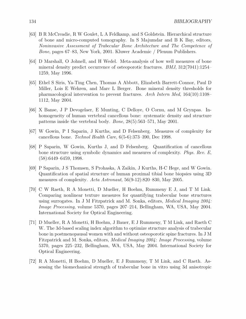
134 BIBLIOGRAPHY

[63] B R McCreadie, R W Goulet, L A Feldkamp, and S Goldstein. Hierarchical structureof bone and micro-computed tomography. In S Majumdar and B K Bay, editors,Noninvasive Assessment of Trabecular Bone Architecture and The Competence of

Bone, pages 67–83, New York, 2001. Kluwer Academic / Plenum Publishers.

[64] D Marshall, O Johnell, and H Wedel. Meta-analysis of how well measures of bonemineral density predict occurrence of osteoporotic fractures. BMJ, 312(7041):1254–1259, May 1996.

[65] Ethel S Siris, Ya-Ting Chen, Thomas A Abbott, Elizabeth Barrett-Connor, Paul DMiller, Lois E Wehren, and Marc L Berger. Bone mineral density thresholds forpharmacological intervention to prevent fractures. Arch Intern Med, 164(10):1108–1112, May 2004.

[66] X Banse, J P Devogelaer, E Munting, C Delloye, O Cornu, and M Grynpas. In-homogeneity of human vertebral cancellous bone: systematic density and structurepatterns inside the vertebral body. Bone, 28(5):563–571, May 2001.

[67] W Gowin, P I Saparin, J Kurths, and D Felsenberg. Measures of complexity forcancellous bone. Technol Health Care, 6(5-6):373–390, Dec 1998.

[68] P Saparin, W Gowin, Kurths J, and D Felsenberg. Quantification of cancellousbone structure using symbolic dynamics and measures of complexity. Phys. Rev. E,(58):6449–6459, 1998.

[69] P Saparin, J S Thomsen, S Prohaska, A Zaikin, J Kurths, H-C Hege, and W Gowin.Quantification of spatial structure of human proximal tibial bone biopsies using 3Dmeasures of complexity. Acta Astronaut, 56(9-12):820–830, May 2005.

[70] C W Raeth, R A Monetti, D Mueller, H Boehm, Rummeny E J, and T M Link.Comparing nonlinear texture measures for quantifying trabecular bone structuresusing surrogates. In J M Fitzpatrick and M. Sonka, editors, Medical Imaging 2004:

Image Processing, volume 5370, pages 207–214, Bellingham, WA, USA, May 2004.International Society for Optical Engineering.

[71] D Mueller, R A Monetti, H Boehm, J Bauer, E J Rummeny, T M Link, and Raeth CW. The 3d-based scaling index algorithm to optimize structure analysis of trabecularbone in postmenopausal women with and without osteoporotic spine fractures. In J MFitzpatrick and M. Sonka, editors, Medical Imaging 2004: Image Processing, volume5370, pages 225–232, Bellingham, WA, USA, May 2004. International Society forOptical Engineering.

[72] R A Monetti, H Boehm, D Mueller, E J Rummeny, T M Link, and C Raeth. As-sessing the biomechanical strength of trabecular bone in vitro using 3d anisotropic

BIBLIOGRAPHY 135

non-linear texture measures: The scaling vector method. In J M Fitzpatrick andM. Sonka, editors, Medical Imaging 2004: Image Processing, volume 5370, pages215–224, Bellingham, WA, USA, May 2004. International Society for Optical Engi-neering.

[73] H Boehm, T M Link, R A Monetti, D Mueller, E J Rummeny, D Newitt, S Majumdar,and C W Raeth. Application of the minkowski functionals in 3d to high resolutionmr images of trabecular bone: Prediction of the biomechanical strength by non-lineartopological measures. In J M Fitzpatrick and M. Sonka, editors, Medical Imaging

2004: Image Processing, volume 5370, pages 172–180, Bellingham, WA, USA, May2004. International Society for Optical Engineering.

[74] D C Newitt, S Majumdar, B van Rietbergen, G von Ingersleben, S T Harris, H KGenant, C Chesnut, P Garnero, and B MacDonald. In vivo assessment of archi-tecture and micro-finite element analysis derived indices of mechanical properties oftrabecular bone in the radius. Osteoporos Int, 13(1):6–17, Jan 2002.

[75] J Tasgal and E M Williams. The effect of prolonged propranolol administration onmyocardial transmural capillary density in young rabbits. J Physiol, 315:353–367,Jun 1981.

[76] T Hildebrand and P Ruegsegger. Quantification of Bone Microarchitecture with theStructure Model Index. Comput Methods Biomech Biomed Engin, 1(1):15–23, 1997.

[77] T M Link and S Majumdar. Osteoporosis imaging. Radiol Clin North Am, 41(4):813–839, Jul 2003.

[78] T M Link, J Bauer, A Kollstedt, I Stumpf, M Hudelmaier, M Settles, S Majumdar,E M Lochmueller, and F Eckstein. Trabecular bone structure of the distal radius,the calcaneus, and the spine: which site predicts fracture status of the spine best?Invest Radiol, 39(8):487–497, Aug 2004.

Acknowledgments

138 BIBLIOGRAPHY

As trabecular networks are complex, the network of support, ideas and en-couragement I received from various people is complex, too:

In chronological order I really want to thank the following people for facili-tating me to write this thesis:

Andrei Andreyevich Markov’s work built the fundament of this research bybreaking down complex views to manageable local views onto the object ofinterest. Instead of loosing the facility to describe the whole object under in-vestigation, the decomposition of complexity in combination with a probabilityembedded simultaneous conjunction of local aspects seems to characterise thewhole object more comprehensively than an integration of simple aspects overthe whole structure. Hence, without Markov’s groundbreaking way of mod-elling stochastic processes with local relationships, a complex view of simpleparts of the puzzle would not have substituted the usual simple view of acomplex object.

Prof. Dr. Gerald Sommer not only provided me with all the knowledge nec-essary to utilise image processing and statistical theories during my studies atthe Chair of Cognitive Systems at the Christian-Albrechts-University. Addi-tionally, he supervised me during the time of this thesis in a most inspirative,fruitful atmosphere. I owe Prof. Sommer main inspirations with regard to theMarkov Theory and deep insights from very delightful discussions to the fieldof Markovian aspects of structures. I experienced the Cognitive Systems Re-search Group during the work at a theoretical approach applied to a practicalproblem as an ideal and supportive background.

Prof. Dr. Martin Heller and Prof. Dr. Claus-C. Gluer gave me the opportu-nity to work in an extremely interesting interdisciplinary field and, moreover,supported all theories and ideas independent of its distance to clinical practise.I appreciated the possibility to perform fundamental research in the Clinic ofDiagnostic Research of the University Hospital Schleswig-Holstein very much,since this kind of research is more an investigation into the future than im-mediately usable. During his supervision Prof. Gluer brought the fascinationof the living organ bone and its numerous exciting aspects to me. Further, heextensively and steadily introduced me into the medical background of boneand osteoporosis as well as various statistical knowledge and strategies.

The possibility of writing an interdisciplinary thesis somewhere in between ofboth worlds of Markov Theory and Trabecular Networks I owe the cooperationof Prof. Dr. Gerald Sommer and Prof. Dr. Claus-C. Gluer. I thank both ofthem for having always an open door and mind.

The Oberseminar Cognitive Systems was very helpful in discussing strategies

BIBLIOGRAPHY 139

and intermediate results several times. All the more I am thankful for themost valuable interdisciplinary thoughts and hints obtained there.

The members of the Medical Physics Research Group headed by Prof. Gluerprovided a very helpful environment for countless discussions, impulses andaccompaniment. I would especially like to thank Bernd Stampa for compre-hensively introducing me into the world of structural characterisations. Dr.Barkmann discussed and answered numerous statistical questions at almostevery time of day and gave me a broad insight into the area of bone research.Christian Graeff supported me with many discussions and ideas. Additionally,he took over responsibilities when time was very short which I appreciatedvery much. All other members of the research group like Jennifer Wolter, Dr.Norber Karger and Dr. Steffen Lusse were very helpful in discussing thingsregularly.

The reader will thank Roswitha Marunde at least as much as I do to guaranteea readable English text: I am really thankful for the huge amount of work shedid in transferring this thesis from a sequence of English words into a pieceof work making some sense.

Both Prof. Dr. Felix Eckstein and Dr. Eva Maria Lochmuller provided thevertebrae needed for this study, which I appreciated very much.

Many special thanks to Margrit for an unforgettable pastry.

Of course, my family participated at and contributed to this work, too:

My sister Ortrun spent her creativity to arrange a beautiful, harmonic cover.

My parents enabled me to go this way, which was not short. I thank Hartmutand Ingrid for the burdens they took to open this way for me.

My wife Susanne provided me with every support imaginable and shared allmoments whether good or bad. This work clearly would not have been possiblewithout her steady understanding of the specific situation a thesis causes. Ihope I can give back sometime all the encouragements, help and love she gaveto me.

Erklarung:

Hiermit versichere ich, dass ich die vorliegende Arbeit selbstandig verfasstund ausschließlich die angegebenen Hilfsmittel und Quellen verwendet habe.

Haselau, den

Markovianity of Trabecular Networks Dissertation

Documents

Transcript of Markovianity of Trabecular Networks Dissertation