
MARKOVASAI
155
Markov Logic: An Interface Layer for Artificial Intelligence
-
Upload
nina-ramirez -
Category
Documents
-
view
15 -
download
0
description
markov's random fields
Transcript of MARKOVASAI

Markov Logic:An Interface Layer forArtificial Intelligence


Synthesis Lectures onArtificial Intelligence and
Machine Learning
EditorsRonald J. Brachman, Yahoo! ResearchThomas Dietterich, Oregon State University
Markov Logic: An Interface Layer for Artificial IntelligencePedro Domingos and Daniel Lowd2009
Introduction to Semi-Supervised LearningXiaojin Zhu and Andrew B. Goldberg2009
Action Programming LanguagesMichael Thielscher2008
Representation Discovery using Harmonic AnalysisSridhar Mahadevan2008
Essentials of Game Theory: A Concise Multidisciplinary IntroductionKevin Leyton-Brown, Yoav Shoham2008
A Concise Introduction to Multiagent Systems and Distributed Artificial IntelligenceNikos Vlassis2007
Intelligent Autonomous Robotics: A Robot Soccer Case StudyPeter Stone2007

Copyright © 2009 by Morgan & Claypool
All rights reserved. No part of this publication may be reproduced, stored in a retrieval system, or transmitted inany form or by any means—electronic, mechanical, photocopy, recording, or any other except for brief quotations inprinted reviews, without the prior permission of the publisher.
Markov Logic: An Interface Layer for Artificial Intelligence
Pedro Domingos and Daniel Lowd
www.morganclaypool.com
ISBN: 9781598296921 paperbackISBN: 9781598296938 ebook
DOI 10.2200/S00206ED1V01Y200907AIM007
A Publication in the Morgan & Claypool Publishers seriesSYNTHESIS LECTURES ON ARTIFICIAL INTELLIGENCE AND MACHINE LEARNING
Lecture #7Series Editors: Ronald J. Brachman, Yahoo! Research
Thomas Dietterich, Oregon State University
Series ISSNSynthesis Lectures on Artificial Intelligence and Machine LearningPrint 1939-4608 Electronic 1939-4616

Markov Logic:An Interface Layer forArtificial Intelligence
Pedro Domingos and Daniel LowdUniversity of Washington, Seattle
With contributions from Jesse Davis, Tuyen Huynh, Stanley Kok, Lilyana Mihalkova, Raymond J.Mooney, Aniruddh Nath, Hoifung Poon, Matthew Richardson, Parag Singla, Marc Sumner, andJue Wang
SYNTHESIS LECTURES ON ARTIFICIAL INTELLIGENCE ANDMACHINE LEARNING #7
CM& cLaypoolMorgan publishers&

ABSTRACTMost subfields of computer science have an interface layer via which applications communicate withthe infrastructure, and this is key to their success (e.g., the Internet in networking, the relationalmodel in databases, etc.). So far this interface layer has been missing in AI. First-order logic andprobabilistic graphical models each have some of the necessary features, but a viable interface layerrequires combining both.Markov logic is a powerful new language that accomplishes this by attachingweights to first-order formulas and treating them as templates for features of Markov randomfields. Most statistical models in wide use are special cases of Markov logic, and first-order logic isits infinite-weight limit. Inference algorithms for Markov logic combine ideas from satisfiability,Markov chain Monte Carlo, belief propagation, and resolution. Learning algorithms make use ofconditional likelihood, convex optimization, and inductive logic programming. Markov logic hasbeen successfully applied to problems in information extraction and integration, natural languageprocessing, robot mapping, social networks, computational biology, and others, and is the basis ofthe open-source Alchemy system.
KEYWORDSMarkov logic, statistical relational learning, machine learning, graphical models, first-order logic, probabilistic logic, Markov networks, Markov random fields, inductive logicprogramming, satisfiability, Markov chain Monte Carlo, belief propagation, collectiveclassification, link prediction, link-based clustering, entity resolution, information ex-traction, social network analysis, natural language processing, robot mapping, compu-tational biology

vii
ContentsAcknowledgments . . . . . . . . . . . . . . . . . . . . . . . . . . . . . . . . . . . . . . . . . . . . . . . . . . . . . . . . . . . . . . . . ix
1 Introduction . . . . . . . . . . . . . . . . . . . . . . . . . . . . . . . . . . . . . . . . . . . . . . . . . . . . . . . . . . . . . . . . . . . . . .1
1.1 The Interface Layer . . . . . . . . . . . . . . . . . . . . . . . . . . . . . . . . . . . . . . . . . . . . . . . . . . . . . . . . . 1
1.2 What Is the Interface Layer for AI? . . . . . . . . . . . . . . . . . . . . . . . . . . . . . . . . . . . . . . . . . . 3
1.3 Markov Logic and Alchemy: An Emerging Solution . . . . . . . . . . . . . . . . . . . . . . . . . . . 4
1.4 Overview of the Book . . . . . . . . . . . . . . . . . . . . . . . . . . . . . . . . . . . . . . . . . . . . . . . . . . . . . . . 7
2 Markov Logic . . . . . . . . . . . . . . . . . . . . . . . . . . . . . . . . . . . . . . . . . . . . . . . . . . . . . . . . . . . . . . . . . . . . 9
2.1 First-Order Logic . . . . . . . . . . . . . . . . . . . . . . . . . . . . . . . . . . . . . . . . . . . . . . . . . . . . . . . . . . 9
2.2 Markov Networks . . . . . . . . . . . . . . . . . . . . . . . . . . . . . . . . . . . . . . . . . . . . . . . . . . . . . . . . . 11
2.3 Markov Logic . . . . . . . . . . . . . . . . . . . . . . . . . . . . . . . . . . . . . . . . . . . . . . . . . . . . . . . . . . . . . 12
2.4 Relation to Other Approaches . . . . . . . . . . . . . . . . . . . . . . . . . . . . . . . . . . . . . . . . . . . . . . 19
3 Inference . . . . . . . . . . . . . . . . . . . . . . . . . . . . . . . . . . . . . . . . . . . . . . . . . . . . . . . . . . . . . . . . . . . . . . . .23
3.1 Inferring the Most Probable Explanation . . . . . . . . . . . . . . . . . . . . . . . . . . . . . . . . . . . . 23
3.2 Computing Conditional Probabilities . . . . . . . . . . . . . . . . . . . . . . . . . . . . . . . . . . . . . . . .25
3.3 Lazy Inference . . . . . . . . . . . . . . . . . . . . . . . . . . . . . . . . . . . . . . . . . . . . . . . . . . . . . . . . . . . . 29
3.4 Lifted Inference . . . . . . . . . . . . . . . . . . . . . . . . . . . . . . . . . . . . . . . . . . . . . . . . . . . . . . . . . . . 35
4 Learning . . . . . . . . . . . . . . . . . . . . . . . . . . . . . . . . . . . . . . . . . . . . . . . . . . . . . . . . . . . . . . . . . . . . . . . .43
4.1 Weight Learning . . . . . . . . . . . . . . . . . . . . . . . . . . . . . . . . . . . . . . . . . . . . . . . . . . . . . . . . . . 43
4.2 Structure Learning and Theory Revision . . . . . . . . . . . . . . . . . . . . . . . . . . . . . . . . . . . . . 52
4.3 Unsupervised Learning . . . . . . . . . . . . . . . . . . . . . . . . . . . . . . . . . . . . . . . . . . . . . . . . . . . . 56
4.4 Transfer Learning . . . . . . . . . . . . . . . . . . . . . . . . . . . . . . . . . . . . . . . . . . . . . . . . . . . . . . . . . 62
5 Extensions . . . . . . . . . . . . . . . . . . . . . . . . . . . . . . . . . . . . . . . . . . . . . . . . . . . . . . . . . . . . . . . . . . . . . . 71
5.1 Continuous Domains . . . . . . . . . . . . . . . . . . . . . . . . . . . . . . . . . . . . . . . . . . . . . . . . . . . . . . 71

viii CONTENTS
5.2 Infinite Domains . . . . . . . . . . . . . . . . . . . . . . . . . . . . . . . . . . . . . . . . . . . . . . . . . . . . . . . . . . 75
5.3 Recursive Markov Logic . . . . . . . . . . . . . . . . . . . . . . . . . . . . . . . . . . . . . . . . . . . . . . . . . . . 84
5.4 Relational Decision Theory . . . . . . . . . . . . . . . . . . . . . . . . . . . . . . . . . . . . . . . . . . . . . . . . .91
6 Applications . . . . . . . . . . . . . . . . . . . . . . . . . . . . . . . . . . . . . . . . . . . . . . . . . . . . . . . . . . . . . . . . . . . . 97
6.1 Collective Classification . . . . . . . . . . . . . . . . . . . . . . . . . . . . . . . . . . . . . . . . . . . . . . . . . . . . 97
6.2 Social Network Analysis and Link Prediction . . . . . . . . . . . . . . . . . . . . . . . . . . . . . . . . 98
6.3 Entity Resolution . . . . . . . . . . . . . . . . . . . . . . . . . . . . . . . . . . . . . . . . . . . . . . . . . . . . . . . . 103
6.4 Information Extraction . . . . . . . . . . . . . . . . . . . . . . . . . . . . . . . . . . . . . . . . . . . . . . . . . . . 104
6.5 Unsupervised Coreference Resolution . . . . . . . . . . . . . . . . . . . . . . . . . . . . . . . . . . . . . . 106
6.6 Robot Mapping . . . . . . . . . . . . . . . . . . . . . . . . . . . . . . . . . . . . . . . . . . . . . . . . . . . . . . . . . . 111
6.7 Link-based Clustering . . . . . . . . . . . . . . . . . . . . . . . . . . . . . . . . . . . . . . . . . . . . . . . . . . . . 113
6.8 Semantic Network Extraction from Text . . . . . . . . . . . . . . . . . . . . . . . . . . . . . . . . . . . . 116
7 Conclusion . . . . . . . . . . . . . . . . . . . . . . . . . . . . . . . . . . . . . . . . . . . . . . . . . . . . . . . . . . . . . . . . . . . . 121
A The Alchemy System . . . . . . . . . . . . . . . . . . . . . . . . . . . . . . . . . . . . . . . . . . . . . . . . . . . . . . . . . . . 125
A.1 Input Files . . . . . . . . . . . . . . . . . . . . . . . . . . . . . . . . . . . . . . . . . . . . . . . . . . . . . . . . . . . . . . .125
A.2 Inference . . . . . . . . . . . . . . . . . . . . . . . . . . . . . . . . . . . . . . . . . . . . . . . . . . . . . . . . . . . . . . . . 127
A.3 Weight Learning . . . . . . . . . . . . . . . . . . . . . . . . . . . . . . . . . . . . . . . . . . . . . . . . . . . . . . . . . 128
A.4 Structure Learning . . . . . . . . . . . . . . . . . . . . . . . . . . . . . . . . . . . . . . . . . . . . . . . . . . . . . . . 128
Bibliography . . . . . . . . . . . . . . . . . . . . . . . . . . . . . . . . . . . . . . . . . . . . . . . . . . . . . . . . . . . . . . . . . . . 131
Biography . . . . . . . . . . . . . . . . . . . . . . . . . . . . . . . . . . . . . . . . . . . . . . . . . . . . . . . . . . . . . . . . . . . . . 145

AcknowledgmentsWe are grateful to all the people who contributed to the development of Markov logic and Alchemy:colleagues, users, developers, reviewers, and others. We thank our families for their patience andsupport.
The research described in this book was partly funded by ARO grant W911NF-08-1-0242,DARPA contracts FA8750-05-2-0283, FA8750-07-D-0185, HR0011-06-C-0025, HR0011-07-C-0060 and NBCH-D030010, NSF grants IIS-0534881, IIS-0803481 and EIA-0303609, ONRgrants N-00014-05-1-0313 and N00014-08-1-0670, an NSF CAREER Award (first author), aSloan Research Fellowship (first author), an NSF Graduate Fellowship (second author) and a Mi-crosoft Research Graduate Fellowship (second author). The views and conclusions contained in thisdocument are those of the authors and should not be interpreted as necessarily representing theofficial policies, either expressed or implied, of ARO, DARPA, NSF, ONR, or the United StatesGovernment.
Pedro Domingos and Daniel LowdSeattle, Washington


1
C H A P T E R 1
Introduction1.1 THE INTERFACE LAYER
Artificial intelligence (AI) has made tremendous progress in its first 50 years. However, it is still veryfar from reaching and surpassing human intelligence. At the current rate of progress, the crossoverpoint will not be reached for hundreds of years. We need innovations that will permanently increasethe rate of progress. Most research is inevitably incremental, but the size of those increments dependson the paradigms and tools that researchers have available. Improving these provides more than aone-time gain; it enables researchers to consistently produce larger increments of progress at a higherrate. If we do it enough times, we may be able to shorten those hundreds of years to decades, asillustrated in Figure 1.1.
If we look at other subfields of computer science, we see that in most cases progress has beenenabled above all by the creation of an interface layer that separates innovation above and below it,while allowing each to benefit from the other. Below the layer, research improves the foundations (or,more pragmatically, the infrastructure); above it, research improves existing applications and inventsnew ones.Table 1.1 shows examples of interface layers from various subfields of computer science. Ineach of these fields, the development of the interface layer triggered a period of rapid progress aboveand below it. In most cases, this progress continues today. For example, new applications enabledby the Internet continue to appear, and protocol extensions continue to be proposed. In many cases,the progress sparked by the new layer resulted in new industries, or in sizable expansions of existingones.
Figure 1.1: The first 100 years of AI. The graph on the right illustrates how increasing our rate ofprogress several times could bring about human-level intelligence much faster.

2 CHAPTER 1. INTRODUCTION
Table 1.1: Examples of interface layers.Field Interface Layer Below the Layer Above the LayerHardware VLSI design VLSI modules Computer-aided
chip designArchitecture Microprocessors ALUs, buses Compilers, operating
systemsOperating systems Virtual machines Hardware SoftwareProgramming systems High-level languages Compilers, Programming
code optimizersDatabases Relational model Query optimization, Enterprise applications
transaction mgmt.Networking Internet Protocols, routers Web, emailHCI Graphical user interface Widget toolkits Productivity suitesAI ??? Inference, learning Planning, NLP, vision,
robotics
The interface layer allows each innovation below it to automatically become available to allthe applications above it, without the “infrastructure” researchers having to know the details of theapplications, or even what all the existing or possible applications are. Conversely, new applications(and improvements to existing ones) can be developed with little or no knowledge of the infrastructurebelow the layer. Without it, each innovation needs to be separately combined with each other, anO(n2) problem that in practice is too costly to solve, leaving only a few of the connections made.When the layer is available, each innovation needs to be combined only with the layer itself. Thus,we obtain O(n2) benefits with O(n) work, as illustrated in Figure 1.2.
In each case, the separation between applications above the layer and infrastructure belowit is not perfect. If we care enough about a particular application, we can usually improve it bydeveloping infrastructure specifically for it. However, most applications are served well enough bythe general-purpose machinery, and in many cases would not be economically feasible without it.For example, ASICs (application-specific integrated circuits) are far more efficient for their specificapplications than general-purpose microprocessors; but the vast majority of applications are still runon the latter. Interface layers are an instance of the 80/20 rule: they allow us to obtain 80% of thebenefits for 20% of the cost.
The essential feature of an interface layer is that it provides a language of operations that is allthe infrastructure needs to support, and all that the applications need to know about. Designing it isa difficult balancing act between providing what the applications need and staying within what theinfrastructure can do. A good interface layer exposes important distinctions and hides unimportantones. How to do this is often far from obvious. Creating a successful new interface layer is thus noteasy. Typically, it initially faces skepticism, because it is less efficient than the existing alternatives,and appears too ambitious, being beset by difficulties that are only resolved by later research. Butonce the layer becomes established, it enables innovations that were previously unthinkable.

1.2. WHAT IS THE INTERFACE LAYER FOR AI? 3
Figure 1.2: An interface layer provides the benefits of O(n2) connections between applications andinfrastructure algorithms with just O(n) connections.
1.2 WHAT IS THE INTERFACE LAYER FOR AI?In AI, the interface layer has been conspicuously absent, and this, perhaps more than any other factor,has limited the rate of progress. An early candidate for this role was first-order logic. However, itquickly became apparent that first-order logic has many shortcomings as a basis for AI, leadingto a long series of efforts to extend it. Unfortunately, none of these extensions has achieved wideacceptance. Perhaps the closest first-order logic has come to providing an interface layer is theProlog language. However, it remains a niche language even within AI. This is largely because,being essentially a subset of first-order logic, it shares its limitations, and is thus insufficient tosupport most applications at the 80/20 level.
Many (if not most) of the shortcomings of logic can be overcome by the use of probability.Here, graphical models (i.e., Bayesian and Markov networks) have to some extent played the part ofan interface layer, but one with a limited range. Although they provide a unifying language for manydifferent probabilistic models, graphical models can only represent distributions over propositionaluniverses, and are thus insufficiently expressive for general AI. In practice, this limitation is oftencircumvented by manually transforming the rich relational domain of interest into a simplifiedpropositional one, but the cost, brittleness, and lack of reusability of this manual work is preciselywhat a good interface layer should avoid. Also, to the extent that graphical models can provide aninterface layer, they have done so mostly at the conceptual level. No widely accepted languages orstandards for representing and using graphical models exist today. Many toolkits with specializedfunctionality have been developed, but none that could be used as widely as (say) SQL engines are indatabases. Perhaps the most widely used such toolkit is BUGS, but it is quite limited in the learningand inference infrastructure it provides. Although very popular with Bayesian statisticians, it failsthe 80/20 test for AI.
It is clear that the AI interface layer needs to integrate first-order logic and graphical models.One or the other by itself cannot provide the minimum functionality needed to support the full rangeof AI applications. Further, the two need to be fully integrated, and not simply provided alongsideeach other. Most applications require simultaneously the expressiveness of first-order logic and the

4 CHAPTER 1. INTRODUCTION
Table 1.2: Examples of logical and statistical AI.Field Logical Approach Statistical ApproachKnowledge representation First-order logic Graphical modelsAutomated reasoning Satisfiability testing Markov chain Monte CarloMachine learning Inductive logic programming Neural networksPlanning Classical planning Markov decision processesNatural language processing Definite clause grammars Probabilistic context-free grammars
robustness of probability, not just one or the other. Unfortunately, the split between logical andstatistical AI runs very deep. It dates to the earliest days of the field, and continues to be highlyvisible today. It takes a different form in each subfield of AI, but it is omnipresent. Table 1.2 showsexamples of this. In each case, both the logical and the statistical approach contribute somethingimportant. This justifies the abundant research on each of them, but also implies that ultimately acombination of the two is required.
In recent years,we have begun to see increasingly frequent attempts to achieve such a combina-tion in each subfield. In knowledge representation, knowledge-based model construction combineslogic programming and Bayesian networks, and substantial theoretical work on combining logic andprobability has appeared. In automated reasoning, researchers have identified common schemas insatisfiability testing, constraint processing and probabilistic inference. In machine learning, statisti-cal relational learning combines inductive logic programming and statistical learning. In planning,relational MDPs add aspects of classical planning to MDPs. In natural language processing, workon recognizing textual entailment and on learning to map sentences to logical form combines logicaland statistical components. However, for the most part these developments have been pursued inde-pendently, and have not benefited from each other.This is largely attributable to the O(n2) problem:researchers in one subfield can connect their work to perhaps one or two others, but connecting itto all of them is not practically feasible.
1.3 MARKOV LOGIC AND ALCHEMY:AN EMERGING SOLUTION
We have recently introduced Markov logic, a language that combines first-order logic and Markovnetworks. A knowledge base (KB) in Markov logic is a set of first-order formulas with weights. Givena set of constants representing objects in the domain of interest, it defines a probability distributionover possible worlds, each world being an assignment of truth values to all possible ground atoms.Thedistribution is in the form of a log-linear model: a normalized exponentiated weighted combinationof features of the world.1 Each feature is a grounding of a formula in the KB, with the correspondingweight. In first-order logic, formulas are hard constraints: a world that violates even a single formula
1Log-linear models are also known as, or closely related to, Markov networks, Markov random fields, maximum entropy models,Gibbs distributions, and exponential models; and they have Bayesian networks, Boltzmann machines, conditional random fields,and logistic regression as special cases.

1.3. MARKOV LOGIC AND ALCHEMY: AN EMERGING SOLUTION 5
Table 1.3: A comparison of Alchemy, Prolog, and BUGS.Aspect Alchemy Prolog BUGSRepresentation First-order logic + Markov networks Horn clauses Bayesian networksInference Model checking, MCMC, lifted BP Theorem proving Gibbs samplingLearning Parameters and structure No ParametersUncertainty Yes No YesRelational Yes Yes No
is impossible. In Markov logic, formulas are soft constraints: a world that violates a formula is lessprobable than one that satisfies it, other things being equal, but not impossible. The weight of aformula represents its strength as a constraint. Finite first-order logic is the limit of Markov logicwhen all weights tend to infinity. Markov logic allows an existing first-order KB to be transformedinto a probabilistic model simply by assigning weights to the formulas, manually or by learningthem from data. It allows multiple KBs to be merged without resolving their inconsistencies, andobviates the need to exhaustively specify the conditions under which a formula can be applied. Onthe statistical side, it allows very complex models to be represented very compactly; in particular,it provides an elegant language for expressing non-i.i.d. models (i.e., models where data points arenot assumed independent and identically distributed). It also facilitates the incorporation of richdomain knowledge, reducing reliance on purely empirical learning.
Markov logic builds on previous developments in knowledge-based model construction andstatistical relational learning, but goes beyond them in combining first-order logic and graphicalmodels without restrictions.Unlike previous representations, it is supported by a full range of learningand inference algorithms, in each case combining logical and statistical elements. Because of itsgenerality, it provides a natural framework for integrating the logical and statistical approaches ineach field. For example, DCGs and PCFGs are both special cases of Markov logic, and classicalplanning and MDPs can both be elegantly formulated using Markov logic and decision theory. WithMarkov logic, combining classical planning and MDPs, or DCGs and PCFGs, does not require newalgorithms; the existing general-purpose inference and learning facilities can be directly applied.
AI can be roughly divided into “foundational” and “application” areas. Foundational areasinclude knowledge representation, automated reasoning, probabilistic models, and machine learn-ing. Application areas include planning, vision, robotics, speech, natural language processing, andmulti-agent systems. An interface layer for AI must provide the former, and serve the latter. We havedeveloped the Alchemy system as an open-source embodiment of Markov logic and implementationof algorithms for it [60]. Alchemy seamlessly combines first-order knowledge representation, modelchecking, probabilistic inference, inductive logic programming, and generative/discriminative pa-rameter learning. Table 1.3 compares Alchemy with Prolog and BUGS, and shows that it providesa critical mass of capabilities not previously available.
For researchers and practitioners in application areas, Alchemy offers a large reduction in theeffort required to assemble a state-of-the-art solution, and to extend it beyond the state of the art.
6 CHAPTER 1. INTRODUCTION
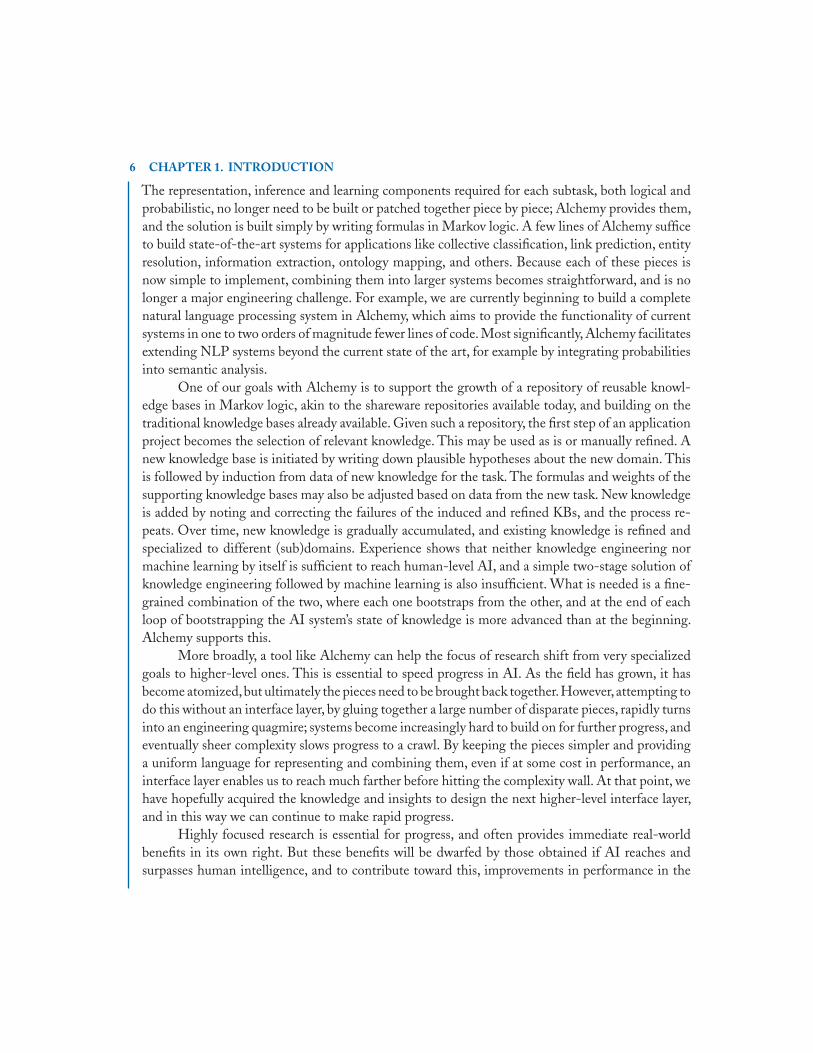
The representation, inference and learning components required for each subtask, both logical andprobabilistic, no longer need to be built or patched together piece by piece; Alchemy provides them,and the solution is built simply by writing formulas in Markov logic. A few lines of Alchemy sufficeto build state-of-the-art systems for applications like collective classification, link prediction, entityresolution, information extraction, ontology mapping, and others. Because each of these pieces isnow simple to implement, combining them into larger systems becomes straightforward, and is nolonger a major engineering challenge. For example, we are currently beginning to build a completenatural language processing system in Alchemy, which aims to provide the functionality of currentsystems in one to two orders of magnitude fewer lines of code. Most significantly, Alchemy facilitatesextending NLP systems beyond the current state of the art, for example by integrating probabilitiesinto semantic analysis.
One of our goals with Alchemy is to support the growth of a repository of reusable knowl-edge bases in Markov logic, akin to the shareware repositories available today, and building on thetraditional knowledge bases already available. Given such a repository, the first step of an applicationproject becomes the selection of relevant knowledge. This may be used as is or manually refined. Anew knowledge base is initiated by writing down plausible hypotheses about the new domain. Thisis followed by induction from data of new knowledge for the task. The formulas and weights of thesupporting knowledge bases may also be adjusted based on data from the new task. New knowledgeis added by noting and correcting the failures of the induced and refined KBs, and the process re-peats. Over time, new knowledge is gradually accumulated, and existing knowledge is refined andspecialized to different (sub)domains. Experience shows that neither knowledge engineering normachine learning by itself is sufficient to reach human-level AI, and a simple two-stage solution ofknowledge engineering followed by machine learning is also insufficient. What is needed is a fine-grained combination of the two, where each one bootstraps from the other, and at the end of eachloop of bootstrapping the AI system’s state of knowledge is more advanced than at the beginning.Alchemy supports this.
More broadly, a tool like Alchemy can help the focus of research shift from very specializedgoals to higher-level ones. This is essential to speed progress in AI. As the field has grown, it hasbecome atomized,but ultimately the pieces need to be brought back together.However, attempting todo this without an interface layer, by gluing together a large number of disparate pieces, rapidly turnsinto an engineering quagmire; systems become increasingly hard to build on for further progress, andeventually sheer complexity slows progress to a crawl. By keeping the pieces simpler and providinga uniform language for representing and combining them, even if at some cost in performance, aninterface layer enables us to reach much farther before hitting the complexity wall. At that point, wehave hopefully acquired the knowledge and insights to design the next higher-level interface layer,and in this way we can continue to make rapid progress.
Highly focused research is essential for progress, and often provides immediate real-worldbenefits in its own right. But these benefits will be dwarfed by those obtained if AI reaches andsurpasses human intelligence, and to contribute toward this, improvements in performance in the

1.4. OVERVIEW OF THE BOOK 7
subtasks need to translate into improvements in the larger tasks. When the subtasks are pursuedin isolation, there is no guarantee that this will happen, and in fact experience suggests that thetendency will be for the subtask solutions to evolve into local optima, which are best in isolationbut not in combination. By increasing the granularity of the tasks that can be routinely attempted,platforms like Alchemy make this less likely, and help us reach human-level AI sooner.
1.4 OVERVIEW OF THE BOOKIn the remainder of this book, we will describe the Markov logic representation in greater detail,along with algorithms and applications.
In Chapter 2, we first provide basic background on first-order logic and probabilistic graphicalmodels. We then define the Markov logic representation, building and unifying these two perspec-tives. We conclude by showing how Markov logic relates to some of the many other combinationsof logic and probability that have been proposed in recent years.
Chapters 3 and 4 present state-of-the-art algorithms for reasoning and learning with Markovlogic. These algorithms build on standard methods for first-order logic or graphical models, includ-ing satisfiability, Markov chain Monte Carlo, and belief propagation for inference; and inductivelogic programming and convex optimization for learning. In many cases, these methods have beencombined and extended to handle additional challenges introduced by the rich Markov logic repre-sentation.
Chapter 5 goes beyond the basic Markov logic representation to describe several extensionsthat increase its power or applicability to particular problems. In particular, we cover how Markovlogic can be extended to continuous and infinite domains, combined with decision theory, andgeneralized to represent uncertain disjunctions and existential quantifiers. In addition to solvingparticular problems better, these extensions demonstrate that Markov logic can easily be adaptedwhen necessary to explicitly support the features of new problems.
Chapter 6 is devoted to exploring applications of Markov logic to several real-world problems,including collective classification, link prediction, link-based clustering, entity resolution, informa-tion extraction, social network analysis, and robot mapping. Most datasets and models from thischapter can be found online at http://alchemy.cs.washington.edu.
We conclude in Chapter 7 with final thoughts and future directions. An appendix provides abrief introduction to Alchemy.
Sample course slides to accompany this book are available athttp://www.cs.washington.edu/homes/pedrod/803/.


9
C H A P T E R 2
Markov LogicIn this chapter, we provide a detailed description of the Markov logic representation. We beginby providing background on first-order logic and probabilistic graphical models and then showhow Markov logic unifies and builds on these concepts. Finally, we compare Markov logic to otherrepresentations that combine probability and logic.
2.1 FIRST-ORDER LOGIC
A first-order knowledge base (KB) is a set of sentences or formulas in first-order logic [37]. Formulasare constructed using four types of symbols: constants, variables, functions, and predicates. Constantsymbols represent objects in the domain of interest (e.g., people: Anna, Bob, Chris, etc.). Variablesymbols range over the objects in the domain.Function symbols (e.g.,MotherOf) represent mappingsfrom tuples of objects to objects. Predicate symbols represent relations among objects in the domain(e.g., Friends) or attributes of objects (e.g., Smokes). An interpretation specifies which objects,functions and relations in the domain are represented by which symbols. Variables and constantsmay be typed, in which case variables range only over objects of the corresponding type, and constantscan only represent objects of the corresponding type. For example, the variable x might range overpeople (e.g., Anna, Bob, etc.), and the constant C might represent a city (e.g., Seattle, Tokyo, etc.).
A term is any expression representing an object in the domain. It can be a constant, a variable, ora function applied to a tuple of terms.For example,Anna,x, and GreatestCommonDivisor(x, y) areterms. An atomic formula or atom is a predicate symbol applied to a tuple of terms (e.g., Friends(x,MotherOf(Anna))). Formulas are recursively constructed from atomic formulas using logical con-nectives and quantifiers. If F1 and F2 are formulas, the following are also formulas: ¬F1 (negation),which is true iff F1 is false; F1 ∧ F2 (conjunction), which is true iff both F1 and F2 are true; F1 ∨ F2
(disjunction), which is true iff F1 or F2 is true; F1 ⇒ F2 (implication), which is true iff F1 is falseor F2 is true; F1 ⇔ F2 (equivalence), which is true iff F1 and F2 have the same truth value; ∀x F1
(universal quantification), which is true iff F1 is true for every object x in the domain; and ∃x F1
(existential quantification), which is true iff F1 is true for at least one object x in the domain. Paren-theses may be used to enforce precedence. A positive literal is an atomic formula; a negative literalis a negated atomic formula. The formulas in a KB are implicitly conjoined, and thus a KB can beviewed as a single large formula. A ground term is a term containing no variables. A ground atomor ground predicate is an atomic formula all of whose arguments are ground terms. A possible world(along with an interpretation) assigns a truth value to each possible ground atom.
A formula is satisfiable iff there exists at least one world in which it is true.The basic inferenceproblem in first-order logic is to determine whether a knowledge base KB entails a formula F , i.e.,

10 CHAPTER 2. MARKOV LOGIC
Table 2.1: Example of a first-order knowledge base and MLN. Fr() is short for Friends(), Sm() forSmokes(), and Ca() for Cancer().
English and First-Order Logic Clausal Form Weight“Friends of friends are friends.”
∀x∀y∀z Fr(x, y) ∧ Fr(y, z) ⇒ Fr(x, z) ¬Fr(x, y) ∨ ¬Fr(y, z) ∨ Fr(x, z) 0.7“Smoking causes cancer.”
∀x Sm(x) ⇒ Ca(x) ¬Sm(x) ∨ Ca(x) 1.5“If two people are friends and onesmokes, then so does the other.”
∀x∀y Fr(x, y) ∧ Sm(x) ⇒ Sm(y) ¬Fr(x, y) ∨ ¬Sm(x) ∨ Sm(y) 1.1
if F is true in all worlds where KB is true (denoted by KB |= F ). This is often done by refutation:KB entails F iff KB ∪ ¬F is unsatisfiable. (Thus, if a KB contains a contradiction, all formulastrivially follow from it, which makes painstaking knowledge engineering a necessity.) For automatedinference, it is often convenient to convert formulas to a more regular form, typically clausal form (alsoknown as conjunctive normal form (CNF)). A KB in clausal form is a conjunction of clauses, a clausebeing a disjunction of literals. Every KB in first-order logic can be converted to clausal form using amechanical sequence of steps.1 Clausal form is used in resolution, a sound and refutation-completeinference procedure for first-order logic [122].
Inference in first-order logic is only semidecidable. Because of this, knowledge bases are oftenconstructed using a restricted subset of first-order logic with more desirable properties. The mostwidely used restriction is to Horn clauses, which are clauses containing at most one positive literal.The Prolog programming language is based on Horn clause logic [72]. Prolog programs can belearned from databases by searching for Horn clauses that (approximately) hold in the data; this isstudied in the field of inductive logic programming (ILP) [65].
Table 2.1 shows a simple KB and its conversion to clausal form. Note that, while theseformulas may be typically true in the real world, they are not always true. In most domains it is verydifficult to come up with non-trivial formulas that are always true, and such formulas capture only afraction of the relevant knowledge.Thus, despite its expressiveness, pure first-order logic has limitedapplicability to practical AI problems. Many ad hoc extensions to address this have been proposed.In the more limited case of propositional logic, the problem is well solved by probabilistic graphicalmodels such as Markov networks, described in the next section. We will later show how to generalizethese models to the first-order case.
1This conversion includes the removal of existential quantifiers by Skolemization, which is not sound in general. However, in finitedomains an existentially quantified formula can simply be replaced by a disjunction of its groundings.

2.2. MARKOV NETWORKS 11
2.2 MARKOV NETWORKS
A Markov network (also known as Markov random field) is a model for the joint distribution of aset of variables X = (X1, X2, . . . , Xn) ∈ X [99]. It is composed of an undirected graph G and aset of potential functions φk . The graph has a node for each variable, and the model has a potentialfunction for each clique in the graph. A potential function is a non-negative real-valued functionof the state of the corresponding clique. The joint distribution represented by a Markov network isgiven by
P(X=x) = 1
Z
∏k
φk(x{k}) (2.1)
where x{k} is the state of the kth clique (i.e., the state of the variables that appear in that clique).Z, known as the partition function, is given by Z = ∑
x∈X∏
k φk(x{k}). Markov networks are oftenconveniently represented as log-linear models, with each clique potential replaced by an exponentiatedweighted sum of features of the state, leading to
P(X=x) = 1
Zexp
⎛⎝∑
j
wjfj (x)
⎞⎠ (2.2)
A feature may be any real-valued function of the state. Except where stated, this book will focuson binary features, fj (x) ∈ {0, 1}. In the most direct translation from the potential-function form(Equation 2.1), there is one feature corresponding to each possible state x{k} of each clique, withits weight being log φk(x{k}). This representation is exponential in the size of the cliques. However,we are free to specify a much smaller number of features (e.g., logical functions of the state of theclique), allowing for a more compact representation than the potential-function form, particularlywhen large cliques are present. Markov logic will take advantage of this.
Inference in Markov networks is #P-complete [123]. The most widely used method for ap-proximate inference in Markov networks is Markov chain Monte Carlo (MCMC) [40], and inparticular Gibbs sampling, which proceeds by sampling each variable in turn given its Markov blan-ket. (The Markov blanket of a node is the minimal set of nodes that renders it independent of theremaining network; in a Markov network, this is simply the node’s neighbors in the graph.) Marginalprobabilities are computed by counting over these samples; conditional probabilities are computedby running the Gibbs sampler with the conditioning variables clamped to their given values.
Another popular method for inference in Markov networks is belief propagation [156], amessage-passing algorithm that performs exact inference on tree-structured Markov networks.When applied to graphs with loops, the results are approximate and the algorithm may not converge.Nonetheless, loopy belief propagation is more efficient than Gibbs sampling in many applications.
Maximum-likelihood or MAP estimates of Markov network weights cannot be computedin closed form but, because the log-likelihood is a concave function of the weights, they can befound efficiently (modulo inference) using standard gradient-based or quasi-Newton optimization

12 CHAPTER 2. MARKOV LOGIC
methods [95]. Another alternative is iterative scaling [24]. Features can also be learned from data,for example by greedily constructing conjunctions of atomic features [24].
2.3 MARKOV LOGICA first-order KB can be seen as a set of hard constraints on the set of possible worlds: if a world violateseven one formula, it has zero probability.The basic idea in MLNs is to soften these constraints: whena world violates one formula in the KB it is less probable, but not impossible. The fewer formulasa world violates, the more probable it is. Each formula has an associated weight that reflects howstrong a constraint it is: the higher the weight, the greater the difference in log probability betweena world that satisfies the formula and one that does not, other things being equal.
Definition 2.1. A Markov logic network L is a set of pairs (Fi, wi), where Fi is a formula in first-order logic and wi is a real number. Together with a finite set of constants C = {c1, c2, . . . , c|C|}, itdefines a Markov network ML,C (Equations 2.1 and 2.2) as follows:
1. ML,C contains one binary node for each possible grounding of each predicate appearing in L.The value of the node is 1 if the ground predicate is true, and 0 otherwise.
2. ML,C contains one feature for each possible grounding of each formula Fi in L. The value ofthis feature is 1 if the ground formula is true, and 0 otherwise. The weight of the feature is thewi associated with Fi in L.
The syntax of the formulas in an MLN is the standard syntax of first-order logic [37]. Free(unquantified) variables are treated as universally quantified at the outermost level of the formula.In this book, we will often assume that the set of formulas is in function-free clausal form forconvenience, but our methods can be applied to other MLNs as well.
An MLN can be viewed as a template for constructing Markov networks. Given different setsof constants, it will produce different networks, and these may be of widely varying size, but all willhave certain regularities in structure and parameters, given by the MLN (e.g., all groundings of thesame formula will have the same weight). We call each of these networks a ground Markov networkto distinguish it from the first-order MLN. From Definition 2.1 and Equations 2.1 and 2.2, theprobability distribution over possible worlds x specified by the ground Markov network ML,C isgiven by
P(X=x) = 1
Zexp
(∑i
wini(x)
)= 1
Z
∏i
φi(x{i})ni(x) (2.3)
where ni(x) is the number of true groundings of Fi in x, x{i} is the state (truth values) of thepredicates appearing in Fi , and φi(x{i}) = ewi . Note that, although we defined MLNs as log-linearmodels, they could equally well be defined as products of potential functions, as the second equalityabove shows. This will be the most convenient approach in domains with a mixture of hard and

2.3. MARKOV LOGIC 13
Cancer(A)
Smokes(A)Friends(A,A)
Friends(B,A)
Smokes(B)
Friends(A,B)
Cancer(B)
Friends(B,B)
Figure 2.1: Ground Markov network obtained by applying the last two formulas in Table 2.1 to theconstants Anna(A) and Bob(B).
soft constraints (i.e., where some formulas hold with certainty, leading to zero probabilities for someworlds).
The graphical structure of ML,C follows from Definition 2.1: there is an edge between twonodes of ML,C iff the corresponding ground predicates appear together in at least one groundingof one formula in L. Thus, the predicates in each ground formula form a (not necessarily maximal)clique in ML,C . Figure 2.1 shows the graph of the ground Markov network defined by the last twoformulas in Table 2.1 and the constants Anna and Bob. Each node in this graph is a ground predicate(e.g., Friends(Anna, Bob)). The graph contains an arc between each pair of predicates that appeartogether in some grounding of one of the formulas. ML,C can now be used to infer the probabilitythat Anna and Bob are friends given their smoking habits, the probability that Bob has cancer givenhis friendship with Anna and whether she has cancer, etc.
Each state of ML,C represents a possible world. A possible world is a set of objects, a set offunctions (mappings from tuples of objects to objects), and a set of relations that hold between thoseobjects; together with an interpretation, they determine the truth value of each ground predicate.The following assumptions ensure that the set of possible worlds for (L, C) is finite, and thatML,C represents a unique, well-defined probability distribution over those worlds, irrespective ofthe interpretation and domain.These assumptions are quite reasonable in most practical applications,and greatly simplify the use of MLNs. For the remaining cases, we discuss below the extent to whicheach one can be relaxed.
Assumption 2.2. Unique names. Different constants refer to different objects [37].
Assumption 2.3. Domain closure. The only objects in the domain are those representable using theconstant and function symbols in (L, C) [37].

14 CHAPTER 2. MARKOV LOGIC
Table 2.2: Construction of all groundings of a first-order formula under Assumptions 2.2–2.4.
function Ground(F )input: F , a formula in first-order logicoutput: GF , a set of ground formulas
for each existentially quantified subformula ∃x S(x) in F
F ← F with ∃x S(x) replaced by S(c1) ∨ S(c2) ∨ . . . ∨ S(c|C|),where S(ci) is S(x) with x replaced by ci
GF ← {F }for each universally quantified variable x
for each formula Fj (x) in GF
GF ← (GF \ Fj (x)) ∪ {Fj (c1), Fj (c2), . . . , Fj (c|C|)},where Fj (ci) is Fj (x) with x replaced by ci
for each formula Fj ∈ GF
repeatfor each function f (a1, a2, . . .) all of whose arguments are constantsFj ← Fj with f (a1, a2, . . .) replaced by c, where c = f (a1, a2, . . .)
until Fj contains no functionsreturn GF
Assumption 2.4. Known functions. For each function appearing in L, the value of that functionapplied to every possible tuple of arguments is known, and is an element of C.
This last assumption allows us to replace functions by their values when grounding formulas.Thus the only ground predicates that need to be considered are those having constants as argu-ments. The infinite number of terms constructible from all functions and constants in (L, C) (the“Herbrand universe” of (L, C)) can be ignored, because each of those terms corresponds to a knownconstant in C, and predicates involving them are already represented as the predicates involving thecorresponding constants. The possible groundings of a predicate in Definition 2.1 are thus obtainedsimply by replacing each variable in the predicate with each constant in C, and replacing each func-tion term in the predicate by the corresponding constant. Table 2.2 shows how the groundings of aformula are obtained given Assumptions 2.2–2.4.
Assumption 2.2 (unique names) can be removed by introducing the equality predicate(Equals(x, y), or x = y for short) and adding the necessary axioms to the MLN: equality is reflexive,symmetric and transitive; for each unary predicate P , ∀x∀y x = y ⇒ (P(x) ⇔ P(y)); and similarlyfor higher-order predicates and functions [37]. The resulting MLN will have a node for each pair ofconstants, whose value is 1 if the constants represent the same object and 0 otherwise; these nodeswill be connected to each other and to the rest of the network by arcs representing the axioms above.

2.3. MARKOV LOGIC 15
Note that this allows us to make probabilistic inferences about the equality of two constants. Theexample in Section 6.3 successfully uses this as the basis of an approach to entity resolution.
If the number u of unknown objects is known, Assumption 2.3 (domain closure) can beremoved simply by introducing u arbitrary new constants. If u is unknown but finite, Assumption 2.3can be removed by introducing a distribution over u, grounding the MLN with each number ofunknown objects,and computing the probability of a formula F as P(F) = ∑umax
u=0 P(u)P (F |MuL,C),
where MuL,C is the ground MLN with u unknown objects.Markov logic can also be applied to infinite
domains; details are in Section 5.2.Let HL,C be the set of all ground terms constructible from the function symbols in L and
the constants in L and C (the “Herbrand universe” of (L, C)). Assumption 2.4 (known functions)can be removed by treating each element of HL,C as an additional constant and applying the sameprocedure used to remove the unique names assumption. For example, with a function G(x) andconstants A and B, the MLN will now contain nodes for G(A) = A, G(A) = B, etc. This leads to aninfinite number of new constants, requiring the corresponding extension of MLNs. However, if werestrict the level of nesting to some maximum, the resulting MLN is still finite.
To summarize, Assumptions 2.2–2.4 can be removed as long the domain is finite. Section 5.2discusses how to extend MLNs to infinite domains. In the remainder of this book we proceed underAssumptions 2.2–2.4, except where noted.
A first-order KB can be transformed into an MLN simply by assigning a weight to eachformula. For example, the formulas (or clauses) and weights in the last two columns of Table 2.1constitute an MLN. According to this MLN, other things being equal, a world where n smokersdon’t have cancer is e1.5n times less probable than a world where all smokers have cancer. Note thatall the formulas in Table 2.1 are false in the real world as universally quantified logical statements,but capture useful information on friendships and smoking habits, when viewed as features of aMarkov network. For example, it is well known that teenage friends tend to have similar smokinghabits [73]. In fact, an MLN like the one in Table 2.1 succinctly represents a type of model that isa staple of social network analysis [149].
It is easy to see that MLNs subsume essentially all propositional probabilistic models, asdetailed below.
Theorem 2.5. Every probability distribution over discrete or finite-precision numeric variables can berepresented as a Markov logic network.
Proof. Consider first the case of Boolean variables (X1, X2, . . . , Xn). Define a predicate of zeroarity Rh for each variable Xh, and include in the MLN L a formula for each possible state of(X1, X2, . . . , Xn). This formula is a conjunction of n literals, with the hth literal being Rh() if Xh
is true in the state, and ¬Rh() otherwise. The formula’s weight is log P(X1, X2, . . . , Xn). (If somestates have zero probability, use instead the product form (see Equation 2.3), with φi() equal to theprobability of the ith state.) Since all predicates in L have zero arity, L defines the same Markovnetwork ML,C irrespective of C, with one node for each variable Xh. For any state, the corresponding

16 CHAPTER 2. MARKOV LOGIC
formula is true and all others are false, and thus Equation 2.3 represents the original distribution(notice that Z = 1). The generalization to arbitrary discrete variables is straightforward, by defininga zero-arity predicate for each value of each variable. Similarly for finite-precision numeric variables,by noting that they can be represented as Boolean vectors. �
Of course, compact factored models like Markov networks and Bayesian networks can stillbe represented compactly by MLNs, by defining formulas for the corresponding factors (arbitraryfeatures in Markov networks, and states of a node and its parents in Bayesian networks).2
First-order logic (with Assumptions 2.2–2.4 above) is the special case of MLNs obtainedwhen all weights are equal and tend to infinity, as described below.
Theorem 2.6. Let KB be a satisfiable knowledge base, L be the MLN obtained by assigning weight w toevery formula in KB, C be the set of constants appearing in KB, Pw(x) be the probability assigned to a (setof ) possible world(s) x by ML,C , XKB be the set of worlds that satisfy KB, and F be an arbitrary formulain first-order logic. Then:
1. ∀x ∈ XKB limw→∞ Pw(x) = |XKB|−1
∀x ∈ XKB limw→∞ Pw(x) = 0
2. For all F , KB |= F iff limw→∞ Pw(F ) = 1.
Proof. Let k be the number of ground formulas in ML,C . By Equation 2.3, if x ∈ XKB thenPw(x) = ekw/Z, and if x ∈ XKB then Pw(x) ≤ e(k−1)w/Z. Thus all x ∈ XKB are equiprobable andlimw→∞ P(X \ XKB)/P (XKB) ≤ limw→∞(|X \ XKB|/|XKB|)e−w = 0, proving Part 1. By defini-tion of entailment, KB |= F iff every world that satisfies KB also satisfies F . Therefore, lettingXF be the set of worlds that satisfy F , if KB |= F then XKB ⊆ XF and Pw(F ) = ∑
x∈XFPw(x) ≥
Pw(XKB). Since, from Part 1, limw→∞ Pw(XKB) = 1, this implies that if ’ KB |= F then Pw(F ) = 1.The inverse direction of Part 2 is proved by noting that if Pw(F ) = 1 then every world with non-zeroprobability must satisfy F , and this includes every world in XKB. �
In other words, in the limit of all equal infinite weights, the MLN represents a uniformdistribution over the worlds that satisfy the KB, and all entailment queries can be answered bycomputing the probability of the query formula and checking whether it is 1. Even when weightsare finite, first-order logic is “embedded” in MLNs in the following sense. Assume without loss ofgenerality that all weights are non-negative. (A formula with a negative weight w can be replacedby its negation with weight −w.) If the knowledge base composed of the formulas in an MLN L
(negated, if their weight is negative) is satisfiable, then, for any C, the satisfying assignments are themodes of the distribution represented by ML,C . This is because the modes are the worlds x withmaximum
∑i wini(x) (see Equation 2.3), and this expression is maximized when all groundings of
2While some conditional independence structures can be compactly represented with directed graphs but not with undirectedones, they still lead to compact models in the form of Equation 2.3 (i.e., as products of potential functions).

2.3. MARKOV LOGIC 17
all formulas are true (i.e., the KB is satisfied). Unlike an ordinary first-order KB, however, an MLNcan produce useful results even when it contains contradictions. An MLN can also be obtained bymerging several KBs, even if they are partly incompatible. This is potentially useful in areas like theSemantic Web [5] and mass collaboration [116].
It is interesting to see a simple example of how MLNs generalize first-order logic. Consider anMLN containing the single formula ∀x R(x) ⇒ S(x) with weight w, and C = {A}.This leads to fourpossible worlds: {¬R(A), ¬S(A)}, {¬R(A), S(A)}, {R(A), ¬S(A)}, and {R(A), S(A)}. From Equation 2.3we obtain that P({R(A), ¬S(A)}) = 1/(3ew + 1) and the probability of each of the other three worldsis ew/(3ew + 1). (The denominator is the partition function Z; see Section 2.2.) Thus, if w > 0, theeffect of the MLN is to make the world that is inconsistent with ∀x R(x) ⇒ S(x) less likely thanthe other three. From the probabilities above we obtain that P(S(A)|R(A)) = 1/(1 + e−w). Whenw → ∞, P(S(A)|R(A)) → 1, recovering the logical entailment.
A first-order KB partitions the set of possible worlds into two subsets: those that satisfy the KBand those that do not. An MLN has many more degrees of freedom: it can partition the set of possibleworlds into many more subsets, and assign a different probability to each. How to use this freedomis a key decision for both knowledge engineering and learning. At one extreme, the MLN can addlittle to logic, treating the whole knowledge base as a single formula, and assigning one probability tothe worlds that satisfy it and another to the worlds that do not. At the other extreme, each formulain the KB can be converted into clausal form, and a weight associated with each clause.3 The morefinely divided into subformulas a KB is, the more gradual the drop-off in probability as a worldviolates more of those subformulas, and the greater the flexibility in specifying distributions overworlds. From a knowledge engineering point of view, the decision about which formulas constituteindivisible constraints should reflect domain knowledge and the goals of modeling. From a learningpoint of view, dividing the KB into more formulas increases the number of parameters, with thecorresponding tradeoff in bias and variance.
It is also interesting to see an example of how MLNs generalize commonly-used statisticalmodels. One of the most widely used models for classification is logistic regression. Logistic re-gression predicts the probability that an example with features f = (f1, . . . , fi, . . .) is of class c
according to the equation:
log
(P(C = 1|F = f )
P (C = 0|F = f )
)= a +
n∑i=1
bifi
This can be implemented as an MLN using a unit clause for the class, C(x), with weight a, and aformula of the form Fi(x) ∧ C(x) for each feature, with weight bi . This yields the distribution
P(C = c, F = f ) = 1
Zexp
(ac +
∑i
bific
)
3This conversion can be done in the standard way [37], except that, instead of introducing Skolem functions, existentially quantifiedformulas should be replaced by disjunctions, as in Table 2.2.
18 CHAPTER 2. MARKOV LOGIC
resulting inP(C = 1|F = f )
P (C = 0|F = f )= exp
(a + ∑
i bifi
)exp(0)
= exp
(a +
n∑i
bifi
)
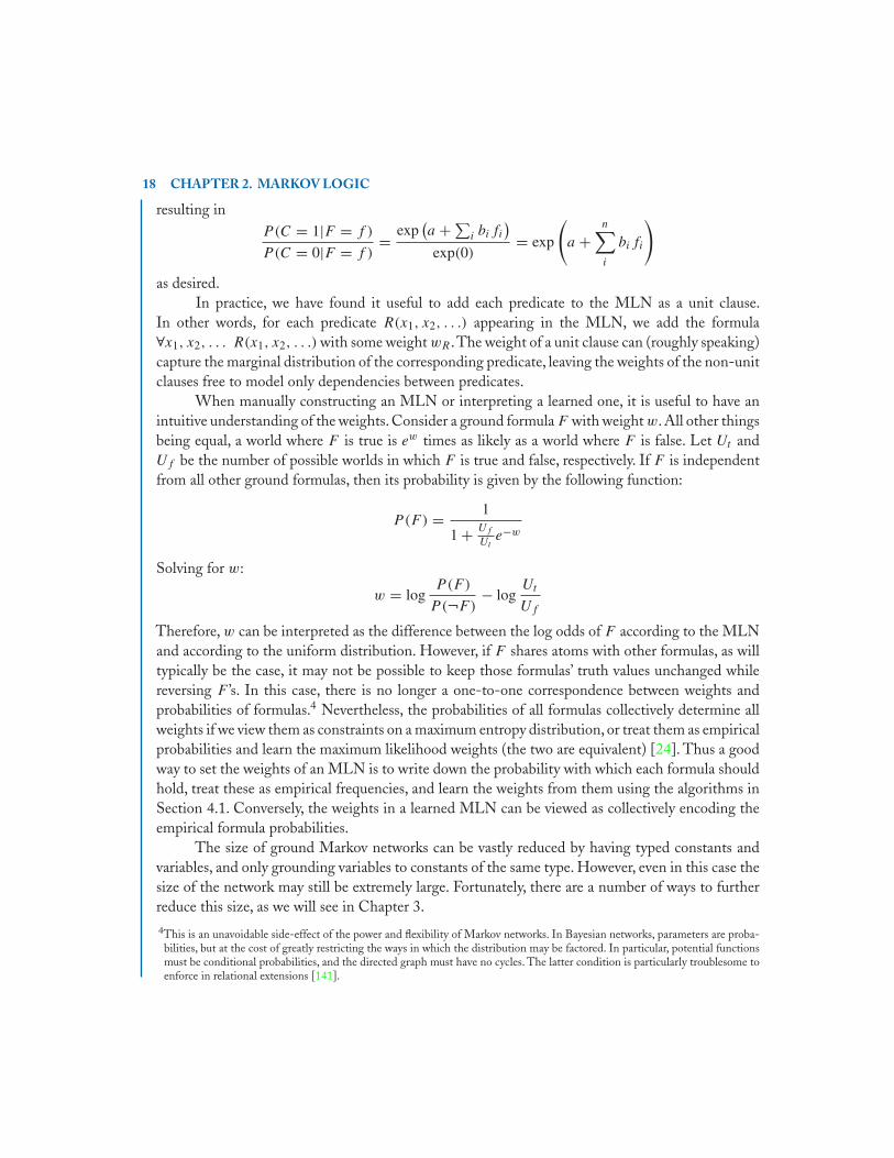
as desired.In practice, we have found it useful to add each predicate to the MLN as a unit clause.
In other words, for each predicate R(x1, x2, . . .) appearing in the MLN, we add the formula∀x1, x2, . . . R(x1, x2, . . .) with some weight wR .The weight of a unit clause can (roughly speaking)capture the marginal distribution of the corresponding predicate, leaving the weights of the non-unitclauses free to model only dependencies between predicates.
When manually constructing an MLN or interpreting a learned one, it is useful to have anintuitive understanding of the weights. Consider a ground formula F with weight w. All other thingsbeing equal, a world where F is true is ew times as likely as a world where F is false. Let Ut andUf be the number of possible worlds in which F is true and false, respectively. If F is independentfrom all other ground formulas, then its probability is given by the following function:
P(F) = 1
1 + Uf
Ute−w
Solving for w:
w = logP(F)
P (¬F)− log
Ut
Uf
Therefore, w can be interpreted as the difference between the log odds of F according to the MLNand according to the uniform distribution. However, if F shares atoms with other formulas, as willtypically be the case, it may not be possible to keep those formulas’ truth values unchanged whilereversing F ’s. In this case, there is no longer a one-to-one correspondence between weights andprobabilities of formulas.4 Nevertheless, the probabilities of all formulas collectively determine allweights if we view them as constraints on a maximum entropy distribution, or treat them as empiricalprobabilities and learn the maximum likelihood weights (the two are equivalent) [24]. Thus a goodway to set the weights of an MLN is to write down the probability with which each formula shouldhold, treat these as empirical frequencies, and learn the weights from them using the algorithms inSection 4.1. Conversely, the weights in a learned MLN can be viewed as collectively encoding theempirical formula probabilities.
The size of ground Markov networks can be vastly reduced by having typed constants andvariables, and only grounding variables to constants of the same type. However, even in this case thesize of the network may still be extremely large. Fortunately, there are a number of ways to furtherreduce this size, as we will see in Chapter 3.4This is an unavoidable side-effect of the power and flexibility of Markov networks. In Bayesian networks, parameters are proba-bilities, but at the cost of greatly restricting the ways in which the distribution may be factored. In particular, potential functionsmust be conditional probabilities, and the directed graph must have no cycles. The latter condition is particularly troublesome toenforce in relational extensions [141].

2.4. RELATION TO OTHER APPROACHES 19
2.4 RELATION TO OTHER APPROACHES
There is a very large literature relating logic and probability; here we will focus only on the approachesmost closely related to Markov logic.
EARLY WORKAttempts to combine logic and probability in AI date back to at least Nilsson [94]. Bacchus [1],Halpern [43] and coworkers (e.g., [2]) studied the problem in detail from a theoretical standpoint.They made a distinction between statistical statements (e.g., “65% of the students in our departmentare undergraduate”) and statements about possible worlds (e.g., “The probability that Anna is anundergraduate is 65%”), and provided methods for computing the latter from the former. In theirapproach, a KB did not specify a complete and unique distribution over possible worlds, leaving itsstatus as a probabilistic model unclear. MLNs overcome this limitation by viewing KBs as Markovnetwork templates.
Paskin [97] extended the work of Bacchus et al. [2] by associating a probability with each first-order formula, and taking the maximum entropy distribution compatible with those probabilities.This representation was still quite brittle, with a world that violates a single grounding of a universallyquantified formula being considered as unlikely as a world that violates all of them. In contrast, inMLNs a rule like ∀x Smokes(x) ⇒ Cancer(x) causes the probability of a world to decrease smoothlyas the number of cancer-free smokers in it increases.
KNOWLEDGE-BASED MODEL CONSTRUCTIONKnowledge-based model construction (KBMC) is a combination of logic programming and Bayesiannetworks [151, 93, 55]. As in MLNs, nodes in KBMC represent ground predicates. Given a HornKB, KBMC answers a query by finding all possible backward-chaining proofs of the query andevidence predicates from each other, constructing a Bayesian network over the ground predicatesin the proofs, and performing inference over this network. The parents of a predicate node in thenetwork are deterministic AND nodes representing the bodies of the clauses that have that node asthe head. The conditional probability of the node given these is specified by a combination function(e.g., noisy OR or logistic regression). MLNs have several advantages compared to KBMC: theyallow arbitrary formulas (not just Horn clauses) and inference in any direction, they sidestep thethorny problem of avoiding cycles in the Bayesian networks constructed by KBMC, and they do notrequire the introduction of ad hoc combination functions for clauses with the same consequent.
A KBMC model can be translated into an MLN by writing down a set of formulas for eachfirst-order predicate Pk(...) in the domain. Each formula is a conjunction containing Pk(...) and oneliteral per parent of Pk(...) (i.e., per first-order predicate appearing in a Horn clause having Pk(...)as the consequent). A subset of these literals are negated; there is one formula for each possiblecombination of positive and negative literals. The weight of the formula is w = log[p/(1 − p)],where p is the conditional probability of the child predicate when the corresponding conjunctionof parent literals is true, according to the combination function used. If the combination function is

20 CHAPTER 2. MARKOV LOGIC
logistic regression, it can be represented using only a linear number of formulas, taking advantageof the fact that a logistic regression model is a (conditional) Markov network with a binary cliquebetween each predictor and the response.Noisy OR can similarly be represented with a linear numberof parents.
OTHER LOGIC PROGRAMMING APPROACHESStochastic logic programs (SLPs) [87, 17] are a combination of logic programming and log-linearmodels. Puech and Muggleton [111] showed that SLPs are a special case of KBMC, and thus theycan be converted into MLNs in the same way. Like MLNs, SLPs have one coefficient per clause,but they represent distributions over Prolog proof trees rather than over predicates; the latter haveto be obtained by marginalization. Similar remarks apply to a number of other representations thatare essentially equivalent to SLPs, like independent choice logic [103] and PRISM [129].
MACCENT [23] is a system that learns log-linear models with first-order features; eachfeature is a conjunction of a class and a Prolog query (clause with empty head). A key differencebetween MACCENT and MLNs is that MACCENT is a classification system (i.e., it predictsthe conditional distribution of an object’s class given its properties), while an MLN represents thefull joint distribution of a set of predicates. Like any probability estimation approach, MLNs canbe used for classification simply by issuing the appropriate conditional queries.5 In particular, aMACCENT model can be converted into an MLN simply by defining a class predicate, adding thecorresponding features and their weights to the MLN, and adding a formula with infinite weightstating that each object must have exactly one class. (This fails to model the marginal distributionof the non-class predicates, which is not a problem if only classification queries will be issued.)MACCENT can make use of deterministic background knowledge in the form of Prolog clauses;these can be added to the MLN as formulas with infinite weight. In addition, MLNs allow uncertainbackground knowledge (via formulas with finite weights). As we demonstrate in Section 6.1, MLNscan be used for collective classification, where the classes of different objects can depend on eachother; MACCENT, which requires that each object be represented in a separate Prolog knowledgebase, does not have this capability.
Constraint logic programming (CLP) is an extension of logic programming where variablesare constrained instead of being bound to specific values during inference [64]. Probabilistic CLPgeneralizes SLPs to CLP [121], and CLP(BN ) combines CLP with Bayesian networks [128].Unlike in MLNs, constraints in CLP(BN ) are hard (i.e., they cannot be violated; rather, they definethe form of the probability distribution).
PROBABILISTIC RELATIONAL MODELSProbabilistic relational models (PRMs) [36] are a combination of frame-based systems and Bayesiannetworks. PRMs can be converted into MLNs by defining a predicate S(x, v) for each (propositionalor relational) attribute of each class, where S(x, v) means “The value of attribute S in object x is v.”
5Conversely, joint distributions can be built up from classifiers (e.g., [44]), but this would be a significant extension of MACCENT.

2.4. RELATION TO OTHER APPROACHES 21
A PRM is then translated into an MLN by writing down a formula for each line of each (class-level)conditional probability table (CPT) and value of the child attribute. The formula is a conjunction ofliterals stating the parent values and a literal stating the child value, and its weight is the logarithmof P(x|Parents(x)), the corresponding entry in the CPT. In addition, the MLN contains formulaswith infinite weight stating that each attribute must take exactly one value. This approach handlesall types of uncertainty in PRMs (attribute, reference and existence uncertainty).
As Taskar et al. [141] point out, the need to avoid cycles in PRMs causes significant represen-tational and computational difficulties. Inference in PRMs is done by creating the complete groundnetwork, which limits their scalability. PRMs require specifying a complete conditional model foreach attribute of each class, which in large complex domains can be quite burdensome. In contrast,MLNs create a complete joint distribution from whatever number of first-order features the userchooses to specify.
RELATIONAL MARKOV NETWORKSRelational Markov networks (RMNs) use database queries as clique templates, and have a featurefor each state of a clique [141]. MLNs generalize RMNs by providing a more powerful language forconstructing features (first-order logic instead of conjunctive queries), and by allowing uncertaintyover arbitrary relations (not just attributes of individual objects). RMNs are exponential in cliquesize, while MLNs allow the user (or learner) to determine the number of features, making it possibleto scale to much larger clique sizes.
STRUCTURAL LOGISTIC REGRESSIONIn structural logistic regression (SLR) [109], the predictors are the output of SQL queries over theinput data. Just as a logistic regression model is a discriminatively-trained Markov network, an SLRmodel is a discriminatively-trained MLN.6
RELATIONAL DEPENDENCY NETWORKSIn a relational dependency network (RDN), each node’s probability conditioned on its Markovblanket is given by a decision tree [90]. Every RDN has a corresponding MLN in the same way thatevery dependency network has a corresponding Markov network, given by the stationary distributionof a Gibbs sampler operating on it [44].
PLATES AND PROBABILISTIC ER MODELSLarge graphical models with repeated structure are often compactly represented using plates [14].MLNs subsume plates as a representation language. In addition, they allow individuals and theirrelations to be explicitly represented (see [18]), and context-specific independencies to be compactlywritten down, instead of left implicit in the node models. More recently, Heckerman et al. [46] haveproposed a language based on entity-relationship models that combines the features of plates and
6Use of SQL aggregates requires that their definitions be imported into the MLN.

22 CHAPTER 2. MARKOV LOGIC
PRMs; this language is a special case of MLNs in the same way that ER models are a special caseof logic. Probabilistic ER models allow logical expressions as constraints on how ground networksare constructed, but the truth values of these expressions have to be known in advance; MLNs allowuncertainty over all logical expressions.
BLOGMilch et al. [84] have proposed a language called BLOG, designed to avoid making the uniquenames and domain closure assumptions. A BLOG program specifies procedurally how to generatea possible world, and does not allow arbitrary first-order knowledge to be easily incorporated. Also,it only specifies the structure of the model, leaving the parameters to be specified by external calls.BLOG models are directed graphs and need to avoid cycles, which substantially complicates theirdesign. We saw in the previous section how to remove the unique names and domain closureassumptions in MLNs. (When there are unknown objects of multiple types, a random variable forthe number of each type is introduced.) Inference about an object’s attributes, rather than those ofits observations, can be done simply by having variables for objects as well as for their observations(e.g., for books as well as citations to them). To our knowledge, BLOG has not yet been evaluatedon any real-world problems, and no learning or general-purpose efficient inference algorithms forit have been developed.
FURTHER READINGSee Richardson and Domingos [117] for a somewhat expanded introduction to the Markov logicrepresentation. See Getoor and Taskar [39] for details on other representations that combine logicand probability. For more background on first-order logic, see Genesereth and Nilsson [37] or othertextbooks. For more background on Markov networks and other graphical models, see Koller andFriedman [61] or Pearl [99].
23
C H A P T E R 3
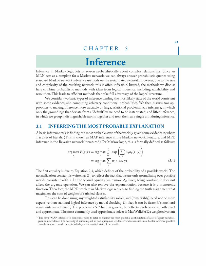
InferenceInference in Markov logic lets us reason probabilistically about complex relationships. Since anMLN acts as a template for a Markov network, we can always answer probabilistic queries usingstandard Markov network inference methods on the instantiated network. However, due to the sizeand complexity of the resulting network, this is often infeasible. Instead, the methods we discusshere combine probabilistic methods with ideas from logical inference, including satisfiability andresolution. This leads to efficient methods that take full advantage of the logical structure.
We consider two basic types of inference: finding the most likely state of the world consistentwith some evidence, and computing arbitrary conditional probabilities. We then discuss two ap-proaches to making inference more tractable on large, relational problems: lazy inference, in whichonly the groundings that deviate from a “default” value need to be instantiated; and lifted inference,in which we group indistinguishable atoms together and treat them as a single unit during inference.
3.1 INFERRING THE MOST PROBABLE EXPLANATIONA basic inference task is finding the most probable state of the world y given some evidence x, wherex is a set of literals. (This is known as MAP inference in the Markov network literature, and MPEinference in the Bayesian network literature.1) For Markov logic, this is formally defined as follows:
arg maxy
P (y|x) = arg maxy
1
Zx
exp
(∑i
wini(x, y)
)
= arg maxy
∑i
wini(x, y) (3.1)
The first equality is due to Equation 2.3, which defines of the probability of a possible world. Thenormalization constant is written as Zx to reflect the fact that we are only normalizing over possibleworlds consistent with x. In the second equality, we remove Zx since, being constant, it does notaffect the arg max operation. We can also remove the exponentiation because it is a monotonicfunction.Therefore, the MPE problem in Markov logic reduces to finding the truth assignment thatmaximizes the sum of weights of satisfied clauses.
This can be done using any weighted satisfiability solver, and (remarkably) need not be moreexpensive than standard logical inference by model checking. (In fact, it can be faster, if some hardconstraints are softened.) The problem is NP-hard in general, but effective solvers exist, both exactand approximate.The most commonly used approximate solver is MaxWalkSAT, a weighted variant1 The term “MAP inference” is sometimes used to refer to finding the most probable configuration of a set of query variables,given some evidence. The necessity of summing out all non-query, non-evidence variables makes this a harder inference problemthan the one we consider here, in which y is the complete state of the world.

24 CHAPTER 3. INFERENCE
Table 3.1: MaxWalkSAT algorithm for MPE inference.
function MaxWalkSAT(L, mt , mf , target, p)inputs: L, a set of weighted clauses
mt , the maximum number of triesmf , the maximum number of flipstarget, target solution costp, probability of taking a random step
output: soln, best variable assignment foundvars ← variables in L
for i ← 1 to mt
soln ← a random truth assignment to varscost ← sum of weights of unsatisfied clauses in solnfor i ← 1 to mf
if cost ≤ targetreturn “Success, solution is”, soln
c ← a randomly chosen unsatisfied clauseif Uniform(0,1) < p
vf ← a randomly chosen variable from celse
for each variable v in ccompute DeltaCost(v)
vf ← v with lowest DeltaCost(v)soln ← soln with vf flippedcost ← cost + DeltaCost(vf )
return “Failure, best assignment is”, best soln found
of the WalkSAT local-search satisfiability solver, which can solve hard problems with hundreds ofthousands of variables in minutes [53]. MaxWalkSAT performs this stochastic search by repeatedlypicking an unsatisfied clause at random and flipping the truth value of one of the atoms in it. Witha certain probability, the atom is chosen randomly; otherwise, the atom is chosen to maximize thesum of satisfied clause weights when flipped. This combination of random and greedy steps allowsMaxWalkSAT to avoid getting stuck in local optima while searching. Pseudocode for MaxWalkSATis shown in Table 3.1. DeltaCost(v) computes the change in the sum of weights of unsatisfied clausesthat results from flipping variable v in the current solution. Uniform(0,1) returns a uniform deviatefrom the interval [0, 1].

3.2. COMPUTING CONDITIONAL PROBABILITIES 25
3.2 COMPUTING CONDITIONAL PROBABILITIESMLNs can answer arbitrary queries of the form “What is the probability that formula F1 holdsgiven that formula F2 does?” If F1 and F2 are two formulas in first-order logic, C is a finite set ofconstants including any constants that appear in F1 or F2, and L is an MLN, then
P(F1|F2, L, C) = P(F1|F2, ML,C)
= P(F1 ∧ F2|ML,C)
P (F2|ML,C)
=∑
x∈XF1∩XF2P(X=x|ML,C)∑
x∈XF2P(X=x|ML,C)
(3.2)
where XFiis the set of worlds where Fi holds, ML,C is the Markov network defined by L and C,
and P(X = x|ML,C) is given by Equation 2.3. Ordinary conditional queries in graphical models arethe special case of Equation 3.2 where all predicates in F1, F2 and L are zero-arity and the formulasare conjunctions. The question of whether a knowledge base KB entails a formula F in first-orderlogic is the question of whether P(F |LKB, CKB,F ) = 1, where L is the MLN obtained by assigninginfinite weight to all the formulas in KB, and CKB,F is the set of all constants appearing in KB or F .The question is answered by computing P(F |LKB, CKB,F ) by Equation 3.2, with F2 = True.
Computing Equation 3.2 directly is intractable in all but the smallest domains. Since MLNinference subsumes probabilistic inference, which is #P-complete, and logical inference, which isNP-complete even in finite domains, no better results can be expected. However, many of the largenumber of techniques for efficient inference in either case are applicable to MLNs. Because MLNsallow fine-grained encoding of knowledge, including context-specific independences, inference inthem may in some cases be more efficient than inference in an ordinary graphical model for the samedomain. On the logic side, the probabilistic semantics of MLNs allows for approximate inference,with the corresponding potential gains in efficiency.
In principle, P(F1|F2, L, C) can be approximated using an MCMC algorithm that rejectsall moves to states where F2 does not hold, and counts the number of samples in which F1 holds.However, this may be too slow for arbitrary formulas. Instead, we focus on the case where F2 is aconjunction of ground literals. While less general than Equation 3.2, this is the most frequent typeof query in practice. In this scenario, further efficiency can be gained by applying a generalization ofknowledge-based model construction [151]. The basic idea is to only construct the minimal subsetof the ground network required to answer the query. This network is constructed by checking if theatoms that the query formula directly depends on are in the evidence. If they are, the construction iscomplete. Those that are not are added to the network, and we in turn check the atoms they dependon. This process is repeated until all relevant atoms have been retrieved. While in the worst case ityields no savings, in practice it can vastly reduce the time and memory required for inference.
Pseudocode for the network construction algorithm is shown in Table 3.2. See Figure 3.1 foran example of the resulting network. The size of the network returned may be further reduced, andthe algorithm sped up, by noticing that any ground formula that is made true by the evidence can
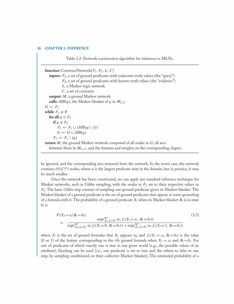
26 CHAPTER 3. INFERENCE
Table 3.2: Network construction algorithm for inference in MLNs.
function ConstructNetwork(F1, F2, L, C)inputs: F1, a set of ground predicates with unknown truth values (the “query”)
F2, a set of ground predicates with known truth values (the “evidence”)L, a Markov logic networkC, a set of constants
output: M , a ground Markov networkcalls: MB(q), the Markov blanket of q in ML,C
G ← F1
while F1 = ∅for all q ∈ F1
if q ∈ F2
F1 ← F1 ∪ (MB(q) \ G)
G ← G ∪ MB(q)
F1 ← F1 \ {q}return M , the ground Markov network composed of all nodes in G, all arcs
between them in ML,C , and the features and weights on the corresponding cliques.
be ignored, and the corresponding arcs removed from the network. In the worst case, the networkcontains O(|C|a) nodes, where a is the largest predicate arity in the domain, but in practice, it maybe much smaller.
Once the network has been constructed, we can apply any standard inference technique forMarkov networks, such as Gibbs sampling, with the nodes in F2 set to their respective values inF2. The basic Gibbs step consists of sampling one ground predicate given its Markov blanket. TheMarkov blanket of a ground predicate is the set of ground predicates that appear in some groundingof a formula with it. The probability of a ground predicate Xl when its Markov blanket Bl is in statebl is
P(Xl =xl|Bl =bl) (3.3)
= exp(∑
fi∈Flwifi(Xl =xl, Bl =bl))
exp(∑
fi∈Flwifi(Xl =0, Bl =bl)) + exp(
∑fi∈Fl
wifi(Xl =1, Bl =bl))
where Fl is the set of ground formulas that Xl appears in, and fi(Xl = xl, Bl =bl) is the value(0 or 1) of the feature corresponding to the ith ground formula when Xl = xl and Bl =bl . Forsets of predicates of which exactly one is true in any given world (e.g., the possible values of anattribute), blocking can be used (i.e., one predicate is set to true and the others to false in onestep, by sampling conditioned on their collective Markov blanket). The estimated probability of a

3.2. COMPUTING CONDITIONAL PROBABILITIES 27
Figure 3.1: Ground network for computing P(Cancer(B)|Smokes(A), Friends(A, B),Friends(B, A)), as built by the ConstructNetwork algorithm (Table 3.2). The constantsand network used are the same as in Figure 2.1, but for this query and evidence the atomsFriends(A, A) and Cancer(A) are irrelevant and can be omitted from the network.
conjunction of ground literals is simply the fraction of samples in which the ground literals are true,after the Markov chain has converged.
HANDLING DETERMINISTIC DEPENDENCIESOne problem with using Gibbs sampling for inference in MLNs is that it breaks down in thepresence of deterministic or near-deterministic dependencies (as do other probabilistic inferencemethods, e.g., belief propagation [156]). Deterministic dependencies break up the space of possibleworlds into regions that are not reachable from each other, violating a basic requirement of MCMC.Near-deterministic dependencies greatly slow down inference, by creating regions of low probabilitythat are very difficult to traverse. Running multiple chains with random starting points does notsolve this problem, because it does not guarantee that each region will be sampled with frequencyproportional to their probability, and there may be a very large number of regions.
The MC-SAT algorithm addresses this problem by combining MCMC with satisfiabilitytesting [105]. MC-SAT is a slice sampling MCMC algorithm which uses a combination of satisfia-bility testing and simulated annealing to sample from the slice.The advantage of using a satisfiabilitysolver (WalkSAT) is that it efficiently finds isolated modes in the distribution, and as a result theMarkov chain mixes very rapidly. The slice sampling scheme ensures that detailed balance is (ap-proximately) preserved.
MC-SAT is orders of magnitude faster than standard MCMC methods such as Gibbs sam-pling and simulated tempering, and is applicable to any model that can be expressed in Markov

28 CHAPTER 3. INFERENCE
Figure 3.2: Visual illustration of the MCMC slice sampling method. Given the kth sample, x(k),we first sample the auxiliary variable u(k) uniformly from the range [0, P (x(k)]. The next sample inthe Markov chain, x(k+1), is sampled uniformly from all x with P(x) ≥ u(k). This set of candidatex ’s is called the slice.
logic, including many standard models in statistical physics, vision, natural language processing,social network analysis, spatial statistics, etc.
Slice sampling [19] is an instance of a widely used approach in MCMC inference thatintroduces auxiliary variables, u, to capture the dependencies between observed variables, x.For example, to sample from P(X=x) = (1/Z)
∏k φk(x{k}), we can define P(X=x, U =u) =
(1/Z)∏
k I[0,φk(x{k})](uk), where φk is the kth potential function, uk is the kth auxiliary variable,I[a,b](uk) = 1 if a ≤ uk ≤ b, and I[a,b](uk) = 0 otherwise. The marginal distribution of X underthis joint is P(X=x), so to sample from the original distribution it suffices to sample from P(x, u)
and ignore the u values.This can be done by alternately sampling P(u|x) and P(x|u). See Figure 3.2for a graphical example of slice sampling.
P(uk|x) is uniform in [0, φk(x{k})], and thus easy to sample from. The main challenge is tosample x given u, which is uniform among all X that satisfy φk(x{k}) ≥ uk for all k. MC-SAT usesSampleSAT [150] to do this. In each sampling step, MC-SAT takes the set of all ground clausessatisfied by the current state of the world and constructs a subset,M , that must be satisfied by the nextsampled state of the world. (For the moment we will assume that all clauses have positive weight.)Specifically, a satisfied ground clause is included in M with probability 1 − e−w, where w is theclause’s weight. We then take as the next state a uniform sample from the set of states SAT (M) thatsatisfy M . (Notice that SAT (M) is never empty because it always contains at least the current state.)Table 3.3 gives pseudocode for MC-SAT. US is the uniform distribution over set S. At each step,

3.3. LAZY INFERENCE 29
Table 3.3: Efficient MCMC inference algorithm for MLNs.
function MC-SAT(L, n)inputs: L, a set of weighted clauses {(wj , cj )}
n, number of samplesoutput: {x(1), . . . , x(n)}, set of n samples
x(0) ← Satisfy(hard clauses in L)for i ← 1 to n
M ← ∅for all (wk, ck) ∈ L satisfied by x(i−1)
With probability 1 − e−wk add ck to M
Sample x(i) ∼ USAT (M)
all hard clauses are selected with probability 1, and thus all sampled states satisfy them. Negativeweights are handled by noting that a clause with weight w < 0 is equivalent to its negation withweight −w, and a clause’s negation is the conjunction of the negations of all of its literals. Thus,instead of checking whether the clause is satisfied, we check whether its negation is satisfied; if it is,with probability 1 − ew we select all of its negated literals, and with probability ew we select none.
It can be shown that MC-SAT satisfies the MCMC criteria of detailed balance and er-godicity [105], assuming a perfect uniform sampler. In general, uniform sampling is #P-hard andSampleSAT [150] only yields approximately uniform samples. However, experiments show thatMC-SAT is still able to produce very accurate probability estimates, and its performance is not verysensitive to the parameter settings of SampleSAT.
3.3 LAZY INFERENCE
One problem with the aforementioned approaches is that they require propositionalizing the domain(i.e., grounding all atoms and clauses in all possible ways), which consumes memory exponential inthe arity of the clauses. Lazy inference methods [135, 108] overcome this by only grounding atomsand clauses as needed.This takes advantage of the sparseness of relational domains,where most atomsare false and most clauses are trivially satisfied. For example, in the domain of scientific researchpapers, most groundings of the atom Author(person, paper) are false, and most groundings ofthe clause Author(p1, paper) ∧ Author(p2, paper) ⇒ Coauthor(p1, p2) are trivially satisfied.With lazy inference, the memory cost does not scale with the number of possible clause groundings,but only with the number of groundings that have non-default values at some point in the inference.
We first describe a general approach for making inference algorithms lazy and then show howit can be applied to create lazy versions of MaxWalkSAT and MC-SAT. This method applies toany algorithm that works by repeatedly selecting a function or variable and recomputing its value
30 CHAPTER 3. INFERENCE
depending only on a subset of the other variables/functions.These include a diverse set of algorithmsfor a variety of applications: WalkSAT, MaxWalkSAT, SampleSAT, DPLL, iterated conditionalmodes, simulated annealing and MCMC algorithms that update one variable at a time (Gibbssampling, single-component Metropolis-Hastings and simulated tempering, etc.), MC-SAT, beliefpropagation, algorithms for maximum expected utility, etc.
Our approach depends on the concept of “default” values that occur much more frequentlythan others. In relational domains, the default is false for atoms and true for clauses. In a domainwhere most variables assume the default value, it is wasteful to allocate memory for all variablesand functions in advance. The basic idea is to allocate memory only for a small subset of “active”variables and functions, and activate more if necessary as inference proceeds. In addition to savingmemory, this can reduce inference time as well, for we do not allocate memory and compute valuesfor functions that are never used.
Definition 3.1. Let X be the set of variables and D be their domain.2 The default value d∗ ∈ D
is the most frequent value of the variables. An evidence variable is a variable whose value is givenand fixed. A function f = f (z1, z2, · · · , zk) inputs zi ’s, which are either variables or functions, andoutputs some value in the range of f .
Although these methods can be applied to other inference algorithms, we focus on relationaldomains. Variables are ground atoms, which take binary values (i.e., D = {true, false}). The defaultvalue for variables is false (i.e., d∗ = false). Examples of functions are clauses and DeltaCost inMaxWalkSAT. Like variables, functions may also have default values (e.g., true for clauses). Theinputs to a relational inference algorithm are a weighted KB and a set of evidence atoms (DB).Eager algorithms work by first carrying out propositionalization and then calling a propositionalalgorithm. In lazy inference, we directly work on the KB and DB.The following concepts are crucialto lazy inference.
Definition 3.2. A variable v is active iff v is set to a non-default value at some point, and x isinactive if the value of x has always been d∗. A function f is activated by a variable v if either v isan input of f , or v activates a function g that is an input of f .
BASIC LAZY INFERENCELet A be the eager algorithm that we want to make lazy. We make three assumptions about A:
1. A updates one variable at a time. (If not, the extension is straightforward.)
2. The values of variables in A are properly encapsulated so that they can be accessed by therest of the algorithm only via two methods: ReadVar(x) (which returns the value of x) andWriteVar(x, v) (which sets the value of x to v). This is reasonable given the conventions insoftware development, and if not, it is easy to implement.
2For simplicity, we assume that all variables have the same domain. The extension to different domains is straightforward.

3.3. LAZY INFERENCE 31
3. A always sets values of variables before calling a function that depends on those variables, asit should be.
To develop the lazy version of A, we first identify the variables (usually all) and functions to makelazy. We then modify the value-accessing methods and replace the propositionalization step withlazy initialization as follows. The rest of the algorithm remains the same.
ReadVar(x): If x is in memory, Lazy-A returns its value as A; otherwise, it returns d∗.
WriteVar(x, v): If x is in memory, Lazy-A updates its value as A. If not, and if v = d∗, no actionis taken; otherwise, Lazy-A activates (allocates memory for) x and the functions activated byx, and then sets the value.
Initialization: Lazy-A starts by allocating memory for the lazy functions that output non-defaultvalues when all variables assume the default values. It then calls WriteVar to set values forevidence variables, which activates those evidence variables with non-default values and thefunctions they activate. Such variables become the initial active variables and their values arefixed throughout the inference.
Lazy-A carries out the same inference steps as A and produces the same result. It neverallocates memory for more variables/functions than A, but each access incurs slightly more overhead(in checking whether a variable or function is in memory). In the worst case, most variables areupdated, and Lazy-A produces little savings. However, if the updates are sparse, as is the case formost algorithms in relational domains, Lazy-A can greatly reduce memory and time because itactivates and computes the values for many fewer variables and functions.
REFINEMENTSThe basic version of lazy inference above is generally applicable, but it does not exploit the character-istics of the algorithm and may yield little savings in some cases. Next, we describe three refinementsthat apply to many algorithms.See Poon et al. [108] for additional optimizations and implementationdetails.
Function activation: To find the functions activated by a variable v, the basic version includes allfunctions that depend on v by traversing the dependency graph of variables/functions, startingfrom v. This can be done very efficiently, but may include functions whose values remainthe default even if v changes its value. A more intelligent approach traverses the graph andonly returns functions whose values become non-default if v changes its value. In general,this requires evaluating the functions, which can be expensive, but for some functions (e.g.,clauses), it can be done efficiently as described at the end of this section. Which approach touse depends on the function.
Variable recycling: In the basic version, a variable is activated once it is set to a non-default value,and so are the functions activated by the variable. This is necessary if the variable keeps the

32 CHAPTER 3. INFERENCE
non-default value, but could be wasteful in algorithms where many such updates are temporary(e.g., in simulated annealing and MCMC, we may temporarily set a variable to true to computethe probability for flipping). To save memory, if an inactive variable considered for flipping isnot flipped in the end, we can discard it along with the functions activated by it. However, thiswill increase inference time if the variable is considered again later, so we should only applythis if we want to trade off time for memory, or if the variable is unlikely to be consideredagain.
Smart randomization: Many local-search and MCMC algorithms use randomization to set initialvalues for variables, or to choose the next variable to update.This is usually done without takingthe sparsity of relational domains into account. For example, WalkSAT assigns random initialvalues to all variables; in a sparse domain where most atoms should be false, this is wasteful,because we will need to flip many atoms back to false. In lazy inference, we can randomize in abetter way by focusing more on the active atoms and those “nearby,” since they are more likelyto become true. Formally, a variable u is a 1-neighbor of a variable v if u is an input of a functionf activated by v; u is a k-neighbor of v (k > 1) if u is a (k − 1)-neighbor of v, or if u is a1-neighbor of a (k − 1)-neighbor of v. For initialization, we only randomize the k-neighborsof initial active variables; for variable selection, we also favor such variables.3 k can be usedto trade off efficiency and solution quality. With large k, this reduces to eager inference. Thesmaller k is, the more time and memory we can save from reducing the number of activations.However, we also run the risk of missing some relevant variables. If the domain is sparse, astypical relational domains are, the risk is negligible, and empirically we have observed thatk = 1 greatly improves efficiency without sacrificing solution quality.
LAZYSATApplying this method to MaxWalkSAT is fairly straightforward: each ground atom is a variable andeach ground clause is a function to be made lazy. Following Singla and Domingos [135], we referto the resulting algorithm as LazySAT. LazySAT initializes by activating true evidence atoms andinitial unsatisfied clauses (i.e., clauses which are unsatisfied when the true evidence atoms are setto true and all other atoms are set to false).4 At each step in the search, the atom that is flipped isactivated, as are any clauses that by definition should become active as a result. While computingDeltaCost(v), if v is active, the relevant clauses are already in memory; otherwise, they will beactivated when v is set to true (a necessary step before computing the cost change when v is set totrue). Table 3.4 gives pseudocode for LazySAT.
See Figure 3.3 for a sample application of LazySAT based on the Friends and Smokersexample.The figure on the left shows the initial state with the evidence Sm(A),Fr(A, B), and Fr(B, C).
3This does not preclude activation of remote relevant variables, which can happen after their clauses are active, or by randomselection (e.g., in simulated annealing).
4 This differs from MaxWalkSAT, which assigns random values to all atoms. However, the LazySAT initialization is a validMaxWalkSAT initialization, and the two give very similar results empirically. Given the same initialization, the two algorithmswill produce exactly the same results.

3.3. LAZY INFERENCE 33
Table 3.4: Lazy variant of the MaxWalkSAT algorithm.
function LazySAT(KB, DB, mt, mf , target, p)inputs: KB, a weighted knowledge base
DB, database containing evidencemt , the maximum number of triesmf , the maximum number of flipstarget, target solution costp, probability of taking a random step
output: soln, best variable assignment found
for i ← 1 to mt
active_atoms ← atoms in clauses not satisfied by DBactive_clauses ← clauses activated by active_atomssoln ← a random truth assignment to active_atomscost ← sum of weights of unsatisfied clauses in solnfor i ← 1 to mf
if cost ≤ targetreturn “Success, solution is”, soln
c ← a randomly chosen unsatisfied clauseif Uniform(0,1) < p
vf ← a randomly chosen variable from celse
for each variable v in ccompute DeltaCost(v), using KB if v ∈ active_atoms
vf ← v with lowest DeltaCost(v)if vf ∈ active_atoms
add vf to active_atomsadd clauses activated by vf to active_clauses
soln ← soln with vf flippedcost ← cost + DeltaCost(vf )
return “Failure, best assignment is”, best soln found

34 CHAPTER 3. INFERENCE
Figure 3.3: Two steps of the LazySAT algorithm. Darkened nodes represent active variables orfunctions.
By checking all clauses that reference these atoms, we can find and activate the one unsatisfied clause,Sm(A) ∧ Fr(A, B) ⇒ Sm(B). LazySAT next selects an unsatisfied clause at random (there is only oneso far) and picks an atom to satisfy it using a random or greedy criterion. In this case, LazySAT picksSm(B) and activates it and the now unsatisfied clause Sm(B) ∧ Fr(B, C) ⇒ Sm(C). By again selectingthe unsatisfied clause and flipping Sm(C) to satisfy it, LazySAT can arrive at a variable assignmentthat satisfies all clauses.
Experiments in a number of domains show that LazySAT can yield very large memory reduc-tions, and these reductions increase with domain size [135]. For domains whose full instantiations fitin memory, running time is comparable; as problems become larger, full instantiation for MaxWalk-SAT becomes impossible.
LAZY-MC-SATRecall the MC-SAT algorithm from Section 3.2, with pseudocode in Table 3.3. MC-SAT initial-izes with a solution to all hard clauses found by WalkSAT. In each iteration, it generates a set ofclauses M by sampling from the currently satisfied clauses according to their weights. It then callsSampleSAT [150] to select the next state by sampling near-uniformly the solutions to M . Sample-SAT initializes with a random state and, in each iteration, performs a simulated annealing step withprobability p and a WalkSAT step with probability 1 − p. To improve efficiency, MC-SAT runsunit propagation in M before calling SampleSAT (i.e., it repeatedly sets atoms in unit clauses to thecorresponding fixed values and simplifies the remaining clauses).
Here, the functions to be made lazy are clauses, clauses’ memberships in M , and whetheran atom is fixed by unit propagation. Effectively, Lazy-MC-SAT initializes by calling LazySATto find a solution to all hard clauses. At each iteration, it computes M-memberships for and runsunit propagation among active clauses only. It then calls Lazy-SampleSAT, the lazy version of

3.4. LIFTED INFERENCE 35
SampleSAT. Lazy-SampleSAT initializes using smart randomization with k = 1. When an inactiveatom v is set to false, no action is taken. When it is set to true, Lazy-SampleSAT activates v
and the clauses activated by v; it then computes M-memberships for these clauses,5 and runs unitpropagation among them; if v is fixed to false by unit propagation, Lazy-SampleSAT sets v backto false and applies variable recycling. It also applies variable recycling to simulated annealing steps.Notice that, when an M-membership or fixed-atom flag is set, this is remembered until the currentrun of Lazy-SampleSAT ends, to avoid inconsistencies.
3.4 LIFTED INFERENCE
The inference methods discussed so far are purely probabilistic in the sense that they propositionalizeall atoms and clauses and apply standard probabilistic inference algorithms. A key property of first-order logic is that it allows lifted inference, where queries are answered without materializing all theobjects in the domain (e.g., resolution [122]). Lifted inference is potentially much more efficientthan propositionalized inference, and extending it to probabilistic logical languages is a desirablegoal. The first approach to lifted probabilistic inference, first-order variable elimination (FOVE),was developed by Poole [104] and extended by Braz et al. [11, 12] and Milch et al. [85]. (Limitedlifted aspects are present in some earlier systems, like Pfeffer et al.’s [101] SPOOK.) Unfortunately,variable elimination has exponential cost in the treewidth of the graph, making it infeasible for mostreal-world applications. Scalable approximate algorithms for probabilistic inference fall into threemain classes: loopy belief propagation (BP), Monte Carlo methods, and variational methods.
We have developed a lifted version of BP [138], building on the work of Jaimovich et al. [51].Jaimovich et al. pointed out that, if there is no evidence, BP in probabilistic logical models can betrivially lifted, because all groundings of the same atoms and clauses become indistinguishable. Ourapproach proceeds by identifying the subsets of atoms and clauses that remain indistinguishableeven after evidence is taken into account. We then form a network with supernodes and superfeaturescorresponding to these sets, and apply BP to it.This network can be vastly smaller than the full groundnetwork, with the corresponding efficiency gains. Our algorithm produces the unique minimal liftednetwork for every inference problem.
BELIEF PROPAGATIONIn our description of Markov networks from Chapter 2, the graph G contains a node for eachvariable and an edge connecting each pair of variables that share a potential function, or factor.Markov networks can also be represented as factor graphs [62]. A factor graph is a bipartite graphwith a node for each variable and factor in the model. (For convenience, we will consider one factorfi(x) = exp(wigi(x)) per feature gi(x), i.e., we will not aggregate features over the same variablesinto a single factor.) Variables and the factors they appear in are connected by undirected edges. SeeFigure 3.4 for an example of a factor graph.
5These clauses must be previously satisfied; otherwise, they would have been activated before.

36 CHAPTER 3. INFERENCE
Figure 3.4: Belief propagation in a factor graph. Above is the equation for messages from variablesto factors; below is the equation for messages from factors to variables.
The main inference task in graphical models is to compute the conditional probability ofsome variables (the query) given the values of some others (the evidence), by summing out theremaining variables. This problem is #P-complete, but becomes tractable if the graph is a tree. Inthis case, the marginal probabilities of the query variables can be computed in polynomial time bybelief propagation, which consists of passing messages from variable nodes to the corresponding factornodes and vice-versa. The message from a variable x to a factor f is
μx→f (x) =∏
h∈nb(x)\{f }μh→x(x) (3.4)
where nb(x) is the set of factors x appears in. The message from a factor to a variable is
μf →x(x) =∑∼{x}
⎛⎝f (x)
∏y∈nb(f )\{x}
μy→f (y)
⎞⎠ (3.5)
where nb(f ) are the arguments of f , and the sum is over all of these except x. The messages fromleaf variables are initialized to 1, and a pass from the leaves to the root and back to the leaves suffices.The (unnormalized) marginal of each variable x is then given by
∏h∈nb(x) μh→x(x). Evidence is
incorporated by setting f (x) = 0 for states x that are incompatible with it.This algorithm can still beapplied when the graph has loops (e.g., Figure 3.4), repeating the message-passing until convergence.

3.4. LIFTED INFERENCE 37
Although this loopy belief propagation has no guarantees of convergence or of giving accurate results,in practice it often does, and can be much more efficient than other methods. Different schedulesmay be used for message-passing. Here we assume flooding, the most widely used and generallybest-performing method, in which messages are passed from each variable to each correspondingfactor and back at each step (after initializing all variable messages to 1).
Belief propagation can also be used for exact inference in arbitrary graphs, by combiningnodes until a tree is obtained, but this suffers from the same combinatorial explosion as variableelimination.
LIFTED BELIEF PROPAGATIONWe begin with some necessary definitions.These assume the existence of an MLN L, set of constantsC, and evidence database E (set of ground literals). For simplicity, our definitions and explanationof the algorithm will assume that each predicate appears at most once in any given MLN clause. Wewill then describe how to handle multiple occurrences of a predicate in a clause.
Definition 3.3. A supernode is a set of groundings of a predicate that all send and receive the samemessages at each step of belief propagation, given L, C and E. The supernodes of a predicate forma partition of its groundings.
A superfeature is a set of groundings of a clause that all send and receive the same messages ateach step of belief propagation, given L, C and E. The superfeatures of a clause form a partition ofits groundings.
Definition 3.4. A lifted network is a factor graph composed of supernodes and superfeatures. Thefactor corresponding to a superfeatureg(x) is exp(wg(x)),wherew is the weight of the correspondingfirst-order clause. A supernode and a superfeature have an edge between them iff some ground atomin the supernode appears in some ground clause in the superfeature. Each edge has a positive integerweight. A minimal lifted network is a lifted network with the smallest possible number of supernodesand superfeatures.
The first step of lifted BP is to construct the minimal lifted network. The size of this networkis O(nm), where n is the number of supernodes and m the number of superfeatures. In the bestcase, the lifted network has the same size as the MLN L; in the worst case, as the ground Markovnetwork ML,C .
The second and final step in lifted BP is to apply standard BP to the lifted network, with twochanges:
1. The message from supernode x to superfeature f becomes
μn(f,x)−1f →x
∏h∈nb(x)\{f }
μh→x(x)n(h,x)
where n(h, x) is the weight of the edge between h and x.

38 CHAPTER 3. INFERENCE
2. The (unnormalized) marginal of each supernode (and, therefore, of each ground atom in it) isgiven by
∏h∈nb(x) μ
n(h,x)h→x (x).
The weight of an edge is the number of identical messages that would be sent from the groundclauses in the superfeature to each ground atom in the supernode if BP was carried out on theground network. The n(f, x) − 1 exponent reflects the fact that a variable’s message to a factorexcludes the factor’s message to the variable.
The lifted network is constructed by (essentially) simulating BP and keeping track of whichground atoms and clauses send the same messages. Initially, the groundings of each predicate fallinto three groups: known true, known false and unknown. (One or two of these may be empty.)Each such group constitutes an initial supernode. All groundings of a clause whose atoms havethe same combination of truth values (true, false or unknown) now send the same messages to theground atoms in them. In turn, all ground atoms that receive the same number of messages fromthe superfeatures they appear in send the same messages, and constitute a new supernode. As theeffect of the evidence propagates through the network, finer and finer supernodes and superfeaturesare created.
If a clause involves predicates R1, . . . , Rk , and N = (N1, . . . , Nk) is a corresponding tupleof supernodes, the groundings of the clause generated by N are found by joining N1, . . . , Nk (i.e.,by forming the Cartesian product of the relations N1, . . . , Nk , and selecting the tuples in which thecorresponding arguments agree with each other, and with any corresponding constants in the first-order clause). Conversely, the groundings of predicate Ri connected to elements of a superfeatureF are obtained by projecting F onto the arguments it shares with Ri . Lifted network constructionthus proceeds by alternating between two steps:
1. Form superfeatures by doing joins of their supernodes.
2. Form supernodes by projecting superfeatures down to their predicates, and merging atomswith the same projection counts.
Pseudocode for the algorithm is shown in Table 3.5. The projection counts at convergence are theweights associated with the corresponding edges.
To handle clauses with multiple occurrences of a predicate, we keep a tuple of edge weights,one for each occurrence of the predicate in the clause. A message is passed for each occurrenceof the predicate, with the corresponding edge weight. Similarly, when projecting superfeatures intosupernodes, a separate count is maintained for each occurrence, and only tuples with the same countsfor all occurrences are merged.
Figure 3.5 demonstrates how the initial supernodes and superfeatures are constructed for afriendship (Fr(x, y)) and smoking (Sm(x)) domain based on the example of Table 2.1. The onlyrule in the MLN is Sm(x) ∧ Fr(x, y) ⇒ Sm(y) (if two people are friends and one smokes, so doesthe other). We assume a set of n constants, {A, B, C, D, . . .} and the evidence Sm(A), Fr(B, C), andFr(C, B).To form the supernodes, each predicate is partitioned into its unknown and true groundings(since there are no false atoms in the evidence), yielding four initial supernodes. These are joined in

3.4. LIFTED INFERENCE 39
Table 3.5: Lifted network construction algorithm.
function LNC(L, C, E)inputs: L, a Markov logic network
C, a set of constantsE, a set of ground literals
output: M , a lifted networkfor each predicate P
for each truth value t in {true, false, unknown}form a supernode containing all groundings of P with truth value t
repeatfor each clause involving predicates P1, . . . , Pk
for each tuple of supernodes (N1, . . . , Nk),where Ni is a Pi supernodeform a superfeature F by joining N1, . . . , Nk
for each predicate P
for each superfeature F it appears inS(P, F ) ← projection of the tuples in F down to the variables in P
for each tuple s in S(P, F )
T (s, F ) ← number of F ’s tuples that were projected into s
S(P ) ← ⋃F S(P, F )
form a new supernode from each set of tuples in S(P ) with thesame T (s, F ) counts for all F
until convergenceadd all current supernodes and superfeatures to M
for each supernode N and superfeature F in M
add to M an edge between N and F with weight T (s, F )
return M

40 CHAPTER 3. INFERENCE
Figure 3.5: Initial supernodes and superfeatures when Sm(A), Fr(B, C), and Fr(C, B) are evidenceand the only formula is Sm(x) ∧ Fr(x, y) ⇒ Sm(y).
all possible ways to produce five superfeatures. For clarity, each superfeature in Figure 3.5 is labeledwith the supernodes it joins. The next step in lifted network construction is to count the numberof times each atom appears in each position in each superfeature, as shown in Table 3.6 for theSm() predicate. Atoms with the same counts are clustered into new supernodes, as indicated by thehorizontal lines in Table 3.6. These new supernodes are joined to produce new superfeatures, thenprojected to produce refined supernodes, and so on until convergence.
Theorem 3.5. Given an MLN L, set of constants C and set of ground literals E, there exists a uniqueminimal lifted network M∗, and algorithm LNC(L, C, E) returns it. Belief propagation applied to M∗produces the same results as belief propagation applied to the ground Markov network generated by L andC.
See Singla and Domingos [138] for the proof.Clauses involving evidence atoms can be simplified (false literals and clauses containing true
literals can be deleted). As a result, duplicate clauses may appear, and the corresponding superfeatures

3.4. LIFTED INFERENCE 41
Table 3.6: Projection of superfeatures from Figure 3.5 down to the Sm() predicate. Two projectedcounts are provided for each feature, since Sm() appears twice in the rule Sm(x) ∧ Fr(x, y) ⇒ Sm(y).Horizontal lines cluster the atoms into a new set of supernodes.
Atom F1 F2 F3 F4 F5
Sm(A) 1 1 n − 1 0 0 n − 1 0 0 0 0Sm(B) 0 0 0 1 1 0 1 1 n − 2 n − 2Sm(C) 0 0 0 1 1 0 1 1 n − 2 n − 2Sm(D) 0 0 0 1 1 0 0 0 n − 1 n − 1Sm(E) 0 0 0 1 1 0 0 0 n − 1 n − 1. . . 0 0 0 1 1 0 0 0 n − 1 n − 1
can be merged. This will typically result in duplicate instances of tuples. Each tuple in the mergedsuperfeature is assigned a weight
∑i miwi , where mi is the number of duplicate tuples resulting
from the ith superfeature and wi is the corresponding weight. During the creation of supernodes,T (s, F ) is now the number of F tuples projecting into s multiplied by the corresponding weight.This can greatly reduce the size of the lifted network. When no evidence is present, the algorithmreduces to the one proposed by Jaimovich et al. [51].
An important question remains: how to represent supernodes and superfeatures.Although thisdoes not affect the space or time cost of belief propagation (where each supernode and superfeatureis represented by a single symbol), it can greatly affect the cost of constructing the lifted network.The simplest option is to represent each supernode or superfeature extensionally as a set of tuples (i.e.,a relation), in which case joins and projections reduce to standard database operations. However, inthis case the cost of constructing the lifted network is similar to the cost of constructing the fullground network, and can easily become the bottleneck. A better option is to use a more compactintensional representation, as done by Poole [104] and Braz et al. [11, 12].6
A ground atom can be viewed as a first-order atom with all variables constrained to be equal toconstants, and similarly for ground clauses. (For example, R(A, B) is R(x, y) with x = A and y = B.)We represent supernodes by sets of (α, γ ) pairs, where α is a first-order atom and γ is a set ofconstraints, and similarly for superfeatures. Constraints are of the form x = y or x = y, where x isan argument of the atom andy is either a constant or another argument.For example,(S(v, w, x, y, z),{w = x, y = A, z = B, z = C}) compactly represents all groundings of S(v, w, x, y, z) compatiblewith the constraints. Notice that variables may be left unconstrained, and that infinite sets of atomscan be finitely represented in this way.
Let the default value of a predicate R be its most frequent value given the evidence (true,false or unknown). Let SR,i be the set of constants that appear as the ith argument of R only in6Superfeatures are related, but not identical, to the parfactors of Poole and Braz et al.. One important difference is that superfeaturescorrespond to factors in the original graph,while parfactors correspond to factors created during variable elimination.Superfeaturesare thus exponentially more compact.

42 CHAPTER 3. INFERENCE
groundings with the default value. Supernodes not involving any members of SR,i for any argumenti are represented extensionally (i.e. with pairs (α, γ ) where γ contains a constraint of the formx = A, where A is a constant, for each argument x). Initially, supernodes involving members of SR,i
are represented using (α, γ ) pairs containing constraints of the form x = A for each A ∈ C \ SR,i .7
When two or more supernodes are joined to form a superfeature F , if the kth argument of F ’sclause is the i(j)th argument of its j th literal, Sk = ⋂
j Sr(j),i , where r(j) is the predicate symbolin the j th literal. F is now represented analogously to the supernodes, according to whether or notit involves elements of Sk . If F is represented intensionally, each (α, γ ) pair is divided into onepair for each possible combination of equality/inequality constraints among the clause’s arguments,which are added to γ . When forming a supernode from superfeatures, the constraints in each (α, γ )
pair in the supernode are the union of (a) the corresponding constraints in the superfeatures on thevariables included in the supernode, and (b) the constraints induced by the excluded variables onthe included ones. This process is analogous to the shattering process of Braz et al. [11].
In general, finding the most compact representation for supernodes and superfeatures is anintractable problem, and is an area of active research.
FURTHER READINGThe MaxWalkSAT algorithm used for MPE inference in Markov logic is described in Kautzet al. [53]. Its source code is available at http://www.cs.rochester.edu/˜kautz/walksat/.MaxWalkSAT is a propositional MaxSAT solver, so the MLN formulas are first grounded in allpossible ways to construct the MaxSAT problem for MaxWalkSAT to solve.
For full details on MC-SAT, including experimental evaluation, see Poon and Domin-gos [105].
For more information about LazySAT,including experiments, see Singla and Domingos [135].For a more general treatment of lazy inference, including details on Lazy-MC-SAT and how tomake other algorithms lazy, see Poon et al. [108].
Recently, Riedel [118] proposed Cutting Plane Inference (CPI), an alternative MAP solverbased on cutting plane methods. CPI is similar to lazy inference in that it adds clauses only asneeded. Riedel uses both MaxWalkSAT and integer linear programming as the “base” solver. Ona semantic role labeling problem, CPI with integer linear programming was able to find the exactMAP solution faster than MaxWalkSAT could approximate it.
An introduction to the original belief propagation algorithm can be found in Yedidia etal. [156]. For details, proofs, and experiments on lifted belief propagation, see Singla and Domin-gos [138]. Publications on exact lifted inference include Poole [104], Braz et al. [11, 12], and Milchet al. [85].
7In practice, variables are typed, and C is replaced by the domain of the argument; and the set of constraints is only stored once,and pointed to as needed.

43
C H A P T E R 4
LearningLearning algorithms use data to automatically construct or refine a Markov logic network, typicallyobtaining much better models with less work than manually specifying the complete model. Webegin by discussing weight learning, in which we try to find the formula weights that maximize thelikelihood or conditional likelihood of a relational database.Our methods for solving this problem arebased on convex optimization but take into account the hardness of inference. Structure learning, inwhich we try to learn the formulas themselves, is a much harder problem.We present two approachesbased on inductive logic programming. Finally, we describe how new concepts can be discoveredthrough statistical predicate invention, and how experience in one domain can help us learn fasterin another through transfer learning. Solutions for these problems naturally use second-order Markovlogic to reason about predicates in much the way that first-order Markov logic reasons about objects.
4.1 WEIGHT LEARNINGGENERATIVE WEIGHT LEARNINGMLN weights can be learned generatively by maximizing the likelihood of a relational database(Equation 2.3). This relational database consists of one or more “possible worlds” that form ourtraining examples. We assume that the set of constants of each type is known. We also make aclosed-world assumption [37]: all ground atoms not in the database are false.1 If there are n possibleground atoms, a database is effectively a vector x = (x1, . . . , xl, . . . , xn) where xl is the truth valueof the lth ground atom (xl = 1 if the atom appears in the database, and xl = 0 otherwise). Note thatwe can learn to generalize from even a single example because the clause weights are shared acrosstheir many respective groundings. Given a database, MLN weights can in principle be learned usingstandard methods, as follows. If the ith formula has ni(x) true groundings in the data x, then byEquation 2.3, the derivative of the log-likelihood with respect to its weight is
∂
∂wi
log Pw(X=x) = ni(x) −∑x′
Pw(X=x′) ni(x′) (4.1)
where the sum is over all possible databases x′, and Pw(X=x′) is P(X=x′) computed using thecurrent weight vector w = (w1, . . . , wi, . . .). In other words, the ith component of the gradientis simply the difference between the number of true groundings of the ith formula in the dataand its expectation according to the current model. We can derive this expression as follows. The
1This assumption can be removed by using the expectation maximization (EM) algorithm [25] to learn from the resulting incompletedata, as we will see in Section 4.3.

44 CHAPTER 4. LEARNING
log-likelihood itself is just the log of Equation 2.3:
Pw(X=x) = 1
Zexp
⎛⎝∑
j
wjnj (x)
⎞⎠
log Pw(X=x) =∑j
wjnj (x) − log Z (4.2)
Now we take the partial derivative.
∂
∂wi
log Pw(X=x) = ∂
∂wi
∑j
wjnj (x) − ∂
∂wi
log Z
= ni(x) − 1
Z
∂
∂wi
Z (4.3)
= ni(x) − 1
Z
∑x′
∂
∂wi
exp
⎛⎝∑
j
wjnj (x′)
⎞⎠ (4.4)
= ni(x) − 1
Z
∑x′
exp
⎛⎝∑
j
wjnj (x′)
⎞⎠ ni(x
′) (4.5)
= ni(x) −∑x′
Pw(X=x′)ni(x′)
Equation 4.3 follows from basic derivative rules. In particular, note that the derivative of wjnj (x)
with respect to wi is zero for j = i. We substitute the definition of Z to obtain Equation 4.4, andwe apply the chain and sum rules to obtain Equation 4.5. By moving Z inside the summation andsubstituting the definition of Pw, we arrive at Equation 4.1.
In the worst case, counting the number of true groundings of a formula in a database isintractable, even when the formula is a single clause, as stated in the following proposition (due toDan Suciu):
Proposition 4.1. Counting the number of true groundings of a first-order clause in a database is #P-complete in the length of the clause.
Proof. Counting satisfying assignments of propositional monotone 2-CNF is #P-complete [123].This problem can be reduced to counting the number of true groundings of a first-order clausein a database as follows. Consider a database composed of the ground atoms R(0, 1), R(1, 0) andR(1, 1). Given a monotone 2-CNF formula, construct a formula F that is a conjunction of atoms ofthe form R(xi, xj ), one for each disjunction xi ∨ xj appearing in the CNF formula. (For example,(x1 ∨ x2) ∧ (x3 ∨ x4) would yield R(x1, x2) ∧ R(x3, x4).) There is a one-to-one correspondencebetween the satisfying assignments of the 2-CNF and the true groundings of F . The latter are the

4.1. WEIGHT LEARNING 45
Figure 4.1:Comparison of pseudo-likelihood and likelihood on a simple three-node network.Shadednodes represent conditioning on the true values. Pseudo-likelihood (above) is the product of theprobability of each node conditioned on its Markov blanket. In contrast, likelihood (below) obeysthe chain rule of probability when decomposed.
false groundings of the disjunction of the negations of all the R(xi, xj ), and thus can be counted bycounting the number of true groundings of this clause and subtracting it from the total number ofgroundings. �
In large domains, the number of true groundings of a formula may be counted approximately,by uniformly sampling groundings of the formula and checking whether they are true in the data.In smaller domains, and in most applications to date, we use an efficient recursive algorithm to findthe exact count.
A second problem with Equation 4.1 is that computing the expected number of true ground-ings is also intractable, requiring inference over the model. Instead, we maximize the pseudo-likelihood of the data, a widely used alternative [6]. If x is a possible world (relational database)and xl is the lth ground atom’s truth value, the pseudo-log-likelihood of x given weights w is
log P ∗w(X=x) =
n∑l=1
log Pw(Xl =xl|MBx(Xl)) (4.6)
where MBx(Xl) is the state of Xl ’s Markov blanket in the data (i.e., the truth values of the groundatoms it appears in some ground formula with). Figure 4.1 illustrates the difference between pseudo-likelihood and likelihood on a simple three-node network.The gradient of the pseudo-log-likelihood

46 CHAPTER 4. LEARNING
is
∂
∂wi
log P ∗w(X=x) =
n∑l=1
[ni(x) − Pw(Xl =0|MBx(Xl)) ni(x[Xl=0])
−Pw(Xl =1|MBx(Xl)) ni(x[Xl=1])] (4.7)
where ni(x[Xl=0]) is the number of true groundings of the ith formula when we force Xl = 0 and leavethe remaining data unchanged, and similarly for ni(x[Xl=1]). Computing this expression (or Equa-tion 4.6) does not require inference over the model, and is therefore much faster. The computationcan be made more efficient in several ways:
• The sum in Equation 4.7 can be greatly sped up by ignoring predicates that do not appear inthe ith formula.
• The counts ni(x), ni(x[Xl=0]) and ni(x[Xl=0]) do not change with the weights, and need onlybe computed once (as opposed to in every iteration of optimization).
• Ground formulas whose truth value is unaffected by changing the truth value of any singleliteral may be ignored, since then ni(x) = ni(x[Xl=0]) = ni(x[Xl=0]). In particular, this holdsfor any clause which contains at least two true literals. This can often be the great majority ofground clauses.
Combined with the L-BFGS optimizer [71], pseudo-likelihood yields efficient learning ofMLN weights even in domains with millions of ground atoms [117].However, the pseudo-likelihoodparameters may lead to poor results when long chains of inference are required. In the next sectionon discriminative learning, we will see how optimizing the conditional likelihood instead can yieldbetter results.
In order to reduce overfitting, we penalize each weight with a Gaussian prior. We apply thisstrategy not only to generative learning, but to all of our weight learning methods, including thoseembedded within structure learning.
DISCRIMINATIVE WEIGHT LEARNINGIn discriminative learning, we know a priori which atoms will be evidence and which ones will bequeried, and the goal is to correctly predict the latter given the former. Such a distinction betweenevidence and query naturally exists in most applications. For example, in collective classification(Section 6.1), the goal is to predict each object’s class given all other attributes and relations. If wepartition the ground atoms in the domain into a set of evidence atoms X and a set of query atomsY , the conditional likelihood of Y given X is
P(Y =y|X=x) = 1
Zx
exp
(∑i
wini(x, y)
)(4.8)
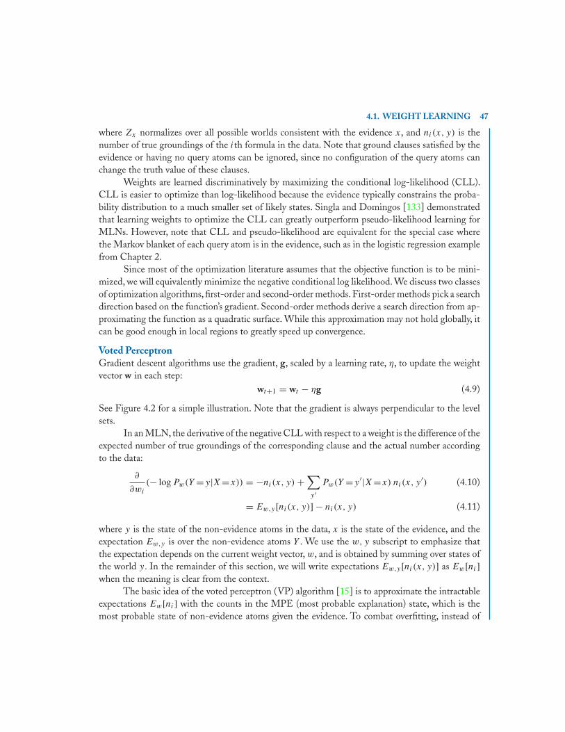
4.1. WEIGHT LEARNING 47
where Zx normalizes over all possible worlds consistent with the evidence x, and ni(x, y) is thenumber of true groundings of the ith formula in the data. Note that ground clauses satisfied by theevidence or having no query atoms can be ignored, since no configuration of the query atoms canchange the truth value of these clauses.
Weights are learned discriminatively by maximizing the conditional log-likelihood (CLL).CLL is easier to optimize than log-likelihood because the evidence typically constrains the proba-bility distribution to a much smaller set of likely states. Singla and Domingos [133] demonstratedthat learning weights to optimize the CLL can greatly outperform pseudo-likelihood learning forMLNs. However, note that CLL and pseudo-likelihood are equivalent for the special case wherethe Markov blanket of each query atom is in the evidence, such as in the logistic regression examplefrom Chapter 2.
Since most of the optimization literature assumes that the objective function is to be mini-mized, we will equivalently minimize the negative conditional log likelihood. We discuss two classesof optimization algorithms, first-order and second-order methods. First-order methods pick a searchdirection based on the function’s gradient. Second-order methods derive a search direction from ap-proximating the function as a quadratic surface. While this approximation may not hold globally, itcan be good enough in local regions to greatly speed up convergence.
Voted PerceptronGradient descent algorithms use the gradient, g, scaled by a learning rate, η, to update the weightvector w in each step:
wt+1 = wt − ηg (4.9)
See Figure 4.2 for a simple illustration. Note that the gradient is always perpendicular to the levelsets.
In an MLN, the derivative of the negative CLL with respect to a weight is the difference of theexpected number of true groundings of the corresponding clause and the actual number accordingto the data:
∂
∂wi
(− log Pw(Y =y|X=x)) = −ni(x, y) +∑y′
Pw(Y =y′|X=x) ni(x, y′) (4.10)
= Ew,y[ni(x, y)] − ni(x, y) (4.11)
where y is the state of the non-evidence atoms in the data, x is the state of the evidence, and theexpectation Ew,y is over the non-evidence atoms Y . We use the w, y subscript to emphasize thatthe expectation depends on the current weight vector, w, and is obtained by summing over states ofthe world y. In the remainder of this section, we will write expectations Ew,y[ni(x, y)] as Ew[ni]when the meaning is clear from the context.
The basic idea of the voted perceptron (VP) algorithm [15] is to approximate the intractableexpectations Ew[ni] with the counts in the MPE (most probable explanation) state, which is themost probable state of non-evidence atoms given the evidence. To combat overfitting, instead of
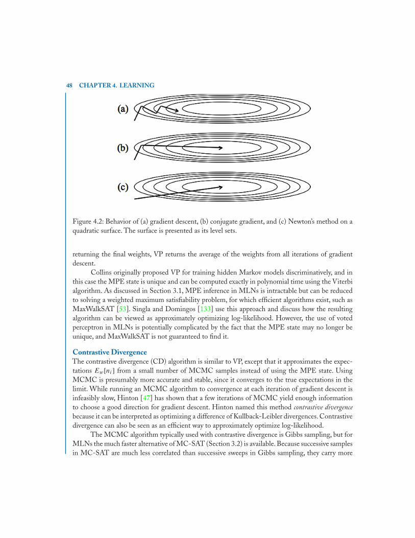
48 CHAPTER 4. LEARNING
Figure 4.2: Behavior of (a) gradient descent, (b) conjugate gradient, and (c) Newton’s method on aquadratic surface. The surface is presented as its level sets.
returning the final weights, VP returns the average of the weights from all iterations of gradientdescent.
Collins originally proposed VP for training hidden Markov models discriminatively, and inthis case the MPE state is unique and can be computed exactly in polynomial time using the Viterbialgorithm. As discussed in Section 3.1, MPE inference in MLNs is intractable but can be reducedto solving a weighted maximum satisfiability problem, for which efficient algorithms exist, such asMaxWalkSAT [53]. Singla and Domingos [133] use this approach and discuss how the resultingalgorithm can be viewed as approximately optimizing log-likelihood. However, the use of votedperceptron in MLNs is potentially complicated by the fact that the MPE state may no longer beunique, and MaxWalkSAT is not guaranteed to find it.
Contrastive DivergenceThe contrastive divergence (CD) algorithm is similar to VP, except that it approximates the expec-tations Ew[ni] from a small number of MCMC samples instead of using the MPE state. UsingMCMC is presumably more accurate and stable, since it converges to the true expectations in thelimit. While running an MCMC algorithm to convergence at each iteration of gradient descent isinfeasibly slow, Hinton [47] has shown that a few iterations of MCMC yield enough informationto choose a good direction for gradient descent. Hinton named this method contrastive divergencebecause it can be interpreted as optimizing a difference of Kullback-Leibler divergences. Contrastivedivergence can also be seen as an efficient way to approximately optimize log-likelihood.
The MCMC algorithm typically used with contrastive divergence is Gibbs sampling, but forMLNs the much faster alternative of MC-SAT (Section 3.2) is available. Because successive samplesin MC-SAT are much less correlated than successive sweeps in Gibbs sampling, they carry more
4.1. WEIGHT LEARNING 49
information and are likely to yield a better descent direction. In particular, the different samplesare likely to be from different modes, reducing the error and potential instability associated withchoosing a single mode.
In an MLN, each state typically contains a large number of instances of each clause, unlikei.i.d. learning, which would contain only one. This makes even a small number of MCMC stepsparticularly effective in relational domains. In our experience, five samples is often sufficient andadditional samples may not be worth the time: any increased accuracy that 10 or 100 samples mightbring is offset by the increased time per iteration. We avoid the need for burn-in by starting at thelast state sampled in the previous iteration of gradient descent. (This differs from Hinton’s approach,which always starts at the true values in the training data.)
Per-Weight Learning RatesVP and CD are both simple gradient descent procedures, and as a result highly vulnerable to theproblem of ill-conditioning. On ill-conditioned problems, the direction of steepest descent is nearlyorthogonal to the direction to the optimum, causing gradient descent to take many iterations toconverge. Ill-conditioning occurs when the condition number, the ratio between the largest andsmallest eigenvalues of the Hessian (matrix of second derivatives), is far from one. In MLNs, theHessian is the negative covariance matrix of the clause counts. Because some clauses can havevastly greater numbers of true groundings than others, the variances of their counts can be corre-spondingly larger, and ill-conditioning becomes a serious issue. Intuitively, gradient descent is slowbecause no single learning rate is appropriate for all weights; a clause with O(n) groundings, suchas Smokes(x) ⇒ Cancer(x), will typically require a much higher learning rate than a clause withO(n3) groundings, such as transitivity.
One solution is to modify both algorithms to have a different learning rate for each weight.Since tuning every learning rate separately is impractical,we use a simple heuristic to assign a learningrate to each weight:
ηi = η
ni
where η is the user-specified global learning rate and ni is the number of true groundings of theith formula. (To avoid dividing by zero, if ni = 0 then ηi = η.) When computing this number, weignore the groundings that are satisfied by the evidence (e.g., A ⇒ B when A is false). This isbecause, being fixed, they cannot contribute to the variance.
Diagonal NewtonWhen the function being optimized is quadratic, as in Figure 4.2, Newton’s method can move tothe global minimum or maximum in a single step. It does so by multiplying the gradient, g, by theinverse Hessian, H−1:
wt+1 = wt − H−1g (4.12)
When there are many weights, inverting the full Hessian becomes infeasible. A common ap-proximation is to use the diagonal Newton (DN) method, which makes the simplifying assumption

50 CHAPTER 4. LEARNING
that all off-diagonal entries of the Hessian are zero, yielding an easily inverted diagonal matrix.DN typically uses a smaller step size than the full Newton method. This is important when apply-ing the algorithm to non-quadratic functions, such as the CLL of an MLN, where the quadraticapproximation is only good within a local region.
The Hessian of the negative CLL for an MLN is simply the covariance matrix:
∂
∂wi∂wj
(− log Pw(Y =y|X=x)) = Ew[ninj ] − Ew[ni]Ew[nj ] (4.13)
Like the gradient, this can be estimated using samples from MC-SAT. Since the off-diagonal entriescapture interactions between different clauses, the diagonal assumption is equivalent to assumingthat all clauses are uncorrelated. This can be a reasonable approximation if the true correlations areweak. In each iteration, we take a step in the diagonal Newton direction:
wi = wi − αEw[ni] − ni
Ew[n2i ] − (Ew[ni])2
(4.14)
The step size α can be computed in a number of ways, including keeping it fixed, but we haveobtained the best results using the following method. Given a search direction d and Hessian matrixH, we compute the step size as follows:
α = −dT gdT Hd + λdT d
(4.15)
where d is the search direction. For a quadratic function and λ = 0, this step size would move to theminimum function value along d. Since our function is not quadratic, a non-zero λ term serves tolimit the size of the step to a region in which our quadratic approximation is good. After each step,we adjust λ to increase or decrease the size of the so-called model trust region [95] based on how wellthe approximation matched the function. Let �actual be the actual change in the function value,and let �pred be the predicted change in the function value from the previous gradient and Hessianand our last step, dt−1:
�pred = dTt−1gt−1 + 1/2 dT
t−1Ht−1dt−1 (4.16)
A standard method for adjusting λ is as follows [35]:
if (�actual/�pred > 0.75) then λt+1 = λt/2if (�actual/�pred < 0.25) then λt+1 = 4λt
Since we cannot efficiently compute the actual change in negative CLL, we approximate it asthe product of the step we just took and the gradient after taking it: �actual = dT
t−1gt . Since thenegative CLL is a convex function, this product is an upper bound on the actual change.This boundis often quite loose. Suppose the last step took us directly to the optimum. At the optimum, the newgradient gt is zero, so �actual is approximated as zero regardless of the actual change in function
4.1. WEIGHT LEARNING 51
value. Therefore, we only increase λ when �actual is positive. In this case, the CLL may be worsethan before, so the step is rejected and redone after adjusting λ.
In models with thousands of weights or more, storing the entire Hessian matrix becomesimpractical. However, when the Hessian appears only inside a quadratic form, as above, we canavoid storing the matrix by computing the values of these forms directly from the clause counts ineach sampled state:
dT Hd = Ew[(∑idini)2] − (Ew[∑idini])2 (4.17)
As with the Equations 4.11 and 4.13, these expectations are over all possible worlds but can beapproximated by a small number of samples. The product of the Hessian by a vector can also becomputed compactly [100]. Note that α is computed using the full Hessian matrix, but the stepdirection is computed from the diagonal approximation, which is easier to invert.
Per-weight learning rates can be seen as a crude approximation of the diagonal Newtonmethod.The number of true groundings not satisfied by evidence is a heuristic approximation to thecount variance, which the diagonal Newton method uses to rescale each dimension of the gradient.The diagonal Newton method, however, can adapt to changes in the second derivative at differentpoints in the weight space. Its main limitation is that clauses can be far from uncorrelated. The nextmethod addresses this issue.
Scaled Conjugate GradientGradient descent can be sped up by, instead of taking a small step of constant size at each iteration,performing a line search to find the optimum along the chosen descent direction. However, on ill-conditioned problems this is still inefficient because line searches along successive directions tend topartly undo the effect of each other: each line search makes the gradient along its direction zero, butthe next line search will generally make it non-zero again. In long narrow valleys, instead of movingquickly to the optimum, gradient descent zigzags (see Figure 4.2).
A solution to this is to impose at each step the condition that the gradient along previousdirections remain zero. The directions chosen in this way are called conjugate, and the methodconjugate gradient [132]. Figure 4.2 shows an example of conjugate gradient on a quadratic surface.We use the Polak-Ribiere method for choosing conjugate gradients since it has generally been foundto be the best-performing one. Conjugate gradient methods are some of the most efficient available,on a par with quasi-Newton ones. Unfortunately, applying them to MLNs is difficult, because linesearches require computing the objective function, and therefore the partition function Z, which ishighly intractable. (Computing Z is equivalent to computing all moments of the MLN, of whichthe gradient and Hessian are the first two.)
Fortunately, we can use the Hessian instead of a line search to choose a step size.This methodis known as scaled conjugate gradient (SCG), and was originally proposed by Møller [86] for trainingneural networks. In our implementation, we choose a step size in the same way as diagonal Newton.
Conjugate gradient is usually more effective with a preconditioner, a linear transformationthat attempts to reduce the condition number of the problem (e.g., [131]). Good precondition-ers approximate the inverse Hessian. We use the inverse diagonal Hessian as our preconditioner.

52 CHAPTER 4. LEARNING
Figure 4.3: Application of the inverse diagonal Hessian preconditioner to two ill-conditioned learn-ing problems. The surfaces of the objective functions are represented by their level sets. When theproblem dimensions are uncorrelated, the final condition number will be 1, as in the upper problem.
Figure 4.3 shows how the inverse diagonal Hessian rescales problems to make them less skewed,reducing their condition number. Performance with the preconditioner is much better than without.
Of these methods, scaled conjugate gradient with a preconditioner is typically the most effec-tive, but diagonal Newton also performs very well. See Lowd and Domingos [75] for more detailsand results.
4.2 STRUCTURE LEARNING AND THEORY REVISIONThe structure of a Markov logic network is the set of formulas or clauses to which we attach weights.In principle, this structure can be learned or revised using any inductive logic programming (ILP)technique. However, since an MLN represents a probability distribution, much better results areobtained by using an evaluation function based on pseudo-likelihood, rather than typical ILP oneslike accuracy and coverage [57]. Log-likelihood or conditional log-likelihood are potentially betterevaluation functions, but are much more expensive to compute. In this section, we describe twoalgorithms for optimizing pseudo-likelihood with an ILP-style structure search. In experimentson real-world datasets, MLN structure learning algorithms have found better MLN rules thanCLAUDIEN [22], FOIL [113], Aleph [140], and a hand-written knowledge base.
TOP-DOWN STRUCTURE LEARNINGThe top-down structure learning (TDSL) methods of Kok and Domingos [57] learn or revise anMLN one clause at a time, one literal at a time. The initial structure can either be an empty networkor existing KB. Either way, it is useful to start by adding all unit clauses (single atoms) to the MLN.

4.2. STRUCTURE LEARNING AND THEORY REVISION 53
Figure 4.4: Top-down structure learning (TDSL) of a single clause through beam search when thebeam width is one. In Step 1, TDSL extends all unit clauses with all possible literals and selectthe highest scoring candidate, Smokes(x) ∨ ¬Friends(x, y). (For space, we only show extensionsof the Smokes(x) unit clause.) This process repeats with the new clause until no additional literalimproves the score. Selected literals are shown in gray.
The weights of these capture (roughly speaking) the marginal distributions of the atoms, allowingthe longer clauses to focus on modeling atom dependencies. To extend this initial model, TDSLeither repeatedly finds the best clause using beam search and adds it to the MLN, or adds all “good”clauses of length l before trying clauses of length l + 1. Candidate clauses are formed by adding eachpredicate (negated or otherwise) to each current clause, with all possible combinations of variables,subject to the constraint that at least one variable in the new predicate must appear in the currentclause. Hand-coded clauses are also modified by removing predicates.
Figure 4.4 shows an example of how TDSL can induce the clauseSmokes(x) ∨ ¬Friends(x, y) ∨ ¬Smokes(y) (i.e., friends have similar smoking habits) throughbeam search. For simplicity, this example starts with the unit clauses and only considers addingliterals.
We now discuss the evaluation measure, clause construction operators, and search strategy ingreater detail.
54 CHAPTER 4. LEARNING
EvaluationAs an evaluation measure, pseudo-likelihood (Equation 4.6) tends to give undue weight to thehighest-arity predicates, resulting in poor modeling of the rest. We thus define the weighted pseudo-log-likelihood (WPLL) as
log P •w(X=x) =
∑r∈R
cr
gr∑k=1
log Pw(Xr,k =xr,k|MBx(Xr,k)) (4.18)
where R is the set of first-order atoms, gr is the number of groundings of first-order atom r , andxr,k is the truth value (0 or 1) of the kth grounding of r . The choice of atom weights cr dependson the user’s goals. By default, we can simply set cr = 1/gr , which has the effect of weighting allfirst-order predicates equally. If modeling a predicate is not important (e.g., because it will always bepart of the evidence), we set its weight to zero. To combat overfitting, TDSL penalizes the WPLLwith a structure prior of e−α
∑Fi=1 di , where di is the number of literals that differ between the current
version of the clause and the original one. (If the clause is new, this is simply its length.) This issimilar to the approach used in learning Bayesian networks [45].
A potentially serious problem that arises when evaluating candidate clauses using WPLL isthat the optimal (maximum WPLL) weights need to be computed for each candidate.Given that thisinvolves numerical optimization, and may need to be done thousands or millions of times, it couldeasily make the algorithm too slow to be practical.TDSL avoids this bottleneck by simply initializingL-BFGS with the current weights (and zero weight for a new clause) and relaxing its convergencethreshold when evaluating candidate clauses. Second-order, quadratic-convergence methods suchas L-BFGS are known to be very fast if started near the optimum. This is what happens in our case;L-BFGS typically converges in just a few iterations, sometimes one. The time required to evaluatea clause is in fact dominated by the time required to compute the number of its true groundings inthe data. This time can be greatly reduced using sampling and other techniques [57].
OperatorsWhen learning an MLN from scratch (i.e., from a set of unit clauses), the natural operator to use isthe addition of a literal to a clause. When refining a hand-coded KB, the goal is to correct the errorsmade by the human experts. These errors include omitting conditions from rules and includingspurious ones, and can be corrected by operators that add and remove literals from a clause. Theseare the basic operators used by TDSL. In addition, we have found that many common errors (wrongdirection of implication, wrong use of connectives with quantifiers, etc.) can be corrected at theclause level by flipping the signs of atoms, and TDSL also allows this. When adding a literal to aclause, TDSL considers all possible ways in which the literal’s variables can be shared with existingones, subject to the constraint that the new literal must contain at least one variable that appears inan existing one.To control the size of the search space,TDSL limits the number of distinct variablesin a clause. TDSL only removes literals from the original hand-coded clauses or their descendants,and only considers removing a literal if it leaves at least one path of shared variables between eachpair of remaining literals.

4.2. STRUCTURE LEARNING AND THEORY REVISION 55
SearchThere are two alternative search strategies, one faster and one more complete. The first approachadds clauses to the MLN one at a time, using beam search to find the best clause to add: starting withthe unit clauses and the expert-supplied ones, TDSL applies each legal literal addition and deletionto each clause, keeps the b best ones, applies the operators to those, and repeats until no new clauseimproves the WPLL. The chosen clause is the one with highest WPLL found in any iteration ofthe search. If the new clause is a refinement of a hand-coded one, it replaces it. (Notice that, eventhough TDSL both adds and deletes literals, no loops can occur because each change must improveWPLL to be accepted.)
The second approach adds k clauses at a time to the MLN, and is similar to that of McCallumfor learning CRFs [78]. In contrast to beam search, which adds the best clause of any length found,this approach adds all “good” clauses of length l before attempting any of length l + 1. We call itshortest-first search. Shortest-first search is usually more expensive than beam search, but it tends toproduce smaller and more accurate MLNs.
BOTTOM-UP STRUCTURE LEARNINGTop-down approaches, such as the one described in the previous section, follow a blind generate-and-test strategy in which many potential changes to an existing model are systematically generatedindependent of the training data, and then tested for empirical adequacy. For complex modelssuch as MLNs, the space of potential revisions is combinatorially explosive and such a search canbecome difficult to control, resulting in convergence to suboptimal local maxima.Bottom-up learningmethods attempt to use the training data to directly construct promising structural changes oradditions to the model, avoiding many of the local maxima and plateaus in a large search space [88].
The BUSL (bottom-up structure learning) algorithm, introduced by Mihalkova andMooney [83], applies this bottom-up approach to the task of learning MLN structure. Empiri-cally, BUSL often yields more accurate models much faster than purely top-down structure learning.
BUSL uses a propositional Markov network structure learner to construct template networksthat then guide the construction of candidate clauses. The template networks are composed of tem-plate nodes, conjunctions of one or more literals that serve as building blocks for creating clauses.Template nodes are constructed by looking for groups of constant-sharing ground literals that aretrue in the data and abstracting them by substituting variables for the constants.Thus, these templatenodes could also be viewed as portions of clauses that have true groundings in the data. To under-stand why conjunctions of literals with true groundings are good candidates for clause components,consider the special case of a definite clause: L1 ∧ · · · ∧ Ln ⇒ P . If the conjoined literals in thebody have no true groundings, then the clause is always trivially satisfied. Therefore, we expect thattrue conjunctions will be most useful for building effective clauses. (Note that the conjunction in theantecedent becomes a disjunction when we rewrite the implication in normal form.) The templateMarkov networks encode independencies among these template nodes. A template network doesnot specify the actual MLN clauses or their weights. To search for these, BUSL generates clause

56 CHAPTER 4. LEARNING
candidates by focusing on each maximal clique in turn and producing all possible clauses consistentwith it.The candidates are then evaluated using the WPLL score, as in top-down structure learning.
We now discuss how BUSL builds template nodes, template networks, and candidate clausesin greater detail. A separate template and set of template nodes is created for each predicate P . First,BUSL creates a head template node consisting of a literal for P in which each argument is assigned aunique variable. This template node is analogous to the head in a definite clause; however, note thatBUSL is not limited to constructing definite clauses. Starting with each ground literal l of predicateP , BUSL finds “chains” of literals connected by shared constant arguments. Each chain is abstractedby replacing constants with variables. The resulting conjunctions of “variablized” literals become thetemplate nodes. BUSL keeps track of which template nodes can be created from each ground literal lof predicate P .These statistics are used to create a set of examples – one example per literal, each withone attribute per template node – for training the template Markov network. Mihalkova and Mooneychose the recent Grow-Shrink Markov Network (GSMN) algorithm by Bromberg et al. [13].GSMNuses χ2 statistical tests to determine whether two nodes are conditionally independent of each other.
The resulting Markov network captures independencies among the template nodes: eachtemplate node is independent of all others given its immediate neighbors (i.e. its Markov blanket).Because of these independencies, BUSL can restrict its structure search for clauses only to thosecandidates whose literals correspond to template nodes that form a clique in the template. BUSLmakes a number of additional restrictions on the search in order to decrease the number of freevariables in a clause, thus decreasing the size of the ground MLN during inference, and furtherreducing the search space. Complying with these restrictions, BUSL considers each clique in whichthe head template node participates and constructs all possible clauses of length one to the size of theclique by forming disjunctions from the literals of the participating template nodes with all possiblenegation/non-negation combinations.
After template creation and clause candidate generation are carried out for each predicate inthe domain, duplicates are removed and the candidates are evaluated using the WPLL. The WPLLscoring is done by generatively learning weights for all clauses at once with L-BFGS. After allcandidates are scored, they are considered for addition to the MLN in order of decreasing score. Toreduce overfitting and speed up inference, only candidates with weight greater than a fixed thresholdare considered. Candidates that do not increase the overall WPLL of the learned structure arediscarded.
See Mihalkova and Mooney [83] for additional details, pseudocode, and examples of howBUSL works.
4.3 UNSUPERVISED LEARNING
In supervised learning, the true values of all predicates are known in the training data; in unsupervisedlearning, this is no longer the case. We will begin by discussing the simple case of missing data,where some or all groundings of a predicate are unknown in the training data. Partial missing datais common when some attributes are more expensive to obtain than others. Model-based clustering

4.3. UNSUPERVISED LEARNING 57
is an example of an entirely unknown predicate: the cluster assignment for each example is neverobserved, but a good model and clustering can be found together with the expectation maximization(EM) algorithm. In these examples, something is always known about the predicate – either thevalues of some of its groundings or the structure of its relationships with other predicates. In thesecond part of this section, we will discuss statistical predicate invention, in which the goal is todiscover new concepts that help explain the observed data with minimal guidance or restrictionson what those concepts could represent. As in the supervised case, we optimize our models bymaximizing the likelihood of the observed data; the key difference is that unsupervised models mustsum out some variables to obtain this likelihood.
WEIGHT LEARNINGSuppose that some subset Y of the ground atoms have unknown values in the training data. Thelikelihood of the observed atoms, X, can be found by summing out the unobserved ones:
Pw(X=x) =∑y
Pw(X=x, Y =y) =∑y
1
Zexp
(∑i
wini(x, y)
)(4.19)
The gradient of the log likelihood is analogous to the fully observed case, except that it is now adifference of expectations:
∂
∂wi
log Pw(x) =∑y′
Pw(x, y′)ni(x, y′) −∑x′,y′
Pw(x′, y′)ni(x′, y′)
= Ew,y[ni(x, y)] − Ew,x,y[ni(x, y)] (4.20)
where the expectation Ew,y is over the unknown atoms,Y , and Ew,y,x is over all atoms,Y ∪ X. (Bothexpectations are computed according to the current model, Pw.) Calculating these expectations istypically intractable, but we can choose to optimize the pseudo-likelihood instead.The key differencefrom weight learning with complete data is that we must run inference to estimate the state of Y
even when using pseudo-likelihood.We can do discriminative weight learning with missing data as well.There are now three classes
of literals in the domain: known evidence atoms, X; observed query atoms, Yo; and unobserved queryatoms, Yu (note the change in notation from the previous paragraph). Since X is evidence and Yu isunknown, the only likelihood we can optimize is that of Yo. Our ability to learn a meaningful modeltherefore depends on having a non-empty set of observed query atoms, Yo. The gradient is the sameas the generative case except that we are now conditioning on the evidence atoms x:
∂
∂wi
log Pw(yo|x) =∑y′u
Pw(yo, y′u|x)ni(x, yo, y
′u) −
∑y′o,y
′u
Pw(y′o, y
′u|x)ni(x, y′
o, y′u)
= Ew,yu[ni(x, yo, yu)] − Ew,yo,yu[ni(x, yo, yu)] (4.21)
The Hessian matrix is now a difference of covariance matrices: the covariance matrix when onlyunknown query atoms vary minus the covariance matrix when all query atoms vary. As in the

58 CHAPTER 4. LEARNING
fully observed case, the gradient and Hessian are intractable to compute but can be approximatedusing MCMC. The same types of numeric optimization methods also apply, with one caveat: the(conditional) log likelihood may no longer be convex when there is missing data. Therefore, whenusing scaled conjugate gradient, we recommend being more conservative in adjusting the size ofthe trust region that limits step size. For more information on unsupervised weight learning and anapplication to coreference resolution, see Poon and Domingos [107].
Missing data can also be handled by the expectation maximization (EM) algorithm [25].EM splits parameter optimization into two steps: the expectation step (E-step) fills in missingdata using the current model and the maximization step (M-step) adjusts the model parameters tomaximize the likelihood of the filled-in data.Repeating these two steps is guaranteed to lead to a localoptimum. In many applications of EM, such as mixture models, the M-step is trivial. For Markovlogic, however, selecting the maximum likelihood parameters is typically very hard – attempting afull weight optimization in every iteration of EM would be very expensive, and almost certainly awaste of effort. Also, in MLNs in general, there is a single, large, interconnected learning example,and so the M step is not amortized over many independent examples. Thus directly optimizing theexpected likelihood using gradient descent (or second-order techniques) is likely to be preferable toEM.
STATISTICAL PREDICATE INVENTIONStatistical predicate invention is the discovery of new concepts, properties and relations from data,expressed in terms of the observable ones, using statistical techniques to guide the process andexplicitly representing the uncertainty in the discovered predicates. These can in turn be used as abasis for discovering new predicates, which is potentially much more powerful than learning basedon a fixed set of simple primitives. Essentially all the concepts used by humans can be viewed asinvented predicates, with many levels of discovery between them and the sensory percepts they areultimately based on.
In statistical learning, this problem is known as hidden or latent variable discovery, and inrelational learning as predicate invention. Both hidden variable discovery and predicate invention areconsidered quite important in their respective communities, but are also very difficult, with limitedprogress to date.
Only a few approaches combine elements of statistical and relational learning. Most of themlearn a single relation or perform a single clustering [110, 153, 91, 155, 74, 124, 16, 21]. Themost advanced approach is the MRC (Multiple Relational Clusterings) algorithm by Kok andDomingos [58]. MRC automatically invents predicates by clustering objects, attributes and relations.MRC learns multiple clusterings, rather than just one, to represent the complexities in relationaldata. The invented predicates capture arbitrary regularities over all relations, and are not just usedto predict a designated target relation.
MRC is based on the observation that, in relational domains,multiple clusterings are necessaryto fully capture the interactions between objects. Consider the following simple example. People have

4.3. UNSUPERVISED LEARNING 59
Figure 4.5: Example of multiple clusterings. Friends are clustered together in horizontal ovals, andco-workers are clustered in vertical ovals.
coworkers, friends, technical skills, and hobbies. People’s technical skills are best predicted by theircoworkers’ skills, and their hobbies by their friends’ hobbies. If we form a single clustering of people,coworkers and friends will be mixed, and our ability to predict both skills and hobbies will be hurt.Instead, we should cluster together people who work together, and simultaneously cluster peoplewho are friends with each other. Each person thus belongs to both a “work cluster” and a “friendshipcluster.” (See Figure 4.5.) Membership in a work cluster is highly predictive of technical skills, andmembership in a friendship cluster is highly predictive of hobbies. The remainder of this sectionpresents a formalization of this idea and an efficient algorithm to implement it.
Notice that multiple clusterings may also be useful in propositional domains, but the needfor them there is less acute because objects tend to have many fewer properties than relations. (Forexample, Friends(Anna, x) can have as many groundings as there are people in the world, anddifferent friendships may be best predicted by different clusters Anna belongs to.)
The statistical model used by MRC is defined using finite second-order Markov logic, in whichvariables can range over relations (predicates) as well as objects (constants). Extending Markov logicto second-order involves simply grounding atoms with all possible predicate symbols as well as allconstant symbols, and allows us to represent some models much more compactly than first-orderMarkov logic. We use it to specify how predicate symbols are clustered.
We use the variable r to range over predicate symbols, xi for the ith argument of a predicate,γi for a cluster of ith arguments of a predicate (i.e., a set of symbols), and for a clustering (i.e., aset of clusters or, equivalently, a partitioning of a set of symbols). For simplicity, we present our rulesin generic form for predicates of all arities and argument types, with n representing the arity of r ;
60 CHAPTER 4. LEARNING
in reality, if a rule involves quantification over predicate variables, a separate version of the rule isrequired for each arity and argument type.
The first rule in our second-order MLN for predicate invention states that each symbol belongsto at least one cluster:
∀x ∃γ x ∈ γ
This rule is hard, i.e., it has infinite weight and cannot be violated. The second rule states that asymbol cannot belong to more than one cluster in the same clustering:
∀x, γ, γ ′, x ∈ γ ∧ γ ∈ ∧ γ ′ ∈ ∧ γ = γ ′ ⇒ x /∈ γ ′
This rule is also hard. It is called the mutual exclusion rule.If r is in cluster γr and xi is in cluster γi , we say that r(x1, . . . , xn) is in the combination of
clusters (γr , γ1, . . . , γn). The next rule says that each atom appears in exactly one combination ofclusters, and is also hard:
∀r, x1, . . . , xn ∃!γr, γ1, . . . , γn
r ∈ γr ∧ x1 ∈ γ1 ∧ . . . ∧ xn ∈ γn
(The ∃! quantifier is used here to mean “exactly one combination exists.”) The next rule is the keyrule in the model, and states that the truth value of an atom is determined by the cluster combinationit belongs to:
∀r, x1, . . . , xn, +γr, +γ1, . . . ,+γn
r ∈ γr ∧ x1 ∈ γ1 ∧ . . . ∧ xn ∈ γn ⇒ r(x1, . . . , xn)
This rule is soft. The “+” notation is syntactic sugar that signifies the MLN contains an instanceof this rule with a separate weight for each tuple of clusters (γr , γ1, . . . , γn). As we will see below,this weight is the log-odds that a random atom in this cluster combination is true. Thus, this is therule that allows us to predict the probability of query atoms given the cluster memberships of thesymbols in them. We call this the atom prediction rule. Combined with the mutual exclusion rule, italso allows us to predict the cluster membership of evidence atoms. Chaining these two inferencesallows us to predict the probability of query atoms given evidence atoms.
To combat the proliferation of clusters and consequent overfitting, we impose an exponentialprior on the number of clusters, represented by the formula
∀γ ∃x x ∈ γ
with negative weight −λ.The parameter λ is fixed during learning, and is the penalty in log-posteriorincurred by adding a cluster to the model. Thus larger λs lead to fewer clusterings being formed.2
A cluster assignment {} is an assignment of truth values to all r ∈ γr and xi ∈ γi atoms. TheMLN defined by the five rules above represents a joint distribution P({}, R) over {} and R, the
2 We have also experimented with using a Chinese restaurant process prior (CRP, [102]), and the results were similar. We thus usethe simpler exponential prior.

4.3. UNSUPERVISED LEARNING 61
vector of truth assignments to the observable ground atoms. Learning consists of finding the clus-ter assignment that maximizes P({}|R) ∝ P({}, R) = P({})P (R|{}), and the correspondingweights. P({}) = 0 for any {} that violates a hard rule. For the remainder, P({}) reduces to theexponential prior. It is easily seen that, given a cluster assignment, the MLN decomposes into a sep-arate MLN for each combination of clusters, and the weight of the corresponding atom predictionrule is the log odds of an atom in that combination of clusters being true. (Recall that, by design,each atom appears in exactly one combination of clusters.) Further, given a cluster assignment, atomswith unknown truth values do not affect the estimation of weights, because they are graph-separatedfrom all other atoms by the cluster assignment. If tk is the empirical number of true atoms in clustercombination k, and fk the number of false atoms, we estimate wk as log((tk + β)/(fk + β)), whereβ is a smoothing parameter.
Conversely, given the model weights, we can use inference to assign probabilities of member-ship in combinations of clusters to all atoms. Thus the learning problem can in principle be solvedusing an EM algorithm, with cluster assignment as the E step, and MAP estimation of weights as theM step. We begin by simplifying the problem by performing hard assignment of symbols to clusters(i.e., instead of computing probabilities of cluster membership, a symbol is simply assigned to itsmost likely cluster). Since performing an exhaustive search over cluster assignments is infeasible, thekey is to develop an intelligent tractable approach. This makes the M step trivial, but the E step isstill extremely complex. Since, given a cluster assignment, the MAP weights can be computed inclosed form, a better alternative to EM is simply to search over cluster assignments, evaluating eachassignment by its posterior probability. This can be viewed as a form of structure learning, where astructure is a cluster assignment.
We now describe the MRC algorithm. The basic idea is that, when clustering sets of symbolsrelated by atoms, each refinement of one set of symbols potentially forms a basis for the furtherrefinement of the related clusters. MRC is thus composed of two levels of search: the top level findsclusterings, and the bottom level finds clusters. At the top level, MRC is a recursive procedure whoseinputs are a cluster of predicates γr per arity and argument type, and a cluster of symbols γi pertype. In the initial call to MRC, each γr is the set of all predicate symbols with the same numberand type of arguments, and γi is the set of all constant symbols of the ith type. At each step, MRCcreates a cluster symbol for each cluster of predicate and constant symbols it receives as input. Nextit clusters the predicate and constant symbols, creating and deleting cluster symbols as it createsand destroys clusters. It then calls itself recursively with each possible combination of the clustersit formed. For example, suppose the data consists of binary predicates r(x1, x2), where x1 and x2
are of different type. If r is clustered into γ 1r and γ 2
r , x1 into x11 and x2
1 , and x2 into x12 and x2
2 ,MRC calls itself recursively with the cluster combinations (γ 1
r , γ 11 , γ 1
2 ), (γ 1r , γ 1
1 , γ 22 ), (γ 1
r , γ 21 , γ 1
2 ),(γ 1
r , γ 21 , γ 2
2 ), (γ 2r , γ 1
1 , γ 12 ), etc.
Within each recursive call, MRC uses greedy search with restarts to find the MAP clusteringof the subset of predicate and constant symbols it received. It begins by assigning all constant symbolsof the same type to a single cluster, and similarly for predicate symbols of the same arity and argument

62 CHAPTER 4. LEARNING
type. The search operators used are: move a symbol between clusters, merge two clusters, and splita cluster. (If clusters are large, only a random subset of the splits is tried at each step.) A greedysearch ends when no operator increases posterior probability. Restarts are performed, and they givedifferent results because of the random split operator used.
Notice that in each call of MRC, it forms a clustering for each of its input clusters, therebyalways satisfying the first two hard rules in the MLN. MRC also always satisfies the third hard rulebecause it only passes the atoms in the current combination to each recursive call.
MRC terminates when no further refinement increases posterior probability, and returns thefinest clusterings produced. In other words, if we view MRC as growing a tree of clusterings, it returnsthe leaves. Conceivably, it might be useful to retain the whole tree, and perform shrinkage [79] overit. This is an item for future work. Notice that the clusters created at a higher level of recursionconstrain the clusters that can be created at lower levels, e.g., if two symbols are assigned to differentclusters at a higher level, they cannot be assigned to the same cluster in subsequent levels. Noticealso that predicate symbols of different arities and argument types are never clustered together. Thisis a limitation that we plan to overcome in the future.
Statistical predicate invention can be seen as an alternative to structure learning in rela-tional domains. Traditional relational structure learning approaches such as ILP build formulasby incrementally adding predicates that share variables with existing predicates. The dependen-cies these formulas represent can also be captured by inventing new predicates. For example,consider a formula that states that if two people are friends, either both smoke or neither does:∀x∀y Fr(x, y) ⇒ (Sm(x) ⇔ Sm(y)). We can compactly represent this using two clusters, one con-taining friends who smoke, and one containing friends who do not. The model introduced in thissection represents a first step in this direction.
4.4 TRANSFER LEARNING
The learning algorithms discussed so far work within a single domain: the only information usedis contained within the dataset or manually specified (e.g., formulas, algorithm parameters, etc.).This approach overlooks a potentially valuable source of information: related domains with similarcharacteristics. Transfer learning is the task of automatically incorporating knowledge learned inthese related domains to improve learning speed or accuracy in a new domain of interest. Interest intransfer learning has grown rapidly in recent years (e.g., [142, 31, 67, 125, 143, 144]). Work to datefalls mainly into what may be termed shallow transfer: generalizing to different distributions overthe same variables, or different variations of the same domain (e.g., different numbers of objects).What remains largely unaddressed is deep transfer: generalizing across domains (i.e.,between domainswhere the types of objects and variables are different). In this section, we describe two recent methodsfor deep transfer learning in relational domains using Markov logic.

4.4. TRANSFER LEARNING 63
DEEP TRANSFER VIA AUTOMATIC MAPPING AND REVISIONProblems that are superficially different often contain analogous concepts. For example, directorsworking with actors on movies are in some ways similar to professors working with students onpublications.Therefore, rules that apply to directors, actors, and movies may also apply to professors,students, and publications.The TAMAR (Transfer via Automatic Mapping and Revision) algorithmdeveloped by Mihalkova et al. [82] finds and adapts these analogies automatically using Markovlogic. Results in several real-world domains demonstrate that this approach successfully reduces theamount of time and training data needed to learn an accurate model of a target domain over learningfrom scratch.
TAMAR begins by learning an MLN for the source domain using structure learning methodssuch as those described in Section 4.2. For each learned rule, it finds the best mapping to predicatesin the target domain, scored by WPLL (Equation 4.18). Once these rules have been mapped into thetarget domain, they are lengthened to become more specific or shortened to become more general.Finally, a relational pathfinding algorithm is used to discover additional rules. We next describe thesesteps in more detail.
Predicate MappingThe first step is to find the best way to map a source MLN into a target MLN. The quality ofa mapping is measured by the performance of the mapped MLN on the target data, as estimatedby the WPLL score. The number of possible predicate mappings is exponential in the number ofpredicates. This makes finding the best global mapping computationally prohibitive in most cases.Instead, TAMAR finds the best local mapping for each clause, independent of how other clauseswere mapped.
TAMAR does this through exhaustive search through the space of all legal mappings. Amapping is legal if each source predicate in a given clause is mapped either to a compatible targetpredicate or to the “empty” predicate, which erases all literals of that source predicate from theclause. Two predicates are compatible if they have the same arity and the types of their argumentsare compatible with any existing type constraints. For any legal mapping, a type in the source domainis mapped to at most one corresponding type in the target domain,and the type constraints are formedby requiring that these type mappings be consistent across all predicates in the clause. After a legalmapping is established, TAMAR evaluates the translated clause by calculating the WPLL of anMLN consisting of only this translated clause. The best predicate mapping for a clause is the onewhose translated clause has the highest WPLL score. Figure 4.6 shows the best predicate mappingfound by the algorithm for a given source clause, when transferring from an academic domain to afilm production one.
Note that because the predicate mapping algorithm may sometimes choose to map a predicateto an “empty” predicate, the entire structure is not necessarily always mapped to the target domain.
The mapped structure is then revised to improve its fit to the data.The skeleton of the revisionalgorithm has three steps and is similar to that of FORTE [115], which revises first-order theories.

64 CHAPTER 4. LEARNING
Source clause:
Publication(T, A) ∧ Publication(T, B) ∧ Professor(A) ∧ Student(B)∧ ¬SamePerson(A, B) ⇒ AdvisedBy(B, A)
Best mapping:
Publication(title, person) → MovieMember(movie, person)Professor(person) → Director(person)Student(person) → Actor(person)
SamePerson(person, person) → SamePerson(person, person)AdvisedBy(person, person) → WorkedFor(person, person)
Figure 4.6: An output of the predicate mapping algorithm.
1. Self-Diagnosis: The purpose of this step is to focus the search for revisions only on theinaccurate parts of the MLN. The algorithm inspects the source MLN and determines foreach clause whether it should be shortened, lengthened, or left as is. For each clause C, thisis done by considering every possible way of viewing C as an implication in which one of theliterals is placed on the right-hand side of the implication and is treated as the conclusion andthe remaining literals serve as the antecedents. The conclusion of a clause is drawn only if theantecedents are satisfied and the clause “fires.” Thus, if a clause makes the wrong conclusion,it is considered for lengthening because the addition of more literals, or conditions, to theantecedent will make it harder to satisfy, thus preventing the clause from firing. On the otherhand, there may be clauses that fail to draw the correct conclusion because there are toomany conditions in the antecedents that prevent them from firing. In this case, we considershortening the clause.
2. Structure Update: Clauses marked as too long are shortened, while those marked as too shortare lengthened. This is done via beam search, using the WPLL for scoring candidate clauses.
3. New Clause Discovery: Relational pathfinding (RPF) [114] finds new clauses in the targetdomain. RPF is a bottom-up ILP technique similar to some of the methods used in BUSL(Section 4.2). Only clauses that improve the WPLL are added to the MLN. RPF and theprevious structure update step operate independently of each other; in particular, the clausesdiscovered by RPF are not diagnosed or revised. However, better results are obtained if theclauses discovered by RPF are added to the MLN before carrying out the revisions.
DEEP TRANSFER VIA SECOND-ORDER MARKOV LOGICSome concepts, such as transitivity, are common to many different domains. Learning these conceptsand looking for them in new domains can lead to faster and more accurate structure learning.

4.4. TRANSFER LEARNING 65
This is the approach used by DTM (Deep Transfer via Markov logic), introduced by Davis andDomingos [20]. Instead of constructing a specific mapping between source and target domains asTAMAR does, DTM extracts general, transferable knowledge that could be applied to any targetdomain. DTM has been successfully used to transfer learned knowledge among social network,molecular biology and Web domains. In addition to improving empirical performance over normalstructure learning, DTM discovered patterns including broadly useful properties of predicates, likesymmetry and transitivity, and relations among predicates, such as homophily.
In order to abstract away superficial domain descriptions, DTM uses second-order Markovlogic, where formulas contain predicate variables to model common structures among first-orderclauses. To illustrate the intuition behind DTM, consider the following two formulas:
Complex(z, y) ∧ Interacts(x, z) ⇒ Complex(x, y)Location(z, y) ∧ Interacts(x, z) ⇒ Location(x, y)
Both are instantiations of the following clause:
r(z, y) ∧ s(x, z) ⇒ r(x, y)
where r and s are predicate variables. Introducing predicate variables allows DTM to represent high-level structural regularities in a domain-independent fashion. This knowledge can be transferred toanother problem, where the clauses are instantiated with the appropriate predicate names. The keyassumption that DTM makes is that the target domain shares some second-order structure with thesource domain.
Given a set of first-order formulas, DTM converts each formula into second-order logic byreplacing all predicate names with predicate variables. It then groups the second-order formulasinto cliques. Two second-order formulas are assigned to the same clique if and only if they are overthe same set of literals. DTM evaluates which second-order cliques represent regularities whoseprobability deviates significantly from independence among their subcliques. It selects the top k
highest-scoring second-order cliques to transfer to the target domain. The transferred knowledgeprovides a declarative bias for structure learning in the target domain.
The four key elements of DTM, introduced in the next subsections, are: (i) how to definecliques, (ii) how to search for cliques, (iii) how to score the cliques and (iv) how to apply cliques toa new problem.
Second-order CliquesDTM uses second-order cliques to model second-order structure. It is preferable to use this rep-resentation as opposed to arbitrary second-order formulas because multiple different formulas overthe same predicates can capture the same regularity. A clique groups those formulas with similareffects into one structure. A set of literals with predicate variables, such as {r(x, y), r(y, x)}, defineseach second-order clique and the states, or features, are conjunctions over the literals in the clique. Itis more convenient to look at conjunctions than clauses as they do not overlap, and can be evaluated

66 CHAPTER 4. LEARNING
separately. The features correspond to all possible ways of negating the literals in a clique. The fea-tures for {r(x, y), r(y, x)} are {r(x, y) ∧ r(y, x)}, {r(x, y) ∧ ¬r(y, x)}, {¬r(x, y) ∧ r(y, x)} and{¬r(x, y) ∧ ¬r(y, x)}.
DTM imposes the following restrictions on cliques:
1. The literals in the clique are connected. That is, a path of shared variables must connect eachpair of literals in the clique.
2. No cliques are the same modulo variable renaming. For example, {r(x, y), r(z, y), s(x, z)}and {r(z, y), r(x, y), s(z, x)}, where r and s are predicate variables, are equivalent as thesecond clique renames variable x to z and variable z to x.
The states of a clique are all possible ways of negating the literals in the clique subject to thefollowing constraints:
1. No two features are the same modulo variable renaming.
2. Two distinct variables are not allowed to unify. For example, r(x, y) ∧ r(y, x) really repre-sents the following formula: r(x, y) ∧ r(y, x) ∧ x = y.This constraint ensures that a possiblegrounding does not appear in two separate cliques.Without this constraint, all true groundingsof r(x, y) ∧ s(x, x) would also be true of r(x, y) ∧ s(x, z) (which appears as a feature in adifferent clique).
Second-Order Clique EvaluationIntuitively, the goal is to assign a high score to a second-order clique that captures a depen-dency between its literals. Each clique can be decomposed into pairs of subcliques, and it shouldcapture a regularity beyond what its subcliques represent. For example, the second-order clique{r(x, y), r(z, y), s(x, z)} can be decomposed into the following three pairs of subcliques: (i){r(x, y), r(z, y)} and {s(x, z)}, (ii) {r(x, y), s(x, z)} and {r(z, y)}, and (iii) {r(z, y), s(x, z)} and{r(x, y)}.
To score a second-order clique, each of its first-order instantiations is evaluated. To scorea first-order clique, DTM checks if its probability distribution is significantly different from theproduct of the probabilities of each possible pair of subcliques that it can be decomposed into. Thenatural way to compare these two distributions is to use the Kullback-Leibler (K-L) divergence:
D(p||q) =∑x
p(x) logp(x)
q(x)(4.22)
where p is the clique’s probability distribution, and q is the distribution it would have if the twosubcliques were independent.DTM uses Bayesian estimates of the probabilities with Dirichlet priorswith all αi = 1.
For each first-order instantiation of a second-order clique, DTM computes its K-L divergenceversus all its decompositions. Each instantiation receives the minimum K-L score over the set of its

4.4. TRANSFER LEARNING 67
decompositions, because any single one could explain the clique’s distribution. Each second-orderclique receives the average score of its top m first-order instantiations, in order to favor second-ordercliques that have multiple useful instantiations.
SearchDTM works with any learner that induces formulas in first-order logic. We have explored twoseparate strategies for inducing formulas in the source domain: exhaustive search and beam search.
Exhaustive search. Given a source domain, the learner generates all first-order clauses up to amaximum clause length and a maximum number of object variables. The entire set of clausesis passed to DTM for evaluation.
Beam search. Exhaustive search does not scale well, as the number of clauses it produces is expo-nential in the clause length, and it becomes computationally infeasible to score long clauses.Beam search, a common strategy for scaling structure learning, is used in top-down structurelearning (TDSL) (Section 4.2). However, transfer learning and structure learning have differ-ent objectives. In transfer learning, the goal is to derive a large, diverse set of clauses to evaluatefor potential transfer to the target domain. Structure learning simply needs to induce a com-pact theory that accurately models the predicates in the source domain. The theories inducedby TDSL tend to contain very few clauses and thus are not ideal for transfer. An alternativeapproach is to induce a separate theory to predict each predicate in the domain. However, theresulting theory may not be very diverse, since clauses will contain only the target predicateand predicates in its Markov blanket (i.e., its neighbors in the network). A better approach isto construct models that predict sets of predicates.
Given the final set of learned models, DTM groups the clauses into second-order cliques andevaluates each clique that appears more than twice.
Transfer MechanismThe next question is how to make use of the transferred knowledge in the target domain. A keycomponent of an inductive logic programming (ILP) [33] system is the declarative bias. Due to thelarge search space of possible first-order clauses, devising a good declarative bias is crucial for achiev-ing good results with an ILP system. In ILP, two primary methods exist for expressing a declarativebias, and both forms of bias are often used in the same system. The first method restricts the searchspace. Common strategies include having type constraints, forcing certain predicate arguments tocontain bound variables, and setting a maximum clause length. The second method involves incor-porating background knowledge. Background knowledge comes in the form of hand-crafted clausesthat define additional predicates, which can be added to a clause under construction. Effectively,background knowledge allows the learner to add multiple literals to a clause at once and overcomethe myopia of greedy search. It is important to note that these common strategies can easily be ex-pressed in second-order logic, and this is part of what motivates this approach. DTM can be viewedas a way to learn the declarative bias in one domain and apply it in another, as opposed to having auser hand-craft the bias for each domain.

68 CHAPTER 4. LEARNING
When applying a second-order clique in a target domain, DTM decomposes the clique intoa set of clauses, and transfers each clause. It uses clauses instead of conjunctions since most structurelearning approaches, both in Markov logic and ILP, construct clauses. In Markov logic, a conjunctioncan be converted into an equivalent clause by negating each literal in it and flipping the sign of itsweight.
There are three different ways to reapply the knowledge in the target domain:
Transfer by Seeding the Beam. In the first approach, the second-order cliques provide a declarativebias for the standard MLN structure search. DTM selects the top k clique templates that haveat least one true grounding in the target domain. At the beginning of each iteration of thebeam search, DTM seeds the beam with the clauses obtained from each legal instantiation ofa clique in the target domain (i.e., only instantiations that conform with the type constraintsof the domain are considered).This strategy forces certain clauses to be evaluated in the searchprocess that would not be scored otherwise and helps overcome some of the limitations ofgreedy search.
Greedy Transfer without Refinement. The second approach again picks the top k clique templatesthat have at least one true grounding in the target domain and creates all legal instantiationsin the target domain. This algorithm imposes a very stringent bias by performing a structuresearch where it only considers including the transferred clauses. The algorithm evaluates allclauses and greedily picks the one that leads to the biggest improvement in WPLL.The searchterminates when no clause addition improves the WPLL.
Greedy Transfer with Refinement. The final approach adds a refinement step to the previous al-gorithm. In this case, the MLN generated by the greedy procedure serves as seed networkduring standard structure learning. The MLN search can now refine the clauses picked by thegreedy procedure to better match the target domain. Additionally, it can induce new clausesto add to the theory.
In transfer learning experiments among social network, molecular biology, a Web domains,we found that DTM was more effective than top-down structure learning (which transfers noknowledge), and that greedy transfer with refinement was the most accurate DTM method [20]. Ingeneral, exhaustive search seems to yield better and more stable results than beam search, perhapsbecause beam search still focuses too heavily on finding a good theory as opposed to finding the bestclauses for transfer.
FURTHER READING
The first learning algorithm for Markov logic was generative weight learning with pseudo-likelihood;see Richardson and Domingos for details and experimental results [117]. Pseudo-likelihood hasalso been used for structure learning by Kok and Domingos [57] and Mihalkova and Mooney [83].

4.4. TRANSFER LEARNING 69
Pseudo-likelihood was originally introduced by Besag [6]; for a theoretical comparison to exactgenerative and discriminative learning, see Liang and Jordan [68].
Discriminative weight learning in Markov logic was first done by Singla and Domingos [133]using a variant of Collins’ voted perceptron algorithm [15]. See Lowd and Domingos [75] fordetails and an empirical comparison of all discriminative weight learning algorithms discussed inthis chapter.
For more information on top-down and bottom-up structure learning, see Kok and Domin-gos [57] and Mihalkova and Mooney [83], respectively. Both approaches outperform directly usingthe output of various ILP algorithms, as previously done by Richardson and Domingos [117]. Mostrecently, Huynh and Mooney [50] introduced a method for discriminative structure and parameterlearning. They examined the classic ILP scenario in which a single predicate is predicted given allothers.Their method consisted of generating clauses using traditional ILP algorithms, selecting andweighting them using Markov logic weight learning with an L1 prior, and adding transitivity clausesas appropriate to allow for joint inference. Biba et al. [8] propose a discriminative structure learningalgorithm that uses pseudo-likelihood to set weights and filter clause candidates, but does the finalclause evaluation by CLL using MC-SAT. Instead of greedy or exhaustive search, the algorithmuses stochastic local search to find many locally optimal candidate clauses.
See Poon and Domingos [107] for an example of unsupervised weight learning. Details onstatistical predicate invention can be found in Kok and Domingos [58]. For a large-scale applicationof these ideas to the Web, see the more recent Kok and Domingos publication [59] (also discussedin Chapter 6).
For transfer learning details and experiments, consult Mihalkova et al. [82] regardingTAMARand Davis and Domingos [20] regarding DTM.


71
C H A P T E R 5
ExtensionsIn this chapter, we describe how to overcome a number of limitations of the basic Markov logicrepresentation introduced in Chapter 2. We extend Markov logic to handle continuous variables andinfinite domains; uncertain disjunctions and existential quantifiers; and relational decision theory.We also describe inference algorithms for these extensions.
5.1 CONTINUOUS DOMAINSIn this section, we discuss how to extend Markov logic networks to hybrid domains involvingboth discrete and continuous variables, as developed by Wang and Domingos [148]. We call thegeneralized representation hybrid Markov logic networks (HMLNs). We have developed efficientalgorithms for inference in HMLNs, combining ideas from satisfiability testing, slice-samplingMCMC, and numerical optimization. Because most probabilistic models are easily translated intoHMLNs, our algorithms are a powerful general-purpose tool for inference in structured domains.Weight learning algorithms are straightforward extensions of existing ones for MLNs.An applicationof HMLNs to a robot mapping domain appears in Chapter 6.
REPRESENTATIONConceptually, extending MLNs to numeric and hybrid domains is quite straightforward: it sufficesto allow numeric properties of objects as nodes, in addition to Boolean ones, and numeric terms asfeatures, in addition to logical formulas. Since the syntax of first-order logic already includes numericterms, no new constructs are required. A numeric term is a term of numeric type, and a numericproperty is a designated function of numeric type. For example, if we are interested in distancesbetween objects as random variables, we can introduce the numeric property Distance(x, y).
Definition 5.1. A hybrid Markov logic network L is a set of pairs (Fi, wi), where Fi is a first-order formula or a numeric term, and wi is a real number. Together with a finite set of constantsC = {c1, c2, . . . , c|C|}, it defines a Markov network ML,C as follows:
1. ML,C contains one node for each possible grounding with constants in C of each predicate ornumeric property appearing in L. The value of a predicate node is 1 if the ground predicate istrue, and 0 otherwise. The value of a numeric node is the value of the corresponding groundterm.
2. ML,C contains one feature for each possible grounding with constants in C of each formula ornumeric term Fi in L. The value of a formula feature is 1 if the ground formula is true, and 0

72 CHAPTER 5. EXTENSIONS
otherwise. The value of a numeric feature is the value of the corresponding ground term. Theweight of the feature is the wi associated with Fi in L.
Thus an HMLN defines a family of log-linear models of the form P(X=x) =1Z
exp(∑
i wisi(x)), where si is the sum of the values of all groundings of Fi in x. Notice that
logical formulas may contain numeric terms and these may contain indicator functions, allowingfor arbitrary hybrid features. As in discrete MLNs, we assume that the value of every function forevery tuple of arguments is known, and thus when grounding an HMLN every functional term canbe replaced by its value. Proper measures and finite solutions are guaranteed by requiring that allvariables have finite range, and features be finite everywhere in this range. For convenience, we allowsome extensions of first-order syntax in defining HMLNs:
Infix notation. Numeric terms may appear in infix form.
Formulas as indicators. First-order formulas may be used as indicator functions within numericterms.
Soft equality. α = β may be used as a shorthand for −(α − β)2, where α and β are arbitrarynumeric terms. This makes it possible to state numeric constraints as equations, with animplied Gaussian penalty for diverging from them. If the weight of a formula is w, the standarddeviation of the Gaussian is σ = 1/
√2w. A numeric domain can now be modeled simply by
writing down the equations that describe it. In our experience, this is the most common useof numeric features in HMLNs.
Soft inequality. α > t may be used as a shorthand for − log(1 + ea(t−α)), and α < t for − log(1 +ea(α−t)), with α an arbitrary numeric term. In other words, the (log) sigmoid function is usedto represent soft inequality, with a controlling the degree of softness.
We now present algorithms for inference in HMLNs by extending the corresponding onesfor MLNs. All algorithms assume logical formulas have been converted to standard clausal form.For simplicity, the exposition assumes that all weights are positive. Weights can be learned usingthe same algorithms as for MLNs, with feature counts generalized to feature sums. Other numericparameters require a straightforward extension of these algorithms. HMLNs structure learning is atopic for future research.
INFERRING THE MOST PROBABLE STATEThe hybrid MaxWalkSAT (HMWS) algorithm performs MPE inference in HMLNs by combiningMaxWalkSAT and L-BFGS [148]. Pseudocode for it is shown in Table 5.1, where x is the currentstate and S(x) is the current sum of weighted features. Numeric variables are initialized uniformly atrandom, with user-determined range. At each search step, HMWS randomly chooses an unsatisfiedclause or numeric feature c, and performs a random step with probability p and a greedy oneotherwise. In random steps, HMWS chooses a variable at random and sets it to the value that

5.1. CONTINUOUS DOMAINS 73
maximizes c(x). For a Boolean variable in an unsatisfied clause, this simply means flipping it. For anumeric variable, the maximization is done using L-BFGS, and HMWS then adds Gaussian noiseto it (with user-determined variance). In greedy steps, HMWS first performs a one-dimensionaloptimization of S(x) as a function of each variable, and chooses the variable change that yields thegreatest improvement in S(x). In numeric features, if all one-variable changes fail to improve S,HMWS performs a greedy or exhaustive search over assignments to the Boolean variables, for eachassignment maximizing the feature sum as a function of the numeric variables using L-BFGS. Thechoice between greedy and exhaustive search is determined by the number of Boolean variables.Theresult of the numeric search for each setting of the Boolean variables is cached, to avoid redoing thesearch in the future. As in MaxWalkSAT, this process continues for a predefined number of steps,and is restarted a predefined number of times. The best assignment found is returned. When allvariables and features are Boolean, HMWS reduces to MaxWalkSAT; when all are numeric, to aseries of calls to L-BFGS.
INFERRING CONDITIONAL PROBABILITIESExtending MC-SAT to handle numeric variables and features requires first extending WalkSATand SampleSAT. A Boolean constraint is a clause. A numeric constraint is an inequality of the formfk(x) ≥ a. Given a set of constraints over Boolean and numeric variables, hybrid WalkSAT (HWS)attempts to find the assignment of values to the variables that maximizes the number of satisfiedconstraints. HWS is similar to HMWS with the functions fk(x) as numeric features, except that ineach step maximization of fk(x) is halted as soon as fk(x) ≥ a, and the global objective function isthe number of satisfied constraints, not the weighted sum of features.
Hybrid SampleSAT (HSS) generates a uniform sample from the states that satisfy a set ofconstraints M . It mixes HWS and simulated annealing steps. The energy (negative log probability)of a state for simulated annealing is the number of satisfied constraints. A new candidate state isgenerated by choosing a variable at random, flipping it if it is Boolean, and adding Gaussian noisewith user-determined variance to it if it is numeric.
Hybrid MC-SAT (HMCS) is a slice sampler with one auxiliary variable per feature. In statex, the auxiliary variable uk corresponding to feature fk is sampled uniformly from [0, ewkfk(x)]. ForBoolean features, the construction of the constraint set M is the same as in MC-SAT. For numericfeature fk , the standard slice sampling constraint fk ≥ log(uk)/wk is added to M .The constraints inM define the slice, and a new state is sampled from it using HSS. Pseudocode for HMCS is shownin Table 5.2, where the first step calls WalkSAT to satisfy all hard (infinite-weight) clauses, and US isthe uniform distribution over set S.The proof that HMCS satisfies ergodicity and detailed balance isanalogous to that for MC-SAT. In purely discrete domains, HMCS reduces to MC-SAT. In purelycontinuous ones, it is a new type of slice sampler, using a combination of simulated annealing andnumerical optimization to very efficiently sample from the slice.

74 CHAPTER 5. EXTENSIONS
Table 5.1: MPE inference algorithm for hybrid MLNs.
function Hybrid-MaxWalkSAT(L, F, mt , mf , p)inputs: L, a set of weighted clauses
F , a set of weighted numeric termsnt , number of triesnf , number of flipsp, probability of a random move
output: x∗, best variable assignment found
x∗ = nullS(x∗) = −∞for i ← 1 to nt
x ← random assignmentfor j ← 1 to nf
if S(x) > S(x∗)x∗ ← xS(x∗) ← S(x)
c ← a random unsatisfied clause or numeric termif uniform(0,1) < p
select a random variable x appearing in c
x ← argmaxxc(x)
if x is numericx ← x + Gaussian noise
elsefor each variable xi in c
x′i ← argmaxxi
S(x)
S(x′i ) ← S(x) with xi ← x′
i
x′f ← x′
i with highest S(x′i )
if S(x′f ) > S(x) or c is a clause
xf ← x′f
elsexc ← argmaxxc
S(x), where xc is the subset of x appearing in c
return x∗

5.2. INFINITE DOMAINS 75
Table 5.2: Efficient MCMC algorithm for hybrid MLNs.
function Hybrid-MC-SAT (L, F, n)inputs: L, a set of weighted clauses {(wj , cj )}
F , a set of weighted numeric terms {(wj , fj )}n, number of samples
output: {x(1), . . . , x(n)}, set of n samples
x(0) ← Satisfy(hard clauses in L)for i ← 1 to n
M ← ∅for all (wk, ck) ∈ C satisfied by x(i−1)
with probability 1 − e−wk add ck to M
for all (wk, fk) ∈ F
uk ∼ U[0,exp(wkfk(x(i−1)))]
add fk(x(i)) ≥ log(uk)/wk to M
sample x(i) ∼ USAT(M)
5.2 INFINITE DOMAINS
One limitation of Markov logic is that it is only defined for finite domains. While this is seldom aproblem in practice, considering the infinite limit can simplify the treatment of some problems, andyield new insights. We would also like to elucidate how far it is possible to combine the full power offirst-order logic and graphical models. Thus, in this section we describe how to extend Markov logicto infinite domains, as done by Singla and Domingos [136]. Our treatment is based on the theoryof Gibbs measures [38]. Gibbs measures are infinite-dimensional extensions of Markov networks,and have been studied extensively by statistical physicists and mathematical statisticians, due to theirimportance in modeling systems with phase transitions. We begin with some necessary backgroundon Gibbs measures. We then define MLNs over infinite domains, state sufficient conditions for theexistence and uniqueness of a probability measure consistent with a given MLN, and examine theimportant case of MLNs with non-unique measures. Next, we establish a correspondence betweenthe problem of satisfiability in logic and the existence of MLN measures with certain properties.We conclude with a discussion of the relationship between infinite MLNs and previous infiniterelational models.
GIBBS MEASURESGibbs measures are infinite-dimensional generalizations of Gibbs distributions. A Gibbs distribu-tion, also known as a log-linear model or exponential model, and equivalent under mild conditions

76 CHAPTER 5. EXTENSIONS
to a Markov network or Markov random field, assigns to a state x the probability
P(X =x) = 1
Zexp
(∑i
wifi(x)
)(5.1)
where wi is any real number, fi is an arbitrary function or feature of x, and Z is a normalizationconstant. In this section we will be concerned exclusively with Boolean states and functions (i.e.,states are binary vectors, corresponding to possible worlds, and functions are logical formulas).Markov logic can be viewed as the use of first-order logic to compactly specify families of thesefunctions. Thus, a natural way to generalize it to infinite domains is to use the existing theory ofGibbs measures [38]. Although Gibbs measures were primarily developed to model regular lattices(e.g., ferromagnetic materials, gas/liquid phases, etc.), the theory is quite general, and applies equallywell to the richer structures definable using Markov logic.
One problem with defining probability distributions over infinite domains is that the prob-ability of most or all worlds will be zero. Measure theory allows us to overcome this problem byinstead assigning probabilities to sets of worlds [9]. Let denote the set of all possible worlds, andE denote a set of subsets of . E must be a σ -algebra, i.e., it must be non-empty and closed undercomplements and countable unions. A function μ : E → R is said to be a probability measure over( , E) if μ(E) ≥ 0 for every E ∈ E , μ( ) = 1, and μ(
⋃Ei) = ∑
μ(Ei), where the union is takenover any countable collection of disjoint elements of E .
A related difficulty is that in infinite domains the sum in Equation 5.1 may not exist. However,the distribution of any finite subset of the state variables conditioned on its complement is still welldefined. We can thus define the infinite distribution indirectly by means of an infinite collection offinite conditional distributions. This is the basic idea in Gibbs measures.
Let us introduce some notation which will be used throughout the section. Consider a count-able set of variables S = {X1, X2, . . .}, where each Xi takes values in {0, 1}. Let X be a finite set ofvariables in S, and SX = S \ X. A possible world ω ∈ is an assignment to all the variables in S.Let ωX denote the assignment to the variables in X under ω, and ωXi
the assignment to Xi . LetX denote the set of all finite subsets of S. A basic event X = x is an assignment of values to a finitesubset of variables X ∈ X , and denotes the set of possible worlds ω ∈ such that wX = x. Let Ebe the set of all basic events, and let E be the σ -algebra generated by E, i.e., the smallest σ -algebracontaining E. An element E of E is called an event, and E is the event space.The following treatmentis adapted from Georgii [38].
Definition 5.2. An interaction potential (or simply a potential) is a family � = (�V)V∈X of functions�V : V → R such that, for all X ∈ X and ω ∈ , the summation
H�X (ω) =
∑V∈X ,V∩X =∅
�V(ωV) (5.2)
is finite. H�X is called the Hamiltonian in X for �.

5.2. INFINITE DOMAINS 77
Intuitively, the Hamiltonian H�X includes a contribution from all the potentials �V that share
at least one variable with the set X. Given an interaction potential � and a subset of variables X, wedefine the conditional distribution γ �
X (X|SX) as1
γ �X (X = x|SX = y) = exp(H�
X (x, y))∑x∈Dom(X)
exp(H�X (x, y))
(5.3)
where the denominator is called the partition function in X for � and denoted by Z�X , and Dom(X)
is the domain of X. Equation 5.3 can be easily extended to arbitrary events E ∈ E by definingγ �
X (E|SX) to be non-zero only when E is consistent with the assignment in SX. Details are skippedhere to keep the discussion simple, and can be found in Georgii [38]. The family of conditionaldistributions γ � = (γ �
X )X∈X as defined above is called a Gibbsian specification.2
Given a measure μ over ( , E) and conditional probabilities γ �X (E|SX), let the composition
μγ �X be defined as
μγ �X (E) =
∫Dom(SX)
γ �X (E|SX) ∂μ (5.4)
μγ �X (E) is the probability of event E according to the conditional probabilities γ �
X (E|SX) and themeasure μ on SX. We are now ready to define Gibbs measure.
Definition 5.3. Let γ � be a Gibbsian specification.Let μ be a probability measure over the measur-able space ( , E) such that, for every X ∈ X and E ∈ E , μ(E) = μγ �
X (E). Then the specificationγ � is said to admit the Gibbs measure μ. Further, G(γ �) denotes the set of all such measures.
In other words, a Gibbs measure is consistent with a Gibbsian specification if its event prob-abilities agree with those obtained from the specification. Given a Gibbsian specification, we canask whether there exists a Gibbs measure consistent with it (|G(γ �)| > 0), and whether it is unique(|G(γ �)| = 1). In the non-unique case, we can ask what the structure of G(γ �) is, and what themeasures in it represent. We can also ask whether Gibbs measures with specific properties exist.The theory of Gibbs measures addresses these questions. In this section, we apply it to the case ofGibbsian specifications defined by MLNs.
DEFINITIONThe first-order formulas in an MLN can be converted to equivalent formulas in prenex conjunc-tive normal form, Qx1 . . . Qxn C(x1, . . . , xn), where each Q is a quantifier, the xi are the quantifiedvariables, and C(. . .) is a conjunction of clauses. We will assume throughout this section that all exis-tentially quantified variables in an MLN have finite domains,unless otherwise specified.While this is1For physical reasons, this equation is usually written with a negative sign in the exponent, i.e., exp[−H�
X (ω)]. Since this is notrelevant in Markov logic and does not affect any of the results, we omit it.
2Georgii [38] defines Gibbsian specifications in terms of underlying independent specifications. For simplicity, we assume theseto be equi-distributions and omit them throughout this section.

78 CHAPTER 5. EXTENSIONS
a significant restriction, it still includes essentially all previous probabilistic relational representationsas special cases. Existentially quantified formulas can now be replaced by finite disjunctions. By dis-tributing conjunctions over disjunctions, every prenex CNF can now be converted to a quantifier-freeCNF, with all variables implicitly universally quantified.
The Herbrand universe U(L) of an MLN L is the set of all ground terms constructible fromthe constants and function symbols in the MLN. The Herbrand base B(L) of L is the set of allground atoms and clauses constructible from the predicates in L, the clauses in the CNF form ofL, and the terms in U(L), replacing typed variables only by terms of the corresponding type. Weassume Herbrand interpretations throughout. We are now ready to formally define infinite MLNs.
Definition 5.4. A Markov logic network (MLN) L is a (finite) set of pairs (Fi, wi), where Fi is aformula in first-order logic and wi is a real number. L defines a countable set of variables S andinteraction potential �L = (�L
X)X∈X , X being the set of all finite subsets of S, as follows:
1. S contains a binary variable for each atom in B(L). The value of this variable is 1 if the atomis true, and 0 otherwise.
2. �LX(x) = ∑
j wjfj (x), where the sum is over the clauses Cj in B(L) whose arguments areexactly the elements of X. If Fi(j) is the formula in L from which Cj originated, and Fi(j)
gave rise to n clauses in the CNF form of L, then wj = wi/n. fj (x) = 1 if Cj is true in worldx, and fj = 0 otherwise.
For �L to correspond to a well-defined Gibbsian specification, the corresponding Hamilto-nians (Equation 5.2) need to be finite. This brings us to the following definition.
Definition 5.5. Let C be a set of first-order clauses. Given a ground atom X ∈ B(C), let theneighbors N(X) of X be the atoms that appear with it in some ground clause. C is said to be locallyfinite if each atom in the Herbrand base of C has a finite number of neighbors, i.e., ∀X ∈ B(C),|N(X)| < ∞. An MLN (or knowledge base) is said to be locally finite if the set of its clauses islocally finite.
It is easy to see that local finiteness is sufficient to ensure a well-defined Gibbsian specification.Given such an MLN L, the distributionγ L
X of a set of variables X ∈ X conditioned on its complementSX is given by
γ LX (X =x|SX =y) =
exp(∑
j wjfj (x, y))
∑x′∈Dom(X) exp
(∑j wjfj (x′, y)
) (5.5)
where the sum is over the clauses in B(L) that contain at least one element of X, and fj (x, y) = 1if clause Cj is true under the assignment (x, y) and 0 otherwise. The corresponding Gibbsianspecification is denoted by γ L.
5.2. INFINITE DOMAINS 79
For an MLN to be locally finite, it suffices that it be σ -determinate.
Definition 5.6. A clause is σ -determinate if all the variables with infinite domains it contains appearin all literals.3 A set of clauses is σ -determinate if each clause in the set is σ -determinate. An MLNis σ -determinate if the set of its clauses is σ -determinate.
Notice that this definition does not require that all literals have the same infinite arguments;for example, the clause Q(x, y) ⇒ R(f(x), g(x, y)) is σ -determinate. In essence, σ -determinacyrequires that the neighbors of an atom be defined by functions of its arguments. Because functionscan be composed indefinitely, the network can be infinite; because first-order clauses have finitelength, σ -determinacy ensures that neighborhoods are still finite.
If the MLN contains no function symbols, Definition 5.4 reduces to the finite case fromChapter 2 (Definition 2.1), with C being the constants appearing in the MLN. This can be easilyseen by substituting X = S in Equation 5.5. Notice it would be equally possible to define featuresfor conjunctions of clauses, and this may be preferable for some applications.
EXISTENCELet L be a locally finite MLN.The focus of this subsection is to show that its specification γ L alwaysadmits some measure μ. It is useful to first gain some intuition as to why this might not always be thecase. Consider an MLN stating that each person is loved by exactly one person: ∀x ∃!y Loves(y, x).(We the ∃! quantifier here to mean “exactly one exists.”) Let ωk denote the event Loves(Pk, Anna),i.e., Anna is loved by the kth person in the (countably infinite) domain. Then, in the limit of infiniteweights, one would expect that μ(
⋃ωk) = μ( ) = 1. But in fact μ(
⋃ωk) = ∑
μ(ωk) = 0. Thefirst equality holds because the ωk ’s are disjoint, and the second one because each ωk has zeroprobability of occurring by itself. There is a contradiction, and there exists no measure consistentwith the MLN above.4 The reason the MLN fails to have a measure is that the formulas are notlocal, in the sense that the truth value of an atom depends on the truth values of infinite others.Locality is in fact the key property for the existence of a consistent measure, and local finitenessensures it.
Definition 5.7. A function f : → R is local if it depends only on a finite subset V ∈ X . AGibbsian specification γ = (γX)X∈X is local if each γX is local.
Lemma 5.8. Let L be a locally finite MLN, and γ L the corresponding specification. Then γ L is local.
3This is related to the notion of a determinate clause in logic programming. In a determinate clause, the grounding of the variablesin the head determines the grounding of all the variables in the body. In infinite MLNs, any literal in a clause can be inferredfrom the others, not just the head from the body, so we require that the (infinite-domain) variables in each literal determine thevariables in the others.
4See Example 4.16 in Georgii [38] for a detailed proof.
80 CHAPTER 5. EXTENSIONS
Proof. Each Hamiltonian H LX is local, since by local finiteness it depends only on a finite number
of potentials φLV . It follows that each γ L
X is local, and hence the corresponding specification γ L isalso local. �
We now state the theorem for the existence of a measure admitted by γ L.
Theorem 5.9. Let L be a locally finite MLN, and γ L = (γ LX )X∈X be the corresponding Gibbsian
specification. Then there exists a measure μ over ( , E) admitted by γ L, i.e., |G(γ L)| ≥ 1.
Proof. To show the existence of a measure μ, we need to prove the following two conditions:
1. The net (γ LX (X|SX))X∈X has a cluster point with respect to the weak topology on ( , E).
2. Each cluster point of (γ LX (X|SX))X∈X belongs to G(γ L).
It is a well known result that, if all the variables Xi have finite domains, then the net in Condition 1has a cluster point (see Section 4.2 in Georgii [38]). Thus, since all the variables in the MLN arebinary, Condition 1 holds. Further, since γ L is local, every cluster point μ of the net (γ L
X (X|SX))X∈Xbelongs to G(γ L) (Comment 4.18 in Georgii [38]). Therefore, Condition 2 is also satisfied. Hencethere exists a measure μ consistent with the specification γ L, as required. �
UNIQUENESSWe now address the question of under what conditions an MLN admits a unique measure.Let us firstgain some intuition as to why an MLN might admit more than one measure. The only condition anMLN L imposes on a measure is that it should be consistent with the local conditional distributionsγ L
X . But since these distributions are local, they do not determine the behavior of the measure atinfinity. Consider, for example, a semi-infinite two-dimensional lattice, where neighboring sites aremore likely to have the same truth value than not. This can be represented by formulas of the form∀x, y Q(x, y) ⇔ Q(s(x), y) and ∀x, y Q(x, y) ⇔ Q(x, s(y)), with a single constant 0 to define theorigin (0, 0), and with s() being the successor function. The higher the weight w of these formulas,the more likely neighbors are to have the same value. This MLN has two extreme states: one where∀x S(x), and one where ∀x ¬S(x). Let us call these states ξ and ξ¬, and let ξ ′ be a local perturbationof ξ (i.e., ξ ′ differs from ξ on only a finite number of sites). If we draw a contour around the siteswhere ξ ′ and ξ differ, then the log odds of ξ and ξ ′ increase with wd, where d is the length ofthe contour. Thus long contours are improbable, and there is a measure μ → δξ as w → ∞. Since,by the same reasoning, there is a measure μ¬ → δξ¬ as w → ∞, the MLN admits more than onemeasure.5
Let us now turn to the mathematical conditions for the existence of a unique measure for agiven MLN L. Clearly, in the limit of all non-unit clause weights going to zero, L defines a unique5Notice that this argument fails for a one-dimensional lattice (equivalent to a Markov chain), since in this case an arbitrarily largenumber of sites can be separated from the rest by a contour of length 2. Non-uniqueness (corresponding to a non-ergodic chain)can then only be obtained by making some weights infinite (corresponding to zero transition probabilities).

5.2. INFINITE DOMAINS 81
distribution.Thus, by a continuity argument, one would expect the same to be true for small enoughweights. This is indeed the case. To make it precise, let us first define the notion of the oscillation ofa function. Given a function f : X → R, let the oscillation of f , δ(f ), be defined as
δ(f ) = maxx,x′∈Dom(X)
|f (x) − f (x′)|= max
x|f (x)| − min
x|f (x)| (5.6)
The oscillation of a function is thus simply the difference between its extreme values. We cannow state a sufficient condition for the existence of a unique measure.
Theorem 5.10. Let L be a locally finite MLN with interaction potential �L and Gibbsian specificationγ L such that
supXi∈S
∑Cj ∈C(Xi)
(|Cj | − 1)|wj | < 2 (5.7)
where C(Xi) is the set of ground clauses in which Xi appears, |Cj | is the number of ground atoms appearingin clause Cj , and wj is its weight. Then γ L admits a unique Gibbs measure.
Proof. Based on Theorem 8.7 and Proposition 8.8 in Georgii [38], a sufficient condition for unique-ness is
supXi∈S
∑V�Xi
(|V| − 1)δ(�LV) < 2 (5.8)
Rewriting this condition in terms of the ground formulas in which a variable Xi appears (seeDefinition 5.4) yields the desired result. �
Note that, as alluded to before, the above condition does not depend on the weight of theunit clauses. This is because for a unit clause |Cj | − 1 = 0. If we define the interaction between twovariables as the sum of the weights of all the ground clauses in which they appear together, then theabove theorem states that the total sum of the interactions of any variable with its neighbors shouldbe less than 2 for the measure to be unique.
Two other sufficient conditions are worth mentioning briefly. One is that, if the weights ofthe unit clauses are sufficiently large compared to the weights of the non-unit ones, the measure isunique. Intuitively, the unit terms “drown out” the interactions, rendering the variables approximatelyindependent.The other condition is that, if the MLN is a one-dimensional lattice, it suffices that thetotal interaction between the variables to the left and right of any edge be finite. This correspondsto the ergodicity condition for a Markov chain.
82 CHAPTER 5. EXTENSIONS
NON-UNIQUE MLNSAt first sight, it might appear that non-uniqueness is an undesirable property, and non-unique MLNsare not an interesting object of study. However, the non-unique case is in fact quite important,because many phenomena of interest are represented by MLNs with non-unique measures (forexample, very large social networks with strong word-of-mouth effects). The question of what thesemeasures represent, and how they relate to each other, then becomes important. This is the subjectof this subsection.
The first observation is that the set of all Gibbs measures G(γ L) is convex. That is, if μ, μ′ ∈G(γ L) then ν ∈ G(γ L), where ν = sμ + (1 − s)μ′, s ∈ (0, 1).This is easily verified by substitutingν in Equation 5.4. Hence, the non-uniqueness of a Gibbs measure implies the existence of infinitelymany consistent Gibbs measures. Further, many properties of the set G(γ L) depend on the set ofextreme Gibbs measures ex G(γ L), where μ ∈ ex G(γ L) if μ ∈ G(γ L) cannot be written as a linearcombination of two distinct measures in G(γ L).
An important notion to understand the properties of extreme Gibbs measures is the notionof a tail event. Consider a subset S′ of S. Let σ(S′) denote the σ -algebra generated by the set ofbasic events involving only variables in S′. Then we define the tail σ -algebra T as
T =⋂
X∈Xσ(SX) (5.9)
Any event belonging to T is called a tail event. T is precisely the set of events which do notdepend on the value of any finite set of variables, but rather only on the behavior at infinity. Forexample, in the infinite tosses of a coin, the event that ten consecutive heads come out infinitely manytimes is a tail event. Similarly, in the lattice example in the previous section, the event that a finitenumber of variables have the value 1 is a tail event. Events in T can be thought of as representingmacroscopic properties of the system being modeled.
Definition 5.11. A measure μ is trivial on a σ -algebra E if μ(E) = 0 or 1 for all E ∈ E .
The following theorem (adapted from Theorem 7.8 in Georgii [38]) describes the relationshipbetween the extreme Gibbs measures and the tail σ -algebra.
Theorem 5.12. Let L be a locally finite MLN, and γ L denote the corresponding Gibbsian specification.Then the following results hold:
1. A measure μ ∈ ex G(γ L)) iff it is trivial on the tail σ -algebra T .
2. Each measure μ is uniquely determined by its behavior on the tail σ -algebra, i.e., if μ1 = μ2 on Tthen μ1 = μ2.

5.2. INFINITE DOMAINS 83
It is easy to see that each extreme measure corresponds to some particular value for all themacroscopic properties of the network. In physical systems, extreme measures correspond to phasesof the system (e.g., liquid vs. gas, or different directions of magnetization), and non-extreme mea-sures correspond to probability distributions over phases. Uncertainty over phases arises when ourknowledge of a system is not sufficient to determine its macroscopic state. Clearly, the study ofnon-unique MLNs beyond the highly regular ones statistical physicists have focused on promisesto be quite interesting. In the next subsection, we take a step in this direction by considering theproblem of satisfiability in the context of MLN measures.
SATISFIABILITY AND ENTAILMENTFrom Theorem 2.6, we know that MLNs generalize finite first-order logic in the infinite-weightlimit. We now extend this result to infinite domains.
Consider an MLN L such that each clause in its CNF form has the same weight w. Inthe limit w → ∞, L does not correspond to a valid Gibbsian specification since the Hamiltoniansdefined in Equation 5.2 are no longer finite. Revisiting Equation 5.5 in the limit of all equal infiniteclause weights, the limiting conditional distribution is equi-distribution over those configurationsX that satisfy the maximum number of clauses given SX = y. It turns out we can still talk about theexistence of a measure consistent with these conditional distributions because they constitute a validspecification (though not Gibbsian) under the same conditions as in the finite weight case. Detailsand proofs can be found in Singla and Domingos [137]. Existence of a measure follows as in thecase of finite weights because of the locality of conditional distributions. We now define the notionof a satisfying measure, which is central to the results presented in this section.
Definition 5.13. Let L be a locally finite MLN. Given a clause Ci ∈ B(L), let Vi denote the set ofBoolean variables appearing in Ci . A measure μ ∈ G(γ L) is said to be a satisfying measure for L if, forevery ground clause Ci ∈ B(L), μ assigns non-zero probability only to the satisfying assignmentsof the variables in Ci , i.e., μ(Vi = vi ) > 0 implies that Vi = vi is a satisfying assignment for Ci .S(γ L) denotes the set of all satisfying measures for L.
Informally, a satisfying measure assigns non-zero probability only to those worlds that areconsistent with all the formulas in L. Intuitively, existence of a satisfying measure for L should be insome way related to the existence of a satisfying assignment for the corresponding knowledge base.Our next theorem formalizes this intuition.
Theorem 5.14. Let K be a locally finite knowledge base, and let L∞ be the MLN obtained by assigningweight w → ∞ to all the clauses in K. Then there exists a satisfying measure for L∞ iff K is satisfiable.Mathematically,
|S(γ L∞)| > 0 ⇔ Satisfiable(K) (5.10)

84 CHAPTER 5. EXTENSIONS
A full proof can be found in Singla and Domingos [137].
Corollary 5.15. Let K be a locally finite knowledge base. Let α be a first-order formula, and Lα∞ be theMLN obtained by assigning weight w → ∞ to all clauses in K ∪ {¬α}. Then K entails α iff Lα∞ has nosatisfying measure. Mathematically,
K |= α ⇔ |S(γ Lα∞)| = 0 (5.11)
Thus, for locally finite knowledge bases with Herbrand interpretations, first-order logic canbe viewed as the limiting case of Markov logic when all weights tend to infinity. Whether theseconditions can be relaxed is a question for future work.
5.3 RECURSIVE MARKOV LOGICIn Markov logic, the unification of logic and probability is incomplete. Markov logic only treatsthe top-level conjunction and universal quantifiers in a knowledge base as probabilistic, when inprinciple any logical combination can be viewed as the limiting case of an underlying probabilitydistribution; disjunctions and existential quantifiers remain deterministic. Thus the symmetry be-tween conjunctions and disjunctions, and between universal and existential quantifiers, is lost (exceptin the infinite-weight limit).
For example, an MLN with the formula R(X) ∧ S(X) can treat worlds that violate both R(X)and S(X) as less probable than worlds that only violate one. Since an MLN acts as a soft conjunction,the groundings of R(X) and S(X) simply appear as distinct formulas. (As usual, we will assume that theknowledge base is converted to CNF before performing learning or inference.) This is not possiblefor the disjunction R(X) ∨ S(X): no distinction is made between satisfying both R(X) and S(X) andsatisfying just one. Since a universally quantified formula is effectively a conjunction over all itsgroundings, while an existentially quantified formula is a disjunction over them, this leads to the twoquantifiers being handled differently.
This asymmetry can be avoided by “softening” disjunction and existential quantification inthe same way that Markov logic softens conjunction and universal quantification. The result is arepresentation in which MLNs can have nested MLNs as features. We call these recursive Markovlogic networks, or recursive random fields (RRFs) for short.
RRFs have many desirable properties, including the ability to represent distributions like noisyDNF, rules with exceptions, and m-of-all quantifiers much more compactly than MLNs. RRFs alsoallow more flexibility in revising first-order theories to maximize data likelihood. Standard methodsfor inference in Markov networks are easily extended to RRFs, and weight learning can be carriedout efficiently using a variant of the backpropagation algorithm.
RRF theory revision can be viewed as a first-order probabilistic analog of the KBANN algo-rithm, which initializes a neural network with a propositional theory and uses backpropagation to

5.3. RECURSIVE MARKOV LOGIC 85
improve its fit to data [145]. A propositional RRF (where all predicates have zero arity) differs froma multilayer perceptron in that its output is the joint probability of its inputs, not the regression ofa variable on others (or, in the probabilistic version, its conditional probability). Propositional RRFsare an alternative to Boltzmann machines, with nested features playing the role of hidden variables.Because the nested features are deterministic functions of the inputs, learning does not require EM,and inference does not require marginalizing out variables.
A recursive random field is a log-linear model in which each feature is either an observablerandom variable or the output of another recursive random field. To build up intuition, we firstdescribe the propositional case, then generalize it to the more interesting relational case. A concreteexample is given in a later subsection, and illustrated in Figure 5.1.
PROPOSITIONAL RRFSWhile our primary goal is solving relational problems, RRFs may be interesting in propositionaldomains as well. Propositional RRFs extend Markov random fields and Boltzmann machines in thesame way multilayer perceptrons extend single-layer ones. The extension is very simple in principle,but allows RRFs to compactly represent important concepts, such as m-of-n. It also allows RRFs tolearn features via weight learning, which could be more effective than current feature-search methodsfor Markov random fields.
The probability distribution represented by a propositional RRF is as follows:
P(X = x) = 1
Z0exp
(∑i
wifi(x)
)
where Z0 is a normalization constant, to ensure that the probabilities of all possible states x sum to1. What makes this different from a standard Markov network is that the features can be built upfrom other subfeatures to an arbitrary number of levels. Specifically, each fi(x) is either:
fi(x) = xj (base case), or
fi(x) = 1
Zi
exp
⎛⎝∑
j
wijfj (x)
⎞⎠ (recursive case)
In the recursive case, the summation is over all features fj referenced by the “parent” featurefi . A child feature, fj , can appear in more than one parent feature, and thus an RRF can be viewedas a directed acyclic graph of features. The attribute values are at the leaves, and the probability oftheir configuration is given by the root. (Note that the probabilistic graphical model represented bythe RRF is still undirected.)
Since the overall distribution is simply a recursive feature, we can also write the probabilitydistribution as follows:
P(X = x) = f0(x)

86 CHAPTER 5. EXTENSIONS
Except for Z0 (the normalization of the root feature, f0), the per-feature normalization con-stants Zi can be absorbed into the corresponding feature weights wki in their parent features fk .Therefore, the user is free to choose any convenient normalization, or even no normalization at all.
It is easy to show that this generalizes Markov networks with conjunctive or disjunctivefeatures. Each fi approximates a conjunction when weights wij are very large. In the limit, fi willbe 1 iff the conjunct is true. fi can also represent disjunctions using large negative weights, alongwith a negative weight for the parent feature fk , wki .The negative weight wki turns the conjunctioninto a disjunction just as negation does in De Morgan’s laws. However, one can also move beyondconjunction and disjunction to represent m-of-n concepts, or even more complex distributions wheredifferent features have different weights.
Note that features with small absolute weights have little effect. Therefore, instead of usingheuristics or search to determine which attributes should appear in which feature, we can includeall predicates and let weight learning sort out which attributes are relevant for which feature. This issimilar to learning a neural network by initializing it with small random values. Since the networkcan represent any logical formula, there is no need to commit to a specific structure ahead of time.This is an attractive alternative to the traditional inductive methods used for learning MRF features.
An RRF can be seen as a type of multi-layer neural network, in which the node function isexponential (rather than sigmoidal) and the network is trained to maximize joint likelihood. Unlikein multilayer perceptrons, where some random variables are inputs and some are outputs, in RRFsall variables are inputs, and the output is their joint probability. In other ways, an RRF resembles aBoltzmann machine, but with the greater flexibility of multiple layers and learnable using a variantof the back-propagation algorithm. RRFs have no hidden variables to sum out since all nodes in thenetwork have deterministic values, making inference more efficient.
RELATIONAL RRFSIn the relational case, relations over an arbitrary number of objects take the place of a fixed numberof variables. To allow parameter tying across different groundings, we use parameterized features, orparfeatures. We represent the parameter tuple as a vector, �g, whose size depends on the arity of theparfeature. Note that �g is a vector of logical variables (i.e., arguments to predicates) as opposed to therandom Boolean variables x (ground atoms) that represent a state of the world. We use subscripts todistinguish among parfeatures with different parameterizations, e.g. fi,�g(x) and f
i, �g′(x) representdifferent groundings of the ith parfeature.
Each RRF parfeature is defined in one of two ways:
fi,�g(x) = Ri(gi1, . . . , gik) (base case)
fi,�g(x) = 1
Zi
exp
⎛⎝∑
j
wij
∑�g′
fj,�g, �g′(x)
⎞⎠ (recursive case)
The base case is straightforward: it simply represents the truth value of a ground relation (as specifiedby x). There is one such grounding for each possible combination of parameters (arguments) of the

5.3. RECURSIVE MARKOV LOGIC 87
parfeature. The recursive case sums the weighted values of all child parfeatures. Each parameter giof a child parfeature is either a parameter of the parent feature (gi ∈ �g) or a parameter of a childfeature that is summed out and does not appear in the parent feature (gi ∈ �g′). (These �g′ parametersare analogous to the parameters that appear in the body but not the head of a Horn clause.) Justas sums of child features act as conjunctions, the summations over �g′ parameters act as universalquantifiers with Markov logic semantics. In fact, these generalized quantifiers can represent m-of-allconcepts, just as the simple feature sums can represent m-of-n concepts.
The relational version of a recursive random field is therefore defined as follows:
P(X = x) = f0(x)
where X is the set of all ground relations (e.g., R(A, B), S(A)), x is an assignment of truth values toground relations, and f0 is the root recursive parfeature (which, being the root, has no parameters).Since f0 is a recursive parfeature, it is normalized by the constant Z0 to ensure a valid probabilitydistribution. (As in the propositional case, all other Zi ’s can be absorbed into the weights of theirparent features, and may therefore be normalized in any convenient way.)
Any relational RRF can be converted into a propositional RRF by grounding all parfeaturesand expanding all summations. Each distinct grounding of a parfeature becomes a distinct feature,but with shared weights.
RRF EXAMPLETo clarify these ideas, let us take the example knowledge base from Chapter 2. The domain consistsof three predicates: Smokes(g) (g is a smoker); Cancer(g) (g has cancer); and Friends(g, h) (g isa friend of h). We abbreviate these predicates as Sm(g), Ca(g), and Fr(g, h), respectively.
We wish to represent three beliefs: (i) smoking causes cancer; (ii) friends of friends are friends(transitivity of friendship); and (iii) everyone has at least one friend who smokes. (The most in-teresting belief from Chapter 2, that people tend to smoke if their friends do, is omitted here forsimplicity.) We demonstrate how to represent these beliefs by first converting them to first-orderlogic, and then converting to an RRF.
One can represent the first belief, “smoking causes cancer," in first-order logic as a univer-sally quantified implication: ∀g Sm(g) ⇒ Ca(g). This implication can be rewritten as a disjunction:¬Sm(g) ∨ Ca(g). From De Morgan’s laws, this is equivalent to: ¬(Sm(g) ∧ ¬Ca(g)), which can berepresented as an RRF feature:
f1,g(x) = 1
Z1exp(w1,1Sm(g) + w1,2Ca(g))
where w1,1 is positive, w1,2 is negative, and the feature weight w0,1 is negative (not shown above).In general, since RRF features can model conjunction and disjunction, any CNF knowledge basecan be represented as an RRF. A similar approach works for the second belief, “friends of people arefriends.”

88 CHAPTER 5. EXTENSIONS
The first two beliefs are also handled well by Markov logic networks. The key advantage ofrecursive random fields is in representing more complex formulas. The third belief, “everyone has atleast one friend who smokes," is naturally represented by nested quantifiers: ∀g∃h Fr(g, h) ∧ Sm(h).This is best represented as an RRF feature that references a secondary feature:
f3,g(x) = 1
Z3exp
(∑h
w3,1f4,g,h(x)
)
f4,g,h(x) = 1
Z4exp(w4,1Fr(g, h) + w4,2Sm(h))
Note that in RRFs this feature can also represent a distribution over the number of smoking friendseach person has, depending on the assigned weights. It is possible that, while almost everyone hasat least one smoking friend, many people have at least two or three. With an RRF, we can actuallylearn this distribution from data.
This third belief is very problematic for an MLN. First of all, in an MLN it is purely logical:there is no change in probability with the number of smoking friends once that number exceedsone. Secondly, MLNs do not represent the belief efficiently. In an MLN, the existential quantifieris converted to a very large disjunction:
(Fr(g, A) ∧ Sm(A)) ∨ (Fr(g, B) ∧ Sm(B)) ∨ · · ·If there are 1000 objects in the database, then this disjunction is over 1000 conjunctions. Further,converting this to clausal form would require 21000 CNF clauses for each grounding of this rule.
These features define a full joint distribution as follows:
P(X = x) = 1
Z0exp
⎛⎝∑
g
w0,1f1,g(x) +∑g,h,i
w0,2f2,g,h,i(x) +∑g
w0,3f3,g(x)
⎞⎠
Figure 5.1 diagrams the first-order knowledge base containing all of these beliefs, along with thecorresponding RRF.
INFERENCEOf the inference methods discussed in Chapter 3, MaxWalkSAT and MC-SAT are not directlyapplicable because they exploit the logical structure of MLNs, which RRFs do not share. Instead,Gibbs sampling is used for computing probabilities and iterated conditional modes (ICM) [7] isused for approximating the most likely state. ICM starts from a random configuration and sets eachvariable in turn to its most likely value, conditioned on all other variables. This procedure continuesuntil no single-variable change will further improve the probability. ICM is easy to implement, fastto run, and guaranteed to converge. Unfortunately, it has no guarantee of converging to the mostlikely overall configuration. Possible improvements include random restarts, simulated annealing,etc. ICM can also be used to find a good initial state for the Gibbs sampling, significantly reducingburn-in time and achieving better predictions sooner.

5.3. RECURSIVE MARKOV LOGIC 89
Figure 5.1: Comparison of first-order logic and RRF structures. The RRF structure closely mirrorsthat of first-order logic, but connectives and quantifiers are replaced by weighted sums.
LEARNINGGiven a particular RRF structure and initial set of weights, we can learn weights using a novel variantof the back-propagation algorithm. As in traditional back-propagation, the goal is to efficientlycompute the derivative of the loss function with respect to each weight in the model. In this case,the loss function is not the error in predicting the output variables, but rather the joint log likelihoodof all variables. We must also consider the partition function for the root feature, Z0. For thesecomputations, we extract the 1/Z0 term from f0, and use f0 refer to the unnormalized feature value.
We begin by discussing the simpler, propositional case. We abbreviate fi(x) as fi for thesearguments. The derivative of the log likelihood with respect to a weight wij consists of two terms:
∂ log P(x)
∂wij
= ∂ log(f0/Z0)
∂wij
= ∂ log(f0)
∂wij
− ∂ log(Z0)
∂wij
The first term can be evaluated with the chain rule:
∂ log(f0)
∂wij
= ∂ log(f0)
∂fi
∂fi
∂wij

90 CHAPTER 5. EXTENSIONS
From the definition of fi (including the normalization Zi):
∂fi
∂wij
= fi
(fj − 1
Zi
∂Zi
∂wij
)
From repeated applications of the chain rule, the ∂ log(f0)/∂fi term is the sum of all derivatives alongall paths through the network from f0 tofi .Given a path in the feature graph {f0, fa, fb, . . . , fk, fi},the derivative along that path takes the form f0wafawbfb · · · wkfkwi . We can efficiently computethe sum of all paths by caching the per-feature partials, ∂f0/∂fi , analogous to back-propagation.
The second term, ∂ log(Z0)/∂wij , is the expected value of the first term, evaluated over allpossible inputs x′. Therefore, the complete partial derivative is:
∂ log P(x)
∂wij
= ∂ log(f0(x))
∂wij
− Ex′[∂ log(f0(x′))
∂wij
]
where the individual components are evaluated as above.Computing the expectation is typically intractable, but it can be approximated using Gibbs
sampling. A more efficient alternative is to instead optimize the pseudo-likelihood [6], as done ingenerative training of MLNs (Section 4.1).
The expression for the gradient of the pseudo-log-likelihood of a propositional RRF is asfollows:
∂ log P ∗(X=x)
∂wi
=n∑
t=1
P(Xt = ¬xt |MBx(Xt )) ×(
∂ log f0
∂wi
− ∂log f0[Xt=¬xt ]∂wi
)
We can compute this by iterating over all query predicates, toggling each one in turn, and computingthe relative likelihood and unnormalized likelihood gradient for that permuted state. Note that wecompute the gradient of the unnormalized log likelihood as a subroutine in computing the gradient ofthe pseudo-log-likelihood.However,we no longer need to approximate the intractable normalizationterm, Z.
To learn a relational RRF, we use the domain to instantiate a propositional RRF with tiedweights. The number of features as well as the number of children per feature will depend on thenumber of objects in the domain. Instead of a weight being attached to a single feature, it is nowattached to a set of groundings of a parfeature. The partial derivative with respect to a weight istherefore the sum of the partial derivatives with respect to each instantiation of the shared weight.
RRFS VS. MLNSBoth RRFs and MLNs subsume probabilistic models and first-order logic in finite domains.Both canbe trained generatively or discriminatively using gradient descent, either to optimize log likelihoodor pseudo-likelihood. For both, when optimizing log likelihood, the normalization constant Z0 canbe approximated using the MPE state or MCMC.
Any MLN can be converted into a relational RRF by translating each clause into an equiv-alent parfeature. With sufficiently large weights, a parfeature approximates a hard conjunction or

5.4. RELATIONAL DECISION THEORY 91
disjunction over its children. However, when its weights are sufficiently distinct, a parfeature can takeon a different value for each configuration of its children. This allows RRFs to compactly representdistributions that would require an exponential number of clauses in an MLN.
Any RRF can be converted to an MLN by flattening the model, but this will typically requirean exponential number of clauses. Such an MLN would be intractable for learning or inference.RRFs are therefore much better at modeling soft disjunction, existential quantification, and nestedformulas.
In addition to being “softer” than an MLN clause, an RRF parfeature can represent manydifferent MLN clauses simply by adjusting its weights. This makes RRF weight learning morepowerful than MLN structure learning: an RRF with n + 1 recursive parfeatures (one for the root)can represent any MLN structure with up to n clauses, as well as many distributions that an n-clauseMLN cannot represent.
This leads to new alternatives for structure learning and theory revision. In a domain wherelittle background knowledge is available, an RRF could be initialized with small random weightsand still converge to a good statistical model. This is potentially much better than MLN structurelearning, which constructs clauses one predicate at a time, and must adjust weights to evaluate everycandidate clause.
When background knowledge is available, we can begin by initializing the RRF to the back-ground theory, just as in MLNs. However, in addition to the known dependencies, we can also adddependencies on other parfeatures or predicates with very small weights. Weight learning can learnlarge weights for relevant dependencies and negligible weights for irrelevant dependencies. This isanalogous to what the KBANN system does using neural networks [145]. In contrast, MLNs canonly do theory revision through discrete search.
With the current algorithms, MLNs remain much more efficient than RRFs. This is partlybecause more work has been done on MLN learning and inference, including optimized implemen-tations in Alchemy, and partly due to Markov logic’s more restricted structure. RRFs are also verysensitive to initial conditions during weight optimization. Due to these factors, MLNs remain amore practical solution for most applications. Coming up with more efficient RRF algorithms andimplementations is an important area for future work. RRFs are not currently available in Alchemy.
5.4 RELATIONAL DECISION THEORY
The problem of extending decision theory [4] to statistical relational models had remained largelyunaddressed to date. The one major exception is relational reinforcement learning and first-orderMDPs. (e.g., [32, 146, 127]). However, the representations and algorithms in these approaches aregeared to the problem of sequential decision-making, and many decision-theoretic problems are notsequential. In particular, relational domains often lead to very large and complex decision problemsfor which no effective general solution is currently available (e.g., influence maximization in socialnetworks, combinatorial auctions with uncertain supplies, etc.).

92 CHAPTER 5. EXTENSIONS
In this section, we describe a framework introduced by Nath and Domingos [89] for relationaldecision theory using Markov logic.This framework allows for very rich utility functions by attachingutility weights as well as probability weights to clauses. In particular, both classical planning andMarkov decision processes are special cases of this framework. Maximizing expected utility in thisrepresentation is intractable, but there are approximate algorithms for it, based on a combination ofweighted satisfiability testing for maximization and MCMC for computing expectations.
MARKOV DECISION NETWORKSAn influence diagram or decision network is a graphical representation of a decision problem [48]. Itconsists of a Bayesian network augmented with two types of nodes: decision or action nodes and utilitynodes. The action nodes represent the agent’s choices; factors involving these nodes and state nodesin the Bayesian network represent the (probabilistic) effect of the actions on the world. Utility nodesrepresent the agent’s utility function, and are connected to the state nodes that directly influenceutility. We can also define a Markov decision network as a decision network with a Markov networkinstead of a Bayesian network.
The fundamental inference problem in decision networks is finding the assignment of values tothe action nodes that maximizes the agent’s expected utility, possibly conditioned on some evidence.If a is a choice of actions, e is the evidence, x is a state, and U(x|a, e) is the utility of x given a ande, then the MEU problem is to compute argmaxaE[U(x|a, e)] = argmaxa
∑x P(x|a, e)U(x|a, e).
MARKOV LOGIC DECISION NETWORKSDecision theory can be incorporated into Markov logic simply by allowing formulas to have utilitiesas well as weights. This puts the expressiveness of first-order logic at our disposal for defining utilityfunctions, at the cost of very little additional complexity in the language. Let an action predicate bea predicate whose groundings correspond to possible actions (choices, decisions) by the agent, anda state predicate be any predicate in a standard MLN. Formally:
Definition 5.16. A Markov logic decision network (MLDN) L is a set of triples (Fi, wi, ui), whereFi is a formula in first-order logic and wi and ui are real numbers. Together with a finite set ofconstants C = {c1, c2, . . . , c|C|}, it defines a Markov decision network ML,C as follows:
1. ML,C contains one binary node for each possible grounding of each state and action predicateappearing in L. The value of the node is 1 if the ground atom is true, and 0 otherwise.
2. ML,C contains one feature for each possible grounding of each formula Fi in L for whichwi = 0. The value of this feature is 1 if the ground formula is true, and 0 otherwise. Theweight of the feature is the wi associated with Fi in L.
3. ML,C contains one utility node for each possible grounding of each formula Fi in L for whichui = 0. The value of the node is the utility ui associated with Fi in L if Fi is true, and 0otherwise.

5.4. RELATIONAL DECISION THEORY 93
We refer to groundings of action predicates as action atoms, and groundings of state predicatesas state atoms. An assignment of truth values to all action atoms is an action choice. An assignment oftruth values to all state atoms is a state of the world or possible world.The utility of world x given actionchoice a and evidence e is U(x|a, e) = ∑
i uini(x, a, e), where ni is the number of true groundingsof Fi . The expected utility of action choice a given evidence e is:
E[U(x|a, e)] =∑
xP(x|a, e)
∑i
uini(x, a, e) =∑
i
uiE[ni] (5.12)
This expectation can be computed using existing algorithms such as MC-SAT.A wide range of decision problems can be elegantly formulated as MLDNs, including both
classical planning and Markov decision processes (MDPs). To represent an MDP as an MLDN,we can define a constant for each state, action and time step, and the predicates State(s!, t)and Action(a!, t), with the obvious meaning. (The ! notation indicates that, for each t, ex-actly one grounding of State(s, t) is true.) The transition function is then represented by theformula State(+s, t) ∧ Action(+a, t) ⇒ State(+s′, t + 1), with a separate weight for each(s, a, s′) triple. (Formulas with + signs before certain variables represent sets of identical for-mulas with separate weights, one for each combination of groundings of the variables with +signs.) The reward function is defined by the unit clause State(∗s, t), with a utility for eachstate (using ∗ to represent per-grounding utilities). Policies can be represented by formulas of theform State(+s, t) ⇒ Action(+a, t). Infinite-horizon MDPs can be represented using infiniteMLNs (Section 5.2). Partially-observable MDPs are represented by adding the observation model:State(+s, t) ⇒ Observation(+o, t).
Since classical planning languages are variants of first-order logic, translating problems for-mulated in these languages into MLDNs is straightforward. For simplicity, suppose the problemhas been expressed in satisfiability form [52]. It suffices then to translate the (first-order) CNF intoa deterministic MLN by assigning infinite weight to all clauses, and to assign a positive utility tothe formula defining the goal states. MLDNs now offer a path to extend classical planning withuncertain actions, complex utilities, etc., by assigning finite weights and utilities to formulas. (Forexample, an action with uncertain effects can be represented by assigning a finite weight to theaxiom that defines them.) This can be used to represent first-order MDPs in a manner analogous toBoitilier et al. [10].
MAXIMIZING EXPECTED UTILITYThe problem of selecting an action grounding assignment that maximizes expected utility has par-allels with the problem of selecting a truth assignment that maximizes the probability of the world.Table 5.3 gives a modified version of the MaxWalkSAT algorithm that maximizes expected utilityinstead of probability. We refer to this algorithm as RMEU (Relational Maximization of ExpectedUtility).

94 CHAPTER 5. EXTENSIONS
Table 5.3: Algorithm for maximizing expected utility in an MLDN.
function RMEU(L, DB, n, mt , mf )inputs: L, a Markov logic decision networkDB, database containing evidencen, number of restartsmt , number of triesmf , number of flipsoutput: highest utility configuration of the action atoms found
for i ← 1 to n
Run WalkSAT to satisfy all hard clauses.for j ← 1 to mt
for k ← 1 to mf
action ← Random action ground atomFlip action.Run WalkSAT to satisfy hard clauses.if flip violates hard clauses
Flip action back.else
Infer probabilities of ground clauses.utility ← ∑F
i=1 ui
∑gi
j=1 pij
return solution with highest utility found.
Computing ProbabilitiesIn each iteration of RMEU, we need to infer the probabilities of all ground clauses with non-zeroutilities. A natural way to do this is to use MC-SAT. However, it may be too expensive to runMC-SAT at every iteration of RMEU. It seems unlikely that flipping a single action groundingwould affect a large number of clauses. The vast majority of clauses are unlikely to be affected bymost flips; it is wasteful to repeatedly infer their probabilities at every iteration. Instead, we use anincremental version of MC-SAT to update only the probabilities of nodes significantly affected bythe flip.
We initialize the probability distribution by running MC-SAT over the whole network beforeflipping any action groundings. After each flip, we run MC-SAT over a network containing theneighbors of the flipped node to see if they are significantly affected. We then add the neighbors ofthe affected nodes to the network, and run inference again. We repeat this until we find a networkcontaining all the nodes significantly affected by the flip. Note that we do not need to calculate

5.4. RELATIONAL DECISION THEORY 95
accurate probabilities during each iteration of incremental MC-SAT; we only need to know whetherthe probability has changed significantly since the last flip.Therefore, we only need a relatively smallnumber of MC-SAT iterations for each iteration of incremental MC-SAT. Once we have foundthe set of nodes affected by the flip, we can run MC-SAT for more iterations to calculate accurateprobabilities for those nodes.
FURTHER READINGFull details for these extensions can be found in their respective publications: hybrid Markov logicfor handling continuous domains was introduced by Wang and Domingos [148]; Markov logicin infinite domains was introduced by Singla and Domingos [138]; recursive random fields wereintroduced by Lowd and Domingos [76]; and relational decision theory was introduced by Nathand Domingos [89].


97
C H A P T E R 6
ApplicationsIn this chapter, we go above the interface layer to show how Markov logic enables us to buildstate-of-the-art solutions for many problem domains. We cover eight applications: collective clas-sification, social network analysis, entity resolution, information extraction, coreference resolution,robot mapping, link-based clustering, and semantic network extraction.
6.1 COLLECTIVE CLASSIFICATIONCollective classification is the task of inferring labels for a set of objects using not just their attributesbut also the relations among them. For example, Web pages that link to each other tend to havesimilar topics. Markov logic makes it easy to incorporate relational information and jointly infer allof the labels at once.
A classic example of this is the WebKB dataset, which consists of labeled Web pages fromthe computer science departments of four universities. In this section, we show how to create asophisticated model for collective classification on WebKB with just a few formulas in Markov logic.We used the relational version of the dataset from Craven and Slattery [16], which features 4165Web pages and 10,935 Web links. Each Web page is marked with one of the following categories:student, faculty, professor, department, research project, course, or other. The goal is to predict thesecategories from the Web pages’ words and links.
We can start with a simple logistic regression model, using only the words on the Web pages:
PageClass(p, +c)Has(p, +w) ⇒ PageClass(p, +c)
The ‘+’ operator here generates a separate rule (and with it, a separate learnable weight) for eachconstant of the appropriate type. The first line, therefore, generates a unit clause for each class,capturing the prior distribution over page classes. The second line generates thousands of rulesrepresenting the relationship between each word and each class. We can encode the fact that classesare mutually exclusive and exhaustive with a set of hard (infinite-weight) constraints:
PageClass(p, +c1) ∧ (+c1 = +c2) ⇒ ¬PageClass(p, +c2)∃c PageClass(p, c)
In Alchemy, we can instead state this property of the PageClass predicate in its definition usingthe ‘!’ operator: PageClass(page, class!), where page and class are type names. (In general, the‘!’ notation signifies that, for each possible combination of values of the arguments without ‘!’, thereis exactly one combination of the arguments with ‘!’ for which the predicate is true.)

98 CHAPTER 6. APPLICATIONS
To turn this multi-class logistic regression into a collective classification model with jointinference, we only need one more formula:
Linked(u1, u2) ∧ PageClass(+c1, u1) ∧ PageClass(+c2, u2)
This says that linked Web pages have related classes.We performed leave-one-out cross-validation, training these models for 500 iterations of
scaled conjugate gradient with a preconditioner (Section 4.1). The logistic regression baseline hadan accuracy of 70.9%, while the model with joint inference had an accuracy of 76.4%. Markov logicmakes it easy to construct additional features as well, such as words on linked pages, anchor text, etc.(See Taskar et al. [141] for a similar approach using relational Markov networks.)
6.2 SOCIAL NETWORK ANALYSIS AND LINK PREDICTIONIn social network analysis, we seek to understand and reason about the connections among a groupof people. A simple example of this is the friends and smokers domain introduced in Chapter 2.Thisexample can easily be extended to include other attributes such as age, sex, etc. or other relationshipssuch as coworker, parent, etc. Given such an MLN, we can predict relationships from the attributes(link prediction); attributes from the relationships (collective classification); or cluster entities basedon their relationships (link-based clustering).
In addition to inferring specific facts, social network analysis is concerned with understandingthe underlying causes and mechanisms that govern observed behavior. For such tasks, examining thelearned weights can provide some intuition about which relationships and rules are most informative.For example, the weight learned for a transitivity clause (e.g., friends of friends are friends) sayssomething about how cliquish a network is.
In the remainder of this section, we present a detailed example of link prediction in a socialnetwork, as done by Richardson and Domingos [117].The specific task is to predict which professorsadvise which graduate students in the University of Washington Department of Computer Scienceand Engineering (UW-CSE). This dataset has been used as a benchmark for weight learning [133],structure learning [57, 83] and transfer learning [82]. We will focus, however, on the simplestscenario: generative weight learning with a manually specified knowledge base, using purely logicaland probabilistic approaches as our baselines. This demonstrates both the applicability of Markovlogic to social network analysis and its advantages over the pure approaches.
DATASETThe domain consists of 12 predicates and 2707 constants divided into 10types. Types include: publication (342 constants), person (442), course (176),project (153), academic quarter (20), etc. Predicates include: Professor(person),Student(person), AuthorOf(publication, person), AdvisedBy(person, person),YearsInProgram(person, years), TeachingAssistant(course,person, quarter),CourseLevel(course,level), TaughtBy(course, person, quarter), etc.
6.2. SOCIAL NETWORK ANALYSIS AND LINK PREDICTION 99
Using typed variables, the total number of possible ground predicates is 4,106,841. Thedatabase contains a total of 3380 tuples (i.e., there are 3380 true ground predicates). We obtainedthis dataset by scraping pages in the department’s Web site (http://www.cs.washington.edu).
To obtain a knowledge base, we asked four volunteers from the department to each provide aset of formulas in first-order logic describing the domain. Merging these yielded a KB of 96 formulas.Formulas in the KB include statements like: students are not professors; each student has at mostone advisor; if a student is an author of a paper, so is her advisor; advanced students only TA coursestaught by their advisors; at most, one author of a given publication is a professor; students in PhaseI of the Ph.D. program have no advisor; etc. Notice that these statements are not always true, butare typically true.
For training and testing purposes, we divided the database into five sub-databases, one for eacharea: AI,graphics,programming languages, systems, and theory.We performed leave-one-out testingby area, testing on each area in turn using the model trained from the remaining four. The test taskwas to predict the AdvisedBy(x, y) predicate given (a) all others (All Info) and (b) all others exceptStudent(x) and Professor(x) (Partial Info). In both cases, we measured the average conditionallog-likelihood of all possible groundings of AdvisedBy(x, y) over all areas, drew precision/recallcurves, and computed the area under the curve.
SYSTEMSIn order to evaluate MLNs, which use logic and probability for inference, we wished to comparewith methods that use only logic or only probability. We were also interested in automatic inductionof clauses using ILP techniques. This subsection gives details of the comparison systems used.
LogicOne important question we aimed to answer with the experiments is whether adding probability toa logical knowledge base improves its ability to model the domain. Doing this requires observingthe results of answering queries using only logical inference, but this is complicated by the factthat computing log-likelihood and the area under the precision/recall curve requires real-valuedprobabilities, or at least some measure of “confidence” in the truth of each ground predicate beingtested. We thus used the following approach. For a given knowledge base KB and set of evidencepredicates E, let XKB∪E be the set of worlds that satisfy KB ∪ E.The probability of a query predicateq is then defined as P(q) = XKB∪E∪q
XKB∪E, the fraction of XKB∪E in which q is true.
A more serious problem arises if the KB is inconsistent (which was indeed the case with theKB collected from volunteers). In this case the denominator of P(q) is zero. (Also, recall that aninconsistent knowledge base trivially entails any arbitrary formula). To address this, we redefinedXKB∪E to be the set of worlds that satisfies the maximum possible number of ground clauses. Weused Gibbs sampling to sample from this set, with each chain initialized to a mode using WalkSat.At each Gibbs step, the step is taken with the following probability: 1 if the new state satisfiesmore clauses than the current one (since that means the current state should have 0 probability),0.5 if the new state satisfies the same number of clauses (since the new and old state then have

100 CHAPTER 6. APPLICATIONS
equal probability), and 0 if the new state satisfies fewer clauses. We then used only the states withmaximum number of satisfied clauses to compute probabilities. Notice that this is equivalent to usingan MLN built from the KB and with all infinite equal weights.
ProbabilityThe other question we wanted to answer with these experiments is whether existing (propositional)probabilistic models are already powerful enough to be used in relational domains without the needfor the additional representational power provided by MLNs.In order to use such models, the domainmust first be propositionalized by defining features that capture useful information about it. Creatinggood attributes for propositional learners in this highly relational domain is a difficult problem.Nevertheless,as a tradeoff between incorporating as much potentially relevant information as possibleand avoiding extremely long feature vectors, we defined two sets of propositional attributes: order-1and order-2. The former involves characteristics of individual constants in the query predicate, andthe latter involves characteristics of relations between the constants in the query predicate. For detailson how these attributes were constructed, see Richardson and Domingos [117].
The resulting 28 order-1 attributes and 120 order-2 attributes (for the All Info case) werediscretized into five equal-frequency bins (based on the training set). We used two propositionallearners: Naive Bayes [30] and Bayesian networks [45] with structure and parameters learned usingthe VFBN2 algorithm [49] with a maximum of four parents per node.The order-2 attributes helpedthe naive Bayes classifier but hurt the performance of the Bayesian network classifier, so below wereport results using the order-1 and order-2 attributes for naive Bayes, and only the order-1 attributesfor Bayesian networks.
Inductive logic programmingThe original knowledge base was acquired from volunteers, but we were also interested in whetherit could have been developed automatically using inductive logic programming methods. We usedCLAUDIEN [22] to induce a knowledge base from data. Besides inducing clauses from the trainingdata, we were also interested in using data to automatically refine the knowledge base provided byour volunteers. CLAUDIEN does not support this feature directly, but it can be emulated by anappropriately constructed language bias.
MLNsOur results compare the above systems to Markov logic networks. The MLNs were trained tomaximize pseudo-log-likelihood, as described in Section 4.1 on generative weight learning. Sincethese experiments were performed before MC-SAT was developed, inference was done using Gibbssampling. Typically, inference converged within 5000 to 100,000 passes.
RESULTSWe compared twelve systems: the original KB (KB); CLAUDIEN (CL); CLAUDIEN with theoriginal KB as language bias (CLB); the union of the original KB and CLAUDIEN’s output inboth cases (KB+CL and KB+CLB); an MLN with each of the above KBs (MLN(KB), MLN(CL),
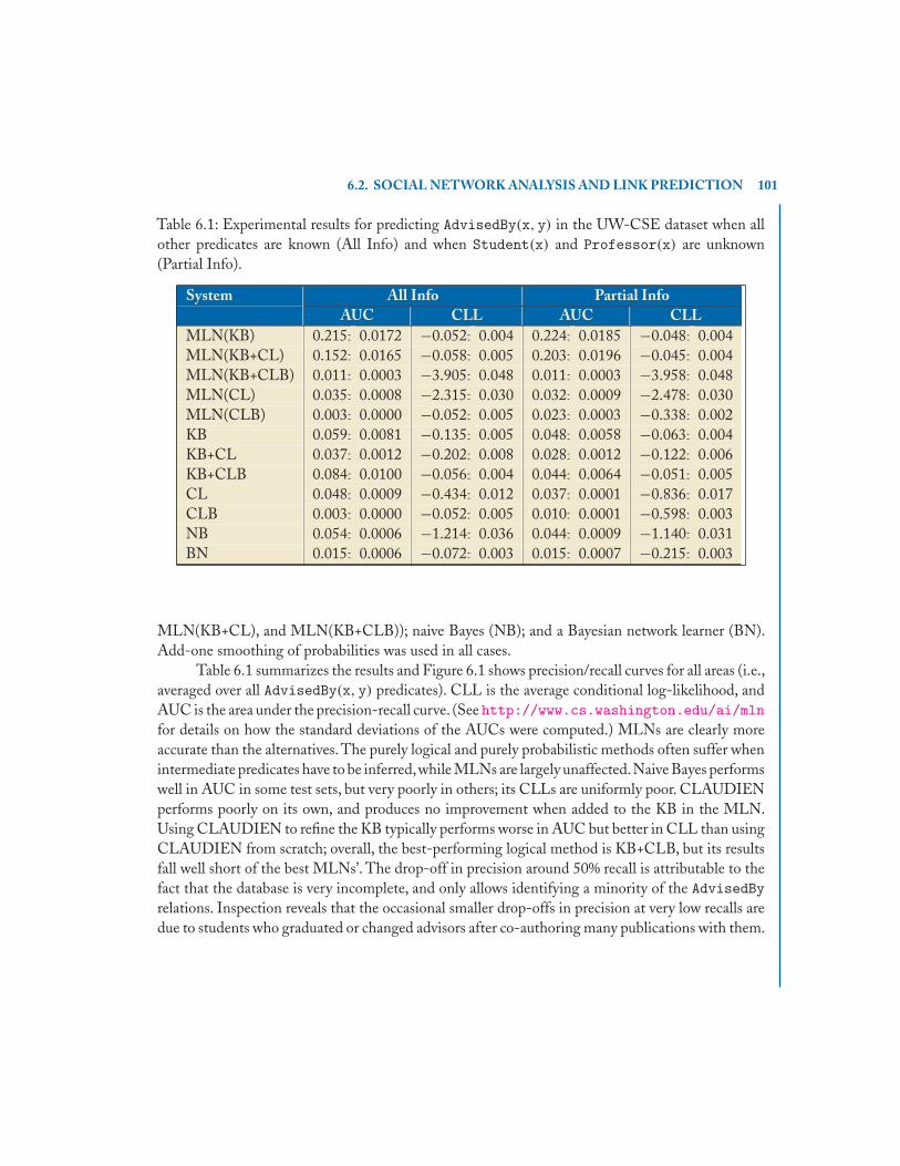
6.2. SOCIAL NETWORK ANALYSIS AND LINK PREDICTION 101
Table 6.1: Experimental results for predicting AdvisedBy(x, y) in the UW-CSE dataset when allother predicates are known (All Info) and when Student(x) and Professor(x) are unknown(Partial Info).
System All Info Partial InfoAUC CLL AUC CLL
MLN(KB) 0.215±0.0172 −0.052±0.004 0.224±0.0185 −0.048±0.004MLN(KB+CL) 0.152±0.0165 −0.058±0.005 0.203±0.0196 −0.045±0.004MLN(KB+CLB) 0.011±0.0003 −3.905±0.048 0.011±0.0003 −3.958±0.048MLN(CL) 0.035±0.0008 −2.315±0.030 0.032±0.0009 −2.478±0.030MLN(CLB) 0.003±0.0000 −0.052±0.005 0.023±0.0003 −0.338±0.002KB 0.059±0.0081 −0.135±0.005 0.048±0.0058 −0.063±0.004KB+CL 0.037±0.0012 −0.202±0.008 0.028±0.0012 −0.122±0.006KB+CLB 0.084±0.0100 −0.056±0.004 0.044±0.0064 −0.051±0.005CL 0.048±0.0009 −0.434±0.012 0.037±0.0001 −0.836±0.017CLB 0.003±0.0000 −0.052±0.005 0.010±0.0001 −0.598±0.003NB 0.054±0.0006 −1.214±0.036 0.044±0.0009 −1.140±0.031BN 0.015±0.0006 −0.072±0.003 0.015±0.0007 −0.215±0.003
MLN(KB+CL), and MLN(KB+CLB)); naive Bayes (NB); and a Bayesian network learner (BN).Add-one smoothing of probabilities was used in all cases.
Table 6.1 summarizes the results and Figure 6.1 shows precision/recall curves for all areas (i.e.,averaged over all AdvisedBy(x, y) predicates). CLL is the average conditional log-likelihood, andAUC is the area under the precision-recall curve. (See http://www.cs.washington.edu/ai/mlnfor details on how the standard deviations of the AUCs were computed.) MLNs are clearly moreaccurate than the alternatives.The purely logical and purely probabilistic methods often suffer whenintermediate predicates have to be inferred,while MLNs are largely unaffected.Naive Bayes performswell in AUC in some test sets, but very poorly in others; its CLLs are uniformly poor. CLAUDIENperforms poorly on its own, and produces no improvement when added to the KB in the MLN.Using CLAUDIEN to refine the KB typically performs worse in AUC but better in CLL than usingCLAUDIEN from scratch; overall, the best-performing logical method is KB+CLB, but its resultsfall well short of the best MLNs’. The drop-off in precision around 50% recall is attributable to thefact that the database is very incomplete, and only allows identifying a minority of the AdvisedByrelations. Inspection reveals that the occasional smaller drop-offs in precision at very low recalls aredue to students who graduated or changed advisors after co-authoring many publications with them.

102 CHAPTER 6. APPLICATIONS
0
0.2
0.4
0.6
0.8
0 0.2 0.4 0.6 0.8 1
Prec
isio
n
Recall
MLN(KB)MLN(KB+CL)
KBKB+CL
CLNBBN
0
0.2
0.4
0.6
0.8
0 0.2 0.4 0.6 0.8 1
Prec
isio
n
Recall
MLN(KB)MLN(KB+CL)
KBKB+CL
CLNBBN
Figure 6.1: Precision and recall for link prediction in UW-CSE dataset: All Info (upper graph) andPartial Info (lower graph).

6.3. ENTITY RESOLUTION 103
6.3 ENTITY RESOLUTION
Entity resolution is the problem of determining which observations (e.g., database records, nounphrases, video regions, etc.) correspond to the same real-world objects, and is of crucial importancein many areas. Typically, it is solved by forming a vector of properties for each pair of observations,using a learned classifier (such as logistic regression) to predict whether they match, and applyingtransitive closure. Markov logic yields an improved solution simply by applying the standard logicalapproach of removing the unique names assumption and introducing the equality predicate and itsaxioms: equality is reflexive, symmetric and transitive; groundings of a predicate with equal constantshave the same truth values; and constants appearing in a ground predicate with equal constants areequal. This last axiom is not valid in logic, but captures a useful statistical tendency. For example,if two papers are the same, their authors are the same; and if two authors are the same, papers bythem are more likely to be the same. Weights for different instances of these axioms can be learnedfrom data. Inference over the resulting MLN, with entity properties and relations as the evidenceand equality atoms as the query, naturally combines logistic regression and transitive closure. Mostimportantly, it performs collective entity resolution, where resolving one pair of entities helps toresolve pairs of related entities.
As a concrete example, consider the task of deduplicating a citation database in which eachcitation has author, title, and venue fields, as done by Singla and Domingos [134]. We can representthe domain structure with eight relations: Author(bib, author), Title(bib, title), andVenue(bib, venue) relate citations to their fields; HasWord(author/title/ venue, word)indicates which words are present in each field; SameAuthor (author, author),SameTitle(title, title), and SameVenue(venue, venue) represent field equality; andSameBib(bib, bib) represents citation equality. The truth values of all relations except for theequality relations are provided as evidence. The objective is to predict the SameBib relation.
We begin with a logistic regression model to predict citation equality based on the words inthe fields. This is easily expressed in Markov logic by rules such as the following:
Title(b1, t1) ∧ Title(b2, t2) ∧ HasWord(t1, +word)∧ HasWord(t2, +word) ⇒ SameBib(b1, b2)
When given a positive weight, each of these rules increases the probability that two citations witha particular title word in common are equivalent. We can construct similar rules for other fields.Note that we may learn negative weights for some of these rules, just as logistic regression may learnnegative feature weights. Transitive closure consists of a single rule:
SameBib(b1, b2) ∧ SameBib(b2, b3) ⇒ SameBib(b1, b3)
This model is similar to the standard solution, but has the advantage that the classifier is learned inthe context of the transitive closure operation.

104 CHAPTER 6. APPLICATIONS
We can construct similar rules to predict the equivalence of two fields as well. The usefulnessof Markov logic is shown further when we link field equivalence to citation equivalence:
Author(b1, a1) ∧ Author(b2, a2) ∧ SameBib(b1, b2) ⇒ SameAuthor(a1, a2)Author(b1, a1) ∧ Author(b2, a2) ∧ SameAuthor(a1, a2) ⇒ SameBib(b1, b2)
The above rules state that if two citations are the same, their authors should be the same, and thatcitations with the same author are more likely to be the same.
Most importantly, the resulting model can now perform collective entity resolution, whereresolving one pair of entities helps to resolve pairs of related entities. For example, inferring that apair of citations are equivalent can provide evidence that the names AAAI-06 and 21st Natl. Conf. onAI refer to the same venue, even though they are superficially very different. This equivalence canthen aid in resolving other entities.
Experiments on citation databases like Cora and BibServ.org show that these methods cangreatly improve accuracy, particularly for entity types that are difficult to resolve in isolation, as in theabove example [134]. Due to the large number of words and the high arity of the transitive closureformula, these models have thousands of weights and ground millions of clauses during learning,even after using canopies to limit the number of comparisons considered. Learning at this scaleis still reasonably efficient: preconditioned scaled conjugate gradient with MC-SAT for inferenceconverges within a few hours [75]. Rather than presenting detailed experimental results for entityresolution, we will show in the next section how to incorporate automatic field segmentation andthen compare the performance of the full system to several state-of-the-art methods.
6.4 INFORMATION EXTRACTIONIn the citation example of the previous section, it was assumed that the fields were manually seg-mented in advance. The goal of information extraction is to extract database records starting fromraw text or semi-structured data sources. Traditionally, information extraction proceeds by first seg-menting each candidate record separately, and then merging records that refer to the same entities.Such a pipeline architecture is adopted by many AI systems in natural language processing, speechrecognition, vision, robotics, etc. Markov logic allows us to perform the two tasks jointly. This en-ables us to use the segmentation of one candidate record to help segment similar ones. For example,resolving a well-segmented field with a less-clear one can disambiguate the latter’s boundaries. Wewill continue with the example of citations, as done by Poon and Domingos [106], but similar ideascould be applied to other data sources, such as Web pages or emails.
The main evidence predicate in the information extraction MLN is Token(t, i, c), which istrue iff token t appears in the ith position of the cth citation. A token can be a word, date, number,etc. Punctuation marks are not treated as separate tokens; rather, the predicate HasPunc(c, i) istrue iff a punctuation mark appears immediately after the ith position in the cth citation. Thequery predicates are InField(i, f, c) and SameCitation(c, c′). InField(i, f, c) is true iff theith position of the cth citation is part of field f, where f ∈ {Title, Author, Venue}, and inferring

6.4. INFORMATION EXTRACTION 105
it performs segmentation. SameCitation(c, c′) is true iff citations c and c′ represent the samepublication, and inferring it performs entity resolution.
Our segmentation model is essentially a hidden Markov model (HMM) with enhanced abilityto detect field boundaries. The observation matrix of the HMM correlates tokens with fields, and isrepresented by the simple rule
Token(+t, i, c) ⇒ InField(i, +f, c)
If this rule was learned in isolation, the weight of the (t, f )th instance would be log(ptf /(1 − ptf )),where ptf is the corresponding entry in the HMM observation matrix. In general, the transitionmatrix of the HMM is represented by a rule of the form
InField(i, +f, c) ⇒ InField(i + 1, +f′, c)However, we (and others, e.g., [41]) have found that for segmentation it suffices to capture the basicregularity that consecutive positions tend to be part of the same field. Thus we replace f′ by f inthe formula above. We also impose the condition that a position in a citation string can be part ofat most one field; it may be part of none.
The main shortcoming of this model is that it has difficulty pinpointing field boundaries.Detecting these is key for information extraction, and a number of approaches use rules designedspecifically for this purpose (e.g., [63]). In citation matching, boundaries are usually marked bypunctuation symbols. This can be incorporated into the MLN by modifying the rule above to
InField(i, +f, c) ∧ ¬HasPunc(c, i) ⇒ InField(i + 1, +f, c)
The ¬HasPunc(c, i) precondition prevents propagation of fields across punctuation marks. Becausepropagation can occur differentially to the left and right, the MLN also contains the reverse formof the rule. In addition, to account for commas being weaker separators than other punctuation, theMLN includes versions of these rules with HasComma() instead of HasPunc().
Finally, the MLN contains rules capturing a variety of knowledge about citations: the firsttwo positions of a citation are usually in the author field, and the middle one in the title; initials (e.g.,“J.”) tend to appear in either the author or the venue field; positions preceding the last non-venueinitial are usually not part of the title or venue; and positions after the first venue keyword (e.g.,“Proceedings”, “Journal”) are usually not part of the author or title.
By combining this segmentation model with our entity resolution model from before, we canexploit relational information as part of the segmentation process. In practice, something a littlemore sophisticated is necessary to get good results on real data. In Poon and Domingos [106], wedefine predicates and rules specifically for passing information between the stages, as opposed tojust using the existing InField() outputs. This leads to a “higher bandwidth” of communicationbetween segmentation and entity resolution, without letting excessive segmentation noise through.We also define an additional predicate and modify rules to better exploit information from similarcitations during the segmentation process. See Poon and Domingos [106] for further details.

106 CHAPTER 6. APPLICATIONS
Table 6.2: CiteSeer entity resolution: cluster recall on each section.
Approach Constr. Face Reason. Reinfor.Fellegi-Sunter 84.3 81.4 71.3 50.6Lawrence et al. (1999) 89 94 86 79Pasula et al. (2002) 93 97 96 94Wellner et al. (2004) 95.1 96.9 93.7 94.7Joint MLN 96.0 97.1 95.1 96.7
Table 6.3: Cora entity resolution: pairwise recall/precision and cluster recall.
Approach Pairwise Rec./Prec. Cluster RecallFellegi-Sunter 78.0 / 97.7 62.7Joint MLN 94.3 / 97.0 78.1
We evaluated this model on the CiteSeer and Cora datasets. For entity resolution in Cite-Seer, we measured cluster recall for comparison with previously published results. Cluster recall isthe fraction of clusters that are correctly output by the system after taking transitive closure frompairwise decisions. For entity resolution in Cora, we measured both cluster recall and pairwise re-call/precision. In both datasets, we also compared with a “standard” Fellegi-Sunter model (see Singlaand Domingos [134]), learned using logistic regression, and with oracle segmentation as the input.
In both datasets, joint inference improved accuracy and our approach outperformed previousones. Table 6.2 shows that our approach outperforms previous ones on CiteSeer entity resolution.(Results for Lawrence et al. (1999) [66], Pasula et al. (2002) [98] and Wellner et al. (2004) [152] aretaken from the corresponding papers.) This is particularly notable given that the models of Pasulaet al. [98] and Wellner et al. [152] involved considerably more knowledge engineering than ours,contained more learnable parameters, and used additional training data.
Table 6.3 shows that our entity resolution approach easily outperforms Fellegi-Sunter onCora, and has very high pairwise recall/precision.
6.5 UNSUPERVISED COREFERENCE RESOLUTION
In natural language processing, the goal of coreference resolution is to identify mentions (typicallynoun phrases) within a document that refer to the same entities. This is a key subtask in many NLPapplications, including information extraction, question answering, machine translation, and others.Supervised learning approaches treat the problem as one of classification: for each pair of mentions,predict whether they corefer or not (e.g., McCallum and Wellner [80]). While successful, theseapproaches require labeled training data, consisting of mention pairs and the correct decisions forthem. This limits their applicability. Unsupervised approaches are attractive due to the availability

6.5. UNSUPERVISED COREFERENCE RESOLUTION 107
of large quantities of unlabeled text. However, unsupervised coreference resolution is much moredifficult. Haghighi and Klein’s model [42], the most sophisticated prior work, still lags behindsupervised ones by a substantial margin.
The lack of label information in unsupervised coreference resolution can potentially be over-come by performing joint inference, which leverages the “easy” decisions to help make related “hard”ones. Markov logic allows us to easily build models involving relations among mentions, like appo-sition and predicate nominals. In this section, we describe Poon and Domingos’ method for jointunsupervised coreference resolution using Markov logic [107]. On the standard MUC and ACEdatasets, this approach outperforms Haghighi and Klein’s using only a fraction of the training data,and often matches or exceeds the accuracy of state-of-the-art supervised models.
AN MLN FOR JOINT UNSUPERVISED COREFERENCE RESOLUTIONIn this subsection, we present an MLN for joint unsupervised coreference resolution. As commonin previous work, we assume that true mention boundaries are given. We do not assume any otherlabeled information. We determined the head of a mention either by taking its rightmost token, orby using the head rules in a parser. We detected pronouns using a list.
Base MLNThe main query predicate is InClust(m, c!), which is true iff mention m is in cluster c. The “c!"notation signifies that for each m, this predicate is true for a unique value of c. The main evidencepredicate is Head(m, t!), where m is a mention and t a token, and which is true iff t is the head ofm. A key component in our MLN is a simple head mixture model, where the mixture componentpriors are represented by the unit clause InClust(+m, +c) and the head distribution is representedby the head prediction rule
InClust(m, +c) ∧ Head(m, +t).
By convention, at each inference step we name each non-empty cluster after the earliestmention it contains. This helps break the symmetry among mentions, which otherwise producesmultiple optima and makes learning unnecessarily harder. To encourage clustering, we impose anexponential prior on the number of non-empty clusters with weight −1.
The above model only clusters mentions with the same head, and does not work well forpronouns. To address this, we introduce the predicate IsPronoun(m), which is true iff the mentionm is a pronoun, and adapt the head prediction rule as follows:
¬IsPronoun(m) ∧ InClust(m, +c) ∧ Head(m, +t)
This is always false when m is a pronoun, and thus applies only to non-pronouns.Pronouns tend to resolve with mentions that are semantically compatible with
them. Thus we introduce predicates that represent entity type, number, and gen-der: Type(x, e!), Number(x, n!), Gender(x, g!), where x can be either a cluster ormention, e ∈ {Person, Organization, Location, Other}, n ∈ {Singular, Plural} and g ∈

108 CHAPTER 6. APPLICATIONS
{Male, Female, Neuter}. Many of these are known for pronouns, and some can be inferred fromsimple linguistic cues (e.g., “Ms. Galen" is a singular female person, while “XYZ Corp." is an orga-nization). Entity type assignment is represented by the unit clause Type(+x, +e) and similarly fornumber and gender. A mention should agree with its cluster in entity type. This is ensured by thehard (infinite-weight) rule
InClust(m, c) ⇒ (Type(m, e) ⇔ Type(c, e))
There are similar hard rules for number and gender.Different pronouns prefer different entity types, as represented by
IsPronoun(m) ∧ InClust(m, c) ∧ Head(m, +t) ∧ Type(c, +e)
which only applies to pronouns, and whose weight is positive if pronoun t is likely to assume entitytype e and negative otherwise. There are similar rules for number and gender.
Aside from semantic compatibility, pronouns tend to resolve with nearby mentions.To modelthis, we impose an exponential prior on the distance (number of mentions) between a pronoun andits antecedent, with weight −1.
Full MLNSyntactic relations among mentions often suggest coreference. Incorporating such relations intoour MLN is straightforward. We illustrate this with two examples: apposition (e.g., “Morgan &Claypool, our publisher”) and predicate nominals (e.g., “Morgan & Claypool is our publisher”). Weintroduce a predicate for apposition, Appo(x, y), where x, y are mentions, and which is true iff y isan appositive of x. We then add the rule
Appo(x, y) ⇒ (InClust(x, c) ⇔ InClust(y, c))
which ensures that x, y are in the same cluster if y is an appositive of x. Similarly, we introduce apredicate for predicate nominals, PredNom(x, y), and the corresponding rule.1 The weights of bothrules can be learned from data with a positive prior mean. For simplicity, we treat them as hardconstraints.
Rule-Based MLNWe also consider a rule-based system that clusters non-pronouns by their heads, and attaches apronoun to the cluster which has no known conflicting type, number, or gender, and contains theclosest antecedent for the pronoun. This system can be encoded in an MLN with just four rules.Three of them are the ones for enforcing agreement in type, number, and gender between a clusterand its members, as defined in the base MLN. The fourth rule is
¬IsPronoun(m1) ∧ ¬IsPronoun(m2) ∧ Head(m1, h1) ∧ Head(m2, h2)∧InClust(m1, c1) ∧ InClust(m2, c2) ⇒ (c1 = c2 ⇔ h1 = h2).
1We detected apposition and predicate nominatives using simple heuristics based on parses, e.g., if (NP, comma, NP) are the firstthree children of an NP, then any two of the three noun phrases are apposition.

6.5. UNSUPERVISED COREFERENCE RESOLUTION 109
With a large but not infinite weight (e.g., 100), this rule has the effect of clustering non-pronounsby their heads, except when it violates the hard rules. The MLN can also include the apposition andpredicate-nominal rules. As in the base MLN, we impose the same exponential prior on the numberof non-empty clusters and that on the distance between a pronoun and its antecedent. This simpleMLN is remarkably competitive, as we will see below.
EXPERIMENTSWe conducted experiments on MUC-6, ACE-2004, and ACE Phrase-2 (ACE-2). We evaluatedour systems using the commonly-used MUC scoring program [147].
The MUC-6 dataset consists of 30 documents for testing and 221 for training.To evaluate thecontribution of the major components in our model, we conducted five experiments, each differingfrom the previous one in a single aspect. We emphasize that our approach is unsupervised, and thusthe data only contains raw text plus true mention boundaries.
MLN-1 In this experiment, the base MLN was used, and the head was chosen crudely as therightmost token in a mention. Our system was run on each test document separately, using aminimum of training data (the document itself ).
MLN-30 Our system was trained on all 30 test documents together. This tests how much can begained by pooling information.
MLN-H The heads were determined using the head rules in the Stanford parser [56], plus simpleheuristics to handle suffixes such as “Corp.” and “Inc.”
MLN-HA The apposition rule was added.
MLN-HAN The predicate-nominal rule was added. This is our full model.
We also compared with two rule-based MLNs: RULE chose the head crudely as the rightmosttoken in a mention, and did not include the apposition rule and predicate-nominal rule; RULE-HAN chose the head using the head rules in the Stanford parser, and included the apposition ruleand predicate-nominal rule.
We used the ACE Phrase-2 dataset (ACE-2) to enable direct comparisons with Haghighiand Klein [42], Ng [92], and Denis and Baldridge [27]. The English version of the ACE-2004training corpus contains two sections, BNEWS and NWIRE, with 220 and 128 documents, respec-tively. ACE-2 contains a training set and a test set. In our experiments, we only used the test set,which contains three sections, BNEWS, NWIRE, and NPAPER, with 51, 29, and 17 documents,respectively.
We applied the weight learning methods from Section 4.3 to maximize the likelihood ofthe observed query atoms given the evidence atoms, while summing over the unobserved queryatoms: P(yo|x) = ∑
yuP (yo, yu|x). In our coreference resolution MLN, known query atoms (Yo)
include Head and known groundings of Type, Number and Gender; unknown query atoms (Yu)

110 CHAPTER 6. APPLICATIONS
Table 6.4: Comparison of coreference results in MUC scores on the MUC-6 dataset.
# Doc. Prec. Rec. F1H&K 60 80.8 52.8 63.9H&K 381 80.4 62.4 70.3M&W 221 - - 73.4RULE - 76.0 65.9 70.5RULE-HAN - 81.3 72.7 76.7MLN-1 1 76.5 66.4 71.1MLN-30 30 77.5 67.3 72.0MLN-H 30 81.8 70.1 75.5MLN-HA 30 82.7 75.1 78.7MLN-HAN 30 83.0 75.8 79.2
Table 6.5: Comparison of coreference results in MUC scores on the ACE-2 datasets.
BNEWS NWIRE NPAPERPrec. Rec. F1 Prec. Rec. F1 Prec. Rec. F1
Ng 67.9 62.2 64.9 60.3 50.1 54.7 71.4 67.4 69.3D&B 78.0 62.1 69.2 75.8 60.8 67.5 77.6 68.0 72.5MLN-HAN 68.3 66.6 67.4 67.7 67.3 67.4 69.2 71.7 70.4
include InClust and unknown groundings of Type, Number, Gender; and evidence (X) includesIsPronoun, Appo and PredNom. For inference, we adapted MC-SAT and MaxWalkSAT to bet-ter handle mutually exclusive and exhaustive rules. Additional details can be found in Poon andDomingos [107].
Table 6.4 compares our system with previous approaches on the MUC-6 dataset, in MUCscores. Our approach greatly outperformed Haghighi and Klein, the previous state-of-the-art un-supervised system. Our system, when trained on individual documents, achieved an F1 score morethan 7% higher than theirs trained on 60 documents, and still outperformed it when trained on381 documents. Training on the 30 test documents together resulted in a significant gain. (We alsoran experiments using more documents, and the results were similar.) Better head identification(MLN-H) led to a large improvement in accuracy, which is expected since for mentions with aright modifier, the rightmost tokens confuse rather than help coreference (e.g., “the chairman ofMicrosoft"). Notice that with this improvement our system already outperforms a state-of-the-artsupervised system, McCallum and Wellner [80]. Leveraging apposition resulted in another largeimprovement, and predicate nominals also helped. Our full model scores about 9% higher thanHaghighi and Klein, and about 6% higher than McCallum and Wellner. To our knowledge, this
6.6. ROBOT MAPPING 111
is the best coreference accuracy reported on MUC-6 to date.2 Interestingly, the rule-based MLN(RULE) sufficed to outperform Haghighi and Klein, and by using better heads and the appositionand predicate-nominal rules (RULE-HAN), it outperformed McCallum and Wellner, the supervisedsystem. The MLNs with learning (MLN-30 and MLN-HAN), on the other hand, substantiallyoutperformed the corresponding rule-based ones.
Tables 6.5 compares our system to two recent supervised systems, Ng [92] and Denis andBaldridge [27]. Our approach significantly outperformed Ng. It tied with Denis and Baldridge onNWIRE, and was somewhat less accurate on BNEWS and NPAPER.
6.6 ROBOT MAPPINGIn robot mapping, the goal is to infer the map of an indoor environment from laser range data,obtained by the robot as it moves about the environment [69]. Since this domain relies heavily onreal numbers and continuous variables for distances and coordinates, it is best approached usinghybrid Markov logic networks (HMLNs), as described in Section 5.1.
Using the mobile robot sensor data from the Radish robotics data set repository(http://radish.sourceforge.net), the evidence is a set of range finder segments, defined bythe (x, y) coordinates of their endpoints.The output is: (a) a labeling of each segment as Door, Wall,or Other (classification); (b) an assignment of wall segments to the walls they are part of (clustering);and (c) the position of each wall, defined by the (x, y) coordinates of its endpoints (regression). Onaverage, each map consists of about 100 segments. More details on the dataset and experimentalsetups can be found in Wang and Domingos [148].
Wang and Domingos [148] built an HMLN using the following rules. First, every segmentbelongs to exactly one type with some prior probability distribution given by the unit clauses,SegType(s, +t). Doors and walls also have a typical length and depth, represented by numericterms (e.g., SegType(s, Door) · (Length(s) = DoorLength), which has value 0 if the segment isnot a door and −(Length(s) − DoorLength)2 otherwise). A segment’s depth is defined as thesigned perpendicular distance of its midpoint to the nearest wall line. Lines are iteratively estimatedfrom the segments assigned to them, using the formulas below, as part of the HMLN inference. Anumber of rules involving depth and angle between a segment and the nearest line identify segmentsof type Other, whose distribution is more irregular than that of doors and walls.
The type of a segment is predictive of the types of consecutive segments along a wall line:
SegType(s, +t) ∧ Consecutive(s, s′)⇒ SegType(s′, +t′)
Two segments are consecutive if they are the closest segments to each other along either directionof the nearest line. In addition, aligned segments tend to be of the same type:
SegType(s, t) ∧ Consecutive(s, s′) ∧ Aligned(s, s′)⇒ SegType(s′, t)2As pointed out by Haghighi and Klein [42], Luo et al. [77] obtained a very high accuracy on MUC-6, but their system used goldNER features and is not directly comparable.
112 CHAPTER 6. APPLICATIONS
Segments are aligned if one is roughly a continuation of the other (i.e., their angle is below somethreshold, and so is their perpendicular distance). The rules above perform collective classificationof segments into types.
Aligned wall segments are part of the same wall line:
SegType(s, Wall) ∧ SegType(s′, Wall) ∧ Aligned(s, s′) ∧ PartOf(s, l) ⇒ PartOf(s′, l)
This rule clusters wall segments into wall lines. Notice that it captures long-range dependenciesbetween segments along the same corridor, not just between neighboring segments.
A segment is the start of a line if and only if it has no previous aligned segment:3
PartOf(s, l) ⇒ (¬PreviousAligned(s) ⇔ StartLine(s, l))
If a segment is the start of a line, their initial points are (about) the same:
StartLine(s, l) · (xi(s) = xi(l))
where xi(s) is the x coordinate of s’s initial point, etc.; and similarly for y. If a segment belongs toa line, its slope should be the same as the slope of a line connecting their initial points. Multiplyingby the �x’s to avoid singularities, we obtain:
PartOf(s, l) · [(yf(s) − yi(s))(xi(s) − xi(l)) = (yi(s) − yi(l))(xf(s) − xi(s))]where the subscript f denotes final points. Line ends are handled similarly. These rules infer thelocations of the wall lines from the segments assigned to them. They also influence the cluster-ing and labeling of segments (e.g., if a better line fit is obtained by relabeling a segment fromWall to Door and thus excluding it, this will be inferred). Classification, clustering and regres-sion are fully joint. In the next section we show the experimental results obtained by this ap-proach. The full HMLN, containing some additional formulas, is available at the Alchemy Web site(http://alchemy.cs.washington.edu/).
EXPERIMENTAL METHODOLOGYWe learned HMLN weights using Alchemy’s voted perceptron with HMWS for inference, 100steps of gradient descent, and a learning rate of 1.0.To combat ill-conditioning, we divided each for-mula/term’s learning rate by the absolute sum of its values in the data, similar to per-weight learningrates discussed in Section 4.1. Other parameters were learned by fitting Gaussian distributions to therelevant variables. We used leave-one-map-out cross-validation throughout. In all inferences, thecorrect number of walls was given.We evaluated inference results for discrete variables (SegType andPartOf) using F1 score (harmonic mean of precision and recall over all groundings). We used meansquare error (MSE) for continuous variables (xi(l), yi(l), xf(l) and yf(l)). We also computed the3By convention, a point precedes another if it has lower x coordinate and, if they are the same, lower y. Segments and lines areordered by their start points, which precede their final points.
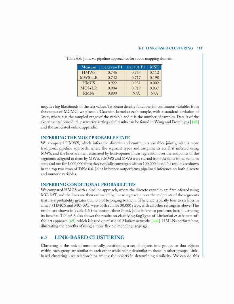
6.7. LINK-BASED CLUSTERING 113
Table 6.6: Joint vs. pipeline approaches for robot mapping domain.
Measure SegType F1 PartOf F1 MSEHMWS 0.746 0.753 0.112
MWS+LR 0.742 0.717 0.198HMCS 0.922 0.931 0.002
MCS+LR 0.904 0.919 0.037RMNs 0.899 N/A N/A
negative log likelihoods of the test values. To obtain density functions for continuous variables fromthe output of MCMC, we placed a Gaussian kernel at each sample, with a standard deviation of3r/n, where r is the sampled range of the variable and n is the number of samples. Details of theexperimental procedure, parameter settings and results can be found in Wang and Domingos [148]and the associated online appendix.
INFERRING THE MOST PROBABLE STATEWe compared HMWS, which infers the discrete and continuous variables jointly, with a moretraditional pipeline approach, where the segment types and assignments are first inferred usingMWS, and the lines are then estimated by least-squares linear regression over the endpoints of thesegments assigned to them by MWS. HMWS and MWS were started from the same initial randomstate and run for 1,000,000 flips; they typically converged within 100,000 flips.The results are shownin the top two rows of Table 6.6. Joint inference outperforms pipelined inference on both discreteand numeric variables.
INFERRING CONDITIONAL PROBABILITIESWe compared HMCS with a pipeline approach, where the discrete variables are first inferred usingMC-SAT, and the lines are then estimated by linear regression over the endpoints of the segmentsthat have probability greater than 0.3 of belonging to them. (There are typically four to six lines ina map.) HMCS and MC-SAT were both run for 30,000 steps, with all other settings as above. Theresults are shown in Table 6.6 (the bottom three lines). Joint inference performs best, illustratingits benefits. Table 6.6 also shows the results on classifying SegType of Limketkai et al.’s state-of-the-art approach [69], which is based on relational Markov networks [141]. HMLNs perform best,illustrating the benefits of using a more flexible modeling language.
6.7 LINK-BASED CLUSTERINGClustering is the task of automatically partitioning a set of objects into groups so that objectswithin each group are similar to each other while being dissimilar to those in other groups. Link-based clustering uses relationships among the objects in determining similarity. We can do this
114 CHAPTER 6. APPLICATIONS
very naturally with the MRC algorithm from Section 4.3, which is based on second-order Markovlogic. Note that second-order formulas are quantified over predicates, so the same second-orderMLN can be applied to different datasets with different predicates. In this section, we describe Kokand Domingos’ [58] experiments with MRC on four datasets. We compare MRC to the infiniterelational model (IRM) [54] and TDSL, the top-down structure learning algorithm presented inSection 4.2.
IRM is a recently-published model that also clusters objects,attributes,and relations.However,unlike MRC, it only finds a single clustering. It defines a generative model for the predicates andcluster assignments. Like MRC, it assumes that the predicates are conditionally independent giventhe cluster assignments, and the cluster assignments for each type are independent. IRM uses aChinese restaurant process prior (CRP) [102] on the cluster assignments. Under the CRP, each newobject is assigned to an existing cluster with probability proportional to the cluster size. Becausethe CRP has the property of exchangeability, the order in which objects arrive does not affectthe outcome. IRM assumes that the probability p of an atom being true conditioned on clustermembership is generated according to a symmetric Beta distribution, and that the truth values ofatoms are then generated according to a Bernoulli distribution with parameter p. IRM finds theMAP cluster assignment using the same greedy search as our model, except that it also searches forthe optimal values of its CRP and Beta parameters.
DATASETSAnimals.This dataset contains a set of animals and their features [96]. It consists exclusively of unarypredicates of the form f(a), where f is a feature and a is an animal (e.g.,Swims(Dolphin)).There are50 animals, 85 features, and thus a total of 4250 ground atoms,of which 1562 are true.This is a simplepropositional dataset with no relational structure, but it is useful as a “base case” for comparison.Notice that, unlike traditional clustering algorithms, which only cluster objects by features, MRCand IRM also cluster features by objects. This is known as bi-clustering or co-clustering, and hasreceived considerable attention in the recent literature (e.g., Dhillon et al. [28]).UMLS. UMLS contains data from the Unified Medical Language System, a biomedical ontol-ogy [81]. It consists of binary predicates of the form r(c, c′), where c and c′ are biomedical concepts(e.g., Antibiotic, Disease), and r is a relation between them (e.g., Treats, Diagnoses). Thereare 49 relations and 135 concepts, for a total of 893,025 ground atoms, of which 6529 are true.Kinship. This dataset contains kinship relationships among members of the Alyawarra tribe fromCentral Australia [26]. Predicates are of the form k(p, p′), where k is a kinship relation and p, p′ arepersons. There are 26 kinship terms and 104 persons, for a total of 281,216 ground atoms, of which10,686 are true.Nations. This dataset contains a set of relations among nations and their features [126]. It consistsof binary and unary predicates.The binary predicates are of the form r(n, n′), where n,n′ are nations,and r is a relation between them (e.g., ExportsTo, GivesEconomicAidTo). The unary predicates

6.7. LINK-BASED CLUSTERING 115
are of the form f(n), where n is a nation and f is a feature (e.g., Communist, Monarchy). There are14 nations, 56 relations and 111 features, for a total of 12,530 ground atoms, of which 2565 are true.
METHODOLOGYExperimental evaluation of statistical relational learners is complicated by the fact that in manycases the data cannot be separated into independent training and test sets. While developing a long-term solution for this remains an open problem, we used an approach that is general and robust:performing cross-validation by atom. For each dataset, we performed ten-fold cross-validation byrandomly dividing the atoms into ten folds, training on nine folds at a time, and testing on theremaining one.This can be seen as evaluating the learners in a transductive setting, because an object(e.g., Leopard) that appears in the test set (e.g., in MeatEater(Leopard)) may also appear in thetraining set (e.g., in Quadrupedal(Leopard)). In the training data, the truth values of the testatoms are set to unknown, and their actual values (true/false) are not available. Thus learnersmust perform generalization in order to be able to infer the test atoms, but the generalization isaided by the dependencies between test atoms and training ones.
TDSL is not directly comparable to MRC and IRM because it makes the closed-worldassumption and our experiments require the test atoms to be open-world. For an approximatecomparison, we set all test atoms to false when running TDSL. Since in each run these are only 10%of the training set, setting them to false does not greatly change the sufficient statistics (true clausecounts). We then ran MC-SAT on the MLNs learned by TDSL to infer the probabilities of the testatoms.
We ran IRM and MRC for ten hours on each fold of each dataset, using default parametersettings for both algorithms. Almost all of MRC’s running time went into the first level of clusteringbecause this is where the sets of objects, attributes and relations to be clustered are by far the largest,and finding a good initial clustering is important for the subsequent learning.
RESULTSFigure 6.2 reports the CLL and AUC for MRC, IRM and TDSL, averaged over the ten folds ofeach dataset. We also report the results obtained using just the initial clustering formed by MRC(Init), in order to evaluate the usefulness of learning multiple clusterings.
TDSL does worse than MRC and IRM on all datasets except Nations. On Nations, it doesworse than MRC and IRM in terms of CLL, but approximately ties them in terms of AUC. Manyof the relations in Nations are symmetric, e.g., if country A has a military conflict with B, then thereverse is usually true. TDSL learns a rule to capture the symmetry, and consequently does well interms of AUC.
MRC outperforms IRM on UMLS and Kinship, and ties it on Animals and Nations. Thedifference on UMLS and Kinship is quite large. Animals is the smallest and least structured of thedatasets, and it is conceivable that it has little room for improvement beyond a single clustering.Thedifference in performance between MRC and IRM correlates strongly with dataset size. (Notice

116 CHAPTER 6. APPLICATIONS
Figure 6.2: Comparison of MRC, IRM, and MLN structure learning (TDSL) on four clusteringdatasets. Init is the initial clustering formed by MRC. Error bars are one standard deviation in eachdirection.
that UMLS and Kinship are an order of magnitude larger than Animals and Nations.) This suggeststhat sophisticated algorithms for statistical predicate invention may be of most use in even largerdatasets. We look at such a dataset in the next section.
MRC outperforms Init on all domains except Animals. The differences on Nations are notsignificant, but on UMLS and Kinship they are very large.These results show that forming multipleclusterings is key to the good performance of MRC. In fact, Init does considerably worse than IRMon UMLS and Kinship;we attribute this to the fact that IRM performs a search for optimal parametervalues, while in MRC these parameters were simply set to default values without any tuning on data.This suggests that optimizing parameters in MRC could lead to further performance gains.
In the Animals dataset, MRC performs at most three levels of cluster refinement. On the otherdatasets, it performs about five. The average total numbers of clusters generated are: Animals, 202;UMLS, 405; Kinship, 1044; Nations, 586. The average numbers of atom prediction rules learnedare: Animals, 305; UMLS, 1935; Kinship, 3568; Nations, 12,169.
6.8 SEMANTIC NETWORK EXTRACTION FROM TEXT
A long-standing goal of AI is to build an autonomous agent that can read and understand text. Agood step towards this goal is automatically building knowledge bases of facts and relationships fromcorpora such as the Web. Kok and Domingos [59] recently introduced Semantic Network Extractor

6.8. SEMANTIC NETWORK EXTRACTION FROM TEXT 117
(SNE), a scalable, unsupervised, and domain-independent system that simultaneously extracts high-level relations and concepts, and learns a semantic network [112] from text. The knowledge in thisnetwork can be used by itself or as a component of larger NLP systems. SNE represents the largest-scale application of Markov logic to date.
SNE is built on top of TextRunner [3], a system for extracting a large set of relational tuplesof the form r(x, y) where x and y are strings denoting objects, and r is a string denoting a relationbetween the objects. TextRunner uses a lightweight noun phrase chunker to identify objects, andheuristically determines the text between objects as relations.However,whileTextRunner can quicklyacquire a large database of ground facts in an unsupervised manner, it is not able to learn generalknowledge that is embedded in the facts.
SNE uses TextRunner to extract ground facts as triples from text, and then extract knowledgefrom the triples. TextRunner’s triples are noisy, sparse, and contain many co-referent objects andrelations. SNE overcomes this by using a probabilistic model based on second-order Markov logicthat clusters objects according to the objects they are related to and relations according to the objectsthey relate.This allows information to propagate between clusters of relations and clusters of objectsas they are created. Each cluster represents a high-level relation or concept. A concept cluster canbe viewed as a node in a graph, and a relation cluster can be viewed as links between the conceptclusters that it relates. Together, the concept clusters and relation clusters define a simple semanticnetwork. Figure 6.3 illustrates part of a semantic network that our approach learns. (More fragmentsare available at http://alchemy.cs.washington.edu/papers/kok08.) SNE is based on theMRC model [58] discussed in Section 4.3, but with a different prior and a more scalable searchalgorithm that finds a single clustering. For full details on SNE, see Kok and Domingos [59].
Our goal is to create a system that is capable of extracting semantic networks from what isarguably the largest and most accessible text resource — the Web. Thus in our experiments, weused a large Web corpus to evaluate the effectiveness of SNE’s relational clustering approach inextracting a simple semantic network from it. Since to date, no other system could do the same,we had to modify three other relational clustering approaches so that they could run on our largeWeb-scale dataset, and compared SNE to them. The three approaches are MRC [58], IRM [54],and Information-Theoretic Co-clustering (ITC) [28].
In order to make MRC and IRM feasible on large Web-scale datasets such as the one usedin our experiments, we used the SNE clustering algorithm in place of the MRC and IRM searchalgorithms. We use MRC1 to denote an MRC model that is restricted to find a single clustering.For IRM, we also fixed the values of the CRP and Beta parameters and applied the CRP prior tocluster combinations instead of clusters.
The ITC model [28] clusters discrete data in a two-dimensional matrix along both dimensionssimultaneously. It greedily searches for the hard clusterings that optimize the mutual informationbetween the row and column clusters. The model has been shown to perform well on noisy andsparse data. ITC’s top-down search algorithm has the flavor of K-means, and requires the numberof row and column clusters to be specified in advance. At every step, ITC finds the best cluster for

118 CHAPTER 6. APPLICATIONS
Table 6.7: Semantic network comparison on gold standard. Object 1 and Object 2 respectively referto the object symbols that appear as the first and second arguments of relations.
Model Relation Object 1 Object 2Prec. Recall F1 Prec. Recall F1 Prec. Recall F1
SNE 0.452 0.187 0.265 0.460 0.061 0.108 0.558 0.062 0.112MRC1 0.054 0.044 0.049 0.031 0.007 0.012 0.05 0.011 0.018IRM 0.201 0.089 0.124 0.252 0.043 0.073 0.307 0.041 0.072ITC 0.773 0.003 0.006 0.470 0.047 0.085 0.764 0.002 0.004
each row or column by iterating through all clusters. This is not tractable for large datasets like ourWeb dataset, which can contain many clusters; instead, we use the SNE clustering algorithm, butwith mutual information in place of change in log posterior probability. We further extended ITCto three dimensions by optimizing the mutual information among the clusters of three dimensions.We follow Dhillon et al.’s [28] suggestion of using a BIC prior, but we applied it to the number ofcluster combinations that contain at least one true ground atom, not the number of clusters.
DATASETWe compared the various models on a dataset of about 2.1 million triples4 extracted in a Webcrawl by TextRunner [3]. Each triple takes the form r(x, y) where r is a relation symbol, andx and y are object symbols. Some example triples are: Named_after(Jupiter, Roman_god) andUpheld(Court, Ruling). There are 15,872 distinct r symbols, 700,781 distinct x symbols, and665,378 distinct y symbols. Two characteristics of TextRunner’s extractions are that they are sparseand noisy. To reduce the noise in the dataset, our search algorithm only considered symbols thatappeared at least 25 times.This leaves 10,214 r symbols, 8942 x symbols, and 7995 y symbols.Thereare 2,065,045 triples that contain at least one symbol that appears at least 25 times. We make theclosed-world assumption for all models (i.e., all triples not in the dataset are assumed false).
RESULTSWe evaluated the clusterings learned by each model against a manually created gold standard. Thegold standard assigns 2688 r symbols, 2568 x symbols, and 3058 y symbols to 874, 511, and 700non-unit clusters respectively. We measured the pairwise precision, recall and F1 of each modelagainst the gold standard. Pairwise precision is the fraction of symbol pairs in learned clusters thatappear in the same gold clusters. Pairwise recall is the fraction of symbol pairs in gold clusters thatappear in the same learned clusters. F1 is the harmonic mean of precision and recall.Table 6.7 showsthe results. We see that SNE performs significantly better than MRC1, IRM, and ITC.
4Publicly available at http://knight.cis.temple.edu/˜yates/data/resolver_data.tar.gz
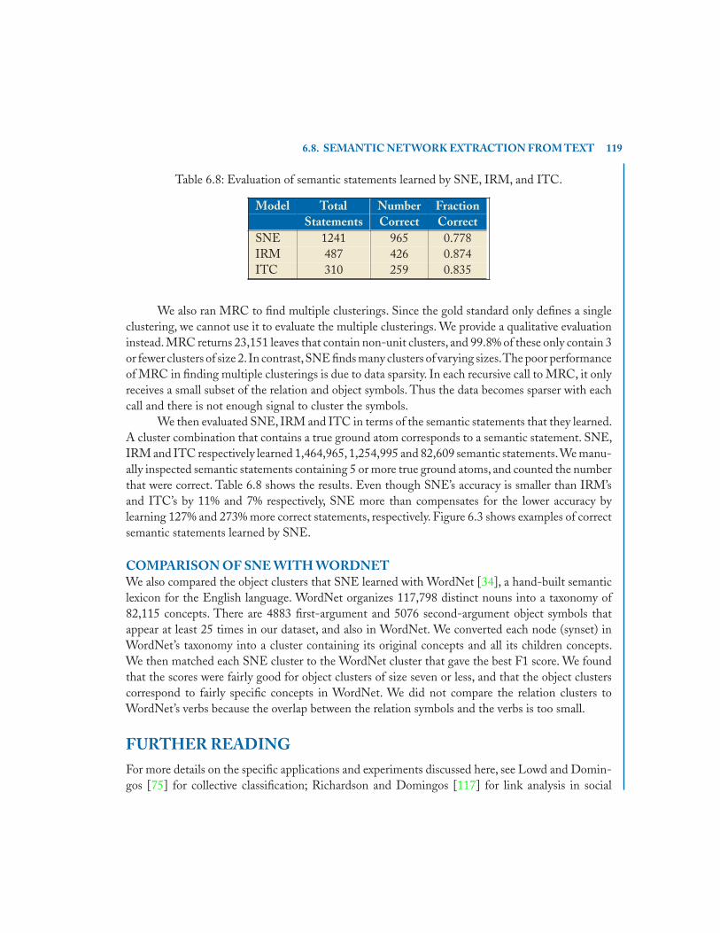
6.8. SEMANTIC NETWORK EXTRACTION FROM TEXT 119
Table 6.8: Evaluation of semantic statements learned by SNE, IRM, and ITC.
Model Total Number FractionStatements Correct Correct
SNE 1241 965 0.778IRM 487 426 0.874ITC 310 259 0.835
We also ran MRC to find multiple clusterings. Since the gold standard only defines a singleclustering, we cannot use it to evaluate the multiple clusterings. We provide a qualitative evaluationinstead. MRC returns 23,151 leaves that contain non-unit clusters, and 99.8% of these only contain 3or fewer clusters of size 2.In contrast,SNE finds many clusters of varying sizes.The poor performanceof MRC in finding multiple clusterings is due to data sparsity. In each recursive call to MRC, it onlyreceives a small subset of the relation and object symbols. Thus the data becomes sparser with eachcall and there is not enough signal to cluster the symbols.
We then evaluated SNE, IRM and ITC in terms of the semantic statements that they learned.A cluster combination that contains a true ground atom corresponds to a semantic statement. SNE,IRM and ITC respectively learned 1,464,965,1,254,995 and 82,609 semantic statements.We manu-ally inspected semantic statements containing 5 or more true ground atoms, and counted the numberthat were correct. Table 6.8 shows the results. Even though SNE’s accuracy is smaller than IRM’sand ITC’s by 11% and 7% respectively, SNE more than compensates for the lower accuracy bylearning 127% and 273% more correct statements, respectively. Figure 6.3 shows examples of correctsemantic statements learned by SNE.
COMPARISON OF SNE WITH WORDNETWe also compared the object clusters that SNE learned with WordNet [34], a hand-built semanticlexicon for the English language. WordNet organizes 117,798 distinct nouns into a taxonomy of82,115 concepts. There are 4883 first-argument and 5076 second-argument object symbols thatappear at least 25 times in our dataset, and also in WordNet. We converted each node (synset) inWordNet’s taxonomy into a cluster containing its original concepts and all its children concepts.We then matched each SNE cluster to the WordNet cluster that gave the best F1 score. We foundthat the scores were fairly good for object clusters of size seven or less, and that the object clusterscorrespond to fairly specific concepts in WordNet. We did not compare the relation clusters toWordNet’s verbs because the overlap between the relation symbols and the verbs is too small.
FURTHER READINGFor more details on the specific applications and experiments discussed here, see Lowd and Domin-gos [75] for collective classification; Richardson and Domingos [117] for link analysis in social

120 CHAPTER 6. APPLICATIONS
Figure 6.3: Fragments of a semantic network learned by SNE. Nodes are concept clusters, and thelabels of links are relation clusters.
networks; Singla and Domingos [134] and Lowd and Domingos [75] for entity resolution; Poonand Domingos [106] for information extraction; Poon and Domingos [107] for coreference res-olution; Wang and Domingos for robot mapping [148]; Kok and Domingos [58] for link-basedclustering; and Kok and Domingos [59] for semantic network extraction from text.
The number of applications of Markov logic is quickly growing. Other applications includethe DARPA CALO personal assistant [29], semantic role labeling in NLP [120], extracting genicinteractions from Medline abstracts [119], predicting protein β-partners [70], extracting ontologiesfrom Wikipedia [154], discovering social relationships in photo collections [139], using the Web toanswer queries [130], and more.

121
C H A P T E R 7
ConclusionProgress in an area of computer science picks up when the right interface layer is defined: an abstractlanguage that separates the infrastructure from the applications, enabling each piece of the infras-tructure to communicate with all the applications without modification, and vice-versa. Markovlogic is an attempt to provide such an interface layer for artificial intelligence.
Markov logic combines first-order logic and probabilistic graphical models. A knowledge basein Markov logic is simply a set of weighted first-order formulas, viewed as templates for features of aMarkov network: given a set of constants representing objects in the domain of interest, the Markovnetwork has one Boolean variable for each possible grounding of each predicate with those constants(e.g., Friends(Anna, Bob), and one Boolean feature for each grounding of each formula, with thecorresponding weight (e.g., Smokes(Anna) ∧ Friends(Anna, Bob) ⇒ Smokes(Bob)). First-orderlogic is the infinite-weight limit of Markov logic.
Most widely used graphical models can be specified very compactly in Markov logic (e.g., twoformulas containing a total of three predicates for logistic regression, three formulas for a hiddenMarkov model, etc.). In turn, this makes it easy to define large, complex models involving combina-tions of these components. For example, a complete information extraction system (performing jointsegmentation and entity resolution) can be specified with just a few formulas, and a state-of-the-artone with a few dozen.
Several implementations of Markov logic exist, of which the most developed is Alchemy [60].Alchemy includes a series of highly efficient inference and learning algorithms for Markov logic,including:
• A weighted satisfiability solver for MAP inference.This and other algorithms use lazy inferencetechniques to minimize the number of ground predicates that are actually created.
• MC-SAT, an MCMC algorithm that uses a satisfiability solver to find modes, for computingconditional probabilities.
• Lifted belief propagation, which allows probabilistic inference to be carried out for whole setsof objects at once, without grounding predicates, like resolution-based theorem proving inProlog.
• Gradient descent, conjugate gradient and quasi-Newton methods for generative and discrim-inative weight learning.
• Inductive logic programming algorithms for learning new formulas from data and refiningmanually specified ones.

122 CHAPTER 7. CONCLUSION
These algorithms make it possible to routinely perform learning and inference on graphicalmodels with millions of variables and billions of features. State-of-the-art solutions to a wide varietyof problems have been developed using Markov logic, including:
• The first system for unsupervised coreference resolution in NLP that outperforms supervisedones on standard benchmarks.
• The first robot mapping system that performs joint labeling of range finder segments, clusteringof segments into walls, and regression to estimate the locations of walls from their segments.
• The winning entry in the LLL-05 competition on extracting gene interactions from Medlineabstracts.
• An inference engine for the DARPA CALO personal assistant.
• The most accurate system to date for extracting ontologies from Wikipedia.
• The first unsupervised system for extracting semantic networks from Web crawls.
• A state-of-the-art system for predicting protein β-partners.
• A probabilistic version of (parts of ) Cyc, the world’s largest knowledge base.
Markov logic makes the prospect of “programming by machine learning” a realistic one. WithAlchemy, the programmer’s work is reduced to specifying the approximate structure of the program;the rest is filled in by learning from data, and the resulting uncertainties are handled by probabilisticinference. With discriminative learning, Markov logic learns the conditional distribution of theprogram outputs given its inputs, and the most likely program is run by performing MAP inference.
Even without learning, weighted logic makes it possible to write knowledge bases that aremuch more compact than the corresponding ones in purely logical languages. It also relaxes therequirements for perfect correctness, consistency and completeness that make writing large KBs andintegrating contributions from many sources a very costly (or even infeasible) enterprise.
Markov logic and Alchemy are not yet at the point where they can be easily used by developersor researchers without expertise in machine learning, automated reasoning, or probabilistic inference.The chief reason for this is that the underlying inference and learning algorithms still require tuning,parameter choices, trial and error, etc., before they produce the desired results. Markov logic suc-cessfully integrates learning, logic and probability, but it inherits the state of the art in each of thesefields, and in each of them there is still much research to be done before “push-button” algorithmsare available.
However, even with this state of art, Markov logic already allows us to attempt much moreambitious applications than before. For example, we are currently developing a complete naturallanguage processing system, using fully joint inference across all stages, and ultimately consisting ofprobably no more than hundreds of (second-order) Markov logic formulas.

123
It is our hope that researchers in machine learning, probabilistic inference, and knowledgerepresentation and reasoning will find it worthwhile to provide their latest algorithms as plug-insto Alchemy using the corresponding APIs, thus making them available to all applications that useMLNs as the interface layer. Conversely, we hope that researchers in natural language, planning,vision and robotics, multi-agent systems, etc., will find Markov logic a useful modeling tool, andcontribute the MLNs they develop to the Alchemy repository, making them available for otherresearchers to build on. Thus Markov logic will help speed progress toward the ultimate goal ofreaching and surpassing human-level intelligence.


125
A P P E N D I X A
The Alchemy SystemAlchemy is an open-source system that aims to make many of the models and algorithmsdiscussed in this book easily accessible to researchers and practitioners. Source code, docu-mentation, tutorials, MLNs, datasets, and publications are available at the Alchemy Web site,http://alchemy.cs.washington.edu. In this appendix, we provide a brief introduction to theAlchemy system.
Alchemy includes algorithms for learning and inference with Markov logic networks andhybrid Markov logic networks. This includes generative and discriminative weight learning, top-down structure learning,1 MAP/MPE inference, and probabilistic inference. Second-order MLNs,recursive random fields, and other extensions are not supported at this time.
Alchemy was developed under Linux, but also works under Windows using Cygwin. (To runAlchemy on a Mac, see additional notes online.) To install Alchemy, first download the source codedistribution from the Web site. Unpacking the downloaded file will create an alchemy directory aswell as various subdirectories, including src.To build Alchemy, run make depend; make from thealchemy/src directory. In addition to the make utility, compiling Alchemy also requires bison,flex, g++, and perl.
A.1 INPUT FILES
Predicates and functions are declared and first-order formulas are specified in .mln files. The firstappearance of a predicate or function in a .mln file is taken to be its declaration. You can expressarbitrary first-order formulas in a .mln file. A variable in a formula must begin with a lowercasecharacter, and a constant with an uppercase one in a formula. A formula can be preceded by a weightor terminated by a period, but not both. A period signifies that a formula is “hard” (i.e., worlds thatviolate it should have zero probability). Types and constants are also declared in .mln files. As inC++ and Java, comments can be included with // and /* */. Blank lines are ignored.
Table A.1 contains an example MLN to model friendship ties between people, their smokinghabits and the causality of cancer. The MLN begins by declaring the predicates Friends, Smokes,and Cancer, each taking one or two arguments of type person. If we wished, we could declare theperson type explicitly by listing its constants, e.g., person = {Anna, Bob, Chris}. Without atype declaration, the constants will automatically be inferred from the database. The two formulaslink smoking to cancer and the smoking habits of friends. When learning, weights may be omittedor used to specify the prior means.
1Bottom-up structure learning has been implemented as an extension to Alchemy, available separately fromhttp://www.cs.utexas.edu/˜ml/mlns/.

126 APPENDIX A. THE ALCHEMY SYSTEM
Ground atoms are defined in .db (database) files. Ground atoms preceded by ! (e.g.,!Friends(Anna,Bob)) are false, by ? are unknown, and by neither are true. If the closed worldassumption is made for a predicate, its ground atoms that are not defined in a .db file are false, whileif the open world assumption is made, its undefined ground atoms are unknown. By default, allpredicates are closed world during learning and only the specified query predicates are open worldduring inference. Table A.2 shows an example database for the “friends and smokers” social networkdomain.
Table A.1: smoking.mln, example MLN for friends and smokers domain.
//predicate declarationsFriends(person, person)Smokes(person)Cancer(person)
// If you smoke, you get cancer1.5 Smokes(x) => Cancer(x)
// Friends have similar smoking habits0.8 Friends(x, y) => (Smokes(x) <=> Smokes(y))
Table A.2: smoking-train.db, an example training database for smoking.mln.
Friends(Anna, Bob)Friends(Bob, Anna)Friends(Anna, Edward)Friends(Edward, Anna)Friends(Bob, Chris)Friends(Chris, Bob)Friends(Chris, Daniel)Friends(Daniel, Chris)Smokes(Anna)Smokes(Bob)Smokes(Edward)Cancer(Anna)Cancer(Edward)

A.2. INFERENCE 127
Although not included in this example, Alchemy also supports user-defined func-tions. Functions are declared in a .mln file, like predicates but with a return type, e.g.,person MotherOf(person). Function values are specified in a .db file. Each line contains ex-actly one definition of the form <returnvalue> = <functionname>(<constant1>, …,<constantn>), e.g., Anna = MotherOf(Bob). The mappings given are assumed to be the onlyones present in the domain. It is also possible to link in externally defined functions and predicates.
Alchemy supports the + notation and ! notation described in Section 6.1. See the online usermanual for more information on Alchemy syntax and other features.
A.2 INFERENCETo perform inference, run the infer executable, e.g.:
ALCHDIR/bin/infer -i smoking.mln -e smoking.db -r smoking.results-q Smokes -ms -maxSteps 20000
-i specifies the input .mln file. All formulas in the input file must be preceded by a weight orterminated by a period (but not both). -e specifies the evidence .db file; a comma-separated list canbe used to specify more than one .db file. -r specifies the output file, which contains the inferenceresults.
-q specifies the query predicates. You can specify more than one query predicate, and restrictthe query to particular groundings, e.g., -q Smokes(Anna),Smokes(Bob). (Depending on theshell you are using, you may have to enclose the query predicates in quotes because of the presenceof parentheses.) You can also use the -f option to specify a file containing the query ground atomsyou are interested in (same format as a .db file without false and unknown atoms). Query atoms inthe evidence database are assumed to be known and will not be inferred.
The output from the example inference command looks something like this:
Smokes(Chris) 0.238926Smokes(Daniel) 0.141286
The probability of Anna, Bob and Edward smoking is not computed since their smoking status isalready known in the database.
Alchemy supports two basic types of inference: computing conditional probabilities (usingMCMC or lifted belief propagation) and finding the most probable state of the world (MAP/MPEinference).The current implementation includes three MCMC algorithms: Gibbs sampling (option-p),MC-SAT (option -ms) and simulated tempering (option -simtp).-maxSteps is used to specifythe maximum number of steps in the MCMC algorithm. Belief propagation is specified with option-bp. When MCMC inference or belief propagation is run, the probabilities that the query atomsare true are written to the output file specified. To use MAP inference instead, specify either the -mor -a option. The former only returns the true ground atoms, while the latter returns both true andfalse ones. All inference options except belief propagation support the -lazy flag to avoid grounding

128 APPENDIX A. THE ALCHEMY SYSTEM
the entire domain (see Section 3.3). Belief propagation supports lifted inference (-lifted) instead(see Section 3.4).
Type ALCHDIR/bin/infer without any parameters to view all options.
A.3 WEIGHT LEARNINGTo learn the weights of formulas, run the learnwts executable, e.g.:
ALCHDIR/bin/learnwts -d -i smoking.mln -o smoking-out.mln-t smoking-train.db -ne Smokes,Cancer
where ALCHDIR is the directory Alchemy is installed in. -d specifies discriminative learning; forgenerative learning (pseudo-log-likelihood), use -g instead. -i and -o specify the input and output.mln files. -t specifies the .db file that is to be used by weight learning. You can specify multiple.db or .mln files in a comma separated list (e.g., -t smoking1.db,smoking2.db). By default,constants are shared across databases.To specify instead that the constants in each .db file belong to aseparate database, use the -multipleDatabases option.The -ne option specifies the non-evidencepredicates, those that will be unknown and inferred at inference time.
During weight learning, each formula is converted to conjunctive normal form (CNF), and aweight is learned for each of its clauses. If the formulas in the input MLN have weights, these canbe used as the means of Gaussian priors on the weights to be learned, with the standard deviationspecified by -priorStdDev <double>. A global prior mean can be specified by -priorMean<double>; the default is 0.
After weight learning, the output .mln file contains the weights of the original formulas(commented out), as well as those of their derived clauses. By default, unit clauses for all predicatesare added to the MLN during weight learning. (You can change this with the -noAddUnitClausesoption.)
Table A.3 shows the result of performing discriminative weight learning with the exampleMLN and database from Tables A.1 and A.2. Note that the second formula has been split into twoclauses to capture both directions of the equivalence. The unit clause Friends(a1, a2) receives aweight of zero because it was not specified as a non-evidence predicate, and is therefore assumed tobe known.
You can view all the options by typing ALCHDIR/bin/learnwts without any parameters.One of the most important is -dNumIters <integer>, which sets the maximum number of iter-ations for discriminative weight learning. Inference options (including -lazy) can also be used withlearnwts when embedded in the -infer option, e.g.: -infer "-ms -maxSteps 100 -lazy".
A.4 STRUCTURE LEARNINGTo learn the structure (clauses and weights) of an MLN generatively, you use the learnstructexecutable, e.g.:

A.4. STRUCTURE LEARNING 129
Table A.3: smoking-out.mln, learned MLN for friends and smokers domain.
//predicate declarationsCancer(person)Friends(person,person)Smokes(person)
//function declarations
// 1.51903 Smokes(x) => Cancer(x)1.51903 !Smokes(a1) v Cancer(a1)
// 0.994841 Friends(x,y) => (Smokes(x) <=> Smokes(y))0.49742 !Friends(a1,a2) v Smokes(a1) v !Smokes(a2)0.49742 !Friends(a1,a2) v Smokes(a2) v !Smokes(a1)
// 0 Friends(a1,a2)0 Friends(a1,a2)
// 0.86298 Smokes(a1)0.86298 Smokes(a1)
// -1.0495 Cancer(a1)-1.0495 Cancer(a1)
ALCHDIR/bin/learnstruct -i smoking.mln -o smoking-out.mln-t smoking.db -penalty 0.5
learnstruct uses beam search to find new clauses to add to an MLN. It can start from both emptyand non-empty MLNs. Its options are similar to those of learnwts. In addition, it has options forcontrolling techniques that speed up the search. You can also restrict the types of clauses createdduring structure learning (see the developer’s manual online). Type ALCHDIR/bin/learnstructwithout any parameters to view all options.
FURTHER READING
For full documentation on Alchemy, see http://alchemy.cs.washington.edu. Many moredetails about syntax and options are available in the user’s guide; information about the internal

130 APPENDIX A. THE ALCHEMY SYSTEM
workings of Alchemy is in the developer’s guide; and a gentle tutorial (including MLN and databasefiles) covers much of Alchemy’s functionality through examples. Additional support is availableby email:[email protected]@cs.washington.edumailinglist is dedicated to discussing topics related to Alchemy.

131
Bibliography
[1] F. Bacchus. Representing and Reasoning with Probabilistic Knowledge. MIT Press, Cambridge,MA, 1990.
[2] F. Bacchus, A. J. Grove, J. Y. Halpern, and D. Koller. From statisticalknowledge bases to degrees of belief. Artificial Intelligence, 87:75–143, 1996.DOI: 10.1016/S0004-3702(96)00003-3
[3] M. Banko, M. J. Cafarella, S. Soderland, M. Broadhead, and O. Etzioni. Open infor-mation extraction from the web. In Proceedings of the Twentieth International Joint Con-ference on Artificial Intelligence, pages 2670–2676, Hyderabad, India, 2007. AAAI Press.DOI: 10.1145/1409360.1409378
[4] J. O. Berger. Statistical Decision Theory and Bayesian Analysis. Springer, New York, NY, 1985.
[5] T.Berners-Lee, J.Hendler, and O.Lassila. The Semantic Web. Scientific American, 284(5):34–43, 2001.
[6] J. Besag. Statistical analysis of non-lattice data. The Statistician, 24:179–195, 1975.DOI: 10.2307/2987782
[7] J. Besag. On the statistical analysis of dirty pictures. Journal of the Royal Statistical Society,Series B, 48:259–302, 1986. DOI:
[8] M. Biba, S. Ferilli, and F. Esposito. Discriminative structure learning of Markov logic net-works. In Proceedings of Eighteenth International Conference on Inductive Logic Programming,pages 59–76, Prague, Czech Republic, 2008. Springer. DOI: 10.1007/978-3-540-85928-4_9
[9] P. Billingsley. Probability and Measure. John Wiley and Sons, New York, 1995.
[10] C. Boutilier, R. Reiter, and B. Price. Symbolic dynamic programming for first-order MDPs.In Proceedings of the Seventeenth International Joint Conference on Artificial Intelligence, pages690–697, Seattle, WA, 2001. Morgan Kaufmann.
[11] R. Braz, E. Amir, and D. Roth. Lifted first-order probabilistic inference. In Proceedingsof the Nineteenth International Joint Conference on Artificial Intelligence, pages 1319–1325,Edinburgh, UK, 2005. Morgan Kaufmann.
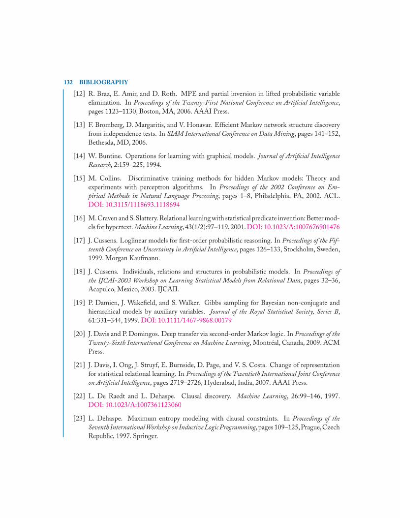
132 BIBLIOGRAPHY
[12] R. Braz, E. Amir, and D. Roth. MPE and partial inversion in lifted probabilistic variableelimination. In Proceedings of the Twenty-First National Conference on Artificial Intelligence,pages 1123–1130, Boston, MA, 2006. AAAI Press.
[13] F. Bromberg, D. Margaritis, and V. Honavar. Efficient Markov network structure discoveryfrom independence tests. In SIAM International Conference on Data Mining, pages 141–152,Bethesda, MD, 2006.
[14] W. Buntine. Operations for learning with graphical models. Journal of Artificial IntelligenceResearch, 2:159–225, 1994.
[15] M. Collins. Discriminative training methods for hidden Markov models: Theory andexperiments with perceptron algorithms. In Proceedings of the 2002 Conference on Em-pirical Methods in Natural Language Processing, pages 1–8, Philadelphia, PA, 2002. ACL.DOI: 10.3115/1118693.1118694
[16] M.Craven and S.Slattery. Relational learning with statistical predicate invention:Better mod-els for hypertext. Machine Learning, 43(1/2):97–119,2001.DOI: 10.1023/A:1007676901476
[17] J. Cussens. Loglinear models for first-order probabilistic reasoning. In Proceedings of the Fif-teenth Conference on Uncertainty in Artificial Intelligence, pages 126–133, Stockholm, Sweden,1999. Morgan Kaufmann.
[18] J. Cussens. Individuals, relations and structures in probabilistic models. In Proceedings ofthe IJCAI-2003 Workshop on Learning Statistical Models from Relational Data, pages 32–36,Acapulco, Mexico, 2003. IJCAII.
[19] P. Damien, J. Wakefield, and S. Walker. Gibbs sampling for Bayesian non-conjugate andhierarchical models by auxiliary variables. Journal of the Royal Statistical Society, Series B,61:331–344, 1999. DOI: 10.1111/1467-9868.00179
[20] J. Davis and P. Domingos. Deep transfer via second-order Markov logic. In Proceedings of theTwenty-Sixth International Conference on Machine Learning, Montréal, Canada, 2009. ACMPress.
[21] J. Davis, I. Ong, J. Struyf, E. Burnside, D. Page, and V. S. Costa. Change of representationfor statistical relational learning. In Proceedings of the Twentieth International Joint Conferenceon Artificial Intelligence, pages 2719–2726, Hyderabad, India, 2007. AAAI Press.
[22] L. De Raedt and L. Dehaspe. Clausal discovery. Machine Learning, 26:99–146, 1997.DOI: 10.1023/A:1007361123060
[23] L. Dehaspe. Maximum entropy modeling with clausal constraints. In Proceedings of theSeventh International Workshop on Inductive Logic Programming,pages 109–125,Prague,CzechRepublic, 1997. Springer.

BIBLIOGRAPHY 133
[24] S. Della Pietra, V. Della Pietra, and J. Lafferty. Inducing features of random fields.IEEE Transactions on Pattern Analysis and Machine Intelligence, 19:380–392, 1997.DOI: 10.1109/34.588021
[25] A. P. Dempster, N. M. Laird, and D. B. Rubin. Maximum likelihood from incompletedata via the EM algorithm. Journal of the Royal Statistical Society, Series B, 39:1–38, 1977.DOI: 10.2307/2984875
[26] W. Denham. The detection of patterns in Alyawarra nonverbal behavior. PhD thesis, Depart-ment of Anthropology, University of Washington, Seattle, WA, 1973.
[27] P. Denis and J. Baldridge. Joint determination of anaphoricity and coreference resolutionusing integer programming. In Proceedings of NAACL HLT 2007, pages 236–243, Rochester,New York, 2007. ACL.
[28] I. S. Dhillon, S. Mallela, and D. S. Modha. Information-theoretic co-clustering. In Proceedingsof the Ninth ACM SIGKDD International Conference on Knowledge Discovery and Data Mining,pages 89–98, Washington, DC, 2003. ACM Press. DOI: 10.1145/956750.956764
[29] T. Dietterich and X. Bao. Integrating multiple learning components through Markov logic.In Proceedings of the Twenty-Third National Conference on Artificial Intelligence, pages 622–627,Chicago, IL, 2008. AAAI Press.
[30] P. Domingos and M. Pazzani. On the optimality of the simple Bayesian classifier underzero-one loss. Machine Learning, 29:103–130, 1997. DOI: 10.1023/A:1007413511361
[31] K. Driessens, J. Ramon, and T. Croonenborghs. Transfer learning for reinforcement learningthrough goal and policy parametrization. In Proceedings of the ICML 2006 Workshop onStructural Knowledge Transfer for Machine Learning, 2006.
[32] S. Džeroski and L. De Raedt. Relational reinforcement learning. In Proceedings of the FifteenthInternational Conference on Machine Learning, pages 136–143, Madison, WI, 1998. MorganKaufmann. DOI: 10.1023/A:1007694015589
[33] S. Džeroski and N. Lavrac, editors. Relational Data mining. Springer, Berlin, Germany, 2001.
[34] C. Fellbaum, editor. WordNet: An Electronic Lexical Database. MIT Press, Cambridge, MA,1998.
[35] R. Fletcher. Practical Methods of Optimization. Wiley-Interscience, New York, NY, secondedition, 1987.
[36] N. Friedman, L. Getoor, D. Koller, and A. Pfeffer. Learning probabilistic relational models.In Proceedings of the Sixteenth International Joint Conference on Artificial Intelligence, pages1300–1307, Stockholm, Sweden, 1999. Morgan Kaufmann.

134 BIBLIOGRAPHY
[37] M. R. Genesereth and N. J. Nilsson. Logical Foundations of Artificial Intelligence. MorganKaufmann, San Mateo, CA, 1987.
[38] H Georgii. Gibbs Measures and Phase Transitions. Walter de Gruyter, Berlin, 1988.
[39] L. Getoor and B. Taskar, editors. Introduction to Statistical Relational Learning. MIT Press,Cambridge, MA, 2007.
[40] W. R. Gilks, S. Richardson, and D. J. Spiegelhalter, editors. Markov Chain Monte Carlo inPractice. Chapman and Hall, London, UK, 1996.
[41] T. Grenager, D. Klein, and C. D. Manning. Unsupervised learning of field segmentationmodels for information extraction. In Proceedings of the Forty-Third Annual Meeting on Associ-ation for Computational Linguistics, pages 371–378, Ann Arbor, Michigan, 2005. Associationfor Computational Linguistics. DOI: 10.3115/1219840.1219886
[42] A. Haghighi and D. Klein. Unsupervised coreference resolution in a nonparametric Bayesianmodel. In Proceedings of the 45th Annual Meeting of the Association for Computational Linguistics,pages 848–855, Prague, Czech Republic, 2007. ACL.
[43] J. Halpern. An analysis of first-order logics of probability. Artificial Intelligence, 46:311–350,1990. DOI: 10.1016/0004-3702(90)90019-V
[44] D. Heckerman, D. M. Chickering, C. Meek, R. Rounthwaite, and C. Kadie. Dependencynetworks for inference, collaborative filtering, and data visualization. Journal of MachineLearning Research, 1:49–75, 2000. DOI: 10.1162/153244301753344614
[45] D. Heckerman, D. Geiger, and D. M. Chickering. Learning Bayesian networks: Thecombination of knowledge and statistical data. Machine Learning, 20:197–243, 1995.DOI: 10.1007/BF00994016
[46] D. Heckerman, C. Meek, and D. Koller. Probabilistic entity-relationship models, PRMs, andplate models. In Proceedings of the ICML-2004 Workshop on Statistical Relational Learningand its Connections to Other Fields, pages 55–60, Banff, Canada, 2004. IMLS.
[47] G. E. Hinton. Training products of experts by minimizing contrastive divergence. NeuralComputation, 14(8):1771–1800, 2002. DOI: 10.1162/089976602760128018
[48] R. A. Howard and J. E. Matheson. Influence diagrams. Decision Analysis, 2(3):127–143, 2005.DOI: 10.1287/deca.1050.0020
[49] G. Hulten and P. Domingos. Mining complex models from arbitrarily large databases inconstant time. In Proceedings of the Eighth ACM SIGKDD International Conference on Knowl-edge Discovery and Data Mining, pages 525–531, Edmonton, Canada, 2002. ACM Press.DOI: 10.1145/775047.775124

BIBLIOGRAPHY 135
[50] T. Huynh and R. Mooney. Discriminative structure and parameter learning for Markov logicnetworks. In Proceedings of the Twenty-Fifth International Conference on Machine Learning,pages 416–423, Helsinki, Finland, 2008. ACM Press. DOI: 10.1145/1390156.1390209
[51] A. Jaimovich, O. Meshi, and N. Friedman. Template based inference in symmetric relationalMarkov random fields. In Proceedings of theTwenty-Third Conference on Uncertainty in ArtificialIntelligence, pages 191–199, Vancouver, Canada, 2007. AUAI Press.
[52] H. Kautz and B. Selman. Planning as satisfiability. In Proceedings of the Tenth EuropeanConference on Artificial Intelligence, pages 359–363, New York, NY, 1992. Wiley.
[53] H. Kautz, B. Selman, and Y. Jiang. A general stochastic approach to solving problems withhard and soft constraints. In D. Gu, J. Du, and P. Pardalos, editors, The Satisfiability Problem:Theory and Applications, pages 573–586. American Mathematical Society, New York, NY,1997.
[54] C. Kemp, J. B. Tenenbaum, T. L. Griffiths, T. Yamada, and N Ueda. Learning systemsof concepts with an infinite relational model. In Proceedings of the Twenty-First NationalConference on Artificial Intelligence, pages 381–388, Boston, MA, 2006. AAAI Press.
[55] K. Kersting and L. De Raedt. Towards combining inductive logic programming with Bayesiannetworks. In Proceedings of the Eleventh International Conference on Inductive Logic Program-ming, pages 118–131, Strasbourg, France, 2001. Springer. DOI: 10.1007/3-540-44797-0
[56] D. Klein and C. Manning. Accurate unlexicalized parsing. In Proceedings of the 41st AnnualMeeting of the Association for Computational Linguistics, pages 423–430, Sapporo, Japan, 2003.ACL. DOI: 10.3115/1075096.1075150
[57] S. Kok and P. Domingos. Learning the structure of Markov logic networks. In Proceedingsof the Twenty-Second International Conference on Machine Learning, pages 441–448, Bonn,Germany, 2005. ACM Press. DOI: 10.1145/1102351.1102407
[58] S. Kok and P. Domingos. Statistical predicate invention. In Proceedings of the Twenty-FourthInternational Conference on Machine Learning, pages 433–440, Corvallis, OR, 2007. ACMPress. DOI: 10.1145/1273496.1273551
[59] S. Kok and P. Domingos. Extracting semantic networks from text via relational clustering.In Proceedings of the Nineteenth European Conference on Machine Learning, pages 624–639,Antwerp, Belgium, 2008. Springer. DOI: 10.1007/978-3-540-87479-9_59
[60] S. Kok, M. Sumner, M. Richardson, P. Singla, H. Poon, D. Lowd, and P. Domin-gos. The Alchemy system for statistical relational AI. Technical report, Departmentof Computer Science and Engineering, University of Washington, Seattle, WA, 2007.http://alchemy.cs.washington.edu.

136 BIBLIOGRAPHY
[61] D. Koller and N. Friedman. Structured Probabilistic Models: Principles and Techniques. MITPress, Cambridge, MA, 2009.
[62] F. R. Kschischang, B. J. Frey, and H.-A. Loeliger. Factor graphs and the sum-product algo-rithm. IEEETransactions on InformationTheory,47:498–519,2001.DOI: 10.1109/18.910572
[63] N. Kushmerick. Wrapper induction: Efficiency and expressiveness. Artificial Intelligence,118(1-2):15–68, 2000. DOI: 10.1016/S0004-3702(99)00100-9
[64] J. Laffar and J.-L. Lassez. Constraint logic programming. In Proceedings of the FourteenthACM Conference on Principles of Programming Languages, pages 111–119, Munich, Germany,1987. ACM Press. DOI: 10.1145/41625.41635
[65] N. Lavrac and S. Džeroski. Inductive Logic Programming: Techniques and Applications. EllisHorwood, Chichester, UK, 1994.
[66] S. Lawrence, K. Bollacker, and C. L. Giles. Autonomous citation matching. In Proceedingsof the Third International Conference on Autonomous Agents, pages 392–393, New York, 1999.ACM Press. DOI: 10.1145/301136.301255
[67] S.-I. Lee, V. Chatalbashev, D. Vickrey, and D. Koller. Learning a meta-level priorfor feature relevance from multiple related tasks. In Proceedings of the Twenty-FourthInternational Conference on Machine Learning, pages 489–496, Corvallis, OR, 2007.DOI: 10.1145/1273496.1273558
[68] P. Liang and M. I. Jordan. An asymptotic analysis of generative, discriminative, andpseudolikelihood estimators. In Proceedings of the Twenty-Fifth International Con-ference on Machine Learning, pages 584–591, Helsinki, Finland, 2008. ACM Press.DOI: 10.1145/1390156.1390230
[69] B. Limketkai, L. Liao, and D. Fox. Relational object maps for mobile robots. In Proceedingsof the Nineteenth International Joint Conference on Artificial Intelligence, pages 1471–1476,Edinburgh, UK, 2005. Morgan Kaufmann.
[70] M.Lippi and P.Frasconi. Markov logic improves protein β-partners prediction. In Proceedingsof the Sixth International Workshop on Mining and Learning with Graphs, Helsinki, Finland,2008.
[71] D. C. Liu and J. Nocedal. On the limited memory BFGS method for large scale optimization.Mathematical Programming, 45(3):503–528, 1989. DOI: 10.1007/BF01589116
[72] J. W. Lloyd. Foundations of Logic Programming. Springer, Berlin, Germany, 1987.

BIBLIOGRAPHY 137
[73] E. Lloyd-Richardson, A. Kazura, C. Stanton, R. Niaura, and G. Papandonatos. Dif-ferentiating stages of smoking intensity among adolescents: Stage-specific psychologicaland social influences. Journal of Consulting and Clinical Psychology, 70(4):998–1009, 2002.DOI: 10.1037/0022-006X.70.4.998
[74] B. Long, Z. M. Zhang, X. Wu, and P. S. Yu. Spectral clustering for multi-type relationaldata. In Proceedings of the Twenty-Third International Conference on Machine Learning, pages585–592, Pittsburgh, PA, 2006. ACM Press. DOI: 10.1145/1143844.1143918
[75] D. Lowd and P. Domingos. Efficient weight learning for Markov logic net-works. In Proceedings of the Eleventh European Conference on Principles and Practiceof Knowledge Discovery in Databases, pages 200–211, Warsaw, Poland, 2007. Springer.DOI: 10.1007/978-3-540-74976-9_21
[76] D. Lowd and P. Domingos. Recursive random fields. In Proceedings of the Twentieth Interna-tional Joint Conference on Artificial Intelligence, pages 950–955, Hyderabad, India, 2007. AAAIPress.
[77] X. Luo, A. Ittycheriah, H. Jing, N. Kambhatla, and S. Roukos. A mention-synchronouscoreference resolution algorithm based on the Bell tree. In Proceedings of the 42nd AnnualMeeting of the Association for Computational Linguistics, pages 135–142, Barcelona, Spain,2004. ACL. DOI: 10.3115/1218955.1218973
[78] A. McCallum. Efficiently inducing features of conditional random fields. In Proceedingsof the Nineteenth Conference on Uncertainty in Artificial Intelligence, Acapulco, Mexico, 2003.Morgan Kaufmann.
[79] A. McCallum, R. Rosenfeld, T. Mitchell, and A. Y. Ng. Improving text classification byshrinkage in a hierarchy of classes. In Proceedings of the Fifteenth International Conference onMachine Learning, pages 359–367, Madison, WI, 1998. Morgan Kaufmann.
[80] A. McCallum and B. Wellner. Conditional models of identity uncertainty with applicationto noun coreference. In Advances in Neural Information Processing Systems 17, pages 905–912,Cambridge, MA, 2005. MIT Press.
[81] A.T.McCray. An upper level ontology for the biomedical domain. Comparative and FunctionalGenomics, 4:80–84, 2003. DOI: 10.1002/cfg.255
[82] L. Mihalkova, T. Huynh, and R. J. Mooney. Mapping and revising Markov logic networksfor transfer learning. In Proceedings of the Twenty-Second National Conference on ArtificialIntelligence, pages 608–614, Vancouver, Canada, 2007. AAAI Press.
[83] L. Mihalkova and R. Mooney. Bottom-up learning of Markov logic network structure. InProceedings of the Twenty-Fourth International Conference on Machine Learning, pages 625–632, Corvallis, OR, 2007. ACM Press. DOI: 10.1145/1273496.1273575

138 BIBLIOGRAPHY
[84] B. Milch, B. Marthi, S. Russell, D. Sontag, D. L. Ong, and A. Kolobov. BLOG: Probabilisticmodels with unknown objects. In Proceedings of the Nineteenth International Joint Conferenceon Artificial Intelligence, pages 1352–1359, Edinburgh, UK, 2005. Morgan Kaufmann.
[85] B. Milch, L. S. Zettlemoyer, K. Kersting, M. Haimes, and L. P. Kaelbling. Lifted probabilisticinference with counting formulas. In Proceedings of the Twenty-Third National Conference onArtificial Intelligence, pages 1062–1068, Chicago, IL, 2008. AAAI Press.
[86] M. Møller. A scaled conjugate gradient algorithm for fast supervised learning. Neural Net-works, 6:525–533, 1993. DOI: 10.1016/S0893-6080(05)80056-5
[87] S. Muggleton. Stochastic logic programs. In L. De Raedt, editor, Advances in Inductive LogicProgramming, pages 254–264. IOS Press, Amsterdam, Netherlands, 1996.
[88] S. Muggleton and C. Feng. Efficient induction of logic programs. In S. Muggleton, editor,Inductive Logic Programming, pages 281–298. Morgan Kaufmann, 1992.
[89] A. Nath and P. Domingos. A language for relational decision theory. In Proceedings of theInternational Workshop on Statistical Relational Learning, Leuven, Belgium, 2009.
[90] J. Neville and D. Jensen. Collective classification with relational dependency networks. InS. Džeroski, L. De Raedt, and S. Wrobel, editors, Proceedings of the Second InternationalWorkshop on Multi-Relational Data Mining, pages 77–91, Washington, DC, 2003. ACMPress.
[91] J. Neville and D. Jensen. Leveraging relational autocorrelation with latent group models. InProceedings of the Fifth IEEE International Conference on Data Mining, pages 49–55, NewOrleans, LA, 2005. IEEE Computer Society Press. DOI: 10.1109/ICDM.2005.89
[92] V.Ng. Machine learning for coreference resolution: From local classification to global ranking.In Proceedings of the 43th Annual Meeting of the Association for Computational Linguistics, pages157–164, Ann Arbor, MI, 2005. ACL. DOI: 10.3115/1219840.1219860
[93] L. Ngo and P. Haddawy. Answering queries from context-sensitive prob-abilistic knowledge bases. Theoretical Computer Science, 171:147–177, 1997.DOI: 10.1016/S0304-3975(96)00128-4
[94] N. Nilsson. Probabilistic logic. Artificial Intelligence, 28:71–87, 1986.DOI: 10.1016/0004-3702(86)90031-7
[95] J. Nocedal and S. Wright. Numerical Optimization. Springer, New York, NY, 2006.
[96] D. N. Osherson, J. Stern, O. Wilkie, M. Stob., and E. E. Smith. Default probability. CognitiveScience, 15:251–269, 1991. DOI: 10.1016/0364-0213(91)80007-R
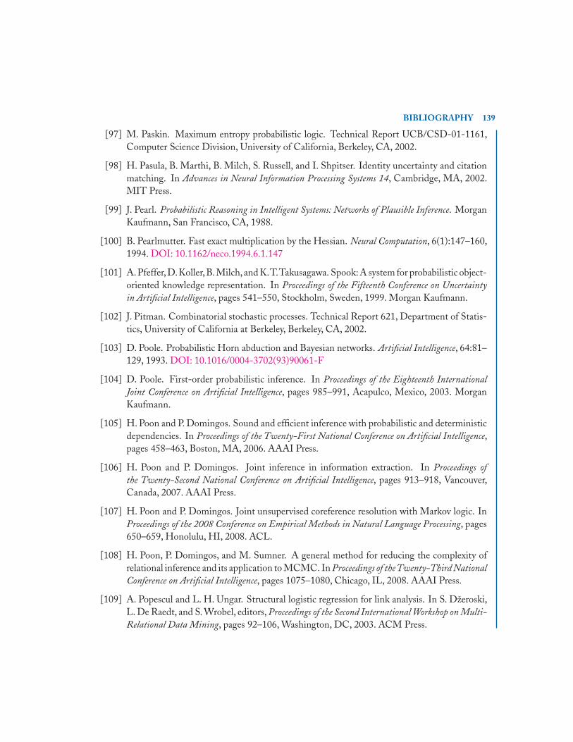
BIBLIOGRAPHY 139
[97] M. Paskin. Maximum entropy probabilistic logic. Technical Report UCB/CSD-01-1161,Computer Science Division, University of California, Berkeley, CA, 2002.
[98] H. Pasula, B. Marthi, B. Milch, S. Russell, and I. Shpitser. Identity uncertainty and citationmatching. In Advances in Neural Information Processing Systems 14, Cambridge, MA, 2002.MIT Press.
[99] J. Pearl. Probabilistic Reasoning in Intelligent Systems: Networks of Plausible Inference. MorganKaufmann, San Francisco, CA, 1988.
[100] B. Pearlmutter. Fast exact multiplication by the Hessian. Neural Computation, 6(1):147–160,1994. DOI: 10.1162/neco.1994.6.1.147
[101] A.Pfeffer,D.Koller,B.Milch,and K.T.Takusagawa. Spook: A system for probabilistic object-oriented knowledge representation. In Proceedings of the Fifteenth Conference on Uncertaintyin Artificial Intelligence, pages 541–550, Stockholm, Sweden, 1999. Morgan Kaufmann.
[102] J. Pitman. Combinatorial stochastic processes. Technical Report 621, Department of Statis-tics, University of California at Berkeley, Berkeley, CA, 2002.
[103] D. Poole. Probabilistic Horn abduction and Bayesian networks. Artificial Intelligence, 64:81–129, 1993. DOI: 10.1016/0004-3702(93)90061-F
[104] D. Poole. First-order probabilistic inference. In Proceedings of the Eighteenth InternationalJoint Conference on Artificial Intelligence, pages 985–991, Acapulco, Mexico, 2003. MorganKaufmann.
[105] H. Poon and P. Domingos. Sound and efficient inference with probabilistic and deterministicdependencies. In Proceedings of the Twenty-First National Conference on Artificial Intelligence,pages 458–463, Boston, MA, 2006. AAAI Press.
[106] H. Poon and P. Domingos. Joint inference in information extraction. In Proceedings ofthe Twenty-Second National Conference on Artificial Intelligence, pages 913–918, Vancouver,Canada, 2007. AAAI Press.
[107] H. Poon and P. Domingos. Joint unsupervised coreference resolution with Markov logic. InProceedings of the 2008 Conference on Empirical Methods in Natural Language Processing, pages650–659, Honolulu, HI, 2008. ACL.
[108] H. Poon, P. Domingos, and M. Sumner. A general method for reducing the complexity ofrelational inference and its application to MCMC. In Proceedings of theTwenty-Third NationalConference on Artificial Intelligence, pages 1075–1080, Chicago, IL, 2008. AAAI Press.
[109] A. Popescul and L. H. Ungar. Structural logistic regression for link analysis. In S. Džeroski,L. De Raedt, and S. Wrobel, editors, Proceedings of the Second International Workshop on Multi-Relational Data Mining, pages 92–106, Washington, DC, 2003. ACM Press.

140 BIBLIOGRAPHY
[110] A. Popescul and L. H. Ungar. Cluster-based concept invention for statistical rela-tional learning. In Proceedings of the Tenth ACM SIGKDD International Conference onKnowledge Discovery and Data Mining, pages 665–664, Seattle, WA, 2004. ACM Press.DOI: 10.1145/1014052.1014137
[111] A. Puech and S. Muggleton. A comparison of stochastic logic programs and Bayesian logicprograms. In Proceedings of the IJCAI-2003 Workshop on Learning Statistical Models fromRelational Data, pages 121–129, Acapulco, Mexico, 2003. IJCAII.
[112] M. R. Quillian. Semantic memory. In M. L. Minsky, editor, Semantic Information Processing,pages 216–270. MIT Press, Cambridge, MA, 1968.
[113] J. R. Quinlan. Learning logical definitions from relations. Machine Learning, 5:239–266,1990. DOI: 10.1007/BF00117105
[114] B. L. Richards and R. J. Mooney. Learning relations by pathfinding. In Proceedings of theTenth National Conference on Artificial Intelligence, pages 50–55, San Jose, CA, 1992. AAAIPress.
[115] B. L. Richards and R. J. Mooney. Automated refinement of first-order Horn-clause domaintheories. Machine Learning, 19(2):95–131, 1995. DOI: 10.1007/BF01007461
[116] M. Richardson and P. Domingos. Building large knowledge bases by mass collaboration.In Proceedings of the Second International Conference on Knowledge Capture, pages 129–137,Sanibel Island, FL, 2003. ACM Press. DOI: 10.1145/945645.945665
[117] M. Richardson and P. Domingos. Markov logic networks. Machine Learning, 62:107–136,2006. DOI: 10.1007/s10994-006-5833-1
[118] S. Riedel. Improving the accuracy and efficiency of MAP inference for Markov logic. InProceedings of the Twenty-Fourth Conference on Uncertainty in Artificial Intelligence, pages 468–475, Helsinki, Finland, 2008. AUAI Press.
[119] S. Riedel and E. Klein. Genic interaction extraction with semantic and syntactic chains.In Proceedings of the Fourth Workshop on Learning Language in Logic, pages 69–74, Bonn,Germany, 2005. IMLS.
[120] S. Riedel and I. Meza-Ruiz. Collective semantic role labelling with Markov logic. In Pro-ceedings of the 2008 Conference on Empirical Methods in Natural Language Processing, pages188–192, Honolulu, HI, 2008. ACL.
[121] S. Riezler. Probabilistic Constraint Logic Programming. PhD thesis, University of Tubingen,Tubingen, Germany, 1998.

BIBLIOGRAPHY 141
[122] J. A. Robinson. A machine-oriented logic based on the resolution principle. Journal of theACM, 12:23–41, 1965. DOI: 10.1145/321250.321253
[123] D. Roth. On the hardness of approximate reasoning. Artificial Intelligence, 82:273–302, 1996.DOI: 10.1016/0004-3702(94)00092-1
[124] D. Roy, C. Kemp, V. K. Mansinghka, and J. B. Tenenbaum. Learning annotated hierarchiesfrom relational data. In Advances in Neural Information Processing Systems 19,pages 1210–1217,Cambridge, MA, 2006. MIT Press.
[125] D. M. Roy and L. P. Kaelbling. Efficient Bayesian task-level transfer learning. In Proceed-ings of the Twentieth International Joint Conference on Artificial Intelligence, pages 2599–2604,Hyderabad, India, 2007. AAAI Press.
[126] R. J. Rummel. Dimensionality of nations project: attributes of nations and behavior of nationdyads, 1950 -1965. ICPSR data file. 1999. DOI: 10.3886/ICPSR05409
[127] S. Sanner. First-Order Decision-Theoretic Planning in Structured Relational Environments.PhD thesis, University of Toronto, 2008.
[128] V. Santos Costa, D. Page, M. Qazi, , and J. Cussens. CLP(BN): Constraint logic pro-gramming for probabilistic knowledge. In Proceedings of the Nineteenth Conference on Uncer-tainty in Artificial Intelligence, pages 517–524, Acapulco, Mexico, 2003. Morgan Kaufmann.DOI: 10.1007/978-3-540-78652-8
[129] T. Sato and Y. Kameya. PRISM: A symbolic-statistical modeling language. In Proceedings ofthe Fifteenth International Joint Conference on Artificial Intelligence, pages 1330–1335, Nagoya,Japan, 1997. Morgan Kaufmann.
[130] S. Schoenmackers, O. Etzioni, and D. S. Weld. Scaling textual inference to the Web. InProceedings of the 2008 Conference on Empirical Methods in Natural Language Processing, pages79–88, Honolulu, HI, 2008. ACL.
[131] F. Sha and F. Pereira. Shallow parsing with conditional random fields. In Proceedings of the2003 Human Language Technology Conference and North American Chapter of the Association forComputational Linguistics, pages 134–141. Association for Computational Linguistics, 2003.DOI: 10.3115/1073445.1073473
[132] J. Shewchuck. An introduction to the conjugate gradient method without the agonizingpain. Technical Report CMU-CS-94-125, School of Computer Science, Carnegie MellonUniversity, 1994.
[133] P. Singla and P. Domingos. Discriminative training of Markov logic networks. In Proceedingsof the Twentieth National Conference on Artificial Intelligence, pages 868–873, Pittsburgh, PA,2005. AAAI Press.

142 BIBLIOGRAPHY
[134] P. Singla and P. Domingos. Entity resolution with Markov logic. In Proceedings of the SixthIEEE International Conference on Data Mining, pages 572–582, Hong Kong, 2006. IEEEComputer Society Press. DOI: 10.1109/ICDM.2006.65
[135] P. Singla and P. Domingos. Memory-efficient inference in relational domains. In Proceedingsof the Twenty-First National Conference on Artificial Intelligence, pages 488–493, Boston, MA,2006. AAAI Press.
[136] P. Singla and P. Domingos. Markov logic in infinite domains. In Proceedings of the Twenty-Third Conference on Uncertainty in Artificial Intelligence, pages 368–375, Vancouver, Canada,2007. AUAI Press.
[137] P. Singla and P. Domingos. Markov logic in infinite domains. Technical report, Dept. Comp.Sci. & Eng., Univ. Washington, 2007.http://alchemy.cs.washington.edu/papers/singla07/tr.pdf.
[138] P. Singla and P. Domingos. Lifted first-order belief propagation. In Proceedings of the Twenty-Third National Conference on Artificial Intelligence, pages 1094–1099,Chicago, IL,2008.AAAIPress.
[139] P. Singla, H. Kautz, J. Luo, and A. Gallagher. Discovery of social relationships in consumerphoto collections using Markov logic. In 2008 CVPR Workshop on Semantic Learning andApplications in Multimedia,Anchorage,Alaska,2008.DOI: 10.1109/CVPRW.2008.4563047
[140] A. Srinivasan. The Aleph manual. Technical report, Computing Laboratory, Oxford Uni-versity, 2000.
[141] B.Taskar, P. Abbeel, and D. Koller. Discriminative probabilistic models for relational data. InProceedings of the Eighteenth Conference on Uncertainty in Artificial Intelligence, pages 485–492,Edmonton, Canada, 2002. Morgan Kaufmann.
[142] M. E. Taylor, A. Fern, and K. Driessens, editors. Proceedings of the AAAI-2008 Workshop onTransfer Learning for Complex Tasks. AAAI Press, Chicago, IL, 2008.
[143] M. E. Taylor and P. Stone. Cross-domain transfer for reinforcement learning. In Proceedingsof the Twenty-Fourth International Conference on Machine Learning, pages 879–886, Corvallis,OR, 2007. ACM Press. DOI: 10.1145/1273496.1273607
[144] L.Torrey,T.Walker, J. Shavlik, and R. Maclin. Relational macros for transfer in reinforcementlearning. In Proceedings of the Seventeenth International Conference on Inductive Logic Program-ming, pages 254–268, Corvallis, OR, 2007. Springer. DOI: 10.1007/978-3-540-78469-2
[145] G. G. Towell and J. W. Shavlik. Knowledge-based artificial neural networks. ArtificialIntelligence, 70:119–165, 1994. DOI: 10.1016/0004-3702(94)90105-8

BIBLIOGRAPHY 143
[146] M. van Otterlo. A survey of reinforcement learning in relational domains. Technical report,University of Twente, 2005.
[147] M. Vilain, J. Burger, J. Aberdeen, D. Connolly, and L. Hirschman. A model-theoretic coref-erence scoring scheme. In Proceedings of the 6th conference on message understanding, pages45–52, Columbia, MD, 1995. ACL. DOI: 10.3115/1072399.1072405
[148] J. Wang and P. Domingos. Hybrid Markov logic networks. In Proceedings of the Twenty-ThirdNational Conference on Artificial Intelligence,pages 1106–1111,Chicago, IL,2008.AAAI Press.
[149] S. Wasserman and K. Faust. Social Network Analysis: Methods and Applications. CambridgeUniversity Press, Cambridge, UK, 1994.
[150] W. Wei, J. Erenrich, and B. Selman. Towards efficient sampling: Exploiting random walkstrategies. In Proceedings of the Nineteenth National Conference on Artificial Intelligence, pages670–676, San Jose, CA, 2004. AAAI Press.
[151] M. Wellman, J. S. Breese, and R. P. Goldman. From knowledge bases to decision models.Knowledge Engineering Review, 7:35–53, 1992.
[152] B. Wellner, A. McCallum, F. Peng, and M. Hay. An integrated, conditional model of infor-mation extraction and coreference with application to citation matching. In Proceedings of theTwentieth Conference on Uncertainty in Artificial Intelligence, pages 593–601, Banff, Canada,2004. AUAI Press.
[153] A. P. Wolfe and D. Jensen. Playing multiple roles: discovering overlapping roles in socialnetworks. In Proceedings of the ICML-2004 Workshop on Statistical Relational Learning and itsConnections to Other Fields, pages 49–54, Banff, Canada, 2004. IMLS.
[154] F. Wu and D. Weld. Automatically refining the Wikipedia infobox ontology. In Proceedings ofthe 17th International World Wide Web Conference, pages 635–644, Beijing,China, 2008. ACMPress. DOI: 10.1145/1367497.1367583
[155] Z. Xu, V. Tresp, K. Yu, S. Yu, and H.-P. Kriegel. Dirichlet enhanced relational learning. InProceedings of the Twenty-Second International Conference on Machine Learning, pages 1004–1011, Bonn, Germany, 2005. ACM Press. DOI: 10.1145/1102351.1102478
[156] J. S. Yedidia, W. T. Freeman, and Y. Weiss. Generalized belief propagation. In T. Leen,T. Dietterich, and V. Tresp, editors, Advances in Neural Information Processing Systems 13,pages 689–695. MIT Press, Cambridge, MA, 2001.


145
Biography
PEDRO DOMINGOSPedro Domingos is Associate Professor of Computer Science and Engineering at the University ofWashington. His research interests are in artificial intelligence, machine learning and data mining.He received a PhD in Information and Computer Science from the University of California atIrvine, and is the author or co-author of over 150 technical publications. He is a member of theeditorial board of the Machine Learning journal, co-founder of the International Machine LearningSociety, and past associate editor of JAIR. He was program co-chair of KDD-2003 and SRL-2009,and has served on numerous program committees. He has received several awards, including a SloanFellowship, an NSF CAREER Award, a Fulbright Scholarship, an IBM Faculty Award, and bestpaper awards at KDD-98, KDD-99 and PKDD-2005.
DANIEL LOWDDaniel Lowd is a PhD candidate in the Department of Computer Science and Engineering atthe University of Washington. His research covers a range of topics in statistical machine learning,including statistical relational representations, unifying learning and inference, and adversarial ma-chine learning scenarios (e.g., spam filtering). He has received graduate research fellowships fromthe National Science Foundation and Microsoft Research.


