Markov switching multinomial logit model: an application ... · Markov switching multinomial logit...

arX

iv:0

811.

3644

v1 [

stat

.AP]

21

Nov

200

8

Markov switching multinomial logit model: an

application to accident injury severities

Nataliya V. Malyshkina ∗, Fred L. Mannering

School of Civil Engineering, 550 Stadium Mall Drive, Purdue University, West

Lafayette, IN 47907, United States

Abstract

In this study, two-state Markov switching multinomial logit models are proposedfor statistical modeling of accident injury severities. These models assume Markovswitching in time between two unobserved states of roadway safety. The states aredistinct, in the sense that in different states accident severity outcomes are generatedby separate multinomial logit processes. To demonstrate the applicability of theapproach presented herein, two-state Markov switching multinomial logit modelsare estimated for severity outcomes of accidents occurring on Indiana roads overa four-year time interval. Bayesian inference methods and Markov Chain MonteCarlo (MCMC) simulations are used for model estimation. The estimated Markovswitching models result in a superior statistical fit relative to the standard (single-state) multinomial logit models. It is found that the more frequent state of roadwaysafety is correlated with better weather conditions. The less frequent state is foundto be correlated with adverse weather conditions.

Key words: Accident injury severity; multinomial logit; Markov switching;Bayesian; MCMC

1 Introduction

Vehicle accidents result in property damage, injuries and loss of people lives.Thus, research efforts in predicting accident severity are clearly very impor-tant. In the past there has been a large number of studies that focused on mod-eling accident severity outcomes. Common modeling approaches of accident

∗ Corresponding author.Email addresses: [email protected] (Nataliya V. Malyshkina),

[email protected] (Fred L. Mannering).

Preprint submitted to Accident Analysis and Prevention

http://arxiv.org/abs/0811.3644v1

severity include multinomial logit models, nested logit models, mixed logitmodels and ordered probit models (O’Donnell and Connor, 1996; Shankar and Mannering,1996; Shankar et al., 1996; Duncan et al., 1998; Chang and Mannering, 1999;Carson and Mannering, 2001; Khattak, 2001; Khattak et al., 2002; Kockelman and Kweon,2002; Lee and Mannering, 2002; Abdel-Aty, 2003; Kweon and Kockelman, 2003;Ulfarsson and Mannering, 2004; Yamamoto and Shankar, 2004; Khorashadi et al.,2005; Eluru and Bhat, 2007; Savolainen and Mannering, 2007; Milton et al.,2008). All these models involve nonlinear regression of the observed accidentinjury severity outcomes on various accident characteristics and related factors(such as roadway and driver characteristics, environmental factors, etc).

In our earlier paper, Malyshkina et al. (2008), which we will refer to as Pa-per I, we presented two-state Markov switching count data models of accidentfrequencies. In this study, which is a continuation of our work on Markovswitching models, we present two-state Markov switching multinomial logitmodels for predicting accident severity outcomes. These models assume thatthere are two unobserved states of roadway safety, roadway entities (road-way segments) can switch between these states over time, and the switchingprocess is Markovian. The two states intend to account for possible hetero-geneity effects in roadway safety, which may be caused by various unpre-dictable, unidentified, unobservable risk factors that influence roadway safety.Because the risk factors can interact and change, roadway entities can switchbetween the two states over time. Two-state Markov switching multinomiallogit models assume separate multinomial logit processes for accident severitydata generation in the two states and, therefore, allow a researcher to studythe heterogeneity effects in roadway safety.

2 Model specification

Markov switching models are parametric and can be fully specified by a like-lihood function f(Y|Θ,M), which is the conditional probability distributionof the vector of all observations Y, given the vector of all parameters Θ ofmodel M. First, let us consider Y. Let Nt be the number of accidents ob-served during time period t, where t = 1, 2, . . . , T and T is the total numberof time periods. Let there be I discrete outcomes observed for accident sever-ity (for example, I = 3 and these outcomes are fatality, injury and property

damage only). Let us introduce accident severity outcome dummies δ(i)t,n that

are equal to unity if the ith severity outcome is observed in the nth accidentthat occurs during time period t, and to zero otherwise. Here i = 1, 2, . . . , I,n = 1, 2, . . . , Nt and t = 1, 2, . . . , T . Then, our observations are the accidentseverity outcomes, and the vector of all observations Y = {δ

(i)t,n} includes all

outcomes observed in all accidents that occur during all time periods. Sec-ond, let us consider model specification variable M. It is M = {M,Xt,n}

2

and includes the model’s name M (for example, M = “multinomial logit”)and the vector Xt,n of all accident characteristic variables (weather and envi-ronment conditions, vehicle and driver characteristics, roadway and pavementproperties, and so on).

To define the likelihood function, we first introduce an unobserved (latent)state variable st, which determines the state of all roadway entities duringtime period t. At each t, the state variable st can assume only two values:st = 0 corresponds to one state and st = 1 corresponds to the other state (t =1, 2, . . . , T ). The state variable st is assumed to follow a stationary two-stateMarkov chain process in time, 1 which can be specified by time-independenttransition probabilities as

P (st+1 = 1|st = 0) = p0→1, P (st+1 = 0|st = 1) = p1→0. (1)

Here, for example, P (st+1 = 1|st = 0) is the conditional probability of st+1 = 1at time t + 1, given that st = 0 at time t. Transition probabilities p0→1 andp1→0 are unknown parameters to be estimated from accident severity data.The stationary unconditional probabilities of states st = 0 and st = 1 arep̄0 = p1→0/(p0→1+ p1→0) and p̄1 = p0→1/(p0→1+ p1→0) respectively.

2 Withoutloss of generality, we assume that (on average) state st = 0 occurs moreor equally frequently than state st = 1. Therefore, p̄0 ≥ p̄1, and we obtainrestriction 3

p0→1 ≤ p1→0. (2)

We refer to states st = 0 and st = 1 as “more frequent” and “less frequent”states respectively.

Next, a two-state Markov switching multinomial logit (MSML) model assumesmultinomial logit (ML) data-generating processes for accident severity in eachof the two states. With this, the probability of the ith severity outcome ob-served in the nth accident during time period t is

1 Markov property means that the probability distribution of st+1 depends onlyon the value st at time t, but not on the previous history st−1, st−2, . . .. Stationarityof {st} is in the statistical sense.2 These can be found from stationarity conditions p̄0 = (1 − p0→1)p̄0 + p1→0p̄1,p̄1 = p0→1p̄0 + (1− p1→0)p̄1 and p̄0 + p̄1 = 1.3 Without any loss of generality, restriction (2) is introduced for the purpose ofavoiding the problem of state label switching 0 ↔ 1. This problem would otherwisearise because of the symmetry of Eqs. (1)–(4) under the label switching.

3

P(i)t,n =

exp(β′(0),iXt,n)

∑Ij=1 exp(β

′(0),jXt,n)

if st = 0,

exp(β′(1),iXt,n)

∑Ij=1 exp(β

′(1),jXt,n)

if st = 1,

(3)

i=1, 2, . . . , I, n = 1, 2, . . . , Nt, t = 1, 2, . . . , T,

Here prime means transpose (so β′(0),i is the transpose of β(0),i). Parameter

vectors β(0),i and β(1),i are unknown estimable parameters of the two standardmultinomial logit probability mass functions (Washington et al., 2003) in thetwo states, st = 0 and st = 1 respectively. We set the first component of Xt,n

to unity, and, therefore, the first components of vectors β(0),i and β(1),i arethe intercepts in the two states. In addition, without loss of generality, we setall β-parameters for the last severity outcome to zero, 4 β(0),I = β(1),I = 0.

If accident events are assumed to be independent, the likelihood function is

f(Y|Θ,M) =T∏

t=1

Nt∏

n=1

I∏

i=1

[

P(i)t,n

]δ(i)t,n

. (4)

Here, because the state variables st,n are unobservable, the vector of all es-timable parameters Θ must include all states, in addition to model parameters(β-s) and transition probabilities. Thus, Θ = [β′

(0),β′(1), p0→1, p1→0,S

′]′, wherevector S = [s1, s2, ..., sT ]

′ has length T and contains all state values. Eqs. (1)-(4) define the two-state Markov switching multinomial logit (MSML) modelconsidered here.

3 Model estimation methods

Statistical estimation of Markov switching models is complicated by unobserv-ability of the state variables st.

5 As a result, the traditional maximum likeli-hood estimation (MLE) procedure is of very limited use for Markov switchingmodels. Instead, a Bayesian inference approach is used. Given a model Mwith likelihood function f(Y|Θ,M), the Bayes formula is

f(Θ|Y,M) =f(Y,Θ|M)

f(Y|M)=

f(Y|Θ,M)π(Θ|M)∫

f(Y,Θ|M) dΘ. (5)

4 This can be done because Xt,n are assumed to be independent of the outcome i.5 Below we will have 208 time periods (T = 208). In this case, there are 2208 possiblecombinations for value of vector S = [s1, s2, ..., sT ]

′.

4

Here f(Θ|Y,M) is the posterior probability distribution of model parametersΘ conditional on the observed data Y and model M. Function f(Y,Θ|M)is the joint probability distribution of Y and Θ given model M. Functionf(Y|M) is the marginal likelihood function – the probability distribution ofdataY given model M. Function π(Θ|M) is the prior probability distributionof parameters that reflects prior knowledge about Θ. The intuition behindEq. (5) is straightforward: given model M, the posterior distribution accountsfor both the observations Y and our prior knowledge of Θ.

In our study (and in most practical studies), the direct application of Eq. (5) isnot feasible because the parameter vector Θ contains too many components,making integration over Θ in Eq. (5) extremely difficult. However, the poste-rior distribution f(Θ|Y,M) in Eq. (5) is known up to its normalization con-stant, f(Θ|Y,M) ∝ f(Y|Θ,M)π(Θ|M). As a result, we use Markov ChainMonte Carlo (MCMC) simulations, which provide a convenient and practi-cal computational methodology for sampling from a probability distributionknown up to a constant (the posterior distribution in our case). Given a largeenough posterior sample of parameter vector Θ, any posterior expectation andvariance can be found and Bayesian inference can be readily applied. A readerinterested in details is referred to our Paper I or to Malyshkina (2008), wherewe describe our choice of the prior distribution π(Θ|M) and the MCMC sim-ulation algorithm. 6 Although, in this study we estimate a two-state Markovswitching multinomial logit model for accident severity outcomes and in Pa-per I we estimated a two-state Markov switching negative binomial model foraccident frequencies, this difference is not essential for the Bayesian-MCMCmodel estimation methods. In fact, the main difference is in the likelihoodfunction (multinomial logit as opposed to negative binomial). So we used thesame our own numerical MCMC code, written in the MATLAB programminglanguage, for model estimation in both studies. We tested our code on arti-ficial data sets of accident severity outcomes. The test procedure included ageneration of artificial data with a known model. Then these data were usedto estimate the underlying model by means of our simulation code. With thisprocedure we found that the MSML models, used to generate the artificialdata, were reproduced successfully with our estimation code.

For comparison of different models we use a formal Bayesian approach. Letthere be two models M1 and M2 with parameter vectors Θ1 and Θ2 respec-tively. Assuming that we have equal preferences of these models, their priorprobabilities are π(M1) = π(M2) = 1/2. In this case, the ratio of the models’posterior probabilities, P (M1|Y) and P (M2|Y), is equal to the Bayes fac-tor. The later is defined as the ratio of the models’ marginal likelihoods (seeKass and Raftery, 1995). Thus, we have

6 Our priors for β-s, p0→1 and p1→0 are flat or nearly flat, while the prior for thestates S reflects the Markov process property, specified by Eq. (1).

5

P (M2|Y)

P (M1|Y)=

f(M2,Y)/f(Y)

f(M1,Y)/f(Y)=

f(Y|M2)π(M2)

f(Y|M1)π(M1)=

f(Y|M2)

f(Y|M1), (6)

where f(M1,Y) and f(M2,Y) are the joint distributions of the models andthe data, f(Y) is the unconditional distribution of the data. As in Paper I,to calculate the marginal likelihoods f(Y|M1) and f(Y|M2), we use theharmonic mean formula f(Y|M)−1 = E [f(Y|Θ,M)−1|Y], where E(. . . |Y)means posterior expectation calculated by using the posterior distribution. Ifthe ratio in Eq. (6) is larger than one, then model M2 is favored, if the ratiois less than one, then model M1 is favored. An advantage of the use of Bayesfactors is that it has an inherent penalty for including too many parametersin the model and guards against overfitting.

To evaluate the performance of model {M,Θ} in fitting the observed data Y,we carry out the Pearson’s χ2 goodness-of-fit test (Maher and Summersgill,1996; Cowan, 1998; Wood, 2002; Press et al., 2007). We perform this test byMonte Carlo simulations to find the distribution of the Pearson’s χ2 quan-tity, which measures the discrepancy between the observations and the modelpredictions (Cowan, 1998). This distribution is then used to find the goodness-of-fit p-value, which is the probability that χ2 exceeds the observed value ofχ2 under the hypothesis that the model is true (the observed value of χ2 iscalculated by using the observed data Y). For additional details, please seeMalyshkina (2008).

4 Empirical results

The severity outcome of an accident is determined by the injury level sustainedby the most injured individual (if any) involved into the accident. In this studywe consider three accident severity outcomes: “fatality”, “injury” and “PDO(property damage only)”, which we number as i = 1, 2, 3 respectively (I = 3).We use data from 811720 accidents that were observed in Indiana in 2003-2006.As in Paper I, we use weekly time periods, t = 1, 2, 3, . . . , T = 208 in total. 7

Thus, the state st can change every week. To increase the predictive powerof our models, we consider accidents separately for each combination of acci-dent type (1-vehicle and 2-vehicle) and roadway class (interstate highways, USroutes, state routes, county roads, streets). We do not consider accidents withmore than two vehicles involved. 8 Thus, in total, there are ten roadway-class-accident-type combinations that we consider. For each roadway-class-accident-

7 A week is from Sunday to Saturday, there are 208 full weeks in the 2003-2006time interval.8 Among 811720 accidents 241011 (29.7%) are 1-vehicle, 525035 (64.7%) are 2-vehicle, and only 45674 (5.6%) are accidents with more than two vehicles involved.

6

type combination the following three types of accident frequency models areestimated:

• First, we estimate a standard multinomial logit (ML) model without Markovswitching by maximum likelihood estimation (MLE). 9 We refer to thismodel as “ML-by-MLE”.

• Second, we estimate the same standard multinomial logit model by theBayesian inference approach and the MCMC simulations. We refer to thismodel as “ML-by-MCMC”. As one expects, the estimated ML-by-MCMCmodel turned out to be very similar to the corresponding ML-by-MLE model(estimated for the same roadway-class-accident-type combination).

• Third, we estimate a two-state Markov switching multinomial logit (MSML)model by the Bayesian-MCMC methods. In order to make comparison of ex-planatory variable effects in different models straightforward, in the MSMLmodel we use only those explanatory variables that enter the correspondingstandard ML model. 10 To obtain the final MSML model reported here, wealso consecutively construct and use 60%, 85% and 95% Bayesian credibleintervals for evaluation of the statistical significance of each β-parameter.As a result, in the final model some components of β(0) and β(1) are re-stricted to zero or restricted to be the same in the two states. 11 We referto this final model as “MSML”.

Note that the two states, and thus the MSML models, do not have to existfor every roadway-class-accident-type combination. For example, they will notexist if all estimated model parameters turn out to be statistically the samein the two states, β(0) = β(1), (which suggests the two states are identical andthe MSML models reduce to the corresponding standard ML models). Also,the two states will not exist if all estimated state variables st turn out to beclose to zero, resulting in p0→1 ≪ p1→0 [compare to Eq. (2)], then the less

9 To obtain parsimonious standard models, estimated by MLE, we choose theexplanatory variables and their dummies by using the Akaike Information Criterion(AIC) and the 5% statistical significance level for the two-tailed t-test. Minimizationof AIC = 2K − 2LL, were K is the number of free continuous model parametersand LL is the log-likelihood, ensures an optimal choice of explanatory variables ina model and avoids overfitting (Tsay, 2002; Washington et al., 2003). For details onvariable selection, see Malyshkina (2006).10 A formal Bayesian approach to model variable selection is based on evaluationof model’s marginal likelihood and the Bayes factor (6). Unfortunately, becauseMCMC simulations are computationally expensive, evaluation of marginal likeli-hoods for a large number of trial models is not feasible in our study.11 A β-parameter is restricted to zero if it is statistically insignificant. A β-parameteris restricted to be the same in the two states if the difference of its values in thetwo states is statistically insignificant. A (1 − a) credible interval is chosen in suchway that the posterior probabilities of being below and above it are both equal toa/2 (we use significance levels a = 40%, 15%, 5%).

7

frequent state st = 1 is not realized and the process stays in state st = 0.

Turning to the estimation results, the findings show that two states of roadwaysafety and the appropriate MSML models exist for severity outcomes of 1-vehicle accidents occurring on all roadway classes (interstate highways, USroutes, state routes, county roads, streets), and for severity outcomes of 2-vehicle accidents occurring on streets. We did not find two states in the cases of2-vehicle accidents on interstate highways, US routes, state routes and countyroads (in these cases all estimated state variables st were found to be close tozero). The model estimation results for severity outcomes of 1-vehicle accidentsoccurring on interstate highways, US routes and state routes are given inTables 1–3. All continuous model parameters (β-s, p0→1 and p1→0) are giventogether with their 95% confidence intervals (if MLE) or 95% credible intervals(if Bayesian-MCMC), refer to the superscript and subscript numbers adjacentto parameter estimates in Tables 1–3. 12 Table 4 gives summary statistics ofall roadway accident characteristic variables Xt,n (except the intercept).

12 Note that MLE assumes asymptotic normality of the estimates, resulting in con-fidence intervals being symmetric around the means (a 95% confidence interval is±1.96 standard deviations around the mean). In contrast, Bayesian estimation doesnot require this assumption, and posterior distributions of parameters and Bayesiancredible intervals are usually non-symmetric.

8

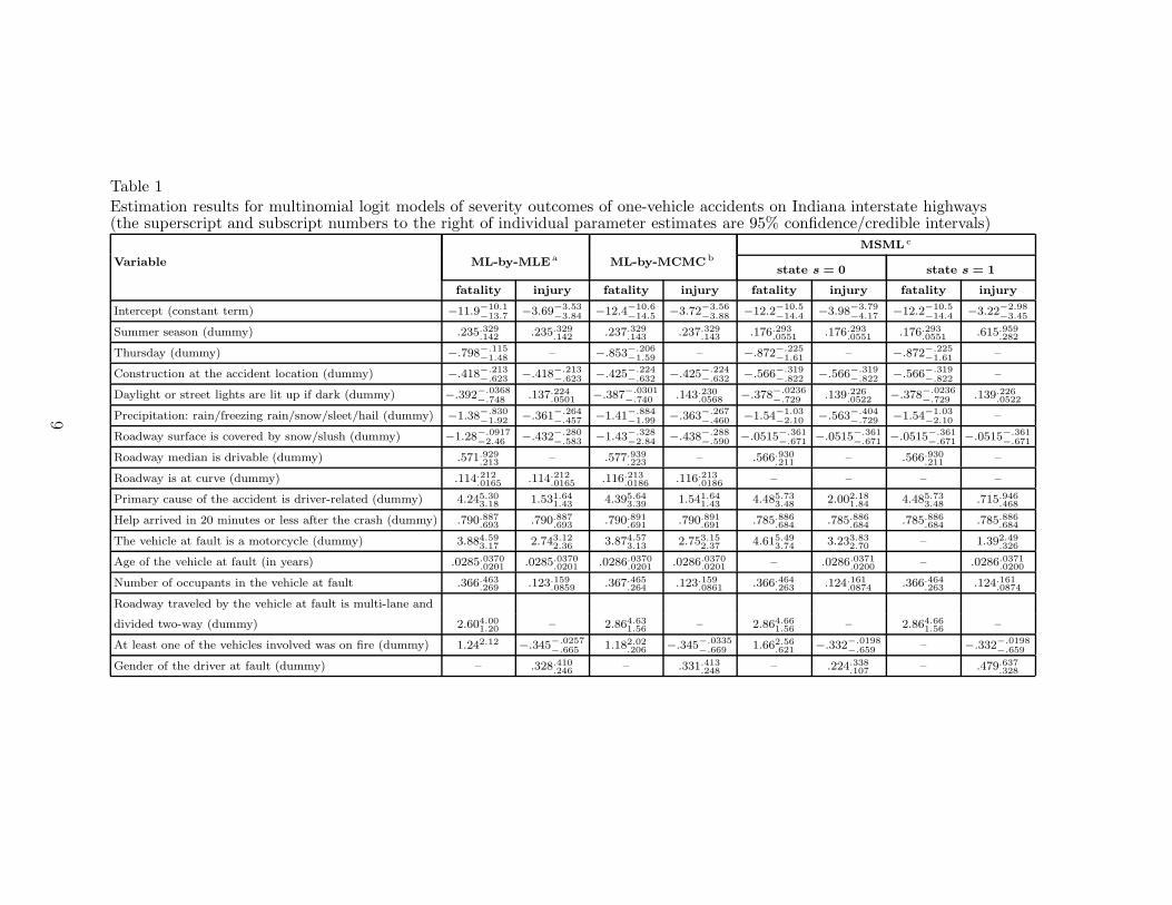
Table 1Estimation results for multinomial logit models of severity outcomes of one-vehicle accidents on Indiana interstate highways(the superscript and subscript numbers to the right of individual parameter estimates are 95% confidence/credible intervals)

MSML c

Variable ML-by-MLE a ML-by-MCMC b

state s = 0 state s = 1

fatality injury fatality injury fatality injury fatality injury

Intercept (constant term) −11.9−10.1−13.7 −3.69−3.53

−3.84 −12.4−10.6−14.5 −3.72−3.56

−3.88 −12.2−10.5−14.4 −3.98−3.79

−4.17 −12.2−10.5−14.4 −3.22−2.98

−3.45

Summer season (dummy) .235.329.142 .235.329

.142 .237.329.143 .237.329

.143 .176.293.0551 .176.293

.0551 .176.293.0551 .615.959

.282

Thursday (dummy) −.798−.115−1.48 – −.853−.206

−1.59 – −.872−.225−1.61 – −.872−.225

−1.61 –

Construction at the accident location (dummy) −.418−.213−.623 −.418−.213

−.623 −.425−.224−.632 −.425−.224

−.632 −.566−.319−.822 −.566−.319

−.822 −.566−.319−.822 –

Daylight or street lights are lit up if dark (dummy) −.392−.0368−.748 .137.224

.0501 −.387−.0301−.740 .143.230

.0568 −.378−.0236−.729 .139.226

.0522 −.378−.0236−.729 .139.226

.0522

Precipitation: rain/freezing rain/snow/sleet/hail (dummy) −1.38−.830−1.92 −.361−.264

−.457 −1.41−.884−1.99 −.363−.267

−.460 −1.54−1.03−2.10 −.563−.404

−.729 −1.54−1.03−2.10 –

Roadway surface is covered by snow/slush (dummy) −1.28−.0917−2.46 −.432−.280

−.583 −1.43−.328−2.84 −.438−.288

−.590 −.0515−.361−.671 −.0515−.361

−.671 −.0515−.361−.671 −.0515−.361

−.671

Roadway median is drivable (dummy) .571.929.213 – .577.939

.223 – .566.930.211 – .566.930

.211 –

Roadway is at curve (dummy) .114.212.0165 .114.212

.0165 .116.213.0186 .116.213

.0186 – – – –

Primary cause of the accident is driver-related (dummy) 4.245.303.18 1.531.641.43 4.395.643.39 1.541.641.43 4.485.733.48 2.002.181.84 4.485.733.48 .715.946.468

Help arrived in 20 minutes or less after the crash (dummy) .790.887.693 .790.887

.693 .790.891.691 .790.891

.691 .785.886.684 .785.886

.684 .785.886.684 .785.886

.684

The vehicle at fault is a motorcycle (dummy) 3.884.593.17 2.743.122.36 3.874.573.13 2.753.152.37 4.615.493.74 3.233.832.70 – 1.392.49.326

Age of the vehicle at fault (in years) .0285.0370.0201 .0285.0370

.0201 .0286.0370.0201 .0286.0370

.0201 – .0286.0371.0200 – .0286.0371

.0200

Number of occupants in the vehicle at fault .366.463.269 .123.159

.0859 .367.465.264 .123.159

.0861 .366.464.263 .124.161

.0874 .366.464.263 .124.161

.0874

Roadway traveled by the vehicle at fault is multi-lane and

divided two-way (dummy) 2.604.001.20 – 2.864.631.56 – 2.864.661.56 – 2.864.661.56 –

At least one of the vehicles involved was on fire (dummy) 1.242.12 −.345−.0257−.665 1.182.02

.206 −.345−.0335−.669 1.662.56

.621 −.332−.0198−.659 – −.332−.0198

−.659

Gender of the driver at fault (dummy) – .328.410.246 – .331.413

.248 – .224.338.107 – .479.637

.328

9

Table 1(Continued)

MSML c




Probability of severity outcome [P(i)t,n given by Eq. (3)], averaged

over all values of explanatory variables Xt,n – – .00724 .176 .00733 .174 .00672 .192

Markov transition probability of jump 0 → 1 (p0→1) – – .151.254.0704


Unconditional probabilities of states 0 and 1 (p̄0 and p̄1) – – .683.814.540 and .317.460

.186

Total number of free model parameters (β-s) 25 25 28

Posterior average of the log-likelihood (LL) – −8486.78−8480.82−8494.61 −8396.78−8379.21

−8416.57

Max(LL): estimated max. log-likelihood (LL) for MLE;

maximum observed value of LL for Bayesian-MCMC −8465.79 (MLE) −8476.37 (observed) −8358.97 (observed)

Logarithm of marginal likelihood of data (ln[f(Y|M)]) – −8498.46−8494.22−8499.21 −8437.07−8424.77

−8440.02

Goodness-of-fit p-value – 0.255 0.222

Maximum of the potential scale reduction factors (PSRF) d – 1.00302 1.00060

Multivariate potential scale reduction factor (MPSRF) d – 1.00325 1.00067

Number of available observations accidents = fatalities + injuries + PDOs: 19094 = 143 + 3369 + 15582

a Standard (conventional) multinomial logit (ML) model estimated by maximum likelihood estimation (MLE).

b Standard multinomial logit (ML) model estimated by Markov Chain Monte Carlo (MCMC) simulations.

c Two-state Markov switching multinomial logit (MSML) model estimated by Markov Chain Monte Carlo (MCMC) simulations.

d PSRF/MPSRF are calculated separately/jointly for all continuous model parameters. PSRF and MPSRF are close to 1 for converged MCMC chains.

10

Table 2Estimation results for multinomial logit models of severity outcomes of one-vehicle accidents on Indiana US routes(the superscript and subscript numbers to the right of individual parameter estimates are 95% confidence/credible intervals)

MSML c





−2.47 −6.62−5.16−8.14 −2.12−1.78

−2.47 −5.72−4.69−6.92 −2.05−1.71

−2.40 −5.72−4.69−6.92 −2.79−2.37

−3.23

Summer season (dummy) .514.894.134 .200.305.0947 .509.883.124 .200.305.0951 .190.300.0789 .190.300.0789 .190.300.0789 –


.101 −.492−.136−.848 .203.296

.110 −.493−.136−.857 .197.290

.105 – .197.290.105

Snowing weather (dummy) −1.17−.170−2.18 – −1.30−.357

−2.47 – −1.10−.151−2.27 .165.317

.0115 −1.10−.151−2.27 .165.317

.0115

No roadway junction at the accident location (dummy) .7011.25.149 .217.335

.0994 .7271.31.199 .213.331

.0968 .7871.36.259 .214.332

.0965 .7871.36.259 .214.332

.0965

Roadway is straight (dummy) −.741−.383−1.10 −.295−.191

−.399 −.739−.377−1.09 −.296−.192

−.399 −7.37−.372−1.09 −.294−.189

−.398 −7.37−.372−1.09 −.294−.189

−.398

Primary cause of the accident is environment-related (dummy) −3.45−2.72−4.18 −1.89−1.78

−1.99 −3.51−2.81−4.32 −1.89−1.79

−2.00 −3.59−2.89−4.40 −2.09−1.96

−2.24 −3.59−2.89−4.40 −.701−.263

−1.16


.507 .562.650.475 .562.650

.475 .560.648.472 .560.648

.472 .560.648.472 .560.648

.472

The vehicle at fault is a motorcycle (dummy) 2.623.471.78 3.203.552.86 2.573.381.65 3.213.562.87 3.223.582.88 3.223.582.88 3.223.582.88 3.223.582.88

Age of the vehicle at fault (in years) .0363.0444.0283 .0363.0444.0283 .0367.0448.0287 .0367.0448.0287 – .0366.0447.0285 – .0366.0447.0285

Speed limit (used if known and the same for all vehicles involved) .0363.0631.00950 .0121.0178

.00640 .0373.0643.0117 .0118.0176

.00616 .0285.0495.0104 .0102.0178

.00635 – .0120.0178.00635

Roadway traveled by the vehicle at fault is two-lane and

one-way (dummy) −.216.0417−.391 −.216.0417

−.391 −.223.0517−.398 −.223.0517

−.398 −.224.0504−.401 −.224.0504

−.401 −.224.0504−.401 −.224.0504

−.401

At least one of the vehicles involved was on fire (dummy) 1.191.94.439 – 1.131.85

.315 – 1.271.98.452 – 1.271.98

.452 –

Age of the driver at fault (in years) .0114.0213.00150 – .0113.0211

.00137 – .0101.0200.0000542 – – –

Weekday (Monday through Friday) (dummy) – −.104.0116−.196 – −.104.0124

−.196 – −.125.0242−.227 – –

Gender of the driver at fault (dummy) – .272.362.183 – .276.365

.186 – .280.369.190 – .280.369

.190

11

Table 2(Continued)

MSML c









.0409



−7364.47




−7380.00









12

Table 3Estimation results for multinomial logit models of severity outcomes of one-vehicle accidents on Indiana state routes(the superscript and subscript numbers to the right of individual parameter estimates are 95% confidence/credible intervals)

MSML c





−1.80 −4.03−3.71−4.36 −1.71−1.58

−1.85 −3.44−3.10−3.79 −1.68−1.54

−1.81 −4.96−4.15−5.96 −1.68−1.54

−1.81

Summer season (dummy) .232.307.156 .232.307

.156 .232.307.157 .232.307

.157 .238.314.163 .238.314

.163 .238.314.163 .238.314

.163

Roadway type (dummy: 1 if urban, 0 if rural) −.390−.302−.478 −.390−.302

−.478 −.395−.306−.483 −.395−.306

−.483 – −.385−.296−.474 −2.05−.954

−3.62 −3.85−.296−.474


.125 −.641−.404−.879 .199.267

.132 −.689−.448−.931 – −.689−.448

−.931 .277.378.177

Precipitation: rain/freezing rain/snow/sleet/hail (dummy) −.854.466−1.24 – −.868−.494

−1.27 – −.829−.448−1.24 – −.829−.448

−1.24 –

Roadway median is drivable (dummy) −.583−.225−.940 – −.596−.250

−.964 – −.589−.241−.960 – −.589−.241

−.960 –

Roadway is straight (dummy) −.284−.214−.353 −.284−.214

−.353 −.283−.214−.352 −.283−.214

−.352 −.117−.0184−.214 −.117−.0184

−.214 −.117−.0184−.214 −.465−.360

−.573

Primary cause of the accident is environment-related (dummy) −4.23−3.59−4.86 −1.83−1.76

−1.91 −4.28−3.67−4.97 −1.84−1.76

−1.91 −4.40−3.79−5.10 −2.30−2.16

−2.44 −4.40−3.79−5.10 −1.41−1.26

−1.55


.762 .863.945.781 .863.945

.781 – .861.944.778 1.642.64

.856 .861.944.778

The vehicle at fault is a motorcycle (dummy) 3.103.312.89 3.103.312.89 3.103.312.89 3.103.312.89 3.373.663.09 3.373.663.09 3.373.663.09 2.823.192.47

Number of occupants in the vehicle at fault .0557.0850.0265 .0557.0850

.0265 .0565.0858.0276 .0565.0858

.0276 .0942.138.0528 .0942.138

.0528 .0942.138.0528 –

At least one of the vehicles involved was on fire (dummy) 1.902.451.33 .456.780.133 1.872.421.28 .447.768.124 1.872.431.28 .461.782.137 1.872.431.28 .461.782.137

Age of the driver at fault (in years)14.621.47.80

× 10−3

−2.80−.800−4.70

× 10−3

14.521.37.67

× 10−3

−2.71−.723−4.69

× 10−3

14.521.47.63

× 10−3

−2.46−.469−4.44

× 10−3

14.521.47.63

× 10−3

−2.46−.469−4.44

× 10−3

Gender of the driver at fault (dummy) −.496−.211−.780 .279.344

.214 −.505−.225−.794 .278.343

.213 −.473−.192−.764 .283.348

.218 −.473−.192−.764 .283.348

.218

Age of the vehicle at fault (in years) – .0334.0392.0276 – .0335.0393

.0277 – .0332.0390.0274 – .0332.0390

.0274

license state of the vehicle at fault is a U.S. state except Indiana

and its neighboring states (IL, KY, OH, MI)” indicator variable – −.449−.217−.681 – −.444−.217

−.679 – −.436−.208−.671 – −.436−.208

−.671

13

Table 3(Continued)

MSML c









.319



−13800.89




−13821.73









14

The top, middle and bottom plots in Figure 1 show weekly posterior proba-bilities P (st = 1|Y) of the less frequent state st = 1 for the MSML modelsestimated for severity of 1-vehicle accidents occurring on interstate highways,US routes and state routes respectively. 13 Because of space limitations, in thispaper we do not report estimation results for severity of 1-vehicle accidents oncounty roads and streets, and for severity of 2-vehicle accidents. However, be-low we discuss our findings for all roadway-class-accident-type combinations.For unreported model estimation results see Malyshkina (2008).

We find that in all cases when the two states and Markov switching multi-nomial logit (MSML) models exist, these models are strongly favored by theempirical data over the corresponding standard multinomial logit (ML) mod-els. Indeed, from lines “marginal LL” in Tables 1–3 we see that the MSMLmodels provide considerable, ranging from 40.5 to 61.4, improvements of thelogarithm of the marginal likelihood of the data as compared to the corre-sponding ML models. 14 Thus, from Eq. (6) we find that, given the accidentseverity data, the posterior probabilities of the MSML models are larger thanthe probabilities of the corresponding ML models by factors ranging from e40.5

to e61.4. In the cases of 1-vehicle accidents on county roads, streets and thecase of 2-vehicle accidents on streets, MSML models (not reported here) arealso strongly favored by the empirical data over the corresponding ML models(Malyshkina, 2008).

Let us now consider the maximum likelihood estimation (MLE) of the standardML models and an imaginary MLE estimation of the MSML models. Wefind that, in this imaginary case, a classical statistics approach for modelcomparison, based on the MLE, would also favors the MSML models over thestandard ML models. For example, refer to line “max(LL)” in Table 1 givenfor the case of 1-vehicle accidents on interstate highways. The MLE gavethe maximum log-likelihood value −8465.79 for the standard ML model. Themaximum log-likelihood value observed during our MCMC simulations for theMSML model is equal to −8358.97. An imaginary MLE, at its convergence,would give a MSML log-likelihood value that would be even larger than thisobserved value. Therefore, if estimated by the MLE, the MSML model wouldprovide large, at least 106.82 improvement in the maximum log-likelihoodvalue over the corresponding ML model. This improvement would come withonly modest increase in the number of free continuous model parameters (β-s) that enter the likelihood function (refer to Table 1 under “# free par.”).

13 Note that these posterior probabilities are equal to the posterior expectations ofst, P (st = 1|Y) = 1× P (st = 1|Y) + 0× P (st = 0|Y) = E(st|Y).14 We use the harmonic mean formula to calculate the values and the 95% confidenceintervals of the log-marginal-likelihoods given in lines “marginal LL” of Tables 1–3.The confidence intervals are calculated by bootstrap simulations. For details, seePaper I or Malyshkina (2008).

15

Jan−03 Jul−03 Jan−04 Jul−04 Jan−05 Jul−05 Jan−06 Jul−060

0.2

0.4

0.6

0.8

1

Date

P(S

t=1|

Y)


0.2

0.4

0.6

0.8

1

Date

P(S

t=1|

Y)


0.2

0.4

0.6

0.8

1

Date

P(S

t=1|

Y)

Fig. 1. Weekly posterior probabilities P (st = 1|Y) for the MSML models estimatedfor severity of 1-vehicle accidents on interstate highways (top plot), US routes (mid-dle plot) and state routes (bottom plot).

Similar arguments hold for comparison of MSML and ML models estimatedfor other roadway-class-accident-type combinations (see Tables 2 and 3).

To evaluate the goodness-of-fit for a model, we use the posterior (or MLE)estimates of all continuous model parameters (β-s, α, p0→1, p1→0) and generate104 artificial data sets under the hypothesis that the model is true. 15 We findthe distribution of χ2 and calculate the goodness-of-fit p-value for the observedvalue of χ2. For details, see Malyshkina (2008). The resulting p-values for ourmodels are given in Tables 1–3. These p-values are around 00–100%. Therefore,all models fit the data well.

15 Note that the state values S are generated by using p0→1 and p1→0.

16

Now, refer to Table 5. The first six rows of this table list time-correlation coef-ficients between posterior probabilities P (st = 1|Y) for the six MSML modelsthat exist and are estimated for six roadway-class-accident-type combinations(1-vehicle accidents on interstate highways, US routes, state routes, countyroads, streets, and 2-vehicle accidents on streets). 16 We see that the states for1-vehicle accidents on all high-speed roads (interstate highways, US routes,state routes and county roads) are correlated with each other. The values ofthe corresponding correlation coefficients are positive and range from 0.263 to0.688 (see Table 5). This result suggests an existence of common (unobserv-able) factors that can cause switching between states of roadway safety for1-vehicle accidents on all high-speed roads.

The remaining rows of Table 5 show correlation coefficients between poste-rior probabilities P (st = 1|Y) and weather-condition variables. These cor-relations were found by using daily and hourly historical weather data inIndiana, available at the Indiana State Climate Office at Purdue University(www.agry.purdue.edu/climate). For these correlations, the precipitation andsnowfall amounts are daily amounts in inches averaged over the week andacross Indiana weather observation stations. 17 The temperature variable isthe mean daily air temperature (oF ) averaged over the week and across theweather stations. The wind gust variable is the maximal instantaneous windspeed (mph) measured during the 10-minute period just prior to the obser-vational time. Wind gusts are measured every hour and averaged over theweek and across the weather stations. The effect of fog/frost is captured by adummy variable that is equal to one if and only if the difference between airand dewpoint temperatures does not exceed 5oF (in this case frost can formif the dewpoint is below the freezing point 32oF , and fog can form otherwise).The fog/frost dummies are calculated for every hour and are averaged overthe week and across the weather stations. Finally, visibility distance variable isthe harmonic mean of hourly visibility distances, which are measured in milesevery hour and are averaged over the week and across the weather stations. 18

From the results given in Table 5 we find that for 1-vehicle accidents on allhigh-speed roads (interstate highways, US routes, state routes and countyroads), the less frequent state st = 1 is positively correlated with extremetemperatures (low during winter and high during summer), rain precipitationsand snowfalls, strong wind gusts, fogs and frosts, low visibility distances. It

16 Here and below we calculate weighted correlation coefficients. For variable P (st =1|Y) ≡ E(st|Y) we use weights wt inversely proportional to the posterior standarddeviations of st. That is wt ∝ min {1/std(st|Y),median[1/std(st|Y)]}.17 Snowfall and precipitation amounts are weakly related with each other becausesnow density (g/cm3) can vary by more than a factor of ten.18 The harmonic mean d̄ of distances dn is calculated as d̄−1 = (1/N)

∑Nn=1 d

−1n ,

assuming dn = 0.25 miles if dn ≤ 0.25 miles.

17

is reasonable to expect that roadway safety is different during bad weatheras compared to better weather, resulting in the two-state nature of roadwaysafety.

The results of Table 5 suggest that Markov switching for road safety on streetsis very different from switching on all other roadway classes. In particular,the states of roadway safety on streets exhibit low correlation with states onother roads. In addition, only streets exhibit Markov switching in the caseof 2-vehicle accidents. Finally, states of roadway safety on streets show littlecorrelation with weather conditions. A possible explanation of these differencesis that streets are mostly located in urban areas and they have traffic movingat speeds lower that those on other roads.

Next, we consider the estimation results for the stationary unconditional prob-abilities p̄0 and p̄1 of states st = 0 and st = 1 for MSML models (see Section 2).In the cases of 1-vehicle accidents on interstate highways, US routes and stateroutes these transition probabilities are listed in lines “p̄0 and p̄1” of Tables 1–3. In the cases of 1-vehicle accidents on county roads and 1- and 2-vehicleaccidents on streets refer to Malyshkina (2008). We find that the ratio p̄1/p̄0is approximately equal to 0.46, 0.13, 0.74, 0.25, 0.65 and 0.36 in the casesof 1-vehicle accidents on interstate highways, US routes, state routes, countyroads, streets, and 2-vehicle accidents on streets respectively. Thus for someroadway-class-accident-type combinations (for example, 1-vehicle accidents onUS routes) the less frequent state st = 1 is quite rare, while for other combi-nations (for example, 1-vehicle accidents on state routes) state st = 1 is onlyslightly less frequent than state st = 0.

Finally, we set model parameters (β-s) to their posterior means, calculate theprobabilities of fatality and injury outcomes by using Eq. (3) and averagethese probabilities over all values of the explanatory variables Xt,n observedin the data sample. We compare these probabilities across the two states ofroadway safety, st = 0 and st = 1, for MSML models [refer to lines “〈P

(i)t,n〉X”

in Tables 1–3 and to Malyshkina (2008)]. We find that in many cases theseaveraged probabilities of fatality and injury outcomes do not differ very signif-icantly across the two states of roadway safety (the only significant differencesare for fatality probabilities in the cases of 1-vehicle accidents on US routes,county roads and streets). This means that in many cases states st = 0 andst = 1 are approximately equally dangerous as far as accident severity is con-cerned. We discuss this result in the next section.

18

5 Conclusions

In this study we found that two states of roadway safety and Markov switch-ing multinomial logit (MSML) models exist for severity of 1-vehicle accidentsoccurring on high-speed roads (interstate highways, US routes, state routes,county roads), but not for 2-vehicle accidents on high-speed roads. One of pos-sible explanations of this result is that 1- and 2-vehicle accidents may differin their nature. For example, on one hand, severity of 1-vehicle accidents mayfrequently be determined by driver-related factors (speeding, falling a sleep,driving under the influence, etc). Drivers’ behavior might exhibit a two-statepattern. In particular, drivers might be overconfident and/or have difficultiesin adjustments to bad weather conditions. On the other hand, severity of a2-vehicle accident might crucially depend on the actual physics involved inthe collision between the two cars (for example, head-on and side impacts aremore dangerous than rear-end collisions). As far as slow-speed streets are con-cerned, in this case both 1- and 2-vehicle accidents exhibit two-state naturefor their severity. Further studies are needed to understand these results. Inthis study, the important result is that in all cases when two states of roadwaysafety exist, the two-state MSML models provide much superior statistical fitfor accident severity outcomes as compared to the standard ML models.

We found that in many cases states st = 0 and st = 1 are approximatelyequally dangerous as far as accident severity is concerned. This result holdsdespite the fact that state st = 1 is correlated with adverse weather conditions.A likely and simple explanation of this finding is that during bad weatherboth number of serious accidents (fatalities and injuries) and number of minoraccidents (PDOs) increase, so that their relative fraction stays approximatelysteady. In addition, most drivers are rational and they are likely take someprecautions while driving during bad weather. From the results presented inPaper I we know that the total number of accidents significantly increasesduring adverse weather conditions. Thus, driver’s precautions are probablynot sufficient to avoid increases in accident rates during bad weather.

References

Abdel-Aty, M., 2003. Analysis of driver injury severity levels at multiple lo-cations using ordered probit models. Journal of Safety Research 34(5), 597-603.

Carson, J., Mannering, F.L., 2001. The effect of ice warning signs on ice-accident frequencies and severities. Accident Analysis and Prevention 33(1),99-109.

Chang, L.-Y., Mannering, F.L., 1999. Analysis of injury severity and vehicle

19

occupancy in truck- and non-truck-involved accidents. Accident Analysisand Prevention 31(5), 579-592.

Cowan, G., 1998. Statistical Data Analysis. Clarendon Press, Oxford Univ.Press, USA

Duncan, C., Khattak, A., Council, F., 1998. Applying the ordered probit modelto injury severity in truck-passenger car rear-end collisions. TransportationResearch Record 1635, 63-71.

Eluru, N., Bhat, C., 2007. A joint econometric analysis of seat belt use andcrash-related injury severity. Accident Analysis and Prevention 39(5), 1037-1049.

Kass, R.E., Raftery, A.E., 1995. Bayes Factors. Journal of the American Sta-tistical Association 90(430), 773-795.

Khattak, A., 2001. Injury severity in multi-vehicle rear-end crashes. Trans-portation Research Record 1746, 59-68.

Khattak, A., Pawlovich, D., Souleyrette, R., Hallmarkand, S., 2002. Factorsrelated to more severe older driver traffic crash injuries. Journal of Trans-portation Engineering 128(3), 243-249.

Khorashadi, A., Niemeier, D., Shankar V., Mannering F.L., 2005. Differencesin rural and urban driver-injury severities in accidents involving large trucks:an exploratory analysis. Accident Analysis and Prevention 37(5), 910-921.

Kockelman, K., Kweon, Y.-J., 2002. Driver Injury Severity: An application ofordered probit models. Accident Analysis and Prevention 34(3), 313-321.

Kweon, Y.-J., Kockelman, K., 2003. Overall injury risk to different drivers:combining exposure, frequency, and severity models. Accident Analysis andPrevention 35(4), 414-450.

Lee, J., Mannering, F.L., 2002. Impact of roadside features on the frequencyand severity of run-off-roadway accidents: an empirical analysis. AccidentAnalysis and Prevention 34(2), 149-161.

Maher M. J., Summersgill, I., 1996. A comprehensive methodology for thefitting of predictive accident models. Accid. Anal. Prev. 28(3), 281-296.

Malyshkina, N.V., 2006. Influence of speed limit on roadway safety in Indiana.MS thesis, Purdue University. http://arxiv.org/abs/0803.3436

Malyshkina, N. V., 2008. Markov switching models: an application of to road-way safety. PhD thesis, Purdue University. http://arxiv.org/abs/0808.1448

Malyshkina, N.V., Mannering, F.L., Tarko, A.P., 2008. Markov switching mod-els: an application to Markov switching negative binomial models: an appli-cation to vehicle accident frequencies. Accepted for publication in AccidentAnalysis and Prevention. http://arxiv.org/abs/0811.1606

Milton, J., Shankar, V., Mannering, F.L., 2008. Highway accident severitiesand the mixed logit model: an exploratory empirical analysis. AccidentAnalysis and Prevention 40(1), 260-266.

O’Donnell, C., Connor, D., 1996. Predicting the severity of motor vehicle ac-cident injuries using models of ordered multiple choice. Accident Analysisand Prevention 28(6), 739-753.

Press, W. H., Teukolsky, S. A., Vetterling, W. T., Flannery B. P., 2007. Nu-

20

http://arxiv.org/abs/0803.3436



merical Recipes 3rd Edition: The Art of Scientific Computing. CambridgeUniv. Press, UK.

Savolainen, P., Mannering, F.L., 2007. Probabilistic models of motorcyclists’injury severities in single- and multi-vehicle crashes. Accident Analysis andPrevention 39(5), 955-963.

Shankar, V., Mannering, F.L., 1996. An exploratory multinomial logit analysisof single-vehicle motorcycle accident severity. Journal of Safety Research27(3), 183-194.

Shankar, V., Mannering, F.L., Barfield, W., 1996. Statistical analysis of ac-cident severity on rural freeways. Accident Analysis and Prevention 28(3),391-401.

Tsay, R. S., 2002. Analysis of financial time series: financial econometrics.John Wiley & Sons, Inc.

Ulfarsson, G., Mannering, F.L., 2004. Differences in male and female injuryseverities in sport-utility vehicle, minivan, pickup and passenger car acci-dents. Accident Analysis and Prevention 36(2), 135-147.

Washington, S.P., Karlaftis, M.G., Mannering, F.L., 2003. Statistical andeconometric methods for transportation data analysis. Chapman &Hall/CRC.

Wood, G. R., 2002. Generalised linear accident models and goodness of fittesting. Accid. Anal. Prev. 34, 417-427.

Yamamoto, T., Shankar, V., 2004. Bivariate ordered-response probit modelof driver’s and passenger’s injury severities in collisions with fixed objects.Accident Analysis and Prevention 36(5), 869-876.

21

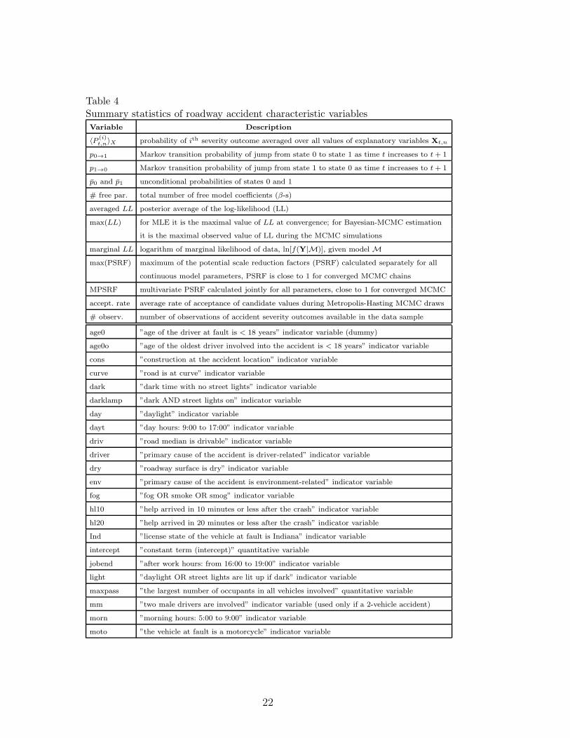
Table 4Summary statistics of roadway accident characteristic variablesVariable Description

〈P(i)t,n〉X probability of ith severity outcome averaged over all values of explanatory variables Xt,n

p0→1 Markov transition probability of jump from state 0 to state 1 as time t increases to t+ 1

p1→0 Markov transition probability of jump from state 1 to state 0 as time t increases to t+ 1

p̄0 and p̄1 unconditional probabilities of states 0 and 1

# free par. total number of free model coefficients (β-s)

averaged LL posterior average of the log-likelihood (LL)

max(LL) for MLE it is the maximal value of LL at convergence; for Bayesian-MCMC estimation

it is the maximal observed value of LL during the MCMC simulations

marginal LL logarithm of marginal likelihood of data, ln[f(Y|M)], given model M

max(PSRF) maximum of the potential scale reduction factors (PSRF) calculated separately for all

continuous model parameters, PSRF is close to 1 for converged MCMC chains

MPSRF multivariate PSRF calculated jointly for all parameters, close to 1 for converged MCMC

accept. rate average rate of acceptance of candidate values during Metropolis-Hasting MCMC draws

# observ. number of observations of accident severity outcomes available in the data sample

age0 ”age of the driver at fault is < 18 years” indicator variable (dummy)

age0o ”age of the oldest driver involved into the accident is < 18 years” indicator variable

cons ”construction at the accident location” indicator variable

curve ”road is at curve” indicator variable

dark ”dark time with no street lights” indicator variable

darklamp ”dark AND street lights on” indicator variable

day ”daylight” indicator variable

dayt ”day hours: 9:00 to 17:00” indicator variable

driv ”road median is drivable” indicator variable

driver ”primary cause of the accident is driver-related” indicator variable

dry ”roadway surface is dry” indicator variable

env ”primary cause of the accident is environment-related” indicator variable

fog ”fog OR smoke OR smog” indicator variable

hl10 ”help arrived in 10 minutes or less after the crash” indicator variable

hl20 ”help arrived in 20 minutes or less after the crash” indicator variable

Ind ”license state of the vehicle at fault is Indiana” indicator variable

intercept ”constant term (intercept)” quantitative variable

jobend ”after work hours: from 16:00 to 19:00” indicator variable

light ”daylight OR street lights are lit up if dark” indicator variable

maxpass ”the largest number of occupants in all vehicles involved” quantitative variable

mm ”two male drivers are involved” indicator variable (used only if a 2-vehicle accident)

morn ”morning hours: 5:00 to 9:00” indicator variable

moto ”the vehicle at fault is a motorcycle” indicator variable

22

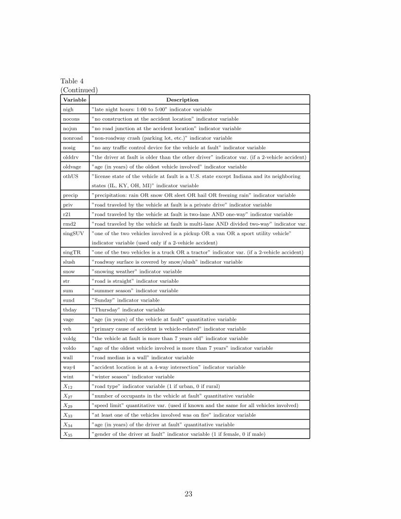
Table 4(Continued)

Variable Description

nigh ”late night hours: 1:00 to 5:00” indicator variable

nocons ”no construction at the accident location” indicator variable

nojun ”no road junction at the accident location” indicator variable

nonroad ”non-roadway crash (parking lot, etc.)” indicator variable

nosig ”no any traffic control device for the vehicle at fault” indicator variable

olddrv ”the driver at fault is older than the other driver” indicator var. (if a 2-vehicle accident)

oldvage ”age (in years) of the oldest vehicle involved” indicator variable

othUS ”license state of the vehicle at fault is a U.S. state except Indiana and its neighboring

states (IL, KY, OH, MI)” indicator variable

precip ”precipitation: rain OR snow OR sleet OR hail OR freezing rain” indicator variable

priv ”road traveled by the vehicle at fault is a private drive” indicator variable

r21 ”road traveled by the vehicle at fault is two-lane AND one-way” indicator variable

rmd2 ”road traveled by the vehicle at fault is multi-lane AND divided two-way” indicator var.

singSUV ”one of the two vehicles involved is a pickup OR a van OR a sport utility vehicle”

indicator variable (used only if a 2-vehicle accident)

singTR ”one of the two vehicles is a truck OR a tractor” indicator var. (if a 2-vehicle accident)

slush ”roadway surface is covered by snow/slush” indicator variable

snow ”snowing weather” indicator variable

str ”road is straight” indicator variable

sum ”summer season” indicator variable

sund ”Sunday” indicator variable

thday ”Thursday” indicator variable

vage ”age (in years) of the vehicle at fault” quantitative variable

veh ”primary cause of accident is vehicle-related” indicator variable

voldg ”the vehicle at fault is more than 7 years old” indicator variable

voldo ”age of the oldest vehicle involved is more than 7 years” indicator variable

wall ”road median is a wall” indicator variable

way4 ”accident location is at a 4-way intersection” indicator variable

wint ”winter season” indicator variable

X12 ”road type” indicator variable (1 if urban, 0 if rural)

X27 ”number of occupants in the vehicle at fault” quantitative variable

X29 ”speed limit” quantitative var. (used if known and the same for all vehicles involved)

X33 ”at least one of the vehicles involved was on fire” indicator variable

X34 ”age (in years) of the driver at fault” quantitative variable

X35 ”gender of the driver at fault” indicator variable (1 if female, 0 if male)

23

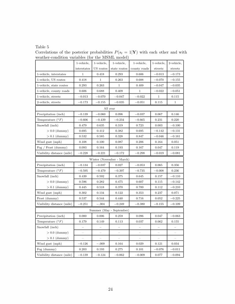
Table 5Correlations of the posterior probabilities P (st = 1|Y) with each other and withweather-condition variables (for the MSML model)

1-vehicle, 1-vehicle, 1-vehicle, 1-vehicle, 1-vehicle, 2-vehicle,

interstates US routes state routes county roads streets streets

1-vehicle, interstates 1 0.418 0.293 0.606 −0.013 −0.173

1-vehicle, US routes 0.418 1 0.263 0.688 −0.070 −0.155

1-vehicle, state routes 0.293 0.263 1 0.409 −0.047 −0.035

1-vehicle, county roads 0.606 0.688 0.409 1 −0.022 −0.051

1-vehicle, streets −0.013 −0.070 −0.047 −0.022 1 0.115

2-vehicle, streets −0.173 −0.155 −0.035 −0.051 0.115 1

All year

Precipitation (inch) −0.139 −0.060 0.096 −0.037 0.067 0.146

Temperature (oF ) −0.606 −0.439 −0.234 −0.665 0.231 0.220

Snowfall (inch) 0.479 0.635 0.319 0.723 0.003 −0.100

> 0.0 (dummy) 0.695 0.412 0.382 0.695 −0.142 −0.131

> 0.1 (dummy) 0.532 0.585 0.328 0.847 −0.046 −0.161

Wind gust (mph) 0.108 0.100 0.087 0.206 0.164 0.051

Fog / Frost (dummy) 0.093 0.164 0.193 0.167 0.047 0.119

Visibility distance (mile) −0.228 −0.221 −0.172 −0.298 −0.019 −0.081

Winter (November - March)

Precipitation (inch) −0.134 −0.037 0.027 −0.053 0.065 0.356

Temperature (oF ) −0.595 −0.479 −0.397 −0.735 −0.008 0.236

Snowfall (inch) 0.439 0.592 0.375 0.645 0.157 −0.110

> 0.0 (dummy) 0.596 0.282 0.475 0.607 0.115 −0.142

> 0.1 (dummy) 0.445 0.518 0.370 0.789 0.112 −0.210

Wind gust (mph) 0.302 0.134 0.122 0.353 0.237 0.071

Frost (dummy) 0.537 0.544 0.440 0.716 0.052 −0.225

Visibility distance (mile) −0.251 −.304 −0.249 −0.380 −0.155 −0.109

Summer (May - September)

Precipitation (inch) 0.000 0.006 0.259 0.096 0.047 −0.063

Temperature (oF ) 0.179 0.149 0.113 0.037 0.062 0.155

Snowfall (inch) – – – – – –

> 0.0 (dummy) – – – – – –

> 0.1 (dummy) – – – – – –

Wind gust (mph) −0.126 −.009 0.164 0.029 0.121 0.034

Fog (dummy) 0.203 0.193 0.275 0.101 −0.076 −0.011

Visibility distance (mile) −0.139 −0.124 −0.062 −0.009 0.077 −0.094

24

Markov switching multinomial logit model: an application ... · Markov switching multinomial logit...

Documents

Transcript of Markov switching multinomial logit model: an application ... · Markov switching multinomial logit...