Markov and semi-Markov switching linear mixed models for ... · PDF fileroughly stationary...

Markov and semi-Markov switching linear mixed models

for identifying forest tree growth components.

Florence Chaubert-Pereira, Yann Guedon, Christian Lavergne, Catherine

Trottier

To cite this version:

Florence Chaubert-Pereira, Yann Guedon, Christian Lavergne, Catherine Trottier. Markovand semi-Markov switching linear mixed models for identifying forest tree growth components..[Research Report] RR-6618, INRIA. 2008. <inria-00311588>

HAL Id: inria-00311588

https://hal.inria.fr/inria-00311588

Submitted on 19 Aug 2008

HAL is a multi-disciplinary open accessarchive for the deposit and dissemination of sci-entific research documents, whether they are pub-lished or not. The documents may come fromteaching and research institutions in France orabroad, or from public or private research centers.

L’archive ouverte pluridisciplinaire HAL, estdestinee au depot et a la diffusion de documentsscientifiques de niveau recherche, publies ou non,emanant des etablissements d’enseignement et derecherche francais ou etrangers, des laboratoirespublics ou prives.

https://hal.archives-ouvertes.fr

https://hal.inria.fr/inria-00311588

appor t de r ech er ch e

ISS

N02

49-6

399

ISR

NIN

RIA

/RR

--66

18--

FR

+E

NG

Thème BIO

INSTITUT NATIONAL DE RECHERCHE EN INFORMATIQUE ET EN AUTOMATIQUE

Markov and semi-Markov switching linear mixedmodels for identifying forest tree growth components

Florence Chaubert-Pereira — Yann Guédon — Christian Lavergne — Catherine Trottier

N° 6618

August 19, 2008

Centre de recherche INRIA Sophia Antipolis – Méditerranée2004, route des Lucioles, BP 93, 06902 Sophia Antipolis Cedex

Téléphone : +33 4 92 38 77 77 — Télécopie : +33 4 92 38 77 65

Markov and semi-Markov switching linear

mixed models for identifying forest tree growth

components

Florence Chaubert-Pereira∗ † , Yann Guedon∗ †, Christian

Lavergne ‡ , Catherine Trottier‡

Theme BIO — Systemes biologiquesEquipe-Projet Virtual Plants

Rapport de recherche n° 6618 — August 19, 2008 — 26 pages

Abstract: Observed tree growth is the result of three components: (i) anendogenous component which is assumed to be structured as a succession ofroughly stationary phases separated by marked change points asynchronousbetween individuals, (ii) a time-varying environmental component which is as-sumed to take the form of local fluctuations synchronous between individuals,(iii) an individual component which corresponds to the local environmental ofeach tree. In order to identify and to characterize these three components,we propose to use semi-Markov switching linear mixed models, i.e. modelsthat combine linear mixed models in a semi-markovian manner. The underly-ing semi-Markov chain represents the succession of growth phases (endogenouscomponent) while the linear mixed models attached to each state of the un-derlying semi-Markov chain represent in the corresponding growth phase boththe influence of time-varying environmental covariates (environmental compo-nent) as fixed effects and inter-individual heterogeneity (individual component)as random effects. In this paper, we address the estimation of Markov and semi-Markov switching linear mixed models in a general framework. We propose aMCEM-like algorithm whose iterations decompose into three steps (samplingof state sequences given random effects, prediction of random effects given thestate sequence and maximization). The proposed statistical modeling approachis illustrated by the analysis of successive annual shoots along Corsican pinetrunks influenced by climatic covariates.

Key-words: Markov switching model, semi-Markov switching model,individual-wise random effect, MCEM algorithm, plant structure analysis

∗ CIRAD, UMR Developpement et Amelioration des Plantes, Montpellier, France† INRIA, Equipe-projet Virtual Plants, Montpellier, France‡ Montpellier III University, Institut de Mathematiques et de Modelisation de Montpellier,

Montpellier, France

Combinaisons markoviennes et

semi-markoviennes de modeles lineaires mixtes

pour identifier les composantes de la croissance

d’arbres forestiers

Resume : La croissance d’un arbre est le resultat de trois composantes: (i)une composante endogene supposee structuree comme une succession de phasesstationnaires separees par des sauts nets asynchrones entre individus, (ii) unecomposante environnementale pouvant varier dans le temps supposee prendrela forme de fluctuations locales synchrones entre individus, (iii) une composanteindividuelle qui correspond a l’environnement local de chaque arbre. Afind’identifier et de caracteriser ces trois composantes, nous proposons d’utiliser lescombinaisons semi-markoviennes de modeles lineaires mixtes, i.e. des modelesqui combinent des modeles lineaires mixtes de maniere semi-markovienne. Lasemi-chaıne de Markov sous-jacente represente la succession des phases de crois-sance (composante endogene) tandis que les modeles lineaires mixtes attaches achaque etat de la semi-chaıne de Markov sous-jacente representent dans la phasede croissance correspondante a la fois l’influence de variables environnementales(composante environnementale) comme des effets fixes et l’heterogeneite inter-individuelle (composante individuelle) comme des effets alatoires. Dans cepapier, nous traitons de l’estimation des combinaisons markoviennes et semi-markoviennes de modeles lineaires mixtes dans un cadre general. Nous proposonsun algorithme de type MCEM dont les iterations se decomposent en trois etapes(simulations des sequences d’etats sachant les effets aleatoires, prediction deseffets aleatoires sachant les sequences d’etats, maximisation). La modelisationproposee est illustree par l’analyse des longueurs de pousses annuelles successivesle long de tronc de pins Laricio, influencees par des covariables climatiques.

Mots-cles : combinaison markovienne de modeles, combinaisonsemi-markovienne de modeles, effet aleatoire “individuel” , algorithme MCEM,analyse de la structure de la plante

Markov and semi-Markov switching linear mixed models 3

1 Introduction

The analysis of plant structure at macroscopic scales is of major importancein forestry and different fields of agronomy; see Candy (1997), Durand et al.(2005), Guedon et al. (2007) and Ninomiya and Yoshimoto (2008) for illustra-tions. Tree development can be reconstructed at a given observation date frommorphological markers (such as cataphyll1 or branching scars that help to de-limit successive annual shoots) corresponding to past events. Observed growth,as given for instance by the length of successive annual shoots along a treetrunk, is assumed to be mainly the result of three components: an endogenouscomponent, an environmental component and an individual component. Theendogenous component is assumed to be structured as a succession of roughlystationary phases that are asynchronous between individuals (Guedon et al.,2007) while the environmental component is assumed to take the form of lo-cal fluctuations that are synchronous between individuals. This environmentalcomponent is thus assumed to be a “population” component as opposed to theindividual component. The environmental factors which modulate the plantdevelopment are mainly of climatic origin such as rainfall or temperature. Theindividual component may cover effects of diverse origins but always includes agenetic effect. Other effects correspond to the local environment of each indi-vidual such as pathogen infestation or competitions between trees for light ornutrient resources. These factors are rarely measurable retrospectively for eachtree.

Guedon et al. (2007) proposed a set of methods for analyzing the endogenousand the environmental components. In particular, hidden semi-Markov chainswith simple observation distributions were applied to forest tree growth data. Inthis case, the underlying semi-Markov chain represents the succession of growthphases and their lengths while the environmental component is characterizedglobally. Hidden semi-Markov chains (Guedon, 2003) generalize hidden Markovchains (Ephraim and Merhav, 2002) with the distinctive property of explicitlymodeling the sojourn time in each state. Chaubert et al. (2007) applied Markovswitching linear mixed models to forest tree growth data. These models com-bine linear mixed models in a Markovian manner. In this case, the underlyingMarkov chain represents the succession of growth phases while the linear mixedmodels attached to each state of the Markov chain represent in the correspond-ing growth phase both the effect of covariates as fixed effect and inter-individualheterogeneity as random effect.

A Gaussian hidden Markov model can be defined as a pair of stochasticprocesses St, Yt where the output process Yt is related to the state pro-cess St, which is a finite-state Markov chain, by the Gaussian distributionYt | St=st

∼ N (µst, Γ2

st). These models, first introduced in speech recognition

in the early 1970s, can be viewed as a finite mixture of Gaussian distributionswith Markovian dependencies (Ephraim and Merhav, 2002; Cappe et al., 2005).Lindgren (1978) introduced Markov switching linear models which extend theclass of Gaussian hidden Markov models by incorporating the influence of covari-ates as fixed effects in the output process. Markov switching linear models have

1A reduced or scarcely developed leaf at the start of a plant’s life or in the early stages ofleaf development.

RR n° 6618

4 Chaubert-Pereira, Guedon, Lavergne & Trottier

been applied in such different fields as for instance econometrics or the analysisof gene regulatory networks in biology (Gupta et al., 2007); see Fruhwirth-Schnatter (2006) for an overview of Markov switching models with differentexamples of application. In the literature, hidden Markov models with randomeffects in the output process have been used in a limited way. Altman (2007)introduced Markov switching generalized linear mixed model and applied thesemodels for modeling lesion counts in multiple sclerosis patients. Lesion countis assumed to follow a Poisson distribution, with the mean being dependenton the patient’s unobserved state. Markov switching generalized linear mixedmodels were also used in the analysis of symptoms in patients with primary andmetastatic brain tumours (Rijmen et al., 2008). Both Altman (2007) and Rij-men et al. (2008) assumed that the individual-wise random effect is independentof the unobservable states.

Here, we introduce semi-Markov switching linear mixed models that gen-eralize both Markov switching linear mixed models and hidden semi-Markovchains. These models can be viewed as a finite mixture of linear mixed modelswith semi-Markovian dependencies. In a semi-Markov switching linear mixedmodel applied to forest tree growth data, the underlying semi-Markov chainrepresents both the succession of growth phases and their lengths, while the lin-ear mixed models attached to each state of the semi-Markov chain represent inthe corresponding growth phase the effect of time-varying climatic covariates asfixed effect and inter-individual heterogeneity as random effect. The objective isboth to characterize the tree population and to analyse the behavior of each in-dividual within the population. Since studies on plant architecture highlightedthe central role played by the endogenous component in plant architecture devel-opment (Barthelemy and Caraglio, 2007), a key point is to understand how theeffect of climatic factors and inter-individual heterogeneity change with phases.

Since both the states of the underlying (semi-)Markov chain and the ran-dom effects are non-observable, (semi-)Markov switching linear mixed modelsinvolve two latent structures and remain difficult to estimate. Altman (2007)proposed a deterministic and a stochastic approximation method for estimatingMarkov switching generalized linear mixed models. The deterministic approx-imation approach combines numerical integration by Gaussian quadrature andquasi-Newton methods and relies on the fact that the hidden Markov model like-lihood can be written as a product of matrices. Since the hidden semi-Markovmodel likelihood cannot be written as a product of matrices, this determinis-tic approximation method cannot be transposed to the semi-Markovian case.Moreover, the deterministic approximation approach can only be applied in thecase of a few random effects. The stochastic approximation method is a MonteCarlo EM (MCEM) algorithm (Wei and Tanner, 1990) where the M-step in-volves quasi-Newton routines. Altman underlined some limitations of the twoproposed methods such as the sensitivity to starting values, the slowness toconverge and a strong computation burden. Since conditional independence as-sumptions within a Markov switching linear mixed model can be represented bya directed acyclic graph, Rijmen et al. (2008) proposed to carry out the E-step bya junction tree algorithm (Smyth et al., 1997; Cowell et al., 1999). The M-stepinvolves numerical integration by Gaussian quadrature and Fisher scoring meth-ods. Since conditional independence assumptions within a hidden semi-Markov

INRIA


model cannot be efficiently represented by a directed acyclic graph, this methodcannot be transposed to the semi-Markovian case. Moreover, the approachesproposed by Altman (2007) and Rijmen et al. (2008) cannot be transposed toour context where it is assumed that the random effects are attached to thestates. Kim and Smyth (2006) proposed an estimation method for a “left-right”semi-Markov switching linear mixed model with individual-state-wise randomeffects. Thus, the states are ordered and each state can be visited at most once.The proposed method which is basically an application of the EM algorithmbased on a forward-backward algorithm for the E-step relies heavily on the twospecific model assumptions (state visited at most once and individual-state-wiserandom effects). Its complexity is cubic in the sequence length (because of thecomputation of the marginal observation distributions for each possible statesegment location).

We here proposed a MCEM-like algorithm for estimating Markov and semi-Markov switching linear mixed models with either individual-wise or individual-state-wise random effects. Its iterations decompose into three steps: samplingof state sequences given random effects, prediction of random effects given astate sequence and maximization.

This paper is organized as follows. Markov switching linear mixed mod-els are formally defined in Section 2. The maximum likelihood estimation ofboth Markov and semi-Markov switching linear mixed models with the proposedMCEM-like algorithm is presented in Section 3. The semi-Markov switching lin-ear mixed model is illustrated in Section 4 by the analysis of successive annualshoots along Corsican pine trunks. Section 5 consists of concluding remarks.

2 Model definition

Let St be a Markov chain with finite-state space 1, . . . , J. This J-stateMarkov chain is defined by the following parameters:

• initial probabilities πj = P (S1 = j), j = 1, . . . , J with∑

j πj = 1;

• transition probabilities pij = P (St = j | St−1 = i), i, j = 1, . . . , J with∑j pij = 1.

Let Yat be the observation and let Sat be the non-observable state for individuala (a = 1, . . . , N), at time t (t = 1, . . . , Ta). Let

∑N

a=1 Ta = T . Y Ta

a1 denotes theTa-dimensional vector of observations on individual a, and Y the T -dimensionalvector of all observations. The vectors of non-observable states, STa

a1 and S, aredefined analogously.

A Markov switching linear mixed model can be viewed as a pair of stochas-tic processes Sat, Yat where the output process Yat is related to the stateprocess Sat, which is a finite-state Markov chain, by a linear mixed model.We introduce two nested families of Markov switching linear mixed models whichdiffer in the assumptions made concerning inter-individual heterogeneity in theoutput process:

RR n° 6618


• Individual-wise random effect:

In state Sat = sat, Yat = Xatβsat+ τsat

ξa + ǫat, (1)

ξa ∼ N (0, 1), ǫat | Sat=sat∼ N (0, σ2

sat).

The individual status (compared to the average individual) within thepopulation is common to all the states.

• Individual-state-wise random effect:

In state Sat = sat, Yat = Xatβsat+ τsat

ξasat+ ǫat, (2)

ξasat∼ N (0, 1), ǫat | Sat=sat

∼ N (0, σ2sat

).

The individual status is different in each state.

In these definitions, Xat is the Q-dimensional row vector of covariates for indi-vidual a at time t, ξa is the individual a random effect. Given the state Sat = sat,βsat

is the Q-dimensional fixed effect parameter vector, ξasatis the individual

a random effect, τsatis the standard deviation for the random effect and σ2

sat

is the residual variance. The individuals are assumed to be independent. Forconvenience, random effects are supposed to follow the standard Gaussian dis-tribution. In the individual-state-wise random effect model, the random effectsfor an individual a are assumed to be independent between the non-observablestates (cov(ξaj , ξaj′ ) = 0; j 6= j′). Including random effects in the output pro-cess cancels the assumption that the successive observations for an individualare conditionally independent given the non-observable states. The successiveobservations for an individual are here assumed to be conditionally independentgiven the non-observable states and random effects. In state j, the introductionof random effects makes it possible to decompose the total variance Γ2

j into two

parts: variance due to inter-individual heterogeneity τ2j and residual variance

σ2j as Γ2

j = τ2j + σ2

j .

3 Maximum likelihood estimation with a Monte

Carlo EM-like algorithm

The Markov switching linear mixed model parameters can be divided into twocategories: the parameters π = (πj ; j = 1, . . . , J) and P = (pij ; i, j = 1, . . . , J)of the underlying Markov chain and the parameters β = (βj ; j = 1, . . . , J),τ = (τj ; j = 1, . . . , J) and σ2 = (σ2

j ; j = 1, . . . , J) of the J linear mixed models.

In the following, we denote by θ = (π, P, β, τ, σ2) the set of parameters to beestimated. The maximum likelihood estimation is presented in the case of theindividual-state-wise random effect model. The transposition to the individual-wise random effect model is straightforward.

Let ξJa1 = (ξaj ; j = 1, . . . , J) be the J-dimensional random effect vector for

individual a. The likelihood function of the observed data is given by:

INRIA


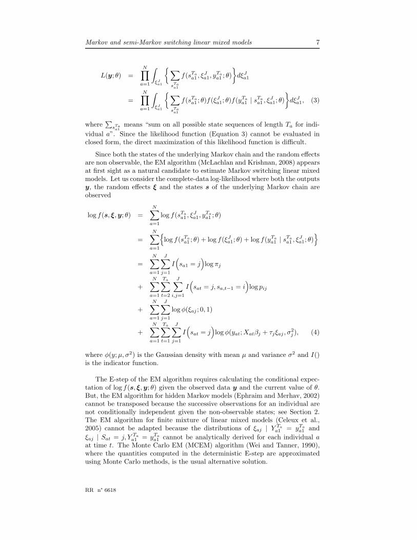
L(y; θ) =N∏

a=1

∫

ξJa1

∑

sTaa1

f(sTa

a1 , ξJa1, y

Ta

a1 ; θ)

dξJ

a1

=

N∏

a=1

∫

ξJa1

∑

sTaa1

f(sTa

a1 ; θ)f(ξJa1; θ)f(yTa

a1 | sTa

a1 , ξJa1; θ)

dξJ

a1, (3)

where∑

sTaa1

means “sum on all possible state sequences of length Ta for indi-

vidual a”. Since the likelihood function (Equation 3) cannot be evaluated inclosed form, the direct maximization of this likelihood function is difficult.

Since both the states of the underlying Markov chain and the random effectsare non observable, the EM algorithm (McLachlan and Krishnan, 2008) appearsat first sight as a natural candidate to estimate Markov switching linear mixedmodels. Let us consider the complete-data log-likelihood where both the outputsy, the random effects ξ and the states s of the underlying Markov chain areobserved

log f(s, ξ, y; θ) =

N∑

a=1

log f(sTa

a1 , ξJa1, y

Ta

a1 ; θ)

=

N∑

a=1

log f(sTa

a1 ; θ) + log f(ξJa1; θ) + log f(yTa

a1 | sTa

a1 , ξJa1; θ)

=

N∑

a=1

J∑

j=1

I(sa1 = j

)log πj

+

N∑

a=1

Ta∑

t=2

J∑

i,j=1

I(sat = j, sa,t−1 = i

)log pij

+N∑

a=1

J∑

j=1

log φ(ξaj ; 0, 1)

+

N∑

a=1

Ta∑

t=1

J∑

j=1

I(sat = j

)log φ(yat; Xatβj + τjξaj , σ

2j ), (4)

where φ(y; µ, σ2) is the Gaussian density with mean µ and variance σ2 and I()is the indicator function.

The E-step of the EM algorithm requires calculating the conditional expec-tation of log f(s, ξ, y; θ) given the observed data y and the current value of θ.But, the EM algorithm for hidden Markov models (Ephraim and Merhav, 2002)cannot be transposed because the successive observations for an individual arenot conditionally independent given the non-observable states; see Section 2.The EM algorithm for finite mixture of linear mixed models (Celeux et al.,2005) cannot be adapted because the distributions of ξaj | Y Ta

a1 = yTa

a1 and

ξaj | Sat = j, Y Ta

a1 = yTa

a1 cannot be analytically derived for each individual a

at time t. The Monte Carlo EM (MCEM) algorithm (Wei and Tanner, 1990),where the quantities computed in the deterministic E-step are approximatedusing Monte Carlo methods, is the usual alternative solution.

RR n° 6618


For the presentation of the estimation algorithm, we adopted the framework ofrestoration-maximization (RM) algorithms proposed by Qian and Titterington(1991) (see also Archer and Titterington (2002)). The Monte Carlo EM algo-rithm proposed by Altman (2007) can be interpreted as a RM algorithm withtwo restoration steps for the two latent structures, a unconditional stochasticone for the random effects and a conditional deterministic one for the state se-quences (the unconditional/conditional qualifier refers to the other latent struc-ture). We did not adopt a similar approach since, in our definition of Markovswitching linear mixed models (see Section 2), the random effects are attachedto the states. Hence, following Shi and Lee (2000), we rather chose to performtwo conditional restoration steps, one for the random effects given the statesequences (and the observed data) and one for the state sequences given therandom effects (and the observed data). The iteration of the proposed RMalgorithm decomposes in:

• Conditional R-step for state sequences:for each individual a, sample sTa

a1 from P (STa

a1 = sTa

a1 | ξJa1, Y

Ta

a1 = yTa

a1 ; θ)by a direct transposition of the forward-backward algorithm proposed byChib (1996),

• Conditional R-step for random effects:for each individual a, compute the best posterior prediction ξJ

a1 fromP (ξJ

a1 | STa

a1 = sTa

a1 , Y Ta

a1 = yTa

a1 ; θ),

• Maximisation-step.

As discussed by Neal and Hinton (1998) in the Gaussian mixture case, sinceMarkov chain parameters and linear mixed model parameters form disjoint setsand influence the complete-data log-likelihood separately (Equation 4), Markovchain parameters can be updated when the distribution of S is re-calculatedand linear mixed model parameters can be updated when the ξ are predicted.It makes sense to immediately re-estimate the parameters before performingthe conditional R-step for the other latent structure. This approach, calledincremental EM algorithm, permits to speed up the convergence. It can benoted that the order of the steps is not important and does not influence theparameters estimation and the convergence of the algorithm.

3.1 Forward-backward algorithm for sampling state se-

quences given the random effects

For each individual a, the state sequences are sampled from the conditionaldistribution P (STa

a1 = sTa

a1 | Y Ta

a1 = yTa

a1 , ξJa1).

For a Markov switching linear mixed model, since

P(STa

a1 = sTa

a1 | Y Ta

a1 = yTa

a1 , ξJa1

)

=

Ta−1∏

t=1

P(Sat = sat | STa

a,t+1 = sTa

a,t+1, YTa

a1 = yTa

a1 , ξJa1

)

× P(SaTa

= saTa| Y Ta

a1 = yTa

a1 , ξJa1

),

the following conditional distributions should be used for sampling state se-quences:

INRIA


• final state (initialization)

P(SaTa

= saTa| Y Ta

a1 = yTa

a1 , ξJa1

),

• previous state

P(Sat = sat | STa

a,t+1 = sTa

a,t+1, YTa

a1 = yTa

a1 , ξJa1

).

The forward-backward algorithm for sampling state sequences given the ran-dom effects can be decomposed into two passes, a forward recursion which issimilar to the forward recursion of the forward-backward algorithm for hiddenMarkov chains, and a backward pass for sampling state sequences (Chib, 1996);see the Appendix for details.

The forward recursion can be used to compute the observed-data log-likelihoodgiven the random effects:

log P (Y = y | ξ; θ) =

N∑

a=1

(log P (Ya1 = ya1 | ξJ

a1; θ)

+

Ta∑

t=2

log P (Yat = yat | Y t−1a1 = yt−1

a1 , ξJa1; θ)

)

=

N∑

a=1

Ta∑

t=1

log Nat. (5)

where Nat is the normalizing factor for individual a at time t; see Appendix.

3.2 Random effect prediction given the state sequence

The predicted vector for the random effects ξJa1 attached to individual a is:

ξJa1(m) = E

[ξJa1 | STa

a1 = sTa

a1 (m), Y Ta

a1 = yTa

a1

](6)

= ΩU (m)a

′(U (m)

a Ω2U (m)a

′ + DiagU (m)a σ2

)−1(yTa

a1 −J∑

j=1

Iaj(m)Xaβj

),

where

• sTa

a1 (m) is the mth state sequence sampled for individual a,

• Ω = Diagτj ; j = 1, . . . , J is the J×J random standard deviation matrix,

• U(m)a is the Ta × J design matrix associated with state sequence sTa

a1 (m),

composed of 1 and 0 with∑

j U(m)a (t, j) = 1 and

∑t

∑j U

(m)a (t, j) = Ta,

• u(m)at =

(I(sat(m) = 1) · · · I(sat(m) = J)

)is the tth row of the design

matrix U(m)a ,

• σ2 = (σ21 · · ·σ

2J )′ is the J-dimensional residual variance vector,

RR n° 6618


• DiagU(m)a σ2 is the Ta×Ta diagonal matrix with u

(m)at σ2; t = 1, . . . , Ta

on its diagonal,

• Iaj(m) = DiagI(sat(m) = j), t = 1, · · · , Ta

is a Ta × Ta diagonal

matrix,

• Xa is the Ta × Q matrix of covariates.

3.3 M-step

In the proposed MCEM-like algorithm, the conditional expectation of the complete-data log-likelihood given the observed data is approximated at iteration k by:

E[log f(s, ξ, y; θ) | Y = y; θ(k)

]=

N∑

a=1

E[log f(sTa

a1 , ξJa1, y

Ta

a1 ; θ) | Y Ta

a1 = yTa

a1 ; θ(k)]

≈1

Mk

N∑

a=1

Mk∑

m=1

log f(s

Ta(k)a1 (m), ξ

J(k)a1 (m), yTa

a1 ; θ(k))

≈1

Mk

N∑

a=1

Mk∑

m=1

J∑

j=1

I(s(k)a1 (m) = j

)log π

(k)j

+1

Mk

N∑

a=1

Mk∑

m=1

Ta∑

t=2

J∑

i,j=1

I(s(k)at (m) = j, s

(k)a,t−1(m) = i

)log p

(k)ij

+1

Mk

N∑

a=1

Mk∑

m=1

J∑

j=1

log φ(ξ(k)aj (m); 0, 1) (7)

+1

Mk

N∑

a=1

Mk∑

m=1

Ta∑

t=1

J∑

j=1

I(s(k)at (m) = j

)log φ(yat; Xatβ

(k)j + τ

(k)j ξ

(k)aj (m), σ

2(k)j ).

where Mk is the number of state sequences sampled at iteration k for eachindividual a.

At iteration k, the new values of the parameters of the Markov switchinglinear mixed model are obtained by maximizing the different terms of Equation7, each term depending on a given subset of θ.

For the parameters of the underlying Markov chain, we obtain:

• initial probabilities

π(k+1)j =

∑a

∑m I

(s(k)a1 (m) = j

)

NMk

,

• transition probabilities

p(k+1)ij =

∑a

∑m

∑Ta

t=2 I(s(k)at (m) = j, s

(k)a,t−1(m) = i

)

∑a

∑m

∑Ta

t=2 I(s(k)a,t−1(m) = i

) .

INRIA


For the parameters of the J linear mixed models, we obtain:

• fixed effect parameters

β(k+1)j =

( ∑

a

∑

m

X ′aI

(k)aj (m)Xa

)−1( ∑

a

∑

m

X ′aI

(k)aj (m)

(yTa

a1 − τ(k)j ξ

(k)aj (m)

)), (8)

• residual variances

σ2(k+1)j =

∑a

∑m

(yTa

a1 − Xaβ(k)j − τ

(k)j ξ

(k)aj (m)

)′

I(k)aj (m)

(yTa

a1 − Xaβ(k)j − τ

(k)j ξ

(k)aj (m)

)

∑a

∑m trI

(k)aj (m)

, (9)

• random effect standard deviations

τ(k+1)j =

∑a

∑m

∑t I

(s(k)at (m) = j

)ξ(k)aj (m)

(yat − Xatβ

(k)j

)2

∑a

∑m

∑t I

(s(k)at (m) = j

)ξ2(k)aj (m)

. (10)

The reestimation of linear mixed model parameters is similar to the reesti-mation of linear model parameters by ordinary least squares. The difference isthat the new values of the linear mixed model parameters are weighted by thenumber of occurrence of states within sampled state sequences.

3.4 Initialisation of the algorithm

Various simulations have been conducted using different starting values. Theproposed MCEM-like algorithm is indeed sensitive to starting values. The moredistant from true values the starting values are, the worse the parameter esti-mates are. We recommend to choose as starting values the parameters estimatedby the EM algorithm for a simple Markov switching linear model or semi-Markovswitching linear model.

3.5 Sample size

The conditional R-steps relies on the restoration of several pairs (sTa

a1 , ξJa1) for

each individual a. As discussed by Wei and Tanner (1990) and Cappe et al.(2005), it is inefficient to start with a large number of sampled state sequencesMk. They recommended to increase Mk as the current approximation movescloser to the true maximizer. In order not to increase exponentially the numberof sampling pairs over the iterations, we propose to introduce a further step inthe RM algorithm proposed at iteration k:

• Conditional R-step for state sequences:sample Mk state sequences from P (STa

a1 = sTa

a1 | ξJa1, Y

Ta

a1 = yTa

a1 ; θ) for eachindividual a,

• Conditional R-step for random effects:predict a random effect from P (ξJ

a1 | STa

a1 = sTa

a1 , Y Ta

a1 = yTa

a1 ; θ) for eachindividual a and each sampled state sequences,

• Maximisation-step,

RR n° 6618


• Choice of sample size-step:increase the number of sampled pairs Mk and sample with replacementMk+1 random effects among the Mk predicted random effects.

Caffo et al. (2005) proposed an adaptative strategy in order to choose the samplesize and to recover the ascent property (increase of the observed data likelihood)of the EM algorithm.

3.6 Convergence of the algorithm

Due to the sample variability introduced by Monte Carlo step, the ascent prop-erty of the EM algorithm is lost (McLachlan and Krishnan, 2008). To determinethe convergence of the MCEM algorithm, Wei and Tanner (1990) recommendedto monitor the plots of θ(k) against the iteration index k and to terminate whenthe plots exhibit random fluctuations around a roughly stationary value θ∗.Another way is to monitor the convergence by the difference between consec-utive observed likelihoods. However, if the observed data likelihood cannot beevaluated analytically, Meng and Schilling (1996) suggested to monitor the con-vergence by the bridge sampling method that can be used to obtain an estimateof the observed data likelihood ratio between two consecutive iterations. Nev-ertheless, in the Markov switching linear mixed model case, the observed datalikelihood cannot be computed at each iteration.

Under assumption of convergence of random effect predictions, we chose tomonitor the convergence of the proposed MCEM algorithm by the differencebetween successive iterations

log P (Y = y | ξ(k+1); θ(k+1)) − log P (Y = y | ξ(k); θ(k)) (11)

where the quantity log P (Y = y | ξ(k); θ(k)) is directly obtained as a byproductof the forward recursion (Equation 5).

3.7 MCEM-like algorithm for individual-wise random ef-

fect models

The transposition to individual-wise random effect models is straightforward.Since the individual-wise random effects are incorporated in the output process,the main difference concerns the conditional R-step of random effect predictiongiven a state sequence (Equation 6). In the M-step (Equations 8, 9 and 10)and in the forward and backward passes (Section 3.1), the random effects ξJ

a1

are replaced by ξa. Using the notations introduced in Section 3.2, the predictedrandom effect ξa for each individual a is given by:

ξa(m) = E[ξa | STa

a1 = sTa

a1 (m), Y Ta

a1 = yTa

a1

]

= τ ′U (m)a

′(U (m)

a ττ ′U (m)a

′ + DiagU (m)a σ2

)−1(yTa

a1 −J∑

j=1

Iaj(m)Xaβj

),

where τ = (τ1 · · · τJ )′ is the J-dimensional random effect standard deviationvector.

INRIA


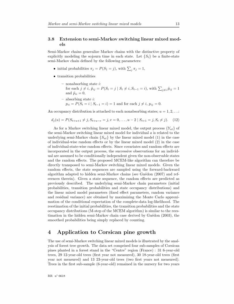
3.8 Extension to semi-Markov switching linear mixed mod-

els

Semi-Markov chains generalize Markov chains with the distinctive property ofexplicitly modeling the sojourn time in each state. Let St be a finite-statesemi-Markov chain defined by the following parameters:

• initial probabilities πj = P (S1 = j), with∑

j πj = 1,

• transition probabilities

– nonabsorbing state i:for each j 6= i, pij = P (St = j | St 6= i, St−1 = i), with

∑j 6=i pij = 1

and pii = 0,

– absorbing state i:pii = P (St = i | St−1 = i) = 1 and for each j 6= i, pij = 0.

An occupancy distribution is attached to each nonabsorbing states; u = 1, 2, . . .:

dj(u) = P (St+u+1 6= j, St+u−v = j, v = 0, . . . , u − 2 | St+1 = j, St 6= j). (12)

As for a Markov switching linear mixed model, the output process Yat ofthe semi-Markov switching linear mixed model for individual a is related to theunderlying semi-Markov chain Sat by the linear mixed model (1) in the caseof individual-wise random effects or by the linear mixed model (2) in the caseof individual-state-wise random effects. Since covariates and random effects areincorporated in the output process, the successive observations for an individ-ual are assumed to be conditionally independent given the non-observable statesand the random effects. The proposed MCEM-like algorithm can therefore bedirectly transposed to semi-Markov switching linear mixed models. Given therandom effects, the state sequences are sampled using the forward-backwardalgorithm adapted to hidden semi-Markov chains (see Guedon (2007) and ref-erences therein). Given a state sequence, the random effects are predicted aspreviously described. The underlying semi-Markov chain parameters (initialprobabilities, transition probabilities and state occupancy distributions) andthe linear mixed model parameters (fixed effect parameters, random varianceand residual variance) are obtained by maximizing the Monte Carlo approxi-mation of the conditional expectation of the complete-data log-likelihood. Thereestimation of the initial probabilities, the transition probabilities and the stateoccupancy distributions (M-step of the MCEM algorithm) is similar to the rees-timation in the hidden semi-Markov chain case derived by Guedon (2003), thesmoothed probabilities being simply replaced by counting.

4 Application to Corsican pine growth

The use of semi-Markov switching linear mixed models is illustrated by the anal-ysis of forest tree growth. The data set comprised four sub-samples of Corsicanpines planted in a forest stand in the “Centre” region (France) : 31 6-year-oldtrees, 29 12-year-old trees (first year not measured), 30 18-year-old trees (firstyear not measured) and 13 23-year-old trees (two first years not measured).Trees in the first sub-sample (6-year-old) remained in the nursery for two years

RR n° 6618


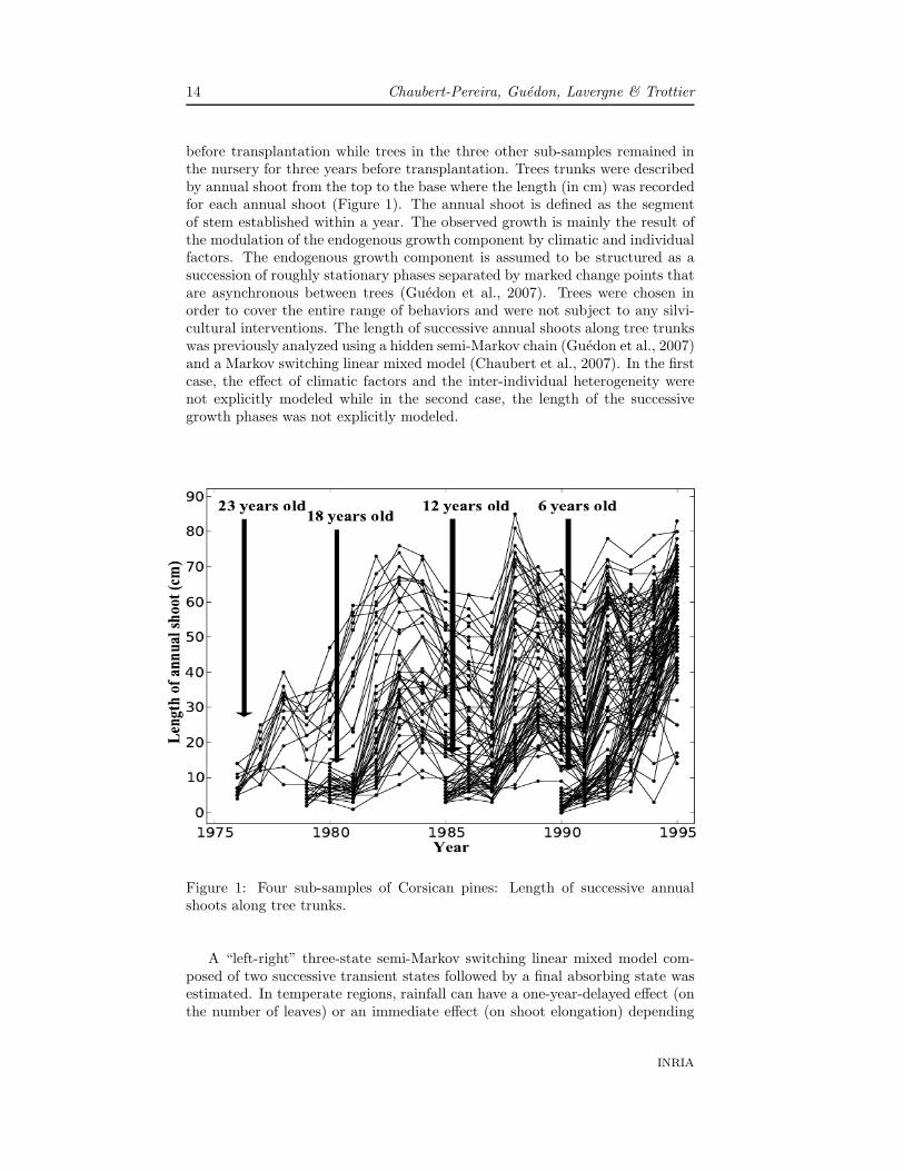
before transplantation while trees in the three other sub-samples remained inthe nursery for three years before transplantation. Trees trunks were describedby annual shoot from the top to the base where the length (in cm) was recordedfor each annual shoot (Figure 1). The annual shoot is defined as the segmentof stem established within a year. The observed growth is mainly the result ofthe modulation of the endogenous growth component by climatic and individualfactors. The endogenous growth component is assumed to be structured as asuccession of roughly stationary phases separated by marked change points thatare asynchronous between trees (Guedon et al., 2007). Trees were chosen inorder to cover the entire range of behaviors and were not subject to any silvi-cultural interventions. The length of successive annual shoots along tree trunkswas previously analyzed using a hidden semi-Markov chain (Guedon et al., 2007)and a Markov switching linear mixed model (Chaubert et al., 2007). In the firstcase, the effect of climatic factors and the inter-individual heterogeneity werenot explicitly modeled while in the second case, the length of the successivegrowth phases was not explicitly modeled.

Figure 1: Four sub-samples of Corsican pines: Length of successive annualshoots along tree trunks.

A “left-right” three-state semi-Markov switching linear mixed model com-posed of two successive transient states followed by a final absorbing state wasestimated. In temperate regions, rainfall can have a one-year-delayed effect (onthe number of leaves) or an immediate effect (on shoot elongation) depending

INRIA


on whether it occurs during organogenesis2 or elongation. We chose to use anintercept and the centered cumulated rainfall (in mm) during a period cover-ing one organogenesis period and one elongation period as fixed effects for eachlinear mixed model. The linear mixed model attached to state j is:

yat | Sat=j = βj1+βj2Xt+τjξaj+ǫat, ξaj ∼ N (0, 1), ǫat | Sat=j ∼ N (0, σ2j ),

where yat is the length of the annual shoot for individual a at time t, βj1 isthe intercept, Xt is the centered cumulated rainfall at time t (E(Xt) = 0) andβj2 is the cumulated rainfall parameter. Because of the centering of climaticcovariate, the intercept βj1 is directly interpretable as the average length ofsuccessive annual shoots within state j.

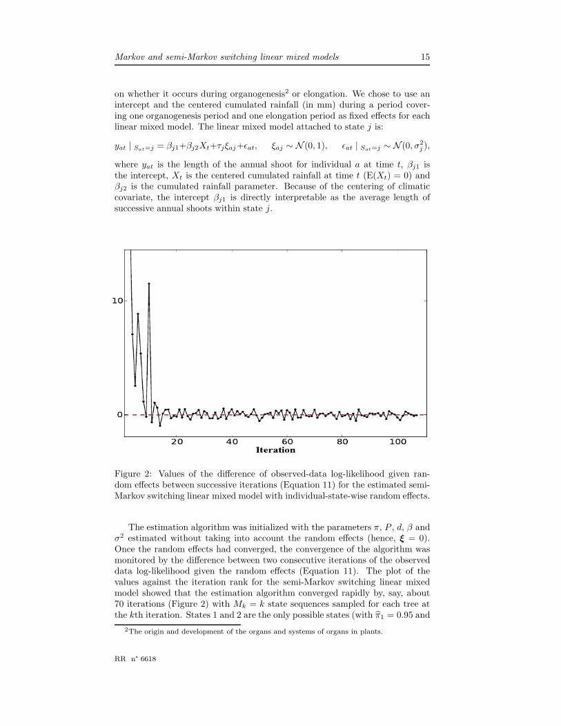
Figure 2: Values of the difference of observed-data log-likelihood given ran-dom effects between successive iterations (Equation 11) for the estimated semi-Markov switching linear mixed model with individual-state-wise random effects.

The estimation algorithm was initialized with the parameters π, P , d, β andσ2 estimated without taking into account the random effects (hence, ξ = 0).Once the random effects had converged, the convergence of the algorithm wasmonitored by the difference between two consecutive iterations of the observeddata log-likelihood given the random effects (Equation 11). The plot of thevalues against the iteration rank for the semi-Markov switching linear mixedmodel showed that the estimation algorithm converged rapidly by, say, about70 iterations (Figure 2) with Mk = k state sequences sampled for each tree atthe kth iteration. States 1 and 2 are the only possible states (with π1 = 0.95 and

2The origin and development of the organs and systems of organs in plants.

RR n° 6618


π2 = 0.05) of the estimated underlying semi-Markov chain; see Figure 3. Theestimated transition probability matrix is degenerated i.e. for each transientstate i, pi,i+1 = 1 and pij = 0 for j 6= i + 1 (and for the final absorbing statepii = 1 and pij = 0 for j 6= i). It should be noted that the succession of states isdeterministic for a degenerated “left-right” semi-Markov switching linear mixedmodel. This deterministic succession of states supports the assumption of asuccession of growth phases.

Figure 3: Estimated underlying semi-Markov chain. Each state is representedby a vertex which is numbered. Vertices representing transient states are edgedby a single line while the vertex representing the final absorbing state is edgedby a double line. Possible transitions between states are represented by arcs(attached probabilities always equal to 1 are not shown). Arcs entering instates indicate initial states. The attached initial probabilities are noted nearby.The occupancy distributions of the nonabsorbing states are shown above thecorresponding vertices. The dotted lines correspond to occupancy distributionsestimated by a simple Gaussian hidden semi-Markov chain (GHSMC) and thepoint lines correspond to occupancy distributions estimated by a semi-Markovswitching linear mixed model (SMS-LMM).

The marginal observation distribution of the linear mixed model attachedto state j is the Gaussian distribution N (µj , Γ

2j) with µj = βj1 +βj2Ej(X) and

Γ2j = τ2

j +σ2j , where Ej(X) is the mean centered cumulated rainfall X in state j.

The marginal observation distribution represents the length of the annual shootsof the average tree in state j. The marginal observation distributions for thedifferent states are well separated (little overlapping between marginal obser-vation distributions corresponding to two successive states); compare the meandifference µj+1 −µj between consecutive states with the standard deviations Γj

and Γj+1 in Table 1.

INRIA


State j

1 2 3

Occupancy GHSMC 2.88, 1.37 5.31, 2.93distributions

mean, sd SMS-LMM 2.73, 0.68 5.56, 2.20Regression Intercept βj1 7.09 25.79 50.25parameters

(SMS-LMM) Cumulated rainfallparameter βj2 0.0027 0.0165 0.0309

Average cumulatedrainfall effect βj2 × sdj(X) 0.30 2.16 4.52

Variability Random variance τ2

j5.79 49.89 69.39

decomposition Residual variance σ2

j4.74 39.95 76.86

(SMS-LMM) Total variance Γ2

j 10.53 89.84 146.25

Proportion of inter-individual heterogeneity 54.99% 55.53% 47.45%

Marginal GHSMC 6.97, 3.26 26.30, 9.12 54.35, 11.39observationdistribution

µj ,Γj SMS-LMM 6.99, 3.24 25.88, 9.48 50.32, 12.09

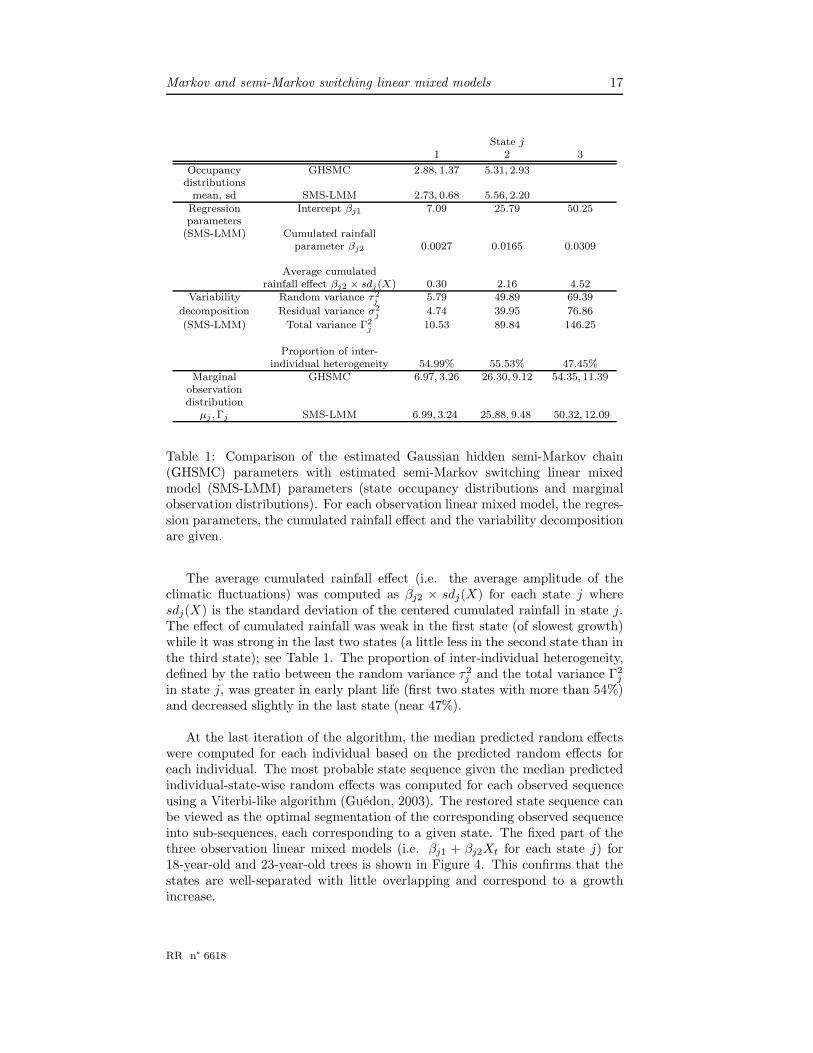
Table 1: Comparison of the estimated Gaussian hidden semi-Markov chain(GHSMC) parameters with estimated semi-Markov switching linear mixedmodel (SMS-LMM) parameters (state occupancy distributions and marginalobservation distributions). For each observation linear mixed model, the regres-sion parameters, the cumulated rainfall effect and the variability decompositionare given.

The average cumulated rainfall effect (i.e. the average amplitude of theclimatic fluctuations) was computed as βj2 × sdj(X) for each state j wheresdj(X) is the standard deviation of the centered cumulated rainfall in state j.The effect of cumulated rainfall was weak in the first state (of slowest growth)while it was strong in the last two states (a little less in the second state than inthe third state); see Table 1. The proportion of inter-individual heterogeneity,defined by the ratio between the random variance τ2

j and the total variance Γ2j

in state j, was greater in early plant life (first two states with more than 54%)and decreased slightly in the last state (near 47%).

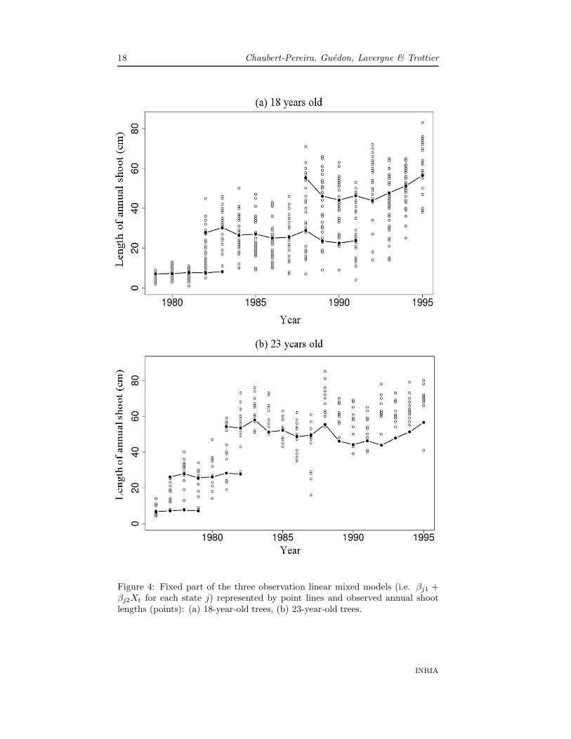
At the last iteration of the algorithm, the median predicted random effectswere computed for each individual based on the predicted random effects foreach individual. The most probable state sequence given the median predictedindividual-state-wise random effects was computed for each observed sequenceusing a Viterbi-like algorithm (Guedon, 2003). The restored state sequence canbe viewed as the optimal segmentation of the corresponding observed sequenceinto sub-sequences, each corresponding to a given state. The fixed part of thethree observation linear mixed models (i.e. βj1 + βj2Xt for each state j) for18-year-old and 23-year-old trees is shown in Figure 4. This confirms that thestates are well-separated with little overlapping and correspond to a growthincrease.

RR n° 6618


Figure 4: Fixed part of the three observation linear mixed models (i.e. βj1 +βj2Xt for each state j) represented by point lines and observed annual shootlengths (points): (a) 18-year-old trees, (b) 23-year-old trees.

INRIA


The characteristics (median and dispersion) of the first year in each statewere extracted for the four sub-samples of Corsican pines on the basis of themost probable state sequences of the observed sequences computed using the es-timated Gaussian hidden semi-Markov chain and semi-Markov switching linearmixed model. The median first year in the second state for the four sub-sampleswas similar for the two models; see Table 2. The median first year in the thirdstate for the 6-year-old Corsican pines was similar for the two models. A shift ofone year was noted for the median first year in the third state between the twomodels for the 12-year-old, 18-year-old and 23-year-old Corsican pines. The dis-persion of the first year in the second and the third state was greatly reduced inthe semi-Markov switching linear mixed model case compared to the Gaussianhidden semi-Markov chain case (Table 2). When the effect of climatic covari-ates and inter-individual heterogeneity were taken into account, this renderedthe states more synchronous between individuals; see also the estimated occu-pancy distributions (Equation 12), and in particular their standard deviations,for the Gaussian hidden semi-Markov chain and for the semi-Markov switchinglinear mixed model in Table 1 and Figure 3.

6 years old 12 years old 18 years old 23 years old

GHSMC 1993 (0.56) 1988 (0.42) 1982 (1.93) 1978 (1.04)State 2

SMS-LMM 1993 (0.56) 1988 (0.50) 1982 (0.56) 1978 (1.17)GHSMC 1995 (0.35) 1993 (1.00) 1988 (2.56) 1981 (0.78)

State 3SMS-LMM 1995 (0.38) 1992 (0.87) 1989 (1.27) 1982 (0.77)

Table 2: Median first year in state 2 and state 3 for each sub-sample deducedfrom the estimated Gaussian hidden semi-Markov chain (GHSMC) and the semi-Markov switching linear mixed model (SMS-LMM). The corresponding standarddeviations are indicated in brackets.

The correlation coefficient between the median predicted random effect instate 1 and the median predicted random effect in state 2 was 0.26 while the cor-relation coefficient between the median predicted random effect in state 2 andthe median predicted random effect in state 3 was 0.62. Hence, the behaviorof an individual is more strongly related between the last two states than be-tween the first two states. The more general assumption of the individual-state-wise random effect model (a random effect attached to each state) compared toindividual-wise random effect model (a random effect common to all states) ismore representative of Corsican pine behavior; see Chaubert et al. (2007) forthe same conclusion in the Markov switching linear mixed model case.

Complementary biological results about Corsican pine growth and other for-est tree species (sessile oaks and Scots pines) can be found in Chaubert-Pereiraet al. (2008).

RR n° 6618


5 Concluding remarks

Semi-Markov switching linear mixed models enable to identify and to charac-terize the different growth components (endogenous, environmental and indi-vidual components) of forest trees. The introduction of climatic covariates andindividual-state-wise random effects renders the endogenous growth componentmore synchronous between individuals than with a simple Gaussian hidden semi-Markov chain. The growth phases are thus not only defined by the averagedlength of annual shoots but also by the amplitude of fluctuations synchronousbetween individuals. Moreover, the behavior of each tree within the populationcan be investigated on the basis of the predicted individual-state-wise randomeffects.

The linear mixed model associated with the third state seems to underes-timate the observed mean length of successive annual shoots in this phase forthe 23-year-old Corsican pines (Figure 4). This behaviour highlights a sub-sample or group effect. A possible extension of the observation linear mixedmodel would be to incorporate a group-wise random effect in addition to theindividual-state-wise random effect and the fixed effect. It can be noted thatincorporating a group-wise random effect can be useful in different situations.The difference between groups can have various causes; for instance, geneticfactors, age, plot density or soil properties.

In the proposed MCEM-like algorithm, the conditional restoration step forstate sequences given random effects relies on simulations while the conditionalrestoration step for random effects given state sequences is deterministic. In thislatter case, an alternative solution would be to sample random effects applyinga Metropolis-Hastings algorithm; see McCulloch (1997) in the generalized linearmixed model case and Lavergne et al. (2007) in the case of mixture of generalizedlinear mixed models.

The estimation algorithms proposed in this paper can directly be transposedto other families of hidden Markov models such as for instance hidden Markovtree models; see Durand et al. (2005) and references therein. Another interestingdirection for further research would be to develop the statistical methodologyfor semi-Markov switching generalized linear mixed models to take into accountnon-normally distributed response variables (for instance, number of growthunits, apex death/life, non flowering/flowering character in the plant architec-ture context). Since the conditional expectation of random effects given statesequences cannot be analytically derived, the proposed MCEM-like algorithmfor semi-Markov switching linear mixed model cannot be transposed to thecase of non-normally distributed observed data and other conditional restora-tion steps, for instance based on a Metropolis-Hastings algorithm, have to bederived for the random effects.

Acknowledgements

The authors are grateful to Meteo-France which freely supplied the meteorolog-ical data and to Yves Caraglio for providing the Corsican pine data.

INRIA


References

R.M. Altman. Mixed hidden Markov models: An extension of the hiddenMarkov model to the longitudinal data setting. Journal of the AmericanStatistical Association, 102:201–210, 2007.

G.E.B Archer and D.M. Titterington. Parameter estimation for hidden Markovchains. Journal of Statistical Planning and Inference, 108:365–390, 2002.

D. Barthelemy and Y. Caraglio. Plant architecture: a dynamic, multilevel andcomprehensive approach of plant form and ontogeny. Annals of Botany, 99(3):375–407, 2007.

B.S. Caffo, W. Jank, and G.L. Jones. Ascent-based Monte Carlo expectation-maximization. Journal of the Royal Statistical Society, Series B, 67(2):235–251, 2005.

S.G. Candy. Estimation in forest yield models using composite link functionswith random effects. Biometrics, 53(1):146–160, 1997.

O. Cappe, E. Moulines, and T. Ryden. Inference in hidden Markov models.Springer Series in Statistics. New York, NY: Springer. xvii, 652 p., 2005.

G. Celeux, O. Martin, and C. Lavergne. Mixture of linear mixed models for clus-tering gene expression profiles from repeated microarray experiments. Statis-tical Modelling, 5:243–267, 2005.

F. Chaubert, Y. Caraglio, C. Lavergne, C. Trottier, and Y. Guedon. A statisticalmodel for analyzing jointly growth phases, the influence of environmentalfactors and inter-individual heterogeneity. Applications to forest trees. In 5thInternational Workshop on Functional-Structural Plant Models, pages P43,1–3, Napier, New Zealand, nov 2007.

F. Chaubert-Pereira, Y. Caraglio, C. Lavergne, and Y. Guedon. Identifyingontogenetic, environmental and individual components of forest tree growth.Submitted, 2008.

S. Chib. Calculating posterior distributions and modal estimates in Markovmixture models. Journal of Econometrics, 75:79–97, 1996.

R.G Cowell, A.P. Dawid, S.L. Lauritzen, and D.J. Spiegelhalter. ProbabilisticNetworks and Expert Systems. Statistics for Engineering and InformationScience. New York, NY: Springer. xii, 321 p., 1999.

J.B. Durand, Y. Guedon, Y. Caraglio, and E. Costes. Analysis of the plantarchitecture via tree-structured statistical models: The hidden Markov treemodels. New Phytologist, 166(3):813–825, 2005.

Y. Ephraim and N. Merhav. Hidden Markov processes. IEEE Transactions onInformation Theory, 48(6):1518–1569, 2002.

S. Fruhwirth-Schnatter. Finite Mixture and Markov Switching models. SpringerSeries in Statistics. New York, NY: Springer. xvii, 492 p., 2006.

RR n° 6618


Y. Guedon. Estimating hidden semi-Markov chains from discrete sequences.Journal of Computational and Graphical Statistics, 12(3):604–639, 2003.

Y. Guedon. Exploring the state sequence space for hidden Markov and semi-Markov chains. Computational Statistics and Data Analysis, 51(5):2379–2409,2007.

Y. Guedon, Y. Caraglio, P. Heuret, E. Lebarbier, and C. Meredieu. Analyzinggrowth components in trees. Journal of Theoretical Biology, 248(3):418–447,2007.

M. Gupta, P. Qu, and J.G. Ibrahim. A temporal hidden Markov regressionmodel for the analysis of gene regulatory networks. Biostatistics, 8(4):805–820, 2007.

S. Kim and P. Smyth. Segmental Hidden Markov Models with Random effectsfor Waveform Modeling. Journal of Machine Learning Research, 7:945–969,2006.

C. Lavergne, M.J. Martinez, and C. Trottier. Finite mixture models for expo-nential repeated data. Technical Report 6119, INRIA, 2007.

G. Lindgren. Markov regime models for mixed distributions and switching re-gressions. Scandinavian Journal of Statistics, Theory and Applications, 5:81–91, 1978.

C.E. McCulloch. Maximum likelihood algorithms for generalized linear mixedmodels. Journal of the American Statistical Association, 92(437):162–170,1997.

G.J. McLachlan and T. Krishnan. The EM algorithm and extensions. 2nd Edi-tion. Wiley Series in Probability and Statistics. New York, NY: John Wiley& Sons., 360 p., 2008.

X.L. Meng and S. Schilling. Fitting full-information item factor models and anempirical investigation of bridge sampling. Journal of the American StatisticalAssociation, 91(435):1254–1267, 1996.

R.M. Neal and G.E. Hinton. A view of the EM algorithm that justifies in-cremental, sparse, and other variants. In Jordan, Michael I. (ed.), Learningin graphical models. Proceedings of the NATO ASI, Ettore Maiorana Centre,Erice, Italy, September 27 - October 7, 1996. Dordrecht: Kluwer AcademicPublishers. NATO ASI Series. Series D. Behavioural and Social Sciences. 89,355-368. 1998.

Y. Ninomiya and A. Yoshimoto. Statistical Method for Detecting StructuralChange in the Growth Process. Biometrics, 64(1):46–53, 2008. doi: 10.1111/j.1541-0420.2007.00844.x.

W. Qian and D.M. Titterington. Estimation of parameters in hidden Markovmodels. Philosophical Transactions of the Royal Society, Series A, 337(1647):407–428, 1991.

INRIA


F. Rijmen, E.H. Ip, S. Rapp, and E.G. Shaw. Qualitative longitudinal analysisof symptoms in patients with primary and metastatic brain tumours. Journalof the Royal Statistical Society, Series A, 171(3):739–753, 2008.

J.Q. Shi and S.Y. Lee. Latent variable models with mixed continuous andpolytomous data. Journal of the Royal Statistical Society, Series B, 62(1):77–87, 2000.

P. Smyth, D. Heckerman, and M.I. Jordan. Probabilistic independence networksfor hidden Markov probability models. Neural Computation, 9(2):227–269,1997.

G. Wei and M. Tanner. A Monte Carlo implementation of the EM algorithmand the poor’s man data augmentation algorithm. Journal of the AmericanStatistical Association, 85:699–704, 1990.

RR n° 6618


Appendix: Forward-backward algorithm for sam-

pling state sequences given random effects

Forward recursion

In the Markov switching linear mixed model case, the forward recursion isinitialized for t = 1 by:

Faj(1) = P(Sa1 = j | Ya1 = ya1, ξ

Ja1

)j = 1, . . . , J ; a = 1, . . . , N ;

=φ(ya1; Xa1βj + τjξaj , σ

2j )

Na1πj ,

where Na1 = P (Ya1 = ya1 | ξJa1) is a normalizing factor with:

Na1 =

J∑

j=1

P (Sa1 = j, Ya1 = ya1 | ξJa1)

=J∑

j=1

φ(ya1; Xa1βj + τjξaj , σ2j ) πj .

For t = 2, . . . , Ta, the forward recursion is given by:

Faj(t) = P(Sat = j | Y t

a1 = yta1, ξ

Ja1

)j = 1, . . . , J ; a = 1, . . . , N ;

=φ(yat; Xatβj + τjξaj , σ

2j )

Nat

J∑

i=1

pijFai(t − 1).

The normalizing factor Nat = P(Yat = yat | Y t−1

a1 = yt−1a1 , ξJ

a1

)is obtained

directly during the forward recursion as follows:

Nat =

J∑

j=1

P (Sat = j, Yat = yat | Y t−1a1 = yt−1

a1 , ξJa1)

=

J∑

j=1

φ(ya1; Xa1βj + τjξaj , σ2j )

J∑

i=1

pijFai(t − 1).

Backward pass

The backward pass can be seen as a stochastic backtracking procedure. Thebackward pass is initialized for t = Ta by:

P(SaTa

= j | Y Ta

a1 = yTa

a1 , ξJa1

)= Faj(Ta) j = 1, . . . , J ; a = 1, . . . , N.

The final state saTais sampled from the smoothed probabilities

(P

(SaTa

= j | Y Ta

a1 = yTa

a1 , ξJa1

); j = 1, . . . , J

).

For t = Ta − 1, . . . , 1, the backward pass is given by:

P(Sat = j | STa

a,t+1 = sTa

a,t+1, YTa

a1 = yTa

a1 , ξJa1

)=

pjsa,t+1Faj(t)

∑J

i=1 pisa,t+1Fai(t)

,

INRIA


where the quantities Faj(t) are directly extracted from the forward recursion.The state sat is sampled from the conditional distribution

(P

(Sat = j | STa

a,t+1 = sTa

a,t+1, YTa

a1 = yTa

a1 , ξJa1

); j = 1, . . . , J

).

RR n° 6618


Contents

1 Introduction 3

2 Model definition 5

3 Maximum likelihood estimation with a Monte Carlo EM-like

algorithm 6

3.1 Forward-backward algorithm for sampling state sequences giventhe random effects . . . . . . . . . . . . . . . . . . . . . . . . . . 8

3.2 Random effect prediction given the state sequence . . . . . . . . 93.3 M-step . . . . . . . . . . . . . . . . . . . . . . . . . . . . . . . . . 103.4 Initialisation of the algorithm . . . . . . . . . . . . . . . . . . . . 113.5 Sample size . . . . . . . . . . . . . . . . . . . . . . . . . . . . . . 113.6 Convergence of the algorithm . . . . . . . . . . . . . . . . . . . . 123.7 MCEM-like algorithm for individual-wise random effect models . 123.8 Extension to semi-Markov switching linear mixed models . . . . 13

4 Application to Corsican pine growth 13

5 Concluding remarks 20

Bibliography 21

Appendix: Forward-backward algorithm for sampling state se-

quences given random effects 24

INRIA

Centre de recherche INRIA Sophia Antipolis – Méditerranée2004, route des Lucioles - BP 93 - 06902 Sophia Antipolis Cedex (France)

Centre de recherche INRIA Bordeaux – Sud Ouest : Domaine Universitaire - 351, cours de la Libération - 33405 Talence CedexCentre de recherche INRIA Grenoble – Rhône-Alpes : 655, avenue de l’Europe - 38334 Montbonnot Saint-Ismier

Centre de recherche INRIA Lille – Nord Europe : Parc Scientifique de la Haute Borne - 40, avenue Halley - 59650 Villeneuve d’AscqCentre de recherche INRIA Nancy – Grand Est : LORIA, Technopôle de Nancy-Brabois - Campus scientifique

615, rue du Jardin Botanique - BP 101 - 54602 Villers-lès-Nancy CedexCentre de recherche INRIA Paris – Rocquencourt : Domaine de Voluceau - Rocquencourt - BP 105 - 78153 Le Chesnay CedexCentre de recherche INRIA Rennes – Bretagne Atlantique : IRISA, Campus universitaire de Beaulieu - 35042 Rennes Cedex

Centre de recherche INRIA Saclay – Île-de-France : Parc Orsay Université - ZAC des Vignes : 4, rue Jacques Monod - 91893 Orsay Cedex

ÉditeurINRIA - Domaine de Voluceau - Rocquencourt, BP 105 - 78153 Le Chesnay Cedex (France)

http://www.inria.fr

ISSN 0249-6399

Markov and semi-Markov switching linear mixed models for ... · PDF fileroughly stationary...

Documents

Transcript of Markov and semi-Markov switching linear mixed models for ... · PDF fileroughly stationary...