•

KHARTOUM, SUDANAUGUST‐ 2010

MARKETS & PRICE MONITORING 

 TRAINING MANUAL    

Sudan Integrated Food Security Information for Action (SIFSIA) funded by European Union (EU) and jointly implemented by the Government of Sudan and the Food and Agriculture Organization of the United Nations (FAO) In collaboration with the Famine Early Warning Systems - Network (FEWS NET) in Sudan funded by USAID.

FAMINE  EARLY         WARNING  SYSTEMS NETWORK (FEWS NET)                 

Prepared for government counterparts as part of the national capacity building programme, by Dr. El Fadil Ahmed Ismaiel

FOOD  SECURITY  TECHNICAL  SECRETARIAT OF  THE MINISTRY OF AGRICULTURE (FAO‐SIFSIA/ SUDAN INTEGRATED FOOD   SECURITY INFORMATION FOR ACTION) 

2

Table of Contents

List of boxes .................................................................................................................. 4 List of figures ................................................................................................................ 5 List of Tables ................................................................................................................ 6 1  INTRODUCTION AND BACKGROUND ........................................................ 7

1.1  Introduction ..................................................................................................... 7 1.2  What is a Market ............................................................................................. 9 1.3  Markets, Marketing and Relation to Food Security ...................................... 11 1.4  The Price and Market Monitoring System .................................................... 12  1.5  Introduction to the Basic Concepts ............................................................... 13

2  MANIPULATION OF PRICE DATA ............................................................. 15

2.1  Cleaning Raw Price Data .............................................................................. 15 2.2  Dealing with Inflation- Introductory ............................................................. 16 2.3  Rounding of Data and Scientific Notation .................................................... 25 2.4  Replacing Missing Values ............................................................................. 26

3  SUMMARIZING PRICE DATA...................................................................... 29

3.1  Basic Principles of Price Indices ................................................................... 29 3.2  Price Indices in More Detail .......................................................................... 29 

3.2.1  Commodity Aggregation ....................................................................... 30 3.2.2  Territorial Aggregation and Market Weights ........................................ 31 3.2.3  Annual Price Indices .............................................................................. 33

4  PRICE AND MARKET ANALYSIS ............................................................... 35

4.1  Analysis of Demand and Supply ................................................................... 35 4.1.1  Basic Price Theory in Relation to Demand and Supply Analysis ......... 36 4.1.2  Price Changes, Trends and Seasonality - Assessing Storage and Seasons …………………………………………………………………………39 4.1.3  Price Time Series –Detailed Analysis .................................................... 48 

4.2  Qualitative Analysis of Impact ...................................................................... 54 4.3  Relative Price Relationships – TOT and International/Domestic Price

comparisons (The Role of External Trade) ................................................... 55 4.4  Surplus and Deficit Markets .......................................................................... 57 4.5  How Food Markets Work – An Introduction ................................................ 58 

4.5.1  Inter – Form Price Differences .............................................................. 59 4.5.2  Assessing Market Integration - Inter-Spatial Price Variation –

Correlation ............................................................................................. 59 4.5.3  Gross Market Margins and Cereal Price Spreads .................................. 61

Cha

pter

One

C

hapt

er T

wo

Cha

pter

Thr

ee

Cha

pter

Fou

r

3

5 REFERENCES 66 6 Annex Annex 1.1: Elements/Aspects of Food Security and Information Needed……….....69 Annex 4.1: Example of Worksheet for the Calculation of Seasonal Price Index……70 Annex 4.2: Crop Calendar and Relation to Food Security Analysis…………………71 Annex 4.3: Most Commonly Used Functional Forms to Evaluate Trends…………..72 Annex 4.4: Practical Example of Import Parity Price………………………………..73 Annex 1 Typical Market Indicators (FEWS NET learnernotes0417)............... 74 Annex 2 Market Related Policy Questions (FEWS NET learnernotes0417) ........... 77 Annex 3: Policy impacts on markets and population (FEWS NET learnernotes0417) ......................................................................................................... 77 Annex 3: Policy impacts on markets and population (FEWS NET learnernotes0417) ......................................................................................................... 79 Limit the inventory to the most important policies otherwise the exercise becomes too long and matrix of impacts too complicated. ............................................................... 79 Annex 8: Market Indicators for Early Warning (FEWS NET learnernotes0417) .... 80 Annex 9: Market Indicators for Emergency Impact Assessment FEWS NET (learnernotes0417) ....................................................................................................... 81 Annex 10: Market Indicators for Recovery and Transition (FEWS NET learnernotes0417) ......................................................................................................... 83 

Ann

ex

4

List of boxes   Box 1.1: Index Numbers……………………………………………………………19 Box 1.2: Derivation of Real Price if Base and Current Year CPI & Nominal

Prices Known …………………….………………………………………19 Box 1.3: The Relative Importance of CPI as a Measure of Inflation ……………...20 Box 1.4: How to compute a Basket Cost …………………………………………..22 Box 3.1: Relative Price Corresponding to a Base Period ……………………….....30 Box 4.1: What is the Appropriate Tool for the Analyis of Variables and Attributes ……..……………… …………………………………………40 Box 4.2: What is the Imported Parity Price(IPP) ………………………………….56

5

List of figures  Figure 2.1: Nominal and Deflated Prices of bread (kilos) over the period January - June in Khartoum state in 2008 (CPI for medium income group) ….…24 Figure 2.2: Example – Interpolation – No Perfect Method ………………….……28 Figure 4.1: Supply and Demand Interactions, Consumer and Producer Surpluses …………………………………………………….……......36 Figure 4.3: Trends of Average Wholesale Prices of Main Cereals in Sudan

2000-2008* (SDG/t) ……………………………………………………....43 Figure 4.4: Real and Nominal Domestic Fresh-Milk Prices In Selected

States 2000-2008* (SDG/lb.)…………….……………………………....43 Figure 4.5: Nominal Average Sheep and Cattle Nominal Prices in El Obeid Markets,

2000-2008 (SDG/Head)……………………………………………...…....44

6

List of Tables   Table 1.1: Typical Commodity Chain Channels……………………………………..13 Table 2.1: Examples for Classifying Inflation……………………………………….17 Table 2.2: Prices of bread (kilos) over the period January - June in Khartoum

State in 2008(CPI for medium income group)………………………...…..23 Table 4.1: Impact of Life Changes on Market Supplies and Food Security (a)...…....37 Table 4.2: Impact of Life Changes on Market Supplies and Food Security (b)...…...38 Table 4.3: Various Price Analysis Techniques Used in Market Assessment..…….…39 Table 4.4: Prices Variations (SDG/ton) for Major Food grain in Three Main

Markets during the Period June, 2007 through June2008…….……….….41 Table 4.5: The Functional Logarithmic Equations and Income Elasticity……….….53 Table 4.6: Example of a Price Impact Matrix for Selected Household Group………55 Table 4.7: The Impact of Simultaneous Price Changes……………………………...55 Table 4.8: Coefficient of Correlation between Monthly Bivariate Results between Main Wholesale Markets during the Period January, 2001

through May, 2010………………………….…………………………..61 Table 4.9: Summary of Marketing Costs and Margins (SD) for Sorghum in

Gedaref State…………………………………………………………..63 Table 4.10: The Various Marketing Costs and Margins for Camels’ Exports(SDG).64 Table 4.11: % of Wholesale Prices Spreads over Destination Markets from

June 2007-June 2008…………………………………………………...65 .

7

Chapter One

1 INTRODUCTION AND BACKGROUND

1.1 Introduction

This training course provides a generic overview of a ‘price and market analysis document’ as an integral part of a comprehensive food security programme initiated by FEWS NET and SIFSIA North. Through this training and capacity building component, the main target is to provide a basic understanding of markets’ issues in relation to food security and livelihoods development as part of food security and vulnerability analysis and show further how to conduct response analysis and design mitigation options and/or alternative. New in this training module is the blending of marketing concepts to those of food security issues in a practical manner with typical day to day events that a food security analyst needs. Therefore, the focus in this marketing-food security concern is to enable analysts to understand how markets could affect food availability and how they could influence access to food. To capture this dilemma, the document introduces basic market and food security concepts usually needed by food security analysts to perform this task. In this training course, much emphasis is made on price monitoring and price analysis which can be used for food security planning and early warning and can also serve in other policy purposes. Moreover, the material is made in such a way to provide the theoretical basis for analysts in this field and simultaneously grasp the concepts to make sound recommendations on scientific grounds. This is why, and from the outset, we draw the attention of users of this document to the fact that much of the guidance material is drawn from text books. In addition, existing practical experiences and information knowledge available by many NGOs involved in food security and market analysis are extensively used as applied examples. Therefore, some of the theoretical and analytical examples should be adjusted to the context of every state’s needs where and when appropriate. Regarding the course contents, an introductory background on the context, purpose, and scope of the training material is clearly illustrated. The training material blends between theorems and practicality/operability in case of price analysis. For instance, responses to price surges to ease processes that lead to decisions and actions to be undertaken as well as on the analytical underpinning tools required to ensure that instruments used are well adapted to the specific conditions prevailing in the country. Various approaches and techniques are used in this training material, but much emphasis is made on having examples of a positive analysis approach. Most of the analyses followed throughout this training material use a range of standardized procedures and simple statistical tools. The positive analysis approach utilizes the measures of central tendency and measures of dispersion (Koutsoyiannis, 1977) are just few examples. Moreover, some examples on markets Structure, Conduct, and

8

Performance approach (SCP) are partially illustrated to analyze the markets and market developments. The training modules are presented in four main sections. The first section gives an introductory overview of the objectives of the training material, illustrates the methodology and approaches used in the training activities as well as the organizational lay out of the materials. The section goes further to describe the price and market monitoring system, and introduces the basic concepts in this regard. Section Two elaborates on how price data is manipulated. This includes the cleaning and replacing of missing values prior to analysis. The section shows how to deal with inflation in manipulating price data and left the details to other sections. The concepts of price indices are elaborated in Section Three. This includes basic principles of price indices, ccommodity aggregation, territorial aggregation and market weights and annual price indices. Section Four gives a comprehensive price and market analysis including practical examples on price changes, trends and seasonality of supply. The section gives appropriate examples on price time series analysis and qualitative analysis of impact from given data. Section Four goes further to illustrate relative price relationships using terms of trade as a proxy for international and domestic price comparisons. The section assesses market integration, gross margins and cereal price spreads analysis, and shows how could spatial price variation affect surplus and deficit markets. To optimize course benefit, participants should have additional knowledge on other types of analyses (this shall be undertaken during the class room discussions to provide a bench mark for appropriate decisions on issues related to current food prices1). Recent emerging price analysis techniques and data sources are recommended for further readings by interested analysts in this training material. The data sources include Ministry of Agriculture and Forestry, Department of Statistics, Ministry of Animal Resources and fisheries, the Central Bank of Sudan, the Strategic Reserves Corporation and SIFSIA Market Bulletins. However, the source of data for this training is variable and data is selected for the following reasons: consistency, reliability, timeliness, historical data availability, and coverage of different levels and markets. Many illustrations are given to participants (information outputs) to help them understand the real world situation as data graphs, figures and tabular forms and formulae showing current prices and trends in some selected states or regions, with supporting texts. Report formats on market conditions by region or state shall be given together with the information required for market intervention (given as

▪ 1 Analysis on food availability and utilization (food balance sheet for key food commodities). ▪ Analysis of information on key food commodities prices in main and secondary markets; import

flows, cereal import bills and price transmission ▪ A brief analysis of food and nutrition insecurity situations with assessment and coverage of current

safety nets, legal entitlements, food aid flows, etc. ▪ Identification of farmers' best needs (seeds, fertilizers, finance, etc) to make a rapid response to

capture the price increase. ▪ An analysis & assessment of current policies (fiscal, monetary, agricultural, trade, industrial, etc.)

and their impact on food prices to identify possible changes. ▪ An assessment of storage and transport capacities to distribute food and/or inputs to optimize

social and productive safety nets implementation.

9

annexes). The training module shall make use of SIFSIA price and market databases and use simple software for price and market analysis (EXCEL and/or SPSS). By the end of this training course, participants are expected to acquire the following:

• An improvement in capacity of participants to conduct price monitoring and market analysis for various purposes as food policy development and food security early warning,

• Participants be able to explain key definitions, concepts and indicators associated with market and price analysis and as such;

– be able to grasp the conceptual framework of food security in a market context,

– be aware of role and importance of markets to understand food security , • An improvement in participants’ skills to demonstrate a working knowledge

of tools, techniques, and methodologies associated with markets and food security. This shall allow participants to conduct successfully comprehensive sequential planning, monitoring and evaluation relevant to food security domains by running practical exercises.

• Having this course material, State or Federal staff can add ideas, adapt, and even modify approaches to suit their specific local needs and situations as ToTs.

Above outcomes can easily be achieved if participants’ skill profile involves good market knowledge and computer skills, particularly the computational software as EXCEL. This course requires a substantial amount of independent readings in food security and marketing, other than material provided. Participants are expected to take personal responsibility and show initiatives in developing their own knowledge and understanding during the computer tutorials.

1.2 What is a Market A market is the place where people, and institutions buy and sell for their agents. A market can be organized as a physical market place where products are exchanged. In this respect, one can distinguish between a seller’s market which is the one with a abundance of goods and services and a buyer’s market which is the one with an shortage of goods and services. Another distinction between markets as referred to ‘consumer markets’ and ‘industrial markets’ is made by Boone and Kurtz (Boone and Kurtz, 1977). “Consumer goods” are those products and services purchased by the consumer for personal use” as clothes, books, food, etc. On the other hand, industrial goods are those products purchased to be used, either directly or indirectly, in the production of other goods for resale. Examples are raw cotton, raw materials, crude oil, etc. The distinction between the two types lies in the purchaser and the reasons for buying the goods. However, markets can be geographically extended (scope and place) to local, national, regional, and international markets. The marketing concept puts marketing at the beginning rather than at the end of the production cycle and integrates marketing into each phase of the business enterprise. In marketing literature numerous definitions are available for the term marketing. In a narrow sense marketing is “the performance of business activities that direct the flow of goods and services from producers to consumers or users”. A broader definition

10

expresses marketing as “the development and efficient distribution of goods and services for chosen consumer segments” (Ibid, 1977). However, the nature and degree of efficiency depends on the kind of business environment the firm is operating in. A simple definition of agricultural marketing is the series of activities involved in finding out what customers want and moving those products profitably from the point of production to the point of consumption (Republic of Zambia, 2004). In the process of identification and selection of market targets we need to know that a market requires:

(a) People, who are the customers and what do they want or need (b) Willingness to buy, (c) The necessary purchasing or buying power, is the number of

goods/services that can be purchased with a unit of currency (d) The where or the place or vicinity buyers and sellers come together,

which may not necessarily be physically come together. This means they may communicate through telecommunication means, and

(e) The authority to make purchase decisions. Broadly speaking, there are four important elements that need to be considered in the marketing process2 and these elements involve but not limited to:

i) prioritising the customer by knowing what the customer needs or wants ii) process of selection by knowing to whom do we sell the product to, iii) determine how and where the produce is marketed iv) promotion by letting customers know that the product is available and of good quality and v) creation of trust by making the customers trust the farmer/producer.

A series of agricultural marketing planning activities is essential (Ibid, 2004) in order to successfully and profitably market new products that consumers want and these include:

i) Identify buyers and their needs ii) Decide on marketing channels to be used iii) Plan production to meet their needs iv) Plan to harvest, process, grade, package or store v) Identify arrangements for transport and delivery of the products vi) Calculate costs vii) Calculate profits

2 In thinking about these elements, farmers need to ask themselves about the six Ps:

• People, • Planning how is the product going to reach the selected customers, what are the steps? • Product: What product is going to be marketed? • Place: Where is the product going to be marketed? • Price: What price will the product be offered on the market for? • Promotion: How are people going to be informed that the product is being offered for the

market?

11

1.3 Markets, Marketing and Relation to Food Security In fact, the four basic objectives for the food system as a whole (efficient economic growth, a more equal distribution of income, nutritional well being, and food security) are analogous to the objectives of the marketing sector in a society (Timmer et al, 1983). Marketing can thus support and contribute to all of the four objectives for its capacity to link domestic markets to international markets and also provides early warning information to decision makers concerning food security status. In general, marketing systems have three broad functions: a logistical function, an informational function and a distributional function. The logistical function includes not only transformation over time (storage), but also embraces place (transportation), and form (processing) activities (FAO, 1997). Thus and therefore, marketing can eventually generate ownership, form, time, and place utilities that can meet the ever-increasing consumers’ demand. Markets make an important contribution to the 4 pillars of food security (Annex 1.1), namely availability of food, access to it, utilization, and stability of supply. For making food available, producers must be able to purchase inputs for producing food and countries usually trade with each other to make sure enough food is available. On access side, households usually sell their products (e.g. crops, livestock, and other non-agricultural commodities) and their labour in the market and earn income. This price of food in the market determines whether a household’s income or resources are sufficient to obtain an adequate quantity and quality of food. Likewise, the movement of food through markets from one location to another, from surplus to deficit areas and across borders, usually helps to ensure stable food supplies over time and space. To ensure satisfactory food security, the whole process requires adequate market information to ensure availability, access, utilization, and stability of food. Market information plays an essential role in policy decisions and food allocation. The market information and analysis contributes to food security analysis by:

- deepening the understanding and analysis of food security situation; - adding a dynamic aspect to food security analysis by adding continuum and up-

to-date information; - linking households to local, national, regional and global economies; - yielding more precise estimates of needs; - improving scenario development and monitoring; - clarifying appropriate type, magnitude and timing of response; and - shedding light on the constraints to food security caused by market irregularities

and inefficiencies (FEWS NET Training documents, 2008-2009) Elements of market efficiency and market failure are key factors and terminologies in addressing marketing problems and therefore should be well understood particulalry when dealing with food security. Moreover, agricultural markets perform both physical marketing functions and the communication of signals to producers and consumers about costs and prices within given market forces. Competition, which is determined by the number of market participants (buyers and sellers), and the equal balance of market information knowledge; provide a more equal distribution of the gains from efficient market price formation that is ever known.

12

Food security analysts should be aware that, an efficiently functioning marketing system depends largely on the availability and interactions of many components that lead to its success. The availability of transportation and storage facilities; efficient communications; common grades and standards that facilitate trading at distance; legal codes to enforce contracts; and credit availability to finance short-run inventories and processing operations can eventually lead to a smoothly functioning marketing system. Market inefficiency or market failure, is of course, associated with lack, poor or non-availability of some of the aforementioned services and activities. On the supply side, fluctuations in rainfall (distribution, quantity, intensity and duration), poor tillage practices, and insufficient capital to carry out timely agricultural practices are few among many other reasons that can lead to such variations in yield and thus variation in prices.

1.4 The Price and Market Monitoring System

For food security analyst, it is highly desirable to monitor what happens to market prices in order to obtain useful knowledge and insights that may help decision makers, families or society at large in understanding food security situations or enhancing competition along the food chain. Increase of transparency along the food supply chain is an important step to encourage competition and improve its resilience to price volatility. The commodity chain describes flow of activities/services from the primary producer to the final consumer (Table 1.1). A commodity chain thus includes all levels of the market and actors that have a role in the distribution and transformation of the commodity. Commodities usually flow from one level to the next, starting with the farm gate, where a commodity is first sold and ending at the retail or consumer market where the final product is purchased by a consumer. Based on transaction level and commodity, four types of price data can be distinguished between types of raw price data. The most commonly considered transaction levels at which prices are observed are:

Farm-gate level, Wholesale level, Retail level (Standard and Non-standard Units),

The term marketing chain is sometimes used to describe the links between transaction levels. These transaction levels are inseparable, though they were completely separated and located in different places. For instance, wholesale and retail marketing can occur in the same place. Market information is essential for all information users and providers and they include traders, consumers, government policy makers, and non-government relief planners, donors, academicians and other users.

13

Table 1.1: Typical Commodity Chain Channels Commodity Chain Channels 1.4.1.1 Definition Farm gate/Producer

Located at or near the farm or place of production. Usually, the location where a commodity is first exchanged.

Assembly Where smaller quantities of a commodity, usually from different farmers and small scale traders are accumulated or aggregated. Assembly markets facilitate marketing and the movement of commodities and reduce marketing costs. They also enable sellers of small surpluses from remote locations to reach distant buyers.

Wholesale Usually, where traders sell to other traders. Volumes per transaction tend to be larger, e.g. multiple 50 kg bags and even metric tons.

Retail/Consumer Where commodities are largely sold to end users, especially consumers. Volumes per transaction tend to be smaller, e.g. by kg or ‘koum’ equivalent to a small bowl.

1.5 Introduction to the Basic Concepts

i) Basic Price concept

Price is the amount of money and/or other items with utility needed to acquire a product or service. In this sense, prices indicate value that has been added to a particular commodity. Thus the price is the cost or value of a good or service expressed in monetary terms, the price you can pay: tuition for receiving an education, interest for receiving a loan, rent for living in a house or using a piece of equipment, salaries or wages for employing workers. The definition of price depends on exactly what is being sold. It is the financial cost paid when one buys a unit of a specific product or service. Therefore price is a combination of:

• The good or service that is the object of the transaction; • Any supplementary services provided, such as a warranty; and, • The benefits provided by the product, which may include non-monetary

benefits. In a pricing strategy, three main things are dealt with and it includes:

- Methods of setting profitable and justifiable prices - Price structure, and - Price formation.

Price signals can carry information about cost of production, transportation, storage, perceptions and desires as well as -in some instances- distortions. As mentioned earlier, transparency along the food supply chain is crucial in maintaining competition and thus improves its resilience to price volatility. In the process of developing a marketing mix to reach target markets and achieve marketing goals, we must determine the pricing policy via identification of three major tasks in pricing:

14

• Setting pricing objectives. • Setting the base price for their products, consistent with their pricing

objectives. • Selecting which strategies, such as discounting, to employ in modifying and

applying the base price.

15

Chapter Two

2  MANIPULATION OF PRICE DATA

2.1 Cleaning Raw Price Data

Food security analysts usually look for data quality which refers to the degree of excellence exhibited by the data in relation to the portrayal of the actual phenomena. Real world data is often soiled with much inconsistency, inaccuracy and mostly incomplete and/or stale. For this reason one may look at the features and characteristics of data that satisfy a given purpose; as related to food security, and optimize the sum of the degrees of excellence for factors related to data cleaning. Data cleaning is often measured in terms of consistency, accuracy, completeness, and timeliness. This is why there has been an increasing demand for data quality tools for effectively detecting and repairing errors in the data. Before undertaking any price analysis, price data needs to be cleaned, by removing implausible values from the data or removing obvious errors. In this respect, plausible upper and lower limits are set so that we can detect obvious errors.

When talking about accuracy of data, we often refer to the degree to which data correctly reflects the real world. On the other hand, completeness of data is the extent to which the expected attributes of data are provided in details and are adequately available. For example, it is possible that data is not available, but it is still considered completed, as it meets the expectations of the user particularly in vulnerable environments where means of access to information is meagre. In this regard one should bear in mind that, every data requirement has 'mandatory' and 'optional' aspects. For example customer's mailing address is mandatory and it is available and because customer’s office address is optional, it would not be a problem if it is not available. However, data can be complete, but inaccurate. For instance, many production or yield data is available but few of them are not correct. Consistency of data means that data across the enterprise field should be in synch with each other and with no or even less contradictory information. However, it worth to mention that, data can be accurate (i.e. represent what happened in real world), but still inconsistent. For instance, one may find monthly information of a year up to 13 rows while it is quite obvious that a calendar year contains only 12 months from January to December. Moreover, data can be complete, but inconsistent, due to a duplication of lines or error mistakes, a probable cause. On the other side, the timeliness of data is extremely important as it reflected achievements within a given frame of time and timeliness depends on user’s expectation. For instance, rainfall gauges or stations should provide timely and up-to date information to the federal authority for aggregation on daily or monthly basis. However, food security analysts should rely mostly on data auditability, a missing dimension on our agricultural data system. Auditability, which means that any transaction, report, accounting entry can be traced back to its originating transaction through a common identifier, which should stay with a transaction as it undergoes transformation, aggregation and reporting.

16

2.2 Dealing with Inflation- Introductory

In economics, inflation is a rise in the general level of prices of goods and services in an economy over a period of time. When the price level rises, each unit of currency buys fewer goods and services; consequently, annual inflation is also a decline in the purchasing power of money – a loss of real value in the internal medium of exchange and unit of account in the economy. A chief measure of price inflation is the inflation rate, the annual percentage change in a general price index (normally the Consumer Price Index) over time. Effects of inflation on an economy are manifold and can simultaneously be positive and negative (for more information see chapter 11, Harcourt Brace & Company, web info and FEWS NET, 2009-a). High rates of inflation and hyperinflation can be caused by an excessive growth of the money supply. Views on which factors determine the low to moderate rates of inflation are more varied. Low or moderate inflation may be attributed to fluctuations in real demand for goods and services or to changes in available supplies such as during scarcities as well as to growth in the money supply. However, the consensus view is that a long sustained period of inflation is caused by money supply growing faster than the rate of economic growth. Today, most mainstream economists favour a low steady rate of inflation. Low inflation (as opposed to zero or negative inflation) may reduce the severity of economic recessions by enabling the labour market to adjust more quickly in a downturn and reduce the risk that a liquidity trap prevents monetary policy from stabilizing the economy. The task of keeping the rate of inflation low and stable is usually given to monetary authorities. Generally, these monetary authorities are the Central Banks of Sudan who control the size of the money supply through the setting of Murabaha, Musharaka and Mudaraba rates (interest rates in conventional system), through open market operations, and through the setting of banking reserve requirements. Inflation is an essential economic factor that influences marketing strategy, and hence impacts food security strategy since any rise in price levels will result in reduction of the purchasing power of the consumers. Substantial rises in prices may even result in changing or modifying consumer behaviour. A more serious type of inflation is stagflation. Stagflation3 is a peculiar type of inflation, which refers to a situation when an economy has high unemployment and a rising price level at the same time. This stagflation makes marketing strategy, and

3 Economists usually use terms as hyperinflation, recession and depressions to express an economic phenomenon. Here is a brief explanation for each one without details. Hyperinflation is simply an inflation that is ‘out of control’ i.e. an inflationary cycle without any tendency toward equilibrium. A recession happens when a country experiences negative growth over a period of time. Generally, an "official" recession occurs when a country’s Gross Domestic Product (GDP) declines for two or more consecutive quarters. A depression occurs when a country experiences negative growth over an extended period of time, usually years.

17

hence food security policy, more difficult. Through the remainder of this section we shall have some numerical examples describing how one could do this exercise.

a- Numerical Examples for Classifying Inflation Inflation (volume- wise) can be of a single-digit (0-9%) or a double-digit one (10-99%) or even more depending on the economic situation of a country. Generally one can see any of four types of economic phenomena in an economy as deflation, inflation, disinflation or hyperinflation. The degree and intensity –severity- of each depends on the type of the economy strength itself and below are some numerical examples (Table 2.1): Table 2.1: Examples for Classifying Inflation

Price Index for 3 Years 100 95 93 Deflation 100 102 103 Creeping Inflation 100 120 130 Disinflation 100 150 700 Hyperinflation

There are two basic approaches or measures by which governments usually deal with inflation. These adjustment measures can either be through: ⇒ Fiscal policy, which concerns the receipts and expenditures of the government.

And to combat inflation the government reduces expenditure or raises revenues through tax or can make control over prices (viz. making a price freeze) or both.

⇒ Monetary policy, referring to the manipulation of the money supply and market rates interest (Mudaraba, Murabaha, Musharaka rates of profits). In periods of rising prices monetary policy dictates that the government takes actions to decrease money supply and increase ‘interest rate’ to restrain the purchasing power. The most important question in this regard is what are the implications for fiscal and monetary policies on food and non-food items?

i) High tax means less consumer purchasing power, which results in sales decline for nonessential goods and services.

ii) Low federal expenditure levels make the government a less attractive customer for many industries.

iii) Low money supply means less liquidity is a available for potential conversion to purchasing power

iv) High interest rates lead to significant slumps (declines) in the construction and housing industry etc.

v) Inflation influences marketing by modifying consumer behaviour (e.g. modest increase in prices form the so-called creeping inflation. The result is an increase in public prices conscious, which can lead to three possibilities

Consumer can decide to buy now for price will be higher later, Consumer may decide to reallocate their purchasing patterns, or Postpone a certain purchase.

18

In practical terms, the presence of inflation4 (increases in all prices in the economy over time) can cause confusion if not catered for when we come to the analysis of food security. We may wrongly conclude that local shortages have caused prices to rise when, in fact, the changes only reflect part of a general trend. However, there is a method for inflation adjustment of price and this is called deflation of data. Deflation of data come to reflect the fact that an increase in income over a period of years does not mean increase in real incomes, rather might be declining due to increase in living costs, and therefore, decrease in purchasing power. In this case, the real income can be obtained by dividing the apparent physical incomes by the cost of living or the consumer price index for the years using an appropriate base period. For most famine and early warning purposes, the Consumer Price Index5 (CPI as an index of retail prices) is used to deflate the data, that is to say normalize the price to be realistic. The CPI is an index of a large number of prices in the economy and reflects general trends in prices, rather than local market conditions. Thus CPI is a measure of the average change over time in the prices paid by urban consumers for a market basket of consumer goods and services. In this sense, it is a measure of change in the purchasing-power of a currency and the rate of inflation. Food security analysts should understand that, the CPI expresses the current prices of a 'basket' of goods and services in terms of the prices during the same period in a previous year to show effect of inflation on purchasing power. Synonymously, the CPI is sometimes called the Cost of Living Index (COLI), which is one of the best known lagging indicators (www.online Business Dictionary).

b- What is an Index Number? Before going deep into analysis using the CPI, we should understand the term index numbers for it frequently comes in interpreting the CPI (Box 1.1). An index number is a statistical measure designed to show changes in a variable or group of related variables with respect to time, geographic location or other characteristics such as income, profession, etc. A collection of index numbers for different years, locations, etc. is sometimes called an index series (Spiegel, 1972). Index numbers can be used to compare food or any other living costs in a place, be it a town or a village, during one year with those of a previous year. Similarly we can

4 Deflation is the opposite of inflation - a continuous decrease in prices, or continue rise in the currency’s value. 5 To compute the CPI, more than 200 categories for all goods and services used by consumers are tracked monthly and placed within eight major groups:

i) Food and Beverages: meat, milk, bread, juices, snacks, etc. ii) Housing: rent of primary residence, owners’ equivalent rent, fuel oil, bedroom furniture,

etc. iii) Apparel: cloths like garments, pants, shirts, sweaters, etc. iv) Transportation: cars, vehicles, airline fares, gasoline, etc. v) Medical Care: hospital services, drugs, medical supplies, glasses, etc. vi) Recreation: TV, pets, movies, pets, etc. vii) Education and Communication: schooling costs, telephone services, computer software,

postage, etc. viii) Other: smoking products, haircuts and other personal services

However, the CPI does not include savings or investment items, like stocks and bonds or real estate.

19

use it to compare the sorghum production in one part of a country during a given year with another part or even among sectors as irrigated versus rain fed agriculture. We can also use index numbers to compare yields in different locations and/or for different years. Indices are often used in forecasting business and economic conditions by providing general information as production indices, wage indices, unemployment indices, yield indices and price indices. One of the simplest examples of an index number is a relative price, which is the ratio of the price of a single commodity in a given period to its price in another period called the base period or reference period (Spiegel, 1972). Box 1.1: Index Numbers More generally if Pa and Pb are prices of a commodity during periods a and b respectively, the price relative in period b with respect to period a is defined as Pb/Pa and is denoted by Pa/b, a notation which will be found useful throughout this training modules. With this notation the relative price in the above equation can be denoted by Po/n A distinction between market prices and nominal prices shall be made to better understand the inflation concept (Box 1.2). For the purpose of this training material, we make a distinction between nominal prices, which are the prices observed on the market and real or deflated prices, which have been adjusted for inflation. Although not correct6, nominal prices have been used interchangeably with market prices. However, a nominal price is an estimated price of an item that may bear transaction. Nominal price is used where either the recent market price has not been established (the item is new), or where demand and supply situation makes the market-price uncertain (the item is scarce). Therefore, Box 1.2: Derivation of Real Price if Base and Current Year CPI & Nominal Prices known

6It is now becoming clear that the distinction is not useful and indeed hides a major confusion. The conventional wisdom is that proportional change in all nominal prices does not affect real price, and hence should not affect either demand or supply and therefore also should not affect output (Wikipedia, 2010).

In relative terms, what is an Index Number? Index Number has a base (starting with 100) that shows change in price of market basket over time. If Pn and Po denote the commodity prices during the base period and the given period respectively, then by definition:

o

nPP

= relative Price

Generally expressed as a percentage (%) multiplied by 100

Real prices = (CPI base year/CPI current year)*nominal price current year i.e.

rCurrentyearCurrentyea

Baseyear alpriceNoCPI

CPImin* Prices Real =

20

Remember that price indices are based on a system of commodity weights and their prices. In this context, weights are calculated based on expenditure shares that are on the proportion of total household expenditure spent on a particular commodity. Various indexes (Box 1.3) have been devised to measure different aspects of inflation.

The “best” measure of inflation for a given application depends on the intended use of the data. The CPI is generally the best measure for adjusting payments to consumers when the intent is to allow consumers to purchase, at today’s prices, a market basket of goods and services equivalent to one that they could purchase in an earlier period. The CPI also is the best measure to use to translate retail sales and hourly or weekly earnings into real or inflation-free currency value (in SDGs or in Dollars terms, $).

Box 1.3: the Relative Importance of CPI as a Measure of Inflation

The formula for calculating the Inflation Rate using the Consumer Price Index is relatively simple. The CBoS generates (usually every month) the current Consumer Price Index (CPI). Therefore, if we want to know how much prices have increased over the last 12 months (the commonly published inflation rate number) we would subtract last year's index from the current index and divide by last year's number and multiply the result by 100 and add a % sign. c- Calculating the Consumer Price Index and the Inflation Rate The formula for calculating the Inflation Rate looks like this:

AABCPI 100*)( −

=

Or in programming form as

((B - A)/A)*100

So if exactly one year ago the Consumer Price Index was 178 and today the CPI is 185, then the calculations would look like this:

((185-178)/178)*100 or (7/178)*100 or 0.0393*100 which equals 3.93% inflation over the sample year.

Various indexes have been devised to measure different aspects of inflation and include:

The CPI, - measures inflation as experienced by consumers in their day-to-day living expenses;

The Producer Price Index (PPI), - measures inflation at earlier stages of the production and marketing process;

The Employment Cost Index (ECI) measures the labour market; The Gross Domestic Product Deflator (GDP Deflator) - measures combination

of experiences with inflation of governments (Federal, State and local), businesses, and consumers.

Finally, there are specialized measures, such as measures of interest rates and measures of consumers’ and business executives’ expectations of inflation.

21

d- What Happens If Prices Go Down? If prices go down and we experienced Price Deflation then "A" would be larger than "B" and we would end up with a negative number. So if last year the Consumer Price Index (CPI) was 189 and this year the CPI is 185 then the formula would look like this:

((185-189)/189)*100 or (-4/189)*100 or -0.021*100 = -2.11

which equals negative (-2.11%) inflation over the sample year. Of course negative inflation is simply deflation.

a- Adjusting For Inflation:

Example 1: If the CPI1990 equals to 29.6 and the CPI 2009 is 130.7, what are 1990 earnings of SDG 1,500 worth in 2009?

1

212

* YCPI

CPIY=

? = 8,000 * 130.7 29.6 $35,324 = $8,000 X 130.7

29.6 Examples 2: Let’s say you spent SDG 20 to buy some goods or services today (2010). How much money would you have needed in 1980 to buy the same amount of goods or services? The CPI for 1980 = 82.4 The CPI for 2010 = 218.8 (June 2010 CPI used) The following formula is then used (Box 1.2) to calculate the price: 2010 Price x (1980 CPI / 2010 CPI) = 1980 Price (which is a real price) Using the actual numbers: SDG 20.00 x (82.4 /218.8) = SDG 7.53 Example 3: Let’s say your parents in 2008 told you that in 1975 a bus ticket had a cost of 50 pts. How could you tell if bus tickets have increased in price faster or slower than most goods and services? To convert that price into today’s piaster or SDG, use the CPI. The CPI for 1975 = 38.8 The CPI for 2008 = 218.8 (June 2008 CPI used) The following formula is then used to calculate the price: 1970 Price x (2008 CPI / 1975 CPI) = 1970 Price

22

Using the actual numbers: SDG 0.50 x (218.8/38.8) = SDG 2.81 Today, a bus ticket in the Sudan will usually run at least SDG 0.5-1. The price of a bus ticket has not increased faster than other goods or services in the Sudan. Box 1.4: How to Compute a ‘Basket’ Cost Step #1: Fix the Basket Step #2: Find the Prices Step #3: Compute the Basket’s Cost Step #4: Choose Base Year Step #5: Calculate Inflation rate

Step #1: Fix the Basket for consumers

2 for Alian 1 for Omeran Step #2: Find the Prices Year Price Alian Price Omeran 1999 $10 $1 2000 $12 $2 2001 $10 $8 Step #3: Compute the Basket’s Cost Year Cost of Basket 1999 $10(2) + $1(1) = $21 2000 $12(2) + $2(1) = $26 2001 $10(2) + $8(1) = $28 Step #4: Choose Base Year Compute index numbers Year Index Number 1999 $21/$21 X 100 = 100.0 2000 $26/$21 X 100 = 123.8 2001 $28/$21 X 100 = 133.3 Step #5: Calculate Inflation rate (Calculating % Change)

1

12 100*)( Change %YYY −

=

Substituting in by numbers, Y1 = 10, Y2 = 12: % Change = ((12-10)/10) X 100 = (2/10) X 100 = 20 percent

23

b- How to Compute CPI? Year Index Number 1999 100.0 2000 123.8 2001 133.3 Step #5: Compute Inflation Rates Year Inflation Rate 2000 ((123.8-100.0)/100.0) X100=23.8% 2001 ((133.3 - 123.8)/123.8)X100= 7.7%

Although the CPI is not a perfect measure of cost of living, yet remain as the available measure for it. The CPI has three problems:

- Substitution bias that is consumers substitute toward goods that become less expensive

- Introduction of new goods, new products and more varieties - Unmeasured quality change might not be reflected in goods’ prices. (Ex:

Faster cars, smaller candy bars Despite these aforementioned problems, nevertheless, we can go ahead using the CPI as a proxy measure for inflationary effects. The following example shows the price of bread in Khartoum State over the period January to June 2008 and the relevant deflated prices taking January month as a base for the computations (Table 2.2). Table 2.2: Prices of bread (kilos) over the period January - June in Khartoum

state in 2008 (CPI for medium income group) months of 2008 January February March April May June General CPI* 44344.8 44727.9 45440.4 44187.8 45352.4 47004.6Nominal Price/Kilo in SDG

3.15 3.465 3.705 3.462 3.46 3.46 Index number 100 100.8639 102.4706 99.64596 102.2722 105.998Deflated Price Per Kilo i SDG

3.15 3.435 3.616 3.474 3.383 3.264 Source: various data sets from MoAF *CPI taken for middle income group and January 2008 as a base period.

24

Fig. 2.1: Nominal and Deflated Prices of bread (kilos) over the period January - June in Khartoum state in 2008 (CPI for medium income group). As mentioned earlier, the deflated prices reflected real prices, provided that nominal prices for the given period(s) is given. In equational forms, Fishers‘ identity; tells that the Nominal interest=Real interest rate X Inflation (CPI). Similarly, we can get the Real rate=Nominal rate/Inflation (CPI)

c- Comparison of the Consumer Price Index versus the GDP Deflator For a comprehensive food security assessment, food security analysts might require food price analysis at both consumer’s level and the country level as well. For this purpose the CPI and the GDP price deflators are important for comparisons, despite the differences in data used.

d- Real and Nominal Interest Rates7

Usually banks give interest rate price of borrowing money by nominal rate. This is to say, the Nominal interest rate is the rate the bank pays in current value. On the other hand real interest rate is the interest rate corrected for inflation as given by the equation.

7 Unless specified otherwise, the term interest rate is used to indicate Mudaraba, Murabaha, and Musharaka rates, and it is by no means, mean the usury conventional form of western economic apparatus.

The CPI: – only consumer goods – includes cost of imports – fixed market basket

The GDP Price Deflator: – all final goods and services – excludes imports – uses current bundle of goods

25

Real interest = Nominal - Inflation The following three examples raise questions (Q) and give answer (A) for real interest rate in contrast to different inflations rates:

Real Interest Nominal Rate Inflation Example 1 Q ? =5% -0%

A 5% =5% -0% Example 2 Q ? =5% -3%

A 2% =5% -3% Example 3 Q ? =5% - (-1%)

A 6% =5% - (-1%)

2.3 Rounding of Data and Scientific Notation Usually agricultural data is faced by many shortcomings as inconsistency, inaccuracy or might even be incomplete and often estimates. Despite this fact, food security analyst should bind themselves with scientific approaches in handling or processing this data. For instance, yield data might require rounding to few decimals to be readable. When we round to the nearest hundredth decimals we usually round to the even integer preceding the 5 i.e. (2, 4, 6, 8, etc.). In other words the last number appeared should be an even and not an odd one to avoid cumulative rounding errors. Example 27.265 is rounded to 27.26 but 57.575 is rounded to 57.58. As such it is very important to learn how to locate the significant digits or significant figures accurately. Look at the following examples:

figure Decimals rounded to 25.6 Nearest unit 26 174.5 Nearest unit 174 6.464 Nearest hundredth 6.46 0.0235 Nearest hundredth 0.024 3.50001 Nearest unit 4 154.95 Nearest tenth 155 469 Nearest hundred 500 7.56501 Nearest hundredth 7.57 64449 Nearest thousand 64000

Scientific notation using the powers of 10 is often employed when dealing with numbers involving many zeros. Some computer outputs (as SPSS) usually use scientific notations to denote some outcomes/outputs of a computation. Ex.1: 100=1, 10-1=0.1, 10-5=0.00001, 774000000= 7.74 x104 In this example, the 10 is called the base while the power is named the exponent.

26

Ex.2: In computer printout it is often written in shorthand, in this way 1.5 3E+ which means 1.5*10 to the power +3 2.6 4E- which means 2.6*10 to the power -4

2.4 Replacing Missing Values

In data sets, missing data makes a lot of simple analysis difficult, particularly when data consistency and accuracy is under question. Food security analysts may find means and ways to come about these problems but too many missing data usually make results very difficult to interpret particularly trends, average prices, or price variability. The simple question that needs answer is what to do with missing values in data set? Replacing missing values usually depends on the tool you are using and the irregularity of data used. For instance, using SPSS –Statistical Package for Social Sciences- you may have three basic options when dealing with missing values.

Option 1 is to do nothing. Leave the data as it is, with the missing values in place.

This is the most frequent approach, for a few reasons. First, the number of missing values is typically small. Second, missing values are typically non-random. Third, even if there are a few missing values on individual items, you typically create composites of the items by averaging them together into one new variable, and this composite variable will not have missing values because it is an average of the existing data. However, if you chose this option, you must keep in mind how SPSS will treat the missing values. SPSS will either use “list-wise deletion” or “pair-wise deletion” of the missing values. You can elect either one when conducting each test in SPSS.

1. List wise deletion – SPSS will not include cases (subjects) that have missing

values on the variable(s) under analysis. If you are only analyzing one variable, then list-wise deletion is simply analyzing the existing data. If you are analyzing multiple variables, then list-wise deletion removes cases (subjects) if there is a missing value on any of the variables. The disadvantage is a loss of data because you are removing all data from subjects who may have answered some of the questions, but not others (e.g., the missing data).

2. Pair-wise deletion – SPSS will include all available data. Unlike list-wise

deletion which removes cases (subjects) that have missing values on any of the variables under analysis, pair-wise deletion only removes the specific missing values from the analysis (not the entire case). In other words, all available data is included. If you are conducting a correlation on multiple variables, then SPSS will conduct the bivariate correlation between all available data points, and ignore only those missing values if they exist on some variables. In this case, pair-wise deletion will result in different sample sizes for each correlation. Pair-wise deletion is useful when sample size is small or missing

27

values are large because there are not many values to begin with, so why omit even more with list-wise deletion8.

Option 2 is to delete cases with missing values. For every missing value in the

dataset, you can delete the subjects with those missing values. Thus, you are left with complete data for all subjects. The disadvantage of this approach is that, you tend reduce the sample size of your data. If you have a large dataset, then it may not be a big disadvantage because you have enough subjects even after you delete the cases with missing values. Another disadvantage to this approach is that the subjects with missing values may be different than the subjects without missing values (e.g., missing values that are non-random), so you have a non-representative sample after removing the cases with missing values. One situation in which we use Option 2 is when particular subjects have not answered an entire scale or page of the study.

Option 3 is to replace the missing values, by the so-called imputations. In this

regard, many methods are available for replacing missing values (RMV): i) mean function (the mean of the nearby or the series); ii) interpolation (common one - linear interpolation)- by joining the points-see

example below (Fig. 2.2); iii) a trend and seasonal factor (with large hole in a price data series – this will

rarely be very instructive).

However, there is little agreement about whether or not to conduct imputation.

There is some agreement, on the other hand, on which type of imputation to conduct. You typically do not conduct mean substitution or regression substitution. Mean substitution is replacing the missing value with the mean of the variable. The mean could either be simple arithmetic mean or using the moving average to smooth the erratic differences as shall be practically seen later. Regression substitution uses regression analysis to replace the missing value. Regression analysis is designed to predict one variable based upon another variable, so it can be used to predict the missing value based upon the subject’s answer to another variable. The favoured type of imputation is replacing the missing values using different estimation methods.

8 In order to better understand how list-wise deletion versus pair-wise deletion influences your results, try conducting the same test using both deletion methods. Does the outcome change? Also, it is important to keep in mind that for each type of test you conduct, you need to identify if SPSS is using list-wise or pair-wise deletion. Most tests allow you to select your preference, but you should always check your output for the number of cases used in each analysis to identify if pair-wise or list-wise deletion was used.

28

Figure 2.2: Example – Interpolation – No Perfect Method Interpolation based on average sheep and cattle prices in Rabak Livestock market, 2000-2008 (SDG/Head)

Examples Filling Missing Value(S) Following Option 3 The following example is used to give information about quantities bought of commodity Z in each year (from 1996-2005 and their respective prices in a given market9: Years 1996 1997 1998 1999 2000 2001 2002 2003 2004 2005Quantity in tons

770 785 790 795 800 805 810 820 840 850

Prices (000 SDGs)

18 16 15 ? 12 10 10 7 9 6

i) Estimate the linear demand function for commodity Z using OLS ii) Estimate the price in 1999 using above information in (i)(Interpolation) iii) Compute the price using the arithmetic average and then compare it with

that of a 2-years moving average. iv) Forecast the demand at year 2007(extrapolation)

9 Intensive examples shall be given on the various uses of regression analysis in price forecast and market integration in subsequent sections.

N.B: The (MVA) Missing Values Analysis add-on module in SPSS contains the estimation methods.

29

Chapter Three

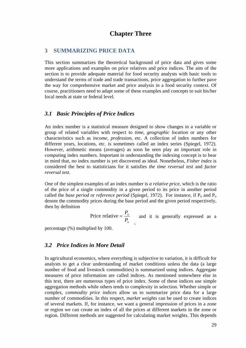
3 SUMMARIZING PRICE DATA This section summarizes the theoretical background of price data and gives some more applications and examples on price relatives and price indices. The aim of the section is to provide adequate material for food security analysts with basic tools to understand the terms of trade and trade transactions, price aggregation to further pave the way for comprehensive market and price analysis in a food security context. Of course, practitioners need to adapt some of these examples and concepts to suit his/her local needs at state or federal level.

3.1 Basic Principles of Price Indices An index number is a statistical measure designed to show changes in a variable or group of related variables with respect to time, geographic location or any other characteristics such as income, profession, etc. A collection of index numbers for different years, locations, etc. is sometimes called an index series (Spiegel, 1972). However, arithmetic means (averages) as soon be seen play an important role in computing index numbers. Important in understanding the indexing concept is to bear in mind that, no index number is yet discovered as ideal. Nonetheless, Fisher index is considered the best to statisticians for it satisfies the time reversal test and factor reversal test. One of the simplest examples of an index number is a relative price, which is the ratio of the price of a single commodity in a given period to its price in another period called the base period or reference period (Spiegel, 1972). For instance, if Pn and Po denote the commodity prices during the base period and the given period respectively, then by definition

o

n

PP

= relative Price ,

and it is generally expressed as a

percentage (%) multiplied by 100.

3.2 Price Indices in More Detail

In agricultural economics, where everything is subjective to variation, it is difficult for analysts to get a clear understanding of market conditions unless the data (a large number of food and livestock commodities) is summarized using indices. Aggregate measures of price information are called indices. As mentioned somewhere else in this text, there are numerous types of price index. Some of these indices use simple aggregation methods while others tends to complexity in selection. Whether simple or complex, commodity price indices allow us to summarize price data for a large number of commodities. In this respect, market weights can be used to create indices of several markets. If, for instance, we want a general impression of prices in a zone or region we can create an index of all the prices at different markets in the zone or region. Different methods are suggested for calculating market weights. This depends

30

on the market condition and the purpose of making the index. For instance, for early warning, it is useful to have an annual index (for prices over time), by doing so we can compare the current year with past years. The complication here is that, the weights given to any commodity vary by season since commodities are purchased or sold at different types of year. Second point is that, all the three types of index can be combined into one annual, all-commodity and multiple market indexes.

More generally if Pa and Pb are prices of a commodity during periods a and b respectively, the relative price in period b with respect to period a is defined as Pb/Pa and is denoted by Pa/b, a notation which will be found useful. With this notation the relative price in above equation can be denoted by Po/n. Example 1: Let us assume the consumer price of a certain commodity item in years 2000 and 2005 were 30 and 35 SDG respectively. Taking 2000 as a base year and 2005 as the given year, we have

%11717.130/352000Pr2005 Prelative Price 2000/2005 =====

iceinpricein

This result simply means than in 2005 the price of the commodity item was 117% of that in 2000. I.e. the price of the commodity had increased by 17%. Example 2: Now let us take same example above assuming the consumer price of a certain commodity item in years 2000 and 2005 were 30 and 35 SDG respectively. By taking 2005as a base year and 2000 as the given year, we can have:

%7.85857.35/302005Pr2000 Prelative Price 2005/2000 =====

iceinpricein

This result simply means than in 2000 the price of the commodity item was 85.7% of that in 2005. I.e. the price of the commodity had decreased by 14.3% Box 3.1: Relative Price Corresponding To a Base Period 3.2.1 Commodity Aggregation In comparing quantities or volumes of the commodity, such as quantity or volume of production, consumption, trade and exports, etc. we often talk about aggregation. In contrast, the previous examples showed price comparisons of a commodity where quantities are assumed constant for any period for simplicity. However, the same remarks and properties pertaining to relative prices are applicable to relative quantities, which are generally expressed as a percentage (%).

o

n

qq

= relative or volumeQuantity

Note that the relative price for a given period with respect to the same period is always 100%. In particular, the price relative corresponding to a base period is always 100. This accounts for the notion often used in statistical literature of writing, for example, 1995=100 indicates that the year 1995 is taken as the base period.

31

More generally if Qa and Qb are quantities or volumes of a commodity during periods a and b respectively, the quantity relative in period b with respect to period a is defined as Qb/Qa and is denoted by Qa/b .With this notation the price relative in above equation can be denoted by Qo/n. Value relatives are important indices same as price and quantity relatives. For instance, if p is the price of a commodity during a period and q is the quantity or volume produced, sold, etc., during the period, then p*q is called the total value. Thus if a 200 items are sold at 40 SDG each the total value is (SDG 40)*(200) = SDG 800. Therefore, if po and qo denote the price and quantity of a commodity during a given period, the total value during these periods are given vo and vn respectively, then: a and b respectively, the quantity relative in period b with respect to period a is defined as Qb/Qa and is denoted by Qa/b .With this notation the price relative in previous equation can be denoted by Qo/n

)(*)(** relative value

o

n

o

n

oo

nn

o

n

qq

pp

qpqp

vv

===

However, the same notation, remarks and properties pertaining to price and quantity relatives are applicable to value relatives. Thus, if pa/b, qa/b and va/b denote the price, quantity and value relatives of period b with respect to period a, then baba qp //a/b *v = 3.2.2 Territorial Aggregation and Market Weights Different commodities have different prices and different relative weights of importance as far as different qualities of same type of commodity are concerned. The problem is how to put all these together to come of a thing of practical significance. Normally we use two approaches, namely the simple aggregate method or the weighted aggregate method.

a) Simple Aggregate Method In this method of computing price index, we express the total commodity prices in the given year as a percentage of total commodity prices in the base year. In symbols

o

n

pp

∑∑=index price aggregate simple

np∑ = sum of all commodity prices in the base year,

op∑ = sum of corresponding commodity prices in the given year.

In other words, value relative= price relative multiplied by quantity relative

Value Relative= Price Relative * Quantity Relative

32

As in similar formula the result is also expressed in percentage terms. Despite the simplicity of the notation, yet two disadvantages of this method are apparent:

i) The method does not take into account the relative importance of various commodities as it gives equal weights to various items (cheese, milk, etc.) in computing living costs, and

ii) The particular units such as kilos, grams, litres, etc affect the value of the index. This problem is even more serious when we discover that local units are basically used instead of international units.

b) Weighted Aggregate Method This method overcomes the disadvantage of the previous simple aggregate method by assigning weights to the price of each commodity by a suitable factor often taken as the quantity or volume of the commodity bought or sold during the base year or some typical year, which may involve an average over several years. In this method, three possible formulae can be utilized depending on whether base year, given year or typical year quantities, denoted by qo, qn, and qt respectively, are used.

1. Laspeyres’ Index or Base Year Method oo

on

qpqp

∑∑= , where

weighted aggregate price index with base year quantity weights. This same formula can also be arrived at if we use the weighted arithmetic mean, of relative prices, where each price is weighed relative to the total value of the commodity in terms of monetary units as SDG.

2. Paasche’s Index, Or Given Year Methodno

nn

qpqp

∑∑=

, where weighted

aggregate price index with given year quantity weights

3. Typical Year Method to

tn

qpqp

∑∑= , where qt denotes the quantity

weight during some typical period t, then weighted aggregate price index with typical year quantity weights. For t=0, and t=n this reduces to above equations (equ. 1of Laspeyres and equ. 2 of Paasche) formulas, respectively.

• Fisher Ideal Index

Fisher ideal index is defined as the geometric mean of the Laspeyres and Paasche index numbers given in equation (1) and (2) above. Important in this equation is that, the Fisher’s ideal index satisfied both the time reversal and factor reversal tests, which give it certain theoretical advantage over other index numbers.

Fisher Ideal Index ))(( ∑∑

∑∑=

no

nn

oo

on

qpqp

qpqp

• The Marshall-Edgeworth Index

33

The Marshall Edgeworth index uses the Weighted Aggregate Typical Year Method where weights are taken as arithmetic mean of base year and given year quantities. This is to say,

)(21

not qqq +=

Substituting this value of qt into equation (3) of Typical Year Method then we get

Marshall-Edgeworth Price Index∑∑

+

+=

)()(

noo

non

qqpqqp

Worth to note is that, when the weights used are prices we get above formula. However, if formula used to describe quantities or volumes then they can easily be modified to obtain quantity or volume index numbers (see equations) by interchanging p and q to get

Simple Arithmetic Mean of Relatives Volume Index Weighted Aggregate Volume Index with Base Year Price Weights (Laspeyres

Volume Index) Weighted Aggregate Volume Index with Given Year Price Weights (Paasche

Volume Index) Similarly value indices can be derived following same procedures above. For

instance, the value index ∑∑=

oo

nn

qpqp

In this equation formula, the numerator represents the total value of all commodities in the given year and the denominator represents the total value of all commodities in the base year. This is called the Simple Aggregate Index, since the values have not been weighted. Other formulae in which we can use weights to indicate the relative importance of the items can be formulated.

c) Changing the Base Period of the Index Numbers In practice, the base period is usually chosen from a period of economic stability which is not too far distant in the past. Therefore, it might be necessary to change this base period from time to time to ensure consistency. If we are to go for changing the base year, two options or possibilities are available.

1. To recomputed all index numbers using the new base period, or 2. Divide all index numbers for the various years corresponding to the old

base period by the index number corresponding to the new base period, expressing the results in percentages. These results represent the new index number, the index number for the new base period being 100 (%), as it should always be10.

3.2.3 Annual Price Indices

10 Note worthy is, this method is applicable only if index numbers satisfies the circular test.

34

The example of Link or Chain Relatives can be used to show annual price indices and how they can relatively change over time. The link relatives represent a series of successive price intervals p1, p2, p3 ….of time 1, 2, 3 ….. Then p1/2, p2/3, p3/4 ….represent price relatives of each time interval with respect to the preceding time interval and is called chain relatives. Example: if the price of a commodity during the period 2000, 2001, 2002, 2003 are 16, 24, 30, 36 SDG respectively. The link relatives are p2000/2001=24/16= 150(%), p2001/2002 =30/24= 125(%), p2002/2003=36/30= 120 (%). For example the relative price of for 2003 with respect to the base year 2000 can be given by the following

p2000/2003= p2000/2001*p2001/2002*p2002/2003

= (24/16)*(30/24)*(36/30) = (36/16) =225(%) The relative prices with respect to a fixed base period can be obtained by using link relatives, sometimes called chain relatives, or the relatives chained to the fixed base Example: taking information in previous examples, the collection of chain relatives for the years 2001, 2002 and 2003 with respect to the base year 2000 are given by

p2000/2001=24/16= 150 (%) p2000/2002= p2000/2001*p2001/2002= (24/16)*(30/24)= 187.5(%)

p2000/2003= p2000/2001*p2001/2002= (24/16)*(30/24)*(36/30)= 225(%)

Worth to note is that, the above is also applicable to quantity and value relatives.

The price relative for a given period with respect to any other period taken as base can always be expressed in terms of link relatives. This is a consequence of cyclical or circular property of relatives.

For example p5/2= p5/4*p4/3*p3/2

35

Chapter Four

4 PRICE AND MARKET ANALYSIS

Before going further into market and price analysis we should have a look at the so called market structures, types and their relation to perfect market economies. Market structure is defined as the organizational characteristics which determine the relations of sellers in the market to each other, of the buyers in the market to each other, of the sellers to buyers, and of the sellers in the market to other potential suppliers of goods including potential new participants which might enter the market (Cloudius and Mueller, 1961). The usual way of determining market structure is to measure the degree of concentration (of buyers and sellers) in that market and transparency of information. The foundation of the market structure is the theory of pure competition. Four different types of market structures (also considered as models) are well acknowledged in economic literature (Enis, 1980). Market types (structures) can come under one of the following:

a) Pure (perfect) competition (as price taker), b) Monopolistic competition (as price maker), c) Oligopoly (as price maker), d) Monopoly (as price maker),

4.1 Analysis of Demand and Supply

a) Demand Analysis Demand is a multivariate relationship that is determined by many factors simultaneously. Some of the most important determinants of the market demand for a particular commodity are its own price, consumer’s income, prices of other commodities (substitutes), consumer’s tastes, income distribution, total population, consumer’s wealth, credit availability, government policy, past level of demand, and past level of income. From previous discussion, the market demand for a given agricultural commodity is the horizontal summation of individual consumers or purchasers in that market. Demand and supply are the two sides of the market and the prices are the signalling device that links the two as shown in the figure below (Fig. 4.1) as well as previous figures. The welfare analysis tells about the producers and consumers surpluses at the point of equilibrium, E. The government can make intervention letting prices at P1 making a shortage (an excess demand) or support producers at price P2. The best course of action is to let the market forces (supply and demand) determine the price which usually sets at equilibrium, E. Figure 4.1.

36

Figure 4.1: Supply and Demand Interactions, Consumer and Producer Surpluses

b) Analysis of Supply

In agriculture the analysis of supply curves require special attention for the variables used in the analysis for a number of reasons. This is because, the complexities of production patterns (multi-cropping and inter-cropping), variation in environmental and natural conditions, prices on inputs and output, institutional organization and the relative use of technology stand as conflicting variables to supply functions, which looks like:

Qy = f (Py, Pz, Pj, Pi, Techn, Env, Inst) 4.1.1 Basic Price Theory in Relation to Demand and Supply Analysis In real life many factors affect price structure and price formation in supply and demand interactions. Government policy, particularly the macro-economic environment affect both supply and demand since the former is affected by production and the latter is affected, as mentioned earlier, by taste, technology, population, etc. In the simple model of price analysis, price changes are determined by changes in supply and/or demand. Other than this simple analysis, studying the factors that lead to changes in supply and demand can provide relevant information on food security situation. Therefore, and in a food security context:

• Supply is the quantity of food available on the market. This includes also local production and food brought into the area by traders or as food aid.

37

• Demand is the quantity of food that is purchased at the prevailing price. Economic theory does not define a particular form of demand curve (straight line or a curve convex to the origin). This is why we can have either a linear demand curve which may be written in the form

Qd = a - bP Or a nonlinear demand function (which form constant –elasticity-demand curve) of the form Qd = aPb

On the supply side, the single variable supply function takes the following form

Qs = a + bP Looking at previous figure and the given equations, food demand is a negative function of the market prices and supplies are positive functions of prices. Of course, no single variable relationship exists in reality and therefore most of these equations can be multivariate.

a) Factors Leading to Changes in Demand and Supplies The general economic conditions, as macroeconomic policies together with market environmental conditions usually influence the structure, conduct and performance that exist in given markets. These economic factors usually affect supply and demand of agricultural commodities such as prices, incomes of population, population density, and availability of affordable inputs. The elasticity11 of demand and supply can also influence the structure, conduct, and performance of the market (FEWS NET, 2008). This is why one needs to understand the price concepts and the mechanism of price changes and how they affect supply and demand. Prices are a standard and important component of market and food security analysis because they serve as an indicator of both food availability and food access (FEWS NET, 2009-a). More precisely, prices are a measure of availability because they tend to rise as the supply of food falls in relation to demand (e.g., poor production, constrained imports of food (Table 4.1) and they usually tend to fall when supply expands in relation to demand (e.g., a bumper crop harvest). Table 4.1: Impact of Life Changes on Market Supplies and Food Security (a)

Probable impact on market supplies

Changes

Reduction in supplies Fall in food production Increase in supplies Increase in food production Reduction in supplies Physical restriction to trade (e.g. Armed

conflict) Increase in supplies Improved in road conditions to market Increase in supplies Increase in local stocks holdings

11 Elasticity is a proxy measure how quantities demanded will adjust in response to a price or income changes. In other words, it predicts price changes as a result of changes in quantity. Thus, elasticity measures the percentage change of one variable when another variable changes by 1 percent.

38

Decrease in supplies Local stock losses Food prices are also a measure of food access because they affect the households’ purchasing power; that is, the ability of a household to acquire goods and services based on the amount of money or other forms of wealth they possess. The purchasing power, as described earlier, is a measurement of the relative value of money in terms of the quality and quantity of goods and services it can buy. It represents the ability of a household to acquire goods and services based on its access to money or other forms of wealth. Therefore, consumer prices of food determine how much food a household can buy given their level of income or wealth (FEWS NET, 2009-a). Particular elements which increase food supply include increase in food production, improvement in market access and communication infrastructures and stocks holdings. On the other hand, any government restriction to trade or civil unrests might have same consequences on people’s demand and also on supply side.

b) Factors Leading to Changes in Demand Individual demand is affected by many factors, as mentioned earlier, like prices of commodities, prices of other commodities or changes in income or consumer taste. However, food aid, and outmigration or displacement tend to reduce demand whereas increases in incomes (or GDP), improvement in general roads and tele-communication infrastructure usually enhances peoples demand for commodities (Table 4.2). Table 4.2: Impact of Life Changes on Market Supplies and Food Security (b)

Probable Impact on Market Demand

Changes

Reduction in demand Sudden out-migration or mortality Increase in demand Major increase in income from livestock production

or cash crop Reduction in demand Major decrease in fish prices, reducing fish income Increase in demand Improvement in road conditions, more people reach

market Reduction in demand Foul weather or civil strife, people cannot reach

market Reduction in market demand Major food aid delivery, people switch to food aid

The usual steps used for price analysis include but not limited to:

Identifying price changes and abnormal market conditions, Conduct trend analysis, Assess Causality, Foresee the impact of price changes on different groups of households or

market participants in the economy, Undertake TOT analysis to give an indication of whether overall price

changes have been favourable or unfavourable, Understanding of market mechanisms through assessing market integration;

storage and external trade.

39

The framework of a comprehensive market assessment and analysis is shown in Table 4.3 below where techniques and methodology used are described hereto. The idea is to expose statistical tools, methods, techniques and their fundamentals to market analysts12. The procedure used will finally train participants on how to scientifically collect, organize- classify-, summarize, present and analyze price data and draw conclusions that help in decision-making. All statistical tools shown on Table 4.3 shall be elaborated hereto after. Table 4.3: Various Price Analysis Techniques Used in Market Assessment

Data Requirements Objectives Price analysis Producer, wholesale and retail prices and their deflators

Availability- incentives to consumption- e.g. Cases or recent price trends

Trends in Real Prices

Sub and comp. prices and input prices

Terms of Trade (tot), -Access case of Gedaref crop market

Relative Price Relationships

IPP(Import Parity Prices and exchange rates

Comparative advantage-Cost Benefit Analysis-Access

International/Domestic Price Comparisons

Prices at different levels at the same place of the same kind of products

Market integration, harvests and storability, supplies of subs, changes in government policies-Shocks & vulnerability-E.g. Seasonality in given markets

Seasonal Price Variation

Prices of different locations/markets

Correlation coefficient and grain flow- sustainability-E.g. Correlation coefficient of Gedaref, El Obeid or other markets.

Inter-Spatial Price Variation

Various conversion ratios relevant to technology used

Integration over form-live animals and meat and meat products. (joint products)

Inter-Form Price Differences

Prices at different levels over time and space

Economic efficiency of marketing as related to availability of transportation, storage or due to lack of effective demand

Gross Margins For Markets And Price Spread

4.1.2 Price Changes, Trends and Seasonality - Assessing Storage and Seasons While supply and demand determine prices, prices usually influence the amount buyers want to buy and amount sellers want to sell. This is to say, supply and demand respond to price changes whatever the cause is. The supply and demand relationship is both determined by and influences prices; one does not necessarily come before the other (FEWS NET, 2009-b).

12Although the emphasis of this training manual is on markets and price analysis, still it draws some examples from pure economics and statistics to make understanding easier. The learner can eventually, of course, adapt this information to his/her relevant field or focus where appropriate.

40

a) Price Changes in a Dynamic Market Simple price changes can be assessed using descriptive statistics beside other statistical tools used in quantitative analysis. Examples for descriptive statistics include measures of central tendency-as the means, mode, and median-, measures of dispersion-as standard deviation and the range-, and ANOVA techniques as regression and covariance analysis. In this regard various experimental designs, single or multiple variables, can be used to achieve marketing analysis depending on the type of problem and objectives aimed at. For instance, for a single variable experimentation, two options namely, a) randomized design, which may have three forms of uses after-only comparisons, before-and-after comparisons, or randomized block design13? And the second one is b) the matched design. For multiple treatments (Box 4.1), there exists multiple-level treatment and multivariate design and in these two types both randomized block design and factorial design can be used. Box 4.1: What is the Appropriate Tool for the Analysis of Variables and Attributes? The regression methods tell about the degree of correlation between two variables or more. For instance, correlation may be linear or nonlinear (curve) depending on the way the points are scattered along the X and Y axis. Generally, the regression line or curve of Y on X is NOT the same as the regression of X on Y. For instance, if we take price trends and seasonality as an example, a number of tools are available to measure price changes or price volatility as follows:

i) If there are two cases to be compared with equal or nearly equal means, then variability can be measured directly by using their standard deviations.

N

XX

s

N

jj∑

=

−

−

= 1

2)(

Or if data collected from the field with frequencies then we insert the frequencies in the formula to compute the variation using same formula above as follows:

N

XXf

s

N

jjj∑

=

−

−

= 1

2)(

ii) However, if their means are widely different or if they are expressed in

different units of measurement, we cannot use the standard deviation, we have to use the relative measures of dispersion in such situations. CV = (STD/Mean)*100

13 At this stage of analysis we might not go for in-depth assessment or use of these tools as simpler ones are exposed to in this training module.

In general, the relationship between variables is found using regression methods while the relationship between attributes is found by using the association coefficients.

41

meanstdVC =.

The following table (Table 4.4) gives outlines of procedure used in computing the STD and the CV. There appear to be consistent differences in prices between sorghum, millet and wheat over the markets which represent different geographical locations, northern, eastern, and western parts of Sudan. The variance of sorghum prices in Gedaref is less than that of Khartoum, El Obeid and El Fasher. Wheat prices showed less tendency to variation across markets (Table 4.4) compared to other cereals as sorghum and millet. Interesting to come across is the less price of sorghum in El Fasher compared to producing areas as Gedaref and El Obeid. This could be explained due to the fact many food aid donations are available and even more, the consumption habit of people tend towards millet than to sorghum. Table 4.4: Prices Variations (SDG/ton) for Major Food grain in Three Main

Markets during the Period June, 2007 through June2008. Markets Time

Covered Crops Means/

averageStandard Deviations SDT

Coefficient Of Variation (CV)

(n)

Gedaref June2007-June 2008

sorghum 515.4 143.2 27.8 13

Gedaref ‘’ ‘’ millet 729.9 228.7 31.3 13 Medani ‘’ ‘’ wheat 1005.2 238.5 23.7 13 El Obeid ‘’ ‘’ sorghum 509.2 146.4 28.8 13 El Obeid ‘’ ‘’ millet 759.0 190.1 25.0 13 Damer ‘’ ‘’ wheat 1162.5 361.8 31.1 13 Khartoum ‘’ ‘’ sorghum 630.8 178.5 28.3 13 El Fasher ‘’ ‘’ millet 859.9 210.4 24.5 13 Khartoum ‘’ ‘’ wheat 1165.8 255.8 21.9 13 El Fasher ‘’ ‘’ sorghum 365.8 112.0 30.6 13 Dongla ‘’ ‘’ wheat 1078.8 245.9 22.8 13 Source: Based on data obtained from Ministry of agriculture and Forestry (deflated real prices) As sorghum is now the most important cereal crop in Sudan in terms of production and also in consumption over the entire countryside, still the relatively high degree of price unpredictability of sorghum prices might have continued beyond 2008 to contribute to a more unstable market environment for producers and consumers as well in following years.

b) Trends and Seasonality

Trends are usually computed by the following formula of OLS14: Pt = a+b*Time

14 The standard t-test for t values and F-statistics in time series should be treated with caution since it can strongly violate the standard assumptions of OLS estimations and end up into (hetereocedasticity, no auto-correlation, etc,). It is advisable to ignore them

42

Where P(t) = the original raw observation of price in period t

a= intercept b= slope Time= time trend

For instance, price trends of food cereals (Table 4.3) show the development of people’s incentive to consume and produce over time from 2000 till mid 2008 where data was available. Price changes, especially of sorghum and millet, are usually governed by the level of the marketable surplus, which forms an important component of the household economy in rural areas (El-Dukheri 2007). Since the marketable surplus is very much a function of the level of domestic production, prices change in response to the locally produced amounts, although international prices might play an important role. For wheat, most local supply is from imports and the world prices would therefore be expected to form the most important determinant of domestic prices.

i) Trends in Wholesale Prices Average wholesale price movements of the three cereals in different markets in the period 2000-2008, shown by Fig. 4.4, indicate fairly normal increasing price trends up to 2006, despite the 2005 peak that was obviously due to low production in season 2004-2005. Price hikes were witnessed in 2007 for millet and wheat and further in 2008 for sorghum and wheat (Faki et al, 2008). It can be calculated that price changes between 2006 and 2008 were 35%, 45% and 63% for sorghum, millet and wheat, respectively (Ibid, 2009). Compared with a general estimated inflation rate of 16% during the same period15, price of the three cereals can be considered to soar enormously with most of the price rises for sorghum and wheat occurring in the 2007-2008 period. SDG/ton

15 Inflation for 2008 was for the January-July period. Since an overall general inflation record was not available for 2008, an average consumer price index was estimated from the available consumer indices of the high, medium and low income groups for the January-July period, according to which the 16% inflation rate was estimated.

43

Years Figure 4.3: Trends of Average Wholesale Prices of Main Cereals in Sudan 2000-2008* (SDG/t)

*Priced deflated by CPI from CBoS. **Prices in 2008 are averages of the January-June period.

ii) Trend in Retail Prices In this example shows the price trend for milk (SDG/lb) in both nominal and real prices. As shown by the figure which clearly depicts, the trend of retail prices in Sudan over the period 2000-2008 was calculated using both nominal and deflated ‘real’ price averages (Fig. 4.4). The CPI is used to deflate the price averages to obtain real prices for comparison purposes. The Figure shows an upward trend of prices using nominal prices while the trend in real terms is obviously not. For instance, real prices of fresh milk began to increase in a decreasing rate from mid 2003 till mid 2008 after which a real decline in prices is expected in 2009. However, nominal prices for same period give an up shooting trend even for 2009 (Fig. 4.4).

Figure 4.4: Real and Nominal Domestic Fresh-Milk Prices In Selected States 2000-2008* (SDG/lb.)

44

Sheep and cattle represent the most important livestock commodities for which price levels substantially affect domestic production and consumption. To show the price changes at retail level for livestock, El Obeid Livestock Market which serves both retail and wholesale markets is taken for this purpose. Nominal average sheep and cattle prices were taken for the period 2000-2008 (SDG/Head) and trends are shown in Fig. 4.5.

Fig. 4.5: Nominal Average Sheep and Cattle Nominal Prices in El Obeid Markets, 2000-2008 (SDG/Head) For cattle, prices fluctuated greatly and reached minima in 2002 and then shot up to peak in 2003. However, sheep prices depicted a steady surge from 2005 to 2007. Despite the differences of prices of sheep and cattle, yet sheep prices remained more or less stable over the period 2000 to 2003, where slightly dropped in 2004 and started to rise moderately since then. In conclusion, for the two livestock types, there is no evidence of soaring prices over the past three years from 2006-2009 and the price developments of live sheep and cattle seem to move within the general pattern of inflation that use to characterize most sectors of the economy (Faki et al, 2008). iii) Seasonality of Supply and Production Calendar Seasonal price movements tend to follow a more or less same or uniform pattern within the year and for a period of years. Seasonality does not necessarily start at the beginning of every year (as January). Seasonal fluctuations are important to decision makers in production and marketing operations (Sarhan, 1988). Seasonality and inter-annual variations in production output, low productivity, and lack of finance, poor road and information infrastructures, and other marketing bottlenecks characterize the agricultural sector of the Sudan16. The annual variations in output are not only due to agro-climatic impact but manmade policy play a

16 Reasons for poor productivity are attributed to natural conditions viz. precipitation, lack of

technology, poor policy formulation, inadequate and untimely supply of inputs, labour shortage due to migration to urban centres, and lack of market for agricultural output as well as uncoordinated research and extension (Ismail, 2004).

45

significant role in this regard. Overall, this effect has an impact on market price behaviour which can be demonstrated with the seasonal graph as shown elsewhere. In theory, better market expectations can be foreseen if seasonal price trends combined with prevailing agro-climatic information as rainfall, agricultural production estimates, and satellite imagery. More practical examples on seasonality and price analysis were done by Dembele et al (2008) who mentioned the different components of nominal price over time to include:

• inflation rate (as a proxy measure of the changes in the general level of prices • the trend of a given product • seasonality • cycles • stochastic factors

Thus, price can be presented as follows:

Pt = P(t-1)*I*T*S*C*E Where

Pt = price of a product in the current period P (t-1) = price of the product in the previous period I = Inflation rate T = Trend S = Seasonality C = Cycle E = Stochastic factor

Our concern will be seasonality and price movements in this part (For more information see Annex 4.1. The moving average is one of the techniques used in analyzing seasonality –seasonal index-as well as trends. Seasonal indices are simply calculated by converting of data into index numbers. An average month is given an index of 100, higher months will have index > 100 (as 9120, 106, etc.) and lesser ones will be < 100 (as 87, 50, etc.) (Sarhan 1988). The procedure as described by Sarhan (1988 See Annex 4.1) starts by:

1) arrange monthly observations in an array of chronological order in column (1) 2) Calculate the centred 12-months moving total by simply adding prices 1

through 12 in column (2). Record this total in column 2 by observation number 6 (June 2001 price)

3) Repeat the above step from observations 2 through 13 and record the sum in column 2 by observation 7 (July, 2001). Continue to repeat calculation until all observations are used. There will be 5 blanks at the beginning of this column and 6 at the end,

4) Calculate a 2- month moving total of column 2 and enter results in column 3 starting with the 7th observation (July, 2001). Repeat the same step for all values in column 2. This process will result in 6 blanks at the beginning and 6 blanks at the end of column 3,

5) Divide the value of column 3 by 24 and enter this in column 4 starting beside observation 7 (July 2001). This is the centred 12-month moving average. Repeat the process until all values in column 4 are recorded.

46

6) Divide original prices of column 1 by the moving average in column 4, and enter these individual monthly indices in column 5 starting beside observation 7 (July, 2001). Repeat the process until all values in column 5 are recorded. There will be no indices for the first and the last 6 rows, i.e. column 5 will have 72 (84-6-6= 72) entries,

7) From column 5, take all the index values for each month and average them. The use of the moving average will result in having n-1 indices to average for each month where n= the number of years in the time series

8) Check to see if the average for all indices is 1.0 or 100%. This is accomplished by adding the 12 monthly average indices and dividing by 12. If result is >1 or <1 then indices should be adjusted to give an average of 1 or 100%. For example if sum of 12 month indices is 12.010, then average is 1.001 then each monthly index is divided by 1.001. And if 12 indices are <12 i.e. 11.92 then average is 0.993. Thus each index is divided by 0.993.

9) Express average from step (8) as a percentage (%). Once these index numbers have been developed they may be applied regardless of the price level changes. The results can be plotted graphically putting indices on Y-axis and Months-along the X-axis. These results can also be regressed to see correlations between the variables overtime. However, if the seasonal pattern changes, then, of course, a new set of indices must be calculated. The Use of Seasonal Index in Forecasting Prices As stated earlier each monthly index expresses the relationship between the price for that month and the yearly average price under normal conditions (i.e. for a typical year). For instance, the index value of 105 for August would suggest that price in august will be 5% above annual average price. In contrast, an index of 97 for December would suggest that price in December will be 3% below the annual average price. This method can be used to forecast and estimating prices in some future months using current prices. The estimated price in future is obtained by dividing the current price by the index of current month and multiplying the result by price index for the future month as follows.

fc

c IIP *P f =

Where Pf = forecasted price in future month Pc = current price Ic = index value for current month If = index value for future month Example: If the current average monthly price for sorghum in Gedaref in June is SDG 75/sack, and the current index is 99.90, then the forecasted average monthly price in three months from now (September index will be 108.9) would be

47

9.51103*9.99

3.50P f SDGSDG==

Examples of using Seasonal Index in Hold/Sell Decisions In storage or sell decision one need to know information on rainfall for it affects production and supplies, stocks, and other market information. Decisions to hold or release stocks is usually made following these four steps

- Estimate storage costs, - Estimate the price likely to prevail in future month, - Estimate the net returns if the commodity is held and sold in a future month, - Estimate the net profit/loss from holding the commodity.

For instance, if selling price of sorghum in Gedaref market in December the 7th is SDG 60/sack. And the price is expected to continue so for the rest of the month. Question: whether this farmer store or not until march of next year? Answer:

Step 1: Estimate storage costs, including opportunity cost of capital, insurance and physical storage losses (assume equal to 1.85/sack/month) and marketing costs will be the same in March as in December Step 2: Estimate the price likely to prevail in future March month, by applying formula

Price in March = (SDG 60)/92.7*97.6= SDG 63.17/sack

Step 3: Estimate the net returns if the commodity is held and sold in a future month Gross returns in March = SDG 63.15 Minus storage cost (3*1.85) = 5.55 Net return/sack = 57.62

Step 4: Estimate the net profit/loss from holding the commodity Net return if sold in March = SDG 57.62/sack _ Net returns if sold in December = SDG 60/sack

Net profit (+) or loss (-) = (-) SDG 2.38/sack According to this example trader will incur a loss of 2.38 SDG. Normal Crop and Rainfall Calendars for Sudan In designing a crop calendar for Sudan, an agricultural sector model is required and should involve the various sectors and sub-sector in order to optimize producers’ and consumers’ surpluses. However, every year the government make its ad-hoc plans while sates make also their own plans, often contrary to the former. As we all know, national supply is usually a function of weather conditions, carryover stocks, and changes in production costs and access to inputs. These inputs include fertilizers, pesticides, seeds, equipment, labour, irrigation, credit and input marketing costs (Annex 4.2). Some of these inputs are not in dry farming for the low level use of inputs in agriculture.

48

The crop calendar should be in conformity, or at least, understand the real world for Sudanese agriculture which is characterized by poor land productivity attributed to natural conditions viz. precipitation, lack of technology, poor policy formulation, inadequate and untimely supply of inputs, labour shortage due to migration to urban centres, and lack of market for agricultural output as well as uncoordinated research and extension. The overall agricultural performance depends not only on production or supply but agricultural markets and marketing plays an important role in this regard (Annex 4.2). Particular attention should be given to infrastructure and feeder roads that are essential to agricultural markets, adequate maintenance and development of market centres (institutional management and infrastructures) that can improve the performance of the whole agricultural plan (Ismail, 2004). 4.1.3 Price Time Series –Detailed Analysis

Some information has already been said about the use time series analysis in previous sections. However, more applications are given in this chapter. Although repeating of information is somewhat boring, nevertheless, it might be useful to strengthen perception of this training material particularly when different perspectives are highlighted. Again, time series17 data is usually used to assess price changes over time, as annual crop production or yields or harvested areas in ha or Feddan. Time series can also be on biannual, daily, monthly or quarterly basis. Worth to note is that, time series data is usually characterized by certain characteristic movements (changes) or variations at varying degrees. These characteristics are often called components of a time series:

a) Components of Times Series

iv) Long term secular movements and they show the trend over a longer time interval. This called secular trend or secular variation (technique used here is the Ordinary Least Square method).

v) Cyclical movements or cyclical variations and refer to long term swings about a trend line (may or may not be periodic i.e. following same pattern after equal intervals of time. Examples include business cycles after recession, depression, and recovery.

vi) Seasonal movements or seasonal variations and refers to identical or almost identical patterns, which time series appears to follow during corresponding months of successive years. Examples of price seasonality -have already been discussed- are given by crop prices where in Sudan prices fluctuate based on seasonality. For instance, prices usually fall at harvest time, and rise again as we go towards the lean season. Future production forecast will then have a positive or negative impact on prices. Although seasonality refer to annual periodicity, but the concept can be extended to include any time interval as hourly, daily, weekly, monthly variations etc. depending on type of data available.

vii) Irregular or random movements and refer to sporadic motion of time series due to chance events such as floods, strikes, elections, etc. Although such events

17 A time series is a set of observations taken at specific times, usually at equal intervals (Spiegel, 1972). The time series data are quite useful in forecast and extrapolation analysis.

49

produce variations which last over a short period but might also extend to be of cyclical or other movements.

In analyzing time series data, the assumption held is that the time series variable Y is a product (by decomposition) of the variables T, C, S, and I which produce respectively the trend, cyclical, seasonal and irregular movements. In symbols,

Y= T x C x S x I = TCSI Some statisticians prefer to consider Y as a sum of T+C+S+I of basic variables involved.

b) Moving Averages and Smoothing of Times Series Moving averages have the property of reducing the amount of variation present in a set of data. This property is used to eliminate or reduce unwanted fluctuations and the process is called smoothing of time series. Because time series might contain missing data or have some irregularities, we often tend to smooth it using the moving average which is described below. For instance, given a set of numbers Y1, Y2, Y3 ...YN, we can define a moving average of order N to be given by the sequence of arithmetic means,

,...21

NYYY N++ ,... 132

NYYY N +++ ,... 243

NYYY N +++

Example: given the numbers 2, 6, 1, 5, 3, 7, 2 a moving average of order 3 is given by the sequence

,3

162 ++ ,3

516 ++ ,3

351 ++ ,3

735 ++3

273 ++

That is to say 3, 4, 3, 5, 4 Important is to place each number in the moving average at its appropriate position relative to the original data as below Original data 2 6 1 5 3 7 2Moving average of order 3 3 4 3 5 4

However, the same formulae above can be modified to compute moving averages if weights are given to presented data. Example: if weights 1, 4, 1 are assigned respectively for figures given in previous example, then the weighted moving average of order 3 is given by the sequence

N.B: The sum of the numerators of (3) are called moving totals of order N

N.B: when data is given on monthly or annual basis, a moving average of order N is called respectively an N moving average or N month moving average. Thus we can speak of 5 years moving average or 12 month moving averages, etc.

50

,141

)1(1)6(4)2(1++++

,141

)5(1)1(4)6(1++++ ,

141)3(1)5(4)1(1

++++ ,

141)7(1)3(4)5(1

++++

,141

)2(1)7(4)3(1++++

And this gives the following moving averages 4.5, 2.5, 4, 5.5

c) Estimation of Trends

Four typical methods can be used to estimate the trend, and they are

i) The Least square Method (or Ordinary Least Square OLS) ii) Freehand Method iii) The Moving Average Method iv) The Method of Semi Averages

i) The Least square Method (or Ordinary Least Square OLS)

The regression method, which tells about the trend, also tells about the degree of correlation between two variables or more. Correlation may be linear or nonlinear (curve) depending on the way the points are scattered along the X and Y axis. Correlation may be positive when the variables are positively correlating, i.e. tend to change in same direction (e.g. supply functions). When they change in opposite direction i.e. increase in one result in decrease of the other it is then called negative correlation (e.g. demand equations). Tow variables are said to be uncorrelated when no correlation or zero correlation exists (no connection between variables). Simple correlation coefficient is obtained by the following formula (Koutsoyiannis, 1973 and 1975) The OLS regression is simply given by the formula

ii

bXaY += , and the product formula for the

correlation coefficient is given by

22,ii

iiYX

yx

yxr

∑∑=

Where

XXx ii −= (Capital letters indicate the observed values and small letters indicate deviations from the mean of the variables.

YYy ii −= ,

n

XX

i∑= , and n

YY

i∑=

Example: determine the correlation between the price and quantity of biscuits supplied by a factory to a given market.

51

Time d

Quantity supplied Yi in tons Price Xi in SDG 1 Y1=10 X1=2 2 Y2=20 X2=4 3 Y3=50 X3=6 4 Y4=40 X4=8 5 Y5=50 X5=10 6 Y6=60 X6=12 7 Y7=80 X7=14 8 Y8=90 X8=16 9 Y9=90 X9=18 10 Y10=120 X10=20 n=10

∑ =n

iiY 610 ∑ =

n

iiX 110

n

XX

i∑= = 110/10=11

n

YY

i∑= 610/10= 61

By substitution in

22ii

iiXY

yx

yxr

∑∑

= , 975.010490330

1810==XYr

The same formula may be rearranged to look like the following Ordinary Least Squares (OLS):

∑ ∑∑ ∑∑ ∑∑

−−

−=

])(][)([ 2222 YYnXXn

YXXYnr

975.0372100)47700(*10*12100)1540(*)10(

)110(*)610()8520(*10=

−−

−=r

52

n Yi Xi XXx ii −= YYy ii −= x2i y2

i xiyi XiYi X2i Y2

i

1 10 2 -9 -51 81 2601 459 20 4 100

2 20 4 -7 -41 49 1681 287 80 16 400

3 50 6 -5 -11 25 121 55 300 36 2500

4 40 8 -3 -21 9 441 63 320 64 1600

5 50 10 -1 -11 1 121 11 500 100 2500

6 60 12 +1 -1 1 1 -1 720 144 3600

7 80 14 +3 +19 9 361 57 1120 196 6400

8 90 16 +5 +29 25 841 145 1440 256 8100

9 90 18 +7 +29 49 841 203 1620 324 8100

10 120 20 +9 +59 81 3481 531 2400 400 14400

∑ ∑ ∑ ∑ ∑ ∑ ∑ ∑ ∑ ∑n=10 Yi X XXx ii −= YYy ii −= x2

i y2i xiyi XiYi X2

i Y2i

610 110 0 0 330 10490 1810 8520 1540 47700

Using the above formulae we can estimate the supply function of the commodity through the following steps:

i) Find the constant by 22

2

0)(

))((

XXn

XYXYXb

∑∑∑ ∑∑∑

−

−=

∧

ii) Find the slope 221)(

))((

XXn

YXXYnb

∑∑∑ ∑∑

−=

∧

Example2:

Find the coefficient of correlation, the slope and the constant of following supply

relationship and write its equation formula

75.33576/19440)108()1020)(12(

)6960)(108()756)(1020(20 ==

−

−=

∧b

n Quantity supplied in tons (Yi) Price in SDG/ton Xi1 69 9 2 76 12 3 52/t 6 4 56 10 5 57 9 6 77 10 7 58 7 8 55 8 9 67 12 10 53 6 11 72 11 12 64 8

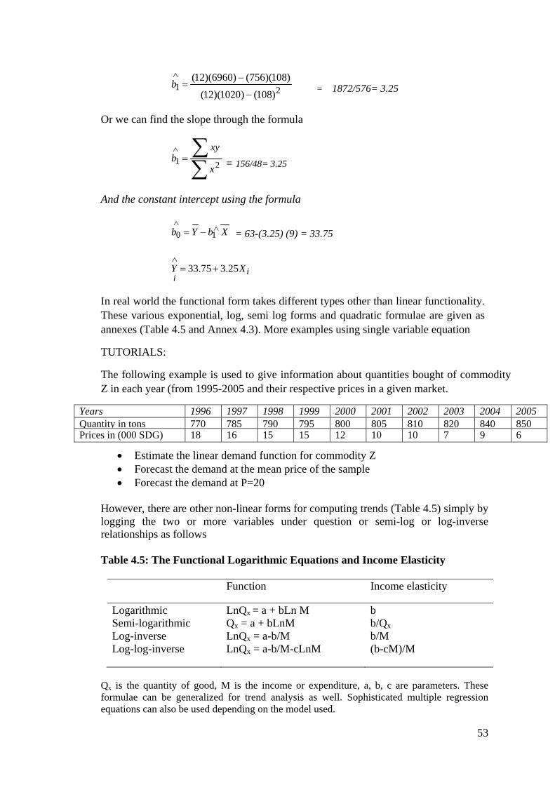
53

21)108()1020)(12(

)108)(756()6960)(12(

−

−=

∧b = 1872/576= 3.25

Or we can find the slope through the formula

∑∑

=∧

21x

xyb = 156/48= 3.25

And the constant intercept using the formula

XbYb ∧∧

−= 10 = 63-(3.25) (9) = 33.75

ii

XY 25.375.33 +=∧

In real world the functional form takes different types other than linear functionality. These various exponential, log, semi log forms and quadratic formulae are given as annexes (Table 4.5 and Annex 4.3). More examples using single variable equation

TUTORIALS:

The following example is used to give information about quantities bought of commodity Z in each year (from 1995-2005 and their respective prices in a given market.

Years 1996 1997 1998 1999 2000 2001 2002 2003 2004 2005 Quantity in tons 770 785 790 795 800 805 810 820 840 850Prices in (000 SDG) 18 16 15 15 12 10 10 7 9 6

• Estimate the linear demand function for commodity Z • Forecast the demand at the mean price of the sample • Forecast the demand at P=20

However, there are other non-linear forms for computing trends (Table 4.5) simply by logging the two or more variables under question or semi-log or log-inverse relationships as follows Table 4.5: The Functional Logarithmic Equations and Income Elasticity

Function Income elasticity

Logarithmic Semi-logarithmic Log-inverse Log-log-inverse

LnQx = a + bLn M Qx = a + bLnM LnQx = a-b/M LnQx = a-b/M-cLnM

b b/Qx b/M (b-cM)/M

Qx is the quantity of good, M is the income or expenditure, a, b, c are parameters. These formulae can be generalized for trend analysis as well. Sophisticated multiple regression equations can also be used depending on the model used.

54

ii) Freehand Method

This method uses individual’s hand to draw the fit line or curve by selecting pairs of corresponding data of x and y variables and plot them graphically along the x and y axis.

iii) The Moving Average Method and the Method of Semi Averages Moving Average Method and the Method of Semi Averages are useful in computing trends. Both methods have been intensively covered where appropriate in filling missing values or data.

4.2 Qualitative Analysis of Impact Despite the complexities involved in qualitative analysis with respect to market prices and food security analysis, nevertheless the analyst should be able to foresee (forecast) how could prices change and the impact of such changes on household food access for different population groups (WFP, 2007). However, when dealing with price impact analysis we are primarily concerned with “market dependent” households and the commodities which they purchase. In context of States like Darfur and some civil unrest areas, for instance, market analysis -as part of a food security assessment- is important in providing knowledge on the degree and extent of interventions needed in terms of:

• Appropriate response option; • Size and type of intervention; • Potential negative effects of food aid; • Targeting strategies; and • Opportunities for local procurement (WFP, 2007).

Besides above information, food security analysts in Darfur and or any other conflict affected areas should be aware that the overall market analysis done by them should provide the following information which can help in decision making for any immediate or future interventions. In this connection, we should describe:

• How domestic markets are affected by conflicts and how well they are functioning and the limitations associated with their performance;

• Whether food availability and access in different areas around these markets is affected and in what sense;

• The extent to which markets will be able to provide food at affordable prices for populations in the affected areas;

• Opportunities that might exist to increase the contribution of markets to making adequate food available to food-insecure households in the affected areas;

• How labour markets function and their contributions to household food access; and the potential for local purchase and what effects such purchases might have on local markets (For more information see WFP, 2007 and FEWS NET, 2009-c).

55

In food security analysis, we need to be able to judge on the consequences of a change in prices for different types of household (Better-off, Middle Income and Poor) (or producers, urbanites, traders, etc. (Table 4.6 & 4.7)). Over and above, we need to know what people produce and purchase and consume. In this respect, qualitative impact analysis can help us to identify the direction of the impact (whether it makes households better off or worse off). Therefore, the impact assessment should involve identification of who loses and who gains from a price change. Consumers will generally gain from decreases in consumer (retail) prices while farmers (or producers in general) will generally benefit from increases in farm-gate or producer prices. In Price changes may have an impact on income (from sales of produce or of labour), on production levels or labour supply, and on consumption of purchased food commodities. Table 4.6: Example of a Price Impact Matrix for Selected Household Groups Group classification

Commodity Impact of Price ChangeIncrease Decrease

Gum Arabic growers who purchase sorghum Gum Arabic +ve -ve Gum Arabic growers who purchase sorghum Sorghum -ve +ve Millet producers/sorghum purchasers Sorghum -ve +ve Millet producers/sorghum purchasers Millet +ve -ve Livestock producers, wheat purchasers Wheat -ve +ve Livestock producers, wheat purchasers Livestock +ve -ve Table 4.7: The Impact of Simultaneous Price Changes Sorghum price

Millet price change Increase Decrease

Increase ? (uncertain/unclear) Gain (clear/certain) Decrease Loss (unambiguous/certain) ? (unclear/ambiguous)

4.3 Relative Price Relationships – TOT and International/Domestic Price Comparisons (The Role of External Trade)

In this section, we shall overview relative price relationships and explain how international/domestic price comparisons could be made by using the so called Terms of Trade (ToT). The definition of the Terms of Trade is that, it is the rate at which one good or service can be exchanged for another and is typically expressed as a ratio. Nationally, the Terms of Trade is expressed generally as the ratio of a nation's export prices to its import prices, more likely, a measure of the country's trading position. At the household level, ToT is defined as the ratio of two prices, for example, the ratio of the price of livestock to the price of a food staple, the ratio of the cash crop price to the price of a food staple, or the ratio of daily wage for unskilled labour to the price of a food staple (WFP, 2007).

56

a) Terms of Trade (TOT) over Livestock and Livestock Products

A complete measure of TOT is the rate at which one good or service can be exchanged for another and is typically expressed as a ratio. In this sense, the price ratio of two commodities can express the meaning of terms of trade. The “terms of trade” indicates how many units of one commodity can be exchanged for a unit of another commodity. It is generally defined as the price ratio of the two commodities. E.g. if a goat is exchanged for millet, how much millet the goat herder receives is determined by their relative prices: the price of goat over the price of millet. For example pastoralists during the dry season usually tend to exchange some items they have with other items which they do not have. In this way, this “terms of trade” can help to measure the purchasing power of pastoralists (Ibid, 2007). During the dry season, they typically shift their consumption from livestock products to cereals and exchange (sell) their animals in order to purchase cereal. At this time, as the number of animals offered is high and the demand for cereal expands, prices of livestock tend to fall and prices of cereals tend to rise. Important to have in mind is that, the TOT equals the price of staple crops in the area/the price of dominantly traded animal due to problem of data availability in measuring weights for livestock. Hence, before concluding on the food security situation in the pastoral areas, it is necessary to look at the relative value of a single animal to their staple crops. In general, the food consumption of pastoral groups is a positive function of income (as income increases, so does demand for food) and a negative function of food prices.

b) Relative Value of Imported Foods The relative value of imported food (whether food aid or usual purchases) is computed by comparing the value of the imported commodity with the wholesale price of the same commodity in a specific area. To do these comparisons, the import parity price and wholesale price at the destination point should be known. The IPP is useful in measuring incentives and disincentives for agricultural production, in a competitive international trade environment. In addition, the parity prices help in identifying the food security situation by analyzing the food security dynamics in a location. Besides detecting unfair commodity pricing, the IPP can also be used to measure the incentives and disincentives of moving commodities from one location to another specifically across borders (FEWS NET, 2008). Box 4.2: What is the Import Parity Price (IPP)

Import parity price (IPP) – is the monetary value of a unit of product bought from a foreign country, valued at a geographic location of interest in the importing country. In literal terms, the term parity price means equal or equivalent price that is, making the price of particular commodity equal or equivalent to a reference price of same commodity in another location (FEWS NET, 2008). For instance, making the price of a ton of wheat in Egypt equal to a price of a ton of wheat in Sudan

The IPP is important in Domestic Resource Costs analysis (DRC).

57

However, a free market transaction is required where the role of the private market in external trade, could be more efficient in trade. Usually when external trade is working efficiently, we can say that domestic market are integrated with the world market and that world market prices can be transmitted to domestic markets. However, food security analysts should look at border price movements as a regular part of monitoring and for understanding the domestic prices behaviour. In computing Import Parity Prices (IPP) for commercial imports we identify all cost components for the commodity free on board of exporting country, then we add all additional costs incurred as ocean freight, insurance to Port Sudan (Annex 4.4). The costs incurred at Port Sudan also involve Port handling charges, loading/ unloading costs, transport costs from Port Sudan to the destination point (e.g. Khartoum) in addition to custom duty (15%), and value added taxes and profit margins by wholesalers (Annex 4.4). Same procedure applied here for imparity prices for inputs can also be applied for food items. When using import parity prices for food we should compare between the import parity price and wholesale price at destination point to conclude whether decision to be made is to import from outside or purchase from local markets, particularly in relief situations. It often happen that price of sorghum imported as food aid costs more than if purchased from local markets. However, donors sometimes insist on importing from outside the country, for political reasons or to get rid of stocks, despite the IPP differences. Problems of food aid donations are many including provision of inappropriate kind of food aid and also mis-targeting which result in benefiting the unintended people in the country. If such cases persist in the country we should provide the food to the people and do not contradict with their consumption pattern, providing the food aid in flour type (wheat or sorghum) to reduce the possibility of reselling. However, existing wheat food aid to the urban areas should be monetized and targeting guidelines for pastoral areas should well be designed including free cash provisions to people.

4.4 Surplus and Deficit Markets

In ordinary cases, food commodities usually flow from surplus to deficit areas and similarly imports usually flow from ports and borders into the hinterland for price differences. Conversely, commodities flow between markets if the price differential is greater than the transaction costs that would be involved in addition to a reasonable profit margin. This price differences is essential in understanding and forecasting food prices and the flows of commodities within the country and across its borders, and therefore to projecting both food availability and access. High prices in deficit areas usually provide incentive to traders to bring food from surplus to deficit areas, thus making food available. In emergency situation market interactions are surely different, and many aspects are to be minded. Planning for an emergency response depends on an understanding of the nature of food markets. This is because, and sometimes, not a question of food availability deficit, but rather a matter of market failure or policy/political failure that aggravate the food insecurity problem. If there is a real food deficit, the gap can be bridged either from local purchases or food aid donations. Local purchases can be an extremely cost-effective method for procuring food for emergency interventions than

58

imports. It also carries high risk of disturbing markets. For this reason, emergency planners need to know which areas are deficit areas and which are in surplus by looking at:

Traditionally surplus areas Exceptionally surplus areas Traditionally deficit areas Exceptionally deficit area, and The methods of Identifying surplus/deficit areas:

– By comparing the level of prices of the same commodities or indices across markets and/or assessing the grain flow.

– Using the food balance approach. However, and before going into in-depth food security analysis, analysts should clarify the following inquiries (WFP, 2007) with respect to emergency issues:

• changes in the direction and volume of commodity flows between regions, comparing the present with previous years;

• potential and/or actual movement of food from surplus to deficit areas; • quantity of stocks held by parastatal organizations, wholesalers and

producers; • identify if hoarding is an issue for the area

As a matter of fact, the existence of a deficit is not itself a sign that there is a need for food assistance. Similarly, the existence of a local surplus does not necessarily mean local purchase capacity.

4.5 How Food Markets Work – An Introduction

Food markets usually work more efficiently when market infrastructures (transportation and storage facilities) are adequately available. The exchange of goods and services in these markets is thus performed through trading. Thus trading has three main roles:

• Transportation of commodities between locations (or spatial arbitrage). For instance, wide geographical distribution and spatially separated markets over the entire Sudan. Marketing of supply inputs, production output and distribution of processed products could really be a problem for the wide geographical distribution of farms, markets and urban consumption centres. Poor roads infrastructure has contributed to the isolation of markets (hindering market integration) and this is further aggravated by the very weak information and poor communication, information and management systems and other infrastructural problems in most of the productive areas.

• Storage of commodities over time. This is called temporal arbitrage .For instance, most of consumers usually purchase small amounts spread evenly over the entire year due to poor capacity to purchase sufficient amounts at the beginning of the harvest season. This makes an over-flood of supply by large number of farmers (to recover some of their loans debts and costs) to be faced by a limited amount of consumers buying little amounts. The absence of stock

59

reserves policy aggravates the problem of sellers incurring serious losses at the beginning of every supply season. • Trade in commodities between countries (international trading)

If the trade is performing these roles well, the results are likely to be more stable and “well behaved” prices. Stable prices are an advantage to both producers and consumers for:

→ They help people to plan and mean that unexpected and damaging price rises or falls can be avoided.

→ They tend to be more stable and less prone to large and sustained price rises because of local falls in supply. Conversely, if markets are not working well, they are likely to be less stable.

The concept of efficiency18underlies most modern economic analysis. The prices paid by consumers for commodities reflect the cost of production, processing and trading of those commodities. In this respect, market performance refers to the extent to which markets or traders do things that society expects. In affirmative words, do they operate efficiently, provide a reliable source of food, supply food at reasonable prices, etc.

4.5.1 Inter – Form Price Differences

Price changes are important parameters to understanding food security impacts on population groups in a given livelihood context (WFP, 2007). The inter-form price difference analysis refers to the analysis done between the raw and processed agricultural commodities. When a commodity is transformed or processed into usable for (sorghum into Kisra) the prices of the latter is different from the former by value addition of extra labour. This also true when animals are processed in El Kadaru and shipped on to the rich Arab or Gulf States. Similarly, when the price of one commodity rises, consumers or agro-processors will decrease their consumption of it and increase consumption of the substitute commodity. Wild and gathered products can be substitutes for preferred staples of food insecure households, especially in times of stress or increasing food insecurity. In this regard food security analysts should take into consideration that high volatility and shocks related to price changes in the agricultural products shows the susceptibility of farmers for their produce. However, prices of processed goods (e.g., Kisra, any kind of sauce, meat, etc.) in urban areas are always much higher than prices in agricultural commodities. However, prices may not reflect the processing costs incurred on agricultural commodities.

4.5.2 Assessing Market Integration - Inter-Spatial Price Variation – Correlation

The definition of correlation, which measures the magnitude and direction of relationship between two variables –systematic interrelationship between variables–

18 Exchange efficiency (Pareto-optimality) refers to a situation in which all benefits from trade have been exhausted and it is not possible to do further exchange without reducing the benefits of another agent.

60

has already been explained in previous sections. This includes the bivariate (Two variables) correlation or regression coefficients which estimate the time series projections/extrapolation of spot wholesale or retail market prices for identical goods at different locations. The sections have also given formulae for multiple variables correlated with respect to a given dependent parameter. In our market analysis, high levels of correlation between prices in different markets may indicate effective integration and/or competition and economic efficiency, or monopoly conditions. For instance, a coefficient of 1 indicates identical price movements in two markets, but this never obtained in reality due to imperfect resource mobility, resulting from transport, storage and/or processing costs; imperfect information, and in some cases, product differentiation. Well-integrated markets tend to be characterized by more stable prices and price hikes and dips last for a short time (the time it takes for traders to respond). Some hints on market integration are given in details.

a) Market Integration Market integration, as has been mentioned above, is a measure of the extent to which markets in different areas are linked. Integrated markets can be defined as markets in which prices for comparable goods do not behave independently in two or more different locations separated by distance (WFP, 2007). The following remarks are important to understand the concept of market integration:

• When markets are integrated, commodities flow between them is easier if the price differential is greater than the transaction costs that would be involved and there is, in addition, a reasonable profit margin,

• In integrated markets, price differentials are closely related to the transaction costs and price movements follow similar patterns – there is “co-movement”,

• Markets are not integrated if they are effectively isolated from each other, and or there is no flow of commodities between them and prices move independently of the differences in transaction costs.

Understanding whether markets are well integrated within the country or with markets across a border in neighbouring countries is critical to understanding and forecasting food prices. Not only this but also the flows of commodities within the country and across its borders, and therefore help projecting both food availability and access. If markets are integrated, food will flow from surplus to deficit areas - and imports will flow from ports and border areas into the hinterland. High prices in deficit areas provide the incentive to traders to bring food from surplus to deficit areas, making food available. The consideration of market integration is crucial in an EFSA analysis as it provides a platform for understanding the extent of commodity flows between places (regions) and price differences between them (see the 2007 FAO/WFP Crop Assessment Missions).

The result of market failure in the transport market is market segmentation -as opposed to market integration- when prices and market conditions are not strongly related between markets. Market segmentation is generally harmful to both producers and consumers and certainly increases the chances serious market inefficiencies.

61

As shown in Table 4.9, the correlation between market prices shows that price changes for sorghum in Khartoum is significantly correlated with price changes in other surplus markets. Unlike expected millet market in Khartoum shows a sort of market segmentation with respect to ElObeid, Damazin and Gedaref markets as reflected by the poor correlation coefficients (Table 4.9). For wheat market, ElObeid and Khartoum show poor correlation indicating market segmentation. However, there exists good market integration for wheat between Dongla and Khartoum markets. Hence, one can conclude that, any policy change introduced in the Khartoum market may well be reflected in terms of price changes in all the surplus and deficit markets of the country over time. However, price correlations alone cannot be used as definitive indicators of market performance, and corroborative evidence is required to explain the resulting correlation characteristics. Table 4.8: Coefficient of Correlation between Monthly Bivariate Results between

Main Wholesale Markets during the Period January, 2001 through May, 2010.

Markets Time Covered Crops Correl. Sig. (n) ElObeid-Khartoum Jan2001-May-2010 Sorghum 0.970 Yes 112 Gedaref-Khartoum Jan2001-May-2010 Sorghum 0.975 Yes 112 Damazin-Khartoum

Jan-2004-May-2010 Sorghum 0.955 Yes 77

El Obeid-Khartoum

May 2009-May 2010

Millet 0.294 No 13

Damazin-Khartoum

May 2009-May 2010

Millet 0.165 No 13

Gedaref-Khartoum May 2009-May 2010

Millet 0.196 No 13

Khartoum-ElObeid May 2009-May 2010

Wheat 0.121 No 13

Dongla-Khartoum May 2009-May 2010

Wheat 0.875 Yes 13

Dongla-ElObeid May 2009-May 2010

Wheat 0.22 No 13

Source: Based on data from MoAF, SIFSIA N. 4.5.3 Gross Market Margins and Cereal Price Spreads

Marketing margin is typically defined as the difference between the price paid by consumers and that obtained by producers. It is also called the farm‐retail price spread. Margins can be calculated all along the market chain and each margin reflects the value added at that level of the market chain (FEWS NET 2009-b). The aim of the marketing margin analysis is to show the relative importance of the marketing costs in order to reveal real differences between and among markets (inter-market variations) for further market integration. The target remains the producer’s share that revolves and gears up the production and marketing mechanisms for the achievement of food security and social welfare objectives (Ismail, 2004). The usual procedure for determining the marketing margins and producer’s share in the market value for the selected crops is made by running marketing costs and margin analysis (Ibid, 2004).

62

a) Gross Market Margins Market margins are the difference between prices at two market levels. Margins represent the price charged for one or a collection of marketing services. For example, the difference between producer and consumer prices is the amount charged for all the marketing services rendered between production and consumption, including buying, bulking, transports, storage, processing, etc. This may help in designing, for instance, a local purchase programs intended to raise producer prices through purchasing grain from wholesalers – timing is critical here – purchasing at harvest time will have a significant impact on producers and vice-versa.

i) Marketing Costs and Margins: An Overview Generally, marketing costs can be differentiated into three distinct types of costs a) direct costs that involve direct marketing functions and services viz. transportation and assembly costs, handling costs (loading, unloading, repackaging, etc), processing and storage costs as well as taxes, levies, customs and duties. b) The operating costs which include the opportunity cost of the tied-up capital (taken as a 10-14%19 annual profits (Ismail, 2004)), and c) physical losses arising from transportation, storage loss or processing (in value terms) as a percentage of the initial market crop value (MoAF, 1988). Net margins (NM) are usually obtained by subtracting the initial buying prices (BP) and the other marketing costs (MC) from the selling price (SP), thus,

NM = SP-BP- MC, The gross margin (GM) is simply the difference between the buying and the selling prices. The GM is composed of two cost items, namely the marketing costs (MC) and the net margin (NM). The gross margin for the entire marketing system is the difference between the farm price (FP) and the retail price (RP) or the FOB prices in case for exports commodities. The systems gross margins is thus,

SGM = RP – FP, or SGM = FOB price – FP

ii) Marketing Costs and Margins: Example of Cereals -Sorghum An example for analysis of marketing costs and margins for sorghum, which relate to season 2003-2004, is taken from Ismail (2004), and prices are converted to current SDG for reader’s convenience. Sorghum is the major staple food crop in the Sudan. It is mainly utilized as a pancake in rural areas with numerous sorghum varieties20 under different local names21. Production areas are mainly the traditional and the

19 These figures are considered satisfactory as it fall within the limits determined by the Central Bank. 20 Various varieties with different price levels are available in the Sudan, but the most popular one is “Feterita”. "Tabat" is the next popular sorghum variety grown in irrigated as well as in rain fed agriculture. Except for prices, the marketing costs for all varieties are almost the same. 21 “Zunary” and “Marig” are common names for sorghum varieties in greater Kordofan. The term “Rayka” is used to denote a sack in Kordofan and some other states (Ismail, 2004).

63

mechanized rain fed areas, Gezira scheme as well as some pockets in other irrigated schemes. The gross margin for the entire marketing system, which is the difference between the farm price (FP) and the retail price (RP), is shown in terms of percentage (Table 4.10). Profit margins in contrast to each market level purchase prices and the entire market system share are also computed and presented in the given table. The producer’s share in market value of sorghum crop is found to be 54.9% in Gedaref (Table 4.10). However, this value was found 32.7% and 80% in Kordofan and Gezira respectively at that time. The drastic variations in Gedaref and Kordofan were due to the fact that farmers become in bad need for cash at the beginning of the harvest season that compel/force them to sell at very low prices. It is clear that, merchant traders (from wholesalers to retailers) harvest the biggest fruits share of agriculture as compared to producers. Table 4.9: Summary of Marketing Costs and Margins (SD) for Sorghum in

Gedaref State Market level Purchase

price SDG/ sack (1)

Sell price SDG/ sack (2)

profit margins% as to purchase price (3)

% Share as to Producers Price (4)

% of marketing costs (5)

Farm gate* 15.31 18.50 20.8% Village market 19.80 22.00 11.1% 18.9% 7.03% Intermed. /rural 23.18 25.63 10.6% 19.6% 6.4% Central market 27.15 28.42 4.7% 15.1% 8.2% Wholesaler 27.95 30.05 7.5% 8.8% -2.5% Retailer 24.35 26.85 10.3% -17.3% -30.8% Entire systems share %

45.1%

Sorghum Feterita. Unit of measurement is 90 Kg. Sack At the farm gate the purchase price is replaced by the production costs to give the producers minimum margin. Source: Ismail field survey data, July 2004.

Table 4.10 shows a producer’s profit margin of 20.8% in contrast to his production cost in Gedaref state. Figures show the producer’s profit margin (Table 4.10) as well as the producer share in the entire market system. Market levels are presented in a chronological and sequential order, although trading of commodities might or might not be sequential in all cases and for all marketing chains. The figures tell that, the retailer can purchase directly from village marketers and/or intermediate markets rather than from central or wholesale markets where prices in the former were less. The latter central and wholesale markets might provide other distant markets in the country than the nearby markets under question. The sum up of percentages of market shares at all levels does not necessarily equal to the entire market system shares, if marketing channels are not cardinally sequential. However, differences in prices among these retail markets, which are quite considerable, might be due to variety differences among Feterita types; but it might also reflect a sort of

64

market disintegration or market segmentation. It was observed that, some Ethiopian traders have access to Gedaref crop markets, and farmers claim that they were exempted from Zakat charges. If these claims were true, this would negatively affect the trading transactions if they decided to resell in domestic the markets22; and gain the Zakat margin difference as a profit. Despite the apparent variation in prices of sorghum, yet, and as a general rule, the marketing costs for this crop were moderately stable as compared to commodity prices at that time.

iii) Marketing Costs and Margins: Example of Livestock Export - Camels Another example for computing the marketing costs and margins for livestock (camels) is given for clarity. Although data relate to 2003 (Ismail, 2003), yet it gives an indication of various cost components involved in exports of livestock (table 4.11). The table gives an overview of all transaction costs and their respective percentages. The entire system gross margin and costs of camel trade from producers to consumers at Egyptian markets amounted to almost 37% of the producer’s value. This amount reaches 20.1% when compared to consumer’s price. Thus, the producers’ market share in the consumers’ price amount to almost 63%.

Table 4.10: The Various Marketing Costs and Margins for Camels’ Exports (SDG)

Cost items in SDG Marketing margins and costs in SDG

%Share as to producer’s price

%Share as to consumer’s price

Price per camel (SD per unit) 736.00 Locality fees and charges 18.50 2.513587 1.711378Guarantee charges 2.00 0.271739 0.185014Shepherd keeper fees 3.00 0.407609 0.277521Transportation fees to Kassala 3.00 0.407609 0.277521Local taxes at kassala 3.00 0.407609 0.277521ZAKAT& Export tax 65.00 8.831522 6.012951Export commission 25.00 3.396739 2.312673Subtotal (SUDAN) 119.50 16.23641 8.836143 Egyptian tax 7.20 0.978261 0.66605Quarantine charges (in Shalatine) 43.90 5.964674 4.061055Purchase charges and transportation fees 86.40 11.73913 7.992599Purchase commission 14.40 1.956522 1.3321Subtotal (EGYPT) 151.90 20.63859 11.23188 Grand total 271.40 36.875 20.068 Market prices are converted to SDGs for reader’s convenience. Source: Ismail, 2003.

b) Cereal Price Spreads

22 Potential rural markets in Gedaref are: Um Kharayeet, Doka, Gizoli, Mahalla, Kassab, Gurisha, Hawata, Heimura, Hilat Hakoma, Galaa Alnahal, Mafaza, Shwak and Teneidba (Ismail, 2003).

65

Price spread is affected by many factors particularly those which add significantly to marketing margins as transport, storage and value addition by processing. For instance, fuel and transport costs are included in the marketing margin or price spread and often account for a considerable percentage of the final price of a commodity. The increase in fuel prices may hinder transport and the movement of supply in substantial ways (FEWS NET, 2009-b).

A recent example of price spread is given in this section. These price spreads, which are computed as the difference between wholesale prices between two (producer (e.g. in Gedaref) and consumer (e.g. in Khartoum)) markets are illustrated in Table 4.12. In equation form, marketing margins or price spread = (selling price – buying price). To know the relative importance of the spread, spreads are computed as a percentage of the wholesale prices of the destination market. Worth to note is that, price spread percentages are so high during the (January, 2007 to June, 2008). In most cases, the spread is so high that it cannot easily be explained by the transportation cost, transaction costs and profit margins of the two markets (E.g. Gedaref vs. Khartoum). This may indicate the inefficiency of the marketing system. Hence, special emphasis should be given to analyzing the causes for the big transaction cost differences in these markets (Table 4.12). Surprisingly millet markets suffer from market segmentation as retailers incur huge losses in El Fasher and El Obeid markets. In this case, the major goal of grain marketing policy should be to reduce costs in the grain marketing system and pass these cost savings onward to producers and consumers, thereby stimulating technology adoption incentives, farm productivity growth, and access to food by low-income consumers. Table 4.11: % of Wholesale Prices Spreads over Destination Markets from

June 2007-June 2008.

Markets Commodity Time span Highest Difference* Price SDG/ton

Lowest Difference* SDG/ton

Gedaref Khartoum Sorghum Jan-2007-June 2008

613.3 (53.0) 304.7 (31.1)

Damazin Khartoum Sorghum Jan-2007-June 2008

454.0 (41.6) 174.7 (20.7)

El Fasher El Fasher Millet Jan-2007-June 2008

205.7 (24.5) -190.3 (-25.0)

ElObeid ElObeid Millet Jan-2007-June 2008

370.0 (36.5) -29.0 (-3.2)

Khartoum Khartoum Wheat Jan-2007-June 2008

684.3 (34.8) 168.3 (14.4)

*Highest and lowest price differences are taken for three months P.S means Price Spread Figure in parenthesis indicate (%) Source: MoAF, 2010.

66

REFERENCES Boone, L. E and Kurtz, D. L. (1977)

Contemporary Marketing. 2nd edition published by The Dryden Press. Hinsdale, Illinois.

Cloudius, Robert L. and Mueller, Willard F. (1961) Market structure Analysis as an orientation for research in agricultural economics. In: Journal of Fram Economics, Vol 17 No. 3 p 513-553.

Dembele, N. N., Staatz, J. M., and Adjao, R. (2008) Training Module for Analyzing Agricultural Prices. Training Workshop presented at Cotonou, 26-27 April 2008. Michigan State University, USA.

Enis, Ben M. (1980) Marketing Principles: 3rd edition. Goodyear publishing company, inc Santa Monica California 90401

El-Dukheri, Ibrahim (2007). Sudan Grain Market Study, Commissioned by WFP. Final Report (Draft), December 2007.

Faki et al, 2008. Determinants of Current Price Hikes and their Implications on the Poor and Assessing Short Run Policy and Program Response Options in Containing, Reversing and Mitigating their Negative Impacts In the 15 Northern States of Sudan. A comprehensive reported submitted to SIFSIA North programme, FAO, October, 2008. Fan, W., Geerts, F. and Jia, X. (2008)

A Revival of Integrity Constraints for Data Cleaning. University of Edinburgh 2Bell Laboratories. Internet source: wenfei@finf.ed.ac.uk, research.bell-labs.comg fgeerts@inf.ed.ac.uk xibei.jia@ed.ac.uk

FAO (1997) Implications of Economic policy for Food Security. A Training Manual prepared for the agricultural policy support service policy assistant division, Food and Agriculture Organization. Rome, and GTZ, 1997. Cited by Ismail, El Fadil. Ahmed. Agricultural Marketing in the Sudan: Current Situation and Future Prospects. Results and Findings. A Report submitted to FAO under TCP/SUD/2906 (A). “Strengthening the Institutional Capacity for Planning, Economic and Policy Analysis (PEPA) for the Agricultural Sector in the Sudan”. Khartoum, Sudan, 2004.

FAO ( 2000) Handbook for Defining and Setting up a Food Security Information and Early Warning System (FSIEWS). Food and Agriculture Organization of the United Nations, Rome 2000.Cited by Ismail, El Fadil. The Existing Food Security Information Systems in the Sudan and Institutional Capacities of System Providers and Users. A Report submitted to FAO under SIFSIS Primary Assessment Mission, 2005.

FAO, 2004 Helping Small Farmers Think About Better Growing and Marketing: A Reference Manual. FAO Pacific Farm Management and Marketing Series (3).FAO, 2004.

FAO (2008)

67

FAO’s Initiative on Soaring Food Prices. Guide for immediate country level action. Food And Agriculture Organization of the United Nations (Second draft), 10 May 2008

FAO-GTZ (undated) Marketing Financial Services – Operational Marketing 2: Pricing Policy. A Self Study Guide. Lesson 1-5.

Republic of Zambia (2004) Agricultural Marketing: What Is It. Steps Required to Successfully Market New Products. International Fund for Agricultural Development (IFAD) in collaboration with Food and Agriculture Organization of the United Nations, November, 2004.

FEWS NET (2008) Structure-Conduct-Performance and Food Security FEWS NET Markets Guidance, No 2 May 2008. FEWS NET Washington 1717 H St NW Washington DC 20006 info@fews.net

FEWS NET (2009-a) Adjusting Prices for Inflation and Creating Price Indices. FEWS NET Markets Guidance, No 3 May 2009. FEWS NET Washington 1717 H St NW Washington DC 20006 info@fews.net

FEWS NET (2009-b) Commodity Market Maps and Price Bulletins: Tools for Food Security Analysis and Reporting FEWS NET Markets Guidance, No 4. July 2009. FEWS NET Washington 1717 H St NW Washington DC 20006 info@fews.net

FEWS NET (2009-c) Terms of Trade and Food Security Analysis. FEWS NET Markets Guidance, No 5. October 2009. FEWS NET Washington 1717 H St NW Washington DC 20006 info@fews.net

Ismail, E.A. (1996) Spatial Organization of Food grain Storage Facilities in Sudan”. Published Ph. D. ISBN 3-86186-135-6. Publisher: Verlag Ulrich E. Grauer Stuttgart, Germany, 1996.

Ismail, E. A. (2003) Livestock Markets and Marketing Systems in Gedaref State. A published book by Khartoum University Press (KUP) 2003.

Ismail, E. A. (2004) Agricultural Marketing In the Sudan: Current Situation and Future Prospects. Results and Findings. A report submitted to FAO under TCP/SUD/2906 (A). “Strengthening the institutional capacity for planning, economic and policy analysis (PEPA) for the agricultural sector in the Sudan”. Khartoum, Sudan, (2004)

Ismail, E. A., (2008) Agricultural Finance in the Sudan: An Organizational Approach & Problem Conceptualization. Volume 91. 2007. In series of: FARMING & RURAL SYSTEMS ECONOMICS. ISBN 978-3-8236-1514-9 & ISSN 1616-9808 Margraf Publisher, Germany.

Ismail, E. A., (2009) A review on: Developments in sugar industry in Sudan: An analysis of the factors affecting sugar production, marketing and consumption (FRC- Journal of Food Science and Technology, No. 2, 2009)

68

Koutsoyiannis, A. (1977& 1972) Theory of Econometrics. 2nd edition. Macmillan Press. London , U.K. MoAF (1988)

Marketing Costs and Margins. Ministry of Agriculture and Natural Resources. Department of Agricultural Economics. The Planning and Agricultural Economics Marketing Section. Khartoum, October, 1988.

Sarhan, M. E. (1988) Seasonal Movements in Sudan’s Agricultural Commodity Prices and the Use of Seasonal Price Indices in Forecasting and Making Sell/Hold Decisions. Technical Support by ASP Project USAID/CHECCHI. Marketing Section. Department of Agricultural Economics and Planning and Agricultural Economics Administration. MoAF, 1988.

Spiegel, R. Murray (1972) Statistics SI metric edition. Schaum’s Outline Series. McGRAW-HILL, BOOK COMPANY.

Sudan Monthly Market Update (2008). Sudan Monthly Market Update Bulletin No. 3, March 2008. SIFSIA N (GNU), FAO-Sudan Khartoum.

Sudan Monthly Market Update (2009). Sudan Monthly Market Update Bulletin No. 21, September 2009. SIFSIA N (GNU), FAO-Sudan Khartoum.

Timmer, C. P., Falcon, W. P. and Pearson, S. R.(1983) Food Policy Analysis. A World Bank publication. John Hopkins University Press, 1983

WFP (2007) Market Analysis in Emergency Food Security Assessments. Guidelines on Market Situation Analysis & Forecast and Response Protocol. An Integral Component of Emergency Food Security Assessment (EFSA). Prepared by: Getachew Dirba, Senior Programme Adviser & Simon Renk, Programme Officer, ODAN Emergency Needs Assessment Service. United Nations World Food Programme, Rome, Italy, August 2007.

Wikipedia (2010) Definitions <<internet source>> www.wikipedia.com

69

ANNEXES Annex 1.1: Elements/Aspects of Food Security and Information Needed

(For more information see reference below)

Adapted from Handbook for Defining and Setting up a Food Security Information and Early Warning System (FSIEWS). Food and Agriculture Organization of the United Nations, Rome 2000.

1.1.1.1.1.1.1.1 Food availability Agro climatic conditions, status of pasture, status of crop and water availability, stable food production in

1.1.1.1.1.1.1.1.1 Food Access Effects of conflicts and tension (vulnerability), population movements and implications, quantity and seasonality of access to food from own crop production, livestock production and sale, wild food, purchase, gifts and

1.1.1.1.1.1.1.1.2 Food Utilization Health information

1.1.1.1.1.1.1.1.4 Stability of food supply Seasonality, climate change, environmental degradation, changes in funding and opportunities for both local purchases and food aid imports, infrastructure (viz. roads, logistics, markets, staple foods marketing, shortages, prices, seasonality dimension, trading system capacity, implementing capacity of humanitarian

Food security

information system

70

Annex 4.1: Example of Worksheet for the Calculation of Seasonal Price Index Using The 12-Month Moving Average Method

col. 1 col. 2 col. 3 col. 4 Column. 5

year month

price SDG/sack

12-month moving avg

2-month moving avg

col.3/24

col.1/col.4

2001 J 63.9 F 59.1 M 58.0 A 56.8 M 55.2 J 50.3 611.28 J 54.9 581.13 1192.41 49.684 1.105 A 55.3 555.40 1136.53 47.356 1.168 S 46.6 531.24 1086.64 45.277 1.0295 O 38.1 505.97 1037.21 43.217 0.881 N 36.3 482.27 988.24 41.177 0.881 D 37.0 463.61 945.88 39.412 0.938

2002 J 33.8 441.21 904.82 37.701 0.895 F 33.3 419.41 860.62 35.860 0.930 M 33.8 406.30 825.71 34.405 0.984 A 31.5 402.22 808.52 33.688 0.935 M 31.5 J 31.6 J 32.5 A 33.5 S 33.5 O 34.0 N 33.0 D 39.4

Source: data from MoAF, SIFSIA N

71

Annex 4.2: Crop Calendar and Relation to Food Security Analysis

Source: Sudan Monthly Market Update. Bulletin No. 21, September 2009. SIFSIA N (GNU), FAO-Sudan Khartoum.

72

Annex 4.3: Most Commonly Used Functional Forms to Evaluate Trends

Source: Ezekiel and Fox (1959) cited by Dembele (2008)

73

Annex 4.4: Practical Example of Import Parity Price

Source: Sudan Monthly Market Update Bulletin No. 3, March 2008. SIFSIA N (GNU), FAO-Sudan Khartoum.

74

Annex 1: Typical Market Indicators (FEWS NET learnernotes0417) 

Indicator Updated regularly or Monitored

Updated infrequently/ Knowledge Base

Macro or National Level Indicators Macroeconomic

Inflation (rate) X

Consumer price index X Exchange rate X Minimum wage ($/hr or day) X Key policies Export/import bans X Import/export quotas X Import/export taxes on key

commodities (percent) X

Price controls (yes/no and $/unit) X Import/export policies of neighbouring

countries X

Availability/ Supply

Cereal imports (total metric tons and by cereal)

X

Cereal exports (total metric tons and by cereal)

X

Cereal production (total metric tons and by cereal)

X

Public cereal stocks (metric tons) X Commercial stocks (metric tons) X Consumption requirements (metric

tons) X

Import parity prices X Export parity prices X Supply elasticity X Demand elasticity X Meso/Local/Subregional Level Indicators Local markets Informal cross border flows (total

metric tons and by cereal) X

Farmgate prices for key commodities ($/unit)

X

Wholesale prices for key commodities ($/unit)

X

Retail prices for cereals ($/unit) X Transport costs (selected routes) -

different seasons X X

Road conditions – different seasons X Distance/time between markets,

catchment areas (km and hrs) X

Price of fuel ($/unit) X Informal fees (approximate amount) X

75

Public and commercial stocks (metric tons)

X

Storage costs ($/bag or metric ton) X Casual labour wage rate ($/day or hr) X Livestock prices ($/herd by species and

type: bull, cow, etc) X

Basic input prices, e.g., fertilizer ($/unit or ha)

X

Supply elasticity X Demand elasticity X Market Structure – Conduct – Performance Indicators Structure Number and type of sellers and buyers

in market X X

% of volume traded by largest market participants

X

Cereal storage capacity (metric tons) X Veterinary services (yes/no, fees) X Access to credit/financing (yes/no,

interest rate) X

Market associations (yes/no) X Conduct Key catchment areas X Alternative catchment areas X Market participant price expectations

($/unit at x time) X

Market participant margin expectations (at x time)

X

Commercial stocking (metric tons) X Large buyer purchasing plans (kgs/

metric tons and when) X X

Government purchasing and selling plans (kgs/MT and when)

Performance Consumer prices for key commodities ($/unit)

X

Wholesale prices for key commodities ($/unit)

X

Farmgate prices for key commodities ($/unit)

X

Terms of trade ($ animal/$grain) X Margins and distribution shares (%

share to participants) X X

Seasonality of supply (annual variation)

X

Seasonal variation in prices of key commodities (maximum difference, coefficient of variation)

X X

Seasonal variation in supplies of key commodities

X

Commodity quality measures X X Spatial distribution of key commodities X X

76

Seasonal variation in terms of trade (maximum difference, coefficient of variation)

X

Market Center Food Security Proxies Indicators Signs of distress

Distress sellers – ethnic/wealth group, origin, gender

X

Number and type of distress sellers X Number and type of buyers X Indicator animals – number of breeders X Variety of commodities for sale X Quality of commodities sold X Size of transactions (kgs/MT/numbers) X

77

Annex 2: Market Related Policy Questions (FEWS NET learnernotes0417) 

In your assessment, you should account for constraints and opportunities that arise as a result of policies, regulations or programmes within the country and across relevant

borders.

Market Related Policy Questions R*

Are there government controlled commodity purchase or sales prices?

Are there import or export restrictions – taxes, bans, quotas?

Are there licensing requirements or fees for engaging in trade?

Are there import or export restrictions in neighbouring countries?

Is there food distribution?

What is the rate of inflation?

What is the exchange rate policy?

Other: R

Other: R

Other: R

*R = relevant to the commodity market.

Annex 3: Policy impacts on markets and population (FEWS NET  learnernotes0417) 

Limit the inventory to the most important policies otherwise the exercise becomes too long and matrix of impacts too complicated.

78

Policy Possible Impacts on Markets Possible Impacts on

Population Import restrictions Reduced supplies, slower and more

limited response, possible smuggling and associated increased costs of trade

Reduced availability, higher prices, smuggling tends to push up prices

Price ceilings on food items

Reduced returns, lower supply Reduced availability, lower prices

Grain reserves Good management leads to more stable supplies; Poor management leads to greater uncertainly and volatile market conditions for traders

Good management leads to more stable supplies with lower and more stable prices; Poor management leads to more erratic supplies and prices

Taxes along the market chain

Depending on elasticity, higher costs of trade and reduced supply

Depending on elasticity, higher prices and less availability

Export ban Reduced market outlets, increased stocks, lower returns

Increased availability, reduced prices

Export ban in neighbouring country

Reduced formal and informal flows into country, reduced supply, slower and insufficient response, possible smuggling and associated increased costs of trade

Reduced availability, higher prices, smuggling tends to push up prices

Import ban in neighbouring country

Reduced market opportunities, lower returns and reduced incomes, more local supplies

Increased or excess availability, reduced access for those whose income is dependent on exports, lower prices

Support prices for producers

Increased production and supply (sometimes a draw for cross border flows)

Better prices for producers, higher prices for consumers, tighter margins for traders

Subsidies to input imports

Increased production Increased availability and lower prices

Food aid distribution

Depending on elasticity, decreased demand for commodities, lower returns, less supply response

Increased availability, decreased prices

Cash transfers Depending on elasticity, increased demand for food; higher returns; greater supply response.

Depending on elasticity, increased access to food; depending on elasticity, increased availability and lower prices

79

Annex 3: Policy impacts on markets and population (FEWS NET  learnernotes0417) 

Limit the inventory to the most important policies otherwise the exercise becomes too long and matrix of impacts too complicated.  

Policy Possible Impacts on Markets Possible Impacts on Population

Import restrictions Reduced supplies, slower and more limited response, possible smuggling and associated increased costs of trade

Reduced availability, higher prices, smuggling tends to push up prices

Price ceilings on food items

Reduced returns, lower supply Reduced availability, lower prices

Grain reserves Good management leads to more stable supplies; Poor management leads to greater uncertainly and volatile market conditions for traders

Good management leads to more stable supplies with lower and more stable prices; Poor management leads to more erratic supplies and prices

Taxes along the market chain

Depending on elasticity, higher costs of trade and reduced supply

Depending on elasticity, higher prices and less availability

Export ban Reduced market outlets, increased stocks, lower returns

Increased availability, reduced prices

Export ban in neighbouring country

Reduced formal and informal flows into country, reduced supply, slower and insufficient response, possible smuggling and associated increased costs of trade

Reduced availability, higher prices, smuggling tends to push up prices

Import ban in neighbouring country

Reduced market opportunities, lower returns and reduced incomes, more local supplies

Increased or excess availability, reduced access for those whose income is dependent on exports, lower prices

Support prices for producers

Increased production and supply (sometimes a draw for cross border flows)

Better prices for producers, higher prices for consumers, tighter margins for traders

Subsidies to input imports

Increased production Increased availability and lower prices

Food aid distribution

Depending on elasticity, decreased demand for commodities, lower returns, less supply response

Increased availability, decreased prices

Cash transfers Depending on elasticity, increased demand for food; higher returns; greater supply response.

Depending on elasticity, increased access to food; depending on elasticity, increased availability and lower prices

80

Annex 8: Market Indicators for Early Warning (FEWS NET learnernotes0417) 

Markets Monitoring and Early Warning Questions Useful Indicators

• What does the supply situation look like within the market catchments – locally, regionally or globally?

• Is there enough food in markets?

• Volume of commodities in the market and other markets within the commodity networks

• Changes in volumes over time

• What is happening to food stocks? • Volume of commodities in public and private stocks

• Flows – direction and magnitude

• Are livestock prices abnormally low and declining, is this anomalous and will this trend continue?

• Are cereal prices abnormally high and rising, is this anomalous and will this trend continue?

• What are the implications for pastoralists?

• Current and average livestock prices • Current and average cereal prices • Current and average terms of trade

• How will demand respond to increasing food prices?

• Elasticities of demand • Prices of substitute commodities • Relative prices • Wage rates

• How will supply respond to the increasing food prices?

• Elasticities of supply • Relative prices in different markets • Stocks • Marketing costs and margins • Market integration • Parity prices

• What are prices likely to be next month, later in the season?

• Prices trends • Expectations of market participants

• Are wage rates and employment opportunities declining, is this abnormal and will this trend continue?

• What do we expect the employment situation to look like in a month, later in season, etc?

• Current and average wage rates • Unemployment rates • Current and expected performance of

markets as sources of employment

• Have there been any important events or changes locally or within the region that could affect the market like:

• Price or exchange rate policies • Fuel and transport costs • Civil unrest • New businesses that may compete for food

(e.g., poultry for grain as feed) • Institutional purchases that may compete for

food (e.g., strategic grain reserves, WFP)

81

Annex 9: Market Indicators for Emergency Impact Assessment FEWS NET  (learnernotes0417) 

Markets Monitoring and Emergencies Useful Indicators

• What is the damage to market related infrastructure?

• Number and percentage of roads and bridges open and in reasonable condition

• Number of vehicles inoperable • Current and previous transport routes • Number of warehouses, storage

facilities damaged and operable/inoperable and capacity

• Number of agro-processing facilities (slaughter houses, mills) operable/inoperable and capacity

• Market-related services operable/inoperable

• What are the losses in terms of commodity and stock?

• Type and number of livestock lost • Type and quantity of commodities lost • Type and quantity of stocks of

commodities lost • Type and quantity of seed lost • Type and quantity of inputs lost

• Which populations are most affected? • Number and impacts to households • Number and impacts to traders • Number and impacts to transporters • Number and impacts to other related

businesses

• What has happened to the supply of food security relevant commodities, including inputs?

• Have purchasing and selling behaviors and strategies changed and how?

• Number of markets open/functioning • Types and volumes of commodities

available • Current catchment for supplies of

different commodities • Change in the number and volume of

commodities available • Market participant expectation of future

trends

82

Markets Monitoring and Emergencies Useful Indicators

• How are markets functioning? • How have markets been changing? • Are commodities affordable? • Are poor consumers buying different types of

commodities? • What has happened to employment

opportunities • What are the major needs and constraints

facing different market participants (traders, transporters)?

• When will markets recover? • Are current humanitarian responses affecting

markets and market participants? • Are coping strategies of the different market

participants helping or hindering the response and recovery?

• Number of markets open/functioning • Types and numbers of sellers and

buyers • Change in the type and number of

sellers and buyers • Types and volumes of commodities in

the market • Change in the types and volumes of

commodities in the market • Quality of commodities • Commodity prices • Variation in prices • Spatial variation in prices • Costs (time and financial) of transport • Commodity margins • Variation in margins • Wage rate • Employment rates • Expectations and impressions of market

participants • Expectations and impressions of local

government staff • Portion of households’ food derived

from the market and change over time • Timeline for market recovery

• If civil insecurity has been an issue, is it improving or deteriorating and how?

• Number and frequency of incidents • Transport delays • Informal fees and movement restrictions • Movement of people and commodities

• What are the expectations for recovery? • What is the expected timeframe for

rehabilitation of certain elements – infrastructure, storage, stocks, herds

• Timeline for the shock or stress factors • Timeline for rehabilitation of

warehouses, storage facilities, market stalls, cold storage

• Timeline for reconstituting stocks of different commodities

• Timeline for next harvest(s)

• What is the current humanitarian response? • Programme type and coverage (population and area)

83

Annex 10: Market Indicators for Recovery and Transition (FEWS NET  learnernotes0417) 

Markets Monitoring and Recovery Useful Indicators

• What is the state of transport, have there been improvements and is there likely to be improvement in the near future?

• What is happening to the costs of transportation?

• Number and percentage of roads and bridges open and in reasonable condition

• Numbers and change in the number of vehicles moving goods and passengers

• Cost and time of transport between locations • Formal and informal fees • New routes

• What has happened to the supply of food security relevant commodities, including inputs?

• Have purchasing and selling behaviors and strategies been changing and how?

• Are supplies becoming more regular over the year?

• Is there more diversity in foods to buy?

• Number of markets open/functioning • Types and volumes of commodities available • Change in the number and volume of

commodities available • Period of time over which commodities are

available • Stocks and storage capacities • Existence and capacity of agro-processing

facilities (slaughter houses, mills) • Market participant expectation of future trends

• Are markets becoming more dynamic and recovering?

• How have markets been changing? • Are commodities affordable? • Are poor consumers buying different

types of commodities? • What are the major constraints facing

different market participants (traders, transporters)?

• When will markets fully recover?

• Number of markets open/functioning • Types and numbers of sellers and buyers • Change in the type and number of sellers and buyers • Types and volumes of commodities in the market • Change in the types and volumes of commodities

in the market • Quality of commodities • Commodity prices • Variation in prices • Spatial variation in prices • Commodity margins • Variation in margins • Employment rates • Expectations and impressions of market participants • Portion of households’ food derived from the

market and change over time

• If civil insecurity has been an issue, is it improving or deteriorating and how?

• Number and frequency of incidents • Transport delays • Informal fees and movement restrictions • Movement of people and commodities

• Should current assistance be modified or discontinued

• Availability of commodities in markets • Presence of food aid in markets • Commodity prices • Impressions of market participants • Impressions of local government agencies

84