1 25/12/2002

Market Structure: The Bounds Approach1

John Sutton

London School of Economics

1 This review has been prepared for the forthcoming Volume 3 of the Handbook of Industrial Organisation, edited by Mark Armstrong and Robert Porter.

2 25/12/2002

1. Introduction

Why are some industries dominated worldwide by a handful of firms? Why is the size

distribution of firms within most industries highly skewed? Questions of this kind

have attracted continued interest among economists for over half a century. One

reason for abiding interest in such questions of ‘market structure’ is that this is one of

the few areas in economics where we encounter strong and sharp empirical regularities

arising over a wide cross-section of industries. The fact that such regularities override

all the idiosyncratic features that distinguish one market from another suggests that

they are moulded by some highly robust economic mechanisms – and if this is so, then

these would seem to be mechanisms to which we should pay particular attention. If,

for example, ideas from the I.O. field are to have relevance in other areas of

economics, such as International Trade or Growth Theory, then it is crucial to look to

results that hold good across all industries, or at least some broad class of industries -

for the questions arising in these fields are normally of the form, “what effect will this

policy have on the economy as a whole?”. In other words, the only kind of

mechanisms that are of interest here, are those that operate with some regularity across

the general run of markets.

The recent literature identifies two mechanisms of this ‘robus’ kind. The first of these

links the nature of price competition in an industry to the level of market concentration.

It tells us, for example, how a change in the rules of competition policy will affect

concentration: if we make anti-cartel rules tougher, for example, concentration will

tend to be higher. (A rather paradoxical result from a traditional perspective, but one

that is quite central to the class of ‘free entry’ models that form the basis of the modern

literature).

3 25/12/2002

The second mechanism relates most obviously to those industries in which R&D or

Advertising play a significant role (though, its range of application extends to any

industry in which it is possible for a firm, by incurring additional fixed (as opposed to

variable) costs, to raise consumers’ willingness-to-pay for its product(s), or to cut its

unit variable cost of producing them.

This mechanism places a limit in such industries, the degree to which a fragmented

(i.e. low concentration) structure can be maintained in the industry; if all firms are

small, relative to the size of the market, it will be profitable for one (or more) firm(s) to

deviate by raising their fixed (and sunk) outlays, and breaking the original

‘fragmented’ configuration.

In what sense can these mechanisms be said to be ‘robust’? Why should we give them

pride of place over many mechanisms that have been explored in the area? These

questions bring us to a central controversy.

1.1 The Bounds Approach

The first volumes of the Handbook of Industrial Organisation, which appeared in 1989,

summed up the research of the preceding decade in game-theoretic I.O. In so doing,

they provided the raw materials for a fundamental and far-reaching critique of this

research programme. In his review of these volumes in the Journal of Political

Economy, Sam Pelzman pointed to what had already been noted as the fundamental

weakness of the project (Shaked and Sutton (1987), Fisher (1989), Pelzman (1991)):

the large majority of the results reported in the game-theoretic literature were highly

sensitive to certain more or less arbitrary features of the models chosen by researchers.

4 25/12/2002

Some researchers have chosen to interpret this problem as a shortcoming of game-

theoretic methods per se, but this is to miss the point. What has been exposed here is a

deeper difficulty: many outcomes that we see in economic data are driven by a number

of factors, some of which are inherently difficult to measure, proxy or control for in

empirical work. This is the real problem, and it arises whether we choose to model the

markets in question using game-theoretic models or otherwise (Sutton (1990)). Some

forms of model hide the problem by ignoring the troublesome ‘unobservables’; it is a

feature of the current generation of game-theoretic models that they highlight rather

than obscure this difficulty. They do this simply because they offer researchers an

unusually rich menu of alternative model specifications within a simple common

framework. If, for example, we model entry processes, we are free to adopt a

‘simultaneous entry’ or ‘sequential entry’ representation; when looking at post-entry

competition, we can represent it using a Bertrand (Nash equilibrium in prices) model,

or a Cournot (Nash equilibrium in quantities) model, and so on. But when carrying out

empirical work, and particularly when using data drawn from a cross-section of

different industries, we have no way of measuring, proxying, or controlling for

distinctions of this kind. When we push matters a little further, the difficulties

multiply: were we to try to defend any particular specification in modelling the entry

process, we would, in writing down the corresponding game-theoretic model, be forced

to take a view (explicitly or implicitly) as to the way in which each firm’s decisions

were or were not conditioned on the decisions of each rival firm. While we might

occasionally have enough information about some particular industry to allow us to

develop a convincing case for some model specification, it would be a hopeless task to

try to carry this through for a dataset which encompassed a broad run of industries.

What, then, can we hope to achieve in terms of finding theories that have empirical

5 25/12/2002

content? Is it the case that this class of models is empirically empty, in the sense that

any pattern that we see in the data can be rationalised by appealing to some particular

‘model specification’?

Two responses to this issue have emerged during the past decade. The first, which

began to attract attention with the publication of the Journal of Industrial Economics

Symposium of 1987, was initially labelled ‘Single Industry Studies’, though the

alternative term ‘Structural Estimation’ is currently more popular. Here, the idea is to

focus on the modelling of a single market, about which a high degree of information is

available, and to ‘customise’ the form of the model in order to get it to represent as

closely as possible the market under investigation. A second line of attack, which is

complementary to (rather than an alternative to) the ‘single industry approach’2, is

offered by the Bounds Approach developed in Sutton (1991, 1998), following an idea

introduced in Shaked and Sutton (1987). Here, the aim is to build the theory in such a

way as to focus attention on those predictions which are robust across a range of model

specifications which are deemed ‘reasonable’, in the sense that we cannot discriminate

a priori in favour of one rather than another on empirical grounds.

A radical feature of this approach is that it involves a departure from the standard

notion of a ‘fully specified model’, which pins down a (unique) equilibrium outcome.

Since different members of the set of admissible models will generate different

equilibrium outcomes, the aim is rather to specify bounds on the set of observable

outcomes: in the space of outcomes, the theory specifies a region, rather than a point.

The question of interest here, is whether the specification of such bounds will suffice to

generate informative and substantial restrictions that can be tested empirically; in what

follows, it is shown that these results (i) replicate certain empirically known relations 2 On the complementarity between these two approaches, see Sutton (1997a).

6 25/12/2002

that were familiar to authors in the pre-game theory literature; (ii) sharpen and re-

specify such relations, and (iii) lead to new, more detailed empirical predictions on

relationships that were not anticipated in the earlier literature.

1.2 The Main Themes

In what follows, we begin by exploring the ‘price competition’ mechanisms and the

‘escalation mechanism introduced above. In so doing, we will be led to consider one

of the main puzzles in the field, identified by Cohen and Levin ( ) in the second

volume of this handbook. This puzzle relates to the status of the much-studied

relationship between the level of R&D-intensity, and its level of concentration. In

resolving the puzzle, we will be led to a discussion of the problem of ‘market

definition’, and to the consideration of markets that contain a number of loosely linked

submarkets. This will in turn provide a suitable context for the next theme to be

explored, which relates to the size distribution of firms within an industry (Section X).

The last part of this chapter returns to the study of the escalation mechanism. First it is

shown that this mechanism extends to industries characterized by ‘learning-by-doing’

and to industries characterized by ‘network externalities’; and it provides a natural way

of unifying the study of these two topics with the study of ‘R&D competition’. Second

we examine the issues that arise once we go beyond the simple stage-game framework

that has been popular in the recent literature, and we examine the extension of the

analysis to the more general setting of ‘dynamic games’.

7 25/12/2002

Preliminary Comments (i) Can Preliminary Returns explain concentration?

It is sometimes argued that high concentration levels are caused by the presence of

‘increasing returns’. The usual (‘static’) interpretation of this term relates to the

presence of a downward sloping average, cost curves a feature common to all the

models considered in this chapter. Increasing returns in this sense can indeed account

for a high level of concentration in ‘small’ markets, i.e. those in which the minimum

efficient scale of operation is large compared to the size of the market. The

mechanism involved here is the first of the two identified above (the ‘price

competition’ mechanism). The key feature of this mechanism lies in the fact that it is

consistent, in the limit where the size of the market increases indefinitely, both with

high concentration, and with a fragmented structure in which each firm has an

arbitrarily low market share (as is the case in standard ‘monopolistic competition’

models; see Section X below). In other words, the presence of ‘increasing returns’ in

this sense is not a sufficient condition for a high level of concentration. There is

however a second sense in which the term ‘increasing returns’ is currently used: this

relates to settings such as ‘learning by doing’ models, or models of ‘network effects’.

Models of this kind turn out to constitute special cases of a more general model, which

falls within the scope of the ‘escalation/proliferation’ mechanism just described

(Section X below).

Preliminary Comments (ii) Barriers to Entry

In the traditional Structure-Conduct-Performance paradigm, which dominated

discussion in the I.O. literature up to the 1980s, the appearance of high concentration

was associated with ‘Barriers to Entry’ (Bain, C.)). In Bain’s original work, these

barriers were identified with the presence of scale economies in production whose

(limited but significant) role in explaining concentration has already been noted. Such

scale economies can properly be thought of as an exogenous ‘industry characteristic’,

and so a candidate ‘explanatory factor’ in explaining concentration. The later

literature, however, extended the list of such ‘barriers’ to include inter alia the

industry’s advertising/sales ratio, and the industry’s R&D/sales ratio. Since these latter

factors are not exogenous industry characteristics, but are endogenous variables whose

levels reflect the choices made by firms, they cannot constitute valid explanatory

factors in explaining concentration. The modern literature as described below,

assumes ‘free entry’ throughout, while allowing the levels of advertising and R&D

outlays to be determined jointly with market structure as part of the equilibrium

outcome.

2. Some Elementary Examples

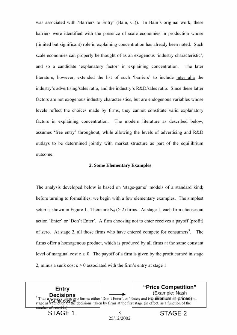
The analysis developed below is based on ‘stage-game’ models of a standard kind;

before turning to formalities, we begin with a few elementary examples. The simplest

setup is shown in Figure 1. There are N0 (≥ 2) firms. At stage 1, each firm chooses an

action ‘Enter’ or ‘Don’t Enter’. A firm choosing not to enter receives a payoff (profit)

of zero. At stage 2, all those firms who have entered compete for consumers3. The

firms offer a homogenous product, which is produced by all firms at the same constant

level of marginal cost c ≥ 0. The payoff of a firm is given by the profit earned in stage

2, minus a sunk cost ε > 0 associated with the firm’s entry at stage 1

8 25/12/2002

3 Thus a forms: either ‘Don’t Enter’, or ‘Enter; and cho cond stage as ecisions taken by firms at the first stage (innumber of entrant )’.

strategy takes twoa function of the d

s

ose an action in the se effect, as a function of the

“Price Competition”Entry Decisions (Sunk cost =

ε)

(Example: Nash Equilibrium in prices)

STAGE 2STAGE 1

9 25/12/2002

Figure 1 A two-stage game.

This second stage subgame can be modelled in various ways; we begin with the

Cournot case: Let the market demand schedule faced by the firms take the form

X = S/p

where p denotes market price and X ≡ Σxj is the total quantity sold by all firms; S

represents total consumer expenditure in the market, and serves as a measure of the

size of the market4. (To avoid technical problems in the case where only one firm

enters, assume that some outside substitute good is available at some (high) price p0,

so that consumers make no purchase if p > p0. The price p0 now serves as a monopoly

price in the model.)

We characterize equilibrium as a perfect Nash equilibrium of the two-stage game.

Taking as given the number N of firms who have entered at stage 1, we solve for a

Nash equilibrium in quantities at stage 2 (Cournot equilibrium). A routine calculation

leads to the familiar result that, at equilibrium, price falls to marginal cost as N rises.

(Figure 2, top panel, schedule C). The equilibrium profit of firm i in the second stage

subgame, is given by S/N2. Equating this to the entry fee ε > 0 incurred at stage 1, we

obtain the equilibrium number of entrants as the (largest integer satisfying) the

condition S/N2 ≥ ε. As S increases, the equilibrium number of firms rises, while

the 1-firm concentration ratio C1 = 1/N falls monotonically to zero (Figure 2).

4 A simple extension of this setup can be made, be equipping consumers with a Cobb-Douglas utility function, so that each consumer spends a fixed fraction of their income in this market, independent of the price p ≤ p0.

Figure 2

Equilibrium price as a function of the number of entrants, N, and equilibrium

concentration (1/N) as a function of market size, for three simple examples (B =

Bertrand, C = Cournot, M = joint profit maximization).

Now consider an alternative version of this model, in which we replace the ‘Cournot’

game by a Bertrand (Nash equilibrium in prices) model at Stage 2. Here, once two or

more firms are present, equilibrium involves at least two firms setting p = c, and all

firms earn zero profit at equilibrium. Here, for any size of market S that suffices to

support at least one entrant, the only (pure strategy) equilibrium for the game as a

whole involves exactly one firm entering, and setting the monopoly price (Figure 2,

schedule B).

10 25/12/2002

11 25/12/2002

Finally consider a third variant of the model, in which we replace our representation of

the second stage subgame by one in which all firms set the monopoly price5. Now, for

any number N of firms entering at stage 1, we have that price equals p0, and each firm

receives a fraction 1/N of monopoly profit; the number of entrants N is the number

which equates this to ε, as before (Figure 2, schedule M).

The results illustrated in Figure 2 serve to introduce an important result. We can

interpret a move from the monopoly model, to the Cournot model, and then to the

Bertrand model, as an increase in the ‘toughness of price competition’, where this

phrase refers to the functional relationship between market structure (here

represented by the 1-firm concentration ratio C1 = 1/N) and equilibrium price6. An

increase in the toughness of price competition (represented by a downward shift in the

function p(N) in the first panel of Figure 2), implies that for any given level of market

size, the equilibrium level of concentration C1 = 1/N is now higher (Figure 2, second

panel). This result turns out to be quite robust, and it will emerge as one of the

empirically testable predictions of the theory in what follows (Section 4).

All the cases considered so far have involved firms that produce a homogenous

product. We may extend the analysis by considering products that are (‘horizontally’)

differentiated, either by geographic location, or by way of product characteristics that

cause some consumers to prefer one variety, while others prefer a different variety,

their prices being equal. When we do this, a new feature appears, since models of this

kind tend to exhibit multiple equilibria. For any given market size, we will in general

5 This can be formalised by replacing stage II by an infinite horizon stage game, and invoking the basic ‘Folk Theorem’ result (see for example, Tirole (1990)). 6 This phrase refers, therefore, to the ‘form of price competition’ which is taken as an exogenously given characteristic of the market. It will depend on such background features of the market as the cost of transport of goods, and on such institutional features as the presence or absence of anti-trust laws. (On the determinants of the ‘toughness of price competition’ see Sutton (1991), Chapter 6 and Section 3 below.) In particular, it does not refer to the equilibrium level of prices, or margins, which, within the two-stage game, is an endogenous outcome.

have a set of equilibrium outcomes; the case in which N firms each offer a single

variety arises as one possible outcome, but there will usually be additional equilibria in

which a smaller number of firms each offers some set of products7.

Now in this setting, the functional relationship between concentration and market size,

illustrated in Figure 2, must be replaced by a lower bound relationship. The lower

bound is traced out by a sequence of ‘single product firm’ equilibria; but there are

additional equilibria lying above the bound (Figure 3). Even if we confine attention to

C1C1

S S (ii) Horizontal P

roduct

ifferentiation D

(i) Homogenous Goods Case

Figure 3.

Market size and concentration: two examples.

a single model, the only restriction that we can place on the concentration-size

relationship is a ‘bounds’ relationship.

This, then, is the first reason to move to a ‘bounds’ approach8. A second, and more

weighty, reason lies in the choice of the model itself. Even within the restricted set of

12 25/12/2002

7 The simplest way to see this point is by thinking in terms of the classic Hotelling model, in which products are differentiated by their locations along a line (see Sutton (1991), pp 38-39). Imagine a ‘single product firm’ equilibrium in which firms occupy a set of discrete locations A, B, C, D, E etc. We can construct, for example, a new equilibrium in which every second location is occupied by a single (‘multiproduct’) firm. There will now be an equilibirum in which prices are the same as before. This firm’s profit function is additively separable, into the functions which represent the separate contributions from each of its products, and its first order conditions for profit maximization coincide with the set of first order conditions for the firms owning products A, C, E etc. in the original setup. If the original ‘single product firm’ configuration constituted an equilibrium of the two-stage game, so too will this ‘high concentration’ configuration in which our multi-product firm owns every second product.

13 25/12/2002

examples we have looked at so far, two fundamental problems arise once we try to

move from theory to application. These problems relate to two feature of the model

that are notoriously difficult to measure, proxy, or control for.

The first of these is the choice of model for the final-stage subgame. Here we face two

issues. First, what is the best way to represent price competition (à la Cournot, à la

Bertrand, or otherwise)? Second, if products are differentiated, are they best modelled

by means of a Hotelling model, or a non-locational model that treats all varieties in a

symmetric fashion9, or otherwise?

The second issue relates to the form of the entry process. In the above examples, we

have confied attention to the case of ‘simultaneous entry’. If we replace this by a

‘sequential entry’ model, the (set of) equilibrium outcomes will in general be different.

For example, in the setting of (horizontal) product differentiation, there may (or may

not) be a tendency in favour of ‘more concentrated’ equilibria, in which the first mover

‘pre-empts’ rivals by introducing several varieties (for an extended example, see

Sutton (1998), Chapter 2 and Appendix 2.1.2).

The main burden of the analysis developed in the next section is concerned with

framing the theory in a way that gets around these two sources of difficulty. Before

proceeding to a general treatment, however, there is one final example that is worth

introducing.

8 One comment sometimes made about this setup is that we might hope, by introducing a ‘richer’ model specification, or by appealing to characteristics of individual firms, to arrive at a model that led to some particular (i.e. unique) equilibrium. To justify such a model – since many such models might be devised – however, we would need to appeal to information about the market and the firms that we would be unlikely to have access to, at least in a cross-industry study. Thus we are led back once again to the problem of ‘unobservables’. 9 Examples of such ‘symmetric’ models include the models of Dixit and Stiglitz (1977), and the ‘linear demand model’ discussed in Shubik and Levitan (1980), Deneckere and Davidson (1985), Shaked and Sutton (1987) and, in a Cournot version, in Sutton (1998).

A key feature that has not arisen in the examples considered so far relates to the

possibility that firms might choose to incur (additional) fixed and sunk costs at stage 1

with a view to improving their competitive position in the final-stage subgame. This

kind of expenditure would include, for example, outlays on R&D designed to enhance

the quality, or technical characteristics, of firm product(s); it would include

advertising outlays that improve the ‘brand-image’ of the product; and it would

include cost-reducing ‘product innovation’ in which R&D efforts are directed towards

the discovery of improved production methods.

We can illustrate this kind of situation by extending the simple Cournot model

introduced above, to incorporate a richer description of consumer demand. Suppose all

consumers have the same utility function of the form

δ−δ= 1z)ux(U

defined over two goods, the good that is the focus of analysis and some other

“outside” good. The quantities of these two goods are denoted x and z respectively.

Increases in u, the index of perceived quality, enhance the marginal utility derived

from the former good. We will, henceforward, refer to this first good x as the “quality”

good, in order to distinguish it from the “outside” good.

Rival firms are assumed to offer various quality goods. Let ui and pi denote the index

of perceived quality and the price respectively of firm i’s offering. Then, the

consumer’s decision problem can be represented as follows given the set of qualities

and prices offered: it is easy to show that the consumer chooses a product that

maximizes the quality-price ratio ui/pi; and the consumer spends fraction δ of his

income on this chosen quality good, and fraction (1-δ) of his income on the outside

14 25/12/2002

good. Total expenditure on the quality goods is therefore independent of the levels of

prices and perceived qualities and equals a fraction δ of total consumer income.

Denote this level of total expenditure on quality goods by S.

The first step in the analysis involves looking at the final stage of the game. Here, the

perceived qualities are taken as given (having been chosen by firms at the preceding

stage). Equilibrium in the final stage of the game is characterised as a Nash

equilibrium in quantities (Cournot equilibrium). This equilibrium can be calculated as

follows: since each consumer chooses the good that maximises ui/pi, the equilibrium

prices of all those firms enjoying positive sales at equilibrium must be proportionate to

their perceived qualities, that is, ui/pi = uj/pj, all i,j.

It can be shown (see Appendix A) that in the final stage subgame, some number of

products survive with positive sales revenue; it may be the case that products with

qualities below a certain level have an output level of zero, and so profits of zero, at

equilibrium. Denoting by N the number of firms that enjoy positive sales (‘survive’) at

equilibrium, the final stage profit of firm i is given by

S)u/1(

1u

1N12

ji

⋅⎪⎭

⎪⎬⎫

⎪⎩

⎪⎨⎧

Σ−

−

Associated with this equilibrium is a threshold level of quality u; all ‘surviving’

products have ui > u and all products with uj < u have an output of zero at equilibrium.

The sum in the above expression is taken over all ‘surviving’ products, and N

represents the number of such products. The threshold u is defined by adding a

15 25/12/2002

hypothetical (N+1)th product to the N surviving products, and equating the above profit

of good N+1 to zero viz. u = uN+1 is implicitly defined by10

∑−=

ju1

1N1

u1

where the sum is taken over j = 1 to N.

Now consider a 3-stage game in which each of the N0 potential entrants decides, at

stage 1, to enter or not enter, at cost Fo > 0. At stage 2, the N firms that have entered

choose a quality level, and in so doing incur additional fixed and sunk costs. Denote

by F(u) the total fixed and sunk cost incurred by an entrant that offers quality u, where

u lies in the range [1,∞) and

F(u) = F0uβ, u ≥ 1

Thus the minimum outlay incurred by an entrant equals F0 (>0).

Given the qualities chosen at stage 2, all firms now compete à la Cournot in stage 3,

their gross profit being defined as above. A firm’s payoff equals its net profit (gross

profit minus the fixed and sunk outlays incurred).

A full analysis of this model will be found in Sutton (1991), Chapter 3. Here, we

remark on the key feature of the relationship between market size and concentration.

At equilibrium, N firms enter and produce a common quality level u. For small S, the

level chosen is the minimum level u = 1, and the size-structure relation mimics that of

the basic Cournot model. But once a certain critical value of S is reached, the returns

16 25/12/2002

10 The number of products that survive can be computed recursively by labelling the products in descending order of quality, so that u1 ≥ u2 ≥ u3 … and considering successive candidate sets of surviving products of the form (u1, u2, … uk). The set of surviving products is the smallest set such that the first excluded product has a quality level uk+1 < u.

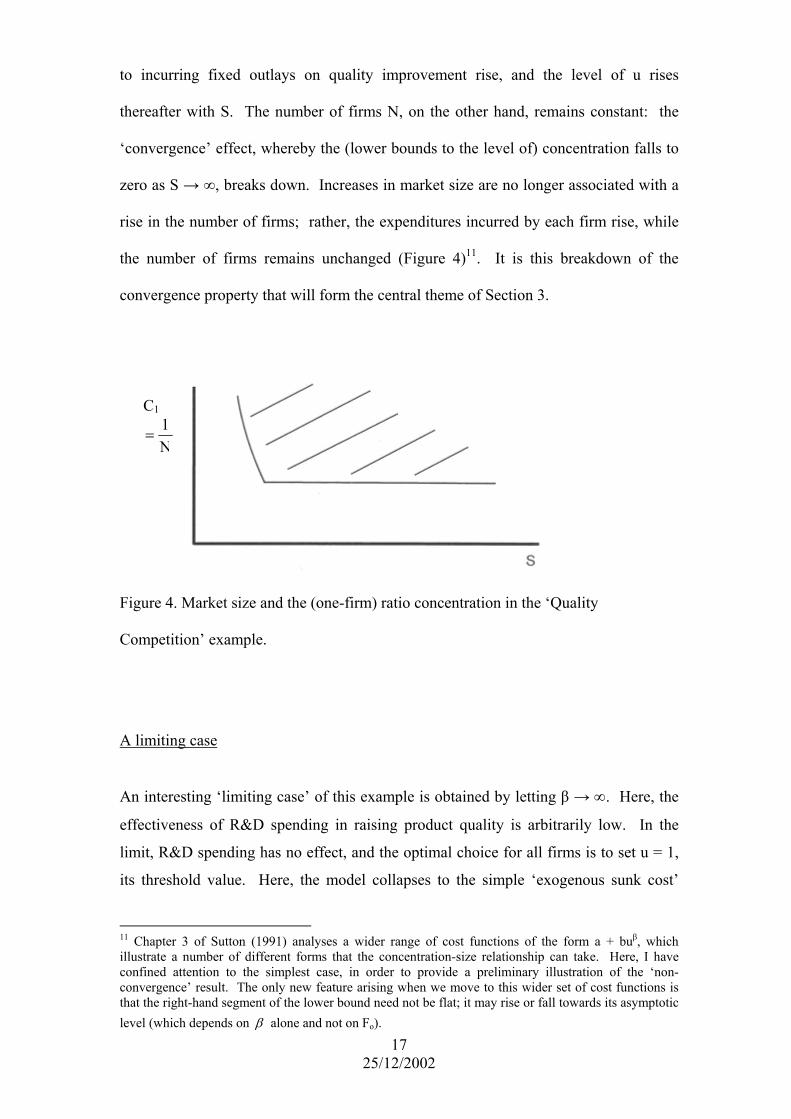
to incurring fixed outlays on quality improvement rise, and the level of u rises

thereafter with S. The number of firms N, on the other hand, remains constant: the

‘convergence’ effect, whereby the (lower bounds to the level of) concentration falls to

zero as S → ∞, breaks down. Increases in market size are no longer associated with a

rise in the number of firms; rather, the expenditures incurred by each firm rise, while

the number of firms remains unchanged (Figure 4)11. It is this breakdown of the

convergence property that will form the central theme of Section 3.

Fig

Co

A

An

eff

lim

its

11 Cilluconconthalev

C1

ure 4. Market size and the (one-firm) ratio concentration in the ‘Quality

mpetition’ example.

N1

=

limiting case

interesting ‘limiting case’ of this example is obtained by letting β → ∞. Here, the

ectiveness of R&D spending in raising product quality is arbitrarily low. In the

it, R&D spending has no effect, and the optimal choice for all firms is to set u = 1,

threshold value. Here, the model collapses to the simple ‘exogenous sunk cost’

hapter 3 of Sutton (1991) analyses a wider range of cost functions of the form a + buβ, which

strate a number of different forms that the concentration-size relationship can take. Here, I have fined attention to the simplest case, in order to provide a preliminary illustration of the ‘non-vergence’ result. The only new feature arising when we move to this wider set of cost functions is t the right-hand segment of the lower bound need not be flat; it may rise or fall towards its asymptotic el (which depends on β alone and not on Fo).

17 25/12/2002

example considered earlier. In fact, as we will note later, it is natural from the point of

view of the theory to interpret the ‘exogenous sunk cost’ example in just this way – as

a limiting case arising within the general (‘endogenous sunk costs’) model.

Capabilities

A more general interpretation of the key idea involved in these examples can be

offered by thinking of the firm’s ‘capability’12 relative to its rivals as consisting of two

elements: the parameter u, which can be thought of as a shift parameter that moves its

demand schedule outwards, and its ‘productivity level’, as measured by its level of unit

cost. We can think of the fixed outlay F as mapping into an enhancement of

‘capability’ in this sense, and the process of competition as involving ‘investment in

capability building’. This way of interpreting the examples set out above is helpful,

especially when we turn to some extensions of the models. (Section 8 and Appendix A

below and Sutton (2001)).

u

price

c

quantity

Figure 5 The ‘capability’ interpretation. Here, the fixed outlays F map into

improvements in c and u, and the firm’s capability is denoted by a (c,u) pair.

18 25/12/2002

12 A substantial literature has discussed the notion of ‘capabilities’ as attributes of the firm (see for example Nelson and Winter (1982), Bell and Pavitt (1993)). Here, I am interpreting ‘capability’ narrowly (static capability, or the firm’s capability at a point in time); on the other hand, I am adopting a wider interpretation than those authors in allowing u to represent all demand-enhancing factors including an advertising-based brand images.

3. Theory I

In this section, we move to a general treatment. We specify a suitable class of stage-

games, and consider a setting in which the fixed and sunk investments that firms make

are associated with their entering of products into some abstract ‘space of products’.

This setup is general enough to encompass the many stage-game models used in the

literature. For example, in a Hotelling model of product differentiation, the (set of)

action(s) taken by a firm would be described by a set of points in the interval [0,1],

describing the location of its products in (geographic) space. In the ‘quality choice’

model considered above, the action of firm i would be to choose a quality level ui ≥ 1.

In the ‘capability’ model illustrated in Figure 5, the firm’s action would be to choose a

pair of numbers (u,c); and so on.

A Class of Stage-Games

We are concerned with a class of games that share the following structure: There are N0

players (firms). Firms take actions at certain specified stages. An action involves

occupying some subset, possibly empty, of “locations” in some abstract “space of

locations,” which we label A. At the end of the game, each firm will occupy some set of

locations.

The notation is as follows: a location is an element of the set of locations A. The set of

locations occupied by firm i at the end of the game is denoted ai, where ai is a subset of A

viz. ai ⊂ A. If firm i has not entered at any location then ai is the empty set, i.e. ∅ =ai .

Associated with any set of locations is a fixed and sunk cost incurred in entering at these

19 25/12/2002

locations. This cost is strictly positive and bounded away from zero, namely, for any

The outcome of the game is described by an N.0F )F(a , a oii >≥∅≠ 0-tuple of all

locations occupied by all firms at the end of the game. Some of the entries in this N0-

tuple may be null, corresponding to firms who have not entered the market. In what

follows, we are concerned with those outcomes in which at least one firm has entered the

market and are interested in looking at the locations occupied by the firms who have

entered (the “active” firms). With that in mind, we label the number of active firms as N

(≥1), and we construct an N-tuple by deleting all the null entries, and re-labelling the

remaining firms from 1 to N. The N-tuple constructed in this way is written as

)a,...,a,(a )(a n21i =

and is referred to as a “configuration”. Here, N can take any value from 1 to N0.

The payoff (profit) of firm i, if it occupies locations ai, is written

)F( - ))(( ii-i aaaΠ

where (a-i) denotes . The function ),...,,( N1i+1i- aaa,...,a1 ) ) ( ( i-i aaΠ is obtained by

calculating firms' equilibrium profits in some final stage subgame (which we refer to as

the “price competition sub-game”), in which the ai enter as parameters in the firms' payoff

functions. It is defined over the set of all configurations. The second argument of the

profit function is an (N-1)-tuple (a-i), which specifies the sets of location occupied by

each of the firm's rivals. Thus, for example, if we want to specify the profit that would be

earned by a new entrant occupying a set of locations a, given some configuration (ai) that

describes the locations of firms already active in the market, we will write this as

) )( ia ( a 1N+Π . If, for example, only one firm has entered, then (a-i) is empty, and the

20 25/12/2002

profit of the sole entrant is written as Π(a1 ⏐ ∅), where a1 is the set of locations that it

occupies. A firm taking no action at any stage incurs zero cost and receives payoff zero.

In writing the profit function Π(⋅) and the fixed cost function F(⋅) without subscripts, we

have assumed that all firms face the same profit and cost conditions, i.e. a firm's payoff

depends only on its actions, and those of its rivals; there are no 'firm-specific' effects.

(Since our focus in on looking at a lower bound to concentration, it is natural to treat

firms as symmetric; see Section 6 below.)

We are interested in examining the set of configurations that satisfy certain conditions.

These conditions will be defined in a way that does not depend upon the order of the

entries in (ai). Two configurations that differ only in the order of their elements are

equivalent, in the sense that each one satisfies the conditions if and only if the other does.

Assumptions

We introduce two assumptions on the games to be considered. The first assumption

relates to the payoff function Π of the final-stage subgame, on which it imposes two

restrictions. Restriction (i) excludes 'non-viable' markets in which no product can cover

its entry cost. Restriction (ii) ensures that the number of potential entrants N0 is large.

(The role of this assumption is to ensure that, at equilibrium, we will have at least one

inactive player, so that N < N0). Denote the configuration in which no firm enters as

. ∅

ASSUMPTION 1: (i) There is some set of locations ao such that

)(F > ) ( oo aa ∅Π .

21 25/12/2002

22 25/12/2002

(ii) The sum of final stage payoffs received by all agents is bounded

above by (N0 - 1)F0, where N0 denotes the number of players and

F0 fis the minimum setup cost (entry fee).

The second assumption relates to the rules specifying the stages at which firms may enter

and/or make investments:

ASSUMPTION 2: (Extensive Form): We associate with each firm i an integer ti (its date of

‘arrival’). Firm I is free to enter any subset of the set of products A at any stage t,

such that ti ≤ t ≤ T.

This assumption excludes a rather paradoxical feature that may arise in some basic

‘sequential entry’ models, where a firm would prefer, if allowed, to switch its place in

the entry sequence for a later position. In practice, firms are always free to delay their

entry; this assumption avoids this anomalous case by requiring that a firm arriving in

the market at stage t is free to make investments at stage t and/or at any subsequent

stage, up to some final stage T (we exclude infinite horizon games).

Equilibrium Configurations

The aim of the present exercise is to generate results that do not depend on (a) the

details of the way we design the final-stage subgame, or (b) the form of the entry

process. To handle (a), we work directly in terms of the ‘solved-out profit function’ of

the final-stage subgame, introduced as our profit function Π(⋅) above. To deal with (b),

the entry process, we introduce an equilibrium concept that is defined, not in the space of

strategies (which can only be specified in the context of some particular entry process),

but in the space of outcomes, or – more precisely – configurations. The key idea here is

this: the set of ‘equilibrium configurations’, defined below includes all outcomes that can

be supported as a (pure strategy, perfect) Nash equilibrium in any stage game of the class

defined by Assumptions 1 and 2 above. In what follows, we develop results which show

that certain (‘fragmented’) market structures can not be supported as Equilibrium

Configurations – and so they can not be supported as (pure strategy, perfect) Nash

equilibria, irrespective of the details of the entry process.

Now there are two obvious properties that must be satisfied by any pure strategy, perfect

Nash equilibrium within this class of models. In what follows, we define the set of all

outcomes satisfying these two properties, as follows:

DEFINITION: The N-tuple (ai) is an Equilibrium Configuration if:

(i) Viability13: For all firms i,

0 )F( - ) )( | ( ii-i ≥Π aaa

(ii) Stability: There is no set of actions a N+1 such that entry is

profitable, viz. for all sets of actions aN+1,

0 )aF( - )) a ( | a( 1Ni1N ≤Π ++

PROPOSITION 1 (Inclusion): Any outcome that can be supported as a (perfect) Nash

equilibrium in pure strategies is an Equilibrium Configuration.

To see why Proposition 1 holds, notice that ‘Viability’ is ensured since all firms have

available the action ‘Don’t Enter’. Assumption 1(ii) ensures that there is at least one firm

23 25/12/2002

13 It is worth noting that the Viability condition has been stated in a form appropriate to the ‘complete information’ context in which we are working here, where exit is not considered. In models where exit is an available strategy, condition (i) must be re-stated as a requirement that profit net of the avoidable cost which can be saved by exiting should be non-negative.

that chooses this action at equilibrium; while if the stability condition does not hold, then

a profitable deviation is available to that firm: given the actions prescribed for its rivals

by their equilibrium strategies, it can profitably deviate by taking action a N+1 at stage T.

3. The Price Competition Mechanism

We can formalize the discussion of the ‘price competition’ mechanism introduced in

Section 2 above. We confine attention, for ease of exposition, to the class of

‘symmetric’ produce differentiation models.14 In these models, each firm chooses

some number η of distinct product varieties to offer, and incurs a setup cost for

each one. The profit of firm I in an equilibrium of the final stage subgame can be

written as

0>ε

))in(n(S i −π

Now consider a family of such models, which comprises models in which the form of

price competition in the final stage subgame differs across models. We consider a one-

parameter family of models that can be ranked in terms of the ‘toughness of price

competition’ in the following sense: we dfine a family of reduced form profit

functions parameterized by , which we denote θ

));in(n( i θ−π

14 Such models include for example the linear demand model (for a Bertrand verstion see Livitan and Shubik ( ), Shaked and Sutton ( ); for a Cournot version see Sutton (1998))) and the model of a Dixit and Stiglitz ( ).

24 25/12/2002

An increase in shifts the profit function downwards, in the sense that, for any given

configuration we have that if

θ

21 θ>θ , then

));in(n());in(n( 2i1i θ−π<θ−π

The parameter θ denotes the ‘toughness of price competition’ in the sense that an

increase in θ reduces the level of final stage profit earned by each firm, for any given

form of market structure (i.e. configuration).

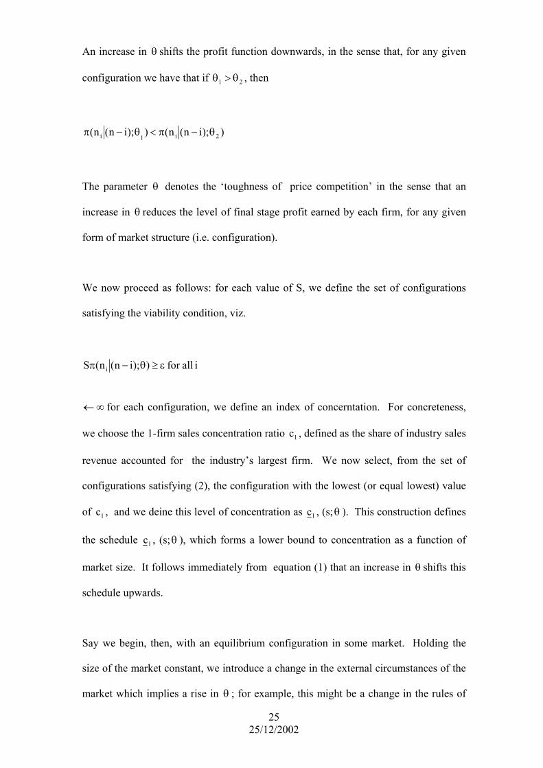
We now proceed as follows: for each value of S, we define the set of configurations

satisfying the viability condition, viz.

i allfor ));in(n(S i ε≥θ−π

∞← for each configuration, we define an index of concerntation. For concreteness,

we choose the 1-firm sales concentration ratio , defined as the share of industry sales

revenue accounted for the industry’s largest firm. We now select, from the set of

configurations satisfying (2), the configuration with the lowest (or equal lowest) value

of , and we deine this level of concentration as

1c

1c 1c , (s; θ ). This construction defines

the schedule 1c , (s; ), which forms a lower bound to concentration as a function of

market size. It follows immediately from equation (1) that an increase in shifts this

schedule upwards.

θ

θ

Say we begin, then, with an equilibrium configuration in some market. Holding the

size of the market constant, we introduce a change in the external circumstances of the

market which implies a rise in θ ; for example, this might be a change in the rules of

25 25/12/2002

competition policy (a law banning cartels, say), or it might be an improvement in the

transport system that causes firms in hitherto separated local markets to come into

direct competition with each other (as with the building of national railway systems in

the nineteenth century, for example).

If the associated shift in is large enough, then the current configuration will no longer

be an equilibrium, and some shift in structure must occur in the long run.

θ

At this point, a caveats is in order: the theory is static, and we can not specify the

dynamic adjustment path that will be followed once equilibrium is disturbed.15

We can, however, distinguish two candidate mechanisms that can restore viability; the

first involves exit, while the second involves a process of consolidation (merger and

acquisition). This remark rests on two assumptions on the underlying profit function:

(a) entry (resp. exit) will lead to a fall (resp. rise) the the (final stage) profit earned by

firms in the industry.

These restrictions are substantive. They hold for a wide range of standard models, but

it is possible to construct models that violate them. For example, the model of

Rosenthal ( ) illustrates the possibility that entry might raise prices, and so (gross)

profit per firm. At the empirical level, a substantial body of evidence supports the

26 25/12/2002

15 The speed of adjustment by firms will be affected inter alia by the extent to which the setup cost ε is sunk, as opposed to fixed. If ε is a sunk cost, then a violation of the viability constraint will not require any adjustment in the short run; it is only in the long run, as the capital equipment needs to be replaced, that (some) firms will, in the absence of any other structural changes, no longer find it profitable to maintain their position, and will exit. If ε is partly fixed, rather than sunk, then exit is likely to occur sooner.

27 25/12/2002

view that a rise in concentration raises prices, and so gross profit per firm, constant

(see in particular, Weiss ( )16.For a fuller discussion, see Sutton ( ,)); in

Given these restrictions, it follows that equilibrium may be restored via a process of

exit and/or consolidation, both leading to a rise in concentration.

Empirical Evidence

The most systematic test of this prediction is that of Symeonidis ( ), who takes

advantage of an unusual ‘natural experiment’ involving a change in competition law in

the U.K. in the 1960s. As laws against the operation of cartels were strengthened, a

general rise in concentration occurred across the general run of manufacturing

industries. Symeonides traces the operation of these changes in detail, and finds a

process at work that is consistent with the operation of the response mechanisms

postulated above.

A number of case studies reported in Sutton (1991) offer further support:

A nice natural experiment in regard to transport costs is provided by the spread of

railways from the mid-nineteenth century. The salt industry, both in the US and

Europe, went through a process of consolidation in the wake of these changes; first

prices fell, rendering many concerns unviable. Attempts to restore profitability via

price coordination failed, due to ‘free riding’ by some firms. Finally, a process of exit,

16 For a fuller discussion see Sutton ( , )); in particular, it should be noted that this claim should not be confused with much stronger, and controversial claims regarding the ‘concentration-profits’ relationship within the tradition Structure-Conduct-Performance literature.

28 25/12/2002

accompanied by mergers and acquisitions, led to the emergence of a concentrated

industry (Sutton, (1991), Chapter 6).

The history of the US sugar industry over the same period follows a similar pattern. In

Continental European countries, on the other hand, a permissive competition policy

regime allowed firms to coordinate their prices, thus permitting the continuance of a

relatively fragmented industry. The Japanese market provides an unusually

informative natural experiment, in that it went through three successive regimes in

respect of competition policy. A tight cartel operated in the period prior to the first

world war, and concentration was low. In the inter-war years, the cartel broke down

and concentration rose. In the years following the second world war, however, the

authorities permitted the industry to operate under a permissive ‘quota’ regime; and

this relaxation in the toughness of price competition encouraged new entry, and a

decline in concentration (Sutton (1991), Chapter 6).

A Quality Choice Model

With this setup in place, we are in a position to develop a general treatment of the

‘endogenous sunk cost’ model. For ease of exposition, we will represent the actions as a

‘choice of quality’, so that the actions of each firm reduces to ‘Don’t Enter’ or ‘Enter with

quality ui’, chosen from the interval [1,∞).

The outcome of firms’ actions is described by a configuration

u = (u1, … ui, … uN)

We associate with every configuration u a number representing the highest level of

quality attained by any firm, viz.

iiumax)(u =u

We summarize the properties of the final-stage subgame in a pair of functions that

describe the profit of each firm and the sales revenue of the industry as a whole. Firm

i’s profit is written as

( ) ( ))(uS)(u iiii −− π≡Π uu

where u-i denotes the N-1 tuple of rivals’ qualities, and S denotes the number of

consumers in the market17. Total industry sales revenue is denoted by

)(Sy)(Y uu ≡

The Cost Function

It is assumed that any firm entering the market incurs a minimum setup cost of F0 and

that increases in the quality index above unity involve additional spending on fixed

outlays such as R&D and Advertising. We choose to label this index so that the fixed

outlay of firm i is related to the quality level ui according to

β= i0i uF)u(F , on , for some ),0[ui ∞∈ 1≥β .

We identify the level of spending on R&D and Advertising as

0ii F)u(F)u(R −=

29 25/12/2002

17 The motivation for writing the profit function (and the industry sales revenue function) in this form (i.e. multiplicative in S), derives from an idea which is standard throughout the market structure literature: Firms have flat marginal cost schedules, and increases in the size of the market involve an increase in the population of consumers, the distribution of consumer tastes being unaltered. Under these assumptions, a rise in the size of the population of consumers S shifts the demand schedule outwards multiplicatively and equilibrium prices are independent of S.

The economics of the model depends only on the composite mapping from firms’ fixed

outlays to firms’ profits, rather than on the separate mappings of fixed outlays to

qualities and from qualities to profits. At this point, the labelling of u is arbitrary up to

an increasing transformation. There is no loss of generality, therefore, in choosing this

functional form for R(ui).18 (The form used here has been chosen for ease of

interpretation, in that we can think of β as the elasticity of quality with respect to fixed

outlays)19.

To avoid trivial cases, we assume throughout that the market is always large enough to

ensure that the level of sales exceeds some minimal level for any configuration, and

that the market can support at least one entrant. With this in mind, we restrict S to the

domain [1,∞), and we assume, following Assumption 1 above,

ASSUMPTION 3: The level of industry sales associated with any nonempty

configuration is bounded away from zero; that is, there is some

such that for every configuration , we have

for all

0>η ∅≠u

0)(y >η≥u ∅≠u .

This assumption, together with Assumption 1(i), implies that the level of industry sales

revenue η≥ S)(Sy u in any Equilibrium Configuration increases to infinity as . ∞→S

A Nonconvergence Theorem

18 There is, however, a (mild) restriction in writing as rather than , as noted in

footnote 14 above. See Sutton (1991), Chapter 3 for details.

)F(uiβiu Fo β

iu bFo +

30 25/12/2002

19 Rather than represent F as a single function, it is convenient to use a family of functions parameterised by β, since we can then hold the profit function fixed while varying β to capture changes in the effectiveness of R&D and Advertising in raising final stage profits.

In what follows, we are concerned with examining whether some kinds of

configuration u are unstable against entry by a ‘high-spending’ entrant. With this in

mind, we investigate the profit of a new firm that enters with a quality level k times

greater than the maximum value û offered by any existing firm. More specifically, we

ask: What is the minimum ratio of this high-spending entrants’ profit to current

industry sales that will be attained independently of the current configuration u and the

size of the market?

For each k, we define an associated number a(k) as follows:

DEFINITION: )(y

)uk(inf)k(a

uu

u

π=

It follows from this definition that, given any configuration u with maximal quality û,

the final-stage profit of an entrant with capability kû, denoted )uk(S uπ , is at least

equal to )(a(k)Y)(a(k)Sy uu = , independently of u and S.

The intuition is as follows: k measures the size of the quality jump introduced by the

new ‘high spending’ entrant. We aim to examine whether such an entrant will earn

enough profit to cover its fixed outlays, and so we want to know what price it will set,

and what market share it will earn. This information is summarised by the number

a(k), which relates the gross (final-stage) profit of the entrant, )uk(S uπ , to pre-entry

industry sales revenue, . Since we wish to develop results that are

independent of the existing configuration, we define a(k) as an infimum over u.

)(Y)(Sy uu =

We are now in a position to state:

31 25/12/2002

THEOREM 1 (Nonconvergence) Given any pair (k,a(k)), a necessary condition for any

configuration to be an equilibrium configuration is that a firm offering the highest level

of quality has a share of industry sales revenue exceeding βk/)k(a .

PROOF Consider any equilibrium configuration u in which the highest quality offered is

û. At least one firm offers quality û. Choose any such firm and denote the sales

revenue earned by that firm by Sŷ, whence its share of industry sales revenue is

Sŷ/SY(u) = ŷ/Y(u).

Consider the net profit of an entrant who attains quality kû. The definition of a(k)

implies that the entrant’s net profit is at least

)u(Fk)(aSy)uk(F)(aSy β−=− uu (1)

where we have written a(k) as a, in order to ease notation.

The stability condition implies that this entrants’ net profit is nonpositive, whence

)(Syka)u(F uβ≥

But the viability condition requires that each firm’s final-stage profit must cover its

fixed outlays. Hence the sales revenue of the firm that offers quality û in the proposed

equilibrium configuration cannot be less than its fixed outlays:

)(Syka)u(FyS uβ≥≥

whence its market share

β≥ka

)(SyySu

.

This completes the proof.

32 25/12/2002

The intuition underlying this result is as follows: if the industry consists of a large

number of small firms, then the viability condition implies that each firm’s spending

on R&D is small, relative to the industry’s sales revenue. In this setting, the returns to

a high-spending entrant may be large, so that the stability condition is violated. Hence

a configuration in which concentration is “too low” cannot be an equilibrium

configuration. This result motivates the introduction of a parameter, which we call

alpha, as the highest value of the ratio a/kβ that can be attained by choosing any value k

≥ 1, as follows:

DEFINITION β=αk

)k(asupk

.

We can now reformulate the preceding theorem as follows. Since the one-firm sales

concentration ratio C1 is not less than the share of industry sales revenue enjoyed by

the firm offering quality û, it follows from the preceding theorem that, in any

equilibrium configuration, C1 is bounded below by α, independently of the size of the

market, viz.

C1 ≥ α (2)

Equation (2) constitutes a restatement of the basic noncovergence result developed in

the preceding theorem. In the light of this result, we see that alpha serves as a measure

of the extent to which a fragmented industry can be destabilised by the actions of a

firm who outspends its many small rivals of R&D or Advertising. The value of alpha

depends directly on the profit function of the final stage subgame, and on the elasticity

of the fixed cost schedule. Hence it reflects both the pattern of technology and tastes

and the nature of price competition in the market. We noted earlier that the results do

not depend on the way we label u, but only on the composite mapping from F to π. To

33 25/12/2002

underline this point, we can re-express the present result as follows: Increasing quality

by a factor k requires that fixed outlays rise by a factor kβ. For any given value of β,

write kβ as K. We can now write any pair (k,a(k)) as an equivalent (K,a(K)) pair.

Alpha can then be described as the highest ratio a(K)/K that can be attained by any

choice of K ≥ 1.

A Family of Models

Within our present context of a classical market in which all goods are substitutes, the

interpretation of alpha is straightforward: it simply measures the degree to which an

increase in the (perceived) quality of one product allows it to capture sales from rivals.

Thus the statement, within this context, that there exists some pair of numbers k and

a(k) satisfying the above conditions is unproblematic (for a detailed justification of this

remark, by reference to a specific representation of consumer preferences), see Sutton

(1991), pp. 75-76). The question of interest is: how costly is it, in terms of fixed

outlays, to achieve this k-fold increase in u? This is measured by the parameter β.

With this in mind, we proceed to define a family of models, parameterised by β, as

follows: we take the form of the profit function, and so the function a(k), as fixed,

while allowing the parameter β to vary. We assume, moreover, that for some value of

k, a(k) > 0. The value of varies with β. (The case α = 0 can be

treated as a limiting case as a(k) → 0 or β → ∞.)

β=α k/)k(asupk

We are now in a position to develop an ancillary theorem whose role is to allow us to

use the observed value of the R&D and/or Advertising to Sales ratio to proxy for the

value of β. The intuition behind the ancillary theorem is this: if the value of β is high,

this implies that the responsiveness of profit to the fixed outlays of the deviant firm is

34 25/12/2002

35 25/12/2002

low, and under these circumstances we might expect that the level of fixed outlays

undertaken by all firms at equilibrium would be small; this is what the theorem asserts.

We establish this by showing that certain configurations must be unstable, in that they

will be vulnerable to entry by a low-spending entrant. The idea is this: if spending on

R&D and Advertising is ineffective, then a low spending entrant may incur much

lower fixed outlays than (at least some) incumbent firm(s), while offering a product

that is only slightly inferior to that of the incumbent(s). It follows as an immediate

consequence of this theorem, that if we fix some threshold level for the ratio of R&D

plus Advertising to sales, and consider the set of industries for which the ratio exceeds

this threshold level, then we may characterize this group as being ‘low β ‘ and so ‘high

alpha’ industries, as against a control group of industries in which R&D and

Advertising levels are (very close to) zero. It is this result which leads to the empirical

test of the non convergence theorem developed below.

A Technicality

The proof of the ancillary theorem rests on an appeal to the entry of a low-spending

firm; and this raises a technical issue: suppose the underlying model of the final stage

subgame, whose properties are summarised in the profit function π(·), takes the form of

the elementary ‘Bertrand model’. In this setting, (where all firms offer the same

quality level), once one firm is present in the market, no further entry can occur; for

any entry leads to an immediate collapse of prices to marginal cost, and so the entrant

can never earn positive margins, and so cover the sunk cost incurred in entering. In

what follows, we will exclude this limiting case. (To exclude it is harmless, relative to

the theory, since the theory aims to place a lower bound on the 1-firm concentration

36 25/12/2002

ratio; and if we are working in this ‘Bertrand limit’, then the 1-firm concentration ratio

is unity.)

To define and exclude this limiting case, we need to specify the relationship between

the profit earned by an entrant, and the pre-entry profit of some active firm (the

‘reference firm’).

Consider an equilibrium configuration in which the industry-wide R&D (or

Advertising) to sales ratio is x (> 0). Within this industry, we select some reference

firm whose R&D and Advertising outlays constitute a fraction x (or greater) of its sales

revenue. There must be at least one such firm in the industry, and since this firm must

satisfy the viability condition, it must earn a gross profit of at least fraction x of its

sales revenues in order to sustain its level of R&D and Advertising.

Now consider an entrant that offers the same quality level as the reference firm.

Insofar as entry reduces prices, this entrant will enjoy a lower price-cost margin than

that earned by the reference firm in the pre-entry situation. But, for a sufficiently high

value of x, we assume that the entrant will enjoy some strictly positive price-cost

margin, so that its final stage profit is strictly positive (this is what fails in the

‘Bertrand limit’).

This is illustrated in Figure 6. The horizontal axis shows the ratio between the quality

of the entrant’s product, and that of the reference firm; k varies from 0 to 1, with a

value of 1 corresponding to the entrant of equal quality. Our assumption states that for

k = 1, the entrant’s post-entry profit is strictly positive. On the vertical axis, we show

the ratio of the entrant’s profit to the pre-entry profit of the reference firm20. Our

exclusion of the Bertrand limit states that, for k = 1, this ratio is strictly positive. We

further assume that the entrant’s profit varies continuously with its quality, and so with

k. It then follows that we can depict the entrant’s profit as a function of k as a curve;

the assumption states that this curve does not collapse inwards to the bottom right-hand

corner of the diagram (the ‘Bertrand limit’). Specifically, it says that, for some

(sufficiently large) value of x, we can ensure that if the price-cost margin exceeds x,

then there is some point in the interior of the square such that the curve we have just

described lies above this point.

•πN+1(k)

πi

k0 1 γ

1

d

Figure 6

The relative profit of a low-quality entrant. The incumbent firm, labelled i, offers

quality ui and earns (pre-entry) profit πi on trajectory. The entrant, labelled firm N+1,

offers quality kui and earns profit πN+1(k).

We state this formally as follows:

37 25/12/2002

20 It is convenient to work in terms of this ratio, so as to state the assumption in a way that does not involve the size of the market S.

ASSUMPTION 4 There is some triple (x, γ, d) with 0 < x,γ < 1, and 0< d < 1, with the

following property: Suppose any firm i attains quality level ui on some trajectory m

and earns final-stage profit that exceeds a fraction of x of its sales revenue. Then an

entrant attaining a quality level equal to max(1,γui) attains a final-stage profit of at

least dπi.

The ancillary theorem linking the R&D/sales ratio to the parameter β now follows:

THEOREM 2 For any threshold value of the R&D/sales ratio exceeding max (x, 1–d),

where x and d are defined as in Assumption 4, there is an associated value of β* such

that for any β > β*, no firm can have an R&D/sales ratio exceeding this threshold in

any equilibrium configuration.21

The intuition underlying Theorem 2 is presented in Appendix B. An implication of

Theorem 2 is that an industry with a high R&D/sales ratio must necessarily be a high-

alpha industry. With this result in place, we are now in a position to formulate an

empirical test of the theory: Choose some (‘sufficiently high’) threshold level for the

R&D/sales ratio (written as R/Y in what follows), and split the sample of industries by

reference to this threshold. The group with a low value of R/Y will contain all the

industries in which alpha is close to zero, and so for this group the lower bound to the

cloud of points in (C,S) space should converge to zero as S → ∞. For all industries in

38 25/12/2002

21 It may be helpful to illustrate the ideas of Assumption 4 and Theorem 2 by reference to a numerical example: suppose x = 0.04 and d=0.95 (intuitively: entry reduces prices only slightly). Say we select all those industries with R&D sales ratios exceeding max (x, 1-d) = 0.05. Now suppose we let ∞→β , so that R & D becomes completely ineffective. Then an entrant to this industry can, by spending nothing on R&D, enjoy a positive net profit: it earns 5% less gross profit than incumbents did pre-entry, but it incurs 5% less cost through avoiding any spending on ineffective R&D. It follows that, once β is ‘sufficiently large’, the pre-entry configuration is not an Equilibrium Configuration.

the group with high R/Y, on the other hand, the value of β will lie below β*, and so the

lower bound to concentration will be bounded away from zero by β≥ 001 k/)k(aC .

In pooling data across different industries, it is appropriate to ‘standardise’ the measure

of market size by reference to some notion of the minimum level of setup cost ε. A

practical procedure to represent this as the cost of a single plant of minimum efficient

scale, and to write the ratio of annual industry sales revenue to minimum setup cost as

ε. This leads to the prediction illustrated in Figure 7 below; tests of this prediction are

reported in the next section.22, 23

Figure 7. The ‘bounds’ prediction on the concentration-market size relationship.

Empirical Evidence I

We have developed this first version of the non-convergence theorem in a context in

which the classical market definition applies, i.e. the market comprises a single set of

22 A further practical issue arises in relation to the use of the (theoretically appropriate) 1-firm concentration ratio C1. Since official statistics never report this, for reasons of confidentiality, it has long been customary in I.O. to use a readily available measure such as C4. The prediction shown in Figure 8 still applies, here, of course.

39 25/12/2002

23 It is interesting to consider the relationship between this prediction and the traditional practice of regressing concentration on a measure of scale economies to market size (essentially S/ε), together with a measure of advertising intensity and R&D intensity. Such regressions indicated that concentration fell with S/ε, and rose (weakly) with the advertising-sales ratio. It can be shown that, under the present theory, these results are predicted to emerge from the (misspecified) regression relationship. For a full discussion, see Sutton (1991), Annex to Chapter 5.

40 25/12/2002

substitute goods, so that an increase in fixed and sunk outlays enhances consumers’

willingness-to-pay for all its products in this market. Now this condition will apply

strictly only in rather special circumstances. One setting in which it applies to a good

approximation is that of certain groups of advertising-intensive industries. Here, even

though the market may comprise a number of distinct product categories, the firm’s

advertising may support a brand image that benefits all its products in the market. (A

similar argument applies, albeit with lesser force, in R&D intensive industries, insofar

as there may be some scope economies in R&D that operate across different groups of

products in the market; see below, Section 4.)

The first test of the nonconvergence theorem (Sutton (1991), Chapter 5) was carried

out on a dataset for 20 industries drawn from the food and drink sector, across the 6

largest Western economies. The industries were chosen from a single sector so as to

keep constant as many extraneous factors as possible. The food and drink sector was

chosen because, alone among the basic 2-digit SIC industry groups, it is the only one in

which there is a nice split between industries that have little or no advertising (sugar,

flour, etc.) and industries that are advertising-intensive (breakfast cereals, petfood,

etc.).

Data was compiled from market research reports, combined with company interviews.

The industry definitions used are those which are standard in the market research

literature, and these correspond roughly to 4-digit SIC definitions. All industries for

which suitable data could be assembled were included. The size of each market was

defined as the number of ‘minimum efficient scale’ plants it would support, where the

size of a m.e.s. plant was measured as the median plant size in the U.S. industry.

The sample was split on the basis of measured advertising sales ratios into a control

group (A/S < 1%) and an experimental group (A/S ≥ 1%); though the large majority of

industries in the latter group had advertising-sales ratios that were very much higher

than 1%.

Figure 8.

A plot of 4C~ versus S/ε for advertising-intensive industries (bottom panel) and a

control group (top panel). The fitted bound for the control group is reproduced in the

bottom panel for comparison purposes. 41

25/12/2002

The data from the study is illustrated in Figure 8, which shows the scatter of

observations for the control group (upper panel) and the experimental group (lower

panel) on plots of (a logit transformation24 of) the 4-firm concentration ratio. A fitted

lower bound25 for the control group indicates an asymptotic value for C4(S) in the

limit S → ∞; the corresponding lower bound for the experimental group is 19%, which

is significantly different from zero at the 5% level.

The non-convergence property has also been investigated by Robinson and Chiang

(1996), using the PIMS data set, a dataset gathered by the Strategic Planning Institute

representing a wide range of firms drawn mostly from the Fortune 1000 list. Firms

report data for each of their constituent businesses (their operations within each

industry, the industry being defined somewhat more narrowly than a 4-digit SIC

industry); for a discussion of the PIMS dataset, see for example Scherer (19xx), Caves

(19xx).

The unit of observation here is the individual business, and the sample comprises 1740

observations. The sample is split into a control group (802 observations) in which both

the advertising-sales ratio and the R&D-sales ratio lie below 1%. The remaining

(‘experimental’) groups comprise markets where one or both ratios exceed 1%.

Within the control group, the authors set out to test a second prediction of the theory

(which was not tested statistically in Sutton (1991)), according to which an increase in

the ‘toughness of price competition’ raises the lower bound Ck(S). They do this by

24 The logit transformed value ))C/(1n(CC~ 444 −= l is defined on (-∞, + ∞) rather than [0,1] and this may be preferred on econometric grounds.

42 25/12/2002

25 Following Smiths’ (1985, 1988) maximum likelihood method. Techniques for bounds estimation are discussed in Sutton (1991) Chapter 5, and Sutton (1998) Chapter 4.

43 25/12/2002

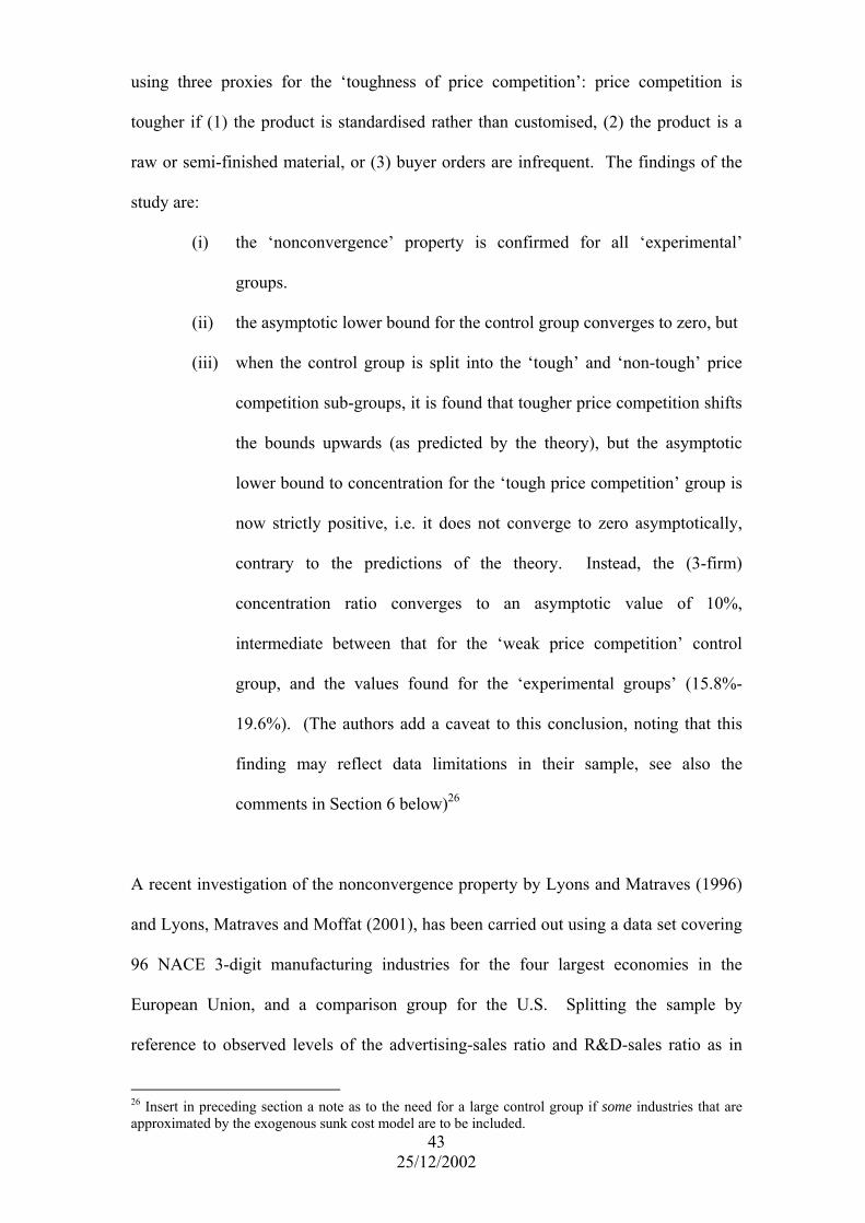
using three proxies for the ‘toughness of price competition’: price competition is

tougher if (1) the product is standardised rather than customised, (2) the product is a

raw or semi-finished material, or (3) buyer orders are infrequent. The findings of the

study are:

(i) the ‘nonconvergence’ property is confirmed for all ‘experimental’

groups.

(ii) the asymptotic lower bound for the control group converges to zero, but

(iii) when the control group is split into the ‘tough’ and ‘non-tough’ price

competition sub-groups, it is found that tougher price competition shifts

the bounds upwards (as predicted by the theory), but the asymptotic

lower bound to concentration for the ‘tough price competition’ group is

now strictly positive, i.e. it does not converge to zero asymptotically,

contrary to the predictions of the theory. Instead, the (3-firm)

concentration ratio converges to an asymptotic value of 10%,

intermediate between that for the ‘weak price competition’ control

group, and the values found for the ‘experimental groups’ (15.8%-

19.6%). (The authors add a caveat to this conclusion, noting that this

finding may reflect data limitations in their sample, see also the

comments in Section 6 below)26

A recent investigation of the nonconvergence property by Lyons and Matraves (1996)

and Lyons, Matraves and Moffat (2001), has been carried out using a data set covering

96 NACE 3-digit manufacturing industries for the four largest economies in the

European Union, and a comparison group for the U.S. Splitting the sample by

reference to observed levels of the advertising-sales ratio and R&D-sales ratio as in

26 Insert in preceding section a note as to the need for a large control group if some industries that are approximated by the exogenous sunk cost model are to be included.

44 25/12/2002

Robinson and Chiang, the authors estimate a lower bound to concentration for each

group.

A key novelty of this study, is that it attacks the question of whether it is more

appropriate to model the concentration-size relationship at the E.U. level, or at the

level of national economies (Germany, UK, France, Italy). The authors construct, for

each industry, a measure (labelled ‘t’) of intra-EU trade intensity. They hypothesise

that, for high (resp. low) values of t, the appropriate model is one that links

concentration in the industry to the size of the European (resp. national) market. They

proceed to employ a maximum likelihood estimation procedure to identify a critical

threshold t* for each country, so that according as t lies above or below t*, the

concentration of an industry is linked to the size of the European market, and

conversely. Within this setting, the authors proceed to re-examine the

‘nonconvergence’ prediction. They find that ‘a very clear pattern emerges, with …

the theoretical predictions … receiving clear support’. (Lyons, Matraves and Moffat,

(2001)).

The key comparison is between the asymptotic lower bound to concentration for the

control group versus that for the experimental groups. Over the eight cases (4

countries, EU versus National Markets) the point estimate of the asymptotic lower

bound for the control group lies below all reported27 estimates for the three

experimental groups, except in two instances (advertising-intensive industries in Italy,

advertising and R&D intensive industries in France; in both these cases the reported

standard errors are very high, and the difference in the estimated asymptotic value is

insignificant.

27 Some cases are unreported due to lack of a sufficient sample size

4. Beyond the Classical Market

The theory set out above rests on an idea of a classical market, in which all goods are

substitutes. We may reasonably apply this model to, for example, a narrowly defined

market in which firms’ advertising outlays create a ‘brand image’ that benefits all the

firms’ offerings in the market. But once we turn to the case of R&D intensive

industries, the formulation of the theory developed above becomes inadequate. For in

this setting, once we define the market broadly enough to incorporate all substitute

goods, we will usually be left with various sets of products, each set being associated

with a different technology. Here, each firm must choose not only its level of R&D

spending, but the way in which its R&D efforts should be divided among the various

technologies (or, equivalently, the various product groups). It is appropriate here to

extend the model by introducing the notion of a set of ‘technological trajectories’, and

their associated ‘submarkets’ as follows:

The capability of firm i is now represented by a set of quality indexes, its quality index

on trajectory m (equivalently, in submarket m), being denoted by ui,m, where m runs

from . A firm’s capability is represented by the vector Mto1

)u,...,u,...,u( M,im,i1,ii =u

And a configuration is written as ),...,,...,( Ni1 uuuu = .

45 25/12/2002

The firm’s fixed cost can now be written as the sum of the costs incurred on each

trajectory28, viz.

∑ β

mm,i0uF

A full discussion of the theory, within this more complex setting lies outside the scope

of this review; for details, the reader is referred to Sutton (1998), Chapter 3. Here, I

confine attention to an informal account of the key idea, which concerns the way in

which we represent the idea of ‘linkages’ across submarkets.

To motivate ideas, we begin by raising some questions. Suppose, firstly, that the

products in the various submarkets are fairly close substitutes. We might expect

intuitively, in this setting, that as firms advanced along one trajectory, they might

‘steal’ market share from firms operating along other trajectories. Can a process of this

kind lead to the emergence of a single dominant trajectory?

At the other extreme, suppose the products in the different submarkets are poor

substitutes. Here, an obvious limiting case arises, in which our market becomes

separable into a number of independent submarkets – and, we might expect that, even

if each of these constituent submarkets is concentrated, the fact that different firms

may be present in different submarkets makes possible an outcome in which the market

as a whole is highly fragmented.

So far, these comments presuppose that the only kind of links between submarkets

occur on the demand side, i.e. by way of substitution among products in different

46 25/12/2002

28 For simplicity, I will confine attention to a setting in which all the submarkets are treated symmetrically. The additive form of the cost function implies that there are no economies of scope in R&D; the introduction of such scope economies is considered below.

47 25/12/2002

submarkets. A second kind of linkage arises on the supply side, and this is of similar

importance in practice: this relates to the possibility that there may be economies of

scope across the different submarkets. A simple way of introducing scope economies

in R&D into the analysis is to replace the above additive cost function by a sub-

additive function. For example, we may suppose that a firm’s quality index on

trajectory m is a function of its spending both on trajectory m, and – to some degree –

on its spending on other trajectories.

Now it will be clear at this point that a general depiction of the nature and strength of

the linkages between submarkets may be rather complicated. It turns out, however,

that for our present purposes a very simple representation proves to be adequate. This

involves introducing a new parameter σ, defined on the interval [0,1], which represents

the strength of linkages between submarkets. Our ‘class of models’, which was

parameterised by β above, is now parameterised by the pair (β,σ). The focus of

analysis lies in distinguishing between two cases: where σ is ‘large’, and where σ

becomes close to zero, the latter case being identified with the limiting case where the

market consists of a set of ‘independent submarkets’.

We begin by asserting the existence of some pair of numbers ko and a(ko) which play

the role of the (‘best’) k and a(k) pair in our preceding discussion – but which relate,

not to the market as a whole, but to any specific sub-market. In other words, we

assume that a firm that raises its capability along some technical trajectory, i.e. raises

the quality u of its product(s) in some associated submarket, will thereby steal sales

from other products in the same submarket; but we leave open the question of what

happens in respect of products in other submarkets. This is stated in the next

assumption, which amounts in effect to a definition of what is meant here by a

‘submarket’ and its related ‘technical trajectory’:

ASSUMPTION 5 There is a pair with such that in

any configuration u with maximum quality attained

along trajectory m, an entrant offering quality along

trajectory m will achieve a final-stage profit of at least

where

)k,a( oo 1k 0, a oo >>

u

uko

,(u)Sya mo (u)Sym denotes the (pre-entry) total

sales revenue in submarket m.

We augment the set of assumptions introduced in the preceding section by two

additional assumptions, whose role is to introduce the parameter σ, and to pin down the

distinction between the two cases just described.

Assumption 6 introduces the substitution parameter. Denote the total industry sales

revenue from products associated with trajectory m by ym(u). For each configuration u

define the configuration u(m), in which firms’ capabilities on trajectory m are as in u,

but all other trajectories are unoccupied (so that goods in category m face no

competition from goods in other categories). The following intuition motivates

assumption 6: Removing substitute products does not decrease the demand for

products of any category, and when goods in different groups are poor substitutes,

demand for products in each group is unaffected by the price and quality of goods in

other groups.

ASSUMPTION 3:

(i) For any σ ≥ 0

48 25/12/2002

)(y)(y m)m(

m uu ≥

whereas for σ = 0, this relation holds as an equality.

(ii) As σ → 0, the ratio

)(y)(y)m(

m

m

uu

converges to 1, uniformly in u.

Part (i) of the assumption says that removing products in other categories does not

diminish the sales of products in category m. Part (ii) of the assumption says that when

σ is close to zero, the removal of these rival products has a negligible effect.

The next assumption constitutes the key step. What it does it to pin down the concept

of σ as a measure of the strength of linkages between trajectories, and in particular to

identify the limiting case where σ → 0 as that of independent trajectories (or

independent submarkets).

We introduce this idea by re-examining the case of a low-quality entrant. We now ask:

how low can the quality ratio fall before this entrant’s final-stage profit becomes zero?

Here it is appropriate to consider the cases of entry both along trajectory m, and along

a different trajectory. In the case of entry along the same trajectory, we might expect

that there is some quality ratio γ0 > 0 sufficiently low that a product of quality less than

u~0γ could not earn positive profit in competition with a product of quality u~ . In the

case of entry along a different trajectory, this should still be true if the products

associated with different trajectories are substitutes. However, if σ = 0, so that demand

for each product category is independent of the prices and qualities of products in other

categories, then this would no longer be so. This motivates:

49 25/12/2002

ASSUMPTION 7: For any σ > 0, there exists a quality ratio ]1,0(0 ∈γ such that a

product of quality u~γ , where γ ≤ γ0, cannot command positive sales revenue if a rival

firm offers a product of quality u~ on any trajectory.

REMARK Assumption 7 is the only assumption that restricts the way in which the

profit function π(·) varies with the parameter σ. The restriction is very weak; in

particular, it imposes no monotonic relationship between σ and π(·). Rather, it simply

imposes a certain restriction for any strictly positive value of σ, thereby leaving open

the possibility that this restriction breaks down in the limit σ → 0.

The intuition behind this assumption may be made clearer by noting what would

follow if γ0 were equal to zero (i.e. if Assumption 7 could not be satisfied for any

strictly positive γ0). This would imply that we could find some pair of products whose

qualities were arbitrarily far apart, both of which could command positive sales at

equilibrium. Assumption 7 states that this can happen only if the products are not

substitutes (σ = 0).29

Within this framework, we can now develop a version of the non-convergence theorem

appropriate to the setting of markets that may contain many submarkets. To do this,

we need to extend the set of ‘observables’ R/Y and C1 used in the preceding section, to

incorporate a third parameter, labelled h, which measures the degree to which the

equilibrium outcome is seen to involve a breaking up of the market into a greater or

lesser number of submarkets.

50 25/12/2002

29 This assumption can be illustrated using Figure 6 above, as follows: it states that for σ > 0, the curve showing the relative profit earned by a new (low quality) entrant will meet the horizontal axis at some strictly positive value of γ. For σ = 0, it may meet at the origin.

We define a ‘homogeneity index’, labelled

)(y)(y

maxh mm u

u=

Here, h represents the share of industry sales revenue accounted for by the largest

product category. If all products are associated with the same trajectory, then h = 1. If

there are many different trajectories, each associated with a small product group, then h

is close to zero. We now state the reformulated version of the non-convergence

theorem:

THEOREM 3: In any equilibrium configuration, the one-firm sales concentration ratio

satisfies

hkaC

0

01 β≥

The proof of this theorem mimics that of Theorem 2 above, and is

omitted here.

It is worth noting that, while β and σ are exogenous parameters that describe the

underlying pattern of technology, and tastes in the market, h is an endogenous

outcome. The intuition is as follows: if σ is very high, so that submarkets are very

closely linked, the process of competition among firms on different trajectories will

lead to the emergence of a single dominant trajectory, so h will be high, and C1 will be

high also. But if σ is close to zero, firms in one submarket have little or no influence

on those in another. One possible form of equilibrium is that in which a different group

of firms operate in each submarket, so that h is low, and C1 is low also. This is not the

only outcome: another equilibrium involves having the same group of firms in each

sub market, so h is low, but C1 is high.

51 25/12/2002

52 25/12/2002

Some Illustrations

The new idea that arises when we move beyond the classical market to this more

complex setting is that two polar patterns may emerge in high-technology industries.

The first is the pattern of ‘R&D escalation’ along a single technical trajectory, leading

to a high level of concentration – this was the pattern explored in the preceding section.

The second is a pattern of ‘proliferation’ of technical trajectories and their associated

submarkets. The key point to note is that the structure of submarkets emerges

endogenously: specific illustrations may be helpful here.

The history of the aircraft industry from the 1920s to the end of the pre-jet era in the

late 1950s illustrates the first pattern. The industry of the 1920s and early 1930s

featured a wide variety of plane types: monoplanes, biplanes and triplanes; wooden

planes and metal planes; seaplanes and so on. Yet buyers were primarily concerned

with one key attribute: the “cost per passenger per mile”. So once one design emerged

which offered the best prospects for minimizing this target (the DC3), the industry

quickly converged on a single technical trajectory (the details of this case are set out in

Sutton (1998), Chapter 16).

The other polar pattern is illustrated by the Flowmeter industry, an industry

characterized by a high level of R&D intensity, which supports a large number of

firms, many of whom specialize in one, or a few, of the many product types

(submarkets) that co-exist in the market. Different types of flowmeter are appropriate

for different applications, and the pattern of ‘substitution’ relationships among them is

complex and subtle (see Sutton (1998), Chapter 6). The focus of R&D spending in the

industry as associated with the introduction of new basic types of flowmeter, which

offer advantages to particular groups of buyers. Thus the pattern here is one of

‘proliferation’ rather than escalation; the underlying pattern of technology and tasks is

such that the industry features a large number of submarkets.

Exogenous Sunk Cost Revisited

As in the examples of Section 2, we note a special limiting case: for any fixed σ, let

β → ∞. Here the firms spend no outlay on R&D at equilibrium, and the equilibria of

the model coincide with those of the corresponding ‘exogenous sunk cost’ model in

which u is fixed at unity, and F(u) ≡ F0, a constant.

It is worth noting that, in this limiting case, the lowest level of concentration that can

be reached is the lowest consistent with the viability condition; though the set of

equilibrium configurations is still defined by appealing to both the viability and

stability conditions, only the former is relevant in defining the lower bound. (For a full

discussion of this point, see Sutton (1998), Chapter 2.

The viability condition can be written in the form

( ) 0iii Fn)n(nS ≥π⋅ −

where ni denotes the number of product varieties offered by firm i. We can introduce

the notion of the ‘toughness of price competition’ by considering a family of profit

functions parameterised by θ, within which a rise in θ (i.e. an increase in the toughness

of price competition) leads to a downward shift in profit, viz. the viability condition

becomes

( ) 0iii Fn;)n(nS ≥θπ⋅ − (2)

53 25/12/2002

54 25/12/2002

INTERPRETING ALPHA

In an industry where alpha is strictly positive, a high-spending entrant can achieve a profit

exceeding some fixed proportion of current industry sales independently of the number of low-

spending rivals. If the industry consists of a large number of firms, all with a small market

share, then this arrangement can be disrupted by the arrival of a single ‘high spender’; the

profits of such a high spender can not be eroded to zero by the presence of low spenders,

however many are present. Even if the prices of the low quality products fall to the unit

(variable) cost of production, at least some fraction of consumers will be willing to pay a price

premium for the high-quality product30.

The interpretation of alpha hinges on the question: can the profit of a high-spending firm be

diluted indefinitely by the presence of a sufficiently large number of low-spending rivals?

A loose but useful analogy is provided by thinking of a lottery in which N players buy tickets

costing $1, and one winner draws a prize of predetermined value Y. The expected payoff to a

high-spending individual who buys k tickets while the remaining (N-1) players buy one ticket

each is equal to kY/[k+(N-1)]. For any k, this can be made arbitrarily close to zero by

choosing N sufficiently high. This captures the nature of an industry where alpha equals zero:

the returns to a high-spending firm can be diluted indefinitely by the presence of many low-

spending rivals. It is possible, in this setting, to have an equilibrium configuration in which a

large number of firms each purchase a single ticket – so that if we measure concentration in

terms of the number of tickets purchased, we have a fragmented industry.

30 It is worth emphasising that our assumption on the cost structure states that a higher value of u involves an increase in fixed (and sunk) outlays; it does not involve a rise in the unit variable cost of production. It is natural in the present context to ask: what if a rise in quality involves both a rise in fixed outlays, and a rise in unit variable cost. The answer is: if the latter effect is small, there will still be an a(k),k pair as defined above, and the ‘non-convergence’ result still holds. But if the rate at which unit variable cost rises with u is sufficiently steep, then a(k) will fall to zero for all k. This idea lies at the heart of the literature on vertical product differentiation. (For an overview of the main ideas, see Sutton (1991) pp. 70-71 and the references cited therein.)

Now a rise in θ reduces π, and once we pass the point at which this inequality becomes

binding, this implies a shift in the configuration (ni) towards a more concentrated

structure, in order to restore condition (2). This is the result illustrated by the examples

of section 2 (Figure 2).

Empirical Evidence II

Theorem 3, together with Theorem 2 above, implies an empirical prediction regarding

the joint distribution of concentration, R&D intensity, and market segmentation

(Figure 10). Suppose we take a group of industries within some large economy for

which the R&D/sales ratio lies above some (high, though unspecified) cutoff value.

Theorem 2 implies that associated with the cutoff level of R&D intensity, there is some

associated value of β* such that for all industries in this group, β ≤ β*. Theorem 3 then

implies that for all industries in this group,

.hkaC

0

01 ⋅≥ β

Figure 9.

The empirical prediction

55 25/12/2002

If we define a control group of industries for which R&D intensity is low, this group

should contain some industries for which the value of alpha is low (either because β is

high or otherwise). Here, according to the theory, the lower bound to concentration

converges to zero as the size of the economy becomes large, independently of the

degree of market segmentation, as measured by h. Hence if we examine such a group,

for a large economy, we expect to find that concentration can be close to zero

independently of h (Figure 9).31

There is one important caveat, however. Linkages between submarkets are of two

kinds: those on the demand side (substitution) and those on the supply side (scope

economies in R&D). The parameter h measures only the demand side effects; the

identification and measurements of scope economies in R&D across submarkets would

not be feasible in practice, and so the above test has been formulated in a way which

neglects these supply-side linkages. But if such linkages are present, how is the

prediction illustrated in Figure 9 affected? It is easy to show that the presence of such

linkages will lead to an upward shift in the lower bound, as illustrated in Figure 10, so

that we will no longer find points in the bottom left hand corner of the diagram.

(For details, see Sutton (1998), Chapter 3).

Figure 10. The Effect of Scope Economies in R&D

56 25/12/2002

31 One of the most widely-run regressions in the traditional I.O. literature was that of concentration versus R&D intensity. As Cohen and Levin (1990) note, no consensus was reached as to whether any relation existed, or as to which form it took. What the present approach suggests, is that regression of this type fails to capture the relationship for two reasons: the underlying relationship is a ‘bounds’ relationship, which is poorly represented by a regression specification; and the conventional regression specification fails to control for the structure of submarkets.

Sutton (1998) reports empirical evidence on the C4,h relationship for U.S. 5-digit

manufacturing industries in 197732.

The control group consists of the 100 5-digit industries for which the combined

advertising and R&D to sales ratio was least (<<1%). The experimental group

consists of all industries with an R&D/sales ratio exceeding 4% (46 industries). The

results are illustrated in Figure 10, and they show a clear pattern of the form predicted.

(A test of the same form as that reported above, following Smith’s (1985, 1988)

Figure 11

The (C4,h) relationship for R&D-intensive industries (bottom panel) and for a control

group (top panel).

57 25/12/2002

32 This is the only census year that coincides with the short period for which the Federal Trade Commission’s Line-of-Business program was in operation, so that figures for R&D intensity computed at the level of the business, rather than the firm, are available, albeit only at the 4-digit level. It is also, fortunately, the case that for that year, sales by product group at the 7-digit level were reported in the Census of Manufactures, thus allowing h to be computed for each 5-digit industry.

maximum likelihood method, indicates that the slope of the ray bounding the

observations from below is significantly different from zero at the 5% level; the same

results holds for the logit-transformed measure ))Cn(1/(1C~ 44 −= l .

A recent study investigating this relationship is that of Marin and Siotis (2001), who

examine use the Chemintell data base to build up a dataset covering 102 markets in the

chemicals sector in Europe (Germany, UK, Italy, France and Spain). Taking the

European market as the relevant market, and splitting the sample into a ‘low R&D’

control group33 of 42 industries and a ‘high R&D’ group of 60 industries, the authors

examine the (C1,h) relationship by carrying out a ‘frontier analysis’ exercise, within

which they examine whether h affects the lower bound to concentration differently as

between the control group and experimental group. They show that the lower bound

rises with h in the experimental group, but is independent of h in the control group,

consistently with the prediction illustrated in Figures 9 and 10 above34.

As in the scatter diagrams from Sutton (1998) shown in Figure 10 above, the scatters

shown by Marin and Siotis show an absence of points in the region of the origin for the

R&D intensive group. As noted above, this is consistent with the presence of (some)

scope economies across (at least some) submarkets in low-h industries; and in the

presence of such scope economies, the asymptotic lower bound to C1(S) will be

bounded away from zero, in datasets collected at the level of the ‘market’; nonetheless,

as Marin and Siotis show, there is an important loss of information involved in

applying the C1(S) relation at this level (i.e. without controlling for h)

33 The cutoff level chosen for the R&D/Sales ratio is 1.8%; the authors choose this level on the basis of a detailed examination of R&D spending figures, together with patent data.

58 25/12/2002

34 They also replicate the form of test used in Sutton (1998), by examining whether the ratio C1/h is bounded away from zero for the experimental group; here, they report that the lower bound to the ratio is significantly different to zero at the 1% level.

59 25/12/2002

Case Studies

It was noted in the introduction that ‘natural experiments’ arising in case histories of

specific industries can provide useful ancillary evidence. Here, we confine attention to

two illustrations.

(i) The ‘price competition’ mechanism

Here, the key prediction is that an increase in the toughness of price

competition will raise (the lower bound to) concentration, given the size of

the market. The two most easily identifiable sources of such a shift in the

toughness of price competition are (a) a fall in the level of transport costs,

which brings hitherto separated geographic sub-markets into closer

competition, and (b) changes in competition policy (antitrust) which make

price coordination among firms more difficult to sustain.

A nice natural experiment in regard to transport costs is provided by the

spread of the railways from the mid-nineteenth century. The salt industry,

both in the US and Europe, went through a process of consolidation in the

wake of these changes: first prices fell, rendering many concerns unviable.

Attempts to restore profitability via price coordination failed, due to ‘free

riding’ by some firms. Finally, a process of exit, accompanied by mergers

and acquisitions, led to the emergence of a concentrated industry (Sutton

(1991), Chapter 6).

The history of the US sugar industry over the same period follows a similar

pattern. In Continental European countries, on the other hand, a permissive

competition policy regime allowed firms to coordinate their prices, thus

permitting the continuance of a relatively fragmented industry. The

Japanese market provides an unusually informative natural experiment, in

that it went through three successive regimes in respect of competition

policy. A tight cartel operated in the period prior to the first world war, and

concentration was low. In the inter-war years, the cartel broke down and

concentration rose. In the years following the second world war, however,

60 25/12/2002

the authorities permitted the industry to operate under a permissive ‘quota’

regime; and this relaxation in the toughness of price competition

encouraged new entry, and a decline in concentration (Sutton (1991),

Chapter 6).

(ii) The escalation mechanism

The above discussion indicates that the (asymptotic) lower bound to

concentration depends on two parameters, β, measuring the effectiveness of

R&D (or Advertising) in raising technical performance (or perceived

quality), and σ, which measures the strength of linkages between

submarkets. It is of interest, therefore, to investigate natural experiments

which are driven by each of these parameters.

The photographic film industry affords a nice example of a shift in β,

associated with the advent of colour film in the 1960s. Up to the early

1960s, black and white film was dominant, and the technology of

production was well-established. There was little incentive to spend on

R&D, as the quality of existing film was high, and few consumers were

willing to pay a premium for higher quality film. Colour film, on the other

hand, was in its infancy, and quality was poor. As quality began to rise, its

share of the market increased, and it became clear that it would in due

course come to dominate the market. As this became apparent to firms,

their R&D efforts escalated, and following a process of exit, and

consolidation by merger and acquisition, the global industry came to be

dominated by two firms (Kodak and Fuji).

A natural experiment involving a shift in σ is provided by the

telecommunications sector. Up to the end of the 1970s, it had been

standard practice for each major producer of switching systems to operate

domestic procurement policies that strongly favoured local firms. A shift in

the US policy marked by the breakup of AT&T in 1982, however, was seen

61 25/12/2002

- both within the US and elsewhere – as signalling a likely move towards

more deregulated markets, in which local procurement would no longer be

the rule. In terms of the theory, this is equivalent to the joining-up of

hitherto separated submarkets (and so to a rise in σ). The aftermath of these

events saw an escalation of R&D efforts in the next generation of switching

devices, and a rise in global concentration levels, to the point where the

world market came to be dominated by five firms by the early 1990s. (The

details of both these cases will be found in Sutton (1998), Chapter 5.)

The above illustrations refer to ‘natural experiments’ arising within particular

industries. It is unusual to find a good ‘natural experiment’ which impinges on the

general run of industries; usually, there are too many confounding influences at work.

An unusually informative natural experiment of this latter kind arises in the U.K.

economy, however, when a series of legal changes relating to cartels and retail price

maintenance occurred in a short period around 1960 led to an increase in the toughness

of price competition. Symeonides (2000, 2001) reports on a detailed investigation of

the consequences of these changes, showing how the change in the competition policy

regime led to a systematic rise in the level of industrial concentration.

5. An Interim Summing-Up

The discussion up to this point has been concerned with the way in which two

mechanisms, the price competition mechanism and the escalation mechanism,

constrain the form of market structure. The analysis has rested on two principles

(Viability and Stability) whose role is to describe a set that contains all outcomes

supportable as Nash equilibria in a certain class of games.

The key picture at which we arrive is that illustrating Theorem 3 above, which is

reproduced as Figures 9 and 10 above. We noted in passing that one potentially

62 25/12/2002

important factor was omitted in passing from the theory to the empirically applicable

representation: the presence of economies of scope in R&D that may operate across

different technological trajectories and their related submarkets. The presence of

such scope economies (which play no part in the definition of h, and which are

extremely difficult to measure or control for) is to eliminate points from the bottom left

hand corner of the shaded area in Figure 9, leading to the modified picture shown in

Figure 10.

But what if such scope economies are absent? Surely there will be, in a sufficiently

large sample of industries, at least some industries where such scope economies are

weak, so that we have many (approximately) independent submarkets? If so, then the

bottom left hand corner would contain at least some industries.

It is this observation which provides a bridge to the second half of the analysis: here

our point of departure lies in a closer examination of markets that contain many

independent submarkets, and our focus of attention lies in examining an aspect of

structure that has been ingnored up to this point: the size distribution of firms in the

market. An examination of the motivating examples used in Section 2 above indicates

that the lower bound to concentration is traced out by equilibria in which all firms have

the same size. This kind of configuration is extremely rare in practice, and is met with

only in very special circumstances (described below).

In practice the size distribution of firms in an industry tends to be skewed, with a small

number of large firms accounting for a disproportionate share of sales. But this

suggests that there is a mechanism, beyond those considered so far, which further

constrains the minimal level of concentration. It is the characterization of this

63 25/12/2002

mechanism which occupies the next two sections. In characterizing it, we will

introduce a third and final principle in addition to the two principles used so far.

Game Theory, the Size Distribution, and Independent Submakets

If we consider a single (‘classical’) market, then a game theoretic analysis indicates

that there is little we can say in general about the size distribution of firms (though

there are some special cases where we can say something, as will be noted below).

These restrictions arise from a fundamental source of asymmetry between firms, viz.

their ages (their ranking in terms of dates of entry to the market). In a market that

contains many (approximately) independent submarkets, as the market grows over

time, successive firms enter; older firms will have been present at certain times when

new investment ‘opportunities’ appeared (associated with the opening up of new

submarkets). Now unless there is some bias against older firms in entering new

submarkets, they will on average be larger than their younger rivals - and it will turn

out that this consideration in itself will suffice to induce a (precisely defined) minimal

degree of inequality in firm sizes. So the key question is: do older and larger firms

experience any systematic advantage or disadvantages in taking up new opportunities

relative to younger and smaller rivals? Suppose, for the sake or argument, that some

strategic effect operates to the disadvantage of a firm which expands within any

submarket in which it is already active. If there are many submarkets, and if no firm is

so large that it occupies a high proportion of all these submarkets, then each firm will

face various investment opportunities, some in submarkets where it is already active

and others in submarkets where it is not yet active. But if the number of submarkets is

sufficiently large, then perhaps the latter kind of opportunity will predominate, and so

– as an approximation – we might suspect that the effect of those strategic

64 25/12/2002

disadvantages faced by a firm within each individual submarket might become

unimportant in the sense that they affect only a small proportion of the new

opportunities available to the firm.

The central result in what follows supports this intuition; it turns out that, irrespective

of the nature of strategic interactions within each submarket, the presence of many

(approximately) independent submarkets suffices to lead to a precisely defined

minimal degree of inequality in firms’ sizes.

Up to this point in the discussion, it has been assumed that all firms are alike, except in

respect of their ages and their histories of activity in the market, i.e. there are no

intrinsic differences (‘firm specific effects’) that distinguish one potential entrant from

another. The reason for setting aside any such differences is worth noting at this point:

since the aim is to find a lower bound to concentration, we are interested in

characterizing the minimal degree of inequality in firm size. Now any asymmetries

between firms will tend to increase the inequality in their final sizes; and so – apart

from their ages, and any differences between them that emerge from their strategic

interactions within some submarket(s), we want to treat them symmetrically. Where

this requirement of symmetry bites, is in their entry to new submarkets. If we have

two firms that have not yet entered some submarket, then – irrespective of their

different histories in other submarkets, and so their ages and their sizes, we assume that

each of these ‘potential entrants’ has the same probability of being selected as the next

entrant to the submarket in question. (We do not impose this property directly; rather

it emerges as a result when we impose a restriction on the strategies of firms; what we

require is that the strategies of the two firms induce the same strategy in the associated

subgame (submarket). This restriction constitutes the third (and final) principle upon

65 25/12/2002

which the Bounds approach rests; and once this restriction is placed on the strategy

space, then our result on ‘equal probabilities’ will follow. The technical link between

the symmetry restriction on strategies and the ‘equal probabilities’ that emerge as a

feature of the associated (mixed strategy) equilibrium is developed in Section 6 below.

An Alternative Perspective

The above discussion turns essentially on the question of whether larger firms may

experience any advantage or disadvantage relative to smaller firms in taking up new

investment ‘opportunities’. This issue is, of course, closely related to the question

posed in the traditional ‘Growth of Firms’ literature which began with Gibrat (1931).

That literature used models which represented the size of each firm as a stochastic

process, and examined how the size distribution of firms evolved over time. At the

heart of the literature lay a rather arbitrary and much-debated assumption (‘Gibrats’

Law’). This states that a firm’s expected proportional growth rate is independent of its

size; in terms of our present discussion, this would mean that if two firms A and B

compete for the next ‘investment opportunity’, then the probability that A (resp. B)

takes up the opportunity is proportional to its present size. In other words, larger firms

are at a (substantial) advantage to smaller rivals. Here, we do not impose this

(conventional) assumption; instead we merely introduce a very weak inequality

constraint: the symmetry principle induces the property, that the probability that firm A

takes up the opportunity is non-decreasing in A’s size, i.e. if A is larger than B, then it

is not less likely to take up the opportunity. (In terms of growth rates, this says that the

absolute rate of growth is non–decreasing in firm size – a very weak restriction, that is

respected throughout the empirical literature on the Growth of Firms).

66 25/12/2002

Before turning to the game-theoretic analysis of the size distribution, it will be useful

to begin by re-considering the traditional ‘stochastic process’ models of the Growth of

Firms literature, and asking: what happens in these (relatively simple) models if we

replace Gibrat’s Law assumption with this weak inequality constraint? It turns out that

this leads to the same bound that we will find in the (richer and more flexible) game-

theoretic models based on ‘independent submarkets,’ as described in Section 6 below.

Moreover, it will lead to a different, and complementary, way of interpreting the

results that follow – and this different way of looking at things will be helpful in

thinking about the size distribution in contexts other than that of markets with many

(approximately) independent submarkets.

6. The Size Distribution of Business

The Traditional Approach

The best known version of the traditional approach is the model developed by Simon and

his several co-authors.35 The setup is one in which a number of ‘currently active’ firms

take up a sequence of ‘new opportunities’ (we may think of these opportunities, for

example, as involving the construction of a single production plant on a new ‘island’

whose size is such that exactly one plant will be viable). A new opportunity may be taken

up either by a currently active firm, or by a new entrant. The model rests on two

assumptions. The first relates to the relative prospects of incumbent firms. Specifically,

if there are two incumbent firms, A and B, whose sizes (as measured by the number of

opportunities they have taken up so far) are denoted nA and nB, then what can we say

about the relative likelihood that the next opportunity will be taken up by A, or by B?

Here, Simon follows the standard route of adopting ‘Gibrat’s Law’, according to which

the probability that firm A (resp. B) takes up the opportunity is proportional to the current

35 See in particular Ijiri and Simon (1964, 1977).

67 25/12/2002

size of firm A (resp. B). This would imply that the growth rates of incumbent firms are

independent of their sizes. Now this assumption, though conventional, is not easy to

defend on theoretical grounds, nor is it easy to justify empirically36. In what follows, this

assumption is replaced by the following weak restriction

CONDITION 1: (The provisional hypothesis) The probability that the next market

opportunity is filled by any currently active firm is nondecreasing in the

size of that firm.

Consider two businesses of different sizes. Condition 1 is violated if the smaller business

is more likely to take up the next market opportunity than is the larger one. The aim of

the present exercise is to explore how this weak inequality restriction induces a bound on

the size distribution of firms (specifically on the Lorenz curve).

To complete the description of the model, we need to add a second assumption, which

deals with the entry of new firms. Here, we follow Simon in noting that no particular

hypothesis suggests itself on a priori grounds. At issue here is the fraction of new

products or plants introduced by new entrants, as opposed to incumbents. What matters,

as will be shown, is not whether this fraction is high or low -the results of interest turn out

to be independent of this - but whether this fraction varies over time, and in what manner.

Fortunately, this is something which can be checked directly. Simon's simple assumption

that this fraction remains constant over time provides a natural benchmark case, and it can

be shown that the empirical predictions developed below are reasonably robust to

36 The evidence suggests that, insofar as any general statement of tendencies is possible, it needs to be formulated in a more subtle way: large firms’ proportional growth rates are lower than those of small firms, but their probability of exit is lower (see Sutton (1996) for a fuller discussion).

relaxations of this condition within the empirically relevant range (Sutton (1998), Chapter

10, Section 6). With this in mind, we follow Simon in postulating37:

CONDITION 2: ('The benchmark case') The probability p that the next market opportunity

is filled by a new entrant is constant over time.

It is shown in Sutton (1998), Chapter 10 that this re-worked Simon model leads, in the

limit where the number of opportunities becomes large, to a size distribution which

features a certain minimum degree of inequality in the size distribution of firms.

Specifically, it leads to the prediction that the Lorenz curve must lie farther from the

diagonal than a limiting ‘reference curve’, which is defined by the relationship

⎟⎠⎞

⎜⎝⎛ −≥

Nkln1

NkCk (3)

where Ck is the k-firm concentration ratio (which here represents the fraction of all

opportunities shared by the k largest firms in the industry, and N is the number of

firms. (The case of equal sizes would correspond to Ck = k/N, and here the Lorenz

curve lies on the diagonal.)

This result has two interesting features:

1. The lower bound to concentration, is independent of the entry parameter p.

This parameter affects average firm size but not the shape of the size

68 25/12/2002

37It might seem attractive to model explicitly the availability of potential entrants and so replace condition 2 by more primitive assumptions. This, however, would merely displace the arbitrariness involved in condition 2 by introducing some new exogenous influence, such as the (probably unmeasurable) distribution of entrepreneurial talent. It seems preferable to develop predictions that are conditioned directly on the rate of capture of opportunities by entrants, a feature of the markets that we can measure directly. In this way, we can assess the robustness of predictions to relaxations of condition 2 across an empirically relevant range of possibilities.

69 25/12/2002

distribution or the associate concentration measures. This contrasts sharply

with the traditional literature on the size distribution of firms, which led to a

family of size distributions of varying skewness, parameterised by p. Simon's

work linked this parameter to the level of the entry rate of new firms to the

market. Other early models also led to a family of size distributions; in Hart

and Prais (1956), for example, the lognormal distribution’s variance could be

linked to the variance of the distribution of shocks to firm size between

successive periods. The present setup contains no free parameters whose

measurement might be subject to error; it leads to a quantitative prediction

regarding the lower bound to concentration, conditional only on the assumed

constancy of the entry rate (condition 2).

2. Various countries publish data on k-firm concentration ratios for several

different values of k. The present result implies that the various k-firm ratios

are all bounded below by a curve which approximates the above reference

curve. In what follows, we take advantage of this in pooling data for various

reported k-firm concentration ratios.

One final comment is in order. So far, we have confined attention to a setting in which all

opportunities are identical, so that a firm's size can be measured by the number of

opportunities that it captures. What if opportunities differ in size?

Suppose that the size of each opportunity is given by an independent random draw from

some distribution, and consider two distributions in which the size of a firm is measured

(a) by a count of the number of opportunities that it has taken up (i.e. the distribution

70 25/12/2002

considered in the preceding discussion), and (b) by the sum of the sizes of the

opportunities it has taken up38.

It can be shown (Sutton (1998), Appendix 10.4) that the Lorenz curve associated with

distribution (b) lies further from the diagonal than that of distribution (a). In other words,

the heterogeneity of opportunities simply adds an additional component to the inequality

in the size distribution. This will cause a greater degree of inequality in firm sizes; it will

not lead to a violation of the bounds specified by the above formula.

The results described in this section emerge from a re-working of the traditional Growth-

of-Firms literature, in which Gibrat’s Law is replaced by a weak inequality constraint on

the size-growth relationship (condition 1). How does this relate to a game-theoretic

analysis? This is the subject of the next section.

Returning to Game Theory: A Preliminary Illustration

We now return to game theory, and to the question of how we might analyse a market that

consists of a number of independent submarkets. We begin by introducing a restriction:

that the strategies used by all firms are such that they induce the same strategies for all

firms in each submarket. In other words, if firms A and B have not yet entered submarket

m, they then employ the same strategies in submarket m (irrespective of their past

histories in other submarkets).

38For the sake of concreteness, we might consider each opportunity to involve an investment of one unit, and to generate a level of sales revenue that was described by a independent random draw from some distribution. We can then interpret distribution (i) as the 'size distribution by assets', and distribution (ii) as the 'size distribution by sales'.

Now this has an immediate consequence: consider a point (node) at which no firm has yet

entered submarket m. Then along the equilibrium path of the game, each of those firms

that is already active in the market as a whole has the same probability of becoming the

‘first entrant’ in submarket m. This is the key idea that drives the results which follow;

before moving to the analysis of the size distribution, it is worth pausing to spell out the

idea involved here in the context of a particular example.

It is convenient to begin with the simple example described earlier, in which each ‘island’

market is large enough to support exactly one plant. Now, as noted earlier, if we confine

attention to pure strategy equilibria, we arrive at the conclusion that there are several

‘mirror image’ equilibria, in which firm 1 (or 2, or 3) enters while all other firms don’t

enter. Here, we aim to ask, what happens when we treat all firms symmetrically? To

motivate ideas, it is useful to look at a single island, and to ask, what does a symmetric

equilibrium look like? As is well known, entry games of this kind always have one

symmetric equilibrium, in which each firm uses the same mixed strategy (of the form,

‘enter with probability p, don’t enter with probability (1-p)’). A feature of this example is

that, with positive probability, we get an ‘excessive’ level of entry. A more interesting

example, from our present standpoint, can be constructed as follows:

Consider a model in which the number of consumers in the market grows over time so

that the number of consumers at time t, S(t), is given by

S)e1()t(S gt−−=

where S denotes the final size of the market, to which we converge asymptotically.

(Figure 12).

71 25/12/2002

In each (short) time interval, the flow of profit per unit of time received by each of the N

firms present in the market is denoted Sπ(N); and let S be such that exactly one firm will

be viable eventually. The parameter g denotes the rate of growth of the market; a single

firm entering at time t, which faces no competition from a rival, incurs a fixed cost ε of

entry at time t, and the net present value of its profit flow, less entry cost, discounted to

time zero is

⎭⎬⎫

⎩⎨⎧

⎥⎦

⎤⎢⎣

⎡+

−π+ε−=

τ−⋅π+ε−

−−

τ−∞ τ−− ∫gtrt

r0

grt

egr

1r1Se

de)e1(S)1(e (4)

Now consider an entry game in which N firms take an action (‘enter’ or ‘don’t enter’)

at each of a series of decision points, t = 0, ∆, 2∆, 3∆ …

72 25/12/2002

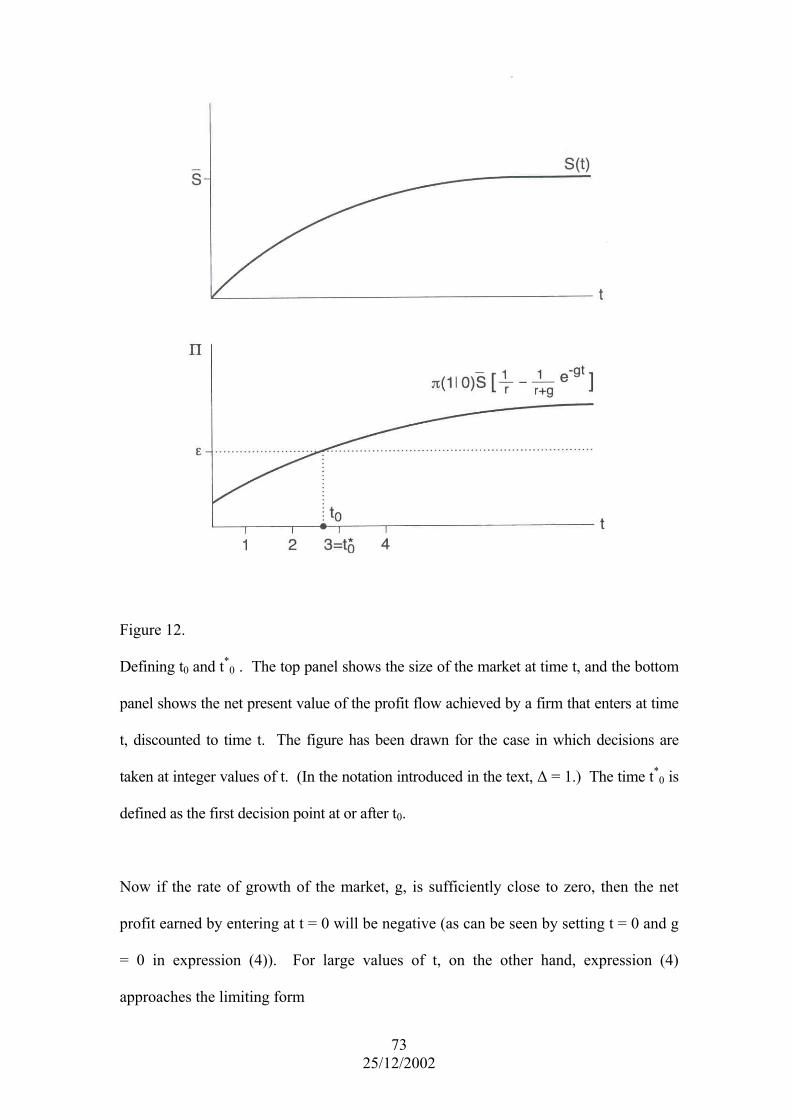
Figure 12.

Defining t0 and t*0 . The top panel shows the size of the market at time t, and the bottom

panel shows the net present value of the profit flow achieved by a firm that enters at time

t, discounted to time t. The figure has been drawn for the case in which decisions are

taken at integer values of t. (In the notation introduced in the text, ∆ = 1.) The time t*0 is

defined as the first decision point at or after t0.

Now if the rate of growth of the market, g, is sufficiently close to zero, then the net

profit earned by entering at t = 0 will be negative (as can be seen by setting t = 0 and g

= 0 in expression (4)). For large values of t, on the other hand, expression (4)

approaches the limiting form

73 25/12/2002

{ }r/S)1(e rt π+ε−−

and our assumption that the eventual size of the market, S , is large enough to support

one firm implies that this expression is (strictly) positive.

We define a time t0 by equating expression (4) to zero; and we assume g is sufficiently

small to ensure that t0 > 0. We define t*0 as the first decision point after t0 (Figure 12).

Our focus of interest lies in investigating equilibrium outcomes in the limit of ∆ → 0.

One form of equilibrium in this game, is that in which firms use pure strategies, and

where any one firm enters at t*, and all other firms choose ‘don’t enter’. It is

straightforward to show, however (Sutton (1998), Chapter 11), that there is also a unique

symmetric equilibrium in mixed strategies, in which each firm enters with the same

probability (p(n)) at every decision point . Moreover, as ∆ → 0, it turns out that

, and the probability of ‘excessive entry’ converges to zero. The outcome

generated by these strategies, in the limit ∆ → 0, is that exactly one firm enters, and each

of the N firms has a

*0tn ≥∆

0)t(p *0 →

thN1 probability of being the entrant.

Now this is a rather special example, which is introduced here simply to illustrate a

general idea: the point to note is that the outcomes arising here correspond to the set of

outcomes that can be obtained as pure strategy outcomes – but now we have a probability

weight attached to these outcomes. The key point to note, is that all potential entrants are

treated symmetrically in that they all have the same probability 1/N of being the entrant

(‘taking up the opportunity’).

74 25/12/2002

75 25/12/2002

This example can be extended to more complex settings, in which the market can support

several firms; it can also be extended to incorporate differentiated products. With these

extensions in place, the pattern of outcomes may be quite complex. For example, along

the equilibrium path of the game, it may be that the first firm to enter ‘pre-empts’ further

entry, (either permanently or temporarily). It may be that a sequence of firms enter, each

with a different number of products, these products being entered at a series of discrete

times (See Sutton (1998), Chapter 11 for examples of this kind.) Once a firm has entered

its first product, then, it is no longer symmetric with firms that have not yet entered, and it

may (and in general will) play a pure strategy in the subgame that follows its entry. But

there is one generic feature that must always hold. This relates to the set of firms that

have not yet entered. It must be the case that, at any decision point at which entry occurs,

then each of these firms has an equal probability of being selected as the entrant.

This suggests a simple nomeclature: we can think of the potential entrants as taking up

‘roles’ in the game, and we can name these roles as ‘first entrant’, ‘second entrant’ and so

on. Along the equilibrium path of the game, the firm filling a particular role (‘first

entrant’ say) may enter a higher number of (differentiated) products than a firm playing a

different (‘second entrant’) role.

Where the ‘symmetry’ comes in, is in the allocation of roles to new entrants: all potential

entrants are treated equally in role assignment. This is the key property of these

examples, and it is this property that we will carry over in the analysis which follows.

The Size Distribution Revisited

We are now in a position to re-visit the evolution of the size distribution. We begin with

the simplest setup, in which the market consists of a number of separated ‘islands’ each

big enough to support one entrant. We imagine that a game of the kind just described is

played on each island in turn. To keep things simple, we imagine that the ‘islands’ open

in some sequence over time, so the ‘time of entry’ t*0 is different in different markets.

We will want to distinguish in what follows between firms that have already taken up at

least one opportunity (‘active firms’) and firms who have not (‘potential entrants’).

In analysing this situation, we re-obtain the limiting results found above, but we do so by

modelling the entry process in a deterministic, rather than a probabilistic way. While this

may seem a less attractive way of doing things, it has a great advantage in terms of

allowing us to use a different and much more flexible method of calculation that can be

extended immediately to the case where each submarket may support many firms.

A new entrant necessarily fills the first submarket. Thereafter, new entrants capture every

m-th submarket, for some integer m ≥ 2. Figure 13 illustrates this process for the case m

= 3. It is convenient to introduce an index i to label firms, and an index k to label

submarkets, as follows: The ith entrant enters by occupying the kth sub market, where k

= 1+m(i-1). The number of firms active immediately following the opening of the kth

sub market, which we denote by Nk, equals 1 + [(k-1)/m] where [·] denotes the integer

part. Similarly, the number of firms that are active immediately following the ith firm’s

entry equals i. (If we substitute for k = 1 +m(i-1) in Nk = 1 + [(k-1)/m] we obtain Nk = I).

Since the first entrant fills the first submarket, we have 1N1 = .

76 25/12/2002

Figure 13

A benchmark case (m = 3, or p = 1/3). A new entrant captures every third sub market.

Note that the ith entrant occupies the kth sub market, where k = 1 + m(i-1). The number

of firms active immediately following the opening of the kth sub market is denoted by Ni.

Note that Nk = 1 +[ (k-1)/m].

Our focus of interest lies in the allocation of the m-1 opportunities which, in each round,

are allocated to one of the currently active firms. In the round immediately following the

arrival of the ith entrant, there are i active firms. The symmetry principle states that each

of these firms has the same probability 1/i of taking up the next opportunity.

It is convenient to introduce the notation p to represent 1/m, i.e. the fraction of

opportunities captured by new entrants. The number of submarkets that are occupied by

active firms following each new entry equals (m-1), and this can be written as (1-p)/p.

Following the entry of the ith active firm, the total number of firms active in the market

equals i, and one of these i firms fills each of the next (m-1) = (1-p)/p submarkets.

77 25/12/2002

Thereafter, the (i+1)th firm enters and each of these (i+1) firms then has an equal

probability 1/(i+1) of capturing each of the next (m-1) = (1-p)/p submarkets, conditional

on the fact that active firms capture these submarkets.

We now turn to a description of the random variable that describes the size of the ith

entrant. Since the entrant must capture one opportunity (submarket) on entering, it is

convenient to write its size, as measured by the number of submarkets it has captured, as

1 + r, where the random variable r is a sum of independent indicator variables (i.e. taking

the values 1 or 0) 39. The distribution of this sum is our focus of interest.

The p.d.f. of r converges in the limit where the number of submarkets becomes large, to a

Poisson distribution.

!re)r(f

ri

ii

λ⋅= λ− ,

where

⎥⎦⎤

⎢⎣⎡ ++

++

−=λ

N1...

1i1

i1

pp1

i (5)

The interpretation of λi is as follows: In the period immediately following its entry, firm

i is one of i firms, each of which has probability 1/i of entering each of the next (m-1)

= (1-p)/p submarkets. The first term [·] represents this contribution. Successive

contributions correspond to the periods between successive entries by firms i+1, i+2,

etc. The final term in [·] corresponds to the contribution made by the (m-1) submarkets

78 25/12/2002

39 A large literature exists on the properties of sums of indicator variables, that is, random variables that take values of 0 or 1. The most familiar example relates to the special case of Poisson variables: If y is the sum of independent random variables that are Poisson distributed with parameters λ1, λ2, … λn, respectively, then the distribution of y is Poisson with parameter λ1 + λ2 + … + λn (Kendall and Stewart 1969). Analogous results are available for sums of indicator variables. A comprehensive survey of results is provided in Barbour, Holst and Janson 1992. Further details will be found in Sutton (1998), pp. 283-4.

that open up following the arrival of the last (nth) firm in the market. Define the

constant Ri,N by writing

N,iRilnNlnN1...

1i1

i1

+−=⎥⎦⎤

⎢⎣⎡ ++

++ (6)

Clearly we have 0 < γ≤→∝ N,iN Rlim , where γ denotes Euler’s constant (≈ 0.577),

whereas for i = 1, γ=→∝ N,iN Rlim .

We now turn to the size distribution of firms, by considering the size (1+r) of a firm

drawn randomly from the final population of N firms. The variate r is now represented

by the unconditional pdf given by40

Prob (r) = Prob (r|i) · Prob (i) ∑=

N

1i

Since all firms have an equal chance of selection, Prob(i) = 1/N. It follows that the pdf of

r is given by

∑=

λ− λ⋅=

N

1i

i .!r

eN1)r(f i (7)

A direct investigation of the properties of the sum in (7) is difficult, but it is easy to

proceed if we approximate the sum by an integral, as follows.

It is clear from inspection of (5) that taking any fixed integers r and m, the total

contribution to f(r) from the first m terms in the sum in (7) tends to zero as N → ∞.

Using (6) and noting that γ≤< ∞→ N,iN Rlim0 , this implies that as N → ∞, the sum

(7) can be approximated in the limit by the integral

79 25/12/2002

40 Here we are conditioning, via the index i, which labels firms in order of entry, on the firm’s age. The intuition is that the size distribution of each age cohort in the population is Poisson, and we are summing over cohorts to get the overall size distribution.

tdr!

µ(t)e N1)r(f

τN

1

µ(t)∫ −=

where

.tNln

tNln

pp1)t(

pp1−

⎟⎠⎞

⎜⎝⎛=⎟

⎠⎞

⎜⎝⎛−

=µ

A straightforward but lengthy calculation (Sutton (1998), p. 286) leads to the result, that

as N→∞, the distribution )r(f converges to a geometric distribution viz.

,...2,1,0r,)p1(p)r(f r =−→

Recall that firm size x = 1+r, from which it follows that the p.d.f. of firm size x takes

the form

,...3,2,1x,)p1(p 1x =− −

It is helpful to approximate this geometric distribution by the corresponding exponential

distribution; and from this it is straightforward to derive the limiting Lorenz curve, which

takes the form shown in the preceding section (Sutton (1998), Chapter 10).

Extensions

The main virtue of the above setup is that it can be extended easily to the case where the

constituent game in each sub market (‘island’) is arbitrarily complex: we can have many

roles, and the roles can have different ‘sizes’ (so a firm’s size is the sum of the sizes of the

roles it occupies). In this setup, the same limiting result applies, if all roles have the same

size. If, however, different roles have different sizes, then the same reference curve still

operates, but only as a bound – the Lorenz curve must lie further from the diagonal than

the above reference curve. (Intuitively the variance in role size adds an extra contribution

80 25/12/2002

81 25/12/2002

to the degree of inequality among firms). This last point is of some interest in empirical

testing (see below).

Why Symmetry?

We have focused here on the ‘symmetry principle’, according to which all potential

entrants to each submarket (i.e. current incumbents in the market as a whole) are treated

equally. Yet in commenting on the Growth of Firms literature, we replaced Gibrat’s Law

by a weak inequality constraint, which stated that a larger incumbent firm will not have a

smaller probability of taking up the next opportunity, than will a smaller firm. The point

here, is that the reference curve was obtained, in that setting, by considering the case were

all firms had the same probability of capturing the next opportunity, independently of

their sizes. Insofar as larger firms are more likely to capture the next opportunity, the

Lorenz curve will lie beyond the reference curve. By the same token, in the present

setting, the case of symmetry corresponds to the case of minimal inequality, where the

Lorenz curve is as close as possible to the diagonal.

An analogous issue, again relating to the symmetry principle arises in respect of firm

specific differences (in efficiency, or otherwise). We have here treated all potential

entrants as being equal; if, however, some are more efficient than others ex ante, then this

will again lead to a bias towards greater ex post inequality – so that once again, the case

of symmetry is associated with the minimal degree of inequality.

A Key Idea

The above treatment achieves two goals,

82 25/12/2002

(i) it replicates what can be done in the traditional Growth of Firms setup,

through replacing Gibrat’s Law with a weak inequality constraint on the size-

growth relationship.

(ii) It shows that the result on the limiting Lorenz curve (reference curve) holds

good independently of the nature of the game within submarkets, and depends

only on the idea that we have many (approximately independent) submarkets.

The juxtaposition of these two ideas will be central in the discussion of empirical

evidence below.

One advantage of combining the ‘traditional’ treatment of this issue with the game-

theoretic model, is that it focuses attention on an alternative interpretation of what drives

the result on the limiting Lorenz curve (reference curve). What it makes clear is that, in

order to violate this result, we need to have a setting in which large firms suffer a

systematic disadvantage relative to smaller rivals, in respect of their growth prospects.

While situations of this kind exist (see below), they are rare; and so, even in markets that

do not contain ‘many independent submarkets’, we would not normally expect to see a

violation of this ‘reference curve’ result. This is important when it comes to looking at

contexts in which to test the implications (see below).

One final technical remark is in order, regarding the role of ‘independence effects’ in the

above analysis. We have worked here in terms of a setup containing many independent

submarkets. Yet it is rare in economics to encounter a market in which the submarkets

are approximately independent (for a definition of the concept of ‘approximate

independence’, see Sutton (1998) and the references cited therein.)41 It is of considerable

41 A simple illustration may be helpful: let … x-1, x0, x1, x2 … be independent random variables. Define the set of random variables θi as follows: for a fixed τ > 1, let θi be a linear combination of xi-τ, xi-τ+1, …

83 25/12/2002

relevance in the present context to note that the results developed above do not require

that the submarkets be independent, but only that they be approximately independent.

Empirical Evidence III

The above ‘bounds’ prediction has been tested using data for manufacturing industries

in the U.S. and Germany (Sutton (1998), Chapter 13). A comparison of the U.S. and

German cases is of particular interest in testing a ‘bounds’ prediction, since it is well

known that, among those countries that produce high quality Census of Manufactures

data, the average level of industrial concentration is relatively high in the U.S., and

relatively low in Germany. Hence we know that the ‘cloud’ of points in (Ck,N) space

for the U.S. will lie much farther above the diagonal than will the cloud for German

data. Yet if a ‘bounds’ approach is appropriate, then we should find that the edge of

the two clouds should lie on the predicted reference curve above. From Figure 14,

which shows the data for the US and Germany, it is clear that this is the case.

xi+ τ. Now the are approximately independent. (note that θ1 is not independent of θ2 as both depend on x1; but θi is independent of all θj, where j ≤ τ-1 or j ≥ τ+1.) This example is of particular economic interest in the context of geographically separated submarkets.

Figure 14. The top panel shows the scatter diagram of Ck against k/N for pooled data

(k=4,8 and 20) for the United States 1987, at the four-digit level. The Lorenz curve

shown on these figures is the reference curve (equation (3) of the text). The bottom

panel shows data for Germany , 1990 (k=3,6,10 and 25).

84 25/12/2002

Figure 15.

Testing proposition 10.2 for US data at the five-digit level, 1977; a scatter diagram of

C4 versus C50. The solid curve shows the lower bound Dk(C50) predicted by the theory.

The ray shown below this curve corresponds to the symmetric equilibrium in which all

firms are of equal size.

A second way of testing the prediction is by examining the induced relationship

between Ck and Cm, where m > k, as described in Sutton (1998), Chapter 10. This test

has the advantage of relying only on the (relatively easy to measure) concentration

ratios, and not on the (much more problematic) count of firm numbers. Results for this

conditional prediction are shown in Figure 15, an interesting feature of these results

appears when the residuals, C4 – C4(C50), are plotted as a histogram (Figure 16). It is

clear that the histogram is strong asymmetrical, with a sharp fall at zero, where the

bound is reached. Such a pattern of residuals can be seen, from a purely statistical

viewpoint, as a ‘fingerprint’ of the bounds representation, suggesting that on statistical

grounds along, this data would be poorly represented by a conventional ‘central

tendency’ model which predicted the ‘centre’ of the cloud of points, rather than its

lower bound.

85 25/12/2002

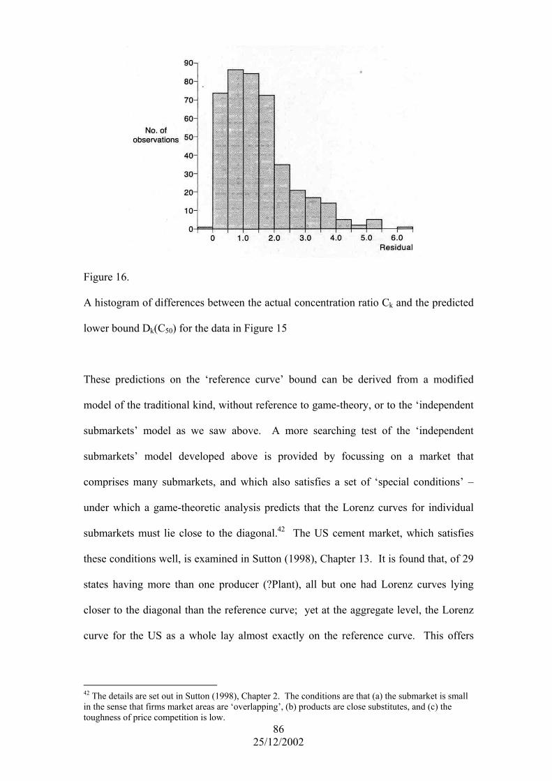
Figure 16.

A histogram of differences between the actual concentration ratio Ck and the predicted

lower bound Dk(C50) for the data in Figure 15

These predictions on the ‘reference curve’ bound can be derived from a modified

model of the traditional kind, without reference to game-theory, or to the ‘independent

submarkets’ model as we saw above. A more searching test of the ‘independent

submarkets’ model developed above is provided by focussing on a market that

comprises many submarkets, and which also satisfies a set of ‘special conditions’ –

under which a game-theoretic analysis predicts that the Lorenz curves for individual

submarkets must lie close to the diagonal.42 The US cement market, which satisfies

these conditions well, is examined in Sutton (1998), Chapter 13. It is found that, of 29

states having more than one producer (?Plant), all but one had Lorenz curves lying

closer to the diagonal than the reference curve; yet at the aggregate level, the Lorenz

curve for the US as a whole lay almost exactly on the reference curve. This offers

86 25/12/2002

42 The details are set out in Sutton (1998), Chapter 2. The conditions are that (a) the submarket is small in the sense that firms market areas are ‘overlapping’, (b) products are close substitutes, and (c) the toughness of price competition is low.

87 25/12/2002

clear support for the ‘independent submarkets’ interpretation of the results described

above, relative to this market43.

A number of recent studies have re-examined these predicted relations on the size

distribution. De Juan (1999) examines the retail banking industry in Spain, at the level

of local (urban area) submarkets (4,977 towns), and at the regional level. As in the

case of the cement market, described above, conditions in the retail banking industry

appear to satisfy the special conditions under which individual submarkets will have

Lorenz curves close to the diagonal. A question that arises here is, how large a town

can be considered as an (independent) submarket in the sense of the theory? A large

city will presumably encompass a number of local submarkets. Rather than decide a

priori on an appropriate size criterion for the definition of a submarket44, the author

sets out to ‘let the data decide’ on the threshold size of a submarket. With this in mind,

she carries out a regression analysis across all towns with population sizes in the range

1000-5000 inhabitants, distinguishing between two sets of explanatory variables:

decomposing the number of branches per town into the product of the number of

branches per submarket, and the number of submarkets per town, she postulates that

the number of branches per submarket depends on population density and the level of

per-capita income, while the number of submarkets per town depends (nonlinearly) on

the population of the town. The results of this regression analysis are used to fix a

threshold that determines a sub-set of ‘single sub market towns’. For this sub-set of

43 It should be emphasised, however, that the two ways of looking at things – in terms of the weak restriction on the size-growth relation, and in terms of the independent submarkets model, are complementary. The latter implies the former, but the former condition may hold even when the market is a single unified market. This is especially pertinent when looking at R&D intensive industries here, if we use a narrow industry definition, we can have a single (high-alpha) market; within such markets, size is an advantage rather than a disadvantage, and we would therefore expect the weak restriction on the size-growth relation to be satisfied. 44 In Sutton (1998), data at state level for the US was chosen as the size of the typical state is of the same order as the typical ‘shipping radius’ for cement plants.

88 25/12/2002

towns, she finds that 96% are ‘maximally fragmented’ (i.e. the Lorenz curve lies on the

diagonal).

The analysis is then extended to larger towns; using a map of branch locations, cluster

analysis methods are used to identify alternative ‘reasonable’ partitionings of the area

of the town into ‘local submarkets’. Examining one typical medium-size town in this

way, she finds that 71% of those local submarkets are maximally fragmented. Finally,

the analysis is extended to the level of major regions, each of which comprises many

towns; here, the Lorenz curves for each region are found to lie farther from the

diagonal than the reference curve.

Buzzacchi and Valletti (1994) examine the motor vehicle insurance industry in Italy.

Here, the institutional framework of the industry is such as to produce an

administratively determined set of submarkets: each vehicle is registered within one of

103 provinces, and owners are required to buy insurance within their own province;

moreover, over nine-tenths of premia are collected through local agents with the

province. The authors argue that the industry satisfies the special conditions for

maximal fragmentation within submarkets. At the sub market level, they find that

Lorenz curves for the 103 provinces lie almost wholly between the reference curve and

the diagonal; once we aggregate up to the national level, however, the Lorenz curve

lies farther from the diagonal than the reference curve defined by equation (3), as

predicted.

In an interesting extension of the analysis, the authors examine, for a set of 13

European countries, the conditional prediction for the lower bound to C5 as a function

89 25/12/2002

of C15; the results show that the cloud of observations lies within, but close to the

predicted lower bound.

While all the empirical tests considered so far deal with geographic submarkets, Walsh

and Whelan (2001) deals with submarkets in product space: specifically, they look at

retail market shares in carbonated soft drinks in Ireland. Within this market, they

identify 20 submarkets; and they justify this level of definition of submarkets by

reference to an estimation of cross-price elasticities, by reference to an estimated

model of demand45.

In this market, the special conditions set out above do not apply; and so the

expectation, under the theory is that the Lorenz curves for submarkets should not stand

in any special relationship to the reference curve; in fact, these submarket level Lorenz

curves lie in a widely dispersed cloud that extends from the diagonal to well beyond

the reference curve. Here, the authors make a important distinction, relative to the

theory, in distinguishing between the Lorenz curve based on a count of roles, versus

the curve based on sales data. The latter incorporates, as noted earlier, an additional

variance component associated with the dispersion in role size, and is expected to lie

farther from the diagonal than the reference curve. One nice feature of the analysis is

that the authors can follow year-to-year fluctuations in role size. It is shown that

(i) the Lorenz curve based on role size is stable from year to year and is very

close to the reference curve defined by equation (3);

45 One caveat is in order here, insofar as many of the firms involved here are foreign firms, and so it is less easy to imagine the entry process in terms of the model set out above.

(ii) the Lorenz curve based on sales data lies farther from the diagonal, and is

relatively volatile over time. (Compare figures 1 and 2, lower panels, on

pp. 28-29 of Walsh and Whelan (2001).)

A Synthesis

The two major themes explored so far relate to (a) the role of the price competition

mechanism and the escalation mechanism in placing a lower bound on C1, and (b) the

idea that inequalities in the sizes of firms within the industry (‘businesses’) will impose

a lower bound in (C1, N) space. These two constraints can be combined by treating

them as separate constraints on outcomes in (C1, N) space, as shown in Figure 17

below. (Here, the bound developed above as an equation (3) has been written as a

function of N, rather than 1/N; for details, and a further discussion see Sutton (1998)

Chapter 13).

Figure 17: Combining the constraints in (C1,N) space.

90 25/12/2002

91 25/12/2002

7. Extensions

In what follows we briefly note a few of the more important extensions of the basic

analysis set out above:

1. Learning-by-Doing Models and Network Externalities

Two special mechanisms often cited in the literature as leading to a concentrated

market structure are the Learning-by-Doing mechanism, and the Network Externality

mechanism. (See for example, Spence (1981), Fudenberg and Tirole (1983, 1985),

Cabral and Riordan (1994), Gruber (1992, 1994). It is shown in Sutton (1998),

Chapters 14 and 15 that these two mechanisms can be captured in the same simple 2-

stage game framework (in this sense, the models are isomorphic). The idea is that the

firms plays the same ‘Cournot’ game in each period, but its second period cost function

(in the Learning-by-Doing model) or the perceived quality of its product (in the

Network Externality model) is affected by its level of output (sales) in the first period.

This induces a linkage between the profit earned in the first period, and in the second.

This effect is precisely analogous to the ‘escalation mechanism’ described above; we

can think of the profit foregone in period 1 (as the firm raises its output beyond the

level that maximizes first period profit) as an ‘opportunity cost’ analogous to the fixed

cost F(u) in the ‘quality competition’ model of Section 3 above. (The details will be

found in Sutton (1998), Chapter 14).

92 25/12/2002

2. Dynamic Games

To what extent can the results of the stage game models developed above be carried

over to a ‘dynamic games’ framework, in which firms spend on fixed outlays in each

successive period, while enjoying a flow of returns in each period that reflects the

current quality and cost levels of the firm and its rivals? This is a difficult question,

which has been explored from two angles. In Sutton (1998), Chapter 13, a dynamic

game is set out in which an exogenously fixed ‘imitation lag’ T is imposed, in the

sense that if a firm raises its (R&D) spending at time t, then the resulting quality jump

occurs only at time t + T; rivals do not observe the expenditure at time t, but do

observe the quality jump at time t + T. The point of this model is to expose the nature

of the implicit assumption that is made in choosing a ‘stage-game’ framework: the

results of such a framework can be mimicked in the dynamic game set up by letting the

lag T become large. In other words, the stage game framework implicitly excludes

certain kinds of equilibria that may arise in dynamic games. It is therefore of particular

interest to ask: to what extent might (‘new’) forms of equilibria appear in an

unrestricted dynamic game, that could undermine the non-convergence results

developed above? The issue of interest turns on the appearance of ‘underinvestment

equilibria’, as described in Sutton (1998). Here the idea is that firms ‘underspend’ on

R&D, because rivals strategies prescribe that any rise in R&D spending by firm 1 at

time t will result in a rise by its rivals at period t + 1. It is shown in Nocke (1999) that

this kind of equilibrium can indeed appear in a suitably specified dynamic game; that it

will be associated with a reduction in the lower bound to concentration; but the ‘non

convergence theorem’ developed above in the stage-game setting continues to hold

good in the dynamic game.

93 25/12/2002

9. Perspectives

Related Literatures

In the traditional I.O. literature, following Bain (1954), considerable attention was

devoted to the notion that high levels of concentration could be attributed to “barriers

to entry”. One problem with this concept is that it was used by different authors in

different ways; more seriously the ‘barriers’ included (properly) certain features of the

underlying technology that were outside firms’ control, and (improperly) certain

features such as R&D outlays that should be modelled as choice variables whose

levels reflect the interplay of firms’ decisions. All the models presented above are

‘free entry’ models, in the sense that any firm is free to enter by paying an exogenous

‘setup cost’ while deciding on how much additional fixed and sunk outlays to incur.

For a discussion of the relationship between this approach and the ‘Bain paradigm’, see

Sutton (1991), Chapter 1, section 1.4.

A closely related issue relates to the alleged link between concentration and

profitability. For a critique of the literature on this issue see Schmalensee’s (1991)

contribution to volume II of this handbook; and for the implications for the relationship

arising from the models discussed above, see Sutton (2002).

There are three modern literatures that are related to the present approach:

a) The Schumpeterian literature on market structure emphasises the use of limited

rationality models, and seeks to characterize the relationship between the nature

of the underlying technology and the form of market structure. The Bounds

94 25/12/2002

approach, in using a ‘class of models’ formulation, involves a relaxation of

strict rationality, as discussed in Sutton (1998). The relationship between this

approach and that of the Schumpeterian school has been explored recently by

Marsili (2000); see also the comments in Sutton (1998), Chapter 1.

b) The literature on ‘market size and firm numbers’ pioneered by Bresnahan and

Reiss (1990, 1991) and Berry (1992) is very closely related to the Bounds

approach; for a discussion, see Sutton (1986).

c) A number of recent ‘single industry studies’ have investigated two basic

mechanisms described above; see Greenstein and Bresnahan (1999) on the

history of the computer industry and Matraves (1999) on the structure of the

pharmaceuticals industry.

d) The approach to modelling industry equilibrium as a dynamic game introduced

by Arial Pakes and his several coauthors (see in particular Ericson and Pakes

(1995)) provides inter alia an alternative vehicle within which to explore the

evolution of structure in a dynamic setting different to that described in Section

7 above. The examples of these models in the published literature to date

employ profit functions that, in the language of the present review, have a value

of alpha equal to zero. In some recent work, however, Hole (1997) has

introduced the simple ‘Cournot model with quality’ example of Section II

above into the Pakes-Ericson framework. The results show that in a 3-firm

example, as the parameter β falls (so that alpha rises), the outcomes cluster in a

region in which two firms account for an arbitrarily high fraction of sales.

95 25/12/2002

These results provide an analog of the ‘non-convergence theorem’ in a

stochastic, dynamic setting.

e) The discussion of the size distribution was developed above by reference to a

market comprising many (approximately) independent submarkets; no

restriction was placed, however, on the distribution of sub-market sizes.

Indeed, it would appear to be difficult to justify any particular restriction of the

way in which the ‘typical’ market is divided into submarkets. Equivalently, it

would seem to be difficult to justify any particular assumption for the way in

which the activities on the ‘typical; firm are broken down into its activities in

different (sub) markets. This questions is of some interest, however, in that it

lies at the heart of the question: in what way is the variance of firms’ growth

rates related to their sizes? It has been shown by Stanley et al (1996) that there

is a strikingly sharp relationship between firm size and the variance of growth

rates; this relationship takes the form of a power law with a ‘low’ exponent.46

Econometric Methods

The methods of Bounds estimation referred to above are described in Sutton (1991),

Chapter 5, following Smith (1984, 1988). An alternative method which has some

attractive features from a theoretical viewpoint, but which has less power than that of

the maximum likelihood methods described by Smith, is that of Mann, Scheuer and

Fertig (1973); see Sutton (1998) for details). Both these approaches are sensitive to the

presence of outliers, and for this reason some authors, including Lyons, Matraves and

Moffat (2000), favour alternative methods that have proved useful in the estimation of 46 A candidate explanation for this observation is given by Sutton (2001), by reference to the notion that each firms consists of a number of approximately independent business, the distribution of sizes of these businesses being modelled by reference to the partitions of integers.

frontier production functions. A very simple method of attack is provided by quantile

regression methods, which Giorgetti (2001) has recently applied, in combination with

maximum likelihood methods, to examine the lower bound to concentration for a

sample of Italian manufacturing industries.47

Caveats and Technicalities

One procedure that has become common in the literature, following Sutton (1991), is

to treat industries as falling into two discrete groups, those in which advertising and

R&D are unimportant, and those in which they play a substantial role. Schmalensee

(1992), in reviewing Sutton (1991), referred to these as Type I and II industries

respectively.

In tandem with this nomenclature, it has become common to identify these two groups

of industries as being represented by the ‘exogenous sunk cost’ model; and the

‘endogenous sunk cost model’ respectively. This leads to some confusion, since it

begs the question: are not all sunk costs endogenous? (A firm can decide, for example,

on its level of plant capacity, or its number of manufacturing plants). While it is

helpful in empirical testing to split the sample into two groups, it is worth noting that it

is more appropriate at the theoretical level to note that the appropriate ‘general’ model

is one of ‘endogenous sunk costs’; and that the ‘exogenous sunk cost model’ is just a

simplified representation of a special limiting case of the endogenous sunk cost model,

corresponding to the limit ∞→β as, noted in the text. What matters to the level of

96 25/12/2002

47 Georgetti’s study focuses on the issues surrounding apparent outlines. It is not feasible to control for the structure of submarkets in his dataset and Georgetti finds, for example, that the ‘Toys’ industry features high R&D spending but low concentration. The high R&D spending appears to be largely associated with the relatively small segment of computer games. Thus on a (C, S) plot, Toys appear as an ‘outlier’. This underlines the importance of controlling for h, as discussed above.

97 25/12/2002

concentration is not the ‘endogeneity of sunk costs’, but the value of α, which may be

zero either because β is high, or because α is low.

One technical issue is worth noting, in respect of the way in which alpha was defined

above. We defined a pair of numbers k and a(k), which describes the ‘size of jump’

made by a high-spending deviant, and the gross profit which it thereby earns. It is

analytically convenient to proceed in two steps, by first seeking a pair k, a(k) which

hold for all configurations (n-tuples of quality). The number α is then defined by

taking the supremum over k. This begs the question: what if, as the quality level(s) of

firms rises, we could always find a suitable pair k, a(k), but only by choosing a

different (larger) value of k, as quality levels increase?

It is possible to construct an example of the kind, in which there is a lower bound to

concentration which is strictly positive – even though there is no single pair k, a (k)

with a (k) > 0 as defined above. This indicates that there is a (slight) restriction

introduced in defining alpha in the manner used above.48

10. Controversies I

The appeal of ‘Increasing Returns’ as a ‘general’ explanation for observed levels of

market concentration is highly problematic, since different authors use this term in

different ways. At one extreme, the term is used in its classic sense, to refer to the

idea that the average cost curve is downward sloping. This feature holds good in all

the models described above, including those cases where alpha equals zero, and the

lower bound to concentration falls to zero in large markets. It follows that an appeal

48 Which is essentially a matter of the order in which the two limits are taken.

to ‘increasing returns’ in this sense does not provide an explanation for high levels of

concentration in large markets.

At the other extreme, the term has been used to refer to the appearance of features such

as ‘network externalities’ in the context of ‘dynamic’ models. Here, the problem is

that there are many models in which equilibrium levels of concentration are ‘high’, but

it is not clear that any uniform definition of ‘increasing returns’ is available which

applied uniformly to all these cases. For a fuller discussion of these issues, see Sutton

(1998).

A second area of controversy relates to the distinction between Fixed and Sunk Costs.

It has been suggested that many of the features of the models described above should

carry over to a setting in which costs are fixed but not sunk (Schmalensee, (1992),

Davies and Lyons, (1996). it is not clear that any general claim of this kind can be

supported by reference to a formal analysis, so long as we identify the ‘2-sdtage’ (or

multistage) game framework with the ‘sunk cost’ interpretation. (For a discussion at

this point ,see Sutton (1991), and for a response, see Schmalensee (1992)). If costs are

fixed but not sunk, it seems appropriate to model firms’ actions by reference to a 1-

shot game in which firms take simultaneous decisions on entry and prices. This

captures the notion introduced in the Contestability literature by Basnnol, Paznor and

Willig, (1982). It is crucial to results of this literature that sunk costs be exactly zero.

The Bertrand example of Section 2 illustrates how an arbitrarily small departure from

this assumption can change the qualitative features of equilibrium outcomes.49 In

practice, it seems to be extremely difficult to find any industry in which sunk costs are

98 25/12/2002

49 If the sunk cost of entry is exactly zero in the Bertrand example, then any number of firms will enter, and price will coincide with marginal cost.

2n ≥

99 25/12/2002

zero; for a recent attempt to quantify the extent to which fixed outlays are sunk, see

Asplund (2000).

11. Controversies II

Critics of the Bounds approach have focussed largely on a series of inter-related points,

all of which are motivated by a concern that the analysis is not based on a ‘completely

specified’ model of the standard kind. The most extreme version of this criticism holds

that the only ‘proper’ type of model is a fully specified model of the standard kind;

while this view is common in economics, it is not widely held in the natural sciences.

(For a discussion of Bounds relationships in thermodynamics, see Sutton (2000)

Chapter 3). Fisher (2002), for example, notes the extreme view, but argues that the

Bounds Approach represents a reasonable compromise approach in the face of

intractable measurement problems. At the opposite extreme, Christ (2002) argues that

the Bounds Approach fits naturally within the standard paradigm of econometrics, in

the sense that it can be thought of as a standard model with one-sided error

distribution.

A related line of argument is developed by Renault (2002), who argues that the

problem posed by ‘unobservables’ is a serious one, but who favours a different

approach, in which ‘latent variables’ are introduced into an econometric model in order

to deal with non-measurable factors. Renault notes that this approach, which is

currently attracting attention in microeconomics, offers a potential advantage over the

Bounds Approach insofar as the estimation of a ‘complete’ model incorporating latent

variables might allow us to develop standard ‘comparative statics’ results regarding the

100 25/12/2002

effect of a change in some exogenous parameter.50 This is an interesting suggestion,

but in the absence of any candidate theory of this type, its merits are hard to evaluate.

It is worth noting, however, that there is one feature special to the study of market

structure that makes the Bounds Approach a natural representation: this relates to the

fact that when we write down particular fully specified game-theoretic models, they

usually contain multiple equilibria, some of which may lie ‘on the bounds’ while

others lie inside it. A shift in some exogenous parameter may affect market structure if

the original configuration is on (or close to) the bound, but have no effect on it

otherwise. This feature seems to be intrinsic to any game-theoretic model of market

structure, and if a ‘latent variable’ representation was devised which had the feature, it

might be difficult to distinguish the approach from a Bounds Approach. (For a fuller

discussion of this controversy, see Renault (2002), Sutton, (2002)).

The Bounds Approach is best seen, as noted in the introduction, as a complement to

‘single industry studies’, and not as a competitor to the approach (for a fuller

exploration of this point, see Sutton (1997)). What it seeks to do is to isolate and

characterise those few competitive mechanisms that operate in a robust way across the

general run of industries. This aim was central to the I.O. literature from the 1950s to

the late ‘70s, and it has become increasingly relevant as ideas from I.O. have been

exported to fields such as International Trade and Growth Theory. As new models

using ideas from I.O. have proliferated in these fields, it has become apparent that most

results are quite fragile to the details of the model used, and it is often difficult to

defend one model over another on a priori grounds. Moreover, it may be difficult in

practice to ‘let the data decide’ between alternative specifications, as model selection

exercises may not yield any clear-cut results. Under the circumstances, it seems

50 Comparative statics results within the Bounds Approach are confined to examining the impact of a shift in some exogenous parameter on the lower bound. This means that testing such results requires in practice that we look to occasional ‘natural experiments’ that involve a large shift in the bound.

101 25/12/2002

reasonable to proceed in a two-step fashion. The Bounds Approach allows us to begin

by developing a limited menu of results while appealing to some general features of

the markets in question, leaving open the question of whether some fuller specification

may be justified which leads to sharper predictions.

APPENDIX A

Some Technical Examples

1. The Cournot Example

The profit of firm i in the second stage subgame is

(p-c)xi = (S/Σxj -c)xi (1.1)

Differentiating this expression w.r.t. xi we obtain the first order condition,

( ) 0cxSx

xS

ji2

j

=−Σ

+⋅Σ

− (1.2)

Summing equation (2) over i, and writing Σxj as X, we obtain

-SX + NSX – NcX2 = 0 (1.3)

whence N

1NcSXx j

−=≡Σ (1.4)

It follows from (1.2), (1.4) that all the xi are equal, whence xi = X/N, whence

2Nfor 1N

11cp andN

1NcSx 2i ≥

⎭⎬⎫

⎩⎨⎧

−+=

−= (1.5)

Substituting(1.4),(1.5) into (1.1) and rearranging, it follows that the profit of firm

at equilibrium equals S/N2.

102 25/12/2002

2. The Cournot Model with Quality

The profit function may be derived as follows. The profit of firm i is

cx - xu = cx - xp =

iii

iiii

λπ (2.1)

where (2.2) )xuS/( = jjj

Σλ

To ease notation it is useful to express the first order condition in terms of λ. With this in

mind, note that

λλ

ΣΣΣ2i

jjj

2i

jjjijj

j

2i S

u - = )xu(

Su - = )xu(dxd

)xu(S - =

dxd (2.3)

Now the first order condition is obtained by differentiating (2.1), viz.

0 = c - dxd

xu + u = dxd

iiii

i

i λλπ

On substituting for λ and dxd

i

λ , from (2.2) and (2.3), and rearranging, this becomes

u1cS - S = xu

i2ii

λλ (2.4)

Summing over all products, we have,

)u/(1 cS - NS = xu jj

2jjj

ΣΣ λλ

103 25/12/2002

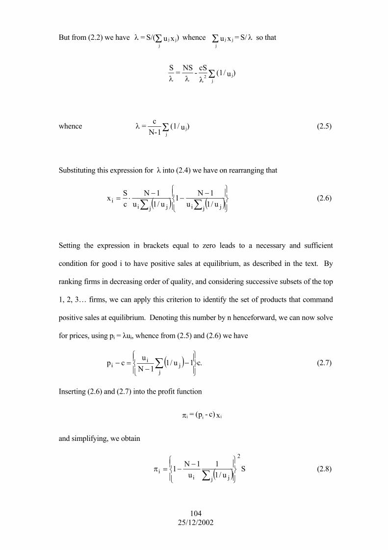
But from (2.2) we have whence )xuS/( = jjj

Σλ λΣ S/ = xu jjj

so that

)u/(1 cS - NS = Sj

j2 Σλλλ

whence )u/(1 1N-

c = jj

Σλ (2.5)

Substituting this expression for λ into (2.4) we have on rearranging that

( ) ( )⎪⎭⎪⎬⎫

⎪⎩

⎪⎨⎧ −

−−

⋅=∑∑ j jij ji

i u/1u1N1

u/1u1N

cSx (2.6)

Setting the expression in brackets equal to zero leads to a necessary and sufficient

condition for good i to have positive sales at equilibrium, as described in the text. By

ranking firms in decreasing order of quality, and considering successive subsets of the top

1, 2, 3… firms, we can apply this criterion to identify the set of products that command

positive sales at equilibrium. Denoting this number by n henceforward, we can now solve

for prices, using pi = λui, whence from (2.5) and (2.6) we have

( ) .c1u/11N

ucp

jj

ii

⎪⎭

⎪⎬⎫

⎪⎩

⎪⎨⎧

−−

=− ∑ (2.7)

Inserting (2.6) and (2.7) into the profit function

xc) - p( = iiiπ

and simplifying, we obtain

( ) Su/1

1u

1N1

2

j jii

⎪⎭

⎪⎬⎫

⎪⎩

⎪⎨⎧ −

−=π∑

(2.8)

104 25/12/2002

3. The Cournot Model with Cost Differences

In what follows, all variables relate to period 2. To ease notation, we avoid introducing

time subscripts. Firm i's output level is written as xi, and its marginal cost level as ci.

Firm i chooses xi to maximize iii )xc(pSπ −= , where

x S/ = p jj

Σ

The first order condition is

0 = c - x

)x(S - p =

c - dxdp

x + p = dxdS

ii2j

j

ii

ii

i

⋅

π

Σ

whence

c pfor S

)x(

)c - (p = x i

2j

jii ≥⋅

Σ (3.1)

Summing over all firms, we have

S

xcxN

S

xcNpx

2

jj

jj

jj

2

jj

jj

jj

⎟⎟⎠

⎞⎜⎜⎝

⎛

⎟⎟⎠

⎞⎜⎜⎝

⎛−=

⎟⎟⎠

⎞⎜⎜⎝

⎛

⋅⎟⎟⎠

⎞⎜⎜⎝

⎛−=

∑∑∑

∑∑∑

whence

( )∑∑ −

=

jjj

j cS1Nx (3.2)

105 25/12/2002

It follows that

1N

c

xSp j

j

jj −

==∑

∑ (3.3)

and, using (3.1),

S c1)(N- )c - (p = xj

j

2

ii ⋅⎥⎥⎥

⎦

⎤

⎢⎢⎢

⎣

⎡

⋅Σ

whence

Sc1N- )c - (p = x)c - (p = S

jj

2

2iiii

⎥⎥⎥

⎦

⎤

⎢⎢⎢

⎣

⎡

πΣ

But from (2.3),

1N

c

cp jj

i −=−

∑

whence

2),/(NccforSc

c1)(N1

Sc

1Nc1N

cSπ

ijji

2

jj

i

2

jj

2

ij

j

i

−⎟⎟⎟

⎠

⎞

⎜⎜⎜

⎝

⎛≤

⎪⎪⎭

⎪⎪⎬

⎫

⎪⎪⎩

⎪⎪⎨

⎧

−−=

⎥⎥⎥⎥

⎦

⎤

⎢⎢⎢⎢

⎣

⎡−

⎥⎥⎥⎥

⎦

⎤

⎢⎢⎢⎢

⎣

⎡

−−

=

∑∑

∑∑

≠

(3.4)

106 25/12/2002

APPENDIX B

Proving the Ancillary Theorem

The intuition underlying the proof of the ancillary theorem can be seen by comparing

Figure 6 of the text with Figure A1 below. The theorem is established by showing that

if R&D intensity is sufficiently high, then the entry of low-quality products can

destabilise the configuration. Denote the quality offered by some reference firm as u~ ,

and note that the fixed outlay required to product a product of quality u~u~k < is kβ

times that required for a product of quality u~ ; and if the product of quality u~ covers

it’s fixed outlays, then for β sufficiently large, entry at quality u~k is profitable. We

can see this in the figure by noting that the relative cost schedule for 1β lies below the

point d) ,(γ .

Figure A1. The cost ratio , for three values of β, where β3 ¸ β2 = β* > β1.

107 25/12/2002

108 25/12/2002

References

Asplund, M. (2000), “What Fraction of a Capital Investment is Sunk Costs?” Journal

of Industrial Economics, vol. 48, pp. 287-304.

Bain, J. S., (1956), Barriers to New Competition, Cambridge MA: Harvard University

Press.

Barbour, A. D., L. Holst, and S. Janson, (1992), Poisson Approximation, Oxford:

Clarendon Press.

Baumol, W. J., J, C. Panzar, and R. D. Willig, (1982), Contestable Markets and the

Theory of Industry Structure, San Diego: Harcourt Brace Jovanovich.

Bell, M. and K. Pavitt, (1993), “Technological Accumulation and Industrial Growth:

Contrasts Between Developed and Developing Countries,” Industrial and Corporate

Change, vol. 2, pp. 157-210.

Berry, S., (1992), “Estimation of a Model of Entry in the Airline Industry,”

Econometrica, vol. 60, pp. 889-917.

Blair, J. M. (1972), Economic Concentration: Structure, Behaviour, and Public Policy.

In New York: Harcourt, Brace, Jovanovich.

Bresnahan, T. F. and S. Greenstein (1999), “Technological Competition and the

Structure of the Computer Industry,” Journal of Industrial Economics, vol. 47, pp. 1-

40.

Bresnahan, T. F. and P. C. Reiss, (1990), “Entry in Monopoly Markets,” Review of

Economics Studies, vol. 57, pp. 531-553.

Bresnahan, T. F. and P. C. Reiss, (1990), “Do Entry Conditions Vary Across

Markets?”, Brookings Paper on Economic Activity, vol. 3, pp. 833-881.

109 25/12/2002

Buzzacchi, L. and Valletti, T., (1999), “Firm Size Distribution: Testing the

‘Independent Submarkets Model’ in the Italian Motor Insurance Industry,” Economics

of Industry Discussion Paper No. EI/24, STICERD, London School of Economics and

Political Science.

Cabral, L. and M. Riordan, (1994), “The Learning Curve, Market Dominance and

Predatory Pricing,” Econometrica 62, pp. 1115-1140.

Caves, R. E. (1986), “Information Structures of Product Markets,” Economic Enquiry,

vol. 24, pp. 195-212.

Christ, C. F., (2001), “Sutton on Marshalls’ Tendencies: A Comment,” Economics and

Philosophy, forthcoming.

Cohen, W. M. and R. C. Levin, (1989), Innovation and Market Structure. In

Handbook of Industrial Organisation, Vol. 2, edited by R. Schmalensee and R. Willig.

Amsterdam: North Holland.

Davies, S. W. and B. R. Lyons, (1996), Industrial Organisation in the European Union:

Structure, Strategy and the Competitive Mechanism, Oxford: Oxford University Press.

De Juan, R., (1999), “The Independent Submarkets Model: An Application to the

Spanish Retail Banking Market,” paper presented at the Economics of Market

Structure Conference, May 1999.

Deneckere, R. and C. Davidson (1985), “Incentives to Form Coalitions with Bertrand

Competition,” Rand Journal of Economics, 16:473-486.

Dixit, A.K. and J.E. Stiglitz (1977), “Monopolistic Competition and Optimum Product

Diversity,” American Economic Review, 67:297-308.

Ericson, R. and A. Pakes, (1995), “Markov-Perfect Industry Dynamics: A Framework

for Industry Dynamics,” Review of Economic Studies, 62, pp. 53-82.

110 25/12/2002

Fisher, F. M. (2001), “Marshall’s Tendencies, Well-Grounded Theory and

Aggregation,” Economics and Philosophy, forthcoming.

Fisher, F. M. (1989), “Games Economists Play: A Noncooperative View,” Rand

Journal of Economics, 20:113-124.

Fudenberg, D. and J. Tirole, (1983), “Learning-by-Doing and Market Peformance,”

Bell Journal of Economics, 14, pp. 522-530.

Fudenberg, D. and J. Tirole, (1985), “Preemption and Rent Equalization in the

Adoption of New Technology,” Review of Economic Studies, 52, pp. 383-402.

Giorgetti, M. L. (2001), “Quantile Regression in Lower Bound Estimation”, STICERD

Discussion Paper EI/29, London School of Economics.

Gibrat, R., (1931), Les Inégalités Économiques. Applications: Aux Inégalités des R à

la Concentration des Enterprises, Aux Populations des Villes, Statistique Familles etc.,

d’ une Loi Nouvelle: La Loi de l’ Effet Proportionnel. Paris: Library Rescueil Sirey.

Gruber, H., (1992), “Persistence of Leadership in Product Innovation,” Journal of

Industrial Economics, 40: pp. 359-375.

Gruber, H., (1994), Learning and Strategic Produce Innovation: Theory and Evidence

from the Semiconductor Industry, London: North-Holland.

Harsanyi, J. C. and R. Selten, (1988), A General Theory of Equilibrium Selection in

Games, Cambridge, MA: MIT Press.

Hart, P.E. and S.J. Prais (1956), “The Analysis of Business Concentration: A Statistical

Approach,” Journal of the Royal Statistical Society (series A) 119:150.

Hole, A., (1997), Dynamic Non-Price Strategy and Competition: Models of R&D,

Advertising and Location, unpublished Ph.D. thesis, University of London.

111 25/12/2002

Hoover, K. D., (2001), “Sutton’s Critique of Econometrics,” Economics and

Philosophy, forthcoming.

Ijiri, Y. and H. Simon, (1964), “Business Firm Growth and Size,” American Economic

Review 54: pp. 77-89.

Ijiri, Y. and H. Simon, (1977), Skew Distributions and the Sizes of Business Firms,

Amsterdam: North-Holland.

Kendall, M. G. and A. Stewart, (1969), The Advanced Theory of Statistics: Volume I,

Distribution Theory, London: Charles Griffin and Company.

Lyons, B.R., Matraves, C. and Moffat, P, (2001), “Industrial Concentration and Market

Integration in the European Union,” Economica, vol. 68(269), pp. 1-26.

Lyons, B.R. and Matraves, C., (1996), “Industrial Concentration,” in Industrial

Organisation in the European Union: Structure, Strategy and the Competitive

Mechanism, S.W. Davies and B.R. Lyons et al. (eds), Oxford: Oxford University

Press.

Mann, N., E. Scheuer, and K. Fertig, (1973), “A New Goodness-of-Fit Test for the

Two-Parameter Weibull or Extreme-Value Distribution with Unknown Parameters,”

Communications in Statistics 2(5): pp. 383-400.

Marin, P and Siotis, G., (2001), “Innovation and Market Structure: An Empirical

Evaluation of the ‘Bounds approach’ in the Chemical Industry,” working paper,

Universidad Carlos III de Madrid and CEPR.

Matraves, C. (1999), “Market Structure, R&D and Advertising in the Pharmaceutical

Industry,” Journal of Industrial Economics, vol. 47, pp. 145-168.

Morgan, M. S. (2001), “How Models Help Economists to Know. Commentary on

John Sutton’s Marshall’s Tendencies: What Can Economists Know,” Economics and

Philosophy, forthcoming.

112 25/12/2002

Nelson, S. and D. Winter, (1982), An Evolutionary Theory of Economic Change,

Cambridge, MA: Harvard University Press.

Nocke, V., (1998), “Underinvestment and Market Structure,” STICERD Working

Paper E1/22, London School of Economics.

Pelzman, S. (1991), “The Handbook of Industrial Organisation: A Review Article,”

Journal of Political Economy, 99:201-217.

Renault, E., (2001), “Sutton on Marshall’s Tendencies: A Comment,” Economics and

Philosophy, forthcoming.

Robinson, W. and Chiang, J., (1996), “Are Sutton’s Predictions Robust?: Empirical

Insights into Advertising, R&D and Concentration,” Journal of Industrial Economics,

vol. 44(4), pp. 389-408.

Scherer, F. M. (2000), ‘Professor Sutton’s “Technology and Market Structure,”’

Journal of Industrial Economics, vol. 48, pp. 215-223.

Scherer, F. M. (1997), International High-Technology Competition, Cambridge MA:

Harvard University Press.

Schmalensee, R., (1992), “Sunk Costs and Market Structure: A Review Article,”

Journal of Industrial Economics 40: pp. 125-133.

Shaked, A. and J. Sutton (1987), “Product Differentiation and Industrial Structure,”

Journal of Industrial Economics, 36:131-146.

Smith, R. L., (1994), “Nonregular Regression,” Biometrika, vol. 81, pp. 173-183.

Shubik, M. and R. Levitan (1980), Market Structure and Behavior, Cambridge, MA:

Harvard University Press.

Smith, R. L. (1985), “Maximum Likelihood Estimation in a Class of Non-regular

Cases,” Biometrika 72: 67-90.

113 25/12/2002

Smith, R. L. (1988), “Extreme Value Theory for Dependent Sequences via the Stein-

Chen Method of Poisson Approximations,” Stochastic Processes and the ir

Applications 30: pp. 317-327.

Spence, A. M. (1981), “The Learning Curve and Competition,” Bell Journal of

Economics, 12, pp. 49-70.

Stanley, M. R., L. A. Nunes Amaral, S. V. Buldyrev, S. Harlin, H. Leschorn, P. Maass,

M. A. Salinger, and H. E. Stanley, (1996), “Scaling Behaviour in the Growth of

Companies,” Nature, vol. 319, 29, pp. 804-806.

Sutton, J. (2002), “Market Structure and Performance,” in International Encyclopaedia

of the Social Sciences, in press.

Sutton, J., (1991), Sunk Costs and Market Structure, Cambridge, MA: MIT Press.

Sutton, J. (1997a), Game Theoretic Models of Market Structure. In Advances in

Economics and Econometrics, edited by D. Kreps and K. Wallis. (Proceedings of the

World Congress of the Econometric Society, Tokyo 1995). Cambridge: Cambridge

University Press, pp. 66-86.

Sutton, J. (1997b), “Gibrat’s Legacy.” Journal of Economics Literature 35, pp. 40-59.

Sutton, J., (1998), Technology and Market Structure, Cambridge, MA: MIT Press.

Sutton, J. (2001), “Rich Trades: Industrial Development Revisited”, (Keynes Lecture,

2000), Proceedings of the British Academy, 2001, pp. forthcoming.

Sutton, J., (2001), “The Variance of Firm Growth Rates: The Scaling Puzzle,” STICERD

Discussion Paper EI.27, London School of Economics.

Symeonides, G. (2000), “Price Competition and Market Structure: The Impact of

Restrictive Practices Legislation on Concentration in the U.K.,” Journal of Industrial

Economics, 48, pp. 1-26.

114 25/12/2002

Symeonides, G. (2001), The Effects of Competition: Cartel Policy and the Evolution of

Strategy and Structure in British Industry, Cambridge MA: MIT Press.

Tirole, J (1990), Theory of Industrial Organisation, Cambridge, MA: MIT Press.

Walsh, P. P. and Whelan, C. (2001), “The Role of Taste Niches in Modelling Market

Structure: An Application to Carbonated Soft Drinks,” working paper, Department of

Economics, Trinity College, Dublin.