General rights Copyright and moral rights for the publications made accessible in the public portal are retained by the authors and/or other copyright owners and it is a condition of accessing publications that users recognise and abide by the legal requirements associated with these rights.

Users may download and print one copy of any publication from the public portal for the purpose of private study or research.

You may not further distribute the material or use it for any profit-making activity or commercial gain

You may freely distribute the URL identifying the publication in the public portal If you believe that this document breaches copyright please contact us providing details, and we will remove access to the work immediately and investigate your claim.

Downloaded from orbit.dtu.dk on: May 17, 2020

Market Integration of HVDC Lines: internalizing HVDC losses in market clearing

Tosatto, Andrea; Weckesser, Johannes Tilman Gabriel; Chatzivasileiadis, Spyros

Published in:I E E E Transactions on Power Systems

Link to article, DOI:10.1109/TPWRS.2019.2932184

Publication date:2019

Document VersionPeer reviewed version

Link back to DTU Orbit

Citation (APA):Tosatto, A., Weckesser, J. T. G., & Chatzivasileiadis, S. (2019). Market Integration of HVDC Lines: internalizingHVDC losses in market clearing. I E E E Transactions on Power Systems, 35(1), 451 - 461.https://doi.org/10.1109/TPWRS.2019.2932184

0885-8950 (c) 2019 IEEE. Personal use is permitted, but republication/redistribution requires IEEE permission. See http://www.ieee.org/publications_standards/publications/rights/index.html for more information.

This article has been accepted for publication in a future issue of this journal, but has not been fully edited. Content may change prior to final publication. Citation information: DOI 10.1109/TPWRS.2019.2932184, IEEETransactions on Power Systems

1

Market Integration of HVDC Lines: internalizingHVDC losses in market clearing

Andrea Tosatto, Student Member, IEEE, Tilman Weckesser, Member, IEEE,and Spyros Chatzivasileiadis, Senior Member, IEEE

Abstract—Moving towards regional Supergrids, an increasingnumber of interconnections are formed by High Voltage DirectCurrent (HVDC) lines. Currently, in most regions, HVDC lossesare not considered in market operations, resulting in additionalcosts for Transmission System Operators (TSOs). Nordic TSOshave proposed the introduction of HVDC loss factors in themarket clearing algorithm, to account for the cost of losses andavoid HVDC flows between zones with zero price difference.In this paper, we introduce a rigorous framework to assess theintroduction of loss factors, in particular HVDC loss factors,in nodal and zonal pricing markets. First, we focus on theidentification of an appropriate loss factor. We propose andcompare three different models: constant, linear, and piecewiselinear. Second, we introduce formulations to include losses inmarket clearing algorithms. Carrying numerical tests for a wholeyear, we find that accounting only for HVDC or AC lossesmay lead to lower social welfare for a non-negligible amountof time. To counter this, this paper introduces a framework forincluding both AC and HVDC losses in a zonal or nodal pricingenvironment. We show both theoretically and through simulationsthat such a framework is guaranteed to increase social welfare.

Index Terms—Electricity Markets, HVDC Losses, HVDCTransmission, Internal European Electricity Market, Loss Fac-tors, Market Operation, Power Losses, Zonal Pricing.

I. INTRODUCTION

W ITH the progress made in the field of power electronicsin the past decades, High Voltage Direct Current

(HVDC) lines are now considered an attractive alternative toAC lines. Indeed, compared to AC, the transmission of powerin the DC form presents several benefits, such as lower powerlosses beyond a certain distance, possibility of connectingasynchronous areas, full controllability of the power flows,no need of reactive power compensation, and others [1]–[3].All these features make HVDC lines particularly convenient inthose applications where bulk power has to be transmitted overlong distances. Consequently, contrary to AC interconnections,which usually span only a few hundred meters, HVDC inter-connectors are often hundreds of kilometers long. Thus, whenconsidering the operation of such long HVDC lines, the costof thermal losses becomes non-negligible and the question thatarises is: who should bear these costs?

Ideally, the operation costs of transmission systems shouldbe covered by generating companies and consumers through

A. Tosatto and S. Chatzivasileiadis are with the Technical Universityof Denmark, Department of Electrical Engineering, Kgs. Lyngby, Denmark(emails: {antosat,spchatz}@elektro.dtu.dk). T. Weckesser is with Dansk En-ergi, Frederiksberg C, Denmark (email: twe@danskenergi.dk). This work issupported by the multiDC project, funded by Innovation Fund Denmark, GrantAgreement No. 6154-00020B.

Under construnction

Operative

Fig. 1. HVDC interconnectors in Europe [4].

the market mechanisms. In the US, for example, CAISO andPJM Interconnection LLC include in the energy price themarginal cost of losses using Marginal Loss Sensitivity Factors(MLFs), which show the marginal increase in system lossesdue to a marginal increase in power injections at a specificlocation [5], [6]. In Australia, losses on interconnectors arecalculated using inter-zonal loss factors and, in a similar way,market participants within a bidding zone are charged basedon intra-zonal loss factors [7], considering losses occurringbetween the Regional Reference Node and their point ofconnection.

In Europe, the Price Coupling of Regions (PCR) projectaims at coupling twenty-five different countries whose elec-tricity markets are operated by eight Power Exchanges [8].To avoid excessive complexity, market operators use a sim-plified model [9] for determining power exchanges betweendifferent regions. Although losses on interconnectors couldbe considered, for the majority this is not done. As a result,the revenues of the Transmission System Operators (TSOs)through the market are insufficient to cover the extra costs oflosses; grid tariffs are introduced to fill this gap, among others.

Different TSOs follow different practices in order to include

0885-8950 (c) 2019 IEEE. Personal use is permitted, but republication/redistribution requires IEEE permission. See http://www.ieee.org/publications_standards/publications/rights/index.html for more information.

This article has been accepted for publication in a future issue of this journal, but has not been fully edited. Content may change prior to final publication. Citation information: DOI 10.1109/TPWRS.2019.2932184, IEEETransactions on Power Systems

2

the cost of losses in the grid tariffs. In certain regions, oncethe market has been cleared, an ex-post settlement is reachedand the cost of losses is allocated across generators and loads,using sensitivity and transmission loss factors [10]. OtherTSOs estimate the total losses with an ex-ante calculationusing offline models and the cost of losses are included inthe grid tariffs. The share of losses among generators andloads varies from country to country, and usually loads carry ahigher share to allow generators to be more competitive in theEuropean Market [11]. In addition to internal losses, losseson interconnectors are handled through special agreementsbetween TSOs: losses are usually shared equally and eachTSO bids in the day-ahead market for its share of losses.Concerning transit flows, the Inter-TSO Compensation Mech-anism (ITC) aims at compensating the use of infrastructuresand losses caused by hosting transit flows [12]. However, itis specified that “There should be no specific network chargefor individual transactions for declared transit of energy” [13],meaning that HVDC flows do not fit in this mechanism.

The problem of losses arises, especially for HVDC lines,when the price differences among zones are very small. Thishappens often in Scandinavia. For example, the price differ-ence between Denmark (DK1) and Norway (NO2) has beenzero for more than 4000 hours during 2018 [14]. These twoareas are connected by a 240-km long HVDC line, Skagerrak.If we consider the power exchanges during these hours, losseshave cost more than 4 million Euros in 2018 while no revenuehas been obtained from the electricity trade. Considering thelarge number of HVDC connections in Europe that face asimilar situation, and the increasing number of new projects(Fig. 1), the cost of losses amounts to tens of millions of euros.

To deal with this problem, some TSOs are considering tointernalize the cost of losses in the market clearing procedure,moving from an “explicit” to an “implicit grid loss” calcu-lation. In [15], the TSOs of the Nordic Capacity CalculationRegion (CCR) propose to include loss factors for only HVDCinterconnectors in the market clearing, as HVDC losses aresubstantial and HVDC flows are fully-controllable. Throughthat, power flows among zones would only be allowed if theprice difference is greater than the marginal cost of losses.In [15], the Nordic TSOs present the results of differentsimulations with implicit grid losses implemented on some ofthe HVDC interconnectors in the Nordic area. The followingquestion arises: is the introduction of loss factors for onlyHVDC interconnectors the best possible action?

The aim of this paper is to introduce a rigorous frameworkfor analyzing the inclusion of losses in the market clearing.More specifically, the contributions of this paper are:

• the introduction of a framework to assess how incorporat-ing the losses of AC and HVDC lines in market clearingaffects the market outcome;

• the investigation of different loss factor formulations andtheir impact, while maintaining the linear formulation ofthe market clearing algorithm;

• a detailed method on how to include cross-border AClosses and intra-zonal losses in a zonal market;

• an analytical proof on how the inclusion of AC and/orHVDC losses impacts the market clearing outcome.

AC grid AC grid

HVDC link

Fig. 2. Simplified representation of a VSC-based full HVDC link.

The paper is organized as follows. Section II outlines themodeling of HVDC interconnectors and AC grids for theOptimal Power Flow (OPF), and Section III describes themarket clearing algorithm for nodal and zonal markets. InSection IV, we propose different loss factor formulationsfor HVDC and AC lines and analyze their properties. InSection V, we propose a methodology to derive loss factors forregional markets, considering also losses due to cross-borderflows. Section VI presents numerical results on a 4-area 96-bus system and Section VII concludes.

II. TRANSMISSION LINE MODELING

Due to the non-linear nature of power flow equations, mostof the market clearing algorithms use a simplified model of thepower system, following a “DC power flow” approximation[16]: line resistances are assumed considerably smaller thanline reactances, thus the transmission network is modeledusing only the imaginary part of line impedances and no ac-tive power losses are implicitly calculated. Moreover, voltagemagnitudes are assumed close to 1 p.u., thus line flows aredetermined only by the angle differences between nodes. Inthe following, the simplified model for HVDC and AC linesis presented.A. Point-to-point HVDC connections

An HVDC point-to-point connection consists of two con-verters connected through a DC power cable. The two con-verters are connected to AC systems, and the way they aremodelled depends on the technology used for the conversion,that is Line-Commutated Converter (LCC) or Voltage-SourceConverter (VSC).

Under the aforementioned assumptions, the complete modelof HVDC lines (that can be found in [17]) can be simplified,as shown in Fig. 2. In this model, all components inside theconverter stations are substituted with an AC voltage sourceand the DC system is not included. With these modifications,the model is lossless and the power flowing over the line isequal to the power sent and received at the connected nodes.

If we indicate with f DCl the power flowing over line l, the

power balance equation becomes:∑n

IDCn,l · f DC

l = 0, (1)

where IDC is the HVDC line incidence matrix, defined as:

IDCn,l =

1, if bus n is the receiving bus of line l−1, if bus n is the sending bus of line l0, otherwise.

(2)

IDC is a nbus×nlineDC matrix, where nlineDC is the number ofHVDC lines in the system and nbus the number of nodes.

0885-8950 (c) 2019 IEEE. Personal use is permitted, but republication/redistribution requires IEEE permission. See http://www.ieee.org/publications_standards/publications/rights/index.html for more information.

This article has been accepted for publication in a future issue of this journal, but has not been fully edited. Content may change prior to final publication. Citation information: DOI 10.1109/TPWRS.2019.2932184, IEEETransactions on Power Systems

3

This HVDC model is a simplified version and is used onlyfor the determination of power exchanges between biddingzones during the market clearing. The complete HVDC model,as outlined in [17], is used for offline calculation of losses,available transmission capacity and for security considerations.

B. Meshed AC grids

AC lines are generally modeled with a π-equivalent model,consisting of an electrical impedance (R + jX) between thesending and receiving nodes and two shunt capacitances (j bsh2 )at the connected nodes [18].

As mentioned above, by neglecting line resistances andshunt elements, AC lines can be modeled by their line suscep-tances, resulting in the simplified model used for DC powerflow studies [16].

Contrary to point-to-point connections, in a meshed gridline flows are not free decision variables, but functions of thepower injected at each node:

f AC = PTDF · P INJ (3)

The Power Transfer Distribution Factor (PTDF) matrixshows the marginal variation in the power flows due to amarginal variation in the power injections and it is used tocalculate how power flows are distributed among transmissionlines.

For a power system with nline lines and nbus buses, thePTDF matrix is an nline × nbus matrix and can be calculatedas:

PTDF = BlineB−1

bus (4)

where Bline is the line susceptance matrix and B−1

bus is theinverse of the bus susceptance matrix after removing the rowand the column corresponding to the slack bus [16].

III. MARKET CLEARING ALGORITHM

Under the assumption of perfectly competitive electricitymarkets, the market-clearing outcome is a Nash equilibrium,that is a state in which none of the producers or consumerscan increase its profit by deviating from the equilibrium, i.e.changing unilaterally its schedule. The equilibrium model ofelectricity markets consists of four blocks, each one rep-resenting a different market participant. In the first block,each producer maximizes its profit from the sale of energy.Similarly, in the second block, each elastic load maximizes itsprofit from the purchase of energy. The third block representsthe profit-maximization problem of the transmission systemoperator, who seeks to maximize the profit from the tradeof electricity among different areas. Finally, the last blockconsists of the common market constraints, i.e. power balanceequations. The formulation of an optimization problem foreach market participant gives the freedom to arbitrarily changetheir objective functions and, thus, include losses.

All the optimization problems in the equilibrium modelare linear and convex, thus it is possible to substitute themwith their Karush-Kuhn-Tucker (KKT) optimality conditions.By doing so, the equilibrium model is recast as a mixed-complementarity problem (MCP) including the KKT condi-tions and the linking constraints. MCPs can be solved using

the PATH solver on GAMS, or other similar solvers. Anotherpossibility, under certain circumstances, is to recast the MCPas a single optimization problem. This is possible only whenthere exists an optimization problem with the same optimalityconditions as the original MCP [19]. In this case, since allthe market participants are price-takers, the dual variables(that influences the market prices) are parameters in theiroptimization problems. Thus, it is possible to recast the MCPproblem as a single optimization problem [19].

In order to obtain a feasible dispatch, i.e. a set of injectionsthat does not violate any network constraint, the transmissionnetwork is included in the market model. Depending on howthe network is modeled, different pricing mechanisms arepossible. In the following, a brief description of nodal andzonal pricing markets is given.

A. Nodal pricing markets

In a nodal pricing system, all transmission lines and trans-former substations are included in the network model. Lo-cational Marginal Prices (LMPs) are defined for each nodeof the network, and generators and loads are subjected to adifferent price according to the substation they are connectedto [20]. This is the case of different markets in the US, e.g. theCalifornian electricity market operated by CAISO (CaliforniaIndependent System Operator) or the market operated by PJMInterconnection LLC (Pennsylvania-NewJersey-Maryland) [5],[21], and other markets, such as New Zealand’s Exchange(NZX) [22].

In its simplest form, the market-clearing problem can beformulated as the following optimization problem:

maxg,d,fDC

uᵀd− cᵀg (5a)

s.t. G ≤ g ≤ G (5b)

D ≤ d ≤D (5c)

f AC = PTDF · (IGg − IDd− p lossN + IDCf DC) (5d)

− F AC ≤ f AC ≤ F AC: µAC,µ AC (5e)

− F DC ≤ f DC ≤ F DC(5f)∑

j

dj +∑n

p lossNn −

∑i

gi = 0 : λ (5g)

where u and c are respectively load utilities and generatorcosts, g and d are the output levels of generators and con-sumption of loads, IG and ID are the incidence matrices ofgenerators and load, G, G, D and D are respectively theminimum and maximum generation and consumption of eachgenerator and load, f AC and f DC are the power flows overAC and HVDC lines, F

ACand F

DCare the capacities of AC

and HVDC lines, µAC and µ AC are the lagrangian multipliersassociated with AC line limits, λ is the lagrangian multiplierassociated with the power balance equation and p lossN arethe nodal losses. For now, it is assumed that losses are justparameters in the optimization problem, which are estimatedusing off-line models before the market is cleared.

The objective of the market operator is to maximize thesocial welfare, expressed in (5a) as the difference betweenload pay-offs and generator costs. Constraints (5b) and (5c)

0885-8950 (c) 2019 IEEE. Personal use is permitted, but republication/redistribution requires IEEE permission. See http://www.ieee.org/publications_standards/publications/rights/index.html for more information.

This article has been accepted for publication in a future issue of this journal, but has not been fully edited. Content may change prior to final publication. Citation information: DOI 10.1109/TPWRS.2019.2932184, IEEETransactions on Power Systems

4

enforce the lower and the upper limits of generation andconsumption, while constraints (5e) and (5f) ensure that linelimits are not exceeded. The flows over AC interconnectorsare defined through constraint (5d) using the PTDF matrix(see Section II-B).

The LMPs are computed as follows [23]:

LMPn = λ+∑l

PTDFn,l(µACl− µ AC

l ) (6)

B. Zonal pricing markets

In a zonal pricing system, the network is split into price-zones in case of congestion on certain flowgates. The intra-zonal network is not included in the model, and a singleprice per zone is defined. The main difference between nodaland zonal pricing is that, in case of congestion, in a nodalpricing market all the nodes are subjected to different prices,while in a zonal pricing market price differences arise onlyamong zones, with all generators and loads subjected to theirzonal price [20]. An example of this pricing system is theAustralian electricity market operated by AEMO (AustralianEnergy Market Operator) [24]. An evolution of zonal pricingis the Flow-Based Market Coupling (FBMC), which aims atcoupling different independent markets. FBMC includes twoclearing processes: first the energy market clearing, where aclearing price per zone is determined according to the internalpower exchanges, and second, the import and export tradesvia the interconnections [20]. As for zonal pricing, the intra-zonal flows are not represented in the model; in addition,cross-border lines to another zone are aggregated into a singleequivalent interconnector. This is the underlying concept ofthe Price Coupling of Regions (PCR) project of the EuropeanPower Exchanges (EPEX) [25].

As a result, in zonal pricing market, the PTDF matrixbecomes an nline × nzone matrix and must be estimatedtaking into consideration the intra-zonal networks that areomitted in the market model, so that the resulting flowsfrom the market clearing can resemble the actual ones. Theestimation of PTDFs is based on statistical factors related toflows on the bidding zone borders under different load andgeneration conditions [26]. The PTDF matrix is calculatedas follows. One at a time, the output of all generators isincreased by 1 MW: for each generator, power flow analysesare carried out considering the extra megawatt consumed at adifferent bus every time. For all the generation patterns andload conditions, the marginal variation of the power flows onthe interconnectors is calculated. At the end, the PTDFs areestimated by statistical analysis using linear regression.

Once the zonal PTDF is calculated, the market is clearedsolving the optimization problem (5). Zonal prices are stillcalculated with Eq. (6), but they refer to regions and not tosingle buses.

IV. LOSS FACTOR FORMULATIONS

A. HVDC losses

The power losses of an HVDC link can be calculated as thesum of the losses in the two converter stations plus the losses

on the DC cable. The latter are the ohmic losses due to theresistance of the cable, calculated as:

pcable = R∣∣I line∣∣2 , (7)

where R is the resistance of the cable and∣∣I line∣∣ is the

magnitude of the line current.

In an HVDC converter station, most of the losses are dueto the transformer, the AC filter, the phase reactor and theconverter. Transformer losses are calculated in the same wayas for conventional power transformers in AC grids, and theycan be divided into iron losses (no-load losses) and copperlosses (load losses). Due to the high harmonic content of thecurrent, however, losses tent to be higher than in conventionaltransformers [27]. Losses in the filters and in the phase reactorare due to their parasitic resistances which are modeled asequivalent series resistances. For load flow analysis, the abovementioned losses are calculated by including the impedancesof these elements in the admittance matrix of the system.

Converter losses can be divided into switching and con-duction losses: the first are caused by the turn-on and turn-off of power electronic devices, the second are the ohmiclosses caused by their parasitic resistances during the on-state mode. Power losses can vary significantly dependingon the converter technology: LCC converters use thyristorsas switching devices, while VSCs use IGBT’s. Thyristors aresemiconductor devices that can only be turned on by controlaction, resulting in a single commutation per cycle [28]. WithIGBT’s, both turn-on and turn-off can be controlled, givingan additional degree of freedom. This controllability comeswith a price, since IGBT’s are switched on and off manytimes (typically between 20 and 40) per cycle. For this reason,switching losses are significantly higher in VSC converters[29]. With increasing number of IGBT’s per arm, switchinglosses tend to decrease. In a three-level topology, for example,the number of commutations per cycle is half compared toa two-level topology. With Modular Multi-level Converters(MMCs), each valve is composed by several independentconverter submodules containing two IGBT’s connected inseries. In each submodule, IGBT’s are switched on and offonly once per cycle, resulting in less switching losses [30].As a rule of thumb, one can say that a typical LCC-HVDCconverter station has power losses of around 0.7%, a VSC-HVDC converter station of around 2-3% and MMC-HVDCconverter station of around 1% [30]. The switching frequencydoes not only influence the converter losses, but has alsoan impact on the losses produced by the other devices.Indeed, switching losses increase with the switching frequency,but the harmonic distortion decreases. Since losses in othercomponents depends on the RMS value of the current, theirlosses increase with its harmonic content, thus with lowerswitching frequencies. Concerning the operating mode, when aVSC converter is operating as a rectifier, diodes are conductingmore frequently than IGBT’s, and since IGBT’s have higherconduction losses than diodes, the losses are lower comparedto the inverter mode, when IGBT’s are used more frequently[27]. This does not happen with LCC converters, since theonly difference between the two operating modes is the firing

0885-8950 (c) 2019 IEEE. Personal use is permitted, but republication/redistribution requires IEEE permission. See http://www.ieee.org/publications_standards/publications/rights/index.html for more information.

This article has been accepted for publication in a future issue of this journal, but has not been fully edited. Content may change prior to final publication. Citation information: DOI 10.1109/TPWRS.2019.2932184, IEEETransactions on Power Systems

5

angle and there are always two valves conducting at a time.The operation of the converter station requires also a certain

number of auxiliary services, such as auxiliary power supply,valve cooling, air conditioning, fire protection, etc. Accordingto [31], the total power consumption of auxiliary devicesis around 0.1% of the converter station rating. The lossesof the remaining equipment, such as switchgear, instrumenttransformers, surge arresters, etc., are negligible compared tothe above mentioned losses [32].

The modeling of losses through the calculation of equivalentimpedances would require a detailed knowledge of all the in-dividual loss contributions of these devices, thus, the converterstation losses are commonly represented with the generalizedloss model [17]:

pconv = a |Iconv|2 + b |Iconv|+ c, (8)

where a, b and c are numerical parameters reflecting thequadratic, linear and constant dependence of the losses on theline current and |Iconv| is the magnitude of the current flowingthrough the converter. The constant parameter represents theamount of losses that is produced also when the HVDC link isnot operated, that is when the converter station is energized butthe valves are blocked. With the right choice of a, b and c, thisgeneralized loss model is suitable for both VSC- and LCC-based HVDC converter stations and for different convertertopologies. Examples of these parameters can be found in [17],[27].

The losses on an HVDC line are thus quadratic functionof the current, as shown in (7) and (8). However, as ex-plained in Section II, many market-clearing algorithms usea simplified model that considers linear functions of activepower. The first step towards a linear approximation of HVDClosses is to replace the line current in (7) and the convertercurrent in (8) with the HVDC active power flow. Since noshunt elements are considered in the simplified model, then|Iconv| =

∣∣I line∣∣ = |IDC|. Working in the per unit system, andassuming |V | = 1 p.u. at each bus (which is the standard DCpower flow approximation), then |f DC| = |IDC|. As a result,for the HVDC line l, the total losses can be approximated to:

plossDCl = Al |f DC

l |2

+Bl |f DCl |+ Cl. (9)

with Al = ainvl + arectl + Rl, Bl = 2bl and Cl = 2cl, whereRl is the resistance of the cable and ainvl , arectl , bl and cl arerespectively the quadratic, linear and constant loss coefficientsof the converter stations (one operating in inverter mode, theother in rectifier mode). Different linearization techniques arepresented in Section IV-C.

B. AC losses

Losses in AC grids are produced by a large number ofdevices; however, under the assumption of DC power flows,it is common practice to only include transmission lines andtransformers in the network model.

Since no reactive power flows are considered, losses on atransmission line can be expressed as [33]–[35]:

pline=R|Iline|2 (10)

where R is the resistance of the line and∣∣I line∣∣ the magnitude

of the line current.As described in Section IV-A, transformer losses can be

divided into iron and copper losses, and are modeled throughequivalent resistances:

ptran = Req∣∣Itran∣∣2 (11)

where Req is the equivalent resistance of the transformer and|Itran| is the current flowing through the transformer. How-ever, when solving a DC power flow problem, no distinction ismade between transformers and transmission lines. Moreover,using the per-unit system, the line or transformer current canbe substituted by the active power flow. It is possible, thus, toexpress the losses occurring between two AC buses with thegeneral loss function:

plossACl = Rl |f AC

l |2 (12)

C. Linearization techniques

To avoid excessive complexity, most of the market clearingsoftware (e.g. [9] or [36]) don’t allow polynomial constraintswith degree above 1. In this section, three linearization tech-niques are introduced: constant, linear and piecewise linear.

1) Constant loss factors: One possibility is to consider thelosses constant:

plossl = βl. (13)

The coefficient βl can be estimated considering losses duringthe maximum power flowing through the line, or losses occur-ring with a certain power flow. In the second case, the averagepower flowing on the line can be calculated considering a timewindow of one year.

2) Linear loss factors: If we consider linear dependence oflosses on the power flow, the loss equation becomes:

plossl = αl |fl|+ βl. (14)

Parameters αl and βl can be estimated in different ways, e.g.using the least squares approach, connecting stand-by losses tomaximum losses, linearizing around a certain range of flows,through the derivative at a certain flow, etc.

3) Piecewise linear loss factors: A better approximation oflosses is obtained by constructing a piecewise linear function.With K segments, the loss equation becomes:

plossl =

α1,l |fl|+ β1,l, if |fl| ≤ f∗

1

...

αK,l |fl|+ βK,l, if f∗K−1 ≤ |fl| ≤ f∗

K

(15)

For each line segment k, parameters αk,l and βk,l can becalculated in a similar way as explained above for linear lossfactors.D. Inclusion of losses in the market clearing

Although convex, the absolute value operator is non-linear.For this reason, when added to problem (5), equation (14) oreach equality of (15) is recast as two inequalities in the formof:

plossl ≥ αlfl + βl : σ+l ∀l

plossl ≥ αl(−fl) + βl : σ−l ∀l

(16)

0885-8950 (c) 2019 IEEE. Personal use is permitted, but republication/redistribution requires IEEE permission. See http://www.ieee.org/publications_standards/publications/rights/index.html for more information.

This article has been accepted for publication in a future issue of this journal, but has not been fully edited. Content may change prior to final publication. Citation information: DOI 10.1109/TPWRS.2019.2932184, IEEETransactions on Power Systems

6

Once losses are calculated, they are considered as an addi-tional load and equally split between the buses at the sendingand the receiving end. For this purpose, a loss distributionmatrix is defined as follows:

Dn,l =

{0.5, if line l is connected to bus n0, otherwise

(17)

Nodal losses plossN and zonal losses plossZ are now calculatedas:

plossN = DDC · plossDC +DAC · plossAC

plossZ = DDC · plossDC +DAC · plossAC + p intra (18)

where plossAC and plossDC are the losses on AC and HVDClines, DAC and DDC are the AC and HVDC loss distribu-tion matrices and p intra are the intra-zonal losses that areparameters calculated offline. In case that the losses are notconsidered implicit for certain interconnectors (e.g. the AC orthe HVDC interconnectors), then the corresponding losses arenot elements of plossAC or plossDC, but are included in p intra.

Finally, nodal (and zonal) prices are calculated as:

LMPn = λ+∑l

PTDFn,l(µACl− µ AC

l ) +∑l

αACl PTDFn,l(σ

AC,−l − σAC,+

l )(19)

As problem (5) aims at minimizing total generation costs,and losses are considered in the power balance equation (5g),the optimization will try to minimize losses. This will leadone of the two inequalities (16) to become binding, and, asa result, accurately represent (14) or (15). However, in caseof negative LMPs, the solver might decide to create artificiallosses in order to reduce the system cost [37]–[39]. In orderto address this issue, in the following the causes of negativeLMPs are discussed and a condition for the relaxation to beexact is provided.

Lemma For a DC optimal power flow problem as (5), negativeLMPs can occur when the cost functions of generators are neg-ative (negative bids) [37]–[40], when the total demand is lessthan the total minimum generation [37], when inter-temporalconstraints are included [40] and, in case of congestion, whenthe difference between the marginal costs of production ofthe marginal generators is big enough and some of the nodeinjections contribute to relieve the congestion.

Due to the equal distribution of losses between the twoconnected nodes (respectively l(f) and l(t)), artificial lossesare created when the average price of the two nodes isnegative. In the following, we prove that if average prices arealways positive, no artificial losses are created.

Proposition If the original problem is feasible and12 (LMPl(f) + LMPl(t)) > 0, ∀l, then the inclusion of lossfunctions in the form of two inequalities does not create arti-ficial losses in the system, and the two inequality constraintsrepresent in an exact way the linearized loss functions.

Proof From the stationarity conditions of the problem we have:

1

2(LMPl(f) + LMPl(t))− (σ+

l + σ−l ) = 0, ∀l (20)

Being σ+l and σ−

l Lagrangian multipliers associated withinequality constraints, they are always non-negative. Moreover,only one of the two inequality constraints can be binding at atime, depending on the direction of the flow. For this reason,given that the average price between the two connected nodeis greater than zero, the stationarity condition is satisfied onlyif either σ+

l or σ−l are greater than zero. This means that one

of the two inequality constraints is binding, ensuring that noartificial losses are created. �

Negative prices are occasionally seen in different markets[41], [42]. In case of negative prices, many market clearingsoftware use a Branch and Bound algorithm to limit lossesto their physical value [36]. This is also done in case of loopflows on parallel cables [9], [36]. Another option is the Big Mmethod, introducing a binary variable per line and two con-tinuous variables for the flow in the two directions. Althoughsimple, this method slows down the clearing process. However,we never experienced negative prices in our simulations, andno artificial losses were created. For this reason we used theformulation in (5) without any of the proposed methods.

Reconnecting with the analysis in [15], including HVDCloss factors for only HVDC interconnectors might be sub-optimal. Indeed, only by including losses on both AC andHVDC lines, the power flows are distributed in a way thatminimizes total losses.

Proposition: If AC and HVDC loss factors are included for alltransmission lines in the market clearing algorithm, the totallosses are minimized and the social welfare is always greaterthan or equal to the case where no losses or only HVDC (orAC) losses are considered.

Proof Let’s call Problem 1 the optimization problem (5)with no loss factors and constant losses p lossN, Problem 2 theoptimization problem with only HVDC (or AC) loss factors,i.e. only plossDC are variables in (18) and plossAC are stillparameters (or vice versa), and Problem 3 the optimizationproblem with both AC and HVDC loss factors, i.e. all theelements of (18) are variables and only p intra is a parameter.

For Problem 3, the vector of decision variables is x3 =[g;d;f DC;plossAC;plossDC] and the feasible space Γ3 is theset of solutions that satisfy Eq. (5b)-(5g), Eq. (16) and Eq.(19). Including losses as parameters in Problem 2 is equivalentto adding a new set of constraints to Γ3, fixing plossAC to acertain value p lossAC calculated offline . This means that Γ2 isa subset of Γ3. A restriction of the feasible space means thatthe objective value of Problem 2 can only be less or equal tothe objective value of Problem 3.

The question arises what would happen if p lossAC is not fea-sible for Problem 3. In that case, p lossAC is an underestimationof the losses considered in Problem 3. Given that Problem3 provides a better approximation of the actual losses, thesolution of Problem 2 would require the purchase of additionalreserves to cover the losses that were not accounted for in theday-ahead. The cost of such reserves are almost always higherthan the day-ahead market. As a result, solution x∗3 alwaysleads to a higher social welfare and an economic benefit.

Following the same approach, x∗1 leads to an objective valuethat is less or equal the objective value obtained with x∗3, as in

0885-8950 (c) 2019 IEEE. Personal use is permitted, but republication/redistribution requires IEEE permission. See http://www.ieee.org/publications_standards/publications/rights/index.html for more information.

This article has been accepted for publication in a future issue of this journal, but has not been fully edited. Content may change prior to final publication. Citation information: DOI 10.1109/TPWRS.2019.2932184, IEEETransactions on Power Systems

7

EXAMPLE 1~~

~~

~~

~~

1 2

3

g1 g2

d

EXAMPLE 2~~

~~

~~

~~

~

~

~

~

12

3

g1

d

g2

Fig. 3. 3-zone test system.

TABLE IGENERATOR, LOAD AND LINE DATA

GENERATORS

ID Gmax c(MW) ($/MWh)

g1 300 20g2 80 10

AC LINES

Line FmaxAC B

(MW) (p.u.)

1-3 200 0.106

LOADS

ID D(MW)

d 292

HVDC LINES

Line FmaxDC

(MW)

1-2 2002-3 200

TABLE IIHVDC LOSS FACTORS

Type Line 1-2 Line 2-3

Constant β = 0.0348 β = 0.0332

Linear α = 0.0403 α = 0.0373β = 0.0001 β = 0.0010

PW-linear

α1 = 0.0188 α1 = 0.0171β1 = 0.0095 β1 = 0.0100α2 = 0.0403 α2 = 0.0373β2 = −0.0048 β2 = −0.0036α3 = 0.0618 α3 = 0.0576β3 = −0.0335 β3 = −0.0306

Problem 1 all the losses are fixed to a certain value calculatedoffline, while in Problem 3 the total losses are allowed to beminimized. �

E. Comparison of loss factor formulations

Consider the three-bus network in Fig. 3. To make thisillustrative example general, the term “bus” is used to referto different locations in the network: these might correspondto nodes or to zones depending on the pricing scheme. Inaddition, the load is considered inelastic. Two different systemconfigurations are analyzed: on the left, generator g2 is locatedin zone 2 and load d in zone 3, while, on the right, theirposition is swapped. Generator, load and network data arelisted in Table I. To study the differnet properties of theproposed formulations, loss factors are introduced only forHVDC lines (Table II), as proposed in [15]. The base poweris 100 MW and the base voltage 400 kV.

To compare the impact of the different loss factor formu-lations, the optimization problem (5) is solved four times.The first time, no HVDC loss factors are included. The othertimes, constraint (18) is included together with, respectively,constant, linear and piecewise linear loss factors. Fig. 4 showsthe different prices and power flows obtained with the fourformulations.

EXAMPLE 1

1 2 3

19

20

21

22

Zone

Pric

e($

/MW

h)

Zonal Prices

1-2 1-3 2-3

−2

−1

0

1

2

0

Line

Flow

(p.u

.)

Power Flows

EXAMPLE 2

1 2 3

19

20

21

22

Zone

Pric

e($

/MW

h)

Zonal Prices

1-2 1-3 2-3

−2

−1

0

1

2

0

Line

Flow

(p.u

.)

Power Flows

No LFs Constant LFs Linear LFs PW-linear LFs

Fig. 4. Zonal prices and line flows.

In Example 1, most of the power flows from bus 1 to bus3. With this configuration, the power has two possible paths,either over one AC interconnector or over two HVDC lines.When the market is cleared without loss factors, no distinctionis made between HVDC and AC lines and, thus, there areseveral power flow solutions for the market equilibrium. Ifconstant loss factors are introduced, losses still do not dependon the power flows, so prices and flows remain unchanged.

The situation changes when linear and piecewise linear lossfactors are introduced. Indeed, losses are now a function of thepower flow, and thus the more the HVDC lines are used, thehigher the losses are. For this reason, the use of HVDC lines islimited to the cases when the AC capacity constraint violationcannot be resolved by any other measure. In addition, a pricedifference is forced between buses 1-2 and buses 2-3 whenthe HVDC line is used. These price differences are functionsof the linear coefficients of losses and can be calculated as:

LMP2 =1 + 0.5αDC

1

1− 0.5αDC1

·LMP1 LMP3 =1 + 0.5αDC

2

1− 0.5αDC2

·LMP2. (21)

These equations are derived from the KKT optimality condi-tions, and give the relation between the lagrangian multipliersassociated with the power balance equations. Once the limitof line 1-3 is reached, the only way to supply the load isthrough the two HVDC lines. An increase of consumption∆d at bus 3 would correspond to an increase of generationequal to ∆d plus the losses, and thus it would be moreexpensive than an equal increase at bus 1 or 2. In case ofpiecewise linear loss factors, the coefficients appearing in(21) are the linear coefficients of the binding loss functions.It should be mentioned that (21) depends on the directionof the HVDC flows. In case of opposite flow between e.g.zone 1 and 2, then the signs in (21) will be opposite, i.e.LMP2 = [(1− 0.5αDC

1 )/(1 + 0.5αDC1 )]LMP1.

In Example 2, the load is moved to bus 2 and g2 to bus3. Now both paths for supplying the load include an HVDCline. As Fig. 4 shows, with no loss factors or with constantloss factors the market outcome is very similar: in the first

0885-8950 (c) 2019 IEEE. Personal use is permitted, but republication/redistribution requires IEEE permission. See http://www.ieee.org/publications_standards/publications/rights/index.html for more information.

This article has been accepted for publication in a future issue of this journal, but has not been fully edited. Content may change prior to final publication. Citation information: DOI 10.1109/TPWRS.2019.2932184, IEEETransactions on Power Systems

8

0 20 40 60 80 10002468

10

Line loading (%)

Los

ses

(%)

HVDC interconnector

Line lossesLinearization

0 20 40 60 80 10002468

10

Line loading (%)

Los

ses

(%)

AC interconnector

Line lossesLinearization

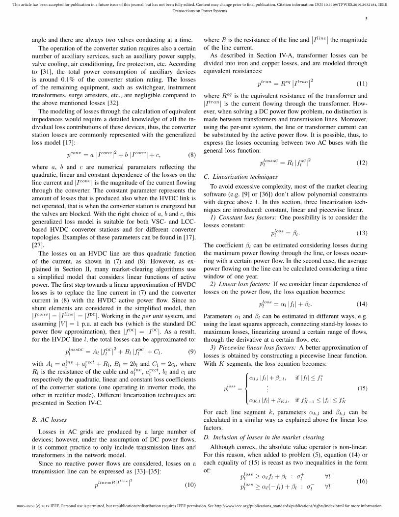
Fig. 5. Inclusion of intra-zonal losses on HVDC and AC loss factors. Linelosses are the losses on the interconnector, black dots are the intra-zonal lossesdue to cross-border flows. The linearization is made with 10 segments.

case no distinction between AC and HVDC lines is made,and in the second case losses do not depend on the flows andthus prices and flows remain unchanged. Again, the situationis different when linear or piecewise linear loss factors areintroduced. With linear loss factors, the slope of the lossfunction determines the path that results in less losses. Indeed,the power flow over line 2-3 is equal to its capacity, whileonly the remaining power is supplied through line 1-2. Withpiecewise linear loss factors, the slope of the loss functionchanges depending on the flow. For this reason, the solveridentifies the least costly path by moving back and forth fromone line to the other, when the slope of the loss functionchanges. In this way the two lines are used in a more efficientway, and the price difference, although greater, reflects betterthe cost of losses.

V. INTRA-ZONAL LOSSES

In our initial investigations, and as we also demonstrate inour numerical tests in Section VI, the social welfare does notalways increase by introducing AC and HVDC loss factor inzonal pricing markets. This is due to the fact that intra-zonallosses are not variables in the optimization problem, and thuscannot be minimized. This chapter introduces a method forconsidering a part of intra-zonal losses, which is produced bycross-border flows, in the calculation of loss factors.

Intra-zone losses are caused by both cross-border and in-ternal flows. Loss factors are meant to account only for thelosses due to inter-zonal flows, so the internal losses have tobe excluded from the calculation. We calculated the new lossfactors as follows. Two zones connected are considered at atime: in Zone 1 all the loads are removed, while in Zone 2all generators are removed. The statistical population of lossesis calculated running 10’000 AC power flows, where differentgeneration patterns and load conditions are considered. Thesame procedure is then repeated inverting generation andconsumption in the two areas. We repeat these two steps for allthe zones connected by AC lines. Ideally, the losses betweenany two zones would have been the result of the superpositionof the losses found for each pair of zones. However, in thatcase we account for the losses in each transit zone more thanonce. As a result, we carry out a similar analysis considering

=

~

=

~

=

~

=

~Area 1 Area 2

Area 4 Area 3

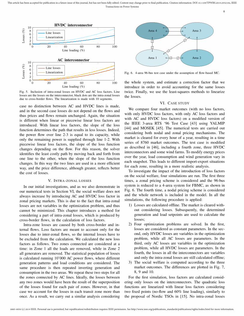
Fig. 6. 4-area 96-bus test case under the assumption of flow-based MC.

the whole system, and estimate a correction factor that weintroduce in order to avoid accounting for the same lossestwice. Finally, we use the least-squares methods to linearizethe losses.

VI. CASE STUDY

We compare four market outcomes (with no loss factors,with only HVDC loss factors, with only AC loss factors andwith AC and HVDC loss factors) on a modified version ofthe IEEE 3-area RTS ‘96 Test Case [43] using YALMIP[44] and MOSEK [45]. The numerical tests are carried outconsidering both nodal and zonal pricing mechanisms. Themarket is cleared for every hour of a year, resulting in a timeseries of 8760 market outcomes. The test case is modifiedas described in [46], including a fourth zone, three HVDCinterconnectors and some wind farms. To modify energy pricesover the year, load consumption and wind generation vary ineach snapshot. This leads to different import-export situationsfor each zone, resulting in a more realistic analysis.

To investigate the impact of the introduction of loss factorson the social welfare, four simulations are run. The first threetimes, a zonal pricing scheme is considered and the 96-bussystem is reduced to a 4-area system for FBMC, as shown inFig. 6. The fourth time, a nodal pricing scheme is consideredand the whole network is included in the model. In all thesimulations, the following procedure is applied:

1) Losses are calculated offline. The market is cleared with-out considering losses. Subsequently, the determinedgeneration and load setpoints are used to calculate thelosses;

2) Four optimization problems are solved. In the first,losses are considered as constant parameters. In the sec-ond, only HVDC losses are variables in the optimizationproblem, while all AC losses are parameters. In thethird, only AC losses are variables in the optimizationproblem, while all HVDC losses are parameters. In thefourth, the losses in all the interconnectors are variablesand only the intra-zonal losses are still calculated offline;

3) The social welfare is computed according to the threemarket outcomes. The differences are plotted in Fig. 7,8, 9 and 10.

For the first simulation, loss factors are calculated consid-ering only losses on the interconnectors. The quadratic lossfunctions are linearized with linear loss factors consideringtwo fixed points (no-flow and 60% line loading), similarly tothe proposal of Nordic TSOs in [15]. No intra-zonal losses

0885-8950 (c) 2019 IEEE. Personal use is permitted, but republication/redistribution requires IEEE permission. See http://www.ieee.org/publications_standards/publications/rights/index.html for more information.

This article has been accepted for publication in a future issue of this journal, but has not been fully edited. Content may change prior to final publication. Citation information: DOI 10.1109/TPWRS.2019.2932184, IEEETransactions on Power Systems

9

−5000

5001,0001,5002,000

HVDC LOSS FACTORS

−5000

5001,0001,5002,000

Savi

ngs

($)

AC LOSS FACTORS

0 1,000 2,000 3,000 4,000 5,000 6,000 7,000 8,000−500

0500

1,0001,5002,000

Time (h)

AC-HVDC LOSS FACTORS

Fig. 7. FBMC: comparison of market outcomes. Loss factors calculated basedon line losses and linear approximation.

−5000

5001,0001,5002,000

HVDC LOSS FACTORS

−5000

5001,0001,5002,000

Savi

ngs

($)

AC LOSS FACTORS

0 1,000 2,000 3,000 4,000 5,000 6,000 7,000 8,000−500

0500

1,0001,5002,000

Time (h)

AC-HVDC LOSS FACTORS

Fig. 8. FBMC: comparison of market outcomes. Loss factors calculated basedon line losses and piecewise linear approximation.

are considered in the loss factor calculation. Fig. 7 shows thedifferences in social welfare between the base case (no lossfactors) and the other optimization problems, with implicit gridloss implemented respectively on only HVDC, only AC andboth AC and HVDC interconnectors.

Overall, the inclusion of losses in the market clearing hasa positive impact. However, in many simulations, the socialwelfare is decreased. First of all, the estimation of lossesis not very accurate. As explained, the market is clearedwithout losses, and these are calculated based on the set pointsof generators and loads. Including losses as constant loadsalters the flows, thus the losses calculated are not precise.This happens also in reality, since losses are forecast. Theunderestimation of losses requires the purchase of this powerin the balancing market resulting in higher costs, thus havinga representation of losses in the market clearing is a goodsolution. Moreover, internal losses are not considered whendefining the power exchanges: different power flows on theinterconnectors might result in higher amount of internallosses, and thus in higher costs.

For the second simulation, still no intra-zonal losses areconsidered, but line losses are now linearized using piecewiselinear functions with segments of the length of 60 MW. Bydoing so, flows are distributed in a better way, since the solvermoves back and forth from one loss function to the otherdetermining the least costly path. Moreover, the quadraticloss functions are approximated in a better way. This leadsto a partial improvement of the results, as shown in Fig. 8.

−5000

5001,0001,5002,000

HVDC LOSS FACTORS

−5000

5001,0001,5002,000

Savi

ngs

($)

AC LOSS FACTORS

0 1,000 2,000 3,000 4,000 5,000 6,000 7,000 8,000−500

0500

1,0001,5002,000

Time (h)

AC-HVDC LOSS FACTORS

Fig. 9. FBMC: comparison of market outcomes. Loss factors calculated basedon line losses, intra-zonal losses and piecewise linear approximation.

−5000

5001,0001,5002,000

HVDC LOSS FACTORS

−5000

5001,0001,5002,000

Savi

ngs

($)

AC LOSS FACTORS

0 1,000 2,000 3,000 4,000 5,000 6,000 7,000 8,000−500

0500

1,0001,5002,000

Time (h)

AC-HVDC LOSS FACTORS

Fig. 10. Nodal pricing: comparison of market outcomes. Loss factorscalculated based on piecewise linear approximation.

However, with only AC loss factors, the situation seems toget worse. This is because, in most of the situations, Zone1 and 4 are exporting. With AC loss factors, the power fromArea 4 is rerouted through Area 1, creating more losses on theinterconnectors and causing also more internal losses, while,with DC loss factors, HVDC lines are the only path from Zone1 to the others, thus HVDC lines are used anyways, and withboth loss factors, all the lines are used in an optimal way.

In the third simulation, additionally to line losses, intra-zonal losses due to cross-border flows are included in thecalculation of loss factors. Different points of connectionmight result in different internal losses, and this is nowconsidered. As a consequence, the results are further improved,as shown in figure Fig. 9.

Finally, a similar analysis is carried out with a nodal pricingscheme, considering the whole network. Contrary to the othersimulations, there are now 156 AC lines and 3 HVDC lines.This means that the possibility of controlling the flows isreduced, and thus the amount of savings as well. However,the representation of losses in the market clearing is moreaccurate, and there are fewer situations where the socialwelfare is decreased. Also, one would expect to have onlypositive increments with AC and HVDC loss factors, howeverthe inaccuracy of the loss estimation procedure affects theresults.

TABLE III presents the total savings in the different situa-tions. In all simulations, the inclusion of both AC and HVDCloss factors gives the greatest benefit, as theoretically expected.

0885-8950 (c) 2019 IEEE. Personal use is permitted, but republication/redistribution requires IEEE permission. See http://www.ieee.org/publications_standards/publications/rights/index.html for more information.

This article has been accepted for publication in a future issue of this journal, but has not been fully edited. Content may change prior to final publication. Citation information: DOI 10.1109/TPWRS.2019.2932184, IEEETransactions on Power Systems

10

TABLE IIITOTAL SAVINGS (M$)

HVDC LF AC LF AC-HVDC LF

Simulation 1 1.16 1.12 1.38Simulation 2 1.05 0.90 1.51Simulation 3 2.52 1.23 3.10Simulation 4 0.99 1.77 1.81

VII. CONCLUSION

The introduction of loss factors for HVDC lines, also calledimplicit grid loss calculation, has been proposed by the TSOsof Nordic Capacity Calculation Region to avoid HVDC flowsbetween zones with zero price difference. Currently, it isunder investigation for real implementation in the market clear-ing algorithm. In this paper, we have introduced a rigorousframework to assess the impact of the shift towards implicitgrid losses, considering the introduction of loss factors fordifferent interconnectors. We develop different loss factor for-mulations and study their main properties on a representativetest system. We find that although the introduction of HVDCloss factors is in general positive, it may lead to a decreaseof the social welfare for a non-negligible amount of timeas it disproportionately increases the AC losses. For zonalpricing markets, this might happen also when implicit gridlosses are implemented in all interconnectors because of intra-zonal losses. To counter that, we introduce a methodology toestimate loss factors based on statistical analysis and linearregression. We prove theoretically that the introduction of bothAC and HVDC loss factors in market clearing is guaranteedto increase the social welfare. We confirm our results throughnumerical tests in a representative test system.

REFERENCES

[1] ABB Group. Economic and Environmental Advantages — Why chooseHVDC over HVAC. [Online]. Available: https://new.abb.com/systems/hvdc/why-hvdc/economic-and-environmental-advantages [Accessed:2018-09-28]

[2] ABB Group. Technical Advantages — Why choose HVDC over HVAC.[Online]. Available: https://new.abb.com/systems/hvdc/why-hvdc/technical-advantages [Accessed: 2018-09-28]

[3] R. Rudervall, J. P Charpentier, and R. Sharma, “High Voltage DirectCurrent (HVDC) Transmission Systems Technology Review Paper,”January 2000.

[4] ENTSO-E. Grid Map. [Online]. Available: https://www.entsoe.eu/data/map/ [Accessed: 2018-09-20]

[5] California ISO, “Fifth Replacement FERC Electric Tariff,” Tech. Rep.,December 2017.

[6] PJM Interconnection LLC, “Locational Marginal Pricing Components,”Tech. Rep., July 2017.

[7] AEMO, “Proportioning Inter-regional Losses to Regions,” Tech. Rep.,September 2009.

[8] EPEX SPOT SE, “PCR Project . Main Features,” Tech. Rep., October2018.

[9] NEMO Committee, “EUPHEMIA Public description- Single Price Cou-pling Algortithm,” Tech. Rep., April 2019.

[10] ELEXON, “Load Flow Model Specification for the Calculation of NodalTransmission Loss Factors,” Tech. Rep., May 2017.

[11] Energinet.dk, “Regulation A: Principles for the electricity market,” Tech.Rep., December 2007.

[12] European Commision, Commision Regulation (EU) No 838/2010. Of-ficial Journal of the European Union, September 2010.

[13] European Parliament and Council of the European Union, Regulation(EC) No 714/2009. Official Journal of the European Union, July 2009.

[14] Nord Pool Group. Market Data — Elspot Day-Ahead. [Online].Available: https://www.nordpoolgroup.com/ [Accessed: 2018-08-30]

[15] Fingrid, Energinet, Statnett, Svenska Kraftnat, “Analyses on the effectsof implementing implicit grid losses in the Nordic CCR,” Tech. Rep.,April 2018.

[16] S. Chatzivasileiadis, “Optimization in modern power systems: LectureNotes on Optimal Power Flow,” Technical University of Denmark, 2018.Available: https://arxiv.org/pdf/1811.00943.pdf.

[17] J. Beerten, S. Cole, and R. Belmans, “Generalized Steady-State VSCMTDC Model for Sequential AC/DC Power Flow Algorithms,” IEEETransactions on Power Systems, vol. 27, no. 2, pp. 821–829, May 2012.

[18] L. Soder and M. Ghandhari, Static Analysis of Power Systems. KTHRoyal Institute of Technology, Stockholm, 2015.

[19] S. A. Gabriel, A. J. Conejo et al., Complementarity Modeling in EnergyMarkets. Springer New York, 2013.

[20] T. Krause, Evaluating Congestion Management Schemes in LiberalizedElectricity Markets Applying Agent-based Computational Economics.Doctoral thesis, Swiss Federal Institute of Technology, Zurich, Switzer-land, 2006.

[21] PJM Interconnection LLC, “Market Settlements - Energy and Transac-tion Billing Examples,” Tech. Rep., May 2017.

[22] Transpower New Zealand, “Market 101 - Part 2,” Tech. Rep., July 2018.[23] S. Chatzivasileiadis, T. Krause, and G. Andersson, “HVDC line place-

ment for maximizing social welfare - An analytical approach,” in 2013IEEE PowerTech Grenoble, June 2013, pp. 1–6.

[24] AEMO, “An introduction to Australia’s National Electricity Market,”Tech. Rep., July 2010.

[25] CWE TSOs, “CWE Enhanced Flow-Based MC,” Tech. Rep., October2013.

[26] B. Jegleim, Flow-based Market Coupling. Master’s thesis, NorwegianUniversity of Science and Technology, Trondheim, Norway, 2015.

[27] G. Daelemans, VSC HVDC in meshed networks. Master’s thesis,Katholieke Universiteit Leuven, Leuven, Belgium, 2008.

[28] A. Peter and K. Saha, “Power Losses Assessments of LCC-based HVDCConverter Stations using Datasheet Parameters and IEC 61803 STD,” in2018 International Conference on the Domestic Use of Energy (DUE),April 2018.

[29] IEC, Power losses in voltage sourced converter (VSC) valves for high-voltage direct current (HVDC) systems. International Standard 62751,IEC, 2014.

[30] P. Jones and C. Davidson, “Calculation of power losses for MMC-basedVSC HVDC stations,” in 2013 15th European Conference on PowerElectronics and Applications (EPE), September 2013.

[31] IEEE Standards, “IEEE Recommended Practice for Determination ofPower Losses in High-Voltage Direct-Current (HVDC) Converter Sta-tions,” IEEE Std 1158-1991, pp. 1–53, February 1992.

[32] IEC, Determination of power losses in high-voltage direct current(HVDC) converter stations. International Standard 61803, IEC, 1999.

[33] W. Hongfu, T. Xianghong et al., “An Improved DC Power FlowAlgorithm with consideration of Network Loss,” in 2014 InternationalConference on Power System Technology, October 2014, pp. 455–460.

[34] A. Helseth, “A Linear Optimal Power Flow Model considering NodalDistribution of Losses,” in 2012 9th International Conference on theEuropean Energy Market, May 2012, pp. 1–8.

[35] C. Coffrin, P. Van Hentenryck, and R. Bent, “Approximating Line Lossesand Apparent Power in AC Power Flow Linearizations,” in 2012 IEEEPower and Energy Society General Meeting, July 2012, pp. 1–8.

[36] Transpower New Zealand, “Scheduling, Pricing and Dispatch Software,”Tech. Rep., May 2012.

[37] M. Irvinga and M. Sterling, “Economic dispatch of active power byquadrativ programming using a sparse linear complementary algorithm,”International Journal of Electrical Power & Energy Systems, vol. 7,no. 1, pp. 2–6, January 1985.

[38] R. A. Jabr, “Modeling network losses using quadratic cones,” IEEETransactions on Power Systems, vol. 20, no. 1, February 2005.

[39] O. W. Akinbode and K. W. Hedman, “Fictitious losses in the DCOPFwith a piecewise linear approximation of losses,” in 2013 IEEE PowerEnergy Society General Meeting, July 2013, pp. 1–5.

[40] L. Deng, B. F. Hobbs, and P. Renson, “What is the Cost of Negative Bid-ding by Wind? A Unit Commitment Analysis of Cost and Emissions,”IEEE Transactions on Power Systems, vol. 30, no. 4, pp. 1805–1814,July 2015.

[41] Florence School of Regulation. Negative prices for electricity. [Online].Available: http://fsr.eui.eu/negative-prices-electricity/ [Accessed: 2019-15-04]

[42] Fresh Energy. Negative prices in the MISO market. [Online].Available: https://fresh-energy.org/negative-prices-in-the-miso-market-whats-happening-and-why-should-we-care/ [Accessed: 2019-15-04]

0885-8950 (c) 2019 IEEE. Personal use is permitted, but republication/redistribution requires IEEE permission. See http://www.ieee.org/publications_standards/publications/rights/index.html for more information.

This article has been accepted for publication in a future issue of this journal, but has not been fully edited. Content may change prior to final publication. Citation information: DOI 10.1109/TPWRS.2019.2932184, IEEETransactions on Power Systems

11

[43] C. Grigg, P. Wong et al., “The IEEE Reliability Test System-1996.”IEEE Transactions on Power Systems, vol. 14, no. 3, pp. 1010–1020,Aug 1999.

[44] J. Lofberg, “YALMIP : A Toolbox for Modeling and Optimizationin MATLAB,” in In Proceedings of the CACSD Conference, Taipei,Taiwan, 2004.

[45] MOSEK Aps, The MOSEK optimization toolbox for MATLAB manual.Version 8.1. , 2017. [Online]. Available: http://docs.mosek.com/8.1/toolbox/index.html [Accessed: 2018-10-14]

[46] A. Tosatto, T. Weckesser and S. Chatzivasileiadis, “A modified versionof the IEEE 3-area RTS ’96 Test Case for time series analysis,”arXiv.org, May 2019. Available: https://arxiv.org/pdf/1906.00055.pdf.

Andrea Tosatto received a M.Sc. degree in Elec-trical Engineering from the Royal Institute of Tech-nology (KTH), Stockholm, Sweden, and a secondM.Sc. degree in Electrical Engineering from the In-stitute Polytechnique de Grenoble, Grenoble, France.Currently, he is a Ph.D. student at the Technical Uni-versity of Denmark (DTU), Department of ElectricalEngineering, Centre for Electric Power and Energy.His research interests include convex optimizationin power systems, applied game theory and marketintegration of multi-area AC/HVDC grids.

Tilman Weckesser received his M.Sc. and Ph.D.degree from the Technical University of Denmark(DTU), Lyngby, Denmark, in 2011 and 2015, re-spectively. He was affiliated with the University ofLige, Belgium, as a postdoctoral researcher and withthe Technical University of Denmark as an AssistantProfessor. Currently, he is consultant at the DanishEnergy Association in the Grid technology depart-ment. His research interests are in electric powersystem dynamics, stability and electric mobility.

Spyros Chatzivasileiadis (S’04, M’14) is an As-sociate Professor at the Technical University ofDenmark (DTU). Before that he was a postdoctoralresearcher at the Massachusetts Institute of Technol-ogy (MIT), USA and at Lawrence Berkeley NationalLaboratory, USA. Spyros holds a Ph.D. from ETHZurich, Switzerland (2013) and a Diploma in Elec-trical and Computer Engineering from the NationalTechnical University of Athens (NTUA), Greece(2007). In March 2016 he joined the Center forElectric Power and Energy at DTU. He is currently

working on power system optimization and control of AC and HVDC grids,and data-driven optimization and security assessment of transmission anddistribution grids.