1

Market Efficiency, the Pareto Wealth Distribution,

and the Lévy Distribution of Stock Returns

Moshe Levy*

October 2001

*The Jerusalem School of Business Administration at The Hebrew University of Jerusalem,Jerusalem, Israel, 91905. mslm@mscc.huji.ac.il. Tel: 972 2 588 3219. Fax: 972 2 588 1341.I am grateful to Tony Bernardo, Michael Brennan, Haim Levy, Victor Ríos-Rull, Richard Roll,Eduardo Schwartz, Joel Slemrod, Sorin Solomon, and Ed Wolff for their helpful commentsand suggestions. This study has been financially supported by the Zagagi Fund.

2

Market Efficiency, the Pareto Wealth Distribution,

and the Lévy Distribution of Stock Returns

Abstract

The Pareto (power-law) wealth distribution, which is empirically observed in

many countries, implies rather extreme wealth inequality. For instance, in the U.S. the

top 1% of the population holds about 40% of the total wealth. What is the source of

this inequality? The answer to this question has profound political, social, and

philosophical implications. We show that the Pareto wealth distribution is a robust

consequence of a fundamental property of the capital investment process: it is a

stochastic multiplicative process. Moreover, the Pareto distribution implies that

inequality is driven primarily by chance, rather than by differential investment ability.

This result is closely related to the concept of market efficiency, and may have direct

implications regarding the economic role and social desirability of wealth inequality.

We also show that the Pareto wealth distribution may explain the Lévy distribution of

stock returns, which has puzzled researchers for many years. Thus, the Pareto wealth

distribution, market efficiency, and the Lévy distribution of stock returns are all

closely linked.

Keywords: wealth distribution, inequality, Pareto, market efficiency, distribution ofstock returns.

JEL Classification: D31, E44, G10.

3

1. Introduction

In this study we focus on three seemingly unrelated issues: a) the distribution

of wealth and wealth inequality, b) market efficiency: do some investors have stock

selection or market “timing” ability, or is success and failure in capital investments

primarily due to chance? c) the distribution of stock returns, and in particular, the “fat

tailed” Lévy distribution observed by Mandelbrot [1963], and recently precisely

measured by Mantegna and Stanley [1995] and others. We show in this paper that

although it seems that these are three unrelated research topics (the first in economics,

and the other two in finance), they are, in fact, very closely related.

The Pareto wealth distribution is shown to be a robust consequence of the

stochastic multiplicative nature of the investment process. However, we find that the

Pareto distribution can occur only if the market is efficient – which implies that

success and failure in investments is primarily due to chance. Thus, it is chance, rather

than differential investment ability, which drives the Pareto wealth distribution and

the rather extreme inequality which it implies. Furthermore, the Pareto wealth

distribution can explain the (truncated) Lévy distribution of stock returns. The

mechanism we suggest implies a surprising and empirically testable prediction: the

exponent of the Lévy return distribution should be equal to the Pareto constant.

Cross-country empirical investigation reveals striking agreement between these two

a-priori unrelated parameters: U.S.: αL = 1.37, αw = 1.35; U.K.: αL = 1.08, αw=1.06;

France: αL = 1.82, αw = 1.83, where αL is the Lévy characteristic exponent and αw is

the Pareto constant. Thus, the Pareto wealth distribution, market efficiency, and the

Lévy distribution of stock returns, are all tightly linked.

4

When examining the wealth distribution in society one typically finds two

distinct regions. At the lower-wealth range the distribution of wealth can be

approximated by the log-normal distribution. At the high-wealth range the distribution

is described by the Pareto distribution (see, for example, Stiendl [1965]). In this

paper we focus on the Pareto distribution which characterizes the high-wealth range.

This range is extremely important because, although it accounts for a relatively small

part of the population (typically about 5%), it accounts for most of the wealth1. In

addition, when considering wealth accumulation through capital investments, it is the

high-wealth range which is relevant to the analysis.2

A century ago Pareto [1897] discovered that at the high wealth range, wealth

(and also income) are distributed according to a power-law distribution. The parameters

of this distribution may change across societies, but regardless of the social or political

conditions, taxation, etc., Pareto claimed that the wealth distribution obeys this general

distribution law, which became known as the Pareto distribution or Pareto law. The

Pareto distribution is given by the following probability density function:

1According to Wolff [1995] the top 1% of the population in the U.S. holds more than 40% of the totalwealth. Díaz-Giménez, Quadrini, and Ríos-Rull [1997] report that the top 5% of the population holds55% of the wealth.

2Several researchers employ neoclassical growth models with uninsurable idiosyncratic earning shocks

in order to explain the entire empirically observed wealth and income distributions (see Auerbach andKotlikoff [1987], Aiyagari [1994], Ríos-Rull [1995], Huggett [1996], Krusell and Smith [1996], andCastaneda, Díaz-Giménez and Ríos-Rull [1997] ). This is a formidable task as it aims to explain thedistribution both at the high-wealth range and the low-wealth range with a single model. This isdifficult because the main factors influencing the wealth of a person at the lower range are usuallylabor income and consumption, while the wealth of individuals in the high-wealth range typicallychanges mainly due to capital investments. Indeed, as Quadrini and Ríos-Rull [1997] report, thesemodels typically produce distributions of wealth which differ significantly from the empirical U.S.wealth distribution. Regarding the fit of income distributions to the Pareto distribution Blinder [1974]asserts:�It may well be no accident that the upper tails of almost all income distributions, where returns tocapital dominate and earnings play a minor role, exhibit a striking resemblance to the Paretodistribution� (pp. 7-8).Here we focus only on capital investments and on the high-wealth range.

5

)1(CW)W(P α+−= for 0WW ≥ (1)

where W stands for wealth, P(W) is the density function, W0 is the lower end of the

high wealth range, and C is a normalization constant, and α is known as the Pareto

constant.

Pareto's finding has been shown in numerous studies to provide an excellent fit to

the empirical wealth distribution in various countries (see, for example, Steindl

[1965], Atkinson and Harrison [1978], Persky [1992], Levy and Solomon [1997]).

Several researchers claim that the Pareto law is very universal. Davis [1941] argues

that:

No one however, has yet exhibited a stable social order, ancient or modern, which

has not followed the Pareto pattern at least approximately. (p. 395)

Snyder [1939] writes:

Pareto�s curve is destined to take its place as one of the great generalizations of

human knowledge

Several examples of the fit of the Pareto law to the empirical wealth distribution are

provided by Figures 8-10, which depict the wealth distribution in France, the U.K.

and the U.S. These figures are discussed in detail in section 5.

The first to suggest an explanation for the Pareto distribution of wealth was

Pareto himself (Pareto [1906]). Pareto suggested that the distribution of wealth

corresponds to an underlying distribution of human abilities. However, Pareto has not

offered a mathematical model that would explain the distribution of abilities and its

relation to the Pareto law. Pareto's explanation was advanced by Davis who

introduced the "law of the distribution of special abilities" which asserts that the

probability of an additional unit of ability was independent of the level of ability

(Davis [1941]). This model, however, leads to a normal distribution of ability and

6

therefore presumably to a normal, rather than Pareto, distribution of wealth. A

different model for the distribution of ability was formulated by Boissevain [1939]

who considered the distribution of abilities that could be represented as a product of

several factors, each of which follows a binomial distribution. Boissevain's model

explains the positive skewness in the distributions of wealth and income, but leads to

a log-normal distribution, not the empirically observed Pareto distribution.

The main models that offer an explanation for the precise form of the Pareto

wealth distribution are the Markov chain model of Champernowne [1953], the stream

model of Simon [1955] and the birth-and-death model of Wold and Whittle [1957].3

Although these models are quite different from each other and make various different

assumptions, in all of these models the wealth accumulation process is a stochastic

multiplicative process. A stochastic multiplicative process is a process in which the

value of each element is multiplied by a random variable with each time step. Many

economic processes, and in particular the accumulation of wealth via investment of

capital, are stochastic and multiplicative by nature. For example, if a person invests

her money in a portfolio which yields 10% with probability 1/2 and -5% with

probability 1/2 each year, her wealth will follow a stochastic multiplicative process.

The main difference between multiplicative and additive processes is that in additive

processes (such as random walks) the changes in value are independent of the value,

whereas in multiplicative processes the changes are proportional to the value.

In this paper we argue that the multiplicative nature of the capital investment

process is the reason for the empirically observed Pareto wealth distribution. Indeed,

starting with an arbitrary non-degenerate initial wealth distribution, any process which

3For a review of models generating Pareto distributions see Steindl [1965], Arnold [1983], and Slottje[1989].

7

is stochastically multiplicative and homogeneous leads to the Pareto law.

The homogeneity of the process in essence means that individuals do not posses

8

differential investment abilities and cannot “beat the market”. This idea is closely

related to the concept of market efficiency: in an efficient market one would not

expect to find investors who consistently outperform their peers. We show that

non-homogeneous multiplicative processes lead to a wealth distribution which is

different from the Pareto distribution. Thus, the Pareto distribution implies market

efficiency. Our analysis leads us to conclude that the extreme inequality in modern

western society is a very fundamental and robust outcome of the nature of the capital

investment process. Furthermore, this inequality is driven primarily by chance, rather

than by differential ability.

The structure of this paper is as follows. In section 2 we present the framework

of stochastically multiplicative investment processes. We prove that homogeneous

processes lead to the Pareto wealth distribution, and to the extreme inequality which it

implies. In section 3 we discuss non-homogeneous processes and show that they lead to

wealth distributions different than the Pareto distribution. This section reveals that the

Pareto distribution is closely related to market efficiency, and puts an upper bound on the

degree of market inefficiency. In section 4 we show that the Lévy distribution of stock

returns can be explained by the Pareto wealth distribution. The theoretical prediction

resulting from this analysis is empirically tested in section5. Section 6 concludes.

2. Stochastic Multiplicative Processes

A stochastic multiplicative wealth accumulation process is given by:

ti

ti

1ti

~WW λ=+ (2)

where tiW is the wealth of investor i at time t and t

i

~λ represents the stochastic return,

which is a random variable drawn from some distribution gi( λ~ ). Generally, each

investor may have a different distribution of returns on his investment, hence the

sub-index i in gi( λ~ ).

9

For people at the high-wealth range, changes in wealth are mainly due to

financial investment, and are therefore typically multiplicative. For people at the

lower wealth range, changes in wealth are mainly due to labor income and

consumption, which are basically additive rather than multiplicative. Here we are only

interested in modeling wealth dynamics in the high-wealth range. There are many

ways one could model the boundary between these two regions. We start by

considering the most simple model in which there is a sharp boundary between the

two regions. The specific modeling of the boundary does not change our general

results. As the stochastic multiplicative process (eq.(2)) describes the dynamics only

at the higher wealth range, we introduce a threshold wealth level, W0, above which

the dynamics are multiplicative. We assume that only those people with wealth

exceeding W0 participate in the stochastic multiplicative investment process.

Formally, we require that:

0t

i WW ≥ for all i, and for all t. (3)

In the case that there is an overall drift towards lower wealth values (as in

Champernowne [1953]) one can define the lower bound W0 in absolute terms. In

general, however, we would expect the drift to be towards higher wealth values (as

when there is inflation or a growing economy, for example). In this case, an absolute

lower bound value becomes meaningless, and one has to define the lower bound in

real terms. A natural way to define the lower bound is in terms of the average wealth.

We define the lower bound, W0, as ,WN1W

N

1i

ti0 ∑

=

ω= where N is the number of

investors and ω is a threshold given in absolute terms (ω<1).

As people's wealth changes, they may cross the boundary between the upper

and lower wealth regions. We do not model the dynamics at the lower wealth range,

10

and for the sake of simplicity, we assume that the market has reached an equilibrium

in which the flow of people across the boundary is equal in both directions, i.e. the

number of people participating at the stochastic multiplicative investment process

remains constant. The above assumption simplifies the analysis, but the results

presented here are robust to the relaxation of this assumption.

In a homogeneous process all investors face the same return distribution i.e. :

ti

ti

1ti

~WW λ=+ , 0t

i WW ≥ , and )~(g)~(gi λ=λ for all investors i. (4)

Note that although all investors face the same return distribution )~(g λ , λ~ is drawn

separately for each investor. One way to think of this, is to think of investors who

have the same objective but have different expectations, and therefore hold different

portfolios. At each period every investor will have a different realized return, but if all

investors have the same stock-picking and market-timing abilities, none of them

achieves a return distribution better than the others’, and they draw their returns from

the same distribution (see also footnote 8). A "lucky" investor is one for which many

high values of λ are drawn. Such a lucky investor will become richer than others.

Note that in the homogeneous case investors face the same distribution of returns,

and thus the differentiation in wealth is entirely due to chance.

The next theorem shows that the Pareto wealth distribution is a very robust

result of homogeneous multiplicative processes.

Theorem 1

For any initial wealth distribution and non-trivial return distribution (Var(λ)>0), the

wealth accumulation process given by eq.(4) leads to a convergence of the wealth

distribution to the Pareto distribution.

11

Proof:

Denote the cumulative wealth distribution at time t and at time t+1 by )t,W(F and

)1t,W(F + , respectively. Then, because the wealth of the ith investor changes from

tiW at time t to t

it

i~W λ at time t+1, i.e. t

it

i1t

i~WW λ=+ (see eq.(1)), the cumulative wealth

distribution at t+1 is given by:

λλλ

=+ ∫+∞

d)(g)t,W(F)1t,W(F0

(5)

where all values of λ such that the wealth at t+1 is equal to WW =λλ

are

accounted for4.

Equation (5) describes a process in which the probability )W(F at time t+1 is

a weighted average of the probability at points surrounding W (points λW ) at time t.

Thus, starting from an arbitrary probability density, )0,W(F , the distribution )W(F

undergoes a continuous “smoothing” process. In the presence of an effective lower

bound on wealth ( 0t

i WW ≥ ), this smoothing process is analogues to diffusion

towards a barrier (see Levy and Solomon [1996]). Such a process is well-known to

lead to the convergence of )W(F to a stationary distribution (Boltzmann [1964],

Feynman, Leighton, and Sands [1964]). For the limiting stationary wealth

distribution we have )W(F)t,W(F)1t,W(F ==+ and eq.(5) becomes:

λλ∫ λ=

+∞

d)(g)W(F)W(F0

. (6)

Differentiating with respect to W we obtain the density function:

4 As λ~ represents the total return on capital investment, it can not be less than 0 (which corresponds to

a rate of return of –100%).

12

λλλλ

= ∫+∞

d)(g1)W(f)W(f0

. (7)

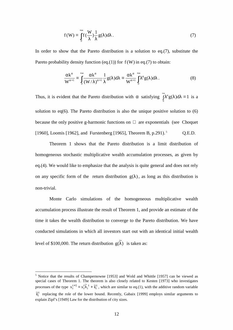
In order to show that the Pareto distribution is a solution to eq.(7), substitute the

Pareto probability density function (eq.(1)) for )W(f in eq.(7) to obtain:

λλλα=λλλλ

α=α∫∫

+∞α

+α

α+∞

+α

α

+α

α

d)(gW

kd)(g1)/W(

kW

k

01

011 . (8)

Thus, it is evident that the Pareto distribution with α satisfying 1d)(g0

=λλ∫λ+∞

α is a

solution to eq(6). The Pareto distribution is also the unique positive solution to (6)

because the only positive g-harmonic functions on ℜ are exponentials (see Choquet

[1960], Loomis [1962], and Furstenberg [1965], Theorem B, p.291). 5 Q.E.D.

Theorem 1 shows that the Pareto distribution is a limit distribution of

homogeneous stochastic multiplicative wealth accumulation processes, as given by

eq.(4). We would like to emphasize that the analysis is quite general and does not rely

on any specific form of the return distribution )(g λ , as long as this distribution is

non-trivial.

Monte Carlo simulations of the homogeneous multiplicative wealth

accumulation process illustrate the result of Theorem 1, and provide an estimate of the

time it takes the wealth distribution to converge to the Pareto distribution. We have

conducted simulations in which all investors start out with an identical initial wealth

level of $100,000. The return distribution )~(g λ is taken as:

5 Notice that the results of Champernowne [1953] and Wold and Whittle [1957] can be viewed asspecial cases of Theorem 1. The theorem is also closely related to Kesten [1973] who investigatesprocesses of the type t

it

iti

1ti

~~xx ε+λ=+ , which are similar to eq.(1), with the additive random variableti

~ε replacing the role of the lower bound. Recently, Gabaix [1999] employs similar arguments toexplain Zipf’s [1949] Law for the distribution of city sizes.

13

λ probability

1.10 ½

0.95 ½

i.e. at every time period each investor has an equal probability to gain 10% or to lose

5%. The lower wealth bound (W0) is set to 20% of the average wealth. We have

recorded the distribution of wealth at different times. The results are shown in Figure

1, which is a two-way logarithmic plot of the probability density as a function of

wealth (in units of the average wealth). The dashed vertical line at 0.2 represents the

minimal wealth threshold W0. Note that the theoretical Pareto distribution (eq.(1)) is

a power-law distribution, and it is therefore linear when plotted on a

double-logarithmic scale.6 The distribution after 10 investment periods (Figure 1a) is

still rather symmetric, and centered around the average wealth (1.0 on the horizontal

axis). However, after 100 time periods the wealth distribution is very close to the

Pareto distribution (Figure 1b). The distribution remains Paretian from then on7.

Figure 1c shows the wealth distribution after 10,000 time periods.

(Insert Figure 1 About Here)

The homogeneity of the process ( )(gi λ = )(g λ for all i) implies an efficient

market: no investor is able to achieve a superior distribution of returns which

dominates )(g λ . In the next section we show that this is indeed a necessary condition

for the emergence of a Pareto distribution8. If the market is inefficient and

6Take the logarithm of both sides of eq.(1) to obtain: ]Wlog[)1(]Clog[)]W(Plog[ α−−= . 7The slope of the line in Figures 2b and 2c is –2.25, which implies 1+ α =2.25 or α =1.25. This valueis typical of western countries, and it is between the value of α in the U.K. (1.06) and the value of αin the U.S. (1.35), (see section 5). 8Market efficiency is necessary, but not sufficient. Even if all investors have similar investment talentthey may still have different distributions of returns, due to different attitudes towards risk. However, ifinvestors have long horizons (which seems reasonable for the high-wealth range), then under mildassumptions regarding preferences, they should all seek to find the investment which maximizes thegeometric mean (see Latané [1959], Markowitz [1976], and Leshno and Levy [1997]). If this is thecase, they have the same goal, and in an efficient market they are likely to draw returns from similardistributions.

14

)(g)(g ji λ≠λ a wealth distribution which is different than the Pareto distribution

emerges.

3. Non-Homogeneous Multiplicative Processes and Market Efficiency

As a first step toward the analysis of the general heterogeneous model

( )(g)(g ji λ≠λ ), we analyze the case of two sub-populations. Consider a market in

which some of the population has “normal” investment skills and faces the return

distribution gnormal )~(λ , while a minority of “smart” investors are able to take

advantage of market inefficiencies and to obtain the superior distribution gsmart )~(λ ,

such that )g()g( normalsmart σ=σ and )g(E)g(E normalsmart > . The resulting wealth

distribution will be different from the Pareto distribution, as the Theorem below

shows.

Theorem 2:

In the case of two different sub-populations, as described above, the wealth

distribution converges to a distribution which does not conform with the Pareto Law.

Proof:

Over time the "smart" investors become on average richer than the "normal"

investors. As the "normal" investors become relatively poorer, more and more of them

will cross the lower wealth threshold, W0, and will exit the market. One might suspect

that in the long run the "normal" population will be completely wiped out. However,

recall that there is an inflow of investors into the market. This is an inflow of

investors from below the threshold who have acquired enough wealth in order to

participate in the investment process. (We do not model the process of wealth

accumulation below the threshold, but assume that the market is in a steady state in

which the inflow of new investors balances the outflow of investors leaving the

market. This assumption simplifies the analysis but is not essential to our results.)

15

Some of the new investors entering the market are of the "normal" type9. As the

number of "normal" investors declines, so does their proportion in the outflow from

the market. Eventually, a balance is reached when the outflow of investors of each

type matches the inflow of that type, and the size of each subgroup converges to a

certain (mean) value.

As the population of each subgroup is homogeneous, the wealth distribution of

each subgroup is subject to the dynamics described by equation (4).10 From the result

of Theorem 1 it follows that the wealth of each subgroup will be divided between the

members of that subgroup according to the Pareto distribution. Thus, the wealth

distribution among "normal" investors is:

)1(normalnormal

normalWC)W(P α+−= , (9)

and the wealth distribution among "smart" investors is:

)1(smartsmart

smartWC)W(P α+−= . (10)

Both distributions are Paretian, but with different parameters C and α. As the average

wealth of the smart population is greater than the average wealth of the normal

9One can think of different ways in which to compose the population of new investors: a) for eachinvestor exiting the market an investor of the same type enters. b) each new investor has a certainprobability p for being "smart" and probability (1-p) of being "normal". The choice between the abovetwo alternatives, and the value of the probability p, may change the specific parameters of the steadystate wealth distribution, but not it's essential features, as described below.

10The interaction between the different subgroups is only through the lower bound W0, which dependson the average wealth of all investors in the market.

16

population, we will have normalsmart α<α .11 The aggregate distribution of wealth is

given by:

)1(2

)1(1

smartnormal WCWC)W(P α+−α+− += , (11)

which is not a Pareto distribution12,13. Q.E.D.

The result of Theorem 2 can be directly generalized to the case of many

sub-populations: in this case the wealth distribution within each sub-population

follows the Pareto Law, but as each sub-population is characterized by a different

parameter α , the aggregate distribution is not Paretian.

Monte Carlo simulations can help illustrate the result of Theorem 2, and

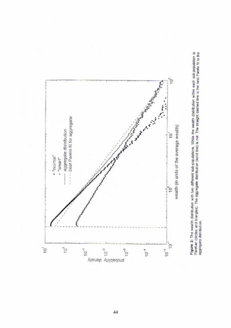
confirm that this result holds for the general case of many sub-populations. Figure 2

shows the wealth distribution in the two-population case, where the “normal”

11The lower the value of the exponent α of the Pareto distribution, the higher the average wealth. α−is the slope of the distribution function on the double-logarithmic scale. It is therefore intuitively clearthat the more moderate the slope (smaller α ) the more weight is given to higher wealth states.Formally:

α−+∞

α+−+∞

−α=== ∫∫ 1

0W

)1(

W

W)1(

CWdWWCWdW)W(P)W(E00

.

(We assume α > 1, otherwise E(W) is infinite. Empirical values of α are typically in the range

1.2-1.6) . From the normalization condition ∫+∞

=0W

1dW)W(P we obtain αα= 0WC . Substituting in

the above equation we obtain :

)1(W)W(E 0 −α

α= ,

which is a monotonically decreasing function of α .

12C1 and C2 replace Cnormal and Csmart because the normalization constraints have changed,

and depend on the relative proportions of the two subgroups, i.e.: normalnormal

1 CN

NC = ;

smartsmart

2 CN

NC = .

13The wealth distribution given in eq.(11) is asymptotically Paretian, i.e. as ∞→W)1(

2smartWC)W(P α+−≈ . Thus, it is approximately Paretian in the wealth range where the investor

population is homogeneous (in the range where all the investors are “smart”). Hence, if we empiricallyobserve that the wealth distribution is closely approximated by the Pareto distribution for the top 5% ofthe population, we may conclude that among these top 5% investment ability is homogeneous.

17

population faces the return process:

λ probability

gnormal )~(λ : 1.10 ½

0.95 ½

while the “smart” investors face the following superior return process:

λ probability

gsmart )~(λ : 1.11 ½

0.96 ½

Figure 2 shows that although the distribution of wealth within each

sub-population follows the Pareto law (αnormal = 1.67, αsmart = 0.63), the aggregate

distribution (solid line) does not. This is evident from the convexity of the aggregate

distribution, while a Pareto distribution should be linear on a double-logarithmic scale

(see footnote 6). The same convex pattern, which contradicts the Pareto distribution,

is also obtained in the general case with many investor sub-populations. Figure 3

depicts the steady-state wealth distribution in a market in which each investor faces a

different return distribution. For all investors the return distribution )~(gi λ is taken as

a normal distribution with a standard deviation of 20%. However, the mean of the

distribution )~(gi λ , iµ , is different for each investor. We assume that µ is distributed

normally in the population with a mean value of 10% and a standard deviation of 2%.

Even though the distribution of talent is rather narrow (for 85% of the investors iµ is

in the range 8%-12%), the resulting distribution of wealth is clearly different than the

Pareto distribution (see Figure 3). The Kolmogorov-Smirnov goodness-of-fit test

confirms that one can safely reject the hypothesis that the generated distribution is

Paretian. Comparing the cumulative distributions of the sample distribution with the

best fit Pareto distribution (with 1000 investors) we obtain a D value of 0.310, which

18

is much larger than the critical D value of 0.052 ( 1000/63.1= ) needed in order to

reject the hypothesis that the distribution is Paretian at a 99% confidence level.

(Insert Figures 2 and 3 About Here)

While the Pareto wealth distribution cannot precisely hold in an inefficient

market with differential investment ability, it can be consistent with some degree of

market inefficiency (and differential investment ability) in the sense that the Pareto

distribution cannot be statistically rejected. Levy and Levy [2001] employ numerical

analysis to show that the Pareto distribution cannot be statistically rejected if the

annual average return across different investor subgroups is within approximately 1%.

Thus, the empirically observed wealth distribution, which is very close to a Pareto

distribution, does not imply a perfectly efficient market, but it does impose a rather

tight upper bound on market inefficiency.

4. The Pareto Wealth distribution and the Lévy distribution of Stock Returns

In this section we suggest that the Pareto wealth distribution can explain the Lévy

distribution of short-term stock returns. We proceed with a brief review of the

distribution of short-term stock returns. Our theoretical result regarding the

distribution of stock returns and its relation to the wealth distribution is given in

Theorem 3. This result has a surprising and testable prediction, which we empirically

investigate in section 5.

4.1 The Lévy Distribution of Stock Returns � Review

It has been long known that the distributions of returns on stocks, especially

when calculated for short time intervals, are not fitted well by the normal distribution.

Rather, the distributions of stock returns are leptokurtic, or "fat tailed". Mandelbrot

[1963a, 1963b] proposed an exact functional form for return distributions. To be

19

specific, he has suggested that log-returns are distributed according to the symmetrical

Lévy probability distribution defined by:

∫∞

αγα ∆γ−

π≡

0

dq)qxcos()qtexp(1)x(L L

L (12)

where )x(LL

γα is the Lévy probability density function at x, αL is the characteristic

exponent of the distribution, γ∆t is a general scale factor, γ is the scale factor for

∆t=1, and q is an integration variable (for this formulation of the Lévy distribution

see, for example, Mantegna and Stanley [1995])14.

Mandelbrot's pioneering work gained enthusiastic support in the first few

years after it's publication.15 Subsequent works, however, have questioned the Lévy

distribution hypothesis ( Hsu, Miller and Wichern [1974], Joyce, Brorsen and Irwin

[1989]), and this hypothesis has temporarily lost favor. In the 90's the Lévy

distribution hypothesis has made a dramatic comeback. Recent extensive analysis of

short-term returns has shown that price differences, log-returns, and rates of return16

are described extremely well by a truncated Lévy distribution. This is not a sharp

truncation in the usual mathematical sense, but rather, it describes a smooth fall-off of

the empirical distribution from the Lévy distribution at some value, (for a general

picture of the empirical short-term rate of return distribution, see Figure 5). Mantegna

14This distribution is also known as the "stable-Paretian" distribution. In order to avoid confusion, wewill use only the term "Lévy distribution" throughout this paper.

15 See Fama [1963a], Fama [1963b], Fama [1965a], Teichmoeller [1971], and Officer [1972]. Roll[1968] extended the analysis from stocks to Treasury Bills. Fama and Roll [1968, 1971] developedmethodologies in order to estimate the parameters of the Lévy distribution. Efficient portfolio selectionin a market with Lévy distributions was analyzed by Fama [1965b] and Samuelson [1967].

16Some studies examine the distribution of price differences, some of log-returns, and someof rates of return. As the focus is on short time intervals (a few seconds to a few days) all ofthe above are very closely related. See also the discussion in Appendix A.

20

and Stanley [1995] analyze tick-by-tick data on the S&P 500 index and find excellent

agreement with a Lévy distribution up to six standard deviations away from the mean

(in both directions). For more extreme observations, the distribution they find falls off

faster than the Lévy distribution17. Similar results have been found in the examination

of the Milan stock exchange (Mantegna [1991]), the CAC40 index (Zajdenweber

[1994]), individual French stocks (Belkacem [1996]), and foreign exchange markets

(Pictet and Muller [1995], Guillaume et al. [1997], and Cont, Potters and Bouchaud

[1997]).

The revival of the (truncated) Lévy distribution awakens an old question: Why

are returns distributed in this very specific way? Below we suggest that the answer

may lie with the Pareto distribution of wealth.

4.2 The Pareto Wealth Distribution and the Lévy Return Distribution

The Levy distribution describes the distribution of returns in the short-term.

We therefore formulate the framework of our analysis in terms of the most

“atomistic” return – a single trade return. Theorem 3 below shows that if investors’

wealth is distributed according to the Pareto distribution, and if the effect of an

investor’s trade on the stock price is proportional (in a stochastic sense) to the

investor’s wealth, the short-term returns will be distributed according to the Lévy

distribution. The assumption of proportionality between the investor’s wealth and the

price impact of the investor’s trade seems natural: it is intuitive that the actions of

an investor with $100 million will, on average, affect prices roughly 10 times as

much as the actions of a similar investor with only $10 million. This is also

consistent with models of constant relative risk aversion, which imply that

17Several authors investigate this fall-off, and find it to be approximated by a power-law with anexponent in the range 2-5 (see Jansen and de Vries [1991], Longin [1996], Gopikrishnan, Meyer,Amaral and Stanley [1998], Stanley et al. [1999], and Cont [2001]).

21

investors make decisions regarding proportions of their wealth (see, for example,

Levy and Markowitz [1979], Samuelson [1989]), and with the finding that the price

impact of a trade is roughly proportional to the volume of the trade, especially for

high volume trades (see Figure 4 in Hausman, Lo and MacKinlay, [1992]). To be

more specific, if investors make decisions regarding proportions of their wealth, then

the volume of a trade is (stochastically) proportional to the investor's wealth. If the

effect of the trade on the price is proportional to the volume of the trade (as implied

by market clearance in most models, and as documented by Lo and Mackinlay), then

the effect that an investor's trade has on the price is (stochastically) proportional to the

investor's wealth. We should stress we do not make any assumptions regarding the

investors’ reason for trading: it can be due to the arrival of new information, liquidity

constraints, portfolio rebalancing, etc.

Theorem 3:

If the wealth of investors is distributed according to the Pareto law with exponent

Wα , and the effect of each investor�s trade on the price is stochastically proportional

to the investor�s wealth, then the resulting return distribution (and price-change

distribution) are given by the Lévy distribution with an exponent WL α=α .

Proof: See Appendix A.

Theorem 3 not only suggests an explanation for the Lévy distribution of

returns, but it also makes a surprising prediction: the exponent of the Lévy return

distribution, Lα , should be equal to the Pareto wealth distribution constant, Wα . This

prediction is surprising, because these two parameters are associated with different

research arenas, and seem to be a-priory unrelated. In the next section we test this

prediction empirically.

22

5. Empirical Evidence

In this section we empirically estimate and compare Lα and Wα for three

countries: the U.S., the U.K., and France.

5.1 Estimation of αL

For the estimation of αL we follow the methodology used by Mantegna and

Stanley [1995]. They denote the density of the symmetric Lévy distribution eq.(12) at

0 by p0, and employ the relation below in order to estimate αL:

( )( ) LL 1

L

L0 t

1)0(Lp α

γα ∆γπα

αΓ=≡ (13)

where Γ is the Gamma function, ∆t is the horizon for which rates of return are being

calculated, and γ is the scale factor for ∆t = 1 (for proof of the relation (13) see

appendix B). Thus, the probability density at 0 decays as L1t α−∆ . Mantegna and

Stanley estimate the density at 0, p0, for various time intervals, ∆t. In order to

estimate αL they run the regression:

( )[ ] [ ] iii0 tlogBAtplog ε+∆+=∆ (14)

and estimate αL as B̂1− . We employ the same technique here.

Our data sets consists of:

S&P 500: all 1,780,752 records of the index between 1990-1995, obtained from the

Chicago Mercantile Exchange.

FTSE 100: all 75,606 records of the index between January 1997 and August 1997,

obtained from the Futures Industry Institute.

CAC 40: all 234,501 records of the index in 1996, obtained from the Bourse de Paris.

23

Following Mantegna and Stanley, for each of these series we estimate the

density p0 (∆t) by going over the entire data set and calculating the rates of return for

intervals of ∆t. We count the number of rates of return within the range

[−0.0001,0.0001] and divide this number by the total number of observations, in order

to get the probability of rate of return in this range18. Then we divide the result by the

size of the range, 0.0002, in order to get the probability density at 0, p0. We repeat this

procedure for different sampling time intervals ∆t. The values of p0 as a function of ∆t

are reported in Figures 4, 6, and 7. In order to obtain an estimate of αL we employ the

regression in eq.(14). For the S&P 500 we obtain αL=1.37 (Figure 4). The standard

error of this estimation is 0.04, and the correlation coefficient is −0.987. This

estimated value that we find for αL is very close to the value of 1.40 reported by

Mantegna and Stanley [1995] for the S&P 500, during the sample period 1984-89.

(Insert Figure 4 About Here)

In order to verify that the empirical rate of return distribution is indeed well

fitted well by the symmetric Lévy distribution with the estimated αL of 1.37, we

compare these two distributions in Figure 5. The empirical distribution is calculated

for 1-minute rates of return, and the plot is semi-logarithmic.19 Figure 5 shows an

excellent agreement between the empirical and theoretical distributions up to rates of

return in the order of 0.001 (or 0.1%), which are about six standard deviations away

from the mean20. For more extreme returns, the empirical distribution falls off from

18Similar estimations of αL are obtained for different choices of small ranges around 0.

19The empirical distribution is estimated by a non-parametric density estimate with a Gaussian/ kerneland the "normal reference rule," (see Scott [1992], p. 131).

20The standard deviation of the 1-minute rate of return distribution for the period 1990-1995 isapproximately 0.00016 or 0.016%.

24

the Lévy distribution. This is the so-called truncation, which will be discussed

below21.

(Insert Figure 5 About Here)

For the FTSE 100 we find αL = 1.08 (Figure 6). The standard error of this

estimation is 0.03, the correlation coefficient is −0.996, and the t-value is −59.7. This

number is close to the αL value of 1.10 which is calculated from the 1993 FTSE 100

data reported by Abhyankar, Copeland, and Wong [1995].

For the CAC 40 we find αL = 1.82 (Figure 7). The standard error of this

estimation is 0.05, the correlation coefficient is −0.978, and the t-value is −35.9.

(Insert Figures 6 and 7 About Here)

5.2 Estimation of αw

Estimating the Pareto wealth distribution exponent αw requires data regarding

the "right-tail" of the distribution, i.e. data about the wealth of the wealthiest

individuals. The French almanac Quid provides wealth data on the top 162,370

individuals in France. This data is in aggregate form, i.e. the numbers of individuals

with wealth exceeding certain wealth levels are reported. According to the Pareto Law

(eq. (1)), the number of individuals with wealth exceeding a certain level Wx should

be proportional to WxW α− :

W

x

W

x

xW W

)1(

Wx WNCdWWNCdW)W(fN)WW(N α−

∞α+−

∞

∫∫ α===> (15)

where N(W > Wx) is the number of individuals with wealth exceeding Wx, and N is

the total number of individuals. If the Pareto distribution is valid, one expects that

21It is interesting to note the secondary peak of the empirical distribution at a rate of return of about−0.001. A similar bimodal distribution was observed by Jackwerth and Rubinstein [1996]. We do nothave an explanation for this phenomenon in the framework of the present model.

25

when plotting N(W > Wx) as a function of Wx on a double-logarithmic graph, the data

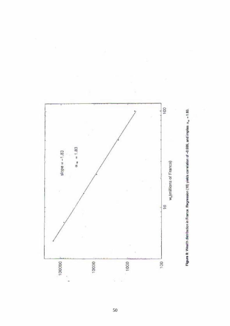
points should fall on a straight line with slope −αw. Figure 8 is a double logarithmic

plot of N(W>Wx) as a function of Wx for the French data provided by Quid. This

figure shows an excellent agreement between the empirical wealth distribution and

the Pareto-law. In order to estimate αw for France, we run the regression:

[ ] [ ] iixix WlogBA)WW(Nlog ε++=> . (16)

The absolute value of the slope of the regression line, which is the estimate for αw is

1.83. (Standard error =0.03, correlation coefficient = −0.999 t-value =-59.5).

(Insert Figure 8 About Here)

For the U.S and the U.K. the available data regarding the wealthiest people is

more detailed but also more limited in scope. For these countries, lists with the

ranking and wealth of the several hundreds of wealthiest individuals are published.

We use the methods suggested by Levy and Solomon [1997] in order to estimate αw

from these data. A Pareto law distribution of wealth with exponent αw implies the

following relation between the rank of an individual in the wealth hierarchy and her

wealth:

W

1

An)n(W α−

= , (17)

where n is the rank (by wealth), and W is the wealth. The constant A is given by

W

1

W

NCA

α−

α

= , where N is the total number of individuals in the population, and C is

the normalization constant from equation (1); (for a mathematical derivation of this

relation see Johnson and Kotz [1970]).

26

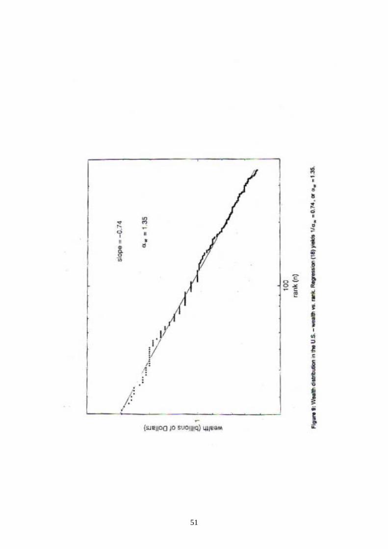
For the U.S. we obtain data from the 1997 Forbes 400 list. Wealth as a

function of rank is plotted in double logarithmic form in Figure 9. Running the

regression:

[ ] iii ]nlog[BA)n(Wlog ε++= (18)

we estimate the slope of the regression as −0.74. This is the estimation of −1/αw, and

it corresponds to an estimation of αw = 1.35 for the U.S. The standard error of this

estimation is 0.005. We would like to clarify that we do not assume that only the

wealthiest 400 individuals determine the S&P rate of return distribution. Rather, we

use the data that we are able to obtain in order to estimate the Pareto constant for the

entire upper wealth range. Our estimation of αw = 1.35 for the U.S., is close to the

estimate of 1.35 ≤ αw ≤ 1.42 which is obtained by the data provided by Wolff [1996]

regarding the percentage of wealth held by the top 1%, 5%, and 10% of the

population (see appendix C).

For the U.K. we obtain data from the Sunday Times Rich List 1997. The data

are plotted in Figure 10. We obtain a slope of −0.94 which corresponds to a value of

1/0.94 = 1.06 for αw (standard error 0.004).

The summary of our empirical results appears in Table 1. This evidence shows

a striking agreement between the values of (the a-priory unrelated) αw and αL for the

three countries investigated.

Table 1

Lα Wα

U.S. 1.37 ± 0.04 005.035.1 ±

U.K. 03.008.1 ± 004.006.1 ±

France 05.082.1 ± 030.083.1 ±

27

(Insert Figures 9 and 10 About Here)

6. Concluding Remarks

The process of wealth accumulation by capital investment is stochastic and

multiplicative by nature. This paper shows that homogeneous stochastic processes

lead to a Pareto wealth distribution. Thus, the Pareto wealth distribution, and the

rather extreme inequality which it implies, is a fundamental and robust outcome of the

nature of the capital investment process. Non-homogeneous processes, in which

investors have differential investment abilities, lead to a wealth distribution which is

different than the Pareto distribution. Thus, the Pareto distribution implies that

chance, rather than differential investment ability, is the main source of inequality at

the high-wealth range.

The Pareto distribution is closely related to market efficiency. A precise Pareto

distribution implies market efficiency. In practice, some degree of market inefficiency

can be consistent with the Pareto distribution, in the sense that the resultidistribution

cannot be statistically rejected. However, the Pareto distribution does impose a rather

tight upper-bound on market inefficiency. The closer the wealth distribution to the

Pareto distribution, the smaller the tolerable level of market efficiency.

The Pareto wealth distribution can also explain the (truncated) Lévy

distribution of short-term returns, a phenomenon which has puzzled researchers for

many years. Our theoretical analysis links between two different research arenas: the

distribution of wealth, which is a central issue in economics, and the distribution of

stock returns, which plays an important role in finance. The analysis leads to a

surprising prediction: the Pareto exponent Wα should be equal to Lα , the exponent of

the Levy return distribution. Empirical evidence from the U.S., the U.K. and France

reveals a striking agreement between these a-priori unrelated parameters (U.S.: αL =

1.37, αw = 1.35; U.K.: αL = 1.08, αw=1.06; France: αL = 1.82, αw = 1.83).

28

References

Abhyankar, A., Copeland, L. S., and Wong, W., 1995, "Nonlinear Dynamics inReal-Time Equity Market Indices: Evidence From the United Kingdom," TheEconomic Journal, 105, 864-880.

Aiyagari, S.R., 1994, “Uninsured Idiosyncratic Risk and Aggregate Saving”,Quarterly Journal of Economics, 109, 659-84.

Atkinson, A. B., and Harrison A. J., 1978, Distribution of Total Wealth in Britain,Cambridge University Press, Cambridge.

Arnold, B. C., Pareto Distributions, International Co-operative Publishing House,Maryland, 1983.

Auerbach, A.J., and L.J. Kotlikoff, Dynamic Fiscal Policy, New York: CambridgeUniversity Press, 1987.

Belkacem, L., 1996, Processus Stables et Applications á la Finance, Thése deDoctorat, Universitá Paris IX.

Blinder, A. S., Towards an Economic Theory of Income Distribution, The MIT Press,Cambridge, Ma., 1974.

Boissevain, C. H., “Distribution of Abilities Depending on Two or More IndependentFactors”, Metron, 13, 1939, 49-58.

Boltzmann, L., Lectures on Gas Theory, University of California Press, Berkeley,1964.

Castaneda, A., Díaz-Giménez, J., and J.V. Ríos-Rull, “Unemployment Spells,Cycllically Moving Factor Shares and Income Distribution Dynamics”,Manuscript, Federal Reserve Bank of Minneapolis, 1997.

Champernowne, D. G., 1953, “A Model of Income Distribution”, Economic Journal,63, 318-351.

Choquet, G., 1960 , “Le theoreme de representation integrale dans les ensemblesconvees compacts”, Ann. Inst. Fourier, 10, 333.

Cont, R., 2001, “Empirical Properties of Asset Returns: Stylized Facts and statisticalIssues”, Quantitative Finance, 1, 223-236.

Cont, R., Potters, M., and Bouchaud, J. P., 1997, "Scaling in Stock Market Prices:Stable Laws and Beyond." Science and Finance Research Group, WorkingPaper 97-02.

Davis, H., “The Analysis of Economic Time Series”, San Antonio: The PrincipiaPress of Trinity University, 1963, originally as monograph No. 6 of theCowles Commission for Research in Economics, 1941.

29

Díaz-Giménez, J., V. Quadrini, and J.V. Ríos-Rull, 1997, “Dimensions of Inequality:Facts on the U.S. Distributions of Earnings, Income, and Wealth”, QuarterlyReview of the Federal Reserve Bank of Minneapolis, 21,2, 3-21.

Fama, E. F., 1963(a), "Mandelbrot and the Stable Paretian Hypothesis." Journal ofBusiness, 36, 4..

Fama, E. F., 1963(b), "The Distribution of the Daily First Differences of Stock Prices:A Test of Mandelbrot's Stable Paretian Hypothesis", (unpublished doctoraldissertation, University of Chicago).

Fama, E. F., 1965(a), "The Behavior of Stock Prices", Journal of Business, 38, 1,34-105.

Fama, E. F., 1965(b), "Portfolio Analysis in a Stable Paretian Market", ManagementScience, 2, 3.

Fama, E. F., and Roll, R., 1968, "Some Properties of Symmetric Stable Distributions",Journal of the American Statistical Association, 63, 817-36.

Fama, E. F., and Roll, R., 1971, "Parameter Estimates for Symmetric StableDistributions.", Journal of the American Statistical Association, 66, 331-38.

Feller, W., 1971, An Introduction to Probability Theory and its Applications, Vol 2.,2nd edn, Wiley, New York.

Feynman, R. P., Leighton, R.B., and Sands, M., The Feynman Lectures on Physics,vol. 1, Addison Wesley, Reading MA., 1964.

Forbes, 1997, Special 400 List Issue, October 13.

Furstenberg, H. , 1965, Bulletin of the American Mathematical Society, 71, 271-326.

Gabaix, X., 1999, “Zipf’s Law for Cities: An Explanation”, Quarterly Journal ofEconomics, 739-767.

Gnedenko, B. V., and Kolmogorov, A. N., 1954, Limit Distributions for Sums ofIndependent Variables, Cambridge, Mass.: Addison-Wesley. Ch. 7.(Translated by K. L. Chung).

Gopikrishnan, P., Meyer, M., Amaral, L.A.N, and Stanley, H.E., 1998, “Inverse CubicLaw for the Probability Distribution of Stock Price Variations”, EuropeanJournal of Physics B, 3, 139-140.

Guillaume, D. M., 1997, "From the Bird's Eye to the Microscope: a Survey of NewStylized Facts of the Intra-day Foreign Exchange Markets", Olsen &Associates Research Group Working Paper.

30

Hausman, J. A., Lo, A. W., and MacKinlay, A. C., 1992, "An Ordered Probit Analysisof Transaction Stock Prices", Journal of Financial Economics, 31 (3), 319-79.

Hsu, D. A., Miller, R. B., and Wichern, D. W., 1974, "On the Stable ParetianBehavior of Stock-Market Prices", Journal of the American StatisticalAssociation, 68, 34.

Huggett, M., 1996, “Wealth Distribution in Life-Cycle Economies”, Journal ofMonetary Economics, 38, 953-69.

Jackwerth, J. C., and Rubinstein, M., 1996, "Recovering Probability Distributionsfrom Option Prices", Journal of Finance, 51, 5, 1611-32.

Jansen, D.W., and de Vries, C.G., 1991, “On the Frequency of Large Stock Returns:Putting Booms and Busts into Perspective”, Review of Economics andstatistics, 73, 18-24.

Johnson, N. L., and Kotz, S., 1970, Continuous Univariate distributions - 1, JohnWiley and Sons, New York.

Joyce, H. A., Brorsen, W., and Irwin, S. H., 1989, "The Distribution of Futures Prices:A Test of the Stable Paretian and Mixture of Normals Hypotheses", Journalof Financial and Quantitative Analysis, 24, 1.

Kesten, H., “Random Difference Equations and Renewal Theory for Products ofRandom Matrices”, Acta Mathematica, 81, 1973, pp. 207-248.

Krusell, P., and A.A. Smith, 1998, “Income and Wealth Heterogeneity in theMacroeconomy”, Journal of Political Economy, 106, 5, 867-896.

Latané H. E., 1959, “Criteria for Choice Among Risky Ventures,” Journal of PoliticalEconomy, LVII, 144-155.

Leshno, M., and Levy, H., 1997, “Approximately Stochastic Dominance”, HebrewUniversity Working Paper.

Levy, H., and Markowitz, H. M., 1979, "Approximating Expected Utility by aFunction of Mean and Variance", American Economic Review, 69, 3, 308-317.

Lévy P., 1925, Calcul des Probabilitiés, Paris: Gauthier Villars, Part II, ch.6.

Levy, M., and Levy, H., 2001, “Investment Talent and the Pareto Wealth Distribution:Theoretical and experimental Analysis”, Hebrew University Working Paper.

Levy, M., and Solomon, S., 1996, “Power Laws are Logarithmic Boltzmann Laws”,International Journal of Modern Physics C , 7, 65-72.

Levy, M., and Solomon, S., 1997, "New Evidence for the Power-Law Distribution ofWealth", Physica A.

31

Longin, F., 1996, “The Asymptotic Distribution of Extreme Stock Market Returns”,Journal of Business, 63, 383-408.

Loomis, L., 1962, “Unique Direct Integral Decompositions on Convex Sets”,American Journal of Mathematics, 84, 509-526.

Mandelbrot, B., 1963(a), "The Variation of Certain Speculative Prices.", Journal ofBusiness, 36, 4.

Mandelbrot, B., 1963(b), "New Methods in Statistical Economics", Journal ofPolitical Economy, 61, 421-40.

Mandelbrot, B., 1997, Fractals and Scaling in Finance: Discontinuity,Concentration, and Risk. Springer-Verlag, New York.

Mankiw, N. G., and Zeldes, S. P., 1991, "The Consumption of Stockholders andNonstockholders." Journal of Financial Economics, 29, 131-35.

Mantegna, R. N., 1991, "Lévy Walks and Enhanced Diffusion in the Milan StockExchange." Physica A, 179.

Mantegna, R. N., and Stanley, H. E., 1994, Physics Review Letters, 73, 2946-49.

Mantegna, R. N., and Stanley, H. E., 1995, "Scaling Behavior in the Dynamics of anEconomic Index." Nature, 376, 46-49.

Markowitz, H., 1976, “Investment for the Long Run: New Evidence for an Old Rule”,Journal of Finance, 31, 1273-86.

Officer, R. R., 1972, "The Distribution of Stock Returns", Journal of the AmericanStatistical Association, 67, 340.

Pareto, V., 1897, Cours d'Economique Politique, Vol 2. Also, see: Manual ofPolitical Economy, New York: Augustus M. Kelley, 1971, translated from theoriginal 1906 Manuale d'Ecoonomia Politica.

Pareto, V. Manual of Political Economy, New York: Augustus M. Kelley, 1971,translated from the original 1906 Manuale d'Ecoonomia Politica.

Pedrosa, M., and Roll, R., 1998, "Systematic Risk in Corporate Bond Credit Spreads",UCLA Working Paper 7-98.

Persky, J., 1992, "Retrospectives: Pareto's Law," Journal of Economic Perspectives,6, 181-192.

Pictet, O. V., and Muller, U. A., 1995, "Statistical Study of Foreign Exchange Rates,Empirical Evidence of a Price Change Scaling Law and Intra-day Analysis,"Journal of Banking and Finance, 14, pp. 1189-1208.

32

Quadrini, V., and J.V. Ríos-Rull, 1997, “Understanding the U.S. Distribution ofWealth”, Quarterly Review of the Federal Reserve Bank of Minneapolis, 21,2,22-36.

QUID, 1998, edited by Fremy, D., RTL, Paris.

Ríos-Rull, J.V., “Models with Heterogeneous Agents”, in Frontiers of Business CycleResearch, ed. T.F. Cooley, 98-125, Princeton, N.J., Princeton UniversityPress, 1995.

Roll, R., 1968, "The Efficient Market Model Applied to U.S. Treasury Bill Rates",(unpublished doctoral dissertation, University of Chicago).

Samuelson, P. A., 1967, "Efficient Portfolio Selection for Pareto-Lévy Investments",Journal of Financial and Quantitative Analysis, 2, 2, 107-22.

Samuelson, P. A., 1989, "The Judgment of Economic Science on Rational PortfolioManagement: Indexing, Timing, and Long-Horizon Effects", The Journal ofPortfolio Management, 4-12.

Scott, D. W., 1992, Multivariate Density Estimation, New York: Wiley.

Simon, H., 1955, “On a Class of Skew distributions”, Biometrica, (reprinted inSimon, H., Models of Man, 1957.)

Slottje, D. J., The Structure of Earnings and the Measurement of Income Inequality inthe U.S., Elsevier Science Publishers, New York, 1989.

Snyder, C., 1940, Capitalism the Creator, Macmillan.

Stanley, H.E., Amaral, L.A.N., Canning, D., Gopikrishnan, P., Lee, Y., and Liu, Y.,1999, “Econophysics: Can Physicists Contribute to the Science ofEconomics?”, Physica A, 269, 156-169.

Steindl, J., 1965, Random Processes and the Growth of Firms − A Study of the ParetoLaw, Charles Griffin & Company, London.

Sunday Times Rich List 1997, http://www.sunday-times.co.uk/news/pages/resources/

library1.n.html?2286097

Takayasu, H., 1990, Fractals in the Physical Sciences, Wiley.

Teichmoeller, J., 1971, "A Note on the Distribution of Stock Price Changes", Journalof the American Statistical Association, 66.

Wold, H., and Whittle, P., 1957, “A Model Explaining the Pareto Distribution ofWealth”, Econometrica, 25, 591-95.

Wolff, E. N., The American Prospect, 22, 1995, 58-64.

33

Wolff, E., 1996, "Trends in Household Wealth During 1989-1992." Submitted to theDepartment of Labor, New York, New York University.

Zajdenweber, D., 1994, "Propriétés Autosimilaires du CAC40." Review d'EconomiePolitique 104, 408-434.

Zipf, G., Human Behavior and the Principle of Least Effort, Cambridge, MA.,Addison-Wesley, 1949.

34

Appendix A: Proof of Theorem 3

Theorem 3:

If the wealth of investors is distributed according to the Pareto law with exponent

Wα , and the effect of each investor�s trade on the price is stochastically proportional

to the investor�s wealth, then the resulting price-change (and return) distribution is

given by the Lévy distribution with an exponent WL α=α .

Proof:

Suppose a single investor is drawn at random to trade with a market maker, and that

the effect of the investor on the price is (stochastically) proportional to the investor’s

wealth. We first prove that in this case a Pareto wealth distribution leads to a Lévy

price-change distribution. Then this result is extended to the return distribution, and to

the case of a stochastic number of investors trading at each period.

Let us denote the single-trade price change at period t as zt. zt is given by:

ttt W~q~z~ = , (19)

where tW~ is the wealth of the investor randomly chosen to trade at time t, and tq~ is a

stochastic proportionality factor which is uncorrelated with tW~ , and which is

distributed according to some probability density function h( q~ ). In what follows we

derive the distribution for single-trade price changes, and the price change distribution

which results from a larger number of trades.

When analyzing the probability of single-trade price changes it is convenient

to separate the discussion to the case of positive price changes (z>0), and negative

price changes (z<0). The probability of obtaining a positive single-trade price change

which is smaller or equal to a certain value z (z>0) is given by:

35

∫∞

∞−

= dq

qzF)q(h)z(G , for z>0 (20)

where G(z) and

qzF are the cumulative distributions of z~ and W~ respectively.

Thus, the density function of z is given by:

∫∞

∞−

= dq

q1

qzf)q(h)z(g , for z>0. (21)

Since we are dealing with the case z>0, and since the Pareto density function f(W) is

non-zero only for W > W0, the contribution to the integral in eq.(21) is only for values

of q such that qz > W0 . Thus, the contribution is non-zero only for

0Wzq0 << (if

q<0 then qz <0 and 0

qzf =

; if q>

0Wz then

qz < W0 and again 0

qzf =

). Hence,

eq.(21) can be written as:

∫

=

0Wz

0

dqq1

qzf)q(h)z(g , for z>0. (22)

Similarly, for negative price changes (z<0) we obtain22:

∫−

=

0

Wz

0

dqq1

qzf)q(h)z(g , for z<0. (23)

Combining equations (22) and (23), and employing the Pareto wealth distribution

(eq.(1)) for f, we obtain:

22For z<0 we have ∫∞

∞−

−= dq

qzF1)q(h)z(G and therefore ∫

∞

∞−

−

= dq

q1

qzf)q(h)z(g , and

the only non-zero contribution to the integral is for values of q in the range 0qW

z

0

<< .

36

−<

>

=

∫

∫α−

α+−

α+−α−

0

Wz

Wz

0

0

W)W1(

0 W)W1(

dqq1)q(hCz0z

dqq1)q(hCz0z

)z(g . (24)

The important property of g(z) is that it is asymptotically Paretian.

Namely,

as ∞→z g(z) )1(1

WzD α+−→ , and as −∞→z g(z) )1(2

WzD α+−→ ,

where D1 and D2 are given by:

dqq1)q(hCD

W

01

α−∞

∫

= , dq

q1)q(hCD

W0

2

α−

∞−∫

−= .

(Asymptotically Paretian distributions are distributions that have power-law “tails”,

see, for example, Fama [1963a] p. 423).

Thus, the single-trade price change distribution generated by a market in

which investors’ wealth is distributed according to the Pareto law with exponent Wα

is asymptotically Paretian with the same exponent Wα . The price change after n

single trades is simply the sum of these single-trade price changes. The

Doblin-Gnedenko result states that the sum of many i.i.d random variables which are

asymptotically paretian with some exponent α converges to a Lévy distribution with

characteristic exponent α (Gnedenko and Kolmogorov [1954], Fama [1963], Feller

[1971]). Thus, the distribution of the total price change, which is the sum of many

single-trade price changes, converges to the Lévy distribution. Moreover, since the

single-trade price changes are asymptotically Paretian with the same exponent as the

Pareto-law wealth exponent Wα , by the Doblin-Gnedenko result the price-change

Lévy distribution will be characterized by the same exponent, i.e. WL α=α . Q.E.D.

37

Similar considerations to those discussed in Theorem 3 lead to a Lévy

distribution with WL α=α for rates of return and for log-returns as well for price

changes. If the price remains at a fairly constant level during the sample period, it is

straightforward that a Lévy price-change distribution implies a Lévy rate of return

distribution: since the rate of return is just the price change divided by the price, if the

price level is fairly constant, the rate of return is just the price change divided by an

(almost) constant number, and therefore if price changes are distributed according to

the Lévy distribution, so are rates of return. This result can also be extended to the

case where the price does change considerably over the sample period, if one also

takes into account the effect of the price level on the average wealth.

Extension: Variable Trading Frequency

In the preceding Theorem 3 we have assumed that at time period t only one

investor is chosen to trade with the market-maker. This assumption can be relaxed to

allow for a stochastic number of investors to trade at each time period. The stochastic

price change due to the effect of a single trade is given by:

Wq~z~ =

In Theorem 3 it was shown that g(z), the probability density function of z, is

asymptotically Paretian with exponent αw. Let us denote the sum of m i.i.d. random

variables z by Sm: Sm ≡ z1 + z2 +…+ zm. Notice that because the z's are asymptotically

Paretian with exponent αw, so is their sum Sm (Gnedenko and Kolmogorov [1954]).

Let us denote the density function of Sm by km. The number of trades taking place at a

given time period is a discrete random variable which we denote by m~ :

38

probability

π

ππ

=

MM

MM

m

2

1

,m

,2,1

m~ (25)

The probability density function of an aggregate price change zt at time period t is

given by:

∑∞

=

π=1m

tmmt )z(k)z(g (26)

where m is the number of trades, km(zt) is the density function of Sm at zt, and the

summation is over all possible numbers of trades in a single time period. As the km's

are asymptotically Paretian distributions with an exponent αw, so is g(zt), their

weighted average. (To see this note that if )1(titi

Wzd)z(k α+−→ as ∞→tz , and

)1(tjtj

Wzd)z(k α+−→ as ∞→tz , then )1(tjjiitjjtii

Wz)dd()z(k)z(k α+−π+π→π+π

as ∞→tz , which implies that the weighted average is also asymptotically Paretian).

As the zt's have been shown to be asymptotically Paretian with exponent αw even if

the number of trades per period is stochastic, according to the Doblin-Gnedenko

result, for a large number of trades, the price-change distribution converges to the

Lévy distribution with the same exponent αw, which is the Pareto constant of the

wealth distribution. Thus, the result of the model is robust to a stochastic number of

trades at each time period.

39

Appendix B: Derivation of the Lévy Probability Density Function at 0

Denote the value of the Lévy p.d.f at 0 by p0.

Lemma:

( )( ) LL 1

L

L0 t

1)0(Lp α

γα ∆γπα

αΓ=≡ (27)

Proof:

From the definition of γαLL (x) in equation (12):

∫∫∞

α∞

αγα ∆γ−

π=×∆γ−

π=

00

dq)qtexp(1dq)0qcos()qtexp(1)0(L LL

L. (28)

Define a new variable Lqtu α∆γ= , and note that ( ) duutdq11

11

LL

L

−

αα

−− ∆γα= .

Substituting in equation (28) we obtain:

( )∫∞

−

α

α

γα −

∆γπα=

0

11

1

L

duu)uexp(t

1)0(L L

L

L. (29)

Recalling that the integral is the definition of

αΓ

L1 we have:

( )( ) LL 1

L

L

t1

)0(L αγα ∆γπα

αΓ= . (30)

40

Appendix C: Alternative Estimate of the Pareto Constant αw for the U.S.

Wolff's [1996] findings regarding the holdings of the top 1%, top 5%, and top

10% of the U.S. population in 1992 are reported in Table II below:

Table 2

k Pk1% 37.2%5% 60.0%10% 71.8%

In this table Pk denotes the percentage of total wealth held by the top k percent

of the population. A Praeto-law wealth distribution with exponent αw implies

the following relationship for any two k's:

W

2

1

11

2

1

k

k

kk

PP α

−

= (31)

(See proof below). Employing this relationship we can estimate αw for the U.S.

by using the data in Table II. By comparing the holdings of the top 1% with the

holdings of the top 5% we obtain:

W

11

05.001.0

600.0372.0 α

−

=

which yields αw = 1.42. A similar comparison of the holdings of the top 1%

with the holdings of the top 10% yields αw = 1.42. Comparing the holdings of

the top 5% with the holdings of the top 10% yields αw = 1.35.

41

Lemma:

A Praeto-law wealth distribution with exponent αw implies the following

relationship for any two k's:

W

2

1

11

2

1

k

k

kk

PP α

−

= .

Proof:

Assuming the Pareto-law (eq.(1)), the number of individuals with wealth

exceeding W is given by:

∫ ∫∞

α−∞

α+−

α===

W WW

)1( WW WNCxNCdx)x(fN)W(n , (32)

where N is the total number of individuals. This number of individuals

corresponds to a proportion Wk

W

WCN

)W(nk α−

α== of the population. The

above result can be restated in the following way: the wealth of the poorest

individual in the top k% of the population is given by:

W

1

Wk C

kW

α−

α

= , (33)

(where k is expressed as a proportion, i.e. 1k0 ≤≤ ). The aggregate wealth held

by the top k% of the population is given by:

(34)

)11()11(

wW

1

W

1k

WW

)1( WWW

k

W

k

W k1

NCW1

NCWdWWNCWdW)W(fN α−

α−α∞

α−∞

α+− α

−α=

−α==∫ ∫ ,

where the last equality is obtained by substituting Wk from equation (33).

42

The percentage of wealth held by the top k% of the population is:

)11()11(

wW

1

totalk

WWW

k1

NCW

1P α−

α−α

α

−α= , (35)

where Wtotal is the total wealth of all the population. Comparing the percentage

of wealth held by the top k1% of the population, with the percentage of wealth

held by the top k2% of the population, we obtain:

W

2

1

11

2

1

k

k

kk

PP α

−

= (36)

Note: In the above proof we have assumed that the Pareto wealth distribution

holds for all wealth levels. However, it is straightforward to show that the

above result is also valid if one assumes a Pareto distribution in the high wealth

range but a different wealth distribution in the low wealth range (as long as the

k's are in the high wealth range, in which the Pareto wealth distribution holds).

43

44

45

46

47

48

49

50

51

52