Market Analysis. The Degree of Competition Classifying markets number of firms freedom of entry to...
43
Market Analysis
-
Upload
ross-fleming -
Category
Documents
-
view
217 -
download
1
Transcript of Market Analysis. The Degree of Competition Classifying markets number of firms freedom of entry to...

Market Analysis

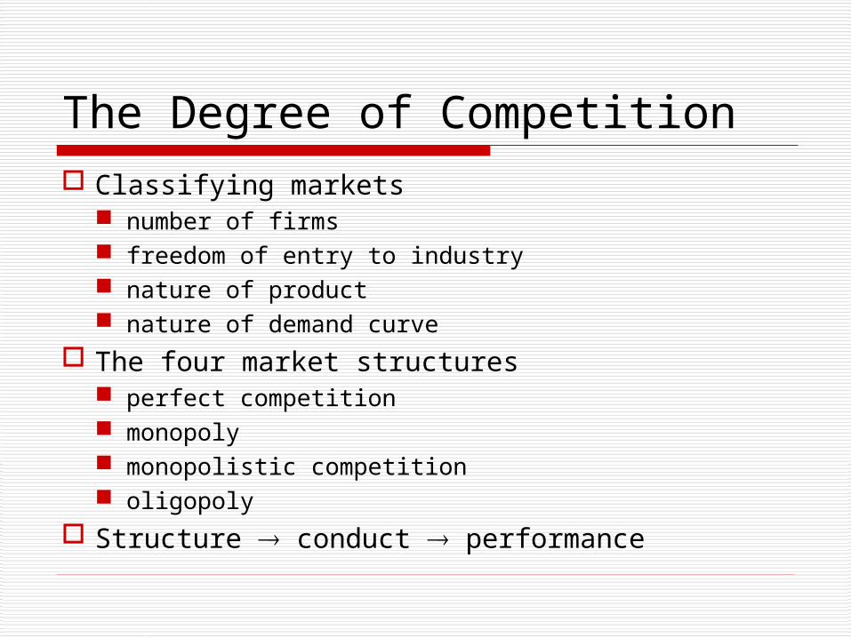
The Degree of Competition
Classifying markets number of firms freedom of entry to industry nature of product nature of demand curve
The four market structures perfect competition monopoly monopolistic competition oligopoly

Features of the four market structuresFeatures of the four market structures

Features of the four market structuresFeatures of the four market structures

Features of the four market structuresFeatures of the four market structures

Features of the four market structuresFeatures of the four market structures

Features of the four market structuresFeatures of the four market structures

Features of the four market structuresFeatures of the four market structures
The Degree of Competition Classifying markets
number of firms freedom of entry to industry nature of product nature of demand curve
The four market structures perfect competition monopoly monopolistic competition oligopoly
Structure conduct performance

Perfect Competition
Assumptions
firms are price takers
freedom of entry
identical products
perfect knowledge
Short-run equilibrium of the firm
price, output and profit

O
£
(b) Firm
Q (thousands)
O
(a) Industry
P
Q (millions)
S
D
Pe
MC
ARD = AR
= MR
Qe
AC
AC
Short-run equilibrium of industry and firm under perfect competition

Qe
P1
D1 = AR1
= MR1
AR1
O O
(a) Industry
P £
Q (millions)
S
D
(b) Firm
MC AC
AC
Q (thousands)
Loss minimising under perfect competitionLoss minimising under perfect competition

Perfect Competition
Assumptions firms are price takers freedom of entry identical products perfect knowledge
Short-run equilibrium of the firm price, output and profit
The short-run supply curve of the firm

O O
(a) Industry
P £
P1
Q (millions)
S
D1
(b) Firm
D1 = MR1
MC
P2
D2 = MR2
D2
P3
D3 = MR3
D3
Q (thousands)
Deriving the short-run supply curveDeriving the short-run supply curve
a
b
c
= S

Perfect Competition
Long-run equilibrium of the firm
all supernormal profits competed away
LRAC = AC = MC = MR = AR

O O
(a) Industry
P £
Q (millions)
S1
D
(b) Firm
LRAC
PL
P1
QL
Se
AR1 D1
ARL DL
Q (thousands)
Long-run equilibrium under perfect competition New firms enterSupernormal profits
Profits returnto normal

£
Q O
(SR)AC
(SR)MC
LRAC
AR = MR
DL
LRAC = (SR)AC = (SR)MC = MR = AR
Long-run equilibrium of the firm under perfect competition

Perfect Competition Benefits of perfect competition
price equals marginal cost
prices kept low
firms must be efficient to survive

In a perfectly competitive market supply and demand functions are
Qs = 1000P + 500 Qd = 5000 – 500P If variable cost function of a firm is
TVC = 103Q – 0.5Q2 1. Profit maximizing output for the firm 2. Economic profit?

XYZ Ltd., operating in a perfectly competitive market, sells a stationery item at Rs.10 per unit. The cost function is given as
TC = 4,000 + 4Q + 0.02Q2
1.The profit maximizing output for the firm?

Softy Cereals Inc. (SCI) produces and markets Tasties, a popular ready-to-eat breakfast cereal. The
demand and supply functions of Tasties are as follows:
QD = 150– 3P QS = 50 +10P.
If excise tax of Rs.3 is imposed on Tasties, what is the proportion of tax that will be borne by the consumers ?

Demand and supply functions for a product are: Qd = 10,000 – 4P Qs = 2,000 + 6P If the government imposes a sales tax of
Rs.100 per unit, what will be the new equilibrium price?

Monopoly Defining monopoly Barriers to entry
economies of scale economies of scope product differentiation and brand loyalty lower costs for an established firm ownership/control of key factors ownership/control over outlets legal protection mergers and takeovers aggressive tactics intimidation

Monopoly
The monopolist’s demand curve downward sloping
MR below AR
Equilibrium price and output Equilibrium output, where MC = MR

Profit maximising under monopolyProfit maximising under monopoly
MR
£
Q O
MC
Qm

Monopoly
The monopolist’s demand curve downward sloping
MR below AR
Equilibrium price and output Equilibrium output, where MC = MR
Equilibrium price, found from demand curve

£
Q O
MC
AC
Qm
MR
AR
AC
Profit maximising under monopolyProfit maximising under monopoly
AR

Monopoly
The monopolist’s demand curve downward sloping
MR below AR
Equilibrium price and output Equilibrium output, where MC = MR
Equilibrium price, found from demand curve
Profit Measuring profit

£
Q O
MC
AC
Qm
MR
AR
AC
Profit maximising under monopolyProfit maximising under monopoly
AR
Total profit

Monopoly The monopolist’s demand curve
downward sloping
MR below AR
Equilibrium price and output Equilibrium output, where MC = MR
Equilibrium price, found from demand curve
Profit Measuring profit
Supernormal profit can persist in long run

Monopoly
Disadvantages of monopoly high prices / low output: short run
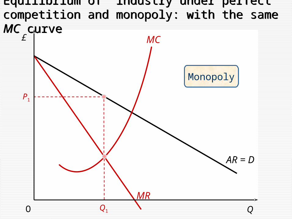
AR = D
MC
MR
£
Q O Q1
P1
Monopoly
Equilibrium of industry under perfect competition and monopoly: with the same MC curve
Equilibrium of industry under perfect competition and monopoly: with the same MC curve

£
Q O
MC ( = supply under perfect competition)
Q1
MR
P1
P2
Q2
AR = D
Comparison withPerfect competition
Equilibrium of industry under perfect competition and monopoly: with the same MC curve
Equilibrium of industry under perfect competition and monopoly: with the same MC curve

Monopoly
Disadvantages of monopoly high prices / low output: short run
high prices / low output: long run

Monopoly
Disadvantages of monopoly high prices / low output: short run
high prices / low output: long run
lack of incentive to innovate

Monopoly
Disadvantages of monopoly high prices / low output: short run
high prices / low output: long run
lack of incentive to innovate

Monopoly
Disadvantages of monopoly high prices / low output: short run
high prices / low output: long run
lack of incentive to innovate
Advantages of monopoly

Monopoly
Disadvantages of monopoly high prices / low output: short run
high prices / low output: long run
lack of incentive to innovate
Advantages of monopoly economies of scale

£
Q O Q1
MR
P1
MCmonopoly
AR = D
Equilibrium of industry under perfect competition and monopoly: with different MC curves
Equilibrium of industry under perfect competition and monopoly: with different MC curves

£
Q O
MC ( = supply)perfect competition
Q1
MR
P1
P2
Q2
MCmonopoly
AR = D
x
Q3
P3
Equilibrium of industry under perfect competition and monopoly: with different MC curves
Equilibrium of industry under perfect competition and monopoly: with different MC curves

Monopoly
Disadvantages of monopoly high prices / low output: short run
high prices / low output: long run
lack of incentive to innovate
Advantages of monopoly economies of scale
profits can be used for investment

Demand functions of a monopolist in two effectively segmented markets are:
Qa = 1,000 – 50Pa
Qb = 800 – 25Pb
Total cost function of the monopolist is TC = 500 + 10Q. If the monopolist does not practice price discrimination,
what is the sales maximizing price ?

Price Discrimination
A firm sells in two markets and has constant marginal costs of production equal to $2 per unit. The demand and demand and marginal revenue equations for the two markets are as follows:
Market 1 Market 2 P1 = 14 – 2Q1 P2 = 10 – Q2
MR1 = 14 – 4Q1 MR2 = 10 – 2Q2
Using third-degree price discrimination, what are the profit-
maximizing prices and quantities in each market? Show that greater profits result from price discrimination than would be obtained if a uniform price were used.