Quantum Science and Technology

Maria Schuld · Francesco Petruccione

Supervised Learning with Quantum Computers

Quantum Science and Technology

Series editors

Raymond Laflamme, Waterloo, ON, CanadaGaby Lenhart, Sophia Antipolis, FranceDaniel Lidar, Los Angeles, CA, USAArno Rauschenbeutel, Vienna University of Technology, Vienna, AustriaRenato Renner, Institut für Theoretische Physik, ETH Zürich, Zürich, SwitzerlandMaximilian Schlosshauer, Department of Physics, University of Portland, Portland,OR, USAYaakov S. Weinstein, Quantum Information Science Group, The MITRECorporation, Princeton, NJ, USAH. M. Wiseman, Brisbane, QLD, Australia

Aims and Scope

The book series Quantum Science and Technology is dedicated to one of today’smost active and rapidly expanding fields of research and development. In particular,the series will be a showcase for the growing number of experimental implemen-tations and practical applications of quantum systems. These will include, but arenot restricted to: quantum information processing, quantum computing, andquantum simulation; quantum communication and quantum cryptography; entan-glement and other quantum resources; quantum interfaces and hybrid quantumsystems; quantum memories and quantum repeaters; measurement-based quantumcontrol and quantum feedback; quantum nanomechanics, quantum optomechanicsand quantum transducers; quantum sensing and quantum metrology; as well asquantum effects in biology. Last but not least, the series will include books on thetheoretical and mathematical questions relevant to designing and understandingthese systems and devices, as well as foundational issues concerning the quantumphenomena themselves. Written and edited by leading experts, the treatments willbe designed for graduate students and other researchers already working in, orintending to enter the field of quantum science and technology.

More information about this series at http://www.springer.com/series/10039

Maria Schuld • Francesco Petruccione

Supervised Learningwith Quantum Computers

123

Maria SchuldSchool of Chemistry and Physics,Quantum Research Group

University of KwaZulu-NatalDurban, South Africa

and

National Institute for TheoreticalPhysics (NITheP)

KwaZulu-Natal, South Africa

and

Xanadu Quantum Computing IncToronto, Canada

Francesco PetruccioneSchool of Chemistry and PhysicsUniversity of KwaZulu-NatalDurban, South Africa

and

National Institute for TheoreticalPhysics (NITheP)

KwaZulu-Natal, South Africa

and

School of Electrical EngineeringKorea Advanced Institute of Scienceand Technology (KAIST)

Daejeon, Republic of Korea

ISSN 2364-9054 ISSN 2364-9062 (electronic)Quantum Science and TechnologyISBN 978-3-319-96423-2 ISBN 978-3-319-96424-9 (eBook)https://doi.org/10.1007/978-3-319-96424-9

Library of Congress Control Number: 2018950807

© Springer Nature Switzerland AG 2018This work is subject to copyright. All rights are reserved by the Publisher, whether the whole or partof the material is concerned, specifically the rights of translation, reprinting, reuse of illustrations,recitation, broadcasting, reproduction on microfilms or in any other physical way, and transmissionor information storage and retrieval, electronic adaptation, computer software, or by similar or dissimilarmethodology now known or hereafter developed.The use of general descriptive names, registered names, trademarks, service marks, etc. in thispublication does not imply, even in the absence of a specific statement, that such names are exempt fromthe relevant protective laws and regulations and therefore free for general use.The publisher, the authors and the editors are safe to assume that the advice and information in thisbook are believed to be true and accurate at the date of publication. Neither the publisher nor theauthors or the editors give a warranty, express or implied, with respect to the material contained herein orfor any errors or omissions that may have been made. The publisher remains neutral with regard tojurisdictional claims in published maps and institutional affiliations.

This Springer imprint is published by the registered company Springer Nature Switzerland AGThe registered company address is: Gewerbestrasse 11, 6330 Cham, Switzerland

For Chris and Monique

Preface

Quantum machine learning is a subject in the making, faced by huge expectationsdue to its parent disciplines. On the one hand, there is a booming commercialinterest in quantum technologies, which are at the critical point of becomingavailable for the implementation of quantum algorithms, and which have exceededthe realm of a purely academic interest. On the other hand, machine learning alongwith artificial intelligence is advertised as a central (if not the central) futuretechnology into which companies are bound to invest to avoid being left out.Combining these two worlds invariably leads to an overwhelming interest inquantum machine learning from the IT industry, an interest that is not alwaysmatched by the scientific challenges that researchers are only beginning to explore.

To find out what quantum machine learning has to offer, its numerous possibleavenues first have to be explored by an interdisciplinary community of scientists.We intend this book to be a possible starting point for this journey, as it introducessome key concepts, ideas and algorithms that are the result of the first few years ofquantum machine learning research. Given the young nature of the discipline, weexpect a lot of new angles to be added to this collection in due time. Our aim is notto provide a comprehensive literature review, but rather to summarise themes thatrepeatedly appear in quantum machine learning, to put them into context and makethem accessible to a broader audience in order to foster future research.

On the highest level, we target readers with a background in either physics orcomputer science that have a sound understanding of linear algebra and computeralgorithms. Having said that, quantum mechanics is a field based on advancedmathematical theory (and it does by no means help with a simple physical intuitioneither), and these access barriers are difficult to circumvent even with the mostwell-intended introduction to quantum mechanics. Not every section is thereforeeasy to understand for readers without experience in quantum computing. However,we hope that the main concepts are within reach and try to give higher leveloverviews wherever possible.

vii

We thank our editors Aldo Rampioni and Kirsten Theunissen for their supportand patience. Our thanks also go to a number of colleagues and friends who havehelped to discuss, inspire and proofread the book (in alphabetical order): BetonyAdams, Marcello Benedetti, Gian Giacomo Guerreschi, Vinayak Jagadish, NathanKilloran, Camille Lombard Latune, Andrea Skolik, Ryan Sweke, Peter Wittek andLeonard Wossnig.

Durban, South Africa Maria SchuldMarch 2018 Francesco Petruccione

viii Preface

Contents

1 Introduction . . . . . . . . . . . . . . . . . . . . . . . . . . . . . . . . . . . . . . . . . . . 11.1 Background . . . . . . . . . . . . . . . . . . . . . . . . . . . . . . . . . . . . . . . . 2

1.1.1 Merging Two Disciplines . . . . . . . . . . . . . . . . . . . . . . . . . 21.1.2 The Rise of Quantum Machine Learning . . . . . . . . . . . . . . 41.1.3 Four Approaches . . . . . . . . . . . . . . . . . . . . . . . . . . . . . . . 51.1.4 Quantum Computing for Supervised Learning . . . . . . . . . . 6

1.2 How Quantum Computers Can Classify Data . . . . . . . . . . . . . . . . 71.2.1 The Squared-Distance Classifier . . . . . . . . . . . . . . . . . . . . 81.2.2 Interference with the Hadamard Transformation . . . . . . . . . 91.2.3 Quantum Squared-Distance Classifier . . . . . . . . . . . . . . . . 131.2.4 Insights from the Toy Example . . . . . . . . . . . . . . . . . . . . 16

1.3 Organisation of the Book . . . . . . . . . . . . . . . . . . . . . . . . . . . . . . 17References . . . . . . . . . . . . . . . . . . . . . . . . . . . . . . . . . . . . . . . . . . . . . 18

2 Machine Learning . . . . . . . . . . . . . . . . . . . . . . . . . . . . . . . . . . . . . . . 212.1 Prediction . . . . . . . . . . . . . . . . . . . . . . . . . . . . . . . . . . . . . . . . . . 22

2.1.1 Four Examples for Prediction Tasks . . . . . . . . . . . . . . . . . 232.1.2 Supervised Learning . . . . . . . . . . . . . . . . . . . . . . . . . . . . 25

2.2 Models . . . . . . . . . . . . . . . . . . . . . . . . . . . . . . . . . . . . . . . . . . . 282.2.1 How Data Leads to a Predictive Model . . . . . . . . . . . . . . . 302.2.2 Estimating the Quality of a Model . . . . . . . . . . . . . . . . . . 322.2.3 Bayesian Learning . . . . . . . . . . . . . . . . . . . . . . . . . . . . . . 342.2.4 Kernels and Feature Maps . . . . . . . . . . . . . . . . . . . . . . . . 35

2.3 Training . . . . . . . . . . . . . . . . . . . . . . . . . . . . . . . . . . . . . . . . . . . 392.3.1 Cost Functions . . . . . . . . . . . . . . . . . . . . . . . . . . . . . . . . 402.3.2 Stochastic Gradient Descent . . . . . . . . . . . . . . . . . . . . . . . 42

2.4 Methods in Machine Learning . . . . . . . . . . . . . . . . . . . . . . . . . . . 442.4.1 Data Fitting . . . . . . . . . . . . . . . . . . . . . . . . . . . . . . . . . . . 452.4.2 Artificial Neural Networks . . . . . . . . . . . . . . . . . . . . . . . . 48

ix

2.4.3 Graphical Models . . . . . . . . . . . . . . . . . . . . . . . . . . . . . . 602.4.4 Kernel Methods . . . . . . . . . . . . . . . . . . . . . . . . . . . . . . . . 64

References . . . . . . . . . . . . . . . . . . . . . . . . . . . . . . . . . . . . . . . . . . . . . 71

3 Quantum Information . . . . . . . . . . . . . . . . . . . . . . . . . . . . . . . . . . . . 753.1 Introduction to Quantum Theory . . . . . . . . . . . . . . . . . . . . . . . . . 76

3.1.1 What Is Quantum Theory? . . . . . . . . . . . . . . . . . . . . . . . . 763.1.2 A First Taste . . . . . . . . . . . . . . . . . . . . . . . . . . . . . . . . . . 783.1.3 The Postulates of Quantum Mechanics . . . . . . . . . . . . . . . 84

3.2 Introduction to Quantum Computing . . . . . . . . . . . . . . . . . . . . . . 913.2.1 What Is Quantum Computing? . . . . . . . . . . . . . . . . . . . . . 913.2.2 Bits and Qubits . . . . . . . . . . . . . . . . . . . . . . . . . . . . . . . . 933.2.3 Quantum Gates . . . . . . . . . . . . . . . . . . . . . . . . . . . . . . . . 973.2.4 Quantum Parallelism and Function Evaluation . . . . . . . . . . 101

3.3 An Example: The Deutsch-Josza Algorithm . . . . . . . . . . . . . . . . . 1033.3.1 The Deutsch Algorithm . . . . . . . . . . . . . . . . . . . . . . . . . . 1033.3.2 The Deutsch-Josza Algorithm . . . . . . . . . . . . . . . . . . . . . . 1043.3.3 Quantum Annealing and Other Computational Models . . . . 106

3.4 Strategies of Information Encoding . . . . . . . . . . . . . . . . . . . . . . . 1083.4.1 Basis Encoding . . . . . . . . . . . . . . . . . . . . . . . . . . . . . . . . 1093.4.2 Amplitude Encoding . . . . . . . . . . . . . . . . . . . . . . . . . . . . 1103.4.3 Qsample Encoding . . . . . . . . . . . . . . . . . . . . . . . . . . . . . . 1123.4.4 Dynamic Encoding . . . . . . . . . . . . . . . . . . . . . . . . . . . . . 113

3.5 Important Quantum Routines . . . . . . . . . . . . . . . . . . . . . . . . . . . . 1143.5.1 Grover Search . . . . . . . . . . . . . . . . . . . . . . . . . . . . . . . . . 1143.5.2 Quantum Phase Estimation . . . . . . . . . . . . . . . . . . . . . . . . 1173.5.3 Matrix Multiplication and Inversion . . . . . . . . . . . . . . . . . 119

References . . . . . . . . . . . . . . . . . . . . . . . . . . . . . . . . . . . . . . . . . . . . . 123

4 Quantum Advantages . . . . . . . . . . . . . . . . . . . . . . . . . . . . . . . . . . . . 1274.1 Computational Complexity of Learning . . . . . . . . . . . . . . . . . . . . 1274.2 Sample Complexity . . . . . . . . . . . . . . . . . . . . . . . . . . . . . . . . . . 131

4.2.1 Exact Learning from Membership Queries . . . . . . . . . . . . 1334.2.2 PAC Learning from Examples . . . . . . . . . . . . . . . . . . . . . 1344.2.3 Introducing Noise . . . . . . . . . . . . . . . . . . . . . . . . . . . . . . 135

4.3 Model Complexity . . . . . . . . . . . . . . . . . . . . . . . . . . . . . . . . . . . 135References . . . . . . . . . . . . . . . . . . . . . . . . . . . . . . . . . . . . . . . . . . . . . 137

5 Information Encoding . . . . . . . . . . . . . . . . . . . . . . . . . . . . . . . . . . . . 1395.1 Basis Encoding . . . . . . . . . . . . . . . . . . . . . . . . . . . . . . . . . . . . . 141

5.1.1 Preparing Superpositions of Inputs . . . . . . . . . . . . . . . . . . 1425.1.2 Computing in Basis Encoding . . . . . . . . . . . . . . . . . . . . . 1455.1.3 Sampling from a Qubit . . . . . . . . . . . . . . . . . . . . . . . . . . 146

x Contents

5.2 Amplitude Encoding . . . . . . . . . . . . . . . . . . . . . . . . . . . . . . . . . . 1485.2.1 State Preparation in Linear Time . . . . . . . . . . . . . . . . . . . 1505.2.2 Qubit-Efficient State Preparation . . . . . . . . . . . . . . . . . . . . 1545.2.3 Computing with Amplitudes . . . . . . . . . . . . . . . . . . . . . . . 159

5.3 Qsample Encoding . . . . . . . . . . . . . . . . . . . . . . . . . . . . . . . . . . . 1595.3.1 Joining Distributions . . . . . . . . . . . . . . . . . . . . . . . . . . . . 1605.3.2 Marginalisation . . . . . . . . . . . . . . . . . . . . . . . . . . . . . . . . 1605.3.3 Rejection Sampling . . . . . . . . . . . . . . . . . . . . . . . . . . . . . 162

5.4 Hamiltonian Encoding . . . . . . . . . . . . . . . . . . . . . . . . . . . . . . . . 1635.4.1 Polynomial Time Hamiltonian Simulation . . . . . . . . . . . . . 1645.4.2 Qubit-Efficient Simulation of Hamiltonians . . . . . . . . . . . . 1665.4.3 Density Matrix Exponentiation . . . . . . . . . . . . . . . . . . . . . 167

References . . . . . . . . . . . . . . . . . . . . . . . . . . . . . . . . . . . . . . . . . . . . . 169

6 Quantum Computing for Inference . . . . . . . . . . . . . . . . . . . . . . . . . . 1736.1 Linear Models . . . . . . . . . . . . . . . . . . . . . . . . . . . . . . . . . . . . . . 173

6.1.1 Inner Products with Interference Circuits . . . . . . . . . . . . . . 1746.1.2 A Quantum Circuit as a Linear Model . . . . . . . . . . . . . . . 1796.1.3 Linear Models in Basis Encoding . . . . . . . . . . . . . . . . . . . 1826.1.4 Nonlinear Activations . . . . . . . . . . . . . . . . . . . . . . . . . . . 183

6.2 Kernel Methods . . . . . . . . . . . . . . . . . . . . . . . . . . . . . . . . . . . . . 1886.2.1 Kernels and Feature Maps . . . . . . . . . . . . . . . . . . . . . . . . 1896.2.2 The Representer Theorem . . . . . . . . . . . . . . . . . . . . . . . . 1916.2.3 Quantum Kernels . . . . . . . . . . . . . . . . . . . . . . . . . . . . . . . 1936.2.4 Distance-Based Classifiers . . . . . . . . . . . . . . . . . . . . . . . . 1966.2.5 Density Gram Matrices . . . . . . . . . . . . . . . . . . . . . . . . . . 201

6.3 Probabilistic Models . . . . . . . . . . . . . . . . . . . . . . . . . . . . . . . . . . 2046.3.1 Qsamples as Probabilistic Models . . . . . . . . . . . . . . . . . . . 2046.3.2 Qsamples with Conditional Independence Relations . . . . . . 2056.3.3 Qsamples of Mean-Field Approximations . . . . . . . . . . . . . 207

References . . . . . . . . . . . . . . . . . . . . . . . . . . . . . . . . . . . . . . . . . . . . . 209

7 Quantum Computing for Training . . . . . . . . . . . . . . . . . . . . . . . . . . 2117.1 Quantum Blas . . . . . . . . . . . . . . . . . . . . . . . . . . . . . . . . . . . . . . 212

7.1.1 Basic Idea . . . . . . . . . . . . . . . . . . . . . . . . . . . . . . . . . . . . 2127.1.2 Matrix Inversion for Training . . . . . . . . . . . . . . . . . . . . . . 2137.1.3 Speedups and Further Applications . . . . . . . . . . . . . . . . . . 218

7.2 Search and Amplitude Amplification . . . . . . . . . . . . . . . . . . . . . . 2197.2.1 Finding Closest Neighbours . . . . . . . . . . . . . . . . . . . . . . . 2207.2.2 Adapting Grover’s Search to Data Superpositions . . . . . . . 2217.2.3 Amplitude Amplification for Perceptron Training . . . . . . . 223

7.3 Hybrid Training for Variational Algorithms . . . . . . . . . . . . . . . . . 2247.3.1 Variational Algorithms . . . . . . . . . . . . . . . . . . . . . . . . . . . 2267.3.2 Variational Quantum Machine Learning Algorithms . . . . . 230

Contents xi

7.3.3 Numerical Optimisation Methods . . . . . . . . . . . . . . . . . . . 2337.3.4 Analytical Gradients of a Variational Classifier . . . . . . . . . 236

7.4 Quantum Adiabatic Machine Learning . . . . . . . . . . . . . . . . . . . . . 2387.4.1 Quadratic Unconstrained Optimisation . . . . . . . . . . . . . . . 2397.4.2 Annealing Devices as Samplers . . . . . . . . . . . . . . . . . . . . 2407.4.3 Beyond Annealing . . . . . . . . . . . . . . . . . . . . . . . . . . . . . . 242

References . . . . . . . . . . . . . . . . . . . . . . . . . . . . . . . . . . . . . . . . . . . . . 243

8 Learning with Quantum Models . . . . . . . . . . . . . . . . . . . . . . . . . . . . 2478.1 Quantum Extensions of Ising-Type Models . . . . . . . . . . . . . . . . . 248

8.1.1 The Quantum Ising Model . . . . . . . . . . . . . . . . . . . . . . . . 2498.1.2 Training Quantum Boltzmann Machines . . . . . . . . . . . . . . 2518.1.3 Quantum Hopfield Models . . . . . . . . . . . . . . . . . . . . . . . . 2538.1.4 Other Probabilistic Models . . . . . . . . . . . . . . . . . . . . . . . . 255

8.2 Variational Classifiers and Neural Networks . . . . . . . . . . . . . . . . . 2568.2.1 Gates as Linear Layers . . . . . . . . . . . . . . . . . . . . . . . . . . . 2578.2.2 Considering the Model Parameter Count . . . . . . . . . . . . . . 2598.2.3 Circuits with a Linear Number of Parameters . . . . . . . . . . 261

8.3 Other Approaches to Build Quantum Models . . . . . . . . . . . . . . . . 2638.3.1 Quantum Walk Models . . . . . . . . . . . . . . . . . . . . . . . . . . 2638.3.2 Superposition and Quantum Ensembles . . . . . . . . . . . . . . . 2668.3.3 QBoost . . . . . . . . . . . . . . . . . . . . . . . . . . . . . . . . . . . . . . 269

References . . . . . . . . . . . . . . . . . . . . . . . . . . . . . . . . . . . . . . . . . . . . . 271

9 Prospects for Near-Term Quantum Machine Learning . . . . . . . . . . . 2739.1 Small Versus Big Data . . . . . . . . . . . . . . . . . . . . . . . . . . . . . . . . 2749.2 Hybrid Versus Fully Coherent Approaches . . . . . . . . . . . . . . . . . . 2769.3 Qualitative Versus Quantitative Advantages . . . . . . . . . . . . . . . . . 2779.4 What Machine Learning Can Do for Quantum Computing . . . . . . 278Reference . . . . . . . . . . . . . . . . . . . . . . . . . . . . . . . . . . . . . . . . . . . . . . 279

Index . . . . . . . . . . . . . . . . . . . . . . . . . . . . . . . . . . . . . . . . . . . . . . . . . . . . . . 281

xii Contents

Acronyms

xm Training input/feature vectorym Training output/target label~x New input/feature vector~y Predicted label of a new inputc Lagrangian parametera Amplitude vectorai Amplitude, ith entry of the amplitude vectorv Input domainY Output domainD Data set, Training setvi Visible unit of a probabilistic modelhj Hidden unit of a probabilistic modelsi Visible or hidden unitbi Binary variablejii ith computational basis state of a qubit systemD Number of classes in a classification problemw Parameter or weight vector of a machine learning modelw0 Bias parameter of a machine learning modelh Set of parameters of a machine learning modelC Cost function for training a machine learning modelL Loss function for training a machine learning modelL Lagrangian objective functionR Regulariser for training a machine learning model/ Feature map from a data input space to a feature spaceu Nonlinear activation function for neural networksj Kernel functiong Learning rateX Data matrix, Design matrixU Unitary matrix, operator, quantum circuitUðhÞ Parametrised quantum circuit/Variational circuit

xiii

Chapter 1Introduction

Machine learning, on the one hand, is the art and science of making computers learnfrom data how to solve problems instead of being explicitly programmed. Quantumcomputing, on the other hand, describes information processing with devices basedon the laws of quantum theory. Both machine learning and quantum computing areexpected to play a role in how society deals with information in the future and it istherefore only natural to ask how they could be combined. This question is exploredin the emerging discipline of quantum machine learning and is the subject of thisbook.

In its broadest definition, quantum machine learning summarises approaches thatuse synergies between machine learning and quantum information. For example,researchers investigate how mathematical techniques from quantum theory can helpto develop newmethods in machine learning, or how we can use machine learning toanalyse measurement data of quantum experiments. Here we will use a much morenarrowdefinition of quantummachine learning and understand it asmachine learningwith quantum computers or quantum-assisted machine learning. Quantum machinelearning in this narrow sense looks at the opportunities that the current development ofquantum computers open up in the context of intelligent data mining. Does quantuminformation add something new to how machines recognise patterns in data? Canquantum computers help to solve problems faster, can they learn from fewer datasamples or are they able to deal with higher levels of noise? How can we developnew machine learning techniques from the language in which quantum computingis formulated? What are the ingredients of a quantum machine learning algorithm,and where lie the bottlenecks? In the course of this book we will investigate thesequestions and present different approaches to quantum machine learning research,together with the concepts, language and tricks that are commonly used.

To set the stage, the following section introduces the background of quantummachine learning. We then work through a toy example of how quantum computerscan learn from data, which will already display a number of issues discussed in thecourse of this book.

© Springer Nature Switzerland AG 2018M. Schuld and F. Petruccione, Supervised Learning with Quantum Computers,Quantum Science and Technology, https://doi.org/10.1007/978-3-319-96424-9_1

1

2 1 Introduction

1.1 Background

1.1.1 Merging Two Disciplines

Computers are physical devices based on electronic circuits which process infor-mation. Algorithms (the computer programs or ‘software’) are the recipes of howto manipulate the current in these circuits in order to execute computations. Al-though the physical processes involve microscopic particles like electrons, atomsand molecules, we can for all practical purposes describe them with a macroscopic,classical theory of the electric properties of the circuits. But if microscopic systemssuch as photons, electrons and atoms are directly used to process information, theyrequire another mathematical description to capture the fact that on small scales, na-ture behaves radically different fromwhat our intuition teaches us. Thismathematicalframework is called quantum theory and since its development at the beginning ofthe 20th century it has generally been considered to be the most comprehensive de-scription of microscopic physics that we know of. A computer whose computationscan only be described with the laws of quantum theory is called a quantum computer.

Since the 1990s quantum physicists and computer scientists have been analysinghowquantumcomputers canbebuilt andwhat they could potentially be used for. Theydeveloped several languages to describe computations executedby aquantumsystem,languages that allow us to investigate these devices from a theoretical perspective.An entire ‘zoo’ of quantum algorithms has been proposed and is waiting to be usedon physical hardware. The most famous language in which quantum algorithms areformulated is the circuit model. The central concept is that of a qubit, which takesthe place of a classical bit, as well as quantum gates to perform computations onqubits [1].

Building a quantum computer in the laboratory is not an easy task, as it requiresthe accurate control of very small systems. At the same time, it is crucial not to disturbthe fragile quantum coherence of these systems, which would destroy the quantumeffects that we want to harvest. In order to preserve quantum coherence throughoutthousands of computational operations, error correction becomes crucial. But errorcorrection for quantum systems turns out to be much more difficult than for classicalones, and becomes one of themajor engineering challenges in developing a full-scalequantum computer. Implementations of most of the existing quantum algorithmswilltherefore have to wait a little longer.

However, full-scale quantum computers are widely believed to become availablein the future. The research field has left the purely academic sphere and is on theagenda of the research labs of some of the largest IT companies. More and morecomputer scientists and engineers come on board to add their skills to the quantumcomputing community. Software toolboxes and quantum programming languagesbased on most major classical computational languages are available, and more arebeing developed every year. In summary, the realisation of quantum technologybecame an international and interdisciplinary effort.

1.1 Background 3

While targeting full-scale devices, a lot of progress has been made in the develop-ment of so called intermediate-term or small-scale devices. These devices have noerror correction, and count around 50–100 qubits that do not necessarily all speakto one another due to limited connectivity. Small-scale quantum devices do in prin-ciple have the power to test the advantages of quantum computing, and gave a newincentive to theory-driven research in quantum algorithmic design. The holy grailis currently to find a useful computational problem that can be solved by a small-scale device, and with a (preferably exponential) speed-up in runtime to the bestknown classical algorithm. In other words, the quest to find a ‘killer-app’, a compactbut powerful algorithm tailor made for early quantum technologies, is on. Machinelearning and its coremathematical problem, optimisation, are oftenmentioned as twopromising candidates, a circumstance that has given huge momentum to quantummachine learning research in the last couple of years.

This brings us to the other parent discipline, machine learning. Machine learninglies at the intersection of statistics, mathematics and computer science. It analy-ses how computers can learn from prior examples - usually large datasets based onhighly complex and nonlinear relationships - how tomake predictions or solve unseenproblem instances. Machine learning was born as the data-driven side of artificialintelligence research and tried to give machines human-like abilities such as imagerecognition, language processing and decision making. While such tasks come nat-urally to humans, we do not know in general how to make machines acquire similarskills. For example, looking at an image of a mountain panorama it is unclear how torelate the information that pixel (543,1352) is dark blue to the concept of a mountain.Machine learning approaches this problem by making the computer recover patternsfrom data, patterns that inherently contain these concepts.

Machine learning is also a discipline causing a lot of excitement in the academicworld as well as the IT sector (and certainly on a much larger scale than quantumcomputing). It is predicted to change the way a large share of the world’s populationinteracts with technology, a trend that has already started. As data is becomingincreasingly accessible, machine learning systems mature from research to businesssolutions and are integrated into PCs, cell phones and household devices. They scanthrough huge numbers of emails every day in order to pick out spammail, or throughmasses of images on social platforms to identify offensive contents. They are usedin forecasting of macroeconomic variables, risk analysis as well as fraud detectionin financial institutions, as well as medical diagnosis.

What has been celebrated as ‘breakthroughs’ and innovation is thereby oftenbased on the growing sizes of datasets as well as computational power, rather than onfundamentally new ideas.Methods such as neural networks, support vector machinesor AdaBoost, as well as the latest trend towards deep learningwere basically inventedin the 1990s and earlier. Finding genuinely new approaches is difficult as many taskstranslate into hard optimisation problems. To solve them, computers have to searchmore or less blindly through a vast landscape of solutions to find the best candidate. Alot of research therefore focuses on finding variations and approximations ofmethods

4 1 Introduction

that work well in practice, and machine learning is known to contain a fair share of“black art” [2]. This is an interesting point of leverage for quantum computing, whichhas the potential of contributing fundamentally new approaches to machine learning.

1.1.2 The Rise of Quantum Machine Learning

In recent years, there has been a growing body of literature with the objective ofcombining the disciplines of quantum information processing and machine learn-ing. Proposals that merge the two fields have been sporadically put forward sincequantum computing established itself as an independent discipline. Perhaps the ear-liest notions were investigations into quantum models of neural networks startingin 1995 [3]. These were mostly biologically inspired, hoping to find explanationswithin quantum theory for how the brain works (an interesting quest which is stillcontroversially disputed for lack of evidence). In the early 2000s the question of sta-tistical learning theory in a quantum setting was discussed, but received only limitedattention. A series of workshops on ‘Quantum Computation and Learning’ were or-ganised, and in the proceedings of the third event, Bonner and Freivals mention that“[q]uantum learning is a theory in the making and its scientific production is ratherfragmented” [4]. Sporadic publications on quantum machine learning algorithmsalso appeared during that time, such as Ventura and Martinez’ quantum associativememory [5] or Hartmut Neven’s ‘QBoost’ algorithm, which was implemented onthe first commercial quantum annealer, the D-Wave device, around 2009 [6].

The term ‘quantummachine learning’ came into use around 2013. Lloyd,Mohseniand Rebentrost [7] mention the expression in their manuscript of 2013, and in2014, Peter Wittek published an early monograph with the title Quantum MachineLearning—What quantum computing means to data mining [8], which summarisessome of the early papers. From 2013 onwards, interest in the topic increased signif-icantly [9] and produced a rapidly growing body of literature that covers all sortsof topics related to joining the two disciplines. Various international workshops andconferences1 have been organised and their number grew with every year. Numerousgroups, most of them still rooted in quantum information science, started researchprojects and collaborations. Combining a dynamic multi-billion dollar market withthe still ‘mysterious’ and potentially profitable technology of quantum computinghas also sparked a lot of interest in industry.2

1Some early events include a workshop at the Neural Information Processing Systems (NIPS)conference in Montreal, Canada in December 2015, the Quantum Machine Learning Workshop inSouth Africa in July 2016 as well as a Quantum Machine Learning conference at the PerimeterInstitute in Waterloo, Canada, in August 2016.2Illustrative examples are Google’s Quantum Artificial Intelligence Lab established in 2013, Mi-crosoft’s Quantum Architectures and Computation group and IBM’s IBM Q initiative.

1.1 Background 5

1.1.3 Four Approaches

As mentioned before, there are several definitions of the term quantum machinelearning, and in order to clarify the scope of this book it is useful to locate ourdefinition in the wider research landscape. For this we use a typology introducedby Aimeur, Brassard and Gambs [10]. It distinguishes four approaches of how tocombine quantum computing and machine learning, depending on whether one as-sumes the data to be generated by a quantum (Q) or classical (C) system, and if theinformation processing device is quantum (Q) or classical (C) (see Fig. 1.1).

The case CC refers to classical data being processed classically. This is of coursethe conventional approach to machine learning, but in this context it relates to ma-chine learning based on methods borrowed from quantum information research. Anexample is the application of tensor networks, which have been developed for quan-tum many-body-systems, to neural network training [11]. There are also numerous‘quantum-inspired’ machine learning models, with varying degrees of foundation inrigorous quantum theory.

The case QC investigates how machine learning can help with quantum comput-ing. For example, when we want to get a comprehensive description of the internalstate of a quantum computer from as few measurements as possible we can use ma-chine learning to analyse the measurement data [12]. Another idea is to learn phasetransitions in many-body quantum systems, a fundamental physical problem withapplications in the development of quantum computers [13]. Machine learning hasalso been found useful to discriminate between quantum states emitted by a source,or transformations executed by an experimental setup [14–16], and applications areplenty.

In this book we use the term ‘quantum machine learning’ synonymously with theremaining CQ and QQ approach on the right of Fig. 1.1. In fact, we focus mainly

Fig. 1.1 Four approachesthat combine quantumcomputing and machinelearning

data processing device

data

gene

rating

system

QC QQ

CC CQ

C - classical, Q - quantum

6 1 Introduction

on the CQ setting, which uses quantum computing to process classical datasets.The datasets consist of observations from classical systems, such as text, images ortime series of macroeconomic variables, which are fed into a quantum computer foranalysis. This requires a quantum-classical interface, which is a challenge we discussin detail in the course of the book. The central task of the CQ approach is to designquantum algorithms for data mining, and there are a number of strategies that havebeen proposed by the community. They range from translations of classical machinelearning models into the language of quantum algorithms, to genuinely new modelsderived from the working principles of quantum computers.

Wewillmostly be concernedwith supervised learning, inwhichonehas access to adataset with solutions to a problem, and uses these solutions as a supervision or figureof merit when solving a new problem. However, we note that quantum reinforcementlearning [17, 18] and unsupervised learning [19–21] are active research fields addinginteresting angles to the content of this book.

The last approach, QQ, looks at ‘quantum data’ being processed by a quantumcomputer. This can have two different meanings. First, the data could be derivedfrom measuring a quantum system in a physical experiment and feeding the valuesback into a separate quantum processing device. A much more natural setting how-ever arises where a quantum computer is first used to simulate the dynamics of aquantum system (as investigated in the discipline of quantum simulation and withfruitful applications to modeling physical and chemical properties that are otherwisecomputationally intractable), and consequently takes the state of the quantum sys-tem as an input to a quantum machine learning algorithm executed on the very samedevice. The advantage of such an approach is that while measuring all informationof a quantum state may require a number of measurements that is exponential inthe system size, the quantum computer has immediate access to all this informationand can produce the result, for example a yes/no decision, directly—an exponentialspeedup by design.

The QQ approach is doubtless very interesting, but there are presently only fewresults in this direction (for example [17]). Some authors claim that their quantummachine learning algorithm can easily be fed with quantum data, but the details maybe less obvious.Does learning fromquantumdata (i.e. thewave function of a quantumsystem) produce different results to classical data? How can we combine the datageneration and data analysis unit effectively? Can we design algorithms that answerimportant questions from experimentalists which would otherwise be intractable? Inshort, although much of what is presented here can be used in the ‘quantum data’setting as well, there are a number of interesting open problems specific to this casethat we will not be able to discuss in detail.

1.1.4 Quantum Computing for Supervised Learning

From now on we will focus on the CQ case for supervised learning problems. Thereare two different strategies when designing quantum machine learning algorithms,

1.1 Background 7

and of course most researchers are working somewhere between the two extremes.The first strategy aims at translating classical models into the language of quantummechanics in the hope to harvest algorithmic speedups. The sole goal is to reproducethe results of a givenmodel, say a neural net or a Gaussian process, but to ‘outsource’the computation or parts of the computation to a quantum device. The translationalapproach requires significant expertise in quantumalgorithmic design. The challengeis to assemble quantum routines that imitate the results of the classical algorithmwhile keeping the computational resources as low as possible. While sometimesextending the toolbox of quantum routines by some new tricks, learning does notpose a genuinely new problem here. On the contrary, the computational tasks tosolve resemble rather general mathematical problems such as computing a nonlinearfunction,matrix inversion or finding the optimumof a non-convex objective function.Consequently, the boundaries of speedups that can be achieved are very much thesame as in ‘mainstream’ quantum computing. Quantum machine learning becomesan application of quantum computing rather than a truly interdisciplinary field ofresearch.

The second strategy, whose many potential directions are still widely unexplored,leaves the boundaries of known classicalmachine learningmodels. Instead of startingwith a classical algorithm, one starts with a quantum computer and asks what typeof machine learning model might fit its physical characteristics and constraints,its formal language and its proposed advantages. This could lead to an entirelynew model or optimisation objective—or even an entirely new branch of machinelearning—that is derived from a quantum computational paradigm. We will call thisthe exploratory approach. The exploratory approach does not necessarily rely ona digital, universal quantum computer to implement quantum algorithms, but mayuse any system obeying the laws of quantum mechanics to derive (and then train)a model that is suitable to learn from data. The aim is not only to achieve runtimespeedups, but to contribute innovative methods to the machine learning community.For this, a solid understanding—and feeling—for the intricacies of machine learningis needed, in particular because the new model has to be analysed and benchmarkedto access its potential. We will investigate both strategies in the course of this book.

1.2 How Quantum Computers Can Classify Data

In order to build a first intuition of what it means to learn from classical data with aquantum computer we want to present a toy example that is supposed to illustrate arange of topics discussed throughout this book, and for which no previous knowledgein either field is required. More precisely, we will look at how to implement a typeof nearest neighbour method with quantum interference induced by a Hadamardgate. The example is a strongly simplified version of a quantum machine learningalgorithm proposed in [22], which will be presented in more detail in Sect. 6.2.4.2.

8 1 Introduction

Table 1.1 Mini-dataset for the quantum classifier example

Raw data Preprocessed data Survival

Price Cabin Price Cabin

Passenger 1 8,500 0910 0.85 0.36 1 (yes)

Passenger 2 1,200 2105 0.12 0.84 0 (no)

Passenger 3 7,800 1121 0.78 0.45 ?

1.2.1 The Squared-Distance Classifier

Machine learning always starts with a dataset. Inspired by the kaggle3 Titanic dataset,let us consider a set of 2-dimensional input vectors {xm = (xm

0 , xm1 )T },m = 1, . . . , M .

Each vector represents a passenger who was on the Titanic when the ship sank inthe tragic accident of 1912, and specifies two features of the passenger: The pricein dollars which she or he paid for the ticket (feature 0) and the passenger’s cabinnumber (feature 1). Assume the ticket price is between $0 and $10,000, and the cabinnumbers range from 1 to 2,500. Each input vector xm is also assigned a label ym thatindicates if the passenger survived (ym = 1) or died (ym = 0).

To reduce the complexity even more (possibly to an absurd extent), we con-sider a dataset of only 2 passengers, one who died and one who survived the event(see Table1.1). The task is to find the probability of a third passenger of featuresx = (x0, x1)T and for whom no label is given, to survive or die. As is common inmachine learning, we preprocess the data in order to project it onto roughly the samescales. Oftentimes, this is done by imposing zero mean and unit variance, but herewe will simply rescale the range of possible ticket prices and cabin numbers to theinterval [0, 1] and round the values to two decimal digits.

Possibly the simplest supervised machine learning method, which is still surpris-ingly successful in many cases, is known as nearest neighbour. A new input is giventhe same label as the data point closest to it (or, in a more popular version, the major-ity of its k nearest neighbours). Closeness has to be defined by a distance measure,for example the Euclidean distance between data points. A less frequent strategywhich we will consider here is to include all data points m = 1, . . . , M , but weigheach one’s influence towards the decision by a weight

γm = 1 − 1

c|x − xm|2, (1.1)

where c is some constant. The weight γm measures the squared distance betweenxm and the new input x, and by subtracting the distance from one we get a higherweight for closer data points. We define the probability of assigning label y to the

3Kaggle (www.kaggle.com) is an open data portal that became famous for hosting competitionswhich anyone can enter to put her or his machine learning software to the test.

1.2 How Quantum Computers Can Classify Data 9

Fig. 1.2 The mini-datasetdisplayed in a graph. Thesimilarity (Euclideandistance) betweenPassengers 1 and 3 is closerthan between Passengers 2and 3

ticket price

cabinnu

mber

Passenger 1

Passenger 2

Passenger 3

new input x as the sum over the weights of all M1 training inputs which are labeledwith ym = 1,

px(y = 1) = 1

χ

1

M1

∑

m|ym=1

(1 − 1

c|x − xm|2

). (1.2)

The probability of predicting label 0 for the new input is the same sum, but overthe weights of all inputs labeled with 0. The factor 1

χis included to make sure that

px(y = 0) + px(y = 1) = 1. We will call this model the squared-distance classifier.A nearest neighbour method is based on the assumption that similar inputs should

have a similar output, which seems reasonable for the data at hand. People froma similar income class and placed at a similar area on the ship might have similarfates during the tragedy. If we had another feature without expressive power toexplain death or survival of a person, for example a ticket number that was assignedrandomly to the tickets, this method would obviously be less successful becauseit tries to consider the similarity of ticket numbers. Applying the squared-distanceclassifier to the mini-dataset, we see in Fig. 1.2 that Passenger 3 is closer to Passenger1 than to Passenger 2, and our classifier would predict ‘survival’.

1.2.2 Interference with the Hadamard Transformation

Now we want to discuss how to use a quantum computer in a trivial way to computethe result of the squared-distance classifier. Most quantum computers are based ona mathematical model called a qubit, which can be understood as a random bit (aBernoulli randomvariable)whose description is not governed by classical probabilitytheory but by quantummechanics. The quantummachine learning algorithm requiresus to understand only one ‘single-qubit operation’ that acts on qubits, the so calledHadamard transformation. We will illustrate what a Hadamard gate does to twoqubits by comparing it with an equivalent operation on two random bits. To relyeven more on intuition, we will refer to the two random bits as two coins that can betossed, and the quantum bits can be imagined as quantum versions of these coins.

10 1 Introduction

Table 1.2 Probability distribution over possible outcomes of the coin toss experiment, and itsequivalent with qubits

State Classical coin State Qubit

Step 1 Step 2 Step 3 Step 1 Step 2 Step 3

(heads, heads) 1 0.5 0.5 |heads〉|heads〉 1 0.5 1

(heads, tails) 0 0 0 |heads〉|tails〉 0 0 0

(tails, heads) 0 0.5 0.5 |tails〉|heads〉 0 0.5 0

(tails, tails) 0 0 0 |tails〉|tails〉 0 0 0

Imagine two fair coins c1 and c2 that can each be in state heads or tails withequal probability. The space of possible states after tossing the coins (c1, c2) consistsof (heads, heads), (heads, tails), (tails, heads) and (heads, heads). As a preparationStep 1, turn both coins to ‘heads’. In Step 2 toss the first coin only and check theresult. In Step 3 toss the first coin a second time and check the result again. Considerrepeating this experiment from scratch a sufficiently large number of times to countthe statistics, which in the limiting case of infinite repetitions can be interpreted asprobabilities.4 The first three columns of Table1.2 show these probabilities for ourlittle experiment. After the preparation step 1 the state is by definition (heads, heads).After the first toss in step 2we observe the states (heads, heads) and (tails, heads) withequal probability. After the second toss in step 3, we observe the same two states withequal probability, and the probability distribution hence does not change betweenstep 2 and 3. Multiple coin tosses maintain the state of maximum uncertainty for theobserver regarding the first coin.

Compare this with two qubits q1 and q2. Again, performing a measurement calleda projective z-measurement (we will come to that later) a qubit can be found to be intwo different states (let us stick with calling them |heads〉 and |tails〉, but later it willbe |0〉 and |1〉). Start again with both qubits being in state |heads〉|heads〉. This meansthat repeated measurements would always return the result |heads〉|heads〉, just asin the classical case. Now we apply an operation called the Hadamard transform onthe first qubit, which is sometimes considered as the quantum equivalent of a faircoin toss. Measuring the qubits after this operation will reveal the same probabilitydistribution as in the classical case, namely that the probability of |heads〉|heads〉and |tails〉|heads〉 is both 0.5. However, if we apply the ‘Hadamard coin toss’ twicewithout intermediate observation of the state, one will measure the qubits always instate (heads, heads), no matter how often one repeats the experiment. This transitionfrom high uncertainty to a state of lower uncertainty is counterintuitive for classicalstochastic operations. As a side note beyond the scope of this chapter, it is crucialthat we do not measure the state of the qubits after Step 2 since this would returna different distribution for Step 3—another interesting characteristic of quantummechanics.

4We are assuming a frequentist’s viewpoint for the moment.

1.2 How Quantum Computers Can Classify Data 11

Let us have a closer look at the mathematical description of the Hadamard opera-tion (and have a first venture into the world of quantum computing). In the classicalcase, the first coin toss imposes a transformation

p =

⎛

⎜⎜⎝

1000

⎞

⎟⎟⎠ → p′ =

⎛

⎜⎜⎝

0.500.50

⎞

⎟⎟⎠ ,

where we have now written the four probabilities into a probability vector. The firstentry of that vector gives us the probability to observe state (heads, heads), the second(heads, tails) and so forth. In linear algebra, a transformation between probabilityvectors can always be described by a special matrix called a stochastic matrix, inwhich rows add up to 1. Performing a coin toss on the first coin corresponds to astochastic matrix of the form

S = 1

2

⎛

⎜⎜⎝

1 0 1 00 1 0 11 0 1 00 1 0 1

⎞

⎟⎟⎠ .

Applying this matrix to p′ leads to a new state p′′ = Sp′, which is in this case equalto p′.

This description works fundamentally differently when it comes to qubits gov-erned by the probabilistic laws of quantum theory. Instead of stochastic matricesacting on probability vectors, quantum objects can be described by unitary (andcomplex) matrices acting on complex amplitude vectors. There is a close relation-ship between probabilities and amplitudes: The probability of the two qubits to bemeasured in a certain state is the absolute square of the corresponding amplitude. Theamplitude vector α describing the two qubits after preparing them in |heads〉|heads〉would be

α =

⎛

⎜⎜⎝

1000

⎞

⎟⎟⎠ ,

which makes the probability of |heads〉|heads〉 equal to |1|2 = 1. In this case theamplitude vector is identical to the probability vector of the quantum system. In thequantum case, the stochastic matrix is replaced by a Hadamard transform acting onthe first qubit, which can be written as

H = 1√2

⎛

⎜⎜⎝

1 0 1 00 1 0 11 0 −1 00 1 0 −1

⎞

⎟⎟⎠

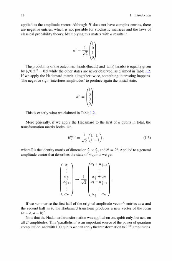
12 1 Introduction

applied to the amplitude vector. Although H does not have complex entries, thereare negative entries, which is not possible for stochastic matrices and the laws ofclassical probability theory. Multiplying this matrix with a results in

α′ = 1√2

⎛

⎜⎜⎝

1010

⎞

⎟⎟⎠ .

The probability of the outcomes |heads〉|heads〉 and |tails〉|heads〉 is equally givenby |√0.5|2 = 0.5 while the other states are never observed, as claimed in Table1.2.If we apply the Hadamard matrix altogether twice, something interesting happens.The negative sign ‘interferes amplitudes’ to produce again the initial state,

α′′ =

⎛

⎜⎜⎝

1000

⎞

⎟⎟⎠ .

This is exactly what we claimed in Table1.2.

More generally, if we apply the Hadamard to the first of n qubits in total, thetransformation matrix looks like

H (q1)n = 1√

2

(1 11 −1

), (1.3)

where I is the identity matrix of dimension N2 × N

2 , and N = 2n. Applied to a generalamplitude vector that describes the state of n qubits we get

⎛

⎜⎜⎜⎜⎜⎜⎜⎜⎝

α1...

α N2

α N2 +1...

αN

⎞

⎟⎟⎟⎟⎟⎟⎟⎟⎠

→ 1√2

⎛

⎜⎜⎜⎜⎜⎜⎜⎜⎜⎝

α1 + α N2 +1

...

α N2

+ αN

α1 − α N2 +1

...

α N2

− αN

⎞

⎟⎟⎟⎟⎟⎟⎟⎟⎟⎠

.

If we summarise the first half of the original amplitude vector’s entries as a andthe second half as b, the Hadamard transform produces a new vector of the form(a + b, a − b)T .

Note that the Hadamard transformation was applied on one qubit only, but acts onall 2n amplitudes. This ‘parallelism’ is an important source of the power of quantumcomputation, andwith 100 qubitswecan apply the transformation to 2100 amplitudes.

1.2 How Quantum Computers Can Classify Data 13

Of course, parallelism is a consequence of the probabilistic description and likewisetrue for classical statistics. However, together with the effects of interference (i.e.,the negative signs in the matrix), quantum computing researchers hope to gain asignificant advantage over classical computation.

1.2.3 Quantum Squared-Distance Classifier

Let us get back to our toy quantum machine learning algorithm. We can use theHadamard operation to compute the prediction of the squared-distance classifier byfollowing these four steps:Step A—Some more data preprocessingTo begin with we need another round of data preprocessing in which the length ofeach input vector (i.e., the ticket price and cabin number for each passenger) getsnormalised to one. This requirement projects the data onto a unit circle, so that onlyinformation about the angles between data vectors remains. For some datasets thisis a desired effect because the length of data vectors has no expressive power, whilefor others the loss of information is a problem. In the latter case one can use trickswhich we will discuss in Chap. 5. Luckily, for the data points chosen in this examplethe normalisation does not change the outcome of a distance-based classifier (seeFig. 1.3).Step B—Data encodingThe dataset has to be encoded in a quantum system in order to use the Hadamardtransform. We will discuss different ways of doing so in Chap. 5. In this example thedata is represented by an amplitude vector (in a method we will later call amplitudeencoding). Table1.3 shows that we have six features to encode, plus two class labels.Let us have a look at the features first. We need three qubits or ‘quantum coins’(q1, q2, q3) with values q1, q2, q3 = 0, 1 to have 8 different measurement results.(Only two qubits would not be sufficient, because we would only have four possible

price room survival

Passenger 1 0.921 0.390 yes (1)

Passenger 2 0.141 0.990 no (0)

Passenger 3 0.866 0.500 ?

ticket price

cabinnu

mber

Passenger 1

Passenger 2

Passenger 3

Fig. 1.3 Left: Additional preprocessing of the data. Each feature vector gets normalised to unitlength. Right: Preprocessed data displayed in a graph. The points now lie on a unit circle. TheEuclidean distance between Passengers 1 and 3 is still smaller than between Passengers 2 and 3

14 1 Introduction

Table 1.3 The transformation of the amplitude vector in the quantum machine learning algorithm

Qubit state Transformation of amplitude vector

q1 q2 q3 q4 Step Bαinit →

Step Cαinter →

Step Dαfinal

0 0 0 0 0 0 0

0 0 0 1 1√40.921 1√

4(0.921 + 0.866) 1√

4χ(0.921 + 0.866)

0 0 1 0 0 0 0

0 0 1 1 1√40.390 1√

4(0.390 + 0.500) 1√

4χ(0.390 + 0.500)

0 1 0 0 1√40.141 1√

4(0.141 + 0.866) 1√

4χ(0.141 + 0.866)

0 1 0 1 0 0 0

0 1 1 0 1√40.990 1√

4(0.990 + 0.500) 1√

4χ(0.990 + 0.500)

0 1 1 1 0 0 0

1 0 0 0 0 0 0

1 0 0 1 1√40.866 1√

4(0.921 − 0.866) 0

1 0 1 0 0 0 0

1 0 1 1 1√40.500 1√

4(0.390 − 0.500) 0

1 1 0 0 1√40.866 1√

4(0.141 − 0.866) 0

1 1 0 1 0 0 0

1 1 1 0 1√40.500 1√

4(0.990 − 0.500) 0

1 1 1 1 0 0 0

Data encoding starts with a quantum system whose amplitude vector contains the features as wellas some zeros (Step 2). The Hadamard transformation “interferes” blocks of amplitudes (Step 3).Measuring the first qubit in state 0 (and aborting/repeating the entire routine if this observationdid not happen) effectively turns all amplitudes of the second block to zero and renormalises thefirst block (Step 4). The renormalisation factor is given by χ = 1

4 (|0.921 + 0.866|2 + |0.390 +0.500|2 + |0.141 + 0.866|2 + |0.990 + 0.500|2)

outcomes as in the example above). Each measurement result is associated withan amplitude whose absolute square gives us the probability of this result beingobserved. Amplitude encoding ‘writes’ the values of features into amplitudes anduses operations such as the Hadamard transform to perform computations on thefeatures, for example additions and subtractions.

The amplitude vector we need to prepare is equivalent to the vector constructed byconcatenating the features of Passenger 1 and 2, as well as two copies of the featuresof Passenger 3,

α = 1√4

(0.921, 0.39, 0.141, 0.99, 0.866, 0.5, 0.866, 0.5)T .

The absolute square of all amplitudes has to sum up to 1, which is why we had toinclude another scaling or normalisation factor of 1/

√4 for the 4 data points. We

1.2 How Quantum Computers Can Classify Data 15

now extend the state by a fourth qubit. For each feature encoded in an amplitude,the fourth qubit is in the state that corresponds to the label of that feature vector.(Since the new input does not have a target, we associate the first copy with the targetof Passenger 1 and the second copy with the target of Passenger 2, but there areother choices that would work too). Table1.3 illuminates this idea further. Addingthe fourth qubit effectively pads the amplitude vector by some intermittent zeros,

αinit = 1√4

(0, 0.921, 0, 0.39, 0.141, 0, 0.99, 0, 0, 0.866, 0, 0.5, 0.866, 0, 0.5, 0)T .

This way of associating an amplitude vector with data might seem arbitrary atthis stage, but we will see that it fulfils its purpose.Step C—Hadamard transformationWenow‘toss’ thefirst ‘quantumcoin’q1, or in otherwords,wemultiply the amplitudevector by the Hadamard matrix from Eq. (1.3). Chapter 3 will give a deeper accountof what this means in the framework of quantum computing, but for now this canbe understood at a single standard computational operation on a quantum computer,comparable with an AND or OR gate on a classical machine. The result can be foundin column αinter of Table1.3. As stated before, the Hadamard transform computes thesums and differences between blocks of amplitudes, in this case between the copiesof the new input to every training input.Step D—Measure the first qubitNow measure the first qubit, and only continue the algorithm if it is found in state0 (otherwise start from scratch). This introduces an ‘if’ statement into the quantumalgorithm, and is similar to rejection sampling. After this operation we know that thefirst qubit cannot be in state 1 (by sheer common sense). On the level of the amplitudevector, we have to write zero amplitudes for states in which q1 = 1 and renormaliseall other amplitudes so that the amplitude vector is again overall normalised (seecolumn αfinal of Table1.3).Step E—Measure the last qubitFinally, we measure the last qubit. We have to repeat the entire routine for a numberof times to resolve the probability p(q4) (sincemeasurements only take samples fromthe distribution). The probability p(q4 = 0) is interpreted as the output of themachinelearning model, or the probability that the classifier predicts the label 0 for the newinput. We now want to show that this is exactly the result of the squared-distanceclassifier (1.2).

By the laws of quantum mechanics, the probability of observing q4 = 0 after thedata encoding and the Hadamard transformation can be computed by adding theabsolute squares of the amplitudes corresponding to q4 = 0 (i.e. the values of evenrows in Table1.3),

p(q4 = 0) = 1

4χ

(|0.141 + 0.866|2 + |0.990 + 0.500|2) ≈ 0.448,

16 1 Introduction

with χ = 14 (|0.921 + 0.866|2 + |0.390 + 0.500|2 + |0.141 + 0.866|2 + |0.990 +

0.500|2). Equivalently, the probability of observing q4 = 1 is given by

p(q4 = 1) = 1

4χ

(|0.921 + 0.866|2 + |0.390 + 0.500|2) ≈ 0.552,

and is obviously equal to 1 − p(q4 = 0). This is the same as

p(q4 = 0) = 1

χ

(1 − 1

4(|0.141 − 0.866|2 + |0.990 − 0.500|2)

)≈ 0.448,

p(q4 = 1) = 1

4χ

(1 − 1

4(|0.921 − 0.866|2 + |0.390 − 0.500|2)

)≈ 0.552.

Of course, the equivalence is no coincidence, but stems from the normalisation ofeach feature vector in Step 1 and can be shown to always be true for this algorithm.If we compare these last results to Eq. (1.2), we see that this is in fact exactly theoutput of the squared-distance classifier, with the constant c now specified as c = 4.

The crux of the matter is that after data encoding, only one single computationaloperation and two simple measurements (as well as a couple of repetitions of theentire routine) were needed to get the result, the output of the classifier. This holdstrue for any size of the input vectors or dataset. For example, if our dataset had 1billion training vectors of size 1 million, we would still have an algorithm with thesame constant runtime of three elementary operations.

1.2.4 Insights from the Toy Example

As much as nearest neighbour is an oversimplification of machine learning, usingthe Hadamard to calculate differences is a mere glimpse of what quantum computerscan do. There are many other approaches to design quantum machine learning algo-rithms, for example to encode information into the state of the qubits, or to use thequantumcomputer as a sampler.And although the promise of a data-size-independentalgorithm first sounds too good to be true, there are several things to consider. First,the initial state αinit encoding the data has to be prepared, and if no shortcuts areavailable, this requires another algorithm with a number of operations that is linearin the dimension and size of the dataset (and we are back to square one). What ismore, the Hadamard transform belongs to the so called Clifford group of quantumgates, which means that the simulation of the algorithm is classically tractable. Onthe other hand, both arguments do not apply to the QQ approach discussed above,in which we process quantum data and where true exponential speedups are to beexpected.

1.2 How Quantum Computers Can Classify Data 17

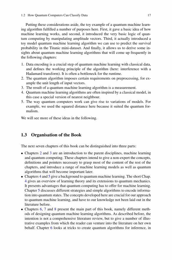
Putting these considerations aside, the toy example of a quantum machine learn-ing algorithm fulfilled a number of purposes here. First, it gave a basic idea of howmachine learning works, and second, it introduced the very basic logic of quan-tum computing by manipulating amplitude vectors. Third, it actually introduced atoy model quantum machine learning algorithm we can use to predict the survivalprobability in the Titanic mini-dataset. And finally, it allows us to derive some in-sights about quantum machine learning algorithms that will come up frequently inthe following chapters:

1. Data encoding is a crucial step of quantum machine learning with classical data,and defines the working principle of the algorithm (here: interference with aHadamard transform). It is often a bottleneck for the runtime.

2. The quantum algorithm imposes certain requirements on preprocessing, for ex-ample the unit length of input vectors.

3. The result of a quantum machine learning algorithm is a measurement.4. Quantum machine learning algorithms are often inspired by a classical model, in

this case a special version of nearest neighbour.5. The way quantum computers work can give rise to variations of models. For

example, we used the squared distance here because it suited the quantum for-malism.

We will see more of these ideas in the following.

1.3 Organisation of the Book

The next seven chapters of this book can be distinguished into three parts:

• Chapters 2 and 3 are an introduction to the parent disciplines, machine learningand quantum computing. These chapters intend to give a non-expert the concepts,definitions and pointers necessary to grasp most of the content of the rest of thechapters, and introduce a range of machine learning models as well as quantumalgorithms that will become important later.

• Chapters 4 and 5 give a background to quantummachine learning. The short Chap.4 gives an overview of learning theory and its extensions to quantum mechanics.It presents advantages that quantum computing has to offer for machine learning.Chapter 5 discusses different strategies and simple algorithms to encode informa-tion into quantum states. The concepts developed here are crucial for our approachto quantum machine learning, and have to our knowledge not been laid out in theliterature before.

• Chapters 6, 7 and 8 present the main part of this book, namely different meth-ods of designing quantum machine learning algorithms. As described before, theintention is not a comprehensive literature review, but to give a number of illus-trative examples from which the reader can venture into the literature on her ownbehalf. Chapter 6 looks at tricks to create quantum algorithms for inference, in

18 1 Introduction

other words to compute a prediction if given an input. Chapter 7 is dedicated totraining and optimisation with quantum devices. Chapter 8 finally introduces someideas that leave the realm of what is known in machine learning and think aboutquantum extensions of classical models, or how to use quantum devices as a modelblack-box.

The conclusion in Chap. 9 is dedicated to the question of what role machine learningplays for applications with intermediate-term quantum devices. The discussion ofquantum machine learning in a closer time horizon will also be useful to summarisesome problems and solutions which came up as the main themes of the book, whilegiving an outlook to potential further research.

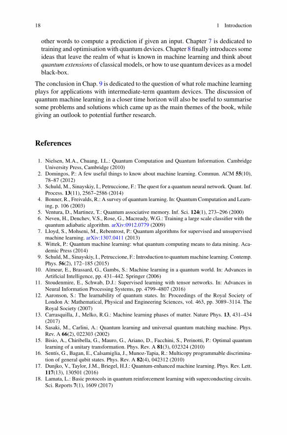
References

1. Nielsen, M.A., Chuang, I.L.: Quantum Computation and Quantum Information. CambridgeUniversity Press, Cambridge (2010)

2. Domingos, P.: A few useful things to know about machine learning. Commun. ACM 55(10),78–87 (2012)

3. Schuld, M., Sinayskiy, I., Petruccione, F.: The quest for a quantum neural network. Quant. Inf.Process. 13(11), 2567–2586 (2014)

4. Bonner, R., Freivalds, R.: A survey of quantum learning. In: Quantum Computation and Learn-ing, p. 106 (2003)

5. Ventura, D., Martinez, T.: Quantum associative memory. Inf. Sci. 124(1), 273–296 (2000)6. Neven, H., Denchev, V.S., Rose, G., Macready, W.G.: Training a large scale classifier with the

quantum adiabatic algorithm. arXiv:0912.0779 (2009)7. Lloyd, S., Mohseni, M., Rebentrost, P.: Quantum algorithms for supervised and unsupervised

machine learning. arXiv:1307.0411 (2013)8. Wittek, P.: Quantum machine learning: what quantum computing means to data mining. Aca-

demic Press (2014)9. Schuld,M., Sinayskiy, I., Petruccione, F.: Introduction to quantummachine learning. Contemp.

Phys. 56(2), 172–185 (2015)10. Aïmeur, E., Brassard, G., Gambs, S.: Machine learning in a quantum world. In: Advances in

Artificial Intelligence, pp. 431–442. Springer (2006)11. Stoudenmire, E., Schwab, D.J.: Supervised learning with tensor networks. In: Advances in

Neural Information Processing Systems, pp. 4799–4807 (2016)12. Aaronson, S.: The learnability of quantum states. In: Proceedings of the Royal Society of

London A: Mathematical, Physical and Engineering Sciences, vol. 463, pp. 3089–3114. TheRoyal Society (2007)

13. Carrasquilla, J., Melko, R.G.: Machine learning phases of matter. Nature Phys. 13, 431–434(2017)

14. Sasaki, M., Carlini, A.: Quantum learning and universal quantum matching machine. Phys.Rev. A 66(2), 022303 (2002)

15. Bisio, A., Chiribella, G., Mauro, G., Ariano, D., Facchini, S., Perinotti, P.: Optimal quantumlearning of a unitary transformation. Phys. Rev. A 81(3), 032324 (2010)

16. Sentís, G., Bagan, E., Calsamiglia, J., Munoz-Tapia, R.: Multicopy programmable discrimina-tion of general qubit states. Phys. Rev. A 82(4), 042312 (2010)

17. Dunjko, V., Taylor, J.M., Briegel, H.J.: Quantum-enhanced machine learning. Phys. Rev. Lett.117(13), 130501 (2016)

18. Lamata, L.: Basic protocols in quantum reinforcement learning with superconducting circuits.Sci. Reports 7(1), 1609 (2017)

References 19

19. Aïmeur, E., Brassard, G., Gambs, S.: Quantum speed-up for unsupervised learning. Mach.Learn. 90(2), 261–287 (2013)

20. Lloyd, S., Mohseni, M., Rebentrost, P.: Quantum principal component analysis. Nature Phys.10, 631–633 (2014)

21. Benedetti,M.,Realpe-Gómez, J., Perdomo-Ortiz,A.:Quantum-assistedHelmholtzmachines: aquantum-classical deep learning framework for industrial datasets in near-term devices. Quant.Sci. Technol. 3, 034007 (2018)

22. Schuld, M., Fingerhuth, M., Petruccione, F.: Implementing a distance-based classifier with aquantum interference circuit. EPL (Europhys. Lett.) 119(6), 60002 (2017)

Chapter 2Machine Learning

Machine learning originally emerged as a sub-discipline of artificial intelligenceresearch where it extended areas such as computer perception, communication andreasoning [1]. For humans, learning means finding patterns in previous experiencewhich help us to deal with an unknown situation. For example, someone who haslived on a farm for thirty years will be very good at predicting the local weather.Financial analysts pride themselves on being able to predict the immediate stockmarket trajectory. This expertise is the result of many iterations of observing mean-ingful indicators such as the clouds, wind and time of the year, or the global politicalsituation and macroeconomic variables. When speaking about machines, observa-tions come in the formof data,while the solution to a newproblemmay be understoodas the output of an algorithm. Machine learning means to automate the process ofgeneralising from experience in order to make a prediction in an unknown situation,and thereby tries to reproduce and enhance a skill typical to humans.

Although still related to artificial intelligence research,1 by the 1990s machinelearning had outgrown its foundations and became an independent discipline thathas—with some intermediate recessions—been expanding ever since. Today,machine learning is another word for data-driven decision making or prediction. Asin the weather and stock market examples, the patterns from which the predictionshave to be derived are usually very complex and we have only little understandingourselves of the mechanisms of each system’s dynamics. In other words, it is verydifficult to hand shape a model of dynamic equations that captures the mechanismwe expect to produce the weather or stock market data (although such models do ofcourse exist). A machine learning approach starts instead with a very general, agnos-tic mathematical model, and uses the data to adapt it to the case. When looking atthe final model we do not gain information on the physical mechanism, but consider

1For example, connections between deep neural networks and the visual cortex of our brain are anactive topic of research [2].

© Springer Nature Switzerland AG 2018M. Schuld and F. Petruccione, Supervised Learning with Quantum Computers,Quantum Science and Technology, https://doi.org/10.1007/978-3-319-96424-9_2

21

22 2 Machine Learning

it as a black box that has learned the patterns in the data in a sense that it producesreliable predictions.

This chapter is an attempt to give a quantum physicist access to major ideas in thevast landscape of machine learning research. There are four main concepts we wantto introduce:

1. the task of supervised learning for prediction by generalising from labelleddatasets (Sect. 2.1),

2. how to do inference with machine learning models (Sect. 2.2),3. how to train models through optimisation (Sect. 2.3),4. howwell-establishedmethods ofmachine learning combine specificmodelswith

training strategies (Sect. 2.4).

The terminology, logic and in particular the machine learning methods presentedin Sect. 2.4 will be referred to heavily when discussing quantum machine learningalgorithms in later chapters. Readers familiar with machine learning can skip thischapter and refer to selected sections only when it becomes necessary. Excellenttextbooks for further reading have been written by Bishop [3] as well as Hastie etal. [4], but many other good introductions were also used as a basis for this chapter[5–10].

2.1 Prediction

Almost all machine learning algorithms have one thing in common: They are fedwith data and produce an answer to a question. In extreme cases the datasets canconsist of billions of values while the answer is only one single bit (see Fig. 2.1).The term ‘answer’ can stand for many different types of outputs. For example, whenfuture values of a time series have to be predicted, it is a forecast, and when thecontent of images is recognised it is a classification. In the context of medical or

Fig. 2.1 Machine learningalgorithms are like a funnelthat turns large datasets intoa simple decision

2.1 Prediction 23

Fig. 2.2 Illustration of image recognition (Example 2.1).While for humans, recognising the contentof pictures is a natural task, for computers it is much more difficult to make sense of their numericalrepresentation. Machine learning feeds example images and their content label to the computer,which learns the underlying structure to classify previously unseen images

fault finding applications the computer produces a diagnosis and if a robot has toact in an environment one can speak of a decision. Since the result of the algorithmis always connected to some uncertainty, another common expression is a guess.Here we will mostly use the term output or prediction of a model, while the data isconsidered to be the input.

2.1.1 Four Examples for Prediction Tasks

Before looking at basic concepts of models, training and generalisation, let us havea look at four typical prediction problems in machine learning.

Example 2.1 (Image recognition)While our brain seems to beoptimised to recogniseconcepts such as ‘house’ or ‘mountain panorama’ from optical stimuli, it is notobvious how to program a computer to do the same, as the relation between thepixels’ Red-Green-Blue (RGB) values and the image’s content can be very complex.In machine learning one does not try to explicitly implement such an algorithm, butpresents a large number of already labelled images to the computer from which it issupposed to learn the relationship of the digital image representation and its content(see Fig. 2.2). In other words, the complex and unknown input-output function ofpixel matrix → content of image has to be approximated. A ‘fruit-fly example’ forimage recognition is the famousMNIST dataset consisting of black andwhite imagesof handwritten digits that have to be identified automatically. Current algorithmsguess the correct digit with a success rate of up to 99.65%.2 An important real-lifeapplication for handwritten digit recognition is the processing of postal addresses onmail.

2See http://yann.lecun.com/exdb/mnist/ as of January 2018.

24 2 Machine Learning

Example 2.2 (Time series forecasting) A time series is a set of data points recordedin consecutive time intervals. An example is the development of the global oil price.Imagine that for every day in the last two years one also records the values ofimportant macroeconomic variables such as the gold price, the DAX index andthe Gross Domestic Products of selected nations. These indicators will likely becorrelated to the oil price, and there will be many more independent variables thatare not recorded. In addition, the past oil price might itself have explanatory powerwith regards to any consecutive one. The task is to predict on which day in theupcoming month oil will be cheapest. This is an important question for companieswho use large amounts of natural resources in their production line.

Example 2.3 (Hypothesis guessing) In a notorious assessment test for job interviews,a candidate is given a list of integers between 1 and 100, for example {4, 16, 36, 100}and has to ‘complete’ the series, i.e. find new instances produced by the same rule.In order to do so, the candidate has to guess the rule or hypothesis with which thesenumbers were randomly generated. One guess may be the rule ‘even numbers outof 100’ (H1), but one could also think of ‘multiples of 4’ (H2), or ‘powers to the 2’(H3). One intuitive way of judging different hypotheses that all fit the data is to preferthose that have a smaller amount of options, or in this example, that are true for asmaller amount of numbers. For example, while H1 is true for 50 numbers, H2 istrue for only 25 numbers, and H3 only fits to 10 numbers. It would be a much biggercoincidence to pick data with H1 that also fulfills H3 than the other way around. Inprobabilistic terms, one may prefer the hypothesis for which generating exactly thegiven dataset has the highest probability. (This example was originally proposed byJosh Tenenbaum [6] and is illustrated in Fig. 2.3.)

Hypothesis 1:Even numbers

Hypothesis 2:Multiples of 4

Hypothesis 3:Powers to the 2

2 4 6 8 10

12 14 16 18 20

22 24 26 28 30

32 34 36 38 40

42 44 46 48 50

52 54 56 58 60

62 64 66 68 70

72 74 76 78 80

82 84 86 88 90

92 94 96 98 100

4 8

12 16 20

24 28

32 36 40

44 48

52 56 60

64 68

72 76 80

84 88

92 96 100

1 4 9

16

25

36

49

64

81

100

Fig. 2.3 Illustration of hypothesis testing (Example 2.3). The circled numbers are given with thetask to find a natural number between 1 and 100 generated by the same rule. There are severalhypotheses that match the data and define the space of numbers to pick from

2.1 Prediction 25

Fig. 2.4 The black andwhite marbles in the boardgame Go can be arranged ina vast number ofconfigurations

Example 2.4 (Board games) A very obvious application for machine learning is toprogram machines to play games such as chess. The machine—in this context calledan agent—learns good strategies through trial games in which it gets rewarded forsuccessful policies and punished for unsuccessful ones. Often the agent does notstart its exploration completely clueless, but is pre-trained with data of moves fromprofessional games. While the world champion in chess was beaten by machinelearning software as early as the 1990s, the Asian board game Go is more complex(see Fig. 2.4). There aremore possible positions ofmarbles on the board than atoms inthe universe, which can make brute force calculations of all possibilities prohibitivefor even one single step. However, one of the leading masters of Go had to admitdefeat to computer software in 2016, namely Google’s AlphaGo [11].

In these four examples, the inputs were given by images, time series, integers andconfigurations of a board game while the outputs were the content of an image, aprice forecast, a number from a set or the next move in the game. If the training dataconsists of input-output pairs as in Examples 2.1 and 2.2 one speaks of supervisedlearning, while data that does not come with target outputs poses an unsupervisedlearning problem as in Example 2.3. A third area of machine learning, illustrated byExample 2.4 is reinforcement learning, in which an agent gets rewarded or punishedaccording to a given rule for its decisions, and the agent learns an optimal strategyby trial and error. This book will focus on the task of supervised learning.

2.1.2 Supervised Learning

The basic structure of a supervised pattern recognition or prediction task can beformally defined as follows.

Definition 2.1 (Supervised learning problem) Given an input domain X and anoutput domain Y , a training data set D = {(x1, y1), . . . , (xM , yM)} of training pairs(xm, ym) ∈ X × Y with m = 1, . . . , M of training inputs xm and target outputs ym ,as well as a new unclassified input x ∈ X , guess or predict the corresponding outputy ∈ Y .

26 2 Machine Learning

Inmost applications considered here (and if not stated otherwise) the input domainX is chosen to be the the spaceRN of real N -dimensional vectors, or for binary vari-ables, the space of N -bit binary strings {0, 1}N . The input vectors are also calledfeature vectors as they represent information on carefully selected features of aninstance. In cases where the raw data is not from a numerical domain or does nothave an obvious distance measure between instances one has to first find a suit-able representation that maps the elements to numerical values. For example, in textrecognition one often uses so called ‘bags of words’, where each word in a dictio-nary is associated with a standard basis vector of the RN , and N is the number ofwords in the dictionary. A document is then defined by a vector where each elementcorresponds to the number of times the corresponding word appears in the text.

Pre-processing the data is central for any machine learning application and inpractice often more important than which model is used for prediction [12]. Thechoice of which features of an instance to consider is called feature selection. Forexample, when preprocessing text data it is useful to exclude stopwords such as‘and’ or ‘the’ which are very unlikely to tell us anything about the topic of thetext document. We can therefore ignore the corresponding dimensions in the bag ofwords vector. Feature scaling changes some statistical properties of the data, suchas transforming it to have a zero mean and unit variance, which helps to avoid theunwanted effect of vastly different scales (think for example of the yearly incomeand age of a person). Lastly, feature engineering has the goal of crafting powerfulfeatures, for example by combining several features in the original dataset to a singleone. In some sense, successful feature engineering is “half the job done” of prediction,because we already recognise and extract the important patterns in the data, whichcan then be further processed by a relatively simple model.

The choice of the output domain determines another important distinction in thetype of problem to be solved. If Y is a set of D discrete class labels {l1, . . . , lD} onespeaks of a classification task. Every D-class classification problem can be convertedinto D − 1 classification!binary problems by successively asking whether the inputis in class ld , d = 1, . . . , D − 1 or not (also called the one-versus-all scheme). Asecond strategy used in practice is to construct binary classifiers for pairs of labels,train them on the training data available for the two labels only, and use all classifierstogether to make a decision on a new input (the one-versus-one scheme). An impor-tant concept for the output domain is the so called one-hot encoding, which writes theoutput of a model as a vector in which each dimension corresponds to one of the Dpossible classes. For example,with D = 3 the prediction of the second classwould bewritten as

y =⎛⎝010

⎞⎠ .

This is not only handy in the context of categorical classes (which cannot be easilytranslated to a numerical scale), but has shown advantages in the field of neuralnetworks. The output of the model is usually not a binary vector, but a general realvector in RD . This vector can be normalised to one and interpreted as a collection of

2.1 Prediction 27

probabilities for the respective classes. A popular normalisation strategy is to add aso called softmax layer. For example, a 3-class classification model which producessome raw output

f (x; θ) =⎛⎝

f1f2f3

⎞⎠

can be mapped to a probability distribution (p1, p2, p3) with p1 + p2 + p3 = 1 viathe softmax function,

pi = e fi∑

j ef j

, i = 1, 2, 3.

From there, picking the label with the highest probability, say p1, produces theprediction (1, 0, 0)T . Using probabilistic outputs has the advantage of revealing theuncertainty associated with a prediction.

Regression refers to problems in which Y is the space of real numbers R or aninterval therein. Although classification and regression imply two different mathe-matical structures, most machine learning methods have been formulated for bothversions. A classification method can often be generalised to regression by switchingto continuous variables and adjusting the functions or distributions accordingly,whilethe outcome of regression can be discretised (i.e. through interpreting y > 0 → 1and y ≤ 0 → 0).

Examples of inputs and outputs for classification and regression problems canbe found in Table 2.1. They might also illustrate why machine learning has gainedso much interest from industry and governments: Good solutions to any of these

Table 2.1 Examples of supervised pattern classification tasks in real-life applications

Input Output

Regression tasks

Last month’s oil price Tomorrow’s oil price

Search history of a user Chance to click on a car ad

Insurance customer details Chance of claiming

Multi-label classification tasks

Images Cat, dog or plane?

Recording of speech Words contained in speech

Text segment Prediction of next word to follow

Binary classification tasks

Text Links to terrorism?

Video Contains a cat?

Email Is spam?

Spectrum of cancer cell Malicious?

28 2 Machine Learning

problems are worth billions of dollars in military, medical, financial, technical orcommercial applications.

2.2 Models

The term ‘model’ and its role in machine learning is comparable with the term of a‘state’ in quantummechanics—it is a central concept with a clear definition for thosewho use it, but it takes practice to grasp all dimensions of it.Mathematically speaking,a map from inputs to outputs as defined above, RN → R or {0, 1}N → {0, 1}, is afunction. From a computational perspective, mapping inputs to outputs is done viaan algorithm. On a more abstract level, a model specifies the rule or hypothesis thatleads from input to output. One could therefore define models in supervised machinelearning as functions, algorithms or rules that define a relationship between inputdata and predictions. For us, the mathematical viewpoint will be the most importantone.

Wewant to distinguish between deterministic and probabilisticmodels. Themath-ematical object defining a deterministic model is the actual function y = f (x) thatmaps from inputs to outputs. We therefore define a deterministic model as follows:

Definition 2.2 (Deterministic model) Let X be an input domain and Y be an outputdomain for a supervised learning problem. A deterministic model is a function

y = f (x; θ), (2.1)

with x ∈ X , y ∈ Y , and a set of real parameters θ = {θ1, . . . , θD}. We also call fthe model function. For general parameters Eq. (2.1) defines a model family.

Note that when we need the parameters to be organised as a vector rather than a setwe will often use the notationw = (w1, . . . , wD)T ∈ R

D and refer to it as theweightvector.

A model can also depend on a set of hyperparameters which we do not includeexplicitly. These hyperparameters define a certain model family from an even largerset of possible models and they are usually high-level choices made by the personselecting a model. In the example with the nearest neighbour method discussed inChap. 1, the hyperparameter was the distance measure that we chose, for examplethe squared distance. The very same example also shows that the parameter set θ

may be empty and the model family only consists of one model.Machine learning, as does statistics, has to deal with uncertainty, and a lot ofmeth-

ods can be formulated or reformulated in a probabilistic language or as probabilisticmodels (as demonstrated in Ref. [6]). Probabilistic models understand the data inputsand outputs as random variables drawn from an underlying probability distributionp(x, y) or ‘ground truth’. One uses the data to construct a model distribution thatapproximates the ground truth. From there one can compute the probability of a cer-tain label given an input p(y|x) (a procedure called marginalisation which is very

2.2 Models 29

Fig. 2.5 Probabilistic models treat inputs and outputs (black dots on the x-y plane) as randomvariables drawn from a “ground truth” probability distribution. We use the data to construct amodel distribution p(x, y), and derive the marginalised distribution over the outputs given the inputp(y|x). The maximum or mean of the marginal (also called class-conditional) distribution can beinterpreted as the output of the model. This is of course also possible for discrete inputs and outputs,where the distribution can be displayed in a table listing all possible states of the random variables

similar to tracing out part of density matrices in quantum theory), and translate thisto a prediction (see Fig. 2.5).

We formally define a probabilistic model as follows:

Definition 2.3 (probabilistic model) Let X be an input domain and Y be an out-put domain for a supervised learning problem. Let X,Y be random variables fromwhich we can draw samples x ∈ X , y ∈ Y , and let θ be a set of real parameters. Aprobabilistic model refers to either the generative model distribution

p(x, y; θ),

or the discriminative model distribution

p(y|x; θ),

over the data.

Generative probabilistic models derive the full distribution from the dataset, whilediscriminativemodels directly try to obtain the slimmer class-conditional distributionp(y|x). Even though generative models contain a lot more information and it mayseem that they need more resources to be derived from data, it is by no means clearwhich type of model is easier to learn [13].

Similarly to the deterministic case, probabilistic models depend on a set of param-eters θ . Examples of such distributions in one dimension are the normal or Gaussian

30 2 Machine Learning

distribution with θ consisting of mean μ and variance σ 2,

p(x;μ, σ) = 1√2πσ

e− (x−μ)2

2σ2 ,

or the Bernoulli distribution for binary variables with θ = q, 0 ≤ q ≤ 1,

p(x; q) = qx (1 − q)1−x .

Depending on the context, σ , μ and q can also be understood as hyperparameters ofa model, especially if another set of parameters is given.

As mentioned above, the probabilistic model can be used for prediction if weinclude a rule of deriving outputs from the class-conditional distribution p(y|x)given an input x . There are two common practices [14]: The maximum a posterioriestimate chooses the output y for which p(y|x) is maximised,

y = maxy

p(y|x), (2.2)

while an alternative is to take the mean of the distribution,

y =∫

dy p(y|x) y, (2.3)

which in classification tasks reduces to a sum.The deterministic and probabilistic approach are highly interlinked. Asmentioned

above, the continuous outcome of a deterministicmodel can be turned into a probabil-ity to predict a class. Introducing noise into amodel makes the outcome probabilistic.Vice versa, probability distributions define a deterministic input-output relation if weinterpret the most likely label for a given input as the prediction. However, the logicof model design and training is rather different for the two perspectives.

2.2.1 How Data Leads to a Predictive Model

Figure 2.6 shows four steps of how data leads to a predictive model in a supervisedlearning problem. Given some preprocessed and carefully featurised data (upperleft), a generic model family has to be chosen (upper right). This can for example bea linear function f (x1 . . . xN ) = w1x1 + · · · + wN xN with parameters w1, . . . , wN ,or a sum of Heaveside functions with given thresholds as in the figure. However, wecould also choose a probabilistic model that defines a distribution over the input-output space. The model is trained by fitting the parameters and hyperparametersto the data (lower left). This means that a specific model function or distribution ischosen from the family. In the case of a classification task, training defines a decisionboundary that separates the input space into regions of different classes. For instance,

2.2 Models 31

x y?

y

x

regression

y

x

classification

x yf(x)

y

x

regression

y

x

classification

x yf(x)

D

y

x

regression

y

x

classification

x yf(x)

y

x

regression

y

x

y

x

classification

y

x

Fig. 2.6 The four basic steps of a generic supervised machine learning algorithm. Upper left: adataset of one-dimensional inputs x and outputs y is given, produced by an unknown relationshipbetween the two. Upper right: one chooses amodel family (in this case a linear model for regression,and a step function for classification). Lower left: training means to fit the model to the dataD usingthe training set. The test set is used to validate the trained model. Lower right: the model can thenbe used to predict the output y for a new input x

in the classification example of Fig. 2.6 the decision boundary chops the x-axis intointervals in which data is predicted as a positive or negative value respectively. Thetraining step can be of a very different nature for different approaches to machinelearning. While sometimes it means to fit thousands of parameters after which thedata can be discarded, it can also refer to finding parameters that weigh the datapoints to compute a prediction. A few models—so called lazy learners—derive theprediction directly from the data without generalising from it first, which means thatthere is no explicit training phase. Once a specific, trained model is derived fromthe data it can be used for prediction (lower right). Another word for the process ofcomputing a prediction for a model is inference.

Machine learning research has developed an entire landscape of models and train-ing strategies to solve supervised pattern recognition tasks and we will introducesome of them below. Each method comes with a distinct language, mathematicalbackground and its own separate scientific community. It is interesting to note thatthese methods are not only numerous and full of variations, but remarkably inter-linked. Onemethod can often be derived from another even though the two are rootedin very different theoretical backgrounds.3

3Different models also have different inductive biases. The inductive bias is the set of assumptionsthat a model uses to generalise from data. For example, linear regression assumes some kind oflinear relationship between inputs and outputs, while nearest neighbour methods assume that closeneighbours share the same class, and support vector machines assume that a good model maximisesthe margin between the decision boundary and the samples of each class.

32 2 Machine Learning

2.2.2 Estimating the Quality of a Model

One of the four steps in the preceding sectionwas to fit themodel of choice to the datain order to select a ‘good’ model from the more general model family. Wementionedseveral times that a goodmodel generalises from the data. But what does this actuallymean?While diving into training only in Sect. 2.3.1, we want to motivate the generalconcepts of generalisation and overfitting here.

In order to optimise the parameters θ of a model, we need an objective that definesthe ‘cost’ of a certain set of parameters, formalised in terms of a cost function C. Thecost function can consist of different terms. Themost important term is the losswhichmeasures how close the model predictions are to the target labels. For example, fora classification task one could consider the accuracy,

accuracy = number of correctly classified examples

total number of examples.

The opposite of the accuracy is the error,

error = 1 − accuracy = number of incorrectly classified examples

total number of examples.

There are more sophisticated measures to be derived by counting correct predictions,for example those that take false positives and false negatives into consideration. Formany optimisation algorithms the loss has to be continuous, as for example theEulidean distance between predictions and targets.

But optimising the loss on the training data cannot be the only figure of merit. Thegoal of machine learning is to predict unseen instances, and a good model is definedby its ability to generalise from the given data. In fact, in many cases perfect fits tothe training data produce much worse generalisation performance than models thatfit less well. This problem known as overfitting, and it is a central concept in machinelearning.

Overfitting becomes intuitive for a physicist when we consider the followingexample. Assume you are an experimentalist who wants to recover the law withwhich an experiment produced some data (see Fig. 2.7). One can always find a high-order polynomial that goes through every data point and thus fits the data (here thetraining set) perfectly well. However, if we look at an additional data point producedby the same experiment, one might discover that the high-order polynomial (bluedashed line) has a large prediction error, simply because it did not recover the trendin the data. Meanwhile, a less flexible model (red dotted line) is much better suitedto reproduce the general structure of the physical law on which the experiment isbased.

A lot of machine learning research goes into the prevention of overfitting, or find-ing the balance between flexible, powerful models and generalisation. Preventing amodel from overfitting is called regularisation. Regularisation can be achieved in

2.2 Models 33

Fig. 2.7 Illustration of the principle of overfitting in linear regression.While the bluemodel functionfits the data points perfectly well, it does not give a very accurate prediction for the new input.Meanwhile, the red model recovers the trend in the data a lot better, even though it does not predictany of them without error

many ways. On the level of model selection one might choose a less flexible modelfamily. One can also consider regularisation as part of the optimisation strategy, forexample by stopping iterative algorithms prematurely or pruning subsets of param-eters to zero. The most common strategy is to write regularisation as a regulariserinto the cost function,

C(θ) = loss + regulariser.

Regularisers are penalty terms that impose additional constraints on the parametersselected in training, for example forcing the solution to be sparse or to have a smallnorm.

The goal of achieving a high generalisation performance has another importantconsequence for training. If we use the entire labelled data set to train the model, wecan compute how well it fits the data, but have no means to estimate the generali-sation performance (since new inputs are unlabelled). This is why one never trainswith the entire dataset, but divides it into three subsets. The training set is used tominimise the cost function, while the validation and the test set serve as an estima-tor for the generalisation performance. While the validation set is used to estimatethe performance after training in order to adapt hyperparamters (for example, thestrength of the regularisation term of the cost function), the test set is only touchedonce the model is fully specified. This is necessary because while adapting hyper-parameters the model is implicitly fitted to the validation set. However, here we willlimit ourselves to the distinction between training and test set only, assuming onlyone ‘round’ of training so that the test set is neither explicitly nor implicitly used tochoose parameters and hyperparameters. Figure 2.8 illustrates the importance of atest set to define the generalisation performance of amodel. Both plots show the sametraining set but two different test sets that suggest two different ways to generalisefrom the same training data.

34 2 Machine Learning

x1

x2

x1

x2

Fig. 2.8 Two different decision boundaries for a binary classification problem in two dimensionsand with the two classes ‘red circles’ and ‘blue squares’. Two different test datasets are displayedas black outlines. For the test set displayed in the left case, a linear decision boundary shows agood performance on the test set, while in the right case, the more flexible decision boundary isfavourable. Before looking at the test data we do not know which decision boundary is better

2.2.3 Bayesian Learning

What we have presented so far is a very common approach to learning, but thereare other approaches with a fundamentally different logic. An important alternativeis called Bayesian learning [5, 6, 15], and looks at learning from a probabilisticperspective. Not surprisingly, this perspective considers probabilistic models andtranslates learning into the mathematical or computational problem of integrationrather than optimisation.

Bayesian learning is based on Bayes famous rule

p(a|b) = p(b|a)p(a)

p(b), (2.4)

where a, b are values of random variables A, B, and p(a|b) is the conditional prob-ability of a given b defined as

p(a|b) = p(a, b)

p(b).

Here, p(a, b) is the probability that both a and b occur. This rule comes with aspecific terminology that has influenced probabilistic machine learning significantly.The term p(b|a) in Eq. (2.4) is called the likelihood, p(a) is the prior and p(a|b)the posterior.

How can we use this rule in the context of learning? Given a training dataset Das before and understanding inputs x and outputs y as random variables, we want tofind the probabilistic model p(x, y|D) which is likely to produce the data. Note thatwe have now made the dependence on the data explicit. Formally one can write

2.2 Models 35

p(x, y|D) =∫

dθ p(x, y|θ)p(θ |D). (2.5)

The first part of the integrand, p(x, y|θ), is the parametrised model distributionp(x, y; θ) that we chose (see Definition 2.3), but written as a conditional probability.The second part of the integrand, p(θ |D), is the probability that a certain set ofparameters is the ‘right one’, given the data. In a sense, this is exactly what we wantto achieve by training, namely to find an optimal θ given the data.

In order to compute the unknown term p(θ |D) we can use Bayes formula, whichreveals

p(θ |D) = p(D|θ)p(θ)∫dθ p(D|θ)p(θ)

. (2.6)

The prior p(θ) describes our previous assumption as to which parameters lead to thebest model before seeing the data. For example, one could assume that the ‘correct’parameters have a Gaussian distribution around zero. The prior is a very specialcharacteristic of Bayesian learning which allows us to make an educated guess atthe parameters without consulting the data, and under certain circumstances it canbe shown to have a close relation to regularisers in an objective function. If nothingis known, the prior can be chosen to be uniform over a certain interval. The likeli-hood p(D|θ) is the probability of seeing the data given certain parameters. Togetherwith the normalisation factor p(D) = ∫

p(D|θ)p(θ)dθ we get the desired posteriorp(θ |D) which is the probability of parameters θ after seeing the data.

The equation shifts the problem from finding the probability of parameters givensome data to finding how likely it is to observe our dataset if we assume someparameters. This second question can be answered by consulting the model. Underthe assumption that the data samples are drawn independently, one can factorise thedistribution and write

p(D|θ) =∏m

p(xm, ym |θ).

Since the expression on the right can be computed, we could in theory integrate overEq. (2.5) to find the final answer. However, for high-dimensional parameters the exactsolution quickly becomes computationally intractable, and may be even difficult toapproximate via sampling. It is therefore common to approach the problem withoptimisation which leads to the famous maximum likelihood problem [15] (see Sect.2.3.1), and considering the prior in a truly Bayesian fashion leads to the closelyrelated maximum a posteriori estimation.

In conclusion, it seems that optimisation and integration are two sides of the samecoin, and both are hard problems to solve when no additional structure is given.

2.2.4 Kernels and Feature Maps

It was mentioned above that there are two types of models. Some ‘absorb’ all infor-mation gained from the data in the parameters and we can discard the data after

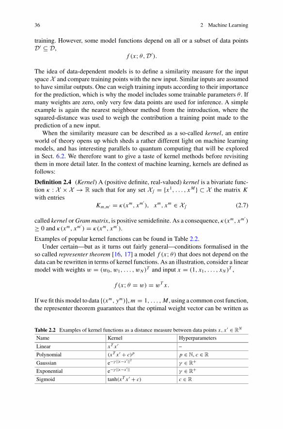
36 2 Machine Learning

training. However, some model functions depend on all or a subset of data pointsD′ ⊆ D,

f (x; θ,D′).

The idea of data-dependent models is to define a similarity measure for the inputspaceX and compare training points with the new input. Similar inputs are assumedto have similar outputs. One can weigh training inputs according to their importancefor the prediction, which is why the model includes some trainable parameters θ . Ifmany weights are zero, only very few data points are used for inference. A simpleexample is again the nearest neighbour method from the introduction, where thesquared-distance was used to weigh the contribution a training point made to theprediction of a new input.

When the similarity measure can be described as a so-called kernel, an entireworld of theory opens up which sheds a rather different light on machine learningmodels, and has interesting parallels to quantum computing that will be exploredin Sect. 6.2. We therefore want to give a taste of kernel methods before revisitingthem in more detail later. In the context of machine learning, kernels are defined asfollows:

Definition 2.4 (Kernel) A (positive definite, real-valued) kernel is a bivariate func-tion κ : X × X → R such that for any set X∫ = {x1, . . . , xM } ⊂ X the matrix Kwith entries

Km,m ′ = κ(xm, xm′), xm, xm ∈ X∫ (2.7)

called kernel orGrammatrix, is positive semidefinite. As a consequence, κ(xm, xm′)

≥ 0 and κ(xm, xm′) = κ(xm, xm

′).

Examples of popular kernel functions can be found in Table 2.2.Under certain—but as it turns out fairly general—conditions formalised in the

so called representer theorem [16, 17] a model f (x; θ) that does not depend on thedata can be rewritten in terms of kernel functions. As an illustration, consider a linearmodel with weights w = (w0, w1, . . . , wN )T and input x = (1, x1, . . . , xN )T ,

f (x; θ = w) = wT x .

If we fit thismodel to data {(xm, ym)},m = 1, . . . , M , using a common cost function,the representer theorem guarantees that the optimal weight vector can be written as

Table 2.2 Examples of kernel functions as a distance measure between data points x, x ′ ∈ RN

Name Kernel Hyperparameters

Linear xT x ′ –

Polynomial (xT x ′ + c)p p ∈ N, c ∈ R

Gaussian e−γ ||x−x ′ ||2 γ ∈ R+

Exponential e−γ ||x−x ′ || γ ∈ R+

Sigmoid tanh(xT x ′ + c) c ∈ R

2.2 Models 37

a linear combination of the data points,

wopt = 1

M

M∑m=1

αmxm,

with real coefficients αm . If we insert this weight back into the linear model, we get

f (x; θ = {αm},D) = 1

M

M∑m=1

αm (xm)T x = 1

M

M∑m=1

αm κ(xm, x).

The inner product (xm)T x is a linear kernel. We have translated the linear modelwith N + 1 parameters w0, . . . , wN into a ‘kernelised’ model with M parametersα1, . . . , αM . This formulation of a model is also called the dual form (as opposed tothe original primal form). The objective of training is now to fit the new parameterswhich weigh the training data points.

Expressing a model in terms of a kernel function that measures distances to datapoints allows us to use the so called kernel trick. The kernel trick can be describedas follows:

Given an algorithm which is formulated in terms of a positive definite kernel κ , one canconstruct an alternative algorithm by replacing κ by another positive definite kernel κ ′. [18]

We can therefore build new models by simply exchanging one kernel with another.It makes intuitive sense that the distance to data points is a useful way to compute

a prediction for a new data point. However, there is more to kernel functions thanjust distance measures. A kernel can be interpreted as an inner product of data thathas been transformed by a feature map φ : X → F ,

k(x, x ′) = 〈φ(x), φ(x ′)〉.

The feature spaceF is a Hilbert space, a complete vector spacewith an inner product,and φ as a—usually nonlinear—transformation that projects into F . This is interest-ing because data can be easier to classify in higher dimensional spaces, for examplewhen it becomes linearly separable.

To illustrate how a feature map can make non-linearly separable data separable,consider the following examples:

Example 2.5 (XOR function) The full dataset of the XOR function is given by

D = {((−1,−1)T , 1), ((−1, 1)T ,−1), ((1,−1)T ,−1), ((1, 1)T , 1)}

and is clearly not linearly separable. A feature map of the form φ((x1, x2)T ) =(x1, x2, x1x2)T allows for a hyperplane cutting through the 3-dimensional space toseparate both classes (see Fig. 2.9).

38 2 Machine Learning

Fig. 2.9 While four data points labelled according to the XOR function (zeros as red circles andones as blue squares in opposite corners of the unit square) cannot be separated by a linear decisionboundary in X , the feature map to F from Example 2.5 separates the two classes by introducing athird dimension

Example 2.6 (Concentric circles) Consider a dataset of two 2-dimensional concen-tric circles, which is impossible to separate by a linear decision boundary (see Fig.2.10). A polynomial feature map

φ((x1, x2)T ) = (x1, x2, 0.5(x

21 + x22 ))

T

transforms the data into a linearly separable dataset in a 3-dimensional space.

Example 2.7 (Infinite dimensional feature spaces) Feature maps can even map intospaces of infinite dimension. Consider the Gaussian kernel from Table 2.2 withx, x ′ ∈ R

N and use the series expansion of the exponential function to get

κ(x, x ′) = e− 12 ||x−x ′ ||2

=∞∑j=0

(xT x ′)k

k! e− 12 |x |2e− 1

2 |x ′ |2

= ⟨φ(x), φ(x ′)

⟩.

The Gaussian kernel effectively implements a feature map, for example leading tofeature vectors with entries [19]

φ(x) =(

1√k!

1k

e− 12k ||x ||2

(k

n1, . . . , nN

) 12

xn11 . . . xnNN

),

with k = 0, . . . ,∞ and n1, . . . , nN such that∑N

i=1 ni = k. Of course one never hasto calculate this rather ugly expression, and can instead evaluate the much simplerGaussian kernel function using the original inputs. Note that there are of course otherfeature maps that lead to a Gaussian kernel [20].

In summary, many models can be expressed in terms of kernel expansions, whichmakes them data-dependent. This shifts the optimisation problem to a different setof parameters, namely the weights of the kernel functions. By replacing one kernelfunction κ by another kernel function κ ′, we effectively change the feature map

2.2 Models 39

Fig. 2.10 Data points of two classes arranged as concentric circles in the 2-d plane cannot beseparated by a linear decision boundary (left), but the feature map from Example 2.6 projects thedata onto a square cone in 3 dimensions allows them to be divided by a hyperplane

and can potentially go into very high-dimensional spaces of many different shapes,and hope that our data gets easier to classify in that space. That way simple linearmodels can get the power of nonlinear classifiers. Of course, designing a good modeltranslates into finding a good feature space, which in turnmeans to find a good kernel.Excellent introductions to kernel methods are found in [18, 21]. A number of kernelmethods will be introduced in Sect. 2.4.

2.3 Training

The goal of training is to select the best model for prediction from a model family.This means we have to define an objective function that quantifies the quality of amodel given a set of parameters, and training becomes an optimisation problem overthe objective. Machine learning tends to define rather difficult optimisation problemsthat require a lot of computational resources. This is why optimisation “lies at theheart ofmachine learning” [22] and often defines the limits ofwhat is possible. In fact,some major breakthroughs in the history of machine learning came with a new wayof solving an optimisation problem. For example, the two influential turning pointsin neural networks research were the introduction of the backpropagation algorithmin the 1980s [23],4 as well as the use of Boltzmann machines to train deep neuralnetworks in 2006 [24]. However, as outlined in the preceding section, optimisationis only a means to generalisation.

4The original paper [23], a Technical Report byRumelhart, Hinton andWilliams, has close to 20,000citation on Google Scholar at the time of writing. It is widely known today that the algorithm hadbeen invented by others long before this upsurge of attention.

40 2 Machine Learning

2.3.1 Cost Functions

As mentioned above, the cost function C(θ) is the function that quantifies the objec-tive according to which we train the parameters of a model. We also said that the costfunction consists of different building blocks. The most important blocks are the lossL(D, θ), which was introduced above to measure how well a model does in predict-ing the training data, and the regulariser R(θ) which imposes extra constraints onthe optimisation. Regularisation has been found to help against overfitting. However,many rather complex and high-dimensional models in use today seem to circumventthis problem in a natural way, and theories of regularisation and overfitting are subjectto new questions [25].

Let us have a look at some popular loss functions and regularisers. Possibly themost common choice for the loss function is the squared loss which compares theoutputs f (xm; θ) produced by the model when fed with training inputs xm with thetarget outputs ym ,

L(θ) = 1

2

M∑m=1

( f (xm; θ) − ym)2. (2.8)

The resulting optimisation problem is known in statistics as least-squares optimisa-tion. In classification problem f and y are binary values, and the squared loss wouldbe a non-continuous function that quantifies the number of misclassified trainingpoints. To make the loss continuous, f is during training often defined to be thecontinuous output of the model, which only gets binarised when the model is usedto make predictions. The squared loss is also called 12 loss (not to be mixed upwith the L2 regulariser), and replacing ( f (xm; θ) − ym)2 with the absolute value| f (xm; θ) − ym | gives rise to the 11 loss.

Anotherway to quantify the distance between outputs and targets is via the expres-sion ym f (xm; θ), which is positive when the two numbers have the same sign andnegative if they are different. One can use this to compute the hinge loss,

L(θ) =M∑

m=1

max(0, 1 − ym f (xm; θ)),

the logistic loss

L(θ) =M∑

m=1

log(1 + e−ym f (xm ;θ)),

or, if the output of the model is a probability f (xm; θ) = pm , the cross entropy loss

L(θ) =M∑

m=1

−ym log pm − (1 − ym) log(1 − pm),

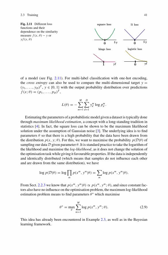
2.3 Training 41

Fig. 2.11 Different lossfunctions and theirdependence on the similaritymeasure f (x, θ) − y ory f (x, θ)

0

1

0

0

square loss l1 loss

logistic losshinge loss

f-y f-y

yf yf

of a model (see Fig. 2.11). For multi-label classification with one-hot encoding,the cross entropy can also be used to compare the multi-dimensional target y =(y1, . . . , yD)T , y ∈ {0, 1} with the output probability distribution over predictionsf (x; θ) = (p1, . . . , pD)T ,

L(θ) = −M∑

m=1

D∑d=1

ymd log pmd .

Estimating the parameters of a probabilisticmodel given a dataset is typically donethrough maximum likelihood estimation, a concept with a long-standing tradition instatistics [4]. In fact, the square loss can be shown to be the maximum likelihoodsolution under the assumption of Gaussian noise [3]. The underlying idea is to findparameters θ so that there is a high probability that the data have been drawn fromthe distribution p(x, y; θ). For this, we want to maximise the probability p(D|θ) ofsampling our dataD given parameter θ . It is standard practice to take the logarithm ofthe likelihood and maximise the log-likelihood, as it does not change the solution ofthe optimisation taskwhile giving it favourable properties. If the data is independentlyand identically distributed (which means that samples do not influence each otherand are drawn from the same distribution), we have

log p(D|θ) = log∏m

p(xm, ym |θ) =∑m

log p(xm, ym |θ).

From Sect. 2.2.3 we know that p(xm, ym |θ) ∝ p(xm, ym; θ), and since constant fac-tors also have no influence on the optimisation problem, themaximum log-likelihoodestimation problem means to find parameters θ∗ which maximise

θ∗ = maxθ

M∑m=1

log p(xm, ym; θ). (2.9)

This idea has already been encountered in Example 2.3, as well as in the Bayesianlearning framework.

42 2 Machine Learning

In terms of regularisers, there are two common choices, L1 and L2 regularisation(named after the norm they are based on). We will call them in our notation the RL1

and RL2 regulariser. The name comes from the respective norm to use. If we writethe parameters as a vector w for the moment and denote by | · | the absolute value,we can define them as

RL1(w) = λ||w||21 =∑i

|wi |,

andRL2(w) = λ||w||22 =

∑i

w2i ,

respectively. The L2 regulariser adds a penalty for the length of the parameter vec-tor and therefore favours parameters with a small absolute value. Adding the L1

regulariser to the cost function favours sparse parameter vectors instead. The hyper-parameter λ regulates how much the regularisation term contributes towards the costfunction.

2.3.2 Stochastic Gradient Descent

Once the cost function is constructed, machine learning reduces to the mathemat-ical problem of optimising the cost function, which naturally becomes a computa-tional problem for any realistic problem size. Mathematical optimisation theory hasdeveloped an extensive framework to classify and solve optimisation problems [26]which are called programmes, and there are important distinctions between types ofprogrammes that roughly define how difficult it is to find a global solution with acomputer. For some problems, even local or approximate solutions are hard to com-pute. Themost important distinction is between convex problems for which a numberof algorithms and extensive theory exists, and non-convex problems that are a lotharder to treat [27]. Convexity thereby refers to the objective function and possibleinequality constraint functions. Roughly speaking, a set is convex if a straight lineconnecting any two points in that set lies inside the set. A function f : X → R isconvex if X is a convex domain and if a straight line connecting any two points ofthe function lies ‘above’ the function (for more details see [26]).

To give an example, least-squares optimisation together with a model functionthat is linear in the parameters forms a rather simple convex quadratic optimisationproblem that has a closed-form solution as we will show in the next section. Forgeneral non-convex problems much less is known, and many machine learning prob-lems fall into this category. Popular methods are therefore iterative searches such asstochastic gradient descent, which performs a stepwise search for the minimum onbatches of the data. Especially in the field of neural networks, gradient-based searchmethods stand almost without an alternative at the moment.

Gradient descent updates the parameters θ of a cost function C(θ) successivelytowards the direction of steepest descent,

2.3 Training 43

Fig. 2.12 Steps of the training updates in a 1-dimensional parameter space. Gradient descent getsstuck in local minima and convergence becomes very slow at saddle points

Fig. 2.13 Steps of the training updates in a 2-dimensional parameter spacewith a thin valley. Lowervalues of the objective function are shaded darker. While conventional gradient descent convergesslower due to strong oscillations (red line starting on the left), the momentummethod of consideringthe direction of past gradients leads to a straighter path (blue line starting on the right). Note that ifthe learning rate is too high, the valley can be missed altogether and training updates could in factincrease the cost function

θ(t+1) = θ(t) − η∇C(θ (t)), (2.10)

whereη is an external parameter called the learning rate and t an integer keeping trackof the current iteration. The gradient ∇C(θ(t)) always points towards the ascendingdirection in the landscape of C , and following its negative means to descend intovalleys. As one can imagine, this method can get stuck in local minima if they exist(see Fig. 2.12).5 Convergence to a minimum can take a prohibitively long time dueto saddle points in which gradients are vanishingly small and the steps therefore onlygradual. Another problem appears in thin valleys where the search path oscillatesheavily.

A solution to increase the convergence is to include a momentum, or to make thechange in parameters of step t dependent on the changewemade for the previous stepst − 1 (see Fig. 2.13). This effectively dampens oscillations and chooses a straighterpath. Also the choice of a learning rate provides a lot of possibilities to shape theconvergence of the training algorithm. For example, one can choose a step-dependentlearning rate η(t) that decreases with each iteration, or adapt the learning rate to thecurrent gradient.

5For large neural networks of thousands of parameters, local minima seem in fact only a minorproblem since the search direction is likely to find a dimension in which a local minima in a subsetof the dimensions can be escaped.

44 2 Machine Learning

training step

test error

training error

Fig. 2.14 Typical behaviour of the error on the training and test set during training. While themodel learns to reduce the error on the training set, the test error usually begins to increase after acertain number of training steps, an indicator that the model begins to overfit. Overfitting means tolearn the specific structure of the training set, so that the classifier looses its ability to generalise

Stochastic gradient descent uses only a subset of the training data for each updateto calculate the cost function. While the original definition of stochastic gradientdescent in fact only considered one randomly sampled training input per iteration,themore common version usesmini-batches of randomly sampled data, and the batchsize becomes a hyperparameter for training. (Full-)batch gradient descent decreasesthe cost function in each iteration (unless the learning rate is large enough to ‘jumpover minima’). Stochastic gradient descent shows fluctuations in training that getstronger the smaller the batch size. However, the stochastic nature of the gradientdirection tends to help in finding minima faster and escaping local minima. Animportant reason to still consider larger batch sizes is the prospect of parallelisingcomputations.

One last practical remark on overfitting may be useful. An iterative method allowsus to recognise overfitting by monitoring the error on the training and test set duringeach step of the optimisation (see Fig. 2.14). Typically, test and training error startto decrease together. When the training starts to fit the particulars of the trainingset, thereby losing generalisation ability, the test error begins to rise while the train-ing error continues to decrease. The optimal point to stop the optimisation is justbefore the renewed increase of the test error, and one should consider regularisationtechniques to avoid such behaviour altogether.

2.4 Methods in Machine Learning

Let us briefly summarise the previous sections. A method in machine learning spec-ifies a general ansatz for a model function or distribution that can be used for pre-diction and a training strategy of how to use the data to construct a specific modelthat generalises from the data. In supervised learning, the training objective is tominimise the error between target outputs and predicted outputs for the trainingset. However, this objective serves the overarching purpose of minimising the gen-eralisation error, which is usually measured on a test or validation set. This section

2.4 Methods in Machine Learning 45

Table 2.3 Summary of the model functions f (x, w) and distributions p(x) of machine learningmethods presented in this section. As further established in the text, x is a model input, s, v, h ando denote different kinds of units or random variables in probabilistic models, while w, W , θ andγm are learnable parameters. We denote by ϕ a nonlinear (activation) function, t a time step, c aspecific class and by Mc the number of training samples from that class. ˜κ is a scalar kernel and κ

a vector of kernel functions, and K a kernel Gram matrix

Method Model function/distribution

Data fitting

Linear regression f (x; w) = wT x

Nonlinear regression f (x; w) = ϕ(w, x)

Artificial neural networks

Perceptron f (x; w) = ϕ(wT x)

Feed-forward neural network f (x;W1,W2, . . .) = · · ·ϕ2(W2ϕ1(W1x)) · · ·Recurrent neural network f (x (t);W ) = ϕ(W f (x (t−1);W ))

Boltzmann machine p(v; θ) = 1Z

∑h e−E(v,h;θ)

Graphical models

Bayesian network p(s) = ∏kp(sk |πk; θ)

Hidden Markov model p(V, O) =T∏t=1

p(v(t)|v(t-1))T∏t=1

p(o(t)|v(t))

Kernel methods

Kernel density estimation p(x |y = c) = 1Mc

∑Mm|ym=c κ(x − xm)

K-nearest neighbour p(x |y = c) = #NNck

Support vector machine f (x) =M∑

m=1γm ymκ(x, xm) + w0

Gaussian process p(y|x) = N [κT K−1y; ˜κ − κT K−1κ]

introduces examples of supervised machine learning methods that become importantin the context of quantum machine learning. They are summarised in Table 2.3 forquick reference. Note that the categorisation of different methods into data fitting,neural networks, graphical models and kernel methods is to some extend arbitrary:Boltzmann machines are graphical models as much as neural networks are a type ofnonlinear regression, while Gaussian processes and support vector machines can bederived from linear models.

2.4.1 Data Fitting

Most physicists are familiar with statistical methods for data fitting such as linearand nonlinear regression.6 These are well-established in statistics and data science

6In this context the term “regression” is both used for the problem of regression as well as themodel.

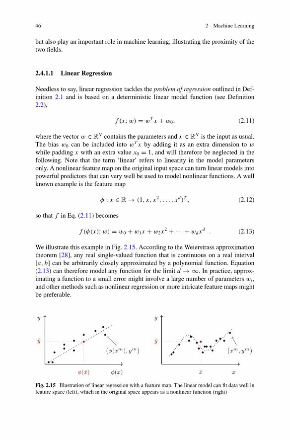
46 2 Machine Learning

but also play an important role in machine learning, illustrating the proximity of thetwo fields.

2.4.1.1 Linear Regression

Needless to say, linear regression tackles the problem of regression outlined in Def-inition 2.1 and is based on a deterministic linear model function (see Definition2.2),

f (x;w) = wT x + w0, (2.11)

where the vector w ∈ RN contains the parameters and x ∈ R

N is the input as usual.The bias w0 can be included into wT x by adding it as an extra dimension to w

while padding x with an extra value x0 = 1, and will therefore be neglected in thefollowing. Note that the term ‘linear’ refers to linearity in the model parametersonly. A nonlinear feature map on the original input space can turn linear models intopowerful predictors that can very well be used to model nonlinear functions. A wellknown example is the feature map

φ : x ∈ R → (1, x, x2, . . . , xd)T , (2.12)

so that f in Eq. (2.11) becomes

f (φ(x);w) = w0 + w1x + w2x2 + · · · + wd x

d . (2.13)

We illustrate this example in Fig. 2.15. According to the Weierstrass approximationtheorem [28], any real single-valued function that is continuous on a real interval[a, b] can be arbitrarily closely approximated by a polynomial function. Equation(2.13) can therefore model any function for the limit d → ∞. In practice, approx-imating a function to a small error might involve a large number of parameters wi ,and other methods such as nonlinear regression or more intricate feature maps mightbe preferable.

y

φ(x)

φ(xm), ym)

y

φ(x)

y

x

xm, ym)

y

x

Fig. 2.15 Illustration of linear regression with a feature map. The linear model can fit data well infeature space (left), which in the original space appears as a nonlinear function (right)

2.4 Methods in Machine Learning 47

Learning in linear regression means to find the parameters w that fit f to thetraining data in order to predict new data points. A very successful approach to findthe optimal7 parameters is least squares estimation. This approach uses the squareloss

L(w) =M∑

m=1

(wT xm − ym)2. (2.14)

It is convenient to express this as a matrix equation,

L(w) = (Xw − y)T (Xw − y),

where we introduced the notation

y =⎛⎜⎝

y1

...

yM

⎞⎟⎠ , X =

⎛⎜⎝x11 . . . x1N...

. . ....

xM1 . . . xM

N

⎞⎟⎠ , w =

⎛⎜⎝

w1...

wN

⎞⎟⎠ .

We call X data or design matrix. If XT X is of full rank, the estimated parametervector can be calculated by the closed-form equation

w = (XT X)−1XT y. (2.15)

To show this, write (Xw − y)2 = (Xw − y)T (Xw − y) = yT y − 2wT XT y +wT XT Xw and calculate the derivative ∂wL(w), which results in−2XT y + 2XT Xw.At theminimum, this expression is zero. The solution to the least squares optimisationproblem for a linear regression model is therefore

w = X+y (2.16)

withX+ = (XT X)−1XT . (2.17)

The matrix X+ is also called a pseudoinverse, a generalisation of the inverse fornon-square or square singular matrices. In computational terms, training a linearregression model reduces to the inversion of a M × K dimensional data matrix,where usually the dimension of the feature space K is larger than the dimension ofthe input vectors. The fastest classical algorithms take time O(K δ), where for thebest current algorithms the constant δ is bounded by 2 ≤ δ ≤ 3.

An alternative way to solve this problem is to write the pseudoinverse as a singularvalue decomposition. A singular value decomposition is the generalisation of aneigendecomposition A = SDST , but for general (i.e. singular) matrices [29]. Anyreal matrix can be written as A = UΣV T , where the orthogonal real matrices U, V

7Least squares can be shown to produce an unbiased estimator with minimum variance [4].

48 2 Machine Learning

carry the singular vectors ur , vr , r = 1, . . . , R as columns, where R is the rank of A.Σ is a diagonal matrix of appropriate dimension containing the R nonzero singularvalues σr . The inverse of A is calculated by inverting the singular values on thediagonal and taking the transpose of U, V . Using the singular value decompositionto decompose X in Eq. (2.17) yields

X+ = (XT X)−1XT

= (VΣUT UΣV T )−1VΣUT

= VΣ−2V T VΣUT

= VΣ−1UT ,

whereweusedUTU = 1which is true for orthogonalmatrices.With this formulationof the pseudoinverse, the solution (2.16) can be expressed in terms of the singularvectors and values,

w =R∑

r=1

1

σruTr y vr . (2.18)

The computational problem is now to find the singular value decomposition of X .

2.4.1.2 Nonlinear Regression

While in linear regression themodel function has a linear dependency on the parame-ters, this conditiongets relaxed innonlinear regression.Onewayof derivingnonlinearregression from the linear version is by replacing the nonlinear feature map φ (seefor example Eq. (2.13)) by a nonlinear function in the inputs and parameters,

f (x) = ϕ(w, x). (2.19)

Currently, the most successful nonlinear regression models in machine learning areneural networks.

2.4.2 Artificial Neural Networks

From a mathematical perspective, neural networks can be seen as a nonlinearregression model with a specific choice for the model function ϕ in Eq. (2.19)[9], namely where the input to the nonlinear function is given by a linear modelϕ(w, x) = ϕ(wT x), an expression which then gets nested several times. Historicallythese models were derived from biological neural networks [30, 31] and they havea beautiful graphical representation reminiscent of neurons that are connected bysynapses. The nonlinear function originally corresponded to the ‘integrate-and-fire’principle found in biological neurons, which prescribes that a neuron fires once theincoming signal surpasses a certain threshold value [32]. Neural network research

2.4 Methods in Machine Learning 49

was abandoned and revived a number of times during its history. Important mile-stones were when Hopfield showed in 1982 that a certain type of network recoversproperties of a memory [31], the rediscovery of the backpropagation algorithm in thelate 80s [33], as well as recent developments in ‘deep’ neural network structures [24].

2.4.2.1 Perceptrons

Perceptrons are the basic building block of artificial neural networks. Their modelfunction is given by

f (x;w) = ϕ(wT x), (2.20)

where the inputs and outputs are either real or binary numbers. Sometimes the math-ematical structure makes it convenient to choose {−1, 1} rather than {0, 1}. Thenonlinear function ϕ is called an activation function and in the original proposal ofa perceptron it referred to the sign or step function

sgn(a) ={1, if a ≥ 0,−1, else.

The perceptron model can be trained by iterating through the data and updating theweights according to

w(t+1)i = w

(t)i + η(ym − ϕ(xTw(t)))xmi ,

where η is the learning rate. The computational properties of a perceptron have beenstudied from as early as the 1960s [32, 34], and show that the learning rule alwaysconverges to the optimal weights. However, after the initial excitement it was foundthat this is only true for linearly separable datasets,8 excluding a simple XOR gatefrom its scope (see Example 2.5). Only when perceptrons were combined to buildmore complex structures did their power become apparent, and the perceptron modelis the core unit of artificial neural networks.

Figure 2.16 shows a perceptron in the typical graphical representation of neuralnetworks, in which inputs and outputs are understood as units with certain valuesthat are updated by the units that feed into them. The connections between units areassociated with a weight. The activation function for the output node is not alwaysdrawn.

2.4.2.2 Feed-Forward Neural Networks

Feed forward neural networks have a model function of the form

8Remember that a dataset is linearly separable if it can be divided by a hyperplane in input space.

50 2 Machine Learning

Fig. 2.16 Illustration of theperceptron model. The inputfeatures are each displayedas nodes of a graph, calledunits or neurons. The inputunits are connected to anoutput unit by weighededges. Together with anactivation function ϕ for theoutput unit, this graphdefines a model functiony = ϕ(wT x)

x0

x1

...

xN

y

w0

w1

wN

weightsneurons/units

INPUT

OUTPUT

f (x,W1,W2, . . .) = · · · ϕ2 (W2 ϕ1(W1x)) · · · . (2.21)

Here ϕ1, ϕ2, . . . are nonlinear activation functions between appropriate spaces.The parameters are summarised as weight matrices Wi , i = 1, 2, . . .. The dots indi-cate thatwe could extend themodel by an arbitrary number of such nested activations,as long as the outermost activation function has to map onto the output space Y .

Thismodel function is a concatenation of ‘linearmodels’ and activation functions,and as the dots suggest, the concatenation can be repeatedmany times. An interestingperspective on the success of neural networks is that they combine the flexibility ofnonlinear dynamics with the data processing power of linear algebra. An importantexistence theorem by Hornik, Stincombe andWhite from 1989 [35] proves that onlyone concatenation of the form

f (x,W1,W2) = W2 ϕ1(W1x)

suffices to make the model a universal function approximator, meaning that up tofinite precision it can be used to express any function on a compact domain (similarto the polynomial from Eq. (2.13)). This might however require weight matrices ofvery large dimensions.

In terms of their graphical representation, feed-forward neural networks connectmultiple perceptrons in layers so that the units of each layer are connected to theunits of the following layer (see Fig. 2.17). The first layer is made up of the inputunits x1, . . . , xN , the following L layers contain the hidden units hl1, . . . , h

lJ (where

l = 1, . . . , L). The last layer contains the output unit(s). Each neuron is updated by anactivation function depending on all neurons feeding into it, and the update protocolprescribes that each layer is updated after the previous one. This way, information is‘fed forward’, and an input fed into the first layer is mapped onto an output that canbe read out from the last layer. The model for the single-hidden-layer feed-forwardneural network reads

f (x;W1,W2) = ϕ2( W2 ϕ1( W1x ) ). (2.22)

2.4 Methods in Machine Learning 51

x1

x2

x3

x4

h1

h2

h3

y1

y2

y3

y4w43 w34

weightsneurons

INPUT

OUTPUT

input layer

hidden layers

output layer

Fig. 2.17 A feed-forward neural network (here with only one hidden layer) feeds informationforward through several layers

Fig. 2.18 Different options for activation functions: a hyperbolic tangent, a sigmoid function andrectified linear units (ReLU)

A feed-forward neural network can be combined with a variety of possible acti-vation functions. Common examples for these functions are a hyperbolic tangent, asigmoid ϕ(a) = 1

1+e−a , as well as ‘rectified linear units’ [36] that are zero for negativeinputs and linear functions for positive inputs (see Fig. 2.18). But also radial basisfunctions have been used, and other activation functions might prove interesting infuture.

The square loss for a single-hidden-layer neural network for some labelled trainingdata D = {(xm, ym)}Mm=1 and the weight matrices W1,W2 reads

C(W1,W2,D) =M∑

m=1

(ϕ2(WT2 ϕ1(W

T1 xm)) − ym)2. (2.23)

For nonlinear activation functions this is in general a non-convex, nonlinear (andhence difficult) optimisation problem. By far the most common training algorithmfor feed-forward neural networks is therefore gradient descent with

52 2 Machine Learning

x1

...

xi

...

xN

h1

...

hj

...

hJ

h = ϕ1(Wx)

y1

...

yk

...

yK

y = ϕ2(Ωh)

wij ωjk

Fig. 2.19 Neural network model used to explain the backpropagation algorithm. The green nodesdenote the input layer encoding the input features x1, . . . , xN , followed by the blue hidden layerwithhidden units h1, . . . , hJ and the yellow output layer of units y1, . . . , yK . The activation function ofthe hidden and output units are ϕ1, ϕ2, respectively. The weights are summarised in weight matricesW and Ω

w(t+1)i j = w

(t)i j − η

∂C(W1,W2)

∂wi j. (2.24)

The updated weight w(t+1)i j is the current weight w(t)

i j minus a step down towards thedirection of the steepest gradient with a step size or learning rate η. Computing gra-dients for neural networks is called backpropagation [33] and although a notationalnightmare, we shall now walk through it. We will have a look at the weight updatefor a neural network with a single hidden layer only, but the generalisation to morelayers is straightforward.

Let us first assemble all relevant expressions (see Fig. 2.19). Assume a cost func-tion with squared loss and no regulariser (wherem = 1, . . . , M can refer to the entiredataset or the current training data batch),

C(W1,W2) = 1

2

M∑m=1

(f (xm;W,Ω) − ym

)2,

with the neural network model function

f (x;W,Ω) = ϕ2(Ωϕ1(W

T x)),

where W ∈ RJ×N and Ω ∈ R

K×J , and N , J , K are the dimensions of the input,hidden and output layer. For notational simplicity, we have renamed W1 = W andW2 = Ω , and their entries are respectively denoted bywi j andω jk , while the kth rowvector is given by a single index, Wk and Ωk . We denote the vector summarising thevalues of the input layer as x , and use h for the hidden layer and y for the output layer.The linear ‘net’ inputs fed into an activation function will be denoted as netyk = Ωkh

2.4 Methods in Machine Learning 53

Fig. 2.20 Updating ahidden-to-output layerweight ωab only requiresgradients of the output unityb it leads to. For notation,see Fig. 2.19

x1

...

xi

...

xN

h1

...

hb

...

hJ

h = ϕ1(Wx)

y1

...

yb

...

yK

y = ϕ2(Ωh)

wia ωab

for the output neurons and nethj = Wj x for the hidden layer. The goal is to compute∂C

∂ω jk, ∂C

∂wi jfor all i = 1 . . . N , j = 1 . . . J, k = 1 . . . K .

First calculate the derivatives of the hidden-to-output layer weights for e generalweight matrix element ωab (see Fig. 2.20),

∂C

∂ωab= ∂C

∂yb

∂yb∂netyb︸ ︷︷ ︸δyb

∂netyb∂ωab

.

The first two terms are summarised by δyb . The derivatives in the above expressionare

∂C

∂yb= −

M∑m=1

(fb − ymb

),

∂yb∂netyb

= (ϕ2)′b,

∂netyb∂ωab

= ha .

Taking the derivative of theb’th component of the second activation function, (ϕ2)′b =

dϕ(z)bdz , requires the activation function to be differentiable. It is no surprise that the

sigmoid, tanh and ‘rectified linear units’ (ReLU) activation functions are popular,since their derivatives are rather simple. For example, the derivative of the sigmoidfunction is given by ϕ′(z) = ϕ(z)(1 − ϕ(z)). Putting it all together we get

∂C

∂ωab= −

M∑m=1

(fb − ymb

)(ϕ2)

′bha = δybha .

54 2 Machine Learning

Fig. 2.21 Updating aninput-to-hidden layer weightrequires gradients of alloutput units and the hiddenunit it leads to. For notation,see Fig. 2.19

x1

...

xi

...

xN

h1

...

hb

...

hJ

h = ϕ1(Wx)

y1

...

yk

...

yK

y = ϕ2(Ωh)

wab ωjk

Now we know how to update the parameters in the second weight matrix Ω

which connects the hidden to the output layer. In order to calculate the update of theinput-to-hidden layer with weights wab we have to consider not only hb but also thederivatives of all neurons that depend on hb (see Fig. 2.21), which in this case are allneurons of the output layer, and that gets a little more messy.

∂C

∂wab=

K∑k=1

∂C

∂yk

∂yk∂netyk︸ ︷︷ ︸δyk

∂netyk∂hb︸ ︷︷ ︸ωbk

∂hb∂nethb︸ ︷︷ ︸(ϕ1)

′b

∂nethb∂wab︸ ︷︷ ︸

xa

=(

K∑k=1

δykωbk

)(ϕ1)

′b

︸ ︷︷ ︸δhb

xa

= δhb xa .

The δ’s are also called the “errors” of a neuron, and one can now see that in orderto compute the error of a hidden neuron, one requires the errors of all followingneurons in the direction of the forward pass. In other words, the error has to be‘backpropagated’ from right to left in the network, which is the reverse direction ofthe classification.

The computational steps needed for one iteration in backpropagation grow poly-nomial with the number of connections N J + J K [8] which can be costly for largerarchitectures, especially in ‘deep’ networks of many layers. Also the convergencetime for the gradient algorithmcan be very long, and training state-of-the art networkscan take weeks on a supercomputer. Numerous tricks like layer-wise pre-training canbe used to facilitate training.

2.4 Methods in Machine Learning 55

2.4.2.3 Recurrent Neural Networks

While feed-forward neural networks are organised in layers, the graphical represen-tation of recurrent neural networks is an all-to-all connected graph of units which arecollectively updated in discrete time steps (Fig. 2.22). Information is therefore notfed-forward through layers, but ‘in time’. The input can be understood as the statethat some units are set to at time t = 0, while the output can be read from one or moredesignated units at time T . The units that are neither fed with input, nor used to readout the output, are called ‘hidden units’ and have a mere computational function.

Let s(t) = (s(t)1 , . . . , s(t)

G )T describe the state of the G (hidden or visible) units ofa recurrent neural network at time t . The edge between si and s j is associated to aweight wi j . The state of the network after each update is given by

s(t+1) = ϕ(WT s(t)),

where the RG×G matrix W contains the weights and ϕ is a nonlinear activation

function.A recurrent neural network can be ‘unfolded’ to a feed-forward structure with

T layers by interpreting every time step as a separate layer. It can then be trainedby backpropagation through time which works exactly like the standard backprop-agation algorithm. This method has some unwanted properties, such as explodingor vanishing gradients during training [37]. Proposals to improve on training rangefrom artificially ‘clipping’ the exploding gradients [37], to introducing time-delaysbetween units [38], to the use of unitary weight matrices [39]. Recurrent neural net-works gained relatively little interest from themachine learning community for a longtime. However, and possibly due to the resemblance of the time-unfolded structure todeep neural networks, this has been changing in the last few years [40]. A prominentexample for an application of a recurrent neural network is sequence-to-sequencemodeling for the translation of text.

One relatively simple class of recurrent neural networks for a task called ‘patternmatching’ or ‘associative memory’ are Hopfield neural networks [31].9 Hopfieldnetworks have binary units, symmetric all-to-all connections with wi i = 0 for i =1, . . . ,G, as well as a threshold activation function. One can easily show that for agiven training point sm1 , . . . , smG , choosing the weights wi j proportional to

∑m smi s

mj

leads to the sm being stable states or ‘attractors’ of the network [8]. Thismeans that anupdate of these states acts as the identity, ϕ(WT sm) = sm . Moreover, the dynamicsof consecutive updates of the units decreases an Ising-type energy function,

E(s;W ) = −sTWs = −1

2

G∑i, j=1

wi j si s j ,

9Although they are not first and foremost used for supervised learning, Hopfield networks appearfrequently in the quantum machine learning literature and are therefore mentioned here.

56 2 Machine Learning

u1

u2

u3

u4

u5

u6

u7

w12

Fig. 2.22 A recurrent neural network is represented by an all-to-all connected graph. The unitsu1, . . . , u4 are used to represent inputs, and at a later time, the outputs of the model (green andyellow nodes). The hidden units u5, u6, u7 (blue) are ‘not accessible’ and can be understood aspure computational units, adding to the complexity of the dynamics of a recurrent neural net. Thenetwork here follows the design of a Hopfield model which does not have self-connections of nodesand where connections have symmetric weights

until one reaches one of these stable states. In other words, the updates drive the sys-tem state from the initial configuration to the closest memorised training pattern [41].

An important characteristic of Hopfield networks is their storage capacity indi-cating how many randomly selected patterns can be stably stored in the model of Nneurons. Without going much into detail [8], one can say that the ratio of storablepatterns to the size of the network is around 0.15. A network of N = 100 neuronscan consequently only store around 15 states. This is not much, considering that itcan represent 2100 patterns.

2.4.2.4 Boltzmann Machines

Boltzmann machines are probabilistic recurrent neural networks. As probabilisticmodels, they do not exhibit a feed-forward or time dynamics, but define a probabilitydistribution over the states of the binary units s = (s1, . . . , sG). Again, the units canbe divided into visible units v = (v1, . . . , vN+K ) and hidden units h = (h1, . . . , hJ ).The visible units can be further divided into input and output units if we deal witha supervised pattern recognition task, so that the first N visible units encode theinputs x1, . . . , xN , and the last K visible units vN+1, . . . , vN+K encode the outputy. In more general, Boltzmann machines do not necessarily require the distinctionbetween inputs and outputs and are primarily used for unsupervised learning.

Boltzmann machines can be understood as Hopfield neural networks [42] forwhich every neuron carries a probability of being in state −1 or 1. Given a states1, .., si , .., sG of a Hopfield network, where all neurons but si are in a given state,the probability of neuron si to be in state 1 is given by

2.4 Methods in Machine Learning 57

p(si = 1) = 1

1 + e−∑

i ′γi i ′ si si ′

. (2.25)

The term∑

i ′ γi i ′si si ′ with the inter-neuron weights γi i ′ is the energy associated withthe given state and si ′ = 1. Overall, a Boltzmann machine assigns the followingparametrised probability distribution to possible values (or ‘states’) s = v, h:

p(v, h; θ) = 1

Ze−E(v,h) (2.26)

where the partition function Z sums over all (v, h)

Z =∑v,h

e−E(v,h), (2.27)

The energy E is an Ising-type energy function that depends on a set of weights θ ,and distinguishing between visible and hidden units makes the energy read

E(v, h) = −∑i, j

wi j vi h j −∑j, j ′

u j j ′ h jh j ′ −∑i,i ′

zii ′ vivi ′

−∑i

ai vi −∑j

b j h j ,

where the weights γ above are now divided into weights wi j between visible andhidden units, weights u j j ′ between hidden units and weights zii ′ between visibleunits (summarised by θ ). We also added the ‘local fields’ ai and b j which give eachseparate unit a energy contribution. The joint probability distribution is thus given bya Boltzmann distribution. This is nothing other than a spin-glass model in statisticalphysics, where physical spins interact with different interaction strengths.

Since only the visible state v = (v1, . . . , vN+K ) is of interest, one can marginalisethe joint probability distribution over the hidden units by summing over all theirconfigurations,

p(v; θ) = 1

Z

∑h

e−E(v,h), (2.28)

which is the probability distribution p(v) of a generative probabilistic machine learn-ingmodel.10 Training aBoltzmannmachinemeans to determine connection and localfield strengths with which the model distribution is likely to generate the distributionof training data points.

It turns out that general Boltzmann machines are hard to train and the modelonly became popular when an efficient training algorithm for restricted Boltzmannmachines was found [43] (see Fig. 2.23). In a restricted Boltzmann machine (RBM),

10Note that this expression can be written in terms of the free energy F(s) known from physics,and training a Boltzmann machine minimises the free energy of the model.

58 2 Machine Learning

v1

...

vN

...

vN+K

h1

...

hj

...

hJ

w11

wNK

INPUT

OUT

HID

DEN

Fig. 2.23 Graphical representation of a restricted Boltzmann machine with visible unitsv1, . . . , vN+K and hidden units h1, . . . , hJ , in which the visible units include input and outputunits. A full Boltzmann machine would also allow for connections in between hidden units as wellas in between visible units

visible units are only connected to hidden units and vice versa, so that uii ′ = z j j ′ = 0and

ERBM(v, h) = −∑i j

wi j vi h j −∑i

aivi −∑j

b j h j .

The objective function is chosen according to maximum log-likelihood estimation,

C(θ) =M∑

m=1

log p(vm; θ),

where sm represents the mth training data point. Inserting the formula for the prob-abilities from Eq. (2.28), the gradient for the interaction weights wi j becomes

∂C(W )

∂wi j= ∂

∂wi j

M∑m=1

log p(vm)

=∑m

(∂

∂wi jlog

∑h

e−E(vm ,h)

)− ∂

∂wi jlog Z

=∑m

1∑h e

−E(vm ,h)

∂

∂wi j

∑h

e−E(vm ,h) − 1

Z

∂

∂wi j

∑v,h

e−E(v,h)

2.4 Methods in Machine Learning 59

=∑m

∑h

e−E(vm ,h)

ZDvmi h j −

∑v,h

e−E(v,h)

Zvi h j , (2.29)

where ZD := ∑h,m e−E(vm ,h) is the partition function over the data set only, while Z

includes a sum over all possible patterns v. Similar expressions can be derived forthe local fields. This result is not surprising: The first term is the expectation value ofthe correlation between hidden and visible units over the data set distribution, whilethe second term is the expectation value over the model distribution, and the goal oflearning is to find a model where the two are as close as possible. The result of Eq.(2.29) is usually abbreviated as

∂C(W )

∂wi j= ⟨

vi h j⟩data − ⟨

vi h j⟩model . (2.30)

Calculating⟨vi h j

⟩data is relatively straightforward, since it is an average over all

data samples [44]. But even getting samples of⟨vi h j

⟩model is intractable due to the

partition function Z that involves computing a number of states which grows expo-nentially with the number of units. One approach would be to approximate it withGibbs sampling. This is aMarkov Chain Monte Carlomethod [45] in which, startingwith an initial state, the values of the random variables v1, . . . , vN+K , h1, . . . , hJ

are iteratively updated by drawing samples from the probability distribution (2.25).After a while the process ‘thermalises’ and values of (s, h) (with a sufficient num-ber of updates between them to avoid correlations) can be interpreted as samplesfor the Boltzmann distribution

⟨si h j

⟩model. However, thermalisation can be very slow

and there is no method that indicates without fail whether an equilibrium is reached[46]. Alsomean-field approximations known from statistical physics perform inmostcases rather poorly [6]. This was why Boltzmann machines were replaced by neuralnetworks with backpropagation training algorithms in the 1980s [47], until in 2002contrastive divergence was proposed [43] as a rather rough but effective approxima-tionmethod. A number of quantummachine learning algorithms refer to this trainingmethod, which is why it shall be sketched briefly.

Contrastive divergence is surprisingly simple. The idea is to use a Markov ChainMonte Carlo sampling method, but stop the chain prematurely after only a few steps.The Markov chain successively samples the state of the visible units as well as thestate of the hidden units. The sampling is designed in a way so that after manysteps in the chain, samples are approximately drawn according the the Boltzmanndistribution.

In the first step of the Markov chain one sets the visible units v(0) to a randomlypicked training sample vm . With the values of the visible units fixed, one samples thehidden units h(0)

j one by one with the probability of Eq. (2.25). Since hidden units areonly connected to visible units in the restricted Boltzmann machine, this probabilityis fully defined by the states of the visible units. Now fix the hidden units to thesampled value and sample the visible units v(1) from Eq. (2.25) to start the first stepin the Markov chain. Again, the restriction in the connectivity makes the sampling

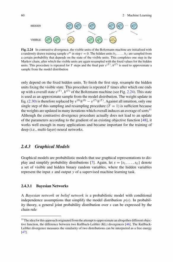
60 2 Machine Learning

HIDDEN

VISIBLE v(0)1 v

(0)2

· · · v(0)N+K

h(0)1 h

(0)2

· · · h(0)J

v(1)1 v

(1)2

· · · v(1)N+K

h(1)1 h

(1)2

· · · h(1)J

· · ·

HIDDEN

VISIBLE v(0)1 v

(0)2

· · · v(0)N+K

h(0)1 h

(0)2

· · · h(0)J

v(1)1 v

(1)2

· · · v(1)N+K

h(1)1 h

(1)2

· · · h(1)J

· · ·

Fig. 2.24 In contrastive divergence, the visible units of the Boltzmann machine are initialised witha randomly drawn training sample vm in step t = 0. The hidden units h1, . . . , hJ are sampled froma certain probability that depends on the state of the visible units. This completes one step in theMarkov chain, after which the visible units are again resampled with the fixed values for the hiddenunits. This procedure is repeated for T steps and the final pair v(T ), h(T ) is used to approximate asample from the model distribution

only depend on the fixed hidden units. To finish the first step, resample the hiddenunits fixing the visible state. This procedure is repeated T times after which one endsup with a overall state v(T ), h(T ) of the Boltzmann machine (see Fig. 2.24). This stateis used as an approximate sample from the model distribution. The weight update inEq. (2.30) is therefore replaced by v(0)h(0) − v(T )h(T ). Against all intuition, only onesingle step of this sampling and resampling procedure (T = 1) is sufficient becausetheweights are updated inmany iterationswhich overall induces an average of sorts11

Although the contrastive divergence procedure actually does not lead to an updateof the parameters according to the gradient of an existing objective function [48], itworks well enough in many applications and became important for the training ofdeep (i.e., multi-layer) neural networks.

2.4.3 Graphical Models

Graphical models are probabilistic models that use graphical representations to dis-play and simplify probability distributions [7]. Again, let s = {s1, . . . , sG} denotea set of visible and hidden binaey random variables, where the hidden variablesrepresent the input x and output y of a supervised machine learning task.

2.4.3.1 Bayesian Networks

A Bayesian network or belief network is a probabilistic model with conditionalindependence assumptions that simplify the model distribution p(s). In probabil-ity theory, a general joint probability distribution over s can be expressed by thechain rule

11The idea for this approachoriginated from the attempt to approximate an altogether different objec-tive function, the difference between two Kullback-Leibler (KL) divergences [46]. The Kullback-Leibler divergence measures the similarity of two distributions can be interpreted as a free energy[47].

2.4 Methods in Machine Learning 61

p(s1, . . . , sG) = p(s1)p(s2|s1)p(s3|s1, s2) . . . p(sG |s1, . . . , sG−1), (2.31)

which follows directly from the definition of a conditional probability

p(sG |sG−1, . . . , s1) = p(sG, . . . , s1)

p(sG−1, . . . , s1).

Two random variables a, b are conditionally independent given another randomvariable z if p(a, b|z) = p(a|z)p(b|z). Assuming externally given conditional inde-pendences between the variables si reduces the conditional probabilities in Eq. (2.31)to p(si |πi ), where πi is the set of variables that si conditionally depends on. Thisreduces the original probability distribution to

p(s1, . . . , sG) =G∏i=1

p(si |πi ). (2.32)

For example, the factor p(s3|s1, s2) in Eq. (2.31) reduces to p(s3|s2) if s3 is condi-tionally independent of s1.

To use the model for inference, the conditional probabilities p(si |πi ) have to bederived from the data with methods discussed before. If they are parametrised byparameters θi , learning means to find the optimal parameters given the data, forexample with maximum (log)-likelihood estimation,

maxθ

∑i,m

log p(smi |πi , θi ). (2.33)

Here, sm = (sm1 , . . . , smG ) is the m’th training point. To use Bayesian networks forprediction in the supervised learning case, one conditions p(s) on the given inputx to get the class-conditional probability distribution p(y|x1 . . . xN ) over the corre-sponding output variable x .

The important graphical representation of Bayesian nets as a directed acyclicgraph makes these independence relations a lot clearer (see Fig. 2.25). Each randomvariable corresponds to a node in the graph. The parents of a node are all nodeswith a directed connection to it. The non-descendants of a node si are all nodes thatcannot be reached by following the connections starting from si . The connectivityof a graph representing a Bayesian net follows the Markov condition: Any nodeis conditionally independent of its non-descendants given its parents. The parentsof a node si therefore correspond to the variables πi . The conditional probabilitiesp(si |πi ) are “attached” to each node of the graph, for example as local conditionalprobability tables.

Note that the graph architecture can be understood as a hyperparameter similar tothe choice of the number and size of layers in neural networks.Not only the local prob-abilities can be learnt, but also the structure of the graph. Structure learning is verydifficult, and even with an infinitely large dataset one can only learn directed connec-

62 2 Machine Learning

R=0 R=10.8 0.2

S=0 S=1R=0 0.6 0.4R=1 0.99 0.01

G=0 G=1R=0 S=0 1.0 0.0R=0 S=1 0.1 0.9R=1 S=0 0.2 0.8R=1 S=1 0.01 0.99

Rain Sprinkler

Grass wet

Fig. 2.25 An example of a Bayesian network with local conditional probability tables indicatingthe conditional probabilities of a child node given the state of its parents. The variable ‘Rain’is conditionally independent from the other two variables, while the variable ‘Sprinkler’ is onlyconditionally independent from the variable ‘Grass wet’. If one knows the value of ‘Rain’ (theinput) and one wants to derive the probability of ‘Grass wet’ (the output), the ‘Sprinkler’ becomesa hidden variable over which one has to marginalise. Each variable comes with a local probabilitytable listing the probability of the state of this variable given the state of the parents

tions up to a property calledMarkov equivalence [49]. This stems from the fact thatdifferent directed graphs encode the same conditional (in)dependence statements.Many algorithms define a scoring metric that measures the quality of a structuregiven the data and find better graphs by brute force search [50].

Also inference inBayesian nets is generally a hard problem. In typical applicationsof Bayesian nets for inference, one observes values for some of the variables whilethe hidden variables remain unknown. In the example in Fig. 2.25 one might wantto know the probability for the grass to be wet (output) given that it rained (input).Mathematically speaking, this means that the remainder of the si (the sprinkler) arehidden units h over which one has to marginalise, so that

p(y|x) =∑h

p(y|x; h1 . . . hJ ).

For binary units, the sum over h grows exponentially with J and inference becomesa NP-hard problem [51]. Some efficient inference algorithms for restricted classes ofBayesian nets are known, such as the message passing algorithm which is in O(J )

(see [52] and references therein). Other solutions are approximate inference methodssuch as Monte Carlo sampling, in most cases with unknown accuracy and runningtime [6].

2.4.3.2 Hidden Markov Models

HiddenMarkovmodels are graphicalmodelswhose properties are a bit different fromthe preceding methods, as they describe sequences of ‘chained events’. Consider theproblem of having a speech recording (i.e., a sequence of frequencies), and the task

2.4 Methods in Machine Learning 63

is to find the most likely sequence of words that correspond to the audio signal. Thesequence of words can be modeled as a sequence of values for a random variable‘word’, while the audio signal is a sequence of frequencies that can be represented byanother random variable ‘signal’. In that sense, the inputs and outputs of the hiddenMarkov model are sequences of values of random variables.

Let {h(t)} be a collection of random variables indexed by time t , and each randomvariable can take values in {h1, . . . , hJ }. Let p(hi |h j ) with i, j = 1, . . . , J be thetime-independent transition probability that indicates how likely it is that the state ofh changes from value h j to hi . A (first order)Markov process is a stochastic processwhere the state of the system changes according to the transition probabilities. TheMarkov property refers to the fact that the current state only depends on the previousone, but not on the history of the sequence. A possible sequence of a Markov processfrom time 0 to T shall be denoted as H(T ) = h(0), . . . , h(T ).

We add a layer of complexity. In hiddenMarkov models the states h of the systemare unknown at any time (the corresponding units are hidden, and hence the name).The only known values are the ‘observations’ at time t modeled by a second randomvariable o(t) with possible values {o1, . . . , oS} [53]. What is also known are theprobabilities p(ok |h j ) of an observation os beingmade given that the system is in stateh j . Sequences of observations up to time T are denoted by O(T ) = o(1), . . . , o(T ).Hidden Markov models are therefore ‘doubly embedded’ stochastic processes. Anexample for a trajectory of the process is illustrated in Fig. 2.26 on the right, whilethe left sketches a graph for the two different kinds of transition probabilities.

The motivation behind this model are machine learning tasks in which we havedata which is a signature or hint of the actual information that we are interested in.In the speech recognition example, the states h may be the words uttered while theobservation is the signal in the recording of a word. Given a recording of a speechas data, we are actually interested in the word sequence. The word sequence itself ismodeled by aMarkov process using transition probabilities that define how likely it isto have oneword following another. The hiddenMarkovmodel can then be employedto find the sequence of words that is the most likely given the recording of a speech.Hidden Markov models also play an important role in many other applications suchas text prediction, DNA analysis and online handwriting recognition [3].

The machine learning task for hidden Markov models is is to find the most likelystate sequence H(T )given anobservation O(T ),which is a typical supervisedpatternrecognition problem (called state estimation in this context [6]). The probabilisticmodel distribution of a hidden Markov model is given by

p(H(T ), O(T )) =T∏t=1

p(h(t)|h(t−1))

T∏t=1

p(o(t)|h(t)),

where p(h(0)|h(−1)) = p(h(0)) is an initial value. In words, to find the probability ofa sequence of states H(T ) and a sequence of observations O(T ) to occur together,one has to calculate the product of transitions between the states in the sequence,p(h(0))p(h(1)|h(0)) . . . p(h(T )|h(T−1))multiplied by the product of probabilities of the

64 2 Machine Learning

h1

h2 h3

o1

o2

...

o12

p(h2|h1)

p(o1|h1)

h1

h2

h3

t1 t2 t3

o12 o4 o8

Fig. 2.26 Illustration of a Hidden Markov model with three possible states h1, h2, h3 and a set ofpossible observations o1, . . . , o12. The transition probabilities p(hi |h j ), i, j = 1, 2, 3 between thestates as well as the probabilities p(os |hi ) of an observation made given a state (with i = 1, 2, 3 ands = 1, . . . , 12) define the model and are illustrated by the graph on the left. A possible trajectory ofthe doubly stochastic Markov process unfolded in three time steps is sketched on the right: Whilethe state jumps from state h1 to h2 and back to h1, the observer ‘receives’ observations o12, o4and o8

observations made given the state, p(o(0)|h(0))p(o(1)|h(1)) . . . p(o(T )|h(T )). Learningin this context means to infer the transition probabilities {p(hi |h j ), p(ok |h j )} froma training data set.

2.4.4 Kernel Methods

The following are some important methods for supervised learning that make use ofthe concept of kernels, which we introduced in Sect. 2.2.4. The model functions anddistributions in kernel methods typically depend on the data. Training in this casedoes not absorb the information from the data into parameters, but finds parametersthat define the importance of a data point for a decision.

2.4.4.1 Kernel Density Estimation

Kernel density estimation [6] for pattern classification derives a class-conditionalmodel distribution from data based on a simple idea. Given a similarity measure orkernel on the input space, define the class-conditional distribution for class y = c as

p(x |y = c) =M∑

m|ym=c

1

Mcκ(x − xm). (2.34)

2.4 Methods in Machine Learning 65

x

p(x)

Fig. 2.27 A kernel density estimator defines a probability distribution over data points that assignshigh probabilities to regions with lots of data. Here we have two different classes of data (red circlesrepresent Class 0 while blue squares represent Class 1). The full line shows the learned probabilitydistribution p(x |y = 0) over the inputs for Class 0, while the dashed line shows p(x |y = 1). Thekernel function κ defines the ‘smoothness’ of the overall distribution

This is the sum of a distance measure κ between all Mc ‘class c’ training inputs(see Fig. 2.27). The total sum is larger if the training inputs from this class are closeto the new input. This classifier is therefore based on the notion of ‘similar inputshave similar outputs’. Also called a Parzen window estimator [6], the distributionis a smoothed version of a histogram over the data. We have used a variation ofthis method in our Titanic example in the introduction and it is a simple example ofhow to define a probabilistic model via kernels. Remember that the class-conditionalprobability is related to the desired distribution for prediction, p(y|x), via Bayesformula in the Bayesian learning framework (see Sect. 2.2.3).

2.4.4.2 k-Nearest Neighbour

The k-nearest neighbour method can be understood as a kernel density estimatorwith a uniform kernel which is a non-zero constant in the radius that encircles thek nearest neighbours and zero else [3]. Given the dataset, one selects the k closesttraining inputs relative to the new input x and according to a predefined distancemetric on the input space (examples are given in Table 2.4). The predicted classlabel y can be chosen according to the majority class amongst the neighbours whenwe consider a classification task (see Fig. 2.28), or as the average of their targetoutputs for regression tasks. Variations to this simple algorithm include weighting

Table 2.4 Examples of distance measures between data points x and x ′ for the nearest neighbourclassifier

Distance measure Data type Formula

Euclidean distance x, x ′ ∈ RN

√∑Ni=1(xi − x ′

i )2

Squared distance x, x ′ ∈ RN ∑N

i=1(xi − x ′i )2

Cosine distance x, x ′ ∈ RN xT x ′

|x ||x ′|Hamming distance x, x ′ ∈ {0, 1}⊗N Number of differing bits

66 2 Machine Learning

x1

x2

x1

x2

Fig. 2.28 Illustration of k-nearest neighbour using the Euclidean distance measure. The symbolsshow the 2-dimensional inputs that have each a class attribute ‘circle’ or ‘rectangle’. A new inputx = (x1, x2) is classified according to its k = 6 nearest neighbours (i.e., taking the class label ofthe majority of its neighbours, in this case ‘rectangle’)

the neighbours according to their distance [54], or replacing the training inputs ofeach class by their centroids.

2.4.4.3 Support Vector machines

Support vector machines were very popular throughout the 1990s, when they tookover from neural networks as the method of choice. They can be derived from linearmodels for which one tries to minimise the distance between the separating hyper-plane and the training vectors (see Fig. 2.29). In other words, the model functionis very simple, but the optimisation problem is more involved than for example inthe perceptron model, where we just want to find a hyperplane that classifies alldata correct, irrespective of the margin. The power of support vector machines only

Fig. 2.29 A support vectormachine is derived from theproblem of finding thediscriminant hyperplane withthe largest margin to theinput vectors. The figureshows the geometricconstruction of theexpression for the distanceds of the margin

x1

x2

xs

ds

wds w

||w||xproj

2.4 Methods in Machine Learning 67

becomes clear when the inner product kernels appearing in the objective functionare replaced by other kernels that effectively implement feature maps [55].

The following outlines the somewhat technical derivation of the model followingthe description of [3] and [10]. We consider a binary classification problem withinput domain X = R

N and output domain Y = {−1, 1} and assume for now that thedata is linearly separable. Start with a linear model,

f (x;w) = wT x + w0. (2.35)

If the data is linearly separable, there is a set of parameters w which defines ahyperplane that separates the training data so that points of the two different classesare on either side of the hyperplane. Mathematically this can be expressed by therestriction f (xm;w) > 0 for training inputs with ym = 1, and f (xm;w) < 0 for datapoints of class ym = −1. In summary, one can write

f (xm;w)ym > 0, (2.36)

form = 1, .., M . The goal is to find the decision boundary thatmaximises themargin,which is the distance between the closest training points (the support vectors) xs andthe separating hyperplane. To formulate the margin via the model and weight vector,decompose the input xs into its orthogonal projection onto the hyperplane xproj,plus a vector of length ds that is orthogonal to the hyperplane (see Fig. 2.29). Thisorthogonal direction is given by the unit vector w

||w|| , so that

xs = xproj + ds w

||w|| .

Calculating the output of this point for our model, f (xs) = wT xproj + ds w2

||w|| , andnoting that w and xproj are orthogonal by construction leads to the distance

ds = f (xs)

||w||Here, || · || is the Euclidean norm. The support vector machine defines the deci-sion boundary such that the margin is maximised while ensuring condition (2.36) isfulfilled.

Since the decision boundary is the same for any length of w, there are infinitelymany solutions. We fix the length with the condition ds ||w|| = 1, so that thatthe optimisation problem becomes equivalent to minimising ||w|| under the con-straint f (xm;w)ym ≥ 1.Alternatively—andmore common—oneminimises 1

2 ||w||2under the same constraint. Using Lagrangianmultipliers γ1, . . . , γM , this constrainedquadratic optimisation problem can be turned into an unconstrained version in whichwe need to minimise the Lagrange function

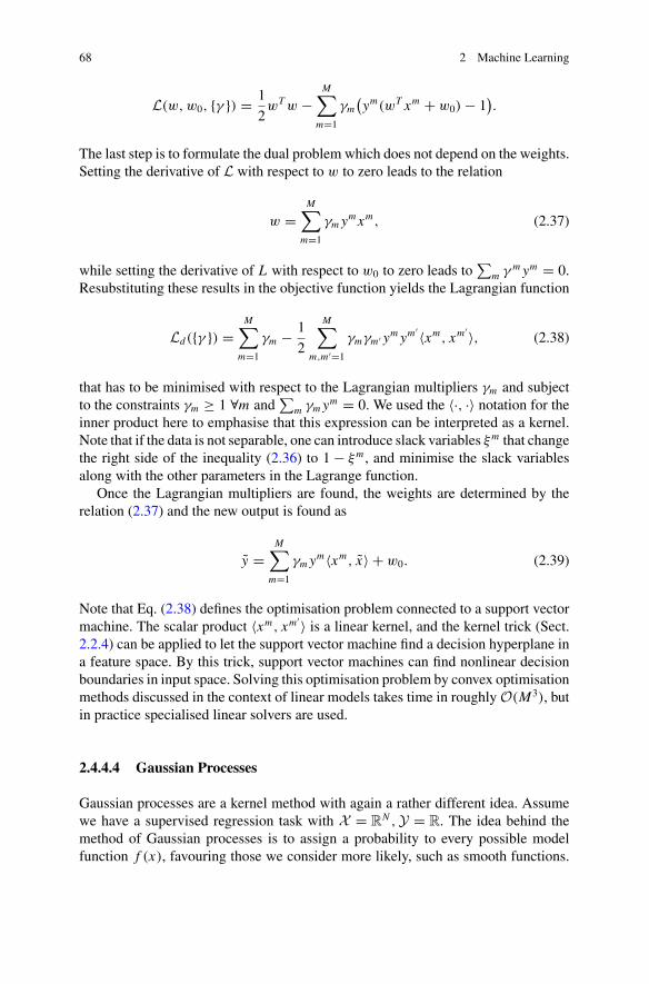
68 2 Machine Learning

L(w,w0, {γ }) = 1

2wTw −

M∑m=1

γm(ym(wT xm + w0) − 1

).

The last step is to formulate the dual problem which does not depend on the weights.Setting the derivative of L with respect to w to zero leads to the relation

w =M∑

m=1

γm ymxm, (2.37)

while setting the derivative of L with respect to w0 to zero leads to∑

m γ m ym = 0.Resubstituting these results in the objective function yields the Lagrangian function

Ld({γ }) =M∑

m=1

γm − 1

2

M∑m,m ′=1

γmγm ′ ym ym′ 〈xm, xm

′ 〉, (2.38)

that has to be minimised with respect to the Lagrangian multipliers γm and subjectto the constraints γm ≥ 1 ∀m and

∑m γm ym = 0. We used the 〈·, ·〉 notation for the

inner product here to emphasise that this expression can be interpreted as a kernel.Note that if the data is not separable, one can introduce slack variables ξm that changethe right side of the inequality (2.36) to 1 − ξm , and minimise the slack variablesalong with the other parameters in the Lagrange function.

Once the Lagrangian multipliers are found, the weights are determined by therelation (2.37) and the new output is found as

y =M∑

m=1

γm ym〈xm, x〉 + w0. (2.39)

Note that Eq. (2.38) defines the optimisation problem connected to a support vectormachine. The scalar product 〈xm, xm

′ 〉 is a linear kernel, and the kernel trick (Sect.2.2.4) can be applied to let the support vector machine find a decision hyperplane ina feature space. By this trick, support vector machines can find nonlinear decisionboundaries in input space. Solving this optimisation problem by convex optimisationmethods discussed in the context of linear models takes time in roughlyO(M3), butin practice specialised linear solvers are used.

2.4.4.4 Gaussian Processes

Gaussian processes are a kernel method with again a rather different idea. Assumewe have a supervised regression task with X = R

N ,Y = R. The idea behind themethod of Gaussian processes is to assign a probability to every possible modelfunction f (x), favouring those we consider more likely, such as smooth functions.

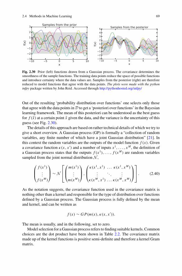
2.4 Methods in Machine Learning 69

Fig. 2.30 Prior (left) functions drawn from a Gaussian process. The covariance determines thesmoothness of the sample functions. The training data points reduce the space of possible functionsand introduce certainty where the data values are. Samples from the posterior (right) are thereforereduced to model functions that agree with the data points. The plots were made with the pythoninfpy package written by John Reid. Accessed through http://pythonhosted.org/infpy/

Out of the resulting ‘probability distribution over functions’ one selects only thosethat agree with the data points inD to get a ‘posteriori over functions’ in the Bayesianlearning framework. The mean of this posteriori can be understood as the best guessfor f (x) at a certain point x given the data, and the variance is the uncertainty of thisguess (see Fig. 2.30).

The details of this approach are based on rather technical details of whichwe try togive a short overview. A Gaussian process (GP) is formally a “collection of randomvariables, any finite number of which have a joint Gaussian distribution” [21]. Inthis context the random variables are the outputs of the model function f (x). Givena covariance function κ(x, x ′) and a number of inputs x1, . . . , xM , the definition ofa Gaussian process states that the outputs f (x1), . . . , f (xM) are random variablessampled from the joint normal distribution N ,

⎛⎜⎝

f (x1)...

f (xM)

⎞⎟⎠ ∼ N

⎡⎢⎣

⎛⎜⎝m(x1)

...

m(xM)

⎞⎟⎠ ,

⎛⎜⎝

κ(x1, x1) . . . κ(x1, xM )...

. . ....

κ(xM , x1) . . . κ(xM , xM )

⎞⎟⎠

⎤⎥⎦ . (2.40)

As the notation suggests, the covariance function used in the covariance matrix isnothing other than a kernel and responsible for the type of distribution over functionsdefined by a Gaussian process. The Gaussian process is fully defined by the meanand kernel, and can be written as

f (x) ∼ GP(m(x), κ(x, x ′)).

The mean is usually, and in the following, set to zero.Model selection for aGaussian process refers to finding suitable kernels. Common

choices are the dot product have been shown in Table 2.2. The covariance matrixmade up of the kernel functions is positive semi-definite and therefore a kernel Grammatrix.

70 2 Machine Learning

Equation (2.40) shows how to draw samples of model outputs f (x) for a set ofinputs, and if we increase the number of inputs we can get a good idea of what thefunction sampled from the Gaussian process looks like. We can use the expressionin Eq. (2.40) for prediction. Instead of some general inputs, we consider the jointdistribution for the training data outputs as well as the new output f (x),

⎛⎜⎜⎜⎝

f (x1)...

f (xM)

f (x)

⎞⎟⎟⎟⎠ ∼ N

⎡⎢⎢⎢⎣

⎛⎜⎝0...

0

⎞⎟⎠ ,

⎛⎜⎜⎜⎝

κ(x1, x1) . . . κ(x1, xM) κ(x1, x)...

. . ....

...

κ(xM , x1) . . . κ(xM , xM) κ(xM , x)κ(x, x1) . . . κ(x, xM) κ(x, x)

⎞⎟⎟⎟⎠

⎤⎥⎥⎥⎦ . (2.41)

To get the desired probability distribution p(y|x) over the predicted output f (x) = ywe have to marginalise the distribution in Eq. (2.41) for the fixed values f (x1) =y1, . . . , f (xM) = yM . This can be thought of as ‘cutting’ through the joint prob-ability distribution in order to reduce the multivariate Gaussian distribution to aunivariate (one-dimensional) distribution. The technical algebraic details of obtain-ing a marginal Gaussian distribution can be found in most statistics textbooks andwe only write down the result here12:

p(y|x) = N [y| κT K−1y︸ ︷︷ ︸mean μ

, ˜κ − κT K−1κ︸ ︷︷ ︸covariance δ

], (2.42)

with the notation

κ =⎛⎜⎝

κ(x1, x)...

κ(xM , x)

⎞⎟⎠ , (2.43)

K =⎛⎜⎝

κ(x1, x1) . . . κ(x1, xM)...

. . ....

κ(xM , x1) . . . κ(xM , xM)

⎞⎟⎠ , (2.44)

˜κ = κ(x, x), (2.45)

y =⎛⎜⎝

y1

...

yM

⎞⎟⎠ . (2.46)

Besides model selection, which involves choosing the kernel and its hyperpa-rameters, Gaussian processes do not have a distinct learning phase. With Eq. (2.42),prediction is mainly a computational problem of efficiently inverting the

12Note that we only consider noise free data here, however, including Gaussian noise simply addsa variance parameter to the matrix K . For more details, see [21].

2.4 Methods in Machine Learning 71

M × M-dimensional kernel matrix K . Gaussian processes do take a lot of compu-tational resources when large datasets have to be processed [6], and many proposalsfor approximations have been put forward [21].

References

1. Russell, S.J., Norvig, P., Canny, J.F., Malik, J.M., Edwards, D.D.: Artificial Intelligence: AModern Approach, vol. 3. Prentice Hall, Englewood Cliffs (2010)

2. Lee,H., Ekanadham,C.,Ng,A.Y.: Sparse deep belief netmodel for visual areaV2. In:Advancesin Neural Information Processing Systems, pp. 873–880 (2008)

3. Bishop, C.M.: Pattern Recognition and Machine Learning, vol. 1. Springer (2006)4. Hastie, T., Friedman, J., Tibshirani, R.: The Elements of Statistical Learning, vol. 1. Springer,

Berlin (2001)5. Duda, R.O., Hart, P.E., Stork, D.G.: Pattern Classification. Wiley, New York (2012)6. Murphy, K.P.: Machine Learning. A Probabilistic Perspective. MIT Press (2012)7. Koller, D., Friedman, N.: Probabilistic Graphical Models: Principles and Techniques. MIT

Press (2009)8. Hertz, J.A., Krogh, A.S., Palmer, R.G.: Introduction to the Theory of Neural Computation,

vol. 1. Westview Press, Redwood City (California) (1991)9. Bishop,C.M.:NeuralNetworks for PatternRecognition, vol. 1. ClarendonPress,Oxford (1995)10. Alpaydin, E.: Introduction to Machine Learning. MIT Press, Cambridge (2004)11. Silver, D., et al.: Mastering the game of go without human knowledge. Nature 550(7676), 354

(2017)12. Domingos, P.: A few useful things to know about machine learning. Commun. ACM 55(10),

78–87 (2012)13. Ng, A.Y., Jordan, A.: On discriminative vs. generative classifiers: a comparison of logistic

regression and naive Bayes. Adv. Neural Inf. Process. Syst. 14, 841–846 (2002)14. Griffiths, T., Yuille, A.: A primer on probabilistic inference. In: Chater, N., Oaksford, M.

(eds.) The Probabilistic Mind: Prospects for Bayesian Cognitive Science, pp. 33–57. OxfordUniversity Press (2008)

15. Ghahramani, Z.: Probabilistic machine learning and artificial intelligence. Nature 521(7553),452–459 (2015)

16. Smola, A.J., Schölkopf, B., Müller, K.-R.: The connection between regularization operatorsand support vector kernels. Neural Netw. 11(4), 637–649 (1998)

17. Schölkopf, B., Smola, A.J.: Learning with Kernels: Support Vector Machines, Regularization,Optimization, and Beyond. MIT Press (2002)

18. Schölkopf, B., Herbrich, R., Smola, A.: A generalized representer theorem. In: ComputationalLearning Theory, pp. 416–426. Springer (2001)

19. Shashua, A.: Introduction to machine learning: Class notes 67577. arXiv:0904.3664 (2009)20. Steinwart, I., Hush, D., Scovel, C.: An explicit description of the reproducing kernel Hilbert

spaces of Gaussian RBF kernels. IEEE Trans. Inf. Theory 52(10), 4635–4643 (2006)21. Rasmussen, C.E.: Gaussian Processes for Machine Learning. MIT Press (2006)22. Bennett, K.P., Parrado-Hernández, E.: The interplay of optimization and machine learning

research. J. Mach. Learn. Res. 7(Jul):1265–1281 (2006)23. Rumelhart, D.E., Hinton, G.E., Williams, R.J.: Learning internal representations by error prop-

agation. Technical report, DTIC Document (1985)24. Hinton, G., Osindero, S., Teh, Y.-W.: A fast learning algorithm for deep belief nets. Neural

Comput. 18(7), 1527–1554 (2006)25. Zhang, C., Bengio, S., Hardt, M., Recht, B., Vinyals, O.: Understanding deep learning requires

rethinking generalization. In: Proceedings of the International Conference on Learning Repre-sentations (2017)

72 2 Machine Learning

26. Boyd, S., Vandenberghe, L.: Convex Optimization. Cambridge University Press (2004)27. Vavasis, S.A.: Nonlinear Optimization: Complexity Issues. Oxford University Press (1991)28. Weierstrass, K.: Über die analytische Darstellbarkeit sogenannter willkürlicher Functionen

einer reellen Veränderlichen. Sitzungsberichte der Königlich Preußischen Akademie der Wis-senschaften zu Berlin 2, 633–639 (1885)

29. Trefethen, L.N., Bau III, D.: Numerical Linear Algebra, vol. 50. Siam (1997)30. McCulloch, W.S., Pitts, W.: A logical calculus of the ideas immanent in nervous activity. Bull.

Math. Biol. 5(4), 115–133 (1943)31. Hopfield, J.J.: Neural networks and physical systems with emergent collective computational

abilities. Proc. Natl. Acad. Sci. 79(8), 2554–2558 (1982)32. Minsky, M., Papert, S.: Perceptrons: An Introduction to Computational Geometry. MIT Press,

Cambridge (1969)33. Rumelhart, D.E., Hinton, G.E., Williams, R.J.: Learning representations by back-propagating

errors. Nature 323(9), 533–536 (1986)34. Novikoff, A.B.J.: On convergence proofs on perceptrons. In: Proceedings of the Symposium

on the Mathematical Theory of Automata, vol. 12, pp. 615–622 (1962)35. Hornik, K., Stinchcombe, M., White, H.: Multilayer feedforward networks are universal

approximators. Neural Netw. 2(5), 359–366 (1989)36. Nair, V., Hinton, G.E.: Rectified linear units improve restricted Boltzmann machines. In: Pro-

ceedings of the 27th International Conference on Machine Learning (ICML-10), pp. 807–814(2010)

37. Pascanu, R., Mikolov, T., Bengio, Y.: On the difficulty of training recurrent neural networks.ICML 3(28), 1310–1318 (2013)

38. El Hihi, S., Bengio, Y.: Hierarchical recurrent neural networks for long-term dependencies. In:NIPS’95 Proceedings of the 8th International Conference on Neural Information ProcessingSystems, vol. 400, pp. 493–499. MIT Press, Cambridge, MA, USA (1995)

39. Arjovsky, M., Shah, A., Bengio, Y.: Unitary evolution recurrent neural networks. J. Mach.Learn. Res. 48 (2016)

40. Bengio, Y., Boulanger-Lewandowski, N., Pascanu, R.: Advances in optimizing recurrent net-works. In: 2013 IEEE International Conference on Acoustics, Speech and Signal Processing,pp. 8624–8628. IEEE (2013)

41. Duda, R.O., Hart, P.E., Stork, D.G.: Pattern Classification, 2 ed. Wiley (2000)42. Rojas, R.: Neural Nets: A Systematic Introduction. Springer, New York (1996)43. Hinton,G.: Training products of experts byminimizing contrastive divergence.Neural Comput.

14(8), 1771–1800 (2002)44. Hinton, G.: A practical guide to training restricted Boltzmann machines. UTML TR 2010-003,

Version 1 (2010)45. Gilks, W.R., Richardson, S., Spiegelhalter, D.J.: Markov ChainMonte Carlo in Practice. Chap-

man & Hall, London (1996)46. Carreira-Perpinan, M.A., Hinton, G.: On contrastive divergence learning. In: Cowell, R.,

Ghahramani, Z. (eds.) AISTATS 2005: Proceedings of the Tenth International Workshop onArtificial Intelligence and Statistics, vol. 10, pp. 33–40. The Society for Artificial Intelligenceand Statistics (2005)

47. Bengio, Y.: Learning deep architectures for AI. Found. TrendsMach. Learn. 2(1), 1–127 (2009)48. Sutskever, I., Tieleman, T.: On the convergence properties of contrastive divergence. In: Inter-

national Conference on Artificial Intelligence and Statistics, pp. 789–795 (2010)49. Pearl, J.: Causality. Cambridge University Press (2009)50. Heckerman, D., Geiger, D., Chickering, D.M.: Learning Bayesian networks: the combination

of knowledge and statistical data. Mach. Learn. 20(3):197–243 (1995)51. Dagum, P., Luby, M.: Approximating probabilistic inference in Bayesian belief networks is

NP-hard. Artif. Intell. 60(1), 141–153 (1993)52. Ben-Gal, I.: Bayesian networks. In: Encyclopedia of Statistics in Quality and Reliability (2007)53. Rabiner, L.R.: A tutorial on hidden Markov models and selected applications in speech recog-

nition. Proc. IEEE 77(2), 257–286 (1989)

References 73

54. Dudani, S.A.: The distance-weighted k-nearest-neighbor rule. IEEE Trans. Syst. Man Cybern.4, 325–327 (1976)

55. Boser, B.E., Guyon, I.M., Vapnik, V.N.: A training algorithm for optimal margin classifiers.In: COLT’92 Proceedings of the Fifth Annual Workshop on Computational Learning Theory,pp. 144–152. ACM (1992)

Chapter 3Quantum Information

While the last chapter introduced readers without a firm background in machinelearning into the foundations, this chapter targets readers who are not closely famil-iar with quantum information. Quantum theory is notorious for being complicated,puzzling and difficult (or even impossible) to understand. Although this impressionis debatable, giving a short introduction into quantum theory is indeed a challengefor two reasons: On the one hand its backbone, the mathematical apparatus with itsobjects and equations requires some solid mathematical foundations in linear alge-bra, and is usually formulated in theDirac notation [1] that takes a little practice to getfamiliar with. On the other hand the physical reality this apparatus seeks to describe isdifficult to grasp from the point of our daily intuition about physical phenomena, andthe interpretation of the results this mathematical apparatus yields, unchallenged andreproduced by thousands of experiments up to today, are still controversially debated.

There are many different ways to introduce quantum theory.1 Scott Aaronson, inhis online lecture notes2 remarks sarcastically that in order to learn about quantumtheory,

[...] you start with classical mechanics and electrodynamics, solving lots of grueling differ-ential equations at every step. Then you learn about the “blackbody paradox” and variousstrange experimental results, and the great crisis these things posed for physics. Next youlearn a complicated patchwork of ideas that physicists invented between 1900 and 1926 totry to make the crisis go away. Then, if you’re lucky, after years of study you finally getaround to the central conceptual point: that nature is described not by probabilities (whichare always non-negative), but by numbers called amplitudes that can be positive, negative,or even complex.

1Common didactic approaches are the historical account of discovering quantum theory, the empir-ical account of experiments and their explanations, the Hamiltonian path from formal classical toquantum mechanics, the optical approach of the wave-particle-dualism, and the axiomatic postula-tion of its mathematical structure [2].2The lecture notes are available at http://www.scottaaronson.com/democritus/, and led to the book“Quantum Computing since Democritus” [3].

© Springer Nature Switzerland AG 2018M. Schuld and F. Petruccione, Supervised Learning with Quantum Computers,Quantum Science and Technology, https://doi.org/10.1007/978-3-319-96424-9_3

75

76 3 Quantum Information

From the perspective of quantum computing this comment certainly containssome truth, since a central concept is the qubit, which is a rather simple quantumsystem. This is why we will neglect many details of quantum theory and focus onfinite, discrete quantum systems.

In the following we will start with an intuition for what operators, states andunitary evolutions are, and proceed to a more rigorous introduction to quantumtheory based on the Dirac notation. We then introduce quantum computing togetherwith the concepts of gates, qubits and quantum algorithms. As a preparation for laterchapters we then discuss different ways to encode information into quantum systemsand present some core quantum routines used in later chapter.

3.1 Introduction to Quantum Theory

3.1.1 What Is Quantum Theory?

Quantum theory (used synonymously with the term quantummechanics) is “first andforemost a calculus for computing the probabilities of outcomes of measurementsmade on physical systems” [4] called quantum systems. A quantum system is typ-ically a collection of microscopic physical objects for which classical Newtonianmechanics does not explain experimental observations. Examples are a hydrogenatom, light of very low intensity, or a small number of electrons in a magnetic field.

Quantum theory incorporates classical mechanics as a limit case [5] and is oftencelebrated as the most accurate physical theory ever developed.3 The reason whydespite this ‘superiority’ over classical mechanics the latter is still commonly used inscience and education is that quantummechanics is impractical to apply to large sys-tems, as the calculations very soon become too complex to execute. At the same time,quantum effects in macroscopic systems are usually small enough to be neglectedwithout a visible error and can formany purposes be replaced by easier, higher aggre-gated classical models. However, and similar to machine learning in which a lot ofproblems are uncomputable in their exact formulation, a range of solvable modelsas well as powerful approximation techniques have been developed which lead to arange of technological applications in the fields of medicine, chemistry, biology andengineering.

Figure3.1 shows a brief historical overview of quantum theory. What Aaronsondescribes as a “complicated patchwork of ideas that physicists invented between1900 and 1926” forms the beginnings of quantum theory as it is still taught today,and which was then used to rethink the entire body of physics knowledge. Theinitial step is commonly attributed to the year 1900 whenMax Planck introduced the

3It shall be remarked that quantum theory has no notion of the concept of gravity, an open problemtroubling physicists who dream of the so called ‘Grand Unified Theory’ of quantum mechanicsand general relativity, and a hint towards the fact that quantum mechanics still has to be developedfurther.

3.1 Introduction to Quantum Theory 77

1900

Max Planckdiscovers quantisationof black-body radiation

1905

Albert Einsteindiscovers quanti-sation of light

1912

Max Bornapplies quantisationto atomic spectrum

1923

de Brogliepostulates the dualityof waves and particles

1926

Erwin regnidorhcSformulates wave

mechanics

1930

1932

Paul Dirac andJohn von Neumannunite approaches

& formulate modernquantum theory

1925

Heisenberg, Jordan, Bornformulate matrix

mechanics

Quantum theory branches outinto physical subdisciplines

TIME

Fig. 3.1 Timeline of the early years of quantum theory

idea that energy (in this case so called black-body radiation) can only take discretevalues as if existing as ‘quanta’ or small energetic portions. With this assumption hewas able to resolve a heated debate regarding the spectrum of black-body radiation[6]. Almost in parallel, Albert Einstein made a similar discovery derived from thestatistical mechanics of gases and derived the concept of a photon—a portion orenergy quantum of light [7, 8].

In the following years, these early ideas of a ‘theory of energy quanta’ wereapplied to atomic spectroscopy (most notably by Niels Bohr), and to light (by Louisde Broglie) but still based on rather ad-hocmethods [6].Werner Heisenberg followedby Jordan, Born and, independently, Paul Dirac formulated the first mathematicallyconsistent version of quantum theory referred to as matrix mechanics in 1925, withwhich Wolfgang Pauli was able to derive the experimental results of measuringthe spectrum of a hydrogen atom. Heisenberg postulated his uncertainty principleshortly after, stating that certain properties of a quantum system cannot be measuredaccurately at the same time. In 1926, following a slightly different and less abstractroute, Erwin Schrödinger proposed his famous equation of motion for the ‘wavefunction’ describing the state of a quantum system. These two approaches wereshown to be equivalent in the 1930s, and a more general version was finally proposedby Dirac and Jordan. In the following years, quantum theory branched out into manysub-disciplines such as quantum many-body systems, quantum thermodynamics,quantum optics, and last but not least, quantum information processing.

78 3 Quantum Information

3.1.2 A First Taste

Quantum theory can be understood as a generalisation of classical probability theoryto make statements about the probabilities of the outcomes of measurements onquantum systems [9]. The rigorous formulation of this generalisation requires someserious mathematics (see for example [10]) and is beyond the scope of this book.However, instead of directly diving into Hilbert spaces and Hermitian operators, thissection starts with a simple classical stochastic system and shows how to constructthe description for a very similar quantum system.

3.1.2.1 States and Observables

Consider a set of N mutually exclusive events S = {s1, . . . , sN }. In physics, eventsusually refer to the outcomes ofmeasurements (‘observations’) onphysical propertiesof a system, but one may also think of other examples such as ‘it is raining’ and ‘itis not raining’. One can associate each event with a random variable X that cantake the values {x1, . . . , xN }, and define a probability distribution over these valuesquantifying our knowledge on how likely an event is to occur. The probabilitiesrelated to the N events, {p1, . . . , pN }, are real numbers, and they fulfill pi ≥ 0 and∑N

i=1 pi = 1. The expectation value of the random variable is defined as

〈X〉 =N∑

i=1

pi xi , (3.1)

and is the weighed average of all values the random variable can take.

Example 3.1 (Particle in a rectangular box)Consider the model of a particle in a 2-dimensional rectangular box which is dividedinto four sections as illustrated in Fig. 3.2. The event space is given by the four eventsof the particle being found in the first, second, third or fourth section, Sparticle ={s1, s2, s3, s4}. The random variable X for the measurement result can take values{1, 2, 3, 4}, and each measurement outcome has a probability pi , i = 1, . . . , 4 tooccur. For example, if p1 = 0.2, p2 = 0.2 , p3 = 0.2, p4 = 0.4 the expectation valueis given by 〈X〉 = 2.8 which reveals that the particle has a higher probability to bein the right half than in the left.

From here one needs two steps in order to arrive at the description of a quantumsystem with N different possible configurations or measurement outcomes: First,

1 2 3 4

Fig. 3.2 Illustration of the particle in a box from Example 3.1

3.1 Introduction to Quantum Theory 79

summarise the probabilities and the outcomes by matrices and vectors, and second,replace real positive probabilities with complex amplitudes.4

For the first step, consider a vector of the square roots of probabilities p1, . . . , pN ,

q =⎛

⎝

√p1...√pN

⎞

⎠ = √p1

⎛

⎝1...0

⎞

⎠ + · · · + √pN

⎛

⎝0...1

⎞

⎠ , (3.2)

as well as a diagonal matrix X corresponding to the random variable with the samename,

X =⎛

⎝x1 . . . 0...

. . ....

0 . . . xN

⎞

⎠ .

The expectation value of Eq. (3.1) can now be written as

〈X〉 = qT Xq =N∑

i=1

pi xi . (3.3)

So far we just made the expression of the expectation value more complicated. InEq. (3.3), the matrix X contributes the values of the random variable, and the vectorq contains the square roots of the probabilities. For simplicity, both objects wereexpressed in the standard basis ofR

N . One can see that the basis vector (1, 0, . . . , 0)T

forms a subspace of theRN that is associated with the first event. Moreover, the outer

product of this basis vector with itself

(1 . . . 0

)

⎛

⎜⎝

1...

0

⎞

⎟⎠ =

⎛

⎜⎝

1 . . . 0...

. . ....

0 . . . 0

⎞

⎟⎠ (3.4)

is a projector onto this subspace.Multiplied to a vector, it ‘picks out’ the first element.This is a motivation why in quantum probability theory, the measurement events arerepresented by projectors onto subspaces which we will see in the next section. Thesum of all projectors to the subspaces of x1, . . . , xN is the identity.

Note that one does not have to use the standard basis, but that any other basis{vi } for which the eigenvalue equations Xvi = xivi hold would have done the job,as can be confirmed by decomposing q = q1v1 + · · · + qNvN and employing theeigenvalue equation to calculate the expectation value.

4In this sense, Aaronson is right in saying that the “central conceptual point” of quantum theoryis “that nature is described not by probabilities […], but by numbers called amplitudes that can bepositive, negative, or even complex”.

80 3 Quantum Information

It turns out that Eq. (3.3) is already very close to howquantummechanics describesexpectation values, but some mathematical properties of the vectors and matrix areslightly different. In order to turn Eq. (3.3) into the formula of computing expectationvalues of measurements on quantum systems, we have to replace q with a complexamplitude vector α = (α1, . . . , αN )T ∈ C

N , and X by a complex, self-adjoint matrixO ∈ C

N×N . Another term for self-adjoint is Hermitian. Hermitian operators havethe property that they are equal to their complex-conjugate transpose, O = (O∗)T ,where in quantummechanics, the symbol for the complex-conjugate transpose is thedagger, (O∗)T = O†.

Let {v1, . . . , vN } be a basis of orthonormal eigenvectors of O which spans theC

N , fulfilling eigenvalue equations Ovi = oivi and normalisations v†i v j = δi j for all

i, j = 1, . . . , N . Any amplitude vector α can be written as a linear combination ofthis basis,5

α = α1v1 + · · · + αNvN .

The expectation value of the random variable O corresponding to the matrix Onow becomes

〈O〉 = α†Oα =N∑

i=1

|αi |2vi †Ovi =N∑

i=1

|αi |2oi . (3.5)

One can see that the |αi |2 take the role of the probabilities in the classical example, andwe therefore demand that

∑i |αi |2 = 1 to ensure that the probabilities sum up to one.

If the basis {v1, . . . , vN } is the standard basis {(1, 0, . . . , 0)T , . . . , (0, 0, . . . , 1)T },the αi will just be the entries of α, and the normalisation condition therefore meansthat the amplitude vector has unit length.

The eigenvalues oi of O correspond to the values of the random variable or theoutcomes of measurements. For example, whenmeasuring the energy configurationsof an atom, oi would simply be an energy value in a given unit. However, withoutfurther constraints the eigenvalues of a complex matrix can be complex, which doesnot make any sense when looking at physically feasible variables (i.e., what is acomplex energy?). This is the reason to choose O to be a Hermitian operator, sincethe eigenvalues of Hermitian operators are always real and therefore physical.

Since O (just like X in the classical example) contains information on the valuesof the random variable, which in a physical setup correspond to possible observationsin a measurement, it is called an observable. The vector α tells us something aboutthe probability distribution of the measurement outcome and is a representation of aso-called quantum state, since probabilistic information is everything we know aboutthe configuration a quantum system is in. Together, observables and states allow usto calculate probabilities and expectation values of measurement outcomes.

5The spectral theorem of linear algebra guarantees that the eigenvectors of a Hermitian operator Oform a basis of theHilbert space, so that every amplitude vector can be decomposed into eigenvectorsof O .

3.1 Introduction to Quantum Theory 81

3.1.2.2 Unitary Evolutions

Physical theories define equations for the evolution of the state of a system over time.Let us once more start with a classical stochastic description and show how to arriveat quantum evolutions.

A map of a discrete probability distribution to another discrete probability dis-tribution (describing the change of our knowledge over time) has to preserve theproperty that the probabilities of all elementary events sum up to one. Consider thecase that we know the probability of transition from one state to the other in one dis-crete time step. Then such an update can bemodelled by applying amatrix containingthese transition probabilities, to a probability vector p = (p1, . . . , pN )T ,

⎛

⎜⎝

m11 . . . m1N...

. . ....

mN1 . . . mNN

⎞

⎟⎠

⎛

⎜⎝

p1...

pN

⎞

⎟⎠ =

⎛

⎜⎝

p′1...

p′N

⎞

⎟⎠ ,

N∑

i=1

pi =N∑

i=1

p′i = 1. (3.6)

The transition matrix M = (m)i j has to ensure that the probability vector remainsnormalised, which implies that M is a so-called stochastic matrix whose columnssum up to one. The stochastic process resulting from the transition matrix is alsocalled a Markov process.

Example 3.2 (Stochastic description of the weather) We observe the weather onconsecutive days and know the probability that it is raining tomorrow if it was rainingtoday is 60% while the probability for the weather to change is 40%. Likewise, ifit was sunny, it rains tomorrow with 40% and it stays sunny with 60%. Let ptod =(p1, p2)T describe the probability p1 that it is raining, or the probability p2 that itis sunny today. We can now calculate the probability of the weather tomorrow byapplying the stochastic or transition matrix to the probabilistic state,

(0.6 0.40.4 0.6

)

ptod = ptom

If we know that it was sunny today, ptod = (0, 1)T , the probability of sun will be 0.6and of rain will be 0.4.

In quantum theory, we work with amplitude vectors with the property that theentries’ sum of absolute squares has to sum up to one. Consequently, an evolutionhas to be described by a unitary matrix (the complex equivalent of an orthogonaltransformation which is known to maintain lengths),

⎛

⎜⎝

u11 . . . u1N...

. . ....

uN1 . . . uNN

⎞

⎟⎠

⎛

⎜⎝

α1...

αN

⎞

⎟⎠ =

⎛

⎜⎝

α′1...

α′N

⎞

⎟⎠ ,

N∑

i=1

|αi |2 =N∑

i=1

|α′i |2 = 1. (3.7)

82 3 Quantum Information

A unitarymatrix has the property that its inverse is its complex conjugated,U−1 =U †.

Besides unitary evolutions, one can performmeasurements on a quantum system,which change the state. Although there are many subtleties, in their basic naturequantummeasurements are equivalent to classical statistics. If we had a probabilisticdescription ptom = (0.6, 0.4)T of the weather tomorrow as in Example 3.2, and wewait one day to observe that the weather is sunny, our knowledge would be bestdescribed by the updated probability state vector p′

tom = (1, 0)T . This discrete tran-sition of (0.6, 0.4)T → (1, 0)T is in quantum theory sometimes referred to as the‘collapse of the wavefunction’ (where the term ‘wavefunction’ refers to the quan-tum state), but is in essence similar to a classical update of our state of knowledge:If the weather is replaced by a quantum spin described by an amplitude vectorα = (

√0.6,

√0.4)T (where the first entry corresponds to the event ‘spin up’ and

the second to ‘spin down’, and we observe ‘spin up’, the amplitude vector after themeasurement would be given by α′ = (1, 0)T .

3.1.2.3 Composite Systems and Subsystems

In classical probability theory, sample spaces are combined using a tensor product.Take the weather example: Let p = (p1, p2)T again describe the probability of rainor sun, while q = (q1, q2)T denotes the probability of the wind blowing strong ornot. A combined description is a 4-dimensional vector c = (c1, c2, c3, c4)T contain-ing the probability for the events ‘wind & sun’, ‘no wind & sun’, ‘wind & rain’,‘no wind & rain’. These four events form the joint event space. If the events areindependent of each other, the probabilities of each elementary event multiply andc = (q1 p1, q1 p2, q2 p1, q2 p2)T , which can be called a product state. If the probabil-ities do not factorise, or in other words c cannot be expressed by a tensor productof p and q, the two variables are non-separable. Creating a joint sample space inthe quantum case is done in exactly the same manner, but using amplitude vectorsinstead of probability vectors.

Let us look at the opposite direction of how tomarginalise over parts of the system.Marginalising over variables basically means to give up information about them, achange in our state of knowledge towards more uncertainty. Given a multivariateprobability distribution, marginalising means to consider ‘cuts’ or ‘subspaces’ of thedistribution. Again, themarginalisation process in quantummechanics is structurallythe same in the classical setting, and has to be modelled ‘on top’ of the quantumprobability. For this one uses a slightly different description of quantum states thanamplitude vectors.

3.1.2.4 Density Matrices and Mixed States

Consider an amplitude vector α = (α1, α2)T . We have perfect knowledge that α is

the state of the system, the state is pure. A stochastic description of this systemmeans

3.1 Introduction to Quantum Theory 83

that we are uncertain if our system is in state α = (α1, α2)T or β = (β1, β2)

T , andthe overall state is called a statistical mixture of two pure states, or a mixed state.

We can incorporate statistical mixtures of quantum states into the formalism ofquantum mechanics by switching from amplitude vectors to so called density matri-ces. A density matrix ρ that corresponds to a pure quantum state α is given by theouter product ρ = ααT . To statisticians, this is known as the covariance matrix of α,which for our 2-d example α = (α1, α2)

T reads

ρ = αα† =(|α1|2 α1α

∗2

α2α∗1 |α2|2

)

.

If we do not know the quantum state of the system, but we know that the systemis in state α with probability p1 and in state β with probability p2, the density matrixto describe such a state reads

ρ = p1αα† + p2ββ† =(p1|α1|2 + p2|β1|2 p1α2α

∗1 + p2β2β

∗1

p1α1α∗2 + p2β1β

∗2 p1|α2|2 + p2|β2|2

)

.

In other words, the density matrix formulation allows us to combine ‘quantumstatistics’ expressed by a quantum state, with ‘classical statistics’ or a probabilisticstate that describes our lack of knowledge. This is possible because ρ’s diagonalcontains probabilities and not amplitudes.

Thedensitymatrix notation lets us elegantly exclude a subsystem from the descrip-tion, and the corresponding mathematical operation is to calculate the partial traceover the subsystem.Wewill later see that this is closely related to the idea ofmarginal-ising over distributions. The partial trace operation in matrix notation is the sum overthe diagonal elements in the corresponding space. Assume a state describing twojoint 2-dimensional system in density matrix notation is given by

ρAB =

⎛

⎜⎜⎝

ρ11 ρ12 ρ13 ρ14

ρ21 ρ22 ρ23 ρ24

ρ31 ρ32 ρ33 ρ34

ρ41 ρ42 ρ43 ρ44

⎞

⎟⎟⎠ ,

and the partial trace over the first subsystem is

trA{ρAB} =(

ρ11 + ρ33 ρ12 + ρ34

ρ21 + ρ43 ρ22 + ρ44

)

,

while the state of the second subsystem is given by

trB{ρAB} =(

ρ11 + ρ22 ρ13 + ρ24

ρ31 + ρ42 ρ33 + ρ44

)

.

84 3 Quantum Information

3.1.3 The Postulates of Quantum Mechanics

Let us switch gears after this more intuitive introduction of the formalism of quantumtheory, and formulate the framework of quantum mechanics more rigorously forfinite-dimensional systems with the help of a number of postulates. These postulatespick up various concepts introduced in the previous section, to which we will referthroughout, but generalise and formalise them with help of the Dirac notation. Thissection is meant to serve as a reference for the remainder of the book, and may benot immediately accessible for readers without a background in quantum physics. Ifthis is the case, we recommend to continue with Sect. 3.1.1 and return here when theneed for more depth arises.

The Dirac notation may be confusing to newcomers to quantum mechanics. Mosttopics of quantum computing can actually be expressed in terms of matrices andvectors, and we will frequently switch between the two notations. However, somequantum systems have operators with a continuous eigenbasis, where discrete andfinite vectors are not very useful. Dirac notation is an abstraction that incorporatessuch cases, and is the standard formalism in quantum computing. Table3.1 comparesthe matrix and Dirac formalisms to illustrate their equivalence from a mathematicalperspective.

3.1.3.1 State Space

A quantummechanical state lives in a Hilbert spaceH, which is a complex separablevector space. As mentioned, for the purposes of this book it suffices to consider

Table 3.1 Comparison of the two different formulations of quantum theory, Heisenberg’s matrixnotation and Dirac’s abstract formalism for discrete finite systems

Vector-matrix formalism Dirac formalism

Quantum state

Vector α = (α1, . . . , αN )T ∈ CN State vector in Hilbert space |ψ〉 ∈ H

Observables

Hermitian matrix O ∈ CN×N Hermitian operator O

Basis

{vi } basis of CN {|vi 〉} basis of H

Eigenvalues

Ovi = oivioi eigenvalue to vi

O|vi 〉 = oi |vi 〉oi eigenvalue to |vi 〉

Evolution

Uα = α′U unitary matrix

U |ψ〉 = |ψ ′〉U unitary operator

3.1 Introduction to Quantum Theory 85

discrete and finite-dimensional Hilbert spaces. These are isomorphic to the Cn , for

n = 2, 3, . . . and a quantum state therefore has a representation as a complex vector.Vectors in Hilbert space are usually denoted by |ψ〉, where |·〉 is a ‘ket’. The

complex vector representation of a ket from a discrete and finite-dimensional Hilbertspace is exactly the amplitude vector α = (α1, . . . , αN )T that we introduced in theprevious section. The norm of a vector is defined in terms of the inner product onH,which in Dirac notation is denoted by 〈·|·〉. The ‘left side’ of the inner product, 〈·|is called a ‘bra’. The corresponding object in vector notation is a complex conjugaterow vector, α† = (α1, . . . , αN ). The inner product is linear in the ‘ket’ |·〉 argumentand anti-linear in the ‘bra’ 〈·|. Thus, for two vectors |ψ1〉 and |ψ2〉 inH we have

〈ψ2|ψ1〉∗ = 〈ψ1|ψ2〉.

The norm of a vector |ψ〉 ∈ H is then

||ψ || = √〈ψ |ψ〉.

For every vector in H there is a complete orthonormal basis {|ei 〉}, i ∈ N, with〈ei |e j 〉 = δi j , such that

|ψ〉 =∑

i

|ei 〉〈ei |ψ〉 =∑

i

〈ei |ψ〉|ei 〉. (3.8)

A particular choice for such a complete orthonormal basis for the vector repre-sentation of quantum states is the standard basis used in Eq. (3.2). Note that Eq.(3.8) describes a basis change, since it expresses |ψ〉 in terms of the basis {|ei 〉}.Furthermore, |ei 〉〈ei | denotes a projector on a one-dimensional sub-space. We havealready seen a projector for the standard basis in Eq. (3.4). Equation (3.8) expressesthe property of separability of Hilbert spaces. The same equation implies that thecompleteness relation

1 =∑

i

|ei 〉〈ei | (3.9)

holds (i.e., to make the first equality sign work).In Sect. 3.1.2.4we saw that the state of a quantummechanical system is sometimes

not completely known, in which case we have to express it as a density matrix. Letus revisit this concept in Dirac notation. Imagine a system is in one of the states |ψk〉,k = 1, . . . , K , with a certain probability pk . The density operator ρ describing thismixed quantum mechanical state is defined as

ρ =K∑

k=1

pk |ψk〉〈ψi |, (3.10)

where all pk ≥ 0 and∑

k pk = 1.

86 3 Quantum Information

3.1.3.2 Observables

As we saw before, observables of a quantum mechanical system are realised as self-adjoint operators O in H that act on the ket |ψ〉 characterizing the system. Suchself-adjoint operators have a diagonal representation

O =∑

i

oi |ei 〉〈ei |,

in terms of the set of eigenvalues {oi } and the corresponding eigenvectors |ei 〉.6 Thisso-called spectral representation is unique and allows to calculate analytic functionsf of the observable according to the formula

f (O) =∑

i

f (oi )|ei 〉〈ei |.

In particular, if the observable is a Hermitian operator H , then for a real scalar ε

U = exp(iεH)

is a unitary operator.In general, expectation values of a quantum mechanical observable O can be

calculated as〈O〉 = tr{ρO},

where ‘tr’ computes the trace of the operator. The trace operation in Dirac notation‘sandwiches’ the expression inside the curly brackets by a sum over a full basis,

tr{A} =∑

i

〈ei |A|ei 〉.

For a system in a pure state ρ = |ψ〉〈ψ |, the expression for the expectation valueof an observable reduces to

〈O〉 =∑

i

〈ei |ψ〉〈ψ |O|ei 〉 =∑

i

〈ψ |ei 〉〈ei |O|ψ〉 = 〈ψ |O|ψ〉,

where we used the completeness relation (3.9). We already encountered this formulain matrix notation in Eq. (3.5).

6From this form of an operator one can see that the density matrix is also an operator on Hilbertspace, although it describes a quantum state.

3.1 Introduction to Quantum Theory 87

3.1.3.3 Time Evolution

The time evolution of a quantum mechanical system is described by the Schrödingerequation

i�d

dt|ψ〉 = H |ψ〉,

where H denotes the Hamiltonian of the system and � is Planck’s constant. In thenext chapter wewill introduce several Hamiltonians relevant to quantum informationprocessing. For time-independent Hamiltonians the solutions of the Schrödingerequation for an initial condition |ψ(t = 0)〉 = |ψ0〉 can be written as

|ψ(t)〉 = U (t)|ψ0〉, (3.11)

whereU (t) = exp(−i

t

�H),

is the unitary time-evolution operator. The unitary operator in Eq. (3.11) correspondsto the unitary matrix we encountered in Eq. (3.7).

The time evolution of a quantum system in a mixed state described by the densityoperator ρ follows immediately from its definition (3.10),

i�d

dtρ(t) = d

dt

∑

i

pi |ψi 〉〈ψi |

= [H, ρ], (3.12)

where we have used the Schrödinger equation and its Hermitian conjugate to derivethe second above equation, which is called the von Neumann equation. The formalsolution of the vonNeumann equation for initial conditionρ(t0) follows along similarlines from Eq. (3.11)

ρ(t) = U (t, t0)ρ(t0)U†(t, t0).

In other words, to evolve a density operator, we have to apply the unitary fromthe left, and its complex conjugate from the right. Note that in theoretical physicsliterature, as well as in this book, the constant � is usually set to 1 in order to simplifythe equations.

3.1.3.4 Quantum Measurement

For a quantum mechanical system in a pure state |ψ〉 we consider an observable O ,with a discrete spectrum, i.e.,

O =∑

i

oi Pi ,

88 3 Quantum Information

where Pi denotes the projector on the eigenspace spanned by the i-th eigenvector.The oi are the measurement results of a measurement associated with projectors Pi .(In Sect. 3.1.2.1 these were the events x1, . . . , xN .) Such a measurement is called aprojective measurement. According to the Born rule, the probability to obtain themeasurement result on is given by

p(on) = tr{Pn|ψ〉〈ψ |} = ||Pn|ψ〉||2.

The state of the system after the measurement is given by

|ψ〉 −→ Pn|ψ〉√〈ψ |Pn|ψ〉 .

In general, if the system is described by a density matrix ρ, the probability ofmeasuring on will be

p(on) = tr{Pnρ}

and the state of the system after the measurement will be7

PnρPntr{Pnρ} .

Consider now a measurement defined by a collection of operators {Am} that donot necessarily have to be projectors. This is a more general case. If, again, the stateof the system is described by the pure state |ψ〉, the probability that the result omrelated to operator Am occurs is given by

p(am) = 〈ψ |A†m Am |ψ〉

and the state after the measurement is

Am |ψ〉√

〈ψ |A†m Am |ψ〉

.

The measurement operators satisfy the completeness relation∑

m A†m Am = 1. If we

defineEm = A†

m Am,

it follows that∑

m Em = 1 and p(om) = 〈ψ |Em |ψ〉. The operators Em are calledPositiveOperator-ValuedMeasure (POVM) elements and their complete set is knownas a Positive Operator-Valued Measurement. This is the most common frameworkto describe quantum measurements.

7This formalism is also known as the Lüders postulate.

3.1 Introduction to Quantum Theory 89

3.1.3.5 Composite Systems

We saw in Sect. 3.1.2.3 that in vector notation, a composite state of two joint quantumsystems is a tensor product of two quantum states, which of course carries over toDirac notation. Let us assume that our quantum system of interest Σ is composed oftwo sub-systems, say Σ1 and Σ2. The sub-system Σi , i = 1, 2, is in a Hilbert spaceHi with dim(Hi ) = Ni , and is spanned by an orthonormal basis set {|eij 〉}, j ∈ N.Then, the Hilbert spaceH of the total system Σ is given by the tensor product of theHilbert spaces of the two sub-systems, i. e., H1 and H2,

H = H1 ⊗ H2.

The states in this joint Hilbert space can be written as

N1∑

j=1

N2∑

k=1

c jk |e1j 〉 ⊗ |e2k 〉

and have dim(H) = N1N2. The coefficients c jk are complex scalars and satisfy∑jk |c jk |2 = 1.

Composite quantum systems have the famous quantum feature of entanglement. Ifa state |ψ〉 can be expressed as

|ψ〉 = |ψ1〉 ⊗ |ψ2〉,

with |ψ1〉 ∈ H1 and |ψ2〉 ∈ H2, it is called separable. If the above representationis not possible, the state is called entangled. Separability and entanglement worksimilarly for density matrices. If the two subsystemsΣ1 andΣ2 are uncorrelated anddescribed by density matrices ρ1 and ρ2, respectively, then the total density matrixρ of the composite system Σ is given by

ρ = ρ1 ⊗ ρ2.

Operators O acting on the total Hilbert space H have the structure

O = O1 ⊗ O2,

where the operators O1 and O2 act on Σ1 and Σ2, respectively. In general, theexpectation value of such an operator can be calculated as

〈O〉 = tr{Oρ} = tr1{O1ρ1} · tr2{O2ρ2}, (3.13)

where tri , i = 1, 2 denotes the partial trace, which only sums over basis states of thesubsystem.

90 3 Quantum Information

Sometimes, one is interested in observables O that operate only on one of the twosubsystems, i.e.

O = O1 ⊗ 12.

In this case, the above expression for the expectation value (3.13) simplifies to

〈O〉 = tr1{O1ρ1}.

3.1.3.6 Open Quantum Systems

The above discussion is at the core of the theory of open quantum systems [11], whereone identifies Σ1 with the open system of interest (sometimes also referred to as thereduced system) andΣ2 with its environment. The aim of the theory of open quantumsystems is to find an effective dynamical description for the open system, through anappropriate elimination of the degrees of freedom of the environment. The startingpoint is, of course, the Hamiltonian evolution of the total system. The density matrixρ of the total system Σ evolves according to the von Neumann equation (3.12)

d

dtρ = −i[H, ρ].

Introducing the reduced density matrix ρ1 of the open system Σ1 as the trace overthe degrees of freedom of system Σ2, i.e.,

ρ1 = tr2{ρ},

the dynamics of the open system can be obtained from (3.12)

d

dtρ1 = −i tr2{[H, ρ]}.

Of course, the above equation is as difficult to evaluate as the dynamical equationof motion for the total system and appropriate approximations are needed to make ituseful. In the case of weak-coupling between the sub-systemsΣ1 andΣ2, a situationthat is typical in quantum optical applications, one can often assume (according tothe Born approximation) that the density matrix of the total system factorizes at alltimes and that the density matrix of the environment is unchanged

ρ(t) ≈ ρ1(t) ⊗ ρ2.

If one further assumes that changes in the environment occur on time scales thatare not resolved, then the dynamics of the open system is described by the so-calledMarkovian Quantum Master equation in Gorini-Kossakowski-Sudarshan-Lindbladform [11], which reads

3.1 Introduction to Quantum Theory 91

d

dtρ1 = −i[H, ρ1] +

∑

k

γk

(

Lkρ1L†k − 1

2L†k Lkρ1 − 1

2ρ1L

†k Lk

)

. (3.14)

The operators Lk introduced above are usually referred to as Lindblad operatorsand describe the transitions in the open system induced by the interaction with theenvironment. The constants γk are the relaxation rates for the different decay modesk of the open system.

3.2 Introduction to Quantum Computing

We will now turn to quantum computing, an application of quantum theory, wherethe abstract concepts introduced in the previous section are filled withmoremeaning.

3.2.1 What Is Quantum Computing?

As quantum theory motivated physicists to rethink all aspects of their discipline fromanewperspective, itwas only amatter of timebefore the question arosewhat quantummechanics means to information processing. In a way, with the debates of non-locality and Einstein’s “spooky action at a distance” this has already been part of theearly days of quantum mechanics. However, it took until the late 1980s for quantuminformation processing research to form an independent sub-discipline. Quantumcomputing is a subfield of quantum information processing, whose central questionsare: What is quantum information? Can we build a new type of computer basedon quantum systems? How can we formulate algorithms on such machines? Whatdoes quantum theory mean for the limits of what is computable? What distinguishesquantum computers from classical ones?

In the media (and possibly much fueled by researchers themselves hunting forgrants), quantum computing is still portrayed as the cure for all, mirrored in thefollowing remark from a machine learner’s perspective:

Much like artificial intelligence in its early days, the reputation of quantum computing hasbeen tarnished by grand promises and few concrete results. Talk of quantum computers isoften closely flanked by promises of polynomial time solutions to NP-Hard problems andother such implausible appeals to blind optimism. [12, p. 3]

It is true that after more than 20years of establishing an independent research dis-cipline, and not-surprisingly, there is still no final answer to many of the questionsposed.Most prominently,we still do not knowexactly howaquantumTuringmachinecompares to a classical Turing machine. Nevertheless, there is a lot more we know.For example, we know that there are quantum algorithms that grow slower in runtimewith the size of the input than known classical algorithms solving the same problem[13–15]. Relative to a black-box function or oracle, quantum algorithms are even

92 3 Quantum Information

QuantumComputing

1996

Luv Groverproposes a quantum

algorithm forunordered search

1994

Peter Shorproposes a quantum

algorithm forprime factoring

2009

Harrow, Hassidim & Lloydpropose a quantumalgorithm to solve

linear systems of equations

QuantumMachineLearning

TIME2013

Fig. 3.3 Timeline of quantum computing and quantum machine learning

proven to be faster than any possible classical algorithm. Another important resultis that every classical algorithm can be implemented on a quantum computer withonly polynomial overhead, so in theory a quantum computer is at least as good as aclassical computer [16] from the perspective of asymptotic complexity.

A rich landscape of quantum computational models and routines has been for-mulated [17], and a database of algorithms is frequently updated by Stephen Jordanat the American National Institute of Standards and Technology.8 Two influentialquantum algorithms were Shor’s factorisation algorithm [15] and Grover’s searchalgorithm [13]. For one branch of the quantum machine learning literature, Harrow,Hassidim and Lloyd’s quantum algorithm for linear systems of equations in 2009 setanother milestone. From roughly 2013 onwards, quantum machine learning becameits own subdiscipline of quantum computing (see Fig. 3.3).

Although there are a variety of computational models that formalise the idea ofquantum computation, most of them are based on the concept of a qubit, which is aquantum system associated with two measurable events, and in some sense similarto a random bit or biased coin toss as we saw in the introduction. Many popularnotions of quantum information claim that the power of quantum computers stemsfrom the fact that qubits can be in a linear combination of 0 and 1, so it can take‘all states in between’. But also a classical random bit (i.e. a classical coin toss)has this property to a certain extent. This is why sampling algorithms are often themost suitable competitors to quantum routines. One major difference however is thatcoefficients of the linear combination—the amplitudes—can be complex numbers inthe quantum case. In Chap. 1 we saw that a certain evolution can make amplitudeseven cancel each other out, or interferewith each other. This fact, together with othersubtleties can lead to measurement statistics that are non-classical, which means thatthey cannot be reproduced by classical systems.

8http://math.nist.gov/quantum/zoo/.

3.2 Introduction to Quantum Computing 93

A quantum computer can be understood as a physical implementation of n qubits(or other basic quantum systems) with a precise control on the evolution of thestate. A quantum algorithm is a targeted manipulation of the quantum system witha subsequent measurement to retrieve information from the system. In this sense aquantumcomputer can be understood as a special sampling device:We choose certainexperimental configurations—such as the strength of a laser beam, or a magneticfield—and read out a distribution over possible measurement outcomes.

An important theorem in quantum information states that any quantum evolution(think again of manipulating the physical system in the lab) can be approximated bya sequence of only a handful of elementary ‘manipulations’, called quantum gates,which only act on one or two qubits at a time [18]. Based on this insight, quantumalgorithms are widely formulated as quantum circuits of these elementary gates. Auniversal quantum computer consequently only has to know how to perform a smallset of operations on qubits, just like classical computers are build on a limited numberof logic gates. Runtime considerations usually count the number of quantum gatesit takes to implement the entire quantum algorithm. Efficient quantum algorithmsare based on evolutions whose decomposition into a circuit of gates grows at mostpolynomially with the input size of the problem. We will speak more about runtimeand speedups in Chap.4.

As much as a classical bit is an abstract model of a binary system that can havemany different physical realisations in principle, a qubit can be used as a modelof many different physical quantum systems. Some current candidates for imple-mentations are superconducting qubits [19], photonic setups [20], ion traps [21] ortopological properties of quasi-particles [22]. Each of them has advantages and dis-advantages, and it is not unlikely that future architectures use a mixture of theseimplementations.

3.2.2 Bits and Qubits

A qubit is realised as a quantum mechanical two-level system and as such can bemeasured in two states, called the basis states. Traditionally, they are denoted by theDirac vectors |0〉 and |1〉.

For our purposes it therefore suffices to describe the transition from a classical to aquantummechanical description of information processing—from bits to qubits—bymeans of a very simple quantization procedure, namely

0 −→ |0〉,1 −→ |1〉.

The vectors |0〉, |1〉 form a orthonormal basis of a 2-dimensional Hilbert spacewhich is also called the computational basis. As a consequence of the superpositionprinciple of quantum mechanics the most general state of a qubit is

94 3 Quantum Information

|ψ〉 = α1|0〉 + α2|1〉, (3.15)

whereα1, α2 ∈ C and because of the normalisation of the state vector |α1|2 + |α2|2 =1. The Hermitian conjugate to the above ket-state, the bra-state, is then

〈ψ | = α∗1〈0| + α∗

2〈1|,

where ∗ denotes complex conjugation.As discussed in the previous sections, such a Dirac vector has a vector represen-

tation, since N -dimensional, discrete Hilbert spaces are isomorphic to the space ofcomplex vectors C

N . In vector notation, a general qubit is expressed as

|ψ〉 =(

α1

α2

)

.

The Hermitian conjugate of this amplitude column vector is the transposed andconjugated row vector

(α∗1 , α

∗2) ∈ C

2.

Furthermore, we can represent the two states |0〉 and |1〉 as the standard basisvectors of the C

2,

|0〉 =(10

)

∈ C2,

|1〉 =(01

)

∈ C2.

Vector notation can be very useful to understand the effect of quantum gates. How-ever, as common in quantum computing, we will predominantly use Dirac notation.

It is sometimes useful to have a geometric representation of a qubit. A genericqubit in the pure state (3.15) can be parametrised as

|ψ〉 = exp (iγ )

(

cosθ

2|0〉 + exp (iφ) sin

θ

2|1〉

)

,

where θ, φ and γ are real numbers with 0 ≤ θ ≤ π and 0 ≤ φ ≤ 2π . The globalphase factor exp (iγ ) has no observable effect and will be omitted in the fol-lowing. The angles θ and φ have the obvious interpretation as spherical coor-dinates, so that the Hilbert space vector |ψ〉 can be visualised as the R

3 vector(sin θ cosφ, sin θ sin φ, cosφ) pointing from the origin to the surface of a ball, theso-called Bloch sphere. The Bloch sphere is illustrated in Fig. (3.4).9

The Dirac notation allows also for a compact description of the inner productof two vectors in Hilbert space that was introduced in Sect. 3.1.3.1. Consider for

9Adapted from https://tex.stackexchange.com/questions/345420/how-to-draw-a-bloch-sphere.

3.2 Introduction to Quantum Computing 95

Fig. 3.4 The Bloch sphererepresentation of a qubit

|ψ〉

x1

x2

x3

φ

θ

example, two vectors in C2, |ψ1〉 = α1|0〉 + α2|1〉 and |ψ2〉 = β1|0〉 + β2|1〉, with

αi , βi ∈ C for i = 1, 2, |α1|2 + |α2|2 = 1 and |β1|2 + |β2|2 = 1. Since |0〉, |1〉 areorthonormal, we have that

〈0|0〉 = 〈1|1〉 = 1, 〈0|1〉 = 〈1|0〉 = 0.

The inner product of |ψ1〉 and |ψ2〉 is therefore given by

〈ψ1|ψ2〉 = α∗1β1 + α∗

2β2.

Of course, this is equivalent the scalar or vector product of the two correspondingamplitude vectors. Similarly, the outer product of two states can be compactly writtenas

|ψ1〉〈ψ2| =(

α1β∗1 α1β

∗2

α2β∗1 α2β

∗2

)

,

which is the outer product of the amplitude vectors.According to Sect. 3.1.3.5, n unentangled qubits are described by a tensor product

of single qubits,|ψ〉 = |q1〉 ⊗ · · · ⊗ |qn〉.

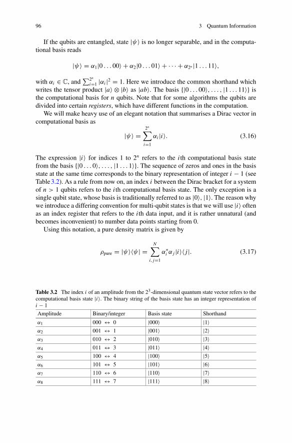
96 3 Quantum Information

If the qubits are entangled, state |ψ〉 is no longer separable, and in the computa-tional basis reads

|ψ〉 = α1|0 . . . 00〉 + α2|0 . . . 01〉 + · · · + α2n |1 . . . 11〉,

with αi ∈ C, and∑2n

i=1 |αi |2 = 1. Here we introduce the common shorthand whichwrites the tensor product |a〉 ⊗ |b〉 as |ab〉. The basis {|0 . . . 00〉, . . . , |1 . . . 11〉} isthe computational basis for n qubits. Note that for some algorithms the qubits aredivided into certain registers, which have different functions in the computation.

We will make heavy use of an elegant notation that summarises a Dirac vector incomputational basis as

|ψ〉 =2n∑

i=1

αi |i〉. (3.16)

The expression |i〉 for indices 1 to 2n refers to the i th computational basis statefrom the basis {|0 . . . 0〉, . . . , |1 . . . 1〉}. The sequence of zeros and ones in the basisstate at the same time corresponds to the binary representation of integer i − 1 (seeTable3.2). As a rule from now on, an index i between the Dirac bracket for a systemof n > 1 qubits refers to the i th computational basis state. The only exception is asingle qubit state, whose basis is traditionally referred to as |0〉, |1〉. The reason whywe introduce a differing convention for multi-qubit states is that we will use |i〉 oftenas an index register that refers to the i th data input, and it is rather unnatural (andbecomes inconvenient) to number data points starting from 0.

Using this notation, a pure density matrix is given by

ρpure = |ψ〉〈ψ | =N∑

i, j=1

α∗i α j |i〉〈 j |. (3.17)

Table 3.2 The index i of an amplitude from the 23-dimensional quantum state vector refers to thecomputational basis state |i〉. The binary string of the basis state has an integer representation ofi − 1

Amplitude Binary/integer Basis state Shorthand

α1 000 ↔ 0 |000〉 |1〉α2 001 ↔ 1 |001〉 |2〉α3 010 ↔ 2 |010〉 |3〉α4 011 ↔ 3 |011〉 |4〉α5 100 ↔ 4 |100〉 |5〉α6 101 ↔ 5 |101〉 |6〉α7 110 ↔ 6 |110〉 |7〉α8 111 ↔ 7 |111〉 |8〉

3.2 Introduction to Quantum Computing 97

For a general mixed state the coefficients do not factorise and we get

ρmixed =N∑

i, j=1

αi j |i〉〈 j |, αi j ∈ C. (3.18)

It is useful to consider the measurement of a qubit in the computational basis toillustrate the more abstract content of Sect. 3.1.3.4. Let us assume that the state beingmeasured is the generic (normalised) qubit state |ψ〉 = α1|0〉 + α2|1〉. In this casethe projectors on the two possible eigenspaces are P0 = |0〉〈0| and P1 = |1〉〈1|. Theprobability of obtaining the measurement outcome 0 is then

p(0) = tr{P0|ψ〉〈ψ |} = 〈ψ |P0|ψ〉 = |α1|2.

Similarly, one finds that p(1) = |α2|2. After the measurement, say of outcome 0,the qubit is in the state

|ψ〉 → P0|ψ〉√〈ψ |P0|ψ〉 = |0〉.

A computational basis measurement can be understood as drawing a sample ofa binary string of length n—where n is the number of qubits—from a distributiondefined by the quantum state.

3.2.3 Quantum Gates

Postulates 3.1.3.3 and 3.1.3.4 highlighted the evolution of quantum states, as wellas their measurement. In analogy, there are two basic operations on qubits that arecentral to quantum computing,

• quantum logic gates,• computational basis measurements.

Quantum logic gates are realised by unitary transformations introduced in Eqs. (3.7)and (3.11). As we have seen, after a projective measurement in the computationalbasis the state of the qubit |ψ〉 = α1|0〉 + α2|1〉, will be either |0〉 with probability|α1|2 or |1〉 with probability |α2|2.

Single qubit gates are formally described by 2 × 2 unitary transformations. It isillustrative to write these transformations as matrices. As an example we considerthe so-called X gate, which is the quantum equivalent of the classical NOT gate, asit acts as

|0〉 �→ |1〉, (3.19)

|1〉 �→ |0〉. (3.20)

98 3 Quantum Information

It is represented by the matrix

X =(0 11 0

)

.

In vector-matrix notation it is easy to check that applying the X gate to the state|0〉 results in the state |1〉

X |0〉 =(0 11 0

) (10

)

=(01

)

= |1〉.

In otherwords, applied to a generic single qubit state, the X gate swaps the amplitudesof the |0〉 and |1〉 components. Obviously, X is unitary,

XX† = XX−1 = 1.

Some useful single qubit gates are summarised in the Table3.3. The first threegates X , Y , Z , are equivalent to the Pauli matrices

σx =(0 11 0

)

, σy =(0 −ii 0

)

, σz =(1 00 −1

)

, (3.21)

which will often appear in later chapters.One gate that we will make frequent use of is the Hadamard gate H (which is

not to be confused with the Hamiltonian of the same symbol). The Hadamard was

Table 3.3 Some useful single qubit logic gates and their representations

Gate Circuit representation Matrix representation Dirac representation

X X

(0 1

1 0

)

|1〉〈0| + |0〉〈1|

Y Y

(0 −i

i 0

)

i |1〉〈0| − i |0〉〈1|

Z Z

(1 0

0 −1

)

|1〉〈0| − |0〉〈1|

H H 1√2

(1 1

1 −1

)

1√2(|0〉 + |1〉)〈0| +

1√2(|0〉 − |1〉)〈1|

S S 1√2

(1 0

0 i

)

1√2|0〉〈0| + 1√

2i |1〉〈1|

R R 1√2

(1 0

0 exp(−iπ/4)

)

1√2|0〉〈0| +

1√2exp−iπ/4 |1〉〈1|

3.2 Introduction to Quantum Computing 99

already introduced in Chap. 1. Its effect on the basis states |0〉 and |1〉 is given as

|0〉 �→ 1√2(|0〉 + |1〉), (3.22)

|1〉 �→ 1√2(|0〉 − |1〉). (3.23)

As made clear from the above expression, the role of H is to create superpositionsof qubits.

Of course, it is important to operate on more qubits at the same time as well.The paradigmatic 2-qubit gate is the so-called CNOT gate, which is an example ofa controlled gate. The state of a qubit is changed, based on the value of another,control, qubit. In the case of the CNOT gate, the NOT operation (or X opera-tion) is performed, when the first qubit is in state |1〉; otherwise the second qubit isunchanged

|00〉 �→ |00〉, |01〉 �→ |01〉, |10〉 �→ |11〉, |11〉 �→ |10〉. (3.24)

Accordingly, the matrix representation of the CNOT gate is given by

CNOT =

⎛

⎜⎜⎝

1 0 0 00 1 0 00 0 0 10 0 1 0

⎞

⎟⎟⎠ .

The CNOT gate (3.24) is a special case of a more general controlled U gate

|00〉 �→ |00〉, |01〉 �→ |01〉, |10〉 �→ |1〉U |0〉, |11〉 �→ |1〉U |1〉, (3.25)

where U is an arbitrary single qubit unitary gate. For the CNOT, we obviously haveU = X . Any multiple qubit gate may be composed by a sequence of single qubitgates and CNOT gates [18]. In Table3.4 we summarize some useful multi-qubitgates.

Tables3.3 and 3.4 reveal also the circuit notation of the respective gates. Circuitnotation allows the graphical visualisation of a quantum routine, and we will intro-duce it with our first little quantum algorithm, the entangling circuit shown in Fig.(3.5).

Example 3.3 (Entangling circuit)Wewill compute the action of the quantum circuitfrom Fig. (3.5) on the initial state of the two qubits, namely |0〉2|0〉1. For clarity, wehave labelled the upper qubit by the subscript 2 and the lower qubit by the subscript1. We read the circuit from left to right and write

CNOT ((H2 ⊗ 11)(|0〉2 ⊗ |0〉1)).

100 3 Quantum Information

Table 3.4 Some useful and common multi-qubit gates: The 2-qubit CNOT and SWAP gate, a wellas the 3-qubit Toffoli gate

Gate Circuit representation Matrix representation

CNOT

•⎛

⎜⎜⎜⎝

1 0 0 0

0 1 0 0

0 0 0 1

0 0 1 0

⎞

⎟⎟⎟⎠

SWAP

××⎛

⎜⎜⎜⎝

1 0 0 0

0 0 1 0

0 1 0 0

0 0 0 1

⎞

⎟⎟⎟⎠

T

••

⎛

⎜⎜⎜⎜⎜⎜⎜⎜⎜⎜⎜⎜⎜⎝

1 0 0 0 0 0 0 0

0 1 0 0 0 0 0 0

0 0 1 0 0 0 0 0

0 0 0 1 0 0 0 0

0 0 0 0 1 0 0 0

0 0 0 0 0 1 0 0

0 0 0 0 0 0 0 1

0 0 0 0 0 0 1 0

⎞

⎟⎟⎟⎟⎟⎟⎟⎟⎟⎟⎟⎟⎟⎠

|0〉2 H •|0〉1

Fig. 3.5 Aquantum circuit that entangles two qubits displayed in graphical notation. A line denotesa so called ‘quantum wire’ that indicates the time evolution of a qubit. The initial state of the qubitis written to the left of the quantum wire, and sometimes the final state is written towards the right.A gate sits on the wires that correspond to the qubits it acts on

Recalling the effect of the Hadamard gate H (3.22), the above expression becomesa fully entangled state

CNOT (1√2|0〉2 ⊗ |0〉1 + 1√

2|1〉2 ⊗ |0〉1)

= 1√2(|0〉2 ⊗ |0〉1 + |1〉2 ⊗ |1〉1).

This state is also known as the Bell state (Fig. 3.5).

3.2 Introduction to Quantum Computing 101

3.2.4 Quantum Parallelism and Function Evaluation

As a first larger example of a quantum algorithm we want to construct a quantumlogic circuit that evaluates a function f (x) (see also [17]). This simple algorithmwill already exhibit one of the salient features of quantum algorithms: quantum par-allelism. Roughly speaking, we will see how a quantum computer is able to evaluatemany different values of the function f (x) at the same time, or in superposition.

To be specific we consider a very simple function f (x), that has a single bit asinput and a single bit as output, i.e. a function with a one bit domain and range,

f (x) : {0, 1} → {0, 1}.

Examples of such a function are the identity function

f (x) = 0, if x = 0 and f (x) = 1, if x = 1,

the constant functions

f (x) = 0 or f (x) = 1,

and the bit flip function

f (x) = 1, if x = 0 and f (x) = 0, if x = 1.

The idea is to construct a unitary transformation U f such that

(x, y)U f−→ (x, y ⊕ f (x)). (3.26)

In the above equation the symbol ⊕ denotes mod 2 addition, i.e. 0 ⊕ 0 =1 ⊕ 1 = 0 and 0 ⊕ 1 = 1 ⊕ 0 = 1. Note, that the more straightforward approachx → f (x) is not suitable for quantum computation, as it is not unitary in general.The unitary transformation U f is represented as a circuit diagram in Fig. 3.6.

For the initial value y = 0, Eq. (3.26) reduces to

(x, 0)U f−→ (x, f (x)).

Fig. 3.6 The schematicrepresentation of the gate U f

|x〉Uf

|x〉|y〉 |y ⊕ f(x)〉

102 3 Quantum Information

It is easy to verify that U f is unitary, we just check that U 2f = 1

(x, [y ⊕ f (x)]) U f−→ (x, [y ⊕ f (x)] ⊕ f (x)) = (x, y),

because f (x) ⊕ f (x) = 0, for any x . ExpressingU f in operator notation, this reads

U f (|x〉 ⊗ |y〉) = |x〉 ⊗ |y ⊕ f (x)〉,

and we obtain the useful expression U f (|x〉 ⊗ |0〉) = |x〉 ⊗ | f (x)〉.We are now in the position to demonstrate quantum parallelism. We consider the

quantum circuit of 2 qubits sketched in Fig. 3.7. The circuit acts in the followingway:

i. We apply the Hadamard gate to the first qubit in state |0〉 to obtain

H |0〉 = 1√2(|0〉 + |1〉).

ii. If the second qubit is in state |0〉, the state |ψ〉 after the application of the unitaryU f is

|ψ〉 = U f (H |0〉 ⊗ |0〉) = U f1√2

(|0〉 ⊗ |0〉 + |1〉 ⊗ |0〉)

= 1√2

(|0〉 ⊗ | f (0)〉 + |1〉 ⊗ | f (1)〉)) .

It is now evident that the state |ψ〉 contains simultaneously the information on f (0)and f (1). The circuit has produced a superposition in one single step state thatcontains f (0) and f (1).

It is important to realize that the above procedure does not (yet) give us an advan-tage over a classical computation. Although |ψ〉 is a superposition of f (0) and f (1),in order to access the information we need to perform a measurement. If we measure∑

x=0,1 |x〉| f (x)〉with a computational basis measurement, we obtain only one valueof x and f (x). In fact, we are only able to get a value of our function at a randomargument. The real power of quantum algorithms will be made evident in the nextexample where we follow [17].

|0〉 HUf|0〉

Fig. 3.7 A simple circuit to demonstrate quantum parallelism. The two-qubit gate is the unitaryU f described in the text

3.3 An Example: The Deutsch-Josza Algorithm 103

3.3 An Example: The Deutsch-Josza Algorithm

3.3.1 The Deutsch Algorithm

The Deutsch algorithm exploits what we have learned so far to obtain informationabout a global property of a function f (x). A function of a single bit can be eitherconstant ( f (0) = f (1)), or balanced ( f (0) �= f (1)). These properties are global,because in order to establish them we need to calculate both f (0) and f (1) andcompare the results. As we will see a quantum computer can do better.

The quantum circuit of the Deutsch algorithm is depicted in Fig. 3.8. Essentially,the Deutsch algorithms computes

|ψ3〉 = (H ⊗ 1)U f (H ⊗ H)|01〉, (3.27)

for an initial state |ψ0〉 = |01〉. Let us discuss the calculation of (3.27) step by step.

(i) In a first step we calculate |ψ1〉

|ψ1〉 = (H ⊗ H)|01〉 = 1√2

(|0〉 + |1〉) 1√2

(|0〉 − |1〉)

= 1

2(|00〉 − |01〉 + |10〉 − |11〉) .

(ii) Next we apply U f to |ψ1〉. It is convenient to write |ψ1〉 as

|ψ1〉 = 1

2

(1∑

x=0

|x〉)

⊗ (|0〉 − |1〉).

In order to evaluate the action of U f on |ψ1〉 we consider separately the casef (x) = 0 and f (x) = 1.For the case f (x) = 0 we find

U f (|x〉 ⊗ (|0〉 − |1〉)) = |x, 0 ⊕ f (x)〉 − |x, 1 ⊕ f (x)〉 = |x, 0 ⊕ 0〉 − |x, 1 ⊕ 0〉= |x〉(|0〉 − |1〉).

Similarly, for f (x) = 1 we find

Fig. 3.8 The quantumcircuit for theimplementation of theDeutsch algorithm

|0〉2 HUf

H

|1〉1 H

104 3 Quantum Information

U f (|x〉 ⊗ (|0〉 − |1〉)) = |x, 0 ⊕ 1〉 − |x, 1 ⊕ 1〉= −|x〉(|0〉 − |1〉).

The two above cases can elegantly be summarised as

|ψ2〉 = U f |ψ1〉 = 1

2

(1∑

x=0

(−1) f (x)|x〉)

⊗ (|0〉 − |1〉) = |φ〉 ⊗ 1√2(|0〉 − |1〉).

In other words, the net result after the application of U f on the input register is

|φ〉 = 1√2

((−1) f (0)|0〉 + (−1) f (1)|1〉) .

(iii) In the last step, just before the measurement, we apply a Hadamard gate to theinput qubit

|ψ3〉 = (H ⊗ 1)

(

|φ〉 ⊗ 1√2(|0〉 − |1〉)

)

.

It is easy to calculate

H |φ〉 = 1

2

((−1) f (0) + (−1) f (1)

) |0〉 + 1

2

((−1) f (0) − (−1) f (1)

) |1〉.

If the measurement of the qubit gives the state |0〉, then we know that f (0) =f (1), as the coefficient in front of |1〉 vanishes, and, hence the function f (x)is constant. If the measurement gives the state |1〉, then f (0) �= f (1), and thefunction is balanced.

Quantumparallelismhas allowed the calculation of the global properties of a functionwithout having to evaluate explicitly the values of the function.

3.3.2 The Deutsch-Josza Algorithm

The Deutsch algorithm can be generalised to functions with multiple input values.Before explaining the general idea behind the so-called Deutsch-Josza algorithm itis useful to briefly discuss how to generalize the input register from one qubit to nqubits. Let us start by considering the example of the case of n = 3 qubits. In thenotation |x〉, x is one of the 8 numbers

000, 001, 010, 011, 100, 101, 110, 111.

In order to exemplify the power of this compact notation we consider the state

3.3 An Example: The Deutsch-Josza Algorithm 105

|ψ〉 = H⊗3|000〉 = (H |0〉) ⊗ (H |0〉) ⊗ (H |0〉)=

(1√2

)3

(|000〉 + |001〉 + |010〉 + |011〉 + |100〉 + |101〉 + |110〉 + |111〉) .

With the convention of Eq. (3.16) this state can now be compactly written as

|ψ〉 = H⊗3|000〉 = 1√23

8∑

i=1

|i〉.

In general we have,

H⊗n|0⊗n〉 = 1√2n

2n∑

i=1

|i〉.

The obvious generalisation of the operator U f can be defined as

U f |x ⊗ z〉 = |x ⊗ [z ⊕ f (x)]〉.

It is important to remark that in this more general case the symbol ⊕ denotes theoperation mod 2 addition without ‘carry over’. As an example, one might consider1101 ⊕ 0111 = 1010.

Eventually, we are in the position to define the Deutsch-Josza problem [14]. Weare given a black box quantum computer (oracle) that implements the function f :{0, 1}n −→ {0, 1}. We are promised that the function is either constant (all outputs 0or all outputs 1) or balanced (returns 1 for half the inputs and 0 for the other half). Thetask is to determine, whether the function is balanced or constant using the oracle.At worse a classical computer will have to evaluate the function 2n/2 + 1 times. Thequantum algorithm suggested by Deutsch and Josza requires just one evaluation ofthe function f [14]. The corresponding quantum circuit can be seen in Fig. 3.9.

In the following we will analyse the Deutsch-Josza algorithm step by step.

i. The input state is |ψ0〉 = |0〉⊗n ⊗ |1〉.ii. After the application of the Hadamard gates on the input state |ψ0〉 the state

becomes

|0〉 / H⊗n

Uf

H⊗n

|1〉 H

|ψ0〉 |ψ1〉 |ψ2〉 |ψ3〉

Fig. 3.9 The quantum circuit for the implementation of theDeutsch-Josza algorithm. The backslashsymbol indicates that there are n quantum wires summarised as one

106 3 Quantum Information

|ψ1〉 = 1√2n

2n∑

i=1

|i〉[

1√2[|0〉 − |1〉]

]

,

where we used the compact index notation introduced in Eq. (3.16).iii. After the evaluation of the function the state evolves to

|ψ2〉 = 1√2n

2n∑

i=1

(−1) f (x)|i〉 1√2[|0〉 − |1〉]

iv. Now, we need to apply another Hadamard transformation to all qubits exceptthe last. We start by considering the effect of the Hadamard transformation.For this we change from summing over an index to explicitly writing i − 1 =x1, . . . , xn or z1, . . . , zn , where xk, zk are binary variables for all k = 1, . . . , n.It is straightforward to check that

H⊗n|x1, . . . , xn〉 = 1√2n

∑

z1,...,zn

(−1)x1z1+···xn zn |z1, . . . , zn〉

= 1√2n

∑

z

(−1)x ·z|z〉,

wherewehave introduced the compact notation of bitwise inner product mod 2,i.e. x · z = x1z1 + . . . xnzn . The third step of the Deutsch-Josza algorithm thusleads to the state

|ψ3〉 = 1

2n∑

z

∑

x

(−1)x ·z+ f (x)|z〉 1√2[|0〉 − |1〉].

v. Lastly, we have to evaluate the probability of measuring the state |0〉⊗n

p(0 . . . 0) =∣∣∣∣∣

1

2n∑

x

(−1) f (x)

∣∣∣∣∣

2

.

Of course, if f (x) = constant, constructive interference leads to p(0 . . . 0) =1. Similarly, if the function f is balanced, destructive interference leads top(0 . . . 0) = 0.

3.3.3 Quantum Annealing and Other Computational Models

Although the circuit model of qubits and gates is by far the most common formalism,there are some other computational models that we want to mention briefly. These

3.3 An Example: The Deutsch-Josza Algorithm 107

have so far been shown to be equivalent up to a polynomial overhead, which meansthat efficient translations from one to the other exist.

Prominent in the quantum machine learning literature is a technique called quan-tum annealing, which can be understood as a heuristic to adiabatic quantum comput-ing. Adiabatic quantum computing [23] is in a sense the analog version of quantumcomputing [24] in which the solution of a computational problem is encoded in theground state (i.e. lowest energy state) of a Hamiltonian which defines the dynam-ics of a system of n qubits. Starting with a quantum system in the ground state ofanother Hamiltonian which is relatively simple to realise in a given experimentalsetup, and slowly adjusting the system so that it is governed by the desired Hamilto-nian ensures that the system is afterwards found in the ground state. The Hamiltoniancan for example be adjusted by changing the interaction strengths between the qubits.

It turns out that for many problems, to keep the system in the ground state duringthe adjustment (the ‘annealing schedule’) requires a very slow evolution from oneto the other Hamiltonian, and often a time exponential in the problem size, whichshows once more that nature seems to set some universal bounds for computation.Quantum annealingmay be seen as a heuristic or ‘shortcut’ to the adiabatic algorithmwhose dynamics work much like simulated annealing in computer science. The maindifference between classical and quantum annealing is that thermal fluctuations arereplaced by quantum fluctuations which enables the system to tunnel through highand thin energy barriers. The probability of quantum tunnelling decreases exponen-tially with the barrier width, but is independent of its height. That makes quantumannealing especially fit for problems with a sharply ragged objective function (seeFig. 3.10).

The great interest in quantumannealing by the quantummachine learning commu-nity has been driven by the fact that an annealing device was the first commercially

E

x

Fig. 3.10 Illustration of quantum annealing in an energy landscape over (here continuous) statesx . The ground state is the configuration of lowest energy (black dot). Quantum tunnelling allowsthe system state to go through high and thin energy barriers (gray dot on the left), while in classicalannealing techniques stochastic fluctuations have to be large enough to allow for jumps over peaks(gray dot on the right)

108 3 Quantum Information

available hardware for quantum computing. Demonstrations of machine learningwith theD-Wave quantumannealer10 date back to as early as 2009 [25]. Current quan-tum annealers are limited to solving a special kind of problem, so called quadraticunconstrained binary optimisation problems which we will introduce in Chap. 7.Measuring the performance of quantum annealing compared to classical annealingschemes is a non-trivial problem, and although advantages of the quantum schemeshave been demonstrated in the literature mentioned above, general statements aboutspeed-ups and ‘real quantum behaviour’ are still controversial [26, 27].

Another famous quantum computationalmodel is one-way ormeasurement-basedquantum computing. The idea [28] is to prepare a highly entangled state called a clus-ter state and to perform a series of single-qubit measurements which conditionallydepend on the output of former single-qubit measurements. This computation is ofcourse not unitary. The result can be either the state of the unmeasured qubits, orthe outcome of a final measurement [29]. Many important quantum algorithms havebeen implemented using one-way computation [30–33]. However, there are notmanyinvestigations into quantum machine learning based on this model, and it is an openquestion whether it offers a particularly suitable framework to approach learningtasks.

While quantum annealing and one-way quantum computing still refer to qubitsas the basic computational unit, continuous-variable quantum computing [34, 35]shows promising features for quantum machine learning [36, 37]. Continuous vari-able systems encode information not in a discrete quantum system such as a qubit,but in a quantum state with a continuous basis. The Hilbert space of such a system isinfinite-dimensional, which can potentially be leveraged to build machine learningmodels [38].

3.4 Strategies of Information Encoding

There are different ways to encode information into a n-qubit system described bya state (3.16), and we will introduce some relevant strategies in this section. Whilefor data mining and machine learning the question of information encoding becomescentral, this is not true for many other topics in quantum computing, which is pre-sumably why quantum computing so far has no terminology for such strategies. Wewill therefore refer to them as basis encoding, amplitude encoding, qsample encod-ing and dynamic encoding. The encoding methods presented here will be exploredin more detail in Chap. 5, where we look at them in relation to quantum machinelearning algorithms.

An illustration of the different encoding methods can be found in Fig. 3.11 anda summary of the notation used here can be found in Table3.5. It is interesting tonote that many quantum algorithms - such as the matrix inversion routine introducedbelow—can be understood as strategies of transforming information from one kindof encoding to the other.

10http://www.dwavesys.com/.

3.4 Strategies of Information Encoding 109

U = e−iHAt

Dynamic encoding of a Hermitian matrix A

|ψ〉 = α1 |00〉 + α2 |01〉 + α3 |10〉 + α4 |11〉

amplitude encoding of unit-length complex vector (α1, α2, α3, α4)T

basis encoding of binary string (10), e.g. to represent integer 2

Fig. 3.11 Illustration of the different encoding strategies for a quantum state of a 2-qubit system

Table 3.5 A summary of the different types of information encoding presented in the text, as wellas their possible variations

Classical data Properties Quantum state

Basis encoding

(b1, . . . , bd ), bi ∈ {0, 1} b encodes x ∈ RN in binary |x〉 = |b1, . . . , bd 〉

Amplitude encoding

x ∈ R2n ∑2n

i=1 |xi |2 = 1 |ψx 〉 = ∑2ni=1 xi |i〉

A ∈ R2n×2m ∑2n

i=1∑2m

j=1 |ai j |2 = 1 |ψA〉 = ∑2ni=1

∑2mj=1 ai j |i〉| j〉

A ∈ R2n×2n ∑2n

i=1 aii = 1, ai j = a∗j i , A

pos.ρA = ∑

i j ai j |i〉〈 j |

Qsample encoding

p(x), x ∈ {0, 1}⊗n ∑x p(x) = 1

∑x√p(x)|x〉

Dynamic encoding

A ∈ R2n×2n A unitary UA with UA = A

A ∈ R2n×2n A Hermitian HA with HA = A

A ∈ R2n×2n – HA with A =

(0 A

A† 0

)

3.4.1 Basis Encoding

Basis encoding associates a computational basis state of a n-qubit system (such as|3〉 = |0011〉) with a classical n-bit-string (0011). In a way, this is the most straightforward way of computation, since each bit gets literally replaced by a qubit, and a‘computation’ acts in parallel on all bit sequences in a superposition. We have usedbasis encoding in the algorithms investigated so far in this chapter.

110 3 Quantum Information

The value of the amplitudes αi of each basis state does not carry any other infor-mation than to ‘mark’ the result of the computation with a high enough probabilityof being measured. For example, if the basis state |0011〉 with amplitude α0011 hasa probability |α0011|2 > 0.5 of being measured, repeated execution of the algorithmand measurement of the final state in the computational basis will reveal it as themost likely measurement result, and hence the overall result of the algorithm. Forthe basis encoding method, the goal of a quantum algorithm is therefore to increasethe probability or absolute square of the amplitude that corresponds to the basis stateencoding the solution.

Like in classical computers, basis encoding uses a binary representation of num-bers. A quantum state |x〉 with x ∈ R will therefore refer to a binary representationof x with the number n of bits that the qubit register encoding |x〉 provides. Thereare different ways to represent a real number in binary form, for example by fixedor floating point representations. In the following it is always assumed that such astrategy is given, and we will elaborate more on this point where the need arises.

Example 3.4 (Basis encoding) Let us choose a binary fraction representation, whereeach number in the interval [0, 1) is represented by a τ -bit string according to

x =τ∑

k=1

bk1

2k. (3.28)

To encode a vector x = (0.1,−0.6, 1.0) in basis encoding, we have to first trans-late it into a binary sequence, where we choose a binary fraction representation withprecision τ = 4 and the first bit encoding the sign,

0.1 → 0 0001 . . .

−0.6 → 1 1001 . . .

1.0 → 0 1111 . . .

The vector therefore corresponds to a binary sequence b = 00001 11001 01111and can be represented by the quantum state |00001 11001 01111〉.

3.4.2 Amplitude Encoding

Amplitude encoding is much less common in quantum computing, as it associatesclassical information such as a real vector with quantum amplitudes, and there aredifferent options to do so. A normalised classical vector x ∈ C

2n ,∑

k |xk |2 = 1 canbe represented by the amplitudes of a quantum state |ψ〉 ∈ H via

3.4 Strategies of Information Encoding 111

x =⎛

⎜⎝

x1...

x2n

⎞

⎟⎠ ↔ |ψx 〉 =

2n∑

j=1

x j | j〉.

In the same fashion a classical matrix A ∈ C2n×2m with entries ai j that fulfil∑

i j |ai j |2 = 1, can be encoded as

|ψA〉 =2m∑

i=1

2n∑

j=1

ai j |i〉| j〉

by enlarging the Hilbert space accordingly. This turns out to be rather useful forquantum algorithms, since the ‘index registers’ |i〉, | j〉 refer to the i th row and thej th column respectively. By fixing either of the register we can therefore address arow or column of the matrix. For Hermitian positive trace-1 matrices A ∈ C

2n×2n ,another option arises: One can associate its entries with the entries of a densitymatrixρA, so that ai j ↔ ρi j .

Encoding information into the probabilistic description of a quantum system nec-essarily poses severe limitations on which operations can be executed. This becomesparticularly important when we want to perform a nonlinear map on the amplitudes,which is impossible to implement in a unitary fashion. This has been extensivelydebated under the keyword of nonlinear quantum theories [39, 40] and it has beendemonstrated that assumptions of nonlinear operators would immediately negatefundamental principles of nature that are believed to be true [41, 42].

Another obvious restriction of this method is that only normalised classical vec-tors can be processed. Effectively this means that quantum states represent the datain one less dimension or with one less degree of freedom: A classical two dimen-sional vector (x1, x2) can only be associated with an amplitude vector (α1, α2) of aqubit which fulfils |α1|2 + |α2|2 = 1. This means that it lies on a unit circle, a one-dimensional shape in two dimensional space. Three-dimensional vectors encoded inthree amplitudes of a 2-qubit quantum system (where the last of the four amplitudesis redundant and set to zero) will reduce the 3-dimensional space to the surface ofa sphere, and so on. A remedy can be to increase the space of the classical vectorby one dimension xN+1 = 1 and normalise the resulting vector. The N -dimensionalspace will then be embedded in a N + 1-dimensional space in which the data isnormalised without loss of information (Fig. 3.12).

Example 3.5 (Amplitude encoding) To encode the same vector from Example 3.4,x = (0.1,−0.6, 1.0), in amplitude encoding, we have to first normalise it to unitlength (rounding to three digits here) and pad it with zeros to a dimension of integerlogarithm,

x ′ = (0.073,−0.438, 0.730, 0.000).

112 3 Quantum Information

x1-1 1 x1

x2

-1 1

Fig. 3.12 Data points in the one-dimensional interval [−1, 1] (left) canbeprojectedonto normalisedvectors by adding a constant value in a second dimension x2 and renormalising

Now it can be represented by a quantum state of 2 qubits:

0.073|00〉 − 0.438|01〉 + 0.730|10〉 + 0|11〉.

This state would at the same time encode the matrix

A =(0.073 −0.4380.730 0.000

)

,

if we interpret the first qubit as an index for the row and the second qubit as an indexfor the column.

3.4.3 Qsample Encoding

Consider an n-qubit quantum state described by an amplitude vector α =(α1, . . . , α2n )

T . Measuring the n qubits in the computational basis is equivalentto sampling a bit string of length n from a discrete probability distribution p1 =|α1|2, . . . , p2n = |α2n |2. By ‘equivalent’ we mean that both the measurement andthe classical sampling routine draw samples with the same probability. This meansthat we can use the amplitude vector to represent a classical discrete probabilitydistribution. Given a classical discrete probability distribution over binary stringsp1, . . . , p2n , the quantum state

|ψ〉 =2n∑

i=1

√pi |i〉

is sometimes referred to as a qsample [43, 44], a term that we will apply here as well.

3.4 Strategies of Information Encoding 113

3.4.4 Dynamic Encoding

For some applications it can be useful to encode matrices into the dynamic evolution,for example into unitary operators. While unitary operators obviously restrict theclass of matrices that they can represent, a useful option from [45] is to associate aHamiltonian H with a squarematrix A. In case A is notHermitian, one can sometimesuse the trick of instead encoding

A =(0 AA† 0

)

, (3.29)

and only considering part of the output. This way, the eigenvalues of A can be pro-cessed in a quantum routine, for example to multiply A or A−1 with an amplitudeencoded vector. Table3.5 summarises the different strategies of information encod-ing mentioned here.

Example 3.6 (Hamiltonian encoding) The matrix

A =(0.073 −0.4380.730 0.000

)

from Example 3.5 can also define the dynamics of a quantum system. Since A is notHermitian we define the Hamiltonian

H =

⎛

⎜⎜⎝

0 0 0.073 −0.4380 0 0.730 0.000

0.073 0.730 0 0−0.438 0.000 0 0

⎞

⎟⎟⎠

The effect of applying the Hamiltonian via e−i Ht to an amplitude vector α can becalculated from the corresponding eigenvalue equations. The eigenvectors/values ofH are

v1 = (−0.108 −0.699 0.704 −0.065), λ1 = −0.736

v2 = (0.699 −0.108 0.065 0.704

), λ2 = −0.435

v3 = (0.699 −0.108 −0.065 −0.704

), λ3 = 0.435

v4 = (0.108 0.699 0.704 −0.064

), λ4 = 0.736.

These eigenvectors form a basis and hence α can be decomposed in this basis as

α = γ1v2 + γ2v

2 + γ3v3 + γ4v

4,

with γi = αT vi for i = 1, . . . , 4. Applying the Hamiltonian therefore leads to

114 3 Quantum Information

ψ = e−i Htα = e−iλ1tγ1v1 + e−iλ2tγ2v

2 + e−iλ3tγ3v3 + e−iλ4tγ4v

4,

or, in Dirac notation,

|ψ〉 = (−0.108e−iλ1tγ1 + 0.699e−iλ2tγ2 + 0.699e−iλ3tγ3 + 0.108e−iλ4tγ4)|00〉+ (−0.699e−iλ1tγ1 − 0.108e−iλ2tγ2 − 0.108e−iλ3tγ3 + 0.699e−iλ4tγ4)|01〉+ (0.704e−iλ1tγ1 + 0.065e−iλ2tγ2 − 0.065e−iλ3tγ3 + 0.704e−iλ4tγ4)|10〉+ (−0.065e−iλ1tγ1 + 0.704e−iλ2tγ2 − 0.704e−iλ3tγ3 − 0.064e−iλ4tγ4)|10〉

3.5 Important Quantum Routines

The quantum machine learning algorithms in later chapters will make use of somewell-known (and a few less well-known) quantum routines that shall be introducedbriefly here. Also, we will discuss the asymptotic complexity - the growth of thenumber of elementary operations needed with the input - of the routines, a conceptwhich will be introduced more rigorously in Sect. 4.1.

3.5.1 Grover Search

Grover’s algorithm (here used synonymously with the term amplitude amplifica-tion) is a quantum routine that finds one or multiple entries in an unstructured (i.e.,arbitrarily sorted) database of N entries in basis encoding, a task that on classicalcomputers takes N operations at worst and N/2 on average. More generally, it is aroutine that given a quantum state in superposition increases the amplitude of somedesired basis states, which is a crucial tool for quantum computing. To illustrate this,imagine one had a 3-qubit register in uniform superposition that serves as an indexregister, joint with a ‘flag’ ancilla qubit in the ground state as well as the databaseentries ei in basis encoding,

|ψ〉 = α1|000〉|0〉|e1〉+ α2|001〉|0〉|e2〉+ α3|010〉|0〉|e3〉+ α4|011〉|0〉|e4〉+ α5|100〉|0〉|e5〉+ α6|101〉|0〉|e6〉+ α7|110〉|0〉|e7〉+ α8|111〉|0〉|e8〉.

3.5 Important Quantum Routines 115

Further, assume that therewas aknownquantumalgorithm that ‘marks’ the desiredoutput |011〉 of the computation by setting the ancilla to 1. This could be a quantumversion of a classical routine that analyses an entry and flags it if it is recognisedas the correct one, with the typical quantum property of applying it in parallel to anexponential amount of entries. The result is state

|ψ ′〉 = a1|000〉|0〉|e1〉+ α2|001〉|0〉|e2〉+ α3|010〉|0〉|e3〉+ α4|011〉|1〉|e4〉+ α5|100〉|0〉|e5〉+ α6|101〉|0〉|e6〉+ α7|110〉|0〉|e7〉+ α8|111〉|0〉|e8〉.

Grover search is an iterative quantum algorithm that increases the desired ampli-tude α3 so that |α3|2 ≈ 1 and a measurement reveals the result of the computation. Itturns out that in order to increase the amplitude, one requires

√N iterations (where

N = 2n is the number of basis states or amplitudes over which to ‘search’) and thatthis is a lower bound for quantum algorithms for this kind of task [46, 47]. In otherwords, for search in unstructured databases (a very generic search and optimisationproblem) we will not see an exponential speed-up of quantum computers as Groversearch is optimal. This is not surprising; if amplitude amplification could be doneexponentially faster, we could answer the question whether there is a right solutionand solve NP-hard problems at a wimp.11

One iteration of the Grover routine consists of the following steps:

1. Mark the desired state using the oracle and multiply the amplitude by −12. Apply a Hadamard transform on the index qubits3. Apply a phase shift of −1 on every computational basis state but the first one

(|0 . . . 0〉)4. Apply a Hadamard transform on the index qubits.

The third step implements an operator 2|0〉〈0| − 1 and together with theHadamards an ‘inversion about the average’ is performed. Steps 2–4 make up the socalled ’Grover operator’ which alters each amplitude according to

αi → −αi + 2α,

11The quadratic speed-up seems to be intrinsic in the structure of quantum probabilities, and derivesfrom the fact that one has to square amplitudes in order to get probabilities.

116 3 Quantum Information

where α = 1N

∑i αi is the average of all amplitudes. After a number of steps

proportional to√N the probability of measuring the state of the marked ampli-

tude is maximised if only one state has been marked. For several marked states thefinal probability depends on their number B and the optimal result (probability ofone to measure one of the marked states) will be achieved after a number of stepsproportional to

√N/B.

A helpful analysis and extension of Grover search for quantum superpositionsthat are not uniform is given in [48] and shows that the distance of unmarked statesto the average of all unmarked states remains constant in every iteration, and thesame is true for marked states. In other words, the average gets shifted periodically.Also, the study finds that although one can show that the optimal probability isobtained after

√N/B iterations, the value of that probability can vary considerably

depending on the initial distribution of the amplitudes. One therefore needs to payattentionwhenworkingwith non-uniform initial distributions. If the number of statesthat are searched for is not known one can use the technique of quantum counting toget an estimate [49].

Example 3.7 (Grover search) Let us have a look at Grover search for two qubits.We start with a uniform superposition of four states with the aim of finding the thirdone

0.5|00〉 + 0.5|01〉 + 0.5|10〉 + 0.5|11〉.

Step 1 in the first iteration marks the basis state

0.5|00〉 + 0.5|01〉 − 0.5|10〉 + 0.5|11〉.

Steps 2–4 in the first iteration are the reflection yielding

|10〉.

Steps 1–4 of the second iteration result in:

−0.5|00〉 − 0.5|01〉 + 0.5|10〉 − 0.5|11〉,

and Steps 1–4 of the third iteration yield:

−0.5|00〉 − 0.5|01〉 − 0.5|10〉 − 0.5|11〉,

from which the entire cycle starts up to a sign and ends in the uniform superpositionin three further steps. One finds that it takes one iteration until measuring the desiredstate has unit probability, a situation which is revisited after 2 cycles. Amplitudeamplification has periodic dynamics.

3.5 Important Quantum Routines 117

3.5.2 Quantum Phase Estimation

Quantum phase estimation is a routine that writes information encoded in the phaseϕ of an amplitude α = |α|eiϕ into a basis state by making use of the quantum Fouriertransform. It is used extensively in quantum machine learning algorithms to extracteigenvalues of operators that contain information about a training set.

3.5.2.1 Discrete Fourier Transform

ThequantumFourier transform implements a discrete Fourier transformon the valuesof the amplitudes. As a reminder, the classical version of the Fourier transform mapsa real vector x ∈ R

2n to another vector y ∈ R2n via

yk = 1√2n

2n∑

j=1

e2π i jk2n x j k = 1, . . . , 2n, (3.30)

using O(n2n) steps. The quantum version maps a quantum state with amplitudesencoding the xk to a quantum state whose amplitudes encode the yk ,

2n∑

j=1

x j | j〉 →2n∑

k=1

1√2n

⎡

⎣2n∑

j

e2π i jk2n x j

⎤

⎦

︸ ︷︷ ︸yk

|k〉,

in onlyO(n2) steps. We need n = m + �log(2 + 12ε )� qubits to get the firstm bits of

the binary string encoding the eigenstate with probability 1 − ε. A quantum Fouriertransform applied to a state that is only in one computational basis state | j〉 (whichcorresponds to the classical case in which all but one x j are zero) makes the sumover the j vanish and leaves

| j〉 →2n∑

k=1

1√2n

⎡

⎣2n∑

j=1

e2π i jk2n x j

⎤

⎦

︸ ︷︷ ︸yk

|k〉. (3.31)

In the quantum phase estimation procedure, the reverse of this transformation willbe used.

3.5.2.2 Estimating Phases

Given a unitary operator acting on n qubits, which, applied to |φ〉will revealU |φ〉 =e2π i ϕ|φ〉 with ϕ ∈ [0, 1). The goal is to get an estimate of ϕ [50].

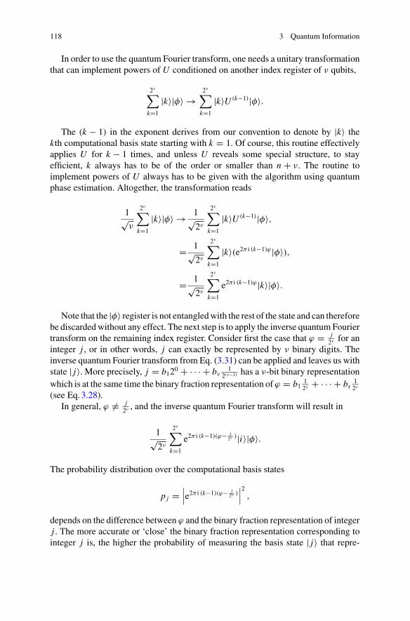
118 3 Quantum Information

In order to use the quantum Fourier transform, one needs a unitary transformationthat can implement powers of U conditioned on another index register of ν qubits,

2ν

∑

k=1

|k〉|φ〉 →2ν

∑

k=1

|k〉U (k−1)|φ〉.

The (k − 1) in the exponent derives from our convention to denote by |k〉 thekth computational basis state starting with k = 1. Of course, this routine effectivelyapplies U for k − 1 times, and unless U reveals some special structure, to stayefficient, k always has to be of the order or smaller than n + ν. The routine toimplement powers of U always has to be given with the algorithm using quantumphase estimation. Altogether, the transformation reads

1√ν

2ν

∑

k=1

|k〉|φ〉 → 1√2ν

2ν

∑

k=1

|k〉U (k−1)|φ〉,

= 1√2ν

2ν

∑

k=1

|k〉(e2π i (k−1)ϕ|φ〉),

= 1√2ν

2ν

∑

k=1

e2π i (k−1)ϕ|k〉|φ〉.

Note that the |φ〉 register is not entangledwith the rest of the state and can thereforebe discarded without any effect. The next step is to apply the inverse quantum Fouriertransform on the remaining index register. Consider first the case that ϕ = j

2ν for aninteger j , or in other words, j can exactly be represented by ν binary digits. Theinverse quantum Fourier transform from Eq. (3.31) can be applied and leaves us withstate | j〉. More precisely, j = b120 + · · · + bν

12(ν−1) has a ν-bit binary representation

which is at the same time the binary fraction representation of ϕ = b1121 + · · · + bs

12ν

(see Eq.3.28).In general, ϕ �= j

2ν , and the inverse quantum Fourier transform will result in

1√2ν

2ν

∑

k=1

e2π i (k−1)(ϕ− j2ν )|i〉|φ〉.

The probability distribution over the computational basis states

p j =∣∣∣e2π i (k−1)(ϕ− j

2ν )∣∣∣2,

depends on the difference between ϕ and the binary fraction representation of integerj . The more accurate or ‘close’ the binary fraction representation corresponding tointeger j is, the higher the probability of measuring the basis state | j〉 that repre-

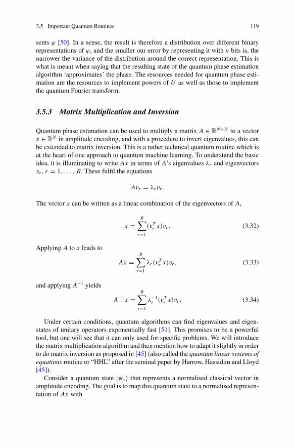
3.5 Important Quantum Routines 119

sents ϕ [50]. In a sense, the result is therefore a distribution over different binaryrepresentations of ϕ, and the smaller our error by representing it with n bits is, thenarrower the variance of the distribution around the correct representation. This iswhat is meant when saying that the resulting state of the quantum phase estimationalgorithm ‘approximates’ the phase. The resources needed for quantum phase esti-mation are the resources to implement powers of U as well as those to implementthe quantum Fourier transform.

3.5.3 Matrix Multiplication and Inversion

Quantum phase estimation can be used to multiply a matrix A ∈ RN×N to a vector

x ∈ RN in amplitude encoding, and with a procedure to invert eigenvalues, this can

be extended to matrix inversion. This is a rather technical quantum routine which isat the heart of one approach to quantum machine learning. To understand the basicidea, it is illuminating to write Ax in terms of A’s eigenvalues λr and eigenvectorsvr , r = 1, . . . , R. These fulfil the equations

Avr = λrvr .

The vector x can be written as a linear combination of the eigenvectors of A,

x =R∑

r=1

(vTr x)vr . (3.32)

Applying A to x leads to

Ax =R∑

r=1

λr (vTr x)vr . (3.33)

and applying A−1 yields

A−1x =R∑

r=1

λ−1r (vT

r x)vr . (3.34)

Under certain conditions, quantum algorithms can find eigenvalues and eigen-states of unitary operators exponentially fast [51]. This promises to be a powerfultool, but one will see that it can only used for specific problems. We will introducethe matrix multiplication algorithm and thenmention how to adapt it slightly in orderto do matrix inversion as proposed in [45] (also called the quantum linear systems ofequations routine or “HHL” after the seminal paper by Harrow, Hassidim and Lloyd[45]).

Consider a quantum state |ψx 〉 that represents a normalised classical vector inamplitude encoding. The goal is to map this quantum state to a normalised represen-tation of Ax with

120 3 Quantum Information

|ψx 〉 =R∑

r=1

〈ψvr |ψx 〉|ψvr 〉 → |ψAx 〉 =R∑

r=1

λr 〈ψvr |ψx 〉|ψvr 〉.

This can be done in three steps. First, create a unitary operatorU = e2π i HA whichencodes A in Hamiltonian encoding, and apply it to |ψx 〉. Second, execute the phaseestimation procedure to write the eigenvalues of A into a register in basis encoding.Third, use a small subroutine to translate the eigenvalues from basis encoding intoamplitude encoding.

1. Simulating AIn the first step, we need a unitary operator U whose eigenvalue equations are givenbyU |ψvr 〉 = e2π iλr |ψvr 〉. If one can evolve a systemwith aHamiltonian HA encodingthe matrix A, the operatorU is given by e2π i HA . To resemble a Hamiltonian, A has tobe Hermitian, but the trick from Eq. (3.29) circumvents this requirement by doublingthe Hilbert with one additional qubit. Techniques to implement general H are calledHamiltonian simulation and are discussed in Sect. 5.4.

The first step prepares a quantum state of the form

1√K

K∑

k=1

|k〉e−2π i(k−1)HA |ψx 〉 = 1√K

K∑

k=1

|k〉R∑

r=1

e2π i(k−1)λr 〈ψvr |ψx 〉|ψvr 〉,

where on the right side, |ψx 〉 was simply expressed in A’s basis as defined in Eq.(3.32), and K = 2ν where ν is again the number of qubits in the index register. Thisis a slight simplification of the original proposal, in which for example the indexregister |k〉 is not in a uniform superposition to exploit some further advantages, butthe principle remains the same.

2. Extracting the eigenvaluesIn the second step, the quantum phase estimation routine is applied to the indexregister |k〉 to ‘reduce’ its superposition to basis states encoding the eigenvalues,

1√K

R∑

r=1

K∑

k=1

αk|r 〈ψvr |ψx 〉|k〉|ψvr 〉. (3.35)

As explained for the quantum phase estimation routine, the coefficients lead toa large probability |αk|r |2 for computational basis states |k〉 that approximate theeigenvalues λr well. If enough qubits ν are given in the |k〉 register, one can assumethat (3.35) is approximately

R∑

r=1

〈ψvr |ψx 〉|λr 〉|ψvr 〉,

where |λr 〉 basis encodes a ν qubit approximation of λr . The time needed to imple-ment this step with an error ε in the final state is in O( 1

ε) [45].

3.5 Important Quantum Routines 121

3. Adjusting the amplitudesThe third step ‘writes’ the eigenvalues into the amplitudes by using a technique wewill present in more detail in Sect. 5.2.2.3. The idea is to apply a sequence of gateswhich rotates an additional ancilla qubit as

R∑

r=1

〈ψvr |ψx 〉|λr 〉|ψvr 〉|0〉 →R∑

r=1

〈ψvr |ψx 〉|λr 〉|ψvr 〉(√1 − λ2

r |0〉 + λr |1〉).

We then do apostselectivemeasurement, whichmeans that the ancilla ismeasured,and the algorithm only continues if we measure it in state |1〉. We will call thisprocedure branch selection. This makes sure we have the state

R∑

r=1

λr 〈ψvr |ψx 〉|λr 〉|ψvr 〉|0〉 →R∑

r=1

λr 〈ψvr |ψx 〉|ψvr 〉,

where on the right side the eigenvalue register was ‘uncomputed’ with an inversequantum phase estimation algorithm, and the ancilla discarded. Note that this is onlypossible because no terms in the sum interfere as a result (one could say that thesuperposition is ‘kept intact’ by the |ψvr 〉 state). The final state |ψAx 〉 corresponds toa normalised version of Ax in amplitude encoding.

Formatrix inversion, the last step is slightly adjusted:When conditionally rotatingthe ancilla qubit, one writes the inverse of the eigenvalue 1

λrinto the respective

amplitude. Since there is no guarantee that these are smaller than 1, a normalisationconstant C has to be introduced that is of the order of the smallest eigenvalue, andthe conditional measurement yields up to normalisation factors

R∑

r=1

〈ψvr |ψx 〉|λr 〉|ψvr 〉(√

1 − C2

λ2r

|0〉 + C

λr|1〉) → C

R∑

r=1

1

λr〈ψvr |ψx 〉|ψvr 〉.

The conditionalmeasurement is a non-unitary operation and requires the routine tobe repeated on averageO( 1

pacc) times until it succeeds. For matrix multiplication, the

acceptance probability is given by pacc = ∑r |〈ψvr |ψx 〉|2λ2

r while for the inversiontechnique pacc = ∑

r |〈ψvr |ψx 〉|2 C2

λ2r

≤ κ−2, where κ is the condition number of thematrix defined as the ratio of the largest and the smallest eigenvalue. The conditionnumber is a measure of how ‘invertible’ or ‘singular’ a matrix is. Just like whenconsidering numerical stability in classical inversion techniques, when the conditionnumber is large, the quantum algorithm takes a long time to succeed on average. Thiscan sometimes be circumvented with so called preconditioning techniques [52].

Example 3.8 (Simulation of the quantum matrix inversion routine) Since the matrixinversion routine is rather technical, this example shall illuminate howaquantumstategets successively manipulated by the routine. The matrix A and vector b consideredhere are given by

122 3 Quantum Information

A =( 2

313

13

23

)

, b =(0.2750.966

)

.

The eigenvalues of A are λ1 = 1 and λ2 = 1/3, with the corresponding eigen-vectors v1 = (1/

√2, 1/

√2)T and v2 = (−1/

√2, 1/

√2)T . The number of qubits

for the eigenvalue register is chosen as τ = 10, and the binary representation ofthe eigenvalues then becomes λ1 = 1111111111 and λ2 = 0101010101. The errorof this representation is < 0.001. The constant C is chosen to be half the smallesteigenvalue, C = 0.5λmin = 1

6 .The qubits are divided into three registers: The first qubit is the ancilla used for

the postselection, the following ten qubits form the eigenvalue register, and the lastqubit initially encodes the vector b, while after the routine it will encode the solutionx .

Encoding b into the last qubit yields

|ψ〉 = 0.275|0 0000000000 0〉 + 0.966|0 0000000000 1〉.

After simulating A and writing the eigenvalues into the second register via phaseestimation in Step 2 we get

|ψ〉 = − 0.343|0 0101010101 0〉+ 0.343|0 0101010101 1〉+ 0.618|0 1111111111 0〉+ 0.618|0 1111111111 1〉.

Rotating the ancilla conditioned on the eigenvalue register leads to

|ψ〉 = − 0.297|0 0101010101 0〉+ 0.297|0 0101010101 1〉+ 0.609|0 1111111111 0〉+ 0.609|0 1111111111 1〉− 0.172|1 0101010101 0〉+ 0.172|1 0101010101 1〉+ 0.103|1 1111111111 0〉+ 0.103|1 1111111111 1〉,

and uncomputing (reversing the computation) in the eigenvalue register prepares thestate

3.5 Important Quantum Routines 123

|ψ〉 = 0.312|0 0000000000 0〉+ 0.907|0 0000000000 1〉− 0.069|1 0000000000 0〉+ 0.275|1 0000000000 1〉

After a successful conditional measurement of the ancilla in 1 we get

|ψ〉 = −0.242|1 0000000000 0〉 + 0.970|1 0000000000 1〉.

The probability of success is given by

p(1) = (−0.069)2 + 0.2752 = 0.080.

The amplitudes now encode the result of the computation, A−1b, as a normalisedvector. The final, renormalised result of the quantum algorithm can be extractedby taking the last amplitude vector (−0.242, 0.970)T and multiplying it with therenormalisation factor C/

√p(1) = 0.588. Note that we can estimate p(1) from the

conditional measurement of the algorithm, andC is our choice, so that the ‘classical’renormalisation can always be accomplished if needed. In applications we wouldbe interested in extracting some compact information from the final quantum state,rather than measuring each amplitude.

The result after renormalisation is x = (−0.412, 1.648)T . A quick calculation byhand or using a linear algebra library confirms that this is the correct outcome up toan error from the finite bit precision used in the calculation.

The Dirac notation shows beautifully how the routine starts with a small super-position (here of only two basis states) that gets ‘blown up’ and then again reducedto encode the two-dimensional output.

References

1. Dirac, P.A.M.: The Principles of Quantum Mechanics. Clarendon Press (1958)2. Gerthsen, K., Vogel, H.: Physik. Springer (2013)3. Aaronson, S.: Quantum Computing Since Democritus. Cambridge University Press (2013)4. Leifer, M.S., Poulin, D.: Quantum graphical models and belief propagation. Ann. Phys. 323(8),

1899–1946 (2008)5. Landau, L., Lifshitz, E.: Quantummechanics: non-relativistic theory. In: Course of Theoretical

Physics, vol. 3. Butterworth-Heinemann (2005)6. Whitaker, A.: Einstein, Bohr and the Quantum Dilemma: From Quantum Theory to Quantum

Information. Cambridge University Press (2006)7. Einstein, A.: Über die von der molekularkinetischen Theorie der Wärme geforderte Bewegung

von in ruhenden Flüssigkeiten suspendierten Teilchen. Annalen der Physik 322(8), 549–560(1905)

8. Einstein, A.: Zur Elektrodynamik bewegter Körper. Annalen der Physik 322(10), 891–921(1905)

124 3 Quantum Information

9. Wilce, A.: Quantum logic and probability theory. In: Zalta, E.N. (ed.), The Stanford Encyclo-pedia of Philosophy. Online encyclopedia (2012). http://plato.stanford.edu/archives/fall2012/entries/qt-quantlog/

10. Rédei, M., Summers, S.J.: Quantum probability theory. Studies in Hist. Phil. Sci. Part B Stud.Hist. Phil. Modern Phys. 38(2), 390–417 (2007)

11. Breuer, H.-P., Petruccione, F.: The Theory of Open Quantum Systems. Oxford University Press(2002)

12. Denil, M., De Freitas, N.: Toward the implementation of a quantum RBM. In: NIPS 2011 DeepLearning and Unsupervised Feature Learning Workshop (2011)

13. Grover, L.K.: A fast quantum mechanical algorithm for database search. In: Proceedings ofthe Twenty-Eighth Annual ACM Symposium on Theory of Computing, pp. 212–219. ACM(1996)

14. Deutsch, D., Jozsa, R.: Rapid solution of problems by quantum computation. In: Proceedingsof the Royal Society of London A:Mathematical, Physical and Engineering Sciences, vol. 439,pp. 553–558. The Royal Society (1992)

15. Peter, W.: Shor. Polynomial-time algorithms for prime factorization and discrete logarithms ona quantum computer. SIAM J. Comput. 26(5), 1484–1509 (1997)

16. Deutsch,D.:Quantum theory, theChurch-Turingprinciple and the universal quantumcomputer.In: Proceedings of the Royal Society of London A: Mathematical, Physical and EngineeringSciences, vol. 400, pp. 97–117. The Royal Society (1985)

17. Nielsen, M.A., Chuang, I.L.: Quantum Computation and Quantum Information. CambridgeUniversity Press, Cambridge (2010)

18. Barenco, A., Bennett, C.H., Cleve, R., DiVincenzo, D.P., Margolus, N., Shor, P., Sleator, T.,Smolin, J.A., Weinfurter, H.: Elementary gates for quantum computation. Phys. Rev. A, 52(5),34–57 (1995)

19. Clarke, J.,Wilhelm, F.K.: Superconducting quantumbits. Nature 453(7198), 1031–1042 (2008)20. Kok, P., Munro, W.J., Nemoto, K., Ralph, T.C., Dowling, J.P., Milburn, G.J.: Linear optical

quantum computing with photonic qubits. Rev. Modern Phys. 79(1), 135 (2007)21. Juan, I.: Cirac and Peter Zoller. Quantum computations with cold trapped ions. Phys. Rev. Lett.

74(20), 4091 (1995)22. Nayak, C., Simon, S.H., Stern, A., Freedman, M., Sarma, S.D.: Non-Abelian anyons and

topological quantum computation. Rev. Modern Phys. 80(3), 1083 (2008)23. Farhi, E., Goldstone, J., Gutmann, S., Sipser, M.: Quantum computation by adiabatic evolution

(2000). arXiv:quant-ph/0001106, MIT-CTP-293624. Das, A., Chakrabarti, B.K.: Colloquium: quantum annealing and analog quantum computation.

Rev. Modern Phys. 80(3), 1061 (2008)25. Neven, H., Denchev, V.S., Rose, G., Macready, W.G.: Training a large scale classifier with the

quantum adiabatic algorithm. arXiv:0912.0779 (2009)26. Heim, B., Rønnow, T.F., Isakov, S.V., Troyer, M.: Quantum versus classical annealing of Ising

spin glasses. Science 348(6231), 215–217 (2015)27. Santoro, G.E., Tosatti, E.: Optimization using quantummechanics: quantum annealing through

adiabatic evolution. J. Phys. A 39(36), R393 (2006)28. Briegel, H.J., Raussendorf, R.: Persistent entanglement in arrays of interacting particles. Phys.

Rev. Lett. 86(5), 910 (2001)29. Nielsen,M.A.: Cluster-state quantum computation. ReportsMath. Phys. 57(1), 147–161 (2006)30. Prevedel, R., Stefanov, A., Walther, P., Zeilinger, A.: Experimental realization of a quantum

game on a one-way quantum computer. New J. Phys. 9(6), 205 (2007)31. Park, H.S., Cho, J., Kang, Y., Lee, J.Y., Kim, H., Lee, D.-H., Choi, S.-K.: Experimental real-

ization of a four-photon seven-qubit graph state for one-way quantum computation. Opt. Exp.20(7), 6915–6926 (2012)

32. Tame, M.S., Prevedel, R., Paternostro, M., Böhi, P., Kim, M.S., Zeilinger, A.: Experimentalrealization of Deutsch’s algorithm in a one-way quantum computer. Phys. Rev. Lett. 98, 140–501 (2007)

References 125

33. Tame, M.S., Bell, B.A., Di Franco, C., Wadsworth, W.J., Rarity, J.G.: Experimental realizationof a one-way quantum computer algorithm solving Simon’s problem. Phys. Rev. Lett. 113,200–501 (2014)

34. Lloyd, S., Braunstein, S.L.: Quantum computation over continuous variables. In: QuantumInformation with Continuous Variables, pp. 9–17. Springer (1999)

35. Weedbrook, C., Pirandola, S., García-Patrón, R., Cerf, N.J., Ralph, T.C., Shapiro, J.H., Lloyd,S.: Gaussian quantum information. Rev. Modern Phys. 84(2), 621 (2012)

36. Lau, H.-K., Pooser, R., Siopsis, G., Weedbrook, C.: Quantum machine learning over infinitedimensions. Phys. Rev. Lett. 118(8), 080501 (2017)

37. Chatterjee, R., Ting, Y.: Generalized coherent states, reproducing kernels, and quantum supportvector machines. Quant. Inf. Commun. 17(15, 16), 1292 (2017)

38. Schuld, M., Killoran, N.: Quantum machine learning in feature Hilbert spaces.arXiv:1803.07128v1 (2018)

39. Gisin, N.:Weinberg’s non-linear quantummechanics and supraluminal communications. Phys.Lett. A 143(1), 1–2 (1990)

40. Polchinski, J.: Weinberg’s nonlinear quantum mechanics and the Einstein-Podolsky-Rosenparadox. Phys. Rev. Lett. 66, 397–400 (1991)

41. Daniel, S.: Abrams and Seth Lloyd. Nonlinear quantum mechanics implies polynomial-timesolution for NP-complete and #P problems. Phys. Rev. Lett. 81(18), 39–92 (1998)

42. Peres, A.: Nonlinear variants of Schrödinger’s equation violate the second law of thermody-namics. Phys. Rev. Lett. 63(10), 1114 (1989)

43. Yoder, T.L., Low, G.H., Chuang, I.L.: Quantum inference on Bayesian networks. Phys. Rev. A89, 062315 (2014)

44. Ozols,M.,Roetteler,M.,Roland, J.:Quantum rejection sampling.ACMTrans.Comput. Theory(TOCT) 5(3), 11 (2013)

45. Aram, W., Harrow, A.H., Lloyd, S.: Quantum algorithm for linear systems of equations. Phys.Rev. Lett. 103(15), 150–502 (2009)

46. Boyer, M., Brassard, G., Høyer, P., Tapp, A.: Tight bounds on quantum searching. Fortsch.Phys. 46, 493–506 (1998)

47. Ambainis, A.: Quantum lower bounds by quantum arguments. In: Proceedings of the Thirty-Second Annual ACM Symposium on Theory of Computing, pp. 636–643. ACM (2000)

48. Biham, E., Biham, O., Biron, D., Grassl, M., Lidar, D.A.: Grovers quantum search algorithmfor an arbitrary initial amplitude distribution. Phys. Rev. A 60(4), 27–42 (1999)

49. Brassard, G., Høyer, P.,Mosca,M., Tapp, A.: Quantum amplitude amplification and estimation.Contemp. Math. 305, 53–74 (2000)

50. Watrous, J.: Theory of Quantum Information. Cambridge University Press (2018)51. Abrams, D.S., Lloyd, S.: Quantum algorithm providing exponential speed increase for finding

eigenvalues and eigenvectors. Phys. Rev. Lett. 83(24), 51–62 (1999)52. Clader, D.B., Jacobs, B.C., Sprouse, C.R.: Preconditioned quantum linear system algorithm.

Phys. Rev. Lett. 110(25), 250–504 (2013)

Chapter 4Quantum Advantages

Before coming to the design of quantummachine learning algorithms, this chapter isan interlude to discuss how quantum computing can actually assist machine learning.Although quantum computing researchers often focus on asymptotic computationalspeedups, there ismore than onemeasure ofmerit when it comes tomachine learning.We will discuss three dimensions here, namely the computational complexity, thesample complexity and the model complexity.1 While the section on computationalcomplexity allows us to establish the terminology already used in previous chapter-s with more care, the section on sample complexity ventures briefly into quantumextensions of statistical learning theory. The last section on model complexity pro-vides arguments towards what has been called the exploratory approach to quantummachine learning, in which quantum physics is used as a resource to build new typesof models altogether.

4.1 Computational Complexity of Learning

The concept of runtime complexity and speedups has already been used in the pre-vious sections and is the most common figure of merit when accessing potentialcontributions of quantum computing to machine learning. Quantum machine learn-ing inherited this focus on runtime speedups from quantum computing, where—forlack of practical experiments—researchers mostly resort to proving theoretical run-time bounds to advertise the power of their algorithms. Let us briefly introduce thebasics of asymptotic computational complexity.

The runtime of an algorithm on a computer is the time it takes to execute thealgorithm, in other words, the number of elementary operations multiplied by theirrespective execution times. In conventional computers, the number of elementary

1The three dimensions were first introduced by Peter Wittek and Vedran Dunjko.

© Springer Nature Switzerland AG 2018M. Schuld and F. Petruccione, Supervised Learning with Quantum Computers,Quantum Science and Technology, https://doi.org/10.1007/978-3-319-96424-9_4

127

128 4 Quantum Advantages

operations could in theory still be established by choosing the fastest implementationsfor every subroutine and count the logic gates. However, with fast technologicaladvancements in the IT industry it becomes obvious that a device-dependent runtimeis not a suitable theoretical tool to measure the general speed of an algorithm. Thisis why computational complexity theory looks at the asymptotic complexity or therate of growth of the runtime with the size n of the input. “Asymptotic” therebyrefers to the fact that one is interested in laws for sufficiently large inputs only. If theresources needed to execute an algorithm or the number of elementary operationsgrow polynomially (that is, not more than a factor nc for a constant c) with the size ofthe input n, it is tractable and the problem in theory efficiently solvable. Of course, if cis large, even polynomial runtime algorithms can take too long to make them feasiblefor certain applications. The argument is that if we just wait a reasonable amount oftime, our technology could in principle master the task. Exponential growth makesan algorithm intractable and the problem hard because for large enough problemsizes, it quickly becomes impossible to solve the problem.

An illustrative example for an intractable problem is guessing the number com-bination for the security code of a safe, which without further structure requires abrute force search: While a code of two digits only requires 100 attempts in theworst case (and half of those guesses in the average case), a code of n = 10 digitsrequires ten billion guesses in the worst case, and a code of n = 30 digits has morepossible configurations than our estimation for the number of stars in the universe.No advancement in computer technology could possibly crack this code.

When thinking about quantum computers, estimating the actual runtime of analgorithm is even more problematic. Not only do we not have a unique implemen-tation of qubits yet that gives us a set of elementary operations to work with, buteven if we agreed on a set of elementary gates as well as a technology, it is nontrivialto decompose quantum algorithms into this set. In many cases, we can claim thatwe know there is such a sequence of elementary gates, but it is by no means clearhow to construct it. The vast majority of authors in quantum information processingare therefore interested in the asymptotic complexity of their routines, and how theycompare to classical algorithms. In a qubit-based quantum computer, the input isconsidered to be the number of qubits n, which we already hinted at by the notation.To avoid confusion when looking at different concepts for the input, we will callpolynomial algorithms regarding the number of qubits qubit-efficient. Algorithmswhich are efficient with respect to the number of amplitudes (see for example Groversearch 3.5.1) will be referred to as amplitude-efficient.

The field of quantum complexity theory has been developed as an extension toclassical complexity theory [1, 2] and is based on the question whether quantumcomputers are in principle able to solve computational problems faster in relationto the runtime complexity. In the following, complexity will always refer to theasymptotic runtime complexity unless stated otherwise. A runtime advantage in thiscontext is called a quantum enhancement, quantum advantage, or simply a quantumspeedup. Demonstrating an exponential speedup has been controversially referred toas quantum supremacy.

4.1 Computational Complexity of Learning 129

A collaboration of researchers at the forefront of benchmarking quantum com-puters came up with a useful typology for the term of ‘quantum speedup’ [3] whichshows the nuances of the term:

1. A provable quantum speedup requires a proof that there can be no classicalalgorithm that performs as well or better than the quantum algorithm. Such aprovable speedup has been demonstrated for Grover’s algorithm, which scalesquadratically better than classical [4] given that there is an oracle to mark thedesired state [5].

2. A strong quantum speedup compares the quantum algorithmwith the best knownclassical algorithm. The most famous example of a strong speedup is Shor’squantum algorithm to factorise prime numbers in time growing polynomially(instead of exponentially) with the number of digits of the prime number, whichdue to far-reaching consequences for cryptography systems gave rise to the firstmajor investments into quantum computing.

3. If we relax the term ‘best classical algorithm’ (which is often not known) to the‘best available classical algorithm’ we get the definition of a common quantumspeedup.

4. The fourth category of potential quantum speedup relaxes the conditions furtherby comparing two specific algorithms and relating the speedup to this instanceonly.

5. Lastly, and useful when doing benchmarking with quantum annealers, is thelimited quantum speedup that compares to “corresponding” algorithms such asquantum and classical annealing.

Although the holy grail of quantum computing remains to find a provable ex-ponential speedup, the wider definition of a quantum advantage in terms of theasymptotic complexity opens a lot more avenues for realistic investigations. Twocommon pitfalls have to be avoided. Firstly, quantum algorithms often have to becompared with classical sampling, which is likewise non-deterministic and has closerelations to quantum computing. Secondly, complexity can easily be hidden in spa-tial resources, and one could argue that quantum computers have to be compared tocluster computing, which will surely be its main competitor in years to come [3, 6].

We want to introduce some particulars of how to formulate the asymptotic com-plexity of a (quantum) machine learning algorithm. The ‘size’ of the input in thecontext of machine learning usually refers to the number of data points M as well asthe number of features N . Since this differs from what the quantum computing com-munity considers as an input, we will call algorithms that are efficient with regardsto the data “data-efficient”. When dealing with sparse inputs that can be representedmore compactly, the number of features is replaced by the maximum number s ofnonzero elements in any training input. Complexity analysis commonly considersother numbers of merit. The error ε of a mathematical object z is the precision towhich z′ calculated by the algorithm is correct, ε = ||z − z′|| (with a suitable norm).When dealing with matrices, the condition number κ , which is the ratio of the largestand the smallest eigenvalue or singular value, is sometimes of interest to find anupper bound for the runtime (since κ gives us an idea of the eigenvalue spectrum of

130 4 Quantum Advantages

Fig. 4.1 Illustration of the big-O notation. If a function f (x) (in this context f is the runtime andx the input) is ‘in’O(g(x)), there exists a λ ∈ R such that | f (x)| ≤ λg(x) for large enough x . TheΩ symbol stands for the inequality | f (x)| ≥ λg(x), while theΘ symbol signifies that there are twoλ1 < λ2 ∈ R such that f (x) lies between the functions λ1g(x) and λ2g(x)

the matrix). Many quantum machine learning algorithms have a chance of failure,for example because of a conditional measurement. In this case the average numberof attempts required to execute it successfully needs to be taken into account as well.A success probability of ps generally leads to a factor of 1/ps in the runtime. Forexample, if the algorithm will only succeed in 1% of the cases, one has to repeat iton average for 100 times to encounter a successful run.

To express the asymptotic complexity, the runtime’s dependency on these vari-ables is given in the"big-O" notation (see Fig. 4.1):

• O(g(x)) means that the true runtime f has an upper bound of λg(x) for someλ ∈ R, a function g and the variable x .

• Ω(g(x)) means that the runtime has a lower bound of λg(x) for some λ ∈ R.• Θ(g(x)) means that the run time has a lower bound of λ1g(x) and an upper boundof λ2g(x) for some λ1, λ2 ∈ R.

Having introduced time complexity, the question remains what speedups can bedetected specifically in quantum machine learning. Of course, machine learning isbased on common computational routines such as search or matrix inversion, andquantum machine learning derives its advantages from tools developed by the quan-tum information processing community. It is therefore no surprise that the speedupsachieved in quantum machine learning are directly derived from the speedups inquantum computing. Roughly speaking (and with more details in the next chapters),three different types of speedups can be claimed:

1. Provable quadratic quantum speedups arise from variations of Grover’s algorith-m or quantum walks applied to search problems. Note that learning can alwaysbe understood as a search in a space of hypotheses [7].

2. Exponential speedups are naturally more tricky, even if we only look at thecategories of either strong or common speedups. Within the discipline, theyare usually only claimed by quantum machine learning algorithms that executelinear algebra computations in amplitude encoding. But these come with seriousconditions, for example about the sparsity or redundancy in the dataset.

4.1 Computational Complexity of Learning 131

3. More specific comparisons occur when quantum annealing is used to solve op-timisation problems derived from machine learning tasks [8], or to prepare aquantum system in a certain distribution [9]. It is not clear yet whether any prov-able speedups will occur, but benchmarking against specific classical algorithmsshow that there are problems where quantum annealing can be of advantage forsampling problems.

Altogether, computational complexity is of course important formachine learning,since it defines what is practically possible. However, limiting the focus only on thisaspect severely and unnecessarily limits the scope of quantum machine learning.Very often, provably hard problems in machine learning can be solved for relevantspecial cases, sometimes without even a solid theoretical understanding why this isso. It is therefore important to look for other aspects in which quantum computingcould contribute to machine learning.

4.2 Sample Complexity

Besides the asymptotic computational complexity, the so called sample complexityis an important figure of merit in classical machine learning, and offers a wealth oftheoretical results regarding the subject of learning, summarised under the keywordstatistical learning theory [10]. It also offers a door to explore more fundamentalquestions of quantum machine learning, for example what it means to learn in aquantum setting, or how we can formulate a quantum learning theory [11]. Althoughsuch questions are not the focus of this book, we use this opportunity for a smallexcursion into the more theoretical branch of quantum machine learning.

loosensee 1 Sample complexity refers to the number of samples needed to gen-eralise from data. Samples can either be given as training instances drawn from acertain distribution (examples) or by computing outputs to specifically chosen inputs(queries). For the supervised pattern recognition problem we analysed so far, thedataset is given as examples and no queries can be made. One can easily imaginea slightly different setting where queries are possible, for example when a certainexperiment results in input-output pairs, and we can choose the settings for the ex-periment to generate the data.

Considerations about sample complexity are usually based on binary functionsf : {0, 1}N → {0, 1}. The sample complexity of a machine learning algorithm refersto the number of samples that are required to learn a concept from a given conceptclass. A concept is the rule f that divides the input space into subsets of the two classlabels 0 and 1, in other words, it is the law that we want to recover with a model.

There are two important settings in which sample complexity is analysed.

1. In exact learning from membership queries [12], one learns the function f byquerying a membership oracle with inputs x and receives the answer whetherf (x) evaluates to 1 or not.

132 4 Quantum Advantages

membershiporacle

quantummembership

oracle

exampleoracle

quantumexampleoracle

x

f(x) f(x); x ∼ p(x)

|x, 0〉

|x, f(x)〉

|0...0〉

∑

x

√p(x)|x, f(x)〉

Fig. 4.2 Different types of oracles to determine the sample complexity of a learning algorithm. Amembership oracle takes queries for a certain input x and returns the class f (x), while an exampleoracle is activated and draws samples of x from a certain (usually unknown) distribution p(x),returning the class of x . The quantum version of a membership oracle is a function evaluation on aregister |x, 0〉, while a quantum example oracle has been defined as the qsample of the distributionp(x)

2. The framework of Probably Approximately Correct (PAC) learning was intro-duced by Valiant [13] and asks how many examples from the original conceptare needed in the worst case to train a model so that the probability of an errorε (i.e., the probability of assigning the wrong label) is smaller than 1 − δ for0 ≤ δ ≤ 1. The examples are drawn from an arbitrary distribution via an exam-ple oracle. This framework is closely related to the Vapnik-Chervonenkis- orVC-dimension of a model (see Sect. 4.3).

To translate these two settings into a quantum framework (see Fig. 4.2), a quantummembership oracle as well as a quantum example oracle are introduced. They are ina sense parallelised versions of the classical sample generators, and with quantuminterference of amplitudes we can hope to extract more information from the dis-tribution than possible in the classical case. Rather surprisingly, it turns out that theclassical and quantum sample complexity are polynomially equivalent, or as statedby Servedio and Gortler [14]:

[F]or any learning problem, if there is a quantum learning algorithm which uses polyno-mially many [samples] then there must also exist a classical learning algorithm which usespolynomially many [samples].

Note that this only concerns the sample complexity; the same authors find an in-stance for a problem that is efficiently learnable by a quantum algorithm in terms ofcomputational complexity, while the best classical algorithm is intractable.

4.2 Sample Complexity 133

4.2.1 Exact Learning from Membership Queries

Sample complexity in relation to queries is closely related to the concept of ‘quantumquery complexity’ which is an important figure of merit in quantum computing inthe oracular setting (for example to determine the runtime of Grover’s algorithm). Aquantum oracle can be described as a unitary operation

U : |x, 0〉 → |x, 0 ⊕ f (x)〉,

where x ∈ {0, 1}n is encoded in the computational basis.Two famous quantum algorithms that demonstrate how for specific types of prob-

lems only a single quantum query can be sufficient, are the Deutsch-Josza algorithm(see Sect. 3.3.1) as well as the famous Bernstein-Vazirani algorithm [1] that we didnot discuss here. They are both based on the principle of applying the quantum oracleto a register in uniform superposition, thereby querying all possible inputs in paral-lel. Writing the outcome into the phase and interfering the amplitudes then revealsinformation on the concept, for example if it was a balanced (half of all inputs mapto 1) or constant (all inputs map to 1) function. Note that this does not mean thatthe function itself is learnt (i.e., which inputs of the balanced function map to 0 or1 respectively) and is therefore not sufficient as an example to prove theorems ongeneral quantum learnability.

In 2003, Hunziker et al. [15] introduced a larger framework which they call “im-patient learning” and proposed the following two conjectures on the actual numberof samples required in the (asymptotic) quantum setting:Conjecture 1: For any family of concept classesC = {Ci }with |C | → ∞, there existsa quantum learning algorithm with membership oracle query complexity O(

√|C |).Conjecture 2: For any family of concept classes C = {Ci } containing |C | → ∞concepts, there exists a quantum learning algorithm with membership oracle querycomplexity O(

log |C |√γ

), where γ ≤ 1/3 is a measure of how easy it is to distinguishbetween concepts, and small γ indicate a harder class to learn.

While the first conjecture was proven by Ambainis et al. [16], the second conjec-ture was resolved in a series of contributions [14, 17, 18]. The classical upper boundfor exact learning from membership queries is given by O(

log |C |γ

).Servedio and Gortler [14] compared these results and found that if any class C

of boolean functions f : {0, 1}n → {0, 1} is learnable from Q quantum member-ship queries, it is then learnable by at most O(nQ3) classical membership queries.This result shows that classical and quantum learnability have at most a polynomialoverhead. It becomes apparent that no exponential speedup can be expected fromquantum sample complexity for exact learning with membership queries.

134 4 Quantum Advantages

4.2.2 PAC Learning from Examples

It is a well-established fact from classical learning theory that a (ε, δ)-PAC learningalgorithm for a non-trivial concept class C of Vapnik-Chervonenkis-dimension drequires at least Ω( 1

εlog 1

δ+ d

ε) examples, but can be learnt with at most O( 1

εlog 1

δ

+ dεlog 1

ε) examples [19, 20].

A first contribution to quantum PAC learning was made by Bshouty and Jack-son in 1998 [21], who define the important notion of a quantum example oracle.The quantum example oracle is equivalent to what has been introduced earlier as aqsample, ∑

i

√p(x)|x, f (x)〉, (4.1)

where the probabilities of measuring the basis states in the computational basis re-flects the distribution p(x) from which the examples are drawn. They show that acertain class of functions (so called “polynomial-size disjunctive normal formexpres-sions” which are actively investigated in the PAC literature) are efficiently learnableby a quantum computer from ‘quantum example oracles’ which draw examples froma uniform distribution. This speedup is achieved by interfering the amplitudes of theqsamplewith a quantumFourier transform.2 However, the PACmodel requires learn-ability under any distribution, and the results of Bshouty and Jackson do thereforenot lead to a statement about the general quantum PAC case.

Servedio and Gortler [14] use the definition of a quantum example oracle fromEq. (4.1) to show that the equivalence of classical and quantum learning extends tothe PAC framework. They prove that if any class C of boolean functions f {0, 1}n →{0, 1} is learnable from Q evaluations of the quantum example oracle, it is thenlearnable by O(nQ) classical examples. Improvements in a later paper by Aticiand Servedio [17] prove a lower bound on quantum learning that is close to theclassical setting, i.e. that any (ε, δ)-PAC learning algorithm for a concept class ofVapnik-Chervonenkis-dimension d must make at least Ω( 1

εlog 1

δ+ d +

√d

ε) calls

to the quantum example oracle from Eq. (4.1). This was again improved by [22] tofinally show that in the PAC setting, quantum and classical learners require the sameamount of examples up to a constant factor. This also holds true for the agnosticlearning framework, which loosens PAC learning by looking for a hypothesis that issufficiently close to the best one [11].

As a summary, under the quantum formulation of classical learning theory basedon the oracles from Fig. 4.2, we are not expecting any exponential advantages fromquantum computing.

2Applying a quantum Fourier transform effectively changes the distribution from which to sample,which leaves some question whether the comparison to a static ‘classical example generator’ is fair.However, they show that while the quantum example oracle can be simulated by a membershipquery oracle, this is not true vice versa. It seems therefore that the quantum example oracle rangessomewhere between a query and an example oracle.

4.2 Sample Complexity 135

4.2.3 Introducing Noise

Even though the evidence suggests that classical and quantum sample complexityare similar up to at most polynomial factors, an interesting observation derives fromthe introduction of noise into the model. Noise refers to corrupted query results orexamples for which the value f (x) is flipped with probability μ. For the quantumexample oracle, noise is introduced by replacing the oracle with a mixture of theoriginal qsample and a corrupted qsample weighted by μ. In the PAC setting witha uniform distribution investigated by Bshouty and Jackson, the quantum algorithmcan still learn the function by consuming more examples, while noise is believedto render the classical problem unlearnable [21]. A similar observation is made byCross, Smith and Smolin [23], who consider the problem of learning n-bit parityfunctions by membership queries and examples, a task that is easy both classicallyand quantumly, and in the sample as well as time complexity sense. Parity functionsevaluate to 1 if the the input string contains an odd number of 1’s. However, Cross etal. find that in the presence of noise, the classical case becomes intractable while thequantum samples required only grow logarithmically. To ensure a fair comparison,the classical oracle is modelled as a dephased quantum channel of the membershiporacle and the quantum example oracle respectively. As a toy model the authorsconsider a slight adaptation of the Bernstein-Vazirani algorithm. These observationsmight be evidence enough that a fourth category of potential quantum advantages,the robustness against noise, could be a fruitful avenue for further research.

4.3 Model Complexity

Lastly, we will come to the third potential advantage that quantum computing couldoffer machine learning. The term ‘model complexity’ is a wide concept that refersto the flexibility, capacity, richness or expressive power of a model. For example,a model giving rise to linear decision boundaries is less flexible than a model withmore complex decision boundaries. A linear fit in regression is less flexible than ahigher-order polynomial. Roughly speaking, more complex model families offer alarger space of possible trained models and therefore have a better chance to fit thetraining data.

Of course, this does not mean that more flexible models have a higher generali-sation power. In fact, they are much more prone to overfitting, which is quantifiedby Vapnik’s famous upper bound for the generalisation error εgen. With probabilityof at least 1 − δ for some δ > 0 the bound is given by [24]

εgen ≤ εemp +√

1

M

(d

(log

(2M

d

)+ 1

)+ log

(4

δ

)). (4.2)

136 4 Quantum Advantages

The generalisation error is bounded from above by the ‘empirical error’ εemp on thetraining set, plus an expression that depends on the so called Vapnik-Chervonenkis-dimensiond. TheVC-dimensionof amodel is closely related to themodel complexityand is defined for binary models, f : X → {0, 1}. It refers to the maximum numberof data points M assigned to two classes for which a hypothesis or ‘trained version’of the model f (x; θ) makes no classification error, or shatters the data. For the nexthigher number of points M + 1 there is no dataset that can always be shattered, nomatter how the labels are assigned. For example, a linear decision boundary canshatter three data points, but there are label assignments for which it cannot separatefour data points. Inequality (4.2) states that we are interested in a low training erroras well as a low flexibility of the model, as previously remarked in Sect. 2.2.2 inthe context of overfitting and regularisation. This means that we are interested in the‘slimmest’ model possible that can still capture the pattern which has to be learnt.

To investigate how quantum models can help machine learning is very much inthe spirit of the ‘exploratory approach’ to quantum machine learning and will besubject of Chap. 8. By the term ‘quantum model’ we refer to a machine learningmodel that is derived from the dynamics of a quantum system and can thereforebe implemented using a quantum device. For example, we will discuss Hopfieldnetworks that are extended via the quantum Ising model, or a neural network whereone layer is computed by a quantum circuit.

Asking how quantummodels can offer advantages in terms of themodel complex-ity has two dimensions. On the theoretical side, an analysis of the VC-dimension ofquantummodels could reveal interesting comparisons to equivalent classes of classi-cal models. In the example above, one could compare a quantum and classical Hop-field network to find out what effect quantum extensions have on the VC-dimension.Given the challenge this poses already in classical machine learning, numerical s-tudies may be crucial in answering this question.

On the more practical side, quantum models could prove to be a useful ansatzto capture patterns in certain datasets. An approach to find a slim but powerfulmodel is to choose a model family which can express the natural dynamics of thesystem producing the data. For example, nonlinearities in the updating function ofrecurrent neural networks allow us to represent nonlinear dynamics of the real-worldsystems they try to recover. In probabilistic graphical models we assume that thesystem has inherent independence relations between variables. In short, an openquestion with regards to the model complexity is whether certain quantum modelsare better at capturing patterns and correlations in data, and if yes, which problemsare suitable for quantum computing. One seemingly obvious case for the use ofquantum models is when the system producing the data is a quantum system, whichhas been termed the QQ case in the introduction. Still, so far there are no studiesthat show how a quantum model is better in capturing quantum correlations. Wesee that the contribution of quantum computing to model complexity has manyoutstanding theoretical and practical research questions that the quantum machinelearning community is only beginning to explore.

References 137

References

1. Bernstein, E., Vazirani, U.: Quantum complexity theory. SIAM J. Comput. 26(5), 1411–1473(1997)

2. Watrous, J.: Quantum computational complexity. In: Encyclopedia of Complexity and SystemsScience, pp. 7174–7201. Springer (2009)

3. Rãnnow, T.F.,Wang, Z., Job, J., Boixo, S., Isakov, S.V.,Wecker, D., Martinis, J.M., Lidar, D.A.,Troyer, M.: Defining and detecting quantum speedup. Science 345, 420–424 (2014)

4. Grover, L.K.: A fast quantum mechanical algorithm for database search. In: Proceedings ofthe Twenty-Eighth Annual ACM Symposium on Theory of Computing, pp. 212–219. ACM(1996)

5. Bennett, C.H., Bernstein, E., Brassard, G., Vazirani, U.: Strengths and weaknesses of quantumcomputing. SIAM J. Comput. 26(5), 1510–1523 (1997)

6. Steiger, D.S., Troyer, M.: Racing in parallel: quantum versus classical. In: Bulletin of theAmerican Physical Society, vol. 61 (2016)

7. Sammut, C., Webb, G.I.: Encyclopedia of Machine Learning. Springer Science & BusinessMedia (2011)

8. Neven, H., Denchev, V.S., Rose, G., Macready, W.G.: Training a large scale classifier with thequantum adiabatic algorithm. arXiv:0912.0779 (2009)

9. Amin, M.H.: Searching for quantum speedup in quasistatic quantum annealers. Phys. Rev. A92(5), 1–6 (2015)

10. Vapnik, V.N., Vapnik, V.: Statistical learning theory, vol. 1. Wiley, New York (1998)11. Arunachalam, S., de Wolf, R.: Guest column: a survey of quantum learning theory. ACM

SIGACT News 48(2), 41–67 (2017)12. Angluin, D.: Queries and concept learning. Mach. Learn. 2(4), 319–342 (1988)13. Valiant, L.G.: A theory of the learnable. Commun. ACM 27(11), 1134–1142 (1984)14. Rocco, A.S., Gortler, S.J.: Equivalences and separations between quantum and classical learn-

ability. SIAM J. Comput. 33(5), 1067–1092 (2004)15. Hunziker,M.,Meyer,D.A., Park, J., Pommersheim, J., Rothstein,M.: The geometry of quantum

learning. Quant. Inf. Process. 9(3), 321–341 (2010)16. Ambainis, A., Iwama, K., Kawachi, A., Masuda, H., Putra, R.H., Yamashita, S.: Quantum

identification of Boolean oracles. In: Annual Symposium on Theoretical Aspects of ComputerScience, pp. 105–116. Springer (2004)

17. Atici, A., Servedio, R.A.: Improved bounds on quantum learning algorithms. Quant. Inf. Pro-cess. 4(5), 355–386 (2005)

18. Kothari, R.: An optimal quantum algorithm for the oracle identification problem. In: Proceed-ings of the 31st International Symposium on Theoretical Aspects of Computer Science (STACS2014), Leibniz International Proceedings in Informatics, vol. 25, pp. 482–493 (2014)

19. Blumer, A., Ehrenfeucht, A., Haussler, D., Warmuth, M.K.: Learnability and the Vapnik-Chervonenkis dimension. J. ACM (JACM) 36(4), 929–965 (1989)

20. Hanneke, S.: The optimal sample complexity of PAC learning. J. Mach. Learn. Res. 17(38),1–15 (2016)

21. Bshouty, N.H., Jackson, J.C.: Learning DNF over the uniform distribution using a quantumexample oracle. SIAM J. Comput. 28(3), 1136–1153 (1998)

22. Arunachalam, S., de Wolf, R.: Optimal quantum sample complexity of learning algorithms.arXiv:1607.00932 (2016)

23. Cross, A.W., Smith, G., Smolin, J.A.: Quantum learning robust against noise. Phys. Rev. A92(1), 012327 (2015)

24. Schölkopf, B., Herbrich, R., Smola, A.: A generalized representer theorem. In: ComputationalLearning Theory, pp. 416–426. Springer (2001)

Chapter 5Information Encoding

If we want to use a quantum computer to learn from classical data—which was inthe introduction referred to as the CQ case—we have to think about how to representfeatures by a quantum system. We furthermore have to design a recipe for “loading”data from a classical memory into the quantum computer. In quantum computing,this process is called state preparation um machine learning algorithm.

Classical machine learning textbooks rarely discuss matters of data representa-tion and data transfer to the processing hardware (although considerations ofmemoryaccess become important in big data applications). For quantum algorithms, thesequestions cannot be ignored (see Fig. 5.1). The strategy of how to represent informa-tion as a quantum state provides the context of how to design the quantum algorithmand what speedups one can hope to harvest. The actual procedure of encoding datainto the quantum system is part of the algorithm and may account for a crucial partof the complexity.1 Theoretical frameworks, software and hardware that address theinterface between the classical memory and the quantum device are therefore centralfor technological implementations of quantummachine learning. Issues of efficiency,precision and noise play an important role in performance evaluation. This is evenmore true since most quantum machine learning algorithms deliver probabilisticresults and the entire routine—including state preparation—may have to be repeatedmany times. These arguments call for a thorough discussion of “data encoding”approaches and routines, which is why we dedicate this entire chapter to questionsof data representationwith quantumstates.Wewill systematically go through the fourencoding methods distinguished in Sect. 3.4 and discuss state preparation routinesand the consequences for algorithm design.

1This is not only true for quantum machine learning algorithms. For example, the classically hardgraph isomorphism problem is efficiently solvable on a quantum computer if a superposition ofisomorph graphs can be created efficiently [1].

© Springer Nature Switzerland AG 2018M. Schuld and F. Petruccione, Supervised Learning with Quantum Computers,Quantum Science and Technology, https://doi.org/10.1007/978-3-319-96424-9_5

139

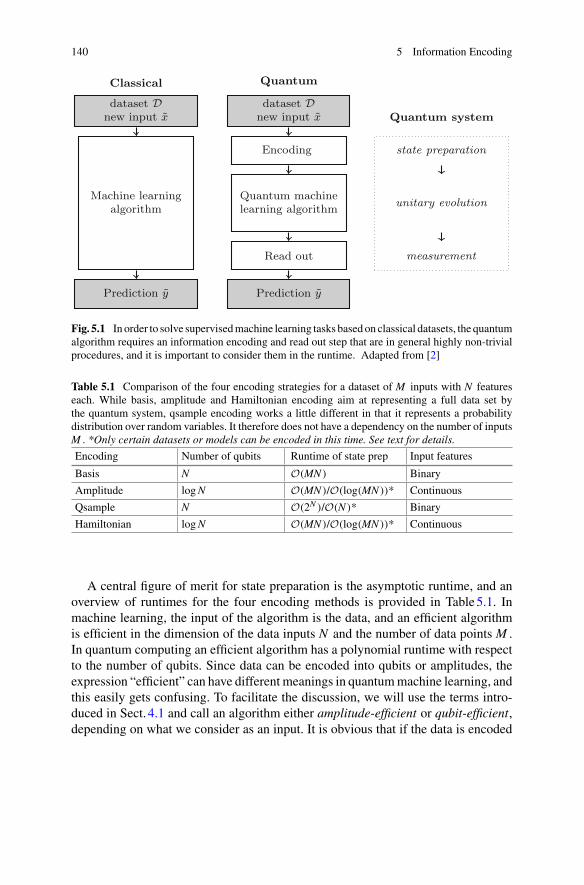
140 5 Information Encoding

Classical

dataset Dnew input x

Machine learningalgorithm

Prediction y

Quantum

dataset Dnew input x

Encoding

Quantum machinelearning algorithm

Read out

Prediction y

Quantum system

state preparation

unitary evolution

measurement

Fig. 5.1 In order to solve supervisedmachine learning tasks based on classical datasets, the quantumalgorithm requires an information encoding and read out step that are in general highly non-trivialprocedures, and it is important to consider them in the runtime. Adapted from [2]

Table 5.1 Comparison of the four encoding strategies for a dataset of M inputs with N featureseach. While basis, amplitude and Hamiltonian encoding aim at representing a full data set bythe quantum system, qsample encoding works a little different in that it represents a probabilitydistribution over random variables. It therefore does not have a dependency on the number of inputsM . *Only certain datasets or models can be encoded in this time. See text for details.

Encoding Number of qubits Runtime of state prep Input features

Basis N O(MN ) Binary

Amplitude logN O(MN )/O(log(MN ))* Continuous

Qsample N O(2N )/O(N )* Binary

Hamiltonian logN O(MN )/O(log(MN ))* Continuous

A central figure of merit for state preparation is the asymptotic runtime, and anoverview of runtimes for the four encoding methods is provided in Table5.1. Inmachine learning, the input of the algorithm is the data, and an efficient algorithmis efficient in the dimension of the data inputs N and the number of data points M .In quantum computing an efficient algorithm has a polynomial runtime with respectto the number of qubits. Since data can be encoded into qubits or amplitudes, theexpression “efficient” can have different meanings in quantummachine learning, andthis easily gets confusing. To facilitate the discussion, we will use the terms intro-duced in Sect. 4.1 and call an algorithm either amplitude-efficient or qubit-efficient,depending on what we consider as an input. It is obvious that if the data is encoded

5 Information Encoding 141

into the amplitudes or operators of a quantum system (as in amplitude and Hamil-tonian encoding), amplitude-efficient state preparation routines are also efficient interms of the data set. If we encode data into qubits, qubit-efficient state preparationis efficient in the data set size. We will see that there are some very interesting casesin which we encode data into amplitudes or Hamiltonians, but can guarantee qubit-efficient state preparation routines. In these cases, we prepare data in time whichis logarithmic in the data size itself. Of course, this requires either a very specificaccess to or a very special structure of the data.

Before we start, a safe assumption when nothing more about the hardware isknown is that we have a n-qubit system in the ground state |0...0〉 and that the data isaccessible from a classical memory. In some cases we will also require some specificclassical preprocessing. We consider data sets D = {x1, ..., xM } of N -dimensionalreal feature vectors. Note that many algorithms require the labels to be encoded inqubits entangled with the inputs, but for the sake of simplicity we will focus onunlabelled data in this chapter.

5.1 Basis Encoding

Assume we are given a binary dataset D where each pattern xm ∈ D is a binarystring of the form xm = (bm1 , ..., bmN )with bmi ∈ {0, 1} for i = 1, ...,N .We can preparea superposition of basis states |xm〉 that qubit-wise correspond to the binary inputpatterns,

|D〉 = 1√M

M∑

m=1

|xm〉. (5.1)

For example, given two binary inputs x1 = (01, 01)T , x2 = (11, 10)T , where fea-tures are encoded with a binary precision of τ = 2, we can write them as binary pat-terns x1 = (0110), x2 = (1110). These patterns can be associated with basis states|0110〉, |1110〉, and the full data superposition reads

|D〉 = 1√2|0101〉 + 1√

2|1110〉. (5.2)

The amplitude vector corresponding to State (5.1) has entries 1√M

for basis statesthat are associated with a binary pattern from the dataset, and zero entries otherwise.For Eq. (5.2), the amplitude vector is given by

α = (0, 0, 0, 0, 0,1√2, 0, 0, 0, 0, 0, 0, 0, 0,

1√2, 0)T

142 5 Information Encoding

Since—except in very low dimensions—the total number of amplitudes 2Nτ is muchlarger than the number of nonzero amplitudes M , basis encoded datasets generallygive rise to sparse amplitude vectors.

5.1.1 Preparing Superpositions of Inputs

An elegant way to construct such ‘data superpositions’ in time linear in M and Nhas been introduced by Ventura, Martinez and others [3, 4], and will be summarisedhere as an example of basis encoded state preparation. The circuit for one step in theroutine is shown in Fig. 5.2. We will simplify things by considering binary inputs inwhich every bit represents one feature, or τ = 1.

We require a quantum system

|l1, ..., lN ; a1, a2; s1, ..., sN 〉

with three registers: a loading register of N qubits |l1, ..., lN 〉, the ancilla register|a1, a2〉 with two qubits and the N -qubit storage register |s1, ..., sN 〉. We start in theground state and apply a Hadamard to the second ancilla to get

1√2|0, ..., 0; 0, 0; 0, ..., 0〉 + 1√

2|0, ..., 0; 0, 1; 0, ..., 0〉.

The left term, flagged with a2 = 0, is called thememory branch, while the right term,flaggedwitha2 = 1, is theprocessing branch. The algorithm iteratively loads patternsinto the loading register and ‘breaks away’ the right size of terms from the processing

A B C D E

|l1〉 Xxm1 •

COMP RESET

|s1〉 X

|l2〉 Xxm2 •

|s2〉 X

|a1〉 X •|a2〉 • • • U(μ)

Fig. 5.2 Circuit for one step of Ventura and Martinez state preparation routine as described inthe text for an example of 2-bit input patterns. The storage and loading qubits are in a slightlydifferent order to facilitate the display. (A) The pattern is written into the loading register by NOTgates. Taking the gate to the power of the bit value xmi is a convenient way to apply the flip onlywhen xmi = 1. (B) Transfer the pattern to the storage register of the processing branch. (C) Split theprocessing branch. (D) Flip the first ancilla back conditioned on a successful comparison of loadingand storage branch. (E) Reset the registers to prepare for the next patterns

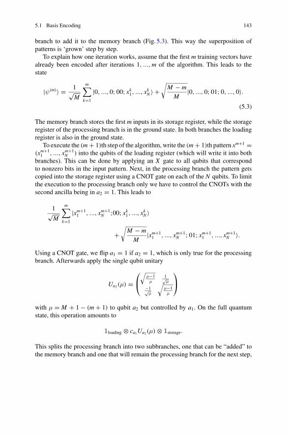
5.1 Basis Encoding 143

branch to add it to the memory branch (Fig. 5.3). This way the superposition ofpatterns is ‘grown’ step by step.

To explain how one iteration works, assume that the first m training vectors havealready been encoded after iterations 1, ...,m of the algorithm. This leads to thestate

|ψ(m)〉 = 1√M

m∑

k=1

|0, ..., 0; 00; xk1, ..., xkN 〉 +√M − m

M|0, ..., 0; 01; 0, ..., 0〉.

(5.3)

The memory branch stores the first m inputs in its storage register, while the storageregister of the processing branch is in the ground state. In both branches the loadingregister is also in the ground state.

To execute the (m + 1)th step of the algorithm,write the (m + 1)th pattern xm+1 =(xm+1

1 , ..., xm+1N ) into the qubits of the loading register (which will write it into both

branches). This can be done by applying an X gate to all qubits that correspondto nonzero bits in the input pattern. Next, in the processing branch the pattern getscopied into the storage register using a CNOT gate on each of the N qubits. To limitthe execution to the processing branch only we have to control the CNOTs with thesecond ancilla being in a2 = 1. This leads to

1√M

m∑

k=1

|xm+11 , ..., xm+1

N ;00; xk1, ..., xkN 〉

+√M − m

M|xm+1

1 , ..., xm+1N ; 01; xm+1

1 , ..., xm+1N 〉.

Using a CNOT gate, we flip a1 = 1 if a2 = 1, which is only true for the processingbranch. Afterwards apply the single qubit unitary

Ua2(μ) =⎛

⎝

√μ−1μ

1√μ

−1√μ

√μ−1μ

⎞

⎠

with μ = M + 1 − (m + 1) to qubit a2 but controlled by a1. On the full quantumstate, this operation amounts to

1loading ⊗ ca1Ua2(μ) ⊗ 1storage.

This splits the processing branch into two subbranches, one that can be “added” tothe memory branch and one that will remain the processing branch for the next step,

144 5 Information Encoding

processing branch memory branch

new pattern

load

split

store

Fig. 5.3 Illustration of Ventura and Martinez state preparation routine [3]. The superposition isdivided into a processing and memory term, flagged by an ancilla. New training input patterns getsuccessively loaded into the processing branch, which gets ‘split’ by a Hadamard on an ancilla, andthe pattern gets ‘merged’ into the memory term

1√M

m∑

k=1

|xm+11 ,..., xm+1

N ; 00; xk1, ..., xkN 〉

+ 1√M

|xm+11 , ..., xm+1

N ; 10; xm+11 , ..., xm+1

N 〉

+√M − (m + 1)√

M|xm+1

1 , ..., xm+1N ; 11; xm+1

1 , ..., xm+1N 〉

To add the subbranch marked by |a1a2〉 = |10〉 to the memory branch, we have toflip a1 back to 1. To confine this operation to the desired subbranch we can conditionit on an operation that compares if the loading and storage register are in the samestate (which is only true for the two processing subbranches), and that a2 = 1 (whichis only true for the desired subbranch). Also, the storage register of the processingbranch as well as the loading register of both branches has to be reset to the groundstate by reversing the previous operations, before the next iteration begins. After the(m + 1)th iteration we start with a state similar to Eq. (5.3) but with m → m + 1.The routine requires O(MN ) steps, and succeeds with certainty.

There are interesting alternative proposals for architectures of quantum RandomAccess Memories, devices that load patterns ‘in parallel’ into a quantum register.These devices are designed to query an index register |m〉 and load the mth binarypattern into a second register in basis encoding, |m〉|0...0〉 → |m〉|xm〉. Most impor-tantly, this operation can be executed in parallel. Given a superposition of the indexregister, the quantum random access memory is supposed to implement the operation

1√M

M−1∑

m=0

|m〉|0...0〉 → 1√M

M−1∑

m=0

|m〉|xm〉. (5.4)

We will get back to this in the next section, where another step allows us to prepareamplitude encoded quantum states. Ideas for architectures which realise this kind of

5.1 Basis Encoding 145

‘query access’ in logarithmic time regarding the number of items to be loaded havebeen brought forward [5], but a hardware realising such an operation is still an openchallenge [6, 7].

5.1.2 Computing in Basis Encoding

Acting on binary features encoded as qubits gives us themost computational freedomto design quantum algorithms. In principle, each operation on bits that we can executeon a classical computer can be done on a quantum computer as well. The argumentis roughly the following: A Toffoli gate implements the logic operation

Input Output0 0 0 0 0 00 0 1 0 0 10 1 0 0 1 00 1 1 0 1 11 0 0 1 0 01 0 1 1 0 11 1 0 1 1 11 1 1 1 1 0

and is a universal gate for Boolean logic [8]. Universality implies that any binaryfunction f : {0, 1}⊗N → {0, 1}⊗D can be implemented by a succession of Toffoligates and possibly some ‘garbage’ bits. The special role of the Toffoli gate stemsfrom the fact that it is reversible. If one only sees the state after the operation, onecan deduce the exact state before the operation (i.e., if the first two bits are 11,flip the third one). No information is lost in the operation, which is in physicalterms a non-dissipative operation. In mathematical terms the matrix representingthe operation has an inverse. Reversible gates, and hence also the Toffoli gate, canbe implemented on a quantum computer. In conclusion, if any classical algorithmcan efficiently be formulated in terms of Toffoli gates, and these can always beimplemented on a quantum computer, this means that any classical algorithm canefficiently be translated to a quantum algorithm. The reformulation of a classicalalgorithm with Toffoli gates may however have a large polynomial overhead andslow down the routines significantly.

Note that once encoded into a superposition, the data inputs can be processed inquantum parallel (see Sect. 3.2.4). For example, if a routine

A(|x〉 ⊗ |0〉) → |x〉 ⊗ |f (x)〉

146 5 Information Encoding

is known to implement a machine learning model f and write the binary predic-tion f (x) into the state of a qubit, we can perform inference in parallel on the datasuperposition,

A(

1√M

M∑

m=1

|xm〉 ⊗ |0〉)

→ 1√M

M∑

m=1

|xm〉 ⊗ |f (xm)〉.

From this superposition one can extract statistical information, for example by mea-suring the last qubit. Such a measurement reveals the expectation value of the pre-diction of the entire dataset.

5.1.3 Sampling from a Qubit

As the previous example shows, the result of a quantummachine learning model canbe basis encoded as well. For binary classification this only requires one qubit. If thequbit is in state |f (x)〉 = |1〉 the prediction is 1 and if the qubit is in state |f (x)〉 = |0〉the prediction is 0. A superposition can be interpreted as a probabilistic output thatprovides information on the uncertainty of the result.

In order to read out the state of the qubit we have to measure it, and we want tobriefly address how to obtain the prediction estimate from measurements, as wellas what number of measurements are needed for a reliable prediction. The field ofreconstructing a quantum state from measurements is called quantum tomography,and there are very sophisticated ways in which samples from these measurementscan be used to estimate the density matrix that describe the state. Here we consider amuch simpler problem, namely to estimate the probability of measuring basis state|0〉 or |1〉. In other words, we are just interested in the diagonal elements of thedensity matrix, not in the entire state. Estimating the ouptut of a quantum model inbasis encoding is therefore a ‘classical’ rather than a ‘quantum task’.

Let the final state of the output qubit be given by the density matrix

ρ =(

ρ00 ρ01ρ10 ρ11

).

We need the density matrix formalism from Chap.3 here because the quantum com-puter may be in a state where other qubits are entangled with the output qubit, and thesingle-qubit-state is therefore a mixed state. We assume that the quantum algorithmis error-free, so that repeating it always leads to precisely the same density matrix ρto take measurements from. The diagonal elements ρ00 and ρ11 fulfil ρ00 + ρ11 = 1and give us the probability of measuring the qubit in state |0〉 or |1〉 respectively. Weassociate ρ11 with the probabilistic output f (x) = p which gives us the probabilitythat model f predicts y = 1 for the input x.

5.1 Basis Encoding 147

To get an estimate p of p we have to repeat the entire algorithm S times andperform a computational basis measurement on the output qubit in each run. Thisproduces a set of samples Ω = {y1, ..., yS} of outcomes, and we assume the samplesstem from a distribution that returns 0 with probability 1 − p and 1 with probabilityp. Measuring a single qubit is therefore equivalent to sampling from a Bernoullidistribution, a problem widely investigated in statistics.2 There are various strategiesof how to get an estimate p from samples Ω . Most prominent, maximum likelihoodestimation leads to the rather intuitive ‘frequentist estimator’ p = p = 1

S

∑Si=1 yi

which is nothing else than the average over all outcomes.An important question is how many samples from the single qubit measurement

we need to estimate pwith error ε. In physics language, wewant an ‘error bar’ ε of ourestimation p ± ε, or the confidence interval [p − ε, p + ε]. A confidence interval isvalid for a pre-defined confidence level, for example of 99%. The confidence level hasthe following meaning: If we have different sets of samples S1, ...,SS and computeestimators and confidence intervals for each of them, pS1 ± εS1 , ..., pSS ± εSS , theconfidence level is the proportion of sample sets for which the true value p lies withinthe confidence interval around p. The confidence level is usually expressed by a socalled z-value, for example, a z-value of 2.58 corresponds to a confidence of 99%.This correspondence can be looked up in tables.

Frequently used is the Wald interval which is suited for cases of large S andp ≈ 0.5. The error ε can be calculated as

ε = z

√p(1 − p)

S.

This is maximised for p = 0.5, so that we can assume the overall error of our esti-mation ε to be at most

ε ≤ z

2√S

with a confidence level of z. In other words, for a given ε and z we need O(ε−2)

samples of the qubit measurement. If we want to have an error bar of at most ε = 0.1and a confidence level of 99% we need about 167 samples, and an error of ε = 0.01with confidence 99% requires at most 17, 000 samples. This is a vast number, butonly needed if the estimator is equal to 0.5, which is the worst case scenario of anundecided classifier (and we may not want to rely on the decision very much in anycase). One can also see that the bound fails for p → 0, 1 [9].

There are other estimates that also work when p is close to either zero or one. Amore refined alternative is theWilson score interval [10] with the following estimatorfor p,

p = 1

1 + z2S

(p + z2

2S

),

2Bernoulli sampling is equivalent to a (biased) coin toss experiment: We flip a coin S times andwant to estimate the bias p, i.e. with what probability the coin produces ‘heads’.

148 5 Information Encoding

Fig. 5.4 Relationshipbetween the sample size Sand the mean valuep = 1

S

∑Si=1 yi for different

errors ε for the Wilson scoreinterval of a Bernoulliparameter estimationproblem as described in thetext

and the error

ε = z

1 + z2S

(p(1 − p)

S+ z2

4S2

) 12

,

with p being the average of all samples as defined above. Again this is maximisedfor p = 0.5 and with a confidence level z we can state that the overall error of ourestimation is bounded by

ε ≤√z2S + z2

4S2.

This can be solved for S as

S ≤ε2√

z4(16ε2+1)ε4

+ z2

8ε2.

With the Wilson score, a confidence level of 99% suggests that we need 173 singlequbit measurements to guarantee an error of less than 0.1. However, now we cantest the cases p = 0, 1 for which S = z2( 1

2ε − 1). For ε = 0.1 we only need about 27measurements for the same confidence level (see Fig. 5.4).

5.2 Amplitude Encoding

An entire branch of quantum machine learning algorithms encode the dataset intothe amplitudes of a quantum state

5.2 Amplitude Encoding 149

|ψD〉 =M∑

m=1

N∑

i=1

xmi |i〉|m〉

=M∑

m=1

|ψxm〉|m〉. (5.5)

This quantum state has an amplitude vector of dimension NM that is constructedby concatenating all training inputs, α = (x11, ..., x

1N , ..., xM1 , ..., xMN )T . As discussed

in Sect. 3.4.2, the dataset has to be normalised so that the absolute square of theamplitude vector is one, |α|2 = 1. The training outputs can either be basis encodedin an extra qubit |ym〉 entangled with the |m〉 register, or encoded in the amplitudesof a separate quantum register,

|ψy〉 =M∑

m=1

ym|m〉.

Amplitude encoding of datasets therefore requires the ability to prepare an arbitrarystate

|ψ〉 =∑

i

αi|i〉, (5.6)

both efficiently and robustly.The main advantage of amplitude encoding is that we only need n = logNM

qubits to encode a dataset ofM inputs with N features each. If the quantum machinelearning algorithm is polynomial in n (or qubit-efficient), it has a logarithmic run-time dependency on the data set size. Promises of exponential speedups from qubit-efficient quantum machine learning algorithms sound strange to machine learningpractitioners, because simply loading the NM features from the memory hardwaretakes time that is of course linear in NM . And indeed, the promises only hold if statepreparation can also be done qubit-efficiently [11]. This is in fact possible in somecases that exhibit a lot of structure. As a trivial example, if the goal is to producea vector of uniform entries we simply need to apply n Hadamard gates - a qubit-efficient state preparation time. Similarly, s-sparse vectors can be prepared with theroutines from the previous section in time sn. On the other hand, there are subspacesin a Hilbert space that cannot be reached from a given initial state with qubit-efficientalgorithms [12] (see Fig. 5.5). It is therefore an important and nontrivial open ques-tion which classes of relevant states for machine learning with amplitude encodingcan be prepared qubit-efficiently.

Similar caution is necessary for the readout of all amplitudes. If the result of thecomputation is encoded in one specific amplitude αi only, the number of measure-ments needed to retrieve it scale with the number of amplitudes (and to measure the

150 5 Information Encoding

Fig. 5.5 Starting from the n-qubit ground state |0...0〉 some quantum states in C2n can be reachedby a quantum algorithm that grows polynomially with n, while others require algorithms that growexponentially with n. In amplitude encoding the number of features is 2n, and state preparationroutines that are polynomial in the number of qubits are therefore logarithmic in the number offeatures

state corresponding to that amplitude once requires on averageO(1/|αi|2) repetitionsof the entire routine). This is why the result of quantummachine learning algorithmsbased on amplitude encoding is often designed in a different manner, for examplethrough a single-qubit measurement as explained in the previous section,.

How can we prepare an arbitrary vector like in Eq. (5.6)? We will first discuss ascheme that is amplitude-efficient (and thereby efficient in N ,M ) and then look atqubit-efficient schemes and their limitations.

5.2.1 State Preparation in Linear Time

Given an n qubit quantum computer, the theoretical lower bound of the depth of anarbitrary state preparation circuit is known to be 1

n2n [13–17]. Current algorithms

perform slightly worse with slighly less than 2n parallel operations, most of whichare expensive 2-qubit gates. To illustrate one way of doing state preparation in lineartime, let us have a look at the routine presented byMöttönen et al. [18]. They considerthe reverse problem, namely to map an arbitrary state |ψ〉 to the ground state |0...0〉.In order to use this algorithm for our purpose we simply need to invert each andevery operation and apply them in reverse order.

The basic idea is to control a rotation on qubit qs by all possible states of theprevious qubits q1, ..., qs−1, using sequences of so called multi-controlled rotations.In other words, we explicitly do a different rotation for each possible branch of thesuperposition, the one inwhich the previous qubitswere in state |0..0〉 to the branch inwhich they are in |1...1〉. This is comparable to tossing s − 1 coins and manipulatingthe sth coin differently depending on the measurement outcome via a look-up table.

A full sequence of multi-controlled rotations around vectors vi with angles βi

consists of the successive application of the 2s−1 gates

5.2 Amplitude Encoding 151

cq1=0 · · · cqs−1=0 Rqs(v1,β1) |q1...qs−1〉|qs〉

cq1=0 · · · cqs−1=1 Rqs(v2,β2) |q1...qs−1〉|qs〉

...

cq1=1 · · · cqs−1=1 Rqs(v2s−1

,β2s−1) |q1...qs−1〉|qs〉.

For example, for s = 3 a full sequence consists of the gates

cq1=0cq2=0 Rq3(v1,β1) |q1q2〉|q3〉

cq1=0cq2=1 Rq3(v2,β2) |q1q2〉|q3〉

cq1=1cq2=0 Rq3(v3,β3) |q1q2〉|q3〉

cq1=1cq2=1 Rq3(v4,β4) |q1q2〉|q3〉,

which rotate q3 in a different way for all four branches of the superposition of q1, q2.The circuit symbol of a single multi-controlled rotation is

|q1〉...|qn−1〉 •|qn〉 R(v,β)

(5.7)

where white circles indicate a control on qubit q being in state 1, or cq=1, and blackcircles a control on qubit q being in state 0, cq=0. The circuit diagram of a fullsequence of multi-controlled rotations on the third of three qubits is

|q1〉 • •|q2〉 • •|q3〉 R(v[1],β1) R(v[2],β2) R(v[3],β3) R(v[4],β4)

(5.8)

Of course, we need a prescription to decompose sequences of multi-controlledrotations into elementary gates. If there are s − 1 control qubits, this is possible with2s CNOTs and 2s single qubit gates [14, 18]. For example, a multi-controlled rotationapplied to the third of three qubits would have the decomposition

|q1〉 •|q2〉 • •|q3〉 R(v, δ1) R(v, δ2) R(v, δ3)

into three single-controlled rotations.For a general quantum state one has to apply two cascades of such operations,

where each cascade is a sequences of multi-controlled rotations that run trough all

152 5 Information Encoding

qubits q1 to qn. The first cascade uses Rz-rotations (which fixes the rotation axis v)and has the effect of ‘equalising’ the phases until the state only has one global phasewhich we can ignore (remember, we are doing reverse state preparation). The secondcascade applies Ry rotations and has the effect of ‘equalising’ all amplitudes to resultin the ground state. Since we are usually interested in real amplitude vectors, we canneglect the first cascade and end up with the circuit

|q1〉· · ·

•· · ·

• Ry(βn1)

...|qn-1〉 • Ry(β21) Ry(β

22n-2)

|qn〉 Ry(β11) Ry(β

12n-1)

The choice of the rotation angles β is related to the amplitudes of the original stateas follows:

βsj = 2 arcsin

⎛

⎜⎜⎜⎜⎝

√2s−1∑l=1

|α(2j−1)2s−1+l |2√

2s∑l=1

|α(j−1)2s+l |2

⎞

⎟⎟⎟⎟⎠(5.9)

Example 5.1 We want to prepare the state

|ψ〉 = √0.2|000〉 + √

0.5|010〉 + √0.2|110〉 + √

0.1|111〉,

with the amplitudes a0 = √0.2, a2 = √

0.5, a6 = √0.2, a7 = √

0.1. The circuitrequires seven multi-controlled y-rotations

cq1=0cq2=0 Ry,q3(β11), β1

1 = 0

cq1=0cq2=1 Ry,q3(β12), β1

2 = 0

cq1=1cq2=0 Ry,q3(β13), β1

3 = 0

cq1=1cq2=1 Ry,q3(β14), β1

4 = 1.231..

cq1=0 Ry,q2(β21), β2

1 = 2.014..

cq1=1 Ry,q2(β22), β2

2 = 3.142..

Ry,q1(β31), β3

1 = 1.159..

5.2 Amplitude Encoding 153

We are left with only four gates to apply, and with the approximate values

sin(1.231

2

)= 0.577, cos

(1.2312

)= 0.816

sin(2.014

2

)= 0.845, cos

(2.0142

)= 0.534

sin(3.142

2

)= 1.000, cos

(3.1422

)= 0

sin(1.159

2

)= 0.548, cos

(1.1592

)= 0.837,

these gates can be written as

cq1=1cq2=1 Ry,q3(β14) =

⎛

⎜⎜⎜⎜⎜⎜⎜⎜⎜⎜⎝

1 0 0 0 0 0 0 00 1 0 0 0 0 0 00 0 1 0 0 0 0 00 0 0 1 0 0 0 00 0 0 0 1 0 0 00 0 0 0 0 1 0 00 0 0 0 0 0 0.816 0.5770 0 0 0 0 0 −0.577 0.816

⎞

⎟⎟⎟⎟⎟⎟⎟⎟⎟⎟⎠

,

cq1=0 Ry,q2(β21) =

⎛

⎜⎜⎜⎜⎜⎜⎜⎜⎜⎜⎝

0.534 0 0.845 0 0 0 0 00 0.534 0 0.845 0 0 0 0

−0.845 0 0.534 0 0 0 0 00 −0.845 0 0.534 0 0 0 00 0 0 0 1 0 0 00 0 0 0 0 1 0 00 0 0 0 0 0 1 00 0 0 0 0 0 0 1

⎞

⎟⎟⎟⎟⎟⎟⎟⎟⎟⎟⎠

,

cq1=1 Ry,q2(β22) =

⎛

⎜⎜⎜⎜⎜⎜⎜⎜⎜⎜⎝

1 0 0 0 0 0 0 00 1 0 0 0 0 0 00 0 1 0 0 0 0 00 0 0 1 0 0 0 00 0 0 0 0 0 1 00 0 0 0 0 0 0 10 0 0 0 −1 0 0 00 0 0 0 0 −1 0 0

⎞

⎟⎟⎟⎟⎟⎟⎟⎟⎟⎟⎠

,

154 5 Information Encoding

and

Ry,q1(β31) =

⎛

⎜⎜⎜⎜⎜⎜⎜⎜⎜⎜⎝

0.837 0 0 0 0.548 0 0 00 0.837 0 0 0 0.548 0 00 0 0.837 0 0 0 0.548 00 0 0 0.837 0 0 0 0.548

−0.548 0 0 0 0.837 0 0 00 −0.548 0 0 0 0.837 0 00 0 −0.548 0 0 0 0.837 00 0 0 −0.548 0 0 0 0.837

⎞

⎟⎟⎟⎟⎟⎟⎟⎟⎟⎟⎠

.

Applying these gates to the amplitude vector (√0.2, 0,

√0.5, 0, 0, 0,

√0.2,

√0.1)T ,

the effect of the first operation is to set the last entry to zero, the second operation setsthe third entry to zero and the third operation swaps the 5th element with the 7th. Thelast operation finally cancels the 5th element and results in (1, 0, 0, 0, 0, 0, 0, 0)T asdesired. State preparation means to apply the inverse gates in the inverse order.

5.2.2 Qubit-Efficient State Preparation

The above routine is always possible to use for amplitude-efficient state preparation,but requires an exponential number of operations regarding the number of qubits.In the gate model of quantum computing, a number of proposals have been broughtforward to prepare specific classes of states qubit-efficiently, or in log(MN ).Wewantto present some of those ideas and the conditions to which they apply.

5.2.2.1 Parallelism-Based Approach

Grover and Rudolph suggest a scheme that is linear in the number of qubits for thecase that we know an efficiently integrable one-dimensional probability distributionp(a) of which the state is a discrete representation [19]. More precisely, the desiredstate has to be of the form

|ψ〉 =2n∑

i=1

√p(iΔa)|i〉 =

2n∑

i=1

√pi|i〉,

withΔa = 12n . The desired quantum state is a coarse grained qsample (see Sect. 3.4.3)

of a continuous distribution p(a) (see Fig. 5.6). The “efficiently integrable” conditionmeans that we need an algorithm on a classical computer that calculates definiteintegrals of the probability distribution efficiently, like for the Gaussian distribution.

5.2 Amplitude Encoding 155

p(a) α100t=3

β101t=3

00 01 10 11 a

Fig. 5.6 Grover and Rudolph’s state preparation algorithm for efficiently integrable probabilitydistributions [19]. After step t = 2 the domain is divided into four regions i = 00, 01, 10, 11 of sizeΔx = 1/22, which defines a 2-qubit quantum state with amplitudes p00, p01, p10, p11 (indicated bythe black dots). In the third step, each of the four regions (here demonstrated for i = 10) gets splitinto two. The parametersα and β are the probability to find a random variable in the left or right partof the region. This procedure successively prepares a finer and finer discretisation of the probabilitydistribution

The idea of the scheme is to successively rotate each of the n qubits and get afiner and finer coarse graining of the distribution. Assume Step (t − 1) prepared aqsample

|ψ(t−1)〉 =2t−1∑

i=1

√p(t−1)i |i〉|00...0〉.

The index register |i〉 contains the first t − 1 qubits. The next step t rotates the t’thqubit according to

|ψ(t)〉 =2t∑

i=1

√p(t−1)i |i〉(√αi|0〉 +√βi|1〉)|0...0〉,

such that αi, [βi] are the probabilities for a random variable to lie in the left [right]half of the i’th interval of the probability distribution. In the tth step, the input domainis discretised into 2t equidistant intervals which is visualised in Fig. 5.6. This definesa new qsample

|ψ(t)〉 =2t∑

i=1

√p(t)i |i〉|0...0〉,

where the index register now has t qubits and the remaining qubits in the groundstate are reduced by one. With each step, this process prepares an increasingly finediscretisation of the probability distribution p(a).

156 5 Information Encoding

TheGrover andRudolph suggestion is in fact rather similar to the state preparationroutine in the previous section, but this time we do not have to hardcode the ‘lookup-table’ for each state of the first t − 1 qubits, but we can use quantum parallelism tocompute the values αi,βi for all possible combinations. This more general versionof the idea was proposed by Kaye and Mosca [20], who do not refer to probabilitydistributions but demand that the conditional probability p(qk = 1|q1...qk−1), whichis the chance that given the state q1...qk−1 of the previous qubits, the k’th qubit is instate 1, is easy to compute. It is an interesting task to find classical datasets whichallow for this trick.

5.2.2.2 Oracle-Based Approach

Soklakov and Schack [21] propose an alternative qubit-efficient scheme to approx-imately prepare quantum states whose amplitudes αi = √

pi represent a discreteprobability distribution pi, i = 1, ..., 2n = N , and all probabilities pi are of the orderof 1/ηN for 0 < η < 1. With this condition, they can use a Grover-type algorithmwhich with probability greater than 1 − ν has an error smaller than ε in the result,and which is polynomial in η−1, ε−1, ν−1. To sketch the basic idea (Fig. 5.7), a seriesof oracles is defined which successively marks basis states whose amplitudes areincreased by amplitude amplification. The first oracle only marks basis states |i〉 forwhich the desired probability pi is larger than a rather high threshold. With eachstep (defining a new oracle) the threshold is lowered by a constant amount. In theend, large amplitudes have been grown in more steps than small ones, and the finaldistribution is as fine as the number of steps allows. One pitfall is that we need toknow the optimal number of Grover iterations for a given oracle. For this quantumcounting can be applied to estimate the number of marked states in the current step.As with all oracle-based algorithms, the algorithm requires an implementation of theoracle to be used in practice.

5.2.2.3 Quantum Random Access Memory

Under the condition that the states to prepare are sufficiently uniform, a more genericapproach is to refer to the quantum random access memory introduced in Eq. (5.4).The quantum random access memory allows access of classically stored informationin superposition by querying an index register and is referred to by many authors inquantum machine learning [22–25]. In Sect. 5.1.1 this was used to prepare a datasetin basis encoding, but with one additional step we can extend its application toamplitude encoding as well. This step involves a conditional rotation and branchselection procedure that we already encountered in Step 3 of the quantum matrixinversion routine of Sect. 3.5.3. Let us assume the quantum random access memoryprepared a state

5.2 Amplitude Encoding 157

i

pi

θk

Fig. 5.7 In the k’th step of the routine of Soklakov and Schack [21], an oracle is applied to markthe states whose probabilities pi are larger than a certain threshold θk (here in red). These states areamplified with the Grover iterator, resulting in a state that looks qualitatively like the red bars only.In the next step, the threshold is lowered to include the states with a slightly smaller probability inamplitude amplification, until the desired distribution of the pi is prepared

1√N

N∑

i=1

|i〉|xi〉|0〉,

where xi ≤ 1 are the entries of a classical real vector we want to amplitude encode.Now rotate the ancilla qubit conditional on the |xi〉 register to get

1√N

N∑

i=1

|i〉|xi〉(√1 − |xi|2|0〉 + xi|1〉). (5.10)

The details of this step depend on how xi is encoded into the register. If we assumebinary fraction encoding, such a conditional rotation could be implemented by τsingle-qubit conditional rotations on the ancilla that are controlled by the q1...qτ

qubits of the second register. For qubit qk the rotation would turn the amplitudecloser to |1〉 by a value of 1

2k .Now the ancilla has to be measured to ‘select the desired branch’ of the super-

position (see Fig. 5.8). If the measurement results in |1〉 we know that the resultingstate is in

1√Npacc

N∑

i=1

xi|i〉|xi〉|1〉,

where pacc is the success or acceptance probability that renormalises the state. Dis-carding the last register and uncomputing the last but one (which is possible becausethe superposition is ‘kept up’ by the index register and no unwanted interference hap-pens), we get a state that amplitude encodes a vector x = (x1, ..., xN )T . Of course,one could also start with a non-uniform superposition and would get a product of the

158 5 Information Encoding

Fig. 5.8 Schematic illustration of the postselective measurement of the branch selection procedure.The two states 0 and 1 of the ancilla qubit are entangled with two different states marked in red andblue. A post-selectivemeasurement selects only one branch of the superposition (here the 0-branch).The state entangled with this branch is formally renormalised

initial and new amplitude. If the measurement results in |0〉, we have to repeat theentire routine.

The routine for arbitrary state preparation with a quantum random access memorysucceeds only with a probability of pacc =∑i |xi|2/N which obviously depends onthe state to encode. A uniform distributionwith xi = 1 ensures that pacc =∑i

1N = 1,

and in the extreme case of only one non-zero amplitude of 1 we get pacc = 1N , which

is exponentially small in the number of qubits n. In other words, we would have torepeat the measurement O(N = 2n) times on average to prepare the correct state.Luckily, very sparse states can be prepared by other methods. For example, for aone-sparse vector one can simply flip the qubit register from the ground state into abasis state representing the index i. Zhao et al. [26] therefore propose that in case of ssparse vectors, one does not apply the quantum random access memory to a uniformsuperposition, but a superposition

1√s

∑

i|xi =0

|i〉

of the basis states representing indices of non-zero amplitudes (Fig. 5.7).There are many other possible ways to prepare quantum states beyond quantum

circuits. An interesting perspective is offered by Aharanov et al. [1]. They present theframework of “adiabatic state generation” as a natural (and polynomially equivalent)alternative to state preparation in the gate model. The idea is to perform an adiabaticevolution of a quantum system that is initially in the ground state of a generic Hamil-tonian, to the ground state of a final Hamiltonian. If the evolution is performed slowenough, we end up with the system in the ground state of the final Hamiltonian,which is the state we wish to prepare. This translates the question of which initialstates can be easily prepared to the question of which ground states of Hamiltoniansare in reach of adiabatic schemes, i.e. have small spectral gaps between the groundand the first excited state. A somewhat related idea is to use the unique stationarystates of a dissipative process in an open quantum system.

In summary, quantum state preparation for amplitude encoded states relevant tomachine learning algorithms is a topic that still requires a lot of attention, and claimsof exponential speedups from qubit-efficient state preparation algorithms shouldtherefore be viewed with a pinch of skepticism.

5.2 Amplitude Encoding 159

5.2.3 Computing with Amplitudes

In contrast to basis encoding, amplitude encoding radically limits the type of com-putations we can perform. As we saw in Chap.3, there are two general operationsfor the manipulation of amplitudes in the formalism of quantum theory: unitarytransformations and measurements.

As stated in detail in Chap.3, unitary transformations are linear transformations ofthe amplitude vector that preserve its length. Even if we consider subsystems (wherethe evolution is not unitary any more), we still get linear dynamics, for exampleexpressed by the so called Kraus formalism (see [27]). In fact, it has been shown thatintroducing a ‘coherent’ nonlinearity to quantumevolution implies the ability to solveNP-hard problems [28]. Essentially this is because we could increase exponentiallysmall signals in a superposition to efficiently measurable information. With this,Grover search could be done exponentially faster. It has also been claimed that anynonlinear map would allow for super-luminal communication [29] and negate thelaws of thermodynamics [30]. In short, a nonlinear version of quantum theory canbe considered highly unlikely.3

A projective measurement is clearly a nonlinear operation, but its outcome isstochastic and if averaging over several runs it will reflect the distribution of ampli-tudes. But not all is lost: An important way to introduce nonlinearities on the levelof amplitudes are post-selective measurements that we used in the branch selectionscheme of the previous section. In a post-selective measurement of a single qubit,the state of the qubit is measured in the computational basis and the algorithm is onlycontinued if this qubit is found in a particular state. This condition works like an “if”statement in programming. Post-selection has the effect of setting the amplitudes ina branch of superpositions to zero, namely the branch that is entangled with the qubitin the state of an unsuccessful measurement. Note that in most cases we can push thepost-selection to the end of the algorithm and reject final measurement outcomes ifthe result of said qubit is in the desired state. A second, closely related idea is to useso called repeat-until-success circuits [32]. Here the unsuccessful measurement doesnot result in repeating the entire algorithm, but prescribes a small correction, whichrestores the state before the postselective measurement. Postselection can thereforebe repeated until success is observed. As mentioned before, these procedures arenon-unitary and for runtime considerations the likeliness of success has to be takeninto account.

5.3 Qsample Encoding

Qsample encoding has been introduced to associate a real amplitude vector(√p1, ...,

√pN )T with a classical discrete probability distribution p1, ..., pN . This

is in a sense a hybrid case of basis and amplitude encoding, since the information

3Note that there are effective nonlinear dynamics, see for example [31].

160 5 Information Encoding

we are interested in is represented by amplitudes, but the N features are encoded inthe qubits. An amplitude-efficient quantum algorithm is therefore exponential in theinput dimension N , while a qubit-efficient algorithm is polynomial in the input.

For a given probability distribution, state preparation works the same way asin amplitude encoding. In some cases the distribution may be a discretisation of aparametrised continuous and efficiently integrable distribution p(x), in which casethe implicit Grover-Rudolph scheme can be applied.

The probabilistic nature of quantum systems lets usmanipulate the classical distri-bution with the quantum system and implement some standard statistic computationsgenerically. We can prepare joint distributions easily, marginalise over qubits ‘forfree’, andwe can perform a rejection sampling step via branch selection. Thesemeth-ods are nothing other than an application of basic quantum theory from Sects. 3.1.2.3and 3.1.3.5, but can be useful when regarded from the perspective of manipulatingdistributions represented by a qsample.

5.3.1 Joining Distributions

When joining two quantum systems representing a qsample,

|ψ1〉 =2n∑

i=1

√ui |i〉,

and

|ψ2〉 =2n∑

j=1

√sj |j〉,

the joint state of the total system is described as a tensor product of the two states(see Sect. 3.1.2.3),

|ψ1〉 ⊗ |ψ2〉 =2n∑

i,j

√uisj |i〉|j〉.

Sampling the binary string ij from this state is observed with probability uisj, whichis a product of the two original probabilities. In other words, the qsample of two jointqsamples is a product distribution.

5.3.2 Marginalisation

Given a qsample,

|ψ〉 =2n∑

i=1

√pi |i〉.

5.3 Qsample Encoding 161

Themathematical operation of tracing over a qubit qk corresponds to omitting the kthqubit from the description, leading to a statistical ensemble over all possible statesof that qubit Sect. 3.1.2.3. The resulting state is in general (that is, unless the k’thqubit was unentangled) a mixed state.

To write down the effect of a trace operation is awkward and hides the simplicityof the concept, but we will attempt to do it anyways in order to show the equivalenceto marginalisation. Remember that the ith computational basis state |i〉 represents abinary sequence, more precisely the binary representation of i − 1 (for example, |1〉represents |0...0〉). Let us define the shorthand i¬k for the binary sequence indicatedby i, but without the kth bit, and let ik=0,1 be the same sequence, but this time the kthbit is set to either 0 or 1. Also, let 〈i|0k〉 and 〈i|1k〉 be the inner product between |i〉and a state 1 ⊗ |0〉 ⊗ 1 and 1 ⊗ |1〉 ⊗ 1, respectively, where |0〉, |1〉 sits at the kthposition. With this notation, tracing out the kth qubit has the following effect,

trk {|ψ〉〈ψ|} = trk

{∑

i

∑

i′

√p(i)p(i′) |i〉〈i′|

}

=∑

i

∑

i′

√p(i)p(i′)

(〈0k |i〉〈i′|0k〉 + 〈1k |i〉〈i′|1k〉)

=∑

i¬k

∑

i′¬k

(√p(ik=0)p(i′k=0) +

√p(ik=1)p(i′k=1)

) |i¬k〉〈i′¬k |.

The probability to measure the computational basis state |i¬k〉 is given by the corre-sponding diagonal element of the resulting density matrix, which is given by

(√p(ik=0)p(ik=0) +√p(ik=1)p(ik=1)

) = (p(ik=0) + p(ik=1)).

This is the sum of the probability of finding k in 0 and the probability of finding k in1, just as we would expect from common sense.

In the classical case, given a probability distribution p(b1...bn) over n-bit stringsb1...bN , marginalising over the state of the k’th bit will yield the marginaldistribution

p(i¬k) = p(b1..bk−1bk+1..bn) (5.11)

= p(b1..bk = 0..bn) + p(b1..bk = 1..bn). (5.12)

This demonstrates that the tracing in the quantum formalism is a ‘classical’ sta-tistical marginalisation. In other words, dropping the k’th qubit from our algorithmeffectively implements a qsample representing a marginal distribution.

162 5 Information Encoding

5.3.3 Rejection Sampling

There is a close relationship between branch selection or postselection and classicalrejection sampling, which can help to understand, design and compare quantumalgorithms. Rejection sampling is a method to draw samples from a distributionp(x) that is difficult to sample from, but for which the probabilities at each pointx are easy to evaluate. The idea is to use a distribution q(x) from which it is easyto draw samples (i.e., a Gaussian or uniform distribution), and scale it such thatp(x) ≤ Kq(x) for an integer K < ∞ (see Fig. 5.9). One then draws a sample x′ fromq(x) as well as a random number u′ from the interval [0, 1]. One accepts the sampleif u′Kq(x′) < p(x′) and rejects it otherwise. In other words, the chance to accept thesample from q(x) depends on the ratio of the original and the alternative distribution.

Obviously, if Kq(x′) and p(x′) are almost equal, the acceptance probability isvery high, but in regions where p(x′) << Kq(x′) we will almost never accept. Whenrepeating this procedure, the accepted samples x′ are effectively drawn from p(x).The general probability of acceptance can be calculated as

pacc =⟨p

(u <

p(x)

Kq(x)

)⟩

=⟨p(x)

Kq(x)

⟩

=∫

p(x)

Kq(x)q(x)dx

= 1

K

∫p(x)dx = 1

K,

which shows that K is an important figure of merit for the runtime [33]. The larger itis, or the bigger the difference between the two distributions, the more samples arerejected.

In branch selection, we have a quantum state of the form

Fig. 5.9 Illustration ofrejection sampling. In orderto sample from the desireddistribution p(x) (smoothline) one samples x′ insteadfrom a distribution K q(x)(dotted line) and accepts thesample with a probabilitydepending on the proportionof the two distributions atthat point x

p(x)

K q(x)

Kq(x′)

p(x′)

x′

5.3 Qsample Encoding 163

N∑

i=1

√ai|i〉(

√1 − bi|0〉 +

√bi|1〉),

where from Eq. (5.10) the uniform coefficients 1√Nwere replaced by more general

amplitudes√a1, ...,

√aN , and the value xi was replaced by

√bi to avoid confusion

with the classical notation. For ease of comparison with classical probability theory,let us assume that the ai and bi are all real numbers in [0, 1]. Bymeasuring the |i〉 reg-ister we sample from the distributionA = {a1, ..., aN }, but our goal is to sample fromthe ‘unknown’ distribution B = {a1b1, ..., aNbN }. The conditional measurement onthe ancilla therefore plays the role of the rejection step if we associate

q(x) ↔ A (5.13)

p(x) ↔ B. (5.14)

To see this, consider the probability bi of measuring the ancilla in |1〉 for state |i〉and compare it to the ‘rejection sampling’ probability of success for sample i. Usingthe replacement of Eqs. (5.14) we get pacc(i) = p(uai < aibi) = p(u < bi) = bi. Thegeneral probability of acceptance is

pacc = 〈p(u < bi)〉= 〈bi〉=∑

i

biai,

where the expectation value is taken with respect to the distributionA. This is equiv-alent to the probability of a successful branch selection.

5.4 Hamiltonian Encoding

While the approaches discussed so far encode features explicitly into quantum states,we can choose an implicit encoding which uses the features to define the evolutionof the quantum system. This approach differs a bit from the previous ones. Insteadof preparing a quantum state which contains the features or a distribution in itsmathematical description, they now define an evolution applied to a state.

We mentioned in Sect. 3.4.4 that there are different ways to encode data into thedynamics of a quantum system, and focused on Hamiltonian encoding. Hamiltonianencoding associates the Hamiltonian of a system with a matrix that represents thedata, such as the design matrix X containing the feature vectors as rows, or the Grammatrix X TX . As discussed in Sect. 3.4.2, we may have to use preprocessing tricksthat make this matrix Hermitian. Section3.5.3 presented ways in which Hamiltonianencoding allows us to extract eigenvalues of matrices, or to multiply them to an

164 5 Information Encoding

amplitude vector. We therefore want to summarise some results on the resourcesneeded to evolve a system by a given Hamiltonian. Similar to amplitude encoding,the general case will yield amplitude-efficient state preparation algorithms, while forsome limited datasets we can get qubit-efficient schemes. Possibly not surprisingly,this is most prominently the case for sparse data.

To use Hamiltonian encoding we need to be able to implement an evolution

|ψ′〉 = e−iHAt|ψ〉 (5.15)

on a quantum computer. The Hamiltonian HA “encodes” a Hermitian matrix A ofthe same dimensions, which means that the matrix representation of HA is entry-wise equivalent to A. The initial quantum state |ψ〉 describes a system of n qubits,and one can think of the final state |ψ′〉 as a quantum state that now“contains” theinformation encoded into theHamiltonian—for exampleH ’s eigenvalues in the phaseof the amplitudes.

The process of implementing a given Hamiltonian evolution on a quantum com-puter is calledHamiltonian simulation [34]. Sinceweonly consider time-independentHamiltonians, any unitary transformation can be written as e−iHAt . Hamiltonian sim-ulation on a gate-based quantum computer4 is therefore very closely related to thequestion of how to decompose a unitary into quantum gates. However, an operator-valued exponential function is not trivial to evaluate, and given H there are morepractical ways than computing the unitary matrix U = e−iHAt and decomposing itinto gates.

The problem of (digital) Hamiltonian simulation can be formulated as follows:Given a Hamiltonian H , a quantum state |ψ〉, an error ε > 0, the evolution time t(which can be imagined as a scaling factor to H ), and an appropriate norm || · || thatmeasures the distance between quantum states, find an algorithm which implementsthe evolution of Eq. (5.15) so that the final state of the algorithm, |ψ〉, is ε-close tothe desired final state |ψ′〉,

|| |ψ′〉 − |ψ〉|| ≤ ε.

We want to summarise the basic ideas of Hamiltonian simulation and then state theresults for qubit-efficient simulations.

5.4.1 Polynomial Time Hamiltonian Simulation

Consider aHamiltonianH that can be decomposed into a sumof several “elementary”HamiltoniansH =∑K

k=1 Hk so that eachHk is easy to simulate. For non-commuting

4Hamiltonian simulation research can be distinguished into analog and digital approaches to sim-ulation. Roughly speaking, analog simulation finds quantum systems that “naturally” simulateHamiltonians, while digital simulation decomposes the time evolution into quantum gates, whichis more relevant in the context of this book.

5.4 Hamiltonian Encoding 165

Hk , we cannot apply the factorisation rule for scalar exponentials, or

e−i∑kHk t =

∏

k

e−iHk t .

An important idea introduced by Seth Lloyd in his seminal paper in 1996 [35] wasto use the first-order Suzuki-Trotter formula instead,

e−i∑kHk t =

∏

k

e−iHk t + O(t2). (5.16)

TheTrotter formula states that for small t the factorisation rule is approximately valid.This can be leveraged when we write the evolution of H for time t as a sequence ofsmall time-steps of length Δt,

e−iHt = (e−iHΔt)t

Δt .

While for the left side, the Trotter formula has a large error, for each small time stepΔt, the error in Eq. (5.16) becomes negligible. Of course, there is a trade-off: Thesmaller Δt, the more often the sequence has to be repeated. But overall, we have away to simulate H by simulating the terms Hk .

This approach shows that if we know a decomposition of Hamiltonians into sumsof elementary Hamiltonians that we know how to simulate, we can approximatelyevolve the system in the desired way. The case-specific decomposition may still benon-trivial, and some examples are summarised in [34]. One example for such adecomposition is a sum of Pauli operators. Every Hamiltonian can be written as

H =∑

k1,··· ,kn=1,x,y,z

ak1,...,kn(σ1k1 ⊗ · · · ⊗ σn

kn). (5.17)

The sum runs over all possible tensor products of Pauli operators applied to the nqubits, and the coefficients

ak1,··· ,kn = 1

2ntr{(σ1

k1 ⊗ · · · ⊗ σnkn)H },

define the entries of the Hamiltonian. For example, for two qubits we can write

H2 = a1,1(σ11 ⊗ σ2

1) + a1,x(σ11 ⊗ σ2

x ) + · · · + az,z(σ1z ⊗ σ2

z ).

This decomposition has 4n = 2n × 2n terms in general. If the evolution describes aphysical problem we can hope that only local interactions—terms in which σi = 1for all but a few neighbouring qubits—are involved. For machine learning this couldalso be interesting, when the features are generated by a “local” process and we canhope that correlations in the data reduce the number of terms in the sum of Eq. (5.17).

166 5 Information Encoding

5.4.2 Qubit-Efficient Simulation of Hamiltonians

There are special classes of Hamiltonians that can be simulated in time that is loga-rithmic in their dimension. If the Hamiltonian encodes a data matrix, this means thatthe runtime is also logarithmic in the dimension of the dataset. The most prominentexample are Hamiltonians that only act on a constant number of qubits, so calledstrictly local Hamiltonians [35]. This is not surprising when we remember that alocal Hamiltonian can be expressed by a constant number of terms constructed fromPauli operators.

More generally, it has been shown that sparse Hamiltonians can be simulatedqubit-efficiently [1, 36, 37].An s-sparseHamiltonian has atmost s non-zero elementsin each row and column. One usually assumes that the non-zero elements of are givenby “oracular” access, whichmeans that for integers i, l ∈ 2n × [1...s], we have accessto the lth non-zero element from the ith row. For example, the non-zero elementscould be stored in a sparse array representation in a classical memory, which we canuse to load them into a quantum register via the oracle call |i, j, 0〉 → |i, j,Hij〉.

Recent proposals [37–39] manage to reduce the asymptotic runtime of formerwork considerably. They employ a combination of demanding techniques which gobeyond the scope of this book, which is whywe only state the result. To recapture, wewant to simulate an s-sparseHamiltonianH for time t and to error ε, andH ’s non-zeroelements are accessible by an efficient oracle. Writing τ = s||H ||maxt, the numberof times we have to query the classical memory for elements of the Hamiltoniangrows as

O(

τlog( τ

ε)

log(log( τε))

)

and the number of 2-qubit gates we need grows with

O(

τ(n + log

52 (

τ

ε)) log( τ

ε)

log(log( τε))

).

The runtime of the algorithm that simulates H is hence roughly linear in s andn, which is the number of qubits. This ensures a poly-logarithmic and thereforelogarithmic dependency on the dimension of the matrix Awe wish to encode into theHamiltonian. It was also shown that this runtime is nearly optimal for Hamiltoniansimulation of sparse Hamiltonians.

Note that there are other classes of qubit-efficiently simulable Hamiltonians. Oneclass are Hamiltonians where the positions of the nonzero entries define a tree-like graph. For example, if a Hamiltonian has the non-zero elements at positions(i, j) = {(1, 2), (1, 3), (3, 6), (3, 7)}, we can read each index pair as an edge betweennodes, and the graph structure is shown in Fig. 5.10. The proof draws on techniquesof quantum walks [40]. How applicable such structures are to machine learningapplications is an open question.

5.4 Hamiltonian Encoding 167

Fig. 5.10 Tree structure forthe example of sparseHamiltonian simulation inthe text

1

2 3

6 7

5.4.3 Density Matrix Exponentiation

There are special conditions under in which we can guarantee qubit-efficiency fordensely populated Hamiltonians. The most important in the context of quantummachine learning is the technique of density matrix exponentiation. This techniquecan be used for more general amplitude-efficient simulations, but becomes qubit-efficient for low-rankHamiltonians. Instead of querying an oracle, the data is initiallyencoded in a density matrix, for which we can apply techniques from previous sec-tions. Although density matrix exponentiation relies on many technical details andits understanding requires a high level of quantum computing expertise, we want totry to briefly sketch the outline of the idea. This section is consequently suited formore advanced readers.

The goal of density matrix exponentiation is to simulate a Hamiltonian eiHρt thatencodes a non-sparse density matrix ρ and apply it to a quantum state σ. This isonly possible because both operators are Hermitian, and every density matrix has anentry-wise equivalent Hamiltonian. It turns out that simulating Hρ is approximatelyequivalent to simulating a swap operator S, applying it to the state ρ ⊗ σ and takinga trace operation. A swap operator is sparse and its simulation therefore efficient. Italso means that whatever data we can encode in the entries of a density matrix, wecan approximately encode it into a Hamiltonian.

The formal relation reads

tr2{e−iSΔt(σ ⊗ ρ)eiSΔt

} = σ − iΔt[ρ,σ] + O(Δt2) (5.18)

≈ e−iρΔtσeiρΔt . (5.19)

Note that σ − iΔt[ρ,σ] are the first terms of the exponential series e−iρΔtσeiρΔt . Inwords, simulating the swap operator that ‘exchanges’ the state of the qubits of stateρ and σ for a short time Δt, and taking the trace over the second quantum systemresults in an effective dynamic as if exponentiating the second density matrix.

To prove the relation, consider two general mixed states ρ =∑Ni,i′=1 aii′ |i〉〈i′| and

σ =∑Njj′=1 bj,j′ |j〉〈j′|, where {|i〉}, {|j〉} are the computational bases in the Hilbert

spaces of the respective states, which have the same dimension. Now write theoperator-valued exponential functions as a series

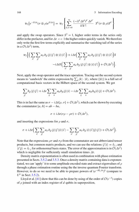
168 5 Information Encoding

tr2{e−iSΔt(σ ⊗ ρ)eiSΔt

} = tr2

⎧⎨

⎩

∞∑

k,k ′=0

(−i)kΔtk ik′Δtk

′

k!k ′! Sk(σ ⊗ ρ)Sk ′

⎫⎬

⎭

and apply the swap operators. Since S2 = 1, higher order terms in the series onlydiffer in the prefactor, and forΔt << 1 the higher orders quickly vanish.We thereforeonly write the first few terms explicitly and summarise the vanishing tail of the seriesin a O(Δt2) term,

tr2{(∑

ii′

∑

jj′aii′bjj′ |j〉〈j′| ⊗ |i〉〈i′|

)+ iΔt

(∑

ii′

∑

jj′aii′bjj′ |j〉〈j′| ⊗ |i〉〈i′|

)S

−iΔtS(∑

ii′

∑

jj′aii′bjj′ |j〉〈j′| ⊗ |i〉〈i′|

)+ O(Δt2)

}.

Next, apply the swap operator and the trace operation. Tracing out the second systemmeans to ‘sandwich’ the entire expression by

∑k〈k| · |k〉, where {|k〉} is a full set of

computational basis vectors in the Hilbert space of the second system. We get

∑

jj′bjj′ |j〉〈j′| + iΔt

∑

ij

∑

k

akibjk |j〉〈i| − iΔt∑

ij

∑

k

aikbkj|i〉〈j| + O(Δt2).

This is in fact the same asσ − iΔt[ρ,σ] + O(Δt2), which can be shown by executingthe commutator [a, b] = ab − ba,

σ + iΔt(σρ − ρσ) + O(Δt2),

and inserting the expressions for ρ and σ,

σ + iΔt(∑

ii′

∑

jj′aii′bjj′ |j〉〈j′||i〉〈i′| −

∑

ii′

∑

jj′aii′bjj′ |i〉〈i′||j〉〈j′|) + O(Δt2

).

Note that the expressions ρσ and σρ from the commutator are not abbreviated tensorproducts, but common matrix products, and we can use the relations 〈j′|i〉 = δj′,i and〈i′|j〉 = δi′,j for orthonormal basis states. The error of the approximation is inO(Δt2)which is negligible for sufficiently small simulation times Δt.

Density matrix exponentiation is often used in combination with phase estimationpresented in Sects. 3.5.2 and 3.5.3. Once a density matrix containing data is exponen-tiated, we can ‘apply’ it to some amplitude encoded state and extract eigenvalues of ρthrough a phase estimation routine using the the inverse quantum Fourier transform.However, to do so we need to be able to prepare powers of (e−iHρΔt)k (compare toUk in Sect. 3.5.2).

Lloyd et al. [41] show that this can be done by using of the order ofO(ε−3) copiesof ρ joined with an index register of d qubits in superposition,

5.4 Hamiltonian Encoding 169

2d∑

k=1

|k〉〈k| ⊗ σ ⊗ ρ(1) ⊗ . . . ⊗ ρ(2d ).

Instead of simulating a single swap operator, we now have to simulate a sequence of2-qubit swap operators, each of which swaps the first state σ with the gth copy of ρ.The swap operator sequences are entangled with an index register, so that for index|k〉 the sequence of swap operators runs up to copy ρ(k),

1

K

K∑

k=1

|kΔt〉〈kΔt| ⊗k∏

g=1

e−iSgΔt

After taking the trace over all copies of ρ, this effectively implements the evolution

K∑

k=1

|k〉〈k| ⊗ e−ikHρΔtσ eikHρΔt + O(Δt2),

which is precisely in the form required to apply the quantum Fourier transform. Fora proof, simply write out the expressions as seen above.

Density matrix exponentiation is qubit-efficient for low-rank matrices, given thatthe state ρ can be prepared qubit-efficiently. To see this, we first have to note thatthe desired accuracy is not necessarily a constant, but depends on the size of Hρ,especially when we are interested in the eigenvalues of ρ. For example, consider theeigenvalues are approximately uniform. Since trρ = 1, they are of the order of 1

N ifN is the number of diagonal elements or the dimension of the Hilbert space of ρ. Wecertainly want the error to be smaller than the eigenvalues themselves, which meansthat ε < 1

N . The number of copies needed for the density matrix exponentiation insuperposition hence grows with N 3, and since we have to apply swap operators toeach copies, the runtime grows accordingly.

As a consequence, density matrix exponentiation for phase estimation is onlypolynomial in the number of qubits or qubit-efficient if the eigenvalues of Hρ aredominated by a few large eigenvalues that do not require a small error to be resolved.In other words, the matrix has to be well approximable by a low-rank matrix. Fordesign matrices containing the dataset, this means that the data is highly redundant.

References

1. Aharonov, D., Ta-Shma, A.: Adiabatic quantum state generation and statistical zero knowledge.In: Proceedings of the Thirty-Fifth annual ACM Symposium on Theory of Computing, pp. 20–29. ACM (2003)

2. Schuld, M., Petruccione, F.: Quantum machine learning. In: C. Sammut, G.I. Webb (eds.)Encyclopaedia of Machine Learning and Data Mining. Springer (2016)

3. Ventura, D., Martinez, T.: Quantum associative memory. Inf. Sci. 124(1), 273–296 (2000)

170 5 Information Encoding

4. Trugenberger, C.A.: Probabilistic quantum memories. Phys. Rev. Lett. 87, 067901 (2001)5. Giovannetti, V., Lloyd, S., Maccone, L.: Quantum random access memory. Phys. Rev. Lett.

100(16), 160501 (2008)6. Raoux, S., Burr, G.W., Breitwisch, M.J., Rettner, C.T., Chen, Y.-C., Shelby, R.M., Salinga, M.,

Krebs, D., Chen, S.-H., Lung, H.-L., et al.: Phase-change random access memory: a scalabletechnology. IBM J. Res. Dev. 52(4.5):465–479 (2008)

7. Kyaw, T.H., Felicetti, S., Romero, G., Solano, E., Kwek, L.-C.: Scalable quantum memory inthe ultrastrong coupling regime. Sci. Rep. 5(8621) (2015)

8. Bennett, C.H.: Logical reversibility of computation. In: M. Demon (ed.) Entropy, Information,Computing, pp. 197–204 (1973)

9. Brown, L.D., Cai, T.T., DasGupta, A.: Interval estimation for a binomial proportion. Stat. Sci.101–117 (2001)

10. Wilson, E.B.: Probable inference, the law of succession, and statistical inference. J. Am. Stat.Assoc. 22(158), 209–212 (1927)

11. Aaronson, S.: Read the fine print. Nat. Phys. 11(4), 291–293 (2015)12. Kliesch, M., Barthel, T., Gogolin, C., Kastoryano, M., Eisert, J.: Dissipative quantum Church-

Turing theorem. Phys. Rev. Lett. 107(12), 120501 (2011)13. Knill, E.: Approximation by quantum circuits (1995). arXiv:quant-ph/950800614. Mikko, M., Vartiainen, J.J., Bergholm, V., Salomaa, M.M.: Quantum circuits for general mul-

tiqubit gates. Phys. Rev. Lett. 93(13), 130502 (2004)15. Vartiainen, J.J., Möttönen, M., Salomaa, M.M.: Efficient decomposition of quantum gates.

Phys. Rev. Lett. 92(17), 177902 (2004)16. Plesch, M., Brukner, C.: Quantum-state preparation with universal gate decompositions. Phys.

Rev. A 83(3), 032302 (2011)17. Iten, R., Colbeck, R., Kukuljan, I., Home, J., Christandl, M.: Quantum circuits for isometries.

Phys. Rev. A 93(3), 032318 (2016)18. Möttönen, M., Vartiainen, J.J., Bergholm, V., Salomaa, M.M.: Transformation of quantum

states using uniformly controlled rotations. Quantum Inf. Comput. 5(467) (2005)19. Grover, L., Rudolph,T.: Creating superpositions that correspond to efficiently integrable prob-

ability distributions (2002). arXiv:0208112v120. Kaye, P., Mosca, M.: Quantum networks for generating arbitrary quantum states. In: Proceed-

ings of the International Conference on Quantum Information, OSA Technical Digest Series,pp. PB28. ICQI (2001). arXiv:quant-ph/0407102v1

21. Soklakov, A.N., Schack, R.: Efficient state preparation for a register of quantum bits. Phys.Rev. A 73(1):012307 (2006)

22. Harrow, A.W., Hassidim, A., Lloyd, S.: Quantum algorithm for linear systems of equations.Phys. Rev. Lett. 103(15), 150502 (2009)

23. Rebentrost, P., Mohseni, M., Lloyd, S.: Quantum support vector machine for big data classifi-cation. Phys. Rev. Lett. 113, 130503 (2014)

24. Prakash, A.: Quantum Algorithms for Linear Algebra and Machine Learning. Ph.D thesis,EECS Department, University of California, Berkeley, Dec 2014

25. Wiebe, N., Braun, D., Lloyd, S.: Quantum algorithm for data fitting. Phys. Rev. Lett. 109(5),050505 (2012)

26. Zhao, Z., Fitzsimons, J.K., Fitzsimons, J.F.: Quantum assisted Gaussian process regression(2015). arXiv:1512.03929

27. Breuer, H.-P., Petruccione, F.: The Theory of Open Quantum Systems. Oxford University Press(2002)

28. Abrams, D.S., Lloyd, S.: Quantum algorithm providing exponential speed increase for findingeigenvalues and eigenvectors. Phys. Rev. Lett. 83(24), 5162 (1999)

29. Gisin, N.:Weinberg’s non-linear quantummechanics and supraluminal communications. Phys.Lett. A 143(1), 1–2 (1990)

30. Peres, A.: Nonlinear variants of Schrödinger’s equation violate the second law of thermody-namics. Phys. Rev. Lett. 63(10), 1114 (1989)

References 171

31. Meyer, D.A., Wong, T.G.: Nonlinear quantum search using the Gross-Pitaevskii equation. NewJ. Phys. 15(6), 063014 (2013)

32. Paetznick, A., Svore, K.M.: Repeat-until-success: Non-deterministic decomposition of single-qubit unitaries. Quantum Inf. Comput. 14, 1277–1301 (2013)

33. Andrieu, C., De Freitas, N., Doucet, A., Jordan, M.I.: An introduction to MCMC for machinelearning. Mach. Learn. 50(1–2):5–43 (2003)

34. Georgescu, I.M., Ashhab, S., Nori, F.: Quantum simulation. Rev. Mod. Phys. 86, 153–185(2014)

35. Lloyd, S.: Universal quantum simulators. Science 273(5278), 1073 (1996)36. Childs, A.M.: Quantum information processing in continuous time. Ph.D thesis, Massachusetts

Institute of Technology (2004)37. Berry, D.W., Ahokas, G., Cleve, R., Sanders, B.C.: Efficient quantum algorithms for simulating

sparse Hamiltonians. Commun. Math. Phys. 270(2), 359–371 (2007)38. Berry, D.W., Childs, A.M., Cleve, R., Kothari, R., Somma, R.D.: Exponential improvement

in precision for simulating sparse Hamiltonians. In: Proceedings of the 46th Annual ACMSymposium on Theory of Computing, pp. 283–292. ACM (2014)

39. Berry,D.W.,Childs,A.M.,Kothari,R.:Hamiltonian simulationwith nearly optimal dependenceon all parameters. In: IEEE 56th Annual Symposium on Foundations of Computer Science(FOCS), pp. 792–809. IEEE (2015)

40. Childs, A.M., Kothari, R.: Limitations on the simulation of non-sparse Hamiltonians. QuantumInf. Comput. 10(7), 669–684 (2010)

41. Lloyd, S., Mohseni, M., Rebentrost, P.: Quantum principal component analysis. Nat. Phys. 10,631–633 (2014)

Chapter 6Quantum Computing for Inference

After the discussion of classical-quantum interfaces, we are now ready to dive intotechniques that can bee used to construct quantum machine learning algorithms.As laid out in the introduction, there are two strategies to solve learning task withquantumcomputers. First, one can try to translate a classicalmachine learningmethodinto the language of quantum computing. The challenge here is to combine quantumroutines in a clever way so that the overall quantum algorithm reproduces the resultsof the classical model. The second strategy is more exploratory and creates newmodels that are tailor-made for the working principles of a quantum device. Here,the numerical analysis of the model performance can be much more important thantheoretical promises of asymptotic speedups. In the remaining chapters we will lookat methods that are useful for both approaches.

This chapter will focus on the first approach and present building blocks for quan-tum algorithms for inference, which we understand as algorithms that implement aninput-output map y = f (x) or a probability distribution p(y|x) of a machine learningmodel. We will introduce a number of techniques, tricks, subroutines and conceptsthat are commonly used as building blocks in different branches of the quantummachine learning literature. The techniques rely very much on the encoding method,and the language developed in the previous chapter will play an important role.

The next Chap.7 will look at training, or how to solve optimisation problems thattypically occur in machine learning with a quantum computer. Chapter 8 considersthe exploratory approach more closely and looks at genuine quantum models suchas Ising models, generic quantum circuits or quantum walks, and shows some firstattempts of how to turn these into machine learning algorithms.

6.1 Linear Models

A linear model, presented before in the contexts of linear regression (Sect. 2.4.1.1)and perceptrons (Sect. 2.4.2.1), is a parametrised model function mappingN -dimensional inputs x = (x1, ..., xN )T to K-dimensional outputs y = (y1, ..., yK )T .

© Springer Nature Switzerland AG 2018M. Schuld and F. Petruccione, Supervised Learning with Quantum Computers,Quantum Science and Technology, https://doi.org/10.1007/978-3-319-96424-9_6

173

174 6 Quantum Computing for Inference

The function is linear in a set of weight parameters that can be written as a K × N -dimensional weight matrix W ,

f (x;W ) = Wx. (6.1)

The output can be the multi-dimensional result of a regression task, or it can beinterpreted as a one-hot encoding to a multi-label classification task (see Sect. 2.1.2).Linear models also appear as linear layersof neural networks, i.e. a layer where theactivation function is the identity.

When the output is a scalar, we have that K = 1 and the linear model becomes aninner product between the input and a weight vector w = (w1, ..., wN )

T ,

f (x;w) = wT x + w0 = w0 + w1x1 + · · · + wNxN . (6.2)

As mentioned before, it is common to include the bias w0 in the inner productby extending the parameter vector to w = (w0, w1, ..., wN )

T and considering theextended input x = (1, x1, ..., xN )T , which is why we will mostly ignore it in theformalism.

In this section we present different strategies to implement a linear model with aquantum computer. First we look at models of the form (6.2) where the inputs arerepresented in amplitude encoding. The goal is to evaluate the inner product 〈ψw|ψx〉if theweights are likewise amplitude encoded, or 〈0|U (w)|ψx〉 if they define a unitaryevolution. Remember that we use |ψa〉 to denote the quantum state representing areal and normalised vector a in amplitude encoding, and thatU (w) is a parametrisedunitary circuit. We will show how a general quantum evolution can be interpretedas a certain type of the general linear model (6.1), and how one can concatenatequantum evolutions as linear layers of a neural network. We then present strategiesthat encode the weights as a unitary evolution, U (w)|x〉, but where the inputs arenow basis encoded. Lastly, we discuss how to add nonlinearities in the differentencodings.

6.1.1 Inner Products with Interference Circuits

A natural way to represent a scalar-valued linear model on a quantum computer isto encode the inputs x and parameters w in quantum state vectors via amplitudeencoding, |ψx〉, |ψw〉 (see Sects. 3.4.2, 5.2), and compute their inner product,

〈ψw|ψx〉 = f (x;w) = wT x.

Inner products of quantum states are a central feature in quantum theory, where theterms ‘ket’ and ‘bra’ originate from “braket”, 〈·|·〉, which is the mathematical symbol

6.1 Linear Models 175

of an inner product. However, while playing a prominent role in the mathematicaldescription of quantum theory, it is actually not trivial to measure the inner productbetween two quantum states. There is a family of small quantum circuits that useinterference between different branches of a superposition to fulfil this task [1]. Themost well-known of the inner product interference routines is the so called swap testand returns the absolute value of the inner product of two separate quantum states.

6.1.1.1 The Swap Test

Weconsider twoqubit registers in the respective quantumstates |ψa〉, |ψb〉 that encodethe real vectors a and b. The swap test is a common trick to ‘write’ the absolute squareof their inner product, |〈ψa|ψb〉|2, into the probability of measuring an ancilla qubitin a certain state. To achieve this, one creates a superposition of the ancilla qubit andswaps the quantum states in one branch of the superposition, after which they areinterfered (see Fig. 6.1).

Starting with a state |0〉|ψa〉|ψb〉, a Hadamard on the ancilla—the qubit in the firstregister—leads to

1√2(|0〉 + |1〉)|ψa〉|ψb〉.

We now apply a swap operator on the two registers |ψa〉, |ψb〉 which is conditionedon the ancilla being in state 1. This operation swaps the states |ψa〉|ψb〉 → |ψb〉|ψa〉in the branch marked by the first qubit being in state 1,

1√2(|0〉|ψa〉|ψb〉 + |1〉|ψa〉|ψb〉).

Another Hadamard applied to the ancilla results in the state

|ψ〉 = 1

2|0〉 ⊗ (|ψa〉|ψb〉 + |ψb〉|ψa〉) + 1

2|1〉 ⊗ (|ψa〉|ψb〉 − |ψb〉|ψa〉) .

This computes two branches of a superposition, one containing a sum between the‘unswapped’ and ‘swapped’ states of the two registers, and the other containing their

Fig. 6.1 Schematic illustration of the swap test routine. An ancilla qubit in state 0 is preparedtogether with two quantum states (turquois and red shapes). The ancilla is superposed and the twostates are swapped in the branch marked by the ancilla’s 1 state. The ancilla is then interfered,writing the sum and difference of the original and the swapped order into each branch

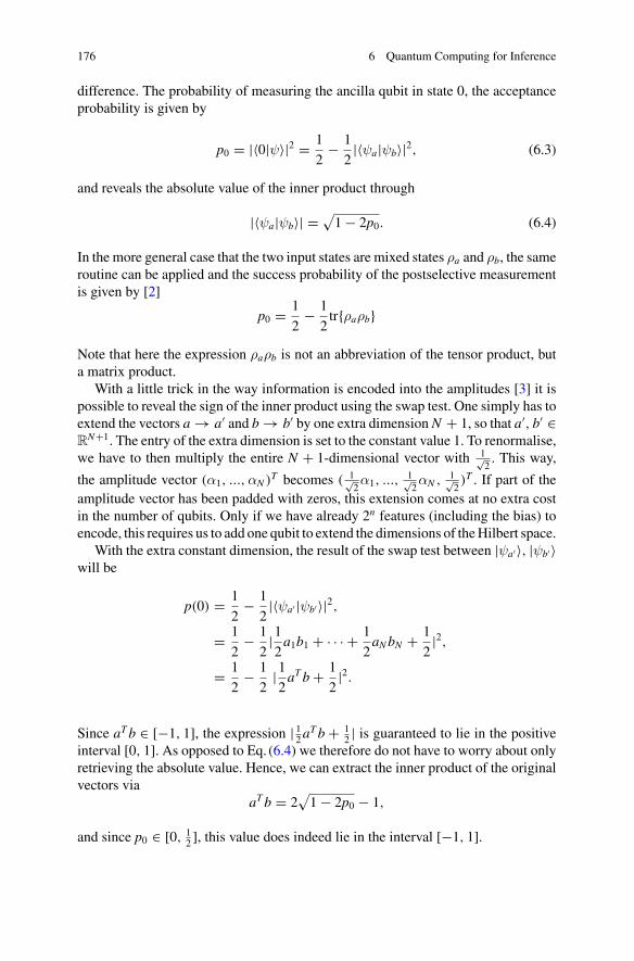
176 6 Quantum Computing for Inference

difference. The probability of measuring the ancilla qubit in state 0, the acceptanceprobability is given by

p0 = |〈0|ψ〉|2 = 1

2− 1

2|〈ψa|ψb〉|2, (6.3)

and reveals the absolute value of the inner product through

|〈ψa|ψb〉| = √1 − 2p0. (6.4)

In the more general case that the two input states are mixed states ρa and ρb, the sameroutine can be applied and the success probability of the postselective measurementis given by [2]

p0 = 1

2− 1

2tr{ρaρb}

Note that here the expression ρaρb is not an abbreviation of the tensor product, buta matrix product.

With a little trick in the way information is encoded into the amplitudes [3] it ispossible to reveal the sign of the inner product using the swap test. One simply has toextend the vectors a → a′ and b → b′ by one extra dimension N + 1, so that a′, b′ ∈R

N+1. The entry of the extra dimension is set to the constant value 1. To renormalise,we have to then multiply the entire N + 1-dimensional vector with 1√

2. This way,

the amplitude vector (α1, ...,αN )T becomes ( 1√

2α1, ...,

1√2αN ,

1√2)T . If part of the

amplitude vector has been padded with zeros, this extension comes at no extra costin the number of qubits. Only if we have already 2n features (including the bias) toencode, this requires us to add one qubit to extend the dimensions of theHilbert space.

With the extra constant dimension, the result of the swap test between |ψa′ 〉, |ψb′ 〉will be

p(0) = 1

2− 1

2|〈ψa′ |ψb′ 〉|2,

= 1

2− 1

2|12a1b1 + · · · + 1

2aNbN + 1

2|2,

= 1

2− 1

2|12aTb + 1

2|2.

Since aTb ∈ [−1, 1], the expression | 12aTb + 12 | is guaranteed to lie in the positive

interval [0, 1]. As opposed to Eq. (6.4) we therefore do not have to worry about onlyretrieving the absolute value. Hence, we can extract the inner product of the originalvectors via

aTb = 2√1 − 2p0 − 1,

and since p0 ∈ [0, 12 ], this value does indeed lie in the interval [−1, 1].

6.1 Linear Models 177

6.1.1.2 Interference Circuit

There is another, slightlymore elegant routine to extract inner products, but it requiresmore sophisticated state preparation. First, let us note that for unit vectors there is aclose relationship between the vector sum and the inner product: Given two real unitvectors a, bwhose inner product one wishes to compute (with |a|2 = |b|2 = 1), then

(a + b)T (a + b) =∑

i

(ai + bi)2

=∑

i

a2i +∑

i

b2i + 2∑

i

aibi

= 2 + 2aTb.

A geometric illustration is given in Fig. 6.2.This fact has implicitly been used in the swap test routine, and helps to evaluate

the inner product of two quantum states together with the correct sign without trickslike the constant shift introduced above. As a precondition, we need to be able toprepare the initial state

|ψ〉 = 1√2(|0〉|ψa〉 + |1〉|ψb〉) . (6.5)

Note that in comparison with the swap test routine, here there is a superposition ofstates |ψa〉, |ψb〉 in one register, as opposed to each state having its own register (seeFig. 6.3). In the standard computational basis, quantum state (6.5) corresponds to anamplitude vector

α = (a1, ..., aN , b1, ..., bN )T .

If we have a routineA to prepare |ψa〉 and another routine B to prepare |ψb〉, one hasto implement these routines conditioned on the respective states of the ancilla qubitprepared in |+〉 = 1√

2(|0〉 + |1〉).

a + ba

b

a + b

a

ba + b

ab

Fig. 6.2 Geometric illustration showing the relation between inner products of two normalisedvectors a and b with their sum. The sum of parallel normalised vectors is at the maximum value,while the sum of antiparallel vectors is zero. This is exploited in the interference circuits introducesin this section

178 6 Quantum Computing for Inference

Fig. 6.3 Schematic illustration of the interference routine for the calculation of inner products. Thetwo states (blue and red shape) are initially entangled with the 0 and 1 state of an ancilla. Interferingthe two branches through a Hadamard gate applied to the ancilla writes the sum and difference ofthe two states into each branch

Once state (6.5) is prepared, a Hadamard gate on the ancilla will result in

|ψ〉 = 1

2|0〉 ⊗ (|ψa〉 + |ψb〉) + 1

2|1〉 ⊗ (|ψa〉 − |ψb〉).

Formally speaking, the ancilla state |0〉 is entangled to an unnormalised quantumstate |ψa+b〉 that encodes the sum of a and b via amplitude encoding. The acceptanceprobability p(0) = |〈0|ψ〉|2 of the ancilla being measured in state 0 is given by

p(0) = 1

4〈ψa+b|ψa+b〉,

= 1

4(2 + aTb),

= 1

2+ 1

2aTb.

This time, there is no absolute value that obscures the sign of the result.If a and b are complex vectors (for example, the result of a unitary evolution), the

interference routine reveals only the real part of the inner product,

p(0) = 1

4(2 +

∑

i

a∗i bi +

∑

i

a∗i bi),

= 1

2+ 1

2Re{a†b}.

This is not surprising, because ameasurement always results in a real value, otherwiseit would be unphysical.

Besides state preparation, evaluating the inner product on a quantum computerrequires only one additional qubit and a number of gates that is at most linear inthe number of qubits (and hence qubit-efficient, or logarithmic in the feature spacedimension). The number of measurements grows with the desired precision (seeSect. 5.1.3). If weights and inputs are encoded in the amplitudes of the same register,we can even reduce this to a single Hadamard operation plus measurements, withoutthe need for an extra qubit.

6.1 Linear Models 179

6.1.2 A Quantum Circuit as a Linear Model

We still assume that the inputs are given in amplitude encoding, |ψx〉, but now lookat the case where the model parameters w are “dynamically encoded” in a unitary,or more general, in a quantum circuit.

6.1.2.1 Unitary Linear Model

Rather trivially, a linear unitary transformation can be interpreted as a special linearmodel,

|ψx′ 〉 = U |ψx〉,

that maps a N -dimensional complex vector onto a N -dimensional complex vector. Ifwe want to get a scalar output, we still need to sum up the elements of x′. An elegantway to do this is to compute the inner product of the final state with a uniformdistribution |ψu〉 = 1√

N

∑i |i〉, which would effectively implement the model

f (x; θ) = 〈ψu|U |ψx〉,= 1√

N(u11 + · · · + uN1)

︸ ︷︷ ︸w1

x1 + · · · + 1√N(uN1 + · · · + uNN )

︸ ︷︷ ︸wN

xN ,

= w1x1 + · · · + wNxN .

If we summarise the coefficients 1√N(u1i + · · · + uNi) aswi, i = 1, ...,N , like shown

above, this is the original linear function from Eq. (6.2). From a geometrical per-spective, the output is represented by a measure of ‘uniformness’ of the stateU |ψx〉,or the overlap with the uniform superposition. Of course, this is just another wayto formulate the idea in the previous section: If we write |ψw〉 = U †|ψu〉 we canunderstand the unitary as a state preparation routine for the parameter quantum statefrom before. Training the model with data means to find a circuit or unitary evolutionU that captures the input-output relation from the data.

6.1.2.2 Non-unitary Linear Model

An interesting twist appears when we look at linear models that map from RN to a

lower-dimensional vector space RK , K < N to implement the layer of a neural netas in Eq. (6.1). If we want to allow for arbitrary concatenation of linear layers, theinput encoding of the quantum algorithm has to be of the same type as the outputencoding, which is not the case for the interference routines above. If we also want toreduce the dimensionality in the map, we have to consider a subsystem of the qubits

180 6 Quantum Computing for Inference

as the output of the evolution (see also [4]). This forces us to use the language ofdensity matrices which was introduced in Sect. 3.1.2.3.

Consider a densitymatrix ρx that encodes an input x on its diagonal, i.e. diag{ρx} =(x1, ..., xN )T . For example, we could encode the square roots of the features xi,i = 1, ...,N in amplitude encoding in a n = logN qubit quantum system, |ψ√

x〉 =∑i√xi|i〉, and computing the density matrix of this pure state, ρx = |ψ√

x〉〈ψ√x|

results in the desired encoding. A unitary evolution in this language is formallywritten as

ρx′ = UρxU†.

From here, we trace out the first 1, ..., n − k of the n qubits so that we end up withonly the last k qubits, reducing the Hilbert space from N = log n dimensions toK = log k dimensions. This yields the “hidden layer density matrix”

ρh = tr1,...,n−k{ρx′ }.

Weare not restricted to reducing the dimension: Adding qubits ρh ⊗ |0 . . . 0〉〈0 . . . 0|,and extending the further evolution to these new qubits can increase the dimensionof the Hilbert space again.

Figure6.4 shows an example of unitary evolutions, system reductions and exten-sions in the graphical representation of neural networks, where the diagonal of thedensitymatrix at any given point of the evolution is interpreted as a layer of ‘neurons’.Initially the quantum system consists of three qubits

|in〉〈in| = |q1, q2, q3〉〈q1, q2, q3|.

|in〉〈in|

|h1〉〈h1|

|h〉〈h|

|h2〉〈h2|

|out〉〈out|

Fig. 6.4 Formally, performing unitary transformations, tracing qubits out and joining qubits corre-sponds to a neural network structure. The layers correspond to the diagonal of the according densitymatrix. Shown here is the evolution described in the text

6.1 Linear Models 181

A unitary evolution applies a linear transformation that leads to an intermediate layer,

|h1〉〈h1| = U1|in〉〈in|U †1 .

Tracing out the first qubit yields the hidden layer,

|h〉〈h| = tr1{|h1〉〈h1|},

and joining a qubit in the ground state,

|h2〉〈h2| = |h2〉〈h2| ⊗ |q4 = 0〉〈q4 = 0|.

creates a quantum state whose density matrix has again 8 diagonal elements, but 4of them have a probability zero (i.e., those corresponding with the last qubit being instate 1, which it is obviously not). This density matrix can be interpreted as a secondintermediate layer. Another full unitary on qubits q2, q3, q4 generates a quantum statethat represents the ‘output layer’,

|out〉〈out| = U2|h2〉〈h2|U †2 .

The decision which qubit is traced out defines the connectivity between a bigger anda smaller layer.

Example 6.1 For n = 2 and the ‘input’ density matrix

ρx =

⎛

⎜⎜⎝

a11 a12 a13 a14a21 a22 a23 a24a31 a32 a33 a34a41 a42 a43 a44

⎞

⎟⎟⎠ ,

tracing out the first or second qubit results respectively in

tr1ρx =(a11 + a33 a12 + a34a21 + a43 a22 + a44

), tr2ρx =

(a11 + a22 a13 + a24a31 + a42 a33 + a44

).

Tracing out the first qubit consequently adds inputs 1, 3 and 2, 4 to define the twounits of the following layer, while tracing out the second qubit adds inputs 1, 2and 3, 4.

Note that in general the first trace operation turns the pure state (full information onthe state) into a mixed state (we lost the information about some qubits). The traceoperation maintains the linearity, but now the full evolution of a linear layer is nolonger described by a unitary operator.

182 6 Quantum Computing for Inference

6.1.3 Linear Models in Basis Encoding

We now tend to the case that inputs and outputs of the linear model are basis encoded.Implementing the model requires us to find a quantum circuit U (w) that takes thestate |x〉|0...0〉 to |x〉|wT x〉, where the result of the linear model is written into thequbits of the second register.

There are many different ways to achieve this transformation, and as an exam-ple we will present an idea based on the quantum phase estimation algorithm fromSect. 3.5.2. It first constructs an evolutionU (w)|x〉|j〉 = e2πi(j−1)wT x|x〉|j〉, fromwhichquantum phase estimation can write the phase wT x into the second quantum regis-ter [5].

Consider a state|x1...xN 〉|0...0〉, (6.6)

where the second register contains ν qubits in the ground state (ν is a hyperparameterthat determines the precision of the output). The first step is to put the second registerinto a uniform superposition by using Hadamards on each of its qubits, leadingto 1√

2ν

∑2ν

j=1 |x1, ..., xN 〉|j〉. The circuit with the desired eigenvalue for eigenstate|x1, ..., xN 〉 can be constructed by using a sequence k = 1, ...,N of parametrisedsingle qubit gatesUk(wk) acting on the kth qubit of the input register. The gates havethe form of an S gate from Table3.3 but with a variable phase defined by wk ,

Uk(wk) =(1 00 e2πiwk

).

The full circuit reads

U (w) = Un(wn)...U2(w2)U1(w1)U0(w0).

The “bias gate” U0 adds a global phase of 2πiw0, where w0 is a real bias parameterin [0, 1). Altogether, applying this circuit to the initial state results in

U (w)|x1, ..., xN 〉|0...0〉 = e2πiwT x|x1, ..., xN 〉|0...0〉.

For phase estimation, we need an oracle O that can apply powers of U (w),

|x〉|j〉 O−→ U (w)j−1|x〉|j〉,

for j = 1...2ν . Remember that we defined |j〉 to be the jth computational basis state,and since wewant |0...0〉 to produceU (w)0, we have to use j − 1 in the exponent. Forsufficiently small ν, this can always be constructed by applying U (w) conditionedon the qubits of the index register. For example, if the last qubit is in 1, apply U (w)

once, if the second last qubit is also in 1, apply U (w) twice more, and if the kth lastqubit is in 1 apply U (w) 2k−1 times more.

6.1 Linear Models 183

With help of such an oracle we can prepare a state

1√2ν

2ν∑

j=1

|x1, ..., xN 〉e2πi(j−1)wT x|j〉.

The quantum phase estimation routine (introduced in Sect. 3.5.2) applies an inversequantum Fourier transform, and if wT x ≈ (j − 1)/2ν for a particular integer j, thisapproximately results in a quantum state |x〉|wT x〉 that represents the “phase”wT x inbasis encoding. For cases wT x �= (j − 1)/2ν it can be shown that in order to obtainwT x accurately up to νacc bits of precisionwith a success probability of 1 − ε, one hasto choose ν = νacc + �log (2 + 1

2ε ) [6]. SincewT x ∈ [0, 1), The qubits q1, ..., qν ofregister |wT x〉 represent the phase via the relationship

wT x ≈ q11

20+ . . . + qν

1

2ν−1.

The computational complexity of this routine with regards to N (the number offeatures) and τ (the number of bits to represent each feature) is inO(Nτ ), comparableto the classical linear model. The dependency on the number of output qubits orprecision hyperparameter ν is slightly more difficult. After ν Hadamards, the oracleto implement powers of U (w) in the most naive form presented above needs to becalledO(

∑2ν−1

i=0 i) times. The inverse quantumFourier transform requires ν(ν+1)2 + 3 ν

2gates [6]. We will see below that when implementing a step function on the result toextend this routine to a perceptron model, we are only interested in the value of thefirst qubit, and ν is therefore sufficiently small.

Linear models in basis encoding such as the example presented here open up acouple of interesting avenues. For example, one can process training sets in superpo-sition by starting with the state

∑Mm=1 |xm〉 instead of |x〉, so that the entire procedure

gets applied in parallel. The result would likewise be a superposition of outputs.From measurements on the output register one can retrieve the accuracy or successrate on an entire dataset in parallel.

6.1.4 Nonlinear Activations

Alinearmodel is not verypowerfulwhen it comes to data that is not linearly separable.We therefore need nonlinearities in the model function. To focus the discussion, wewill look at how to introduce nonlinearities from the perspective of neural networkswhere they enter as nonlinear activation functions ϕ mapping a net input v to ϕ(v).However, the observations can be used in other contexts as well.

184 6 Quantum Computing for Inference

6.1.4.1 Amplitude Encoding

In terms of amplitude encoding, applying an activation function to a layer means toimplement the map |ψv〉 → |ψϕ(v)〉 for a vector or scalar v, an operation that cannotbe achieved by a standard unitary quantum evolution. This has been discussed inSect. 5.2, where it was illustrated why nonlinear transformations of amplitudes arevery likely to be unphysical. However, as we mentioned there is one element inquantum theory that allows for nonlinear updates of the amplitudes: measurement.Measurement outcomes are non-deterministic, and we have seen in Sect. 5.2.2.3 howto make them deterministic by using branch selection. For example, we could storethe net input v temporarily in basis encoding and use the trick of conditional rotationof an ancilla to prepare a state

|ψ〉|0〉|v〉 → |ψ〉(ϕ(v)|0〉 +

√1 − ϕ(v)2|1〉

)|v〉,

where during the conditional rotation of the ancilla we also applied a function ϕ.From here, branch selectionwould lead to a state proportional toϕ(v)|ψ〉|v〉where—depending on the implementation—we could try and invert the storage operation toget rid of the last register. This is a costly detour, and it is therefore questionableif amplitude encoding is suitable for the implementation of feed-forward neuralnetworks. In the next section we will look at an alternative strategy to give amplitudeencoding more power, namely through so called kernel methods.

6.1.4.2 Basis Encoding

In basis encoding, nonlinear transformations of the form |v〉|0〉 → |v〉|ϕ(v)〉 canbe implemented deterministically. As mentioned in Sect. 5.1.2 one can always takea classical algorithm to compute ϕ on the level of logical gates, translate it into areversible routine and use this as a quantum algorithm.Depending on the desired non-linearity, there may be much more efficient options. As three illustrative examples,we consider popular nonlinear functions used as activations in neural networks, thestep function, as well as rectified linear units and a sigmoid function (see Fig. 2.18).

For simplicity, we will fix the details of the binary representation and considerfixed point arithmetic. The real scalar v is represented by a (1 + τl + τr)-bit binarysequence

bsbτl−1 · · · b1b0.b−1b−2 · · · b−τr . (6.7)

The first bit bs indicates the sign, and τl, τr are the numbers of bits left and right ofthe decimal dot (called integer and fractional bits). A real number can be retrievedfrom the bit string via

v = (−1)bs(bτl−12τl−1 + · · · + b02

0 + b−12−1 + b−22

−2 + · · · + b−τr2−τr ).

6.1 Linear Models 185

For example, the binary sequence 111.101 with τl = 2 and τr = 3 corresponds tothe real number (−1)(2 + 1 + 0.5 + 0.125) = −3.625.

A step function defined as

ϕ(v) ={0, if v ≤ 0,

1, else,

is most trivial to implement in this representation [5], and one does not even requirean extra output register to encode the result. Instead, the sign qubit of the inputregister can be interpreted as the output, and the step function is implemented by the‘effective map’ |v〉 = |bsbτl−1...〉 → |bs〉.

Also rectified linear units,

ϕ(v) ={0, if v ≥ 0,

v, else,

are simple to realise. Conditioned on the sign (qu)bit bs, either copy the input registerinto the output register, or do nothing. This requires a sequence of NOT gates, eachcontrolled by |bs〉 as well as |bk〉 for k = τl − 1, ..., 0, ...,−τr . The NOT is appliedto the k’th qubit of the output register.

The sigmoid nonlinearity,

ϕ(v; δ) = 1

1 + e−δv,

poses a bigger challenge. An implementation via division and exponential functionis rather demanding in terms of the number of elementary operations as well as thespacial resources. There are a number of more efficient approximationmethods, suchas piecewise linear approximation [7]. If the overall precision (i.e. the number of bitsto represent a real number) is not very high, one can write down a boolean functionthat reproduces the sigmoid function for binary numbers explicitly. This means todefine the binary representation of ϕ(v) for every possible binary representation ofthe input v. For example, if the input is v = −3.625 with the above binary represen-tation 111.101, the output of the sigmoid function, ϕ(v, δ = 0.1) = 0.410355..., isapproximated by the bitstring 000.011.

Of course, this approach would mean to store a look-up-table of possible inputsand their outputs, whose size grows exponentially with the precision. However,there are optimisation methods to reduce the size of the look-up table significantly,such as Quine-McCluskey [8, 9] methods, whose idea is sketched in the followingexample.

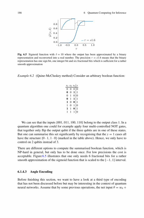
186 6 Quantum Computing for Inference

Fig. 6.5 Sigmoid function with δ = 10 where the output has been approximated by a binaryrepresentation and reconverted into a real number. The precision τ = s1.6 means that the binaryrepresentation has one sign bit, one integer bit and six fractional bits which is sufficient for a rathersmooth approximation

Example 6.2 (Quine-McCluskey method) Consider an arbitrary boolean function:

x1 x2 x3 y0 0 0 00 0 1 10 1 0 00 1 1 11 0 0 11 0 1 01 1 0 11 1 1 0

We can see that the inputs {001, 011, 100, 110} belong to the output class 1. In aquantum algorithm one could for example apply four multi-controlled NOT gates,that together only flip the output qubit if the three qubits are in one of these states.But one can summarise this set significantly by recognising that the y = 1 cases allhave the structure {0 · 1, 1 · 0} (marked in the table above). Hence, we only have tocontrol on 2 qubits instead of 3.

There are different options to compute the summarised boolean function, which isNP-hard in general, but only has to be done once. For low precisions the cost isacceptable. Figure6.5 illustrates that one only needs 6 fractional bits for a rathersmooth approximation of the sigmoid function that is scaled to the [−1, 1] interval.

6.1.4.3 Angle Encoding

Before finishing this section, we want to have a look at a third type of encodingthat has not been discussed before but may be interesting in the context of quantumneural networks. Assume that by some previous operations, the net input θ = w0 +

6.1 Linear Models 187

Fig. 6.6 A y-rotation Ry(v)

rotates the Bloch vector byan angle v around the y axis(that is, in the x-z-plane)

w1x1 + ... + wNxN is written into the angle of an ancilla or “net input qubit”, whichis entangled with an output qubit in some arbitrary state |ψ〉,

Ry(2v)|0〉 ⊗ |ψ〉out.

As a reminder, the rotation around the y axis is defined as

Ry(2v) =(cos v − sin vsin v cos v

).

The net input qubit is hence rotated around the y axis by an angle v (see Fig. 6.6),and Ry(2v)|0〉 = cos v|0〉 + sin v|1〉.1 The goal is now to rotate the output qubit bya nonlinear activation ϕ which depends on v, in other words, we want to prepare theoutput qubit in state Ry(2ϕ(v))|ψ〉.

An elegant way to accomplish this task has been introduced by Cao et al. [11] forthe sigmoid-like function ϕ(v) = arctan(tan2(v)) by using so called repeat-until-success circuits [12, 13]. As mentioned briefly in Sect. 5.2.3, repeat-until-successcircuits apply an evolution to ancillas and an output qubit, and measuring the ancillain state 0 leads to the desired state of the output qubit, while when measuring state1, one can reset the circuit by a simple procedure and apply the evolution oncemore. This is repeated until finally the ancilla is measured in 0. In contrast to branchselection or postselective measurements, we do not have to repeat the entire routineup to the evolution in questionwhen the undesired result wasmeasured for the ancilla.

Let us have a closer look at the simplified circuit in Fig. 6.7 to understand the basicprinciple of the angle encoded activation function.2 The first gate writes the net inputinto the angle of the ‘net input qubit’ as explained above. The second, conditionalgate results in the state

1Such an angle encoded qubit has been called a quron [10] in the context of quantum neuralnetworks.2Thanks to Gian Giacomo Guerreschi for this simplified presentation.

188 6 Quantum Computing for Inference

|0〉 Ry(2v) • Rz(− π2 ) R†

y(2v)

|ψ〉out −iY

Fig. 6.7 Repeat-until-success circuit that turns the output qubit by a sigmoid-like activation functiondepending on the net input v encoded in the net qubit

Ry(2v)|0〉 ⊗ |ψ〉out − sin(v)|1〉 ⊗ (1 + iY )|ψ〉out.

The third gate reverses the net input encoding step. Note that R†y(2v) = Ry(−2v).

Due to the conditional evolution of the second gate, this leads to interference effectsand yields

= |0〉|ψ〉out − sin(v) (sin(v)|0〉 + cos(v)|1〉) ⊗ (1 + iY )|ψ〉out= |0〉 (

1 − sin2(v)1 − i sin2(v)Y )) |ψ〉out − |1〉 sin(v) cos(v)(1 + iY )|ψ〉out

= |0〉 (cos2(v)1 − i sin2(v)Y )

) |ψ〉out − |1〉 sin(v) cos(v)(1 + iY )|ψ〉out.

If we measure the net input qubit in state |0〉 we have to renormalise by a factor(cos4(v) + sin4(v))− 1

2 and get the desired result

cos2(v)1 − i sin2(v)Y√cos4(v) + sin4(v)

= Ry(2ϕ(v)).

Else, if the measurement returns 1, we get the state 1√2(1 + iY )|ψ〉out. Note that here

the measurement induces a renormalisation factor (sin(v) cos(v))−1 which cancelsthe dependence on v out. We therefore simply have to reverse the constant operation1√2(1 + iY ) and can try again.This basic idea can be extended to perceptron models and feed-forward neural

networks for which the value of a neuron is encoded in the angles as described above[11]. Of course, the non-deterministic nature of repeat-until-success circuits impliesthat the runtime is on average slightly longer than the feed-forward pass in a classicalneural network, since we have to repeat parts of the algorithm in case of unsuccessfulmeasurement outcomes. Still, the proposal is an interesting realisation of a nonlinearactivation function in the context of quantum computing.

6.2 Kernel Methods

Section6.1.4 demonstrated thatwhile there is awealth ofmethods to implement linearmodels, nonlinearities can be a lot trickier, especially when it comes to amplitudeencoding. In Sect. 2.2.4 of the introduction to machine learning another strategy has

6.2 Kernel Methods 189

Fig. 6.8 Kernelmethods compute the distance between data point x and x′ through a kernelκ(x, x′).For every positive definite kernel there is a feature space F produced by mapping inputs with anonlinear map ϕ(x), so that the kernel of two inputs is equal to the inner product of their featuremapped versions, κ(x, x′) = 〈ϕ(x)|ϕ(x′)〉

been already revealed to give linear models more power: feature spaces, based onthe theory of kernel methods. We will show in this section that feature spaces andquantumHilbert spaces have a surprisingly similar mathematical formalism and howthis can be used for quantum machine learning. More details can be found in [14].

To recapitulate the highlights from Sect. 2.2.4, one can understand a (positivesemi-definite) kernel as a distance measure on the input space, and use it to computethe distance between each training input and the new input we aim to classify, andfavour the class of “closer” training data when the decision for the prediction istaken. Such a kernel corresponds to an inner product of data points mapped to ahigher dimensional feature space (see Fig. 6.8). The representer theorem shows howa large class of trainedmodels can be expressed in terms of kernels. Finally, the kerneltrick allows us to construct a variety ofmodels that are formulated in terms of a kernelfunction by replacing it with another kernel function. The following Sect. 6.2.1 willreview these concepts once more with slightly more mathematical foundation, afterwhich we show how to understand state preparation and information encoding as a‘quantum feature map’ (Sect. 6.2.3). Finally, we discuss how to compute kernels ordistance measures on input space on a quantum computer (Sect. 6.2.4) and show howto construct density matrices that correspond to a kernel Gram matrix (Sect. 6.2.5).

6.2.1 Kernels and Feature Maps

Let us revisit some concepts from Sect. 2.2.4, following the textbook of Schölkopfand Smola [15]. Let X be a non-empty set of patterns or inputs. As a reminder, a(positive semi-definite) kernel was defined as a map κ : X × X → C where for anysubset of the input set x1, ..., xM ∈ X withM ≥ 2 the Gram matrix with entries

Kij = κ(xi, xj)

190 6 Quantum Computing for Inference

is positive definite. Kernels fulfil κ(x, x) ≥ 0 and κ(x, x′) = κ(x′, x)∗ where the starmarks the complex conjugate.

We can always construct a feature map from a kernel. A feature map was intro-duced before as a map φ : X → F from the input space into a feature space. Previ-ously we looked at some examples where the feature space was a real vector spaceR

K with K > N , for example the map from (x1, x2)T to (x1, x2, x21 + x22)T . It turns

out a feature space can be formalised much more generally as we will see now.The feature map that can always be constructed from a kernel κ (sometimes called

the “canonical feature map”) maps from the input set to complex-valued functionson the input set,

φ : X → CX , x → κ(·, x). (6.8)

Here, the feature vectors in CX are themselves functions that map from the input

space to the space of complex numbers X → C. The functions in feature space arekernels with one “open slot”.

From this feature map we can construct a feature space that is a vector space withan inner product (see [15, 16]). The vector space contains linear combinations of{κ(·, xm)}, where {x1, ..., xM } ⊆ X is an arbitrary set of inputs,

f (·) =M∑

m=1

νmκ(·, xm),

with coefficients νm ∈ R. Using a second vector of the same form,

g(·) =M ′∑

m′=1

μm′κ(·, xm′),

the inner product can be defined as

〈f , g〉 =M∑

m=1

M ′∑

m′=1

ν∗mμm′κ(xm, xm′).

With this inner product, the feature map has the property

〈φ(x)|φ(x′)〉 = 〈κ(·, x),κ(·, x′)〉 = κ(x, x′).

Read from right to left, this relationship is a core idea of the theory of kernel meth-ods which we introduced before: A kernel of two inputs x and x′ computes the innerproduct of the same inputs mapped to a feature space. As a mere technicality in thiscontext, one can extend the inner product vector space by the norm ||f || = √〈·, ·〉and the limit points of Cauchy series under this norm, and get a Hilbert space calledthe Reproducing Kernel Hilbert Space.

6.2 Kernel Methods 191

One can also argue vice versa and construct a kernel from a vector space with aninner product. It follows from the above that given a mapping φ : X → H, whereHis a Hilbert space with vectors φ(x), one can define a kernel via

κ(x, x′) = 〈φ(x),φ(x′)〉.

To see why the resulting kernel is indeed positive semi-definite as requested in thedefinition, consider some patterns x1, ..., xM ∈ X . Then for arbitrary cm, cm′ ∈ C,

M∑

m,m′=1

cmc∗m′κ(xm, xm′) = 〈

∑

m

cmφ(xm),∑

m′cm′φ(xm′)〉

= ||∑

m

cmφ(xm)||2 ≥ 0

The first equality sign is due to the bi-linearity of the inner product, while the inequal-ity sign follows from the properties of a squared norm.

6.2.2 The Representer Theorem

Kernel methods use models for machine learning that are based on kernel functionsthat measure distances between data inputs. They have been popular in the 1990s,before neural networks became again the center of interest of mainstream machinelearning research. However, they are not simply a specific ansatz for a model. Thewide scope of kernel methods is revealed by the representer theorem introduced inSect. 2.2.4. Also here we want to go into slightly more detail in order to motivatekernelmethods as a rather general framework. This can also show away of translatinga range on models into a “kernelised” version.

Consider an input domain X , a kernel κ : X × X → R, a data set D consistingof data pairs (xm, ym) ∈ X × R and a class of model functions f : X → R that canbe written in the form

f (x) =∞∑

l=1

μlκ(x, xl), (6.9)

with x, xl ∈ X , μl ∈ R and ||f || < ∞. (The norm is taken from the ReproducingKernel Hilbert Space associated with κ). Furthermore, assume a cost function C :D → R that quantifies the quality of a model by comparing predicted outputs f (xm)with targets ym, and which has a regularisation term of the form g(||f ||) whereg : [0,∞) → R is a strictlymonotonically increasing function. For example,C could

192 6 Quantum Computing for Inference

be a least squares loss with a l1 regularisation. The representer theorem says that anyfunction f minimising the cost function C can be written as

f (x) =M∑

m=1

νmκ(x, xm). (6.10)

Note that the model function (6.9) from the feature space is expressed by an infinitesum,while expression (6.10) is formulated in termsof kernels over the (finite) traininginputs xm.3 In short, a large class of typical machine learning problems can be solvedby a model that is an expansion over kernels of training data. And although wederived it in a different fashion, the inference model for support vector machines inEq. (2.39) had exactly this form (associating νm with the Lagrange parameters timesthe target outputs).

The following example shows how one can use the representer theorem to turn asimple linear model into its ‘kernelised’ version.

Example 6.3 (Kernelised linear model) Take a standard linear model functionf (x) = wT x. This is of the required form in Eq. (6.9) if we chooseX = R

N , μl = wl

for l = 1...N and μl = 0 for l > N , as well as xl = el to be the standard basis and κto be an inner product kernel:

∞∑

l=1

μlκ(x, xi) =N∑

i=1

wi xT ei = wT x.

Considering a square loss objective with l1 regularisation and g(||f ||) = ||f || with astandard norm, we can apply the representer theorem. According to the theorem, theoptimal linear model with regards to the objective can be expressed as

f (x) =∑

m

νmκ(x, xm).

If we choose κ(x, xm) = xT xm (a linear kernel), this means that the weight vector haseffectively been expanded in terms of the training inputs, w = ∑

m νmxm. In short,the optimal weight vector lies in the subspace spanned by the data.

The kernelised version of amodel is nowamenable to the kernel trick. By exchang-ing κ for another kernel κ′, we can change the feature space in which the data getseffectively mapped.

3The form of Eq. (6.10) is a so called non-parametric model: The number of (potentially zero)parameters νm grows with the sizeM of the training set.

6.2 Kernel Methods 193

6.2.3 Quantum Kernels

Quantum states—just like feature vectors—also live in Hilbert spaces and allow fora very natural definition of a quantum kernel.4 Input encoding (as discussed at lengthin Chap.5) maps x to a vector in a Hilbert space. The main ingredient of a quantumkernel is simply to interpret the process of encoding an input x ∈ X into a quantumstate |φ(x)〉 as a feature map.5

If the quantum state |φ(x)〉 is interpreted as a feature vector in amplitude encoding(which we call a quantum feature state), the inner product of two such quantumfeature states can be associated with a quantum kernel

κ(x, x′) = 〈φ(x)|φ(x′)〉.

Hence, an inner product of quantum states produced by an input encoding routineis always a kernel. Any quantum computer that can compute such an inner productcan therefore be used to estimate the kernel, and the estimates can be fed into aclassical kernel method. If the result of this inner product is impossible to simulateon a classical computer, the kernel is classically intractable. A challenge is thereforeto find quantum kernels for which we have a quantum advantage and which at thesame time prove interesting for machine learning.

The quantum kernel itself depends solely on the input encoding routine, whichis the state preparation circuit that ‘writes’ the input into the quantum state |φ(x)〉.Different encoding strategies give rise to different kernels. To illustrate this, we lookat five different input encoding strategies—some of which have been mentionedbefore—and present their associated quantum kernel (following [14]).

Basis encoding. If the input patterns x are binary strings of length n with integerrepresentation i, and we chose basis encoding (see Sect. 5.1), the feature map mapsthe binary string to a computational basis state,

φ : i → |i〉.

The computational basis state corresponds to a standard basis vector in a 2n-dimensional Hilbert space. The associated quantum kernel is given by the Kroneckerdelta

κ(i, j) = 〈i|j〉 = δij,

which is of course a very strict similarity measure on input space, since it only yieldsa nonzero value (indicating similarity) for inputs that are exactly the same.

4In fact, the Hilbert space of some quantum systems can easily be constructed as a reproducingkernel Hilbert space [14].5Strictly speaking, according to the definition in Eq. (6.8) a feature map maps an input to a function,and not to a vector. However, a quantum state is also called a wave function, and a more generaldefinition of a feature map is a map from X to a general Hilbert space. We can therefore overlookthis subtlety here and refer to [14] for more details.

194 6 Quantum Computing for Inference

Amplitude encoding. If the input patterns x ∈ RN are real vectors of length

N = 2n and we chose amplitude encoding (see Sect. 5.2), we get the feature map

φ : x → |ψx〉.

If the input x is normalised to one, its dimension is a power of 2, n = log2 N , andwe only use the real subspace of the complex vector space, this map is simply theidentity. The kernel is the inner product

κ(x, x′) = 〈ψx|ψx′ 〉 = xT x′,

which is also known as a linear kernel.

Copies of quantum states. Using the trick from [17], we canmap an input x ∈ RN

to copies of an amplitude encoded quantum state,

φ : x → |ψx〉 ⊗ · · · ⊗ |ψx〉

and, no surprise, get the homogeneous polynomial kernel

κ(x, x′) = 〈ψx|ψx′ 〉 ⊗ · · · ⊗ 〈ψx|ψx′ 〉 = (xT x′)d .

If the original inputs are extended by some constant features, for example whenpadding the input to reach the next power of 2, the constant features can play asimilar role to the offset c of a general polynomial kernel κ(x, x′) = (xT x′ + c)d

[18].

Angle encoding. Given x = (x1, .., xN )T ∈ RN once more, we can encode one

feature per qubit like in Sect. 6.1.4.3. To recap, the feature xi is encoded in a qubit as|q(xi)〉 = cos(xi)|0〉 + sin(xi)|1〉 (see also [19]). We get the feature map

φ : x →(cos x1sin x1

)⊗ · · · ⊗

(cos xNsin xN

),

and the corresponding kernel is a cosine kernel:

κ(x, x′) =(sin x1sin x1

)T (cos x′

1sin x′

1

)⊗ · · · ⊗

(cos xNsin xN

)T (cos x′

Nsin x′

N

)

=N∏

i=1

(sin xi sin x′i + cos xi cos x

′i)

=N∏

i=1

cos(xi − x′i).

6.2 Kernel Methods 195

Coherent states. As remarked in Reference [20], coherent states can be used toexplicitly compute so called radial basis function kernels (see Table2.2),

κ(x, x′) = e−δ|x−x′ |2 ,

for the case δ = 1.Coherent states are known in the field of quantum optics as a description of light

modes. Formally, they are superpositions of so called Fock states, which are basisstates from an infinite-dimensional discrete basis {|0〉, |1〉, |2〉, ...}.

A coherent state has the form

|α〉 = e− |α|22

∞∑

n=0

αn

√n! |n〉,

for α ∈ C. Encoding a real scalar input c ∈ R into a coherent state |α = c〉 = |αc〉,induces a feature map to an infinite-dimensional space,

φ : c → |αc〉.

We can encode a real vector x = (x1, ..., xN )T in N joint coherent states,

|αx〉 = |αx1〉 ⊗ |αx2〉 ⊗ · · · ⊗ |αxN 〉.

For two coherent states |αx〉, |αx′ 〉, the kernel corresponding to this feature map is

κ(x, x′) = e−

( |x|22 + |x′ |2

2 −x†x′)

,

and its absolute value is given by

|κ(x, x′)| = |〈αx|αx′ 〉| = e− 12 |x−x′|2 .

Since products of kernels are also kernels, we can construct a new kernel

κ(x, x′) = κ(x, x′) · κ(x, x′)∗,

which is the desired radial basis function or Gaussian kernel.According to the generalised definition of coherent states, one of their character-

istics is that inner products of basis states are not orthogonal, which means that theirinner product is not zero [21]. Generalised coherent states therefore allow the featuremap to map inputs to basis states, while still producing more interesting kernels thana simple delta function as in the basis encoding example above [14, 20].

It is interesting to note that one cannot only use the quantum computer to estimatethe kernel function, but apply a quantum circuit to state |φ(x)〉 to process the inputin the ‘feature Hilbert space’. For example, a trainable or variational circuit (see

196 6 Quantum Computing for Inference

Sects. 7.3 and 8.2) can learn how to process the feature quantum state and compute aprediction from it. Such an approach has been termed the explicit approach to builda quantum classifier from feature maps, since it explicitly computes in feature spaceinstead of implicitly using kernel functions [14].

6.2.4 Distance-Based Classifiers

The last section showed that inner products of quantum states |φ(x)〉 compute a‘quantum’ kernel function κ(x, x′) = 〈φ(x)|φ(x′)〉. Of course, we can also use quan-tum algorithms to implement kernelised classifiers directly, that is without preparing|φ(x)〉. This is the strategy of classical kernel methods, which never visit the featurespace, but perform computations on the inputs only.

In this section we illustrate with two examples how quantum algorithms cancompute the prediction of a generic kernel-based model

f (x) =M∑

m=1

μmκ(x, xm), (6.11)

with real weights μm and training inputs {xm}Mm=1 rather naturally. This is the samemodel for which the representer theorem promises wide applications (see Eq.6.10).Remember that a kernel function is a distance measure between x and x′, which iswhy such a model can also be called a distance-based classifier.

As so often in this book, the two following models are examples for basis andamplitude encoded inputs. The latter revisits the algorithm that has in a simplifiedexample been introduced in the introduction.

6.2.4.1 Kernelised Classifier with Basis Encoded Inputs

To implement a kernelised binary classifier using basis encoding, we need a sub-routine that calculates the distance between two vectors encoded into computationalbasis states. Obviously, the details of the binary representation as well as the desiredmeasure dictate the design of such a routine. A refreshingly simple example has beenproposed in [22] and was adapted to classification in [23] which we will extend here.

Assume that the inputs are encoded in a fixed point binary representation asintroduced in Eq. (6.7). To work with a concrete case, we choose two digits leftof the decimal point and four digits right of it. This means that every feature xi istranslated to a 6-bit binary sequence bsb1b0.b−1b−2b−3 with the relation

xi = (−1)bs(b121 + b02

0 + b−11

21+ b−2

1

22+ b−3

1

23),

6.2 Kernel Methods 197

where the first bit bs indicates the sign. Encoding all N features into the qubits of a6N -qubit register leads to the computational basis state

|x〉 = |(bs)1, (b1)1, ..., (b−3)1, · · · , (bs)N , (b1)N , ..., (b−3)N 〉.

We want to compare two vectors x and x′ through a quantum routine that takesthe two states |x〉|x′〉 encoded in this fashion. Compare each pair of qubits (bj)i, (b′

j)iwith an XOR gate that writes the result

(dj)i ={0, if (bj)i = (b′

j)i

1, else,

into the corresponding qubit of the second register,

|(bs)1, · · · , (b−3)N 〉|(ds)1...(d−3)N 〉.

The second register is now a ‘distance’ register |d(x, x′)〉 which has ones at qubitpositions where |x〉 and |x′〉 did not coincide. Formally, the distance can be read outfrom the distance register as

d(x, x′) =N∑

i=1

(−1)(ds)i∑

j=1,0,...,−3

(dj)i 2j.

We can extract this measure and write it into the phase of the quantum state witha suitable sequence of conditional phase-rotations. This ability to write the distancemeasure into the phase of a quantum state directly leads to a kernelised classifier.Assumewe start with a basis encoded superposition of training inputs entangled withtheir targets and joined by the new input x, and in the fashion outlined above we turnthe second register into a distance register |d(x, x′)〉 that stores the distance bits. Wealso add a an ancilla in uniform superposition,

1√M

M∑

m=1

|xm, ym〉|d(xm, x)〉 1√2(|0〉 + |1〉).

We write the positive distance (that we assume here to lie in [0, 1]) into the phase ofthe branch entangled with the ancilla in 0, and the negative distance into the phaseof the branch entangled with the ancilla in 1, getting

1√2M

M∑

m=1

|xm, ym〉|d(xm, x)〉(ei π2 d(x

m,x)|0〉 + e−i π2 d(x

m,x)|1〉).

198 6 Quantum Computing for Inference

Now we interfere the two branches by a Hadamard gate applied to the ancilla qubit.This results in

1√M

M∑

m=1

|xm, ym〉|d(xm, x)〉(cos

(π

2d(xm, x)

)|0〉 + i sin(π

2d(xm, x)

)|1〉).

A conditional measurement on the ancilla selects the cosine branch (flagged by|0〉) via postselection. The probability of acceptance is given by

pacc = 1

M

M∑

m=1

cos2(π

2d(xm, x)

).

This probability is also a measure of how close the data is to the new input: If thedistance d(xm, x) is large, the sine branch of the superposition will have a largerprobability to be measured. In the worst case scenario, all training vectors have adistance to x that is close to 1 and the probability of the conditional measurement tosucceed will be close to zero. However, in this case the data might not reveal a lot ofinformation for the classification of the new input anyways, and the probability ofacceptance can therefore be seen as a measure of how well-posed the classificationproblem is in the first place.

After a successful conditional measurement, the state becomes

1√Mpacc

M∑

m=1

cos(π

2d(xm, x))|xm; ym〉,

where we ignored the distance register. The training inputs and targets are nowweighedby the cosine of their distance to the new input.Wecan extract a classificationfrom this state in two different manners. A measurement on the class qubit |ym〉 willhave a probability of

p(y = 0) = 1

Mpacc

∑

m|ym=0

cos2(π

2d(xm, x)

),

to predict class 0 and a complementary probability of

p(y = 1) = 1

Mpacc

∑

m|ym=1

cos2(π

2d(xm, x)

)

to predict class 1. Alternatively, when measuring the entire basis state |xm; ym〉, wehave a probability of

p(m) = 1

Mpacccos2

(π

2d(xm, x)

),

6.2 Kernel Methods 199

to pick the mth training vector, and closer training vectors are thus more likely to besampled by the measurement. Doing this repeatedly and recording the state of theclass qubit of the samples, we can estimate whether label ym = 0 or ym = 1 is morepresent ‘in the neighbourhood’ of x.

6.2.4.2 Kernelised Classifier with Amplitude Encoded Inputs

We have already seen in Sect. 6.1 that interference can compute the Euclidean dis-tance between amplitude vectors. This has also been used in the simplified exampleof a quantummachine learning algorithm in the introduction. Here we want to revisitthis idea in more detail and present a slightly more rigorous description of a distance-based classifier via interference circuits following [24] (Fig. 6.9).

Consider four registers |0〉a|0 . . . 0〉m|0 . . . 0〉i|0〉c, that we will use to encode theancilla, the m index over the training data, the i index over the features, and theclass label, respectively. As an initial state, one requires the (normalised) trainingset {(xm, ym)}Mm=1 and the new input x to be encoded in the amplitudes of a quantumstate of the form

1√2M

M∑

m=1

(|0〉|ψx〉 + |1〉|ψxm〉) |ym〉|m〉,

with

|ψxm〉 =N∑

i=1

xmi |i〉, |ψx〉 =N∑

i=1

xi|i〉.

A Hadamard gate on the ancilla interferes the two states and results in

1

2√M

M∑

m=1

(|0〉[|ψx〉 + |ψxm〉

] + |1〉[|ψx〉 − |ψxm〉])|ym〉|m〉.

|0〉a H a

|0 ... 0〉m

S(data)|0 ... 0〉i

|0〉c c

Fig. 6.9 Classification circuit of the distance-based classifier explained in the text. After statepreparation S(data), the circuit only applies a Hadamard and two singe-qubit measurements todraw a sample of the prediction. Repeated applications of the circuit lead to an estimation for theprediction

200 6 Quantum Computing for Inference

A conditional measurement to find the ancilla in |0〉 selects the first branch witha success probability

pacc = 1

4M

∑

m

∑

i

|xi + xmi |2,

which is equal to

1 − 1

4M

∑

m

∑

i

|xi − xmi |2.

As with the basis encoded kernelised classifier, the branch selection procedure ismore likely to succeed if the collective Euclidean distance of the training set to thenew input is small. In the worst case, x ≈ −xm for allm = 1...M , and acceptance willbe very unlikely. However, this means also here that the new input is ‘far away’ fromthe dataset, an indicator for the low expressive power of a classification algorithmbased on distances.

If the conditional measurement was successful, the result is given by

1

2√Mpacc

M∑

m=1

N∑

i=1

(xi + xmi

) |i〉|ym〉|m〉.

The probability of measuring the class qubit |ym〉 in state 0 and predicting class 0 isgiven by

p(y = 0) = 1

4Mpacc

∑

m|ym=0

|x + xm|2,

which is the same as

p(y = 0) = 1 − 1

4Mpacc

∑

m|ym=0

|x − xm|2,

due to the normalisation of the inputs.

Expressing the probability to predict class 0 by the squared distance shows that itis higher the closer the class 0 training vectors are to the input. The kernel in Eq. (6.11)is hence given by κ(x, x′) = 1 − 1

c |x − x′|2 where c is a constant. Figure6.10 showsan example of how such a kernel weighs normalised 2-dimensional inputs.

Note that also in the amplitude encoded case, as an alternative them-register couldbe measured to sample training inputs and their classes with a probability dependingon their squared distance to the new input.

6.2 Kernel Methods 201

Fig. 6.10 Example of howthe kernelised binaryclassifier in this sectionweighs neighbouring traininginputs to come to a decision.The inputs are normalisedand lie on a unit circle. Theinfluence of a training inputon the prediction of the newinput (black square) isdepicted by the colourscheme, and lighter dotshave less influence

6.2.5 Density Gram Matrices

To conclude the discussion of kernel methods and quantum computing, we want tomention another close analogy that can be useful for the design of quantum machinelearning algorithms, namely the formal equivalence between kernel Gram matricesand density matrices. Gram matrices are used in a number of models introduced inChap.2, for example the support vector machine or Gaussian processes.

As a reminder, given a training set of inputs {x1, · · · , xM } and a kernel κ(x, x′),the Gram matrix K is the matrix with entries

(K)m,m′ = κ(xm, xm′).

Gram matrices (of positive semi-definite kernels κ) are positive semi-definite andsymmetric, and if we normalise it to unit trace,

K ′ = K

tr {K} ,

it has the same mathematical form as a density matrix describing a mixed quantumstate. One can therefore prepare a quantum state where the density matrix is entry-wise equivalent to a given Grammatrix.We call such a density matrix a density Grammatrix. This was first explicitly used for a quantum machine learning algorithm in[17] for a linear kernel,

κ(x, x′) = xT x′.

We want to sketch their idea of how to prepare the corresponding density Grammatrix.

We need to first prepare a quantum state where the entire dataset is amplitudeencoded,

202 6 Quantum Computing for Inference

|ψD〉 = 1√M

M∑

m=1

|m〉|ψxm〉 (6.12)

with the normalised training inputs in amplitude encoding |ψxm〉 = ∑i x

mi |i〉. The

corresponding pure density matrix reads

ρD = |ψD〉〈ψD| = 1

M

M∑

m,m′=1

|m〉〈m′| ⊗ |ψxm〉〈ψxm′ |. (6.13)

Taking the partial trace over the register |i〉 in |ψxm〉 computes the mixed quantumstate of the m register only. Mathematically, we have to sum over a complete basis(i.e. the computational basis {|k〉} ) in the N -dimensional Hilbert space of the qubitsof register |i〉,

tri{ρD} =N∑

k=1

〈k|ρD|k〉.

The computational basis states 〈k|, |k〉 do not act on the m register,

tri{ρD} =N∑

k=1

〈k|ψD〉〈ψD|k〉

= 1

M

N∑

k=1

M∑

m,m′=1

|m〉〈m′| 〈k|ψxm〉〈ψxm′ |k〉

= 1

M

M∑

m,m′=1

(N∑

k=1

〈k|ψxm〉〈ψxm′ |k〉)

|m〉〈m′|.

The expressions 〈k|ψxm〉, 〈ψxm′ |k〉 are nothing else than the kth component of themthand m′th training vector respectively. The expression in the bracket is therefore theinner product of these two training vectors. This becomes immediately clear whenwe turn around the inner products and remove the identity

∑k |k〉〈k| = 1,

N∑

k=1

〈k|ψxm〉〈ψxm′ |k〉 =N∑

k=1

〈ψxm′ |k〉〈k|ψxm〉

= 〈ψxm′ |ψxm〉.

We end up with an M × M -dimensional density matrix that describes the state ofthe |m〉 register as a statistical mixture,

tri{ρD} = 1

M

M∑

m,m′=1

〈ψxm |ψxm′ 〉 |m〉〈m′| .

6.2 Kernel Methods 203

This density matrix has entries

ρm,m′ = 〈ψxm |ψxm′ 〉 = (xm)T (xm′) = κ(xm, xm

′) (6.14)

and is therefore identical to the normalised Gram matrix K ′ with a linear, i.e. innerproduct kernel.

As we have seen in Sect. 6.2.3 there is a simple way of generalising this result forpolynomial kernels of order d ,

κ(x, x′) = (xT x′ + c

)d,

with c = 0. Instead of a single copy of |ψxm〉 in Eq. (6.13), start with d copies of|ψxm〉,

1√M

M∑

m=1

|m〉 ⊗ |ψxm〉 ⊗ · · · ⊗ |ψxm〉.

Consequently, instead of using n qubits to encode 2n-dimensional inputs, we needd registers of n qubits, or dn qubits altogether. The state preparation routine for the|ψxm〉 has to be repeated (or applied in parallel) for each register. The density matrixcorresponding to this state is

ρD = 1

M

M∑

m,m′=1

|m〉〈m′| ⊗ |ψxm〉〈ψxm′ | ⊗ · · · ⊗ |ψxm〉〈ψxm′ |.

Tracing out all i registers now results in a reduced density matrix with entries

ρm,m′ =((xm)T (xm

′))d = κ(xm, xm

′),

and corresponds to a normalised Gram matrix for a polynomial kernel with constantoffset c = 0.

In order to include the constant we have to extend the amplitude encoded xm byconstant entries. Let

√c = √

c1, ...,√cN be a N -dimensional vector of constants.

One can add an ancilla to each |i〉 register in state |ψxm〉 and prepare copies of

|0〉|ψxm〉 + |1〉|ψ√c〉.

The inner products 〈ψxm |ψxm′ 〉 in Eq. (6.14) are now replaced by 〈ψxm |ψxm′ 〉 +〈ψ√

c|ψ√c〉 and the resulting kernel has an offset c. With this trick, density Gram

matrices of general polynomial kernels can be created.

204 6 Quantum Computing for Inference

6.3 Probabilistic Models

Wehave so far only dealt with deterministicmodels in this section.Quantummechan-ics is a probabilistic theory, and it is therefore only natural to search for points ofleverage for quantum computing with regards to probabilistic models.

From the perspective of supervised learning, a probabilistic model was definedas a generative probability distribution p(x, y) or a discriminative probability distri-bution p(y|x) over inputs x and labels y, which consist of binary random variablesx1, ..., xN , y1, ..., yK . Probabilistic models often have a graphical representation, inwhich case they are referred to as probabilistic graphical models. Each variable isassociated with a vertex of a graph. Edges indicate interdependence relations suchas conditional independence or direct correlation.

6.3.1 Qsamples as Probabilistic Models

A quantum state can be associated with a probabilistic model by using a techniquethat has been introduced as qsample encoding in Sect. 5.3. A qubit is associatedwith the binary random variable, so that a basis state |i〉 = |x, y〉 describes a specificsample of the randomvariables, which is a possible data point. The squared amplitudecorresponding to this basis state is then interpreted as the probability of data point(x, y),

p(x, y) ⇔ |p(x, y)〉 =∑

x,y

√p(x, y)|x, y〉.

One can now draw samples from the distribution by measuring the qubits in thecomputational basis. To take multiple samples, we have to re-prepare the qsamplefrom scratch each time.

As mentioned in Sect. 5.3.2, using quantum states we get marginal distributions‘for free’. For example, given the qsample for p(x, y), we get the qsample of thedistribution over the labels only,

p(y) =∑

x

p(x, y) ⇔ trx{|p(x, y)〉〈p(x, y)|},

by simply tracing over (in other words, ignoring) the qubits that encode the inputsx. This is not surprising, because we are in a way “simulating” the probabilisticmodel by a probabilistic quantum system, where such operations come naturally.However, quantum theory does not seem to offer ‘magic powers’ for computing thediscriminative distribution of a given observation x = e for the input. In other words,given the qsample |p(y|x)〉 we cannot easily prepare the qsample |p(y|e)〉, at leastnot without further assumptions. This means that inference is still a hard problem.

6.3 Probabilistic Models 205

Most proposals combining quantum computing and probabilistic models usequantum algorithms to facilitate the preparation of (possibly discriminative) qsam-ples from which one can sample (x, y) or y for a given evidence e. Often, amplitudeamplification offers the quantum advantage of a quadratic speedup. The ability ofsampling can be used for inference as discussed in this chapter, but also for training,which is whywewill revisit the idea of preparing qsamples with a quantum computerin the next chapter.

Here wewill present two examples of classical models—Bayesian nets and Boltz-mann machines—and illustrate how to prepare a qsample that corresponds to a prob-abilistic model. Each example reveals a different strategy of preparing the qsam-ple, namely with regards to distributions where each variable is only conditionallydependent on a few parent variables, or distributions that have a good mean-fieldapproximation.

6.3.2 Qsamples with Conditional Independence Relations

To recapitulate, Bayesian netswith vertices s1...sG represent a probability distributionof the form

p(s1, ..., sG) =G∏

i=1

p(si|πi),

where πi is the set of |πi| parent nodes to si ∈ {0, 1}. One can prepare a qsample|p(s1, ..., sG)〉 of this probability distribution in time O(n2|π|max) [25], where |π|max

is the largest number of parents any vertex has. For later use we denote this statepreparation routine by AS .

The state preparation routine is similar to arbitrary state preparation we encoun-tered in Sect. 5.2, but since the state of qubit i only depends on its parents, its rotationis only conditioned on the parent qubits. More precisely, we take a quantum stateof G qubits corresponding to the random variables or vertices of the net, and rotatequbit qi from |0〉 to √

1 − p(si|πi)|0〉 + √p(si|πi)|1〉, conditioned on the state of the

qubits representing the parents πi. Each possible state of the parents has to be consid-ered with a separate conditional operation. The probability p(si|πi) can be read fromthe probability tables of the Bayesian net. The conditioning therefore introduces theexponential dependency on the number of parent nodes, since we need to cater forany of their possible binary values. For instance, if si has three parent nodes, thenp(si|πi) describes a distribution over 23 possible values for the nodes in set πi. Weillustrate how to prepare a qsample for the Bayesian net shown in Fig. 2.25 in thefollowing example.

Example 6.4 (Preparing a Bayesian net qsample) In the example Bayesian netfrom Sect. 2.4.3.1 which is reprinted in Fig. 6.11, one would require a register ofthree qubits |0R0S0G〉 to represent the three binary variables ‘Rain’, ‘Sprinkler’ and

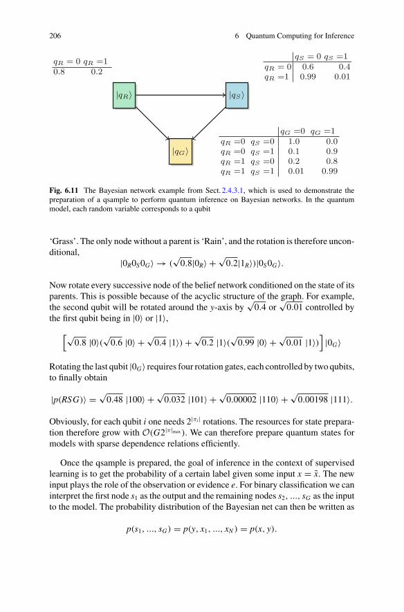
206 6 Quantum Computing for Inference

qR = 0 qR =10.8 0.2

qS = 0 qS =1qR = 0 0.6 0.4qR =1 0.99 0.01

qG =0 qG =1qR =0 qS =0qR =0 qS =1qR =1 qS =0qR =1 qS =1

1.0 0.00.1 0.90.2 0.80.01 0.99

|qR〉 |qS〉

|qG〉

Fig. 6.11 The Bayesian network example from Sect. 2.4.3.1, which is used to demonstrate thepreparation of a qsample to perform quantum inference on Bayesian networks. In the quantummodel, each random variable corresponds to a qubit

‘Grass’. The only node without a parent is ‘Rain’, and the rotation is therefore uncon-ditional,

|0R0S0G〉 → (√0.8|0R〉 + √

0.2|1R〉)|0S0G〉.

Now rotate every successive node of the belief network conditioned on the state of itsparents. This is possible because of the acyclic structure of the graph. For example,the second qubit will be rotated around the y-axis by

√0.4 or

√0.01 controlled by

the first qubit being in |0〉 or |1〉,[√

0.8 |0〉(√0.6 |0〉 + √0.4 |1〉) + √

0.2 |1〉(√0.99 |0〉 + √0.01 |1〉)

]|0G〉

Rotating the last qubit |0G〉 requires four rotation gates, each controlled by two qubits,to finally obtain

|p(RSG)〉 = √0.48 |100〉 + √

0.032 |101〉 + √0.00002 |110〉 + √

0.00198 |111〉.

Obviously, for each qubit i one needs 2|πi | rotations. The resources for state prepara-tion therefore grow with O(G2|π|max). We can therefore prepare quantum states formodels with sparse dependence relations efficiently.

Once the qsample is prepared, the goal of inference in the context of supervisedlearning is to get the probability of a certain label given some input x = x. The newinput plays the role of the observation or evidence e. For binary classification we caninterpret the first node s1 as the output and the remaining nodes s2, ..., sG as the inputto the model. The probability distribution of the Bayesian net can then be written as

p(s1, ..., sG) = p(y, x1, ..., xN ) = p(x, y).

6.3 Probabilistic Models 207

For inference, the nodes or qubits encoding x are replaced by the observed values orevidence x. Our goal is therefore to obtain the discriminative distribution p(y|x) thatallows us to guess a label y. The most straight-forward approach is to draw samples(x, y) and reject every sample where x �= x. The resulting samples are drawn fromp(y|x).

With regards to the quantum model, inference requires us to prepare a qsample|p(y|x)〉. Based on the ideas of quantum rejection sampling introduced in [26], Lowand Chuang [25] show that amplitude amplification can make measurements of aqsample quadratically more efficient than classical rejection sampling. Given theoriginal Bayesian net qsample |p(x, y)〉, one can formally separate the superpositioninto two subbranches, one with basis states that are consistent with the evidence xand one with all other basis states x that do not confirm the evidence,

|p(x, y)〉 = √p(x)|y, x〉 + √

1 − p(x)|s, x〉.

We can apply amplitude amplification to boost the probability of the left branch, theone containing the evidence. A part of the amplitude amplification routine is to applythe state preparation routine AS for each iteration. The number of iterations of thealgorithm (each applyingAS ) needed to fully amplify the ‘evidence’ branch—therebymaking it certain to draw samples from qsample |p(y|x)〉—is inO(p(x)− 1

2 ). Overall,one therefore achieves a runtime ofO(n2|π|maxp(x)− 1

2 ), which is exponentially worsewith respect to the maximum number of parents, but quadratically better with respectto the probability of observing the evidence than classical inference with rejectionsampling.

6.3.3 Qsamples of Mean-Field Approximations

Bayesian nets allow for an elegant state preparation routine due to their intrinsicstructure that factorises the distribution. In other cases one has to resort to approxi-mations in order to use the favourable properties of factorisation. One idea is to startwith a qsample of a mean-field approximation of the desired distribution (which hasto be computed classically beforehand) and then use branch selection to refine thedistribution. This has been introduced in the context of Boltzmann machines [27]which we will use as an example here. The advantage of these two steps is that amean-field approximation is a product state, and we will see that it can be preparedby simply rotating each qubit in the qsample register successively. State preparationcan—under certain circumstances—be therefore qubit-efficient.

To go into a bit more detail, remember that Boltzmann machines are probabilisticmodels defined by the model distribution

p(v, h) = e−E(v,h)

∑v,h e

−E(v,h)

208 6 Quantum Computing for Inference

over the visible variables v1, ..., vN+K and the hidden variables h1, ..., hJ , with thelearnable energy function E(v, h) = E(v, h; θ) (see also Eq.2.26). As before, wesummarise visible and hidden units with s1, ..., sG where G = N + K + J .

Our goal is to prepare the qsample |p(s)〉.We start insteadwith preparing a qsample|q(s)〉 of the mean-field distribution q(s). The mean-field distribution is a productdistribution,whichmeans it can be computed as the product of Bernoulli distributionsover individual features,

q(s) = g(s1;μ1)g(s2;μ2) · · · g(sG;μG).

The individual distributions have the form

g(si;μi) ={

μi, if si = 1,

1 − μi, else,

for 0 ≤ μi ≤ 1 and i = 1, ...,G. The mean-field distribution has the property thatit minimises the Kullback-Leibler divergence to the desired Boltzmann distributionp(s, h) (which is a common measure of distance between distributions). The meanfield parameters μi have to be obtained in a classical calculation. We assume further-more that a real constant k ≥ 1 is known such that p(s) ≤ kq(s).

To prepare a qsample of the form

∑

s

√q(s)|s〉,

where |s〉 = |s1...sG〉 abbreviates a state of the network in basis encoding, one simplyhas to rotate qubit i around the y-axis to

|0〉i → √1 − μi|0〉i + √

μi|1〉i,

for all qubits i = 1, ...,G (similar to the Bayesian network state preparation routine,but without conditioning on the parents).

We have a qsample corresponding to the mean field approximation of the targetdistribution. The second step is based on branch selection presented in Sect. 5.2.2.3.First, add an extra register and load another distribution p(s) in basis encoding toobtain ∑

s

√q(s)|s〉|p(s)〉.

This second distribution is constructed in such a way that q(s)p(s) is proportional top(s). Rotating an extra ancilla qubit,

∑

s

√q(s)|s〉|p(s)〉

(√1 − p(s)|0〉 + √

p(s)|1〉),

6.3 Probabilistic Models 209

and selecting the branch inwhich the ancilla is in state |1〉 leads to the desired qsample|p(s)〉. The success probability is larger than 1/k. If the approximation q(s)was exact,k = 1, and the branch selection succeeds with certainty. The larger the divergencebetween q(s) and p(s), the smaller the success of the conditional measurement. Thisscheme is therefore useful for Boltzmann distributions that are close to a productdistribution, or where the individual variables are not very correlated.

Boltzmann distributions play an important role in quantum machine learning dueto their natural proximity to quantum mechanics. In the machine learning literature,Boltzmann distributions are frequently called ‘Gibbs distribution’6 and they do notonly play a role inBoltzmannmachines, but also in othermodels such asMarkov logicnetworks [28]. In the next chapter wewill discuss other ways of how to prepare Gibbsdistribution qsamples with quantum annealing (Sect. 7.4), and variational circuits(Sect. 7.3). There are also conventional quantumcircuits to prepare such states exactly[29, 30], but not qubit-efficiently.

In summary, interpreting a quantum state as a qsample corresponding to a proba-bilistic model is a fruitful way to combinemachine learning and quantum computing,and a very natural intersection are Boltzmann or Gibbs distributions.

References

1. Cleve, R., Ekert, A., Macchiavello, C., Mosca, M.: Quantum algorithms revisited. In: Proceed-ings of the Royal Society of London A:Mathematical, Physical and Engineering Sciences, vol.454, pp. 339–354. The Royal Society (1998)

2. Kobayashi, H., Matsumoto, K., Yamakami, T.: Quantum Merlin-Arthur proof systems: Aremultiple Merlins more helpful to Arthur? In: Algorithms and Computation, pp. 189–198.Springer (2003)

3. Zhao, Z., Fitzsimons, J.K., Fitzsimons, J.F.: Quantum assisted Gaussian process regression(2015). arXiv:1512.03929

4. Romero, J., Olson, J.P., Aspuru-Guzik, A.: Quantum autoencoders for efficient compressionof quantum data. Quantum Sci. Technol. 2(4), 045001 (2017)

5. Schuld,M., Sinayskiy, I., Petruccione, F.: How to simulate a perceptron using quantum circuits.Phys. Lett. A 379, 660–663 (2015)

6. Nielsen, M.A., Chuang, I.L.: Quantum computation and quantum information. CambridgeUniversity Press, Cambridge (2010)

7. Tommiska, M.T.: Efficient digital implementation of the sigmoid function for reprogrammablelogic. IEE Proc. Comput. Digit. Tech. 150(6), 403–411 (2003)

8. Quine, V.W.: A way to simplify truth functions. Am. Math. Mon. 62(9), 627–631 (1955)9. McCluskey, J.E.: Minimization of boolean functions. Bell Labs Techn. J. 35(6), 1417–1444

(1956)10. Schuld, M., Sinayskiy, I., Petruccione, F.: The quest for a quantum neural network. Quantum

Inf. Process. 13(11), 2567–2586 (2014)11. Cao, Y., Guerreschi, G.G., Aspuru-Guzik, A.: Quantum neuron: an elementary building block

for machine learning on quantum computers (2017). arXiv:1711.1124012. Paetznick, A., Svore, K.M.: Repeat-until-success: non-deterministic decomposition of single-

qubit unitaries. Quantum Inf. Comput. 14, 1277–1301 (2013)

6In statistical physics, a Gibbs distribution is a state of a system that does not change under theevolution of the system.

210 6 Quantum Computing for Inference

13. Wiebe, N., Kliuchnikov, V.: Floating point representations in quantum circuit synthesis. NewJ. Phys. 15(9), 093041 (2013)

14. Schuld, M., Killoran, N.: Quantum machine learning in feature Hilbert spaces (2018).arXiv:1803.07128v1

15. Schölkopf, B., Herbrich, R., Smola, A.: A generalized representer theorem. In: ComputationalLearning Theory, pp. 416–426. Springer (2001)

16. Schölkopf, B., Smola, A.J.: Learning with kernels: support vector machines, regularization,optimization, and beyond. MIT Press (2002)

17. Rebentrost, P., Mohseni, M., Lloyd, S.: Quantum support vector machine for big data classifi-cation. Phys. Rev. Lett. 113, 130503 (2014)

18. Schuld, M., Bocharov, A., Svore, K., Wiebe, N.: Circuit-centric quantum classifiers (2018).arXiv:1804.00633

19. Stoudenmire, E., Schwab, D.J.: Supervised learning with tensor networks. In: Advances inNeural Information Processing Systems, pp. 4799–4807 (2016)

20. Chatterjee, R., Ting, Y.: Generalized coherent states, reproducing kernels, and quantum supportvector machines. Quantum Inf. Commun. 17(15&16), 1292 (2017)

21. Klauder, J.R., Bo-Sture S.: Coherent States: Applications in Physics andMathematical Physics.World Scientific (1985)

22. Trugenberger, C.A.: Quantum pattern recognition. Quantum Inf. Process. 1(6), 471–493 (2002)23. Schuld, M., Sinayskiy, I., Petruccione, F.: Quantum Computing for Pattern Classification.

Lecture Notes in Computer Science, vol. 8862, pp. 208–220. Springer (2014)24. Schuld, M., Fingerhuth, M., Petruccione, F.: Implementing a distance-based classifier with a

quantum interference circuit. EPL (Europhys. Lett.) 119(6), 60002 (2017)25. Yoder, T.J., Low, G.H., Chuang, I.L.: Quantum inference on Bayesian networks. Phys. Rev. A

89, 062315 (2014)26. Ozols,M.,Roetteler,M.,Roland, J.:Quantum rejection sampling.ACMTrans.Comput. Theory

(TOCT) 5(3), 11 (2013)27. Wiebe, N., Kapoor, A., Svore,K.M.: Quantum deep learning (2014). arXiv: 1412.3489v128. Wittek, P., Gogolin, C.: Quantum enhanced inference in markov logic networks. Sci. Rep. 7

(2017)29. Brandão, F.G.S.L., Svore, K.M.: Quantum speed-ups for solving semidefinite programs. In:

2017 IEEE 58th Annual Symposium on Foundations of Computer Science (FOCS), pp. 415–426. IEEE (2017)

30. Poulin, D., Wocjan, P.: Sampling from the thermal quantum gibbs state and evaluating partitionfunctions with a quantum computer. Phys. Rev. Lett. 103(22), 220502 (2009)

Chapter 7Quantum Computing for Training

The previous chapter looked into strategies of implementing inference algorithms ona quantum computer, or how to compute the prediction of a model using a quantuminstead of a classical device. This chapter will be concerned with how to optimisemodels using quantum computers, a subject targeted by a large share of the quantummachine learning literature.

We will look at four different approaches to optimisation in quantum machinelearning: linear algebra calculus, search, hybrid routines for gradient descent andadiabatic methods. The first two approaches are largely based on two famous quan-tum algorithms: the Harrow-Hassidim-Lloyd (HHL) algorithm for matrix inversionandGrover’s routine for unstructured search, respectively. The third approach tacklesgradient descent, one of the most frequently used optimisation methods in machinelearning, which has no clear quantum equivalent. This is why hybrid or variationalapproaches are consulted, in which inference is made on a quantum device, but theoptimisation is performed classically. Lastly, the adiabatic approach loosely sum-marises analog techniques where the result of an optimisation problem is encodedinto the ground state of a quantum system, and the goal of optimisation is to generatethis ground state, starting in a state that is relatively easy to prepare. Increasingly,this technique is also used to prepare qsamples which can be used as distributionsfor sampling-based classical training methods, a strategy that promises to be morefruitful in the face of noise-prone and sparsely connected early technologies.

The output of the quantum(-assisted) optimisation algorithm may be a quantumstate representing the trained parameters, or it might be a classical description of theoptimal parameters, or samples from amodel distribution.While some of the routinespresented here can be ‘plugged’ into classicalmachine learning algorithms, others areparts of quantum implementations of machine learning algorithms. Unsurprisingly,the choice of information encoding plays again an important role in this chapter.

© Springer Nature Switzerland AG 2018M. Schuld and F. Petruccione, Supervised Learning with Quantum Computers,Quantum Science and Technology, https://doi.org/10.1007/978-3-319-96424-9_7

211

212 7 Quantum Computing for Training

7.1 Quantum Blas

The quantum computing community developed a rich collection of quantum algo-rithms for basic linear algebra subroutines, or quantum blas [1], in analogy to thelinear algebra libraries of various programming platforms. Quantum blas includeroutines such as matrix multiplication, matrix inversion and singular value decompo-sition. These can be used to solve optimisation problems, and heavily rely on the ideaof amplitude encoding. The quantummachine learning algorithms based on quantumblas are rather technical combinations of the subroutines introduced in previous chap-ters (see also Table7.1), to which we will refer extensively. Amongst them are statepreparation for amplitude encoding (Sect. 5.2), Hamiltonian evolution (Sect. 5.4),density matrix exponentiation (Sect. 5.4.3), quantum matrix inversion (Sect. 3.5.3),quantum phase estimation (Sect. 3.5.2), and branch selection (Sect. 5.2.3).

Quantum machine learning algorithms constructed from quantum blas inherit aruntime that is logarithmic in the input dimension N as well as the training set sizeM provided a certain structure in the inputs is given. They have different polynomialdependencies on the desired maximum error and/or the condition number of thedesign matrix constructed from the data. Our goal here is not to give an accurateruntime analysis, which can be found in the original references and is often pavedwith subtleties. Instead we want to focus on two main points: (1) How the machinelearning problem translates to a linear algebra calculation, and (2) how to combinequantum subroutines to solve the task. Before coming to that part, the next section isan attempt to give readers with a less extensive background in quantum computingan idea of how the algorithms work.

7.1.1 Basic Idea

A number of learning algorithms contain linear algebra routines such as inverting amatrix or finding a matrix’ eigenvalues and eigenvectors. The matrices are usuallyconstructed from the training set (i.e., the designmatrix that carries all training inputsas rows), and therefore grow with the dimension N and/or number of the trainingvectorsM . The basic idea of the linear algebra approach in quantummachine learningis to use quantum systems for linear algebra calculus, where the design matrix isrepresented by the Hamiltonian of the system via dynamic encoding.

To illustrate this with an example, consider the linear algebra task of a multipli-cation of a vector and a unitary matrix, which we encountered in the discussion oflinear models in amplitude encoding in the last chapter. The evolution of a quan-tum system can be mathematically expressed as Uα, where U is a unitary matrixand α is the complex vector of 2n amplitudes. Performing this evolution effectivelyimplements the unitary matrix multiplication, and the state of the quantum systemafter the evolution encodes the result of the multiplication. But one can do muchmore: Quantum systems are natural eigendecomposers in the sense that the results of

7.1 Quantum Blas 213

measurements are eigenvalues of operators to certain eigenstates (see Sect. 3.1.3.4).One can say that the dynamics of the quantum system emulates a linear algebra cal-culation. This can be used for matrix inversion, as demonstrated in the algorithm forlinear systems by Harrow, Hassidim and Lloyd [2] (see Sect. 3.5.3). In this algorithmone prepares a special quantum system whose evolution is defined by the matrix thatis to be inverted, and the physical evolution allows us to invert the eigenvalues ofthat matrix and read out some desired information via measurements.

The crux of this idea is the same as in amplitude encoding. Many quantum blasrequire a number of manipulations that is polynomial in the number n of qubits,which means that they are qubit-efficient. Algorithms composed of such subroutinesdepend only logarithmic on the number N = 2n of amplitudes, and the same usuallyapplies to the number of training vectors M . A logarithmic dependency is a signifi-cant speedup. For example, a training set of one billion (bn) vectors that each havedimension one million can be represented in a Hamiltonian (using the previous trickof extending the rectangular design matrix to a 2 bn × 2 bn Hermitian matrix) of an = 31 qubit system.

Of course, there has to be a caveat: similar to state preparation, simulating sucha Hamiltonian in general may take of the order of 4 bn operations. But we sawinteresting exceptions in Sect. 5.4, for example where the Hamiltonian is sparseor low-rank. This obviously poses restrictions on the data one can deal with, andonly little has been done to find out which datasets could fulfil the requirements ofqubit-efficient processing. Still, the promises of simulating linear algebra calculuswith quantum systems for big data applications are impressive, and therefore worthinvestigating.

7.1.2 Matrix Inversion for Training

This section presents some selected examples of classical machine learning algo-rithms that rely on eigenvalue decomposition or matrix inversion, and for whichquantum algorithms have been proposed. The basic building blocks are summarisedin Table7.1.

7.1.2.1 Inverting Data Matrices

The first suggestion to use Harrow, Hassidim and Lloyd’s (HHL’s) quantum matrixinversion technique for statistical data analysis was proposed by Wiebe, Braun andLloyd [3]. Closely related to machine learning, their goal was to ‘quantise’ linearregression for data fitting, in which the best model parameters of a linear function forsome data points have to be found. In Sect. 2.4.1.1 it has been shown that basic linearregression (i.e., without regularisation) reduces to finding a solution to the equation

w = (XT X)−1XT y, (7.1)

214 7 Quantum Computing for Training

Table 7.1 Simplified overview of the quantum blas based quantum machine learning algorithmspresented in this chapter. The design matrix X is composed of the training inputs, and y is avector of training outputs. ur ,vr , σr are singular vectors/values of XT X and K is a kernel matrix.Abbreviations: HHL—quantum matrix inversion routine, HHL−—quantum matrix multiplicationroutine (omitting the inversion of the eigenvalues), HHLDME—quantum matrix inversion routinewith density matrix exponentiation to simulate the required Hamiltonian, SWAP—interferencecircuit to evaluate inner products of quantum states.

Classical method Computation Strategy Refs.

Data matrix inversion

Linear regression(sparse)

(X†X)X†y HHL−, HHL [3]

Linear regression(low-rank)

R∑

r=1σ−1r urvTr y HHLDME [4]

Kernel matrix inversion

Support vectormachine

K−1y HHLDME [5]

Gaussian process κT K−1y and κT K−1κ HHL + SWAP [6]

Adjacency matrix inversion

Hopfield network HHL + HHLDME [1]

where w is a N -dimensional vector containing the model parameters, y is a M-dimensional vector containing the target outputs y1, . . . , yM from the dataset, andthe rows of the data matrix X are the N -dimensional training inputs x1, . . . , xM . Themost demanding computational problem behind linear regression is the inversion ofthe square of the data matrix, (XT X)−1.

As a rough reminder, the HHL routine solves a linear system of equations Az = bby amplitude encoding b into a quantum state and applying the evolution ei HAt |ψb〉,where A is encoded into theHamiltonian HA (wherewe can use the trick of Sect. 3.4.4for non-Hermitian A and therefore assume without loss of generality that A is Her-mitian). Quantum phase estimation can extract the eigenvalues of HA and store themin basis encoding, and some quantum post-processing writes them as amplitudes andinverts them, which effectively computes the quantum state |ψA−1b〉. Omitting theinversion step multiplies the matrix A as it is, |ψAb〉.

From Eq. (7.1) we can see that in order to computew, one has to perform a matrixmultiplication as well as a multiplication with an inverted matrix. This can be doneby applying HHL twice. The first step, XT y, is computed following the HHL routinewith A → XT and b → y, but without inverting X . In a second step, the originalHHL routine for matrix inversion is used with A−1 → (XT X)−1 applied to the resultof the first step, b → XT y. The outputs of the quantum algorithm are the normalisedtrained model parameters encoded in the amplitudes of the quantum state |ψw〉. Thisquantum state can be used with a quantum inference algorithm from the last chapter,or by reading out the parameters via quantum tomography.

7.1 Quantum Blas 215

The runtime of the routine grows with the condition number κ of the data matrixX with O(κ6), where the Hamiltonian simulation as well as the conditional mea-surement in the branch selection are each responsible for a termO(κ3). Hamiltoniansimulation furthermore contributes a linear dependency on the sparsity s of the datamatrix with the most recent methods [7]. The runtime grows with the inverse errorasO(1/ log ε)when modern Hamiltonian simulation methods are used. Reading outthe parameters through measurements requires a number of repetitions that is of theorder of N .

A slight variation on the linear regression algorithm allows us to replace thesparsity condition with the requirement that the design matrix is of low rank, or closeto a low rank matrix, and requires only one step of the matrix inversion technique[4, 8]. A low rank means that the data is highly redundant and reducible to onlya few vectors. The basic idea is to express the design matrix as a singular valuedecomposition, which leads to a slightly different expression for the solution w interms of the singular values σr and singular vectors ur , vr of the data design matrix,

w =R∑

r=1

σ−1r urv

Tr y.

The singular vectors of X are the eigenvectors of XT X , while the singular values ofX are the square roots of the eigenvalues of XT X . We therefore only need to performone eigendecomposition of XT X , thereby “saving” the matrix multiplication withXT above. But there is another advantage to taking the route of the singular valuedecomposition. Since XT X is always a positive definite matrix, we can encode it in adensitymatrixρXT X (aswehave shown inSect. 6.2.5) and use the technique of densitymatrix exponentiation to apply eiρXT X t for a time t . Density matrix exponentiationtakes the role of Hamiltonian simulation in the original HHL routine. As discussedbefore, density matrix exponentiation can yield exponential speedups for eigenvalueextraction if XT X can be approximated by a low-rank matrix.

7.1.2.2 Inverting Kernel Matrices

The square of the design matrix, XT X , is an example of a larger class of positivedefinite matrices, namely kernel Gram matrices that we discussed before. The ideato use density matrix exponentiation for optimisation was in fact first explored in thecontext of kernel methods by Rebentrost, Mohseni and Lloyd’s quantum machinelearning algorithm for support vector machines [5]. It was also the first proposal thatapplied quantum blas to machine learning in the stricter sense.

While support vector machines as presented in Sect. 2.4.4.3 do not directly lead toa matrix inversion problem, a version called least-squares support vector machines[9] turns the convex quadratic optimisation into least squares optimisation. In short,

216 7 Quantum Computing for Training

by replacing the inequality constraints in Eq. (2.36)with equalities, the support vectormachine (with a linear kernel) becomes equivalent to a regression problem of theform ⎛

⎜⎝

0 1 . . . 11...1

K

⎞

⎟⎠

(w0

γ

)

=(0y

)

,

with the kernelGrammatrix K of entries (K )mm ′ = (xm)T xm′, theLagrangian param-

eters γ = (γ1, . . . , γM)T , and a scalar biasw0 ∈ R. To obtain the γi one has to invertthe kernel matrix. Note that we simplified the formalism by ignoring so called ‘slackparameters’ that cater for non-linearly separable datasets.

After preparing the kernel matrix as a density matrix, one can use the densitymatrix exponentiation technique to simulate eiρK t and proceed with the HHL algo-rithm to apply K−1 to a quantum state |ψy〉 to obtain |ψK−1 y〉. We call this versionof HHL with density matrix exponentiation (DME) for the Hamiltonian simulationin short the HHLDME routine.

The outcome of the algorithm is a quantum state that encodes the bias w0 as wellas the Lagrangian parameters γ1, . . . , γM as

|ψw0,γ 〉 = 1

w20 + ∑

m γ 2m

(

w0|0..0〉 +M∑

m=1

γm |m + 1〉)

.

With the help of an interference circuit, this state can be used to classify new inputs[5].

Another classicalmachine learning algorithmwhoseoptimisationmethod requiresa kernel matrix inversion are Gaussian processes (see Sect. 2.4.4.4). In Gaussian pro-cesses, the model distribution (see Eq. (2.42)) is given by

p(y|x,D) = N [y| κT K−1y

︸ ︷︷ ︸mean

, κ − κT K−1κ︸ ︷︷ ︸covariance

],

where κ = κ(x, x) is the kernel function with the new input x ‘in both slots’, κ

describes the vector (κ(x, x1), . . . , κ(x, xM ))T which takes the new input and therespective training inputs, and K is the kernel Gram matrix for the training inputswith entries κ(xm, xm

′) for m,m ′ = 1 . . . M . Again the main computational task

is the inversion of a M × M dimensional kernel matrix to compute the mean andvariance at a new input x . In order to compute these values, Zhao et al. [6] essentiallyapply the HHL routine to prepare a quantum state representing K−1y. For the innerproduct with κT one can use an interference circuit as the one shown in the previouschapter.

7.1 Quantum Blas 217

7.1.2.3 Inverting Adjacency Matrices

Amongst the problems that can be mapped to matrix inversion is (maybe surpris-ingly) also the Hopfield model. As presented in Sect. 2.4.2.3, the Hopfield model isa recurrent neural network with certain restrictions on the connectivity, which canbe used for associative memory. To “train” such a model, one can set the weighingor adjacency matrix of the graph to

W = 1

MN

M∑

m=1

xm(xm)T − 1

N1,

a technique known as the Hebbian learning rule [10]. This rule foresees that everyweight wi j connecting two units i, j is chosen as the average of the product xi x j offeatures over the entire dataset. The famous thumb rule is “neurons that fire together,wire together”.

Given a new pattern x of which only some values are known (and the others areset to zero), the usual operation mode of a Hopfield network is to update randomlyselected units according to a step activation rule (i.e., if the weighted sum of theadjacent neural values is larger than a threshold value, a neuron gets set to 1, else to0). One can show that this decreases or maintains the energy E = − 1

2 xTWx + wT x

until the ‘closest’ memory pattern is found. The vector w contains the “constantfields” that weigh each feature.

The matrix inversion formulation of a Hopfield neural network can be achievedby noting that wewant the known units of the new input to coincide with the solution,which means that

Px = x, (7.2)

if P is a projector onto the known features’ subspace. We can then construct theLangrangian for this optimisation problem to minimise E under the side constraintof Eq. (7.2),

L = −1

2xTWx + wT x − γ T (Px − x) + λ

2xT x .

In this equation, the vector γ and the scalar λ are Lagrangian parameters to learn.The optimisation problem can be written as a system of linear equations of the formAz = b with

A =(W − λ1 P

P 0

)

, z =(xγ

)

, b =(

w

x

)

.

Pattern retrieval or associative memory recall can be done by applying the pseu-doinverse A+ to a quantum state |ψb〉 that encodes the vector b. However, A cannotbe assumed to be sparse. One can therefore use a mixed approach: Decompose Ainto the three matrices B, C , and D,

218 7 Quantum Computing for Training

A =(0 PP 0

)

+(−(λ + 1

N )1 00 0

)

+(

1MN

∑m xm(xm)T 00 0

)

= B + C + D.

According to the so called Suzuki-Trotter formula that we introduced in Eq. (5.16),instead of exponentiating or simulating ei At , one can simulate the three stepsei BteiCtei Dt , if we accept an error of O(t2). While B and C are sparse and can betreated with Hamiltonian simulation, D is not sparse. However, D contains the sumof outer products of the training vectors which we can associate with the quantumstate

ρW = 1

M

M∑

m=1

|xm〉〈xm |.

If we can prepare copies of ρW , we can use density matrix exponentiation to simulateei Dt . The quantum algorithm for associative memory recall in Hopfield networksshows how to combine the preceding approaches to solve more and more complexproblems.

7.1.3 Speedups and Further Applications

The preceding examples demonstrated how quantum blas can be combined andapplied to machine learning optimisation problems whose solutions are formulatedas a linear algebra computation. The subroutines are rather involved, and requirea full-blown fault tolerant quantum computer that can execute a large number ofgates coherently. As mentioned before, the promise of this approach does not lie innear-term applications, but in the longer-term potential for exponential speedups.

Overall, one can roughly summarise under which conditions quantum blas-basedtraining algorithms are qubit-efficient, thereby bearing a super-polynomial speedupfor machine learning tasks relative to the input dimension N and the data set size M(see also [11]):

1. The input matrix has a constant sparsity (when Hamiltonian simulation is used)or can be approximated by a constant rank matrix (when density matrix expo-nentiation is used). This means that the sparsity or the rank of the matrix do notgrow with the data size and are reasonably small.

2. The input state which the (inverted) matrix is applied to can be prepared inlogarithmic time in N , M .

3. The condition number of the matrix that has to be inverted depends at mostpoly-logarithmically on the data size and is reasonably small. Note that this cansometimes be ensured by clever preprocessing of the data [12].

4. We do not request the final state as classical information, whichmeans that we donot have to read out every amplitude via repeated measurements. Authors referto three possible scenarios here. We are a) only interested in some properties of

7.1 Quantum Blas 219

the solution, or we can b) feed the solution into an efficient quantum inferenceroutine, or it is enough to c) sample from the solution.

Note that a question that is often left open is what these requirements posed on thedata sets mean for machine learning, for example whether they still define a usefulproblem. Also reformulating a classical problem as a least-squares or quadratic opti-misation problem might change the statistical properties of the model significantlyand influence the quality of solutions.

Matrix inversion was used here as an illustrative example of how to exploit quan-tum blas for supervised machine learning. There are many other machine learningalgorithms based on linear algebra routines. For example, the density matrix expo-nentiation routine introduced in Sect. 5.4.3 in the context of simulating Hamiltonianshas originally been proposed as a principal component analysis technique [13], wherethe task is to identify the dominant eigenvalues of a datamatrix. This scheme has beenused for a quantum algorithm for dimensionality reduction and classification [14].An application beyond supervised learning are recommendation systems, where themain task is matrix completion [15]. Recommendation systems are based on a pref-erence matrix R that stores a rating of M users for N different items (an illustrativeexample is the user rating of movies) and which is incomplete. The learning task isto predict the unknown rating of a user for a specific item, which is given by an entryof the preference matrix. The complete preference matrix R is assumed to be of lowrank, which can be interpreted as there are being only a few ‘prototypes of taste’ thatallow us to deduce user rankings from others. Beyond these examples, the literatureon quantum machine learning with quantum blas is continuously growing.

7.2 Search and Amplitude Amplification

The second line of approaches in using quantum computing for optimisation isbased on Grover search and amplitude amplification, which has been introducedin Sect. 3.5.1. These algorithms typically promise a quadratic speedup compared toclassical techniques. We illustrate the idea with three examples. First, we presentthe Dürr-Høyer algorithm which extends Grover’s routine to solve an optimisation(rather than a search) problem. This technique has been proposed in the contextof nearest neighbour [16] and clustering [17] methods to find closest data points.Second, we look at a slight modification [18] of Grover search to handle data super-positions, in which we want to maintain zero amplitude for data points that are notpresent in a given dataset to speed up the search. This has been applied to associativememory but can potentially be useful in other contexts as well. Third, we will lookat an example that uses amplitude amplification to search for the best model, in thiscase amongst decision boundaries of a perceptron.

220 7 Quantum Computing for Training

7.2.1 Finding Closest Neighbours

Dürr andHøyer [19] developed aquantumsubroutine usingGrover’s algorithm tofindtheminimumof a functionC(x) over binary strings x ∈ {0, 1}n . Let 1√

N

∑x |x〉|xcurr〉

be a superposition where we want to search through all possible basis states |x〉. Ineach step an oracle marks all states |x〉 that encode an input x so that C(x) is smallerthan C(xcurr) (see Fig. 7.1). To perform the comparison, xcurr is saved in an extraregister. The marked amplitudes get amplified, and the |x〉 register measured to drawa sample x ′. If the result x ′ is indeed smaller than xcurr, one replaces the currentminimum by the newly found one, xcurr = x ′. The routine gets repeated until theoracle runs empty, at which point xcurr is the desired minimum.

In principle, this routine could be used to find the set of model parameters |w〉that minimises a given cost function, and brute force search could be improved by aquadratic speedup. However, it is not difficult to see that this search over all possiblesets of parameters is hard in the first place. If we have D parameters and each isdiscretised with precision τ , we have to search over 2Dτ binary strings, and even animprovement to

√2Dτ would be hopeless.

However, the Dürr andHøyer routine can be applied to the task of finding the clos-est neighbour in clustering [17] and nearest neighbour methods [16]. For example,given a data superposition

|[x]〉M−1∑

m=0

|m〉|[xm]〉|0 . . . 0〉,

C(x)

x

C(xcurr)

xcurr

Fig. 7.1 Illustration of Dürr and Høyer’s optimisation algorithm. A quantum register in uniformsuperposition represents the inputs xm in basis encoding. In each iteration all states |xm〉 with alower cost than the current best solution, C(xcurr) > C(xm) (here shown with slightly longer blueticks), are marked by an oracle and their amplitudes are amplified. The register is measured and ifthe result x ′ fulfills C(xcurr) > C(x ′), the current candidate for the minimum (longest red tick) getsreplaced by x ′

7.2 Search and Amplitude Amplification 221

where [x], [xm] indicates that the encoding of the new input and the training inputsis arbitrary. To find the nearest neighbour of the new input x amongst the traininginputs xm , one has to compute the distance between the new input and all trainingpoints (see also Sect. 6.2.4) in superposition and write it into the last register,

|[x]〉M−1∑

m=0

|m〉|[xm]〉|[dist(x, xm)]〉.

This “distance register” stores the “cost” of a training point and can serve as a lookuptable for the cost function. Iteratively reducing the subspace of possible solutionsto the training points that have a lower cost than some current candidate xl willeventually find the closest neighbour.

7.2.2 Adapting Grover’s Search to Data Superpositions

In some contexts it can be useful to restrict Grover’s search to a subspace of basisvectors. For example, the data superposition in basis encoding,

1√M

M∑

m=1

|xm〉,

corresponds to a sparse amplitude vector that has entries 1√M

for basis states thatcorrespond to a training input, and zero else. Standard Grover search rotates this datasuperposition by the average, and thereby assigns a nonzero amplitude to traininginputs that were not in the database. This can decrease the success probability ofmeasuring the desired result significantly.

Example 7.1 (Common Grover search. [18])We want to amplify the amplitude of search string 0110 in a sparse uniform super-position,

|ψ〉 = 1√6(|0000〉 + |0011〉 + |0110〉 + |1001〉 + |1100〉 + |1111〉),

which in vector notation corresponds to the amplitude vector

1√6(1, 0, 0, 1, 0, 0, 1, 0, 0, 1, 0, 0, 1, 0, 0, 1)T .

In conventional Grover search, the first step is to mark the target state by a negativephase,

222 7 Quantum Computing for Training

1√6(1, 0, 0, 1, 0, 0,−1, 0, 0, 1, 0, 0, 1, 0, 0, 1)T ,

afterwhich every amplitudeαi is ‘rotated’ or transformedviaαi → −αi + 2α (whereα is the average of all amplitudes) to get

1

2√6(−1, 1, 1,−1, 1, 1, 3, 1, 1,−1, 1, 1,−1, 1, 1,−1)T .

In the second iteration we mark again the target state

1

2√6(−1, 1, 1,−1, 1, 1,−3, 1, 1,−1, 1, 1,−1, 1, 1,−1)T

and each amplitude gets updated as

1

8√6(5,−3,−3, 5,−3,−3, 13,−3,−3, 5,−3,−3, 5,−3,−3, 5)T .

As we see, the basis states that are not part of the data superposition end up havinga non-negligible probability to be measured.

Ventura andMartinez [18] therefore introduce a simple adaptation to the amplitudeamplification routine that maintains the zero amplitudes. After the desired state ismarked and the Grover operator is applied for the first time rotating all amplitudesby the average, a new step is inserted which marks all states that were originally inthe database superposition. The effect gives all states but the desired one the samephase and absolute value, so that the search can continue as if starting in a uniformsuperposition of all possible states.

Example 7.2 (Ventura-Martinez version of Grover search [18])Getting back to the previous example and applying the Ventura-Martinez trick, start-ing with the same initial state, marking the target, and ‘rotating’ the amplitudes forthe first time,

1

2√6(−1, 1, 1,−1, 1, 1, 3, 1, 1,−1, 1, 1,−1, 1, 1,−1)T ,

the adapted routine ‘marks’ all amplitude that correspond to states in the data super-position,

1

2√6(1, 1, 1, 1, 1, 1,−3, 1, 1, 1, 1, 1, 1, 1, 1, 1)T ,

followed by another rotation,

1

4√6(1, 1, 1, 1, 1, 1, 9, 1, 1, 1, 1, 1, 1, 1, 1, 1)T .

7.2 Search and Amplitude Amplification 223

From now on we can proceed with Grover search as usual. The second iterationmarks again the target,

1

4√6(1, 1, 1, 1, 1, 1,−9, 1, 1, 1, 1, 1, 1, 1, 1, 1)T ,

and the rotation leads to

1

16√6(−1,−1,−1,−1,−1,−1, 39,−1,−1,−1,−1,−1,−1,−1,−1, −1)T .

It is obvious from this example that the amplitude amplification process is muchfaster, i.e. leads to amuch larger probability ofmeasuring the target state thanwithoutthe adaptation.

7.2.3 Amplitude Amplification for Perceptron Training

Another straight forward application of amplitude amplification to machine learningis suggested in [20] and targets the training of perceptrons. Perceptron models havethe advantage that rigorous bounds for training are known. Using the standard learn-ing algorithm outlined in Sect. 2.4.2.1 and for training vectors of unit norm1 assignedto two classes that are each separated by a positive margin γ , the training is guaran-teed to converge to a zero classification error on the training set in O( 1

γ 2 ) iterationsover the training inputs. A slightly different approach to training in combination withamplitude amplification allows us to improve this to O( 1√

γ).

The basic idea is to use a dual representation of the hyperplanes that separatethe data correctly. In this representation, the hyperplanes or decision boundaries aredepicted as points on a hypersphere (determined by the normalised weight vector)while training points define planes that cut through the hypersphere and define a“bad” subspace in which the desired solution is not allowed to lie, as well as a“good” subspace of allowed solutions (see Fig. 7.2). Assume we have K randomlysampled decision boundaries, represented by their weight vectors w1, . . . , wK . Onecan show that a sample decision boundary perfectly separates the training set withprobabilityO(γ ). In turn, thismeanswe have to startwithO( 1

γ) samples tomake sure

the procedure does work on average. This is the first ‘quadratic speedup’ comparedtoO( 1

γ 2 ), and so far a purely classical one. The advantage of this step is that we onlyhave K potential decision boundaries, with which we can now perform a Groversearch of the best.

The second speedup comes from Grover search itself and is therefore a quantumspeedup. We basis encode the weight vectors in a data superposition

1An assumption that allows us to omit that the bounds also depend on the norm.

224 7 Quantum Computing for Training

Fig. 7.2 In the dual representation, the normal vector of the separating hyperplanes w1 and w2

of a perceptron model are represented by points on a hypersphere, while the training set identifiesa feasible region for the separating hyperplanes. Each training vector corresponds to a plane that‘cuts away’ part of the hypersphere (illustrated by the grey planes)

1√K

K∑

k=1

|wk〉,

and gradually reinforce the amplitude of the weight vectorswk that were found in thefeasible subspace defined by the training data. For this purpose we need a quantumsubroutine or ‘oracle’ that marks such ‘desirable’ weight vectors in the superposi-tion. For example, considering only one training input, such an oracle would markall weight vectors that classify the single input correctly. The number of iterationsneeded grows with O( 1√

γ). This convergence result can also be translated into an

improvement of the mistake bound or the maximum number of misclassified datapoints in the test set after training [20].

7.3 Hybrid Training for Variational Algorithms

With full-blown fault-tolerant quantum computers still in the future, a class of hybridclassical-quantum algorithms has become popular to design near-term applicationsfor quantum devices of the first generation. The idea of hybrid training of varia-tional algorithms is to use a quantum device—possibly together with some classicalprocessing—to compute the value of an objective function C(θ) for a given set ofclassical parameters θ . A classical algorithm is then used to optimise over the param-eters by making queries to the quantum device [21].

As shown in Fig. 7.3, the quantum device implements a parametrised circuitU (θ)

that prepares a state U (θ)|0〉 = |ψ(θ)〉 which depends on a set of circuit parame-ters θ . A parametrised circuit can be thought of as a family of circuits where theparameters define one particular member of the family. For simplicity we will only

7.3 Hybrid Training for Variational Algorithms 225

Quantum device|0〉

U(θ)...

...

|0〉

Classical device

θ(t)

θ(t+1)θ(t+1)

update

rerun

Fig. 7.3 The idea of a hybrid quantum-classical training algorithm for variational circuits is to usethe quantum device to compute terms of an objective function or its derivatives, and subsequentlyuse a classical device to compute better circuit parameters with respect to the objective. The entireroutine gets iterated until the objective is minimised or maximised

consider unitary circuits here, but the concepts are easily extended to the evolutionof subsystems and mixed states.

Measurements on the final state |ψ(θ)〉 return estimates of expectation values,for example the energy expectation value, or the state of a certain qubit. Theseexpectations depend on the circuit parameters θ . A cost function C(θ) uses theexpectation values to define how good θ is in a given problem context. The goal ofthe algorithm is to find the circuit parameters θ of the variational circuit U (θ) thatminimise C(θ).

To find the optimal circuit parameters, a classical algorithm iteratively queries thequantum device. These queries can either be the expectation values that define thecost, or—as wewill see below—different expectation values that reveal the gradientsof the variational circuit. Since training is a joint effort by a quantum and a classicalalgorithm, the training is called a “hybrid” scheme.

The variational circuit U (θ) is an ansatz that defines a set of all possible states|ψ(θ)〉 it is able to prepare. It is typically much smaller than the space of all unitaries,since that would require a number of parameters that is quadratic in the Hilbert spacedimension, which quickly becomes prohibitive with a growing number of qubits.Similar to the task of choosing a good model in machine learning, a fundamentalchallenge in variational algorithms lies in finding an ansatz that is rich enough to allowthe parametrised state to approximate interesting solutions to the problemwith as fewparameters as possible. An interesting point is that for qubit-efficient circuits U (θ)

that are not classically simulable, the overall training scheme exhibits an exponentialquantum speedup, because the objective function could not be computed efficientlyon a classical computer.

The great appeal of variational schemes is that they are suitable for near-termquantum technologies for the following reasons. Firstly, they do only require a frac-tion of the overall algorithm to run coherently (that is, as a quantum circuit), which

226 7 Quantum Computing for Training

leads tomuch smaller circuits. Second, there aremany possible ansätze for the circuit,which means that it can be designed based on the strength of the device. Third, thefact that the circuit is learned can introduce robustness against systematic errors—iffor example a certain quantum gate in the device systematically over-rotates the state,the parameters adjust themselves to correct for the error. Fourth, compared to othertypes of algorithms, optimisation as an iterative scheme can work with noise, forexample in the estimations of the objective function terms.

In the context of this book, hybrid training of variational circuits is a promisingcandidate for quantummachine learning on near-term quantum devices. To show theworking principle of variational circuits we will present two of the first variationalalgorithms from the quantum computing literature. We will then sketch two appli-cations of these algorithms in quantum machine learning. The final sectionwill havea closer look at how to perform the parameter updates on a classical computer, andexplores different strategies of hybrid training that can be used in conjunction withthese methods.

7.3.1 Variational Algorithms

The canon of quantum computing has been extended by a variety of variationalalgorithms. The first example, the variational eigensolver, stems from the physics-inspired problemof findingminimumenergy eigenstates. The second example, the socalled quantum approximate optimisation algorithm or QAOA, aims at solving com-binatorial optimisation problems, and defines an interesting ansatz for the variationalcircuit itself.

7.3.1.1 Variational Eigensolvers

Variational algorithms were initially proposed as a prescription to find groundstates—that is, lowest energy eigenstates—of quantum systems, where the cost issimply the energy expectation value. These schemes are also called variational eigen-solvers [22]. The variational principle of quantum mechanics tells us that the groundstate |ψ〉 minimises the expectation

〈ψ |H |ψ〉〈ψ |ψ〉 , (7.3)

where H is the Hamiltonian of the system. The best approximation |ψ(θ∗)〉 to theground state given an ansatz |ψ(θ)〉 minimises (7.3) over all sets of parameters θ .Assuming the kets are normalised, the cost function of the variational algorithm istherefore given by

C(θ) = 〈ψ(θ)|H |ψ(θ)〉.

7.3 Hybrid Training for Variational Algorithms 227

The quantum device estimates C(θ) for an initial parameter set and hybrid trainingiteratively lowers the energy of the system by minimising the cost function.

In theory, we can perform measurements on the state |ψ(θ)〉 to get an estimateof the expectation value of H . However, for general Hamiltonians this can involve aprohibitive number of measurements.

Example 7.3 ((Estimation of energy expectation)) Consider the Hamiltonian H of a26 = 64 dimensionalHilbert space, i.e., |ψ(θ)〉 can be expressed by a 64-dimensionalamplitude vector and describes a system of 6 qubits. Assume H has a −1 at the 13thdiagonal entry and zeros else, in other words, the ground state of the Hamiltonianis the 13th basis state of the 6-qubit system. The expectation value 〈ψ(θ)|H |ψ(θ)〉is then effectively the probability of measuring the 13th computational basis state,multiplied by (−1). Naively, to determine this probability we would have to measurethe state |ψ(θ)〉 repeatedly in the computational basis and divide the number of timeswe observe the 13th basis state by the total number of measurements. For a uniformsuperposition we need of the order of 2n measurements to do this, which is infeasiblefor larger systems and defies the use of a quantum device altogether.

Luckily, in many practical cases H can be written as a weighted sum of local (i.e.1- or 2-qubit) operators, H = ∑

k hk Hk with hk ∈ R ∀k. We have already discussedsuch a case for qubit-efficient Hamiltonian simulation in Sect. 5.4.1. The overallexpectation is then given by a sum

C(θ) =∑

k

hk〈ψ(θ)|Hk |ψ(θ)〉

of the estimates of ‘local’ expectation values 〈ψ(θ)|Hk |ψ(θ)〉. The local estimatesare multiplied by the coefficients hk and summed up on the classical device. These‘local’ energy expectations are much easier to estimate, which reduces the numberof required measurements dramatically. If the number of local terms in the objectivefunction is small enough, i.e. it only grows polynomially with the number of qubits,estimating the energy expectation through measurements from the quantum deviceis qubit-efficient.

To give one example, remember that the Hamiltonian of a qubit system can alwaysbe written as a sum over Pauli operators,

H =∑

i,α

hiασ iα +

∑

i, jα,β

hi jα,βσ iασ

jβ + · · · , (7.4)

and the expectation value becomes sum of expectations,

〈H〉 =∑

i,α

hiα〈σ iα〉 +

∑

i, jα,β

hi jα,β〈σ iασ

jβ 〉 + · · · ,

228 7 Quantum Computing for Training

where the superscripts i, j denote the qubit that the Pauli-operator acts on, whilethe subscripts define the Pauli operator α, β = 1, x, y, z. From this representationwe see that the energy expectation becomes qubit-efficient if the Hamiltonian canbe written as a sum of only a few (i.e. tractably many) terms, each involving onlya few Pauli operators. This is common in quantum chemistry, where Hamiltoniansdescribe electronic systems under Born-Oppenheimer approximation, as well as inmany-body physics and the famous Ising/Heisenberg model [22].

Generally speaking, variational quantum eigensolvers minimise the expectationvalue of an operator, here the Hamiltonian, using a quantum device to estimate theexpectation. Eigensolvers are particularly interesting in cases where the estimationis qubit-efficient on a quantum device, while simulations on a classical computer areintractable.

7.3.1.2 Quantum Approximate Optimisation Algorithm

Another popular variational algorithm has been presented by Farhi and Goldstone,and in its original version solves a combinatorial optimisation problem [23]. For us,the most important aspect is the ansatz for |ψ(θ)〉 for a given problem that will beadapted to prepare Gibbs states in the quantum machine learning algorithm below.

Consider an objective function that counts the number of statements from a pre-defined set of statements {Ck} which are satisfied by a given bit string z = {0, 1}⊗n ,

C(z) =∑

k

Ck(z).

A statement can for instance be “(z1 ∧ z2) ∨ z3”, which is fulfilled for z = z1z2z3 =000 but violated by z = 010. If statement k is fulfilled by z, Ck(z) is 1, and else itis 0. We can represent this objective function by the expectation values 〈z|C |z〉 of aquantum operator that we also call C . In matrix representation, the operator containson its diagonal the number of statements satisfied by a bit string z, whereby theinteger representation i of z defines the element Hi+1,i+1 = C(z) of the Hamiltonian(the ‘+1’is necessary to start the index count from 1). The matrix has only zerooff-diagonal elements.

Example 7.4 Consider an objective function defined on bit strings of length n =2 with statements C1(z1, z2) = (z1 ∧ z2) and C1(z1, z2) = (z1 ∨ z2), the matrixexpression of operator C = C1 + C2 would be given by

⎛

⎜⎜⎝

〈00|C |00〉 〈00|C |01〉 〈00|C |10〉 〈00|C |11〉〈01|C |00〉 〈01|C |01〉 〈01|C |10〉 〈01|C |11〉〈10|C |00〉 〈10|C |01〉 〈10|C |10〉 〈10|C |11〉〈11|C |00〉 〈11|C |01〉 〈11|C |10〉 〈11|C |11〉

⎞

⎟⎟⎠ =

⎛

⎜⎜⎝

0 0 0 00 1 0 00 0 1 00 0 0 2

⎞

⎟⎟⎠ ,

and contains the number of fulfilled statements on the diagonal.

7.3 Hybrid Training for Variational Algorithms 229

If we interpret a quantum state |ψ〉 = ∑z αz|z〉 as a qsample that defines a prob-

ability distribution over z-strings, then 〈ψ |C |ψ〉 is the expectation value of operatorC under this distribution. Measuring |ψ〉 in the computational basis means to drawsamples from the space of all bit strings.

We now define the ansatz |ψ(θ)〉 of the variational algorithm. For this we need asecond operator, a sum of Pauli σx or ‘flip operators’ on all bits,

B =n∑

i=1

σ ix .

Together, B and C define the ansatz for the parametrised state preparation scheme.Consider the two parametrised unitaries

U (B, β) = exp−iβB, U (C, γ ) = exp−iγC .

Starting with a uniform superposition |s〉 = 1√2n

∑z |z〉 and alternately applying

U (B, β) U (C, γ ) for short times t prepares the parametrised state

|ψ(θ)〉 = U (B, βK )U (C, γK ) . . .U (B, β1)U (C, γ1)|s〉.

The set of parameters θ consists of the 2K parameters β1, . . . , βK , γ1, . . . , γK .Farhi andGoldstein have shown that for K → ∞, themaximumexpectation value

over all θ is equal to the maximum of the objective function,

limK→∞ max

θ〈ψ(θ)|C |ψ(θ)〉 = max

zC(z).

Let θ∗ be the parameter set that maximises 〈ψ(θ)|C |ψ(θ)〉. The above suggests thatsampling computational basis states from |ψ(θ∗)〉 will reveal good candidates for z,since the state assigns more probability to basis states that correspond to z valueswhich fulfil a lot of statements. For example, if in the extreme case there is onlyone z′ that fulfills all statements and all other z fulfil none of them, we would get|ψ(θ∗)〉 = |z′〉 as the optimal solution, and sampling would always retrieve z′. Notethat a “good candidate” in this context does not refer to a high probability to samplethe optimal z, but to draw a reasonably good solution for which C(z) is close to theglobal optimum. Farhi and Goldstone’s investigations suggest that also for low K ,even for K = 1, this algorithm can have useful solutions.

As a final side-note, the quantum approximate optimisation algorithm has itsorigins in the quantum adiabatic algorithm, in which a simple starting Hamiltonian(corresponding to B) gets slowly turned into the target Hamiltonian (hereC) withoutleaving the ground state. Instead of a smooth continuous transition one uses tworapidly alternating evolutions defined byU (B, β) andU (C, γ ). A subsequent paperby Farhi and Harrow [24] claims that sampling from |ψ(θ)〉 even for small circuitdepths K is classically intractable, giving this model a potential exponential quantumadvantage.

230 7 Quantum Computing for Training

7.3.2 Variational Quantum Machine Learning Algorithms

Based on these two variational algorithms, we present two suggestions of how to usevariational algorithms in the context of quantum machine learning. First, we discusshow the variational eigensolvers can be extended to implement a binary classifierin which the expectation value of a quantum observable is interpreted as the outputof a machine learning model. Second, we show how to use quantum approximateoptimisation to prepare approximations of Gibbs states. These Gibbs states can beused as qsamples to train Boltzmann machines.

7.3.2.1 Variational Classifiers

The idea of a variational eigensolver can be extended for supervised learning tasksby interpreting the expectation value of an observable O as the output of a classifier,

f (x; θ) = 〈ψ(x; θ)|O|ψ(x; θ)〉. (7.5)

The resulting model is what we call a variational classifier. Note that the variationalcircuit also has to depend on the model inputs x .

One way to associate an expectation value with a binary model output f (x; θ) isto define

f (x; θ) = 〈ψ(x; θ)|σ jz |ψ(x; θ)〉,

where the right side is the expectation value of the σz operator applied to the j thqubit. The σz operator measures whether a qubit is in state 0 or 1, and the expectationvalue is equivalent (up to a simple transformation) to measuring the probability ofthis qubit being in state 1, as we have discussed several times before.

Example 7.5 The expectation value ofσz with respect to thefirst qubit of the quantumstate |ψ〉 = a0|00〉 + a1|01〉 + a2|10〉 + a3|11〉 is given by

〈ψ |σ 1z |ψ〉 = |a0|2 + |a1|2 − |a2|2 − |a3|2,

while with respect to the second qubit the expectation value is

〈ψ |σ 2z |ψ〉 = |a0|2 − |a1|2 + |a2|2 − |a3|2.

The expectation value hence sums up the probabilities corresponding to basis stateswhere the qubit is in state 1, and subtracts those where the qubit is in state 0. We cantranslate the expectation value into a probability of measuring the qubit in state 1 byperforming the scaling-shift

p(q j = 1) = 0.5〈〈ψ |σ jz |ψ〉〉 + 1.

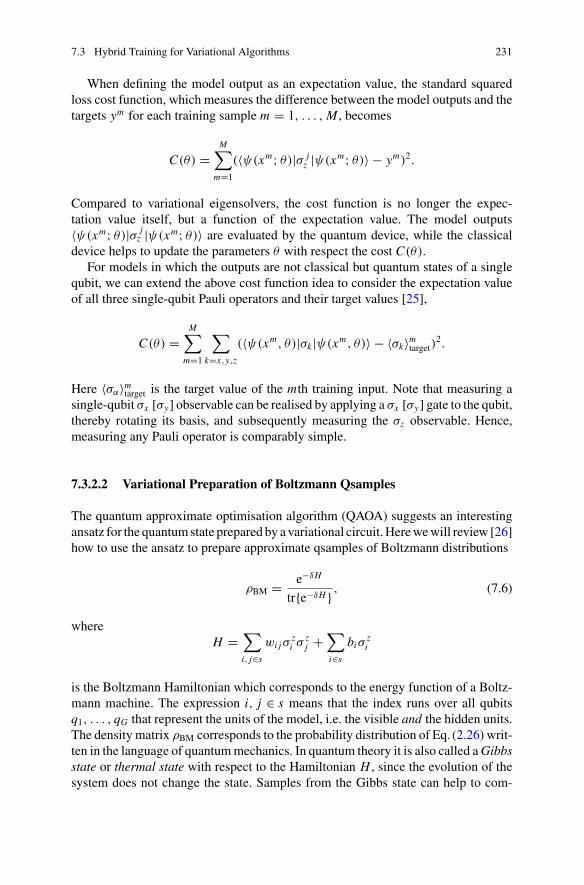
7.3 Hybrid Training for Variational Algorithms 231

When defining the model output as an expectation value, the standard squaredloss cost function, which measures the difference between the model outputs and thetargets ym for each training sample m = 1, . . . , M , becomes

C(θ) =M∑

m=1

(〈ψ(xm; θ)|σ jz |ψ(xm; θ)〉 − ym)2.

Compared to variational eigensolvers, the cost function is no longer the expec-tation value itself, but a function of the expectation value. The model outputs〈ψ(xm; θ)|σ j

z |ψ(xm; θ)〉 are evaluated by the quantum device, while the classicaldevice helps to update the parameters θ with respect the cost C(θ).

For models in which the outputs are not classical but quantum states of a singlequbit, we can extend the above cost function idea to consider the expectation valueof all three single-qubit Pauli operators and their target values [25],

C(θ) =M∑

m=1

∑

k=x,y,z

(〈ψ(xm, θ)|σk |ψ(xm, θ)〉 − 〈σk〉mtarget)2.

Here 〈σα〉mtarget is the target value of the mth training input. Note that measuring asingle-qubit σx [σy] observable can be realised by applying a σx [σy] gate to the qubit,thereby rotating its basis, and subsequently measuring the σz observable. Hence,measuring any Pauli operator is comparably simple.

7.3.2.2 Variational Preparation of Boltzmann Qsamples

The quantum approximate optimisation algorithm (QAOA) suggests an interestingansatz for the quantumstate prepared by a variational circuit.Herewewill review [26]how to use the ansatz to prepare approximate qsamples of Boltzmann distributions

ρBM = e−δH

tr{e−δH } , (7.6)

whereH =

∑

i, j∈swi jσ

zi σ

zj +

∑

i∈sbiσ

zi

is the Boltzmann Hamiltonian which corresponds to the energy function of a Boltz-mann machine. The expression i, j ∈ s means that the index runs over all qubitsq1, . . . , qG that represent the units of the model, i.e. the visible and the hidden units.The density matrix ρBM corresponds to the probability distribution of Eq. (2.26) writ-ten in the language of quantummechanics. In quantum theory it is also called aGibbsstate or thermal state with respect to the Hamiltonian H , since the evolution of thesystem does not change the state. Samples from the Gibbs state can help to com-

232 7 Quantum Computing for Training

pute the weight update in a gradient descent algorithm for the training of (quantum)Boltzmann machines [26]. The technique to prepare ρBM with the QAOA has beencalled quantum approximate thermalisation [26].

In quantum approximate thermalisation, the operator B of the QAOA is replacedby the mixer Hamiltonian

HM =∑

i∈sσ ix ,

while the operatorC is replaced by H from above. As in theQAOA, theHamiltoniansare applied for K iterations in an alternating fashion,

K∏

k=1

e−iβk HM e−iγk H ,

with the real, classical parameters {β1, . . . , βK , γ1, . . . , γK }. The goal is to find theparameters for which this sequence of operators approximately transforms the initialstate2

ρ0 = e−δHM

tr{e−δHM } ,

to the desired Boltzmann qsample from Eq. (7.6).The iterative parameter optimization minimises the cost

C(β1, . . . , γK ) = tr{ρBM(β1, . . . , γK ) H}

by a numerical method such as Nelder-Mead. For this one has to estimate C with aquantum device or a simulation thereof. The cost is the expectation of H with respectto its approximate thermal state ρBM.

Recall from Sect. 2.4.2.4 that for maximum likelihood optimisation in the trainingof Boltzmann machines one has to not only sample the values of ‘neurons’ from themodel distribution (which is the Boltzmann distribution we just looked at), but alsofrom a “data” distribution where the visible units are ‘clamped’ to a training input.We therefore also need to prepare ‘clamped’ Boltzmann qsamples. For this one canuse the same procedure as before, but has to use slightly different operators,

HM =∑

i∈hσ ix , H =

∑

i, j∈s|(i∈h)∨( j∈h))

wi jσzi σ

zj +

∑

i∈hbiσ

zi ,

2The initial state plays the role of the uniform superposition that we started with in the origi-nal quantum approximate optimisation algorithm. It can be prepared by starting with the state⊗

j

√

2 cosh(δ)∑

± e∓ β2 |±〉 j |±〉E j and tracing out the E j (‘environment’) register (which has as

many qubits as the visible register) [26].

7.3 Hybrid Training for Variational Algorithms 233

where h is the set of qubits associated with hidden units. These clamped or ‘partial’Hamiltonians exclude terms from the full Hamiltonians which are acting on visibleunits only. The initial state is now the thermal state of HM with the visible units pre-pared in a randomly sampled training input |xm〉, in other words, they are ‘clamped’to a specific value. An interesting variation uses either a superposition or a statisticalmixture of training inputs for the visible qubits, called quantum randomised clamp-ing, which was reported to improve the results of numerical simulations significantly[26].

7.3.3 Numerical Optimisation Methods

We have so far ignored the issue of how to optimise the classical parameters θ =θ1, . . . , θD in the hybrid training scheme. Since the quantum algorithm providesmeasurement samples for the expectation of an operator, we only have an estimationof the output, whose precision can be increased by repeating the algorithm andmeasurement. We distinguish three classes of methods to use these measurementestimates for optimisation, derivative-free, numerical gradient-based and analyticalgradient-based methods.

7.3.3.1 Derivative-Free Methods

As the name suggests, derivative-free methods do not use gradients for optimisation.Amongst derivative-free methods one can again distinguish between one-shot anditerative methods. One-shot methods compute the optimal parameters on a classicalcomputer and use the quantum device solely for state preparation. An example hasbeen suggested in the context of the quantum approximate optimisation algorithmand the so-called MaxCut problem for graphs with bounded degree [23]. However,such classical solutions are very problem-specific, can be computationally expensiveand may be difficult to construct.

Iterative derivative-free methods use successive evaluations of the objective func-tion (and thereby of the expectation values estimated from the quantum computer)

Fig. 7.4 The Nelder-Mead or simplex algorithm finds the minimum by successively updating thenode of a simplex that has the highest cost value. It is gradient-free and simple to implement, butnot very robust in high-dimensional landscapes

234 7 Quantum Computing for Training

for optimisation. A prominent example is the Nelder-Mead method [27], in whichthe vertices of a D + 1-simplex are iteratively updated, incrementally shrinking thearea of the simplex around a minimum (Fig. 7.4). The algorithm terminates wheneither the distance between the points or the differences of the cost between twoupdates fall under a certain threshold. Other well-known candidates are genetic andparticle swarm optimisation algorithms, but little is known about their performancein the context of variational quantum computing (for an exception see [28]).

7.3.3.2 Numerical Gradient-Based Methods

Gradient-based methods also have two sub-categories, numerical and analyticalmethods. If only black-box access to the cost function is provided, one can usefinite-differences to compute the gradient numerically,

∂C(θ)

∂θl= C(θ1, .., θl , .., θD) − C(θ1, .., θl + Δθl, .., θD)

Δθl+ O(Δθ2

l ) + O(ε

Δθl).

(7.7)The last term stems from the error of the estimation of the cost function C(θ), and ε

is the error of the estimation.Guerreschi et al. [29] provide some useful rules when considering the finite-

differences method to compute gradients. Most importantly, we want the error inter-vals of the two cost function evaluations not to overlap. In other words, the differencebetweenC(θ1, . . . , θl , . . . , θD) andC(θ1, . . . , θl + Δθl, . . . , θD)has to be larger thantwice the error (see Fig. 7.5), which means by Eq. (7.7) that

2ε ≤ Δθl∂C(θ)

∂θl.

Fig. 7.5 The finite-difference method approximates a gradient with the linear function determinedby function evaluations at two points with distance Δθ (here for a one-dimensional parameterspace). The precision ε for each function evaluationC(θ) has to be smaller for small gradients (left)than for large ones (right)

7.3 Hybrid Training for Variational Algorithms 235

As a consequence, the smaller the gradient, the more precision we need in estimatingthe cost function, and the more repetitions of the algorithm are required. Numericalfinite-differences methods are therefore particularly difficult in situations where theminimum has to be approximated closely, or when the optimisation landscape hasmany saddle points, and where the algorithm produces measurements with a highvariance.

7.3.3.3 Analytical Gradient-Based Methods

The second type of gradient-based methods uses analytical gradients [29–31]. Con-sider a quantum circuit

U (θ) = G(θL) . . .G(θl) . . .G(θ1),

that consists of L parametrised “elementary unitary blocks” G. These blocks areeach defined by a set of parameters θl , l = 1, . . . , L . Let μ be an arbitrary parameterin θ . The analytical gradient ∇μC(U (θ)) of a cost function C(U (θ)) that dependson the variational circuit usually consists of the ‘derivative of the circuit’, ∂μU (θ).We define the partial derivative of a matrix here as the matrix that results from takingthe partial derivative of each element.

The problem with the expression ∂μU (θ) is that these derivatives of circuits arethemselves not necessarily unitaries, and therefore no quantum circuits. That meanswe cannot estimate any expectations from these circuits with the quantum device.However, one can often use tricks to estimate ∂μU (θ) with the device, and therebyuse the analytical gradients in a hybrid training scheme. If possible, this is muchpreferred over numerical gradients that are less robust.

Assume that μ only appears in the set of parameters θl (although the calculationbecomes only slightly more complex when several parameters are tied to each other).Then

∂μU (θ) = G(θL) . . . ∂μG(θl) . . .G(θ1). (7.8)

This is significant: Due to its linearity, the ‘derivative of the circuit’ is exactly thesame as the original circuit except from one block.

A useful observation arises for cases in which

∂μG(θl) =∑

i

aiGi (θl) (7.9)

holds. This means that the derivative of the unitary block can be computed as theweighed sum of other blocks. Below we will discuss two cases, one where Gi (θl) =G(ri (θl)) (which means that only the parameters are transformed by a set of knownand fixed functions ri ), and the other where the Gi form a decomposition of thegenerator O of the gate G = expiθl O for a single parameter θl .

Inserted back into expression (7.8), one finds

236 7 Quantum Computing for Training

∂μU (θ) =∑

i

aiG(θL) . . .Gi (θl) . . .G(θ1) =∑

i

aiUi (θ). (7.10)

The ‘derivative of a circuit’ is a linear combination of circuits. The gradient can there-fore often be estimated by running the original variational circuit but with slightlydifferent parameters or gates, and by combining the different outputs on the classicaldevice. This has been termed a classical linear combination of unitaries [31]. Theclassical linear combination of unitaries trick allows us to use exactly the same quan-tum hardware to estimate gradients. Of course, the particulars of the computationdepend on the parametrisation of the blocks G, the cost function and the expectationvalue that is evaluated from the circuit.

7.3.4 Analytical Gradients of a Variational Classifier

7.3.4.1 Derivatives of Gates

To give a concrete example of this still rather abstract notion of estimating gradientsof circuits, consider a circuit constructed from elementary blocks that are generalsingle qubit gates (see also [31] and Sect. 8.2.1),

G(α, β, γ ) =(

eiβ cosα eiγ sin α

−e−iγ sin α e−iβ cosα

)

. (7.11)

“General” in this context means that any single qubit gate (up to an unmeasurableglobal phase factor) can be represented in this form [32]. The derivative of such agate with respect to the parameters μ = α, β, γ are as follows:

∂αG(α, β, γ ) = G(α + π

2, β, γ ), (7.12)

∂βG(α, β, γ ) = 1

2G(α, β + π

2, 0) + 1

2G(α, β + π

2, π), (7.13)

∂γG(α, β, γ ) = 1

2G(α, 0, γ + π

2) + 1

2G(α, π, γ + π

2). (7.14)

Comparing this to Eq. (7.9), one sees that the transformations ri (θ) of the parametersconsists of shifting some parameters by π

2 and setting others to a constant. This ishence an illustration of the case where the linear combination of gates uses the samegate, but with transformed parameters, Gi (θl) = G(ri (θl)). Controlled single qubitgates can be decomposed into linear combinations of unitaries in a similar fashion.

As a second example, consider a variational circuit that is parametrised as Paulimatrices, so that the building blocks read

G(μ) = eiμO

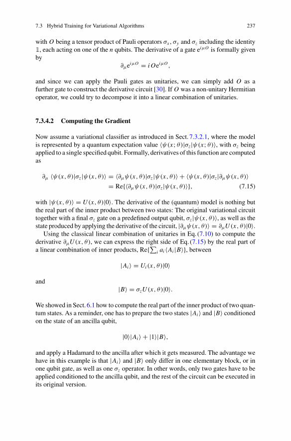
7.3 Hybrid Training for Variational Algorithms 237

with O being a tensor product of Pauli operators σx , σy and σz including the identity1, each acting on one of the n qubits. The derivative of a gate eiμO is formally givenby

∂μeiμO = i OeiμO ,

and since we can apply the Pauli gates as unitaries, we can simply add O as afurther gate to construct the derivative circuit [30]. If O was a non-unitary Hermitianoperator, we could try to decompose it into a linear combination of unitaries.

7.3.4.2 Computing the Gradient

Now assume a variational classifier as introduced in Sect. 7.3.2.1, where the modelis represented by a quantum expectation value 〈ψ(x; θ)|σz|ψ(x; θ)〉, with σz beingapplied to a single specified qubit. Formally, derivatives of this function are computedas

∂μ 〈ψ(x, θ)|σz|ψ(x, θ)〉 = 〈∂μψ(x, θ)|σz|ψ(x, θ)〉 + 〈ψ(x, θ)|σz|∂μψ(x, θ)〉= Re{〈∂μψ(x, θ)|σz|ψ(x, θ)〉}, (7.15)

with |ψ(x, θ)〉 = U (x, θ)|0〉. The derivative of the (quantum) model is nothing butthe real part of the inner product between two states: The original variational circuittogether with a final σz gate on a predefined output qubit, σz|ψ(x, θ)〉, as well as thestate produced by applying the derivative of the circuit, |∂μψ(x, θ)〉 = ∂μU (x, θ)|0〉.

Using the classical linear combination of unitaries in Eq. (7.10) to compute thederivative ∂μU (x, θ), we can express the right side of Eq. (7.15) by the real part ofa linear combination of inner products, Re{∑i ai 〈Ai |B〉}, between

|Ai 〉 = Ui (x, θ)|0〉

and|B〉 = σzU (x, θ)|0〉.

We showed in Sect. 6.1 how to compute the real part of the inner product of two quan-tum states. As a reminder, one has to prepare the two states |Ai 〉 and |B〉 conditionedon the state of an ancilla qubit,

|0〉|Ai 〉 + |1〉|B〉,

and apply a Hadamard to the ancilla after which it gets measured. The advantage wehave in this example is that |Ai 〉 and |B〉 only differ in one elementary block, or inone qubit gate, as well as one σz operator. In other words, only two gates have to beapplied conditioned to the ancilla qubit, and the rest of the circuit can be executed inits original version.

238 7 Quantum Computing for Training

Whenwe are dealing with the Pauli-matrix-generator-form of the second examplefrom above, the evaluation of gradients becomes surprisingly simple [33]. Let us goback to the derivative of the expectation value in Eq. (7.15). If the gate that we wantto derive is of the form e−iμσ , where σ is an arbitrary Pauli matrix, we get

∂μ 〈ψ(x, θ)|σz|ψ(x, θ)〉 = 〈0| . . . ∂μe−iμσ . . . σz . . . eiμσ . . . |0〉

+〈0| . . . e−iμσ . . . σz . . . ∂μeiμσ . . . |0〉

= 〈0| . . . (−iσ)e−iμσ . . . σz . . . eiμσ . . . |0〉+〈0| . . . e−iμσ . . . σz . . . (iσ)eiμσ . . . |0〉

= 〈0| . . . (1 − iσ)e−iμσ . . . σz . . . (1 + iσ)eiμσ . . . |0〉+〈0| . . . (1 + iσ)e−iμσ . . . σz . . . (1 − iσ)eiμσ . . . |0〉

In the last step we used the well-known relation

expiμσ = cos(μ)1 + i sin(μ)σ.

Noting that (1 ± iσ) = e±i π2 σ , we find that we can estimate the analytical gradient of

the expectation value by evaluating the original expectation once with an additionalei

π2 σ gate, and once with an additional gate e−i π

2 σ gate. The additional gate is insertedbefore (or after) the gate that we derive for. (Of course, this is equivalent to shiftingthe μ parameter by ±π

2 for the two evaluations.) One can show that we can write anexpression like Re{∑i ai 〈Ai |B〉} as the difference of two expectation values for anygenerator that is unitary and Hermitian.

In summary, for certain cases of variational quantummachine learningprotocols—namely those including derivatives of circuits that can be estimated from a classicallinear combination of unitaries—we can use slightly different circuits to estimateanalytical gradients. This is a very useful alternative to numerical methods.

7.4 Quantum Adiabatic Machine Learning

The last type of quantum algorithms for training we discuss in this chapter is basedon the ideas of adiabatic quantum computing and annealing (see Sect. 3.3.3). Thegoal is to prepare the ground state of a quantum system, the quantum state of nqubits with the lowest energy. The ground state typically encodes the solution to abinary optimisation problem, or represents a qsample from which we want to drawsamples. The dataset typically defines the Hamiltonian (and thereby the dynamics) ofthe system, which can be understood as a type ofHamiltonian or dynamic encoding.

Quantum annealing appears prominently in the quantum machine learning litera-ture, which is partly due to the fact that it was one of the first technologies for whichexperiments beyond proof-of-principle setups were possible. An early generation ofstudies looked at how to formulate machine learning tasks as an optimisation prob-

7.4 Quantum Adiabatic Machine Learning 239

lem that could be solved by quantum annealing (see following Sect. 7.4.1) and testedthe ideas with the D-Wave device. However, experiments confirmed the ambiguousresults of other quantum annealing studies, where there is still no conclusive answeras to which speedups are possible with this technique [34, 35]. It is therefore notclear where the advantage compared to classical annealing and sampling techniqueslies. Noise and connectivity issues in this early-stage technology further complicatedthe picture.

Quantum machine learning research therefore focused on another twist of thestory. Instead of employing annealing devices as an analogue solver of optimisationproblems, they are used as an analogue sampler (see Sect. 7.4.2). The annealingprocedure prepares a quantum state that can be interpreted as a qsample from whichmeasurements can draw samples. One important observation was for example thatthe qsample distribution prepared by D-Wave may be sufficiently close to a classicalGibbs distribution to use the samples for the training of a Boltzmann machine.

Beyond annealing, other proposals, most of them experimental in nature, havesporadically been brought forward and some of them are summarised in Sect. 7.4.3.

7.4.1 Quadratic Unconstrained Optimisation

The first generations of D-Wave’s commercial quantum annealing devices con-sisted of up to n = 1024 physical qubits with sparse programmable interactionstrengths of an Ising-type model, and annealed objective functions in the formatof quadratic unconstrained binary optimisation. The ground state or solution is thebinary sequence x1 . . . xn that minimises the ‘energy function’

n∑

i≤ j=1

wi j xi x j , (7.16)

with the coefficients or weights wi j . A central task for this approach of quantummachine learning is therefore to cast a learning task into such an optimisation prob-lem.

There have been a number of proposals of how to translate machine learningproblems into an unconstrained binary optimisation problem (see also Sect. 8.3.3).Machine learning problems that lend themselves especially well for combinatorialoptimisation are structure learning problems for graphs, for example of Bayesiannets [36]. Each edge of the graph is associated to a qubit in state 1, while a missingedge corresponds to a state 0 qubit, so that the graph connectivity is represented bya binary string. For example, a fully connected graph of K nodes is represented bya register of K (K−1)

2 qubits in state |11 . . . .1〉, Under the assumption for Bayesiannets that no node has more than |π |max parents, a ‘score Hamiltonian’ can be definedthat assigns an energy value to every permitted graph architecture/bit string, and thestring with the lowest energy is found via quantum annealing. Other examples have

240 7 Quantum Computing for Training

been in the area of image matching (recognising that two images show the samecontent but in different light conditions or camera perspectives) [37], as well as insoftware verification and validation [38].

A machine learning task that naturally comes in the shape of a quadratic uncon-strained optimisation problem is the memory recall of a Hopfield neural network(see also Sect. 2.4.2.3). In Eq. (7.16) the weights wi j are determined by a learningrule such as the Hebb rule, and define the solution to the corresponding minimisationproblem. The xi , x j are bits of the new input pattern with binary features. Quantumannealing then retrieves the ‘closest’ pattern—the nearest minimum energy state—inthe ‘memory’ of the Hopfield energy function.

7.4.2 Annealing Devices as Samplers

Much of the more recent work on quantum annealing for training uses annealingdevices in a less obvious way, namely to sample from an approximation to the Gibbsdistribution in order to estimate the expectations

〈vi h j 〉model =∑

v,h

e−E(v,h)

Zvi h j

in Eq. (2.30) for the training ofBoltzmannmachines.Wehave already seen a variationof this idea in the previous Sect. based on the quantum approximate optimisationalgorithm.

It turns out that the natural distributions generated by quantum annealers can beunderstood as approximations to the Boltzmann distribution [39]. Strictly speakingthese would be quantum Boltzmann distributions, where the (Heisenberg) energyfunction includes a transverse field term for the spins, but under certain conditionsquantum dynamics might not play a major role. Experiments on the D-Wave deviceshowed that the distributions it prepares as qsamples can in fact significantly deviatefrom a classical Boltzmann distribution, and the deviations are difficult to modeldue to out-of-equilibrium effects of fast annealing schedules [40]. However, thedistributions obtained still seem toworkwell for the training of (possibly pre-trained)Boltzmann machines, and improvements in the number of training steps comparedto contrastive divergence have been reported both for experimental applications andnumerical simulations [40–44]. As an application, samples from the D-Wave devicehave been shown to successfully reconstruct and generate handwritten digits [41, 44].A great advantage compared to contrastive divergence is also that fully connectedBoltzmann machines can be used.

While conceptually, the idea of using physical hardware to generically ‘simulate’a distribution seems very fruitful, the details of the implementationwith the relativelynewhardware are at this stage rather challenging [44]. For example, researchers reportGaussian noise perturbing the parameters fed into the systemby an unknown function

7.4 Quantum Adiabatic Machine Learning 241

which prohibits precise calibration. A constant challenge is also the translation of thecoupling of visible and hidden units (or even an all-to-all coupling for unrestrictedBoltzmann machines) into the sparse architecture of the connections between qubitsin the D-Wave quantum annealer. Fully connected models need to be encoded in aclever way to suit the typical chimera graph structure.

Figure7.6a shows the connectivity of qubits in the early D-Wave devices. Onlythose qubits that are connected by an edge can communicate with each other. Wecannot natively represent a fully connected graph by the qubits and their interaction,but have only limited connectivity between nodes (see Fig. 7.6b). One therefore needsclever embedding strategies in which one variable in the model or one node in thegraph is represented by multiple qubits. Another solution to deal with connectivityis to consider only problems with a structure that suits the limitations of the chimeragraph connectivity. In the example of Fig. 7.6c the task is to embed an image repre-sented by amatrix of pixels into the chimera graph. Assuming that only pixels that areclose to each other are correlated, we associate blocks of neighbouring pixels withblocks of densely interconnected qubits (where the connection runs through somehidden units). For instance, the blocks of pixel 1a and 4d are not directly connectedin the chimera graph structure, but also lie in opposite corners of the image and aretherefore not expected to be correlated as much as neighbouring pixels.

Another serious problem when using the D-Wave device as a sampler is the finite‘effective inverse temperature’ of the device. The distribution implemented by themachine contains an inverse temperature parameter β in e−βE(s,h)

Z , which can fluctuate

Fig. 7.6 In the original D-Wave annealing device, the qubits are connected by a so called chimeragraph structure shown in a for a 32 qubit system. Some qubits in the chimera graph (green-yellowvertices) are used as visible units, while others (blue vertices with dotted outline) are used ashidden units. If we want the interactions between qubits to represent the weights between variablesin a graphical model, we can therefore only encode sparse models with a connectivity shown in(b). However, in some applications the limited connectivity is not a problem. For example, whenembedding the pixels of an image c into the chimera graph, we can use the assumption that not allpixels are strongly correlated, and associate pixels that are far away from each other with qubits inblocks that are not directly connected. Figure adapted from [42], with thanks to Marcello Benedetti

242 7 Quantum Computing for Training

during the annealing process. Estimating this effective inverse temperature allowsus to correct the samples taken from the annealer and use them to approximate thedesired Boltzmann distribution [42].

The D-Wave device is only one example of an early-stage quantum technology,and we use it here to point out that another myriad of challenges appear when usingreal quantum devices for quantum machine learning. Connectivity and noise aretwo issues that occur in other platforms as well. These experimental challenges areconstantly met with new engineering solutions, which may open another researchbranch to quantum machine learning altogether. We will discuss this point further inthe conclusion when we consider quantum machine learning with intermediate-termquantum devices.

7.4.3 Beyond Annealing

Physical implementations other than quantum annealers or gate-based quantum com-puters have been used to investigate the idea of encoding the solution of a machinelearning problem into the ground state of a quantum system. For example, an earlycontribution of a rather different kind was made by Horn and Gottlieb [46]. Theiridea is to define a potential V for a Hamiltonian (which is traditionally decomposedinto a kinetic and potential energy, H = T + V ) such that a wave function withhigh probabilities in regions of high data density is the ground state of the Hamilto-nian. The wave function serves as a kernel density estimator function introduced inSect. 2.4.4.1. This idea has been subsequently used for clustering [47].

Another contribution is a demonstration that shows how an Hopfield-network-like associative memory recall can be executed with a nuclear magnetic resonancesetup [45]. The proof-of-principle experiment only looks at binary strings of length2. The idea is to encode the two binary values into the spectrum of nuclear spinsin H and C atoms (see Fig. 7.7). A positive peak at the left region of the spectrumindicates a 1 while a negative peak in the right part of the spectrum indicates a−1. A ‘no signal’ encodes a 0, which means that the bit is unknown. Setting aweight parameter to w = 1 stores the two memory patterns (−1, 1), (1,−1) intothe spectrum of the nuclear magnetic resonance system, while the configurationw = −1 stores the patterns (−1,−1), (1, 1). Starting the system with inputs x in thathave blanks at different positions leads to the desired memory recall. For example,for w = 1, the input x in = (−1, 0) recalls the memory pattern x∗ = (−1, 1). Thisis a minimal example of a quantum associative memory implemented by a quantumphysical system. Interesting enough, the quantum model can lead to ground statesthat are superpositions of patterns.

These two examples illustrate that even though the focus of quantum machinelearning lies on quantum computing devices, there are other quantum systems andexperimental setups which can implement quantum machine learning algorithms ormodels.

References 243

Fig. 7.7 Associated memory recall with atomic spectra of H and C atoms. Each spectrum encodesa−1 by a negative peak towards the left and a 1 by a positive peak towards the right. If both positiveand negative peaks are present, the signal represents a superposition of −1 and 1. Depending on the‘weight’ w = 1,−1, starting with an input signal x in1 , x in2 with a blank (0 or no signal) at differentpositions retrieves different solutions (x∗

1 , x∗2 ) from the memory. Image modified from [45]

References

1. Rebentrost, P., Bromley, T.R., Weedbrook, C., Lloyd, S.: A QuantumHopfield Neural Network(2017). arXiv:1710.03599

2. Harrow, A.W., Hassidim, A., Lloyd, S.: Quantum algorithm for linear systems of equations.Phys. Rev. Lett. 103(15), 150502 (2009)

3. Wiebe, N., Braun, D., Lloyd, S.: Quantum algorithm for data fitting. Phys. Rev. Lett. 109(5),050505 (2012)

4. Schuld, M., Sinayskiy, I., Petruccione, F.: Prediction by linear regression on a quantum com-puter. Phys. Rev. A 94(2), 022342 (2016)

5. Rebentrost, P., Mohseni, M., Lloyd, S.: Quantum support vector machine for big data classifi-cation. Phys. Rev. Lett. 113, 130503 (2014)

6. Zhao, Z., Fitzsimons, J.K., Fitzsimons, J.F.: Quantum Assisted Gaussian Process Regression(2015). arXiv:1512.03929

7. Berry,D.W.,Childs,A.M.,Kothari,R.:Hamiltonian simulationwith nearly optimal dependenceon all parameters. In: IEEE 56th Annual Symposium on Foundations of Computer Science(FOCS), pp. 792–809. IEEE (2015)

8. Wang, G.: Quantum algorithm for Linear Regression. Phys. Rev. A 96, 012335 (2017)9. Suykens, J.A.K., Vandewalle, J.: Least squares support vector machine classifiers. Neural Pro-

cess. Lett. 9(3), 293–300 (1999)10. Hebb, D.O.: The Organization of Behavior: a Neuropsychological Theory. Wiley, New York

(1949)11. Aaronson, S.: Read the fine print. Nat. Phys. 11(4), 291–293 (2015)12. Clader, B.D., Jacobs, B.C., Sprouse, C.R.: Preconditioned quantum linear system algorithm.

Phys. Rev. Lett. 110(25), 250504 (2013)13. Lloyd, S., Mohseni, M., Rebentrost, P.: Quantum principal component analysis. Nat. Phys. 10,

631–633 (2014)14. Cong, I., Duan, L.: Quantum discriminant analysis for dimensionality reduction and classifi-

cation. New J. Phys. 18, 073011 (2016)15. Kerenedis, I., Prakash, A.: Quantum recommendation systems. In: Kerenidis, I., Prakash, A.

(eds.), QuantumRecommendation Systems. LIPIcs-Leibniz International Proceedings in Infor-matics, vol. 67 (2017)

16. Wiebe, N., Kapoor, A., Svore, K.: Quantum nearest-neighbor algorithms for machine learning.Quantum Inf. Comput. 15, 0318–0358 (2015)

244 7 Quantum Computing for Training

17. Aïmeur, E., Brassard, G., Gambs, S.: Quantum speed-up for unsupervised learning. Mach.Learn. 90(2), 261–287 (2013)

18. Ventura, D., Martinez, T.: Quantum associative memory. Inf. Sci. 124(1), 273–296 (2000)19. Dürr, C., Hoyer, P.: A QuantumAlgorithm for Finding theMinimum (1996). arXiv:9607014v220. Kapoor, A., Wiebe, N., Svore, K.: Quantum perceptron models. In: Advances in Neural Infor-

mation Processing Systems, pp. 3999–4007 (2016)21. McClean, J.R., Romero, J., Babbush, R., Aspuru-Guzik, A.: The theory of variational hybrid

quantum-classical algorithms. New J. Phys. 18(2), 023023 (2016)22. Peruzzo,A.,McClean, J., Shadbolt, P., Yung,M.-H., Zhou,X.-Q., Love, P.J., Aspuru-Guzik, A.,

Obrien, J.L.: A variational eigenvalue solver on a photonic quantum processor. Nat. Commun.5 (2014)

23. Farhi, E., Goldstone, J., Gutmann, S.: A Quantum Approximate Optimization Algorithm(2014). arXiv:1411.4028

24. Farhi, E., Harrow, A.W.: Quantum Supremacy Through the Quantum Approximate Optimiza-tion Algorithm (2016). arXiv:1602.07674

25. Wan, K.H., Dahlsten, O., Kristjánsson, H., Gardner, R., Kim, M.S.: Quantum generalisationof feed forward neural networks. npj Quantum. Inf. 3(1), 36 (2017)

26. Verdon, G., Broughton, M., Biamonte, J.: A Quantum Algorithm to Train Neural Networksusing Low-Depth Circuits (2017). arXiv:1712.05304

27. Nelder, J.A.,Mead, R.: A simplexmethod for functionminimization. Comput. J. 7(4), 308–313(1965)

28. Spagnolo, N., Maiorino, E., Vitelli, C., Bentivegna, M., Crespi, A., Ramponi, R., Mataloni, P.,Osellame, R., Sciarrino, F.: Learning an unknown transformation via a genetic approach. Sci.Rep. 7(1), 14316 (2017)

29. Guerreschi, G.G., Smelyanskiy, M.: Practical Optimization for Hybrid Quantum-ClassicalAlgorithms (2017). arXiv:1701.01450

30. Farhi, E., Neven, H.: Classification with Quantum Neural Networks on Near Term Processors(2018). arXiv:1802.06002

31. Schuld, M., Bocharov, A., Wiebe, N., Svore, K.: A Circuit-Centric Variational Quantum Clas-sifier (2018). arXiv:1804.00633

32. Barenco, A., Bennett, C.H., Cleve, R., DiVincenzo, D.P., Margolus, N., Shor, P., Sleator,T., Smolin, J.A., Weinfurter, H.: Elementary gates for quantum computation. Phys. Rev. A52(5):3457 (1995)

33. Mitarai, K., Negoro, M., Kitagawa, M., Fujii, K.: Quantum Circuit Learning (2018).arXiv:1803.00745

34. Heim, B., Rønnow, T.F., Isakov, S.V., Troyer, M.: Quantum versus classical annealing of Isingspin glasses. Science 348(6231), 215–217 (2015)

35. Troels, F.: Rnnow, Zhihui Wang, Joshua Job, Sergio Boixo, Sergei V. Isakov, David Wecker,John M. Martinis, Daniel A. Lidar, and Matthias Troyer. Defining and detecting quantumspeedup. Science 345, 420–424 (2014)

36. O’Gorman, B., Babbush, R., Perdomo-Ortiz, A., Aspuru-Guzik, A., Smelyanskiy, V.: Bayesiannetwork structure learning using quantum annealing. Eur. Phys. J. Spec. Top. 224(1):163–188(2015)

37. Neven, H., Rose, G., Macready, W.G.: Image recognition with an adiabatic quantum computeri. Mapping to Quadratic Unconstrained Binary Optimization (2008). arXiv:0804.4457

38. Pudenz, K.L., Lidar, D.A.: Quantum adiabatic machine learning. Quantum Inf. Process. 12(5),2027–2070 (2013)

39. Denil, M., De Freitas, N.: Toward the implementation of a quantum RBM. In: NIPS 2011 DeepLearning and Unsupervised Feature Learning Workshop (2011)

40. Korenkevych, D., Xue, Y., Bian, Z., Chudak, F., Macready, W.G., Rolfe, J., Andriyash, E.:Benchmarking Quantum Hardware for Training of Fully Visible Boltzmann Machines (2016).arXiv:1611.04528

41. Adachi, S.H., Henderson,M.P.: Application of QuantumAnnealing to Training of DeepNeuralNetworks (2015). arXiv:1510.06356

References 245

42. Benedetti, M., Realpe-Gómez, J., Biswas, R., Perdomo-Ortiz, A.: Estimation of effective tem-peratures in quantum annealers for sampling applications: a case study with possible applica-tions in deep learning. Phys. Rev. A 94(2), 022308 (2016)

43. Amin, M.H., Andriyash, E., Rolfe, J., Kulchytskyy, B., Melko, R.: Quantum Boltzmannmachine. Phys. Rev. X 8:021050 (2018)

44. Benedetti, M., Realpe-Gómez, J., Biswas, R., Perdomo-Ortiz, A.: Quantum-assisted learningof hardware-embedded probabilistic graphical models. Phys. Rev. X 7, 041052 (2017)

45. Neigovzen, R., Neves, J.L., Sollacher, R., Glaser, S.J.: Quantumpattern recognitionwith liquid-state nuclear magnetic resonance. Phys. Rev. A 79(4):042321 (2009)

46. Horn, D., Gottlieb, A.: Algorithm for data clustering in pattern recognition problems based onquantum mechanics. Phys. Rev. Lett. 88(1), 018702 (2002)

47. Cui, Y., Shi, J., Wang, Z.: Lazy quantum clustering induced radial basis function networks(LQC-RBFN) with effective centers selection and radii determination. Neurocomputing 175,797–807 (2016)

Chapter 8Learning with Quantum Models

The last two chapters were mainly concerned with the translation of known machinelearning models and optimisation techniques into quantum algorithms in order toharvest potential runtime speedups known from quantum computing. This chapterwill look into ‘genuine’ quantum models for machine learning which either have nodirect equivalent in classical machine learning, or which are quantum extensions ofclassical models with a new quality of dynamics. A quantummodel as we understandit here is amodel function or distribution that is based on themathematical formalismof quantum theory, or naturally implemented by a quantum device. For example, ithas been obvious from the last chapters that Gibbs distributions play a prominentrole in some areas of machine learning. At the same time, quantum systems can bein a ‘Gibbs state’. Previously, we described a number of attempts to use the quantumGibbs states in order to sample froma (classical)Gibbs distribution.Butwhat happensif we just use the ‘quantum Gibbs distribution’? What properties would such modelsor training schemes exhibit?What ifwe use other distributions that are easy to prepareon a quantum device but difficult on a classical one, and construct machine learningalgorithms from them? How powerful are the classifiers constructed from variationalcircuits in Sect. 7.3.2.1, that is if we use the input-output relation of a quantum circuitas a core machine learning model f (x) and train the circuit to generalise from data?

This chapter sheds some light onto what has been earlier called the exploratoryapproach of quantum machine learning. It focuses less on speedups, but is interestedin creating and analysing new models based on quantum mechanics, that serve asan addition to the machine learning literature. Although still in its infancy, the greatappeal of this approach is that it is suited for near-term or noisy as well as non-universal quantum devices, because of the change in perspective: We start with aquantum system and ask whether it can be used for supervised learning, rather thantranslating models that were tailor-made for classical computers.

In the usual demeanour of this book we will present a couple of illustrative exam-ples rather than an exhaustive literature review. Amongst them are quantum exten-sions of Ising models (Sect. 8.1) as well as variational circuits (Sect. 8.2). The last

© Springer Nature Switzerland AG 2018M. Schuld and F. Petruccione, Supervised Learning with Quantum Computers,Quantum Science and Technology, https://doi.org/10.1007/978-3-319-96424-9_8

247

248 8 Learning with Quantum Models

Sect. 8.3 summarises further ideas, namely to replace Markov chains by quantumMarkov chains, to use quantum superposition for ensemble methods, and to createspecial cost functions to be optimised by quantum annealing.

8.1 Quantum Extensions of Ising-Type Models

Hopfield networks and Boltzmann machines are both important machine learningmethods that are based on one of the most successful family of models in physics, socalled Ising models. The original Ising model describes ferromagnetic properties instatistical mechanics, namely the behaviour of a set of two-dimensional spin systemsthat interact with each other via certain nearest-neighbour interactions. We use theterm in a wider sense here, to denote models of interacting units or particles of anyconnectivity and weight.

The Ising model is also no stranger to machine learning. Hopfield networks—which have a historical significance in reconnecting artificial neural networks withbrain research—have in fact been introduced by a physicist, James Hopfield, whotransferred the results from statistical physics to recurrent neural networks. Boltz-mann machines can be understood as a probabilistic version of Hopfield networks.In both cases, the spins or particles are associated with binary variables or neurons,while the interactions correspond to the weights that connect the units. The physicalequivalence gives rise to a well-defined quantum extension of these two methodswhich we will review in the following.

Let us first briefly summarise some central equationswhich have been explained inmore detail in Sects. 2.4.2.3 and 2.4.2.4. Hopfield networks and Boltzmannmachinesare both a special case of recurrent neural networks consisting of G binary variabless = s1...sG with si ∈ {−1, 1} or si ∈ {0, 1} for all i = 1, . . . ,G. The units can bedistinguished into a set of visible and hidden units s = vh = v1...vNv

h1...hNh withNv + Nh = N .1 We can define an Ising-type energy function that assigns a real valueto each configuration of the system,

E(s) = −∑

i, j

wi j si s j −∑

i

bi si , (8.1)

with parameters {wi j , bi } and i, j = 1, . . . ,G.InHopfieldmodels theweights are symmetric (wi j=w j i ) and non-self-connecting

(wi i = 0), and there is no constant field bi = 0. With this architecture, the state ofeach unit is successively (synchronously or chronologically) updated according tothe perceptron rule,

1In earlier chapters we referred to the number of visible units as N + K to stress that in a supervisedlearning setting, the visible units can be divided into N input and K output units. For the sake ofsimplicity we will not make this distinction here.

8.1 Quantum Extensions of Ising-Type Models 249

s(t+1)i = sgn(

∑

j

wi j s(t)j ).

The updates can be shown to lower or maintain the energy of the state in every timestep t → t + 1, until it converges to the closest local minimum. These dynamics canbe interpreted as an associative memory recall of patterns saved in minima.

The recall algorithm is similar to a Monte Carlo algorithm at zero temperature.In every step a random neuron si is picked and the state is flipped to si if does notincrease the energy, that means if

E(s1 . . . si . . . sN ) ≤ E(s1 . . . si . . . sN ).

A generalised version of the Hopfield model [1] allows for a finite temperature andprobabilistic updates of units in the associative memory recall. If one defines theprobability of updating unit si to go from s = s1 . . . si . . . sN to s = s1 . . . si . . . sN as

p(s) = 1

1 + e−2E(s),

we arrive at Boltzmann machines (with the temperature parameter set to 1). Herethe binary units are random variables and the energy function defines the probabilitydistribution over states {s} via

p(s) = 1

Ze−E(s). (8.2)

As before, Z is the partition function

Z =∑

s

e−E(s). (8.3)

For restricted Boltzmann machines, the parameters wi j connecting two hidden ortwo visible units are set to zero.

8.1.1 The Quantum Ising Model

In the transition to quantum mechanics, the interacting units of the Ising model arereplaced by qubits, the Hamiltonian energy function becomes an operator

H = −1

2

∑

i j

wi jσizσ

jz −

∑

i

biσiz ,

250 8 Learning with Quantum Models

by replacing the values si by Pauli-σz operators acting on the i th or j th qubit. Whenwe express the Hamiltonian as a matrix in the computational basis, it is diagonal.The reason for this is that the computational basis {|k〉} is an eigenbasis to the σz

operator, which means that the off-diagonal elements disappear, or 〈k|σ iz |k ′〉 = 0 and

〈k|σ izσ

jz |k ′〉 = 0 for all i, j if k �= k ′. The eigenvalues on the diagonal are the values

of the energy function (8.1). For example, the Ising Hamiltonian for a 2-qubit systemtakes the following shape:

H =

⎛

⎜⎜⎝

E(s = 00) 0 0 00 E(s = 01) 0 00 0 E(s = 10) 00 0 0 E(s = 11)

⎞

⎟⎟⎠ ,

where we omitted the dependence on θ from Eq. (8.1).The quantum state of the system (here expressed as a density matrix) defines a

probability distribution over the computational basis states. For an Ising model it isgiven by

ρ = 1

Ze−H , (8.4)

with the partition function being elegantly expressed by a trace,

Z = tr{e−H }.

For diagonal matrices H , the matrix exponential e−H is equal to a matrix carryingexponentials of the diagonal elements on its diagonal. Consequently, ρ is diagonalwith

diag{ρ} = (1

Ze−E(s=0...0), ...,

1

Ze−E(s=1...1)).

The diagonal elements of the density matrix define the Boltzmann probability distri-bution of Eqs. (8.2) and (8.3) for all different possible states of the system’s spins orneurons, and the operator formalism is fully equivalent to the classical formalism.

Having formulated the (still classical) Ising model in the language of quantummechanics, it is not difficult to introduce quantum effects by adding terms with theother two Pauli operators that do not commute with σz . Non-commuting operators donot share an eigenbasis, and the resulting operator is not diagonal in the computationalbasis. It is therefore not anymore a different mathematical formalism for the classicalIsing model, but the non-zero off-diagonal elements give rise to genuine quantumdynamics.

It is common to only introduce a few ‘quantum terms’, such as the transverse orx-field,

H = −1

2

∑

i j

wi jσizσ

jz −

∑

i

biσiz −

∑

i

ciσix , (8.5)

8.1 Quantum Extensions of Ising-Type Models 251

where the Pauli operator σ ix is applied to the i th qubit with a strength ci . Since the

Hamiltonian for the transverse Isingmodel is no longer diagonal in the computationalbasis, superpositions of basis states are eigenstates of H , and the system exhibitsdifferent dynamics compared to the classical system.

The strategy of extending the Hamiltonian illustrates a more general recipe todesign quantum versions of machine learning models based on statistical physics:

1. Formulate the classical model in the language of quantum mechanics, for exam-ple using quantum state ρ to describe the probability distribution, and usingoperators to describe the ‘evolution’ of the system

2. Add terms that account for quantum effects, such as a transverse field in theHamiltonian or, as we will see below, a coherent term in a master equation

3. Analyse the resulting quantummodel for learning and characterise effects deriv-ing from the extension.

We will now show some examples from the literature of how this has been donefor Boltzmannmachines and Hopfield networks. Point 3, the analysis of the quantumextension formachine learning purposes, is still mainly an open issue in the literature.

8.1.2 Training Quantum Boltzmann Machines

The above strategy of adding a transverse field to the Hamiltonian has been used topropose a quantum version of Boltzmann machines by Amin et al. [2]. The quantumBoltzmann machine defines the model as the quantum state ρ from Eq. (8.4) withthe ‘tansverse’ Hamiltonian (8.5). One can understand ρ as a qsample, from whichwe can draw samples of computational basis states that correspond to states of thevisible units. A crucial question is how to train such a model to learn the weightswi j , bi and ci . As it turns out, the strategy from classical training does not carry overto the quantum model.

In order to write down the gradient from Eq. (2.29) in the language of quantummechanics, we need to define the probability of observing the visible state v′ bymeans of the model ρ,

p(v′) = tr{Λv′ρ}.

The operatorΛv′ = |v′〉〈v′| ⊗ 1h,

is a projector that in matrix notation has a single 1 entry at the diagonal position〈v′| · |v′〉 and zeros else. In other words, the operator ‘picks out’ the diagonal elementρv′v′ , which is the probability to measure the computational basis state |v′〉 or tosample v′ from the quantum model. With this definition and inserting the expressionfor ρ from Eq. (8.4), the log likelihood objective becomes

252 8 Learning with Quantum Models

C(θ) = −M∑

m=1

logtr{Λvme−H(θ)}tr{e−H(θ)} , (8.6)

where we state the dependence of H on the parameters θ = {wi j , bi , ci } now explic-itly.2 Compared to maximum likelihood estimation we consider the negative log-likelihood to formulate a cost function, which is minimised.

For gradient descent optimisation we need the derivative of the objective functionfor each parameter μ ∈ θ , which, applying logarithm derivation rules, is given by

∂μC(θ) =M∑

m=1

(tr{Λv∂μe−H(θ)}tr{Λve−H(θ)} − tr{∂μe−H(θ)}

tr{e−H(θ)})

. (8.7)

In the classical version of Eq. (2.9) we were able to execute the partial derivationvia the chain rule, which for the interaction parameters μ = wi j ended up to bethe difference of two expectation values over units from the data versus the modeldistribution from Eq. (2.30),

∂wi j C(θ) = 〈si s j 〉data − 〈si s j 〉model.

These expectation values were approximated via sampling, for example with thecontrastive divergence approach.

Using the quantum model, the operators ∂wi j H and H do not commute, whichmeans that the chain rule of basic derivation cannot be applied. However, due to theproperties of the trace, one still finds a similar relation for the right term in Eq. (8.7),

tr{∂wi j e−H(θ)} = −tr{e−H(θ)∂wi j H(θ)}.

The trace over ‘operator’ ∂wi j H(θ) for a Gibbs state ρ = e−H(θ) divided by thepartition function tr{e−H(θ)} is nothing other than the expectation value over theBoltzmanndistribution 〈∂wi j H(θ)〉model = 〈σ i

z , σjz 〉model. For the left termofEq. (8.7),

tr{Λv∂wi j e−H(θ)}

tr{e−H(θ)} , (8.8)

the additional operator inside the trace prohibits this trick. Without a strategy toapproximate this term, common training methods are therefore not applicable, evenif we only consider restricted Boltzmann machines. This is a good example of howquantum extensions can require different approaches for training.

A strategy proposed in [2] is to replace the Hamiltonian H in this troublesometerm in Eq. (8.8) with a “clamped” Hamiltonian Hm(θ) = H(θ) − lnΛvm , whichpenalises any states other than |vm〉. One can show that the new cost function is an

2Note that we simplified the original expression in [2] to be consistent with the more commondefinition of the log-likelihood introduced in Sect. 2.9.

8.1 Quantum Extensions of Ising-Type Models 253

upper bound for the original objective from Eq. (8.6). We can hence write the leftterm in Eq. (8.7) as

M∑

m=1

p(vm; θ)tr{e−Hm (θ)∂wi j Hm(θ)}

tr{e−Hm (θ)} = 〈∂wi j Hm(θ)〉data = 〈σ iz , σ

jz 〉data.

One can show that this corresponds to minimising an upper bound of the objective[2]. This works well for parameter updates wi j , bi , but fails for the updating rule ofthe ci , the parameters of the transverse field strength, which in the worst case have tobe simply guessed. However, trainingwith samples from a (clamped) quantumBoltz-mann machine can have better convergence properties than a classical Boltzmannmachine [2].

Other versions of quantumBoltzmannmachines have been proposed, for exampleusing a fermionic rather than a stochastic Hamiltonian, more general (i.e. quantum)training data sets, as well as relative entropy rather than a log-likelihood objective [3].

8.1.3 Quantum Hopfield Models

A number of studies on ‘quantum Hopfield models’ follow the same approach as inthe previous section and investigate how the introduction of an transverse field termas in Eq. (8.5) changes the dynamics of the associative memory recall. For example,qualitative differences regarding noise and the capacity (ratio of stored patterns tosystem size) of the network have been reported [4–7]. But, as we will establish inthis section, one can also look at quantum extensions of Ising-type models startingfrom the differential equations of the system. As an example, we follow Rotondo etal. [8] who formulate a quantum version of the Hopfield model as an open quantumsystem governed by a quantum master equation. We have not covered this topicmuch in the foundations of Chap. 3, and will therefore only sketch the general ideahere. Interested readers can refer to [9] for more details on the theory and descriptionof open quantum systems.

Unitary evolutions in quantum mechanics – which we have discussed at length—are the solution of the Schrödinger equation (3.1.3.3), which applies to closed quan-tum systems. In closed quantum systems, no information about the state is lost andthe evolution is fully reversible. But the associative memory dynamics of a mem-ory recall is a dissipative evolution in which the energy of the system is not pre-served, which means that we do not have reversible dynamics. This requires an openquantum systems approach, where the equivalence of the Schrödinger equation isa quantum master equation.3 A popular formulation of a quantum master equation

3Master equations appear in many other sub-disciplines of physics.

254 8 Learning with Quantum Models

describing the evolution of a dissipative quantum system is theGorini-Kossakowski-Sudarshan-Lindblad equation that we mentioned in Sect. 3.1.3.6. As a reminder, theGKSL equation defines the time evolution of a density operator, in this case

d

dtρ = −i[H, ρ] +

K∑

k=1

∑

γ=±

(Lkγ ρL†

kγ − 1

2L†kγ Lkγ ρ − 1

2ρL†

kγ Lkγ })

. (8.9)

The first part, −i[H, ρ], describes the coherent part of the evolution, namely thequantum effects. The second part, containing the Lindblad operators Lkγ , describesa stochastic evolution, which can be roughly thought of as transitions between statesof the system represented by the Lkγ , according to a probability defined by ρ.

For the quantum version of the Hopfield model’s dynamic, the jump operatorsLkγ are defined as

Lk± = e∓1/2ΔEk

√2 cosh(ΔEk)

σ k±.

The value of ΔEk is the energy difference of a system in state s and a system in states resulting from flipping the state of the kth unit. Furthermore, the plus/minus Paulioperators are defined as σ k± = (σ i

x ± iσ iy)/2. For the coherent term, the Hamiltonian

can for example be chosen as the transverse field term from before,

H = c∑

i

σ ix ,

butwith constant coefficients ci = c. If the coherent term is not included, theLindbladequation becomes a classical equation. Rotondo et al. [8] show this in detail in theHeisenberg picture, where instead of the dynamics of the state ρ in Eq. (8.9), onelooks at the same (but purely classical) dynamics for the σ k

z operators,

d

dtσ kz =

K∑

k=1

∑

γ=±

(Lkγ σ k

z L†kγ − 1

2L†kγ Lkγ σ k

z − 1

2σ kz L

†kγ Lkγ

)

and finds that the operator expectation value 〈σ kz 〉 has the same expression as the

well-known mean field approximation for the value of each spin in the classical spinglass model,

〈sk〉 = tanh

⎛

⎝∑

j

wi j 〈s j 〉⎞

⎠ .

The dynamics of the quantum model can be analysed with mean-field techniquesthat lead to a phase diagram [8]. Phase diagrams are important tools in statistical

8.1 Quantum Extensions of Ising-Type Models 255

physics to study the behaviour of a system in different parameter regimes. In thiscase we are interested in the phase diagram of field strength parameter c and thetemperature T . For any temperature, if c is sufficiently low, the general structure ofthe classical associative memory remains valid. For large temperatures and large cthere is a parametric phase where the model converges to a zero pattern. A qualita-tively new dynamics enters for small temperatures and large field strengths and is alimit cycle phase. This means that the state of the system periodically goes througha fixed sequence of states, a limit cycle. Such limit cycles are known from classicalHopfieldmodelswith asymmetric connectionswi j �= w j i . For example, an asymmet-ric Hopfield network with two nodes s1, s2 and connections w12 = −0.5, w21 = 0.5will update the state of the two nodes according to

s(t+1)1 = ϕ(−0.5s(t)

2 ), s(t+1)2 = ϕ(0.5s(t)

1 ),

which, starting with s1 = 1, s2 = 1 and with ϕ being a step function with a thresholdat 0, sends the state into the limit cycle

(11

)→

(−11

)→

(−1−1

)→

(1

−1

)→

(11

).

Hopfield remarked that Hopfield networks with asymmetric connections show asimilar behaviour to dynamics of the Ising model at finite temperature [10]. Rotondoet al. argue that the limit-cycle phase of the quantum Hopfield model is instead aproduct of competition between coherent and dissipative dynamics, not a result ofasymmetry or self-connections. The quantum model therefore promises to exhibitanother quality of dynamics compared to the classical one.

8.1.4 Other Probabilistic Models

Not only Ising-type models have natural quantum extensions. Another probabilisticmodel that lends itself easily to this purpose are hidden Markov models, wherea system undergoes a sequence of state transitions under observations, and eitherthe transition/observation probabilities, or the next transition is to be learned (seeSect. 2.4.3.2). State transitions and observation probabilities are central to quantumphysics as well, where they can be elegantly described in the formalism of densitymatrices and open quantum systems.

Monras, Beige and Wiesner [11] introduce a quantum formulation of hiddenMarkov models, in which the state of the system is a density matrix ρ and statetransitions are formally represented by so called Kraus operators K with associatedprobabilities tr{Kρ} [9]. Although the primary idea is to use these quantum modelsto learn about partially observable quantum systems, Monras et al. observe thatthe number of internal states necessary for generating some stochastic processes is

256 8 Learning with Quantum Models

smaller than of a comparable classical model.4 The ‘reinforcement learning’ versionof hidden Markov models are partially observable Markov decision processes andhave been generalised to a quantum setting by Barry, Barry and Aaronson [13]. Theyshow that a certain type of problem—the existence of a sequence of actions that canreach a certain goal state—is undecidable for quantum models. Another variation ofa hidden Markov model is proposed in [14] and is based on a certain formulation ofquantum Markov processes.

A further branch of ‘quantum-extendable’ probabilisticmodels are graphicalmod-els. Leifer et al. [15] give a quantummechanical version of belief propagation, whichis an algorithm for inference in graphicalmodels. Directed graphicalmodels inwhicha directed edge stands for a causal influence are called causal models. A goal thatgains increasing attention in the classical machine learning community is to discovercausal structure from data, which is possible only to some extent [16] in the classicalcase. Quantum systems exhibit very different causal properties, and it is sometimespossible to infer the full causal structure of a model from (quantum) data [17, 18].Costa and Shrapnel [19] introduce quantum analogues of causal models for the dis-covery of causal structure, and propose a translation for central concepts such as the‘Markov condition’ or ‘faithfulness’. Whether such quantum models can have anyuse for classical data (or even for quantum data) is a largely open question.

8.2 Variational Classifiers and Neural Networks

The second approach presented in this chapter is based on variational quantum cir-cuits which have been introduced in Sect. 7.3 in the context of hybrid training. Asa reminder, a variational circuit is a quantum circuit that consists of parametrisedgates, and where the parameters (and thereby the circuit) can be optimised or learntaccording to a certain objective. If we use some circuit parameters to feed inputs intothe circuit, and understand the result computed by the circuit as an output, we caninterpret a variational circuit as a mathematical model for supervised learning.

Learning models based on variational circuits are a prime example for theexploratory approach to quantum machine learning. The quantum device is usedas a computational (sub-)routine in a mathematical model. It is treated as a black-box that produces—or assists in producing—predictions when fed with (possiblypre-processed) inputs. Hence, one works with a model that can be naturally imple-mented by a quantum device.

In the following we will revisit the ansatz of Sect. 7.3.3.2, where we considereda decomposition of a variational circuit into parametrised single-qubit gates andcontrolled versions thereof. We want to show now how to interpret such a quantumgate as a linear layer in the language of neural networks. This may help to tap into

4In a later paper, Monras and Winter [12] also perform a mathematical investigation into the taskof learning a model from example data in the quantum setting, i.e. to ask whether there is there aquantum process that realises a set of measurements or observations.

8.2 Variational Classifiers and Neural Networks 257

the rich theory for neural nets in order to develop and analyse quantum modelsbased on variational circuits. It also raises interesting questions about the number ofparameters needed to build a sufficiently powerful classifier. We will finally look atsome proposals from classical machine learning to decompose N × N -dimensionalunitaries into matrices which can be computed in time O(N ) or below.

8.2.1 Gates as Linear Layers

Let us consider a variational circuit that consists of parametrised gates as defined inEq. (7.11) of the previous section. Instead of trigonometric functions, we can use twocomplex numbers z, u ∈ C with each a real and an imaginary value as parameters,

G(z, v) =(

z u−u∗ z∗

). (8.10)

To neglect the global phase we can include the condition that |z|2 + |v|2 = 1. Anadvantage of this parametrisation is that it does not introduce nonlinear dependenciesof the circuit parameters on the model output, while a disadvantage in practice isthat during training the normalisation condition has to be enforced. We will use thisparametrisation here simply for ease of notation.

Let us have a look at the structure of the overall matrix representation of a (con-trolled) single qubit gate. As a reminder, a single qubit gate applied to the i th qubitof an n qubit register has the following structure:

Gqi = 11 ⊗ · · · ⊗ G(z, v)︸ ︷︷ ︸position i

⊗ · · · ⊗ 1n.

The 2n × 2n matrix Gqi is sparse and its structure depends on which qubit i the gateacts on.

Example 8.1 (Parametrised single qubit gate). For n = 3 and i = 1:

Gq1 =

⎛

⎜⎜⎜⎜⎜⎜⎜⎝

z v 0 0 0 0 0 0−v∗ z 0 0 0 0 0 00 0 z v 0 0 0 00 0 −v∗ z∗ 0 0 0 00 0 0 0 z v 0 00 0 0 0 −v∗ z∗ 0 00 0 0 0 0 0 z v0 0 0 0 0 0 −v∗ z∗

⎞

⎟⎟⎟⎟⎟⎟⎟⎠

, (8.11)

while for n = 3 and i = 2:

258 8 Learning with Quantum Models

Gq2 =

⎛

⎜⎜⎜⎜⎜⎜⎜⎝

z 0 v 0 0 0 0 00 z 0 v 0 0 0 0

−v∗ 0 z∗ 0 0 0 0 00 −v∗ 0 z∗ 0 0 0 00 0 0 0 z 0 v 00 0 0 0 0 z 0 v0 0 0 0 −v∗ 0 z∗ 00 0 0 0 0 −v∗ 0 z∗

⎞

⎟⎟⎟⎟⎟⎟⎟⎠

, (8.12)

and lastly n = 3 and i = 3 yields

Gq3 =

⎛

⎜⎜⎜⎜⎜⎜⎜⎝

z 0 0 0 v 0 0 00 z 0 0 0 v 0 00 0 z 0 0 0 v 00 0 0 z 0 0 0 v

−v∗ 0 0 0 z∗ 0 0 00 −v∗ 0 0 0 z∗ 0 00 0 −v∗ 0 0 0 z∗ 00 0 0 −v∗ 0 0 0 z∗

⎞

⎟⎟⎟⎟⎟⎟⎟⎠

. (8.13)

To make the elementary gate set universal, we also consider the application of thesingle qubit gate Gqi controlled by another qubit j , which we denote by cq j Gqi . Asingle qubit gate applied to qubit i and controlled by qubit j carries a ‘diagonal unitentry’ in some columns and rows as opposed to the single qubit gate.

Example 8.2 (Controlled parametrised single qubit gate). Gq1 from Eq. (8.11) canbe controlled by q3 and becomes

cq3Gq2 =

⎛

⎜⎜⎜⎜⎜⎜⎜⎜⎜⎜⎝

1 0 0 0 0 0 0 00 z 0 u 0 0 0 00 0 1 0 0 0 0 00 −u∗ 0 z∗ 0 0 0 00 0 0 0 1 0 0 00 0 0 0 0 z 0 u0 0 0 0 0 0 1 00 0 0 0 0 −u∗ 0 z∗

⎞

⎟⎟⎟⎟⎟⎟⎟⎟⎟⎟⎠

. (8.14)

As a product of matrices, a variational circuit

U (θ) = G(θL) · · ·G(θ1)

with θ1, . . . , θL ⊂ θ can be understood as a sequence of linear layers of a neuralnetwork where the layers have a constant size. This perspective allows us to usegraphical representations to visualise the connectivity power of a single qubit gateand helps to understand the mechanics of the unitary circuit as a classifier. Theposition of the qubit as well as the control qubit determine the architecture of eachlayer, i.e. which units are connected and which weights are tied (i.e., have the samevalue).

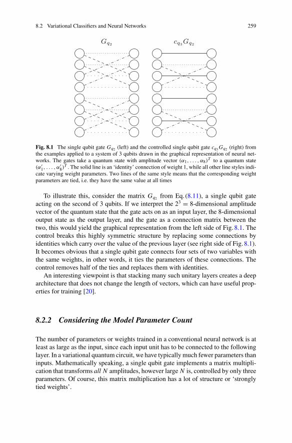
8.2 Variational Classifiers and Neural Networks 259

Gq2 cq3Gq2

Fig. 8.1 The single qubit gate Gq2 (left) and the controlled single qubit gate cq3Gq2 (right) fromthe examples applied to a system of 3 qubits drawn in the graphical representation of neural net-works. The gates take a quantum state with amplitude vector (α1, . . . , α8)

T to a quantum state(α′

1, . . . , α′8)

T . The solid line is an ‘identity’ connection of weight 1, while all other line styles indi-cate varying weight parameters. Two lines of the same style means that the corresponding weightparameters are tied, i.e. they have the same value at all times

To illustrate this, consider the matrix Gq2 from Eq. (8.11), a single qubit gateacting on the second of 3 qubits. If we interpret the 23 = 8-dimensional amplitudevector of the quantum state that the gate acts on as an input layer, the 8-dimensionaloutput state as the output layer, and the gate as a connection matrix between thetwo, this would yield the graphical representation from the left side of Fig. 8.1. Thecontrol breaks this highly symmetric structure by replacing some connections byidentities which carry over the value of the previous layer (see right side of Fig. 8.1).It becomes obvious that a single qubit gate connects four sets of two variables withthe same weights, in other words, it ties the parameters of these connections. Thecontrol removes half of the ties and replaces them with identities.

An interesting viewpoint is that stacking many such unitary layers creates a deeparchitecture that does not change the length of vectors, which can have useful prop-erties for training [20].

8.2.2 Considering the Model Parameter Count

The number of parameters or weights trained in a conventional neural network is atleast as large as the input, since each input unit has to be connected to the followinglayer. In a variational quantum circuit, we have typically much fewer parameters thaninputs. Mathematically speaking, a single qubit gate implements a matrix multipli-cation that transforms all N amplitudes, however large N is, controlled by only threeparameters. Of course, this matrix multiplication has a lot of structure or ‘stronglytied weights’.

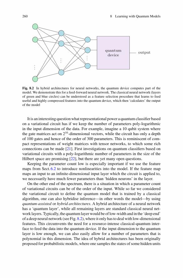
260 8 Learning with Quantum Models

...

...

...

quantumdevice

output

Fig. 8.2 In hybrid architectures for neural networks, the quantum device computes part of themodel. We demonstrate this for a feed-forward neural network. The classical neural network (layersof green and blue circles) can be understood as a feature selection procedure that learns to feeduseful and highly compressed features into the quantum device, which then ‘calculates’ the outputof the model

It is an interesting questionwhat representational power a quantumclassifier basedon a variational circuit has if we keep the number of parameters poly-logarithmicin the input dimension of the data. For example, imagine a 10 qubit system wherethe gate matrices act on 210-dimensional vectors, while the circuit has only a depthof 100 gates and hence of the order of 300 parameters. This is reminiscent of com-pact representations of weight matrices with tensor networks, to which some richconnections can be made [21]. First investigations on quantum classifiers based onvariational circuits with a poly-logarithmic number of parameters in the size of theHilbert space are promising [22], but there are yet many open questions.

Keeping the parameter count low is especially important if we use the featuremaps from Sect. 6.2 to introduce nonlinearities into the model. If the feature mapmaps an input to an infinite-dimensional input layer which the circuit is applied to,we necessarily have much fewer parameters than ‘hidden neurons’ in the layer.

On the other end of the spectrum, there is a situation in which a parameter countof variational circuits can be of the order of the input. While so far we consideredthe variational circuit to define the quantum model that is trained by a classicalalgorithm, one can also hybridise inference—in other words the model—by usingquantum-assisted or hybrid architectures. A hybrid architecture of a neural networkhas a ‘quantum layer’, while all remaining layers are standard classical neural net-work layers. Typically, the quantum layerwould be of low-width and in the ‘deep end’of a deep neural network (see Fig. 8.2), where it only has to dealwith low-dimensionalfeatures. This circumvents the need for a resource-intense classical-quantum inter-face to feed the data into the quantum device. If the input dimension to the quantumlayer is low enough, we can also easily allow for a number of parameters that ispolynomial in this dimension. The idea of hybrid architectures has been originallyproposed for probabilistic models, where one samples the states of some hidden units

8.2 Variational Classifiers and Neural Networks 261

from a quantum device and computes classical samples for the next hidden and vis-ible layer from the quantum samples [23]. Whether this approach shows significantadvantages in real applications is still mostly an open research question.

8.2.3 Circuits with a Linear Number of Parameters

An alternative connection between unitary circuits and neural networks comes inter-estingly enough from the classical machine learning literature. In the context ofrecurrent neural networks, unitary weight matrices that update the neurons in everytime step are used to avoid the exploding/vanishing gradients problem [24–26]. Aunitary matrix has the property of preserving the length of the vector it is applied toand therefore maintains the scale of the signal fed forward (in time), and the errorspropagated backwards.

The proposal in Arjovsky et al. [24] aims at a decomposition of an N × N unitarymatrix U into several unitary matrices which all have the property that they can becomputed in time O(N ),

U = D3T2F−1D2ΠT1FD1.

The decomposition includes the following types of matrices:

• The three matrices D1, D2, D3 are diagonal with diag{D} = (eiω1 , ..., eiωN ) andreal parameters ω1, ..., ωN .

• The twomatrices T1, T2 are reflection matrices defined by a N -dimensional reflec-tion vector v via

Ti = 1 − 2viv

†i

||vi ||2 ,

for i = 1, 2.• The fixed matrices F, F−1 implement a Fourier transform and its inverse.• The fixed matrix Π implements a constant permutation.

The learnable parameters are in this case the {ω} of each diagonal matrices, aswell as the entries of the reflection vectors that define T1 and T2. In total, these are5N parameters, and all computations can be performed linear in N . To a quantumcomputing expert, the building blocks of the unitary layer are all very familiar fromquantum computing, and such a layer—excluding the final nonlinear activation usedin the paper [24], could be implemented as a variational circuit. Most notably, theFourier transform can be implemented in poly-logarithmic time relative to N , awell-known exponential speedup (see Sect. 3.5.2).

Another unitary decomposition ansatz from the literature on unitary recurrentneural nets allows us to tune through architectures from O( N

2 ) parameters to a fullrepresentation of a general unitary with O(N 2) parameters. It is inspired by aninfluential physics paper by Reck, Zeilinger, Bernstein and Bertani [27], and its later

262 8 Learning with Quantum Models

Fig. 8.3 Right: A 2-levelrotation Ti j can beinterpreted as a linear layerthat connects only twodimensions i and j .Summarising several 2-levelrotations to a single 2-levelrotation layer connects pairsof adjacent dimensions witheach other

Tij

...i

j

...

...i′

j′

...

T12...TN−1,N

...

...

...

...

extension [28]. The original paper showed how to experimentally realise any unitarytransformation through a network of certain building blocks (in their case, betweena set of optical channels via beam splitters). On a more abstract level, these buildingblocks can be written as 2-level rotation operators, each of which has the form

Ti j (α, β) =

⎛

⎜⎜⎜⎜⎜⎜⎜⎜⎜⎜⎜⎜⎜⎜⎜⎜⎝

1 0 · · · · · · · · · · · · · · · 00 1

......

. . ....

... eiα cosβ − sin β...

... eiα sin β cosβ...

.... . .

...... 1 00 · · · · · · · · · · · · · · · 0 1

⎞

⎟⎟⎟⎟⎟⎟⎟⎟⎟⎟⎟⎟⎟⎟⎟⎟⎠

. (8.15)

Applied to an amplitude vector, this operator only touches the i th and j th amplitudeand rotates them similar to a single qubit rotation controlled by all other qubits. Inthe graphical representation of layers we introduced above, this operation correlatestwo input nodes as depicted in Fig. 8.3.

Anyunitarymatrix canbedecomposed into the networkof 2-level-rotations shownin Fig. 8.4 (see [28] for a proof). Formally the network can be written as

U = (T1,2...TN−1,N ) (T2,3...TN−2,N−1) (T1,2...TN−1,N ) ...(T1,2...TN−1,N ).

In other words, the network is a concatenation of even and odd 2-level rotation layers(summarised in the round brakets). Odd layers connect neighbours [1, 2], [3, 4] . . .,while even layers connect neighbours [2, 3], [4, 5] . . .. The full parametrisation

8.2 Variational Classifiers and Neural Networks 263

Fig. 8.4 A square grid of 8rotation layers (where the 28parametrised Ti j rotationsfrom Eq. (8.15) sit atintersections of the dottedlines) can represent anyunitary transformation of an8-dimensional input vector,represented by the circles

requires N (N − 1)/2 rotation gates. Reducing the number of layers can be a usefulstrategy to limit the number of model parameters, as shown in [25].

Not surprisingly, also this building block of a unitary layer is common in quantumcomputing. The study of unitary layers in neural networks therefore offers a fruitfulconnection between quantum machine learning models based on variational circuitsand classical machine learning.

8.3 Other Approaches to Build Quantum Models

In this last section, three other ideas to create quantum models for machine learningare summarised in order to demonstrate the variety of the explorative approach. Thefirst idea is again to replace a classical formalism, Markov chains or random walks,by the quantum version [29]. The second idea looks at quantum superposition andhow it can be used to create ensembles of classifiers in parallel to get a “training-free”predictor [30]. The final idea was one of the first demonstrations of quantummachinelearning andconstructs a cost function for binary classificationwith ensembles,whichis tailor-made for the D-Wave device [31].

8.3.1 Quantum Walk Models

Any graph of N vertices—such as the graph in Fig. 8.5—gives rise to aMarkov chain.A Markov chain is a sequence of states that is governed by a stochastic process (seealso Sect. 3.1.2.2). Markov chains are described by a stochastic matrix R

N×N with∑Nj=1 mi j = 1 and entries mi j representing the weight of the directed edge going

264 8 Learning with Quantum Models

Fig. 8.5 A weighed directedgraph of three nodes and thecorresponding Markov chainrepresented by stochasticmatrix M

3

1 2

0.5

0.5 0.7

0.9

0.10.1

M =

⎛⎝

0 0.9 0.50. .9 0 1 00. .1 0 7 0.5

⎞⎠

from vertex i to j . These weights can be interpreted as a transition probability to gofrom site i to j . Repeatedly applying M to a n-dimensional stochastic vector π with∑N

l=1 πl = 1 evolves an initial probability distribution through discrete time steps,whereby π(t + 1) only depends on π(t) and the graph architecture (hence the name‘Markov chain’). With this formalism, the probability of being at vertex i changesaccording to

dπi

dt= −

∑

j

Mi jπ j (t). (8.16)

Markov chains with equal probability to jump from site i to any of the d sitesadjacent to i are also known as random walks on a graph. Random walks are basedon the idea of an abstract walker who in each step tosses a d-dimensional coin tochoose one of d possible directions at random (or, in the language of graphs, choosesa random vertex that is connected to the vertex the walker is currently at). Randomwalks have been proven to be powerful tools in constructing efficient algorithms incomputer science (see references in [32]).

In the most common quantum equivalent of random walks [33–37], a quantumwalker walks between sites by changing its position state |i〉 ∈ {|1〉, ..., |N 〉}. Todecide the next position, a ‘quantum coin’ is tossed, which is a qubit register with Ndegrees of freedom. The coin toss is performed by applying a unitary operator, andthe next position is chosen conditioned on the state of the ‘coin register’, which canof course be in a superposition. The difference to classical walks is twofold: First,the various paths interfere with one another, and a measurement samples from thefinal distribution. Secondly, the unitarity of quantumwalks implies that the evolutionis reversible.

There is another, equivalent definition [38] which derives quantum walks via thequantisationofMarkov chains [39], andwhich featuredmore prominently in quantummachine learning.We follow [29, 40] and their concise presentation to briefly outlinethe formalism of these Szegedy quantum walks. Given a Markov chain M on a graphof N nodes. We represent an edge between the i th and j th node by the quantum state|i〉| j〉. Define the operator

Π =N∑

j=1

|ψ j 〉〈ψ j |,

8.3 Other Approaches to Build Quantum Models 265

P1

P2

P3

P4

P5

P6

Fig. 8.6 In Google’s PageRank algorithm, a graph of links (edges) between homepages (nodes)is created and the Markov process or random walk on the graph will show a high probability fornodes with lots of neighbours linking to them, which is represented by the darkness of the node.Here, P4 is the most strongly ranked page, followed by P3 and P2. Quantum walks show evidenceof weighing ‘second hubs’ such as node P3 and P2 stronger than classical PageRank

with5

|ψ j 〉 =N∑

k=1

√Mk, j | j〉|k〉,

as well as the swap operator

S =N∑

j,k=1

| j, k〉〈k, j |.

One step of the quantumwalk corresponds to applying the operatorU = S(2Π − 1).While the the term in the brackets is a reflection around the subspace spanned by the|ψ j 〉, the swap operator can be interpreted as taking the step to the next node.

Random walks are similar to Grover search and the Ising model in the sense thatwhere ever they appear one can make the attempt of replacing them by their quantumversion and hope for an improvement. The goal of the exercise is either to obtaina (usually quadratic) speedup in the time of reaching a desired node, or to obtain adifferent quality of the Markov chain’s dynamics. Paparo andMartin-Delgado’s [29]approach toGoogle’s PageRank algorithmwith tools of Szegedy quantumwalks is anexample of the latter. PageRank attributes weights to homepages and was the initialcore routine of the famous Google search routine, now replaced by more advancedmethods. The ranking is based on a rule that gives high weights to sites that arelinked by many other pages, while not linking to many other pages themselves.

5Note that this is something in between an amplitude encoded matrix and a qsample according tothe terminology developed in Sect. 3.4.

266 8 Learning with Quantum Models

Fig. 8.7 Ensemble methodsconsult the predictions ofvarios classifiers to increasethe overall predictive powerof a model. Adapted from[30] selection

procedure

f(x; θ1)

f(x; θ2)

...

f(x; θN ) x

decisionprocedure

ydecisionprocedure

Homepages can therefore be understood as a graph where directed edges representlinks between pages (see Fig. 8.6). A Markov chain on the graph will after manyiterations lead to a probability distribution over nodes, where nodes that have manydirected edges leading to them have a high probability of being visited, while thosewith few connections or many outgoing edges get a much smaller ‘weight’.

Paparo andMartin-Delgado quantise theMarkov chain associatedwith the PageR-ank algorithm using a Szegedy quantumwalk and analyse the properties of the result-ing quantum Markov chain via its spectral properties [29]. Their simulations showthat the quantum version weighs pages differently than the classical PageRank algo-rithm. In a follow-up study Paparo et al. find that the “quantum PageRank algorithmis capable of unveiling the structure of the graph to a finer degree”, for example bygiving more weight to “secondary hubs” of less importance than the most referencedpages [41]. Another study [42] confirms these findings and notes that the quantumversion “resolves ranking degeneracy” of pages with a similar weight. Even thoughbeing not directly related to supervised learning, this line of research is a beautifulexample for the qualitative difference a quantum extension of a model can give riseto, as we already saw in Sect. 8.1.

Quantumwalks have been used in the context of reinforcement learning [41] basedon the projective simulation model [43]. Projective simulation is a formulation ofsupervised learning which considers a graph of interconnected ‘memory clips’, andupon a stimulus (a new input or percept) the agent performs an internal randomwalk on the graph until one of the memory clips is connected to an action (output).Replacing the random walk by a quantum walk can yield a quadratic speedup inthe transversing time of the graph from inputs to outputs. For certain graph types,exponential speedups in hitting times have been established [44], and it remains tobe seen if this can find application in machine learning as well.

8.3.2 Superposition and Quantum Ensembles

In the preceding chapter we saw that coherent or ‘quantum’ training is difficult,especially if the model leads to a nonconvex objective function for the selection of

8.3 Other Approaches to Build Quantum Models 267

model parameters θ . We will now demonstrate how a change in perspective, namelyto consider integration instead of optimisation, could potentially be a solution to thisproblem. This idea is derived from classical ensemble methods and their links toBayesian learning.

Consider a parametrised deterministic model

y = f (x; θ), (8.17)

for a supervised learning task with input x and parameters θ . Themodel also dependson a set of hyperparameters, for example defining the architecture of a neural network.Now, training the model can lead to very different results depending on the initialchoice of parameters. Even if we pick the best set of parameters by consulting thetest set, we will most likely neglect other candidates that recover a local structurein input space much better than the best overall candidate. For example, one modelmight have learned how to deal with outliers very well, but at the expense of beingslightly less accurate with the rest of the inputs.

Ensemble methods try to construct better classifiers by considering not only onetrained model but an entire committee of them. An ensemble of trained models (alsocalled ‘experts’, ‘ensemble members’, ‘committee members’ or ‘classifiers’) takesthe decision for a new prediction together, thereby combining the advantages of itsmembers (see Fig. 8.7). Considering how familiar the principle of shared decisionmaking is in most societies, it is surprising that this thought only gained widespreadattention in machine learning as late as the 1990s. It is by now standard practice touse ensemble methods on top of a core machine learning routine.

There are numerous proposals for ensemble methods, and they can be distin-guished by the selection procedure of choosing the members of the ensemble, aswell as the procedure of decision making. For example, mixtures of experts train anumber of classifiers using a specific error function and in the next step train a ‘gatingnetwork’ that weighs the predictions of each expert to produce a final answer [45].Bagging [46] and Boosting [47] train classifiers on different partitions of the trainingset and decide by a majority voting rule. Any ensemble method that selects differentversions of the model family (8.17) can be formally written as

y = g

⎛

⎝∫

θ

w(θ) f (x; θ)

⎞

⎠ , (8.18)

where g defines the map to the chosen output space (i.e., a sign function). Theargument of g is the expectation value of all models over a weight distribution w(θ).Note that this principle is similar to a perceptron, where the incoming nodes are themodel predictions instead of inputs. The weighing distribution w(θ) defines whichmodels are selected and which are not, and of course it has to ensure that the integralactually exists. In case that a finite number of models are considered, the integral isreplaced by a sum.

268 8 Learning with Quantum Models

The expression (8.18) closely resembles theBayesian learningmodel in Sect. 2.2.3if we associate f (x; θ) with the likelihood p(x |θ), and w(θ) with the conditionalprobability of a parameter given the dataD, p(θ |D). This opens up an important linkbetween ensembles and Bayesian learning (studied in the theory of Bayesian ModelAveraging [48]): Instead of training a few classifiers and combining their decisions,we can weigh and add all possible classifiers with a clever rule.

Thinking about ensembles from a quantum perspective, quantum parallelismimmediately comes to mind. We want to review a very general framework of how,given a quantum classifier, one can use superposition to construct an ensemble ofclassifiers according to (8.18). The details to this idea can be found in [30], togetherwith a more concrete example for application.

We need two basic ingredients. First, we need a quantum classifier, by which wemean a quantum routineA which maps a quantum state that ‘encodes a model’ |[θ ]〉via its parameters θ , as well as a quantum state |[x]〉 encoding an input x , to an outputstate | f (x; θ)〉,

A |[x]〉|[θ ]〉|0〉 → |[x]〉|[θ ]〉| f (x; θ)〉.

To keep things as abstract as possible, we indicate by the brackets “[·]” that theinformation encoding strategy can be arbitrary, except from the output which is basisencoded. Assuming the task is binary classification, we can understand the a singleoutput qubit to encode the final result. We have discussed in Chap.6 how to constructsuch models. Note thatA can be implemented in parallel to a superposition of statesin the ‘model register’.

A |[x]〉∑

θ

αθ |[θ ]〉 |0〉 → |[x]〉∑

θ

αθ |[θ ]〉 | f (x; θ)〉.

Second, we need a state preparation routine that defines the weighing distributionand thereby the quantum ensemble (given the base quantum classifier). Consider auniform superposition 1√

2n

∑θ |[θ ]〉 of all 2n possible models encoded into the n

qubits of register |[θ ]〉. We define W as a routine that prepares a qsample from auniform distribution over the classifiers,

W 1√2n

∑

θ

|[θ ]〉|0〉 →∑

θ

√wθ |θ〉|0〉.

Note that the distribution is here discrete because we are thinking of qubit systems,but a continuous variable quantum system may be used as well.

Applying the two routines one after the other yields

WA |[x]〉 1√2n

∑

θ

|[θ ]〉|0〉 → |[x]〉∑

θ

√wθ |[θ ]〉| f (x; θ)〉.

The state on the right hand side is a weighed superposition of all predictions f (x; θ).

8.3 Other Approaches to Build Quantum Models 269

The expectation value of the σz operator, which, as remarked in Sect. 7.3.2.1, isequivalent to the probability of measuring the output qubit in state 1, reveals theaverage prediction of the ensemble. In short, model selection is shifted from optimi-sation to find the best set of parameters θ∗, to preparing a qsample of a distributionthat strengthens the influence of good models towards a collective decision. The dis-tribution could for instance favour models with a good performance on the trainingset, which can be evaluated in quantum parallel for each model [30]. Finally, thedistributions can include complex and negative amplitudes, so that the prediction isthe result of quantum interference. Once more, the question in which situations thiscan be useful is still investigated by current research.

8.3.3 QBoost

QBoost was developed by researchers atGoogle andD-Wave labs [31, 49, 50] beforequantum machine learning became popular, and it is a beautiful illustration of howcasting a problem into the format amenable for quantumannealing devices can lead tonew methods for machine learning. The basic machine learning model is—again—an ensemble of K binary classifiers fk(x), k = 1, . . . , K , that are combined by aweighted sum of the form f (x) = sgn(

∑Kk=1 wT fk(x)) with x ∈ R

N and f (x) ∈{−1, 1}. We assume that the individual classifiers are trained, and therefore omittheir model parameters.

Training the ensemble means to find the weights of the individual classifiers. Wechoose to minimise a least-squares loss function, and add a L0 regularisation termto prevent overfitting,

1

M

M∑

m=1

( f (xm) − ym)2 + λ||w||0,

where || · ||0 counts the number of nonzero parameters (and is hence a sparsity-inducing norm), and λ tunes the strength of regularisation. The problem is already inthe form of quadratic unconstrained binary optimisation as can be seen by evaluatingthe square brackets,

K∑

k,k ′=1

wkwk ′

(M∑

m=1

fk(xm) fk ′(xm)

)+

K∑

k=1

wk(λ − 2 fk(x

m)ym).

The known terms∑

m fk(xm) fk ′(xm) and λ − 2 fk(xm)ym serve as the interactionand field strengths of the Ising model, while the weights take the role of the xi , x j

from Eq. (7.16). This is sometimes called an inverse Ising model.However, the formulation requires that the weights wi , i = 1, . . . , K are binary

variables. One can replace them by binary strings with a little more modelling effort,

270 8 Learning with Quantum Models

Fig. 8.8 Illustration ofQBoost. Several classifiershk(x) are combined by aperceptron-like gatingnetwork that builds theweighed sum of the indiviualpredictions and applies a stepactivation function on theresult to retrieve thecombined classificationdecision y

h1(x)

h2(x)

...

hK(x)

y

w1

w2

wN

but current quantum hardware limits us to a very low bit depth τ if wi ∈ {0, 1}τ .Luckily, estimations show that low-bit representations of parameters can still rep-resent a sufficiently rich space of decision boundaries, or more precisely that “therequired bit depth for weight variables only grows logarithmically with the ratio ofthe number of training examples to the number of features” [49]. This is consistentwith some successful application of binary weights to deep neural networks [51](Fig. 8.8).

Neven and his co-workers claim that compared to AdaBoost, the structure ofthe QBoost cost function shows various advantages even if executed on a classi-cal computer (and with a predefined set of weak classifiers fk(x)). It produces astrong classifier that in some cases is able to beat classical AdaBoost through alower generalization error, employing fewer weak classifiers and requiring fewerboosting iterations. These advantages are suspected to be largely due to an intrin-sic regularisation by the low-bit depth binary representation of the weights and thegood performance of the least-square objective function (as opposed to AdaBoost’sstepwise weighing of the training vectors).

Denchev et al. [52] add to this work by introducing a special loss function (q-loss) for perceptron models of the form used for QBoost. This loss function canbe generically formulated as a quadratic unconstrained optimisation problem, andpromises better robustness against large outliers than the square loss. Less optimisticresults are obtained by Dulny and Kim [53], who find that in a realistic setting usinga Kaggle6 competition dataset, classical state-of-the-art methods perform better thanQBoost. Even though research in cost functions tailor-made to quantum annealershas since been less in the focus of quantum machine learning, QBoost illustratesonce more the exploratory approach, but this time with a cost function adapted to aquantum device, rather than the model itself.

6See https://www.kaggle.com/.

References 271

References

1. Amit, D.J., Gutfreund, H., Sompolinsky, H.: Spin-glass models of neural networks. Phys.Rev. A 32(2), 1007–1018 (1985)

2. Amin, M.H., Andriyash, E. Rolfe, J., Kulchytskyy, B., Melko, R.: Quantum Boltzmannmachine. Phys. Rev. X 8, 021050 (2018)

3. Kieferova,M.,Wiebe, N.: Tomography and generative datamodeling via quantumBoltzmanntraining. Phys. Rev. A 96, 062327 (2017)

4. Inoue, J.: Application of the quantum spin glass theory to image restoration. Phys. Rev. E63(4), 046114 (2001)

5. Shcherbina, M., Tirozzi, B.: Quantum Hopfield model. arXiv:1201.5024v1 (2012)6. Nishimori, H., Nonomura, Y.: Quantum effects in neural networks. J. Phys. Soc. Jpn. 65(12),

3780–3796 (1996)7. Inoue, J-I.: Pattern-recalling processes in quantum Hopfield networks far from saturation. In

Journal of Physics: Conference Series, vol. 297, p. 012012. IOP Publishing (2011)8. Rotondo, P., Marcuzzi, M., Garrahan, J.P., Lesanovsky, I., Müller, M.: Open quantum gener-

alisation of Hopfield neural networks. J. Phys. A: Math. Theor. 51(11), 115301 (2018)9. Breuer, H-P., Petruccione, F.: The Theory ofOpenQuantumSystems. OxfordUniversity Press

(2002)10. Hopfield, J.J.: Neural networks and physical systems with emergent collective computational

abilities. Proc. Natl. Acad. Sci. 79(8), 2554–2558 (1982)11. Monras, A., Beige, A., Wiesner, K.: Hidden quantumMarkov models and non-adaptive read-

out of many-body states. Appl. Math. Comput. Sci. 3 (2011)12. Monras, A., Winter, A.: Quantum learning of classical stochastic processes: the completely

positive realization problem. J. Math. Phys. 57(1), 015219 (2016)13. Barry, J., Barry, D.T., Aaronson, S.: Quantum partially observableMarkov decision processes.

Phys. Rev. A 90, 032311 (2014)14. Cholewa, M., Gawron, P., Głomb, P., Kurzyk, D.: Quantum hidden Markov models based on

transition operation matrices. Quantum Inf. Process. 16, 101 (2015)15. MS Leifer and David Poulin: Quantum graphical models and belief propagation. Ann. Phys.

323(8), 1899–1946 (2008)16. Pearl, J.: Causality. Cambridge University Press (2009)17. Ried, K., Agnew, M., Vermeyden, L., Janzing, D., Spekkens, R.W., Resch, K.J.: A quantum

advantage for inferring causal structure. Nat. Phys. 11(5), 414–420 (2015)18. Brukner, C.: Quantum causality. Nat. Phys. 10(4) (2014)19. Costa, F., Shrapnel, S.: Quantum causal modelling. New J. Phys. 18, 063032 (2016)20. Saxe, A.M., McClelland, J.L., Ganguli, S.: Exact solutions to the nonlinear dynamics of

learning in deep linear neural networks. arXiv preprint arXiv:1312.6120 (2013)21. Stoudenmire, E., Schwab, D.J.: Supervised learning with tensor networks. In: Advances in

Neural Information Processing Systems, pp. 4799–4807 (2016)22. Schuld, M., Bocharov, A., Wiebe, N., Svore, K.: A circuit-centric variational quantum clas-

sifier. arXiv preprint arXiv:1804.00633 (2018)23. Benedetti,M., Realpe-Gómez, J., Perdomo-Ortiz, A.: Quantum-assistedHelmholtzmachines:

a quantum-classical deep learning framework for industrial datasets in near-term devices.Quantum Sci. Technol. 3, 034007 (2018)

24. Arjovsky, M., Shah, A., Bengio, Y.: Unitary evolution recurrent neural networks. J. Mach.Learn. Res. 48 (2016)

25. Jing, L., Shen, Y., Dubcek, T., Peurifoy, J., Skirlo, S., LeCun, Y., Tegmark, M., Soljacic,M.: Tunable efficient unitary neural networks (EUNN) and their application to RNN. In:International Conference on Machine Learning, pp. 1733–1741 (2017)

26. Wisdom, S., Powers, T., Hershey, J., Le Roux, J., Atlas, L.: Full-capacity unitary recurrentneural networks. In: Advances in Neural Information Processing Systems, pp. 4880–4888(2016)

272 8 Learning with Quantum Models

27. Reck, M., Zeilinger, A., Bernstein, H.J., Bertani, P.: Experimental realization of any discreteunitary operator. Phys. Rev. Lett. 73(1), 58 (1994)

28. Clements, W.R., Humphreys, P.C., Metcalf, B.J., Kolthammer, W.S., Walmsley, I.A.: Optimaldesign for universal multiport interferometers. Optica 3(12), 1460–1465 (2016)

29. Paparo, G.D., Martin-Delgado, M.A.: Google in a quantum network. Sci. Rep 2 (2012)30. Schuld, M., Petruccione, F.: Quantum ensembles of quantum classifiers. Sci. Rep. 8(1), 2772

(2018)31. Neven, H., Denchev, V.S., Rose, G., Macready, W.G.: Training a large scale classifier with

the quantum adiabatic algorithm. arXiv preprint arXiv:0912.0779 (2009)32. Moore, C., Russell, A.: Quantum walks on the hypercube. In: Randomization and Approxi-

mation Techniques in Computer Science, pp. 164–178. Springer (2002)33. Kendon, V.: Decoherence in quantum walks. A review. Math. Struct. Comput. Sci. 17, 1169–

1220 (2007). (11)34. Kempe, J.:Quantum randomwalks: an introductory overview.Contemp. Phys. 44(4), 307–327

(2003)35. Venegas-Andraca, S.E.: Quantum walks: A comprehensive review. Quantum Inf. Process.

11(5), 1015–1106 (2012)36. Wang, J., Manouchehri, K.: Physical Implementation of Quantum Walks. Springer (2013)37. Travaglione, B.C., Milburn, G.J.: Implementing the quantum random walk. Phys. Rev. A 65,

032310 (2002)38. Wong, T.G.: Equivalence of Szegedys and coined quantum walks. Quantum Inf. Process.

16(9), 215 (2017)39. Szegedy, M.: Quantum speed-up of Markov chain based algorithms. In: Proceedings of 45th

Annual IEEE Symposium on Foundations of Computer Science, 2004, pp. 32–41. IEEE(2004)

40. Loke, T., Wang, J.B.: Efficient quantum circuits for Szegedy quantum walks. Ann. Phys. 382,64–84 (2017)

41. Paparo, G.D., Dunjko, V., Makmal, A., Martin-Delgado, M.A., Briegel, H.J.: Quantumspeedup for active learning agents. Phys. Rev. X 4(3), 031002 (2014)

42. Loke, T., Tang, J.W., Rodriguez, J., Small, M., Wang, J.B.: Comparing classical and quantumpageranks. Quantum Inf. Process. 16(1), 25 (2017)

43. Briegel, H.J., De las Cuevas, G.: Projective simulation for artificial intelligence. Sci. Rep. 2,1–16 (2012)

44. Kempe, J.: Quantum randomwalks hit exponentially faster. Probab. Theory Relat. Fields 133,215–235 (2005)

45. Jacobs, R.A., Jordan, M.I., Nowlan, S.J., Hinton, G.E.: Adaptive mixtures of local experts.Neural Comput. 3(1), 79–87 (1991)

46. Breiman, L.: Random forests. Mach. Learn. 45(1), 5–32 (2001)47. Schapire, R.E.: The strength of weak learnability. Mach. Learn. 5(2), 197–227 (1990)48. Minka, TP.: Bayesian model averaging is not model combination. http://www.stat.cmu.edu/

minka/papers/bma.html (2000). Comment available electronically49. Neven, H., Denchev, V.S., Rose, G., Macready, W.G.: Qboost: large scale classifier training

with adiabatic quantum optimization. In: Asian Conference on Machine Learning (ACML),pp. 333–348 (2012)

50. Neven, H., Denchev, V.S., Rose, G.. Macready, W.G.: Training a binary classifier with thequantum adiabatic algorithm. arXiv preprint arXiv:0811.0416 (2008)

51. Courbariaux, M., Hubara, I., Soudry, D., El-Yaniv, R., Bengio, Y.: Binarized neural networks:training deep neural networks with weights and activations constrained to +1 or −1. arXivpreprint arXiv:1602.02830 (2016)

52. Denchev, V.S., Ding, N., Vishwanathan, S.V.N., Neven, H.: Robust classification with adia-batic quantum optimization. In: Proceedings of the 29th International Conference onMachineLearning (ICML-12), pp. 863–870 (2012)

53. Dulny III, J., Kim, M.: Developing quantum annealer driven data discovery. arXiv preprintarXiv:1603.07980 (2016)

Chapter 9Prospects for Near-Term QuantumMachine Learning

In order to run the quantum machine learning algorithms presented in this book weoften assumed to have a universal, large-scale, error-corrected quantum computeravailable. Universal means that the computer can implement any unitary operationfor the quantum system it is based on, and therefore any quantum algorithm we canthink of. Large-scale refers to the fact that we have a reasonably high number ofqubits (or alternative elementary quantum systems) at hand. Error-corrected meansthat the outcomes of the algorithm are exactly described by the theoretical equationsof quantum theory, in other words, the computer does not make any errors in thecomputation besides those stemming from numerical instability.

But as we discussed in the introduction, quantum computing is an emerging tech-nology, and the first generation of quantum computers, which have been called noisyintermediate-term devices [1], does not fulfil these conditions. Firstly, intermediate-term devices are not necessarily universal. Sometimes they do not aim at universality,for example in the case of quantum annealers that are specialised to solve a specificproblem. But even quantum computers that in principle are designed as universaldevices may not have fully connected architectures, or only implement a subset ofgates reliably. Secondly, we usually have a rather small number of qubits available,which is why intermediate-term devices are also called small-scale devices. Thirdly,early-generation quantum computers are noisy. Not only do the gates have a limitedfidelity or precision, they also do not have mechanisms to detect and correct errorsthat decohere the qubits and disturb the calculation. Hence, we can only apply asmall number of gates before the result of the computation is too noisy to be useful.

While for non-universality, every technology has different challenges to whichsolutions will be increasingly available, the small scale and noisiness of most earlytechnologies impose general limitations on the ‘size’ of the quantum algorithms theycan implement: We only have a small number of qubits (i.e., a low circuit width) andhave to keep the number of gates (the circuit depth) likewise small enough to containerror propagation. As a rule of thumb, the quantum community currently speaks ofintermediate-term algorithms if we use of the order of 100 qubits and of the order

© Springer Nature Switzerland AG 2018M. Schuld and F. Petruccione, Supervised Learning with Quantum Computers,Quantum Science and Technology, https://doi.org/10.1007/978-3-319-96424-9_9

273

274 9 Prospects for Near-Term Quantum Machine Learning

of 1, 000 gates. An important question is therefore what approaches to quantummachine learning are actually feasible in noisy intermediate-term devices. In otherwords, are there quantum machine learning algorithms for real-life problems thatuse only about 100 qubits, have a circuit depth of about 1, 000 gates and are robustto some reasonable levels of noise?

This last question is the subject of active research, and given its difficulty it mightremain so for some time. In this final chapter we want to discuss some aspects of thequestion in the context of what has been presented in this book, both as a summaryand as an outlook.

9.1 Small Versus Big Data

We have attributed a lot of space in this book to questions of data encoding, or howto feed the full information we have for a certain problem, most notably the dataset,into the quantum device. In many situations, it is the bottleneck of an algorithm.This was driven to the extreme in our introductory ‘Titanic’ classification examplein Chap.1, where besides data encoding, the algorithm only took one Hadamard gateand two measurements to produce a prediction. It is not surprising that in general,data encoding costs linear time in the data size, because every feature has to beaddressed. Even fancy technologies like quantum Random Access Memories wouldstill require the data to be written into the memory. The linear costs pose a dilemmafor intermediate-term applications: A dataset of only 100 inputs, each of dimension10, would already “use up” of the order of 1, 000 gates. In addition to that, datarepresentation in basis encoding has severe spatial limitations for the dimension ofthe data; if every feature is encoded in a τ -bit binary sequence, we can only encode100/τ features into 100 qubits.

The bottleneck of data encoding means that, besides some few special cases,quantum machine learning will most likely not offer intermediate-term solutionsfor big data processing. Of course, some algorithms—most notably hybrid trainingschemes—only process a subset of samples from the dataset at a time, thereby liftingthe restrictions on the number M of data samples. For example, in Sect. 7.3.3.2 welooked at hybrid gradient descent training where the quantum device was used to es-timate numerical or analytical gradients. Combining this with single-batch stochasticgradient descent, the quantum device only has to process one data point at a time,and the quantum subroutine is independent of the number of samples in the trainingset. Another example are hybrid kernel methods in which the quantum computercomputes the ‘quantum kernel’ as a measure of distance between two data points(see Sect. 6.2.3). However, if the dimension N of the data samples is large, we stillhave to face the problem of extensive time and spatial resources needed to feed thesamples into a quantum computer.

In order to deal with high-dimensional data we have two basic options. First,we can introduce structure that allows faster state preparation at the cost of accu-racy. We call this largely unexplored strategy approximate data encoding. We have

9.1 Small Versus Big Data 275

indirectly touched upon this topic in the context of probabilistic models in Sect. 6.3.The task of preparing a qsample, which in principle is nothing else than arbitrary statepreparation, was addressed by preparing a mean field approximation of the distribu-tion instead, which was linear—rather than exponential—in the number of qubits.Another topic in which approximate data encoding played a role was in the quan-tum basic linear algebra routines in combination with density matrix exponentiation,where once the data was given as a density matrix, we could read out eigenvalues ofits low-rank approximation qubit-efficiently (Sect. 5.4.3). Whether the ‘sweet spot’in the trade-off between state preparation time/circuit length and accuracy of thedesired state is useful for pattern recognition, and whether it suits the requirementsof intermediate-term devices are both open questions.

Second, we have touched upon the suggestion of considering quantum-assistedmodel architectures, in which only a small part of the machine learning model iscomputed by the quantum device. It was suggested in the literature that the deep andcompact layers in a deep learning model could play this role. Again, we introducestructure to reduce complexity. While approximate data encoding would try to beas faithful as possible to the original dataset, the idea of deep quantum layers is touse a classical part of the model to select a few powerful features that are fed intothe quantum device. Hopes are that the quantum device can use the reduced featuresmore easily, or explore a different class of feature reduction strategies. Again, alot more research is required to determine the potential of quantum-assisted modelarchitectures, and an important question is how to incorporate them into trainingalgorithms such as gradient descent.

There is one setting in which high-dimensional (even exponentially large) inputscould be classified by quantum machine learning algorithms, and this is the idea ofusing ‘quantum data’. This has been discussed in Sect. 1.1.3 of the introduction, buthas not been the topic of later chapters because of a lack of research results at thetime of writing. The idea was to use quantummachine learning algorithms to classifyquantum states that are produced by a quantum simulator. Althoughmachine learningfor problems in quantum physics has shown fruitful applications, the combinationof solving a quantum problem by a quantum machine learning algorithm is still amostly untouched research agenda.

Although the promise of quantum methods for big data sounds appealing andthe difficulties sobering, one should possibly not be too concerned. Besides theworldwide excitement about big data, problems where data collection is expensiveor where data is naturally limited are plentiful, and there are many settings wherepredictors have to be built for extremely small datasets. An example is data gen-erated by biological experiments, or specific data from the domain of reasoning. Ifquantum computing can show a qualitative advantage, for example in terms of whatwe discussed as ‘model complexity’ in Sect. 4.3, there will indeed be worthwhileapplications in the area of small data.

276 9 Prospects for Near-Term Quantum Machine Learning

9.2 Hybrid Versus Fully Coherent Approaches

In the course of this book we have seen quantum algorithms that range from thefully coherent training and classification strategies based on quantum basic linearalgebra (blas) routines, to hybrid schemes where only a small part of the model iscomputed by a quantum device. Unsurprisingly, the latter is much more suitablefor intermediate-term technologies. Hybrid quantum algorithms have the advantageof using quantum devices only for relatively short routines intermitted by classicalcomputations. Another great advantage of hybrid techniques is that the parametersare available as classical information, whichmeans they can be easily stored and usedto predict multiple inputs. In contrast, many quantum blas-based algorithms producea quantum state that encodes the trained parameters, and classification consumesthis quantum state so that training has to be fully repeated for every prediction. Evenif ‘quantum memories’ to store the quantum parameter state were developed, theno-cloning theorem in quantum physics prohibits the replication of the state.

Amongst hybrid algorithms, variational circuits are particularly promising (seeSects. 7.3 and 8.2). Here, an ansatz of a parametrised circuit is chosen and the pa-rameters are fitted to optimise a certain objective. For example, one can define aninput-output relation with regards to the quantum circuit and train it to generalise theinput-output relations from the training data. While the idea is rather simple, the im-plementation opens a Pandora’s box of questions, some of which we have previouslymentioned. What is a good ansatz for such a circuit for a given problem? We wouldlike the ansatz to be slim in the circuit depth, width and the number of parametersused, but also as expressive as possible. This is nothing other than one of the funda-mental questions of machine learning, namely to find simple but powerful models.Every hyperparameter allows more flexibility, but also complicates model selectionfor practical applications. Training is another issue. How can we train a model that isnot given as a mathematical equation, but as a physical quantum algorithm? Can wedo better than numerical optimisation, for example by using techniques such as theclassical linear combination of unitaries presented in Sect. 7.3.3.2? The parametrisa-tion of the quantum circuit can play a significant role in the difficulty to train amodel,as it defines the landscape of the objective function. What are good parametrisationstrategies? Do we have to extend the tricks of classical iterative training, such as mo-mentum and adaptive learning rates, by those fitted to quantummachine learning? Inshort, variational algorithms for machine learning open a rich research area with thepotential of developing an entirely new subfield of classical machine learning. In thelarger picture, quantum machine learning could even pioneer a more general classof approaches in which ‘black-box’ analogue physical devices are used as machinelearning models and trained by classical computers.

9.3 Qualitative Versus Quantitative Advantages 277

9.3 Qualitative Versus Quantitative Advantages

Quantum computing is a discipline with strong roots in theory. While the mathemat-ical foundations were basically laid in the 1930s, we are still exploring the wealth oftheir practical applications today. This is also true for quantum computing, where al-gorithmic design had to revert to theoretical proofs to advertise the power of quantumalgorithms, since without hardware numerical arguments were often out of reach.Quantum machine learning seems to follow in these footsteps, and a large share ofthe early literature tries to find speedups that quantum computing could contribute tomachine learning (see for example the Section on quantum blas for optimisation 7.1).In other words, the role of quantum computing is to offer a quantitative advantagedefined in terms of asymptotic computational complexity as discussed in Sect. 4.1.The methods of choice are likewise purely theoretical, involving proofs of upperand lower bounds for runtime guarantees, and the ‘holy grail’ is to show exponen-tial speedups for quantum machine learning. Such speedups are typically proven byimposing very specific constraints on the data, and little is known on applicationsthat fulfil these constraints, or whether the resulting algorithm is useful in practice.Needless to say, judging from the journey quantum computing has taken so far, it ishighly unlikely that it provides solutions to NP-complete problems and can solve allissues in machine learning.

On the other hand, machine learning methods tend to be based on problems thatare in general intractable, a fact that does not stop the same methods from being verysuccessful for specific cases. Consider for example non-convex optimisation in high-dimensional spaces, which is generally intractable, but still solved to satisfaction bythe machine learning algorithms in use. Methods employed in machine learning arelargely of practical nature, and breakthroughs often the result of huge numericalexperiments.1 Computational complexity is one figure of merit among others suchas the generalisation power of a model, its ease of use, mathematical and algorithmicsimplicity and wide applicability, whether it allows the user to interpret the results,and if its power and limits are theoretically understood.

Quantum machine learning may therefore have to rethink its roots in quantumcomputing and develop into a truly interdisciplinary field. We have motivated thisin our distinction between explorative versus translational approaches in Sect. 1.1.4.Especially in the first generation of papers on quantum machine learning, it waspopular to choose the prototype of a classical machine learning model and try toreproduce it with a quantum algorithm that promises some asymptotic speedup,in other words to translate the model into the language of quantum computing.The explorative approach that we highlighted in Chap.8 is interested in creatingnew models, new dynamics and new training strategies that extend the canon ofmachine learning. Instead of theoretical analysis, these contributions benchmark theirmodels against standard algorithms in numeric experiments. Their paths may diverge

1A prominent joke attributes the success in machine learning to “graduate descent”, describing aworldwide army of graduate students that manually search through the infinite space of possiblemodels.

278 9 Prospects for Near-Term Quantum Machine Learning

from what is popular in classical machine learning at the moment. For example,it was demonstrated in Sects. 6.2 and 6.3 where it was argued that the ideas ofkernel methods and probabilistic models are much closer to quantum theory than theprinciple of huge feed-forward neural networks. The overall goal of the explorativeapproach is to identify a new quality that quantum theory can contribute to patternrecognition.

Of course, whether to focus on qualitative versus quantitative advantages is notnecessarily an ‘either-or’ question. Constraints stemming from computational com-plexity are a major factor in shaping successful algorithms, and speedups, evenquadratic ones, can prove hugely useful. It may not be possible to simulate a quan-tum model classically, which is in itself an exponential speedup. And the theoreticalrigour of quantum researchers can prove a useful resource to develop the theoryside of machine learning. But with intermediate-term quantum technologies pavingthe way to turn quantum computing into a numerical playground, quantum machinelearning has good reasons to be at the forefront of these efforts.

9.4 What Machine Learning Can Do for QuantumComputing

This book tried to show ways of how quantum computing can help with machinelearning, in particular with supervised learning. We want to conclude by turning thequestion around and ask what machine learning has to offer for quantum computing.One answer is trivial. Many researchers hope that machine learning can contributea ‘killer app’ that makes quantum computing commercially viable. By connectingthe emerging technology of quantum computing with a multi-billion dollar market,investments are much more prone to flow and help building large-scale quantumcomputers.

But another answer has been touched upon in the previous three sections of thisconclusion. Quantum computing on the one hand is predominantly focused on theo-retical quantum speedups, rather than hybrid algorithms that offer a new quality andwhich draw their motivation from successful numerical implementations rather thanproofs. Machine learning on the other hand has to deal with uncertainty, noise, hardoptimisation tasks and the ill-posed mathematical problem of generalisation. Maybemachine learning can inspire quantum computing in the era of intermediate-scaledevices to add a number of methods to the toolbox, methods that are less rigorousand more practical, less quantitative and more qualitative.

Finally, machine learning is not only a field in computer science, but also basedon philosophical questions of what it means to learn. Quantum machine learningcarries the concept of learning into quantum information processing, and opens up alot of questions on an abstract level—questions that aim at increasing our knowledgerather than finding commercial applications.

Reference 279

Reference

1. Preskill, J.: Quantum computing in the NISQ era and beyond. arXiv preprint arXiv:1801.00862(2018)

Index

AAccuracy, 32Activation function, 49, 50, 53

nonlinear, 50rectified linear units, 53, 185sigmoid, 53, 185step function, 185tanh, 53

AdaBoost, 3, 270Adiabatic quantum computing, 107Adiabatic state generation, 158Amplitude, 79Amplitude amplification, 114, 223Amplitude-efficient, 128, 140, 154, 160Amplitude encoding, 121, 148Amplitude vector, 11, 80Analytical gradient-based methods, 233Ancilla register, 142Approach

exploratory, 7, 127, 136, 247translational, 7

Artificial intelligence, 21Associative memory, 55, 218, 249, 253

BBackpropagation, 49, 52Backpropagation algorithm, 39Backpropagation through time, 55Bagging, 267Bags of words, 26Basis change, 85Basis encoding, 141Bayes formula, 34, 35, 65Bayesian learning, 267, 268Bayesian model averaging, 268

Bayesian network, 60, 62, 205, 239Belief network, 60Bell state, 100Bernoulli distribution, 147, 208Bernstein-Vazirani algorithm, 133, 135Bias gate, 182Big data, 274Binary classification, 146Black-body radiation, 77Bloch sphere, 94Board games, 25Boltzmann distribution, 57Boltzmann machine, 39, 45, 56, 205, 207,

239, 240, 248, 249quantum, 251restricted, 57, 249

Boltzmann qsamples, 231, 240Boosting, 267Born approximation, 90Born-Oppenheimer approximation, 228Born rule, 88Bra, 85Branch selection, 121, 156, 162, 212

CCascade, 151Chimera graph, 241Circuit depth, 273Circuit parameter, 225Circuit width, 273Classical linear combination of unitaries,

236Classical statistics, 83Classification, 22, 219

binary, 67

© Springer Nature Switzerland AG 2018M. Schuld and F. Petruccione, Supervised Learning with Quantum Computers,Quantum Science and Technology, https://doi.org/10.1007/978-3-319-96424-9

281

282 Index

Classification task, 26Classifier

distance based, 196quantum squared-distance, 13squared-distance, 8, 9

Clifford group, 16Clipping, 55Cluster state, 108Coherent state, 195Completeness relation, 85Complexity

asymptotic computational, 127, 128computational, 127model, 127quantum query, 133sample, 127

Composite system, 89Computational basis, 93, 96Concentric circles, 38Concept class, 131Confidence interval, 147Contrastive divergence, 59Copies of quantum states, 194Cost, 32Cost function, 32, 40, 42CQ case, 139Cross entropy, 41

DData-efficient, 129Data encoding, 139Data fitting, 45Data matrix, 47, 214Data pre-processing, 13, 26Data superposition, 141, 142Decision, 23Deep neural networks, 54Density matrix, 83, 85, 89Density matrix exponentiation, 167, 212,

216Density operator, 85Dephased quantum channel, 135Derivative-free method, 233Design matrix, 47Deutsch algorithm, 103Deutsch-Josza algorithm, 104, 133Diagnosis, 23Dimensionality reduction, 219Dirac notation, 75, 84, 85Discrete spectrum, 87Distance-based classifier, 196Distribution

discriminative model, 29generative model , 29

DNA analysis, 63Dual form of a model, 37Dürr-Høyer algorithm, 219D-Wave, 4, 239, 240, 263

EEncoding

amplitude, 13, 108, 110, 158, 179, 184,194, 199

angle, 186, 194approximate data, 275basis, 108, 109, 182, 184, 193, 196data, 13, 15dynamic, 108, 113, 238Hamiltonian, 113, 163, 238one-hot, 26qsample, 108, 112, 159, 204

Ensemble method, 267Ensemble of classifier, 263Entanglement, 89Event, 78Expectation value, 78, 230

FFalse negatives, 32False positives, 32Feature, 8Feature engineering, 26Feature map, 37, 46, 67, 190

canonical, 190nonlinear, 48

Feature scaling, 26Feature selection, 26Feature space, 37, 68, 189

infinite dimensional, 38Feature vector, 26Fixed point arithmetic, 184Fock states, 195Forecast, 22Fractional bit, 184Function

balanced, 103constant, 103

GGate

CNOT, 99Hadamard, 98multi-qubit, 99

Index 283

NOT, 97parametrised single qubit, 257, 258S, 98SWAP, 99Toffoli, 99, 145X, 97, 98Y, 98Z, 98

Gating network, 267Gaussian distribution, 35Gaussian noise, 41Gaussian process, 7, 45, 68

kernel, 69Generalisation, 32Generalised coherent states, 195Gibbs sampling, 59Gibbs state, 247Global property, 103Gorini-Kossakowski-Sudarshan-Lindblad

equation, 90, 254Gradient-based method, 234Gradient descent, 42, 51Gram matrix, 36, 69, 163, 189

density, 201Graphical model, 45, 60, 256Grover algorithm, 114Grover operator, 115Grover-Rudolph scheme, 160Grover search, 116, 128, 159, 211, 219, 223,

265common, 221Ventura-Martinez version, 222

Guess, 23

HHadamard gate, 7Hadamard transformation, 9, 11, 14, 15Hamiltonian

sparse, 166strictly local, 166

Hamiltonian evolution, 212Hamiltonian simulation, 120, 164, 218

qubit-efficient, 227Handwriting recognition, 63Harrow-Hassidim-Lloyd (HHL) algorithm,

211, 213Hebbian learning rule, 217Hermitian operator, 78, 80, 86Hidden Markov model, 62

quantum, 255Hidden units, 55, 56Hilbert space, 78, 84, 94

reproducing kernel, 190, 191History of quantum mechanics, 76Hopfield model, 217

generalised, 249quantum, 253

Hopfield network, 55, 136, 217, 248asymmetric, 255

Hopfield neural network, 56, 240Hybrid architecture, 260Hybrid training, 225Hyperparameters, 28Hypothesis guessing, 24

IImage recognition, 23Index register, 96, 118Inductive bias, 31Inference, 17, 22, 31, 62, 173Inner product, 174Input, 23Input-to-hidden layer, 54Integer bit, 184Integrate-and-fire principle, 48Integration, 35Interference

constructive, 106destructive, 106

Interference circuit, 177, 199Intermediate-term device, 3, 273Intermediate-term quantum device, 242Ising/Heisenberg model, 228Ising model, 247, 265

quantum, 249Ising-type energy function, 55, 57Iterative method, 233

KKaggle, 8, 270Kernel, 36, 67, 68

cosine, 194Gaussian, 38, 195homogenous polynomial, 194linear, 194positive semi-definite, 189quantum, 193radial basis function, 195

Kernel density estimation, 64Kernelised binary classifier, 199

quantum, 196Kernel method, 45, 64, 184, 189Kernel trick, 37, 189

284 Index

Ket, 85Killer app, 278K-nearest neighbour, 65Kraus formalism, 159Kraus operator, 255

LLazy learners, 31Learning

Bayesian, 34, 35, 41, 65, 69impatient, 133Probably Approximately Correct (PAC),132

quantum reinforcement, 6reinforcement, 25supervised, 6, 22, 25unsupervised, 6, 25

Learning rate, 43Least squares estimation, 47Likelihood, 34Lindblad operator, 91, 254Linear model, 45

kernelised, 192Linear regression, 33, 46Loading register, 142Log-likelihood, 41Look-up table, 150Loss, 32, 33, 40

12, 40hinge, 40logistic, 40squared, 40

Lüders postulate, 88

MMachine learning, 3

quantum, 1, 4quantum-assisted, 1supervised, 8

Margin, 67Marginalisation, 28, 82, 160Markov chain, 263Markov Chain Monte Carlo method, 59Markov condition, 61Markov decision process, 256Markov equivalence, 62Markov logic network, 209Markov process, 63, 81Matrix completion, 219Matrix inversion, 119, 121, 211, 217Matrix multiplication algorithm, 119MaxCut problem, 233

Maximum a posteriori estimate, 30Maximum a posteriori estimation, 35Maximum likelihood estimation, 35, 41, 147Measurement, 17, 80

computational basis, 97Membership query, 131Memory branch, 142Message passing algorithm, 62Mixed state, 83, 85, 97Mixture of experts, 267MNIST dataset, 23Model, 28

deterministic, 28probabilistic, 28

Model complexity, 135Model family, 28Model function, 28Monte Carlo algorithm, 249Monte Carlo sampling, 62Multi-controlled rotation, 150

NNearest neighbour, 8Nearest neighbour method, 7Near-term quantum device, 226Nelder-Mead method, 234Neural network, 3, 7, 39, 45, 48

deep, 21, 49, 60, 270feed-forward, 49, 51, 55, 184Hopfield, 56linear layer, 174probabilistic recurrent, 56quantum, 186recurrent, 55, 261single-hidden-layer, 50

Neuron, 54Newtonian mechanics, 76Noise, 135Nonlinear regression, 45, 48Non-locality, 91Non-parametric model, 192NP-hard, 159, 186NP-hard problem, 62, 91, 115Nuclear magnetic resonance, 242Numerical gradient-based method, 233

OObservable, 80, 86One-hot encoding, 41One-shot method, 233One-versus-all scheme, 26

Index 285

Open quantum system, 90, 253, 255Optimisation, 22, 35, 39, 42, 185

convex, 68convex quadratic, 42least-squares, 40, 42non-convex, 42quadratic, 67quadratic unconstrained binary, 239

Output, 23Overfitting, 32, 33, 44, 136

PPageRank algorithm, 265

quantum, 266Partial trace, 83, 89Parzen window estimator, 65Pattern classification, 64Pattern matching, 55Pattern recognition

supervised, 25, 56Pauli matrix, 98, 230Pauli operators, 250Perceptron, 49, 50, 66, 219, 223, 248, 267,

270Phase estimation, 169Planck’s constant, 87PositiveOperator-ValuedMeasure (POVM),

88Posterior, 34Postselection, 121, 158, 159, 162, 176, 198Prediction, 22, 23Prediction task, 25Preprocessing, 17Primal form of a model, 37Prior, 34Probabilistic graphical model, 204Probabilistic model, 28Probability vector, 11Processing branch, 142Product state, 82Programmes, 42Projective measurement, 88Projective simulation model, 266Projector, 79Pure state, 83, 87

QQBoost, 269, 270QBoost algorithm, 4Q-loss, 270QQ case, 136Qsample, 112, 134, 135

Quadratic Unconstrained Binary Optimisa-tion (QUBO), 108

Quantum adiabatic algorithm, 229Quantum advantage, 128Quantum algorithm, 2, 17, 91Quantum annealing, 107, 238, 239Quantum approximate optimisation algo-

rithm, 226, 231Quantum approximate thermalisation, 232Quantum-assisted architecture, 260Quantum associative memory, 4, 242Quantum blas, 212, 218, 276Quantum circuits, 93Quantum classifier, 260, 268Quantum coherence, 2Quantum coins, 13Quantum complexity theory, 128Quantum computer, 1, 2, 6

fault-tolerant, 224Quantum computing, 1

continuous-variable, 108measurement-based, 108

Quantum counting, 116Quantum data, 6, 275Quantum enhancement, 128Quantum ensemble, 268Quantum example oracle, 134Quantum extensions, 18Quantum Fourier transform, 117, 169

inverse, 118, 168Quantum gate, 2, 93, 257Quantum information, 75Quantum information processing, 91, 128Quantum interference, 7Quantum kernel, 193Quantum learning theory, 131Quantum linear systems of equations rou-

tine, 119Quantum logic gate, 97Quantum machine learning, 17Quantum Markov chain, 248Quantum Markov process, 256Quantum master equation, 90, 253Quantum matrix inversion, 212Quantum mechanics, 76Quantum model, 136Quantum oracle, 133Quantum page rank, 266Quantum parallelism, 101

for data processing, 183Quantum phase estimation, 117, 120, 182,

212, 214Quantum programming language, 2

286 Index

Quantum random access memory, 144, 156,274

Quantum randomised clamping, 233Quantum simulation, 6Quantum speedup, 128

common, 129limited, 129potential, 129provable, 129strong, 129

Quantum state, 80, 83Quantum statistics, 83Quantum supremacy, 128Quantum system, 76

composite, 82evolutions of, 81time evolution, 87

Quantum theory, 2, 75Quantum tomography, 146Quantum tunneling, 107Quantum Turing machine, 91Quantum walk, 166, 264

Szegedy, 264, 265unitary, 264

Quantum walk model, 263Qubit, 2, 3, 76, 92Qubit-efficient, 128, 140, 149, 154, 156, 160,

169, 178Qubit register, 96Quine-McCluskey method, 185Quron, 187

RRandom variable, 78Random walk, 264Regression, 27

linear, 45nonlinear, 45

Regularisation, 32, 42, 136Regulariser, 33, 40Rejection sampling, 162Repeat-until-success circuit, 187Representer theorem, 36, 189, 191, 192, 196

SSample complexity, 131Schrödinger equation, 87, 253Self-adjoint matrix, 80Self-adjoint operator, 80, 86Separability, 85Separable state, 89Sequence-to-sequence modeling, 55

Settraining, 33validation, 33

Singular value decomposition, 47, 48Singular vectors, 48Small data, 275Small scale device, 3, 273Softmax, 27Spectral representation, 86Spectral theorem, 80Spooky action at a distance, 91State estimation, 63State preparation, 139

amplitude encoding, 212linear time, 150oracle based, 156parallelism-based, 154

Statistical learning theory, 127Stochastic gradient descent, 42, 44Stochastic matrix, 11, 81Stochastic process, 63

doubly embedded, 63Storage register, 142Super-luminal communication, 159Superposition principle, 93Support vector, 67Support vector machine, 3, 45, 66, 215

least-squares, 215Suzuki-Trotter formula, 165, 218Swap test, 175

TTensor network, 260Test set, 33Text prediction, 63Thermalisation, 59Thermal state, 231Thermodynamics, 159Time-evolution operator, 87Time series forecasting, 24Training, 30, 39Training error, 32Training strategies, 22

UUnitary matrix, 81, 82

VVapnik-Chervonenkis dimension, 132, 134,

136Variational algorithm

Index 287

hybrid training, 224Variational circuit, 195, 225, 256Variational classifier, 230, 237Variational eigensolver, 226Visible units, 56Von Neumann equation, 87, 90

WWald interval, 147

Weak-coupling, 90Weierstrass approximation theorem, 46Weight vector, 28Wilson score interval, 147

XXOR function, 37